arX

iv:c

ond-

mat

/991

1380

v2 1

0 M

ar 2

000

Charge ordering and long-range interactions in layered transition metal oxides: a

quasiclassical continuum study

Branko P. Stojkovic,1 Z. G. Yu,2 A. L. Chernyshev,3† A. R. Bishop,1 A. H. Castro Neto3 and NielsGrønbech-Jensen4

1Theoretical Division and Center for Nonlinear Studies, Los Alamos National Laboratory, Los Alamos, New Mexico 875452Department of Chemistry, Iowa State University, Ames, IA 50011

3Department of Physics, University of California, Riverside, CA 925214Department of Applied Science, University of California, Davis, California 95616

and

NERSC, Lawrence Berkeley Laboratory, Berkeley, California 94720

(February 1, 2008)

The competition between long-range and short-range interactions among holes moving in anantiferromagnet (AF), is studied within a model derived from the spin density wave picture oflayered transition metal oxides. A novel numerical approach is developed which allows one to solvethe problem at finite hole densities in very large systems (of order hundreds of lattice spacings),albeit in a quasiclassical limit, and to correctly incorporate the long-range part of the Coulombinteraction. The focus is on the problem of charge ordering and the charge phase diagram: at lowtemperatures four different phases are found, depending on the strength of the magnetic (dipolar)interaction generated by the spin-wave exchange, and the density of holes. The four phases arethe Wigner crystal, diagonal stripes, a grid phase (horizontal-vertical stripe loops) and a glassy-clumped phase. In the presence of both in-plane and out-of-plane charged impurities the stripeordering is suppressed, although finite stripe segments persist. At finite temperatures multiscale(intermittency) dynamics is found, reminiscent of that in glasses. The dynamics of stripe meltingand its implications for experiments is discussed.

I. INTRODUCTION

Charge ordering in layered transition metal oxides has recently attracted a significant research interest, due to itspossible relation to the mechanism of high temperature superconductivity in doped cuprates1 and bismuthates.2 Inparticular, stripe-like ordering, which involves holes ordered into linear arrays, separated by an antiferromagnetically(AF) ordered electronic background, have been discussed as a candidate for the explanation of pseudogap effectsin underdoped cuprate compounds.1 In addition, the formation of domain walls has been discussed in terms ofthe proximity to phase separation.3 Quite generally, phase separation on mesoscopic and even macroscopic scalesis potentially relevant for any strongly correlated organic and inorganic electronic system, including systems withspin-density-wave (SDW),4 charge-density-wave (CDW),5 and Jahn-Teller broken-symmetry6 ground states.

On the experimental side, mesoscopic (nanoscale) phase separation has been observed in many compounds. In thecase of La2−xSrxNiO4+y stripes have been observed both using nuclear magnetic resonance (NMR) methods and moredirectly, using high-resolution electron diffraction7. In addition, stripes have also been identified in La1−xCaxMnO3 forspecific commensurate values of doping8. In cuprates static stripe order has been observed in La1.6−xSrxNd0.4CuO4

in both elastic and inelastic neutron scattering experiments9, and x-ray diffraction experiments10. There are alsoevidences that stripes exist in some form in high-Tc compounds. In the oxygen doped La2CuO4+δ

11 stripes have beenobserved using the nuclear magnetic resonance (NMR) techniques. Magnetic susceptibility measurements12, nuclearquadrupole resonance13 (NQR) and muon spin resonance14 all indicate formation of domains in La2−xSrxCuO4 andrecent inelastic neutron scattering (INS) experiments in La2−xSrxCuO4 and YBa2Cu3O7−δ superconductors yieldresults consistent with stripe formation15–17, although the width of the INS lines in, e.g., YBCO materials is large,which may suggest dynamic charge ordering.

On the theoretical side, stripes have been proposed by several research groups. Since in strongly correlated systems,such as cuprate superconductors, electrons exhibit a strong on-site repulsion, numerous studes have been devoted tothe Hubbard and t-J models. It has been shown that a mean-field treatment of the Hubbard model yields a stripephase as a locally stable solution18. Many other studies view the stripes as an outcome of the competition betweenkinetic energy of holes and exchange energy of spins alone and frequently neglect the role of the long-range part

1

of the Coulomb interaction.19,20 and only recently, an attempt to incorporate the long-range forces into the mean-field approach to the Hubbard model has been made.21 Another point of view emphasizes the intrinsic instabilityof a strongly correlated electronic system towards a phase separation as a necessary starting point.22,23 Then it isassumed that such an instability is prevented by the long-range Coulomb forces. Therefore, the competition betweenthis instability, whose existence in the physical range of parameters of the realistic models is yet to be proven, andCoulomb repulsion gives rise to a stripe phase. Thus, these two approaches agree on the importance of the correlationsbut disagree on the role of long-range forces. More recently, it has been shown that phase separation is indeed a verycommon phenomenon close to quantum critical points.24

One would expect that the existence of stripes in the widely studied “minimal” t − J or Hubbard models canbe either proven or disproven by some unbiased numerical technique. Unfortunately, numerically the stability of thestripe phase has been established less clearly. Numerical studies of the t-J model are presenting conflicting conclusionsas to the existance of stripe phases in the ground state of this “basic” strongly correlated model which might be theresult of the strong finite-size effects25,26. For example, even a Monte Carlo simulation of the doped Ising model,without the long-range forces, yields holes ordered into loops, rather than into geometric arrays.27 In fact, with anexception of the recent Density Matrix Renormalization Group (DMRG) simulations of White and Scalapino25, whichhave found stripe formation in relatively large t − J clusters, no microscopic calculation to date has shown that thestripes are a stable entity. Most importantly, no stripe formation in a system with long-range interaction has beenstudied in a direct simulation. In addition, the sizes of the clusters available with modern day computers for solvingquantum models of spins and holes are still too small to study role of the the long-range Coulomb interaction and befree from significant finite-size effects.

In this situation we propose a different strategy: one can study a quasiclassical limit of the quantum problemof holes in an AF spin environment analytically and incorporate all essential correlations in an effective hole-holeinteraction. In this case the AF background is effectively integrated out, and the focus is on the charge subsystem.Then the motion of “classical” holes at finite density, interacting via an effective magnetic interaction and in thepresence of long-range Coulomb forces, can be studied numerically in much larger systems. In other words, in thispaper we combine analytical and numerical approaches to study the charge ordering in transition metal oxides.

Our numerical approach is based on the spin density wave (SDW) picture of Schrieffer, Wen and Zhang,28 whichis closely related29 to the semiclassical approach to the t-J model by Shraiman and Siggia30 in which the interactionbetween doped holes stems from the spiral distortion of the local Neel vector near a hole. As shown below, inthe quasiclassical limit, the problem can be solved using classical Monte Carlo (MC) or molecular dynamics (MD)methods. In a systematic numerical study we explore the interplay between long-range Coulomb interaction andshort (or intermediate)-range AF interactions of dipolar nature, which we take to have both isotropic and anisotropiccomponents (depending on the lattice structure).

Our main results can be summarized as follows: in the absence of disorder we find four phases depending on thedensity of holes and the characteristic AF energy scales: (i) a Wigner crystal, (ii) diagonal (glassy) stripes, (iii)a geometric phase, characterized by horizontal-vertical stripes or checkerboard (grid), and (iv) a “clumped” phase(phase separation). In our study the stripe-like phases emerge as a kind of melting of the Wigner crystal phase, hencethe long-range Coulomb interaction is a necessary ingredient for their occurrence. In the geometric phase the stripes,resulting from the competition of the short-range and long-range interactions, are characterized by a particular AFdipolar alignment. The patterns are very stable, showing large “string tension,” while the motion of holes within astripe is much softer. If one takes into account the kinetic energy of the holes along the stripes one is lead to theconcept of a quantum liquid crystal as proposed recently by Emery, Fradkin and Kivelson.31 On the other hand,the ground state of the geometric phase is not well defined in that there are many geometric phases with very lowenergies, comparable to that of the ground state, implying a rugged energy landscape. We find that, on lowering thetemperature, the geometric hole ordering is characterized by occurence of secondary defects in the structure. At highertemperatures we find that the dynamic hole ordering is characterized by temporally intermittent pattern formation(i.e., spatio-temporal intermittency). Finally, we find that a sufficient concentration of randomly placed impuritiesdestroys the geometric hole pattern, although, regardless of the impurity type, stripe segments are preserved.

The paper is organized as follows: in the next section we present a review of the theoretical model and thecomputational methods we use. In section III we present our numerical results and in particular we present the phasediagram showing how the obtained phases emerge as a function of doping and interaction strengths. Finally, in sectionIV we summarize our conclusions and experimental implications.

2

II. MODEL

We begin with the spin density wave (SDW) picture of layered transition metal oxides. This picture has beenvery successful in describing the stoichiometric insulating AF phase of these systems at low temperatures.32,28 In thispicture the electrons move with hopping energy t in the self-consistent staggered field of its spin, as described by, e.g.,the Hubbard model (the calculation is presented in detail in Appendix A):

H = −t∑

〈i,j〉

(c†icj + h.c.) + U∑

i

ni,↑ni,↓. (1)

Because the translational symmetry of the system is broken, the electronic band is split into upper and lower Hubbardbands.33 On performing a Bogoliubov transformation, one defines the valence (hk,α) and conduction band (pk,α)operators, respectively:

pk,α = ukck,α + αvkck+Q,α (2)

hk,α = ukck,α − αvkck+Q,α, (3)

where uk, vk are the Bogolioubov weights and α is the sublattice index. The upper and lower Hubbard bands areseparated by the Mott-Hubbard gap, ∆ = US/2, where S is the expectation value of the staggered field Sz,

〈Sz(q)〉 = −2∑

k,α

uk+q−Qvk〈hk+q−Q,αh†k,α〉, (4)

calculated at momentum transfer q = Q. At half filling the lower band is filled and the upper band is empty. Thispicture is consistent with the angle resolved photoemission data in the layered AF insulator Sr2CuO2Cl2.

34 On dopingthe system with holes with planar density σs, at low temperatures, T ≪ ∆/kB , the low frequency physics reflectspurely the lower Hubbard band (LHB). It has been shown35 that, regardless of the band structure, the LHB has amaximum at four wavevectors ki = (±1,±1)π/(2a), where a is the lattice spacing, and therefore the long wavelengththeory of the problem can be studied by assuming the momentum of the holes to be close to these points.

Then the two hole interaction Hamiltonian can be separated into the longitudinal and transverse parts (Hz andHxy, respectively), whose Fourier transform, for quasiparticle momenta near ki, is equal to:29

H(r)=[

Azσz1σ

z2 −Axy

(

σ+1 σ

−2 + σ−

1 σ+2

)]

δ(r) −

Bxy

[

d1 · d2

r2− 2

(d1 · r) (d2 · r)r4

]

(

σ+1 σ

−2 + σ−

1 σ+2

)

, (5)

where r = |r1 − r2| is a relative hole-hole distance, ri is a coordinate of a hole in units of a, σz(±)i = c†ασ

z(±)αβ cβ is a

spin-density operator, with σz(±) Pauly matrices, di is a unity vector in the direction of the dipole moment of thehole. In the SDW formalism the interaction strengths Az , Axy and Bxy ∼ Axy/2π are all of order Hubbard U . Theinteraction (5) is clearly rotationally invariant and valid for r ≥ a, while for r → 0 it yields an unphysical divergenceof the (attractive) dipolar interaction. We observe that this form of the Hamiltonian is not particular to the SDWtheory of the Hubbard model, but stresses the fact that a mobile carrier in an antiferromagnet produces a dipolardistortion of the magnetic background. We demonstrate this explicitly in Appendix B where we show that the t-Jmodel has exactly the same type of interaction terms. In other words, at finite density the holes interact via twodifferent mechanisms: a uniform short-range attractive force due to AF bond–breaking and a long-range magneticdipolar interaction (contained by Eq. (5), see Ref. 28). The latter term is due to the long range spiral distortionof the AF background, which is a consequence of quasiparticles interacting with soft (Goldstone) modes of the spinsystem.29,30 The magnetic dipole moment associated with each hole is due to the coherent hopping of holes betweendifferent sublattices and scales with the AF magnetic energy. This implies that the quantum effects associated withhole kinetic energy can be neglected, which is correct in the limit t ≪ J , believed to be valid in nickelates. This isalso why the hole-hole interaction obtained in the weak coupling SDW picture is equivalent29 to that in the effectiveHamiltonian found by Shraiman and Siggia30, based on the t − J model, where the dipolar interaction is obtainedusing semiclassical analysis of the spin part of the model, as well as symmetry considerations. It is also possibleto prove, using Ward identities, that the remaining spin part of the problem is equivalent to the two dimensional(2D) non-linear σ model in the long wavelength limit36. It has been argued30 that at physical values t/J ≫ 1 allcoupling strengths (Az , Axy and Bxy), and therefore the hole-hole interaction, will be renormalized to the value ofsuper-exchange constant J .

3

In pure two dimensions at finite T the system is magnetically disordered, characterized by a finite magnetic cor-relation length, ξ (see Ref. 37), and the range of the dipolar interaction between the holes, mediated by the AFbackground, is also of order ξ. In fact, even at T = 0 and finite hole concentration the correlation lenght is restrictedand the dipolar interaction is effectively short ranged.

It has been noted38 that the dipolar twist of the magnetic background would imply local time-reversal symmetrybreaking which puts some restrictions on the applicability of the picture to the real systems where such symmetrybreaking has not been experimentally observed. Indeed, the time-reversal symmetry is already broken in the Neelstate, as well as in any magnetically ordered state. However, in two-dimensional spin systems at finite temperatureall symmetries are restored and we expect this to be true also for the hole-doped case studied here.

Besides the AF interactions the holes also experience the long-range Coulomb interaction. This is clear if weconsider that rs = r0/a0 (where r0 is the mean inter-particle distance and a0 is the Bohr radius) is very large in theunderdoped systems (rs ≈ 8). In other words, in systems with a small density of holes the screening, which is due tothe density fluctuations, is very weak and one must take the Coulomb interaction into account.

Finally, each hole carries a spin degree of freedom as well. However inspection of Eq. (5) reveals that the overallspin energy is minimized in the spin anti-symmetric channel. Hence we neglect the spin-symmetric channel and thusin our approach, we only consider the charge channel with an effective (magnetic in origin) interaction between twoholes, 1 and 2, of the form (see Eq. (5))

V (r) =q2

ǫr− Ae−r/a −B cos(2θ − φ1 − φ2)e

−r/ξ. (6)

where we have asssumed that r can be relaxed from a crystal lattice position to an arbitrary (continuous) value. Wereturn to this point later.

In Eq. (6) q is the hole charge, ǫ is the dielectric constant (which we assume to be of order 1), θ is the angle madebetween r and a fixed axis and φ1,2 are the angles of the magnetic dipoles relative to the same fixed axis. A is thestrength of the uniform (short-range) interaction and B is the strength of the magnetic dipolar interaction, which wewill assume to be independent adjustable parameters, which, in real materials, should be of order ∼ 1 eV. Note that wehave introduced B ∼ Bxy/l

2, where l is some appropriate average length, a < l < ξ, in order to avoid the unphysicaldivergence of the dipolar part of the interaction in Eq. (5), while keeping the necessary symmetry of the interaction.Moreover, in the SDW picture, at low doping, φ1 and φ2 are restricted to the angles (2n + 1)π/4, the four anglesdetermined by the vectors ki. In addition, the dipole moment vectors are also restricted to ki, which justifies our useof Eq. (6) where we have assumed a fixed size of the dipole moment for each hole. However, at larger doping levelsthese angles can be relaxed to arbitrary values, provided the interaction is short-ranged. Of course, we have verifiedby an explicit calculation that restricting dipole angles to the discrete values does not qualitatively change our results,presented in the next section. It is interesting to note that the hole-hole interaction in the form almost identical toEq. (6) has been obtained by Aharony et al.39 for the static holes residing on Cu-O bonds within the framework ofa classical model of an AF diluted by ferromagnetic bonds. In this case the value of the coupling constant B is alsorestricted by a few J . Indeed, starting from the insulating phase of cuprates, the holes are injected into the CuO2

planes at high temperatures during the sample preparation. The hole distribution in this case is annealed (insteadof quenched as proposed in Ref. 39) since the holes have enough phase space for interactions. As the temperature islowered the holes can adjust themselves to V (r) and form the structures we discuss below.

Quite generally, one can think of an AF as an active media generating long range dipolar forces in response onsome local distortion. Therefore, the interaction V (r), Eq. (6) is of more general significance than just a result of theSDW picture, and the study of the system of particles interacting via V (r) is of wider interest.

In general, the many-body problem of holes in an AF background is extremely complicated, involving many-particle interaction terms. However, at low densities, where the average distance between holes is comparable to theAF correlation length, it is reasonable to assume that the interaction of any two holes is weakly perturbed by otherholes, and the total potential energy can be expressed in terms of two-particle energies, provided the Af correlationlength is replaced by an effective correlation length, which, to avoid clutter, we also denote as ξ. We therefore studythe system of “classical” particles in a computational box of size Lx × Ly, interacting via a potential

HI =∑

<i,j>

V (rij), (7)

where V (r) is given by (6). However, we emphasize that our approach is not a self-consistent one in the sense thatthe true interaction must include many particle terms (omitted here), which stem from the fact that the SDW stateis altered due to the charge ordering. The self-consistent approach to charge ordering will be presented elsewhere. Inaddition, superconducting fluctuations have been neglected. Moreover, the kinetic energy of the holes may lead to aquantum melting of the phases discussed here.

4

Ly

Lx

0

5

10

15

20

25

30

35

0 0.2 0.4 0.6 0.8 1

E (

arb.

uni

ts)

r/L

LeknerCoulomb

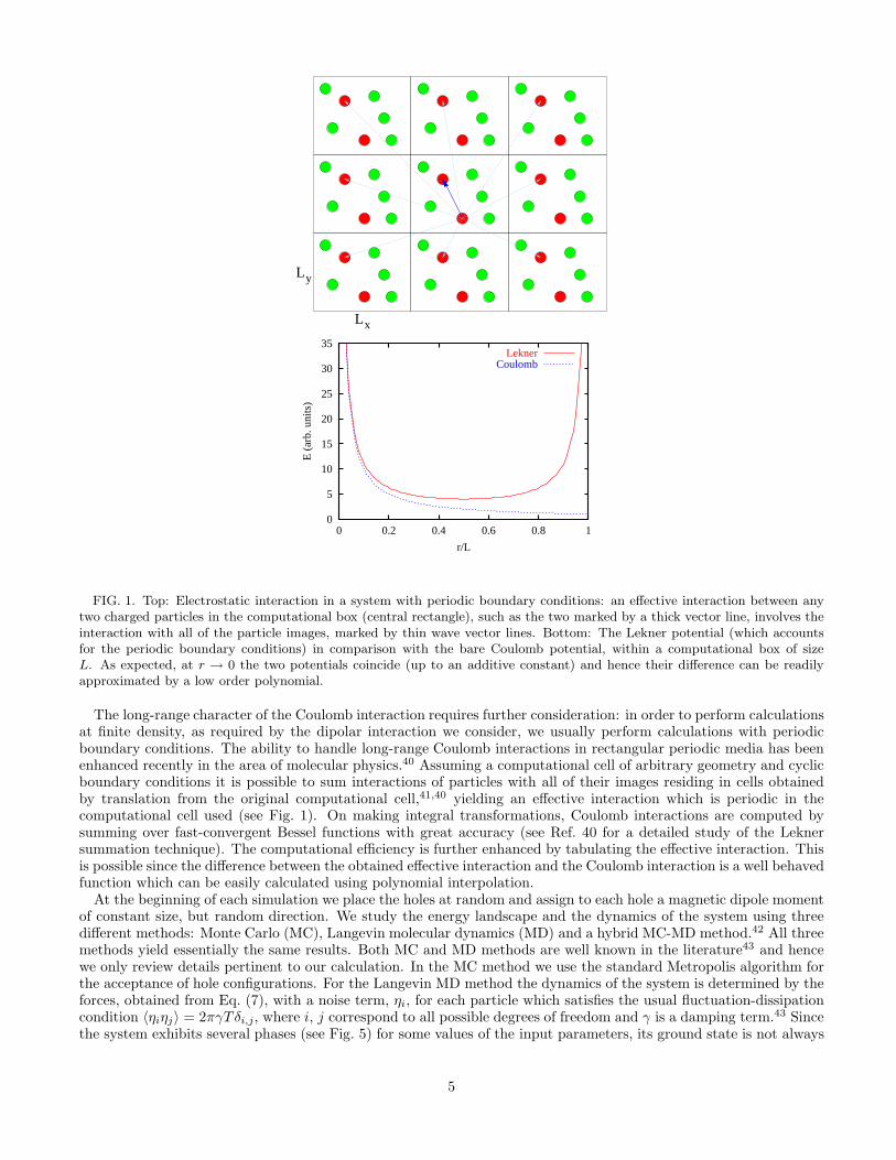
FIG. 1. Top: Electrostatic interaction in a system with periodic boundary conditions: an effective interaction between anytwo charged particles in the computational box (central rectangle), such as the two marked by a thick vector line, involves theinteraction with all of the particle images, marked by thin wave vector lines. Bottom: The Lekner potential (which accountsfor the periodic boundary conditions) in comparison with the bare Coulomb potential, within a computational box of sizeL. As expected, at r → 0 the two potentials coincide (up to an additive constant) and hence their difference can be readilyapproximated by a low order polynomial.

The long-range character of the Coulomb interaction requires further consideration: in order to perform calculationsat finite density, as required by the dipolar interaction we consider, we usually perform calculations with periodicboundary conditions. The ability to handle long-range Coulomb interactions in rectangular periodic media has beenenhanced recently in the area of molecular physics.40 Assuming a computational cell of arbitrary geometry and cyclicboundary conditions it is possible to sum interactions of particles with all of their images residing in cells obtainedby translation from the original computational cell,41,40 yielding an effective interaction which is periodic in thecomputational cell used (see Fig. 1). On making integral transformations, Coulomb interactions are computed bysumming over fast-convergent Bessel functions with great accuracy (see Ref. 40 for a detailed study of the Leknersummation technique). The computational efficiency is further enhanced by tabulating the effective interaction. Thisis possible since the difference between the obtained effective interaction and the Coulomb interaction is a well behavedfunction which can be easily calculated using polynomial interpolation.

At the beginning of each simulation we place the holes at random and assign to each hole a magnetic dipole momentof constant size, but random direction. We study the energy landscape and the dynamics of the system using threedifferent methods: Monte Carlo (MC), Langevin molecular dynamics (MD) and a hybrid MC-MD method.42 All threemethods yield essentially the same results. Both MC and MD methods are well known in the literature43 and hencewe only review details pertinent to our calculation. In the MC method we use the standard Metropolis algorithm forthe acceptance of hole configurations. For the Langevin MD method the dynamics of the system is determined by theforces, obtained from Eq. (7), with a noise term, ηi, for each particle which satisfies the usual fluctuation-dissipationcondition 〈ηiηj〉 = 2πγTδi,j, where i, j correspond to all possible degrees of freedom and γ is a damping term.43 Sincethe system exhibits several phases (see Fig. 5) for some values of the input parameters, its ground state is not always

5

well defined and a numerically obtained low temperature state may, in fact, depend on the initial and boundaryconditions. Hence, in order to rapidly reach a hole configuration with the lowest global minimum energy we performsimulated annealing from high temperatures.

The hybrid MC method includes elements of both the MC and MD methods: the hole configuration is again deter-mined using the standard Metropolis algorithm, but here a new configuration is obtained by letting the system evolvethrough a classical MD calculation over a certain time period. Note that, in principle, in classical MD calculations theenergy is a conserved quantity, hence every step should in principle be accepted. In reality the MD method introduceserrors which typically slightly lower the system energy, just as required by the Metropolis algorithm. Hence thismethod yields extremely high MC acceptance ratios.42

III. RESULTS

In this section we discuss the results of our numerical calculations. We first present the obtained ordered phasesand the phase diagram of the system and discuss its implications. We then show the hole ordering in the presenceof disorder. Finally we show the properties of the system as a function of T and in particular the dynamics of theobserved (stripe) pattern formation.

Before we begin with the presentation of our results we address the input parameters of the model, namely thehole density, σs (or the doping level n), the strength of the isotropic and dipolar part of the AF interaction, A and Brespectively, the AF correlation length, ξ, the temperature T and the concentration of impurities, ci, for the systemswith static point disorder. We define the doping level n as the hole density measured in units of cuprate latticespacing; thus n = 1% corresponds to 1 hole per 100 a2, where a ≈ 3.8 A.

The input parameters are not necessarily independent of each other, e.g., A and B should be proportional to eachother, with A ≈ U when t ≫ U and A ≈ 4t2/U when U ≫ t (see Ref. 29). However, since the range of the bondbreaking and dipolar interactions is vastly different, it is reasonable to treat A, B and ξ as independent parameters.Clearly both A and B should be of order of the Hubbard U in the SDW approach and of the order of J in the strongcoupling limit, and the correlation length is of order 1 to 10 lattice spacings in cuprates.

We begin with the low temperature properties (ground state) of the system as a function of B. The relevant orderparameter for charge ordering is the Fourier transform of the hole density:

ρ(q) =1

N

N∑

i=1

eiq·ri , (8)

where ri is the position of the ith hole and N is the total number of holes. A peak in ρ(q) at some wave-vector q = K

indicates ordering. Returning to the SDW picture, presented in Sec. II, we recall that the hole density is given by

ρk =∑

q,α

h†k+q,αhq,α. (9)

From the definition of the staggered magnetization, Eq. (4), it is immediately clear that 〈Sz(q)〉 ∝ δq,K+Q, i.e., a peakin ρk at K leads to a magnetic peak at Q+K and by symmetry at Q−K.

Since the interaction due to the second term in Eq. (6) (isotropic attractive interaction) is extremely short-range(in fact in an infinite system it is a δ function), it is initially reasonable to set A = 0 and explore the behavior ofthe system as a function of B. We return later to the role of A. As explained in Sec. II low T properties have beenobtained by annealing the system from some high temperature (T ∼ 5000K) down to temperatures of order 1K. Inthe extreme case B = 0 we find a Wigner crystal with small distortions, to be the state of lowest energy, as expected44

(see Fig. 2a).

6

(b)

(a)

0

20

40

60

80

100

0 20 40 60 80 100

10

20

30

40

50

60

70

80

0 10 20 30 40 50 60 70FIG. 2. Low T states of the hole vacancy system. (a) For B = 0 the holes (circles) form the Wigner crystal and (b) for

B → ∞ (an unphysical case) they form a “clump” pattern, a characteristic of the “mesoscopic phase separation.” The dipoleorientation (shown by the segments, originating from the circle centers) indicates finite magnetization at each star cluster. Inboth panels the doping level is n = 15%.

The small distortion of the Wigner crystal structure is due to the periodicity, which introduces a small spatialanisotropy into the system due to the shape of the computational box. Indeed, upon setting, e.g., Ly/Lx =

√3/2,

we obtain a perfect Wigner crystal to be the ground state. Another extreme case is when B → ∞. In this case theAF dipolar interaction dominates over the average Coulomb interaction; one then finds star shaped clumps of holes,similar in shape to those found in Ref. 45, which can, at sufficiently high density, form a geometric structure (e.g., aWigner crystal of clumps). We note that this case is rather unphysical, as macroscopic phase separation is inconsistentwith our initial assumption of the two-body dipolar interaction being independent of the many-hole effects. On theother hand, ordering of macroscopically hole rich regions is in agreement with the conjecture that all ground statesare geometrically ordered.46

On increasing B > 0, at fixed density, the Wigner crystal becomes unstable and a new phase with diagonal stripesis formed, as shown in Fig. 2a of Ref. 47. The main characteristic of this phase is a ferro-magnetic ordering of the AFdipoles. The situation here is very similar to that observed in La2−xSrxNiO4+y (see Ref. 7). Note that such a statewith a dipole ordering appeares to violate time reversal symmetry. On the other hand the true ground state in thiscase also involves hole ordering, with holes aligned in stripes either perpendicular or parallel to the dipole orientation.However, the interstripe distance, in this case, is close to that between holes within a stripe and hence a simulationinevitably yields a “glassy” state, with many defects. This is reflected in the shape of ρk, which shows broad peaks(see Fig. 2b in Ref. 47), indicating an average interstripe distance.

7

(a)

0

20

40

60

80

100

0 20 40 60 80 100

(b)

10

20

30

40

50

60

0 10 20 30 40 50

(c)

-0.4 -0.2 0 0.2 0.4

-0.4

-0.2

0

0.2

0.4

FIG. 3. Low T state for larger finite values of B, B = 4eV , at n = 15% doping level. The holes (circles) form a grid47

(panel (a)) with dipoles orientated along line segments and a dipole rotation at grid intersections (panel (b)). Panel (c) showsa contour plot of the average charge density ρk in arbitrary units, indicating “perfect” geometric order.47 Even after averagingover many solutions in this case the charge peaks are much sharper than those found in the ferro-dipolar phase (see Fig. 2b inRef. 47).

As shown in Fig. 3a, at larger values of B a linear stripe is formed, which, with increasing density tends to closeinto a loop. More importantly, the loop formation is accompanied by magnetic dipole orientation along the straightportion of a loop with gradual rotation by π/2 at each corner.48 Due to the rotation of dipoles at corners the loopsinteract, and eventually form the checkerboard (grid) pattern.49 The size of the distance between holes within a lineis determined by the ratio of B (or the sum of A and B, for A 6= B) and the Coulomb energy; the grid sizes aredetermined by the hole density alone. These results appear to be consistent with the DMRG numerical solution ofthe t − J model25 which also finds loops of holes, except that in our case the periodic boundary conditions and theCoulomb interaction yield a “tile grid” as opposed to “droplets.” Note the almost perfect (infinite charge correlationlength, ξc) crystal structure obtained (Fig. 3c). It is noteworthy that a typical solution yields a finite dipole moment ateach grid intersection, which, in turn, can take one of the two orientations (along two diagonals of the computationalbox), thus creating a highly degenerate system of moments (see Fig. 6 below).

We recall that the presented solution is obtained assuming an arbitrary dipole orientation with a constant holedipole magnitude, i.e., a continuum of angles between the dipoles and a fixed axis. As explained in the previous

8

section, at very low doping the dipoles would reside near the BZ diagonals, i.e., they would assume almost “discrete”orientations. In order to study the effect of this “discreteness” we have performed the same simulation this timeassuming that hole dipoles can take only one of four directions (determined by the momenta of the maxima of thelower Hubbard band). We find that the physics of the pattern formation is qualitativelly unaltered (hence we do notpresent them here), except for one important difference: the “bending” of stripes at the grid intersections disappears,i.e., one no longer has a finite dipole moment at these intersections.

Another way of quantifying this ordered phase is by straightforwardly calculating the “string tension,” which, atT → 0 is equal to ∂2U/∂x2, where U is the total potential energy and x is a small hole (or stripe) displacement; alarge string tension indicates a high stability of the obtained phase, and vice versa. In Fig. 4a we show the stringtension for motion perpendicular to a grid side compared with the motion along a side. As seen in the figure, the gridphase (and, as discussed below, the stripe phase) is extremely stable with respect to the hole motion perpendicularto the holes line segments, due to the Coulomb interacton. On the other hand, at larger doping values and fixed holedensity the stripes are almost compressible, i.e., the motion of holes along a stripe is rather soft. The anisotropy ofthe perpendicular and longitudinal string tension decreases with decreasing B.

-0.02

0

0.02

0.04

0.06

0.08

0.1

0.12

0.14

0.16

-0.15 -0.1 -0.05 0 0.05 0.1 0.15

Pot

entia

l Ene

rgy

[eV

/par

ticle

]

Displacement [10-8 cm]

LongitudinalTransverse

0

0.2

0.4

0.6

0.8

1

1.2

1.4

1 1.5 2 2.5 3 3.5 4

Stri

ng te

nsio

n

B [eV]FIG. 4. Top: Energy as a function of a hole position, reflecting the string tension in the stripe, for B = 4 eV and n = 15%.

Clearly, the motion of holes perpendicular to the the grid directions is quite hard and while the motion along a line stripeis much softer (see also text). Bottom: average string tension as a function of B, at n = 15% Note the almost exponentialdependence (solid line) up to the critical value of B ∼ 4 eV where the system undergoes the first order transition between theferro-dipolar and grid phases.

At fixed AF correlation length the four observed phases yield a diagram which we show in Fig. 5a. We remarkthat in all phases a non-vanishing value of A leads to a decrease in the effective value of B at which the transitionsoccur, as shown in Fig. 5b. The isotropic term A alone never produces any non-trivial geometric phase (e.g., stripes),even with inclusion of lattice effects. We find that the transition between the ferro-dipolar and the grid phases is firstorder, as indicated by the coexistence of phases in Fig. 6. Note that this transition always occurs on increasing thedoping level to sufficiently (and artificially) high values, where our theory need not apply. No coexistence of phaseshas been observed at other transitions, suggesting that they are second order. We also recall that our calculationsare quasiclassical and thus the obtained geometric (stripe) phases are insulating. Moreover, in our formalism the holedensity within a stripe can assume an arbitrary value, depending on the dipolar interaction strength.

9

0

(a)

2

4

6

8

10

0 2 4

Dop

ing

(%)

Dipolar B (eV)

DiagonalStripes Geometric

Phase

ClumpsWignerCrystal

(b)D

opin

gDiagonal Stripes

Geometric

Wigner

Clumps

Phase

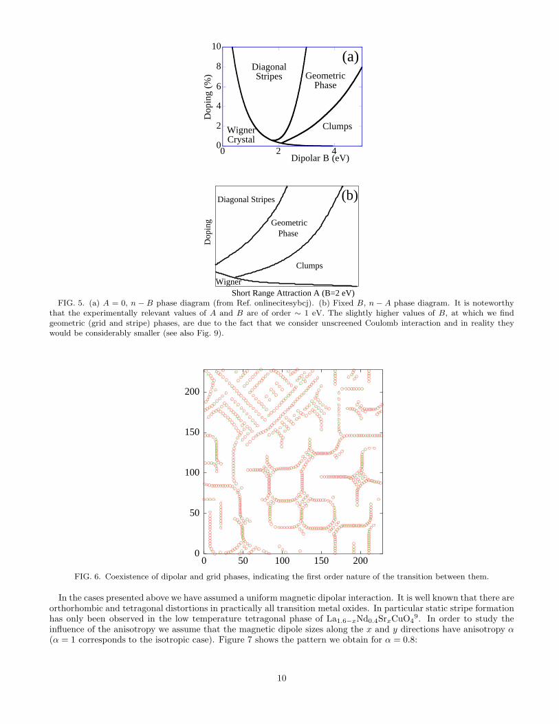
Short Range Attraction A (B=2 eV) FIG. 5. (a) A = 0, n − B phase diagram (from Ref. onlinecitesybcj). (b) Fixed B, n − A phase diagram. It is noteworthy

that the experimentally relevant values of A and B are of order ∼ 1 eV. The slightly higher values of B, at which we findgeometric (grid and stripe) phases, are due to the fact that we consider unscreened Coulomb interaction and in reality theywould be considerably smaller (see also Fig. 9).

0

50

100

150

200

0 50 100 150 200

FIG. 6. Coexistence of dipolar and grid phases, indicating the first order nature of the transition between them.

In the cases presented above we have assumed a uniform magnetic dipolar interaction. It is well known that there areorthorhombic and tetragonal distortions in practically all transition metal oxides. In particular static stripe formationhas only been observed in the low temperature tetragonal phase of La1.6−xNd0.4SrxCuO4

9. In order to study theinfluence of the anisotropy we assume that the magnetic dipole sizes along the x and y directions have anisotropy α(α = 1 corresponds to the isotropic case). Figure 7 shows the pattern we obtain for α = 0.8:

10

0 20 40 60 80 1000

50

100

FIG. 7. With a small x− y directional anisotropy in the dipolar interaction, Eq. (6), with the anisotropy parameter α = 0.8(in the uniform case α = 1), the holes (shown by circles) form a stripe, rather than a grid pattern. Note the hole dipoleorientations (shown by the line segments), altering direction in neighbouring stripes, corresponding to the π phase shift of thelocal magnetization between magnetic domains separated by stripes.22

The rotational symmetry is broken and a stripe superlattice is formed, with a charge ordering vector K = (2π/ℓ)x,where ℓ is the inter-stripe distance. More importantly, the total dipole moment in this state vanishes. As explainedin Sec. II, this yields a Fourier transform of the magnetization S(q) = 〈Sz(q)〉 peaked at Q±K in momentum space.Of course, it is reasonable to assume that in twinned single crystals, used in inelastic neutron scattering experiments,one has domains which average out this anisotropy. Note that in both calculated geometric phases (see Figs. 3 and7), the interstripe distance is much larger than the intrastripe distance, in agreement with experimental findings inunderdoped cuprates.

Our results are somewhat sensitive to the applied boundary conditions. First, for a small computational box theexact size of the grid depends on its commensuration with the box length, which, in turn depends on the density. Onincreasing of the size of the computational box, the grid size depends only on the physical parameters, as explainedbelow Fig. 3. In addition, for a large computaitonal box the grid pattern, shown in Fig. 3a, acquires point or linedefects, shown in Fig. 8a.

(a)

0 100 200 3000

100

200

300

11

(b)

-0.5 -0.25 0 0.25 0.5-0.5

-0.25

0

0.25

0.5

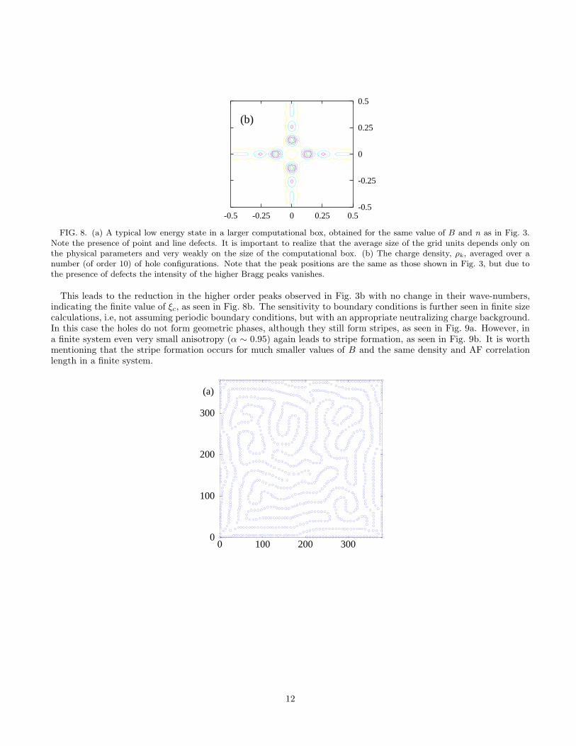
FIG. 8. (a) A typical low energy state in a larger computational box, obtained for the same value of B and n as in Fig. 3.Note the presence of point and line defects. It is important to realize that the average size of the grid units depends only onthe physical parameters and very weakly on the size of the computational box. (b) The charge density, ρk, averaged over anumber (of order 10) of hole configurations. Note that the peak positions are the same as those shown in Fig. 3, but due tothe presence of defects the intensity of the higher Bragg peaks vanishes.

This leads to the reduction in the higher order peaks observed in Fig. 3b with no change in their wave-numbers,indicating the finite value of ξc, as seen in Fig. 8b. The sensitivity to boundary conditions is further seen in finite sizecalculations, i.e, not assuming periodic boundary conditions, but with an appropriate neutralizing charge background.In this case the holes do not form geometric phases, although they still form stripes, as seen in Fig. 9a. However, ina finite system even very small anisotropy (α ∼ 0.95) again leads to stripe formation, as seen in Fig. 9b. It is worthmentioning that the stripe formation occurs for much smaller values of B and the same density and AF correlationlength in a finite system.

0 100 200 3000

100

200

300

(a)

12

0 100 200 3000

100

200

300

(b)

-0.5 -0.25 0 0.25 0.5-0.5

-0.25

0

0.25

0.5(c)

-0.5 -0.25 0 0.25 0.5-0.5

-0.25

0

0.25(d)

0.5

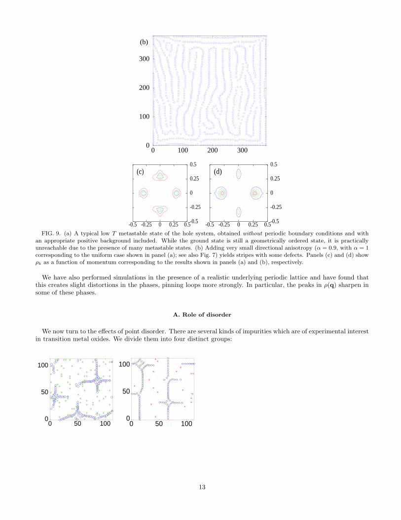
FIG. 9. (a) A typical low T metastable state of the hole system, obtained without periodic boundary conditions and withan appropriate positive background included. While the ground state is still a geometrically ordered state, it is practicallyunreachable due to the presence of many metastable states. (b) Adding very small directional anisotropy (α = 0.9, with α = 1corresponding to the uniform case shown in panel (a); see also Fig. 7) yields stripes with some defects. Panels (c) and (d) showρk as a function of momentum corresponding to the results shown in panels (a) and (b), respectively.

We have also performed simulations in the presence of a realistic underlying periodic lattice and have found thatthis creates slight distortions in the phases, pinning loops more strongly. In particular, the peaks in ρ(q) sharpen insome of these phases.

A. Role of disorder

We now turn to the effects of point disorder. There are several kinds of impurities which are of experimental interestin transition metal oxides. We divide them into four distinct groups:

0 50 1000

50

100

0 50 1000

50

100

13

0 50 1000

50

100

0 50 1000

50

100

FIG. 10. The effects of impurities of different types. The four panels show hole (circles) and impurity (stars) positions,for the case of: charged impurities, placed d = 6Aout-of-plane (top left), in-plane repulsive uncharged impurities (top right),in-plane repulsive charged impurities (bottom left), and in-plane impurities with a local magnetic moment which destroys localAF ordering (bottom right). Clearly, all impurities destroy the stripe order, although the out-of-plane impurities and theuncharged in-plane impurities are nearly as effective as the in-plane charged impurities. The latter lead to the a glassy phaseof stripe segments at relatively low concentrations, of order a few percent.

(I) out-of-plane impurities, such as Sr in LSCO compounds, (II) in-plane charged impurities, such as (presumably)Li,50 (III) in-plane uncharged impurities, such as Ni and (IV) in plane uncharged impurities which induce a magneticmoment, such as Zn. Hence, we model the impurity effects by adding a random (in position) potential to theHamiltonian (7), which is either short-ranged and located in plane or, as in the case of charged impurities, long-ranged (Coulomb) and either in-plane or out-of-plane (a distance d from the plane where the holes are located). Inthe case of type IV we have also altered the dipolar interaction in the vicinity of an impurity, i.e., the magneticinteraction is multiplied by a factor tanh(r/Ri), where r is the distance of a hole to a nearby impurity and Ri is theeffective radius of the impurity, which, for the case of Zn, has been estimated to be of order 2 lattice sites aroundeach impurity atom.51 Examples of the effects of the four types of impurities are presented in Fig. 10.

Clearly, all four types of impurities lead to the destruction of the geometric (stripe or grid) hole order at sufficientlylarge impurity concentration, ci. On the other hand, in all four cases stripe ordering persists through the formationof line segments of holes, resulting in a new, glassy phase.52 Moreover, the four impurity types exhibit different mech-anisms for destroying the stripe order. The charge ordered phases are practically unaffected by a small concentrationof uncharged impurities (see Fig. 10b), i.e., the stripes simply avoid impurity sites. Consequently, the stripes persistto relatively high concentrations of this type of disorder.

The charged impurities first lead to stripe deformation, i.e., the stripes pass either very close to the impurities (forattractive, pinning impurities) or very far from the impurities (for repulsive impurities), in order to maximize thepotential energy (see Figs. 10a and 10c). With increasing ci the stripes rupture and only stripe segments persist.Finally, the impurities with a local magnetic moment affect the formation of the spiral spin phase, responsible forthe (attractive) dipolar interaction. Since the magnetic interaction is strongly suppressed in the vicinity of such animpurity site, even the stripe segments cannot exist there, as shown in Fig. 10d.

Impurities are especially effective in destroying the ordered phases found at small B. For example, the Wignercrystal state becomes glassy at relatively low impurity concentrations. This happens because, e.g., in the case ofimpurity type I, the attractive Coulomb energy between impurities and holes scales like e2/d, where d is the distancebetween the planes in which the impurities and holes reside, while the average inter-hole Coulomb energy behaveslike e2

√σs. Thus when σs < 1/d2 the holes are pinned by impurities.

In general the role of impurities depends strongly on the impurity concentration, ci. However, the magnetic dipoleinteraction is sufficient to retain the main orientation, as seen in Fig. 11 where we have plotted the correlation lengthas a function of ci. This leads us to conjecture that with the addition of the kinetic energy the holes can move instring segments in an orientation given basically by the phase diagram of the clean system. The stripe motion wouldthen be caused by mesoscopic thermal or quantum tunneling of the finite strings between the minima of the overallpotential. This would lead to non-linear field dependence in the low temperature conductivity.53

14

0

50

100

150

200

250

Impurity concentration (%)C

orre

latio

n le

ngth

[A

]o

0 1 2 3 4 5

FIG. 11. Zero temperature charge correlation length as a function of impurity concentration for the in-plane charged impuritycase: the result is obtained by measuring the static correlation length, and then averaging over many (of order 20) differentimpurity configurations.

B. Finite temerature results

We now proceed to the finite T results. The numerical procedure is identical, except that the temperature is loweredadiabatically to a finite value (i.e., a numerical annealing). In a classical simulation this is equivalent to introducingkinetic energy into the system.

In the case of a Wigner crystal, B = 0, we find that the introduction of finite T melts the crystalline structure andthe resulting phase is the 2D Coulomb gas. The diagonal (glassy) phase is also unstable at relatively low temperatures.On the other hand, the geometricaly ordered states, for as ≪ ξ, where as is the distance between holes within a stripesegment, are all stable up to T of order ∼ B/σsa

2s. At even higher temperatures, the stripe array melts with a

temporal intermittency of the observed pattern: i.e., spatio-temporal intermittency. Fig. 12 shows four stages ofthis melting process. We observed that the stripe melts through a rupture which results in creation of finite stripesegments that eventually (at constant and high T ) disperse into individual holes.

Note that the temporal geometric pattern (panel (b)) is not the same as that in the ground state. As mentionedbefore, there are many low lying geometric states, close in energy to the ground state, which can temporarily occurat finite T . Hence the dynamics of the stripe ordering is similar to that observed in glasses, characterized by non-gaussian fluctuations. To show this we follow the dynamics of the hole system at temperatures slightly below themelting temperature: we start from a low lying metastable state, such as that depicted in Fig. 12b, increase thetemperature adiabatically to the point at which the structure begins to melt (which is a measure of the activationenergy) and let the system equillibrate.

0

20

40

60

80

100

0 20 40 60 80 100

15

0

20

40

60

80

100

0 20 40 60 80 100

0

20

40

60

80

100

0 20 40 60 80 100FIG. 12. Spatio-temporal intermittent behavior of hole ordering near the melting transition: three snapshots are shown.

Panel (a) corresponds to a state which is clearly withing the basin of attraction of the ground state (the same pattern, albeitdeformed), while panel (b) shows a state which is within the basin of attraction of another low lying geometric state withmore dense stripes along one of the axis. Panel (c) shows the melted nematic crystal–like phase with the hole dipole momentsaligned.

In Fig. 13a we plot an energy histogram at this temperature (with the energy shifted by an arbitrary additive constant),thus indicating an intensity of the energy states (bands):

0

2000

4000

6000

8000

10000

12000

14000

0 0.2 0.4 0.6 0.8 1 1.2

Inte

nsi

ty

Energy [eV/particle]

16

100

1000

1x104

1x105

1x106

0 2 4 6 8 10 12 14 16

Po

we

r S

pe

ctru

m

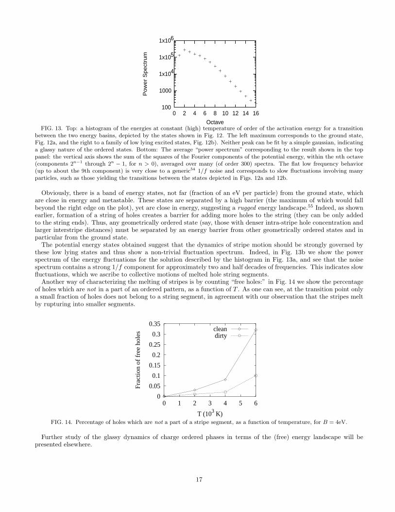
OctaveFIG. 13. Top: a histogram of the energies at constant (high) temperature of order of the activation energy for a transition

between the two energy basins, depicted by the states shown in Fig. 12. The left maximum corresponds to the ground state,Fig. 12a, and the right to a family of low lying excited states, Fig. 12b). Neither peak can be fit by a simple gaussian, indicatinga glassy nature of the ordered states. Bottom: The average “power spectrum” corresponding to the result shown in the toppanel: the vertical axis shows the sum of the squares of the Fourier components of the potential energy, within the nth octave(components 2n−1 through 2n

− 1, for n > 0), averaged over many (of order 300) spectra. The flat low frequency behavior(up to about the 9th component) is very close to a generic54 1/f noise and corresponds to slow fluctuations involving manyparticles, such as those yielding the transitions between the states depicted in Figs. 12a and 12b.

Obviously, there is a band of energy states, not far (fraction of an eV per particle) from the ground state, whichare close in energy and metastable. These states are separated by a high barrier (the maximum of which would fallbeyond the right edge on the plot), yet are close in energy, suggesting a rugged energy landscape.55 Indeed, as shownearlier, formation of a string of holes creates a barrier for adding more holes to the string (they can be only addedto the string ends). Thus, any geometrically ordered state (say, those with denser intra-stripe hole concentration andlarger interstripe distances) must be separated by an energy barrier from other geometrically ordered states and inparticular from the ground state.

The potential energy states obtained suggest that the dynamics of stripe motion should be strongly governed bythese low lying states and thus show a non-trivial fluctuation spectrum. Indeed, in Fig. 13b we show the powerspectrum of the energy fluctuations for the solution described by the histogram in Fig. 13a, and see that the noisespectrum contains a strong 1/f component for approximately two and half decades of frequencies. This indicates slowfluctuations, which we ascribe to collective motions of melted hole string segments.

Another way of characterizing the melting of stripes is by counting “free holes:” in Fig. 14 we show the percentageof holes which are not in a part of an ordered pattern, as a function of T . As one can see, at the transition point onlya small fraction of holes does not belong to a string segment, in agreement with our observation that the stripes meltby rupturing into smaller segments.

0

0.05

0.1

0.15

0.2

0.25

0.3

0.35

0 1 2 3 4 5 6

Fra

ctio

n of

fre

e ho

les

T (103 K)

cleandirty

FIG. 14. Percentage of holes which are not a part of a stripe segment, as a function of temperature, for B = 4eV.

Further study of the glassy dynamics of charge ordered phases in terms of the (free) energy landscape will bepresented elsewhere.

17

IV. CONCLUSIONS

In summary, on employing the SDW picture of transition metal oxides, we have studied the short-range and dipolarattractive forces generated by the AF fluctuations, together with long-range Coulomb forces. We have developed anovel numerical technique, which enables us to treat doped hole vacancies at finite concentration. We have studied thecompetition between long-range and short-range interactions and its influence on hole ordering in layered transitionmetal oxides. We have found a rich phase diagram for the clean system which includes a Wigner solid, diagonalstripes, grid (loops) and a macroscopic phase separation. For intermediate values of magnetic interaction this phasediagram is consistent with several different experimental measurements, such as the inelastic neutron scattering. Inaddition, on adding a small, but finite amount of anisotropy to the dipolar interaction we find that the ground state ofthe system of holes is the striped phase, found in La2−y−xNdySrxCuO4. In the geometric phases with strong magneticinteraction strength we have found a large string tension for the motion of holes perpendicular to the stripe direction.This is due to the Coulomb interaction and indicates strong stability of the obtained phases.

We have also found the system of holes to be quite sensitive to the presence of charged impurities. In particular,adding out-of-plane attractive impurities pins the holes and, for small pinning energies, increases the melting tem-perature of the stripe phase, although it does yield a finite charge correlation length. In general, charged impuritiesare very effective in destroying the stripe order, especially those residing in the same plane as the holes, regardless ofwhether they are attractive or repulsive, although the stripe phases survive as finite stripe segments up to relativelyhigh impurity concentrations. This suggests that nonlinear conductivity should be prevalent.

The resulting hole patterns are the result of frustration (competition between short-range and long-range forces):this frustration leads to collective motions, involving large number of particles which ultimately lead to geometriclyordered ground states. We have also studies the dynamics of the geometric phase formation and its melting. We findthat the dynamics is characterized by a “glassy” behavior in that the energy landscape is rugged, as characterized bythe spatio-temporal intermittency of the observed behavior. More importantly, we find that, for fixed (large) size ofthe magnetic (dipolar) interaction, there are fewer number of sharper minima, while the string tension of the stripesis larger. As a consequence, in this case the melting of the stripe phase occurs at higher temperature with increaseddoping concentration.

The energy landscape is also characterized by formation of domains, separated by defects. This picture is inagreement with recent NMR experiments11 in which small activation energies are easily attributed to domain growthand/or motion. Thus, further study of our model will include the dynamics of the domain growth and their melting.

ACKNOWLEDGMENTS

We gratefully acknowledge valuable discussions with A. Balatsky, A. Chubukov, N. Curro, J. Gubernatis, C.Hammel, G. Ortiz, D. Pines, D. Scalapino, J. Schmalian, S. White and J. Zaanen. A. H. C. N. acknowledges supportfrom the Alfred P. Sloan foundation. Work at Los Alamos was supported by the U. S. Department of Energy. Work atthe University of California, Riverside, was partially supported by a Los Alamos CULAR project. Work at LawrenceBerkeley Laboratory was partly supported by the Director, Office of Advanced Scientific Computing Research Divisionof Mathematical, Information, and Computational Sciences of the U.S. Department of Energy under contract numberDE-AC03-76SF00098.

† Also at the Institute of Semiconductor Physics, Novosibirsk, Russia.1 V. J. Emery, S. A. Kivelson and O. V. Zachar, Physical Review B 56, 6120 (1997).2 Y. Yacoby, S. M. Held and E. A. Stern, Solid State Comm. 101, 801 (1997); A. Aharony and A. Auerbach, Phys. Rev. Lett.70, 1874 (1993) and references therein.

3 Phase separation in cuprate superconductors, ed. by K. A. Muller and G. Benedek (World Scientific, Singapore, 1993).4 See, e.g., R. H. McKenzie, Phys. Rev. Lett. 74, 5140 (1995) and references therein.5 See, e.g., J. P. Lorenzo and S. Aubry, Physica D 113 276 (1998), and references therein.6 See, e.g., S. Yunoki, A. Moreo and E. Dagotto, Phys. Rev. Lett. 81, 5612 (1998) and references therein.7 J. M. Tranquada et al., Phys. Rev. Lett. 70, 445 (1993).8 S. Mori et al., Nature 392, 473 (1998).9 J. M. Tranquada et al., Nature, 375, 561, (1995).

18

10 A. Bianconi, Phys. Rev. B 54, 12018 (1996); M. v. Zimmermann et al., Europhys. Lett. 41, 629 (1998).11 P.C. Hammel et al., in Proceedings of the Conference Anharmonic Properties of High Tc Cuprates (1994).12 J. H. Cho et al., Phys. Rev. Lett. 70, 222 (1993).13 F. C. Chou et al., Phys. Rev. Lett. 71, 2323 (1993)14 F. Borsa et al., Phys. Rev. B 52,7334 (1995).15 S. Wakimoto et al., Phys. Rev. B 60, R769 (1999).16 J. M. Tranquada et al., cond-mat/9702117.17 G. Aeppli et al., Science 278, 1432 (1997).18 H. J. Schulz, J. Phys. France 50, 2833 (1989); J. Zaanen and J. Gunnarsson, Phys. Rev. B 40, 7391 (1989); A. R. Bishop et

al., Europhysics Letters, 14 ,157 (1991).19 P. Prelovsek and X. Zotos, Phys. Rev. B 47, 5984 (1993); P. Prelovsek and I. Sega, Phys. Rev. B 49, 15 241 (1994); E.

W. Carlson et al., Phys. Rev. B 57, 14 704 (1998); C. Nayak and F. Wilczek, Phys. Rev. Lett. 78, 2465 (1997); A. H.Castro Neto, Z. Phys. B 103, 185 (1997); J. Zaanen et al., Phys. Rev. B 58, R11 868 (1998); M. Vojta and S. Sachdev,cond-mat/9906104.

20 A. L. Chernyshev, A. H. Castro Neto, and A. R. Bishop, cond-mat/9909128.21 G. Seibold et al., Phys. Rev. B 58, 13 506 (1998).22 V. J. Emery and S. A. Kivelson, Physica C 209, 597 (1993).23 U. Low et al., Phys. Rev. Lett. 72, 1918 (1994).24 F. Guinea, G. Gomez-Santos, and D. Arovas, cond-mat/9907184.25 S. R. White and D. J. Scalapino, Phys. Rev. Lett. 80, 1272 (1998); ibid. 81, 3227 (1998).26 C. S. Hellberg and E. Manousakis, Phys. Rev. Lett. 83, 132 (1999); cond-mat/9910142; S. R. White and D. J. Scalapino,

cond-mat/9907243.27 J. Zaanen, private communication.28 J. R. Schrieffer, X. G. Wen and S. C. Zhang, Phys. Rev. B 39, 11663 (1989).29 D. M. Frenkel and W. Hanke, Phys. Rev. B 42, 6711 (1990).30 B. I. Shraiman and E. D. Siggia, Phys. Rev. B 40, 9162 (1989).31 S. A. Kivelson, E. Fradkin and V. J. Emery, Nature 393, 550 (1998).32 J. C. Slater, Phys. Rev. 82, 538 (1951).33 N. F. Mott in Metal-Insulator Transitions (Taylor & Francis, London, 1974), pg. 141.34 B. O. Wells et al., Phys. Rev. Lett. 74, 964 (1995).35 A. Chubukov and K. Muselian, Phys. Rev. B 51, 12605 (1995).36 E. Fradkin in Field Theories of Condensed Matter Systems (Addison-Wesley, Redwood City, 1991), pg. 48.37 S. Chakravarty et al., Phys. Rev. Lett. 60, 1057 (1988).38 We are thankful to S. Kivelson for attracting our attention to this problem.39 A. Aharony et al., Phys. Rev. Lett. 60, 1330 (1988).40 N. Grønbech-Jensen et al., Molec. Phys. 92, 941 (1997).41 J. Lekner, Physica (Amsterdam) 176A, 485 (1991).42 J. Bonca and J. E. Gubernatis, Phys. Rev. E 53, 6504 (1996).43 W.H. Press et al, Numerical Recipes: The Art of Scientific Computing (Cambridge, Cambridge, 1992).44 E. P. Wigner, Phys. Rev. 46, 1002 (1934).45 N. M. Salem and R. J. Gooding, Europhys. Lett. 35, 603 (1996).46 P.W. Anderson, Basic Notions in Condensed Matter (Addison-Wesley, Reading, 1997).47 B.P. Stojkovic et al, Phys. Rev. Lett. 82, 4679 (1999).48 This is a highly degenerate configuration which can be mapped into a classical six vertex model. See, for instance, R. J. Baxter

in Exactly Solved Models in Statistical Mechanics (Academic Press, London, 1982), pg. 127.49 The simulations show the presence of topological defects in the phase of the magnetic dipole moments, i.e., the total phase

in a loop may be shifted by 2π.50 Some impurities, on donating a hole or an electron to CuO planes, become charged ions.51 S. Zagoulaev, P. Monod, J. Jegoudez, Phys. Rev. B 52, 10474 (1995).52 R. J. Gooding, N. M. Salem, R. J. Birgeneau, and F. C. Chou, Phys. Rev. B 55, 6360 (1997).53 J. Bardeen, Phys. Rev. Lett. 45, 1978 (1980); D. S. Fisher, Phys. Rev. B 31, 1396 (1985).54 See, e.g., M. B. Weissman, Physica D 107, 421 (1997).55 See, e.g., C. Dasgupta and O.T. Valls, Phys. Rev. E 59, 3123 (1999).

APPENDIX A: MAGNETIC DIPOLES OF THE HUBBARD MODEL

In this appendix we study the Hubbard model, Eq. (1) in the SDW state. Our approach is similar to that presentedin Refs. 28,35. Hence we only briefly review the calculation leading to Eq. (5), the central equation of the paper.

19

The relevant order parameter in our case is the spin density in the z direction:

Sz(q) =∑

k,α

αc†k+q,αck,α , (A1)

which in the SDW state has a finite expectation value at q = Q = (π/a, π/a) because of the nesting of the half-filledFermi surface. In this case the mean field Hamiltonian reads

HMF =∑

k,α

ǫkc†k,αck,α − USN

2

∑

k,α

αc†k+Q,αck,α , (A2)

where

S =1

N〈Sz(Q)〉 ,

ǫk = −2t (cos(kxa) + cos(kya)) . (A3)

The Hamiltonian (A2) can be diagonalized immediately using the Bogoliubov transformation:

γck,α = ukck,α + αvkck+Q,α

γvk,α = vkck,α − αukck+Q,α (A4)

where

uk =

√

1

2

(

1 +ǫkEk

)

vk =

√

1

2

(

1 − ǫkEk

)

Ek =√

ǫ2k + ∆2

∆ = −US2. (A5)

In this case the mean-field Hamiltonian reads

HMF =∑

k,α

Ek

(

γc†k,αγ

ck,α − γv†

k,αγvk,α

)

, (A6)

where the sum over k is restricted to the magnetic Brillouin zone and, at half filling, the ground state |0〉 is definedsuch that

γck,α|0〉 = 0

γv†k,α|0〉 = 0 . (A7)

Thus, at half-filling the conduction band is empty and the valence band is separated from it by energy ∆ which isthe Mott-Hubbard gap. It is known that this theory recovers the results of the Heisenberg model very well. Consider,for instance, the average spin density in (A1) in terms of the new operators (recall that the conduction band is emptyand therefore does not contribute)

〈Sz(q)〉 = −2∑

k,α

uk+q−Qvk〈γv†k+q−Q,αγ

vk,α〉

= −4δq,Q

∑

k

ukvk = −4δq,Q

∑

k

∆

2Ek, (A8)

which, together with (A5), yields the gap equation:

1

N

∑

k

1√

ǫ2k + ∆2=

1

U. (A9)

20

Since we are going to consider hole doping we can neglect the terms involving the conduction band operators fortemperatures T ≪ ∆. As shown in 28 new interactions are generated by the antiferromagnet in the presence of theholes, given by Hz and Hxy. The non-interaction hole Hamiltonian is, from (A6):

H0 = −∑

k,α

Ekγv†k,αγ

vk,α . (A10)

Close to the half-filled Fermi surface one sees that the hole mass is

mh ≈ ∆

8t2a. (A11)

For any state |Ψ〉 of the system we can define the hole operators as

γvk,α|Ψ〉 = h†−k,−α|Ψ〉 (A12)

in which case the Hamiltonian reads

H0 =∑

k,α

Ekh†k,αhk,α (A13)

plus unimportant constants.The interacting parts of the Hamiltonian can also be written in terms of this new operators. For instance,

Hz =1

N

∑

k,α

[

(Vz(Q) − Vz(2k− Q)/4)m2k,k − Vz(2k)l2k,k/4

]

h†k,αhk,α

− 1

4N

∑

k,k′

(

Vz(k − k′)l2k,k′h†k,ασ

zα,α′hk′,α′h†−k,βσ

zβ,β′h−k′,β′

+ Vz(k − k′ + Q)m2k,k′h

†k,αhk′,αh

†−k,βh−k′,β

)

, (A14)

where the sum over spin indices is implicit and

Vz(q) =U2χz

0(q)

1 − Uχz0(q)

(A15)

with

χz0(q, ω) = − 1

2N

∑

k

(

1 − ǫkǫk+q + ∆2

EkEk+q

) (

1

ω − Ek+q − Ek− 1

ω + Ek+q + Ek

)

. (A16)

A similar expression is valid for the transverse components of the interaction

Hxy = − 4

N

∑

k,α

(1 − α)[

V+−(2k)n2k,k − V+−(Q + 2k)p2

k,k

]

h†k,αhk,α

− 1

4N

∑

k,k′

[

V+−(k − k′)n2k,k′ − V+−(k − k′ + Q)p2

k,k′

]

× h†k,ασ+α,α′hk′,α′h†−k,βσ

−β,β′h−k′,β′ , (A17)

where V+− is given by an expression similar to (A15) with χz0 replaced by

χ+−0 (q, ω) == − 1

2N

∑

k

(

1 − ǫkǫk+q − ∆2

EkEk+q

) (

1

ω − Ek+q − Ek− 1

ω + Ek+q + Ek

)

. (A18)

Moreover, the coefficients that appear in these expressions are defined by

mk,k′ = ukvk′ + vkuk′

lk,k′ = ukuk′ + vkvk′

pk,k′ = ukvk′ − vkuk′

nk,k′ = ukuk′ − vkvk′ . (A19)

21

Observe that the interactions renormalize the dispersion of the holes as well, that is, Ek → ERk . While Hz is

essentially a short range attractive interaction in the spin-symmetric channel, Hxy has two components: one of themis also an attractive interaction in the spin-symmetric channel but the other is a long range dipolar interaction whichdepends on the momentum of the hole.

The Hamiltonian, which consists of terms given by Eqs. (A14) and (A17), is very hard to deal with. One notices,however, that the mean field energy Ek is degenerate along the magnetic Brillouin zone. This is an artifact of thetheory and the degeneracy is broken by any small perturbation such as the corrections discussed before or a nextnearest hopping, t′, for instance. In this case, the dispersion has a minimum at (±π/2,±π/2). Thus, in order tostudy the long wavelength limit of the theory it is sufficient to focus on these points of the Brillouin zone. In thepaper by Schrieffer, Wen and Zhang28 the authors focused entirely on the Hz part of the Hamiltonian since the formfactors nk,k′ and pk,k′ vanish at the Brillouin zone. As shown by Frenkel and Hanke,29 if one keeps the leading orderin momentum we can write

pk,k′ ≈ t

∆|(kx − k′x) + (ky − k′y)|

V+−(q + Q) ≈ 1

t21

q2(A20)

and therefore the interaction term becomes

V+−(q + Q)p2k,k+q ≈ 2U

(qx + qy)2

q2= 2U

(

1 + 2qxqyq2

)

, (A21)

which has dipolar form.Thus, in the first quantized language the interactions have the form

HI ≈[

Aσz(r1)σz(r2) −B

(

σ+(r1)σ−(r2) + σ−(r1)σ

+(r2))]

δ(r1 − r2)

− Cxy

r4(

σ+(r1)σ−(r2) + σ−(r1)σ

+(r2))

, (A22)

where σ are spin operators. Notice that the singlet state | ↑, ↓〉 − | ↓, ↑〉, clearly minimizes the energy of interactionbetween the two holes. In this case we end up with the charge interactions only.

From our simulations we see that the charge orders with some characteristic vector K such that

ρ(q) =∑

k,α

h†k+q,αhk,α (A23)

acquires a finite expectation value at q = K. Thus, we can always write down a mean field version of (A22) plus thelong range Coulomb interaction as

HI = −ρN2

∑

k,α

Vkh†k+K,αhk,α , (A24)

where Vk has to be calculated from (A14) and (A17) and

ρ =1

N〈ρ(K)〉 . (A25)

Observe that in this case the Brillouin zone is further reduced and we can define new operators

d+k,α = wkhk,α + tkh

†k+K,α

d−k,α = tkhk,α − wkh†k+K,α (A26)

with

wk =

√

1

2

(

1 +ER

k

ETk

)

tk =

√

1

2

(

1 − ERk

ETk

)

ETk =

√

(ERk )2 +

(ρVk)2

4(A27)

22

and the Hamiltonian is diagonal

H =∑

k,α

ETk

(

d+†k,αd

+k,α − d−†

k,αd−k,α

)

, (A28)

where the sum is done in the new Brillouin zone. Self-consistency requires that

ρ =1

N

∑

k,α

wktk

(

〈d+†k,αd

+k,α〉 − 〈d−†

k,αd−k,α〉

)

(A29)

which can be evaluated for any hole-filling.Now let us go back to the issue of magnetization which is important for neutron scattering. From (A8) one has

〈Sz(q)〉 = −2∑

k,α

uk+q−Qvk〈γv†k+q−Q,αγ

vk,α〉

= −2∑

k,α

uk+q−Qvk〈hk+q−Q,αh†k,α〉

= −2δq,Q+K

∑

k,α

uk+Kvk〈hk+K,αh†k,α〉

− 2δq,Q+K

∑

k,α

uk+Kvktkwk

(

〈d+k,αd

+†k,α〉 − 〈d−k,αd

−†k,α〉

)

(A30)

and one sees that the magnetization is now peaked around Q + K instead of Q. For stripes aligned along the y

direction this is possible of course when

K = ±2π

ℓx , (A31)

where ℓ is the inter-stripe distance.

APPENDIX B: DIPOLES OF THE T − J MODEL

Let us consider the SDW theory of the t− J model a la Shraiman and Siggia,30 described by

H = −t∑

〈i,j〉

c†i,σcj,σ + h.c.+ J∑

〈i,j〉

Si · Sj (B1)

and use the slave fermion representation

ci,σ = ψ†α,izα,i,σ , (B2)

where ψ†α,i creates a hole (fermion) on a site i in the sublattice α = A,B (which labels the ”spin” of the hole) and

zα,i,σ is a Schwinger boson on the same sublattice (spin wave). In order to obtain the dynamics of the holes alone wetrace out the spin-wave degrees of freedom. The static part of the interaction is30

HSS = − 1

N

∑

k,k′,q

V (k,k′,q)ψ†A(k)ψB(k + q)ψ†

B(k′ + q)ψA(k′) , (B3)

where the momentum sum is restricted to the magnetic Brillouin zone and

V (k,k′,q) = −g[

(λk − λk+q) (λk′ − λk′+q)

1 − λq

+(λk + λk+q) (λk′ + λk′+q)

1 + λq

]

(B4)

with

23

λq =1

2(cos(qx) + cos(qy)) . (B5)

The coupling constant g is a function of t and J . In the strong coupling limit (t << J) g ≈ 8t2/J , while in the weakcoupling limit (t >> J) we have g ≈ J29.

Observe that (B3) does not have a kinetic term for the holes. The kinetic energy has to be obtained from the holeself-energy at zero frequency and can be written as

H0 =∑

k,α=A,B

ǫkψ†α(k)ψα(k) , (B6)

where ǫk has a minimum at (±π/2,±π/2)30. For a low density of holes these are the only points of interest andtherefore we can look at the interaction (B4) strength close to these points. Observe that at these points we haveλq → 0 and therefore the interactions are dominated by the first term in (B4) which describes the fluctuations of thestaggered magnetization (with characteristic wave-vector Q = (π, π)). The second term describes the fluctuationsof the homogeneous magnetization (q = 0) which is not of direct interest here. In this case, for k and k′ close(±π/2,±π/2) to the interaction can be approximated by

V (k,k′,q) ≈ −g λk+qλk′+q

1 − λq

. (B7)

The problem can be further simplified if one works with the upper half-part of the original BZ instead of the magneticBZ, as shown in Fig.15. This can be accomplished by a shift of the lower part of the BZ by Q.

πk

π−π

−π

k x

y

k x

k y

π−π

π

k

k

12

FIG. 15. Choice of the BZ.

24

Moreover, working in the long wave-length limit, that is, with q → 0, one sees that there are four values of V (k,k′,q)of relevance: 1) when k = k′ = Q/2

V11(q) ≈ −g (qx + qy)2

q2; (B8)

2) when k = k′ = Q∗/2 (where Q∗ = (−π, π)) and

V22(q) ≈ −g (qx − qy)2

q2; (B9)

3)when k = Q/2 and k′ = Q∗/2

V12(q) ≈ gq2x − q2yq2

; (B10)

4)and finally k = Q∗/2 and k′ = Q/2

V21(q) = V12(q) . (B11)

We can now split the sums in (B3) to the regions around these two points and introduce a cut-off in the momentumsum Λ such that q << Λ << π. In this case the Hilbert space of the problem is divided into two different sub-Hilbertspaces and the hole operator can be rewritten as

ψα,i =∑

k

eik·riψα(k)

≈ ψα,i,1 cos

(

Q

2· r

)

+ ψα,i,2 cos

(

Q∗

2· r

)

, (B12)

where

ψα,i,1 ≈∑

q

eiq·riψα(Q

2+ q)

ψα,i,2 ≈∑

q

eiq·riψα(Q∗

2+ q) . (B13)

It is convenient to define the operator

pa(q) =∑

k

ψ†B,a(k + q)ψA,a(k)

p†a(q) =∑

k

ψ†A,a(k)ψB,a(k + q) =

∑

k

ψ†A,a(k − q)ψB,a(k) (B14)

with a = 1, 2. Using these new operators and results (B8)-(B11), we can rewrite the Hamiltonian (B3) as

HSS ≈ − g

N

∑

q

1

q2

[

q2(

p†1(q)p1(q) + p†2(q)p2(q))

− (q2x − q2y)(

p†1(q)p2(q) + p†2(q)p1(q))

+ 2qxqy

(

p†1(q)p1(q) − p†2(q)p2(q))]

. (B15)

This does not have a very transparent form. In order to see that this Hamiltonian has the form of a dipole-dipoleinteraction we define the vector operator

D(q) =1√2

(p1(q) − p2(q), p1(q) + p2(q))

D†(q) =1√2

(

p†1(−q) − p†2(−q), p†1(−q) + p†2(−q))

(B16)

25

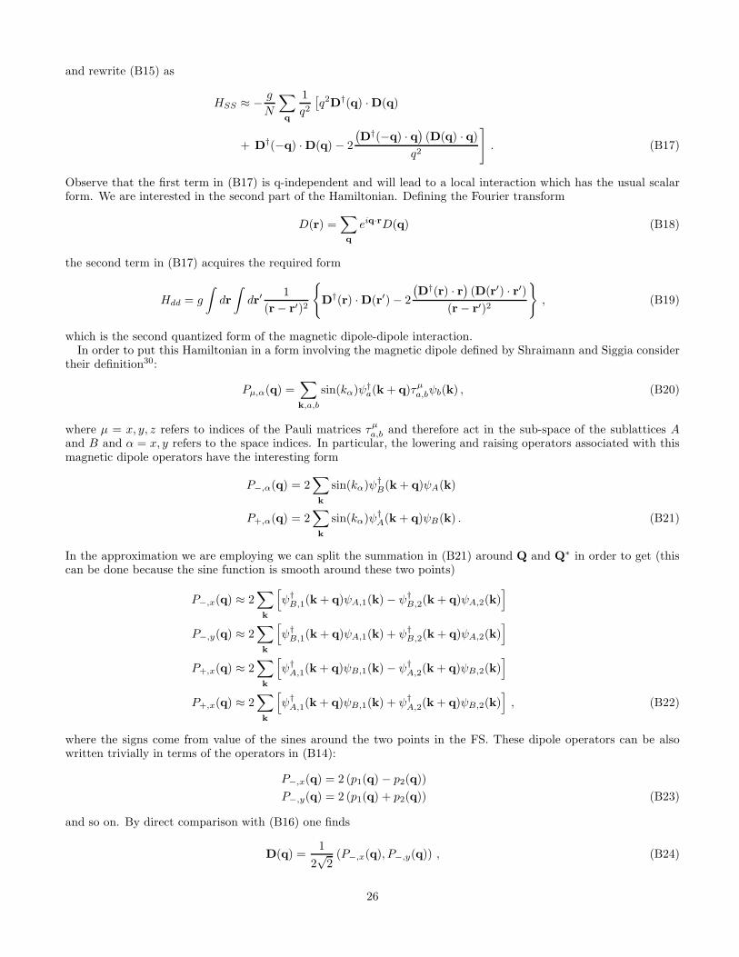
and rewrite (B15) as

HSS ≈ − g

N

∑

q

1

q2[

q2D†(q) ·D(q)

+ D†(−q) · D(q) − 2

(

D†(−q) · q)

(D(q) · q)

q2

]

. (B17)

Observe that the first term in (B17) is q-independent and will lead to a local interaction which has the usual scalarform. We are interested in the second part of the Hamiltonian. Defining the Fourier transform

D(r) =∑

q

eiq·rD(q) (B18)

the second term in (B17) acquires the required form

Hdd = g

∫

dr

∫

dr′1

(r − r′)2

{

D†(r) · D(r′) − 2

(

D†(r) · r)

(D(r′) · r′)(r − r′)2

}

, (B19)

which is the second quantized form of the magnetic dipole-dipole interaction.In order to put this Hamiltonian in a form involving the magnetic dipole defined by Shraimann and Siggia consider

their definition30:

Pµ,α(q) =∑

k,a,b

sin(kα)ψ†a(k + q)τµ

a,bψb(k) , (B20)

where µ = x, y, z refers to indices of the Pauli matrices τµa,b and therefore act in the sub-space of the sublattices A

and B and α = x, y refers to the space indices. In particular, the lowering and raising operators associated with thismagnetic dipole operators have the interesting form

P−,α(q) = 2∑

k

sin(kα)ψ†B(k + q)ψA(k)

P+,α(q) = 2∑

k

sin(kα)ψ†A(k + q)ψB(k) . (B21)

In the approximation we are employing we can split the summation in (B21) around Q and Q∗ in order to get (thiscan be done because the sine function is smooth around these two points)

P−,x(q) ≈ 2∑

k

[

ψ†B,1(k + q)ψA,1(k) − ψ†

B,2(k + q)ψA,2(k)]

P−,y(q) ≈ 2∑

k

[

ψ†B,1(k + q)ψA,1(k) + ψ†

B,2(k + q)ψA,2(k)]

P+,x(q) ≈ 2∑

k

[

ψ†A,1(k + q)ψB,1(k) − ψ†

A,2(k + q)ψB,2(k)]

P+,x(q) ≈ 2∑

k

[

ψ†A,1(k + q)ψB,1(k) + ψ†

A,2(k + q)ψB,2(k)]

, (B22)

where the signs come from value of the sines around the two points in the FS. These dipole operators can be alsowritten trivially in terms of the operators in (B14):

P−,x(q) = 2 (p1(q) − p2(q))

P−,y(q) = 2 (p1(q) + p2(q)) (B23)

and so on. By direct comparison with (B16) one finds

D(q) =1

2√

2(P−,x(q), P−,y(q)) , (B24)

26

which makes clear the connection. On taking the Fourier transform of the magnetic dipole operators back to realspace one finds, for instance,

Dx,i =1√2

(

ψ†B,1,iψA,1,i − ψ†

B,2,iψA,2,i

)

Dy,i =1√2

(

ψ†B,1,iψA,1,i + ψ†

B,2,iψA,2,i

)

. (B25)

This explicitely justifies our earlier claim that the dipolar interaction is due to the coherent hoping of holes betweentwo different sublattices (at the same position in space).

27