Calibration of the PA6 Short-Fiber Reinforced Material Model ...

Citation: Kurkin, E.; Spirina, M.;

Espinosa Barcenas, O.U.; Kurkina, E.

Calibration of the PA6 Short-Fiber

Reinforced Material Model for 10% to

30% Carbon Mass Fraction

Mechanical Characteristic Prediction.

Polymers 2022, 14, 1781. https://

doi.org/10.3390/polym14091781

Academic Editor: Ana

María Díez-Pascual

Received: 31 March 2022

Accepted: 22 April 2022

Published: 27 April 2022

Publisher’s Note: MDPI stays neutral

with regard to jurisdictional claims in

published maps and institutional affil-

iations.

Copyright: © 2022 by the authors.

Licensee MDPI, Basel, Switzerland.

This article is an open access article

distributed under the terms and

conditions of the Creative Commons

Attribution (CC BY) license (https://

creativecommons.org/licenses/by/

4.0/).

polymers

Article

Calibration of the PA6 Short-Fiber Reinforced Material Modelfor 10% to 30% Carbon Mass Fraction MechanicalCharacteristic PredictionEvgenii Kurkin * , Mariia Spirina, Oscar Ulises Espinosa Barcenas and Ekaterina Kurkina

Joint Russian-Slovenian Laboratory Composite Materials and Structures, Samara National Research University,34 Moskovskoe Shosse, Samara 443086, Russia; [email protected] (M.S.);[email protected] (O.U.E.B.); [email protected] (E.K.)* Correspondence: [email protected]; Tel.: +7-960-831-9009

Abstract: Short-fiber reinforced composites are widely used for the mass production of high-resistanceproducts with complex shapes. Efficient structural design requires consideration of plasticity andanisotropy. This paper presents a method for the calibration of a general material model for stress–strain curve prediction for short-fiber reinforced composites with different fiber mass fractions.A Mori–Tanaka homogenization scheme and the J2 plasticity model with layered defined fiberorientation were used. The hardening laws: power, exponential, and exponential and linear werecompared. The models were calibrated using experimental results for melt front, orientation tensoranalysis, fiber length, and diameter and tension according to ISO 527-2, for samples of PA6 whichwere either non-reinforced, or reinforced with 10%, 15%, 20%, and 30% carbon fiber mass fractions.The novelty of this study lies in the transition from the strain–stress space to the strain–stress–fiberfraction space in the approximation of the material model parameters. We found it necessary tosignificantly reduce the fiber aspect ratio for the correct prediction of the mechanical characteristicsof a composite using the Mori–Tanaka scheme. This deviation was caused by the ideal solution ofellipsoidal inclusion in this homogenization scheme. The calculated strength limits using Tsai–Hillfailure criteria, based on strain, could be used as a first approximation for failure prediction.

Keywords: composite; mechanical characteristics; material model; short fibers; polyamide 6; fibermass fraction

1. Introduction

Reinforced polyamide 6 (PA6), like many other reinforced thermoplastics, has foundapplications in durable goods, computer hardware, biomedical, automobile, and aerospacesectors [1–4]. For example, in the aerospace industry, short-fiber reinforced thermoplasticshave been utilized in several components of A340-600 and C295 [5], A350 XWB [6], and V-22tilt-rotor aircraft [7]. Reinforced thermoplastics are of interest for their high performancein structural applications, low-cost manufacturing process, ease of manipulation [1], andability to meet waste and recycling regulations [8–10]. However, the difficulty of predictingthe anisotropy throughout the design process leads to their implementation in secondarycomponents more than in primary structures [11,12]. For example, accounting for the effectof anisotropy on the mechanical behavior of the components [13–18] requires knowledgeof both the fiber length distribution and the fiber orientation distribution, which depend onthe fiber content, the geometry of the mold, the processing conditions, and the injectiongate [19,20].

Currently, anisotropy is considered in structural analysis by implementing a solutionto the inclusion problem by introducing Eshelby’s tensor [21], and a micromechanicalmethod such as the Mori–Tanaka model for predicting the effective properties of two-phasecomposites [22]. Contemporary investigation has focused on the mechanical behavior

Polymers 2022, 14, 1781. https://doi.org/10.3390/polym14091781 https://www.mdpi.com/journal/polymers

https://doi.org/10.3390/polym14091781


https://creativecommons.org/

https://creativecommons.org/licenses/by/4.0/

https://creativecommons.org/licenses/by/4.0/

https://www.mdpi.com/journal/polymers

https://www.mdpi.com

https://orcid.org/0000-0002-0893-9878

https://orcid.org/0000-0001-6538-7283


https://www.mdpi.com/journal/polymers

https://www.mdpi.com/article/10.3390/polym14091781?type=check_update&version=2

Polymers 2022, 14, 1781 2 of 20

of short-fiber reinforced polymers (SFRP) with high fiber volume fractions [15,16], andthe theory presented by Fu. S.-Y. on modeling SFRP [13,14] provides evidence of theimportance of studying the influence of the fiber content on the mechanical characteristicsof the polymers [23]. Furthermore, creating a more precise short-fiber model is a relevanttopic that has been addressed by [24,25]. Although these studies increase the reliability ofmodeling for anisotropy, data for SFRP are generally provided for a specific fiber volumefraction, which limits the material model. Hence, selecting the material in the early stagesof design requires the usage of an accurate material model with the ability to adjust thefiber weight fraction.

This study presents a general material model for PA6 reinforced with different fibermass fractions. To create the model, experimental studies were conducted using PA6reinforced with different short carbon fiber weight fractions. The results of the experimentswere used to obtain the mechanical characteristics as well as the fiber length and fiberorientation distributions, which were subsequently used for modeling the material using asecond-order Mori–Tanaka homogenization scheme and three different hardening laws.The material models obtained are presented alongside their calibration data, which wereobtained by applying curve fitting through optimization of the material parameters.

2. Materials and Methods

The creation of a composite material model requires knowledge of the mechanicalcharacteristics of its components. We started by obtaining the mechanical characteristicsof non-reinforced PA6 using a tensile test. The fiber aspect ratio was then determined byburning a sample of reinforced PA6. The unidirectional short-fiber reinforced compositewas modeled as a transversely isotropic material by application of the Mori–Tanaka ho-mogenization scheme. Tucker’s procedure was applied to transform the material from aunidirectional transversely isotropic one into a composite, which depended on the fiberorientation. We assumed that the stress and strain of the composite depend on its per-centage content fractions. The plasticity of the matrix was modeled using the J2 plasticitymodel. The following three different laws were used to model hardening: the power, theexponential, and the exponential and linear laws.

2.1. Plate Molding Experiment

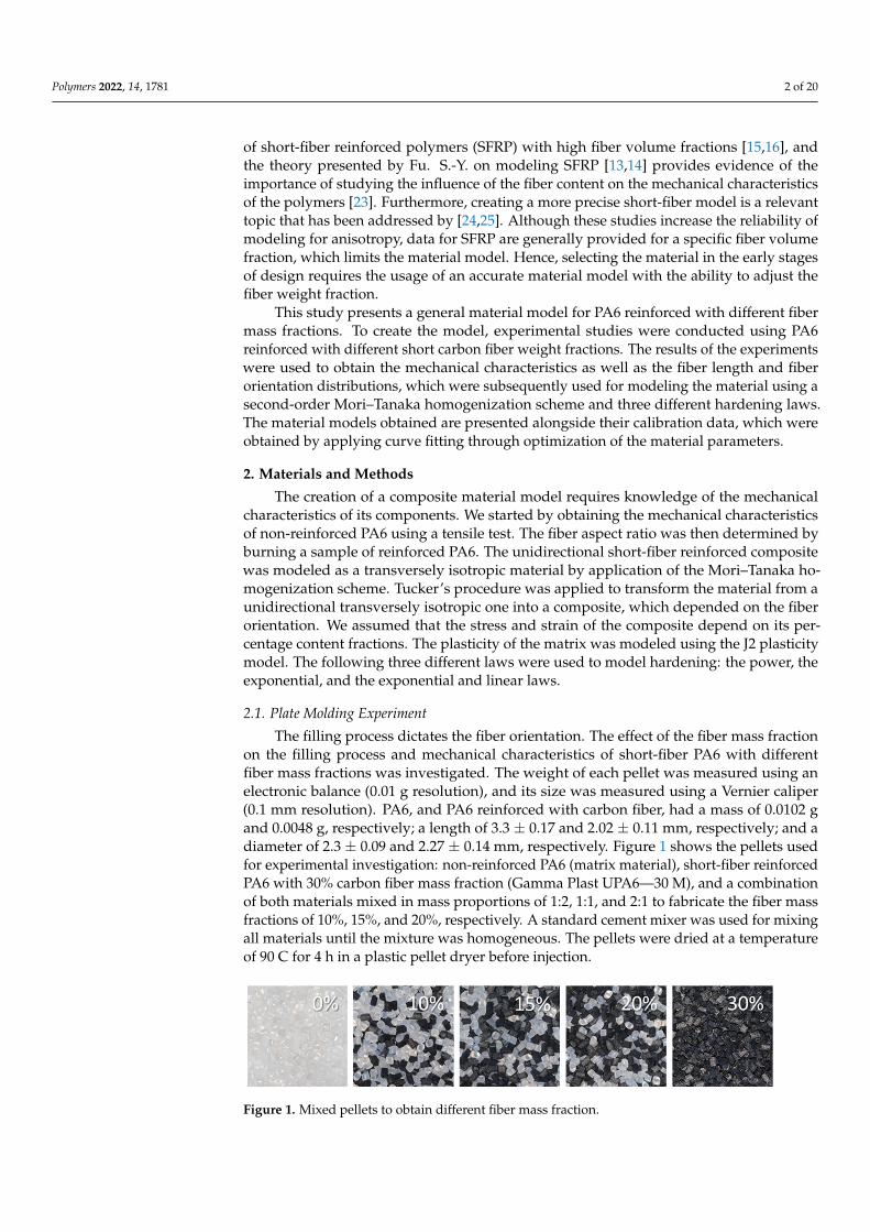
The filling process dictates the fiber orientation. The effect of the fiber mass fractionon the filling process and mechanical characteristics of short-fiber PA6 with differentfiber mass fractions was investigated. The weight of each pellet was measured using anelectronic balance (0.01 g resolution), and its size was measured using a Vernier caliper(0.1 mm resolution). PA6, and PA6 reinforced with carbon fiber, had a mass of 0.0102 gand 0.0048 g, respectively; a length of 3.3 ± 0.17 and 2.02 ± 0.11 mm, respectively; and adiameter of 2.3 ± 0.09 and 2.27 ± 0.14 mm, respectively. Figure 1 shows the pellets usedfor experimental investigation: non-reinforced PA6 (matrix material), short-fiber reinforcedPA6 with 30% carbon fiber mass fraction (Gamma Plast UPA6—30 M), and a combinationof both materials mixed in mass proportions of 1:2, 1:1, and 2:1 to fabricate the fiber massfractions of 10%, 15%, and 20%, respectively. A standard cement mixer was used for mixingall materials until the mixture was homogeneous. The pellets were dried at a temperatureof 90 C for 4 h in a plastic pellet dryer before injection.

Polymers 2022, 14, x FOR PEER REVIEW 2 of 20

phase composites [22]. Contemporary investigation has focused on the mechanical behav-ior of short-fiber reinforced polymers (SFRP) with high fiber volume fractions [15,16], and the theory presented by Fu. S.-Y. on modeling SFRP [13,14] provides evidence of the im-portance of studying the influence of the fiber content on the mechanical characteristics of the polymers [23]. Furthermore, creating a more precise short-fiber model is a relevant topic that has been addressed by [24,25]. Although these studies increase the reliability of modeling for anisotropy, data for SFRP are generally provided for a specific fiber volume fraction, which limits the material model. Hence, selecting the material in the early stages of design requires the usage of an accurate material model with the ability to adjust the fiber weight fraction.

This study presents a general material model for PA6 reinforced with different fiber mass fractions. To create the model, experimental studies were conducted using PA6 re-inforced with different short carbon fiber weight fractions. The results of the experiments were used to obtain the mechanical characteristics as well as the fiber length and fiber orientation distributions, which were subsequently used for modeling the material using a second-order Mori–Tanaka homogenization scheme and three different hardening laws. The material models obtained are presented alongside their calibration data, which were obtained by applying curve fitting through optimization of the material parameters.

2. Materials and Methods The creation of a composite material model requires knowledge of the mechanical

characteristics of its components. We started by obtaining the mechanical characteristics of non-reinforced PA6 using a tensile test. The fiber aspect ratio was then determined by burning a sample of reinforced PA6. The unidirectional short-fiber reinforced composite was modeled as a transversely isotropic material by application of the Mori–Tanaka ho-mogenization scheme. Tucker’s procedure was applied to transform the material from a unidirectional transversely isotropic one into a composite, which depended on the fiber orientation. We assumed that the stress and strain of the composite depend on its percent-age content fractions. The plasticity of the matrix was modeled using the J2 plasticity model. The following three different laws were used to model hardening: the power, the exponential, and the exponential and linear laws.

2.1. Plate Molding Experiment The filling process dictates the fiber orientation. The effect of the fiber mass fraction

on the filling process and mechanical characteristics of short-fiber PA6 with different fiber mass fractions was investigated. The weight of each pellet was measured using an elec-tronic balance (0.01 g resolution), and its size was measured using a Vernier caliper (0.1 mm resolution). PA6, and PA6 reinforced with carbon fiber, had a mass of 0.0102 g and 0.0048 g, respectively; a length of 3.3 ± 0.17 and 2.02 ± 0.11 mm, respectively; and a diam-eter of 2.3 ± 0.09 and 2.27 ± 0.14 mm, respectively. Figure 1 shows the pellets used for experimental investigation: non-reinforced PA6 (matrix material), short-fiber reinforced PA6 with 30% carbon fiber mass fraction (Gamma Plast UPA6—30 M), and a combination of both materials mixed in mass proportions of 1:2, 1:1, and 2:1 to fabricate the fiber mass fractions of 10%, 15%, and 20%, respectively. A standard cement mixer was used for mix-ing all materials until the mixture was homogeneous. The pellets were dried at a temper-ature of 90 C for 4 h in a plastic pellet dryer before injection.

Figure 1. Mixed pellets to obtain different fiber mass fraction. Figure 1. Mixed pellets to obtain different fiber mass fraction.

Polymers 2022, 14, 1781 3 of 20

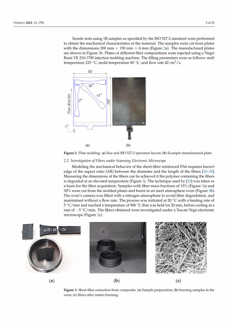
Tensile tests using 1B samples as specified by the ISO 527-2 standard were performedto obtain the mechanical characteristics of the material. The samples were cut from plateswith the dimensions 200 mm × 150 mm × 4 mm (Figure 2a). The manufactured platesare shown in Figure 2b. Plates of different fiber compositions were injected using a NegriBossi VE 210-1700 injection molding machine. The filling parameters were as follows: melttemperature 225 ◦C, mold temperature 80 ◦C, and flow rate 42 cm3/s.


Tensile tests using 1B samples as specified by the ISO 527-2 standard were performed to obtain the mechanical characteristics of the material. The samples were cut from plates with the dimensions 200 mm × 150 mm × 4 mm (Figure 2a). The manufactured plates are shown in Figure 2b. Plates of different fiber compositions were injected using a Negri Bossi VE 210-1700 injection molding machine. The filling parameters were as follows: melt temperature 225 °C, mold temperature 80 °C, and flow rate 42 cm3/s.

Figure 2. Plate molding: (a) Size and ISO 527-2 specimen layout; (b) Example manufactured plate.

2.2. Investigation of Fibers under Scanning Electronic Microscope Modeling the mechanical behavior of the short-fiber reinforced PA6 requires

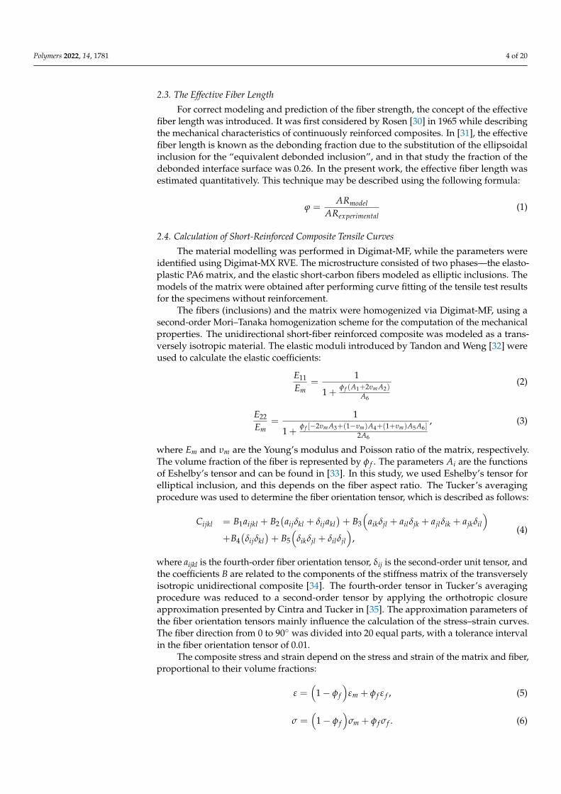
knowledge of the aspect ratio (AR) between the diameter and the length of the fibers [26–28]. Measuring the dimensions of the fibers can be achieved if the polymer containing the fibers is degraded at an elevated temperature (Figure 3). The technique used by [29] was taken as a basis for the fiber acquisition. Samples with fiber mass fractions of 15% (Figure 3a) and 30% were cut from the molded plates and burnt in an inert atmosphere oven (Fig-ure 3b). The oven’s camera was filled with a nitrogen atmosphere to avoid fiber degrada-tion, and maintained without a flow rate. The process was initiated at 20 °C with a heating rate of 5 C/min and reached a temperature of 900 °C that was held for 20 min, before cooling at a rate of −5 °C/min. The fibers obtained were investigated under a Tescan Vega electronic microscope (Figure 3c).

Figure 3. Short fiber extraction from composite: (a) Sample preparation; (b) burning samples in the oven; (c) fibers after matrix burning.


2.2. Investigation of Fibers under Scanning Electronic Microscope

Modeling the mechanical behavior of the short-fiber reinforced PA6 requires knowl-edge of the aspect ratio (AR) between the diameter and the length of the fibers [26–28].Measuring the dimensions of the fibers can be achieved if the polymer containing the fibersis degraded at an elevated temperature (Figure 3). The technique used by [29] was taken asa basis for the fiber acquisition. Samples with fiber mass fractions of 15% (Figure 3a) and30% were cut from the molded plates and burnt in an inert atmosphere oven (Figure 3b).The oven’s camera was filled with a nitrogen atmosphere to avoid fiber degradation, andmaintained without a flow rate. The process was initiated at 20 ◦C with a heating rate of5 ◦C/min and reached a temperature of 900 ◦C that was held for 20 min, before cooling at arate of −5 ◦C/min. The fibers obtained were investigated under a Tescan Vega electronicmicroscope (Figure 3c).


Tensile tests using 1B samples as specified by the ISO 527-2 standard were performed to obtain the mechanical characteristics of the material. The samples were cut from plates with the dimensions 200 mm × 150 mm × 4 mm (Figure 2a). The manufactured plates are shown in Figure 2b. Plates of different fiber compositions were injected using a Negri Bossi VE 210-1700 injection molding machine. The filling parameters were as follows: melt temperature 225 °C, mold temperature 80 °C, and flow rate 42 cm3/s.


2.2. Investigation of Fibers under Scanning Electronic Microscope Modeling the mechanical behavior of the short-fiber reinforced PA6 requires

knowledge of the aspect ratio (AR) between the diameter and the length of the fibers [26–28]. Measuring the dimensions of the fibers can be achieved if the polymer containing the fibers is degraded at an elevated temperature (Figure 3). The technique used by [29] was taken as a basis for the fiber acquisition. Samples with fiber mass fractions of 15% (Figure 3a) and 30% were cut from the molded plates and burnt in an inert atmosphere oven (Fig-ure 3b). The oven’s camera was filled with a nitrogen atmosphere to avoid fiber degrada-tion, and maintained without a flow rate. The process was initiated at 20 °C with a heating rate of 5 C/min and reached a temperature of 900 °C that was held for 20 min, before cooling at a rate of −5 °C/min. The fibers obtained were investigated under a Tescan Vega electronic microscope (Figure 3c).

Figure 3. Short fiber extraction from composite: (a) Sample preparation; (b) burning samples in the oven; (c) fibers after matrix burning. Figure 3. Short fiber extraction from composite: (a) Sample preparation; (b) burning samples in theoven; (c) fibers after matrix burning.

Polymers 2022, 14, 1781 4 of 20

2.3. The Effective Fiber Length

For correct modeling and prediction of the fiber strength, the concept of the effectivefiber length was introduced. It was first considered by Rosen [30] in 1965 while describingthe mechanical characteristics of continuously reinforced composites. In [31], the effectivefiber length is known as the debonding fraction due to the substitution of the ellipsoidalinclusion for the “equivalent debonded inclusion”, and in that study the fraction of thedebonded interface surface was 0.26. In the present work, the effective fiber length wasestimated quantitatively. This technique may be described using the following formula:

ϕ =ARmodel

ARexperimental(1)

2.4. Calculation of Short-Reinforced Composite Tensile Curves

The material modelling was performed in Digimat-MF, while the parameters wereidentified using Digimat-MX RVE. The microstructure consisted of two phases—the elasto-plastic PA6 matrix, and the elastic short-carbon fibers modeled as elliptic inclusions. Themodels of the matrix were obtained after performing curve fitting of the tensile test resultsfor the specimens without reinforcement.

The fibers (inclusions) and the matrix were homogenized via Digimat-MF, using asecond-order Mori–Tanaka homogenization scheme for the computation of the mechanicalproperties. The unidirectional short-fiber reinforced composite was modeled as a trans-versely isotropic material. The elastic moduli introduced by Tandon and Weng [32] wereused to calculate the elastic coefficients:

E11

Em=

1

1 +φ f (A1+2υm A2)

A6

(2)

E22

Em=

1

1 +φ f [−2υm A3+(1−υm)A4+(1+υm)A5 A6]

2A6

, (3)

where Em and υm are the Young’s modulus and Poisson ratio of the matrix, respectively.The volume fraction of the fiber is represented by φ f . The parameters Ai are the functionsof Eshelby’s tensor and can be found in [33]. In this study, we used Eshelby’s tensor forelliptical inclusion, and this depends on the fiber aspect ratio. The Tucker’s averagingprocedure was used to determine the fiber orientation tensor, which is described as follows:

Cijkl = B1aijkl + B2(aijδkl + δijakl

)+ B3

(aikδjl + ailδjk + ajlδik + ajkδil

)+B4

(δijδkl

)+ B5

(δikδjl + δilδjl

),

(4)

where aijkl is the fourth-order fiber orientation tensor, δij is the second-order unit tensor, andthe coefficients B are related to the components of the stiffness matrix of the transverselyisotropic unidirectional composite [34]. The fourth-order tensor in Tucker’s averagingprocedure was reduced to a second-order tensor by applying the orthotropic closureapproximation presented by Cintra and Tucker in [35]. The approximation parameters ofthe fiber orientation tensors mainly influence the calculation of the stress–strain curves.The fiber direction from 0 to 90◦ was divided into 20 equal parts, with a tolerance intervalin the fiber orientation tensor of 0.01.

The composite stress and strain depend on the stress and strain of the matrix and fiber,proportional to their volume fractions:

ε =(

1 − φ f

)εm + φ f ε f , (5)

σ =(

1 − φ f

)σm + φ f σf . (6)

Polymers 2022, 14, 1781 5 of 20

The stress–strain state of the matrix is described using the J2 plasticity model [36],based on the von Mises equivalent stress, σeq. When σeq exceeds the initial yield stress, theresponse becomes nonlinear and plastic deformation appears. Plastic strength is expressedas follows:

σeq = σY + R(εp), (7)

where σY is the initial yield stress; R(εp)

is the isotropic strain hardening function; and εpis the accumulated plastic strain.

Poisson’s ratio of the matrix, in the plastic range, is predicted through Lame parametersusing spectral decomposition [37]; elastic bulk module K is taken as a constant, and shearmoduli G will be

G = Ge

1 − 3Ge

3Ge +d R(εp)

d εp

, (8)

where Ge, the elastic shear modulus, is defined using a Lame parameter, based on the givenYoung’s modulus and the Poisson’s ratio of the matrix in the elastic range.

For all models so described, the matrix Poisson’s ratio in the elastic range is equal to theexperimentally measured average value. Poisson’s ratio of the matrix in the elastic rangehad a slight effect on the stress–strain curves for reinforced PA6 when reverse-engineeringthe curves, and was not accurate, therefore, Poisson’s ratio of the matrix in the elastic rangewas excluded from the reverse-engineered parameters.

A comparison between the three hardening stress functions is provided in [38]:

• Power law [39]:R(εp)= kεp

m; (9)

• Exponential law:R(εp)= R∞

[1 − e−mεp

]; (10)

• Exponential and linear law:

R(εp)= kεp + R∞

[1 − e−mεp

]. (11)

where k is linear hardening modulus, MPa; m is hardening exponent; and R∞ ishardening modulus, MPa.

3. Results3.1. Melt Front and Microstucture Experimental Investigation

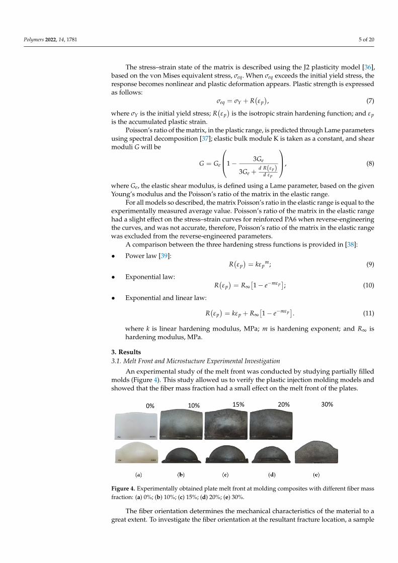
An experimental study of the melt front was conducted by studying partially filledmolds (Figure 4). This study allowed us to verify the plastic injection molding models andshowed that the fiber mass fraction had a small effect on the melt front of the plates.


The stress–strain state of the matrix is described using the J2 plasticity model [36], based on the von Mises equivalent stress, . When exceeds the initial yield stress, the response becomes nonlinear and plastic deformation appears. Plastic strength is ex-pressed as follows: = + , (7)

where is the initial yield stress; ( ) is the isotropic strain hardening function; and is the accumulated plastic strain.

Poisson’s ratio of the matrix, in the plastic range, is predicted through Lame param-eters using spectral decomposition [37]; elastic bulk module K is taken as a constant, and shear moduli G will be

= 1 − 33 + , (8)

where Ge, the elastic shear modulus, is defined using a Lame parameter, based on the given Young’s modulus and the Poisson’s ratio of the matrix in the elastic range.

For all models so described, the matrix Poisson’s ratio in the elastic range is equal to the experimentally measured average value. Poisson’s ratio of the matrix in the elastic range had a slight effect on the stress–strain curves for reinforced PA6 when reverse-en-gineering the curves, and was not accurate, therefore, Poisson’s ratio of the matrix in the elastic range was excluded from the reverse-engineered parameters.

A comparison between the three hardening stress functions is provided in [38]: • Power law [39]: = ; (9)

• Exponential law: = 1 − ; (10)

• Exponential and linear law: = + 1 − . (11)

where is linear hardening modulus, MPa; m is hardening exponent; and is harden-ing modulus, MPa.

3. Results 3.1. Melt Front and Microstucture Experimental Investigation

An experimental study of the melt front was conducted by studying partially filled molds (Figure 4). This study allowed us to verify the plastic injection molding models and showed that the fiber mass fraction had a small effect on the melt front of the plates.

Figure 4. Experimentally obtained plate melt front at molding composites with different fiber mass fraction: (a) 0%; (b) 10%; (c) 15%; (d) 20%; (e) 30%.

Figure 4. Experimentally obtained plate melt front at molding composites with different fiber massfraction: (a) 0%; (b) 10%; (c) 15%; (d) 20%; (e) 30%.

The fiber orientation determines the mechanical characteristics of the material to agreat extent. To investigate the fiber orientation at the resultant fracture location, a sample

Polymers 2022, 14, 1781 6 of 20

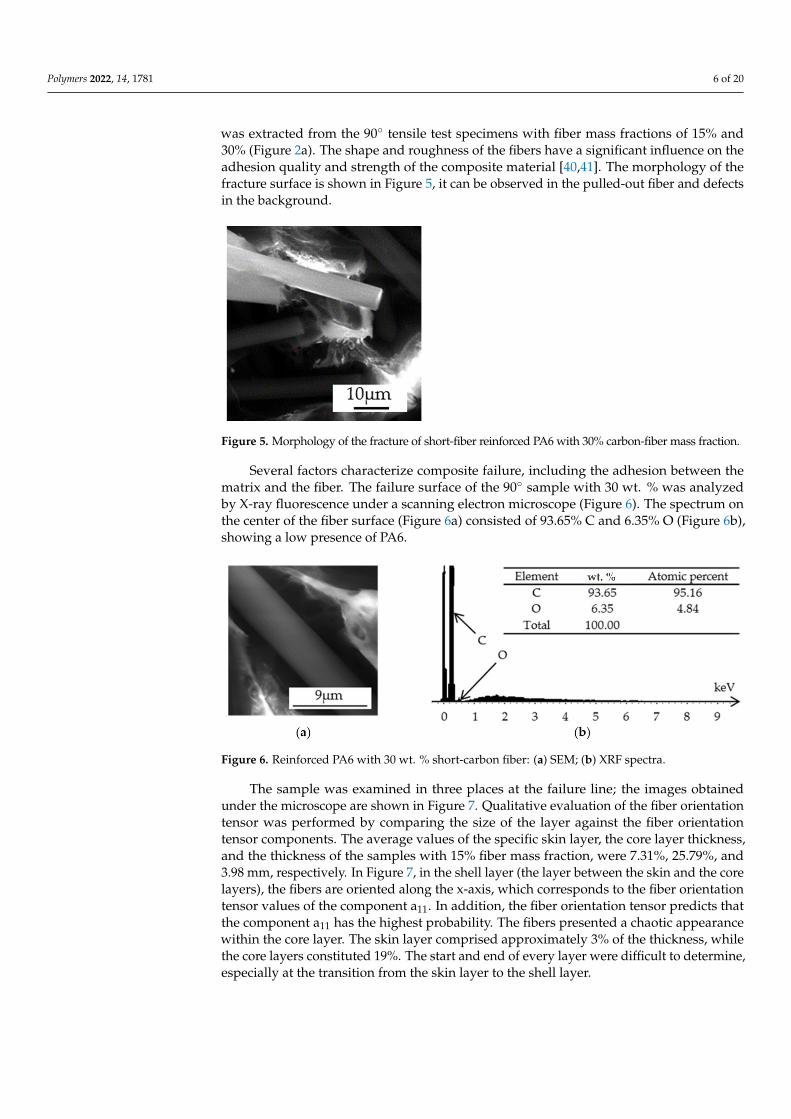
was extracted from the 90◦ tensile test specimens with fiber mass fractions of 15% and30% (Figure 2a). The shape and roughness of the fibers have a significant influence on theadhesion quality and strength of the composite material [40,41]. The morphology of thefracture surface is shown in Figure 5, it can be observed in the pulled-out fiber and defectsin the background.


The fiber orientation determines the mechanical characteristics of the material to a great extent. To investigate the fiber orientation at the resultant fracture location, a sample was extracted from the 90° tensile test specimens with fiber mass fractions of 15% and 30% (Figure 2a). The shape and roughness of the fibers have a significant influence on the ad-hesion quality and strength of the composite material [40,41]. The morphology of the frac-ture surface is shown in Figure 5, it can be observed in the pulled-out fiber and defects in the background.

Figure 5. Morphology of the fracture of short-fiber reinforced PA6 with 30% carbon-fiber mass frac-tion.

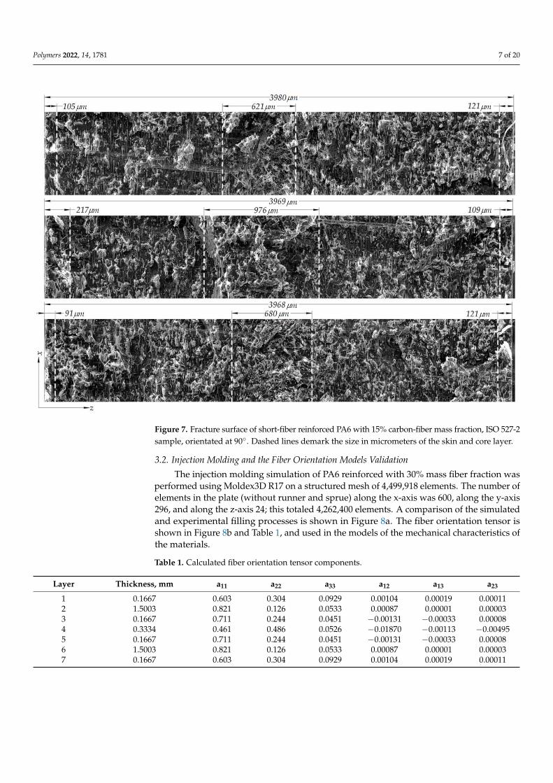
Several factors characterize composite failure, including the adhesion between the matrix and the fiber. The failure surface of the 90° sample with 30 wt. % was analyzed by X-ray fluorescence under a scanning electron microscope (Figure 6). The spectrum on the center of the fiber surface (Figure 6a) consisted of 93.65% C and 6.35% O (Figure 6b), show-ing a low presence of PA6.

Figure 6. Reinforced PA6 with 30 wt. % short-carbon fiber: (a) SEM; (b) XRF spectra.

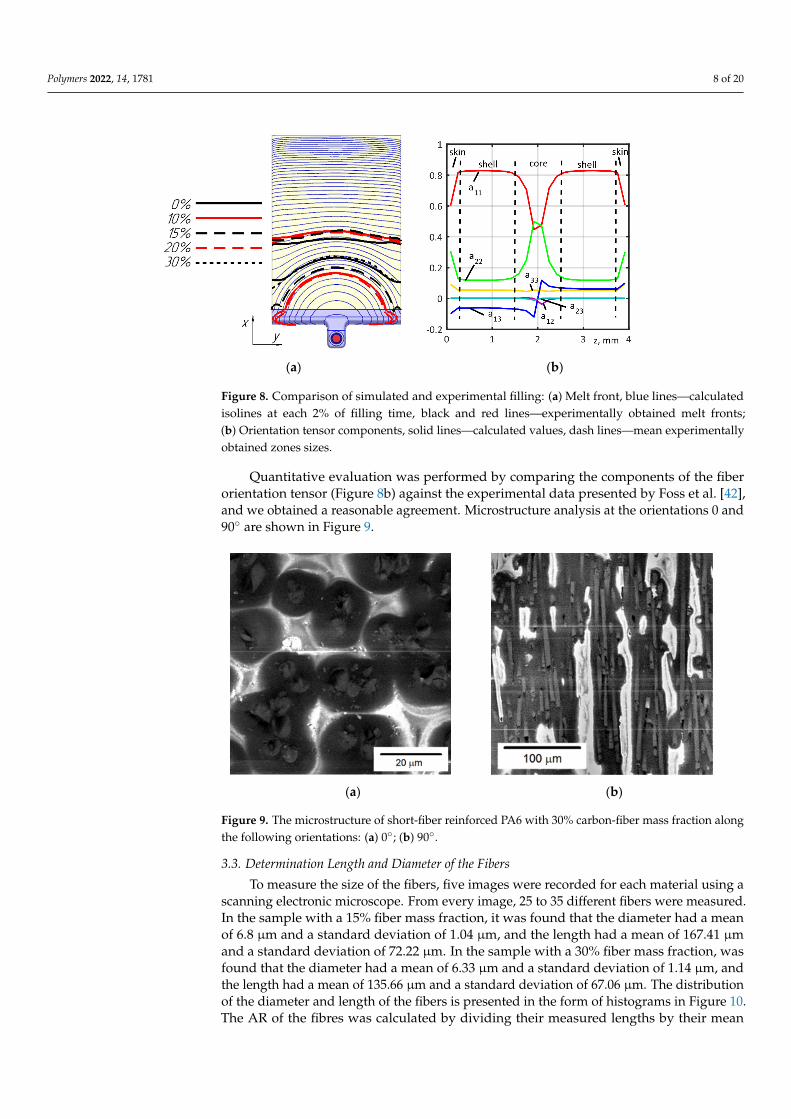
The sample was examined in three places at the failure line; the images obtained un-der the microscope are shown in Figure 7. Qualitative evaluation of the fiber orientation tensor was performed by comparing the size of the layer against the fiber orientation ten-sor components. The average values of the specific skin layer, the core layer thickness, and the thickness of the samples with 15% fiber mass fraction, were 7.31%, 25.79%, and 3.98 mm, respectively. In Figure 7, in the shell layer (the layer between the skin and the core layers), the fibers are oriented along the x-axis, which corresponds to the fiber orientation tensor values of the component a11. In addition, the fiber orientation tensor predicts that the component a11 has the highest probability. The fibers presented a chaotic appearance within the core layer. The skin layer comprised approximately 3% of the thickness, while the core layers constituted 19%. The start and end of every layer were difficult to deter-mine, especially at the transition from the skin layer to the shell layer.

Figure 5. Morphology of the fracture of short-fiber reinforced PA6 with 30% carbon-fiber mass fraction.

Several factors characterize composite failure, including the adhesion between thematrix and the fiber. The failure surface of the 90◦ sample with 30 wt. % was analyzedby X-ray fluorescence under a scanning electron microscope (Figure 6). The spectrum onthe center of the fiber surface (Figure 6a) consisted of 93.65% C and 6.35% O (Figure 6b),showing a low presence of PA6.


The fiber orientation determines the mechanical characteristics of the material to a great extent. To investigate the fiber orientation at the resultant fracture location, a sample was extracted from the 90° tensile test specimens with fiber mass fractions of 15% and 30% (Figure 2a). The shape and roughness of the fibers have a significant influence on the ad-hesion quality and strength of the composite material [40,41]. The morphology of the frac-ture surface is shown in Figure 5, it can be observed in the pulled-out fiber and defects in the background.

Figure 5. Morphology of the fracture of short-fiber reinforced PA6 with 30% carbon-fiber mass frac-tion.

Several factors characterize composite failure, including the adhesion between the matrix and the fiber. The failure surface of the 90° sample with 30 wt. % was analyzed by X-ray fluorescence under a scanning electron microscope (Figure 6). The spectrum on the center of the fiber surface (Figure 6a) consisted of 93.65% C and 6.35% O (Figure 6b), show-ing a low presence of PA6.


The sample was examined in three places at the failure line; the images obtained un-der the microscope are shown in Figure 7. Qualitative evaluation of the fiber orientation tensor was performed by comparing the size of the layer against the fiber orientation ten-sor components. The average values of the specific skin layer, the core layer thickness, and the thickness of the samples with 15% fiber mass fraction, were 7.31%, 25.79%, and 3.98 mm, respectively. In Figure 7, in the shell layer (the layer between the skin and the core layers), the fibers are oriented along the x-axis, which corresponds to the fiber orientation tensor values of the component a11. In addition, the fiber orientation tensor predicts that the component a11 has the highest probability. The fibers presented a chaotic appearance within the core layer. The skin layer comprised approximately 3% of the thickness, while the core layers constituted 19%. The start and end of every layer were difficult to deter-mine, especially at the transition from the skin layer to the shell layer.


The sample was examined in three places at the failure line; the images obtainedunder the microscope are shown in Figure 7. Qualitative evaluation of the fiber orientationtensor was performed by comparing the size of the layer against the fiber orientationtensor components. The average values of the specific skin layer, the core layer thickness,and the thickness of the samples with 15% fiber mass fraction, were 7.31%, 25.79%, and3.98 mm, respectively. In Figure 7, in the shell layer (the layer between the skin and the corelayers), the fibers are oriented along the x-axis, which corresponds to the fiber orientationtensor values of the component a11. In addition, the fiber orientation tensor predicts thatthe component a11 has the highest probability. The fibers presented a chaotic appearancewithin the core layer. The skin layer comprised approximately 3% of the thickness, whilethe core layers constituted 19%. The start and end of every layer were difficult to determine,especially at the transition from the skin layer to the shell layer.

Polymers 2022, 14, 1781 7 of 20Polymers 2022, 14, x FOR PEER REVIEW 7 of 20

Figure 7. Fracture surface of short-fiber reinforced PA6 with 15% carbon-fiber mass fraction, ISO 527-2 sample, orientated at 90°. Dashed lines demark the size in micrometers of the skin and core layer.

3.2. Injection Molding and the Fiber Orientation Models Validation The injection molding simulation of PA6 reinforced with 30% mass fiber fraction was

performed using Moldex3D R17 on a structured mesh of 4,499,918 elements. The number of elements in the plate (without runner and sprue) along the x-axis was 600, along the y-axis 296, and along the z-axis 24; this totaled 4,262,400 elements. A comparison of the simulated and experimental filling processes is shown in Figure 8a. The fiber orientation tensor is shown in Figure 8b and Table 1, and used in the models of the mechanical characteristics of the materials.

Figure 7. Fracture surface of short-fiber reinforced PA6 with 15% carbon-fiber mass fraction, ISO 527-2sample, orientated at 90◦. Dashed lines demark the size in micrometers of the skin and core layer.

3.2. Injection Molding and the Fiber Orientation Models Validation

The injection molding simulation of PA6 reinforced with 30% mass fiber fraction wasperformed using Moldex3D R17 on a structured mesh of 4,499,918 elements. The number ofelements in the plate (without runner and sprue) along the x-axis was 600, along the y-axis296, and along the z-axis 24; this totaled 4,262,400 elements. A comparison of the simulatedand experimental filling processes is shown in Figure 8a. The fiber orientation tensor isshown in Figure 8b and Table 1, and used in the models of the mechanical characteristics ofthe materials.

Table 1. Calculated fiber orientation tensor components.

Layer Thickness, mm a11 a22 a33 a12 a13 a23

1 0.1667 0.603 0.304 0.0929 0.00104 0.00019 0.000112 1.5003 0.821 0.126 0.0533 0.00087 0.00001 0.000033 0.1667 0.711 0.244 0.0451 −0.00131 −0.00033 0.000084 0.3334 0.461 0.486 0.0526 −0.01870 −0.00113 −0.004955 0.1667 0.711 0.244 0.0451 −0.00131 −0.00033 0.000086 1.5003 0.821 0.126 0.0533 0.00087 0.00001 0.000037 0.1667 0.603 0.304 0.0929 0.00104 0.00019 0.00011

Polymers 2022, 14, 1781 8 of 20Polymers 2022, 14, x FOR PEER REVIEW 8 of 20

(a) (b)

Figure 8. Comparison of simulated and experimental filling: (a) Melt front, blue lines—calculated isolines at each 2% of filling time, black and red lines—experimentally obtained melt fronts; (b) Orientation tensor components, solid lines—calculated values, dash lines—mean experimentally obtained zones sizes.


Layer Thickness, mm a11 a22 a33 a12 a13 a23 1 0.1667 0.603 0.304 0.0929 0.00104 0.00019 0.00011 2 1.5003 0.821 0.126 0.0533 0.00087 0.00001 0.00003 3 0.1667 0.711 0.244 0.0451 −0.00131 −0.00033 0.00008 4 0.3334 0.461 0.486 0.0526 −0.01870 −0.00113 −0.00495 5 0.1667 0.711 0.244 0.0451 −0.00131 −0.00033 0.00008 6 1.5003 0.821 0.126 0.0533 0.00087 0.00001 0.00003 7 0.1667 0.603 0.304 0.0929 0.00104 0.00019 0.00011

Quantitative evaluation was performed by comparing the components of the fiber orientation tensor (Figure 8b) against the experimental data presented by Foss et al. [42], and we obtained a reasonable agreement. Microstructure analysis at the orientations 0 and 90° are shown in Figure 9.

(a) (b)

Figure 9. The microstructure of short-fiber reinforced PA6 with 30% carbon-fiber mass fraction along the following orientations: (a) 0°; (b) 90°.

Figure 8. Comparison of simulated and experimental filling: (a) Melt front, blue lines—calculatedisolines at each 2% of filling time, black and red lines—experimentally obtained melt fronts;(b) Orientation tensor components, solid lines—calculated values, dash lines—mean experimentallyobtained zones sizes.

Quantitative evaluation was performed by comparing the components of the fiberorientation tensor (Figure 8b) against the experimental data presented by Foss et al. [42],and we obtained a reasonable agreement. Microstructure analysis at the orientations 0 and90◦ are shown in Figure 9.


(a) (b)

Figure 8. Comparison of simulated and experimental filling: (a) Melt front, blue lines—calculated isolines at each 2% of filling time, black and red lines—experimentally obtained melt fronts; (b) Orientation tensor components, solid lines—calculated values, dash lines—mean experimentally obtained zones sizes.


Layer Thickness, mm a11 a22 a33 a12 a13 a23 1 0.1667 0.603 0.304 0.0929 0.00104 0.00019 0.00011 2 1.5003 0.821 0.126 0.0533 0.00087 0.00001 0.00003 3 0.1667 0.711 0.244 0.0451 −0.00131 −0.00033 0.00008 4 0.3334 0.461 0.486 0.0526 −0.01870 −0.00113 −0.00495 5 0.1667 0.711 0.244 0.0451 −0.00131 −0.00033 0.00008 6 1.5003 0.821 0.126 0.0533 0.00087 0.00001 0.00003 7 0.1667 0.603 0.304 0.0929 0.00104 0.00019 0.00011

Quantitative evaluation was performed by comparing the components of the fiber orientation tensor (Figure 8b) against the experimental data presented by Foss et al. [42], and we obtained a reasonable agreement. Microstructure analysis at the orientations 0 and 90° are shown in Figure 9.

(a) (b)

Figure 9. The microstructure of short-fiber reinforced PA6 with 30% carbon-fiber mass fraction along the following orientations: (a) 0°; (b) 90°. Figure 9. The microstructure of short-fiber reinforced PA6 with 30% carbon-fiber mass fraction alongthe following orientations: (a) 0◦; (b) 90◦.

3.3. Determination Length and Diameter of the Fibers

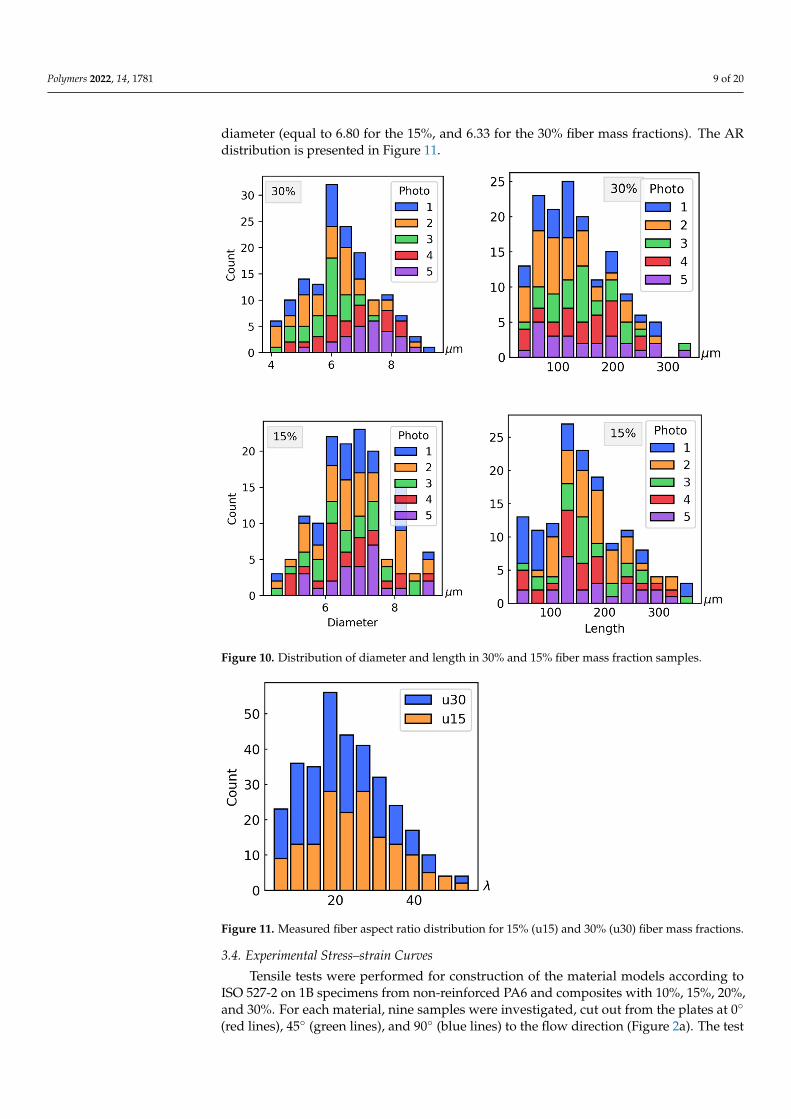
To measure the size of the fibers, five images were recorded for each material using ascanning electronic microscope. From every image, 25 to 35 different fibers were measured.In the sample with a 15% fiber mass fraction, it was found that the diameter had a meanof 6.8 µm and a standard deviation of 1.04 µm, and the length had a mean of 167.41 µmand a standard deviation of 72.22 µm. In the sample with a 30% fiber mass fraction, wasfound that the diameter had a mean of 6.33 µm and a standard deviation of 1.14 µm, andthe length had a mean of 135.66 µm and a standard deviation of 67.06 µm. The distributionof the diameter and length of the fibers is presented in the form of histograms in Figure 10.The AR of the fibres was calculated by dividing their measured lengths by their mean

Polymers 2022, 14, 1781 9 of 20

diameter (equal to 6.80 for the 15%, and 6.33 for the 30% fiber mass fractions). The ARdistribution is presented in Figure 11.


3.3. Determination Length and Diameter of the Fibers To measure the size of the fibers, five images were recorded for each material using

a scanning electronic microscope. From every image, 25 to 35 different fibers were meas-ured. In the sample with a 15% fiber mass fraction, it was found that the diameter had a mean of 6.8 μm and a standard deviation of 1.04 μm, and the length had a mean of 167.41 μm and a standard deviation of 72.22 μm. In the sample with a 30% fiber mass fraction, was found that the diameter had a mean of 6.33 μm and a standard deviation of 1.14 μm, and the length had a mean of 135.66 μm and a standard deviation of 67.06 μm. The distri-bution of the diameter and length of the fibers is presented in the form of histograms in Figure 10. The AR of the fibres was calculated by dividing their measured lengths by their mean diameter (equal to 6.80 for the 15%, and 6.33 for the 30% fiber mass fractions). The AR distribution is presented in Figure 11.

Figure 10. Distribution of diameter and length in 30% and 15% fiber mass fraction samples. Figure 10. Distribution of diameter and length in 30% and 15% fiber mass fraction samples.


Figure 11. Measured fiber aspect ratio distribution for 15% (u15) and 30% (u30) fiber mass fractions.

3.4. Experimental Stress–strain Curves Tensile tests were performed for construction of the material models according to

ISO 527-2 on 1B specimens from non-reinforced PA6 and composites with 10%, 15%, 20%, and 30%. For each material, nine samples were investigated, cut out from the plates at 0° (red lines), 45° (green lines), and 90° (blue lines) to the flow direction (Figure 2a). The test machine MTS 322.21, as well as the biaxial extensometer MTS 632.85F-14, were used for registering the force and displacement of the specimens.

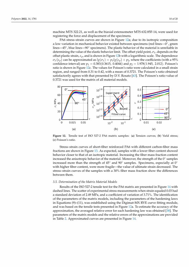
PA6 stress–strain curves are shown in Figure 12a; due to its isotropic composition a low variation in mechanical behavior existed between specimens (red lines—0°, green lines—45°, blue lines—90° specimens). The plastic behavior of the material is unreliable in determining the value of the elastic behavior limit. The offset yield point, , depends on the offset plastic strain, , and is shown in Figure 12b with a logarithmic scale. The dependence ( ) can be approximated as ( ) = ( ) + , where the coeffi-cients (with a 95% confidence interval) are = 0.383(0.3615, 0.4044) and =1.978(1.945, 2.012). Poisson’s ratio is shown in Figure 12c. The values for Poisson’s ratio were calculated in a small strain region, and ranged from 0.31 to 0.42, with a mean of 0.3721. The Poisson’s ratio obtained satisfactorily agrees with that presented by D.V. Rosato [43]. The Poisson’s ratio value of 0.3721 was used for the matrix of all material models.

Figure 12. Tensile test of ISO 527-2 PA6 matrix samples: (a) Tension curves; (b) Yield stress; (c) Poisson’s ratio.

Stress–strain curves of short-fiber reinforced PA6 with different carbon-fiber mass fractions are shown in Figure 13. As expected, samples with a lower fiber content showed


3.4. Experimental Stress–strain Curves

Tensile tests were performed for construction of the material models according toISO 527-2 on 1B specimens from non-reinforced PA6 and composites with 10%, 15%, 20%,and 30%. For each material, nine samples were investigated, cut out from the plates at 0◦

(red lines), 45◦ (green lines), and 90◦ (blue lines) to the flow direction (Figure 2a). The test

Polymers 2022, 14, 1781 10 of 20

machine MTS 322.21, as well as the biaxial extensometer MTS 632.85F-14, were used forregistering the force and displacement of the specimens.

PA6 stress–strain curves are shown in Figure 12a; due to its isotropic compositiona low variation in mechanical behavior existed between specimens (red lines—0◦, greenlines—45◦, blue lines—90◦ specimens). The plastic behavior of the material is unreliable indetermining the value of the elastic behavior limit. The offset yield point, σY, depends on theoffset plastic strain, εp, and is shown in Figure 12b with a logarithmic scale. The dependenceσY(εp)

can be approximated as lg(σY) = p1lg(εp)+ p2, where the coefficients (with a 95%

confidence interval) are p1 = 0.383(0.3615, 0.4044) and p2 = 1.978(1.945, 2.012). Poisson’sratio is shown in Figure 12c. The values for Poisson’s ratio were calculated in a small strainregion, and ranged from 0.31 to 0.42, with a mean of 0.3721. The Poisson’s ratio obtainedsatisfactorily agrees with that presented by D.V. Rosato [43]. The Poisson’s ratio value of0.3721 was used for the matrix of all material models.



3.4. Experimental Stress–strain Curves Tensile tests were performed for construction of the material models according to

ISO 527-2 on 1B specimens from non-reinforced PA6 and composites with 10%, 15%, 20%, and 30%. For each material, nine samples were investigated, cut out from the plates at 0° (red lines), 45° (green lines), and 90° (blue lines) to the flow direction (Figure 2a). The test machine MTS 322.21, as well as the biaxial extensometer MTS 632.85F-14, were used for registering the force and displacement of the specimens.

PA6 stress–strain curves are shown in Figure 12a; due to its isotropic composition a low variation in mechanical behavior existed between specimens (red lines—0°, green lines—45°, blue lines—90° specimens). The plastic behavior of the material is unreliable in determining the value of the elastic behavior limit. The offset yield point, , depends on the offset plastic strain, , and is shown in Figure 12b with a logarithmic scale. The dependence ( ) can be approximated as ( ) = ( ) + , where the coeffi-cients (with a 95% confidence interval) are = 0.383(0.3615, 0.4044) and =1.978(1.945, 2.012). Poisson’s ratio is shown in Figure 12c. The values for Poisson’s ratio were calculated in a small strain region, and ranged from 0.31 to 0.42, with a mean of 0.3721. The Poisson’s ratio obtained satisfactorily agrees with that presented by D.V. Rosato [43]. The Poisson’s ratio value of 0.3721 was used for the matrix of all material models.

Figure 12. Tensile test of ISO 527-2 PA6 matrix samples: (a) Tension curves; (b) Yield stress; (c) Poisson’s ratio.

Stress–strain curves of short-fiber reinforced PA6 with different carbon-fiber mass fractions are shown in Figure 13. As expected, samples with a lower fiber content showed

Figure 12. Tensile test of ISO 527-2 PA6 matrix samples: (a) Tension curves; (b) Yield stress;(c) Poisson’s ratio.

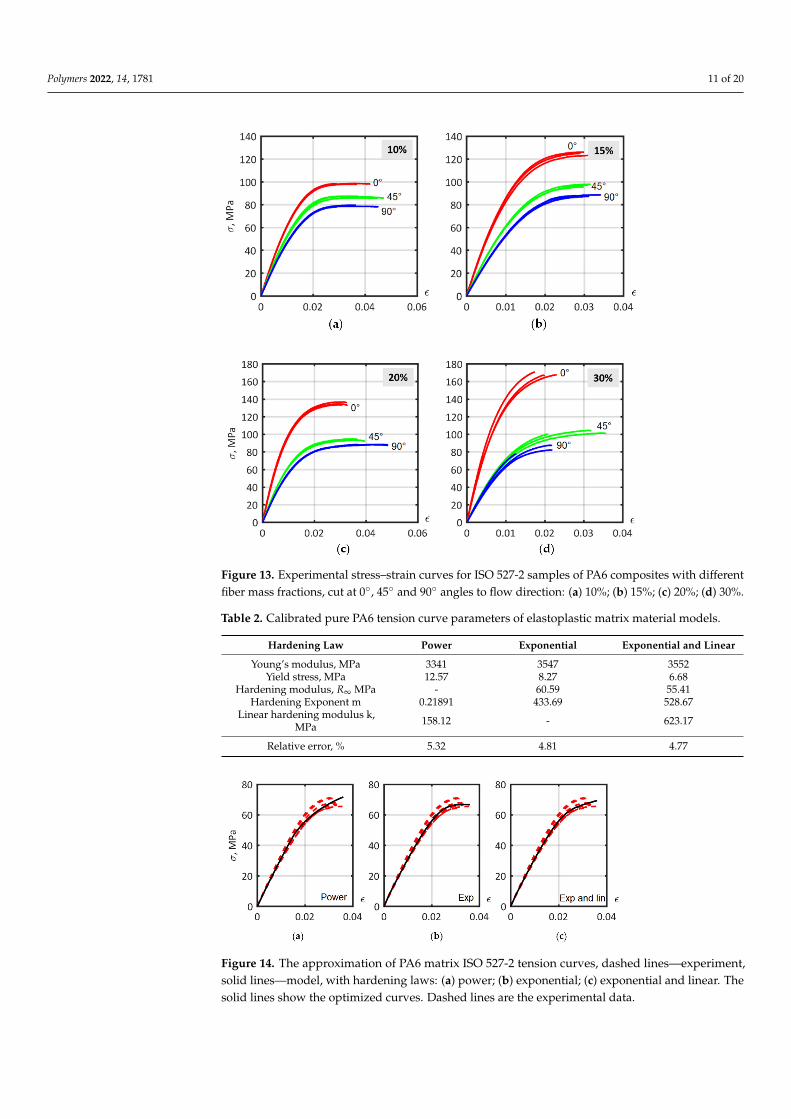
Stress–strain curves of short-fiber reinforced PA6 with different carbon-fiber massfractions are shown in Figure 13. As expected, samples with a lower fiber content showedbehavior closer to that of an isotropic material. Increasing the fiber mass fraction contentincreased the anisotropic behavior of the material. Moreover, the strength of the 0◦ samplesincreased more than the strength of 45◦ and 90◦ samples. Specimens, especially at 0◦

with higher fiber content, were more fragile—the value of ultimate strain decreased. Thestress–strain curves of the samples with a 30% fiber mass fraction show the differencesbetween them.

3.5. Determination of the Matrix Material Models

Results of the ISO 527-2 tensile test for the PA6 matrix are presented in Figure 14 withdashed lines. The scatter of experimental stress measurements when strain equaled 0.03 hada standard deviation of 2.49 MPa, and a coefficient of variation of 3.71%. The identificationof the parameters of the matrix models, including the parameters of the hardening lawsin Equations (9)–(11), was established using the Digimat-MX RVE curve fitting module,and was based on the tensile tests presented in Figure 12a. To estimate the accuracy of theapproximation, the averaged relative error for each hardening law was obtained [38]. Theparameters of the matrix models and the relative errors of the approximations are providedin Table 2. Approximated curves are presented in Figure 14.

Polymers 2022, 14, 1781 11 of 20


behavior closer to that of an isotropic material. Increasing the fiber mass fraction content increased the anisotropic behavior of the material. Moreover, the strength of the 0° sam-ples increased more than the strength of 45° and 90° samples. Specimens, especially at 0° with higher fiber content, were more fragile—the value of ultimate strain decreased. The stress–strain curves of the samples with a 30% fiber mass fraction show the differences between them.

Figure 13. Experimental stress–strain curves for ISO 527-2 samples of PA6 composites with different fiber mass fractions, cut at 0°, 45° and 90° angles to flow direction: (a) 10%; (b) 15%; (c) 20%; (d) 30%.

3.5. Determination of the Matrix Material Models Results of the ISO 527-2 tensile test for the PA6 matrix are presented in Figure 14 with

dashed lines. The scatter of experimental stress measurements when strain equaled 0.03 had a standard deviation of 2.49 MPa, and a coefficient of variation of 3.71%. The identi-fication of the parameters of the matrix models, including the parameters of the hardening laws in Equations (9)–(11), was established using the Digimat-MX RVE curve fitting mod-ule, and was based on the tensile tests presented in Figure 12a. To estimate the accuracy of the approximation, the averaged relative error for each hardening law was obtained [38]. The parameters of the matrix models and the relative errors of the approximations are provided in Table 2. Approximated curves are presented in Figure 14.

Figure 13. Experimental stress–strain curves for ISO 527-2 samples of PA6 composites with differentfiber mass fractions, cut at 0◦, 45◦ and 90◦ angles to flow direction: (a) 10%; (b) 15%; (c) 20%; (d) 30%.

Table 2. Calibrated pure PA6 tension curve parameters of elastoplastic matrix material models.

Hardening Law Power Exponential Exponential and Linear

Young’s modulus, MPa 3341 3547 3552Yield stress, MPa 12.57 8.27 6.68

Hardening modulus, R∞ MPa - 60.59 55.41Hardening Exponent m 0.21891 433.69 528.67

Linear hardening modulus k,MPa 158.12 - 623.17

Relative error, % 5.32 4.81 4.77




Young’s modulus, MPa 3341 3547 3552 Yield stress, MPa 12.57 8.27 6.68

Hardening modulus, MPa - 60.59 55.41 Hardening Exponent m 0.21891 433.69 528.67

Linear hardening modulus k, MPa 158.12 - 623.17 Relative error, % 5.32 4.81 4.77

Figure 14. The approximation of PA6 matrix ISO 527-2 tension curves, dashed lines—experiment, solid lines—model, with hardening laws: (a) power; (b) exponential; (c) exponential and linear. The solid lines show the optimized curves. Dashed lines are the experimental data.

3.6. Comparison of the Effect of Considering the Distribution of Fiber Lengths and the Distribution of the Orientation Tensor on the Accuracy of Approximation of the Tensile Curves of a Short-Reinforced Composite

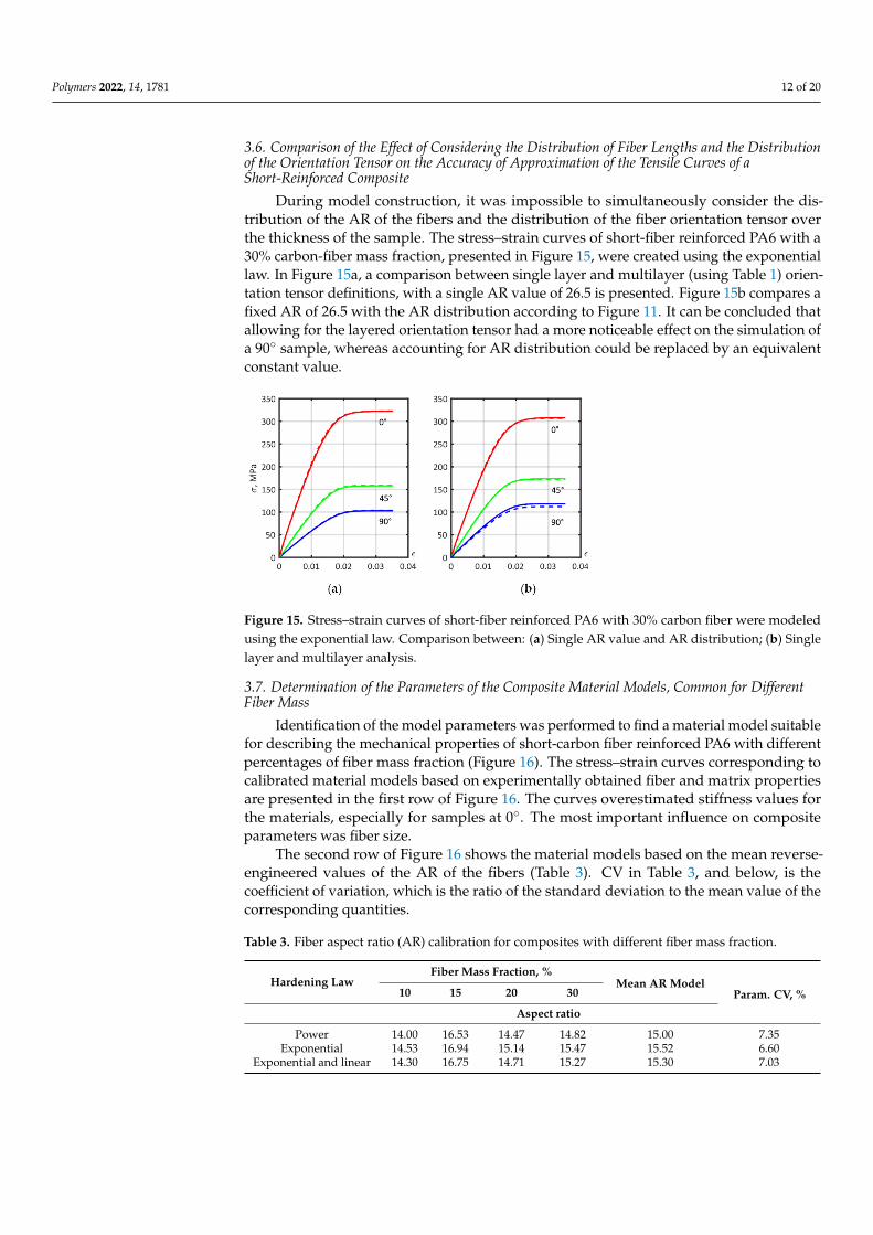
During model construction, it was impossible to simultaneously consider the distri-bution of the AR of the fibers and the distribution of the fiber orientation tensor over the thickness of the sample. The stress–strain curves of short-fiber reinforced PA6 with a 30% carbon-fiber mass fraction, presented in Figure 15, were created using the exponential law. In Figure 15a, a comparison between single layer and multilayer (using Table 1) orienta-tion tensor definitions, with a single AR value of 26.5 is presented. Figure 15b compares a fixed AR of 26.5 with the AR distribution according to Figure 11. It can be concluded that allowing for the layered orientation tensor had a more noticeable effect on the simulation of a 90° sample, whereas accounting for AR distribution could be replaced by an equiva-lent constant value.

Figure 15. Stress–strain curves of short-fiber reinforced PA6 with 30% carbon fiber were modeled using the exponential law. Comparison between: (a) Single AR value and AR distribution; (b) Single layer and multilayer analysis.

Figure 14. The approximation of PA6 matrix ISO 527-2 tension curves, dashed lines—experiment,solid lines—model, with hardening laws: (a) power; (b) exponential; (c) exponential and linear. Thesolid lines show the optimized curves. Dashed lines are the experimental data.

Polymers 2022, 14, 1781 12 of 20

3.6. Comparison of the Effect of Considering the Distribution of Fiber Lengths and the Distributionof the Orientation Tensor on the Accuracy of Approximation of the Tensile Curves of aShort-Reinforced Composite

During model construction, it was impossible to simultaneously consider the dis-tribution of the AR of the fibers and the distribution of the fiber orientation tensor overthe thickness of the sample. The stress–strain curves of short-fiber reinforced PA6 with a30% carbon-fiber mass fraction, presented in Figure 15, were created using the exponentiallaw. In Figure 15a, a comparison between single layer and multilayer (using Table 1) orien-tation tensor definitions, with a single AR value of 26.5 is presented. Figure 15b compares afixed AR of 26.5 with the AR distribution according to Figure 11. It can be concluded thatallowing for the layered orientation tensor had a more noticeable effect on the simulation ofa 90◦ sample, whereas accounting for AR distribution could be replaced by an equivalentconstant value.




Young’s modulus, MPa 3341 3547 3552 Yield stress, MPa 12.57 8.27 6.68

Hardening modulus, MPa - 60.59 55.41 Hardening Exponent m 0.21891 433.69 528.67

Linear hardening modulus k, MPa 158.12 - 623.17 Relative error, % 5.32 4.81 4.77

Figure 14. The approximation of PA6 matrix ISO 527-2 tension curves, dashed lines—experiment, solid lines—model, with hardening laws: (a) power; (b) exponential; (c) exponential and linear. The solid lines show the optimized curves. Dashed lines are the experimental data.

3.6. Comparison of the Effect of Considering the Distribution of Fiber Lengths and the Distribution of the Orientation Tensor on the Accuracy of Approximation of the Tensile Curves of a Short-Reinforced Composite

During model construction, it was impossible to simultaneously consider the distri-bution of the AR of the fibers and the distribution of the fiber orientation tensor over the thickness of the sample. The stress–strain curves of short-fiber reinforced PA6 with a 30% carbon-fiber mass fraction, presented in Figure 15, were created using the exponential law. In Figure 15a, a comparison between single layer and multilayer (using Table 1) orienta-tion tensor definitions, with a single AR value of 26.5 is presented. Figure 15b compares a fixed AR of 26.5 with the AR distribution according to Figure 11. It can be concluded that allowing for the layered orientation tensor had a more noticeable effect on the simulation of a 90° sample, whereas accounting for AR distribution could be replaced by an equiva-lent constant value.

Figure 15. Stress–strain curves of short-fiber reinforced PA6 with 30% carbon fiber were modeled using the exponential law. Comparison between: (a) Single AR value and AR distribution; (b) Single layer and multilayer analysis.

Figure 15. Stress–strain curves of short-fiber reinforced PA6 with 30% carbon fiber were modeledusing the exponential law. Comparison between: (a) Single AR value and AR distribution; (b) Singlelayer and multilayer analysis.

3.7. Determination of the Parameters of the Composite Material Models, Common for DifferentFiber Mass

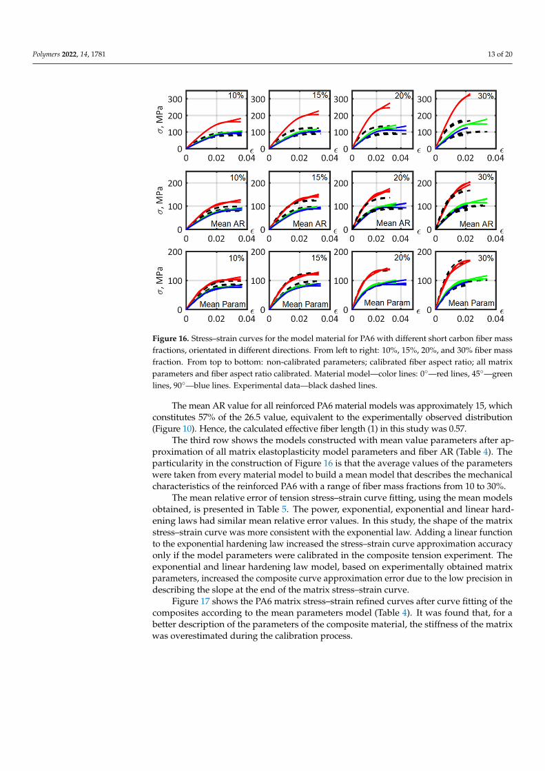
Identification of the model parameters was performed to find a material model suitablefor describing the mechanical properties of short-carbon fiber reinforced PA6 with differentpercentages of fiber mass fraction (Figure 16). The stress–strain curves corresponding tocalibrated material models based on experimentally obtained fiber and matrix propertiesare presented in the first row of Figure 16. The curves overestimated stiffness values forthe materials, especially for samples at 0◦. The most important influence on compositeparameters was fiber size.

The second row of Figure 16 shows the material models based on the mean reverse-engineered values of the AR of the fibers (Table 3). CV in Table 3, and below, is thecoefficient of variation, which is the ratio of the standard deviation to the mean value of thecorresponding quantities.

Table 3. Fiber aspect ratio (AR) calibration for composites with different fiber mass fraction.

Hardening LawFiber Mass Fraction, %

Mean AR ModelParam. CV, %10 15 20 30

Aspect ratio

Power 14.00 16.53 14.47 14.82 15.00 7.35Exponential 14.53 16.94 15.14 15.47 15.52 6.60

Exponential and linear 14.30 16.75 14.71 15.27 15.30 7.03

Polymers 2022, 14, 1781 13 of 20


3.7. Determination of the Parameters of the Composite Material Models, Common for Different Fiber Mass

Identification of the model parameters was performed to find a material model suit-able for describing the mechanical properties of short-carbon fiber reinforced PA6 with different percentages of fiber mass fraction (Figure 16). The stress–strain curves corre-sponding to calibrated material models based on experimentally obtained fiber and ma-trix properties are presented in the first row of Figure 16. The curves overestimated stiff-ness values for the materials, especially for samples at 0°. The most important influence on composite parameters was fiber size.

Figure 16. Stress–strain curves for the model material for PA6 with different short carbon fiber mass fractions, orientated in different directions. From left to right: 10%, 15%, 20%, and 30% fiber mass fraction. From top to bottom: non-calibrated parameters; calibrated fiber aspect ratio; all matrix pa-rameters and fiber aspect ratio calibrated. Material model—color lines: 0°—red lines, 45°—green lines, 90°—blue lines. Experimental data—black dashed lines.

The second row of Figure 16 shows the material models based on the mean reverse-engineered values of the AR of the fibers (Table 3). CV in Table 3, and below, is the coef-ficient of variation, which is the ratio of the standard deviation to the mean value of the corresponding quantities.

Table 3. Fiber aspect ratio (AR) calibration for composites with different fiber mass fraction.

Hardening Law Fiber Mass Fraction, % Mean AR

Model Param. CV, %

10 15 20 30 Aspect ratio

Power 14.00 16.53 14.47 14.82 15.00 7.35 Exponential 14.53 16.94 15.14 15.47 15.52 6.60

Exponential and lin-ear 14.30 16.75 14.71 15.27 15.30 7.03

Figure 16. Stress–strain curves for the model material for PA6 with different short carbon fiber massfractions, orientated in different directions. From left to right: 10%, 15%, 20%, and 30% fiber massfraction. From top to bottom: non-calibrated parameters; calibrated fiber aspect ratio; all matrixparameters and fiber aspect ratio calibrated. Material model—color lines: 0◦—red lines, 45◦—greenlines, 90◦—blue lines. Experimental data—black dashed lines.

The mean AR value for all reinforced PA6 material models was approximately 15, whichconstitutes 57% of the 26.5 value, equivalent to the experimentally observed distribution(Figure 10). Hence, the calculated effective fiber length (1) in this study was 0.57.

The third row shows the models constructed with mean value parameters after ap-proximation of all matrix elastoplasticity model parameters and fiber AR (Table 4). Theparticularity in the construction of Figure 16 is that the average values of the parameterswere taken from every material model to build a mean model that describes the mechanicalcharacteristics of the reinforced PA6 with a range of fiber mass fractions from 10 to 30%.

The mean relative error of tension stress–strain curve fitting, using the mean modelsobtained, is presented in Table 5. The power, exponential, exponential and linear hard-ening laws had similar mean relative error values. In this study, the shape of the matrixstress–strain curve was more consistent with the exponential law. Adding a linear functionto the exponential hardening law increased the stress–strain curve approximation accuracyonly if the model parameters were calibrated in the composite tension experiment. Theexponential and linear hardening law model, based on experimentally obtained matrixparameters, increased the composite curve approximation error due to the low precision indescribing the slope at the end of the matrix stress–strain curve.

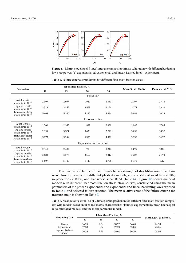
Figure 17 shows the PA6 matrix stress–strain refined curves after curve fitting of thecomposites according to the mean parameters model (Table 4). It was found that, for abetter description of the parameters of the composite material, the stiffness of the matrixwas overestimated during the calibration process.

Polymers 2022, 14, 1781 14 of 20

Table 4. Calibration of all parameters of the matrix elastoplasticity model and fiber aspect ratio.

ParameterFiber Mass Fraction, %

Mean Parameters Model Parameters CV, %10 15 20 30

Power Law

Young’s modulus, MPa 4383 4437 4162 3759 4185 7.4Yield stress, MPa 12.3 12.6 10.2 9.9 11.2 12.3

Hardening modulus, MPa 147.6 161.9 124.6 137.0 142.8 11.1Hardening exponent 0.1995 0.2238 0.2023 0.2475 0.2183 10.2

Fibers’ AR 8.84 12.23 14.19 16.79 13.01 25.8

Exponential Law



Fibers’ AR 9.02 12.25 13.37 16.62 12.8 24.4

Exponential and linear law



Hardening linear modulus, MPa 208.8 216.0 144.1 188.4 189.3 17.1Fibers’ AR 8.82 12.36 13.80 16.54 12.9 24.9

Table 5. Mean relative error of stress–strain curve prediction of different fiber mass fraction com-posites with models based on fibers and matrix characteristics obtained experimentally, mean fiberaspect ratio calibrated models, and the mean parameter model.

Hardening LawFiber Mass Fraction, % Mean Level

of Error, %10 15 20 30

Models, based on fibers and matrix characteristics obtained experimentally

Power 29.0 25.7 35.8 35.9 31.6Exponential 27.8 25.2 33.7 34.7 30.4

Exponential andlinear 28.6 25.9 36.1 35.7 31.6

Mean fiber aspect ratio calibrated models



Mean with the calibration of all matrix and fiber aspect ratio parameters



3.8. Failure Criterion Parameter Identification for Short-Fiber Reinforced Thermoplastic Composites

For strength prediction, the Tsai–Hill 3D transversely isotropic strain-based failurecriterion was applied to the reinforced PA6 (composite level) in the local finite elementcoordinate system (local axes) [38]. The critical fraction of failed pseudo-grains was 0.75,and multilayer failure occurred using the all-layer failure condition. The results of theidentification of the model parameters are presented in Table 6.

Polymers 2022, 14, 1781 15 of 20


Exponential 27.8 25.2 33.7 34.7 30.4 Exponential and linear 28.6 25.9 36.1 35.7 31.6

Mean fiber aspect ratio calibrated models Power 11.7 12.1 12.0 11.1 11.7


Mean with the calibration of all matrix and fiber aspect ratio parameters Power 7.4 7.6 4.9 7.7 6.9


Figure 17 shows the PA6 matrix stress–strain refined curves after curve fitting of the composites according to the mean parameters model (Table 4). It was found that, for a better description of the parameters of the composite material, the stiffness of the matrix was overestimated during the calibration process.

Figure 17. Matrix models (solid lines) after the composite stiffness calibration with different hard-ening laws: (a) power; (b) exponential; (c) exponential and linear. Dashed lines—experiment.

3.8. Failure Criterion Parameter Identification for Short-Fiber Reinforced Thermoplastic Composites

For strength prediction, the Tsai–Hill 3D transversely isotropic strain-based failure criterion was applied to the reinforced PA6 (composite level) in the local finite element coordinate system (local axes) [38]. The critical fraction of failed pseudo-grains was 0.75, and multilayer failure occurred using the all-layer failure condition. The results of the identification of the model parameters are presented in Table 6.

Table 6. Failure criteria strain limits for different fiber mass fraction cases.

Parameters Fiber Mass Fraction, % Mean Strain

Limits Parameters

CV, % 10 15 20 30 Power law

Axial tensile strain limit, 10−2 2.009 2.957 1.944 1.880 2.197 23.16 Inplane tensile strain limit, 10−2 3.516 3.855 3.573 2.151 3.274 23.30

Transverse shear strain limit, 10−2 5.606 5.140 5.235 4.364 5.086 10.26 Exponential law


Transverse shear strain limit, 10−2 5.873 5.249 5.355 4.076 5.138 14.77 Exponential and linear law


Transverse shear strain limit, 10−2 5.607 5.140 5.140 4.798 5.171 6.42

Figure 17. Matrix models (solid lines) after the composite stiffness calibration with different hardeninglaws: (a) power; (b) exponential; (c) exponential and linear. Dashed lines—experiment.

Table 6. Failure criteria strain limits for different fiber mass fraction cases.

ParametersFiber Mass Fraction, %

Mean Strain Limits Parameters CV, %10 15 20 30

Power law

Axial tensilestrain limit, 10−2 2.009 2.957 1.944 1.880 2.197 23.16

Inplane tensilestrain limit, 10−2 3.516 3.855 3.573 2.151 3.274 23.30

Transverse shearstrain limit, 10−2 5.606 5.140 5.235 4.364 5.086 10.26

Exponential law




Exponential and linear law




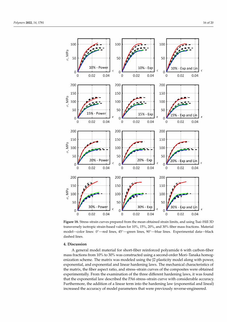
The mean strain limits for the ultimate tensile strength of short-fiber reinforced PA6were close to those of the different plasticity models, and constituted axial tensile 0.02,in-plane tensile 0.032, and transverse shear 0.051 (Table 6). Figure 18 shows materialmodels with different fiber mass fraction stress–strain curves, constructed using the meanparameters of the power, exponential and exponential and lineal hardening laws exposedin Table 4, and selected failure criterion. The mean relative error of the failure criteria forfracture strain is shown in Table 7.

Table 7. Mean relative error (%) of ultimate strain prediction for different fiber mass fraction compos-ites with models based on fiber and matrix characteristics obtained experimentally, mean fiber aspectratio calibrated models, and the mean parameter model.

Hardening LawFiber Mass Fraction, %

Mean Level of Error, %10 15 20 30



Polymers 2022, 14, 1781 16 of 20


The mean strain limits for the ultimate tensile strength of short-fiber reinforced PA6 were close to those of the different plasticity models, and constituted axial tensile 0.02, in-plane tensile 0.032, and transverse shear 0.051 (Table 6). Figure 18 shows material models with different fiber mass fraction stress–strain curves, constructed using the mean param-eters of the power, exponential and exponential and lineal hardening laws exposed in Table 4, and selected failure criterion. The mean relative error of the failure criteria for fracture strain is shown in Table 7.

Figure 18. Stress–strain curves prepared from the mean obtained strain limits, and using Tsai–Hill 3D transversely isotropic strain-based values for 10%, 15%, 20%, and 30% fiber mass fractions. Ma-terial model—color lines: 0°—red lines, 45°—green lines, 90°—blue lines. Experimental data—black dashed lines.

Figure 18. Stress–strain curves prepared from the mean obtained strain limits, and using Tsai–Hill 3Dtransversely isotropic strain-based values for 10%, 15%, 20%, and 30% fiber mass fractions. Materialmodel—color lines: 0◦—red lines, 45◦—green lines, 90◦—blue lines. Experimental data—blackdashed lines.

4. Discussion

A general model material for short-fiber reinforced polyamide 6 with carbon-fibermass fractions from 10% to 30% was constructed using a second-order Mori–Tanaka homog-enization scheme. The matrix was modeled using the J2 plasticity model along with power,exponential, and exponential and linear hardening laws. The mechanical characteristics ofthe matrix, the fiber aspect ratio, and stress–strain curves of the composites were obtainedexperimentally. From the examination of the three different hardening laws, it was foundthat the exponential law described the PA6 stress–strain curve with considerable accuracy.Furthermore, the addition of a linear term into the hardening law (exponential and lineal)increased the accuracy of model parameters that were previously reverse-engineered.

Polymers 2022, 14, 1781 17 of 20

The results from general calibration produced models for PA6 reinforced composite whichcould determine the mechanical characteristics of materials with different fiber mass fractions.The novelty of this approach lies in the transition from two-dimensional (stress–strain) tothree-dimensional (stress–strain–fiber fraction) approximation space (Figure 19).


Table 7. Mean relative error (%) of ultimate strain prediction for different fiber mass fraction com-posites with models based on fiber and matrix characteristics obtained experimentally, mean fiber aspect ratio calibrated models, and the mean parameter model.

Hardening Law Fiber Mass Fraction, % Mean Level of

Error, % 10 15 20 30 Power 16.24 7.79 18.92 56.63 24.90


4. Discussion A general model material for short-fiber reinforced polyamide 6 with carbon-fiber

mass fractions from 10% to 30% was constructed using a second-order Mori–Tanaka ho-mogenization scheme. Тhe matrix was modeled using the J2 plasticity model along with power, exponential, and exponential and linear hardening laws. The mechanical charac-teristics of the matrix, the fiber aspect ratio, and stress–strain curves of the composites were obtained experimentally. From the examination of the three different hardening laws, it was found that the exponential law described the PA6 stress–strain curve with considerable accuracy. Furthermore, the addition of a linear term into the hardening law (exponential and lineal) increased the accuracy of model parameters that were previously reverse-engineered.

The results from general calibration produced models for PA6 reinforced composite which could determine the mechanical characteristics of materials with different fiber mass fractions. The novelty of this approach lies in the transition from two-dimensional (stress–strain) to three-dimensional (stress–strain–fiber fraction) approximation space (Figure 19).

(a) (b) (c)

Figure 19. Common mass fraction composite material models for all fibers. Exponent and linear hardening law case. For angles between the flow and load directions: (a) 0°; (b) 45°; (c) 90°.

It was found that the use of the experimental AR value in the construction of the models increased the strength and stiffness of 0° samples by a factor of 1.7. Such a devia-tion may have been caused by a failure to account for fibers with a low AR during the electron microscopy analysis; however, a more probable reason is the inadequate consid-eration of the influence of including the closed surface (ellipsoid) [32] and its ideal solution in the Mori–Tanaka homogenization scheme. Moreover, the introduction of an equivalent AR value was able to replace the AR distribution, simplifying the material model. The relative effective fiber length, i.e., the ratio between the equivalent and experimental ARs, was φ = 0.57, which corresponds to a virtual length reduction of the fiber, at both ends, of approximately 21.5%.

Figure 19. Common mass fraction composite material models for all fibers. Exponent and linearhardening law case. For angles between the flow and load directions: (a) 0◦; (b) 45◦; (c) 90◦.

It was found that the use of the experimental AR value in the construction of themodels increased the strength and stiffness of 0◦ samples by a factor of 1.7. Such a deviationmay have been caused by a failure to account for fibers with a low AR during the electronmicroscopy analysis; however, a more probable reason is the inadequate considerationof the influence of including the closed surface (ellipsoid) [32] and its ideal solution inthe Mori–Tanaka homogenization scheme. Moreover, the introduction of an equivalentAR value was able to replace the AR distribution, simplifying the material model. Therelative effective fiber length, i.e., the ratio between the equivalent and experimental ARs,was ϕ = 0.57, which corresponds to a virtual length reduction of the fiber, at both ends, ofapproximately 21.5%.

The mean values for the material models obtained after performing curve fitting tothe reinforced matrix’s parameters were used for the construction of the mean models. Amean model was produced that was capable of modeling reinforced PA6 across a widerange of fiber mass fraction, from 10 to 30%, and allowed the prediction of the mechanicalcharacteristics with a mean relative error of 6.60%.

The calibration of mean Tsai–Hill strength failure criteria based on strain, via a trans-versely isotropic statement, was performed, and produced a description of the strength ofreinforced PA6 with 10 to 30% carbon fiber mass fractions. The calibrated strength failurecriteria could be used only as a first approximation for the failure of carbon-reinforcedPA6 structures because the fracture strain mean relative error value, the large dispersionin the experimental fracture strain values, and the question of failure criteria requirefurther investigation.

5. Conclusions

The Mori–Tanaka model allowed us to accurately predict the stiffness of a short-reinforced composite with an arbitrary fraction of reinforcing fibers, but required curvefitting for the whole composite because using fiber and matrix parameters obtained experi-mentally led to an erroneous overestimation of the composite’s mechanical characteristics.Fiber elongation had a decisive influence on the stiffness of the composite. It was foundthat for the correct prediction of the mechanical characteristics of a composite using theMori–Tanaka model, it was necessary to significantly reduce the fiber aspect ratio. Theexponential hardening law of the matrix provided a good description of the tensile diagramof the composite. Adding a linear term and switching to an exponential and linear modelallowed an even more accurate demonstration of material behavior when approaching the

Polymers 2022, 14, 1781 18 of 20

strength limit, but required attention to the calibration of the slope of the tensile curve athigh strain values.

When dealing with different fiber fractions, adding a third dimension to the two-dimensional stress–strain space in the form of a fiber fraction allowed us to combine theflexibility of the Mori–Tanaka model with the accuracy of calibrated tension curves from asingle fiber fraction composite material. This makes it possible to improve the accuracyof the selection of the fiber fraction in material to be used in the construction of structuresduring the early stages of design.

In this work, averaging of the parameters of the tension curves calibrated for individ-ual volume fractions was used to construct a three-dimensional, calibrated, Mori-Tanakamodel. In the future, we plan to develop an algorithm and software that would allow simul-taneous calibration of three-dimensional models over the entire volume of experimentaldata available.

Author Contributions: Conceptualization, E.K. (Evgenii Kurkin); methodology, E.K. (Evgenii Kurkin);validation, E.K. (Evgenii Kurkin) and O.U.E.B.; formal analysis, M.S. and E.K. (Ekaterina Kurkina);investigation, E.K. (Evgenii Kurkin) and M.S.; data curation, O.U.E.B., M.S. and E.K. (EkaterinaKurkina); writing—original draft preparation, E.K. (Evgenii Kurkin) and O.U.E.B.; writing—reviewand editing, E.K. (Evgenii Kurkin) and O.U.E.B.; visualization, O.U.E.B.; supervision, E.K. (EvgeniiKurkin); project administration, E.K. (Evgenii Kurkin); funding acquisition, E.K. (Evgenii Kurkin).All authors have read and agreed to the published version of the manuscript.

Funding: This research was funded by Russian Science Foundation, grant number 19-79-10205.

Institutional Review Board Statement: Not applicable.

Informed Consent Statement: Not applicable.

Data Availability Statement: The raw data cannot be shared at this time as the data also forms partof an ongoing study.

Acknowledgments: The authors thank A.A Pavlov and S.E. Selivanov, for providing help to performthe tensile tests. The authors thank Pladep Ltd. for help in plate molding. The authors thank R.V.Shafigulin for help with burning of samples.

Conflicts of Interest: The authors declare no conflict of interest. The funders had no role in the designof the study; in the collection, analyses, or interpretation of data; in the writing of the manuscript; orin the decision to publish the results.

References1. Chawla, K.K. Composite Materials: Science and Engineering; Springer: New York, NY, USA, 2016.2. Rana, S.; Fangueiro, R. Advanced Composites in Aerospace Engineering. In Advanced Composite Materials for Aerospace Engineering;

Elsevier: Amsterdam, The Netherlands, 2016; pp. 1–15. [CrossRef]3. Fu, S.-Y.; Lauke, B.; Mai, Y.-W. Science and Engineering of Short Fibre Reinforced Polymers Composites. In Woodhead Publishing in

Materials; CRC Press: Boca Raton, FL, USA, 2009.4. Nakonieczny, D.S.; Kern, F.; Dufner, L.; Antonowicz, M.; Matus, K. Alumina and Zirconia-Reinforced Polyamide PA-12 Compos-

ites for Biomedical Additive Manufacturing. Materials 2021, 14, 6201. [CrossRef] [PubMed]5. Díaz, J.; Rubio, L. Developments to Manufacture Structural Aeronautical Parts in Carbon Fibre Reinforced Thermoplastic

Materials. J. Mater. Processing Technol. 2003, 143–144, 342–346. [CrossRef]6. Miaris, A.; Edelmann, K.; von Hayek Boelingen, M. A350 WXB: Thousands of Thermoplastic Composite Parts in an FRP

Aircraft-SAMPE. Available online: https://www.nasampe.org/store/viewproduct.aspx?id=4417947 (accessed on 25 March 2022).7. Chang, I.Y.; Pratte, J.F. LDF™ Thermoplastic Composites Technology. J. Thermoplast. Compos. Mater. 1991, 4, 227–252. [CrossRef]8. Eguemann, N.; Giger, L.; Roux, M.; Dransfeld, C.; Thiebaud, F.; Perreux, D. Compression Moulding of Complex Parts for the

Aerospace with Discontinuous Novel and Recycled Thermoplastic Composite Materials. In Proceedings of the 19th InternationalConference on Composite Materials, Paris, France, 28 July–2 August 2013; pp. 1–11.

9. European Bioplastics. Fact Sheet: Mechanical Recycling; European Bioplastics eV: Berlin, Germany, 2010.10. Andrzejewski, J.; Anisko, J.; Szulc, J. A Comparative Study of Biocarbon Reinforced Polyoxymethylene and Polyamide: Materials

Performance and Durability. Compos. Part A Appl. Sci. Manuf. 2022, 152, 106715. [CrossRef]11. Steffens, M.; Himmel, N.; Maier, M. Design and Analysis of Discontinuous Long Fiber Reinforced Thermoplastic Structures for

Car Seat Applications. Trans. Eng. Sci. 1998, 21, 35–44.

http://doi.org/10.1016/B978-0-08-100037-3.00001-8

http://doi.org/10.3390/ma14206201

http://www.ncbi.nlm.nih.gov/pubmed/34683792

http://doi.org/10.1016/S0924-0136(03)00450-3

https://www.nasampe.org/store/viewproduct.aspx?id=4417947

http://doi.org/10.1177/089270579100400302

http://doi.org/10.1016/j.compositesa.2021.106715

Polymers 2022, 14, 1781 19 of 20

12. Kondapalli, P.S.; Grumm, K.; Cao, Y.; Laurent, V. Application and CAE simulation of over molded short and continuous fiberthermoplastic composite: Part II. 12th Int LS-DYNA® Users Conf. FEA Inf. Eng. J. 2013, 2, 1–10.

13. Fu, S. Effects of Fiber Length and Fiber Orientation Distributions on the Tensile Strength of Short-Fiber-Reinforced Polymers.Compos. Sci. Technol. 1996, 56, 1179–1190. [CrossRef]

14. Fu, S.-Y.; Hu, X.; Yue, C.-Y. Effects of Fiber Length and Orientation Distributions on the Mechanical Properties of Short-Fiber-Reinforced Polymers. J. Soc. Mater. Sci. Jpn. 1999, 48, 74–83. [CrossRef]

15. Capela, C.; Oliveira, S.E.; Pestana, J.; Ferreira, J.A.M. Effect of Fiber Length on the Mechanical Properties of High Dosage CarbonReinforced. Procedia Struct. Integr. 2017, 5, 539–546. [CrossRef]

16. Capela, C.; Oliveira, S.E.; Ferreira, J.A.M. Mechanical Behavior of High Dosage Short Carbon Fiber Reinforced Epoxy Composites.Fibers Polym. 2017, 18, 1200–1207. [CrossRef]

17. Karsli, N.G.; Aytac, A.; Deniz, V. Effects of Initial Fiber Length and Fiber Length Distribution on the Properties of Carbon-Fiber-Reinforced-Polypropylene Composites. J. Reinf. Plast. Compos. 2012, 31, 1053–1060. [CrossRef]

18. Kufel, A.; Para, S.; Kuciel, S. Basalt/Glass Fiber Polypropylene Hybrid Composites: Mechanical Properties at Different Tempera-tures and under Cyclic Loading and Micromechanical Modelling. Materials 2021, 14, 5574. [CrossRef] [PubMed]

19. Moritzer, E.; Heiderich, G.; Hirsch, A. Fiber Length Reduction during Injection Molding; AIP Publishing: Dresden, Germany, 2019;p. 070001. [CrossRef]

20. Kurkin, E.I.; Lukyanov, O.E.; Chertykovtseva, V.O.; Espinosa Barcenas, O.U. Molding Gate Optimization for Weld Line LocationAway from Structures Loaded Area. J. Phys. Conf. Ser. 2021, 1925, 012056. [CrossRef]

21. Eshelby, J. The Determination of the Elastic Field of an Ellipsoidal Inclusion, and Related Problems. Proc. R. Soc. Lond. A 1957,241, 376–396. [CrossRef]

22. Mori, T.; Tanaka, K. Average Stress in Matrix and Average Elastic Energy of Materials with Misfitting Inclusions. Acta Metall.1973, 21, 571–574. [CrossRef]

23. Su, N.; Pierce, R.S.; Rudd, C.; Liu, X. Comprehensive Investigation of Reclaimed Carbon Fibre Reinforced Polyamide (RCF/PA)Filaments and FDM Printed Composites. Compos. Part B Eng. 2022, 233, 109646. [CrossRef]

24. Mentges, N.; Dashtbozorg, B.; Mirkhalaf, S.M. A Micromechanics-Based Artificial Neural Networks Model for Elastic Propertiesof Short Fiber Composites. Compos. Part B Eng. 2021, 213, 108736. [CrossRef]

25. Pietrogrande, R.; Carraro, P.A.; De Monte, M.; Quaresimin, M. A Novel Pseudo-Grain Approach for the Estimation of the ElasticStress Distributions within the Matrix of Short Fiber-Reinforced Polymers. Compos. Part B Eng. 2018, 150, 115–123. [CrossRef]

26. Templeton, P.A. Strength Predictions of Injection Molding Compounds. J. Reinf. Plast. Compos. 1990, 9, 210–225. [CrossRef]27. Chin, W.-K.; Liu, H.-T.; Lee, Y.-D. Effects of Fiber Length and Orientation Distribution on the Elastic Modulus of Short Fiber

Reinforced Thermoplastics. Polym. Compos. 1988, 9, 27–35. [CrossRef]28. Friedrich, K. Microstructural efficiency and fracture toughness of short fiber/thermoplastic matrix composites. Comp. Sci. Tech.

1985, 22, 43–74. [CrossRef]29. Verdejo de Toro, E.; Coello Sobrino, J.; Martínez Martínez, A.; Miguel Eguía, V.; Ayllón Pérez, J. Investigation of a Short Carbon

Fibre-Reinforced Polyamide and Comparison of Two Manufacturing Processes: Fused Deposition Modelling (FDM) and PolymerInjection Moulding (PIM). Materials 2020, 13, 672. [CrossRef] [PubMed]

30. Rosen, B.W.; Dow, N.F.; Hashin, Z. Mechanical Properties of Fibrous Composites; General Electric Co.: Philadelphia, PA, USA, 1964.31. Jain, A.; Abdin, Y.; Van Paepegem, W.; Verpoest, I.; Lomov, S.V. Effective Anisotropic Stiffness of Inclusions with Debonded

Interface for Eshelby-Based Models. Compos. Struct. 2015, 131, 692–706. [CrossRef]32. Tandon, G.P.; Weng, G.J. The Effect of Aspect Ratio of Inclusions on the Elastic Properties of Unidirectionally Aligned Composites.

Polym. Compos. 1984, 5, 327–333. [CrossRef]33. Li, H.; Zare, Y.; Rhee, K.Y. Mathematical Simplification of the Tandon–Weng Approach to the Mori–Tanaka Model for Estimating

the Young’s Modulus of Clay/Polymer Nanocomposites. JOM 2017, 69, 2819–2824. [CrossRef]34. Gusev, A.A. Finite Element Estimates of Viscoelastic Stiffness of Short Glass Fiber Reinforced Composites. Compos. Struct. 2017,

171, 53–62. [CrossRef]35. Cintra, J.S.; Tucker, C.L. Orthotropic Closure Approximations for Flow-induced Fiber Orientation. J. Rheol. 1995, 39, 1095–1122.

[CrossRef]36. Borja, R.I.; Borja, R.I. Plasticity: Modeling & Computation; SpringerLink; Springer: Berlin/Heidelberg, Germany, 2013.37. Castañeda, P.P. Exact Second-Order Estimates for the Effective Mechanical Properties of Nonlinear Composite Materials. J. Mech.

Phys. Solids 1996, 44, 827–862. [CrossRef]38. Digimat Documentation. MF and MX User’s Guide. Digimat 2022.1—Online Help (HTML). Available online: https://help.

mscsoftware.com/bundle/digimat_2022.1/page/digimat_main.htm (accessed on 25 March 2022).39. Hollomon, J. Tensile Deformation. AIME Trans 1945, 32, 268–290.40. Chen, J.; Zhao, L.; Zhou, K. Improvement in the Mechanical Performance of Multi Jet Fusion–Printed Aramid Fiber/Polyamide

12 Composites by Fiber Surface Modification. Addit. Manuf. 2022, 51, 102576. [CrossRef]41. Xu, Z.; Yang, T.; Nakamura, M.; Yang, Y.; Hamada, H. Effect of Carbon Powder Surface Treatment on Carbon Fiber Reinforced PA

Composites. Energy Procedia 2016, 89, 15–23. [CrossRef]

http://doi.org/10.1016/S0266-3538(96)00072-3

http://doi.org/10.2472/jsms.48.6Appendix_74

http://doi.org/10.1016/j.prostr.2017.07.159

http://doi.org/10.1007/s12221-017-7246-0

http://doi.org/10.1177/0731684412452678

http://doi.org/10.3390/ma14195574


http://doi.org/10.1063/1.5084845

http://doi.org/10.1088/1742-6596/1925/1/012056

http://doi.org/10.1098/rspa.1957.0133

http://doi.org/10.1016/0001-6160(73)90064-3

http://doi.org/10.1016/j.compositesb.2022.109646

http://doi.org/10.1016/j.compositesb.2021.108736

http://doi.org/10.1016/j.compositesb.2018.05.038

http://doi.org/10.1177/073168449000900301

http://doi.org/10.1002/pc.750090105

http://doi.org/10.1016/0266-3538(85)90090-9

http://doi.org/10.3390/ma13030672


http://doi.org/10.1016/j.compstruct.2015.06.007

http://doi.org/10.1002/pc.750050413

http://doi.org/10.1007/s11837-017-2609-y

http://doi.org/10.1016/j.compstruct.2017.03.021

http://doi.org/10.1122/1.550630

http://doi.org/10.1016/0022-5096(96)00015-4

https://help.mscsoftware.com/bundle/digimat_2022.1/page/digimat_main.htm

https://help.mscsoftware.com/bundle/digimat_2022.1/page/digimat_main.htm

http://doi.org/10.1016/j.addma.2021.102576

http://doi.org/10.1016/j.egypro.2016.05.003

Polymers 2022, 14, 1781 20 of 20

42. Foss, P.H.; Tseng, H.-C.; Snawerdt, J.; Chang, Y.-J.; Yang, W.-H.; Hsu, C.-H. Prediction of Fiber Orientation Distribution in InjectionMolded Parts Using Moldex3D Simulation. Polym. Compos. 2014, 35, 671–680. [CrossRef]

43. Rosato, D.V.; Rosato, D.V. Plastics Engineered Product Design; Elsevier Advanced Technology: Inglaterra/Estados Unidos, UK, 2003.

http://doi.org/10.1002/pc.22710

Calibration of the PA6 Short-Fiber Reinforced Material Model ...

Documents

Transcript of Calibration of the PA6 Short-Fiber Reinforced Material Model ...