Butanol and Ethanol Production from D-glucose in a Fixed-Film Fluidized Bed Clostridium acetobutylicum Biological Reactor

by

Erin Elizabeth Sislo B.S., Chemical Engineering

University of North Dakota, 2016

A thesis submitted to the College of Engineering at Florida Institute of Technology

in partial fulfillment of the requirements for the degree of

Master of Science in

Chemical Engineering

Melbourne, Florida December 2017

We, the undersigned committee, hereby approve the attached thesis, “Butanol and Ethanol Production from D-glucose in a Fixed-Film Fluidized Bed Clostridium

acetobutylicum Biological Reactor,” by Erin Elizabeth Sislo.

_________________________________________________ Paul A. Jennings, Ph.D., PE. Associate Professor Department of Chemical Engineering

_________________________________________________ James Brenner, Ph.D. Associate Professor Department of Chemical Engineering

_________________________________________________ Alan Leonard, Ph.D. Professor Department of Biological Sciences

_________________________________________________ Manolis Tomadakis, Ph.D. Professor and Department Head Department of Chemical Engineering

iii

Abstract

Title: Butanol and Ethanol Production from D-glucose in a Fixed-Film Fluidized Bed

Clostridium acetobutylicum Biological Reactor

Author: Erin Elizabeth Sislo

Advisor: Paul A. Jennings, Ph.D.

The development of biologically created fuel is proving to be not only an

environmentally conscious research path but also a commercially viable means of

production due to abundant lignocellulosic biomasses and carbohydrates. Fermentation

is an environmentally conscious and economical process that can be used biologically,

through bacterium or fungi driven digestion, to create high-value fuels such as butanol

and ethanol. Clostridium acetobutylicum is able to digest D-glucose and favor the

production of butanol at a high rate under anaerobic conditions, while yeast is able to

digest D-glucose with the simultaneous production of ethanol under anaerobic

conditions. By creating a fixed film fluidized bed biological reactor with either of these

microorganisms, a biologically created fuel can be produced through fermentation on a

continuous basis. A fixed film fluidized bed biological reactor was chosen as the

continuous reactor for this experimental testing because it allows the reaction, or in this

case digestion, to occur over a length of the reactor, rather than only in a particular area,

allowing for high efficiency.

Based on a theoretical model previously developed for an aerobic system, an

anaerobic microorganism was tested to determine if a fixed film could be formed during

fluidization in a reactor column. It was determined that the anaerobic bacteria,

Clostridium acetobutylicum, was unable to form this structure under the high flow rate

conditions needed for particle fluidization; however, yeast cells were able to form this

iv

biological layer under the described conditions in the fluidized reactor. The theoretical

model, developed previously, was then tested and verified on the anaerobic fungi system

by forming a fixed film on the particles present in the fluidized bed reactor.

During the digestion of D-glucose, biomass accumulation of the fungi occurred

due to the growth of the fungi in a nutrient-rich environment. A manual scouring

method was used and demonstrated to be effective; but, the method was not time

efficient due to the constant growth of the fungi under conditions of the consistent

nutrient flow.

v

Table of Contents

Abstract ................................................................................................................ iii

Table of Contents ................................................................................................. v

List of Figures .................................................................................................... vii

List of Tables ..................................................................................................... viii

Acknowledgement ................................................................................................ x

Dedication ........................................................................................................... xi

Chapter 1 Introduction ................................................................................... 1 1.1 Introduction ........................................................................................................ 1 1.2 Literature Survey ............................................................................................... 3 1.3 Thesis Objectives .............................................................................................. 10

Chapter 2 Theoretical Analysis .....................................................................12 2.1 Theoretical Analysis Introduction .................................................................. 12 2.2 Theoretical Model Analysis ............................................................................. 12

Chapter 3 Materials and Methods .................................................................19 3.1 Fermentation, Microorganism, and Medium:

Clostridium acetobutylicum .............................................................................. 19 3.2 Fermentation, Microorganism, and Medium: Yeast ..................................... 20 3.3 Apparatus and Operation ................................................................................ 21 3.4 Fluidization Analysis ........................................................................................ 24 3.5 Operating Procedures: Start-Up ..................................................................... 26 3.6 Gas Chromatography Analysis ....................................................................... 28 3.7 Benedicts Test and Spectrophotometry Analysis .......................................... 31 3.8 Theoretical Model Analysis ............................................................................. 33 3.9 Operating Procedures: Variation of Fluidization ......................................... 34 3.10 Operating Procedures: Sampling .................................................................... 34 3.11 Operating Procedures: Nitrogen Sparge ........................................................ 34 3.12 Operating Procedures: Control of Cell Mass Accumulation........................ 35

Chapter 4 Results and Discussion ............................................................... 36 4.1 Fermentation Verification: Clostridium acetobutylicum ............................... 36 4.2 Fermentation Verification, Yeast .................................................................... 47 4.3 Theoretical Model Verification, Performed on Yeast Digestion .................. 52 4.4 Demonstration of Manual Scouring Method on the Yeast Culture ............. 54

Chapter 5 Summary ...................................................................................... 58 5.1 Conclusions: Clostridium acetobutylicum ....................................................... 58 5.2 Conclusions: Yeast ........................................................................................... 59 5.3 Engineering Significance ................................................................................. 60

vi

5.4 Suggestions for Future Research .................................................................... 61

References .......................................................................................................... 62

Appendix A Nomenclature ................................................................................ 68

Appendix B Theoretical Model Derivation.........................................................71 B.1 Film Biological Boundary Layer ..................................................................... 71 B.2 Biological Film Model ...................................................................................... 74 B.3 Fluid Boundary Layer ..................................................................................... 80 B.4 Fluidized Bed Model ........................................................................................ 85 B.5 Effect of Dispersion on the Model ................................................................... 89 B.6 Summary ........................................................................................................... 90

Appendix C Methods and Materials Raw Data and Calculations .................... 106 C.1 Fluidization Analysis Raw Data .................................................................... 106 C.2 Gas Chromatography Analysis Raw Data ................................................... 107 C.3 Benedicts Test and Spectrophotometer Analysis Raw Data ....................... 111

Appendix D Apparatus Photos .......................................................................... 112

Appendix E Results and Discussion Raw Data ................................................ 116 E.1 Fermentation Verification: Clostridium acetobutylicum Raw Data ........... 116 E.2 Fermentation Verification, Yeast Raw Data ................................................ 124 E.3 Theoretical Model Verification Analysis Raw Data .................................... 128 E.4 Demonstration of a Manual Scouring Method, Raw Data Analysis .......... 130

vii

List of Figures

Figure 2.1: Representation of Biological Film Layer Surrounding a Spherical Particle ......................................................................................................... 13 Figure 3.1: Biological Reactor ............................................................................................... 23 Figure 3.2: Fluidization Curve ............................................................................................... 25 Figure 3.3: GC Standardization Curve for Butanol ........................................................... 30 Figure 3.4: GC Standardization Curve for Ethanol ........................................................... 31 Figure 3.5: D-glucose Standardization Analysis ................................................................. 33 Figure 4.1: Experimental Data for Glucose Removal ....................................................... 54 Figure 4.2: Experimental Data for Bed Height Expansion Before and After Scouring

Excess Yeast Biofilm ..................................................................................................... 56 Figure 4.3: Experimental Data for Substrate Removal Before and After Scouring ...... 57 Figure B.1: Representation of Biological Film Layer Surrounding a Spherical Particle ......................................................................................................... 72 Figure B.2: Comparison of Kinetic Approximations [29][30] .......................................... 93 Figure B.3: Effect of Influent Substrate Concentration [29][30] ..................................... 95 Figure B.4: Effect of Biokinetic Parameters [29][30] ......................................................... 96 Figure B.5: Effect of Biolayer Thickness [29][30] .............................................................. 97 Figure B.6: Effect of Stagnant Liquid Layer [29][30] ........................................................ 98 Figure B.7: Effect of Particle Radius [29][30] ..................................................................... 99 Figure D.1: Reactor Column ............................................................................................... 112 Figure D.2: Reactor Column and Fluidization Pump ..................................................... 113 Figure D.3: Inlet Tap Water, Nitrogen Sparge Tank, Fluidization Pump, and

Concentrated Substrate Reservoir ............................................................................. 114 Figure D.4: Concentrated Substrate Reservoir, Substrate Pump, and Fluidization

Pump ............................................................................................................................. 115

viii

List of Tables

Table 4.1: Day 1, Normal Operation Spectrophotometer Analysis on Clostridium acetobutylicum Reactor Effluent, Average Glucose Concentrations ......................... 38

Table 4.2: Day 1, Normal Operation Gas Chromatography Analysis on Clostridium acetobutylicum Reactor Effluent, Average Biofuel Concentrations ........................... 39

Table 4.3: Day 2, Continuous Normal Operation Spectrophotometer Analysis on Clostridium acetobutylicum Reactor Effluent, Average Glucose Concentrations ...... 40

Table 4.4: Day 2, Normal Operation Gas Chromatography Analysis on Clostridium acetobutylicum Reactor Effluent, Average Biofuel Concentrations ........................... 41

Table 4.5: Gas Chromatograph Analysis on Biological Reactor Column and Reservoir After Recycle, Clostridium acetobutylicum ....................................................................... 46

Table 4.6: Day 1, Normal Operation Spectrophotometer Analysis on Yeast Reactor Effluent, Average Glucose Concentrations ............................................................... 49

Table 4.7: Day 2, Continuous Normal Operation Spectrophotometer Analysis on Yeast Reactor Effluent, Average Glucose Concentrations ..................................... 51

Table B.1: Active Layer Depth Approximate Calculations [29][30] ................................ 80 Table B.2: Values Used in Previous Study [29][30] .......................................................... 103 Table C.1: Fluidized Bed Reactor Parameters .................................................................. 106 Table C.2: Raw Fluidization Data ...................................................................................... 107 Table C.3: Gas Chromatograph Raw Data ....................................................................... 107 Table C.4: Spectrophotometer Standardization Data ...................................................... 111 Table E.1: Raw Data from Spectrophotometer, First Experiment ............................... 116 Table E.2: Day 1, Normal Operation Spectrophotometer Analysis on Clostridium

acetobutylicum Reactor Effluent, Raw Data ................................................................ 117 Table E.3: Day 1, Normal Operation Gas Chromatography Analysis on Clostridium

acetobutylicum Reactor Effluent, Raw Data ................................................................ 119 Table E.4: Day 2, Continuous Normal Operation Spectrophotometer Analysis on

Clostridium acetobutylicum Reactor Effluent, Raw Data ............................................. 121 Table E.5: Day 2, Normal Continuous Operation Gas Chromatography Analysis on

Clostridium acetobutylicum Reactor Effluent, Raw Data ............................................. 122 Table E.6: Raw Data from Spectrophotometer, Experiment 5 ..................................... 123 Table E.7: Raw Data from Spectrophotometer, Experiment 7 ..................................... 124 Table E.8: Raw Data from Spectrophotometer, Experiment 9 ..................................... 124 Table E.9: Day 1, Normal Operation Spectrophotometer Analysis on Yeast Reactor

Effluent, Raw Data ...................................................................................................... 125 Table E.10: Day 2, Continuous Normal Operation Spectrophotometer Analysis on

Yeast Reactor Effluent, Glucose Concentration Raw Data .................................. 127 Table E.11: Raw Data from Fluidization Theoretical Model Verification on Yeast ......................................................................................................................... 129

ix

Table E.12: Raw Data from Manual Scouring of the Yeast Biofilm, Bed Height, Absorbance, and Concentration ................................................................................ 130

Table E.13: Raw Data from Manual Scouring, Calculation of Residence Time ......... 131 Table E.14: Raw Data from Manual Scouring, Calculation of Slope ............................ 131

x

Acknowledgement

I would like to thank the Chemical Engineering Department at FIT for partial support

of this research effort. I would also like to thank Dr. Alan Leonard and Dr. James

Brenner for their constructive discussions and intellectual support during this thesis

research. Lastly, I would also like to thank Dr. Paul Jennings for being a constant

inspiration and supporting me throughout this process.

xi

Dedication

I would like to dedicate this thesis to my father and mother, Joseph and Kathy. Thank

you, both, for being continuous supporters and helping me to always achieve my goals.

1

Chapter 1 Introduction

1.1 Introduction

The development of biotechnology production of fuels is proving to be not only

an environmentally conscious research path, but also a commercially viable means of

production due to abundant lignocellulosic biomasses and carbohydrates.

Fermentation-derived fuels, such as butanol and ethanol, exhibit characteristics that

allow blending with conventional fuels at many varying ratios [1][2].

Butanol has several advantages over ethanol and traditional gasoline. Butanol’s

advantages over ethanol include low vapor pressure, low water solubility, low volatility,

and high energy density that is close to the energy density of commercial gasoline [3].

Butanol also only produces 2 kg of carbon dioxide per kilogram burned, compared to

commercial gasoline, which produces 3.3 kg of carbon dioxide per kilogram burned

[2][3][4]. It also does not yield any sulfoxide compounds, nitroxide compounds, or

carbon monoxide due to combustion of gasoline and other fossil fuel products. Butanol

is generally less corrosive than ethanol and can be shipped and distributed without

vaporization concerns [3][5]. Butanol is also able to be used in conventional combustion

engines without modifications [1][2].

Despite its many advantages, butanol is not used in combustion engines due to

two main concerns. First, there is little known about the effects of butanol on health

when burned. It is assumed that it will have a similar effect on living species as ethanol

does; however, without a significant study on the health effects due to a mass burning,

butanol ceases to be a highly sought fuel [6]. Second, the current input of energy needed

2

to produce butanol, not involving biological means, is higher than the energy that the

butanol can produce. By using biological production through anaerobic digestion, the

energy input to produce butanol will be less than the energy that butanol can produce

[7]. With the development of a reliable and economical fermentation process and further

study on the burning effect of butanol, all combustion engines could be run with

biologically produced butanol.

Despite the advantages of biologically created butanol over ethanol, bioethanol

is the highest sought after biofuel worldwide due to its significant contribution to the

reduction of crude oil consumption and pollution caused by the consumption. Ethanol

is highly sought for in the commercial sustainable fuels industry due to its low cost

production and its ease of blending with traditional gasoline. Ethanol can be blended at

varying ratios, depending on the use of the fuel, allowing for versatility. Bioethanol

production is kept at a low cost because it can be produced from varying feedstocks

such as sucrose, starch, and lignocellulosic biomass. Production is done by

microorganisms, mostly yeast strains, during a batch fermentation process. As a fuel, it

has several advantages over gasoline such as high octane rating, broader flammability

limits, higher flame speeds, and a higher heat of vaporization. Ethanol is less toxic,

biodegradable, and produces less airborne pollutants during combustion when

compared to petroleum products [8].

Despite improving technology, problems arise during yeast fermentation that

inhibit ethanol production such as high temperature, toxicity due to high ethanol

concentration, and inability of the microorganism to ferment pentoses. The

immobilization of yeast is proven to be an approach to solve these problems through in

situ control of the culture and removal of the toxic ethanol [8].

Creating a biological fixed film fluidized bed producing ethanol on a continuous

basis would be advantageous due to the efficiency of the method. A fluidized bed

biological reactor has uniform mixing of particles, causing a uniform digestion of a

substrate over the length of the bed. Due to this uniform mixing, there is also a uniform

3

temperature and a uniform concentration. The development of an anaerobic fixed film

fluidized bed biological reactor producing a biofuel at a bench-scale process level could

yield a more efficient fermentation pathway can be used on a commercial scale.

1.2 Literature Survey

Butanol can be produced from carbohydrate substrates through Acetone,

Butanol, Ethanol (ABE) fermentation by Clostridium acetobutylicum [1]. For the purposes

of this thesis, D-glucose is the substrate being digested by the anaerobe. This strictly

anaerobic, heterofermentative, spore-forming bacterium is one of the only known

bacterium that is able to favor the production of butanol at a high rate over other

fermentation compounds, such as ethanol and acetone. The fermentation by Clostridium

acetobutylicum is divided into two phases: the acid fermentation phase and the solvent

fermentation phase [9][10].

In the acid fermentation phase, the bacterium grows rapidly while forming

acetate and butyrate, which; subsequently; lowers the external pH. The acetate and

butyrate act as inducers for the solvent fermentation phase [11]. After re-entrance into

the cells, the production of the acids cause growth of the bacterium to cease.

Subsequently, because of the re-entrance of acid into the cells, the external pH of the

environment increases [12]. This causes the bacterium to begin solventogenesis where

further carbon atoms and electrons are directed to the formation of the solvents

butanol, ethanol, and acetone [9].

During the solventogenesis phase, Clostridium acetobutylicum is able to utilize and

digest many carbon sources, either in single substrate solution or a multiple substrate

solution [1][4][13][14]. These carbon sources can include glucose, galactose, cellobiose,

mannose, xylose, and arabinose [1][4][14]. During digestion, butanol accumulates in the

reaction reservoir, creating a basic environment for the bacteria, decreasing the pH to a

level that cannot be tolerated by the bacteria. For this reason, it was hypothesized that

pH must be monitored and controlled during the fermentation phase; however, this

4

research concluded that acid accumulation occurs rather than increased solvent

production by the bacterium [4].

Batch, immobilized cells, and continuous bioreactors are the most commonly

used anaerobic fermentation technologies, but fermentation technology available is not

economical when compared with butanol production through the petrochemical route.

However, Clostridium acetobutylicum not only favors the production of butanol in ABE

fermentation, but also the off-gassing of hydrogen as a byproduct, which could be

separated and captured to be used as an additional fuel product. This anaerobic

bacterium also has the ability to digest sugars present in solid agricultural waste [13].

Despite studies proving aerobic bioreactors yield higher substrate removal than

anaerobic bioreactors [15][16][17], butanol is not produced by the aerobic digestion

pathway.

Clostridium acetobutylicum was shown to produce biobutanol through batch

digestion, also called free cell digestion, of sugars [1]. When bacteria are evenly

distributed throughout the bulk growth solution containing the substrate it is known as

free cell batch digestion, or dispersed batch digestion. These bacteria can digest seven

polysaccharides to produce butanol at a favorable high rate [4][18] Clostridium

acetobutylicum is able to utilize all of the substrates simultaneously as well as singularly

[18]. The overall kinetics of the digestion of these five polysaccharides suggest that the

bacteria favors a faster digestion of d-glucose and l-arabinose over d-xylose and lactose

due to the acid production phase of the bacterium as well as the hydrolysis path of the

microorganism’s digestion [1][18].

The amount of butanol production depends on the amount of sugar digestion

by the bacteria. A maximum sugar concentration exists that no longer will increase

butanol production (approximately 200 g/L for D-glucose) [19]. The conversion of

sugars to fuel also depends on the interference of other chemicals present during

fermentation such as ferrous sulfate, manganese sulfate, and calcium carbonate [1][18].

5

Thus, the growth medium and substrate must be accurately selected to optimize the

fermentation.

One approach for biofuel reactors was continuous fermentation by

immobilized cells or stirred tank reactors. These continuous fermentations have been

studied alongside batch reactions for anaerobes. An immobilized cell is a bacteria that

is attached to a medium forming a biofilm during fermentation, causing a stationary

state of the bacteria [21]. When anaerobes are not suspended in solution for batch

digestion, they form a biofilm due to the flowing substrate over a growth structure

[22][23]. A biofilm attaches to a surface and protects the bacteria from the

environmental stresses and chemical toxicities [24][25]. Immobilization of the

microorganism has been shown to decrease the time of fermentation when compared

to batch fermentation due to the biofilm formation [20].

Biofilms consist of a large diverse group of microorganisms that interact with

the environment; therefore, studing the mechanisms of a reactor system requires a

dynamic model to be developed to fully understand them. One of the most complete

biolayer models studied was formulated by assuming a smooth and constant thickness

of the film, constant cell mass density, and an existence of a steady state gradient of

substrate concentration [29][30]. The substrate concentration assumption is based on

the fact that there are only two competing mechanisms of the biofilm for the loss of

substrate: diffusion and metabolism. The active layer of the biofilm was defined due to

only one limiting nutrient existing in the film, the substrate; therefore, the substrate

removal rate was defined by the active layer. The diffusion transport process of the bulk

liquid to the biolayer through the boundary layer of “stagnant liquid” was also defined

via a nonlinear set of equations [29][30][32].

Biological activity present in fluidized bed reactors depend on the substrate

present in the influent to the bed. A theoretical model to determine steady state removal

of a single substrate was formed as a function of residence time, bed expansion, surface

area exposed to the bulk liquid, total cell mass present in the system, and bed media

6

diameter [29][30]. This model was verified using a bench scale fluidized bed aerobic

bioreactor. It was shown that the removal of a substrate was a weak function of the total

cell mass in the system, but a strong function of the area exposed to the bulk liquid

[29][30].

Clostridium acetobutylicum is primarily used in industries to optimize acetone,

butanol, and ethanol production due to their high capacity to degrade polysaccharides

by forming a biolayer; however, this biofilm formation is not well studied or

documented. It is assumed that this anaerobe not only forms the biofilm to survive, but

also performs regulatory functions in the biofilm to maintain the film structure [21].

Growth structures allow bacteria to mature in low concentrate substrates by forming

either bacterial slime or colonial growth while attached to the surface of the structure.

When the active biolayer has formed on the growth structure, the biological formation

and regeneration of the film is greatly accelerated [25].

Fluidized bed bioreactors continue to be developed for wastewater treatement

due to their high removal rates and ease of operation. Fluidized bed bioreactors develop

a biofilm on the chosen material that is fluidized in the reactor. This allows for the

microorganism digestion to occur over a percentage of the column rather than one area

of the column [33]. This type of reactor also makes it easy to add a recirculation process

of the substrate to the increase residence time, yeilding more product. Anaerobic

fluidized beds also tend to have higher solid removal efficiency that aerobic fluidized

beds [33][36][37].

Fluidized bed bioreactors also allow for continuous production. This bioreactor

functions by flowing substrate in an upward motion to cause the growth media to act

as a fluid even though it is a solid structure [15][16]. Clostridium acetobutylicum has not

been studied on a fluidized bed, but was evaluated in a stagnant packed bed, where the

solid growth structure is immobile, as well as by dispersed digestion. The influence of

different support materials was studied for these fluidized bed reactors for varying

anaerobes. Different support structures yield varying favorability of production while

7

more uniform shaped objects favor the production of gas whereas irregular objects

favor solvent production [38]. High density suspended solid particles can be also be

anaerobically digested in fluidized bed reactors [39][40].

During the digestion of D-glucose, biomass accumulates on the surface of the

support media due to the growth of the bacteria in a nutrient-rich environment. Stagnant

packed bed bioreactors are normally used in a parallel design, in order for one to be shut

down, to clean the medium [1][18]. Mechanical scouring agents have also been used to

limit membrane fouling, as an alternative to chemical cleaners [35]. Most of the

mechanical cleaning agents are used in situ, such as adsorbents and granular media. These

agents either adsorb the biolayer formed on the growing structure or the biolayer is

scraped off. After removal the agents are discarded. The best biolayer accumulation

control for the membrane reactors, in order from most efficient to least efficient, are

hydrodynamics (including bubble size, air flow rate, liquid velocity, and design of the

reactor), scouring media, membrane design, bulk substrate composition, and choice of

anaerobe [35].

Biologically derived fuels can be produced from bacterium processes as well as

fungal processes. The industrial production of ethanol is done in two ways, either

petrochemically, by the hydration of ethane to ethanol, or biologically, by fermentation

of sugars with yeast. The hydration of ethane occurs when a mixture of steam and ethane

gases are passed over a phosphoric acid catalyst at a temperature of 300ºC and a reaction

pressure of 60 atmospheres where the reversible reaction takes place [43]. The efficiency

of a single pass conversion is about 5% while all other unconverted gas is recycled to

eventually yield an overall conversion of 95%.

Ethanol is most commonly produced biologically by fermentation. Saccharomyces

cerevisiae metabolizes sugar and forms carbon dioxide and ethanol in an anaerobic

environment. The presence or absence of oxygen in the process is crucial due to the

fungi’s ability to metabolize either anaerobically or aerobically. During aerobic

respiration, the fungus produces carbon dioxide and water, where as during anaerobic

8

respiration the fungus produces ethanol and carbon dioxide. If oxygen is allowed into

the anaerobic reaction, the ethanol will also degrade into acetic acid. This process can

only produce relatively dilute concentrations of ethanol in the water due to the toxicity

of ethanol to the fungi. Members of the Saccharomyces family, can only survive in up to

25% ethanol by volume [41].

The main challenges to yeast fermentation are temperature control and ethanol

toxicity. Most yeast strains are only able to handle a small temperature change; however,

ethanol fermentations normally see a stark rise in temperature, anywhere from a 35ºC

to 40ºC increase. Ethanol, in high volume quantities ranging from 25% to 35%, are also

toxic to the yeast cells by inhibiting the growth and viability of the cells. Another major

challenge when performing yeast fermentation is the constraint of the yeast cells being

only able to digest certain sugars. Most bioethanol fermentations are not able to utilize

pentose sugars. Certain strains of yeast, such as Pichia, Candida, Schizosaccharomyces, and

Pachysolen are capable of fermenting pentoses to ethanol. Strains of yeast have been

genetically altered to overcome the challenges of thermal inhibitors as well as sugar

fermentation limitations. These strains, such as K. marxianus is a thermotolerant yeast

that can also co-ferment hexose and pentose sugars [8].

Most ethanol production in the United States is produced from starch-based

crops by mill processing. In dry milling the starch crop is ground into flour and then

fermented into ethanol with byproducts, including distiller grains and carbon dioxide.

Wet milling is a process that also is fermented, and the production of ethanol includes

the byproducts of crop oil and starch. Dry milling does not include the byproduct of

crop oil, which can be used as an additive in plastics [42].

Commercialized production of ethanol as a fuel begins with the pretreatment of

the grain. Due to the pulverization of the grain, simple sugars are produced due to the

depolymerization of the cellulose present in the plant. They are then subsequently

fermented by the microorganism creating ethanol as a byproduct [43][44]. Batch

9

fermentations, the simplest fermentation processes, are performed by inoculating

microorganism into a closed system where there is a high concentration of nutrients.

On a commercial scale, fed-batch fermentations are the most commonly found

because of its ability to have the advantages of both a continuous reaction as well as a

batch reaction. Microorganisms present in the reactor are fed with low substrate

concentrations. This processing provides higher yield and productivity than batch

cultures because the system is able to reach the maximum cell concentration, which

prolongs culture life, and allows for accumulation of a high concentration of product

[43][44]. Continuous fermentation is normally favored at low substrate concentrations

due to their high efficiency. Continuous fermenters are most commonly stirred batch

reactors or plug flow reactors. Ethanol produced from these fermenters is recovered by

distillation or distillation combined with adsorption, due to the formation of an

azeotrope between ethanol and water [43][44].

Biological production of ethanol is carbon dioxide neutral, due to the growing

phase of the source crop, the gas is absorbed by the plant and oxygen is released in a

one-to-one volume ratio that the ethanol is burned. This creates the advantage of

ethanol over fossil fuels with low emission of carbon dioxide and water. Ethanol also

does not contain any toxic emissions due to its pure sourcing. Ethanol also has a higher-

octane number than commercial gasoline. It is also more efficient than gasoline in

optimized spark ignition engines and has already been implemented in blending

processes with commercial gasoline in the United States and Brazil [44].

Immobilization of yeast is efficient in the production of ethanol due to the ability

to control the culture as well as other parameters to solve the challenges of ethanol

production [44]. This type of processing can be done by either batch or continuous;

however, this process has not been developed at industry scale [47]. The production of

ethanol in a batch reactor, packed bed reactor, and a fluidized bed reactor have been

studied and compared. The reaction performance was 95% total conversion of glucose

to ethanol [44].

10

Despite the positive impacts of immobilization, it can cause cellular stress. The

restricted mass transfer is the largest stressor imposed on the yeast cells due to

entrapment in the support structure causing diffusional limitations [50].

Immobilized cells are more tolerant against ethanol toxicity than freely

suspended yeast cells. The increased saturation of fatty acids in the yeast film create a

more protected environment, due to the limited mass diffusion [47]. Other parameters

that were investigated and found to have a considerable influence on the fermentation

of ethanol include operating mode, temperature, and dilution rates of the substrate [48].

It was also proven that as the growth structure in the fluidized bed, smaller bead

diameters yielded high ethanol production due to increased surface to volume ratio.

Recirculation is required to completely utilize any substrate at high concentrations in

this type of configuration [50]. As stated previously, it has been found that continuous

reactors yield higher efficiencies and higher conversion rates than batch reactions.

Cell immobilization technologies have contributed to biological process

optimization. Cell immobilization allows high volumetric productivity, small operation

volumes, cell protection against inhibitory products, and shorter reaction times [48].

Despite the many advantages that a continuous fixed film fluidized biological bed

reactor would bring to an industrial scale, it has not been implemented due to

unexplored costs, engineering issues, and unexplored physiological and metabolic

properties of yeast. However, the recent demand for sustainable energy has intensified

the research aimed at developing new biological created fuels to sustain the demand for

energy [47].

1.3 Thesis Objectives

Despite the many advantages of butanol being produced as a biofuel through

anaerobic fermentation, continuous self-sustaining processes are inefficient.

The first objective of this study was to demonstrate the ability of a

microorganism to efficiently ferment and reproduce while maintaining an anaerobic

11

fixed film structure in the fluidized bed reactor. Without the presence of the biological

fixed film, the microorganism would not remain in the reactor and will wash out with

the waste, causing fermentation to cease. The presence of the biofilm on a fluidized bed

allows for an area of the reactor to be digested, rather than just one section. This creates

a high surface area of bacteria present on the fluidized bed, aiding in the development

of an efficient continuous biofuel production reactor.

The second objective of this study was to verify the theoretical model, previously

developed aerobically [29][30], using a bench scale anaerobic fixed film fluidized bed

biological reactor. This has been verified by an aerobic process [29][30] to obtain high-

quality effluents for wastewater treatment. This model reflected that the removal rate of

substrate was independent of fluidization and, therefore, is mass transfer limited and is

only a function of the fluidized bed surface area [29][30]. The reasoning for the

apparatus, substrate, medium, and bacteria choices can be found in Chapter 3.

The third and final objective of this study was to demonstrate the effectiveness

of a manual scouring method of the fixed film attached to the fluidized carbon particle

bed. As the bio-film grows in the reactor, the fluidized bed expands, eventually causing

a blockage. It has been found for an aerobic process that biofilm accumulation poses a

major problem when trying to control a fluidized bed system [29][30]. Without a

scouring method implemented, the reactor cannot be made continuous. By manually

scouring the reactor, the biofilm will lessen, thus creating a larger flow, preventing

blockage.

By creating a fixed film fluidized bed reactor, biofuel can be produced through

fermentation on a continuous basis with in situ scouring. To ensure a continuous

scouring method can be implemented in the fixed film fluidized bed biological reactor,

the reactor and fermentation must prove to be efficient in the production of butanol.

By creating this reactor, a continuous process can be established allowing for the

production of a sustainable biologically created fuel.

12

Chapter 2 Theoretical Analysis

2.1 Theoretical Analysis Introduction

The second objective of this study was to verify the theoretical mathematical

model, developed previously and tested on an aerobic system, for the steady-state

anaerobic removal of a single component substrate. The complete derivation of this

model was completed by Jennings and can be found in Appendix B [29][30]. The partial

derivation of this model can be found in Section 2.2. The model created by Jennings

was tested on an aerobic bacteria fluidized bed reactor model including a biolayer model,

a fluid boundary layer model, and the bed model [29][30]. For the purpose of this thesis,

the model originally created was validated through experimental anaerobic testing. The

model was used to determine its accuracy when used for an anaerobic system rather

than an aerobic system.

2.2 Theoretical Model Analysis

The fluidized bed biological reactor can be divided into two parts for modeling

purposes, the biological boundary layer, and the fluid boundary layer. Both of these

layers surround an individual porous growth structure particle. The model developed

starts with a differential equation and boundary conditions describing the biological

layer. The effect of the fluid boundary layer on the biological layer was then considered.

Jennings then developed equations describing the bed along with the effect of axial

dispersion on the reactor. Solutions were provided for the set of equations generated

and presented as zeroth and first-order approximations for the nonlinear Monod

biological reaction rate expression. These were then compared to the solution of the

nonlinear equations provided through integration. Dimensionless parameters were also

13

identified to describe the system including their effects on the solution. Nomenclature

for all equations can be found in Appendix A.

Figure 2.1: Representation of Biological Film Layer Surrounding a Spherical Particle

Figure 2.1 represents the biological film that forms around each individual

growth structure. The biological layer is assumed to have a uniform thickness of rX

that coats the carbon particle with a radius of R. This biological layer is then covered by

a liquid boundary layer with a thickness of rs which is surrounded by the bulk liquid

substrate. The concentration of substrate present within the carbon particle, biological

layer, liquid layer, and bulk liquid are Cp, Cx, Cs, and Cb, respectively. It was assumed that

the cell mass density was constant throughout the biological layer and; therefore, the

14

concentration of substrate present in the biological layer is only a function of r, the radial

distance from the center of the carbon particle.

A material balance over the differential thickness of the biological layer yields

Equation B.10 shown below.

𝑫𝒆𝒙

𝐫𝟐

𝒅

𝒅𝒓𝐫𝟐 𝒅𝐂𝒙

𝒅𝒓− 𝐔 =

𝒅𝐂𝒙

𝒅𝒕

(B.10)

𝑼 is the rate of utilization of the substrate by the bacteria given by the classical

Monod expression, found in Equation B.11.

𝑼 = ��

𝒀∙ 𝑿 ∙

𝑪𝒙

𝑲𝒙+𝑪𝒙 (B.11)

It is assumed that steady state condition exists within the biological layer. With

that, the term, 𝑑C𝑥

𝑑𝑡 , can be eliminated since there is no change of concentration of

substrate in the biological layer with respect to time. Equation B.11 can also be

substituted into Equation B.10. By elimination and substitution, Equation B.10 becomes

Equation B.12, shown below.

(1

r2

𝑑

𝑑𝑟r2 𝑑C𝑥

𝑑𝑟) − (

��𝑋

𝑌𝐷𝑒𝑥 ∙

𝐶𝑥

𝐾𝑠+𝐶𝑥) = 0 (B.12)

In order to solve the differentials present in Equation B.12, two boundary

conditions are required. One boundary condition can be found by assuming no substrate

degradation occurs in the particle pores. In other words, there is no biofilm present

inside the carbon particles. This is a fair assumption because the majority of the carbon

particles are less than 0.2 m in diameter [29][30]. This size diameter is too small for the

microorganism to penetrate and form a biological layer. The boundary condition derived

from this assumption is that at r = R, where Cx = Cp, Equation B.13 exists. For

15

nonporous particles, this condition is also valid and CP would be assumed to be the

substrate concentration at the particles’ surface.

𝑑𝐶𝑥

𝑑𝑟 (𝑟 = 𝑅) = 0 (B.13)

The second boundary condition can be found by assuming that the thickness of

the liquid boundary layer, rS, is negligible, creating Equation B.14. This boundary

condition is suitable to complete a closed form solution for Equation B.12.

𝐶𝑥 (𝑟 = 𝑅 + ∆𝑟𝑥 ) = 𝐶𝑏 (B.14)

The substrate flux, NX, into the biological layer is defined in Equation B.15.

𝑁𝑥 = 𝐷𝑒𝑥 ∙𝑑𝐶𝑥

𝑑𝑟 (𝑟 = 𝑟 + ∆𝑟𝑥) (B.15)

In order to determine the influence of each parameter, equations can be put into

dimensionless form. Equations B.12, B.13, and B.14 can be put into dimensionless form

by defining �� = 𝑟

𝑅 , 𝐶𝑥

= 𝐶𝑥

𝐶0, and 𝐶𝐵

=𝐶𝑏

𝐶0. C0 is the influent substrate concentration. By

defining these termas and substituting them into Equations B.12, B.13, and B.14,

Equations B.16, B.17, and B.18, respectively, are defined below.

1

��2

𝑑

𝑑𝑟 ��2

𝑑��𝑥

𝑑��− (𝜆2 𝛼)

��𝑥

𝛼+𝐶��= 0 (B.16)

𝑑��𝑥

𝑑�� (�� = 1) = 0 (B.17)

𝐶�� (�� = 𝛾𝑥) = 𝐶�� (B.18)

The terms 𝜆 , 𝛼 , and 𝛾𝑥 are defined in Equations B.19, B.20, and B.21,

respectively. These dimensionless parameters sufficiently describe the system.

16

𝜆2 =��𝑋𝑅2

𝑌𝐾𝑠𝐷𝑒𝑥 (B.19)

𝛼 = 𝐾𝑠

𝐶0 (B.20)

𝛾𝑥 = 1 + ∆𝑟𝑥

𝑅 (B.21)

For the purpose of data analysis or process design, an analytical solution to the

system of equations is preferable for the model to be of use. Approximate solutions can

be helpful in determining analytical solutions. Equation B.11 can be approximated by

linearizing by assuming either Cx >> Ks or Cx << Ks. The first assumption would be to

assume zeroth order kinetics, while the second assumption assumes first order kinetics.

By using the dimensionless form of Equation B.11, found in Equation B.16,

analytical solutions can be determined for the first order kinetics.

The solution of Equation B.16, listed above and below, where it is assumed that

𝛼 ≫ 𝐶��, or first order kinetics, becomes B.29.

1

��2 𝑑

𝑑𝑟 ��2

𝑑��𝑥

𝑑��− (𝜆2 𝛼)

��𝑥

𝛼+𝐶��= 0 (B.16)

1

��2

𝑑

𝑑�� ��2 𝑑��𝑥

𝑑��− 𝜆2𝐶�� = 0 (B.29)

It is defined that 𝐶�� =ℎ

��, then equations B.30, B.31, and B.32 are true.

𝑑2ℎ

𝑑��2 − 𝜆2ℎ = 0 (B.30)

𝐶�� = (𝑎𝑒𝜆�� + 𝑏𝑒−𝜆��)1

�� (B.31)

𝑑��𝑥

𝑑��= (𝑎𝑒𝜆�� − 𝑏𝑒−𝜆��)

𝜆

��− (𝑎𝑒𝜆�� + 𝑏𝑒−𝜆��)

1

��2 (B.32)

17

Applying Equations B.17 and B.18, listed below, to Equations B.30 and B.31

yields Equations B.33 and B.34.

𝑑��𝑥

𝑑�� (�� = 1) = 0 (B.17)

𝐶�� (�� = 𝛾𝑥) = 𝐶�� (B.18)

(𝑎𝑒𝜆 − 𝑏𝑒−𝜆) − (𝑎𝑒𝜆 + 𝑏𝑒−𝜆) = 0 (B.33)

(𝑎𝑒𝜆𝛾𝑥 + 𝑏𝑒−𝜆𝛾𝑥)1

𝛾𝑥= 𝐶�� (B.34)

From Equation B.33, B.35 is also generated.

𝑏 = 𝑎 (𝜆−1

𝜆+1) 𝑒2𝜆 (B.35)

Substituting equation B.35 into Equations B.33 and B.34 yields equation B.36.

𝑎 = 𝛾𝑥𝐶��𝑒−𝜆𝛾𝑥 ((1−𝜆

1+𝜆) 𝑒−2𝜆(𝛾𝑥−1) + 1)

−1

(B.36)

From Equation B.36, Equation B.37, B.38, and B.39 are formed. For first-order

kinetics, the second assumption, Equations B.37 and B.39 describe the system.

𝐶�� = 𝐶��𝛾𝑥𝑒𝜆(𝛾𝑥−��) (𝜆+1

𝜆−1 𝑒2𝜆(𝛾𝑥−1) + 1)

−1

(𝜆+1

𝜆−1𝑒2𝜆(��−1) + 1)

1

�� (B.37)

𝑑��𝑥

𝑑��(�� = 𝛾𝑥) = 𝑁𝐶�� (B.38)

𝑁𝑥 = 𝐷𝑒𝑥𝐶0

𝑅 𝑁𝐶�� (B.39)

The full derivation of this model can be found in Appendix B.

18

The first order kinetics model created by Jennings leads to a close approximation

to the nonlinear solution of Monod kinetics even when the basic assumption of Cx <<

Ks is void [29][30]. This is due to the stark concentration gradient of substrate between

the liquid boundary layer and the biological film layer. Regardless of the substrate

concentration at the surface of the biofilm, the concentration of substrate is relatively

low inside of the biofilm. When the bulk liquid concentration is large, the concentration

within the biological film layer is low, producing first order kinetic behavior.

To verify the theoretical model developed previously, where the derivation is

present in Appendix B, Equations B.92 and B.93, were the only equations needed to be

used for experimental raw data.

𝑙𝑛 (𝐶𝐹

𝐶0) = −𝑚 (

𝐿0

𝐿𝑒) 𝜃 (B.92)

𝑚 =3(1−𝜀0)𝐷𝑒𝑋

𝛾𝑥𝑅2 (𝑁

1+𝜏𝑁) (B.93)

These two equations were assuming first-order due to the steep decrease in

concentration of the substrate as it enters the biofilm. In Equation B.93, m is the slope

of the linear plot of −𝑙𝑛 (𝐶𝑓

𝐶0) versus (

𝐿0

𝐿𝑒) 𝜃, where the two operating parameters of the

system are 𝐿0

𝐿𝑒, being a measure of bed expansion and 𝜃, equal to

𝐿𝑒

𝐴𝑞, being the “empty

bed” residence time.

The only parameters subject to change during experimentation to determine if

the model is valid for an anaerobic system, to complete the model review, were the bed

expansion and the residence time, which were related. All testing of the theoretical

model was performed by varying the fluidization velocity, subsequently changing the

residence time, while keeping all other parameters constant or scouring of the biological

film formation to remove excess biofilm built on the carbon particles.

19

Chapter 3 Materials and Methods

3.1 Fermentation, Microorganism, and Medium: Clostridium acetobutylicum

Fermentation is an anaerobic process in which a microorganism digests a

carbohydrate to produce alcohol. The anaerobic bacteria Clostridium acetobutylicum digests

starch, sugar, cellulose, lignin, and whey to produce varying amounts of acetone,

butanol, and ethanol through fermentation [4]. This bacterium is an obligate anaerobe,

being that it is harmed by the presence of oxygen. By digesting glucose, the bacteria tend

to favor the production of butanol over ethanol and acetone under batch fermentation

[9].

The largest influence on the choice of Clostridium acetobutylicum for this study was

that it is one of the predominant anaerobes that favors the production of butanol over

other carbon-based molecules. The second objective of this thesis was to verify that the

model, previously developed [29][30], would hold true in an anaerobic system. An

anaerobic microorganism was also chosen for this study to verify this model

anaerobically. This system also eliminated the need for an aeration supply to the reactor.

This anaerobe also does not require removal of chlorine disinfectants from tap water

used for dilution of substrate feed.

This system was a single substrate and single organism system. Glucose was

chosen as the substrate being that this microorganism favors the digestion of glucose

over other polysaccharides [4]. A single substrate and single organism system were

chosen for study for ease of completing the mathematical model and the proof of

concept to satisfy the objectives of this thesis. D-glucose mixed with yeast extract, as a

carbon and nitrogen source, respectively, was chosen as a medium because Clostridium

acetobutylicum favors the production of butanol with this medium [1].

20

Clostridium acetobutylicum was purchased from Presque Isle Cultures located in

Erie, PA and was inoculated in a lab-prepared thioglycollate broth and incubated for a

minimum of 48 hours at 37ºC, per chemical instruction. After incubation and visual

verification of a culture formation, the thioglycollate broth containing Clostridium

acetobutylicum was inoculated into the reactor system, by submerging and pipetting the

broth and culture, into the growth medium.

The initial growth medium, for the recycling start-up step, was 100 mg/L of

yeast extract and 500 mg/L of D-glucose. The yeast extract was not initially autoclaved

for the first experiment because it was unsure if this step was required for the process.

The need for a recycling process can be found in Section 3.5. This medium was recycled

through the reactor for 3 days to ensure a fixed film formation, which was verified

visually on the third day. After three days of recycling, the reactor entered normal

operation without recycling. The start-up operation can be found in Section 3.5. After

the biofilm was visually verified after 3 days, the reactor was taken into normal

operation. During normal operation, the medium concentration entering the reactor

could diluted to as low as 6 mg/L of D-glucose and 1 mg/L of yeast extract. The initial

concentration of 6 mg/L was calculated based on the results of the gas chromatograph

standardization curve, found in Section 3.6. Despite the potential for a low influent

concentration, a concentration of 500 mg/L of glucose and 100 mg/L of yeast was used

as the starting influent. These concentrations were used to create a nutrient-rich

environment for the microorganisms, being that the culture formed under these

conditions during the recycle operation. The recycle operation discussion can be found

in Section 3.5.

3.2 Fermentation, Microorganism, and Medium: Yeast

Yeasts are single-celled fungi. Saccharomyces cerevisiae is the species of yeast that is

most commonly used in industry to produce ethanol on a commercial level. It is one of

the few species that can handle wide ranges of temperatures, pH levels, and high ethanol

21

concentrations. Yeast was chosen as a backup microorganism for this thesis due to its

ability to ferment and produce a viable fuel. The yeast extract was used as it was readily

available from the previous anaerobic bacteria experiment. It is also easy to maintain a

culture under both aerobic and anaerobic conditions. This yeast extract was not

autoclaved because this would kill the potential live yeast cells present in the extract.

This fungus also does not require removal of chlorine disinfectants from tap water used

for dilution of substrate feed.

Yeast extract was purchased from Fisher Scientific. The strain of the yeast was

unknown. The yeast extract was inoculated directly into the substrate solution

containing glucose.

The initial growth medium, for the recycle start-up, was 1 g/L of yeast extract

and 5 g/L of d-glucose. The medium was recycled through the reactor for 3 days to

ensure a fixed film formation, verified visually on the third day. After three days of

recycling, the reactor entered normal operation without recycling. After the biofilm was

visually verified after 3 days, the reactor was taken into normal operation. During normal

operation, the medium concentration entering the reactor was diluted to 1 g/L of D-

glucose. A higher concentration of glucose used in the yeast experiment due to the low

growth rate of the microorganism in the anaerobic environment.

3.3 Apparatus and Operation

The apparatus consisted of the biological fluidized bed reactor, pumps, and

reservoirs. A fluidized bed reactor was chosen for numerous reasons such as

minimization of the following: bed clogging, head loss, and frequency of biomass

removal. The fluidization of the bed allowed for scouring of the biomass without

disruption of operation and ease of cell mass collection. This fluidized bed also

minimized channeling, dispersion growth of the microorganism, and inconsistent

buildup of biomass in the reactor.

22

The bioreactor was a plexiglass tube fastened with a ¼” Büchner funnel inlet,

on the bottom of the tube, and a 3/8” outlet, on the side, 2” below the top of the tube.

The Büchner funnel, which had a 2” inner diameter perforation area, served as a

screening device by preventing any activated carbon or bacteria attached to the activated

carbon bed from leaving the reactor from the bottom. The perforation area also served

as a flow distributor. The inner diameter of the column was 2” while the height was 36”.

The biological reactor was initially filled with 12” of activated carbon with a diameter of

approximately 0.25”. Figure 3.1 displays the flow diagram of the fluidized bed biological

reactor.

It is hypothesized that biomass accumulated and grew on the activated carbon

bed as the bacteria/yeast digest the D-glucose present in the growth solution. The

biomass was purged by manual scouring on a regular basis to ensure blockage did not

occur in the biological reactor.

23

Figure 3.1: Biological Reactor

Water was drawn into the reactor by pumping action. The pumps used for this

study were Fluid Metering Incorporated, type “Q” pumps. These are adjustable stroke

piston pumps of varying capacities with constant volumetric flow rates. Two pumps to

be adjusted to achieve the proper concentration and flow rate through the reactor. A

substrate pump was used to pump the concentrated substrate from the reservoir to the

mixing point where water would dilute it. A fluidization pump was used to pump the

influent medium into the reactor column while also fluidizing the carbon media/ The

substrate pump had a maximum capacity of delivering 3 mL/s and 46 cc/min, while the

fluidization pump had a maximum capacity of delivering 30 mL/s and 550 cc/min.

Before entering, the pure water was purged of dissolved oxygen with a nitrogen

sparge, then was mixed with a concentrated solution of glucose, yeast extract, and water

24

in order to achieve the proper concentration of glucose at a mixing point. Water, which

contained glucose and yeast extract, for the anaerobic bacteria system, and glucose, for

the yeast system, at the proper concentration, entered the bottom of the reactor by

pumping action, through the Büchner funnel, where it fluidized the activated carbon

bed and bacteria/yeast attached to the bed.

The activated carbon served as a growing structure for the bacteria/yeast. The

activated carbon allowed the bacteria to expand with the bed as fermentation was taking

place. Activated carbon was used because it is a low-density material, allowing for a low

fluidization velocity, allowing for smaller equipment, lower electrical power, and less

growth solution needed. The bacteria/yeast, attached to the activated carbon bed, began

to ferment the D-glucose to produce butanol, ethanol, and acetone, which exited 2”

from the top of the reactor in solution. Samples were taken from the outlet stream

through a ¼” drainage valve attached by a T-connector to the 3/8” outlet port. Samples

taken were analyzed to ensure the production of butanol through fermentation.

3.4 Fluidization Analysis

Fluidization occurs when granular media, in this case, activated carbon, acts like

a fluid in a dynamic state of motion. For this process, activated carbon was fluidized to

create a structure for the bacteria to grow on, for the formation of a biofilm. This

fluidization allowed the bacteria to digest glucose over a percentage of the length of the

reactor rather than just the bottom of the reactor.

To conduct a fluidization analysis, the biological reactor was filled with 11.8” of

activated carbon. Water was then subsequently pumped into the bottom of the reactor.

The volumetric flow rate through the reactor was varied to obtain different bed

expansion heights.

For each change in volumetric flow rate, the total bed height was recorded along

with the flow rate of the water in the effluent. The volumetric flow rate was then

converted to velocity, based on the cross-sectional area of the reactor. This fluidization

25

test performed on the reactor was needed to determine the bed height expansion

percentage for each velocity.

This fluidization test was performed on the column before the bacteria or yeast

was added. The varying test velocities, corresponding volumetric flow rates, and percent

bed length expansion can be found in Appendix C, Table C.2. From this data, a

fluidization curve was created to determine the velocity range that the biological reactor

would operate in. Figure 3.2 displays the fluidization curve for the biological reactor.

Figure 3.2: Fluidization Curve

From the figure, the minimum fluidization velocity and bed expansion

percentages were found, creating a fluidization model for the reactor. It was determined

from the figure that a 30% bed length expansion corresponds to a bed height of 21.3”

0

5

10

15

20

25

30

0 0.5 1 1.5

Bed

Hei

ght

(in

)

Velocity (in/s)

Fluidization

Minimum Fluidization Velocity0.43 in/s

26

with a velocity of 0.96 in/s. The first testing point for normal experimental operation

of the bed was to be at 30% bed length expansion. This point was chosen to prevent

loss of bacteria, attached to the activated carbon particle, through the effluent.

This fluidization curve created for the biological reactor was used for the testing

of the feasibility of the production of butanol through a fixed film fluidized bed

biological reactor. The raw data and reactor parameters for the creation of the

fluidization curve can be found in Appendix C.

3.5 Operating Procedures: Start-Up

Operation of the reactor began with the mixing of the reservoir tank. The initial

concentration used for the reservoir of the bacteria was 500 mg/L of D-glucose and

100 mg/L of yeast extract. The initial concentration used for the reservoir of the fungi

was 5 g/L of D-glucose and 1 g/L of yeast extract. These concentrations were used for

recycling to create a nutrient-rich environment for the microorganisms. The reservoir

was purged with a nitrogen sparge for 10 minutes to remove any dissolved oxygen that

might harm the anaerobic system. The reservoir was then pumped into the reactor

without dilution of water.

After the reactor was half full, pumping was halted, and the microorganism was

inoculated directly into the column. After 50 mL of bacterial culture was inoculated into

the reactor, 12 inches of wet activated carbon was slowly added to the column. After 50

mL of 1 g/L concentration of yeast extract was inoculated into the reactor, 20 inches of

the wet activated carbon was slowly added to the column.

The activated carbon was added slowly after the microorganism to potentially

capture cells of the microorganism to promote biofilm formation. The wet activated

carbon was immersed in water for 96 hours before the addition to the column. Once

the activated carbon was added, where 12 inches corresponded to one-third of the

column and 20 inches was over half the column, the pump from the reservoir to the

column was again turned on. A third of the column was full of the activated carbon, for

27

the bacteria, to use as a starting point for the removal of d-glucose to ensure no loss of

the carbon and sequential loss of the microorganism from the column. The yeast was

filled to over half the column to improve glucose utilization due to the results found

from the initial bacteria experiments. The anaerobic experiments showed a low biofuel

production, suggesting a larger fluidization bed was potentially needed based on the

reaction rate law of a packed bed reactor.

For both the yeast extract and the anaerobe experiments, the effluent of the

biological reactor was fed directly back to the reservoir, creating a recycle without

dilution. The initial flow rate for the recycle was 9.8 mL/s, creating an environment that

was not fluidized for the promotion of the biofilm generation by preventing scouring

by the flow. After the first day of recycling, the influent flow rate to the column was

increased to start fluidization of the carbon bed. This recycle was run for three days to

promote the formation of a biological layer of the microorganism. After the third day,

the biological layer was verified visually to be present.

After the three days of recycling, samples were taken from the column and from

the reservoir, for both the yeast extract and anaerobic experiments. On day three, the

bed was visually verified to contain microorganism growth. If the biofilm was not

visually verified, the recycle was ran until the biofilm could be visually verified. These

samples were tested for butanol, by gas chromatography analysis, discussed in Section

3.5, and for glucose, by the Benedict’s test and spectrophotometry analysis, discussed in

Section 3.6. These tests were done to determine if the microorganisms, either yeast

extract or Clostridium acetobutylicum, were present. Once the tests were run and the

microorganism was digesting the glucose present in the reactor, normal operation of the

column began.

The initial influent concentration used for the introduction to the reactor for

normal operation, for the anaerobic bacteria, was 500 mg/L of glucose and 100 mg/L

of yeast. The initial influent concentration used for the yeast to the reactor for normal

28

operation was 1 g/L of glucose. These initial influent concentrations were verified when

normal operation began.

The reservoir contained a concentrated solution of the glucose and yeast, for

the anaerobe experiments. The reservoir contained a concentrated solution of the

glucose, for the yeast experiments. The reservoir was filled with the concentrated

medium before normal operation began. This was an attempt prevent potentially

depleted nutrients during recycle stage. The reservoir was sparged before being pumped

to the mixing point, where it was diluted to the proper concentration by water. The

reservoir was continually monitored and filled as needed with the concentrated solution

of glucose and yeast to allow for continuous operation.

The water used for dilution was sparged with nitrogen before the mixing

connection. This dilution was then pumped into the reactor at a flow rate of 28.3 mL/s

to ensure that the entire bed was fluidized. The effluent from the reactor was then

discarded, while any off-gas was released to a fume hood. Once data was gathered from

this initial operation, changes were made to reflect any problems encountered, which

can be found in Section 4.1 and Section 4.2.

3.6 Gas Chromatography Analysis

Gas chromatographic analysis is used to determine the presence of compounds

through vaporization and adsorption, rather than a chemical reaction or decomposition

of the compounds. In gas chromatography, the analyte is injected into the column

entrance where it then enters the mobile phase. The chemical constituents of the analyte

exit the mobile phase at different rates that depend on chemical and physical properties.

The constituents of the analyte then interact with the column packing, the stationary

phase. The stationary phase of the column separates the different compounds. This

causes the chemicals to exit the column at varying times, called retention times. The

retention time of each compound in solution identifies what molecule it is while the area

of the retention time identifies the concentration of the compound when a

29

standardization curve is created. The GC used in this method was a Gow-Mac Series

580 gas chromatograph.

This test began with pure solutions of water, ethanol, and butanol. The pure

components were injected into the GC to determine retention times for each molecule.

Each different retention time corresponded to the individual compound so that the

molecule can be identified when in a mixture.

Known mixtures were then prepared from water, ethanol, and butanol. The

mixtures were injected into the GC to determine and the area for each retention time,

corresponding to each compound. The corresponding areas for each compound,

identified by the retention times, collected from the GC of the known solutions

correlated to the concentration of each compound in the mixture. From preparing many

known mixtures, standardization curves were created from the results of the analysis of

the known concentrations. To determine ethanol and butanol concentration in an

unknown solution created from the anaerobic digestion, these standardization curves

were utilized.

Retention times from pure molecules were 0.1, 0.75, and 1.98 minutes for water,

ethanol, and butanol, respectively. The calibration curves generated are shown in Figure

3.3 for butanol and Figure 3.4 for ethanol. The raw data for this analysis can be seen

for ethanol and butanol, in Appendix C, Table C.3. As can be seen from the

standardization relationship, the peak area of retention time increases as the

concentration increases through a linear relationship. The equation for the

standardization linear relationships were calculated and is displayed in Equations 3.1 and

3.2 for butanol and ethanol respectively, where A is the peak area and C is the

concentration in percent by volume.

CBOH = 2.0 x 10-7 ABOH (3.1)

30

CEtOH = 2.0 x 10-7 AEtOH (3.2)

Clostridium acetobutylicum produces more than or equal to 0.1% by volume of

butanol per 1 mg of glucose digestion. The lowest possible concentration by volume

that the GC correlates to a peak area is 0.6% by volume [1]. Therefore, to get an accurate

representation through the GC, the lowest concentration that was fed to the reactor was

6 mg/L.

These standardization linear relationships created from the gas chromatograph

were used for determining unknown butanol and ethanol concentrations in solution

after anaerobic digestion took place. This test inferred that the digestion of D-glucose

was occurring during the digestion process of either the fungi or the bacterium.

Figure 3.3: GC Standardization Curve for Butanol

y = 2.0E-07xR² = 0.996

0.0%

1.0%

2.0%

3.0%

4.0%

5.0%

6.0%

7.0%

8.0%

9.0%

0.0E+00 1.0E+05 2.0E+05 3.0E+05 4.0E+05 5.0E+05

Co

nce

ntr

atio

n (

Per

cen

t by

Vo

lum

e)

Area

31

Figure 3.4: GC Standardization Curve for Ethanol

3.7 Benedicts Test and Spectrophotometry Analysis

The chemical test, Benedict’s Test, is used to determine the existence of

monosaccharides in solution. This test utilizes both Benedict’s Reagent and a

spectrophotometer. One liter of Benedict’s Reagent consists of 1 L of water, 100 g of

anhydrous sodium carbonate, 173 g of sodium citrate, and 17.3 g of copper(II) sulfate.

The Benedict’s Reagent for this method was purchased from Fisher Scientific.

The foundation of the Benedict’s test is the concept that when monosaccharides

are heated in the presence of an alkali, the sugars convert into enediols. These enediols

perform a reduction reaction on the cupric compound found in Benedict’s Reagent

which causes a color change from blue to green, yellow, orange, or red, depending on

the concentration of the monosaccharide in the solution. By examining the absorbance

of light, through a spectrophotometer, due to the color change (the absence of the blue

of the copper), a standardization curve can be generated for future unknown solutions

C = 2.0E-07AR² = 0.988

0.0%

1.0%

2.0%

3.0%

4.0%

5.0%

6.0%

7.0%

8.0%

9.0%

10.0%

0.0E+00 1.0E+05 2.0E+05 3.0E+05 4.0E+05 5.0E+05

Co

nce

ntr

atio

n (

Per

cen

t by

Vo

lum

e)

Area

32

containing D-glucose. The spectrophotometer used in this method was a Spectronic

Genesys 5.

This test began with known solutions of glucose all containing 1 drop of

Benedict’s Reagent, causing the solutions to appear blue. The solutions were submerged

in boiling water and incubated for 15 minutes. After incubation, the solutions were

cooled and stirred vigorously. The color of the solution was noted before

spectrophotometer analytics. The solutions were decanted then placed in the

spectrophotometer at a wavelength reading of 735 nanometers. The absorbances

collected from the spectrophotometer of the known solutions corresponded to the

concentration in the solutions.

To determine glucose concentration in an unknown solution a standardization

curve was created from the results of the Benedict’s Test. The raw data for these results

can be seen in Appendix C, Table C.4. As can be seen from the standardization curve

based on absorbance, in Figure 3.5, that as concentration increases the absorption also

increases through a linear relationship. The equation for the standardization linear

relationship, based on percent transmittance was calculated and is displayed in Equation

3.3. The equation for the standardization linear relationship, based on absorbance was

calculated and is displayed in Equation 3.3, where A is the absorbance, in AU, and C is

the concentration, in mg/L.

This standardization linear relationship created from the Benedict’s test was

used for unknown glucose concentrations to determine glucose utilization by Clostridium

acetobutylicum and yeast. Low concentrations were tested for this standardization curve

because the influent concentration of glucose was 500 mg/L for the bacterium. It was

assumed that the concentration of glucose would decrease below 40 mg/L in the

effluent during normal operation. This standardization curve was hypothesized to be a

non-biphasic model; however, in higher concentrations it may prove to be biphasic. If

at higher concentrations the standardization curve is biphasic, some results of the

calculated glucose concentration may contain slight errors.

33

Figure 3.5: D-glucose Standardization Analysis

A = 0.0015 C (3.3)

3.8 Theoretical Model Analysis

The theoretical model reviewed for this thesis was tested by an anaerobic system

rather than an aerobic system. Jennings determined that this model, in an aerobic system,

the biological removal of a pure substrate is limited by the nutrient throughout the

fluidized bed [29][30]. The model also proved that the removal of substrate is a weak

function of total cell mass, but a strong function of the surface area exposed.

Testing these conclusions and the model in an anaerobic system required the

observation of a biofilm with constant surface area. The model was tested to determine

if the removal of substrate was a strong function of the total surface area. This

experimentation was conducted by varying the fluidization of the bed. By increasing the

y = 0.0015xR² = 0.920

0.00

0.01

0.02

0.03

0.04

0.05

0.06

0.07

0.08

0.09

0 10 20 30 40 50 60

Ab

sorb

ance

(A

U)

Concentration (mg/L)

34

total depth of the bed, while maintaining the same substrate concentration and total cell

mass density, the surface area does not change. By recording the influent and effluent

concentration of glucose along with the initial bed height, the model, present in Chapter

2, was verified with experimental data.

3.9 Operating Procedures: Variation of Fluidization

The variation of fluidization was done to verify the theoretical model. This was

done by adjusting both the concentrate pump and the fluidization pump to maintain a

constant concentration of glucose and yeast entering the biological reactor. By varying

the flow rate through the reactor, samples of the effluent were taken to determine if the

glucose utilization by the microorganism had changed. Determining this provided the

data needed to verify the theoretical model.

3.10 Operating Procedures: Sampling

Sampling of the reservoir was taken through pipetting the solution. The

biological reactor was fitted with a valve located on the effluent line. This valve was used

as a sampling port for the column to analyze the effluent.

3.11 Operating Procedures: Nitrogen Sparge

The nitrogen sparge was used to purge any dissolved oxygen that was present

either in the reservoir or the dilution water. Since the microorganism was purely

anaerobic, any dissolved oxygen would harm the microorganism. This was also done for

the yeast, being that the microorganism can only form ethanol under anaerobic

conditions.

The concentrated mixture of glucose and yeast was purged from dissolved

oxygen for 10 minutes before being added to the reservoir. The dilution water was run

under a constant nitrogen sparge during the operation.

35

3.12 Operating Procedures: Control of Cell Mass Accumulation

Controlling the cell mass accumulation was done by manually scouring the

biofilm off the activated carbon with a glass rod. This was done during operation of the

reactor, where fluidization was occurring. All excess biomass was disposed of through

the effluent.

36

Chapter 4 Results and Discussion

4.1 Fermentation Verification: Clostridium acetobutylicum

Experiment 1: Recycling Clostridium acetobutylicum

The first experiment was set up as stated in Chapter 3. After 24 hours of

recycling the medium and the inoculated Clostridium acetobutylicum, a connecting pipe

from the fluidization pump to the reactor had burst, spilling all contents of the reactor

and the reservoir. After the pipe was replaced, recycling started again after the initial set

up stated in Chapter 3.

After three days of recycling the using the original parameters, no biofilm was

visually verified. A sample was taken from the reactor to determine if there was glucose

still present in the solution. It was determined that there was still a large concentration

of glucose, 400 mg/L, in the reactor and; therefore, recycling was continued for an

additional day. The recycling was continued to visually verify that a biofilm was present

on the activated carbon bed. After the fourth day of recycling, a large leak occurred at

the bottom of the reactor column, where the Büchner funnel was attached to the

plexiglass tube. After recycling ceased, the column and they reservoir were drained to

fix the leak.

Once the leak was fixed, the start-up procedure, presented in Chapter 3, was

again attempted. After 2 days of recycling, power was lost to the building, which stopped

recycling. When the power was restored, and the building was open for use, the start-

up procedure was conducted.

After 3 days of recycling, a small biofilm was visually verified to be present on

the activated carbon bed. This biofilm appeared to be a semi-transparent white layer

present around the carbon particles. A sample was taken from both the reactor effluent

and the reservoir to determine the glucose, butanol, and ethanol present in the samples.

37

The samples were both first tested in the spectrophotometer, using the

Benedict’s test, to determine the concentration of glucose present. The results of the

recycle average concentration of D-glucose from the spectrophotometer for the reactor

effluent and the reservoir were 100 mg/L and 131 mg/L, respectively. The raw data for

these samples can be found in Appendix E, Table E.1. The starting concentration of

glucose present in the reservoir solution was 500 mg/L. Due to the stark drop in the

concentration of glucose, it was assumed that the anaerobe was utilizing the glucose for

digestion. The samples from the reactor and the reservoir were subsequently tested for

butanol and ethanol using the gas chromatograph. Despite the disappearance of glucose,

assuming utilization, found from the spectrophotometer readings, butanol was not

recovered using gas chromatography analysis.

It was predicted that Clostridium acetobutylicum was present in the reactor and

performing anaerobic digestion from the spectrophotometer analytical results. Due to

the hypothesis of anaerobic digestion occurring, normal operation began.

Experiment 2: Normal Operation of Clostridium acetobutylicum Fluidized Bed

Reactor, Day 1

Before normal operation began, the reservoir was filled with new medium,

including yeast extract and glucose, to potentially protect the bacteria from depletion of

nutrients that may have occurred during the three days of recycling. During the first day

of normal operation with no recycle, four samples were taken at four different hours.

Each sample was taken from the effluent of the reactor. The reservoir was continually

monitored and filled as needed with the correct concentrated solution of glucose and

yeast to allow for continuous operation. The average results from the

spectrophotometer analysis, displaying the concentration of glucose present in the

effluent, can be found in Table 4.1. The raw data for this table can be found in Appendix

E, Table E.2.

38

Table 4.1: Day 1, Normal Operation Spectrophotometer Analysis on Clostridium acetobutylicum Reactor Effluent, Average Glucose Concentrations

Day 1 Sample Time Taken

Average Reactor Effluent Sample

Absorbance (AU)

Average Reactor Effluent Glucose

Concentration (mg/L)

7:13 AM 0.202 135

1:03 PM 0.132 87.7

5:54 PM 0.038 25.3

10:49 PM 0.035 23.3

The first column of Table 4.1 shows the time that the sample was taken. The

second column is the average reactor sample absorbance observed by the

spectrophotometer and the third column is the calculated average glucose concentration

for the absorbance observed. The third column was calculated using Equation 3.3,

found from Figure 3.5, in Section 3.7. From Table 4.1, it was predicted that the glucose

was utilized because the starting glucose influent concentration to the reactor was 500

mg/L and by the end of the day the effluent concentration had dropped to an average

of 23.3 mg/L.

After the spectrophotometry analysis was completed on the four samples for

the first day, the same samples were analyzed using the gas chromatograph to determine

the amount of biofuel present in the effluent. The average results from the gas

chromatography analysis can be found in Table 4.2. The raw data for this table can be

found in Appendix E, Table E.3.

39

Table 4.2: Day 1, Normal Operation Gas Chromatography Analysis on Clostridium acetobutylicum Reactor Effluent, Average Biofuel Concentrations

The first column of Table 4.2 shows the time that the sample was taken. The

second column of the table displays the average total peak area recorded for the

experimental injections of sample. The third, fourth, and fifth columns show the average

peak areas recorded for water, ethanol, and butanol for the sample experimental

injections. The final two columns show the concentration of ethanol and butanol,

respectively, calculated from Equation 3.1 for butanol and Equation 3.2 for ethanol.

These equations were derived from Figure 3.3 and Figure 3.4 for butanol and ethanol,

respectively, located in Section 3.6.

Table 4.2 does not have any values listed in the fifth column because there was

no recorded peak area for butanol during these experimental runs. Because butanol was

not recovered through gas chromatography analysis, presented in Table 4.2, it was

hypothesized that the bacterial digestion of glucose, predicted by Table 4.1, was

producing ethanol instead of butanol. The anaerobe, Clostridium acetobutylicum, was not

predicted to favor the production of ethanol over butanol [1][18][19]; therefore, it was

decided that analysis would continue from the current culture growing in the reactor.

The current culture was continually monitored to gain insight on why butanol was not

being produced in the Clostridium acetobutylicum reactor.

Day 1

Effluent Sample

Time Taken

Total

Average Peak

Area From GC

Average Peak Area

for Water (Retention

Time = 0.08 -

0.12)

Average Peak Area

for Ethanol

(Retention Time =

0.60 - 0.85)

Average Peak Area

for Butanol

(Retention Time =

1.75 - 2.05)

Average

Calculated Concentration

of Ethanol (% by Volume)

Average

Calculated Concentration

of Butanol (% by Volume)

7:13 AM 11794596 11693660 100936 1.94% 0.00%

1:03 PM 12137729 11822500 315229 2.40% 0.00%

5:54 PM 10954003 10894411 59592 1.02% 0.00%

10:49 PM 10697476 10684500 12976 0.80% 0.00%

40

Experiment 3: Continuous Normal Operation of Clostridium acetobutylicum

Fluidized Bed Reactor, Day 2

The culture present in the biological reactor from the first day continually

fermented and grew overnight until the second day. Three samples were taken the

second day from the effluent of the reactor. The fluidization pump head cracked during

operation on the second day, causing the fermentation to cease after the last sample was

taken. Until a new pump head arrived, experimentation on the Clostridium acetobutylicum

biological reactor stopped.

The average results from the spectrophotometer analysis, from the second day

of continual operation, can be found in Table 4.3. The raw data for this table can be

found in Appendix E, Table E.4.

Table 4.3: Day 2, Continuous Normal Operation Spectrophotometer Analysis on Clostridium acetobutylicum Reactor Effluent, Average Glucose

Concentrations

Day 2 Sample Time Taken

Average Effluent Reactor Sample

Absorbance (AU)

Average Effluent Reactor Glucose

Concentration (mg/L)

8:14 AM 0.139 92.7

10:33 AM 0.138 92.0

1:02 PM 0.154 103

The first column of Table 4.3 shows the time that the sample was taken. The

second column is the average reactor sample absorbance observed by the

spectrophotometer and the third column is the calculated average glucose concentration

41

for the absorbance observed. The third column was calculated using Equation 3.3,

found from Figure 3.5, in Section 3.7. From Table 4.3, it was inferred that the glucose

was still being continually utilized, as it was in the first experiment.

After the spectrophotometry analysis was completed on the three samples for

the second day experiment, the same samples were analyzed using the gas

chromatograph to determine the amount of biofuel present in the effluent. The average

results from the gas chromatography analysis can be found in Table 4.4. The raw data

for this table can be found in Appendix E, Table E.4.

Table 4.4: Day 2, Normal Operation Gas Chromatography Analysis on Clostridium acetobutylicum Reactor Effluent, Average Biofuel Concentrations

The first column of Table 4.4 shows the time that the sample was taken. The

second column of the table displays the average total peak area recorded for the

experimental injections of sample. The third, fourth, and fifth columns show the average

peak areas recorded for water, ethanol, and butanol for the sample experimental

injections. The final two columns show the concentration of ethanol and butanol,

respectively, calculated from Equation 3.1 for butanol and Equation 3.2 for ethanol.

These equations were derived from Figure 3.3 and Figure 3.4 for butanol and ethanol,

respectively, located in Section 3.6.

Day 2 Sample

Time Taken

Total Average

Peak Area

Average

Peak Area for Water

(Retention Time =

0.08 - 0.12)

Average Peak Area

for Ethanol

(Retention Time =

0.60 - 0.85)

Average

Peak Area for

Butanol (Retention

Time = 1.75 - 2.05)

Average Calculated

Concentration of Ethanol (%

by Volume)

Average Calculated

Concentration of Butanol (%

by Volume)

8:14 AM 11661676 11640400 21276 0.2% 0.0%

10:33 AM 11968520 11830600 137920 1.5% 0.0%

1:02 PM 12609160 12372000 237160 1.8% 0.0%

42

During this second day of continual operation, it was observed that the glucose

utilization increased by the end of the day, as shown in Table 4.3. The concentration of

glucose present in the effluent was also higher than the first day experiment, 23.3 mg/L

for the first day versus 103 mg/L found the second day. This observation could suggest

that the microorganism digesting the glucose could be dying off, potentially due to a

lack of nutrients.

Table 4.4 does not have any values listed in the fifth column because there was

no recorded peak area for butanol during these experimental runs. Because butanol was

not recovered through gas chromatography analysis, presented in Table 4.4, and it was

not present in the day 1 experiment, found in Table 4.2, it was hypothesized that

Clostridium acetobutylicum was not digesting the glucose. This hypothesis seemed to

directly relate with the observed increase in glucose concentration found in the effluent,

shown in Table 4.3. It was possible that the anaerobe was dying off due to lack of

nutrients; therefore, the bacteria was not performing a digestion of the glucose.

Microscopic analysis was then conducted, using the third sample from day 2

taken at 1:02 PM, to determine if the anaerobe was present in the sample. This analysis

revealed that Clostridium acetobutylicum was not present in the sample. It was hypothesized

that the anaerobe was not present because the bacteria was not receiving proper

nutrients. This seemed like a potential answer because during this analysis, live yeast

cells were found in the sample. This colonization of yeast cells could potentially explain

why there was ethanol present, rather than butanol, in the gas chromatograph analysis.

The live yeast cells and the Clostridium acetobutylicum were potentially competing for the

nutrients that the glucose provided. Instead of the Clostridium acetobutylicum utilizing the

glucose, it was possible that the live yeast cells were digesting it. The presence of live

yeast cells may have also caused the bacteria to die because the anaerobe was potentially

not receiving the nutrients from the yeast extract. This could explain why the effluent

glucose concentration increased over time, as shown in Tables 4.1 and 4.3.

43

Experiment 4: Batch Reaction of Clostridium acetobutylicum Without Yeast

Extract

After the revelation from the microscopic analysis, Clostridium acetobutylicum was

inoculated into a small batch reactor to determine if the anaerobe would grow. 10 mL

of the anaerobe was inoculated into a vial containing growth media consisting of 500

mg/L of glucose and 100 mL of tap water. The media was sparged with nitrogen for 5

minutes before inoculation. The vial was then incubated for 96 hours at 36°C. It was

visually determined, by a white semi-transparent colony formation at the bottom of the

vial, that the Clostridium acetobutylicum grew in the media.

Experiment 5: Recycling Clostridium acetobutylicum Without Yeast Extract

with an Influent Glucose Concentration of 500 mg/L

Due to the results of the batch reaction, it was hypothesized that the Clostridium

acetobutylicum could survive without the nutrients that the yeast extract provided. By this

time in experimentation, the new pump head for the fluidization pump had arrived.

With all parameters remaining the same as Experiment 1, except for the addition of the

yeast extract, the startup procedure of the column began again.

After 3 days of recycling, no biofilm was visually verified. The recycling was then

continued for 2 additional days. After 5 days of recycling without the presence of yeast

extract and no visual verification of a biofilm, a sample of the reactor effluent was

analyzed. The sample revealed that the glucose concentration in the effluent was equal

to the glucose concentration in the influent. The raw data from this analysis can be

found in Appendix E, Table E.5. Since the effluent concentration of glucose was the

same as the influent concentration of glucose, it was assumed that fermentation did not

occur; therefore, the sample would not contain any biofuel. The same sample was then

analyzed microscopically. This analysis revealed that there was no anaerobe present in

the reactor, suggesting that the bacteria died due to lack of nutrients. This lack of

nutrients was hypothesized to be from lack of a carbon source.

44

Experiment 6: Recycling Clostridium acetobutylicum Without Yeast Extract

with an Influent Glucose Concentration of 5 g/L

To potentially solve the lack of nutrients hypothesis, presented in Experiment

5, 5 g/L of D-glucose was used as a startup concentration of D-glucose. During this

experiment, no yeast extract was used to prevent competition with potentially growing

yeast cells. With all parameters remaining the same as Experiment 5, except for the

higher concentration of glucose, the startup procedure of the column began.

After 3 days of recycling, no biofilm was visually verified. The recycling was

continued for two additional days due to the lack of biofilm. After 5 days of recycling

without the addition of yeast extract and an influent glucose concentration of 5 g/L, a

sample of the reactor effluent was analyzed despite the lack of a biofilm. The sample

concluded that the glucose concentration in the effluent was equal to the glucose

concentration in the influent. Since the effluent concentration of glucose was equal to

the influent concentration of glucose, it was assumed that fermentation did not occur;

therefore, the sample would not contain any biofuel. The same sample was then

analyzed microscopically. This analysis revealed that there was no anaerobe present in

the reactor, suggesting that the bacteria died due to lack of nutrients. This lack of

nutrients was hypothesized to be from lack of a nitrogen source, that would be present

in yeast extract.

Experiment 7: Recycling Clostridium acetobutylicum with Autoclaved Yeast

Extract and an Influent Glucose Concentration of 5 g/L

After Experiments 5 and 6 failed to promote the digestion of glucose by the

Clostridium acetobutylicum, it was hypothesized that the bacteria could not sustain growth

on a continuous basis with the only source of nutrients being present in tap water. To

continue experimentation, a solution of yeast extract and water was then autoclaved for

30 minutes. This autoclaving was performed to kill any potential live yeast cells present

45

in the yeast extract. The autoclaved yeast extract was to be used as a source of nutrients

in Experiment 7, as suggested by the thesis committee.

The autoclaved yeast extract was combined with glucose the biological reactor

reservoir. The growth media present in the reservoir contained 5 g/L of glucose and 1

g/L of autoclaved yeast extract. This high growth media concentration was used to

create a nutrient-rich environment that would potentially promote the growth of a

biofilm on the activated carbon particles present in the bed of the reactor.

After 3 days of recycling, the biofilm was unable to be verified visually. Recycling

was then continued for 2 additional days. After 5 days of recycling, a biofilm was visually

verified to be present on the activated carbon particles. A sample was taken from both

the reactor effluent and the reservoir to determine the glucose, butanol, and ethanol

present.

The samples were both first tested in the spectrophotometer, using the

Benedict’s test, to determine the concentration of glucose present. The results of the

recycle average concentration of D-glucose from the spectrophotometer for the reactor

effluent and the reservoir were 122 mg/L and 116 mg/L, respectively. The raw data for

these samples can be found in Appendix E, Table E.7.

The original concentration of glucose present in the solution was 5 g/L. Due to

the stark drop in the concentration of glucose, it was assumed that the anaerobe was

utilizing the glucose for digestion. The samples from the reactor effluent and the

reservoir were subsequently tested for butanol and ethanol using the gas

chromatograph. The results from the gas chromatography analysis can be found in

Table 4.5.

46

Table 4.5: Gas Chromatograph Analysis on Biological Reactor Column and Reservoir After Recycle, Clostridium acetobutylicum

The first column of Table 4.5 indicates if the trial was from the reactor effluent

sample or the reservoir sample. The second column of the table displays the total peak

area recorded for the experimental injection of sample. The third, fourth, and fifth

columns show the peak areas recorded for water, ethanol, and butanol for the

experimental injection of the sample. The final two columns show the concentration of

ethanol and butanol, respectively, calculated from Equation 3.1 for butanol and

Equation 3.2 for ethanol. These equations were derived from Figure 3.3 and Figure 3.4

for butanol and ethanol, respectively, located in Section 3.6.

Table 4.5 does not have any values listed in the fourth column because there

was no recorded peak area for ethanol during these experimental runs. Due to the large

concentration of butanol present in the gas chromatography analysis, shown in Table

4.5, and the stark drop of the glucose concentration in the effluent of the reactor, it was

hypothesized that the anaerobe was performing an anaerobic digestion of the glucose.

Reactor/

Reservoir

Total

Peak Area

Peak Area

for Water (Retention

Time = 0.08 -

0.12)

Peak Area

for Ethanol

(Retention Time =

0.60 - 0.85)

Peak Area

for Butanol

(Retention Time =

1.75 - 2.05)

Concentration

of Ethanol (% by Volume)

Concentration

of Butanol (% by Volume)

Reactor 6566990 5173200 1393790 0.00% 21.22%

Reactor 6456110 5191430 1264680 0.00% 19.59%

Reactor 2464300 1980000 484300 0.00% 19.65%

Reactor 1698840 1399980 298860 0.00% 17.59%

Reactor 2174870 1774900 399970 0.00% 18.39%

Reservoir 2299650 1897700 401950 0.00% 17.48%

Reservoir 2390850 1914300 476550 0.00% 19.93%

Reservoir 2558980 2035000 523980 0.00% 20.48%

Reservoir 2575320 2046400 528920 0.00% 20.54%

Reservoir 2458180 1966900 491280 0.00% 19.99%

47

Normal operation began from this recycled culture because of this hypothesis formed

from the analytical results.

Experiment 8: Normal Operation of Clostridium acetobutylicum Reactor with

Autoclaved Yeast Extract and an Influent Glucose Concentration

of 5 g/L

After the results from Experiment 7 suggested that anaerobic digestion was

occurring, normal operation of the reactor began. 1 g/L of autoclaved yeast extract and

5 g/L of d-glucose were used as the inlet concentrations because it was hypothesized

that anaerobic digestion occurred at these concentrations during recycling, in

Experiment 7. These concentrations were used in an attempt to limit stress on the

microorganisms during normal operation.

Four reactor effluent samples were taken at four separate times and tested for

glucose during the normal operation. Spectrophotometry analysis revealed that the

influent glucose concentration was equal to the effluent glucose concentration, at 5 g/L.

It was determined through this analysis glucose was not being utilized and;

therefore, no biofuel was produced through anaerobic digestion. This suggested that the

anaerobe was not present in the reactor. Visually, no biofilm could be seen during this

experiment. Microscopic analysis of the carbon bed particles proved that Clostridium

acetobutylicum was not forming a biofilm. At this point, after numerous experimental

trials, it was determined that the Clostridium acetobutylicum could not develop a fixed film

under the conditions present in this particular fluidized bed biological reactor.

4.2 Fermentation Verification, Yeast

After numerous failed attempts at forming a fixed film of Clostridium

acetobutylicum on the activated carbon bed, yeast, from the yeast extract, was used as the

microorganism present in the fluidized bed biological reactor. In Experiments 1, 2, and

3 it was hypothesized that ethanol produced from live yeast cell digestion of glucose.

48

Yeast extract was used because it was readily available, as it was used for a nutrient

source in the Clostridium acetobutylicum experiments.

Experiment 9: Recycling Yeast Extract

This experiment, using yeast extract, was set up as stated in Chapter 3. After

three days of recycling using the original parameters, a biofilm was visually verified to

be present on the activated carbon bed. This biofilm appeared to be a semi-transparent

white layer present around the carbon particles. The initial height of activated carbon

bed was 20” before Experiment 9 was conducted. After the third day of recycling, the

activated carbon bed height increased to 23.5”, with a constant flow rate into the reactor.

This was another indication that a biofilm had formed, since the carbon bed had

expanded. A sample was taken from both the reactor effluent and the reservoir to

determine the glucose and biofuel present in the samples.

The samples were both first tested in the spectrophotometer, using the

Benedict’s test, to determine the concentration of glucose present. The results of the

recycle average concentration of D-glucose from the spectrophotometer for the reactor

effluent and the reservoir were 1.2 g/L and 1.2 g/L, respectively. The raw data for these

samples can be found in Appendix E, Table E.8.

The original concentration of glucose present in the solution was 5 g/L. Due to

the stark drop in the concentration of glucose, it was assumed that the yeast was utilizing

the glucose for digestion. The samples from the reactor and the reservoir were

subsequently tested for butanol and ethanol using the gas chromatograph. Despite the

disappearance of glucose, assuming utilization, found from the spectrophotometer

readings, ethanol was not recovered using gas chromatography analysis.

It was predicted from the spectrophotometer analytical results that live yeast

cells were colonizing in the reactor and performing anaerobic digestion. It was

hypothesized that the unknown yeast strain, present in the yeast extract that developed

a living culture, was a non-ethanol producing yeast. This assumption was inferred

49

because ethanol was not found in the effluent in the biofilm, but there was a large drop

in the glucose concentration. Due to the hypothesis of anaerobic digestion occurring,

normal operation began.

Experiment 10: Normal Operation of Yeast Fluidized Bed

Reactor, Day 1

Before normal operation began, the reservoir was filled with new medium,

containing only glucose, to potentially protect the yeast from depletion of nutrients that

may have occurred during the three days of recycling. During the first day of normal

operation with no recycle, four samples were taken at four different hours. Each sample

was taken from the effluent of the reactor. The reservoir was continually monitored and

filled as needed with the correct concentrated solution of glucose to allow for

continuous operation. The average results from the spectrophotometer analysis,

displaying the concentration of glucose present in the effluent, can be found in Table

4.6. The raw data for this table can be found in Appendix E, Table E.9.

Table 4.6: Day 1, Normal Operation Spectrophotometer Analysis on Yeast Reactor Effluent, Average Glucose Concentrations

Day 1 Sample Time Taken

Average Effluent Reactor

Absorbance (AU)

Average Effluent Glucose

Concentration (mg/L)

12:00 PM 0.799 533

3:00 PM 0.850 567

5:00 PM 0.570 380

10:00 PM 0.460 307

50

The first column of Table 4.6 shows the time that the sample was taken. The

second column is the average reactor sample absorbance observed by the

spectrophotometer and the third column is the calculated average glucose concentration

for the absorbance observed. The third column was calculated using Equation 3.3,

found from Figure 3.5, in Section 3.7. From Table 4.6, it was predicted that the glucose

was utilized because the starting glucose influent concentration to the reactor was 1 g/L

and by the end of the day the effluent concentration had dropped to an average of 307

mg/L.

After the spectrophotometry analysis was completed on the four samples for

the first day, the same samples were analyzed using the gas chromatograph to determine

the amount of biofuel present in the effluent. Despite the disappearance of glucose,

assuming utilization, found from the spectrophotometer readings in Table 4.6, ethanol

was not recovered using gas chromatography analysis. This led to the assumption that

the unknown yeast strain, present in the yeast extract, was utilizing the glucose but not

creating a biofuel. It is unknown what byproducts were created during this digestion.

To further solidify the assumption that a biofilm was forming, a measurement

of the activated carbon bed was recorded as 25.2”, during the 5:00 PM sample. Since

the flow rate to the reactor did not change, but the carbon bed increased in height from

23.5” to 25.2”, it was assumed that the biofilm was continuously growing. Normal

operation continued with the current culture growing in the reactor because a visible

and measurable biofilm was found to be forming in the carbon bed. The current culture

was continually monitored to gain insight on the fermentation and biofilm formation.

Experiment 11: Continuous Normal Operation of Yeast Fluidized Bed Reactor,

Day 2

The culture present in the biological reactor from the first day continually

fermented and grew overnight until the second day. Four samples were taken the second

day from the effluent of the reactor at four separate times.

51

The average results from the spectrophotometer analysis, from the second day

of continual operation, can be found in Table 4.7. The raw data for this table can be

found in Appendix E, Table E.10.

Table 4.7: Day 2, Continuous Normal Operation Spectrophotometer Analysis on Yeast Reactor Effluent, Average Glucose Concentrations

Day 2 Sample Time Taken

Average Reactor

Absorbance (AU)

Average Reactor Glucose

Concentration (mg/L)

9:30 AM 0.358 239

1:00 PM 0.352 235

7:00 PM 0.445 297

10:00 PM 0.385 257

The first column of Table 4.7 shows the time that the sample was taken. The

second column is the average reactor sample absorbance observed by the

spectrophotometer and the third column is the calculated average glucose concentration

for the absorbance observed. The third column was calculated using Equation 3.3,

found from Figure 3.5, in Section 3.7. From Table 4.7, it was inferred that the glucose

was still being continually utilized, as it was in the tenth experiment.

After the spectrophotometry analysis was completed on the three samples for

the second day experiment, the same samples were analyzed using the gas

chromatograph to determine the amount of biofuel present in the effluent. Despite the

disappearance of glucose, assuming utilization, found from the spectrophotometer

readings in Tables 4.6 and 4.7, ethanol was not recovered using gas chromatography

analysis. This, again, verified the assumption that the unknown yeast strain, present in

the yeast extract, was utilizing the glucose but not creating a biofuel.

52

To further solidify the assumption that a biofilm was forming, a measurement

of the activated carbon bed was recorded as 26”, during the 7:00 PM sample. Since the

flow rate to the reactor did not change, but the carbon bed increased in height from

25.2” to 26” between measurements, it was assumed that the biofilm was continuously

growing. Normal operation continued with the current culture growing in the reactor

because a visible and measurable biofilm was found to be forming in the carbon bed.

The current culture was continually monitored to gain insight on the biofilm formation.

From the results present in Experiment 10 and Experiment 11, it was inferred

that yeast was utilizing glucose; therefore, the first thesis objective was completed.

Despite failed ethanol production verification, the yeast was hypothesized to

digest glucose in a fixed film fluidized bed biological reactor with an average of 64.8%

utilization rate. Measurable increases in bed height along with depletion of glucose

allowed for this hypothesis to be a likely scenario. Since yeast extract was used, rather

than a pure strain of yeast, it was inferred that the strain used was from a non-ethanol

forming yeast. This hypothesis would explain ethanol was not recovered in the effluent

despite evidence that a biofilm of the yeast had formed.

4.3 Theoretical Model Verification, Performed on Yeast Digestion

The reaction culture present in Experiment 11 was maintained to verify the

theoretical model. Three bed height measurements were recorded during the

development of this culture, spanning over Experiments 9, 10, and 11. Before

Experiment 9 began the activated carbon bed height was 20”. After Experiment 9

concluded, but before Experiment 10 began, the bed height was measured at 23.5”. At

the end of Experiment 11, the bed height was finally measured at 26”. These three

measurements inferred that a yeast biological film was forming on the bed because the

fluidization velocity entering the reactor remained unchanged.

53

To verify the theoretical model, the flow rate into the column was varied, while

the concentration of glucose entering the column remained the same, at 1 g/L. For each

flow rate variation, the inlet concentration was tested to maintain consistency. The raw

data collected for the flow rate, absorbance, and activated carbon bed height can be

found in Appendix E, Table E.11. The beginning flow rate measured for fluidization

was 11 mL/s because this was the first flow rate where fluidization was differentiated

visually.

Other than the individual parameters of bed expansion and residence time,

previous work [29][30] had verified that the theoretical model was heavily dependent on

R, the radius of the particle, for the percent removal of the substrate. If the theoretical

model is valid, as proven by previous work [29][30], the plot of experimental data for ln

(Cf/C0) versus (L0/Le) should yield a straight line with the slope of “m.” A typical value

used in previous work [29][30] was equal to 1.94 min-1. However, due to uncertainty in

biokinetic parameters, and the unlikelihood of establishing identical cultures, this value

may vary.

Experimental conditions did not change over the course of the testing, and,

therefore, single values for the parameters of X, R, k, x, S, and 0 were used from

previous literature data to be equal to 30 mg/mL, 707 m, 0.0033 cm/s, 70.7 m, 70.7

m, and 0.40, respectively [29][30]. For the substrate, using previous work values, the

values of Y, D, and Dx were equal to 0.428 g/g, 0.606 x 10-5 cm2/s, and 0.515 x 10-5

cm2/s, respectively [29][30]. Figure 4.1 shows the results of plotting –ln(Cf/C0) versus

(L0/Le) for seven varying fluidization rates.

54

Figure 4.1: Experimental Data for Glucose Removal

The line slope, m = 1.06 min-1, found in Figure 4.1, is defined by the data from

the raw data, found in Appendix E. This value of m is slightly lower than the “typical

value” found from the previous work [29][30], as expected. However, Figure 4.1 shows

a distinctly linear plot, verifying previous findings that removal rate was highly

dependent on the surface area of the fluidized bed.

4.4 Demonstration of Manual Scouring Method on the Yeast Culture

After the theoretical model was tested and verified through a changing bed

height, the same reactor culture of yeast was tested with the scouring method. The

purpose of scouring was to control the biomass accumulation on the activated carbon

y = 1.06xR² = 0.948

0.00

0.50

1.00

1.50

2.00

2.50

0.00 0.50 1.00 1.50 2.00

-ln

(Cf/

C0)

(L0/Le) , min

55

particles. Without control of the biomass accumulation, the fluidized bed can potentially

clog, preventing the glucose digestion performed by the yeast.

To demonstrate the scouring method, a glass rod was submerged into the bed

and subsequently stirred during the fluidization. This stirring motion removed excess

yeast biofilm coating the carbon particles, causing the bed to decrease in height, despite

the constant fluidization velocity of 14.4 mL/s. The excess yeast biomass was discarded

through the effluent with the flow of water. During this process the influent

concentration of glucose was maintained at 1 g/L. The raw data collected before and

after the scouring can be seen in Appendix E, Tables E.12, E.13, and E.14. Time after

scouring was only recorded for 1 hour because the fluidization pump internally failed,

due to vibrational stress, requiring repair. The demonstration of the manual scouring

method ceased after the pump failure.

With the removal of excess biolayer, and thus, decreasing the thickness of the

biological layer, it is important to distinguish that control of a biolayer does not control

the substrate removal, as verified through this work and previous work [29][30].

Figure 4.2 displays the bed height versus the time elapsed before and after

scouring. This figure is important because it distinctly shows the amount that the bed

height decreased after the removal of excess yeast biofilm. The data displayed in this

figure is defined by the raw data found in Appendix E, Table E.12.

56

Figure 4.2: Experimental Data for Bed Height Expansion Before and After Scouring Excess Yeast Biofilm

Figure 4.3 displays the slope of the theoretical model, found in Chapter 2, versus

the elapsed time before and after scouring. This figure is important because it distinctly

shows that the slope is not changing, despite the removal of excess biomass.

20.0

21.0

22.0

23.0

24.0

25.0

26.0

27.0

-1.5 -1.0 -0.5 0.0 0.5 1.0 1.5

Bed

Hei

ght

(In

ches

)

Time Before and After Scouring (Hours, 0 = Time of Scour)

57

Figure 4.3: Experimental Data for Substrate Removal Before and After Scouring

Figure 4.2 and Figure 4.3 display the verification, conducted through this thesis

experimental work, that the thickness of the biological layer does not have an impact on

the substrate removal. This conclusion agreed with the previous experimental work

conducted with this theoretical model [29][30].

0.10

0.15

0.20

0.25

0.30

0.35

0.40

-1.5 -1.0 -0.5 0.0 0.5 1.0 1.5

m =

-(L

0/L

e)*

(1/

) ln

(Cf/

C0)

Time Before and After Scouring (0 = Time of Scour), hours

58

Chapter 5 Summary

5.1 Conclusions: Clostridium acetobutylicum

After numerous attempts to form a biofilm of Clostridium acetobutylicum on

activated carbon particles present in a fluidized bed reactor, it was inferred through

experiments that the bacterium was not able to form the biological layer under the

conditions present during normal operation. Although it is unclear of why the bacteria

could not form the layer under the fluidization conditions, propositions as to why the

biofilm was not developed can be accounted for.

One interpretation could be that the bacteria did not form a fixed film due to

the structure of the cells or its ability to secrete lipids. Clostridium acetobutylicum was shown

to form a biological layer in literature [1][18][19][21]; however, statements on the

physical structure of the film were not found during the literature survey. The bacterium

is physically shaped like a club, good for preventing entanglement. However, this

structure is not suitable for potentially forming conglomerates of the bacteria. The

bacteria is also required to secrete a certain amount of lipids in order to form a biolayer,

by sticking to the growth media and to other bacteria. If this bacterium does not produce

enough secretions, the bacteria will not form a biofilm on a growth structure at high

velocities.

If the bacteria could not form a fixed film, it would not show a significant

utilization of D-glucose, nor butanol production in a single pass fluidized bed biological

reactor. Due to experimental analysis, it was inferred that the glucose utilization that

occurred during the normal fluidization operation was occurring because the digestion

performed by live yeast cells. When the yeast was autoclaved, for Experiments 7 and 8,

a “film” was visually seen in Experiment 7 during the recycling. This “film” could have

potentially been biomass accumulation in the carbon bed due to filtration, rather than a

59

film formation. Most continuous reactors described in the literature used multiple pass

reactors for continuous reactions [1][18][19][21]. Since most continuous reactors in the

literature surveyed described success while attempting the formation of a biofilm, this

inference is most likely not the reason for the inability of a biological film formation

under the parameters present in the experiments.

Another proposition to explain the failure of biolayer formation could be the

high flow rates needed in these experiments for fluidization. The literature surveyed did

not discuss at what velocity or flow rate the bacteria would shear off the growth media

due to fluid flow stress. Therefore, it was inferred that the bacteria did not maintain a

film at high flow rates, such as 27 mL/s, which was used in these experiments. If

Clostridium acetobutylicum was unable to sustain a film at high-velocity flow rates, all

bacteria would have washed out after the normal operation began due to scouring by

the water flow. This is the most likely explanation for the failure of biofilm formation.

5.2 Conclusions: Yeast

The theoretical mathematical model, developed previously [29][30], describing

the biological substrate removal in a porous bed of biological coated particles assuming

a plug flow reaction with steady state conditions was tested. This model was verified on

a yeast biofilm formed in an anaerobic fluidized bed reactor due to the inferred

formation of a yeast biological film which coated activated carbon particles in a fluidized

bed reactor. This biological film formed was inferred to be formed because of the

measurable expansion of the carbon bed during fluidization, without a change in flow.

As shown by Jennings [29][30], the theoretical results obtained using the nonlinear,

Monod, biological reaction rate expression along with zeroth and first-order

approximations, for substrate concentrations, proved that the first order approximation

was valid over a wide range of parameter values, including those found in all experiments

in his work and this thesis [29][30]. The results from this thesis agreed with the previous

findings [29][30].

60

Of the individual parameters, other than bed expansion and residence time, only

R, the radius of the particles in the bed (corresponding to the total surface area), was

shown to significantly affect the percent removal of the substrate. Removal increases

with a decreasing radius, as also shown by Jennings and this thesis [29][30].

This process is a practical configuration for the removal of D-glucose by the

anaerobic digestion; however, control of the cell mass accumulation within the bed

proved to be a significant problem, as it was for Jennings work as well [29][30]. While

the manual scouring method was effective for this work, as presented in Figure 4.2, the

process was not efficient. When the amount of cell mass is properly controlled within

the bed, consistent removal of glucose was obtained with minimization of particle

agglomeration, bed clogging, and channel problems.

5.3 Engineering Significance

As also found by Jennings [29][30], and proven by this thesis, the major result

of engineering significance was that the removal of the substrate is a weak function of

total cell mass in the system, but a strong function of the surface area exposed to the

bulk liquid. If this process were implemented on a larger scale, the particles chosen for

the growth structure would have to be optimized for the fluidization properties as well

as maintaining the maximum possible surface area. Fluidization properties that need to

be considered include, but are not limited to, potential washout of particles and

minimum fluidization velocity required. Maintaining the biological layer thickness would

also need to be taken into consideration to minimize particle agglomeration, bed

clogging, and channeling without decreasing the substrate removal rate. Control of cell

mass accumulation, since it does not influence the removal rate of the substrate, would

also need to be considered for when optimizing the process.

61

5.4 Suggestions for Future Research

For design purposes, control of cell mass accumulation efficiently would be

most desirable in creating a process that can be implemented on a larger scale. It has

been seen that for both an aerobic, in Jennings work [29][30], and an anaerobic system,

present in this thesis, the control of cell mass accumulation is crucial in being able to

maintain a continuous process. Only manual scouring was available for cell mass control

in this thesis, limiting the continuity of the reactor design. By creating an in situ scouring

method for cell mass accumulation control, continuous fermentation in a fixed film

fluidized bed biological reactor can be achieved.

From an economical standpoint, bacteria or fungi with the ability to ferment

and produce a viable fuel in a small, single pass, fluidized bed biological reactor would

also be desirable. Without a microorganism that produces a viable fuel at this level, the

process would not be worth pursuing economically. It would be economical to test a

type of yeast that will be able to produce ethanol that also develops a biological film on

the fluidized bed. In this thesis, the yeast type was unable to produce ethanol; however,

it was still able to form a fixed film in the fluidized bed. By using an ethanol producing

yeast with proof of a biological fixed film formation, this technology can proceed into

implementation on a continuous basis. In the case that a yeast strain that produces

ethanol is not able to form a viable fixed film, a bacterium or fungus able to digest

wastewater could also be used. Determining the most viable process by using the correct

microorganism would be the most crucial step in furthering this research.

62

References

[1] Raganati, F., Procentese, A., Olivieri, G., Russo, M.E., Gotz, P., Salatino, P.,

Marzocchella, A. (2016). Butanol Production by Clostridium acetobutylicum

in a Series of Packed Bed Biofilm Reactors. Chemical Engineering Science.

152, 678-688.

[2] Cascone, R. (2008). Biobutanol – A Replacement for Bioethanol? Chemical

Engineering Progress, 104(8), S4-S9.

[3] Jin, C., Yoa, M., Liu, H., Lee, C. F., Ji, J. (2011). Progress in the Production and

Application of n-Butanol as a Biofuel. Renewable and Sustainable Energy

Reviews, 15, 4080-4106.

[4] Jiang, W., Wen, Z., Wu, M., Li, H., Yang, J., Lin, ZJ., Lin, Y., Yang, L., Cen, P.

(2014). The Effect of pH Control on Acetone-Butanol-Ethanol

Fermentation by Clostridium acetobutylicum ATTC 824 with Xylose and D-

Glucose and D-Xylose Mixture. Chinese Journal of Chemical Engineering. 22,

937-942.

[5] Xue, C., Zhao, X. Q., Liu, C. G., Chen, L. J., Bai, F. W. (2013). Prospective and

Development of Butanol as an Advanced Biofuel. Biotechnology Advances

31, 1575-1584.

[6] Jang, Y., Malaviya, A., Cho, C., Lee, J., Lee, S. Y. (2012). Butanol Production

from Renewable Biomass by Clostridia. Bioresources Technology. 123, 653-

663.

[7] Nasser, N.K., Shorgani, A., Shukor, H., Abdeshahian, P., Kalil, M.S., Yusoff,

W.M., Hamid, A. A. (2016). Enhanced Butanol Production by

Optimization of Medium Parameters Using Clostridium acetobutylicum

YM1. Saudi Journal of Biological Sciences. 10, 460-473.

63

[8] Azhar, S., Abdulla, R., Jambo, S. A., Marbawi, H., Gansau, J. A., Faik, A. A.,

Rodrigues, K. F. (2017). Yeasts in Sustainable Bioethanol Production: A

Review. Biochemistry and Biophysics Reports. 10, 52-61.

[9] Gheshlaghi, R., Scharer, J.M., Moo-Young, M., Chou, C.P. (2009). Metabolic

Pathways of Clostridia for Producing Butanol. Biotechnology Advances. 27,

764-781.

[10] Wang, Y. F., Tian, J., Ji, Z. H., Song, M. Y., Li, H. (2016). Metabolic changes of

Clostridium acetobutylicum and Promotion to Butanol Tolerance During

Biobutanol Fermentation. The International Journal of Biochemistry and Cell

Biology. 78, 297-306.

[11] Ballongue J, Amine J, Petitdemange H, Gay R. (1986) Regulation of Acetate

Kinase and Butyrate Kinase by Acids in Clostridium acetobutylicum. FEMS

Microbiol Lett. 1, 295–301

[12] Terracciano JS, Kashket ER. (1986). Intracellular Conditions Required for

Initiation of Solvent Production by Clostridium acetobutylicum. Applied

Environmental Microbiology. 1, 86–91.

[13] Ezeji, T. C., Qureshi, N., Blaschek, H.P. (2007) Bioproduction of Butanol from

Biomass: From Genes to Bioreactors. Energy Biotechnology 18, 220-227.

[14] Raganati, F., Olivieri, G., Götz, P., Marzocchella, A., Salatino, P. (2015) Butanol

Production from Hexoses and Pentoses by Fermentation of Clostridium

acetobutylicum. Anaerobe 34, 146-155.

[15] Weber, W.J., Jr., Hopkins, C. B., Bloom, R. (1965). Expanded Bed Adsorption

Systems for Treatment of Sewage Effluents. AIChE, Chemical Engineering

Program Symposium Series, 67 (107), 541-533.

[16] Weber, W. J., Jr., Hopkins, C. B., Bloom, R. (1970). Physiochemical Treatment

of Wastewater. JWPCF, 42 (1), 83-99.

64

[17] Eckenfelder, W.W., Williams, T., Schlossnagle, G. (1972). Physical and

Biological Interrelationships in Carbon Adsorption. Applications of New

Concepts of Physical-Chemical Waste Water Treatment. 1, 159-166.

[18] Procentese, A., Raganati, F., Olivieri, G., Russo, M. E., Salatino, P.,

Marzocchella, A. (2015) Continuous Xylose Fermentation by Clostridium

acetobutylicum – Assessment of Solventogenic Kinetics. Bioresource

Technology 192, 142-148 and 330-337.

[19] Maddox, I. S., Qureshi, N., Roberts-Thompson, K. (1995). Production of

Acetone-Butanol-Ethanol from Concentrated Substrates Using

Clostridium acetobutylicum in an Integrated Fermentation-Product Removal

Process. Process Biochemistry 30(3), 209-215.

[20] Dolejš, I., Krasńan, V., Stolukal, R., Rosenberg, M., Rebroš, M. (2014) Butanol

Production by Immobilized Clostridium acetobutylicum in Repeated Batch,

Fed-Batch, and Continuous Modes of Fermentation. Bioresource

Technology 169, 723-730.

[21] Pantalèon, V., Bouttier, S., Soavelomandroso, A. P., Janoir, C., Candela, T.

(2014) Biofilms of Clostridium Species. Anaerobe 30, 193-198.

[22] Kalinske, A.A. (1972) Enhancement of Biological Oxidation of Organic Wastes

Using Activated Carbon in Microbial Suspensions. Water Sewage Works

119 (6), 62-64.

[23] Levin, G.V., Cohen, O. P., Topol, G. L. (1971) Engineering Research for

Improving Biological Treatment Plants. AIChE, Chemical Engineering

Program Symposium Series, 67 (107), 581-584.

[24] Zobell, C.E., (1943) The Effect of Solid Surfaces on Biological Activity.

Bacterium 46, 39-56.

[25] Heukelekian, H. and Heller, A. (1940) Relation Between Food Concentration

and Surface for Bacterial Growth. Agricultural Experiment Station. 547-

558.

65

[26] Wang, Q. and Zhang, T. (2010) Review of Mathematical Models for Biofilms.

Solid State Communications 150, 1009-1022.

[27] Eberl, H. J., Jalbert, E. M., Dumitrache, A., Wolfaardt, G. M. (2017) A Spatially

Explicit Model of Inverse Colony Formation of Cellulolytic Biofilms.

Biochemical Engineering Journal 122, 141-151.

[28] Zhang, X., Wang, X., Sun, Q. (2017) Modeling of Biofilm Growth on Ager

Substrate Using the Extended Finite Element Method. Procedia IUTAM

23, 33-41.

[29] Jennings, P.A., E.S.K. Chian, and V.L. Snoeyink. (1976). A Theoretical Model

for Submerged Biological Filter, Biotechnol. Bioeng. 18(9): 1249-1273.

[30] Jennings, P.A., E. S. K. Chain, and V. L. Snoeyink. (1975) A Mathematical

Model for Biological Activity in Expanded Bed Adsorption Columns.

Dissertation. University of Illinois. Print.

[31] Johnson, R. L., Baumann, E. R. (1971). Advanced Organics Removal by Pulsed

Adsorption Beds. JWPCF, 43 (8), 1640-1657.

[32] Williamson, K. J. and McCarty, P. L. (1973). A Model of Substrate Utilization

by Bacterial Films. Water Pollution Control Federation, 48 (1), 9-24.

[33] Nelson, M. J., Nakhla, G., Zhu, J. (2017) Fluidized-Bed Bioreactor Applications

for Biological Wastewater Treatment: A Review of Research and

Developments. Engineering 3, 330-342.

[34] Bae, J., Shin, C., Lee, E., Kim, J., McCarty, P. L. (2014) Anaerobic Treatment of

Low-Strength Wastewater: A Comparison Between Single and Staged

Anaerobic Fluidized Bed Membrane Bioreactors. Bioresource Technology

165, 75-80.

[35] Aslam, M., Charfi, A., Lesage, G., Heran, M., Kim, J. (2017) Membrane

Bioreactors for Wastewater Treatment: A Review of Mechanical

Cleaning by Scouring Agents to Control Membrane Fouling. Chemical

Engineering Journal 307, 897-913.

66

[36] He, C., Lee, M., Kuo, Y., Wu, T., Li, S. (2017) The Influence of Support

Structures on Cell Immobilization and Acetone-Butanol-Ethanol (ABE)

Fermentation Performance. Journal of the Taiwan Institute of Chemical

Engineers 78, 27-31.

[37] Napoli, F., Olivieri, G., Russo, M. E., Marzocchella, A., Salatino, P. (2010)

Butanol Production by Clostridium acetobutylicum in a Continuous Packed

Bed Reactor. Microbiology Biotechnology 37, 603-608.

[38] Barros, A. R., Silva, E. L. (2012) Hydrogen and Ethanol Production in

Anaerobic Fluidized Bed Reactors: Performance Evaluation for Three

Support Materials Under Different Operating Conditions. Biochemical

Engineering Journal 61, 59-65.

[39] Andalib, M., Elbeshbishy, E., Mustafa, N., Hafez, H., Nakhla, G., Zhu, J. (2014)

Performance of an Anaerobic Fluidized Bed Bioreactor (AnFBR) for

Digestion of Primary Municipal Wastewater Treatment Biosolids and

Bioethanol Thin Stillage. Renewable Energy 71, 276-285.

[40] Andalib, M., Hafez, H., Elbeshbishy, E., Nakhla, G., Zhu, J. (2012) Treatment

of Thin Stillage in a High-Rate Anaerobic Fluidized Bed Bioreactor.

Bioresource Technology 121, 411-418.

[41] Chum, Helena L., Warner, E. (2013). A Comparison of Commercial Ethanol

Production Systems from Brazilian Sugarcane and US Corn. Biofuels,

Bioproducts, and Biorefining, 10 (8), 205-223.

[42] Alternative Fuels Data Center. (2017). Ethanol Production and Distribution.

United States Department of Energy.

[43] Kostas, E. T., White, D. A., Du, C., Cook, D. J. (2016) Selection of Yeast Strains

for Bioethanol Production from UK Seaweeds. Journal of Applied Physiol.

28, 1427-1441.

67

[44] Krishna, B., Kakadiya, U. K. (2015). Performance Evaluation for Bioethanol

Production in Three Reactors: Batch, Packed Bed, and Fluidized Bed

Bio-Reactors. International Journal of Applied Bioengineering. 9, 20-25.

[45] Zabed, H., Sahu, J. N., Boyce, A. N., Faruq, G. (2016). Fuel Ethanol Production

from Lignocellulosic Biomass: An Overview on Feedstocks and

Technological Approaches. Renewable and Sustainable Energy Reviews. 66,

751-774.

[46] Hahn-Hägerdal, Karhumaa, K., Larsson, C., Gorwa-Grauslund, M., Görgens, J.,

Van Zyl, W. H. (2005). Role of Cultivation Media in the Development

of Yeast Strains for Large Scale Industrial Use. Microbial Cell Factories. 4,

31-46.

[47] Verbelen, P. J., DeSchutter, D. P., Delvaux, F., Verstrepen, K. J.,

Delvaux, F. R. (2006). Immobilized Yeast Cell Systems for Continuous

Fermentation Applications. Biotechnology Reviews. 28, 1515-1525.

[48] Gabardo, S., Rech, R., Ayub, M. A. Z. (2011). Performance of Different

Immobilized-Cell Systems to Efficiently Produce Ethanol from Whey:

Fluidized Batch, Packed-Bed, and Fluidized Continuous Bioreactors.

Journal of Chemical Technology and Biotechnology. 87, 1194-1201

[49] Sarrouh, B. F., Converti, A., Silvério da Silva, S. (2008), Evaluation of

Hydrodynamic Parameters of a Fluidized- Bed Reactor with

Immobilized Yeast. Journal of Chemical Technology and Biotechnology. 83, 576-

580.

[50] Göksungur, Y., Zorlu, N. (2001). Production of Ethanol from Beet Molasses by

Ca-Alginate Immobilized Yeast Cells in a Packed Bed Bioreactor.

Turkish Journal of Biological Technology. 25, 265-275.

68

Appendix A Nomenclature

A Cross-sectional area of the expanded fluidized bed

As Interfacial area per unit bed volume between bulk liquid and fluid boundary layers

a,b Constants of integration used in the derivation of analytical solutions

C Dimensionless biolayer substrate concentrate

Cb Bulk liquid substrate concentration

𝐶b Dimensionless bulk liquid substrate concentration = 𝐶𝑏

𝐶0

Cf Effluent substrate concentration

C0 Influent substrate concentration

Cp Substrate concentration present in the carbon particle, intraparticle/pore substrate

concentration

Cs Fluid boundary layer substrate concentration

𝐶s Dimensionless boundary layer substrate concentration = 𝐶𝑠

𝐶0

Cx Biological layer substrate concentration

𝐶𝑥 Dimensionless boundary layer substrate concentration =

𝐶𝑥

𝐶0

De Bulk liquid diffusion coefficient

Dex Biological layer diffusion coefficient

E Axial dispersion coefficient

h Correction Variable = ��𝐶��

jd Dimensionless empirical correlation for mass transfer coefficient (k)

Ks Monod half velocity coefficient

k Fluid boundary layer mass transfer coefficient

Le Expanded bed depth

L0 Unexpanded bed depth

m Slope of straight line plot of –ln(𝐶𝑓

𝐶0) versus (

𝐿0

𝐿𝑒) 𝜃

69

N Flux constant

Ns Substrate flux into fluid boundary layer

Nx Substrate flux into biological layer

Q Volumetric flow rate through the reactor

R Particle radius

Re Reynolds’ number

Rem Modified Reynolds’ number

r Radial coordinate, distance from the center of a particle

�� Dimensionless radial coordinate = 𝑟

𝑅

Sc Schmidt number

Sh Sherwood number

U Substrate utilization rate

u Approach velocity to the reactor = 𝑄

𝐴

X Cell mass concentration in biological film layer

x Axial distance coordinate

�� Dimensionless axial distance coordinate = 𝑥

𝐿𝑒

Y Cell yield constant

y Dimensionless radial coordinate

𝛼 Dimensionless parameter

𝛽 Dimensionless parameter

Γ Percent removal

𝛾𝑠 Dimensionless parameter

𝛾𝑥 Dimensionless parameter

∆𝑟𝑠 Thickness of fluid boundary layer

∆𝑟𝑥 Thickness of biological film layer

휀𝑒 Porosity of expanded bed

휀0 Porosity of unexpanded bed

𝜂 Dimensionless parameter

70

𝜃 Empty bed residence time = 𝐿𝑒𝐴

𝑄=

𝐿𝑒

𝑢

𝜅 Dimensionless parameter

𝜆 Dimensionless parameter

𝜇 Viscosity

�� Maximum growth rate

𝜌 Fluid density

𝜎 Dimensionless parameter

𝜏 Dimensionless parameter

𝜙 Ratio, by weight, of substrate utilization

𝜒 Fraction of substrate incompletely metabolized

71

Appendix B Theoretical Model Derivation

B.1 Film Biological Boundary Layer

In order to determine a material balance over the differential thickness of the

biological layer, an overall material balance equation was written. Equation B.1 is the

overall material balance equation for all systems.

In – Out + Generation – Consumption = Accumulation (B.1)

To simplify this equation the following assumptions were made; first, there was

no generation of the substrate. Second, all substrate present in the biological layer is

consumed by the microorganism and no substrate leaves the biological film to enter the

liquid layer. Third, there is an accumulation of substrate in the biological layer due to no

substrate leaving the biological layer. Using these three assumptions, Equation B.1 then

simplifies to Equation B.2, shown below.

In – Consumption = Accumulation (B.2)

It is assumed that the consumption of the substrate is equivalent to the

generation of cells of the microorganism, to support the Monod Model [29][30]. When

combining this with the variables found in Figure B.1, shown below, Equation B.2

becomes Equation B.3, shown below.

72

Figure B.1: Representation of Biological Film Layer Surrounding a Spherical Particle

(Substrate in at R + rx) – (generation of microorganism within rx) =

(Accumulation of substrate in the biological film layer) (B.3)

Figure B.1 represents the biological film that forms around each individual

growth structure. The biological layer is assumed to have a uniform thickness of rX

that coats the carbon particle with a radius of R. This biological layer is then covered by

a liquid boundary layer with a thickness of rs which is surrounded by the bulk liquid

substrate. The concentration of substrate present within the carbon particle, biological

layer, liquid layer, and bulk liquid are Cp, Cx, Cs, and Cb, respectively. It was assumed that

the cell mass density was constant throughout the biological layer and; therefore, the

73

concentration of substrate present in the biological layer is only a function of r, the radial

distance from the center of the carbon particle.

The rate of the substrate in at R + rx is shown in Equation B.4, below, where

Wr is equal to the molar flux of substrate at R + rx and Awr is equivalent to the total

area of voids and solids normal to the direction of the molar flux.

Rate of substrate in at R = Wr Awr = Wr 4r2rx R+rx (B.4)

The generation of microorganisms, and subsequently the consumption of

substrate within rx is U. The accumulation of substrate within rx is Cxt. Equation

B.3. subsequently becomes Equation B.5, shown below.

(Wr 4r2rx r+rx) – (U) = Cxt (B.5)

Equation B.5 was then divided by (– 4rx) and limits, as rx 0 and t 0,

were taken to yield Equation B.6.

𝑑(𝑊rr2)

𝑑𝑟− U =

𝑑C𝑥

𝑑𝑡 (B.6)

The molar flux, Wr, is equivalent to Equation B.7 which includes the biolayer

diffusion coefficient and the concentration of the substrate in the biolayer. Equation

B.7 can then be substituted into Equation B.6 to yield Equation B.8.

𝑊𝑟 = −𝑐𝐷𝑒𝑥𝑑𝑦𝑥

𝑑𝑟= −𝐷𝑒𝑥

𝑑C𝑥

𝑑𝑟 (B.7)

𝑑(−𝐷𝑒𝑥

𝑑C𝑥𝑑𝑟

r2)

𝑑𝑟− Ur2 =

𝑑C𝑥

𝑑𝑡 (B.8)

74

The equation was then divided by r2 in order to simplify the equation, as

equation B.9. Equation B.9 was then rearranged to result in Equation B.10.

𝑑(𝐷𝑒𝑥𝑑C𝑥𝑑𝑟

)

r2𝑑𝑟− U =

𝑑C𝑥

𝑑𝑡 (B.9)

𝐷𝑒𝑥

r2

𝑑

𝑑𝑟r2 𝑑C𝑥

𝑑𝑟− U =

𝑑C𝑥

𝑑𝑡 (B.10)

B.2 Biological Film Model

A material balance over the differential thickness of the biological layer yields

Equation B.10 shown below.

𝑫𝒆𝒙

𝐫𝟐

𝒅

𝒅𝒓𝐫𝟐 𝒅𝐂𝒙

𝒅𝒓− 𝐔 =

𝒅𝐂𝒙

𝒅𝒕

(B.10)

𝑼 is the rate of utilization of the substrate by the bacteria given by the classical

Monod expression, found in Equation B.11.

𝑼 = ��

𝒀∙ 𝑿 ∙

𝑪𝒙

𝑲𝒙+𝑪𝒙 (B.11)

It is assumed that steady state condition exists within the biological layer. With

that, the term, 𝑑C𝑥

𝑑𝑡 , can be eliminated since there is no change of concentration of

substrate in the biological layer with respect to time. Equation B.11 can also be

substituted into Equation B.10. By the elimination and substitution, Equation B.10

becomes Equation B.12, shown below.

(1

r2

𝑑

𝑑𝑟r2 𝑑C𝑥

𝑑𝑟) − (

��𝑋

𝑌𝐷𝑒𝑥 ∙

𝐶𝑥

𝐾𝑠+𝐶𝑥) = 0 (B.12)

75

In order to solve the differentials present in Equation B.12, two boundary

conditions are required. One boundary condition can be found by assuming no substrate

degradation occurs in the particle pores. In other words, there is no biofilm present

inside the carbon particles. This is a fair assumption because the majority of the carbon

particles are less than 0.2 m in diameter [29][30]. This size diameter is too small for the

microorganism to penetrate and form a biological layer. The boundary condition derived

from this assumption is that at r = R, where Cx = Cp, Equation B.13 exists. For

nonporous particles, this condition is also valid and CP would be assumed to be the

substrate concentration at the particles’ surface.

𝑑𝐶𝑥

𝑑𝑟 (𝑟 = 𝑅) = 0 (B.13)

The second boundary condition can be found by assuming that the thickness of

the liquid boundary layer, rS, is negligible, creating Equation B.14. This boundary

condition is suitable to complete a closed form solution for Equation B.12.

𝐶𝑥 (𝑟 = 𝑅 + ∆𝑟𝑥 ) = 𝐶𝑏 (B.14)

The substrate flux, NX, into the biological layer is defined in Equation B.15.

𝑁𝑥 = 𝐷𝑒𝑥 ∙𝑑𝐶𝑥

𝑑𝑟 (𝑟 = 𝑟 + ∆𝑟𝑥) (B.15)

In order to determine the influence of each parameter, equations can be put into

dimensionless form. Equations B.12, B.13, and B.14 can be put into dimensionless form

by defining �� = 𝑟

𝑅 , 𝐶𝑥

= 𝐶𝑥

𝐶0, and 𝐶𝐵

=𝐶𝑏

𝐶0. C0 is the influent substrate concentration. By

defining these termas and substituting them into Equations B.12, B.13, and B.14,

Equations B.16, B.17, and B.18, respectively, are defined below.

76

1

��2 𝑑

𝑑𝑟 ��2

𝑑��𝑥

𝑑��− (𝜆2 𝛼)

��𝑥

𝛼+𝐶��= 0 (B.16)

𝑑��𝑥

𝑑�� (�� = 1) = 0 (B.17)

𝐶�� (�� = 𝛾𝑥) = 𝐶�� (B.18)

The terms 𝜆 , 𝛼 , and 𝛾𝑥 are defined in Equations B.19, B.20, and B.21,

respectively. These dimensionless parameters sufficiently describe the system.

𝜆2 =��𝑋𝑅2

𝑌𝐾𝑠𝐷𝑒𝑥 (B.19)

𝛼 = 𝐾𝑠

𝐶0 (B.20)

𝛾𝑥 = 1 + ∆𝑟𝑥

𝑅 (B.21)

For the purpose of data analysis or process design, an analytical solution to the

system of equations is preferable for the model to be of use. Approximate solutions can

be helpful in determining analytical solutions. Equation B.11 can be approximated by

linearizing by assuming either Cx >> Ks or Cx << Ks. The first assumption would be to

assume zeroth order kinetics, while the second assumption assumes first order kinetics.

The solution of Equation B.16, where it is assumed that 𝛼 ≪ 𝐶��, or zeroth order

kinetics, becomes Equation B.22.

1

��2

𝑑

𝑑����2 𝑑��𝑥

𝑑��− 𝜆2𝛼 = 0 (B.22)

The boundary conditions, listed previously and below, as Equations B.17 and

B.18, satisfy this equation.

77

𝑑��𝑥

𝑑�� (�� = 1) = 0 (B.17)

𝐶�� (�� = 𝛾𝑥) = 𝐶�� (B.18)

The solution to equation B.19, listed previously and below, in terms of two

arbitrary constants, a and b, are given by equations B.23 and B.24.

1

��2

𝑑

𝑑����2 𝑑��𝑥

𝑑��− 𝜆2𝛼 = 0 (B.22)

𝑑��𝑥

𝑑��=

1

3𝜆2𝛼�� +

2

��2 (B.23)

𝐶�� =1

6𝜆2𝛼��2 −

𝑎

��+ 𝑏 (B.24)

Applying Equation B.17, listed previously, to equation B.23 gives equations B.25

and B.26.

𝑎 = −1

3𝜆2𝛼 (B.25)

𝑏 = 𝐶�� +𝑎

𝛾𝑥−

1

6𝛾2𝛼𝛾𝑥

2 = 𝐶�� −1

3𝜆2𝛼 (

1

𝛾𝑥+

1

2𝛾𝑥

2) (B.26)

Equations B.25 and B.26 yield equation B.27 and B.28. By using the

dimensionless form of Equation B.11, found in Equation B.16, analytical solutions can

be determined for the zeroth order kinetics. For zeroth order kinetics, the first

assumption, Equations B.27 and B.28 describe the system, shown below.

𝐶�� = 𝐶�� − 1

6𝜆2𝛼(𝛾𝑥

2 − ��2) +1

3𝜆2𝛼 (

1

��−

1

𝛾𝑥) (B.27)

𝑁𝑥 = 𝐷𝑒𝑥𝐶0

𝑅 𝑑��𝑥

𝑑�� (�� = 𝛾𝑥) =

1

3𝜆2𝛼 (

𝛾𝑥3−1

𝛾𝑥2 )

𝐷𝑒𝑥𝐶0

𝑅 (B.28)

78

By using the dimensionless form of Equation B.11, found in Equation B.16,

analytical solutions can be determined for the first order kinetics.

The solution of Equation B.16, listed above and below, where it is assumed that

𝛼 ≫ 𝐶��, or first order kinetics, becomes B.29.

1

��2 𝑑

𝑑𝑟 ��2

𝑑��𝑥

𝑑��− (𝜆2 𝛼)

��𝑥

𝛼+𝐶��= 0 (B.16)

1

��2

𝑑

𝑑�� ��2 𝑑��𝑥

𝑑��− 𝜆2𝐶�� = 0 (B.29)

It is defined that 𝐶�� =ℎ

��, then equations B.30, B.31, and B.32 are true.

𝑑2ℎ

𝑑��2 − 𝜆2ℎ = 0 (B.30)

𝐶�� = (𝑎𝑒𝜆�� + 𝑏𝑒−𝜆��)1

�� (B.31)

𝑑��𝑥

𝑑��= (𝑎𝑒𝜆�� − 𝑏𝑒−𝜆��)

𝜆

��− (𝑎𝑒𝜆�� + 𝑏𝑒−𝜆��)

1

��2 (B.32)

Applying Equations B.17 and B.18, listed above and below, to Equations B.30

and B.31 yields Equations B.33 and B.34.

𝑑��𝑥

𝑑�� (�� = 1) = 0 (B.17)

𝐶�� (�� = 𝛾𝑥) = 𝐶�� (B.18)

(𝑎𝑒𝜆 − 𝑏𝑒−𝜆) − (𝑎𝑒𝜆 + 𝑏𝑒−𝜆) = 0 (B.33)

(𝑎𝑒𝜆𝛾𝑥 + 𝑏𝑒−𝜆𝛾𝑥)1

𝛾𝑥= 𝐶�� (B.34)

From Equation B.33, B.35 is also generated.

𝑏 = 𝑎 (𝜆−1

𝜆+1) 𝑒2𝜆 (B.35)

79

Substituting equation B.35 into Equations B.33 and B.34 yields equation B.36.

𝑎 = 𝛾𝑥𝐶��𝑒−𝜆𝛾𝑥 ((1−𝜆

1+𝜆) 𝑒−2𝜆(𝛾𝑥−1) + 1)

−1

(B.36)

From Equation B.36, Equation B.37, B.38, and B.39 are formed. For first-order

kinetics, the second assumption, Equations B.37 and B.39 describe the system.

𝐶�� = 𝐶��𝛾𝑥𝑒𝜆(𝛾𝑥−��) (𝜆+1

𝜆−1 𝑒2𝜆(𝛾𝑥−1) + 1)

−1

(𝜆+1

𝜆−1𝑒2𝜆(��−1) + 1)

1

�� (B.37)

𝑑��𝑥

𝑑��(�� = 𝛾𝑥) = 𝑁𝐶�� (B.38)

𝑁𝑥 = 𝐷𝑒𝑥𝐶0

𝑅 𝑁𝐶�� (B.39)

The variable N used in Equation B.26 is described in Equation B.40.

𝑁 = (𝜆 + 1

𝛾𝑥) (

𝜆+1

𝜆−1𝑒2𝜆(𝛾𝑥−1) + 1)

−1

(𝜆𝛾𝑥−1

𝜆𝛾𝑥+1 𝜆+1

𝜆−1𝑒2𝜆(𝛾𝑥−1) − 1) (B.40)

It has been shown that there exists an “active depth” in which metabolic

processes of the microorganism take place. Beyond this layer within the biofilm,

metabolic processes do not take place [29][30]. The thickness of this active layer is

dependent on the limiting nutrient in solution, which is if all nutrients are present in

proper stoichiometric quantities, the nutrient with the lowest diffusivity [29][30]. If the

substrate is the limiting nutrient, Equation B.37 estimates the thickness of the active

layer of the biofilm if the thickness is defined as that at which the pore concentration is

a given fraction of the bulk concentration. This then may be solved for 𝛾𝑥. Jennings

80

calculated several values of 𝛾𝑥, which are relevant to this study, assuming that Cp is one

percent of Cb [29][30]. The corresponding values of ∆𝑟𝑥 are also given. These values can

be found in Table B.1.

Table B.1: Active Layer Depth Approximate Calculations [29][30]

𝝀 𝜸𝒙 𝚫𝒓𝒙 (m)

15 1.370 259

20 1.275 192

25 1.218 152

The values calculated, using Equation B.37, are lower than those calculated by a

numerical integration of Equation B.16 due to the first order approximation of Equation

B.11, which requires a larger value of the substrate utilization rate. These values are also

higher than most of the values found in literature [29][30] as well as reported

experiments [29][30]. From this, it is proven that the active layer depth will not be

exceeded as long as the stoichiometric ratios of nutrients are present in the bulk liquid.

B.3 Fluid Boundary Layer

Fluid boundary layers present between a solid surface and a flowing bulk liquid

can be modeled by either solving a diffusion equation for the layer or utilization a mass

transfer coefficient. Utilization of the mass transfer coefficient method allows for the

substrate flux, Ns, from the bulk liquid into the boundary layer to be equal to Equation

B.41.

𝑁𝑠 = 𝑘𝐶0 [𝐶�� − 𝐶��(�� = 𝛾𝑥)] (B.41)

When it is assumed that substrate degradation does not occur in the liquid

boundary layer, the fluxes into and out of the layer are related by Equation B.42, where

the variable 𝛾𝑠 is equal to Equation B.43.

81

𝑁𝑠 = (𝛾𝑥

𝛾𝑠)

2

𝑁𝑥 (B.42)

𝛾𝑠 = 1 +∆𝑟𝑥

𝑅+

∆𝑟𝑠

𝑅 (B.43)

Using these developed equations, Equation B.18, listed previously and below,

then becomes Equation B.44 for the liquid boundary layer.

𝐶�� (�� = 𝛾𝑥) = 𝐶�� (B.18)

𝐶��(�� = 𝛾𝑥) = 𝐶�� (�� = 𝛾𝑥) (B.44)

The boundary conditions for Equation B.16, listed previously and below, are

found in Equation B.15 and Equation B.41, both listed previously and below, along with

Equation B.42 and Equation B.44, both listed above.

𝑁𝑥 = 𝐷𝑒𝑥 ∙𝑑𝐶𝑥

𝑑𝑟 (𝑟 = 𝑟 + ∆𝑟𝑥) (B.15)

1

��2 𝑑

𝑑𝑟 ��2

𝑑��𝑥

𝑑��− (𝜆2 𝛼)

��𝑥

𝛼+𝐶��= 0 (B.16)

𝑁𝑠 = 𝑘𝐶0 [𝐶�� − 𝐶��(�� = 𝛾𝑥)] (B.41)

By substituting the boundary conditions in Equations B.42 and B.44 into

Equation B.41, Equation B.45 is formed.

(𝛾𝑥

𝛾𝑠)

2

𝑁𝑥 = 𝑘𝐶0[𝐶�� − 𝐶��(�� = 𝛾𝑥)] (B.45)

When Equation B.15 is substituted into Equation B.45, Equation B.46 is

formed.

82

(𝛾𝑥

𝛾𝑠)

2 𝐷𝑒𝑥𝐶0

𝑅

𝑑��𝑥

𝑑��(�� = 𝛾𝑥) = 𝑘𝐶0[𝐶�� − 𝐶��(�� = 𝛾𝑥)] (B.46)

Rearranging B.46 yields B.47.

𝐶��(�� = 𝛾𝑥) + (𝛾𝑥

𝛾𝑠)

2 𝐷𝑒𝑥

𝑘𝑅

𝑑��𝑥

𝑑��(�� = 𝛾𝑥) = 𝐶�� (B.47)

By combining Equations B.15, B.41, B.42, and B.44, all listed previously and

below, a new boundary condition can be defined for Equation B.16, listed previously

and below, presented in Equation B.48 where 𝜏 is defined in Equation B.49.

𝑁𝑥 = 𝐷𝑒𝑥 ∙𝑑𝐶𝑥

𝑑𝑟 (𝑟 = 𝑟 + ∆𝑟𝑥) (B.15)

𝑁𝑠 = 𝑘𝐶0 [𝐶�� − 𝐶��(�� = 𝛾𝑥)] (B.41)

𝑁𝑠 = (𝛾𝑥

𝛾𝑠)

2

𝑁𝑥 (B.42)

𝐶��(�� = 𝛾𝑥) = 𝐶�� (�� = 𝛾𝑥) (B.44)

1

��2 𝑑

𝑑𝑟 ��2

𝑑��𝑥

𝑑��− (𝜆2 𝛼)

��𝑥

𝛼+𝐶��= 0 (B.16)

At �� = 𝛾𝑥 , 𝐶�� + 𝜏𝑑��𝑥

𝑑��= 𝐶�� (B.48)

𝜏 = 𝐷𝑒𝑥

𝑘𝑅 (

𝛾𝑥

𝛾𝑠)

2

(B.49)

Replacing Equation B.18, listed previously and below, with Equation B.44, listed

above, does not affect Equation B.28, listed previously and below.

𝐶�� (�� = 𝛾𝑥) = 𝐶�� (B.18)

83

𝑁𝑥 = 𝐷𝑒𝑥𝐶0

𝑅 𝑑��𝑥

𝑑�� (�� = 𝛾𝑥) =

1

3𝜆2𝛼 (

𝛾𝑥3−1

𝛾𝑥2 )

𝐷𝑒𝑥𝐶0

𝑅 (B.28)

Substituting into Equation B.42 yields Equation B.50. For zeroth order kinetics,

the boundary layer has no effect on the removal of the substrate and the flux can be

described, as shown in Equation B.50.

𝑁𝑠 = (𝛾𝑥

𝛾𝑠)

2

𝑁𝑥 (B.42)

𝑁𝑠 =1

3

𝐷𝑒𝑥𝐶0

𝑅𝜆2𝛼 (

𝛾𝑥3−1

𝛾𝑠2 ) (B.50)

When Equation B.44 is applied to Equation B.31, both listed previously and

below, Equation B.39, listed previously and below, becomes Equation B.51.

𝐶��(�� = 𝛾𝑥) = 𝐶�� (�� = 𝛾𝑥) (B.44)

𝐶�� = (𝑎𝑒𝜆�� + 𝑏𝑒−𝜆��)1

�� (B.31)

𝑁𝑥 = 𝐷𝑒𝑥𝐶0

𝑅 𝑁𝐶�� (B.39)

𝑁𝑥 =𝐷𝑒𝑥𝐶0

𝑅 𝑁𝐶��(�� = 𝛾𝑥) (B.51)

Substituting Equation B.51, listed above, into Equation B.42, listed previously

and below, yields Equation B.52.

𝑁𝑠 = (𝛾𝑥

𝛾𝑠)

2

𝑁𝑥 (B.42)

𝑁𝑠 = (𝛾𝑥

𝛾𝑠)

2 𝐷𝑒𝑥𝐶0

𝑅 𝑁𝐶��(�� = 𝛾𝑥) (B.52)

84

Substituting Equation B.52 into Equation B.41, both found previously and

below, produces B.53.

𝑁𝑠 = 𝑘𝐶0 [𝐶�� − 𝐶��(�� = 𝛾𝑥)] (B.41)

𝑁𝑠 = (𝛾𝑥

𝛾𝑠)

2 𝐷𝑒𝑥𝐶0

𝑅 𝑁𝐶��(�� = 𝛾𝑥) (B.52)

𝑁𝑠 = 𝑘𝐶0 [𝐶�� −𝑅

𝑁𝐷𝑒𝑥𝐶0(

𝛾𝑥

𝛾𝑠)

2

𝑁𝑠] (B.53)

Rearranging Equation B.53, listed above, yields Equation B.54, forming the

solution to Equation B.16, listed previously and below. For first-order kinetics, the

solution is unchanged from the zeroth order except for the addition of a multiplication

constant, as shown in Equation B.54.

1

��2 𝑑

𝑑𝑟 ��2

𝑑��𝑥

𝑑��− (𝜆2 𝛼)

��𝑥

𝛼+𝐶��= 0 (B.16)

𝑁𝑠 [1

𝑘𝐶0+

𝑅

𝑁𝐷𝑒𝑥𝐶0(

𝛾𝑥

𝛾𝑠)

2

] = 𝐶�� ,

𝑁𝑠𝑅

𝑁𝐷𝑒𝑥𝐶0= (

𝛾𝑥

𝛾𝑠)

2

(𝑁

1+𝜏𝑁) 𝐶��,

𝑁𝑠 =𝐷𝑒𝑥𝐶0

𝑅(

𝛾𝑥

𝛾𝑠)

2

(𝑁

1 + 𝜏𝑁) 𝐶��

𝑁𝑠 =𝐷𝑒𝑥𝐶0

𝑅(

𝛾𝑥

𝛾𝑠)

2

(𝑁

1+𝜏𝑁) 𝐶�� (B.54)

From the system presented, it is determined that the substrate utilization rate

and the flux into the biolayer must be lower than both the zeroth order and first order

kinetics approximations in order to follow the nonlinear Monod kinetics that is present.

85

B.4 Fluidized Bed Model

The interfacial area between the bulk liquid and the fluid boundary layer is

4𝜋(𝛾𝑠𝑅)2 while the flow of substrate from the bulk liquid into the boundary

layer/biofilm layer around a single particle is 4𝜋(𝛾𝑠𝑅)2𝑁𝑠. If 휀𝑒 is given as the bulk

porosity of the expanded bed, the number of particles contained in a differential depth

of ∆𝑥 of the cross-sectional area of the bed, A, is𝐴 ∆𝑥

3

4 (1−휀𝑒)

𝜋(𝛾𝑥𝑅)3 . The total substrate

removal rate over the differential bed depth is then given by the expression 𝐴𝑠𝑁𝑠𝐴(∆𝑥),

where As is the interfacial area per unit bed volume, which is equal to Equation B.55.

𝐴𝑠 =3(1−𝜀𝑒)𝛾𝑠

2

𝛾𝑥3𝑅

(B.55)

When steady state plug flow is assumed through the bed along with axial

dispersion, the material balance over the differential depth of the bed is described as

Equation B.56.

𝐸𝐴휀𝑒𝑑2𝐶𝑏

𝑑𝑥2 − 𝑄𝑑𝐶𝑏

𝑑𝑥− 𝐴𝑁𝑠𝐴𝑠 = 0 (B.56)

Equation B.56 can be described in dimensionless form by defining �� =𝑥

𝐿𝑒 and

𝜃 =𝑉

𝑄 = empty bed residence time, as shown in Equation B.57 where 𝜂 and 𝜅 are

defined in Equations B.58 and B.59.

𝑑2𝐶𝑏

𝑑��2− 2𝜂

𝑑��𝑏

𝑑��− 2𝜂𝜅

𝑑��𝑥

𝑑�� (�� = 𝛾𝑥) = 0 (B.57)

𝜂 = 1

2

𝐿𝑒𝑄

𝐸𝐴𝜀𝑒=

1

2

𝐿𝑒2

𝐸𝜃𝜀𝑒 (B.58)

86

𝜅 = 3(1−𝜀𝑒)𝐷𝑒𝑥𝜃

𝛾𝑥𝑅2 (B.59)

The zeroth order approximation for the bed model is given by Equation B.57.

Combining Equations B.15 and B.42, both listed previously and below, yields equation

B.60.

𝑁𝑥 = 𝐷𝑒𝑥 ∙𝑑𝐶𝑥

𝑑𝑟 (𝑟 = 𝑟 + ∆𝑟𝑥) (B.15)

𝑁𝑠 = (𝛾𝑥

𝛾𝑠)

2

𝑁𝑥 (B.42)

𝑑��𝑥

𝑑��(�� = 𝛾𝑥) =

𝑅

𝐷𝑒𝑥𝐶0(

𝛾𝑠

𝛾𝑥)

2

𝑁𝑠 (B.60)

By substituting Equation B.60 into Equation B.57, Equation B.61 is formed.

𝑑2𝐶𝑏

𝑑��2 − 2𝜂𝑑��𝑏

𝑑��− 2𝜂𝜅

𝑅

𝐷𝑒𝑥𝐶0(

𝛾𝑠

𝛾𝑥) 𝑁𝑠 = 0 (B.61)

Equation B.57, listed previously and below, requires two boundary conditions

to create a closed system for an analytical solution. One boundary condition is given by

Equation B.62, which in dimensionless form is displayed in Equation B.63.

𝑑2𝐶𝑏

𝑑��2− 2𝜂

𝑑��𝑏

𝑑��− 2𝜂𝜅

𝑑��𝑥

𝑑�� (�� = 𝛾𝑥) = 0 (B.57)

𝐶𝑏(𝑥 = 0) = 𝐶0 (B.62)

𝐶��(�� = 0) = 1 (B.63)

When Equation B.50, shown previously and below, is substituted into Equation

B.61, Equation B.64 is formed with the boundary conditions listed as Equations B.62

and B.63.

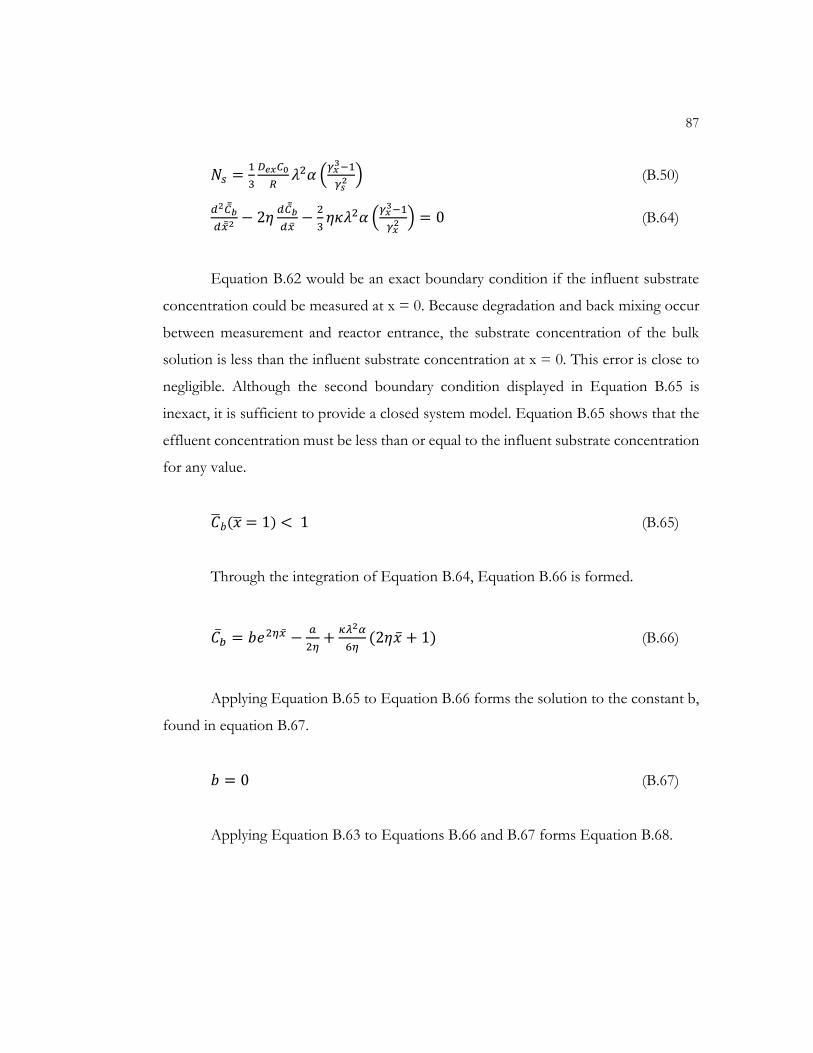
87

𝑁𝑠 =1

3

𝐷𝑒𝑥𝐶0

𝑅𝜆2𝛼 (

𝛾𝑥3−1

𝛾𝑠2 ) (B.50)

𝑑2𝐶𝑏

𝑑��2− 2𝜂

𝑑��𝑏

𝑑��−

2

3𝜂𝜅𝜆2𝛼 (

𝛾𝑥3−1

𝛾𝑥2 ) = 0 (B.64)

Equation B.62 would be an exact boundary condition if the influent substrate

concentration could be measured at x = 0. Because degradation and back mixing occur

between measurement and reactor entrance, the substrate concentration of the bulk

solution is less than the influent substrate concentration at x = 0. This error is close to

negligible. Although the second boundary condition displayed in Equation B.65 is

inexact, it is sufficient to provide a closed system model. Equation B.65 shows that the

effluent concentration must be less than or equal to the influent substrate concentration

for any value.

��𝑏(�� = 1) < 1 (B.65)

Through the integration of Equation B.64, Equation B.66 is formed.

𝐶�� = 𝑏𝑒2𝜂�� −𝑎

2𝜂+

𝜅𝜆2𝛼

6𝜂(2𝜂�� + 1) (B.66)

Applying Equation B.65 to Equation B.66 forms the solution to the constant b,

found in equation B.67.

𝑏 = 0 (B.67)

Applying Equation B.63 to Equations B.66 and B.67 forms Equation B.68.

88

𝑎 =1

3𝜅𝜆2𝛼 − 2𝜂 (B.68)

Equation B.69 displays the zeroth order kinetics for the boundary conditions,

which is independent of both 𝜂 and 𝜏, found by applying Equation B.63 to B.66 with

Equations B.67 and B.68.

𝐶�� = 1 −1

3𝜅𝛼𝜆2 (

𝛾𝑥3−1

𝛾𝑥2 ) (B.69)

The first order approximation for the model is given by first substituting

Equation B.54, shown previously and below, into Equation B.61 to form Equation B.70.

𝑁𝑠 =𝐷𝑒𝑥𝐶0

𝑅(

𝛾𝑥

𝛾𝑠)

2

(𝑁

1+𝜏𝑁) 𝐶�� (B.54)

𝑑2𝐶𝑏

𝑑��2 − 2𝜂𝑑��𝑏

𝑑��− 2𝜂𝜅

𝑅

𝐷𝑒𝑥𝐶0(

𝛾𝑠

𝛾𝑥) 𝑁𝑠 = 0 (B.61)

𝑑2𝐶𝑏

𝑑��2 − 2𝜂𝑑��𝑏

𝑑��− 2𝜂𝜅 (

𝑁

1+𝜏𝑁) 𝐶�� = 0 (B.70)

Through the integration of Equation B.70, Equation B.71 is formed, where the

parameter 𝛽is given by equation B.72.

𝐶�� = 𝑎𝑒(η+β)�� + b𝑒(η−β)�� (B.71)

𝛽 = (𝜂2 +2𝜅𝜂𝑁

1+𝜏𝑁)

1

2 (B.72)

Applying Equation B.65, shown previously and below, yields a = 0. Applying

Equation B.63, shown previously and below, yields b = 1; therefore, Equation B.70 is

generated. Equation B.70 displays the first order kinetics.

89

��𝑏(�� = 1) < 1 (B.65)

𝐶��(�� = 0) = 1 (B.63)

𝑙𝑛𝐶�� = 𝜂 [1 − (1 +2𝜅𝑁

𝜂+𝜏𝑁)

1

2] �� (B.70)

B.5 Effect of Dispersion on the Model

When the dispersion is neglected, Equation B.57 becomes Equation B.71.

𝑑2𝐶𝑏

𝑑��2 − 2𝜂𝑑��𝑏

𝑑��− 2𝜂𝜅

𝑑��𝑥

𝑑�� (�� = 𝛾𝑥) = 0 (B.57)

𝑑��𝑏

𝑑𝑥+ 𝜅

𝑑��𝑥

𝑑�� (�� = 𝛾𝑥) = 0 (B.71)

Only one boundary condition is required to satisfy this equation, displayed in

Equation B.63, shown previously and below.

𝐶��(�� = 0) = 1 (B.63)

For zeroth order kinetics, the solution is unchanged from Equation B.71, shown

above. The solution for first-order kinetics is displayed in Equation B.72.

𝑙𝑛𝐶�� = −𝜅 (𝑁

1+𝜏𝑁) �� (B.72)

The effect of dispersion decreases the removal of the substrate; however, the

dispersion is negligible because the values predicted by Equation B.70 and B.72 are equal

when equation B.73 exists.

90

𝑙𝑛𝐶�� = 𝜂 [1 − (1 +2𝜅𝑁

𝜂+𝜏𝑁)

1

2] �� (B.70)

𝑁

𝜂(1+𝜏𝑁)< 0.1 (B.73)

Predicted values for 𝜂 were found to always be greater than 100 and the values

of 𝜅𝑁

1+𝜏𝑁 was less than 5 [29][30]. The effect of dispersion was, therefore, neglected for

this model.

B.6 Summary

Equations B.16, B.17, B.48, B.63, and B.71, all listed previously and below,

describe the complete mathematical system of the physical-biological fixed film fluidized

reactor.

1

��2 𝑑

𝑑𝑟 ��2

𝑑��𝑥

𝑑��− (𝜆2 𝛼)

��𝑥

𝛼+𝐶��= 0 (B.16)

𝑑��𝑥

𝑑�� (�� = 1) = 0 (B.17)

At �� = 𝛾𝑥 , 𝐶�� + 𝜏𝑑��𝑥

𝑑��= 𝐶�� (B.48)

𝐶��(�� = 0) = 1 (B.63)

𝑑��𝑏

𝑑𝑥+ 𝜅

𝑑��𝑥

𝑑�� (�� = 𝛾𝑥) = 0 (B.71)

Zeroth and first-order kinetic approximations were completed and shown in

Equations B.69 and B.72, shown below and previously.

𝐶�� = 1 −1

3𝜅𝛼𝜆2 (

𝛾𝑥3−1

𝛾𝑥2 ) (B.69)

𝑙𝑛𝐶�� = −𝜅 (𝑁

1+𝜏𝑁) �� (B.72)

91

Integration can be used to solve the nonlinear system of equations. Normalizing

the variables, �� and ��𝑥, allow for simplification of programming. The dimensionless

radial coordinate, y, and the dimensionless biolayer substrate concentration, C, are

defined in Equations B.74 and B.75 to simplify the descriptive equations.

𝑦 =𝑟−𝑅

(𝛾𝑥−1)𝑅=

��−1

𝛾𝑥−1 (B.74)

𝐶 = 𝐶𝑥

𝐶𝑏 (B.75)

The descriptive equations, with these newly defined dimensionless parameters,

are present in Equations B.76 and B.77.

𝑑2𝐶

𝑑𝑦2 + 2

𝜎+𝑦

𝑑𝐶

𝑑𝑦−

𝜆2𝛼

𝜎2 𝐶

𝛼+ ��𝑏𝐶= 0 (B.76)

𝑑��𝑏

𝑑��+ 𝜅𝜎𝐶��

𝑑𝐶

𝑑𝑦(𝑦 = 1) = 0 (B.77)

The boundary condition equations required to solve this system are displayed in

Equations B.78, B.79, and B.63.

𝐶(𝑦 = 1) + 𝜏𝜎𝑑𝐶

𝑑𝑦(𝑦 = 1) = 1 (B.78)

𝑑𝐶

𝑑𝑦(𝑦 = 0) = 0 (B.79)

𝐶��(�� = 0) = 1 (B.63)

92

The relevant dimensionless parameters are listed as Equations B.19, B.20, B.49,

B.59, and B.80.

𝜆2 =��𝑋𝑅2

𝑌𝐾𝑠𝐷𝑒𝑥 (B.19)

𝛼 = 𝐾𝑠

𝐶0 (B.20)

𝜏 = 𝐷𝑒𝑥

𝑘𝑅 (

𝛾𝑥

𝛾𝑠)

2

(B.49)

𝜅 = 3(1−𝜀𝑒)𝐷𝑒𝑥𝜃

𝛾𝑥𝑅2 (B.59)

𝜎 =1

𝛾𝑥−1 (B.80)

Equation B.69 can be rewritten as Equation B.81.

𝐶�� = 1 −1

3𝜅𝛼𝜆2 (

𝛾𝑥3−1

𝛾𝑥2 ) (B.69)

��𝑏 = 1 −1

3𝜅𝛼𝜆2 (3𝜎2+3𝜎+1)

𝜎(𝜎+1)2 �� (B.81)

However, Equation B.72 remains unchanged.

𝑙𝑛𝐶�� = −𝜅 (𝑁

1+𝜏𝑁) �� (B.72)

Equation B.40, which is the definition of the flux constant, can be rewritten as

Equation B.82.

𝑁 = (𝜆 + 1

𝛾𝑥) (

𝜆+1

𝜆−1𝑒2𝜆(𝛾𝑥−1) + 1)

−1

(𝜆𝛾𝑥−1

𝜆𝛾𝑥+1 𝜆+1

𝜆−1𝑒2𝜆(𝛾𝑥−1) − 1) (B.40)

𝑁 =(𝜆𝜎+𝜆+𝜎)

(𝜎+1)(

𝜆+1

𝜆−1𝑒

2𝜆

𝜎 + 1)−1

(𝜆+1

𝜆−1 𝜆𝜎+𝜆−𝜎

𝜆𝜎+𝜆+𝜎𝑒

2𝜆

𝜎 − 1) (B.82)

93

The three kinetic expressions were compared through a computer program and

the data was plotted by Jennings [29][30], shown in Figure B.2.

Figure B.2: Comparison of Kinetic Approximations [29][30]

The first order approximation is much closer to the nonlinear solution than the

zeroth order even with a low value of 𝛼. The results of Figure B.2 show that the zeroth

order approximation is closer to the nonlinear solution only at low values of 𝛼, high

influent substrate concentration, and low values of 𝜆, small particle diameter. In the

research performed by Jennings [29][30], the values of percent removal predicted by the

first order model had only a 1% to 2% error when compared to the nonlinear solution.

Figures B.3, B.4, B.5, and B.6 display the effect of the dimensionless parameters

on 𝑙𝑛𝐶�� as a function of 𝜅, prepared by Jennings [29][30]. Values for 𝛼, 𝜆, 𝜎, and 𝜏

were calculated to be approximately 1, 25, 10, and 0.05, respectively, for comparison. It

was stated that these graphs may be misleading due to the fact that dimensionless

94

parameters generally cannot be varied independently of each other or over a large range.

It was shown that only three parameters can be expected to vary by more than a factor

of 2: influent concentration, C0; particle radius, R; and residence time, 𝜃 . Influent

concentration and residence time only appear in one of the dimensionles parameters

and the effects of the variances are shown in Figures B.3 and B.6, whereas the particle

radius is found in three parameters; therefore, Figure B.7 was plotted to display 𝑙𝑛𝐶��

versus 𝜃 as a function of R.

First order kinetics of the model created by Jennings [29][30] leads to the close

approximation to the nonlinear solution of Monod kinetics even when the basic

assumption of Cx << Ks is void. This is due to the stark concentration gradient between

the liquid boundary layer and the biological film layer. When the bulk liquid

concentration is large, the concentration within the biological film layer is low,

producing first order kinetic behavior. Equation B.72 was used to analyze experimental

data in work by Jennings [29][30] and was also used to analyze experimental data in this

thesis due to a desirable analytical solution rather than a numerical one.

95

Figure B.3: Effect of Influent Substrate Concentration [29][30]

96

Figure B.4: Effect of Biokinetic Parameters [29][30]

97

Figure B.5: Effect of Biolayer Thickness [29][30]

98

Figure B.6: Effect of Stagnant Liquid Layer [29][30]

99

Figure B.7: Effect of Particle Radius [29][30]

Parameter values of the theoretical model developed are expected to be the same

as found in the work done by Jennings [29][30]. Since the theoretical model that was

developed and tested previously had proven to be valid, approximate values of the

100

operating parameters used in the previous study, such as R, Q, A, Le, and L0, were

calculated using Equation B.72, whereas all other parameter values were found in the

literature [29][30]. Values found in the previous work [29][30] were used for this work

as well, being that they would be close to the previous values, if not equal. The values

found in literature [29][30] in previous work [29][30] were for the parameters ��, 𝐾𝑆, Y,

X, D, 𝐷𝑋, 𝛿𝑋, 휀𝑒, and k. The values of the dimensionless parameters 𝜆, 𝜅, 𝜎, and 𝜏 were

then calculated from the parameters. The average values of �� and 𝐾𝑆 used in previous

work were 0.51 and 21, respectively [29][30]. It should be noted that these values were

calculated from a wide range of literature values [29][30] found and may deviate from

the actual values. However, despite this deviation, the ratio of ��

𝐾𝑠 is expected to only vary

in a narrow range, where the average was 0.0496, using literature values [29][30].

The cell yield coefficient, Y, used in previous research ranged from 0.44 to 0.64

for glucose [29][30]. True steady-state conditions are not able to be established in the

reactor; therefore, this coefficient could not be directly measured. An estimation of Y,

from the previous research [29][30], was made from , the ratio of carbon dioxide

production to glucose utilization, using an empirical formula for cell mass, C5H7O2N.

For glucose, the respiration step in an anaerobic system is given below for both ethanol

and butanol production. The synthesis of cell mass is given below using the empirical

formula for cell mass.

Respiration, Formation of Butanol: C6H12O6 C4H9OH + 2 CO2 + H2O

Respiration, Formation of Ethanol: C6H12O6 C2H5OH + 2 CO2

Cellular Synthesis: 6 NH3 + 5C6H12O6 6 C5H7O2N + 18 H2O

From these empirical chemical equations, and Y can be estimated below,

shown in Equation B.83A and B.83B [29][30].

101

𝜙 =192

180(1 −

900

678𝑌) (B.83A)

𝑌 = 0.7533 (1 − 0.9375𝜙) (B.83B)

These equations assume that the only products of glucose utilization are butanol,

ethanol, or cell mass. If a certain portion, 𝜒, of the glucose utilized remains in solution

as an organic metabolite, Equation B.83B becomes Equation B.84.

𝑌 = 0.7533(1 − 𝜒 − 0.9375𝜙) (B.84)

Using previous experimental values, calculated in the previous work [29][30]

developing this theoretical model, the value of Y for glucose was 0.541, without the use

of 𝜒. With the use of 𝜒 = 0.15, as done in previous work, the value of Y for glucose

was 0.428, where a typical value is between 0.25 to 0.60 g/g [29][30].

The previous work has shown that the value of 𝜒 to be dependent on the total

thickness of the biolayer and the amount of shear force on the layer from fluidization

flow. Reported values in the previous work range from 20 to 150 mg/mL, and the

reasonable value used in the previous work was 50 mg/mL.

The thickness of the biological layer and the stagnant liquid layer, 𝛿𝑋and 𝛿𝑠 ,

respectively, are impossible to measure directly. However, thickness theoretically should

have little effect on the results, as discussed previously, but limits need to exist. In the

previous development of this model for the thickness, 𝛿𝑋 , the lower limit was

approximately 10 m whereas the upper limit was 200 m. The thickness of the biolayer

is also not expected to be greater than the particle radius. A reasonable value for 𝛿𝑋

used in the previous work and this work was 70 m [29][30].

The value of 𝛿𝑠 is normally very low for fluidized particles due to the moving

fluid. In the previous study [29][30], the minimum value for 𝛿𝑠 was 30 m while the

maximum was 700 m. The value used was 70 m.

102

The porosity of the expanded bed, 휀𝑒, is also impossible to measure directly.

However, this value can be related to the porosity of the unexpanded bed, 휀0, through

a particle mass balance, shown in Equations B.85 and B.86. However, the value of 휀0 is

also unable to be measured directly because each individual carbon particle can have its

own porosity. The reasonable value used in the previous study and this study was 0.40,

found from literature for carbon particles.

𝐴𝐿𝑒(1 − 휀𝑒) = 𝐴𝐿0(1 − 휀0) (B.85)

(1 − 휀𝑒) = (1 − 휀0)𝐿0

𝐿𝑒 (B.86)

The diffusivity of the substrate through the bulk liquid was found in the previous

study through a literature search. The value for the diffusivity, D, for glucose, was found

to be 0.61 x 10-5 cm2/s, where the value of diffusivity through the biological layer, DX,

was found to be 0.72 x 10-5 cm2/s [29][30].

The value of the coefficient of mass transfer through the stagnant liquid layer,

k, was estimated using an empirical correlation, from the previous study [29][30]. For

1<Re<30, Equation B.87 was used, where Sh, Sc, Re, and Rem were the dimensionless

Sherwood, Schmidt, Reynolds, and modified Reynolds numbers, respectively.

𝑗𝐷 =𝑆ℎ

𝑆𝑐1

3⁄ 𝑅𝑒= 5.7𝑅𝑒𝑚

−0.78 (B.87)

These numbers are defined below, as Equation B.88A, B.88B, B.88C, and

B.88D.

𝑆ℎ = 2𝑘𝑅

𝐷 (B.88A)

𝑆𝑐 = 𝜇

𝜌𝐷 (B.88B)

𝑅𝑒 = 2𝜌𝑅𝑢

𝜇 (B.88C)

103

𝑅𝑒𝑚 = 2𝜌𝑅𝑢

𝜇(1−𝜀𝑒) (B.88D)

Rearranging Equation B.87, Equation B.89 is generated.

𝑘 = 𝑢𝑆𝑐−2

3⁄ 𝑗𝐷 = 5.7𝑢𝑆𝑐−2

3⁄ 𝑅𝑒𝑚−0.78 (B.89)

Using Equation B.89, the value of k was calculated in the previous development

of the theoretical model to be 0.0033 cm/s.

The particle size is able to be varied; however, it was not varied during this thesis

and, therefore, the previous value was used as 0.707 mm. Because of this the operating

variables were reduced to Le, L0, and Q (or Le/L0 and ), as it was in the previous study.

Table B.2 summarizes the values used in the previous study and this study to create the

theoretical model [29][30].

Table B.2: Values Used in Previous Study [29][30]

Parameter Value Used Units

�� 0.50 hours-1

𝐾𝑆 20.0 mg/L

Y 0.40 g/g

X 50 mg/L

De 0.85 x 10-5 cm2/s

DeX 0.72 x 10-5 cm2/s

𝛿𝑋 70.7 microns

𝛿𝑆 70.7 microns

휀𝑒 0.40

R 707 microns

k 0.0033 cm/sec

24.5

104

Parameter Value Used Units

10.0

0.0301

𝜅(

𝐿𝑒𝐿0

⁄ )

𝜃⁄

0.141 min-1

Equation B.72 is the theoretical model that yields the relationship for substrate

concentration at any point within the fluidized bed as a function of many parameters

such as axial position.

𝑙𝑛𝐶�� = −𝜅 (𝑁

1+𝜏𝑁) �� (B.72)

It is assumed that during testing all substrate removal will occur within the

fluidized bed; therefore, the effluent concentration can be assumed to be equal to the

bed concentration at x=Le. When this assumption is made, Equation B.72 becomes

Equation B.90, where 𝜅 is defined by Equation B.59.

ln (𝐶𝑓

𝐶0) = −

𝜅𝑁

1+𝜏𝑁 (B.90)

𝜅 = 3(1−𝜀𝑒)𝐷𝑒𝑥𝜃

𝛾𝑥𝑅2 (B.59)

When Equation B.90 is substituted into Equation B.59, Equations B.91, B.92,

and B.93 are generated.

𝜅 = 3(1−𝜀0)𝐷𝑒𝑋

𝛾𝑥𝑅2

𝐿0

𝐿𝑒𝜃 (B.91)

𝑙𝑛 (𝐶𝐹

𝐶0) = −𝑚 (

𝐿0

𝐿𝑒) 𝜃 (B.92)

𝑚 =3(1−𝜀0)𝐷𝑒𝑋

𝛾𝑥𝑅2 (𝑁

1+𝜏𝑁) (B.93)

105

In Equation B.93, m is the slope of the linear plot of −𝑙𝑛 (𝐶𝑓

𝐶0) versus (

𝐿0

𝐿𝑒) 𝜃,

where the two operating parameters of the system are 𝐿0

𝐿𝑒, being a measure of bed

expansion and 𝜃, equal to 𝐿𝑒

𝐴𝑞, being the “empty bed” residence time.

106

Appendix C Methods and Materials Raw Data and Calculations

C.1 Fluidization Analysis Raw Data

Table C.1 displays the parameters for the fluidized bed reactor including

activated carbon diameter, the diameter of the reactor, the total height of the reactor,

original bed height, activated carbon height, and the cross-sectional area.

The raw fluidization data can be found in Table C.2. The time, volume, and bed

height was measured manually. The volumetric flow rate was found by dividing the

volume collected by the time. The velocity was then subsequently found by dividing the

volumetric flow rate by the cross-sectional area of the reactor. The minimum

fluidization velocity occurs when the bed height changes from stagnant to fluidized.

This can be found in the fluidization graph by determining when the curve begins to

slope upwards. The minimum fluidization velocity was found to be 1.1 cm/s and is

displayed in Figure 3.2.

Table C.1: Fluidized Bed Reactor Parameters

Parameter Value Value

Activated Carbon Diameters 0.125 in

Diameter of Column 2 in 5.08 cm

Total Column Height 47.25 in

Original Bed Height with Glass Beads 16.25 in 21.125 cm

Glass Beads Height 4.25 in

Activated Carbon Height 12 in

Cross Sectional Area 20.27 cm2

107

Table C.2: Raw Fluidization Data

C.2 Gas Chromatography Analysis Raw Data

Table C.3 displays the gas chromatograph raw data including sample contents

and data collected from the gas chromatograph.

Table C.3: Gas Chromatograph Raw Data

Water in

Sample (mL)

Butanol in

Sample (mL)

Ethanol in

Sample (mL)

% Butanol/Ethanol

by Volume

Area from GC (Water)

Area from GC (Ethanol)

Area from GC (Butanol)

10 1 1 8.33% 9.05E+06 468900 431020

10 1 1 8.33% 9.02E+06 457900 427850

10 1 1 8.33% 9.12E+06 460400 426900

25 1 1 3.70% 1.01E+07 198670 188760

25 1 1 3.70% 1.03E+07 192540 184220

25 1 1 3.70% 1.09E+07 201770 194890

108

Water in

Sample (mL)

Butanol in

Sample (mL)

Ethanol in

Sample (mL)

% Butanol/Ethanol

by Volume

Area from GC (Water)

Area from GC (Ethanol)

Area from GC (Butanol)

50 1 1 1.92% 1.02E+07 90882 91376

50 1 1 1.92% 1.05E+07 88782 89564

50 1 1 1.92% 1.01E+07 86857 85478

75 1 1 1.30% 1.08E+07 57135 58545

75 1 1 1.30% 1.00E+07 56473 59821

75 1 1 1.30% 9.81E+06 51125 53949

100 1 1 0.98% 9.98E+06 38471 41017

100 1 1 0.98% 1.08E+07 39492 42938

100 1 1 0.98% 1.04E+07 38328 41942

125 1 1 0.79% 1.07E+07 30718 34387

125 1 1 0.79% 1.05E+07 28471 33107

125 1 1 0.79% 1.05E+07 29654 32764

150 1 1 0.66% 1.08E+07 23585 28389

150 1 1 0.66% 9.73E+06 21642 24924

150 1 1 0.66% 1.04E+07 22595 27350

175 1 1 0.56% 1.13E+07 20428 24901

175 1 1 0.56% 1.05E+07 18417 22390

175 1 1 0.56% 1.09E+07 18595 21967

200 1 1 0.50% 9.49E+06 13400 16942

200 1 1 0.50% 9.60E+06 11919 15355

200 1 1 0.50% 1.04E+07 13375 18015

225 1 1 0.44% 9.77E+06 11638 12238

225 1 1 0.44% 1.03E+07 12445 16432

225 1 1 0.44% 1.02E+07 11578 16313

250 1 1 0.40% 9.83E+06 10172 14123

250 1 1 0.40% 1.02E+07 10935 14783

250 1 1 0.40% 1.02E+07 9982 14802

275 1 1 0.36% 1.05E+07 9256 13114

275 1 1 0.36% 1.02E+07 9205 13096

109

Water in

Sample (mL)

Butanol in

Sample (mL)

Ethanol in

Sample (mL)

% Butanol/Ethanol

by Volume

Area from GC (Water)

Area from GC (Ethanol)

Area from GC (Butanol)

275 1 1 0.36% 1.06E+07 9088 13529

300 1 1 0.33% 1.02E+07 7300 11898

300 1 1 0.33% 1.02E+07 7927 12041

300 1 1 0.33% 1.03E+07 8100 11995

325 1 1 0.31% 1.04E+07 2968 11191

325 1 1 0.31% 1.02E+07 6438 10844

325 1 1 0.31% 1.08E+07 5934 11617

350 1 1 0.28% 1.07E+07 6299 10609

350 1 1 0.28% 1.03E+07 5591 10087

350 1 1 0.28% 1.03E+07 3846 10130

375 1 1 0.27% 1.05E+07 4565 9430

375 1 1 0.27% 1.03E+07 5552 9522

375 1 1 0.27% 1.07E+07 3742 9532

400 1 1 0.25% 1.05E+07 5763 8797

400 1 1 0.25% 1.03E+07 5065 8642

400 1 1 0.25% 1.01E+07 4747 8503

625 1 1 0.16% 9.74E+06 3275 5227

625 1 1 0.16% 1.01E+07 3300 4598

625 1 1 0.16% 1.06E+07 3353 5824

625 1 1 0.16% 1.15E+07 3465 6621

650 1 1 0.15% 1.09E+07 3340 5952

650 1 1 0.15% 1.09E+07 3094 5743

650 1 1 0.15% 1.03E+07 3285 5343

650 1 1 0.15% 1.08E+07 2680 5812

650 1 1 0.15% 9.90E+06 3788 5437

675 1 1 0.15% 1.06E+07 2194 5546

675 1 1 0.15% 1.05E+07 3427 4464

675 1 1 0.15% 1.05E+07 2744 5499

675 1 1 0.15% 1.06E+07 2161 5466

110

Water in

Sample (mL)

Butanol in

Sample (mL)

Ethanol in

Sample (mL)

% Butanol/Ethanol

by Volume

Area from GC (Water)

Area from GC (Ethanol)

Area from GC (Butanol)

675 1 1 0.15% 1.03E+07 2234 5389

700 1 1 0.14% 1.09E+07 2209 5173

700 1 1 0.14% 1.07E+07 3582 5062

111

C.3 Benedicts Test and Spectrophotometer Analysis Raw Data

Table C.4 displays the raw data gathered from the output of the

spectrophotometer after the Benedict’s test was performed.

Table C.4: Spectrophotometer Standardization Data

Tube number

Concentration (mg/L)

Adsorbance (AU) at 735 nm (DISTILLED WATER BLANK)

1 0.0 0.083

0.078

2 47.7 0.162

0.162

3 38.0 0.135

0.138

4 28.5 0.110

0.110

5 19.0 0.103

0.102

6 9.5 0.115

0.098

7 5.7 0.119

0.127

8 4.8 0.125

0.109

9 3.8 0.102

0.106

10 2.9 0.123

0.124

112

Appendix D Apparatus Photos

Figure D.1: Reactor Column

113

Figure D.2: Reactor Column and Fluidization Pump

114

Figure D.3: Inlet Tap Water, Nitrogen Sparge Tank, Fluidization Pump, and Concentrated Substrate Reservoir

115

Figure D.4: Concentrated Substrate Reservoir, Substrate Pump, and Fluidization Pump

116

Appendix E Results and Discussion Raw Data

E.1 Fermentation Verification: Clostridium acetobutylicum Raw Data

Experiment 1: Recycling Clostridium acetobutylicum

Table E.1 displays the raw data from the spectrophotometer gathered from the

first experiment, after the recycle. There were two samples in this raw data, one sample

from the reactor effluent and one sample from the reservoir. The absorbance is the

reading from the spectrophotometer using the Benedict’s Test. Each absorbance

reading corresponds to one trial. The concentration provided next to the absorbance is

the concentration of glucose present in the sample calculated using the standardization

curve, present in Chapter 3, Figure 3.5.

Table E.1: Raw Data from Spectrophotometer, First Experiment

Reservoir Absorbance

(AU)

Reservoir Calculated Glucose

Concentration (mg/L)

Reactor Absorbance

(AU)

Reactor Calculated Glucose

Concentration (mg/L)

0.190 127 0.140 93.3

0.196 131 0.156 104

0.206 137 0.132 88.0

0.195 130 0.169 113

117

Experiment 2: Normal Operation of Clostridium acetobutylicum Fluidized Bed

Reactor, Day 1

Table E.2 displays the raw data from the spectrophotometer gathered from

Experiment 2, day 1 of normal operation on the Clostridium acetobutylicum fluidized bed

biological reactor. The first column is the time that the sample was taken. Each row

represents one trial of the sample. The absorbance is the reading from the

spectrophotometer using the Benedict’s Test. The concentration provided next to the

absorbance is the concentration of glucose present in the effluent of the reactor

calculated using the standardization curve, present in Chapter 3, Figure 3.5.

Table E.2: Day 1, Normal Operation Spectrophotometer Analysis on Clostridium acetobutylicum Reactor Effluent, Raw Data

Day 1 Sample Time Taken

Reactor Absorbance (AU)

Reactor Calculated

Glucose Concentration

(mg/L)

7:13 AM 0.190 127

7:13 AM 0.196 131

7:13 AM 0.208 139

7:13 AM 0.215 143

1:03 PM 0.134 89.3

1:03 PM 0.133 88.7

1:03 PM 0.123 82.0

1:03 PM 0.136 90.7

5:54 PM 0.048 32.0

5:54 PM 0.022 14.7

118

Day 1 Sample Time Taken

Reactor Absorbance (AU)

Reactor Calculated

Glucose Concentration

(mg/L)

5:54 PM 0.032 21.3

5:54 PM 0.050 33.3

10:49 PM 0.035 23.3

10:49 PM 0.040 26.7

10:49 PM 0.026 17.3

10:49 PM 0.039 26.0

Table E.3 displays the raw data from the gas chromatograph gathered from

Experiment 2, day 1 of normal operation on the Clostridium acetobutylicum fluidized bed

biological reactor. The first column is the time that the sample was taken. Each row

represents one trial of the sample. The columns containing the total peak area, peak area

for water, peak area for ethanol, and peak area for butanol were taken directly from the

gas chromatograph’s output. The columns containing the concentration of ethanol and

concentration of butanol were calculated using Equation 3.1 for butanol and Equation

3.2 for ethanol, located in Section 3.6. Any cell left blank in Table E.3 was an indication

that there was no recorded peak area for the molecule during the experimental run.

119

Table E.3: Day 1, Normal Operation Gas Chromatography Analysis on Clostridium acetobutylicum Reactor Effluent, Raw Data

Day 1 Sample

Time Taken

Total

Peak Area

Peak Area

for Water (Retention

Time = 0.08 -

0.12)

Peak Area

for Ethanol

(Retention Time =

0.60 - 0.85)

Peak Area

for Butanol

(Retention Time =

1.75 - 2.05)

Calculated Concentration

of Ethanol (% by Volume)

Calculated Concentration

of Butanol (% by Volume)

7:13 AM 18520000 18520000 0.00% 0.00%

7:13 AM 17284000 17284000 0.00% 0.00%

7:13 AM 21538000 21538000 0.00% 0.00%

7:13 AM 1296230 1206300 89930 6.94% 0.00%

7:13 AM 15328000 14608000 720000 4.70% 0.00%

7:13 AM 15335000 15335000 0.00% 0.00%

7:13 AM 20146000 20146000 0.00% 0.00%

7:13 AM 1725700 1644700 81000 4.69% 0.00%

7:13 AM 5195000 5094600 100400 1.93% 0.00%

7:13 AM 1578030 1560000 18030 1.14% 0.00%

1:03 PM 1111500 1111500 0.00% 0%

1:03 PM 13108270 12618000 490270 3.74% 0%

1:03 PM 18454000 18454000 0.00% 0%

1:03 PM 15100560 14765000 335560 2.22% 0%

1:03 PM 12528500 11676000 852500 6.80% 0%

1:03 PM 13160270 12632000 528270 4.01% 0%

1:03 PM 11501000 11501000 0.00% 0%

5:54 PM 11101000 11101000 0.00% 0%

5:54 PM 10948000 10948000 0.00% 0%

5:54 PM 18749000 18749000 0.00% 0%

5:54 PM 11358000 11358000 0.00% 0%

5:54 PM 15525000 15525000 0.00% 0%

5:54 PM 7263620 6820700 442920 6.10% 0%

5:54 PM 15258000 15258000 0.00% 0%

120

Experiment 3: Continuous Normal Operation of Clostridium acetobutylicum

Fluidized Bed Reactor, Day 2

Table E.4 displays the raw data from the spectrophotometer gathered from

Experiment 3, day 2 of normal operation on the Clostridium acetobutylicum fluidized bed

biological reactor. The first column is the time that the sample was taken. Each row

represents one trial of the sample. The absorbance is the reading from the

spectrophotometer using the Benedict’s Test. The concentration provided next to the

absorbance is the concentration of glucose present in the effluent of the reactor

calculated using the standardization curve, present in Chapter 3, Figure 3.5.

Day 1 Sample

Time Taken

Total

Peak Area

Peak Area

for Water (Retention

Time = 0.08 -

0.12)

Peak Area

for Ethanol

(Retention Time =

0.60 - 0.85)

Peak Area

for Butanol

(Retention Time =

1.75 - 2.05)

Calculated Concentration

of Ethanol (% by Volume)

Calculated Concentration

of Butanol (% by Volume)

5:54 PM 1577910 1543000 34910 2.21% 0%

5:54 PM 6805500 6747000 58500 0.86% 0%

10:49 PM 14252880 14224000 28880 0.20% 0%

10:49 PM 13163000 13163000 0.00% 0%

10:49 PM 11182000 11182000 0.00% 0%

10:49 PM 12480000 12480000 0.00% 0%

10:49 PM 10960000 10960000 0.00% 0%

10:49 PM 10903000 10903000 0.00% 0%

10:49 PM 1201930 1127000 74930 6.23% 0%

10:49 PM 11437000 11437000 0.00% 0%

121

Table E.4: Day 2, Continuous Normal Operation Spectrophotometer Analysis on Clostridium acetobutylicum Reactor Effluent, Raw Data

Day 2 Sample Time Taken

Reactor Absorbance

(AU)

Reactor Calculated

Glucose Concentration

(mg/L)

8:14 AM 0.140 93.3

8:14 AM 0.148 98.7

8:14 AM 0.130 86.7

8:14 AM 0.138 92.0

10:33 AM 0.132 88.0

10:33 AM 0.143 95.3

10:33 AM 0.135 90.0

10:33 AM 0.142 94.7

1:02 PM 0.153 102

1:02 PM 0.152 101

1:02 PM 0.157 105

1:02 PM 0.153 102

Table E.5 displays the raw data from the gas chromatograph gathered from

Experiment 3, day 2 of continuous normal operation on the Clostridium acetobutylicum

fluidized bed biological reactor. The first column is the time that the sample was taken.

Each row represents one trial of the sample. The columns containing the total peak area,

peak area for water, peak area for ethanol, and peak area for butanol were taken directly

from the gas chromatograph’s output. The columns containing the concentration of

ethanol and concentration of butanol were calculated using Equation 3.1 for butanol

122

and Equation 3.2 for ethanol, located in Section 3.6. Any cell left blank in Table E.5 was

an indication that there was no recorded peak area for the molecule during the

experimental run.

Table E.5: Day 2, Normal Continuous Operation Gas Chromatography Analysis on Clostridium acetobutylicum Reactor Effluent, Raw Data

Experiment 5: Recycling Clostridium acetobutylicum Without Yeast Extract

with an Influent Glucose Concentration of 500 mg/L Raw Data

Table E.6 displays the raw data from the spectrophotometer gathered from the

fifth experiment, after recycling for 5 days. There were two samples in this raw data, one

sample from the reactor effluent and one sample from the reservoir. Each absorbance

reading corresponds to one trial. The absorbance is the reading from the

Day 2 Sample

Time Taken

Total

Peak Area

Peak Area

for Water (Retention

Time = 0.08 -

0.12)

Peak Area

for Ethanol

(Retention Time =

0.60 - 0.85)

Peak Area for Butanol

(Retention Time =

1.75 - 2.05)

Calculated Concentration

of Ethanol (% by Volume)

Calculated Concentration

of Butanol (% by Volume)

8:14 AM 11427000 11427000 0.00% 0.00%

8:14 AM 11041000 11041000 0.00% 0.00%

8:14 AM 12296700 12288000 8700 0.07% 0.00%

8:14 AM 12009000 12009000 0.00% 0.00%

8:14 AM 11534680 11437000 97680 0.85% 0.00%

10:33 AM 11279000 11279000 0.00% 0.00%

10:33 AM 13268000 13268000 0.00% 0.00%

10:33 AM 11592600 10903000 689600 5.95% 0.00%

10:33 AM 12265000 12265000 0.00% 0.00%

10:33 AM 11438000 11438000 0.00% 0.00%

1:02 PM 12291000 12291000 0.00% 0.00%

1:02 PM 11750800 11253000 497800 4.24% 0.00%

1:02 PM 14671000 13983000 688000 4.69% 0.00%

1:02 PM 12988000 12988000 0.00% 0.00%

1:02 PM 11345000 11345000 0.00% 0.00%

123

spectrophotometer using the Benedict’s Test. The concentration provided next to the

absorbance is the concentration of glucose present in the sample calculated using the

standardization curve, present in Chapter 3, Figure 3.5.

Table E.6: Raw Data from Spectrophotometer, Experiment 5

Reactor Absorbance

(AU)

Reactor Calculated Glucose

Concentration (mg/L)

Reservoir Absorbance

(AU)

Reservoir Calculated

Glucose Concentration

(mg/L)

0.752 501 0.774 516

0.748 499 0.741 494

0.755 503 0.748 499

0.750 500 0.746 497

Experiment 7: Recycling Clostridium acetobutylicum With Autoclaved Yeast

Extract with an Influent Glucose Concentration of 5 g/L Raw

Data

Table E.7 displays the raw data from the spectrophotometer gathered from the

seventh experiment, after the recycle. There were two samples in this raw data, one

sample from the reactor effluent and one sample from the reservoir. Each absorbance

reading corresponds to one trial. The absorbance is the reading from the

spectrophotometer using the Benedict’s Test. The concentration provided next to the

absorbance is the concentration of glucose present in the sample calculated using the

standardization curve, present in Chapter 3, Figure 3.5.

124

Table E.7: Raw Data from Spectrophotometer, Experiment 7

E.2 Fermentation Verification, Yeast Raw Data

Experiment 9: Recycling Yeast Extract Raw Data

Table E.8 displays the raw data from the spectrophotometer gathered from the

ninth experiment, after the recycle. There were two samples in this raw data, one sample

from the reactor effluent and one sample from the reservoir. The absorbance is the

reading from the spectrophotometer using the Benedict’s Test. Each absorbance

reading corresponds to one trial. The concentration provided next to the absorbance is

the concentration of glucose present in the sample calculated using the standardization

curve, present in Chapter 3, Figure 3.5.

Table E.8: Raw Data from Spectrophotometer, Experiment 9

Reactor Absorbance

(AU)

Reactor Calculated Glucose

Concentration (g/L)

Reservoir Absorbance

(AU)

Reservoir Calculated Glucose

Concentration (g/L)

1.759 1.2 1.768 1.2

1.724 1.1 1.963 1.3

1.942 1.3 1.718 1.1

1.875 1.3 1.730 1.2

1.757 1.2 1.752 1.2

1.728 1.2 1.858 1.2

Reactor Absorbance (AU)

Reactor Calculated

Glucose Concentration (mg/L)

Reservoir Absorbance (AU)

Reservoir Calculated

Glucose Concentration (mg/L)

0.172 115 0.188 125

0.177 118 0.172 115

0.192 128 0.163 109

0.187 125 0.172 115

125

Experiment 10: Normal Operation of Yeast Fluidized Bed Reactor, Day 1

Table E.9 displays the raw data from the spectrophotometer gathered from

Experiment 10, day 1 of normal operation on the yeast fluidized bed biological reactor.

The first column is the time that the sample was taken. Each row represents one trial of

the sample. The absorbance is the reading from the spectrophotometer using the

Benedict’s Test. The concentration provided next to the absorbance is the concentration

of glucose present in the effluent of the reactor calculated using the standardization

curve, present in Chapter 3, Figure 3.5.

Table E.9: Day 1, Normal Operation Spectrophotometer Analysis on Yeast Reactor Effluent, Raw Data

Day 1 Sample Time Taken

Reactor Absorbance (AU)

Reactor Calculated

Glucose Concentration

(mg/L)

12:00 PM 0.847 565

12:00 PM 0.852 568

12:00 PM 0.716 477

12:00 PM 0.665 443

12:00 PM 0.895 597

12:00 PM 0.819 546

3:00 PM 0.656 437

3:00 PM 0.624 416

3:00 PM 0.932 621

3:00 PM 0.817 545

3:00 PM 1.047 698

3:00 PM 1.024 683

5:00 PM 0.459 306

5:00 PM 0.468 312

5:00 PM 0.675 450

126

Day 1 Sample Time Taken

Reactor Absorbance (AU)

Reactor Calculated

Glucose Concentration

(mg/L)

5:00 PM 0.699 466

5:00 PM 0.544 363

5:00 PM 0.576 384

10:00 PM 0.393 262

10:00 PM 0.460 307

10:00 PM 0.416 277

10:00 PM 0.472 315

10:00 PM 0.48 320

10:00 PM 0.540 360

Experiment 11: Continuous Normal Operation of Yeast Fluidized Bed Reactor,

Day 2 Raw Data

Table E.10 displays the raw data from the spectrophotometer gathered from

Experiment 11, day 2 of normal operation on the yeast fluidized bed biological reactor.

The first column is the time that the sample was taken. Each row represents one trial of

the sample. The absorbance is the reading from the spectrophotometer using the

Benedict’s Test. The concentration provided next to the absorbance is the concentration

of glucose present in the effluent of the reactor calculated using the standardization

curve, present in Chapter 3, Figure 3.5.

127

Table E.10: Day 2, Continuous Normal Operation Spectrophotometer Analysis on Yeast Reactor Effluent, Glucose Concentration Raw Data

Day 2 Sample Time Taken

Reactor Absorbance (AU)

Reactor Calculated

Glucose Concentration

(mg/L)

9:30 AM 0.540 360

9:30 AM 0.329 219

9:30 AM 0.333 222

9:30 AM 0.372 248

9:30 AM 0.311 207

9:30 AM 0.264 176

1:00 PM 0.270 180

1:00 PM 0.365 243

1:00 PM 0.415 277

1:00 PM 0.346 231

1:00 PM 0.396 264

1:00 PM 0.322 215

7:00 PM 0.382 255

7:00 PM 0.465 310

7:00 PM 0.473 315

7:00 PM 0.543 362

7:00 PM 0.328 219

7:00 PM 0.481 321

10:00 PM 0.395 263

10:00 PM 0.341 227

10:00 PM 0.428 285

10:00 PM 0.377 251

10:00 PM 0.381 254

10:00 PM 0.388 259

128

E.3 Theoretical Model Verification Analysis Raw Data

Table E.11 displays the raw data collected for the theoretical model verification

performed on the yeast reactor culture developed from Experiments 9, 10, and 11. The

first column contains the fluidization flow rate measured. Each row represents one trial

of the fluidization flow rate in question. The second column contains the reactor

absorbance measured by the spectrophotometer using the Benedict’s test. The

concentration, in the third column, provided next to the absorbance is the concentration

of glucose present in the effluent of the reactor calculated using the standardization

curve, present in Chapter 3, Figure 3.5. The fourth column is the unexpanded carbon

bed height while the fifth column is the expanded carbon bed height. The sixth column

is the ratio of the unexpanded carbon bed height to the expanded carbon bed height.

The sixth column was calculated for each trial, where the fourth column was divided by

the fifth column.

The seventh column was the calculated empty bed residence time. This was

calculated by multiplying the expanded carbon bed height and the ratio of cross sectional

area of the expanded fluidized bed to the volumetric flow rate in question. The eighth

column was the product of the sixth and the seventh column. The ninth column was

the ratio of effluent glucose concentration to the influent glucose concentration. The

tenth and final column was the negative natural logarithm of the ninth column. These

calculations were performed based on the theoretical model derived by Jennings

[29][30], found in Appendix B.

129

Table E.11: Raw Data from Fluidization Theoretical Model Verification on Yeast

130

E.4 Demonstration of a Manual Scouring Method, Raw Data Analysis

Tables E.12, E.13, and E.14 display the raw data gathered from the

demonstration of a manual scouring method.

Table E.12: Raw Data from Manual Scouring of the Yeast Biofilm, Bed Height, Absorbance, and Concentration

Time (hours)

Bed Height

Reactor Effluent

Absorbance (AU)

Reactor Calculated

Glucose Concentration

(mg/L)

-1.0 26.1 0.395 263

-0.5 26.2 0.365 243

0.0 26.2 0.382 255

0.0 22.3 0.412 275

0.5 22.3 0.421 281

1.0 22.4 0.384 256

Column one of Table E.12 describes the elapsed time, in hours, before and after

scouring. For example, -1.0 hours refers to 1 hour before scouring. The first reading of

zero hours was immediately before the carbon bed was scoured while the second reading

of zero hours was immediately after the carbon bed was scoured. The second column

is the recorded carbon bed height during the elapsed time. The absorbance in the third

column is the reading from the spectrophotometer using the Benedict’s Test. The

concentration provided next to the absorbance is the concentration of glucose present

in the effluent of the reactor calculated using the standardization curve, present in

Chapter 3, Figure 3.5.

131

Table E.13: Raw Data from Manual Scouring, Calculation of Residence Time

Time (hours)

L0 (in) Le (in) L0/Le secLe*A/Q

-1.0 22.3 26.1 0.85 1.56

-0.5 22.3 26.1 0.85 1.56

0.0 22.3 26.1 0.85 1.56

0.0 22.3 26.1 0.85 1.56

0.5 22.3 26.1 0.85 1.56

1.0 22.3 26.1 0.85 1.56

Column one of Table E.13 describes the elapsed time, in hours, before and after

scouring. For example, -1.0 hours refers to 1 hour before scouring. The first reading of

zero hours was immediately before the carbon bed was scoured while the second reading

of zero hours was immediately after the carbon bed was scoured. The second column

is the unexpanded carbon bed height while the third column is the expanded carbon

bed height. The fourth column is the ratio of the second column to the first column.

The fifth column was the calculated empty bed residence time. This was

calculated by multiplying the expanded bed height and the ratio of cross sectional area

of the expanded fluidized bed to the volumetric flow rate.

Table E.14: Raw Data from Manual Scouring, Calculation of Slope

Time (hours)

1/ (sec-1) Cf/C0 -ln(Cf/C0) m = - (L0/Le)*

(1/) ln(Cf/C0)

-1.0 0.64 0.26 1.33 0.30

-0.5 0.64 0.24 1.41 0.29

0.0 0.64 0.25 1.37 0.30

0.0 0.64 0.27 1.29 0.30

0.5 0.64 0.28 1.27 0.30

1.0 0.64 0.26 1.36 0.30

132

Column one of Table E.14 describes the elapsed time, in hours, before and after

scouring. For example, -1.0 hours refers to 1 hour before scouring. The first reading of

zero hours was immediately before the carbon bed was scoured while the second reading

of zero hours was immediately after the carbon bed was scoured. The second column

is the inverse of the calculated empty bed residence time. The third column was the ratio

of the effluent concentration of glucose to the influent concentration of glucose. The

fourth column was the negative natural logarithm of the third column. The fifth column

was the calculation of the slope of the line, which was plotted against the elapsed time

in Figure 4.3.