Broadline region kinematics and black hole mass in Markarian 6

Mon. Not. R. Astron. Soc. 426, 416–426 (2012) doi:10.1111/j.1365-2966.2012.20843.x

Broad-line region kinematics and black hole mass in Markarian 6

V. T. Doroshenko,1,2,3� S. G. Sergeev,1,3� S. A. Klimanov,4

V. I. Pronik1,3 and Yu. S. Efimov1†1Crimean Astrophysical Observatory, P/O Nauchny, Crimea 98409, Ukraine2Crimean base of the Moscow MV Lomonosov State University, Sternberg Astronomical Institute, Moscow, Russia, P/O Nauchny, 98409 Crimea, Ukraine3Isaak Newton Institute of Chile, Crimean Branch, Ukraine4Central Astronomical Observatory of Pulkovo, Pulkovskoe Shosse 65, 196140 St. Petersburg, Russia

Accepted 2012 February 28. Received 2012 February 23; in original form 2011 July 25

ABSTRACTWe present the results of optical spectral and photometric observations of the nucleus ofMarkarian 6 made with the 2.6-m Shajn telescope at the Crimean Astrophysical Observatory.The continuum and emission Balmer-line intensities varied by more than a factor of twoduring 1992–2008. The lag between the continuum and Hβ emission-line flux variations is21.1 ± 1.9 days. For the Hα line the lag is about 27 days, but its uncertainty is much larger. Weuse Monte Carlo simulations of random time series to check the effect of our data samplingon the lag uncertainties and we compare our simulation results with those obtained by therandom subset selection (RSS) method of Peterson et al. The lags in the high-velocity wingsare shorter than those in the line core in accordance with virial motion. However, the lag isslightly larger in the blue wing than in the red wing. This is a signature of infall gas motion.Probably the broad-line region kinematic in the Mrk 6 nucleus is a combination of Keplerianand infall motions. The velocity-delay dependence is similar for individual observationalseasons. Measurements of the Hβ line width in combination with the reverberation lag permitus to determine the black hole mass, MBH = (1.8 ± 0.2) × 108 M�. This result is consistentwith active galactic nucleus scaling relationships between the broad-line region radius and theoptical continuum luminosity (RBLR ∝ L0.5) as well as with the black hole mass–luminosityrelationship (MBH–L) under an Eddington luminosity ratio for Mrk 6 of Lbol/LEdd ∼ 0.01.

Key words: galaxies: active – galaxies: individual: Mrk 6 — galaxies: nuclei – galaxies:Seyfert.

1 I N T RO D U C T I O N

Over the past 30 years or so, the method of reverberation mapping(RM: Peterson 1988 and reference therein) has become one of thestandard methods for studying active galactic nuclei (AGNs). It isbased on the assumption that in a typical Seyfert galaxy the sourceof continuous radiation near a black hole, named as the accretiondisc (AD), is expected to be of order 1013–1014 cm. Photoioniza-tion of the gas located at a distance of order 1016 cm producesbroad emission lines. The relationship between the continuum andemission-line fluxes can be represented by the equation (Blandford& McKee 1982)

L(t) =∫

�(τ )C(t − τ ) dt,

where C(t) and L(t) are the observed continuum and emission-line light curves and �(τ ) is the one-dimensional transfer function

�E-mail: [email protected] (VTD); [email protected] (SGS)†Deceased, 2011 October 21.

(TF). The TF determines the emission-line response to a δ-functioncontinuum pulse as seen by a distant observer. Thus, the emissionlines ‘echo’ or ‘reverberate’ in response to the continuum changeswith a delay τ . The size of the region where broad lines are formed(broad-line region, hereafter BLR) can be written as RBLR = cτ .The primary task of the RM method is to use the observable C(t)and L(t) to solve the above integral equation for the TF in orderto obtain information about the geometry and physical conditionsin the BLR. Unfortunately, it is very difficult to find a unique andreliable solution to this equation. However, it is possible to find atemporal shift (lag) between the continuum and emission-line lightcurves using cross-correlation analysis.

Applying the virial assumption, the mass of the black hole canbe determined when the BLR size and the velocity dispersion of theBLR gas are known (Peterson et al. 2004). The tremendous progresscurrently being made in black hole mass estimates can be attributedto the reverberation method.

On the other hand, different segments of a single emission lineseem to be formed at different effective distances from the ionizingsource. In that case, the response in the flux of an emission line

C© 2012 The AuthorsMonthly Notices of the Royal Astronomical Society C© 2012 RAS

Dow

nloaded from https://academ

ic.oup.com/m

nras/article/426/1/416/1008666 by guest on 24 July 2022

Black hole mass in Mrk 6 417

at line-of-sight velocity Vr and time delay τ is caused by the two-dimensional transfer function or ‘velocity-delay map’ (Horne et al.2004). The reverberation technique applied to different parts ofa single emission line allows one to make conclusions about thevelocity field of the BLR gas. To the present time, considerableprogress has been made in understanding the direction of the BLRgas motion (Bentz et al. 2008; Denney et al. 2009; Gaskell 2009;Bentz et al. 2010). For example, some distinctive signatures forinfalling gas motions in NGC 3516 and Arp 151 (Bentz et al. 2009b;Denney et al. 2009) were revealed: the blue side of the line lags thered side. NGC 5548 shows virialized gas motion with symmetriclag on both red and blue sides of the line. However, the BLR gasin NGC 3227 shows the signature of radial outflow: shorter lagsfor blueshifted gas and longer lags for redshifted gas (Denney et al.2009).

More than 40 AGNs have been studied by the RM up to now(Peterson et al. 2004; Bentz et al. 2009b; Denney et al. 2010).However, the Mrk 6 nucleus is absent in this list. Just a few studiesof this galaxy have been made by the reverberation method. Inparticular, we mention the paper by Doroshenko & Sergeev (2003)based on the archive spectra of Mrk 6 obtained from 1970–1991using the image-tube spectrograph at the 2.6-m telescope of theCrimean Astrophysical Observatory (CrAO). There is also anotherpaper by Sergeev et al. (1999) that includes the results of the 1992–1997 observations with the same spectrograph but with a CCDdetector. In this paper, a lag in the flux variations of hydrogen lineswith respect to the adjacent continuum flux variations was reportedfor the first time and changes in the line profiles were studied.

Mrk 6 is a Seyfert 1.5 galaxy (Sy 1.5). This galaxy was one ofthe first galaxies in which strong variability of the Hβ emission-lineprofile was detected by Khachikian & Weedman (1971). Althoughthere have not been many optical observations of Mrk 6, thereare some radio studies of Mrk 6 available (Kukula et al. 1996;Kharb et al. 2006), which reveal the complex structure of the radioemission. The X-ray emission from the Mrk 6 nucleus (Feldmeieret al. 1999; Immler et al. 2003; Malizia et al. 2003; Schurch, Griffits& Warwick 2006) exhibits complex X-ray absorption and someauthors assume that the BLR is a possible location of this absorptioncomplex (Malizia et al. 2003).

In this paper we present the results of our optical spectroscopicobservations of Mrk 6 during the monitoring campaign from 1998–2008 performed after publishing our earlier papers with observa-tions made from 1970–1997. For completeness we apply our anal-ysis to all spectral CCD observations that have been made since1992 and we also use the results of our photometric observations inthe V band. Throughout the entire work, we take z = 0.01865 fromour spectral estimates, the distance to Mrk 6 equal to D = 81 Mpcand H0 =70 km s−1 Mpc−1. The observations and data reduction aredescribed in Section 2. We present the cross-correlation analysis inSection 3 and the line-width measurements in Section 4; estimates ofthe black hole mass, mass–luminosity and lag–luminosity diagramsare presented in Sections 5 and 6; a velocity-resolved reverberationlag analysis is performed in Section 7. The results are summarizedin Section 8.

2 O BSERVATIONS

2.1 Spectral observations and data processing

The Hα and Hβ spectra of the Seyfert galaxy Mrk 6 were obtainedfrom the CrAO 2.6-m Shajn telescope. Prior to 2005 we used the

Astro-550 CCD which had a size of 580 × 520 pixels and was cooledby liquid nitrogen. The dispersion was 2.2 Å pixel−1 and the spectralresolution was about 7–8 Å. The working wavelength range wasabout 1200 Å. The entrance slit width was 3 arcsec. For technicalreasons it was not always possible to set the same position angle(PA) of the entrance slit. Most of the observations were performedalong PA ∼ 125◦ or PA ∼ 90◦. The typical exposure time was aboutone hour. The ‘extraction window’ was equal to 11 arcsec.

In 2005 July the Astro-550 CCD was replaced with the SPEC-101340 × 100 pixel CCD, thermoelectrically cooled up to −100 ◦C.In this case the dispersion was 1.8 Å pixel−1. A 3.0-arcsec slit witha 90◦ position angle was utilized for these observations. The higherquantum efficiency (95 per cent maximum) and the lower read noiseof this CCD allowed us to obtain higher quality spectra under shorterexposure times. The spectral wavelength range for these data setswas about 2000 Å near the Hα and Hβ regions. However, the red andblue edges of the CCD frame are unusable because of vignetting.Generally, all spectra in both spectral regions were obtained with asingle exposure during the whole night. Our final data set for 1998–2008 consists of 135 spectra in the Hβ region and 48 spectra in Hα.The mean signal-to-noise ratio (S/N) is equal to 32 for Astro-550and 73 for SPEC-10 in the Hβ region and is equal to 40 and 66 inthe Hα region, respectively.

As a rule, each observation was preceded by four short-time(∼10 s) exposures of the standard star BS 3082, spectra of whichwere obtained at approximately the same zenith distance as thatof the galaxy. The spectral energy distribution for these spectrawas taken from Kharitonov, Tereshchenko & Knyazeva (1988).The standard star spectra were used to remove telluric absorptionfeatures from the spectra of Mrk 6, to provide relative flux calibra-tion and to measure the seeing parameter defined as the full widthat half-maximum (FWHM) of the cross-dispersion profile on theCCD image. The description of the primary data processing as wellas some details of absolute calibration and measurements of thespectra are given in Sergeev et al. (1999).

The flux calibration was carried out by assuming the nar-row emission-line fluxes to be constant. We chose the narrow[O III] λ5007 (for the Hβ region) and [S II] λλ6717, 6732 emis-sion lines (for the Hα region) as the internal flux standards. Theirabsolute fluxes were measured from the spectra obtained under pho-tometric conditions by using the spectra of the comparison star BS3082. The mean fluxes in these lines are given in Sergeev et al.(1999): F([O III] λ5007) = (6.90 ± 0.11) × 10−13 erg s−1 cm−2;F[S II] λλ(6717 + 6731) = (1.61 ± 0.09) × 10−13 erg s−1 cm−2

and F[O I] λ6300 = (0.597 ± 0.035) × 10−13 erg s−1 cm−2. The[S II] lines reside on the far wings of the broad Hα line. Thus,to measure their fluxes, we selected the pseudo-continuum zonesclosely spaced around each line. The line fluxes were measuredby integrating the spectra over the specified wavelength intervalsand above the continuum (or local pseudo-continuum), which wasfitted with a straight line in the selected zones. The mean contin-uum flux per unit wavelength was determined in two windows:at 5162–5186 Å (designated as F5170) and 6985–7069 Å (desig-nated as F7030). The continuum zones and integration limits arethe same as in Sergeev et al. (1999). The line and continuum fluxuncertainties contain errors related to the S/N of the source spectra,atmospheric dispersion, changes in the position angle of the slitand seeing effects. Evaluation of these uncertainties is consideredin Sergeev et al. (1999). The mean spectrum of Mrk 6 producedby combining 23 quasi-simultaneous pairs of spectra from the Hα

and Hβ regions is shown in Fig. 1. Fig. 2 shows the mean and

C© 2012 The Authors, MNRAS 426, 416–426Monthly Notices of the Royal Astronomical Society C© 2012 RAS

Dow


ic.oup.com/m


418 V. T. Doroshenko et al.

Figure 1. Mean Mrk 6 spectrum obtained by combining quasi-simultaneouspairs of spectra from the Hα and Hβ spectral regions (SPEC-10 CCD only).

Figure 2. Mean and rms spectra of Mrk 6 in the Hβ region from ourobservations 1992–2008.

root-mean-square (rms) spectra of Mrk 6 based on our observationsin 1992–2008.

2.2 Optical photometry

In order to improve the time resolution of our data set in the F5170continuum, we added the V-band photometry to our spectral ob-servations. Photometric data came from two sources: the UBV ob-servations were made at the Crimean Laboratory of the SternbergAstronomical Institute of Moscow University and the BVRI obser-vations were obtained at the CrAO. The UBV observations wereobtained in the standard Johnson photometric system and werecarried out from 1986–2009 at the 60-cm Zeiss telescope with aphotomultiplier detector through the aperture A = 27.5 arcsec. Themean uncertainty of Mrk 6 in the V band is 0.022 mag. These datawere partially published by Doroshenko (2003).

In 2001 we started regular observations of Mrk 6 using the CrAO70-cm AZT-8 telescope and the AP7p CCD. The CCD field covers

Figure 3. Light curves of Mrk 6 shown for the continuum and Hα, Hβ andHγ lines. Narrow lines were not subtracted from the fluxes. The bottompanel shows the merged continuum light curve used for cross-correlationanalysis. Units are 10−13 erg cm−2 s−1 and 10−15 erg cm−2 s−1 Å−1 forlines and continua, respectively. The vertical dash–dotted lines show theboundaries of the five time intervals considered in the present paper.

15 arcmin × 15 arcmin. Photometric fluxes were measured withinan aperture of 15.0 arcsec. The mean uncertainty of the V-band CCDobservations is 0.009 mag. Further details about the instrumentation,reductions and measurements of the BVRI photometric data canbe found in Doroshenko et al. (2005). These data were partiallypublished by Sergeev et al. (2005).

2.3 Light curves

Light curves in Hα and Hβ and the adjacent continuum are shownin Fig. 3 for spectral observations corrected for seeing. The con-tinuum light curves obtained from the photometric V-band obser-vations were scaled to the flux density measured from the spectro-scopic observations. To this end, we used the observations madeon the same nights almost simultaneously. We have 29 appropri-ate observational nights at the 2.6-m and 70-cm telescopes (spec-tra plus CCD photometry) and 40 appropriate nights at the 2.6-mand 60-cm telescopes (spectra plus UBV photoelectric photometry).The correlation coefficient between the spectral continuum and theV-band CCD flux for the appropriate nights is r = 0.984 (n =29 points) and the correlation coefficient between the spectral con-tinuum and the V-band flux from the UBV observations is r = 0.993(n = 40 points). Using the regression equations, we converted our


Dow


ic.oup.com/m



Table 1. F5170 spectral continuum, Hβ and Hγ line fluxes. This isa sample of the full table, which is available in the online version ofthis article (see Supporting Information).

JD −244 0000 F5170 Hβ Hγ

10869.449 5.932 ± 0.057 3.980 ± 0.079 –10875.449 6.279 ± 0.087 3.987 ± 0.093 –··· ··· ··· ···14779.629 7.584 ± 0.127 4.711 ± 0.106 1.328 ± 0.07014804.566 8.214 ± 0.093 4.650 ± 0.086 1.305 ± 0.070

Units are 10−13 erg cm−2 s−1 and 10−15 erg cm−2 s−1 Å−1 for thelines and continuum, respectively.

Table 2. F7030 spectral continuum and Hα fluxes. Thisis a sample of the full table, which is available in the on-line version of this article (see Supporting Information).

Julian Date F7030 Hα

10869.359 6.858 ± 0.194 31.959 ± 0.79610876.453 7.063 ± 0.177 32.400 ± 0.833··· ··· ···14622.367 7.785 ± 0.204 32.227 ± 0.89014804.543 10.004 ± 0.242 38.158 ± 0.965

Units are 10−13 erg cm−2 s−1 and10−15 erg cm−2 s−1 Å−1 for the Hα line and con-tinuum, respectively.

Table 3. Combined F5170 continuum fluxes from spectral andphotometric observations. This is a sample of the full table, whichis available in the online version of this article (see SupportingInformation).

Julian Date F5170 Julian Date F5170

8630.5781 4.072 ± 0.107 9783.2969 7.666 ± 0.0988716.4258 5.003 ± 0.143 9814.2656 7.775 ± 0.124··· ··· ··· ···14512.5400 6.981 ± 0.131 14802.5980 8.346 ± 0.05214522.2720 6.496 ± 0.084 14804.5660 8.214 ± 0.093

a Continuum fluxes are in units of 10−15 erg cm−2 s−1 Å−1.

V-band photometric fluxes to the spectral continuum fluxes(F5170). For the nights where both spectral and photometric obser-vations were available, the continuum fluxes are calculated as theweighted average. The fluxes were not corrected for host starlightcontamination and Galactic reddening.

Tables 1 and 2 give the light curves from the spectral obser-vations for 1998–2008 (the data for 1991–1997 are available inSergeev et al. 1999). The Hβ and Hγ line fluxes, together with thespectral continuum fluxes F5170, are shown in Table 1. The Hα linefluxes and the spectral continuum fluxes F7030 are shown in Table 2.Table 3 gives combined continuum fluxes from both spectral obser-vations and V-band photometric measurements for 1991–2008. Allthe fluxes are seeing-corrected. These light curves have been usedfor the subsequent time-series analysis.

The bottom panel in Fig. 3 shows the combined light curve fromdifferent telescopes. The combined light curve shows long-time-scale continuum variability in Mrk 6 as well as more rapid randomchanges. Flux maxima were observed in 1995–1996 and in 2007.

Statistical parameters of the light curves for the lines and con-tinuum are listed in Table 4. Column 1 gives the spectral features,

Table 4. Light-curve statistics.

Time N dt-med Mean stdb Fvar Rmax

seriesa (days) Fluxb

(1) (2) (3) (4) (5) (6) (7)

1992–2008, JD 244 8630–245 4804F5170s 235 14 6.093 1.101 0.18 ± 0.03 2.65 ± 0.06F5170scp 742 3 5.780 1.277 0.22 ± 0.05 3.16 ± 0.08Hβ 235 14 4.065 0.658 0.16 ± 0.03 2.70 ± 0.09F7030s 102 29 6.897 1.261 0.18 ± 0.04 2.43 ± 0.17Hα 102 29 32.06 3.77 0.11 ± 0.02 1.83 ± 0.09

a The letters in the first column indicate the origin of the continuum fluxes:‘s’ from spectral observations only and ‘scp’ from combined spectral andphotometric observations (‘c’ denotes CCD photometry and ‘p’ photoelec-tric photometry).b Mean fluxes and standard deviations (std) are in units of10−13 erg cm−2 s−1 and 10−15 erg cm−2 s−1 Å−1 for the lines and the con-tinuum, respectively.

column 2 the number of data points and column 3 the median timeinterval between the data points. The combined continuum lightcurve is sampled better than the Hβ light curve, while the Hβ lightcurve is sampled better than Hα. The mean flux and standard devi-ation are given in columns 4 and 5, and column 6 lists the varianceFvar calculated as the ratio of the rms fluctuation, corrected for theeffect of measurement errors, to the mean flux. Rmax in column 7 isthe ratio between the maximum and minimum fluxes corrected forthe measurement errors. Uncertainties in Fvar and Rmax were com-puted assuming that a light curve is a set of statistically dependentvalues, i.e. a random process. The Fvar values in Table 4 are thelowest limits of actual Fvar because the observed fluxes were notcorrected for starlight contamination.

3 C RO S S - C O R R E L AT I O N B E T W E E N T H EC O N T I N U U M A N D T H E I N T E G R A LBA L M E R - L I N E F L U X VA R I AT I O N S

As mentioned in the Introduction, estimating the light-travel timedelay between the continuum and emission-line flux variations is ofspecial relevance for the determination of the BLR size, which, inturn, can be used for black hole mass measurements (see Wandel,Peterson & Malkan 1999; Peterson et al. 2004). This time delay(or lag) is estimated through the cross-correlation function (CCF).Koratkar& Gaskell (1991) demonstrated that the CCF centroid givesthe luminosity-weighted radius, in contrast to the CCF peak, whichis more influenced by gas at small radii according to Gaskell &Sparke (1986).

The time delays were computed using the interpolated cross-correlation function (ICCF: Gaskell & Sparke 1986; White &Peterson 1994; Peterson 2001). We computed the lag related toboth the CCF peak (τ pk) and the CCF centroid (τ cn). The CCF cen-troid was adopted to be measured above the correlation level at r≥ 0.8rmax. The lag uncertainties were computed using the model-independent Monte Carlo flux randomization/random subset selec-tion (FR/RSS) technique described by Peterson et al. (1998). Thenumber of realizations was as large as 4000. The uncertainties werecomputed from the distribution function for τ pk and τ cn at 68 percent confidence, which corresponds to ±1σ errors for the normaldistribution.

The spectra for the 1992 season were obtained with a 2-arcsecentrance slit and thus were discarded from the CCF analysis inorder to exclude aperture effects. The results of the cross-correlation


Dow


ic.oup.com/m



Table 5. Cross-correlation results for 1993–2008.

First set Second set rmax τ cn τ pk

Hβ F5170s 0.84 21.5+3.9−2.1 21.0+1.6

−4.9

Hβ F5170scp 0.83 21.9+2.6−2.7 21.0+1.2

−4.0

Hα F7030s 0.88 31.6+10.9−8.4 18.0+8.3

−6.4

Hα F5170scp 0.85 26.8+10.6−4.8 22.0+6.9

−6.9

Hα Hβ 0.93 8.5+8.6−4.2 2.5+0.4

−1.6

F7030s F5170s 0.97 7.2+3.7−4.4 5.5+2.5

−1.5

F7030s F5170scp 0.96 8.4+2.1−3.6 3.2+4.4

−1.8

Hγ F5170sc 0.53 33.1+9.2−11.6 27.1+17.1

−5.9

Hγ Hβ 0.82 8.9+8.1−9.1 −0.6+18.3

−2.3

Meaning of symbols ‘s’ and ‘scp’ is the same as in Table 4.

Figure 4. CCFs of Mrk 6 between the Hβ and continuum F5170 fluxes(left panel), as well as between Hα and continuum F7090, in 1993–2008(thick lines). ACFs are shown by dashed lines.

analysis for the 1993–2008 interval are presented in Table 5. Themeaning of symbols ‘s’ and ‘scp’ in the first and second columnsof Table 5 is the same as in Table 4: ‘s’ denoting ‘from spectralobservations only’ and ‘scp’ denoting ‘from combined spectral andphotometric observations’ (where c = CCD, p = photoelectric).

Fig. 4 shows the cross-correlation results for the Hβ and Hα linefluxes with the continuum as well as autocorrelation functions of thecontinuum for the 1993–2008 time interval. Table 5 gives the cross-correlation results. When the continuum light curve is a combinationof the spectral and photometric data (designated as F5170scp inTable 5) then the CCF computation has been carried out with therebinning the F5170scp light curve to the times of observationsof the first time series. This is because the combined continuumlight curve has many more data points than the continuum lightcurves, which consist of spectral data only (designated as F5170sin Table 5). For the F5170s light curve, we follow the standardmethod of CCF computation with rebinning of both time series.

The variations of Hα and Hβ fluxes are tightly correlated, as wellas variations of the continuum fluxes near both lines (the correlationcoefficients are equal to 0.93 and 0.97, respectively). The positivelag values for the ‘Hα–Hβ’ and ‘F7030–F5170’ light curves meanthat the region of effective continuum emission at λ5170 is probablysmaller than that at λ7030 and the region of effective Hβ emissionis probably smaller than that Hα. The probability that the delay for‘F7030–F5170’ and ‘Hα–Hβ’ is less than zero is equal to 0.023and 0.036, respectively.

The time interval 1993–2008, which has been used for cross-correlation analysis, is very long. We have divided it into fivesubintervals in order to check whether the lag values for individ-ual subintervals are the same as for the entire 1993–2008 period,

Table 6. Time intervals for time-series analysis in the Hβ region.

Time JD 244 0000+ N �tmed

series Hβ conta Hβ cont

1 09250–09872 38 51 sp 14.0 8.92 09980–10777 54 90 sp 11.9 3.03 10869–11516 27 59 sp 16.0 6.14 11557–13356 47 266 scp 19.1 2.05 13611–14804 58 242 scp 10.8 2.1

a Meaning of symbols ‘sp’ and ‘scp’ is the same as in Table 4.

Table 7. Cross-correlation results for the Hβ line for the five subin-tervals.

Subset N points τ cn τ pk rmax

number Hβ F5170

1 38 38 22.7+7.4−3.0 20.5+4.7

−2.8 0.939

2 54 54 20.8+3.0−2.6 18.1+3.6

−1.0 0.942

3 27 27 19.3+4.0−6.0 18.2+7.7

−6.1 0.761

4 47 199a 26.2+12.3−6.8 14.2+14.6

−1.4 0.898

5 58 230a 20.2+5.0−3.9 26.8+0.3

−13.8 0.794

Mean value: 21.4 ± 2.0 19.3 ± 1.9

1 38 51b 21.2+4.0−3.2 21.0+4.0

−3.4 0.923

2 54 90b 20.7+3.0−2.4 22.0+1.3

−4.7 0.939

3 27 59b 20.5+5.6−7.0 28.5+1.4

−21.9 0.683

4 47 266c 23.9+17.0−7.3 9.5+15.6

−1.2 0.881

5 58 242c 20.4+4.6−4.1 21.8+5.1

−8.7 0.803

Mean value 21.1 ± 1.9 20.5 ± 2.2

a Continuum light curve was combined from the spectral data andfrom the CCD photometry.b Continuum light curve was combined from the spectral data andfrom the photoelectric photometry.c Continuum light curve was combined from the spectral data andfrom both the CCD and photoelectric photometry.

whether they are changed in time and whether they are correlatedwith the fluxes and line widths. In particular, the effective region ofbroad-line emission can depend on the incident continuum flux, sothe lag can depend on the continuum flux. Under a virialized motionof the line-emitting gas, the expected relation between the lag τ andthe line width V is as follows: V ∝ τ−1/2. To this end, we used onlythe Hβ spectra because we have a more reliable lag estimate for thisline, and we carried out the cross-correlation analysis separately foreach of the five time intervals listed in Table 6. The first and secondintervals were taken to be the same as in the paper by Sergeev et al.(1999).

The cross-correlation results for the five time subintervals aregiven in Table 7. For the continuum light curve in Table 7 thatconsists of the spectral data only (i.e. when the number of datapoints in both the Hβ and continuum light curves is the same)we have used the standard method of CCF computation with therebinning of both time series. When the photometric data are addedto the continuum light curve, only the continuum light curve wasrebinned to the times of observation of the Hβ light curve. As forthe entire period, the lag uncertainties for the individual subintervalswere computed using the FR/RSS method as given by Peterson et al.(1998). The uncertainties for each subinterval were computed using4000 FR/RSS realizations and the probability distributions for both


Dow


ic.oup.com/m



τ cn and τ pk were calculated. Each of these distributions was foundto be very different from the normal distribution. To obtain theunweighted mean lag and its uncertainties we have sequentially(one after another) performed the convolution of the five individualdistributions and then we have scaled the τ -axis by dividing itby the number of subintervals (i.e. by five). After the convolutionoperation, the final probability distribution was found to be almostnormal, with the expectation and standard deviation as given inTable 7 for the mean lag.

Since there are large gaps in our time series, we decided toinvestigate in more detail their effect on the lag uncertainties forMrk 6. To make sure that the uncertainties in our lag estimatesare realistic, we decided to verify the effect of the sampling of ourtime series on the lag determination and to compare results withthose obtained by the random subset selection (RSS) method. Wehave generated random time series with the same autocorrelationfunction (ACF) as the observed ACF. A stationary random process(or time series) with a given ACF can be generated from an arrayof independent random values ξ 1, ξ 2, ξ 3, . . ., ξ n. To do this, it isnecessary to find a matrix Uij, such that the multiplication of thematrix U by the vector ξ gives a vector of dependent random valuesx1, x2, x3, . . ., xn, with a given correlation matrix ρ ij = ACF(tj −ti), where t1, t2, t3, . . ., tn are times of observations. The matrix U isrelated to the correlation matrix ρ as follows:

ρ = UUT, (1)

where ‘T’ denotes the transposition operation. We used our ownalgorithm to compute the matrix U from the ACF.

First we have generated 1000 realizations of the continuum lightcurve with a time resolution of 1 day over a period of 6452 days,which is longer than the real observed time interval (6175 days).

To simulate the Hβ light curve from the continuum light curve,we have experimented with the three kinds of transfer functions:(1) delta function δ(τ − 20); (2) �-shaped function, which is aconstant for 0 < τ < 40; (3) triangular function, which linearlydecreases down to a zero value from τ = 0 to τ = 68.3. Here the lagτ is in units of days. After convolution with the simulated contin-uum light curves, all the transfer functions give the Hβ light curvewith a lag of about 20 days. Next the simulated continuum and linelight curves were rebinned to real moments of observations andthe cross-correlation functions were computed for each realization.The lag peak and centroid were measured. The largest uncertain-ties were obtained when we used the triangular transfer function.These uncertainties are only due to the sampling of the observationdata. Table 8 gives a comparison of both methods for uncertaintyestimates (i.e. random time series versus RSS method) for the tri-angular transfer function. The columns designated as τ pk and τ cn

are lags with ±1σ uncertainties computed from the random timeseries, while the other two columns designated as RSS give ±1σ

uncertainties computed from the RSS method for τ pk and τ cn, re-

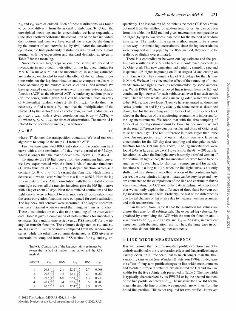
Table 8. Comparison of the lag uncertainty estimates be-tween the method of random time series and the RSSmethod.

Interval τ pk RSS τ cn RSS rsim

1 20.8+2.4−2.1 2.1 22.2+2.8

−2.8 2.7 0.9682 20.8+1.5

−1.6 1.6 22.2+2.8−2.8 2.1 0.960

3 20.5+2.8−2.8 6.0 22.4+4.6

−4.6 4.3 0.9404 20.4+2.6

−2.6 3.4 22.1+4.4−4.0 8.5 0.980

5 20.6+2.4−2.7 6.9 22.4+3.7

−3.5 3.3 0.978

spectively. The last column of the table is the mean CCF peak valueobtained from the method of random time series. As can be seenfrom this table, the RSS method gives uncertainties comparable toor larger (by up to two times) than those for the method of randomtime series. The random time series method seems to be a moredirect way to estimate lag uncertainties; since the lag uncertaintieswere computed in this paper by the RSS method, they seem to berealistic or slightly overestimated.

There is a contradiction between our lag estimate and the pre-liminary results on Mrk 6 published in a conference proceedingsby Grier et al. This new campaign had a nightly sampling rate andit spanned 125 nights beginning on 2010 August 31 and ending on2011 January 3. They claimed a lag of 8 ± 3 days for the Hβ linein Mrk 6. We have first checked the effect of the removing of lineartrends from our light curves (as recommended by some authors,e.g. Welsh 1999). We have removed linear trends from the Hβ andcontinuum light curves for each subinterval, even if no such trendsexist. Then we have recalculated a mean lag value, which was foundto be 19 d, i.e. two days lower. Then we have generated random timeseries (continuum and Hβ) by exactly the same means as describedabove, but for the sampling rate of Grier et al., in order to checkwhether the duration of the monitoring programme is important forthe lag measurements. We found that with the data sampling ofGrier et al. our lag estimate must be lower by one more day, andso the total difference between our results and those of Grier et al.must be three days. The real difference is much larger than threedays. An unexpected result of our simulation was very large laguncertainties for the 125-day data sampling and triangular transferfunction for the Hβ line (see above). The lag uncertainties werefound to be as large as ±6 days! However, for the δ(τ − 20) transferfunction (i.e. when the line light curve is simply a shifted version ofthe continuum light curve) the lag uncertainties were found to be assmall as ∼0.1 days. Thus, for short-term campaigns and for transferfunctions with a long tail (i.e. when the line light curve is not onlyshifted but is a strongly smoothed version of the continuum lightcurve), the uncertainties in lag estimates can be very large and theyare connected to the extrapolation of the line and continuum fluxeswhen computing the CCF, not to the data sampling. We concludedthat we can only explain the difference of three days between ourlag measurements and theirs. Probably, the rest of the difference isdue to real changes of lag or else due to measurement uncertaintiesand their underestimation.

It can be seen from Table 8 that the simulated lag values arealmost the same for all subintervals. The expected lag value can beobtained by convolving the ACF with the transfer function and itwas found to be τ pk = 20.7 days and τ cn = 22.4 day, in excellentagreement with the simulation results. Thus, the large gaps in ourtime series do not shift the lag measurements.

4 LI NE-WI DTH MEASUREMENTS

It is well known that the emission-line profile evolution cannot beentirely attributed to the reverberation effect and that profile changesusually occur on a time-scale that is much longer than the flux-variability time-scale (see Wanders & Peterson 1996). To decreasethe effect of long-term profile changes on line-width measurementsand to obtain sufficient statistics, we measured the Hβ and Hα linewidths for the five subintervals presented in Table 6. The line widthis typically characterized by its FWHM or by the second momentof the line profile, denoted as σ line. To measure the FWHM for themean Hα and Hβ line profiles, we removed narrow lines from thebroad-line profiles. This is not required for rms profiles. However,


Dow


ic.oup.com/m



Table 9. The broad Hβ and Hα line-width measurementsfor 1993–2008.

FWHM σ line

(km s−1)

Hβ (mean spectrum) 6278 ± 378 2821 ± 13Hβ (rms spectrum) 5445 ± 468 2884 ± 97

Hα (mean spectrum) 5322 ± 142 2870 ± 22Hα (rms spectrum) 4443 ± 338 2780 ± 35

the spectra must be optimally aligned in wavelength and in spectralresolution in order to reduce the narrow line residuals in the rmsprofiles. It is difficult to measure the FWHM because both the meanbroad and rms Hβ profiles are double-peaked and so the scatter inthe FWHM measurements is much larger than that in σ line, whichis well defined for arbitrary line profiles. The uncertainties in theline width were obtained using the bootstrap method described byPeterson et al. (2004). The Hβ and Hα line widths (both FWHMand σ line) and their uncertainties are listed in Table 9 for 1993–2008.Table 10 gives the σ line computed separately for each subintervalconsidered and for the Hβ line only.

We examined the relationship between the Hβ lag, Hβ width andcontinuum flux (see Fig. 5). No significant correlations among abovethree parameters were found. In particular, the virial relationshipbetween the lag and width does not contradict our data, but thecorrelation coefficient between them does not differ significantlyfrom the zero value. More subintervals and fewer lag uncertaintiesare required.

5 B L AC K H O L E M A S S O F M R K 6

Determination of the black hole mass from reverberation mappingrests upon the assumption that the gravity of the central supermas-sive black hole dominates over gas motions in the BLR. The blackhole mass is defined by the virial equation

MBH = fcτ (�V )2

G,

where τ is the measured emission-line time delay, c is the speedof light, cτ represents the BLR size and �V is the BLR velocitydispersion. The dimensionless parameter f is the scaling factor,which depends on the BLR structure, kinematics and inclination ofthe BLR. Peterson et al. (2004) argued that τ cn for the time delay τ

Figure 5. The relation between the continuum flux and the lag (τ cn) for Hβ

in Mrk 6, as well as between the Hβ width and the lag (τ cn).

and σ line measured from the Hβ emission line in the rms spectrumfor the emission-line width �V provide the most robust estimates ofthe black hole mass with the reverberation technique. Later, Collinet al. (2006) confirmed that in most cases for the black hole massestimate the line dispersion σ line is more suitable than the FWHM,and σ line from the rms spectrum is more suitable than σ line from themean spectrum.

We adopt an average value of f = 5.5 based on the assumption thatAGNs follow the same MBH–σ ∗ relationship as quiescent galaxies(Onken et al. 2004). This is consistent with Woo et al. (2010) andallows easy comparison with previous results, but this is about afactor of two larger than the value of f computed by Graham et al.(2011). The value of f can be decreased due to the effect of radiationpressure, as was explored by Marconi et al. (2008, 2009). Marconiet al. suggested that neglecting the effect of radiation pressure canlead to underestimation of the true black hole mass, especially inobjects close to their Eddington limit. Discussion between Marconiet al. (2008, 2009) and Netzer (2009) shows that there are many un-clear questions in this area. Naturally, a corrective term for radiationpressure will decrease the f factor.

We calculated the black hole mass for Mrk 6 with the use of τ cn =21.1 ± 1.9 for the time delay averaged over five time intervals andσ line = 2882 ± 100 km s−1 from the rms spectra for Hβ. With τ cn

taken in days and (�V) in km s−1, and taking into account thetime-dilation correction for the value of τ cn, the mass is equal to

MBH/M� = 0.1952 × f × τcn(obs)

(1 + z)× (�V )2.

The black hole mass calculated from the Hβ line is (1.85 ± 0.21)× 108 M�. For the Hα line, τ cn = 26.8 ± 7.7 days and σ line =

Table 10. Results for the five subintervals.

Time Mean fluxa τ cn σ line (km s−1) MBHb in units of 108 M�

series F(5170) F(Hβ) days (mean) (rms) (mean) (rms)1 2 3 4 5 6 7 8

1 6.446 3.632 21.2+4.0−3.2 2813 ± 13 2836 ± 48 1.77+0.33

−0.27 1.80+0.34−0.28

2 6.472 3.976 20.7+3.0−2.4 2804 ± 6 2626 ± 37 1.72+0.25

−0.20 1.50+0.22−0.18

3 5.730 3.587 20.5+5.6−7.0 2808 ± 14 2876 ± 46 1.70+0.46

−0.58 1.79+0.49−0.61

4 4.594 2.677 23.9+17.0−7.3 2870 ± 13 3222 ± 39 2.07+1.50

−0.63 2.62+1.80−0.80

5 7.027 3.523 20.4+4.6−4.1 2807 ± 8 2864 ± 35 1.69+0.38

−0.34 1.77+0.40−0.36

Average: 21.1 ± 1.9 2812 ± 10c 2882 ± 100c 1.76 ± 0.16 1.85 ± 0.21

a Same flux units as in Table 1 for 5170-Å continuum and Hβ, respectively.b Using Onken et al. (2004) calibration, f = 5.5.c The line width and uncertainties were computed as weighted averages and assuming different expectationsof the line widths among individual periods of observations.


Dow


ic.oup.com/m



2780 ± 35 km s−1 and the black hole mass is equal to (2.2 ± 0.6)× 108 M�.

The black hole masses calculated for each of five periods ofobservation are listed in columns 7 and 8 of Table 10 for the σ line

from the mean and rms spectra. One can see that all estimates ofthe black hole mass based on the Hβ line are the same within thescatter.

6 T H E B L R S I Z E – L U M I N O S I T Y A N DMAS S–LU M INOSITY RELATIONSHIPS

Many characteristics of the Mrk 6 galaxy are typical for activegalaxies. In this connection, it is of interest to see the localizationof this galaxy on the BLR radius–luminosity and mass–luminositydiagrams. These diagrams determine a relationship between funda-mental characteristics of AGNs. To this end, the Mrk 6 luminosityshould be known. Up to the present, for many AGNs the luminosityin the rest-frame λ0 = 5100 Å has been corrected for host-galaxystarlight contribution within the apertures used in spectral obser-vations (see Bentz et al. 2009a). Bentz et al. used high-resolutionHubble Space Telescope (HST) images to measure the starlight con-tribution. This contribution was found to be significant, especiallyfor low-luminosity AGNs.

We tried to get at least a rough estimate of the host-galaxy con-tribution using the observations made by Neizvestny (1987) at theSpecial Astrophysical Observatory (SAO) in 1984 October withdifferent apertures from A = 4.3–55 arcsec. The surface brightnessdistribution in the host galaxy of the Mrk 6 nucleus calculated onthe basis of these measurements is shown in Fig. 6.

The galaxy contribution in our 3 arcsec × 11 arcsec spectralwindow was found to be Vgal = 15.6 mag or Fgal = 2.08 ×10−15 erg s−1 cm−2 Å−1. The mean flux observed in the continuumnear λ0 = 5100 Å is F(gal +nuc) = 6.093 × 10−15 erg s−1 cm−2 Å−1

(see Table 4) and thus the mean flux corrected for the galaxy con-tribution is equal to Fnuc = 4.013 × 10−15 erg s−1 cm−2 Å−1. Thevariability amplitude Fvar increases from 18 per cent to 27 per centafter accounting for the galaxy contribution. The mean flux was alsocorrected for Galactic reddening according to the NASA/IPAC Ex-tragalactic Data base (NED: Schlegel, Finkbeiner & Davis 1998).The luminosity was found to be λLλ(5100) = (2.51 ± 0.78) × 1043

erg s−1, adopting the galaxy distance D = 81 Mpc and in the casewhen the galaxy contribution is removed.

The bolometric luminosity of the Mrk 6 nucleus was adopted tobe Lbol 9λLλ(5100 Å) according to Kaspi et al. (2000) and it isequal to Lbol(nucl) = 2.26 × 1044 erg s−1. This luminosity is far

Figure 6. Surface brightness distribution for Mrk 6 in the V band on thebasis of multi-aperture photoelectric photometry by Neizvestny (1987). Thesolid curve corresponds to the model μ(r) = a + br + cr1/4.

Figure 7. Top: Hβ BLR size versus luminosity at 5100 Å according toBentz et al. (2009a) and Denney et al. (2010). The luminosity of all nucleiwas corrected for the host galaxy contribution. The solid line is the best fitto the relationship log (RBLR) = −21.3 + 0.519log (L). Bottom: the mass–luminosity diagram. The black hole mass of the majority of AGNs was takenfrom Peterson et al. (2004), except for Mrk 290, Mrk 817, NGC 3227, NGC3516, NGC 4051 and NGC 5548, for which new results by Denney et al.(2010) were used. Solid lines show the Eddington limit LEdd and its 10 and1 per cent fractions. The position of the Mrk 6 nucleus is indicated on bothplots.

from the Eddington limit (LEdd), which is equal to LEdd = 2.16 ×1046 erg s−1 for a black hole mass of 1.8 × 108 M�. In other words,the Eddington ratio for Mrk 6 is Lbol/LEdd 0.01. In this case andbecause there are no clear indications of gas outflow from the BLR,the radiation pressure has a negligible effect on the reverberationmass estimate.

The position of the Mrk 6 nucleus on the BLR size–luminositydiagram is shown in Fig. 7. The BLR size and the luminosity ofother galaxies in Fig. 7 are taken from Bentz et al. (2009a) andDenney et al. (2010). The black hole masses in Fig. 7 are takenfrom Peterson et al. (2004), except for the galaxies Mrk 290, Mrk817, NGC 3227, NGC 3516 and NGC 4051, for which we used newdata from Denney et al. (2010).

7 V E L O C I T Y- R E S O LV E D R E V E R B E R AT I O NL AG S

7.1 Entire time interval: 1993–2008

The question about whether the direction of gas motion can bedetermined from the response of the line profile to the continuumchanges was first raised by Fabrika (1980). Generally speaking, the


Dow


ic.oup.com/m



BLR gas velocity field can consist of random circular orbits, radialgas outflow or infall or Keplerian motion. Examples demonstratinghow the velocity-resolved responses can be related to different typesof BLR gas kinematics are given in Peterson (2001) and Bentzet al. (2009b). The random circular orbits generate a symmetriclag profile with the highest lag observed around zero velocity. Theinfall kinematics produces longer lags in the blueshifted emission,and the outflow gas produces longer lags in the redshifted emission.

Horne et al. (2004) formulated some important observational re-quirements for determining a reliable velocity field of the BLR:(1) the time duration of observations should be at least three timeslarger than the longest time-scale of response, (2) the mean timebetween subsequent observations should be at least two times lessthan the BLR light-crossing time and (3) the velocity sampling �Vused for the velocity-delay maps should be no lower than the spec-tral resolution of the data. According to Horne et al. (2004), suchconditions can allow one to distinguish clearly between alternativekinematic models of the BLR gas motion.

In order to obtain the velocity-delay map, we measured the lagas a function of velocity in several bins across the line profile. Wedivided both the Hα and Hβ lines into ten bins of equal flux, and thewidth of these bins was no less than 1000–1500 km s−1. For eachbin we calculated light curves from the Balmer-line fluxes. Theneach of these light curves was cross-correlated with the continuumlight curve following the same procedure as described in Section 3.Fig. 8 shows hydrogen-line profiles (mean and rms) subdivided intobins (two upper panels). The two middle panels demonstrate the lagmeasurements for each of the bins. The vertical error bars show 1σ

uncertainties for the time lag and the horizontal bars represent thebin width. The horizontal solid and dashed lines in the two middlepanels show the mean BLR lag and associated errors as listed inTable 5. The bottom panels show the peak correlation coefficientbetween the bin flux in the line and continuum, rmax. Fig. 8 showsthe following.

Figure 8. The two top panels show the Hβ mean and rms profiles (left)and the Hα mean profile (right) divided into ten bins of equal flux sepa-rated by vertical dashed lines. The flux units for the mean and rms profilesare 10−13 erg cm−2 s−1 Å−1. The third panels from the top show the corre-sponding velocity-resolved time lag response, where the delays are plottedat the flux centroid of each velocity bin. Here the vertical error bars are 1σ

uncertainties in the lag for each velocity bin denoted by the horizontal errorbars. The horizontal dotted and dashed lines on the third panels mark themean centroid lag and 1σ uncertainty, respectively, for the entire emissionline. The bottom panels show the peak value of the correlation coefficientbetween the bin flux in the line and continuum. Here the horizontal dottedlines mark the correlation coefficient rmax between the entire emission lineand the continuum, as calculated in Table 5.

(1) The mean and rms profiles of Hβ and Hα are not symmetricwith respect to zero velocity. The centroid of the mean and rmsprofiles is shifted to the short-wave part of the line. The variableparts of Hβ and Hα have two well-defined peaks; one of them isalmost central (between 5 and 6 bins) and another is blueshifted. Inaddition, there is a weaker peak in the red part of the line profile.

(2) The time delay between the higher velocity gas in the BLRand the continuum is shorter than the delay between the low-velocitygas and the continuum. Such a behaviour is typical for virializedgas motions.

(3) The lag in the blue wing of the Hβ line is greater than the lagon the red side of this line. The Hα velocity-resolved lag shows thesame tendency. This is consistent with expectations from the infallmodel of gas motion. Thus, it is possible we have virialized motioncombined with infall signatures.

(4) The correlation coefficient of different segments of thelines is different. The bin corresponding to a radial velocity ofVr ≈ +1500 km s−1 shows poor correlation with the continuumvariation, especially in Hβ. This fact was earlier noted by Sergeevet al. (1999).

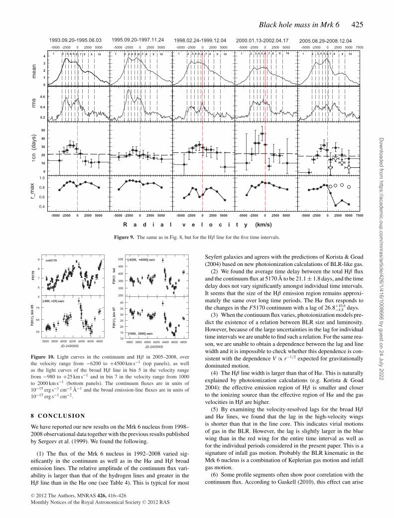
7.2 Velocity-delay maps in the five time intervals

We have computed the velocity-resolved time delays for the fivetime intervals given in Table 6. For each subset we carried outa velocity-dependent cross-correlation analysis for the Hβ line-profile bins as described in the previous section. The Hβ line wasselected because its sampling is better. In Fig. 9 the mean andrms Hβ profiles, velocity-resolved time lag response and velocity-dependent peak correlation coefficient are shown for the five timeintervals. Upon inspection of Fig. 9 it becomes clear that the meanand rms profiles are different amongst the five periods. The relativeintensity in the blue and central peaks changes very strongly: duringthe first interval the blue peak is higher than the red one. Theopposite situation is seen in the fifth interval. The flux in continuumas well the flux in the Hβ line systematically decrease from thesecond to the fourth time interval, as is seen in Figs 3 and 7. The Hβ

rms profile shows two peaks in the first, second and third periods,a flat top in the fourth period and in the fifth period we see threepeaks.

Fig. 8 demonstrates that the high-velocity gas in the wings ex-hibits a shorter lag than the low-velocity gas, supporting the virialnature of gas motion in BLRs: gas kinematics that is dominated bythe central massive object.

However, the lag is slightly larger in the blue wing than in the redwing for all subintervals. This is a signature of the infall gas motion.In the fifth period (2005–2008) the velocity-delay map is moresymmetric, but the seventh bin shows very small lag, as well as inthe previous time interval. For 2005–2008 there is a poor correlationwith the continuum for bins 7–10. A more detailed examination ofthe bin light curves for 2005–2008 (Fig. 10) revealed that there is atrend for the Hβ flux in bins 7–10, which is almost absent in bins1–6. Following the advice of our reviewer, we removed the trendfrom the Hβ light curves for bins 7–10. No more significant trendswere found for other time intervals. In Fig. 9 the detrended lagsand correlation coefficients are shown by open circles. After thedetrending procedure, the lag–velocity dependence became moresimilar to the lag–velocity dependence for the first period, for whichthe difference in lag between the blue and red wings is largest.

Thus, it is most likely that the BLR kinematic in Mrk 6 is acombination of Keplerian gas motion and infall gas motion.


Dow


ic.oup.com/m



Figure 9. The same as in Fig. 8, but for the Hβ line for the five time intervals.

Figure 10. Light curves in the continuum and Hβ in 2005–2008, overthe velocity range from −6200 to +4500 km s−1 (top panels), as wellas the light curves of the broad Hβ line in bin 5 in the velocity rangefrom −980 to +25 km s−1 and in bin 7 in the velocity range from 1000to 2000 km s−1 (bottom panels). The continuum fluxes are in units of10−15 erg s−1 cm−2 Å−1 and the broad emission-line fluxes are in units of10−15 erg s−1 cm−2.

8 C O N C L U S I O N

We have reported our new results on the Mrk 6 nucleus from 1998–2008 observational data together with the previous results publishedby Sergeev et al. (1999). We found the following.

(1) The flux of the Mrk 6 nucleus in 1992–2008 varied sig-nificantly in the continuum as well as in the Hα and Hβ broademission lines. The relative amplitude of the continuum flux vari-ability is larger than that of the hydrogen lines and greater in theHβ line than in the Hα one (see Table 4). This is typical for most

Seyfert galaxies and agrees with the predictions of Korista & Goad(2004) based on new photoionization calculations of BLR-like gas.

(2) We found the average time delay between the total Hβ fluxand the continuum flux at 5170 Å to be 21.1 ± 1.8 days, and the timedelay does not vary significantly amongst individual time intervals.It seems that the size of the Hβ emission region remains approxi-mately the same over long time periods. The Hα flux responds tothe changes in the F5170 continuum with a lag of 26.8+10.6

−4.8 days.(3) When the continuum flux varies, photoionization models pre-

dict the existence of a relation between BLR size and luminosity.However, because of the large uncertainties in the lag for individualtime intervals we are unable to find such a relation. For the same rea-son, we are unable to obtain a dependence between the lag and linewidth and it is impossible to check whether this dependence is con-sistent with the dependence V ∝ r−1/2 expected for gravitationallydominated motion.

(4) The Hβ line width is larger than that of Hα. This is naturallyexplained by photoionization calculations (e.g. Korista & Goad2004): the effective emission region of Hβ is smaller and closerto the ionizing source than the effective region of Hα and the gasvelocities in Hβ are higher.

(5) By examining the velocity-resolved lags for the broad Hβ

and Hα lines, we found that the lag in the high-velocity wingsis shorter than that in the line core. This indicates virial motionsof gas in the BLR. However, the lag is slightly larger in the bluewing than in the red wing for the entire time interval as well asfor the individual periods considered in the present paper. This is asignature of infall gas motion. Probably the BLR kinematic in theMrk 6 nucleus is a combination of Keplerian gas motion and infallgas motion.

(6) Some profile segments often show poor correlation with thecontinuum flux. According to Gaskell (2010), this effect can arise


Dow


ic.oup.com/m



because off-axis sources of ionizing continuum flux can appear,which might not make a detectable contribution to the total contin-uum flux variability but will have an influence on the line only, overa narrow range of radial velocity in the BLR. If these local off-axisevents vary out of phase with the variability of the dominant source,the result will be to give a weak correlation between the continuumflux and the line flux in a narrow range of radial velocity.

(7) We determined the black hole mass from the lag and line-width measurements of the Hβ and Hα lines. The mass was foundto be MBH = (1.8 ± 0.2) × 108 M� for the Hβ line and slightlylarger and less reliable for the Hα line. Under such a mass and theluminosity λLλ(5100) = (2.51 ± 0.38) × 1043 erg s−1, the Mrk 6nucleus is located on the upper edge of the mass–luminosity dia-gram, which corresponds to an Eddington ratio of about 0.01. Thisconfirms the assumption (e.g. Sergeev et al. 2011) that there is anti-correlation between broad line widths and the Eddington luminosityratio Lbol/LEdd. The Mrk 6 position on the BLR size–luminosity di-agram does not contradict the fit RBLR ∝ L0.5 determined by Bentzet al. (2009a).

AC K N OW L E D G M E N T S

We thank the anonymous reviewer for useful comments and sugges-tions. We also thank S. Nazarov and the staff of the 2.6-m and 0.7-m telescope for help during our observations. SSG acknowledgesthe support to CrAO in the frame of the ‘CosmoMicroPhysics’Target Scientific Research Complex Programme of the NationalAcademy of Sciences of Ukraine (2007–2012). VTD acknowledgesthe support of the Russian Foundation of Research (RFBR, projectno. 09-02-01136a). The CrAO CCD cameras were purchasedthrough the US Civilian Research and Development for IndependentStates of the Former Soviet Union (CRDF) awards UP1-2116 andUP1-2549-CR-03.

R E F E R E N C E S

Bentz M. C. et al., 2008, ApJ, 689, L21Bentz M. C., Peterson B. M., Netzer H., Pogge R. W., Vestergaard M.,

2009a, ApJ, 697, 160Bentz M. C. et al., 2009b, ApJ, 705, 199Bentz M. C. et al., 2010, ApJ, 716, 993Blandford R. D., McKee C. F., 1982, ApJ, 255, 419Collin S., Kawaguchi T., Peterson B. M., Vestergaard M., 2006, A&A, 456,

75Denney K. D. et al., 2009, ApJ, 704, L80Denney K. D. et al., 2010, ApJ, 721, 715Doroshenko V. T., 2003, A&A, 405, 903Doroshenko V. T., Sergeev S. G., 2003, A&A, 405, 909Doroshenko V. T., Sergeev S. G., Merkulova N. I., Sergeeva E. A., Gol-

ubinsky Yu. V., Pronik V. I., Okhmat N. N., 2005, Astrophysics, 48,156

Fabrika S. N., 1980, Astron. Tsirk., 1109, 1Feldmeier J. J., Brandt W. N., Elvis M., Fabian A. C., Iwasawa K., Mathur

S., 1999, ApJ, 510, 167Gaskell C. M., 2009, in Maraschi L., Ghisellini G., Della Ceca R., Tavecchio

F., eds, ASP Conf.Ser. Vol 427, Inflow of the Broad-Line Region and theFundamental Limitations of Reverberation Mapping. Astron. Soc. Pac.,San Francisco, p. 68

Gaskell C. M., 2010, preprint (arXiv:1008.1057)Gaskell C. M., Sparke L. S., 1986, ApJ, 305, 175Graham A. W., Onken Ch. A., Athanassoula E., Combes F., 2011, MNRAS,

412, 2211

Grier C. J., Peterson B. M., Denney K. D., Martini P., PoggeR. W., Bentz M. C., PoS(NLS1)052, pos.sissa.it/archive/conferences/126/052/NLS1_052.pdf

Horne K., Peterson B. M., Collier S. J., Netzer H., 2004, PASP, 116, 465Immler S., Brandt W. N., Vignali C., Bauer F. F., Crenshaw D. M., Feldmeier

J. J., Kraemer S. B., 2003, AJ, 126, 153Kaspi S., Smith P. S., Netzer H., Maoz D., Jannuzi B. T., Giveon U., 2000,

ApJ, 533, 631Khachikian E. Ye., Weedman D. W., 1971, ApJ, 164, L109Kharb P., O’Dea C. P., Baum S. A., Colbert E. J. M., Xu C., 2006, ApJ, 652,

177Kharitonov A. V., Tereshchenko V. M., Knyazeva L. N., 1988, Spectropho-

tometric Catalogue of Stars, Science. Nauka, MoscowKoratkar A. P., Gaskell C. M., 1991, ApJS, 75, 719Korista K. T., Goad M. R., 2004, ApJ, 606, 749Kukula M. J., Holloway A. J., Pedlar A., Meaburn J., Lopez J. A., Axon

D. J., Schilizzi R. T., Baum S. A., 1996, MNRAS, 280, 1283Malizia A., Bassani L., Capalbi M., Fabian A. C., Fiore F., Nicastro F., 2003,

A&A, 406, 105Marconi A., Axon D. J., Maiolino R., Nagao T., Pastorini G., Pietrini P.,

Robinson A., Torricelli G., 2008, ApJ, 678, 693Marconi A., Axon D. J., Maiolino R., Nagao T., Pietrini P., Risaliti A.,

Robinson A., Torricelli G., 2009, ApJ, 698, L103Neizvestny S. I., 1987, Izv. SAO, 24, 3Netzer H., 2009, ApJ, 695, 793Onken C. A., Ferrarese L., Merritt D., Peterson B. M., Pogge R. W., Vester-

gaard M., Wandel A., 2004, ApJ, 615, 645Peterson B. M., 1988, PASP, 100, 18Peterson B. M., 2001, in Aretxaga I., Kunth D., Mujica R., eds, Ad-

vanced Lectures on the Starburst – AGN connection. World Scientific,Singapore, p. 3

Peterson B. M., Wanders I., Horne K., Collier S., Alexander T., Kaspi S.,Maoz D., 1998, PASP, 110, 660

Peterson B. M. et al., 2004, ApJ, 613, 682Schlegel D. J., Finkbeiner D. P., Davis M., 1998, ApJ, 500, 525Schurch N. J., Griffits R. E., Warwick R. S., 2006, MNRAS, 371, 211Sergeev S. G., Pronik V. I., Sergeeva E. A. Malkov Yu. F., 1999, ApJS, 121,

159Sergeev S. G., Doroshenko V. T., Golubinskiy Yu. V., Merkulova N. I.,

Sergeeva E. A., 2005, ApJ, 622, 129Sergeev S. G., Klimanov S. A., Doroshenko V. T., Efimov Yu. S., Nazarov

S. V., Pronik V. I., 2011, MNRAS, 410, 1877Wandel A., Peterson B. M., Malkan M. A., 1999, ApJ, 526, 579Wanders I., Peterson B. M., 1996, ApJ, 466, 174Welsh W. F., 1999, PASP, 111, 1347White R. J., Peterson B. M., 1994, PASP, 106, 879Woo J.-H. et al., 2010, ApJ, 716, 269

S U P P O RT I N G I N F O R M AT I O N

Additional Supporting Information may be found in the online ver-sion of this article:

Table 1. F5170 spectral continuum, Hβ and Hγ line fluxes.Table 2. F7030 spectral continuum and Hα fluxes.Table 3. Combined F5170 continuum fluxes from spectral andphotometric observations.

Please note: Wiley-Blackwell are not responsible for the content orfunctionality of any supporting materials supplied by the authors.Any queries (other than missing material) should be directed to thecorresponding author for the article.

This paper has been typeset from a TEX/LATEX file prepared by the author.


Dow


ic.oup.com/m


Broadline region kinematics and black hole mass in Markarian 6

Documents

Transcript of Broadline region kinematics and black hole mass in Markarian 6