Breeding strategies to make sheep farms resilient to ...
188
Breeding strategies to make sheep farms resilient to uncertainty Ian James Rose
-
Upload
khangminh22 -
Category
Documents
-
view
0 -
download
0
Transcript of Breeding strategies to make sheep farms resilient to ...

Breeding strategies to make sheep farms
resilient to uncertainty
Ian James Rose

Thesis committee
Promotor
Prof. Dr J.A.M. van Arendonk
Professor of Animal Breeding and Genomics
Wageningen University
Co-promotor
Dr H.A. Mulder
Assistant professor, Animal Breeding and Genomics Centre
Wageningen University
Prof. Dr J.H.J. van der Werf
Professor of Animal Breeding & Genetics
University of New England, Armidale, Australia
Other members
Prof. Dr B. Kemp, Wageningen University Prof. Dr J. Sölkner, University of Natural Resources and Life Sciences, Vienna, Austria Dr R. Banks, Animal Breeding and Genetics Unit, Armidale, Australia Dr E.P.C. Koenen, CRV, Arnhem
This research was conducted under the auspices of the Graduate School of
Wageningen Institute of Animal Sciences (WIAS).

Breeding strategies to make sheep
farms resilient to uncertainty
Ian James Rose
Thesis
submitted in fulfillment of the requirements for the degree of doctor
at Wageningen University
by the authority of the Rector Magnificus
Prof. Dr M.J. Kropff,
in the presence of the
Thesis Committee appointed by the Academic Board
to be defended in public
on Wednesday 8 October, 2014
at 4 p.m. in the Aula.

Ian James Rose
Breeding strategies to make sheep farms resilient to uncertainty
188 pages.
PhD thesis, Wageningen University, Wageningen, NL (2014)
With references, with summaries in English and Dutch
ISBN 978-94-6257-090

5
Abstract
Rose, G. (2014). Breeding strategies to make sheep farms resilient to uncertainty.
PhD thesis, Wageningen University, the Netherlands
The sheep industry in Western Australian has had many challenges over the last 20
years which have caused sheep numbers to decline. This decline is because sheep
farms are not resilient to uncertain pasture growth and commodity prices. One way
to improve resilience and profitability of farming systems is through breeding of
sheep. Therefore, this thesis had two aims; 1. Quantify the potential to select and
breed sheep that are more resilient and 2. Quantify how sheep breeding can make
farming systems more resilient. To determine if sheep can be bred to be resilient to
varying pasture growth I investigated if live weight change is a heritable trait. I
investigated live weight change in adult Merino ewes managed in a Mediterranean
climate in Katanning in Western Australia. Live weight change traits were during
mating and lactation. The heritability of live weight change was low to moderate.
Therefore that live weight change could be a potential indicator trait for resilience
to uncertain pasture growth. To include live weight change in a breeding goal,
correlations with other traits are needed. I calculated the genetic correlations
between live weight change during mating, pregnancy and lactation, and
reproduction traits. Most genetic correlations were not significant, but genetically
gaining live weight during mating in two-year old ewes and during pregnancy for
three-year-old ewes improved reproduction. Therefore, optimised selection
strategies can select for live weight change and reproduction simultaneously. To
investigate optimal breeding programs to make sheep farms resilient to uncertain
pasture growth and prices, I modelled a sheep farm in a Mediterranean
environment. The economic value of seven traits in the breeding objective were
estimated. Including variation in pasture growth and commodity prices decreased
average profit and increased the economic value of all breeding goal traits
compared to the average scenario. Economic values increased most for traits that
had increases in profit with the smallest impact on energy requirements. I also
compared optimal breeding programs for across 11 years for 10 regions in Western
Australia with different levels of reliability of pasture growth. I identified two
potential breeding goals, one for regions with low or high pasture growth reliability
and one for regions with medium reliability of pasture growth. Regions with low or
high reliability of pasture growth had similar breeding goals because the
relationship between economic values and reliability of pasture growth were not
linear for some traits. Therefore, farmers can customise breeding goals depending
on the reliability of pasture growth on their farm.


7
Contents
1. General Introduction 9
2. Merino ewes can be bred for live weight change to be more tolerant to uncertain
feed supply 21
3. Genetic correlations between live weight change and reproduction traits in
Merino ewes depend on age 41
4. Varying pasture growth and commodity prices change the value of traits in sheep
breeding objectives 61
5. Breeding objectives for sheep should be customised depending on variation in
pasture growth across years 95
6. General discussion 123
References 147
Summary 163
Samenvating 169
Acknowledgments 175
Curriculum Vitae 179


1 General Introduction


1 General Introduction
11
1.1 Introduction to the Western Australian sheep
industry
The bulk of Western Australia’s sheep are managed in the Warm-summer and Hot-
Summer Mediterranean climatic zones (Squires, 2006). These zones are
characterised by warm/hot dry summers and cool/mild wet winters. This
combination of temperature and rainfall means that there is a period of no pasture
growth during summer and autumn, with pasture growing mostly in late winter and
spring. This distribution of pasture growth has implications for ewe management
with most farmers lambing in June and July to match peak energy requirements
during late pregnancy and lactation with peak pasture supply (Curtis, 2008). Most
farmers manage self-replacing Merino flocks and 76% of ewes are mated to Merino
rams and 24% are mated to terminal meat rams (Curtis, 2008). This mix in ram use
enables farmers to produce enough Merino lambs to replace old ewes whilst
improving meat income by selling faster growing lambs produced by cross
breeding. This means that breeding programs for Merino ewes focus on wool
production, whilst there are generally two lines of sires, one for wool and one for
meat. In this thesis I focus on Merino breeders who are selecting sheep
predominantly for wool production, selling wethers (male castrates) for meat
between one and two years old. I focus on this segment of the market because it
represents the bulk of sheep production in Western Australia.
The Western Australian sheep industry has had many challenges over the last 20
years. Sheep numbers in Western Australia have declined (Figure 1.1) as farmers
reduce their sheep flock by selling more lambs for meat (Figure 1.2) and changing
their preference to other enterprise types. This reduction in sheep numbers has
occurred nationwide and is the main cause of the farm value of wool in Australian
decreasing from AU$4.7 billion to $AU1.8 billion per year between 1992 and 2010
(Rowe, 2010). In comparison, a shift towards meat production and higher meat
prices increased the farm value of meat from around $AU0.5 billion per year to
$AU1.75 billion per year (Rowe, 2010). The decline in sheep numbers and wool
production is due to a combination of social, economic and environmental factors.
The biggest cause of the shift away from sheep production is the increase in the
relative profitability of cropping. Most farms in the Mediterranean climate zones
have mixed crop and sheep (Kingwell and Pannell, 2005). This mixed farming
system is preferred because regions with a Mediterranean climate of mild wet
winters and dry hot summers support dryland cropping that is complemented by
sheep which graze the crop residues over summer and autumn and aid in weed

1 General Introduction
12
control (Ewing et al., 1992). The decrease in sheep numbers over the last 20 years
coincided with an increase in area sown to cereals by over 50 percent between
1990 and 2005.
Figure 1.1 Number of sheep and in Western Australia between 1990 and 2008.
(Australian Bureau of Statistics).
Figure 1.2 Number of lambs slaughtered in Western Australia between 1990 and 2008.
(Australian Bureau of Statistics).

1 General Introduction
13
Cropping has become more profitable because it has had higher rates of
productivity gain (Zhao et al., 2008; Nossal and Sheng, 2010). These productivity
gains are from more crop options such as lupins and canola, and improved varieties
such as wheat varieties with different flowering times that suit more environments
(Beare et al., 1999; Zhao et al., 2008). Additionally, cropping has become easier
with the introduction of new herbicides (Gill and Holmes, 1997) large machinery
that provides economies of scale benefits (Liao and Martin, 2009) and new
machinery technology such as direct drill sowing (Kokic et al., 2006) and GPS-based
controlled traffic systems (Fuschbichler and Kingwell, 2010). Alternatively, sheep
technology has remained relatively stagnant, and although the introduction of live
sheep export created a new market option for farmers, the benefits of cropping
often have outweighed those of sheep.
In addition to improved crop technologies, the number of farms is decreasing
(Figure 1.3) while the average size of farms is increasing. This increase in farm size
has meant higher debt levels for farmers particularly due to the high interest rates
during the 1980s and 1990s (Australian Bureau of Agriculture and Resource
Economics, 2001). This increase in debt has caused farmers to turn to cropping to
increase farm income. Additionally, management of larger farms has become more
complex due to increased availability of technology, crop choice, rotation options,
marketing and information services (Kingwell, 2011). Therefore, farmers have
become more selective in how they allocate their time and investments.
Figure 1.3 Number of farm businesses in Western Australia between 1990 and 2013.
(ABARE farm survey data available on AgSurf.)

1 General Introduction
14
Farm benchmarking suggests that the labour requirement for sheep is high
compared to cropping (Holmes and Sackett, 2009). Additionally, many farms in
Western Australia experience problems in attracting and retaining farm labour
(Rabobank, 2007). Therefore, when farm management labour is scarce, sheep
management can place high demands on that labour. Moreover, because of the
dominance of cropping in Western Australia over recent decades, many young
farmers who have specialised in cropping, have limited experience, knowledge and
skills for managing sheep (Dymond, 2006). This means that some farmers, because
of time pressures or limited knowledge, are managing low maintenance sheep
systems.
These time pressures as well as fluctuation in pasture growth between years have
caused most farmers to manage set stocking systems with low stocking rates set
for poor seasons to increase resilience to uncertain pasture supply (Doyle et al.,
1993). This type of management means that pasture utilisation in most years is low
and pasture is lost through decay from spring to autumn (Doyle et al., 1996). Given
the strong relationship between stocking rate and profit (White and Morley, 1977;
White et al., 1980; Young et al., 2010), there is potential on many farms to increase
stocking rates and make more money from sheep. Additionally, there is an optimal
stocking rate which if exceeded farm profits decrease (White and Morley, 1977;
White et al., 1980) and soil health is compromised (Moore et al., 2009). This
optimal stocking also varies depending on the season, particularly when available
pasture fluctuates (White and Morley, 1977; White et al., 1980). Farming systems
in Western Australia are characterised by fluctuating levels of pasture biomass
(Rossiter, 1966). Additionally, combine harvesters are becoming more efficient and
leaving less grain behind making crop stubbles an unreliable feed resource (Landau
et al., 2000). Therefore, increasing stocking rate reduces the resilience of farming
systems to low pasture growth in poor seasons causing farmers to adopt
conservative stocking rates.
This shift away from sheep towards crop has created many challenges for farmers
including poor soil health, herbicide resistant weeds in crops and salinity. Although
continuous cropping is profitable in the short term, long periods of cropping have
negative impacts on soil health and soil nitrogen reserves (Reeves and Ewing,
1993). Additionally, crop dominant farming increases herbicide resistance which
develops when overuse of herbicides causes intense selection pressure on weeds
(Doole and Pannell, 2008). Livestock are the best long term solution to herbicide
resistance when used to control weeds in combination with herbicides (Monjardino
et al., 2004). Furthermore, much of southern Australia has experienced dryland
salinity because native vegetation has been replaced with annual crops and

1 General Introduction
15
pastures for agriculture (Hatton and Nulsen, 1999). Annual crops have shorter root
systems which use less water than native vegetation causing the water table to rise
(Asseng et al., 2001). This rising of water tables brings salt deposits to the surface
of soil profiles making the land saline and unsuitable for annual crops and pastures.
In the cropping regions of Australia salinity was predicted to cost AU$238 million in
foregone profits (Kingwell, 2003). The best solution to prevent salinity is replacing
annual crops and pastures with perennial pastures to be grazed by livestock (Cocks,
2003). Saltland pastures are also an option for slightly saline areas that are no
longer suitable for annual crops and pastures. O’Connell et al. (2006) found that
saltland pastures planted and grazed by sheep on moderately saline environments
increased profit and reduced recharge of water. Therefore, livestock systems in
Western Australia have been faced with declining livestock numbers but remain an
important enterprise.
Finally, Darnhofer et al. (2014) state that farming systems need to be diverse to be
resilient to environmental and economic changes. Therefore it is important for
sheep enterprises to remain profitable for farmers to maintain a good enterprise
mix. Additionally, all components of sheep enterprises, for example meat and wool,
need to be viable to maintain resilience within the farming system. Therefore, it is
important to find solutions to increase the profitability and viability of sheep
production systems in Western Australia.
1.2 Aims of thesis
Resilience to variation in pasture growth is important for the farming system as
well as sheep managed on the farming system. In addition to being resilient the
farming system also has to be profitable across years regardless of variation in the
production environment and prices. One way to improve resilience and profitability
of farming systems is through breeding of sheep. Breeding sheep to be more
profitable requires selecting the sheep that will make the most money in a
production system. This selection of sheep can be easily integrated in the
management of the flock and the annual genetic changes of sheep flock are
cumulative and permanent. This permanent nature of genetic change means that
farmers should ensure they are selecting the right sheep to breed for the longer
term. Animal breeding aims to select the animals that will perform best in a given
production system. Consequences of breeding for resilience can be investigated at
the animal level, by selecting sheep that are resilient to variation in pasture growth,
or at the farm system level, by selecting sheep that will lead to the most
profitability at farm level.

1 General Introduction
16
In the last 20 years the Australian sheep industry has made significant genetic gains
in production traits through its use of MERINOSELECT, a quantitative genetic
evaluation system of Merino rams (Banks et al., 2006). During the 1990s Australian
farmers have selected sheep to decrease fibre diameter and increase fleece weight
so sheep produce more fine wool (Taylor and Atkins, 1997). However, an increase
in meat prices and a decrease in wool price and fibre diameter premium (Figure 1.4
and Figure 1.5) have shifted breeding emphasis more towards lamb production.
These breeding goals have focused mostly on improving production in sheep. This
production focus has reduced resilience in Merino sheep managed in Western
Australia’s Mediterranean regions (Adams et al., 2006; Adams et al., 2007).
The Mediterranean regions in Western Australia have large variations in pasture
growth between years with the length and severity of drought periods between
years hard to predict. There is limited information on how to identify the best type
of sheep to breed in these environments when pasture growth and price variability
may affect the optimal breeding scheme for farmers in these regions. This erratic
feed supply between years is predicted to worsen due to the effects of climate
change (IPCC, 2008). Therefore, farmers will become more reliant on grain
supplements to fill the feed gap during summer and autumn (Purser, 1981) which
impacts on whole farm profit (Kingwell, 2002; Kopke et al., 2008). Therefore
farmers should consider improving animal traits that make sheep more robust to
periods of low nutrition and will require less supplementary feeding during summer
and autumn.
The growth of green feed during winter and spring means that sheep generally
have a positive energy balance during this period and a negative energy balance
during summer and autumn. This negative energy balance in autumn is
exaggerated as Merino ewes in Mediterranean environments are normally
pregnant during autumn (Croker et al., 2009). This means ewes generally lose
weight during summer and autumn and regain weight during late winter and spring
when their energy balance is positive (Adams and Briegel, 1998). Adams and
Briegel (1998) recorded average live weight loss of 12 kg for Merino ewes during
summer and autumn in Bakers Hill in Western Australia. This high weight loss
significantly decreases the maternal performance of ewes and the survival of lambs
(Kelly and Ralph, 1988; Kelly, 1992).
Therefore, live weight change may be an appropriate trait to represent sheep that
require less supplementary feeding during drought periods. Live weight change in
adult ewes could represent the performance of sheep under a fluctuating feed
supply, with sheep losing less live weight during drought being more resilient. This
approach is similar to the research for body condition score (Berry et al., 2002;

1 General Introduction
17
Veerkamp et al., 2001) as an indicator of energy balance in dairy cattle.
Additionally, phenotypic correlations reported in other studies (Kelly and Ralph,
1988; Kelly, 1992) suggest that live weight change has important phenotypic
correlations with reproduction in sheep. If there are significant genetic correlations
between live weight change and reproduction, then this could have implications for
optimal breeding strategies.
Figure 1.4 Over the hooks lamb price in Australia, for lambs with 20-22 kg carcass
weight, fat score 2-4. (Meat and Livestock Australia.
Figure 1.5 Wool price for clean wool with fibre diameter of 19 and 20 µm (Western
Region micron price guide). (Wool Desk, Department of Agriculture and Food WA, and
Australian Wool Exchange).
1 General Introduction
18
The current genetic evaluation system called MERINOSELECT provides selection
indices to breeders of Merino sheep in Australian (Brown et al., 2006). This system
uses the SHEEPOBJECT software (Swan et al., 2007) which does not consider the
impact of variation in pasture growth and prices to estimate the economic values
of different traits.
There are many studies on how farms can be managed to improve resilience to
uncertain pasture (Olson and Mikesell, 1988; Kingwell et al., 1993; Jacquet and
Pluvinage, 1997; Kobayashi et al., 2007) and prices (Lambert, 1989; Barbier and
Bergeron, 1999; Lien and Hardaker, 2001; Ridier and Jacquet, 2002; Mosnier et.al.,
2009; Mosnier et.al., 2011). These studies provide insights into how management
can be optimised to increase profit under uncertainty but have not been applied to
animal breeding. Therefore, these techniques can be applied to a breeding context
and will help to bridge the gap in knowledge between economics and breeding.
Furthermore, in Western Australia’s sheep growing area there are big differences
between regions in the amount and variation of pasture growth within and
between years (Rossiter, 1966; Schut et al., 2010). These differences between
regions in pasture growth can affect the optimal management of livestock in each
system (Chapman et al., 2009). These changes in management may also affect
optimal breeding goals because changing each trait changes the energy
requirements of sheep by different amounts and at different times of the year.
Therefore, it is important to understand if different regions need adapted breeding
goals, or if one breeding goal for all regions can be used.
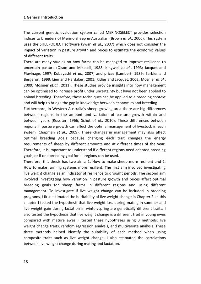
Therefore, this thesis has two aims; 1. How to make sheep more resilient and 2.
How to make farming systems more resilient. The first aim involved investigating
live weight change as an indicator of resilience to drought periods. The second aim
involved investigating how variation in pasture growth and prices affect optimal
breeding goals for sheep farms in different regions and using different
management. To investigate if live weight change can be included in breeding
programs, I first estimated the heritability of live weight change in Chapter 2. In this
chapter I tested the hypothesis that live weight loss during mating in summer and
live weight gain during lactation in winter/spring are genetically different traits. I
also tested the hypothesis that live weight change is a different trait in young ewes
compared with mature ewes. I tested these hypotheses using 3 methods: live
weight change traits, random regression analysis, and multivariate analysis. These
three methods helped identify the suitability of each method when using
composite traits such as live weight change. I also estimated the correlations
between live weight change during mating and lactation.

1 General Introduction
19
In Chapter 3 I tested the hypothesis that increases in ewe live weight during the
mating and pregnancy periods would have significant positive genetic correlations
with reproduction traits. These correlations were important to estimate because
live weight change has important phenotypic correlations with reproduction. I
compared correlations estimated with and without correcting live weight for
reproductive performance. I did this comparison to identify the best method of
estimating correlations between live weight and reproduction which have high
genetic and phenotypic correlations.
To identify if sheep breeding can be used to make farming systems more resilient,
in Chapter 4 I tested the hypothesis that accounting for the variation in pasture
growth and meat, wool and grain prices across years changes the relative economic
value of traits in the breeding goal. I also tested whether the change in profit due
to variation across years was affected by how much energy requirements change
when traits are changed. To test these hypotheses I made a bio-economic model of
a sheep farm with high variation in pasture growth and prices across years to
calculate economic values of production traits. The model used dynamic recursive
analysis to simulate a farmer that has to make decisions in each year in reaction to
change in pasture growth and prices. I compared economic values using average
pasture growth and prices and using varying pasture growth and prices across 5
years.
In Chapter 5 I tested the hypothesis that economic values and response to selection
of sheep breeding goal traits change for different regions depending on how
pasture growth is distributed across years. I tested this hypothesis by modifying the
model from Chapter 4 to calculate economic values for 11 years, but assuming
farmers keep sheep constant across all years. I also included 9 more regions with
different reliability of pasture growth defined by the amount and variation across
years. I also calculated the response to selection of each breeding program
estimated for the 10 regions to compare the direction of change for each trait.
In the general discussion (Chapter 6) I combine the results of Chapters 2 to 5 to
bring together breeding sheep for resilience and how breeding can be used to
make sheep farms more resilient. Results from the four chapters are discussed and
compared to gain insight into the how breeding can help production systems be
more profitable and resilient to uncertain pasture growth and prices.


2 Merino ewes can be bred for live weight
change to be more tolerant to uncertain feed supply
Gus Rose12
, Antti Kause1, Han A Mulder
1, Julius H J van der Werf
23, Andrew N
Thompson245
, Mark B Ferguson245
, Johan AM van Arendonk1
1 Animal Breeding and Genomics Centre, Wageningen University, PO Box 338, 6700
AH, Wageningen, The Netherlands; 2 CRC for Sheep Industry Innovation, University
of New England, Armidale, NSW, 2351, Australia; 3 School of Environmental and
Rural Science, University of New England, Armidale, NSW, 2351, Australia; 4
Department of Agriculture and Food Western Australia, 3 Baron-Hay Court, South
Perth, WA, 6151, Australia; 5 School of Veterinary and Life Sciences, Murdoch
University, 90 South Street, Murdoch, WA, 6150, Australia
Journal of Animal Science (2013) 91:2555-2565 1
1 In this chapter alterations were made to the printed article, changing English from
US to United Kingdom, replacing body weight with live weight and changing the format of headings and tables to make it consistent with the rest of the thesis.

2 Adult ewes can be bred for live weight change
23
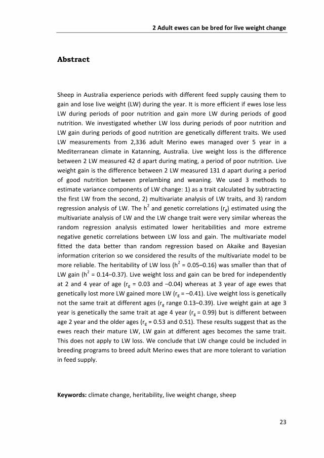
Abstract
Sheep in Australia experience periods with different feed supply causing them to
gain and lose live weight (LW) during the year. It is more efficient if ewes lose less
LW during periods of poor nutrition and gain more LW during periods of good
nutrition. We investigated whether LW loss during periods of poor nutrition and
LW gain during periods of good nutrition are genetically different traits. We used
LW measurements from 2,336 adult Merino ewes managed over 5 year in a
Mediterranean climate in Katanning, Australia. Live weight loss is the difference
between 2 LW measured 42 d apart during mating, a period of poor nutrition. Live
weight gain is the difference between 2 LW measured 131 d apart during a period
of good nutrition between prelambing and weaning. We used 3 methods to
estimate variance components of LW change: 1) as a trait calculated by subtracting
the first LW from the second, 2) multivariate analysis of LW traits, and 3) random
regression analysis of LW. The h2 and genetic correlations (rg) estimated using the
multivariate analysis of LW and the LW change trait were very similar whereas the
random regression analysis estimated lower heritabilities and more extreme
negative genetic correlations between LW loss and gain. The multivariate model
fitted the data better than random regression based on Akaike and Bayesian
information criterion so we considered the results of the multivariate model to be
more reliable. The heritability of LW loss (h2 = 0.05–0.16) was smaller than that of
LW gain (h2 = 0.14–0.37). Live weight loss and gain can be bred for independently
at 2 and 4 year of age (rg = 0.03 and –0.04) whereas at 3 year of age ewes that
genetically lost more LW gained more LW (rg = –0.41). Live weight loss is genetically
not the same trait at different ages (rg range 0.13–0.39). Live weight gain at age 3
year is genetically the same trait at age 4 year (rg = 0.99) but is different between
age 2 year and the older ages (rg = 0.53 and 0.51). These results suggest that as the
ewes reach their mature LW, LW gain at different ages becomes the same trait.
This does not apply to LW loss. We conclude that LW change could be included in
breeding programs to breed adult Merino ewes that are more tolerant to variation
in feed supply.
Keywords: climate change, heritability, live weight change, sheep

2 Adult ewes can be bred for live weight change
24
2.1 Introduction
The wool and lamb industry in Australia is mostly in the Mediterranean climate
regions of southern Australia, using mostly Merino ewes. The rainfall patterns of
these regions are expected to be more variable and less winter dominant (IPCC,
2007) with the length and severity of the annual periods of drought harder to
predict. This erratic climate will make managing sheep more difficult as most
Merino ewes lose live weight (LW) during summer and autumn and then regain LW
during late winter and spring (Adams and Briegel, 1998). Farmers currently
overcome some of the deficit in pasture feed by feeding grain, hay, or silage but
this has major feed and labor costs (Young et al., 2011b).
A possible solution is to breed sheep that can maintain LW during times of feed
shortage and are therefore more resilient to variation in feed supply. Borg et al.
(2009) and Rauw et al. (2010) estimated moderate heritabilities for LW loss and
gain in adult ewes grazing in rangelands. However, these studies did not investigate
if LW change is genetically different between periods of poor and good nutrition.
They also did not compare LW change in younger ewes to older ewes, which could
be genetically different traits.
Also, heritability of LW change can be calculated using the variance of each LW
measurement and the covariance between them. These variances can be estimated
treating each LW measurement as an individual trait in a multivariate analysis or
treating LW as a repeated measure over time in a random regression model (Van
der Werf et al., 1998).
In this study we tested the hypothesis that LW loss during summer and LW gain
during pasture growth are different traits. We also tested the hypothesis that LW
change is a different trait in young ewes compared with mature ewes. We tested
these hypotheses using 3 methods: LW change traits, random regression analysis,
and multivariate analysis.
2.2 Materials and methods
The management of the ewes was approved by the Animal Ethics and Welfare
Committee from the Department of Agriculture, Western Australia. More details
about how the ewes were managed are in Greeff and Cox (2006)
Animals and their management
We used LW information from 2,336 fully pedigreed adult ewes from the Merino
Resource flocks of the Department of Agriculture and Food Western Australia at
Katanning (33°41′ S, 117°35′ E, and elevation 310 m). Katanning is in the

2 Adult ewes can be bred for live weight change
25
Mediterranean climate region with hot dry summers and mild wet winters. This
combination of temperature and rainfall means there is a period when pasture
does not grow during summer and autumn. All ewes were managed on 1 farm
under conditions typical for commercial farms in that area. The ewes were fed two-
thirds lupins and one-third oats. The amount fed varied between years but on
average ewes were fed 100 g per animal per day in late December increasing
gradually to 800 g per head per day at lambing. Hay was fed ab libitum during
lambing. Lambing time was in July and ewes were shorn in October when the
weight of greasy wool was recorded.
Live weight data
We used LW recorded from years 2000 to 2005. Ewes were weighed 4 times
annually at approximately the same time each year (Table 2.1). The 4 LW were
premating LW (WT1), postmating LW (WT2), prelamb LW (WT3), and weaning LW
(WT4). There were 898 ewes with 1 year set, 715 with 2 year sets, and 723 with 3
year sets of all 4 LW, WT1, WT2, WT3, and WT4. There were 4,497 animal–age
combinations of all 4 LW with on average 1.9 years data per ewe of which 1,868
were for 2-year-old ewes in their first parity, 1,501 for 3-year-old ewes, and 1,128
for 4-year-old ewes. The total pedigree file consisted of 29,300 sheep tracing back
10 generations, with 760 sires and 8,540 dams. One sire was mated with an
average of 20 ewes with 1 paddock per ram.
Table 2.1 Timing of four live weight (WT) recordings in Katanning Resource Flock from
2000 to 2005.
Year Traits
WT1 WT2 WT3 WT4
2000 10-Jan 23-Feb 30-May 27-Sep 2001 16-Jan 23-Feb 06-May 25-Sep 2002 15-Jan 26-Feb 03-Jun 08-Oct 2003 13-Jan 26-Feb 03-Jun 07-Oct 2004 13-Jan 23-Feb 17-May 07-Oct 2005 11-Jan 25-Feb 18-May 03-Oct Average 13-Jan 24-Feb 23-May 02-Oct Average days from start of year
13 55 143 274

2 Adult ewes can be bred for live weight change
26
We adjusted LW for wool weight, assuming constant wool growth during the year
regardless of season and for conceptus weight using the equations from the
GRAZPLAN model (Freer et al., 1997). We estimated conceptus weight using actual
birth weight of the lambs instead of standard birth weight used by Freer et al.
(1997). Over the 6 years, 590 ewes gave birth to no lambs, 2,637 gave birth to 1
lamb, and 1,270 ewes gave birth to multiple lambs.
Genetic Analysis
To compare LW change at different times during the year and at different ages, we
used 3 different methods to identify the best way to analyse LW change.
Live weight Change Trait Analysis. The first LW was subtracted from the second
LW to define a LW change trait such as in Borg et al. (2009) and Rauw et al. (2010).
Then we estimated the variance components of the LW change traits at each age
and the genetic correlations between ages (e.g., between young ewes and mature
ewes).
Multivariate Analysis of LW. Here we used the LW at each time point as different
traits in a multivariate analysis to estimate genetic covariance or variance between
each LW point during the year within each age group. Subsequently, these
estimates were used to calculate heritabilities and genetic correlations for LW loss
and gain using variance and covariance rules.
Random Regression Analysis of LW. Here we used random regression to model
changes in variances and covariances of LW within a year using continuous
polynomial functions. This allows the genetic variance to be estimated for LW
change between any days within a year.
Variance components were estimated using ASReml (Gilmour et al., 2006).
Convergence was assumed if the REML log-likelihood changed less than 0.002 × the
previous log-likelihood and the variance parameter estimates changed less than 1%
over 6 runs. Goodness of fit of the multivariate and random regression analysis of
LW was determined using the Akaike’s information criterion (AIC; Akaike, 1973)
and the Bayesian-Schwarz information criterion (BIC; Schwarz, 1978). It was not
possible to compare these analyses that use 4 LW to the LW change trait analysis
that uses 2 LW change traits.

2 Adult ewes can be bred for live weight change
27
Fixed effects
We included fixed effects in all models for all traits for year (2000 to 2005), number
of lambs born by each ewe in the year of LW measurement (0 to 2), number of
lambs reared in the year of LW measurement (0 to 2), number of lambs born in the
year before the LW measurements (0 to 2), and number of lambs weaned in the
year before the LW measurements (0 to 2). In the random regression analyses we
nested a fixed curve for average LW over time within these fixed effects.
Live weight Change Trait Analysis
To analyse LW loss and gain as 2 separate traits, we defined LW loss (LOSS) as LOSS
= WT2 – WT1 and LW gain (GAIN) as GAIN = WT4 – WT3. This means that if LOSS or
GAIN is negative, then the ewe lost LW, and if LOSS or GAIN is positive, then the
ewe gained LW. The WT1 and WT2 were on average 42 d apart and recorded
during a period of poor nutrition in January and February during mating. Live
weights WT3 and WT4 were measured on average 131 d apart during a period of
good nutrition period between May and October, during lactation.
We did multivariate analyses for LOSS and GAIN for ages 2, 3, and 4 years. The
model used for age-specific LOSS and GAIN was
[
age age3 age4
] [
age 0 0
0 age3 0
0 0 age4
] [
age age3 age4
] [
age 0 0
0 age3 0
0 0 age4
] [
age age3 age4
] [
age age3 age4
]
in which age , age3, and age4are the observations for LOSS or GAIN when ewes are
2, 3, and 4 years old, bi is the vector of fixed effects, ai is the vector of additive
genetic effects, ei is the vector of error effects, and Xi and Zi are the incidence
matrices (i = age 2, age 3, and age4 years).
var [
age age3 age4
] where [
e age cove age age3 cove age age4
cove age3 age e age3 cove age3 age4
cove age4 age cove age4 age3 e age4
] and
var [
age age3 age4
] where [
a age cova age age3 cova age age4
cova age3 age a age3 cova age3 age4
cova age4 age cova age4 age3 a age4
],
in which I is the identity matrix, A is the additive genetic relationship matrix, and
is the direct matrix product operator.
We used bivariate analyses to estimate genetic correlations between each LOSS
and GAIN at each age, similarly as between ages.

2 Adult ewes can be bred for live weight change
28
Multivariate Analysis of LW
We estimated the covariance or variance components between the 4 LW
measurements (WT1, WT2, WT3, and WT4) in each age group using a multivariate
analysis:
[
WT1 WT WT3 WT4
] [
WT1 0 0 00 WT 0 00 0 WT3 00 0 0 WT4
] [
WT1
WT
WT3
WT4
]
[
WT1 0 0 00 WT 0 00 0 WT3 00 0 0 WT4
] [
WT1
WT
WT3
WT4
] [
WT1
WT
WT3
WT4
]
where WT1, WT , WT3 and WT4 are the observations for WT1, WT2, WT3 and
WT4,. i is the vector of fixed effects, is the vector of additive genetic effects and
is the vector of residuals. i and i are the incidence matrices ( =WT1, WT2, WT3
and WT4
var [
WT1
WT
WT3
WT4
] ,
[
e WT1 cove WT1 WT cove WT1 WT3 cove WT1 WT4
cove WT WT1 e WT cove WT WT3 cove WT WT4
cove WT3 WT1 cove WT3 WT e WT3 cove WT3 WT4
cove WT4 WT1 cove WT4 WT cove WT4 WT3 e WT4 ]
and
var [
WT1
WT
WT3
WT4
] ,
[
a WT1 cova WT1 WT cova WT1 WT3 cova WT1 WT4
cova WT WT1 a WT cova WT WT3 cova WT WT4
cova WT3 WT1 cova WT3 WT a WT3 cova WT3 WT4
cova WT4 WT1 cova WT4 WT cova WT4 WT3 a WT4 ]
Where is the identity matrix, is the relationship matrix.
Calculation of Genetic Parameters Using Multivariate Analysis of LW
We estimated the additive genetic and residual variance for LOSS and GAIN using
the variances of the 2, involved LW and the covariance between them. For
example, the additive genetic variance for LOSS (WT2 –WT1) was calculated using
a (WT WT1 a WT
a WT1 cova(WT ,WT1
in which a WT and a WT1
are the additive genetic variances of WT1 and WT2,
respectively, and cova(WT ,WT1) is the additive genetic covariance between WT2
and WT1. This means that when the covariance between LW points is positive,
variance in LW change exists only when twice the covariance between 2 points is
lower than the variance of the 2 points. This means highly correlated points will
have less variance for the LW change between them.

2 Adult ewes can be bred for live weight change
29
We calculated the genetic covariance between LOSS (WT2 – WT1) and GAIN (WT4 –
WT3) using
cova(WT WT1,WT4 WT3
cova(WT ,WT4 cova(WT ,WT3 cova(WT1,WT4 cova(WT1,WT3
in which cova is the additive genetic covariance between LW at each measurement
time indicated in the parentheses.
Random Regression Analysis of LW
We used random regression to analyse LW change as a continuous function of time
across the seasons (Henderson, 1982; Schaeffer, 2004). This random regression
analysis was done separately for ages 2, 3, and 4 years.
a a p p ,
In which is a vector of observations for live weights of individual ewes; is the
incidence matrix for the vector of the fixed effects ; a and p are the matrices
with orthogonal polynomial coefficients of j x i dimensions in which j is the number
of polynomial coefficients and i is the number of live weight points standardised to
the first and last time points. a and p correspond to the matrices with additive
genetic and permanent environmental random regression coefficients a and p,
and is the random residual. Permanent environmental effects were estimated to
account for non-genetic variance between the repeated live weight measurements.
We fitted the fixed curve of average LW as a third order polynomial nested within
year, number of lambs born by each ewe in the year of LW measurement (0 to 2),
number of lambs reared in the year of LW measurement (0 to 2), number of lambs
born in the year before the LW measurements (0 to 2), and number of lambs
weaned in the year before the LW measurements (0 to 2). The third order was the
greatest possible order using 4 data points and was the best fit based on F-tests.
We then selected the order of fit for the random effects, additive genetic and
permanent environmental, by comparing the 9 possible models for each age from
order 1 to 3. The best fit of the 9 different models was based on the BIC. The
optimum fit for all ages was the third order for additive genetic effects and the first
order for permanent environmental effects.
We included 4 separate residual variance classes along the time x axis, 1 for each
time point, because the residual variance for each separate LW measurement
estimated using the multivariate analysis was different. Due to the small variation
in measurement date between years, these classes were 10 to 16, 54 to 57, 126 to
154, and 268 to 281 d from the start of the year. We used these 4 time points
because it maximised the number of individuals that could be included in the

2 Adult ewes can be bred for live weight change
30
analysis as most ewes were culled between weaning and the next mating, so most
ewes had LW for the first 4 LW of the year.
The variances and covariances between the 4 LW points were calculated based on
the random regression variance–covariance functions at 13, 55, 143, and 274 d
from the start of the year.
The additive genetic variance and permanent environmental variance and
covariance between LOSS and GAIN were calculated using the same equations as in
the multivariate analysis of LW analysis. The only difference was that the
phenotypic variance for LOSS and GAIN was estimated by adding the additive
genetic and permanent environmental variances estimated from the random
curves to the estimates for residual variance at the relevant time points. These
residual estimates were assumed to be independent of each other because we
estimated the permanent environmental effects to account for environmental
covariances between time points.
2.3 Results
As ewes aged they got heavier and their LW varied less over the year (Table 2.2).
The ewes were lighter at age 2 years at each point in the year and ewes aged 4
years were the heaviest. Additionally, the ewes on average lost LW between WT1
and WT2 (LOSS) and gained LW between WT3 and WT4 (GAIN) at all ages with
younger ewes (age 2 years) losing and gaining more LW than older ewes (age 3
years and age 4 years). This suggests that ewes aged 2 years were still growing to
maturity.
Variance of LW
The additive genetic variance of LW was mostly similar when estimated using
multivariate analysis of LW and random regression (Figure 2.1). At age 3 years the
additive variance of LW estimated using random regression as compared with
multivariate analysis was greater for WT1 and WT2 and lower for WT4. The
additive variance at age 4 years was greater for WT3 and lower for WT4 when
estimated with random regression compared with multivariate analysis of LW. We
used these variances and the covariance between each LW measurement to
estimate the heritability of LW change.

2 Adult ewes can be bred for live weight change
31
Additive Genetic Variance, Phenotypic Variance, and Heritability
Estimates for LW loss
The multivariate analysis of LW fit the data better than random regression at all
ages according to the BIC and AIC (Table 2.3). Table 2.4 shows estimates of the
variance components for LOSS using the variance and covariance estimated with
random regression and multivariate analyses of LW. The additive variance for LOSS
was greater using multivariate whereas residual variance was greater using random
regression. The heritability of LOSS calculated using random regression was lower
than those calculated using multivariate (Table 2.5) analysis of LW and the LW
change trait methods.
Table 2.2 Mean and standard deviation (SD) of live weight 1 to 4, LOSS and GAIN of ewes
aged 2, 3 and 4 years old.
Trait Mean (kg) SD (kg)
WT1 age = 2 50.2 6.24 WT1 age = 3 58.6 7.09 WT1 age = 4 61.7 7.30 WT2 age = 2 48.0 6.46 WT2 age = 3 58.0 6.45 WT2 age = 4 60.7 6.62 WT3 age = 2 50.3 6.04 WT3 age = 3 58.5 6.77 WT3 age = 4 60.9 7.13 WT4 age = 2 56.9 7.41 WT4 age = 3 61.7 8.13 WT4 age = 4 63.7 8.70 LOSS age = 2 -2.23 2.73 LOSS age = 3 -0.606 3.95 LOSS age = 4 -0.968 3.79 GAIN age = 2 6.55 7.20 GAIN age = 3 3.14 7.20 GAIN age = 4 2.83 7.41

2 Adult ewes can be bred for live weight change
32
Figure 2.1 Variance components for LW estimated using multivariate analysis of LW and
random regression analysis with third order polynomial for additive genetic variance and
first order polynomial for permanent environmental effects. The residual for the random
regression includes the permanent environmental and residual variance together.
Plotted for age 2, 3, and 4 years.
Table 2.3 Akaike’s information criterion (AIC), and the Bayesian-Schwarz information
criterion (BIC) for multivariate and random regression analysis of live weight at ages 2, 3
and 4.
Method Age 2 Age 3 Age 4
ΑΙC Multivariate 25713 22630 17389 Random Regression 25757 22685 17443 BIC Multivariate 25851 22764 17517 Random Regression 25875 22799 17552

2 Adult ewes can be bred for live weight change
33
Additive, Phenotypic, and Heritability Estimates for LW gain
The additive variance for GAIN estimated using multivariate analysis was greater
than that estimated using random regression (Table 2.6). As a consequence, the
heritability estimated using random regression was lower than the heritability
estimated with the multivariate analysis of LW and LW change trait analyses (Table
2.7). Additionally, GAIN became less heritable as ewes aged using all 3 methods. At
age 2 years, heritability of GAIN was greater compared with at age 3 years and age
4 years. The heritabilities for GAIN were always greater than LOSS.
Genetic Correlations between LW loss and LW gain
There was almost 0 genetic correlation between LOSS and GAIN except a medium
negative correlation at age 3 years when correlations were estimated with
multivariate analysis of LW and the LW change trait (Table 2.8). At age 2 and 4
years the genetic correlation between LOSS and GAIN was nearly 0 when estimated
using the LW change trait and the multivariate analysis of LW (Table 2.8).
Alternatively, these genetic correlations estimated using random regression were
moderate and negative for age 2 and 4 years. The genetic correlations between
LOSS and GAIN for age 3 years were greater than age 2 and 4 years for all 3
methods. For ewes aged 3 years, the genetic correlations estimated using LW
change trait and multivariate analysis of LW were moderate and negative whereas
the estimate using random regression analysis was very negative.
Genetic Correlations between Ages
The LOSS had low to moderate positive genetic correlations between ages (Table
2.9). The GAIN at age 2 years was moderately and positively correlated with GAIN
at age 3 years whereas LW gain at age 3 years is the same trait as GAIN at age 4
years. The correlations between LOSS at age 2 years and LOSS at age 3 and 4 years
are moderate whereas correlation between ages 3 and 4 years is low. This is not
expected as ages 2 and 3 years or ages 3 and 4 years ought to have a greater
genetic correlation than ages 2 and 4 years although the SE are high for these
correlations. The genetic correlations for the GAIN traits were more in line with
expectations, with age 3 and 4 years being highly correlated whereas there were
lower correlations between age 2 and 3 years as well as ages 3 and 4 years. These
results suggest that early growth to maturity at age 2 years is different to growth in
adult Merino during periods of high nutrient availability.

2 Adult ewes can be bred for live weight change
34
Table 2.4 Additive genetic ( a (WT -WT1) and residual plus permanent environmental
( e (WT -WT1) ) variance of LOSS calculated using the variance for each live weight and
covariance between live weights estimated using multivariate analysis of live weight and
random regression analyses. For example, the additive genetic variance was estimated
using a (WT -WT1) a WT
a WT1 - cova(WT ,WT1). Permanent environmental variance
was only estimated for the random regression.
Additive genetic a WT1 a WT
cova (WT1,WT (
Age = 2 Multivariate 17.7 (1.79) 15.5 (1.62) 16.2 (1.61) 0.89 (0.26) Random regression 18.5 (1.73) 16.6 (1.65) 17.3 (1.68) 0.63 (0.23) Age = 3 Multivariate 19.7 (2.74) 20.2 (2.50) 19.1 (2.50) 1.69 (0.56) Random regression 20.5 (2.64) 19.7 (.46) 19.7 (2.49) 0.79 (0.48) Age = 4 Multivariate 24.5 (3.64) 22.5 (3.13) 22.9 (3.21) 1.24 (0.65) Random regression 23.2 (3.37) 22.1 (3.11) 22.4 (3.18) 0.42 (0.35)
Residual + Permanent environmental
e WT1 e WT
cove (WT1,WT ) e (WT WT1)
Age = 2 Multivariate 9.16 (1.17) 9.17 (1.08) 6.49 (1.05) 5.35 (0.28) Random regression 8.74 (1.09) 8.54 (1.01) 5.83 (1.05) 5.62 (0.27) Age = 3 Multivariate 20.5 (2.11) 14.0 (1.78) 12.6 (1.81) 9.24 (0.58) Random regression 20.0 (2.09) 14.7 (1.72) 12.4 (1.77) 9.81 (0.54) Age = 4 Multivariate 17.9 (2.75) 13.9 (2.30) 11.1 (2.34) 9.69 (0.72) Random regression 19.4 (2.67) 14.6 (2.29) 11.8 (2.33) 10.3 (0.64)
Table 2.5 Estimates of additive ( a OSS ) and phenotypic variance ( p OSS
) and heritability
(h2) for LOSS with standard errors in brackets estimated using multivariate analysis of
live weight, random regression and the live weight change trait analyses.
Method Age a OSS p OSS
1 h
2
Multivariate 2 0.89 (0.26) 6.24 (0.20) 0.14 (0.04) Random regression 2 0.63 (0.23) 6.06 (0.20) 0.07 (0.03) Live weight change trait 2 0.86 (0.26) 6.24 (0.21) 0.14 (0.04)
Multivariate 3 1.69 (0.56) 10.9 (0.41) 0.15 (0.05) Random regression 3 0.79 (0.48) 10.6 (0.40) 0.07 (0.03) Live weight change trait 3 1.51 (0.55) 10.8 (0.41) 0.14 (0.05)
Multivariate 4 1.24 (0.65) 10.9 (0.47) 0.11 (0.06) Random regression 4 0.42 (0.35) 10.7 (0.48) 0.04 (0.03) Live weight change trait 4 1.23 (0.65) 10.9 (0.47) 0.11 (0.06)
1 the phenotypic variance of LOSS by adding the additive, residual and permanent
environmental variances from Table 2.4.

2 Adult ewes can be bred for live weight change
35
Table 2.6 Additive genetic ( a (WT4-WT3) ) and residual plus permanent environmental
( e (WT4-WT3) ) variance of GAIN calculated using the variance for each live weight and
covariance between live weights estimated using multivariate analysis of live weight
and random regression. For example, the additive genetic variance was estimated using
a (WT4-WT3) a WT4
a WT3 - cova(WT4,WT3). Permanent environmental variance was
only estimated for the random regression.
Additive genetic a WT3 a WT4
cova (WT3,WT4 ( WT3
Age = 2 Multivariate 18.4 (1.81) 21.0 (2.59) 15.8 (1.88) 7.73 (1.31) Random regression 15.9 (1.60) 19.9 (2.01) 16.0 (1.68) 3.62 (0.83) Age = 3 Multivariate 19.8 (2.48) 26.7 (3.67) 20.4 (2.67) 5.95 (1.55) Random regression 19.6 (2.35) 23.5. (2.85) 20.3 (2.44) 2.63 (1.13) Age = 4 Multivariate 20.5 (3.27) 27.5 (4.42) 21.4 (3.38) 5.24 (1.78) Random regression 21.8 (3.07) 24.5 (3.70) 21.2 (3.12) 3.87 (1.42)
Residual + Permanent environmental
e WT3 e WT4
cove (WT3,WT4 e (WT4 WT3)
Age = 2 Multivariate 9.08 (1.17) 19.9 (1.87) 6.61 (1.25) 15.8 (1.11) Random regression 10.5 (1.08) 17.5 (1.78) 6.03 (1.09) 15.9 (1.09) Age = 3 Multivariate 14.9 (1.80) 24.5 (2.76) 8.78 (1.90) 21.9 (1.51) Random regression 15.7 (1.60) 24.3 (2.51) 8.91 (1.71) 22.2 (1.51) Age = 4 Multivariate 19.3 (2.57) 26.5 (3.48) 11.0 (2.58) 5.24 (1.78) Random regression 17.3 (2.33) 28.5 (3.14) 10.9 (2.32) 3.87 (1.42)
Table 2.7 Estimates of additive genetic ( a AI ) and phenotypic variance ( p AI
) and
heritability (h2) for GAIN with standard errors in brackets estimated with multivariate
analysis of live weight, random regression and the live weight change trait methods.
Method Age a AI p AI
1 h
2
Multivariate 2 7.73 (1.31) 23.5 (0.83) 0.33 (0.05) Random regression 2 3.62 (0.83) 19.5 (1.24) 0.18 (0.04) Live weight change trait 2 7.92 (1.32) 23.5 (0.84) 0.33 (0.05)
Multivariate 3 5.95 (1.55) 27.8 (1.05) 0.21 (0.05) Random regression 3 2.63 (1.13) 24.9 (1.75) 0.11 (0.04) Live weight change trait 3 4.89 (1.37) 27.6 (1.03) 0.18 (0.05)
Multivariate 4 5.24 (1.78) 29.1 (1.25) 0.18 (0.06) Random regression 4 3.87 (1.42) 27.8 (2.1) 0.14 (0.05) Live weight change trait 4 5.71 (1.68) 29.3 (1.26) 0.19 (0.05)
1 the phenotypic variance of GAIN by adding the additive, residual and permanent
environmental variances from Table 2.6.

2 Adult ewes can be bred for live weight change
36
2.4 Discussion
Our study found that LW loss during periods of poor nutrition and LW gain during
periods of good nutrition are genetically different traits. Additionally, LW loss and
gain are genetically different in young ewes compared with old ewes. The
estimates of heritability and correlations for LW change were different depending
on the method used.
Comparison of Methods
In this paper we used 3 methods for estimating genetic parameters. The estimates
from the random regression analysis were clearly different from the estimates from
the 2 other methods. The preferred method of the 3 is either the multivariate
analysis of LW or LW change trait analyses because the multivariate analysis fit the
data better than random regression according to the AIC and BIC. The LW change
analysis cannot be directly compared with the multivariate and random regression
analyses based on AIC and BIC but yields very similar results as the multivariate
analyses. The random regression approach has a number of theoretical advantages
but in our case was not an appropriate method. In our research, genetic
cova(WT1,WT3 cova(WT ,WT4 cova(WT1,WT4 cova(WT ,WT3
Table 2.8 Estimates of genetic correlations between LOSS and GAIN (rg OSS AI ) with
standard errors in brackets estimated with multivariate analysis of live weight, random regression and the live weight change trait analyses.
Method Age cov(LOSS,GAIN)1 rg OSS AI
Multivariate 2 -0.00 (0.42)1 -0.00 (0.16)
Random regression 2 -0.59 (0.25) 1
-0.47 (0.13) Live weight change trait 2 0.08 (0.43) 0.03 (0.16)
Multivariate 3 -1.32 (0.66) 1
-0.42 (0.19) Random regression 3 -1.27 (0.42)
1 -0.87 (0.21)
Live weight change trait 3 -1.33 (0.66) -0.42 (0.20)
Multivariate 4 -0.09 (0.76) 1
-0.03 (0.30) Random regression 4 -0.75 (0.50)
1 -0.57 (0.24)
Live weight change trait 4 -0.06 (0.75) -0.02 (0.30) 1 estimated using; cova(WT -WT1,WT4-WT3)
Table 2.9 Genetic correlations between ages for live weight loss and gain (± s.e. in brackets). LOSS = live weight loss and GAIN = live weight gain.
LOSS GAIN
Age Age 3 Age 4 Age 3 Age 4
Age 2 0.34 (0.24) 0.39 (0.30) 0.53 (0.14) 0.51 (0.15) Age 3 0.13 (0.32) 0.99 (0.15)

2 Adult ewes can be bred for live weight change
37
correlations between LW at different time points were greater with random
regression than with multivariate analysis of LW. This makes the heritability of LW
change lower because there is less genetic variation in the difference between LW
when they are highly correlated. This is different to the analysis by Huisman et al.
(2002) who found that the correlations between 5 LW points in growing pigs had a
similar correlation using both multivariate and random regression analysis. With
our data with only 4 LW points, multivariate analysis uses 20 parameters compared
with the random regression, which uses 17, so there is not a major disadvantage
for using the multivariate analysis whereas the multivariate analysis fits the data
better than the random regression analysis.
Random regression could however be useful when data has more time points
during the year because fewer parameters are required to predict variance and
covariance using curves compared with multivariate analysis between many time
points (van der Werf et al., 1998). Additionally, if the measurements are recorded
on different days for each individual making it harder to define specific traits or
there are many missing values, random regression would be preferred. This is
because multi-trait models become over parameterised as the model tries to
estimate variance and covariance for time points with few records (Veerkamp et
al., 2001). In our study however, the LW points were well clustered together
making 4 distinct traits so there is no clear advantage of using random regression.
Therefore, the multivariate analysis or the LW change analysis is preferred.
The multivariate analysis of LW change and the LW change trait were very similar in
terms of heritabilities of LW change and the genetic correlations between loss and
gain. The preferred method of the 2 is the multivariate analysis because fixed
effects can be allocated to each LW separately. For example, the number of lambs
born would affect weight at lambing more than at the start of mating. Therefore,
the fixed effect of number of lambs born can be better modeled for each LW trait
separately.
An important conclusion from our analysis is the difficulty in estimating variances
and correlations between LW change traits. To estimate the correlation between
LOSS and GAIN using multivariate and random regression, 4 estimated variances
and 6 estimated covariances were used. Although the differences between the
random regression and the multivariate estimates are not large in terms of model
fit and variance components, differences in estimates accumulate in calculating
genetic correlations between LW changes resulting in very different outcomes
between random regression and multivariate analysis.

2 Adult ewes can be bred for live weight change
38
Heritability Estimates
Our analysis revealed that LOSS and GAIN are genetically different traits with LOSS
less heritable than GAIN. This can be partly explained by the difference in periods
over which GAIN and LOSS were calculated. The trait LOSS was LW change during
mating on poor quality pasture and GAIN was LW change during lactation on good
quality pasture. Therefore, the physiological process of the LW change would be
different between the 2 periods. Also, GAIN was estimated from LW 131 d apart
compared with the LOSS LW, which were 42 d apart. We did not divide LW change
by the number of days of each period because there was little variation in number
of days between animals for each period. Longer time between points allows
bigger genetic differences to accumulate. Our study is in line with the previous
studies showing that genetic variation exists in farmed animal populations to breed
for increased tolerance against climate change (Ravagnolo and Miszal, 2000; Borg
et al., 2009; Hayes et al., 2009; Rauw et al., 2010; Bloemhof et al., 2012).
Our estimates of heritability where different from other studies with Rauw et al.
(2010) estimating greater heritability for LW loss and Borg et al. (2009) estimating a
lower heritability. Also, Borg et al. (2009) estimated a lower heritability for LW gain.
Both of these studies were done in a semi-arid environment and used different
breeds. Additionally, our heritabilities were estimated at each age independently,
which makes a difference compared with pooling information from all ages
together. For example, Vehviläinen et al. (2008) estimated lower heritability for
survival with pooled generations compared with individual generations.
Furthermore, we found genetic correlations between ages for LOSS and GAIN
mostly less than 1. Therefore, LOSS and GAIN are not the same traits when ewes
are maturing compared with when ewes are mature. The combination of different
method, breed, environment, and timing of measurements may explain the
different heritabilities between our study and the research by Borg et al. (2009)
and Rauw et al. (2010).
Genetic Correlations between LOSS and GAIN
The genetic correlations suggest that LOSS and GAIN can be bred for independently
and that LOSS and GAIN are different traits at different ages. There was close to 0
genetic correlation between LOSS and GAIN at ages 2 and 4 years whereas there
was a moderate negative (–0.42) correlation at age 3 years when estimated with
the multivariate analysis of LW and the LW change trait methods. Therefore, ewes
can be selected to lose less LW potentially requiring less supplementary feeding
and to gain more LW during spring and use more of the cheap feed supply,
increasing their reserves before summer and autumn. The negative correlation at
2 Adult ewes can be bred for live weight change
39
age 3 years means that ewes that lose more LW also gain more LW, but the
negative genetic correlation may have been due to sampling given the large
standard errors.
Live weight loss appears to be lowly heritable at all ages, with little association
across ages. Live weight gain appears to be moderately heritable, particularly
among 2-year-old ewes. The genetics of gain therefore resembles that of a growth
trait. In contrast, loss behaves more like a physiological trait with less genetic
variation. Live weight LOSS is genetically a different trait at different ages and is a
different trait at age 2 years compared with age 3 and 4 years and GAIN at age 3
and 4 years are genetically the same. This is probably because ewes at age 2 years
are still growing to mature size whereas ewes at age 3 and 4 years are mature.
Although GAIN is the same trait at age 3 and 4 years, it is recommended to consider
LOSS and GAIN at different ages as different traits in genetic evaluation as well as in
a selection index.
Implications for Breeding
The heritability estimates in this study show that it is feasible to breed adult Merino
ewes that gain more LW. Live weight loss can also be selected for although the
response to selection will be lower than for LW gain due to the lower heritability.
Additionally, genetic correlations between LOSS and GAIN are mostly low,
indicating that selection can be directed to one of them without affecting the other
much. This means that sheep can be bred to lose less LW during periods of poor
nutrition and gain more LW during periods of good nutrition. The implications of
this depend on the role of LW change in the breeding goal and selection index of
Merino sheep breeders.
Live weight change does not have a direct economic value in a selection index.
However, it may be used in a selection index if it is genetically correlated to feed
intake or efficiency. For example, LW loss could be used to represent breeding goal
traits to reduce energy requirements for maintenance or increase intake when
grazing poor quality feed (Fogarty et al., 2009; Silanikove, 2000). A study by Young
et al. (2011a) calculated that reducing maintenance costs or increasing intake on
poor pasture had a high economic value. The increase in profit was because
farmers could manage more ewes on each hectare of land if they are more
efficient. If ewes are, however, able to maintain or gain LW during summer due to
reallocating resources from other competing body functions such as fertility or
immunity (van der Waaij, 2004), then LW change does not represent efficiency
within the breeding goal and is less valuable. Therefore, it will be useful to
understand if ewes lose or gain more LW because they allocate their resources

2 Adult ewes can be bred for live weight change
40
differently to wool, pregnancy, or lactation. This means that the genetic
correlations between LW change and other production traits are needed before LW
change can be used as an index trait.
Although all ewes had access to the same feed, the grazing behavior and actual
intake by each ewe is not known. Therefore, it is possible that some ewes were
more efficient at grazing or had first access to supplementary feed. To get better
insight why some ewes lose less weight or gain more LW, individual feed intake
data would be required.
2.5 Conclusion
In conclusion it is possible to breed adult ewes that lose less LW during periods of
poor nutrition and gain LW during periods of good nutrition. More research is
required to see if LW change can be used as an indicator trait for breeding goal
traits such as feed intake or efficiency. If LW change is included in a breeding
program, breeders need to consider the age of ewes and the timing of
measurements. This research would benefit from a dataset with more
measurements during the year that represents the trajectory of the LW curve
better.
Acknowledgements
This research was financed by the Department of Food and Agriculture Western
Australia, The Sheep Cooperative Research Centre, Meat and Livestock Australia,
and Wageningen University. We are grateful for the help that Craig Lewis and
Mario Calus gave for this research.

3 Genetic correlations between live weight change and reproduction traits in Merino
ewes depend on age
Gus Rose12
, Han A Mulder1, Julius H J van der Werf
23, Andrew N Thompson
245,
Johan AM van Arendonk1
1 Animal Breeding and Genomics Centre, Wageningen University, PO Box 338, 6700
AH, Wageningen, The Netherlands; 2 CRC for Sheep Industry Innovation, University
of New England, Armidale, NSW, 2351, Australia; 3 School of Environmental and
Rural Science, University of New England, Armidale, NSW, 2351, Australia; 4
Department of Agriculture and Food Western Australia, 3 Baron-Hay Court, South
Perth, WA, 6151, Australia; 5 School of Veterinary and Life Sciences, Murdoch
University, 90 South Street, Murdoch, WA, 6150, Australia
Journal of Animal Science (2013) 92:3249-32572
2 In this chapter alterations were made to the printed article, changing English from
US to United Kingdom, replacing body weight with live weight and changing the format of headings and tables to make it consistent with the rest of the thesis.


3 Genetics of live weight change and reproduction
43
Abstract
Merino sheep in Australia experience periods of variable feed supply. Merino sheep
can be bred to be more resilient to this variation by losing less live weight when
grazing poor quality pasture and gaining more live weight when grazing good
quality pasture. Therefore, selection on live weight change might be economically
attractive but correlations with other traits in the breeding objective need to be
known. The genetic correlations (rg) between live weight, live weight change, and
reproduction were estimated using records from ~7350 fully pedigreed Merino
ewes managed at Katanning in Western Australia. Number of lambs and total
weight of lambs born and weaned were measured on ~5300 2-year-old ewes,
~4900 3-year-old ewes and ~3600 4-year-old ewes. On a proportion of these ewes
live weight change was measured: ~1950 two-year-old ewes, ~1500 three old ewes
and ~1100 four-year-old ewes. The live weight measurements were for three
periods. The first period was during mating period over 42 days on poor pasture.
The second period was during pregnancy over 90 days for ewes that got pregnant
on poor and medium quality pasture. The third period was during lactation over
130 days for ewes that weaned a lamb on good quality pasture. Genetic
correlations between weight change and reproduction were estimated within age
classes. Genetic correlations were tested to be significantly greater magnitude than
zero using likelihood ratio tests. Nearly all live weights had significant positive
genetic correlations with all reproduction traits. In two-year old ewes, live weight
change during the mating period had a positive genetic correlation with number of
lambs weaned (rg = 0.58); live weight change during pregnancy had a positive
genetic correlation with total weight of lambs born (rg = 0.33) and a negative
genetic correlation with number of lambs weaned (rg = -0.49). All other genetic
correlations were not significantly greater magnitude than zero but estimates of
genetic correlations for three-year-old ewes were generally consistent with these
findings. The direction of the genetic correlations mostly coincided with the energy
requirements of the ewes, and the stage of maturity of the ewes. In conclusion,
optimised selection strategies on live weight changes to increase resilience will
depend on the genetic correlations with reproduction, and are dependent on age.
Keywords: live weight change; genetic correlations, Merino ewes, reproduction

3 Genetics of live weight change and reproduction
44
3.1 Introduction
Most Merino sheep in Australia are farmed in Mediterranean climate regions and
they generally lose live weight during summer and autumn and regain live weight
during late winter and spring (Adams and Briegel, 1998). Managing the extent and
timing of live weight loss and gain in relation to pasture supply and animal
requirements can affect whole farm profit (Young et al., 2011b). Management of
live weight of ewes will become more difficult if length of annual periods of
drought during summer and winter become longer and harder to predict (IPCC,
2007). One way to make sheep production systems more resilient to uncertain
pasture supply is to select sheep that lose less live weight when the supply and
quality of paddock feed is low (Rose et al., 2013).
Phenotypically, Merino ewes that are heavier at mating have a higher reproductive
rate (Ferguson et al., 2011). Additionally, there are positive phenotypic correlations
between live weight gain during pregnancy and birth and weaning weight in lambs,
with heavier lambs more likely to survive both prior to and after weaning (Oldham
et al., 2011; Thompson et al., 2011).
Genetic correlations between live weight change and reproduction depend on
correlations between live weight at all times during the reproductive cycle and
reproduction traits. Therefore it is important to know the genetic correlations
between live weight at key times during the reproductive cycle and reproduction
traits. Ewe live weight prior to mating has a positive genetic correlation with
fertility (Owen et al., 1986; Cloete and Heydenrych, 1987). Borg et al. (2009)
estimated positive genetic correlations between number of lambs born and live
weight change during late lactation but correlations during the mating period and
pregnancy are still unknown. Based on these correlations the hypothesis that
increases in ewe live weight during the mating and pregnancy periods would have
significant positive genetic correlations with reproduction traits was tested.
3.2 Materials and methods
Records from 7,346 Merino ewes were used from 697 sires and 4,724 dams using
pedigree records from 17,836 sheep over 10 generations. These sheep were from
the Merino Resource flocks of the Department of Agriculture and Food Western
Australia located at Katanning (33°41´S, 117°35´E, elevation 310m). Katanning is in
a Mediterranean climatic region with hot dry summers and mild wet winters. This
combination of temperature and rainfall means that there is a period of no pasture
growth during summer and autumn, typically extending from November to May
each year. All ewes were managed on one farm under conditions typical for

3 Genetics of live weight change and reproduction
45
commercial farms in the area. The amount of supplement fed varied between years
but on average ewes were fed 100 grams of an oats and lupin grain mixture per
head per day in late December increasing gradually to 800 grams per head per day
at lambing in July. Hay was fed ab libitum during lambing. More information about
how the flock was managed can be found in Greeff and Cox (2006).
Live weight change
To estimate change in live weight of ewes live weight data from ewes aged 2, 3 and
4 years old was used and live weight at each age was treated as different traits,
using the same data as used by Rose et al. (2013). The age groups were 2, 3, and 4
years old at lambing in July. The ewes were weighed 4 times during the year. The
average dates for each live weight were: 13th of January for premating weight
(WT1), 24th of February for postmating weight (WT2), 23rd May for prelambing
weight (WT3) and 2nd of October for weaning weight (WT4). The timing of
measurements varied between years with WT1, WT2 and WT4 all measured within
a week of each other while WT3 was measured within a month. Live weights were
corrected for wool weight by estimating wool growth from shearing to the day the
live weight was measured. These estimates were based on the greasy fleece weight
of ewes, and assumed that wool growth was linear across the year. Conceptus
weight was estimated using equations from the GRAZPLAN model (Freer et al.,
1997) and subtracted from WT2 and WT3.
Live weight change was then split into three parts of the reproduction cycle;
mating, pregnancy and lactation. For live weight change during the mating period
all ewes that were mated were included, for pregnancy only ewes that gave birth
to lambs were included, and for lactation only ewes that weaned at least one lamb
were included. Therefore, new live weight traits were created that only included
the relevant ewes. These traits were for mating, WT1mate and WT2mate, for
pregnancy WT2preg and WT3preg, and for lactation WT3lact and WT4lact. These
three groups were derived because ewes that did not bear or rear lambs have
different energy and protein requirements compared with ewes that were
pregnant and lactating. Therefore, live weight change in ewes that do not bear or
rear lambs may be genetically different than live weight change in ewes that do
bear or rear lambs.
Using these new live weights the genetic parameters for live weight change during
mating period (ΔWTmate WT mate – WT1mate), during pregnancy (ΔWTpreg
WT3preg – WT2preg) and during lactation (ΔWTlact WT4lact – WT3lact) could be
estimated. Live weight change during mating period (ΔWTmate) was measured in
summer when pasture was dry, ΔWTpreg was measured in autumn when pasture

3 Genetics of live weight change and reproduction
46
was dry and the start of winter when pasture started growing, and ΔWTlact was
measured during winter and spring when pasture growth was most rapid.
The variance components of these live weight change traits were calculated by
estimating the covariance between both live weights. The additive genetic variance
of change in live weight ΔWT ( 2a(ΔWT)) is;
2a (ΔWT)
2a WT2
2a WT1 – 2 x cova(WT2,WT1) Eq. 1
where 2
a WT2 is the additive genetic variance of WT2, 2
a WT1 is the additive genetic
variance of WT1 and cova(WT2,WT1) is the additive genetic covariance between
WT2 and WT1.
Live weights were used instead of calculating live weight change because the
number of records for the four traits was different. Therefore, only including
records from animals with both traits would bias the estimates for live weight
change. Additionally, the fixed effects can be fitted to each live weight trait
separately.
Reproduction data
Reproduction traits at 2 (first lambing opportunity), 3 (second lambing opportunity)
and 4 years of age (third lambing opportunity) were used. These traits were total
weight of lambs born (TBW) and total weight of lambs weaned (TWW) in each age
group. These traits incorporate most of the aspects of reproduction such as
fecundity, mothering ability and ease of birth into one composite trait (Snowder
and Fogarty, 2009). Variances and covariances for total number of lambs born in
each year (NLB) and total number of lambs weaned in each year (NLW) were also
estimated. Both NLB and NLW were estimated as linear traits including ewes that
had no lambs born or weaned. Traits TBW and TWW were only measured in ewes
that gave birth to or weaned lambs. The genetic correlations between live weight
change and reproduction traits were estimated in the same year at the same age.
Genetic correlations between number of lambs born and weaned with live
weight change
The genetic correlations (rg) between live weights during the mating, pregnancy
and lactation periods, and NLB and NLW were calculated by estimating the genetic
covariance between the two live weights and each reproduction trait using
equation 2. This equation was used to estimate the genetic correlations between
live weight change during pregnancy and lactation and NLB and NLW. Equation 2 is
[
trait wta wtb
] [
trait 0 00 wta 0
0 0 wtb
] [
trait wta wtb
] [
trait 0 00 wta 0
0 0 wtb
] [
trait wta wtb
] [
trait wta wtb
] Eq. 2

3 Genetics of live weight change and reproduction
47
where trait are the observations for NLB and NLW, wtaare the observations for the
first live weight used to calculate live weight change and wtb are the observations
for the second live weight used to calculate live weight change, i is the vector of
fixed effects, i is the vector of additive genetic effects and i is the vector of error
effects. i and i are the incidence matrices (i = trait, wta and wtb). The random
effects i and i are trivariate normally distributed with mean zero and variance:
var [
trait wta wtb
] where R [
e trait e trait wta e trait wtb
e wta trait e wta e wta wtb
e wtb trait e wtb wta e wtb
] and
var [
trait wta wtb
] where G [
a trait a trait wta a trait wtb
a wta trait a wta a wta wtb
a wtb trait a wtb wta a wtb
]
I is the identity matrix and is the additive genetic relationship matrix between
ewes.
Variance components and their standard errors were estimated using ASReml
(Gilmour et al., 2006). For all traits fixed effects were for year (1982-2005), the age
of the dam of the ewe (years), birth and rearing type of the ewe (single or multiple)
and birthdate as a fixed covariate.
Reproductive performance of a ewe affects live weight change during pregnancy
and lactation, as more lambs will cause a higher foetal and lactation burden. Ewes
that produce larger litters are expected to lose more live weight during pregnancy
and lactation. Therefore, correlations between live weight change during
pregnancy and lactation and reproduction were calculated with and without fixed
effects fitted for number of lambs born and reared by the ewes in the year of
measurement. Differences in correlations using both methods are in Appendix A
for number of lambs born and weaned and Appendix B for total weaning weight
and total birth weight.
The genetic correlations between live weight change and reproduction traits were
calculated from the covariances between the two live weights and the
reproduction trait and the variances of all three traits. For example, the genetic
correlation between live weight change and NLB (rg ΔWT, B) is;
rg WT, B
cova(WT , B cova(WT1, B)
a B √ a WT a WT1
cova(WT1,WT ) E . 3
To test if this genetic correlation was significantly greater magnitude than zero a
likelihood ratio test was used to compare the fit of two models. The first model was
with no restrictions on the estimates for variance and covariance and the second
model required the covariance between WT2 and NLB to be equal to the

3 Genetics of live weight change and reproduction
48
covariance between WT1 and NLB. Making the covariances between each live
weight and NLB equal makes the numerator for the correlation zero. The second
model therefore reflects our null hypothesis that the genetic correlation is equal to
zero.
Genetic correlations between total birth and weaning weights with live
weight change
Removing the ewes that did not give birth to or weaned a lamb from the analysis
would bias the estimates for variance of TBW and TWW and the covariance
between these traits and other traits (Thompson, 1973). Therefore when TBW was
analysed a binary trait was included for ewes that were mated and did (1) or did
not (0) give birth to any lambs (HAVELAMB). When TWW was analysed a binary
trait was included for ewes that were mated and did (1) or did not (0) wean any
lambs (WEANLAMB). These binary traits were included in multivariate analyses
with reproduction traits (TBW or TWW) and the two live weight traits used to
estimate the live weight change trait at ages 2, 3 and 4 using equation 4.
[
bin repro wta wtb
]
[ bin 0 0 00 repro 0 0
0 0 wta 0
0 0 0 wtb]
[ bin repro wta wtb ]
[ bin 0 0 00 repro 0 0
0 0 wta 0
0 0 0 wtb]
[
bin repro wta wtb
] [
bin repro wta wtb
] E . 4
where bin are the observations for the binary reproduction traits HAVELAMB or
WEANLAMB, repro are the observations for the reproduction traits TBW or TWW,
wtaare the observations for the first live weight used to calculate live weight
change, wtb are the observations for the second live weight used to calculate live
weight change, i is the vector of fixed effects, i is the vector of additive genetic
effects and i is the vector of error effects. i and i are the incidence matrices (i =
bin, repro, wta and wtb). The random effects i and i are multivariate normally
distributed with mean zero and variance:
var [
bin repro wta wtb
] where
[
1 0 e bin wta e bin wtb0 e repro
e repro wta e repro wtb e wta bin e wta repro e wta
e wta wtb e wtb bin e wtb repro e wtb wta e wtb
]
and

3 Genetics of live weight change and reproduction
49
var [
bin repro wta wtb
] where
[
a bin a bin repro a bin wta a bin wtb
a repro bin a repro a repro wta a repro wtb
a wta bin a wta repro a wta a wta wtb
a wtb bin a wtb repro a wtb wta a wtb
]
For HAVELAMB and WEANLAMB traits a LOGIT link function was used and the
residual variance was set to one. The residual covariance between the binary and
reproduction traits was set to zero. The implicit residual variance on the underlying
scale for the logit link is π2/3 ~ 3.3 (Gilmour et al., 2006). The genetic correlations
between live weight change and the reproduction traits (TWW and TBW) were
calculated using equation 3.
3.3 Results
Trait information and heritability
Two-year-old ewes had the lowest live weights and live weight increased as ewes
got older (Table 3.1). Two-year-old ewes were still growing to maturity and gained
the most live weight between lambing and weaning (Table 3.1). At all ages ewes
were on average heaviest at weaning (WT2lact). Weight differences between ages
were significant (P<0.05). The heritability of live weight was moderate to high (0.47
to 0.72) and decreased with age (Table 3.1).Within each age group the heritability
of live weight at different weight measurements were different (Table 3.1). For
ewes aged 2 years, heritabilities were highest for prelambing weights (WT3preg
and WT3lact) while for older ewes (aged 3 and 4 years) heritabilities were highest
for postmating weights (WT2mate and WT2preg) (Table 3.1). For ewes aged 2 and
3 years, heritability was lowest for weaning weight (WT4lact) while for ewes aged 4
years, heritability was lowest for prelambing weights (WT3preg and WT3lact)
(Table 3.1).
At all ages ewes on average lost live weight during mating period (ΔWTMATE) and
gained weight during lactation (ΔWTlact; Table 3. ). During pregnancy (ΔWTpreg),
2-year-old pregnant ewes gained weight, 3-year-old ewes slightly gained weight
and 4-year-old ewes slightly lost weight (Table 3.2). Differences in changes in body
weight between ages were significant (P<0.05). The heritability of live weight
change was highest at all ages for lactating ewes (ΔWTlact; Table 3. ). For ewes
aged 2 years the heritability of live weight change was lowest for pregnant ewes
(ΔWTpreg), while for ewes aged 3 and 4 years old heritability of live weight change
during mating period was lowest (Table 3.2).

3 Genetics of live weight change and reproduction
50
Ewes gave birth to more lambs (NLB) as they aged and the total weight of those
lambs at birth (TBW) increased (p < 0.05) (Table 3.3). In addition, as ewes aged they
weaned more lambs (NLW) and the total weight of those lambs at weaning (TWW)
increased (p < 0.05) (Table 3.3). The heritability of reproduction traits NLB, NLW,
TBW, and TWW was low to moderate (0.08-0.17; Table 3.3). Heritabilities of birth
traits (NLB and TBW) decreased when age of ewes increased while heritabilities of
weaning traits (NLW and TWW) were highest at age 2 years and lowest at age 3
years (Table 3.3). Although some differences in heritability were substantial, they
were generally not statistically significant due to the relatively large approximated
standard errors.
Table 3.1 Weight measurements by age, number of observations, mean, phenotypic
variance ( p ) and heritability (h
2) (standard errors)
Weight traits1 Records Mean (kg) p
(kg) h2
Age 2 WT1mate 1940 50.4 8.64 0.70 (0.05) WT2mate 1940 48.2 25.10 0.68 (0.05) WT2preg 1540 48.7 21.53 0.68 (0.06) WT3preg 1540 50.7 33.33 0.72 (0.05) WT3lact 1290 50.8 20.19 0.72 (0.06) WT4lact 1280 55.3 34.54 0.60 (0.07)
Age 3 WT1mate 1520 58.8 7.89 0.52 (0.06) WT2mate 1520 58.2 20.20 0.63 (0.06) WT2preg 1330 58.5 21.70 0.58 (0.06) WT3preg 1330 58.7 26.35 0.57 (0.06) WT3lact 1150 58.5 22.06 0.53 (0.07) WT4lact 1140 61.2 25.69 0.52 (0.07)
Age 4 WT1mate 1110 62.1 8.03 0.56 (0.07) WT2mate 1110 61.2 15.70 0.58 (0.07) WT2preg 960 61.4 21.59 0.59 (0.08) WT3preg 960 61.1 24.25 0.47 (0.08) WT3lact 850 61.1 22.75 0.47 (0.08) WT4lact 840 62.5 25.77 0.53 (0.09)
1Weight traits: WT1mate = live weight premating of all ewes that were mated; WT2mate
= live weight postmating of all ewes that were mated; WT2preg = live weight postmating
for ewes that got pregnant; WT3preg = live weight prelambing for all ewes that got
pregnant; WT3lact = live weight prelambing for ewes that weaned lambs; WT4lact = live
weight at weaning for ewes that weaned lambs.

3 Genetics of live weight change and reproduction
51
Genetic correlations live weights and reproduction
All genetic correlations between all live weights and reproduction traits were
positive. The highest genetic correlations were between live weights and total
weaning weight (TWW; Table 3.4). At age 2 TBW and TWW had the highest genetic
correlation with WT1mate while NLB and NLW had the highest genetic correlation
with WT2preg (Table 3.4). At age 3 TBW had the highest genetic correlation with
WT1mate while TWW and NLW had the highest genetic correlation with WT3wean,
Table 3.2 Live weight change measurements by age, mean, phenotypic variance ( ) and
heritability (h2) (standard errors).
Weight change traits1 Mean (kg) p
(kg) h2
Age 2 ΔWTmate -2.20 6.43 0.14 (0.04) ΔWTpreg 2.00 8.82 0.13 (0.04) ΔWTlact 4.60 22.8 0.36 (0.06)
Age 3 ΔWTmate -0.50 11.5 0.15 (0.05) ΔWTpreg 0.20 9.14 0.16 (0.06) ΔWTlact 2.70 29.5 0.24 (0.06)
Age 4 ΔWTmate -0.90 10.8 0.12 (0.06) ΔWTpreg -0.3 11.1 0.18 (0.07) ΔWTlact 1.4 32.1 0.24 (0.07)
1Weight change traits: ΔWTmate change in live weight during mating for all ewes that
were mated; ΔWTpreg change in live weight during pregnancy for ewes that got
pregnant; ΔWTlact change in live weight lactation for ewes that reared lambs.
Table 3.3 Reproduction trait measurements by age, mean, phenotypic variance ( p ) and
heritability (h2) (standard errors).
Traits1 Units Age Number Mean p
h2
NLB lambs 2 6756 0.78 0.26 0.15 (0.02) NLB lambs 3 5585 1.05 0.33 0.12 (0.02) NLB lambs 4 4360 1.11 0.41 0.10 (0.02) TBW kg 2 4699 4.85 0.75 0.17 (0.02) TBW kg 3 4609 5.13 1.07 0.15 (0.02) TBW kg 4 3551 5.36 1.32 0.12 (0.03) NLW lambs 2 4699 0.64 0.27 0.11 (0.02) NLW lambs 3 4609 0.87 0.36 0.08 (0.02) NLW lambs 4 3551 0.94 0.41 0.09 (0.02) TWW kg 2 4092 26.5 22.2 0.17 (0.03) TWW kg 3 4089 27.6 29.7 0.13 (0.03) TWW kg 4 3363 28.10 36.3 0.15 (0.03)
1Reproduction traits: NLB = number of lambs born; TBW = total weight of lambs born;
NLW = total number of lambs weaned; TWW = total weight of lambs weaned.

3 Genetics of live weight change and reproduction
52
and NLB had the highest genetic correlation with WT2mean (Table 3.4). For 4-year-
old ewes TBW had the highest genetic correlation with WT3preg while TWW, NLB,
and NLW had the highest genetic correlation with WT3wean (Table 3.4). All
reproduction traits had lowest genetic correlations with WT4wean at all ages
except for TWW at age 3, which had the lowest genetic correlation with WTmate
(Table 3.4).
Table 3.4 Genetic correlations between live weights and reproduction traits at ages 2, 3
and 4 with standard errors in brackets. Correlations in bold are significantly larger than
zero.
Weight traits2 Reproduction traits
1
TBW TWW NLB NLW
Age 2 WT1mate 0.40 (0.09) 0.76 (0.09) 0.36 (0.09) 0.29 (0.11) WT2mate 0.37 (0.09) 0.75 (0.09) 0.46 (0.09) 0.46 (0.11) WT2preg 0.27 (0.10) 0.65 (0.10) 0.48 (0.09) 0.47 (0.11) WT3preg 0.33 (0.09) 0.64 (0.10) 0.37 (0.10) 0.31 (0.11) WT3wean 0.37 (0.10) 0.63 (0.10) 0.32 (0.10) 0.26 (0.12) WT4wean 0.24 (0.11) 0.50 (0.11) 0.28 (0.12) 0.29 (0.13)
Age 3 WT1mate 0.34 (0.11) 0.39 (0.12) 0.36 (0.13) 0.27 (0.16) WT2mate 0.31 (0.10) 0.45 (0.11) 0.49 (0.11) 0.41 (0.15) WT2preg 0.21 (0.11) 0.46 (0.13) 0.43 (0.12) 0.36 (0.16) WT3preg 0.24 (0.11) 0.49 (0.13) 0.40 (0.13) 0.45 (0.16) WT3wean 0.24 (0.12) 0.55 (0.14) 0.40 (0.13) 0.52 (0.16) WT4wean 0.15 (0.12) 0.52 (0.14) 0.19 (0.15) 0.24 (0.18)
Age 4 WT1mate 0.39 (0.14) 0.66 (0.14) 0.23 (0.16) 0.29 (0.16) WT2mate 0.48 (0.13) 0.73 (0.13) 0.33 (0.15) 0.41 (0.15) WT2preg 0.52 (0.14) 0.76 (0.14) 0.35 (0.16) 0.37 (0.16) WT3preg 0.53 (0.16) 0.75 (0.15) 0.32 (0.18) 0.33 (0.18) WT3wean 0.47 (0.16) 0.78 (0.16) 0.42 (0.18) 0.49 (0.18) WT4wean 0.12 (0.16) 0.60 (0.16) 0.19 (0.19) 0.26 (0.19)
1Reproduction traits: NLB = number of lambs born; TBW = total weight of lambs born;
NLW = total number of lambs weaned; TWW = total weight of lambs weaned. 2Weight traits: WT1mate = live weight premating of all ewes that were mated; WT2mate
= live weight postmating of all ewes that were mated; WT2preg = live weight postmating
for ewes that got pregnant; WT3preg = live weight prelambing for all ewes that got
pregnant; WT3lact = live weight prelambing for ewes that weaned lambs; WT4lact = live
weight at weaning for ewes that weaned lambs.

3 Genetics of live weight change and reproduction
53
Genetic correlations live weight change and reproduction
The genetic correlations between live weight change and reproduction traits
ranged between -0.49 and 0.58 (Table 3.5) but only four out of 26 were
significantly greater magnitude from zero. These significant genetic correlations
were at age 2 between NLW and ΔWTmate (0.58), between NLW and ΔWTpreg (-
0.49), and between TBW and ΔWTpreg (0.33; Table 3.5). The other genetic
correlation significantly different from zero was at age 4 between TBW and
ΔWTlact (-0.42; Table 3.5). For 3-year-old ewes some correlations were close to
significance with a p-value less than 0.10. These were between ΔWTmate, and B,
between ΔWTmate and W, between ΔWTpreg and W, between ΔWTlact, and
W, and between ΔWTlact and B (Table 3.5).
Table 3.5 Genetic correlations between live weight change and reproduction traits at
ages 2, 3 and 4 with standard errors in brackets. Correlations in bold are significantly
larger than zero.
Weight change trait2 Reproduction traits
1
TBW TWW NLB NLW
Age 2 ΔWTmate -0.26 (0.16) -0.20 (0.17) 0.27 (0.17) 0.58 (0.17) ΔWTpreg 0.33 (0.17) 0.24 (0.20) -0.34 (0.17) -0.49 (0.19) ΔWTlact -0.15 (0.13) -0.1 (0.14) -0.08 (0.14) 0.00 (0.16)
Age 3 ΔWTmate -0.1 (0.16) 0.24 (0.19) 0.39 (0.20) 0.48 (0.23) ΔWTpreg 0.21 (0.19) 0.16 (0.21) 0.15 (0.24) 0.53 (0.27) ΔWTlact -0.09 (0.16) 0.06 (0.18) -0.35 (0.18) -0.46 (0.20)
Age 4 ΔWTmate 0.26 (0.24) 0.13 (0.23) 0.27 (0.29) 0.33 (0.29) ΔWTpreg -0.07 (0.22) -0.22 (0.21) -0.15 (0.25) -0.21 (0.25) ΔWTlact -0.42 (0.20) 0.00 (0.20) -0.21 (0.22) -0.20 (0.22)
1Reproduction traits: NLB = number of lambs born; TBW = total weight of lambs born;
NLW = total number of lambs weaned; TWW = total weight of lambs weaned. 2Weight change traits: ΔWTmate change in live weight during mating for all ewes that
were mated; ΔWTpreg change in live weight during pregnancy for ewes that got
pregnant; ΔWTlact change in live weight lactation for ewes that reared lambs.

3 Genetics of live weight change and reproduction
54
3.4 Discussion
In this study, the genetic correlations between live weight change during mating
and pregnancy and reproduction traits in Merino ewes varied. The only significant
positive genetic correlations estimated were between live weight change during
mating period and number of lambs weaned and between live weight change
during pregnancy and total birth weight for two-year-old ewes. Moreover, there
was a significant negative genetic correlation between live weight change during
pregnancy and number of lambs weaned in two-year-old ewes. However, there
were suggestive positive genetic correlations between live weight change during
mating period and number of lambs born and weaned and between live weight
change during pregnancy and number of lambs weaned in three-year-old ewes.
Overall, the hypothesis that live weight change during mating and pregnancy would
have significant positive genetic correlations with reproduction traits in Merino
ewes was rejected.
For two-year-old and three-year-old mated ewes, number of lambs weaned had a
larger genetic correlation with live weight postmating than live weight premating.
These correlations made the genetic correlation between live weight change during
mating period and number of lambs weaned positive, and significantly greater than
zero for two-year-old ewes. Live weight during the mating period and energy
balance affects fertility (Forcada and Abecia, 2006). Therefore, ewes that gain
weight during mating period would be expected to wean more lambs because they
have a positive energy balance.
For pregnant ewes, the correlations were not as clear as for mated ewes, with two–
year-old ewes having different correlations than three-year-old ewes. For two-year-
old pregnant ewes, number of lambs weaned had a larger genetic correlation with
live weight postmating than live weight prelambing. For three-year-old pregnant
ewes, number of lambs weaned had a larger genetic correlation with live weight
prelambing than with live weight postmating. These correlations meant that for
two-year-old ewes, total birth weight had a genetic correlation with live weight
change during pregnancy significantly less than zero, while for three-year-old ewes
the correlation was in the opposite direction. Additionally, for two-year-old ewes,
total birth weight had a larger genetic correlation with live weight prelambing than
live weight postmating. These correlations made the genetic correlation between
live weight change during pregnancy and total birth weight significantly greater
than zero. These genetic correlations meant that two-year-old ewes that gained
weight during pregnancy gave birth to a higher total birth weight but weaned fewer
lambs while three year old ewes that gained more weight during pregnancy

3 Genetics of live weight change and reproduction
55
weaned more lambs. These different correlations between ages are perhaps due to
differences in physiology between young and older ewes.
There were differences in live weight and reproductive performance between two
and three-years-old ewes that could affect the physiology of the two age groups.
Two-year-old ewes were still growing to maturity and were 10-12 kg lighter at the
start of mating than 3 and 4-year-old ewes. Additionally, three-year-old ewes gave
birth to and weaned more twin lambs than two-year-old ewes. This may explain
why weight change during pregnancy for pregnant two-year-old ewes had a
positive genetic correlation with total birth weight but a negative correlation with
number of lambs weaned. Because two-year-old ewes mostly had 1 lamb, number
of lambs weaned indicates if the ewes got pregnant. The total birth weight
indicates how big the lamb was at lambing. Getting pregnant is probably more
related to energy balance during mating period while lamb growth is probably
related to energy balance during pregnancy. Therefore, if two-year-old ewes are
selected to gain live weight during mating and pregnancy periods, the correlated
response will be to wean a lamb which has a higher birth weight. In three-year-
olds, more ewes weaned multiple lambs than two-year-old ewes. This was because
two lambs require more resources from the ewe for successful weaning of lambs,
with resources requirements peaking after lambing. Therefore, three-year-old ewes
require positive energy balance during mating, and during pregnancy, to ensure
that lambs can survive to weaning. So despite the differences in physiology and
genetic correlations between two and three-year-old ewes, selecting ewes to gain
weight during mating and pregnancy periods will have a favourable correlated
response in number of lambs weaned.
For four-year-old lactating ewes, total birth weight had a larger genetic correlation
with live weight prelambing than live weight at weaning. This was also the case for
three-year-old ewes with number of lambs born and number of lambs weaned
both having larger genetic correlations with live weight prelambing than live weight
at weaning. These genetic correlations suggest that these ewes needed to be
heavier at lambing to have enough energy for milk production but then lose that
weight during lactation. Therefore, losing live weight during lactation period will
increase the number of lambs born and weaned in three-year-old ewes, and
increase total birth weight in four-year-old ewes. These genetic correlations are
supported by three and four-year-old lactating ewes weaning more lambs than
young ewes.
Including fixed effects for lambs born and reared for live weight change during
pregnancy and lactation changed the interpretation of the live weight traits. Our
results showed that ewes that gained live weight during pregnancy gave birth to a

3 Genetics of live weight change and reproduction
56
higher total birth weight but weaned less lambs. When live weight change during
pregnancy was corrected for number of lambs born and reared, the genetic
correlation with number of lambs weaned became less negative and not greater
magnitude than zero. This change means that correcting for number of lambs
weaned reduces the importance of the correlation. The correlation became less
negative because of a reduced covariance between live weight change and number
of lambs weaned. Therefore, correcting live weight change for number of lambs
weaned reduced the influence of live weight change on number of lamb weaned.
Additionally, including number of lambs born and weaned had more effect on the
correlations between live weight change with number of lambs weaned and born,
than the correlations with total birth and weaning weight. To best test the
hypothesis that live weight change during pregnancy and lactation is genetically
correlated with reproduction traits, live weight change uncorrected for
reproduction provides the best interpretation of the trait to account for changes in
reproduction. This is the best interpretation because the covariance between live
weight change and reproduction is not altered by correcting live weight for
reproduction at the same time.
The genetic correlations between live weight change during all periods and both
total weaning weight, and number of lambs born were not significant. Genetic
correlations between total weaning weight and live weights and most of the
genetic correlations between total birth weight and live weights were all similar
during mating period, pregnancy and lactation. When the genetic correlations
between two live weights and reproduction are similar, then the covariance
between live weight change and reproduction will tend towards zero. This meant
that the genetic correlations between total weaning weight, and total birth weight
and live weight change were near zero because heavy ewes at any time during the
reproductive cycle weaned a higher total weight of lambs. Ewes that weaned
multiple lambs had a higher total weaning weight (p <0.05) than ewes that weaned
one lamb, but the weight of each lamb was lower (p < 0.05). Therefore, the positive
genetic correlations between live weight and total weaning weight are mainly due
to higher number of lambs weaned. Furthermore, maternal genetic effects might
be confounded with direct genetic effects on weaning weight of each lamb
Separation of these effects is difficult because each ewe has one record for
weaning weight at each age. Additionally, ewes on average did not lose a lot of
weight during mating and pregnancy periods. Mating period was short, and
pregnancy period was perhaps too long to accurately describe changes in live
weight. The pregnancy period perhaps should be split into two periods, early
pregnancy and late pregnancy, as ewes generally lose weight during early

3 Genetics of live weight change and reproduction
57
pregnancy and gain weight during late pregnancy in Mediterranean environments
(Ferguson et al., 2011). Therefore, the physiology of the animals would be different
during these periods, as animals that lose weight during early pregnancy and gain
weight during late pregnancy would be treated the same as those that did not lose
or gain any weight during pregnancy.
The heritability of traits estimated in our study are similar to those estimated in
previous studies and range from 0.47 to 0.72 for live weight, 0.10 to 0.15 for
number of lambs born and 0.08 to 0.11 for number of lambs weaned. Huisman et
al. (2008) estimated a heritability of 0.44 for live weight, 0.09 for number of lambs
born and 0.07 for number of lambs weaned for 2-year-old Merino ewes. Cloete et
al. (2002) estimated a heritability of 0.04 for total weaning weight which was much
smaller than the range found in this study 0.13-0.17. Additionally, Owen et al.
(1986) estimated a positive genetic correlation (0.40) between live weight
premating and prolificacy in Cambridge sheep, similar to our estimates between
live weights pre and postmating and number of lambs born. Cloete and Heydenrych
(1987) estimated low positive genetic correlations between live weight premating
and number of lambs born (0.24) and number of lambs weaned (0.20) in two-year-
old Tygerhoek Merino ewes. These estimates had higher error than our estimates
which were higher and significantly greater than zero. Borg et al. (2009) estimated
a low positive genetic correlation (0.12) between adult live weight post weaning
and number of lambs born. These estimates were smaller than our estimates
between weaning live weight and number of lambs born. It is reasonable to
conclude that our heritabities are in the range of other studies, suggesting our
dataset is appropriate to study correlations between live weight change and
reproduction.
These results are important because ewes on sheep farms in Mediterranean
regions of Australia are mated during periods of low nutrition availability (Pitta et
al., 2005; Demmers et al., 2011; Ferguson et al., 2011). This means farmers put a
high emphasis on nutrition of ewes during the mating period to increase ovulation
rate and during pregnancy to increase lamb survival. Selecting for ewes that lose
less weight during pregnancy will have mostly favourable correlated responses in
reproductive traits. Therefore, the advantage of breeding two and three-year-old
ewes to be robust to this low nutrition is that they are both easier to manage
during the mating period and are genetically more fertile.
Optimal selection strategies on live weight changes to increase resilience depend
on the genetic correlations with reproduction, and are dependent on age. Index
selection could be used to minimise undesired effects on total weaning weight and
number of lambs born. This means that Australian sheep farmers and breeders can

3 Genetics of live weight change and reproduction
58
select for live weight change to make adult ewes more robust to uncertain feed
supply and increase reproduction simultaneously.
3.5 Conclusion
Live weight change during mating period, pregnancy and lactation had significant
genetic correlations with number of lambs weaned and total birth weight. These
genetic correlations are caused by different strengths of genetic correlations
between live weights and reproduction. The interpretation of the genetic
correlations implies gaining weight during certain stages of reproduction will affect
how many lambs are weaned and the total weight of lambs born.
The direction of the genetic correlations mostly coincided with the energy
requirements of the ewes, and the stage of maturity of the ewes. Live weight
change during mating period was most important for two year old ewes which
were still growing to maturity and required energy during mating period to get
pregnant. Live weight change during pregnancy was more important for three-
year-old ewes which gave birth to and weaned more lambs and required more
energy at the end of pregnancy and during lactation.
Therefore, optimised selection strategies on live weight changes to increase
resilience will depend on the genetic correlations with reproduction, and are
dependent on age.
Acknowledgements
This research was financed by the Department of Food and Agriculture Western
Australia, The Sheep Cooperative Research Centre, Meat and Livestock Australia,
and Wageningen University.
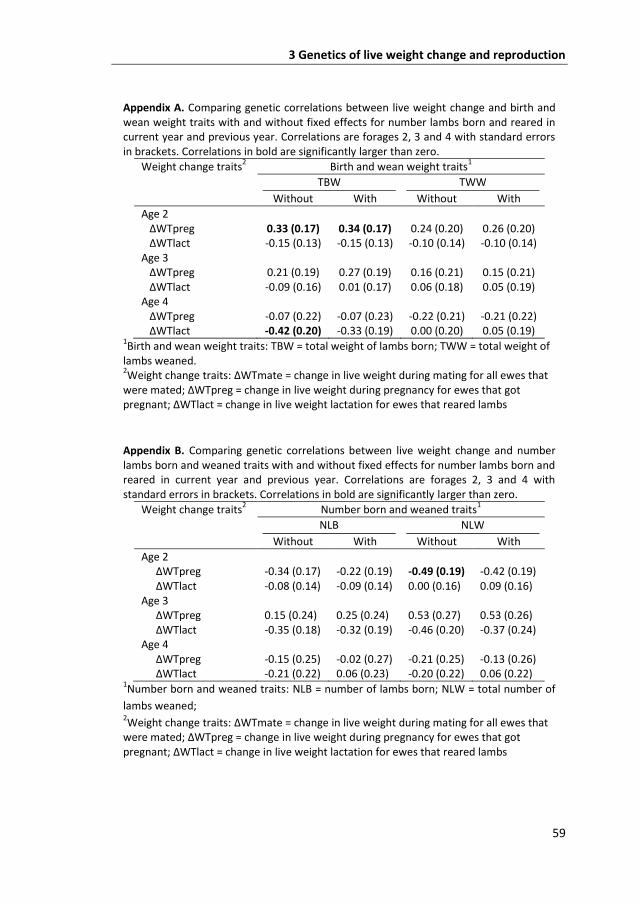
3 Genetics of live weight change and reproduction
59
Appendix A. Comparing genetic correlations between live weight change and birth and wean weight traits with and without fixed effects for number lambs born and reared in current year and previous year. Correlations are forages 2, 3 and 4 with standard errors in brackets. Correlations in bold are significantly larger than zero.
Weight change traits2 Birth and wean weight traits
1
TBW TWW
Without With Without With
Age 2 ΔWTpreg 0.33 (0.17) 0.34 (0.17) 0.24 (0.20) 0.26 (0.20) ΔWTlact -0.15 (0.13) -0.15 (0.13) -0.10 (0.14) -0.10 (0.14) Age 3 ΔWTpreg 0.21 (0.19) 0.27 (0.19) 0.16 (0.21) 0.15 (0.21) ΔWTlact -0.09 (0.16) 0.01 (0.17) 0.06 (0.18) 0.05 (0.19) Age 4 ΔWTpreg -0.07 (0.22) -0.07 (0.23) -0.22 (0.21) -0.21 (0.22) ΔWTlact -0.42 (0.20) -0.33 (0.19) 0.00 (0.20) 0.05 (0.19)
1Birth and wean weight traits: TBW = total weight of lambs born; TWW = total weight of
lambs weaned. 2Weight change traits: ΔWTmate change in live weight during mating for all ewes that were mated; ΔWTpreg change in live weight during pregnancy for ewes that got pregnant; ΔWTlact change in live weight lactation for ewes that reared lambs
Appendix B. Comparing genetic correlations between live weight change and number lambs born and weaned traits with and without fixed effects for number lambs born and reared in current year and previous year. Correlations are forages 2, 3 and 4 with standard errors in brackets. Correlations in bold are significantly larger than zero.
Weight change traits2 Number born and weaned traits
1
NLB NLW
Without With Without With
Age 2 ΔWTpreg -0.34 (0.17) -0.22 (0.19) -0.49 (0.19) -0.42 (0.19) ΔWTlact -0.08 (0.14) -0.09 (0.14) 0.00 (0.16) 0.09 (0.16)
Age 3 ΔWTpreg 0.15 (0.24) 0.25 (0.24) 0.53 (0.27) 0.53 (0.26) ΔWTlact -0.35 (0.18) -0.32 (0.19) -0.46 (0.20) -0.37 (0.24)
Age 4 ΔWTpreg -0.15 (0.25) -0.02 (0.27) -0.21 (0.25) -0.13 (0.26) ΔWTlact -0.21 (0.22) 0.06 (0.23) -0.20 (0.22) 0.06 (0.22)
1Number born and weaned traits: NLB = number of lambs born; NLW = total number of
lambs weaned; 2Weight change traits: ΔWTmate change in live weight during mating for all ewes that were mated; ΔWTpreg change in live weight during pregnancy for ewes that got pregnant; ΔWTlact change in live weight lactation for ewes that reared lambs


4 Varying pasture growth and commodity prices change the value of traits in sheep breeding
objectives
Gus Rose12
, Han A Mulder1, Andrew N Thompson
235, Julius H J van der Werf
24,
Johan AM van Arendonk1
1 Animal Breeding and Genomics Centre, Wageningen University, PO Box 338, 6700
AH, Wageningen, The Netherlands; 2 CRC for Sheep Industry Innovation, University
of New England, Armidale, NSW, 2351, Australia; 3 Department of Agriculture and
Food Western Australia, 3 Baron-Hay Court, South Perth, WA, 6151, Australia; 4
School of Environmental and Rural Science, University of New England, Armidale,
NSW, 2351, Australia; 5 School of Veterinary and Life Sciences, Murdoch University,
90 South Street, Murdoch, WA, 6150, Australia
Accepted to Agricultural Systems3
3 In this chapter alterations were made to the printed article changing the format of
headings and tables to make it consistent with the rest of the thesis.

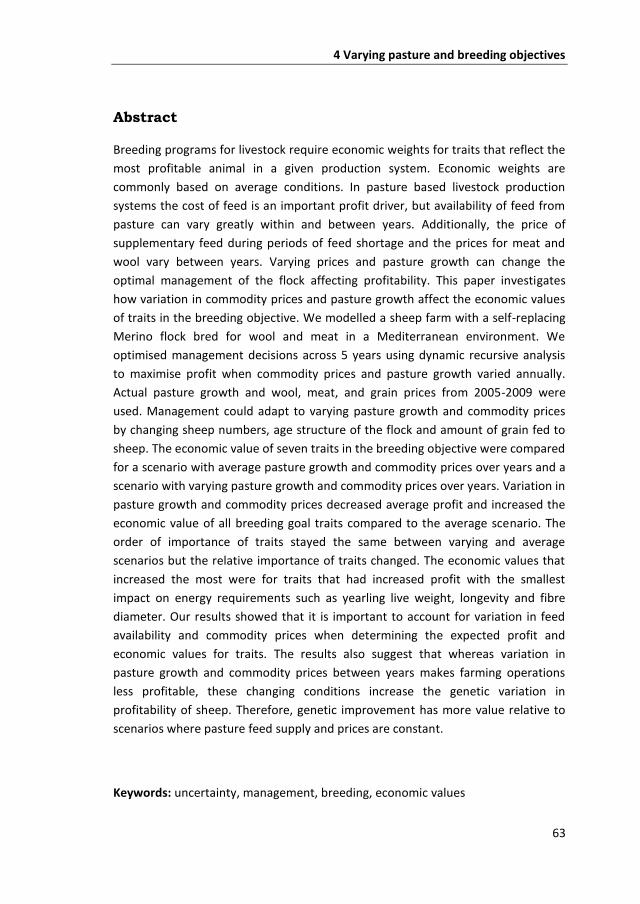
4 Varying pasture and breeding objectives
63
Abstract
Breeding programs for livestock require economic weights for traits that reflect the
most profitable animal in a given production system. Economic weights are
commonly based on average conditions. In pasture based livestock production
systems the cost of feed is an important profit driver, but availability of feed from
pasture can vary greatly within and between years. Additionally, the price of
supplementary feed during periods of feed shortage and the prices for meat and
wool vary between years. Varying prices and pasture growth can change the
optimal management of the flock affecting profitability. This paper investigates
how variation in commodity prices and pasture growth affect the economic values
of traits in the breeding objective. We modelled a sheep farm with a self-replacing
Merino flock bred for wool and meat in a Mediterranean environment. We
optimised management decisions across 5 years using dynamic recursive analysis
to maximise profit when commodity prices and pasture growth varied annually.
Actual pasture growth and wool, meat, and grain prices from 2005-2009 were
used. Management could adapt to varying pasture growth and commodity prices
by changing sheep numbers, age structure of the flock and amount of grain fed to
sheep. The economic value of seven traits in the breeding objective were compared
for a scenario with average pasture growth and commodity prices over years and a
scenario with varying pasture growth and commodity prices over years. Variation in
pasture growth and commodity prices decreased average profit and increased the
economic value of all breeding goal traits compared to the average scenario. The
order of importance of traits stayed the same between varying and average
scenarios but the relative importance of traits changed. The economic values that
increased the most were for traits that had increased profit with the smallest
impact on energy requirements such as yearling live weight, longevity and fibre
diameter. Our results showed that it is important to account for variation in feed
availability and commodity prices when determining the expected profit and
economic values for traits. The results also suggest that whereas variation in
pasture growth and commodity prices between years makes farming operations
less profitable, these changing conditions increase the genetic variation in
profitability of sheep. Therefore, genetic improvement has more value relative to
scenarios where pasture feed supply and prices are constant.
Keywords: uncertainty, management, breeding, economic values

4 Varying pasture and breeding objectives
64
4.1 Introduction
Breeding programs for livestock require clearly defined breeding objectives that
select the animals that are most profitable in a given production system. To
calculate the economic value of changing traits in animals, changes in optimal
management need to be accounted for before calculating the change in profit
(Groen, 1989; Amer, 1994). Economic weights used to optimise selection on
multiple traits can be derived from profit models of such systems and those models
are usually based on average conditions (Byrne et al., 2010; Conington et al. ,2004;
Wolfova et al., 2009). However, many livestock production systems have high levels
of variability in pasture growth and commodity prices across years. For example,
periods of drought in summer and autumn in Mediterranean climates require
farmers to feed grain, which is more expensive than feeding pasture (Purser, 1981,
p 181). Additionally, the length and severity of these drought periods varies
between years (Thompson et al., 1994; Kingwell, 2002; Kopke et al., 2008). Farmers
manage variation in pasture growth by altering the grain feeding and the number
of sheep managed from year to year (Saul and Kearney, 2002; Young et al., 2011b).
Despite the influence on varying prices and pasture growth, little attention has
been paid to how variation across years affects the importance of traits within
breeding objectives.
Changes in management depend largely on the energy requirements of the flock,
and since the energy requirements of sheep change when most traits in the
breeding objective are altered, uncertainty in pasture growth and prices may also
affect the economic value of traits in the breeding objective. These changes in
energy are not always at the same time of the year. For example, energy
requirements for reproduction peak around lambing time, whereas the energy
requirements for wool growth are distributed evenly across the whole year and
changing the diameter of wool fibres has no impact on energy requirements.
Therefore, the economic values of traits may respond differently to varying pasture
growth and commodity prices across years.
The effect of variation in commodity prices and pasture growth on breeding
objectives can be simulated in bio-economic models that optimise management to
adapt to such changes. Recursive dynamic models can be used to optimise farmer
decisions in response to variation in commodity prices and pasture growth
between years where the management of the current year depends on the optimal
management of previous years (Mosnier et al., 2009). Many models have
investigated the impact of pasture (Olson and Mikesell, 1988; Kingwell et al., 1993;
Jacquet and Pluvinage, 1997; Kobayashi et al., 2007) and price (Lambert, 1989;

4 Varying pasture and breeding objectives
65
Barbier and Bergeron, 1999; Lien and Hardaker, 2001; Ridier and Jacquet, 2002;
Mosnier et.al., 2009; Mosnier et.al., 2011) uncertainty, providing insights into
optimal management of farming systems under uncertainty. There are limited
studies, however, into how variability in pasture growth and commodity prices
across years affects the relative economic value of changing breeding goal traits.
In this study, we tested the hypothesis that accounting for the variation in pasture
growth and meat, wool and grain prices across years changes the relative economic
value of traits in the breeding goal. We also tested whether the change in profit
due to variation across years was affected by how much energy requirements
change when traits are changed.
4.2 Materials and methods
Testing the hypotheses that economic values of breeding goal traits are affected by
variation in prices and pasture growth across years required three steps:
1. Model – model a sheep farm that can optimise farm profit across years for
the purpose of calculating economic values for sheep.
2. Scenarios – define scenarios for different pasture growth and prices across
years.
3. Economic values – calculate the economic values for each pasture growth
and price scenario for individual years and across years. We calculated
economic values for seven breeding goal traits: weaning weight, yearling
weight, fleece weight, fibre diameter, longevity, and number of lambs
weaned.
Model description
We modelled monthly production decisions for a sheep farm in an environment
which experiences significant variation in pasture growth and wool, meat, and grain
prices between years. The modelled farm had a self-replacing Merino sheep flock
bred for wool and meat. The parameters of the farm and sheep represent a typical
sheep enterprise in South Western Australia with one lambing per year in July and
lambs weaned at 3 months old. There was no allowance for buying and selling of
livestock additional to those bred on the farm. We based pasture growth on the
Katanning region (33°41´S, 117°35´E, elevation 310m). Katanning is located in a
Mediterranean climatic region with hot dry summers and mild wet winters. This
combination of temperature and rainfall means that there is a period of no pasture
growth during summer and autumn, typically extending from ovember to May
each year.

4 Varying pasture and breeding objectives
66
Profit from wool and sheep sales was maximised for the sheep farm per hectare
(ha) by optimising sheep sales and grain feeding based on pasture availability and
prices of grain, wool and meat. We maximised profit per ha because pasture growth
(pgr) per ha affects how many sheep can be managed on the farm and the number
of sheep managed mostly determines farm profit (Warn et al., 006; Young et al.,
011b). Therefore, we optimised management of sheep sales and grain feeding per
ha using the eneral Algebraic Modelling System with the linear programming
solver BDM P (Brooke, Drud, and Meeraus linear program) Brooke et al., ( 013).
The optimisation included five groups of e uations, profit (objective function), flock
structure, pasture, energy re uirements and intake. Profit depended on the
number of sheep (via wool sales and variable costs), sheep sold and grain intake.
The amount of pasture available affected how much pasture could be eaten by
sheep which also affected how much was available in the next period. The number
of sheep depended on energy re uirements, potential intake, and the number of
sheep sold. The amount of pasture and grain eaten was constrained by the
potential intake of the sheep, whilst pasture and grain eaten had to match the
energy re uirements of the sheep. Figure 4.1 shows that all the relevant
interactions between price, pasture growth, flock structure, energy re uirements
and intake were in the model, and how the variables and parameters interacted in
the optimisation of profit.
The model optimised profit for five years using dynamic recursive programming to
simulate the sequential decision-making of farmers based on changes in prices and
pasture growth from year to year. The first year had the current prices and pasture
growth whilst years 2-5 used average prices and pasture growth. This simulates a
farm where decisions have to be made in the current year without knowledge of
pasture growth or prices in the following years. Average pasture growth and prices
are used as the best source of information to make decision in the current year,
considering the long term profit of the farm. The profit from the first year was
recorded and the optimised values from the first year used as the starting point for
the next analysis, with new prices or pasture growth values for the first year of
analysis. We used prices and pasture growth from years 2005-2009. The starting
points for variables in the first optimisation step for 2005 were taken from the
equilibrium from average prices and pasture growth. The optimised variables from
the first analysis of 2005 was used as starting values for the first month of the first
year to optimise management for 2006, again assuming the following four years
had average prices and pasture growth. This was done until all years up until 2009
were optimised. Predictions for each year were optimal for the five year planning
horizon and different to optimising years 2005-2009 together. This is because the

4 Varying pasture and breeding objectives
67
modelled farmer could adjust management based on anticipated sudden changes
in prices and pasture growth across the 5 years.
It was assumed that ewes were kept up to an age of 78 months and litter size varied
between 0 and lambs. This resulted in 79 categories for age-months (a =
{0,1, ,3…,78}), 3 categories for litter size at birth (b {0,1, }), and litter size at
weaning (r = {0,1,2}), and two categories for sex (s = {wether (castrated male) or
ewe (female)}). Ewes were first mated at 20 months old. There were 6 categories
for litter size at birth and litter size at weaning: 0 born and 0 weaned, 1 and 0, 1
and 1, 2 and 0, 2 and 1, and 2 and 2. In total there were 78 (age) x 2 (sex) x 6 (litter
size at birth and weaning) = 936 categories of sheep. Energy requirements and
potential intake were calculated for the 936 categories, whilst grain and pasture
intake, and sheep numbers were optimised for the 936 categories.
The parameters, variables and optimisation equations for prices and pasture were
for years (y {1, ,3,4,5}) and months (m {1, ,3,…,1 }). There were two types of
pasture (p = {green, dry}). All parameters and variables were calculated for monthly
periods. Parameters that varied within a month, such as foetus growth and milk
production, were estimated daily and averaged over each month. Lupins and oats
could be used as supplements in any month. These monthly categories were linked
to the sheep age categories based on the age of each sheep in each month of the
year, with lambs born in July.
Figure 4.1 interactions between parameters (white boxes) and variables (grey boxes) and how they affect profit (black box).

4 Varying pasture and breeding objectives
68
Profit equation. The production system was optimised by maximising the net
present value of profit over a five year period to simulate a farmer’s long term
decision horizon. The profit was the gross margin for each year ( OSSMA I y)
summed across the five years and discounted at 4% per year (Lence 2000). The
gross margin was the income minus variable costs. To terminate the five years (y =
5 and m = 12) and ensure that all the sheep were not sold, we included the value of
selling sheep for meat in the final month (E D A ), discounted for five years (disc =
discount rate). This allowed the five year period to be evaluated assuming that the
farmer will continue farming after 5 years.
P OFIT ∑ ((1 disc)y 1 x OSSMA I y
Y
y0
) (1 disc)Y x E D A
The gross margin in each year was income from meat and wool sales minus variable
and grain costs. Meat sales were the product of number of sheep sold, live weight,
price per kg carcass and carcass dressing percentage. Sheep sales were split into
mutton (over 20 months old) and hoggets (less than 20 months old) with different
prices for both classes. We assumed the minimum carcass weight that sheep can
be sold was 16kg. Wool income was the product of number of sheep in November
(shearing month), wool weight, and wool price minus shearing costs. Variable costs
were the product of sheep number and variable costs per sheep. Variable costs
included crutching, drenching, pregnancy scanning, fly control, and marking lambs
including all additional labour associated with these activities (DAFWA 2005). Grain
costs were a product of grain intake and grain prices. We assumed that labour costs
for the farmer were constant and we did not consider fixed costs. We did not
include costs for labour despite the high labour requirements for grain feeding
sheep (Rose et al., 2009) and assumed that farmers work longer hours in periods
that require more grain feeding. Live weights, wool information and variable costs
are in Additional Files 4.A and 4.B. The profit equation therefore included all the
relevant incomes and costs to calculate the impact of varying prices and pasture
growth on profit.
Flock equations. The flock equations were recursive functions that calculated the
number of sheep based on deaths and sales. Number of sheep in each category for
age, sex, birth and rear category ( S EEP a,s,b,r) for each month m of year y
depended on the number of sheep ( S EEPa -1,s,b,r , survival (surva -1,s,b,r), and
sheep sold (SA ESa -1,s,b,r) one month earlier.
S EEPa,s,b,r S EEPa 1,s,b,rx surva 1,s,b,r SA ESa 1,s,b,r

4 Varying pasture and breeding objectives
69
We assumed that sheep died and were sold on the last day of the month. Survival
was calculated for each age assuming that ewes had the same probability of
surviving in each month. Survival rates are in Additional files 4.A, Table A4.4.
The number of lambs born in each sex and litter size at birth category was e ual to
the number of mated ewes in each birth category in July multiplied by the number
of lambs in each category. The number of lambs weaned in each sex, litter size at
birth and litter size at weaning was the number of mated ewes in each litter and
birth category in October (weaning month) multiplied by the number of lambs in
each category. The proportion of ewes in each litter size at birth and litter size at
weaning category was deducted from Figure A4.3 in the additional files, with the
proportion of ewes with 0, 1 and lambs changing as the average number of lambs
weaned changed. The birth and rear categories for a ewe in different years were
assumed independent. ew categories were made for each year.
Starting values for sheep numbers for m = 1 and y = 1 were taken from the
equilibrium of optimal production for a year with average prices and pasture
growth. This equilibrium was calculated by cycling through the flock function for
one year. These starting numbers simulated a farmer that has had a series of
average years and has adjusted stocking rate ready for another average year.
We constrained the model to sell all sheep before they reached 78 months old.
Pregnant and lactating ewes could not be sold during pregnancy and lactation,
from February to September. Non pregnant ewes could be sold in April after
pregnancy scanning. This is a common practice for farmers that want to reduce
stock numbers, particularly in years with low pasture growth. Ewe numbers could
increase or decrease by adjusting the number of sheep sold either through culling
of hogget ewes before first mating, selling of ewes during the year and selling ewes
after their 5th
parity. Changing the number of ewes sold affected the number of
lambs born which subsequently affected the number of ewes that could be
selected for the first mating two years later. So the cycling of sheep numbers made
the flock structure dynamic through selling or retaining sheep for future years.
Sheep characteristics. The sheep were medium fibre diameter Merinos bred for
wool and meat. A detailed description of the sheep is in Appendix A. The sheep had
a mature body weight of 50kg. The weights of sheep from birth till 20 months of
age depended on the sex and birth and rear category. Wethers grew faster than
ewes, whilst lambs born into a higher litter size initially had lower growth rate until
12 months of age. Live weights were assumed the same by 20 months of age
independent on litter size based on Thompson et al. (2011). Live weights of sheep
above 20 months of age were assumed to be managed the same regardless of how

4 Varying pasture and breeding objectives
70
many lambs the ewes gave birth to or reared. These weights were based on Young
et al., (2011b). Average fibre diameter across all ages was 20.9 and average clean
fleece weight was 3.35 kg. The diameter of wool increased with age and the weight
of wool increased until 5 years old and then decreased as the ewes got older
(Cloete et al., 2003). The average number of lambs weaned per ewe mated across
all age groups was 0.87. With increasing age of ewes, litter size increased with a
maximum at their fourth mating and decreased thereafter (Cloete et al., 2003).
Mortality of ewes decreased with age until 5 years of age and then increased in the
oldest age groups (Turner and Young, 1969). The characteristics of sheep at each
age has implications for the optimum flock structure, with older ewes weaning
more lambs and growing more wool but the diameter of the wool increases.
Therefore, changes in the structure of flock age changed the income from the total
flock.
Pasture equations. The pasture equations were recursive functions that calculated
the amount of green and dry (p) pasture (PAST Ey, m, p) in each month (m) of each
year (y) based on proportion of pasture decay (decayy,m-1,p), growth (pgry,m,p),
intake (PAST EI Ty,m,g) and proportion of trampling (trampley,m,p).
PAST Ey, m, p
PAST Ey,m 1,px (1 decayy,m 1,p) 30.4(pgry,m,p PAST EI Ty,m,g(1 trampley,m,p)
The pasture intake variable for each sheep class was assigned to a month based on
the age of each sheep in each class. For example, ages of sheep in the lambing
month July were am=7 = {0, 12, 24, 36, 48, 60, 72}. The pasture intake is the total
intake for all sheep in each class. We fixed green pasture to 0 kg DM/ha in months
when pasture did not grow (pgr = 0) and dry pasture to 0 kg DM/ha when pasture
grew (pgr > 0) except for the first month of pasture growth. Additionally, in months
when no pasture grew we fixed dry pasture greater or equal to 700 kgDM/ha. This
lower limit prevented pasture being grazed too low which causes soil erosion
(Moore et al. 2009). The assumptions for pasture are in Additional files 4.C.
Therefore the pasture equations included the interactions between pasture intake
and pasture available that could be used to optimise the number of sheep
managed on the farm.
Energy equations. Energy equations made sure sheep from each age, sex, litter size
at birth and litter size at weaning category consumed at least the energy they
required. Energy was required for maintenance (main), live weight gain (growth),
wool growth (wool), pregnancy (preg), and lactation (lact), whilst energy was

4 Varying pasture and breeding objectives
71
available for other functions from losing live weight (loss) (e = {main, growth, wool,
preg, lact, loss}; e=main+growth+wool+preg+lact-loss). Live weight loss and gain
were the difference between live weight in the following month and the current
month. We assumed sheep gained or lost the same amount of weight on each day
of the month, i.e. linear growth. The net energy required from pasture and grain
was the total energy required (equations in Additional files 4.D) minus the energy
available from losing live weight. All energy equations were from Freer et al. (1997)
and Freer et al. (2007).
Sheep convert metabolisable energy into net energy with different efficiencies
(equations in Additional files 4.E) depending on quality of the diet. Lupins and oats
had higher digestibility than pasture, so the efficiency of using metabolisable
energy from lupins and oats was higher. Therefore, we split the energy equation
into two sets of equations. The first set of equations constrained the net energy
provided by pasture ( EPAST Ep) and grain ( E AI g) for each sex (s), age (a),
birth (b) and rear (r) category and each energy type (e) to be more than the net
energy (ne) minus net energy available from weight loss (nee-loss).
S EEPs,a,b,r (∑ nee,s,a,b,r nee loss,s,a,b,r)
e
∑ ( EPAST Ep,e,s,a,b,r E AI g,e,s,a,b,r)
e
We included number of sheep in this equation to calculate the total metabolisable
energy eaten by all sheep in that class. The second set of energy equations
calculated the optimum amount of pasture and grain that had to be eaten to match
the metabolisable energy requirements. There were two equations for this step,
one for pasture and one for grain.
mepasturep PAST EI Tp,s,a,b,r EPAST Ee,p,s,a,b,r
kpe,p
megraing AI I Tg,s,a,b,r E AI e,g,s,a,b,r
kge,g
here mepasturep is the metabolisable energy available in pasture (MJ/kg),
kpe,g was the efficiency of transferring net energy into metabolisable energy for
each pasture type,
megraing is the metabolisable energy available in grain (MJ/kg),
kge,g was the efficiency of transferring net energy into metabolisable energy for
each grain type and
AI I Tg,s,a,b,r is the grain intake by each sex, age, birth and rear type.
These energy equations had an important link with the pasture equation through
pasture intake. The equations also optimised grain feeding depending on energy
requirements how much pasture can be eaten. Splitting the energy equation into

4 Varying pasture and breeding objectives
72
pasture and grain meant that the efficiency of transferring net energy into
metabolisable energy for grain and pasture could be correctly allocated to the
relevant intake type.
Intake equations. Sheep in each age, sex, litter size at birth and litter size at
weaning had a maximum daily intake. This maximum had to be equal or less than
total pasture and grain intake of each sheep. The digestibility and amount of
pasture affected the maximum intake because poor quality pasture took longer to
digest and low amounts of pasture were harder to graze. Therefore, the intake
equation included parameters maximum intake (maxint), limit in intake due to
digestibility (limdm) and limit in intake due to amount of pasture (limpasture) and
variables pasture intake (PAST EI T), grain intake ( AI I T) and number of
sheep ( S EEP). We included number of sheep to sum the total requirements of
sheep in each category. PAST EI Ts,a,b,rlimdm limpasture
AI I Ts,a,b,r maxints,a,b,r S EEPs,a,b,r
The limit in pasture intake due to digestibility and amount of pasture was different
for green and dry pasture. The parameter depended on the variable
PAST E. In linear programming it is not possible to divide a variable (PAST EI T)
by another variable (PAST E), which would require non-linear programming.
Therefore, we calculated limpasture by estimating amount of pasture without the
variables PAST EI T and S EEP, as if no pasture was eaten. Equations for intake
are in Additional files 4.F.
Scenarios
We optimised profit for two scenarios: average pasture growth and average prices
and varying pasture growth and varying prices. These pasture growth and prices
were from 2005-2009 (Figure 4.2). We selected these years because they had
typical pasture growth and prices. Pasture growth was very high in 2005 and very
low in 2006, grain prices were low in 2005 and high in 2007 and 2008, wool prices
were low in 2005 and high in 2007, and meat prices were very high in 2009.
Average pasture growth and prices were monthly averages across the five years and
are at the right of Figure 4. . We included monthly averages to keep the seasonality
of pasture growth and prices. We fixed wool prices to the prices of wool in
ovember, when the sheep were shorn.
Pasture growth was estimated from “Pastures from Space” ( ill et al., 1999)
recorded at Katanning Western Australia (www.pasturesfromspace.csiro.au). Wool
prices were taken from the Western region micron price guide from the Wool Desk,

4 Varying pasture and breeding objectives
73
Department of Agriculture and Food WA and Australian Wool Exchange (DAFWA,
009). Meat prices were hogget and mutton prices from Meat and ivestock
Australia’s ational ivestock eporting Service (M A, 009). rain prices were
based on Co-operative Bulk andling (CB , 009).
Figure 4.2 Prices for wool, meat and grain, and pasture growth for the 5 years used. The
average is the average price for the total period and the average pasture is the average
for each month.

4 Varying pasture and breeding objectives
74
Economic values
Breeding programs aim to increase profit per animal by genetic improvement of
traits that affect profit. Therefore, running a breeding program starts with
specifying the traits affecting profit and quantifying the economic values for each
trait, i.e. the change in profit when the trait is genetically improved by one unit
keeping all other traits constant. All other traits are kept constant to avoid double
counting the value of changing traits when the economic values are used in a
breeding index. Mathematically, the breeding goal can be represented as a linear
equation in which breeding values for each trait are multiplied with economic
values (Hazel, 1943). We calculated the economic value for 7 traits: weaning live
weight, yearling live weight, adult live weight, adult fleece weight, adult fibre
diameter, adult longevity, and number of lambs weaned (Table 4.1). We chose
these traits because they are used in various industry indexes in Australia.
We calculated economic values by increasing each trait by one genetic standard
deviation (Table 4.1) because a genetic standard deviation is a measure of how
easy it is to select for each trait and makes economic values more comparable
between traits. For adult live weight we increased all live weights and the standard
reference weight of sheep above 20 months. A change in weaning or yearling live
weight implied an alteration of the growth curve from birth to 20 months of age
depending on the age of the live weight measurement (Additional files 4.A, Figure
A4.2). The economic value of longevity was estimated by altering the probability of
surviving each year (surv). For example, changing the survival from age 20 months
to 70 months from 0.85 to 0.90 is equivalent to adding an extra 115 productive
days. The economic value for longevity was then calculated by multiplying the
associated change in profit by a factor 304/115, where 304 is the value (in days) of
one genetic standard deviation for longevity. This procedure is similar to Fuerst-
Waltl and Baumung (2009). The economic value for fibre diameter is the value of
decreasing the diameter of wool. We decreased fibre diameter because finer wool
is more profitable than broad wool. The value of increasing number of lambs
weaned was calculated from the change in proportion of ewes with 0, 1, and 2
lambs born and weaned. We calculated economic values per ha and expressed
them as economic values per ewe. We calculated the economic values per ha
because the farm area is the main limitation of production. We presented the
economic values per sheep ($AU/genetic standard deviation) because in selection
index theory, it is easier to interpret the economic values as the extra value
obtained per ewe mating.

4 Varying pasture and breeding objectives
75
Economic values were calculated by maximising profit after traits were increased by
one genetic standard deviation (Table 4.1) and subtracting the maximised profit
using mean trait values. The economic value per ha was the profit optimised with
the average genotype subtracted from the re-optimised profit after changing the
trait. We then divided the economic value per ha by the number of ewes mated to
calculate the economic value per sheep. We also calculated the economic value for
each trait relative to the economic value of number of lambs weaned. This indicates
the relative importance of each trait.
With changes in trait mean due to genetic change, the optimal management
changes for the scenario with average prices and pasture growth. Therefore we
calculated new e uilibrium values for the number of sheep and pasture with
average prices and pasture growth after each trait was changed. These e uilibrium
values were used as the starting values for y 1 and m 1 when analysed with prices
and pasture growth varying.
Table 4.1 Definition of traits with genetic standard deviations ( g and the equations
each trait affects.
Variable Unit g Flock Energy Intake
weaning weight kg 3.6
1
yearling weight kg 3.41
adult live weight kg 3.561
fleece weight kg 0.361
fibre diameter μm 0.951
longevity days 3043,4
lambs weaned lambs 0.124
2
1Huisman et al. (2008)
2Cloete et al. (2004)
3Fuerst-Waltl and Baumung (2009)
4changing reducing death% by 1% in adult ewes was equivalent to 115 extra days of
productive life. Therefore, the economic values for longevity were scaled by 304/115

4 Varying pasture and breeding objectives
76
Tab
le 4
.2 V
aria
ble
s gr
een
an
d d
ry p
astu
re, l
up
ins
and
oat
s fe
d a
nd
nu
mb
er o
f w
eth
er a
nd
ew
e sh
eep
fro
m a
vera
ge p
astu
re g
row
th,
pri
ces
an
d
gen
oty
pe.
To
tals
are
bo
ld.
Var
iab
le
Jan
Fe
b
Mar
A
pr
May
Ju
n
Jul
Au
g Se
p
Oct
N
ov
Dec
pas
ture
(kg
DM
/ha)
Gre
en
-
- -
30
6
38
4
29
6
29
6
53
4
11
08
1
49
0
10
47
-
Dry
9
04
7
95
7
00
-
- -
- -
- -
- 1
02
7
gr
ain
(kg
/mo
nth
)
lup
ins
1
45
5
5
73
5
0
3
0
0
0
1
0
1
13
2
oat
s
18
0
0
0
0
0
0
0
0
0
14
to
tal
16
3
55
7
3
5
0
30
0
0
1
0
1
1
46
nu
mb
er
for
each
age
cla
ss in
mo
nth
s fo
r ew
es (
ewe
s/h
a)
0
-5
- -
- -
- -
3.0
0
3.0
0
2.4
2
2.4
2
2.4
2
.38
6
-17
2
.37
2
.35
2
.33
2
.31
2
.29
1
.26
1
.25
1
.25
1
.24
1
.24
1
.23
1
.23
1
8-2
9
1.2
2
1.2
1
1.2
1
1.2
1
.2
1.1
9
1.1
9
1.1
9
1.1
8
1.1
8
1.1
7
1.1
7
30
-41
1
.17
1
.16
1
.16
1
.16
1
.15
1
.15
1
.15
1
.14
1
.14
1
.14
1
.13
1
.13
4
2-5
3
1.1
3
1.1
2
1.1
2
1.1
2
1.1
2
1.1
1
1.1
1
1.1
1
1.1
1
.1
1.1
1
.1
54
-65
1
.1
1.0
9
1.0
9
1.0
9
1.0
9
1.0
8
1.0
8
1.0
8
1.0
8
1.0
7
1.0
7
1.0
7
66
-77
1
.07
1
.06
1
.06
1
.06
1
.06
1
.05
1
.05
0
.9
0.9
0
.89
0
.89
0
nu
mb
er
for
each
age
cla
ss (
wet
her
s/h
a)
1-6
-
- -
- -
- 3
3
2
.42
2
.42
2
.4
2.3
8
7-1
8
2.3
7
2.3
5
2.3
3
2.3
1
2.2
9
2.2
8
1.0
9
0.9
2
0
0
0
0
to
tal1
1
0.4
3
10
.34
1
0.3
1
0.2
5
10
.2
9.1
2
13
.92
1
3.5
9
11
.48
1
1.4
6
11
.39
1
0.4
6
1 tota
l fo
r w
eth
ers
and
ew
es

4 Varying pasture and breeding objectives
77
4.3 Results
Average scenario
For the average scenario with no fluctuations in prices or pasture growth across
years, pasture started growing in April and peaked in October at 1407 kg DM/ha
(Table 4.2). After the pasture dried off in December, the amount of pasture
decreased until April and the amount of grain fed was highest during these months.
Almost no grain was fed from July to October.
The number of sheep was highest in July when the lambs were born. The drop in
sheep numbers in the 0-5 month old category from August to September was from
lamb deaths between birth and weaning. The drop in ewes in the 6-17 month old
category from May to June was from culling hogget ewes. The drop in ewes in the
66-77 month old category was from selling ewes that did not give birth to any
lambs. All ewes were sold by 76 months old. Most of the wether hoggets were sold
at the end of May when they were 11 months old with the remainder sold when
they were 14 months old in August. These hoggets were sold in August because
they were born and reared in a litter size of 2 and grew slower.
Comparing average scenario to varying pasture and price
Varying pasture growth and prices decreased the average profit from 2005-2009 by
12% compared to the average scenario (Table 4.3). Profit decreased because grain
costs increased by 40% compared to the average scenario. This increase in grain
feeding was partly attributed to an 11% increase in ewes mated. This increase in
ewes mated increased hogget income by 9%, mutton income by 16% and wool
income by 10% compared to the average scenario, but this was not enough to
offset the higher grain costs. The decrease in average profit across the five years
was due mostly to large decreases in profit in 2005, 2006, and 2008, which were
not offset by the large increase in profit in 2009.
In 2005 profit decreased by 26% compared to the average scenario because of low
wool prices and low grain prices. Additionally, high mutton prices meant no ewe
hoggets were sold in 2005 because it was optimal to sell 5 year old ewes and retain
extra hogget ewes to be mated in 2006. More ewes were mated in 2006 because
high pasture growth reduced grain requirements for managing a high number of
ewes into 2006, which was anticipated to be an average year. The increase in ewes
mated in 2006, in combination with low pasture growth and high grain prices at the
end of 2006, decreased profit by 70% compared to the average scenario.
Additionally the number of ewes mated in 2007 decreased because high grain
prices and low pasture growth towards the end of the year made it unprofitable to

4 Varying pasture and breeding objectives
78
carry high ewe numbers into 2007. Carrying over more ewes from 2005 to 2006 in
anticipation of an average year was the main cause of the profit decrease in 2006
and made the farm vulnerable to a poor year like 2006, where pasture growth was
low and grain prices were high. High wool prices in 2007 offset the low pasture
growth at the end of 2007 and profit increased by 2% compared to the average
scenario. High pasture growth and high wool prices meant it was optimal to
increase the number of ewes mated in 2008 because it was cheap to maintain the
ewes and shear them at the end of 2007. High grain prices, lower than average
pasture growth and more ewes mated in 2008 decreased profit by 33% compared
to the average scenario. In response to these high grain prices and high meat prices
at the end of 2008 more adult ewes were sold decreasing the number of ewes
mated in 2009. High meat prices in 2009, high pasture growth at the end of 2009
and an increase in lambs born in 2008 increased profit by 69% in 2009 compared to
the average scenario.
In summary, profit was lower with varying prices and pasture growth mainly due to
changes in management in reaction to changes in pasture growth and prices. These
changes in management, in particular, changing the number of ewes mated, made
farm profit vulnerable to unfavourable changes in pasture growth and commodity
prices. Additionally, positive deviations of prices and pasture growth did not
compensate the impacts of their negative variations.
Comparing economic values between average and varying scenarios
The economic value for lambs weaned had the highest economic value per head
per genetic standard deviation for both average and varying scenarios (Table 4.4).
The order of importance of the other traits was fleece weight, fibre diameter,
longevity, yearling weight, weaning weight and adult weight. This order did not
change between the average and varying scenarios. Additionally, the economic
values were all higher per mated ewe for the varying scenario compared to the
average scenario. Although the order of importance of traits did not change, the
relative contribution of each trait changed. Yearling weight increased the most
when pasture growth and commodity prices were varied, followed by longevity,
fibre diameter, lambs weaned and fleece weight. Weaning weight increased from a
small negative to a small positive economic value whereas adult live weight
became slightly less negative.

4 Varying pasture and breeding objectives
79
Table 4.3 Profit, ewes mated, sheep sales, age of ewes (months), lambs weaned, hogget, mutton, and wool income and grain costs for 2005-2010 for average, varying prices and varying pasture scenarios.
Variable Scenario Year Mean
2005 2006 2007 2008 2009
profit ($AU/ha) Average 184 184 184 184 184 184 Varying 136 55.9 188 123 311 162 ewes mated (ewes/ha) Average 5.27 5.27 5.27 5.27 5.27 5.27 Varying 5.27 6.18 5.71 6.34 5.72 5.84 ewe hoggets sold /ha Average 0.95 0.95 0.95 0.95 0.95 0.95 Varying 0.00 1.06 0.74 1.17 1.49 0.89 wether hoggets sold /ha Average 2.10 2.10 2.10 2.10 2.10 2.10 Varying 2.10 2.10 2.38 2.27 2.52 2.23 adult ewes sold /ha Average 0.97 0.97 0.97 0.97 0.97 0.97 Varying 1.06 1.30 0.79 1.51 0.94 1.12 average age of ewes Average 32.2 32.2 32.2 32.2 32.2 32.2 Varying 31.2 29.4 30.4 29.9 31.7 30.5 hogget income ($AU/ha) Average 151 151 151 151 151 151 Varying 99 136 147 188 254 164 mutton income ($AU/ha) Average 23.7 23.7 23.7 23.7 23.7 23.7 Varying 25.6 32.8 16.8 36.5 25.3 27.4 wool income ($AU/ha) Average 201 201 201 201 201 201 Varying 151 210 310 182 254 221 grain costs ($AU/ha) Average 136 136 136 136 136 136 Varying 85 262 224 220 160 190

4 Varying pasture and breeding objectives
80
The economic values were higher when prices and pastures varied because
optimisation caused changes of trait means to have more effect on profit when
prices varied. This resulted in higher economic values for the varying scenario than
the average scenario, even though the profit per ha was lower (Appendix A). When
prices and pasture growth were average, it was optimal to manage high stocking
rates because there was no consequence in following years. Therefore, the number
of ewes mated increased more for each trait for the average scenario compared to
the varying scenario. For the varying scenario, stocking rate was re-optimised each
year based on the new pasture growth and prices. These adjustments could either
capitalise on favourable prices or avoid high costs (see Appendix B). That is why the
grain costs increased more for the average scenario when traits changed compared
to the varying scenario. Therefore, it can be concluded that varying prices and
pasture growth changed economic values substantially.
The economic value of traits was different between the average and varying
scenario depending on how much each trait changed the energy requirements of
the sheep. For example, increasing the productive life of ewes did not increase the
energy requirements but changed the flock structure which increased the number
of lambs weaned, the number of ewes shorn and the number of ewes sold at the
end of their productive life. Decreasing fibre diameter improved the quality of wool
without requiring extra energy. Increasing the number of lambs weaned increased
the energy requirements of ewes, but it was optimal to manage fewer ewes,
decreasing maintenance costs and increasing hogget income. Alternatively,
increasing clean fleece weight and adult live weight increased energy costs for the
whole year, making the farm relatively more vulnerable to variation in pasture
growth compared to other traits, which meant its economic value did not increase
as much as other traits. Weaning weight increased energy requirements for a short
period only on a small proportion of the flock so it did not decrease profit as much
as adult live weight. Increasing weaning weight did not coincide with sale time and
had a low not impact on hogget income. The increase in live weight for yearling live
weight is expressed as increased income from selling heavier hoggets. Yearling live
weight had the biggest increase in value when pasture growth and commodity
prices varied because more income from selling hoggets was not offset by the
increase in energy requirements, which increased on a relative small proportion of
the flock.

4 Varying pasture and breeding objectives
81
4.4 Discussion
The economic values of wool, carcass and reproduction traits in the breeding
objective of a self-replacing Merino flock increased when commodity prices and
pasture growth varied between years. The relative importance of each trait also
changed, with longevity and yearling weight becoming more important when
commodity prices and pasture growth varied. These changes in traits were caused
by differences in management between average scenarios and scenarios where
pasture growth and prices varied. When pasture growth and prices varied, profit
decreased compared to the average scenario because optimum management of
the flock in previous years was not optimal when new prices and pasture growth
were introduced. This decrease in profit between the average and varying scenario
created more potential to improve profit when traits changed. Additionally, when
prices and pasture growth favoured a particular trait, management could be
Table 4.4 Comparing economic values ($AU per ewe mated per genetic standard deviation), economic values relative to number of lambs weaned, and ewes mated for each trait for the average and varying scenario.
Variable Trait Mean Varying Change
Economic value Lambs weaned 2.61 4.84 2.23 Fleece weight 2.33 3.59 1.26 Fibre diameter 1.77 3.46 1.69 Longevity 1.06 3.11 2.04 Yearling weight 0.59 1.86 1.28 Weaning weight -0.01 0.1 0.11 Adult weight -0.35 -0.25 0.11 Economic value relative Lambs weaned 1 1 0 to lambs weaned Fleece weight 0.89 0.74 -0.15 Fibre diameter 0.68 0.71 0.04 Longevity 0.41 0.64 0.23 Yearling weight 0.23 0.39 0.16 Weaning weight 0 0.02 0.03 Adult weight -0.14 -0.05 0.08 Ewes mated/ha Lambs weaned 5.36 5.37 0.01 Fleece weight 5.59 6.08 0.49 Fibre diameter 5.66 6.07 0.41 Longevity 5.64 6.05 0.41 Yearling weight 5.44 5.9 0.46 Weaning weight 5.3 5.88 0.58 Adult weight 5.1 5.66 0.56

4 Varying pasture and breeding objectives
82
optimised in that year. Therefore, we accepted our hypothesis that accounting for
uncertainty in pasture growth and commodity prices across years changes the
economic value of breeding goal traits.
Our model is, to our knowledge, the first analysis of the effects of fluctuations in
prices and feed availability on the economic values of breeding goal traits. We
showed how breeding goals should be adapted to a production system with
uncertain pasture growth and prices. For example, breeding goals for wool should
aim less at production volume, such as fleece weight, but more on quality traits,
such as fibre diameter. This is an important result because previous breeding
programs have put high emphasis on fleece weight (Taylor and Atkins, 1997) and
our results suggest that fleece weight has less importance.
The estimation of economic values using dynamic programming to optimise
management across years when future pasture growth and prices are unknown
captured the effects of pasture and price uncertainty. Optimising management in
each year meant that management could be adapted based on current pasture
growth and prices. This had both advantages and disadvantages for the economic
value of traits. For example, when wool price was high, more ewes could be carried
over to the next year to increase the amount of wool sold. This management
option, however, was disadvantageous when pasture growth or wool price was
low, or grain prices were high, in the following year, particularly if energy
requirements increased when traits changed. Therefore, traits that caused bigger
changes in management in favourable years, in particular, increasing sheep
numbers, made the farming system more vulnerable to variation in pasture growth
and prices. This vulnerability was further increased when changing traits increased
energy requirements. Therefore, it is important to account for variation across
years when calculating economic values for breeding goal traits.
We used historic pasture growth and prices similar to Kulak et al. (2003) which
indicate variation in those specific years. Animal breeding should anticipate future
prices and pasture growth which is difficult, although the mean and variation of
historic pasture growth and prices give a good guideline for which parameters vary
the most. Annual pasture growth and the distribution of pasture growth across the
year are expected to become more variable and harder to predict due to changes
in the climate (IPCC, 2007). Future research could include more variation in pasture
growth to investigate how economic values are affected by extreme variation in
pasture growth across years.
It was optimal to manage more ewes when prices and pasture varied compared to
the average scenario. Australian farmers generally reduce sheep numbers to avoid
having too many sheep in years with low pasture growth or low prices (Austen et

4 Varying pasture and breeding objectives
83
al., 2002; Robertson and Wimalasuriya, 2004). Many studies have shown that
climate variability decreases the number of livestock managed per unit of land
(Olson and Mikesell, 1988; Kingwell et al., 1993; Kobayashi et al., 2007). Kobayashi
et al. (2007) found that several drought years are required to significantly reduce
stocking rate. We used average pasture growth as the estimate of future pasture
growth, whilst most years pasture growth was below average. Therefore,
maintaining or increase sheep numbers in years with high pasture growth was not
optimal when the following year had below average pasture growth. The actual
optimal number of sheep across all years may be lower than estimated in our
study. If we had optimised sheep numbers across all years of pasture growth, then
the traits that made the farming system more vulnerable to changes in pasture
growth would potentially have more value, and differences between scenarios
would be less obvious. We believe, however, that we represented the paradox that
farmers experience every year when deciding how many ewes to mate when the
years events are unknown, and the temptation to manage more sheep in years
when pasture growth is favourable.
Uncertain pasture growth and prices make it difficult for farmers to anticipate
conditions in the following year. We assumed farmers use average pasture growth
and prices to guide their decisions for the future. Farmers' decisions, however, may
not be based on average years and could be affected by the current years pasture
growth and prices. Mosnier et al. (2009), for example, included current anticipation
for future prices, with a weighting for future prices based on the current years
prices. This anticipation for future prices may be beneficial for the start of the
following year, however, the price information we used had large variation in prices
within years. Therefore, modelling farmers anticipation for future pasture growth
and prices is difficult, particularly when this anticipation may be different
depending on each farmer's experiences in previous seasons. Despite these
differences in anticipation, using average pasture growth and prices still captures
the uncertainty of managing sheep because management decision based on
pasture growth can not be made until pasture starts growing in Autumn and early
winter.
Our results show that longevity, fibre diameter and yearling weight would be
undervalued if varying prices and pasture growth were not considered. Changes in
the relative importance of traits will affect the expected response of the traits
resulting from the breeding program. Previous research on economic values has
shown that reproduction and weaning weight are important for meat flocks
(Conington et al., 2004; Wolfova et al, 2009; Byrne et al., 2010). This is in
agreement with our results. In addition our results show that for a mixed meat and

4 Varying pasture and breeding objectives
84
wool breeding program, wool, and survival traits are also important. Our results
can be used as a guideline for how to manage a sheep flock when pasture growth
and prices are uncertain. Therefore, our model is a valuable tool to support
management and breeding decisions for farms in environments with uncertain
pasture growth and prices.
Conclusions
Our study gives a comprehensive description of how management and breeding
goals for a sheep farm change when prices and pasture growth vary across years.
Varying prices and pasture growth decreased average profit but increased the
economic value of all breeding goal traits compared to a scenario with no variation.
The economic values increased most for traits that had increases in profit for a
small increase in energy requirements such as yearling live weight, longevity and
wool quality. This suggests that traits that make production systems less vulnerable
to changes in pasture and prices are those that increase profit with small changes
in energy requirements. Our results show that varying pasture growth and prices
across years should be considered when estimating the economic value of breeding
goal traits.
Acknowledgements
This research was financed by the Department of Food and Agriculture Western
Australia, The Sheep Cooperative Research Centre, Meat and Livestock Australia
and Wageningen University. The authors acknowledge the anonymous reviewers
for their constructive and useful reviews.

4 Varying pasture and breeding objectives
85
Appendix A. Profit, Hogget income, mutton income, wool income, and grain costs for each trait in each year for the varying pasture growth and prices and average pasture growth and prices scenarios.
Variable Trait Varying Average
Years Mean
2005 2006 2007 2008 2009
profit Weaning weight 96.9 101 190 119 309 163 184 ($AU/ha) Yearling weight 141 71.5 208 130 318 173 187 Adult weight 97.1 99 180 121 310 161 182 Fleece weight 155 73.6 225 130 339 184 198 Fibre diameter 152 76.7 229 133 327 183 194 Longevity 148 74.3 222 144 319 181 190 Lambs weaned 191 85 210 159 297 188 198 hogget Weaning weight 62.2 188 148 187 255 168 150 Income Yearling weight 108 153 184 203 273 184 167 ($AU/ha) Adult weight 59.5 181 138 182 248 162 147 Fleece weight 105 149 159 199 262 175 159 Fibre diameter 106 154 166 196 257 176 162 Longevity 108 157 174 198 265 180 167 Lambs weaned 164 159 196 195 260 195 188 mutton Weaning weight 25.8 33.1 16.9 36.4 23.5 27.1 23.9 income Yearling weight 26.4 33.9 17.4 36.6 26.1 28.1 24.5 ($AU/ha) Adult weight 26.6 34.2 17.5 39.3 27.2 29.0 24.6 Fleece weight 27.2 34.1 18.2 39.3 28.1 29.4 24.8 Fibre diameter 27.5 36.8 18 36.4 30.5 29.8 25.5 Longevity 28.2 40.6 18.4 39.1 29.2 31.1 26.2 Lambs weaned 20.5 51 15.4 40.6 15.8 28.7 27.4 wool Weaning weight 152 211 311 183 255 222 203 Income Yearling weight 156 216 317 180 246 223 208 ($AU/ha) Adult weight 146 202 299 175 247 214 195 Fleece weight 173 241 350 203 277 249 231 Fibre diameter 170 234 344 195 265 242 227 Longevity 163 224 330 182 254 231 217 Lambs weaned 163 203 288 171 230 211 211 grain Weaning weight 87.5 270 224 223 162 193 137 costs Yearling weight 92.4 269 249 227 167 201 155 ($AU/ha) Adult weight 81.7 259 216 213 153 185 131 Fleece weight 91.4 285 239 246 165 205 159 Fibre diameter 92 282 236 229 163 200 160 Longevity 92.1 282 236 210 167 197 160 Lambs weaned 94.2 263 227 186 149 184 166

4 Varying pasture and breeding objectives
86
Appendix B. Economic values and ewes mated for each trait for each year for varying pasture growth and prices scenario.
Variable Trait Year Mean
2005 2006 2007 2008 2009
Economic value Weaning weight -38.6 44.8 1.7 -3.1 -1.6 0.6 ($AU/ha) Yearling weight 5.8 15.7 19.3 7.2 7.1 11.0 Adult weight -38.4 43.2 -8.9 -2.0 -0.9 -1.4 Fleece weight 19.7 17.7 36.4 7.1 28.0 21.8 Fibre diameter 16.6 20.8 40.3 10.8 16.6 21.0 Longevity 12.0 18.5 33.5 21.8 8.4 18.8 Lambs weaned 55.7 29.1 21.9 36.3 -13.2 26.0 Ewes mated/ha Weaning weight 5.3 6.22 5.74 6.36 5.76 5.88 Yearling weight 5.44 6.38 5.81 6.23 5.62 5.9 Adult weight 5.1 5.98 5.5 6.2 5.52 5.66 Fleece weight 5.59 6.56 5.95 6.53 5.76 6.08 Fibre diameter 5.66 6.64 5.88 6.39 5.77 6.07 Longevity 5.64 6.69 5.85 6.37 5.71 6.05 Lambs weaned 5.36 5.92 5.09 5.55 4.91 5.37

4 Varying pasture and breeding objectives
87
Additional files Chapter 4
Additional files 4.A – sheep parameters
Live weight We assumed that adult females were managed to have the same live
weight regardless of their litter size at birth and litter size at weaning. The adult live
weights are the live weights recommended for sheep farmers managing sheep in
Mediterranean climate zones of Australia (Figure A4.1) (Young et al., 2011b). Live
weight in sheep younger than 20 months old depended on the sex, age and litter
size which they were born and raised in (Figure A4.2). All sheep of the same sex
weighed the same at 20 months old, the age of first mating for females. We made
sheep the same weight based on results from Thompson et al. (2011).
Monthly live weight change (Δliveweighta) at each age was the difference between
live weight in the next month (liveweighta+1) and live weight in the current month
(liveweighta)
Δliveweighta = liveweighta+1 – liveweighta
Figure A4.1 live weight of female sheep from 20 months til 80 months old with the month that each age corresponds to. These live weights are the same for all litter size at birth and litter size at weaning categories.

4 Varying pasture and breeding objectives
88
Figure A4.2 weight of young sheep depending on how they were born and raised and the alterations for calculating economic values for weaning weight and yearling weight.

4 Varying pasture and breeding objectives
89
Wool parameters Wool weight of all age groups was based on Cloete et al. (2003).
The diameter of wool increased as ewes got older and wool weight increased til
four years old and then decreased (Table A4.1). The proportion of wool grown in
each month was seasonal and based on Adams and Briegel (1998) (Table A4.2).
Reproduction Ewes weaned on average more lambs as they got older until their
last parity when number of lambs weaned decreases (Table A4.3) (Cloete et al.,
2003). The number of ewes in each of the 6 birth and wean categories was
estimated from the reproduction of 8 information nucleus flocks (Sheep CRC) from
Australia over 3 years. We fitted curves to these points and estimated the number
of sheep in the 6 litter size at birth and litter size at weaning category (Figure A4.3).
Table A4.1 Parameters for each age group of the females for wool, number of lambs weaned and deaths at each yearly age group.
Wool parameter Age (months)
0-11 12-23 24-35 36-47 48-51 52-63 64-71
wool weight (kg/sheep)
2.0 3.0 3.54 3.72 3.78 3.74 3.67 fibre diameter(μm) 19 20 20.5 21.0 21.5 22.0 22.5
Table A4.2 Proportion of wool grown in each month.
Jan Feb Mar Apr May Jun Jul Aug Sep Oct Nov Dec
11 9 8 6 5 5 6 8 9 10 10 11
Table A4.3 proportion of females in each litter size at birth and litter size at weaning categories at each lambing age for the average genotype.
lambing age NLW litter size birth litter size weaning
0 1 2
20-31 0.65 0 0.31 NV NV 1 0.10 0.41 NV 2 0.04 0.05 0.10 32-43 0.86 0 0.19 NV NV 1 0.08 0.47 NV 2 0.03 0.06 0.16 44-55 0.97 0 0.16 NV NV 1 0.07 0.45 NV 2 0.03 0.08 0.22 56-67 0.98 0 0.15 NV NV 1 0.07 0.45 NV 2 0.03 0.08 0.23 68-79 0.90 0 0.18 NV NV 1 0.08 0.47 NV 2 0.03 0.07 0.18
NV means no value.

4 Varying pasture and breeding objectives
90
Flock The survival rates of ewes at each age based on Turner and Young (1969) p
235 are in Table A4.4.
Additional files 4.B – variable costs
Variable costs are in Table A4.5.
Figure A4.3. The proportion of ewes that give birth to and wean lambs based the average number of lambs weaned per ewe mated. The dots are the values recorded in the information nucleus flocks and the lines are the predicted values used in the model.
Table A4.4 The survival rates of each age group.
Age (months) 0-11 12-23 24-35 36-47 48-51 52-63 64-71
surv
0.960 0.965 0.924 0.926 0.850 0.790 0.760
Table A4.5 Variable costs for sheep at each age ($AU)
Age (months) Crutching Health Marking
1 0 0 3 8 1 3 0 0 1 3 0 3 1 3 0 44 1 3 0 56 1 3 0 68 1 3 0 80 1 3 0

4 Varying pasture and breeding objectives
91
Additional files 4.C – pasture
The dry matter digestibility (dmd) of dry and green pasture was estimated from
Schut et al. (2010) (Table A4.6).
The metabolisable energy from green and dry pasture (mepast) included dry
matter digestibility (dmd).
mepast = 0.172 x (dmd/100) - 1.707
(Freer et al., 2007, p 9)
The limit in pasture intake (limdm) due to dry matter digestibility included dry
matter digestibility and clover.
limdm = min(1 ,1 - 1.7 x (0.8-dmd)+0.17 x (clover/100))
(Freer et al., 2007, p 220)
The limit in pasture intake due to the amount of pasture (limpasture) included the
estimate of pasture available based on the pasture equation excluding pasture
intake and sheep number (pasture).
limpasture = max(0.1,(1-exp(-1.4(pasture/1000)) x
(1+0.6xexp(-1.4(pasture/1000)2)))
Table A4.6 green pasture information each month.
month dmd% clover% decay%
January 75 40 3 February 75 40 3 March 75 23 3 April 75 20 4 May 75 20 5 June 75 18 6 July 75 25 7 August 75 37 8 September 75 43 9 October 75 47 10 November 64 42 12 December 52 42 12

4 Varying pasture and breeding objectives
92
Additional files 4.D – Net energy requirements
The net energy requirements (netenergy) were used in the energy equation. The
following equations were used to calculate net energy requirements before being
divided by the efficiency of converting maintenance energy into net energy. Net
energy requirements for maintenance included live weight and standard reference
weight (SRW). Additionally, 9% of total metabolisable energy requirements was
included in metabolisable energy requirements for maintenance.
netenergym=0.28 liveweight0.75
exp(-0.03 SRW)
(Freer et al., 2007, p19)
The net energy required for weight change at each age (netenergylive weight change)
included the change in live weight, live weight and standard reference weight. If
sheep lost weight then net energy required was negative, if sheep gained weight
then the net energy requirements were positive.
netenergy live weight change =
(Δliveweight) x (5.7- 17.3/(1+exp(-6 x (0.4 (liveweight/SRW))))
(Freer et al., 2007, p 36)
Net energy requirements for required for wool growth at each age (netenergywool)
included wool growth at each age (wool) above 6 grams/day. Wool growth up to 6
grams/day is assumed to be included in maintenance energy requirements.
Parameter woolper is the percentage of wool that grew in each month (Table
A4.2).
(netenergy wool) =max(0, 0.13((woola x (woolper/100) x 1000)/30.4 -6))
(Freer et al., 2007, p 46)
Net energy for pregnancy included the number of lambs born (lb), standard birth
weight (sbr), and day of pregnancy (dop). We calculated pregnancy requirements
for each day of pregnancy and averaged them for each month of pregnancy.
nepreg= lb x sbw exp(7.64-11.46(exp(-0.000643xdop))
(Freer et al., 2007, p 32)
where lb is the number of lambs born (0,1 or 2)

4 Varying pasture and breeding objectives
93
The maximum amount net energy available from milk included a lactation
parameter, standard reference weight, day of lactation (dol), and live weight of the
sheep.
maxmilk =min( lactp x srw0.75
(dol/22) exp(1-dol/22), 4.5 lwt0.75
0.3+0.41exp(-0.071
x dol))
(Freer et al., 1997)
lactp was 0.48 for sheep that wean one lamb and 0.78 for sheep that wean two
lambs.
If the net energy required by lambs was less than maximum amount energy a ewe
can produce in milk then the net energy of lactation equaled maxmilk, otherwise
the energy required from lactation equalled net energy required by lambs
(nereqlamb). Net energy required by lambs included the net energy required for
live weight change, maintenance and wool
netere lamb (1.1 ne lwt)/0.763 netenergym/0.85 + netenergywool
(Freer et al., 1997)
Additional files 4.E - Efficiency of using metabolisable energy
The efficiency that metabolisable energy was converted to net energy for
maintenance, lactation, and live weight gain included the energy available from
green grass, dry grass, lupins and oats. Efficiency of using net energy for live weight
gain when sheep were eating pasture also included the proportion of clover,
latitude (lat), and day of the year (doy).
km = 0.02 mef + 0.5
(Freer et al., 2007, p 20)
klact = 0.02 mef + 0.4
(Freer et al., 2007, p 47)
kga* = 0.035 mef (1+0.33(clover/100))(1+0.12 (lat x sin(0.0172 doy)/40))
(Freer et al., 2007, p 43)
* for grain kg = 0.43xmef

4 Varying pasture and breeding objectives
94
Additional files 4.F - Intake equations
The potential intake of dry matter included standard reference weight (srw) and
normal weight (nwt).
pint = 0.04 srw x (nwt/srw) x (1.7-nwt/srw)
(Freer et al., 2007, p 9)
Normal weight included standard reference weight and standard birth weight (sbw)
nwt=srw-(srw-sbw)x exp(-0.47 x age x srw0.27
)
(Freer et al., 2007, p 207)
Potential intake of non milk diets for lambs before they were weaned included the
age of the lamb (ageindays)
pintnm = (1/(1+EXP(-0.5x(ageindays-25)))
(Freer et al., 2007, p 211)
Potential intake of sheep when lactating included the time from parturition (T)
potintlact = 1.0 + 0.025 x n x T1.4
exp(-0.05T)
(Freer et al., 2007, p 210)
Where n = 1.0 for a sheep with 1 lamb suckling and a value of 1.35 for a sheep with
two lambs suckling

5 Breeding objectives for sheep should be
customised depending on variation in pasture growth across years
Gus Rose12
, Han A Mulder1, Andrew N Thompson
235, Julius H J van der Werf
24,
Johan AM van Arendonk1
1 Animal Breeding and Genomics Centre, Wageningen University, PO Box 338, 6700
AH, Wageningen, The Netherlands; 2 CRC for Sheep Industry Innovation, University
of New England, Armidale, NSW, 2351, Australia; 3 Department of Agriculture and
Food Western Australia, 3 Baron-Hay Court, South Perth, WA, 6151, Australia; 4
School of Environmental and Rural Science, University of New England, Armidale,
NSW, 2351, Australia; 5 School of Veterinary and Life Sciences, Murdoch University,
90 South Street, Murdoch, WA, 6150, Australia
Submitted to Animal

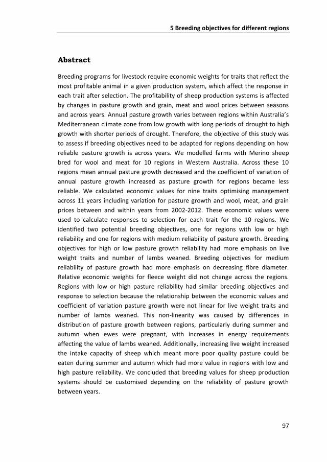
5 Breeding objectives for different regions
97
Abstract
Breeding programs for livestock require economic weights for traits that reflect the
most profitable animal in a given production system, which affect the response in
each trait after selection. The profitability of sheep production systems is affected
by changes in pasture growth and grain, meat and wool prices between seasons
and across years. Annual pasture growth varies between regions within Australia’s
Mediterranean climate zone from low growth with long periods of drought to high
growth with shorter periods of drought. Therefore, the objective of this study was
to assess if breeding objectives need to be adapted for regions depending on how
reliable pasture growth is across years. We modelled farms with Merino sheep
bred for wool and meat for 10 regions in Western Australia. Across these 10
regions mean annual pasture growth decreased and the coefficient of variation of
annual pasture growth increased as pasture growth for regions became less
reliable. We calculated economic values for nine traits optimising management
across 11 years including variation for pasture growth and wool, meat, and grain
prices between and within years from 2002-2012. These economic values were
used to calculate responses to selection for each trait for the 10 regions. We
identified two potential breeding objectives, one for regions with low or high
reliability and one for regions with medium reliability of pasture growth. Breeding
objectives for high or low pasture growth reliability had more emphasis on live
weight traits and number of lambs weaned. Breeding objectives for medium
reliability of pasture growth had more emphasis on decreasing fibre diameter.
Relative economic weights for fleece weight did not change across the regions.
Regions with low or high pasture reliability had similar breeding objectives and
response to selection because the relationship between the economic values and
coefficient of variation pasture growth were not linear for live weight traits and
number of lambs weaned. This non-linearity was caused by differences in
distribution of pasture growth between regions, particularly during summer and
autumn when ewes were pregnant, with increases in energy requirements
affecting the value of lambs weaned. Additionally, increasing live weight increased
the intake capacity of sheep which meant more poor quality pasture could be
eaten during summer and autumn which had more value in regions with low and
high pasture reliability. We concluded that breeding values for sheep production
systems should be customised depending on the reliability of pasture growth
between years.

5 Breeding objectives for different regions
98
Keywords: Pasture growth uncertainty, Price uncertainty, Sheep, Breeding
objectives, Economic values
5.1 Introduction
Breeding programs for livestock require clearly defined breeding objectives that
enable the selection of animals that will make the most money per hectare in a
given production system. Changes in optimal management need to be accounted
for when calculating how the profitability of a farm is influenced by changing traits
of animals (Groen, 1989; Amer, 1994). In areas where sheep are produced in
Western Australia there are big differences between regions in the amount and
variation of pasture growth within and between years (Rossiter, 1966; Schut et al.,
2010). These differences between regions in pasture growth can affect the optimal
management of livestock (Chapman et al., 2009; Young et al., 2011b). These
changes in management may also affect optimal breeding objectives because
changing each trait can change the energy requirements of sheep by different
amounts and at different times of the year. It is not known if different regions
require different breeding objectives, or if one breeding objective will maximise
profitability for all regions.
Farming systems become more vulnerable when pasture growth and prices vary
across years, because the optimal stocking rate is different in each year (Rose et al.,
2014). Many modelling studies have shown that increased climate variability
decreases the number of livestock that can be managed per unit of land (Kingwell
et al., 1993; Kobayashi et al., 2007; Olson and Mikesell, 1988). This modelling is
supported by surveys of farmers that suggest most Australian farmers manage the
stocking system at a fixed, managable number of ewes to avoid having too many
sheep in years with low pasture growth (Doyle et al., 1993; Austen et al., 2002;
Robertson and Wimalasuriya, 2004).
Rose et al. (2014) used actual pasture growth information for one region to show
that variation in pasture growth across years changes the economic value of traits
in the breeding objective. That study used a management perspective where
farmers were willing to change flock structure in response to variability in pasture
growth and prices. This perspective is different to farmers that prefer to keep the
flock size constant at more conservative numbers to reduce the risk of overstocking
in poor years. It is important to understand how different strategies to manage risk
affect breeding objectives across regions with different degrees of reliability in
pasture growth.

5 Breeding objectives for different regions
99
Changing the perspective of breeding objectives to constant stocking rates
compared to optimising management and adjusting stocking rates in each year may
change the optimal breeding program. Brascamp et al. (1985) found that different
perspectives of management for pigs have different optimal breeding programs
and Rose et al. (2014) also found that traits that affect energy requirements the
most had lower economic values when pasture growth varies between years. This
was because managing sheep at high stocking rates in years with favourable
pasture growth and grain prices created problems when the following year had
unfavourable pasture growth and grain prices. These problems led to a larger
decrease in profit, especially with traits that increase energy requirements such as
wool weight. Therefore, optimising management across all years should yield
higher economic values for traits with high energy requirements compared to
optimising management in each year.
Finally, traits that have a greater effect on energy requirements are likely to have
more value in regions that vary less across each year, because drought periods are
less common. Therefore, we tested the hypothesis that economic values and
responses to selection of sheep breeding objective traits change for different
regions depending on how pasture growth varies across years.
5.2 Material and methods
Testing the hypothesis that economic values and optimal response to selection in
sheep depend on climatic region required four steps:
1. Define climatic zones - pasture growth and meat, wool, and grain prices
defined for regions with different reliability of pasture growth.
2. Model – develop a bio-economic model of a sheep farm with interactions
between pasture growth, sheep production and commodity prices.
3. Economic values – calculate economic values for each trait using this bio-
economic model, and vary assumptions about pasture variability and
associated price changes for grain, wool and meat.
4. Response to selection – calculate optimal responses to selection for each
trait for each climatic zone, given the genetic parameters and economic
values of traits.
Climatic zones
We used ten climatic zones that represent the range of sheep farming areas of
Western Australia (Figure 5.1, Table 5.1). These regions are characterised by
warm/hot dry summers and cool/mild wet winters and have different amounts and
distribution of pasture growth across the year (see Figure A5.1a and A5.1b for total

5 Breeding objectives for different regions
100
pasture growth in additional material). The mean annual pasture growth decreases
and standard deviation of annual pasture growth increases the further north and
east the regions are from the ocean (Table 5.1). The length of the pasture growth
season also decreases and becomes more variable across years the further the
regions are away from the ocean. Therefore, the coefficient of variation (CV) of
pasture growth increases and the reliability of pasture growth decreases when
moving further from the ocean. This decrease in reliability makes these 10 regions
ideal to investigate if breeding programs are affected by the variability in pasture
growth.
Figure 5.1 location of sheep regions of Western Australia used in this study.
Table 5.1 longitude, latitude, mean annual pasture growth and mean length of growing
season (months) from 2002-2012 for the 10 study regions. The standard deviation (SD)
and coefficient of variation (CV) of annual pasture growth and standard deviation of
length of growing season across the 11 years are also shown.
Region Latitude Longitude Pasture growth (kgDM/day)
Growing season
Mean SD CV Mean SD
Kulin -3 .67◦S 118.16◦E 4.65 3.16 0.68 5.10 1.73 Kondinin -3 .49◦S 118. 7◦E 3.54 2.27 0.64 4.40 1.17 Narembeen -3 .07◦S 118.39◦E 3.85 2.45 0.64 4.09 1.58 Dumbleyung -33.31◦S 117.74◦E 5.5 3.23 0.59 5.09 1.70 Katanning -33.69◦S 117.56◦E 8.23 4.36 0.53 5.82 1.60 Tambellup -34.04◦S 117.64◦E 10.6 5.55 0.52 6.55 1.44 Broomehill -33.84◦S 117.64◦E 10.3 5.12 0.50 6.36 1.57 Cranbrook -34.3◦S 117.55◦E 16.6 5.25 0.32 7.64 1.29 Kojonup -33.83◦S 117.16◦E 16.7 4.75 0.29 7.55 1.13 Mt Barker -34.63◦S 117.66◦E 19.5 5.07 0.26 7.82 1.47

5 Breeding objectives for different regions
101
We used 11 years of pasture growth (Figure A5.1a and A5.1b in additional material)
and prices (Figure A5.2) from 2002-2012. We included the actual prices for grain,
meat and wool in Figure A5.2 so any correlations between pasture growth and
prices are included in the calculations for economic values. We assumed that all
regions had the same prices, since sheep producers in these regions have access to
the same markets for sheep and wool sales. The fluctuation of prices reflects the
supply and demand of each commodity over time which is affected by many factors
including the amount of pasture growth in all regions of the state. Therefore,
including different pasture growth for each region but the same prices will include
all of the relevant correlations between prices and pasture growth in each region.
Pasture growth rates were used from Pastures from Space (Hill et al., 1999)
(http://www.pasturesfromspace.csiro.au/index.asp). Wool prices used were from
the Western region micron price guide from the Wool Desk, Department of
Agriculture and Food WA and Australian Wool Exchange (DAFWA, 2012). Meat
prices used were hogget and mutton prices from Meat and ivestock Australia’s
National Livestock Reporting Service (MLA, 2012). Grain prices used were from Co-
operative Bulk Handling (CBH, 2012).
Model
We modelled monthly production decisions for sheep farms with self-replacing
Merino flocks bred for wool and meat using an adapted version of the model
described by Rose et al. (2014). This model maximised profit from wool and sheep
sales per hectare (ha) by optimising sheep numbers, sheep sales and grain feeding
based on pasture availability and prices of grain, wool and meat. We maximised
profit per ha because pasture growth per ha affects how many sheep can be
managed on the farm and the number of sheep per ha mostly determines farm
profit (Warn et al., 2006; Young et al., 2011b). Therefore, we optimised
management of sheep sales and grain feeding per ha using the General Algebraic
Modelling System with the linear programming solver BDMLP (Brooke et al., 2013).
The model of Rose et al. (2014) optimised management decisions across five years
using dynamic recursive analysis to maximise profit when commodity prices and
pasture growth varied annually. Actual pasture growth and wool, meat, and grain
prices from 005- 009 were used. Management could adapt to varying pasture
growth and commodity prices by changing sheep numbers, age structure of the
flock and amount of grain fed to sheep. In this study, however, we optimised
management across all years to find the most profitable long term stocking rate
rather than optimising stocking rate every year, representing farmers trying to
avoid managing high sheep numbers in unfavourable years. Additionally, we

5 Breeding objectives for different regions
102
maximised profit across 11 years to provide a better long term indication of the
effect of pasture growth on profit and the economic values of traits.
The optimisation included five groups of equations, profit (objective function), flock
structure, pasture, energy and intake. Profit depended on the number of sheep,
sheep sold and grain intake. The amount of pasture available affected how much
pasture could be eaten by sheep, which also affected how much is available in the
next period. The number of sheep depended on energy requirements, potential
intake, and the number of sheep sold. The amount of pasture and grain eaten was
constrained by the potential intake of the sheep, while pasture and grain eaten had
to match the energy requirements of the sheep.
Profit was derived from income from meat and wool sales minus variable and grain
costs. Meat sales were the product of number of sheep sold, live weight, price per
kg carcass and carcass dressing percentage. Sheep sales were split into mutton
(over 20 months old) and hoggets (less than 20 months old) with different prices
for both classes. We assumed that the minimum carcass weight that sheep can be
sold was 16 kg. Wool income was the product of number of sheep in November
(shearing month), wool weight, and wool price minus shearing costs. The profit
equation therefore included all the relevant incomes and costs to calculate the
impact of varying prices and pasture growth on breeding objectives.
We maximised profit across 11 years by optimising each year in a sequence, fixing
the number of sheep across years and carrying over the amount of pasture from
one year to the next. We found the optimal flock size by fixing the number of ewes
mated and increasing the number by small increments until we found the
maximum profit for the 11 study years. An example of how optimal profit was
found is in Figure A5.3 for Narembeen in the additional material. The flock
structure was optimised for each climatic region and each trait using average
pasture growth and prices. Using these methods, we were able to optimise
management of sheep across 11 years to estimate economic values for traits. In
this way, we could account for optimal management across years with respect to
changes in number of sheep and flock structure.
We limited the amount of pasture in December to be at least 800 kg/ha. This lower
limit prevented pasture being grazed too low which causes soil erosion (Moore et
al. 2009). In years when pasture growth was not enough to have 800 kgDM/ha in
December, we lowered the lower limit of pasture in December by 10 kgDM/ha
increments until the program became feasible. We did not include any
consequences for future pasture growth when the pasture limit was lowered. The
final amount of Pasture in December became the starting amount for the next
year’s analysis.

5 Breeding objectives for different regions
103
Economic values
Breeding programs aim to increase profit per animal through genetic improvement
of traits that affect profit. Therefore, running a breeding program starts with
specifying the traits affecting profit. The next step is to estimate the economic
values for each trait, i.e. the change in profit when the trait is genetically improved
by one unit keeping all other traits constant. Mathematically, the breeding
objective can be represented as a linear equation in which breeding values for each
trait are multiplied with economic values (Hazel, 1943). We calculated the
economic value for nine traits shown in Table 5.2. These traits represent the
economically important traits in current Merino breeding programs in Australia
(Swan et al., 2007), with live weight and number of lambs weaned important for
meat income and clean fleece weight and fibre diameter important for wool
income.
We calculated the economic values for each trait as the difference in profit when
increasing the trait by one genetic standard deviation compared to when the trait
was not improved, while keeping all other traits constant. We changed the traits by
one genetic standard deviation because this represents how easy traits change
under selection. When we changed the traits, the energy requirements and
potential feed intake of all animals changed. Increasing live weight, clean fleece
weight and number of lambs weaned increased the metabolisable energy
requirements. Increasing live weight increased the potential intake of sheep
because bigger sheep can eat more. Neither energy requirements nor potential
intake changed when we changed fibre diameter.
For adult live weight we increased live weights and standard reference weight of
sheep older than 20 months but did not change the live weight change at any other
age. For weaning, yearling and hogget live weight we changed the live weight at
the relevant age and adapted the curves from birth to 20 months old (Figure A5.4).
Table 5.2 phenotypic variance, and heritability of traits used to calculate economic values and responses to selection from MERINOSELECT database (Brown et al. 2006).
Traits Heritability Phenotypic variance
Weaning weight (kg) 0.40 18.6 Yearling live weight (kg) 0.43 28.3 Hogget live weight (kg) 0.39 35.1 Adult live weight (kg) 0.44 28.8 Hogget clean fleece weight (kg) 0.36 0.18 Adult clean fleece weight (kg) 0.50 0.26 Hogget fibre diameter (µm) 0.62 1.68 Adult fibre diameter (µm) 0.67 1.35 Number lambs weaned 0.07 0.27

5 Breeding objectives for different regions
104
These adaptations meant that the weights before and after each measurement
were also altered. For example, when weaning weight increased by one genetic
standard deviation, we adjusted the curve so that there was a higher growth rate
up to weaning. Therefore growth rate after weaning was lower so that weights at
older ages were not altered. Increasing number of lambs weaned changed the
proportion of ewes with 0, 1, and 2 lambs born and weaned based on Figure A5.5,
the same as described in Rose et al. (2014). Using the relationships in Figure A5.5,
we estimated the number of ewes in each birth and wean class based on number
of lambs weaned per ewe in the flock. Increasing the number of lambs weaned
increased the proportion of ewes that gave birth to and weaned 2 lambs and
decreased the proportion of ewes that gave birth to and weaned no lambs. Ewes
that give birth to and wean two lambs have higher energy requirements for
pregnancy and lactation than ewes that give birth and wean one lamb. Additionally,
the flock structure changed when the number of lambs weaned increased. For
more details, see Rose et al. (2014).
We used the economic values per unit of the trait ( ) to calculate the relative
contribution (cx ) of each trait (x) to the genetic variance (
= T ) of the
breeding objective (H) using the equation;
cx
T
Where is a matrix with economic values on the diagonal, is the genetic
variance-covariance matrix and is a vector of economic values. More detailed
information about how we calculated the relative contributions is in section 5.C of
the additional files. We also calculated the correlations between breeding
objectives for each region (r i, j) using the equation
r i, j iT j
√ i j
Where are the vectors with the economic values for breeding objectives i and j, G
is the genetic variance-covariance matrix and is the variance of breeding
objectives i and j. The correlations between breeding objectives show how much
the breeding objectives are genetically different.
Response to selection
Response to selection is the expected genetic change in each trait when selecting
on the index defined by the economic values. When multiple traits are included in a
breeding objective then the response to selection is the response in the aggregate
genotype, which is the product of the economic values for all traits and the

5 Breeding objectives for different regions
105
responses per trait. The ease of changing traits depends on the additive genetic
variance of each trait, but also the heritability and the genetic correlations with
other traits in the aggregate genotype. Traits with higher genetic variation have a
higher potential to be improved. Because the aggregate genotype also includes the
genetic correlations between traits, putting more emphasis on one trait will also
change traits that are correlated.
The expected response to selection with the economic values from each climatic
region was calculated using SelAction (Rutten et al., 2002). For each region, we
assumed that the same breeding program and genetic parameters, from the
MERINOSELECT database (Brown et al., 2006), were used (see Table 5.2 and Table
5.3) so that differences between regions were due to differences in economic
values and not due to differences in breeding programs. We assumed first mating
at 19 months of age with a ewe to ram ratio of 20 to 1. Each ewe gave birth to 0.8
lambs once per year with 10% death and culling for ewes and 50% for rams. We
used 7 age classes representing one year each, with weaning weight, yearling
weight, fibre diameter and clean fleece weight measured at age 1 and hogget
weight measured at age 2, and adult fibre diameter, clean fleece weight and live
weight and number of lambs weaned recorded for classes 3-7. Rams and ewes
were selected based on own performance and based on 15 half sibs from 19 dams
for all traits apart from number of lambs weaned. For number of lambs weaned
ewes were selected based on own performance and 7 half sib sisters from 9 ewes.
For number of lambs weaned, rams were selected based on the performance of 8
half sib sisters from 10 dams. For all traits at all ages, ewes and sires were selected
based on BLUP-EBV. Selection responses were predicted with a pseudo-BLUP
selection index (Rutten et al., 2002).
Table 5.3 genetic (above diagonal) and phenotypic (below diagonal) correlations between breeding objective traits from MERINOSELECT database (Brown et al., 2006).
wwt ywt hwt awt hcfw acfw hfd afd nlw
wwt 0.70 0.66 0.36 0.24 0.17 0.05 0.02 0.04 ywt 0.47 0.90 0.61 0.30 0.23 0.18 0.14 0.13 hwt 0.41 0.70 0.65 0.26 0.26 0.18 0.16 0.12 awt 0.60 0.80 0.89 0.15 0.15 0.20 0.20 0.35 hcfw 0.20 0.24 0.24 0.26 0.80 0.30 0.30 -0.10 acfw 0.05 0.15 0.19 0.22 0.58 0.26 0.34 -0.10 hfd 0.10 0.20 0.19 0.19 0.27 0.23 0.90 0.00 afd 0.10 0.15 0.16 0.17 0.23 0.29 0.78 0.00 nlw 0.15 0.30 0.34 0.15 -0.01 0.02 0.00 -0.01 wwt = weaning live weight; ywt = yearling weaning weight; hwt = hogget live weight;
hcfw = hogget clean fleece weight; acfw = adult clean fleece weight; hfd = hogget fibre
diameter; afd = adult fibre diameter; nlw = number of lambs weaned.

5 Breeding objectives for different regions
106
Statistical analysis of breeding objectives and response to selection
For each trait we tested if the relationship between the CV of annual pasture
growth was significant with economic values, relative contribution to breeding
objective, and response to selection. We tested the significance using analysis of
variance in the R software (R Core Team 2012). Our first null hypothesis was that
CV does not significantly explain differences in economic values, relative
contribution to breeding objective, and response to selection. If we rejected this
null hypothesis, we then tested a second null hypothesis that a linear function fits
the data better than a quadratic function. We rejected the null hypothesis if the
probability of a better fit was less than 0.05. These tests were important to
interpret how economic values, relative contribution to breeding objective, and
response to selection are affected by pasture growth and variation in each region.
5.3 Results
Effect of varying pasture growth on profit
Profit decreased when the CV of pasture growth between years increased (Figure
5.2). This decrease in profit was mostly because less sheep could be managed per
ha when CV of pasture growth increased (Figure A5.6). Additionally, income and
costs decreased as the CV of pasture growth increased (Figure 5.2), but the
contribution of income and costs to profit changed for each pasture growth region
with grain costs having more influence on profit as the coefficient of variation of
pasture growth increased (Figure A5.7). This increase in grain requirements was
because the frequency and length of drought periods increased as the CV of
pasture growth increased. Therefore, as pasture reliability decreased, stocking rate
decreased and grain costs increased which decreased profit.
Economic values and breeding objectives
The economic value of weaning weight, hogget live weight and adult live weight
were close to zero and mostly negative (Table 5.4). These economic values were
mostly negative because of higher energy requirements when live weight
increased. The relationship between economic values and CV of pasture growth
were quadratic (p < 0.01) and regions with high and low CV of pasture growth had
higher economic values for these traits than regions with medium CV of pasture
growth.

5 Breeding objectives for different regions
107
Figure 5.2 Profit, incomes and costs for each region are represented as a function of coefficient of variation of annual pasture growth. Table 5.4 Economic values/ha per genetic standard deviation across regions represented by coefficient of variation of annual pasture growth (CV).
CV wwt2 ywt
1 hwt
2 awt
2 hcfw
1 acfw
1 hfd
1 afd
1 nlw
2
0.68 0.8 6.1 -0.8 1.7 7.7 9.6 -3.6 -3.6 9.7 0.64 0.7 4.3 -0.6 0.5 5.7 7.6 -2.7 -2.7 7.0 0.64 0.8 4.5 -0.4 0.8 6.2 8.1 -3.1 -3.1 7.6 0.59 0.8 5.0 -3.2 -1.3 8.7 11.7 -5.0 -5.0 9.5 0.53 -0.6 6.7 -5.2 -3.5 12.3 17.4 -8.7 -9.8 14.5 0.52 -0.2 12.7 -4.8 -4.8 17.0 22.6 -11.6 -11.7 17.4 0.50 -1.2 9.0 -4.6 -5.2 15.4 20.7 -12.3 -12.5 16.3 0.32 3.0 15.4 -1.4 -4.0 30.3 38.6 -15.1 -14.5 35.5 0.29 3.1 19.9 -0.5 -2.9 33.9 42.5 -16.7 -16.0 40.8 0.26 3.5 17.2 0.1 -4.4 36.2 45.8 -17.7 -16.7 45.0
wwt = weaning live weight; ywt = yearling weaning weight; hwt = hogget live weight; hcfw = hogget clean fleece weight; acfw = adult clean fleece weight; hfd = hogget fibre diameter; afd = adult fibre diameter; nlw = number of lambs weaned 1 linear relationship between economic value and coefficient of variation of pasture
growth P<0.05). 2 significant quadratic relationship between economic value and coefficient of variation
of pasture growth (P<0.01).

5 Breeding objectives for different regions
108
Yearling weight, hogget fleece weight, adult fleece weight and number of lambs
weaned had the largest effect on income, and their economic values decreased as
the CV of pasture growth increased. As the CV of pasture growth increased, these
traits had less value per ha because less sheep could be managed, and the benefits
of improving traits in each sheep was lower. The economic value for fibre diameter
traits increased as the reliability of pasture growth decreased. The economic values
for yearling live weight and wool traits increased linearly with increasing CV of
pasture growth (p < 0.01) but the economic value for number of lambs weaned had
a quadratic relationship with CV (p < 0.01). The slope of the economic value for
lambs weaned decreased as CV of pasture growth increased and economic values
were similar between regions when CV was higher than 0.5. This can be seen in
more detail in Figure A5.8, with economic values for all traits changing profit by a
higher proportion when the CV of pasture growth was highest.
The relative contribution of traits to the breeding objective was highest for adult
fleece weight, hogget fleece weight and number of lambs weaned (Table 5.5). The
next main contributors were yearling live weight and fibre diameter traits,
depending on the relationships between economic values and reliability of pasture
growth. The relationship between CV of pasture growth and relative importance of
all traits was quadratic across regions (P<0.01), apart from hogget fleece weight
which was linear (P < 0.01) and adult fleece weight which had no relationship with
CV of pasture growth. The relative importance of weaning live weight, yearling live
weight, adult live weight, and number of lambs weaned had a minimum around CV
of annual pasture growth of 0.5, increasing as CV increased and decreased. The
relative importance of hogget and adult fibre diameter had a maximum around CV
of pasture growth of 0.5 and decreased as CV increased and decreased. The
relative importance of hogget live weight and hogget fleece weight decreased
linearly as CV of pasture growth increased. The relative importance of adult fleece
weight was the same for all regions. These results show that relationships between
relative contributions and CV of pasture growth for each trait are a consequence of
the relationships between economic values and CV of pasture growth.
The non-linearity of relative contribution of traits was caused by non-linearity in
economic values, particularly for live weight traits and number of lambs weaned.
Therefore, in regions with high or low CV of pasture growth, the number of lambs
weaned and live weight traits contributed more to the breeding objective
compared to fibre diameter traits. Alternatively, in regions with medium CV of
pasture growth, the opposite was found with fibre diameter traits contributing
more to the breeding objective than lambs weaned and live weight traits.

5 Breeding objectives for different regions
109
Table 5.5 Relative contribution of each trait (%) to the breeding objective across regions represented by coefficient of variation of pasture growth (CV).
CV wwt2 ywt
2 hwt
1 awt
2 hcfw
1 acfw
0 hfd
1 afd
2 nlw
2
0.68 1.7 18.6 -1.8 4.9 22.7 28.5 0.1 0.2 25.0 0.64 1.8 16.8 -1.7 1.9 24.5 33.1 0.3 0.3 23.2 0.64 2.2 16.4 -0.9 2.7 23.8 31.3 0.5 0.5 23.6 0.59 1.0 9.5 -2.8 -2.0 27.7 38.6 3.9 3.6 20.5 0.53 -0.2 5.2 -0.7 -2.0 23.4 35.1 8.9 9.9 20.4 0.52 -0.1 11.9 -2.1 -3.5 26.6 35.8 7.1 6.9 17.4 0.50 -0.4 5.9 -0.9 -2.3 23.9 33.0 12.1 11.9 16.7 0.32 1.3 10.3 -0.6 -2.4 28.3 36.4 1.6 1.4 23.8 0.29 1.3 12.7 -0.2 -1.7 27.1 34.0 1.1 1.0 24.7 0.26 1.3 9.7 0.0 -2.3 27.5 35.2 1.3 1.1 26.3
wwt = weaning live weight; ywt = yearling weaning weight; hwt = hogget live weight; hcfw = hogget clean fleece weight; acfw = adult clean fleece weight; hfd = hogget fibre diameter; afd = adult fibre diameter; nlw = number of lambs weaned. 1 no relationship between economic value and coefficient of variation of pasture growth.
1 linear relationship between economic value and coefficient of variation of pasture
growth (p < 0.05). 2 quadratic relationship between economic value and coefficient of variation of pasture
growth (p < 0.01). Table 5.6 Correlations between regions represented by coefficient of variation of annual pasture growth (CV) for relative contribution (above diagonal) and response to selection (below diagonal).
CV 0.68 0.64 0.64 0.59 0.53 0.52 0.50 0.32 0.29 0.26
0.68 1 1 0.94 0.87 0.93 0.86 0.98 0.99 0.98 0.64 1 1 0.96 0.89 0.95 0.88 0.99 1 0.99 0.64 1 1 0.96 0.89 0.94 0.88 0.99 0.99 0.99 0.59 0.89 0.92 0.91 0.98 0.99 0.97 0.99 0.98 0.98 0.53 0.71 0.75 0.74 0.94 0.99 1 0.94 0.93 0.94 0.52 0.88 0.91 0.9 1 0.96 0.99 0.98 0.97 0.97 0.50 0.73 0.77 0.75 0.95 1 0.96 0.93 0.92 0.92 0.32 0.97 0.98 0.98 0.98 0.86 0.97 0.87 1 1 0.29 0.99 1 0.99 0.95 0.81 0.94 0.82 1 1 0.26 0.98 0.99 0.98 0.97 0.84 0.96 0.85 1 1
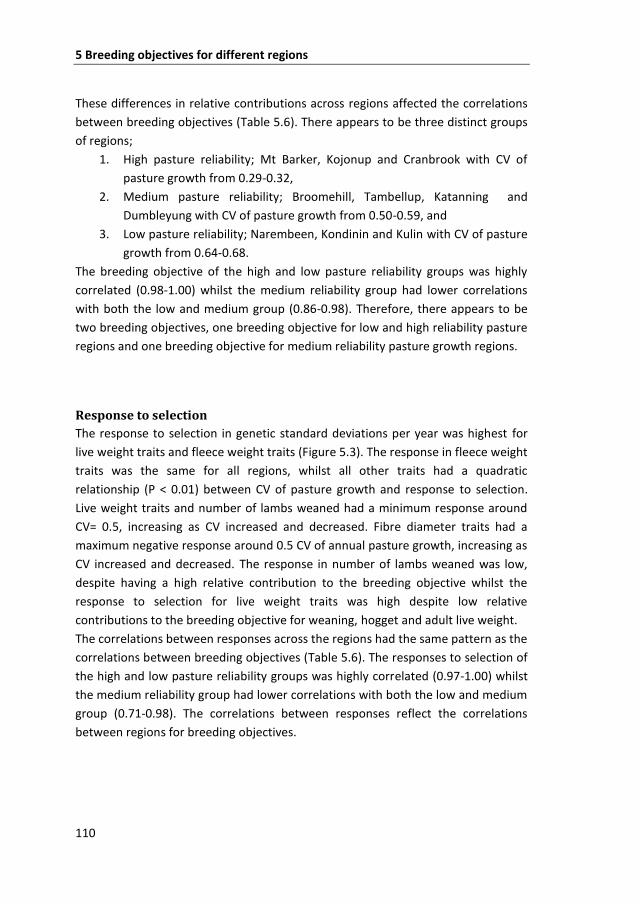
5 Breeding objectives for different regions
110
These differences in relative contributions across regions affected the correlations
between breeding objectives (Table 5.6). There appears to be three distinct groups
of regions;
1. High pasture reliability; Mt Barker, Kojonup and Cranbrook with CV of
pasture growth from 0.29-0.32,
2. Medium pasture reliability; Broomehill, Tambellup, Katanning and
Dumbleyung with CV of pasture growth from 0.50-0.59, and
3. Low pasture reliability; Narembeen, Kondinin and Kulin with CV of pasture
growth from 0.64-0.68.
The breeding objective of the high and low pasture reliability groups was highly
correlated (0.98-1.00) whilst the medium reliability group had lower correlations
with both the low and medium group (0.86-0.98). Therefore, there appears to be
two breeding objectives, one breeding objective for low and high reliability pasture
regions and one breeding objective for medium reliability pasture growth regions.
Response to selection
The response to selection in genetic standard deviations per year was highest for
live weight traits and fleece weight traits (Figure 5.3). The response in fleece weight
traits was the same for all regions, whilst all other traits had a quadratic
relationship (P < 0.01) between CV of pasture growth and response to selection.
Live weight traits and number of lambs weaned had a minimum response around
CV= 0.5, increasing as CV increased and decreased. Fibre diameter traits had a
maximum negative response around 0.5 CV of annual pasture growth, increasing as
CV increased and decreased. The response in number of lambs weaned was low,
despite having a high relative contribution to the breeding objective whilst the
response to selection for live weight traits was high despite low relative
contributions to the breeding objective for weaning, hogget and adult live weight.
The correlations between responses across the regions had the same pattern as the
correlations between breeding objectives (Table 5.6). The responses to selection of
the high and low pasture reliability groups was highly correlated (0.97-1.00) whilst
the medium reliability group had lower correlations with both the low and medium
group (0.71-0.98). The correlations between responses reflect the correlations
between regions for breeding objectives.

5 Breeding objectives for different regions
111
5.4 Discussion
Variation in pasture growth across years influenced the optimum breeding
objectives for Merino based sheep production systems in different regions of
Western Australia. As the reliability of pasture growth across years decreased the
profit per ha decreased because less sheep could be managed per ha. Additionally,
as the reliability of pasture growth decreased, the economic value of most traits
decreased, although this decrease was not always linear. This non-linear decrease
for some traits caused differences in the relative contribution of traits to the
breeding objective, which also affected the response to selection. Therefore, we
accepted the hypothesis that economic values and response to selection of sheep
breeding objective traits change depending on the distribution and variation of
pasture growth across years.
Figure 5.3 Response to selection in genetic standard deviations across regions represented by coefficient of variation of annual pasture growth for relative contribution for each trait.

5 Breeding objectives for different regions
112
Furthermore, based on correlations between breeding objectives and responses to
selection we found that a single breeding objective was suitable for regions with
high or low reliability of pasture growth between years. This single breeding
objective existed despite big differences in the amount and variation of pasture
growth between regions with low and high pasture growth reliability. Additionally,
regions with medium pasture growth reliability had a different breeding objective
to regions with low and high pasture growth reliability. The first breeding objective
had more emphasis on live weight and number of lambs weaned and the second
had more emphasis on fibre diameter traits.
Interactions between how traits change energy requirements and potential intake
with the amount and distribution of pasture growth across years caused the
differences in economic values, relative contributions of traits, and the response to
selection of the traits. These interactions suggest that breeding programs should be
customised based on the amount and distribution of pasture growth across years.
Regions with low or high reliability of pasture growth had similar breeding
objectives because differences in the distribution of pasture growth in each month
caused quadratic responses in economic values to changes in CV of pasture growth
for live weight traits and the number of lambs weaned. Live weight traits at
weaning, hogget and adult ages had more value in regions with high or low
reliability of pasture growth than regions with medium reliability of pasture growth
because increasing live weight increases potential intake or intake capacity of
sheep (Freer et al., 2007). This increase of potential intake is important because dry
pasture has low digestibility and takes longer to digest limiting the amount of
pasture that can be eaten. If sheep can eat more dry pasture, a higher proportion
of their energy requirements can be met from dry pasture, and the costs of
supplementary feeding are reduced, especially in regions with low reliability of
pasture growth which have long periods of drought. Regions with high reliability of
pasture growth have big peaks in pasture growth during spring. Despite this high
peak in pasture growth, stocking rate is limited by periods of drought. This
limitation occurs because a lot of pasture grows in a short period in spring which is
not utilised unless sheep are managed at a high stocking rate. The optimal stocking
rate, however, is still limited by the short period of drought in each year. Therefore,
increasing the potential intake reduces the influence of drought periods which
means more sheep can be managed and more of the pasture grown in spring is
utilised. The benefits of increasing intake capacity were not as high in the regions
with medium pasture growth reliability because periods of drought were shorter
than the low reliability regions, and the peak of pasture in spring were lower than
the high reliability regions. This extra value of live weight is similar to what Groen

5 Breeding objectives for different regions
113
and Korver (1989) found in dairy cattle, where more forage can be given when
potential intake increases, reducing the amount of concentrate required. We found
that the benefit of increased intake capacity is not only relevant for regions with
low pasture growth, but can be advantageous in regions with high pasture growth,
which is an important conclusion.
The quadratic relationship between economic value for lambs weaned and CV of
pasture growth was due to differences in distribution of pasture growth between
years. Every region had pasture growth during July and August in most years, the
months with peak energy requirements for pregnancy and lactation. Therefore,
when the number of lambs and weaned increased, there was mostly green pasture
available to match the increase in energy requirements. As regions became less
reliable, the length of the growing season decreased due mostly to a later start to
the season during autumn and early winter. The growing seasons shortened
considerably between the 3 regions with high pasture growth reliability and regions
with medium pasture growth reliability. Because autumn and early winter
coincided with the start of pregnancy, the value of weaning more lambs was less
for regions with medium pasture growth reliability than for regions with high
pasture growth reliability. The decrease in length of growing season was not so
extreme between regions with medium and low pasture growth reliability.
Therefore, the decrease in economic values in relation to coefficient of variation of
pasture growth between regions with medium and low pasture growth was also
lower, causing a quadratic relationship between economic values for number of
lambs weaned and CV of pasture growth, contributing to different breeding
objectives between regions with low and high pasture growth reliability and
regions with medium pasture growth reliability.
The magnitude of the relative contribution of traits to the breeding objective and
the response to selection did not always match. For example, number of lambs
weaned had a low response to selection despite a high contribution to the breeding
objective. This low response was because number of lambs weaned was only
measured in adult ewes which decreased the accuracy of selection compared to all
other traits which were recorded at more ages. Additionally the heritability of
number of lambs weaned is low decreasing the accuracy of selection. Live weight,
fleece weight and fibre diameter traits were recorded at several ages, with high
correlations between each age group. Therefore, high response to selection at one
age caused a high response at all other ages. Live weight had a high value at
yearling age which increased response at all other ages, even though their
economic values were close to zero. These differences also caused the correlations
between regions for responses to selection to be lower than for breeding

5 Breeding objectives for different regions
114
objectives. This difference in correlations has been demonstrated in cattle (Hirooka
and Groen, 1999) and pigs (Dube et al., 2013). Therefore, responses to selection
need to be calculated before comparing breeding programs because the
differences in economic weights do not directly translate into equal differences in
selection responses.
We found that regions with different pasture growth have different breeding
objectives but there could also be differences in the performance of animals within
each region. This variation in pasture availability across regions can cause genotype
by environment interactions changing the ranking of the best animals to select
between environments (Falconer and Mackay, 1996). Additionally, within each
region changes in pasture growth between years can also cause genotype by
environment interactions. For example, several studies for beef cattle (Sousa Júnior
et al., 2012) and dairy cattle (Kearney et al., 2004; McCarthy and Veerkamp, 2012)
found genotype by environment interactions for production traits when resources
were different either because of the time of year, amount of rainfall or amount of
grain supplement provided. Therefore, genotype by environment interactions
between regions could make it difficult to use one breeding scheme for all
environments (e.g. Mulder et al., 2006). Additionally, genotype by environment
interactions between seasons make it difficult to select animals that have high
performance in all seasons. For example, several studies have shown that selection
for the best animals in good years can increase the sensitivity of animals to varying
environments (Falconer, 1990; van der Waaij, 2004). This environmental sensitivity
can reduce performance in poor years which can have economic and welfare
consequences. Therefore, optimal breeding programs for regions could be further
affected by the genotype by environment interactions between regions and
between seasons.
Rose et al. (2014) reported that including varying pasture growth and prices
increased the estimated economic values for different traits compared to using
average pasture growth and prices. The study by Rose et al. (2014) used dynamic
programming to simulate farmers altering their management decisions in response
to changes in pasture growth and prices each year, whereas in this study we
optimised sheep numbers across all years. We can compare the economic values
from Katanning in this study to those of Rose et al. (2014). The economic values for
number of lambs weaned decreased from $AU26/ha to 15, for adult fibre diameter
increased from -21 to -10 and for adult fleece weight decreased from 22 to 17. The
magnitude of economic values decreased between the studies, however in this
study the relative importance of fleece weight was higher than the study by Rose et
al. (2014). This difference in economic values was because fleece weight made the

5 Breeding objectives for different regions
115
farm more vulnerable to changes in pasture growth and prices when management
was optimised each year. Optimising management across all years meant that
fleece weight made the farm less vulnerable because an optimal stocking rate
across all years could be estimated. Although it is difficult to compare the two
studies because they used different study years, it appears that there were big
differences in the relative importance of traits when sheep numbers are optimised
in each year or across years. In conclusion, this study provides a set of economic
values for farmers that manage variation in pasture growth by managing the same
number of sheep at a lower stocking rate, which is a different type of farmer
simulated in the study by Rose et al. (2014).
We used the coefficient of variation as the indicator of pasture reliability but
average pasture growth decreased as the coefficient of variation increased.
Therefore, it was difficult to disentangle the effects of total pasture growth and
variation across years. Within the groups of regions with low, medium and high
pasture growth it is possible to investigate the effects of pasture growth because
the coefficient of variation of pasture growth was similar within the groups.
Additionally, we could have simulated pasture growth to have the same mean
pasture growth and different variation across years. However, using real pasture
growth data makes our research more relevant for farmers who have uncertain
pasture growth across years than using simulated data.
Finally, we limited the amount of pasture in December to be at least 800 kg/ha and
lowered the limit by 10kg DM/ha until the model became feasible. This lowering of
the lower limit has implications for the optimisation of economic values. For
example, in years with no pasture growth at all, or a drought for the whole year,
there is no pasture left in December. Therefore, in the following years, there is no
pasture available until pasture starts growing. Having no pasture in December has
many consequences for soil health (Moore et al., 2009) which could affect pasture
growth in the following year. We had trouble finding relevant information about
how pasture growth is affected in a year with high soil erosion. However, in our
study the consequence of no pasture growth on the following year is still
represented through not having any pasture available in summer and autumn in
the following year.
Acknowledgements
This research was financed by the Department of Food and Agriculture Western
Australia, The Sheep Cooperative Research Centre, Meat and Livestock Australia
and Wageningen University.

5 Breeding objectives for different regions
116
Additional files Chapter 5
Additional files 5.A – Pasture growth, prices and profit
Fi
gure
A5
.1a
Pas
ture
gro
wth
rat
e o
f th
e 5
leas
t re
liab
le c
limat
ic r
egi
on
s st
ud
ied
fo
r th
e 1
1 y
ears
fro
m 2
00
2-2
01
2.

5 Breeding objectives for different regions
117
Fi
gure
A5
.1b
Pas
ture
gro
wth
rat
e o
f th
e 5
mo
st r
elia
ble
clim
atic
re
gio
ns
stu
die
d f
or
the
11
yea
rs f
rom
20
02
-20
12
.

5 Breeding objectives for different regions
118
Figu
re A
5.2
Wo
ol,
mea
t an
d g
rain
pri
ces
fro
m 2
00
2 t
o 2
01
2.

5 Breeding objectives for different regions
119
Additional files 5.B – trait characteristics
Figure A5.4 alterations of live weight for growing sheep used to calculate economic values of weaning, yearling and hogget live weight. Only lambs that were born and reared as one lamb are shown.
Figure A5.3 Example of how optimal stocking rate is found to optimise profit by increasing number of ewes mated by a small increment.

5 Breeding objectives for different regions
120
Additional files 5.C - Relative contribution calculations
We calculated the relative contribution of each trait to the breeding goal using the
equation
cx v
v v
Where is a matrix with economic values on the diagonal, is the genetic
variance-covariance matrix and v is a vector of economic values.
An example of the calculation using two traits with
[v1 00 v
] ,
[x aa y] and
[v1v
]
Where the variance of the breeding goal is
v1 x v1v a v1v a v
y
And the relalative emphasis for trait 1 v1 x v1v a
var
Figure A5.5 The number of ewes in each of the 6 birth and wean categories based on
number of weaned per ewe mated estimated from 8 information nucleus flocks (Sheep
CRC) from Australia over 3 years. We fitted curves to these points and estimated the
number of sheep in the 6 litter size at birth and litter size at weaning category.

5 Breeding objectives for different regions
121
Additional files 5.D – supplementary results
Figure A5.6 Number of ewes mated per ha plotted against coefficient of variation of annual pasture growth.
Figure A5.7 Relative contribution of each costs and income to profit plotted against coeffienct of variation of annual pasture growth.

5 Breeding objectives for different regions
122
Figure A5.8 Change in profit after changing trait by 1 genetic standard deviation relative to profit before changing traits plotted again coefficient of variation of annual pasture growth.

6 General discussion


6 General Discussion
125
In this thesis, I studied breeding strategies for sheep in environments which have
high uncertainty of pasture growth and wool, meat and grain prices between years.
The main objective of breeding programs is to select the animals that will make the
most money per hectare in a production system. Additionally, breeding programs
should ensure the welfare level of animals is maintained and that production
systems are sustainable. The objectives of breeding programs for production
systems with varying pasture growth between years are difficult to clearly define
because every year is different which requires different management systems and
perhaps a different type of sheep. Breeding objectives, however, need to be longer
term and therefore cannot be aimed at conditions in one particular year.
Therefore, breeding objectives need to be estimated for a particular region of
group of farms and aimed at selecting the sheep that will be most suitable for this
region or group of farms in the future. Therefore, I aimed to provide farmers with
breeding strategies to select sheep most suitable for farming systems in
environments with uncertainty in pasture growth between years.
To provide clear breeding strategies for sheep farmers and breeders, this thesis had
two aims; 1. Quantify how to make sheep more resilient to variation in pasture
growth and 2. Quantify how to make farming systems more resilient to variation in
pasture growth and commodity prices. In the general discussion, I compare these
aims, and link these to the general topic of breeding better animals for the future.
The discussion is split into four sections that explore how sheep can be bred to be
resilient to uncertainty. I address two questions;
1. Can sheep be bred to be more resilient using live weight change as a trait?
2. Optimal breeding to reduce variation across years - are some traits more
sensitive to variation in pasture growth and prices across years?
These questions will be addressed in the first two sections. In the third section I
review definitions of resilience for production systems and breeding strategies. In
the fourth section I relate the results of my thesis to the review of resilience and
breeding, making conclusions about the best strategies to make farming systems
resilient to uncertain pasture growth and commodity prices.
6.1 Breeding resilient sheep
In Chapter 2 I showed that live weight change can be selected for and in Chapter 3
that live weight change had important genetic correlations with reproduction. It is
important to understand how live weight change is related to resilience to drought
periods and hence determine if it could serve as an indicator trait for resilience to
drought periods. Additionally, if live weight change is to be used as an indicator

6 General Discussion
126
trait for resilience to drought periods, an economic value for live weight and
resilience is required before it can be used in a breeding objective. This will give an
indication of the relative importance of resilience compared to other traits.
Furthermore, since live weight change contains two live weight measurements, live
weight change is expected to be correlated with the live weights. These
correlations might make it difficult to simultaneously select for live weight change
and live weight at the start and end of the live weight change period in different
directions. Since farmers may have different desired directions to select for live
weight change and live weights it is important to understand the consequence of
selecting for live weight change on the selection response of live weight. Therefore,
in this section I will discuss three subjects; first how live weight change might serve
as an indicator trait for resilience to drought periods, second how an economic
value can be estimated for live weight change as an indicator for resilience, and
third, whether live weight change and live weight traits can be selected for
simultaneously.
Live weight change as an indicator trait for resilience
If live weight change is an indicator trait for resilience, then resilient sheep may
lose less weight during droughts. These resilient sheep may lose less live weight
because they have lower energy requirements for maintenance or have increased
intake or digestion capabilities when grazing poor quality feed (Silanikove, 2000;
Fogarty et al., 2009). Losing less live weight improves the efficiency of sheep and
this improved efficiency would change the energy balance of sheep which could
make the sheep easier to manage and improve the welfare status of sheep as they
are able to withstand severe stress from drought periods. Being resilient to drought
means sheep would have a better chance to survive and reproduce. Therefore, live
weight change would qualify as a resilience trait based on the definition by Prayaga
and Henshall (2005) and Barker (2009).
Live weight change gives an indication of the energy balance of sheep. Increasing
live weight implies that animals have a positive energy balance, and therefore
energy left over to gain live weight. There is a distinction between breeding for
heavier sheep at a single time point and live weight change. If sheep are selected to
be heavier it does not infer anything about how live weight changes between two
time points. Additionally, live weight change could be important at difference times
of the year. For example, sheep that lose less live weight change during drought
periods indicates that sheep have to mobilise less energy stored as tissue into
energy for other functions. Additionally, gaining live weight during periods of high
pasture growth could be advantageous as an energy store which can be mobilised
6 General Discussion
127
during other periods when energy requirements are higher such as during
pregnancy and lactation. In Chapter 2 I showed that live weight loss and gain can
potentially be selected for independently, which gives farmers flexibility in
choosing how they want to change the live weight profile of sheep during the year.
Therefore, the live weight profile of sheep can be manipulated to increase the
resilience of sheep to drought periods.
Selection can change the fat stores and energy balance of animals. Ermias et al.
(2002) found breed differences in the ability of animals in storing body fat. They
suggested that fat storage can be used as a way to manage sheep in years with
good pasture growth because accumulated fat stores can then be used for
pregnancy and lactation during years with poor pasture growth. Additionally, sheep
that lose less live weight during drought periods will have more energy stores
during pregnancy, lambing and lactation. This is a similar concept to dairy cattle
where it is recommended to include body condition score in indexes to ensure that
cows store enough energy resources that can be mobilised when energy
requirements for milk production peak (Veerkamp and Brotherstone, 1997). Collard
et al. (2000) also found that periods of negative energy balance are associated with
increased incidence of health problems in dairy cattle. Therefore, a positive energy
balance is important for storing tissue that can be utilised during periods of stress
and to maintain the welfare status of animals. In conclusion live weight change
could be included into sheep breeding programs to ensure enough energy is stored
to be used during periods of drought.
In Chapter 3, I showed that live weight change has some important positive genetic
correlations with reproduction, particularly in older ewes that bear and wean more
lambs than younger ewes. Furthermore, I found a favourable genetic correlation
between live weight gain during pregnancy and number of lambs born and live
weight at lambing was important for total birth weight and number of lambs
weaned. Genetic correlations between live weight change during lactation and
reproduction were negative reflecting the high energy demands of pregnancy and
lactation. This suggests that having enough resources at lambing by gaining live
weight during pregnancy ensured better reproduction performance. Beilharz et al.
(1993) defined fitness as the ability to pass genes from generation to generation.
Reproduction and survival are two important components of fitness. Our results
show that the ability of animals to store and mobilise body reserves can improve
the reproductive performance of sheep, therefore improving fitness. Berube et al.
(1999) found that body mass at the end of summer in 6-year-old ewes was
positively correlated with longevity. Therefore, live weight change could be an
important component of breeding programs for animals to indicate animals that

6 General Discussion
128
have a positive energy balance, and to improve the reproduction in survival,
making sheep more resilient to periods of drought.
An economic value for live weight change
The relative value of live weight change as an indicator of resilience compared to
other traits needs to be determined if live weight change is to be included in
breeding programs. Farmers could put a high value on live weight change because
they value resilience, or an economic value can be estimated based if resilience
increases profit on a farming system. Animals could lose less live weight during
drought periods due to reduced energy requirements for maintenance and or
increased intake when grazing poor quality feed (Silanikove, 2000; Fogarty et al.,
2009). Therefore, I can estimate the value of sheep that have lower maintenance
requirements or eat more dry pasture, which could reduce supplementary feeding
requirements and increase profit.
The economic value of live weight change as an indicator for resilience can be
calculated by comparing the economic performance of a sheep that loses one kg of
live weight less than another sheep. For example, consider two sheep that eat the
same amount of energy. If one sheep loses live weight whilst the other gains live
weight one assumption is that this sheep is more efficient and has lower
maintenance energy requirements. If the farmer wanted to manage both sheep to
have the same change in live weight, then the sheep that loses live weight would
require more grain than the sheep that gains live weight or the sheep that gains
weight could be run at higher stocking rates. Therefore, I could calculate an
economic value for live weight change as an indicator for a sheep that requires less
metabolisable energy when managed at the same live weight change as a sheep
that loses more live weight. This would give an indication of the extra value of
increasing the resilience of sheep to periods of drought.
Therefore, if I assume that sheep that lose less live weight have lower maintenance
energy requirements, I can estimate an economic value of these lower energy
requirements. To calculate the economic value of lower maintenance energy
requirements I subtracted the energy stored in one genetic standard deviation of
live weight change from the metabolisable energy requirements of sheep. I
calculated the lower maintenance energy requirement using the equation;
MEmaintenance ΔWT MEWT
days

6 General Discussion
129
Where MEmaintenance is the lower metabolisable energy requirements for
maintenance per day for sheep that lose less live weight,
ΔWT is the genetic standard deviation of live weight change for three-year-old
ewes during pregnancy = 1.47 kg,
MEWT is the metabolisable energy stored in 1 kg of live weight = 24 MJ
metabolisable energy and
days is time between live weight post mating and pre lambing = 69 days.
Therefore, the metabolisable energy requirements for maintenance per day less
sheep require if they lose less live weight is;
ME maintenance 1.47 4
69 0.51 MJ metabolisable energy per day
Therefore I subtracted 0.51 MJ ME/day from the metabolisable energy
requirements of adult ewes during March and April. I then optimised management
over 11 years for Katanning using the model in Chapter 5. I also calculated an
economic value to having a sheep that loses 1.47 kg less live weight without
decreasing metabolisable energy requirements. This provides a comparison of
economic values with and without improvements in efficiency.
Increasing live weight change without reducing energy requirements had a
negative economic value because losing less live weight reduced energy mobilised
for other functions (Table 6.1). Keeping live weight change the same but assuming
that ewes that genetically lose less live weight require less metabolisable energy
had a positive economic value, because more sheep could be managed due to
lower pasture intake per sheep and lower grain costs. These results highlight the
importance of understanding why sheep have different live weight change during
periods of drought.
Table 6.1 Ewes mated per ha, profit per ha and economic value per genetic standard
deviation for live weight gain per ha.
Trait Ewes mated /ha Profit/ha Economic value
No change 6.95 189.9 Weight gain without less energy 6.91 186.4 -3.5 Weight gain with less energy 7.2 195.3 8.0

6 General Discussion
130
Furthermore, I estimated the economic value of live weight change for the 10
regions used in Chapter 5. The economic value for live weight change per ha
decreased as coefficient of variation (CV) of pasture growth increased with a
quadradic function (p < 0.01; Figure 6.1). The economic value per mated ewe was
highest at high CV of pasture growth and followed a quadradic function (p < 0.01),
decreasing to CV of 0.5 and increasing again as CV decreased. Therefore, sheep
that require less energy during summer and autumn have a higher value in regions
with low or high reliability of pasture growth, indicated by CV of pasture growth
between years. This is a similar result to what I found in Chapter 5.
Regions with low or high reliability of pasture growth have a higher value when
ewes require less energy during autumn because of the distribution of pasture
across years and within years. Regions with low pasture growth reliability have long
periods of drought so decreasing energy requirements decreases supplementary
feed costs. Regions with high reliability of pasture growth have big peaks in pasture
growth during spring. Despite this high peak in pasture growth, stocking rate is
limited by periods of drought. This limitation occurs because a lot of pasture grows
in a short period in spring which is not utilised unless sheep are managed at a high
stocking rate. Therefore, increasing the potential intake reduces the influence of
drought periods increasing stocking rate and pasture utilisation. Therefore, the
value ofresilience is different for regions, which could effect the relative
importance of live weight change compared to other traits in the breeding goal.
Figure 6.1 Economic value for live weight change assuming that it indicates a reduction
in maintenance energy requirements. Coefficienct of variation of annual pasture growth
are from the 10 regions in Chapter 5 estimated across years 2002-2012.

6 General Discussion
131
Response to selection for live weight change and live weight
The economic values calculated in the previous section can be used to include live
weight change in a breeding goal as an indicator of resilience to drought periods. I
can use this economic value to estimate the response to selection of live weight
change, and the expected response in other traits. The expected responses in live
weight change and other traits in the breeding objective depend on the
information used to estimate breeding values of selection candidates and the
covariances between traits in the index and breeding goal. Given live weight
change and live weight are likely to have high covariances, it might be difficult to
change live weight change without changing live weight. The aim of this section is
to identify if it is possible to select for live weight change and live weight in
different directions.
It is important to understand if live weight change and live weight can be selected
in different directions because farmers may have different preferences for the
direction they want to change live weight. Conington et al. (2004), Wolvova et al.
(2009) and Byrne et al. (2010) all found that adult live weight has a negative
economic value whilst I found in Chapter 4 and 5 that the economic value for adult
live weight ranges from negative to slightly positive depending on the region. Live
weight had a positive economic value in my study because I included variation in
pasture growth between and within years and the intake capacity of sheep.
Including intake capacity increased the value of live weight compared to other
studies because sheep were able to eat more poor quality pasture with higher live
weight. Therefore, it is important to understand if live weight can be selected in
different desired directions when also selecting for live weight change.
To understand if live weight change and live weight can be selected in different
desired directions, the response to selection of these traits under different
selection directions can be estimated. I estimated responses to selection for live
weight and live weight change using SelAction (Rutten et al., 2002). Responses to
selection were estimated using two methods; first using the economic values for
live weight estimated for Katanning in Chapter 5 and the economic value for live
weight change estimated in the previous section assuming a decrease in
maintenance energy requirements and second using desired gains approaches. The
desired gains approach involves putting different weightings on traits to change
traits in different desired directions. These methods give an indication of how easy
it is to change live weight and live weight change in different directions.

6 General Discussion
132
Table 6.2 Phenotypic variance and heritability of live weight post mating (WT2), live
weight pre lambing (WT3) and live weight change during pregnancy (ΔWTP E ) for
three-year-old ewes.
Trait Phenotypic variance Heritability
WT2 36.5 0.62 WT3 37.6 0.61 ΔWTP E 9.1 0.16
Table 6.3 Genetic correlations between live weight change and live weight at each age
group with standard errors in brackets. ΔWTMATE weight change during mating,
ΔWTP E weight change during pregnancy and ΔWT ACT weight change during
lactation. WT1 = live weight at pre mating, WT2 = live weight at post mating, WT3 = live
weight at lambing, WT4 = live weight at weaning.
Weight change Weight Age 2 Age 3 Age 4
ΔWTMATE WT1 -0.37 (0.11) -0.19 (0.14) -0.22 (0.19)
ΔWTMATE WT2 -0.15 (0.13) 0.10 (0.14) 0.00 (0.20)
ΔWTMATE WΤ3 -0.27 (0.12) 0.03 (0.14) -0.06 (0.21)
ΔWTMATE WΤ4 -0.39 (0.13) -0.16 (0.16) -0.15 (0.21)
ΔWTP E WT1 0.27 (0.12) 0.00 (0.15) -0.36 (0.17)
ΔWTP E WT2 0.18 (0.13) -0.07 (0.14) -0.41 (0.15)
ΔWTP E WΤ3 0.42 (0.10) 0.19 (0.13) -0.13 (0.19)
ΔWTP E WΤ4 0.36 (0.13) 0.09 (0.16) -0.20 (0.19)
ΔWT ACT WT1 -0.21 (0.13) -0.10 (0.19) 0.24 (0.14)
ΔWT ACT WT2 -0.29 (0.14) -0.22 (0.20) 0.20 (0.14)
ΔWT ACT WΤ3 -0.28 (0.14) -0.27 (0.21) 0.16 (0.15)
ΔWT ACT WΤ4 0.54 (0.06) 0.43 (0.09) 0.52 (0.07)
Table 6.4 Phenotypic and genetic correlations between live weight post mating (wt2),
live weight pre lambing (wt3) and live weight change during pregnancy (ΔWTP E ) for
three-year-old ewes.
Phenotypic correlation Genetic correlation
Traits WT3 ΔWTP E WT3 ΔWTP E
WT2 0.73 -0.22 0.96 -0.07 WT3 0.27 0.17

6 General Discussion
133
To estimate the response to selection for live weight and live weight change I
assumed the same selection intensity, selection groups and generation interval
used in Chapter 5. Additionally, I used the phenotypic variance and heritabilities for
live weights (WT2 and WT3) and live weight change (ΔWTP E ) estimated in
Chapter 3 for 3-year-old ewes during pregnancy (Table 6.2). To calculate response
to selection between live weight and live weight change, the genetic and
phenotypic correlations between live weight and live weight change are required. I
calculated these correlations from the analysis in Chapter 3 (Table 6.3). Most of the
genetic correlations between live weight change and live weight were low to
moderate (-0.41 to 0.54) and in different directions. Table 6.4 shows the
phenotypic and genetic correlations between live weights and live weight change
estimated from the analysis in Chapter 3. Therefore, all the required information is
available to estimate response to selection of live weight and live weight change.
Using the economic values for live weight calculated with the bio-economic model
in Chapter 5 for Katanning and the economic value for live weight change resulted
in a positive response in live weight change and a negative response in both live
weights. I also found using desired gains techniques that live weight change during
pregnancy can have the same response to selection whilst changing live weights in
any desired direction (Table 6.5). The response in the second live weight is always a
more positive response than the first live weight. This is to be expected since
increasing live weight change implies either a decrease in the first live weight or an
increase in second live weight. The results in Table 6.5 suggest that live weight
change and live weight can be changed in the desired direction simultaneously.
Table 6.5 Economic values and response to selection in kg for live weight and live weight
change estimated using the bio-economic model in Chapter 5 and with desired gains
techniques. Traits are live weight post mating (WT2), live weight pre lambing (WT3) and
live weight change during pregnancy (ΔWTP E ) for three-year-old ewes. Response to
selection in genetic standard deviations in brackets
Economic values ($AU/kg) Response to selection (kg)
WT2 WT3 ΔWTP E WT2 WT3 ΔWTP E
Bio-economic model -0.15 -0.15 5.4 -1.08 (-0.23) -0.82 (-0.17) 0.20 (0.17)
Desired gains
0.85 -0.90 10 0.00 (0.00) 0.29 (0.06) 0.23 (0.19) 1 1.15 10 -2.89 (-0.61) 0.00 (0.00) 0.23 (0.19)
-0.2 -0.2 10 -0.78 (-0.16) -0.51 (-0.11) 0.23 (0.19) 0.2 0.2 10 0.95 (0.20) 1.22 (0.25) 0.23 (0.19)
-0.80 0.67 10 -0.15 (-0.03) 0.15 (0.03) 0.23 (0.19)

6 General Discussion
134
These estimates of responses to selection for live weight and live weight change do
not include all traits in the breeding objective which could change the responses in
live weight and live weight change. In Chapter 5 I showed that adult live weight had
a positive response to selection despite having a low economic value in relation to
other traits. This high response was due to high a positive economic value of
yearling live weight which increased the response in adult live weight due to the
high genetic correlation between these traits. Therefore, it is also important to
understand how live weight change would interact with other traits, considering I
found significant genetic correlations between live weight change and reproduction
in Chapter 3.
The genetic parameters estimated in Chapter 2 and 3 showed it is possible to select
adult Merino ewes that lose less weight during summer and autumn, whilst having
mostly favourable responses in reproduction. Live weight change has a positive
economic value only if sheep that lose less live weight are more energy efficient.
Additionally, I have shown that although the heritability of live weight change is
largely determined by the correlation between weights at start and end of the
interval, it is possible to select for live weights and live weight change in different
directions. In conclusion, the results in this thesis demonstrate that live weight
change could be a potential trait to select sheep that are more resilient to years
with poor pasture growth.
6.2 Breeding sheep to make sheep farms more resilient to
uncertainty
In Chapters 4 and 5 I showed that variation in pasture growth and commodity
prices affects the optimum breeding objectives of sheep farmers. Chapters 4 and 5
investigated two different management types, optimising management in each
year and across years. These different management styles may change optimum
breeding objective of sheep farming systems. Chapter 4 showed that including
variation in pasture growth across years changed the relative importance of traits
in the breeding objective. Chapter 5 showed that different regions have different
breeding objectives based on how much pasture growth varies across years. These
results can be used to customise breeding programs that select the most
appropriate sheep for the environments that differ in the degree of uncertainty on
or variation in pasture growth. These chapters explored how breeding animals
affect the profitability of farming systems that experience uncertainty. This theme
can be explored more by investigating how profit across years is sensitive to
changes in pasture growth and commodity prices. Therefore, in this section I will

6 General Discussion
135
discuss three subjects; first the sensitivity of the economic value of traits to
variation in pasture growth; second how different management types affect
optimum breeding goals, and third, how different management types affect the
sensitivity of economic values to variation in pasture growth and commodity prices.
Sensitivity of traits to variable pasture growth
A successful breeding program contributes to an increase in profit of a production
system by improving traits that affect profit. In environments with uncertain
pasture supply and prices, the farming system and/or sheep need to be resilient to
uncertainty otherwise in years with low pasture growth the farming system is not
profitable. Therefore, a resilient farming system needs to be defined. One
definition of a resilient farming system is how stable is the system and how capable
it is able to resist uncertainty (Holling, 1973; Ludwig et al., 1996; Palumbi et al.,
2008). Therefore, a resilient farming system should be profitable in all years
regardless of the availability and costs of resources. Assessing the profitability of
traits across years gives an indication of how traits contribute to the resilience of
the farming system over the long term.
To understand if some traits make farming systems more resilient to uncertain
pasture growth, I plotted the economic values estimated for Katanning in Chapter 5
for yearling fleece weight and adult fibre diameter estimated in each year against
the average pasture growth for years 2002-2012 (Figure 6.2). I also included the
economic values for live weight change assuming a reduction in energy
requirements estimated in Section 6.1. I chose these traits because they have a
similar magnitude of economic value, hogget clean fleece weight = 12.3, adult fibre
diameter = -9.8 and live weight change = 8.0. The economic value for hogget fleece
weight varied a lot more (range -42 to 53) than adult fibre diameter (-12.6 to -2.6),
and live weight change (3.7 to 11.7) (Figure 6.2). Additionally, increasing hogget
fleece weight decreases profit in years with low pasture growth. The economic
values for adult fibre diameter and live weight change decrease as average pasture
growth increases whilst hogget fleece weight increases. This means that decreasing
fibre diameter and increasing live weight change has more value in drought years
than increasing fleece weight. The higher economic value of fibre diameter is more
related to price than resilience to pasture growth because changing fibre diameter
does not change energy requirements and there was a higher premium for fine
wool in years with low pasture growth. Therefore I can conclude from the higher
variation in economic values that fleece weight is more sensitive to variation in
pasture growth than fibre diameter and live weight change.

6 General Discussion
136
This sensitivity to pasture growth of traits may affect farmers preference for the
type of sheep they would prefer based on Figure 6.2. Some farmers may prefer to
make more money in the good seasons as a buffer for poor seasons and would give
a preference to sheep with a relatively high clean fleece weight. Other farmers may
prefer to have a more constant income across years and put more emphasis on
sheep with low fibre diameter or less live weight loss, even though the average
profit over years might be lower. Therefore, the emphasis that farmers put on each
trait may not only depend on the value of trait across all years, but also how each
trait affects profit in each year.
Resilience management and optimal breeding goals
In Chapter 4 and 5 I showed that the sensitivity of traits to pasture growth may also
depend on the management of the production system. Additionally, hogget fleece
weight was sensitive to variation in pasture growth (Figure 6.2) because profit
across all years was maximised when the flock was managed at a high stocking
rate. This optimal management meant fleece weight had high value in years with
high pasture growth which offset the negative value in poor years. Sheep farmers
in Australia often reduce sheep numbers to avoid having too many sheep in years
with low pasture growth (Austen et al., 2002; Robertson and Wimalasuriya 2004).
Figure 6.2 Economic values of hogget fleece weight, adult fibre diameter, and live weight
change plotted against average daily pasture growth from 2002-2012, The economic
values for hogget fleece weight and adult fibre diameter are from the analysis in Chapter
5 for Katanning whilst the economic values for live weight change are from the analysis
in Section 6.1 assuming a reduction in energy requirements

6 General Discussion
137
Therefore, I assessed how reducing stocking rates affects the economic value of
traits.
When farms are managed at stocking rates below optimum, the profit decreases.
However, the decrease in profit may also mean that profit across years is more
constant, with lower sensitivity to changes in pasture growth. Therefore, I plotted
profit in each year against pasture growth for Katanning from Chapter 5 (Figure
6.3). Profit was compared for different stocking rates below the optimum stocking
rate, fixed at 5, 6 and 7 ewes mated per ha. As stocking rate decreased, profit in
years with high pasture growth decreased but profit in years with low pasture
growth increased. Therefore, decreasing stocking rate is a good strategy to reduce
sensitivity of profit to changes in pasture growth.
When the farm is managed at fixed stocking rates, the perspective of the breeding
program changes and is no longer limited by the area of the farm, but by the
number of sheep that are managed. This new perspective affects the value of traits
depending on the density the stock are managed. Figure 6.4 shows profit calculated
for Katanning using the model in Chapter 5 before genetic change (no change) and
when number of lambs weaned and adult fleece weight are increased by one
genetic standard deviation. Profit is plotted against the stocking rate of the farm
(ewe mated per ha). Increasing number of lambs weaned has more value than
Figure 6.3 Profit plotted against pasture growth in years 2002-2012 for Katanning. Profit
was estimated using the model in Chapter 5.

6 General Discussion
138
increasing adult fleece weight until a stocking rate of ~6.3 ewes mated per ha.
When the farm is stocked higher than 6.3 ewes per ha then increasing adult fleece
weight has more value than increasing number of lambs weaned. Therefore, if
farmers reduce stocking rate in response to variation in pasture growth, number of
lambs weaned would become more important than clean fleece weight.
This change in the relative importance of number of lambs weaned and adult fleece
weight is because there is a different optimum stocking rate when both traits are
improved. This change in relative importance of traits is simliar to optimal breeding
objectives for dairy cattle. When a farming system has a quota or fixed amount of
milk that can be produced the optimal breeding objective changes compared to
when there is no limit on the amount of milk produced (Veerkamp et al., 2002).
Additionally, different perspectives between production systems can impact on the
economic values (Brascamp et al. 1985). Therefore, it is important to consider how
farming systems are managed in response to variation in pasture growth because
this changes the otimal breeding program of the farming system.
Figure 6.4 Profit plotted against stocking rate (ewes mated per ha) when there is no
change to traits (no change) and when number of lambs weaned and adult fleece weight
are increased by one genetic standard deviation. Profit was estimated using the model in
Chapter 5 across years 2002-2012 for Katanning.

6 General Discussion
139
Resilience management and breeding to increase resilience
I have shown in this section that some traits are more sensitive to variation in
pasture growth. Additionally, reducing stocking rate to increase the resilience of
the farm to variation decreases the sensitivity of farm profit to changes in pasture
growth and changes the optimal breeding objectives of the farm. The next step is
to investigate whether decreasing stocking rate to make the farm more resilient
changes the sensitivity of economic values to changes in pasture growth and
commodity prices. Therefore, I plotted economic values for hogget fleece weight,
adult fibre diameter and live weight change assuming a decrease in maintenance
energy requirements against pasture growth in each year when stocking rate was
fixed. The estimated are from the model in Chapter 5 where stocking rate was
optimised across all years.
Decreasing stocking rate decreases the senstitivity of all traits to variation in
pasture growth (Figure 6.5). This decrease in sensitivity of traits to variation in
pasture growth caused a re-ranking between stocking rates for hogget fleece
weight with low stocking rates having higher economic values at low pasture
growth and high stocking rate having higher economic values at high pasture
growth. The economic value becomes more negative for adult fibre diameter and
more positive for live weight change as pasture growth decreases. This change in
economic values caused a scaling effect for fibre diameter and live weight change
for stocking rate on pasture growth. Therefore, decreasing stocking rate had more
effect on the economic values for hogget fleece weight across years than adult
fibre diameter and live weight change.
The re-ranking for hogget fleece weight occurred because managing sheep at a
higher stocking rate would require more grain when pasture growth is low and
consequently profit from high wool sales would be lower in that those years
compared to years when pasture growth is high. For adult fibre diameter the
scaling effect is related to price because there was higher premium for fine wool in
years with low pasture growth. For live weight change the scaling was because
increasing the efficiency of sheep has a higher economic value when sheep are
managed at high stocking rate. Decreasing maintenance energy requirements
decreases the amount of dry pasture eaten by sheep. If low sheep numbers are
managed then pasture growth does not limit production and there is no value of
decreasing energy requirements of sheep. Therefore, live weight change and
efficiency has more value when farmers are managing their flock close to the
optimal stocking rate compared to farmers that manage at lower stocking rates.
In conclusion, decreasing stocking rate in response to variation in pasture growth
also reduces the sensitivity of traits to variation in pasture growth. Additionally, the

6 General Discussion
140
relative importance of traits across all years when sheep are managed below
optimal stocking rates changes. Therefore, managing production systems at lower
stocking rates to reduce high loses in years with poor pasture growth also increases
the value of production traits in years with poor pasture growth compared to
production system managed at higher stocking rates.
6.3 Breeding to making farming systems resilient
The role of breeding in making farming systems resilient has been explored in many
other livestock and plant species. Additionally, there are many theories about how
to make farming systems and resilient. To understand the role of breeding in
making farming systems resilient I will discuss three subjects in this section; first
the characteristics of a resilient farming system, second how plants and animals
have been selected to have increased resilience, and third, how breeding objectives
have been used to increase resilience of farming systems.
Figure 6.5 Economic values ($ha/genetic standard deviation) plotted against average
pasture growth for 2002-2012 for hogget fleece weight, adult fibre diameter, and live
weight change when ewes per ha are fixed at 5, 6 or 7. The economic values for hogget
fleece weight and adult fibre diameter were taken from the analysis in Chapter 5 for
Katanning whilst the economic values for live weight change are from the analysis in
section 6.1 assuming a reduction in energy requirements.

6 General Discussion
141
Characteristics of a resilient farming system
Howden et al. (2007) suggest production systems need to be adapted to reduce
sensitivity to climate variations, the biggest cause of variation in production in
many regions. This adaptation means farms need to become more resilient to
climate variation. Studies into resilience investigate how periods of gradual and
rapid change interact with a system (Folke, 2006). There are two main definitions
of resilience in the literature. The first is the time after a disturbance that a system
needs to return to equilibrium (Ives, 1995; Mittelbach et al., 1995; Neubert and
Caswell, 1997; van Apeldoorn et al., 2011). The second is how stable a system is
(Holling, 1973; Ludwig et al., 1996; Palumbi et al., 2008) which implies that resilient
systems are managed to avoid being out of equilibrium and to avoid bankruptcy.
The overall aim of resilience is to maintain income whilst ensuring the farming
system is healthy to avoid future losses in profit.
The most common recommendation to make farming systems resilient is by
maintaining diversity (Altieri, 1999; Tscharntke et al., 2005; Hajjar et al., 2008;
Darnhofer et al., 2014). Maintaining diversity increases the stability of farming
systems by buffering against environmental and economic risks and increases the
ability of farms to be productive during stresses and shocks (Altieri, 1999). Kenny
(2011) suggests there is variation in resilience across farms, with some farmers
managing uncertainty better than others. Ghimire et al. (2012) found that
integrating crop and livestock increases profit. This increase was from optimising
the use of available resources by minimising economic risks and negative
environmental effects of more specialised systems. Gunderson (2000) suggested
farmers can buffer against poor years by managing more animals than required in
good years as a buffer that can be removed in poor years. These management
techniques increase resilience, but there is little research about how breeding can
make sheep farming systems more resilient to variation in pasture growth and
prices. To understand the role of breeding to increase the resilience of farming
systems, research from other animals and plants can provide insight.
Selecting animals with increased resilience
All animal and plant species are managed in a range of environments with
differences in management, disease, feed availability, price and quality, and
temperatures (Star et al., 2008). To match these differences, animals and plants
require appropriate breeding programs to optimise production across these
differences. Prayaga and Henshall (2005) and Barker (2009) suggest resilient
animals should be able to reproduce and survive in uncertain environments, with
good performance across all years. Therefore, most research into breeding and

6 General Discussion
142
resilience suggest that functional or robustness traits need to be incorporated into
breeding objectives due to the negative impact that high selection on production
has on robustness (Rauw et al., 1998). In this section I will discuss how animals and
plants have been bred to be more resilient.
In poultry breeding, high selection for production and intensification of production
systems have increased behavioural, physiological, and immunological disorders
(Rauw et al., 1998). Therefore, Star et al. (2008) suggested that traits related to
cannibalism, growth problems and diseases should be incorporated into chicken
breeding goals. Knap (2005) in his review of robustness in pig breeding suggested
that robustness traits have an economic value similar to production traits.
Additionally, pigs can be more robust by improving fitness traits such as leg quality,
mortality rates, and longevity.
In pasture based industries, resistance to parasites is a common breeding goal in
sheep (Bisset et al., 1994; Baker et al., 2003). In dairy cattle traits such as lameness,
body condition score and hock lesions are included in breeding goals to increase
longevity (Jørgensen et al., 2010). There has also been an effort to use breeds more
suited to certain production system environments, for example, production
systems which rely on pasture or systems that rely on concentrates (Horn et al.,
2013). Also energy balance and feed capacity have been researched to make dairy
cattle more resilient during lactation when requirements for energy are high
(Veerkamp et al., 2001).
Plant breeders use similar techniques to select for resilience as animal breeders by
increasing genetic diversity by including more functional traits in breeding goals
seen as the best way to combat uncertainty in farming systems (Reusch et al,.
2005; Hajjar et al., 2008). For example drought, salt and water-logging-resistant
species and varieties of crops and short-duration crops have been recommended to
increase resilience (Verulkar et al., 2010; Mijatović, 013).
Another approach is to breed for a stable performance in production traits to
decrease environmental sensitivity (Brown, 1988; Louw, 1990). This type of
selection ensures plants and animals perform well in a range of environmental
conditions (Knap, 2005). Identifying animals with low sensitivity to an environment
involves estimating the breeding value in relation to the environment by fitting a
reaction norm or slope to the breeding values. Animals with reaction norms with
high slopes have a high sensitivity to the environment and a genotype by
environment interaction is said to exist.
Therefore, there are similarities in techniques between plants and animals for the
best way to breed for increased resilience by increasing the resilience of individual
breeds and animals. There is limited information about how it is applicable in

6 General Discussion
143
systems. For example, there are many studies into how to make the system
resilient and how to breed animals to be resilient. There is a gap in joining the two
to find out how to breed to make the system resilient.
Breeding objectives to increase the resilience of farming systems
Selecting animals that have a lower sensitivity to variation in the environment can
also be applied to breeding objectives, to make farm income more resilient to
variation. This type of modification to breeding objectives has been used by
applying risk to breeding objectives. Farmers that are risk adverse may prefer to
select for traits that are more resilient to variation as a way to increase cash flow in
years with unfavourable conditions. Although the overall profit may be lower, the
distribution of profit across years is more consistent.
This concept of risk has been used by Eskridge and Johnson (1991), Kulak et al.
(2003) and Okeno et al. (2012) who recommend breeding objectives for beef cattle
and chicken, and recommend soybean cultivars based on famer preferences for
stability of income and yield. Kulak et al. (2003) and Okeno et al. (2012) calculated
optimal economic values when discounts for variation in profit were included in the
profit equation (farmers adverse to risk) and compared it to profit without
considering variation in profit (risk neutral). These methods were useful for
optimising management within a system when farmers prefer stable profit. These
or similar methods could also be considered in comparing the differences in
production systems.
Additionally, farmers’ attitude to risk can also be reflected in their individual
preference to traits in breeding programs. Many studies have used choice
modelling to investigate how farmer and breeder preferences are affected by
differences in production system and environments (Sae-Lim et al., 2011, Byrne et
al., 2012). These techniques capture the perspectives of farmer attitudes towards
management of animals and the perceived value of traits. This perceived value of
traits could depend on how the farmer was taught to breed animals in the past,
their experiences or perception of future climate or prices.
Byrne et al. (2012) found significant differences between economic values from
bio-economic modelling and choice modelling for traits that do not have a straight
forward value, such as adult live weight and fat. These differences between bio-
economic modelling and choice modelling experiments may also be attributed to
the complexity of farming systems where the value of traits is often not clear.
Therefore, based on farmers’ experiences with animals losing lots of live weight in
drought years, they might prefer to select for resilience traits to breed sheep that
are easier to manage in drought years. Additionally, farmers may put more

6 General Discussion
144
emphasis on traits that are less sensitive to the environment. Therefore, our study
could provide farmers with more insight into the type of sheep they prefer to select
for on their farm. Apart from these techniques, there is limited information about
how breeding objectives are affected by variation in pasture growth prices.
6.4 Contribution of my research to breeding and
resilience and conclusions
Most of the research into breeding for resilience has focused on improving the
robustness of animals and plants. There is limited information about how to
optimise breeding programs when the availability and price of resources is
uncertain. In our study I showed that some production traits reduce the resilience
of sheep production systems more than others because they have a higher
sensitivity to changes in pasture growth and prices. Therefore, including variation
gives a more accurate estimate of the economic values of production traits.
Additionally, the variation of traits can be used by farmers who can make informed
decisions about which traits ensure a more stable income across years.
In Section 6.1 I showed that live weight change as an indication of reduced
maintenance energy requirements has a high economic value in relation to other
production traits. Additionally, live weight change was less sensitive to variation in
pasture growth than some production traits and increased profit in years with low
pasture growth. In Chapter 4 longevity also had a high economic value which
increased when variation in pasture growth and prices were considered. Therefore,
selecting animals and plants for robustness and functional traits can increase the
resilience of farming systems. There were other production traits, however, such as
fibre diameter that also increased the resilience of farming systems. Therefore,
although robustness traits are required to ensure that animals have an adequate
level of welfare, production traits can also be used to increase the resilience of
farming systems to variation. Furthermore, since breeding objectives have focused
mainly on production traits in the past, and production traits are easier to select for
than robustness traits, it is important that the right emphasis is put on production.
The emphasis on production traits is important because an unbalanced breeding
program can significantly reduce the resilience of farming system which may be
difficult to reverse.
Additionally, to make farming systems more resilient, producers can adapt their
management or their breeding program (Hoffman, 2010). Hoffman (2010) suggests
that farmers first change management and only change genetics when it is
unavoidable. I showed in Chapters 4 and 5 and Section 6.2 that changes in
6 General Discussion
145
management in response to variability also changes optimum breeding objectives.
Therefore, I have shown that farming systems will become more resilient if
management and breeding are adapted simultaneously. In conclusion, it is
important to understand the value of traits at the level of the production system,
because all of the interactions between environment and production can be
included. Therefore, studies into resilience should be done at the farm level and
not at the animal level.
Studying resilience at the farm level, incorporating all elements of variation is
different to incorporating risk into profit equations such as the studies by Kulak et
al., (2003) and Okeno et al., (2012). This difference is because economic values of
traits need to be assessed within the constraints of the system and at the correct
perspective, such as flexible stocking rates or fixed stocking rates. Therefore, our
methods are useful and distinguished from other studies into risk as it considers
profit across a range of years.
Furthermore, investigating the sensitivity of economic values to changes in the
environment can be applied to all livestock systems that have variation in
environments, prices and disease across years. For example, diseases may on
average have low impact on profit, but a serious outbreak could make a farming
system unviable. Severe outbreaks of disease can have serious implication for fish
(Leung and Bates, 2013), shrimp (Chen, 1996) and pig (Elbers et al., 1999) farms
causing many deaths and replacement of stock. In these cases, resilience to disease
outbreaks would not have a high value most of the time but extremely high value
during outbreaks. Therefore, understanding sensitivity of economic values to
changes in the environment gives a more robust analysis of the value of traits
across all possible scenarios.
Bio-economic models, such as those in Chapter 4 and 5, can therefore be used to
estimate the reaction norm of traits in relation to their economic value, estimating
the economic by environment interactions. I showed in Chapter 4 and 5 that these
economic by environment interaction can occur within a production system and
between production systems in different regions. Because genotype by
environment interactions can occur with and between environments, these bio-
economic models can incorporate the genotype by environment interactions to
understand how selecting sheep that are resilient to variation in pasture growth
can further make the production systems resilient.
Additionally, bio-economic modelling of variation across years has advantages over
using choice modelling (Sae-Lim et al., 2011, Byrne et al., 2012). Bio-economic
models can include long term price and pasture information which indicates long
term profit and economic values. Incorporating this long term information is one

6 General Discussion
146
advantage of bio-economic models, because choice modelling captures farmers’
preferences at one point in time. This preference could be biased by the pasture
growth and prices in the current years, which may be why Byrne et al. (2012) found
differences between bio-economic models and choice modelling. Therefore, bio-
economic models are a useful tool for calculating long term impacts of pasture
growth and prices, which can assist farmers in choosing the optimal breeding
program for their production system.
Conclusions
Breeding sheep to make farms resilient to uncertainty and profitable across all
years, may involve selecting sheep for resilience traits, but could also involve
adapting the emphasis of production traits to decrease sensitivity to a varying
environment. Additionally, the value of resilient sheep depends on how farmers
manage their sheep. I found that sheep can be selected to lose less live weight
during periods of drought which, if related to with lower energy requirements, has
a high value in relation to production traits. Breeding for resilience also decreases
the environmental sensitivity of farms, although other production traits, such as
wool quality, also have a low environmental sensitivity. In conclusion, resilience
traits have value on farms with high variation in pasture growth, but should be
balanced with production traits to maximise profit across all years.
Additionally, most studies into resilience aim to make the animal or plant more
resilient. In this thesis I show that the effectiveness of breeding for resilience
depends on how the system is managed. Therefore, studies into breeding and
resilience should be done at the farm level and not on the individual level.
Furthermore, variation in pasture growth and prices should be incorporated into
breeding objectives to understand how to select the best animals that will make
the farming system resilient in the long term.
This thesis has contributed strategies that could help increase the profitability and
viability of sheep production systems in Western Australia. These strategies could
help sheep farmers overcome the challenge of managing sheep on farms with high
pasture growth and commodity price uncertainty. This improved management
could help reverse the downward trend in sheep production and profitability of the
Western Australian sheep industry. Additionally, the techniques used in this thesis
can be applied to other animals and plants to devise strategies to make farming
systems more resilient to uncertainty in resource availability and diseases.

References


References
149
Adams NR and Briegel JR 1998. Liveweight and wool growth responses to a
Mediterranean environment in three strains of Merino sheep. Australian Journal
of Agricultural Research 49, 1187-1193.
Adams NR, Briegel JR and Greeff JC 2007. Responses of wool growth rate and body
reserves to nutrition in Merino ewes: a potential biological link between
production and fitness. Australian Journal of Agricultural Research 58, 913-920.
Adams NR, Briegel JR, Greeff JC and Bermingham EN 2006. Feed intake, body
composition, and plasma metabolic hormones in Merino sheep that differ
genetically in fleece weight or fibre diameter. Australian Journal of Agricultural
Research 57, 27-32.
Akaike H 1973. Information theory and an extension of the maximum likelihood
principle. In: Proc. nd Int. Sympοsium Information Theory, Akademiai Kiado,
Budapest, Hungary. p 267–281.
Altieri MA 1999. The ecological role of biodiversity in agroecosystems. Agriculture,
ecosystems and environment 74, 19-31.
Amer PR 1994. Economic theory and breeding objectives. Proceedings of the 5th
World Congress on Genetics Applied to Livestock Production, August 7-12,
Guelph, ON, Canada. Guelph: Department of Animal and Poultry Science,
University of Guelph, 28, 197-204.
Asseng S, Dunin FX, Fillery IRP, Tennant D and Keating BA 2001. Potential deep
drainage under wheat crops in a Mediterranean climate. II. Management
opportunities to control drainage. Australian Journal of Agricultural Research 52,
57-66.
Austen EA, Sale PW , Clark S and raetz S 00 . A survey of farmers’ attitudes,
management strategies and use of weather and seasonal climate forecasts for
coping with climate variability in the perennial pasture zone of south-east
Australia. Australian Journal of Experimental Agriculture 42, 173-183.
Australian Bureau of Agricutlure and Resource Economics 2001. Commodity News,
ABARE Update 20, October 2001.
Baker RL, Nagda S, Rodriguez-Zas SL, Southey BR, Audho JO, Aduda EO and Thorpe
W 2003. Resistance and resilience to gastro-intestinal nematode parasites and
relationships with productivity of Red Maasai, Dorper and Red Maasai X Dorper
crossbred lambs in the sub-humid tropics. Animal Science 76, 119-136.
Banks RG, Werf Jvd and Gipson JP 2006. An integrated progeny test for the
Australian sheep industry, 8th World Congress on Genetics Applied to Livestock
Production, August 13-18, 2006, Belo Horizonte, MG, Brasil.

References
150
Barbier B and Bergeron G 1999. Impact of policy interventions on land
management in Honduras: results of a bioeconomic model. Agricultural Systems
60, 1-16.
Barker JSF 2009. Defining fitness in natural and domesticated population. In: van
der Werf JHJ, Graser HU, Frankham R and Gondoro C (Eds.), Adaptation and
Fitness in Animal Populations. Evolutionary and Breeding Perspectives on Genetic
Resource Management. Springer, The Netherlands.
Beare S, Chapman L and Heany A 1999. Broadacre agriculture: change in land use
and returns in Australia in the 1990s’. Australian Commodities 6, 522-530.
Beilharz RG, Luxford BG and Wilkinson JL 1993. Quantitative genetics and
evolution: Is our understanding of genetics sufficient to explain evolution?
Journal of Animal Breeding and Genetics 110, 161-170.
Berry DP, Buckley F, Dillon P, Evans RD, Rath M and Veerkamp RF 2002. Genetic
parameters for level and change of body condition score and body weight in
dairy cows. Journal of Dairy Science 85, 2030-2039.
Berube CH, Festa-Bianchet M and Jorgenson JT 1999. Individual differences,
longevity, and reproductive senescence in bighorn sheep. Ecology 80, 2555-2565.
Bisset SA, Morris CA, Squire DR, Hickey SM and Wheeler M 1994. Genetics of
resilience to nematode parasites in Romney sheep. New Zealand Journal of
Agricultural Research 37, 521-534.
Bloemhof S, Kause A, Knol EF, Van Arendonk JAM and Misztal I 2012. Heat stress
effects on farrowing rate in sows: Genetic parameter estimation using within-line
and crossbred models. Journal Animal Science 90, 2109-2119.
Borg RC, Notter DR and Kott RW 2009. Phenotypic and genetic associations
between lamb growth traits and adult ewe body weights in Western Range
sheep. Journal Animal Science 87, 3506-3514.
Brascamp EW, Smith C and Guy DR 1985. Derivation of economic weights from
profit equations. Animal Production 40, 175-180.
Brooke A, Kendrick D and Meeraus A 2013. GAMS a User's Guide, GAMS
Development Corporation, Washington DC.
Brown DJ, Ball AJ, Huisman AE, Swan AA, Atkins RD, Graser HU, Banks R, Swan A
and Woolaston RR 2006. Sheep Genetics Australia: A national genetic evaluation
system for Australian sheep. Proceedings of the 8th World Congress on Genetics
Applied to Livestock Production, Belo Horizonte, Brazil, 13-18 August, p 05-03.
Brown J 1988. An alternative approach to multivariate selection in plant breeding
where genotypes are evaluated at many locations. Theoretical and Applied
Genetics 76, 76-80.

References
151
Byrne TJ, Amer PR, Fennessy PF, Cromie AR, Keady TWJ, Hanrahan JP, McHugh MP
and Wickham BW 2010. Breeding objectives for sheep in Ireland: A bio-economic
approach. Livetock Science 1, 135-144.
Byrne TJ, Amer PR, Fennessy PF, Hansen P and Wickham BW 2012. preference-
based approach to deriving breeding objectives: applied to sheep breeding.
Animal 6, 778-788.
CBH 2009. Co-operative Bulk Handling, West Perth, WA, Australia.
www.cbh.com.au.
Chapman DF, Cullen BR, Johnson IR and Beca D 2009. Interannual variation in
pasture growth rate in Australian and New Zealand dairy regions and its
consequences for system management. Animal Production Science 49, 1071-
1079.
Chen SN 1996. Current status of trade in cultured shrimps. Scientific and Technical
Review of the Office International des Epizooties 15, 517-521.
Cloete SWP, Greeff JC and Lewer RP 2002. Heritability estimates and genetic and
phenotypic correlations of lamb production parameters with hogget liveweight
and fleece traits in Western Australian Merino sheep. Australian Journal of
Agricultural Research 53, 281-286.
Cloete SWP and Heydenrych HJ 1987. Genetic parameters for reproduction rate in
the Tygerhoek Merino flock. 2. Genetic correlations with wool and live mass
traits. South African Journal of Animal Science 17, 8-14.
Cloete SWP, Gilmour AR, Olivier JJ and van Wyk JB 2003. Age trends in
economically important traits of Merino females subjected to 10 years of
divergent selection for multiple rearing ability. South African Journal of Animal
Science 33, 43-51.
Cloete SWP, Gilmour AR, Olivier JJ and van Wyk JB 2004. Genetic and phenotypic
trends and parameters in reproduction, greasy fleece weight and liveweight in
Merino lines divergently selected for multiple rearing ability. Australian Journal of
Experimental Agriculture 44, 745-754.
Cocks PS 2003. Land-use change is the key to protecting biodiversity in salinising
landscapes. Australian Journal of Botany 51, 627-635.
Collard BL, Boettcher PJ, Dekkers JCM, Petitclerc D and Schaeffer LR 2000.
Relationships between energy balance and health traits of dairy cattle in early
lactation. Journal of Dairy Science 83, 2683-2690.
Conington J, Bishop SC, Waterhouse A and Simm G 2004. A bioeconomic approach
to derive economic values for pasture-based sheep genetic improvement
programs. Journal of Animal Science 82, 1290-1304.

References
152
Croker K, Curtis K and Jane S 2009. Wool Desk report - February 2009, Time of
lambing in Australian flocks - 2005 to 2007. Department of Agriculture and Food
Western Australia, South Perth.
Curtis K 2008. Flock demographics and producer intentions – Results of a national
survey conducted in February 2008. Department of Agriculture and Food
Western Australia, South Perth, Australia.
DAFWA 2005. Gross Margins 2005, Department of Agriculture and Food, Western
Australia, South Perth.
DAFWA 2009. Department of Agriculture and Food Western Australia. South Perth,
WA, Australia. www.agric.wa.gov.au.
Darnhofer Ι, Fairweather J and Moller H 2014. Assessing a farm's sustainability:
insights from resilience thinking. International Journal of Agricultural
Sustainability 8, 186-198.
Demmers KJ, Smaill B, Davis GH, Dodds KG and Juengel JL 2011. Heterozygous
Inverdale ewes show increased ovulation rate sensitivity to pre-mating nutrition.
Reproduction Fertility and Development 23, 866-875.
Dube B, Mulugeta SD and Dzama K 2013. Evaluating breeding objectives for sow
productivity and production traits in Large White Pigs. Livestock Science 157, 9-
19.
Doole GJ and Pannel DJ 2008. Optimisation of a large, constrained simulation
model using compressed annealing. Journal of Agricultural Economics 59, 188-
206.
Doyle PT, Carter DJ, Speijers EJ, Plaisted TW, Hetherington RW and Love RA 1996.
Changes in the amount and nutritive characteristics of annual pastures from late
spring to autumn on the south coast of Western Australia. Australian Journal of
Experimental Agriculture 36, 791-801.
Doyle PT, Grimm M and Thompson AN 1993. Grazing for pasture and sheep
management in the annual pasture zone. In Kemp DR and Michalk DL (eds),
Pasture management – technology for the 21st Century CSIRO, Armidale NSW,
pp 71-90.
Dymond W 2006. Findings from interviews conducted by the Grain and Graze Avon
team with mixed farmers in the Central Wheatbelt of Western Australia. Grain
and Graze.
Elbers ARW, Stegeman A, Moser H, Ekker HM, Smak JA and Pluimers FH 1999. The
classical swine fever epidemic 1997±1998 in the Netherlands: descriptive
epidemiology. Preventive Veterinary Medicine 42, 157-184.

References
153
Ermias E, Yami A and Rege JEO 2002. Fat deposition in tropical sheep as adaptive
attribute to periodic feed fluctuation. Journal of Animal Breeding and Genetics
199, 235-246.
Eskridge KM and Johnson BE 1991. Expected utility maximization and selection of
stable plant cultivars. Theoretical and Applied Genetics 81, 825-832.
Ewing MA, Bathgate AD, French RJ and Revell CK 1992. The role of crop and pasture
legumes in rotations on duplex soils. Australian Journal of Experimental
Agriculture 32, 971-979.
Falconer DS 1990. Selction in different environments: effects on environmental
sensitivity (reaction norm) and on mean performance. Genetical Research 56, 57-
70.
Falconer DS and Mackay TFC 1996. Intoduction to quantitative genetics. 4th ed.
Pearson Education Limited, Essex, United Kingdom.
Ferguson MB, Thompson AN, Gordon DJ, Hyder M.W, Kearney GA, Oldham CM and
Paganoni BL 2011. The wool production and reproduction of Merino ewes can be
predicted from changes in liveweight during pregnancy and lactation. Animal
Production Science 51, 763-775.
Fogarty NM, Safari E, Mortimer SI, Greeff JC and Hatcher S 2009. Heritability of
feed intake in grazing Merino ewes and the genetic relationships with production
traits. Animal Production Science 49, 1080-1085.
Folke C 2006. Resilience: the emergence of a perspective for social-ecological
systems analyses. Global Environmental Change 16, 253-267.
Forcada F and Abecia JA 2006. The effect of nutrition on the seasonality of
reproduction in ewes. Reprodution Nutrition Development 46, 355-365.
Freer M, Dove H and Nolan JV 2007. Nutrient requirements of domesticated
ruminants. CSIRO Publishing, Collingwood, Vic, Australia.
Freer M, Moore AD and Donnelly JR 1997. GRAZPLAN: Decision support systems for
Australian grazing enterprises. II. The animal biology model for feed intake,
production and reproduction and the GrazFeed DSS. Agricultural Systems 54, 77-
126.
Fuerst-Waltl B and Baumung R 2009. Economic values for performance and
functional traits in dairy sheep. Italian Journal of Animal Science 8, 341-357.
Fuschbichler A and Kingwell R 2010. Assessing the whole-farm benefits of
Controlled Traffic technology, Refereed conference paper presented to the 15th
Australian Agronomy Conference, Lincoln University, New Zealand, 15-18
November 2010.

References
154
Ghimire R, Norton JB, Norton U, Ritten JP, Stahl PD and Krall JM 2012. Long-term
farming systems research in the central High Plains. Renewable Agriculture and
Food Systems 28, 183-193.
Gill GS and Holmes JE 1997. Efficacy of cultural control methods for combating
herbicide-resistant Lolium rigidum. Pesticide Science 51, 352-358.
Gilmour AR, Gogel BJ, Cullis BR and Thompson R 2006. ASReml user guide release
2.0. VSN International Ltd., Hemel Hempstead, UK.
Greeff JC and Cox G 2006. Genetic changes generated within the Katanning Merino
Resource flocks. Australian Journal Experimental Agriculture 46, 803-808.
Groen AF 1989. Cattle breeding goals and production circumstances. Ph.D. thesis,
Wageningen Agricultural University, The Netherlands, 167 pp.
Groen AF and Korver S 1989. The economic value of feed intake capacity of dairy
cows. Livestock Production Science 22, 269-281.
Gunderson L 2000. Ecological resilience — in theory and application. Annual Review
of Ecology, Evolution and Systematics 31, 425-439.
Hajjar R, Jarvis DI and Gemmill-Herren B 2008. The utility of crop genetic diversity
in maintaining ecosystem services. Agriculture, Ecosystems and Environment
123, 261-270.
Hatton T and Nulsen R 1999. Towards achieving functional ecosystem mimicry with
respect to water cycling in southern Australian agriculture. Agroforestry Systems
45, 203-214.
Hayes BJ, Bowman PJ, Chamberlain AJ, Savin K, van Tassell CP, Sonstegard TS and
Goddard ME 2009. A validated genome wide association study to breed cattle
adapted to an environment altered by climate change. PLoS ONE 4 e6676.
Hazel LN 1943. The genetic basis for constructing selection indexes. Genetics 28,
476-490.
Henderson CR 1982. Analysis of covariance in the mixed model-higher-level, non-
homogeneous and random regressions. Biometrics 38, 623-640.
Hill MJ, Donald GE, Vickery PJ, Moore AD and Donnelly JR 1999. Combining satellite
data with a simulation model to describe spatial variability in pasture growth at a
farm scale. Australian Journal of Experimental Agriculture 39, 285-300.
Hirooka H and Groen AF 1999. Effects of production circumstances on expected
responses for growth and carcass traits to selection of bulls in Japan. Journal of
Animal Science 77, 1135-1143.
Hoffman I 2010. Climate change and the characterization, breeding and
conservation of animal genetic resources. Animal Genetics 41, 32-46
Holling CS 1973. Resilience and stability of ecological systems. Annual Review of
Ecology, Evolution and Systematics 4, 1-23

References
155
Holmes and Sackett 2009. Planning for improved labour efficiency. On farm issue.
Horn M, Steinwidder A, Gasteiner J, Podstatzky L, Haiger A and Zollitsch W 2013.
Suitability of different dairy cow types for an Alpine organic and low-input milk
production system. Livestock Science 153, 135-146.
Howden SM, Soussana J, Tubiello FN, Chhetri N, Dunlop M and Meinke H 2007.
Adapting agriculture to climate change. Proceedings of the National Academy of
Sciences of the United States of America 104, 19691-19696.
Huisman AE, Brown DJ, Ball AJ and Graser H 2008. Genetic parameters for
bodyweight, wool, and disease resistance and reproduction traits in Merino
sheep 1. Description of traits, model comparison, variance components and their
ratios. Australian Journal of Experimental Agriculture 48, 1177-1185.
Huisman AE, Veerkamp RF and van Arendonk JAM 2002. Genetic parameters for
various random regression models to describe the weight data of pigs. Journal of
Animal Science 80, 575–582.
IPCC 2008. Climate Change 2007: Synthesis Report. Assessment of the
Intergovernmental Panel on Climate Chagne, Cambridge Univeristy, Cambridge,
United Kingdom and New York, NY, USA.
Ives AR 1995. Measuring resilience in stochastic systems. Ecological Monographs
65, 217-33.
Jacquet F and Pluvinage J 1997. Climatic uncertainty and farm policy: a discrete
stochastic programming model for cereal-livestock farms in Algeria. Agricultural
Systems 53, 387-407.
Jørgensen HBH, Pedersen LD, Sørensen MK, Thomsen PT and Norberg E 2010. Short
communication: Born to be a loser cow? Journal of Dairy Science 93, 4386-4390.
Leung TLF and Bates AE 2013. More rapid and severe disease outbreaks for
aquaculture at the tropics: implications for food security. Journal of Applied
Ecology 50, 215-222
Louw JH 1990. A selection index to cope with genotype-environment interaction
with an application to wheat breeding. Plant Breeding 104, 346-352
Kearney JF, Schutz MM, Boettcher PJ and Weigel KA 2004. Genotype × Environment
Interaction for Grazing Versus Confinement. I. Production Traits. Journal of Dairy
Science 87, 501-509.
Kenny G 2011. Adaptation in agriculture: lessons for resilience from eastern regions
of New Zealand. Climatic Change 106, 441-462
Kelly RW 1992. Lamb mortality and growth to weaning in commercial Merino flocks
in Western Australia. Australian Journal of Agricultural Research 43, 1399-1416.

References
156
Kelly RW and Ralph IG 1988. Lamb and wool production from ewes differentially
fed during pregnancy. Proceedings Australian Society of Animal Production 17,
218-221.
Kingwell RS Pannell DJ and Robinson SD 1993. Tactical responses to seasonal
conditions in whole farm planning in Western Australia. Agricultural Econics 8,
211-226.
Kingwell R 2002. Sheep animal welfare in a low rainfall Mediterranean
environment: a profitable investment? Agricultural Systems 74, 221-240.
Kingwell R (Ed) 2003. Economic evaluation of salinity management options in
cropping regions of Australia, NDSP & GRDC, Canberra, pp 179.
Kingwell R and Pannell D 2005. Economic trends and drivers affecting the
Wheatbelt of Western Australia to 2030. Australian Journal of Agricultural
Research 56, 553-561.
Kingwell R 2011. Managing complexity in modern farming. Australian Journal of
Agricultural and Resource Economics 55, 12-34.
Knap PW 2005. Breeding robust pigs. Australian Journal of Experimental Agriculture
45, 763–773.
Kobayashi M, Howitt RE, Jarvis LS and Laca EA 2007. Stochastic rangeland use
under capital constraints. American Journal of Agricultural Economics 89, 205-
817.
Kokic P, Davidson P and Rodriguez V 2006. Australia's grains industry: factors
influencing productivity growth, Australian Commodities 13, 705-712.
Kopke E, Young J and Kingwell R 2008. The relative profitability and environmental
impacts of different sheep systems in a Mediterranean environment. Agricultural
Systems 96, 85-94.
Kulak K, Wilton J, Fox G and Dekkers J 2003. Comparisons of economic values with
and without risk for livestock trait improvement. Livestock Production Science
79, 183-191.
Lambert DK 1989. Calf retention and production decisions over time. Western
Journal of Agricultural Economics 14, 9-19.
Landau S, Perevolotsky A, Bonfil D, Barkai D and Silanikove N 2000. Utilization of
low quality resources by small ruminants in Mediterranean agro-pastoral
systems: the case of browse and aftermath cereal stubble, Livestock Production
Science 64, 39-49.
ence S 000. sing a consumption and asset return data to estimate farmers’
time preference and risk attitudes. American Journal of Agricultural Economics
82, 934-947.

References
157
Liao B and Martin P 2009. Farm innovation in the broadacre and dairy industries,
2006-2007 to 2007-2008. ABARE research report 09.16, Canberra, November.
Lien G and Hardaker JB 2001. Whole-farm planning under uncertainty: impacts of
subsidy scheme and utility function on portfolio choice in Norwegian agriculture.
European Review of Agricultural Economics 28, 17-36.
Ludwig D, Walker B and Holling CS 1996. Sustainability, stability and resilience.
Conservation Ecology 1, 1-27
McCarthy J and Veerkamp RF 2012. Estimation of genetic parameters for test-day
records of dairy traits in a seasonal calving system. Journal of Dairy Science 95,
5365-5377.
Mijatović D, van Oudenhoven F, Eyzaguirre P and Hodgkin T 2013. The role of
agricultural biodiversity in strengthening resilience to climate change: towards an
analytical framework. International Journal of Agricultural Sustainability 11, 95-
107.
Mittelbach G, Turner A, Hall D and Rettig J 1995. Perturbation and resilience—a
long-term, whole-lake study of predator extinction and reintroduction. Ecology
76, 2347-2360.
MLA 2009. Meat Prices. Meat and Livestock Australia, North Sydney, NSW,
Australia. http://www.mla.com.au.
Monjardino M, Pannel DJ and Powles SB 2004. The economic value of pasture
phases in the integrated management of annual ryegrass and wild radish in a
Western Australian farming system. Australian Journal of Experimental
Agriculture 44, 265-271.
Moore AD, Bell LW and Revell DK 2009. Feed gaps in mixed-farming systems:
insights from the Grain & Graze program. Animal Production Science 49, 736-748.
Mosnier C, Agabriel J, Lherm M and Reynaud A 2009. A dynamic bio-economic
model to simulate optimal adjustments of suckler cow farm management to
production and market shocks in France. Agricultural Systems 102, 77-88.
Mosnier C, Agabriel J, Lherm M and Reynaud A 2011. On-farm weather risk
management in suckler cow farms: A recursive discrete stochastic programming
approach. In Bio-Economic Models applied to Agricultural Systems (pp. 137-154):
Springer.
Mulder HA, Veerkamp RF, Ducro BJ, van Arendonk JAM and Bijma P 2006.
Optimization of dairy cattle breeding programs for different environments with
genotype by environment interaction. Journal of Dairy Science 89, 1740-1752.
Neubert MG and Caswell H 1997. Alternatives to resilience for measuring the
responses of ecological-systems to perturbations. Ecology 78, 653-665

References
158
Nossal K and Sheng Y 2010. Productivity growth: Trends, drivers and opportunities
for broadacre and dairy industries. Australian Commodities 10.1, March Quarter,
216-230.
O’Connell M, Young J and Kingwell 006. The economic value of saltland pastures
in a mixed farming system in Western Australia. Agricultural Systems 89, 371-
389.
Okeno TO, Magothe TM, Kahi AK and Peters KJ 2012. Application of risk-rated profit
model functions in estimation of economic values for indigenous chicken
breeding. Tropical Animal Health and Production 44,1279-1287.
Oldham CM, Thompson AN, Ferguson MB, Gordon DJ, Kearney GA and Paganoni BL
2011. The birthweight and survival of Merino lambs can be predicted from the
profile of liveweight change of their mothers during pregnancy. Animal
Production Science 51, 776-783
Olson KD and Mikesell CL 1988. The Range Stocking Decision and Stochastic Forage
Production. Staff Paper p988-16 of University of Minnesota.
Owen JB, Crees SRE, Williams JC and Davies DAR 1986. Prolificacy and 50-day lamb
weight of ewes in the Cambridge sheep breed. Animal Production 42, 355-363.
Palumbi SR, KL McLeod and Grünbaum D 2008. Ecosystems in action: Lessons from
marine ecology about recovery, resistance, and reversibility. BioScience 58, 33-
42.
Pitta DW, Barry TN, Lopez-Villalobos N and Kemp PD 2005. Effects on ewe
reproduction of grazing willow fodder blocks during drought. Animal Feed
Science and Technology 120, 217-234.
Prayaga KC and Henshall JM 2005. Adaptability in tropical beef cattle: genetic
parameters of growth, adaptive and temperament traits in a crossbred
population. Australian Journal of Experimental Agriculture 45, 971-983.
Purser BH 1981. Nutritional value of Mediterranean Pastures. in Morley FHW (ed.),
Grazing Animals. Elsevier Scientific Publishing Company, Amsterdam.
Rabobank 2007. Positive outlook sees WA farmers most confident in nation,
though farm labour and issue, results from Rabobank confidence survey,
Rabobank Australia.
Rauw WM, Thain DS, Teglas MB, Wuliji T, Sandstrom MA and Gomez-Raya L 2010.
Adaptability of pregnant Merino ewes to the cold desert climate in Nevada.
Journal of Animal Science 88, 860-870.
Rauw WM, Kanis E, Noordhuizen-Stassen EE and Grommers FJ 1998. Undesirable
Side Effects of Selection for High Production Efficiency in Farm Animals: A
Review. Livestock Production Science 56, 15-33.

References
159
Ravagnolo O and Misztal I 2000. Genetic component of heat stress in dairy cattle,
parameter estimation. Journal of Dairy Science 83, 2126-2130.
R Core Team (2012). R: A language and environment for statistical computing. R
Foundation for Statistical Computing, Vienna, Austria. ISBN 3-900051-07-0, URL
http://www.R-project.org/.
Reeves TG and Ewing MA 1993. Is ley farming in Mediterranean zones just a
passing phase? XVII International Grasslands Congress. Quebec: International
Grasslands Society, Hobart, Tasmania 2169-2177.
Reusch T, Ehlers A, Hammerli A and Worm B 2005. Ecosystem recovery after
climatic extremes enhanced by genotypic diversity. Proceedings of the National
Academy of Sciences 102, 2826-2831
Ridier A and Jacquet F 2002. Decoupling direct payments and the dynamics of
decisions under price risk in cattle farms. Journal of Agricultural Economics 53,
549-565.
Robertson SM and Wimalasuriya RK 2004. Limitations to pasture and sheep
enterprises and options for improvement in the Victorian Mallee. Australian
Journal of Experimental Agriculture 44, 841-849.
Rose G and Kingwell R 2009. Seasonal labour is the most profitable use of labour in
broadacre crop dominant farms, Australian Agricultural and Resource Economics
Society's annual conference, Cairns.
Rose G, Kause A, Mulder HA, van der Werf JHJ, Thompson AN, Ferguson MB and
van Arendonk JAM 2013. Merino ewes can be bred for body weight change to be
more tolerant to uncertain feed supply. Journal of Animal Science 91, 2555-2565.
Rose G, Mulder HA, Thompson AN, van der Werf JHJ and van Arendonk JAM 2014.
Varying pasture growth and wool, meat and grain prices change the value of
traits in sheep breeding objectives. Accepted with minor revisions in Agricultural
Systems.
Rossiter RC 1966. Ecology of the Mediterranean annual type pasture. Advances in
Agronomy 18, 1-56.
Rowe JB 2010. The Australian sheep industry – undergoing transformation. Animal
Production Science 50, 991-997.
Rutten MJM, Bijma P, Woolliams JA and van Arendonk JAM 2002. SelAction:
Software to Predict Selection Response and Rate of Inbreeding in Livestock
Breeding Programs. Journal of Heredity 93, 456-458.
Sae-Lim P, Komen H, Kause A, van Arendonk JAM, Barfoot AJ, Martin KE and
Parsons JE 2012. Defining desired genetic gains for rainbow trout breeding
objective using analytic hierarchy process. Journal of Animal Science 90, 1766-
1776.

References
160
Saul GR and Kearney GA 2002. Potential carrying capacity of grazed pastures in
southern Australia. Wool Technology and Sheep Breeding 50, 492-498.
Schaeffer LR 2004. Application of random regression models in animal breeding.
Livestock Production Science 86, 35-45.
Schut AGT, Gherardi SG, Wood DA 2010. Empirical models to quantify the nutritive
characteristics of annual pastures in south-west Western Australia. Crop and
Pasture Science 61, 32–43.
Schwarz G 1978. Estimating the dimension of a model. Annals of Statistics 6, 461-
464.
Sheep CRC 2013. Sheep Co-operative Research Centre, Armidale, NSW, Australia,
http://www.sheepcrc.org.au/about/information-nucleus-overview.php
Silanikove N 2000. The physiological basis of adaptation in goats to harsh
environments. Small Ruminant Research 35, 181-193.
Snowder GD and Fogarty NM 2009. Composite trait selection to improve
reproduction and ewe productivity: a review. Animal Production Science 49, 9-
16.
Sousa Júnior SC, Diaz IDPS, dos Santos KR, de Sousa JER, Sarmento JLR and Filho RM
2012. Genotype by environment interaction in different birth seasons for weight
at 240, 365 and 450 days of age in Tabapuã cattle. Revista Brasileira de Zootecnia
41, 169-2175.
Squires VR 2006. Range and animal production in the arid lands of Australia.
Sécheresse 17, 295-308.
Star L, Ellen ED, Uitdehaag K and Brom FWA 2008. A plea to implement robustness
into a breeding goal: poultry as an example. Journal of Agricultural and
Environmental Ethics 21, 109-125.
Swan AA, van der Werf JHJ and Atkins KD 2007. Developments in breeding
objectives for the Australian sheep industry. Proceedings of the 17th Congress for
the Association Association for the Advancement of Animal Breeding and
Genetics, Armidale, New South Wales, Australia, 23-26 September 2007. 483-
486.
Taylor PJ and Atkins KD 1997. Genetically improving fleece weight and fibre
diameter of the Australian Merino - the Trangie QPLUS Project. International
Journal of Sheep and Wool Science 45, 92-107.
Thompson AN, Ferguson MB, Campbell AJD, Gordon DJ, Kearney GA, Oldham CM
and Paganoni BL 2011. Improving the nutrition of Merino ewes during pregnancy
and lactation increases weaning weight and survival of progeny but does not
affect their mature size. Animal Production Science 51, 784-793.

References
161
Thompson AN, Doyle PT and Grimm M 1994. Effects of stocking rate in spring on
liveweight and wool production of sheep grazing annual pastures. Australian
Journal of Agricultural Research 45, 367-389.
Thompson R. 1973. The estimation of variance and covariance components with an
application when records are subject to culling. Biometrics 29, 527.
Tscharntke T, Klein AM, Kruess A, Steffan-Dewenter I and Thies C 2005. Landscape
perspectives on agricultural intensification and biodiversity – ecosystem service
management. Ecology Letters 8, 857-874.
Turner HN and Young SSY 1969. Quantitative Genetics in Sheep Breeding
Macmillan, Australia.
van Apeldoorn DF, Kok K, Sonneveld MPW and Veldkamp TA 2011. Panarchy Rules:
Rethinking Resilience of Agroecosystems, Evidence from Dutch Dairy-Farming.
Ecology and Society 16, 39-.
van der Waaij EH 2004. A resource allocation model describing consequences of
artificial selection under metabolic stress. Journal of Animal Science 82, 973-981.
van der Werf JHJ, Goddard ME and Meyer K 1998. The use of covariance functions
and random regressions for genetic evaluation of milk production based on test
day records. Journal of Dairy Science 81, 3300-3308.
Veerkamp RF and Brotherstone S 1997. Genetic correlations between linear type
traits, food intake, live weight and condition score in Holstein Friesian dairy cattle
Animal Science 64, 385-392.
Veerkamp RF, Dillon P, Kelly E, Cromie AR and Groen AF 2002. Dairy cattle breeding
objectives combining yield, survival and calving interval for pasture-based
systems in Ireland under different milk quota scenarios. Livestock Production
Science 76, 137-151.
Veerkamp RF, Koenen EPC and De Jong G 2001. Genetic correlations among body
condition score, yield, and fertility in first-parity cows estimated by random
regression models. Journal of Dairy Science 84, 2327-2335.
Vehviläinen H, Kause A, Quinton C, Koskinen H and Paananen T 2008. Survival of
the currently fittest: Genetics of rainbow trout survival across time and space.
Genetics 180, 507-516.
Verulkar SB, Mandal NP, Dwivedi JL, Singh BN, Sinha PK, Mahato RN, Dongre P,
Singh ON, Bose LK, Swain P, Robin S, Chandrababu R, Senthil S, Jain A, Shashidhar
HE, Hittalmani S, Cruz CV, Paris T, Raman A, Haefele S, Serraj R, Atlin G and
Kumar A 2010. Breeding resilient and productive genotypes adapted to drought-
prone rainfed ecosystem of India. Field Crops Research 117, 197-208.
Warn LK Geenty KG and McEachern S 2006. What is the optimum wool-meat
enterprise type? Woolmeetsmeat. In Proceedings of the 2006 Australian Sheep

References
162
Industry CRC Conference (Eds PB Cronje, D Maxwell) pp. 60–69. (Australian
Sheep Industry CRC: Armidale, NSW)
White DH, McConchie BJ, Curnow BC and Ternouth AH 1980. A comparison of
levels of production and profit from grazing Merino ewes and wethers at various
stocking rates in northern Victoria. Australian Journal of Experimental Agriculture
20, 296-307.
White DH and Morley FHW 1977. Estimation of optimal stocking rate of Merino
sheep. Agricultural Systems 2, 289-304.
Wolfova M, Wolf J and Milerski M 2009. Calculating economic values for growth
and functional traits in non-dairy sheep. Journal of Animal Breeding and Genetics
126, 480-491.
Young JM, Thompson AN and Kennedy AJ 2010.Bioeconomic modelling to identify
the relative importance of a range of critical control points for prime lamb
production systems in south-west Victoria. Animal Production Science 50, 748-
756.
Young JM, Ferguson MB and Thompson AN 2011a. The potential value of genetic
differences in liveweight loss during summer and autumn in Merino ewes differs
with production environment. In: Proc. 19th Assoc. Advancement of Animal
Breeding Genetics, Perth, Australia. p. 307-310.
Young JM, Thompson AN, Curnow M and Oldham CM 2011b. Whole-farm profit
and the optimum maternal liveweight profile of Merino ewe flocks lambing in
winter and spring are influenced by the effects of ewe nutrition on the progeny's
survival and lifetime wool production. Animal Production Science 51, 821-833.
Zhao S, Nossal K, Kokic P and Elliston L 2008. Productivity growth: Australian
broadacre and dairying industries. Australian Commodities 15, 236-242.

Summary


Summary
165
The sheep industry in Western Australian has had many challenges over the last 20
years which have caused sheep numbers to decline from 35 million to 15 million.
The move away from sheep has been driven by farmers’ preference for cropping
because it has had higher rates of productivity gain and profitability compared to
sheep. Sheep management remains labour intensive and farmers have trouble
managing profitable sheep systems due to high variation in pasture growth and
commodity prices between years. Nevertheless, it is important that farming
systems remain diverse to be resilient to environmental and economic changes and
sheep will remain an important component of Western Australian farm systems
especially if systems can be developed to improve their profitability.
One way to improve resilience and profitability of mixed farming systems is
through breeding of sheep. These improvements are cumulative and permanent
and are easy to integrate into current management. Breeding for resilience can be
investigated at the animal level, by selecting sheep that are resilient to variation in
pasture growth, or at the farming system level, by selecting sheep that will
maximise profitability at the farm level. Therefore, this thesis had two aims; 1.
Quantify the potential to select and breed sheep that are more resilient to varying
pasture growth and 2. Quantify how sheep breeding can make farming systems
more resilient to varying pasture growth and meat, wool, and grain prices. The first
aim involved investigating live weight change as an indicator of resilience to
drought periods. The second aim involved investigating how variation in pasture
growth and prices affect optimal breeding goals for sheep farms in different
regions and using different management.
To determine if sheep can be bred to be resilient to varying pasture growth, in
Chapter 2 I investigated if live weight change is a heritable trait. Selecting sheep
that lose less live weight during drought periods could increase the resilience of
these animals. I investigated live weight change measured on 2,336 pedigreed
adult Merino ewes managed in a Mediterranean climate in Katanning in Western
Australia. Live weight change traits were during mating when ewes on average lost
weight and during lactation when ewes on average gained live weight. I used three
methods to estimate variance components of live weight change: 1) as a trait
calculated by subtracting the first live weight from the second, 2) multivariate
analysis of live weight traits, and 3) random regression analysis of live weight traits.
The multivariate model fitted the data better than random regression based on
Akaike and Bayesian information criterion so I considered the results of the
multivariate model to be more reliable. The heritability of live weight loss (h2 range
= 0.05 to 0.16) was smaller than that of live weight gain (h2 range = 0.14 to 0.37).
Based on these heritabilities I concluded that live weight change could be included

Summary
166
in breeding programs as a potential indicator trait for resilience to variation in
pasture growth.
To include live weight change in a breeding goal, correlations with other traits in
the breeding objective need to be known. In Chapter 3 the genetic correlations (rg)
between live weight change during mating, pregnancy and lactation, and
reproduction traits were estimated using records from ~7350 fully pedigreed
Merino ewes managed at Katanning in Western Australia. Reproduction traits were
number of lambs and total weight of lambs born and weaned. Genetic correlations
between live weight change and reproduction were estimated within age classes.
In two-year old ewes, live weight change during the mating period had a positive
genetic correlation with number of lambs weaned (rg = 0.58); live weight change
during pregnancy had a positive genetic correlation with total weight of lambs born
(rg = 0.33) and a negative genetic correlation with number of lambs weaned (rg = -
0.49). All other genetic correlations were not significantly greater magnitude than
zero but estimates of genetic correlations for three-year-old ewes were generally
consistent with these findings. The direction of the genetic correlations was
consistent with variations in the energy requirements of the ewes during
pregnancy and lactation, and the stage of maturity of the ewes. In conclusion, most
of the genetic correlations between live weight change and reproduction traits
across the three age groups were not significant. The significant correlations were
mostly in favourable directions. Therefore, optimised selection strategies can select
for live weight change and reproduction simultaneously.
In Chapter 4 I investigated how variation in pasture growth and meat, wool, and
grain prices affect the economic values of sheep traits. I modelled a sheep farm
with a self-replacing Merino flock bred for wool and meat in a Mediterranean
environment. Management decisions were optimised across 5 years using dynamic
recursive analysis to maximise profit when commodity prices and pasture growth
varied annually. The economic value of seven traits in the breeding objective were
compared for a scenario with average and a scenario with varying pasture growth
and commodity prices over years. Variation in pasture growth and commodity
prices decreased average profit and increased the economic value of all breeding
goal traits compared to the average scenario. The economic values that increased
the most when variation in pasture growth and commodity prices were included
were for traits that had increases in profit with the smallest impact on energy
requirements such as yearling live weight, longevity and fibre diameter. Therefore,
our results showed that it is important to account for variation in feed availability
and commodity prices when determining the expected profit and economic values
for traits.

Summary
167
In Chapter 5 I investigated if breeding goals need to be adapted for different
regions depending on the reliability of pasture growth across years. I did this
because within Australia’s Mediterranean climate zone, the distribution of annual
pasture growth is different between regions. I modified the model in Chapter 4,
optimising management across 11 years for 10 regions in Western Australia. These
10 regions represented different levels of reliability of pasture growth with mean
annual pasture growth decreasing and the coefficient of variation of annual pasture
growth increasing as the pasture growth became less reliable. I calculated
economic values and selection responses for nine traits by optimising sheep
management across 11 consecutive years. I identified two potential breeding goals,
one for regions with low or high pasture growth reliability and one for regions with
medium reliability of pasture growth. The breeding goal for regions with high or
low reliability of pasture growth had more emphasis on live weight traits and
number of lambs weaned. The second breeding goal for regions with medium
reliability of pasture growth had more emphasis on decreasing fibre diameter.
Regions with low or high reliability of pasture growth had similar breeding goals
and response to selection because the relationship between economic values and
the coefficient of variation for pasture growth were not linear for live weight traits
and number of lambs weaned. Therefore, this study can be used by farmers to
customise breeding goals depending on the reliability of pasture growth on their
farm.
In the general discussion (chapter 6) I combined the results of chapters 2 to 5 to
bring together breeding sheep for resilience and how breeding can be used to
make sheep farms more resilient. An economic value for live weight change during
pregnancy was estimated using the model from Chapter 5. This economic value
was calculated assuming that sheep that lose less live weight have lower
metabolisable energy requirements and showed that increasing the efficiency of
animals during drought had high value compared to production traits. Additionally,
I showed that live weight change and live weights can be selected independently
depending on the desired direction of change for each trait. I also showed that the
economic value of fleece weight is more sensitive to variation in pasture growth
across years than fibre diameter and live weight change and this sensitivity
decreases if sheep are managed at lower stocking rates in response to variation in
pasture growth across years. From this study, I concluded that breeding sheep to
be resilient to variation in pasture growth across years can contribute towards
making farming systems more resilient to variation in pasture growth and prices,
but some production traits were also effective at increasing the resilience of
farming systems. In addition, the economic value of traits depends on the

Summary
168
management of the farming system, which means resilience studies should be
done at the farming system level and not on the animal level.
This thesis has contributed strategies that could help increase the profitability and
viability of sheep production systems in Western Australia. These strategies could
help sheep farmers overcome the challenge of managing sheep on farms with high
pasture growth and commodity price uncertainty. This improved management
could help reverse the downward trend in sheep production and profitability of the
Western Australian sheep industry.

Samenvatting


Samenvatting
171
De schapensector in West-Australië heeft de afgelopen 20 jaar een moeilijke tijd
gehad waardoor het aantal schapen is gedaald van 35 naar 15 miljoen. Boeren zijn
gestopt met het houden van schapen omdat er met akkerbouw meer te verdienen
was. Het houden van schapen is arbeidsintensief en er is veel onzekerheid over de
opbrengsten van de schapenhouderij vanwege grote schommelingen in grasgroei
en prijzen van vlees en graan over de jaren. Het is belangrijk dat
landbouwsystemen voldoende divers blijven om zo bestand te zijn tegen
veranderende milieu en economische omstandigheden. De schapenhouderij is een
belangrijk onderdeel van de West-Australische landbouw, maar om dit voor de
toekomst veilig te stellen is het nodig om systemen te ontwikkelen waarin de
winstgevendheid groter is.
Fokkerij van schapen is een manier om gemengde bedrijfssystemen winstgevender
te maken en bij te dragen aan vermindering van gevoeligheid voor fluctuaties in
grasgroei en prijzen. Verbeteringen door fokkerij zijn cumulatief en permanent en
zijn eenvoudig in het huidige systeem in te passen. Fokkerij dient gericht te worden
op vergroting van de robuustheid van schapen door het fokken van dieren die
beter kunnen omgaan met variatie in grasgroei en die bijdragen aan verbetering
van winstgevendheid van het bedrijf. Dit vraagt om nieuwe methoden en inzichten.
De doelstellingen van het onderzoek beschreven in dit proefschrift zijn om 1. te
kwantificeren hoe groot de mogelijkheden zijn om schapen te fokken die robuuster
zijn als grasgroei varieert en 2. te kwantificeren hoe fokkerij de schapenhouderij als
systeem meer robuust kan maken voor variatie in grasgroei en prijzen van vlees,
wol en graan. Voor de eerste doelstelling is gekeken of verandering in gewicht
gebruikt kan worden als indicator voor robuustheid voor periode van droogte
waarin grasgroei afwezig is. Voor de tweede doelstelling is gekeken hoe variatie in
grasgroei en prijzen kan worden opgenomen in het fokdoel en wat de effecten
hiervan zijn voor schapenbedrijven onder verschillende omstandigheden.
In Hoofdstuk 2 is gekeken naar de erfelijkheid van verandering in gewicht als
indicator voor robuustheid voor droogteperiodes. Het selecteren van schapen die
minder gewicht verliezen tijdens droogte, kan de robuustheid vergroten. Daartoe is
verandering in gewicht van 2336 volwassen Merino schapen met bekende
afstamming geanalyseerd die gehouden zijn in het mediterrane klimaat van
Katanning in West-Australië. Er is gekeken naar gewichtsverandering tijdens het
dekseizoen, periode waarin ooien gemiddeld gewicht verliezen, en naar
gewichtsverandering tijdens lactatie, periode waarin ooien gemiddeld in gewicht
toenemen. Drie methodes zijn gebruikt om de genetische parameters te schatten
voor gewichtsverandering, te weten: 1. door gewichtsverandering te berekenen als
verschil tussen gewichten en dit als kenmerk te analyseren, 2. door multivariate

Samenvatting
172
analyse van gewicht op verschillende tijdstippen, en 3. door random regressie
analyse van gewicht op verschillende tijdstippen. Op basis van Akaike en
Bayesiaans informatie criterium is geconcludeerd dat met het multivariate model
de data beter beschreven worden dan met random regressie. De resultaten van het
multivariate model waren het meest betrouwbaar. De erfelijkheidsgraad van
gewichtsverlies was kleiner (0.05 – 0.16) dan van gewichtstoename (0.14 -0.37).
Gebaseerd op deze erfelijkheidsgraden kan geconcludeerd worden dat
gewichtsverandering kan worden meegenomen in het fokprogramma als potentiële
indicator voor robuustheid.
Om verandering in gewicht in het fokprogramma op te nemen, moeten de
correlaties met andere kenmerken in het fokdoel bekend zijn. In Hoofdstuk 3 zijn
de genetische correlaties (rg) geschat tussen gewichtsverandering tijdens dekken,
dracht en lactatie enerzijds en reproductiekenmerken anderzijds. Voor deze
analyses zijn gegevens van circa 7350 Merino ooien geanalyseerd. Deze ooien
werden in Katanning in West-Australië gehouden. Voor reproductiekenmerken is in
deze studie gekeken naar het aantal lammeren, het totale gewicht van de
lammeren bij geboorte en bij spenen. Genetische correlaties tussen
gewichtsverandering en reproductiekenmerken zijn geschat binnen
leeftijdsgroepen. In tweejarige ooien was de genetische correlatie tussen
gewichtsverandering tijdens het dekseizoen met het aantal gespeende lammeren
positief (rg=0.58); tussen gewichtsverandering tijdens dracht met het aantal
geboren lammeren was eveneens positief (rg=0.33). De genetische correlatie van
gewichtsverandering tijdens dracht met het aantal gespeende lammeren was
echter negatief (rg=-0.49). Alle andere genetische correlaties waren niet significant
verschillend van 0. In driejarige ooien waren genetische correlaties in dezelfde
richting als bij tweejarige ooien. De richting van de genetische correlaties stemde
overeen met de richting die verwacht kan worden op basis van energiebehoefte
van ooien tijdens dracht en lactatie en groei. Er is geconcludeerd dat de meeste
genetische correlaties tussen gewichtsverandering en reproductie niet significant
waren en dat de meeste significante genetische correlaties gunstig zijn. Daardoor is
het goed mogelijk om middels selectie niet alleen gewichtsverandering, maar ook
reproductiekenmerken in de gewenste richting te verbeteren.
In hoofdstuk 4 is gekeken naar hoe variatie in grasgroei en prijzen van vlees, wol en
graan invloed hebben op de economische waardes van kenmerken van schapen.
Daarvoor is een simulatiemodel ontwikkeld van een schapenbedrijf met eigen
aanfok van ooien en rammen in een mediterraan milieu, waarbij Merino schapen
gehouden worden voor de productie van wol en vlees. Management beslissingen in
dit model zijn geoptimaliseerd om winst te maximaliseren over een tijdsperiode

Samenvatting
173
van 5 jaar waarbij grasgroei en prijzen van vlees, wol en graan varieerden tussen de
jaren. Voor de optimalisatie is gebruik gemaakt van een dynamisch recursief
model. Economische waardes van zeven kenmerken in het fokdoel zijn berekend.
Deze berekeningen zijn uitgevoerd voor een situatie zonder verschillen tussen jaren
in grasgroei en prijzen en een situatie met verschillen tussen jaren in grasgroei
en/of prijzen. Variatie in grasgroei en prijzen zorgde voor een lagere gemiddelde
winst, maar voor een stijging van economische waardes vergeleken met situatie
zonder variatie. De toename in economische waarde met variatie in grasgroei of
prijzen was het grootst voor kenmerken die slechts een klein effect hebben op de
energiebehoefte van de schapenkudde, zoals het gewicht van eenjarige schapen,
levensduur en de diameter van wol vezel. Op basis van de resultaten is
geconcludeerd dat het belangrijk is om bij de berekening van winst en economische
waardes van kenmerken rekening te houden met variatie in grasgroei en prijzen.
In hoofdstuk 5 is gekeken hoe fokdoelen aangepast moeten worden voor
verschillende regio’s als de omvang van variatie in grasgroei verschilt tussen jaren.
In de mediterrane klimaatzone van Australië is de variatie in jaarlijkse grasgroei
namelijk heel verschillend tussen gebieden. Het model uit hoofdstuk 4 is toegepast
voor 10 regio’s in West-Australië. Deze 10 regio’s verschillen in de mate van
variatie in grasgroei, waarbij de gemiddelde grasgroei afneemt bij toename van de
coëfficiënt van variatie. Economische waardes en de genetische vooruitgang per
kenmerk zijn berekend voor 9 kenmerken. Op basis hiervan zijn twee fokdoelen
geïdentificeerd: één voor regio’s met een lage of hoge coëfficiënt van variatie voor
grasgroei en één voor regio’s met een gemiddelde coëfficiënt van variatie in
grasgroei. et fokdoel voor regio’s met een lage of hoge coëfficiënt van variatie in
grasgroei legt meer nadruk op gewichtskenmerken en het aantal gespeende
lammeren, terwijl het fokdoel voor regio’s met een gemiddelde coëfficiënt van
variatie meer nadruk legt op het verfijnen van de wol vezel. egio’s met een lage of
hoge coëfficiënt van variatie hadden vergelijkbare fokdoelen omdat de relatie
tussen economische waardes en de coëfficiënt van variatie niet-lineair was voor
gewichtskenmerken en het aantal gespeende lammeren. Deze resultaten kunnen
gebruikt worden om een bedrijfsspecifiek fokdoel vast te stellen dat is toegesneden
op de omvang van variatie in grasgroei op het betreffende bedrijf.
In de algemene discussie (hoofdstuk 6) zijn de resultaten van de voorgaande
hoofdstukken samengebracht. Op de eerste plaats wordt beschreven hoe enerzijds
schapen gefokt kunnen worden die robuuster zijn voor variatie in grasgroei en hoe
anderzijds schapen gefokt kunnen worden die bedrijven robuuster maken. Daartoe
is beschreven hoe het model van hoofdstuk 5 gebruikt kan worden om de
economische waarde te berekenen voor gewichtsverandering tijdens dracht. De

Samenvatting
174
economische waarde is berekend door aan te nemen dat schapen die minder
gewicht verliezen een lagere energiebehoefte hebben. De economische waarde
was groot ten opzichte van productiekenmerken, omdat in feite de voerefficiëntie
wordt vergroot tijdens droogteperiodes. Verder is aangetoond hoe er zowel op
gewicht als op gewichtsverandering geselecteerd kan worden. De economische
waarde van wolgewicht was gevoeliger voor variatie in grasgroei dan de
economische waarde van diameter van wolvezel en gewichtsverandering. De
gevoeligheid van economische waarden neemt af wanneer het aantal schapen per
hectare afneemt. Er wordt geconcludeerd robuustheid van schapen verbeterd kan
worden door het selecteren van schapen die minder gewichtsverliezen. Verder kan
selectie van robuustere schapen bijdragen aan het robuuster maken van het
schapenbedrijf voor variatie in grasgroei en prijzen van vlees, wol en graan. Ook het
aanpassen van het fokdoel met betrekking tot de productiekenmerken zoals wol en
vlees kan bijdragen van verbetering van robuustheid van het systeem voor variatie
in grasgroei en prijzen. Tot slot wordt geconcludeerd dat studies naar verbetering
van robuustheid uitgevoerd moeten worden op bedrijfsniveau en niet op
dierniveau.
Dit proefschrift biedt aanknopingspunten voor verbetering van de winstgevendheid
en levensvatbaarheid van schapenproductiesystemen in West-Australië maar ook
in andere delen van de wereld. Door aanpassing van fokkerij en
managementstrategieën kunnen schapenbedrijven beter omgaan met de variatie
in grasgroei en prijzen.

Acknowledgments

Acknowledgments
177
I am grateful for the help and support of many people that have contributed to
finishing my PhD. Dank je wel Han voor uw enthousiasme, structuur, geduld, hard
werken en veel tijd dat uw heb naar mij thesis gebracht. Zonder uw dan zonder
thesis. Dankzij u heb ik enthuousiamse te verder gaan. Voor dit ben ik dankbaar.
Dank je wel ook voor de discussies over koe landbouw en de vergelijken met
schapen landbouw. Tijden deze discussies was de meest leuk en ontspannen tijd
voor ons.
Dank je wel Johan voor de discussies en richting. Uw heb altijd tijd gevonded voor
mij ook al heb je het druk hebt en altijd met eits nuttig en inzichtelijke. Ik was altijd
verbaased hoeveel uw begreep mijn ondersoek met alleen kort tijd om te lezen.
Dank je wel Julius voor uw helpen en tijd. Uw altijd scherpe reacties gehad over mij
ondersoeken, en hebben vers en constructief bekeken over schapen in Australië,
zelfs voor en Nederlandse man.
Thanks Antti for your help in the beginning. Luckily your sentence was short, but
unfortunately for me I missed out on more of our nice discussion, in and out of the
office. Thank you also for broadening my experience of the Wageningen night life
and all the dark and wonderful places.
Thanks Thommo for your practical guidance and advice to keep my research
relevant. Your comments and enthusiasm for my project helped improve my work
a lot.
Dank je wel Henk and Piter voor discussies over mij werk. Was handig om en vers
uitzicht over mij werk te hebben. Dank je wel de administratie vrouwen voor hun
help. Ook extra bedankt Lisette voor de extra hard werken voor mij proefschrift.
Thanks Laurent for your help getting me a little bit computer literate and
comments about my work. I was always amazed at how much more about my topic
you knew than me even though it is totally unrelated to your work. Thanks also for
the discussions about life in general over Chouffes and various other types of beer.
Thanks big G for our long discussions about my project and sheep. Also thanks for
the dinners and visits to De Poort for a bit of music and beer. Thanks Yogesh for
your help with computer stuff and the Nepalese dinners and your good Karma.
Thanks Albert for your help with R. There was no other option after you so
enthusiastically promoted its features and you were right. It is a ‘life changing’
program!
Thanks to my friends in the big W for the good times. You were my family away
from home. To the ‘strap in boys’ roommates at conferences ‘oh no, it’s ok’. I have
never slept in the same bed with a Uruguayan, French and Brazilian within one
week before. Bedankt Biggus voor de geode tijden met muziekfestivalen, lunchen
en bier drinken. En voor de Nederlands taal lessen. To the Pub quiz crew. We rarely

Acknowledgements
178
did well but often jagged the booze prize but had fun nonetheless. Thanks Katrijn,
Coach, Elske, Panos and Hamed for the dinners and good times. Coach and André
for the pump sessions. Bob and Bosse for the tennis. Machew for your youthful
enthusiasm, funny jokes and LCA music. André for your love of the Aussie language.
You are ready to move there and offend everyone. Cheers Davidé for our yarns
about random stuff.
Thanks Guizmo for sharing the house with me. It was off the ook. Was a happy time
sharing music, having a bud, watching the game, and having plenty of insightful
talks about life and leisure.
Thanks to my office mates – Mark, Ilse, Aniek, Mahlet and Brit de Burp. Was good
to have some distractions from work every now and again to chat and make some
jokes.
Thanks Mum and Dad for your support since always. It was often difficult being far
from home and your encouragement helped me to get it done. Your visits were lots
of fun and skype calls an important catchup. Thanks to the rest of my family for
supporting me and looking after me on my trips home. Thanks Amanda for drawing
the cover.
Thanks Grigorios for the joy. You were a pleasant distraction away from my
Discussion writing! Ρέα, η πιο ωραία . Εμφανί τηκες τη ζωή μου απρό μενα, η
μικρή Ελληνίδα με την όμορφη πί ω όψη. Μαζί ου έφερες χαρά, πραότητα και
μια αι ιόδοξη προοπτική για τη ζωή. Ή ουν υπομονετική, μου παρείχες πολύτιμο
feedback για τη δουλειά μου και τάθηκες δίπλα μου ε όλα. Σε ευχαρι τώ που
εί αι το πιο ημαντικό κομμάτι της ζωής μου.

Curriculum Vitae


Curriculum Vitae
181
About the author
Gus Rose was born on 13 March 1981 in Subiaco and raised on a sheep and grain
farm in Tarwonga, Australia. In 1998 he graduated from Narrogin Senior High
School. In 1999 Gus studied Civil Engineering for a year before starting a Bachelor
of Animal Science at the University of Western Australia. In 2004 he received his
Bachelor with an honours thesis comparing the profitability of sheep with different
growth rates. From 2004 to 2007 Gus worked at the Department of Agriculture
Western Australia evaluating how effectively the research project ‘ ifetime wool’
changed how farmers managed their sheep and quantifying the benefits of the
project to the sheep industry. Between 2007 and 2009 he did a Master in
Agricultural and Resource Economics at the University of Western Australia. He
investigated how labour shortages on Western Australian farms effect farm profit.
He also investigated outsourcing sheep management to companies as an option to
increase the efficiency of farm management and increase farm profit. In 2009 Gus
started a PhD at the Animal Breeding and Genomics Centre, Wageningen
University. During his PhD, Gus investigated breeding strategies to make sheep
farms more resilient to uncertainty, published in this thesis.

Curriculum Vitae
182
Peer reviewed publications
G Rose, HA Mulder, JHJ van der Werf, AN Thompson and JAM van Arendonk.
Breeding objectives for sheep should be customised depending on variation in
pasture growth across years. Submitted to Animal.
G Rose, HA Mulder, AN Thompson, JHJ van der Werf and JAM van Arendonk 2014.
Varying pasture growth and commodity prices change the value of traits in sheep
breeding objectives. Accepted to Agricultural Systems.
G Rose, HA Mulder, JHJ van der Werf, AN Thompson and JAM van Arendonk 2014.
Genetic correlations between live weight change and reproduction traits in
Merino ewes depend on age. Journal of Animal Science 92, 3249-3257.
G Rose, A Kause, HA Mulder, JHJ van der Werf, AN Thompson, MB Ferguson and
JAM van Arendonk 2013. Merino ewes can be bred for live weight change to be
more tolerant to uncertain feed supply. Journal of Animal Science 91, 2555-2565.
Curnow M, Oldham C, Whale J, Gordon D, Rose G, Thompson A and Behrendt R
2009. Successful adoption of new guidelines for the nutritional management of
ewes is dependent on the development of appropriate tools and information.
Animal Production Science 51, 851-856.
Jones A, Behrendt R, Curnow M, Gordon D, Oldham C, Rose G, Thompson A and
Van Burgel A 2009 Lifetimewool: Evaluation of the impact on wool producers.
Animal Production Science 51, 857-865.
Dart J, Behrendt R, Curnow M, Oldham C, Rose G and Thompson A 2009. The
national Lifetimewool project: a journey in evaluation. Animal Production Science
51, 842-850.
Curriculum Vitae
183
Conference proceedings
G Rose, HA Mulder, JHJ van der Werf, AN Thompson and JAM van Arendonk.
Optimal breeding strategies for sheep should consider variation in feed
availability. Proceedings of the 10th
World Congress on Genetics Applied to
Livestock Production, Vancouver, Canada, 17-22 August 2014.
G Rose and HA Mulder. Breeding can make sheep farming systems more resilient to
climate uncertainty. The 64th
Annual Meeting of the European Association of
Animal Production, Nantes, France, 26-30 August 2013.
G Rose, HA Mulder, JHJ van der Werf, AN Thompson, MB Ferguson and JAM van
Arendonk. Genetically, Merino ewes that lose less live weight during joining have
a higher chance of having lambs but the total weight of the born lambs is not
affected. The 2nd
Joint conference of the New Zealand and Australian Society of
Animal Production, Lincoln, New Zealand, 2-5 July 2012.
G Rose, HA Mulder, JHJ van der Werf, AN Thompson, MB Ferguson and JAM van
Arendonk. Genetics show that adaptation to drought periods means less lambs
for young ewes and more for old. The 63rd
Annual Meeting of the European
Association of Animal Production, Bratislava, Slovakia, 27-31 August 2012.
G Rose, A Kause, HA Mulder, JHJ van der Werf, AN Thompson, MB Ferguson and
JAM van Arendonk. Adult Merino ewes can be bred for live weight change to be
more tolerant to climate change. The 19th
Bi-annual meeting for the Association
for the Advancement of Animal Breeding and Genetics, Perth, Australia, 19-21
July 2011.
G Rose, A Kause, HA Mulder, JHJ van der Werf, AN Thompson, MB Ferguson and
JAM van Arendonk. Adult Merino ewes can be bred for live weight change to be
more tolerant to climate change. The 62rd
Annual Meeting of the European
Association of Animal Production, Stavanger, Norway, 26 August-2 September
2011.
G Rose and Kingwell R. Seasonal labour is the most profitable use of labour in
broadacre crop dominant farms, Contributed paper to the 53rd
Annual
Conference for the Australian Agricultural & Resource Economics Society, Cairns,
Australia, 11-13 February 2009.

Curriculum Vitae
184
Training and supervision plan
The Basic Package (3 ECTS) Year
WIAS Introduction Course 2010 Ethics and Philosophy of Animal Science 2010 Scientific Exposure (21.6 ECTS)
International conferences (10.5 ECTS) 9
th WCGALP, Leipzig, Germany 2009
62rd
annual meeting EAAP, Stavanger, Norway 2011 19
th bi-annual meeting AAABG, Perth, Australia 2011
63rd
annual meeting EAAP, Bratislava, Slovakia 2012 2
nd Joint conference NZASAP, Lincoln, New Zealand 2012
64th
annual meeting EAAP, Nantes, France 2013 10
th WCGALP, Vancouver, Canada 2014
Seminars and workshops (3.1 ECTS) Sheep CRC postgraduate conference, Coffs Harbour, Australia 2010 Healthy as a sport horse, Wageningen, The Netherlands 2011 WIAS science day, Wageningen, The Netherlands 2011 Genomics and Animal Breeding, Wageningen, The Netherlands 2011 WIAS Science Day, Wageningen, The Netherlands 2012 Fokkerij en Genetica connective dagen, Vught, the Netherlands 2012 WIAS Science Day, Wageningen, The Netherlands 2013 Presentations (9 ECTS) Adult Merino ewes can be bred for live weight change to be more
tolerant to climate change. 62rd
EAAP, Stavanger, Norway (Award winning poster)
2011
Adult Merino ewes can be bred for live weight change to be more tolerant to climate change 19
th AAABG, Perth, Australia (oral)
2011
Genetics show that adaptation to drought periods means less lambs for young ewes and more for old. 63
rd EAAP, Bratislava, Slovakia
(oral)
2012
Genetically, Merino ewes that lose less live weight during joining have a higher chance of having lambs but the total weight of the born lambs is not affected. 2
nd NZASAP, Lincoln, New Zealand
(oral)
2012
Breeding sheep for uncertain environments, WIAS science day, Wageningen, The Netherlands (award winning oral)
2013

Curriculum Vitae
185
Schapen klaar voor klimaatverandering, FnG, Vught, the Netherlands (oral)
2012
Breeding can make sheep farming systems more resilient to climate uncertainty. 64
th EAAP, Nantes, France,
2013
Optimal breeding strategies for sheep should consider variation in feed availability. 10
th WCGALP, Vancouver, Canada (oral)
2014
In depth studies (9.7 ECTS) Disciplinary and interdisciplinary courses (9.7 ECTS) Getting started with AS-REML, Wageningen, The Netherlands 2010 Quantitative genetics with a focus on selection theory,
Wageningen, The Netherlands 2010
Genetic improvement of livestock, Wageningen University, The Netherlands
2010
Modern statistics for life sciences, Wageningen University, The Netherlands.
2011
PhD students discussion groups (1.5 ECTS) Quantitative genetics discussion group, Animal Breeding and
Genomics Centre, Wageningen University, The Netherlands 2009-2014
Professional skills support cources (3.3 ECTS) Communication with the Media and the General Public,
Wageningen, The Netherlands 2012
Course Techniques for Scientific Writing, Wageningen, The Netherlands
2013
Communication in Interdisciplinary Research, Wageningen, The Netherlands
2013
Research skills training (7.6 ECTS) Wrote PhD research proposal 2010 Introduction to R for statistical Analysis 2010 Reviewer Research Master Cluster 2011 Reviewer Research Master Cluster 2013 Didactic skills training (4 ECTS) Supervising practicals and excursions Genetic Improvement of Livestock, ABG-31306, Wageningen
University 2011
Genetic Improvement of Livestock, ABG-31306, Wageningen University
2012

Curriculum Vitae
186
Management skills training (1.5 ECTS) Organising of seminars and courses WIAS science day committee 2012 Membership of boards and committees PhD representative for staff meetings at Animal Breeding and
Genomics Centre 2011-2012
Education and training total 51 ECTS


Colophon
188
This research was financed by the Department of Food and Agriculture Western
Australia, The Sheep Cooperative Research Centre, Meat and Livestock Australia
and Wageningen University.
Artwork on cover by Amanda Rose
Printed by GVO drukkers en vorngevers B.V./Ponsen & Looijen, Ede, The
Netherlands