Pattern Recognition Letters 26 (2005) 2491–2499

www.elsevier.com/locate/patrec

Blind source separation of more sources than mixturesusing sparse mixture models

Zhenwei Shi a,*, Huanwen Tang b, Yiyuan Tang c,d,e

a State Key Laboratory of Intelligent Technology and Systems, Department of Automation, Tsinghua University,

Beijing 100084, PR Chinab Institute of Computational Biology and Bioinformatics, Dalian University of Technology, Dalian 116023, PR China

c Institute of Neuroinformatics, Dalian University of Technology, Dalian 116023, PR Chinad Laboratory of Visual Information Processing, The Chinese Academy of Sciences, Beijing 100101, PR China

e Key Lab for Mental Health, The Chinese Academy of Sciences, Beijing 100101, PR China

Received 21 December 2003; received in revised form 24 September 2004

Available online 12 July 2005

Communicated by E. Backer

Abstract

In this paper, blind source separation is discussed with more sources than mixtures. This blind separation technique

assumes a linear mixing model and involves two steps: (1) learning the mixing matrix for the observed data using the

sparse mixture model and (2) inferring the sources by solving a linear programming problem after the mixing matrix is

estimated. Through the experiments of the speech signals, we demonstrate the efficacy of this proposed approach.

� 2005 Elsevier B.V. All rights reserved.

Keywords: Blind source separation; Overcomplete representation; Sparse mixture model; Independent component analysis; Signal

processing

1. Introduction

Independent component analysis (ICA)

(Hyvarinen et al., 2001) is a technique that hasreceived a great deal of attention due to various

0167-8655/$ - see front matter � 2005 Elsevier B.V. All rights reserv

doi:10.1016/j.patrec.2005.05.006

* Corresponding author.

E-mail addresses: szw1977@yahoo.com.cn (Z. Shi),

yy2100@163.net (Y. Tang).

applications in blind source separation, blind

deconvolution, feature extraction, and so on. The

goal of ICA is to recover independent sources

given only sensor observations that are unknownlinear mixtures of the unobserved independent

source signals (Amari et al., 1996; Bell and

Sejnowski, 1995; Cardoso and Laheld, 1996;

Comon, 1994; Hyvarinen, 1999; Lee et al., 1999a;

Murata et al., 2001, 2002; Shi et al., 2004a).

ed.

2492 Z. Shi et al. / Pattern Recognition Letters 26 (2005) 2491–2499

The standard formulation of ICA requires at

least as many sensors as sources. Several research-

ers proposed various methods for the noise model

and the noise free model which generalized the

standard ICA. For the noise model, Lewicki andOlshausen (1999) and Lewicki and Sejnowski

(2000) derived a gradient-based method for learn-

ing overcomplete representations of the data that

allowed for more basis vectors than dimensions

in the inputs where there was a requirement for

the assumption of a low level of noise. Lee et al.

(1999b) demonstrated that three speech signals

could be separated given only two mixtures ofthe three signals using overcomplete representa-

tions. An expectation-maximization (EM) algo-

rithm for learning sparse and overcomplete data

representations was presented by Girolami

(2001). The proposed algorithm exploited a varia-

tional approximation to a range of heavy-tailed

distributions whose limit was the Laplacian. Based

on the EM algorithm, Zhong et al. (2004) pre-sented a method for inferring the most probable

basis coefficients and learning the overcomplete

basis vectors. The conditional moments of the

intractable posterior distribution were estimated

by maximum a posteriori (MAP) estimation.

Zibulevsky and Pearlmutter (2001) and Zibulevsky

et al. (2001) suggested that the mixing matrix and

the sources were estimated by using maximum aposteriori approach. The blind separation tech-

nique presented by Shi et al. (2004b) included

two steps. The first step was to estimate the mixing

matrix, and the second was to estimate the sources.

If the sources were sparse, the mixing matrix could

be estimated by using the generalized exponential

mixture model. After estimating the mixing ma-

trix, the sources could be obtained by using maxi-mum a posteriori approach. For the noise free

model, the blind separation technique proposed

by Li et al. (2003) included two steps. The first step

was to estimate the mixing matrix, the second was

to estimate the sources. The mixing matrix was

estimated using K-means clustering algorithm.

In this paper, we consider the noise free model.

Motivated by these methods, we present a gradientlearning algorithm for the sparse mixture model

that is able to estimate the mixing matrix. After

the mixing matrix is estimated, the sources are esti-

mated by using a linear programming algorithm.

Experiments with speech signals demonstrate good

separation results.

2. Overcomplete representation and

sparse mixture model

In blind source separation a sensor signal

x = (x1, . . . ,xM)T 2 RM can be described using an

overcomplete basis by the following noise free lin-

ear model:

x ¼ As; ð1Þwhere the columns of the mixing matrix A 2 RM·L

(L > M) define the overcomplete basis vectors,

s = (s1, . . . , sL)T 2 RL is the source signal (or the

representation of the sensor signal). The elements

of s are assumed mutually statistical independent.

This means that the joint probability distributionof s is factorable, i.e., pðsÞ ¼

QLl¼1pðslÞ, where

p represents the probability density function

(p.d.f.). In addition, each prior p(sl) is assumed

to be sparse typified by the Laplacian distribution

(Lewicki and Sejnowski, 2000). Sparsity means

that only a small number of the sl differ signifi-

cantly from zero. We aim to estimate the mixing

matrix A and the source signal s given only the ob-served data x.

For a given mixing matrix A, the source signal

can be found by maximizing the posterior distribu-

tion p(sjx,A) (Lewicki and Sejnowski, 2000). This

can be solved by a standard linear program when

the prior is Laplacian (Chen et al., 1996; Lewicki

and Sejnowski, 2000; Li et al., 2003). Thus, we

can estimate the mixing matrix A first.The phenomenon of data concentration along

the directions of the mixing matrix columns can

be used in clustering approaches to source separa-

tion (Zibulevsky et al., 2001). In a two-dimen-

sional space, the observations x were generated

by a linear mixture of three independent sparse

sources (the same three sources of nature speech

signals and mixing matrix as used in (Lee et al.,1999b)), as shown in Fig. 1 (Left) (scatter plot of

two mixtures x1 versus x2). The three distinguished

directions, which correspond to the columns of the

mixing matrix A, are visible. In order to determine

Fig. 1. Basis vectors (the columns of the mixing matrix): Left: In a two-dimensional space, the observations x are generated by a linear

mixture of three independent sparse sources (scatter plot of two mixtures x1 versus x2). Right: After the learning algorithm converges,

the learned basis vectors (the long arrows) are close to the true basis vectors (the short arrows).

Z. Shi et al. / Pattern Recognition Letters 26 (2005) 2491–2499 2493

orientations of data concentration, we project the

data points onto the surface of a unit sphere by

normalizing the sensor data vectors at every par-

ticular time index t: xt = xt/kxtk(xt = (x1(t),x2(t))T,

t = 1, . . . ,T). Next, the data points were moved to

a half-sphere, e.g., by forcing the sign of the firstcoordinate x1(t) to be positive (without this opera-

tion each �line� of data concentration would yield

two clusters on opposite sides of the sphere). For

each point xt, the data point at ¼ sin�1ðx2ðtÞÞ wascomputed by the second coordinate x2(t). This is

a 1–1 mapping from Cartesian coordinates to po-

lar coordinates, because the data vectors are nor-

malized. Thus, the data a = {a1, . . . ,aT} also havethe centers of the three clusters corresponding to

the three distinguished directions for two mixtures.

The histogram of the data a is presented in Fig. 2

(Left). The coordinates of the centers of the three

clusters determine the columns of the estimated

mixing matrix A.

We can see that the density function of the data

a is formed from a linear combination of sparsefunctions. We therefore write this model for den-

sity as a linear combination of component densi-

ties p(ajk) (i.e., the kth cluster density) in the form

pðaÞ ¼XKk¼1

pðajkÞpðkÞ; ð2Þ

where the coefficients p(k) are called the mixing

parameters. Such a model is called a mixture mod-el. When the component densities p(ajk) are mod-

elled as Gaussian, it is called a Gaussian mixture

model. Here we consider that the component den-

sities p(ajk) are modelled as sparse densities, and

we call it the sparse mixture model. The sparse

density typified by the Laplacian distribution is

pðajkÞ / bk expð�bkja � bkjÞ; ð3Þ

where bk, bk are the parameters for the Laplacian

distribution. Fig. 2 (Right) shows a linear combi-

nation of three sparse densities typified by the

Laplacian distributions. The sparse mixture distri-

bution makes a good representation for the density

function generating the data a.Thus, we should determine cluster centers of the

sparse mixture distribution using a specific algo-

rithm (i.e. estimate the cluster centers bk). Their

coordinates will determine the columns of the esti-

mated mixing matrix A.

3. A gradient learning algorithm for sparsemixture model

We consider the n-dimensional sparse mixture

model in this section. Assume that the data

a = {a1, . . . ,aT} are drawn independently and gen-

erated by a sparse mixture model. The likelihood

of the data is given by the joint density

pðajHÞ ¼YTt¼1

pðatjHÞ.

2 1.5 1 0.5 0 0.5 1 1.5 20

100

200

300

400

500

600

700

800The histogram of the data

2 1.5 1 0.5 0 0.5 1 1.5 20

1

2

3

4

5

6Linear combination of three sparse densities

Fig. 2. Three sources and two mixtures: Left: The histogram of the data a. Right: A linear combination of three sparse densities

typified by the Laplacian distributions. It makes a good representation for the density function generating the data a.

2494 Z. Shi et al. / Pattern Recognition Letters 26 (2005) 2491–2499

The mixture density is

pðatjHÞ ¼XKk¼1

pðatjhk; kÞpðkÞ;

where H = (h1, . . . ,hK) are the unknown parame-

ters for each p(atjhk,k). We assume that the com-

ponent densities p(atjhk,k) are modelled as sparse

densities typified by the n-dimensional Laplacian

distributions, i.e.

pðatjhk; kÞ / bnk exp �bk

Xni¼1

jati � bki j !

;

where hk = {bk,bk} are the parameters for the

Laplacian distribution and bk 2 R, bk = (bk1, . . . ,bkn)

T 2 Rn, at = (at1, . . . ,atn)T 2 Rn. Our goal is to

infer the cluster centers bk from the data a =

{a1, . . . ,aT}. Then, the coordinates of the centers

of the clusters determine the columns of the esti-

mated mixing matrix A. We derive an iterative

learning algorithm which performs gradient ascent

on the total likelihood of the data as follows (see

Appendix A):

Dbk / pðkjat;HÞðbk tanhðcðat � bkÞÞÞ;

Dbk / pðkjat;HÞ nbk

�Xni¼1

jati � bki j !

;

where tanh(c(at � bk)) = (tanh(c(at1 � bk1)), . . . ,tanh(c(atn � bkn)))

T, c is a large positive constant.

Thus we obtain the learning algorithm as

follows:

(i) Normalize the data vectors at every particu-

lar time index t: xt = xt/kxtk.(ii) The data points are moved to a half-sphere.

(iii) For each point xt, the data point at is

obtained by computing the polar coordinates

of the data point xt (i.e. from n-dimensional

Cartesian coordinates to n � 1-dimensional

polar coordinates, because the data vectorsare normalized).

(iv) The learning algorithm for the sparse mix-

ture model is used for estimating the mixing

matrix (using the n � 1-dimensional sparse

mixture model, i.e. estimating the cluster

centers bk for a, and the coordinates of bkdetermine the columns of the estimated

mixing matrix by transforming n � 1-dimen-sional polar coordinates of bk to n-dimen-

sional Cartesian coordinates).

(v) After the mixing matrix is estimated, the lin-

ear programming algorithm (Lewicki and

Sejnowski, 2000; Li et al., 2003) is performed

for obtaining the sources.

4. Simulation examples

We considered separating three speech sources

from two mixtures. The observations x were gen-

Z. Shi et al. / Pattern Recognition Letters 26 (2005) 2491–2499 2495

erated by a linear mixture of the three speech sig-

nals used in Section 2. Then we used the same

method in Section 2 to compute the data a =

{a1, . . . ,aT}. The learning algorithm for the sparse

mixture model in Appendix A was used forestimating the mixing matrix (using the one-

A ¼0.4755 �0.2939 0.7694 �0.2939 0.4755

0.3455 0.9045 0.5590 �0.9045 �0.3455

0.8090 0.3090 �0.3090 0.3090 �0.8090

0B@

1CA.

dimensional sparse mixture model, i.e. estimating

the three cluster centers bk for a, K = 3 here). The

parameters were randomly initialized and the

learning rates were set to be 0.0005 (typically

40–60 iterations). Fig. 1 (Right) shows the

learned basis vectors (the long arrows) and the

true basis vectors (the short arrows). After

the mixing matrix was estimated, we performedthe linear programming algorithm for obtain-

ing the sources. Three original signals, two mix-

tures, and three separated output signals are

shown in Fig. 3. From a subjective listening

point of view, the separation of the three nature

speech example was remarkable for the high

intelligibility of the recovered sentences, in spite

of some background noise and crosstalk. Inorder to measure the accuracy of separation, we

normalized the original sources with ksjk2 = 1,

j = 1, 2, 3, and the estimated sources with

k~sjk2 ¼ 1; j ¼ 1; 2; 3. The error was computed

as

Error ¼ k~sj � sjk2.

For the noise free linear model, generally, if the

mixing matrix was known, the sources were esti-

mated by the linear programming algorithm

(Zibulevsky et al., 2001; Li et al., 2003). If the mix-

ing matrix was accuracy, we performed the linear

programming algorithm for obtaining the esti-mated sources to aid comparison. The error of

the three estimated sources was 0.5402, 0.3780

and 0.3240, respectively. And the error of the three

estimated sources computed by our algorithm was

0.5407, 0.3788 and 0.3241, correspondingly.

Next, we considered the problem of separating

five speech sources from three mixtures. The five

speech signals (available at http://people.ac.upc.

es/pau/shpica/instant.html and http://www.cnl.

salk.edu/~tewon/Over) were mixed by a 3 · 5matrix, such as

The sensor data vectors were normalized at every

particular time index t: xt = xt/kxtk, (xt = (x1(t),

x2(t), x3(t))T, t = 1, . . . ,T). Next, the data points

were moved to a half-sphere: IF x3(t) < 0, THEN

xt = � xt. For each point xt, the data at = (a1(t),a2(t))

T was computed from:

x3ðtÞ ¼ sinða1ðtÞÞ; x2ðtÞ ¼ cosða1ðtÞÞ sinða2ðtÞÞ;

x1ðtÞ ¼ cosða1ðtÞÞ cosða2ðtÞÞ.

The learning algorithm for the sparse mixture

model was used for estimating the mixing matrix

(using the two-dimensional sparse mixture model,i.e. estimating the five cluster centers bk for a,K = 5 here). The parameters were randomly initial-

ized and the learning rates were set to be 0.0005

(typically 60–80 iterations). After the mixing ma-

trix was estimated, we performed the linear pro-

gramming algorithm for obtaining the sources.

Fig. 4 shows the correlations between the esti-

mated sources and the true sources (scatter plotsof the estimated sources Si-esti versus the true

sources Si-true, i = 1,2,3,4,5). We can see that

the five recovered sources are nicely correlated

with one of the true sources and uncorrelated with

the remaining sources. For the goal of compari-

son, we performed the linear programming algo-

rithm for obtaining the estimated sources if the

mixing matrix was accuracy. The error of the fiveestimated sources was 0.2419, 0.5100, 0.5185,

0.6263 and 0.6928, respectively. And the error of

the five estimated sources computed by our algo-

rithm was 0.3021, 0.6394, 0.6185, 0.6614 and

0.8570, correspondingly.

Fig. 4. Demonstration of the separation of five speech source signals from three mixtures. Scatter plots of the estimated sources Si-esti

versus the true sources Si-true, i = 1,2,3,4,5.

1erutxiM

Three speech experiment

2erutxiM

1ecruoS1revoce

R2ecruoS

2revoceR

3ecruoS3revoce

R

Fig. 3. Three speech experiment: Two mixtures, three original signals and three recovered signals.

2496 Z. Shi et al. / Pattern Recognition Letters 26 (2005) 2491–2499

Z. Shi et al. / Pattern Recognition Letters 26 (2005) 2491–2499 2497

5. Conclusions

In this paper we have presented a procedure for

the blind separation with more sources than mix-

tures. If the sources are sparse, the mixing matrixcan be estimated by using the sparse mixture

model. The sparse mixture model is a powerful

simple framework for modelling sparse distribu-

tion and provides a general method to learn the

mixing matrix for sparse sources. We derive an

iterative learning algorithm for the n-dimensional

sparse mixture model. The coordinates of the clus-

ter centers determine the columns of the estimatedmixing matrix. After the mixing matrix is esti-

mated, the sources are estimated by solving a lin-

ear programming problem. Several experiments

have been presented involving speech signals, with

good results, including the successful separation of

three sources from two mixtures and five sources

from three mixtures. Combining the sparse mixing

model with the frequency information (Bofill andZibulevsky, 2001; Li et al., 2003) and the exact

choice of the sparseness measure will be considered

in our future work.

Acknowledgements

We are grateful to all the anonymous reviewerswho provided insightful and helpful comments.

The work was supported by NSFC (60472017,

90103033), MOE (KP0302) and MOST

(ICPDF2003).

Appendix A

Derivation of a learning algorithm for sparse

mixture model

Assume that the data a = {a1, . . . ,aT} are drawnindependently and generated by a n-dimensional

sparse mixture model. We derive an iterative learn-

ing algorithm which performs gradient ascent on

the total likelihood of the data. The likelihood ofthe data is given by the joint density

pðajHÞ ¼YTt¼1

pðatjHÞ. ðA:1Þ

The mixture density is

pðatjHÞ ¼XKk¼1

pðatjhk; kÞpðkÞ; ðA:2Þ

where H = (h1, . . . ,hK) are the unknown parame-ters for each p(atjhk,k), and we aim to infer them

from the data a = {a1, . . . ,aT} (the number K is

known in advance). The log-likelihood L is then

L ¼XTt¼1

log pðatjHÞ ðA:3Þ

and using (A.2), the gradient for the parameters hkis

rhk L ¼XTt¼1

1

pðatjHÞrhk pðatjHÞ

¼XTt¼1

rhk

PKk¼1pðatjhk; kÞpðkÞ

�pðatjHÞ

¼XTt¼1

rhk pðatjhk; kÞpðkÞpðatjHÞ . ðA:4Þ

Using the Bayes�s rule, we obtain

pðkjat;HÞ ¼ pðatjhk; kÞpðkÞPKk¼1pðatjhk; kÞpðkÞ

¼ pðatjhk; kÞpðkÞpðatjHÞ . ðA:5Þ

Substituting (A.5) in (A.4) leads to

rhk L ¼XTt¼1

pðkjat;HÞrhk pðatjhk; kÞpðkÞpðatjhk; kÞpðkÞ

¼XTt¼1

pðkjat;HÞrhk log pðatjhk; kÞ. ðA:6Þ

We assume that the component densitiesp(atjhk,k) are modelled as sparse densities typified

by the n-dimensional Laplacian distributions,

i.e.,

pðatjhk; kÞ / bnk exp �bk

Xni¼1

jati � bki j !

; ðA:7Þ

where hk = {bk,bk}, bk 2 R, bk = (bk1, . . . ,bkn)T 2

Rn, at = (at1, . . . ,atn)T 2 Rn. We adapt the cluster

centers bk with (A.6)

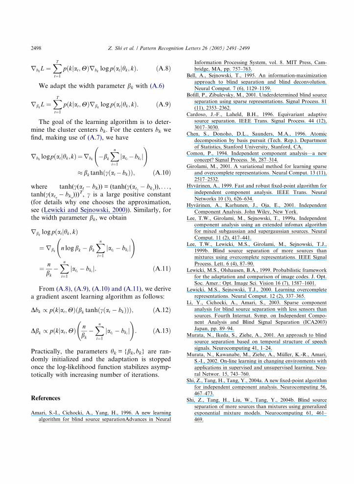
2498 Z. Shi et al. / Pattern Recognition Letters 26 (2005) 2491–2499

rbkL ¼XTt¼1

pðkjat;HÞrbk log pðatjhk; kÞ. ðA:8Þ

We adapt the width parameter bk with (A.6)

rbk L ¼XTt¼1

pðkjat;HÞrbk log pðatjhk; kÞ. ðA:9Þ

The goal of the learning algorithm is to deter-

mine the cluster centers bk. For the centers bk we

find, making use of (A.7), we have

rbk logpðatjhk;kÞ¼rbk �bk

Xni¼1

jati �bki j !

bk tanhðcðat�bkÞÞ; ðA:10Þ

where tanh(c(at � bk)) = (tanh(c(at1 � bk1)), . . . ,tanh(c(atn � bkn)))

T, c is a large positive constant

(for details why one chooses the approximation,see (Lewicki and Sejnowski, 2000)). Similarly, for

the width parameter bk, we obtain

rbk log pðatjhk; kÞ

¼ rbk n log bk � bk

Xni¼1

jati � bki j !

¼ nbk

�Xni¼1

jati � bki j. ðA:11Þ

From (A.8), (A.9), (A.10) and (A.11), we derive

a gradient ascent learning algorithm as follows:

Dbk / pðkjat;HÞðbk tanhðcðat � bkÞÞÞ; ðA:12Þ

Dbk / pðkjat;HÞ nbk

�Xni¼1

jati � bki j !

. ðA:13Þ

Practically, the parameters hk = {bk,bk} are ran-

domly initialized and the adaptation is stopped

once the log-likelihood function stabilizes asymp-

totically with increasing number of iterations.

References

Amari, S.-I., Cichocki, A., Yang, H., 1996. A new learning

algorithm for blind source separationAdvances in Neural

Information Processing System, vol. 8. MIT Press, Cam-

bridge, MA, pp. 757–763.

Bell, A., Sejnowski, T., 1995. An information-maximization

approach to blind separation and blind deconvolution.

Neural Comput. 7 (6), 1129–1159.

Bofill, P., Zibulevsky, M., 2001. Underdetermined blind source

separation using sparse representations. Signal Process. 81

(11), 2353–2362.

Cardoso, J.-F., Laheld, B.H., 1996. Equivariant adaptive

source separation. IEEE Trans. Signal Process. 44 (12),

3017–3030.

Chen, S., Donoho, D.L., Saunders, M.A., 1996. Atomic

decomposition by basis pursuit (Tech. Rep.). Department

of Statistics, Stanford University, Stanford, CA.

Comon, P., 1994. Independent component analysis—a new

concept? Signal Process. 36, 287–314.

Girolami, M., 2001. A variational method for learning sparse

and overcomplete representations. Neural Comput. 13 (11),

2517–2532.

Hyvarinen, A., 1999. Fast and robust fixed-point algorithm for

independent component analysis. IEEE Trans. Neural

Networks 10 (3), 626–634.

Hyvarinen, A., Karhunen, J., Oja, E., 2001. Independent

Component Analysis. John Wiley, New York.

Lee, T.W., Girolami, M., Sejnowski, T., 1999a. Independent

component analysis using an extended infomax algorithm

for mixed subgaussian and supergaussian sources. Neural

Comput. 11 (2), 417–441.

Lee, T.W., Lewicki, M.S., Girolami, M., Sejnowski, T.J.,

1999b. Blind source separation of more sources than

mixtures using overcomplete representations. IEEE Signal

Process. Lett. 6 (4), 87–90.

Lewicki, M.S., Olshausen, B.A., 1999. Probabilistic framework

for the adaptation and comparison of image codes. J. Opt.

Soc. Amer.: Opt. Image Sci. Vision 16 (7), 1587–1601.

Lewicki, M.S., Sejnowski, T.J., 2000. Learning overcomplete

representations. Neural Comput. 12 (2), 337–365.

Li, Y., Cichocki, A., Amari, S., 2003. Sparse component

analysis for blind source separation with less sensors than

sources. Fourth Internat. Symp. on Independent Compo-

nent Analysis and Blind Signal Separation (ICA2003)

Japan, pp. 89–94.

Murata, N., Ikeda, S., Ziehe, A., 2001. An approach to blind

source separation based on temporal structure of speech

signals. Neurocomputing 41, 1–24.

Murata, N., Kawanabe, M., Ziehe, A., Muller, K.-R., Amari,

S.-I., 2002. On-line learning in changing environments with

applications in supervised and unsupervised learning. Neu-

ral Networ. 15, 743–760.

Shi, Z., Tang, H., Tang, Y., 2004a. A new fixed-point algorithm

for independent component analysis. Neurocomputing 56,

467–473.

Shi, Z., Tang, H., Liu, W., Tang, Y., 2004b. Blind source

separation of more sources than mixtures using generalized

exponential mixture models. Neurocomputing 61, 461–

469.

Z. Shi et al. / Pattern Recognition Letters 26 (2005) 2491–2499 2499

Zhong, M., Tang, H., Chen, H., Tang, Y., 2004. An EM

algorithm for learning sparse and overcomplete representa-

tions. Neurocomputing 57, 469–476.

Zibulevsky, M., Pearlmutter, B.A., 2001. Blind source separa-

tion by sparse decomposition in a signal dictionary. Neural

Comput. 13 (4), 863–882.

Zibulevsky, M., Pearlmutter, B.A., Bofill, P., Kisilev, P., 2001.

Blind source separation by sparse decomposition in a signal

dictionary. In: Robers, S., Everson, R. (Eds.), Independent

Component Analysis: Principles and Practice. Cambridge

University Press.