arX

iv:g

r-qc

/041

0056

v1 1

3 O

ct 2

004

Bianchi type I universe with viscous fluid: A qualitative analysis

Bijan Saha and V. Rikhvitsky

Laboratory of Information TechnologiesJoint Institute for Nuclear Research, Dubna

141980 Dubna, Moscow region, Russia∗

(Dated: February 7, 2008)

The nature of cosmological solutions for a homogeneous, anisotropic Universe given bya Bianchi type-I (BI) model in the presence of a CosmologicalconstantΛ is investigated bytaking into account dissipative process due to viscosity. The system in question is thoroughlystudied both analytically and numerically. It is shown the viscosity, as well as theΛ termexhibit essential influence on the character of the solutions. In particular a negativeΛ givesrise to an ever-expanding Universe, whereas, a suitable choice of initial conditions plus apositiveΛ can result in a singularity-free oscillatory mode of expansion. For some specialcases it is possible to obtain oscillations in the exponential mode of expansion of the BImodel even with a negativeΛ, where oscillations arise by virtue of viscosity.

PACS numbers: 03.65.Pm, 04.20.Jb and 04.20.Ha

Keywords: Bianchi type I (BI) model, Cosmological constant, viscous fluid

I. INTRODUCTION

The investigation of relativistic cosmological models usually has the energy momentum tensorof matter generated by a perfect fluid. To consider more realistic models one must take intoaccount the viscosity mechanisms, which have already attracted the attention of many researchers.Misner [1, 2] suggested that strong dissipative due to the neutrino viscosity may considerablyreduce the anisotropy of the blackbody radiation. Viscosity mechanism in cosmology can explainthe anomalously high entropy per baryon in the present universe [3, 4]. Bulk viscosity associatedwith the grand-unified-theory phase transition [5] may leadto an inflationary scenario [6, 7, 8].

A uniform cosmological model filled with fluid which possesses pressure and second (bulk)viscosity was developed by Murphy [9]. The solutions that hefound exhibit an interesting featurethat the big bang type singularity appears in the infinite past. Exact solutions of the isotropichomogeneous cosmology for open, closed and flat universe have been found by Santos et al [10],with the bulk viscosity being a power function of energy density.

The nature of cosmological solutions for homogeneous Bianchi type I (BI) model was inves-tigated by Belinsky and Khalatnikov [11] by taking into account dissipative process due to vis-cosity. They showed that viscosity cannot remove the cosmological singularity but results in aqualitatively new behavior of the solutions near singularity. They found the remarkable propertythat during the time of thebig bang matter is created by the gravitational field. BI solutions incaseof stiff matter with a shear viscosity being the power function of of energy density were obtainedby Banerjee [12], whereas BI models with bulk viscosity (η) that is a power function of energydensityε and when the universe is filled with stiff matter were studiedby Huang [13]. The effect

∗Electronic address: saha@thsun1.jinr.ru; URL:http://thsun1.jinr.ru/~saha/

2 Bijan Saha and V. Rikhvitsky rykh.tex February 7, 2008

of bulk viscosity, with a time varying bulk viscous coefficient, on the evolution of isotropic FRWmodels was investigated in the context of open thermodynamics system was studied by Desikan[14]. This study was further developed by Krori and Mukherjee [15] for anisotropic Bianchi mod-els. Cosmological solutions with nonlinear bulk viscositywere obtained in [16]. Models with bothshear and bulk viscosity were investigated in [17, 18].

Though Murphy [9] claimed that the introduction of bulk viscosity can avoid the initial singu-larity at finite past, results obtained in [19] show that, it is, in general, not valid, since for somecases big bang singularity occurs in finite past.

We studied a self-consistent system of the nonlinear spinorand/or scalar fields in a BI spacetimein presence of a perfect fluid and aΛ term [20, 21] in order to clarify whether the presence of a sin-gular point an inherent property of the relativistic cosmological models or is it only a consequenceof specific simplifying assumptions underlying these models? Recently we have considered a sys-tem of nonlinear spinor field in a BI Universe filled with viscous fluid [22]. Since the viscous fluiditself presents a growing interest, we have studied the influence of viscous fluid andΛ term in theevolution of the BI Universe [23]. In that paper we consider only some special cases those allowexact solutions. In this paper along with those special cases we study some general cases, giving aqualitative analysis of the system of equations. We also perform some numerical calculations andcompare the results obtained with those given in some pioneering papers in this field, e.g. [11]

II. DERIVATION OF BASIC EQUATIONS

Using the variational principle in this section we derive the fundamental equations for the grav-itational field from the action (2.1) :

S (g;ε) =∫

L√−gdΩ (2.1)

withL = Lgrav. +Lvf . (2.2)

The gravitational part of the Lagrangian (2.2)Lgrav. is given by a Bianchi type-I metric,whereas the termLvf describes a viscous fluid.

We also write the expressions for the metric functions explicitly in terms of the volume scaleτ defined bellow (2.18). Defining Hubble constant (2.28) in analogy with a flat Friedmann-Robertson-Walker (FRW) Universe, we also derive the systemof equations forτ, H andε, with εbeing the energy density of the viscous fluid, which plays thecentral role here.

A. The gravitational field

As a gravitational field we consider the Bianchi type I (BI) cosmological model. It is the sim-plest model of anisotropic universe that describes a homogeneous and spatially flat space-timeand if filled with perfect fluid with the equation of statep = ζ ε, ζ < 1, it eventually evolvesinto a FRW universe [24]. The isotropy of present-day universe makes BI model a prime candi-date for studying the possible effects of an anisotropy in the early universe on modern-day dataobservations. In view of what has been mentioned above we choose the gravitational part of theLagrangian (2.2) in the form

Lg =R2κ

, (2.3)

Bianchi type I universe with viscous fluid 3

whereR is the scalar curvature,κ = 8πG being the Einstein’s gravitational constant. The gravita-tional field in our case is given by a Bianchi type I (BI) metric

ds2 = dt2−a2dx2−b2dy2− c2dz2, (2.4)

with a, b, c being the functions of timet only. Here the speed of light is taken to be unity.

B. Viscous fluid

The influence of the viscous fluid in the evolution of the Universe is performed by means of itsenergy momentum tensor, which acts as the source of the corresponding gravitational field. Thereason for writingLvf in (2.2) is to underline that we are dealing with a self-consistent system.The energy momentum tensor of a viscous field has the form

T νµ (m) = (ε + p′)uµuν − p′δ ν

µ +ηgνβ [uµ;β +uβ :µ −uµuαuβ ;α −uβ uαuµ;α ], (2.5)

where

p′ = p− (ξ − 23

η)uµ;µ . (2.6)

Hereε is the energy density,p - pressure,η andξ are the coefficients of shear and bulk viscosity,respectively. Note that the bulk and shear viscosities,η andξ , are both positively definite, i.e.,

η > 0, ξ > 0. (2.7)

They may be either constant or function of time or energy, such as :

η = |A|εα , ξ = |B|εβ . (2.8)

The pressurep is connected to the energy density by means of a equation of state. In this reportwe consider the one describing a perfect fluid :

p = ζ ε, ζ ∈ (0,1]. (2.9)

Note that hereζ 6= 0, since for dust pressure, hence temperature is zero, that results in vanishingviscosity.

In a comoving system of reference such thatuµ = (1, 0, 0, 0) we have

T 00(m) = ε, (2.10a)

T 11(m) = −p′ +2η

aa, (2.10b)

T 22(m) = −p′ +2η

bb, (2.10c)

T 33(m) = −p′ +2η

cc. (2.10d)

Let us introduce the dynamical scalars such as the expansionand the shear scalar as usual

θ = uµ;µ , σ2 =

12

σµν σ µν , (2.11)

4 Bijan Saha and V. Rikhvitsky rykh.tex February 7, 2008

where

σµν =12

(

uµ;αPαν +uν;αPα

µ

)

− 13

θPµν . (2.12)

HereP is the projection operator obeying

P2 = P. (2.13)

For the space-time with signature(+, −, −, −) it has the form

Pµν = gµν −uµ uν , Pµν = δ µ

ν −uµuν . (2.14)

For the BI metric the dynamical scalar has the form

θ =aa

+bb

+cc

=ττ, (2.15)

and

2σ2 =a2

a2 +b2

b2 +c2

c2 −13

θ2. (2.16)

C. Field equations and their solutions

Variation of (2.1) with respect to metric tensorgµν gives the Einstein’s field equation. Inaccount of theΛ-term for the BI space-time (2.4) this system of equations can be rewritten as

bb

+cc

+bb

cc

= κT 11 −Λ, (2.17a)

cc

+aa

+cc

aa

= κT 22 −Λ, (2.17b)

aa

+bb

+aa

bb

= κT 33 −Λ, (2.17c)

aa

bb

+bb

cc

+cc

aa

= κT 00 −Λ, (2.17d)

where over dot means differentiation with respect tot andT µν is the energy-momentum tensor of

a viscous fluid given above (2.10).

1. Expressions for the metric functions

To write the metric functions explicitly, we define a new timedependent functionτ(t)

τ = abc =√−g, (2.18)

which is indeed the volume scale of the BI space-time.Let us now solve the Einstein equations. In account of (2.10)from (2.17a), (2.17b), and (2.17c)

one finds the following expressions for the metric functionsexplicitly [23]

a(t) = A1τ1/3exp

[

(B1/3)

∫

e−2κ∫

ηdt

τdt

]

, (2.19a)

b(t) = A2τ1/3exp

[

(B2/3)∫

e−2κ∫

ηdt

τdt

]

, (2.19b)

c(t) = A3τ1/3exp

[

(B3/3)

∫

e−2κ∫

ηdt

τdt

]

, (2.19c)

Bianchi type I universe with viscous fluid 5

where the constantsAi’s andBi’s obey the following relations

A1A2A3 = 1,

B1 +B2+B3 = 0.

Thus, the metric functions are found explicitly in terms ofτ and viscosity.As one sees from (2.19a), (2.19b) and (2.19c), forτ = tn with n > 1 the exponent tends to unity

at larget, and the anisotropic model becomes isotropic one.

2. Singularity analysis

Let us now investigate the existence of singularity (singular point) of the gravitational case,which can be done by investigating the invariant characteristics of the space-time. In generalrelativity these invariants are composed from the curvature tensor and the metric one. In a 4DRiemann space-time there are 14 independent invariants. Instead of analyzing all 14 invariants,one can confine this study only in 3, namely the scalar curvature I1 = R, I2 = RµνRµν , and theKretschmann scalarI3 = Rαβ µν Rαβ µν [25, 26].. At any regular space-time point, these threeinvariantsI1, I2, I3 should be finite. Let us rewrite these invariants in detail.

For the Bianchi I metric one finds the scalar curvature

I1 = R = −2( a

a+

bb

+cc

+aa

bb

+bb

cc

+cc

aa

)

. (2.20)

Since the Ricci tensor for the BI metric is diagonal, the invariant I2 = Rµν Rµν ≡ Rνµ Rµ

ν is a sumof squares of diagonal components of Ricci tensor, i.e.,

I2 =[

(

R00

)2+(

R11

)2+(

R22

)2+(

R33

)2]

. (2.21)

Analogically, for the Kretschmann scalar in this case we haveI3 = Rµναβ Rαβ

µν , a sum of squared

components of all nontrivialRµνµν , which can be written as

I3 = 4

[

(

R0101

)2+(

R0202

)2+(

R0303

)2+(

R1212

)2+(

R2323

)2+(

R3131

)2]

= 4[( a

a

)2+( b

b

)2+( c

c

)2+( a

abb

)2+( b

bcc

)2+( c

caa

)2]

. (2.22)

Let us now express the foregoing invariants in terms ofτ. From Eqs. (2.19) we have

ai = Aiτ1/3exp

(

(Bi/3)

∫

e−2κ∫

ηdt

τ(t)dt

)

, (2.23a)

ai

ai=

τ +Bie−2κ∫

ηdt

3τ(i = 1,2,3,), (2.23b)

ai

ai=

3ττ −2τ2− τBie−2κ∫

ηdt −6κητBie−2κ∫

ηdt +B2i e−4κ

∫

ηdt

9τ2 , (2.23c)

6 Bijan Saha and V. Rikhvitsky rykh.tex February 7, 2008

i.e., the metric functionsa,b,c and their derivatives are in functional dependence withτ. FromEqs. (2.23) one can easily verify that [23]

I1 ∝1τ2 , I2 ∝

1τ4 , I3 ∝

1τ4 .

Thus we see that at any space-time point, whereτ = 0 the invariantsI1, I2, andI3 become infinity,hence the space-time becomes singular at this point.

D. Equations for determining τ

In the foregoing subsection we wrote the corresponding metric functions in terms of volumescaleτ. In what follows, we write the equation forτ and study it in details.

Summation of Einstein equations (2.17a), (2.17b), (2.17c)and 3 times (2.17d) gives

τ − 32

κξ τ =32

κ(

ε − p)

τ −3Λτ. (2.24)

For the right-hand-side of (2.24) to be a function ofτ only, the solution to this equation is well-known [27].

The energy-momentum conservation law, i.e.,

T νµ;ν = T ν

µ,ν +Γνρν T ρ

µ −Γρµν T ν

ρ = 0, (2.25)

in our case gives the following equation forε :

ε +ττ

ω − (ξ +43

η)τ2

τ2 +4η(κT 00 −Λ) = 0, (2.26)

whereω = ε + p, (2.27)

is the thermal function.Defining a generalized Hubble constantH :

ττ

=aa

+bb

+cc

= 3H. (2.28)

the Eqs. (2.24) and (2.26) in account of (2.10) can be rewritten as

H =κ2

(

3ξ H −ω)

−(

3H2−κε +Λ)

, (2.29a)

ε = 3H(

3ξ H −ω)

+4η(

3H2−κε +Λ)

. (2.29b)

In terms of dynamical scalarsθ andσ the system (2.29) takes a very simple form

θ =3κ2

(

ξ θ −ω)

−3σ2, (2.30a)

ε = θ(

ξ θ −ω)

+4ησ2. (2.30b)

Note that the Eqs. (2.30) coincide with the ones given in [12].

Bianchi type I universe with viscous fluid 7

III. QUALITATIVE ANALYSIS AND SOME SPECIAL SOLUTIONS

In this subsection we simultaneously solve the system of equations forτ, H, and ε. It isconvenient to rewrite the Eqs. (2.28) and (2.29) as a single system :

τ = 3Hτ, (3.1a)

H =κ2

(

3ξ H −ω)

−(

3H2−κε +Λ)

, (3.1b)

ε = 3H(

3ξ H −ω)

+4η(

3H2−κε +Λ)

. (3.1c)

In account of (2.27),(2.8) and (2.9) the Eqs. (3.1) now can berewritten as

τ = 3Hτ, (3.2a)

H =κ2

(

3Bεβ H − (1+ζ )ε)

−(

3H2−κε +Λ)

, (3.2b)

ε = 3H(

3Bεβ H − (1+ζ )ε)

+4Aεα(3H2−κε +Λ)

. (3.2c)

The system (3.1) have been extensively studied in literature either partially [9, 12, 13] or ingeneral [11]. In what follows, we consider the system (3.1) for some special choices of the param-eters.

A. Qualitative analysis

Following Belinski and Khalatnikov [11] let us now study thecharacters of the solutions of thedynamical system (3.1) or (3.2). We first rewrite the system (3.1), namely (3.1b) and (3.1c) in thematrix form :

(

Hε

)

=

(

κ/2 −13H 4η

)(

3ξ H −ω3H2−κε +Λ

)

. (3.3)

Note that unlike the system studied by Belinski and Khalatnikov the system in consideration con-tains a Cosmological constantΛ.

1. General properties of the system

Easy to note that the solutions cannot intersect the axisε = 0, sinceε|ε=0 = 0, as well as theparabola

3H2−κε +Λ = 0, (3.4)

as far as (3.4) is itself the integral curve. Thus, starting from the point(H,ε) = (+∞,0), thesolutions cannot enter into the ”prohibited region” insidethe parabola (3.4). Whether they mayachieveH < 0 depends on the value ofΛ. Note that, unlike the system considered by Belinskiet.al [11] the system in this report contains a nonzeroΛ term.

2. Critical points of the dynamical system

a) By virtu of linear independence of the columns of the matrix of the Eq. (3.3) the criticalpoints are the solutions of the equations

3ξ H −ω = 0, (3.5a)

3H2−κε +Λ = 0. (3.5b)

8 Bijan Saha and V. Rikhvitsky rykh.tex February 7, 2008

i.e., they necessarily lie on the parabola (3.4). Solutionsto the system (3.5) will be the roots of theequation

3κB2ε1+2β − (1+ζ )2ε2 − 3ΛB2ε2β = 0, (3.6a)

H =1+ζ3B

ε1−β . (3.6b)

The quantity of the positive roots of the Eq. (3.6) accordingto Cartesian law is equal to thenumber of changes of sign of coefficients of equations or lessthan that by an even number. So, for

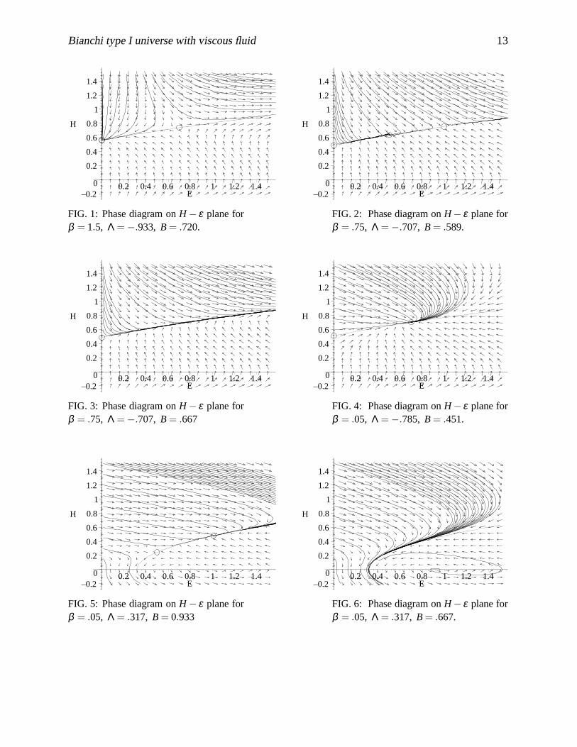
Λ < 0 and 1/2 < β < 1 (Fig.2,Fig.3)or Λ > 0 and β < 1/2 (Fig.5,Fig.6)

the number of roots is either 2 or zero. For the remaining cases

Λ < 0 and β > 1 (Fig.1),Λ < 0 and β < 1/2 (Fig.4),Λ > 0 and β > 1/2 (Fig.7)

there exists only one root. The corresponding pictures of the phase curves are given in figurescited above. The critical points are denoted by small circles. Note that here we consider the casewith η = 0, i.e.,A = 0. In case ifη 6= 0, with the increase ofA the separatrix of the saddle tilts(inclines) to the left. Since the overall picture forA 6= 0 remains qualitatively unaltered, we onlyshow the corresponding phase portrait for two cases, namelyFig. 8 corresponds to Fig. 1, Fig.9 corresponds to Fig. 4. Note that for numerical calculations we setκ = 1, ζ = 0.333 (if notmentioned otherwise). In the Figs. 1 - 7η is taken to be zero. Note that in the Figs.E andT standfor ε andτ, respectively.

Since, the equation forε only containsη, the energy density for nontrivialη undergoes essen-tial changes, whereasH andτ remain virtually unchanged.

The types of critical points lying on the integral curve alternate: . . . saddle, attracting knot,saddle. . .. So it is sufficient to consider the case with maximum number of roots. Taking intoaccount the Eqs. (3.1c) and (3.4) let us now calculate

limε→+∞

ε3Hε

= limε→+∞

3Bεβ√κε −Λ− ε(1+ζ )

ε

= 3B√

κε(2β−1) −Λε−2− (1+ζ ) =

−(1+ζ ) < 0, β < 1/2,

+∞ > 0, β > 1/2.(3.7)

So, the latest critical point forβ < 1/2 is attracting knot and forβ > 1/2 is saddle.b) It is obvious that if Lambda ≤ 0 the points of intersection of the boundary are the critical

points

H = ±√

−Λ/3, (3.8a)ε = 0. (3.8b)

c) For H < 0 there may exist critical points , if the columns of the matrix of (3.3) are linearlydependent. In that case the critical points are the roots of the equation

3κ(ζ −1)ε +6κ2ABεα+β +8κ2A2ε2α +6Λ = 0, (3.9)

Bianchi type I universe with viscous fluid 9

and

H = −23

κAεα . (3.10)

In case ofη = 0 the roots of the characteristic equation∣

∣

∣

D(H, ε)

D(H, ε)−µ

∣

∣

∣= 0, (3.11)

are

µ1,2 =3κξ ±

√

9κ2ξ 2−48Λ(1+ζ )

4. (3.12)

The critical point (H, ε) = (0, 2Λ/[κ(1−ζ )]) is of type divergent focus ifΛ > 9κ2ξ 2/[48(1+ζ )] or divergent knot ifΛ < 9κ2ξ 2/[48(1+ζ )] .

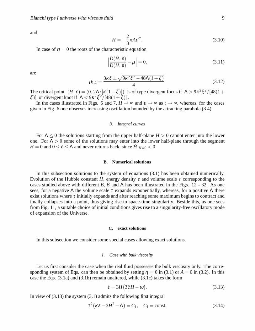
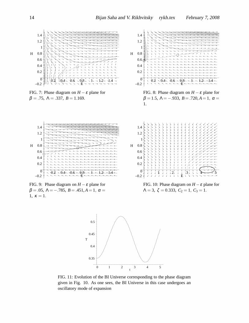
In the cases illustrated in Figs. 5 and 7,H → ∞ andε → ∞ ast → ∞, whereas, for the casesgiven in Fig. 6 one observes increasing oscillation boundedby the attracting parabola (3.4).

3. Integral curves

For Λ ≤ 0 the solutions starting from the upper half-planeH > 0 cannot enter into the lowerone. ForΛ > 0 some of the solutions may enter into the lower half-plane through the segmentH = 0 and 0≤ ε ≤ Λ and never returns back, sinceH|H=0 < 0.

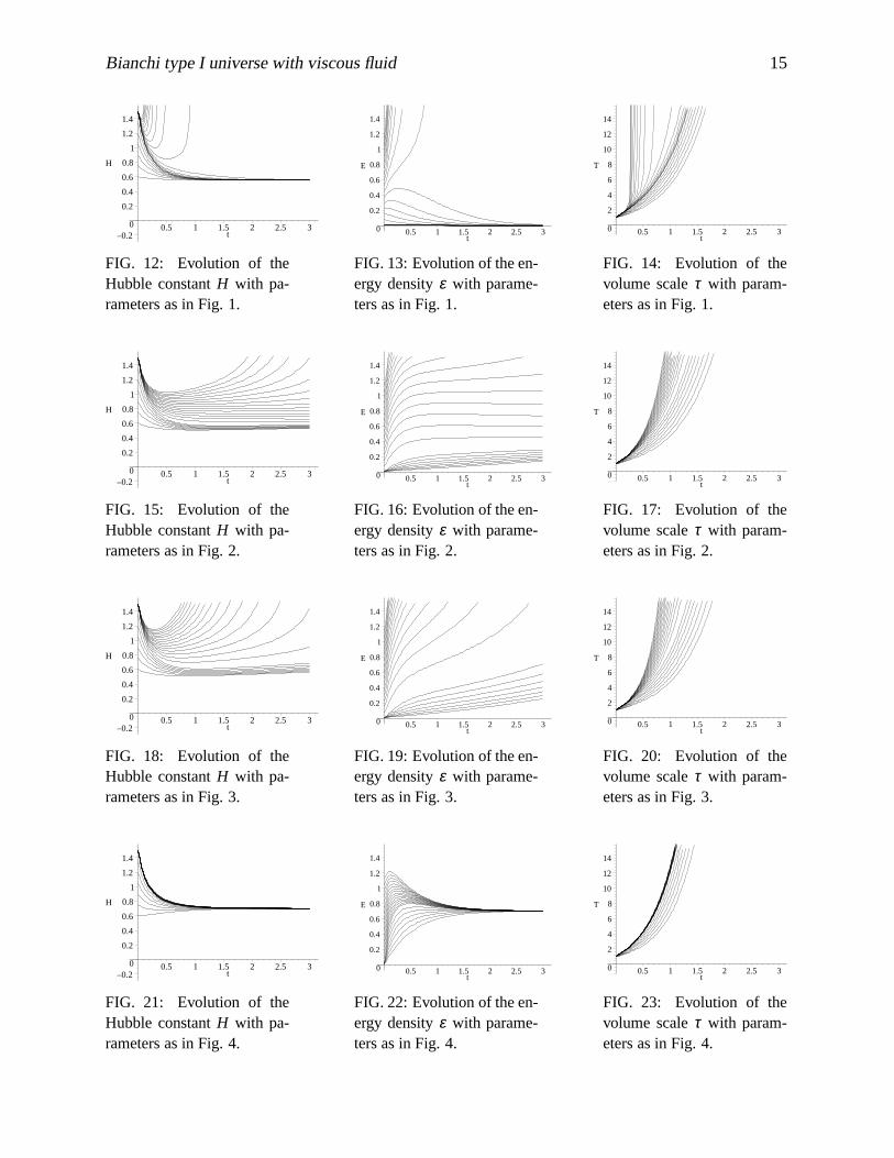
B. Numerical solutions

In this subsection solutions to the system of equations (3.1) has been obtained numerically.Evolution of the Hubble constantH, energy densityε and volume scaleτ corresponding to thecases studied above with differentB, β andΛ has been illustrated in the Figs. 12 - 32. As onesees, for a negativeΛ the volume scaleτ expands exponentially, whereas, for a positiveΛ thereexist solutions whereτ initially expands and after reaching some maximum begins tocontract andfinally collapses into a point, thus giving rise to space-time singularity. Beside this, as one seesfrom Fig. 11, a suitable choice of initial conditions gives rise to a singularity-free oscillatory modeof expansion of the Universe.

C. exact solutions

In this subsection we consider some special cases allowing exact solutions.

1. Case with bulk viscosity

Let us first consider the case when the real fluid possesses thebulk viscosity only. The corre-sponding system of Eqs. can then be obtained by settingη = 0 in (3.1) orA = 0 in (3.2). In thiscase the Eqs. (3.1a) and (3.1b) remain unaltered, while (3.1c) takes the form

ε = 3H(

3ξ H −ω)

. (3.13)

In view of (3.13) the system (3.1) admits the following first integral

τ2(κε −3H2−Λ)

= C1, C1 = const. (3.14)

10 Bijan Saha and V. Rikhvitsky rykh.tex February 7, 2008

The relation (3.14) can be interpreted as follows. At the initial stage of evolution the volume scaleτ tends to zero, while, the energy densityε tends to infinity. Since the Hubble constant and theΛterm are finite, the relation (3.14) is in correspondence with the current line of thinking. Let us seewhat happens as the Universe expands. It is well known that with the expansion of the Universe,i.e., with the increase ofτ, the energy densityε decreases. Suppose at some stage of expansionτ → ∞, henceε → 0. Then from (3.14) follows that at the stage in question

3H2+Λ → 0. (3.15)

In case ofΛ = 0, we findH = 0, i.e., in absence of aΛ term, onceτ → ∞, the process of evolutionis terminated. As one sees from (3.15), for theH to make any sense, theΛ term should be negative.In presence of a negativeλ term the evolution process of the Universe never comes to a halt, iteither expands further or begin to contract depending on thesign ofH = ±

√

−Λ/3, Λ < 0.Let us now consider the case when the bulk viscosity is inverse proportional to expansion, i.e.,

ξ θ = C2, C2 = const. (3.16)

Now keeping into mind thatθ = τ/τ = 3H, also the relations (3.1a), (2.27) and (2.9) the Eq.(3.13) can be written as

εC2− (1+ζ )ε

=ττ. (3.17)

From the Eq. (3.17) one finds

ε =1

1+ζ[

C2+C3τ−(1+ζ )]

, (3.18)

with C3 being some arbitrary constant. Further, insertingε from (3.18) into (2.24) one finds theexpression forτ explicitly.

Taking into account the equation of state (2.9) in view of (3.16) and (3.18), the Eq. (2.24)admits the following solution in quadrature :

∫

dτ√

C22 +C0

0τ2+C11τ1−ζ

= t + t0, (3.19)

whereC22 andt0 are some constants. Further we sett0 = 0. Here,C0

0 = 3κC2/(1+ ζ )−3Λ andC1

1 = 3κC3/(1+ζ ). As one sees,C00 is negative for

Λ > κC2/(1+ζ ). (3.20)

It means that for a positiveΛ obeying (3.20) (we assume that the constantC2 is a positive quantity)τ should be bound from above as well. It should be noted that fora suitable choice ofC2

2 andτ0(the initial value ofτ), it is possible to obtain oscillatory mode of expansion with τ being alwayspositive, i.e., a singularity free evolution of the Universe. The phase portrait of the(H, ε) planeand the evolution of the BI Universe corresponding to this portrait allowing oscillatory solutionsare given in Figs. 10 and 11.

As a second example we consider the case, whenζ = 1. From (3.19) one then finds

τ(t) =(

exp(√

C00 t)−C2

2 exp(√

C00 t))

/(2√

C00), C0

0 > 0, (3.21a)

τ(t) = (C22/√

|C00|)sin(

√

|C00| t). C0

0 < 0. (3.21b)

Bianchi type I universe with viscous fluid 11

Taking into account thatC00 > 0 for any non-positiveΛ, from (3.21a) one sees that, in case of

Λ ≤ 0 the Universe may be infinitely large (there is no upper bound), which is in line with theconclusion made above. On the other hand,C0

0 may be negative only for some positive value ofΛ. Thus we see that a positiveΛ can generate a oscillatory mode of expansion of a BI Universe.The oscillation takes place around the critical point(H, ε) = (0, (2Λ−κC2)/[κ(1−ζ )]) havingthe type of cycle under the conditionΛ > κC2/(1+ζ ). It was shown in [20, 21] that in case of aperfect fluid a positiveΛ always invokes oscillations in the model, whereas, in the present modelwith viscous fluid, it is the case only whenΛ obeys (3.20). Unlike the case with radiation whereBI admits a singularity-free oscillatory mode of evolution, here, in case of a stiff matter one findsthe BI Universe first expands, reaches its maximum and then contracts into a point, thus givingrise to space-time singularity.

2. Case with shear and bulk viscosity

Let us now consider the general case with the shear viscosityη being proportional to the ex-pansion, i.e.,

η ∝ θ = 3H. (3.22)

We will consider the case when

η = − 32κ

H. (3.23)

In this case from (3.1b) and (3.1c) one easily find

3H2 = κε +C4, C4 = const. (3.24)

From (3.24) it follows that at the initial state of expansion, whenε is large, the Hubble constantis also large and with the expansion of the UniverseH decreases as doesε. Inserting the relation(3.24) into the Eqs. (3.1b) one finds

∫

dH√AH2 +BH +C

= t, (3.25)

where,A = −1.5(1+ζ ), B = 1.5κξ , andC = 0.5C4(ζ −1)−Λ. For ξ being a constant, (3.25)admits sinusoidal solution, i.e.,H evolves oscillatory. Further, from (3.1a) one finds the expressionfor τ, which is exponential one accompanied by a sinusoidal mode [23].

IV. CONCLUSION

We investigated the cosmological solutions to the equations of General Relativity for the ho-mogeneous anisotropic Bianchi type I model by taking into account dissipative processes dueto viscosity and Cosmological constant (Λ term). A detailed analysis showed that the viscosity,as well as theΛ term exhibit essential influence on the character of the solutions. The classifi-cation of the solutions was pursued for the viscosity being some power law of energy density,namely,η = Aεα andξ = Bεβ . It was noticed that forΛ < 0 the Universe expands forever witha logarithmic velocityH, which, depending on the viscosity either becomes constantor increasesinfinitely. In the process behavior of the energy densityε is analogous to that ofH except the casewhenε → 0. ForΛ > 0, beside the variants mentioned above, there exists few other possibilities:contraction of the Universe into a point, thus giving rise toa space-time singularity; a regime ofincreasing oscillation corresponding to suitable initialconditions. It was also noticed that a special

12 Bijan Saha and V. Rikhvitsky rykh.tex February 7, 2008

case withΛ > 0, η = 0 andξ H = const. the model admits a singularity-free oscillatory mode ofexpansion.

[1] W. Misner, Nature214, 40 (1967).[2] W. Misner, Astrophys. J.151, 431 (1968).[3] S. Weinberg, Astrophys. J.168, 175 (1972).[4] S. Weinberg,Gravitation and Cosmology (New York, Wiley, 1972)[5] P. Langacker, Phys. rep.72, 185 (1981).[6] L. Waga, R.C. Falcan, and R. Chanda, Phys. Rev. D33, 1839 (1986).[7] T. Pacher, J.A. Stein-Schabas, and M.S. Turner, Phys. Rev. D 36, 1603 (1987).[8] Alan Guth, Phys. Rev. D23, 347 (1981).[9] G.L. Murphy, Phys. Rev. D8, 4231 (1973).

[10] N.O. Santos, R.S. Dias, and A. Banerjee, J. Math. Phys.26, 876 (1985).[11] V.A. Belinski and I.M. Khalatnikov, Soviet Journal JETP69, 401, (1975).[12] A. Banerjee, S.B. Duttachoudhury, and A.K. Sanyal, J. Math. Phys.26, 3010 (1985).[13] W. Huang, J. Math. Phys.31, 1456 (1990).[14] K. Desikan, Gen. Relativ. Gravit.29, 435 (1997).[15] K.D. Krori and A. Mukherjee, Gen. Relativ. Gravit.32, 1429 (2000).[16] L.P. Chimento, A.S. Jacubi, V. M`endez, and R. Maartens, Class. Quantum Grav.14, 3363 (1997).[17] H. van Elst, P. Dunsby, and R. Tavakol, Gen. Relativ. Gravit. 27, 171 (1995).[18] V.R. Gavrilov, V.N. Melnikov, and R. Triay, Class. Quantum Grav.14, 2203 (1997).[19] J.D. Barrow, Nuc. Phys. B310, 743 (1988).[20] Bijan Saha, Phys. Rev. D64, 123501 (2001).[21] Bijan Saha and Todor Boyadjiev, Phys. Rev. D69, 124010 (2004).[22] Bijan Saha, ”Nonlinear spinor field in Bianchi type-I Universe filled with viscous fluid: some special

solutions” (to appear in Romanian Report of Physics in 2005).[23] Bijan Saha, ”Bianchi type I Universe with viscous fluid”[arXiv: gr-qc/0409104].[24] K.C. Jacobs, Astrophys. J.153, 661 (1968).[25] K.A. Bronnikov and G.N. Shikin, Gravitation Cosmol.7, 231 (2001).[26] S. Fay, Class. Quantum Grav.17, 2663 (2000).[27] E. Kamke, Differentialgleichungen losungsmethoden und losungen (Akademische Verlagsge-

sellschaft, Leipzig, 1957).

Bianchi type I universe with viscous fluid 13

–0.20

0.2

0.4

0.6

0.8

1

1.2

1.4

H

0.2 0.4 0.6 0.8 1 1.2 1.4 E –0.2

0

0.2

0.4

0.6

0.8

1

1.2

1.4

H

0.2 0.4 0.6 0.8 1 1.2 1.4 E

FIG. 1: Phase diagram onH − ε plane forβ = 1.5, Λ = −.933, B = .720.

FIG. 2: Phase diagram onH − ε plane forβ = .75, Λ = −.707, B = .589.

–0.20

0.2

0.4

0.6

0.8

1

1.2

1.4

H

0.2 0.4 0.6 0.8 1 1.2 1.4 E –0.2

0

0.2

0.4

0.6

0.8

1

1.2

1.4

H

0.2 0.4 0.6 0.8 1 1.2 1.4 E

FIG. 3: Phase diagram onH − ε plane forβ = .75, Λ = −.707, B = .667

FIG. 4: Phase diagram onH − ε plane forβ = .05, Λ = −.785, B = .451.

–0.20

0.2

0.4

0.6

0.8

1

1.2

1.4

H

0.2 0.4 0.6 0.8 1 1.2 1.4 E –0.2

0

0.2

0.4

0.6

0.8

1

1.2

1.4

H

0.2 0.4 0.6 0.8 1 1.2 1.4 E

FIG. 5: Phase diagram onH − ε plane forβ = .05, Λ = .317, B = 0.933

FIG. 6: Phase diagram onH − ε plane forβ = .05, Λ = .317, B = .667.

14 Bijan Saha and V. Rikhvitsky rykh.tex February 7, 2008

–0.20

0.2

0.4

0.6

0.8

1

1.2

1.4

H

0.2 0.4 0.6 0.8 1 1.2 1.4 E –0.2

0

0.2

0.4

0.6

0.8

1

1.2

1.4

H

0.2 0.4 0.6 0.8 1 1.2 1.4 E

FIG. 7: Phase diagram onH − ε plane forβ = .75, Λ = .337, B = 1.169.

FIG. 8: Phase diagram onH − ε plane forβ = 1.5, Λ =−.933, B = .720,A = 1, α =

1.

–0.20

0.2

0.4

0.6

0.8

1

1.2

1.4

H

0.2 0.4 0.6 0.8 1 1.2 1.4 E –0.2

0

0.2

0.4

0.6

0.8

1

1.2

1.4

H

1 2 3 4 5 E

FIG. 9: Phase diagram onH − ε plane forβ = .05, Λ =−.785, B = .451,A = 1, α =

1, κ = 1.

FIG. 10: Phase diagram onH −ε plane forΛ = 3, ζ = 0.333, C2 = 1, C3 = 1.

0.35

0.4

0.45

0.5

T

0 1 2 3 4 5t

FIG. 11: Evolution of the BI Universe corresponding to the phase diagramgiven in Fig. 10. As one sees, the BI Universe in this case undergoes anoscillatory mode of expansion

Bianchi type I universe with viscous fluid 15

–0.20

0.2

0.4

0.6

0.8

1

1.2

1.4

H

0.5 1 1.5 2 2.5 3t

0

0.2

0.4

0.6

0.8

1

1.2

1.4

E

0.5 1 1.5 2 2.5 3t

0

2

4

6

8

10

12

14

T

0.5 1 1.5 2 2.5 3t

FIG. 12: Evolution of theHubble constantH with pa-rameters as in Fig. 1.

FIG. 13: Evolution of the en-ergy densityε with parame-ters as in Fig. 1.

FIG. 14: Evolution of thevolume scaleτ with param-eters as in Fig. 1.

–0.20

0.2

0.4

0.6

0.8

1

1.2

1.4

H

0.5 1 1.5 2 2.5 3t

0

0.2

0.4

0.6

0.8

1

1.2

1.4

E

0.5 1 1.5 2 2.5 3t

0

2

4

6

8

10

12

14

T

0.5 1 1.5 2 2.5 3t

FIG. 15: Evolution of theHubble constantH with pa-rameters as in Fig. 2.

FIG. 16: Evolution of the en-ergy densityε with parame-ters as in Fig. 2.

FIG. 17: Evolution of thevolume scaleτ with param-eters as in Fig. 2.

–0.20

0.2

0.4

0.6

0.8

1

1.2

1.4

H

0.5 1 1.5 2 2.5 3t

0

0.2

0.4

0.6

0.8

1

1.2

1.4

E

0.5 1 1.5 2 2.5 3t

0

2

4

6

8

10

12

14

T

0.5 1 1.5 2 2.5 3t

FIG. 18: Evolution of theHubble constantH with pa-rameters as in Fig. 3.

FIG. 19: Evolution of the en-ergy densityε with parame-ters as in Fig. 3.

FIG. 20: Evolution of thevolume scaleτ with param-eters as in Fig. 3.

–0.20

0.2

0.4

0.6

0.8

1

1.2

1.4

H

0.5 1 1.5 2 2.5 3t

0

0.2

0.4

0.6

0.8

1

1.2

1.4

E

0.5 1 1.5 2 2.5 3t

0

2

4

6

8

10

12

14

T

0.5 1 1.5 2 2.5 3t

FIG. 21: Evolution of theHubble constantH with pa-rameters as in Fig. 4.

FIG. 22: Evolution of the en-ergy densityε with parame-ters as in Fig. 4.

FIG. 23: Evolution of thevolume scaleτ with param-eters as in Fig. 4.

16 Bijan Saha and V. Rikhvitsky rykh.tex February 7, 2008

–0.20

0.2

0.4

0.6

0.8

1

1.2

1.4

H

0.5 1 1.5 2 2.5 3t

0

0.2

0.4

0.6

0.8

1

1.2

1.4

E

0.5 1 1.5 2 2.5 3t

0

2

4

6

8

10

12

14

T

0.5 1 1.5 2 2.5 3t

FIG. 24: Evolution of theHubble constantH with pa-rameters as in Fig. 5.

FIG. 25: Evolution of the en-ergy densityε with parame-ters as in Fig. 5.

FIG. 26: Evolution of thevolume scaleτ with param-eters as in Fig. 5.

–0.20

0.2

0.4

0.6

0.8

1

1.2

1.4

H

0.5 1 1.5 2 2.5 3t

0

0.2

0.4

0.6

0.8

1

1.2

1.4

E

0.5 1 1.5 2 2.5 3t

0

2

4

6

8

10

12

14

T

0.5 1 1.5 2 2.5 3t

FIG. 27: Evolution of theHubble constantH with pa-rameters as in Fig. 6.

FIG. 28: Evolution of the en-ergy densityε with parame-ters as in Fig. 6.

FIG. 29: Evolution of thevolume scaleτ with param-eters as in Fig. 6.

–0.20

0.2

0.4

0.6

0.8

1

1.2

1.4

H

0.5 1 1.5 2 2.5 3t

0

0.2

0.4

0.6

0.8

1

1.2

1.4

E

0.5 1 1.5 2 2.5 3t

0

2

4

6

8

10

12

14

T

0.5 1 1.5 2 2.5 3t

FIG. 30: Evolution of theHubble constantH with pa-rameters as in Fig. 7.

FIG. 31: Evolution of the en-ergy densityε with parame-ters as in Fig. 7.

FIG. 32: Evolution of thevolume scaleτ with param-eters as in Fig. 7.