arX

iv:g

r-qc

/070

3124

v2 6

Jun

200

8

Interacting spinor and scalar fields in Bianchi type-I Universe filled withviscous fluid: exact and numerical solutions

Bijan Saha

Laboratory of Information TechnologiesJoint Institute for Nuclear Research, Dubna

141980 Dubna, Moscow region, Russia∗

(Dated: September 7, 2008)

We consider a self-consistent system of spinor and scalar fields within the framework of aBianchi type I gravitational field filled with viscous fluid inpresence of aΛ term. Exact self-consistent solutions to the corresponding spinor, scalar and BI gravitational field equationsare obtained in terms ofτ , whereτ is the volume scale of BI universe. System of equationsfor τ and ε , whereε is the energy of the viscous fluid, is deduced. Some special casesallowing exact solutions are thoroughly studied.

PACS numbers: 03.65.Pm and 04.20.Ha

Keywords: Spinor field, Bianchi type I (BI) model, Cosmological constant

I. INTRODUCTION

The investigation of relativistic cosmological models usually has the energy momentum tensorof matter generated by a perfect fluid. To consider more realistic models one must take intoaccount the viscosity mechanisms, which have already attracted the attention of many researchers[1, 2, 3, 4, 5, 6, 7, 8, 9, 10].

The nature of cosmological solutions for homogeneous Bianchi type I (BI) model was investi-gated by Belinsky and Khalatnikov [11] by taking into account dissipative process due to viscosity.In [12, 13] we reinvestigate the problem posed in [11] in presence of aΛ term. Though that Mur-phy [9] claimed that the introduction of bulk viscosity can avoid the initial singularity at finitepast, but Belinsky and Khalatnikov [11] showed that viscosity cannot remove the cosmologicalsingularity but results in a qualitatively new behavior of the solutions near singularity. To elimi-nate the initial singularities a self-consistent system ofnonlinear spinor and BI gravitational fieldwas considered by us in a series of papers [14, 15, 16, 17]. Forsome cases we were able to findfield configurations those were always regular. Recently it was found that the introduction of aspinor field into the system may explain the late time acceleration of the Universe, hence can beconsidered as an alternative to dark energy [18].

Given the importance of viscous fluid and spinor field to construct a more realistic model of theUniverse, we in [19, 20] we introduced spinor field into the system and solved the system for somespecial choice of viscosity. The purpose of this paper is to study an interacting system of spinorand scalar fields within the scope of a Bianchi type I cosmological model filled with viscous fluidin presence of aΛ term and clarify the role of viscosity and field interaction in the evolution of theUniverse.

∗Electronic address: saha@thsun1.jinr.ru, bijan@jinr.ru; URL: http://thsun1.jinr.ru/∼saha/

2 Bijan Saha

II. DERIVATION OF BASIC EQUATIONS

In this section we derive the fundamental equations for the interacting spinor, scalar and gravi-tational fields from the action and write their solutions in term of the volume scaleτ defined bellow(2.16). We also derive the equation forτ which plays the central role here.

We consider a system of nonlinear spinor, scalar and BI gravitational field in presence of perfectfluid given by the action

S (g;ψ, ψ) =∫

L√−gdΩ (2.1)

withL = Lg +Lss+Lm. (2.2)

The gravitational part of the Lagrangian (2.2) is given by a Bianchi type I (BI hereafter) space-time, whereasLss describes the interacting spinor and scalar field lagrangian andLm stands forthe lagrangian density of viscous fluid.

A. Material field Lagrangian

We choose the interacting spinor and scalar field Lagrangianas

Lss=i2

[

ψγµ ∇µψ −∇µ ψγµψ]

−mψψ +12

ϕ,αϕ ,α(1+λF), (2.3)

Herem is the spinor mass,λ is the coupling constant andF = F(I ,J) with I = IS = S2 = (ψψ)2

andJ = IP = P2 =(iψγ5ψ)2. We would like to mention that there are 5 invariants constructed frombilinear spinor from. Using Fierz transformation it can be shown that among the five invariantsonly I andJ are independent as all other can be expressed by them:IV = −IA = IS+ IP andIQ =2(IS− IP) [21, 22, 23, 24]. Since the the bilinear identities appear tohave been given in literatureonly partially and the relation between the invariants are given as problem [cf. eg. [24, 25]], wework them out in the appendix below. Therefore, the choiceF = F(I ,J), describes the nonlinearityin the most general of its form [15]. Note that settingλ = 0 in (2.3) we come to the case withminimal coupling.

B. The gravitational field

As a gravitational field we consider the Bianchi type I (BI) cosmological model. It is thesimplest model of anisotropic universe that describes a homogeneous and spatially flat space-timeand if filled with perfect fluid with the equation of statep = ζ ε, ζ < 1, it eventually evolvesinto a FRW universe [26, 27]. The isotropy of present-day universe makes BI model a primecandidate for studying the possible effects of an anisotropy in the early universe on modern-daydata observations. In view of what has been mentioned above we choose the gravitational part ofthe Lagrangian (2.2) in the form

Lg =R2κ

, (2.4)

whereR is the scalar curvature,κ = 8πG being the Einstein’s gravitational constant. The gravita-tional field in our case is given by a Bianchi type I (BI) metric

ds2 = dt2−a2dx2−b2dy2−c2dz2, (2.5)

with a, b, c being the functions of timet only. Here the speed of light is taken to be unity.

Interacting spinor and scalar fields in Bianchi type-I Universe· · · 3

C. Field equations

Let us now write the field equations corresponding to the action (2.1).Variation of (2.1) with respect to spinor fieldψ (ψ) gives spinor field equations

iγµ∇µψ −mψ +Dψ +G iγ5ψ = 0, (2.6a)

i∇µψγµ +mψ −Dψ −G iψγ5 = 0, (2.6b)

where we denote

D =λ2

ϕ,αϕ ,α ∂F∂S

, G =λ2

ϕ,αϕ ,α ∂F∂P

.

Varying (2.1) with respect to scalar field we find

1√−g∂

∂xν

(√−ggνµ(1+λF)ϕ,µ

)

= 0. (2.7)

Variation of (2.1) with respect to metric tensorgµν gives the Einstein’s field equation. For theBI space-time (2.5) on account of theΛ term this system has the form

bb

+cc

+bb

cc

= κT11 +Λ, (2.8a)

cc

+aa

+cc

aa

= κT22 +Λ, (2.8b)

aa

+bb

+aa

bb

= κT33 +Λ, (2.8c)

aa

bb

+bb

cc

+cc

aa

= κT00 +Λ, (2.8d)

where over dot means differentiation with respect tot andTµν is the energy-momentum tensor of

the material field given by

Tρµ =

i4

gρν(

ψγµ ∇νψ + ψγν ∇µψ −∇µ ψγν ψ −∇ν ψγµ ψ)

(2.9)

+(1−λF)ϕ,µϕ ,ρ −δ ρµ L +T ν

µ m.

HereTνµ m is the energy-momentum tensor of a viscous fluid having the form

Tνµ m = (ε + p′)uµuν − p′δ ν

µ +ηgνβ [uµ;β +uβ :µ −uµuαuβ ;α −uβ uαuµ;α ], (2.10)

where

p′ = p− (ξ − 23

η)uµ;µ . (2.11)

Hereε is the energy density,p - pressure,η andξ are the coefficients of shear and bulk viscosity,respectively. In a comoving system of reference such thatuµ = (1, 0, 0, 0) we have

T00m = ε, (2.12a)

T11m = −p′ +2η

aa, (2.12b)

T22m = −p′ +2η

bb, (2.12c)

T33m = −p′ +2η

cc. (2.12d)

4 Bijan Saha

In the Eqs. (2.6) and (2.9)∇µ is the covariant derivatives acting on a spinor field as [28, 29]

∇µψ =∂ψ∂xµ −Γµψ, ∇µψ =

∂ψ∂xµ + ψΓµ , (2.13)

whereΓµ are the Fock-Ivanenko spinor connection coefficients defined by

Γµ =14

γσ(

Γνµσ γν −∂µ γσ

)

. (2.14)

For the metric (2.5) one has the following components of the spinor connection coefficients

Γ0 = 0, Γ1 =12

a(t)γ1γ0, Γ2 =12

b(t)γ2γ0, Γ3 =12

c(t)γ3γ0. (2.15)

The Dirac matricesγµ(x) of curved space-time are connected with those of Minkowski one asfollows:

γ0 = γ0, γ1 = γ1/a, γ2 = γ2/b, γ3 = γ3/c

with

γ0 =

(

I 00 −I

)

, γ i =

(

0 σ i

−σ i 0

)

, γ5 = γ5 =

(

0 −I−I 0

)

,

whereσi are the Pauli matrices:

σ1 =

(

0 11 0

)

, σ2 =

(

0 −ii 0

)

, σ3 =

(

1 00 −1

)

.

Note that theγ and theσ matrices obey the following properties:

γ i γ j + γ j γ i = 2η i j , i, j = 0,1,2,3

γ i γ5+ γ5γ i = 0, (γ5)2 = I , i = 0,1,2,3

σ jσk = δ jk + iε jkl σ l , j,k, l = 1,2,3

whereηi j = 1,−1,−1,−1 is the diagonal matrix,δ jk is the Kronekar symbol andε jkl is thetotally antisymmetric matrix withε123 = +1.

We study the space-independent solutions to the spinor and scalar field equations (2.6) so thatψ = ψ(t) andϕ = ϕ(t). Here we define

τ = abc=√−g (2.16)

Under this assumption from (2.7) for the scalr field we find

ϕ = C∫

[τ(1+λF)]−1dt, C = const. (2.17)

The spinor field equation (2.6a) in account of (2.13) and (2.15) takes the form

iγ0(

∂∂ t

+τ2τ

)

ψ −mψ +Dψ +G iγ5ψ = 0. (2.18)

Interacting spinor and scalar fields in Bianchi type-I Universe· · · 5

SettingVj(t) =√

τψ j(t), j = 1,2,3,4, from (2.18) one deduces the following system of equa-tions:

V1+ i(m−D)V1−GV3 = 0, (2.19a)V2+ i(m−D)V2−GV4 = 0, (2.19b)V3− i(m−D)V3+GV1 = 0, (2.19c)V4− i(m−D)V4+GV2 = 0. (2.19d)

From (2.6a) we also write the equations for the invariantsS, P andA = ψ γ5γ0ψ

S0−2G A0 = 0, (2.20a)P0−2(m−D)A0 = 0, (2.20b)

A0 +2(m−D)P0+2G S0 = 0, (2.20c)

whereS0 = τS, P0 = τP, andA0 = τA. The Eq. (2.20) leads to the following relation

S2+P2+A2 = C21/τ2, C2

1 = const. (2.21)

Giving the concrete form ofF from (2.19) one writes the components of the spinor functionsin explicitly and using the solutions obtained one can writethe components of spinor current:

jµ = ψγµψ. (2.22)

The componentj0

j0 =1τ[

V∗1 V1+V∗

2 V2+V∗3 V3+V∗

4 V4]

, (2.23)

defines the charge density of spinor field that has the following chronometric-invariant form

ρ = ( j0 · j0)1/2. (2.24)

The total charge of spinor field is defined as

Q =

∞∫

−∞

ρ√

−3gdxdydz= ρτV , (2.25)

whereV is the volume. From the spin tensor

Sµν,ε =14

ψ

γεσ µν +σ µν γεψ. (2.26)

one finds chronometric invariant spin tensor

Si j ,0ch =

(

Si j ,0Si j ,0)1/2, (2.27)

and the projection of the spin vector onk axis

Sk =

∞∫

−∞

Si j ,0ch

√

−3gdxdydz= Si j ,0ch τV. (2.28)

6 Bijan Saha

Let us now solve the Einstein equations. To do it we first writethe expressions for the compo-nents of the energy-momentum tensor explicitly:

T00 = mS+

C2

2τ2(1+λF)+ ε ≡ T0

0 , (2.29a)

T11 = DS+G P− C2

2τ2(1+λF)− p′ +2η

aa≡ T1

1 +2ηaa, (2.29b)

T22 = DS+G P− C2

2τ2(1+λF)− p′ +2η

bb≡ T1

1 +2ηbb, , (2.29c)

T33 = DS+G P− C2

2τ2(1+λF)− p′ +2η

cc≡ T1

1 +2ηcc, . (2.29d)

In account of (2.29) from (2.8) we find the metric functions [15]

a(t) = Y1τ1/3 exp

[

X1

3

∫

e−2κ∫

ηdt

τ(t)dt

]

, (2.30a)

b(t) = Y2τ1/3 exp

[

X2

3

∫

e−2κ∫

ηdt

τ(t)dt

]

, (2.30b)

c(t) = Y3τ1/3 exp

[

X3

3

∫

e−2κ∫

ηdt

τ(t)dt

]

, (2.30c)

with the constantsYi andXi obeying

Y1Y2Y3 = 1, X1+X2+X3 = 0.

As one sees from (2.30a), (2.30b) and (2.30c), forτ = tn with n> 1 the exponent tends to unityat larget, and the anisotropic model becomes isotropic one.

Further we will investigate the existence of singularity (singular point) of the gravitationalcase, which can be done by investigating the invariant characteristics of the space-time. In generalrelativity these invariants are composed from the curvature tensor and the metric one. In a 4DRiemann space-time there are 14 independent invariants. Instead of analyzing all 14 invariants,one can confine this study only in 3, namely the scalar curvature I1 = R, I2 = RR

µν µν , and the

Kretschmann scalarI3 = Rαβ µνRαβ µν . At any regular space-time point, these three invariantsI1, I2, I3 should be finite. One can easily verify that

I1 ∝1τ2 , I2 ∝

1τ4 , I3 ∝

1τ4 .

Thus we see that at any space-time point, whereτ = 0 the invariantsI1, I2, I3, as well as the scalarand spinor fields become infinity, hence the space-time becomes singular at this point.

In what follows, we write the equation forτ and study it in details.Summation of Einstein equations (2.8a), (2.8b), (2.8c) and(2.8d) multiplied by 3 gives

τ =32

κ(

T00 + T1

1

)

τ +3κητ +3Λτ, (2.31)

which can be rearranged as

τ − 32

κξ τ =32

κ(

mS+DS+G P+ ε − p)

τ +3Λτ. (2.32)

Interacting spinor and scalar fields in Bianchi type-I Universe· · · 7

For the right-hand-side of (2.32) to be a function ofτ only, the solution to this equation is well-known [30].

On the other hand from Bianchi identityGνµ;ν = 0 one finds

Tνµ;ν = Tν

µ,ν +ΓνρνTρ

µ −ΓρµνTν

ρ = 0, (2.33)

which in our case has the form

1τ(

τT00

)·− aa

T11 − b

bT2

2 − ccT3

3 = 0. (2.34)

This equation can be rewritten as

˙T00 =

ττ

(

T11 − T0

0

)

+2η( a2

a2 +b2

b2 +c2

c2

)

. (2.35)

Recall that (2.20) gives(m−D)S0−G P0 = 0.

In view of that after a little manipulation from (2.35) we obtain

ε +ττ

ω − (ξ +43

η)τ2

τ2 +4η(κT00 +Λ) = 0, (2.36)

whereω = ε + p, (2.37)

is the thermal function. Let us now in analogy with Hubble constant introduce the quantityH,such that

ττ

=aa

+bb

+cc

= 3H. (2.38)

Then (2.32) and (2.36) in account of (2.29) can be rewritten as

H =κ2

(

3ξH −ω)

−(

3H2−κε −Λ)

+κ2

(

mS+DS+G P)

, (2.39a)

ε = 3H(

3ξH −ω)

+4η(

3H2−κε −Λ)

−4ηκ[

mS+C2

2τ2(1+λF)

]

. (2.39b)

Thus, the metric functions are found explicitly in terms ofτ and viscosity. To writeτ and compo-nents of spinor field as well and scalar one we have to specify the functionF. In the next sectionwe explicitly solve Eqs. (2.19) and (2.39) for some concretevalue ofF.

III. SOME SPECIAL SOLUTIONS

In this section we first solve the spinor field equations for some special choice ofF, which willbe given in terms ofτ. Thereafter, we will study the system (2.39) in details and give explicitsolution for some special cases.

A. Solutions to the spinor field equations

As one sees, introduction of viscous fluid has no direct effect on the system of spinor fieldequations (2.19). Viscous fluid has an implicit influence on the system throughτ. A detailedanalysis of the system in question can be found in [15]. Here we just write the final results.

8 Bijan Saha

1. Case with F= F(I)

Here we consider the case when the nonlinear spinor field is given byF = F(I). As in the casewith minimal coupling from (2.20a) one finds

S=C0

τ, C0 = const. (3.1)

For components of spinor field we find [15]

ψ1(t) =C1√

τe−iβ , ψ2(t) =

C2√τ

e−iβ ,

(3.2)

ψ3(t) =C3√

τeiβ , ψ4(t) =

C4√τ

eiβ ,

with Ci being the integration constants and are related toC0 asC0 = C21 +C2

2 −C23 −C2

4. Hereβ =

∫

(m−D)dt.For the components of the spin current from (2.22) we find

j0 =1τ[

C21 +C2

2 +C23 +C2

4

]

, j1 =2aτ

[

C1C4+C2C3]

cos(2β ),

j2 =2bτ

[

C1C4−C2C3]

sin(2β ), j3 =2cτ

[

C1C3−C2C4]

cos(2β ),

whereas, for the projection of spin vectors on theX, Y andZ axis we find

S23,0 =C1C2 +C3C4

bcτ, S31,0 = 0, S12,0 =

C21 −C2

2 +C23 −C2

4

2abτ.

Total charge of the system in a volumeV in this case is

Q = [C21 +C2

2 +C23 +C2

4]V . (3.3)

Thus, forτ 6= 0 the components of spin current and the projection of spin vectors are singularity-free and the total charge of the system in a finite volume is always finite. Note that, settingλ = 0,i.e.,β = mt in the foregoing expressions one get the results for the linear spinor field.

2. Case with F= F(J)

Here we consider the case withF = F(J). In this case we assume the spinor field to be massless.Note that, in the unified nonlinear spinor theory of Heisenberg, the massive term remains absent,and according to Heisenberg, the particle mass should be obtained as a result of quantization ofspinor prematter [31]. In the nonlinear generalization of classical field equations, the massiveterm does not possess the significance that it possesses in the linear one, as it by no means definestotal energy (or mass) of the nonlinear field system. Thus without losing the generality we canconsider massless spinor field puttingm = 0. Then from (2.20b) one gets

P = D0/τ, D0 = const. (3.4)

Interacting spinor and scalar fields in Bianchi type-I Universe· · · 9

In this case the spinor field components take the form

ψ1 =1√τ(

D1eiσ + iD3e−iσ)

, ψ2 =1√τ(

D2eiσ + iD4e−iσ)

,

(3.5)

ψ3 =1√τ(

iD1eiσ +D3e−iσ)

, ψ4 =1√τ(

iD2eiσ +D4e−iσ)

.

The integration constantsDi are connected toD0 by D0 = 2(D21 + D2

2−D23−D2

4). Here we setσ =

∫

G dt.For the components of the spin current from (2.22) we find

j0 =2τ[

D21+D2

2+D23 +D2

4

]

, j1 =4aτ

[

D2D3 +D1D4]

cos(2σ),

j2 =4bτ

[

D2D3−D1D4]

sin(2σ), j3 =4cτ

[

D1D3−D2D4]

cos(2σ),

whereas, for the projection of spin vectors on theX, Y andZ axis we find

S23,0 =2(D1D2+D3D4)

bcτ, S31,0 = 0, S12,0 =

D21−D2

2+D23−D2

4

2abτWe see that for any nontrivialτ as in previous case the components of spin current and the pro-jection of spin vectors are singularity-free and the total charge of the system in a finite volume isalways finite.

B. Determination of τ

In this subsection we simultaneously solve the system of equations forτ andε. Since settingm= 0 in the equations forF = F(I) one comes to the case whenF = F(J), we consider the casewith F being the function ofI only. Let F be the power function ofS, i.e., F = Sn. As it wasestablished earlier, in this caseS= C0/τ, or settingC0 = 1 simplyS= 1/τ. for simplicity we alsosetC = 1. EvaluatingD in terms ofτ we then come to the following system of equations

τ =32

ξ τ +3κ2

(mτ

+λn2

τn−1

(λ + τn)2

)

+3κ2

(

ε − p)

τ −3Λτ, (3.6a)

ε = − ττ

ω +(ξ +43

η)τ2

τ2 −4η[m

τ+

τn−2

2(λ + τn)+Λ

]

, (3.6b)

or in terms ofH

τ = 3Hτ, (3.7a)

H =12

(

3ξH −ω)

−(

3H2− ε −Λ)

+κ2

[mτ

+λn2

τn−2

(λ + τn)2

]

, (3.7b)

ε = 3H(

3ξH −ω)

+4η(

3H2− ε −Λ)

−4η[m

τ+

τn−2

2(λ + τn)

]

. (3.7c)

Hereη andξ are the bulk and shear viscosity, respectively and they are both positively definite,i.e.,

η > 0, ξ > 0. (3.8)

10 Bijan Saha

They may be either constant or function of time or energy. We consider the case when

η = Aεα , ξ = Bεβ , (3.9)

with A andB being some positive quantities. Forp we set as in perfect fluid,

p = ζ ε, ζ ∈ (0,1]. (3.10)

Note that in this caseζ 6= 0, since for dust pressure, hence temperature is zero, that results invanishing viscosity.

The system (3.7) without spinor field have been extensively studied in literature either partially[9, 32, 33] or as a whole [11]. Here we try to solve the system (3.6) for some particular choice ofparameters.

1. Case with bulk viscosity

Let us first consider the case with bulk viscosity alone setting coefficient of shear viscosityη = 0. In this case from (2.31) and (2.35) we find the following relation

κT00 = 3H2−Λ+C00, C00 = const. (3.11)

We also demand the coefficient of bulk viscosity be inverse proportional to expansion, i.e.,

ξ θ = 3ξH = C2, C2 = const. (3.12)

Insertingη = 0, (3.12) and (3.10) into (3.7c) one finds

ε =1

1+ζ[C2−C3/τ1+ζ ]. (3.13)

Then from (3.6a) we get the following equation for determiningτ:

τ =32

κm+3[C2

2κ +Λ

]

τ +3κ(1−ζ )

2(1+ζ )

C2τ1+ζ −C3

τζ +3κλn

4τn−1

(λ + τn)2 ≡ F (q,τ), (3.14)

whereq is the set of problem parameters. As one sees, the right hand side of the Eq. (3.14) isa function ofτ, hence can be solved in quadrature [30]. We solve the Eq. (3.14) numerically. Itcan be noted that the Eq. (3.14) can be viewed as one describing the motion of a single particle.Sometimes it is useful to plot the potential of the corresponding equation which in this case is

U (q,τ) = −2∫

F (q,τ)dτ. (3.15)

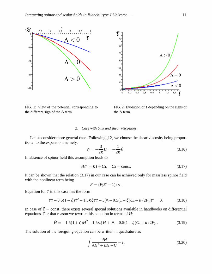
The problem parameters are chosen as follows:κ = 1, m= 1, λ = 0.5, ζ = 1/3,n= 4,C2 = 2 andC3 = 1. Here we consider the cases with differentΛ, namely withΛ = −2,0,1, respectively. Theinitial value ofτ is taken to be a small one, whereas, the first derivative ofτ, i.e., τ at that pointof time is calculated from (3.11). In Fig. 1 we have illustrated the potential corresponding to Eq.(3.14). It can be immediately seen that independent of the sign of Λ we have always expandinguniverse. But as is seen from Fig. 2 a positiveΛ results in accelerated mode of expansion, whilethe negative one causes deceleration.

Interacting spinor and scalar fields in Bianchi type-I Universe· · · 11

FIG. 1: View of the potential corresponding tothe different sign of theΛ term.

FIG. 2: Evolution ofτ depending on the signs oftheΛ term.

2. Case with bulk and shear viscosities

Let us consider more general case. Following [12] we choose the shear viscosity being propor-tional to the expansion, namely,

η = − 32κ

H = − 12κ

θ . (3.16)

In absence of spinor field this assumption leads to

3H2 = κε +C4, C4 = const. (3.17)

It can be shown that the relation (3.17) in our case can be achieved only for massless spinor fieldwith the nonlinear term being

F = (F0S2−1)/λ .

Equation forτ in this case has the form

ττ −0.5(1−ζ )τ2−1.5κξ ττ −3[Λ−0.5(1−ζ )C4+κ/2F0]τ2 = 0. (3.18)

In case ofξ = const. there exists several special solutions available in handbooks on differentialequations. For that reason we rewrite this equation in termsof H:

H = −1.5(1+ζ )H2+1.5κξH +[Λ−0.5(1−ζ )C4+κ/2F0]. (3.19)

The solution of the foregoing equation can be written in quadrature as

∫

dHAH2 +BH+C

= t, (3.20)

12 Bijan Saha

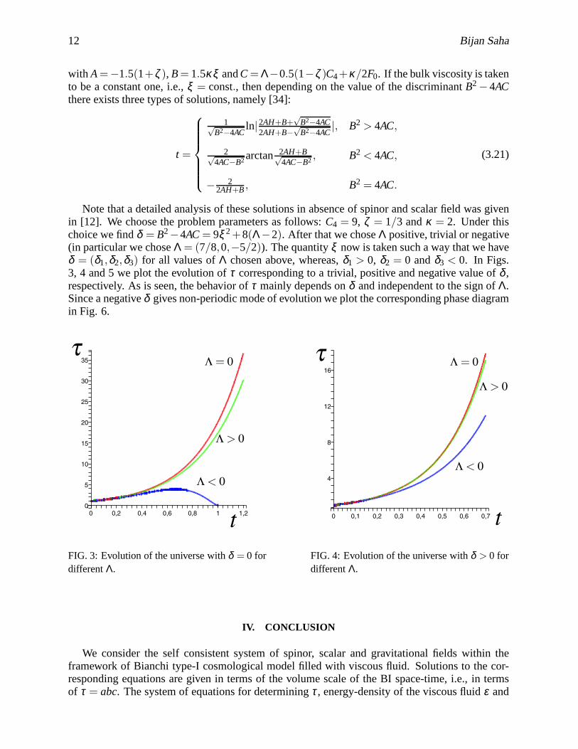
with A=−1.5(1+ζ ), B= 1.5κξ andC= Λ−0.5(1−ζ )C4+κ/2F0. If the bulk viscosity is takento be a constant one, i.e.,ξ = const., then depending on the value of the discriminantB2−4ACthere exists three types of solutions, namely [34]:

t =

1√B2−4AC

ln|2AH+B+√

B2−4AC2AH+B−

√B2−4AC

|, B2 > 4AC,

2√4AC−B2arctan 2AH+B√

4AC−B2 , B2 < 4AC,

− 22AH+B, B2 = 4AC.

(3.21)

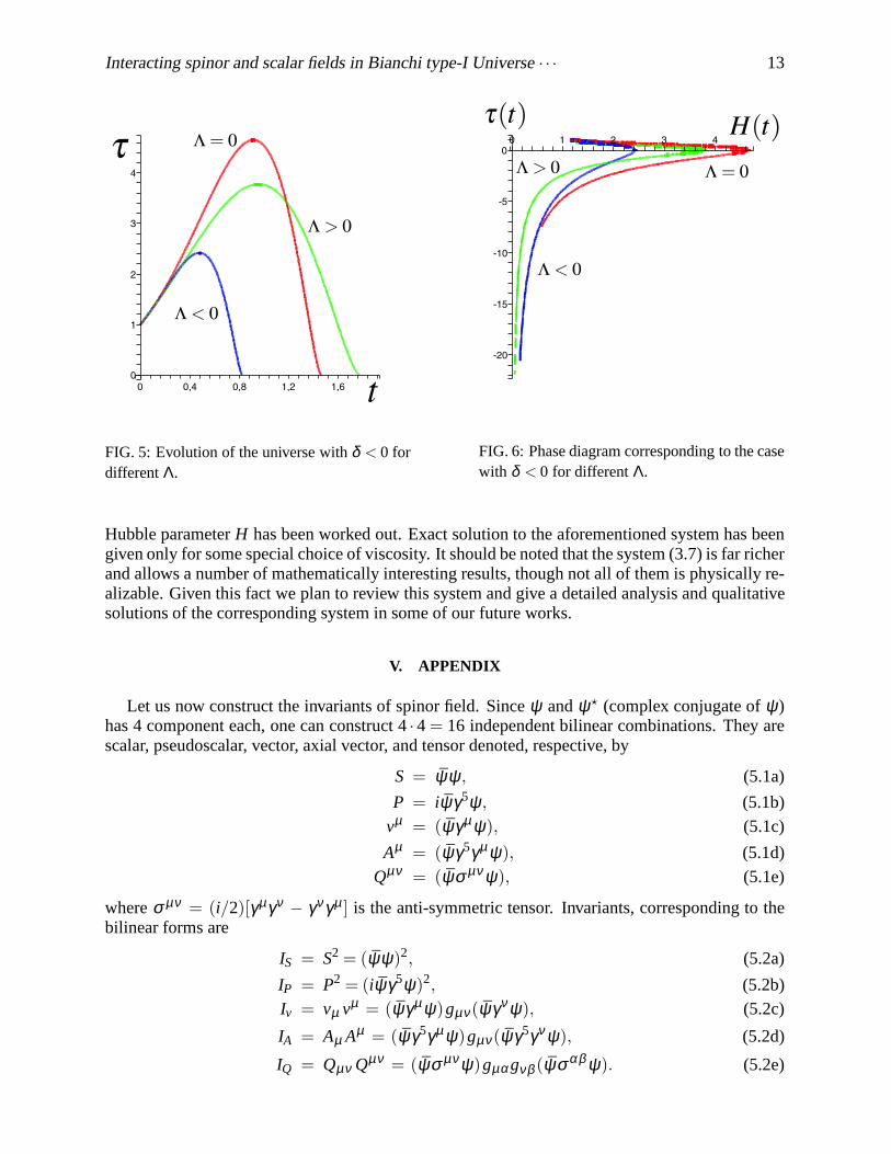
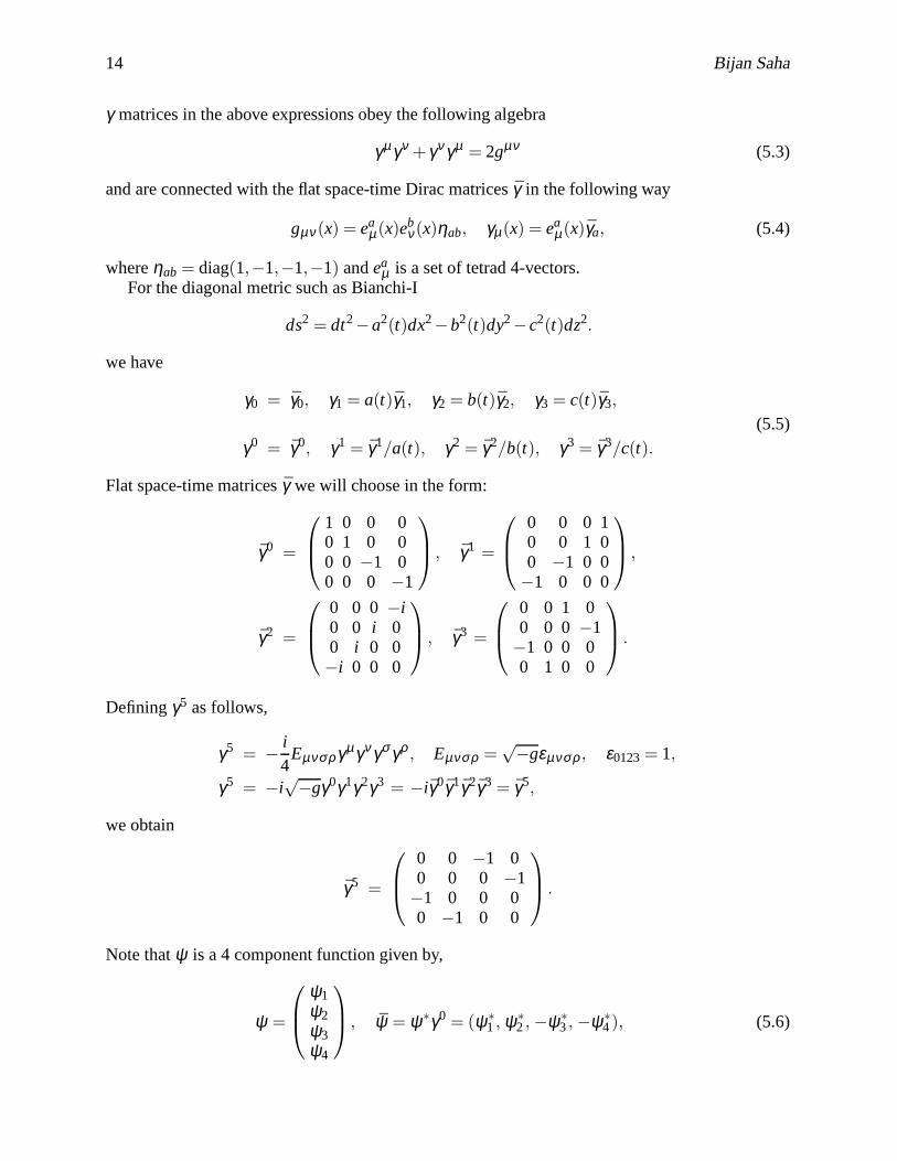
Note that a detailed analysis of these solutions in absence of spinor and scalar field was givenin [12]. We choose the problem parameters as follows:C4 = 9, ζ = 1/3 andκ = 2. Under thischoice we findδ = B2−4AC= 9ξ 2+8(Λ−2). After that we choseΛ positive, trivial or negative(in particular we choseΛ = (7/8,0,−5/2)). The quantityξ now is taken such a way that we haveδ = (δ1,δ2,δ3) for all values ofΛ chosen above, whereas,δ1 > 0, δ2 = 0 andδ3 < 0. In Figs.3, 4 and 5 we plot the evolution ofτ corresponding to a trivial, positive and negative value ofδ ,respectively. As is seen, the behavior ofτ mainly depends onδ and independent to the sign ofΛ.Since a negativeδ gives non-periodic mode of evolution we plot the corresponding phase diagramin Fig. 6.

FIG. 3: Evolution of the universe withδ = 0 fordifferentΛ.

FIG. 4: Evolution of the universe withδ > 0 fordifferentΛ.

IV. CONCLUSION

We consider the self consistent system of spinor, scalar andgravitational fields within theframework of Bianchi type-I cosmological model filled with viscous fluid. Solutions to the cor-responding equations are given in terms of the volume scale of the BI space-time, i.e., in termsof τ = abc. The system of equations for determiningτ, energy-density of the viscous fluidε and

Interacting spinor and scalar fields in Bianchi type-I Universe· · · 13

FIG. 5: Evolution of the universe withδ < 0 fordifferentΛ.

FIG. 6: Phase diagram corresponding to the casewith δ < 0 for differentΛ.

Hubble parameterH has been worked out. Exact solution to the aforementioned system has beengiven only for some special choice of viscosity. It should benoted that the system (3.7) is far richerand allows a number of mathematically interesting results,though not all of them is physically re-alizable. Given this fact we plan to review this system and give a detailed analysis and qualitativesolutions of the corresponding system in some of our future works.

V. APPENDIX

Let us now construct the invariants of spinor field. Sinceψ andψ⋆ (complex conjugate ofψ)has 4 component each, one can construct 4·4 = 16 independent bilinear combinations. They arescalar, pseudoscalar, vector, axial vector, and tensor denoted, respective, by

S = ψψ, (5.1a)

P = iψγ5ψ, (5.1b)vµ = (ψγµ ψ), (5.1c)

Aµ = (ψγ5γµ ψ), (5.1d)Qµν = (ψσ µν ψ), (5.1e)

whereσ µν = (i/2)[γµγν − γνγµ ] is the anti-symmetric tensor. Invariants, corresponding to thebilinear forms are

IS = S2 = (ψψ)2, (5.2a)

IP = P2 = (iψγ5ψ)2, (5.2b)Iv = vµ vµ = (ψγµ ψ)gµν(ψγνψ), (5.2c)

IA = Aµ Aµ = (ψγ5γµ ψ)gµν(ψγ5γν ψ), (5.2d)

IQ = Qµν Qµν = (ψσ µνψ)gµαgνβ (ψσ αβ ψ). (5.2e)

14 Bijan Saha

γ matrices in the above expressions obey the following algebra

γµ γν + γν γµ = 2gµν (5.3)

and are connected with the flat space-time Dirac matricesγ in the following way

gµν(x) = eaµ(x)eb

ν(x)ηab, γµ(x) = eaµ(x)γa, (5.4)

whereηab = diag(1,−1,−1,−1) andeaµ is a set of tetrad 4-vectors.

For the diagonal metric such as Bianchi-I

ds2 = dt2−a2(t)dx2−b2(t)dy2−c2(t)dz2.

we have

γ0 = γ0, γ1 = a(t)γ1, γ2 = b(t)γ2, γ3 = c(t)γ3,

(5.5)γ0 = γ0, γ1 = γ1/a(t), γ2 = γ2/b(t), γ3 = γ3/c(t).

Flat space-time matricesγ we will choose in the form:

γ0 =

1 0 0 00 1 0 00 0 −1 00 0 0 −1

, γ1 =

0 0 0 10 0 1 00 −1 0 0−1 0 0 0

,

γ2 =

0 0 0 −i0 0 i 00 i 0 0−i 0 0 0

, γ3 =

0 0 1 00 0 0 −1−1 0 0 00 1 0 0

.

Definingγ5 as follows,

γ5 = − i4

Eµνσρ γµγν γσ γρ , Eµνσρ =√−gεµνσρ , ε0123= 1,

γ5 = −i√−gγ0γ1γ2γ3 = −iγ0γ1γ2γ3 = γ5,

we obtain

γ5 =

0 0 −1 00 0 0 −1−1 0 0 00 −1 0 0

.

Note thatψ is a 4 component function given by,

ψ =

ψ1ψ2ψ3ψ4

, ψ = ψ∗γ0 = (ψ∗

1 , ψ∗2 , −ψ∗

3 , −ψ∗4), (5.6)

Interacting spinor and scalar fields in Bianchi type-I Universe· · · 15

DenotingF bilinear spinor form in Minkowski spacetime andF in curve spacetime (in our case inBI) we find the following expressions for the non-trivial components of bilinear spinor form:

S = (ψ∗1ψ1 +ψ∗

2ψ2−ψ∗3ψ3−ψ∗

4ψ4), S= S, (5.7)P = −i(ψ∗

1ψ3 +ψ∗2ψ4−ψ∗

3ψ1−ψ∗4ψ2), P = P, (5.8)

V0 = (ψ∗1ψ1 +ψ∗

2ψ2 +ψ∗3ψ3 +ψ∗

4ψ4), V0 = V0, (5.9)

V1 = (ψ∗1ψ4 +ψ∗

2ψ3 +ψ∗3ψ2 +ψ∗

4ψ1), V1 = V1/a, (5.10)

V2 = −i(ψ∗1ψ4−ψ∗

2ψ3 +ψ∗3ψ2−ψ∗

4ψ1), V2 = V2/b, (5.11)

V3 = (ψ∗1ψ3−ψ∗

2ψ4 +ψ∗3ψ1−ψ∗

4ψ2), V3 = V3/c, (5.12)

A0 = (ψ∗1ψ3 +ψ∗

2ψ4 +ψ∗3ψ1 +ψ∗

4ψ2), A0 = A0, (5.13)

A1 = (ψ∗1ψ2 +ψ∗

2ψ1 +ψ∗3ψ4 +ψ∗

4ψ3), A1 = A1/a, (5.14)

A2 = −i(ψ∗1ψ2−ψ∗

2ψ1 +ψ∗3ψ4−ψ∗

4ψ3), A2 = A2/b, (5.15)

A3 = (ψ∗1ψ1−ψ∗

2ψ2 +ψ∗3ψ3−ψ∗

4ψ4), A3 = A3/c, (5.16)

Q01 = i(ψ∗1ψ4+ψ∗

2ψ3−ψ∗3ψ2−ψ∗

4ψ1), Q01 = Q01/a, (5.17)

Q02 = (ψ∗1ψ4−ψ∗

2ψ3−ψ∗3ψ2 +ψ∗

4ψ1), Q02 = Q02/b, (5.18)

Q03 = i(ψ∗1ψ3−ψ∗

2ψ4−ψ∗3ψ1+ψ∗

4ψ2), Q03 = Q03/c, (5.19)

Q12 = (ψ∗1ψ1−ψ∗

2ψ2−ψ∗3ψ3 +ψ∗

4ψ4), Q12 = Q12/ab, (5.20)

Q23 = (ψ∗1ψ2 +ψ∗

2ψ1−ψ∗3ψ4−ψ∗

4ψ3), Q23 = Q23/bc, (5.21)

Q13 = i(ψ∗1ψ2−ψ∗

2ψ1−ψ∗3ψ4+ψ∗

4ψ3), Q13 = Q13/ac. (5.22)(5.23)

Using the above expressions we find

IS = S2 = (ψ∗1ψ1)

2+(ψ∗2ψ2)

2+(ψ∗3ψ3)

2+(ψ∗4ψ4)

2

+ 2[ψ∗1ψ1ψ∗

2ψ2−ψ∗1ψ1ψ∗

3ψ3−ψ∗1ψ1ψ∗

4ψ4

− ψ∗2ψ2ψ∗

3ψ3−ψ∗2ψ2ψ∗

4ψ4+ψ∗3ψ3ψ∗

4ψ4]. (5.24)

IP = P2 = −(ψ∗1ψ3)

2− (ψ∗2ψ4)

2− (ψ∗3ψ1)

2− (ψ∗4ψ2)

2

− 2[ψ∗1ψ3ψ∗

2ψ4−ψ∗1ψ1ψ∗

3ψ3−ψ∗1ψ3ψ∗

4ψ2

− ψ∗2ψ4ψ∗

3ψ1−ψ∗2ψ2ψ∗

4ψ4+ψ∗3ψ1ψ∗

4ψ2]. (5.25)

IV = (V0)2− (V1)2− (V2)2− (V3)2

= (ψ∗1ψ1)

2+(ψ∗2ψ2)

2+(ψ∗3ψ3)

2+(ψ∗4ψ4)

2

− (ψ∗1ψ3)

2− (ψ∗2ψ4)

2− (ψ∗3ψ1)

2− (ψ∗4ψ2)

2

+ 2[ψ∗1ψ1ψ∗

2ψ2−ψ∗1ψ1ψ∗

4ψ4−ψ∗2ψ2ψ∗

3ψ3+ψ∗3ψ3ψ∗

4ψ4

− ψ∗1ψ4ψ∗

2ψ3−ψ∗3ψ2ψ∗

4ψ1 +ψ∗1ψ3ψ∗

4ψ2 +ψ∗2ψ4ψ∗

3ψ1]

= IS+ IP. (5.26)

16 Bijan Saha

IA = (A0)2− (A1)2− (A2)2− (A3)2

= −(ψ∗1ψ1)

2− (ψ∗2ψ2)

2− (ψ∗3ψ3)

2− (ψ∗4ψ4)

2

+ (ψ∗1ψ3)

2+(ψ∗2ψ4)

2+(ψ∗3ψ1)

2+(ψ∗4ψ2)

2

− 2[ψ∗1ψ1ψ∗

2ψ2−ψ∗1ψ1ψ∗

4ψ4−ψ∗2ψ2ψ∗

3ψ3 +ψ∗3ψ3ψ∗

4ψ4

− ψ∗1ψ4ψ∗

2ψ3−ψ∗3ψ2ψ∗

4ψ1 +ψ∗1ψ3ψ∗

4ψ2 +ψ∗2ψ4ψ∗

3ψ1]

= −(IS+ IP). (5.27)

IQ = 2[(Q12)2+(Q13)2+(Q23)2− (Q01)2− (Q02)2− (Q03)2]

= (ψ∗1ψ1)

2+(ψ∗2ψ2)

2+(ψ∗3ψ3)

2+(ψ∗4ψ4)

2

+ (ψ∗1ψ3)

2+(ψ∗2ψ4)

2+(ψ∗3ψ1)

2+(ψ∗4ψ2)

2

+ 2[ψ∗1ψ1ψ∗

2ψ2−ψ∗1ψ1ψ∗

4ψ4−ψ∗2ψ2ψ∗

3ψ3 +ψ∗3ψ3ψ∗

4ψ4

+ ψ∗1ψ4ψ∗

2ψ3+ψ∗3ψ2ψ∗

4ψ1−ψ∗1ψ3ψ∗

4ψ2−ψ∗2ψ4ψ∗

3ψ1]

− 4(ψ∗1ψ1ψ∗

3ψ3 +ψ∗2ψ2ψ∗

4ψ4) = 2(IS− IP). (5.28)

Thus we see that that the invariantsIV , IA andIQ can be expressed in terms ofIS andIP.An alternative proof ofIV =−IA = (IS+ IP) andIQ = 2(IS− IP) can be given using Feirz trans-

formation. In doing so we recall that any 4x4 matrixΓ can be presented as a linear combination ofγA:

Γ = ∑A

cAγA, cA =14

TrγAΓ. (5.29)

Explicitly it can be presented as

Γik =14∑

A

ΓlmγAmlγAik. (5.30)

HereγA = I , γ5, γµ , iγµ γ5, iσ µ,ν, A = 1,2..16. (5.31)

The completeness condition gives

δi j δkl =14∑

A

γAikγAkl. (5.32)

Multiplying the foregoing expression byψai ψb

k ψcmψd

l one gets

(ψaψd)(ψcψb) =14∑

A

(ψaγAψb)(ψcγAψd). (5.33)

Replacingψd → γBψd andψb → γCψb and using the expression

γAγB = ∑R

CRγR, CR =14

TrγAγBγR, (5.34)

Interacting spinor and scalar fields in Bianchi type-I Universe· · · 17

one gets the other identities. DenotingIS= (ψaψb)(ψcψd), I ′S= (ψaψd)(ψcψb) · · · ... one finds[21]

4I ′S = IS+ IP+ IV + IQ + IA, (5.35)4I ′P = IS+ IP− IV + IQ− IA, (5.36)4I ′V = 4IS−4IP−2IV +2IA, (5.37)4I ′Q = 6IS+6IP−2IQ, (5.38)

4I ′A = 4IS−4IP +2IV −2IA. (5.39)

After a little manipulations from the foregoing system one comes to desired relations between theinvariants of the bilinear spinor fields.

[1] W. Misner, Nature214, 40 (1967).[2] W. Misner, Astrophysical Journal151, 431 (1968).[3] S. Weinberg, Astrophysical Journal168, 175 (1972).[4] S. Weinberg, Gravitation and Cosmology (New York, Wiley, 1972)[5] P. Langacker, Physics report72, 185 (1981).[6] I. Waga, R.C. Falcao, and R. Chanda, Physical Review D33, 1839 (1986).[7] T. Pacher, J.A. Stein-Schabes, and M.S. Turner, Physical Review D36, 1603 (1987).[8] A.H. Guth, Physical Review D23, 347 (1981).[9] G.L. Murphy, Physical Review D8, 4231 (1973).

[10] N.O. Santos, R.S. Dias, and A. Banerjee, Journal of Mathematical Physics26, 876 (1985).[11] V.A. Belinski and I.M. Khalatnikov, Journal of Experimantal and Theoretical Physics69, 401, (1975).[12] Bijan Saha, Modern Physics Letters A20(28), 2127 (2005).[13] Bijan Saha and V. Rikhvitsky, Physica D219, 168 (2006).[14] B. Saha and G.N. Shikin, Journal of Mathematical Physics 38, 5305 (1997).[15] Bijan Saha, Physical Review D64, 123501 (2001).[16] B. Saha, and G.N. Shikin, General Relativity and Gravitation29, 1099 (1997).[17] Bijan Saha, Modern Physics Letters A,16, 1287 (2001).[18] B. Saha, Phys. Rev. D74, 124030 (2006).[19] Bijan Saha, Romanian Report of Physics57 (1), 7 (2005).[20] Bijan Saha,Nonlinear spinor field in Bianchi type-I Universe filled withviscous fluid: numerical

solutionsgr-qc/0703085.[21] M. Fierz, Z. Phys.104, 553 (1937).[22] F.A. Kaempffer, Phys. Rev. D23, 918 (1981)[23] Y. Takahashi, Phys. Rev. D26, 2169 (1982).[24] V.B. Berestetski, E.M. Lifshitz and L.P. Pitaevski,Quantum Electrodynamics(Nauka, Moscow, 1989).[25] M.E. Peskin and D.V. Schroeder,An introduction to quantum field theory(Reading, MA, Addison-

Wesley, 1995)[26] K.C. Jacobs, Astrophysical Journal153, 661 (1968).[27] L.P. Chimento, Physical Review D68, 023504 (2003)[28] V.A. Zhelnorovich, Spinor theory and its application in physics and mechanics(Nauka, Moscow,

1982).[29] D. Brill and J. Wheeler, Review of Modern Physics29, 465 (1957).[30] E Kamke,Differentialgleichungen losungsmethoden und losungen(Leipzig, 1957).

18 Bijan Saha

[31] W. Heisenberg,Introduction to the unified field theory of elementary particles (Interscience Publ.,London, 1966).

[32] A. Banerjee, S.B. Duttachoudhury, and A.K. Sanyal, Journal of Mathematical Physics26, 3010(1985).

[33] W. Huang, Journal of Mathematical Physics31, 1456 (1990).[34] A.P. Prudnikov, Yu.A. Brychkov, and O.I. Marichev,Integrals and series. v.1: Elementary functions

(New York, Gordon and Breach, 1986).