Positioning and tuning of viscous damper on flexible structure

ARTICLE IN PRESS

JOURNAL OFSOUND ANDVIBRATION

0022-460X/$ - s

doi:10.1016/j.js

�CorrespondE-mail addr

Journal of Sound and Vibration 304 (2007) 845–862

www.elsevier.com/locate/jsvi

Positioning and tuning of viscous damper on flexible structure

K. Engelen�, H. Ramon, W. Saeys, W. Franssens, J. Anthonis

Laboratory of Agro-Machinery and Processing, Division of Mechatronics, Biostatistics and Sensors, Department of Biosystems,

Katholieke Universiteit Leuven, Kasteelpark Arenberg 30, 3001 Leuven, Belgium

Received 5 October 2006; received in revised form 14 March 2007; accepted 19 March 2007

Available online 8 May 2007

Abstract

The complex eigenvalues of a flexible structure including a viscous damper are derived by solving the root locus of a

transfer function that is composed of very easily identifiable parameters: the static stiffness of the structure at the damper

location, the resonance frequencies of the undamped structure and the resonance frequencies of the structure in which the

damper is replaced by a rigid link. Approximate solutions are proposed for the complex eigenvalues and formulas are

derived for the maximum modal damping ratio and the optimal damping constant. The correctness of the formulas is

illustrated by numerical examples of a cantilever beam with attached viscous damper. Although approximate solutions

exist which are not restricted to the case of a single damper, these are only accurate when the difference between the

undamped and constrained eigensolution is sufficiently small, while the approximations obtained in the present paper are

accurate in a broader range without losing simplicity.

r 2007 Elsevier Ltd. All rights reserved.

1. Introduction

Improving the dynamic behavior of flexible structures with low inherent damping is a research topic thathas been given considerable attention in the last decades, especially in the fields of spacecraft dynamics [1] anddynamics of buildings and bridges [2]. It has been shown that incorporation of viscous dampers in thestructure can be a very effective means of reducing unwanted vibrations [2]. From a design point of view, thismeans two questions have to be answered: (I) what are good locations for placing the dampers in the structureand (II) what are the optimal damping constants resulting in minimized vibrations.

In answering these questions, one starts generally from a discrete model of the structure, for example bymeans of finite elements. When the excitation mechanisms are known, forced responses can be performed fordifferent locations and sizes of the dampers, hereby searching for an optimal configuration that minimizesstructural responses like for example displacements, accelerations or internal forces. An other criterium that isoften employed in the design of dampers consists of maximizing the damping level in specific vibration modes.This is certainly interesting when the excitation mechanisms are not well understood and the problematicmodes are known.

ee front matter r 2007 Elsevier Ltd. All rights reserved.

v.2007.03.020

ing author. Tel.: +3216328527; fax: +3216328590.

ess: [email protected] (K. Engelen).

www.elsevier.com/locate/jsvi

dx.doi.org/10.1016/j.jsv.2007.03.020

mailto:[email protected]

ARTICLE IN PRESSK. Engelen et al. / Journal of Sound and Vibration 304 (2007) 845–862846

In both of the previously described approaches for designing dampers, the complex eigenvalues are requiredand in the case of the forced response also the complex mode shapes have to be known. These can both beobtained by solving the complex eigenvalue problem corresponding to free vibrations of the structure.However, repeatedly solving this complex eigenproblem for different damper locations and different dampingconstants can be very time consuming for structures with a large number of degrees of freedom. Therefore,Main and Krenk [3] suggest an approximate solution that requires solving only two real-valued eigenproblemsfor each damper location: the eigenproblem of the undamped structure and the eigenproblem of the structurein which each damper is replaced by a rigid link, corresponding to a damping constant of, respectively, zeroand infinity. The solutions for intermediate values of the damping constant are approximated by aninterpolation between the solutions for these two limiting cases. An explicit form of the approximate solutionis obtained for the case the difference between the two solutions is sufficiently small, and an iterative scheme isproposed for the case where this difference is larger. Similar approximate solutions have been derived forvarious continuous structures such as a taut cable [4] and a simply supported beam [5]. Høgsberg and Krenk[6] recently used this two-component representation technique to study active control algorithms forcollocated systems.

In this paper, an alternative approach is suggested to obtain the complex eigenvalues for the case where onlyone damper is implemented in the structure. It also starts from the solutions of the two limiting eigenvalueproblems of the structure without and with locked damper, however, the root locus technique is applied toobtain results for intermediate values of the damping constant. Approximate expressions are obtained for themaximal attainable modal damping at a given damper location and the corresponding optimal dampingconstant. The only parameters in these expressions are the stiffness of the structure at the damper location andthe resonance frequencies of the structure without and with locked damper. These parameters are easilyobtainable from any commercial finite element package that is able to perform static and modal analysis.Besides, these parameters are also easily experimentally identifiable, making them very useful in practicaldesign. The correctness of the formulas is verified for two numerical examples: a cantilever Bernouilli–Eulerbeam equipped with a translational viscous damper and a rotational viscous damper. Beam elements aresimple elements, representative for many real systems and are often used to investigate the dynamic behaviorof flexible structures with attached viscous dampers [5,7,8].

The formulas for the maximum modal damping and optimal damping constant derived here are similar tothose derived by Preumont [1] for active control of structures with collocated sensors and actuators applyingintegral force feedback (IFF), i.e. the position is controlled as the integral of the force, which in fact isequivalent to viscous damping. Krenk [4] and Main and Jones [9] derived similar formulas for the special caseof a taut cable with a viscous damper attached near the end. Main and Krenk [3] found approximate solutionsfor the damping constant that maximizes the decay rate of a general discrete structure with viscous dampers,which is only slightly different from the damping constant that maximizes the modal damping ratio.Previously published research results are compared with the results of this paper in Section 5.

2. Transfer function for collocated systems

In this section, the transfer function between the force f exerted on a flexible structure and its collocateddisplacement x is derived. Collocated means that the displacement at the location of the applied force isconsidered (Fig. 1a). This transfer function will be used in the subsequent section to find the eigenvalues of aviscously damped structure by solving a root locus problem. First the eigenvalues of an undamped structureare derived, which are used to construct the transfer function.

2.1. Eigenvalues of an undamped structure

The free response of an undamped discrete linear structure with n degrees of freedom is governed by theequations of motion

M€qþ Kq ¼ 0, (1)

whereM and K are the n� n mass and stiffness matrices and q is the n� 1 vector of generalized displacements.

ARTICLE IN PRESS

f

x

a

l

(a)

(b)

(c)

Fig. 1. (a) Cantilever beam with applied force and collocated displacement; (b) mode shape of cantilever beam with additional restraint;

(c) cantilever beam with attached viscous damper.

ff

f

q2q1 q3q2q1 q3

(b)(a)

Fig. 2. Three mass system excited by an actuator acting on (a) relative motion and (b) absolute motion.

K. Engelen et al. / Journal of Sound and Vibration 304 (2007) 845–862 847

Assuming solutions of the form q ¼ uest, yields the eigenvalue problem

ðMs2 þ KÞui ¼ 0. (2)

Non-trivial solutions are found by solving the characteristic equation

detðMs2 þ KÞ ¼ 0, (3)

where the eigenvalues s ¼ �jOi are purely imaginary in case of an undamped structure, Oi are the resonancefrequencies of the structure and ui are the corresponding modeshapes.

2.2. Transfer function for collocated systems

When an undamped structure is excited by a single force, the equations of motion can be written as follows:

M€qþ Kq ¼ bf , (4)

where b is the n� 1 influence vector, which indicates the location and orientation of the point of excitation inthe structure. For example, the influence vector of the three mass system of Fig. 2 is b ¼ ½0 � 1 1�T in the casewhere the actuator forces a relative motion of the masses, while it is b ¼ ½0 1 0�T where the actuator acts onabsolute motion.

Taking the Laplace transform of Eq. (4) and assuming zero initial conditions results in

ðMs2 þ KÞQðsÞ ¼ bF ðsÞ. (5)

The displacement x that is collocated with the applied force f is related to the vector of generalizeddisplacements q by the influence vector b as

X ðsÞ ¼ bTQðsÞ. (6)

Combination of Eqs. (5) and (6) gives the transfer function GðsÞ between the force f and the collocateddisplacement x:

X ðsÞ

F ðsÞ¼ bTðMs2 þ KÞ�1b ¼ GðsÞ. (7)


The inverse is written as a function of the determinant and the adjoint, yielding

GðsÞ ¼ bTadjðMs2 þ KÞ

detðMs2 þ KÞb. (8)

The determinant of the denominator is exactly the same determinant that has to be solved for finding the non-trivial solutions of the free response of the undamped structure (Eq. (3)). It can therefore be expressed as

detðMs2 þ KÞ ¼ g1

Yn

i¼1

ðs2 þ O2i Þ, (9)

where Oi are the resonance frequencies of the undamped structure and g1 is a constant.It can be shown that the numerator of Eq. (8) can be written as

bTadjðMs2 þ KÞb ¼ detðMcs2 þ KcÞ, (10)

where Mc and Kc are the mass and stiffness matrices of the constrained structure where the actuator has beenreplaced by a rigid link. This is easily verified in the case an absolute actuator is acting on the structure. Forexample, for the three mass system (Fig. 2b), the numerator of Eq. (8) equals

bTadjðMs2 þ KÞb ¼ detðM2;2s2 þ K2;2Þ, (11)

where M2;2 and K2;2 are the mass and stiffness matrices of the original structure from which the 2nd row andthe 2nd column have been removed. This corresponds to the system with an additional constraint at the degreeof freedom the damper acts on.

For the case of a relative actuator this relation might be less clear at first sight, however, we can alwayschange variables such that one of the variables corresponds to the actuator displacement. For the three masssystem of Fig. 2a we can change variables for example to q ¼ ½q1 q2 q3 � q2�

T, whereby b ¼ ½0 0 1�T and thenumerator of Eq. (8) equals

bTadjðMs2 þ KÞb ¼ detðM3;3s2 þ K3;3Þ, (12)

where M3;3 and K3;3 are the mass and stiffness matrices of the original structure from which the 3rd row andthe 3rd column have been removed. Again, this corresponds to a system that is equivalent to the structure forwhich the actuator is replaced by a rigid link.

So, an equivalent expression as in Eq. (9) can be obtained for the determinant

detðMcs2 þ KcÞ ¼ g2

Yn�1i¼1

ðs2 þ o2i Þ, (13)

where oi are the resonance frequencies of the constrained structure, also called anti-resonance frequencies(Fig. 1b) and g2 is a constant.

By combination of Eqs. (8)–(10) and (13), the transfer function of the collocated system can be rewritten as

GðsÞ ¼g2

g1

Qn�1i¼1 ðs

2 þ o2i ÞQn

i¼1ðs2 þ O2

i Þ. (14)

In system theory, it is a common practice to express transfer functions in this form, in terms of resonance andanti-resonance frequencies [1]. The gain of this transfer function is deduced from the static stiffness of thestructure at the location of the actuator k, by substitution of s ¼ 0 in Eq. (14), which gives

Gð0Þ ¼X ð0Þ

F ð0Þ¼

1

k¼

g2

g1

Qn�1i¼1 ðo

2i ÞQn

i¼1ðO2i Þ

(15)

such that the transfer function finally reads

GðsÞ ¼1

k

Qni¼1 O

2iQn�1

i¼1 o2i

Qn�1i¼1 ðs

2 þ o2i ÞQn

i¼1ðs2 þ O2

i Þ, (16)

ARTICLE IN PRESSK. Engelen et al. / Journal of Sound and Vibration 304 (2007) 845–862 849

where k can be derived from the stiffness matrix K by substitution of s ¼ 0 in Eq. (7):

k ¼ ðbTK�1bÞ�1. (17)

3. Eigenvalues of a structure with a single viscous damper

In this section, the possibilities of obtaining the eigenvalues of a structure including a viscous damper arediscussed. First, the classical approach is repeated, where solutions are found by solving a quadraticeigenvalue problem. Next it is shown how the eigenvalues can be derived by solving a root locus problem,which is computationally less time consuming. Moreover, the transfer function from which the root locus iscomputed is composed of parameters that are easily obtainable from any commercial finite element packagethat offers the opportunity to perform static and modal analysis. The stiffness and mass matrices, required forthe classical approach, are not available in all finite element packages. Finally, simple approximate solutionsare proposed, which are very useful in the design of dampers.

3.1. Quadratic eigenvalue problem

The force exerted by a viscous damper is proportional to the velocity of the piston, in a direction opposite tothe piston motion

f ¼ �c _x, (18)

where c is the damping constant.The free response of a structure including a viscous damper (Fig. 1c) is governed by the equations of

motion

M€qþ C_qþ Kq ¼ 0, (19)

where C ¼ cbbT is the damping matrix. Non-trivial solutions are found by solving the quadratic eigenvalueproblem

ðMs2 þ Csþ KÞu ¼ 0, (20)

where the eigenvalues are generally complex for a damped structure. They are typically written inthe form

s ¼ on;ið�xi � j

ffiffiffiffiffiffiffiffiffiffiffiffiffi1� x2i

qÞ, (21)

where on;i is the modulus of the ith eigenvalue and xi is the modal damping ratio.

3.2. Complex eigenvalues by solving root locus problem

Taking the Laplace transform of Eq. (18) and assuming zero initial conditions gives

F ðsÞ ¼ �csX ðsÞ. (22)

Combination of Eqs. (7) and (22) results in the closed-loop system of the structure with attached viscousdamper

1þ csGðsÞ ¼ 0. (23)

From this equation it is clear that the root locus of sGðsÞ shows the effect of changing the damping constant onthe poles of the structure with attached viscous damper. Typical examples of such root locus plots are shownin Fig. 3. It is seen that the poles and zeros alternate along the imaginary axis, which is characteristic for anundamped collocated system [1]. It should be clear that in contrast to the resonance frequencies, the values ofthe anti-resonance frequencies do depend on the location of the damper in the structure and there is alwaysexactly one anti-resonance between two consecutive resonances. For zero damping constant, the closed-looppoles coincide with the undamped resonance frequencies of the structure. Now, increasing the damping

ARTICLE IN PRESS

j�1

j�2

j�3

j�1

j�2

j�3

Im(s)

Re(s)

j�1

j�2

j�3

j�1

j�2

j�3

Im(s)

Re(s)

j�1

j�2

j�3

j�1

j�2

j�3

Im(s)

Re(s)

(a) (b) (c)

Fig. 3. Typical root locus plots of an undamped discrete structure (degrees of freedom n43) with attached viscous damper for varying

damping constant c. (Only the upper half of the s-plane is shown, the diagram is symmetrical with respect to the real axis.)

K. Engelen et al. / Journal of Sound and Vibration 304 (2007) 845–862850

constant initially increases the modal damping, reaching a maximum value for a particular value of c. In casethe mode is critically damped at this point, this mode shall typically remain critically damped by furtherincreasing c, as can be seen for example in Fig. 3b for the second mode. For all the other cases shown in Fig. 3further increase of c from its optimal value decreases the modal damping and finally it goes to zero for aninfinite damping constant. The closed loop poles then coincide with the anti-resonance frequencies of thestructure and the damper acts like a support.

Because a viscous damper can only dissipate energy, the branches of the root-locus diagram are allcontained in the left half-plane. The form of the root locus diagram of Fig. 3a is typical for situations such asan absolute damper located near the support of a structure, or a relative damper incorporated in the structure.Here, the anti-resonance frequencies differ only slightly from the resonance frequencies and moderate valuesof modal damping are achieved for the optimal damping constant. As will be seen in the numerical example ofa cantilever beam with attached translational viscous damper, in some cases it is possible to achieve criticaldamping for a mode, as can be seen for example in Fig. 3b for the second mode. Fig. 3c gives an example of aroot locus diagram where the third pole is attracted by the second zero, which is very close to this pole. Herebythe branch of the second mode goes to the third zero. It is clearly seen in these examples that the amount ofachievable damping is small for poles that have a zero in the near neighborhood and gets larger when they aremore separated. When a zero coincides with a pole, the mode is uncontrollable for the corresponding damperlocation.

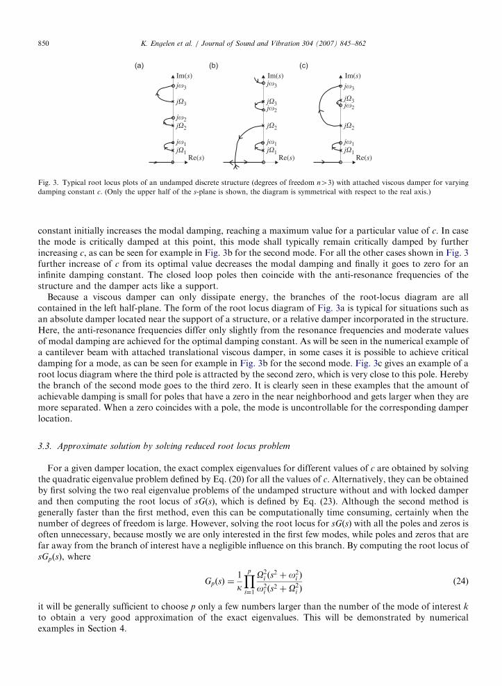
3.3. Approximate solution by solving reduced root locus problem

For a given damper location, the exact complex eigenvalues for different values of c are obtained by solvingthe quadratic eigenvalue problem defined by Eq. (20) for all the values of c. Alternatively, they can be obtainedby first solving the two real eigenvalue problems of the undamped structure without and with locked damperand then computing the root locus of sGðsÞ, which is defined by Eq. (23). Although the second method isgenerally faster than the first method, even this can be computationally time consuming, certainly when thenumber of degrees of freedom is large. However, solving the root locus for sGðsÞ with all the poles and zeros isoften unnecessary, because mostly we are only interested in the first few modes, while poles and zeros that arefar away from the branch of interest have a negligible influence on this branch. By computing the root locus ofsGpðsÞ, where

GpðsÞ ¼1

k

Yp

i¼1

O2i ðs

2 þ o2i Þ

o2i ðs

2 þ O2i Þ

(24)

it will be generally sufficient to choose p only a few numbers larger than the number of the mode of interest k

to obtain a very good approximation of the exact eigenvalues. This will be demonstrated by numericalexamples in Section 4.


3.4. Approximating formulas for the optimal damping

In this section, approximating formulas for the optimal damping constant and maximum modal dampingratio are derived. These are very useful in the design of dampers.

From the knowledge of the values of the poles and zeros, it is not trivial to predict whether a pole will becritically damped, or attracted to one of the zeros. However, it can be stated that it is most probable that apole will be attracted by the nearest zero. Certainly when the distance is small compared to the other poles andzeros, this probability is large. Because the poles and zeros alternate on the imaginary axis, it should be clearthat for the pole that coincides with the kth resonance frequency Ok, the nearest zero is the one that coincideswith either the subsequent anti-resonance frequency ok, or the previous anti-resonance frequency ok�1 (whenka1). Because the maximal distance that a zero can be removed from a pole is determined by the distance ofthis pole to the next (or previous) pole, the closeness of a zero to a pole will be defined here as a fraction of thismaximal distance. Therefore, we define

�k1 ¼jOk � okj

jOk � Okþ1j(25)

as the relative distance of the kth pole to the subsequent zero compared to the distance of this pole to thesubsequent pole. Similarly we define

�k2 ¼jOk � ok�1j

jOk � Ok�1j(26)

as the relative distance of the kth pole to the previous zero compared to the distance of this pole to theprevious pole.

Now, two cases can be considered, depending on which of the two distances �k1 or �k2 is smallest. If thedistance is sufficiently small and the distance to all the other poles and zeros is large, it will be shown that forboth cases approximate values for the eigenvalues can be obtained by solving a reduced root locus problemwhere only the factors involving the kth pole and the kth or ðk � 1Þth zero are retained. From this reducedroot locus problem, approximate values for the maximum modal damping and the optimal damping constantcan be derived.

3.4.1. Case 1: �k1p�k2

If we assume that the distance of jOk to jok is small compared to the distance to all the other poles andzeros, then Eq. (16) can be simplified in the vicinity of jOk as follows:

GðsÞjs�jOk�

1

kk;k

ðs2 þ o2kÞ

ðs2 þ O2kÞ¼ H1ðsÞ, (27)

with

kp;z ¼ kQz

i¼1 o2iQp

i¼1 O2i

. (28)

This result is obtained by replacing the factors ðs2 þ w2Þ where w ¼ O1; . . . ;Ok�1 and w ¼ o1; . . . ;ok�1 by s2

and replacing the factors ðs2 þ w2Þ where w ¼ Okþ1; . . . ;On and w ¼ okþ1; . . . ;on�1 by w2.Substitution of Eq. (27) in Eq. (23) gives

1þ csH1ðsÞ ¼ 1þcs

kk;k

ðs2 þ o2kÞ

ðs2 þ O2kÞ¼ 0 (29)

resulting in typical root locus plots for the individual eigenmodes as in Fig. 4a. This root locus plot can bederived from the root locus plots of Fig. 3 by moving all the poles and zeros that are larger than jok to infinityand all the poles and zeros that are smaller than jOk to the origin.

For each eigenmode, there is an optimal value for c that results in maximum modal damping. Bysubstitution of Eq. (21) in Eq. (29), differentiating it with respect to c and assuming that qxi=qc ¼ 0, the

ARTICLE IN PRESS

j�k

j�k

Im(s)

Re(s)

�kmax �k

max

j�k-1

j�k

Im(s)

Re(s)

(a) (b)

Fig. 4. Root locus of (a) sH1ðsÞ and (b) sH2ðsÞ.


maximum modal damping and the corresponding optimal damping constant are found:

xmaxk ¼

ok � Ok

2Ok

(30)

and

coptk ¼ kk;k

ffiffiffiffiffiffiffiffiffiffiffiffiffiffiOk=ok

pok

. (31)

The maximum modal damping is proportional to the relative spacing of the resonance frequency of theundamped structure and the resonance frequency of the structure with locked damper. This means that theproblem of finding a good damper location can be reduced to the problem of finding a location for a rigid linkthat results in the largest possible increase of the resonance frequency. The importance of inducing suchfrequency shifts has been demonstrated before for active devices controlled by the IFF algorithm [1], for a tautcable with attached viscous damper [4,9] and for a general discrete structure including viscous dampers [3]. Acomparison with the results obtained in this paper is made in Section 5.

3.4.2. Case 2: �k14�k2 ðka1ÞIf we assume that the distance of jOk to jok�1 is small compared to the distance to all the other poles and

zeros, then Eq. (16) can be simplified in the vicinity of jOk as follows:

GðsÞjs�jOk�

1

kk;k�1

ðs2 þ o2k�1Þ

s2ðs2 þ O2kÞ¼ H2ðsÞ. (32)

This result is obtained by replacing the factors ðs2 þ w2Þ where w ¼ O1; . . . ;Ok�1 and w ¼ o1; . . . ;ok�2 by s2

and replacing the factors ðs2 þ w2Þ where w ¼ Okþ1; . . . ;On and w ¼ ok; . . . ;on�1 by w2.Substitution of Eq. (32) in Eq. (23) gives

1þ csH2ðsÞ ¼ 1þc

kk;k�1

ðs2 þ o2k�1Þ

sðs2 þ O2kÞ¼ 0 (33)

resulting in typical root locus plots for the individual eigenmodes as in Fig. 4b. For each eigenmode, themaximum modal damping and optimal damping constant are

xmaxk ¼

Ok � ok�1

2ok�1(34)

and

coptk ¼ kk;k�1Ok

ffiffiffiffiffiffiffiffiffiffiffiffiffiffiffiffiffiffiOk=ok�1

p. (35)

Note that these formulas are very similar to the formulas of case 1.

3.5. Explicit approximations

An explicit approximate solution for the damping ratio as a function of the damping constant can be usefulin practical design situations, because very often suboptimal damping constants are used for reasons of


economy. Such explicit approximations are derived in this section for the two cases considered in the previoussection, in a similar way as in Ref. [3].

3.5.1. Case 1: �k1p�k2

Eq. (29) can be rearranged as follows

ðs2 þ O2kÞ

ðO2k � o2

kÞ¼

cs=kk;k

1þ cs=kk;k. (36)

Now, small perturbations of the resonance frequencies are assumed:

s ¼ jOk þ d1; jd1j � Ok,

ok ¼ Ok þ d2; jd2j � Ok, (37)

whereby the numerator and the denominator of the left-hand side of Eq. (36) can be approximated by

s2 þ O2k ’ 2jOkðs� jOkÞ,

O2k � o2

k ’ 2OkðOk � okÞ. (38)

Substituting these approximations in Eq. (36) and assuming that s ¼ jok in the right-hand side of Eq. (36)gives an explicit approximate solution for the eigenvalues

s ¼ jOk þ ðOk � okÞZk

1þ jZk

, (39)

where the non-dimensional damping constant Zk is defined by

Zk ¼cok

kk;k. (40)

Eq. (39) is the same as the explicit approximate solution obtained by Main and Krenk [3], only the value of Zk

is different. Krenk derived previously explicit approximations in the same form for the special case of a tautcable [4] and a beam with rotational viscous dampers at the end [5].

An explicit equation for the damping ratio can be deduced from Eq. (39) by dividing the negative real partof the eigenvalue by its absolute value:

xk ¼�ReðsÞ

jsj¼

ðok � OkÞZkffiffiffiffiffiffiffiffiffiffiffiffiffiffiffiffiffiffiffiffiffiffiffiffiffiffiffiffiffiffiffiffiffiffiffiffiffiffiffiffiffiðZ2ko

2k þ O2

kÞð1þ Z2kÞq . (41)

3.5.2. Case 2: �k14�k2 ðka1ÞExplicit approximating solutions can be derived in a similar way as for case 1. This results in equations of

exactly the same form as Eq. (39) and Eq. (41), only ok should be replaced by ok�1 and Zk is defined by

Zk ¼c

kk;k�1Ok

. (42)

4. Cantilever beam example

The correctness of the foregoing approximate solutions of the eigenvalues is verified by means of numericalexamples for a cantilever Bernouilli–Euler beam of length l with a viscous damper attached at a distance a

from the clamping point, as depicted in Fig. 1c. The quadratic eigenvalue problem Eq. (20) for a beam withmass per unit length m and bending stiffness EI, discretizated by n finite elements is expressed in non-dimensional form as

ðMb ~s2 þ ~c bbT ~sþ KbÞu ¼ 0, (43)

where ~s ¼ s

ffiffiffiffiffiffiffiffiffiffiffiffiffiffiffiffiml4=EI

qare the non-dimensional complex eigenvalues, u ¼ ½n1 y1 � � � nn yn�

T are thecorresponding modeshapes consisting of one translational degree of freedom nk and one rotational degree


of freedom yk for each node k and ~c ¼ cl=ffiffiffiffiffiffiffiffiffiffimEIp

is the non-dimensional damping constant. The stiffness andmass matrices Kb and Mb are given in Appendix A. The number of beam elements is chosen 50 for thefollowing numerical examples, resulting in a total of 100 degrees of freedom. Hereby the first fifteeneigenvalues are converged within an error of 0.1% of their asymptotic values.

Two cases are considered for this numerical example: a beam with a damper acting on the translationaldegrees of freedom n and on the rotational degrees of freedom y.

4.1. Cantilever beam with translational viscous damper

The exact solution of the modal damping ratio is compared to the approximate solutions in Fig. 5 for thefirst three modes of a cantilever with a translational damper located at a=l ¼ 0:06 and 0.2. It is seen that thesolutions obtained by solving the root locus of sGpðsÞ where GpðsÞ is defined by Eq. (24) are visiblyindistinguishable from the exact solution for all cases when only three extra pole-zero pairs are consideredabove the pole-zero pair corresponding to the mode of interest.

Fig. 5 also shows explicit approximations defined by Eq. (41). It is clear that these are very accurate whenthe difference in eigenvalues between the undamped case and the constrained case are small, which is true forsmall values of a=l. For larger values of a=l the accuracy of the explicit approximations reduces.

Also plotted in Fig. 5 are the the solutions for the root locus of sH1ðsÞ, defined by Eq. (29). Theoptimum of these curves corresponds to the approximating formulas for the maximum modal damping(Eq. (30)) and the optimal damping constant (Eq. (31)). The equations off case 1 are used here, becausefor all three modes the subsequent zeros are closer to the corresponding pole than the previous zeros for adamper located at a=l ¼ 0:06 and 0.2, as can be seen in Fig. 6a. The approximations are very good forall cases, except for the case of Fig. 5f. This can be explained by the fact that the closest zero is relativelyfar away from the pole for this case, which seems to be critically damped for values of c larger than a certaincritical value.

0 5000 100000

0.02

0.04

0.06

(a)

� 1

0 1000 20000

0.02

0.04

0.06

� 2

0 500 10000

0.02

0.04

0.06

� 3

0 200 4000

0.05

0.1

0.15

0.2

0.25

� 1

0 50 1000

0.05

0.1

0.15

0.2

0.25

� 2

0 50 1000

0.2

0.4

0.6

0.8

1

� 3

(b) (c)

(d) (e) (f)

c

c c c

c c

Fig. 5. Modal damping ratio for a cantilever beam with translational damper. Exact, —; explicit approximation Eq. (41), þ;

approximation by root locus of sGkþ1ðsÞ, n; approximation by root locus of sGkþ3ðsÞ, ; approximation by root locus of sH1ðsÞ, . (a)

Mode 1, a=l ¼ 0:06; (b) mode 2, a=l ¼ 0:06; (c) mode 3, a=l ¼ 0:06; (d) mode 1, a=l ¼ 0:2; (e) mode 2, a=l ¼ 0:2; (f) mode 3, a=l ¼ 0:2.

ARTICLE IN PRESS

0 0.2 0.4 0.6 0.8 10

50

100

Im(s

)

0 0.2 0.4 0.6 0.8 10

50

100

a/l a/l

Im(s

)

(a) (b)

Fig. 6. Location of the poles (if �1kp�2k, m; if �2ko�1k, .) and zeros () on the imaginary axis in the s-plane for a cantilever beam with

translational damper (a) and rotational damper (b).


Computation of the exact and approximate solutions of the eigenvalues is repeated for different values ofthe damper location a=l. The maximum modal damping ratios obtained by the approximating formulas forcase 1 (Eq. (30)) and case 2 (Eq. (34)) are compared with the exact optimal values in Fig. 7. It is seen that if theclosest zero is located within a margin of 45% of its maximal possible distance, the approximations are verygood (this situation is indicated by a marker that is filled black in Fig. 7). Over the larger part of the beam,good approximations are found, except for the regions where the modes are critically damped. It should benoted here, that the root locus diagram for a cantilever beam with a translational damper has the formdepicted by Fig. 3b. There is always one mode that is critically damped, while modes with a higher modenumber fulfill the condition of case 2 and modes with a lower mode number fulfill the condition of case 1. Thenumber of the mode that is critically damped increases with a decreasing value of a=l.

The exact optimal values of the damping constant are compared to the approximations for case 1 and case 2by, respectively, Eq. (31) and Eq. (35) in Fig. 8. For damper locations where a mode can be critically damped,the minimal value of c for which critical damping is achieved is plotted here. As for the prediction of theoptimal damping constant, it is seen that when the closest zero is located within a relative distance of 0:45compared to the distance of the next (or previous) pole, the difference between the approximate dampingconstant and the exact value is very small. The largest differences are visible at locations where the maximummodal damping approaches zero, thus the least interesting regions. And even here, the maximal difference issmaller than 2 dB, which coincides with a factor 1.26. Because of the typical robust character of the modaldamping versus the damping constant at the optimal point, as illustrated for example in Fig. 5, a difference ofthis magnitude results in a modal damping ratio that is very close to its optimal value. Note that if norestriction would be made on the allowed relative distance of the considered pole and zero, the prediction ofthe optimal damping constant would be good over the entire range of the beam length, even in regions wherecritical damping is achieved. The error on the approximate value of the damping constant for the case theformulas of the closest zero are used, is smaller than 2 dB over the entire beam length.

4.2. Cantilever beam with rotational viscous damper

The same calculations are repeated here for a cantilever beam with attached absolute rotational viscousdamper. In contrast to the previous example, the subsequent zeros are always closer here than the previouszeros, as shown in Fig. 6b. The root locus plots all have the form of Fig. 3a.

As depicted in Fig. 9, the approximate values of the maximum modal damping are in very good agreementwith the exact values, except for a small region at the end of the beam for the second and third mode. For thisexample too, a good approximation is guaranteed when the distance of the closest zero to the pole is smallerthan 45% of the distance to the next (or previous) pole. This can also be concluded for the prediction of theoptimal damping constant (Fig. 10). The largest difference in the region at the end of the beam for mode twoand three is smaller than 3 dB, which coincides with a factor 1.41. Again in these regions the maximum modaldamping approaches zero. And again the prediction of the optimal damping constant would be good over the

ARTICLE IN PRESS

0 0.2 0.4 0.6 0.8 1−5

0

5

10

15

20

25

30

a/l

0 0.2 0.4 0.6 0.8 1−5

0

5

10

15

20

25

30

a/l

0 0.2 0.4 0.6 0.8 1−5

0

5

10

15

20

25

30

a/l

copt (a

/l)2

[dB

]1

~ copt (a

/l)2

[dB

]2 copt (a

/l)2

[dB

]3

(b) (c)(a)

~ ~

Fig. 8. Optimal damping constant for beam with translational damper. Exact, —; approximating formula of case 1, triangles: if �1kp�2k

and �1kp0:45, m, otherwise, n; approximating formula of case 2, circles: if �2ko�1k and �2kp0:45, �; otherwise, . (a) Mode 1; (b) mode 2;

(c) mode 3.

0 0.2 0.4 0.6 0.8 10

0.5

1

1.5

2

a/l

(a)

� 1max

� 2max

� 3max

0 0.2 0.4 0.6 0.8 10

0.5

1

1.5

2

a/l

(b)

0 0.2 0.4 0.6 0.8 10

0.5

1

1.5

2

a/l

(c)

Fig. 7. Maximum modal damping for beam with translational damper. Exact, —; approximating formula of case 1, triangles: if �1kp�2k

and �1kp0:45, m, otherwise, n; approximating formula of case 2, circles: if �2ko�1k and �2kp0:45, �; otherwise, . (a) Mode 1; (b) mode 2;

(c) mode 3.


entire beam length if no restriction would be made on the allowed relative distance of the considered pole andzero. So, actually the results of this example confirm the results of the previous example.

5. Comparison with previous research

The approximate solutions for the complex eigenvalues and the formulas for the optimal damping are verysimilar to results obtained in the work of Preumont [1] and Main and Krenk [3]. In this paper however, analternate approach is used, which leads to new insights. A comparison is made in this section.

The most striking difference is that this paper presents two approximations, depending on whether the rootlocus terminates at the kth or the ðk � 1Þth anti-resonance frequency, while in Refs. [1,3] only one case isconsidered, i.e. the case where the root locus terminates at the kth anti-resonance frequency. On the otherhand, it should be clear that the method represented in this paper is restricted to a single damper, while theworks of Preumont [1] and Main and Krenk [3] propose solutions where multiple devices are used. Moreover,

ARTICLE IN PRESS

0 0.2 0.4 0.6 0.8 1−60

−50

−40

−30

−20

−10

a/l

c1opt (a

/l)2

[dB

]

0 0.2 0.4 0.6 0.8 1−60

−50

−40

−30

−20

−10

a/l

c2o

pt (a

/l)2

[dB

]

0 0.2 0.4 0.6 0.8 1−60

−50

−40

−30

−20

−10

a/l

c 3opt (a

/l)2

[dB

]

(b) (c)(a)

~~ ~

Fig. 10. Optimal damping constant for beam with rotational damper. Exact, —; approximating formula of case 1, triangles: if �1kp�2k and

�1kp0:45, m, otherwise, n; approximating formula of case 2, circles: if �2ko�1k and �2kp0:45, �; otherwise, . (a) Mode 1; (b) mode 2; (c)

mode 3.

0 0.2 0.4 0.6 0.8 10

0.5

1

1.5

2

a/l

ξ 1ma

x

0 0.2 0.4 0.6 0.8 10

0.5

1

1.5

2

a/l

ξ 2ma

x

0 0.2 0.4 0.6 0.8 10

0.5

1

1.5

2

a/l

ξ 3ma

x

(b) (c)(a)

Fig. 9. Maximum modal damping for beam with rotational damper. Exact, —; approximating formula of case 1, triangles: if �1kp�2k and

�1kp0:45, m, otherwise, n; approximating formula of case 2, circles: if �2ko�1k and �2kp0:45, �; otherwise, . (a) Mode 1; (b) mode 2; (c)

mode 3.


in contrast to Ref. [3], no solution for obtaining the modeshapes is presented in this paper. Whereas these areobviously the most remarkable differences, the discussion below reveals some other important differences.

Preumont [1] investigated the effect of active devices controlled with the integral force feedback controlalgorithm, which is equivalent to viscous damping. By using a diagonalization technique, Preumont foundequations with exactly the same form as Eq. (29)1 for a truss structure with piezoelectric actuators (Eqs. (5.38)and (13.31) in Ref. [1]) and tendon control of cable structures with active devices (Eq. (14.14) in Ref. [1]). Theequations have exactly the same form, only kk;k is replaced in Ref. [1] by, respectively, the stiffness of the activestruts and the stiffness of the cables for the two studied cases. Very important is that the approximationsobtained in Ref. [1] are only valid for the special case where a series connection of a spring and a damper is

1The equations of Ref. [1] are equivalent to Eq. (29) and not Eq. (33). The usage of the symbols ok and Ok is reversed here in

comparison with Ref. [1].

ARTICLE IN PRESS

T0

a

l

10−2 100 102

−20

0

20

40

60

κc/κb

κc

(b)(a)

c1o

pt [d

B]

Fig. 11. (a) Cable stayed cantilever beam with damper at the cable support. (b) Optimal damping constant of the first mode, a/l ¼ 0.4.

Exact, —; approximation by Eq. (44), ; approximation by Eq. (31), þ.


included in the structure, while the approximations obtained in the present paper are valid for the general casewhere a damper is included in the structure. According to the authors it is not possible to use the samediagonalization technique as in Ref. [1] to obtain similar approximations for the general case.

Now, let us consider the example of a cantilever beam with a cable attached at a relative distance a=l fromthe clamping point. The cable pre-tension is T0 and a damper is placed between the cable and the support asdepicted in Fig. 11a. As in Section 14.5 of Ref. [1], the dynamics of the cable are neglected such that the cablebehaves like a bar with stiffness kc. The approximate formulas for the maximum modal damping ratio derivedby Preumont (Eq. (14.15)) are exactly the same as the formulas obtained in the present paper (Eq. (30)).However, the corresponding optimal damping constant is different. Preumont suggests a value of

coptk ¼ kc

ffiffiffiffiffiffiffiffiffiffiffiffiffiffiOk=ok

pok

, (44)

where kc is the cable stiffness. It should be clear that this value is only correct when kc is smaller thanthe stiffness of the beam at the attachment point of the cable kb. This is confirmed by the graph of Fig. 11b,which compares the optimal damping constant obtained from Eq. (44) with the exact value for differentvalues of the cable stiffness. If we compare the exact value with the optimal damping constant obtained in thepresent paper (Eq. (31)), we can see that there is a very good agreement, even for values of kc that are largerthan kb. For the examples considered in Ref. [1], the condition kcokb is satisfied, such that Eq. (44) isapplicable. If for an other problem this would not be the case, the approximations of the present paper shouldbe used.

While both in the present paper and in the work of Preumont [1] the problem is treated from a control pointof view, Main and Krenk [3] used a different approach, where an approximate solution to the complexeigenproblem was obtained by assuming a linear interpolation between the solutions of the undampedeigenproblem and the constrained eigenproblem with rigid links at the dampers. This resulted in a quarticequation (Eq. (28) in Ref. [3]) which can be solved iteratively. This equation was further simplified byassuming small perturbations of the eigenfrequencies, leading to a cubic equation (Eq. (38) in Ref. [3]) withexactly the same form as Eq. (29) of this paper, except that kk;k is replaced in this reference by ðo2

k �

O2kÞ=ðb

TukÞ2 for the case of a single damper, where uk is the mass normalized modeshape of the kth undamped

eigenmode. The value of kk;k is not exactly the same as the value of ðo2k � O2

kÞ=ðbTukÞ

2. These values influencethe scaling factor of the damping constant, so the prediction of the optimal damping constant is different withboth values. Fig.12 shows that the difference is small for the numerical examples of the cantilever beam in theregion of interest, which is the region where the kth anti-resonance frequency is relatively close to the kthresonance frequency. So, the approximate solutions are similar, but a formulation in terms the static stiffnessat the damper location might be preferred over a formulation in terms of the mass normalized modeshape. Thestatic stiffness is easily obtainable from most commercial finite element software packages and is also easilyexperimentally identifiable. Certainly when damping is introduced in the structure by incorporating a hinge inthe structure and placing a spring and damper in parallel at the created degree of freedom, a representation of

ARTICLE IN PRESS

0 0.2 0.4 0.6 0.8 1

0

10

20

30

a/l

c 1opt (a

/l)2

[dB

]

0 0.2 0.4 0.6 0.8 1

0

10

20

30

a/l

c 2opt (a

/l)2

[dB

]0 0.2 0.4 0.6 0.8 1

0

10

20

30

a/l

c 3o

pt (a

/l)2

[dB

]0 0.2 0.4 0.6 0.8 1

−60

−40

−20

a/l

c 1o

pt (a

/l)2

[dB

]

0 0.2 0.4 0.6 0.8 1−60

−40

−20

a/l

c 2o

pt (a

/l)2

[dB

]

c 3o

pt (a

/l)2

[dB

]0 0.2 0.4 0.6 0.8 1

−60

−40

−20

a/l

(b) (c)

(e) (f)

(a)

(d)

~ ~ ~

~ ~ ~

Fig. 12. Optimal damping constant. Exact, —; approximating formula of case 1, þ; approximating formula of case 1 where kk;k is

replaced by ðo2k �O2

kÞ=ðbTukÞ

2, . (a) Mode 1, translational damper; (b) mode 2, translational damper; (c) mode 3, translational damper;

(d) mode 1, rotational damper; (e) mode 2, rotational damper; (f) mode 3, rotational damper.


results in terms of the static stiffness is interesting, since the static stiffness is equal to the spring stiffness inthat case. Damping is introduced in this way for example in spray boom structures [10].

The explicit expression (39) is derived here in an equivalent way as in Ref. [3]. However, formulas for theoptimal damping are not obtained from this explicit expression as given in Ref. [3]. They are derived heredirectly from the more accurate Eq. (29), in a similar way as in Ref. [1]. The optimum of the explicit expressioncorresponds to:

Zk ¼ffiffiffiffiffiffiffiffiffiffiffiffiffiffiOk=ok

p; xk ¼

ok � Ok

ok þ Ok

. (45)

It is shown in Figs. 13 and 14 that the approximations corresponding to Eq. (45) are only accurate for smallvalues of a=l. This is explained by the fact that the explicit expression was derived subject to assumptions ofsmall perturbations of the eigenfrequencies. Judging from the location of the poles and zeros in Fig. 6, thisassumption is only valid for small values of a=l. For larger values of a=l the assumption of small perturbationsis clearly violated, such that the approximations are compared here outside their range of applicability. In fact,Main and Krenk [3] suggested to optimize the decay rate xkon;k of the explicit expression instead of the modaldamping ratio. The maximum decay rate coincides with the values:

Zk ¼ 1; xkon;k ¼ok � Ok

2; xk ¼

ok � Okffiffiffi2p ffiffiffiffiffiffiffiffiffiffiffiffiffiffiffiffiffi

o2k þ O2

k

q . (46)

However, from Figs. 13 and 14 it is clear that the values which maximize the decay rate are only slightlydifferent from the values which maximize the modal damping ratio, certainly for small values of a=l. Now, the

ARTICLE IN PRESS

0 0.2 0.4 0.6 0.8 1 1−5

0

5

10

15

20

25

30

a/l

0 0.2 0.4 0.6 0.8−60

−50

−40

−30

−20

−10

0

a/l

(b)(a)

c1o

pt (a

/l)2

[dB

]∼ c

1opt (a

/l)2

[dB

]∼

Fig. 14. Optimal damping constant. Exact, —; approximating formula of case 1 (Eq. (31)), þ; approximating formula of Eq. (45), ;

approximating formula of Eq. (46), . (a) Mode 1, translational damper; (b) mode 1, rotational damper.

0 50 100 1500

0.05

0.1

0.15

0.2

0.25

c c c

� 2

0 20 400

0.2

0.4

0.6

0.8

1

� 2

0 20 400

0.2

0.4

0.6

� 2

(a) (b) (c)

Fig. 15. Modal damping ratio for a cantilever beam with translational damper. Exact, —; approximation by root locus of sGkþ3ðsÞ, þ;

approximation by iterative scheme of Ref. [3], . (a) Mode 2, a=l ¼ 0:2; (b) mode 2, a=l ¼ 0:4; (c) mode 2, a=l ¼ 0:6.

0 0.2 0.4 0.6 0.8 10

0.5

1

1.5

2

a/l

ξ 1ma

x

ξ 1ma

x

0 0.2 0.4 0.6 0.8 10

0.5

1

1.5

2

a/l

(b)(a)

Fig. 13. Maximum damping ratio. Exact, —; approximating formula of case 1 (Eq. (30)), þ; approximating formula of Eq. (45), ;

approximating formula of Eq. (46), . (a) mode 1, translational damper; (b) mode 1, rotational damper.


formulas for the optimal damping derived in the present paper (Eqs. (30)–(31)) are obtained directly fromEq. (29), which is more accurate than the explicit expression (39). This explains why the new approximationsare accurate over a broader range, as illustrated in Figs. 13 and 14.


The quartic equation derived by Main and Krenk (Eq. (28) in Ref. [3]) can be solved iteratively to obtainsolutions for the complex eigenvalues with a better accuracy than those obtained from the explicit expression.Fig. 15a shows that the iterative scheme converges to the exact solution as long as the root-locus is of the formof Fig. 3a, i.e. the poles are attracted by the subsequent zeros. In case a pole is attracted by the previous zero,or critical damping is achieved, the iterative scheme no longer converges to the exact solution, as depicted inFigs. 15b and c, while the approximate solution with the reduced root locus represented in Section 3.3 doesconverge to the exact solution.

6. Conclusion

The complex eigenvalues of a flexible structure including a viscous damper are derived by solving the rootlocus of a transfer function that is composed of easily identifiable parameters: the static stiffness of thestructure at the damper location, the resonance frequencies of the undamped structure and the resonancefrequencies of the structure in which the damper is replaced by a rigid link. Exact solutions are obtained bytaking all the resonance frequencies and anti-resonance frequencies into account. Since for structures with alarge number of degrees of freedom computation time can be large, an approximate solution is proposedwhere only a limited number (p) of resonance frequencies and anti-resonance frequencies are considered. Fornumerical examples of a cantilever beam with attached viscous damper, it was shown that taking p ¼ k þ 3,where k is the mode number of the mode of interest, is sufficient to obtain a good approximation.

Approximating formulas are derived for the maximum modal damping ratio and the corresponding optimaldamping constant. For a given mode, the maximal attainable damping ratio is proportional to the relativespacing of the resonance frequency of the undamped structure and the closest resonance frequency of thestructure with locked damper. This means that the problem of finding a good damper location can be reducedto the problem of finding a location for a rigid link that results in the largest deviation of the closest resonancefrequency. This is an extension to the classical statement that achievable damping is proportional to theinduced frequency shift in the sense that the closest anti-resonance frequency is taken into account and notonly the subsequent anti-resonance frequency.

The correctness of the predicted value of the maximum modal damping ratio for the kth mode can bechecked by computing the relative distance of the kth resonance frequency to the closest anti-resonancefrequency (�k1 or �k2). This value should be sufficiently small to ensure a good approximation. For theconsidered numerical examples it is seen that a value smaller than 0.45 is sufficient. In fact this means that agood prediction of the modal damping ratio is only ensured when the achievable amount of damping islimited. This may seem contradictory, but in many cases it is not possible to obtain large damping ratios,because of practical considerations. This is for example the case for damping of a taut cable where the distanceof the damper attachment point to the end of the cable should be small. On the other hand, it is shown in thenumerical examples of this paper, that fairly high levels of modal damping can be predicted very well, certainlyfor the lowest mode of vibration, which is often the mode of interest.

Because of the typical robust character of the modal damping versus the damping constant at the optimalpoint, the prediction of the optimal damping constant is not very critical. For the considered numericalexamples of a cantilever beam with attached translational or rotational damper, the approximating formulasgive a good prediction of the optimal damping constant of the first three modes for all possible damperlocations.

The approximate solutions for the complex eigenvalues presented in this paper are very similar to existingapproximations obtained in Refs. [1,3]. A thorough comparison revealed that the new approximations,obtained with the root-locus method, are applicable in a broader range, without losing simplicity. On the otherhand, it should be mentioned that the method represented in this paper is restricted to a single damper, whileRefs. [1,3] also propose solutions for the case multiple devices are used.

7. Acknowledgments

The authors want to express their gratitude to the Interuniversity Attraction Poles program (Belgian SciencePolicy) and the FWO Vlaanderen (Fund of Scientific Research Flanders) for their financial support.


Appendix A. Stiffness and mass matrices for cantilever beam

The stiffness and mass matrices that appear in the non-dimensional form of the quadratic eigenvalueproblem Eq. (43) of a cantilever beam, discretizated by n finite elements of section length h ¼ l=n are,respectively,

Kb ¼ n3

K11 þ K22 K12

KT12 K11 þ K22 K12

. ..

KT12 K11 þ K22 K12

KT12 K22

266666664

377777775

(A.1)

and

Mb ¼1

420n

M11 þM22 M12

MT12 M11 þM22 M12

. ..

MT12 M11 þM22 M12

MT12 M22

266666664

377777775, (A.2)

where

K11 ¼12 6h

6h 4h2

� �; K12 ¼

�12 6h

�6h 2h2

� �; K22 ¼

12 �6h

�6h 4h2

� �(A.3)

and

M11 ¼156 22h

22h 4h2

� �; M12 ¼

54 �13h

13h �3h2

� �; M22 ¼

156 �22h

�22h 4h2

� �. (A.4)

References

[1] A. Preumont, Vibration Control of Active Structures: An Introduction, second ed., Kluwer, Dordrecht, 2002.

[2] T.T. Soong, B.F. Spencer, Supplemental energy dissipation: state-of-the-art and state-of-the practice, Engineering Structures 24 (2002)

243–259.

[3] J.A. Main, S. Krenk, Efficiency and tuning of viscous dampers on discrete systems, Journal of Sound and Vibration 286 (2005) 97–122.

[4] S. Krenk, Vibrations of a taut cable with an external damper, Journal of Applied Mechanics 67 (2000) 772–776.

[5] S. Krenk, Complex modes and frequencies in damped structural vibrations, Journal of Sound and Vibration 270 (2004) 981–996.

[6] J.R. Høgsberg, S. Krenk, Linear control strategies for damping of flexible structures, Journal of Sound and Vibration 293 (2006)

59–77.

[7] M. Gurgoze, H. Erol, Dynamic response of a viscously damped cantilever with a viscous end condition, Journal of Sound and

Vibration 298 (2006) 132–153.

[8] D. Cha, A general approach to formulating the frequency equation for a beam carrying miscellaneous attachments, Journal of Sound

and Vibration 286 (2005) 921–939.

[9] J.A. Main, N.P. Jones, Free vibrations of taut cable with attached damper. I: Linear viscous damper, Journal of Engineering

Mechanics 128 (2002) 1062–1071.

[10] K. Engelen, H. Ramon, J. Anthonis, Damping of spray boom structures with non-linear dampers, Proceedings of ISMA 2006

International Conference on Noise and Vibration Engineering, Leuven, Belgium, September 2006, pp. 147–156.

Positioning and tuning of viscous damper on flexible structure

Documents

Transcript of Positioning and tuning of viscous damper on flexible structure