This article appeared in a journal published by Elsevier. The attachedcopy is furnished to the author for internal non-commercial researchand education use, including for instruction at the authors institution

and sharing with colleagues.

Other uses, including reproduction and distribution, or selling orlicensing copies, or posting to personal, institutional or third party

websites are prohibited.

In most cases authors are permitted to post their version of thearticle (e.g. in Word or Tex form) to their personal website orinstitutional repository. Authors requiring further information

regarding Elsevier’s archiving and manuscript policies areencouraged to visit:

http://www.elsevier.com/copyright

Author's personal copy

Modeling and testing of a field-controllable magnetorheological fluid damper

S-evki C- es-meci, Tahsin Engin n

University of Sakarya, Department of Mechanical Engineering, Esentepe Campus, 54187 Sakarya, Turkey

a r t i c l e i n f o

Article history:

Received 6 February 2009

Received in revised form

16 April 2010

Accepted 26 April 2010Available online 4 May 2010

Keywords:

Semi-active vibration control

Magnetorheological damper

MR/ER damper

MR fluids

Bingham plastic flow model

Modified Bouc–Wen model

a b s t r a c t

In this study, an experimental and a theoretical study were carried out to predict the dynamic

performance of a linear magnetorheological (MR) fluid damper. After having designed and fabricated

the MR damper, its dynamic testing was performed on a mechanical type shock machine under

sinusoidal excitation. A theoretical flow analysis was done based on the Bingham plastic constitutive

model to predict the behavior of the prototyped MR damper. The theoretical results were then validated

by comparing them against experimental data, and it was shown that the flow model can accurately

capture the dynamic force range of the MR damper. In addition to the flow model, a modified

parametric algebraic model was proposed to capture the hysteretic behavior of the MR damper. The

superiority of the proposed modified model was shown by comparing it with the Alg model as well as

with a widely adopted modified Bouc–Wen model through an error analysis. It is observed that

although all the three models are comparable at the excitation velocities of 0.05, 0.10, and 0.15 m/s, the

mAlg model is remarkably successful at the highest excitation velocity of 0.2 m/s over the other two.

The improvements in the predictions were found to be over 50%, relative to unmodified model

especially at lower current inputs. Therefore, it was concluded that the present flow model can be

successfully adopted to design and predict the dynamic behavior of MR dampers, while the mAlg model

can be used to develop more effective control algorithms for such devices.

& 2010 Elsevier Ltd. All rights reserved.

1. Introduction

Magnetorheological (MR) fluids are suspensions of softparticles, having a diameter of 1–5 mm, in a special carrier liquidsuch as water, mineral oil, synthetic oil, and glycol. The essentialfeature of the MR fluids is that they can reversibly change theirstates from a Newtonian fluid to a semi-solid or even a solid withcontrollable dynamic yield stress within a few milliseconds, whenthey are subjected to a controlled magnetic field [1]. Over the pastdecade, there has been an increasing interest in the MR fluids andtheir engineering applications. This is likely due to the con-trollable interface produced by the MR fluid enabling the device tointeract with a controller to continuously regulate the mechanicaloutput the device. MR dampers are one of the most promisingnew semi-active devices for semi-active control of mechanicalvibration. These dampers have attracted very much interest ofsuspension designers and researchers due to their variabledamping feature, mechanical simplicity, robustness, low powerconsumption, and fast response. MR dampers are not onlyadvantageous in their ability to provide variable damping forcesto the suspension; they are also inherently fail-safe devices froman electronic point of view [2]. If there was a fault in the system,the MR damper could act as a passive damping device within

certain performance parameters. Potential applications of MRdampers include the areas of automotive and aerospace industries[3,4,5], seismic protection of bridges and buildings [6,7].

MR fluids demonstrate highly nonlinear complex behavior due to

the applied magnetic field, applied load, strain amplitude and

frequency of excitation in the dynamic conditions. A great effort has

been made to characterize the nonlinear properties of MR devices in

the literature. However, accurate models are still needed in order to

understand and predict the operational and dynamic behavior of

such devices. Although various models both in non-parametric and

parametric have been recently proposed to capture the dynamic

behavior of MR fluids and their devices, the simplest one is the

Bingham plastic model, which is a steady-state model assuming that

the fluid is in the post-yield phase and is flowing at a constant shear

rate [2,8,9,10]. However, since the magnetically active gap, through

which MR fluid flows, is relatively small compared to radius of

annulus, it is seen in the literature that the infinitely wide parallel-

plate approximation of the flow has been extensively used to

capture the dynamic behavior of MR dampers [11,12].In the present study, a theoretical flow analysis was made in

order to predict the behavior of a field-controllable magnetorheo-

logical fluid damper. The flow analysis uses simple Bingham plastic

constitutive model for the dynamic shear stress in order to account

for non-Newtonian characteristic of the MR fluid. The theoretical

results were then validated by comparing them against the

experimental data. To do this, an MR damper was designed,

fabricated, and tested at the Applied Fluid Mechanics Laboratory

ARTICLE IN PRESS

Contents lists available at ScienceDirect

journal homepage: www.elsevier.com/locate/ijmecsci

International Journal of Mechanical Sciences

0020-7403/$ - see front matter & 2010 Elsevier Ltd. All rights reserved.

doi:10.1016/j.ijmecsci.2010.04.007

n Corresponding author. Tel.: +90 264 295 5859; fax: +90 264 295 5601.

E-mail addresses: scesmeci@sakarya.edu.tr (S- . C- es-meci), engint@sakarya.edu.tr

(T. Engin).

International Journal of Mechanical Sciences 52 (2010) 1036–1046

Author's personal copyARTICLE IN PRESS

(AFML), University of Sakarya. It was shown that the developedmodel can accurately capture the nonlinear behavior of the MRdamper, and can be used to analyze, design and develop controlalgorithms for MR dampers. One major deficiency associated withthe present flow modeling is the fact that it cannot characterize thehysteretic behavior of the MR damper, which is the case whenhysteretic loop is relatively large. This is crucially important so as toelectronically control the vibration of a mechanical system equippedwith MR dampers. For this reason, a parametric mechanical model[1] was adopted and modified to improve its capability of capturingthe hysteretic loop of the MR damper, and the associated parameterswere determined by the least-square method.

2. Magnetorheological fluid damper configuration

Most devices that use MR fluids can be classified as havingeither fixed poles (pressure driven flow mode) or relatively

moveable poles (direct-shear mode). Schematic for the two basicoperational modes are given in Fig. 1.

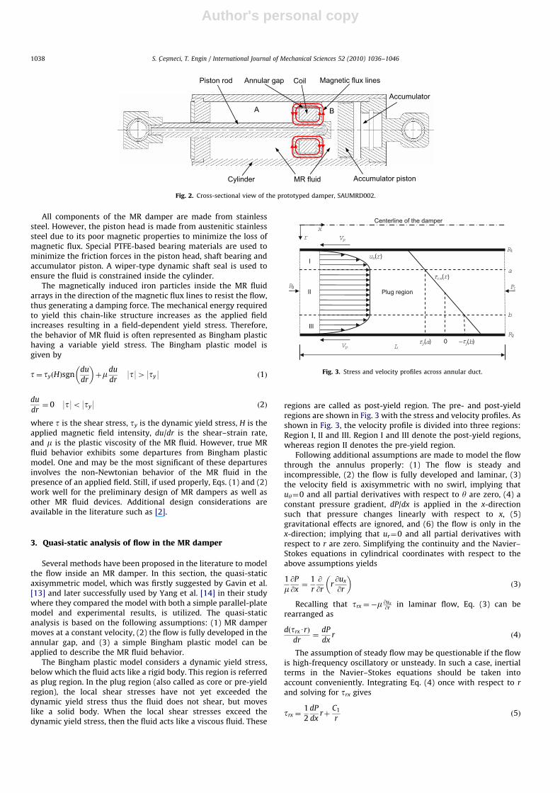
The hydraulic devices that use MR fluids, including dampers,servo-valves, shock absorbers, are generally in pressure driven flowmode while MR brakes and clutches are in direct-shear mode.A schematic diagram for the damper used in this study is given inFig. 2 with its primary components. The portions denoted as A and Bin Fig. 2 are filled with MR fluids whereas the accumulator, which isfor compensating the additional volume into the chamber caused bythe movement of the piston rod, is filled with the pressurizednitrogen gas. The MR fluid used in this study is MRF-122ED of LordCorporation. During the motion of the MR damper’s piston rod, fluidflows through the annular gap opened on the piston head. Inside thepiston head, a coil is wound around the bobbin shaft with aninsulated wire. When electrical current is applied to the coil, amagnetic field develops around the piston head. The magnetic fluxlines will look like as shown in Fig. 2.

Flow( )

Applied field

Pressure Force

Applied field

Fig. 1. Basic operational modes for field-controllable fluid devices: (a) pressure driven flow mode and (b) direct-shear mode.

Symbols

a Inner plug radius measured from shaft axis, displace-ment amplitude

Ap Frontal area of the piston headAs Cross-sectional area of the shaftb Outer plug radius measured from shaft axisC Integral constantD Dynamic rangeDchannel,i Inner diameter of the flow channelDchannel,o Outer diameter of the flow channelDcyl,i Inner diameter of the cylinderDp Diameter of the piston headDs Shaft diameterF Damping forceFcompression Damping force of the MR damper when it is in

compression modeFexp Measured forceFf Friction forceFgas Gas forceFpre Predicted forceFrebound Damping force of the MR damper when it is in

rebound modeg Gap of the flow channelH Applied magnetic field intensityI CurrentK Fluid indexL Length of the flow channelLactive Active pole lengthLdamper Total length of the damper at its maximum extensionLinactive Inactive pole lengthn Fluid indexP PressureQ Volume flow rateQp Volume flow rate displaced by the piston head

QT Total volume flow rate through the flow channelr Radial coordinate measured from the shaft axisR1 Inner radius of the flow channel measured from the

shaft axisR2 Outer radius of the flow channel measured from the

shaft axisS Maximum strokeu(r) Velocity distribution in the flow channelVp Piston velocityw Width of the flow channelx Longitudinal coordinate_g Shear–strain rateDPm Viscous component of the pressure dropDPt Field-dependent induced yield stress component of

the pressure dropm Plastic viscosityt Shear stressmF Mean measured forcety Dynamic yield stressDP Pressure drop across annular gapo Angular velocity

Brevities

Alg Algebraic modelmAlg Modified algebraic modelmBW Modified Bouc-Wen model

Subscripts

Alg Algebraic modelmAlg Modified algebraic modelt Timex Displacement_x Velocity

S. C- es-meci, T. Engin / International Journal of Mechanical Sciences 52 (2010) 1036–1046 1037

Author's personal copyARTICLE IN PRESS

All components of the MR damper are made from stainlesssteel. However, the piston head is made from austenitic stainlesssteel due to its poor magnetic properties to minimize the loss ofmagnetic flux. Special PTFE-based bearing materials are used tominimize the friction forces in the piston head, shaft bearing andaccumulator piston. A wiper-type dynamic shaft seal is used toensure the fluid is constrained inside the cylinder.

The magnetically induced iron particles inside the MR fluidarrays in the direction of the magnetic flux lines to resist the flow,thus generating a damping force. The mechanical energy requiredto yield this chain-like structure increases as the applied fieldincreases resulting in a field-dependent yield stress. Therefore,the behavior of MR fluid is often represented as Bingham plastichaving a variable yield stress. The Bingham plastic model isgiven by

t¼ tyðHÞsgndu

dr

� �þmdu

dr9t949ty9 ð1Þ

du

dr¼ 0 9t9o9ty9 ð2Þ

where t is the shear stress, ty is the dynamic yield stress, H is theapplied magnetic field intensity, du/dr is the shear–strain rate,and m is the plastic viscosity of the MR fluid. However, true MRfluid behavior exhibits some departures from Bingham plasticmodel. One and may be the most significant of these departuresinvolves the non-Newtonian behavior of the MR fluid in thepresence of an applied field. Still, if used properly, Eqs. (1) and (2)work well for the preliminary design of MR dampers as well asother MR fluid devices. Additional design considerations areavailable in the literature such as [2].

3. Quasi-static analysis of flow in the MR damper

Several methods have been proposed in the literature to modelthe flow inside an MR damper. In this section, the quasi-staticaxisymmetric model, which was firstly suggested by Gavin et al.[13] and later successfully used by Yang et al. [14] in their studywhere they compared the model with both a simple parallel-platemodel and experimental results, is utilized. The quasi-staticanalysis is based on the following assumptions: (1) MR dampermoves at a constant velocity, (2) the flow is fully developed in theannular gap, and (3) a simple Bingham plastic model can beapplied to describe the MR fluid behavior.

The Bingham plastic model considers a dynamic yield stress,below which the fluid acts like a rigid body. This region is referredas plug region. In the plug region (also called as core or pre-yieldregion), the local shear stresses have not yet exceeded thedynamic yield stress thus the fluid does not shear, but moveslike a solid body. When the local shear stresses exceed thedynamic yield stress, then the fluid acts like a viscous fluid. These

regions are called as post-yield region. The pre- and post-yieldregions are shown in Fig. 3 with the stress and velocity profiles. Asshown in Fig. 3, the velocity profile is divided into three regions:Region I, II and III. Region I and III denote the post-yield regions,whereas region II denotes the pre-yield region.

Following additional assumptions are made to model the flowthrough the annulus properly: (1) The flow is steady andincompressible, (2) the flow is fully developed and laminar, (3)the velocity field is axisymmetric with no swirl, implying thatuy¼0 and all partial derivatives with respect to y are zero, (4) aconstant pressure gradient, dP/dx is applied in the x-directionsuch that pressure changes linearly with respect to x, (5)gravitational effects are ignored, and (6) the flow is only in thex-direction; implying that ur¼0 and all partial derivatives withrespect to r are zero. Simplifying the continuity and the Navier–Stokes equations in cylindrical coordinates with respect to theabove assumptions yields

1

m@P

@x¼

1

r

@

@rr@ux

@r

� �ð3Þ

Recalling that trx ¼�m @ux

@r in laminar flow, Eq. (3) can berearranged as

dðtrxUrÞ

dr¼

dP

dxr ð4Þ

The assumption of steady flow may be questionable if the flowis high-frequency oscillatory or unsteady. In such a case, inertialterms in the Navier–Stokes equations should be taken intoaccount conveniently. Integrating Eq. (4) once with respect to r

and solving for trx gives

trx ¼1

2

dP

dxrþ

C1

rð5Þ

Piston rod Annular gap Magnetic flux lines

Cylinder MR fluid

Coil

Accumulator piston

A B

Accumulator

Fig. 2. Cross-sectional view of the prototyped damper, SAUMRD002.

Plug region

Centerline of the damper

Fig. 3. Stress and velocity profiles across annular duct.

S. C- es-meci, T. Engin / International Journal of Mechanical Sciences 52 (2010) 1036–10461038

Author's personal copyARTICLE IN PRESS

Bingham plastic model describes the yield stress as in Eqs. (1) and(2). Because of their different natures, each region in Fig. 3 should beevaluated separately. In region I, the shear stress in given by

trxðrÞ ¼ tyþmduðrÞ

drðdu=dr40, and thus sgnðdu=drÞ ¼ 1Þ ð6Þ

Substituting Eq. (6) into Eq. (5) gives

tyþmduðrÞ

dr¼

1

2

dP

dxrþ

C1

rð7Þ

rearranging

duðrÞ

dr¼

1

2mdP

dxrþ

C1

m1

r�ty

m ð8Þ

integrating once with respect to r

uðrÞ ¼1

4mdP

dxr2þ

C1

m lnðrÞ�ty

m rþC2 ð9Þ

where C1 and C2 are the integral constants which can bedetermined by the boundary conditions in region I. Boundaryconditions for each region are listed in Table 1.

One can conclude with

uðrÞ ¼�1

4mdP

dxðR2

1�r2ÞþC1

m lnr

R1

� ��ty

m ðr�R1Þ�Vp; R1rrra ð10Þ

by applying the boundary condition given for region I. In regionIII, the shear stress in given by

trxðrÞ ¼�tyþmduðrÞ

drðdu=dro0, and thus sgn ðdu=drÞ ¼�1Þ

ð11Þ

In a similar fashion as we did for region I, one can end up with

uðrÞ ¼�1

4mdP

dxðR2

2�r2ÞþC1

m lnr

R2

� ��ty

m ðR2�rÞ�Vp; brrrR2

ð12Þ

for region III. It is evident from Fig. 3 that duðrÞ=dr¼ 0 across theplug region, thus u(r¼a)must be equal to u(r¼b), which yields

�1

4mdP

dxðR2

1�a2ÞþC1

m lna

R1

� ��ty

m ða�R1Þ�Vp

¼�1

4mdP

dxðR2

2�r2ÞþC1

mln

r

R2

� ��ty

mðR2�rÞ�Vp

ð13Þ

or

dP

dx¼

4

R21�R2

2þb2�a2D1ln

a

b

R2

R1

� �þtyðR1þR2�a�bÞ

� �ð14Þ

The shear stresses at each boundary of the plug are equal tothe yield stress of the MR fluid and can be expressed astrx(r¼a)¼ty and trx(r¼b)¼�ty. Thus,

1

2

dP

dxaþ

C1

a¼�

1

2

dP

dxb�

C1

bð15Þ

or

C1 ¼�ab

2

dP

dxð16Þ

Now consider a differential fluid element of thickness b�a,length dx as shown in Fig. 4. A force balance on the volumeelement in the flow direction gives

dP

dxpðb2�a2Þdxþ2ptyðbþaÞdx¼ 0 ð17Þ

or

dP

dx¼�

2ty

b�að18Þ

C1 can be determined by substituting Eq. (18) into Eq. (16) as

C1 ¼abty

b�að19Þ

The law of conservation of mass requires that the total volumeflow rate through the annular gap must be equal to thesummation of the volume flow rates through the three regions:Region I, II and III. Once the velocity profiles at each of the threeregions are known, the total volume flow rate can be determinedfrom

QT ¼ 2pRaR1

�1

4mdP

dxðR2

1�r2ÞþC1

m lnr

R1

� ��ty

m ðr�R1Þ�Vp

� �rdr

þ2pR b

a �1

4mdP

dxðR2

2�b2ÞþC1

mln

b

R2

� ��ty

mðR2�bÞ�Vp

� �rdr

þ2pR R2

b �1

4mdP

dxðR2

2�r2ÞþC1

m lnr

R2

� ��ty

m ðR2�rÞ�Vp

� �rdr

ð20Þ

On the other hand, by definition, the total volume flow ratethrough the annuli must be equal to the volume flow ratedisplaced by the piston head, Qp¼(Ap�As)Vp. Thus, we have

Q a,bð Þ�Qp ¼ 0 ð21Þ

There are two unknowns, a and b, but we have only oneequation, Eq. (21), at hand. The second equation comes from thesubstitution of Eq. (18) into Eq. (14)

4

R21�R2

2þb2�a2C1ln

a

b

R2

R1

� �þtyðR1þR2�a�bÞ

� �þ

2ty

b�a¼ 0 ð22Þ

The Newton–Raphson method is employed to solve theresulting nonlinear system of these two algebraic equations,Eqs. (21) and (22), to determine a and b. Once a and b have beendetermined the pressure gradient can be determined fromEq. (18). Hence, the pressure drop due to the field-dependentyield stress can be calculated from

DPt ¼�dP

dxLactive ð23Þ

where Lactive is the active pole length exposed magnetic field.Now, the damping force of the MR damper can be determinedfrom

Frebound ¼� DPt Ap�As

� �þFf þFgas

� �ð24Þ

Fcompression ¼DPt ApþFf þFgas ð25Þ

Fig. 4. Free-body diagram of a ring-shaped differential fluid element of thickness

b–a and length dx.

Table 1List of boundary conditions.

Regions Boundary conditions

R1rrra

Region I u (R1)¼–Vp, duðaÞdr ¼ 0

Region II u(a)¼u(b)

brrrR2

Region III u (R2)¼�Vp, duðbÞdr ¼ 0

S. C- es-meci, T. Engin / International Journal of Mechanical Sciences 52 (2010) 1036–1046 1039

Author's personal copyARTICLE IN PRESS

Note that the damping force of the MR damper variesaccording to its motion, whether it is in rebound or compressionmode.

3.1. Special case: No magnetic field

So far we have performed calculations for the flow of MR fluidinduced by a magnetic field. However, in the regions of inactivemagnetic field, the regions particularly adjacent to the windingwhere ty¼0, MR fluid exhibits a Newtonian like behavior andthus should be evaluated separately. The shear stress across anannular gap was given by Eq. (5). Integrating Eq. (5) with respectto r gives

uðrÞ ¼1

4mdP

dxr2þ

C1

m ln rþC2 ð26Þ

C1 and C2 can be determined from the boundary conditions: Atr¼R1 u¼�Vp and at r¼R2 u¼�Vp. Once the velocity profile isknown, one can calculate the total volume flow rate through theflow channel from

QT ¼ 2pZ R2

R1

uðrÞr dr ð27Þ

Recall that the total volume flow rate through the annuli mustbe equal to the volume flow rate displaced by the piston head,Qp¼(Ap�As)Vp. Therefore,

QT�Qp ¼ 0 ð28Þ

One can solve Eq. (28) for dP/dx and use it to determine thepressure drop due to the viscous effects only as

DPm ¼�dP

dxLinactive ð29Þ

And thus the damping force

Frebound ¼� DPm Ap�As

� �þFf þFgas

� �ð30Þ

Fcompression ¼DPm ApþFf þFgas ð31Þ

where Linactive¼L�Lactive. Note that for the case of zero magneticfield Linactive is equal to L.

4. Experimental study

4.1. Test set-up

The MR damper is subjected to sinusoidal excitations on amechanical scotch-yoke type damper dynamometer to validatethe models. The primary components of the test set-up are shownin Fig. 5. The shock machine has its own software to collect thedata from the data card and use them to plot force vs. time, forcevs. displacement and force vs. velocity graphs for each test.A programmable ‘‘GWinstek PPE 3223’’ power supply is used tofeed current to the MR damper. The machine also has an IRtemperature sensor to read the temperature data during the tests.The damper is fixed to the machine via grippers as shown in theFig. 5. The machine excites the damper’s piston rod sinusoidally,while a load cell of 22 kN measures the force on the damper and alinear variable displacement transducer (LVDT) measures thedisplacement of the piston rod as well as the relative velocitybetween the two ends of the damper.

4.2. Test procedure and conditions

A series of tests is conducted to determine the dynamicresponse of the damper by varying the applied current from 0 to2 A in increments of 0.2 A, while maintaining the frequency at

constant levels of 0.63, 1.27, 1.90 and 2.54 Hz, respectively. Thetechnical specifications of the test damper are given in Table 2.

5. Test results and validation of the proposed model

5.1. Test results

Fig. 6 represents the force vs. velocity and force vs.displacement plots for an oscillation frequency of 2.54 at adisplacement amplitude of 12.5 mm. Similar test results wereobserved for other frequencies as well. The gas and friction forcesmeasured to be approximately 60 and 110 N, respectively. As canbe seen from Fig. 6, the lowest damping force which is only due tothe viscous forces occurs at zero current input, and the dampingforce increases with increasing current inputs. It is clear fromFig. 6 that the controllable damping forces can easily be acquiredby changing the electric current input. This implies that an MRdamper can be viewed as a versatile device in the sense that it canprovide infinitely variable load cycles within a specified dynamicoperating range compared to a classical dashpot.

For an MR damper the increase in the damping force due toapplied current is not unlimited. A careful look at Fig. 6 reveals

Table 2Technical specifications of SAUMRD002.

Parameter Value Unit

Damping force, F 200–2000 N

Operating current, I 0–2 A

Yield strength, ty 5750–23500 Pa

Plastic viscosity, m 0.07 Pa s

Piston velocity, Vp 0–0.2 m/s

Piston diameter, Dp 0.039 m

Shaft diameter, Ds 0.010 m

Maximum stroke, S 0.055 m

Inner diameter of the cylinder, Dcyl,i 0.040 m

Gap of the flow channel, g 0.0004 m

Length of the flow channel, L 0.020 m

Active pole length, Lactive 0.008 m

Outer diameter of the flow channel, Dchannel,o 0.032 m

Inner diameter of the flow channel, Dchannel,i 0.03102 m

Total length of the damper at its maximum extension 0.27 m

Fig. 5. Photograph of the test set-up.

S. C- es-meci, T. Engin / International Journal of Mechanical Sciences 52 (2010) 1036–10461040

Author's personal copyARTICLE IN PRESS

that this increase decays gradually as the applied currentincreases, especially, to its high values, which is illustrated byFigs. 7 and 8 for convenience. One can observe from Fig. 7 that thevariation in force levels off in the vicinity of 2 A. In Fig. 8, the plotof the derivative of force with respect to current (dF/dI) versuscurrent is sketched in order to depict the susceptibility of thedamping force to the applied current. It is clear from Fig. 8 thatthe damping force increases with the applied current to reach itspeak value around 0.5 A and then decreases asymptotically. Thisis due to the fact that the MR fluid is magnetically saturatedwithin a certain range of magnetic field. This phenomenon is ofcritical importance in design considerations of an MR damper andshould be taken into account properly for determination of thebest efficient operating range of the damper. Also, operating athigher current inputs may cause the temperature of the coil wireto rise, which is not desired.

5.2. Validation of the theoretical flow model

In this section the fluid dynamics model has been verified bycomparing the model results with the experimental data.Comparisons between the model and experimental values arepresented in Fig. 9. It is observed that the predicted values withthe fluid dynamics model agree well with the measured values,except in the hysteretic region seen in the force vs. velocity plot.One can infer from Fig. 9a that as the current input increases, thelocal slopes of the force vs. velocity curves increase. This can beattributed to the fact that the apparent viscosity of the MR fluidchanges with shear–strain rate leading to shear-thinning or -thickening behavior of the MR fluid. The Bingham plastic modelused in this study does not account for such behavior assummingthe plastic viscosity to be constant. However, the Herschel–Buckley constitutive model with t¼ tyþK _gn, where ty is the yieldstress of the MR fluid, _g is the deformation rate, and K and n arethe consistency and flow indexes both of which are determinedexperimentally, can be used to predict this characteristic of MRfluids [12,15]. Further studies on shear-thinning or -thickeningbehaviors of MR fluids can be found in the literature, such as [15].

There is also another fluid mechanics model called as Biviscousmodel to simulate the force response of the MR damper. In thismodel, the damping behavior is due to leakage, defined as asecond path of Newtonian flow in addition to the Bingham plasticflow through an ER/MR valve. Leakage is typically introducedto smooth the force response of the damper as the damper

0 0.5 1 1.5 20

500

1000

1500

Current (A)

dF/d

I (N

/A)

0.05 m/s0.10 m/s0.15 m/s0.20 m/s

Fig. 8. Susceptibility of SAUMRD002 to the applied current.

-0.2 -0.1 0 0.1 0.2-2500

-2000

-1500

-1000

-500

0

500

1000

1500

2000

2500

Velocity (m/s)

Forc

e (N

)

0 A 0.2 A

0.4 A 0.6 A 0 .8A 1A

2 A 1.5 A

-0.015 -0.01 -0.005 0 0.005 0.01 0.015-2500

-2000

-1500

-1000

-500

0

500

1000

1500

2000

2500

Displacement (m)

Forc

e (N

)

Fig. 6. Force vs. velocity and force vs. displacement plots of SAUMRD002 at

2.54 Hz sinusoidal excitation.

0 0.5 1 1.5 2-2000

-1500

-1000

-500

0

500

1000

1500

2000

2500

Current (A)

Forc

e (N

) 0.05 m/s Rebound0.05 m/s Compression0.10 m/s Rebound0.10 m/s Compression0.15 m/s Rebound0.15 m/s Compression0.20 m/s Rebound0.20 m/s Compression

Fig. 7. Force vs. current plots of SAUMRD002.

S. C- es-meci, T. Engin / International Journal of Mechanical Sciences 52 (2010) 1036–1046 1041

Author's personal copyARTICLE IN PRESS

undergoes transitions through the low velocities, whereas in theabsence of leakage ER/MR dampers usually exhibit a high-frequency chatter in their force response [16]. As can be seenfrom Fig. 9a, Bingham Plastic model like other fluid mechanicsbased models such as Herschel–Bulkley and Biviscous cannotdescribe the hysteretic behavior of MR dampers. NeverthelessBingham Plastic model can still be successfully adopted to predictthe dynamic operating range of MR dampers owing to itssimplicity. The total area enclosed in force vs. displacementcurves represents the energy dissipated by an MR damper. It isclear from Fig. 9b that higher applied magnetic field will result inhigher energy dissipation.

5.3. Modeling the hysteretic behavior of MR damper

The dislocation movement and plastic slipping among mole-cular chains or crystal lattices consume energy such that therestoring force of an MR damper always delays the inputdisplacement or velocity. This phenomenon of energy dissipationis generally referred to as hysteresis. Different models havebeen studied in the literature to describe the hysteretic behaviorof MR dampers. These models can be classified into two maincategories as quasi-static flow models and dynamic models. While

the quasi-static flow models can be successfully adapted to designMR dampers, they unfortunately fail to capture the dynamicoperational behavior of these dampers. That is, a quasi-static flowmodel such as Bingham plastic model can describe the force–displacement range of an MR damper effectively in the pre-liminary design process; however, it is not capable of describingthe highly hysteretic force–velocity characteristic, which is, infact, of crucial importance for a successful control performance ofthe damper. Therefore, a dynamic hysteresis model is needed tosimulate the hysteresis phenomenon of MR dampers. To this end,various models have been proposed in the literature such asparametric viscoelastic-plastic model based on the Binghammodel [9], the Bouc–Wen model [17], non-parametric models[18], and many more. In this study, the model used by Guo andHu[1] to define an additional nonlinear stiffness is exploited andmodified to give more accurate results. The model is given by

FðtÞ ¼ f0þCb _xðtÞþ2

p fytan�1 k _xðtÞ� _x0sgn €xðtÞð Þ� �

ð32Þ

where F represents the damping force of the MR damper, f0 thepreload of the nitrogen accumulator, Cb the coefficient of viscousdamping, fy the yielding force, k the shape coefficient, _x0 thehysteretic velocity, _x and €x the excitation velocity and accelera-tion of the piston in the damper, respectively. This mathematicalmodel is developed based on some physical phenomena. Whilethe first term is to represent the preload force of the pressurizednitrogen gas in the accumulator, the second term is to describethe viscous force of the damper and the third one is to reflect theobserved hysteretic behavior, respectively. The mathematicaldescriptions of the first two terms come from classical mechanics,whereas of the third one is developed based on the definition of atrigonometric arctangent function which best resembles thecharacteristic force–velocity curve of the damper. Further, thetwo terms in the braces of the arctangent function are to accountfor the lag in the force response to a sinusoidal excitation.

In the model xðtÞ ¼ asin ðotÞ, _xðtÞ ¼ ao cos ðotÞ, and€xðtÞ ¼�ao2 sinðotÞ where a is the displacement amplitude ando is the angular velocity. In Eq. (32), f0, Cb, fy, k, and _x0 are theunknown parameters and to be determined on the basis ofexperimental data by using least-square curve fitting method.

It is observed that there is a general good agreement betweenthe estimated and measured values except at lower currentinputs, i.e. 0 and 0.2 A of the highest excitation velocity of 0.2 m/s(Fig. 10). We have reasoned that this could be presumably due tothe fluid inertial force, which becomes more significant at lowercurrent inputs compared to induced yield stress force, as theexcitation acceleration increases. Starting from this point, wemodified the model given by Eq. (32) by adding an inertial forceterm in order to improve the agreement

FðtÞ ¼ f0þCb _xðtÞþ2

p fytan�1 k _xðtÞ� _x0sgn €xðtÞð Þ� �

þm €xðtÞ ð33Þ

where m represents the virtual mass which has to be determinedbased on the experimental data. It is obvious from Fig. 11 thatthe proposed modified algebraic model (mAlg) removed thedisagreement at the mention lower current input region. Modelparameter estimates are given in Table 3.

Fig. 12 represents the velocity (0–0.2 m/s) averaged variationof model parameters with the applied current for mAlg model.Each parameter in Eqs. (32) and (33) has an effect on the shape ofthe curve such that f0 slides the curve up or down maintaining theshape of the whole curve, fy controls the dynamic force range, Cb

controls the slope of the whole curve, whereas k and _x0 controlsthe slope and the span of the low velocity hysteresis loop,respectively. In addition to these parameters, m controls the spanof the high velocity hysteresis loop.

-0.2 -0.1 0 0.1 0.2-2500

-2000

-1500

-1000

-500

0

500

1000

1500

2000

2500

Velocity (m/s)

Forc

e (N

)

ExperimentalModel

0.2 A 0 A

0.4 A 0.6 A 0 .8A 1A 1.5 A 2 A

-0.015 -0.01 -0.005 0 0.005 0.01 0.015-2500

-2000

-1500

-1000

-500

0

500

1000

1500

2000

2500

Displacement (m)

Forc

e (N

)

ExperimentalModel

Fig. 9. Comparisons between the model predictions and experimental data: (a)

force vs. velocity and (b) force vs. displacement.

S. C- es-meci, T. Engin / International Journal of Mechanical Sciences 52 (2010) 1036–10461042

Author's personal copyARTICLE IN PRESS

Under these considerations, one can reveal that there is directcorrelation between the model parameters and the experimentaldata by comparing Fig. 12 against Fig. 6a. It should be noted that asmall change in the parameters may correspond to relatively largechanges in the experimental data. For instance, one can expect fy

to increase with the current input since the dynamic dampingforce of the MR damper increases with the applied current. Acloser look at Fig. 12 will indicate that it really does. The variationin all other parameters can be validated in a similar fashion.

More emphasis should be made on the additional parameter m

as it enhanced the success of the model. As discussed previously,m controls the span of the high velocity hysteresis loop. It can beseen from Fig. 6a, the span of the high velocity hysteresis loopdecreases with the applied current. Now, a careful look at Fig. 12will reveal that m decreases with the current input as well, whichagrees with our expectation.

Also, it can be deduced from the Fig. 12 that the variation inthe model parameters levels off as the applied current approachedits maximum value 2 A, as discussed in the previous sections.

In addition to graphical comparison of the mAlg model withthe Alg model, we intend to compare these two models with alsoa previously suggested modified Bouc–Wen’s (mBW) modelthrough an error analysis in order to better reveal the success ofthe mAlg model. One of the earliest models that have been

extensively used in modeling dynamic behavior of hystereticsystems is the standard Bouc–Wen model, which is extremelyversatile and can exhibit a wide variety of hysteretic behavior.However, the nonlinear force–velocity response of the Bouc–Wenmodel does not roll-off in the region where the acceleration andvelocity have opposite signs and the magnitudes of the velocitiesare small, Spencer et al. [16] proposed a modified version of theBouc–Wen model in order to predict the dynamic behavior of theMR damper in this region to enhance the success of the model.The modified Bouc–Wen model was given by

F ¼ azþc0ð _x� _yÞþk0ðx�yÞþk1ðx�x0Þ ð34Þ

where the evolutionary variable z is governed by

_z ¼�g9 _x� _y99z99z9n�1�bð _x� _yÞ9z9n

þAð _x� _yÞ ð35Þ

where

_y ¼1

ðc0þc1Þazþc0 _xþk0ðx�yÞ �

ð36Þ

In this modified model, the accumulator stiffness is repre-sented by k1 and the viscous damping observed at larger velocitiesis represented by c0. A dashpot, represented by c1, is included inthe model to produce the roll-off that was observed in theexperimental data at low velocities, k0 is present to control the

-0.25 -0.2 -0.15 -0.1 -0.05 0 0.05 0.1 0.15 0.2 0.25

-1000

-800

-600

-400

-200

0

200

400

600

800

1000

Velocity (m/s)

Forc

e (N

)

ExperimentalModel

0.2 A

0 A

-0.015 -0.01 -0.005 0 0.005 0.01 0.015

-1000

-800

-600

-400

-200

0

200

400

600

800

1000

Forc

e (N

)

Displacement (m)

ExperimentalModel

Fig. 11. Hysteretic loops of damping force of SAUMRD002 with respect to (a)

velocity and (b) displacement obtained from the model given by Eq. (33) at current

inputs of 0 and 0.2 A.

-0.25 -0.2 -0.15 -0.1 -0.05 0 0.05 0.1 0.15 0.2 0.25

-1000

-800

-600

-400

-200

0

200

400

600

800

1000

0 A

0.2 A

ExperimentalModel

-0.015 -0.01 -0.005 0 0.005 0.01 0.015

-1000

-800

-600

-400

-200

0

200

400

600

800

1000

Forc

e (N

)

Displacement (m)

ExperimentalModel

Fig. 10. Hysteretic loops of damping force of SAUMRD002 with respect to (a)

velocity and (b) displacement obtained from the model given by Eq. (32) at current

inputs of 0 and 0.2 A.

S. C- es-meci, T. Engin / International Journal of Mechanical Sciences 52 (2010) 1036–1046 1043

Author's personal copyARTICLE IN PRESS

stiffness at large velocities and x0 is the initial displacement ofspring k1 associated with the nominal damper force due to theaccumulator. A schematic for the model is given in Fig. 13.

For all of the models, the error between the predicted force andthe measured force was calculated as a function of time,displacement and velocity over a complete period. The followingexpressions were used to represent the errors [17]

Et ¼et

sF, Ex ¼

ex

sF, E _x ¼

e _xsF

ð37Þ

where

e2t ¼

Z T

0Fexp�Fpre

� �2dt ð38Þ

e2x ¼

Z T

0Fexp�Fpre

� �2 dx

dt

��������dt ð39Þ

e2_x ¼

Z T

0Fexp�Fpre

� �2 d _x

dt

��������dt ð40Þ

s2F ¼

Z T

0Fexp�mF

� �2dt ð41Þ

The resulting normalized errors are presented in Table 4.It is seen that although all the three models are equivalent at

the excitation velocities of 0.05, 0.10, and 0.15 m/s, mAlg model isremarkably successful at the highest excitation velocity of0.2 m/s. This is presumably due to effect of the added inertialterm to the Alg model because the inertial forces are dominant asthe excitation acceleration is increased. Also if we focus on thehighest excitation velocity, when comparing the Alg model andmAlg model, one can note that as the current inputs increases theerror differences between the Alg model and the mAlg modeldecreases. This can be attributed to the fact that the viscous forcesand thus inertial force effects are getting less dominant with the

Table 3Parameter estimates for mAlg model.

V(m/s) Parameters Applied current, I (A) (mAlg)

0 0.2 0.4 0.6 0.8 1 1.5 2

0.05 Cb 3427.4 3685.1 4459.2 5520.5 5788.3 6086.3 5900.3 6859.4

f0 �42.1 �36.7 �34 �35.3 �34 �31.9 �28.3 �27.3

fy 8.4 15.5 22.5 25 27.5 28.9 31.5 32.1

k 428.4 433.9 334.5 326.3 293.4 288.3 244 266.4

m 55.3 48.8 30.6 22.3 1 12.5 �33.4 �75.3_x0 0.0019 0.0006 0.0017 0.0021 0.0023 0.0024 0.003 0.0033

0.1 Cb 3264 3242.8 3470.7 3567.7 3721 3982.2 4325 4384.8

f0 18.3 23.3 22.7 16.2 15.7 12.6 13.6 13.9

fy 11.3 19.5 25.1 28.4 30.6 31.5 33.7 35.1

k 243.4 164.3 149.4 133.2 130.8 134.9 128.3 131.5

m 7.7 6.9 6 �1.8 �4.3 �5.1 �12.1 �13.3_x0 0.0062 0.0053 0.006 0.0072 0.0075 0.0078 0.0087 0.0106

0.15 Cb 3264 3211.8 3235.8 3284 3391.3 3479.4 3590.6 3627.7

f0 �32.5 �31.5 �33.8 �32.7 �35 �34.8 �37.3 �36.2

fy 11.3 19.6 26.3 29.5 31.9 33.5 35.8 37.2

k 243.4 107.5 92.8 83.5 80.8 80.1 83.5 82.7

m 7.7 �3.4 �5.7 �7.2 �9.6 �12.7 �14.6 �17.3_x0 0.0062 0.0051 0.0069 0.008 0.0094 0.0093 0.0108 0.0114

0.2 Cb 3175.6 2996.8 2930.4 2872.7 2824.5 2818 2915.7 2847.2

f0 �54.5 �47.7 �48.2 �45.4 �48.9 �50.8 �52.9 �52.2

fy 11.6 19.8 26.2 30.2 33.1 34.6 37 38.7

k 108 75.3 67 60.8 55.6 57.2 56.1 53.7

m �0.7 �2 �3.2 �5.6 �8.6 �8.2 �10.7 �12.5_x0 0.0078 0.0097 0.0111 0.0127 0.0137 0.0142 0.0154 0.0171

0 0.2 0.4 0.6 0.8 1 1.2 1.4 1.6 1.8 2-50

-25

0

25

50

75

Current (A)

Mod

el p

aram

eter

s

f0Cb/200

fyk/10x0*1000

m

Fig. 12. Velocity (0–0.2 m/s) averaged variation of the model parameters with

current input.

Fig. 13. . The modified Bouc-Wen model for the MR damper.

S. C- es-meci, T. Engin / International Journal of Mechanical Sciences 52 (2010) 1036–10461044

Author's personal copyARTICLE IN PRESS

increased current inputs. This actually agrees with our intuitionssince we added an inertial term to modify the model to accountfor the inertial effects of the MR fluid.

Apart from its high accuracy, mAlg model is also morepreferable in terms of its low computational expenses comparedto differential modified Bouc–Wen’s model which is highlycomputationally demanding. It is hoped that the presentimproved model will aid to develop more effective controlstrategies and algorithms for MR dampers.

6. Conclusions

An experimental and a theoretical analysis were conducted tomodel the dynamic behavior of an MR damper. To this end, an MRdamper was designed, manufactured and tested on a conventionalshock machine. A flow analysis of an MR damper was done based onthe Bingham plastic constitutive model and the prediction results wascompared against the test data. The comparisons showed that therewas a very good agreement between the flow model and test results.Therefore, it was concluded that the Bingham plastic model couldsatisfactorily predict the operational force range of the MR damper.However, this model was found to be not capable of capturing theinherent hysteretic behavior of the MR damper, which is of crucialimportance for a successful control performance. For this reason, analgebraic model (Alg), which we have modified by adding an inertialforce term (mAlg), was employed to describe the hysteretic behaviorof the MR damper. The unmodified and modified forms of thealgebraic model, which are parametric in nature, were compared withthe experimental data. It was shown that the mAlg model reduced theerrors associated with force vs. time, force vs. velocity and force vs.

displacement characteristics remarkably. Then, in order to betterreveal the success of the mAlg model, Alg model, mAlg model, and apreviously suggested modified Bouc–Wen’s (mBW) model werecompared through a quantitative error analysis. It was seen thatalthough all three models are equivalent at the excitation velocities of0.05, 0.10, and 0.15 m/s, mAlg model is remarkably successful at thehighest excitation velocity of 0.2 m/s. This is presumably due to effectof the added inertial term to the Alg model because the inertial forcesare dominant as the excitation acceleration is increased. And, whencomparing Alg and mAlg models, the reductions in errors were foundto be over 50% especially for low currents rated at the highestexcitation velocity of 0.2 m/s. This is presumably attributed to the factthat the inertial forces become more comparable to the induced yieldforce at lower current inputs as the excitation acceleration isincreased. The effect of the inertial force vanishes at high currentinputs since the induced yield forces are dominated with the increasein the current input, as expected.

It was deduced that the proposed mAlg model could overcomethe shortcomings of the original Alg model and it can successfullybe employed to describe the hysteretic behavior of the MRdamper so as to develop effective control algorithms due to itshigh accuracy, low computational expenses compared to atraditionally widely adopted modified Bouc–Wen’s model, whichis computationally highly demanding.

Acknowledgements

The authors gratefully acknowledge to The Scientific andTechnological Research Council of Turkey (TUB_ITAK) for makingthis project possible under Grant No. 104M157. The authors also

Table 4Error norms for each model.

V (m/s) 0.05 0.10 0.15 0.20

I (A) Et Ex E _x Et Ex E _x Et Ex E _x Et Ex E _x

Model

mBW0.0 0.019 0.003 0.007 0.018 0.004 0.014 0.018 0.005 0.020 0.021 0.007 0.029

0.2 0.041 0.004 0.018 0.025 0.004 0.021 0.018 0.004 0.022 0.020 0.006 0.031

0.4 0.044 0.005 0.019 0.023 0.004 0.019 0.021 0.004 0.025 0.023 0.006 0.038

0.6 0.049 0.005 0.021 0.022 0.003 0.019 0.022 0.005 0.026 0.026 0.007 0.041

0.8 0.028 0.003 0.013 0.023 0.004 0.020 0.021 0.005 0.027 0.026 0.007 0.042

1.0 0.030 0.003 0.013 0.022 0.003 0.019 0.022 0.005 0.027 0.026 0.007 0.042

1.5 0.030 0.003 0.013 0.021 0.003 0.018 0.021 0.004 0.027 0.025 0.006 0.042

2.0 0.028 0.003 0.012 0.021 0.004 0.018 0.022 0.004 0.027 0.026 0.007 0.043

Average 0.034 0.004 0.015 0.022 0.004 0.019 0.021 0.005 0.025 0.024 0.007 0.038

Alg0.0 0.056 0.007 0.023 0.031 0.006 0.025 0.024 0.006 0.029 0.028 0.009 0.042

0.2 0.035 0.005 0.015 0.020 0.004 0.016 0.016 0.004 0.018 0.021 0.007 0.032

0.4 0.029 0.004 0.012 0.019 0.003 0.017 0.018 0.004 0.022 0.022 0.006 0.034

0.6 0.029 0.004 0.013 0.022 0.003 0.019 0.020 0.004 0.025 0.024 0.006 0.039

0.8 0.029 0.003 0.013 0.023 0.003 0.020 0.020 0.004 0.025 0.025 0.007 0.040

1.0 0.030 0.003 0.014 0.024 0.003 0.021 0.022 0.004 0.028 0.026 0.007 0.042

1.5 0.031 0.003 0.014 0.024 0.003 0.021 0.023 0.004 0.030 0.027 0.007 0.044

2.0 0.031 0.003 0.014 0.023 0.004 0.021 0.024 0.005 0.032 0.027 0.007 0.046

Average 0.034 0.004 0.015 0.023 0.004 0.020 0.021 0.005 0.026 0.025 0.007 0.040

mAlg (This study)0.0 0.035 0.004 0.014 0.018 0.003 0.023 0.017 0.004 0.019 0.015 0.005 0.022

0.2 0.034 0.004 0.025 0.022 0.003 0.024 0.020 0.003 0.022 0.013 0.004 0.025

0.4 0.035 0.004 0.020 0.020 0.003 0.026 0.021 0.003 0.020 0.014 0.004 0.022

0.6 0.035 0.004 0.021 0.022 0.004 0.024 0.020 0.004 0.024 0.015 0.004 0.024

0.8 0.035 0.004 0.020 0.023 0.004 0.026 0.022 0.004 0.026 0.015 0.004 0.024

1.0 0.033 0.004 0.021 0.023 0.004 0.027 0.019 0.004 0.021 0.017 0.004 0.025

1.5 0.034 0.004 0.019 0.021 0.004 0.026 0.022 0.004 0.025 0.017 0.004 0.026

2.0 0.035 0.004 0.019 0.023 0.004 0.028 0.023 0.004 0.025 0.017 0.004 0.025

Average 0.035 0.004 0.020 0.022 0.003 0.026 0.021 0.004 0.023 0.016 0.004 0.024

S. C- es-meci, T. Engin / International Journal of Mechanical Sciences 52 (2010) 1036–1046 1045

Author's personal copyARTICLE IN PRESS

acknowledge to TUB_ITAK-Munir Birsel Graduate ScholarshipFoundation for its financial support to the first author (S-evkiC- esmeci).

References

[1] Guo D, Hu H. Nonlinear-Stiffness of a magnetorheological fluid damper.Nonlinear Dynamics 2005;40:241–9.

[2] Chooi WW, Oyadiji SO. Design, modeling and testing of a magnetorheological(MR) dampers using analytical flow solutions. Computers & Structures2008;86:473–82.

[3] Choi S.B., Lee H.S., Hong S.R., and Cheong C.C. Control and responsecharacteristics of a magnetorheological fluid damper for passenger vehicles.Smart Structures and Integrated Systems. In: Proceedings of SPIE conferenceon smart materials and structures Edited by Norman M. Wereley 2000;3895:pp. 438–443.

[4] Kamath GM, Wereley NM, Jolly MR. Characterization of magnetorheologicalhelicopter lag dampers. Journal of the American Helicopter Society1999;44(3):234–48.

[5] Gordaninejad F, Kelso SP. Fail-Safe magneto-rheological fluid dampers for off-highway. High-Payload Vehicles. Journal of Intelligent Material Systems andStructures 2001;11(5):395–406.

[6] Lee T.Y., Kawashima K. Semi-active control of seismic-excited nonlinear isolatedbridges. In: Proceedings of the eighth US national conference on earthquakeengineering. April 18–22, San Francisco, California, USA 2006:pp. 423.

[7] Unsal M. Semi-active vibration control of a parallel platform mechanism usingmagnetorheological damping. Ph. D. Dissertation: University of Florida; 2006.

[8] Kamath GM, Hurt MK, Wereley NM. Analysis and testing of Bingham plasticbehavior in semi-active eletrorheological fluid dampers. Smart Materials andStructures 1996;5:576–90.

[9] Wereley NM, Lindler J, Rosenfeld N, Choi YT. Biviscous damping behavior inelectrorheological shock absorbers. Smart Materials and Structures 2004;13:743–52.

[10] Wang XJ, Gordaninejad F. Flow analysis and modeling of field-controllable,electro- and magneto-rheological fluid dampers. Journal of Applied Mechan-ics—Transactions of the ASME 2007;74(1):13–22.

[11] Jolly M.R., Bender J.W., and Carlson J.D. Properties and applications ofcommercial magnetorheological fluids. In: Proceedings of the SPIE fifthannual ınternational symposium on smart structures and materials: SanDiego, CA 1998.

[12] Wang XJ, Gordaninejad F. Flow analysis of field-controlled electro- andmagneto-rheological fluids using Herschel–Bulkley model. Journal of In-telligent Material Systems and Structures 1999;10(8):601–8.

[13] Gavin HP, Hanson RD, Filisko FE. Electrorheological dampers. Part 1:Analysis and Design. Journal of Applied Mechanics, ASME 1996;63(9):669–75.

[14] Yang G, Spencer Jr. BF, Carlson JD, Sain MK. Large-scale MR fluid Dampers:modeling, and dynamic performance considerations. Engineering Structures2002;24(3):309–23.

[15] Dimock G.A., Lindler J.E., and Wereley N.M. Bingham Biplastic analysis ofshear thinning and thickening in magnetorheological dampers, In: Proceed-ings of the SPIE’s seventh ınternational symposium on smart structures andmaterials, Newport Beach, CA, 2000, pp. no:398549.

[16] Wereley NM, Lindler J, Rosenfeld N, Choi Y-T. Biviscous damping behavior inelectrorheological shock absorbers. Smart Material and Structures 2004;13:743–52.

[17] Spencer Jr. BF, Dyke SJ, Sain MK, Carlson JD. Phenomenological model of amagnetorheological damper. Journal of Engineering Mechanics, ASCE1997;123:230–8.

[18] Song X, Ahmadian M, Southward SC. Modeling magneto-rheological damperswith multiple hysteresis nonlinearities. Journal of Intelligent MaterialSystems and Structures 2005;16(5):421–32.

S. C- es-meci, T. Engin / International Journal of Mechanical Sciences 52 (2010) 1036–10461046