IOP PUBLISHING SMART MATERIALS AND STRUCTURES

Smart Mater. Struct. 18 (2009) 015013 (10pp) doi:10.1088/0964-1726/18/1/015013

Optimal design of a vehiclemagnetorheological damper consideringthe damping force and dynamic rangeQuoc-Hung Nguyen and Seung-Bok Choi1

Smart Structures and Systems Laboratory, Department of Mechanical Engineering,Inha University, Incheon 402-751, Korea

E-mail: seungbok@inha.ac.kr

Received 4 August 2008, in final form 21 October 2008Published 8 December 2008Online at stacks.iop.org/SMS/18/015013

AbstractThis paper presents an optimal design of a passenger vehicle magnetorheological (MR) damperbased on finite element analysis. The MR damper is constrained in a specific volume and theoptimization problem identifies the geometric dimensions of the damper that minimize anobjective function. The objective function consists of the damping force, the dynamic range,and the inductive time constant of the damper. After describing the configuration of the MRdamper, the damping force and dynamic range are obtained on the basis of the Bingham modelof an MR fluid. Then, the control energy (power consumption of the damper coil) and theinductive time constant are derived. The objective function for the optimization problem isdetermined based on the solution of the magnetic circuit of the initial damper. Subsequently, theoptimization procedure, using a golden-section algorithm and a local quadratic fittingtechnique, is constructed via commercial finite element method parametric design language.Using the developed optimization tool, optimal solutions of the MR damper, which areconstrained in a specific cylindrical volume defined by its radius and height, are determined anda comparative work on damping force and inductive time constant between the initial andoptimal design is undertaken.

(Some figures in this article are in colour only in the electronic version)

1. Introduction

Vehicle suspension is normally used to attenuate unwantedvibration from various road conditions. The successfulsuppression of the vibration leads to an improvement of vehiclecomponents’ life, and the ride comfort, as well as steeringstability. Various suspension methods have been developedand applied to the vibration control of vehicles. Essentially,based on the amount of external power required for thesystem, vehicle suspension systems are classified into threeapproaches: passive, active, and semi-active [1].

The passive suspension system, featuring fixed springs andshock absorbers, provides design simplicity, but performancelimitations are inevitable in the relatively high frequencyrange. Thus, a passive system cannot provide optimal

1 Author to whom any correspondence should be addressed.http://www.ssslab.com.

vibration isolation for various road conditions. In order tocompensate for these limitations, active suspension systemsare utilized. With an additional active force introduced asa part of a suspension unit, the system is then controlledusing different algorithms to make it more responsive tosources of disturbance. Generally, an active suspensionsystem provides high control performance in a wide frequencyrange, but it requires high power sources, complicatedcomponents such as sensors, servo valves, and a sophisticatedcontrol algorithm. The semi-active (also known as adaptive–passive) suspension configuration addresses these drawbacksby effectively integrating a tuning control scheme with tunablepassive devices. For this, active force generators are replacedby modulated variable compartments such as a variable ratedamper and stiffness. Therefore, semi-active suspension canoffer desirable performance without requiring large powersources and expensive hardware.

0964-1726/09/015013+10$30.00 © 2009 IOP Publishing Ltd Printed in the UK1

Smart Mater. Struct. 18 (2009) 015013 Q-H Nguyen and S-B Choi

Recently, various semi-active suspension systems fea-turing magnetorheological (MR) fluid have been proposedand successfully applied in vehicle suspension systems [2–6].Much research on the modeling and design of MR dampershas been undertaken based on the quasi-static assumption ofan MR damper [7–10]. In order to accurately model MRdampers, various dynamic models considering the hysteresisbehavior of MR dampers have also been proposed [11–15].However, research on the optimal design of MR dampersis still considerably rare. Rosenfeld and Wereley [16]proposed an analytical optimization design method for MRvalves and dampers based on the assumption of constantmagnetic flux density throughout the magnetic circuit to ensurethat one region of the magnetic circuit does not saturateprematurely and cause a bottleneck effect. Nevertheless, thisassumption leads to a suboptimal result because the valveperformance depends not only on the magnetic circuit butalso on the geometry of the ducts through which the MRfluid passes. Nguyen et al [17] proposed a finite elementmethod (FEM) based optimal design of MR valves constrainedin a specified volume. This work considered the effectsof all geometric variables of MR valves by minimizing thevalve ratio calculated from the FE analysis. However, thecontrol energy and time response of the MR valves was notconsidered in this research. Recently, Nguyen et al [18] hasstudied an optimal design of MR valves that satisfies specificoperational requirements such as pressure drop with minimumcontrol energy. The inductive time constant was also takeninto account as a state variable. It is noted that in thisstudy the power consumption of the valve was chosen as anobjective function while the pressure drop and inductive timeconstant were treated as state variables with their constraints.Therefore, it is necessary to convert the optimization problemwith constrained state variables to an unconstrained one, whichincreases the computation time and results in low quality of theoptimal design parameters.

Consequently, the main contribution of this research workis to extend the previous research works [17, 18] to vehicle MRdampers considering an advanced objective function whichincludes the damping force, dynamic range, and inductivetime constant altogether. In this study, the cylindrical MRdamper for vehicle suspension proposed by Lee and Choi [4]is considered. The research can be easily extended to otherMR dampers. After describing the configuration and workingprinciple of an MR damper, the damping force and dynamicrange are derived from a quasi-static model which is basedon the Bingham model of an MR fluid. Then, the controlenergy and the inductive time constant are obtained. Theinitial geometric dimensions of the damper are determinedbased on the assumption of constant magnetic flux densitythroughout the magnetic circuit of the damper [16], and theobjective function of the optimization problem is proposedbased on the solution of the initial damper. Subsequently, theoptimization procedure using a golden-section algorithm and alocal quadratic fitting technique is constructed via the ANSYSparametric design language (APDL). Using the developedoptimization tool, optimal solutions of the MR damper, whichare constrained in a specific cylindrical volume defined by

Figure 1. Configuration of the MR damper.

its radius and height, are determined and presented, with adiscussion.

2. Configuration and modeling of the MR damper

The cylindrical MR damper for vehicle suspension proposedby Lee and Choi [4] is presented in figure 1. The MR damperis divided into upper and lower chambers by the piston, andfully filled with the MR fluid. As the piston moves, theMR fluid flows from one chamber to the other through theorifices at both ends and the annular duct between the innerand outer cylinders. The gas chamber located outside acts asan accumulator of the MR fluid flow induced by the motion ofthe piston. By neglecting the frictional force between oil sealsand assuming quasi-static behavior of the damper, the dampingforce of the MR damper can be expressed as follows:

Fd = P2 Ap − P1(Ap − As) (1)

where Ap and As are the piston and the piston-shaft areas,respectively. P1 and P2 are pressures in the upper and lowerchamber of the damper, respectively. The relations between P1,P2 and the pressure in the gas chamber, Pa, can be expressedas follows:

P2 = Pa + �P2; P1 = Pa − �P1 − �P3 (2)

where �P1, �P2, and �P3 are the pressure drops of MR flowthrough the upper MR valve orifice, the lower MR valve orificeand the annular duct between the outer and inner cylinders,respectively. The pressure in the gas chamber can be calculatedas follows:

Pa = P0

(V0

V0 + Asxp

)γ

(3)

where P0 and V0 are the initial pressure and volume of theaccumulator. γ is the coefficient of thermal expansion, whichranges from 1.4 to 1.7 for adiabatic expansion. xp is the piston

2

Smart Mater. Struct. 18 (2009) 015013 Q-H Nguyen and S-B Choi

displacement. By neglecting the minor loss, the pressure drops�P1, �P2, and �P3 can be calculated as follows:

�P1 = 12ηLm

π t3m R1

(Ap − As)xp + 2cLm

tmτy sgn(xp)

�P2 = 12ηLm

π t3m R1

Ap xp + 2cLm

tmτy sgn(xp)

�P3 = 6ηL

π t3g R2

(Ap − As)xp

(4)

where τy is the yield stress of the MR fluid induced by theapplied magnetic field, and η is the field-independent plasticviscosity (the base viscosity). L is the length of the innercylinder, and tg is the gap of the annular duct between the innerand outer cylinders. R1 and R2 are the average radii of theintermediate pole and the annular duct, respectively. Lm is thelength of the magnetic pole, and tm is the gap of the orifice ofthe MR valve structure. c is a coefficient which depends on theflow velocity profile, and it has a value range from a minimumvalue of 2.07 to a maximum value of 3.07. The coefficient ccan be approximately estimated as follows [10]:

c = 2.07 + 12Qη

12Qη + 0.8π R1t2mτy

(5)

where Q is the flow rate of the MR fluid flow through the valvestructures. From equations (1), (2), and (4) the damping forceof the MR damper can be calculated by

Fd = Pa As + cvis xp + FMR sgn(xp) (6)

where

cvis = 6η

π

[(L

R2t3g

+ 2Lm

R1t3m

)(Ap − As)

2 + 2Lm

R1t3m

A2p

];

FMR = (2Ap − As)2cLm

tmτy.

The first term in equation (6) represents the elastic force fromthe gas compliance. The second term represents the dampingforce due to MR fluid viscosity. The third term is the force dueto the yield stress of the MR fluid, which can be continuouslycontrolled by the intensity of the magnetic field through theMR fluid ducts. This is the dominant term of the dampingforce, which is expected to have a large value in MR damperdesign. The dynamic range of the damper (defined as the ratioof the peak force with a maximum current input to the one withzero current input) can be approximately expressed as follows:

λd = cvis xp + FMR

cvis xp. (7)

The dynamic range is also an important parameter in evaluatingthe overall performance of the MR damper. A large value of thedynamic range is expected to provide a wide control range ofthe MR damper.

In this work, the commercial MR fluid (MRF132-LD)from Lord Corporation is used. The induced yield stress of theMR fluid as a function of the applied magnetic field intensity(Hmr) is shown in figure 2. By applying the least square

Figure 2. Yield stress of the MR fluid as a function of magnetic fieldintensity.

curve fitting method, the yield stress of the MR fluid can beapproximately expressed by

τy = C0 + C1 Hmr + C2 H 2mr + C3 H 3

mr. (8)

In equation (8), the unit of the yield stress is kPa, whilethat of the magnetic field intensity is kA m−1. The coefficientsC0, C1, C2, and C3 are respectively identified as 0.3, 0.42,−0.001 16, and 1.0513 × 10−6. In order to calculate thedamping force of the MR damper, it is necessary to solve themagnetic circuit of the damper. From the magnetic circuitsolution, the yield stress of the MR fluid in the active volume(the volume of the MR fluid where the magnetic flux crosses)can be obtained using equation (8). The damping force is thencalculated from equation (6).

The magnetic circuit can be analyzed using the magneticKirchoff’s law as follows:

∑Hklk = Nc I (9)

where Hk is the magnetic field intensity in the kth link of thecircuit and lk is the overall effective length of that link. Nc

is the number of turns of the valve coil and I is the appliedcurrent in the coil wire. The magnetic flux conservation rule ofthe circuit is given by

� = Bk Ak (10)

where � is the magnetic flux of the circuit, and Ak and Bk

are the cross-sectional area and magnetic flux density of thekth link, respectively. At low magnetic field, the magneticflux density, Bk , increases in proportion to the magneticintensity Hk as follows: Bk = μ0μk Hk , where μ0 is themagnetic permeability of free space (μ0 = 4π10−7 T m A−1)and μk is the relative permeability of the kth link material.As the magnetic field becomes large, its ability to polarizethe magnetic material diminishes and the material is almostmagnetically saturated. Generally, a nonlinear B–H curve isused to express the magnetic property of a material.

It is very difficult and complicated to find the exactsolution of the magnetic circuit. Therefore, an approximate

3

Smart Mater. Struct. 18 (2009) 015013 Q-H Nguyen and S-B Choi

solution of the magnetic circuit is used in general. For theproposed MR damper, the approximate magnetic circuit isshown in figure 3, and equations (9) and (10) can be rewrittenas follows:

8∑i=1

Hili = Nc I (11)

� = Bi Ai ; i = 1, . . . , 8. (12)

Due to small gap size of the MR ducts and the small thicknessof the intermediate pole, equations (11) and (12) can beapproximately expressed as follows:

2H1l1 + H2l2 + Hmrlmr + H8l8 = Nc I (13)

� = B1 A1 = B2 A2 = Bmr Amr = B8 A8. (14)

In the above, Hmr and Bmr are the effective magnetic fieldintensity and the flux density of the MR fluid link, respectively.Amr and lmr are respectively the effective cross-sectional areaand the length of the MR link, given by

lmr = 2tm; Amr = 2π R1 Lm.

From equations (13) to (14) and the B–H curves of the MRfluid and the valve structure material, the magnetic circuit ofthe valve can be solved. At low magnetic field, the magneticfield intensity over the MR fluid link can be approximated asfollows:

Hmr = Nc I

2tm + 2l1μmr Amr

μA1+ l2μmr Amr

μA2+ l8μmr Amr

μA8

(15)

where μmr and μ are the relative permeability of the MR fluidand the valve core material, respectively.

In order to improve the accuracy of the magnetic circuitsolution, the FEM has been employed [19, 20]. In this study,the commercial FEM software ANSYS is used. Becausethe geometry of the valve structure is axisymmetric, the2D-axisymmetric coupled element (PLANE13) is used forelectromagnetic analysis. It is noted that a reasonably accuratesolution is expected by using the FEM with a fine mesh becauseboth a large number of links and the difference of flux densityalong the active MR volume are considered.

3. Optimization of the MR damper

In this study, the FEM integrated with an optimization tool isused to obtain the optimal geometric dimensions of the MRdamper in order to minimize an objective function. For vehiclesuspension design, the ride comfort and the suspension travel(the rattle space) are the two conflicting performance indicesto be considered. In order to reduce the suspension travel,a high damping force is required. On the other hand, forimproving the ride comfort, a low damping force is expected,thus a large dynamic range is required. Furthermore, a fasttime response MR damper is also expected in order to improvethe controllability of the suspension system. Taking the above

Figure 3. Approximate magnetic circuit of the MR damper.

requirements into account, the following objective function isproposed:

OBJ = αFFMR,r

FMR+ αd

λd,r

λd+ αT

T

Tr(16)

where FMR, λd, and T are, respectively, the yield stress force,dynamic range, and inductive time constant of the damper (theduration time required for current in the coil to reach 63%of its final value when a step voltage is applied to the coil),which are determined based on the FE solution of the dampermagnetic circuit. FMR,r, λd,r, and Tr are the reference dampingforce, the dynamic range, and the inductive time constant ofthe damper, respectively. αF , αd , and αT are, respectively, theweight factors for the damping force, the dynamic range, andthe inductive time constant (αF +αd +αT = 1). Noteworthily,values of these weighting factors are chosen depending on eachspecific suspension system. For suspension systems designedfor uneven or unpaved road, a large damping force is required.Thus, large values of αF and αT are chosen. On the other hand,a large value of αd is used in the design of suspension systemsfor flat roads.

The inductive time constant and control energy of the MRdamper can be calculated as follows:

T = L in/Rw (17)

N = I 2 Rw (18)

where L in is the inductance of the valve coil given by L in =Nc�/I , and Rw is the resistance of the coil wire, which can beapproximately calculated as follows:

Rw = Lwrw = Ncπdcr

Aw. (19)

In the above, Lw is the length of the coil wire, rw is theresistance per unit length of the coil wire, dc is the averagediameter of the coil, Aw is the cross-sectional area of the coilwire, r is the resistivity of the coil wire (r = 0.017 26 ×10−6 m for copper wire), Nc is the number of coil turns,which can be approximated by Nc = Ac/Aw, and Ac is thecross-sectional area of the coil.

4

Smart Mater. Struct. 18 (2009) 015013 Q-H Nguyen and S-B Choi

The reference damping force, dynamic range, andinductive time constant of the damper are obtained fromthe solution of the MR damper at initial values of designparameters. The initial geometric dimensions of the damperare determined based on the assumption of constant magneticflux density throughout the magnetic circuit of the damper.Thus, the initial values of the core radius Rc, the coil width wc,and the valve housing thickness th are determined as follows:

Rc = 2Lm; wc =√

R2v − 4L2

m − 2Lm;th = Rv − wc − Rc.

(20)

In the above, Rv is the outside radius of the valve structure.The initial value of the pole length Lm is determined such thatthe magnetic flux density does not exceed the saturation valueof the valve core material (silicon steel), which is 1.5 T in thisstudy. It is noted that the permeability of the MR fluid is muchsmaller than that of the valve core material. Therefore, fromequation (15) the magnetic field intensity of the MR fluid linkcan be approximated by Hmr = Nc I/2tm. In this case, in orderto meet the saturation constraint of the valve core material, thefollowing condition should be satisfied:

B8 = BmrAmr

A8= μ0μmr Nc I

2tm

Amr

A8� 1.5

or

μ0μmr I (√

R2 − 4L2m − 2Lm)(H − 2Lm)

2tm Aw

R1

2Lm� 1.5. (21)

In order to find the optimal solution of the MR damperusing the FEM, first an analysis file for solving the magneticcircuit of the damper and calculating the objective function isbuilt using the ANSYS parametric design language (APDL).In the analysis file, the design variables (DVs) such as the coilwidth, the pole length, the MR orifice gap, and the core radiusmust be coded as variables, and initial values are assigned tothem. The geometric dimensions of the valve structure arevaried during the optimization process, so the meshing sizeshould be specified by the number of elements per line ratherthan by element size. As mentioned above, the magnetic fieldintensity is not constant along the pole length. Therefore, it isnecessary to define paths along the MR active volume wherethe magnetic flux passes. The average magnetic field intensityacross the MR ducts (Hmr) is calculated by integrating the fieldintensity along the defined path and then dividing by the pathlength. Thus, the magnetic flux and magnetic field intensity aredetermined as follows:

� = 2π R1

∫ Lm

0Bmr(s) ds; Hmr = 1

Lm

∫ Lm

0Hmr(s) ds

(22)where Bmr(s) and Hmr(s) are the magnetic flux density andmagnetic field intensity at each nodal point on the defined path.

In this study, the first-order method implemented in theANSYS optimization tool is used to find the optimal solution.The procedures to achieve the optimal design parameters ofthe MR damper using the first-order method of the ANSYS

Figure 4. Flow chart to achieve the optimal design parameters of theMR damper.

optimization tool are shown in figure 4. Starting with initialvalues of the DVs, by executing the analysis file, the magneticflux, field intensity, damping force, dynamic range, inductivetime constant, and objective function are calculated. TheANSYS optimization tool then transforms the optimizationproblem with constrained DVs to an unconstrained one viapenalty functions. The dimensionless, unconstrained objectivefunction f is formulated as follows:

f (x) = OBJ

OBJ0+

n∑i=1

Pxi (xi) (23)

where OBJ0 is the reference objective function value that isselected from the current group of design sets. Pxi is theexterior penalty function for the design variable xi . For theinitial iteration ( j = 0), the search direction of DVs is assumedto be the negative of the gradient of the unconstrained objectivefunction. Thus, the direction vector is calculated by

d(0) = −∇ f (x (0)). (24)

The values of DVs in the next iteration ( j +1) is obtained fromthe following equation:

x ( j+1) = x ( j) + s j d( j) (25)

where the line search parameter s j is calculated by usinga combination of a golden-section algorithm and a localquadratic fitting technique. The analysis file is then executedwith the new values of the DVs and the convergence ofthe objective function is checked. If convergence occurs,the values of the DVs at this iteration are the optimum.

5

Smart Mater. Struct. 18 (2009) 015013 Q-H Nguyen and S-B Choi

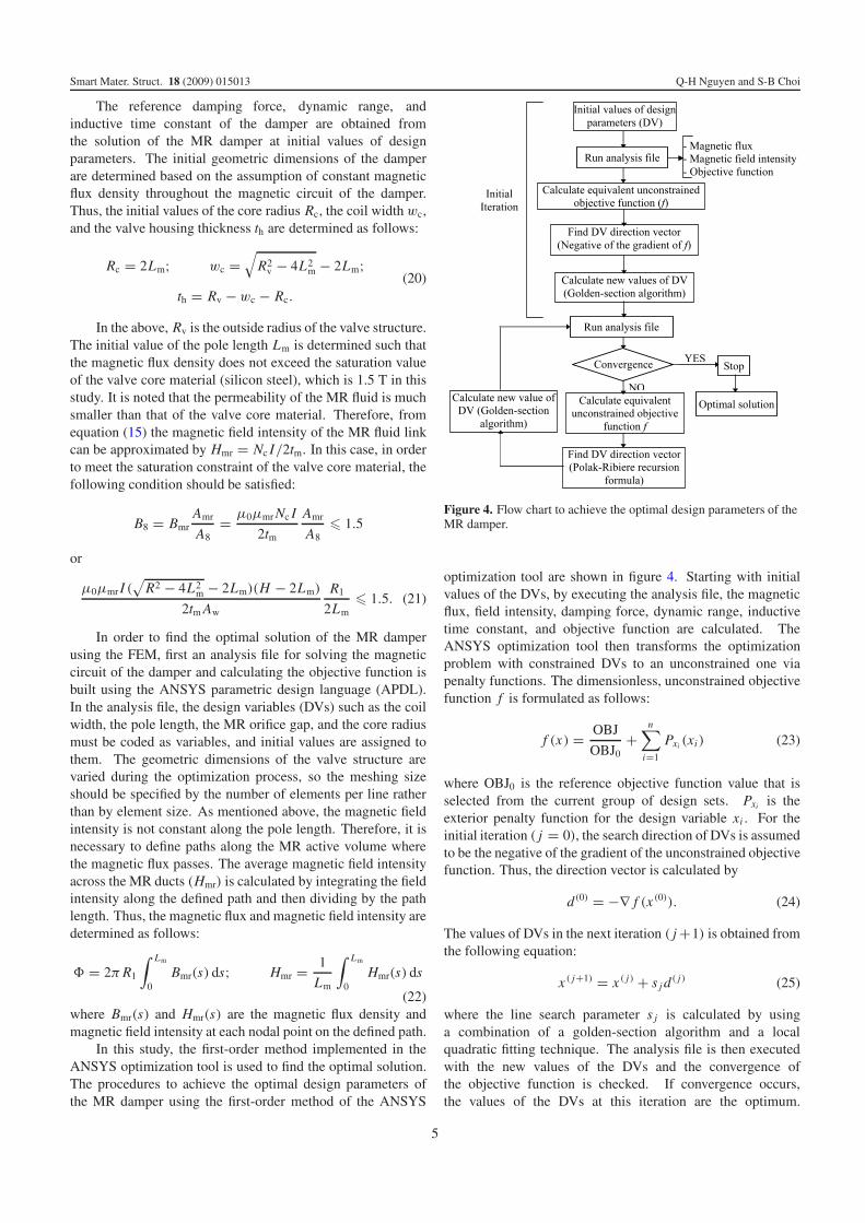
Figure 5. Magnetic properties of silicon steel and MR fluid.(a) B–H curve of silicon steel. (b) B–H curve of the MR fluid.

If not, subsequent iterations will be performed. In thesubsequent iterations, the procedures are similar to those of theinitial iteration except that the direction vectors are calculatedaccording to Polak–Ribiere recursion formula as follows:

d( j) = −∇ f (x ( j)) + r j−1d( j−1) (26)

r j−1 = [∇ f (x ( j)) − ∇ f (x ( j−1))]T∇ f (x ( j))

|∇ f (x ( j−1))|2 . (27)

Thus, each iteration is composed of a number of subiterationsthat include search direction and gradient computations.

4. Results and discussions

In this section, the optimal solution for the MR damper iscomputed based on the optimization procedure developed insection 3. Silicon steel, whose magnetic property is shown infigure 5(a), is used for the valve core. The magnetic propertyof the MR fluid is shown in figure 5(b). The coil wire ismade of copper whose relative permeability is assumed to beequal to that of free space, μc = 1. The base viscosity ofthe MR fluid is assumed to be constant, η = 0.092 Pa s,and the piston velocity used in the optimization problem is

Figure 6. Geometric dimensions of the MR damper.

vp = 0.4 m s−1. The significant dimensions of the MR damperare presented in figure 6, in which the coil with wc, the valvehousing thickness th, the valve orifice gap tm and the polelength Lm are assigned as design variables. It is noteworthythat the piston-shaft area is kept unchanged (As = π R2

s , Rs =6 mm) during the optimization process. However, the pistonarea is varied depending on the design variables (Ap = π R2

p ,Rp = Rv − th − tm − tin). The coil wires are sized as 24-gauge (diameter = 0.5106 mm) and the maximum allowablecurrent of the wire is 3 A. In this study, the maximum valueof the applied current to the coil is I = 2 A. The currentdensity applied to the coils can be approximately calculatedby J = I/Aw.

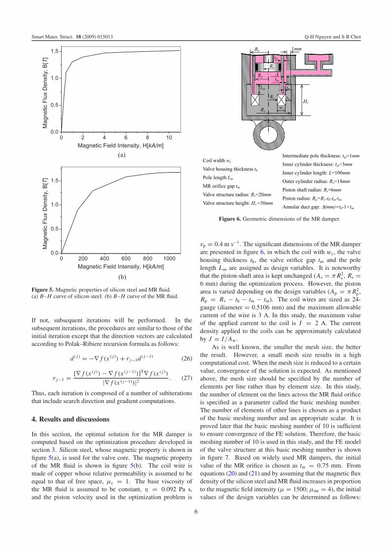
As is well known, the smaller the mesh size, the betterthe result. However, a small mesh size results in a highcomputational cost. When the mesh size is reduced to a certainvalue, convergence of the solution is expected. As mentionedabove, the mesh size should be specified by the number ofelements per line rather than by element size. In this study,the number of element on the lines across the MR fluid orificeis specified as a parameter called the basic meshing number.The number of elements of other lines is chosen as a productof the basic meshing number and an appropriate scalar. It isproved later that the basic meshing number of 10 is sufficientto ensure convergence of the FE solution. Therefore, the basicmeshing number of 10 is used in this study, and the FE modelof the valve structure at this basic meshing number is shownin figure 7. Based on widely used MR dampers, the initialvalue of the MR orifice is chosen as tm = 0.75 mm. Fromequations (20) and (21) and by assuming that the magnetic fluxdensity of the silicon steel and MR fluid increases in proportionto the magnetic field intensity (μ = 1500; μmr = 4), the initialvalues of the design variables can be determined as follows:

6

Smart Mater. Struct. 18 (2009) 015013 Q-H Nguyen and S-B Choi

Figure 7. Finite element model to solve the magnetic circuit of thedamper.

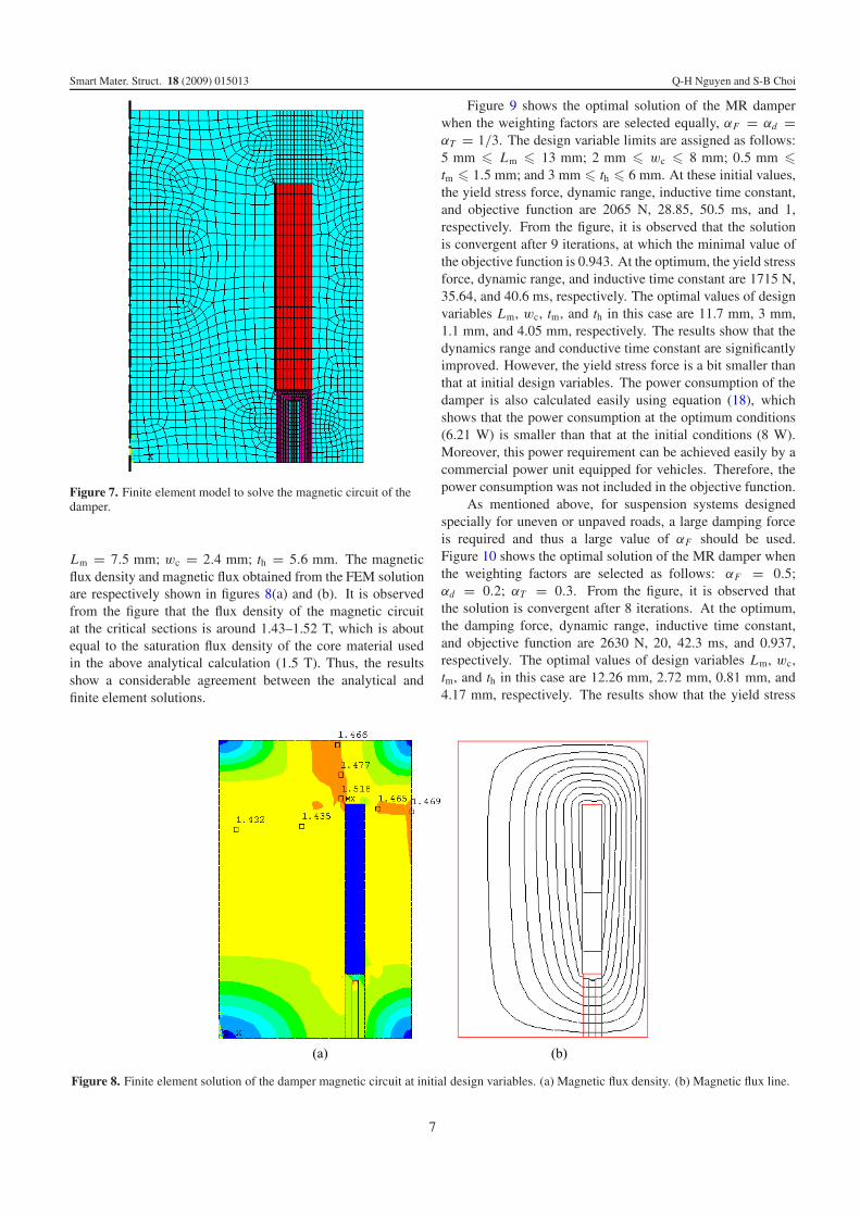
Lm = 7.5 mm; wc = 2.4 mm; th = 5.6 mm. The magneticflux density and magnetic flux obtained from the FEM solutionare respectively shown in figures 8(a) and (b). It is observedfrom the figure that the flux density of the magnetic circuitat the critical sections is around 1.43–1.52 T, which is aboutequal to the saturation flux density of the core material usedin the above analytical calculation (1.5 T). Thus, the resultsshow a considerable agreement between the analytical andfinite element solutions.

Figure 9 shows the optimal solution of the MR damperwhen the weighting factors are selected equally, αF = αd =αT = 1/3. The design variable limits are assigned as follows:5 mm � Lm � 13 mm; 2 mm � wc � 8 mm; 0.5 mm �tm � 1.5 mm; and 3 mm � th � 6 mm. At these initial values,the yield stress force, dynamic range, inductive time constant,and objective function are 2065 N, 28.85, 50.5 ms, and 1,respectively. From the figure, it is observed that the solutionis convergent after 9 iterations, at which the minimal value ofthe objective function is 0.943. At the optimum, the yield stressforce, dynamic range, and inductive time constant are 1715 N,35.64, and 40.6 ms, respectively. The optimal values of designvariables Lm, wc, tm, and th in this case are 11.7 mm, 3 mm,1.1 mm, and 4.05 mm, respectively. The results show that thedynamics range and conductive time constant are significantlyimproved. However, the yield stress force is a bit smaller thanthat at initial design variables. The power consumption of thedamper is also calculated easily using equation (18), whichshows that the power consumption at the optimum conditions(6.21 W) is smaller than that at the initial conditions (8 W).Moreover, this power requirement can be achieved easily by acommercial power unit equipped for vehicles. Therefore, thepower consumption was not included in the objective function.

As mentioned above, for suspension systems designedspecially for uneven or unpaved roads, a large damping forceis required and thus a large value of αF should be used.Figure 10 shows the optimal solution of the MR damper whenthe weighting factors are selected as follows: αF = 0.5;αd = 0.2; αT = 0.3. From the figure, it is observed thatthe solution is convergent after 8 iterations. At the optimum,the damping force, dynamic range, inductive time constant,and objective function are 2630 N, 20, 42.3 ms, and 0.937,respectively. The optimal values of design variables Lm, wc,tm, and th in this case are 12.26 mm, 2.72 mm, 0.81 mm, and4.17 mm, respectively. The results show that the yield stress

Figure 8. Finite element solution of the damper magnetic circuit at initial design variables. (a) Magnetic flux density. (b) Magnetic flux line.

7

Smart Mater. Struct. 18 (2009) 015013 Q-H Nguyen and S-B Choi

Figure 9. Optimized solution of the MR damper when the weightingfactors are selected as follows: αF = αd = αT = 1/3. (a) Objectivefunction. (b) Design variables. (c) Yield stress force, time constant,and dynamic range.

force and conductive time constant are significantly improvedwhile the dynamic range is smaller than that at initial designvariables. Thus, by changing the weighting factors, a newoptimal solution of the damper can be obtained in which theterm with larger value of the weighting factor will becomedominant. The power consumption at the optimum is 5.16 Wfor this case.

In order to improve the ride comfort, the damping forcedue to the MR fluid viscosity (the damping force when no

Figure 10. Optimized solution of the damper when the weightingfactors are selected as follows: αF = 0.5; αd = 0.2; αT = 0.3.(a) Objective function. (b) Design variables. (c) Yield stress force,time constant, and dynamic range.

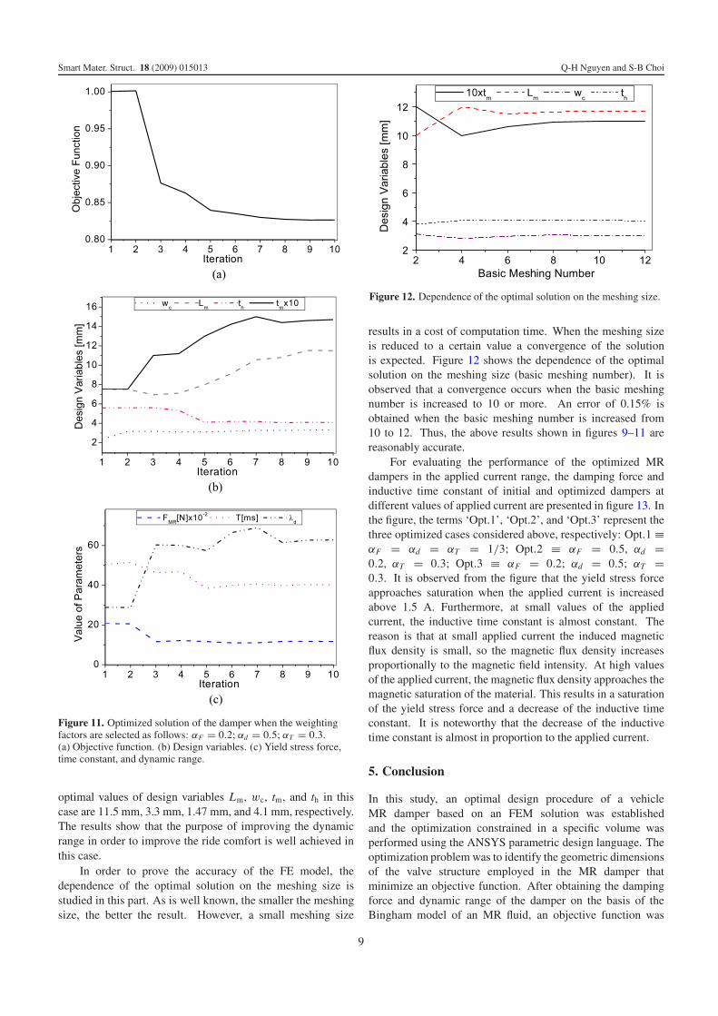
current is applied) should be small. Thus, a large value ofthe dynamic range is required. Figure 11 shows the optimalsolution of the MR damper when the weighting factors areselected as follows: αF = 0.2; αd = 0.5; αT = 0.3.The convergence of the solution occurs after 10 iterations.At the optimum, the damping force, dynamic range, powerconsumption, inductive time constant, and objective functionare 1170 N, 63, 6.6 W, 40.3 ms, and 0.826, respectively. The

8

Smart Mater. Struct. 18 (2009) 015013 Q-H Nguyen and S-B Choi

Figure 11. Optimized solution of the damper when the weightingfactors are selected as follows: αF = 0.2; αd = 0.5; αT = 0.3.(a) Objective function. (b) Design variables. (c) Yield stress force,time constant, and dynamic range.

optimal values of design variables Lm, wc, tm, and th in thiscase are 11.5 mm, 3.3 mm, 1.47 mm, and 4.1 mm, respectively.The results show that the purpose of improving the dynamicrange in order to improve the ride comfort is well achieved inthis case.

In order to prove the accuracy of the FE model, thedependence of the optimal solution on the meshing size isstudied in this part. As is well known, the smaller the meshingsize, the better the result. However, a small meshing size

Figure 12. Dependence of the optimal solution on the meshing size.

results in a cost of computation time. When the meshing sizeis reduced to a certain value a convergence of the solutionis expected. Figure 12 shows the dependence of the optimalsolution on the meshing size (basic meshing number). It isobserved that a convergence occurs when the basic meshingnumber is increased to 10 or more. An error of 0.15% isobtained when the basic meshing number is increased from10 to 12. Thus, the above results shown in figures 9–11 arereasonably accurate.

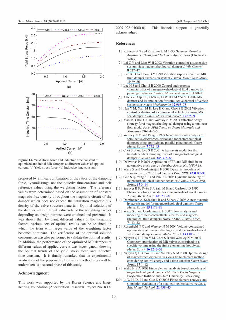
For evaluating the performance of the optimized MRdampers in the applied current range, the damping force andinductive time constant of initial and optimized dampers atdifferent values of applied current are presented in figure 13. Inthe figure, the terms ‘Opt.1’, ‘Opt.2’, and ‘Opt.3’ represent thethree optimized cases considered above, respectively: Opt.1 ≡αF = αd = αT = 1/3; Opt.2 ≡ αF = 0.5, αd =0.2, αT = 0.3; Opt.3 ≡ αF = 0.2; αd = 0.5; αT =0.3. It is observed from the figure that the yield stress forceapproaches saturation when the applied current is increasedabove 1.5 A. Furthermore, at small values of the appliedcurrent, the inductive time constant is almost constant. Thereason is that at small applied current the induced magneticflux density is small, so the magnetic flux density increasesproportionally to the magnetic field intensity. At high valuesof the applied current, the magnetic flux density approaches themagnetic saturation of the material. This results in a saturationof the yield stress force and a decrease of the inductive timeconstant. It is noteworthy that the decrease of the inductivetime constant is almost in proportion to the applied current.

5. Conclusion

In this study, an optimal design procedure of a vehicleMR damper based on an FEM solution was establishedand the optimization constrained in a specific volume wasperformed using the ANSYS parametric design language. Theoptimization problem was to identify the geometric dimensionsof the valve structure employed in the MR damper thatminimize an objective function. After obtaining the dampingforce and dynamic range of the damper on the basis of theBingham model of an MR fluid, an objective function was

9

Smart Mater. Struct. 18 (2009) 015013 Q-H Nguyen and S-B Choi

Figure 13. Yield stress force and inductive time constant ofoptimized and initial MR dampers at different values of appliedcurrent. (a) Yield stress force. (b) Inductive time constant.

proposed by a linear combination of the ratios of the dampingforce, dynamic range, and the inductive time constant, and theirreference values using the weighting factors. The referencevalues were determined based on the assumption of constantmagnetic flux density throughout the magnetic circuit of thedamper which does not exceed the saturation magnetic fluxdensity of the valve structure material. Optimal solutions ofthe damper with different value sets of the weighting factorsdepending on design purpose were obtained and presented. Itwas shown that, by using different values of the weightingfactors, various sets of optimal results can be obtained, inwhich the term with larger value of the weighting factorbecomes dominant. The verification of the optimal solutionconvergence was also performed to validate the optimal results.In addition, the performance of the optimized MR dampers atdifferent values of applied current was investigated, showingthe optimal trends of the yield stress force and inductivetime constant. It is finally remarked that an experimentalverification of the proposed optimization methodology will beundertaken as a second phase of this study.

Acknowledgment

This work was supported by the Korea Science and Engi-neering Foundation (Acceleration Research Project No. R17-

2007-028-01000-0). This financial support is gratefullyacknowledged.

References

[1] Korenev B G and Reznikov L M 1993 Dynamic VibrationAbsorbers: Theory and Technical Applications (Chichester:Wiley)

[2] Lai C Y and Liao W H 2002 Vibration control of a suspensionsystem via a magnetorheological damper J. Vib. Control8 527–47

[3] Kim K D and Jeon D Y 1999 Vibration suppression in an MRfluid damper suspension system J. Intell. Mater. Syst. Struct.10 79–86

[4] Lee H S and Choi S B 2000 Control and responsecharacteristics of a magneto-rheological fluid damper forpassenger vehicles J. Intell. Mater. Syst. Struct. 11 80–7

[5] Yao G Z, Yap F F, Chen G, Li W H and Yeo S H 2002 MRdamper and its application for semi-active control of vehiclesuspension system Mechatronics 12 963–73

[6] Han Y M, Nam M H, Lee H G and Choi S B 2002 Vibrationcontrol evaluation of a commercial vehicle featuring MRseat damper J. Intell. Mater. Syst. Struct. 13 575–9

[7] Mao M, Choi Y T and Wereley N M 2005 Effective designstrategy for a magnetorheological damper using a nonlinearflow model Proc. SPIE Symp. on Smart Materials andStructures 5760 446–55

[8] Wereley N M and Pang L 1997 Nondimensional analysis ofsemi-active electrorheological and magnetorheologicaldampers using approximate parallel plate models SmartMater. Struct. 7 732–43

[9] Choi S B and Lee S K 2001 A hysteresis model for thefield-dependent damping force of a magnetorheologicaldamper J. Sound Vib. 245 375–83

[10] Delivorias P P 2004 Application of ER and MR fluid in anautomotive crash energy absorber Report No. MT04.18.

[11] Wang X and Gordaninejad F 2001 Dynamic modeling ofsemi-active ER/MR fluid dampers Proc. SPIE 4331 82–91

[12] Guo S Q, Yang S P and Pan C Z 2006 Dynamic modeling ofmagnetorheological damper behavior J. Intell. Mater. Syst.Struct. 17 3–14

[13] Spencer B F, Dyke S J, Sain M K and Carlson J D 1997Phenomenological model for a magnetorheological damperJ. Eng. Mech. ASCE 123 230–8

[14] Dominguez A, Sedaghati R and Stiharu J 2006 A new dynamichysteresis model for magnetorheological dampers SmartMater. Struct. 15 1179–89

[15] Wang X J and Gordaninejad F 2007 Flow analysis andmodeling of field-controllable, electro- and magnetorheological fluid dampers Trans. ASME, J. Appl. Mech.74 13–22

[16] Rosenfield N C and Wereley N M 2004 Volume-constrainedoptimization of magnetorheological and electrorheologicalvalves and dampers Smart Mater. Struct. 13 1303–13

[17] Nguyen Q H, Han Y M, Choi S B and Wereley N M 2007Geometry optimization of MR valves constrained in aspecific volume using the finite element method SmartMater. Struct. 16 2242–52

[18] Nguyen Q H, Choi S B and Wereley N M 2008 Optimal designof magnetorheological valves via a finite element methodconsidering control energy and a time constant Smart Mater.Struct. 17 1–12

[19] Walid H E A 2002 Finite element analysis based modeling ofmagnetorheological dampers Master’s Thesis VirginiaPolytechnic Institute and State University, Blacksburg

[20] Li W H, Du H and Guo N Q 2003 Finite element analysis andsimulation evaluation of a magnetorheological valve Int. J.Adv. Manuf. Technol. 21 438–45

10