damping estimation of plates for statistical energy analysis

DAMPING ESTIMATION OF PLATES FOR STATISTICAL ENERGY ANALYSIS

by

KRANTHI KUMAR VATTI

Submitted to the graduate degree program in Aerospace Engineering and the

Graduate Faculty of the University of Kansas in partial fulfillment of the

requirements for the degree of Master of Science.

________________________________

Chairperson Dr. Mark S. Ewing

________________________________

Dr. Rick Hale

________________________________

Dr. Saeed Farokhi

Date Defended: 9th

March, 2011

ii

The Thesis Committee for Kranthi Kumar Vatti

certifies that this is the approved version of the following thesis:

DAMPING ESTIMATION OF PLATES FOR STATISTICAL ENERGY ANALYSIS

________________________________

Chairperson Dr. Mark S. Ewing

Date Approved: 11th

March, 2011

iii

ABSTRACT

The Power Input Method (P.I.M.) and the Impulse Response Decay Method (I.R.D.M.)

are used to evaluate how the accuracy of damping loss factor estimation for plates is affected

with respect to various processing parameters, such as the frequency resolution, the frequency

bandwidth, the number of measurement locations, and the signal to noise ratio. In several

computational experiments, accuracy is assessed for a wide range of damping loss factors from

low (0.1%) to moderate (1%) to high (10%). A wide range of frequency is considered, including

―low frequencies‖ for which modal density is less than one per band.

The Power Input Method (P.I.M.) is first validated with computational studies of an

analytical single degree of freedom oscillator. Experimental loss factor estimates for plates

(multiple degree of freedom systems) are also computed using the P.I.M. algorithm. The P.I.M.

is shown to estimate loss factors with reasonable accuracy for highly damped plates in the 300

Hz – 4000 Hz, wherein modal density exceeds unit value. In this case ―reasonable accuracy‖

means the estimated loss factors are within 10% of those predicted by the impulse response

decay method. For lower damping levels the method fails.

The analytical Impulse Response Decay Method (I.R.D.M.) is validated by the use of two

computational models: a single degree of freedom oscillator and a uniform rectangular panel.

The panel computational model is a finite element model of a rectangular plate mechanically

excited at a single point. The computational model is used to systematically evaluate the effect of

frequency resolution, frequency bandwidth, the number of measurement points used in the

computations, and noise level for all the three levels of damping. The ―optimized‖ I.R.D.M. is

shown to accurately estimate damping in plate simulations with low to moderate levels of

iv

damping with a deviation of no more than 2% from the known damping value. For highly

damped plates the I.R.D.M. tends to under-estimate loss factors at high frequency. Experimental

loss factor estimation for an aluminum plate with full constrained layer damping treatment,

classified as a highly damped plate, and an undamped steel plate, classified as a lightly damped

plate are computed using the ―optimized‖ I.R.D.M. algorithm.

Statistical Energy Analysis (S.E.A.), which is a natural extension of the Power Input

Method, is used to evaluate coupling loss factors for two sets of plates, one set joined along a

line and the other set joined at a point. Two alternative coupling loss factor estimation algorithms

are studied, one using individual plate loss factor estimations, and the other using the loss factors

of the plates estimated when the plates are coupled. The modal parameters (modal density and

coupling loss factors) for both sets of plates are estimated experimentally and are compared with

theoretical results. The estimations show reasonable agreement between agreement and theory

that is, within 5 % for the damped system of plates. For the undamped system of plates the

results are less accurate with deviations of more than 100% at low modal density and

approximately 30% variation at higher frequencies.

v

ACKNOWLEDGEMENTS

I want to express my gratitude to those individuals who, during the past three and half

years, have supported me in some way or another. To my advisor, Professor Dr. Mark S. Ewing,

a special thanks for giving me the opportunity to work with him and for his patience, tolerance,

understanding, and encouragement. I am truly grateful.

Further encouragement came from my committee members Dr. Rick Hale, and Dr. Saeed

Farokhi to whom I am indebted for their patience. I really appreciate their time and effort for

being part of my committee. Additional thanks are extended to Dr. Richard Colgren and Dr.

Shariar Keshmiri for their advice during the course of my study.

I want to thank Spirit Aerosystems, particularly Dr. Mark Moeller and Mr. Albert Allen

for the support of this work and for technical assistance. Thanks are extended to Wanbo Liu who

constructed many of the specimens that are used for various experiments and providing the

analytical Nastran data. I also want to thank Ignatius Vaz at ESI group who helped me in

learning the statistical energy analysis simulation software.

I would also like to thank all the faculty and staff of the Department of Aerospace

Engineering, particularly Amy Borton, as a whole for their support.

Special thanks go to friends Himanshu Dande, Akhilesh Katipally, Kolapan Jayachandran

Saiarun, Vamshi Zillepalli, Jayasimha Tutika, Pradeep Attalury, Ranganathan Parthasarathy, and

Viraj Singh. They were encouraging me during my whole research.

Finally, without the support and encouragement of my parents, Vatti Venkat Reddy and

Vatti Vanitha Vani, I could not have made it this far. Thank you.

vi

TABLE OF CONTENTS

ABSTRACT ................................................................................................................................ III

ACKNOWLEDGEMENTS ......................................................................................................... V

TABLE OF CONTENTS ............................................................................................................ VI

LIST OF FIGURES ..................................................................................................................... IX

1 OVERVIEW OF THE DAMPING ESTIMATION TECHNIQUES ................................ 1

1.1 INTRODUCTION ............................................................................................................. 1

1.2 DAMPING IN STRUCTURES ........................................................................................ 2

1.2.1 FREE VIBRATIONS OF A SINGLE DEGREE OF FREEDOM (SDOF) SYSTEM .................. 2

1.2.2 FORCED VIBRATIONS OF A SDOF SYSTEM ................................................................... 9

1.2.2.1 HARMONIC EXCITATION ......................................................................................... 10

1.2.2.2 IMPULSE RESPONSE................................................................................................. 12

1.2.2.3 LOGARITHMIC DECREMENT ................................................................................... 16

1.2.2.4 FREQUENCY RESPONSE FUNCTION ESTIMATION ................................................... 18

1.3 MEASUREMENT SETUP FOR LOSS FACTOR MEASUREMENTS ................... 20

1.4 OVERVIEW OF STATISTICAL ENERGY ANALYSIS........................................... 22

1.4.1 BASIC ENERGY FLOW CONCEPTS ............................................................................... 23

1.4.2 THE TWO SUBSYSTEM MODEL .................................................................................... 25

1.5 TEST ARTICLES CONSIDERED ................................................................................ 28

1.5.1 ALUMINUM PLATE WITH FULL CONSTRAINED LAYER DAMPING .............................. 28

1.5.2 UNDAMPED STEEL PLATE ............................................................................................ 29

1.5.3 TWO STEEL PLATES JOINED ALONG A LINE ............................................................... 30

1.5.4 UNDAMPED ALUMINUM PLATES JOINED AT A POINT ................................................. 31

2 LOSS FACTOR ESTIMATION USING THE POWER INPUT METHOD ................. 32

2.1 THEORY OF THE POWER INPUT METHOD ......................................................... 32

2.2 SINGLE DEGREE OF FREEDOM ANALYSIS ......................................................... 34

2.2.1 INTRODUCTION TO SINGLE DEGREE OF FREEDOM SYSTEMS .................................... 34

2.2.2 ANALYTICAL LOSS FACTOR ESTIMATION OF SDOF SYSTEMS .................................. 37

2.2.2.1 USING A TRUE RANDOM FORCE ............................................................................. 37

2.2.2.2 USING A SINUSOIDAL FORCE .................................................................................. 41

vii

2.3 PLATE – EXPERIMENTS ............................................................................................ 44

2.3.1 ALUMINUM PLATE WITH FULL CONSTRAINED LAYER DAMPING .............................. 45


2.3.3 EFFECT OF FREQUENCY RESOLUTION ON DAMPING ESTIMATION ............................ 49

3 IMPULSE RESPONSE DECAY METHOD ..................................................................... 51

3.1 THEORY OF THE IMPULSE METHOD FOR LOSS FACTORS .......................... 51

3.2 SINGLE DEGREE OF FREEDOM SYSTEMS .......................................................... 54

3.2.1 LOSS FACTOR USING THE IMPULSE FUNCTION .......................................................... 54

3.2.2 LOSS FACTOR USING A SINUSOIDAL IMPULSE FORCE ............................................... 58

3.3 PLATES – ANALYTICAL AND EXPERIMENTAL IRDM ..................................... 63

3.3.1 ANALYTICAL ESTIMATION- NASTRAN MODEL ........................................................... 63

3.3.2 EXPERIMENTAL RESULTS ............................................................................................ 70

3.3.2.1 ALUMINUM PLATE WITH CONSTRAINED LAYER DAMPING ................................... 70

3.3.2.2 UNDAMPED STEEL PLATE ....................................................................................... 71

3.3.2.3 OBSERVATIONS ........................................................................................................ 72

3.3.3 SELECTION OF APPROPRIATE PROCESSING PARAMETERS FOR IRDM ...................... 73

3.3.3.1 EFFECT OF FREQUENCY BANDWIDTHS .................................................................. 74

3.3.3.2 EFFECT OF FREQUENCY RESOLUTION ................................................................... 75

3.3.3.3 EFFECT OF VARIABLE NUMBER OF MEASUREMENT POINTS ................................ 77

3.3.3.4 EFFECT OF NOISE .................................................................................................... 80

4 STATISTICAL ENERGY ANALYSIS .............................................................................. 83

4.1 MODAL DENSITY [AND MODES IN BAND] ........................................................... 83


4.1.2 STEEL PLATE WITH PARTIAL CONSTRAINED LAYER DAMPING ................................ 86

4.1.3 UNDAMPED ALUMINUM PLATE ................................................................................... 88

4.2 LOSS FACTOR ESTIMATION .................................................................................... 89

4.3 COUPLING LOSS FACTORS ...................................................................................... 90

4.3.1 TWO PLATES JOINED ALONG A LINE .......................................................................... 90

4.3.2 TWO PLATES JOINED AT A POINT ............................................................................... 94

5 CONCLUSIONS AND FUTURE WORK ......................................................................... 99

5.1 CONCLUSIONS .............................................................................................................. 99

5.1.1 POWER INPUT METHOD ............................................................................................... 99

5.1.2 IMPULSE RESPONSE DECAY METHOD ....................................................................... 100

viii

5.1.3 STATISTICAL ENERGY ANALYSIS .............................................................................. 101

5.2 FUTURE WORK .......................................................................................................... 101

REFERENCES: ......................................................................................................................... 102

APPENDIX A MATLAB CODES ........................................................................................... A-1

A.1. GENERATE A TRUE RANDOM SIGNAL ....................................................................... A-1

A.2. IMPULSE RESPONSE FUNCTION ................................................................................. A-1

A.3. LOSS FACTOR ESTIMATION BY POWER INPUT METHOD: SYNTHETIC, 1 DOF,

RANDOM EXCITATION ........................................................................................................... A-2

A.4. POWER INPUT METHOD: SYNTHETIC, 1 DOF, SINUSOIDAL EXCITATION ............... A-4

A.5. IMPULSE RESPONSE DECAY METHOD: SYNTHETIC, 1 DOF, IMPULSE FUNCTION .. A-6

A.6. IMPULSE RESPONSE DECAY METHOD: SYNTHETIC, 1 DOF, HALF SINE PULSE ..... A-8

A.7. EXPERIMENTAL POWER INPUT METHOD................................................................ A-11

A.8. EXPERIMENTAL IMPULSE RESPONSE DECAY METHOD ......................................... A-13

A.9. FREQUENCY RESPONSE FUNCTION EXTRACTION FROM NASTRAN FO6 FILES ..... A-15

A.10. MANUAL DECAY MEASUREMENT ............................................................................ A-16

A.11. MODAL DENSITY AND MODES IN BAND MEASUREMENT ...................................... A-18

A.12. ALTERNATIVE EXPERIMENTAL POWER INPUT METHOD ....................................... A-19

A.13. COUPLING LOSS FACTORS ALGORITHM ................................................................. A-22

ix

LIST OF FIGURES

Figure 1-1 Single Degree of Freedom System ................................................................................ 3

Figure 1-2 Response of the Underdamped System ......................................................................... 6

Figure 1-3 Response of an Overdamped System ............................................................................ 7

Figure 1-4 Response of a Critically Damped System ..................................................................... 8

Figure 1-5 Transient Response of a Single Degree of Freedom System ....................................... 14

Figure 1-6 Peak Amplitude and Slope of the Transient Response ................................................ 15

Figure 1-7 Logarithmic Decrement of the Transient Response .................................................... 16

Figure 1-8 Free Decay of an Underdamped System ..................................................................... 17

Figure 1-9 General Input/Output Model ....................................................................................... 18

Figure 1-10 Scanning Laser Vibrometer and the Shaker Configuration ....................................... 21

Figure 1-11 A Typical Experimental Setup Used ......................................................................... 22

Figure 1-12 A Two Subsystem S.E.A. Model ............................................................................... 27

Figure 1-13 Damped Aluminum Plate with Full Constrained Layer Damping ............................ 28

Figure 1-14 Undamped Steel Plate ................................................................................................ 29

Figure 1-15 Two Undamped Steel Plates Joined Along a Line .................................................... 30

Figure 1-16 Two Undamped Aluminum plates connected at a point ............................................ 31

Figure 2-1 Random Force and the Force with the Hanning Window ........................................... 39

Figure 2-2 Velocity Response and Velocity after Applying the Hanning Window ...................... 39

Figure 2-3 Comparison between the Input Loss Factors and the Analytically Estimated Loss

Factors of a Single Degree of Freedom System for a True Random Excitation. .......................... 40

Figure 2-4 Force and Velocity with a Hanning Window Applied ................................................ 42

Figure 2-5 Comparison between the Input Loss Factors and the Analytically Estimated Loss

Factors of a Single Degree of Freedom System for a Sinusoidal Excitation ................................ 43

Figure 2-6 Estimation of Loss Factor for the Highly Damped Aluminum Plate with Constrained

Layer Damping by the Power Input Method in Full Frequency Spectrum ................................... 47

Figure 2-7 Loss Factor for the Aluminum Plate with Full Constrained layer Damping Estimated

in Full Octave Bands with 1/3rd

Octave Center Frequencies ........................................................ 48

Figure 2-8 Loss Factor Estimation by the Power Input Method for the Undamped Steel Plate ... 49

Figure 2-9 Effect of Frequency Resolution on the Estimated Loss Factors for the Aluminum

Plate with Full Constrained Layer Damping Treatment ............................................................... 50

Figure 3-1 Transient Response of a Single Degree of Freedom System ....................................... 51

Figure 3-2 Peak Amplitude of the Transient Response ................................................................. 52

file:///C:/Users/Kranthi/Documents/MATLAB/Thesis/Damping%20Estimation%20of%20Plates%20for%20Statistical%20Energy%20Analysis.docx%23_Toc287626084

file:///C:/Users/Kranthi/Documents/MATLAB/Thesis/Damping%20Estimation%20of%20Plates%20for%20Statistical%20Energy%20Analysis.docx%23_Toc287626087

x

Figure 3-3 Logarithmic Decay of the Single Degree of Freedom System .................................... 53

Figure 3-4 Plot of the Impulse Function ....................................................................................... 55

Figure 3-5 Real and Imaginary of Hilbert Transform of the Impulse Function (Top) and the

Absolute Value of the Hilbert Transform (Bottom) ...................................................................... 56

Figure 3-6 Logarithmic Decrement of the Hilbert Transform ...................................................... 57

Figure 3-7 Loss Factor with Various ‗Skip‘ and ‗Consider‘ Parameter Values for a SDOF System

with a True Impulse Excitation ..................................................................................................... 58

Figure 3-8 Simulated Impulse and the Response by the Convolution Integral ............................. 59

Figure 3-9 Fourier Transform of the Force, Response and the Impulse Function ........................ 60

Figure 3-10 Impulse Response Function and the Hilbert Transform ............................................ 61

Figure 3-11 Logarithmic Decrement of the Hilbert Transform of the Response of a SDOF

System with a Sinusoidal Excitation ............................................................................................. 61

Figure 3-12 Loss Factors with various ‗Skip‘ and ‗Consider‘ Parameters for a SDOF System

with a Sinusoidal Excitation .......................................................................................................... 62

Figure 3-13 Computational Model with Regular Pattern of Excitation and Response Points ...... 64

Figure 3-14 Accelerance FRF for the Thin Plate, for the Full Spectrum (Top) and in the Octave

Band Centered at 1250 Hz (Below) .............................................................................................. 66

Figure 3-15 Averaged Decay Signatures for a range of Full Octave Bands, with the Linear

Estimate of Slope and the Resulting Loss Factor shown for Input LF of 0.01 ............................. 67

Figure 3-16 Estimated Loss Factor for a Input Loss Factor of 0.01 [1 %] ................................... 68

Figure 3-17 Estimated Loss Factor for a Input Loss Factor of 0.001 [0.1 %] .............................. 69

Figure 3-18 Estimated Loss Factor for a Input Loss Factor of 0.1 [10 %] ................................... 70

Figure 3-19 loss factors of damped aluminum plate by the impulse response decay method ...... 71

Figure 3-20 Estimated Loss Factors of the Undamped Steel Plate ............................................... 72

Figure 3-21 Comparison of the Experimental IRDM and Experimental PIM for the Aluminum

Plate with Full coverage Constrained Layer Damping ................................................................. 73

Figure 3-22 Variation of Loss Factor for a Range of Octave Bandwidth‘s Centered at 1/3 Octave

Center Frequencies. ....................................................................................................................... 74

Figure 3-23 Effect of Frequency Resolution for a Input Loss Factor of 0.001 [0.1%] ................. 75

Figure 3-24 Effect of Frequency Resolution for a Input Loss Factor of 0.01 [1%] ...................... 76

Figure 3-25 Effect of Frequency Resolution for a Input Loss Factor of 0.1 [10%] ...................... 77

Figure 3-26 Estimation of Loss Factors by Varying the Number of Measurement Points for a

Input Loss Factor of 0.001 [0.1%] ................................................................................................ 78


Input Loss Factor of 0.01 [1%] ..................................................................................................... 79

xi


Input Loss Factor of 0.1 [10 %] .................................................................................................... 79

Figure 3-29 Loss Factor Estimation for Various Noise Levels, Input Loss Factor of 10 % ......... 81

Figure 3-30 Loss Factor Estimation for Various Noise Levels, Input Loss Factor of 1 % ........... 81

Figure 3-31 Loss Factor Estimation for Various Noise Levels, Input Loss Factor of 0.1 % ........ 82

Figure 4-1 Modal Density in the Undamped Steel Plate ............................................................... 85

Figure 4-2 Modes per Band of the Undamped Steel Plate ............................................................ 86

Figure 4-3 Modal Density in the Partial Damped Steel Plate ....................................................... 87

Figure 4-4 Modes in Band for the Partial Damped Steel Plate ..................................................... 87

Figure 4-5 Modal Density in Undamped Aluminum Plate ........................................................... 88

Figure 4-6 Modes in Band in the Undamped Aluminum Plate ..................................................... 89

Figure 4-7 Coupling Loss Factors along a Line (Big Plate to Small Plate) .................................. 93

Figure 4-8 Coupling Loss Factors along a Line (Small plate to Big Plate) .................................. 94

Figure 4-9 Coupling Loss Factors along a Point (Bottom Plate to Top Plate) .............................. 97

Figure 4-10 Coupling Loss Factors along a Point (Top Plate to Bottom Plate) ............................ 98

ii

LIST OF TABLES

Table 1-1 Dimensions of Damped Aluminum Plate with Full Constrained Layer Damping ....... 28

Table 1-2 Material Properties of the Undamped Steel Plate ......................................................... 29

Table 1-3 Material Properties of the Steel Plates Joined Along a Line ........................................ 30

Table 1-4 Material Properties of Aluminum Plates Joined at a Point ........................................... 31

1

1 OVERVIEW OF THE DAMPING ESTIMATION TECHNIQUES

1.1 INTRODUCTION

Vibrating structures accumulate the energy of vibration in the form of kinetic energy

(stored by mass) and potential energy (stored by elasticity). Each real, vibrating structure

dissipates and radiates energy. In all materials, internal dissipation leads to conversion of

mechanical energy into thermal energy [1]. There are also many engineered damping

mechanisms [2] which are used to transform the mechanical energy into heat. Mechanisms of

energy dissipation include sliding friction, liquid viscosity, and both magnetic and mechanical

hysteresis [3].

Dissipation of mechanical energy from a vibrating system is usually by conversion of the

mechanical energy into heat. Damping serves to limit the steady-state resonant response and to

attenuate traveling waves in the structure. There are two types of damping: material damping and

system damping. Material damping is the damping that is inherent in the material while system

damping includes the damping due to engineered devices as well as damping mechanisms at the

supports, boundaries, joints, interfaces, etc. Since utilizing engineered damping materials is the

most common way to reduce resonance responses, accurate measurements of both material and

system damping are crucial to the proper design and modeling of systems from a vibration

reduction standpoint [4].

A variety of nomenclature exists to denote damping. These include: damping ratio(ζ), log

decrement(δ), loss factor (η), specific damping capacity (ψ), quality factor (Q), etc., There are

2

also many different test methods for predicting damping in structures. The various damping test

methods can broadly be classified into three groups [5]:

a) Frequency-domain modal analysis curve-fitting methods,

b) Time domain decay-rate methods, and

c) Other methods based on energy and wave propagation.

In this thesis, the damping loss factor estimations by the Impulse Response Decay

Method (I.R.D.M.) and the Power Injection Method (P.I.M.) are investigated. The I.R.D.M. and

P.I.M. are validated by a single degree of freedom oscillator for various types of excitation

signals. The I.R.D.M. is validated using a computationally-modeled plate element with varying

levels of damping loss factor specifically 0.001, 0.01, and 0.1. The experimental validations of

both the P.I.M. and the I.R.D.M. are shown with two plates, one an aluminum panel with full

covering constrained layer damping treatment, and the second an undamped steel plate.

Statistical Energy Analysis (S.E.A.) is used to study the coupling loss factors between two sets of

coupled plate elements, one set joined at a point and the other set joined along a line.

1.2 DAMPING IN STRUCTURES

1.2.1 FREE VIBRATIONS OF A SINGLE DEGREE OF FREEDOM (SDOF) SYSTEM

Consider the single degree of freedom system shown in Figure 1-1. The general form of

the differential equation describing the response is

0 0( ), (0) , (0)mx cx kx f t x x x (1.1)

3

where ( )x t is the position of the mass, m is the mass, c is the damping rate, k is the stiffness,

and ( )f t is the external dynamic load. The initial displacement of the system is 0x and the initial

velocity is 0 . Let us consider the case with no external applied load i.e., ( ) 0.f t

FIGURE 1-1 SINGLE DEGREE OF FREEDOM SYSTEM

A unique solution of Equation (1.1) for ( ) 0f t can be found for specified initial conditions

assuming that ( )x t is of the form

( ) tx t Ae (1.2)

substituting Equation (1.2) into Equation (1.1) yields

4

2( ) 0tc k

A em m

(1.3)

Since the trivial solution is not desired 0,A and te is never zero. Equation (1.3) yields

2 0

c k

m m (1.4)

Equation (1.4) is called the characteristic equation of Equation (1.1). Using simple algebra, the

two solutions for are

2

1.2 2

14

2 2

c c k

m m m (1.5)

The quantity under the radical is called the discriminant and, together with the signs of ,m c

and ,k determines whether the roots are complex or real. Physically, , , and m c k are all positive

for this case, so the determinant of Equation (1.5) determines the nature of the roots of Equation

(1.4).

The dimensionless damping ratio, is defined as

2

c

km (1.6)

In addition the damped natural frequency is defined (for 0< <1) by

21d n (1.7)

5

substituting Equation (1.6) and Equation (1.7) into Equation (1.1) we now have,

22 0n nx x x (1.8)

and Equation (1.5) becomes

2

1,2 1 , 0 1n n n d j (1.9)

The value of the damping ratio, determines the nature of the solution of Equation (1.1).

There are three cases of interest.

Under-damped. This case occurs if the parameters of the system are such that

0 1

so the discriminant given by Equation (1.9) is negative and the roots form a complex conjugate

pair of values. The solution of Equation (1.8) then becomes

( ) ( cos sin )

( ) sin( )

n

n

t

d d

t

d

x t e A t B t

or

x t Ce t

(1.10)

where A, B, C, and are constants determined by the specified initial velocity, o and the initial

position, :ox

6

2 2

0

1

( ) ( ),

, tan

o n o o d

d

o n o o d

d o n o

x xA x C

x xB

x

(1.11)

The response of the underdamped system has the form given in Figure 1-2

FIGURE 1-2 RESPONSE OF THE UNDERDAMPED SYSTEM

Over-damped. This case occurs if the parameters of the system are such that

1

so that the discriminant given by Equation (1.9) is positive and the roots are a pair of negative

real numbers. The solution of Equation (1.8) then becomes

0 5 10 15 20 25 30 35 40

-1

-0.8

-0.6

-0.4

-0.2

0

0.2

0.4

0.6

0.8

1

Time [ Seconds ]

Dis

pla

ce

me

nt

Response of the underdamped system

7

2 2( 1) ( 1)

( ) n nt tx t Ae Be

(1.12)

where A and B are again constants determined by 0 0 and .x They are

2 2

0 0

2 2

( 1) ( 1),

2 ( 1) 2 ( 1)

o n o n

n n

x xA B

The response of an overdamped system has the form given in Figure 1-3. An overdamped system

does not oscillate, but rather returns to its rest position exponentially.

FIGURE 1-3 RESPONSE OF AN OVERDAMPED SYSTEM

Critically-damped. This case occurs if the parameters of the system are such that

1

0 2 4 6 8 10 12 14 16 18 20

-1

-0.5

0

0.5

1

Time [ Seconds ]

Dis

pla

ce

me

nt

Response of a Over-damped system

Increasing

Damping

8

so that the discriminant given by Equation (1.9) is zero and the roots are a pair of negative real

repeated numbers. The solution of Equation (1.8) then becomes

[( ) ]

( ) n o n o ot x t xx t e

(1.13)

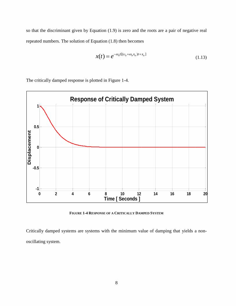
The critically damped response is plotted in Figure 1-4.

FIGURE 1-4 RESPONSE OF A CRITICALLY DAMPED SYSTEM

Critically damped systems are systems with the minimum value of damping that yields a non-

oscillating system.

0 2 4 6 8 10 12 14 16 18 20

-1

-0.5

0

0.5

1

Time [ Seconds ]

Dis

pla

ce

me

nt

Response of Critically Damped System

9

1.2.2 FORCED VIBRATIONS OF A SDOF SYSTEM

The preceding analysis considers the vibration of structure as a result of some initial

disturbance i.e., ( ) 0f t . The equation of motion for the forced vibration of the system becomes,

( )mx cx kx f t (1.14)

Equation (1.14) is a linear, time variant, second order differential equation. The total solution to

this problem involves two parts as follows:

( ) ( ) ( )c px t x t x t

where:

( ) Transient portion

( ) Steady state portion

c

p

x t

x t

By setting ( )f t =0, the homogeneous (transient) form of Equation (1.14) can be solved.

The homogeneous solution of the Equation (1.14) is:

1 2

1 2( )t t

cx t X e X e

where 1X and 2X are constants determined from the initial conditions imposed on the system at

0.t

10

1.2.2.1 HARMONIC EXCITATION

In many environments, rotating machinery, motors, and other mechanical systems cause

periodic motions of structures to induce vibrations into other nearby mechanical devices and

structures nearby. It is common practice to approximate the driving forces, ( )f t as periodic of

the form

( ) sinf t F t

The equation for the forced vibration of the system becomes

sin( )mx cx kx F t (1.15)

The particular solution (steady state) is a function of the form of the forcing function. If the

forcing function is a pure sine wave of a single frequency, the response will also be a sine wave

of the same frequency. If the forcing function is random in form, the response is also random.

The particular solution has the form

( ) sin( )px t X t (1.16)

where X is the steady state amplitude and is the phase shift at steady state. Substitution of

Equation (1.16) into Equation (1.15) yields

2 2 2

/

(1 / ) ( / )

F kX

m k c k

(1.17)

Equation (1.17 ) can be rewritten as

11

2 2 2

2 2 2

1

(1 / ) ( / )

1

(1 ) ( )

Xk

F m k c k

X

F m c

and we have

2 2

2 ( / )( / )tan

1 / 1 ( / )

n

n

c k

m k

(1.18)

where /n k m

as mentioned before. Since the system is linear, the sum of the two solutions

is a solution, and the total time response for the system for the case 0 1 becomes

( ) ( sin cos ) sin( )nt

d dx t e A t B t X t

(1.19)

Here, A and B are constants of integration determined by the initial conditions and the forcing

function (and in general will be different from the values of A and B determined for the free

response).

From Equation (1.19) the following conclusions can be drawn.

1. As t becomes larger, the transient response (the first term) becomes very small, and

hence the steady state response term is assigned to the particular solution (the second

term).

2. The coefficient of the steady state response, or particular solution, becomes large when

the excitation frequency is close to the undamped natural frequency, i.e., n . This

12

phenomenon is known as resonance and is extremely important in vibration analysis and

testing.

Alternatively the equation of motion for damped free vibrations of a system can also be

obtained from energy concepts by incorporating an energy dissipation function into the energy

balance equation. Hence,

( ) /d T U dt (1.20)

where is the power (the negative sign indicates that the power is removed from the system).

Power is force velocity , and the power dissipated from a system with viscous damping is,

2 2v v nF x c x m (1.21)

From Equation (1.21) we have the damping loss factor ( 2 ) as

2

nmx

(1.22)

Equation (1.22) is the basis for the Power Input Method (PIM) which is discussed in Chapter 2.

1.2.2.2 IMPULSE RESPONSE

Impulse response, namely the response of the spring-mass-damper system given by

Equation (1.1) to an impulse, is established in terms of a fictitious function called the unit

impulse function, or the Dirac delta function.

13

This delta function is defined by the two properties

( ) 0,

( ) 1

t a t a

t a dt

(1.23)

where a is the instant of time at which the impulse is applied. The response of the system for the

underdamped case (with 0o oa x ) can be given by

0,

( ) sin,

t

d

d

t a

x t e tt a

m

(1.24)

The response of a system to an impulse may be used to determine the response of an

underdamped system to any input ( )F t by defining the impulse response function as

1( ) sinnt

d

d

h t e tm

(1.25)

Then the solution of

( ) ( ) ( ) ( )mx t cx t kx t F t

for the case of zero initial conditions is given by

0 0

1( ) ( ) ( ) ( ) sin ( )n n

t t

t t

d

d

x t F h t d e F e t dm

(1.26)

14

This last expression gives an analytical representation for the response to any driving force that

has an integral [5]. Equation (1.26) is called the convolution integral.

Consider the response of the system given by Equation (1.25). The system‘s response

amplitude when plotted versus time will have a slope proportional to ( ) ,f te

where f is the

frequency, is the loss factor, and t is time [6]. A typical transient response of a S.D.O.F.

system is shown in Figure 1-5.

FIGURE 1-5 TRANSIENT RESPONSE OF A SINGLE DEGREE OF FREEDOM SYSTEM

0 0.1 0.2 0.3 0.4 0.5 0.6 0.7 0.8 0.9 1-0.2

-0.15

-0.1

-0.05

0

0.05

0.1

0.15

0.2

Time [ Seconds ]

Ma

gn

itu

de

Transient Response of a SDOF system

( )f te

15

The energy of the system is proportional to the peak amplitude squared; therefore, the system

response will decay at a rate equal to ( )f tGe where G is related to the peak response amplitude

of the system. The peak amplitude and the slope are shown in Figure 1-6.

FIGURE 1-6 PEAK AMPLITUDE AND SLOPE OF THE TRANSIENT RESPONSE

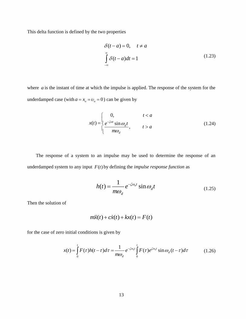
The loss factor can be found for a single, well-defined modal resonance or as the average loss

factor of many modal resonances over a given frequency range [6]. In both cases, the initial

decay slope is found by plotting the system‘s response on a logarithmic amplitude scale, with a

linear time scale. The loss factor is given by the slope of the logarithmic decrement shown in

Figure 1-7. The loss factor is estimated with the following equation,

( / sec)

27.3

t

n

dB

f

0 0.2 0.4 0.6 0.8 1 1.20

0.05

0.1

0.15

0.2

Time [ Seconds ]

Am

pli

tud

e


( )f tGe

16

where t is the decay rate in / secdB and nf is the natural frequency.

FIGURE 1-7 LOGARITHMIC DECREMENT OF THE TRANSIENT RESPONSE

1.2.2.3 LOGARITHMIC DECREMENT

The decay rate of the single degree of freedom spring-mass-damper system shown in

Figure 1-7 can be used to estimate the damping, and the ‗logarithmic decrement‘, , has

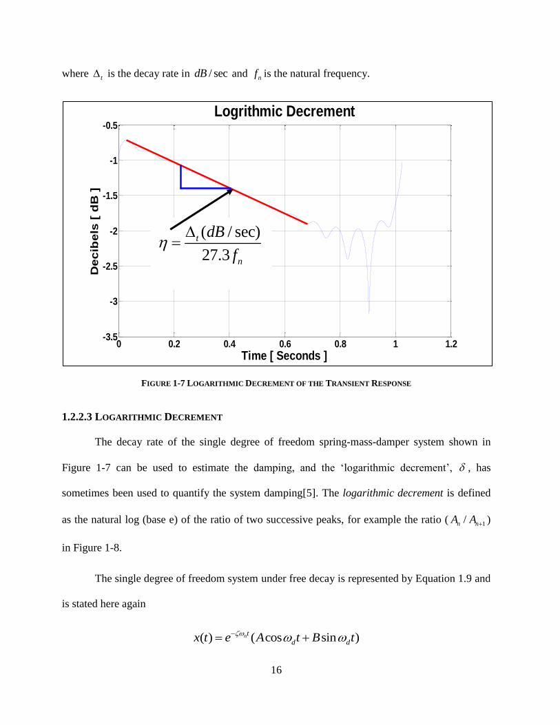
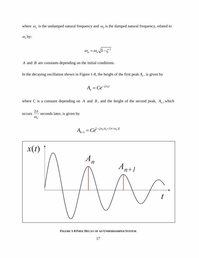
sometimes been used to quantify the system damping[5]. The logarithmic decrement is defined

as the natural log (base e) of the ratio of two successive peaks, for example the ratio ( 1/n nA A )

in Figure 1-8.

The single degree of freedom system under free decay is represented by Equation 1.9 and

is stated here again

( ) ( cos sin )nt

d dx t e A t B t

0 0.2 0.4 0.6 0.8 1 1.2-3.5

-3

-2.5

-2

-1.5

-1

-0.5

Time [ Seconds ]

De

cib

els

[ d

B ]

Logrithmic Decrement

( / sec)

27.3

t

n

dB

f

17

where n is the undamped natural frequency and d is the damped natural frequency, related to

n by:

21d n

A and B are constants depending on the initial conditions.

In the decaying oscillation shown in Figure 1-8, the height of the first peak nA , is given by

nt

nA Ce

where C is a constant depending on A and B , and the height of the second peak, 1nA which

occurs 2

d

seconds later, is given by

1[ ( 2 / )]

1n dt

nA Ce

FIGURE 1-8 FREE DECAY OF AN UNDERDAMPED SYSTEM

18

then the ratio 1/n nA A is

2

2( )

1

1

n

n

Ae

A

(1.27)

The logarithmic decrement is then defined as:

2

1

2log

1

ne

n

A

A

(1.28)

From the above Equation (1.28) the viscous damping rate, can be found by solving the

following quadratic equations,

2 2 2 2

2 2 22 0

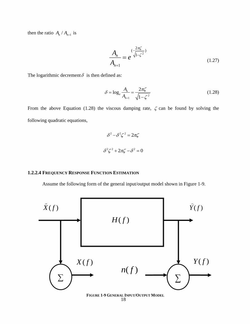
1.2.2.4 FREQUENCY RESPONSE FUNCTION ESTIMATION

Assume the following form of the general input/output model shown in Figure 1-9.

( )X f

( )H f

( )Y f

( )Y f

( )n f

( )X f

FIGURE 1-9 GENERAL INPUT/OUTPUT MODEL

19

Then,

( ) ( )

( ) ( ) ( )

X f X f

Y f Y f n f

(1.29)

where ( )X f is the measured input, which is equal to the correlated or ideal input ( )X f , and

( )Y f is the measured output, which is equal to the sum of the correlated or ideal output ( )Y f

and the uncorrelated output ( ) which is noisen f [7].

The Frequency Response Function (F.R.F.) of the system is given as:

*

1 11

*

1 1

K K

k k xy

k k

K K

k k xx

k k

X Y Gcross spectrum

H Hinput autospectrum

X X G

(1.30)

where and k kX Y are the individual Fourier Spectra of input x and output y .

The symbol * means complex conjugate. xxG is the auto spectrum of the input point x ,

xyG is the cross spectrum between the input point x and the output point y and 1H

is a complex

valued function. The magnitude of the F.R.F. is referred to as gain, and the phase angle is the

angle between the outputs relative to the input, which is obtained from the cross-spectrum in the

numerator of the F.R.F. estimator.

The impulse response function of a system given by Equation (1.24) is the inverse

Fourier Transform of the frequency response function.

The coherence function, 2 ( )xy measures the degree of the correlation between the

signals in the frequency domain. It is defined as

20

2 1 1

1 1

( )

K K

xy yx

k kxy K K

xx yy

k k

G G

G G

(1.31)

where yyG is the auto spectrum of the output point y and yxG

is the cross spectrum between the

output point y and the input point x .The coherence function is such that20 ( ) 1xy , and it

provides an estimate of the proportion of the output that is due to the input. For an ideal single

input, single output system with no extraneous noise at the input or output stages the coherence

function is equal to unity.

2

2

2

( ) ( )( ) 1

( ) ( ) ( )

xx

xy

xx xx

G

G G

(1.32)

The signal to noise ratio of a system is a function of the coherence function and is defined as

2

2

( )

1 ( )

xy

xy

Sn

(1.33)

1.3 MEASUREMENT SETUP FOR LOSS FACTOR MEASUREMENTS

The experiments are carried out in the Structural Acoustics Laboratory (S.A.L.) at the

University of Kansas. Aluminum and Steel plates are used to simulate aerospace structures,

especially structural skin panels. Constrained layer damping (C.L.D.) treatment was applied to

two plates; one has full covering C.L.D. and the other has partial covering C.L.D. The damping

21

material used here is visco-elastic damping polymer, 3MF9469PC. To ensure good bonding

between the visco- elastic material and the structure, surfaces are cleaned before attachment and

vacuum is drawn after the attachment to apply a pressure of about 51 10 Pascal. Plates were

suspended from a stand by the use of elastic strands or aluminum wires to simulate free boundary

conditions with respect to out-of-plane vibration [8]. The signal of excitation is in the form of

white noise which was passed through the amplifier to a typical magneto-dynamic shaker. The

output force is transmitted to the plate by using a thin steel rod known as a stinger as shown in

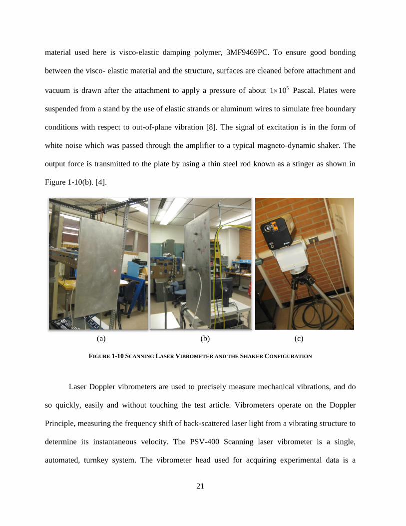
Figure 1-10(b). [4].

FIGURE 1-10 SCANNING LASER VIBROMETER AND THE SHAKER CONFIGURATION

Laser Doppler vibrometers are used to precisely measure mechanical vibrations, and do

so quickly, easily and without touching the test article. Vibrometers operate on the Doppler

Principle, measuring the frequency shift of back-scattered laser light from a vibrating structure to

determine its instantaneous velocity. The PSV-400 Scanning laser vibrometer is a single,

automated, turnkey system. The vibrometer head used for acquiring experimental data is a

(a) (b) (c)

22

Polytec 056, which is shown in Figure 1-10(c). Software that controls the scanning laser

vibrometer is Polytec version 7.1. All experiments used a frequency resolution of 1 Hz. This

Vibrometer can only give up to 6400 frequency lines. To achieve a resolution of 1 Hz with data

up to 6400 Hz, a sampling frequency of 16384 Hz is used. The Nyquist Frequency is more than

twice of 6400 Hz, so we can have good loss factor estimation up to 6400 Hz. A typical

experimental setup is shown in Figure 1-11.

FIGURE 1-11 A TYPICAL EXPERIMENTAL SETUP USED

1.4 OVERVIEW OF STATISTICAL ENERGY ANALYSIS

Statistical energy analysis (S.E.A) is a modeling procedure for the estimation of the

dynamic characteristics of, the vibrational response levels of, and the noise radiation from

complex, resonant, built-up structures using energy flow relationships [9][10]. These energy flow

relationships between the various coupled systems (e.g. plates) that comprise the built-up

Scanning Laser Vibrometer

Shaker

Power Amplifier Workstation

Signal Generator

Test Article

Signal Conditioner

Velocity

Force Transducer

Force

23

structure have a simple thermal analogy. S.E.A. is also used to predict interactions between

resonant structures and reverberant sound fields in acoustic volumes. Many random noise and

vibration problems associated with large built-up structures, like aircraft, cannot be practically

solved by classical methods, and S.E.A. therefore provides a basis for the prediction of average

noise and vibration levels, particularly in high frequency regions where modal densities are high.

The successful prediction of noise and vibration levels of coupled structural elements and

acoustic volumes using the S.E.A. techniques depends to a large extent on an accurate estimate

of three parameters:

1. The modal densities of the individual subsystems

2. The internal loss factors (damping) of the individual subsystems, and

3. The coupling loss factors (degree of coupling) between the subsystems.

S.E.A. is particularly attractive in high frequency regions where a deterministic analysis of

all the resonant modes of vibration is not practical. This is because at these frequencies there are

numerous resonant modes, and numerical computational techniques such as the finite element

method have very little applicability.

1.4.1 BASIC ENERGY FLOW CONCEPTS

An individual oscillator driven in the steady-state condition at a single frequency has

potential and kinetic energy stored within it. In the steady-state, the input power, in has to

balance with the power dissipated, .diss The power dissipated is related to the energy stored in

the oscillator via damping:

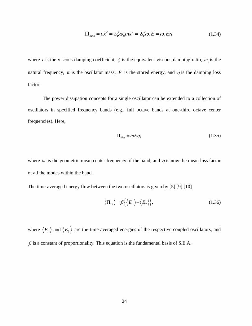
24

2 22 2diss n n ncx mx E E (1.34)

where c is the viscous-damping coefficient, is the equivalent viscous damping ratio, n is the

natural frequency, m is the oscillator mass, E is the stored energy, and is the damping loss

factor.

The power dissipation concepts for a single oscillator can be extended to a collection of

oscillators in specified frequency bands (e.g., full octave bands at one-third octave center

frequencies). Here,

,diss E (1.35)

where is the geometric mean center frequency of the band, and is now the mean loss factor

of all the modes within the band.

The time-averaged energy flow between the two oscillators is given by [5] [9] [10]

12 1 2 ,E E (1.36)

where 1 2 and E E are the time-averaged energies of the respective coupled oscillators, and

is a constant of proportionality. This equation is the fundamental basis of S.E.A.

25

1.4.2 THE TWO SUBSYSTEM MODEL

For two groups of lightly coupled oscillators with modal densities 1n and 2n respectively,

the average energy flow, 12 is expressed by extending Equation (1.36) as

12 1 1 2 2/ / ,E n E n (1.37)

where is another constant of proportionality, which is only a function of the oscillator

parameters. It should be noted that 1 2 and E E are total energies of the respective

subsystems; 1 1 2 2/ and /E n E n are the respective modal energies. The coupling loss factor,

ij , relates to energy flow from subsystem i to subsystem j , and is a function of the modal

density, in , of the subsystem i , the constant of proportionality, , and the center frequency, ,

of the band. Equation (1.37) can be expressed in power dissipation terms; the net energy flow

from subsystem1 to subsystem 2 is the difference between the power dissipated during the flow

of energy from subsystem 1 to subsystem 2 and the power dissipated during the flow of energy

from subsystem 2 back to subsystem 1. Hence, using the power dissipation concepts from

Equation (1.34),

12 1 12 2 21E E (1.38)

where 12 21 and , are the coupled loss factors between subsystems 1 and 2, and 2 and 1,

respectively. From Equations (1.37) and (1.38) we have,

12 21

1 2

, and .n n

26

Thus

1 12 2 21n n (1.39)

Equation (1.39) is the reciprocity relationship between the two subsystems. By substituting this

reciprocity relationship into Equation (1.38), we have

112 12 1 2

2

.n

E En

(1.40)

Figure 1-12 shows a two subsystem model (numerous modes in each subsystem) where

subsystem 1 is driven directly by external force and the other subsystem, subsystem 2 is driven

only through the coupling. 1 is the power input to subsystem 1; 2 0 is the power input to

subsystem 2; 1 2 and n n are the modal densities and 1 2 and are the internal loss factors of

subsystems 1 and 2 respectively; 12 21 and are the coupling loss factors associated with energy

flow from 1 to 2 and from 2 to 1; and 1 2 and E E are the vibrational energies associated with

subsystems 1 and 2.

Using the consistency relationship given by Equation (1.39) [11]

2 2 12

1 2 2 1 12

,E n

E n n

(1.41)

and thus,

12 2 2

2 2 1 1 2

.n E

n E n E

(1.42)

27

Equation 1.42 is only valid for direct excitation of subsystem 1, with subsystem 2 being excited

indirectly via the coupling joint. If the experiment is reversed then we will have the following,

12 2 1

1 1 2 2 1

.n E

n E n E

(1.43)

FIGURE 1-12 A TWO SUBSYSTEM S.E.A. MODEL

2 0

1 1E

2 2E

2 21E 1 12E

1

1E 1n

1

2E 2n

2

28

1.5 TEST ARTICLES CONSIDERED

1.5.1 ALUMINUM PLATE WITH FULL CONSTRAINED LAYER DAMPING

FIGURE 1-13 DAMPED ALUMINUM PLATE WITH FULL CONSTRAINED LAYER DAMPING

TABLE 1-1 DIMENSIONS OF DAMPED ALUMINUM PLATE WITH FULL CONSTRAINED LAYER DAMPING

Material Dimensions (m) Mass(gms)

Base Layer CLAD 2024-T3 0.349X0.2029X0.0016002 573.7

Damping Layer 3M F9469PC at20 oC 0.349×0.2029×0.000127 4.125

Constraining Sheet CLAD 2024-T3 0.349X0.2029X0.0016002 48.06

29

1.5.2 UNDAMPED STEEL PLATE

FIGURE 1-14 UNDAMPED STEEL PLATE

TABLE 1-2 MATERIAL PROPERTIES OF THE UNDAMPED STEEL PLATE

Material Dimensions(m) Mass (gms)

Steel 0.39 x 0.28 x 0.003 2750

30

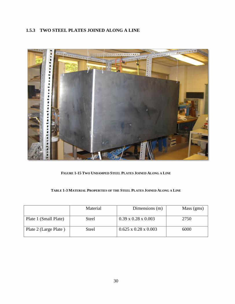
1.5.3 TWO STEEL PLATES JOINED ALONG A LINE

FIGURE 1-15 TWO UNDAMPED STEEL PLATES JOINED ALONG A LINE

TABLE 1-3 MATERIAL PROPERTIES OF THE STEEL PLATES JOINED ALONG A LINE

Material Dimensions (m) Mass (gms)

Plate 1 (Small Plate) Steel 0.39 x 0.28 x 0.003 2750

Plate 2 (Large Plate ) Steel 0.625 x 0.28 x 0.003 6000

31

1.5.4 UNDAMPED ALUMINUM PLATES JOINED AT A POINT

FIGURE 1-16 TWO UNDAMPED ALUMINUM PLATES CONNECTED AT A POINT

TABLE 1-4 MATERIAL PROPERTIES OF ALUMINUM PLATES JOINED AT A POINT

Material Dimensions (m) Mass(gms)

Top Plate CLAD 2024-T3 0.53 x 0.40 x 0.00635 3628

Bottom Plate CLAD 2024-T3 0.61 x 0.46 x 0.00635 4820

The plates are connected through a force transducer.

32

2 LOSS FACTOR ESTIMATION USING THE POWER INPUT METHOD

2.1 THEORY OF THE POWER INPUT METHOD

The Power Input Method (P.I.M.) is based on a comparison of the dissipated energy of a

system to its maximum total energy under steady state vibration. Some errors may be introduced

through the measurement technique, but the P.I.M. is fundamentally unbiased at the natural

frequencies of well-defined modes or when the loss factors are frequency-band averaged over

many modes. These ―frequency-averaged‖ damping loss estimates are widely used in the

automotive and aerospace industry for vehicle computer models based on Finite Element Method

(F.E.M.) and Statistical Energy Analysis (S.E.A.) [6].

The damping loss factor per cycle in the frequency band centered at , for a structural system is

defined as [4]

( ) diss IN

Total Total

E E

E E (2.1)

where INE is the input energy, dissE is the energy dissipated from damping and TotalE is the time

averaged total energy of the system. Assuming a stationary input energy at the fixed location, the

energy dissipated, dissE can be replaced with input energy INE because the input energy is equal

33

to the dissipated energy under steady state conditions. Unfortunately, INE cannot be measured

directly. But the input energy can be calculated from the simultaneous measurements of the force

and velocity at the point of energy input. dissE can then be computed as

1Re[ ( )] ( ),

2IN diss ff ffE E G

(2.2)

where ff is the driving point mobility function (the force-to-velocity transfer function), and

ffG is the power spectral density of the input force. Obtaining an estimate for TotalE requires

making a few assumptions. First, since the total energy cannot be calculated directly from force

and velocity measurements, it can be replaced with twice the maximum kinetic energy –which

holds true at the natural frequencies of an undamped system. But, the error in making this

assumption is, for instance only 0.5% for a damping level of 10%. Secondly, the system being

measured should be approximated by a summation as opposed to a volume integral when taking

measurements. Thus the kinetic energy is evaluated by the following equation:

1

1( ),

2

N

KE i ii

i

E m G

(2.3)

where, KEE is the system kinetic energy, N is the number of measurement locations, im is the

mass of the discrete portion of the system, and iiG is the power spectral density of the velocity

response at each measurement location. Finally, assuming that the system is linear, allows use

of:

34

2 ( )( ) ,

( )

iiff

ff

GH

G

(2.4)

where, ffH is the driving point mobility function. With the above mentioned assumptions, and

all measurement points uniformly spaced throughout the system in equal mass portions, we have

the damping in the structure defined as,

2

1

Re ( )( )

( )

ff

N

if

i

H

m H

(2.5)

where ifH is the mobility between the driving point f and the point i . To obtain accurate loss

factors estimations, it is essential to have highly accurate measurements of the driving point FRF

( ffH ) [4]; otherwise, large errors could be introduced. In particular, if the phase information in

ifH is not carefully resolved, the loss factor estimation may be negative which is physically

unrealizable. One way to address deficiencies in phase information is to increase frequency

resolution in the measurement.

2.2 SINGLE DEGREE OF FREEDOM ANALYSIS

2.2.1 INTRODUCTION TO SINGLE DEGREE OF FREEDOM SYSTEMS

A system with a single degree of freedom (S.D.O.F. system) is the simplest among the

vibratory systems. It consists of three elements: inertia element (mass), elastic element (spring),

35

and damping element. The dynamic state of the system is fully described by one variable that

characterizes deflection of the inertia element from the equilibrium position. One key assumption

for the spring-mass-damper system is that the spring has no damping or mass, the mass has no

stiffness or damping; and the damper has no stiffness or mass. Furthermore, the mass is allowed

to move in only one direction. The role of single degree of freedom systems in vibration theory is

very important because any linear vibratory system behaves like an S.D.O.F. system near an

isolated natural frequency and as a connection of S.D.O.F. systems in a wider frequency range.

The general form of the differential equation describing a single degree of freedom oscillator is,

0 0( ) ( ) ( ) ( ), (0) , (0)mx t cx t kx t f t x x x v (2.6)

where ( )x t is the position of the mass, m is the mass, c is the viscous damping rate, k is the

stiffness, and ( )f t is the external dynamic load. The initial displacement is 0x , and the initial

velocity is 0v

Free vibrational response of lightly damped systems decay over time. Damping may be

introduced into a structure through diverse mechanisms, including linear viscous damping,

friction damping, and plastic deformation. All but linear viscous damping are somewhat

complicated to analyze with closed form expressions, so we will restrict our attention to linear

viscous damping, in which the damping force Df is proportional to the velocity,

Df cx

36

The two types of energies in a system are kinetic energy, T, and the potential energy, U.

Their sum T U is the total energy of vibration. Generally, it is the time-averaged energy values

and ,T U that are required. Since it is known that T U and2

E m v .

For a damped system, the energy decays exponentially with time. The mean square

velocity is obtained by differentiating the underdamped solution given by

2 1/2( ) sin (1 )nt

T nx t X e t

(2.7)

In the above equation the viscous damping ratio , is now replaced with the structural loss

factor and the relation between the two is given by 2 .

/2 2 1/2( ) sin (1 ( / 2) )nt

T nx t X e t

(2.8)

The mean-squared velocity is obtained by differentiating Equation (2.8) and subsequently

integrating the square value over a time interval. It is

22 ,

2

ntV e

(2.9)

where V is the maximum velocity level. The corresponding mean-square displacement is

2

2

2

n

x

(2.10)

37

The above equations are approximations and assume small damping, i.e. d n . For the case of

the underdamped oscillator, ,T U so the total time averaged energy is,

22 ,E T m . Therefore, the time-averaged power dissipation is given by

2 2/ .n ndE dt c m E (2.11)

Hence, the structural loss factor is [6] [12]

n E

(2.12)

The structural loss factor is thus related to the time-averaged power dissipation and the time

averaged energy of vibration.

2.2.2 ANALYTICAL LOSS FACTOR ESTIMATION OF SDOF SYSTEMS

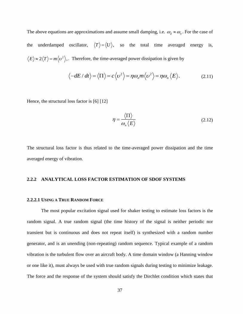
2.2.2.1 USING A TRUE RANDOM FORCE

The most popular excitation signal used for shaker testing to estimate loss factors is the

random signal. A true random signal (the time history of the signal is neither periodic nor

transient but is continuous and does not repeat itself) is synthesized with a random number

generator, and is an unending (non-repeating) random sequence. Typical example of a random

vibration is the turbulent flow over an aircraft body. A time domain window (a Hanning window

or one like it), must always be used with true random signals during testing to minimize leakage.

The force and the response of the system should satisfy the Dirchlet condition which states that

38

these signals and the first time derivative of the signals are zero at the beginning and end of the

time record.

The single degree of freedom system is excited with a random force. The random force is

created using a random phase angle approach. A typical true random signal before and after

applying a Hanning window is shown in Figure 2-1. The MatLAB code to generate the random

signal is given in Appendix A. The SDOF system has a mass of 0.5 Kg , damping rate of 0.5

/Ns mand a stiffness of 1000 /N m .

The natural frequency of the system n which is given by /n k m is calculated as

44.7214. The damping coefficient which is given by 2 n

c

m

is calculated to be 0.0112.

Since the structural damping loss factor of the system is given as 2 , the input loss factor

for the SDOF system is 0.224. The damped natural frequency d of the system given by

21d n , is calculated to be 44.7186. Note that d n .

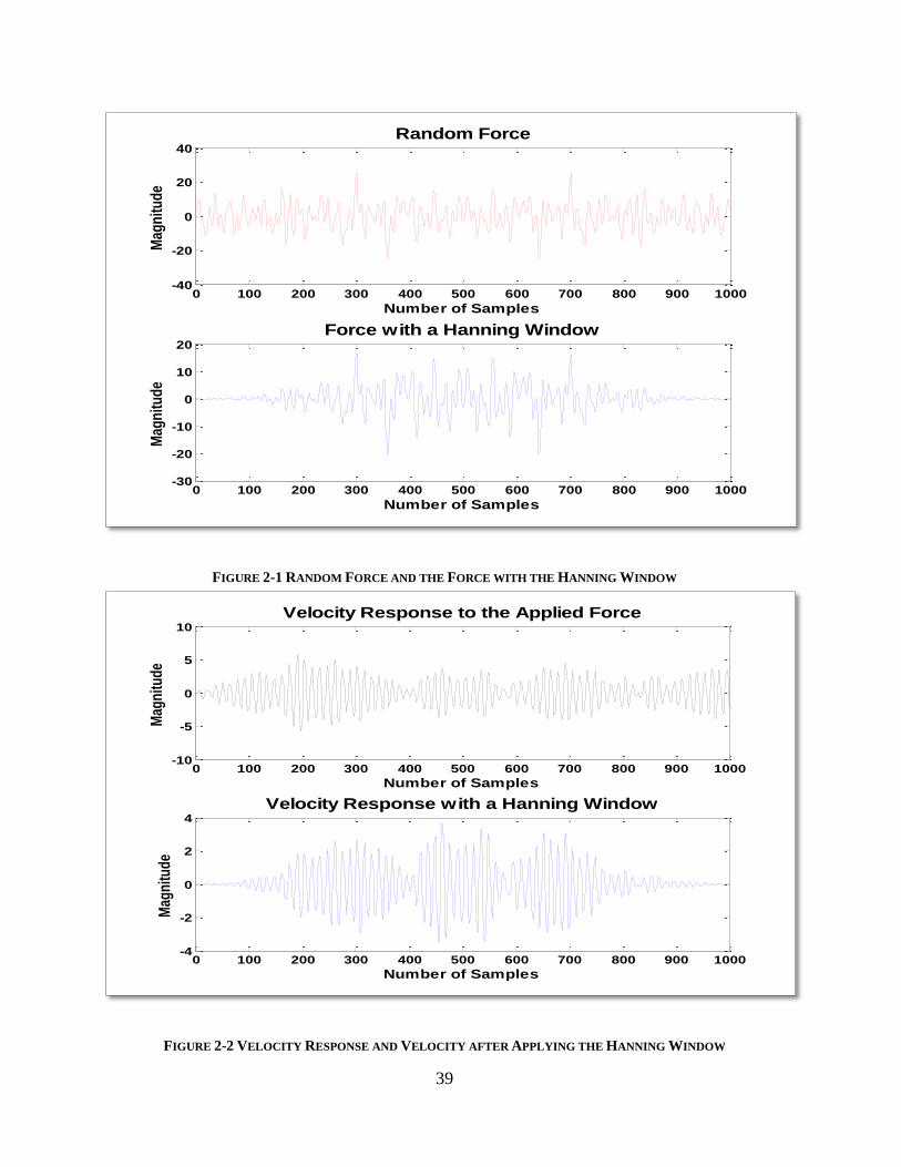
The response of the system for this true random excitation signal is given by the impulse

function, shown in Equation (1.25) and stated here

1( ) sinnt

d

d

h t e tm

The velocity is then obtained by differentiating the velocity in the time domain.

Figure 2-2 shows the velocity response of the single degree of freedom system subjected to

random excitation. Again a Hanning window is used for the velocity response to minimize

leakage.

39

FIGURE 2-1 RANDOM FORCE AND THE FORCE WITH THE HANNING WINDOW

FIGURE 2-2 VELOCITY RESPONSE AND VELOCITY AFTER APPLYING THE HANNING WINDOW

0 100 200 300 400 500 600 700 800 900 1000-40

-20

0

20

40

Number of Samples

Mag

nit

ud

e

Random Force

0 100 200 300 400 500 600 700 800 900 1000-30

-20

-10

0

10

20

Number of Samples

Mag

nit

ud

e

Force with a Hanning Window

0 100 200 300 400 500 600 700 800 900 1000-10

-5

0

5

10

Number of Samples

Mag

nit

ud

e

Velocity Response to the Applied Force

0 100 200 300 400 500 600 700 800 900 1000-4

-2

0

2

4

Number of Samples

Mag

nit

ud

e

Velocity Response with a Hanning Window

40

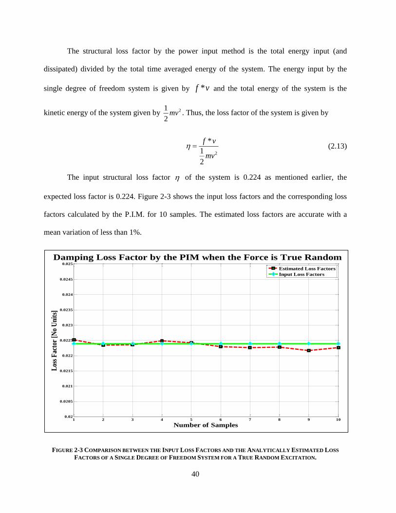
The structural loss factor by the power input method is the total energy input (and

dissipated) divided by the total time averaged energy of the system. The energy input by the

single degree of freedom system is given by *f v and the total energy of the system is the

kinetic energy of the system given by 21

2mv . Thus, the loss factor of the system is given by

2

*

1

2

f v

mv

(2.13)

The input structural loss factor of the system is 0.224 as mentioned earlier, the

expected loss factor is 0.224. Figure 2-3 shows the input loss factors and the corresponding loss

factors calculated by the P.I.M. for 10 samples. The estimated loss factors are accurate with a

mean variation of less than 1%.

FIGURE 2-3 COMPARISON BETWEEN THE INPUT LOSS FACTORS AND THE ANALYTICALLY ESTIMATED LOSS

FACTORS OF A SINGLE DEGREE OF FREEDOM SYSTEM FOR A TRUE RANDOM EXCITATION.

1 2 3 4 5 6 7 8 9 100.02

0.0205

0.021

0.0215

0.022

0.0225

0.023

0.0235

0.024

0.0245

0.025

Number of Samples

Los

s F

acto

r [N

o U

nit

s]

Damping Loss Factor by the PIM when the Force is True Random

Estimated Loss Factors

Input Loss Factors

41

2.2.2.2 USING A SINUSOIDAL FORCE

The single degree of freedom system is dynamically forced to vibrate with a sinusoidal

forcing function, ( ) cos( )of t F t where is the frequency of the forcing function in radians

per second. If ( )f t is persistent, then after several cycles the system will respond only at the

frequency of vibration of the external forcing .

The sine wave excitation signal has been used since the early days of structural dynamic

measurements. It was the only signal that could be effectively used with traditional analog

instrumentation. Even after broad band testing methods (like impact testing), have been

developed for use with Fast Fourier Transforms (F.F.T.) analyzers, sine wave excitation is still

useful in some applications. The primary purpose for using a sine wave excitation signal is to put

energy into a structure at a specified frequency. Slowly sweeping sine wave excitation is also

useful for characterizing non-linearities in structures.

The single degree of freedom system with a mass of 0.5 Kg , damping rate of 0.5 /Ns m

and a stiffness of 1000 /N m is excited with a sinusoidal input force of frequency, which is equal

to the damped natural frequency of the system. The natural frequency of the system n which is

given by /n k m is calculated as 44.7214. The damping coefficient which is given by

2 n

c

m

is calculated to be 0.0112. Since the structural damping loss factor of the system is

given as 2 , the input loss factor for the S.D.O.F. system is 0.224. The damped natural

frequency d of the system given by 21d n is calculated to be 44.7186. Note that

d n .

42

The response of the system for this periodic excitation signal is given by the impulse

function, shown in Equation (1.25) and stated here again

1( ) sinnt

d

d

h t e tm

The sinusoidal excitation force and the velocity response of the single degree of freedom system

are plotted in Figure 2-4. The force and the response must satisfy the Dirchlet condition and so a

Hanning window is used.

FIGURE 2-4 FORCE AND VELOCITY WITH A HANNING WINDOW APPLIED

Once we have the response of the system to the periodic excitation signal the velocity of

the system is calculated by simple differentiation and the total energy is measured as the kinetic

0 200 400 600 800 1000 1200 1400 1600 1800 2000-1

-0.5

0

0.5

1

Number of Samples

Mag

nit

ud

e

Sinusoidal Force with the Hanning Window

0 200 400 600 800 1000 1200 1400 1600 1800 2000-2

-1

0

1

2

Number of Samples

Mag

nit

ud

e

Velocity Response with the Hanning Window

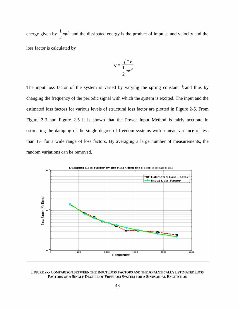
43

energy given by 21

2mv and the dissipated energy is the product of impulse and velocity and the

loss factor is calculated by

2

*

1

2

f v

mv

.

The input loss factor of the system is varied by varying the spring constant k and thus by

changing the frequency of the periodic signal with which the system is excited. The input and the

estimated loss factors for various levels of structural loss factor are plotted in Figure 2-5. From

Figure 2-3 and Figure 2-5 it is shown that the Power Input Method is fairly accurate in

estimating the damping of the single degree of freedom systems with a mean variance of less

than 1% for a wide range of loss factors. By averaging a large number of measurements, the

random variations can be removed.

FIGURE 2-5 COMPARISON BETWEEN THE INPUT LOSS FACTORS AND THE ANALYTICALLY ESTIMATED LOSS

FACTORS OF A SINGLE DEGREE OF FREEDOM SYSTEM FOR A SINUSOIDAL EXCITATION

0 500 1000 1500 2000 250010

-4

10-3

10-2

Frequency

Los

s F

acto

r [N

o U

nits

]

Damping Loss Factor by the PIM when the Force is Sinusoidal

Estimated Loss Factor

Input Loss Factor

44

2.3 PLATE – EXPERIMENTS

For the experimental validation of the Power Input Method a couple of relatively simple

systems are chosen. A 2024-T3 aluminum plate with a full covering constrained layer damping

treatment and a steel plate with no damping are used as the test articles. Plates are chosen over

other simple structures (i.e., bars, etc.) because plates have a higher modal density. Most of the

concepts of the single degree of freedom systems can be directly extended to the case of the

multiple degree of freedom systems [1]. There are n natural frequencies each associated with its

own mode shape, for a system having n degrees of freedom. Plates are typically modeled

analytically as a finite-numbered collection of modal responses or a finite element approximation

[5].

As discussed in the introduction section of Chapter 2, the Power Input Method [13], [11],

[14] approximates the loss factor of the system by the ratio of energy dissipated within the

system per radian of motion to its total strain energy. Hence the loss factor is given by

( ) diss IN

Total Total

E E

E E

the numerator in the equation can be replaced with

1Re[ ( )] ( )

2IN if ffE H G

where ifH is the mobility (velocity/force) between the driving point f and the point i ,

The total energy of the system i.e., the total time averaged kinetic energy of the system is given

by

45

1

1( ),

2

N

KE i ii

i

E m G

.

The mobility transfer function, which is the ratio of the Power Spectral Density (P.S.D.) of

velocity response at the measurement location i to the P.S.D. of input force at the chosen input

location, is given by [14]

2 ( )( )

( )

iiff

ff

GH

G

where ffH is the mobility of the driving point.

Hence the loss factor of the multi degree of freedom system is determined by the equation,

2

1

Re ( )( )

( )

ff

N

if

i

H

m H

(2.14)

2.3.1 ALUMINUM PLATE WITH FULL CONSTRAINED LAYER DAMPING

The 2024-T3 aluminum plate is suspended with a thin aluminum wire to create free-free

boundary condition as shown in Figure 1-10(a, b). The other end of the wire is attached to a

massive and stiff frame, so vibrational energy is reflected back to the test article with minimum

energy loss at the boundary. Wolf Jr. [8] provided a rule-of-thumb for designing suspension

systems: to simulate free boundary conditions; the first rigid body mode under the constraint of

the suspension should be no more than 1/10 of the first elastic mode. For example, the most

dominant rigid body mode (the vertical translational mode) for this damped aluminum plate is

measured to be at 1.43 Hz, which is much less than 1/10 of the plate‘s first bending mode which

46

is 90.6Hz. As mentioned in the discussion about the measurement techniques, to eliminate the

effects of mass loading due to an accelerometer, a Polytec laser, model OFV 056 is used.

Vibrational response of the plate due to a steady excitation is measured at 225 points by placing

a grid of scanning points over the entire surface of the plate. This is similar to using a Finite

Element approach where we divide the test specimen in to finite elements of smaller size and the

response of each finite element is calculated to give a close representation of the entire plate. In a

finite element analysis the solution should asymptotically approach a constant value as the total

number of finite elements is increased. Similarly as the number of scanning points are increased,

the loss factor measurements should asymptotically approach a constant value. The plate is

excited from 0 Hz to 6.4 KHz with a resolution of 1 Hz via a LDS Model V203 electrodynamic

shaker and a LDS PA25E power amplifier. A PCB force gage was connected to the shaker with a

stinger and attached to the back of the plate to measure the input force while the scanning laser

vibrometer measures the vibrational responses of the system.

It must be noted here that the laser vibrometer cannot measure the driving point mobility

directly; instead it measures the velocity of the point on the front of the plate immediately

opposite the forcing point. The accurate measurement of the driving point mobility is critical to

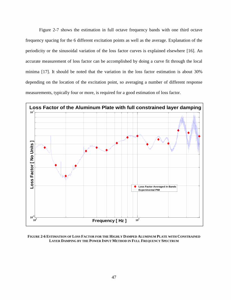
get a good estimation of loss factors. Figure 2-6, presents the loss factors as a function of

frequency for one excitation point. The loss factors estimated in 1/3 octave frequencies by

averaging the loss factors in the respective full octave band are also shown in the graph. The

oscillatory behavior of the estimated loss factors is attributed to the limitations of the

experimental technique and a curve fit through the local minima is a closer estimate of the loss

factors for the plate [17].

47

Figure 2-7 shows the estimation in full octave frequency bands with one third octave

frequency spacing for the 6 different excitation points as well as the average. Explanation of the

periodicity or the sinusoidal variation of the loss factor curves is explained elsewhere [16]. An

accurate measurement of loss factor can be accomplished by doing a curve fit through the local

minima [17]. It should be noted that the variation in the loss factor estimation is about 30%

depending on the location of the excitation point, so averaging a number of different response

measurements, typically four or more, is required for a good estimation of loss factor.

FIGURE 2-6 ESTIMATION OF LOSS FACTOR FOR THE HIGHLY DAMPED ALUMINUM PLATE WITH CONSTRAINED

LAYER DAMPING BY THE POWER INPUT METHOD IN FULL FREQUENCY SPECTRUM

102

103

10-2

10-1

Frequency [ Hz ]

Lo

ss

Fa

cto

r [

No

Un

its

]

Loss Factor of the Aluminum Plate with full constrained layer damping

Loss Factor Averaged in Bands

Experimental PIM

48

FIGURE 2-7 LOSS FACTOR FOR THE ALUMINUM PLATE WITH FULL CONSTRAINED LAYER DAMPING ESTIMATED

IN FULL OCTAVE BANDS WITH 1/3RD

OCTAVE CENTER FREQUENCIES


The undamped steel plate is shown in Figure 1-14. Although the plate has no external

damping treatment applied it has an inherent material damping. Steel has very low internal

damping but the purpose of this experiment is to determine the limitations of the power input

method. The steel plate is suspended with metal cords but could still be considered as free-free

boundary conditions. To simulate free boundary condition the first rigid body mode under the

constraint of suspension should be no more than 1/10th of the first elastic mode [8], [4] which it

is in this case. It can be seen from Figure 2-8 that the damping loss estimation of the plate fails

as it predicts negative loss factors. It is hence concluded that although the power input method

0.01

0.1

1

100 1000 10000

Lo

ss F

act

or

[ N

o U

nit

s ]

Frequency [ Hz ]

Aluminum Plate with full constrained layer damping

Excitation Point 1 Excitation Point 2



Average

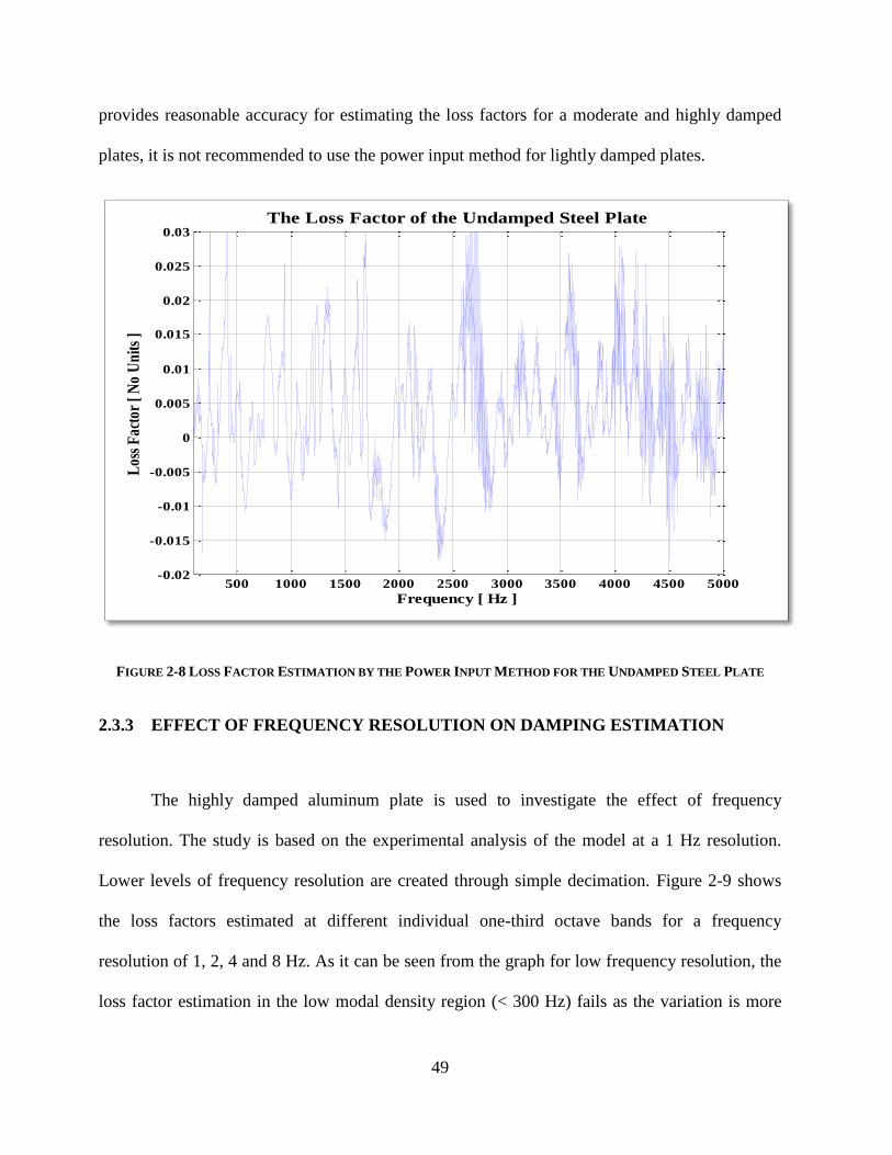
49

provides reasonable accuracy for estimating the loss factors for a moderate and highly damped

plates, it is not recommended to use the power input method for lightly damped plates.

FIGURE 2-8 LOSS FACTOR ESTIMATION BY THE POWER INPUT METHOD FOR THE UNDAMPED STEEL PLATE

2.3.3 EFFECT OF FREQUENCY RESOLUTION ON DAMPING ESTIMATION

The highly damped aluminum plate is used to investigate the effect of frequency

resolution. The study is based on the experimental analysis of the model at a 1 Hz resolution.

Lower levels of frequency resolution are created through simple decimation. Figure 2-9 shows

the loss factors estimated at different individual one-third octave bands for a frequency

resolution of 1, 2, 4 and 8 Hz. As it can be seen from the graph for low frequency resolution, the

loss factor estimation in the low modal density region (< 300 Hz) fails as the variation is more

500 1000 1500 2000 2500 3000 3500 4000 4500 5000-0.02

-0.015

-0.01

-0.005

0

0.005

0.01

0.015

0.02

0.025

0.03

Frequency [ Hz ]

Los

s F

acto

r [

No

Un

its

]

The Loss Factor of the Undamped Steel Plate

50

than 100% over the loss factors with adequate frequency resolution. For low resolution there will

not be adequate information to capture all the modes in a particular band that is centered at these

1/3rd

octaves and so the damping cannot be estimated accurately.

FIGURE 2-9 EFFECT OF FREQUENCY RESOLUTION ON THE ESTIMATED LOSS FACTORS FOR THE ALUMINUM

PLATE WITH FULL CONSTRAINED LAYER DAMPING TREATMENT

0.001

0.01

0.1

1

10 100 1000

Loss

Fact

ors

[ N

o U

nit

s ]

Frequency [ Hz ]

Effect of Frequency Resolution for Damped Aluminum Plate

1 Hz Resolution

2 Hz Resolution

4 Hz Resolution

8 Hz Resolution

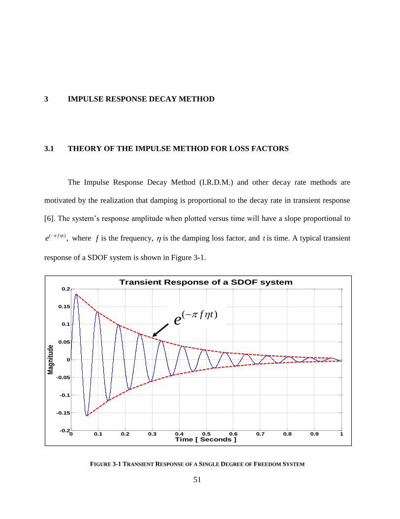
51

3 IMPULSE RESPONSE DECAY METHOD

3.1 THEORY OF THE IMPULSE METHOD FOR LOSS FACTORS

The Impulse Response Decay Method (I.R.D.M.) and other decay rate methods are

motivated by the realization that damping is proportional to the decay rate in transient response

[6]. The system‘s response amplitude when plotted versus time will have a slope proportional to

( ) ,f te where f is the frequency, is the damping loss factor, and t is time. A typical transient

response of a SDOF system is shown in Figure 3-1.

FIGURE 3-1 TRANSIENT RESPONSE OF A SINGLE DEGREE OF FREEDOM SYSTEM

0 0.1 0.2 0.3 0.4 0.5 0.6 0.7 0.8 0.9 1-0.2

-0.15

-0.1

-0.05

0

0.05

0.1

0.15

0.2

Time [ Seconds ]

Mag

nit

ud

e


( )f te

52

The energy of the system is proportional to the peak amplitude squared; therefore, the

system response will decay at a rate equal to ( )f tGe

where G is related to the peak response

amplitude of the system. The peak amplitude of the response is shown in Figure 3-2.

FIGURE 3-2 PEAK AMPLITUDE OF THE TRANSIENT RESPONSE

The loss factor can be found for a single, well-defined modal resonance or as the average

loss factor of many modal resonances over the particular frequency range. The initial decay slope

is found by plotting the system‘s response on a logarithmic amplitude scale, with a linear time

scale. The plot of the decay rate is shown in Figure 3-3. The loss factor is estimated by the

following equation,

( / sec)

27.3

t

n

dB

f

0 0.2 0.4 0.6 0.8 1 1.20

0.05

0.1

0.15

0.2

Time [ Seconds ]

Am

pli

tud

e


( )f tGe

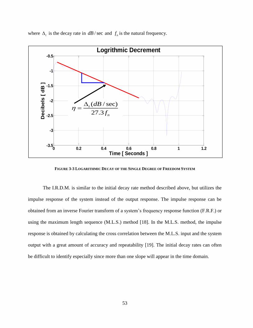
53

where t is the decay rate in / secdB and nf is the natural frequency.

FIGURE 3-3 LOGARITHMIC DECAY OF THE SINGLE DEGREE OF FREEDOM SYSTEM

The I.R.D.M. is similar to the initial decay rate method described above, but utilizes the

impulse response of the system instead of the output response. The impulse response can be

obtained from an inverse Fourier transform of a system‘s frequency response function (F.R.F.) or

using the maximum length sequence (M.L.S.) method [18]. In the M.L.S. method, the impulse

response is obtained by calculating the cross correlation between the M.L.S. input and the system

output with a great amount of accuracy and repeatability [19]. The initial decay rates can often

be difficult to identify especially since more than one slope will appear in the time domain.

0 0.2 0.4 0.6 0.8 1 1.2-3.5

-3

-2.5

-2

-1.5

-1

-0.5

Time [ Seconds ]

De

cib

els

[ d

B ]

Logrithmic Decrement

( / sec)

27.3

t

n

dB

f

54

3.2 SINGLE DEGREE OF FREEDOM SYSTEMS

3.2.1 LOSS FACTOR USING THE IMPULSE FUNCTION

The impulse function is a mathematical function which is zero for all time except at a

single instant of time. The impulse response function of a underdamped system is given by the

Equation (1.25) and re-stated here,

( )1( ) sin( )nt

d

d

h t e tm

where n is the natural frequency, d is the damped natural frequency, m is the mass and is

the viscous damping co-efficient. The response of a single degree of freedom system with a mass

of 0.5 Kg , damping rate of 0.5 /Ns m and a stiffness of 1000 /N m is calculated by the impulse

response function. The natural frequency of the system n which is given by /n k m is

calculated as 44.7214. The damping coefficient which is given by 2 n

c

m

is calculated to

be 0.0112. Since the structural damping loss factor of the system is given as 2 , the input

loss factor for the SDOF system is 0.224. The damped natural frequency d of the system given

by, 21d n is calculated to be 44.7186. Note that d n . A plot of the impulse response

function as a function of time is shown in Figure 3-4.

55

FIGURE 3-4 PLOT OF THE IMPULSE FUNCTION

The response of the single degree of freedom system is defined as the convolution of the

Impulse Response Function with the applied force. The response of the system to a unit impulse,

the impulse response function is then used in convolution with the applied force to get the

response. The convolution integral is given by Equation (1.26) and is re-stated here,

0 0

1( ) ( ) ( ) ( ) sin ( )n n

t t

t t

d

d


(2.15)

The Hilbert transform of this response has the real and imaginary components which can be seen

in Figure 3-5. Also plotted in Figure 3-5 is the absolute value of the Hilbert transform as a

function of time.

0 0.05 0.1 0.15 0.2 0.25 0.3 0.35 0.4 0.45 0.5-0.05

-0.04

-0.03

-0.02

-0.01

0

0.01

0.02

0.03

0.04

0.05

Time [ Seconds ]

H(t

)

Plot of Impulse function

56

FIGURE 3-5 REAL AND IMAGINARY OF HILBERT TRANSFORM OF THE IMPULSE FUNCTION (TOP) AND THE

ABSOLUTE VALUE OF THE HILBERT TRANSFORM (BOTTOM)

The logarithmic decrement of the Hilbert transform of the response denoted by

represents the response decay of the system. It is used to find the damping loss factor for the

damped or undamped systems in time domain. It is the natural logarithm of the amplitudes of

any two successive peaks. The logarithmic decrement in the mathematical terms is given by

01ln

n

x

n x

where 0x is the greater of the two amplitudes and nx is the amplitude of a peak n

periods away. The logarithmic decrement of the S.D.O.F. subjected to the unit impulse function

is shown in Figure 3-6.

0 0.05 0.1 0.15 0.2 0.25 0.3 0.35 0.4 0.45 0.5-0.05

0

0.05

Time [ Seconds ]

Hil

be

rt T

ran

sfo

rmReal and Imaginary Hilbert Transform of the Impulse Function

0 0.05 0.1 0.15 0.2 0.25 0.3 0.35 0.4 0.45 0.50

0.02

0.04

0.06

Time [ Seconds ]

Absolute Value of the Hilbert Transform

57

FIGURE 3-6 LOGARITHMIC DECREMENT OF THE HILBERT TRANSFORM

The slope of the logarithmic decrement curve is the loss factor of the system. It was

necessary for the user to determine the initial slope of decay signals manually. It becomes

apparent that this user input could be a possible source of error for the loss factor calculation. So

a study of the effect of skipping different lengths of time from the impulse before starting the

slope fit and considering the decay for different lengths of time is done. In this study the ‗skip‘

and ‗consider‘ time periods were varied systematically [20]. The loss factors of the system are

then plotted as a function of various skip and consider periods and are shown in Figure 3-7. The

estimated loss factor is 0.224, except when the initial decay of the response is used for slope

determination, in which case there is apparent under prediction of loss factor.

0 0.2 0.4 0.6 0.8 1 1.2-3.5

-3

-2.5

-2

-1.5

-1

-0.5

Time [ Seconds ]

De

cib

els

[ d

B ]

Logrithmic Decrement of the Hilbert Transform

Skip

this

early

decay

Consider this

58

FIGURE 3-7 LOSS FACTOR WITH VARIOUS ‘SKIP’ AND ‘CONSIDER’ PARAMETER VALUES FOR A SDOF SYSTEM

WITH A TRUE IMPULSE EXCITATION

3.2.2 LOSS FACTOR USING A SINUSOIDAL IMPULSE FORCE

The impulse function which causes a S.D.O.F. system to have the impulse response

discussed in the previous section, if viewed from a purely mathematical standpoint, is not strictly

a function, because no real function is equal to zero everywhere but a single point. So a real unit

impulse function cannot be observed in a real world situation. The I.R.D.M. is then validated for

a S.D.O.F. system by simulating the impulse with a half sine pulse of short duration. The single

degree of freedom system has a mass of 0.5 Kg , damping rate of 0.5 /Ns m and a stiffness of

1020

3040

5060

7080

90100

1020

3040

5060

7080

90100-0.3

-0.25

-0.2

-0.15

-0.1

-0.05

0

0.05

Consider

Loss Factor as a Function of 'Skip' and 'Consider' Parameters

Skip

Lo

ss F

act

or

59

1000 /N m . The natural frequency of the system n which is given by /n k m is calculated

as 44.7214. The damping coefficient which is given by 2 n

c

m

is calculated to be 0.0112.

Since the structural damping loss factor of the system is given as 2 , the input loss factor

for the SDOF system is 0.224.

The response of the single degree of freedom system is given by the convolution integral

which is given by Equation (1.26) and restated here

0 0

1( ) ( ) ( ) ( ) sin ( )n n

t t

t t

d

d


The half sine impulse and the calculated response are shown in Figure 3-8.

FIGURE 3-8 SIMULATED IMPULSE AND THE RESPONSE BY THE CONVOLUTION INTEGRAL

0 0.002 0.004 0.006 0.008 0.01 0.0120

0.5

1

1.5

2

Simulated Half Sine Impulse

0 0.01 0.02 0.03 0.04 0.05 0.06 0.07 0.08 0.09 0.10

0.5

1

1.5

2

Simulated Half Sine Impulse

0 0.05 0.1 0.15 0.2 0.25 0.3 0.35 0.4 0.45 0.5-4

-2

0

2

4x 10

-3

Time [ Seconds ]

Ma

gn

itu

de

Response due to Half Sine Impulse

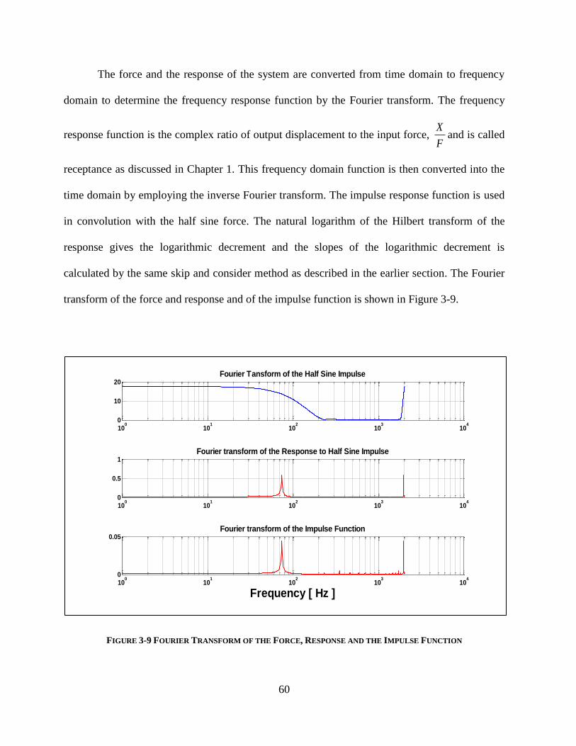
60

The force and the response of the system are converted from time domain to frequency

domain to determine the frequency response function by the Fourier transform. The frequency

response function is the complex ratio of output displacement to the input force, X

Fand is called

receptance as discussed in Chapter 1. This frequency domain function is then converted into the

time domain by employing the inverse Fourier transform. The impulse response function is used

in convolution with the half sine force. The natural logarithm of the Hilbert transform of the

response gives the logarithmic decrement and the slopes of the logarithmic decrement is

calculated by the same skip and consider method as described in the earlier section. The Fourier

transform of the force and response and of the impulse function is shown in Figure 3-9.

FIGURE 3-9 FOURIER TRANSFORM OF THE FORCE, RESPONSE AND THE IMPULSE FUNCTION

100

101

102

103

104

0

10

20Fourier Tansform of the Half Sine Impulse

100

101

102

103

104

0

0.5

1Fourier transform of the Response to Half Sine Impulse

100

101

102

103

104

0

0.05Fourier transform of the Impulse Function

Frequency [ Hz ]

61

FIGURE 3-10 IMPULSE RESPONSE FUNCTION AND THE HILBERT TRANSFORM

FIGURE 3-11 LOGARITHMIC DECREMENT OF THE HILBERT TRANSFORM OF THE RESPONSE OF A SDOF SYSTEM

WITH A SINUSOIDAL EXCITATION

0 0.02 0.04 0.06 0.08 0.1 0.12 0.14 0.16 0.18 0.2-4

-2

0

2

4x 10

-4 Impulse Response Function

0 0.02 0.04 0.06 0.08 0.1 0.12 0.14 0.16 0.18 0.2-5

0

5x 10

-4 Real and Imaginary parts of the Hilbert Transform

0 0.1 0.2 0.3 0.4 0.5 0.6 0.70

2

4x 10

-4

Time [ Seconds ]

Absolute value of the Hilbert Transform

0 0.1 0.2 0.3 0.4 0.5 0.6 0.7 0.8 0.9 1-16

-15

-14

-13

-12

-11

-10

-9

-8

Time [ Seconds ]

Mag

nitu

de [

dB ]

Logrithmic Decrement of the Hilbert Transform

62

FIGURE 3-12 LOSS FACTORS WITH VARIOUS ‘SKIP’ AND ‘CONSIDER’ PARAMETERS FOR A SDOF SYSTEM WITH

A SINUSOIDAL EXCITATION

The impulse response function and the real, imaginary, and absolute value of the Hilbert

transform are then plotted and are shown in Figure 3-10. Figure 3-11 shows the logarithmic

decrement, in decibels, of the response decay of the S.D.O.F. system which is excited with a half

sine impulse and the subsequent loss factors estimated are shown in Figure 3-12. The estimated

loss factor is 0.224 which is equal to the input loss factor, except when the initial decay is taken

into consideration.

From the analytical studies of estimation of loss factors by the I.R.D.M. applied to the

single degree of freedom systems excited with a half sine impulse it can be concluded that the

estimation of loss factors is quite accurate with a variation of less than 1% for the single degree

of freedom systems. In subsequent sections, the analytical and experimental validation of the

impulse response decay method for multiple degree of freedom systems is discussed.

1020

3040

5060

7080

90100

0

20

40

60

80

100

-0.04

-0.02

0

0.02

0.04

0.06

0.08

0.1

0.12

Consider

Loss Factor as a Function of 'Skip' and 'Consider' Parameters

Skip

Lo

ss

Fa

cto

r

63

3.3 PLATES – ANALYTICAL AND EXPERIMENTAL IRDM

3.3.1 ANALYTICAL ESTIMATION- NASTRAN MODEL

The thin plate (of in-plane dimensions, a.b) has an aspect ratio of 1.5 (a/b), a thickness

ratio of 385 (b/t) and a specific stiffness (E/ρ) of 72.59*10 . /N m Kg . The damping loss factor, η,

is assigned values from 0.001[0.1%] to 0.01[1%] and 0.1[10%]. The plate is considered to be

free of external supports and is loaded by a concentrated mechanical force.

Although an analytical model is undoubtedly available, a computational model has been

developed using MSC/NASTRAN Version 2008. There are a total of 14065 Nodes and 13824

elements are used to represent the whole model. QUAD4 elements (of dimensions, A.B) with a

quadrilateral element fineness of approximately 80 (b/B or a/A) have been used to create a

regular, rectangular mesh. As such, the spatial Nyquist frequency—at which modal half-

wavelengths approaches the element width (A or B)—is estimated at approximately 10 kHz. The

mechanical loads are applied in the center of one quadrant of the plate to a single node, modeling

physical loading via the bottom surface of a small force gage. Responses to excitation at the

single forcing point were computed at approximately the 17 points indicated in Figure 3-13,

below, wherein each square region represents 100 elements. 4 different excitation points are used

for the study and for each excitation point the responses are computed at the above mentioned 17

points. The four excitation points are shown as red dots in Figure 3-13. The input points are

named as Point 1, Point 2, Point 3 and Point 4 named clockwise from the top left and are shown

in Figure 3-13.

64

FIGURE 3-13 COMPUTATIONAL MODEL WITH REGULAR PATTERN OF EXCITATION AND RESPONSE POINTS

For the computational studies, the best frequency resolution for a frequency response

function (F.R.F.) attempted is 1 Hz over a 10 kHz frequency range. This F.R.F.s are inverted

using the inverse Fourier transform, resulting in the analogous impulse response functions

(I.R.F.s). Based on the frequency resolution, f = 1 Hz, and the number of ―lines‖ in the F.R.F.,

N = 10,000, the length of the IRF is 1/ f = 1 second. Since there were ―N‖ lines in the F.R.F.,

the number of response points in the IRF is 2N = 20,000, which corresponds to a temporal

Four Excitations Points

(also response points)

65

resolution of 1/20,000 = 50 microseconds. As such, the temporal resolution in the computational

studies allows resolution of responses up to 10 kHz, but only good responses up to about 4 kHz.

For experimental studies, the sampling frequency is 64.4 kHz, which provides a temporal

resolution of 15.52 microseconds. The expectation, then, is that vibration frequencies may be

resolved poorly to 32.2 kHz, but rather well to 13 kHz.

The damping loss factor, whether for a structural element or an entire structure, is known

to have frequency dependence. This frequency-dependence is partly due to frequency-dependent

material properties of the constituent materials and partly due to the distribution of material

strain as a function of frequency [16]. Assigning a single damping loss factor for a structure

requires specifying some sort of process to account for the spatially-variable response, mobility

or accelerance upon which the damping loss factor is based. Analytically, an integrated response

can be used, allowing the prediction of a frequency- and spatially-dependent loss factor to be

expressed. Experimentally, of course, only a finite number of points is available, which suggests

averaging the response from multiple points. Some researchers have shown that responses from a

small number of randomly-selected points seem to show convergence to a common value [23].

In this study convergence is studied with regard to the number of and location of response

measurements.

The impulse response decay method is based on the estimation of the decay rate in a

spring-mass-damper system. But, for a real structure, there are many modes of vibration excited

by an impulse (or any other type of excitation). A popular means of estimating damping loss

factor uses band-limited segments of the F.R.F., which, when inverted in the Fourier sense, yield

a decaying response with arbitrarily narrow frequency content. The assumption is that the decay

observed in these frequency bands tends to represent the frequency-dependent damping loss

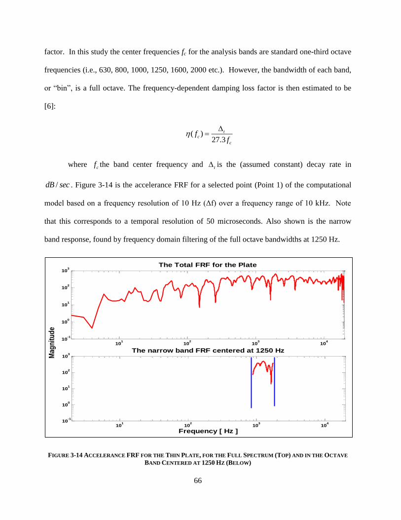
66

factor. In this study the center frequencies fc for the analysis bands are standard one-third octave

frequencies (i.e., 630, 800, 1000, 1250, 1600, 2000 etc.). However, the bandwidth of each band,

or ―bin‖, is a full octave. The frequency-dependent damping loss factor is then estimated to be

[6]:

( )27.3

tc

c

ff

where cf the band center frequency and t is the (assumed constant) decay rate in

/dB sec . Figure 3-14 is the accelerance FRF for a selected point (Point 1) of the computational

model based on a frequency resolution of 10 Hz (Δf) over a frequency range of 10 kHz. Note

that this corresponds to a temporal resolution of 50 microseconds. Also shown is the narrow

band response, found by frequency domain filtering of the full octave bandwidths at 1250 Hz.

FIGURE 3-14 ACCELERANCE FRF FOR THE THIN PLATE, FOR THE FULL SPECTRUM (TOP) AND IN THE OCTAVE

BAND CENTERED AT 1250 HZ (BELOW)

101

102

103

104

10-1

100

101

102

103

The Total FRF for the Plate

101

102

103

104

10-1

100

101

102

103

Frequency [ Hz ]

Mag

nit

ud

e

The narrow band FRF centered at 1250 Hz

67

The inverse fourier transform of the full octave, band-limited F.R.F. at each of the one-

third octave frequencies is first computed. The value of the loss factor is then estimated from

the slope of the envelope of the decay signatures. Figure 3-15 is a composite of average

acceleration free decay signatures for a set of 16 regularly-spaced response points. From these

average decay signatures, the frequency-dependent loss factors were estimated. The estimated

loss factors for the responses of the computational model with an input loss factor of 0.01 are

shown in Figure 3-16. The loss factors estimated for the four different excitation points are

plotted. It is evident that the I.R.D.M. is fairly accurate with an acceptable variation of 10% for

estimating this relatively moderate loss factors. The location of the excitation point has some

induced errors as one location point may excite greater number of modes than the other.

FIGURE 3-15 AVERAGED DECAY SIGNATURES FOR A RANGE OF FULL OCTAVE BANDS, WITH THE LINEAR

ESTIMATE OF SLOPE AND THE RESULTING LOSS FACTOR SHOWN FOR INPUT LF OF 0.01

0 0.2 0.4 0.6 0.8 1-8

-6

-4

-2

0Frequency = 20

0 0.2 0.4 0.6 0.8 1-20

-15

-10

-5

0Frequency = 40

0 0.2 0.4 0.6 0.8 1-30

-20

-10

0Frequency =80

0 0.2 0.4 0.6 0.8 1-40

-30

-20

-10

0Frequency = 160

0 0.2 0.4 0.6 0.8 1-60

-40

-20

0Frequency = 315

0 0.2 0.4 0.6 0.8 1-60

-40

-20

0Frequency =500

0 0.2 0.4 0.6 0.8 1-80

-60

-40

-20

0Frequency =800

0 0.2 0.4 0.6 0.8 1-80

-60

-40

-20

0Frequency =1250

0 0.2 0.4 0.6 0.8 1-80

-60

-40

-20

0Frequency =3000

Eta= 0.0107 Eta=0.0102 Eta=0.01

Eta=0.01Eta=0.01 Eta=0.01

Eta=0.01 Eta=0.01 Eta=0.01

68

FIGURE 3-16 ESTIMATED LOSS FACTOR FOR A INPUT LOSS FACTOR OF 0.01 [1 %]

For a very low input loss factor of 0.001[0.1%] the estimated loss factors by the I.R.D.M. is

shown in Figure 3-17. The loss factors for the four different excitation points are estimated. It

can be seen that in the low frequency range (< 200 Hz) the estimated loss factors are not accurate

However in the 200 Hz – 8000 Hz frequency range the estimated loss factors are accurate within

2% of the input loss factor. As mentioned earlier some error is introduced as a result of the

location of the excitation point. Within few limitations in the low frequency zone for systems

that are lightly damped the impulse response decay method yields consistent results (98%

accurate) and it is shown to be better than the power input method (P.I.M.). Also it is suggested

that averaging more input-output pairs is an added advantage for increasing the accuracy of

measured loss factors when using the I.R.D.M. for lightly damped structures.

0.001

0.01

10 100 1000 10000

Lo

ss F

act

or

[ N

o U

nit

s ]

Frequency [ Hz ]

Estimated Loss Factor for Input Loss Factor of 0.01

Excitation Point 1

Excitation Point 2

Excitation Point 3

Excitation Point 4

69

FIGURE 3-17 ESTIMATED LOSS FACTOR FOR A INPUT LOSS FACTOR OF 0.001 [0.1 %]

Figure 3-18 shows the estimated loss factors of the panel for a very high input damping level of

10 %. The loss factors from the four different excitation points are plotted showing some

variation (approximately 10% mean variation) based on the location of the excitation point. The

loss factors are under estimated at frequencies above 1000 Hz. Some of the response points are

in the direct field of vibration, where the response is significantly higher than the other response

points which results in under prediction of loss factors.

0.0001

0.001

0.01

0.1

1

10 100 1000 10000

Lo

ss F

act

or

[ N

o U

nit

s ]

Frequency [ Hz ]


Excitation Point 1

Excitation Point 2

Excitation Point 3

Excitation Point 4

70

FIGURE 3-18 ESTIMATED LOSS FACTOR FOR A INPUT LOSS FACTOR OF 0.1 [10 %]

3.3.2 EXPERIMENTAL RESULTS

3.3.2.1 ALUMINUM PLATE WITH CONSTRAINED LAYER DAMPING

The analytical estimation of the loss factors uses the accelerance frequency response

functions; however the mobility functions can also be used to estimate the loss factors. Using a

scanning laser vibrometer the mobility functions for the aluminum plate with constrained layer

damping treatment were measured. The mobility response functions are measured at 225

response points and the plate is excited at 4 different locations across the plate. In the

computations 8 response points, (two response points randomly chosen from each quarter) are

used, so well averaged loss factor measurements are achieved. Figure 3-19 shows the estimated

0.01

0.1

1

10 100 1000 10000

Lo

ss F

act

or

[ N

o U

nit

s ]

Frequency [ Hz ]


Excitation Point 1

Excitation Point 2

Excitation Point 3

Excitation Point 4

71

loss factors for the plate. As discussed in previous sections, since the plate is rather highly

damped (approx. 0.1), the estimated loss factors should be fairly accurate, well within 10% mean

variation, except at lower frequencies where the variation is greater than 10%. Clearly there is an

apparent under-prediction above 2000 Hz. The variation introduced by the location of the

excitation point is also seen.

FIGURE 3-19 LOSS FACTORS OF DAMPED ALUMINUM PLATE BY THE IMPULSE RESPONSE DECAY METHOD

3.3.2.2 UNDAMPED STEEL PLATE

The mobility data for the undamped steel plate is collected at 187 response points for

each of the 4 excitation points. Figure 3-20 shows the loss factors estimated for four different

excitation points and the averaged loss factors. The loss factors estimated by the power input

method show that the plate has an inherent damping of about 1%. The experimental impulse

response decay method provides fairly consistent estimates for different excitation points, well

0.001

0.01

0.1

1

10 100 1000 10000

Lo

ss F

act

or

[ N

o U

nit

s ]

Frequency [ Hz ]

Estimated Loss Factors for the Aluminum Plate

Excitation Point 1

Excitation Point 2

Excitation Point 3

Excitation Point 4

Average

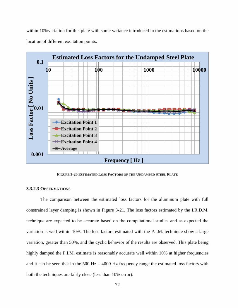
72

within 10%variation for this plate with some variance introduced in the estimations based on the

location of different excitation points.

FIGURE 3-20 ESTIMATED LOSS FACTORS OF THE UNDAMPED STEEL PLATE

3.3.2.3 OBSERVATIONS

The comparison between the estimated loss factors for the aluminum plate with full

constrained layer damping is shown in Figure 3-21. The loss factors estimated by the I.R.D.M.

technique are expected to be accurate based on the computational studies and as expected the

variation is well within 10%. The loss factors estimated with the P.I.M. technique show a large

variation, greater than 50%, and the cyclic behavior of the results are observed. This plate being

highly damped the P.I.M. estimate is reasonably accurate well within 10% at higher frequencies

and it can be seen that in the 500 Hz – 4000 Hz frequency range the estimated loss factors with

both the techniques are fairly close (less than 10% error).

0.001

0.01

0.1

10 100 1000 10000

Lo

ss F

act

or

[ N

o U

nit

s ]

Frequency [ Hz ]

Estimated Loss Factors for the Undamped Steel Plate

Excitation Point 1

Excitation Point 2

Excitation Point 3

Excitation Point 4

Average

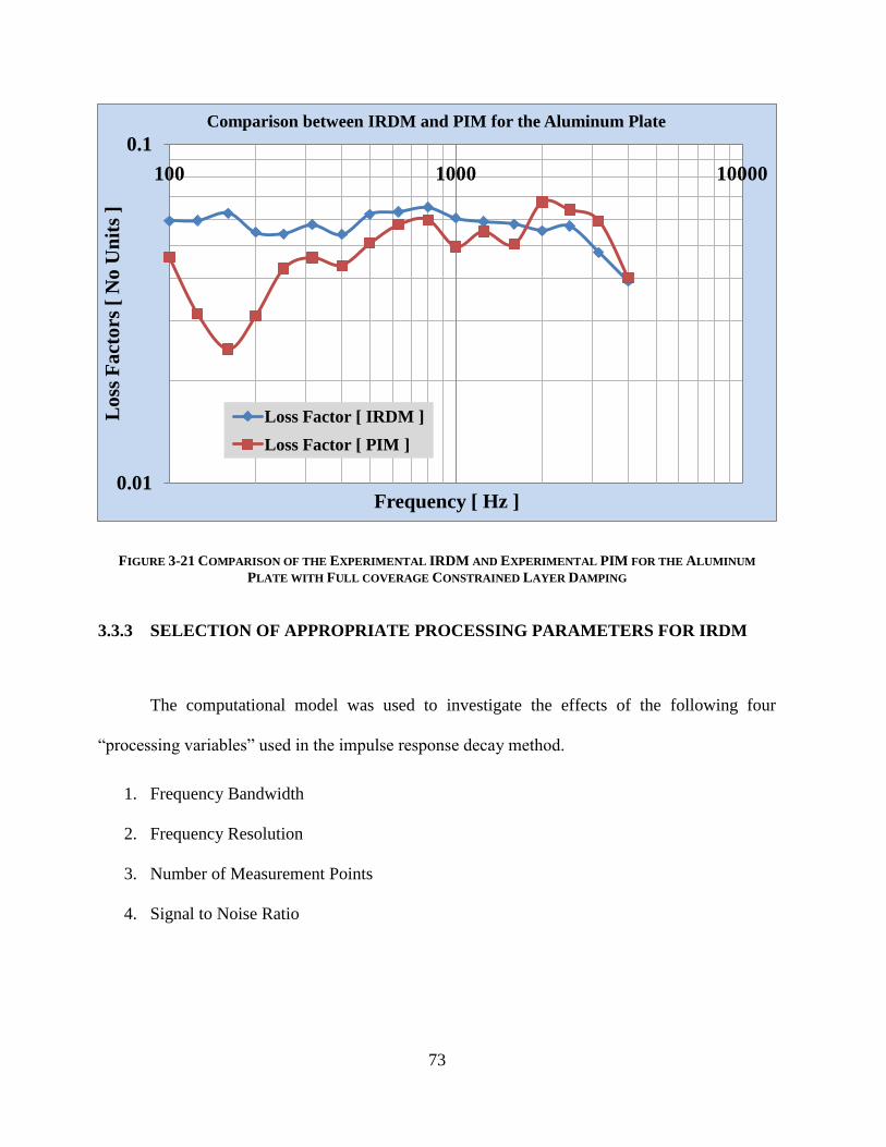
73

FIGURE 3-21 COMPARISON OF THE EXPERIMENTAL IRDM AND EXPERIMENTAL PIM FOR THE ALUMINUM

PLATE WITH FULL COVERAGE CONSTRAINED LAYER DAMPING

3.3.3 SELECTION OF APPROPRIATE PROCESSING PARAMETERS FOR IRDM

The computational model was used to investigate the effects of the following four

―processing variables‖ used in the impulse response decay method.

1. Frequency Bandwidth

2. Frequency Resolution

3. Number of Measurement Points

4. Signal to Noise Ratio

0.01

0.1

100 1000 10000

Lo

ss F

act

ors

[ N

o U

nit

s ]

Frequency [ Hz ]

Comparison between IRDM and PIM for the Aluminum Plate

Loss Factor [ IRDM ]

Loss Factor [ PIM ]

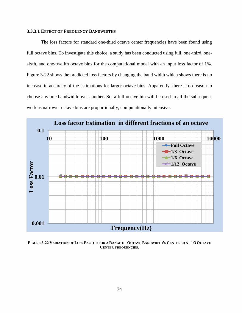
74

3.3.3.1 EFFECT OF FREQUENCY BANDWIDTHS

The loss factors for standard one-third octave center frequencies have been found using

full octave bins. To investigate this choice, a study has been conducted using full, one-third, one-

sixth, and one-twelfth octave bins for the computational model with an input loss factor of 1%.

Figure 3-22 shows the predicted loss factors by changing the band width which shows there is no

increase in accuracy of the estimations for larger octave bins. Apparently, there is no reason to

choose any one bandwidth over another. So, a full octave bin will be used in all the subsequent

work as narrower octave bins are proportionally, computationally intensive.

FIGURE 3-22 VARIATION OF LOSS FACTOR FOR A RANGE OF OCTAVE BANDWIDTH’S CENTERED AT 1/3 OCTAVE

CENTER FREQUENCIES.

0.001

0.01

0.1

10 100 1000 10000

Lo

ss F

act

or

Frequency(Hz)

Loss factor Estimation in different fractions of an octave

Full Octave

1/3 Octave

1/6 Octave

1/12 Octave

75

3.3.3.2 EFFECT OF FREQUENCY RESOLUTION

The effect of frequency resolution has been studied for the loss factor levels of 0.001,

0.01 and 0.1. This study was based on the frequency response functions from the computational

model, for which the frequency resolution is 1 Hz. Lower levels of frequency resolution are

created through simple decimation of the accelerance frequency response function before

applying the impulse response decay method.

The estimated loss factors for the three levels of loss factors in the computational model

for five different frequency resolutions is shown in Figure 3-23, Figure 3-24 and Figure 3-25.

Figure 3-23, for the case of a 0.1% damping, shows that only the 1 Hz resolution allows

successful estimation; say within 1% above 300 Hz.

FIGURE 3-23 EFFECT OF FREQUENCY RESOLUTION FOR A INPUT LOSS FACTOR OF 0.001 [0.1%]

0.0001

0.001

0.01

0.1

1

10 100 1000 10000

Lo

ss F

act

or

[ N

o U

nit

s ]

Frequency [ Hz ]

Effect of Frequency Resolution, Input LF of 0.001

16 Hz Resolution

8 Hz Resolution

4 Hz Resolution

2 Hz Resolution

1 Hz resolution

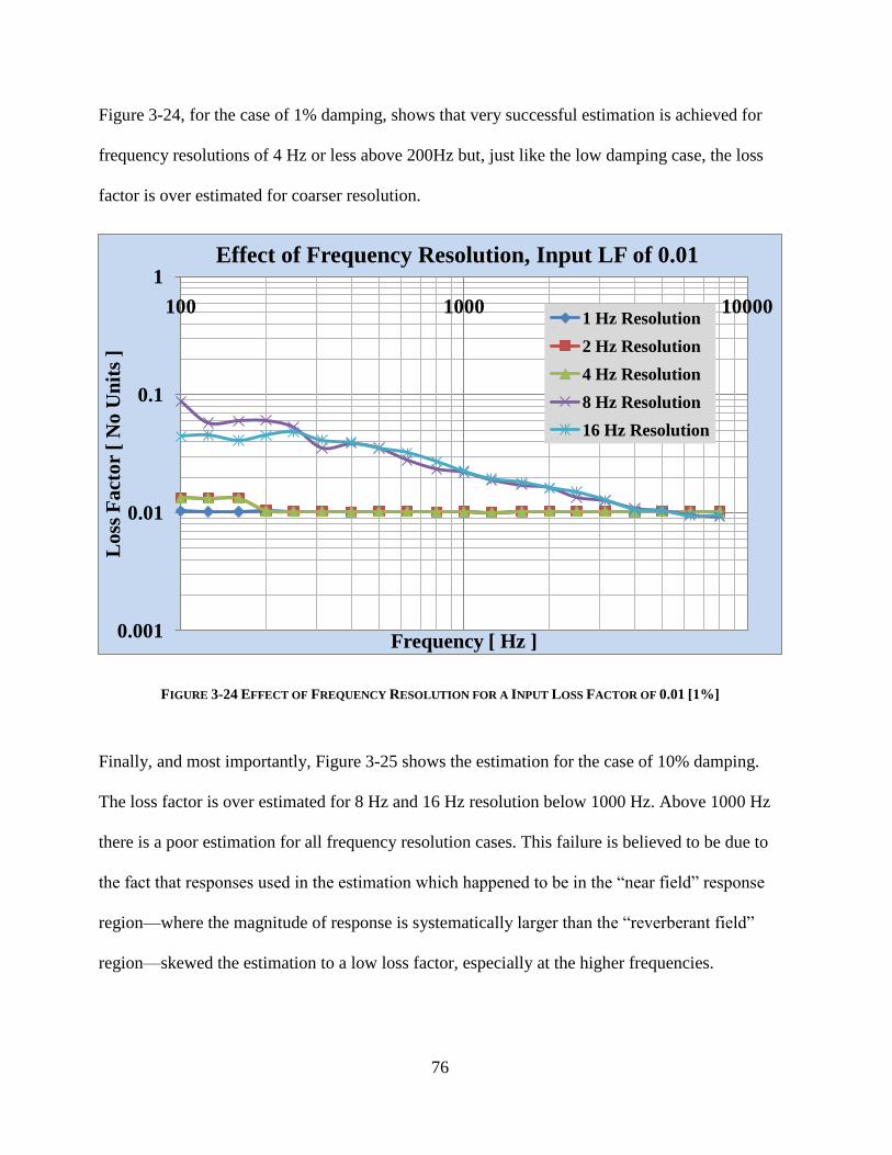
76

Figure 3-24, for the case of 1% damping, shows that very successful estimation is achieved for

frequency resolutions of 4 Hz or less above 200Hz but, just like the low damping case, the loss

factor is over estimated for coarser resolution.

FIGURE 3-24 EFFECT OF FREQUENCY RESOLUTION FOR A INPUT LOSS FACTOR OF 0.01 [1%]

Finally, and most importantly, Figure 3-25 shows the estimation for the case of 10% damping.

The loss factor is over estimated for 8 Hz and 16 Hz resolution below 1000 Hz. Above 1000 Hz

there is a poor estimation for all frequency resolution cases. This failure is believed to be due to

the fact that responses used in the estimation which happened to be in the ―near field‖ response

region—where the magnitude of response is systematically larger than the ―reverberant field‖

region—skewed the estimation to a low loss factor, especially at the higher frequencies.

0.001

0.01

0.1

1

100 1000 10000

Lo

ss F

act

or

[ N

o U

nit

s ]

Frequency [ Hz ]


1 Hz Resolution

2 Hz Resolution

4 Hz Resolution

8 Hz Resolution

16 Hz Resolution

77

FIGURE 3-25 EFFECT OF FREQUENCY RESOLUTION FOR A INPUT LOSS FACTOR OF 0.1 [10%]

3.3.3.3 EFFECT OF VARIABLE NUMBER OF MEASUREMENT POINTS

One of the goals of the study reported here is to determine the variance of estimated loss

factors as a function of the number of response points averaged. Although more information is

typically better, knowledge of the number of response points needed to get an acceptable

estimation of the loss factor results would be useful. Figure 3-26 shows the damping loss factor

estimates resulting from averages of 20, 15, 10 and 5 sets of 4, 8, 12 and 16 responses,

respectively, due to excitation at a single excitation point for the lightly damped computational

model. For this study, the sets of 4, 8, 12 and 16response points were selected at random from

the set of 4 excitations and 16 responses for each excitation that are considered. Note that in this

case, data from 8 response points are needed to get acceptable estimates of damping loss factor

(within 1% of the known value of 0.01) in the 40-8000 Hz range.

0.01

0.1

1

10 100 1000 10000

Lo

ss F

act

or

[ N

o U

nit

s ]

Frequency [ Hz ]


1 Hz Resolution 2 Hz Resolution

4 Hz Resolution 8 Hz Resolution

16 Hz Resolution

78

FIGURE 3-26 ESTIMATION OF LOSS FACTORS BY VARYING THE NUMBER OF MEASUREMENT POINTS FOR A INPUT

LOSS FACTOR OF 0.001 [0.1%]

Figure 3-27 shows the estimated loss factors for the moderately damped case and there is

very little improvement above 100 Hz is apparent when more points are considered (less than

10%). From Figure 3-28, shown below, which is a highly damped case it can be seen that there is

very little improvement (less than 1% variation) in estimation of loss factor when using more

than 4 response points.

0.0001

0.001

10 100 1000 10000

Lo

ss F

act

or

[ N

o U

nit

s ]

Frequency [ Hz ]

Effect of Measurement Points, Input LF = 0.001

4 Output Points

8 Output Points

12 Output Points

16 Output Points

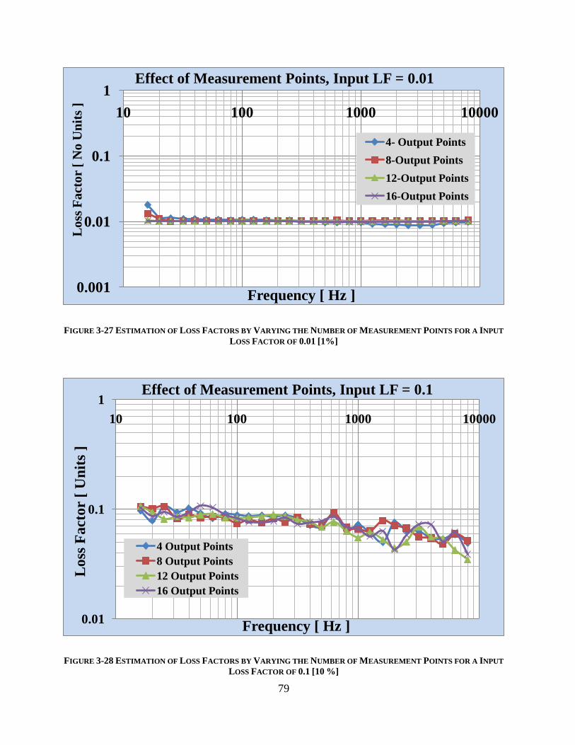
79


LOSS FACTOR OF 0.01 [1%]


LOSS FACTOR OF 0.1 [10 %]

0.001

0.01

0.1

1

10 100 1000 10000

Lo

ss F

act

or

[ N

o U

nit

s ]

Frequency [ Hz ]


4- Output Points

8-Output Points

12-Output Points

16-Output Points

0.01

0.1

1

10 100 1000 10000

Lo

ss F

act

or

[ U

nit

s ]

Frequency [ Hz ]


4 Output Points

8 Output Points

12 Output Points

16 Output Points

80

3.3.3.4 EFFECT OF NOISE

Experimental measurements will always be affected by surrounding noise and the

atmosphere, so the effect of noise on the estimated loss factors for the three damping levels is

investigated. The signal to noise ratio is given a function of the coherence and is given by

Equation (1.33) and is restated here,

2

2

( )

1 ( )

xy

xy

Sn

Noise was added to the accelerance frequency response measurements before employing the

I.R.D.M. and the loss factors are estimated. Three different signal to noise levels (100, 50, and

10) are investigated to account for various experimental conditions. Eight measurement points,

randomly selected from the four quarters (two from each quarter) are used to compute the loss

factors. The estimated loss factors for an input loss factor of 0.1 are shown in Figure 3-29. The

effect of noise is felt in the low frequency level (below 100 Hz) where there is significant over

estimation of loss factors (50% variation) but above 100 Hz there is no apparent affect except at

few discrete frequency bands around 1000 Hz (less than 10% variation). Reasons for this

behavior have to be investigated and are suggested for further study. Figure 3-30 and Figure 3-31

show the estimated loss factors for input loss factor of 0.01 and 0.001. For the plate with

moderate damping there was no effect of noise for frequencies above 500 Hz and there is less

than 10% error for the frequencies below 500 Hz which is admissible. For lightly damped model

there is very little effect of noise above 500 Hz (well within 1% variation), and at low

frequencies the estimation is inaccurate (greater than 50% variation).

81

FIGURE 3-29 LOSS FACTOR ESTIMATION FOR VARIOUS NOISE LEVELS, INPUT LOSS FACTOR OF 10 %

FIGURE 3-30 LOSS FACTOR ESTIMATION FOR VARIOUS NOISE LEVELS, INPUT LOSS FACTOR OF 1 %

0.01

0.1

1

10 100 1000 10000

Lo

ss F

act

or

[ N

o U

nit

s ]

Frequency [ Hz ]

Effect of Noise, Input LF = 0.1

No Noise

SNR of 100

SNR of 50

SNR of 10

0.001

0.01

0.1

10 100 1000 10000

Lo

ss F

act

or

[ N

o U

nit

s ]

Frequency [ Hz ]

Effect of Noise, Input LF = 0.01

No NoiseSNR of 100SNR of 50SNR of 10

82

FIGURE 3-31 LOSS FACTOR ESTIMATION FOR VARIOUS NOISE LEVELS, INPUT LOSS FACTOR OF 0.1 %

0.0001

0.001

0.01

10 100 1000 10000

Lo

ss F

act

or

[ N

o U

nit

s ]

Frequency [ Hz ]

Effect of Noise , Input LF = 0.001

No Noise

SNR of 100

SNR of 50

SNR of 10

83

4 STATISTICAL ENERGY ANALYSIS

4.1 MODAL DENSITY [AND MODES IN BAND]

Following the theory from Lyon and DeJong [9] , the modal density is based on

measurements or computation of the average conductance in a plate based on power input at a

point, sy in a frequency band centered on c :

1

,

( )(4 )

2c s

cw y c

nG M f

M

Here, M is the mass of the structure, ( )cn is the Modal Density of the structure in the

frequency band c , and c is the bandwidth of the frequency band centered on c

In the interval c the number of modes that can contribute to the average, the ―modes in band‖

is given by ( ) ( )c c cN n


Based on the techniques given in above section, the modal densities of the plates and

modes per band were calculated. For the experimental study, the plate is hung by bungee cords,

thereby enforcing essentially free-free boundary conditions [8]. For these experiments, excitation

was applied with an electrodynamic shaker at one of four essentially randomly-selected

84

locations. The responses at several hundred points were recorded using a Polytec laser

vibrometer, leading to experimental estimates of modal density and modes in band. Analytically

and computationally, the modal densities were calculated using S.E.A. and the finite element

method, within VA One. The modal density of the undamped steel plate measured analytically,

calculated by the finite element method and the experimentally calculated modal density are

plotted in Figure 4-1.

The sinusoidal behavior of the experimental results is expected as the modal density

depends on the experimentally calculated loss factors from the power input method. In the

frequency range of interest of this current study, i.e., 500 Hz to 2500 Hz the experimentally

calculated modal density, the modal densities calculated by the finite element method and the

modal densities calculated analytically with Auto-SEA are in some agreement (30% mean

variation). The cyclic behavior is also present in the F.E.A. results which show that the modal

densities calculated from the experimentally estimated energies will not be necessarily a straight

line as are obtained from the modal densities obtained by solving the wave equation.

85

FIGURE 4-1 MODAL DENSITY IN THE UNDAMPED STEEL PLATE

The mode count is a very important parameter in S.E.A. because it represents the number

of resonant modes available to receive and store energy in a subsystem. The theoretical mode

count for distributed systems is based on combining geometric information about the allowed

mode shapes of the system with the dispersion relation for free waves in the system. Figure 4-2

shows the modes in band for the same undamped steel plate and as it can be observed the modes

in band have some agreement (30% mean variation) in the 500 Hz – 2500 Hz frequency range

but the modes in band are not really accurate in the low frequency i.e., below 500 Hz where the

number of modes is less than one – but S.E.A. is based on the assumption that the number of

modes in band approach infinity. The modes in band are directly proportional to the modal

density according to Lyon and Dejong and are related by the frequency bandwidth. The current

analysis was done at one-third octave frequencies with a full octave band width.

0.00001

0.0001

0.001

0.01

100 1000 10000

Mo

da

l D

ensi

ty

Frequency [ Hz ]

Modal Density in the Undamped Steel Plate

Experimental SEA

Analytical SEA

Finite Element Method

86

FIGURE 4-2 MODES PER BAND OF THE UNDAMPED STEEL PLATE

4.1.2 STEEL PLATE WITH PARTIAL CONSTRAINED LAYER DAMPING

The modal density of the steel plate with partial constrained layer damping treatment,

which has a damping level of approximately 2%, is shown in Figure 4-3. Since this plate has

more damping than the other steel plate [which has a 1% damping] the estimated modal density

and the modes in band are better compared to the undamped case, but are not in total agreement

with the analytical and F.E. results and have the same 30% variation. The estimated modes in

band are shown in Figure 4-4. The results are as expected for lightly damped plates, that is, fairly

well.

0.001

0.01

0.1

1

10

100

100 1000 10000

Mo

des

in

Ba

nd

Frequency [ Hz ]

Modes in Band for the Undamped Steel Plate

Experimental SEA

Analytical SEA


87

FIGURE 4-3 MODAL DENSITY IN THE PARTIAL DAMPED STEEL PLATE

FIGURE 4-4 MODES IN BAND FOR THE PARTIAL DAMPED STEEL PLATE

0.001

0.01

100 1000 10000

Mo

da

l D

ensi

ty

Frequency [ Hz ]

Modal Density in the Partial Damped Plate

Experimental SEA

Analytical SEA


0.1

1

10

100

100 1000 10000

Mod

es i

n B

an

d

Frequency [ Hz ]

Modes in Band for the Partial Damped Steel Plate

Experimental SEA

Analytical SEA


88

4.1.3 UNDAMPED ALUMINUM PLATE

The estimated modal densities and the modes in band for the undamped aluminum plates

shown in Figure 1-16 are shown in Figure 4-5 and Figure 4-6 respectively. These plates have no

damping and the material damping is estimated to be about 0.5 %. As expected, as was the case

with the undamped steel plate the estimated results are inaccurate in lower frequencies but are

shown to have some agreement (30% variation) with the analytical and F.E. results.

FIGURE 4-5 MODAL DENSITY IN UNDAMPED ALUMINUM PLATE

1.00E-05

1.00E-04

1.00E-03

1.00E-02

1.00E-01

1.00E+00

100 1000 10000

Mo

da

l D

ensi

ty

Frequency [ Hz ]

Modal Density for the Undamped Aluminum Plate

Experimental SEA

Analytical SEA


89

FIGURE 4-6 MODES IN BAND IN THE UNDAMPED ALUMINUM PLATE

4.2 LOSS FACTOR ESTIMATION

For a single plate, the energy input to the plate in a band c centered at c must, eventually be

dissipated by damping. i.e., ( , ) ( , )in diss

c cE E .Using the theory of the power input

method, the loss factor of the plate in the band c centered at c can be evaluated as

( )( )

2 ( )

in

cc k

c c

E

Here εk is the time-integrated kinetic energy of the system. For simplicity t is dropped.

Using Parseval‘s theorem, the input energy can be calculated as [22]

0 0

1 1( ) ( ) Re{ ( ) *( )} Im{ ( ) *( ) / }inE f t v t dt F V d F A d

0.001

0.01

0.1

1

10

100

100 1000 10000

Mo

des

Per

Ba

nd

Frequency [ Hz ]

Modes in Band for the Undamped Aluminum Plate

Experiment SEAAnalytical SEAFinite Element Method

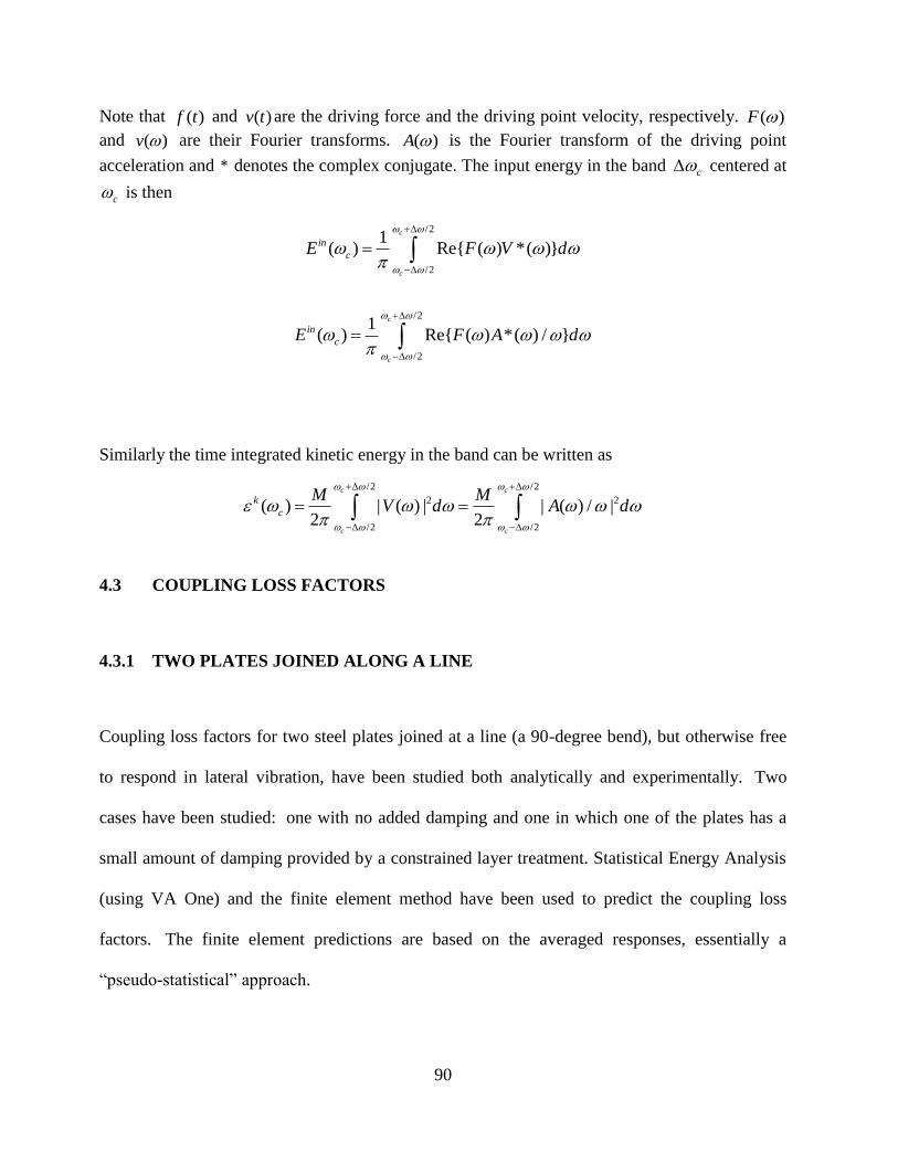
90

Note that ( )f t and ( )v t are the driving force and the driving point velocity, respectively. ( )F

and ( )v are their Fourier transforms. ( )A is the Fourier transform of the driving point

acceleration and * denotes the complex conjugate. The input energy in the band c centered at

c is then

/2

/2

1( ) Re{ ( ) *( )}

c

c

in

cE F V d

/2

/2

1( ) Re{ ( ) *( ) / }

c

c

in

cE F A d

Similarly the time integrated kinetic energy in the band can be written as

/2 /2

2 2

/2 /2

( ) | ( ) | | ( ) / |2 2

c c

c c

k

c

M MV d A d

4.3 COUPLING LOSS FACTORS

4.3.1 TWO PLATES JOINED ALONG A LINE

Coupling loss factors for two steel plates joined at a line (a 90-degree bend), but otherwise free

to respond in lateral vibration, have been studied both analytically and experimentally. Two

cases have been studied: one with no added damping and one in which one of the plates has a

small amount of damping provided by a constrained layer treatment. Statistical Energy Analysis

(using VA One) and the finite element method have been used to predict the coupling loss

factors. The finite element predictions are based on the averaged responses, essentially a

―pseudo-statistical‖ approach.

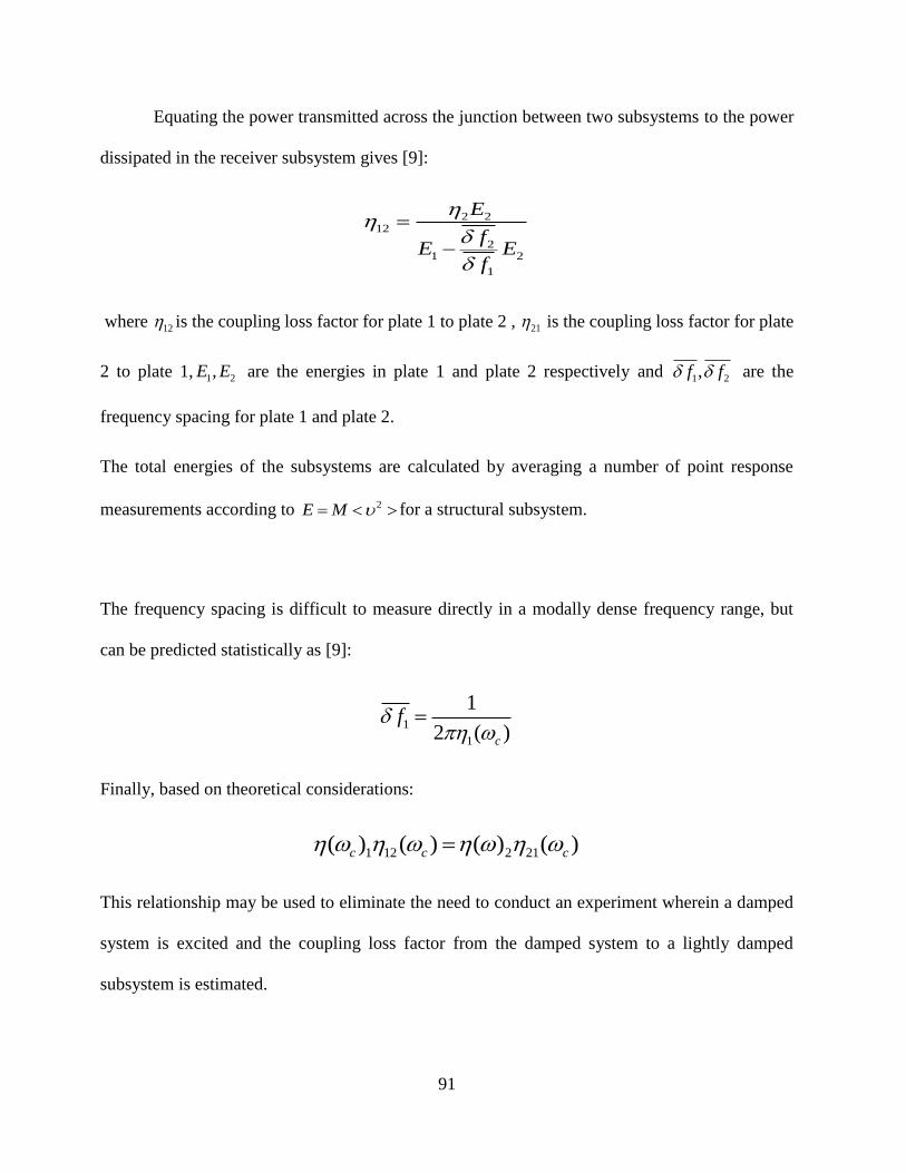
91

Equating the power transmitted across the junction between two subsystems to the power

dissipated in the receiver subsystem gives [9]:

where 12 is the coupling loss factor for plate 1 to plate 2 , is the coupling loss factor for plate

2 to plate 1, are the energies in plate 1 and plate 2 respectively and are the

frequency spacing for plate 1 and plate 2.

The total energies of the subsystems are calculated by averaging a number of point response

measurements according to for a structural subsystem.

The frequency spacing is difficult to measure directly in a modally dense frequency range, but

can be predicted statistically as [9]:

Finally, based on theoretical considerations:

This relationship may be used to eliminate the need to conduct an experiment wherein a damped

system is excited and the coupling loss factor from the damped system to a lightly damped

subsystem is estimated.

2 212

21 2

1

E

fE E

f

21

1 2,E E1 2,f f

2E M

1

1

1

2 ( )c

f

1 12 2 21( ) ( ) ( ) ( )c c c

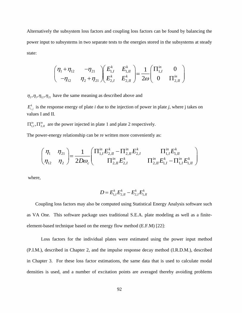
92

Alternatively the subsystem loss factors and coupling loss factors can be found by balancing the

power input to subsystems in two separate tests to the energies stored in the subsystems at steady

state:

have the same meaning as described above and

is the response energy of plate i due to the injection of power in plate j, where j takes on

values I and II.

are the power injected in plate 1 and plate 2 respectively.

The power-energy relationship can be re written more conveniently as:

where,

Coupling loss factors may also be computed using Statistical Energy Analysis software such

as VA One. This software package uses traditional S.E.A. plate modeling as well as a finite-

element-based technique based on the energy flow method (E.F.M) [22]:

Loss factors for the individual plates were estimated using the power input method

(P.I.M.), described in Chapter 2, and the impulse response decay method (I.R.D.M.), described

in Chapter 3. For these loss factor estimations, the same data that is used to calculate modal

densities is used, and a number of excitation points are averaged thereby avoiding problems

1 12 21 1, 1, 1,

12 2 21 2, 2, 2,

01

02

k k in

I II I

k k in

I II II

E E

E E

2 1 12 21, , ,

,

k

i jE

1, 2,,in in

I II

1 21 1, 2, 2, 2, 1, 1,

12 2 2, 2, 2, 1, 1, 1,

1

2

in k in k in k

I II II I I II

in k in k in k

II I II I I IIc

E E E

E E ED

1, 2, 2, 1,

k k k k

I II I IID E E E E

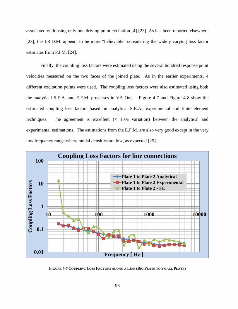
93

associated with using only one driving point excitation [4] [23]. As has been reported elsewhere

[23], the I.R.D.M. appears to be more ―believable‖ considering the widely-varying loss factor

estimates from P.I.M. [24].

Finally, the coupling loss factors were estimated using the several hundred response point

velocities measured on the two faces of the joined plate. As in the earlier experiments, 4

different excitation points were used. The coupling loss factors were also estimated using both

the analytical S.E.A. and E.F.M. processes in VA One. Figure 4-7 and Figure 4-8 show the

estimated coupling loss factors based on analytical S.E.A., experimental and finite element

techniques. The agreement is excellent (< 10% variation) between the analytical and

experimental estimations. The estimations from the E.F.M. are also very good except in the very

low frequency range where modal densities are low, as expected [25].

FIGURE 4-7 COUPLING LOSS FACTORS ALONG A LINE (BIG PLATE TO SMALL PLATE)

0.01

0.1

1

10

100

10 100 1000 10000

Co

up

lin

g L

oss

Fa

cto

rs

Frequency [ Hz ]

Coupling Loss Factors for line connections

Plate 1 to Plate 2 Analytical

Plate 1 to Plate 2 Experimental

Plate 1 to Plate 2 - FE

94

FIGURE 4-8 COUPLING LOSS FACTORS ALONG A LINE (SMALL PLATE TO BIG PLATE)

4.3.2 TWO PLATES JOINED AT A POINT

Coupling loss factors for two lightly damped plates joined at a point, but otherwise free to

respond in lateral vibration, have been studied both analytically and experimentally. This study

forms the basis for on-going estimations of the transient coupling loss factors of the same

system.

Statistical Energy Analysis (using VA One) and the finite element method (using VA

One‘s Energy Flow Method) have been used to predict the coupling loss factors. The finite

element predictions are based on the averaged responses, essentially a ―pseudo-statistical‖

approach.

0.001

0.01

0.1

1

100 1000 10000

Co

up

lin

g L

oss

Fa

cto

rs

Frequency [ Hz ]

Coupling Loss Factors for line connections

Plate 2 to Plate 1 Analytical

Plate 2 to Plate 1 Experimental

Plate 2 to Plate 1 - FE

95

Experimentally, using the technique used by Lai and Soom, a force transducer has been used to

measure the force between the plates as it is used to attach them. Simultaneously, the kinetic

energies in the two plates are measured by 4 accelerometers attached to each plate during both

transient and persistent excitation of the plates, one at a time. The coupling loss factors are

estimated by balancing the transmitted energies with the kinetic energies in the two plates. The

coupling loss factors can also be assessed by a more ―traditional‖ experimental approach, namely

balancing the power input to a plate with the energies of the plates. This approach will be

presented at the conference. The coupling loss factors are also estimated using two techniques

available in VA One, namely the traditional S.E.A. and the energy flow method. The estimations

from the three approaches reported here compare as well as may be expected for these lightly

damped plates.

Consider now the power input method applied to the calculation of coupling loss factors.

If we consider two tests, one where an external force is applied to plate 1, and another with the

force applied to plate 2, the energy transferred between the coupled plates can be represented by

the individual plate loss factors and the coupling loss factors [26]

1 12 21 1, 1, 1,

12 2 21 2, 2, 2,

01

02

k k in

I II I

k k in

I II II

E E

E E

1 2, are the individual loss factors for the plates 1 and 2 respectively.

12 21, are the coupling loss factors for plate 1 to plate 2 and plate 2 to plate 1, respectively.

,

k

i jE is the kinetic energy of plate i due to the injection of power in plate j, where in this case j

takes on the values I and II.

96

1, 2,,in in

I II are the power injected in plate 1 and plate 2 respectively.

The above Equation can be re written as follows

1 21 1, 2, 2, 2, 1, 1,

12 2 2, 2, 2, 1, 1, 1,

1

2

in k in k in k

I II II I I II

in k in k in k

II I II I I IIc

E E E

E E ED

Where, 1, 2, 2, 1,

k k k k

I II I IID E E E E

As an alternative, Lai and Soom [21][25] have developed expressions for the time-varying

coupling loss factors, in terms of the time-integrated kinetic energies, εk, and the measured (or

computed) energy transferred between plates.

211, 1, 21,

122, 2, 21,

( , )( , ) ( , ) ( , )2

( , )( , ) ( , ) ( , )

k k tr

cI c II c I c

c k k tr

cI c II c II c

tt t E t

tt t E t

Here I and II represent the plate on which the excitation is applied. The subscripts 12 and 21

indicate energy transferred from plate 1 to 2 and 2 to 1, respectively. Note that this formulation

requires a force transducer between the plates.

Using the power input method (P.I.M.), described in Chapter 2, and the impulse response

decay method (I.R.D.M.), loss factors for the individual plates were estimated. For these

experiments, both hammer and electrodynamic shaker excitation were used (separately). All

responses were captured with 8 accelerometers distributed about the plates, 6 at the same

locations as Lai and Soom [21] [25] and one extra location per plate. Two sets of hammer

excitation were used, one with a hard (metal) tip and the other with a softer (plastic) tip.

Hammer excitation results are for 50 hits with each tip type, with roughly equal numbers of hits

97

applied in the near vicinity of the accelerometers. Therefore, these estimations are based only on

driving point measurements.

The loss factors estimated for plates 1 and 2 were used in the analytical S.E.A. and

E.F.M. estimations of coupling loss factor. For the experimental study, since the transmitted

energy was measured, the individual plate loss factors were not needed. Excitation was applied

to plate 1 half the time and to plate 2 otherwise. Figure 4-9 and Figure 4-10 show the estimated

coupling loss factors for all 4 cases of excitation: hammer and shaker experiments, analytical

S.E.A. and the finite element method. The agreement is as good as can be expected: wide

variation of 10% at higher frequencies and more than 100% in lower frequencies) for lightly-

damped plate [26].

FIGURE 4-9 COUPLING LOSS FACTORS ALONG A POINT (BOTTOM PLATE TO TOP PLATE)

0.0001

0.001

0.01

0.1

1

100 1000 10000

Co

up

lin

g L

oss

Fa

cto

rs

Frequency [ Hz ]

Coupling Loss Factors for point junctions

Shaker Test Eta 21

Hammer Test Eta 21

Analytical SEA Eta 21

Finite Element Method Eta21

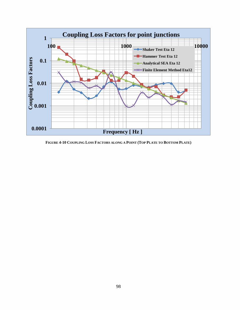
98

FIGURE 4-10 COUPLING LOSS FACTORS ALONG A POINT (TOP PLATE TO BOTTOM PLATE)

0.0001

0.001

0.01

0.1

1

100 1000 10000

Co

up

lin

g L

oss

Fa

cto

rs

Frequency [ Hz ]

Coupling Loss Factors for point junctions

Shaker Test Eta 12

Hammer Test Eta 12

Analytical SEA Eta 12

Finite Element Method Eta12

99

5 CONCLUSIONS AND FUTURE WORK

5.1 CONCLUSIONS

5.1.1 POWER INPUT METHOD

1. The analytical power input method is validated with a single degree of freedom with a

random excitation and a sinusoidal excitation. P.I.M. works very well for these S.D.O.F.

systems for all levels of damping.

2. Experiments show that for lightly damped plates [ 0.001 ] the method fails. For highly

damped plates [ 0.1 ] the P.I.M. estimates loss factors well i.e., the estimates are

within 10% of the I.R.D.M. prediction in the range of 100 Hz – 4000 Hz.

3. For moderately damped plates [ 0.01 ] the loss factors estimated with high resolution

(i.e., 1Hz and 2 Hz resolution) performed essentially the same but as the resolution is

decreased beyond 2 Hz [4 Hz and 8 Hz ] the loss factor estimation fails.

100

5.1.2 IMPULSE RESPONSE DECAY METHOD

1. The analytical impulse response decay method is validated with a single degree of

freedom system with a true impulse and a half sine impulse excitation. For these S.D.O.F.

systems the estimated loss factors are accurate for a wide range of loss factors.

2. The method is also validated by a computational plate model, for three damping levels of

10 %, 1%, and 0.1%. The loss factors estimated are accurate for low and moderate

damping levels in the range 100 Hz – 8000 Hz but for highly damped plates the loss

factors are under estimated at high frequency because the responses from the near field

are used in the computational process. The method fails for all three analyzed levels of

damping below 100 Hz, where modal density is low and the method is expected to fail.

3. There was no effect on the estimated loss factor by employing either full octave, 1/3rd

,

1/6th

or 1/12th

octave filters. The 1/3rd

, 1/6th

and 1/12th

octave are computationally-

intensive making them less attractive. It is recommended to use full octave filters,

centered at 1/3rd

octave frequencies.

4. The accuracy of the estimated loss factors is greatly affected if the frequency resolution is

increased for lightly damped and moderately damped plates. For highly damped plates

there is no such effect.

5. By increasing the number of measurement points the loss factor estimation is more

accurate. However more response points are computationally-intensive and require more

resources to measure and hence it is recommended that only 4 response points are needed

to get reasonable estimation.

101

5.1.3 STATISTICAL ENERGY ANALYSIS

1. The modal densities and the mode count are evaluated for lightly damped and moderately

damped plates and compared with theoretical values. The estimation fails for lightly

damped plates but for moderately damped plates, the estimation is fairly accurate.

2. The coupling loss factors of two sets of plates are estimated experimentally. When the

loss factors are computed individually for the plates joined along a line, the coupling loss

factor estimation is fairly accurate. When the loss factor is evaluated for the coupled

plates there is moderate agreement of the experimental solution with the analytical

solution.

5.2 FUTURE WORK

1. Further work on the PIM should focus on experimental methods to eliminate phase errors

which cause negative damping estimation.

2. For validating the impulse response decay method the computational analysis was done

with uniformly spaced excitation and response points. This method needs to be validated

with randomly selected excitation and response points.

3. Further experimental studies on I.R.D.M. are needed to evaluate the effects of

measurement noise on the estimated loss factors.

4. Experimental studies of S.E.A. considering various different boundary conditions and

damping levels are needed to expand the understanding of this method.

102

REFERENCES:

[1] Rao S. S, Mechanical Vibrations. Addison-Wesley Publishing Company, 1984.

[2] Valette C, and Cacracciolo A., "Damping mechanisms governing plate vibration,"

Molecular and Quantum Acoustics, Acta Acoustica, vol. 7 pp. 393-404, 1995.

[3] Iwaniwec Mark, "Damping Loss factor Estimation in Plates," Molecular and Quantum

Acoustics, Acta Acoustica, vol. 24, pp. 276-287, 2003.

[4] Liu Wanbo, "Experimental and Analytical Estimation of Damping in beams and plates with

damping treatments", PhD Dissertation ,University of Kansas, Lawrence, November 2008.

[5] Norton M and Karczub D., Fundamentals of Noise and Vibration Analysis for Engineers.

Cambridge, UK: Cambridge University Press, 2003.

[6] Bloss B. and Rao M.D., "Estimation of frequency-averaged loss factors by the power input

method and the impulse response decay method ," Journal of Acoustical Society of

America, vol. 117, no. 1, pp. 240-249, 2004.

[7] Nuno Manuel Mendes Maia and Montalvao Julio, Theoretical and Experimental Modal

Analysis. New York, USA: John Wiley & Sons Inc..

[8] Wolf Jr., J.A. "The influence of mounting stiffness on frequencies measured in a vibration

test.," vol. SAE Paper 840480, Society of Automotive Engineers, 1984.

[9] DeJong R.H. and, Lyon R.G., Theory and Application of Statistical Energy Analysis, 2nd

ed. Newton, MA,USA: Butterworth-Heinmann, 1995.

[10] Lyon R.H., Statistical Energy Analysis of dynamic systems: theory and applications.

cambridge: M.I.T. Press, 1975.

[11] Bies D.A. and Hamid S., "In situ determination of loss and coupling loss factors by the

power injection method," Journal of Sound and Vibration, vol. 70, no. 2, pp 187-204, 1980.

[12] Bloss B. and Rao M.D., "Measurement of Damping In Structures by the Power Input

Method," Journal of Sound and Vibration, Vol 26(3) pp. 234-238, 1986.

[13] Carfangi M. and Pierini M., "Determining the Loss Factors by the Power Input Method. I.

Nemerical Investigation,", Journal of Vibrations and Acoustics, vol.121(2), pp 417- 422,

1997.

[14] Citti P., Pierini M. and Carfangi M., "Determining loss factors using the power input

method with shaker excitation," , 1998 Proceedings of the XVIth IMAC,CA, 585-590,1998.

[15] Fujimoto J and Okada T., "Radiation noise reduction by applying vibration damping

material," Inter Noise 94, Yokohama, 1994.

[16] Liu W and Ewing M.S, "Predicting Damping Loss Factors for Beams and Plates with

103

Constrained Layer Damping," in AIAA Structures, Structural Dynamics and Materials

Conference, Shaumberg, IL, April 2008.

[17] Ewing S. Mark and Wanbo Liu, "Experimental and Analytical Estimation of Loss factors by

the Power Input Method," AIAA Journal, vol. 45, no. 2, pp. 477-484, 2007.

[18] Rife D. D., and Vanderkooy J., "Transfer-function measurement with maximum length

sequences," Journal of Audio Engineering Society, vol. 37, no. 6, pp. 419-443, 1989.

[19] Vorlander M. and Kob M., "Practical aspects of MLS measurements in building acoustics,"

Applied Acoustics, vol. 52, no. 3/4, pp. 239-258, 1997.

[20] Agren A., Soundback U., and Wu L., "A study of initial decay rate of two-dimensional

vibrating structures in relation to estimates of loss factor," Journal of Sound and Vibration,

vol. 206, no. 5, pp. 663-684, 1997.

[21] Lai M.L and Soom A., "Prediction of transient envelopes using statistical energy analysis

techniques," Journal of Vibration and Acoustics, vol. 112, pp. 127-137, January 1990.

[22] Mace B and Shoter P, "Energy Flow Models from the finite element analysis," Journal of

sound and vibration, vol. 233, no. 3, pp. 369-389, January 2000.

[23] Ewing, M. S., Dande H., and Vatti, K., "Validation of Panel Damping Loss factors

Estimation Algorithms using a Computational Model," Proceedings of 50th

AIAA/ASME/ASCE/AHS/ASC Structures, Structural Dynamics and Materials Conference,

Palm Springs, CA, 2009.

[24] Ewing M. S., Vatti K., and Vaz I., "Coupling Loss Factor Estimation for Plates Joined

Along a Line: Analysis and Experiment," Journal of Acoustical Society of America, Volume

127, Issue 3, PP 1769 - 1769, March 2010

[25] Lai M.L, "Modelling of Transient Vibrations with Statistical Energy Analysis,", PhD

Dissertation., State university of New York, Buffalo, September 1988.

[26] Ewing M. S., Vatti K., and Vaz I., "Coupling Loss Factor Estimation for Plates Joined

Along a Point: Analysis and Experiment," Journal of Acoustical Society of America,

Volume 127, Issue 3, PP 1769 - 1769, March 2010

A-1

APPENDIX A MATLAB CODES

A.1. GENERATE A TRUE RANDOM SIGNAL

%%%%%%%%%%%%%%%%%%%%%%%%%%%%%%%%%%%%%%%%%%%%%%%%%%%%%%%%%%%%%%%%%%%%%%%% %%%%%------------GENERATE A TRUE RANDOM SIGNAL---------------------%%%%% %%%%%%%%%%%%%%%%%%%%%%%%%%%%%%%%%%%%%%%%%%%%%%%%%%%%%%%%%%%%%%%%%%%%%%%% clear all close all clc Fms=1; %what is the mean square value of the force you want fs=100; %set the sample rate npts=10*fs; %set the number of points in this case 10secs worth deltaf=fs/npts; %what is the deltaf for the prescribed spectrum f_low=1; %we are doing the flat sprctrum with a low frequency cut off f_high=10; %and ahigh frequency cutoff band=f_high-f_low; % what is the band width f_cutoff_low=round(f_low/deltaf)+1; % find the low bin of the spectrum f_cutoff_high=round(f_high/deltaf)+1; % find the high bin of the spectrum So=Fms/band; % the spectrum level P=zeros(npts/2+1,1); % zero all bins %specify the level in the meaning full bins P(f_cutoff_low:f_cutoff_high,1)=So*ones(f_cutoff_high-f_cutoff_low+1,1); N=length(P); %scale P level=P/2; % single sided to double sided level=npts*(npts*deltaf)*level; %scale for ifft level=sqrt(level); phase=2*pi*rand(N,1); %make random phase H=level.*(cos(phase)+i*sin(phase)); % positive side of fft H(N+1:2*(N-1))=conj(flipud(H(2:N-1))); %build the other side F=real(ifft(H));

A.2. IMPULSE RESPONSE FUNCTION

%%%%%%%%%%%%%%%%%%%%%%%%%%%%%%%%%%%%%%%%%%%%%%%%%%%%%%%%%%% %%%%-------------IMPULSE RESPONSE FUNCTION-------------%%%% %%%%%%%%%%%%%%%%%%%%%%%%%%%%%%%%%%%%%%%%%%%%%%%%%%%%%%%%%%% function [hir]=impresp(t,mass,Wn,Zeta) Wd=Wn*sqrt(1-Zeta^2); hir=1/Wd/mass*exp(-Zeta*Wn*t)*sin(Wd*t);

A-2

A.3. LOSS FACTOR ESTIMATION BY POWER INPUT METHOD: SYNTHETIC, 1 DOF, RANDOM

EXCITATION

%%%%%%%%%%%%%%%%%%%%%%%%%%%%%%%%%%%%%%%%%%%%%%%%%%%%%%%%%%%%%%%%%%%%%%%%% %%%%---LOSS FACTOR ESTIMATION OF A SDOF BY THE POWER INPUT METHOD----%%%% %%%%%%%%%%%%%%%%%%%%%%%%%%%%%%%%%%%%%%%%%%%%%%%%%%%%%%%%%%%%%%%%%%%%%%%%% clear all close all clc

%SYSTEM PROPERTIES mass=0.5; k=1000; c=0.5; Wn=sqrt(k/mass);%Natural Frequency Zeta=c/(2*mass*Wn);%Damping Coefficient Wd=sqrt(1-Zeta^2)*Wn;% Damped Natural Frequency %response is set to zero resp=zeros(1000,1); figure(1) subplot(2,1,1) plot(F,'r')% the true random force xlabel('Number of Samples','FontSize',14,'FontWeight','b') ylabel('Magnitude','FontSize',14,'FontWeight','b') title('Random Force','FontSize',16,'FontWeight','b') RF=F(500:1000); RRF=F.*(hanning(1000)); subplot(2,1,2) plot(RRF) xlabel('Number of Samples','FontSize',14,'FontWeight','b') ylabel('Magnitude','FontSize',14,'FontWeight','b') title('Force with a Hanning Window','FontSize',16,'FontWeight','b') dt=1/100; for n=1:1000 for j=1:n h=impresp((n-j)*dt,mass,Wn,Zeta);% calculation of the impulse

response function resp(n)=resp(n)+F(j)*h*dt;% the response of the system to the random

force end if n>1 velocity(n)=(resp(n)-resp(n-1))/dt; % calculation of the velocity

using the respone end end figure(2) plot(resp(1:1000),'m') xlabel('Number of Samples','FontSize',14,'FontWeight','b') ylabel('Magnitude','FontSize',14,'FontWeight','b') title('Displacement Response to the Applied

Force','FontSize',14,'FontWeight','b') VVelocity=velocity.*transpose(hanning(1000)); figure(3) subplot(2,1,1) plot(velocity,'k')

A-3

xlabel('Number of Samples','FontSize',14,'FontWeight','b') ylabel('Magnitude','FontSize',14,'FontWeight','b') title('Velocity Response to the Applied

Force','FontSize',16,'FontWeight','b') Velocity=velocity(500:1000); subplot(2,1,2) plot(VVelocity) xlabel('Number of Samples','FontSize',14,'FontWeight','b') ylabel('Magnitude','FontSize',14,'FontWeight','b') title('Velocity Response with a Hanning

Window','FontSize',16,'FontWeight','b')

Energydissipated=VVelocity*RRF;% calculation of the total energy that is

dissipated in the system KE=(mass/2)*VVelocity*transpose(VVelocity);% the total kinetic energy in the

system lossfactor(i)=Energydissipated/(2*Wn*KE);% loss factor

A-4

A.4. POWER INPUT METHOD: SYNTHETIC, 1 DOF, SINUSOIDAL EXCITATION

%%%%%%%%%%%%%%%%%%%%%%%%%%%%%%%%%%%%%%%%%%%%%%%%%%%%%%%%%%%%%%%%%%%%%%%%% %%%%---LOSS FACTOR ESTIMATION OF A SDOF BY THE POWER INPUT METHOD----%%%% %%%%%%%%%%%%%%%%%%%%%%%%%%%%%%%%%%%%%%%%%%%%%%%%%%%%%%%%%%%%%%%%%%%%%%%%% clear all close all clc for ii=1:1:10

mass=0.5; k=[600 1800 3000 4200 5400 6800 9000 12000 18000 25000]*100; k=k(ii); c=0.5; %All the above values are given %computed as per the formula,Natural frequency Wn=sqrt(k/mass); freq(ii)=Wn; %damping coefficient Zeta=c/(2*mass*Wn) zeta(ii)=Zeta; % damping frequency Wd=sqrt(1-Zeta^2)*Wn; %Accelaration due to gravity a=9.8; %this for loop computes the values of the impulse function for 200 %intervals of time Impulse(1999)=0; for i=1:1:1999 t=i/100; Impulse(i+1)=sin(Wd*t); end %response is set to zero resp=zeros(2000,1); dt=1/100; for n=1:2000 for i=1:n h=impresp((n-i)*dt,mass,Wn,Zeta); resp(n)=resp(n)+Impulse(i)*h*dt; end if n>1 velocity(n)=(resp(n)-resp(n-1))/dt; end end fontname='Times New Roman'; figure(1) subplot(2,1,1) plot(Impulse,'r') xlabel('Number of Samples','FontSize',14,'FontWeight','b','FontName','Times') ylabel('Magnitude','FontSize',14,'FontWeight','b') title('Sinusoidal Force','FontSize',16,'FontWeight','b') subplot(2,1,2) plot(velocity,'k') xlabel('Number of Samples','FontSize',14,'FontWeight','b') ylabel('Magnitude','FontSize',14,'FontWeight','b')

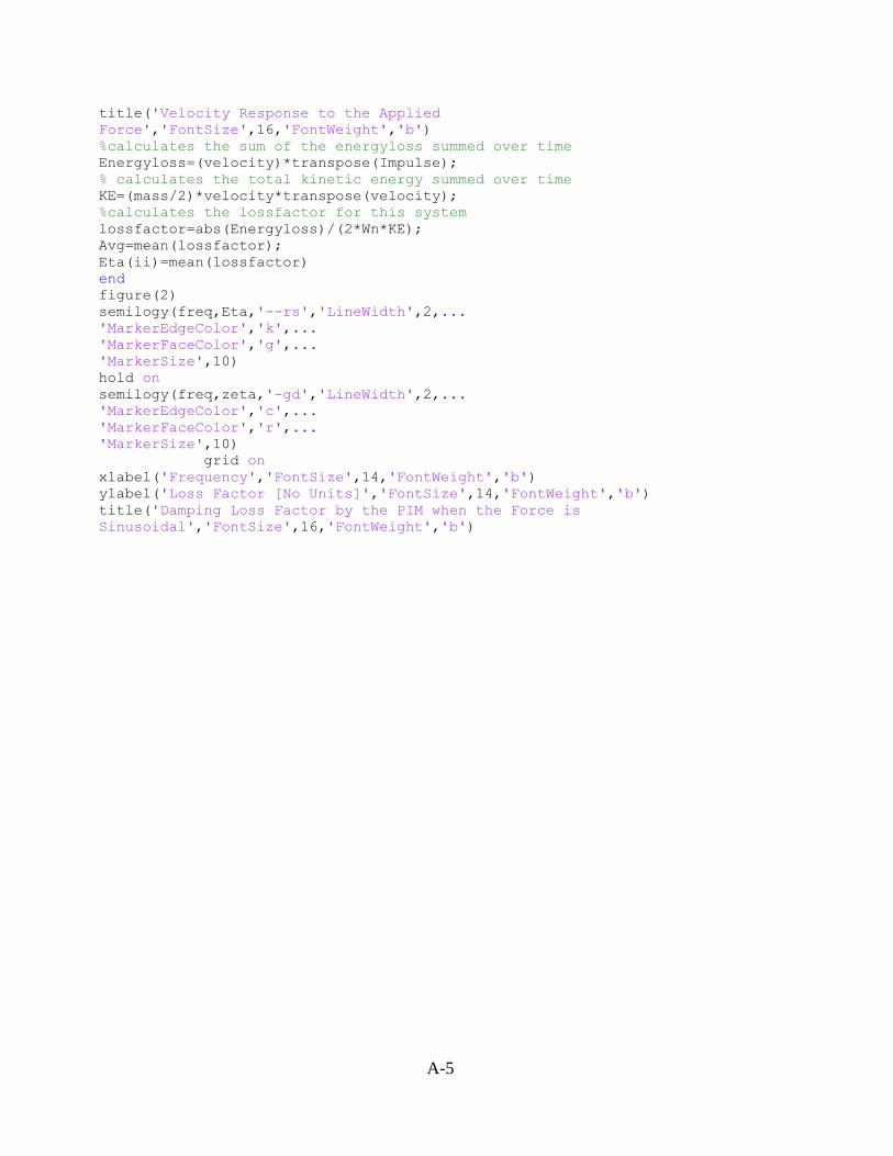
A-5

title('Velocity Response to the Applied

Force','FontSize',16,'FontWeight','b') %calculates the sum of the energyloss summed over time Energyloss=(velocity)*transpose(Impulse); % calculates the total kinetic energy summed over time KE=(mass/2)*velocity*transpose(velocity); %calculates the lossfactor for this system lossfactor=abs(Energyloss)/(2*Wn*KE); Avg=mean(lossfactor); Eta(ii)=mean(lossfactor) end figure(2) semilogy(freq,Eta,'--rs','LineWidth',2,... 'MarkerEdgeColor','k',... 'MarkerFaceColor','g',... 'MarkerSize',10) hold on semilogy(freq,zeta,'-gd','LineWidth',2,... 'MarkerEdgeColor','c',... 'MarkerFaceColor','r',... 'MarkerSize',10) grid on xlabel('Frequency','FontSize',14,'FontWeight','b') ylabel('Loss Factor [No Units]','FontSize',14,'FontWeight','b') title('Damping Loss Factor by the PIM when the Force is

Sinusoidal','FontSize',16,'FontWeight','b')

A-6

A.5. IMPULSE RESPONSE DECAY METHOD: SYNTHETIC, 1 DOF, IMPULSE FUNCTION

%%%%%%%%%%%%%%%%%%%%%%%%%%%%%%%%%%%%%%%%%%%%%%%%%%%%%%%%%%%%%%%%%%%%%%%%% %-LOSS FACTOR ESTIMATION OF A SDOF BY THE IMPULSE REDPONSE DECAY METHOD-% %%%%%%%%%%%%%%%%%%%%%%%%%%%%%%%%%%%%%%%%%%%%%%%%%%%%%%%%%%%%%%%%%%%%%%%%% clear all close all clc

%SYSTEM PROPERTIES

m=0.5; k=1000; c=0.5; %All the above values are given %computed as per the formula,Natural frequencuy Wn=sqrt(k/m); %damping coefficient Zeta=c/(2*m*Wn); % damping frequency Wd=sqrt(1-Zeta^2)*Wn;

%TOTAL NUMBER OF ITERATIONS

npts=8192; dt=0.001;

%CALCULATION OF IMPULSE USING THE IMPULSE RESPONSE FUNCTION

h(npts+1)=0; for i=0:1:npts t=i*dt; h(i+1)=1/(Wd*m).*exp(-Zeta*Wn.*t)*sin(Wd.*t); end t=(0:1:npts)/100; time =t./80; figure(1) plot(time,h) xlabel('Time [ Seconds ]','FontSize',14,'FontWeight','b') ylabel('H(t)','FontSize',14,'FontWeight','b') title('Plot of Impulse function','FontSize',16,'FontWeight','b')

%hilbert command takes the impulse function and puts a hilbert transform on %it to have the hilbert transform

%Hilbert function has a real part and an imaginary part the real part is %computed here and the imaginary part is computed in the next statement

H=hilbert(h); figure(2) subplot(2,1,1) plot(time,real(H)),hold on plot(time,imag(H),':'),hold off xlabel('Time [ Seconds ]','FontSize',14,'FontWeight','b')

A-7

ylabel('Hilbert Transform','FontSize',14,'FontWeight','b') title('Real and Imaginary Hilbert Transform of the Impulse

Function','FontSize',16,'FontWeight','b') subplot(2,1,2) plot(time,abs(H)) xlabel('Time [ Seconds ]','FontSize',14,'FontWeight','b') ylabel('Hilbert Transform','FontSize',14,'FontWeight','b') title('Absolute Value of the Hilbert

Transform','FontSize',16,'FontWeight','b')

z=log10(abs(H)); figure(3) plot(time,z) xlabel('Time [ Seconds ]','FontSize',14,'FontWeight','b') ylabel('Decibels [ dB ]','FontSize',14,'FontWeight','b') title('Logrithmic Decrement of the Hilbert

Transform','FontSize',16,'FontWeight','b') %the loss factor is calculated for a particular interval of time in the %graph and the average of this loss factor is calculated subsequently

for i=1:1:10 skip=i*10; for j=1:1:10 delay=j*10; for n=delay+1:delay+10 Eta(n-10)=-(z(n+skip)-z(n))/(skip*dt) *2/Wn/0.4343; Avg(i,j)=mean(Eta)/0.0224; end

end

end

Skip=zeros(10,1); for k=1:10 Skip(k)=k*10; end Delay=zeros(10,1); for l=1:10 Delay(l)=l*10; end figure(4) mesh(Delay,Skip,Avg) xlabel('Delay','FontSize',14,'FontWeight','b') ylabel('Skip','FontSize',14,'FontWeight','b') zlabel('Lossfactor','FontSize',16,'FontWeight','b') title('Loss Factor as a Function of Skip and

Delay','FontSize',16,'FontWeight','b')

A-8

A.6. IMPULSE RESPONSE DECAY METHOD: SYNTHETIC, 1 DOF, HALF SINE PULSE

%%%%%%%%%%%%%%%%%%%%%%%%%%%%%%%%%%%%%%%%%%%%%%%%%%%%%%%%%%%%%%%%%%%%%%%%% %-LOSS FACTOR ESTIMATION OF A SDOF BY THE IMPULSE REDPONSE DECAY METHOD-% %%%%%%%%%%%%%%%%%%%%%%%%%%%%%%%%%%%%%%%%%%%%%%%%%%%%%%%%%%%%%%%%%%%%%%%%% clear all close all clc %SYSTEM PROPERTIES mass=0.5; k=1000; c=0.5; Wn=sqrt(k/mass); Zeta=c/(2*mass*Wn) Wd=Wn*(sqrt(1-Zeta^2)); tpts=4096*8; dt=0.005; npts=tpts/4; Wnf=0.1*Wn; dt=0.005; for i=1:1:tpts t=i*dt-dt; f1(i)=1-cos(Wnf*t); end

for i=282:1:tpts t=i*dt-dt; f2(i)=-1+cos(Wnf*t); end f=f1+f2; for i=1:1:npts t=i-1; F1(i)=f(4*t+1); end for i=1:1:npts/4 t=i-1; F(i)=F1(4*t+1); end time=linspace(0,1,2048); figure(1) subplot(3,1,1) plot(time(1:25),F(1:25),'*') xlabel('Time [ Seconds ]','FontSize',14,'FontWeight','b') ylabel('Magnitude','FontSize',14,'FontWeight','b') title('Simulated Half Sine Impulse','FontSize',16,'FontWeight','b') subplot(3,1,2) plot(time,F) xlabel('Time [ Seconds ]','FontSize',14,'FontWeight','b') ylabel('Magnitude','FontSize',14,'FontWeight','b') title('Simulated Half Sine Impulse','FontSize',16,'FontWeight','b') %%RESPONSE USING THE CONVOLUTION INTEGRAL R1=zeros(1,npts/4); for n=1:npts/4 for i=1:n

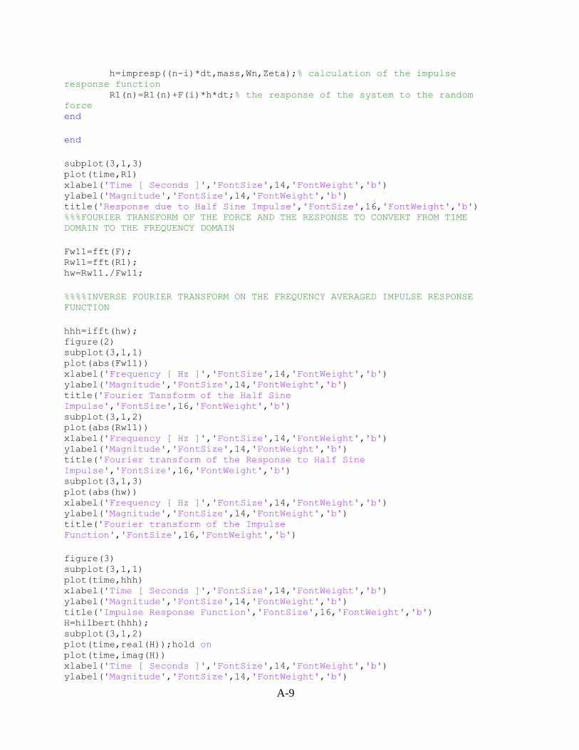
A-9

h=impresp((n-i)*dt,mass,Wn,Zeta);% calculation of the impulse

response function R1(n)=R1(n)+F(i)*h*dt;% the response of the system to the random

force end

end

subplot(3,1,3) plot(time,R1) xlabel('Time [ Seconds ]','FontSize',14,'FontWeight','b') ylabel('Magnitude','FontSize',14,'FontWeight','b') title('Response due to Half Sine Impulse','FontSize',16,'FontWeight','b') %%%FOURIER TRANSFORM OF THE FORCE AND THE RESPONSE TO CONVERT FROM TIME

DOMAIN TO THE FREQUENCY DOMAIN

Fw11=fft(F); Rw11=fft(R1); hw=Rw11./Fw11;

%%%%INVERSE FOURIER TRANSFORM ON THE FREQUENCY AVERAGED IMPULSE RESPONSE

FUNCTION

hhh=ifft(hw); figure(2) subplot(3,1,1) plot(abs(Fw11)) xlabel('Frequency [ Hz ]','FontSize',14,'FontWeight','b') ylabel('Magnitude','FontSize',14,'FontWeight','b') title('Fourier Tansform of the Half Sine

Impulse','FontSize',16,'FontWeight','b') subplot(3,1,2) plot(abs(Rw11)) xlabel('Frequency [ Hz ]','FontSize',14,'FontWeight','b') ylabel('Magnitude','FontSize',14,'FontWeight','b') title('Fourier transform of the Response to Half Sine

Impulse','FontSize',16,'FontWeight','b') subplot(3,1,3) plot(abs(hw)) xlabel('Frequency [ Hz ]','FontSize',14,'FontWeight','b') ylabel('Magnitude','FontSize',14,'FontWeight','b') title('Fourier transform of the Impulse

Function','FontSize',16,'FontWeight','b')

figure(3) subplot(3,1,1) plot(time,hhh) xlabel('Time [ Seconds ]','FontSize',14,'FontWeight','b') ylabel('Magnitude','FontSize',14,'FontWeight','b') title('Impulse Response Function','FontSize',16,'FontWeight','b') H=hilbert(hhh); subplot(3,1,2) plot(time,real(H));hold on plot(time,imag(H)) xlabel('Time [ Seconds ]','FontSize',14,'FontWeight','b') ylabel('Magnitude','FontSize',14,'FontWeight','b')

A-10

title('Real and Imaginary parts of the Hilbert

Transform','FontSize',16,'FontWeight','b') subplot(3,1,3) plot(time,abs(H)) xlabel('Time [ Seconds ]','FontSize',14,'FontWeight','b') ylabel('Magnitude','FontSize',14,'FontWeight','b') title('Absolute value of the Hilbert

Transform','FontSize',16,'FontWeight','b') figure(4) z=log(abs(H)); plot(time,z) xlabel('Time [ Seconds ]','FontSize',14,'FontWeight','b') ylabel('Magnitude [ dB ]','FontSize',14,'FontWeight','b') title('Logrithmic Decrement of the Hilbert

Transform','FontSize',16,'FontWeight','b')

for i=1:1:20 skip=10*i; for j=1:1:30 delay=10*j;

for n=delay+1:delay+10 Eta(n-10)=-(z(n+skip)-z(n))/(skip*dt) *2/(Wn); avg(i,j)=mean(Eta); end end

end

Skip=zeros(20,1); for k=1:20 Skip(k)=k*10; end Delay=zeros(30,1); for l=1:30 Delay(l)=l*10; end figure(5) mesh(Delay,Skip,avg) xlabel('Delay','FontSize',14,'FontWeight','b') ylabel('Skip','FontSize',14,'FontWeight','b') zlabel('Loss factor','FontSize',16,'FontWeight','b') title('Loss Factor as a Function of Skip and

Delay','FontSize',16,'FontWeight','b')

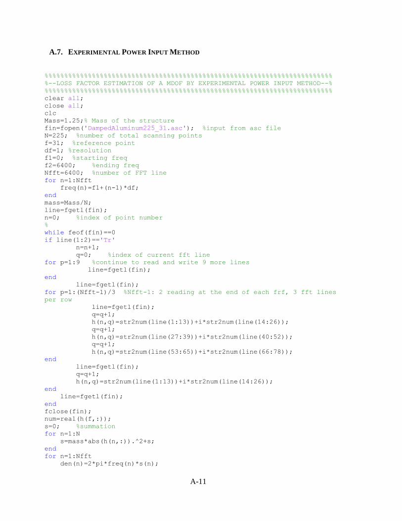
A-11

A.7. EXPERIMENTAL POWER INPUT METHOD

%%%%%%%%%%%%%%%%%%%%%%%%%%%%%%%%%%%%%%%%%%%%%%%%%%%%%%%%%%%%%%%%%%%%%%%%% %--LOSS FACTOR ESTIMATION OF A MDOF BY EXPERIMENTAL POWER INPUT METHOD--% %%%%%%%%%%%%%%%%%%%%%%%%%%%%%%%%%%%%%%%%%%%%%%%%%%%%%%%%%%%%%%%%%%%%%%%%% clear all; close all; clc Mass=1.25;% Mass of the structure fin=fopen('DampedAluminum225_31.asc'); %input from asc file N=225; %number of total scanning points f=31; %reference point df=1; %resolution f1=0; %starting freq f2=6400; %ending freq Nfft=6400; %number of FFT line for n=1:Nfft freq(n)=f1+(n-1)*df; end mass=Mass/N; line=fgetl(fin); n=0; %index of point number % while feof(fin)==0 if line(1:2)=='Tr' n=n+1; q=0; %index of current fft line for p=1:9 %continue to read and write 9 more lines line=fgetl(fin); end line=fgetl(fin); for p=1:(Nfft-1)/3 %Nfft-1: 2 reading at the end of each frf, 3 fft lines

per row line=fgetl(fin); q=q+1; h(n,q)=str2num(line(1:13))+i*str2num(line(14:26)); q=q+1; h(n,q)=str2num(line(27:39))+i*str2num(line(40:52)); q=q+1; h(n,q)=str2num(line(53:65))+i*str2num(line(66:78)); end line=fgetl(fin); q=q+1; h(n,q)=str2num(line(1:13))+i*str2num(line(14:26)); end line=fgetl(fin); end fclose(fin); num=real(h(f,:)); s=0; %summation for n=1:N s=mass*abs(h(n,:)).^2+s; end for n=1:Nfft den(n)=2*pi*freq(n)*s(n);

A-12

end eta=num./den;

fid = fopen('DampedAluminum225_31_Eta.txt','w'); for n=1:Nfft fprintf(fid,'%12.8f %12.8f\n',freq(n),eta(n)); end fclose(fid)

for n=1:Nfft rms(n)=norm(h(:,n))/length(h(:,n)); %1884.7 hz end fid = fopen('DampedAluminum225_31_Rms.txt','w'); for n=1:Nfft fprintf(fid,'%12.8f %12.8f\n',freq(n),rms(n)); end fclose(fid);

save DampedAluminum225_31h

f_c=[16 20 25 32 40 50 63 80 100 125 160 200 250 315 400 500 630 800 1000

1250 1600 2000 2500 3150 4000 5000 6300 8000].'; f_l=f_c*2^(-1/6); f_u=f_c*2^(1/6); f=linspace(f1,f2,Nfft); for i=1:1:length(f_c) I=find(f>=f_l(i)& f<f_u(i)); DD(i)=length(I); LF(i)=sum(eta(I))/(DD(i)); end LF=abs(LF); figure(1) loglog(f_c,LF,'d',f_c,LF) xlabel('Frequency [ Hz ]','FontSize',14) ylabel('Loss Factor','FontSize',14) title('The Loss factor of the Plate In Bands','FontSize',16);grid on figure(2) plot(freq,eta) xlabel('Frequency [ Hz ]','FontSize',14) ylabel('Loss Factor','FontSize',14) title('The Loss factor of the Plate','FontSize',16);grid on

A-13

A.8. EXPERIMENTAL IMPULSE RESPONSE DECAY METHOD

%%%%%%%%%%%%%%%%%%%%%%%%%%%%%%%%%%%%%%%%%%%%%%%%%%%%%%%%%%%%%%%%%%%%%%%%% %---LOSS FACTOR ESTIMATION OF A MDOF BY IMPULSE RESPONSE DECAY METHOD---% %%%%%%%%%%%%%%%%%%%%%%%%%%%%%%%%%%%%%%%%%%%%%%%%%%%%%%%%%%%%%%%%%%%%%%%%% clear all close all clc

load input_1_quadrant_1_2.mat load input_1_quadrant_2_3.mat load input_1_quadrant_3_2.mat load input_1_quadrant_4_1.mat

Fs=20000; N=20002; f=linspace(0,20001,20001); Frf1=zeros(1,10001); Frf2=zeros(1,10001); Frf3=zeros(1,10001); Frf4=zeros(1,10001); for k=1:1:10001 Frf1(k)=input_1_quadrant_1_2(k); Frf2(k)=input_1_quadrant_2_3(k); Frf3(k)=input_1_quadrant_3_2(k); Frf4(k)=input_1_quadrant_4_1(k); end Frf1(10002:20002)=fliplr(conj(Frf1(1:10001))); Frf2(10002:20002)=fliplr(conj(Frf2(1:10001))); Frf3(10002:20002)=fliplr(conj(Frf3(1:10001))); Frf4(10002:20002)=fliplr(conj(Frf4(1:10001)));

f_c =[16 20 25 32 40 50 63 80 100 125 160 200 250 315 400 500 630 800 1000

1250 1600 2000 2500 3150 4000 5000 6300 8000].'; f_l = f_c*2^(-1/2); %full octave bandwidths f_u = f_c*2^(1/2);

TwoH1stack=zeros(4,20002); TwoH1stack(1,:)=Frf1; TwoH1stack(2,:)=Frf2; TwoH1stack(3,:)=Frf3; TwoH1stack(4,:)=Frf4;

analsum = zeros(length(f_c),N);

A-14

for acc=1:1:4 for i=1:1:length(f_c)

temp = zeros(N,1)*(eps + 1j*eps);

I = find(f >= f_l(i) & f < f_u(i)); temp(I+2) = TwoH1stack(acc,I); %I added the +2 to make temp

'conjugate symmetric', but i think it may be spuriously shifting the

frequencies. Probably has negligable effect. temp(N-I+2) = conj((TwoH1stack(acc,I))); decay = ifft(temp,N,'symmetric'); anal = hilbert(real(decay)).'; %calculating the analytical signal anal = abs(anal)./max(abs(anal)); %normalizing for easy visualization

later analsum(i,:) = anal + analsum(i,:); end end analAVG = analsum/4; dbdecay_full = 20*log10(analAVG.'); %dB decays for exporting out to excel save dbdecay_fulldbdecay_full

A-15

A.9. FREQUENCY RESPONSE FUNCTION EXTRACTION FROM NASTRAN FO6 FILES

%%%%%%%%%%%%%%%%%%%%%%%%%%%%%%%%%%%%%%%%%%%%%%%%%%%%%%%%%%%%%%%%%%%%%%%%% %%%%-------------DATA EXTRACTION FROM NASTRAN FO6 FILES--------------%%%% %%%%%%%%%%%%%%%%%%%%%%%%%%%%%%%%%%%%%%%%%%%%%%%%%%%%%%%%%%%%%%%%%%%%%%%%% close all clear all clc

fin=fopen('steady_state_less.f06'); %input from asc file ff=1; %reference point number in patran/nastran f1=0; %starting freq f2=10000; %ending freq Ndf=10000+1; %number of frequency increments df=(f2-f1)/(Ndf-1); %frequency resolution

n1=0; n2=0; n3=0;

line=fgetl(fin); while feof(fin)==0 temp=size(line); if temp(1,2)==26 & line(23 :26)=='7033' line=fgetl(fin); temp=size(line); if temp(1,2)==88 & line(44:88)=='C O M P L E X A C C E L E R A T I O N V

E C T O R' line=fgetl(fin); line=fgetl(fin); line=fgetl(fin); temp=size(line); if temp(1,2)== 109& line(7:15)=='FREQUENCY' for i=1:1:16 n1=n1+1; liner=fgetl(fin); freq(n1)=str2num(liner(4:15)); linei=fgetl(fin); h4(n1)=str2num(liner(57:69)); h5(n1)=str2num(linei(57:69)); end end

end end line=fgetl(fin);

end fclose(fin);

A-16

A.10. MANUAL DECAY MEASUREMENT

%%%%%%%%%%%%%%%%%%%%%%%%%%%%%%%%%%%%%%%%%%%%%%%%%%%%%%%%%%%%%%%%%%%%%%%%% %%%%---------------MANUAL DECAY MEASUREMENT ALGORITHM----------------%%%% %%%%%%%%%%%%%%%%%%%%%%%%%%%%%%%%%%%%%%%%%%%%%%%%%%%%%%%%%%%%%%%%%%%%%%%%% clear all clc close all

f_c =[16 20 25 32 40 50 63 80 100 125 160 200 250 315 400 500 630 800 1000

1250 1600 2000 2500 3150 4000 5000 6300 8000 ].';

for j=1:1:length(f_c)

while(1<2) calculate(j) choice1=input('Do you wish to Proceed(y/n):','s') if (choice1=='y') display('Will Go to Next Graph') break elseif (choice1=='n') display('Will Exit From The Program') plot(dbdecay) calculate(55) break

end end end

%%%%%%%%%%%%%%%%%%%%%%%%%%%%%%%%%%%%%%%%%%%%%%%%%%%%%%%%%%%%%%%%%%%%%%%%% %%%%---------------MANUAL DECAY MEASUREMENT ALGORITHM----------------%%%% %%%%%%%%%%%%%%%%%%%%%%%%%%%%%%%%%%%%%%%%%%%%%%%%%%%%%%%%%%%%%%%%%%%%%%%%% function Calculate(j)

clear dbdecay_full.mat load dbdecay_full.mat

dbdecay=dbdecay_full; f2=linspace(0,1,20002);

f_c =[16 20 25 32 40 50 63 80 100 125 160 200 250 315 400 500 630 800 1000

1250 1600 2000 2500 3150 4000 5000 6300 8000].';

close all figure(1) F=dbdecay(:,j); plot(f2,F) xlabel('Time') title('Log Decrement')

A-17

keyboard H=ginput(2); K=H(:,1); K2=H(:,2); frequency=f_c(j)

N=H(2,1)-H(1,1);

D=H(2,2)-H(1,2);

%%%%%%%%%%%%%

Eta=-D/N/f_c(j)/27.3 figure(2)

plot(f2,dbdecay(:,j)),hold on plot(K,K2,'r','LineWidth',3),hold off

xlabel('Time') title('Log Decrement') choice=input('Are You Satisfied(y/n):','s') if (choice=='n') Eta(j)=-D/N/f_c(j)/27.3; calculate(j) elseif (choice=='y') display('The Loss Factor is') Eta=-D/N/f_c(j)/27.3

return end end

A-18

A.11. MODAL DENSITY AND MODES IN BAND MEASUREMENT

%%%%%%%%%%%%%%%%%%%%%%%%%%%%%%%%%%%%%%%%%%%%%%%%%%%%%%%%%%%%%%%%%%%%%%%%% %%%%---------MODAL DENSITY AND MODES IN BAND MEASUREMENT ------------%%%% %%%%%%%%%%%%%%%%%%%%%%%%%%%%%%%%%%%%%%%%%%%%%%%%%%%%%%%%%%%%%%%%%%%%%%%%% close all clear all clc load DampedAluminum225_31.mat Mass=1.25;% Mass of the total system N=225; % Total number of scanning Points f=31; % The Drive point L=6400; % Total number of FFT lines df=3.125; % Frequency resolution Mobility=h; f_c=[125 160 200 250 315 400 500 630 800 1000 1250 1600 2000 2500 3150 4000

5000 6300 8000 ].'; f_l=f_c*2^(-1/6); f_u=f_c*2^(1/6); f1=linspace(1,20000,L); HH=zeros(1,length(f_c)); mass=Mass/N; M=zeros(1,L); M(1:L)=real(Mobility(f,1:L)); for i=1:1:length(f_c) I=find(f1>=f_l(i)& f1<f_u(i)); DD(i)=length(I); HH(i)=sum(M(I))*2*Mass/(pi*DD(i)); end

figure(1) semilogx(f_c,HH,'^',f_c,HH,'LineWidth',2,'Color',[1 0 0]);grid on; xlabel('Frequency(Hz)--1/3 Octave','FontSize',14) ylabel('Modal Density','FontSize',14) title('Modal Density of the Plate','FontSize',16) HHH=(HH).*DD; figure(2) loglog(f_c,HHH,'^',f_c,HHH,'LineWidth',2,'Color',[1 0 0]);grid on; xlabel('Frequency(Hz)--1/3 Octave','FontSize',14) ylabel('Modes Per Band','FontSize',14) title('Modes per band in the plate','FontSize',16)

A-19

A.12. ALTERNATIVE EXPERIMENTAL POWER INPUT METHOD

%%%%%%%%%%%%%%%%%%%%%%%%%%%%%%%%%%%%%%%%%%%%%%%%%%%%%%%%%%%%%%%%%%%%%%%%% %%%%---------LOSS FACTORS BY THE LAI AND SOOM METHOD-----------------%%%% %%%%%%%%%%%%%%%%%%%%%%%%%%%%%%%%%%%%%%%%%%%%%%%%%%%%%%%%%%%%%%%%%%%%%%%%%

% The mass of the plates is M1=4.82; M2=3.628;

clear all close all clc

% load the data set; This is extracted from the file and saved as % plastictipdata

load Plate2Hammer65536.mat M=3.628; % mass of the plate H=P2_data; [U,V]=size(H); %pre allocating memory for the six accelerations and the two force data hits=20; u1=U/hits; P1_Acc=zeros(3,U); P2_Acc=zeros(3,U); H=transpose(H); for i=1:1:3 P1_Acc(i,:)=H(i+2,:); P2_Acc(i,:)=H(i+5,:); end Force1=H(2,:); Force2=H(9,:);

% Each force data above has ten individual data sets and each of them is % taken seperately and stored in respective arrays Acc1=zeros(hits,u1); Acc2=zeros(hits,u1); Acc3=zeros(hits,u1); Acc4=zeros(hits,u1); Acc5=zeros(hits,u1); Acc6=zeros(hits,u1); P1_Force=zeros(hits,u1); P2_Force=zeros(hits,u1);

% each of the Accelerometers has a sensitivity and so the sensitivity is % therefore accounted for in this section

for i=1:1:hits for j=1:1:u1 k=(i-1)*u1+j; Acc1(i,j)=P1_Acc(1,k)/0.984; Acc2(i,j)=P1_Acc(2,k)/0.931; Acc3(i,j)=P1_Acc(3,k)/1.036; Acc4(i,j)=P2_Acc(1,k)/0.974; Acc5(i,j)=P2_Acc(2,k)/1.012;

A-20

Acc6(i,j)=P2_Acc(3,k)/1.021; P1_Force(i,j)=Force1(1,k)*77.39; P2_Force(i,j)=Force2(1,k)*77.39; end end

clear H % Since we are dealing in the frequency domain we convert all the time data % to frequency domain data by doing a fourier transform on the data

for i=1:1:hits Acc1(i,:)=fft(Acc1(i,:)); Acc2(i,:)=fft(Acc2(i,:)); Acc3(i,:)=fft(Acc3(i,:)); Acc4(i,:)=fft(Acc4(i,:)); Acc5(i,:)=fft(Acc5(i,:)); Acc6(i,:)=fft(Acc6(i,:)); P1_Force(i,:)=fft(P1_Force(i,:)); P2_Force(i,:)=fft(P2_Force(i,:)); end

% defining the frequency; Sampling frequency is 65536 Hz

freq=linspace(0,65536,u1);

% Taking the complex conjugate of the drive point acceleration

for i=1:1:hits Acc7(i,:)=conj(Acc6(i,:)); end

% Defining the centers frequencies for the different Octave bands

f_c =[16 20 25 32 40 50 63 80 100 125 160 200 250 315 400 500 630 800 1000

1250 1600 2000 2500 3150 4000 5000 6300 8000 10000 ].'; f_l=f_c/sqrt(2); f_u=f_c*sqrt(2); N=u1;

% This loop calculates the Internal energy and Kinetic energy for all the % different 10 force sets.

for i=1:1:hits for j=1:1:length(f_c) temp1 = zeros(N,1)*(eps + 1j*eps); temp2 = zeros(N,1)*(eps + 1j*eps); temp3 = zeros(N,1); temp4 = zeros(N,1)*(eps + 1j*eps); temp5 = zeros(N,1); I = find(freq >= f_l(j) & freq < f_u(j)); temp1(I)=P1_Force(i,I); temp2(I)=Acc7(i,I); temp3(I)=freq(I); temp4(I)=Acc6(i,I); A1=temp1.*temp2;

A-21

A2=A1./temp3; IE(i,j)=sum(imag(A2))*(1/pi); IE=abs(IE); temp5(I)=(temp4(I)./temp3(I)); KE(i,j)=sum(abs(temp5(I)).*abs(temp5(I)))*(M/2/pi);

end end

% initialize the size of loss factor array for easy computing.

Eta=zeros(hits,29);

% calculates loss factors for each frequency band and for all the ten % different sets of data

for i=1:1:hits for j=1:1:29 Eta(i,j)=IE(i,j)/2/f_c(j)/abs(KE(i,j)); end end

% The loss factors are averaged to get a averaged coupling loss factor

LF=zeros(1,29); for i=1:1:hits LF=LF+Eta(i,:); end LF=LF/hits;

% the results are plotted

figure(1) loglog(f_c,LF,'d',f_c,LF,'r','LineWidth',2) xlabel('Frequency [ Hz ]','FontSize',16) ylabel('Loss Factor [ No Units ]','FontSize',20) title('The Loss Factor Plate 1 In Bands','FontSize',16);grid on

A-22

A.13. COUPLING LOSS FACTORS ALGORITHM

%%%%%%%%%%%%%%%%%%%%%%%%%%%%%%%%%%%%%%%%%%%%%%%%%%%%%%%%%%%%%%%%%%%%%%%%%% %%%%----------COUPLING LOSS FACTOR MEASUREMENT ALGORITHM--------------%%%% %%%%%%%%%%%%%%%%%%%%%%%%%%%%%%%%%%%%%%%%%%%%%%%%%%%%%%%%%%%%%%%%%%%%%%%%%% clear all close all clc

% internalenergy11 is the internal energy of plate 1 when plate 1 is % excited

load internalenergy11.mat e11=IE; clear IE







% kineticenergy11 is the kinetic energy due to excitation at plate 1

load kineticenergy11.mat E1=KE; clear KE

% kineticenergy22 is the kinetic energy due to excitation at plate 2

load kineticenergy22.mat E2=KE; clear KE

f_c =[16 20 25 32 40 50 63 80 100 125 160 200 250 315 400 500 630 800 1000

1250 1600 2000 2500 3150 4000 5000 6300 8000 10000 ].';

for i=1:1:hits

A-23

for j=1:1:length(f_c) D1=[e21(i,j) -e11(i,j)]; D2=[e22(i,j) -e12(i,j)]; C=[D1;D2]*2*f_c(j); K=inv(C)*[E1(i,j);E2(i,j)]; LF21(i,j)=K(1); LF12(i,j)=K(2); end end

Eta12=zeros(1,29); Eta21=zeros(1,29); for i=1:1:hits Eta12=Eta12+LF12(i,:); Eta21=Eta21+LF21(i,:); end Eta12=Eta12/hits; Eta21=Eta21/hits;

figure(1) loglog(f_c,Eta12,'d',f_c,Eta12,'r','LineWidth',2);hold on; loglog(f_c,Eta21,'*',f_c,Eta21,'b','LineWidth',2) legend('Eta12','Eta21') xlabel('Frequency [ Hz ]','FontSize',14) ylabel('Loss Factor [ No Units ]','FontSize',14) title('The Coupling Loss Factors for the Plates','FontSize',18);grid on

University of Kansas

Downloaded from KU ScholarWorks https://kuscholarworks.ku.edu/

Engineering Theses

http://hdl.handle.net/1808/7876

Share your story about how Open Access to this item benefits YOU at https://openaccess.ku.edu/you

damping estimation of plates for statistical energy analysis

Documents

Transcript of damping estimation of plates for statistical energy analysis