Behavioral choices based on patch selection: a model using aggregation methods

Behavioral choices based on patch selection:a model using aggregation methods

Giovanna Chiorino a,b,*, Pierre Auger a, Jean-Luc Chass�e a,Sandrine Charles a

a UMR CNRS 5558, Laboratoire de Biom�etrie, G�en�etique et Biologie des Populations,

Universit�e Claude Bernard Lyon l, 69622 Villeurbanne, Cedex, Franceb I.P.R.A., Laboratoire de Math�ematiques Appliqu�ees, Universit�e de Pau et des Pays de l'Adour,

64000 Pau, France

Received 31 December 1997; received in revised form 19 August 1998; accepted 9 October 1998

Abstract

The aim of this work is to study the in¯uence of patch selection on the dynamics of a

system describing the interactions between two populations, generically called `popu-

lation N' and `population P'. Our model may be applied to prey±predator systems as

well as to certain host±parasite or parasitoid systems. A situation in which population P

a�ects the spatial distribution of population N is considered. We deal with a

heterogeneous environment composed of two spatial patches: population P lives only

in patch 1, while individuals belonging to population N migrate between patch 1 and

patch 2, which may be a refuge. Therefore they are divided into two patch sub-popu-

lations and can migrate according to di�erent migration laws. We make the assumption

that the patch change is fast, whereas the growth and interaction processes are slower.

We take advantage of the two time scales to perform aggregation methods in order to

obtain a global model describing the time evolution of the total populations, at a slow

time scale. At ®rst, a migration law which is independent on population P density is

considered. In this case the global model is equivalent to the local one, and under certain

conditions, population P always gets extinct. Then, the same model, but in which in-

dividuals belonging to population N leave patch 1 proportionally to population P

density, is studied. This particular behavioral choice leads to a dynamically richer global

system, which favors stability and population coexistence. Finally, we study a third

example corresponding to the addition of an aggregative behavior of population N on

* Corresponding author.

0025-5564/99/$ ± see front matter Ó 1999 Elsevier Science Inc. All rights reserved.

PII: S 0 0 2 5 - 5 5 6 4 ( 9 8 ) 1 0 0 8 2 - 2

Mathematical Biosciences 157 (1999) 189±216

patch 1. This leads to a more complicated situation in which, according to initial

conditions, the global system is described by two di�erent aggregated models. Under

certain conditions on parameters a stable limit cycle occurs, leading to periodic varia-

tions of the total population densities, as well as of the local densities on the spatial

patches. Ó 1999 Elsevier Science Inc. All rights reserved.

Keywords: Predation; Parasitism; Density-dependent migrations; Time scales; Spatial

distribution

1. Introduction

The kind of modeling considered in this paper is related to the interactionsbetween two distinct species, which will be generically called `population N'and `population P', and whose dynamics are coupled. The biological frame-work of this study ®ts a vast variety of prey±predator systems and certain host-parasite or parasitoid systems (in a sense that will be explained); in either casesmembers of population N are susceptible of being `attacked' by members ofpopulation P.

We want to model a situation in which di�erent behavioral choices of in-dividuals of population N lead to di�erent results, with respect to the dynamicsof the associated system. Other authors were also interested in incorporatingindividual behaviors into population dynamics models (Refs. [1±3]); in theframework of prey±predator systems, a study of this kind was performed forexample by Ives and Dobson [4], who considered two interacting species withtightly coupled dynamics and analyzed the in¯uence of antipredator behaviorson the stability of the system. They showed how e�cient antipredator be-haviors might also have a negative e�ect on the prey growth rate, thus in¯u-encing the population dynamics.

We present a simple model and translate di�erent behavioral choices intoexplicit mathematical laws. We deal with a heterogeneous environment, withpopulation P living in one de®ned region and population N migrating betweenthis region and another one, which may be considered as a refuge. Dispersalbetween patches occurs at a faster time scale, compared to growth and inter-action processes. Behavior modi®cation when population P is present is ob-tained by introducing density-dependent migration rates between the twopatches. Di�erent kinds of patch selection are then compared, withoutchanging the structure of the model.

In the case of host±parasite interactions we refer to certain parasites orparasitoids which are similar to predators in their search and attack behavior;they live and infect their hosts in some areas where hosts are compelled to go(for example to ®nd some food) and their action signi®cantly increases themortality of hosts. To defend themselves against parasitism, hosts may modify

190 G. Chiorino et al. / Mathematical Biosciences 157 (1999) 189±216

their behavior (Refs. [5,6]): grooming, animal grouping, ¯y-repelling behaviorand foraging behavior to avoid fecal-borne parasites are examples of defensivepatterns adopted by hosts.

Other strategies such as habitat selection (Refs. [7±10]) and group vigilance[11] may be considered as general antipredator behaviors, chosen by preys inorder to decrease the per capita predation rate.

We are mainly interested in ®nding out the consequences of taking intoaccount spatial heterogeneity [12] and the possibility for population N ofadopting di�erent migration strategies: is there a stabilizing e�ect on theemerging dynamics of the system or does it lead to oscillations? Is the systemmore likely to reach exclusion or stable coexistence equilibria?

In Section 2, the general assumptions considered throughout the paper aredescribed and the mathematical framework is presented. Our hypotheses aretranslated into a set of ordinary di�erential equations, which describe thesystem at the local level (at the two time scales: the fast one for migrations, theslower one for growth and individual interactions on patch 1).

In Section 3, a global system which describes the evolution of the two totalpopulations at the slow time scale is obtained by means of aggregationmethods. The case of constant migration rates is then discussed and our ap-proach to computer simulations is presented.

Section 4 is devoted to the analysis of two kinds of density-dependent mi-gration laws and to the emergence of new dynamic properties in the relatedglobal models. Some real examples of host±parasite and prey±predator systemssatisfying the hypotheses of our models are also described.

In Section 5 a discussion and a comparison of the local stability resultsrelated to the di�erent migration strategies are presented.

2. Assumptions

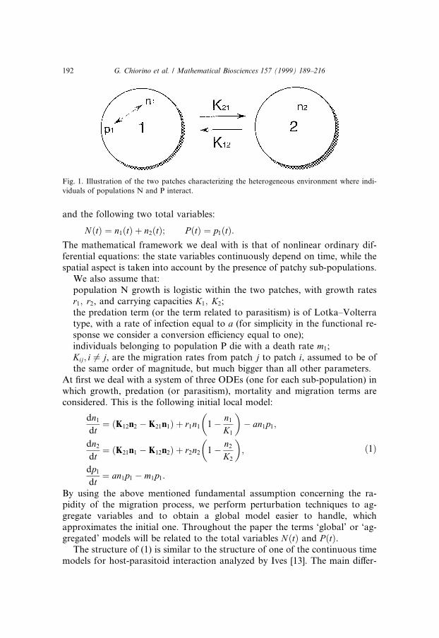
In our general framework individuals belonging to population P live andreproduce themselves in a certain region, called patch 1, while individualsbelonging to population N move continually between this patch and anotherregion, called patch 2. This heterogeneous environment is represented in Fig. 1.We suppose that predation takes place only in patch 1 and that, in the case ofparasitism, the process of infection a�ects host individual ®tness by depletingbody resources, and increases the mortality of hosts.

As a consequence of migrations, population N can be divided into two sub-populations, according to the spatial region occupied. The following three localvariables are considered:

n1�t�: number of individuals of population N in patch 1 at time t;n2�t�: number of individuals of population N in patch 2 at time t;p1�t�: number of individuals of population P in patch 1 at time t;

G. Chiorino et al. / Mathematical Biosciences 157 (1999) 189±216 191

and the following two total variables:

N�t� � n1�t� � n2�t�; P �t� � p1�t�:The mathematical framework we deal with is that of nonlinear ordinary dif-ferential equations: the state variables continuously depend on time, while thespatial aspect is taken into account by the presence of patchy sub-populations.

We also assume that:population N growth is logistic within the two patches, with growth ratesr1; r2, and carrying capacities K1; K2;the predation term (or the term related to parasitism) is of Lotka±Volterratype, with a rate of infection equal to a (for simplicity in the functional re-sponse we consider a conversion e�ciency equal to one);individuals belonging to population P die with a death rate m1;Kij; i 6� j, are the migration rates from patch j to patch i, assumed to be ofthe same order of magnitude, but much bigger than all other parameters.

At ®rst we deal with a system of three ODEs (one for each sub-population) inwhich growth, predation (or parasitism), mortality and migration terms areconsidered. This is the following initial local model:

dn1

dt� �K12n2 ÿ K21n1� � r1n1 1ÿ n1

K1

� �ÿ an1p1;

dn2

dt� �K21n1 ÿ K12n2� � r2n2 1ÿ n2

K2

� �;

dp1

dt� an1p1 ÿ m1p1:

�1�

By using the above mentioned fundamental assumption concerning the ra-pidity of the migration process, we perform perturbation techniques to ag-gregate variables and to obtain a global model easier to handle, whichapproximates the initial one. Throughout the paper the terms `global' or `ag-gregated' models will be related to the total variables N�t� and P �t�.

The structure of (1) is similar to the structure of one of the continuous timemodels for host-parasitoid interaction analyzed by Ives [13]. The main di�er-

Fig. 1. Illustration of the two patches characterizing the heterogeneous environment where indi-

viduals of populations N and P interact.


ences concern the time scale of the migration process and the presence of arefuge in our model. Moreover, parasitism occurs only in one patch and it isconsidered to be proportional to parasitoid density. This means that the per-capita rate at which hosts are parasitized is assumed to be just proportional tothe number of parasitoids, as a ®rst initial approach.

In the framework of prey±predator models, this corresponds to a type Ifunctional response. The presence of di�erent growth rates and carrying ca-pacities in the two patches should be interpreted in terms of patch quality andresources.

3. The method

In this section, the tools which permit to obtain the aggregated model and toanalyze it both qualitatively and numerically are presented, in the particularcase of constant Kij.

3.1. From the initial local model to the aggregated one

In model (1) the fast migration part is written in bold characters. Assumingthat K12 and K21 are of the same order of magnitude, one can write thesequantities in the form

K12 � k12

e; K21 � k21

e; �2�

where e is a small dimensionless number �e ' 0:05� and kij are constant andpositive parameters of the same order as all the other parameters in the model.

By substituting relations (2) into system (1), the following local model isobtained, at the slow time scale:

edn1

dt� �k12n2 ÿ k21n1� � e r1n1 1ÿ n1

K1

� �ÿ an1p1

� �;

edn2

dt� �k21n1 ÿ k12n2� � e r2n2 1ÿ n2

K2

� �� ;

edp1

dt� e�an1p1 ÿ m1p1�:

�3�

Let us now change the time scale, in order to obtain a new local model at thefast time scale t � es. To do this we can write the following relations:

edni

dt� dni

dsand e

dp1

dt� dp1

ds; i � 1; 2 �4�

and substitute them into system (3). We obtain


dn1

ds� �k12n2 ÿ k21n1� � e r1n1 1ÿ n1

K1

� �ÿ an1p1

� �;

dn2

ds� �k21n1 ÿ k12n2� � e r2n2 1ÿ n2

K2

� �� ;

dp1

ds� e�an1p1 ÿ m1p1�:

�5�

As we see, the dynamics in system (5) are driven by the migration part, thedemographic one being only a small perturbation. We are now interested in thefast dynamics and therefore we neglect the small terms �e � 0�. The quantitiesN�s� and P �s� are invariant for the fast dynamics:

n1�s� � n2�s� � N ; p1�s� � P : �6�The fast equilibrium is thus a solution of

dn1

ds� k12�N ÿ n1� ÿ k21n1 � 0 �7�

that is

n�1 �k12

k12 � k21

N ) m�1 �k12

k12 � k21

;

n�2 �k21

k12 � k21

N ) m�2 �k21

k12 � k21

:

�8�

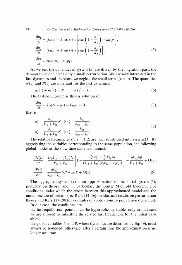
The relative frequencies m�i ; i � 1; 2, are then substituted into system (3). Byaggregating the variables corresponding to the same population, the followingglobal model at the slow time scale is obtained:

dN�t�dt� �r1k12 � r2k21�N

k12 � k21

1ÿ � r1

K1k2

12 � r2

K2k2

21�N�k12 � k21��r1k12 � r2k21�

" #ÿ ak12NP

k12 � k21

�O�e�;

dP �t�dt� ak12

k12 � k21

NP ÿ m1P �O�e�: �9�

The aggregated system (9) is an approximation of the initial system (1);perturbation theory, and, in particular, the Center Manifold theorem, giveconditions under which the errors between this approximated model and theinitial one are of order e (see Refs. [14±16] for classical results on perturbationtheory and Refs. [17±20] for examples of applications to population dynamics).

In our case, the conditions arethe fast equilibrium points must be hyperbolically stable: only in that casewe are allowed to substitute the related fast frequencies for the initial vari-ables;the global variables N and P, whose dynamics are described by Eq. (9), mustalways be bounded: otherwise, after a certain time the approximation is nolonger accurate.


In this section we considered constant migration rates, but the same rea-soning holds for the density-dependent case, where relations analogous to (7)and (8) allow to obtain the patch frequencies of hosts at fast equilibrium. Laterin this article, we will analyze di�erent possible host migration laws betweenpatches and study the asymptotic behavior of the solutions of the related ag-gregated models, by linearization of each system in a neighborhood of itsequilibrium points.

3.2. Aggregated model analysis

In the case of a constant migration scenario, the initial system has a fastequilibrium point which is hyperbolically stable, and from Eq. (8) constant fastfrequencies are obtained. The aggregated model can be rewritten as

dN�t�dt� RN 1ÿ N

K

� �ÿ ANP ;

dP �t�dt� ANP ÿ m1P ;

�10�

with:

R � r1k12 � r2k21

k12 � k21

;

1

K� 1

�k12 � k21��r1k12 � r2k21�r1

K1

k212 �

r2

K2

k221

� �;

A � ak12

k12 � k21

:

This kind of model is the same as the one we used to describe local inter-actions on patch 1 (we refer to the ®rst and the third equations of system (1),without considering the migration part) and its mathematical analysis (steadystates and stability) can be found for example in Ref. [21].

Two kinds of stable equilibrium points can occur, according to parametervalues and independently on initial conditions. These are:

(i) an exclusion point for population P, if �m1=A� > K;(ii) a coexistence point for the two interacting populations, if �m1=A� < K.It can be interesting to perform a comparison with the local stability of the

initial system without patch 2, by looking at the conditions on parameters inboth models. For example, if we consider only a single patch, the condition tohave a stable exclusion point is given by

m1

a> K1; �11�

but it is easy to demonstrate (see Appendix A) that when the values of theparameters in the model are such that


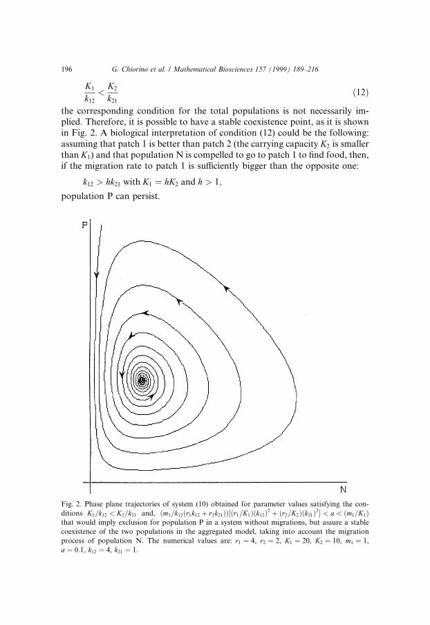
K1

k12

<K2

k21

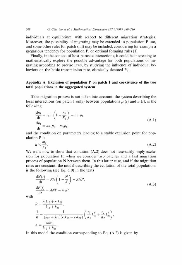
�12�the corresponding condition for the total populations is not necessarily im-plied. Therefore, it is possible to have a stable coexistence point, as it is shownin Fig. 2. A biological interpretation of condition (12) could be the following:assuming that patch 1 is better than patch 2 (the carrying capacity K2 is smallerthan K1) and that population N is compelled to go to patch 1 to ®nd food, then,if the migration rate to patch 1 is su�ciently bigger than the opposite one:

k12 > hk21 with K1 � hK2 and h > 1;

population P can persist.

Fig. 2. Phase plane trajectories of system (10) obtained for parameter values satisfying the con-

ditions K1=k12 < K2=k21 and, �m1=k12�r1k12 � r2k21��r1=K1��k12�2 � �r2=K2��k21�2� < a < �m1=K1�that would imply exclusion for population P in a system without migrations, but assure a stable

coexistence of the two populations in the aggregated model, taking into account the migration

process of population N. The numerical values are: r1 � 4, r2 � 2, K1 � 20, K2 � 10, m1 � 1,

a � 0:1, k12 � 4, k21 � 1.


This example is useful in understanding how the introduction of spatialpatterns can in¯uence the global behavior of the system. When one of thepatches is a prey refuge, we can conclude that its presence might preventpredator extinction and thus favor coexistence of prey and predator. In somecases in fact, the absence of prey refuges can decrease the likelihood of pre-dator persistence. For example, an experimental study on Paramecium±Did-inium interactions [22] showed that without a refuge Didinium died out afterdevouring all the Paramecium, while it sometimes survived when a refuge waspresent. An interesting study on the e�ects of prey refuges on prey±predatorinteractions can be found in Ref. [23].

3.3. Trajectory simulations

In order to simulate the trajectories of a particular system, the followingsteps are made:

a speci®c value is assigned to each parameter, being careful about the biolog-ical meaning;a Runge-Kutta numerical method is applied in order to integrate the initialand the aggregated systems, considering the same initial conditions for bothmodels;the two families of trajectories are compared graphically (for the simulationof the phase-plane trajectories of the aggregated model we use the packageMacMath; otherwise, we implement a Fortran program for the integrationof ODEs).

If the value of e is su�ciently small and all the other conditions required toapply aggregation methods are veri®ed, then the trajectories of the initialsystem and the corresponding trajectories of the global one are very close (seeRef. [24], where some examples of graphical comparison are shown so as tocon®rm the validity of the method).

Two other hypotheses are now considered, corresponding to migration ratesthat are no longer constant. The emergence of new dynamical properties in therelated aggregated models is shown, together with a biological interpretation ofthe results.

4. Density dependent migrations

In this section we want to add the possibility for hosts or preys to adapt theirbehavior to the presence of individuals belonging to population P. We studythe same model as in Section 2, but with some modi®cations in the way ofmigrating between patches.


4.1. Avoiding interactions with population P

It is reasonable to think that individuals belonging to population N areinterested in ®nding a way of reducing their interactions with individuals ofpopulation P; they might adopt di�erent strategies, such as that of avoidingpatches where they are more likely to be `attacked'.

Parasites may in¯uence host patch selection in many ways (Refs. [5,25,26]):for example, the presence of a large number of parasites in certain micro-habitats where hosts are used to spend some time can make them move to otherareas, where there is no risk of infection. In the context of antiparasite patchselection we can mention the example of some cervids [5], which are often seenrunning to the nearest pond when warble ¯ies are present in their grazingpatch. This way, their legs and lower abdomen are in the water and parasitic¯ies cannot deposit their eggs on them.

An example of modi®cation of habitat choice by preys in the presence ofpredators can be found in Ref. [7], where the behavior of small bluegill sun®sh(Lepomis macrochirus) in the presence of largemouth bass predators (Microp-terus salmoides) is described. Both species live in ponds characterized by twodistinct habitats: sheltered areas poor in food and open areas where more foodcan be found. When predators are absent, sun®sh visit both patches, but theychoose the more protected habitat if predators are put into the pond. This way,their predation rate decreases, but their growth rate is a�ected too, as a cost ofthis antipredator behavior.

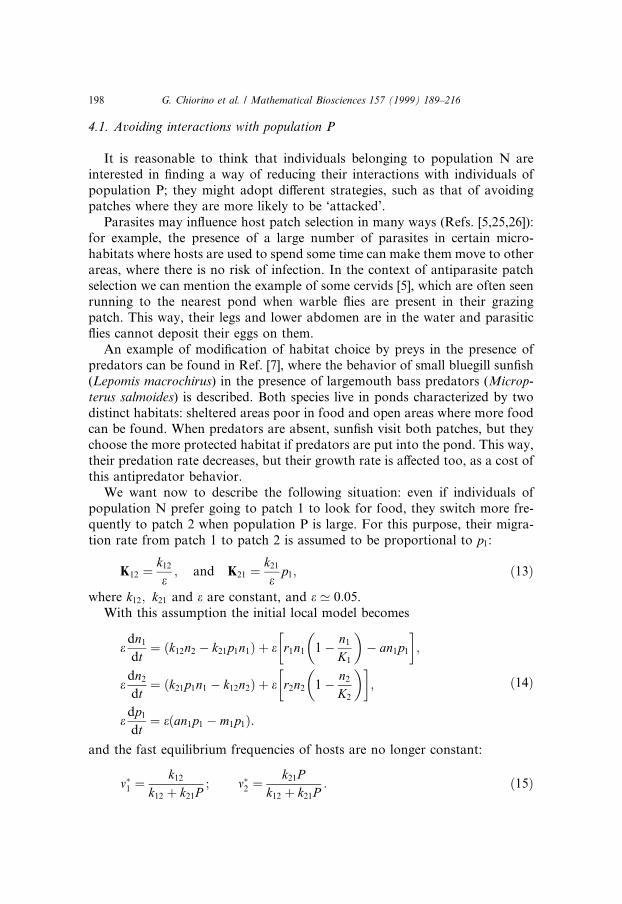
We want now to describe the following situation: even if individuals ofpopulation N prefer going to patch 1 to look for food, they switch more fre-quently to patch 2 when population P is large. For this purpose, their migra-tion rate from patch 1 to patch 2 is assumed to be proportional to p1:

K12 � k12

e; and K21 � k21

ep1; �13�

where k12; k21 and e are constant, and e ' 0:05.With this assumption the initial local model becomes

edn1

dt� k12n2 ÿ k21p1n1� � � e r1n1 1ÿ n1

K1

� �ÿ an1p1

� �;

edn2

dt� k21p1n1 ÿ k12n2� � � e r2n2 1ÿ n2

K2

� �� ;

edp1


�14�

and the fast equilibrium frequencies of hosts are no longer constant:

m�1 �k12

k12 � k21P; m�2 �

k21Pk12 � k21P

: �15�


The aggregated model associated to these frequencies is of the followingform:

dN�t�dt� N

k12 � k21Pk12r1 � �k21r2 ÿ ak12�P ÿ r1k2

12NK1�k12 � k21P�

�ÿ r2k2

21NP 2

K2�k12 � k21P��;

dP �t�dt� P

ak12Nk12 � k21P

ÿ m1

� �:

�16�

The structure of this system is completely new, with respect both to therelated original system and to the classical models we generally ®nd in math-ematical ecology; it has been partially studied in Ref. [27].

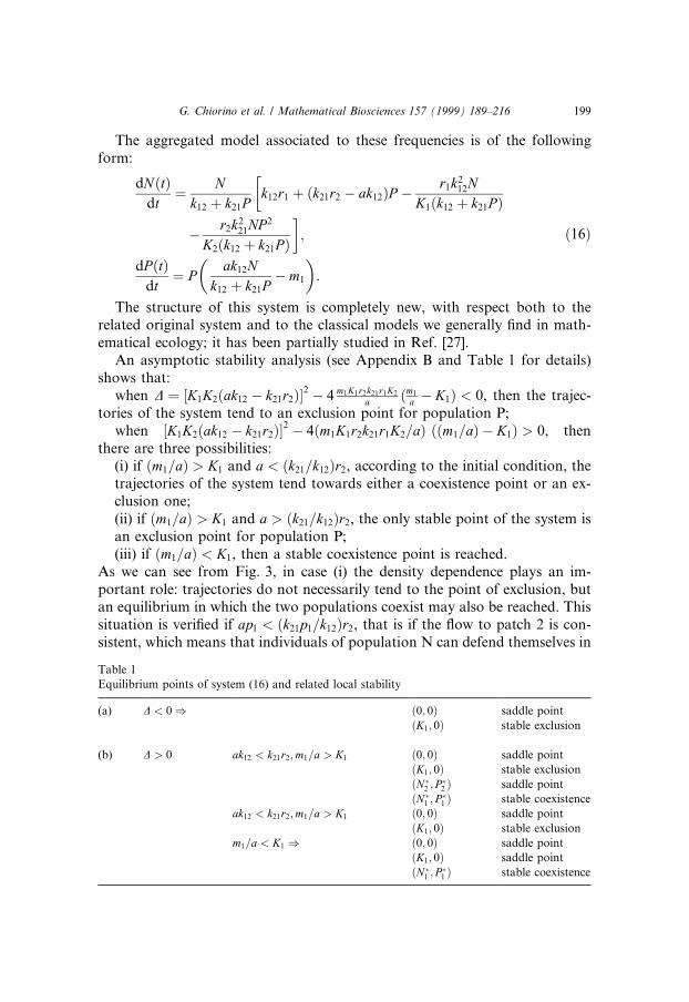
An asymptotic stability analysis (see Appendix B and Table 1 for details)shows that:

when D � �K1K2�ak12 ÿ k21r2��2 ÿ 4 m1K1r2k21r1K2

a �m1

a ÿ K1� < 0, then the trajec-tories of the system tend to an exclusion point for population P;

when �K1K2�ak12 ÿ k21r2��2 ÿ 4�m1K1r2k21r1K2=a� ��m1=a� ÿ K1� > 0, thenthere are three possibilities:

(i) if �m1=a� > K1 and a < �k21=k12�r2, according to the initial condition, thetrajectories of the system tend towards either a coexistence point or an ex-clusion one;(ii) if �m1=a� > K1 and a > �k21=k12�r2, the only stable point of the system isan exclusion point for population P;(iii) if �m1=a� < K1, then a stable coexistence point is reached.

As we can see from Fig. 3, in case (i) the density dependence plays an im-portant role: trajectories do not necessarily tend to the point of exclusion, butan equilibrium in which the two populations coexist may also be reached. Thissituation is veri®ed if ap1 < �k21p1=k12�r2, that is if the ¯ow to patch 2 is con-sistent, which means that individuals of population N can defend themselves in

Table 1

Equilibrium points of system (16) and related local stability

(a) D < 0) �0; 0� saddle point

�K1; 0� stable exclusion

(b) D > 0 ak12 < k21r2;m1=a > K1 �0; 0� saddle point


�N �2 ; P �2 � saddle point

�N �1 ; P �1 � stable coexistence

ak12 < k21r2;m1=a > K1 �0; 0� saddle point


m1=a < K1 ) �0; 0� saddle point

�K1; 0� saddle point



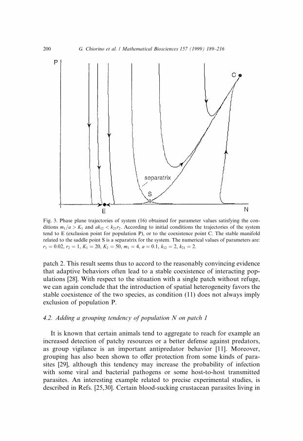
patch 2. This result seems thus to accord to the reasonably convincing evidencethat adaptive behaviors often lead to a stable coexistence of interacting pop-ulations [28]. With respect to the situation with a single patch without refuge,we can again conclude that the introduction of spatial heterogeneity favors thestable coexistence of the two species, as condition (11) does not always implyexclusion of population P.

4.2. Adding a grouping tendency of population N on patch 1

It is known that certain animals tend to aggregate to reach for example anincreased detection of patchy resources or a better defense against predators,as group vigilance is an important antipredator behavior [11]. Moreover,grouping has also been shown to o�er protection from some kinds of para-sites [29], although this tendency may increase the probability of infectionwith some viral and bacterial pathogens or some host-to-host transmittedparasites. An interesting example related to precise experimental studies, isdescribed in Refs. [25,30]. Certain blood-sucking crustacean parasites living in

Fig. 3. Phase plane trajectories of system (16) obtained for parameter values satisfying the con-

ditions m1=a > K1 and ak12 < k21r2. According to initial conditions the trajectories of the system

tend to E (exclusion point for population P), or to the coexistence point C. The stable manifold

related to the saddle point S is a separatrix for the system. The numerical values of parameters are:

r1 � 0:02, r2 � 1, K1 � 20, K2 � 50, m1 � 4, a � 0:1, k12 � 2, k21 � 2.


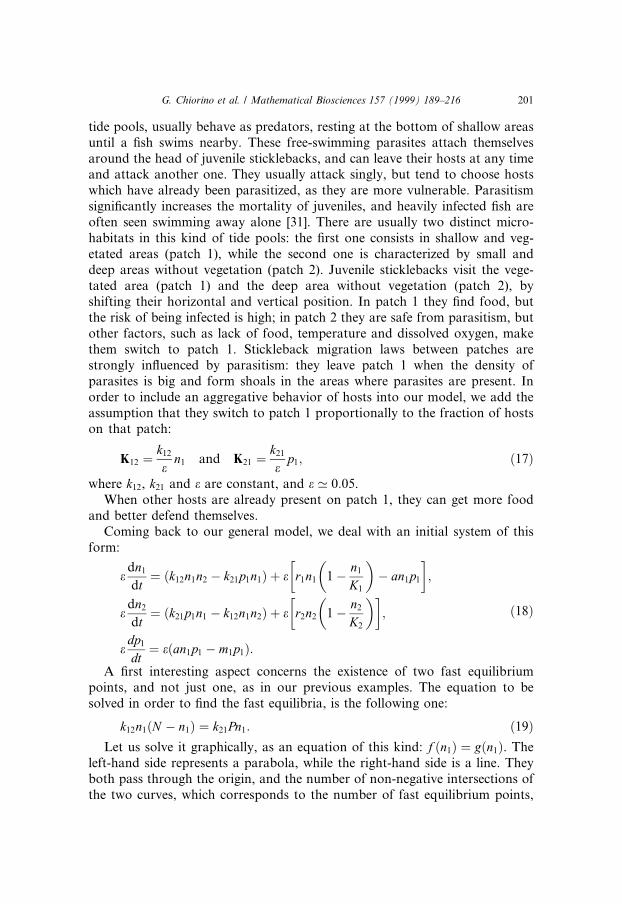
tide pools, usually behave as predators, resting at the bottom of shallow areasuntil a ®sh swims nearby. These free-swimming parasites attach themselvesaround the head of juvenile sticklebacks, and can leave their hosts at any timeand attack another one. They usually attack singly, but tend to choose hostswhich have already been parasitized, as they are more vulnerable. Parasitismsigni®cantly increases the mortality of juveniles, and heavily infected ®sh areoften seen swimming away alone [31]. There are usually two distinct micro-habitats in this kind of tide pools: the ®rst one consists in shallow and veg-etated areas (patch 1), while the second one is characterized by small anddeep areas without vegetation (patch 2). Juvenile sticklebacks visit the vege-tated area (patch 1) and the deep area without vegetation (patch 2), byshifting their horizontal and vertical position. In patch 1 they ®nd food, butthe risk of being infected is high; in patch 2 they are safe from parasitism, butother factors, such as lack of food, temperature and dissolved oxygen, makethem switch to patch 1. Stickleback migration laws between patches arestrongly in¯uenced by parasitism: they leave patch 1 when the density ofparasites is big and form shoals in the areas where parasites are present. Inorder to include an aggregative behavior of hosts into our model, we add theassumption that they switch to patch 1 proportionally to the fraction of hostson that patch:

K12 � k12

en1 and K21 � k21

ep1; �17�

where k12, k21 and e are constant, and e ' 0:05.When other hosts are already present on patch 1, they can get more food

and better defend themselves.Coming back to our general model, we deal with an initial system of this

form:

edn1

dt� k12n1n2 ÿ k21p1n1� � � e r1n1 1ÿ n1

K1

� �ÿ an1p1

� �;

edn2

dt� k21p1n1 ÿ k12n1n2� � � e r2n2 1ÿ n2

K2

� �� ;

edp1


�18�

A ®rst interesting aspect concerns the existence of two fast equilibriumpoints, and not just one, as in our previous examples. The equation to besolved in order to ®nd the fast equilibria, is the following one:

k12n1�N ÿ n1� � k21Pn1: �19�Let us solve it graphically, as an equation of this kind: f �n1� � g�n1�. The

left-hand side represents a parabola, while the right-hand side is a line. Theyboth pass through the origin, and the number of non-negative intersections ofthe two curves, which corresponds to the number of fast equilibrium points,


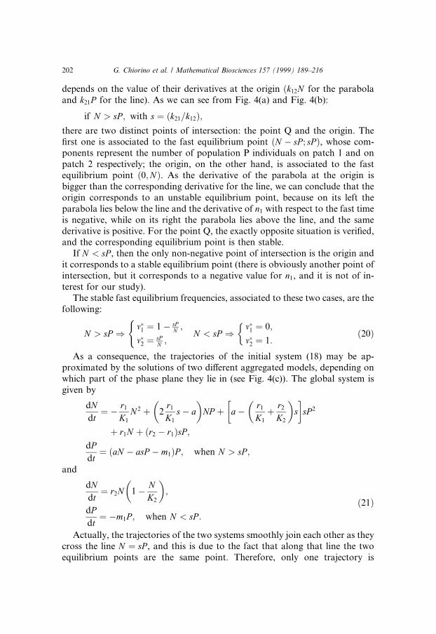
depends on the value of their derivatives at the origin �k12N for the parabolaand k21P for the line). As we can see from Fig. 4(a) and Fig. 4(b):

if N > sP ; with s � �k21=k12�;there are two distinct points of intersection: the point Q and the origin. The®rst one is associated to the fast equilibrium point �N ÿ sP ; sP �, whose com-ponents represent the number of population P individuals on patch 1 and onpatch 2 respectively; the origin, on the other hand, is associated to the fastequilibrium point �0;N�. As the derivative of the parabola at the origin isbigger than the corresponding derivative for the line, we can conclude that theorigin corresponds to an unstable equilibrium point, because on its left theparabola lies below the line and the derivative of n1 with respect to the fast timeis negative, while on its right the parabola lies above the line, and the samederivative is positive. For the point Q, the exactly opposite situation is veri®ed,and the corresponding equilibrium point is then stable.

If N < sP , then the only non-negative point of intersection is the origin andit corresponds to a stable equilibrium point (there is obviously another point ofintersection, but it corresponds to a negative value for n1, and it is not of in-terest for our study).

The stable fast equilibrium frequencies, associated to these two cases, are thefollowing:

N > sP ) m�1 � 1ÿ sPN ;

m�2 � sPN ;

(N < sP ) m�1 � 0;

m�2 � 1:

��20�

As a consequence, the trajectories of the initial system (18) may be ap-proximated by the solutions of two di�erent aggregated models, depending onwhich part of the phase plane they lie in (see Fig. 4(c)). The global system isgiven by

dNdt� ÿ r1

K1

N 2 � 2r1

K1

sÿ a� �

NP � aÿ r1

K1

� r2

K2

� �s

� �sP 2

� r1N � �r2 ÿ r1�sP ;

dPdt� �aN ÿ asP ÿ m1�P ; when N > sP ;

and

dNdt� r2N 1ÿ N

K2

� �;

dPdt� ÿm1P ; when N < sP :

�21�

Actually, the trajectories of the two systems smoothly join each other as theycross the line N � sP , and this is due to the fact that along that line the twoequilibrium points are the same point. Therefore, only one trajectory is


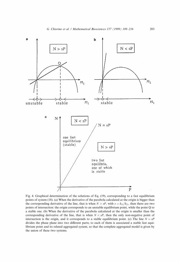
Fig. 4. Graphical determination of the solutions of Eq. (19), corresponding to a fast equilibrium

points of system (18). (a) When the derivative of the parabola calculated at the origin is bigger than

the corresponding derivative of the line, that is when N > sP , with s � k12=k21, then there are two

points of intersection: the origin corresponds to an unstable equilibrium point, while the point Q to

a stable one. (b) When the derivative of the parabola calculated at the origin is smaller than the

corresponding derivative of the line, that is when N < sP , then the only non-negative point of

intersection is the origin, and it corresponds to a stable equilibrium point. (c) The line N � sPdivides the phase plane into two di�erent parts; to each of them is associated a stable fast equi-

librium point and its related aggregated system, so that the complete aggregated model is given by

the union of these two systems.


associated to each initial condition in the positive phase plane. A completeanalysis of the local stability of the aggregated system (21) is presented inAppendix C. Here the main results are discussed (see also Table 2):

when D � �m1 ÿ r2s�2 ÿ �4r1r2m1s2=K2a�� m1

K1aÿ 1� < 0, then the trajectories ofthe system tend towards an exclusion point for population P;when D � �m1 ÿ r2s�2 ÿ �4r1r2m1s2=K2a�� m1

K1aÿ 1� > 0, then the followingpossibilities may occur:(i) if �m1=a� > K1 and m1 < sr2 then there are two coexistence equilibrium

points (one is stable and the other one is a saddle) and an exclusion stablepoint. Therefore, according to the initial condition, the trajectories of thesystem tend towards either an exclusion point or a coexistence one;

(ii) if �m1=a� > K1 and m1 < sr2 an exclusion point for population P isreached;

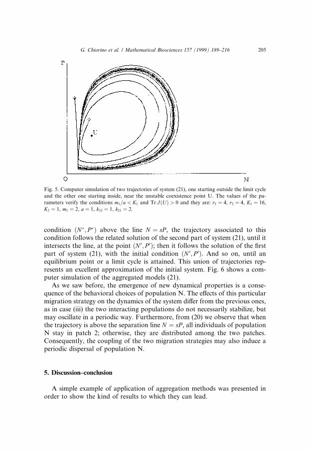
(iii) if �m1=a� < K1 there is an exclusion equilibrium point, which is a saddle,and only one coexistence point. If we look at the sign of the trace of the Ja-cobian matrix calculated at the coexistence point, we see that it may change asparameters vary. If the trace is negative, then a stable equilibrium is reached,while a stable limit cycle occurs when the trace is positive (see Fig. 5 andAppendix C for the proof).

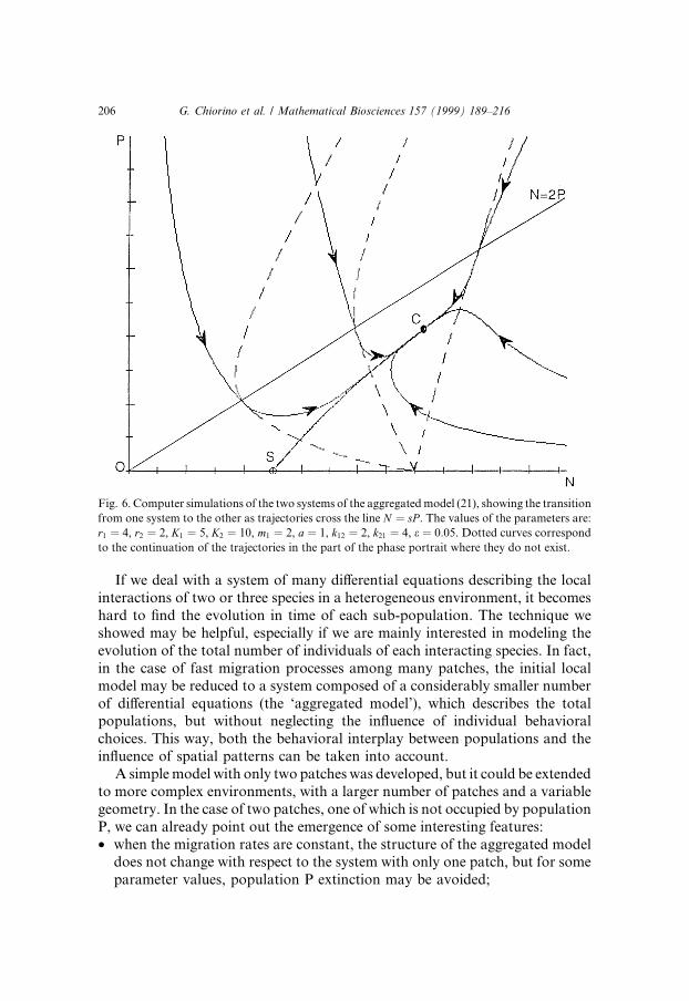
It is interesting to see how the trajectories of the system are obtained: theyare the union of di�erent pieces of curves, which correspond to the solutions ofthe two aggregated models of system (21). For example, starting from an initial

Table 2

Equilibrium points of system (21) and related local stability

(a) D < 0) �0; 0� saddle point


(b) D > 0 m1 < sr2;m1=a > K1 �0; 0� saddle point


�N �2 ; P �2 � saddle point


m1 > sr2;m1=a > K1 �0; 0� saddle point


TrJ � < 0;m1=a < K1 �0; 0� saddle point



TrJ � > 0;m1=a < K1 �0; 0� saddle point


�N �1 ; P �1 � unstable coexistence

around �N �1 ; P �1 � stable limit cycle


condition �N �; P �� above the line N � sP , the trajectory associated to thiscondition follows the related solution of the second part of system (21), until itintersects the line, at the point �N 0; P 0�; then it follows the solution of the ®rstpart of system (21), with the initial condition �N 0; P 0�. And so on, until anequilibrium point or a limit cycle is attained. This union of trajectories rep-resents an excellent approximation of the initial system. Fig. 6 shows a com-puter simulation of the aggregated models (21).

As we saw before, the emergence of new dynamical properties is a conse-quence of the behavioral choices of population N. The e�ects of this particularmigration strategy on the dynamics of the system di�er from the previous ones,as in case (iii) the two interacting populations do not necessarily stabilize, butmay oscillate in a periodic way. Furthermore, from (20) we observe that whenthe trajectory is above the separation line N � sP , all individuals of populationN stay in patch 2; otherwise, they are distributed among the two patches.Consequently, the coupling of the two migration strategies may also induce aperiodic dispersal of population N.

5. Discussion±conclusion

A simple example of application of aggregation methods was presented inorder to show the kind of results to which they can lead.

Fig. 5. Computer simulation of two trajectories of system (21), one starting outside the limit cycle

and the other one starting inside, near the unstable coexistence point U. The values of the pa-

rameters verify the conditions m1=a < K1 and Tr J�U� > 0 and they are: r1 � 4, r2 � 4, K1 � 16,

K2 � 1, m1 � 2, a � 1, k12 � 1, k21 � 2.


If we deal with a system of many di�erential equations describing the localinteractions of two or three species in a heterogeneous environment, it becomeshard to ®nd the evolution in time of each sub-population. The technique weshowed may be helpful, especially if we are mainly interested in modeling theevolution of the total number of individuals of each interacting species. In fact,in the case of fast migration processes among many patches, the initial localmodel may be reduced to a system composed of a considerably smaller numberof di�erential equations (the `aggregated model'), which describes the totalpopulations, but without neglecting the in¯uence of individual behavioralchoices. This way, both the behavioral interplay between populations and thein¯uence of spatial patterns can be taken into account.

A simple model with only two patches was developed, but it could be extendedto more complex environments, with a larger number of patches and a variablegeometry. In the case of two patches, one of which is not occupied by populationP, we can already point out the emergence of some interesting features:· when the migration rates are constant, the structure of the aggregated model

does not change with respect to the system with only one patch, but for someparameter values, population P extinction may be avoided;

Fig. 6. Computer simulations of the two systems of the aggregated model (21), showing the transition

from one system to the other as trajectories cross the line N � sP . The values of the parameters are:

r1 � 4, r2 � 2, K1 � 5, K2 � 10, m1 � 2, a � 1, k12 � 2, k21 � 4, e � 0:05. Dotted curves correspond

to the continuation of the trajectories in the part of the phase portrait where they do not exist.


· when individuals belonging to population N leave patch 1 according to themigration law (13), then the system is more likely to reach a stable equilib-rium where both species coexist, as a result of the new emerging dynamics;from Table 1 it comes out that the condition �m1=a� > K1 is not su�cient tohave exclusion (as in the model with only one patch), but it may lead to thestable coexistence point �N �1 ; P �1 �;

· if in addition they go to patch 1 according to the migration law (17), then theglobal system is described by the union of two di�erent aggregated models.From Table 2, we can also conclude that, under the condition �m1=a� < K1,not only a stable coexistence point (as in the previous case) but also a stablelimit cycle may be attained by the two interacting populations.

The introduction of density-dependent migrations leads then to the emer-gence of aggregated systems which are not classical. In both cases, a necessaryalthough not su�cient condition to have stable exclusion of population P ism1 > aK1, which means a strong mortality for population P, especially when K1

is large, that is patch 1 is potentially favorable for population N, and as aconsequence for interactions between the two populations.

A remark should be done concerning the mathematical formulation of thetwo density-dependent migration laws considered in Section 4. In expression(13), a more realistic choice would be that of considering a saturation e�ect onthe migration process; for example, the coe�cient K21 may be of the followingform:

K21 � 1

eap1

1� p1

� �: �22�

This way, the migration rate from patch 1 would be an increasing function ofpopulation P, but it would not go above the constant a. On the other hand, inexpression (17), it is possible to avoid the arrest of the migration process topatch 2 when n1 is equal to zero, by considering for example:

K12 � 1

e�bn1 � c�: �23�

These hypotheses will be considered in a future work.We are thus able to make some predictions about the local stability of a class

of systems satisfying our qualitative hypotheses, but it will be interesting tomatch our modeling to quantitative biological data.

Another perspective concerns the study of the e�ects of patch selection on thedensities of populations N and P at equilibrium. As a result of patch choicesadopted to avoid attacks from predators (or parasites), population N may reacha bene®t, but at the same time it pays a cost, related for example to reducedfecundity or increased mortality caused by other factors [4]. Starting from thesame initial condition, it would be interesting to compare the total number of


individuals at equilibrium, with respect to di�erent migration strategies.Moreover, the possibility of migrating may be extended to population P too,and some other rules for patch shift may be included, considering for example agregarious tendency for population P, or optimal foraging rules [1].

Finally, in the context of host-parasite interactions, it could be interesting tomathematically explore the possible advantage for both populations of mi-grating according to precise laws, by studying the in¯uence of individual be-haviors on the basic transmission rate, classically denoted R0.

Appendix A. Exclusion of population P on patch 1 and coexistence of the two

total populations in the aggregated system

If the migration process is not taken into account, the system describing thelocal interactions (on patch 1 only) between populations p1�t� and n1�t�, is thefollowing:

dn1

dt� r1n1 1ÿ n1

K1

� �ÿ an1p1;

dp1

dt� an1p1 ÿ m1p1;

�A:1�

and the condition on parameters leading to a stable exclusion point for pop-ulation P is

a <m1

K1

: �A:2�We want now to show that condition (A.2) does not necessarily imply exclu-sion for population P, when we consider two patches and a fast migrationprocess of population N between them. In this latter case, and if the migrationrates are constant, the model describing the evolution of the total populationsis the following (see Eq. (10) in the text)

dN�t�dt� RN 1ÿ N

K

� �ÿ ANP ;

dP �t�dt� ANP ÿ m1P ;

�A:3�

with

R � r1k12 � r2k21

k12 � k21

;

1

K� 1

�k12 � k21��r1k12 � r2k21�r1

K1

k212 �

r2

K2

k221

� �;

A � ak12

k12 � k21

:

In this model the condition corresponding to Eq. (A.2) is given by


A <m1

K�A:4�

that is

ak12

k12 � k21

<m1

�k12 � k21��r1k12 � r2k21�r1

K1

�k12�2 � r2

K2

�k21�2� �

: �A:5�From relation (A.2) we have

ak12 <m1

K1

k12; �A:6�and from (A.5)

ak12 <m1

�r1k12 � r2k21�r1

K1

�k12�2 � r2

K2

�k21�2� �

: �A:7�Therefore, when the following relation is satis®ed:

m1

K1

k12 >m1

�r1k12 � r2k21�r1

K1

�k12�2 � r2

K2

�k21�2� �

; �A:8�both relations (A.2) and (A.4) may be veri®ed at the same time. (A.8) isequivalent to

k12

K1

>1

�r1k12 � r2k21�r1

K1

�k12�2 � r2

K2

�k21�2� �

) k12 >r1K2�k12�2 � r2K1�k21�2�r1k12 � r2k21�K2

) 0 > ÿ r2k21

�r1k12 � r2k21� �r2K1�k21�2

�r1k12 � r2k21�K2k12

) 0 >ÿr2k21K2k12 � r2K1�k21�2�r1k12 � r2k21�K2k12

) K1

k12

<K2

k21

:

Appendix B. Linear stability analysis of the aggregated model (16)

Let us recall the system we want to analyze:

dN�t�dt� N

k12 � k21Pk12r1 � �k21r2 ÿ ak12�P�

ÿ r1k212N

K1�k12 � k21P� ÿr2k2

21NP 2

K2�k12 � k21P ��;

dP �t�dt� P

ak12Nk12 � k21P

ÿ m1

� �:

�B:1�


The positive quadrant of the �N ; P �-plane is positively invariant; the origin(0, 0), the point �K1; 0� and the solutions of

N � m1

k12a�k12 � k21P�;

N � K1K2�k12r1 � �k21r2 ÿ ak12�P ��k12 � k21P �K2r1k2

12 � K1r2k221P 2

;�B:2�

having non-negative components, are the equilibrium points we are interestedin. By substituting the ®rst equation into the second one, we obtain

m1K1r2�k21�2ak12

P 2 � K1K2�ak12 ÿ k21r2�P � r1K2k12

m1

aÿ K1

� �� 0: �B:3�

The discriminant of Eq. (B.3) is given by

D � K21 K2

2 �ak12 ÿ k21r2�2 ÿ 4m1K1r2�k21�2

ar1K2

m1

aÿ K1

� �P 0:

Case (D > 0): Eq. (B.3) has two positive solutions, corresponding to twonon-trivial equilibrium points, if the following conditions are veri®ed:

ak12 < k21r2;m1

a> K1;

�B:4�

it has only one positive solution if

m1=a < K1; �B:5�and two negative solutions otherwise.

Let us now proceed to the analysis of the local stability of the system. To dothis we have to study the eingenvalues of the Jacobian matrices calculated atthe equilibrium points.

As the determinant of the Jacobian matrix calculated at the origin is alwaysnegative, the origin is a saddle point for system (B.1).

The Jacobian matrix calculated at the point �K1; 0� is

J�K1; 0� � ÿr1K1

k12�k21�r1 � r2� ÿ ak12�

0 aK1 ÿ m1

!: �B:6�

Therefore, two possible situations can occur:(i) if �m1=a� > K1, i.e. the determinant of this matrix is positive and the trace

is negative, then the point �K1; 0� is asymptotically stable (it is a sink);(ii) if �m1=a� < K1, then �K1; 0� is a saddle point.When (B.4) is veri®ed, then condition (i) is implied. As Eq. (B.3) has two

positive solutions, there are two other equilibrium points in the positivequadrant; we call them �N �1 ; P �1 � and �N �2 ; P �2 �, where

P �1;2 �ÿK1K2�ak12 ÿ k21r2� �

��Dp

2 m1K1r2�k21�2ak12

and N �1;2 �k21

k12

m1P �1;2 �m1

a: �B:7�


The trace of the Jacobian matrices calculated at both equilibrium points isnegative. The point �N �1 ; P �1 �, that is associated to the plus sign in expression(B.7), is asymptotically stable, as the determinant of the related Jacobianmatrix is positive; while �N �2 ; P �2 � is a saddle point.

If condition (ii) is veri®ed, Eq. (B.3) has only one positive solution, and therelated equilibrium point is always asymptotically stable, as the signs of thedeterminant and the trace of the related Jacobian matrix are respectivelypositive and negative.

There is still one possibility to be analyzed: the one corresponding to twonegative solutions of Eq. (B.3). In this case, as m1=a > K1, the only stable pointof the system is �K1; 0�, which corresponds to an exclusion point forpopulation P.

Case �D > 0�: As Eq. (B.3) has no real solutions, the only two equilibriumpoints of the system are the origin, which is always a saddle point, and (K1; 0).From the negativeness of the discriminant of Eq. (B.3) it follows thatm1=a > K1, and therefore we can conclude that the point (K1; 0) is stable.

Appendix C. Stability analysis of the aggregated model (21)

To begin our analysis, let us consider the ®rst system of the aggregatedmodel (21):

dNdt� ÿ r1

K1

N 2 � 2r1

K1

sÿ a� �

NP � aÿ r1

K1

� r2

K2

� �s

� �sP 2

� r1N � �r2 ÿ r1�sP ;

dPdt� �aN ÿ asP ÿ m1�P ; �C:1�

where N > sP and s � �k21=k12�, and ®nd the related nullclines. The equationdN=dt � 0 represents the equation of a conic, while dP=dt � 0 is the product ofthe axis P � 0 and the line N � sP � �m1=a�.

A ®rst point of equilibrium for system (C.1) is given by the origin (0, 0);another one is the point �K1; 0� and the remaining equilibria are given by thesolutions of the following system:

N � sP � m1

a;

ÿ r1

K1

N 2 � 2r1

K1

sÿ a� �

NP � aÿ r1

K1

� r2

K2

� �s

� �sP 2 � r1N � �r2 ÿ r1�sP

� 0: �C:2�By substituting the ®rst equation into the second one, we obtain


r2

K2

s2P 2 � �m1 ÿ r2s�P � r1m1

am1

K1aÿ 1

� �� 0 �C:3�

This is a second degree equation, and its discriminant is given by

D � �m1 ÿ r2s�2 ÿ 4r2

K2

s2 r1m1

am1

K1aÿ 1

� �: �C:4�

Case �D > 0�: Eq. (C.3) has two positive solutions if

m1 ÿ r2s < 0;m1

a> K1; �C:5�

it has only one positive solution if

m1

a< K1; �C:6�

and two negative solutions otherwise.The expression of the roots of Eq. (C.3) is the following:

P �1;2 �r2sÿ m1 �

��Dp

2 r2

K2s2

; �C:7�

where the sub-index 1 is associated to the sign plus and the sub-index 2 to thesign minus. The related values of N are given by

N �1;2 � sP �1;2 �m1

a: �C:8�

From expression (C.8) we can see that a positive value for N is associated toany positive solution of (C.3).

Let us now consider Jacobian matrices calculated at the equilibrium pointsof the system. For the origin we have

J�0; 0� � r1 �r2 ÿ r1�s0 ÿm1

� �: �C:9�

As its determinant is always negative, we can conclude that the origin is asaddle point.

The Jacobian matrix calculated at the point �K1; 0� is given by

J�K1; 0� �ÿr1 r1s� r2 ÿ aK1

0 aK1 ÿ m1

� �: �C:10�

Two possible situations can occur:(i) if �m1=a� > K1, that is the determinant of this matrix is positive and the

trace is negative, then the point �K1; 0� is asymptotically stable (it is a sink);(ii) if �m1=a� < K1, then �K1; 0� is a saddle point.

If (C.5) is veri®ed, that is if Eq. (C.3) has two positive solutions, we have alsoto analyze the stability of the equilibrium points �N �1 ; P �1 � and �N �2 ; P �2 �. Therelated Jacobian matrices have a negative trace, while the determinant is


positive for �N �1 ; P �1 � and negative for �N �2 ; P �2 �. Therefore the ®rst point is as-ymptotically stable and the second one is a saddle point. In this case condition(i) is satis®ed and the point �K1; 0� is asymptotically stable.

When condition (ii) is veri®ed, Eq. (C.3) has only one positive solution, andthe determinant of the Jacobian matrix calculated at the related equilibriumpoint is always positive. The expression of the trace is given by

Tr J � � ÿ 2r1m1

K1a� r1 � a�1� s� K2

2r2s2�m1 ÿ r2sÿ

��Dp�: �C:11�

When (C.11) is negative, then the equilibrium point is asymptotically stable,while it is unstable as the trace becomes positive.

When Eq. (C.3) has two negative solutions, that is if the following conditionis veri®ed:

m1 ÿ r2s > 0;m1

a> K1; �C:12�

then there are only two equilibrium points in the positive part of the phaseplane. They are the origin, a saddle point, and �K1; 0�, which is asymptoticallystable.

Case �D < 0�: When the discriminant of Eq. (C.3) is negative, then there areno real intersections between the conic and the line N � sP � �m1=a�. Thereforethe only equilibrium points are the origin, which is a saddle point, and �K1; 0�.The condition m1=a > K1 is implied by the negativeness of the discriminant,and then the point �K1; 0� is asymptotically stable.

Observation 1. As the line N � sP is always parallel to the nullclineN � sP � �m1=a�, all the equilibrium points of system (C.1) which lie in thepositive quadrant are also equilibrium points of model (21).

In fact the nullcline N � sP � �m1=a� intersects the N axis at m1=a; 0� � and,apart from the origin and the point �K1; 0�, all the other equilibrium points ofsystem (C.1) are on this nullcline. Therefore all of them lie below the lineN � sP , that is the part of the phase plane where model (21) is given by system(C.1). This is true also for �K1; 0� and for (0, 0), which is on the boundary ofthis region.

Let us now proceed to the analysis of the second system of model (21), thatis

dNdt� r2N 1ÿ N

K2

� �;

dPdt� ÿm1P :

�C:13�

In this simple system the positive quadrant of the �N ; P �-plane is positivelyinvariant and there are only two equilibrium points: the origin (0, 0), which isalways a saddle point, and the point �K2; 0�, which is always stable. But the


latter is not an equilibrium point for the aggregated model (21), because it liesin the part of the phase plane which is below the line N � sP .

From the analysis of the two systems, we can conclude that all the trajec-tories associated to initial conditions which are above the line N � sP go downin the direction of the point �K2; 0� until they encounter the line N � sP ; as theycross this line, they follow the dynamics of system (C.1). If they do not en-counter the line N � sP again, then it means that they have reached an equi-librium point; otherwise, they follow again the dynamics of system (C.13), andthe reasoning is repeated.

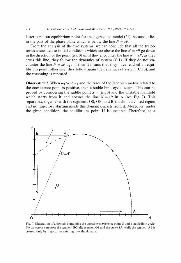
Observation 2. When m1=a < K1 and the trace of the Jacobian matrix related tothe coexistence point is positive, then a stable limit cycle occurs. This can beproved by considering the saddle point S � �K1; 0� and the unstable manifoldwhich starts from it and crosses the line N � sP in A (see Fig. 7). Thisseparatrix, together with the segments OS, OB, and BA, delimit a closed regionand no trajectory starting inside this domain departs from it. Moreover, underthe given condition, the equilibrium point U is unstable. Therefore, as a

Fig. 7. Illustration of a domain containing the unstable coexistence point U and a stable limit cycle.

No trajectory can cross the segment BO, the segment OS and the curve SA, while the segment AB is

crossed only by trajectories entering into the domain.


consequence of the Poincar�e±Bendixson theorem, a limit cycle occurs insidethis closed region.

When the trace given by expression (C.11), which is a continuous function ofthe parameters of the system, changes signs and becomes positive, a Hopfbifurcation occurs. In fact, the trajectories of the system do not spiral towardsa new stable equilibrium point, but tend to a limit cycle.

References

[1] M. Mangel, B.D. Roitberg, Behavioral stabilization of host±parasite population dynamics,

Theor. Pop. Biol. 42 (1992) 308.

[2] M.P. Hassel, R.M. May, From individual behavior to population dynamics, in: R.M. Sibly,

R.H. Smith (Eds.), Behavioral ecology; ecological consequences of adaptive behavior.

Blackwell, Oxford, 1985, p. 3.

[3] G.A. Parker, Population consequences of evolutionarily stable strategies, in: R.M. Sibly, R.H.

Smith (Eds.), Behavioral Ecology; Ecological Consequences of Adaptive Behavior, Blackwell,

Oxford, 1985, p. 33.

[4] A.R. Ives, A.P. Dobson, Antipredator behavior and the population dynamics of simple

predator±prey systems, Am. Natural 130 (1987) 431.

[5] B.L. Hart, Behavioural defense against parasites: interaction with parasite invasiveness,

Parasitology 109 (1994) 139.

[6] C. Loehle, Social barriers to pathogen transmission in wild animal population, Ecology 76

(1995) 326.

[7] E.E. Werner, J.F. Gilliam, D.J. Hall, G.G. Mittelbach, An experimental test of the e�ects of

predation risk on habitat use in ®sh, Ecology 64 (1983) 1540.

[8] A. Sih, Optimal behavior: can foragers balance two con¯icting demands?, Science (Wash.,

DC) 210 (1980) 1041.

[9] A. Sih, Antipredator responses and the perception of danger by mosquito larvae, Ecology 67

(1986) 434.

[10] D.F. Fraser, F.A. Huntingford, Feeding and avoiding predation hazard: the behavioral

response of the prey, Ethology 73 (1986) 56.

[11] H.R. Pulliam, T. Caraco, Living in groups: is there an optimal group size? in: J.R. Krebs, N.B.

Davies (Eds.). Behavioural Ecology: an Evolutionary Approach, 2d ed., Sinauer, Sunderland,

MA, 1984, p. 122.

[12] R.D. Holt, M.P. Hassel, Environmental heterogeneity and the stability of host-parasitoid

interactions, J. Anim. Ecol. 62 (1993) 89.

[13] A.R. Ives, Continuous-time models of host-parasitoid interactions, Am. Natural 140 (1992) 1.

[14] N. Fenichel, Persistence and smoothness in invariant manifolds for ¯ows, Indiana Univ.

Math. J. 21 (1971) 193.

[15] F.C. Hoppensteadt, Singular perturbations of the in®nite interval, Trans. Am. Math. Soc. 123

(1966) 521.

[16] Tihonov, On the dependence of the solutions of di�erential equations on a small parameter.

Mat. Sbornik 22 (1948) 193.

[17] J.-C. Poggiale, Application des vari�et�es invariantes �a la mod�elisation de l'h�et�erog�en�eit�e en

dynamique des populations. Thesis. Universit�e de Bourgogne, Dijon, Laboratoire de

Topologie, 1994.

[18] P. Auger, R. Roussarie, Complex ecological models with simple dynamics: from individuals to

populations, Acta Biotheoretica 42 (1994) 111.


[19] P. Auger, J.C. Poggiale, Emergence of population growth models: fast migration and slow

growth, J. Theor. Biol. 182 (1996) 99.

[20] J. Michalski, J.-C. Poggiale, R. Arditi, P. Auger, Macroscopic dynamic e�ects of migrations in

patchy predator±prey systems, J. Theor. Biol. 185 (1997) 459.

[21] L. Edelstein-Keshet, Mathematical Models in Biology, Random House Birkhauser, Boston,

1988.

[22] G.F. Gause, The Struggle for Existence, Williams and Wilkins, Baltimore, 1934.

[23] J.N. McNair, The e�ects of refuges on predator±prey interactions: a reconsideration, Theor.

Pop. Biol. 29 (1986) 38.

[24] P. Auger, J.-C. Poggiale, Emerging properties in population dynamics with di�erent time

scales, J. of Biolog. Syst. 32 (1995) 591.

[25] R. Poulin, G.J. Fitzgerald, Risk of parsitism and microhabitat selection in juvenile

sticklebacks, Can. J. Zool. 67 (1989) 14.

[26] H. Tashiro, H.H. Schwardt, Biological studies of horse ¯ies in New York, J. Econ. Entomol.

46 (1953) 813.

[27] S. Morand, P. Auger, J.-L. Chass�e, Parasitism and host patch selection: a model using

aggregation methods, Mathemat. Comp. Model. 27 (4) (1998) 73.

[28] C. Combes, Interactions Durables, Ecologie et Evolution du Parasitisme, vol. 26, Collection

Ecologie, Masson, Paris, 1995.

[29] M.S. Mooring, B.L. Hart, Animal grouping for protection from parasites: sel®sh herd and

encounter-dilution e�ects, Behaviour 123 (1992) 173.

[30] R. Poulin, G.J. Fitzgerald, Shoaling as an anti-ectoparasite mechanism in juvenile stickle-

backs, Behav. Ecol. Sociobiol. 24 (1989) 251.

[31] J.F. Guthrie, R.L. Kroger, Schooling habits of injured and parasitized menhanden, Ecology

55 (1974) 208.


Behavioral choices based on patch selection: a model using aggregation methods

Documents

Transcript of Behavioral choices based on patch selection: a model using aggregation methods