Making Choices in Risky Situations

CHAPTER 3

Making Choices in Risky Situations

Chapter Outline3.1 Introduction 55

3.2 Choosing Among Risky Prospects: Preliminaries 56

3.3 A Prerequisite: Choice Theory Under Certainty 61

3.4 Choice Theory Under Uncertainty: An Introduction 63

3.5 The Expected Utility Theorem 66

3.6 How Restrictive Is Expected Utility Theory? The Allais Paradox 72

3.7 Behavioral Finance 753.7.1 Framing 76

3.7.2 Prospect Theory 78

3.7.2.1 Preference Orderings with Connections to Prospect Theory 83

3.7.3 Overconfidence 84

3.8 Conclusions 85

References 85

3.1 Introduction

The first stage of the equilibrium perspective on asset pricing consists of developing an

understanding of the determinants of the demand for securities of various risk classes.

Individuals demand securities (in exchange for current purchasing power) in their attempt

to redistribute income across time and states of nature. This is a reflection of the

consumption-smoothing and risk-reallocation function central to financial markets.

Our endeavor requires an understanding of three building blocks:

1. How financial risk is defined and measured.

2. How an investor’s attitude toward or tolerance for risk is to be conceptualized and

then measured.

3. How investors’ risk attitudes interact with the subjective uncertainties associated with

the available assets to determine an investor’s desired portfolio holdings (demands).

In this and the next chapter, we give a detailed overview of points 1 and 2; point 3 is

treated in succeeding chapters.

55Intermediate Financial Theory.

© 2015 Elsevier Inc. All rights reserved.

3.2 Choosing Among Risky Prospects: Preliminaries

When we think of the “risk” of an investment, we are typically thinking of uncertainty in

the future cash-flow stream to which the investment represents title. Depending on the state

of nature that may occur in the future, we may receive different payments and, in particular,

much lower payments in some states than others. That is, we model an asset’s associated

cash flow in any future time period as a random variable.

Consider, for example, the investments listed in Table 3.1, each of which pays off next

period in either of two equally likely states. We index these states by θ5 1,2 with their

respective probabilities labeled π1 and π2.

First, this comparison serves to introduce the important notion of dominance. Investment 3

clearly dominates both investments 1 and 2 in the sense that it pays as much in all states of

nature and strictly more in at least one state. The state-by-state dominance illustrated here

is the strongest possible form of dominance. Without any qualification, we will assume that

all rational individuals would prefer investment 3 to either of the other two. Basically, this

means that we are assuming the typical individual to be nonsatiated in consumption: she

desires more rather than less of the consumption goods these payoffs allow her to buy.

In the case of dominance, the choice problem is trivial and, in some sense, the issue of

defining risk is irrelevant. The ranking defined by the concept of dominance is, however,

very incomplete. If we compare investments 1 and 2, we see that neither dominates the

other. Although it performs better in state 2, investment 2 performs much worse in state 1.

There is no ranking possible on the basis of the dominance criterion. The different

prospects must be characterized from a different angle. The concept of risk enters

necessarily.

On this score, we would probably all agree that investments 2 and 3 are comparatively

riskier than investment 1. Of course, for investment 3, the dominance property means that

the only risk is an upside risk. Yet, in line with the preference for smooth consumption

discussed in Chapter 1, the large variation in date 1 payoffs associated with investment 3 is

to be viewed as undesirable in itself. When comparing investments 1 and 2, the qualifier

Table 3.1: Asset payoffs ($)

Value at t5 1

π15π25 1/2

Cost at t5 0 θ51 θ5 2

Investment 1 21000 1050 1200Investment 2 21000 500 1600Investment 3 21000 1050 1600

56 Chapter 3

“riskier” undoubtedly applies to the latter. In the worst state, the payoff associated with 2 is

much lower; in the best state it is substantially higher.

These comparisons can alternatively, and often more conveniently, be represented if we

describe investments in terms of their performance on a per dollar basis. We do this by

computing the state-contingent rates of return (ROR) that we will typically associate

with the symbol r. In the case of the above investments, we obtain the results given

in Table 3.2.

One sees clearly that all rational individuals should prefer investment 3 to the other two and

that this same dominance cannot be expressed when comparing 1 and 2.

The fact that investment 2 is riskier, however, does not mean that all rational risk-averse

individuals would necessarily prefer 1. Risk is not the only consideration, and the ranking

between the two projects is, in principle, preference dependent. This is more often the case

than not; dominance usually provides a very incomplete way of ranking prospects. This fact

suggests we must turn to a description of preferences, the main objective of this chapter.

The most well-known approach at this point consists of summarizing such investment

return distributions (i.e., the random variables representing returns) by their mean ðEriÞ andvariance ðσ2

i Þ, i5 1,2,3. The variance (or its square root, the standard deviation) of the rate

of return is then naturally used as the measure of “risk” of the project (or the asset). For the

three investments just listed, we have:

Er1 5 12:5%; σ215

1

2ð5212:5Þ2 1 1

2ð20212:5Þ2 5 ð7:5Þ2; or σ15 7:5%

Er2 5 5%; σ25 55% ðsimilar calculationÞEr3 5 32:5%; σ35 27:5%

If we decided to summarize these return distributions by their means and variances only,

investment 1 would clearly appear more attractive than investment 2: it has both a higher

mean return and a lower variance. In terms of the mean�variance criterion, investment 1

dominates investment 2; 1 is said to mean�variance dominate 2. Our previous discussion

makes it clear that mean�variance dominance neither implies nor is implied by state-by-

state dominance. Investment 3 mean�variance dominates 2 but not 1, although it dominates

Table 3.2: State-contingent ROR (r)

θ51 θ5 2

Investment 1 5% 20%Investment 2 250% 60%Investment 3 5% 60%

Making Choices in Risky Situations 57

them both on a state-by-state basis! This is surprising and should lead us to be cautious

when using any mean�variance return criterion. Later, we will detail circumstances where

it is fully reliable. At this point, let us anticipate that it is not generally so and that

restrictions will have to be imposed to legitimize its use.

The notion of mean�variance dominance, which plays a prominent role in modern portfolio

theory, can be expressed in the form of a criterion for selecting investments of equal

magnitude:

1. For investments of the same Er, choose the one with the lowest σ.2. For investments of the same σ, choose the one with the greatest Er.

In the framework of modern portfolio theory, one could not understand a rational agent

choosing investment 2 rather than investment 1.

We cannot limit our inquiry to the concept of dominance, however. Mean�variance

dominance provides only an incomplete ranking among uncertain prospects,

as Table 3.3 illustrates.

When we compare these two investments, we do not clearly see which is best; there is no

dominance in either state-by-state or mean�variance terms. Investment 5 is expected to pay

1.25 times the expected return of investment 4, but, in terms of standard deviation, it is also 3

times riskier. The choice between 4 and 5, when restricted to mean�variance

characterizations, would require specifying the terms at which the decision maker is willing

to substitute expected return for a given risk reduction. In other words, what decrease in

expected return is the decision maker willing to accept for a 1% decrease in the standard

deviation of returns? Or, conversely, does the 1 percentage point additional expected return

associated with investment 5 adequately compensate for the (3 times) larger risk? Responses

to such questions are preference dependent (i.e., they vary from individual to individual).

Suppose, for a particular individual, the terms of the trade-off are well represented by the

index E/σ. Since (E/σ)45 4 while (E/σ)55 5/3, investment 4 is better than investment 5 for

that individual. Of course, another investor may be less risk averse; i.e., he may be willing

to accept more extra risk for the same expected return. For example, his preferences may be

Table 3.3: State-contingent ROR (r)

θ51 θ52

Investment 4 3% 5%Investment 5 2% 8%

π15π25 12

ER45 4%; σ45 1%ER55 5%; σ55 3%

58 Chapter 3

adequately represented by (E2 1/3σ) in which case he would rank investment 5 (with an

index value of 4) above investment 4 (with a value of 32

3).1

All these considerations strongly suggest that we have to adopt a more general viewpoint

for comparing potential return distributions. This viewpoint is part of utility theory, to

which we now turn after describing some of the problems associated with the empirical

characterization of return distributions in Box 3.1.

1 Observe that the proposed index is not immune to the criticism discussed above: investment 3 (E/σ5 1.182)

is inferior to investment 1 (E/σ5 1.667). Yet, we know that three dominates one because it pays a higher

return in every state. This problem is pervasive with the mean�variance investment criterion: whatever the

terms of the trade-off between mean and variance or standard deviation, one can produce a paradox such as

the one illustrated above. Accordingly, this criterion is not generally applicable without additional restrictions.

The index E/σ resembles, but is not identical to, the Sharpe ratio, ðE ~r2 rfÞ=σ ~r , where rf denotes the

risk-free rate.

BOX 3.1 Computing Means and Variances in Practice

Useful as it may be conceptually, calculations of distribution moments such as the mean andthe standard deviation are difficult to implement in practice: we rarely know what the futurestates of nature are, let alone their probabilities. We also do not know the returns in eachstate. A frequently used proxy for a future return distribution is its historical distribution. Thisamounts to selecting a historical time period and a periodicity, say monthly prices for the past60 months, and computing the historical (net) returns as follows:

a. Discrete compounding

rej 5 ðnetÞ return to stock ownership in month j5 ððqej 1 djÞ=qej21Þ2 1

where qej is the price of the stock in month j, and dj its dividend, if any, that month; 11 rejis referred to as the gross return. We then summarize the past distribution of stock returnsby the average historical return and the variance of the historical returns. By doing so, we,in effect, assign an equal probability of 1

60 to each past observation or event.

b. Continuous compounding

To understand how to compute period-by-period returns “under continuouscompounding,” we must first explain what this convention entails. Conceptually,continuous compounding is the result of discrete compounding when the correspondingtime interval becomes infinitesimally small. Suppose an investor’s wealth is Y0, which heinvests at a rate r for one period (let us say a month as in (a)). If the rate r is continuouslycompounded over this single period, the cumulative wealth consequence is as follows:

Y0/Y0 limn/N

11r

n

� �n5 Y0e

r

(Continued)


BOX 3.1 Computing Means and Variances in Practice (Continued)

which exceeds the cumulative effect under discrete compounding (Y0er . Y0ð11 rÞ

if r. 0). It also follows from this identification that if a one period rate r iscontinuously compounded for a succession of J periods, the cumulative wealth effectwill be

Lastly, if wealth Y0 is invested successively at the continuously compounded discrete ratesr1 and r2, the cumulative effect will be

i.e., under continuous compounding rates of return may simply be added to givetheir cumulative effect. As we will see in subsequent chapters, this additive featurewill allow various calculations to be simplified if the continuous compoundingconvention is assumed. Note also that our notation assigns the “age interpretation”to time periods: period 10, say, corresponds to the end of the 10th time intervaljust as a child’s 10th birthday is celebrated at the conclusion of his 10th yearof life.Given this setting, how are returns computed from discrete data under the continuouscompounding convention? Again, let us assume the following data for some stock ispresented to us:

t1 j2 1 t1 j

qej21 qej 1 divj

(Continued)

60 Chapter 3

3.3 A Prerequisite: Choice Theory Under Certainty

A good deal of financial economics is concerned with how people make choices.

The objective is to understand the systematic part of individual behavior and to be able to

predict (at least in a loose way) how an individual will react under specific economic

circumstances. Economic theory describes individual behavior as the result of a process of

optimization under constraints, the objective to be reached being determined by individual

preferences, and the constraints being a function of the person’s income or wealth level and

of market prices. This approach, which defines the homo economicus and the notion of

economic rationality, is justified by the fact that individual behavior is predictable only to

the extent that it is systematic, which must mean that there is an attempt to achieve a well-

defined objective. It is not to be taken literally or normatively.4

BOX 3.1 Computing Means and Variances in Practice (Continued)

We may now ask the question: what discrete rate of return re;cont:j , when continuouslycompounded, was earned by this stock in the course of period j? Equivalently, what rateof return re;cont:j satisfies:

qej21 ere; cont:j 5 qej 1 divj?

Thus,

re; cont:j 5 ‘nqej 1 divj

qej21

!5 lnð11 rej Þ

In what follows in this book, the unspoken assumption is that reported return data iscomputed under the continuous compounding convention as per the above calculation.Accordingly, we generally do not employ the “cont.” superscript.2

Using the pattern of historical returns (however measured) to infer properties of the futurereturn distribution makes sense if we think the “mechanism” generating these returns is“stationary”: that the future will in some sense closely resemble the past. In practice, thishypothesis is rarely fully verified and, at the minimum, it requires careful checking.3

2 When returns are small, rj� ln(11 rj). This is a standard approximation. Note that continuously compoundedreturns are the natural logarithm of discrete gross returns and, in this sense, are the continuously compoundedcointegral to discrete gross returns.

3 The accuracy of the mean and variance estimates from historical data as stand-ins to the underlying returndistribution’s true (future) mean and variance is a topic of great significance and to which we will return(c.f. Chapter 7).

4 By this we mean that economic science does not prescribe that individuals maximize, optimize, or simply

behave as if they were doing so. It just finds it productive to summarize the systematic behavior of economic

agents with such tools.


To develop this sense of rationality systematically, we begin by summarizing the objectives

of investors in the most basic way: we postulate the existence of a preference relation,

represented by the symbol j, describing investors’ ability to compare various bundles of

goods and services. For two bundles a and b, the expression

akb

is to be read as follows: For the investor in question, bundle a is either strictly preferred to

bundle b, or he is indifferent between them. Pure indifference is denoted by aBb, strict

preference by agb.

The notion of economic rationality can then be summarized by the following assumptions:

A.1 Every investor possesses such a preference relation and it is complete, meaning that

he is able to decide whether he prefers a to b, b to a, or both, in which case he is

indifferent with respect to the two bundles. That is, for any two bundles a and b,

either ajb or bja, or both. If both hold, we say that the investor is indifferent with

respect to the bundles and write aBb.

A.2 This preference relation satisfies the fundamental property of transitivity: For any

bundles a, b, and c, if ajb and bjc, then ajc.

A further requirement is also necessary for technical reasons:

A.3 The preference relation j is continuous in the following sense: Let {xn} and {yn} be

two sequences of consumption bundles such that xn/x and yn/y.5 If xnjyn for all

n, then the same relationship is preserved in the limit xjy.

A key result can now be expressed in the following proposition.

Theorem 3.1 Assumptions A.1 through A.3 are sufficient to guarantee the existence of a

continuous, time-invariant, real-valued utility function6 u, such that for any two objects of

choice (consumption bundles of goods and services),

akb if and only if

uðaÞ$ uðbÞ:

Proof See, for example, Mas-Colell et al. (1995), Proposition 3.C.1.

This result asserts that to endow decision makers with a utility function (which they are

assumed to maximize) is, in reality, no different than to assume their preferences among

objects of choice define a relation possessing the (weak) properties summarized in A.1

through A.3.

5 We use the standard sense of (normed) convergence in RN.6 In other words, u: RN-R1.

62 Chapter 3

Note that Theorem 3.1 implies that if u( ) is a valid representation of an individual’s

preferences, any increasing transformation of u( ) is also valid since such a transformation,

by definition, will preserve the ordering induced by u( ). Note also that the notion of a

consumption bundle is, formally, very general. Different elements in a bundle may

represent the consumption of the same good or service in different time periods. One

element might represent a vacation trip in the Bahamas this year; another may represent

exactly the same vacation next year. We can further expand our notion of different goods

to include the same good consumed in mutually exclusive states of the world. Our

preference for hot soup, for example, may be very different if the day is warm rather than

cold. These thoughts suggest that Theorem 3.1 is really quite general and can, formally at

least, be extended to accommodate uncertainty. Under uncertainty, however, ranking

bundles of goods (or vectors of monetary payoffs, see below) involves more than pure

elements of taste or preferences. In the hot soup example, it is natural to suppose that our

preferences for hot soup are affected by the probability we attribute to the day being hot or

cold. Disentangling pure preferences from probability assessments is the subject to which

we now turn.

3.4 Choice Theory Under Uncertainty: An Introduction

Under certainty, the choice is among consumption baskets with known characteristics.

Under uncertainty, however, our emphasis changes. The objects of choice are typically

no longer consumption bundles but vectors of state-contingent money payoffs

(we will reintroduce consumption in Chapter 5). Such vectors are formally what we

mean by an investment or an asset available for purchase. When we purchase a share

of a stock, for example, we know that its sale price in one year will differ depending on

what events transpire within the firm and in the world economy. Under financial

uncertainty, therefore, the choice is among alternative investments leading to different

possible income levels and, hence, ultimately different consumption possibilities. As

before, we observe that people do make investment choices, and if we are to make sense

of these choices, there must be a stable underlying order of preference defined over

different alternative investments. The spirit of Theorem 3.1 will still apply. With

appropriate restrictions, these preferences can be represented by a utility index defined

on investment possibilities, but obviously something deeper is at work. It is natural to

assume that individuals have no intrinsic taste for the assets themselves (IBM stock as

opposed to Royal Dutch Petroleum stock (hereafter RDS), for example). Rather, they are

interested to know what payoffs these assets will yield and with what likelihood

(see Box 3.2, however).


One may further hypothesize that investor preferences are indeed very simple after

uncertainty is resolved: They prefer a higher monetary payoff to a lower one or,

equivalently, to earn a higher return rather than a lower one. Of course they do not know

ex ante (i.e., before the state of nature is revealed) which asset will yield the higher payoff.

They have to choose among prospects, or probability distributions representing these

payoffs. And, as we saw in Section 3.2, typically, no one investment prospect will strictly

dominate the others. Investors will be able to imagine different possible scenarios, some of

which will result in a higher return for one asset, with other scenarios favoring other

assets. For instance, let us go back to our favorite situation where there are only two

states of nature; in other words, two conceivable scenarios and two assets, as seen in

Table 3.4.

There are two key ingredients in the choice between these two alternatives. The first is the

probability of the two states. All other things being the same, the more likely is state 1, the

more attractive IBM stock will appear to prospective investors. The second is the ex post

(once the state of nature is known) level of utility provided by the investment. In Table 3.4,

IBM yields $100 in state 1 and is thus preferred to RDS, which yields $90 if this scenario is

realized. RDS, however, provides $160 rather than $150 in state 2. Obviously, with

BOX 3.2 Investing Close to Home

Although the assumption that investors only care for the final payoff of their investmentwithout any trace of “romanticism” is standard in financial economics, there is some evidenceto the contrary and, in particular, for the assertion that many investors, at the margin at least,prefer to purchase the claims of firms whose products or services are familiar to them.In particular, Huberman (2001) examines the stock ownership records of the seven regionalBell operating companies (RBOCs) (due to a series of mergers, these seven firms havecombined into presently two entities, Verizon and AT&T). He discovered that, with theexception of residents of Montana, Americans were more likely to invest in their local RBOCthan in any other. When they did, their holdings averaged $14,400. For those who venturedfarther from home and hold stocks of the RBOC of a region other than their own, the averageholding is only $8246. Considering that every local RBOC cannot be a better investmentchoice than all of the other six, Huberman interprets his findings as suggesting investors’psychological need to feel comfortable with where they put their money.

Table 3.4: Forecasted price per share in one period

State 1 State 2

IBM $100 $150RDS $90 $160

Current price of both assets is $100.

64 Chapter 3

unchanged state probabilities, things would look different if the difference in payoffs were

increased in one state as in Table 3.5.

Here even if state 1 is slightly more likely, the superiority of RDS in state 2 makes it look

more attractive. A more refined perspective is introduced if we go back to our first scenario

but now introduce a third contender, Sony, with payoffs of $90 and $150, as seen in

Table 3.6.

Sony is dominated by both IBM and RDS. But the choice between the latter two can now

be described in terms of an improvement of $10 over the Sony payoff, either in state 1 or in

state 2. Which is better? The relevant feature is that IBM adds $10 when the payoff is low

($90), while RDS adds the same amount when the payoff is high ($150). Most people

would think IBM more desirable, and with equal state probabilities, would prefer IBM.

Once again this is an illustration of the preference for smooth consumption (smoother

income allows for smoother consumption).7 In the present context, one may equivalently

speak of risk aversion or of the well-known microeconomic assumption of decreasing

marginal utility (the incremental utility steadily declines when adding ever more

consumption or income).

The expected utility theorem provides a set of hypotheses under which an investor’s

preference ranking over investments with uncertain money payoffs may be represented by a

utility index combining, in the most elementary way (i.e., linearly), the two ingredients just


State 1 State 2

IBM $100 $150RDS $90 $200

Current price of both assets is $100.


State 1 State 2

IBM $100 $150RDS $90 $160Sony $90 $150

Current price of all assets is $100.

7 Of course, for the sake of our reasoning, one must assume that nothing else important is going on

simultaneously in the background, and that other things, such as income from other sources, if any, and the

prices of the consumption goods to be purchased with the assets’ payoffs, are unchanged irrespective of what

the payoffs actually are.


discussed—the preference ordering on the ex post money payoffs and the respective

probabilities of these payoffs.

We first illustrate this notion in the context of the two assets considered earlier. Let the

respective probability distributions on the price per share of IBM and RDS be described,

respectively, by ~pIBM5 pIBMðθiÞ and ~pRDS5 pRDSðθiÞ together with the probability πi thatthe state of nature θi will be realized. In a two-state context, the expected utility theorem

provides sufficient conditions on an agent’s preferences over uncertain asset payoffs,

denoted j, such that there exists a function Uð Þ, defined over uncertain asset payoffs, and

an associated utility-of-money function U( ) such that

i. ~pIBMk ~pRDS if and only if Uð ~pIBMÞ$Uð ~pRDSÞ whereii. Uð ~pIBMÞ5EUð ~pIBMÞ5π1UðpIBMðθ1ÞÞ1π2UðpIBMðθ2ÞÞ

.π1UðpRDSðθ1ÞÞ1π2UðpRDSðθ2ÞÞ5EUð ~pRDSÞ5Uð ~pRDSÞ

More generally, for these preferences, the utility of any asset A with payoffs pA(θ1),pA(θ2),. . ., pA(θN) in the N possible states of nature with probabilities π1, π2,. . ., πN can be

represented as

Uð ~pAÞ5EUð pAðθiÞÞ5XNi51

πiUð pAðθiÞÞ

In other words, by the weighted mean of ex post utilities using the state probabilities as

weights. Uð ~pAÞ is a real number. Its precise numerical value, however, has no more

meaning than if you are told that the temperature is 40� when you do not know if the scale

being used is Celsius or Fahrenheit. It is useful, however, for comparison purposes.

By analogy, if it is 40� today, but it will be 45� tomorrow, you at least know it will be

warmer tomorrow than it is today. Similarly, the expected utility number is useful because

it permits attaching a number to a probability distribution and this number is, under

appropriate hypotheses, a good representation of the relative ranking of a particular member

of a family of probability distributions (assets under consideration).

3.5 The Expected Utility Theorem

We elect to discuss this theorem in the simple context where objects of choice take the

form of simple lotteries. A generic lottery will be denoted (x,y,π); it offers payoff(consequence) x with probability π and payoff (consequence) y with probability 12π.This notion of a lottery is actually very general and encompasses a huge variety of possible

payoff structures. For example, x and y may represent specific monetary payoffs as in

Figure 3.1, or x may be a payment while y is a lottery as in Figure 3.2, or even x and y

may both be lotteries as in Figure 3.3. Extending these possibilities, some or all of the xi’s

66 Chapter 3

π

1 – π

x

(x, y, π):

y

Figure 3.1A simple lottery (x, y are monetary payoffs).

y1

y2

1 − π

1 − τ1

τ1

π

(x, y, π) = (x, (y1,y2,τ1), π) :

x

Figure 3.2A compound lottery ( y is itself a lottery).

x1

x2

y1

y2

1 – π

1 – τ1

τ1

1 – τ2

τ2

π

(x, y, π) = ((x1,x2,τ2), (y1, y2, τ2), π) :

Figure 3.3A compound lottery (both x and y are themselves lotteries).


and yi’s may themselves be lotteries, and so on. We also extend our choice domain to

include individual payments, lotteries where there is one, certain, monetary payoff;

for instance,

ðx; y;πÞ5 x if ðand only ifÞ π5 1 ðsee axiom C:1Þ

Moreover, the theorem holds as well for assets paying a continuum of possible payoffs,

but our restriction to discrete payoffs makes the necessary assumptions and justifying

arguments easily accessible. Our objective is conceptual transparency rather than absolute

generality. All the results extend to much more general settings.

Under these representations, we will adopt the following axioms and conventions:

C.1. a. (x,y,1)5 x

b. (x,y,π)5 (y,x, 12π)c. (x,z,π)5 (x,y,π1 (12π)τ) if z5 (x,y,τ)

C.1c informs us that agents are concerned with the net cumulative probability of

each outcome. Indirectly, it further accommodates lotteries with multiple outcomes;

see Figure 3.4, for an example with lotteries (x, y, π0), and (z, w, π ), where π1 = π0,π5π11π2, etc.

C.2. There exists a preference relation j, defined on lotteries, which is complete

and transitive.

C.3. The preference relation is continuous in the sense of A.3 in Section 3.3.

By C.2 and C.3 alone, we know (Theorem 3.1) that there exists a utility function,

which we will denote by Uð Þ, defined both on lotteries and on specific payments

y

z

x

w

1 – π

π

= (p, q, π)=

π�

x

y

z

w

1 – π

1 – π �

π

π1

π2

π3

π4

ˆ

ˆ

Figure 3.4A lottery with multiple outcomes reinterpreted as a compound lottery.

68 Chapter 3

since, by assumption C.1a, a payment may be viewed as a (degenerate) lottery.

For any payment x, we identify

UðxÞ5Uððx; y; 1ÞÞ (3.1)

Our remaining assumptions are thus necessary only to guarantee that U assumes

the expected utility form.

C.4. Independence of irrelevant alternatives. Let (x, y, π) and (x, z, π) be any two lotteries;

then, yjz if and only if (x, y, π)j(x, z, π).C.5. For simplicity, we also assume that there exists a best (i.e., most preferred lottery), b,

as well as a worst, least desirable, lottery w.

In our argument to follow (which is constructive, i.e., we explicitly exhibit the

expected utility function), it is convenient to use relationships that follow directly

from these latter two assumptions. In particular, we will use C.6 and C.7:

C.6. Let x, k, z be consequences or payoffs for which x. k. z. Then there exists a π such

that (x, z, π)Bk.

C.7. Let xgy. Then (x, y, π1)j(x, y, π2) if and only if π1.π2. This follows directlyfrom C.4.

Theorem 3.2 Consider a preference ordering, defined on the space of lotteries, that

satisfies axioms C.1 to C.7. Then there exists a utility function U defined on the lottery

space, with associated utility-of-money function U( ), such that:

Uððx; y;πÞ5πUðxÞ1 ð12πÞUðyÞ (3.2)

Proof We outline the proof in a number of steps:

By Theorem 3.1 we know that Uð Þ exists with associated U( ) as its restriction to certain

monetary payments, defined as per Eq. (3.1). We must now show that Uð Þ and U( ) are

related by Eq. (3.2).

1. Without loss of generality, we may normalize Uð Þ so that UðbÞ5 1, UðwÞ5 0.

2. For all other lotteries z, define UðzÞ5πz where πz satisfies (b, w, πz)Bz

Constructed in this way UðzÞ is well defined since

a. by C.6, UðzÞ5πz exists, and

b. by C.7, UðzÞ is unique. To see this latter implication, assume, to the contrary, that

UðzÞ5πz and also UðzÞ5π0z where πz.π0

z. By assumption C.4,

zBðb;w;πzÞgðb;w;π0zÞBz; a contradiction

3. It follows also from C.7 that if mgn, UðmÞ5πm.πn5UðnÞ. Thus, Uð Þ has theproperty of a utility function.


4. Lastly, we want to show that Uð Þ has the required property. Let x, y be monetary

payments, π a probability. By C.1a, U(x), U(y) are well-defined real numbers. By C.6,

ðx; y;πÞBððb;w;πxÞ; ðb;w;πyÞÞ;πÞBðb;w;ππx1 ð12πÞπyÞ; by C:1c:

Thus, by definition of Uð Þ,Uððx; y;πÞÞ5ππx1 ð12πÞπy 5πUðxÞ1 ð12πÞUðyÞ

Although we have chosen x, y as monetary payments, the same conclusion holds if they

are lotteries.

Before going on to refine our understanding of the expected utility theorem, it is important

to be absolutely clear on terminology: First, the overall Uð Þ is defined over lotteries. It is

referred to as the von Neumann�Morgenstern (VNM) utility function, so named after the

originators of the theory, the justly celebrated mathematicians John von Neumann and

Oskar Morgenstern. In the construction of a VNM utility function, it is customary first to

specify its restriction to certainty monetary payments, the so-called utility-of-money

function U( ) or simply (and hereafter) the utility function. Note that the VNM utility

function and its associated utility function are not the same. The VNM utility function is

defined over uncertain asset payoff structures, while its associated utility function is defined

over individual money payments.

The key identifier of the “expected utility” construct is that these two concepts are linearly

related: either the utility function is linearly related to the VNM function via the probability

weights or the VNM function is linearly related to the state probabilities, with weights

being the state-by-state utility-of-money values. The second interpretation leads to the

common expression that VNM-expected utility preferences are “linear in the probabilities.”

Given the objective specification of probabilities (thus far assumed), it is the utility function

that uniquely characterizes an investor. As we will see shortly, different additional

assumptions on U( ) will identify an investor’s tolerance for risk. We do, however, impose

the maintained requirement that U( ) be increasing for all candidate utility functions

(more money is preferred to less). Note also that the expected utility theorem confirms that

investors are concerned only with an asset’s final payoffs and the cumulative probabilities

of achieving them. For expected utility investors, the structure of uncertainty resolution is

thus irrelevant (Axiom C.1c).8

Although the introduction to this chapter concentrates on comparing rates of return

distributions, our expected utility theorem in fact gives us a tool for comparing different asset

8 See Section 5.7.1 for a generalization on this score.

70 Chapter 3

payoff distributions. Without further analysis, it does not make sense to think of the utility

function as being defined over a rate of return. This is true for a number of reasons.

First, returns are expressed on a per unit (per US$, Swiss CHF, etc.) basis and do not identify

the magnitude of the initial investment to which these rates are to be applied. We thus have

no way to assess the implications of a return distribution for an investor’s wealth position.

It could, in principle, be anything. Second, the notion of a rate of return implicitly suggests a

time interval: the payout is received after the asset is purchased. So far we have only

considered the atemporal evaluation of uncertain investment payoffs. In Chapter 4, we

generalize the VNM representation to preferences defined over rates of returns.

As in the case of a general order of preferences over bundles of commodities, the

VNM-expected utility representation is preserved under linear transformations. If Uð Þ is avon Neuman�Morgenstern utility function, then Vð Þ5 aUð Þ1 b, where a. 0, is also such

a function. To verify this assertion, let (x, y, π) be some uncertain payoff, and let U( ) be

the utility-of-money function associated with U.

Vððx; y;πÞÞ5 aUððx; y;πÞ1 b5 a½πUðxÞ1 ð12πÞUðyÞ�1 b

5π½aUðxÞ1 b�1 ð12πÞ½aUðyÞ1 b�5πVðxÞ1 ð12πÞVðyÞ

Every linear transformation of an expected utility function is thus also an expected utility

function. The utility-of-money function associated with V is [aU( )1 b]; Vð Þ represents thesame preference ordering over uncertain payoffs as Uð Þ. On the other hand, a nonlinear

transformation does not always respect the preference ordering. It is in that sense that utility

is said to be cardinal.

Lastly, we need to clarify the direct connection between U( ) and u( ) (c.f., Theorem 3.1).

Economic science recognizes that money has no value per se; its significance lies in the

consumption goods that may be purchased with it. Accordingly, consider some financial

asset (portfolio) that pays (Y(θ1),. . ., Y(θN)), with Y(θi) denoting its money payoff in state θi,i5 1, 2,. . ., N. Suppose also that the investor who acquires this asset has available to him J

distinct consumption goods in each of the states. The proportions of the consumption goods

the investor elects to consume may differ across states reflecting potentially different state-

contingent prices as denoted by (P1(θi), P2(θi),. . ., PJ(θi)), where Pj(θi) is the price of good j

in state θi.

Presuming the investor wishes to spend his money as wisely as possible irrespective of

what state may be realized, we can define the utility-of-money function U(Y(θi)) as themaximum level of consumption utility he may achieve in state i given his income Y(θi) andthe consumption goods prices noted above; in effect, we define U(Y(θi)) by

UðYðθiÞÞ � defmax uðc1ðθiÞfc1ðθiÞ;...;cJ ðθiÞg

; . . .; cJðθiÞÞ (3.3)


s:t: c1ðθiÞP1ðθiÞ1?1 cJðθiÞPJðθiÞ# YðθiÞ

where cj(θi) is the consumption of good j in state θi. The constraint is referred to as the

investor’s budget constraint. Note that U(Y(θi)) subsumes three important quantities: the

investor’s relative preference for the different goods available in state θi (as per u( )),the relative prices of these goods, and the investor’s state θi income, Y(θi).

A fuller treatment of this identification would also acknowledge that investors typically

save some portion of their income. This consideration requires a multiperiod setting and

comes to the fore beginning in Chapter 4.

3.6 How Restrictive Is Expected Utility Theory? The Allais Paradox

Although apparently innocuous, the above set of axioms has been hotly contested as

representative of rationality. In particular, it is not difficult to find situations in which

investor preferences violate the independence axiom. Consider the following four possible

asset payoffs (lotteries):

L1 5 ð10; 000; 0; 0:1Þ L25 ð15; 000; 0; 0:09ÞL3 5 ð10; 000; 0; 1Þ L45 ð15; 000; 0; 0:9Þ

When investors are asked to rank these payoffs, the following ranking is frequently

observed:

L2gL1

(presumably because L2’s positive payoff in the favorable state is much greater than L1’s

while the likelihood of receiving it is only slightly smaller) and

L3gL4

(Here it appears that the certain prospect of receiving 10,000 is worth more than the

potential of an additional 5000 at the risk of receiving nothing.)

By the structure of compound lotteries, however, it is easy to see that:

L1 5 ðL3; L0; 0:1ÞL2 5 ðL4; L0; 0:1Þ where L05 ð0; 0; 1Þ

By the independence axiom, the ranking between L1 and L2, on the one hand, and L3 and

L4, on the other, should thus be identical!

72 Chapter 3

This is the Allais paradox.9 There are a number of possible reactions to it.

1. Yes, my choices were inconsistent; let me think again and revise them.

2. No, I’ll stick to my choices. The following kinds of things are missing from the theory

of choice expressed solely in terms of asset payoffs:

• the pleasure of gambling, and/or

• the notion of regret.

The idea of regret is especially relevant to the Allais paradox, and its application in the

prior example would go something like this. L3 is preferred to L4 because of the regret

involved in receiving nothing if L4 were chosen and the bad state ensued. We would, at that

point, regret not having chosen L3, the certain payment. The expected regret is high because

of the nontrivial probability (0.10) of receiving nothing under L4. On the other hand, the

expected regret of choosing L2 over L1 is much smaller (the probability of the bad state is

only 0.01 greater under L2, and in either case the probability of success is small), and

insufficient to offset the greater expected payoff. Thus L2 is preferred to L1.

The Allais paradox is but the first of many phenomena that appear to be inconsistent with

standard preference theory. Another prominent example is the general pervasiveness of

preference reversals, events that may approximately be described as follows. Individuals

participating in controlled experiments were asked to choose between two lotteries, (4, 0,

0.9) and (40, 0, 0.1). More than 70% typically chose (4, 0, 0.9). When asked at what price

they would be willing to sell the lotteries if they were to own them, however, a similar

percentage demanded the higher price for (40, 0, 0.1). At first appearances, these choices

would seem to violate transitivity. Let x, y be, respectively, the sale prices of (4, 0, 0.9) and

(40, 0, 0.10). Then this phenomenon implies

xBð4; 0; 0:9Þgð40; 0; 0:1ÞBy; yet y. x

Alternatively, it may reflect a violation of the assumed principle of procedure invariance,

which is the idea that investors’ preference for different objects should be indifferent to the

manner by which their preference is elicited. Surprisingly, more narrowly focused

experiments, which were designed to force a subject with expected utility preferences to

behave consistently, gave rise to the same reversals. The preference reversal phenomenon

could thus, in principle, be due either to preference intransitivity or to a violation of the

independence axiom, or of procedure invariance.

Through a series of carefully constructed experiments, some researchers have attempted to

assign responsibility for preference reversals to procedure invariance violations. But this is

a particularly alarming conclusion as Thaler (1992) notes. It suggests that “the context and

9 Named after the Nobel Prize-winner Maurice Allais who was the first to uncover the phenomenon.

See Allais (1964).


procedures involved in making choices or judgements influence the preferences that are

implied by the elicited responses. In practical terms this implies that (economic) behavior is

likely to vary across situations which economists (would otherwise) consider identical.”

This is tantamount to the assertion that the notion of a preference ordering is not well

defined. While investors may be able to express a consistent (and thus mathematically

representable) preference ordering across television sets with different features (e.g., size of

the screen and quality of the sound), this may not be possible with lotteries or consumption

baskets containing widely diverse goods.

Grether and Plott (1979) summarize this conflict in the starkest possible terms:

Taken at face value, the data demonstrating preference reversals are simply inconsistent

with preference theory and have broad implications about research priorities within eco-

nomics. The inconsistency is deeper than the mere lack of transitivity or even stochastic

transitivity. It suggests that no optimization principles of any sort lie behind the simplest

of human choices and that the uniformities in human choice behavior which lie behind

market behavior result from principles which are of a completely different sort from

those generally accepted.

At this point it is useful to remember, however, that the ultimate goal of financial

economics is not to describe individual, but rather market, behavior. There is a real

possibility that occurrences of seeming individual irrationality essentially “wash out” when

aggregated at the market level. On this score, the proof of the pudding is in the eating and

we have little alternative but to see the extent to which the basic theory of choice we are

using is able to illuminate financial phenomena of interest. All the while, the discussion

above should make us alert to the possibility that unusual phenomena might be the outcome

of deviations from the generally accepted preference theory articulated above. While there

is, to date, no preference ordering that accommodates preference reversals—and it is not

clear there will ever be one—more general constructs than expected utility have been

formulated to admit other, seemingly contradictory, phenomena. Further complications

arise under collective choice; see Box 3.3.

BOX 3.3 On the Rationality of Collective Decision Making

Although the discussion in the text pertains to the rationality of individual choices, it is a factthat many important decisions are the result of collective decision making. The limitations tosuch a process are important and, in fact, better understood than those arising at theindividual level. It is easy to imagine situations in which transitivity is violated once choicesresult from some sort of aggregation over more basic preferences.

Consider three portfolio managers who decide which stocks to add to the portfolios theymanage by majority voting. The stocks currently under consideration are General Electric

(Continued)

74 Chapter 3

3.7 Behavioral Finance

“The political man of the Greeks, the religious man of the Hebrews and Christians, the

enlightened economic man of eighteenth century Europe (the original of that mythical

present day character the ‘good European’) [have] been superseded by a new model for the

conduct of life. Psychological man is. . . more native to American culture than the Puritan

sources of that culture would indicate.”10

The notion of a “rational investor” underlies most of financial theory and, indeed, most of

what is presented in this book. A rational investor, very simply, is one with two essential

attributes: (i) his preferences over random money payoffs are VNM-expected utility, as just

described, and (ii) the probabilities he assigns to these payoffs are objective in that they

incorporate all past and present information available to the investor in a manner that

respects correct statistical procedure.11 Unless specified otherwise, VNM-expected utility

will represent our default context going forward. But despite the elegant and straightforward

nature of the rational investor construct, there remain numerous empirical choice

phenomena, which it cannot rationalize. How are they to be understood? One answer to this

question lies in the domain of “behavioral finance”.

10 Reiff (2006, page 48). Reiff (2006) is speaking of social trends, but it is not surprising that economic science

would be similarly swept along.11 In equilibrium contexts, we will go one step further and strengthen the latter requirement to one of “rational

expectations.” This means that the probabilities objectively computed for the random payoffs in fact coincide

with the payoffs’ true probability distribution.

BOX 3.3 On the Rationality of Collective Decision Making (Continued)

(GE), Daimler (DAI), and Sony (S). Based on his fundamental research and assumptions,each manager has rational (i.e., transitive) preferences over the three possibilities:

Manager 1: GEj1 DAIj1 SManager 2: Sj2 GEj2 DAIManager 3: DAIj3 Sj3 GE

If they were to vote all at once, they know each stock would receive one vote (each stock hasits advocate). So they decide to vote on pairwise choices: (GE versus DAI), (DAI versus S),and (S versus GE). The results of this voting (GE dominates DAI, DAI dominates S, and Sdominates GE) suggest an intransitivity in the aggregate ordering. Although an intransitivity, itis one that arises from the operation of a collective choice mechanism (voting) rather thanbeing present in the individual orders of preference of the participating agents. There is a largeliterature on this subject that is closely identified with Arrow’s “Impossibility Theorem”. SeeArrow (1963) for a more exhaustive discussion.


Behavioral finance is a theory-in-progress which seeks to fill this gap by departing from the

rational investor assumptions in ways that are thought to better reflect various findings in

experimental psychology. Most of the assumptions in behavioral finance have not been

axiomatized in the context of choices-over-lotteries. Rather, they are supported by

circumstantial empirical evidence. We give illustrations of several behavioral notions

below. The difficulty in evaluating these concepts in the present context lies precisely in the

absence of a formal axiomatic basis underlying them. In that sense we do not yet fully

grasp “what they imply.”

3.7.1 Framing

“Framing” is simply the notion that individuals’ choices may be substantially influenced by

the context in which they are presented. As a very simple illustration, would your decision

to purchase a steak versus fish for dinner be different if the steak is advertised as:

“90% fat free,” or

“10% fat content”?

While ex post recognizing that these alternatives convey the same information, it seems

apparent that the former description is more likely to elicit a positive “steak” decision for

the majority of shoppers.12

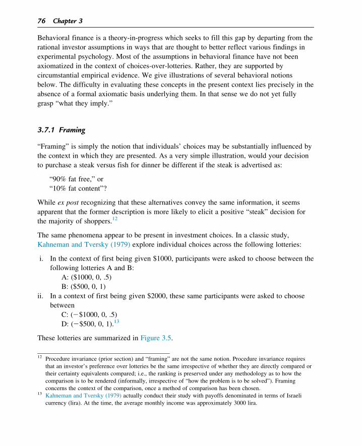
The same phenomena appear to be present in investment choices. In a classic study,

Kahneman and Tversky (1979) explore individual choices across the following lotteries:

i. In the context of first being given $1000, participants were asked to choose between the

following lotteries A and B:

A: ($1000, 0, .5)

B: ($500, 0, 1)

ii. In a context of first being given $2000, these same participants were asked to choose

between

C: (2$1000, 0, .5)

D: (2$500, 0, 1).13

These lotteries are summarized in Figure 3.5.

12 Procedure invariance (prior section) and “framing” are not the same notion. Procedure invariance requires

that an investor’s preference over lotteries be the same irrespective of whether they are directly compared or

their certainty equivalents compared; i.e., the ranking is preserved under any methodology as to how the

comparison is to be rendered (informally, irrespective of “how the problem is to be solved”). Framing

concerns the context of the comparison, once a method of comparison has been chosen.13 Kahneman and Tversky (1979) actually conduct their study with payoffs denominated in terms of Israeli

currency (lira). At the time, the average monthly income was approximately 3000 lira.

76 Chapter 3

For a majority of those participating in the experiment, BgA and CgD despite the fact

that A and C are equivalent as are B and D when taking full account of the differing initial

payments.

How do we interpret these (inconsistent) choices? Apparently, it mattered to most

participants that the choice between lotteries A and B was presented as a choice of gains

relative to $1000 while in the second case the choices were presented as losses relative to

$2000. This distinction is viewed as a manifestation of the phenomenon of framing. Note

that under VNM-expected utility, framing, as illustrated above, is irrelevant since only total

wealth payoffs matter.

Framing is often cited as one factor potentially contributing to the failure of investors to

diversify; i.e., to invest their wealth in portfolios of more than a few (one) assets. It is the

idea that when investors consider the acquisition of various assets, they frame the decision

on the basis of bilateral comparisons alone, without considering the interaction of multiple

asset return patterns and the benefits that may follow. To illustrate this notion in the

simple context of three assets and two states of nature θ1 and θ2, consider the assetsin Figure 3.6.

+$1000 + A =

$1000 + B =

$2000 + C =

$2000 + D =

0.5

$1000

$1000

0.5

0.5

$1000

0

0.5 =

0.5

$2000

$1000

0.5

+0

$1000

0

1

0

$500

0

1 =

0

1

$1500

0

+0.5

$2000

$2000

0.5

0.5

0

–$1000

0.5 =

0.5

$2000

$1000

0.5

+0

$2000

0

1

0

– $500

0

1 =

0

1

$1500

0

Figure 3.5Four lotteries with preceding initial payments.


Assume π5 1/2, and let the prices of the assets be qE5 qG5 qRF5 $100. Under narrow

framing, an investor may individually compare E and G to RF, find each individually less

desirable (both E and G have large payoff variances and a substantial probability of

significant loss), and end up with a portfolio composed exclusively of asset RF.

Nevertheless, we see from Figure 3.7 that RF is clearly state by state dominated by the

portfolio {1/2E, 1/2G}.

It is unclear what utility specification would eliminate all framing phenomena.

3.7.2 Prospect Theory

At present, Kahneman and Tversky’s (1979, 1992) Prospect Theory is the most highly

developed behavioral theory of choice.14 It rests on a number of experimental observations:

i Consider the random payoff ($110, 2 $100, 1/2). In experimental settings, a majority of

participants declined to accept this lottery, irrespective of their level of personal wealth,

even if it was offered to them at zero cost.

ii Consider the four basic lotteries from Section 3.7.1

A: ($1000, 0, .5)

B: ($500, 0, 1)

C: (2$1000, 0, .5)

D: (2$500, 0, 1).

1–π

π

½ ($150) + ½ ($70) = $110

½ ($80) + ½ ($170) = $125

Figure 3.7Payoff outcomes, portfolio {1/2E, 1/2G}.

14 Barberis (2013) provides a detailed overview of the theory and applications that have followed from it.

This section owes much to him.

Asset:

1–π

150

80

π

70

170

105

RF(the risk-free asset)

GE

Payoff: π

1–π

π

105 1–π

Figure 3.6Three candidate assets.

78 Chapter 3

When offered for comparison without any prior wealth distinctions (no issues of

framing), a majority of participants displayed the following preference:

BgA and CgD.

iii Participants generally displayed a preference for both lotteries and insurance when

offered in closely related choice settings; in particular, see Figure 3.8.

Building on these and other observations Kahneman and Tversky (1979) propose a theory

of choice under uncertainty (Prospect Theory) with four principal ingredients.

1. Investors ultimately derive utility not from their absolute wealth levels (as in the

VNM-expected utility case) but from gains or losses relative to some reference or

benchmark value. This (critical) element in their theory is suggested by observation (i):

since at very high wealth levels, the acceptance or rejection of ($110, $2100, 1/2) is

really of little consumption consequence, its rejection at all wealth levels suggests that

it is the gains or losses themselves, possibly relative to some preconceived benchmark,

that really matter to investors. They thus propose a utility-of-money function of the

form UðY 2 YÞ where Y is the benchmark. The benchmark can be thought of as either a

minimally acceptable wealth level or, under the proper transformations, a cutoff rate of

return. It can be changing through time reflecting prior experience. Unfortunately,

Prospect Theory does not offer a general guide as to how the benchmark should be

selected in any specific choice setting.

2. Since ($110, $2100, 1/2) has a positive expected value, its rejection at all wealth levels

also suggests that agents feel losses more acutely than gains (of greater comparative

(in either case the expected payoff is $5) and,

(In either case the expected payoff is –$5.)

(1–π) = 0.999

$5000π = 0.001

(Most preferthe lottery)

$5

0 0(1–π) = 0

π = 1

(1–π) = 0

$–5π = 1

(Most prefer“insurance”)

–$5,000

0 0(1–π) = 0.999

π = 0.001

Figure 3.8Preferences for lotteries and insurance.


magnitude). This is the sense of loss-averse preferences or simply “loss aversion.”

The simplest illustration of a loss-averse utility-of-money function is seen in Figure 3.9,

where Y 5 0, a zero benchmark.

3. As a further refinement, consider the choices in observation (ii). The fact that most

participants prefer lottery B to lottery A suggests dislike of risk over positive gain

lotteries. The preference for lottery C over lottery D, however, suggests “risk loving”

behavior over losses. As we will see in the next chapter these features imply that

UðY 2 YÞ is concave for Y . Y but convex for Y, Y .

An illustration of a utility representation satisfying (1)�(3) is as follows: Let Y

denote the benchmark payoff and define the investor’s utility-of-money function

U(Y) by

UðYÞ5

ðjY2Y jÞ12γ1

12 γ1; if Y $ Y

2λðjY2YjÞ12γ2

12 γ2; if Y # Y

8>>>><>>>>:

where λ. 1 captures the extent of the investor’s aversion to “losses” relative to the

benchmark, and γ1. 0 and γ2. 0 need not coincide (but γ16¼1, γ26¼1). In other words,

the curvature of the function may differ for deviations above or below the benchmark.

See Figure 3.10 for an illustration. Clearly, all three features can have a large impact on

the relative ranking of uncertain lottery payoffs.

4. There is a fourth attribute of Prospect Theory that also has its origins in observation.

(iii) One interpretation of the choices found in that observation is that investors

overweight low probability tail events, both favorable and unfavorable. Following on

U(Y )

Y (gains, losses)

U(Y ) =λ1 Y, λ1 > 0 for Y > 0

λ2 Y, λ2 > 0 for Y < 0, and λ2 > λ1.

0

Figure 3.9Loss-averse utility function.

80 Chapter 3

this possibility, Kahneman and Tversky (1979) elect to weigh the utilities of the various

outcomes using a nonlinear function of the true probabilities which is asymmetric in a

manner that gives a high weighting to tail events. These weightings are not necessarily

to be interpreted as erroneous probability estimates, but as perhaps reflecting relative

welfare consequences of the outcomes for the investor that are not observable.

See Tversky and Kahneman (1992) for a full discussion. A sample weighting function

taken from Tversky and Kahneman (1992) is found in Figure 3.11. Note that this

weighting function resembles a probability distribution function where there is a large

likelihood of “extreme” events.

As a paradigm for rationalizing laboratory observations (i)�(iv), Prospect Theory has no

equal at the moment. But does it have any direct advantage over VNM-expected utility in

explaining equilibrium market phenomena? There are at least two relevant works in this

regard, Barberis and Huang (2008) and Benartzi and Thaler (1995). In the first paper, the

authors show that the skewness in the return distribution of a common stock can have

important pricing implications when investors’ loss-averse preferences are defined over

–350

–300

–250

–200

–150

–100

–50

0

100

500

0 200 400 600 800 1000 1200 1400 1600 1800 2000Y

U

Parameter values: Y = 1000; γ1 = γ2 = 0.5, λ = 5

Figure 3.10Utility function for Prospect Theory.


changes in the value of their portfolios. In particular, securities with positively skewed

return distributions are priced higher (and have lower average returns) and negatively

skewed securities lower (and have higher average returns) than would be the case in a

VNM-expected utility environment, a consequence that follows from the asymmetric

weighting function fundamental to Prospect Theory. It is a feature that appears to be present

in the cross section of security returns (see, for example, Boyer et al. (2010) and

Conrad et al. (2013).

The basic intuition in the Benartzi and Thaler (1995) paper is that loss-averse investors will

dislike equity securities because stock market returns are much more highly dispersed relative

to bond returns. This fact should lead, they argue, to a higher equity premium in an equilibrium

setting where investors have loss-averse preferences than would be possible in the same

environment where investors are VNM-expected utility. In a formal dynamic equilibrium

quantitative model where investors have loss-averse preferences, Barberis and Huang (2001) go

on to confirm the assertions of Benartzi and Thaler (1995), subject to qualifications.

There are many other utility forms that have been proposed over the past 30 years which

are linked in some way to Prospect Theory. Some are widely employed in the research

literature. We conclude this section by enumerating a few of them below.

1

0.9

0.8

0.7

0.6

0.5

0.4

0.3

0.2

0.1

00 0.1 0.2 0.3 0.4 0.5 0.6 0.7 0.8 0.9 1

Figure 3.11The probability weighting function. Source: This figure is taken from Tversky and Kahneman (1992)

as presented in Barberis (2013).

82 Chapter 3

3.7.2.1 Preference Orderings with Connections to Prospect Theory

i. Survival benchmark: Investors evaluate lotteries according to Uð ~YÞ5EUð ~Y2 YÞ whereY represents a minimum level of income for a decent lifestyle.

ii. Habit formation preferences: Investors become accustomed to a particular income level

and measure their utility by the extent to which their present income realization

departs from it. For example,

Uð ~YtÞ5EUð ~Yt 2 Yt21Þwhere the habit is identified by the prior period’s income (and associated consumption)

level, thereby introducing a time dimension. See Constantinides (1990) and Sundaresan

(1989).

iii. “Keeping up with the Joneses” or relative income status: Once again investors evaluate

lotteries according to

Uð ~YÞ5EUð ~Y 2 YÞexcept that Y represents the average income level in the investor’s reference

community. See Abel (1990).15

iv. “Disappointment aversion”; Gul (1991): Here we will need to be a bit more detailed in

our representation of the expectations operator E. A disappointment averse investor

evaluates lotteries according to

Uð ~YÞ5ðBY

uðYÞdFðYÞ1AY

ðYB

uðYÞdFðYÞ

where Y , Y denote, respectively, the minimum and maximum payoffs associated with~Y , A is a number 0,A, 1, and B is a certain payment (a certainty equivalent) in

exchange for which the investor would be willing to sell the lottery ~Y . With A, 1, the

investor effectively weighs payments above this benchmark level less heavily than

ones below it—a sort of indirect “loss” aversion. He is, essentially, more concerned

with low-value outcomes, low in the sense of falling short of the amount for which the

investor would have been willing to sell the lottery. Routledge and Zinn (2003) modify

the original Gul (1991) representation in a way that endogenizes the construction of

B so as to make low payoff realizations even more painful than in Gul (1991).

v. The notion of regret; Loomis and Sugden (1982): The idea here is that if an investor

selects one lottery over another, then his utility benefit of a particular state’s payment

will be diminished had the payoff to the rejected asset in that same state been higher;

i.e., given the realized state, the investor experiences regret for not having chosen the

15 In all these three cases, the benchmark is calculated so that the utility function U( ) is always defined

over a positive quantity.


other asset. More formally, in deciding which of lotteries ~Y1 and ~Y2 to choose, the

investor computes (for ~Y1; ~Y2 is evaluated symmetrically):

Uð ~Y1Þ5EUð ~Y1Þ1ERð ~Y12 ~Y2Þ

5XNi51

πðθ1ÞuðY1ðθiÞÞ1 δXNi51

πðθiÞRðY1ðθiÞ2 Y2ðθiÞÞ

where i indexes the states, δ. 0 and, like U( ), R( ), the regret function, is a monotone,

strictly increasing function which satisfies R(0)5 0 and 2R(2ξ)5R(ξ) for any ξ. 0.

R( )16 diminishes expected utility in those states where ~Y2 has the higher outcome.

In this sense the alternative asset’s payoff serves as the benchmark on a state-by-state

basis. Loomes and Sugden (1982) demonstrate that regret preferences can rationalize

many of the choice anomalies presented in Kahneman and Tversky (1979). As one

might expect, however, regret preferences do not satisfy the VNM transitivity axiom

which has the implication that, per se, they cannot necessarily be used to isolate the

best (highest expected utility) of a collection of eligible lotteries.

Preference representations (i)�(v) are a representative sample of “what’s out there”. Except

for disappointment aversion, all lack a full axiomatic basis grounded in choices-over-

lotteries. It is also not clear what the corresponding “reverse engineered” preferences over

consumption goods would look like, a problem that is typically sidestepped by assuming

one composite consumption good with a normalized price of one so that income and

consumption are always numerically equal. In all cases, however, the takeaway is the same:

investors evaluate gains and losses relative to a benchmark and do so asymmetrically in a

way that tends to “overweight losses” relative to expected utility.

3.7.3 Overconfidence

A variety of studies find evidence that suggests pervasive overconfidence among

physicians, nurses, attorneys, engineers, and others.17 Monitor (2007) finds, in a survey,

that more than 70% of professional portfolio managers regard the service they provide as

“above average.” These various studies measure overconfidence in different ways,

consistent with the difficulties inherent in making the notion precise in individual contexts.

A more formal study again suggestive of overconfidence is Barber and Odean (2000);

see also Odean (1998, 1999). Using data from 78,000 individually managed accounts at a

large discount brokerage company, these authors find that these accounts substantially

underperform various commonplace benchmarks largely because of the large transaction

16 Alternatively, R( ) could assume the form R(Y1(θi)2 Y2(θi))5min{0,(Y1(θi)2 Y2(θi))}, etc.17 Some references are Baumann et al. (1991), Wagenaar and Kern (1986), Russo and Schoemaker (1992),

and De Bont and Thaler (1990) for, respectively, nurses, attorneys, high-level managers, and portfolio

managers.

84 Chapter 3

costs attendant to frequent trading. They interpret these findings as suggesting that

individual investors are overconfident in their ability to pick “winning stocks.”

It is not clear how the notion of overconfidence can be modeled in a framework where

agent preferences are represented by utility functions of some type. One possible approach

is to borrow from Prospect Theory as regards subjective weightings on the various possible

outcomes. In particular, we might expect that an overconfident investor is one who assigns

lower weightings to negative outcomes than does the typical investor or who assumes the

information he has collected regarding a stock’s future return distribution is more precise

than it actually is. This latter approach is taken by Daniel et al. (1998), who study the

consequences of overconfidence in an equilibrium security pricing model. These authors

find that overconfidence, modeled in this way, can lead to “momentum”-like effects: price

increases today followed, on average, by further price increases tomorrow, and vice versa.

3.8 Conclusions

The expected utility theory is the workhorse of choice theory under uncertainty. It will be

put to use systematically in this book, as it is in most of financial theory. We have argued

in this chapter that the expected utility construct provides a straightforward, intuitive

mechanism for comparing uncertain asset payoff structures. As such, it offers a

well-defined procedure for ranking the assets themselves.

Two ingredients are necessary for this process:

1. An estimate of the probability distribution governing the asset’s uncertain payments.

While it is not trivial to estimate this quantity, it must also be estimated for the much

simpler and less flexible mean/variance criterion.

2. An estimate of the agent’s utility-of-money function; it is the latter that fully

characterizes his preference ordering. How this can be identified is one of the topics

of the next chapter.

Behavioral theories represent plausible, experimentally based deviations from the axioms

underlying expected utility. They make us aware of departures from “rationality” that have

potential implications for explaining phenomena that are difficult to account for in the

standard VNM framework.

References

Abel, A., 1990. Asset pricing under habit formation and catching up with the Joneses. Am. Econ. Rev. Pap.

Proc. 80, 38�42.

Allais, M., 1964. Le comportement de l’homme rationnel devant le risque: Critique des postulats de l’ecole

Americaine. Econometrica. 21, 503�546.

Arrow, K.J., 1963. Social Choice and Individual Values. Yale University Press, New Haven, CT.


http://refhub.elsevier.com/B978-0-12-386549-6.00003-6/sbref1







Barberis, N., 2013. Thirty years of prospect theory in economics: a review and assessment. J. Econ. Perspect.

27, 173�196.

Barberis, N., Huang, M., 2001. Mental accounting, loss aversion, and individual stock returns. J. Finan. 56,

1247�1292.

Barberis, N., Huang, M., 2008. Stocks as lotteries: the implications of probability weighting for security prices.

Am. Econ. Rev. 98, 2066�2100.

Barber, B., Odean, T., 2000. Trading is hazardous to your wealth: the common stock performance of individual

investors. J. Finan. 55, 773�806.

Baumann, A., Deber, R., Thompson, G., 1991. Overconfidence among physicians and nurses: the macro-

certainty, micro-uncertainty phenomenon. Soc. Sci. Med. 32, 167�174.

Benartzi, S., Thaler, R., 1995. Myopic loss aversion and the equity premium puzzle. Q. J. Econ. 110, 73�92.

Boyer, B., Mitton, T., Vorkink, K., 2010. Expected idiosyncratic skewness. Rev. Finan. Stud. 23, 169�202.

Conrad, J., Dittmar, R., Ghysels, E., 2013. Ex ante skewness and expected stock returns. J. Finan. 68, 85�124.

Constantinides, G., 1990. Habit formation: a resolution of the equity premium puzzle. J. Polit. Econ. 98,

519�543.

Daniel, K., Hirshleifer, D., Subrahmanyam, A., 1998. Investor psychology and security market under- and

overreactions. J. Finan. 53, 1839�1885.

DeBont, W., Thaler, R., 1990. Do security analysts overreact? Am. Econ. Rev. 80, 52�57.

Grether, D., Plott, C., 1979. Economic theory of choice and the preference reversal phenomenon. Am. Econ.

Rev. 75, 623�638.

Gul, F., 1991. A theory of disappointment aversion. Econometrica. 59, 667�686.

Huberman, G., 2001. Familiarity breeds investment. Rev. Financ. Stud. 14, 659�680.

Kahneman, D., Tversky, A., 1979. Prospect theory: an analysis of decision under risk. Econometrica. 47,

263�291.

Loomes, G., Sugden, R., 1982. Regret theory: an alternative theory of rational choice under uncertainty. Econ. J.

92, 805�824.

Mas-Colell, A., Whinston, M.D., Green, J.R., 1995. Microeconomic Theory. Oxford; New York: Oxford

University Press.

Monitor, J., 2007. Behavioral Investing: A Practitioner’s Guide to Applying Behavioral Finance. John Wiley &

Sons, West Sussex.

Odean, T., 1998. Are investors reluctant to realize their losses? J. Finan. 53, 1775�1798.

Odean, T., 1999. Do investors trade too much? Am. Econ. Rev. 89, 1279�1298.

Reiff, P., 1966. The Triumph of the Therapeutic, New York: Harper and Row, 1966; quote taken from the

reprinted edition, ISI Books: Wilmington, Delaware (2006).

Routledge, B., Zin, S., 2003. Generalized appointment aversion and asset prices, NBER Working Paper no.

10107.

Russo, J., Schoemaker, P., 1992. Managing overconfidence. Sloan Manage. Rev. 33, 7�17.

Sundaresan, S., 1989. Intertemporally dependent preferences and the volatility of consumption and wealth. Rev.

Finan. Stud. 2, 73�89.

Thaler, R.H., 1992. The Winner’s Curse. Princeton University Press, Princeton, NJ.

Tversky, A., Kahneman, D., 1992. Advances in prospect theory: cumulative representation of uncertainty.

J. Risk Uncertain. 5, 297�323.

Wagenaar, W., Keren, G., 1986. Does the expect know? the reliability of predictions and confidence ratios of

experts. In: Hollnagel, E., Mancini, G., Woods, D.D. (Eds.), Intelligent Decision Support in Process

Environments. Springer, Berlin.

86 Chapter 3































































Making Choices in Risky Situations

Documents

Transcript of Making Choices in Risky Situations