Working Paper Series

This paper can be downloaded without charge from: http://www.richmondfed.org/publications/

Risky Higher Education and Subsidies¤y

Ahmet Akyol

Department of Economics

York University

Kartik Athreyaz

Research Department

Federal Reserve Bank of Richmond

Federal Reserve Bank of Richmond Working Paper 03-02

August 12, 2003

Abstract

Tertiary education in the U.S. requires large investments that are risky, lumpy,and well-timed. Tertiary education is also heavily subsidized. By making the riskof human capital investment more acceptable, especially to low wealth households,subsidies may increase investment in human capital, lower long-run inequality, andreduce aggregate precautionary savings. However, subsidies also encourage more poorlyprepared students to attend and are usually …nanced via distortionary taxes. In thispaper, we …nd that observed collegiate subsidies improve welfare substantially relativeto the fully decentralized (zero subsidy) outcome. We show that subsidies help smoothconsumption, lower skill premia, increase interest rates as precautionary savings fall,lower the inequality of both consumption and wealth, increase intergenerational incomemobility and raise welfare, even when …nanced by distortionary taxes.

¤JEL Classi…cation: E60, I22yKeywords: Human Capital Risk, Heterogeneous Agents, College EducationzWe thank seminar participants at the Universities of Colgate, Iowa, Singapore, Toronto, Virginia, and

York, the Federal Reserve Bank of Richmond, and the 2002 Midwest Macro Conference. We are indebtedto Krishna Kumar for detailed comments on an earlier draft. We also thank Andreas Hornstein, SteveWilliamson, Huberto Ennis, Pierre Sarte, Nicole Simpson, and John Weinberg for comments and suggestions,Elliot Martin for able research assistance, and especially Beth Ingram.

1. Introduction

Tertiary education in the U.S. requires large investments that are risky, lumpy, and well-timed. Without subsidies, the investment necessary for college is a …xed amount across households. Even with subsidies, the outcomes generated by this large and uncertain in-vestment are income streams that do not depend on initial wealth, but rather are of given absolute size. For standard preferences, this implies that poor households will be less willing to attempt college, all else equal, than their wealthier counterparts. In turn, such households will remain poorer over generations, making subsequent generations even less willing to take the risk. Therefore, cross-sectional inequality will be larger, and intergenerational incomes more persistent, than they would otherwise be.

Subsidies reduce the cost of taking the risk of investing in human capital. In turn, collegiate investment becomes more acceptable, especially to low wealth households. More widespread college investment may improve allocations in several ways. First, there is strong evidence that college-educated parents have relatively better prepared children. For example, Ishitani and DesJardins (2002), Warburton et. al. (2001), Chen (2001), and Nunez and Horn (2000) all document the presence of strong “1-st generation” (students whose parents did not complete college) e¤ects, even after controlling for family income. Therefore, the e¤ects of subsidies are likely to extend beyond the lifetime of an individual. Second, as Ljungqvist (1995) has argued, a high skill premium implies that collegiate outcomes can result in large changes in consumption and wealth accumulation. Subsidies can increase unskilled wages and lower skilled wages by encouraging more people to attend college, thereby compressing the skill premium and lowering the consequences of collegiate failure. Third, it is known from Aiyagari (1994) that stationary equilibria in environments with uninsurable risks display overinvestment in physical capital in the sense that the interest rate will be strictly below the rate of time preference. Education subsides lower this excess capital via two di¤erent channels. First, subsidies decrease the private cost of education investment. Therefore, households do not have to save large amounts against the possibility of having college-ready children. Second, subsidies leave households better able to gamble on a college investment when children of uncertain ability arrive, thereby lowering the precautionary demand for assets. Lastly, a lower level of capital stock raises the rate of return on savings, which in turn improves consumption smoothing. However, the bene…ts above require bearing two potentially large types of costs. First, subsidies generate adverse selection by encouraging progressively more poorly prepared students to attend. Second, subsidies must be …nanced via taxation and when markets are incomplete, even lump-sum taxes are distortionary.

In this paper, we ask the following question. How does higher education subsidy policy a¤ect welfare, the skill premium, inequality, output, and the dynamics of the intergener-

2

ational earnings process? We …nd that observed collegiate subsidies improve welfare sub­stantially relative to the fully decentralized (zero subsidy) outcome. Subsidies help smooth consumption, lower skill premia, increase interest rates as precautionary savings fall, lower the inequality of both consumption and wealth, and increase intergenerational income mo­bility. We …nd also that mean consumption rises with subsidies even though physical capital shrinks. This occurs as the increase in human capital raises steady state output and average consumption. Our model thus quanti…es the extent of underinvestment in risky human cap­ital emerging from current and proposed subsidy rates. In our benchmark case, risky human capital accumulation falls well short of the welfare maximizing value. The risk of failure in college is by itself su¢cient to explain subsidies to college education observed in the U.S. and other OECD countries. The largest welfare gains from subsidies occur at rates below 40%, with much smaller gains from further subsidization. This feature provides insight into why OECD countries simultaneously display both uniformly high subsidies as well as the absence of explicit private insurance against failure: additional insurance, private or public, is not very useful. An important feature of our study is that we focus on the role of subsidies in mitigating risk arising in the acquisition of human capital. We therefore shut down other sources of bene…ts from subsidies, such as externalities and endogenous growth. We also do not impose credit constraints on student loans, as the U.S. government provides full loan guarantees on college loans via such programs as PLUS. Interestingly, despite removing most obstacles to …nancing college, the government continues to subsidize it heavily.

In the U.S. and other OECD nations, college education is a risky investment. Using NLSY data, Altonji (1993) …nds that of high school students intending to complete college in 1972, 90% did enroll, yet only 58.1% had completed seven years later. The risk of failure is also present for the seemingly well-prepared. For example, at colleges classi…ed as “Highly Selective” by the ACT, the dropout rate averages roughly 19%. More striking is that even among those with both standardized test scores and family incomes in the top quintile, the drop-out rate does not fall to zero, but only to about 10% (NCES 1999). In recent work, Chen (2001) …nds that roughly 16% of 1997 high-school graduates with test scores in the top quartile did not even attempt college.1 Estimates of Willis (1986) and Card (1995), for example, show the rate of return on college to be between 8% and 13%, a signi…cantly higher rate than on …nancial assets. Given the risks, it appears that a portion of this high rate of return is a risk premium, and Chen (2001) estimates the risk premium associated with a four-year college education to be one-fourth of the total return.

College is also a lumpy investment. First, most students who fail to complete college do so only after spending a substantial amount of time enrolled. NCES data show that while

1Work of Cameron and Heckman (1999), Heckman and Carneiro (2001), and Keane and Wolpin (2001) suggests that short-term credit constraints are not important enough to explain this fact.

3

the dropout rate exceeds 10% in the …rst year, it is even higher at the end of the second year, and is still nontrivial, at over 5%, in the third and fourth years of college.2 Stinebrickner and Stinebrickner (2001) use a di¤erent dataset and …nd that the median time to dropping out is two years. Worse yet is that dropping out, even after several years in college, is typically very damaging. Hungerford and Solon (1987), and Card and Kreuger (1992) both …nd that returns are highest in the later years of college, and substantially greater than those obtained in the …rst two years. The risky and lumpy nature of investment in college may therefore be dissuading even talented high-school completers from attempting college at all, implying systematic underinvestment in human capital. These individual-level risks are re‡ected in aggregate tertiary education failure rates in the OECD that exceed 30%. Data from the National Center for Education Statistics (NCES) shows that for the U.S., the unconditional dropout rate was approximately 37% for the period 1993-1998.

Given the lumpiness in collegiate investment, failure is very costly. With respect to size, in the U.S., for example, the median resource cost of college in tuition and fees, room, and board exceeds $60,000.3 Even beyond this large explicit cost of college, the opportunity cost of lost wages is large, at approximately $17,000 per full-time student annually in the U.S.4

Also, the current wage premium for college education of 1.6 implies very large di¤erences in mean lifetime income between those who complete college and those who do not.

There is typically only a narrow window of time available for college education, as the opportunity cost rises sharply with age, as households form and children are produced. For example, Cameron and Heckman (2001) show that approximately 90% of college entry occurs, if at all, within two years of completing high school. It is also not easy to overcome an initial failure in college via re-enrollment at a later time, nor is it costless to delay entry. Ahlburg et al. (2002) …nd that even after accounting for endogeneity in the decision to delay college entrance, the likelihood of dropout rises by 32% for high school graduates who postpone college entry. In such an environment, relatively poor families–even those with well-prepared children, may choose not to send them to invest in a risky college education, even if student loans are assumed to be comprehensive enough to allow all households to feasibly do so. Such outcomes exacerbate cross-sectional inequality and endogenous intergenerational persistence in income and wealth.

In addition to the risk faced by those trying acquire a college education, U.S. households appear to bear a considerable amount of uninsurable idiosyncratic labor income risk. The

2Levhari and Weiss (1974) note that “In fact, the length of schooling itself may be random, since the ability to complete a given schooling program is also to some extent unknown” (footnote 1, p. 951). However, they do not model this source of uncertainty in their analysis, whereas this is a key aspect of our study.

3NCES (1999). 4National Center for Education Statistics (NCES, www.nces.ed.gov).

4

empirical tests of Cochrane (1991), Hayashi, Altonji, and Kotliko¤ (1996), and Carroll (2000) all document strong departures from complete risk sharing, both between and even within families. The research of Levhari and Weiss (1974) and that of Eaton and Rosen (1980), and Hamilton (1987) emphasizes the uncertainty in returns to human capital, and the associated di¢culties in diversi…cation of such risk. The long-run implications of uninsurable risk are explored in recent work by Castaneda et al. (1999), Diaz-Jimenez, et al. (1997), and DiNardi (2000). These authors show that the high income and wealth inequality observed in the U.S. can be plausibly accounted for by parsimonious, incomplete market models, with exogenously speci…ed earnings processes. One indirect contribution of this paper is that, in analyzing subsidies, we endogenize the mean of the household earnings processes by allowing household to choose skills in response to stochastic income shocks, educational risk, skill premia, and subsidies.

The environment we develop is most closely related to that of Caucutt and Kumar (2003) and Restuccia and Urrutia (2002).5 Caucutt and Kumar (2003) study a model with het­erogeneity in ability, and …nd that subsidies have modest e¤ects on educational attainment and welfare. Restuccia and Urrutia (2002) study an environment that distinguishes between pre-college and college investment. Early investments are found to have the largest e¤ects on intergenerational persistence, with college investments accounting for most of the ob­served inequality in earnings. There are important di¤erences between our work and both of the preceding papers. First, Caucutt and Kumar (2003) and Restuccia and Urrutia (2002) prohibit borrowing to …nance education. Recent work of Cameron and Heckman (1999), Heckman and Carneiro (2002), and Keane and Wolpin (2001) …nds that borrowing con­straints do not appear to a¤ect college enrollment decisions. Therefore, we always allow individuals to borrow to pay for college tuition, room, and board, even though households face (state-dependent) limits on their overall debt. Second, we follow Levhari and Weiss (1974), Eaton and Rosen (1980), Hamilton (1987), Chen (2002), and others in assuming that human capital, once acquired, produces uncertain returns. Furthermore, we limit in-come insurance possibilities to self-insurance via capital accumulation. Conversely, both Restuccia and Urrutia (2002) and Caucutt and Kumar (2003) assume full insurance of labor income and do not allow physical capital accumulation. These di¤erences allow us to study the quantitative implications of subsidies for the wealth distribution.6 Methodologically, our

5Krebs (2003) …nds a welfare improving role for state-contingent transfers in an endogenous growth model with riskless physical and risky human capital. However, in order to focus on growth and portfolio choice, Krebs’ model abstracts from lumpiness, irreversibility, and timing frictions in human capital investment, as well as heterogeniety in ability. Also, Krebs (2003) studies reductions in human capital risk, once acquired. In our model, human capital acquisition itself is risky.

6Hanushek et al. (2001) develop a general equilibrium model of risky schooling and income distribution under risk neutrality, and thus do not consider either intragenerational or intergenerational risk sharing. To

5

approach to susbidies is also similar to Li (2002). A few other recent studies examine college subsidies but do not provide quantitative measures in general equilibrium, or analyze the implications of subsidies for the skill premium or wealth inequality.7

Our paper is organized as follows. In Section 2, we lay out the model. Section 3 de…nes equilibrium and Section 4, the welfare measure. We parameterize the model in Section 5. We discuss the results in Section 6, and conclude in Section 7. The computational algorithm is detailed in the Appendix.

2. Model

2.1. Preferences, Endowments, Assets

The economy consists of a continuum of in…nitely lived dynasties with unit mass. Each agent/dynasty has CRRA preferences over the single consumption good c:

E0

1X

t=0

c1¡¹

¯t t

1 ¡ ¹ , (2.1)

where ¯ denotes the discount factor, and ¹ is the coe¢cient of relative risk aversion. All agents are endowed with one unit of time, which they supply inelastically. Agents

supply skilled labor if they have obtained education, unskilled labor otherwise. The private cost of college is denoted by °. The steady-state wage rate for skilled labor is denoted by ws, and the unskilled steady-state wage is denoted wu. To re‡ect uncertainty in the returns to human capital, agents are subject to idiosyncratic labor productivity shocks. These shocks are denoted ² 2 f²l; ²hg, where h and l denote high and low productivity states respectively. Shocks follow a Markov process with transition probabilities phh =Pr(²0 = ²hj² = ²h), and pnormalized to unity and is denoted by ². ll=Pr(²0 = ²lj² = ²l ). The unconditional expected labor productivity for a given agent is

To capture the presence of uninsurable risk, agents are limited to trade in a risk-free bond with steady-state interest rate r. Agents are liquidity constrained with respect to private credit markets. Agents di¤er, however, in their credit limits. Those who are unskilled choose asset holdings a up to a debt limit du < 0 units in any given period, but no more. To re‡ect the ability of higher-wage skilled households to borrow at least what low-wage unskilled

focus attention on high-school rather than college schooling, Benabou (2001) studies optimal subsidies with liquidity constraints on human capital and without precautionary savings motives. Seshadri and Yuki (2001) examine both need-based transfers and educational transfers in a model of investment in a child’s education when ability is not clearly known.

7These include Jacobs and VanWijnbergen (2001), as well as Wigger and von Weizacker (2001). Our approach is also indirectly related to a larger literature, including Becker and Tomes (1986), Glomm and Ravikumar (1992), Tomes (1981), Loury (1981), Banerjee and Newman (1991), Galor and Zeira (1993).

6

households can, those who have decided to acquire skills are given extended credit limits. Let the private cost of education be denoted by ° > 0. The extension of credit limits is kept simple. In the period in which agents attend college, their credit limit is extended by the total private cost of education ° > 0. Their limit is denoted dus , where dus ´ du ¡ °.8

Thus, while agents do face constraints on borrowing, these constraints will never prevent a household from being able to …nance a college education, and so do not provide any additional rationale for subsidies. Once agents are skilled, they face an extended limit of ds

units, where ds · dus .

2.1.1. Young Agents

Each household periodically produces a new generation ready for college, referred to as “young.” 9 The arrival of a young (college-ready) member of a family is treated each period as the outcome of a Bernoulli random variable with parameter ½. The ratio 1 is then the½

average time between college-ready agents within a dynasty, and is observable. To avoid exogenously imposing intergenerational persistence, we assume that the young agent draws shock ² from the unconditional distribution of productivity.

Young agents are the representative decision makers for the family/dynasty. 10 Agents are young for only one period, and in subsequent periods are referred to as “adults”. Our treatment of families thus closely follows the (related) models of Yaari (1965) and Blanchard (1985).11

Young agents face the family’s current period budget constraint and must decide whether to invest in a risky college education or not, given the productivity shock they draw, and the information they possess on their likelihood of success. Importantly, we follow Ljungqvist (1993), Caucutt and Kumar (2002), and Fernandez and Rogerson (1995) and assume that college education is a discrete, lumpy investment that cannot be done partially.

8See for example, www.ed.gov, for a description of the PLUS loan program, which explicitly allows parents to borrow to …nance a dependent child’s college education. These loans are not capped in amount.

9The process of primary and high school education is not central here and children are modeled as arriving having completed high school.

10Heuristically, the parents should be thought of living even after their high-school educated child arrives, as is realistic. However, because we are concerned here with the college education decision of the young agent, we abstract from parents solving another decision problem.

11While it will allow a reduction in the size of the state vector for the household, the probabilistic arrival of children in the model will not play a substantive role in our results. While the production (arrival) of children may be deterministic, the production of college ready children (as in the model) is certainly not. NCES data show that over 30% of high-school completers are “marginally” quali…ed or “unquali…ed” for college.

7

2.1.2. Schooling and Information on Ability

There are two levels of human capital in the model. Those who complete college have human capital level Hs and are referred to as skilled. Those who do not complete college have human capital Hu, and are referred to as unskilled. Skilled agents have higher average productivity than unskilled agents. Skilled workers earn a wage of ws per unit of labor time, and unskilled agents earn a wage of wu per unit of labor time.

Young agents choose whether or not to pay the cost and enroll in college. To capture the presence of rapidly increasing opportunity costs following high school completion, unskilled agents born in prior periods do not have the option to acquire education. The explicit private resource cost of obtaining education is denoted by °, and represents tuition and room and board payments paid by an individual inclusive of all available subsidies. The full cost of education clearly involves the opportunity cost of foregone earnings while in college. Given that students may supply positive hours of labor while also a full time student, we allow them to supply À < 1 units of unskilled labor while in college.

Our environment features adverse selection as Young agents are di¤erentially informed as to the likelihood of successfully completing college. At the beginning of the period, all young agents receive a signal I, drawn from a probability distribution º (I), which determines the information young agents have on their likelihood of success if they attempt college. The signal divides the population of young agents into three groups, denoted by I =fIs; If ; U Ig, and is i.i.d across households and over time. In reality, some high-school completers do not meet college admission standards, and so will not be able to attend college, and are therefore irrelevant to our study. Let If denote the set of households who know they will fail in college with probability one. Conversely, we denote by Is the set of “informed” households who know that they will succeed with probability one. Thus, the Is and If groups represent the right and left tails of the distribution of collegiate preparedness, respectively.

The remainder of households are “uninformed”, denoted UI, and are those facing uncer­tainty with respect to collegiate success. However, within this group, students face uncer­tainty in college that depends on whether they come from a college-educated or high-school educated household.12 The likelihood of failure in college for UI households is given by ¸ = f¸s; ¸ug, where ¸s and ̧ u denote the probability of failure for young agents from skilled and unskilled families respectively. In order to remain conservative in our approach strictly

12Allowing greater heterogeneity in preparedness to enrich the representation of adverse selection is pos­sible, but would result in more parameters than calibration targets. Furthermore, such a model would also contain a positive selection e¤ect among well-prepared but poor non-1-st generation students. This latter e¤ect will act as an o¤setting force to adverse selection. We therefore restrict heterogeniety in ex-ante pre­paredness to these four groups as our calibration will remain disciplined by observable dropout rates among groups well identi…ed in the data.

8

and avoid generating welfare gains by easing liquidity constraints via subsidies, we treat the probabilities of failure as primitive to the household, and unrelated to tuition levels. Empiri­cal support for this restriction is found in Stinebrickner and Stinebrickner (2002), who study a novel experiment whereby a 100% tuition subsidy was given to students at a Kentucky col­lege. They found that even with full subsidization, failure di¤erentials among income groups persisted, suggesting that “home-environment” e¤ects are important.13 Given that the skill premium strongly ties income di¤erentials to education di¤erentials, the law of motion for college preparedness is kept simple: UI children of skilled parents will be relatively better prepared, with ¸ = ¸s, with ¸s < ¸u.14

Adverse selection is generated in the model by the presence of less-prepared 1-st genera­tion students enrolling in response to subsidies. The latter turn out to respond much more to changes in subsidies than rich non-1st generation students. In turn, overall dropout rates increase, especially among 1st-generation households. However, as the government must balance its budget, the cost of subsidy programs arising from adverse selection is explicitly accounted for in our framework.

2.1.3. The Timing of Failure

A critical issue is when the uncertainty regarding collegiate success or failure resolves itself. That is, do college dropouts fail immediately and costlessly, or must they wait for a fairly long period in order to learn that they will not be able to successfully complete college? The former entails smaller costs for the individual and the government, relative to the latter. We denote by µ° 2 [0; 1], the fraction of the total available time that is required for UI households to …nd out whether they will succeed or fail. Note that the fraction µ° is equivalent to the fraction of the private cost of college that must be paid before uncertainty resolves. If µ° = 1, households must pay the entire private cost of college to learn whether they will fail or not. Conversely, if µ° = 0, it is costless to learn about collegiate success, and there is no insurance role for subsidies. In the intermediate cases, for µ° 2 (0; 1), there is a potentially nontrivial trade-o¤. When µ° approaches 0, the insurance bene…ts of subsidies fall, but so do the costs of …nancing such programs via distortionary taxes. Conversely, when uncertainty resolves

13Stinebrickner and Stinebrickner (2002) also contains additional references documenting income-dependent home-environment e¤ects. They note however that college students from low-income families may still respond to shocks to their families (perhaps parental sickness or unemployment) by returning home. Ex-ante, the risk of such events, to the extent that they lead to attrition from college, implies completion risk, just as failure for any other reason would.

14For agents who are informed, ¸ is trivially pinned down. In the case of the informed young agent who will succeed for sure, i.e., I =Is , it is clear that ¸ = ¸u = ¸s = 0. Similarly, when an agent is sure to fail, i.e., I =If , it is clear that ¸ = ¸u = ¸s = 1.

9

Table 2.1: Sequence of Events for Young Agents

(a) Period t begins. Labor productivity shocks, ², occur to all agents.Young agents observe their information set.They are either informed, (I), and know the outcome of college

investment, or are uninformed (UI), and do not know with certainty.(b) Informed young agents who can …nish college education successfully (I =Is) may choose college

by paying °, the private cost of college. If enrolled, they become skilled in period t + 1.Informed agents who will fail with certainty (I = If ) do not enroll in college, and remain

unskilled for the rest of their life.(c) Uninformed (UI) agents decide whether or not to enroll in college. If enrolled, they pay a fraction µ° of the cost of college, where µ° 2 [0; 1], after which the uncertainty of …nishing college education, ´ is resolved. (d) If the agent is successful, she pays the remaining fraction 1 ¡ µ° of the private cost of college °; in period t+1, and becomes skilled. Otherwise, young agent drops out from college, and stays unskilled.

very slowly, with µ° approaching 1, the insurance bene…ts of subsidies grow relatively large, but so do the distortions arising from the taxes needed to …nance college.

If informed of success, young agents continue their college education by paying the rest of the college cost, (1 ¡ µ° )°. If informed of failure, young agents drop out of college and continue as an unskilled agent in the next period. The timing of payments for college among the uninformed (UI) is set to capture the idea that failing students will typically pay only a fraction of the total private cost of college, as they dropout before completing all coursework, as well as to separate the time before, and time after, information revelation without imposing a sub-period in the model. Table 2.1 summarizes the timing.

2.1.4. Subsidies and Taxes, and Limited Liability

Subsidies are modeled as a direct reduction in the private cost of college education. In this respect, subsidies in the model are closest to the U.S. public college education system. Given

° a subsidy rate ', the true resource cost of college is 1¡' . The subsidy rate is …nanced by proportional taxes on labor and capital income, ¿ l and ¿c respectively. For all experiments studied here, we use the NCES (1995) estimates to pin down the e¤ective subsidy rate '

under current U.S. subsidy programs.15

15We will focus exclusively on the direct subsidies and loan guarantees available to students, and abstract from loan subsidies. Loan subsidies and guarantees have the potential to be important in relaxing liquidity constraints. However, the cost reduction from subsidized loans is miniscule relative to the massive absolute

10

There are two forms of limited liability in the model, intergenerational limited liability, (IL), and collegiate limited liability (CL). Given our speci…cation of di¤erential borrowing limits for skilled and unskilled agents, we will require that young agents have intergenera­tional limited liability for debts incurred by their parents. That is, we assume that parents cannot pass on more than dIL units of debt to their college-ready child. A young agent’s assets are therefore given by a¤ ´ max(dIL ; a). The second limited liability condition applies to the discharge of debts accumulated in college.16 Limited liability is denoted dCL , and is set in the benchmark such that agents who fail are relieved of debt in excess of the limit for unskilled agents, du .17

2.2. The Recursive Formulation

When an agent is young, she must choose between acquiring a college education or not, and her value function will represent the better of these two options. A young agent’s state vector is comprised of four objects, her information level I =fIs; If ; UIg, her preparedness ¸ = f¸s; ¸ug, her asset level, a, and her current period labor productivity, ². Her value function is denoted V Y (I; ¸; a; ²) and must therefore satisfy

V Y (I; ¸; a¤; ²) = maxfWC;WNCg (2.2)

where W C and W NC denote the values from choosing to attend college, or not, respectively. If the agent chooses to attempt college, she will fail to complete college with probability ¸, and will attain V A (Hu; a¤0; ²0), the value of entering a period as an adult who is unskilled (Hu), with assets and labor productivity a¤0 , and ²0 respectively. She will succeed in college with probability (1 ¡ ̧ ), and will then obtain V AColl(Hs; a0 ; ²0 ), the value of being a skilled adult (Hs) who just completed college. In the current period she must pay µ° ° units, and will pay the remainder if she succeeds. An agent’s labor endowment while in college is limited by À < 1. Therefore, as seen in equation 2.4, the labor income of a college student is given by ºwu ²(1 ¡ ¿ l). If she fails, her asset holdings are protected by the limited liability restriction whereby she is only obligated to pay up to dCL . Thus, WC satis…es the following functional equation.

amounts of subsidy directly provided to colleges, public and private. 16We restrict limited liability to those who fail, as in practice the discharge of student loans requires a

formal demonstration of hardship. Student loans also are not dischargeable in a personal bankruptcy. 17We emphasize that intergenerational limited liability here is not zero liability, which is the level that

prevails in the U.S. at the time of death. A household’s debt at the time of a child’s college entrance is to be thought of here as the result of consumption smoothing e¤orts by parents for themselves and their pre-college child.

11

¾ (2.3)WC(I; ¸; a¤; ²) = max

c;a0

½ c1¡¹

1 ¡ ¹ + ¸¯EV A(Hu; a¤0 ; ²0 ) + (1 ¡ ̧ )¯EV AColl(Hs; a0 ; ²0 )

subject to

c + a0 + µ° ° · Àwu ²(1 ¡ ¿ l) + a¤ (1 + r) ¡ a¤r¿c (2.4)

a0 ¸ dus , c > 0, a¤ ´ max(dI L; a), a¤0 ´ max(dCL; a0)

where primes denote next period’s variables. If an agent chooses not to go to college, she loses the opportunity to obtain a college education thereafter. She receives utility from current consumption, and becomes an unskilled adult from next period onwards, realizing value V A(Hu; a0 ; ²0 ). The value function WNC therefore satis…es:

WNC (I; ¸; a¤; ²) = max c;a0

½ c1¡¹

1 ¡ ¹ + ̄ EV A(Hu ; a0; ²0)

¾

(2.5)

subject to

c + a0 · wu ²(1 ¡ ¿ l) + a¤ (1 + r) ¡ a¤r¿c (2.6)

a0 ¸ du , c > 0, a¤ ´ max(dI L; a)

Notice that the borrowing constraint of the college bound is extended to dus units. Fol­lowing Cameron and Heckman (1999), this extension re‡ects the large number of public loan guarantee programs in existence, and rules out credit constraints in college as a determinant of outcomes.

A newly skilled adult who has just completed college must pay the remainder of her college costs, (1 ¡ µ° )°, as seen in equation 2.8 below, but is otherwise identical to all other adult agents. In the current period, she obtains utility from consumption. In the following period, she generates a college-ready young agent with probably ½, whereby she obtains V Y (I; ¸s; a¤0 ; ²0 ). If she does not generate a child, she will instead obtain value ¯EV A(Hs; a0 ; ²0 ).18 Therefore, V AColl, satis…es the following:

V AColl(Hs; a; ²) = max c;a0

½ c1¡¹

1 ¡ ¹ + ½¯EV Y (I; ¸s; a¤0; ²0) + (1 ¡ ½)¯EV A(Hs; a0 ; ²0 )

¾ (2.7)

subject to

c + a0 + (1 ¡ µ° )° · ws ²(1 ¡ ¿ l) + a(1 + r) ¡ ar¿ c (2.8) 18Note that the joint distribution that the expectation term, EV Y (I; ¸s; a¤0; ²0), is taken with respect to

di¤ers from the distribution with respect to which the second expectation, EV A (Hs ; a0; ²0), is taken.

12

a0 ¸ ds , c > 0, a¤0 ´ max(dI L; a0)

For the remaining agent-types, we have a quite standard consumption/savings prob­lem. We present the formulation under the benchmark case, with all other cases involving straightforward modi…cations of the parameters and constraints. An adult agent who did not acquire skills in the previous period is described by her human capital level H = fHs; Hu g, asset level, a, and current period labor productivity, ². When an adult is skilled, she max­imizes current period utility, knowing that any children she has will be college-ready with probability ½. This yields a value function, V A , that satis…es:

½ ¾ c1¡¹

V A(Hs; a; ²) = max 1 ¡ ¹

+ ½¯EV Y (I; ¸s; a¤0 ; ²0 ) + (1 ¡ ½)¯EV A(Hs; a0 ; ²0 ) (2.9) c;a0

subject to

c + a0 · ws ²(1 ¡ ¿ l ) + a(1 + r) ¡ ar¿c (2.10)

a0 ¸ ds , c > 0, a¤0 ´ max(dI L; a0)

The preceding can be understood as follows. Adult agents get utility from current con­sumption, and are replaced with the next generation with probability ½. If an adult agent is replaced, the young agent becomes the primary decision maker, assumes the assets of the household, must choose whether to attend college or not, and will receive V Y . If an adult agent is not replaced, which occurs with probability (1 ¡ ½), she realizes the value V A in the next period. Unskilled adults are either those who were adults in the previous period, young agents who tried college in the previous period and failed, or young agents who did not attempt college in the previous period. In all three cases, their optimization problem is given above in 2.9, with only the subscript on human capital H, changing. We turn now to the …rm’s problem and the government budget constraint.

2.3. Firms

Let T denote the aggregate raw labor time devoted to labor supply, given that those who attend college can only work À units of time.

Z T = [1 ¡ (1 ¡ À)½ I(W C (x) > W NC(x))d!] (2.11)

x

In the preceding, the term, ! refers to the equilibrium stationary distribution of agents, which will be made explicit below. The indicator function I = 1 if W C (x) > WNC(x); and I = 0 otherwise.

13

Ns and bTotal raw labor hours supplied are given by b Nu denoting raw skilled and un­skilled labor hours respectively. Wages in the economy will also re‡ect the presence of any systematic bias in college attendance among those unskilled with high productivity. That is, to the extent that young agents with the high productivity shock are more likely to enroll in college than those with low productivity shocks, the pool of skilled individuals may have higher productivity on average than the unskilled pool. Let ²s and ²u denote the average productivities of skilled and unskilled agents respectively, noting that they might di¤er from unity due to selection bias. Thus, the e¤ective supply of skilled and unskilled labor are Ns = ²s bNs, and Nu = ²u(T ¡ bNs) respectively.

There is a neoclassical production function F (¢) which transforms aggregate physical capital, K , and per capita e¤ective skilled and unskilled labor supply, Ns and Nu respectively, into per capita output Y as follows.

Y = K ®1 Nu®2 Ns

1¡®1 ¡®2 (2.12)

Factor and goods markets are competitive, and steady-state pre-tax factor prices (per e¤ec­tive unit) must satisfy the following …rst-order conditions. For skilled labor we have:

ws = Fs(K;Ns; Nu) (2.13)

For unskilled workers, we have:

wu = Fu(K;Ns; Nu) (2.14)

Lastly, the net rental rate of capital satis…es:

r = FK (K;Ns; Nu) ¡ ± (2.15)

where ± denotes the rate of depreciation of physical capital. Given interest rates, and the …rst-order conditions for the rental rate, we can de…ne a

demand function for capital, K(r). We denote demand for skilled labor as Nsd , and demand

for unskilled labor by Nud . Labor supply for skilled and unskilled labor are denoted Ns

s and Nus respectively.

2.4. Government

The expenditures for the government arise from the need to service existing debt (1 + r)B, to pay for government consumption and transfers, G and TR respectively, to …nance subsidy payments to those acquiring human capital, gsub, and to cover both types of limited liability payments. As above, we let young agents’ information level be given by I =fIs; If ; UI g, A

14

be the domain of asset holdings, " be the support of the distribution of productivity shocks, and H 2 fHs; Hug be the set of human capital levels. X=I £ A £ " £ H denotes the state space for agents, where ÂB will be the Borel ¾-algebra on X , and !(Z) will be the measure of agents over the state space. The term gsub is found by looking at the ‡ow of young agents into college: · Z

'°µgsub = ½

x I(W C(x) >W NC (x))d!

¸

1 ¡ ' (2.16)

where the fraction '°µ is the cost of providing the subsidy for each student. I(:) is as de…ned1¡'

in equation 2.11. LIL , the aggregate expenditure of the government to cover intergenerational limited liability, is found by multiplying the measure of young agents each period in steady state with the conditional mean of their “excess” debt, LIL = ½E(djd < dIL).

Total limited liability payments for those who accumulate debts for college are given by LCL , and is de…ned analogously to LIL .

The government raises revenues in two ways, by issuing new bonds B 0 , and by levying taxes on labor and capital income at rates ¿ l and ¿ c respectively. The term Ar refers to interest earned on aggregate asset holdings, conditional on assets being non-negative (since it is only these agents who face capital income taxes). Labor income tax revenues depend on the total wage bill. This is given by the aggregate level of skilled agents, Ns; and unskilled agents, Nu = (T ¡ Ns), multiplied by the respective wages, (wsNs + wuNu ). In order for budget balance to obtain, we require the following constraint be satis…ed.

G + TR + (1 + r)B + gsub + LIL + LCL = B0 + ¿ l(wsNs + wuNu) + ¿ c(Ar) (2.17)

3. Equilibrium

We employ the standard recursive stationary equilibrium concept in incomplete-markets models. In particular, we require …rst that agents optimize, taking prices as given. Second, we require that goods markets, asset markets, and labor markets all clear. Lastly, we require the government to maintain a balanced budget.

The individual’s asset decision rule for per-capita assets is denoted a(x). The decision rule and the uncertainty of labor income together imply a stochastic process for consumption and asset holdings with an associated transition function Q(x; Z); 8Z 2 ÂB on the measurable space (X;ÂB ). This transition function implies a stationary probability measure !(Z) 8Z 2 ÂB that describes the joint distribution of agents on consumption, asset holdings and credit market status. Given a government debt/output ratio B=Y , and a subsidy rate ', and birth rate ½, the following equations will de…ne equilibrium.

15

De…nition 3.1 (Equilibrium). a stationary equilibrium of the model is a pro…le fa(x); Ns; Nu ; !(Z); T ; r¤; w¤s; w¤u ; ¿ l¤; ¿ c¤; ² s; ² ug, that satis…es six conditions: (i) The decision rule, a(x), is optimal, given r and '. (ii) Factor prices satisfy equRations 2.13, 2.14, and 2.15 above. (iii) Bond market clearing: a(x)d! = K(r) + B: x

(iv) Labor markets clear: Ns = Nss = Ns

d; and Nu = NR s = N d u u .19

(v) !(Z) is a stationary probability measure: !(Z) = x Q(x; Z)d!

(vi) The government budget constraint, equation 2:17, is satis…ed.

4. Welfare

The welfare criterion used here is simply the expected discounted sum of utilities evaluated under the equilibrium stochastic process for consumption. The welfare function also weights all agents equally. It is denoted by W and is given below.

Z W = V (Z)d!¤(Z) (4.1)

Z 2ÂB

In the above, Z is an element of the ¾-algebra ÂB de…ned earlier on the state space, and indicates current skill, wealth, and productivity levels. V (:) is the agent’s value function, and !¤ (:) is the equilibrium stationary joint density of agents over the state space. This criterion is used in Aiyagari and McGrattan (1998), who provide further justi…cation for its use. In order to compare welfare di¤erent subsidy policies, we use a measure of equivalent variation that asks the following question. What proportional increment/decrement in benchmark consumption, », will an agent require to make her/him indi¤erent between being assigned according to probability measure !¤ the benchmark economy and a world with the proposed policy experiment? Thus, » > 0 implies that a proposed policy improves welfare, and » < 0, the reverse. Let W B denote welfare in the benchmark economy, and let W p denote welfare under a proposed policy. Given CRRA preferences and the de…nition of welfare, for risk aversion parameter ¹ > 1, we have:

1

» = µ W p 1¡¹

¡ 1 (4.2)W B

¶

19Note that the aggregate time endowment of the economy is dependent on the relative price of college, as the ‡ow of new college students do not work full-time, but rather À < 1 units. This is accounted for in this de…nition of labor market clearing, where Ns + Nu = T .

16

5. Parameterization

5.1. Preferences and Income Processes

As the model period is one year, we set ¯ = 0:96. Risk aversion, ¹, is set at 2.20 As mentioned earlier, the persistence of individual income processes is a subject of some debate. We study two cases, which we label the moderate persistence, or “MP”, and high-persistence, or “HP”, cases, respectively. The benchmark MP labor productivity process used is that of Heaton and Lucas (1997), whereby phh = pll = 0:75, and " h = 1:25, and " l = 0:75. The HP benchmark is set to roughly accord with the evidence of higher persistence documented in Storesletten, Telmer, and Yaron (2000) and elsewhere, and uses phh = pll = 0:95.21

5.2. Production and Measurement of Hours

Factor shares are set as follows. With our Cobb-Douglas speci…cation, the capital share ®1

is set at 0.36, as in Kydland and Prescott (1982). Labor income shares are set in accordance with the observed skill premium of 1.59 estimated by Autor, Katz, and Kreuger (1998). The fraction of hours supplied by full-time college equivalents Ns, is given by 38.6%, (Autor, Katz, and Kreuger, 1998). The measure reported in the literature (e.g. Autor, Katz, Kreuger (1998), is the fraction of labor hours supplied by high-skilled and low-skilled agents. However, the total number of hours supplied to the labor market is endogenous, since some agents attend college rather than work full-time. We also do not know hours spent in school or other activities directly. This leads to a distinction between skilled labor hours as a fraction of the total number of hours available to agents, and skilled labor hours as a fraction of labor hours alone. Given Cobb-Douglas production, we can still use the measured ratio of unskilled to skilled labor hours of 1.6, and the observed skill premium of 1.6, to infer identical factor shares with ®2 = 1 ¡ ®1 ¡ ®2 = 0:32.22 The depreciation rate of capital, ±, is set at 0.076, following Aiyagari (1994). College students can work up to À units of unskilled labor time while in college. NCES (2001) survey data indicate median hours worked by full-time students at 4-year schools are approximately 25 hours per week, so we set À = 0:5.

20See, for example, Huggett (1993), Aiyagari and McGrattan (1998), Kubler and Schmedders (2001), and Sheshadri and Yuki (2002).

21Kydland (1984), and Mincer (1991) …nd that unskilled households face higher risks. However, to isolate the role of subsidies in insuring failure risk, as opposed to subsequent risk on the return from human capital, we restrict attention to identical shock processes across skilled and unskilled agents.

22Note that the skill premium, relative labor hours, and factor shares are related by: ws Nu ®s= wu N s ®u

17

5.3. Costs and Subsidies

The private cost of college education, °, is set by noting that the present discounted cost of a public university education was approximately $45,000 (1999 dollars), under current subsidy programs. This is seven percent greater than the average labor earnings for skilled agents of $42,000 (1999 dollars). Therefore, we …x °, in consumption units, to be 1.07ws. In order to …x the subsidy rate, ', we follow NCES (1995) estimates of total subsidies at U.S. public institutions of 40%. This is also consistent with the share of costs borne by students and their families for U.S. tertiary education, as measured by OECD (2000). We focus exclusively on direct subsidization of education via reductions in tuition, room, and board at public universities, as these constitute the overwhelming majority of total subsidy for public tertiary education. Thus, we set ' = 0:4. This parameter is the exclusive representation of subsidies in the model, and is varied systematically in our analysis. We explore subsidy rates of up to 100% of the out-of-pocket explicit costs of college. We do not consider subsidizing the opportunity costs of college, or beyond. This restriction in subsidy rates keeps us from confounding costs/bene…ts arising directly from subsidies with those arising from tax-transfer schemes beyond college.

5.4. Borrowing Limits

The borrowing limit for unskilled agents in the benchmark is set at du =-2. Recall that agents who are unskilled, but choose to attend college are given a further extension in the credit by exactly the private cost of education, i.e. dus ´ du ¡°. This extension in credit is independent of preparedness, and represents the complete distortion of lender’s decisions by the presence of the government loan guarantee. For simplicity, skilled agents also receive an extension

° ° beyond du equal to the unsubsidized cost of college education, 1¡', i.e. ds = du ¡ 1¡' .

23

5.5. Collegiate Preparedness

The set of households who we de…ne to be informed is set in accordance with the empirical distribution of extremely well-prepared and extremely poorly prepared students. For this, we employ the NCES Four-Year College Quali…cation Index.24 This index is a qualitative measure based on a vector of characteristics, including high school coursework, the 1992 National Education Longitudinal Study Cognitive Test Battery, and SAT or ACT standard-

23Credit limits are not easily observable, and we wish to avoid …nding a positive role for subsidies merely by imposing tight restrictions on asset trade. Therefore, our parameterization of credit limits is deliberately lax relative to the “no-borrowing” constraints used by Aiyagari (1994), and others, but is in line with limits explored by Huggett (1993).

24 source: http://www.nces.ed.gov/programs/coe/2000/section3/tables/t30_1.html

18

ized test scores. We de…ne the set of households who are informed of certain success to be those de…ned by the above index to be “very highly quali…ed”.25 According to the index, this set comprised 13.8% of 1992 U.S. high school graduates. By contrast, the set of house-holds informed of certain failure is taken to be those the index de…nes to be “marginally or unquali…ed”, and this set comprised 35.5% of the 1992 U.S. high school graduates.26 This set of households will be insensitive to subsidies because their test scores and school course-work will deny them admission to essentially any college. Thus, we set º(I = Is)=0.138, and º(I = If )=0.355. The remainder of the high school graduating population will be the group of uninformed agents who face a probability of failure conditional on their 1-st gen­eration status. This implies that º(I = UI)=0.507. As subsidies are increased, adverse selection will take place whereby less prepared students enter. However, even though the preparedness levels of entering students are discrete, the change in equilibrium dropout rates respond smoothly to subsidies, as households of di¤erent wealth levels respond di¤erently to reductions in the cost of college.

Preparedness levels for uninformed agents, as de…ned by failure probabilities, are found in the NCES (1999) data on the relative and absolute completion rates of 1st-generation, and non-1-st generation students. We de…ne a dropout to be the event that after 5 years, the person has no degree, including associates degree or other certi…cate and is no longer enrolled. The failure rate for 1-st generation students is 42% and is 24% for non-1st gen­eration students. Source: NCES (1999): nces.ed.gov/pubs/99. Failure probabilities will be calibrated such the model reproduces the observed skill composition in equilibrium. Autor, Katz, and Kreuger (1998), using CPS(1996) data, estimate that the fraction of college of hours supplied by college-equivalents is 0.386. Because the children of high income/skilled parents typically attend college (see NCES 95-769), we …x the failure probability for non-1-st generation young, ¸s, equal to the observed dropout rate of 24%.27 For 1-st generation

25The NCES de…nition for this group is: those whose highest value on any of the …ve criteria would put them among the top 10 percent of 4-year college students (speci…cally the NELS 1992 graduating seniors who enrolled in 4-year colleges and universities) for that criterion. Minimum values were GPA=3.7, class rank percentile=96, NELS test percentile=97, combined SAT=1250, composite ACT=28.

26The NCES de…nition for Marginally or unquali…ed is: “those who had no value on any criterion that would put them among the top 75 percent of 4-year college students (i.e., all values were in the lowest quartile). In addition, those in vocational programs (according to their high school transcript) were classi…ed as not college quali…ed.”

27Approximately ten percent of students do not complete high school, and would, in the presence of any selection bias, be at least as likely to fail as the unconditional drop out rate, were they to attempt college. In particular, to the extent that the high school dropout rate is higher among unskilled households, the measured likelihood of failure rate of …rst generation students is likely to understate the unconditional (on college attendance) probability of failure. In practice, we therefore calibrate ¸u , holding ¸s …xed at 0.24. Alternatively, we could recalibrate ½ to re‡ect high-school dropouts, but our approach here is more ‡exible,

19

students however, we calibrate the failure probability to match the observed ratio of hours supplied by skilled to that supplied by unskilled labor. While underlying failure rates are un­observable and so are calibrated, dropout rates are observable endogenous variables re‡ecting equilibrium college entrance decisions by the various types of young agents. Therefore, the model’s performance in replicating dropout rates will be evaluated. Lastly, the parameter governing the resolution of collegiate uncertainty, µ° , is also not de…nitively observed, but work by Stinebrickner and Stinebrickner (2001) and NCES data together suggest that the median time of failure is roughly two years. We therefore set µ° =0.5 in the benchmark case, but also experiment with a broad range of alternative values, ranging from 0.25(1 year), 0.375 (1.5 years) to 0.75 (3 years).

5.6. Children and Government

The waiting time between generations of college-ready students, ½, is set at 0.0357, re‡ect­

ing a twenty-eight year average period between college-ready generations. This is set in

accordance with the unconditional mean age of a U.S. mother at the time of a child’s birth

(source: Statistical Abstract of United States, 1999). Lastly, we follow Aiyagari and McGrat­

tan (1998) and set the government consumption/GDP ratio G=Y , at 0.22, and the public

debt/GDP ratio B=Y to 0.66. Transfers, TR, are set to zero, for simplicity. The table below

documents all model parameters.as it distinguishes between …rst and second generation students.

20

Parameters P arameter V alue Source ¯ 0:96 Aiyagari (1994) ¹ 2 "

± 0:076 "

phh f0:75; 0:95g Heaton and Lucas(1997) pll f0:75; 0:95g "

² f0:75; 1:25g "

®1 0:36 Kydland and Prescott (1982) ®2 0:32 CPS (1996) N d s 0:38 ¡ 0:40 Autor, et. al. (1998), Katz and Murphy (1992)

°b 1:07ws U.S.Dept.of Education (2000),CPS (1999) ' 0:4 NCES (1995) du ¡2 Huggett (1993), Kubler and Schmedders (2000) dus ¡2 ¡ °b ds ¡2 ¡ °

1¡'

dI L ¡2

dCL ¡2

¸ ¸s = 0:24; ̧ u = [0:5350; 0:5975] NCES(2000),calibrated µ° f0:250; 0:375; 0:500; 0:750g½ 0:0357 Statistical Abstract of United States (1999) À 0:5 NCES (2001) G=Y 0:217 Aiyagari and McGrattan(1998) B=Y 0:667 "

K=Y 3:0 Cooley and Prescott (1995)

Given these parameters, the model produces the aggregate labor endowment, T ; skilled and unskilled wages, ws , and wu , respectively, an interest rate r, tax rates on capital and labor, ¿c , and ¿ l, the skill composition of the labor force Ns and Nu, and consumption and wealth distributions. For tractability and to avoid complicating the results via the e¤ects of di¤erential distortions on factors, we set capital and labor taxes equal, resulting in a single, proportional, factor tax, denoted ¿ .

6. Results

Our results are striking, robust, and easily summarized. Subsidies to college education improve welfare substantially relative to the fully decentralized allocation. Additionally,

21

subsidies in excess of those observed in the U.S appear to be welfare improving, given plausi­ble measures of failure risk, although the gains from subsidies beyond rates seen in the U.S. are only modest. We …nd that increased subsidies lower skill premia, increase interest rates (as precautionary savings fall), lower the variability and inequality of both consumption and wealth, and increase intergenerational income mobility.

Our …ndings are robust with respect to the timing of the resolution of collegiate uncer­tainty, µ° , and the process used for labor income risk. We study four cases for the resolution of uncertainty and “lumpiness” of college. In particular, we set µ° = f0:25; 0:375; 0:50; 0:75g, which represents 1, 1.5, 2, and 3 years of enrollment respectively before the outcome of col­lege investment is learned. For each level of lumpiness, we study two substantially di¤erent levels of income persistence, MP, and HP, with implied serial correlations of 0.5 and 0.9 respectively. In all cases, we vary subsidies from 0% to 100%. All tables and …gures are located in the Appendix.

In Figures 2 and 3, and in the associated tables, we display the welfare gains (losses) of changing the subsidy rate from the benchmark rate (40%) in the MP and HP cases respectively, for each of the four levels of µ° . These …gures show that subsidies increase welfare substantially in all cases. For the benchmark case with µ° = 0:50, the loss in welfare amounts to 8.4% in consumption both in the HP and MP case when the subsidy rate is decreased from 40% to 0%. Additionally, for both HP and MP income shock processes, welfare is maximized at a subsidy rate of approximately 80%. The loss of being at the current subsidy rate of 40%, rather than at 80% is however, only 0.8% of consumption in the HP case and 0.7% in the MP case. A robust feature of our model is that we observe large gains from subsidies between 0% and 40%, but with very little gain or loss beyond 40%. The preceding point provides an explanation for the absence of explicit private insurance contracts against college failure. The gains from trade in such contracts, given observed subsidies, are simply very small.

The welfare gains from subsidies come from three sources. First, subsidies increase un­skilled wages and lower skilled wages as more people attend college, narrowing the skill premium and lowering the consequences of collegiate failure. Second, increased subsidies improve e¢ciency in production by causing the reallocation of investment towards human capital, raising both total output and the interest rate. In fact, for low subsidy rates, output rises even though the physical capital stock falls. A lower capital stock pushes up the return on savings, further aiding consumption smoothing, exactly as in Aiyagari and McGrattan (1998).28 The fall in the steady-state stock of physical capital occurs because households

28 In all cases considered in this paper, our results understate the true gains from increasing subsidies from zero to the welfare-maximizing level, as there are welfare gains along the transition path, as agents consume capital.

22

shift their investment to human capital, and because with high subsidy rates (i.e. lower pri­vate cost of education), less savings in capital stock is needed to …nance college education, or insure against failure in it. Third, subsidies generate an increase in the proportion of “non-1st generation” students, implying lower average collegiate risk in the economy.

The narrowing of the skill premium provides insurance exactly as in Ljungqvist (1995). Tables 1 and 2 report skill premia for the HP and MP case with di¤erent levels of µ° . In the HP case with µ° = 0:50, the skill premium goes up from 1.600 in the benchmark economy to 1.946 when subsidies are eliminated, and from 1.600 to 1.896 in the MP case. This corresponds to an increase of more than 21% in skill premium in the HP case, and a 19% increase in the MP case. Note that these changes originate in part from a decrease in the unskilled wage rate, from 0.451 to 0.412, corresponding to a decrease of 9.5% in the HP case, with a 7.7% fall in the MP case.29 Interestingly, the skill premium as a function of subsidy rates has a shape similar to the welfare function; it is steep for low rates of subsidy, and becomes ‡at for higher rates. For an example of the latter property, note that in the HP case, with µ° = 0:50, the skill premium drops only slightly from 1.600 to 1.597 under a 100% subsidy rate.

In terms of consumption, output, and welfare, eliminating subsidies from the current level implies a drop of 2.79% in average consumption in the HP case, as average consumption falls from 0.466 units to 0.453 units, and in the MP case, a 2.99% drop. A subsidy rate of 100% decreases the average consumption by merely 0.43% from the benchmark level in the HP case and 0.86% in the MP case. Thus, average consumption also has the inverted U-shape of the welfare function. As precautionary savings fall with increased subsidies, interest rates increase monotonically. For example, (pre-tax) interest rates in the HP case rise substantially from 5.09% under 0% subsidization to 5.51% under 100% subsidies.

With respect to the volatility of consumption, can agents smooth consumption more easily in an economy with higher subsidy rates? The results are recorded in Tables 1 and 2. In the HP case, consumption volatility, as measured by the coe¢cient of variation, goes up from 0.34 in the benchmark to 0.43 in the 0% subsidy case (an increase of 27%); and goes up from 0.32 to 0.40 (an increase of 24%) in the MP case. Beyond a subsidy rate of 40% however, consumption smoothing does not improve in either the HP or the MP cases.30

29Note that the drops in unskilled wage rate are exacerbated by the unavailability of insurance contracts against income shocks.

30Consumption volatility drops monotonically with higher subsidy rates in the MP case. However, the magnitude of change decreases substantially for higher rates of subsidy.

23

6.1. Enrollment and Dropout Rates

When we examine the behavior of enrollment as a response to di¤erent subsidies we obtain a better understanding of the welfare response to subsidies. As subsidies are introduced into the fully decentralized economy, enrollment and welfare increase. Speci…cally, as we move from 0% subsidies to 40% in the HP case with µ° = 0:5, enrollment rates increase from 54.86% to 64.23%. Such a substantial response of enrollments is re‡ected in large welfare gains. However, as subsidy rates rise beyond 40%, agents do not attend college at a higher rate. Thus, subsidies are not very e¤ective beyond a rate of 40%, and consequently, equilibrium allocations and welfare do not change very much.

As µ° is increased, we observe that the enrollment e¤ects of subsidies grow stronger. From Tables 3 and 4, we see that when µ° is increased from 0.25 to 0.375, and then to 0.5 and 0.75, there is a systematic increase in the response of enrollment to subsidies. Under MP income shocks, when subsidies are increased from 0 to 40%, enrollment rises from 62.11% to 64.43% when µ° =0.25, from 58.54% to 64.43% when µ° = 0:375, from 53.99% to 64.43% when µ° = 0:50, and from 42.98% to 64.43% when µ° = 0:75. Furthermore, as µ° increases, the initial enrollment rate with a subsidy rate of 0% falls sharply, from 64.43 % when µ° = 0:25

to just 42.98% when µ° = 0:75, a 33% drop. In turn, the skill premium under a subsidy rate of 0% is much higher when uncertainty is resolved in later years. Therefore, subsidies not only make the risk of college palatable, but in so doing cause the skill premium to fall more rapidly in response to subsidies the lumpier is college investment. Welfare, in turn, responds more for a given change in subsidy rates in these cases.

With respect to 1-st generation status, we …nd that the model performs well in terms of generating the right levels of 1-st generation enrollment. Under MP income shocks and for µ° = 0:50, the 1st-generation enrollment under the benchmark 40% subsidy rate of 62.41% is quite close to the observed rate of 59%. The match is close for other values of µ° . For non 1-st generation students, the model produces fewer dropouts than observed. This is due to the assumption that all agents informed of success complete college with certainty, while in the data, failure rates remain above zero for all groups. As seen in Tables 3 and 4, this feature is robust to income shock persistence as well.

The change in enrollment documented above reveals clearly that 1st generation house-holds are the principal bene…ciaries from subsidy programs. Their enrollment rates rise rapidly with subsidies, while the enrollment rate of non-1st generation households responds minimally. Non 1-st generation households are richer on average, and therefore better able to tolerate collegiate uncertainty. For example, under MP income shocks, when µ° = 0:50, we see that 1-st generation enrollment rises by nearly 15 percentage points, from 47.58% under 0% subsidies, to 62.41% under 40% subsidies, while non-1st generation enrollment rises by

24

1.3% percentage points from 66.43% to 67.65%. Thus, ex-post, it appears that the direct subsidies o¤ered to lower tuition rates bene…t some at the expense of others. However, in an ex-ante sense, this insurance o¤ered by subsidies still clearly implies a welfare gain for all households, given failure risk.

In terms of success in college, we …nd that while enrollment rates rise with subsidies, so do dropout rates. As argued above, adverse selection occurs as subsidies encourage UI agents, particularly 1-st generation students, to invest in risky college education. This change in incentives is possibly welfare reducing, if the change in drop out rates among the UI, was very large. It is not. The results are given in Tables 5 and 6. Overall dropout rates rise marginally, in the benchmark MP, µ° = 0:50, case, from 31.66% to 34.18.% as subsidies rise from 0% to 100%. When µ° = 0:75, the case where enrollment e¤ects are the largest, dropout rates rise from 27.64% to 32.38%.31

Among 1-st generation students, dropout rates rise by slightly more than among non 1-st generation students. Again, in the benchmark (MP, µ° = 0:50) case, 1-st generation dropout rates rise from 42.15% to 44.97% as subsidies rise from 0% to 100%. In contrast, for …rst generation students, dropout rates for this case rise from 17.09% to just 18.22%. The model also does a very good job matching the data on the 45% dropout rate of 1-st generation students in the MP, µ° =0.50 case. However, the model underestimates the dropout rate of 24% among non-1st generation students, as it had underestimated the very high 83% enrollment rate among this group. Thus, there appear to be additional incentives to attend college among poorly prepared rich children.32 These features are seen to be robust across levels of µ° .

6.2. Intergenerational Persistence

We …nd that in all cases, income mobility is enhanced by subsidies, often in a quantitatively important way. We measure intergenerational mobility by the correlation of the lifetime incomes of adjacent generations. The model con…rms the widely held view that subsidies can play a useful role in mitigating persistence in incomes across generations.

In the MP, µ° = 0:25 case, as subsidies are increased from 0% to 100%, we see from Table 7 that the correlation of lifetime income across adjacent generations falls very slightly from 0.039 to 0.036. The correlations themselves are very small in this case. Why? First, recall that income shocks are drawn from the unconditional distribution when an new generation arrives. Second, when µ° = 0:25, the educational risk is of little consequence, and income risk

31Note that for overinvestment to occur, failure rates would have to be exceptionally high, given the small cost of college relative to the large di¤erence in mean lifetime income between skilled and unskilled households.

32Assortative matching is one possibility.

25

is e¤ectively smoothed away. Therefore, when µ° = 0:25, intergenerational income smoothing does not depend importantly on subsidies, as seen in Tables 7 and 8. This result highlights the fact that the model’s internal dynamics are driven by educational lumpiness and uncertainty. As µ° rises, the role of subsidies becomes more important for intergenerational mobility. When µ° = 0:50, the intergenerational earnings correlation is 0.185 under a subsidy rate of 0%. This correlation quickly falls as subsidy rates rise; with a subsidy rate of 40%, the correlation decreases to 0.100. This e¤ect is even more pronounced when µ° = 0:75, with the correlation falling from 0.242 to 0.0870. Interestingly, our model still substantially understates the income persistence of approximately 0.400 found by Zimmerman (1992), and Solon (1992) in U.S. data. Indeed our results are closer to the estimates of income persistence of the earlier literature, approximately 0.20 (see for example, Becker and Tomes (1986)).33

Interestingly, we …nd that as income shock persistence rises, to the HP case, lifetime earnings persistence is almost always lower than in the MP case. This occurs because with each new generation, shocks are drawn from the unconditional distribution of income shocks. These shocks are, by construction, uncorrelated with those of the previous period. In turn, a highly persistent process has shocks at all dates that are not highly correlated with shocks of the previous generation. Thus, higher shock persistence implies lower correlation of income across generations. Nevertheless, subsidies further lower lifetime income correlations across generations. Relatedly, under HP income shocks, we see from Table 8 that mobility is less dependent on the time to failure, µ° , than in the MP case. In the latter, under 0% subsidies, mobility rises from 0.039 to 0.242, as µ° goes from 0.25 to 0.75, while in the HP case persistence rises from 0.014 to 0.155. Thus, subsidies are more e¤ective in the MP case.

Wealth persistence does not change dramatically with subsidies, but appears to weakly increase, for given persistence in the shock process. This occurs because precautionary savings fall with increased subsidies, as households will be less a¤ected by the shock of having a UI child, relative to an Is (or If ) child. That is, holding µ° and income persistence …xed, the similar expected labor income of households (given parental skill levels), along with subsidies, prevent generations from growing “too di¤erent”. Therefore, the correlation of wealth across generations (which is also the correlation of lifetime wealth across households at a point in time) rises. The details are presented in Tables 7 and 8. In contrast, holding subsidy rates …xed, we see that wealth persistence falls appreciably, as we move from the MP case to the HP case. This occurs for the same reason that lifetime earnings correlations

33Assortative matching in college may also further stratify college graduates from high school graduates. If so, the risk of failure in college is even greater than documented here, as it may also mean a lower likelihood of …nding a college-educated spouse with whom to produce well-prepared children. That is, subsidies, by encouraging young households to take the risk of college, may be even more bene…cial in increasing mobility than they are in the present model.

26

across generations falls with persistence. Given that the initial income shock when young is drawn unconditionally, lifetime wealth accumulation, which depends on inherited wealth, but also on lifetime income, becomes less correlated with that of the previous generation as shocks become more persistent.

6.3. The Timing of the Resolution of Collegiate Uncertainty

We now assess the robustness of the results to the resolution of uncertainty in collegiate success, by altering µ° . As mentioned earlier, beyond the benchmark µ° = 0:50 case, we compute the equilibria of three additional cases, whereby µ° = f0:25; 0:375; 0:75g. Figures 2 and 3 reveal that the later the resolution of uncertainty (i.e. a larger µ° ), the greater is the welfare gain from moving from very low subsidy rates to high ones. The timing of the resolution of uncertainty in collegiate investment strongly a¤ects the gains from moving away from the observed subsidy rate. When it takes three years to learn about success for uninformed households, (i.e. µ° = 0:75), the loss relative to current subsidies of eliminating all subsidies is very large, at approximately 22% of annual median income in the MP case, or $10000 per household, and 10% in the HP case, or $5000. What is notable is that even when success or failure can be determined in one year, (µ° = 0:25), we …nd the welfare response to increased subsidies to be strictly positive and nontrivial for low subsidy rates. In the MP case with µ° = 0:25, we see a nearly 3% gain in consumption, or $1260 per household, as we move from 0% subsidies to 40%, and gain of 1.74%, or $700 per household, for the same change in the HP case. The preceding shows that failure risk remains a dominant force in the welfare e¤ects of subsidies, even when collegiate uncertainty resolves itself failry early.

As µ° shrinks, so does the distinction in welfare losses between the HP and MP cases arising from eliminating subsidies altogether. These welfare losses from eliminating subsidies are also order of magnitude smaller than the large losses occurring when µ° = 0:75, which are 22% and 12% respectively. We next observe that as income persistence is nearly doubled, from the MP case to the HP case, that the maximal gains for subsidies, for µ° given, are generally larger in the MP case. That is, subsidies are more bene…cial for income smoothing than they are in the HP case.

To assess the importance of information regarding collegiate success, consider the follow­ing exercise. For a …xed subsidy rate, how much do households gain by learning the outcome of college earlier? For the HP case with a subsidy rate of 40%, the gain in consumption is 3.6% if µ° decreases from 0.5 to 0.25 (i.e. from 2 years to 1 year). The gain is 0.4% for the MP case. These results also indirectly provide an economic evaluation of the signi…cance of shorter tertiary education programs, such as 2-year programs o¤ered by community colleges, and vocational programs.

27

6.4. Subsidy Policy

Perhaps the most interesting …nding in this paper is that the optimal subsidy rate is still relatively stable across experiments when it takes longer to …nd out the outcome of college education. As µ° approaches 1, the cost of failure grows, thereby increasing the value of a given subsidy rate. However, as µ° approaches 1, the cost of a given subsidy program also rises, and demands higher levels of distorting taxes. As a quantitative matter, these e¤ects seem broadly o¤setting. That is, optimal subsidy rates do not move much, but the gains from subsidies grow much larger as college education becomes more uncertain and lumpy. In spite of this insensitivity, the gains from moving to the optimal subsidy rate depend crucially on how early the uncertainty of college investment is resolved.

Our model suggests precisely that it is the gains from increasing subsidies from 0% to 40% that are greatest, with welfare gains ‡attening out sharply afterwards. That is, employing much higher subsidy rates than 40% appears unlikely to do much damage, while being too stringent with subsidies entails much larger welfare losses. Our results thus help reconcile the observations that subsidy rates vary a great deal across OECD nations, and are typically in excess of 40%. Furthermore, the shape of the welfare function provides insight into why, in the OECD, with its uniformly high subsidies, explicit private insurance against failure appears unavailable: it is unnecessary. It should also be noted that even though the gains from insurance are large under 0% subsidies, adverse selection is likely to impede private provision of such insurance. In particular, highly prepared students will not participate in private insurance programs (a population of 13.8% in our model), while less prepared students (e.g 1-st generation students) will. A subsidy program, by contrast, forces the participation of all groups.

7. Conclusion

In this paper, we investigated the e¤ect of current tertiary education subsidy policy, espe­cially with respect to its role in encouraging students to invest in risky and lumpy college education. Our results are striking, and easily summarized. We …nd that not only do existing higher education subsidies improve welfare substantially relative to the fully decentralized equilibrium, but even higher subsidy rates than observed in the U.S. are bene…cial. Our results therefore suggest that moderate collegiate subsidies can be justi…ed by appeal to failure risk alone. With respect to prices, quantities, and distribution, we …nd that increased subsidies lower skill premia, increase interest rates as precautionary savings fall, lower the variability and inequality of both consumption and wealth, and increase intergenerational income mobility.

28

Our results obtain despite fairly conservative assumptions on the bene…ts of subsidies and their costs. First, with respect to modeling the bene…ts of subsidies, as NCES data show, even highly prepared students still fail to complete college at nonzero rates. Rather than allowing such households to face this risk, we posit that they succeed with certainty. Second, by construction no household is credit constrained with respect to …nancing college education. Third, human capital in our model produces no externalities or growth e¤ects, but rather has only level e¤ects. With respect to the costs of subsidies, our environment is one where subsidies do lower the average quality of student, and where subsidies are required to be …nanced via distortionary taxation.

29

References Ahlburg, D., McCall, B. and Na, I-g. “Time to Dropout from College: A Hazard Model with Endogenous Waiting”, HRRI Working Paper 01-02, Industrial Relations Center, University of Minnesota

Aiyagari, S. R. “Uninsured Idiosyncratic Risk and Aggregate Saving.” Quarterly Journal of Economics 109 (August 1994): 659-684.

Aiyagari, S. R. and McGrattan, E. “The Optimum Quantity of Debt.” Journal of Monetary Economics 42 (December 1998): 447-469.

Altig, D, and Davis, S. “The Timing of Intergenerational Transfers, Tax Policy, and Aggre­gate Savings.” American Economic Review 85 (December 1992): 1191-1220.

Altonji, J., “The Demand for and Return to Education When Education Outcomes are Uncertain”, Journal of Labor Economics, 11 (1) (January 1993):48-83.

Autor, D., Katz, L, and Kreuger, A. “Computing Inequality: Have Computers Changed the Labor Market?” The Quarterly Journal of Economics 113 (November 1998): 1169-1213.

Banerjee A, and Newman, A. “Risk-Bearing and the Theory of Income Distribution.” Review of Economic Studies 58 (April 1991): 221-235.

Becker, Gary, and Tomes, Nigel, “Human Capital and The Rise and Fall of Families”, Journal of Labor Economics, 4, 1986, 1-39.

Benabou, R. “”Tax and Education Policy in a Heterogeneous Agent Economy: What Levels of Redistribution Maximize Growth and E¢ciency?” (2002), Econometrica. (70): 481-517.

Blanchard, O. “Debt, De…cits, and Finite Horizons.” Journal of Political Economy 93 (April 1985): 223-247.

Blankenau, William. “A Welfare Analysis of Policy Responses to the Skilled Wage Pre­mium”, Review of Economic Dynamics, 4,1999, 820-849.

Cameron, S. and Heckman, J. “Can Tuition Policy Combat Rising Wage Inequality”, 76-124, in Marvin Kosters, ed. Financing College Tuition, (1999), AEI Press.

Castaneda, A., Diaz-Jimenez, J., and Rios-Rull, J.V. “Accounting for Earnings and Wealth Inequality.” Working paper, University of Pennsylvania, 2000.

Caucutt, E., and Kumar, K., “Higher Education Subsidies and Heterogeneity: A Dynamic Analysis.” Journal of Economic Dynamics and Control 27 (2003), 1459-1502..

Card, D., “Earnings, Schooling, and Ability Revisited.” In Research in Labor Economics, 1995a, ed. Solomon Polachek, Greenwich, Conn, JAI Press. 23-48.

30

Card, D., and Kreuger, A. “Does School Quality Matter? Returns to Education and the Characteristics of Public Schools in the United States” Journal of Political Economy, (1992):1-40.

Chen, S. “Is Investing in College Education Risky?”, mimeo. (2001) University of Rochester and SUNY Albany.

Choy, S. P. “Students Whose Parents Did Not Go to College: Access, Persistence, and Attainment”, The Condition of Education, NCES, 2001.

Cochrane, J, “A Simple Test of Consumption Insurance” Journal of Political Economy, 99, 1991, 957-976.

Cooley, T., and Prescott, E. “Economic Growth and Business Cycles.” In Frontiers of Business Cycle Research, edited by Thomas Cooley, Princeton, NJ. Princeton University Press, 1995.

Diaz-Gimenez, J.; Quadrini, V.; and Rios-Rull J.V. “Dimensions of Inequality: Facts on the U.S. Distributions of Earnings, Income, and Wealth.” Federal Reserve Bank of Minneapolis Quarterly Review 21 (Spring 1997): 3-21.

DiNardi, Cristina, “Wealth Inequality and Intergenerational Links”, Mimeo, University of Minnesota, (October 2000).

Drazen, A. “Government Debt, Human Capital and Bequests in a Life-Cycle Model.” Jour­nal of Political Economy 86 (June 1978): 505-516.

Eaton, J, and Rosen, H. “Taxation, Human Capital, and Uncertainty”, American Economic Review, 70, (1980) 705-715.

Fernandez, R. and Rogerson, R. “On the Political Economy of Education Subsidies.” Review of Economic Studies 62 (April 1995): 249-262.

Galor, O, and Zeira, J. “Income Distribution and Macroeconomics.” Review of Economic Studies 60 (January 1993): 35-52.

Glomm, G., and Ravikumar, B. “Public versus Private Investment in Human Capital: En­dogenous Growth and Income Inequality.” Journal of Political Economy 100 (August 1992): 818-834.

Hamilton, J. “Optimal Wage and Income Taxation”, International Economic Review, (28) 1987, 373-388.

Hanushek, E., Leung, C, and Yilmaz, K, “Redistribution Through Education and Other Transmission Mechanisms. (2001), NBER working paper 8588.

Hayashi , F, Altonji, J, and Kotliko¤, L “Risk-Sharing Between and Within Families”, Econometrica, (64), March 1996, 261-294.

31

Heaton, J., and Lucas, D. “Market Frictions, Savings Behavior, and Portfolio Choice.”

Macroeconomic Dynamics 1 (1997):76-101.

Huggett, M. “The Risk-Free Rate in Heterogenous Agent Incomplete Insurance Economies.”

Journal of Economic Dynamics and Control 17 (1993): 79-91.Hungerford, T. and Solon G. “Sheepskin E¤ects in the Return to Education, Review ofEconomics and Statistics, 69 no.1, (1987): 175-77.

Ishitani, T, and DesJardins, S, “A Longitudinal Investigation of Dropouts from College in

the United States”, mimeo, University of Iowa, 2001

Jacobs, B. and Van Wijnbergin, S. “Optimal Financing of Education with Imperfect CapitalMarkets and Risk”, (2000), mimeo, University of Amsterdam and Tilburg.

Keane M. P., and Wolpin, K. I. “The E¤ect of Parental Transfers and Borrowing Constraintson Educational Attainment.” International Economic Review, vol: 42 (November 2001):1051-1103

Kotliko¤ L. and Spivak, A. “The Family as an Incomplete Annuities Market.” Journal ofPolitical Economy 89 (April 1981): 372-391.

Krebs, T, “Human Capital Risk and Economic Growth”, Quarterly Journal of Economics,May 2003.

Kubler, F., and Schmedders, K. “Incomplete Markets, Transitory Shocks, and Welfare.”

Discussion Paper No.1285, The Center For Mathematical Studies in Economics and Finance,Northwestern University, Evanston, Ill., February 10, 2000.

Kydland, F.E, “Labor Force Heterogeneity and the Business Cycle” Carnegie-Rochester Se­

ries on Public Policy, 21 (Autumn 1984): 173-208.

Kydland, F., and Prescott, E.C., “Time to Build and Aggregate Fluctuations”, Economet­

rica, 50, (1982): 1345-1370.

Laitner, J. “Random Earnings Di¤erences, Lifetime Liquidity Constraints, and Altruistic

Intergenerational Transfers.” Journal of Economic Theory 58 (1992): 135-170.

Levhari, David, and Y. Weiss, “The E¤ect of Risk on Investment in Human Capital”, Amer­

ican Economic Review, (1974), 64, 950-963.

Li, W. “Entrepreneurship and Government Subsidies: A General Equilibrium Analysis.”

Journal of Economic Dynamics and Control (September 2002), pp. 1815-44.

Ljungqvist, L. “Economic Underdevelopment, The Case of a Missing Market for Human

Capital.” Journal of Development Economics 40 (1993), 219-239.

Ljungqvist, L. “Wage Structure as Implicit Insurance on Human Capital in Developed versusUnderdeveloped Countries.” Journal of Development Economics 46 (1995).

32

Lucas, Robert E., Jr. “Supply-Side Economics, an Analytical Review”, Oxford Economic Papers,42, (1990), 293-316.

Loury, G. “Intergenerational Transfers and the Distribution of Earnings.” Econometrica 49, (1981): 843-67.

Mincer, J. “Education and Unemployment”, NBER working paperno. 3838., 1991. Paying for Tertiary Education: The learner perspective, OECD, 2000.

Available at: http://www.oecd.org/els/pdfs/EDSEPDOCA023.pdf

Restuccia, D, and Urrutia, C, “Intergenerational Persistence of Earnings: The Role of Early and College Education” mimeo, (2002), University of Toronto.

Seshadri, A. and Yuki, K. “Equity and E¢ciency E¤ects of Redistributive Policies” (2000), mimeo.

Solon, Gary, “Intergenerational Income Mobility in the U.S.” American Economic Review, 82 (1992), 393-408.

Stinebrickner, Todd, and Stinebrickner, Ralph. “The Relationship Between Family Income and Schooling Attainment: Evidence from a Liberal Arts College with a Full Tuition Subsidy Program”, mimeo, (2001), University of Western Ontario.

Stokey, Nancy, “Shirtsleeves to Shirtsleeves: The Economics of Social Mobility”, Nancy L. Schwartz Lecture, May 8, 1996.

Storesletten, Kjetil, Telmer, C. and Yaron, A. “Asset pricing with Idiosyncratic risk and Overlapping Generations”, mimeo, July 1999.

Tomes, Nigel, “The Family, Inheritance, and the Intergenerational Transmission of Inequal­ity”, Journal of Political Economy, 89, (1981), 928-958.

Warburton, E.C., Bugarin, R. and Nunez, A.-M. (2001), “Bridging the Gap: Academic Preparation and Post-Secondary Success of First-Generation Students.” (NCES 2001-153). NCES. Washington D.C., U.S. Government Printing O¢ce.

Wigger, B., and Von.Wiezsacker, R.K. “Risk, Resources, and Education”, IMF Sta¤ Papers. Vol.48, no.3, (2001): 547-560.

Willis, Robert A. “Wage Determinants: A Survey and Reinterpretation of Human Cap­ital Earnings Functions”, in Handbook of Labor Economics, edited by O.Ashenfelter and R.Layard. New York: North Holland, 1986.

Yaari, M. E. “Uncertain Lifetime, Life Insurance, and the Theory of the Consumer.” Review of Economic Studies 32 (April 1965): 137-150.

Zimmerman, David J. “Regression Towards Mediocrity in Economic Stature” American Eco­nomic Review, 82 (1992), 409-429.

33

8. Appendix: Computation

We compute the stationary equilibrium for the benchmark case as follows. The value func­tions for the agent’s problem are approximated by iterating on the value functions above. Given value functions, we …nd policy functions for agents by interpolation. With these pol-icy functions in hand, we simulate shock processes and compute quantities by monte-carlo integration.34

In the benchmark case, we require that the model generate the observed fraction of skilled (and unskilled) agents in equilibrium. Therefore, we …x the birth rate ½, subsidy rates ', and preference and technology parameters according to the data. We guess initial average labor productivities ² 0

s , and ² u 0 , and an initial value for total labor supply, T 0 ,

given steady state education decisions and an initial interest rate r0 . Given interest rates, labor productivities, and our estimates of factor shares, we know equilibrium wages ws¤ , and wu¤ from the marginal conditions in the representative …rm’s problem. Given prices, we solve the consumer’s problem as described above, and iterate on the non-completion rates for low-preparedness students ¸u to match observed skill composition.35 We next check capital market clearing, and bisect on interest rates until this market clears. We then check the government’s budget constraint, and iterate on tax rates until this constraint is satis…ed. We continue until we converge to a vector (r¤; ¿ c¤; ¿ l¤ ) of interest rates and tax rates respectively such that capital markets clear and the government budget constraint is satis…ed. Lastly, we check to see if we have a …xed point in T , ² s

0 , and ² u 0 , and if not, update our guesses.

Outside the benchmark case, we cannot take wages and the skill composition as facts to be matched, but rather must derive them as endogenously determined outcomes. Therefore, we …rst …x T 0; ² s

0 , and ² u 0 , an interest rate r0 , and a skilled wage rate ws

0 , and then solve the pair of nonlinear …rst-order conditions for capital demand k0 , and skilled labor demand, (Ns

d)0 . This gives us unskilled labor demand (Nud)0 , and the competitive unskilled

wage, w0 u, conditional on k0 and (Ns

d )0 .36 The agent’s problem can now be solved, as all prices (r0 ; w0

s; w0 u) are speci…ed. We then iterate on skilled wages ws until the skilled labor

market clears. Given that this market is cleared, we know that the unskilled labor demand is satis…ed, and by construction, that the unskilled wage is the competitive one, given the interest rate. We next iterate on the interest rate until the capital market clears. Finally, we iterate on the tax rate, and then the time endowment in order to satisfy the government budget constraint.

34We use series of length 30,000. 35As dicussed in Section 6, this calibration is disciplined by observable bounds on non-completion rates in

the data. 36Equilibrium unskilled labor demand is just “Time” less skilled labor hours, where “Time” is aggregate

labor hours adjusted for the part-time labor supply of students in college.

34

Figure 1a: OECD Tertiary Subsidy Rates

100%

90%

80%

70%

Ter

tiar

y S

ub

sid

y R

ate 60%

50%

40%

30%

20%

10%

0%

Australi

a

Austria

Canada

Czech R

epub

lic

Denmark

France

Germany

Hungary

Icelan

d

Irelan

d Italy

Japan

Korea

Mexico

Netherla

nds*

Norway

Portugal

Spa

in

Swede

n

itzerlan

d Tu

rkey

Sw ited King

dom

ited State

s

UnUn

Source: OECD Country

Num

ber

of C

ount

ries

10

9

8

7

6

5

4

3

2

1

0

Figure 1b: OECD Tertiary Education Subsidy Rates

0 - 10 % 10 - 20 % 20 - 30 % 30 - 40 % 40 - 50 % 50 - 60 % 60 - 70 % 70 - 80 % 80 - 80 % 90 - 100 %

Source: OECD Subsidy Rate

Welfare Effects of Subsidies (MP)

Time to Fail \ Subsidy Rate 1 year 1.5 years 2 years 3 years

0% -2.93% -6.18% -8.40% -22.20% 20% -0.91% -1.11% -3.26% -5.71% 40% 0.00% 0.00% 0.00% 0.00% 60% -0.72% -0.40% 1.73% 2.60% 80% -0.28% -0.40% 0.70% 1.80%

100% -0.57% -0.40% 0.70% 2.40%

Welfare Effects of Subsidies (HP)

Time to Fail \ Subsidy Rate 1 year 1.5 years 2 years 3 years

0% -1.74% -9.70% -8.44% -10.27% 20% 0.23% -3.53% -3.11% -4.38% 40% 0.00% 0.00% 0.00% 0.00% 60% -0.98% -0.40% 0.44% 2.22% 80% -1.39% -0.23% 0.89% 1.81%

100% -1.65% -0.82% -0.40% 1.28%

Figure 2: Welfare Effects of Subsidies (MP)

-25.00%

-20.00%

-15.00%

-10.00%

-5.00%

0.00%

5.00%

0% 10% 20% 30% 40% 50% 60% 70% 80% 90% 100% Subsidy Rate

Wel

fare

Gai

n/L

oss

1 year 1.5 years 2 years 3 years

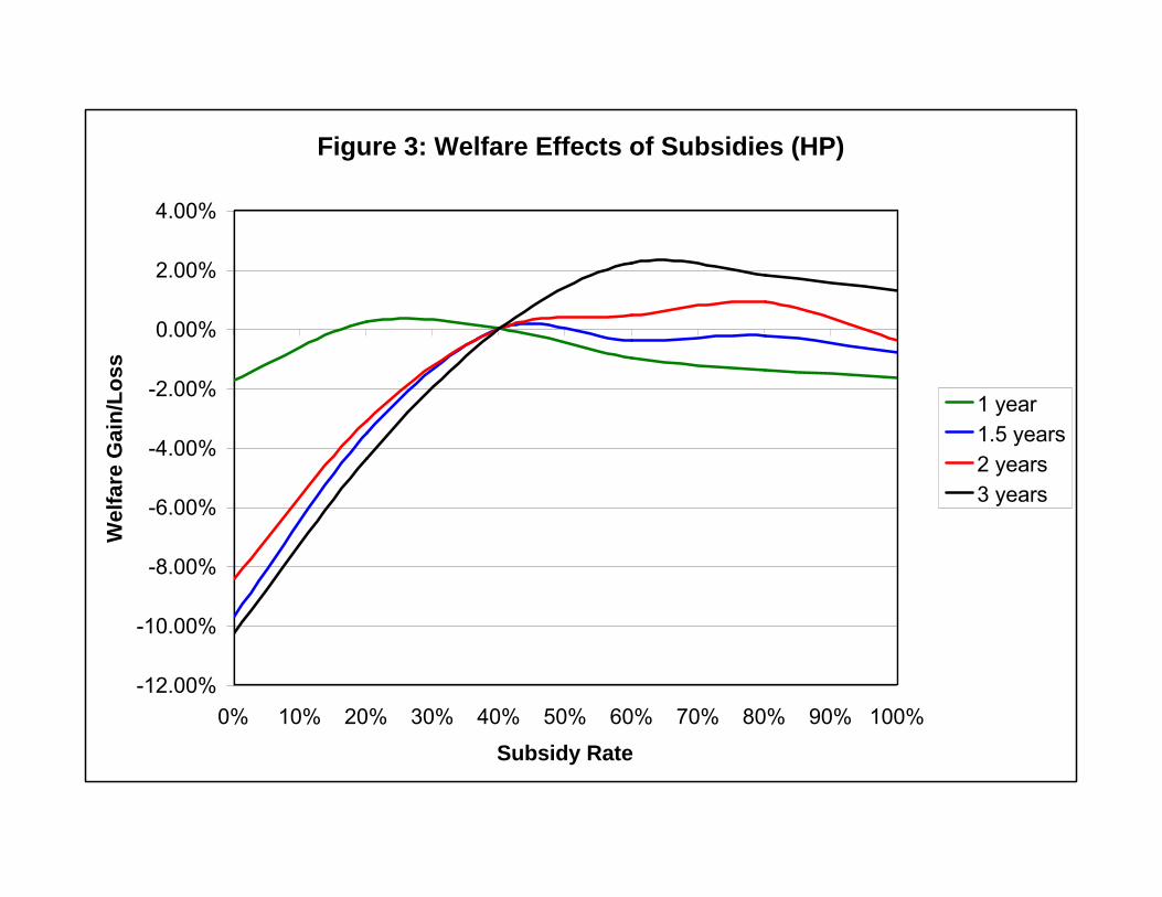
Figure 3: Welfare Effects of Subsidies (HP)

-12.00%

-10.00%

-8.00%

-6.00%

-4.00%

-2.00%

0.00%

2.00%

4.00%

0% 10% 20% 30% 40% 50% 60% 70% 80% 90% 100% Subsidy Rate

Wel

fare

Gai

n/L

oss

1 year 1.5 years 2 years 3 years

Table 1: Prices and Quantities: MP case

Subsidy Rate Interest Rate (pre-tax) Tax Rate

Skilled Wage

Unskilled Wage

Skill Premium

Fraction of Skilled Workers

Capital/ Output Ratio

Avg. Cons.

Cons./ Output Ratio C.V.-Cons.

Data 40% 6% 35% N/A N/A 1.6 38.00% 3 N/A 0.6 N/A MP, 1 Year 0.00% 5.48% 30.50% 0.739 0.433 1.709 36.52% 2.753 0.465 0.551 0.341 MP, 1-Year 20.00% 5.55% 31.20% 0.715 0.445 1.605 37.94% 2.738 0.467 0.552 0.320 MP, 1 Year 40.00% 5.60% 31.70% 0.714 0.446 1.600 38.00% 2.728 0.467 0.552 0.320 MP, 1-Year 60.00% 5.57% 32.29% 0.713 0.445 1.601 38.00% 2.734 0.467 0.552 0.314 MP, 1 Year 80.00% 5.63% 32.90% 0.711 0.444 1.601 38.01% 2.721 0.467 0.553 0.307 MP, 1-Year 100.00% 5.71% 33.46% 0.709 0.442 1.604 37.96% 2.704 0.467 0.555 0.308

MP, 1.5-Years 0.00% 5.36% 31.00% 0.757 0.427 1.772 35.70% 2.777 0.458 0.543 0.377 MP, 1.5-Years 20.00% 5.52% 31.30% 0.722 0.442 1.635 37.52% 2.744 0.466 0.550 0.325 MP, 1.5-Years 40.00% 5.58% 31.60% 0.714 0.446 1.600 38.16% 2.731 0.469 0.553 0.321 MP, 1.5-Years 60.00% 5.64% 32.40% 0.709 0.445 1.591 38.15% 2.719 0.466 0.552 0.319 MP, 1.5-Years 80.00% 5.70% 33.10% 0.706 0.445 1.588 38.20% 2.706 0.465 0.552 0.311 MP, 1.5-Years 100.00% 5.77% 33.90% 0.705 0.443 1.593 38.13% 2.693 0.464 0.552 0.300

MP, 2-Years 0.00% 5.32% 31.30% 0.784 0.414 1.896 34.20% 2.786 0.454 0.541 0.400 MP, 2-Years 20.00% 5.48% 31.60% 0.738 0.434 1.700 36.64% 2.753 0.461 0.546 0.347 MP, 2-Years 40.00% 5.59% 31.80% 0.714 0.446 1.600 38.16% 2.729 0.468 0.553 0.322 MP, 2-Years 60.00% 5.63% 32.10% 0.705 0.448 1.574 38.40% 2.721 0.469 0.554 0.313 MP, 2-Years 80.00% 5.70% 32.80% 0.701 0.448 1.567 38.52% 2.707 0.468 0.555 0.306 MP, 2-Years 100.00% 5.81% 34.00% 0.700 0.445 1.573 38.42% 2.685 0.464 0.552 0.292

MP, 3-Years 0.00% 5.00% 32.60% 0.933 0.358 2.607 27.51% 2.857 0.420 0.524 0.557 MP, 3-Years 20.00% 5.41% 32.30% 0.762 0.422 1.806 35.29% 2.768 0.453 0.538 0.376 MP, 3-Years 40.00% 5.60% 32.00% 0.714 0.446 1.600 38.17% 2.728 0.464 0.549 0.329 MP, 3-Years 60.00% 5.66% 32.20% 0.693 0.455 1.523 39.19% 2.715 0.469 0.553 0.302 MP, 3-Years 80.00% 5.80% 33.60% 0.692 0.450 1.538 38.94% 2.687 0.463 0.550 0.288 MP, 3-Years 100.00% 5.89% 34.10% 0.686 0.451 1.522 39.20% 2.669 0.463 0.551 0.274

Table 2: Prices and Quantities: HP case

Subsidy Rate Interest Rate (pre-tax) Tax Rate

Skilled Wage

Unskilled Wage

Skill Premium

Fraction of Skilled Workers

Capital/ Output Ratio

Avg. Cons.

Cons./ Output Ratio C.V.-Cons.

Data 40% 6% 35% N/A N/A 1.6 38.00% 3 N/A 0.6 N/A HP, 1 Year 0.00% 5.17% 30.85% 0.743 0.442 1.682 36.53% 2.415 0.467 0.545 0.334 HP, 1 Year 20.00% 5.26% 31.11% 0.727 0.448 1.622 37.99% 2.398 0.471 0.549 0.313 HP, 1 Year 40.00% 5.39% 32.00% 0.723 0.446 1.620 37.99% 2.362 0.469 0.551 0.313 HP, 1 Year 60.00% 5.49% 32.78% 0.718 0.445 1.612 37.99% 2.334 0.465 0.548 0.317 HP, 1 Year 80.00% 5.57% 33.37% 0.715 0.444 1.611 37.99% 2.312 0.465 0.550 0.322 HP, 1 Year 100.00% 5.63% 33.90% 0.710 0.445 1.596 37.99% 2.299 0.466 0.551 0.328

HP, 1.5-Years 0.00% 5.04% 31.00% 0.811 0.410 1.980 33.14% 2.401 0.453 0.538 0.442 HP, 1.5-Years 20.00% 5.20% 31.00% 0.755 0.434 1.741 36.10% 2.397 0.465 0.545 0.385 HP, 1.5-Years 40.00% 5.35% 31.85% 0.722 0.451 1.600 38.04% 2.378 0.469 0.548 0.341 HP, 1.5-Years 60.00% 5.39% 32.44% 0.719 0.448 1.605 38.04% 2.363 0.466 0.547 0.339 HP, 1.5-Years 80.00% 5.46% 33.06% 0.716 0.448 1.599 38.04% 2.344 0.467 0.548 0.337 HP, 1.5-Years 100.00% 5.49% 33.70% 0.717 0.445 1.611 38.04% 2.333 0.466 0.549 0.347

HP, 2-Years 0.00% 5.09% 31.20% 0.803 0.412 1.946 33.60% 2.392 0.453 0.538 0.433 HP, 2-Years 20.00% 5.23% 31.20% 0.752 0.435 1.728 36.34% 2.391 0.463 0.544 0.382 HP, 2-Years 40.00% 5.36% 32.00% 0.721 0.451 1.600 38.04% 2.376 0.466 0.545 0.342 HP, 2-Years 60.00% 5.41% 32.40% 0.714 0.451 1.584 38.04% 2.362 0.466 0.546 0.336 HP, 2-Years 80.00% 5.45% 32.80% 0.715 0.448 1.595 38.04% 2.349 0.468 0.550 0.336 HP, 2-Years 100.00% 5.51% 33.80% 0.714 0.447 1.597 38.04% 2.331 0.464 0.547 0.346

HP, 3-Years 0.00% 4.98% 31.00% 0.831 0.402 2.065 32.46% 2.404 0.451 0.537 0.460 HP, 3-Years 20.00% 5.18% 31.20% 0.767 0.428 1.790 35.39% 2.396 0.460 0.541 0.399 HP, 3-Years 40.00% 5.35% 32.00% 0.721 0.451 1.600 37.92% 2.378 0.466 0.544 0.346 HP, 3-Years 60.00% 5.44% 32.20% 0.695 0.462 1.503 39.27% 2.367 0.469 0.547 0.324 HP, 3-Years 80.00% 5.51% 33.10% 0.696 0.459 1.518 39.27% 2.345 0.467 0.547 0.327 HP, 3-Years 100.00% 5.58% 34.10% 0.693 0.458 1.514 39.27% 2.326 0.465 0.546 0.331

Table 3: Enrollment Rates: MP case Table 4: Enrollment Rates: HP case Non-1st Non-1st

Subsidy Gen. 1st Gen. Subsidy Gen. 1st Gen. Rate Students Students All Young Rate Students Students All Young

Data 0.00% 83.00% 59.00% 75.20% MP, 1 Year 0.00% 65.83% 59.96% 62.11% MP, 1-Year 20.00% 67.37% 62.62% 64.43% MP, 1 Year 40.00% 67.37% 62.62% 64.43% MP, 1-Year 60.00% 67.37% 62.62% 64.43% MP, 1 Year 80.00% 67.37% 62.62% 64.43% MP, 1-Year 100.00% 67.37% 62.62% 64.43%

MP, 1.5-Years 0.00% 66.72% 54.01% 58.54% MP, 1.5-Years 20.00% 66.88% 61.24% 63.36% MP, 1.5-Years 40.00% 67.53% 62.52% 64.43% MP, 1.5-Years 60.00% 67.53% 62.52% 64.43% MP, 1.5-Years 80.00% 67.53% 62.52% 64.43% MP, 1.5-Years 100.00% 67.53% 62.52% 64.43%

MP, 2-Years 0.00% 66.43% 47.58% 53.99% MP, 2-Years 20.00% 67.02% 56.68% 60.46% MP, 2-Years 40.00% 67.65% 62.41% 64.43% MP, 2-Years 60.00% 67.65% 62.41% 64.43% MP, 2-Years 80.00% 67.65% 62.41% 64.43% MP, 2-Years 100.00% 67.65% 62.41% 64.43%

MP, 3-Years 0.00% 68.59% 33.29% 42.98% MP, 3-Years 20.00% 67.41% 48.55% 55.25% MP, 3-Years 40.00% 67.94% 59.12% 62.49% MP, 3-Years 60.00% 68.23% 61.97% 64.43% MP, 3-Years 80.00% 68.03% 61.94% 64.33% MP, 3-Years 100.00% 68.23% 61.97% 64.43%

Data 0.00% 83.00% 59.00% 75.20% HP, 1 Year 0.00% 67.17% 57.82% 61.24% HP, 1 Year 20.00% 67.37% 62.62% 64.43% HP, 1 Year 40.00% 67.37% 62.62% 64.43% HP, 1 Year 60.00% 67.37% 62.62% 64.43% HP, 1 Year 80.00% 67.37% 62.62% 64.43% HP, 1 Year 100.00% 67.37% 62.62% 64.43%

HP, 1.5-Years 0.00% 67.90% 47.24% 54.09% HP, 1.5-Years 20.00% 66.89% 56.23% 60.08% HP, 1.5-Years 40.00% 67.53% 62.52% 64.43% HP, 1.5-Years 60.00% 67.53% 62.52% 64.43% HP, 1.5-Years 80.00% 67.53% 62.52% 64.43% HP, 1.5-Years 100.00% 67.53% 62.52% 64.43%

HP, 2-Years 0.00% 67.84% 48.30% 54.86% HP, 2-Years 20.00% 66.99% 57.20% 60.76% HP, 2-Years 40.00% 67.53% 62.21% 64.23% HP, 2-Years 60.00% 67.53% 62.52% 64.43% HP, 2-Years 80.00% 67.53% 62.52% 64.43% HP, 2-Years 100.00% 67.53% 62.52% 64.43%

HP, 3-Years 0.00% 67.25% 41.90% 50.13% HP, 3-Years 20.00% 68.51% 50.38% 56.80% HP, 3-Years 40.00% 68.26% 58.20% 62.01% HP, 3-Years 60.00% 68.37% 61.88% 64.43% HP, 3-Years 80.00% 68.37% 61.88% 64.43% HP, 3-Years 100.00% 68.37% 61.88% 64.43%

Table 5: Dropout Rates: MP case

Subsidy Rate

1st Gen. Students

Non-1st Gen. Students All Young

Data 0.00% 45.00% 24.00% 37.00% MP, 1 Year 0.00% 47.21% 17.67% 35.77% MP, 1-Year 20.00% 46.52% 17.74% 35.08% MP, 1 Year 40.00% 46.52% 17.74% 35.08% MP, 1-Year 60.00% 46.52% 17.74% 35.08% MP, 1 Year 80.00% 46.52% 17.74% 35.08% MP, 1-Year 100.00% 46.52% 17.74% 35.08%

MP, 1.5-Years 0.00% 44.17% 17.89% 33.50% MP, 1.5-Years 20.00% 45.82% 18.01% 34.76% MP, 1.5-Years 40.00% 45.89% 18.05% 34.78% MP, 1.5-Years 60.00% 45.89% 18.05% 34.78% MP, 1.5-Years 80.00% 45.89% 18.05% 34.78% MP, 1.5-Years 100.00% 45.89% 18.05% 34.78%

MP, 2-Years 0.00% 42.15% 17.09% 31.66% MP, 2-Years 20.00% 43.82% 18.11% 33.39% MP, 2-Years 40.00% 44.97% 18.22% 34.18% MP, 2-Years 60.00% 44.97% 18.22% 34.18% MP, 2-Years 80.00% 44.97% 18.22% 34.18% MP, 2-Years 100.00% 44.97% 18.22% 34.18%

MP, 3-Years 0.00% 35.60% 17.44% 27.64% MP, 3-Years 20.00% 38.58% 17.74% 29.55% MP, 3-Years 40.00% 41.80% 18.59% 32.15% MP, 3-Years 60.00% 42.31% 18.41% 32.38% MP, 3-Years 80.00% 42.31% 18.48% 32.43% MP, 3-Years 100.00% 42.31% 18.41% 32.38%

Table 6: Dropout Rates: HP case

Subsidy Rate

1st Gen. Students

Non-1st Gen. Students All Young

Data 0.00% 45.00% 24.00% 37.00% HP, 1 Year 0.00% 45.00% 18.11% 34.23% HP, 1 Year 20.00% 46.52% 17.74% 35.08% HP, 1 Year 40.00% 46.52% 17.74% 35.08% HP, 1 Year 60.00% 46.52% 17.74% 35.08% HP, 1 Year 80.00% 46.52% 17.74% 35.08% HP, 1 Year 100.00% 46.52% 17.74% 35.08%

HP, 1.5-Years 0.00% 42.51% 16.74% 31.79% HP, 1.5-Years 20.00% 43.55% 18.40% 33.44% HP, 1.5-Years 40.00% 45.89% 18.05% 34.78% HP, 1.5-Years 60.00% 45.89% 18.05% 34.78% HP, 1.5-Years 80.00% 45.89% 18.05% 34.78% HP, 1.5-Years 100.00% 45.89% 18.05% 34.78%

HP, 2-Years 0.00% 42.17% 17.37% 31.87% HP, 2-Years 20.00% 43.50% 18.65% 33.55% HP, 2-Years 40.00% 45.61% 18.05% 34.59% HP, 2-Years 60.00% 45.89% 18.05% 34.78% HP, 2-Years 80.00% 45.89% 18.05% 34.78% HP, 2-Years 100.00% 45.89% 18.05% 34.78%

HP, 3-Years 0.00% 37.20% 17.26% 28.52% HP, 3-Years 20.00% 38.87% 18.73% 30.27% HP, 3-Years 40.00% 40.91% 18.28% 31.46% HP, 3-Years 60.00% 42.16% 18.35% 32.23% HP, 3-Years 80.00% 42.16% 18.35% 32.23% HP, 3-Years 100.00% 42.16% 18.35% 32.23%

Table 7: Inequality and Mobility: MP case Subsidy Rate Gini-Cons. Gini-Wealth C.V.-Cons. C.V.-Wealth

Inc. Mobil.

Wealth Mobil.

Data 40% 0.30 0.78 N/A N/A 0.4 N/A MP, 1 Year 0.00% 0.20 0.56 0.341 1.051 0.039 0.400 MP, 1-Year 20.00% 0.18 0.56 0.320 1.038 0.036 0.385 MP, 1 Year 40.00% 0.18 0.55 0.320 1.048 0.036 0.410 MP, 1-Year 60.00% 0.18 0.55 0.314 0.996 0.036 0.363 MP, 1 Year 80.00% 0.18 0.52 0.307 0.942 0.036 0.348 MP, 1-Year 100.00% 0.18 0.51 0.308 0.928 0.036 0.336

MP, 1.5-Years 0.00% 0.22 0.63 0.377 1.182 0.147 0.939 MP, 1.5-Years 20.00% 0.19 0.56 0.325 1.032 0.115 0.943 MP, 1.5-Years 40.00% 0.19 0.56 0.321 1.054 0.105 0.952 MP, 1.5-Years 60.00% 0.18 0.55 0.319 1.036 0.105 0.949 MP, 1.5-Years 80.00% 0.18 0.53 0.311 0.988 0.105 0.945 MP, 1.5-Years 100.00% 0.17 0.50 0.300 0.908 0.105 0.937

MP, 2-Years 0.00% 0.23 0.63 0.400 1.166 0.185 0.935 MP, 2-Years 20.00% 0.20 0.58 0.347 1.073 0.124 0.942 MP, 2-Years 40.00% 0.19 0.55 0.322 1.045 0.100 0.951 MP, 2-Years 60.00% 0.18 0.54 0.313 1.019 0.100 0.949 MP, 2-Years 80.00% 0.18 0.53 0.306 0.975 0.100 0.945 MP, 2-Years 100.00% 0.17 0.49 0.292 0.883 0.100 0.937

MP, 3-Years 0.00% 0.30 0.73 0.557 1.457 0.242 0.921 MP, 3-Years 20.00% 0.22 0.60 0.376 1.122 0.167 0.936 MP, 3-Years 40.00% 0.19 0.57 0.329 1.069 0.097 0.950 MP, 3-Years 60.00% 0.17 0.53 0.302 1.006 0.087 0.950 MP, 3-Years 80.00% 0.17 0.50 0.288 0.899 0.087 0.940 MP, 3-Years 100.00% 0.16 0.47 0.274 0.847 0.087 0.941

Table 8: Inequality and Mobility: HP case Subsidy Rate Gini-Cons. Gini-Wealth C.V.-Cons. C.V.-Wealth

Inc. Mobil.

Wealth Mobil.

Data 40% 0.30 0.78 N/A N/A 0.4 N/A HP, 1 Year 0.00% 0.18 0.50 0.334 0.956 0.014 0.251 HP, 1 Year 20.00% 0.17 0.46 0.313 0.881 0.015 0.238 HP, 1 Year 40.00% 0.17 0.45 0.313 0.869 0.015 0.238 HP, 1 Year 60.00% 0.17 0.45 0.317 0.901 0.015 0.238 HP, 1 Year 80.00% 0.18 0.46 0.322 0.929 0.015 0.238 HP, 1 Year 100.00% 0.18 0.48 0.328 0.961 0.015 0.255

HP, 1.5-Years 0.00% 0.24 0.66 0.442 1.282 0.150 0.897 HP, 1.5-Years 20.00% 0.21 0.61 0.385 1.166 0.104 0.903 HP, 1.5-Years 40.00% 0.19 0.55 0.341 1.036 0.089 0.899 HP, 1.5-Years 60.00% 0.19 0.54 0.339 1.022 0.089 0.899 HP, 1.5-Years 80.00% 0.19 0.53 0.337 1.014 0.089 0.903 HP, 1.5-Years 100.00% 0.19 0.54 0.347 1.059 0.089 0.911

HP, 2-Years 0.00% 0.24 0.65 0.433 1.262 0.138 0.898 HP, 2-Years 20.00% 0.21 0.61 0.382 1.165 0.095 0.902 HP, 2-Years 40.00% 0.19 0.56 0.342 1.041 0.089 0.899 HP, 2-Years 60.00% 0.19 0.54 0.336 1.022 0.089 0.902 HP, 2-Years 80.00% 0.19 0.53 0.336 1.015 0.089 0.903 HP, 2-Years 100.00% 0.19 0.55 0.346 1.066 0.089 0.911

HP, 3-Years 0.00% 0.25 0.67 0.460 1.299 0.155 0.893 HP, 3-Years 20.00% 0.22 0.62 0.399 1.201 0.105 0.901 HP, 3-Years 40.00% 0.19 0.56 0.346 1.050 0.078 0.899 HP, 3-Years 60.00% 0.18 0.54 0.324 1.020 0.071 0.907 HP, 3-Years 80.00% 0.18 0.54 0.327 1.024 0.071 0.909 HP, 3-Years 100.00% 0.18 0.54 0.331 1.041 0.071 0.913