Locational Choices: Modeling Consumer ... - Simon Blanchard

Article

Locational Choices: Modeling ConsumerPreferences for Proximity to Othersin Reserved Seating Venues

Simon J. Blanchard, Tatiana L. Dyachenko, and Keri L. Kettle

AbstractThis article proposes a measurement approach to determine how consumers prefer to locate themselves in proximity toothers during consumption experiences, such as when they purchase reserved seating tickets to a performance. Applied to datafrom locational choice experiments that simulate reserved seating assortments, administered to more than 2,000 participants,this approach reveals the importance of modeling proximity to others when studying locational choices. It also emphasizes thedegree to which consumers are heterogeneous in their preferences for proximity to both focal elements (e.g., stage, screen,aisles) and other consumers. Therefore, event operators should collect data beyond purchase ticket logs and also includeconsumers who did not purchase. Furthermore, this study illustrates how managers can use fitted, individual-level parametersand an optimization model to make more effective seat-level availability decisions. In addition to these recommendations formanagers of reserved seating venues, this article offers novel contributions to research related to advance selling, spatialmodels, and personal space.

Keywordsadvance selling, concert halls, locational choices, personal space, movie theaters, spatial models

Online supplement: https://doi.org/10.1177/0022243720941525

When consumers visit a theater or book a flight, they agree to

locate themselves near strangers, a situation that demands a

locational choice. Such choices represent common but also

challenging human experiences, with considerable implica-

tions for the ultimate consumption experience. For activities

such as sporting events and concerts, consumers might derive

utility from sharing a communal consumption experience (Holt

1995) and enjoying their shared reactions (Gainer 1995). Yet

close proximity to strangers also can create discomfort, which

consumers aim to minimize (Argo, Dahl, and Manchanda

2005; Maeng, Tanner, and Soman 2013; Szpak et al. 2015).

Given these distinct goals, people’s locational preferences vary

widely across both different environments and individuals. A

pregnant film consumer might prefer to sit near the aisle, know-

ing that she will need to leave her seat frequently during the

show; another consumer might prefer to sit near the back to

avoid having anyone behind her who might kick her seat; and

yet another may prefer sitting in the middle of the row to get the

best view of the screen.

Noting the importance of these locational preferences, many

venues try to accommodate consumer heterogeneity in a way

that benefits their firm-level outcomes. Reserved seating sys-

tems, available through in-theater kiosks or online seat maps,

allow movie theater consumers to maximize their individual

locational preferences, with likely benefits for the provider as

well. Because proximity to preferred focal elements in the

consumption space (e.g., movie screen, aisles) and to others

can influence consumers’ enjoyment and satisfaction (Pedersen

1977), these systems can (1) offer the promise of additional

revenues if firms charge a premium for the most desired loca-

tions (Xie and Shugan 2001), (2) increase the likelihood that

consumers make supplementary purchases (Gardete 2015), and

(3) enhance customer responses to marketing promotions

(Andrews et al. 2015).

To attain positive firm-level outcomes, venues first must

understand how individual-level locational preferences affect

Simon J. Blanchard is Beyer Family Associate Professor of Marketing,

Georgetown University, USA (email: [email protected]).

Tatiana L. Dyachenko is Assistant Professor of Marketing, University of

Georgia, USA (email: [email protected]). Keri L. Kettle is Assistant

Professor of Marketing, University of Manitoba, Canada (email: keri.kettle@

umanitoba.ca).

Journal of Marketing Research2020, Vol. 57(5) 878-899

ª American Marketing Association 2020Article reuse guidelines:

sagepub.com/journals-permissionsDOI: 10.1177/0022243720941525

journals.sagepub.com/home/mrj

https://doi.org/10.1177/0022243720941525

mailto:[email protected]




https://sagepub.com/journals-permissions

https://doi.org/10.1177/0022243720941525

http://journals.sagepub.com/home/mrj

occupancy (i.e., whether most seats are taken when an event

begins). Operators prefer high occupancy and use various stra-

tegies to ensure that most seats are taken most nights (Desiraju

and Shugan 1999; Kim, Natter, and Spann 2009).1 Prior to the

start of an event (when consumers still can purchase tickets), an

assortment of seats surrounded by others or in less desirable

locations may lead consumers to decide not to purchase. If they

do purchase tickets, their proximity to others in crowded spaces

may lead consumers to reduce their time spent in the venue

(Hui, Fader, and Bradlow 2009) or blame any negative expe-

rience on the firm, which may decrease their future consump-

tion (Wangenheim and Bayon 2007).

To understand which data operators typically use to exam-

ine locational preferences, in support of our research goal of

determining which data might enable them to identify drivers

of occupancy more accurately, we conducted a survey of 45

managers and operators of movie theaters and concert halls,

with the help of a panel company.2 As we expected, most of

these venues (77.7%) offer advance seat selection online or

through an on-site kiosk, and two-thirds mentioned their access

to a dashboard that provides them an aggregate view of which

seat locations have been purchased. Furthermore, the majority

(64.4%) stated that they try to collect information about what

drives consumers’ decisions not to purchase, but the informa-

tion collected tends to be limited to individual consumer names

and text comments (e.g., complaints) or relies on anonymous

surveys with multiple choice questions.

Another potential source of information is purchase logs,

which often are contained in the dashboards that depict aggre-

gated seat maps of upcoming and past events. By using these

logs, managers can determine how locations’ popularity varies

as a function of proximity to focal elements (e.g., screen, aisles,

exits). If firms construct their logs to facilitate reconstructions

of individual-level assortments, they can enhance their under-

standing and predictions of occupancy, using individual-level

models that incorporate the substantial heterogeneity in loca-

tional preferences.3 However, even if these individual-level

assortment data were combined with the best individual-level

models, such analyses would pertain only to choices that

resulted in a purchase.

With the present investigation, we argue that to influence

occupancy, reserved seating venues need to leverage

individual-level assortment data from consumers who did not

purchase as well as those who did. Therefore, we propose a

novel measurement approach that makes three key contribu-

tions. First, seat choice predictions based on aggregate data and

model results are inherently limited, because locational prefer-

ences are highly heterogeneous across contexts and individual

consumers. Therefore, we establish a practical need to collect

individual-level locational choice data and analyze them

according to individual-level preferences for proximity to focal

elements (e.g., screen, stage) and to other consumers. Second,

we argue that operators that need to predict and understand the

drivers of event occupancy should collect data that include the

assortments presented both to those who purchase seats and to

those who ultimately do not purchase. With such data, opera-

tors can make more effective seat availability decisions at the

seat level. Third, we propose a specific, novel mechanism (i.e.,

seat-level availability based on locational preferences), whose

effectiveness can be further investigated as a driver of

occupancy.

Drawing on psychology literature pertaining to perceptions

of personal space, we present a measurement model to capture

the decision-making process for locational choices in the next

section. This utility specification captures heterogeneous pre-

ferences for proximity to both focal elements and other con-

sumers and can be readily estimated using hierarchical Bayes

analyses. In four experiments involving 2,119 participants, we

present two analyses of common locational choice experiences

with reserved seating (attending a concert or a movie), while

varying the number of locations to be chosen (single vs. a pair

of seats). We show that consumers are heterogeneous with

respect to their locational preferences, depending on both the

event type (concerts vs. movies) and whether they are attending

with someone else. We provide evidence that our measurement

and estimation approach provide excellent prediction accuracy.

In turn, we illustrate how operators can use our parameter

estimates to improve expected occupancy by altering seat

availability. For this illustration, we first describe a seat-level

availability optimization model that maximizes occupancy

based on trained parameter estimates. Then, using observa-

tional data obtained from local ticket sales, we apply the pro-

posed optimization model to identify which additional

locations should be marked as unavailable. We also provide

preliminary experimental evidence that seat-level availability

based on estimated locational preferences can be leveraged to

improve expected occupancy rates.

1 A focus on occupancy as a metric is common, because gross revenue mainly

comes from ticket sales, even if reserved seating venues also enjoy higher

profit margins from food and beverage sales. For example, AMC Theatres

reports a gross profit margin of 49.2% but a profit margin of 83.6%

specifically for food and beverage sales. Still, the importance of occupancy

in driving profitability is evident in earnings announcements, which primarily

focus on “attendance per screen” (AMC 2019)2 The average age of these respondents was 36.70 years (min ¼ 21 years, max

¼ 72 years), 60% were women, and they noted average managerial experience

of 7.73 years (min¼ 1, max¼ 30), involving 26–50 employees and an average

of 10 screens or stages (min ¼ 1, max ¼ 60). Twelve informants were concert

theater/hall operators, and 33 were movie theater operators. We paid $18 per

participant.3 Time-stamped lists of seat choices might not accurately reconstruct the

precise choice set for each consumer. In our discussions with operators, they

offered various reasons for the lack of detailed choice data. For example,

front-end sales systems often restrict seat offerings to facilitate consumers’

choices, but those restrictions are not recorded. Seat changes also may be

collected separately from purchases, and they often reflect specific price

tiers. Finally, locations may be released sequentially or depend on fare

restrictions or shopper status (Williams 2018), such that some consumers

have options that other consumers do not. In most data we have seen,

purchase logs need to be augmented with availability data to recreate

accurate individual-level assortments.

Blanchard et al. 879

Consumer-Level Locational Choice UtilitySpecification

We begin by assuming that consumers aim to maximize the

realized utility of a selected location, given the options avail-

able to them. The locational choice element we consider is a

grid, in which each potential location can be assigned a set of

Cartesian coordinates from the set of all possible coordinates,

St. The probability that consumer h in task t chooses a location

assigned to row i and column j is thus (we omit h throughout

the text, for expositional clarity):

Pr�

yt ¼ ði; jÞj ��¼ Prðut;ij ¼ maxfutgÞ; ð1Þ

where ut is the set of realized utilities for available locations,

and the utility for location fi; jg is

ut;ij ¼ Vt;ij þ et;ij 8fi; jg 2 SAt : ð2Þ

Here, Vt;ij is the deterministic component of the utility func-

tion, and SAt � St is the subset of coordinates that captures

all available locations for a specific task t. Assuming that

the error Et;ij in Equation 2 comes from an extreme value

Type I distribution with a location parameter 0 and scale

parameter 1, the probability of selecting location fi; jg in

task t is

Pr�

yt ¼ ði; jÞj ��¼ expðVt;ijÞXfk2SA

t gexpðVt;kÞ

: ð3Þ

In the sections that follow, we detail the two main com-

ponents of our consumer-level utility function Vt;ij: (1)

proximity to focal elements in the space and (2) proximity

to others.

Utility from Proximity to Focal Elements

In a locational choice, many aspects of the environment are

directly relevant to the consumption experience. For example,

concertgoers attend to the position of seats relative to the stage,

and moviegoers evaluate the position of seats relative to the

screen. However, within a venue, other physical elements of

the space could be important. For example, being on one edge

of a space can be important for some consumers (e.g., being

next to an aisle enables the consumer to leave more easily);

physical and psychological factors also could lead consumers

to focus more on specific aspects of the environment, such as

reference points established through experience or expecta-

tions. For example, when choosing a seat at a movie theater,

consumers may prefer a central location because they believe

the center of the room provides the best viewing angle and

sound quality. Thus, the desired level of proximity to focal

elements likely varies across individual consumers (e.g., some

people insist on aisle seats) and context (e.g., a consumer might

prefer to be close to the stage for a rock concert but in the

middle for a movie).

To define the attributes of single-person locational choice

options formally (i.e., available seats4), we denote XL;t as a

design matrix for a layout t with two dimensions: xrtas a vector

of row assignments (front-to-back) and xctas a vector of col-

umn assignments (left-to-right), within the Cartesian coordi-

nate system:

XL;t ¼ ½xr;t xc;t�: ð4Þ

We transform the elements in XL;t to restrict them between 0

and 1, reflecting the bounded nature of the environment and the

characteristics of each location, relative to the focal elements.

We use indexes for the rows to identify the front (i.e., where the

person faces) and back. For each location, a value of xr;t close

to 0 indicates a seat closest to the focal element (front), whereas

1 signals a location that is farthest from this focal element

(back). The indexes for columns instead refer to the lateral

dimension, corresponding to the edges of the environment as

reference points. A value of xc;t close to 0 on the lateral dimen-

sion refers to a location that is the farthest left possible in the

environment (left to right), and xc;t close to 1 is the rightmost

location. Location fxr;t xc;tg ¼ f:5 :5g thus represents the

center of the room.

The attribute space denoted by Equation 4 assumes that only

one seat is chosen. However, it is fairly safe to assume that a

consumer choosing a pair of seats for an event would consider

the two locations jointly and not independently. One way to

handle this dependence, as we observe in all our data and as

intuition would suggest, is to assume that most consumers

looking for two seats only consider two seats side-by-side in

the same row. If we assume two seats are selected and that they

must be contiguous in the same row, the design matrix in

Equation 4 can be adapted for pairs of seats to

xc;t ¼ :5ðxc1;t þ xc2;tÞ, where c1 and c2 are the column coordi-

nates of two available and contiguous seats (i.e., assumed

choice for pairs of seats). For the choice of a pair, xr;t does not

change, but xc;t is the midpoint between the two seats.

The design matrix XL;t thus provides a way to describe

available locations in the environment, but preferences for each

location also depend on the utility for the individual consumer,

as detailed in Equation 2. To accommodate the various ways in

which a location’s position affects consumers’ choices, as a

result of its proximity to focal elements, we specify this com-

ponent of the deterministic part of the utility function as a

bivariate quadratic function (we omit the subscript t for exposi-

tional clarity):

VL ¼ br;1x2r þ bc;1x2

c þ br;2xr þ bc;2xc þ br;cxrxc: ð5Þ

There is no intercept, and the preference parameters’ bs are

estimated relative to preferences for a seat with xr ¼ 0 and

xc ¼ 0, for identification purposes. Equation 5 is a flexible

4 Options within a locational choice (locations) may or may not be actual seats.

A movie theater may offer wheelchair-accessible locations, for example. We

still refer to them as seats.

880 Journal of Marketing Research 57(5)

specification that allows for heterogeneous effects of proximity

to focal elements. For example, considering their preferences in

the lateral dimension (left to right), consumers attending a

movie likely prefer to be located near the center of the room,

so the closer xL;th ¼ ði jÞ is to ð:5 :5Þ, the greater their

utility for a central location. However, some might prefer to

sit all the way to the left or right so that they can position

themselves near an edge in the space. Furthermore, the prox-

imal and lateral dimensions might interact; consumers attend-

ing a concert might be willing to forgo the best viewing angle if

they can get very close to the stage, for example.

The specification in Equation 5 provides several advantages

in terms of our effort to reflect heterogeneous preferences

regarding the ideal proximity to focal elements. The function

may have a vertex that represents either a utility maximum or a

minimum. For example, a person who wants a seat exactly in

the middle of the theater would produce a concave function on

both dimensions, with maximum utility at the center. However,

a person who wants to avoid the center and sit close to an aisle

instead produces a convex function across columns, with

higher utility at the edges. The location of the vertex also might

shift with changes in layouts and venues, in which the focal

point is not necessarily the center of the environment. A linear

functional form without the quadratic term is a special case of

Equation 5, when br;1 ¼ 0 and bc;1 ¼ 0. The parameter br;c

captures the potential interaction—whether a trade-off or a

compensating relationship—between the front-to-back (row)

and left-to-right (column) dimensions.

(Dis)utility from Proximity to Others

Because each potential location features proximity to others,

we seek to capture the potential (dis)utility of numerous imme-

diate and less proximal others.

Capturing the effect of immediately proximal others. Immediate

proximity may be sensed in any direction, so we use Lp spaces

to specify a one-unit L1 sphere around each seat (i.e., the dis-

tance between an available location and any other is determined

by the greatest distance along any coordinate dimension).

Because each seat varies in the number of seats around it, we

capture the presence of immediate others as the proportion of

locations at the boundary of the sphere (R1) that also are occu-

pied by others.

Formally, assume that consumer h is considering an avail-

able seat ði; jÞ for choice task t, and St is a set of the coordinates

of all seats in the environment, such that ði; jÞ defines the

origin (i.e., coordinates are centered at ½i; j�). We set attribute

xi;jR1 ¼ jSB

R1j=jSR1j, where SR1 ¼ fa 2 St : jjajj1 ¼ 1g; in addi-

tion, SBR1 � SR1 refers to the subsets of seats already occupied

by others. Therefore, xi;jR1 captures the proportion of seats at

exactly one unit away (in one or more dimension) that are occu-

pied by others. Proximal locations that do not offer seats (e.g., the

aisle is to the left) thus are not immediately proximal locations.

Finally, xR1 provides the row vector of all available seats, andbR1

is the corresponding parameter. Then the equation

VR1 ¼ xR1bR1 ð6Þ

captures the component of the utility from being surrounded by

others (i.e., proportion of occupied seats at the boundary of the

L1 one-unit sphere).

Although Equation 6 may be helpful for capturing a com-

bined effect of numerous immediately proximal others, those in

immediate proximity likely are more relevant, due to the risk

that they intrude on the focal consumer’s personal space. Thus,

an important consideration in proximity studies is the recogni-

tion that personal space is a function of others’ immediate

closeness to the individual, not general density in the space

(Harrell, Hutt, and Anderson 1980). This salience of close oth-

ers is evident in colloquial descriptions of personal space as a

“bubble” (or sphere), which can be defined as an “infinitely

malleable entity that is exquisitely responsive to situational

demands” (Hayduk 1983, p. 297). The shape of this region is

generally circular but is especially sensitive to frontal invasions

(Argyle 2013). Defining immediate closeness requires consid-

erations of not just distance perceptions but also situational,

personal, and cultural factors that may influence the shape of

the sphere. In particular, models of the effect of immediately

proximate others should reflect the direction in which those

others are located. We therefore differentiate the front (i.e.,

between the consumer and the most focal element, such as a

screen or stage), back (behind the consumer), and sides (to the

left or right of the consumer) and how they relate to different

uses of the environment and expectations. If the focal element

in the environment is a screen, a proximal person in front may

block the field of vision, which would affect the experience

differently than a proximal person to the focal consumer’s side

or back. Therefore, we introduce a (directional) specification of

the effect of immediately proximal others:

VPS ¼ XPSbPS; ð7Þ

where XPS is a design matrix.

Our use of the subscript “PS” reflects a common terminol-

ogy to refer to the immediate proximity of others that impinge

on personal space. The vector bPS includes the corresponding

parameters that describe the effects of attributes on the utility

of each potential seat. Each available seat is represented by a row

vector xPS. The elements ðxleft; xright; xfront; xbackÞ represent

the number of occupied seats in these directions. For a single seat

choice, the count for all four elements of the vector is necessarily 0

(empty) or 1 (occupied). However, for pairs of contiguous seats,

xfront and xback can take values of 0, 1, or 2, so we code them as

spaces occupied. Finally, we count the number of occupied seats

in front or back corners: xcountFc and xcountBc, respectively. The

vector for the directional proximity to immediate others is

xPS ¼ ðxleft xright xfront xback xintLR xcountFc xcountBcÞ;ð8Þ

and the parameter vector is


bPS ¼ ðblef t bright bf ront bback bintLR bcountFc bcountBcÞ:ð9Þ

We further note that xLRint equals 1 if seats to both the left

and right are occupied (e.g., middle seat). If a consumer derives

negative utility from the immediate proximity of others, simul-

taneous intrusions on personal space from multiple dimensions

might provide a strong deterrent, due to the superadditive prop-

erty of this (dis)utility. Public transit passengers often exhibit a

preference to stand rather than to take an empty seat between

two occupied seats (Fried and DeFazio 1974). Accordingly, the

disutility of having somebody in seats to both the immediate

left and the immediate right could be even greater than the sum

of the individual disutilities of having someone in either seat

(Hayduk 1978). In turn, the parameter bintLR would be negative,

such that conditional on neighboring seats already being occu-

pied (e.g., on the right), adding a second occupied seat (e.g., on

the left) is worse than if that occupancy occurred in conjunction

with an otherwise empty seat. A consumer who expresses such

values likely is particularly averse to invasions of personal

space on that dimension. However, if bintLR is positive, it indi-

cates a subadditive property of the utility; a person might be

averse to an invasion of personal space to the left and right, but

the effect of adding the second neighbor might not be as neg-

ative as would be implied by the original additive structure in

this case.

Capturing the effect of less proximal others. Others outside the

boundary defined by the one-unit L1 sphere could also influ-

ence the utility of a potential seat. For example, those within

two seats (in any direction) may have an effect, such that

consumers might extract information about popular areas in

the space. Expanding beyond immediately proximal locations,

but assuming that directionality becomes less important

beyond immediate proximity, we can define larger spheres of

potential effects of (less) proximal others. For any number n,

we set xi;jRn ¼ jSB

Rnj=jSRnj, where SRn ¼ fa 2 St : jjajj1 ¼ 1g.Here again, SB

Rn � SRn is the subset of locations already occu-

pied by others. Then, we can define

VRn ¼ xRnbRn; ð10Þ

where xRn is a row vector that, for each available location,

records the proportion of seats that are occupied within an n-

unit sphere (still in L1 norm), and bRn is a parameter that

captures the effects. Figure 1 summarizes how our various

measures capture proximity to others with respect to R1, PS,

R2, and R3 around the focal location ði; jÞ.

Hierarchical Model

Consumers’ choice from a set of available seats can be a func-

tion of preferences with respect to any combination of the

proximity to focal elements (VL) and the proximity to others

(VPS, VR1, VR2, and VR3) Depending on the assumptions of the

data-generating mechanism, we can consider different model

specifications. For example, the model

Vt;ij ¼ VLt;ijþ VPSt;ij

þ VR2t;ijþ VR3t;ij

ð11Þ

combines proximity to focal elements (VL), immediate prox-

imity of others according to a directional one-unit sphere (VPS),

and effects of nonproximal others (VR2 and VR3) to describe

the deterministic component of the model in Equation 2, using

Figure 1. Visual depictions of how proximity to (immediate) others is captured.Notes: In the left panel, xR1 ¼ :5, xR2 ¼ :38, and xR3 ¼ :42. With respect to XPS, xleft ¼ 0; xright ¼ 1; xfront ¼ 1, xback ¼ 1; xintLR ¼ 0; xcountFc ¼ 1 and xcountBc ¼ 0.In the right panel, xR1 ¼ :5, xR2 ¼ :38 and xR3 ¼ :42. With respect to XPS, xleft ¼ 0;xright ¼ 1; xfront ¼ 2, xback ¼ 1; xintLR ¼ 1; xcountFc ¼ 0 and xcountBc ¼ 0.


the specification in Equations 5, 7, and 10. It assumes that no

outside option is available; the consumer must choose. But in

most cases, consumers have the outside option, because they

are not forced to choose seats. Exercising this outside option

takes many forms in the real world (e.g., buying seats for

another event), but we assume that it entails skipping the par-

ticular event for which the assortment is being presented. Con-

sistent with prior literature, we refer to it as the “no-choice”

option. To estimate bno-choice, which describes a preference for

the no-choice option, we modify the design matrix for each

choice by adding a row for the no-choice alternative in each

choice’s design matrix, as well as a column of zeroes to all

except the row representing the no-choice option (see Haaijer,

Kamakura, and Wedel 2001).

The probability of selecting a location ði; jÞ is given by

Prðyt ¼ mj�Þ ¼ expðVt;mÞXfk2fSA

t ;no-choiceggexpðVt;kÞ

; ð12Þ

where m is either a seat or an outside option. In this example,

the likelihood for all respondents h ¼ f1; :::;Hg in all tasks

t ¼ f1; :::;Tg is

‘ ¼YHh¼1

YT

t¼1

Prðyh;tjXLh;t;XPSh;t

;XR2h;t;XR3h;t

; bLh; bPSh

; bR2h; bR3h

; bno-choicehÞ:

ð13Þ

In the hierarchical model specification for heterogeneous

preferences among consumers, the parameter vectors

bh ¼ fbLh; bPSh

; bR2h; bR3h

; bno-choice;hg are specific to each

individual and assumed to reflect a normal distribution with

parameters:

bh*NðD0zh;DbÞ; ð14Þ

where zh is a vector of respondent-specific or environment-

specific covariates. If no individual-level or context-level cov-

ariates are used, zh is a vector of 1s.

We investigate all models that vary in terms of whether (and

how) the proximity of others is considered. We estimate our

models within a Bayesian framework, which provides multiple

well-established benefits for researchers, and especially for

estimating hierarchical models to accommodate heterogeneous

consumer preferences or making probabilistic statements about

the parameters. The details of the estimation are in Web

Appendix A, and a simulation study (for parameter recovery

and convergence) is in Web Appendix B.

Prediction Benchmarks

To provide managers with insights into how consumers make

locational choices and to enable individual-level predictions,

we introduce both a way to codify individual-level locational

data and an individual-level utility function with a significant

amount of structure. If the focus is not necessarily on under-

standing the precise nature of the heterogeneous patterns, such

that the operator solely wishes to make predictions about which

available seat(s) are likely to be chosen, it could resort to the

many available supervised learning methods that can be trained

to recover the latent structure (e.g., Equation 11) or learn it

from data. Convolutional neural networks (CNNs) are particu-

larly useful for inferring structures from marketing data auto-

matically (e.g., Xia, Chatterjee, and May 2019; Timoshenko

and Hauser 2019). With sufficient data and an appropriate

specification, such models should be able to recover the utility

specification that we propose. However, their ability to do so

depends on the amount of data provided per consumer and

whether there is substantial individual heterogeneity to accom-

modate. These networks benefit from pooling operations, so

substantive individual heterogeneity would make the predic-

tion problem more difficult for them.

To illustrate the difficulty of this prediction exercise and

provide guidance for users interested solely in prediction,

we implement a CNN. For layouts with sizes of up to 20

locations per dimension, we create an input vector of size

400, where 0 indicates that the location is unavailable and 1

implies it is available. Locations that pad the space (i.e.,

that are not seats) are marked by 0. Then, we use PyTorch

(Paszke et al. 2017) to devise a model with one convolu-

tional layer, one channel, a kernel size of three, a stride of

one, and a linear layer of 400 � 400. In the linear layer, all

the neurons (i.e., locations) are connected, so we can define

spatial preferences within the room. With the 3 � 3 con-

volutional layer, we capture effects that are spatially invar-

iant.5 The convolutional layer thus should capture

immediate proximity to others, whereas the fully connected

layer captures the preference for locations within the phys-

ical space. We trained the model with Adam (Kingma and

Ba 2014), to minimize networks’ cross-entropy losses,

which is equivalent to minimizing the negative log-

likelihood of the data. Throughout this manuscript, we

report the in-sample and holdout prediction using this

benchmark predictive model. We reserve our interpretation

of the benchmark model’s results for the “General Dis-

cussion” section.

Experimental Insights

We gathered experimental data about two locational choices

that are common consumer experiences: reserved seating at

movie theaters and concert halls. In both cases, we expect

heterogeneous location preferences, thus substantiating the

need to use individual-level locational data when studying

occupancy. Before we turn to our analyses, we offer three key

points.

First, our data were collected entirely through experiments

involving a locational choice platform, seatmaplab.com. As we

5 Across our experiments, we find little evidence that additional convolutional

layers would be helpful. A multilayer perceptron instead performs nearly as

well as the final CNN.


http://seatmaplab.com

noted previously, ticket purchase logs do not capture the

individual-level choice set of those who choose not to pur-

chase, rendering individual-level analyses of the drivers of

occupancy questionable at best.

Second, we report only two analyses based on subsets of

data from four large experiments collected as part of this

project. Our four experiments varied the context (movie/con-

certs) and the number of tickets (pairs/single). However, we

conducted these experiments in hopes of providing expansive

coverage of many other factors that may be relevant to loca-

tional preference, such as existing occupancy (i.e., proportion

of seats already purchased in the map shown to a participant),

whether a no-choice option is offered, the timing of the event

(e.g., soon or a few months away), and the room layout (e.g.,

portrait vs. landscape). To maintain clarity, we only discuss

subsets of these data. We encourage readers who are inter-

ested in understanding how we could (and did) incorporate

important covariates, such as occupancy (e.g., popularity of

the event), to refer to Appendix A, which details each

experiment.

The analyses herein are organized into two sections. In the

first, we illustrate descriptively how aggregate analyses threa-

ten to mask substantial heterogeneity in individual-level pre-

ferences and systematic differences based on the number of

locations chosen (a pair vs. a single seat). In the second section,

we provide further evidence of the need to analyze individual-

level locational choice data in a different context, namely, pairs

of seats for a concert. Relative to the movie theater analysis,

these locational preferences are drastically different, yet still

heterogeneous at the individual level. Finally, we use a concert

context to provide an example of a usage scenario for the

model’s parameter estimates, designed to identify optimal

seat-level availability.

One or Two Seats for the Movies

We present an analysis of seat selections in a high occupancy

(75%) showing (i.e., only 25% of seats were left), such that

participants choose tickets for either one or two seats, or else

the outside option not to attend the movie. This analysis is

based on two subsets of our experimental data.

First, we asked participants to pick two seats for a movie.

Specifically, we asked participants from Amazon Mechanical

Turk (MTurk) to complete a ten-minute study about going to

the movies with a friend. When they started the study, partici-

pants had to imagine the following scenario:

You and a friend have a few hours to kill, and you walk to the

movie theater to see a movie you’ve wanted to see. You stop by

one of the ticket machines and look at the seat map. The movie

starts in a few minutes. Which seats would you choose? If you

don’t like the options available, you may decide to walk away and

go do something else.

After reviewing the instructions, participants received the loca-

tional choice interface (see Figure 2), which was a seating chart

similar to ones found on real-world seat booking websites. On a

left panel, we reminded participants that they needed to choose

two seats and that they would see different assortments in a

12� 12 theater. A counter of their progress appeared on the

screen. A color-coded legend indicated which seats were (un)a-

vailable,6 and a clickable text button below the seating chart

represented the no-choice option. After participants indicated

their choice, the software platform recorded the chosen pair of

locations, the seating layout characteristics, and the random

Figure 2. Movie analysis: Sample locational choice experimentinterface.Notes: This participant has selected the first of a pair of seats. The seats markedas occupied cannot be selected.

6 Choosing seats for the movies (or for a concert) is such a common experience

that we expected participants to have well-defined preferences. As such, we

expected that the specific way we chose to randomize would have little impact

on the coefficients extracted over repeated choices. In this experiment, we

proceeded with the simplest approach. For each participant’s load of a seat

map layout, based on occupancy (e.g., 75% occupied), a seat would be drawn

from two univariate uniforms. If the seat was available, it was then marked as

occupied. The process was repeated until the desired occupancy was reached.

We appreciate that such a randomization may not perfectly recreate the way

halls naturally fill. As such, we also experimented alternative randomization

processes (e.g., adding people by groups or based on an expected distribution).

We did not find meaningful differences with respect to model estimates or

accuracy.


seat availability that they saw. The analyses rely on data from

233 participants who completed at least 15 of 16 such choices.

The data and file details (E1-Movie-Pairs.NC:75) are in

Appendix A.

Second, in another experiment, we asked participants to

pick one seat for a movie. Specifically, we used data from

300 participants who first completed 12 tasks for which

occupancy was 75% in a similar 12� 12 theater, with a

no-choice option. Here, 18.7% (or 56) of participants pre-

ferred to skip the movie at least once, and the no-choice

option represented 4.4% of all choices. The data and file

details (E2-Movie-Singles.NC/FC: NC) are in Appendix A,

and we provide detailed estimations results for both these

analyses in Web Appendix C.

Model-free evidence. Figure 3 displays the frequencies of seat

choices separately for those who chose a pair of seats and those

who chose a single seat. When participants chose pairs of seats,

58% (or 136) of them opted for the no-choice option at least

once. Even though some participants always chose seats,

26.5% of all seat choices offered resulted in the participant

choosing to skip the movie and that number was not driven

by a few unmotivated participants.

Across both data sets, we find that the most popular seats

are the two in the middle center (row 7, columns 6 and 7);

we also note some preference for the middle aisles and back

center. However, participants selecting a pair of seats are

more likely to prefer being in the center and slightly to the

back relative to other popular locations. The choice fre-

quency also appears more dispersed than that among parti-

cipants who choose a single seat. For example, we find a

relatively stronger preference for the aisles in single seat

choice contexts. Unfortunately, this evidence does not allow

us to make statements about whether individual preferences

are dispersed similarly for all respondents or if the various

preferred locations might be preferred by different individ-

ual consumers.

Model fit. Table 1 presents the model fit statistics for both pairs

and single seat selections. First, we report the Newton and

Raftery estimator (Newton and Raftery 1994) of log-marginal

density (LMD NR).7 Second, we report the average choice

probability of the selected seats, as predicted by the model.

Third, we present the hit rate, obtained by selecting the option

with the highest choice probability. We break down the mean

choice probabilities and hit rate by in-sample and holdout sets.

The in-sample fit reflects data used to estimate the model;

holdout fit instead refers to the predictive fit of three choices

randomly removed from the sample. For these measures,

higher numbers indicate the model offers better fit and predic-

tive ability.

The results in Table 1 suggest that proximity to others is an

important determinant, regardless of whether one is choosing

one or two seats. Fit improves when we incorporate the para-

meters related to the proximity of others; this result is not

merely due to an increase in the number of parameters esti-

mated in the models. When looking for pairs, including the

directional effects of immediately proximate others (i.e., VPS)

improves both in-sample and holdout fit more than including

the three nondirected spheres of proximate others (i.e.,

VR1;VR2, and VR3). That is, adding the directional effects

of immediately proximate others increases the mean probabil-

ity and hit rate by 7%–10%, for both in-sample and holdout

choices. The importance of breaking down the directionality

of personal space is less important when buying a single seat;

it offers no improvement in holdout samples. In both cases,

Figure 3. Movie context: Observed choice probability by seat loca-tion and number of seats to be chosen (pairs vs. single).Notes: The movie screen was indicated to be ahead of row 1 (at the top). Thecolor bar values indicate the percentage of choices that were in that location(e.g., 2.5 is 2.5%). Uniform preference over all locations would lead to .7% inthe movie-pair condition, and 2.7% in the movie-single condition.

7 Details of the estimation and convergence diagnostics are in Web

Appendix C.


proximity to others is particularly important, and it is largely

limited to immediate proximity; the improvements between L

þ PS and L þ PS þ R1R2 are smaller than the change

between L þ R1R2R3 and L þ PS þ R1R2. All these models

substantially outperform chance, which is approximately 7%,

and our benchmark model. Taken together, these fit results

suggest that our individual-level measurement model is an

excellent approximation of the individual process involved

in choosing either one or two seats and that the inclusion of

proximity to not only focal elements but also others is

necessary.

Interpretation of parameters. Table 2 contains the posterior

means and 95% credible intervals (CI) of the upper-level para-

meter estimates, based on the best fitting model for single and

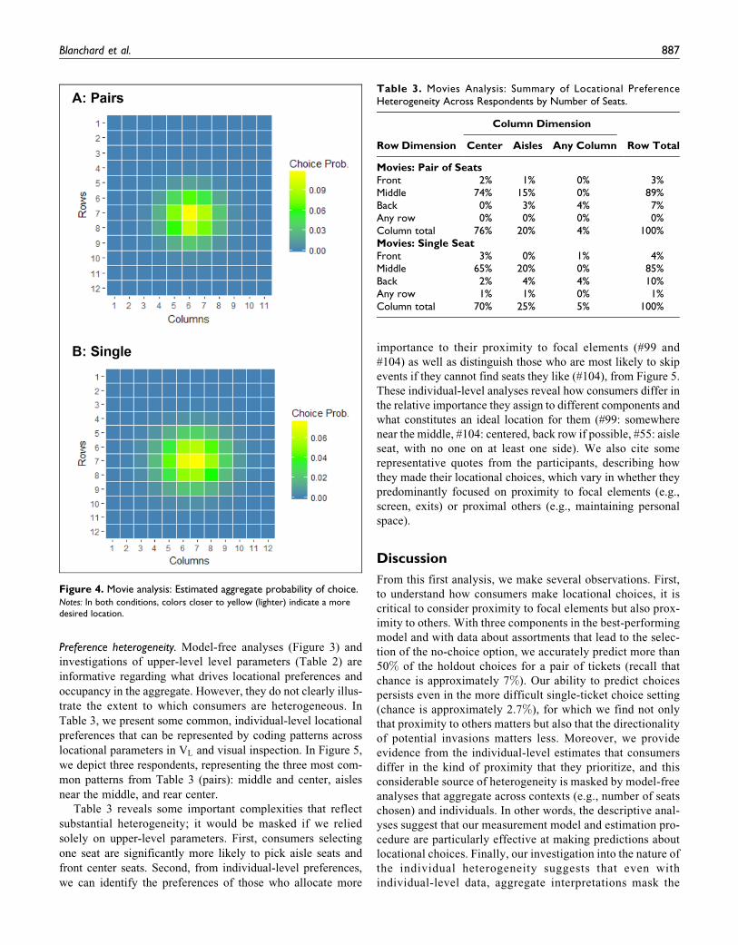
pairs of seat choices. Figure 4 displays a predictive “heat map”

for proximity to focal elements (i.e., excluding proximity to

others).

We note several similarities between the decision to buy a

pair of seats and the decision to buy a single seat. In terms of

locational preferences, in neither case do we find any evidence

that the rows and columns interact (i.e., the CI of brc includes

0).8 As we can show with Figure 4, participants exhibit a pre-

ference to sit in the middle of the theater, as well as a desire to

avoid less proximal others, such that both bR2and bR3

are

negative.

Yet we also can specify some pertinent differences.

When choosing a pair of seats, the potential lateral inva-

sions of personal space (i.e., someone to the left or right of

the pair) have a greater (negative) impact than do people to

the front or back. The presence of one person on either side

makes the addition of a second person on the other side

seemingly minimal. However, consumers choosing only one

seat are more likely to insist on being in the middle of the

theater (front to back), at the expense of both personal space

(i.e., fewer significant parameters with VPS) and a centered

view (left to right).

Table 1. Movie Seat Analysis: Model Fit and Predictive Ability.

Model LMD NR

Mean Probability Hit Ratea CNN Benchmark

In-Sample Holdout In-Sample Holdout In-Sample Holdout

Pair of SeatsL �2,942 .3783 .3850 50.95% 49.93%L þ R1R2R3 �2,833 .5838 .5407 71.20% 64.52%L þ PS �2,310 .6927 .5853 81.92% 64.95%L þ PS þ R2R3a �2,270 .7009 .5879 82.22% 64.80% 41.78% 25.55%Single SeatL �6,972 .2116 .1836 33.40% 26.17%L þ R1R2R3 �6,896 .2193 .1861 35.27% 26.50%L þ PS �6,721 .2535 .1876 42.93% 26.17%L þ PS þ R2R3 �6,682 .2598 .1898 44.03% 26.33% 14.52% 7.02%

aIn the single-seat data, chance was 2.7%. In the pair-of-seats data, chance was 6.9%, because there are fewer options (contiguous pairs of seats) available.Notes: Boldface indicates the best model within each column.

Table 2. Movie Analysis: Posterior Means and 95% Credible Intervals(L þ PS þ R2R3: 75% Occupancy).

Parameter

Sample

Pairs Single

Mean 95% CI Mean 95% CI

br1 �49.3 (�56.4, �42.4) �42.5 (�78.8, �37.8)br2 56.7 (49.1, 64.1) 46.2 (40.8, 52.2)bc1 �38.6 (�47, �31.1) �29.6 (�36.6, �22.7)bc2 39.8 (32.2, 48.6) 31.0 (24.3, 37.8)brc �.4 (�3, 1.9) 1.0 (�2.8, 1.2)

bleft �1.25 (�1.88, �.6) �.08 (�.23, .08)bright �1.07 (�1.63, �.43) �.19 (�.38, �.05)

bLR .47 (�.15, .99) �.01 (�.23, .22)bfront �.19 (�.38, �.01) �.06 (�.17, .07)bback .05 (�.13, .23) .06 (�.07, .17)bcornersF �.08 (�.24, .12) �.08 (�.16, .01)bcornersB �.01 (�.17, .19) �.13 (�.23, �.03)

bR2 �.32 (�1.23, .65) �.67 (�1.08, �.25)bR3 �1.03 (�1.99, .12) �.48 (�.99, 0)bno-choice 20.71 (17.62, 24.07) 16.28 (13.66, 19.03)

Notes: Boldfaced values represent the means for which the 95% CI does notinclude 0. Recall that for locational parameters, (0, 0) is at the front left of thetheater.

8 In the presence of two quadratic terms and an interaction term (bRC), we must

be careful to interpret the locational parameters. Recall that the design matrix X

is coded such that (0,0) represents the front-left of the room, and bRC captures

the interaction between the two locational dimensions. To use the parameters in

Table 2 to obtain marginal effects, we must set a value of X between (0,0) and

(1,1) to serve as reference point. For example, selecting a pair of seats at ð:5; :5Þ(middle of the room) offers locational utility of 26.13. Moving from this seat to

midway between the aisle and middle ð:5; :75Þ reduces utility by 7.08, or nearly

as much as moving completely to the aisle, which implies a 9.30 reduction

ð:5; 1Þ.


Preference heterogeneity. Model-free analyses (Figure 3) and

investigations of upper-level level parameters (Table 2) are

informative regarding what drives locational preferences and

occupancy in the aggregate. However, they do not clearly illus-

trate the extent to which consumers are heterogeneous. In

Table 3, we present some common, individual-level locational

preferences that can be represented by coding patterns across

locational parameters in VL and visual inspection. In Figure 5,

we depict three respondents, representing the three most com-

mon patterns from Table 3 (pairs): middle and center, aisles

near the middle, and rear center.

Table 3 reveals some important complexities that reflect

substantial heterogeneity; it would be masked if we relied

solely on upper-level parameters. First, consumers selecting

one seat are significantly more likely to pick aisle seats and

front center seats. Second, from individual-level preferences,

we can identify the preferences of those who allocate more

importance to their proximity to focal elements (#99 and

#104) as well as distinguish those who are most likely to skip

events if they cannot find seats they like (#104), from Figure 5.

These individual-level analyses reveal how consumers differ in

the relative importance they assign to different components and

what constitutes an ideal location for them (#99: somewhere

near the middle, #104: centered, back row if possible, #55: aisle

seat, with no one on at least one side). We also cite some

representative quotes from the participants, describing how

they made their locational choices, which vary in whether they

predominantly focused on proximity to focal elements (e.g.,

screen, exits) or proximal others (e.g., maintaining personal

space).

Discussion

From this first analysis, we make several observations. First,

to understand how consumers make locational choices, it is

critical to consider proximity to focal elements but also prox-

imity to others. With three components in the best-performing

model and with data about assortments that lead to the selec-

tion of the no-choice option, we accurately predict more than

50% of the holdout choices for a pair of tickets (recall that

chance is approximately 7%). Our ability to predict choices

persists even in the more difficult single-ticket choice setting

(chance is approximately 2.7%), for which we find not only

that proximity to others matters but also that the directionality

of potential invasions matters less. Moreover, we provide

evidence from the individual-level estimates that consumers

differ in the kind of proximity that they prioritize, and this

considerable source of heterogeneity is masked by model-free

analyses that aggregate across contexts (e.g., number of seats

chosen) and individuals. In other words, the descriptive anal-

yses suggest that our measurement model and estimation pro-

cedure are particularly effective at making predictions about

locational choices. Finally, our investigation into the nature of

the individual heterogeneity suggests that even with

individual-level data, aggregate interpretations mask the

Figure 4. Movie analysis: Estimated aggregate probability of choice.Notes: In both conditions, colors closer to yellow (lighter) indicate a moredesired location.

Table 3. Movies Analysis: Summary of Locational PreferenceHeterogeneity Across Respondents by Number of Seats.

Row Dimension

Column Dimension

Row TotalCenter Aisles Any Column

Movies: Pair of SeatsFront 2% 1% 0% 3%Middle 74% 15% 0% 89%Back 0% 3% 4% 7%Any row 0% 0% 0% 0%Column total 76% 20% 4% 100%Movies: Single SeatFront 3% 0% 1% 4%Middle 65% 20% 0% 85%Back 2% 4% 4% 10%Any row 1% 1% 0% 1%Column total 70% 25% 5% 100%


extent to which consumers fail to attain utility from locations

that may be liked by many others. In the next subsection, we

further illustrate how vastly different locational preferences

are among individuals and across contexts (concerts vs.

movies). We also investigate how operators might use our

model output to influence occupancy; they must first gather

data that include seat assortments presented to consumers who

ultimately do not choose any seat.

Figure 5. Movies, pair of seats: Preference heterogeneity.


One or Two Seats at a Concert Hall and Seat-LevelAvailability to Influence Expected Occupancy

An important implication of collecting individual-level loca-

tional choice data, including those derived from assortments

from which consumers choose to not make a purchase, is that

we can make recommendations about which seats in an assort-

ment will be preferred as well as whether a consumer is likely to

choose any seat from each assortment. Across many individual

consumers, such individual-level estimates of the no-choice

probability can be used as a proxy for expected occupancy. That

is, our parameter estimates provide information about seat-level

availability decisions. Notably, offering early (premium) access

or last-minute discount seats, as well as withholding (and releas-

ing) seats, are common tactics for many venues; they might hold

seats for the press, members of the staff, or other stakeholders,

for example (e.g., Sutterman 2015). With this analysis, we can

also explore how seat-level availability decisions can be made to

influence event-level occupancy rates.

First, we collect experimental data about the choice to attend

a concert with a friend and which seats are chosen. We report

the model fit and describe the magnitude of individual hetero-

geneity in locational choices that would be masked by aggre-

gated seat location “heat maps.” This part is similar to the

analysis of movie seat preferences but focuses solely on

choices of pairs of seats, as a common consumption experience.

Second, we propose an optimization model that uses the fitted

parameters as input to identify which seats should be marked as

unavailable (i.e., seat-level availability). Third, we provide pre-

liminary evidence that the use of the layout as suggested by the

optimization model can improve intentions to attend.

Locational Preferences for a Concert

For the locational choice experiment data, we recruited partici-

pants from MTurk for a study about attending concerts. The

scenario explained that they were thinking about going to a

concert with a friend. After reviewing the instructions, partici-

pants considered the same locational choice interface: a panel, a

reminder that they needed to choose two seats and that they

would do so for multiple assortments, a counter of their progress,

a color-coded legend indicating which seats were (un)available,

and a clickable text button located below the seating chart as the

no-choice option. After participants indicated their choice, by

clicking on two available seats or skipping the concert, the soft-

ware platform recorded the chosen pair of locations, the seating

layout characteristics, and the seat availability they saw. The

analyses rely on data from 383 participants who chose 30 pairs

of seats for a concert at least a few days in advance, with varying

occupancy levels (40%, 60%, and 80%), in a layout that was

either 12� 20 or 20� 12. The data and file details (E3-Concert-

Pairs.FC/NC: NC) are in Appendix A.

Model-free evidence. In Figure 6, we present the aggregate

(rescaled) frequency heat map of the most often chosen loca-

tions (i.e., seats). Aggregate locational choices noticeably

differ from what we observed in the movie analysis. For con-

certs, the most chosen locations are in the front-center, and any

departures away from those locations strongly influence the

odds of a seat being selected. However, at a certain level, being

in the middle-center is preferred over being slightly closer to

the stage.9 What is unclear from these observational data, how-

ever, is whether such a pattern reflects individual-level loca-

tional preferences or substantial individual-level heterogeneity

among consumers with very different locational preferences.

Model fit. Table 4 includes the in-sample and holdout fit sta-

tistics. Four choices were used as the holdout sample for each

participant. The results show that proximity to others is an

important determinant of participants’ choices, further

emphasizing the need to gather locational choices with

individual-level assortment data. Specifically, the model that

incorporates both proximities to focal elements and to others

fits the data best. Similar to our results from the movie illus-

tration, including the directional effects of immediately prox-

imate others (i.e., VPS) improves fit more than including all

three nondirected spheres for proximate others (i.e., VR1;VR2,

and VR3). We also find a significant (but small) improvement

achieved by including less proximal others. However, we do

not find strong evidence that improvement due to the addition

Figure 6. Concert analysis: Observed choice probabilities.Notes: The concert hall’s stage was on top of row 1 (top). The color bar valuesindicate the percentage of choices in that location (e.g., 2.5 is 2.5%). We scaledfrequencies to a 13 � 13 space for the chart, because the layouts varied theorientation of the layout.

9 One way to compare the two-dimensional distributions is to use the Earth

mover’s distance (EMD) (Rubner, Tomasi, and Guibas 2000) to compare the

two-dimensional empirical distributions from the movie and concert (pairs)

selection studies. The EMD is zero when there are differences between the

distributions. Considered in a bivariate form, EMD ¼ 4.26 indicates a

significant difference between the (normalized) distributions. Univariate

comparisons (row and columns separately) suggest that the contexts mostly

differ from the row dimension ( EMD R ¼ 4:22 vs : EMD C ¼ :47).


of parameters to capture the proximity to others holds in terms

of holdout prediction.

Interpretation of parameters. Table 5 reports the posterior

means and 95% CIs of the upper-level parameter estimates.

Figure 7 depicts the aggregate preferences, based on the full

model.

With regard to proximity to focal elements, in sharp contrast

with the movie analysis but in line with the model-free evi-

dence, we find an interaction between proximity to the stage

(front to back) and consumers’ willingness to sacrifice their

viewing angle (brc<0). We also find little evidence that con-

sumers actively try to avoid proximate others. Instead, the pos-

itive upper-level parameters of immediate directional

proximity (PS) indicate that when attending a concert with a

friend, consumers prefer locations that are in proximity to oth-

ers. Those who are more than two seats away (i.e., R3) have

little impact. Whereas these upper-level parameters imply that

most concert-goers would be pleased with a seat that is front

and center and surrounded by others, it may be that substantial

heterogeneity exists and needs to be considered.

Preference heterogeneity. Therefore, we turn from the upper-level

parameters to consumer-level heterogeneity. Although we obtain

strong evidence of consumers’ tendency to prefer seats close to

the stage, especially in the center, intuitively we anticipate that

concertgoers might vary more in what they consider an ideal

location, particularly when the ideal seats are not available.

Recall from Figure 6 that we saw some preference for the front

and center, some for the front aisles, and some for the center. In

Table 6, we summarize how we can capture individual hetero-

geneity. In Figure 8, we take three participants, representative of

the most common preference categories: front and center, front

aisles, and middle and center.

The first consumer (#10) represents the aggregate pattern

fairly well. He chose his seats based on proximity to the front and

center, with little regard for much else. However, the second

consumer (#161) strongly prefers aisles, due to her desire to avoid

others; she would not consider the popular front and center seats

Table 4. Concerts Analysis: Model Fit and Predictive Ability.


Model LMD NR In-Sample Holdout In-Sample Holdout In-Sample Holdout

L �13,134 .4580 .4316 60.79% 56.85%L þ R1 þ R2 þ R3 �12,733 .4737 .4427 62.42% 56.85%L þ PS �12,199 .5050 .4548 64.75% 56.33%L þ PS þ R2 þ R3 �12,038 .5129 .4592 65.57% 56.66% 45.91% 35.93%

aChance is approximately 5%.

Table 5. Concert Analysis: Posterior Means and 95% CIs.

Parameter Mean 95% CI

br1 .0 (�3.2, 3.2)br2 �15.1 (�18.5, �11.8)bc1 �50.1 (�54.9, �45)bc2 50.7 (45.4, 55.5)brc �2.0 (�3.4, �.1)bleft .48 (.30, .67)bright .57 (.38, .74)

bLR �.5 (�.24, .13)bfront .17 (.10, .25)bback �.02 (�.08, .04)bcornersF .14 (.07, .21)bcornersB �.04 (�.10, .03)bR2 .49 (.16, .87)bR3 .23 (�.14, .61)bno-choice 6.60 (5.07, 8.08)

Notes: Boldfaced values represent means for which the 95% CI does notinclude 0.

Figure 7. Concert analysis: Estimated locational preferences.

Table 6. Concert Analysis: Individual-Level Locational Heterogeneity.

Column Dimension

Row Dimension Center Aisles Any Column Rows Total

Front 53% 4% 11% 68%Middle 24% 4% 1% 29%Back 1% 1% 0% 1%Any row 1% 0% 0% 2%Column total 79% 9% 12% 100%


or anything in the front. The third respondent (#132) expresses a

preference for anywhere in the back row, which she attributes (in

her words) to being noise sensitive. Another preference (though

she did not state it directly) becomes evident when we note that

despite her claim that she must be in the back row, she trades off

sides (left or right) to avoid having others right next to her.

We thus continue to find substantive evidence of the impor-

tance of collecting individual-level data and applying models

that allow for substantial individual-level heterogeneity in

locational choice data. Looking only at heat maps or upper-

level parameters prevents insights into whether most concert-

goers are likely to choose a seat in front and center. It is clearly

a high-utility location for many consumers, yet approximately

half of our participants cite equivalent or even greater utility

with different locations, such as the center or anywhere in the

front row.

Figure 8. Concert analysis: Locational heterogeneity across respondents.


Optimal Seat-Level Availability Based on LocationalPreferences

Our specification acknowledges that consumers express their tol-

erance for immediately proximate others but also evaluate the

presence of less proximate others (e.g., people two or more seats

away). In the analysis of concertgoers looking for two tickets, we

find that most decision makers are tolerantof potential invasions to

their personal space (i.e., nonnegative coefficients for counts

within the one-unit L1 sphere) and even exhibit positive utility

for seats in areas where many others are present (i.e., positive

coefficients for the count on the two- and three-unit L1 spheres).

Therefore, it should be possible to identify which individual seats

should be marked as unavailable, in an effort to increase the aver-

age expected utility of the assortment, relative to the utility of a no-

choice option. That is, it should be possible to use individual-level

locational preferences to inform seat-level availability decisions

associated with any given assortment and thereby reduce the odds

that a consumer selects the no-choice option.

To begin, we assume that all model coefficients (i.e.,

individual-specific posterior means) have been estimated using

a training sample. Thus, �bh

are known for each participant h in

the sample, and the set of available seats SA can be further

reduced to SA0¼ SA � SB, where SB includes a subset of sets

that could be marked as unavailable, such that

SA0¼ arg min

SB

XH

h¼1

expðVhno-choiceÞ

expðVhno-choiceÞ þ

Xk2ðSA�SBÞ

expðVhkÞ

8>><>>:

9>>=>>;:

ð15Þ

In this instance, there are 2jSAj possible SB sets of unavail-

able seats, so solving the seat-level availability problem in

Equation 15 would create exponentially great time complexity

demands. Therefore, we devise a greedy heuristic for this com-

binatorial problem in Algorithm 1.

The heuristic begins with the entire set of seats S, those that

are currently available SA, and empty set SB. Through each

major loop, it marks as unavailable the seat that provides the

greatest reduction in the average no-choice probability across

all individuals. The algorithm stops when marking a seat as

unavailable no longer reduces the expected probability of a

no-choice option selection. The heuristic rapidly converges to

a critical point, though there is no guarantee that it will be to a

global (or even a local) minimum. In the “General Discussion”

section, we discuss metaheuristic frameworks that can be used

to improve this local search procedure.

Illustrative Usage Scenario for a Concert at the John F.Kennedy Center

On September 4, 2019, the National Symphony Orchestra and

Jim James (frontman of the indie-rock band My Morning

Jacket) held a concert at the John F. Kennedy Center in

Washington, D.C. On September 1, three days before the event,

the middle section of the opera-level rows had 196 seats (14 �14) that were initially made available, and 84 seats remained.

The seat map in Figure 9, Panel A, is what would have been

visible to a visitor considering seats in this section. The layout

and occupancy pattern in this section is similar to what we have

observed experimentally. Specifically, we note consumers’

strong preference to sit near the front of the section, though

some choose aisles over closer seats, and a few prefer locations

near the back.

Figure 9, Panel B, presents the aggregate predicted probabil-

ities for someone looking for a pair of tickets, based on the

individual-level parameter estimates. In this rescaled locational

choice map, gray indicates unavailable, contiguous pairs of seats.

Thus, row 6, column 3, is available (shaded) in Figure 9, Panel A,

but the seat to the right (column 4) is not, so the pair beginning in

row 6, column 3, is marked as unavailable. We expect most con-

certgoers to pick a pair of seats in front when the concert hall is

completely empty (.066% no-choice probability), yet the average

individual-level no-choice probability in response to this assort-

ment actually is much higher. The most preferred seats become

those in the middle-center instead of front-center. When we apply

Algorithm 1 to the layout in Figure 9, Panel B, it shows that

marking an additional 24 seats unavailable could reduce the aver-

age no-choice probability by 12.5% (from 48% to 42%). Figure 9,

Panel C, displays the various choice probabilities for a pair of

seats in this treatment layout.

We illustrate some individual-specific changes in no-

choice probability in Figure 10. The second column contains

the predicted probabilities for three individual consumers,

identified from the concert data set. Individual 5 indicates a

strong preference for the front-center of the theater, likely

moving back to the middle if the first seven rows are unavail-

able. Individual 166 weakly prefers the middle-right, and

individual 247 wants to be in one of the front aisles. That

is, two of these three consumers likely have smaller odds of

selecting the no-choice option when the seat map shows

higher occupancy (individuals 166 and 247). For individual

Algorithm 1. Greedy Heuristic for Seat-Level Availability DecisionsBased on Locational Preferences SB

Require: S (layout coordinates), SA (available seats), βh (fitted parameters)1: Initialize SB = {},2: repeat3: SA′

= SA − SB

4: Pr′ =∑H

h=1

{Prh

no−choice |SA′, βh

}

5: for each (i) ∈ SA′do

6: SA′′= SA′ − (i)

7: Pr′′[i] =∑H

h=1

{Prh

no−choice |SA′′, βh

}

8: end for9: i∗ ← arg mini (Pr′′[i])

10: Δ = Pr′ −Pr′′ [i∗]11: if Δ ≥ 0 then SB = SB + (i∗)12: until Δ < 013: return SB


5, this probability instead would increase. The layout in Fig-

ure 9, Panel C, thus would decrease the probability of select-

ing the no-choice option for 54.8% (210 of 383) of

participants.

Using these data, we can investigate seat-level availability

decisions, using locational preference data and our optimization

model, in an attempt to reduce the chances that people select the

no-choice option. We therefore conduct an experiment that fea-

tures two layouts: the one visible on the Kennedy Center’s web-

site (control), as well as one marked with additional unavailable

seats, in accordance with our optimization model (treatment).

For this experiment, we asked 523 MTurk participants to imag-

ine they had been contacted by a friend who was interested in

seeing a concert, happening in three days. The friend had recom-

mended buying tickets in a section for which the ticket price was

$29.99 but has asked the participant to decide if they should go

and, if so, which seats to pick. The respondents then were ran-

domly assigned (between-subjects) to either the control or treat-

ment condition. After they made their choice, we asked these

participants to describe how they chose or why they did not make

a seat choice. After eliminating 35 participants who selected the

no-choice option or noted that they randomly picked seats because

they would never consider going to such a concert (17 in the

control, 18 in the treatment condition), we were left with 488

participants for our analyses for whom the task is relevant. Parti-

cipants presented with the treatment layout were marginally less

likely (5.3%) to select the no-choice option than those in the con-

trol condition (9.4%, relative risk: .57;w2ð487Þ ¼ 2:91; p ¼ :09).

General Discussion

We propose a novel measurement approach to study the drivers

of locational choices and occupancy. Drawing on psychology

literature pertaining to personal space, our approach begins

with the specification of a utility function to describe the

data-generating mechanism behind locational choices, which

could vary based on proximity to focal elements and proximity

to others. Across multiple experimental investigations, using

our developed locational choice experimental platform, we

show both that the proposed specification predicts locational

choices effectively, by using proximity to others, and that it can

accommodate heterogeneity in individual preferences and con-

texts (e.g., number of tickets, concert vs. movie). Moreover, we

illustrate that it is possible to use individual-level outputs from

a trained locational choice model to influence occupancy, by

selectively marking certain seats as unavailable (i.e., seat-level

availability).

Substantive Implications and Recommendations

We offer three recommendations for marketing scientists work-

ing for venue operators. First, they should use dashboards and

recommendation agents that model individual-level locational

choice data over multiple assortment decisions. Second, opera-

tors should augment their purchase log data to include consu-

mers who do not purchase alongside the assortment data

pertaining to those who do. Third, we encourage reserved seat-

ing venue operators to take advantage of experimental plat-

forms to explore how changes to seating charts could affect

occupancy.

Gather and analyze locational choice data at the individual level overmultiple purchase occasions. Our exploratory survey of operators

Figure 9. Counterfactual illustration: Choice set for “The NSOPresents Jim James.”Notes: Column dimensionality reduces to 14 � 13 in the charts in Panels B andC, which reflects the choice pair beginning in the leftmost seat.


and review of prior research show that operators are con-

cerned with occupancy, yet the data collected to understand

its drivers are limited mainly to survey measures or logs of

purchased seats. To make more strategic decisions, manag-

ers should augment their data and capture individual-level

choice-set data. As we show, aggregate analyses mask

significant latent heterogeneity; aggregate representations

of the concert seats preference data suggest a higher fre-

quency of choice in the first row center, which diminishes

as we move to the sides or toward the back. We also find a

slightly higher choice frequency in the middle of the room.

The aggregated analysis may suggest that everyone prefers

the front- or middle-center, but we show that a more com-

mon pattern of individual preferences involves preferences

for the front aisles. Roughly one-fourth of the sample would

prefer to be in the middle, from front to back. Simply

put, locational data contain so much heterogeneity that

aggregate analyses can indicate false individual preference

patterns that do not exist (Hutchinson, Kamakura, and

Lynch 2000).

Figure 10. Concert hall illustration: Preference heterogeneity.


Train models and recommendation agents on locational choiceassortments that do not result in purchases. Even if operators can

reconstruct individual-level assortment data for visits that lead

to purchases, such insights ignore data associated with assort-

ments that do not prompt a purchase. Purchase logs only note

choices made; at best, they record the locations of those who

made a selection, not those who reviewed the available options

and decided to pass. Failing to train models with data from

consumers who opt for the no-choice option can affect

model performance. In Appendix B, we report on a second

set of choices that participants make when they lack a no-

choice option. Specifically, training a model on forced-

choice data affects its predictions, which may be inaccurate

when the real choice process includes a no-choice option

(and vice versa). We find that a model trained only on

forced-choice data, then applied to a context with a no-

choice option, is approximately 24% less accurate. When

training locational choice models, scientists thus should

train their models using data from locational choice assort-

ments that do not result in a purchase.

Conduct locational choice experiments to test seat-level(un)availability or seat map designs. If an operator has access to

individual-level locational choice data that also capture oppor-

tunities that lead to no-choice, it can use the output of our

parametric model to decide which seats to mark (temporarily)

as unavailable to improve occupancy rates. Our optimization

model for seat-level availability decisions that are not based on

price also can be used and updated nearly in real-time for

dynamic seat presentations to consumers. We provide an illus-

trative example of how an operator could use an experimental

environment, similar to a conjoint analysis, to compare occu-

pancy expectations among alternative layouts. Even if they

suffer from reduced external validity, seating chart experiments

such as ours can provide experimentally controlled assessments

of which of several layouts is likely to lead to greater occu-

pancy or, perhaps, willingness to pay. Like conjoint analysis

experiment, locational choice experiments offer an alternative

to using secondary data to approximate relative shares of pre-

ferences among seat assortments. Moreover, such experiments

can be adapted to include various types of location-specific

characteristics (e.g., prices, reclining, accessibility, VIP

access), which can be used with ticket purchases. It is important

to adapt the experimental paradigm to make it as externally

valid as possible. One should give participants a full picture of

the event’s popularity, timing, and expectations, and develop-

ing an incentive-aligned mechanism is important if one is try-

ing to use our model’s estimates to make predictions on real

data.

Theoretical and Methodological Implications

Firms can maximize revenue by adjusting their pricing accord-

ing to the (expected) occupancy as the time to an event shortens

(Desiraju and Shugan 1999; Shugan and Xie 2000). Research

on dynamic seat pricing (e.g., Williams 2018) shows that

dynamic pricing and demand affect each other in turn. The

early release of seats at a premium price appears optimal from

a revenue perspective, as long as marginal costs are small and

consumers are uncertain about whether they will miss out on an

opportunity for seats (Desiraju and Shugan 1999; Shugan and

Xie 2000). Such practices are effective when consumers are

heterogeneous in their willingness to pay. Yet venues cannot

always expect to be at capacity for every event. We therefore

suggest an alternative mechanism (i.e., individual-level prefer-

ences for proximity to focal elements and others) for defining

seat-level availability decisions (i.e., withholding or release of

seats), which may help improve occupancy at such events.

We also contribute to the marketing literature on spatial

models. Spatial models are used when consumer behaviors

depend on the actions of proximal others (e.g., Andrews

et al. 2015; Bell and Song 2007; Jank and Kannan 2005). Most

spatial models incorporate the influence of others by consider-

ing whether consumers are more likely to make the same

choice (e.g., buy the same product, choose the same store)

when distance between consumers decreases. In locational

choices, we focus on consumers’ choice of location, which

cannot be identical by incorporating the characteristics of both

surrounding others and the physical environment (i.e., Type II

spatial model; see Bradlow et al. 2005). We thus contribute

novel insights into how consumers prefer to locate themselves

when they expect to be near others (Hui, Fader, and Bradlow

2009).

We also contribute to the literature on personal space. Col-

loquially, people describe personal space as a “bubble” into

which unwanted intrusions cause discomfort. We show that

personal space is both context-dependent and spatially

oriented, as well as highly malleable. Whereas prior research

has implied that the personal space sphere is circular and inten-

sified in the front (Argyle 2013), we find that tolerance for

immediately proximate others differs depending on the loca-

tional choice context. In a movie theater, consumers avoid

immediately proximate others to their sides but are generally

indifferent to having somebody in front of them. In a concert

hall, consumers show greater overall tolerance for immediately

proximate others, and presence to their sides offers little poten-

tial discomfort, perhaps because in this context proximity to

others is expected.

We would be remiss to ignore the COVID-19 pandemic’s

impact on current and future locational choice research.

Although any pandemic probably decreases consumers’ toler-

ance for proximate others, we anticipate substantial heteroge-

neity in the willingness to risk personal space invasions and

consumer willingness to pay to reduce such risk. Whereas our

research has focused on personal space in terms of seat loca-

tions at reserved seating venues, we speculate that intolerance

for proximate others during a pandemic provides opportunity

for firms to offer (and charge for) reserved space in consump-

tion venues such as restaurants and grocery stores. As one

example, applying our approach to different venues offers the

potential for additional revenues by charging a premium for a

greater amount of personal space, or increasing the likelihood


of attendance (vs. not attending due to an expected lack of

personal space).

Future Research

Dynamic optimization of seat-level availability decisions. The output

of our parametric model, with layouts including both available

and unavailable seats, establishes a new, exponential-time, bin-

ary unconstrained optimization model for seat-level availabil-

ity decisions. The optimization model in our case also is

myopic, in that it only aims to maximize expected occupancy

when all members of the sample have access to the same assort-

ment at one point in time. Such a scenario is not realistics as

consumers who purchase early (with lower occupancy) versus

late (with higher occupancy) also likely express different utility

functions (Williams 2018; e.g., business travelers are more

likely to purchase tickets at the last minute). Even without any

such modification and for modest problem sizes, solving the

problem in Equation 15 to a global optimum is difficult and we

proposed a greedy heuristic to illustrate the problem. Further

research could leverage the literature on metaheuristics to gen-

erate algorithmic approaches that in turn might produce suffi-

ciently good solutions in real time (e.g., Variable

Neighborhood Search; see Blanchard, Aloise, and DeSarbo

2017; Mladenovic and Hansen 1997).

Improved model-free classifiers. With sufficient data, the best

machine learning models should learn the data structure and

outperform our statistical model. We did not find that the

benchmark CNNs were able to learn the theoretically proposed

structure that we suggest and that we implemented using the

design matrix. Considering the potentially close links between

the locational choice task and image classification—a task for

which neural network models perform particularly well—this

outcome seemed surprising. Perhaps the disparity in perfor-

mance is due to our implementation. However, locational

choice tasks are not like typical image classification tasks in

which the researcher does not care about the precise nature of

each individual pixel in an image. Rather, we can set up a

model that relies on pooling to see the “big picture,” beyond

the more detailed-level characteristics (e.g., edge, shape). For

locational seat maps, each pixel represents a seat, and each

seat’s characteristics are important. Pooling seats therefore

results in the loss of important information, for which networks

need to compensate by obtaining more data. These data then

become compounded by the presence of substantial individual

heterogeneity (e.g., disagreements among decision makers).

Even augmenting the input vector with additional information

(e.g., individual participant indicator) did not improve the fit

significantly; as a reference, we find that even 50,000 data

points (e.g., 463 people � 115 training choices) is insufficient.

Still, considering that a neural network model can be estimated

in a matter of seconds, finding ways to apply machine learning

methods successfully to predict locational choices, perhaps

starting with the proposed attribute structure, could be fruitful.

Appendices

Appendix A: List of Experiments

In this section, we provide a full list of the experiments and

the conditions we manipulated in each of them. To refer to

the appropriate data sets, we name the analysis files as a

function of the experiment number (as indicated in the main

text), the context (movie or concert), and the number of

locations to be chosen (pairs versus singles) in Table A.1.

Each experiment may include several between- or within-

subject conditions, such as the presence of a no-choice

option or the density of the room (see Table A.2). Thus for

example, E1-Movie-Pairs.NC:75 refers to the first experi-

ment, a pair of movie tickets (E1-Movies-Pairs), and the

between-subject condition for which tasks offered a

no-choice option or not. Occupancy was manipulated

within-respondents, to be either 50% or 75%, so the data

set E1-Movie-Pairs.NC:75 refers to a subset of choices for

which occupancy was set to 75%.

Appendix B: Using Only Customers Who Chose Seats

For many events, including concerts and movies, the loca-

tional choices have an outside option. In the experiments in

the main text, we explain the outside option; it refers to a

decision not to attend the event (no-choice option at the

event level). But an outside option can take various other

forms too. For example, a customer who decides not to

attend one showing might attend another, buy tickets for a

different event (e.g., different artist, another movie), pur-

chase from a competitor, or not buy anything. Data col-

lected through movie and concert ticket sales instead tend

to omit assortment information about consumers who exer-

cise the no-choice option.

In this Appendix, we collect data from consumers who

make a choice in the presence or absence of an outside

option. We then present the parameter estimates and predic-

tions that result when we use a model trained without a no-

choice option to make predictions about choice scenarios

that actually do include this option. Detailed descriptions

of the samples are in Web Appendices C (movies) and D

(concerts). Across studies, the results support our proposi-

tion: To understand locational choices, it is critical to use

data that capture locational details when consumers do not

end up selecting any seat.

Model fit comparisons. In Table B.1, we present the results when

we find fit between the assumed process (with or without a no-

choice option) and the training and holdout prediction data.

Comparing the forced-choice and no-choice data (with the

appropriate model) seems inconclusive. On the one hand, with

movie data, the mean probabilities and hit rates are better for

no-choice than for forced choice. On the other hand, for con-

certs, fit is better for forced choice than no-choice. However,

concertgoers and moviegoers rarely would be forced to attend,

so using information obtained with forced-choice data likely


Tab

leA

.1.

List

and

Pro

per

ties

ofG

ener

ated

Dat

aSe

tsfr

om

the

Exper

imen

ts.

Nu

mb

er

of

Ch

oic

es

inA

naly

sis

Gen

era

ted

Files

Sam

ple

Siz

eT

ota

lIn

-Sam

ple

Ho

ldo

ut

Use

din

…

E1-M

ovi

e-Pai

rs.N

C:5

0–75

233

30–32

27–29

3W

ebA

ppen

dix

B.1

E1-M

ovi

e-Pai

rs.N

C:7

5233

15–16

12–13

3M

ovi

eA

nal

ysis

E1-M

ovi

e-Pai

rs.F

C:5

0–75

267

30–32

27–29

3W

ebA

ppen

dix

B.1

E2-M

ovi

e-Si

ngl

es.N

C/F

C:N

C300

12

10

2M

ovi

eA

nal

ysis

E2-M

ovi

e-Si

ngl

es.N

C/F

C:FC

300

12

10

2A

ppen

dix

CE2-M

ovi

e-Si

ngl

es.F

C/N

C:FC

300

12

10

2A

ppen

dix

C,W

ebA

ppen

dix

B.2

E2-M

ovi

e-Si

ngl

es.F

C/N

C:N

C300

12

10

2A

ppen

dix

C,W

ebA

ppen

dix

B.2

E3-C

once

rt-P

airs

.FC

/NC

:FC

383

22–24

18–20

4W

ebA

ppen

dix

C.1

E3-C

once

rt-P

airs

.FC

/NC

:N

C383

28–30

24–26

4C

once

rtA

nal

ysis

,A

ppen

dix

CE4-C

once

rt-S

ingl

es.F

C463

120

115

5W

ebA

ppen

dix

C.2

Not

es:FC¼

forc

edch

oic

e;N

C¼

no-c

hoic

e.

Tab

leA

.2.

Exper

imen

tD

etai

ls.

Exp

eri

men

tN

um

ber

Ven

ue

Nu

mb

er

of

Seats

Ou

tsid

eO

pti

on

Co

nd

itio

n

Data

Ch

ara

cte

rist

ics

Occu

pan

cy

(Even

lyS

plit

Wit

hin

-Su

bje

ct)

Layo

ut

an

dS

cen

ari

oC

hara

cte

rist

ics

(Wit

hin

-Su

bje

ct)

#o

fP

art

icip

an

tsT

ota

l#

of

Ch

oic

es

#o

fC

ho

ices

per

Su

bse

tV

en

ue

Siz

eT

imin

gG

en

era

ted

Files

Exper

imen

t1

Movi

e2

Gro

up

1(N

C)

300

32

Subse

t50:16

50%

12�

12

Ina

few

min

ute

sE1-M

ovi

e-Pai

rs.N

C:5

0–75

Subse

t75:16

75%

E1-M

ovi

e-Pai

rs.N

C:7

5G

roup

2(F

C)

300

32

Subse

t50:16

50%

12�

12

Ina

few

min

ute

sE1-M

ovi

e-Pai

rs.F

C:5

0–

75

Exper

imen

t2

Movi

e1

Gro

up

1(N

Cfir

st,FC

seco

nd)

319

24

Subse

tN

C:12

75%

12�

12

E2-M

ovi

e-Si

ngl

es.N

C/

FC:N

CSu

bse

tFC

:12

Ina

few

min

ute

sE2-M

ovi

e-Si

ngl

es.N

C/

FC:FC

Gro

up

2(F

Cfir

st,N

Cse

cond)

311

24

Subse

tFC

:12

E2-M

ovi

e-Si

ngl

es.F

C/

NC

:FC

Subse

tN

C:12

E2-M

ovi

e-Si

ngl

es.F

C/

NC

:N

C

Exper

imen

t3

Conce

rt2

Gro

up

1(F

C,N

C)

426

54

Subse

tFC

:24

40%

,60%

or

80%

12�

20

or

20�

12

Ina

few

day

sor

ina

few

month

s

E3-C

once

rt-P

airs

.FC

/N

C:FC

Subse

tN

C:30

E3-C

once

rt-P

airs

.FC

/N

C:N

C

Exper

imen

t4

Conce

rt1

Gro

up

1(F

C)

463

120

—225%

,50%

or

75%

10�

20,10�

10,

20�

10,o

r20�

20

Ina

few

day

sE4-C

once

rt-S

ingl

es.F

C

Not

es:FC¼

forc

edch

oic

e;option

tosk

ipth

eev

ent

was

not

avai

lable

.N

C¼

no-c

hoic

e;option

tosk

ipth

eev

ent

was

avai

lable

.

897

leads to erroneous predictions about the decision process that

consumers encounter in reality, in which they have an outside

option.

We investigate this conjecture with the concert-pairs study,

in which participants had to make both types of choices in a

within-subject design. For each consumer, we thus compare

the predictive accuracy of a model estimated with forced-

choice (no-choice) data, which we then use to forecast the

holdout choice by consumers who do (not) have an outside

option. The results are in Table B.2. We find that a model

trained on no-choice data performs similarly on both forced-

choice and no-choice holdout tasks (2.21% increase when

applied to predict forced-choice holdout tasks). However, a

model trained on forced-choice data does considerably worse

on no-choice tasks than on forced-choice tasks (approxi-

mately 24% worse; 14% hit-rate reduction), regardless of

whether we include the 11% of selections of the no-choice

option, which are obviously mispredicted by a model that

does not include this option.

Acknowledgments

The authors thank Theo Moins, Quentin Fournier, and Alexander

Dyachenko for their technical expertise. Finally, they extend their

sincere gratitude to the JMR review team for its constructive sugges-

tions throughout the revision process. All locational choice data sets

were obtained using http://www.seatmaplab.comseatmaplab.com.

Data and codes (R and Python) are stored at https://github.com/blas

imon/locationalchoicegithub.com/blasimon/locationalchoice.

Author Contributions

The first two authors contributed equally to this article.

Associate Editor

Fred Feinberg

Declaration of Conflicting Interests

The author(s) declared no potential conflicts of interest with respect to

the research, authorship, and/or publication of this article.

Funding

The author(s) disclosed receipt of the following financial support for

the research, authorship, and/or publication of this article: The authors

thank the Marketing Science Institute (grant 4000114) and the Penn

State Center for Sports Business Research for financial support.

References

AMC (2019), “AMC Entertainment Holdings Third Quarter 2019

Results,” https://www.businesswire.com/news/home/

20191107005322/en/AMC-Entertainment-Holdings-Announces-

Quarter-2019-Results.

Table B.1. Effect of Using a Model Trained on No-Choice/Forced-Choice Data to Predict Holdout No-Choice/Forced-Choice Data (Match).Model L þ PS þ R2R3.


Data Set LMD NR In-Sample Holdout In-Sample Holdout In-Sample Holdout

Movie-PairsE1-Movie-Pairs.NC:50–75 �7,341 .5410 .4845 68.60% 58.80% 26.59% 23.25%E1-Movie-Pairs.FC:50–75 �8,945 .5063 .4425 65.14% 55.06% 22.43% 17.07%Movie-Singles: First BatchE2-Movie-Singles.NC/FC: NC �6,682 .2598 .1898 44.03% 26.33% 14.52% 7.02%E2-Movie-Singles.FC/NC: FC �6,540 .2553 .1958 44.10% 28.67% 11.64% 10.53%Movie-Single: Second BatchE2-Movie-Singles.FC/NC: NC �6,355 .2892 .2164 46.27% 30.67% 12.45% 12.39%E2-Movie-Singles.NC/FC: FC �6,568 .2623 .2051 43.20% 28.33% 16.73% 7.89%Concert-PairsE3-Concert-Pairs.FC/NC: NC �12,038 .5129 .4592 65.57% 56.66% 45.91% 35.93%E3-Concert-Pairs.FC/NC: FC �8,136 .5620 .5138 69.80% 61.55% 49.43% 40.05%

Notes: FC ¼ forced choice; NC ¼ no-choice.

Table B.2. Concert-Pairs: Effect of Using a Model Trained on No-Choice/Forced-Choice Data to Predict Holdout Forced-Choice/No-Choice Data (Mismatch). Hit Rates.

Prediction Sample

HoldoutFC Tasks

Holdout NC Tasks

Estimation Model/Training Data Used

NC OptionNot Chosena

AllChoices

Vno�choice Included/NCdata

57.91% 56.66% 56.66%

Increase due to mismatch þ2.21%Vno�choice Excluded / FC

data61.55% 47.11% 46.78%

Reduction due tomismatch

�23.46% �24.00%

aIf we use a model without no-choice and predict choices when the no-choiceoption is available, the parameters cannot predict the no-choice option. Taskswith a no-choice option selected are excluded; they all would have beenmispredicted.

Notes: NC ¼ no-choice; FC ¼ forced choice.


http://www.seatmaplab.comseatmaplab.com

https://github.com/blasimon/locationalchoicegithub.com/blasimon/locationalchoice

https://github.com/blasimon/locationalchoicegithub.com/blasimon/locationalchoice

https://www.businesswire.com/news/home/20191107005322/en/AMC-Entertainment-Holdings-Announces-Quarter-2019-Results



Andrews, Michelle, Xueming Luo, Zheng Fang, and Anindya Ghose

(2015), “Mobile Ad Effectiveness: Hyper-Contextual Targeting

with Crowdedness,” Marketing Science, 35 (2), 218–33.

Argo, Jennifer J., Darren W. Dahl, and Rajesh V. Manchanda (2005),

“The Influence of a Mere Social Presence in a Retail Context,”

Journal of Consumer Research, 32 (2), 207–12.

Argyle, Michael (2013), Bodily Communication. Abingdon, UK:

Routledge.

Bell, David R. and Sangyoung Song (2007), “Neighborhood Effects and

Trial on the Internet: Evidence from Online Grocery Retailing,”

Quantitative Marketing and Economics, 5 (4), 361–400.

Blanchard, Simon J., Daniel Aloise, and Wayne S. DeSarbo (2017),

“Extracting Summary Piles from Sorting Task Data,” Journal of

Marketing Research, 54 (3), 398–414.

Bradlow, Eric T., Bart Bronnenberg, Gary J. Russell, Neeraj Arora,

David R. Bell, Sri Devi Duvvuri, et al. (2005), “Spatial Models in

Marketing,” Marketing Letters, 16 (3/4), 267–78.

Desiraju, Ramarao and Steven M. Shugan (1999), “Strategic Service

Pricing and Yield Management,” Journal of Marketing, 63 (1),

44–56.

Fried, Matthew L. and Victor J. DeFazio (1974), “Territoriality and

Boundary Conflicts in the Subway,” Psychiatry, 37 (1), 47–59.

Gainer, Brenda (1995), “Ritual and Relationships: Interpersonal Influ-

ences on Shared Consumption,” Journal of Business Research, 32

(3), 253–60.

Gardete, Pedro M. (2015), “Social Effects in the in-flight Market-

place: Characterization and Managerial Implications,” Journal of

Marketing Research, 52 (3), 360–74.

Haaijer, Rinus, Wagner Kamakura, and Michel Wedel (2001), “The

‘No-Choice’ Alternative in Conjoint Choice Experiments,” Inter-

national Journal of Market Research, 43 (1), 93–106.

Harrell, Gilbert D., Michael D. Hutt, and James C. Anderson (1980),

“Path Analysis of Buyer Behavior Under Conditions of

Crowding,” Journal of Marketing Research, 17 (1), 45–51.

Hayduk, Leslie A. (1978), “Personal Space: An Evaluative and Orient-

ing Overview,” Psychological Bulletin, 85 (1), 117–34.

Hayduk, Leslie A. (1983), “Personal Space: Where We Now Stand,”

Psychological Bulletin, 94 (2), 293–335.

Holt, Douglas B. (1995), “How Consumers Consume: A Typology of

Consumption Practices,” Journal of Consumer Research, 22 (1),

1–16.

Hui, Sam K., Peter S. Fader, and Eric T. Bradlow (2009), “Path Data

in Marketing: An Integrative Framework and Prospectus for Model

Building,” Marketing Science, 28 (2), 320–35.

Hutchinson, J. Wesley, Wagner A. Kamakura, and John G. Lynch Jr

(2000), “Unobserved Heterogeneity as an Alternative Explanation

for ‘Reversal’ Effects in Behavioral Research,” Journal of Con-

sumer Research, 27 (3), 324–44.

Jank, Wolfgang and P.K. Kannan (2005), “Understanding Geographi-

cal Markets of Online Firms using Spatial Models of Customer

Choice,” Marketing Science, 24 (4), 623–34.

Kim, Ju-Young, Martin Natter, and Martin Spann (2009), “Pay What

You Want: A New Participative Pricing Mechanism,” Journal of

Marketing, 73 (1), 44–58.

Kingma, Diederik P. and Jimmy Ba (2014), “Adam: A Method for

Stochastic Optimization,” arXiv preprint arXiv:1412.6980.

Maeng, Ahreum, Robin J. Tanner, and Dilip Soman (2013),

“Conservative When Crowded: Social Crowding and Consumer

Choice,” Journal of Marketing Research, 50 (6), 739–52.

Mladenovic, Nenad and Pierre Hansen (1997), “Variable Neighbor-

hood Search,” Computers & Operations Research, 24 (11),

1097–1100.

Newton, Michael A. and Adrian E. Raftery (1994), “Approximate

Bayesian Inference with the Weighted Likelihood Bootstrap,”

Journal of the Royal Statistical Society. Series B (Methodological),

56 (1), 3–48.

Paszke, Adam, Sam Gross, Soumith Chintala, Gregory Chanan,

Edward Yang, Zachary DeVito, et al. (2017), “Automatic Differ-

entiation in PyTorch,” in 31st Conference on Neural Information

Processing Systems, https://openreview.net/pdf?id¼BJJsrmfCZ.

Pedersen, Darhl M. (1977), “Relationship of Ratings of Classroom

Performance and Enjoyment with Seat Selection,” Perceptual and

Motor Skills, 45 (2), 601–02.

Rubner, Yossi, Carlo Tomasi, and Leonidas J. Guibas (2000), “The

Earth Mover’s Distance as a Metric for Image Retrieval,” Interna-

tional Journal of Computer Vision, 40 (2), 99–121.

Shugan, Steven M. and Jinhong Xie (2000), “Advance Pricing of

Services and Other Implications of Separating Purchase and Con-

sumption,” Journal of Service Research, 2 (3), 227–39.

Sutterman, K. (2015). “For Entertainment Venues, ‘Sold Out’ Doesn’t

Always Mean Sold Out: Corridor Concertgoers Not Getting All the

Seats in the House,” The Gazette (March17), https://www.thegaz

ette.com/2013/03/17/for-entertainment-venues-sold-out-doesnt-

always-mean-sold-out.

Szpak, Ancret, Tobias Loetscher, Owen Churches, Nicole A. Thomas,

Charles J. Spence, and Michael E. Nicholls (2015), “Keeping Your

Distance: Attentional Withdrawal in Individuals Who Show Physio-

logical Signs of Social Discomfort,” Neuropsychologia, 70, 462–67.

Timoshenko, Artem and John R. Hauser (2019), “Identifying Cus-

tomer Needs from User-Generated Content,” Marketing Science,

38 (1), 1–20.

Wangenheim, Florian v. and Tomas. Bayon (2007), “Behavioral Con-

sequences of Overbooking Service Capacity,” Journal of Market-

ing, 71 (4), 36–47.

Williams, Kevin R. (2018), “Dynamic Airline Pricing and Seat

Availability,” Cowles Foundation Discussion Paper No. 2103,

http://dx.doi.org/10.2139/ssrn.3026383.

Xia, Feihong, Rabikar Chatterjee, and Jerrold H. May (2019), “Using

Conditional Restricted Boltzmann Machines to Model Complex

Consumer Shopping Patterns,” Marketing Science, 38 (4), 711–27.

Xie, Jinhong and Steven M. Shugan (2001), “Electronic Tickets,

Smart Cards, and Online Prepayments: When and How to Advance

Sell,” Marketing Science, 20 (3), 219–43.


https://openreview.net/pdf?id=BJJsrmfCZ

https://openreview.net/pdf?id=BJJsrmfCZ

https://www.thegazette.com/2013/03/17/for-entertainment-venues-sold-out-doesnt-always-mean-sold-out



Copyright of Journal of Marketing Research (JMR) is the property of American MarketingAssociation and its content may not be copied or emailed to multiple sites or posted to alistserv without the copyright holder's express written permission. However, users may print,download, or email articles for individual use.

Locational Choices: Modeling Consumer ... - Simon Blanchard

Documents

Transcript of Locational Choices: Modeling Consumer ... - Simon Blanchard