Battery Model Parameter Estimation Using a Layered Technique: An Example Using a Lithium Iron...

ABSTRACT

Lithium battery cells are commonly modeled using an equivalent circuit with large lookup tables for each circuit element, allowing flexibility for the model to closely match measured data. Pulse discharge curves and charge curves are collected experimentally to characterize the battery performance at various operating points. It can be extremely difficult to fit the simulation model to the experimental data using optimization algorithms, due to the number of values in the lookup tables.

This challenge is addressed using a layered approach to break the parameter estimation problem into smaller tasks. The size of each estimation task is reduced to a small subset of data and parameter values, so that the optimizer can better focus on a specific problem. The layered approach was successful in fitting an equivalent circuit model to a lithium iron phosphate (LFP) cell data set to within a mean of 0.7mV residual error, and max of 9.2mV error at a transient.

INTRODUCTION

Parameter estimation is commonly used to fit an equivalent circuit model to a specific battery cell. It requires data in the form of pulse discharge and charge curves, or mixed discharge/charge pulses sometimes referred to as high-performance pulse characterization (HPPC) data curves. Parameter estimation using this data involves repetitive computer simulation of the equivalent circuit model with the use of a numerical

optimization algorithm. The optimization adjusts parameters to minimize error between each experimental battery data set and the corresponding simulated results, given identical input signals [1,2, 3, 4].

Pulse curves help to provide a high-fidelity representation of battery performance, including the transient response, at multiple state-of-charge (SOC) values [4, 5, 6]. To incorporate this high-fidelity representation into equivalent circuit models requires the nonlinear circuit elements to be very flexible to the operating conditions and states of the battery cell. Lookup tables are frequently used to provide this flexibility [1, 2, 3, 4, 5, 6].

Previous work has shown lookup tables present unique challenges when using numerical optimization routines to determine the parameters for a specific battery cell [2]. Fitting the entire set of lookup tables in a single estimation task worked well with a simpler model for lithium nickel manganese cobalt (NMC) cells [4-5], but it did not yield acceptable results for LFP cells. The LFP cells tested exhibited more complex transient dynamics including notable hysteresis. We found that having too little flexibility in the model for LFP data caused the optimization routine to get stuck. In this case, the simulated result would not converge toward the measured cell data. To correct this problem, we added more flexibility by placing additional R-C branches in the equivalent circuit, but this also made the parameter estimation significantly more complex.

Battery Model Parameter Estimation Using a Layered Technique: An Example Using a Lithium Iron Phosphate Cell

2013-01-1547

Published04/08/2013

Robyn Jackey, Michael Saginaw, Pravesh Sanghvi and Javier GazzarriMathWorks

Tarun Huria and Massimo CeraoloUniversità di Pisa

Copyright © 2013 The MathWorks, Inc.

doi:10.4271/2013-01-1547

THIS DOCUMENT IS PROTECTED BY U.S. AND INTERNATIONAL COPYRIGHT.It may not be reproduced, stored in a retrieval system, distributed or transmitted, in whole or in part, in any form or by any means.

Downloaded from SAE International by Robyn Jackey, Tuesday, March 26, 2013 07:52:19 AM

http://dx.doi.org/10.4271/2013-01-1547

A common approach to solve a complex estimation is to break up the problem into multiple smaller tasks, before scaling up to a larger estimation problem [2-3]. This way, each optimization problem is simpler, and will be more likely to converge on a desired solution. Independent variables that can be held relatively constant, such as electrolyte temperature, can be easily split into separate estimation tasks. However, SOC changes dynamically during the test conditions. There is not a straightforward way to break up the pulse discharge curves to estimate parameters at each individual SOC breakpoint in the lookup tables.

The proposed approach involves layering optimization tasks to estimate the parameters along the SOC breakpoints of a lookup table. The estimation tasks must be defined in a way that the data sufficiently exercises the “free” parameters that are being tuned during that task. However, the task must also have enough free parameters that the optimization routine can achieve a good fit to the measured data.

Layering estimation tasks significantly increases the number of estimation steps that are needed. However, it reduces the complexity of each task by greatly reducing the number of free parameters in each task. We found it critical to break up the overall problem using this approach.

In the sections that follow, we discuss:

• The general equivalent circuit model

• The experimental data we collected

• How we chose the equivalent circuit topology

• The parameter estimation problem, and the proposed layered approach

• How we implemented and automated the parameter estimation

• The final results of the estimation process

GENERAL EQUIVALENT CIRCUIT MODEL

The equivalent circuit model is commonly used for two purposes: to predict battery performance and to provide SOC estimation in embedded battery management systems. For predicting battery performance, the equivalent circuit of one cell is used as a component in modeling the complete battery pack. The battery pack model is then used inside a larger system-level model that interfaces with other electrical components and transducers, converting electrical energy to mechanical or other physical domains.

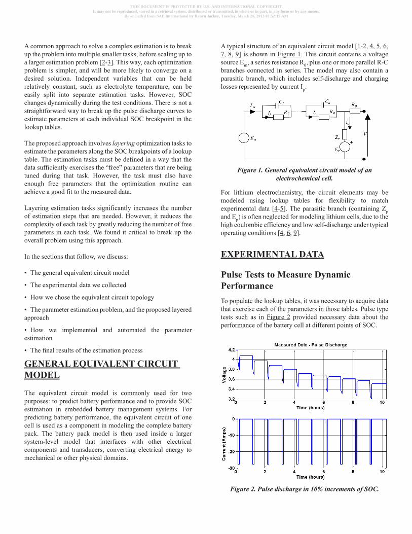
A typical structure of an equivalent circuit model [1-2, 4, 5, 6, 7, 8, 9] is shown in Figure 1. This circuit contains a voltage source Em, a series resistance R0, plus one or more parallel R-C branches connected in series. The model may also contain a parasitic branch, which includes self-discharge and charging losses represented by current Ip.

Figure 1. General equivalent circuit model of an electrochemical cell.

For lithium electrochemistry, the circuit elements may be modeled using lookup tables for flexibility to match experimental data [4-5]. The parasitic branch (containing Zp and Ep) is often neglected for modeling lithium cells, due to the high coulombic efficiency and low self-discharge under typical operating conditions [4, 6, 9].

EXPERIMENTAL DATA

Pulse Tests to Measure Dynamic PerformanceTo populate the lookup tables, it was necessary to acquire data that exercise each of the parameters in those tables. Pulse type tests such as in Figure 2 provided necessary data about the performance of the battery cell at different points of SOC.

Figure 2. Pulse discharge in 10% increments of SOC.



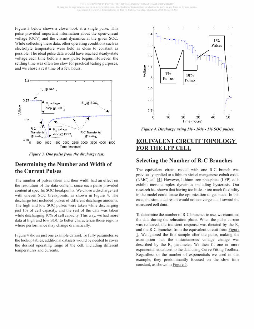
Figure 3 below shows a closer look at a single pulse. This pulse provided important information about the open-circuit voltage (OCV) and the circuit dynamics at the given SOC. While collecting these data, other operating conditions such as electrolyte temperature were held as close to constant as possible. The ideal pulse data would have reached steady-state voltage each time before a new pulse begins. However, the settling time was often too slow for practical testing purposes, and we chose a rest time of a few hours.

Figure 3. One pulse from the discharge test.

Determining the Number and Width of the Current PulsesThe number of pulses taken and their width had an effect on the resolution of the data content, since each pulse provided content at specific SOC breakpoints. We chose a discharge test with uneven SOC breakpoints, as shown in Figure 4. The discharge test included pulses of different discharge amounts. The high and low SOC pulses were taken while discharging just 1% of cell capacity, and the rest of the data was taken while discharging 10% of cell capacity. This way, we had more data at high and low SOC to better characterize those regions where performance may change dramatically.

Figure 4 shows just one example dataset. To fully parameterize the lookup tables, additional datasets would be needed to cover the desired operating range of the cell, including different temperatures and currents.

Figure 4. Discharge using 1% - 10% - 1% SOC pulses.

EQUIVALENT CIRCUIT TOPOLOGY FOR THE LFP CELL

Selecting the Number of R-C BranchesThe equivalent circuit model with one R-C branch was previously applied to a lithium nickel-manganese-cobalt oxide (NMC) cell [4]. However, lithium iron phosphate (LFP) cells exhibit more complex dynamics including hysteresis. Our research has shown that having too little or too much flexibility in the model could cause the optimization to get stuck. In this case, the simulated result would not converge at all toward the measured cell data.

To determine the number of R-C branches to use, we examined the data during the relaxation phase. When the pulse current was removed, the transient response was dictated by the R0 and the R-C branches from the equivalent circuit from Figure 1. We ignored the first sample after the pulse, making the assumption that the instantaneous voltage change was described by the R0 parameter. We then fit one or more exponential equations to the data using Curve Fitting Toolbox. Regardless of the number of exponentials we used in this example, they predominantly focused on the slow time constant, as shown in Figure 5.



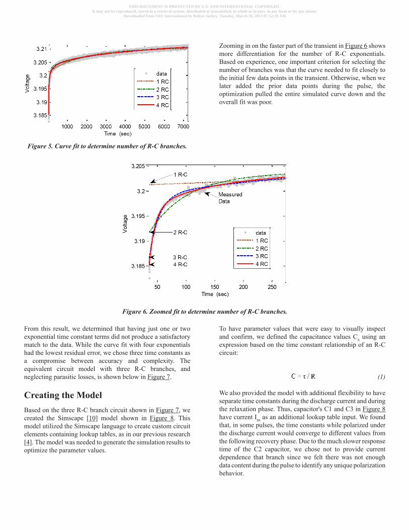
Figure 5. Curve fit to determine number of R-C branches.

Zooming in on the faster part of the transient in Figure 6 shows more differentiation for the number of R-C exponentials. Based on experience, one important criterion for selecting the number of branches was that the curve needed to fit closely to the initial few data points in the transient. Otherwise, when we later added the prior data points during the pulse, the optimization pulled the entire simulated curve down and the overall fit was poor.

Figure 6. Zoomed fit to determine number of R-C branches.

From this result, we determined that having just one or two exponential time constant terms did not produce a satisfactory match to the data. While the curve fit with four exponentials had the lowest residual error, we chose three time constants as a compromise between accuracy and complexity. The equivalent circuit model with three R-C branches, and neglecting parasitic losses, is shown below in Figure 7.

Creating the ModelBased on the three R-C branch circuit shown in Figure 7, we created the Simscape [10] model shown in Figure 8. This model utilized the Simscape language to create custom circuit elements containing lookup tables, as in our previous research [4]. The model was needed to generate the simulation results to optimize the parameter values.

To have parameter values that were easy to visually inspect and confirm, we defined the capacitance values Cx using an expression based on the time constant relationship of an R-C circuit:

(1)

We also provided the model with additional flexibility to have separate time constants during the discharge current and during the relaxation phase. Thus, capacitor's C1 and C3 in Figure 8 have current Im as an additional lookup table input. We found that, in some pulses, the time constants while polarized under the discharge current would converge to different values from the following recovery phase. Due to the much slower response time of the C2 capacitor, we chose not to provide current dependence that branch since we felt there was not enough data content during the pulse to identify any unique polarization behavior.



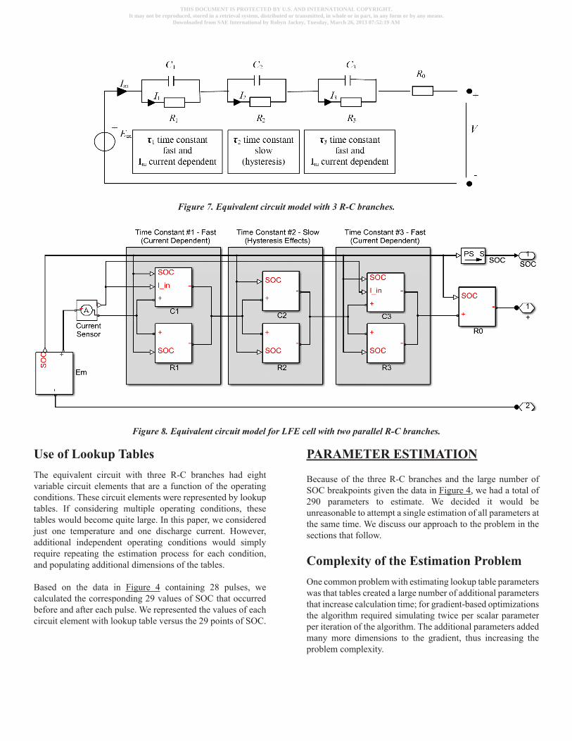
Figure 7. Equivalent circuit model with 3 R-C branches.

Figure 8. Equivalent circuit model for LFE cell with two parallel R-C branches.

Use of Lookup TablesThe equivalent circuit with three R-C branches had eight variable circuit elements that are a function of the operating conditions. These circuit elements were represented by lookup tables. If considering multiple operating conditions, these tables would become quite large. In this paper, we considered just one temperature and one discharge current. However, additional independent operating conditions would simply require repeating the estimation process for each condition, and populating additional dimensions of the tables.

Based on the data in Figure 4 containing 28 pulses, we calculated the corresponding 29 values of SOC that occurred before and after each pulse. We represented the values of each circuit element with lookup table versus the 29 points of SOC.

PARAMETER ESTIMATION

Because of the three R-C branches and the large number of SOC breakpoints given the data in Figure 4, we had a total of 290 parameters to estimate. We decided it would be unreasonable to attempt a single estimation of all parameters at the same time. We discuss our approach to the problem in the sections that follow.

Complexity of the Estimation ProblemOne common problem with estimating lookup table parameters was that tables created a large number of additional parameters that increase calculation time; for gradient-based optimizations the algorithm required simulating twice per scalar parameter per iteration of the algorithm. The additional parameters added many more dimensions to the gradient, thus increasing the problem complexity.



Given the model with three R-C branches and identical parameter values, each of these branches had the same effect on voltage and current observed at the terminals. Aside from differing initial conditions and constraints, the numerical optimizer had no way to separate parameters that had the same effect on the simulation [2]. Even if a computationally-expensive global optimization algorithm were used, it would not have mitigated the fact that if the algorithm were to swap the parameters of the two R-C branches, the simulation output would not change.

Because of the above two issues, it was very likely that, assuming a gradient-based optimization algorithm, the error gradient used in the algorithm would have local minima. It was imperative to have good initial conditions and constraints that isolate the effects that each R-C branch had on the model. Additionally, our previous research showed it was extremely important to have data which exercised all parameters in the model [2].

Finally, the size of the data set in Figure 4 was quite large. This affected the speed and memory consumption of the parameter estimation process. At the same time, one of the challenges with estimating parameters was that setting up the problem often involved a great deal of trial-and-error with choosing good initial conditions, settings, and constraints [2]. If the estimation task also took a long time, the engineering or programming time required became significant.

As a result of this complexity, we broke down the estimation into smaller, more manageable tasks.

Reducing the Problem with a Layered ApproachBecause of the issues previously discussed, it was advantageous to break down the problem into manageable pieces. It was obvious that, for some operating conditions like temperature and current exercised in separate data sets, we could perform separate estimation tasks to parameterize the corresponding parts of the lookup tables. SOC, however, was a dependent variable that changed dynamically.

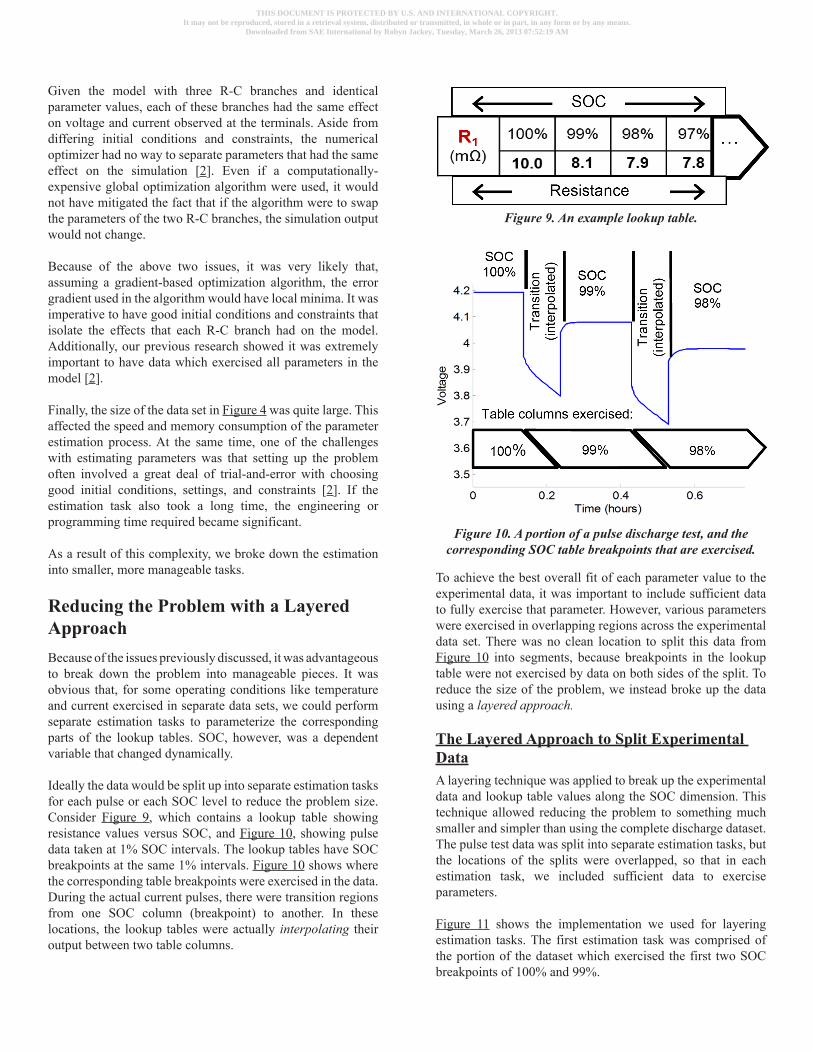
Ideally the data would be split up into separate estimation tasks for each pulse or each SOC level to reduce the problem size. Consider Figure 9, which contains a lookup table showing resistance values versus SOC, and Figure 10, showing pulse data taken at 1% SOC intervals. The lookup tables have SOC breakpoints at the same 1% intervals. Figure 10 shows where the corresponding table breakpoints were exercised in the data. During the actual current pulses, there were transition regions from one SOC column (breakpoint) to another. In these locations, the lookup tables were actually interpolating their output between two table columns.

Figure 9. An example lookup table.

Figure 10. A portion of a pulse discharge test, and the corresponding SOC table breakpoints that are exercised.

To achieve the best overall fit of each parameter value to the experimental data, it was important to include sufficient data to fully exercise that parameter. However, various parameters were exercised in overlapping regions across the experimental data set. There was no clean location to split this data from Figure 10 into segments, because breakpoints in the lookup table were not exercised by data on both sides of the split. To reduce the size of the problem, we instead broke up the data using a layered approach.

The Layered Approach to Split Experimental DataA layering technique was applied to break up the experimental data and lookup table values along the SOC dimension. This technique allowed reducing the problem to something much smaller and simpler than using the complete discharge dataset. The pulse test data was split into separate estimation tasks, but the locations of the splits were overlapped, so that in each estimation task, we included sufficient data to exercise parameters.

Figure 11 shows the implementation we used for layering estimation tasks. The first estimation task was comprised of the portion of the dataset which exercised the first two SOC breakpoints of 100% and 99%.



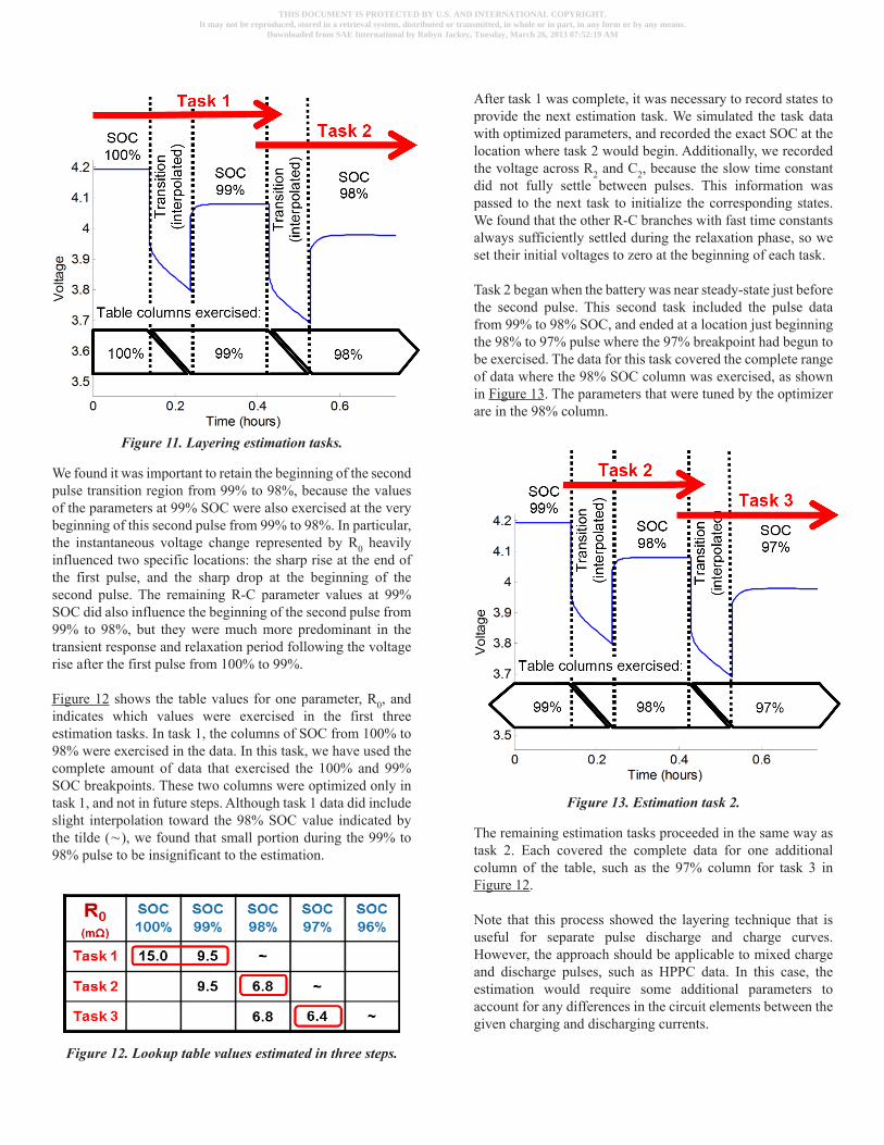
Figure 11. Layering estimation tasks.

We found it was important to retain the beginning of the second pulse transition region from 99% to 98%, because the values of the parameters at 99% SOC were also exercised at the very beginning of this second pulse from 99% to 98%. In particular, the instantaneous voltage change represented by R0 heavily influenced two specific locations: the sharp rise at the end of the first pulse, and the sharp drop at the beginning of the second pulse. The remaining R-C parameter values at 99% SOC did also influence the beginning of the second pulse from 99% to 98%, but they were much more predominant in the transient response and relaxation period following the voltage rise after the first pulse from 100% to 99%.

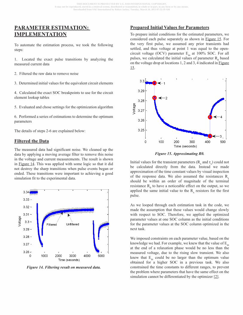
Figure 12 shows the table values for one parameter, R0, and indicates which values were exercised in the first three estimation tasks. In task 1, the columns of SOC from 100% to 98% were exercised in the data. In this task, we have used the complete amount of data that exercised the 100% and 99% SOC breakpoints. These two columns were optimized only in task 1, and not in future steps. Although task 1 data did include slight interpolation toward the 98% SOC value indicated by the tilde (∼), we found that small portion during the 99% to 98% pulse to be insignificant to the estimation.

Figure 12. Lookup table values estimated in three steps.

After task 1 was complete, it was necessary to record states to provide the next estimation task. We simulated the task data with optimized parameters, and recorded the exact SOC at the location where task 2 would begin. Additionally, we recorded the voltage across R2 and C2, because the slow time constant did not fully settle between pulses. This information was passed to the next task to initialize the corresponding states. We found that the other R-C branches with fast time constants always sufficiently settled during the relaxation phase, so we set their initial voltages to zero at the beginning of each task.

Task 2 began when the battery was near steady-state just before the second pulse. This second task included the pulse data from 99% to 98% SOC, and ended at a location just beginning the 98% to 97% pulse where the 97% breakpoint had begun to be exercised. The data for this task covered the complete range of data where the 98% SOC column was exercised, as shown in Figure 13. The parameters that were tuned by the optimizer are in the 98% column.

Figure 13. Estimation task 2.

The remaining estimation tasks proceeded in the same way as task 2. Each covered the complete data for one additional column of the table, such as the 97% column for task 3 in Figure 12.

Note that this process showed the layering technique that is useful for separate pulse discharge and charge curves. However, the approach should be applicable to mixed charge and discharge pulses, such as HPPC data. In this case, the estimation would require some additional parameters to account for any differences in the circuit elements between the given charging and discharging currents.



PARAMETER ESTIMATION: IMPLEMENTATION

To automate the estimation process, we took the following steps:

1. Located the exact pulse transitions by analyzing the measured current data

2. Filtered the raw data to remove noise

3. Determined initial values for the equivalent circuit elements

4. Calculated the exact SOC breakpoints to use for the circuit element lookup tables

5. Evaluated and chose settings for the optimization algorithm

6. Performed a series of estimations to determine the optimum parameters

The details of steps 2-6 are explained below:

Filtered the Data

The measured data had significant noise. We cleaned up the data by applying a moving average filter to remove this noise in the voltage and current measurements. The result is shown in Figure 14. This was applied with some logic so that it did not destroy the sharp transitions when pulse events began or ended. These transitions were important to achieving a good simulation fit to the experimental data.

Figure 14. Filtering result on measured data.

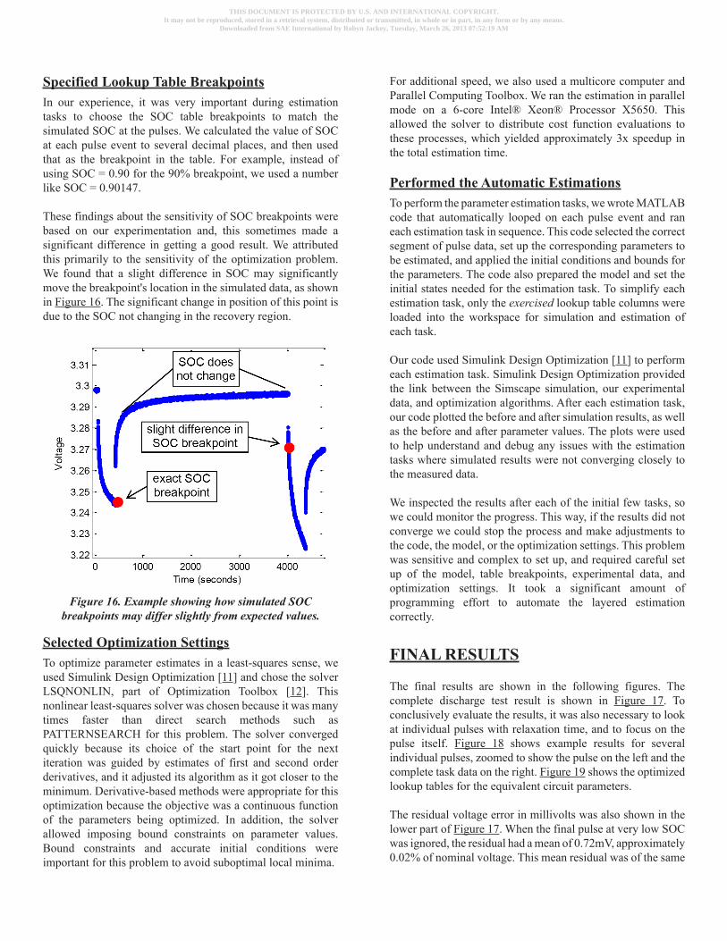
Prepared Initial Values for ParametersTo prepare initial conditions for the estimated parameters, we considered each pulse separately as shown in Figure 15. For the very first pulse, we assumed any prior transients had settled, and thus voltage at point 1 was equal to the open-circuit voltage (OCV) parameter Em at 100% SOC. For all pulses, we calculated the initial values of parameter R0 based on the voltage drop at locations 1, 2 and 3, 4 indicated in Figure 15.

Figure 15. Approximating R0.

Initial values for the transient parameters (Rx and τx) could not be calculated directly from the data. Instead we made approximation of the time constant values by visual inspection of the response data. We also assumed the resistances Rx should be within an order of magnitude of the terminal resistance R0 to have a noticeable effect on the output, so we applied the same initial value to the Rx resistors for the first pulse.

As we looped through each estimation task in the code, we made the assumption that these values would change slowly with respect to SOC. Therefore, we applied the optimized parameter values at one SOC column as the initial conditions for the parameter values at the SOC column optimized in the next task.

We imposed constraints on each parameter value, based on the knowledge we had. For example, we knew that the value of Em at the end of a relaxation phase would be no less than the measured voltage, due to the rising slow transient. We also knew that Em could be no larger than the optimum value obtained for a higher SOC in a previous task. We also constrained the time constants to different ranges, to prevent the problem where parameters that have the same effect on the simulation cannot be differentiated by the optimizer [2].



Specified Lookup Table BreakpointsIn our experience, it was very important during estimation tasks to choose the SOC table breakpoints to match the simulated SOC at the pulses. We calculated the value of SOC at each pulse event to several decimal places, and then used that as the breakpoint in the table. For example, instead of using SOC = 0.90 for the 90% breakpoint, we used a number like SOC = 0.90147.

These findings about the sensitivity of SOC breakpoints were based on our experimentation and, this sometimes made a significant difference in getting a good result. We attributed this primarily to the sensitivity of the optimization problem. We found that a slight difference in SOC may significantly move the breakpoint's location in the simulated data, as shown in Figure 16. The significant change in position of this point is due to the SOC not changing in the recovery region.

Figure 16. Example showing how simulated SOC breakpoints may differ slightly from expected values.

Selected Optimization SettingsTo optimize parameter estimates in a least-squares sense, we used Simulink Design Optimization [11] and chose the solver LSQNONLIN, part of Optimization Toolbox [12]. This nonlinear least-squares solver was chosen because it was many times faster than direct search methods such as PATTERNSEARCH for this problem. The solver converged quickly because its choice of the start point for the next iteration was guided by estimates of first and second order derivatives, and it adjusted its algorithm as it got closer to the minimum. Derivative-based methods were appropriate for this optimization because the objective was a continuous function of the parameters being optimized. In addition, the solver allowed imposing bound constraints on parameter values. Bound constraints and accurate initial conditions were important for this problem to avoid suboptimal local minima.

For additional speed, we also used a multicore computer and Parallel Computing Toolbox. We ran the estimation in parallel mode on a 6-core Intel® Xeon® Processor X5650. This allowed the solver to distribute cost function evaluations to these processes, which yielded approximately 3x speedup in the total estimation time.

Performed the Automatic EstimationsTo perform the parameter estimation tasks, we wrote MATLAB code that automatically looped on each pulse event and ran each estimation task in sequence. This code selected the correct segment of pulse data, set up the corresponding parameters to be estimated, and applied the initial conditions and bounds for the parameters. The code also prepared the model and set the initial states needed for the estimation task. To simplify each estimation task, only the exercised lookup table columns were loaded into the workspace for simulation and estimation of each task.

Our code used Simulink Design Optimization [11] to perform each estimation task. Simulink Design Optimization provided the link between the Simscape simulation, our experimental data, and optimization algorithms. After each estimation task, our code plotted the before and after simulation results, as well as the before and after parameter values. The plots were used to help understand and debug any issues with the estimation tasks where simulated results were not converging closely to the measured data.

We inspected the results after each of the initial few tasks, so we could monitor the progress. This way, if the results did not converge we could stop the process and make adjustments to the code, the model, or the optimization settings. This problem was sensitive and complex to set up, and required careful set up of the model, table breakpoints, experimental data, and optimization settings. It took a significant amount of programming effort to automate the layered estimation correctly.

FINAL RESULTS

The final results are shown in the following figures. The complete discharge test result is shown in Figure 17. To conclusively evaluate the results, it was also necessary to look at individual pulses with relaxation time, and to focus on the pulse itself. Figure 18 shows example results for several individual pulses, zoomed to show the pulse on the left and the complete task data on the right. Figure 19 shows the optimized lookup tables for the equivalent circuit parameters.

The residual voltage error in millivolts was also shown in the lower part of Figure 17. When the final pulse at very low SOC was ignored, the residual had a mean of 0.72mV, approximately 0.02% of nominal voltage. This mean residual was of the same



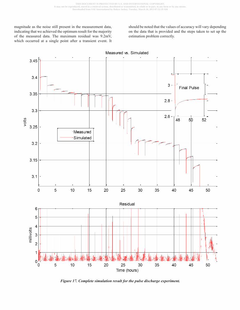
magnitude as the noise still present in the measurement data, indicating that we achieved the optimum result for the majority of the measured data. The maximum residual was 9.2mV, which occurred at a single point after a transient event. It

should be noted that the values of accuracy will vary depending on the data that is provided and the steps taken to set up the estimation problem correctly.

Figure 17. Complete simulation result for the pulse discharge experiment.



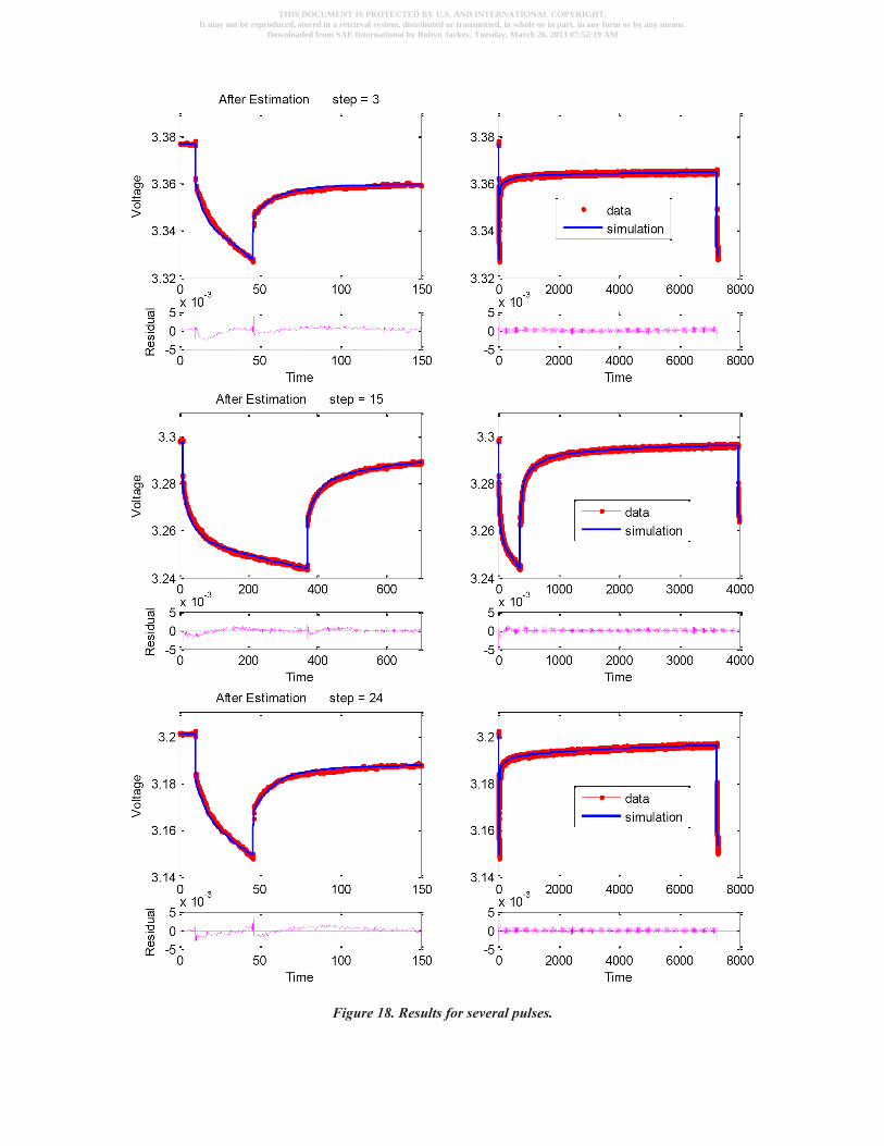
Figure 18. Results for several pulses.



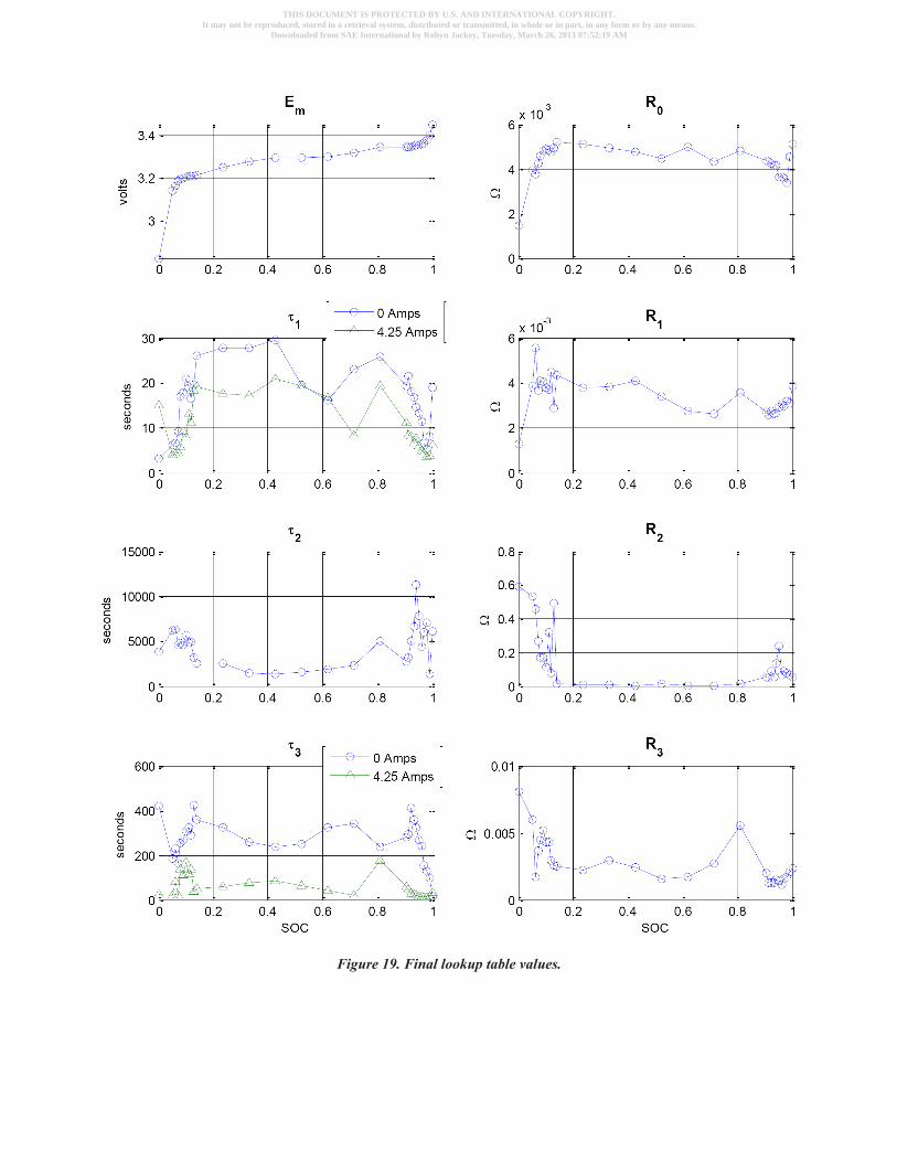
Figure 19. Final lookup table values.



SUMMARY/CONCLUSIONS

After unsuccessful attempts to apply the NMC cell parameter estimation approach from our previous research [4] to LFP battery cell data, we applied an automated, layered approach to break up the complex estimation problem. The layered approach reduced the size of each estimation task to a small subset of experimental data. The resulting values provided us with an optimized equivalent circuit model that closely matched a measured data set of a lithium iron phosphate battery cell to within 0.72 mV mean error, and 9.2mV max error immediately after a transient event.

REFERENCES

1. Jackey, R., “A Simple, Effective Lead-Acid Battery Modeling Process for Electrical System Component Selection,” SAE Technical Paper 2007-01-0778, 2007, doi:10.4271/2007-01-0778.

2. Jackey, R., Plett, G., and Klein, M., “Parameterization of a Battery Simulation Model Using Numerical Optimization Methods,” SAE Technical Paper 2009-01-1381, 2009, doi:10.4271/2009-01-1381.

3. Deland, S., “Optimization of Hydroelectric Flow with MATLAB”, http://www.mathworks.com/company/newsletters/articles/optimization-of-hydroelectric-flow-with-matlab.html, MathWorks, Dec. 2012.

4. Huria, T., Ceraolo, M., Gazzarri, J., Jackey, R., “High fidelity electrical model with thermal dependence for characterization and simulation of high power lithium battery cells,” Electric Vehicle Conference (IEVC), 2012 IEEE International, March 2012 doi: 10.1109/IEVC.2012.6183271.

5. Chen, M. and Rincon-Mora, G.A., “Accurate electrical battery model capable of predicting runtime and I-V performance,” IEEE Transactions on Energy Conversion, vol.21, no.2, pp. 504-511, June 2006 doi: 10.1109/TEC.2006.874229.

6. Ceraolo, M., Lutzemberger, G., and Huria, T., “Experimentally-Determined Models for High-Power Lithium Batteries,” SAE Technical Paper 2011-01-1365, 2011, doi:10.4271/2011-01-1365.

7. Ceraolo, M., “New Dynamical Models of Lead-Acid Batteries”, IEEE Transactions on Power Systems, 15(4):1184-1190, 2000, doi: 10.1109/59.898088.

8. Ceraolo, M. and Barsali, S., “Dynamical models of lead-acid batteries: Implementation issues,” IEEE Transactions on Energy Conversion, 17(1):16-23, 2002, doi: 10.1109/60.986432.

9. Huria, T., “Rechargeable lithium battery energy storage systems for vehicular applications”, http://etd.adm.unipi.it/t/etd-04262012-182954/, Ph.D. thesis, Department of Energy and Systems Engineering, University of Pisa, 2012.

10. MathWorks, “Simscape”, http://www.mathworks.com/products/simscape/, Dec. 2012.

11. MathWorks, “Simulink Deisgn Optimization”, http://www.mathworks.com/products/sl-design-optimization/, Dec. 2012.

12. MathWorks, “Optimization Toolbox”, http://www.mathworks.com/products/optimization/, Dec. 2012.

ACKNOWLEDGMENTS

The reasearch leading to these results has received funding from the European Union Seventh Framework Programme (FP7/2007-2013) under grant agreement n° 234019 for the Hybrid Commercial Vehicle (HCV) Project.

DEFINITIONS/ABBREVIATIONS

Cn - variable capacitor n of an equivalent circuit modelEm - voltage source of an equivalent circuit model that repre-sents the open circuit voltageEp - voltage source of the parasitic branch of an equivalent circuit modelHPPC - high-performance pulse characterization data, a type of experimental data which contains discharge and pulse discharges at different SOC valuesLFP - lithium iron phosphate, a type of battery cellNMC - lithium nickel-manganese-cobalt oxide, a type of battery cellOCV - open circuit voltage (V)Rn - variable resistor n of an equivalent circuit modelR-C branch - a portion of an equivalent circuit comprised of a parallel variable resistor and variable capacitorSOC - state of charge as a fraction of the total cell capacity, ranging from 0 to 1 (or 0% to 100%)τn - time constant n for an R-C branch of an equivalent circuit modelZp - variable impedance of the parasitic branch of an equiva-lent circuit model



http://www.sae.org/technical/papers/2007-01-0778

http://dx.doi.org/10.4271/2007-01-0778


http://dx.doi.org/10.4271/2009-01-1381

http://www.mathworks.com/company/newsletters/articles/optimization-of-hydroelectric-flow-with-matlab.html



http://dx.doi.org/10.1109/IEVC.2012.6183271

http://dx.doi.org/10.1109/TEC.2006.874229

http://dx.doi.org/10.1109/TEC.2006.874229


http://dx.doi.org/10.4271/2011-01-1365

http://dx.doi.org/10.1109/59.898088

http://dx.doi.org/10.1109/60.986432

http://etd.adm.unipi.it/t/etd-04262012-182954/

http://etd.adm.unipi.it/t/etd-04262012-182954/

http://www.mathworks.com/products/simscape/

http://www.mathworks.com/products/simscape/

http://www.mathworks.com/products/sl-design-optimization/

http://www.mathworks.com/products/sl-design-optimization/

http://www.mathworks.com/products/optimization/

http://www.mathworks.com/products/optimization/

The Engineering Meetings Board has approved this paper for publication. It has successfully completed SAE’s peer review process under the supervision of the session organizer. This process requires a minimum of three (3) reviews by industry experts.

All rights reserved. No part of this publication may be reproduced, stored in a retrieval system, or transmitted, in any form or by any means, electronic, mechanical, photocopying, recording, or otherwise, without the prior written permission of SAE.

ISSN 0148-7191

Positions and opinions advanced in this paper are those of the author(s) and not necessarily those of SAE. The author is solely responsible for the content of the paper.

SAE Customer Service:Tel: 877-606-7323 (inside USA and Canada)Tel: 724-776-4970 (outside USA)Fax: 724-776-0790Email: [email protected] Web Address: http://www.sae.orgPrinted in USA



Battery Model Parameter Estimation Using a Layered Technique: An Example Using a Lithium Iron...

Documents

Transcript of Battery Model Parameter Estimation Using a Layered Technique: An Example Using a Lithium Iron...