LOW LYING STATES OF LITHIUM HYDRIDE

By

ROBERT MICHAEL PREDNY

A DISSERTATION PRESENTED TO THE GRADUATE COUNOL OF

THE UNIVERSITY OF FLORIDA

IN PARTIAL FULFILLMENT OF THE REQUIREMENTS FOR THE

DEGREE OF DOCTOR OF PHILOSOPHY

UNIVERSITY OF FLORIDA

1969

Dedicated to

rrry Parents

wife and family

ACKNOWLEDJMENT S

I would like to express my appreciation to Dr. Yngve

Ohm and Dr. Darwin W. Smith for their encouragement and inter­

est in directing this research.

I am also indebted to Dr. Harvey Michels for the sugges­

tion or this problem and also the computer program to carry

it out. His helpful discussions were indispensable.

The assistance of the members of the Quantum Theory

Project was greatly appreciated.

I am particularly grateful to the Computing Center.

Without its generous support this study could not have been

completed.

I especially thank my wife, Faye, for her interest and

the long hours she spent in typing this manuscript.

iii

TABLE OF CONTENTS

Page

ACKNOWLEIXiME'NTS • • • • • • • • • • • • • • • • • iii

LIST OF TABLES • • • • • • • • • • • • • • • • • vi

LIST OF FIGURES

Chapter

• • • • • • • • • • • • • • • • • viii

I. INTRODUCTION. • • • • • • • • • • • • • • 1

II.

III.

1.1. Review of the Experimental Properties of Lithium Hydride • • • •

1.2. Theoretical Calculations • • • • • •

MEl'HOD OF CALCULATION • • • • • • • • • •

COMPUTATIONAL PROCEDURES ••••••• • •

3.1. Basis Orbitals. • • • • • • • • • • •

3.2. Configurations •• • • • • • • • • • •

1

10

17

25

25

27

3.3. Spin Functions • • • • • • • • • • • • • 31

'IV. LOWEST STATES OF 3~+, 371 AND 1 71' SD1lfflRY • • • • • • • • • • • • • • • • • • 32

4.1. The Lowest Lithium Hydride 3~+ State •• 32

4. 2. The Lowest Lithium Hydride 3rr state • • 36

4.3. The Lowest Lithium Hydride 1 1T state. • 39

V. POTENTIAL CURVES FOR LOW LYDm LITHIUM HYDRIDE STATES • • • • • • • • • • • • • • • • • • • 43

5.1. Basis Orbitals. • • • • • • • • • • • 43

5. 2. The Lithium Hydride l r + States • • • • 46

iv

5.3. The Lithium Hydride 3 L+ States ••••• • 59

5.4. The Lithium Hydride 3TT States •••••• o9 l 5.5. The Lithium Hydride TT States •••••• 75

5.o. The Lithium Hydride x2 f + State •••••• 81

VI. DISCUSSION AND SUMMARY

APPENDIX I • • • • • • • • • • • • • • • • • • • • • • • 88

APPENDIX II • • • • • • • • • • • • • • • • • • • •

BIBLIOGRAPHY - • • • • • • • • • • • • • • • • • • •

BIOGRAPHICAL SKETCH. • • • • • • • • • • • • • • •

V

• 93

109

LIST OF TABLES

TABLE

1. SPECTROSCOPIC CONSTANTS. • • • • • • • • • •

2. BASIS SLATER TYPE ORBITALS FOR THE LOWEST 3 ~ + SI'ATE OF LITHTC!M HYDRIDE •

3. ENERGY FOR THE LOWEST 3 2.. + SI'ATE OF LITHIUM HIDRIDE • • • • • • • • • • •

4. BASIS SLATER TYPE ORBITALS FOR THE LOWEST 3 rr srATE OF LITHIUM HYDRIDE •

5. ENERGIES FDR THE LOWEST 3rr srATE OF LITHitn.lf HYDRIDE • • • • • • • • • • •

6. BASIS SLATER TYPE ORBITALS FDR THE LOWEST 1 TI' 6'TATE OF LITHIUM HIDRIDE •

7. ENmGY FOR THE LOWEST l 7T srATE OF LITHIUM HYDRIDE • • • • • • • • • • •

8. BASIS SLATER TYPE ORBITALS FDR THE CALCULATIONS ON THE LOW LYJNG STATES

• • •

• • • •

• • • •

• • • •

• • • •

• • • •

Page

2

33

34

37

38

40

OF LITHIU11 HD)RJDE • • • • • • • • • • • • • • 44

9. POTENI'IAL ENERGIES FOR THE l i + SfATES OF LITHIUM HYDRIDE ••••••••••• • • • • 48

10. 125 CONFIGURATIONAL WAVEFUNCTION FOR THE 1~ + S'fATES OF LITHIUM HYDRIDE • • • • • • 50

ll. POTENTIAL ENERGIES FOR THE l~ + srATFS OF LITHml HYDRilJE USING AN EXTENDED BASIS SEI'. • 55

12. POTENTIAL EN:rnGIF.S FDR THE 3~ + srATES OF LITHIUM HYDR1DE •••••••••••••••• 60

13. 125 CONFIGURATIONAL WAVEI<"'UNcrimr FOR THE 3 L + STATES OF LITHIUM HYDRIDE • • • • • • • • 62

l4. COEFFICIENTS OF THE ~IN+OONFIGURATICNS OF THE SECOND AND THIRD ~ SI'ATES • • • • • • • 66

vi

1.,. POTENI'IAL ENERGIES FOR THE J 2.. + STATES OF LITHIUM HYDRIDE USING AN EXTENDED BASIS SET. • • • •

lo. POTENI'IAL ENEIDIES ltUR THE 3TT STATES OF

17.

18.

LITHIUM HYDRIDE • • • • • • • • • • • • •

125 CONFIGURATIONAL WAVEFtJNm'IDN FOR THE JTT STATES OF LITHIUM HYDRIDE ••••••

POTEm IAL ENE.FOIES FOR THE l 7T STATF..S OF LITHIUM HYDRIDE • • • • • .. • • • • • • •

19. f5 CONFIGURATIONAL WAVEFUNCTION FOR THE TI STATES OF LITHIUI1 HYDRIDE ••••••

20. POTENTIAL ENEIDY OF THE 2 r + STATE OF

• • • • • •

• • • • • •

• • • • • •

• • • • • •

• b1

• 70

• 72

• 1b

• 78

LITHIUM HYDRIDE PLUS • • • • • • • • • • • • • • • • • 82

21. ~5 CONFIGURATIDNAL WAVEF01lCTION FOR THE r + STATE OF LITHIUM HYDRIDE PLUS • • • • • • • • • • 84

22. CONFIGURATIONS AND OOEFFICIENTS OF THE WAVEFUNCTION USED FOR THE LOWF.ST 3~ + STATE OF LITHIUM HYDRIDE • • • • • • • • • • • • • • • • • • • 94

2J. CONFIGURATIONS AND COEFFICIENTS 0) THE WAVEFUNC!'ION USED FOR THE l.OWEST TT STATE OF LITHIUM HYDRIDE • • • • • • • • • • • • • • • • • • 99

24. CONFIGURATIONS AND COEFFICIENrS OF THE WAVEFUNCI'ION USED FOR THE LOWEST l7t STATE OF LITHIUM HYDRIDE ••••• •• •••••• • • • • •• 104

25. COEFFICIENTS OF THE 125 CONFIGURATIONAL WAVE.FUNCTION FOR THE LITHIU1 HYDRIDE lL+ STATES ••• 110

2o. COEFFICIENTS OF THE J2.5 CONFIGURATIONAL WAVE.FUNCTION FOR THE LI'llIIUM HYDRIDE .3 J:+ STATES ••• llo

27. COEFFICIENTS OF THE 125 CONFIGURATIONAL WAVEFUNCTION FOR THE LITHIUM HYDRIDE 371 STATES ••• 122

28. OOEFFICIENTS OF THE 125 OONFIGURATIONAL WAVEFUNCTION :FOR THE LITHIUM HYDRIDE 1 TT STATES ••• 128

29. COEFFICIENTS OF THE 125 CONFIGURATIONAL WAVEFUNCTION FOR THE LITHitM HYDRIDE PLUS 2 ~ + STATE • • • • • • • • • • • • • • • • • • • .134

vii

LIST OF FIGURES

l. POTENTIAL ENERGY CURVF.S FOR THE l ~ + srAT:ES OF LITHIUI1 HYDRIDE • • • • • • • • • • • • • • • • 49

2. POTENTIAL ENERGY CURVES FOR THE 3 ~ + srATES OF LITHIUM HYDRIDE • • • • • • • • • • • • • • • • 61

.3. POTENTIAL ENERGY CURVES FOR THE 37f STATES OF LITHIUM HYDRIDE • • • • • • • • • • • • • ••• 71

4. POTENTIAL ENERGY CURVES FOR THE l 7r srATE.S OF LITHIUM HYDRIDE ••••••••• • • • • ••• 77

,. POTENTIAL ENERGY CURVE. FOR THE 2 ~ + STATE OF LITHIUM HYDRIDE PLUS • • • • • • • • • • • • • 83 .

viii

CHAPTER I

INTRODUm'ION

l.l. Review of the Experimental Properties

of Lithium Hydride

The experimental potential energy curves for diatomio

molecules are obtained from their absorption spectra . Diatomic

lithium hydride or deuteride gas is obtained by combining Li

metal and excess H2 or n2 gas at temperatures of 1000° C.

When the reaction has stopped, the absorption spectrum is

obtained by irradiating the gas in the UV region. Exposure

times of 2 hours or more are used. Crawford and Jorgensen(!)

investigated the absorption spectra of LiH and LiD between

3200 and 4300 i. Thirty-five bands of the 1 ~ -1 Z:: spectrum

were measured for LiD and 28 bands for LiH. Two emission

bands were also obtained for Lillo Vibrational and rotational

constants we"'."8 d~tennined for the xl~+ and A1 l+ states.

Their potential energy curves were obtained for low lying vibra­

tional. levels by the use of Dunham's molecular potential energy

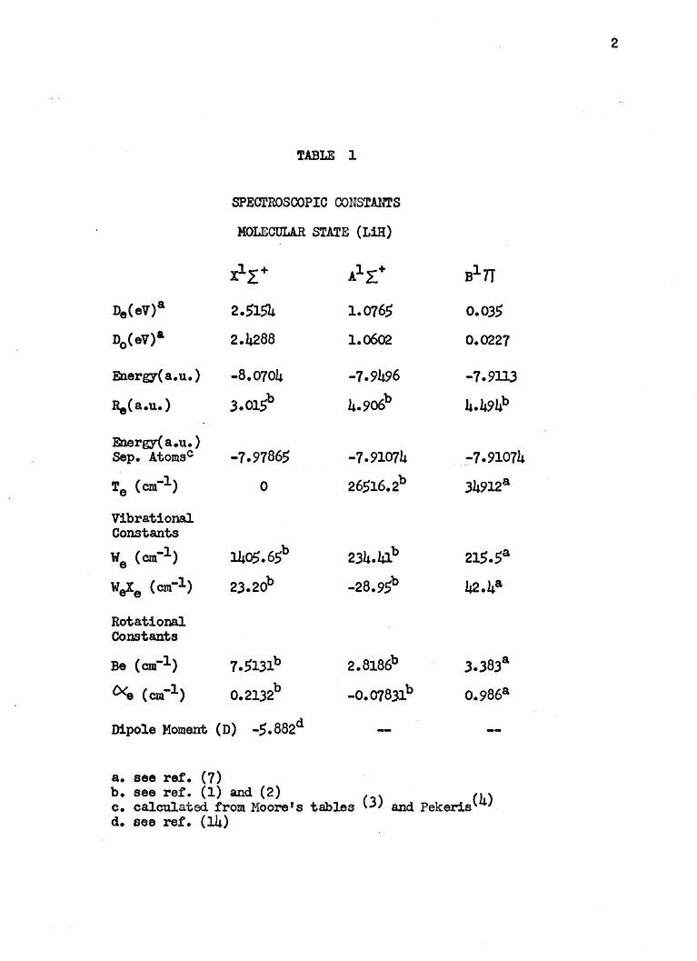
function. Crawford and Jorgensen's values for the spectroscopic

constants of these states are listed by Herzberg.( 2) The values

are given in Table 1. The values !'or the energy of the separated

1

2

TABLE 1

SPEm'ROSOOPIC OONSTANTS

MOLECULAR STATE (LiH)

x1r+ Alr_+ Bl7T

De(eV)4 2.,154 1.0765 0.035

D0 (ev)• 2.4288 1.o602 0.0227

Energy-( a. u.) -8.0704 -7.9496 -7.9113

Re(a.u.) 3.015b 4.906b 4.494b

:Energy-( a.u.) Sep. Atomsc -7-97865 -7.91074 -7-91074

Te (cm-1) 0 26,516.2b 34912a

Vibrational Constants

we (cm-1) 1405.65b 234.41b 215.5a

WeXe (cm-1) 23.20b -28.95b 42.4a

Rotational Constants

Be (cm-1) 7.5131b 2.8186b 3.383&

D<e (cm-1) 0.2132b -0.078.31b 0.9868

Dipole Moment (D) -5.882d

a. see ref. (7) b. see ret. (1) and (2) · (4) c. calculated from Moore's tables (3) and Pekeris d. see ref. (14)

atoms were calculs.t.(lld from Moore's tables<3) and the results

of Pekeris. (4)

ihe first excited state of LiH was found to exhibit

anomalous behavior as seen by its abnomal. band spectrum con­

stants. This A1Z:. + state's unusual shape was explained by

Mulliken<5) as being due to its Li+u"- character at large

internuclear distances. In this analysis the ground state,

i.e. x1r+ state, has mainly ionic Li+ii- character around its

equilibrium. internuclear separation,while the All,+ state is

predo~in.antly Li+u"- at large internuclear separations. A plot(5)

of these two states and a curve of the Li+Ir interaction showed

that the ionic Li +ir curve crosses the A1 E + curve at large

uiternuclear distances. The x1r + state dissociates into the

112s(1s22s) plus H2s(ls) states. The A1 ~ + state goes into the

ti2P(ls22p) plus H2s(ls) atomic states. Rosenbaum< 6) used Klein's

method to obtain the experimente.l potential energy curve for the

A1!_ + state. He found that this curve crosses the coulombic

curve of Li+Ii.

Velasco(7) analyzed the UV absorption spectrum of LiH

between 2000 and 3200 X. He found a new band system between the

ground state and an excited 11T state. From the breaking off of

the rotational structure of the Bl TT -x1 2.. + system bands he deter­

mined vecy accurate dissociation limits for the B1 7T state. There­

fore he has bean able to obtain accurate dissociation energies of

the three experimentally observed states of lithium hydride. The

dissociation energy, D8 , for the x1 2_ + state is 2.5154:o.0002ev.

3

For the A1 2+ state D8 is 1.0765!0.0002ev and 0.035!0.00leV for

the B1 TT state. The spectroscopic constants for the B1 TT state

are given in Table 1.

Potential energy curves for the x1 r +, A1 l. + and B1 TT states

of L1H haTe been calculated by Fallon, Vanderslice and Mason< 8)

using the lcy'dberg-Klein-Rees (RKR) method. The curve for the

A1 I, + istate using this method also .has been obtained by

Singh and Jain. ( 9) Reduced potential curves tor the states of

LiH have been obtained by Jenc(lO) using the rum method and

compared to theoretical calculations. He concluded that the

anomalous behavior of the A1 ~ + state of LiH was due to effects

which wruld not be accOllllted for in the usual adiabatic approx­

imation. Krupenie, et al.(ll) estimated long range attractive

potentials for the x12. + state of Lill by extrapolation of .func­

tions fitted to the mm potential curves. They also estimated

curves for the lowest 3t+ state. Using the collision integrals

computed from the potentials, they calculated values for the

diffusion coefficient and viscosity of gaseous LiH systems. Halmann

and Laulicht(l2) have computed Frank-Condon factors based on rum

potential functions. These factors control the distribution of

intensity between vibrational bands.

KlempererC13) and his coworkers studied the inf'rared

absorption spectrum of gaseous LiH. In order to obtain an

appreciable absorption it is necessary to work at temperatures

greater than looOO c. They analyzed the P and R branches of the

0-1 and 1-2 ba.'lds. From the line intensities a dipole derivative

4

ot l.8!0.3 was calculated. Wharton, Gold and Klemperer(l.4)

used molecular beam resonance methods to obtain values f'or the

dipole manent by analyzing the J•l, Mj•O, to J•l, IMjl •l

transition. They obtained values for the dipole moment, quad­

ru.pole coupling constant;, spin rotation constant arxl. rotational.

magnetic moment by adjustment of constants of the effective

Hamiltonian to tit the spectrum. The lowest vibrational. level

has a dipole moment of -5.882:!:o.003 debyes for LiH and -5.868:!: + 0.003 for LiD. The rotational magnetic moment is -0.654-

+ (15) 0.007nm. for LiH and -0.272-0.005 for LiD. Lawrence, et al.

observed resonances of the rotational magnetic moments in molecular

beams ot LiH and LiD. Their rotational. magnetic moments agreed

+ with those above. They obtained a dipole moment of -5.9-0.5

debyes with the polarity of Li +H- e Rothstein ( 16) aJ..so used

molecular beam techniques to obtain dipole moments and nuclear

hyperfine interaction constants.

Under standard con:litions, lithium hydride is a white

crystalline solid. Recent reviews of its properties are given

in references (17) to (20). It is generally prepared(l9, 20)

b;y the reaction between liquid lithium and excess hydrogen gas

at high temperatures. A typical reaction temperature is 750°

with a run time around 48 hoursf 20) . The crystal has the NaCl

type structure. It consists ot two ions and four electrons in

the primitive unit cell. The space group is ~5 or Fm3m. The

most recent crystallographic data on lithium hydride :are given

b:, Staritzky and Walker( 2l) who reported that the lattice constant

5

•

of LiH is 4.0834!0.000:5 i and that of LiD is 4.o684!0.000:5 i. They also investigated the refractive index.

flle solid has a melting point of 961° Kand a latent heat

or fusion of 4,900:!:700 cal/mole. This value was obtained by

Messer<22 > from freezing point lowerings. The standard heat of

formation of LiH is -21.666!0.026 kcal/mole and that of LiD

is -21.7a4:o.021 kcal/mole. These results were obtained by

Gunn and Green <23> from the heat of hydrolysis of Li and Lill

at 2.5.00!0.04° C,using a calorimetric bomb. They also calculated

the crystal energy- of Lili to be 217.76 kcal/mole and that of LiD

to be 218.76 kcal/mole.

The ionic character of lithium hydride was demonstrated

by Moers< 24) in a study of the electrical coniuctivity of molten

and solid LiII. The H2/LilI electrode was of interest recent1y( 25)

1n regard to fuel cells. Johnson, et a1.< 26) determined thenno­

d;ynarnic properties from emf measurements on solid LiH between

675 and 885° K. Using the heat capacity data of Vogt~ 27 ) they

obtained the following results for a temperature of 298° K;

AHr0 a-21.79!0.29 kcal/mole,~Gf0 ~16.16!0.o, kcal/mole and

A O 8 + 4 _, / . (28) uSr ""-1 .9-0. Cd..1/deg.mole. Kelley and Kl.Ilg obtained

the value -16.3 cal/deg.mole for 6Sr O •

Numerous other thermal properties of LiH,_ for example,

dissociation pressure of H2, heat capacity of solid and liquid

LiH, coefficient of thermal expansion, etc., are presented in

references (19) and (29). Compressibility studies(JO) of LiH

did not show any evidence of a phase change up to a pressure

of 240 kilo bars.

6

Lithium hydride reacts readily with water. Machin and

Tompkins(3l) studied the kinetics or the reaction between J¼O

vapor and crystalline LiH in the temperature range 0-121° C.

The chemical nature of the product is determined by the amount

or water vapor. The product is predominantly 1120 when only

enough H20 is present to react with a single surface layer or

LiH. With more H20 the product is almost exclusively LiOH. The

rate controlling step in the production of 112 from the reaction

is the formation or the oxide.

LiH will also react readily with tm atomspheric gases

02 and n2 at elevated temperatures. With N2 the products,

~, Li2NH or Li3N may be formed. At high temperature LiH

will react violently with the halogens. With ammonia, lithium

amids ·will ba fo:rmad. And depending on the tempe~atu.,"""e the reac­

tion with 002 will form either the thiosulfate or the sulfide.

Lithium hydride reacts with alcohols with the formation of

lithium alcoholates. It is also slightly soluble in ether and

other polar organic solvents. Due to its solubility and the

fact that it is a strong reducing agent it can be used for

organic reduction. Recently it has been used in polymerization

reactions.

Schlesinger and otheraC32) investigated the use or Lili

in producing other hydrides by hydrogen exchange reactions,

i.e. LiH + MX~MH + LiX. Lill has been used to produce SiJ\ and

B2H6 from the respective halides. L1A1H4 is a more useful com­

pound for hydride synthesis and it is also quite soluble in ether.

7

8

It is formed by the reaction between lithiwn hydride and

aluminum chloride. The majority of the applications of LiH to

chemical synthesis are through LiA1H4 since this product is more

reactive and soluble than LiH i tsel:f.

Alkali hydride crystals are considered to be ionic in

character. The amount of ionicity in solid lithium hydride has

been investigated and found to be around 80%. Both Lwidquist(33)

and Hurst(34) calculated the cohesive energy an:i structure

factors for crystall.ine lithium hydride,assuming complete ioniza­

tion. Morita and Takahash1(3.5) in a calculation of the cohesive

energy took into account the covalent character of LiH, using the

method of semi-localized crystal orbitals. All of them calculated

values within ±25 kcal/mole of the experimental value. Phillips

and Harris(36) obtained values of the crystal structure factors

which they used to determine electron density distributions.

They found that an ionic model with overlaps gave the best

agreement with tba experimental data. Calder, et al. 0 7) per­

formed X-ray and neutron diffraction analysis of LiH in order to

obtain structure factors am electron distributions. The theo­

retical. results of Waller and Lundquist03) and Hurst<34) colli)ared

well with their results. They indicated that the Li+ ion was

largely unaffected by the crystal field wh:i.le the r ion had a

pronoun.cad contraction as suggested by Lundqul.st. <33) They also

predicted that bonding in LiH is between 80 and 100,% ionic from

the ·x-ray data.

Brodsky and Burstein08) analyzed the infrared (IR) renec­

tion spectra of single crystal LiH and LiD. Using a shell model

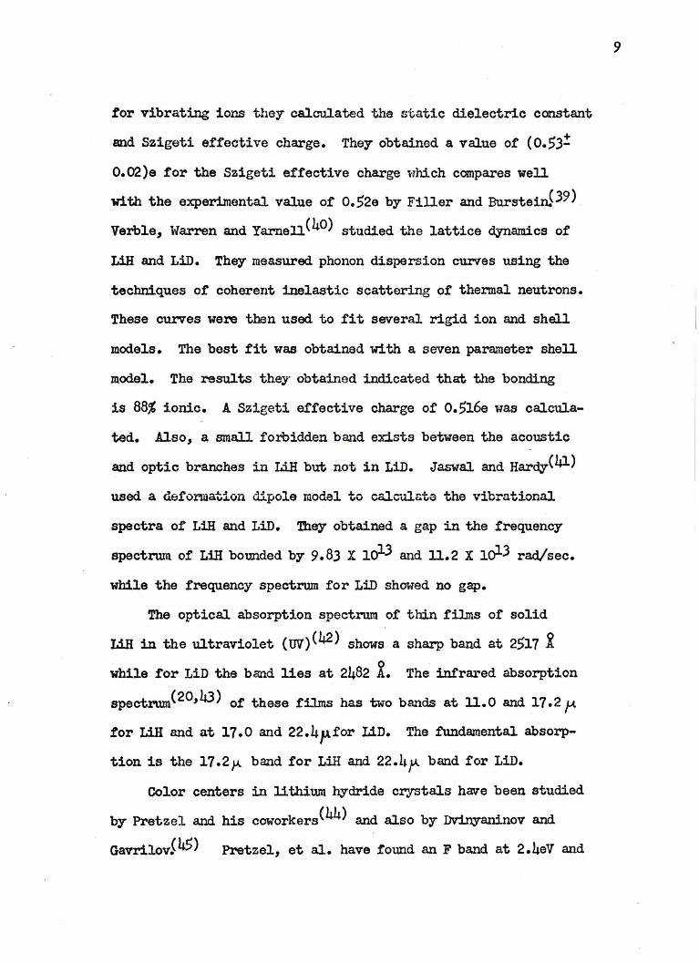
tor vibrating ions they calculated the static dielectric constant

and Szigeti effective charge. They obtained a value of (0.53!

0.02)e for the Szigeti effective charge which compares well

with the experimental value of 0.52e by Filler and Bu.rste1rJ39) .

Verble, Warren and Yarnell (40) studied the lattice dynamics of

LiH and LiD. They measured phonon dispersion curves using the

techniques of coherent inelastic scattering of themal neutrons.

These curves were then used to fit several rigid ion and shell

models. The best fit was obtained with a seven parameter shell

model. The results they· obtained indicated that the bonding

is 88% ionic. A Szigeti effective charge of 0.516e was calcula­

ted. .Also, a small forbidden band exists between the acoustic

and optic branches in LiH but not in LiD. Jaswal and Harczy-(41)

used a def'omation dipole model to calcu.lsta the vibrational

spectra of LiH and LiD. They obtained a gap in the frequency

spectrum of Lili bounded by 9.83 X 1ol3 and 11.2 X 1ol3 rad/sec.

while the frequency spectrum for LiD showed no gap.

The optical absorption spectrum of thin films of solid

Lill in the ultraviolet (UV) (42) shows a sharp band at 2517 j

while for LiD the bcmd lies at 2482 X. The infrared absorption

spectrum(20,43) of these films has two bands at 11.0 and 17.2JA,

tor LiH and at 17.0 and 22.4~for Li.D. The fundamental absorp­

tion is the 17 .2 p. band for Lili and 22.!i JA- band for LiD.

Color centers in lithium hydride crystals have been studied

by Pretzel and his coworker/44) and also by Dvinyaninov and

Gavrilov$45) Pretzel, et al. have folllld an F band at 2.4eV and

9

a V1 bam at 3.5eV and discussed their formation in detail. The

F band is produced by the formation of electrons while the Vi

band most probably results trom a H2

molecule trapped in an

anion site. They have also studied Li colloid bands and impur­

i ty absorption bands.

1.2. Theoretical Calculations

Lithium hydride has been the subject of many theoretical

calculations since the first treatment by Knipp. (h6) Dile to

its simplicity with only four electrons, two of which are

bonding and two are in a closed inner shell, Lili has been used

as a test case for many theoretical procedures. Karo and_

01Bon<47) carried out the first extensive calculation of the

pvtantial energy curves of the x1 ! + and 1..1 I_+ states. Thay

used configuration interaction ( CI) in the framework of both the

valence bond (VB) and salt-consistent field molecular orbital

(SCF-MO) methods. They considered internuclear separations from

2.0 to 8.0 a.u. For the ground state they obtained a D8 •1.669eV

with Re•3.245 a.u. and a dipole moment,µ., of -6.0SD. For the

first excited state they calculated that De~0.8487eV at Raa4.90 a.u.

and µ.•+3.44D. Karo(4B) also performed electron population anal­

ysis of his wavefunctions. His results disagreed with Mulliken1s(5)

prediction that the A 1 ~ + state 1s predominantly Li +H- at large

internuclear separations. Karo found that the strongest inter­

action 1s between nonpolar configurations.

Ehbing<49) used a set of 10 orbitals in elliptical

coordinates ani 53 configurations in a SCF-CI study of the rr +

10

state at 2.99 a.u. His value for the energy was -8.04).28 a.u.

an:l -5.96D for the dipole moment;. In a calculation on the

ground state of Lili Matsen and Browne ( 50) obtained an energy ot

-8.04379 a.u. at 3.075 a.u. arxl a dipole moment of -5.51D using

21 basis Slater type orbitals (ST0's) and 20 configurations.

Harris am TaylorC5l) studied the potential curve for the x1 r +

state using open shell techniques with CI and an elliptic orbital

basis.

Kahalas and Nesbet<52) carried out a calculation on LiH

using the HF-Roothaan method. They also considered configuration

interaction. Besides the energy and dipole mo~nt th97 reported

a value of 35.3 kc/sec for the quadrupole coupling constant of

D in LiD. Using a HF-Roothaan wave.function, Cade and nu/53)

calculated e value of -6.002D for the dipole moment of Li.H.

They (54) also obtained the best Hartree-Fock energy for the

LiH x1 1 + state. They used 16 basis SI'O' s with optimized orbital

exponents and obtained analytic SCF wavefunctions from a solution

11

of the HF-Roothaan equations. Their calculated energy was -7.98731 a.u.

at an internuclear separation of J.015 a.u. The spectroscopic

constants obtained from their potential curve agreed well with

the experimental values. An ionization potential of 7.02ev

was calculated for Lill. They also presented a very extensive

review of the calculations on lithium hydride.

The best ene.rgies of Lill were obtained by Browne and

Mats~n(55) and Bender and Davidson.(56) Browne and MatsenC55)

used a mixed Slater and elliptic type orbital basis. The

Slater type orbitals were used to represent the lithium inner

core orbitals, and the elliptic orbitals, the boming orbitals.

Their basis consisted of 11 sro• s and 10 elliptic orbitals and

their wavefunction had up to 28 terms. Using a VB-CI method

they calculated an energy or -8.0:561 a.u. at R•J.046 a.u., a

dissociation energy of 2.J4eV, and a dipole moment of 5.9,3D.

They also evaluated spectroscopic constants and obtained a

quadrupole coupling constant of .34.2 kc/sec for Din LiD.

Bender and Davidson<56) used an iterative natural orbital

procedure to obtain an energy of -8.0606 a.u. at an intermiclear

distance or 3.0147 a.u. They calculated a dipole moment of

5.96500. They used .32 elliptic orbital basis functions and 45

configurations consisting of 12 c:r, 6 n and 5 o molecular orbitals.

Brown and Shull(57) obtained accurate potential energy

and dipole moment curves for low lying 1f + states of LiH

between internuclear separations of 1.0 and 10.0 a.u. Their

wavef'u.nction consisted of 69 configurations and 25 elliptic basis

orbitals which were taken fran two optimized sets, one for the

xl~+ state and the other for the Al~+ state. They calculated

34 points on the potential curves and obtained an energy of

-B.0556 a.u. at 3.060 a.u. with a dipole moment of ..;5.B9D for

the ground state and -7.9372 a.u. at 4.928 a.u. and +3.96n

respectively for the first excited state. A munerical vibra­

tional and rotational analysis was performed for both states

and the spectroscopic parameters obtained agreed well with

experiment. They computed natural spin orbitals for these states

12

13

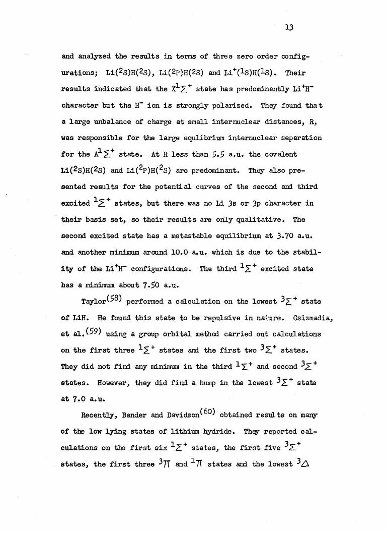
and analyzed the results in tenns of three zero order config­

urations; Li(2s)H(2s), Li(2P)H(2S) and Li+(ls)H(ls). Their

results indicated that the x1 Z:. + state has predominantly Li +u­character but the H- ion is strongly polarized. They found th.at

a large unbalance of charge at small intermclear distances, R,

was responsible for the large equlibriwn internuclear separation

for the AlL+ state. At R less than 5.5 a.u. the covalent

Li(2s)H(2s) and Li(2P)H( 2s) are predominant. They also pre­

sented results for the potenti. al curves of the second aDi third

excited 12, + states, but there was no Li Js or 3p character in

their basis set, so their results are only qualitative. The

second excited state has a metastable equilibrium at 3.70 a.u.

and another minimum around 10.0 a.u. which is due to the stabil-

1 ty of the Li +n- configurations. The third l r + excited state

has a minimum about 7 .50 a.u.

TaylorC5B) performed a calculation on the lowest 3 L + state

of LiH. He found this state to be repulsive in nature. Csizmadia,

et al.(59) using a group orbital methcxi carried out calculations

on the first three 1l+ states am. the first two 3.z:.+ states.

They did not fim any minimum in the third 1 L + and second 3 ~ +

states. However, they did find a hump in the lowest 3 L. + state

at 7 .o a. u.

Recently, Bender and Davidson( 60) obtained results on many

of. the low lying states of lithium hydride. They reported cal­

culations on tre first six l~+ states, the first five JL+

states, the first three 37r and 1 TI states am the lowest 3 ~

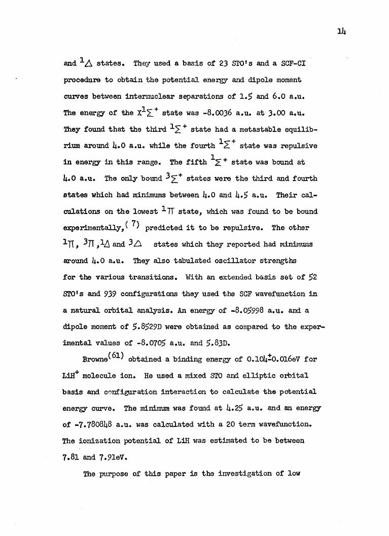
and l ~ states. They used a basis of 23 STO I a and a SCF-CI

procedure to obtain the potential energy and dipole moment

curves between internuclear separations of 1.5 and 6.o a.u.

The energy of the x1~ + state was -8.0036 a.u. at 3.00 a.u.

They found that the third 1 ~ + state had a metastable equilib­

rium around 4.0 a.u. while the fourth l~+ state was repulsive 1

in energy in this range. The fifth z. + state was bound at

4.0 a.u. The only bolll'ld 3~+ states were the third and fourth

states which had minimums between 4.0 and 4.5 a.u. Their cal­

culations on the lowest 1 TT state, which was found to be bound

experimentally, ( 7) predicted it to be repulsive. The other

1 TT , 3n , 1,6 and 3 .D. states which they reported had minimums

around 4. 0 a. u. They also tabulated oscillator strengths

r or the various transitions. With an extended basis set of 52

ST01s and 939 configurations they used the SCF wavefunction in

a natural orbital analysis. An energy of -8.05998 a.u. and a

dipole moment of 5.B529D were obtained as compared to the exper­

imental values of -8.0705 a.u. and 5.8JD.

Browne( 6l) obtained a binding energy of o.104!0.016ev for

LiH+ molecule ion. He used a mixed STO am elliptic orbital

basis and configuration interaction to calculate the potential

energy curve. The minimum was found at 4.25 a.u. and an energy

of -7.780848 a.u. was calculated with a 20 term wavefu.nction.

The ionization potential of LiH was estimated to be between

7.81 and 7.91ev.

The purpose of this paper iB the investigation of low

' ,

15

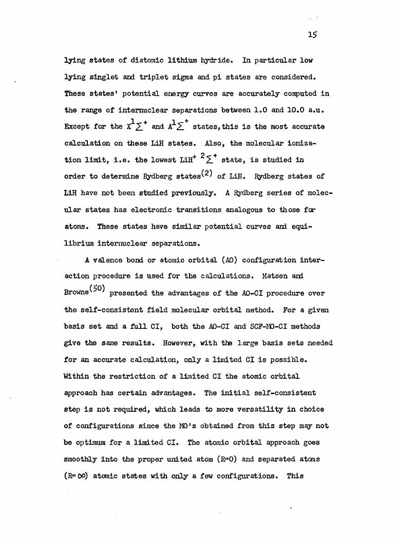
lying states of diatomic lithium hydride. In particular low

lying singlet an::l triplet sigma and pi states are considered.

These states' potential energy curves are accurately con:puted in

the range of internuclear separations between 1.0 and 10.0 a.u. 1 + l +

Except for the r 2,__ and A L states, this is the most accurate

calculation on these Lili states. Also, the molecular ioniza­

tion limit, i.e. the lowest Lili+ 2 z_+ state, is studied in

order to determine Rydberg states<2) of LiH. Rydberg states of

Lili have not been studied previously. A Rydberg series of molec­

ular states has electronic transitions analogous to those fer

atoms. These states have similar potential curves ani equi­

librium internuclear separations.

A valence bond or atomic orbital (AO) configuration inter­

action procedure is used for the calculations. Matsen an:l

Browne<50) presented the advantages of the AO-CI procedure over

the self-consistent field molecular orbital method. For a given

basis set and a full CI, both the AO-CI and SCF-MJ-CI methods

give the same results. However, with tha large basis sets needed

for an accurate calculation, only a limited CI is possible.

Within the restriction of a limited CI the atomic orbital

approach has certain advantages. The initial self-consistent

step is not required, which leads to more versatility in choice

of configurations since the l-1) 1s obtained from this step may not

be optimum for a limited CI. The atomic orbital approach goes

smoothly into the proper united atom (R=-0) and separated atans

(R"' 00) atanic states with only a few configurations. This

16

makes the choices of optimum orbital exponents for the basis .

orbitals easier since the calculations can be carried in f'rom

these eDi points. Also, open shell configurations and states

which do not have closed shell singlet symmetry are less diffi­

cult to treat by the atomic orbital approach.

The basis orbitals used are Slater type orbitals. This

basis set is obtained .from the separated atom states and united

atom states. The optimized STO I s f'rom these atomic states are

combined to give the molecular basis. Slater type orbitals are

not as good as elliptic orbitals in representing bonding orbitals

in the molecule. However, this disadvantage is overcome with a

large con.figuration interaction treatment. Also, STO's provide

a better description of atomic-like orbitals and therefore give

better results at large internuclear separations. For the pro­

cedure used here, they only need to be optimized for the limit­

mg atomic states rather than at a number of internuclear

separations for each molecular state which would be desirable

for elliptic orbitals.

These calculations were carried out on an IBM 360/.50

computer using a diatomic molecule program of H.H. Michels.

This program was developed by Michels and F. Harris and mod­

ified for use on the IBM 360/.50 conputer by the author.

CHAPTER II

METIDD OF CALCULATIDN

The methods used in this calculation have been previoua­

ly reported by Harris, Taylor, Michels, etc.< 62-66) In

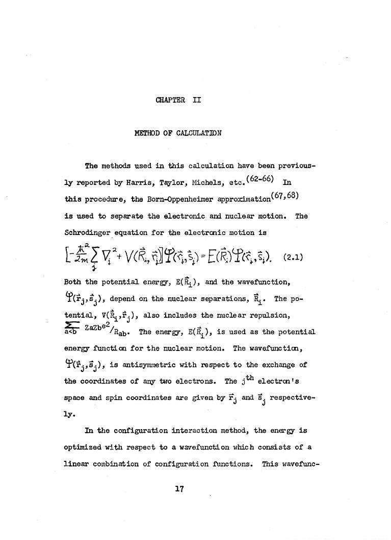
this procedure, the Born-Oppenheimer approxirnation( 67, 68)

is used to separate the electronic am nuclear motion. The

Schrodinger _equation for the electrcnic motion is

L-.C['f+ vcR,,~jfc~v,)~[cib<fcf.,SJ (2.1) . }

Both the potential energy, E(~), and the wavefunction,

Cf(rj,s), depend on the nuclear separations, Ri. The po­

tential, V(i\_,i\), also includes the nuclear repulsion,

~ ZaZbe2/ .... . a<o Rab• The energy, E(R.), is used as the potential l.

energy f'uncticn for the nuclear motion. The wavefuncticn,

<f(rj,sj), is antisymmetric with respect to the exchange of

the coordinates of any two electrons. The j th electrcn I s

space and spin coordinates are given by rj .and sj respective­

ly.

In the configuration interaction method, the energy is

optimized with respect to a wavefunction which consists of a

linear combination of configuration functions. This wavefunc-

17

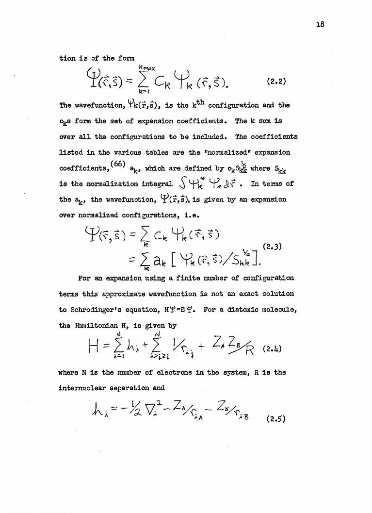
tion is of the form

CtJ ~x lu T(~s) =: L ck T k (.f, s).

~.::.)

(2.2)

The wave.function, lrk(r,s), is the kth configuration am. the

cics fom the set of expansion coefficients. The k sum is

over all the configurations to be included. The coefficients

listed in the various tables are the "normalized" expansion

coefficients, ( 66) 8k, which are defined by ck~ where Sick

is the normalization integral S ~k~ ~ J t . In tems of

the 8i(, the wavefunction, lf (r,s), is given by an expansion

over nomalized con!'igurations, i.e.

'fc~, s') = L ck ~kc~, s) ~ \ (2.J)

= 2. ak [ 'f~ c~, s)/s:k ]~ k:

For an expansion using a finite nwnber of configuration

tenns this approximate wavefunction is not an exact solution

to Schrodinger1 s equation, H't' =E 'f. For a diatomic molecule,

the H!uniltonian H, is given by tJ "1

H = f. .h, + l21 ½, t + ZA ½ (2,4)

where N is the number of electrons in the system, R is the

internuclear separation and

18

19

where A and B refer to the two nuclei. In order to obtain the

best wavefunction, tbs coefficients, <;c, are detennined by

applying the variation principle to the expectation value of

the Hamiltonian,

S4'.y-(~\s) Hlfc;,s)J.~~s =Stpc'f,s)EPn\s)J~J~

=-Lc~tck H.,e~-= 2..cf ck E 511e ~k ,Q,k

(2.6)

where

S LP/en~ c-r )Af and

(2.7)

This procedure leads to the following set 0£ secular equations

(2 •. 8)

Non-trival solutions 0£ this system of equations exist only

when their determinant van~hes

det / H 9-k - E S ~~ I ::: 0. (2.9)

The roots, Ei' obtained are upper bounds ( 69) to the true energies

of the i states considered. The lowest root is more accurate

than the other roots.

In the valence bond or atomic orbital approach, each

configuration function,~k(r,s), is given by an antisynmie­

trized product of space and spin orbitals( 65, 7o, 7l)

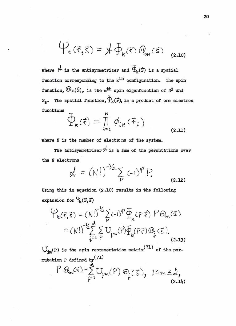
(2.10)

where * is the antisymmetrizer and c}k(r) is a spatial

f'imction coITesponding to the kth configuration. The spin

f'imction, ®m( S), is the mth spin eigenfunction of s2 and

Sz• The spatial function, Pie(~), is a product of om electron

functions N

P~ c~J == 7f J,.w. ct; J ;.:1 (2.11)

where N is the number of electrons of the system.

The antisymmetrizer 54- is a sum of the permutations over

the N electrons

J :=. {N n-Y"-L c-1)'f' P. p (2.12)

Using this in equation (2.10) results in the following

expansion for o/k(r,s)

<+>ie(f $) = ( N ~)¼-L C-l)f p C pf) P @'m (5) ) p ~

-l/4 J. = (N n 21- 2. u~W-(P)p~C?~) ej. (SJ.

}-l p (2.13)

Ujm(P) is the spin representation matrix:( 7l) of the per­

mutation P defined by( 7l) ,l

p @'Mcs')=J U~'MCP') ®·(SJ ~~ 1 J- a- '

20

where the j sum is over the set of spin eigenfunctions ot

s2 and Sz•

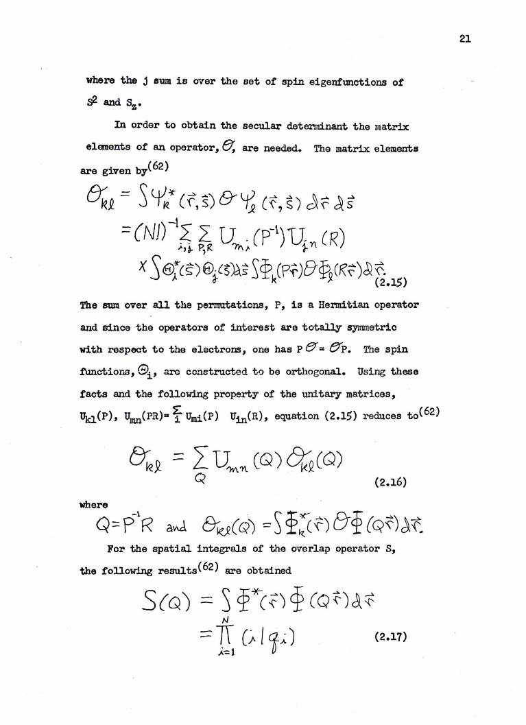
In order to obtain the secular determinant the matrix

elements or an operator, fl, are needed. The matrix elements

are given by( 62 )

½.i = S <f/ (f,S) e-i Ci\ S) Jf ,H

=cN1r12, L u . cv1)u (R) .,..,~ P,R "tr..1- } 'Y\

X s~rcs)0~(s)c\s SP,JPi)&pp(R~)~~-~ ~ ,. (2.15)

'l'he sum over all the permutations, P, is a Hennitian operator

and since the operators of interest are totally symmetric

with respect to the electrons, one has P et"" t}'p. The spin

f'unctions, ®1 , a..-c com~truct-ed to be orthogonal. Using these

tacts and the following property of the unitary matrices,

Uici(P), t1mzi(PR)a t' Um1(P) U1n(R), equation (2.15) reduces toC 62)

Lu%~ CQ)~co) Q .

(2.16)

where

Q==P1

R a~ &~(Q') =ST:C?)&p(qZ)jt_ For the spatial integrals of the overlap operators,

the following resultsC 62 ) are obtained

S<o ') == S cf*c~> cp cot)~~ N :::: JI Ci- I j,.;) c2.11i

21

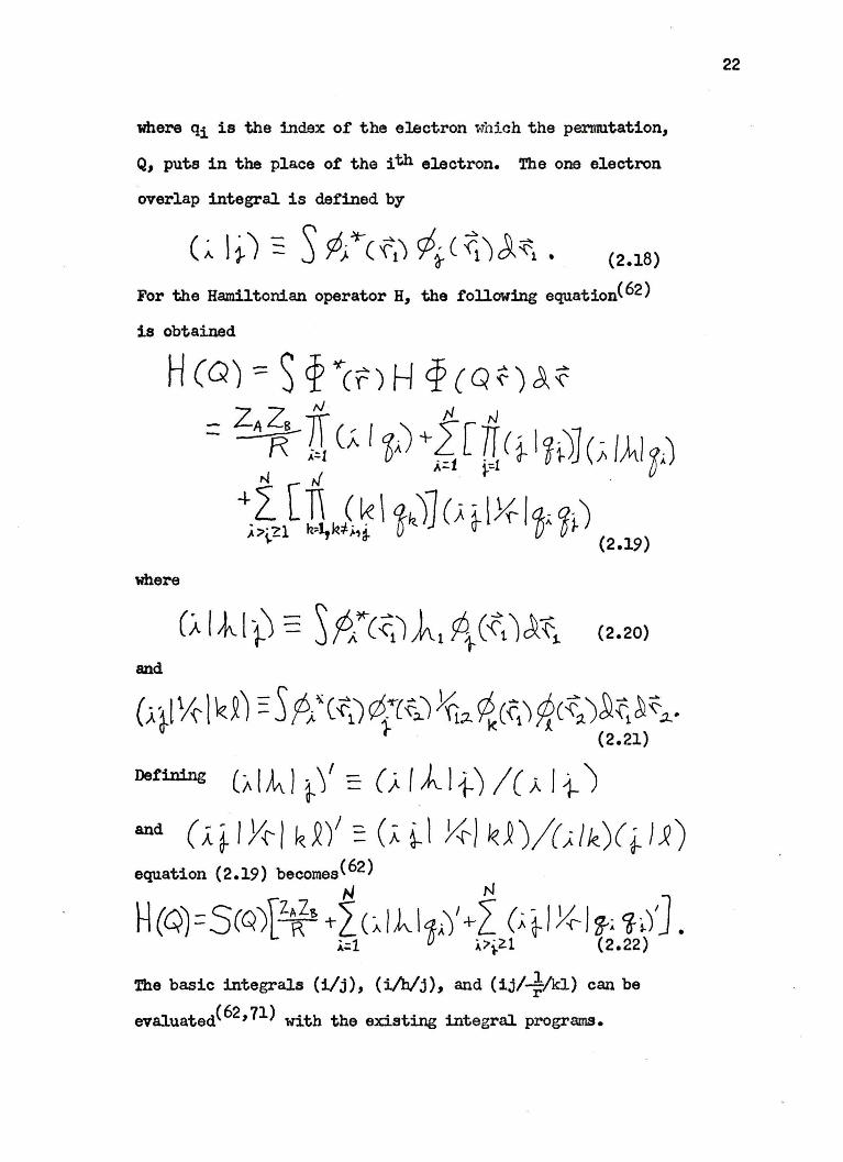
where qi is the ind.ex of the electron which the permutation.,

Q., puts in the place of the 1th electron. The one electron

overlap integral is defined by

(2.18)

For the Hamiltonian operator H., the following equationC62)

is obtained

where

and

(,;_ti 1/" l k ~) = S ,¢/ c iD 1ztHil ~;,_ ~ c fi) ~c-f,. J~ :f; ~ f "-. · (2.21)

Defining ( ~ I ~ ) t ')' - (; f ;h_ l 1-') / ( t I 1-> and ( A } / Y{' / ~ ~ / :_ ( A ~ l K) ~ J J /{;. / k) ( j_ } J} equation (2.19) becomes< 62 )

N N

H(QJ=S(Q'>F~ -1-Lc;.1_i__11_.J'+L <•~l¼--/i; is]. 4;;1 i.;,i-21 (2.22)

The basic integrals (i/j)., (i/h/j)., and (ij/ ~) can be

evaluated( 62 , 71) with the existing integral programs.

22

The bases used for the one electron spatial .f'tmction,

~(:j), are Slater type orbitals (ST0 1a)

rl ( t) ::: p (-N <'~ . ,()'\ v' Y\~ --1 0 l'M.~ I( I'"\ ) y.;.,. 1- ex \A.;.,}+-" ?Yl." r~ J, i- 1,9_. cos tt~

} A (2.23)

in spherical coordinates, or

¢/ f 1-l= ex p(-S, ~i-). '1/-' m, ~) r,-i ~~"'}~os t1i! (2.24)

with mixed spherical and elliptical coordinates< 65) where

r j Di -1 P11 lmi. I ( cos 8 j) can be expressed in terms of ~ j and 'lj• The orbital exponent b1=! )i,.,O(iR/2, where R is the

interzmclear separation, and the llj_, 11 and !llj_ refer to the

appropriate quantum numbers.

The important spin representation matrices, Ujm(P), for

N electrons can be constructed from those for N-1 electrons(7o, 7i)

or from the coefficients< 62 ) of the terms containing the electron

spins, CX and f->, when the spin basis .functions are constructed

using the genealogical. method.(70,7l) This procedure automat­

ically gives orthogonal linearlJ" independent spin basis functions.

For a three electron doublet there are two linearly independent

The four electron singlet state also has two basis functions

which are

23

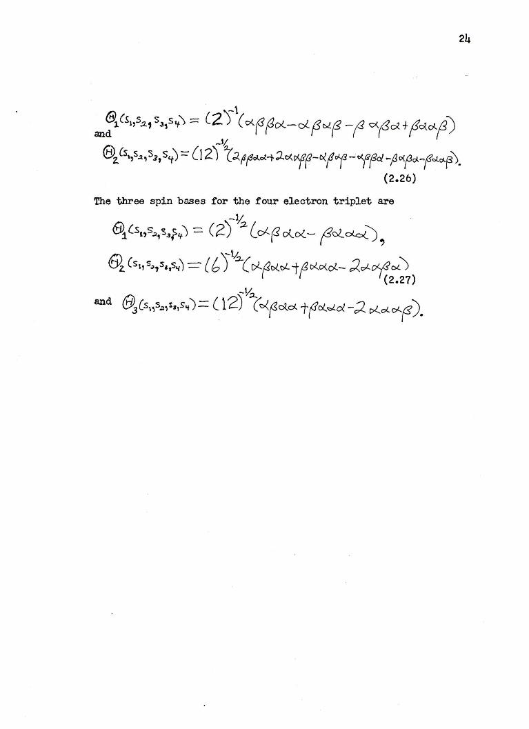
The three spin bases for the four electron triplet are

-1~

8>1 Cs" s .:i, s 3 ,S '+ > = ( 2) ::i. l d (J ex. ex. - f cl ol.o() , \¼ ~ ~ Cs 1, s~,s,,s~') -==- ( b ) ~c r:;J..t.2.rx._r;;J._ ta r:J....DZcJ..- :2d--ctf,. ol )

1- r c2.21) -V.:2...

and @1[sl,s.,,i,1s'tJ := ( 12) ( ~f ex.ct tfcx..,_,1.cx -;2_ e>Zcx.ot-.r5 ).

24

CHAPTER III

OOMPUTATIONAL PROCEDURES

3.1. Basis Orbitals

Diatanic molecules are considered to have tvo limiting

points: the separated ato~ with infinite internuclear separa­

tion, i.e. R=tDO, and the united atom with zero separation,

i.e. RaO. Each molecular state therefore, in the context of

these limiting separations, connects to particu1ar atomic states.

In the case of lithium hydride the united atom is beryllium

am the separated atoms are lithium and ~rogen. As an

example, the ground x1 ~ + state of LiH necessarily has an

united atom limit of the lowest Be2S(ls22s2) state and a

separated atoms limit of the lowest Li2S(l.s22s) state and the

lowest H2s(ls) state.

IdeallJr, the parameters of the basis orbitals for the

t"l+ state of LiH would vary with internuclear separation, R,

from those appropriate tor Be2s(1s22s2) at R-0 and those ror

Li2S(ls22s) and II2s(la) at R11 00. Computati<nally, it would be

too expensive to optimize these parameters at each internuclear

separation; then-efore, it would be convenient to use a fixed

basis set. For the purposes of . this calculat.ion the basis set

used consists of Slater type orbitals (ST0 1s) optimized for each

of the limiting atomic states and combined to give a basis set

25

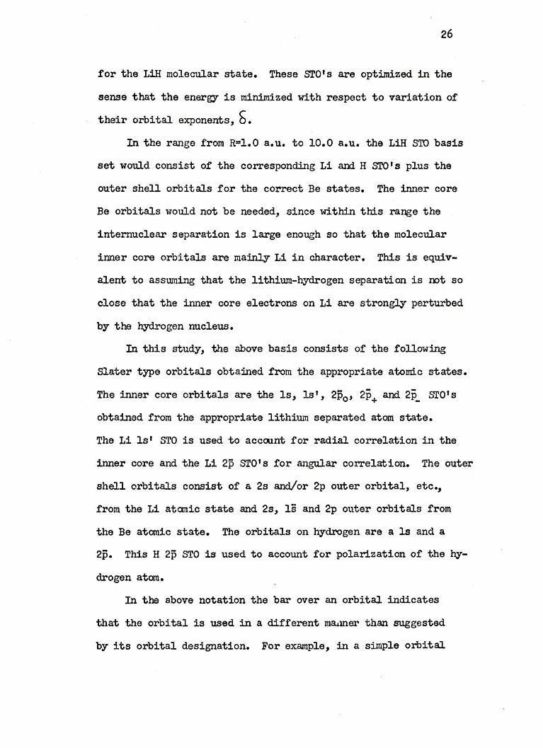
26

for the Lill molecular state. These STO's are optimized in the

sense that the energy is minimized with respect to variation of

their orbital exponents, 5 . In the range from R=l.O a.u. to 10.0 a.u. the LiH SID basis

set would consist of the corresponding Li an:l H STO's plus the

outer shell orbitals for the correct Be states. The inner core

Be orbitals would not be needed, since within this range the

internuclear separation is large enough so that the molecular

inner core orbitals are mainly Li in character. This is equiv­

alent to assuming that the lithium-hydrogen separation is mt so

close that the inner core electrons on Li are strongly perturbed

by the hydrogen nucleus.

In this study, the above basis consists of the following

Slater type orbitals obtained from the appropriate atomic states.

The inner core orbitals are the ls, ls', 2p0 , 2p+ and 2p_ STO's

obtained from the appropriate lithium separated atom state.

The Li ls' STO is used to accrunt for radial correlation in the

inner core and the Li 2p STO' s for angular correlation. The outer

shell orbitals consist of a 2s and/or 2p outer orbital, etc.,

from the Li atanic state and 2s, ls and 2p outer orbitals from

the Be atomic state. The orbitals on hydrogen are a ls and a

2p. This H 2p STO is used to account for polarization of the hy­

drogen atom.

In the above notation the bar over an orbital indicates

that the orbital is used in a different m~mer than suggested

by its orbital designation. For example, in a simple orbital

description of lithium, i.e. Li2S(ls22s) or Li2P(ls22p), the

ls orbital is used for the two inner coro electrons while the

2s or 2p orbital is used for the outer electron. In other

words, its quantum munber n indicates that the orbital is used to

describe the nth shell. In the standard notation an orbital

is designated by ns, np, etc. The bar over an orbital indicates

that this orbital is not used in the nth electron shell. The

2p STO's are used to obtain angular correlation in the inner

core of the appropriate atom. This is indicated by their rel­

atively large orbital exponents. The beryllium ls sro has an

orbital exponent which is appropriate for an outer shell orbital.

In the beryllium atondc state calculation it is used to give a

node to the 2s STO and therefore has the same orbital exponent.

27

The hydrogen 2p orbital can be considered to form a limar

combination with the hydrogen ls orbital. The resulting hybrid­

ized orbital is used to represent the polarizability of the hydrogen

electron. The orbital exponent of this 2p orbital is set equal to

that of the ls orbital.

The procedures for obtaining the appropriate sro bases

for the beryllium and 11 thium atontlc states are listed and

discussed in detail by the author in reference (72). The atomic

energies obtai..~ed were 99.6% of the experimental value or better

with the configuration interaction wave.functions presented.

3.2. Configurations

For the purposes of constructing the configurations for

the c. I. wave.function, the following grouping of orbitals was

28

used. The molecular inner core orbitals grouped togethEr were

- - -the lithium atomic orbitals ls, ls', 2p0 , 2p+' and 2p_ am the

· beryllium orbital. ls. The Be ls orbi ta1 was arbitrarily includ~d

in this group. The outer shell orbitals used to represent lith­

ium in Li.H consisted ot the lithium outer shell atondc orbitals,

2s, 2p, etc., and the beryllium orbitals 2s an1. 2p. The last

groq> consisted of the hydrogen ls, 2p0 , 2p +, and 2p_ STO' s.

In describing the configurations, the inner core orbitals

used to represent the two inne:nnost electrons on lithium in LiH

will be denoted by i, 11 , etc., the outer orbitals on Li by o, o',

etc., and the hydrogen orbitals by h, h', etc. The primary covalent

type configuration derived from physical intuition wruld coo.sist of

two electrons in the Li inner core, one in a Li outer orbital and

one in a hydrogen orbital, i.e. ii' oh. Similarily, primary

+ -Li H type configurations will be represented by i 11 h h' and

Li-H+ type by i i I o o 1 • These starting configurations can be

seen from physical ir,tuition to represent the grCWld state. The

trutt gi•otuld state can be thought of as a mixture of three ideal-

+n- • i- + ized descriptions, i.e • . covalent LiH, ionic Lin ani ionic L H.

The state will be represented as a superposition of these classes

of configurations. From each of these initial configurations

three other types can be formed by substitution. One type will be

formed by substituting an Li imler core orbital for an outer

shell o orbital. The second will have one of the i inner core orbit­

als in a configuration replaced by an o outer shell orbital in order

to represent a single excitation. The third will have both i inner

core orbitals replaced by an o outer shell orbital to give a

dou.ble excitation.

29

The computer program has a limit of 125 configurations. Due

to the large basis sets used in the calculations, many more than

125 configurations are possible. Therefore, some must be elimi­

nated to give a limited CI wavefunction. Considering that from its

properties lithium hydride is somewhere between being covalent LiH

az¥i. ionic Li+H-, the important initial configurations should be of

the LiH aJXl Li+Ir primary types. From physical intuition the most

important covalent LiH ccnfiguration would have two electrons in

lithium la-type orbitals for the inner core, and one electron in

a lithium 2s~type orbital, and one in a hydrogen ls-type orbital

for the outer shell. The most important ionic Li +H- configurations

would have a similar inner care, but would have two electrons in

~drogen ls-type orbitals for the outer shell.

With these configurations as a starting point, a limited

search through the configuration list was performed in order to

obtain the best 125 configurations. In general grrups of config­

urations, for example, thcs e of the (LilaBe2s )be type where b runs

over the other outer shell orbital.a and cover the hydrogen basis

orbitals, were added to the starting configurations and tmir

effect on the energy observed. Unless trey lowered the energy

those configurations with the smallest coefficients in the wave­

function were eliminated. About 20 to 30 configurati ans were

eliminated and other different groups of configurations tried.

This procedure was repeated until a comprehensive sampling

30

of configurations was covered. A set of configurations was chosen

from those tried in the described procedure. This set was varied

slightly among these chosen configurations. The final set used

was the one which gave the best energy. This procedure was used

at an internuclear separation of either 2.0 a.u. or 4.0 a.u.

since with the basis orbitals used the wavefunction is less

accurate at small internuclear separations. The final set of

configurations obtained was then used for the energy calculations

at the other internuclear separations.

It must be noted that this procedure does not guarantee

the best 125 configurations. The contribution of any config­

uration to the energy depends on the other configurations in the

wave.tunction. Therefore, to conduct a conplete search would be

prohibitively time consuming. The magnitude of a configuration's

coefficient in the wavefunction does not directly give the

configuration's contribution to the energy. Two approximately

linearly dependent configurations would have nearly equal and per­

haps large coefficients but together would not contribute more to

the lowering of the energy than one of them alone. For the case

of non-orthogonal basis orbitals, approximate linear dependencies

are always present to some degree and must be checked.

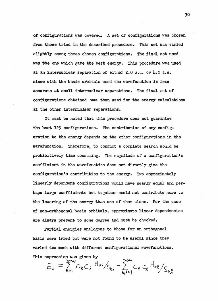
Partial energies analogous to those for an orthogonal

basis were tried but were not fom1d to be useful since they

varied too much with different configurational wavetunctions.

This expression was given by 1 _

"'~ . r<..-.x

E,;. == L C~C;: Hk;/sk .-f Ciecp_Hie.Q/s 0 k=t >- k,.t::1 /. k;,.,.

Jl

where the i..T1dex k runs over a truncated part of the CI expan­

sion of about 40 configurations.

Although the procedure described for choosing configurations

has many inadequacies in obtaining the best possible 125 configur­

ations, it does lead to a qualitative measure of the importance of

various types of groups of configurations without very great expense.

The maximum energy difference between the worst and best set of

configurations used during the search was about 0.006 a.u.

3. J. Spin Functions

The spin states considered in this calculation are:

the three electron doublet, the four electron singlet and the

four electron triplet. The three electron doublet and four

electron singlet have two linearly independent spin functions.

The four electron triplet has three linearly independent spin

functions. In the computer program only the G\ spin function

is used. For example, in the case of four electrc:1 singlet the

LilsLils'Li2sHls configuration with the spin function would

have singlet coupling; while the LilsLi2sLils 1llls configuration

with the @1 spin function would have triplet coupling. This

would be equivalent to the½( B 1-J.f@2) spin function. The

functions E)i, and ½( G>1 -./J G2) are linearly independent and

therefore can be used as a basis for this spin state. The results

for the three electron doublet and the four electron triplet are

similar.< 72 ) The spin representation matrices are constructed

from the ®1 spin functions.

CHAPTER IV

LOWEST STATES OF J 2. +, 3]1 and 1 Jr SD1METRY

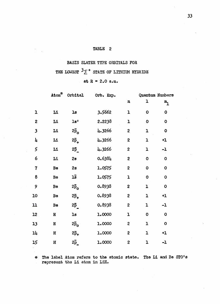
4.1. The Lowest Lithium Hydride 3 E+ State

The lowest LiH 3~+ state connects with the lithium

2s(ls22s) plus eydrogen 2s(ls) atomic states in the separated

atom limit and the beryllium .3p(ls22s2p) atcmic state in the

united atom limit. Therefore, the basis orbitals used to des­

cribe the lithi1.m1 atom in LiH 3~ + consist of those far tm

Li2S(ls22s) ~tate plus the 2s, ls and 2p ST0 1 s for the BeJP

(ls22s2p) state. These basis orbitals used for the LiH Ji+

state are listed in Table 2. Their parameters are given at an

internuclear separation of 2.0 a. u. At this internuclear separa­

tion the basis STO I s for LiH have the same scaling as for the

atomic states.

This state was found to be repulsive in energy. The

energies calculated and the various intemuclear separations

used are given in Table J. The configurations and their coef­

ficients in the wavefunction are arbitrarily listed at an inter­

nuclear separation of 4.0 a.u. in Table 22 of .Appendb: I. The

majority of low lying states of LiH have minimwnB at"ound 4.0 a.u.

The energy at R= 00 is obtained from a calculation of the

Li2S(ls22s) state using the basis STO' s in Table 2 excluding those

for hydrogen.

.32

33

TABLE 2

BASIS SLATER TYPE ORBITALS FOR

THE LOWEST 3 L + srATE OF LITHIUM HYIRIDE

at R • 2.0 a.u.

Atom* Orbital Orb. Exp. Quantum Numbers n 1 ~

1 Li ls 3.5662 1 0 0

2 Li ls' 2.2238 1 0 0

3 Li 2po 4.3266 2 1 0

4 Li 2p+ 4.3266 2 1 +l

5 Li 2p_ 4.3266 2 1 -1

6 Li 2s o.6J84 2 0 0

7 Be 2s 1.0575 2 0 0

8 Be ls 1.0575 1 0 0

9 Be 2po 0.8938 2 l 0

10 Be 2p+ 0.8938 2 l +l

11 Be 2p 0.8938 2 l -1

12 H ls 1.0000 1 0 0

13 H 2po 1.0000 2 l 0

14 H 2i5+ 1.0000 2 1 +l

15 H 2p_ 1.0000 2 l -1

* The label Atom refers to the atomic state. The Li and Be ST0 I s represent the Li atom in LiH.

R(a.u.)

1.0

2.0

3.0

4.0

5.0

6.o

7.0

a.o 00

TABLE .3

ENERGY FOR THE LOWEST 3E° STATE

OF LrI'HIUM HYDRIDE

Electronic Energy (a.u.)

-10.289798

-9.346228

--8.931927

-8.699008

-8.557275

-8.462710

-8.394165

-8.)41880

-1.967903

.34

Potential Energy (a.u.)

-1.2897979

-7.8462279

-7.9319268

-7.9490082

-7.9572745

-7.9627102

-1.9655932

-7.9668797

-1.9679025

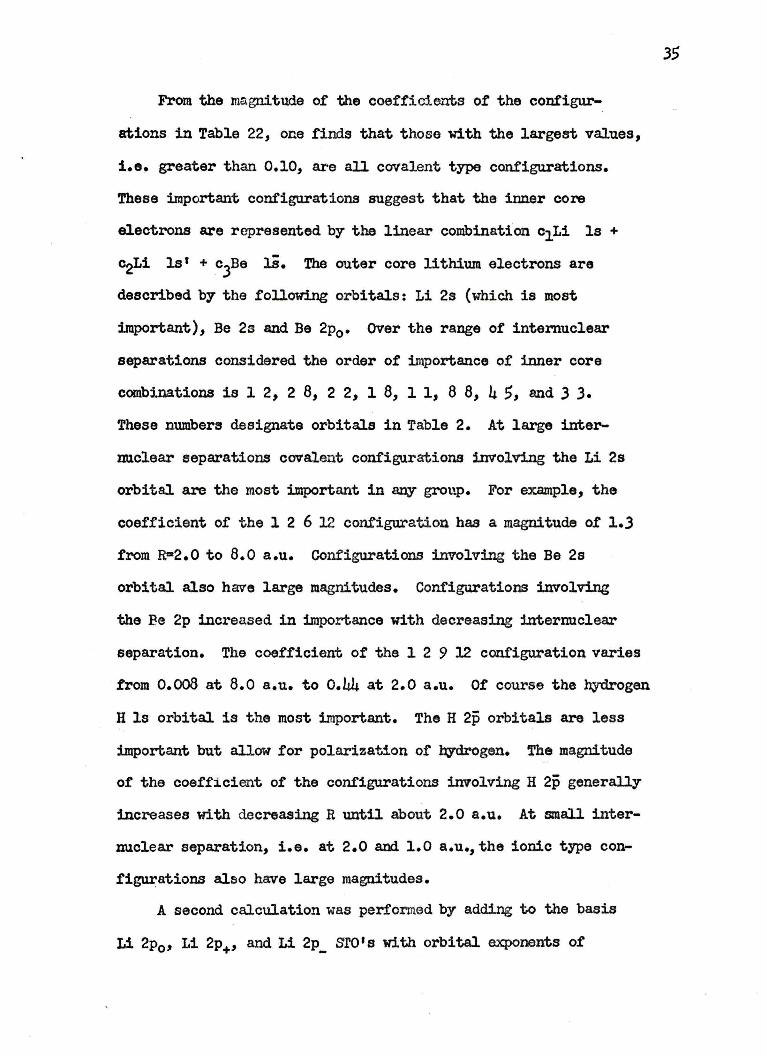
From the magnitude of the coefficients of the configur­

ations in Table 22, one finds that those with the largest values,

i.e. greater than 0,10, are all covalent type configurations.

These important configurations suggest that the inner core

electrons are represented by the linear combination c111 ls+

~Li la'+ c3Be ls. The outer core lithium electrons are

described by the following orbitals: Li 2s (which is most

important), Be 2s and Be 2p0 • over the range of internuclear

separations considered the order of importance of inner core

combinations is 1 2, 2 8, 2 2, l 8, l 1, 8 8, 4 5, and 3 3.

These numbers designate orbitals in Table 2. At large inter­

nu.clear separations covalent configurations involving the Li 2s

orbital. are the most important in 8JJY' group. For example, the

coefficient of the l 2 6 12 configuration has a magnitude of 1.3

from R .. 2.0 to 8.0 a.u. Configurations involving the Be 2s

orbital also have large magnitudes. Configurations involving

the Ee 2p increased in importance with decreasing internuclear

separation. The coefficient of the 12912 configuration varies

from 0.008 at 8.0 a.u. to 0.44 at 2.0 a.u. Of course the hydrogen

H ls orbital is the most important. The H 2p orbitals are less

important but allow for polarization of b;ydrogen. The magnitude

of the coefficient of the configurations involving H 2p generally

increases with decreasing R until about 2.0 a.u. At small inter­

nuclear separation, i.e. at 2.0 and 1.0 a.u.,the ionic type con­

figurations also have large magnitudes.

A second calculation was perfomed by adding to the basis

Li 2p0 , Li 2p+, and Li 2p_ sro•s with orbital exponents of

35

0.5237 at 2.0 a.u. The wavefunctian consisted of 125 configur­

ations and a limited search through configurations was performed.

The: energy or the lowest root at an internuclear separation ot

4.0, 6.o and 8.o a.u. is -7.9528961, -7.9633712, and -7.8244385

a.u. respectively. The energy of the next root is -7.8244385,

-7.8795953, and -7.8946733 a.u. respectively.

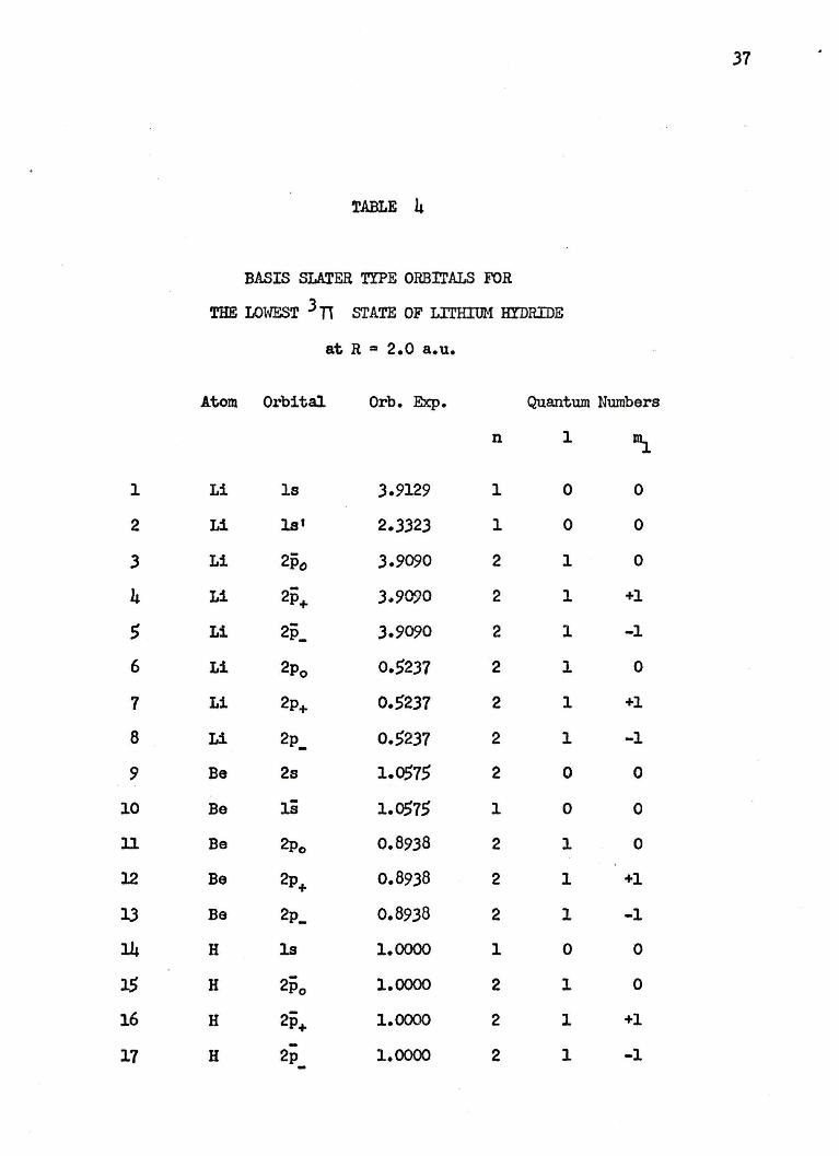
4.2. The Lowest Lithium Hydride 3rr State

The lowest 3 TT state of lithium hydride cormects to the

lowest Li2P(ls22p) state plus H2S(ls) state in the separated

atom limit and the Ba3P(ls22s2p) state in the united ~tan limit.

Its ST0 basis therefore is corrposed of those functions obtained

from a calculation of the Li2P(ls22p) state, the 2s, ls and 2p

ST0's fran the Be3P(ls22s2p) state and ls plus 2p functions for

hydrogen. The ST0 basis is given in Table 4 tor an internuclear

separation of 2.0 a.u.

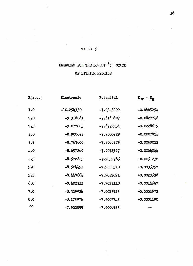
This 3 lf state is bound with its minimum lying around

4.0 a.u. The potential energy calculated. at the various

intermiclear separations is given in Table 5. For Ra4.0 a.u.,

E(OO)-E(R) equals 0.0064044 a.u. or 0.1743 e.v. The energy at

R• 00 is calculated using the basis of Table 4 minus the hydrogen

sro•s. The configurations and their coefficients for this wave­

function at the minimum of R•4.0 a.u. are given in Table 23 of

Appendix I.

As seen f'rom the most important configurations in the

wavefunction of Tabla 23, i.e. those with coefficients greater

than 0.10, the most significant inner core canbinations are

36

37

TABLE 4

BASIS SLATER TYPE ORBrrALS FOR

THE LOWli'~T J TI STATE OF LITHIUM HYDRIDE

at R .. 2.0 a.u.

Atom Orbital Orb. Eicp. Quantum Numbers

n 1 ~

1 Li ls J.9129 1 0 0

2 Li ls' 2.3323 1 0 0

3 Li 2pc 3.9090 2 1 0

4 Li 2p+ 3.9090 2 l +l

s Li 2-p_ 3.9090 2 1 -1

6 Li 2po 0.5237 2 l 0

7 Li 2p+ 0.,237 2 1 +l

8 Li 2p_ 0.,237 2 1 -1

9 Be 2s 1.057, 2 0 0

10 Be ls 1.057, l 0 0

11 Be 2po 0.8938 2 l 0

12 Be 2p+ 0.8938 2 1 +l

lJ Be 2p_ 0.8938 2 1 -1

14 H ls 1.0000 1 0 0

l5 H 2po 1.0000 2 l 0

16 H 2p+ 1.0000 2 1 +l

-17 H 2p 1.0000 2 1 -1 -

R(a.u.)

1.0

2.0

2.~

3.0

3.5

4.0

4.S

,.o

5.5

6.o 7.0

a.o 00

TABLE 5

ENERGIES FOR THE LOWEST 3 lT STATE

OF LITHIUM HYDRIDE

Electronic Potential

-10.254330 -7.2.543299

-9.)18081 -1.8180807

-9.077003 -7.8779934

-8.900073 -7.9000729

-8.763800 -1.9066515

-8.657260 -7.9072597

-8.572645 -7.9059785

-8.504451 -7.9044510

-8.448664 -7.9032091

-8.402311 -7.9023110

-8.329924 -7.9013525

-8.275974 -7.9009743

-1.900855 -1.9008553

38

Eoo - Ea

-o.64652.54

-0.0827746

-0.0228619

-0.0007824

+0.0058022

+0.0064044

+0.0051232

+0.0035957

+0.0023538

+0.0014557 . +0.0004972

+0.0001190

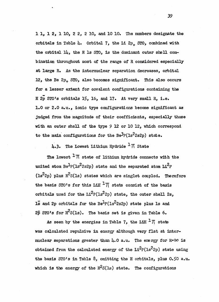
39

11., 12.,110., 22,210, and 10 10. The numbers designate the

orbitals in Tabla 4. Orbital 7, the Li 2p+ STO, ccmbined with

the orbital 14, the H ls STO, is the daninant outer smll com­

binaticn throughout most of the range of R considered especial.ly

at large R. As the internuclear separation decreases, orbital

12, the Be 2p+ STO, also becomes significant. This also occurs

for a lesser extent for covalent configurations containing the

-H 2p ST0 1s orbitals 1.5, 16, and 17. At very small R, i.e.

1.0 or 2.0 a.u., ionic type ccnfigurations become significant as

judged from the magnitude of their coefficients, especially those

with an outer shell of the type 9 12 or 10 12, which correspond

to the mai.Ii configurations for the Be3P(ls22s2p) state.

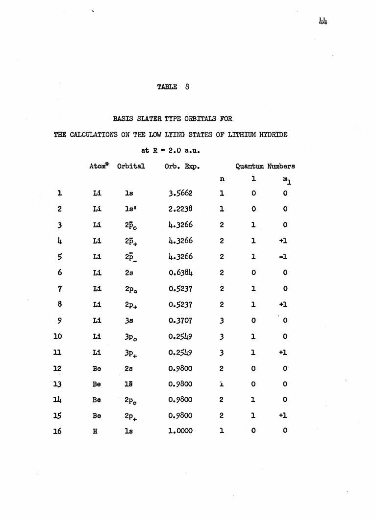
4· • .3. The Lowest LithiUlll Hydride 1 TT State

The lowest 1 TI state of lithium hydride connects with the

united atom Be1P(ls22s2p) state and the separated atom Li2P

(1s22p) plus n2s(ls) states which are singlet coupled. Therefore

the basis ST0 1s for this Lili 1TI state consist of the basis

orbitals used for the Li2P(ls22p) state, the outer shell 2s,

ls and 2p orbitals for the Be1P(1s22s2p) state plus ls and

2p ST0 1s for n2s(ls). The basis set is given in Table 6.

As seen by the energies in Table 7, the LiH 1 71 sta"te

was calculated repulsive in energy although vecy flat at inter­

nuclear separations greater than 4. 0 a. u. The em rgy for R=OO is

obtainad from the calculated energy of the Li2P(ls22p) state using

the basis STO's in Table 8, omitting the H orbitals, plus 0.50 a.u.

which is tm energy of the H2S(ls) state. The configurations

40

TABLE 6

BASIS SLATER TYPE ORBITALS FOR

THE LOWEST 1 1T STATE OF LITHIUM HYDRIDE

at R • 2.0 a.u.

Atom Orbital Orb. Exp. Quantum Numbers

n 1 1\ l Li ls 3.9129 1 0 0

2 Li ls' 2.3323 1 0 0

3 Li 2i5o 3.9090 2 l 0

4 Li 2p+ 3.9oc;o 2 1 +l

5 Li · 2-p_ 3.9090 2 1 -1

6 Li 2po 0.5237 2 l 0

7 Li 2p+ 0.5237 2 1 +l

8 Li 2p_ 0.5237 2 1 -1

9 Be 2s · 1.2218 2 0 0

10 Be ls 1.2218 1 0 0

11 Be 2po 0.4760 2 l 0

12 Be 2p+ 0.4760 2 1 +l

lJ Be 2p_ 0.4760 2 1 -1

14 H ls 1.0000 1 0 0

15 H 2po 1.0000 2 1 0

16 H 2p 1.0000 2 l +l +

17 H 2p_ 1.0000 2 1 -1

R(a.u.)

1.0

2.0

3.0

4.0

s.o 6.o 7.0

a.o 00

TABLE 7

ENERGY FOR THE LOWEST 1 TT STATE

OF LITHIUM HYDRIDE

Electronic Energy (a.u.)

-10.212022

-9.296431

-8.884393

-8.648280

-8.S00286

-8.400598

-8.329226

-8.275685

-7.900779

Potential Energy (a.u.)

-1.2120221

-7.7964313

-7.8843933

-7.8982803

-1.9002859

-7.9005977

-7.9006549

-7-9006845

-7.9007787

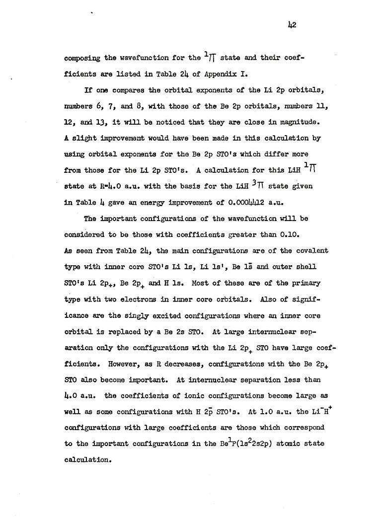
composing the wavefunction for the 1 TT state and their coef­

ficients are listed in Table 24 of Appendix I.

If one compares the orbital exponents of the Li 2p orbitals,

numbers 6, 7, and 8, with those of the Be 2p orbitals, numbers ll,

12, am 13, it will be noticed that they are close in magnitude.

A slight improvement would have been made in this calculation by

using orbital exponents for the Be 2p sro' s which differ more

. lTT from those for the Li 2p ST0 1s. A calculation for this LIB

state at R•4.o a.u. with the basis for the LIB 3TT state given

in Table 4 gave an energy :llllprovement of 0.0004412 a.u.

The important configurations of the wavefunction will be

considered to be those with coefficients greater than 0.10.

AB seen from Table 24, the main configurations are of the covalent

type with inner core ST0 1 s Li ls, Li ls', Be ls and outer shell

STO' s Li 2p+J Be 2p+ and H ls. Moat of these are of the primary

type with two electrons in izmer core orbitals. Also of signif­

icance are the singly excited configurations where an inner core

orbital is replaced by a Be 2s sro. At large internuclear sep­

aration only the configurations with the Li 2p+ ST0 have large coef­

ficients. However, as R decreases, configurations with the Be 2P+

STO also become important. At internuclear separation less than

4.0 a.u. the coefficients of ionic configurations become large as

- - + well as some configurations with H 2p ST0 1s. At 1.0 a.u. the Li H

configurations with large coefficients are those which correspond

to the important configurations in the Be¾>(1s22s2p) atanic state

calculation.

CHAPTER V

POTENI'IAL CURVES FOR LOW LYING LITHIUM HYilUDE STATF.s

$.1. Basis Orbitals

For the purposes of econonzy- in calculating the integrals,

the same basis set was used in the calculations for all the

states considered in this chapter. The basis STO' s are listed

in Table 8 with parameters for an internuclear separation of

2.0 a.u. The inner core lithium orbitals, ls, ls', 2p0

, 2p+

and 2p_, were obtained from a calculation on the Li2S(ls22s) state

where an optimization of the orbital exponents was performed.

The Li 2s STO was also obtained from this calculation. The

ensrg;y of this calculation was -7.46b.517 a.u. The Li 3a STO

was obtained by optimizing the orbital exponents of the 6 pre­

viously mentioned orbitals and the Ja sro in a calculation of

the Li2S(ls2Js) state. The energy of the Li2S(ls23s) state from

this calculation was -7.342461 a.u. and the energy of the

Li2S(ls22s) state was -7.4ob733 a.u. The Li 2p0 STO was obtained

by optimizing the orbital exponents of the basis set in a

calculation of the Li2P(ls22p) state. The energy obtained

for the Li2P(ls22p) state was -7.399894 a.u. The Li 3p0

STO's

orbital exponent was obtained in a calculation of the Li2P(ls23p)

43

44

TABLE 8

BASIS SLATER TYPE ORBITALS FOR

THE CALCULATIONS ON THE LOW LYING STATES OF LITHIUM HYDRIDE

at R .• 2.0 a.u.

Atom* Orbital Orb. Exp. Quantum Numbers

n l Illi l Li ls 3.5662 l 0 0

2 Li ls' 2.2238 l 0 0

3 Li 2i5o 4.3266 2 l 0

4 Li 2i5+ 4.3266 2 l +l

5 Li 2p_ 4 • .3266 2 l -1

6 Li 2s 0.6384 2 0 0

7 Li 2Po 0.52.37 2 l 0

8 Li 2P+ 0.5237 2 l +l

9 Li Js 0.3707 3 0 0

10 Li 3p0 0.2549 3 l 0

ll Li .3P+ 0.2549 3 l +l

12 Be 2s 0.9800 2 0 0

13 Be ls 0.9800 :.i. 0 0

14 Be 2po 0.9800 2 l 0

15 Be 2p+ 0.9800 2 l +l

16 H ls 1.0000 l 0 0

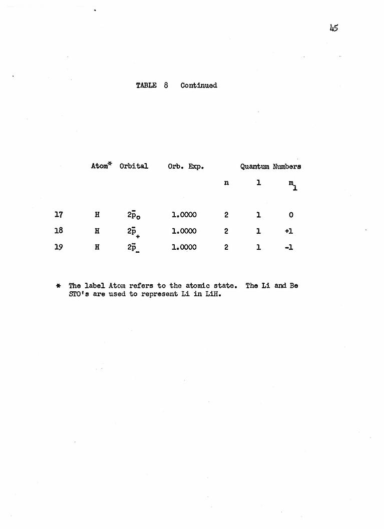
TABLE 8 Continued

Atom* Orbital Orb. Exp. Quantum Numbers

n 1 ~

17 H 2po 1.0000 2 1 0

18 H 2-p+ 1.0000 2 1 +l

19 H 2p_ 1.0000 2 1 -1

* The label Atom refers to the atomic state. The Li am Be STO's are used to represent Li in Lill.

state. This calculation was similar to that for the Li2S(ls23s)

state. The energy calculated tor the Li2P(ls2Jp) state was

-1.328178 a.u.

The orbital exponents of the Be 2s and Be ls 5'T0 1s were

restricted to be the same since the ls SI'O was used to represent

a node for the 2s STO. The Be 2s, ls and 2p0

sro•s were obtained

from a ca1culation of the Be1S(ls22s2) state in which the orbital

exponents of these outer shell orbitals were optimized while hold­

ing the parameters of the inner core oribtala fixed. These inner

core orbitals were similar to those used for the lithiwn calcula­

tions and obtained by optimization in a calculation of the Be+2

1s(ls2) state.

46

The orbital exponents of the Li 2P+, Li 3P+ and Be 2p+ sro•s

are the same as those of the Li 2p0 , Li Jp0 , and Be 2p0

STO's. The

orbital exponent of the H ls, 2p0 , 2p and 2p STO' s were set + -

equal to 1.0000. Due to computer limitations it was not possible

to include the Li 2p , Li Jp and Be 2p STO's in the basis set. - - -Therefore covalent configurations with n coupled bonding, i.e.

(Lils)2Li2p+H2p_ and (Lils)2Li2p_H2P+,could not be included in the

t state calculations. It was tound that inclusion of this type

of configuration lowered the energy less than 0.0001 a.u. There­

fore neg1ecting l'\Coupled configurations was not a poor approxima­

tion.

5.2. The Lithiwn Hydride 1~ + states

The four lowest LiH 1L. + states were considered in this

calculation. In the separated atom limit these states connect

with the ti2s(ls22s), Li2P(ls22p), Li2s(ls2Js) and Li2P(ls2Jp)

states plus the H2s(ls) state. Experimentally, the separated

atom limits are -7.97865, -7.91074, -7.85469 and -7.83775 a.u.

respectively. These values are obtained from Moore's tables(3)

aid the results of Pekeris(4).

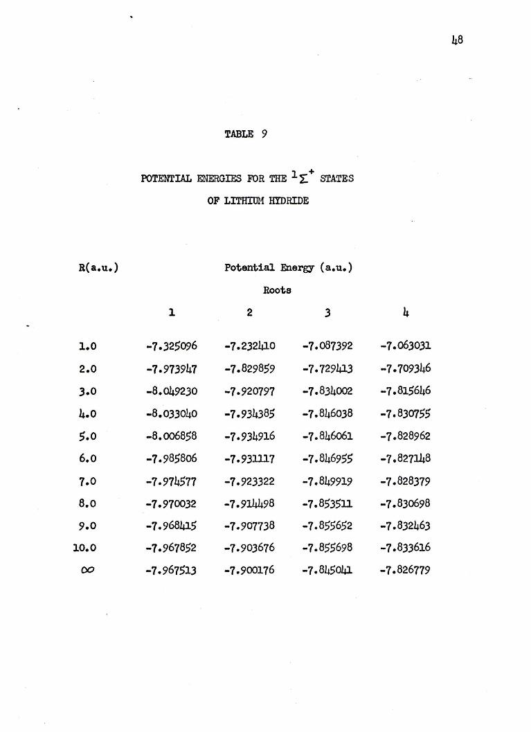
The potential energies obtained are listed 1n Table 9, and

the potential curves are presented in Figure 1. The energies at

R• 00 are obtained from a calculation of the Li atomic states

using the basis of Table 8 without the H sro• s. The H2S(ls)

47

energy ot 0.50 a.u. is added to the Li energies to obtain the values

tor R• 00. The binding energies of the Ill+ and the A1 2,+ states

are estimated to be 2.223.SeV and 0.9453eV. The farm of the

coulombic potential curve for Li +il- was obtained f'ran Mulliken~ 5 )

This curve is only qualitatively accurate and is included for

illustrative purposes. The equation is

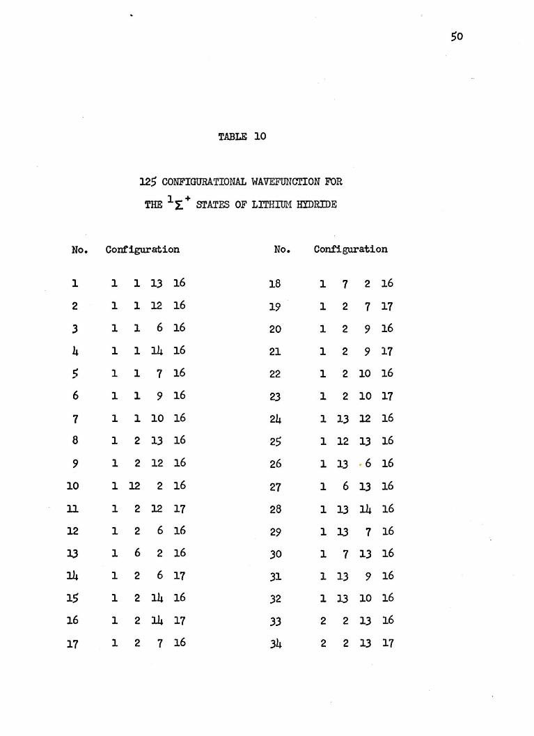
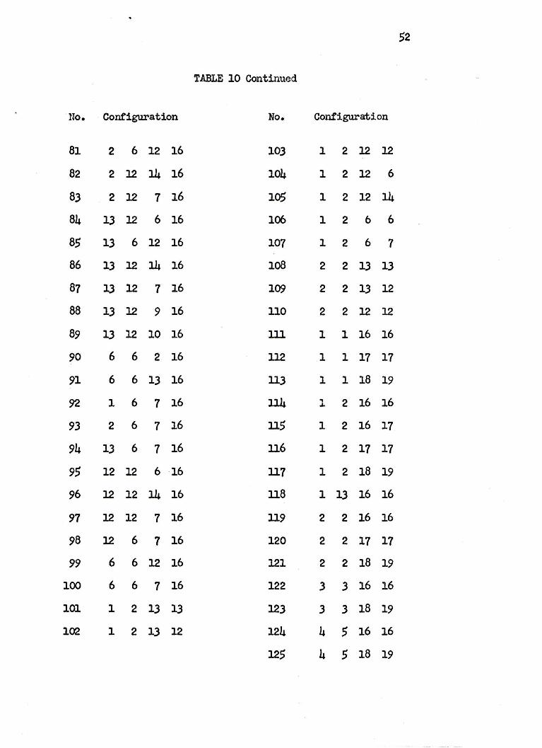
The configuration list for these wavefunctions is given in

Table 10. The coefficients obtained for the various states

are arbitrarily given at 4.0 a.u. in Table 25 of Appendix II.

The wavefunctions used are complicated and hard to analyze

especially at small internuclear separations where a great many

configurations have large coefficients. In general, at large R

the most important conf'igurat ion in any group is the covalent

configuration w1 th the outer shell Li orbital. corresponding to the

molecular state's correct separated atom limit.

,As discussed by Mulliken(5) and seen in Figure 1, the shape

of the potential curve of the ground state of Lill resembles quite

strongly the Li+If" curve. Therefore, it is likely that the X1 .L +

R(a.u.)

1.0

2.0

3.0

4.0

5.0

6.o

7.0

a.o 9.0

10.0

00

TABLE 9

POTENTIAL ENERGIES FOR THE l t, + srATES

OF LITHIUM HYDRIDE

Potential Energy- (a.u.)

Roots

l 2 3

-1.325096 -7.232410 -7.087392

-7.973947 -1.829859 -7-729413

-8.049230 -7-920797 -7.834002

-8.033040 -7.934385 -7.846038

-8.006858 -7.934916 -7.846061

-7-985806 -7.93lll7 -7.846955

-7.974577 -7.923322 -7.849919

-7.970032 -7.914498 -1.853511

-7.968415 -1.907738 -7.855652

-7.967852 -1.903676 -1.855696

-7.967513 -1.900176 -7.845041

48

4

-1.063031

-7.709346

-7.815646

-1.830755

-7.828962

-7.827148

-7.828379

-7.830698

-7.832463

-1.833616

-7.826779

-1.70

-7.80

-. ::s . C'IS ........

~ -1.90 H Q)

~

-8.oo

-8.10 o.o 1.0 2.0

..­/

/

' .,.,/ , ____ .,

3.0 4.0

.,,,,,.­

5.0

-__ __. . ..-- --

q

2. --- -- - -L._-;11-- - >,. "

,- 1 ,,,,,,., ,,.,---- ----....-----­

6.0 7.0 B.o 9 •. 0 10.0 Internuclear Separation (a.u.)

FIGURE 1. POTENTIAL ENERGY CURVES FOR THE lL + STATES

OF LITHIUM HYDRIDE

00

No.

1

2

.3

4

5

6

7

8

9

10

11

12

13

14

15

16

17

TABLE 10

125 CONFIGURATION.AL WAVEFUNCTION FOR

THE l~+ STATES OF LITHIUM HYDRIDE

Conf"igura:tion No. Configuration

1 l 13 16 18 l 7 2 16

1 l 12 16 19 l 2 7 17

l 1 6 16 20 1 2 9 16

l 1 14 16 21 l 2 9 17

1 1 7 16 22 l 2 10 16

1 l 9 16 23 1 2 10 17

1 1 10 16 24 1 13 12 16

1 2 13 16 25 1 12 13 16

1 2 12 16 26 1 13 • 6 16

l 12 2 16 27 1 6 1.3 16

1 2 12 17 28 1 13 14 16

1 2 6 16 29 1 13 7 16

1 6 2 16 30 1 7 13 16

1 2 6 17 31 1 13 9 16

1 2 14 16 32 l 13 10 16

l 2 14 17 33 2 2 13 16

1 2 7 16 34 2 2 13 17

50

51

TABLE 10 Continued

No. Configuration No. Configuration

35 2 2 12 16 56 13 13 14 16

36 2 2 12 17 59 13 13 7 16

37 2 2 6 16 60 13 13 9 16

38 2 2 6 17 61 13 13 10 16

39 2 2 14 16 62 3 3 12 16

40 2 2 7 16 63 3 3 6 16

1.il 2 2 7 17 64 3 3 7 16

42 2 2 9 16 65 3 3 9 16

43 2 2 10 16 66 3 3 10 16

44 2 13 12 16 67 4 5 13 16

45 2 12 13 16 68 4 5 12 16

46 2 13 6 16 69 4 5 6 16

47 2 6 13 16 70 4 5 7 16

48 2 13 14 16 71 4 5 9 16

49 2 14 13 16 72 4 5 10 16

50 2 13 7 16 73 12 12 1 16

51 2 7 13 16 74 12 12 2 16

52 2 13 9 16 75 12 12 13 16

53 2 13 10 16 76 l 12 6 16

54 13 13 1 16 77 1 6 12 16

55 13 13 2 16 78 l 12 14 16

56 13 13 12 16 79 1 12 7 16

57 13 13 6 16 80 2 12 6 16

52

TABLE 10 Continued

No. Configuration No. Configuration

81 2 6 12 16 103 1 2 12 12

82 2 12 14 16 104 1 2 12 6

83 2 12 7 16 105 1 2 12 14

84 13 12 6 16 106 1 2 b 6

85 13 6 12 16 107 1 2 6 1

86 13 12 14 16 108 2 2 13 13

87 lJ 12 7 16 109 2 2 13 12

88 13 12 9 16 ll0 2 2 12 12

89 13 12 10 16 lll 1 1 16 16

90 6 6 2 16 112 .1 1 17 17

91 6 6 13 16 ll3 1 1 18 19

92 1 6 7 16 ll4 ., 2 16 16 .L

93 2 6 1 16 ll5 1 2 16 17

94 13 6 1 16 U6 1 2 17 17

95 12 12 6 16 ll7 l 2 18 19

96 12 12 14 16 ll8 1 lJ 16 16

97 12 12 7 16 ll9 2 2 16 16

98 12 6 7 16 120 2 2 17 17

99 6 6 12 16 121 2 2 18 19

100 6 6 7 16 122 3 3 16 16

101 1 2 lJ lJ 123 3 3 18 19

102 1 2 lJ 12 124 4 5 16 16

125 4 5 18 19

state has a large amount of Li+H- character in this region

where the two curves resemble each other so closezy-. This can

also be seen by looking at the ionic Li~- type configurations in

the wavefunction. For the x1 r+ state, they have a maximum

importance at 3.0 a.u. and then gradually trail off. For the

A1~ + state their importance gradually increases to a maximum

around 6. 0 a. u. For the next two 1 ~ + states tmse Li~- config­

urati ans become important at large interzmclear separations.

The potential energies of Table 9 for the third 1 L + and

l~+ fourth £- states indicate that these states are bound at R•lO. O

a.u. since the energies at 10.0 a.u. lie below the calculated

separated atom limits. In fact, at 10.0 a.u. the third l~+

state lies below the experimental separated atom limit of -7.85469

a.u. A metastable equilibrium is also observed in the fourth lL+

state at 4.0 a.u. However, it is felt that this is due to inter­

action between third and fourth wave.functions in this range of R

and iua;r not be the case pb;ysically. Brown and Shull(57) observed

a metastable equilibrium in the third 1 L + state at 3. 70 a.u. and

conjectured that there is another equilibrium around 10.0 a.u.

They- found a minimum in the fourth 1~+ state at 7.50 a.u.

However, their basis set did not include an:, lithium Js and 3p

character and therefore is only roughly qualitative. Bemer and

Davidson< 60) calculated the potential curves of these states

between 1.5 and 6.0 a.u. They found that the third lL.+ state

has a metastabi.e equilibrium at 4. 0 a. u. and that the fourth 1 L. +

state is repulsive in this range. They also fo,md that the

S3

fourth excited state, i.e. the 1 .Z:+ state, has a minimum around 4.0

a.u.

In order to study the third and fourth 1 r_ + states in

more detail at large R, a double precision integral program

was used. This program gives more accurate results at these

large interzmclear separations. Also, a Li 3<1<, and a Li 4s

sro were added to the basis set with orbital exponents 0.3333

and 0.2500 respectively which were detemined using Slater's

rules. Twenty configurations which seemed to have the smallest

effect on the energy were replaced by appropriate covalent con­

figurations containing the 3do and 4s STO' s. Also, when Brown

and Shull 1 s potential curves for the first two l.L + states

were compared with the curves obtained from this calculation,

it was found that this calculation is much poorer than theirs

in two regions. For the xl~ + state this region was from 1.0

to 6.0 a.u. and for the A1 2_ + state from 5.0 to 9.0 a.u. These

are the regions in which the LiT character of these states has

its greatest importance. Therefore, the wavefunction used in

this calculation does not have enough Li +u- chara.:.;ter. In order

to test this conjecture a hydrogen ls' sro with orbital exponent

0.60oo was added to the basis set of Table 8 along with the Li

3do and 4s sro 1 s. Eight of the configurations involving 3d0

54

and 4s were replaced by ionic LiY type configurations involv­

ing the H ls I sro. Another set of calculations was perfomed

using this H ls I orbital. The potential energy results for these

two states are given in Table 11. Tha energies between 8.0 and

12.0 a.u. and for R=oo were obtamed using the double precision

integral program, while those between 3.0 and 6.o a.u. were

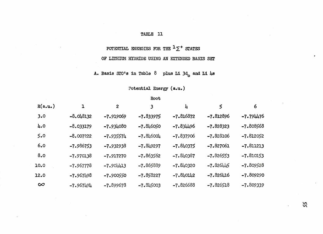
TABLE 11

POTENTIAL :ENERGIES FOR THE lL+ srATES

OF LITHIUM HYDRIDE USING AN EXTENDED BASIS SE?

A. Basis sro I s in Table 8 plus Li Jd0

and Li 4s

Potential Energy ( a. u.)

Root

R(a.u.) l 2 3 4 5 6

3.0 -8.048132 -7-919069 -7.833915 -7.816872 -1.812896 -7-794476

4.0 -8.033179 -7.934080 -7.846050 -7.834496 -7.828323 -7.808568

5.0 -8.007~22 -7.935574 -7.846004 -1.837906 -7.828106 -7.812052

6.o -7.986753 -7.932938 -7.849297 -7.840375 -1.827061 -7.8ll213

8.o -7.970138 -7-917270 -7.863562 -7.840387 -7.826553 -7.810153

10.0 -1.967778 -7.904413 -7.865889 -7.840320 -7.826445 -7.809528

12.0 -7-967498 -7.900550 -7.858227 -7.840142 -7.826416 -7.809290

00 -7.967494 -1.899678 -7.845003 -1.826688 -7.826518 -1.809339

TABLE 11 Continued

B. Basis sro•s in A plus H ls'

Potential Energy ( a. u.)

Root

R(a.u.) 1 2 3 4 5 6

3.0 -8.050361 -1.920136 -7.828385 -7.811764 -7.806254 -7.787900

4.0 -8.035330 -7.934960 -7.839725 -7.829840 -7.821650 -7.801895

5.0 -8.009438 -1.931021 -1.839363 -7.834826 -1.821398 -7.805327

6.o -1.988639 -7-935619 -7.847456 -7.835929 -7.820319 -7.804619

8.o -1.910530 -7.922071 -1.868937 -7.834898 -7.819812 -1.803696

10.0 -1.967813 -7-906894 -7.875406 -7.834905 -7.819692 -7.802882

12.0 -7.967497 -7-901001 -7.869659 -7.835328 -7.819642 -7.802514

51

obtained using the single precision version. With the druble

precision integral program at 4.0 a.u., and the wavef'unctiion

. of Table 11, part A, the energies obtained were -8.033175,

-7.934073, -7.846154, -7.834288, -7.828192 and -7.810720 a.u.

respectively. Except for the sixth root, the results obtained

with the two integral programs agree vecy well.

In comparing these two sets of calculations for the x1 !. +

state, it is evident that while their energies are almost identical

for ~8.0 a.u., the energy obtained using the H ls' orbital is

better between 3.0 airl 6.0 a.u. For the A1f+ state the energies

of the two calculations are almost the same at 4. 0 a. u. and

12.0 a.u. but the calculation using the H 1s 1 STO is much better

between 5.0 and 10.0 a.u. The enorgy for the third 1 L.+ state

is also better with the H ls I orbital at R 2: 8. 0 a. u. Both

calculations indicate that the third 1 L + state is bound at

10.0 a.u. Also, a vecy slight metastable equilibrium is now

observed in the third 1 ~ + state at 4.0 a.u. instead of the

fourth as in Table 9. For the higher l~+ states the calcula­

tions without the H ls' orbital give lower energies since these

states do not have strong Li~ character. The results indi-

1-c+ cate that the fourth , state is bound between 6.0 and 8.0

a.u. The fif'th and sixth states seem to have minimums between

4.0 and 5.0 a.u •

. These results suggest that for low lying Lili l l + states

the bonding and shape of their potential curves are determined to

some extent by the Li +n- character in these states. This char-

acter accounts for the equilibrium internuclear separation and

1 + depth of the potential curve of the x-_t state. The second,

third and fourth 1 L + states all have min:iJnums at large inter­

nuclear separations and the importance of the Li+Ir configura­

tions of these states increases at these large R. In view of

this fact, it saems that generally the Li+H- character is

important where the Li+H- curve is near the potential curve of

these states and this character accounts for the above behavior.

Mulliken(,) first used this analysis to accrunt for the shape

of these potential curves. With higher excited states this

character would occur at extremely large internuclear separ­

ations. Therefore, these states should be Rydberg states with

minimums around 4.0 a.u. The Rydberg limit would be the LiH+

x2 2_ + state which has a equilibrium internuclear separation at

4.25 a.u. according to Browne.< 61) The separated atan limit

of the Li+Ir state is estimated to be -7.80802 a.u. from the

electron affinity of n< 2) and the ionization potential of 11.(3)

This lies between the separated atom limits of Li2F(ls24f') plus

H2S(ls) and 112s(1s25s) plus H2s(ls) which have energies of

-7.81175 and -7.80415 a.u. respectively. Any 11+ state with

separated t1to."ll limits above that of Li +H- would not be influ­

enced by this ionic state.

The binding energies obtained for the x1 L+ state and

Alz:+ are estimated to be 2.2248eV and l.Ol63eV from the best

calculations of Table 11 as canpared to the experimental values

of 2.5154eV and l.0765eV respectively. The binding energies for

58

59

the third l r+ and fourth 1 z:+ states are 0.827JeV and 0.J728eV

respectively as obtained from their lowest, calculated energies.

The binding energies of the fifth and sixth 1 2.. + states whi. ch

seem to be Rydberg states are estimated to be 0.049leV and

0.0738eV respectively. For the transition between the first

two l~+ states, Te equals 25,089.0 cm-1 compared to the exper­

imental value of 26,516.2 cm-1•

5.J. The Lithiwn Hydride 3 r+ States

The first four li thiwn hydride 3 2.. + states are considered

in this calculation. These states connect with the Li2S(ls22s),

Li2P(ls22p), -Li2S(ls2Js) or Li2P(ls2Jp) plus H2S(ls) separated

atom states. The calculated potential energies are given in

Table 12 and the potential curves are presented in Figure 2.

The configuration list for the wavefunctions is given in Table

13. The coefficients of the configurations in these wavefunc­

tions are given at 4.0 a.u. in Table 26 o~ Appendix II.

The lowest 3 ~ + state arises from the Li 2 S( ls22s) atomic

state and is repulsive in energy. The second JL.+ state is also

repulsive. It arises from the Li2P(1s22p) plus H2s(ls) separated

atom states and becomes strongly repulsive in energy between 4.0

and 6.0 a.u. At 4.0 a.u. it levels off before rising sharply.

The third 3 ~ + state has a shallow minimum at 5. 0 a. u. Fran

Figure 2 there see~s to be an avoided curve crossing between the

second and third 3 r_+ states between 4.0 and 5.0 a.u. An

avoided crossing would be indicated by an analysis of the wave­

function. Although potential energy curves of states of the same

R(a.u.)

1.0

2.0

3.0

4.0

5.0

6.o

7.0

a.o 9.0

10.0

(X)

TABLE 12

POTENTIAL ENERGIES FOR THE 3 I:+ STATES

OF LITHIUM HYDRIDE

Potential Energy (a.u.)

Roots

1 2 3

-7.257414 -7.122746 -7.098189

-7.845943 -1.150506 -1.718697

-1-935399 -7.842231 -7.822275

-7-952601 -7.851053 -7.839600

-7.959172 -7.86ll84 -7.847245

-1.963361 -7.880403 -7.844216

-7.965724 -7.890ll6 -7.842676

-1.966859 -7.894990 -7.842244

-7.967332 -7.897424 -7.842387

-7.967510 -7.898615 -7.842773

-7.967513 -7.900176 -7.845041

60

4

-1.037354

-7.680528

-1.110582

-1.808986

-7.829753

-1.828983

-7.826754

-7.824595

-7.823024

-7.822235

-1.828362

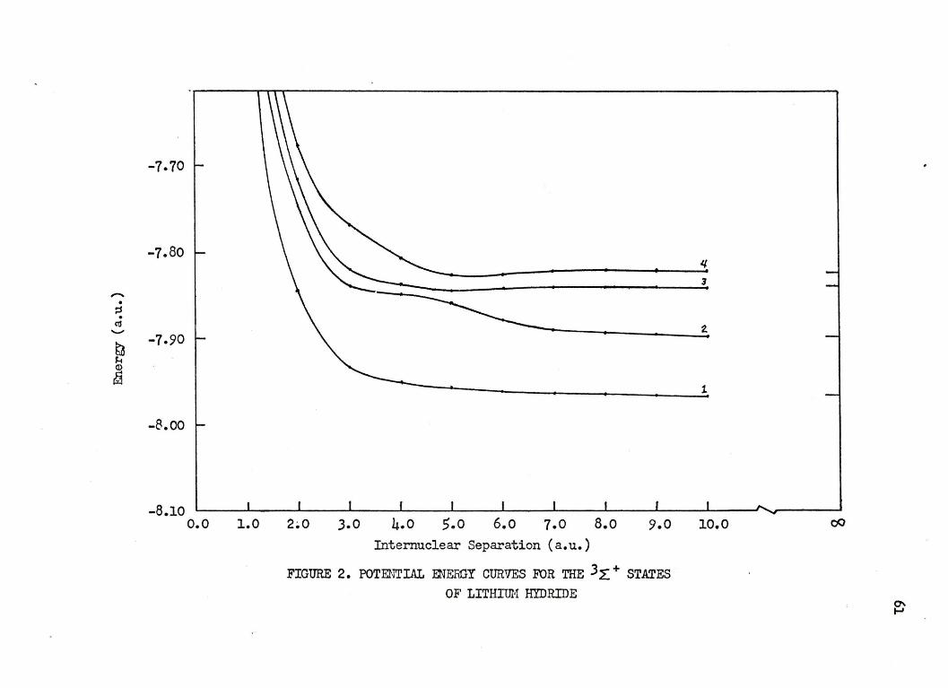
-• ::s •

<IS ........

6'.3 S.. (I)

~

-1.10

-7.80

-1.90

-8.00

-8.10 o.o 1.0 3.0 4.0 5.o 6.o 8.0 9.0

Internuclear Separation (a.u.)

FIGURE 2. POTENTIAL ENEiiGY CURVES FOR THE 3 L + STATES

OF LITHIUM HYDRIDE

" 3

2.

1

10.0

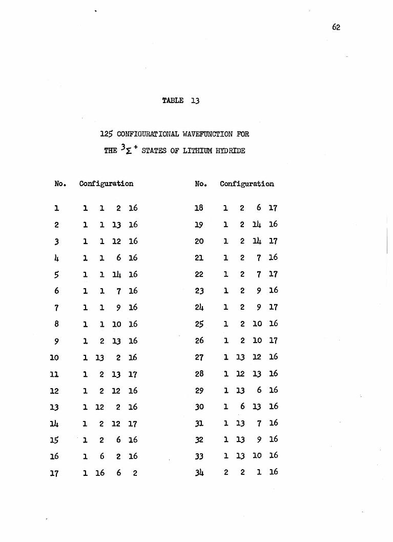
No.

l

2

3

4

5

6

7

8

9

10

11

12

13

14

15

16

17

TABLE 13

125 CONFIGURATIONAL WAVEFUNCTION FOR

THE 3L + STATES OF LITHIUM HYDRIDE

Configuration No. Configuration

l 1 2 16 18 1 2 6 17

l 1 13 16 19 1 2 14 16

l 1 12 16 20 l 2 14 17

1 1 6 16 21 l 2 7 16

1 1 14 16 22 1 2 7 17

1 1 7 16 23 1 2 9 16

l 1 9 16 24 1 2 9 17

1 l 10 16 25 l 2 10 16

l 2 13 16 26 l 2 10 17

1 13 2 16 27 l 13 12 16

1 2 13 17 28 l 12 13 16

1 2 12 16 29 1 1.3 6 16

l 12 2 16 .30 l 6 13 16

l 2 12 17 31 1 13 7 16

· 1 2 6 16 32 1 13 9 16

l 6 2 16 .33 1 13 10 16

l 16 6 2 34 2 2 1 16

62

63

TABLE 13 ContiDUed

No. Contigurat:1.on No. Conf'igu.ration

35 2 2 13 16 58 lJ 13 1 16

36 2 2 13 17 59 13 13 2 16

37 2 2 12 16 60 lJ 13 12 16

38 2 2 12 17 61 13 13 6 16

39 2 2 6 16 62 13 lJ 14 16

40 2 2 6 17 63 13 13 7 16

41 2 2 14 16 64 13 13 9 16

42 2 2 7 16 6.5 13 13 10 16

43 2 2 7 17 66 3 3 13 16

44 2 2 9 16 67 ··3 3 12 16

4.5 2 2 9 17 68 3 3 6 16

46 2 2 10 16 69 3 3 7 16

47 2 2 10 17 70 3 3 9 16

48 2 l.3 12 16 7l 3 3 10 16

49 2 12 13 16 72 4 5 13 16

50 2 13 6 16 73 4 5 12 16

51 2 6 13 16 74 4 5 6 16

.52 2 16 6 13 15 4 5 7 16

53 2 13 6 17 76 4 5 9 16

54 2 13 14 16 77 4 5 10 16

55 2 13 7 16 78 12 12 1 16

56 2 13 9 16 79 12 12 2 16

51 2 13 10 16 80 12 12 13 16

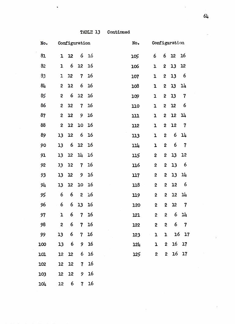
64

TABLE 13 Continued

No. Configuration No. Con!igaration

81 1 12 6 16 105 6 6 12 16

82 1 6 12 16 106 1 2 13 12

83 1 ]2 7 16 107 1 2 13 6

84 2 12 6 16 108 1 2 1.3 14

85 2 6 12 16 l()C) 1 2 13 7

86 2 12 7 16 no 1 2 12 6

87 2 12 9 16 lll 1 2 12 14

88 2 12 10 16 112 1 2 12 7

89 13 12 6 16 ll3 1 2 6 14

90 13 6 12 16 ll4 1 2 6 7

91 13 12 14 16 n, 2 2 1.3 12

92 13 12 7 16 ll6 2 2 13 6

93 13 12 9 16 ll7 2 2 13 14

94 13 12 10 16 ll8 2 2 12 6

95 6 6 2 16 ll9 2 2 12 14

96 6 6 13 16 120 2 2 12 7

97 1 6 7 16 121 2 2 6 14

98 2 6 7 16 122 2 2 6 7

99 13 6 7 16 123 1 l 16 17

100 13 6 9 16 124 l 2 16 17

101 12 12 6 16 125 2 2 16 17

102 12 12 7 16

103 12 12 9 16

104 12 6 7 16

65

synnnetry do oot cross, their wavefunctions may. In the region of

the avoided crossing, the wavefunction of the lower state becomes

that of the upper state and vice versa. For example, some of the

main configurations in the second and third J Z + states are given

in Table 14 along with their coefficients at 4.0, 5.0 am 6.0 a.u.

The switching of magnitude of these coefficients at 4.0 am 5.0 a.u.

indicates an avoided curve crossing. About 102 out of 12.5 ccni'ig­

urations switch the magnitude of their coefficients between the

second and the third 3~+ states from 4.0 to 5.0 a.u. The major­

ity of c<Xl.figurations which do not change involve the lithium

3p0

orbital. One can state,from observing the coeffic:l.ents

of the configurations for the 3~ + state, that the wavefunction

of the secon:l 32, + state at ,5.o a.u. strongly resembles the wave­

fu.L'1.ction or the third 3z. + state at 4.0 a.u. and vice versa. This

would indicate that a curve crossing has taken place.

The fourth root obtained from this calculation rises rapidly

for R less than 5.0 a.u. This disagrees with the results obtained

by Bender and Davidson. (60) Therefore, this calculation was re­

peated with Li 3d0 and Li 4a STO's with orbital exponents of

0.333.3 and 0.2500 respectively added to the basis set. The

energies obtained are given in Table 15. At 5.0 am 6.0 a.u.

the character of the outer lithium orbital of the fourth root

is Jp. At smaller internuclear separations of 3.0 and 4.0 a.u.

the configurations in the fourth root containing the Jp STO

decrease in magnitude while those in the sixth root increase.

At ,3.0 a.u. the fourth 32.+ state contains strong 3d character.

This state has a minimum araind 4.0 a.u. The fifth 3~+ state

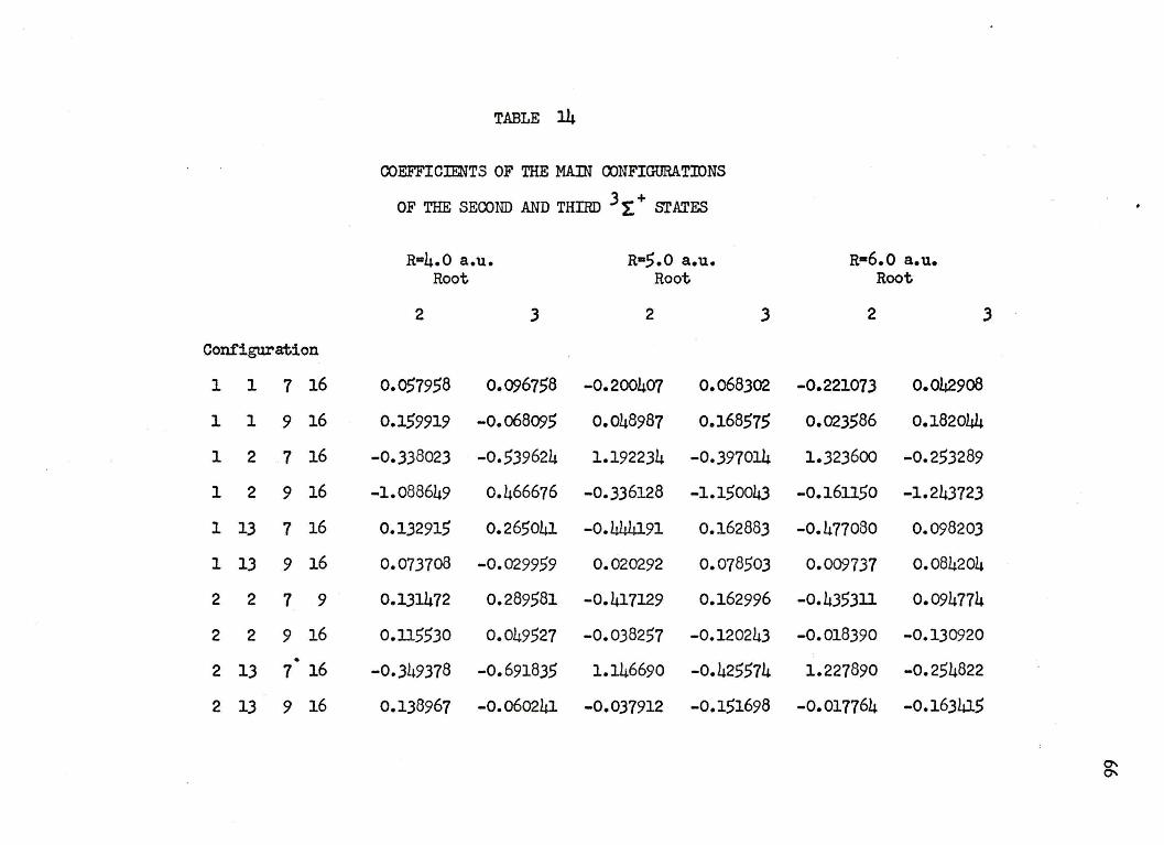
TABLE 14

COEFFICIFNTS OF THE MAIN OONFIGURATIONS

OF THE SEOOND AND THIRD 3 l: + srATES

R•4.0 a.u. R•5.0 a.u. R•6.0 a.u. Root Root Root

2 3 2 3 2 3

Configuration

1 1 7 16 0.057958 0.096758 -0.200407 0.068302 -0.221073 0.0429o8

1 l 9 16 0.159919 -0.068095 0.048987 0.168575 0.023586 0.182044

1 2 7 16 -0.338023 -0.539624 1.192234 -0.397014 1.323600 -0.253289

1 2 9 16 -1.088649 0.466676 -0.336128 -1.150043 -0.161150 -1.243723

l 13 7 16 0.132915 0.265041 -0.444191 0.162883 -0.477080 0.098203

1 13 9 16 0.073708 -0.029959 0.020292 0.078503 0.009737 0.084204

2 2 7 9 0.131472 0.289581 -0.417129 0.162996 -0.435311 0.094774

2 2 9 16 0.115530 0.049527 -0.038257 -0.120243 -0.018390 -0.130920

2 13 7 • 16 -0.3h9378 -0.691835 1.146690 -0.425574 1.227890 -0.254822

2 13 9 16 0.138967 -0.060241 -0.037912 -0.151698 -0.017764 -0.163415

TABLE 15

POTENTIAL ENERGIES FOR THE 3 L+ STATES

OF LITHIUM HYDRIDE USING AN EXTENDED BASIS SEr

Potential Energy ( a. u.) Root

R(a.u.) 1 2 3 4 5 6

3.0 -7.935270 -7.842564 -7.824803 -7.816025 -7.796752 -7.756968

4.0 -7.952681 -7.851989 -7.849158 -7.831905 -7.810431 -7.780805

5.0 -7.959302 -7.869541 -7.848113 -7.83llll -7.813350 -7.801399

6.o -7-963416 -7.883772 -7.845357 -7.829005 -1.813080 -7.804662

10.0 -1.967385 -7.898732 -7.843317 -1.826603 -7.8ll914 -7.808145

00 -7.967494 -1.899678 -7.845003 -1.826688 -7.826518 -1.809339

has a minimum around ,.o a.u. The main configurations for this

state are those containing the Li 4s sro. Those containing the

Li 3<lo increase at large R. At 10.0 a.u. this state lies higher

than its separated atan limit which is the Li 2n(ls23d) state.

Evidently, there are not enough configurations containing the

68

Li 3d0

sro in this wavefunction. The sixth 3 ~ + state is repul­

sive and rises sharply around 5.0 a.u. The wavefunctions for these

3L+ states are complicated; however, from the results obtained

above, there would seem to be curve crossings between the fourth,

fifth and sixth 3 ~+ states.

Considering that the Lili 3 t+ states arising from the

Li2P(ls22p) and Li3P(ls2Jp) states are similar it may be plausible

to generalize such behavior to all 3 L + states arising from sim-

ilar atomic lithium states. These states have an outer orbital

whose value for 1 quantum number is odd. Therefore, the potential

energy curves for the 3 2. + states may be explained using the above

facts. The 3L+ states arising fran lithium atomic states that

have outer orbitals with even 1 tend to be bound and perhaps Ryd­

berg states of LiH+. However, 3 ~ + states arising from lithium

atomic states that have outer orbitals with odd 1 are repulsive

and rise sharply around 6.o a.u. Therefore at small R, i.e.

between 2.0 and 6.0 a.u.,the shape of the various potential energy

curves are determined by interaction between these two types of

states. The shapes would therefore be accounted for by avoided curve

crossings.

Three bound 3 L+ states were observed. These are the third,

fourth and perhaps the fifth state. Their binding energies are

69

estimated to be 0.1131, 0.1420 and O.OJ9loV respectively from

the best results obtained.

5.4. The Lithium Hydride 37i States

The f'irst two lithium hydride 37t states are considered.

These states connect to the Li2P(ls22p) or Li2P(ls23p) plus

H2s(ls) atomic states in the separated atom limit. The inter­

nuclear separations considered and the potential energies ob­

tained are presented in Table 16. The potential energy curves

are given in Figure 3. The configuration list for this calcula­

tion is given in Table 17 and the coefficients for the wavefunc­

tion at 4.0 a.u. are listed in Table 27 of Appendix II.

The most important configurations in the first 3TT state are

the covalent configurations involving the Li 2P+ sro. For the

second 31f state the configurations involving the Li 3P+ and H

ls sro 1s have the largest magnitude although those involving Li 2p+

are also large at all the internuclear separations considered.

The first 37f state is the lowest bound triplet state of

lithium hydride. It has a minimum around 4.0 a.u. with an

estimated binding energy of O.lBOOeV. The second 31T state is bound

at 4.0 a.u. with a calculated binding energy of 0.0792eV. Bender

and Davidson( 60) also observed that these two states were bound, as

well as the third 37T state, with equilibrium internuclear separa­

tions near 4.0 a.u. The fact that the Lili+ 2Z:. + state is

bound at 4.25 a.u. would indicate that the LIB 31f states were

Rydberg states with the dissociation limit Lili+. The binding

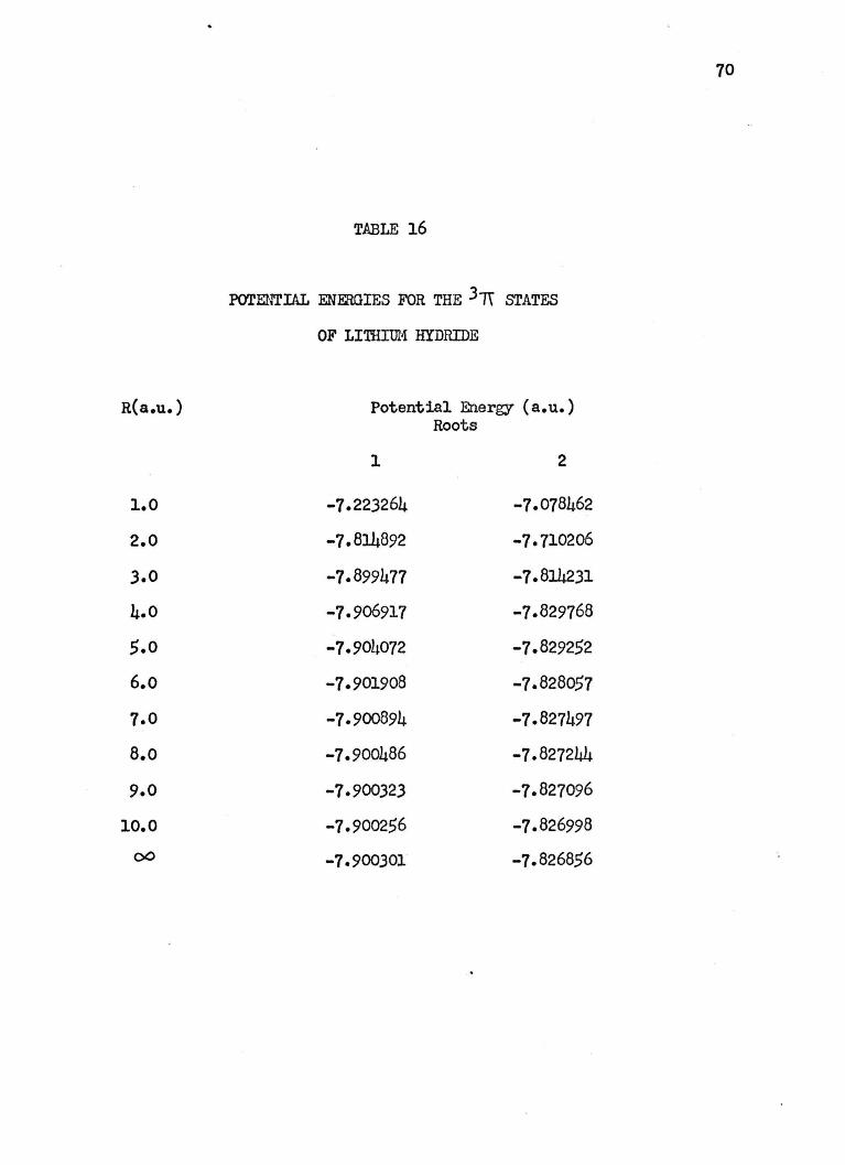
R(a.u.)

1.0

2.0

3.0

4.0

,.o

6.o

7.0

a.o 9.0

10.0

00

TABLE 16

POTENTIAL ENERGIES FOR THE 3n srATES

OF LITHill1 HYDRIDE

Potential Energy (a.u.) Roots

1 2

-7.223264 -7.078462

-7.814892 -1.710206

-7.899477 -7.814231

-7-906917 -7.829768

-7.904072 -7.829252

-1.901908 -7.828057

-7-900894 -7.827497

-7-900486 -7.827244

-7-900323 -1.827096

-7.900256 -1.826998

-7.900301 -7.826856

70

-• :::1 • cu .........

~ f-t Q)

~

-7.60

-1.10

-7.80

-7-90

-8.oo o.o 1.0

z.

1

2.0 3.0 4.0 5.0 6.0 1.0 a.o 9.0 10.0 Internuclear Separation (a.u.)

FIGURE 3. POTENTIAL ENERGY CURVES FUR THE 3,r STATES

OF LITHIUM HYDRIDE

00

No.

l

2

3

4

5

6

7

8

9

10

ll

12

lJ

14

15

16

17

TABLE 17

125 CONFIGURATION.AL WAVEFUNC'l'ION FOR

THE 31T STATES OF LITHIUM HYDRIDE

Configuration No. Configuration

l l 13 18 18 1 15 2 16

l l 12 18 19 l 2 15 17

l 1 - 6 18 20 1 2 7 18

1 l 14 18 21 1 2 8 16

1 1 15 16 22 1 8 2 16

1 l 15 17 23 1 16 8 2

1 l 7 18 24 l 2 8 17

l l 8 16 25 l 2 9 18

1 l 8 17 26 l 2 10 18

l l ll 16 27 l 2 ll 16

1 l ll 17 28 l 2 11 17

1 2 4 16 29 1 13 15 16

l 2 13 18 .30 1 13 8 16

1 2 12 18 31 l 8 ]J 16

1 2 6 18 32 1 ]J 8 17

1 2 14 18 33 1 ]J 11 16

l 2 15 16 34 2 2 l 18

72

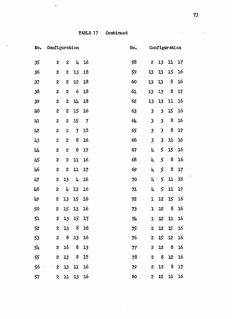
73

TABLE 17 Continued

No. Configuration No. Configar ation

35 2 2 4 16 58 2 13 11 17

36 2 2 13 18 59 13 l3 15 16

37 2 2 12 18 6o l3 l3 8 16

38 2 2 6 18 61 13 13 8 17

39 2 2 14 18 62 13 13 11 16

40 2 2 15 16 63 3 3 15 16

41 2 2 15 7 64 3 3 8 16

42 2 2 7 18 65 3 3 8 17

43 2 2 8 16 66 3 3 11 16

44 2 2 8 17 67 4 5 15 16

45 2 2 11 16 68 4 5 8 16

46 2 2 11 17 69 4 5 8 17

47 2 13 4 16 70 4 5 ll 16

48 2 4 13 16 71 4 5 11 17

49 2 13 15 16 72 1 12 15 16

50 2 15 13 16 73 1 12 8 16

51 2 13 15 17 74 1 l2 11 16

52 2 13 8 16 15 2 12 l5 16

53 2 8 13 16 76 2 15 12 16

54 2 16 8 13 77 2 12 8 16

55 2 JJ 8 17 78 2 8 12 16

56 2 13 11 16 79 2 12 8 17

51 2 ll 13 16 80 2 12 ll 16

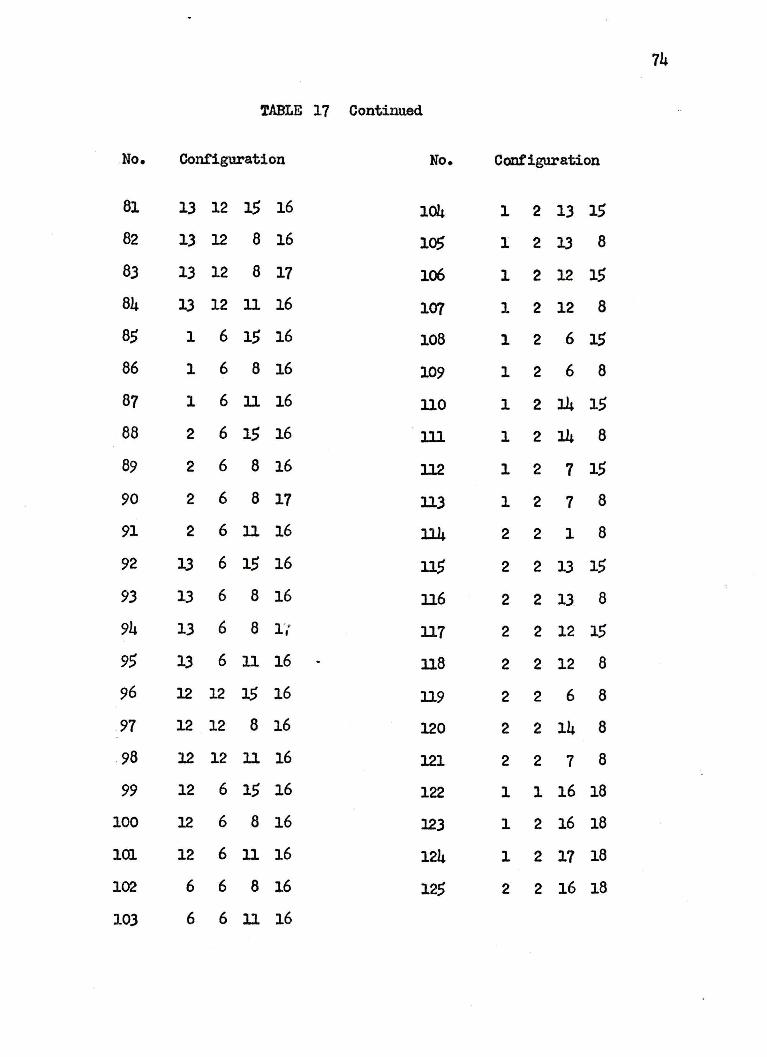
74

TABLE 17 Continued

No. Configuration No. Configuration

81 13 12 15 16 104 1 2 13 15

82 13 12 8 16 105 1 2 13 8

83 13 12 8 17 106 1 2 12 15

84 13 12 11 16 107 1 2 12 8

85 1 6 15 16 108 1 2 6 15

86 1 6 8 16 109 1 2 6 8

87 1 6 11 16 no 1 2 14 15

88 2 6 15 16 lll 1 2 14 8

89 2 6 8 16 112 1 2 7 15

90 2 6 8 17 113 1 2 7 8

91 2 6 11 16 114 2 2 1 8

92 13 6 15 16 115 2 2 13 15

93 13 6 8 16 116 2 2 13 8

94 13 6 8 l'j 117 2 2 12 15

95 13 6 11 16 - ll8 2 2 12 8

96 12 12 15 16 119 2 2 6 8

91 12 12 8 16 120 2 2 14 8

98 12 12 11 16 121 2 2 1 8

99 12 6 15 16 122 1 1 16 18

100 12 6 8 16 123 1 2 16 18

101 12 6 11 16 124 1 2 17 18

102 6 6 8 16 125 2 2 16 18

103 6 6 11 16

energies of these states ~re less than 0.2sV and the potential

curves are very similar in appearance to that of Ll.Ir".

5.5. The Lithium Hydride l7r states

Calculations were performed on the first two LiH 1 TT

states. These states connect to the separated atom limits of

Li2P(ls22p) plus u2s(ls) and Li2P(ls23p) plus H2s(la) respec­

tively. The internuclear separations considered and the pot­

ential energies obtained are listed in Table 18. The potential

curves are presented in Figure 4. The configurations used for

these wavefunctions are listed in Table 19. Their coefficients

are given in Table 28 of Appendix II.

The most important configurations in the first 1TI state

are those involving the Li 2p+ and H ls ST0 1s. For the second

1 7r the configurations with the largest magnitude are the covalent

configurations containing the Li 3P+ STO. Those involving the

Li 2p+ orbital are also large for this state.

The calculated potential curve for the first 17f state

is repulsive in energy but extremely flat. Experimentally, this

state has been studied by VelascoC7) who found it to be bound with

a binding energy of O.OJ5eV and an equilibrium internuclear separ­

ation of 4.49 a.u. Bender and Davidson1s(60) calculation which

included a Li 3d STO, also predicted this state to be repulsive.

Therefore, probably more inner core correlation is needed in order

to obtain a brund state. The second 1 lT state is found to be bound

with a minimum between 4.0 and ,.o a.u. and an approximate binding

15

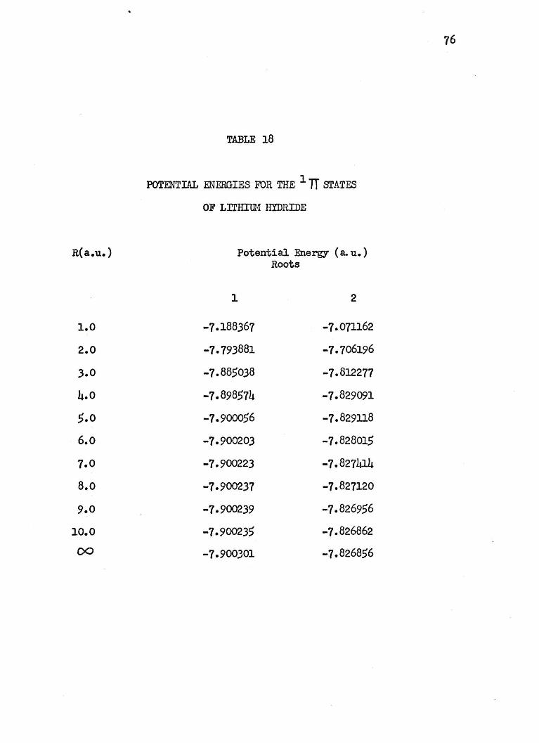
R(a.u.)

1.0

2.0

3.0

4.0

5.0

6.o

1.0

8.o

9.0

10.0

00

TABLE 18

POTENTIAL ENERGIES FOR THE l 1T STATE:S

OF LTIHit11 HYDRIDE

Potential Energy ( a. u. ) Roots

l 2

-1.188367 -7.07ll62

-1.793881 -1.106196

-7.885038 -7.812277

-7.898574 -7.829091

-1-900056 -7.829ll8

-1.900203 -1.828015

-7.900223 -7.827414

-7-900237 -7.827120

-1.900239 -7.826956

-7-900235 -1.826862

-7-900301 -7.826856

76

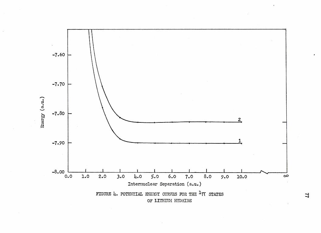
-• ::s . <ii -k3 H 0)

~

-7.60

-1.10

-7.80

-7.90

-8.oo o.o 1.0 2.0 3.0 4.0 5.o 6.o 7.0 8.0

Internuclear Separation (a.u.)

FIGURE 4. POTENTIAL ENERGY CURVES FOR THE 1TT STATES

OF LITHIUM HYDIUDE

2

1

c,O

No.

1

2

3

4

5

6

7

8

9

10

11

12

13

14

15

16

17

TABLE 19

125 CONFIGURATIONAL WAVEFUNCTION FOR

THE 1 Ti STATES OF LITHIUM HYDRIDE

Configuration No. con:tigurat.ion

1 1 13 18 18 l 2 15 16

1 1 12 18 19 1 15 2 16

1 1 6 18 20 1 2 1.5 17

1 1 14 18 21 1 2 7 18

1 1 15 16 22 1 2 8 16

1 1 1.5 17 23 1 8 2 16

l 1 7 18 24 1 2 8 17

1 1 8 16 25 1 2 9 18

1 l 8 17 26 l 2 10 18

1 l 11 16 27 1 2 11 16

1 l 11 17 28 l 2 11 17

l 2 4 16 29 l 13 15 16

1 4 2 16 30 1 13 8 16

1 2 13 18 31 1 8 13 16

1 2 12 18 32 1 13 8 17

1 2 6 18 33 1 13 11 16

1 2 14 18 34 2 2 1 18

78

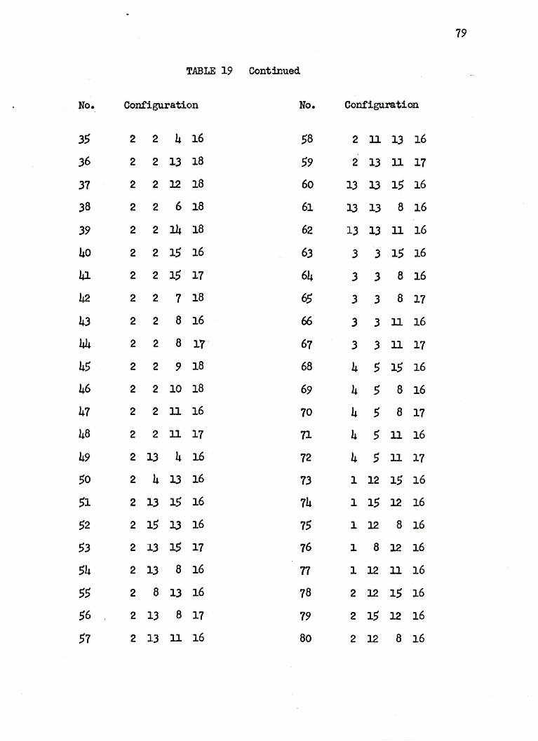
19

TABLE 19 Continued

No. Configuration No. Configuration

35 2 2 4 16 58 2 11 13 16

36 2 2 13 18 59 2 13 11 17

37 2 2 12 18 60 13 l3 15 16

38 2 2 6 18 61 l3 13 8 16

39 2 2 14 18 62 13 13 11 16

40 2 2 15 16 63 3 3 15 16

41 2 2 15 17 64 3 3 8 16

42 2 2 7 18 65 3 3 8 17

43 2 2 8 16 66 3 3 11 16

44 2 2 8 l,f' 67 3 3 11 17

45 2 2 9 18 68 4 5 15 16

46 2 2 10 18 69 4 5 8 16

47 2 2 11 16 70 4 5 8 17

48 2 2 11 17 71 4 5 11 16

49 2 13 4 16 72 4 5 11 17 50 2 4 l3 16 73 1 12 15 16

51 2 13 15 16 74 l 15 12 16

52 2 15 l.3 16 15 1 12 8 16

53 2 l.3 15 17 76 l 8 12 16

54 2 13 8 16 77 l 12 11 16

55 2 8 13 16 78 2 12 15 16

56 2 13 8 17 79 2 15 12 16

57 2 13 ll 16 80 2 J2 8 16

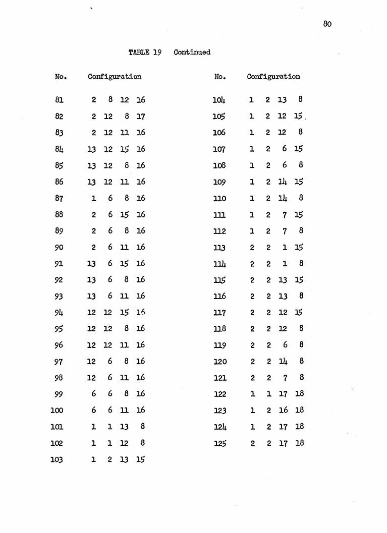
80

TABLE 19 Continued

No. Configuration No. Configuration

81 2 8 12 16 104 1 2 13 8

82 2 12 8 17 105 l 2 12 15 .

83 2 12 11 16 lo6 1 2 12 8

84 13 12 15 16 107 1 2 6 15

85 13 12 8 16 lo8 1 2 6 8

86 13 12 11 16 109 1 2 14 15

87 1 6 8 16 no l 2 14 8

88 2 6 15 16 lll 1 2 7 15

89 2 6 8 16 112 1 2 7 8

90 2 6 ll 16 113 2 2 1 15

91 13 6 15 16 114 2 2 1 8

92 13 6 8 16 J.J5 2 2 13 15

93 13 6 11 16 ll6 2 2 13 8

94 12 12 15 16 ll7 2 2 12 l5

95 12 12 8 16 118 2 2 12 8

96 12 12 11 16 ll9 2 2 6 8

91 12 6 8 16 120 2 2 14 8

98 12 6 11 16 121 2 2 1 8

99 6 6 8 16 122 1 1 17 18

100 6 6 ll 16 123 1 2 16 18

101 l l 13 8 124 1 2 17 18

102 1 1 12 8 125 2 2 17 18

103 l 2 13 15

energy of O. 0615eV. Bender and Davidson also fotmd the third

17T state to be bound at 4.0 a.u. The equilibrium interm.iclear

separations of these states are aromid 4.0 a..u. and the potential

energy curves are all shallow. This wouJ.d indicate that the

LiH 1 TI states are also Rydberg states with the Lili+ x2~ + state

as the limit.

5.6. The Lithium Hydride Plus x2L+ State

The lowest lithium hydride plus ground 2 r + state was

considered in this calculation. The potential energies calcu­

lated are presented in Table 20 and the potential curve is

given in Figure 5. The configuration list used is given in Table

21 and their coefficients are listed in Table 29 of Appendix II.

This state connects to the Li+ 1s(ls2) plus II2s(ls) sep­

arated atom states. The energy of the Li+ 1s(ls2) atomic state

is calculated using the basis in Table 8. and 32 configurations.

An energy of -7.27133 a.u. as compared to an experimental value

of -7 .28049 a.u. is obtained. The Lili+ x2 z:_+ state is calcula­

ted to have an estimated binding energy of 0.1098eV and an

equilibrium internuclear separation aromid 4.0 a.u. This result

agrees with the values obtained by Browne( 6l) who calculated

dissociation energies of o.104!0.016eV and an equilibrium inter­

m.iclear separation of 4.25 a.u. BrO'Wlle 1s energy, -7.780848 a.u.

at Re,is better than the result obtained here. However, the

energies of the potential curve are more accurate in this calcula­

tion.

81

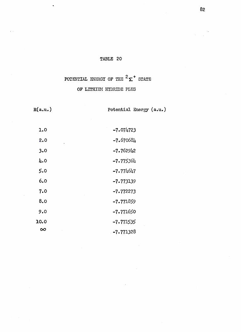
R(a.u.)

1.0

2.0

3.0

4.0

,.o

6.o

1.0

B.o

9.0

10.0

00

TABLE 20

POTENTIAL ENERGY OF THE 2 I:+ STATE

OF LITHIUM HYDRIDE PLUS

Potential Energy (a.u.)

-7.074723

-7.670684

-7-762942

-7-775364

-7. 774647

-7-773139

-7-772273

-7.771859

-7.771650

-7-771535

. -7. 771328

82

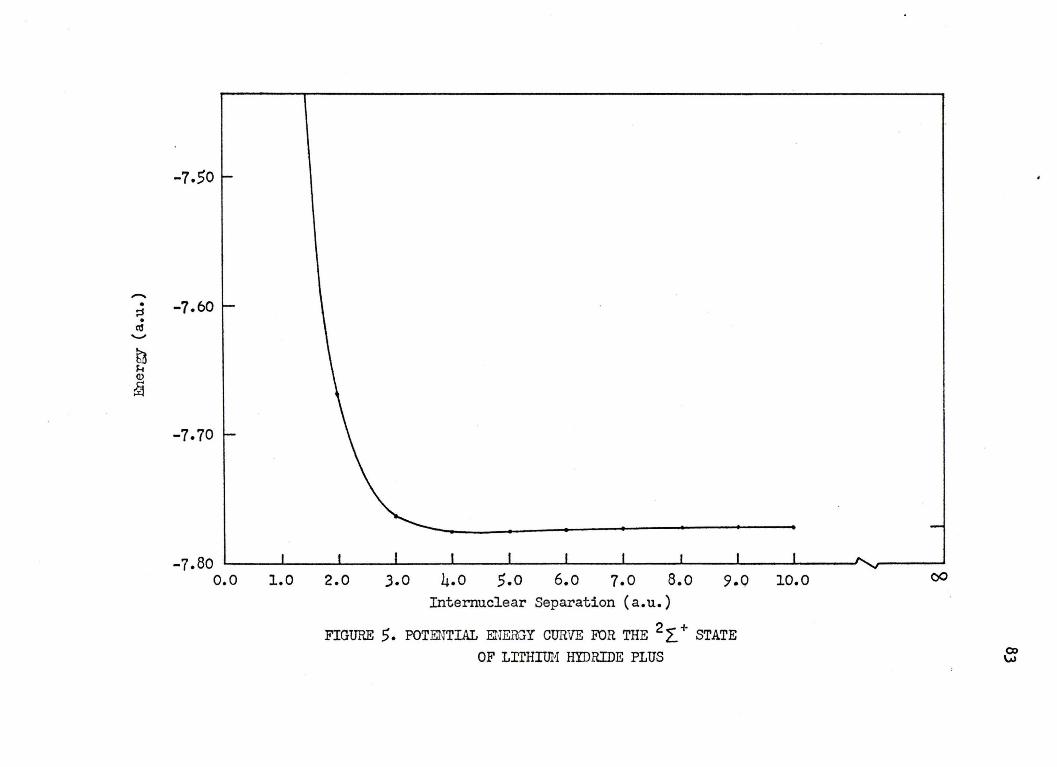
-• ~ • (1S

'-"

k3 r-. Q)

~

-7.50

-7.60

-1.10

-7.80 o.o 1.0 2.0 .3.0 4.0 5.0 6.o 8.0 9.0 10.0

Internuclear Separation (a.u.)

FIGURE 5. POTENTIAL EHEffiY CURVE FOR THE 2 L + STATE

OF 1rrHnn1 HYDRIDE PLUS

No.

1

2

3

4

5

6

7

8

9

10

11

12

lJ

14

15

16

17

TABLE 21

125 CONFIGURATIONAL WAVEFUNCTION FOR

THE 2t.+ STATE OF LITHIUM HYDRIDE PLUS

Configuration No. Configuration

1 1 16 18 3 3 17

1 1 17 19 4 , 16

1 2 16 20 4 , 17

l 2 17 21 l 12 16

1 13 16 22 1 16 12

l 16 13 23 l 12 17

l 13 17 24 l 6 16

2 2 16 25 1 16 6

2 2 17 26 l 6 17

2 4 19 27 l 14 16

2 5 18 28 l 16 14

2 13 16 29 l 14 17

2 16 13 30 l 7 16

2 13 17 31 1 16 7

13 13 16 32 l 7 17

13 13 17 33 1 9 16

3 3 16 34 2 12 16

84

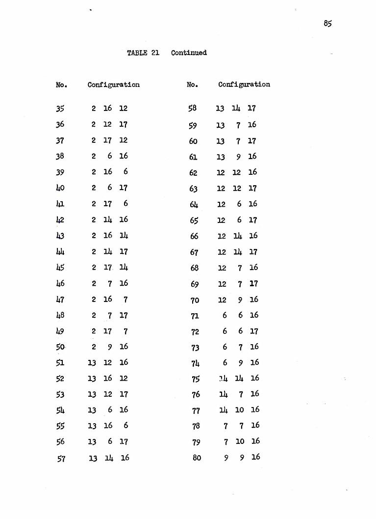
85

TABLE 21 Continued

No. Configuration No. Configuration

35 2 16 12 58 13 14 17

36 2 12 17 59 13 7 16

31 2 17 12 60 l3 7 17

38 2 6 16 61 13 9 16

39 2 16 6 62 12 12 16

40 2 6 17 63 12 12 17

la. 2 17 6 64 12 6 16

42 2 14 16 65 12 6 17

43 2 16 14 66 12 14 16

44 2 14 17 67 12 14 17

45 2 17. 14 68 12 7 - , J.O

46 2 7 16 69 12 7 17

47 2 16 7 70 12 9 16

48 2 7 17 71 6 6 16

49 2 17 7 72 6 6 17

50- 2 9 16 73 6 7 16

51 13 12 16 74 6 9 16

52 13 16 12 75 14 14 16

53 13 12 17 76 14 7 16

54 13 6 16 77 l4 10 16

55 13 16 6 78 7 7 16

56 13 6 17 79 7 10 16

57 13 14 16 80 9 9 16

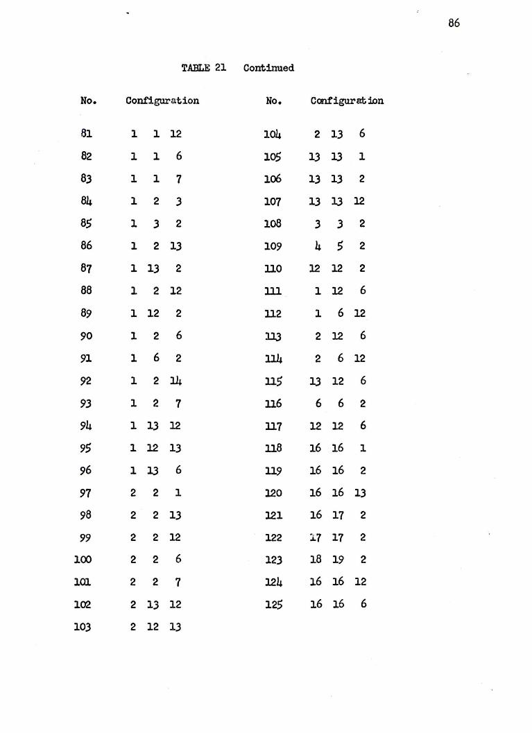
86

TABLE 21 Continued

No. Configuration No. Ccnf'igurat ion

81 1 1 12 104 2 13 6

82 l l 6 105 13 13 l

83 1 1 7 lo6 13 13 2

84 1 2 3 107 13 13 l2

85 1 3 2 108 3 3 2

86 l 2 13 109 4 5 2

87 l 13 2 ll0 12 12 2

88 l 2 12 lll 1 12 6

89 l 12 2 ll2 l 6 12

90 l 2 6 lJJ 2 12 6

91 1 6 2 ll4 2 6 12

92 l 2 14 n, 13 12 6

93 1 2 7 ll6 6 6 2

94 1 13 12 ll7 12 12 6

95 l 12 13 ll8 16 16 1

96 l 13 6 ll9 16 16 2

91 2 2 1 120 16 16 13

98 2 2 13 121 16 17 2

99 2 2 12 122 17 17 2

100 2 2 6 123 18 19 2

101 2 2 7 124 16 16 12

lO'l 2 13 12 125 16 16 6

103 2 12 13

. This state has not been observed experimentally. The lithium

hydride ground state would ionize to give this molecular ion state.

From the results obtained the ionization potential would be approx­

imately 7.45l8eV. This state 'WOuld be the ionization limit of

the Icy-dberg states. The equilibrium internuclear separations of

these LiH Rydberg states would lie around 4.0 a.u. and their

potential energy curves would be similar to that of LiH+.

87

CHAPTER VI

DISCUSSION AND SUMMA.RY

Potential energy curves have been obtained for low

lying states of diatomic lithium hydride and the ground

x2 ~ + state of LiH+. Large STO bases and 125 configurational

interaction wavefunctions were used in this study. The sro

bases were obtained from optimized basis sets for the appro­

priate united and separated atom states. Except for the LiH

ground x1~ + state and the first excited Alf+ state this

investigation is the most accurate study of the potential

energy curves of the low lying lithium hydride states con­

aio.ered. Only three LiH states, i.e. the x1 L +, A1 2+, and

131-TI, have been observed experimentally.

All of the 1 ~ + states studied are bound. The bin.ding

energies of the calculated x1z:_ +, A1 Z:., + states are 89 and 88%

of the experimental values respectively. The next two 11 +

states are bound at large internuclear separations around

1O.O and 8.o a.u. respectively, due perhaps to their Li+H­

character at large R. The fifth and sh-th 1 ~ + states are

bound between 4.0 and 5.0 a.u. These and higher l~+ states

are probably Rydberg states with an equilibrium internuclear

separation, Req, around 4.0 a.u.

88

69

Brown and Shull(57) have obtained more extensive curves

for the x1 ~+ and A1 ~+ states. Also, their results for the

x1 L. + state were better around the equilibrium internuclear

separation. The best energy obtained by the author was -8.054571

a.u. at 3.0 a.u. using 132 configurations and a 20 sro basis as

compared to -8.05549 a.u. by Brown and Shull. The sro basis

was similar to that of Table 8 except that the outer Li 3s, Jp,

etc. sro•s wero not present. Also, inner core Li Jp sro 1s with

the same orbital exponents as the Li 2p STO I s and a H ls I and

2p' sro with orbital exponents of o.6000 were added to the

basis.

An estimate of the accuracy of 1 2. + curves can be made

by comparing the energies of Table 9 with the experimental

results at Req and R= oo. At R= 00 the x1 L+ and A1L+ states

are approximately 0.J0eV higher than the experimental vaJ.ues.

At their Req values, the x1 L.. + and A 1 ~+ states lie 0. 58 am

0.40eV, respective~r, above the experimental energies. Since

these states have different character at different internuclear

separations their spectroscopic constants are needed for a

more accurate analysis. A comparison with the experimental

energies also shows that the higher 1 Z: + states are also in error

by 0.JOeV at R .. co. However, due to the fact that the basis

does not take into acccunt correlation in their outer shells

these higher 1 z.+ states are probably less accurate at smaller

R than the xl~+ and A1 ~+ states. It can al.so be stated with

certainty that the third and fourth 1 L + states are bound around

8.0 to 10.0 a.u. since the lowest energies of these states

both lie below the experimental energies of their respective

separated atom limits and the energies obtained nru.st be upper

bound to the true values. Also, the integrals calculated

are accurate at the large R considered and other LiH states

go correctly to their separated atom limits.

The lowest Jr+ state is repulsive in energy. The second

J L+ state is also repulsive but shows a sharp rise in energy

between 4.0 and 6.0 a.u. The third, fourth and fifth JL.+

states are bound between 4.0 and 5.0 a.u. The sixth JL+

state also rises sharply between 4.0 and 6.0 a.u. Evidence of

an avoided curve crossing is found between the second and third

3L+ states around 4.0 a.u. and perhaps between the fourth,

fifth and sixth 3~+ states at larger R. Therefore, the pot­

ential energy curves for the 3 L + states are complicated by

interactions between them at R 6.0 a.u. In cases where there

is strong interacti~n between states of the same symmetry, the

Born-Oppenheimer approximation and the concept of a potential

energy curve is no longer accurate.< 2)

The lowest bound triplet state is the lowest 37t state

which is bound at 4.0 a.u. The second 31f state is also

observed to be bcund at 4.0 a.u. This agrees with the results

of Bender and Davidson< 60) who also found that the third JTT

state has a minimum around 4.0 a.u.

The B1 1T state is found to be extremely flat but repul­

sive. This state is found experimentally( 7) to have binding

90

energy of 0.0J5eV. Evidently, more correlation is needed in

the wavefunction. The nex:t 1 11 state is bound between 4.0

am. 5.0 a.u. Bender and Davidson found the third 1 Tf state

to be bound around 4.5 a.u. and also strong evidence of :inter­

action between the second and third 1 TT states.

A comparison or the energy of the B1 7T state with the

experimental value at Req and Ra 00 shows that they differ

by 0.JOeV This value can be taken as a rough estimate of the

error in the other Rydberg states and the repulsive curves.

It must be remembered, however, with the bases used, the results

are less accurate at small internuclear separations. Also,

1£ the wavefunction for a particular state does not have the

correct character in a certain region of internuclear separ­

ations, such as the Li+iI- character needed for the first four

lL.+ states, the results will be less accurate in this region.

The x2 ~ + state of LiH+ is calculated to have a binding

energy of 0.llOeV with a minimum near 4.0 a.u. The ionization

potential of LiH is estimated to be 7.45eV fran the difference

in energy between the Lili x1 2._ + state and the Lili+ x2 2_ + state.

Bender and Davidson have found that the lowest 1 [),, and 3 b..

states are botmd with minimums between 4.0 and 4.5 a.u. The

shapes and minimums of the potential cuwes of the 1 TT , 1 b. ,

3 7f and 3 ~ states and the higher 1 ~ + states are very sim-

Uar to that of the LiH+ x2 ~ + state. This indicates that

these states are .lcy'dberg states of lithiwn hydride.

Not many transitions are likely to be observed in the

diatontf..c Lili system. Transitions between the ground x1 2+

91

92

state and third or fourth 12+ state are not very probable

since their equilibrium internuclear separations differ greatly

from that of the ground state. Transitions to higher lz+

states are possible if these states are bound between 4.0 and

5.0 a.u. Transitions between the ground state and the l TT

states are also likely to occur. Icy-dberg series of transitions

occur between the ground state and 11 + or 1 TT states which

arise from Li2P(ls2np) atomic states. other Rydberg series

occur from the Al~+ or E1TI states. Since singlet-triplet

transitions are forbidden and the lowest triplet state is re­

pulsive, not many transitions are likely to be observed between

triplet states. Bands involving triplet states are most likely

to originate from the lowest 37T state.

APPENDIX I

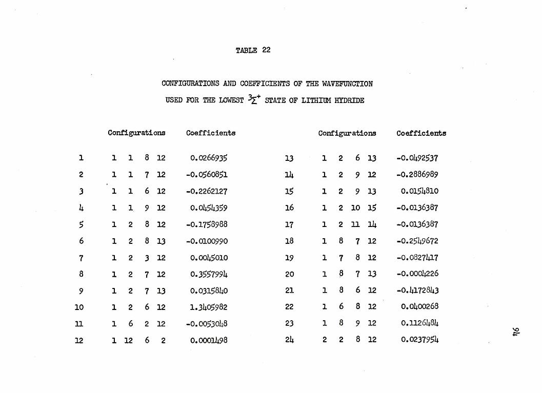
1

2

3

4

5

6

7

8

9

10

11

12

TABLE 22

CONFIGURATIONS AND COEFFICIENTS OF THE WAVEFUNCTION

USED FOR THE LOWEST Jr+ STATE OF LITHitM HYDRIDE

Con:f'igurati ons Coefficients Configurations

1 1 8 12 0.0266935 13 1 2 6 13

1 1 1 12 -0.0560851 14 1 2 9 12

1 1 6 12 -0.2262127 15 1 2 9 13

1 1 9 12 0.0454359 16 1 2 10 15

1 2 8 12 -0.1758988 17 1 2 11 14

1 2 8 13 -0.0100990 18 1 8 1 12

1 2 3 12 0.0045010 19 1 1 8 12

1 2 7 12 0.3557994 20 1 ~ 7 13

1 2 1 13 0.0315840 21 1 8 6 12

1 2 6 12 1.3405982 22 1 6 8 12

1 6 2 12 -0.0053048 23 1 8 9 12

1 12 6 2 0.0001498 24 2 2 8 12

Coefficients

-0.0492537

-0.2886989

0.0154810

-0.0136387

-0.0136387

-0.2549672

-0.0827417

-0.0004226

-0.4172843

0.0400268

0.1126484 'O

0.0237954 .i:-

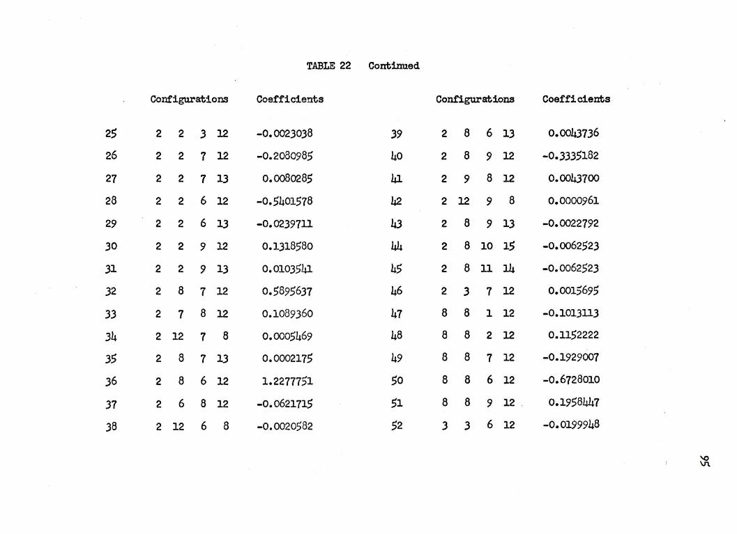
TABLE 22 Continued

Configurations Coefficients Configurations Coeffi cient;s

25 2 2 3 12 -0.0023038 39 2 8 6 13 0.0043736

26 2 2 7 12 -0.2080985 40 2 8 9 12 -0.3335182

27 2 2 7 13 0.0080285 41 2 9 8 12 0.0043700

28 2 2 6 12 -0.5401578 42 2 12 9 8 0.0000961

29 2 2 6 13 -0.0239711 43 2 8 9 13 -0.0022792

30 2 2 9 12 0.1318580 44 2 8 10 15 -0.0062523

31 2 2 9 13 0.0103541 45 2 8 11 14 -0.0062523

32 2 8 7 12 o.5895637 46 2 3 7 12 0.0015695

33 2 7 8 12 0.1089360 47 8 8 1 12 -0.1013113

34 2 12 7 8 0.0005469 48 8 8 2 12 0.1152222

35 2 8 7 13 0.0002175 49 8 8 7 12 -0.1929007

36 2 8 6 12 1.2277751 50 8 8 6 12 -0.6728010

31 2 6 8 12 -0.0621715 51 8 8 9 12 . 0.1958447

38 2 12 6 8 -0.0020582 52 3 3 6 12 -0.0199948

'O V\

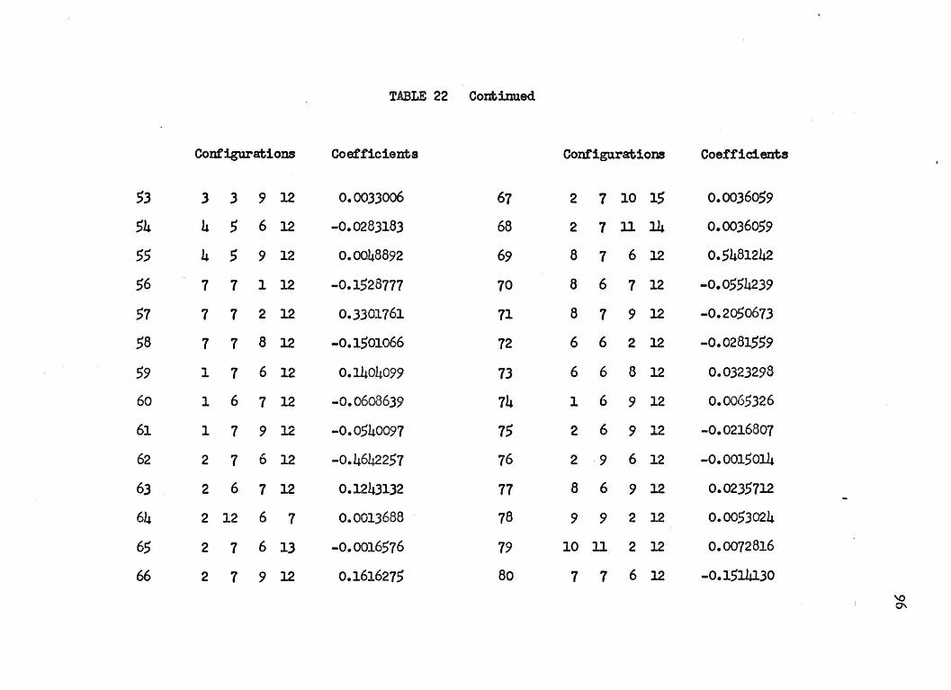
TABLE 22 Continued

Configurations Coefficients Configurations Coefficients

53 3 3 9 12 0.0033006 67 2 7 10 1.$ 0.00360,$9

.54 4 .5 6 12 -0.0283183 68 2 7 11 14 0.0036059

55 4 .5 9 12 0.0048892 69 8 7 6 12 o.5481242

56 7 7 1 12 -0.1528777 10 8 6 1 12 -0.0554239

51 1 7 2 12 0.3301761 71 8 7 9 12 -0.2050673

58 7 7 8 12 -0.1501066 72 6 6 2 12 -0.0281559

59 l 7 6 12 0.1404099 73 6 6 8 12 0.0323298

60 1 6 1 12 -0.0608639 74 1 6 9 12 o.0065326

61 l 1 9 12 -0.0540097 75 2 6 9 12 -0.0216807

62 2 7 6 12 -0.4642257 76 2 9 6 12 -0.0015014

63 2 6 7 12 0.1243132 11 8 6 9 12 0.0235712

64 2 12 6 1 0.0013688 78 9 9 2 12 0.0053024

65 2 7 6 13 -0.0016576 19 10 11 2 12 0.0072816

66 2 7 9 12 0.1616275 80 7 1 6 12 -0.1514130 '-0

°'

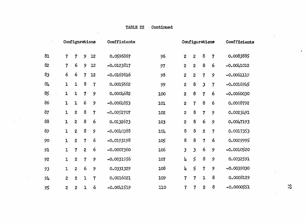
TABLE 22 · Continued

Configurations CoefficiEnts Configurations Coefficients

81 7 7 9 12 0.0596867 96 2 2 8 7 o.oo83885

82 7 6 9 12 -0.0123817 97 2 2 8 6 -0.0041012

83 6 6 7 12 -0.0167616 98 2 2 7 9 -0.006lll9

84 1 1 8 1 0.0015662 99 2 8 3 1 -0.0016945

85 1 1 7 9 0.0004682 100 2 8 1 6 -0.0060030

86 1 1 6 9 -0.0064853 101 2 1 8 6 0.0008792

87 1 2 8 7 -0.0052707 102 2 8 7 9 0.0023491

88 1 2 8 6 0.0132673 103 2 8 6 9 0.0047193

89 1 2 8 9 -0.0040388 104 8 8 2 1 0.0017353

90 1 2 1 6 -0.0193198 105 8 8 1 6 0.0029995

91 1 1 2 6 -0.0007360 106 3 3 6 9 -0.0010520

92 1 2 1 9 -0.0031956 107 4 5 8 9 0.0032591

93 1 2 6 9 0.0331329 108 4 5 1 9 -0.0039030

94 2 2 1 7 0.0016021 109 1 1 1 8 0.0008129

95 2 2 1 6 -0.0041519 llO 1 7 2 8 -0.0000551 \0 ~

TABLE 22 Continued

Configurations Coefficients

-lll 10 11 2 8 -0.0006460

112 7 7 2 9 0.0011563

113 2 7 6 9 -0.0006758

114 8 7 6 9 -0.0003369

115 12 12 2 8 -0.0012231

116 1 2 12 13 0.0282231

117 2 2 12 13 0.0103671

118 2 8 12 13 0.00lll39

119 14 15 2 8 -0.0002199

120 12 12 1 9 0.0010385

121 12 12 2 7 0.0010888

122 12 13 2 7 0.0002033

123 12 2 13 7 0.0004135

124 12 13 2 6 -0.0009174

12.5 12 2 13 6 -0.0016738 "° 0)

Configurations

1 l l 10 16

2 l l 9 16

3 l 1 ll 16

4 1 l 12 14

5 1 l 7 14

6 1 l 7 15

7 1 2 10 16

8 1 2 9 16

9 1 2 ll 16

10 1 2 12 14

ll 1 12 2 14

12 1 2 12 15

TABLE 23

CONFIGURATIONS AND COEFFICIENTS OF THE WAVEFUNCTION

USED FOR THE LOWEST JTT STATE OF LITHIUM HYDRIDE

Coefficients Configurations

0.0061788 13 l 2 6 16

-O.Oll8624 14 1 2 7 14

-0.0054767 15 1 2 7 15

0.0059459 16 1 10 12 14

0.1595967 17 l 10 7 14

-0.0065657 18 1 7 10 14

-0.0369713 19 2 2 1 16

o.o605217 20 2 2 10 16

0.0142526 21 2 2 9 16

-0.0346271 22 2 2 4 14

-0.0008593 23 2 2 11 16

-0.0155563 24 2 2 12 14

Coefficients

0.0063277

-0.8323309

0.0481456

0.0029845

0.1895050

0.0019983

-0.0089587

-0.0439125

0.0613864

0.0009688

0.0027119

0.0103988

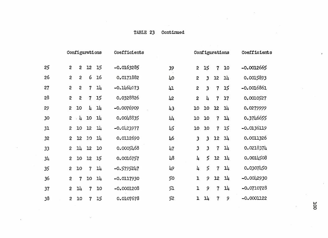
TABLE 23 Continued

Configurations Coefficients Configurations Coefficients

25 2 2 12 15 -0.0163285 39 2 15 7 10 -0.0012665

26 2 2 6 16 0.0171882 40 2 3 12 14 0.0015893

27 2 2 7 14 -0.1464073 41 2 3 7 15 -0.0016861

28 2 2 7 15 0.0328826 42 2 4 7 17 0.0010527

29 2 10 4 14 -0.0076909 43 10 10 12 14 0.0279999

30 2 . 4 10 14 0.0048835 44 10 10 7 14 0.3746655

31 2 10 12 14 -0.0423977 45 10 10 7 15 -0.01J6ll9

32 2 12 10 14 0.0112690 46 3 3 12 14 0.0011326

33 2 14 12 10 0.000.5468 47 3 3 7 14 0.0218374

34 2 10 12 15 0.0016757 48 4 5 12 14 0.0014508

35 2 10 7 14 -0.5795247 49 4 5 7 14 0.0307450

36 2 7 10 14 -0.0117930 50 1 9 12 14 -0.0042930

37 2 14 7 10 -0.0001208 51 1 9 7 14 -0.0710728

38 2 10 7 15 0.0107678 52 1 14 7 9 -0.0001122 I-'

8

TABLE 23 Contirmed

Configurations Coefficients Configurations Coefficients

53 2 9 4 14 0.0025038 67 2 15 7 ll 0.0003880

54 2 9 12 14 0.0146437 68 2 6 7 14 0.0000763

55 2 12 9 14 o.oo458h3 69 9 9 12 14 0.0046537

56 2 14 12 9 -0.0003719 70 9 9 7 14 0.0851890

51 2 9 7 14 0.2340378 71 9 9 7 15 -0.0048898

58 2 9 7 15 -0.0064742 72 1 1 10 7 -0.0026846

59 2 15 7 9 0.0010986 73 1 1 10 12 0.0028626

60 10 9 12 14 -0.0213323 74 1 1 9 7 -0.0010018

61 10 9 7 14 -0.3333986 15 1 1 j 7 -0.0013238

62 10 9 7 15 0.0149061 76 l 1 6 7 0.0006009

63 1 11 7 15 -0.0020402 77 1 2 10 7 0.0242567

64 2 ll 12 14 -0.0004055 78 1 10 2 7 0.0014727

65 2 ll 7 14 O.Ooo6153 79 1 2 10 12 -0.0241227

66 2 14 7 ll -0.0000393 80 1 2 9 7 -0.0080595 b .....

TABLE 23 Continued

Configuration Coefficients Configurations Coefficients

81 1 9 2 7 -0.0012002 96 2 2 ll 12 -0.0072878

82 1 2 9 12 0.0195243 97 2 2 6 7 -0.0232298

83 1 2 3 7 0.0009144 98 2 10 9 7 0.003JJ.hO

84 1 2 11 7 0.0286169 99 2 9 10 7 -0.0001625

85 1 2 12 6 -0.0047011 100 2 10 9 12 -0.0015013

86 1 2 6 7 -0.0212063 101 2 9 10 12 -0.0002022

87 1 10 9 7 -0.0022711 102 2 10 11 7 0.0165882

88 2 2 1 7 0.0126810 103 10 10 1 7 -0.0006116

89 2 2 1 12 -0.0062956 104 10 10 2 7 -0 .. 0022434

90 2 2 10 7 O.Ol.49644 105 10 10 ll 7 -0.0073127

91 2 2 10 12 -0.0126451 106 10 3 9 7 0.00010n

92 2 2 9 7 -0.0164796 107 3 3 9 7 -0.0010065

93 2 2 9 12 0.0154993 108 3 3 ll 7 -0.0023520

94 2 2 3 7 0.0018880 109 3 3 6 7 0.0013327 t-'

95 2 2 11 7 0.0279527 110 4 5 2 7 0.0011556 2

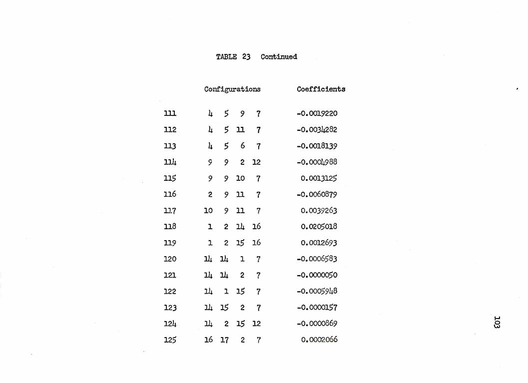
TABLE 23 Continued

Configurations Coefficients

lll 4 5 9 7 -0.0019220

112 4 5 11 7 -0.0034282

113 4 5 6 ·7 -0.0018139

114 9 9 2 12 -0.0004988

115 9 9 10 7 0.0013125

116 2 9 ll 7 -0.0060879

117 10 9 11 7 0.0039263

118 1 2 14 16 0.0205018

119 1 2 15 16 0.0012693

120 14 14 1 7 -0.0006583

121 14 14 2 7 -0.0000050

122 14 1 15 7 -0.0005948

123 14 15 2 7 -0.0000157

124 14 15 -0.0000869 ...,

2 12 a 125 16 17 2 7 0.0002066

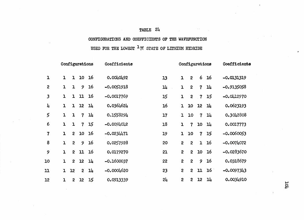
1

2

3

4

5

6

7

8

9

10

11

12

TABLE 24

CONFIGURATIONS AND COEFFICIENTS OF THE WAVEFUNGI'ION

USED FOR THE LOWEST l7t STATE OF LrrHIUM HIDRIDE

Configurations Coefficients Configurations

l 1 10 16 0.0040492 l3 1 2 6 16

l 1 9 16 -0.0051918 14 1 2 7 14

1 l 11 16 -0.0017769 15 1 2 7 15

1 1 12 14 0.0364624 16 1 10 12 14

1 1 7 14 0~1558294 17 1 10 7 14

1 1 7 15 -0.0094042 18 1 7 10 14

l 2 10 16 -0.0234471 19 1 10 7 15

1 2 9 16 0.0257928 20 2 2 1 16

1 2 11 16 0.0179270 21 2 2 10 16

1 2 12 14 -0.1600037 22 2 2 9 16

1 12 2 14 -0.0004620 23 2 2 11 16

1 2 12 15 0.0913339 24 2 2 12 14

Coef'ficie.ata

-0.0131319

-0.9135058

-0.0412970

o.o623193

0.3042808

0.0017773

-0.0060053

-0.0074072

-0.0283670

0.0318679

-O.CXYJ7343

0.0034910 ..., g.

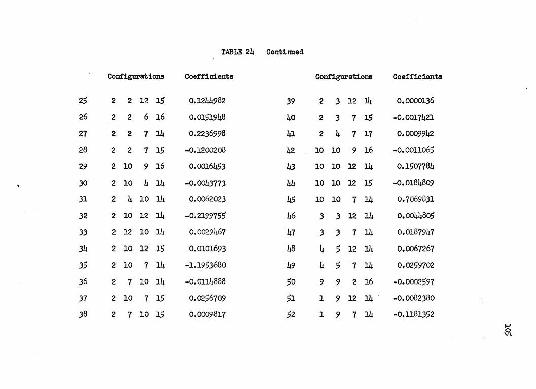
TABLE 24 Contirmed

Configurations Coefficients Contiguratioll!I Coefficients

25 2 2 l?. 15 0.1244982 39 2 3 12 l4 0.0000136

26 2 2 6 16 0.0151948 40 2 3 7 15 -0.0017421

27 2 2 7 14 0.2236998 41 2 4 7 17 0.0009942

28 2 2 7 15 -0.1200208 42 10 10 9 16 -o.oono65

29 2 10 9 16 0.0016453 43 10 10 12 14 0.1507784

30 2 10 4 14 -0.0043773 44 10 10 12 15 -0.0184809

31 2 4 10 14 0.0062023 45 10 10 7 14 0.7069831

32 2 10 12 14 -0.2199755 46 3 3 12 14 0.0044805

33 2 12 10 14 0.0029467 47 3 3 1 14 0.0187947

34 2 10 12 15 0.0101693 48 4 5 12 14 0.0067267

35 2 10 7 14 -1.1953680 49 4 5 7 14 0.0259702

36 2 7 10 14 -0.0114888 50 9 9 2 16 -0.0002597

37 2 10 7 15 0.0256709 51 1 9 12 14 . -0.0082)80

38 2 7 10 15 0.0009817 52 1 9 7 14 -0.1181352 ~

5l

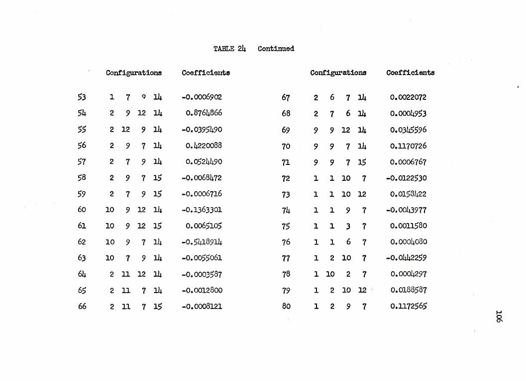
TABLE 24 Continued

Configurations Coefficients Conf'igurations Coefficients

53 1 7 Q 14 -0.0006902 67 2 6 7 14 0.0022072

54 2 9 12 14 o.8764866 68 2 7 6 14 0.0004953

55 2 12 9 14 -0.0395490 69 9 9 12 14 0.0345596

56 2 9 7 14 0.4220088 70 9 9 7 14 O.ll70726

51 2 7 9 14 0.0524490 71 9 9 7 15 o.ooo6767

58 2 9 7 15 -0.0068472 72 1 1 10 7 -0.0122530

59 2 7 9 15 -0.0006716 73 1 1 10 12 O.Ol58li22

60 10 9 12 14 -0.1363301 74 1 1 9 7 -0.0043977

61 10 9 12 15 o.oo65105 75 1 1 3 7 0.0011580

62 10 9 7 14 -0.5418914 76 1 1 6 7 0.0004080

63 10 7 9 14 -0.0055061 77 1 2 10 7 -0.0442259

64 2 11 12 14 -0.0003587 78 1 10 2 1 0.0004297

65 2 11 7 14 -0.0012800 79 1 2 10 12 . 0.0188587

66 2 ll 7 15 -0.0008121 80 1 2 9 7 0.1112565 t-' ~

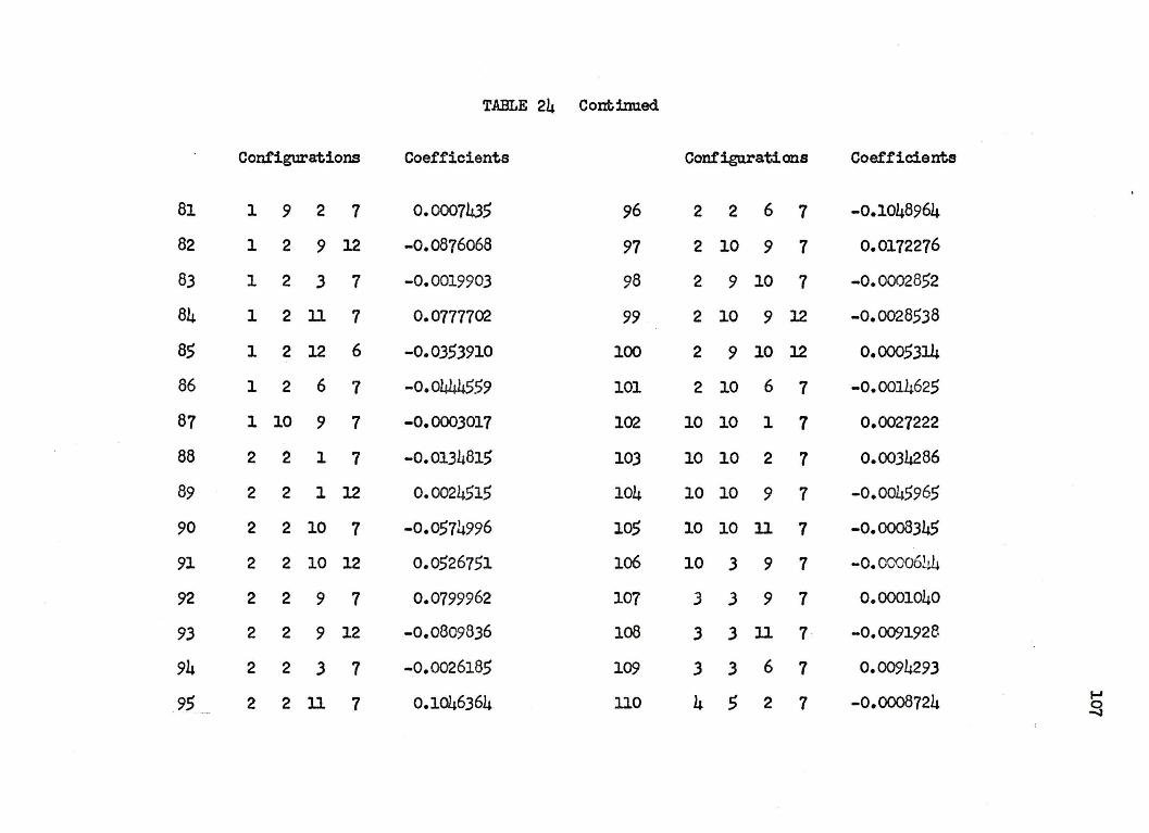
TABLE 24 Continued

Configurations Coefficients Configurations Coefficients

81 1 9 2 7 0.0007435 96 2 2 6 7 -0.1048964

82 1 2 9 12 -0.0876068 91 2 10 9 7 0.0172276

83 1 2 3 7 -0.0019903 98 2 9 10 7 -0.0002852

84 1 2 11 7 0.07777(12. 99 2 10 9 12 -0.0028538

85 1 2 12 6 -0.03.53910 100 2 9 10 12 0.0005314

86 1 2 6 7 -0.0444559 101 2 10 6 7 -0. OOJ.4625

87 1 10 9 7 -0.0003017 1(12. 10 10 1 7 0.0027222

88 2 2 1 7 -0.0134815 103 10 10 2 7 0.0034286

89 2 2 1 12 0.00245'15 104 10 10 9 7 -0.0045965

90 2 2 10 7 -0.0574996 10, 10 10 11 7 -0.0008345

91 2 2 10 12 0.0526751 106 10 3 9 7 -o.oooo6Li.4

92 2 2 9 7 0.0799962 107 3 3 9 7 0.0001040

93 2 2 9 12 -0.0809836 lo8 3 3 11 7 -0.0091928

94 2 2 3 7 -0.0026185 109 3 3 6 7 0.0094293

95 2 2 11 7 0.1046364 110 4 5 2 7 -0.0008724 I-' ~

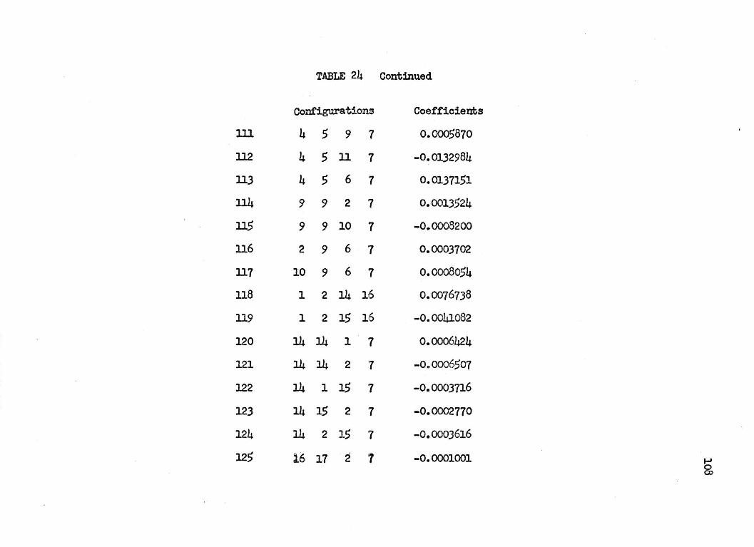
TABLE 24 Continued

Configurations Coefficients

111 4 5 9 7 0.000,870

l12 4 5 11 7 -0.0132984

ll3 4 5 6 7 0.0137151

114 9 9 2 1 0.0013524

115 9 9 10 1 -0.0008200

116 2 9 6 1 0.0003702

117 10 9 6 7 0.0008054

118 1 2 14 16 0.0076738

119 1 2 15 16 -0.004lo82

120 14 14 1 7 0.0006424

121 14 14 2 ·7 -000006507

122 14 1 15 7 -0.0003716

123 14 15 2 7 -0.0002770

124 14 2 15 1 -0.0003616

125 16 17 2 1 -0.0001001 .... 8

APPENDIX II

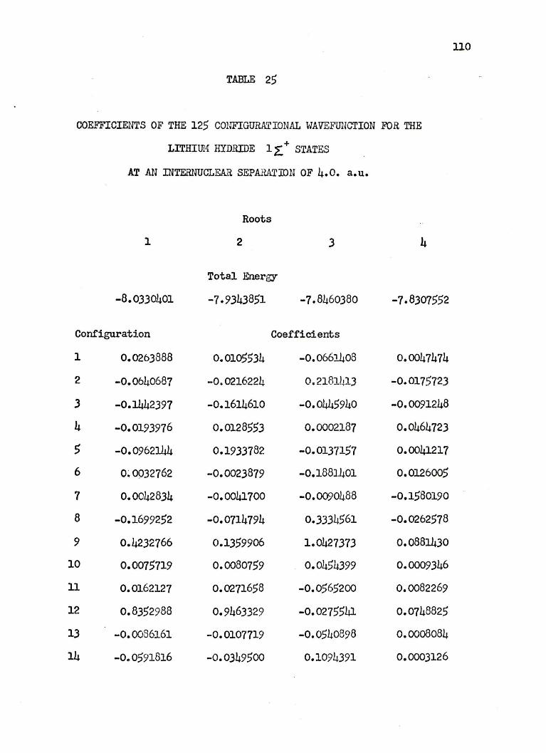
TABLE 2.5

COEFFICIENTS OF THE 125 CONFIGURATIONAL WAVEFUNCTION FOR THE

LrrHIU1'1 H'IDRIDE 1 ~ + STATES

AT AN INTERNUCLEAR SEPAHATJDN OF 4.0. a.u.

Roots

1 2 3 4

Total Energy

-8.0330401 -7-9343851 -7.8460380 -7.8307552

Configuration Coefficients

1 0.0263888 0.010.5534 -0.0661408 0.0047474

2 -0.0640687 -0.0216224 0.218lhl3 -0.0175723

3 -0.1442397 -0.1614610 -0.0445940 -0.0091248

4 -0.0193976 0.0128553 0.0002187 0.0464723

5 -0.0962144 0.1933782 -0.0137157 0.0041217

6 0~0032762 -0.0023879 -0.1881.401 0.0126005

7 0.0042834 -0.0041700 -0.0090488 -0.1580190

8 -0.1699252 -0.0714794 0.3334561 -0.0262578

9 0.4232766 0.1359906 1.0427373 0.0881430

10 0.0075719 0.0080759 0.0454399 0.0009346

ll 0.0162127 0.0271658 -0.0565200 0.0082269

12 0.8352988 0.9463329 -0.0275541 0.0748825

13 -0.0036161 -0.0107719 -0.0.540898 0.0008084

14 -0.0591816 -0.0349500 0.1094391 0.0003126

llO

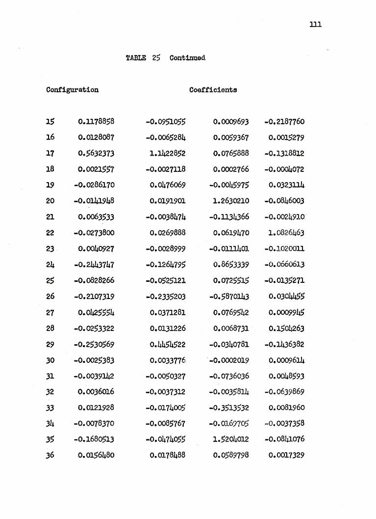
lll

1'AJ3LE 25 Continued

Configuration Coefficients

15 0.1178858 -0.0951055 0.0009693 -0.2187760

16 0.0128087 -0.0065284 0.0059367 0.0015279

17 0.$632373 1.1422852 0.0165888 -0.1318812

18 0.0021557 -0.0027ll8 0.0(X)2.766 -0.0004072

19 -0.0286170 0.0476069 -0.0045915 0.0323114

20 -0.0141948 0.0191901 1.2630210 -o.0846003

21 o.0063533 -0.0038474 -0.1134366 -0. 0024910.

22 -0.0273800 0.0269888 0.0619470 1.0826463

23 o.0040927 -0.0028999 -O.Ol.11401 -0.10-ioon

24 -0.2443747 -0.1264795 o.8653339 -0.0660613

25 -0.0828266 -0.0525121 0.0125515 -0.013,271

26 -0.2107319 -0.2335203 -0.5870143 0.030445,

27 0.0425.554 0.0371281 0.0769542 0.0009945

28 -0.0253322 0.0131226 0.0068731 · 0.1$'04263

29 -0.2530569 0.4454522 -0.0340781 -0.1436382

30 -0.0025383 0.0033776. --0.0(X)2.019 0.0009614

31 -0.0039142 · -o. 00.50327 -0.0736036 o.0048593

32 0.0036016 -0.0037312 -0.0035814 -0.0639869

33 0.0121928 -0.0174005 -0.3513532 0.0081960

34 -0.0078370 -0.0085767 -0.0169705 -0.0037358

35 -0.1680513 -0.0474055 1.5204012 -0.0841076

36 0.0156480 0.0178488 0.0589798 0.0017329

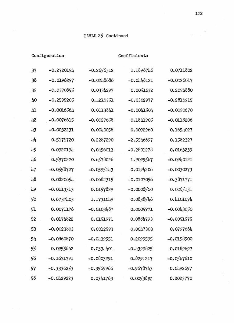
ll2

TABLE 25 Continued

Configuration Coefficients

37 -0.2720194 -0.2656312 1.1898746 0.0711802

38 -0.0196297 -0.0248686 -0.0448121 -0.0026017

39 -0.0370855 0.0334297 0.0051632 0.2094880

40 -0.2595205 0.421635:L -0.0302977 -0.2816915

41 -0.0016564 0.0113841 -0.0041504 -0.0090670

42 -0.0076615 -0.0027658 0.1841905 -0.0118206

43 -0.0032231 0.0040058 0.0092960 0.1654027

44 0.5171720 0.2287290 -2.5546697 0.1582327

45 0.0920194 0.0456013 -0.2801278 0.0163239

46 0.5970220 0.6578026 1.9099567 -0.0940121

47 -0.0558727 -0.0395143 0.0194206 -0.0030273

48 0.0820654 -0.0682315 -0.0107056 -0.3871771

49 -0.0113313 0.0157829 -0.0008560 0.0065131

50 0.6737403 1.1731049 0.0838546 0.4101094

51 0.0071176 -0.0103487 0.0005971 -0.0043650

52 0.0174822 0.0151971 0.0884793 -0.0051575

53 -0.0023803 0.0012593 0.0047303 0.0797664

54 -0.086o870 -0.0439551 0.2099595 -0.0158500

55 0.0955862 0.0334401 -0.4399825 0.0189697

56 -0.1671791 -0.0803291 0.8291217 -0.0567610

57 -0.3336253 -0.3569966 -0.96787h3 0.0492697

58 -0.0429223 0.0341763 0.005)892 0.2023770

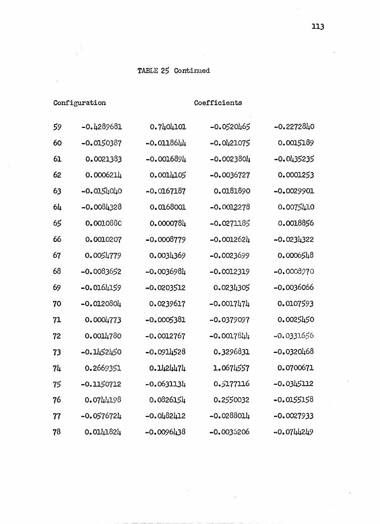
113

TABLE 25 Contirmed

Configuration Coefficients

59 -0.4289681 0.7404101 -0.0520465 -0.2272840

60 -0.0150387 -O.Oll8644 -0.0421075 0.0015189

61 0.0021383 -0.0016894 -0.0023804 -0.0435235

62 0.0006214 0.0014105 -0.0036727 0.0001253

63 -0.0154040 -0.0167187 0.0181890 -0.0029901

64 -0.0084328 0.0168001 -0.0012278 0.0075410

65 0.0010880 0.0000784 -0.0271185 0.0018856

66 0.0010207 -0.0008779 -0.0012624 -0.0234322

67 0.0054779 0.0034369 -0.0023699 0.0006548

68 -0.0083652 -0.0036984 -0.0012319 -o.ooos:no

69 -0.0164159 -0.0203512 0.0234305 -0.0036066

70 -0.0120804 0.0239617 -0.0017474 0.0107593

71 0.0004773 -0.0005381 -0.0379097 0.0025450

72 0.0014780 -0.0012767 -0.0017844 -0.03.31656

73 -0.1452450 -0.0914528 0.3296831 -0.0320468

74 0.2669351 0.1.h24474 1.0674557 0.0700671

75 -O.ll,50712 -0.0631134 0.5177116 -0.034.5112

76 0.0744198 o.o826154 0.2550032 -0.0155158

77 -0.0576724 -0.0482412 -0.0288014 -0.0027933

78 O.OJ.41824 -0.0096438 -0.0035206 -o.07w_a49

114

'!'ABLE 25 Continued

79 0.1402528 -0.2426648 0.0190643 o.0869297

80 -0.2531644 -0.2761684 -0.8604312 0.0422363

81 0.1000523 0.0720312 -0.1413969 0.0102632

82 -0.0341895 0.0281542 0.0050032 0.1768521

83 -0.3944873 0.6774129 -0.0476278 -0.2199378

84 0.3104043 0.3243362 o.8940498 -0.0041948

85 -0.0378873 -0.02682o6 0.0916156 -0.0054065

86 0.0380790 -0.0279030 -0.0052609 -0.1943496

87 0.5538764 -0.9446554 o.0652214 0.2563430

88 0.0058514 0.0045586 0.0123723 -0.0001995

89 -0.0008554 0.0006491 0.0007363 o.ol.44068

90 -0.0233746 -0.0252594 -0.0873642 0.0027054

91 0.01308n 0.0305485 0.0844360 -0.0021480

92 -0.0294641 0.0485515 -0.0032622 -0.0048623

93 0.0879222 -0.1458636 0.0089379 0.0161453

94 -0.1162156 0.1924423 -0.0123160 -0.0208725

95 -0.0993821 -0.0950310 -0.1639708 0.0059739

96 -0.0098808 0.0061391 0.001.3744 0.0516542

97 -0.2039225 0.3446249 -0.0235170 -0.0800938

98 o.0895933 -0.1476303 0.0098885 0.0158876

99 -0.0168966 -0.0152966 .:..0.0213074 0.0000512

100 -O.Ol0685Q 0.0174745 -0.0013420 -0.0018109

101 0.0319674 0.0369218 0.0079342 0.00ll966

102 -0.0669328 -0.1005279 -0.0325759 -0.0050891

103 0.0214392 0.0772908 0.0124342 0.0069015

ll5

TABLE 25 Continued

Configuration Coefficients

104 0.0251298 0.0170822 0.0498680 -0.0000798

105 0.0025056 0.0251599 -0.0023091 0.0106974

106 -0.0428306 -0.0273083 -0.0313395 0.0046043

107 -0.0259258 0.0073324 0.0090460 0.0013069

108 -0.0478330 -0.0389176 0.0220485 -0.0000720

109 0.1039194 o.0841579 -0.0338383 -0.0025580

no -0.0623721 -0.0501604 0.0165524 0.0039244

lll -0.0312008 0.0175334 0.0056904 0.0108303

ll2 0.0054775 -0.0042877 0.0014473 0.0008919

ll3 0.0094624 -0.0036871 0.0000669 -0.0009237

ll4 0.2173553 -0.1212672 -0.0340561 -0.0159013

ll5 0.0199116 -0.0159525 -0.0057344 -0.0059246

ll6 -0.0534346 0.0315159 0.0036232 0.0135260

ll7 -0.0801366 0.0306611 -0.0003185 0.0077100

ll8 -0.0068136 0.0038718 0.0011238 0.0023523

ll9 0.0503284 -0.0286807 -0.0062468 -0.0152!'14

120 -0.0125658 0.0058415 -0.0006565 -0.0044196

121 -0.0191333 0.0074094 -0. OOOJ.145 0.0018571

122 -0.0051167 0.0028848 0.0008747 0.0017882

123 0.0019283 -0.0007385 0.0000081 -0.0001856

124 -0.0071817 0.0040523 0.0012327 0.0025124

125 0.0027267 -0.001041~7 0.OOOOll5 -0.0002626

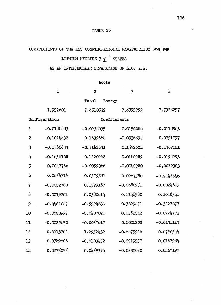
ll6

TABLE 26

COEFFICIENTS OF THE 125 CONFIGURATIONAL WAVEFUNCTION FUR THE

LITHIUM HYDRIDE 3 i: + STATES

AT AN INTERNUCLEAR SEPARATION OF 4.0. a.u.

Roots

1 2 3 4

Total Energy

7.952601 7.851C>532 7.8395999 7.7328257

Configuration Coefficients

1 -0.0188883 -0.0238635 0.0156086 -0.0118563

2 0.1014832 0.1639664 -0.0936894 0.0751097

3 -0.1386833 -0.3142631 0.1592624 -0.1369021

4 -0.1658108 0.1220262 0.0180989 -0.0198293

5 0.0047766 -0.0059366 -0.0042980 -0.0079303

6 0.0654314 0.0579581 0.0967580 -0.2148646

7 -0.0052760 0.1599187 -0.0680951 -0.0024609

8 -0.0019201 0.0380614 O.ll48580 0.1018341

9 -0.4461087 -0.5994639 0.36298~,1 -0.3227677

10 -0.0653997 -0.0407020 0,0382542 -0.0221.7j;3

11 -0.0022650 -0.0057617 0.0006208 -0.013lll3

12 0.6913762 1.2952432 -0.6875926 0,6790544

13 0.0789606 -0.0103452 -0.0219551 0.0167984

14 0.0235055 0.0459394 -0.0232090 0.0467197

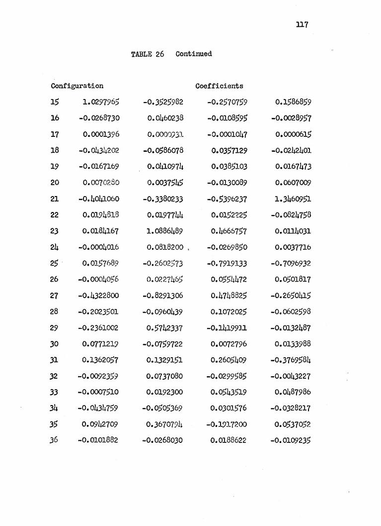
117

TABLE 26 Continued

Configuration Coefficients

15 1.0297965 -0.3525982 -0.2570159 0.1586859

16 -0.0268730 0.0460238 -0.0108595 -0.0028957

17 0.0001396 0.0000)31 -0.0001047 o.0000615

18 -0.0434202 -0.0586078 0.0357129 -0.0242401

19 -0.0167169 0.0410974 0.0385103 0.0167473

20 0.0070280 0.0037545 -0.0130089 0.0607009

21 -0.4041060 -0.3380233 -0.5396237 1.3460951

22 0.0194818 0.0197744 0.0152'225 -0.0824758

23 0.0184167 1.0886489 0.4666757 o.oll4031

24 -0.0004016 0.0818200 . -0.0269850 0.0037716

25 · 0.0157689 -0.2602573 -0.7919133 -0.?096932

26 -0.0004056 0.0227465 0.0554472 0.0501817

27 -0.4322800 -0.8291306 o.4748825 -0.2650415

28 -0.2023,01 -0.0960439 0.1072025 -0.0602598

29 -0.2361002 0.5742337 -O.l.419911 -0.0132487

30 0.0771219 -0.0759722 0.0072796 0.0133988

31 0.1362057 0.1329151 0.2605409 -0.3769584

32 -0.0092359 0.0737080 -0.0299585 -0.0043227

33 -0.0007510 0.0192300 0.0543519 0.0487986

34 -0. 0431.i759 -0.0505369 0.0301576 -0.0328217

35 0.0942709 0.3670794 -0.1917200 0.0537052

36 -0.0101882 -0.0268030 0.0188622 -0.0109235

118

TABLE 26 Continued

Configuration Coefficients

37 -0.2669473 1.3226911 0.6368131 · -0.2574004

38 0.0225475 0.0506198 -0.0352085 0.0292187

39 -0.3192135 1.0079879 -0.2978982 -0.0106865

40 -0.0245280 -0.0354731 0.0244531 -0.0115956

41 0.0106556 0.0125481 0.0128062 -0.0213964

42 0.1165173 0.1314716 0.2895814 -0.2907909

43 0.0105317 0.0078919 0.0020806 -0.0135754

44 0.0018813 -0.1155295 0.0495274 -0.0027123

45 0.0007123 0.0353580 -0.0128215 0.0022729

46 0.0039175 -0.0210006 -0.0738882 -0.0702184

47 -0.0005910 0.0098568 0.0250363 0.0174152

48 0.5858855 2.1235385 1.0697071 0.5324224

49 0.1359620 0.2418183 -0.1508315 0.0591415

50 o.8416597 -1.6928902 0.4017660 o.o680507

51 -0.0710207 -0.0124634 0.0293626 -0.0186667

52 -0.0003340 -0.0002294 0.0001513 0.0001031

53 0.0009050 -0.0005712 0.0004787 -0.0018339

54 -0. 013!~645 -0.0048595 -0.0067552 0.0298214

55 -0.3492834 -0.3493783 ·-0.6918346 0.9689382

- 56 -0.0069663 -0.1389673 0.0602410. 0.0087452

51 -o.00002L8 -0.0463147 -0.1301345 -0.111+2285

58 -0.2444397 -0.2693873 0.1903388 -0.1027564

59 0.1582,388 0.3966706 -0.2213104 0.0912642

60 -0.1530332 -0.6918924 0.3346289 -0.1782213

119

TABLE 26 Cont,inued

Configuration Coefficients

61 -0..5029422 0.8987696 -0.2030476 -0.0450674

62 0.0047435 0.0032897 0.0035214 -0.0053650

63 0.2096680 0.2105915 o.4155584 -0.5769063

64 0.0042283 0.0554785 -0.0234780 -0.0068544

65 -0.0003063 0.0230524 o.o6JJ54h 0.0572444

66 0.0040704 0.0024688 -0.0017096 0.0031563

67 -0.0053546 -0.0032962 0.0016760 -0.0080082

68 -0.0170318 -0.0080523 0$0099907 -0.0037178

69 0.0060492 0.0034021 0.0052780 -0.0222960

70 -Oc0001211 0.0229354 -Oe00983h9 0.0001.456

71 -0.0004043 0.0058854 0.0167478 0.0154588

72 0.0057940 0.0034549 -0.0024892 0.0045759

73 -0.0076164 -0.0046232 0.0024487 -0.0114406

74 -0.0240701 -0.0ll4ll0 0.0140966 -0.0052234

75 0.0086311 0.0048131 0.0071.918 -0.0317544

76 -0.0001762 000324508 -0.0139061 0.0001985

77 -o.ooor,853 0.0033362 0.0236970 0.0218958

78 -0.2548742 -0.3216469 . 0.21.59264 -0.ll79183

19 0.3209737 0.9431477 -0.5040255 0.2375647

80 -0.1174168 -0.4587775 0.2315261 -o.n78998

81 0.0893538 -0.2586416 0.0729176 0.0080ll3

82 -0.0905024 0.0371163 0.0132402 -0.0254814

120

TABLE 26 Continued

Configuration Coefficients

83 -0.0707844 -0.0729532 -0.l.486555 0.1842327

84 -0.3384973 0.8155384 -0.2107166 -0.0356566

65 0.1294057 0.1198048 -0.0932942 0.0587421

86 0.1919564 0.1969113 0.3905110 -0.5100838

87 0.0184992 0.0l.41629 -0.0091726 0.0014779

88 -0.0005763 0.0089690 0.0252314 0.0240547

89 0.488ll52 -0.8878131 0.2185625 0.0428684

90 -0.0475055 -0.0741615 0.0471670 -0.0297181

91 -0.0016260 -0.0017lll -0.0016045 -0.0000845

92 -0.2447831 -0.2524331 -0.4974478 o.6488119

93 -0.0202534 -0.0043040 0.0044533 0.0010542

94 0.0003141 -0.0105556 -0.0288159 -0.0267387

95 -0.0420157 0.0899421 -0.0256793 -0.0017617

96 0.,0489689 -0.0829952 0.0228636 0.0004288

91 o.ol142o8 0.0l.15997 0.0239820 -0.0300282

98 -0.0328028 -0.0357330 -0.0700373 o.0869514

99 0.0370189 0.0403762 0.0781753 -0.0975609

100 -0.0027505 0.0025.318 -0.0005101 -0.0010022

101 -0.1537779 0.1865492 -0.0338830 -0.0262342

102 0.0776372 0.0812263 0.1597197 -0.1990745

103 0.0113541 -0.0134886 o.003s,65B 0.0018216

104 -0.0204079 -0.0218773 -0.0423461 o.0528495

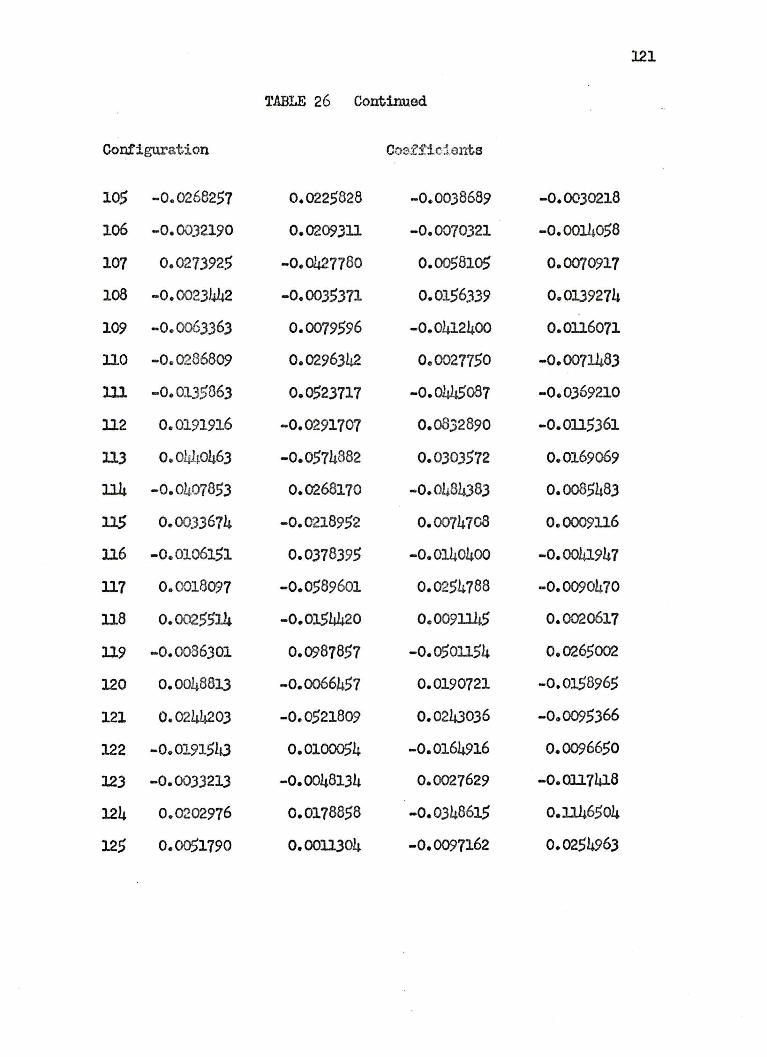
121

TABLE 26 Continued

Configuration Cosf'!ic:ta11ts

105 -0.0268257 0.0225828 -0.0038689 -0.0030218

106 -0.0032190 0.0209311 -0.0070321 -0.0014058

107 0.0273925 -0.0427780 0.0058105 0.0070917

lo8 -0.0023442 -0.0035371 o. 0156.3.39 0.0139271,

109 -0. 0063363 0.0079596 -0.0412400 0.0116071

llO -0. 0286809 0.0296342 Oe0027750 -0.0071483

lll -0.0135063 0.0523717 -0.0445o87 -0.0369210

ll.2 0.0191916 -0.0291707 0.0832890 -0.0115361

113 o.o4ho463 -0.0574882 0.0303572 0.0169069

114 -0.0407853 0.0268170 -0.0484383 o.0085483

us 0. 0033674 -0.0218952 0.0074708 0 .. 0009116

ll.6 -0.0106151 0.0378395 -0.0140400 -0.0041947

ll.7 0.0018097 -0.05896ol 0.0254788 -0.0090470

ll.8 0. 0025514 -0.0154420 0.0091145 0.0020617

119 -0.0086301 0.09878.5'7 -0.0501154 0.0265002

120 0.0048813 -o.0066457 0.0190721 -0.0158965

121 0.0244203 -0.0521809 0.0243036 -000095366

122 -0.0191543 0.0100054 -0.0164916 0.0096650

123 -0.0033213 -0.0048134 0.0027629 -O.OJ.17418

124 0.0202976 0.0178858 -0.0348615 0.1146504

125 0.0051790 0.0011304 -0.0097162 0.02$4963

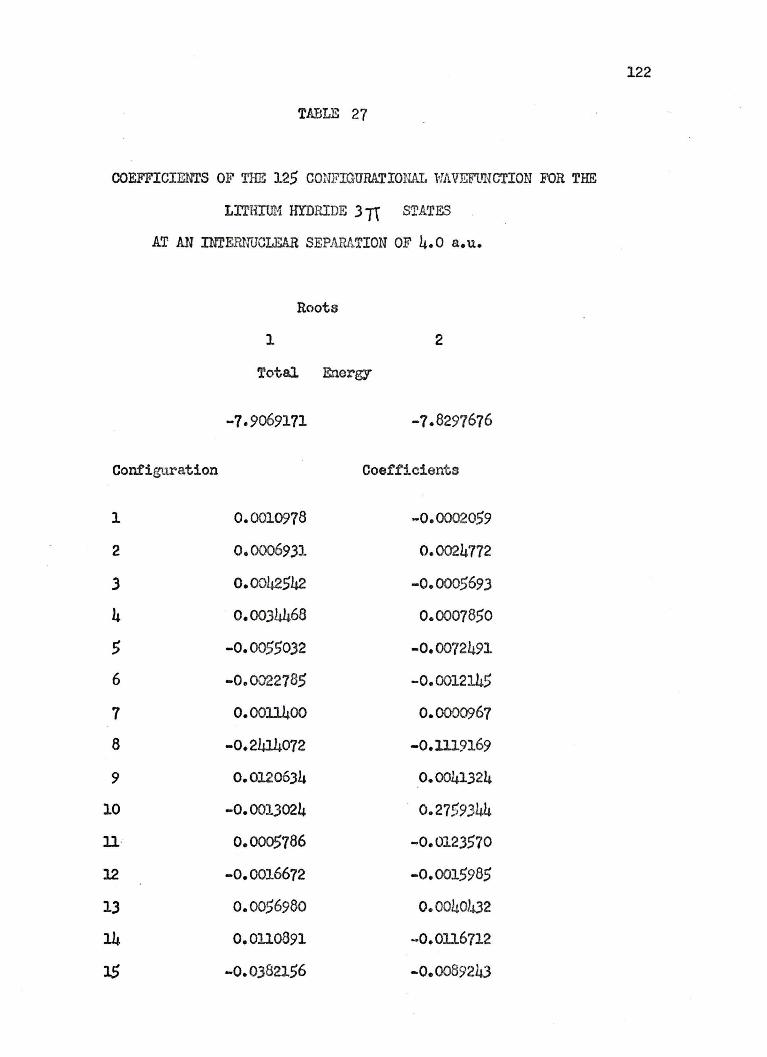
122

TABLE 27

COEFFICIENTS OF THE 125 CONFIGURATION.AL WAVEFUNCTION FOR THE

Ll'THIOM HYDRIDE 3 TT STATES .

AT AN INTEIDTaCLEAR SEPARt.TION OF 4.0 a.u.

Roots

1 2

Total Energy

-7.9069171 -7.8297676

Configuration Coef.f'icients

1 0. 0010978 -0. 00020.59

2 0. 0006931 0.0024772

3 0.0042.542 -0.0005693

4 0.0034468 0.0007850

5 -0.005.5032 -0.0072491

6 -Oe 0022785 -0.0012145

7 0. 0011400 0.000Cf967

8 -0.2414072 -O. lll9169

9 0.0120634 0. 0041324

10 -0.0013024 0.2759344

11· 0.0005786 -0.0123570

12 -0.0016672 -0.0015985

13 0. 0056980 0.0040J.u2

14 0.0110891 -O.Oll6712

15 -0.0382156 -0.0089243

123

TABLE 27 Continued

Contiguration Coefficients

16 -0.0089841 -0.0069345

17 0.0467373 0.0489718

18 -0.0013825 0.0001332

19 0.0162788 0.0195249

20 -0.0225342 -0.0023090

21 1.4238663 0. 6628978

22 0~0030551 0.0008921

23 0. 0000570 -0.0000166

24 -0.0726042 -0.0452362

25 0.0009940 0.0089503

26 0.0023160 0.0026671

27 O.Oll5418 1.6431907

28 -0.0043030 0.0978935

29 -0.0030551 -O.OD.6226

JO -0.5334562 -0.2468175

31 -0.0031479 -0.0013465

32 0.0057240 -0.0009941

33 0.0002013 0.5934870

34 O. OOJ.4053 0.0005589

35 0.0043619 0.0022922

36 0.0107419 0. 0091400

37 -0.0131879 -0.0150671

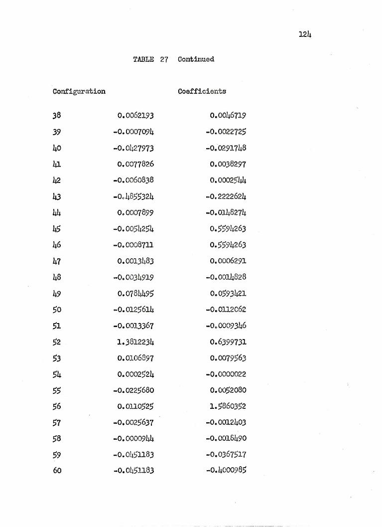
124

TABLE 27 Continued

Configuration Coef'ficients

38 0.0062193 0.0046719

39 -0.0007094 -0.0022725

40 -0.0427973 -0.0291748

41 0.0077826 0.0038297

42 -0.0060838 0.0002544

43 -0~4855324 -0.2222624

44 0.0007899 -0.0148274

45 -0.0054254 o.5594263

46 -0.0008711 0.5594263

47 0.001348.3 0.0006291

48 -0.0034919 -0.0014828

49 0.078!'495 0.0593421

50 -0.0125614 -o.0112c62

51 -0.0013367 -0 .. 0009346

52 1.3812234 0.6399731

53 0.0106897 0.0079563

54 0.0002524 -0.0000022

55 -0.0225680 0.00,2080

56 0.0110525 l.58603.52

57 -0.0025637 -0.0012403

58 -0.0000944 -0.0016490

59 -O.Oh5ll83 -0.0367.517

60 -0.0451183 -0.4000985

125

TABLE 27 Continued

Configuration Coe£ r i cierrt s

61 0.0115243 -0.0016486

62 -0.0060140 0.9903097

63 -0.0008685 -0.00082,36

64 -000205333 -0.0094620

65 0.0016371 -0.0002531

66 -0.0001419 0.0234624

67 -0.0010383 -0.0010672

68 -o. 0290950 -o.0134lo6

69 0.0022211 0.0010612

70 -0.0001755 0.0332170

71 0.0002899 -0.0032615

72 0.0060170 0.0091330

73 0.288fi850 0.1333896

74 0.0003760 -0.3248344

15 -0.0427492 -0.0308346

76 -0.0035701 0. 0028378

77 -0.7870071 -0.3665858

78 0.0014254 -0.0018704

19 0.0083046 -0.0014467

80 -0.0058083 0.9041769

81 0. 0487410 0.0407477

82 1.0922392 0.5078604

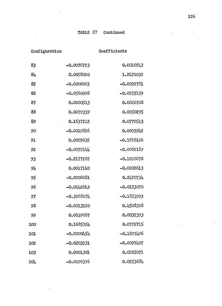
126

TABLE 27 Continued

Configuration Coefficients

8.3 -0.007672.3 0. 001094.3

84 o. 0058020 1.2471032

85 -0.000600.3 -0.0022781

86 -0.0560998 -0. 0255159

87 0.0000513 0.0626708

88 0.00793.39 0.00,0295

89 0.1637212 0.077051.3

90 -0.0019826 0.0003942

91 0. 0009635 -0.1876196

92 -0.0079144 -o.oo62189

93 -0. 2177282 -0.1020878

94 0.0017140 -0. 0002613

95 -0.0006081 0.2470734

96 -O.Ol.42043 -0.012.3070

91 -0.3968174 -0.185.399.3

98 -0.0013120 0. 4508328

99 0. 0039067 0.0032.39.3

100 0.1685354 0.0795715

101 -0.0000454 · -0.1897496

102 -0. 020.3231 -0.0097407

103 0.0001301 0. 0225071

104 -0.0096376 0.0253684

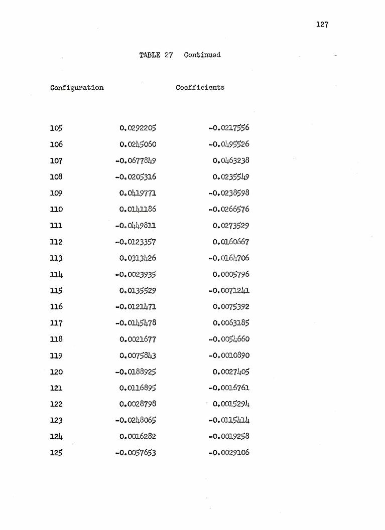
127

TABLE 27 Continued

Configuration Coefficients

105 0.0292205 -0.0217556

106 0. 0245060 -0.0495526

107 -0.0677849 0. 0463238

108 -0.0205316 0.0235549

109 0. 0419771 -0.0238598

110 0.0141186 -o.~66576

111 -O.Olw.9811 0.0273529

112 -0. 0123357 0.0160667

113 0. 0313426 -0.0164706

114 -0. 0023935 0. 000!?/96

115 0.0135529 -0. 0071241

116 -0. 0121471 0.0075392

117 -O.Ol.45478 0. 0063185

118 0.0021677 -0.0054660

119 0. 0075843 -0.0010890

120 -0.0188925 0.0027405

121 0.0116895 - 0. 0016761

122 0.0028798 0.001529h

123 -0.0248o65 -0. 0115414

124 0.0016282 -0. 0019258

125 -0. 0057653 -0.0029106

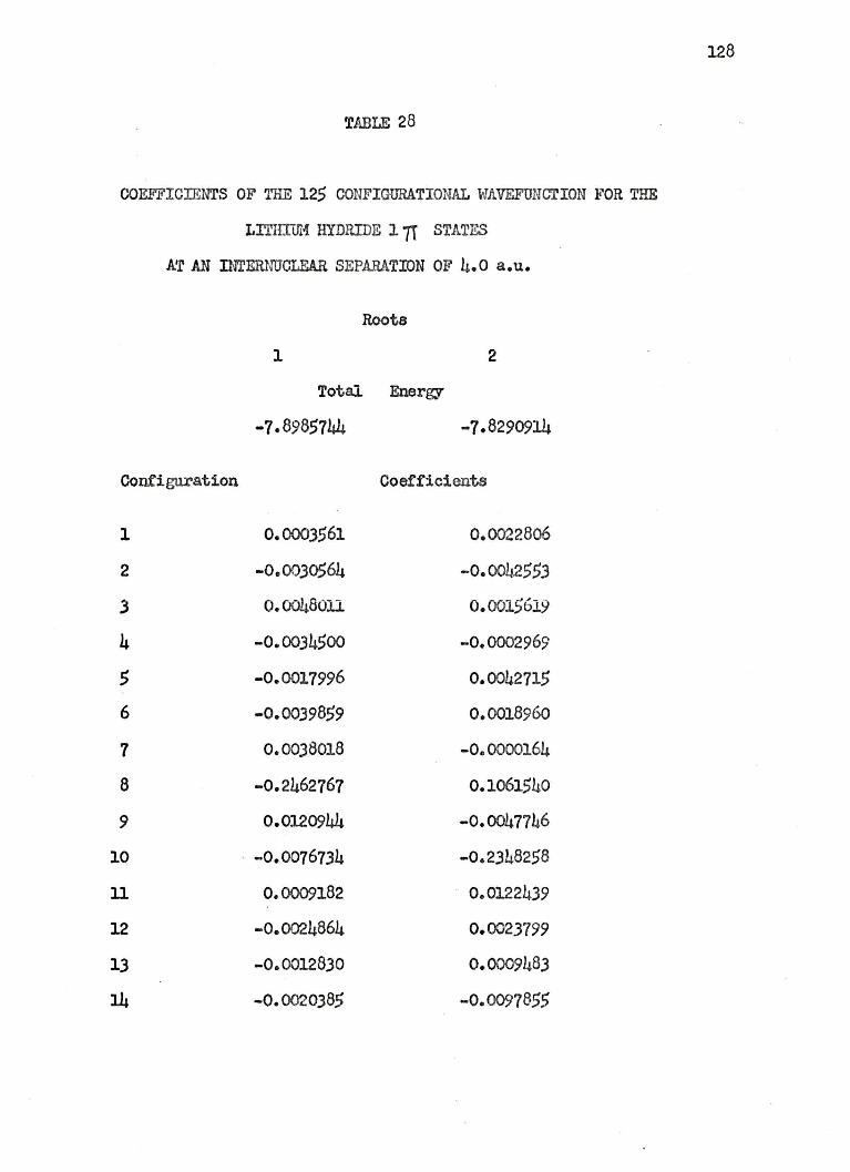
TABLE 28

COEFFICIENTS OF THE 125 CONFIGURATIONAL WAVEFUNCTION FOR THE

LITIIImi HYDRIDE l 7T STATES

AT AN INTERNUCLEAR SEPARATION OF 4. 0 a. u.

Roots

l 2

Total Energy

-7.8985744 -7.8290914

Configuration Coefficients

1 0.0003561 0.0022806

2 -0.0030564 -0.00~2553

3 0.0048011 0. 0015619

4 -0.0034500 -0.0002969

5 -0.0017996 0.0042715

6 -0.0039859 0.0018960

7 0.0038018 -0.0000164

8 -0.2462767 0.1061540

9 0.0120944 -0.0047746

10 -0.0076734 -0.2348258

11 0. 0009182 0.0122439

12 -0.0024864 0.0023799

13 -0.0012830 0.0009483

14 -0.0020385 -0.0091855

128

129

TABLE 28 Continued

Configuration Coeff'icienta

16 -0. 0355481 0. 0037679

17 0.0120217 -0.0010556

18 0.0352355 -0.0374471

19 0.0023lll -0.0016476

20 0. 0198814 -0.0211507

21 -0. 0179257 0.0022072

22 1.4568477 -o.6465U8

23 -0.00ll336 0.0000515

24 - 0.0678790 0.0483374

25 0.0031839 -0.0068254

26 0. 0031112 -0.0020307

27 0. 0486181 1.J.i..398704

28 -0.00770!µ. -0. 0982802

29 0.0053606 0.0002091

30 - 0.5350676 0.1722202

31 -0.0003669 0.0016825

32 0.00154o6 0. 0005519

33 -0. 0105330 . -0.3607801

34 0.0001354 -0.0017218

35 0.0046123 -0.0025749

36 0.0016487 -O.OOll.478

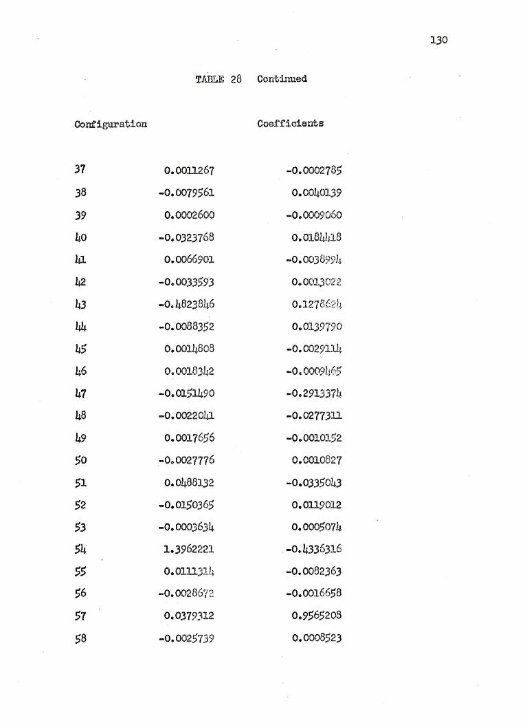
130

TABLE 28 Continued

Confi guration Coefficients

37 o.oon267 -0.0002785

38 -0.0079561 0.0040139

39 0.0002600 -0.0009060

40 -0.0323768 0.0184!µ.8

41 0.0066901 -o.003899h

42 -0.0033593 0. 0013022.

43 -0.4823846 0.12786211.

44 -0. 0088352 0.0139790

45 0.0014808 -0.0029114

46 0. 0018.342 - 0~0009L~65

47 -0. 0151490 -0. 291.337li

48 -0.0022041 -0. 0277.311

49 0.0017656 -0.0010152

50 -Oe 0027776 0.0010827

51 0.0488132 -0.033.5043

52 -o. 0150365 0.0119012

53 -0.0003634 o. 000.r,074

54 1.3962221 .-0. 4336316

55 0. 011131).. -0.0082363

56 -0. 00286'( :.:: -0.0016658

51 0.0.379312 0.9565208

58 -0. 0025739 0.0008523

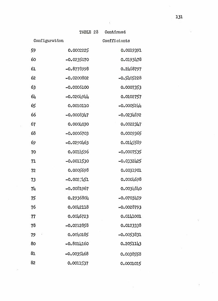
131

TABLE 28 Continued

Configuration Coeffic.i.ents

59 0.0002225 0.0019391

60 -0.0235070 0.0193478

61 -0.8778998 0.2468797

62 -0.0200802 -0.5405228

63 -0.0006100 0.0007353

64 -0. 0201.,944 0.0102757

65 000010110 -0.0005244

66 -0.0008347 -0.0234892

67 0.0004030 0.0022347

68 -0.0006703 0.0009365

69 -0.0290463 0.0145589

70 0.0014.596 -0.0007535

71 -0.0011530 -0.0332425

72 Og0005698 0.0031901

73 -0.002~451 0.0004698

74 -0.0081967 0.0034840

75 0.2936804 -0.0703479

76 0.0042ll8 -0.0028793

77 0.0046723 0.0141001

78 -0.0212858 0.0123338

79 0.0040185 -0.0053831

Bo -0.801.4160 0.2051143

81 -0.0035468 0.0038558

82 O.OOll537 0.0001015

132

TABLE 28 Continued

Configuration Coefficients

83 -0.0178181 -0.4393820

84 0. 0188079 -0.0164961

85 1.1153902 -0.2496899

86 0.0185870 0.5291036

87 -0.0570366 0.0017409

88 0.0043014 -0.0004659

89 0.1671636 -0.0215743

90 0.0019221 0.0400142

91 -0.0024101 0.0010174

92 -0.2232593 0.0211223

93 -0.0012784 -0.0365303

94 -0.0025225 OaOOJ2820

95 -0~ 4071389 o.o6414o5

96 -0.0039372 -0.1277358

91 0.1731089 -0.0017076

98 - 0.0003982 -0.0059860

99 -0.0206123 - 0.0036528

100 0.0003056 0.0094232

101 -0.0076874 0.0001057

102 0.0082466 -0.0008564

103 0. 0149232 0.0130191

104 -0.0019923 -0.0199331

105 -0.0382853 -0.0268018

106 o.04n936 0.0445940

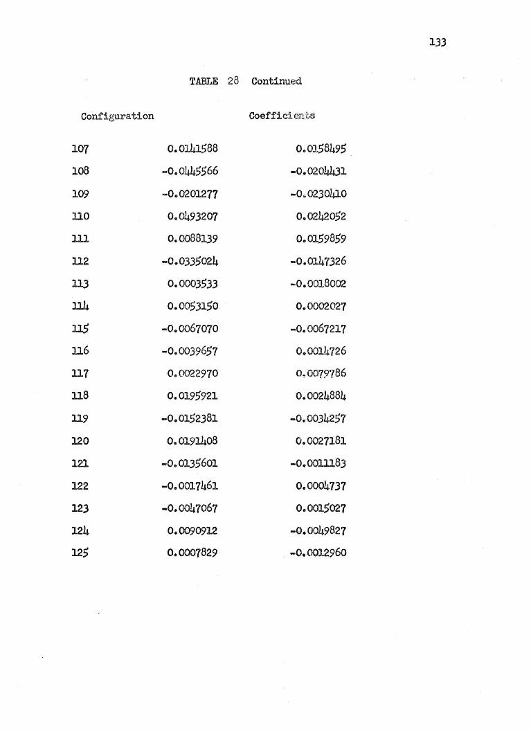
133

TABLE 28 Continued

Configuration Coeffidents

l(Jl 0.0141.588 0.,0158495

108 -0.0445566 -0.0204431

109 -0.0201277 -0~0230410

llO 0.0493207 0.0242052

lll 0.0088139 0.0159859

ll2 -0.0335024 -0.0147326

ll3 0.0003533 -0.0018002

114 0.0053150 0.0002027

11.5 -0.0067070 -0.0067217

ll6 -0.0039657 0.0014726

ll7 0.0022970 0~0079786

ll8 0.0195921 0.0024884

ll9 -0.01.52381 -0.0034257

120 0.0191408 0.0027181

121 -0.013.5601 -O.OOlll83

122 -0.0017461 0.0004737

123 -0.0047067 0.0015027

124 0.0090912 -0.0049827

125 0.0007829 . -0. 00)296o

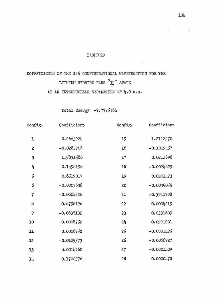
TABLE 29

COEFFICIENTS OF THE 12.5 CONFIGURATIONAL WAVEFUNCTION FOR THE

LrrHIUM HYDRIDE PLUS 2 ~ + STATE

AT AN INTERNUCLEAR SEPARATION OF 4.0 a.u.

Total Energy -7.777.5364

Config. Coefficient Config. Coefficient

1 0.2663924 15 1.2112970

2 -0.0283708 16 -0.1019457

3 1.5831586 17 0.0211898

4 0.14.58196 18 -0.0024629

5 0.6519017 19 0.0301473

6 -0.0003638 20 -0.0035055

7 -O.o604220 21 -0.3911798

8 0.67,58196 22 0.0004215

9 -0.0637132 2.3 0.0.331609

10 0.0008752 24 0.0991201

ll 0. 0008752 25 -0.0001495

12 -0.018.5.573 26 -0.0066927

13 0.0014960 27 -0.0001409

14 0.1700576 28 0. 0000478

134

135

TABLE 29 Continued

Config. Coefficient. Conf'ig. Coefficient

29 -0.0013250 51 1.67CY2.766

30 -0.0004914 52 0.001370}

31 -0.0001920 53 0.1290326

32 0.0005207 54 o.4288826

33 -0.0127870 55 -0.0003451

34 1.1573330 56 -O.CY2.61173

35 -0.0025185 51 -0.0011322

36 -0.0986109 58 0.0030867

37 0.0004073 59 -0.0018912

38 -O.Jll.3464 60 -0.0012018

39 0.0004282 61 -0.0510053

40 0.0212907 62 o.6611432

hJ. 0.0002851 63 -0.0474384

h2 0.0017068 64 -o • .:;6047o6

43 -0.000:5431 65 O.CY2.04602

h4 -0.0058104 66 0.0007274

45 0.0015882 67 -0.0018307

46 0.0012794 68 0.0013399

47 0.0003857 69 0.0007539

48 0.0027228 70 0.0390429

49 -0.0009377 71 0.0553998

50 0.0420400 72 -0.0025125

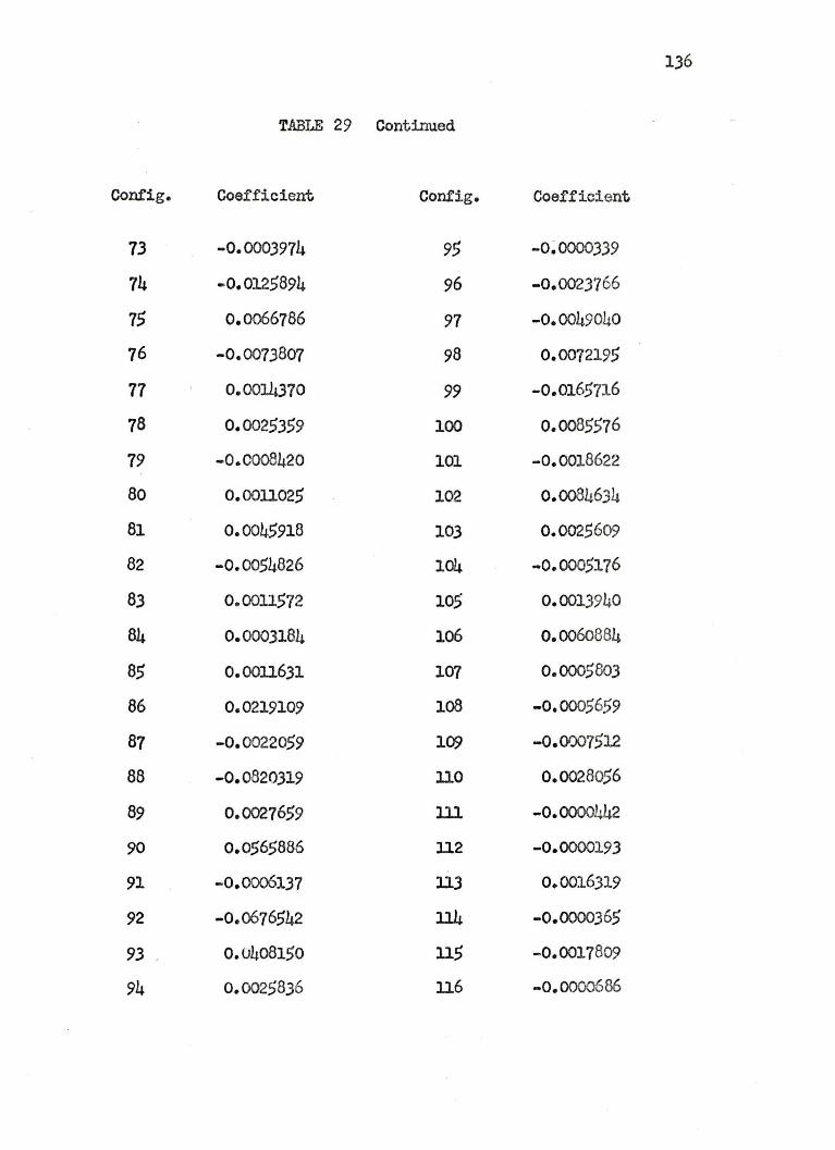
136

TABLE 29 Continued

Config. Coefficient Config. Coefficient

13 -0.0003974 95 -0~0000339

74 -0.0125894 96 -0.0023766

15 0.0066786 97 -0.0049040

76 -0.0073807 98 0.0072195

77 0.0014370 99 -0.0165716

78 0.0025359 100 o.0085576

19 -0.0008420 101 -0.0018622

80 0.0011025 102 o.0084634

81 0.0045918 103 0.0025609

82 -0.0054826 104 -0.0005176

83 O.OOll572 105 0.0013940

84 0.0003184 106 o.oo6o884

85 0.0011631 107 0.0005803

86 0.0219109 108 -0.0005659

87 -0.0022059 1C9 -0.0007512

88 -0.0820319 110 0.0028056

89 0.0027659 lll -0.0000442

90 0.0565886 112 -0.0000193

91 -0.0006137 113 0.0016319

92 -0.0676542 114 -0.0000365

93 0.0408150 115 -0.0017809

94 0.0025836 116 -0.0000686

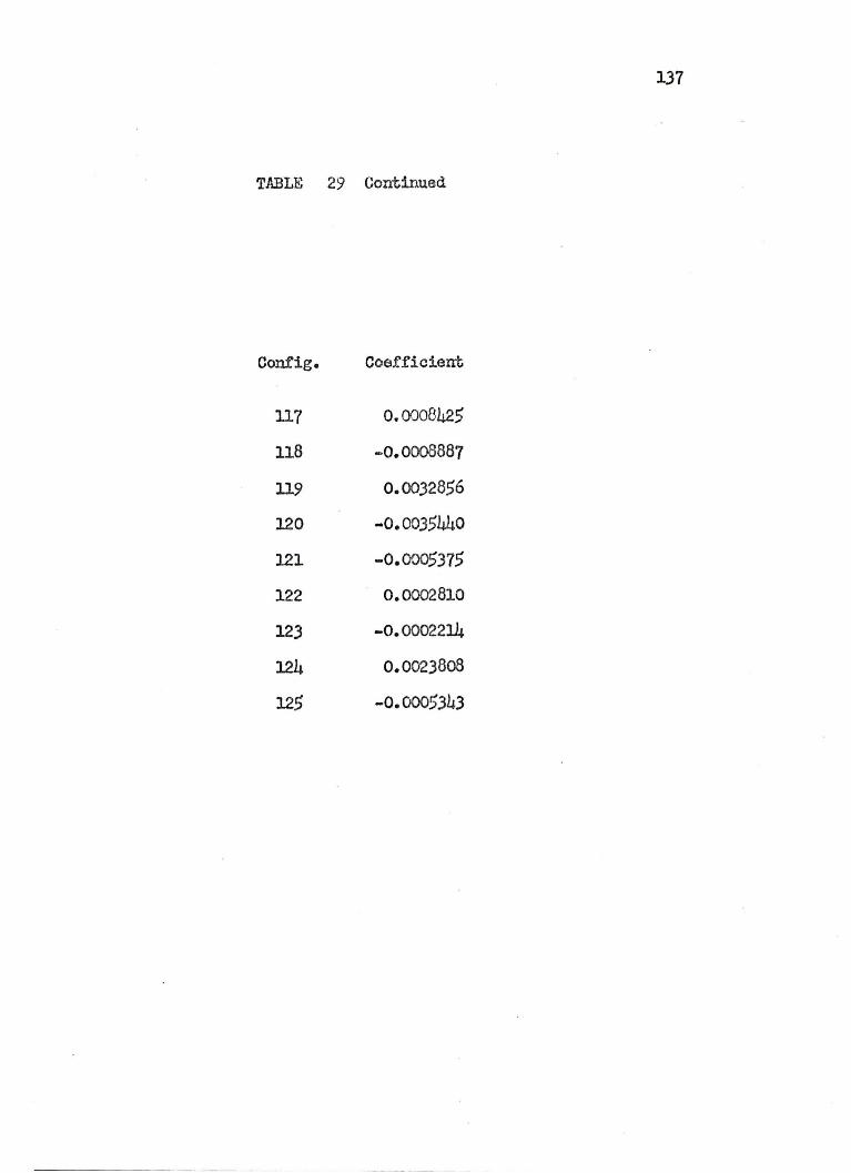
137

TABLE 29 Continued

Con.fig. Coefficient

117 0.0008425

118 -0.0008887

119 0.0032856

120 -0.0035440

121 -0.0005315

122 0.0002810

123 -0.0002211+

124 o.00238o8

125 -0.0005343

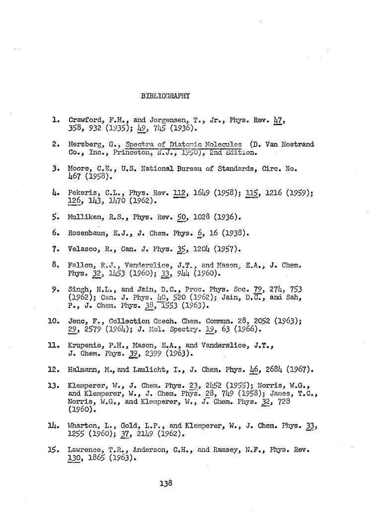
BIBLIOGRAPHY

1. Crawford, F.H., and Jorgensen, T., Jr., Phys. Rev. l!I, 358, 932 (1935); !±2,, 745 (1936).

2. Herzberg, G., Spect.ra of Diatom1.c Molecules (D. Van Nostrand Co., Inc., Princeton, iJ .'J., 195'"0), 2nd Edition.

3. Moore, c.E., u.s. National Bureau of Standards, Gire. No. 467 (1958).

4. Pekeris, C.L., Phys. Rev. ll2, 1649 (1958); ll5, 1216 (1959); ~6, 143, 1470 (1962). -

s. Mulliken, R.s., Phys. Rev. 2,Q, 1028 (1936).

6. Rosenbaum, E.J., J. Cham. Phys.~' 16 (1938).

7. Velasco, R., Can. J. Phys.~, 1204 (1957).

8~ Fallonj R,J.; Va.~derslice, J.T., and Mason; E.A.; J. Chema Phys. ;g_, J.453 (1960); Jl, 944 (1960).

9. Singh, N.L., and Jain, D.C., Proc. Phys. Soc . 79, 274, 753 (1962); Can. J. Phys. 40, 520 (1962); Jain, D.C:, and Sah, ?., J. Chem. Phys . ~,-i553 (1963 ).

10. Jene, F. , Collectio11 Czech. Chem. Commun. 28, 2052 (1963); _gz, 2579 (1964); J. Nol. Spectry. ~, 63 (1966).

ll. Krupenio, P.H., Mason, E.A., and Vanderslice, J.T., J. Chem. Phys. 1,2, 2399 (1963).

12. Halmar..n, M.,and Laulicht, I., J. Chem. Phys. 46, 2684 (1967).

13. K1emperer, W., J. Chems Phys. 23, 2li52 (1955); Norris, W.G., and Klemperer, W., J . Chem. Phys. 28, 749 (1958); James , T.C., Norris, W.G., and Klemperer, w., J7 .Chem. Phys . 32, 728 (1960). -

l4. Wharton, L •. , Gold, L.P., and Klemperer, W., J. Chem. Phys. _ll, 1255 (1960); E_, 2149 (1962).

].5. Lawrence, T.R., Anderson, C.H., and Ramsey, N.F., Phys. Rev. !_30, 1865 (1963).

138

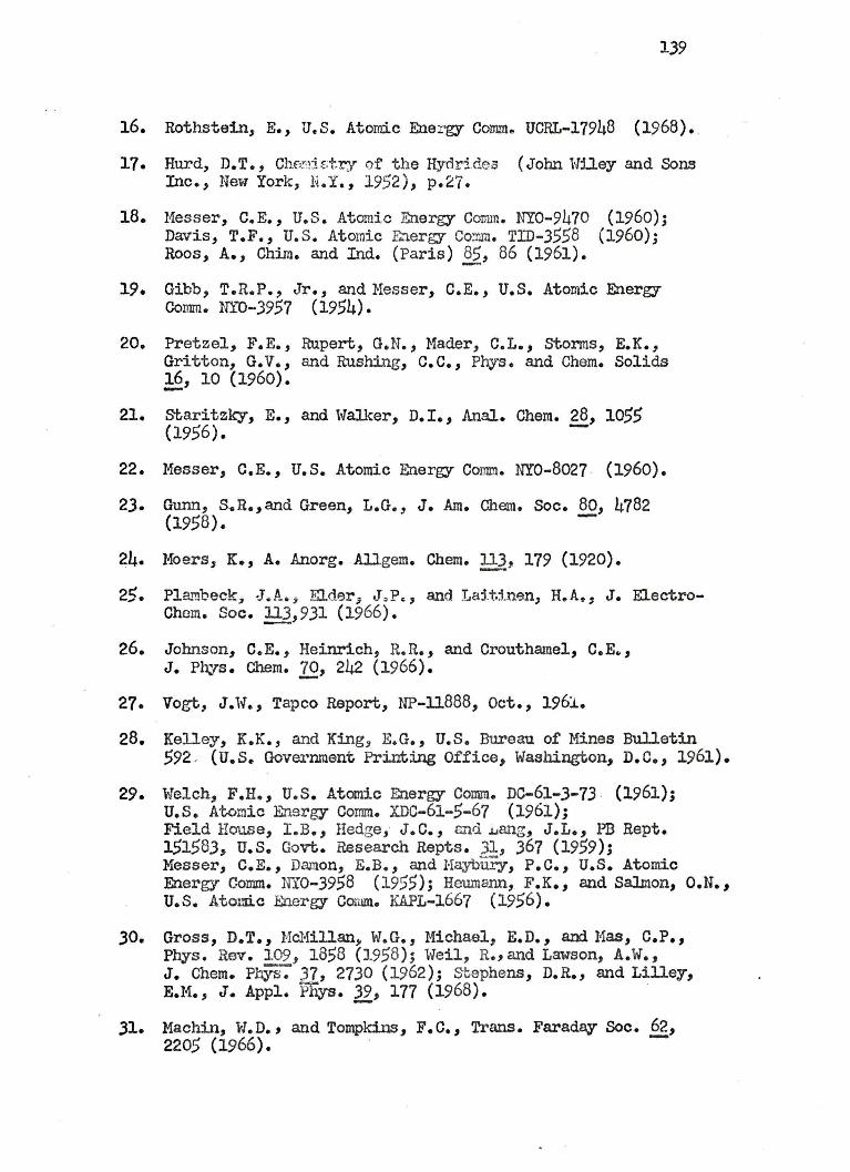
139

16. Roth.stein, E., U.S. Atomic Ener-gy Comm .. UCRL-17948 (1968).

17. Hurd, D.T., ChEw::t~try of the Hydrl.des (John Wiley and Sons Inc., New York, N.Y., 1952), p.27.

18. Messer, C.E., U.S. Atomic Energy Comm. NY0-9470 (1960); Davis, T.F., u.s. Atomic Energy COTJU. TID-3558 (1960); Roos, A., Chim. and L~d. (Paris)~' 86 (1961).

19. Gibb, T.R.P., Jr., and Messer, C.E., U.S. Atomic Energy Comm. Ni""()-3957 (1954).

20. Pretzel, F.E., Rupert, G.N., Mader, C.L., storms, E.K., Gritton, G.v., and Rushing, c.c., Phys. and Chem. Solids ~, 10 (1960).

21. staritzky, E., and Wa:Iker, D.I., Anal. Chem.~, 1055 (1956).

22. Messer, C.E., U.S. Atomic Energy Comm. NY0-8027 (1960).

23. Gunn, S.R.,and Green, L.G., J. Am. Chem. Soc. §.Q, 4782 (1958).

24. Moers, K., A. Anorg. Allgem. Chem.±!}, 179 (1920).

25. Plal'!lbeckj J.AQj Elder,. J.P., and. Laj_t.:,_nen, H.A,, J. Electro­Chem. Soc. 113,931 (1966).

26. Johnson, C.E., Heinrich, R.R. , and Crouthamel, C.E~, J. Ph:.,s. Chem. 12,, 242 (1966).

27. Vogt, J.W., Tapco Report, NP-11888, Oct., 1961.

28. Kelley, K.K., and King, E.G., U.S. Bureau of Mines Bulletin 592 - (U.S. Government Printing Office, Washington, D.c., 1961).

29. Welch, F.H., U.S. Atomic Energy Comm. DC-61-3-73 (1961); U.S. Atomic Energy Comm. XDC-61-5-67 (1961); Field House, I.B., Hedge, J.C., end .i..ang, J.L., PB Rept. 151583, U.S. Govt. Research Repts. 31, 367 (1959); Messer, C.E., Damon, E.B., and Haybury, P.C., u.s. Atomic Energy C-omm. lfi0-3958 (1955); Heumann, F.K., and Salmon, O.N., U.S. Atoud.c Energy Comm. KAPL-1667 (1956).

30. Gross, D.T., McMillan.,. W.G., Michael, E.D., am Mas, C.P., Phys. Rev. 109, 1858 (1958); Weil, R.,and Lawson, A.W., J. Chem. Phys: 37, 2730 (1962); Stephens, D.R., and Lilley, E.M., J. Appl. Phys. l,2, 177 (1968). .

31. Machin, W.D., and Tompkins, F.c., Trans. Faraday Soc.~, 2205 (1966).

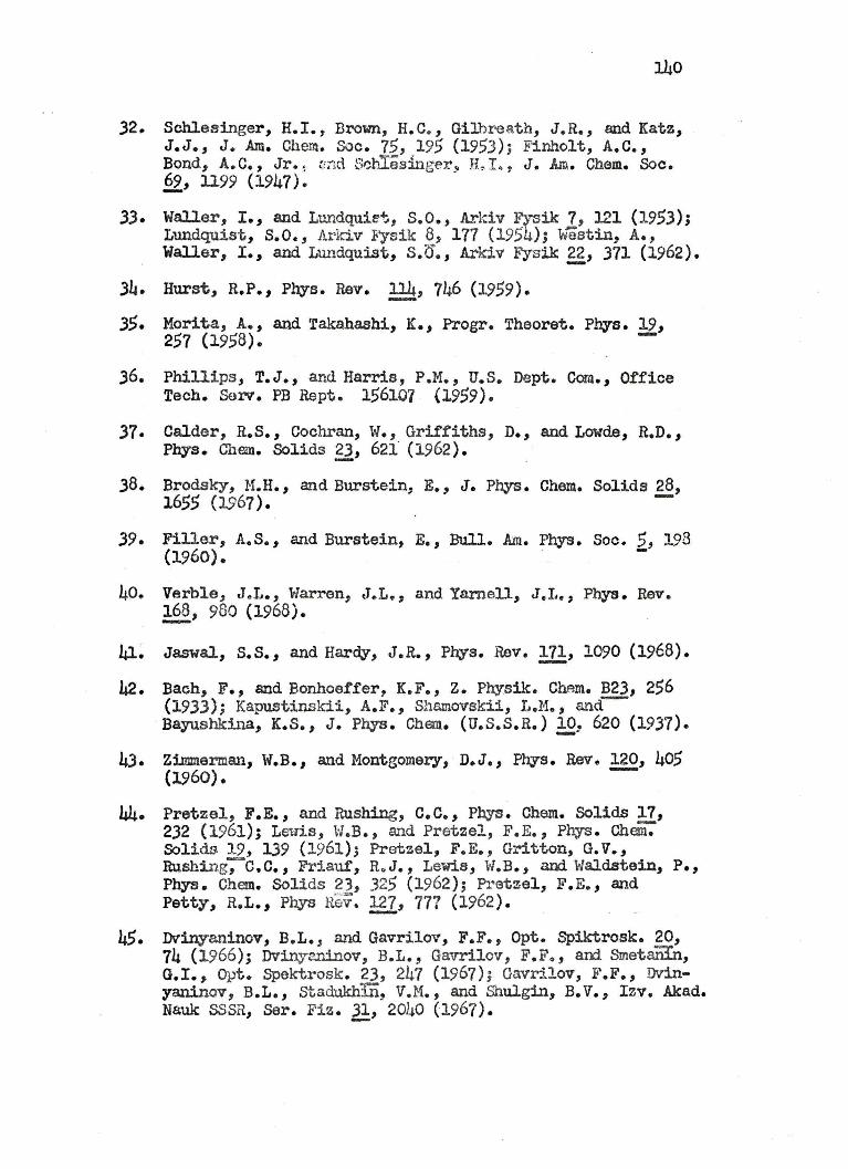
140

32. Schlesinger, H.I., Brown, H.C., Gilbreath, J.R., and Katz, J.J., J. Am. Chem. Soc. 75, 195 (1953); Finholt, A.c., Bond, A. c., Jr. 1 .;nd t1oblasinge:r.-_, H~ Lr J. Am. Chem. Soc • .22, 1199 (1947) •

.3.3. Waller, I., and Lundquiet, s.o., Arkiv fysik 7, 121 (195.3); Lundquist , S.O., Arkiv F'ysik 8, 177 (1954); woatin, A., Waller, I., and Lundquist, s.IT., Arkiv Fysik g, 371 (1962).

,34. Hurst, R.P., Phys. Rev. 114, 746 (1959). -.35. Morita., A .. , and Takahashi, K., Progr. Theoret. Phys. 19,

257 (1958). -

36. Phillips, T.J., and Harris, P.M., U.S. Dept. Com., Office Tech. Sen-. PB Rept. 156107 (1959).

37. Calder, R.S., Cochran, W., Griffiths, D., and Lowd.a, R.D., Phys. Chem. Solids Q, 621 (1962).

,38. Brodsky, M.H., and Burstein, E., J. Phys. Chem. Solids ~, 1655 (l.967) •

.39. Filler, A.s., and Burstein, E., Bull. Am. Phys. Soc. 2, 198 (1960).

40. Verble, JeL., Warren, tTeL~, and Yarnell, J.L~, Phys. Rev. 168, 980 (1968). -

41: Jaswal, s.s., and Harey, J.R., Phys. Rev. ,!I!, 1090 (1968).

42. Bach, F., and Bonhoetfer, K.F., z. Physik. Chem. B2.3, 256 (193.3); Kapuatinskii, A.F., Shsmovskii, L.M., and­Bayushkina, K.s., J. Phys. Chem. (u.s.s.R.) !Q, 620 (1937).

4.). Z:iJnmarman, W.B., and Montgomery, D.J., Phys. Rev. 120, 405 (1960). -

44.

45.

Pretzel, F.E., and Rushing, C.C., Phys . Chem. Solids 17, 232 ( 1961); Leuis, W .B. , and Pretzel, F. E. , Phys. Chem." Solids 19, 1.39 (1961); Pretzel, F.E., Gritton, G.V., Rushing-;-c.c., Friauf, RoJ., Lewis, W.B., and Wald.stein, P., Phys • Chem. Solids 2 3, 325 ( 19 62) ; Pretzel, F. E. , and Petty, R.L., Phys Hev. gz_, 777 (1962).

Dvinyaninov, B.L., and Gavrilov, F.F., Opt. Spiktrosk. 20, 74 (1966); Dvi.n,yaninov, B.L., Gavrilcv, F.Fo, ar:rl Smetanin, G.I., Opt. Spektrosk. 2.3, 247 (1967); Gavrilov, F.F., Dvin­yaninov, B.L., stadukhlri, V.M., and Shulgin, B.V., Izv. Akad. Nauk SSSR, Ser. Fiz . J!, 2040 (1967) .

46. Knipp, J.K., J. Cham. Phys.~, 300 (1936).

47. Karo , A.M.? arrl Olson, A.R., J. Chem. Phys. 30, 1232, 1241 (1959). -

48. Karo, A.M., J. Chem. Phys. ;g, 182 (1959); E , 907 (1960).

49. Ebbing, D.D., J. Chem. Phys.~' 1361 (1962).

50. Matsen, F .A., and Browne, J.C., J. Phys. Chem. ~, 2332 (1962).

51. Harris, F.E., and Taylor, H.S., Physica J.Q, 105 (1964).

52. Kahalas, S.L. , and Nesbet, R.K., J. Chem Phys. 12, 529 (1963).

53. Cade, P.E., and Huo, W.M., J. Chem. Phys. ~' 1063 (1966).

54. Cade, P.E., and Huo, W.M., J. Chem. Phys. hl,, 614 (1967).

55. Browne, J.C., and Matsen, F.A., Phys. Rev. 135, A.1227 (1964).

56. Bender, C. F., and Davidson, E.R., J. Physe Chem. ]!2, 2675 (1966).

57. Brown, R.E., and Shull, H., Int. J. Quantum Chem.~, 663 (1968 ).

58. Taylor, H.S., J. Chem. Phys • .22, 3382 (1963).

59. Csizmadia, I.G., Sutcliffe, B.T. , and Barnett, M.P., Can. J. Chem. 42 , 1645 (1964).

60. Bender, C.F., and Davidson, E.R., J. Chem. Phys. !!2, 4222 (1968 ).

61. Browne, J.C., J. Chem Phys. g, 3495 (1964).

62. Harris, F.E., J. Chem. Phys. J_g, 3 (1960).

63. Taylor, H.S., and Harris, F.E., Mol. Ph.fa. 6, 186 (1963); J. Chem. Phys.~' 2591 (1963). -

64. Michels, H.H., and Harris, F.E., J. Chem. Phys. 39, 1465 (1963). - ,

65. Schneiderman, S.B., and Michels, H.H., J. Ghem. Phys.~, 3706 (1965).

66. Michels, H.H., J. Chem. Phys.!±!!, 3834 (1966).

67. Slater, J.C., ~~tum Theor,;r of Holecules and Solids, Vol. 1 (McGraw-H:iirBook Co., Inc., New York, N.Y., 1963).

68. Kotani, M., Ohno, K., and Kaya.ma, K., Handbuch Der Physik, Vol. XXXVTI/2, Molecules II (1961), p.39-J.42.

69. Hylleraas, E.A., and Undheim, B., z. Physik 65, 159 (1930); Mac.Donald, J.K.L., Phys . Rev. 43, 830 (1933); Shull, H., and Lowd.in, P.O., Phys . Rev. l.Io, 1466 (1958).

70. Paunz, R., Alternant Molecular Orbital Method (W.B. Saunders Co., Philadelphia, Pa., 1967) .

71. Kotani, M., Amemiya, A., Ishiguro, E., and Kimura, T., Tables of Molecular Integrals . (Haruzen Co., Tokoyo, 1955).

72. Predny, R.M., Master's Thesis, University of Florida . (1968).

BIOGRAPHICAL SKETCH

Robert Michael Predny was born November 2, 1941, at

Chicago, Illinois. He graduated from Lind.bloom High School in

Jm1e, 1959. He attended the Illinois Institute of Technology

and received the degree of Bachelor of Science in June, 1963.

He was awarded a National Defense Act Fellowship from September,

J.963 through August, 1966 to continue st,udies <lt the University

of Florida. He received the degree Master of Science in March,

1968. For the school term September, 1966 through June, 1969,

he has been a teaching and a graduate research assistant in the

ryepartment of Chemist~-.

aobert Michael is married to the former Faye Marie Krause

and they have a dauehter, Robin Michelle. He is a member of

Phi Lamba Upsilon Chemical Society.

143

This dissertation was prepared under the direction

of t he chairman of the candidate's supervisory committee

and has been approved by all members o~ t.hat committee.

It was submitted to the Dean of the College of Arts and

Sciences and to the Graduate Council, and was approved

as partial f'u.l:fillment of the requirements for the degree

of Doctor of Philosophy.

August, 1969

Dean,

Dean, Graduate School

;{ . .L; I ---r .. .1 .. , .z (! '-.f_. l c, L/ - c L-

• ) , J