Bangor University DOCTOR OF PHILOSOPHY An economic ...
248
Bangor University DOCTOR OF PHILOSOPHY An economic approach to assessing the value of recreation with special reference to forest areas. Christensen, Jens Bjerregaard Award date: 1985 Awarding institution: Bangor University Link to publication General rights Copyright and moral rights for the publications made accessible in the public portal are retained by the authors and/or other copyright owners and it is a condition of accessing publications that users recognise and abide by the legal requirements associated with these rights. • Users may download and print one copy of any publication from the public portal for the purpose of private study or research. • You may not further distribute the material or use it for any profit-making activity or commercial gain • You may freely distribute the URL identifying the publication in the public portal ? Take down policy If you believe that this document breaches copyright please contact us providing details, and we will remove access to the work immediately and investigate your claim. Download date: 27. May. 2022
-
Upload
khangminh22 -
Category
Documents
-
view
3 -
download
0
Transcript of Bangor University DOCTOR OF PHILOSOPHY An economic ...

Bangor University
DOCTOR OF PHILOSOPHY
An economic approach to assessing the value of recreation with special reference toforest areas.
Christensen, Jens Bjerregaard
Award date:1985
Awarding institution:Bangor University
Link to publication
General rightsCopyright and moral rights for the publications made accessible in the public portal are retained by the authors and/or other copyright ownersand it is a condition of accessing publications that users recognise and abide by the legal requirements associated with these rights.
• Users may download and print one copy of any publication from the public portal for the purpose of private study or research. • You may not further distribute the material or use it for any profit-making activity or commercial gain • You may freely distribute the URL identifying the publication in the public portal ?
Take down policyIf you believe that this document breaches copyright please contact us providing details, and we will remove access to the work immediatelyand investigate your claim.
Download date: 27. May. 2022

AN ECONOMIC APPROACH TO ASSESSI. NG THE VALUE OF RECREATION WITH SPECIAL REFERENCE TO FOREST AREAS
Jens Rjerregaard Christensen (Cand. silv. )
Department of Forestry and Wood -
Science University College of North Wales Bangor, Gwynedd U. K.
December, 1985

ST COPY
AVAILA L
Variable print quality

ABSTRACT
Christensen, Jens Bjerregaard', 1985: An Economic Approach to Assessirv, the Value of Recreation viith Special Reference -to Forest Areas. -Unpubl. Th--. D. the-sis, University of Wales. 18jpp.
Different methods of estimating the value of recreational areas are discussed with particular attention being given to socioeconomic methods - the survey method and Clawson's method. Aspects of consumer's surplus and aggregating welfare measures have been dealt with. A-Clawson method has been applied to empirical data from a forest area in Wales and data from a region in Denmark. In the case from Wales, it was found that 73% of all visitor groups in the sample were on holiday. In addition, for many visitor groups (48%) the visit to the forest area was just one part of the day's outing. Therefore, it was considered necessary to modify the Clawson method. Problems with the weighting of points for the trip demand curve have been given considei-able attention. The data from Denmark give rise. to consideration of the problem of substitute areas and a classification system was used to select population
_zones for the Clawson analysis.
Different models for the trip demand curve have been tested and the exponential was found to be the most appropriate.
Key words: Recreation/ Consumer's surplus/ Welfare/ Clawson's method/ Weighting/ Yodels

Preface
-The work presented here has been undertaken as a Ph. D. study under the supervision of Dr. Colin Price at the Department of Forestry and Wood Science, University College of North Wales, Bangor, during the period May 197q. to January, 1982.
The work has been funded by a scholarship from the Royal Veterinary and Agricultural University, Copenhagen (J. No. A. 4-4-2-36) and a grant from the Social Science Research Council, Copenhagen (J. No. 14-1834).

TABLE OF CONTENTS
ABSTRACT PREFACE TABLE OF CONTENTS LIST OF FIGURES LIST OF TABLES LIST OF. STMBOLS
1. INTRODUCTION
1.1 General Background 1.2 Valuation of Recreation Forestry 1.3 Plan 1.4 Methods of Assessing the Economic Value of Recreation
1.4.1 Empirical Methods 1.4-1.1 Pure Economic Methods 1.4.1.2 Socioeconomic Methods
1.4.2 Normative Methods' 1.4.2.1 Rules of Thumb 1.4.2.2 Standards
1.4.3 Methods Based on Auxilliary and Substitute Values 1.5 Conclusion
2. WELFARE ECONOMICS
2.1 Consumer's Surplus 2.2 Development 2.3 The Four Consumer's Surpluses
2.3.1 Compensating Variation (CV) 2.3.2 Equivalent Variation (EV) 2.3.3 Compensating Surplus 2.3.4 Equivalent Surplus
2.4 An Evaluation of the Consumer's Surplus 2.5 Compensating Variation, 'Consumer's Surplus' or Equivalent
Variation - 2.5.1 The Hicksian Compensated Demand Curve (HCDC) 2.5.2 Willig's Approximation Formulae
2.6 Aggregation of Welfare Changes 2.6.1 Pareto Optimality 2.6.2 Kaldor - Hicks - Scitovsky Criterion 2.6.3 Little's Criterion 2.6.4 Explicit Equity Considerations
2.7 Conclusion
SOCIOECONOMIC METHODS
3.1 Survey Method 3.2 Clawson's Method
3.2.1 Problems and-Defects in the Clawson Method 3.2.2 Urban Applications 3.2.3 Homogeneity of Populations 3.2.4 Multiple Benefits
" from Trips
3.2.5 Reactiah. to Site Entrance. Fees 3.2.6 Time Bias
3 3 3 4 4 5 5 6 7 7
8 9
10 10 13 14 14 15
16 16 18 21 21 21 22 22 23
24 -27 35 36 37 37 38 40

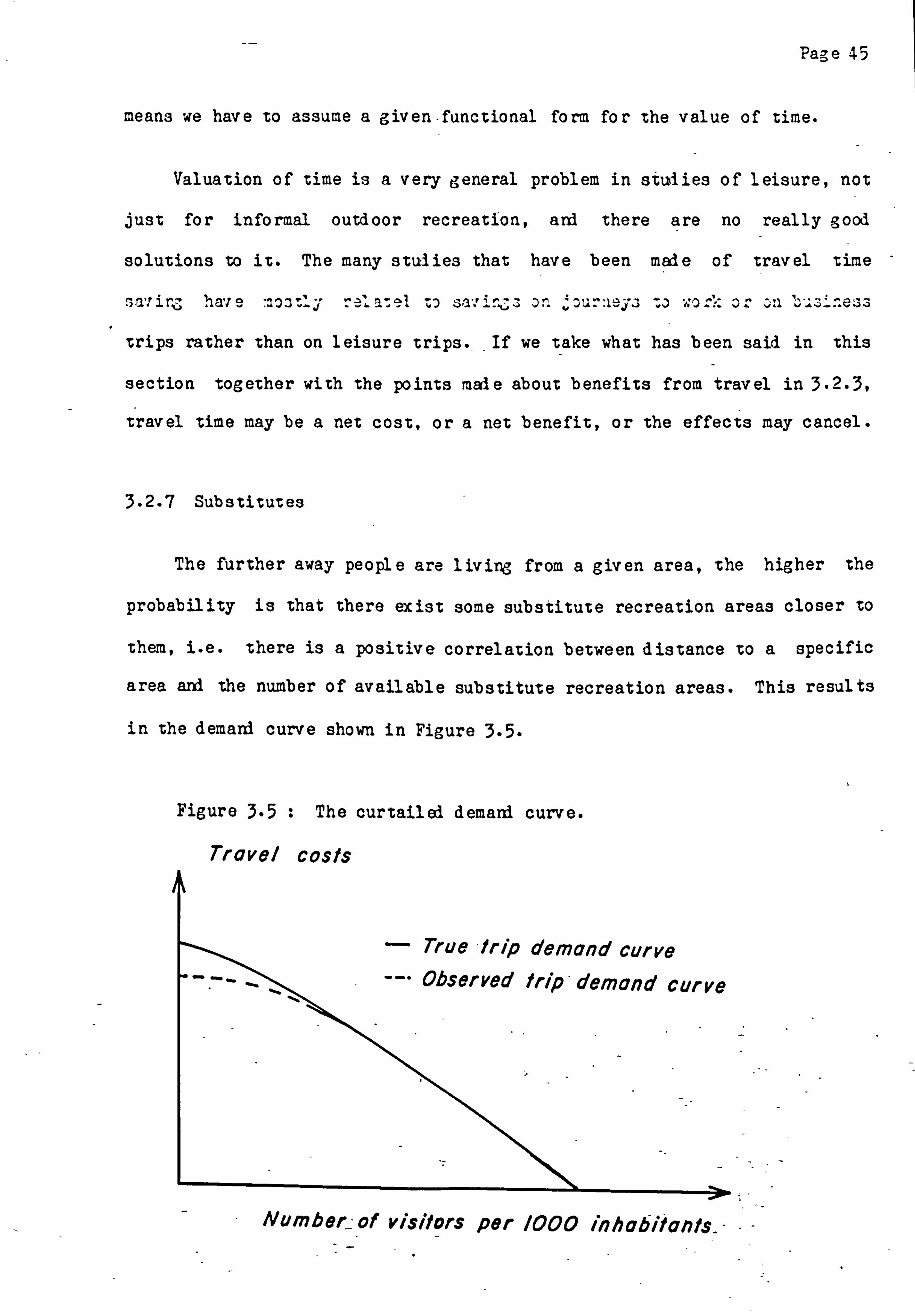
3.2.7 Substitutes 3.2-7.1 Substitutes and Attractiveness.
3.2.8 Congestion 3.2.8.1 Estimating the Value of Recreation under
Congestion 3.2.8.2 The Technique of Exclusion
3.2.9 The Functional Form of the Demand Function 3.2.10 Aggregation of Data
3.3 Conclusion
A SURVEY IN CWYDYR FOREST
45 51 53
54 56 57 58 60
4.1 Introduction 4.2 Methodology
4.2.1 The Descriptive Statistics 4.2.2 A Clawson Analysis
4.2.2.1 A Revised Clawson Method 4.2.2.1.1 Models for the Trip Demand Curve 4.2.2.1.2 Weighting of the Trip Demand Curve 4.2-2.1.3 A Comparison of the Weighting Methods 4.2.2.1.4 Bias Due tj Length of Stay 4.2-2-1.5 Zoning 4.2.2.1.6 Calculation of Consumer's Surplus 4.2-2-1.7 Fvaluation 4.2.2.1.8 Alternative Methods
4.2.2.2 A Traditional Clawson Method 4.2.2.3 The Computer Programme
4.2.3 Total Willingness to Pay_ 4.3 Results
4.3.1 The Descriptive Statistics 4.3-1.1 Stated Willingness to Pay 4.3-1.2 Estimated Running Costs for Cars
4.3.2 Results from a Clawson Analysis 4.3.2.1 Results from a Revised Clawson Method 4.3.2.2 Results from a Traditional Clawson Method
4.4 Summary of Methods and Results
THE ECONOMICS OF FORESTRY RECREATION IN A REGION OF DENMARK
5.1 Introduction 5.2 Previous Work in the Field of Forestry Recreation
Economics in Scandinavia 5.3 Project Forestry and Folk 5.4 Methodology
5.4.1 Aims of the Study 5.4.2 The Region Investigated 5.4.3 Unit of Visitation 5.4-4- Zoning Unit
- 5.4.. 5 Unit of Travel Costs 5.4.6 The Data from PFAF 5.4*7 Distances
5.4-7.1 Distances for-Visitor Groups. 5.4-7.2 Logical Distances
ý5-4.8 Weighting 5.4.9 Selecting a Model for- the Trip Demand Curve
65 66 66 67 68 73 75 79 82 86 88 94 95 98 99
100 101 101 101 105 106 106 114 117
123
123 128- 130 130 133 135 136 137 138 141 141 142 143 145

5.4.09.1 Models of Interest 145 5.4. q. 2 The Advantages of Using Fxponential Curvefits 146
5.4.10 Me thod s 148 5.4.10.1 Database 148 5.4-10.2 Clawson*Analysis 149 5.4.10.3 Computer"Programmes 150
5.5 -Results 150 5.5.1 -A Comparison of Methods 151
5.5-1.1 'Hareskoven og Jonstrup. Vang' 151 5.5.1 .2 'Jaegersborg Dyrehave og Hegn m. v.. ' 154
, 5.5.2 Comparison of the Forests 157 5.5.3 All Forests as One 162
5.6 Conclusion 163
FINAL CONCLUSIONS AND RECOMMENDATIONS
6.1 Multi-site Visits 168 6.2 Substitution Between Sites 169 6.3 Weighting of Data 171 6.4 Aggregation of Data 172 6.5 Functional Form of the Demand Regression 172 6.6 Integration of Consumer's Surplus 175 6.7 Some Outstanding Problems 175 6.8 The Evaluation of Forest Recreation 177
ACKNOWLEDGMENTS .- 179
UTERATURE CITED ISO
APPENDICES
A-3.1 Calculating Clawson's Surplus from Recreation A. 3.2 Consumer's Surplus for R, A-3.3 Mathematical Derivation of Consumer' s Surplus Measure in
Recreation A-3.4 The Value of R1 and R2 Together A-3.5 The Value of R2 when R, is closed A-3.6 The Value of R, after R2 is Introduced A-3.7 Including Cost of Time in the Evaluation of Rj- A-3.8 The Value of R1 under conditions of Excess Demand
% A-4.1 Computer Programme CLAWSON A. 4.2 Modification of Data Files
A-5.1 Comparison of Sample Estimate and Regression Estimate' % A-5.2 Computer Programme PFAFO1-FqR % A. 5.3 Computer Programme PFAF02. FOR-and PFAF03. FOR % A-5.4 Example of Output
SECONDARY APPENDICES (Stored at U. C. N. W. ) Chapter 4 Appendices begin-with 'B. ' Chapter 5 Appendices begin with"PSOF. '
%-separately bound

LIST OF FIGURES
2.1 Demand curve for-good Xi 8 2.. 2 Indifference curves -for quantity of good Xi and
- income Yi il 2.3 The Hicksian compensated demand curve 17
3.1 The investigated area 29 3.2 The trip demand curve 30 3.3 The aggregate demand curve 32 3.4 Separate demand
, curves for each zone 42
3.5 The curtailed demand curve 45 3.6 A recreation system with substitute areas 47 3.7 Aggregate demand curve for for area R2 49 3.8 Demand curves under congestion 54
4.1ý The separation of travel costs used in the revised Clawson analysis 70
4.2 Trip demand curve with negative visit rates 90 4.3 Conversion of Consumer's surplus 92 4.4 Trip demand curves disaggregated to holiday length 97
5.1 Map of North Zealand with investigated forests - marked 134a 5.2 North Zealand: Postal areas and Population Density 137a 5.3 The data from PFAF 138a 5.4 The creation of the data base 148a 5.5 An example of trip demand curves 149a 5.6 Trip_ demand and aggregate demand curves for
'Hareskovene og Jonstrup Vang' 151a

LIST OF TABLES
3.1 Data for trip demand curve for area R, 29 3--2 Data for aggregate demand curve for area R, 32 3.3 Data for trip demand curve when time costs are
included 44 3.4 Data for trip demand curve for area R2 48 3.5 Data for aggregate demand curve for area R2 48 3.6 Data for trip demand curve in the case of congestion 56
4.1 4.2 4.3 4.4 4.5 4.6 4.7 4.8 4.9 4.10 4.11 4.12 4.13 4.14 4.15 4.16 4.17 4.18 4.19 4.20 4.21 4.22 4.23 4.24
5.1 5.2 5.3
5.4
5.5 5.6
Distribution of interviews to sites Length of stay in forest Starting point distances and home point distances A comparison of weighting methods Predicted number of visitor groups Conversion of length of stay to hours Average travel costs for zones Zoning system for visitors to Gwydyr Distribution of holiday length Grouped holiday length Distribution of prompts on sites Points for the trip demand curve Results from CLAW2 Number of visitor groups distributed Results from CLAW6 Results from CLAW15 and CLAW15B Equidistant zoning system Average travel costs with equidistani Results from CLAW17 Points for the trip demand curve Results from CLAW14 Results from CLAW18 Rezoned zoning system Results from CLAW19
Forest
to zones
zoning
The investigated forests Postal areas and number of households Consumer's surplus for 'Hareskovene og Jonstrup Vang' Consumer's surplus for 'Jaegersborg Dyrehave og Hegn Move I Consumer's surplus for all forests investigated Consumer's surplus for 'all forests as one'
65 68 71 79 80 85 86 83 96 96
102 107 107 a 109 112a 112b 113 114 114a 115 11 5a i 15b 116 l16a
133a 136a
150a
154a 157a-e 162a

LIST OF SYMBOLS
A, B, C, D Population -zones (centres)
ci, cij, ci Travel costs (for visitor group j) from zone i CM Travel costs per mile CS Consumer's surplus
CSI CS on individuals CSP CS per predicted visitor group CSR CS regulated to observed no. of visitor groups CSZ CS on zone basis
CV Compensating variation Di Distance from zone i
DI ij distance from home to the recreation area
D2 ij distance from home to the startpoint for the day
D3 ij distance from startpoint for the day to the
EV EW f F G HCDC 1 L M max
recreation area (for visitor rroup j in zone i) Equivalent variation Expected value of x function Attractiveness of recreation centre Attractiveness of population centre Hicks' compensated demand curve Length of stay Length of holiday Number of recreation sites Maximum max D4 maximum distance to any zone, i. e. the furthest away
n
N ODC ovg p PFAF pv9 q Q ri Ri, R t rj3 T v v Var(x) y
Number of visitors, visitor groups Income elasticity of demand Population Ordinary demand curve Observed number of visitor groups Price, entrance fee Project Forest and Folk Predicted number of visitor groups Quantity, number of visitorsl visitor groups Number of predicted visitor groups Distance f rom zone i to R, Recreational areas Travel costs at distance. ri Time costs Individual's visit rate Population's visit rate Variance of x Income

1. INTRODUCTION
11 General Background
During the last two decades, researchers and planners have become
increasingly interested in multiple use forestry. Forest areas have always
produced a variety of products such as timber, fuelwocxi, forage. game,
grazing etc. although the importance of each of these products has
changed over time The problem now is a growing demand for the
production' of additional goods, especially forestry recreation. This
good is not priced in the normal market system and hence no commercial
value has been put on it. This has become a problem as the demand for
recreation grows with the steady increase in leisure time, income and
thereby. mobility. In order to estimate the level of supply which should
be aimed for, it is first necessary to estimate the value of recreation.
In Denmark. the yearly number of forest visits has been estimatel at 100 -
150 million (Koch 1978) which "irdicates that the recreational value of
woods in Denmark is far above the value as a production factor of trees"
(Groes 1979). It is, therefore, important to find methods which can be
used in a planning process to optimise the mix of outputs from forest areas
in order to maximise social welfare and, thereby, hopefully minimise
conflicts between different groups of interest.
1.2 Valuation of Recreation Forestry
To be able to make a thorough valuation of recreation forestry, one
need s to know about the costs ard benefits that accrue from providing the
good, recreation. Of these two items, the benefits are the more difficult

? a, - e
to measure, as in that case we are trying to measure the value of a-good
which is not priced in the normal market system. The cost side is somewhat
easier to estimate as we can get the direct costs of proviiing certain
goods such as picnic places. etc. We can also find the opportunity costs
from either not growing any trees in a particular area or only growing
hardwoods where conifers would be the more profitable. Thus, the cost side
is not too difficult to handle and there are several works from Scardinavia
which do exactly that : measure the opportunity costs of providing certain
facilities to the public (See 5-2). The opportunity cost can be calculated
as - the net present value under optimum private management minus the net
present value given the restrictions proposed. This measure would be
appropriate for a negotiation with the government concerning coapensation
for restrictions put on forestry under private management. However. this
work is concerned with how the government initially decides that it wants
to put certain restrictions on forest use or perhaps rather to provide
certain facilities to the public. This means that, in addition to the
previously mentioned opportunity costs we have to provide the decision
makers with a measure for the benefits of a particular plan. Combining
these two measures will then give an estimate for the changes in social
welfare due to a given plan.
Therefore the purpose of this work is to explain the concepts behind
welfare economics and various methods for estimating recreation benefits.
to try to solve some of the problems occurring. when applying the methods to
empirical data.

Fave Z)
1 .3 Plan
A short outline for the thesis is-
Chapter I- An introduction to the methods of- evaluating recreation
economics.
Chapter 2- On welfare economics the theory behind consumer's surplus and
the aggregation of welfare will be dealt with.
Chapter 3 Socioeconomic methods - the survey method and Clawson's method
are discussed.
Chapter 4: A Clawson method is applied to data from a forest area (Gwydyr
Forest) in Snowdonia. A revised model of the method is developed.
Chapter 5: Economics of recreation in a region of Denmark - in addition to
a literature review of previous works in Scaniinavia. a Clawson analysis is
carried out on forests in North Zealand.
Chapter 6i Final conclusions and recommendations for further research.
1.4 Methods of Assessingg the Economic Value of Recreation.
In this section a brief summary will be given of the methods which
hav e been most commonly employed when evaluating recreation. The
systematization has been adopted from Gundermann 0976)
1.4.1 Empirical Methods
Empirical methods are those ýihich use data obtained by analy8ing a*
particular area. They can be divided into pure -economic methods and
socioeconomic methods.

Page 4
1.4.1.1 Pure Economic Methois
The most important-of these is the 'opportunity cost method' which
finds the _cost
of providing certain recreational facilities to the public.
This has been the method most often used in Scandinavia (See 5.2) which c. Rn
probably be explaine4 by the close relationship between the forestry
education and the private forestry sector in these countries. However as
pointed out in Section, 1 3. this method does not provide a guide for
selection among alternatives as it considers only the cost of providing,
facilities.
1.4.1.2 Socioeconomic XethoO. s
Socioeconomic methods attempt to measure the benefits to society, i. e.
the changes in welfare, according to a given project The most important
of these methods are the 'survey method' ard 'Clawson's zone method'. Both
have a measure of consumer's surplus as a base which is discussed more
fully in Chapter 2. The survey method is based on a questionnaire or an
interview which attempts to reveal people's willingness to pay for the good
while the Clawson method derives the same thing from people's behaviour.
The result from both methods is a demand curve from which the consumer's
surplus can be calculated. The two methods are explained and discussed in
Chapter
Another socioeconomic method is the 'gross expenditure method' which
measures the benefits from recreation as the total costs incurred by the
useris, including both travel and on-site costs. "the justification for
this approach is that these costs must represent at least a lower bound to
the value the recreationist places on the activity for otherwise -if it was

? age 5 -- I
worth less than these costs to him, he would not undertake it. - This
argument is valid as far as it goes. but it does not go far enough
(Binkley 1977). The gross expenliture method is considered unacceptable as
it is "the margin above the cost of taking advantage of the recreation
opportunity which measures the real monetary value that would be lost, if
the recreation opportunity -were
not available" (Clawson ard Knetsch 1966.
p. 225). A fourth socioeconomic method is the 'property value method' in
which an attempt is made to relate property value as a function of distance
from the recreational area. The method-has several shortcomings, which are
reviewed in Price (1978). and it is not considered useful in this case
For recreation evaluation in urban areas. where travel distances are
shorter, this method may be mora useful.
1 . 4.2 Normative Methods
-- '-'The concept of normative methods includes assessments realized on the
basis of uniformly predetermined standard values or rules of thumb"
(Gundermann 1976).
1.4 2.1 Rules. of Th=b
The most simple normative method is the one referred to as the 'Cost
method' (Clawson ani Knetsch 1966). The method was popular in the 1950's
and assumes that the value of an outdoor recreation resource is equal to
the- cost of generating it or even. in some case to a multiple of that
(Ibid., P. 225).

Page
The method is quite unacceptable, as it automatically justifies any
project and it does not provide a guide for ranking alternatives except in
that the most expensive one is the best
Another normative method is the 'market value of fish method' where it
is assumed that the value of sport fishery equals the market value of the
fish caught (Crutchfield 1962). He. himself, points out the major
objection to this method the fact that it is implied that obtaining meat
is the objective of angling He goes on to conclule "in another sense.
however, the commercial value of the sport catch could legitimately be
regaried as a minimum estimate"(Ibid., p. 150). This might not be true in
some cases.
1.4.2.2 Standards
The normative method called the 'market value method' is probably the
most common and has often been used in the Unite4 States by Federal
agencies. It consists of attributing certain predetermined values per
visit or per recreation day. Then the attributed value multiplied by the
attendance can be used as an estimate for the value of the site The
chosen value is normally related to prices charged at privately ownel
recreation areas, but it is "precisely because private areas are not fully
comparable with public areas that users are willing to pay fees or charges"
(Clawson and Knetsch 1966. P. 227). Furthermore, the value found in this way
might vary quite considerably from the consumer's surplus measure as' it
must be assumed that a private owner tends to maximise profit-.

Pag e7
1.4.3 Methods Based on Auxilliary ani Substitutive Values.
One of the most interesting methods in this group is that of 11jew ani
Gordienko (1973)1 . who have found a relationship between enhancement of
man's working capacity and recreation. They found an annual increase in an
in(lividual's working capacity of about 3 percent.
In some woeics, simple scaling methods in non-economic terms have been
applied (Helliwell 1969)
1.5 Conclusion
It is the author's belief that the way to proceed is by using the
socioeconomic methods (either the survey or the Clawson method) because
they measure the contribution to social welfare in a way which is both
commensurate with other economic values, ard compatible with the theory of
welfare economics. They will. with further- refinements. provide -a
reasonable tool for ranking public alternatives. Nevertheless. there are
many difficulties. Pirst is the dispute in welfare economics about the
interpretation of consumer's surplus, how it is to be measured, and how to
aggregate consumer' surplus for different individuals. This is the subject
of Chapter 2. The reader who is familiar with this debate can proceed
directly to Chapter 3- In that chapter will be examined the many problems
that have been identified in the theory ard apilication of -the survey and
Clawson methods*" Some of the attempts to solve these problems will be
discussed, and the contribution which this thesis hopes to make will be
outlined.
I Here from Gund ermann (1976).

I
2. WELFARE ECONOMICS
2.1 Consumer's Surplus
The Clawson method as well as all other socioeconomic methods which
are used to estimate the benefits 4erivel from recreational areas. is base4
on consumer's surplus measurements. Consumer's surplus can be describel as
the difference between what people are willing to pay for a good ard what
they actually do pay. Figure 2.1 shows the dernaril curve for a good. Xil
For a given price, pl. people will buy a quantity q, of good Xi - The
shaded area in the Figure is equal to the consumer's surplus and can be
interpreted as the contribution to increase in social welfare by
introducing that good.
-Figure 2.1 : Demard curve for good X
Price
Pl
The consumer's surplus measure is a crucial concept in cost-benefit
calculations bezause " for all except marginal changes in the amount of a
good, the, market price prevailing in a perfectly competitive setting is an
inadequate index for the value of a good. " (Mishan 1975, p. 24).
q1 quantity

Page 9
Unfortunately, however. it is very difficult to estimate cons-amer's
surplus because the 3hape of the demard curve for most gools is either
unknown or known only for a small area around the established market price.
Probably because of that. most manuals for cost-benefit analysis of
projects do not use the consumer Is surplus concept but have other measures
as numeraire (Little ard Mirrlees 1974; UNIDO 1972; Squire and van der
Tak 1975). Little, in fact, goes so far as to say that consumer's surplus
is a totally useless theoretical toy (Little 1957, p-180). Nevertheless,
in the evaluation of recreational facilities, the consumer's surplus is a
convenient tool ard it is usei throughout this stuiy.
" Consumer's surplus " is a somewhat ambiguous term itself although
other commonly usel terms have evolvel from it. Therefore. the remainler
of this Chapter is concernel with the development ani the concept of
consumer*s surplus.
2.2 Development
Dupuit (1844) first described the notion which Marshall (1924)
referred to as consumer's surplus : ".... he thus derives from a purchase a
surplus of satisfaction. The e%cess of the price he would be willing to
pay, rather than go without the thing, over that which he actually does
pay, is the economic measure of this surplus of satisfaction It may be
called consumer's surplus " (Marshall 1924. p. 124)
In addition to baptising the concept, Marshall gave the very important
qualification that the accuracy of the above measure requires the ma rg inal.
util; ty of income to -be constant. The topic was examined by Hicks and . he
statel

Pace 10 zý
"... the best way of looking at consumer's surplus is to rep,, ard it as a
means of expressing in terms of income. the gain which accrues to the
consumer as a result of a fall in price. Or better. it is the compensating 0
variation in income, whose loss would just offset the fall in price and
leave the consumer no better off than before " (Hicks 1946, P. 40)
Herderson (1941 ) pointed out that the definitions above differ in the
sense that the Marshallian definition does not allow quantity aijustments
while the latter does. After this comment Hicks reconsiierei the whole
problem ani defined four different consumer's surpluses (Hicks 1943).
These four measures. viz. compensating variation, equivalent
variation. compensatizig surplus, ard equivalent surplus are explainel below
by using irdifference curves. In a later section, the concept off the
Marshallian demand curve adjusted for income effects will be discussed.
2.3 The Four Consumer's Surpluses
2.3.1 Compensating Variation (CV)
This measure was introduced by Hicks 0939) ard as quoted in Section
2-2. it is, for a price fall. the loss of income which would just offset
the fall in price. leaving the consumer no better off than before. For a
price increase. -the compensating variation is. of course, the increase in
income which will maintain the consumer's utility level.
The compensating variation is illustrated graphically in Figure 2.2,
with the aid of indifference curves. The horizontal axis refers to the
holding of a- good Xi and the vertical axis to the income Yi (or all other
*

? age
"X goods) Each indifference curve represents combinations of amounts of I
ard income Yi which provide equal utility for the indiviAual in question.
For example. the points A and B on curve I, provide equal utility. Points
C and D on curve 12 provide equal utility as well but at a higher level
than provided ýby A or B.
Figure 2.2 - Indifference curves for quantity of good Xi and income Y,
Income
Y4 Y2
YO
Y3 Yl
xxxx Ouonlity of good, X ADBci
Consider Yo as the individual's initial income when the good Xi has a
given price structure p 11 Then, b, is the iniividual's budget line for
income Yo and quantity of Xi In order to maximise his utility, the
individual will buy the amount XA Of Xj, that is the amount corresponding
to the point A where an indifference curve just touches the budget line.
If the price for the good. Xi, is lowered t3 a new price structure. P2' it
follows that the individual now can buy corresponding to line b2_ and - that
he - will be able to reach a higher utility level, i. e. the point C on the
? age I'; '
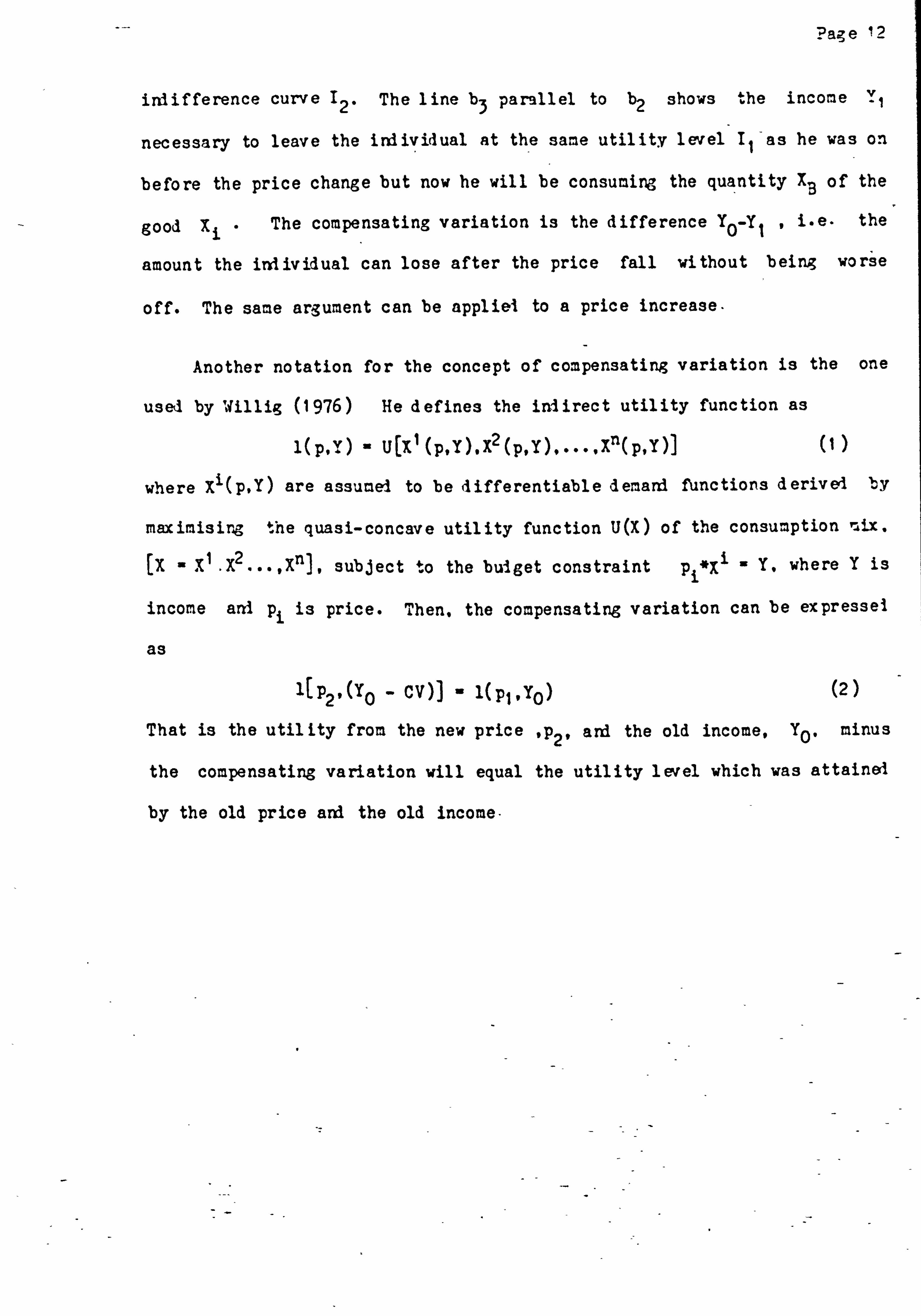
irdifference curve 1 2, The 1 ine b3 parallel to b2 shows the income Y,
necessary to leave the irdiviiual at the same utility level 11-as he was on
before the price change but now he will be consuming the quantity XB of the
good Xi The compensating variation is the difference YO-Y, v i. e. the
amount the indivOual can lose after the price fall without being worse
off. The same argument can be appliei to a price increase.
Another notation for the concept of compensating variation is the one
usel by Willig (1976) He defines the iMirect utility function as
.)_ U(XI(p, y). X2(p, y),..., Xn(p, y)] 0 , (P, v
where Xi(p, Y) are assumei to be differentiable demani functions deriveri by
maximising the quasi-concave utility function U(X) of the consumption mix.
[X . yI. X2..., Xn], subject to the bulget constraint p, *Xi - Y, where Y is
income ard pi is price. Then. the compensating variation can be expressei
as
'ýPV(YO - CV)] - l(PIIYO) (2)
That is the utility from the new price p 2' and the old income, YO. minus
the compensating variation will equal the utility level which was attainei
by the old price ard the old income-

Page 13
2.3 2 Equivalent Variation (EV)
This measure can be defined as " the gain in income which. - if
experiencel without the price falling, would make the consumer as much .I
better off, as he is maie by the fall in price without any change in money
income. " (Hicks 1943. p. 34-35). The opposite can, of course. be applied for
a price increase
This measure can also be explained with the aid of Figure 2.2 - if
the price was lowerel to p2, then the inlividual wou14 be able to increase
his utility to level 1 2' consuminp,, the amount correspording to point C,
i-e quantity IC. With the prevailing price . he must have an income Y2
to reach the same utility. Line N is Darallel to line b, ani the
inlividual maximises his utility at point D where b4 is tangent to 12 *
The difference, Y2 - YO is the equivalent variation or the sum that must be
given to the consumer to leave him as well off as if there had been a price
change from p, to P2 without any change in income.
Using the same notation as in 2.3-1, we can express the equivalent
variation as*
l[Pj9(YO + EV)] - '(P21YO) (3)
Here. too, the opposite argument can be applied to a price increase. The
equivalent variation for a price increase vill have the same consequence as
a confiscation of the income difference Y0- Yj or equal to the
compensating variation for a price decrease from pl, i. e., the inc ome which
consumers at C -are willing to- forgo _in
order to avoid the price -increase to
P, is equal to the sum we can confiscate from consumers at A if -we lower
the Price to p2
1- This- is easily seen by changing (3) to the qquivalent variation- from a price income from p2 to p, . which compared vith--(2) gives EV - C_V.

Page 14
2 2-3.3 Compensating Surplus
Compensating, surplus is the amount O'f compensation, paid or
received. that will leave the consumer in his initial welfare position
following the change in pri ce. if he is constrained to buy at the new price
in the absence of compensation " (Currie et al. 1971. p. 746).
From Figure 2.2 we can see that after a fall in price from the
initial price, pl. at point A to price P29 the individual will buy an
amount XC correspording to point C In oider to buy the amount Xr, ard
keep the welfare he previously had, the irdividual now only needs an income
equal to Y3. The difference YO -Y3 is the compensating surplus or. in
this case. the amount that we can confiscate leaving the consumer at the
same ut -ility level as before the price decrease. 'For a fall in price the
compensating C3. g surplus is always less than the compensating variation.
2.3-4. Equivalent Surplus 3
" Equivalent surplus is the amount of compensation, paid or received,
that will leave the consumer in his subsequent welfare position in the
absence of the price change. if he is constrained to buy at the old price
the quantity he would have bought at that price in the absence of
compensation " (Ibid p. 746)
In Figure 2 2, the equivalent surplus is the sum equal to AF, i. e. -, _
Y4- YO, because if the price had fallen to p2, _
the individual could have
ýeached the utility level 12. In order to let him reach that level and
2 Hicks called this the quantitycompensating variation. 3. The measure is what Hicks called the quantity equivalent variation.
I

Page 15
still consume the same quantity, he neels an income. Y 4. For a price fall,
this measure is bigger than the equivalent variation.
2.4 An Evaluation of the Consumer's Surpluses
Hicks (1943) shows that a fall in price implies - compensating
surplus < compensating -variation < -equivalent variation <_ equivalent
surplus.
But which of these measures should then be used ?
Mishan (1948) argues that out of these five measures 4.
only two can be
usel the compensating variation ard equivalent variation The
compensating surplus and equivalent surplus are unjustifie4 as they
Is allow people to consume at an other than optimal level. That is. the
compensating surplus is calculated in point E (Figure 2.2). However,
consuming less of the good. X, wi_th -the same income could bring more
satisfaction to the consumer. The consumer should consume where the budget
line is tangent to an indifference curve. Freeman (1979, p-37) states that
the compensating surplus and equivalent surplus measures are too
restrictive in their assumptions to be useful. " So most authors have
accepted that the discussion must be between the use of compensating
variation, equivalent variation or simply the area under the Marshallian
demand curve -which, in Section 2-5.1 will be shown to -lie
between these
two measures (Dwyer et al. 1977- Gordon and Knetsch 1979 Bockstael
and McConnell 1980).
4- A fifth measure was Suggested by Knight 944)

Paz, e
Mi shan (1975)_ argues that the basic concept 'by reference to -which
gains and losses are to be estimatel is the compensating variation.
However. in a later paper. (flishan-1976) he states that the equivalent*
variation (EV) concept is. _no
less- -. a valid basis than the compensating
variation (CV) concept for cost benefit analysis. Thus, the7 choice must
depend upon what the measure is to be used for because " we can equal
willingness to pay to compensating variation for price decreases and to
equivalent variation for price increases. Similarly, willingness to sell
is equivalent variation for price decreases and compensating variation for
price increases " (Bockstael and McConnell op. cit., D-56).
2.5 Compensating Variation.
Variation ?-
Consumer's . Surplus or Equivalent
2.5.1 The Hicksian Compensated Demand Curve (HCDC)
This section deals with the relationship between the area under the
ordinary demand curve (in the following called consumer's surplus) and the
compensating variation and the equivalent variation. respectively.
The ordinary demand curve (ODC), or the Marshallian demand curve.
gives the quantity/price relationship for a given income. The HCDC curve
gives the quantity/price relationship assuming, that income is adjusted
according to ihe initial indifference curve.
/
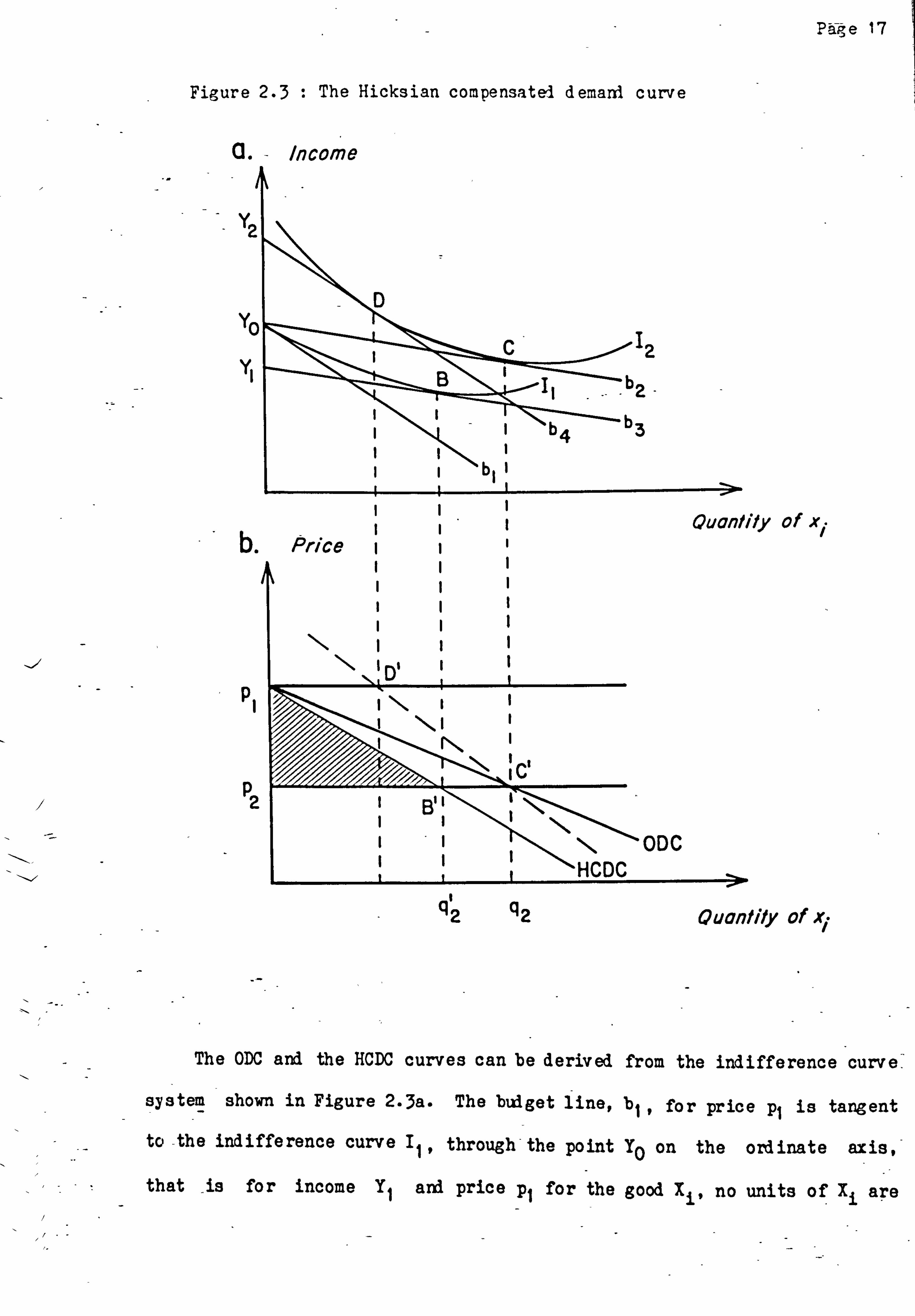
Figure 2.3 : The Hicksian compensatel demaril curve
Cl. - Income
/
Y( Y,
Price
Pl
P2
q2 q2
Pbage 17 1
Ouonlily of xi
Ouantity of xi
The ODC and the HCDC curves can be derived from the indifference curve-
system shown in Figure 2.3a. The budget line, bi , for price pi is tarigent
to-the indifference curve I,. through-the point Yo on the ordinate axis, -
that -is
for income Yj and price p, for the good Xi, no units of Xi are

? ae ie
bought. If the price is lowered to p2. the consumer buys q2- units, i. e.
he is consuming at point C where the line b2 is-tangent to the inlifference
curve 12. If the consumer's income is adjusted so that he maintains the
utility level previous to the price decrease (i. e. lowering the income
Y Oy confiscating the compensating variation) then he buys less units - in.
this case. q2' units. It is shown . by Hicks 0 956) that the shad ed area
P1 P2B' in Figure 2-3b is equal to the amount YO - Y, , i. e. a measure for
the compensating-variation.
CDC curve fro= The equivalent variation can be found by deriving the H.
the indifference curve which the consumer would have reacherl following a
price change, anl finally, integrating the area under thp curve arti between
the two i)rice lines. In Figure 2-3b the equivalent variation for a price
decrease from p, to P2 is the area piD'. C'p2. Figure 2.3b also shows that
the consumer's surplus unier the ODC is to be found somewhere between the
compensating, variation and the equivalent variation.
It is evident that if the income effect is zero (indifference curves
are parallel) then the ODC curve and the HCDC curves will coincide and all
three measures will yield the same result.
2 5.2 Willig's Approximation Formulae
As shown in the previous section, _ an exact measure of welfare changes
requiresl knowledge about the compensated demand curves, i. e. we need to
know the marginal utility of money so that we can derive 'the compensated
demand curve from the demand curve observed in the market in question.

Page 19
But willig (1976; 1979) provides formulae for upper and lower limits on
the perc-entage error of approximating the compensating variation and
equivalent variation-with consumqr's surplus. His to result implies that
consumer's surplus is usually a very good approximation to the appropriate
welfare measures. " 0976 P-589). In addition to giving the exact formulae.
I Willig offers rules of thumb which can be used when the following-
conclitions are met :
if C-S/2'/. l 1ý-: 0.05
Z 7.. ' 1 --4- 0-0
and C-Sly. <0-9
V- C- S then:
and 7 LC S 14 CS - EV Z_-: z
ý
Tc- s1 2710 where!
CS = consumer's- surplus under the ord_inary . demard curve and
between the two prices in question
CV = the compensating variation corresponding to the price change
EV - the equivalent variation corresponling to the price change
YO the consumer's base income.
41 the largest income elasticity ot demand in the area.
the smallest income elasticity of demand in the area.
These results have been used to justify the use of consumer's surplus
as the correct welfare measure. Dwyer et al. (1977) states ifsing the
area under the demard curve (the ODC)5 as an approximation of willingness
of. users to pay is satisfactory only under certain conditions, but these
conditions are almost always met for- the_. recreation_ output- of resource
management alternatives "(Ibid., p. 11
5. My pomment

Pa --I e 2)
Freeman (1979) also argues in favour of thi: 5 approximation - ani says
that " the differences among the measures appear to be small and almost
trivial for most realistic cases "(Ibid., p. 47)
Bockstael and McConnell (1980) argue that although " Willig's results
are unquestionably correct, they are not a panacea for applied resource
economists for a number of reasons "(Ibid., p. 59). Their ar, 3ument is,
basically, that resource economy is often concerned not with small price
changes but rather with the provision or elimination of a resource and
therefore often large CS or values. Furthermore. they show that
often Willig's bounds are nonexistent.
Explicit estimations of compensating variation or equivalent variation
using Willig's formulae have not, to this author's kn. owlelgei' been
publi3hed. However some authors (Hammack ard Brown 1974 ; Banforl et al.
1977) have found considerable difference between compensating variation and
equivalent variation. They have used the survey method and this may be the
reason why the difference has occurred. This will be discussed later in
Section 3.1 on the survey method.

I
2.6 Aggregation of Welfare Changes
Paiz e 21 1
According to Freeman (1979) there are basically four different ways in
which we can aggregate the changes in social welfare_due to a certain 6
project. _ They will be described briefly in the following
2.6.1 Pareto Optimality
The traditional criterion in welfare economics is the Pareto criterion
which states that no policy shall be accepted unless at least one person is
made better off and no individual is made worse off. By this strictness,
the criterion is the rule of 'unanimity'. The unanimity rule is clearly
unexceptionable; the real problem is that it hardly, - if eveir, has
relevence to actual decision making processes (Dasgupta ard Pearce 1978)
and in situations where some individuals prefer state x to state y and
others prefer state y to state x, the criterion does not offer any guidance
to decision makers.
2.6.2 Kaldor-Hicks-Scitovsky Criterion
Kaldor (1939) exterded the Pareto criterion to situations in which
people both benefited and lost. He stated it to be an improvement if those
who benefited were so much better off that they could- afford to compensate
the losers and yet-still be in a better position-than before-the change.
This compensation principle that Kaldor described was slightly changed by
Hicks 0939) who pointed out the contradiction that in-some cases A would
6. For a thorough discussion see Price 0 978)., Sugden -(1981 and Mishan (1960).

Page 22
be better off than B ard also that B would be better off than A. He,
therefore. suggested a more negative criterion! that the 'losers' should
not be able to compensate- the 'gainers' ard still be better off than they
would have been after the change. Scitovsky (1941-2) showed that both
Kaldor's and Hicks' conditions need to be met if a change should be
declared to be an improvement This is known as the Kaldor-Hicks-Scitovsky
criterion.
2.6.3 Little's Criterion
Price (1978) points out that by accepting the personal assessment of
changes in utility in money terms, the cconomist accepts that the
distribution of income is satisfactory. Little (1957) was aware of this
and suggestel a criterion in which in order to be acceptei, a project hal
to both pass the Kaldor-Hicks-Scitovsky criterion and to improve the
distribution of- income. Al though this criterion focuses on the
distributional problem. it is not very operational as it does not offer anY
suggestions for how to measure whether one distribution is better than
another.
2.6.4 Explicit Equity Considerations
Little's criterion is of limited use as it does not quantify the
-distributional effects (Pearce ard Nash 1981 Therefore, the newest
approach is to make a specific social judgement regarding - equity and to
introduce equity considerations systematically in the evaluation of social
policy. The most common way to do this is to introduce - weights to the
individual welfare changes, e. g. explicitly to weight income according to

Page 23
the income group to which it accrues (Squire ard Van der Tak 1975).
2.7 Conclusion
The previous sections of this chapter have shown that the appropriate
measure for estimating the benefits or co sts is either the compensating
variation or the equivalent variation. However. the question of how to
quantify these measures remains unanswered. It does not seem suitable
simply to rely on Willig's approximations and it may be that the survey
method to be discussed in the next chapter will prove to be a useful
alternative methol.
Concerning which of the measures. compensating or equivalent
variation, to use, it is interesting to add as a comment to section 2.4
that by introducing a new recreational area, the equivalent variation
measure could be used as a mesure for the benefits. This would certainly
give a higher value than obtained from the compensating variation measure
and the justification should be that the opening of the park is a
reestablishment of human rights to nature or, as Mishan 0976) states
The pro-environmental economist would, of course. like to use the CV
test in order to defer projects that destroy amenity and to use the EV in
order to encourage projects that create amenity. And it is interesting to
reflect that he could in effect have it both - ways in a society that
recognized constitutional amenity rights for its citizens covering a
s- pecific range of environmental goods. "(Ibid P-195).

SOCIOECONOMIC METHODS-
3.1 Survey lelethod
Survey method, in the context of this study. is understood to mean th, e
estimation of the demanI for a recreational facility through non-market
means such as surveys, questionnaires bidding games ani voting. Freeman
(1979) gives three approaches to the problem of revealirLa, consumer's
preferences' -
Get people to state their willingness to pay (for a given quantity of
consumption) -
, iv en , ood they would demani at Get people to state how much of a-a
price.
Get people to vote on alternative programmes.
Approach 1 has been usei for estimating recreational benefits (Davis
1963; Hammack and Brown 1974). The problems when applying the surVey
method are - can people assign a value? aid can people be induced
directly or indirectly to reveal their preferences without behaving
strategically?
These problems have been investigated theoretically by several authors
and methods which should induce people to give 'honest' answers have been
suggested (Bohm 1971 ; TO eman 1972; Kurz 1974). Bohm (1972 ) tested five
different approaches tied to a paymenf scheme to reveal stated willingness
to pay and found no significant differences between the methods, 'A six ih
I The approach will be interpreted here as both willingness to pay and willirgness to sell.

Page 25
approach which did not involve any payment was however. significantly
different from the others. In that I one, people werre oimply askei to
estimate their maximum willingness to - pay. Bohn concluiel that -"this -
result may be seen as still another reason to doubt the useýfulness of
responses to hypothetical -questions, in general-... lt (Ibid., p. 125) ard- he
conclules that if questions are asked with "counters trateg ic " arguments, 0
people do not use to cheating strategies to - He suggests that two approaches
should be used - one which can be expected to produce an overstatement and
one which will give an understatement - in order to get an interval for the CO
willingness to pay. This work has later been critisised by Vaux and
Williams (1977) for-
1. its relatively small sample size.
2. the relatively small sums of money involved, and
3 the fact that the experimental proceiures may have biasei the
participants' responses in a crucial way (Ibid.. p. 496).
Davis (1963) used a bidding game technique where the initial value
was determined by the distance people had to come. Brookshire et al.
976) also used a bidding game technique and found that ". it is important
to note that the two applications of a bidding game technique are
impressively consistent (Ibid., p. 339). They concluded that- when
consumers act rationally they will only overstate their willingness to pay
if they believe their personal willingness to pay is above average, br
understate it if they believe it is below average. This should lead to a-,
bimodal distribution of willingness to pay if-they-are answering questions
strategically. They find no evidence of this in their results, Therefore
they suggest that, if carefully desi-ned and- applied, the bidding 9 game
technique is feasible for valuation_of consumerls preferences* Rabdall -et;

Pave 26
al. (1978) have applied this result to evaluating development of a
coal f ield -
Moeller et al. (1980) suggested an -informal interview technique for
recreation research. The method is very expensive and Christensen (1980)
argues against the method for ethical reasons, since the interviewed person
is being deceived about the interviewer's intentions.
Hammack and Brown (1974) found considerable differences when asking
people about their willingness to pay ard willingness to sell. i. e. the
price they would demand to give up their right to an area (247 dollars and
1044 dollars per season)
An attempt to use approach 2- that of getting people to state how
much of a good they would demard at a given price has been male by
Humphreys (1981 ) but visitors found it difficult to quantify.
In Chapter 4 some results are presented from a study at the Department
of Forestry and Wood Science, University College of North Wales, U. K. in
which four different prompting methods were used in order to reveal
visitors' willingness to pay. In this study, we found significant
differences between the prompting methods used (See 4.3.1 .1
The third approach, using-voting for preferences, has been used by,
among others, Price (1979) in relation to congestion management programmes.
However, the voting approach has the problem that it does not allow
expression of intensity of-preference by visitors.

Page 27
3.2 Clawson's Method
The idea underlying this method was first suggestel by Professor
Hotelling in a letter to Prewitt (1949)
If we assume that the benefits are the same no matter what the
distance, we have, for those living near the parý, a consumer Is surplus
consisting of the difference in transportation costs ,2
In that statement, Hotelling assumes that the-. - overall clemani curve
will be horizontal, i. e. that the total willingness to pay will be
constant for all users-
The method was applied to an area in the Sierra Nevada- Mountains by
Trice and Wood (1958). They dividel the areas from where the visitors came
into zones and the contribution to the consumer's surplus was the sum of
the differences between the maximum travel cost and the travel costs of the
visitors from each zone. Trice and Wood used the goth percentile as the
bulk line value The consumer's surplus can be expressed as
CS (maxci - ci)*ni
i where
Ci - the travel costs from zone i to the recreation area
maxci - the maximum travel costs spent by an individual i
to get to the recreation area.
ni the number of people in- zone' visiting the recreation
area.
From Brown et al.. 1964;

Page 28
The method had one obvious major weakness as Trice ani Wood pointel
out themselves, In Professor Hotelling's approach it is assumed that
people enjoy parks-to a similar if not identical extent and the ones.
who visit the area from furthest awýy have in fact establishei. the value of
recreation to everyone " (Ibid., p. 203)
This shortcoming was corrected by Clawson (1959). lie used the same
concentric zone method as the previous authors did but he assumed that the
last visitor from each zone to a given area was the marginal -user in the
sense that his total trav el cost just equalled his estimate of total
satisfaction.
By that method. Clawson first obtaine(I a curve for the total
recreation experience and from that one, a second curve was obtained which
gave him the demand for the recreation opportunity per se
A short example should clarify the solution
Example I
The area we want to examine is shown in Figure 3.1. In the centre is
the recreation area R, and around that are a are four zones from which
visitors come. By doing a survey at R1, the numbers of visitors3 coming
from each zone are determined as shown in Table 3.1. Also found in this
Table are the estimated travel costs from each-zone to the recreation area
and the total population per-zone'. - Finally, the number of visitors per
1000 inhabitants is calculated. It is assumed that no visitor came from
further than zone D and that there was no initial entrance fee. _
3. -, It- could also be number of visits rather- than number of visitors which is determined. This would. take into account the same person making more than one visit. ,

Figure 3.1 - The investigatel area
RI )ABCD
15,000
30,000
10,000
70,000
Page 29
Table 3.1 Data for trip demanJ curve for area R Zone
ABCD
No. visitors from zone 120 1 E6_ 40 140 Population in zone 15.000-30.000 10 000 70,000 Visitors/iOOO inhabitants 8642 Travel costs- (pence) 20 30 40 50
Now the trip demani curve which relates the travel costs to1he number
of visitors per 1000 inhabitants'can be drawn. This is shown in__Figure
3 2*

Pa-- e 30
Here, the demand curve has been representel as a straight line in
order to simplify the example. In practice it might well be a curve convex
to the origin. It should be noted that the-curve shows the demand for the
to. tal- trip. package - travel-costs and entrance-fee, which in this case is
zero.
Figure 3.2 : The trip demand curve.
rrovel cost (pence)
60
50 -
40
30 -
20 -
10 -
0 0123456789 10 11 12 13
Number of visitors per /000 inhabitants
A curve for the actual demand for the area R, can be derived from
Table 3-1 and Figure 3.2. It is done by assuming that visitors react to
the introddetion of an in-crease in entrance fee in the s ame way as they
would react to an increase in travel costs. Introducing different entrance
fees, we get the results shown- in T able 3.2.

Page 31
Table 32 Data for aggregate demani curve for area R,
Entrance Fee Visitors from zone (pence) ABCD Total
0 120 180 40 140 480 10 90 120 20 - 230 20 60 60 - 120 30 30 - 30 40 --
A value of 120 visitors from Zone B at an entrance fee of 10 pence is
found by the following reasoning: Travel costs from Zone B to the
recreation area total 30 pence accorAing to Table 3.1. With an entrance
fee of 10 pence. the total expenditure will be 40 pence. From Figure 3.2,
we find that 4 out of every 1000 people will visit the area, R1, at the
total cost- of 40 pence. The population of Zone B is 30,000. Therefore,
120 people will visit the area R, from Zone B.
The results from Table 3.2 are plotted in Figure 3.3 as the total
number of visitors for different entrance fees. The curve is called the
aggregate demand curve.
Figure 3.3 The aggregate demard curve
Price (pence)
50'ý
40
30
20
10
100 200.300 400-- 500 Number of visitors

Pag e 32
The aggregate lemard curve is interpreted as follows - if the
entrance fee is zero. 480 persons will visit the area. If the entrance fee
is increasel to 20 pence, 120 people will visit the area and so on.
Clawson's paper was primarily concerned with estimating the demani
curve -rather than actually trying to evaluate the consumer's surplus and
he, in fact, defined the value of the recreational area as an amount equal
to the maximum that a non-discriminating monopolist could gain setting a
single charge for all users. He stated the followin,,,,,, -
" From the second type of demani curve (the aggregate demard curve)4,
it might be possible to calculate the level of entrance fees ard the method
of development and managr; ment of the area that would yield the maximum net
revenue to the owner of the area. This would certainly provide one basis
of comparison with other possible uses of water ani other resources in the
same area. "(Ibid ., P. 36)
In the above example. this revenue would be approximately 26.27 pounds
gained from 170 visitors each paying approximately 15-45 pence. The exact
figures showing the optimization procedure can be found in Appendix A3.1-
Clawson takes a private owner's view to the problem and in the same
paper, he questions the whole idea of consumer's surplus :
In _fact
the usefulness of estimating consumer's surplus is
questionable in any situation. Under almost any circumstances. some users
of outdoor recreation- will gain more -from it than they would have* been
willing to pay if necessary. This may be taken for granted.; but can you
capture it, -would public policy permit you to try, and what is to be gained
My addition

Paz- e 33
from estimating its amount ? "(Ibid.. -P. 3i).
The above misund erstard ing was correctel by , Knetsch (1963) when he
reformulated the value concept stating that " the value or benefit. in an
economic sense, which is derived from a given use of resources i-s- simply
the value it has for the consumer and is measurei by his willingness to pay
for it. "(Ibid. P-392 In our example, the value of the area R, will then
5 simply be the total area unier the curve, which is equal to 62 pounis.
For an early discussion of the value concept, see Seckl er (1966) who
also criticizes Clawson's approach of using the maximum revenue obtainable
by a non-discriminating monopolist. See also R. J. Smith in Searle (1975).
The two results given above for the value of the recreation site can
be contrasted with that given by the method employed by Trice ani Wood
(1958). They would assume that the gross benefit of recreation is the 90th
percentile of travel cost - 50 pence. Deducting actual travel costs from
each zone from this sum, we find a consumer's surplus of 76 pounds.
The Trice and Wood method need not always estimate net benefit, but,
because it assumes a high gross benefit for every visitor, it -tenis to do
so The method does not have a correct theoretical justification. ard it
will not be used. Instead, the Clawson method will be examined in'more
d et ai-1
5 In Ap , endix A3.2,. the consumer's surplus is calculated following
Equation

Page 34
Mathematically, the Clawson method can be expressel as :
V f(p + t(ri))
where
V= the rate of visits
P= the entrance fee
t(ri) the travel cost from -zone i at distance ri from the
recreation area R,.
And the consumer's surplus can be written 6
j>- t( ri) cs =,
E i *f f (p+ t(ri»*d
iN0 where -
Ni= the population in zone i at distance ri.
p= the maximum price (toll ani travel cost) that will be paid -
by an inlividual (t(my ri) - p)
The above formulation is more or less the one still being used
although the demand function (2) has been extended to include more
variables. The method is described by Clawson and Knetsch (1966) ard Dwyer
et al. (1977). For theoretical discussions of the methodology see, among
others, Mansfield (1971 ), Vickerman 0 975), Searle (1975), Common (1973)
ard Flegg (1976). A major review of the theory of measuring the benefits
of recreation by methods related to the Clawson method has been-carried out
by Baxter (1979a), while a-more general review on cost-benefit methods in
recreation can be found in Curry (1980).
6. The mathematical derivations of consumer's surplus measure- in recreation is shown in Appendix AM -

Page 35
Since its introduction, there have been numerous applications of the
method, particularly in the Unitel States. In the U. K., early applications
of the method were for trout fishing, at Grafham. Water (Smith and K av a nag h,
1969; Smith, 1971) and for recreation in the Lake District (Mnsfield, ---
1969; 1971).
In the following sections, problems ard- defects of the method,
together with some. suggestions which have been made to improve it, will be
discussed.
3.2.1 Problems ard Defects in the Cla%son Method
The major problems of the method are:
Certain limitations on its application:
1. It is only easily applicable where -travel costs occur, e. g. not so
suitable for sites close -to or within urban areas, or when people value the
option to participate but do not actually visit.
Questionable assumptions underlying the method:
2. The assumption of identical preferences between zones.
3. The assumption that the only good the visitor gets from his visiting
expenditures is the recreational experience within the area investigated,
i. e. no utility from the travel itself or from other sites visited in a
trip.
4. The assumption that the visitor reacts in -the same way- to' a higher
admission fee as to an increase in travel cost.
Omission of certain factors which may influence participation:
5. Valuation of time spent in travel to and recreation*az the site.

Page 36
6. The effect of subsitute sites on recreation demani.
7. Capacity constraints ard the effect of congestion.
8. The functional form, i. e. the mathematical expression which best
repr esents the data. This may be affected by the -approach usel to
substitution effects, ard in its turn may affect the valuation of time.
The d eg ree to which d ata are to be d isaggregated -
Some more exterAed comments will now be given on each of these points.
3.2.2 Urban applications
If the forest area is so close to an urban area that no travel costs
occur or no people from far away attend due To substitute areas, the survey
method might prove a better guide (See 3.2.6). An application of the
method in an urban situation has been made by Harrison ani Stabler (1981
Tucker (1933) has also applied the Clawson method to urban parks using
travel time rather than monetary cost, and overcoming the substitutes
problem by defining- market boundaries for recreation sites.
In the case of option demand, i. e. that people are willing to pay for
an option on later use, the Clawson method also fails to estimate part of
the net benefit. This is dealt with by Weisbrod (1964). Long (1967) has
argued that option demand is just another way of measuring consumer's
surplus, but he has not distinguished the concept clearly. Price 0 978)
discusses the various elements of option demand and proposes that some of
them may represent- double- counting-, while others have to be measured
separately.

Page 37
3.2.3 Homogeneity of populations
The assumption of identical preferences might be shown -to
be
-inappropriate if there are considerable differences in social
characteristics, i. e. - income, education, or if some zones have different
recreation alternatives. For a theoretical discussion of the effect of
income, see Seckler (1966; 1968) who argues that, if one corrects for
inequalities in income, one will get a flatter demand curve. Burt and
Brewer (1971 ) and Lewis- and Whitby (1972) are among those who have
attempted to allow for income effects by including an income variable in
their models. McConnell (1975) discusses the relative merits of this
procedure 'as opposed to separate Clawson analysis for each income group.
Pearse (1968) has also usej income group data in a method of recreation
evaluation, but this is similar to Trice ard Wood's method (1953) and
ignores the refinements introduced by Clawson.
In addition, even within the same zone ard income group, visitors may
have different preferences with respect to, for example, one-day trips
versus weekend trips. This is actually a question relating to aggregation,
_and Flegg's results 0976) suggest that the orthodox practice of not
estimating separate demani functions for holders of daily and seasonal
permits is unsound (Ibid., p. 362). This point about aggregation is further
discussed in Chapter 4.
3.2.4 Multiple benefits from trips
Many authors have argued that the benefits of the recreation
experience are not confined to the destination site. Cheshire and Stabler
0976) have questioned whether visitors to recreational sites -regard

Page 33
their journey as pure costs or even costs at all " (Ibid., p. 350). In their
survey of travel to a recreation site in south Englard they f ird some
evidence against that view,
In a survey of the Forest of Dean, Colenutt (1969) found that " more
than 70 per cent of the trippers from the major centres of trip generation,
Bristol, Newport, Cardiff and Birmingham, do not take the shortest route to
the Park either on the outward or on the return journey. (Ibid., p. 45).
He concludes that distance is not a simpl e 4isuzilit .y and, instead of
minimizing travel -time, it seems that the tripper tries to maximize the
recreational benefits he can obtain from both travel time and time spent on
stopping points.
In ?a similar study, Elson (1975) fourd that 31% of all trips incluted
at least two stops (i. e. a stop in addition to the destination) al-A, of
this group, 41.5% made two stops in addition to the destination.
If there is benefit from the travel in itself, or if some other size
is visited on the trip, the Clawson method will overestimate the benefits
attributable to the site under investigation.
I-
3.2.5 Reaction to site entrance fees
The mathematical formulation of 'the Clawson method (see equations (2)
and (3) above) proposes that a reduction in the number of visits that would
be brought about by a given entrance fee is equal to the reduction brought
about by the same cost of travel. However, this need not always be true.

Page 39
Various reasons can be found which might explain the inconsiszency
between reaction to entrance fee and travel cost. 'For example', as will be
discussed in 3.2-5., time is a part of travel cost. The rate at which
recorded visits decline with increasing distance is due zo increase in both
money and time costs. The decline will not be so rapid if it is only money
cost that increases. Therefore responses derived from-the-money and time
costs of travel will underestimate the visits that would be -made when
entrance fees are postulated.
In addition. the effect of a capacity constraint is dealt with by
McConnell and Duff (1976). They show that, under conditions of excess
demaril, more than one trip is requirei on average to gain one admission.
Therefore response to cost defined in relation to a single trip will again
underestimate the visits that would be made if an entrance fee was aided to
travel cost.
In addition, people may simply differ in the way they respond to
different types of cost, or may not have a very clear idea of what some
classes of costs are. In a survey of canal-based recreation, Harrison and
Stabler 0 931 )f ird that " the results show that- motorized visitors
perceive leisure travel expenditures independent of other leisure
expenditures. " They conclude this " also means that the concept of using a
consumers surplus deduced from the visit rate demand curve cannot be
justified. (Ib. id., P. 356).
Some efforts to solve the timd and capacity problems wi1_1 be described
in 3.2.5 al-A 3.2-7., normally working along the lines of more---detailed
specification of the model. Incorrec-t or unclear perception -of travel
costs raises important problems which are discussed later, _
though it is

Pave 40 D
probably true that on longer journeys to forest recreation sites it becomes
more difficult to ignore the travel costs.. If however response to
entrance fees differs from response to travel costs only because people are
expressing ethical objections to 'the idea of charging (as we found in our
survey, described in Chapter 4), The Clawson method may still be valti. We
might not be able to use it to estimate how people would responil to an
entrance fee (e. g. if we wanted to prevent overuse of the site) but if we
want to interpret willingness to pay as utility, the method can still be
useful -
3.2.6 Time Bias
As the number of visits expressed in Equation (2) is only a function
of entrance fee and travel costs based on distance ani does not incluie any
variable for time, a bias arises when calculating consumers surplus.
For a major stuly on the theory of allocation of time see Becker
(1965) who has built his theory on the " assumption that households are
producers as well as consumers; they produce commodities by combining
inputs of goods and time according to the cost- minimization rules of the
traditional theory of the firm. " (Ibid., p. 516). Although Becker's work is
concerned with the work/leisure trade-off, the same principles apply here.
The reason for not including a time factor in many recreation studies
is that travel time is highly correlated with travel distance and it ist
therefore, not posbible to estimate both factors accurately at the same
time. Instead, the obtained trip demand curve is, in. fact, an observation
of trip response to ýoth time and travel costs, but"'i-t is treated as a:
response -to money costs only. This leads to the observed demand curve

Page 41
n17 the being consistently biased to the left of the true demand curve. causi ,
consumer's surplus to be underestimated. Knetsch (1963) explained the
problem by describing the inverse situation If we could somehow reduce
the -money cost of the more distant group to that of the less distant one,
the number of visits would increase. But it would almost certainly not
increase to the rate of the. second group because they still need to spend
some more time than this group and many could not or would not take the
time to travel to the area (Ibid., p. 395). Another way to treat the
problem is to look at each zone as having its own demand curve
Vi- fi(DiTitP) (6)
where
Vi = the visit rate from distance zone i.
Ti= the time from zone-i.
Di= the distance from zone i to the recreational area.
P= the entrance fee-
So the number of visits is a function of the travel costs. time costs
and entrance fee. The curves are shown in Figure 3.4., one curve for each
zorfe, in such a way that the curves become more and more inelastic the
further the distances.
b-

Page 42
Figure 3.4 : Separate iemanl curves for each zone
7*-ý- I ---a
This follows Knetsch's research (1964) where he found 'o... results
are consistent with the expectation that recreation resources exhibit
elastic demand curves for users within close proximity to recreation
facilities. where a dollar change in price has a large effect on low visit
costs with more inelastic curves for users at greater distances, where a
similar price change would have less effect on already high cost
visit. "(Ibid ., p. 1153). 7
What will be observed in a Clawson analysis is actually the dotted
line in Figure 34 or the intersection points, i. e. the marginal user from
each zone. It is obvious that'by using this curve we will underestimate
7. It is not clear-whether Knetsch distinguishes correctly between --slope and elasticity.
Number of visitors1copita

Page 43
the true value for consumer Is surplus.
Cesario and Knetsch (1970) proposed a trade-off function between time
and money costs-of the following fo M
Travel co9ts C*T (7)
where
C= money costs
T= time costs
The above function (7) ensures convexity as is normal for welfare
trade-off functions but ".. though the original bias is not present. the new
formulation does require an assumption concerning, the trade-off function
between time and money. There is no guarantee, without some empirical
verification, that the slope indicated by this particular formulation of
the trade-off between time and money is correct. "(Ibid., P. 704).
In a later work the same authors (Cesario and Knetsch 1976) estimatei
travel cost by using two alternative forms, one convex like the one above
(7) and another one linear Testing the models, they found no substantial
differences between estimates -obtained by using alterna_tive formulations
except that the convex one always gave benefit exceeding the linear one.
The results of using a linear trade7off -function
for time in the
previous example are shown-below, _
though it must be*emphasized that this is
only one possible functional form.

Page 44
Example 2:
We extend Example 1 by adding time costs to the travel. expenditure.
The shadow price for time is given as 60 pence per hour for the sake of
illustration. Taken together, the costs rise as- shown in Tabl-e. 3-3 below
Table 3.3 Data fo r trip d emard curv e when time costs are includ el
Zone Travels costs Time for travel Time costs Total costs (pence) (pence) (pence)
A 20 10 10 30 B 30 15 15 45 C 40 20 20 60 D 50 25 25 75
From Table 3.5. we can calculate the demanl curve and as shown in
Apperdix A3.7 the consumer's surplus will now be 93-00 pounds or an
increase of 50 %--
In the same way as we may underestimate consumer's surplus by ignoring
time costs in our calculations, we may overestimate the consumer's surplus
if the shalow price for time is too high. For example. many studies have
shown that non-work time is actually valued far below the hourly wage rate
(e. g. Beesley 1965)- Cesario 0976) founi - "... that on the basis of
evidence collected to date the value of time with respect to non work
travel is between one quarter and one half of the wage rate. "(Ibid -, p-37).
This can be partly because people are comparing time saving with
post-tmc wages. Also Collings (1974) stated that the value of travel time
savings is the resource cost offset by the. enjoyment derived froM-. travel
time. This does not much help us in solving the problem, because we might
want to ase some technique based on the Clawson method to determine the
enjoyment derived from travel time. Common (1973) has suggested an
econometric method to'valUe-'-travel time for recreation-. jourzieys, --but -it
Pace 4,5 Z>
means we have to assume a given -functional form for the value of time.
Valuation of time is a very general problem in stulies of leisure, not
just for informal outdoor recreation, and there are no really good
solutions to it. The many stulies that have been made of travel time
sa, iirZ have -ao3t. '1,7 rela-. el o: i ý: )uraeyz -, a o: .. i '.; z-ne3S
trips rather than on leisure trips.. If we take what has been said in this
section together with the points male about benefits from travel in 3.2-3,
travel time may be a net cost, or a net benefit, or the effects may cancel.
3.2.7 Substituzes
The further away people are living from a given area, the higher the
probability is that there exist some substitute recreation areas closer to
them, i. e. there is a positive correlation between distance to a specific
area and the number of available substitute recreation areas. This results
in the demand curve shown in Figure 3-5.
Figure 3.5 : The cur-tailed demand curve.
rrovel costs
rrue'trip demand curve Observed trip - demand curve
Number--of visitors Per /000 inha, 6itants_--

a -1 e
The problem implies that the value for - p, the maximum su. -. l of
willimigness to pay- or the maximum travel cost usei in Equation (3 ) will be-
underestimated and- that this will cause Ahe total consumer's surplus to be
underestimated -as well.
An overestimation of an area's value can also occur if _the
influence
of the substitute- area is ignorel when deriving the aggregate demand curve.
This can happen if people from an area A havean identical recreation area
to that analysed at a distance from the recreational area to which the
additional transportation cost is. say, 10 pence. When, from the observed
trip demand curve, we derive the aggregate demand curve, we then have to
take into account the fact that the people from area A -dill neve .r be
willing to pay an entrance fee increase of more than 10 pence. Otherwise
they will just shift to the area further away. The following example.
which continues from the previous one, will serve to illustrate the
problem.
Example 3.
I
We will now extend Example I. In order to make it easier to
illustrate the problem, we will change the previous assumptions so that the
four zones, A, B, C, and D now are interpreted as four population centres.
This makes no theoretical or- practical- difference. We -now plan to-
-introduce another recreational area., R2 in addition to the already existing
area R1. The situation is illustrated in Figure 3.6 along with the given
travel -costs from population centres to recreational areas. The two-areas
R, an4 R2, are supposed to hav e- the -same recreational quality

? are 4"
Figure 3.6 A recreation system with. substitute areas
30
20
0 Recreational area
Population centre
30 Travel cost from population centre- to -recreational area
(in pence)
The problem is now to try ex ante to estimate the value of the planned
area R2 In Example I we have already established the demand for
recreation which is shown in- the trip demaril curve in. Figure 3.2. From
Figure 3.6, we can see that people from C will now go to area R2 instead of
R, because travel costs to 112 are 30 pence as opposed to the 40 pence they
were spending to go to R, - However, - people from C wilf only go to-22 as
-long as the entrance fee is less than or equal to 10 pence otherwise they
will 'switch back to R1. This is summarized in Table. -3.4.

Page 48
Table 3.4 Daza for trip demani curve for area R2
Zone - AB-CD
Will go to R2 + + + Population 15,000 30,000'
- 10,000- 70,000 Travel costs to R 2 10 (40) 30 20
(pence) Travel costs to R 1 20 ý30) To 50 (pence)
, Will shift to R when fee at R2 10 (-10) 10 30
The data for -che imputel demanI curve are derived below in Table 3.5.
Table 3.5 : Data for aggregate Aemani curve for area R2
Entrance Fee Number of visits from (pence) ABCD Total
0 150 60 560 770 10 120 40 420 580
MO -- 420 420 20 -- 280 280 30 -- 140 140
>30 ----
The aggregate demanI curve, which is seen to be stepped, is shown in
Figure 3.7 and from that, we can fird the consumer's surplus to be 123-50
pounds.
The problem can also be solved with a normal microeconomic approach.
From Figure 3.6, we can see that the people from C going for recreation now
save 10 pence per visit which makes a total of 4 pounds (Table 3.2 tells us
. that there- are 40 visitors). -The same procedure, - for -A and D makes a total
of 53 pounds in saved, travel 'costs. ' -Then, from Figure -3.2, -we see that a
decrease in travel costs from 40 pence to 30 penc, 3 generates two more
visits per-1000 inhabitants or, a. -total of 40-- more visits from C. The
consumer's surplus from these 20 people will be I pound since the average
is 5 pence pe. r-persoa. Again, applYing the same procedure- to C and -D gives

Page 49
a total of 65-50 poun4s from new visitors ani the total consumer's surplus
from introducing R2 will be 58-00 + 65-50 = 1-23-50 pounis.
Figure 3.7 Aggregate demand curve for area R2
Price
A 3040
20 -
lo [
0
0 100 200 300
Number of visits
400 500 600 700
It is noted that in the above example, " the loss in value that
befalls an old facility can and should be ignored in the net gain
attributable to a new facility but the measure of the gain to the new, if
it is to provide a proper guide, must take appropriate account of existing
facilities. " (Knetsch 1977, p. 129) At first glance, this may seem strange
but returning to the example we can see that the value of R, and R2 must be
62-00 + 123-50 185-50 pounds-. The same value is found if we calculate
the benefits -for Rj,, and R2 together -as shown in- Appendix A3.4. Even more
interesting is that if we calculate the value of R2 assuming that R, does
not exist. we will get a value of-, 170.50 pounds as shown in Appendix A3.5.
If we want to find the yeal value-of R 2. we must subtra - ct - the opportunity
costs which are, . in this case, -equal to the value of R, before R was 2

? age 50
introlucel minus the value of R, after R2 was introducal. 8 So the value of
R2 equals 170-50 - (62.00 --15.00) = 123 . 50 pounds as we found before.
Howe. (1977) has also addressed the problem, ani states the principle
of that we want to measure thd differential willingness of former users of
the old facility to pay for the new, i. e. the increa3a in their
willingness to pay. For all users who for the first time are attracted to
recreation at the new facility, total willingness-to-pay is appropriate. "
(Ibid., p. 496).
Mansfield found that "there is a considerable discrepancy between
estimates of the benefits to be derived from new recreation facilities, as
calculated by the t crude I Clawson method of estimating them from some other
recreation sites of comparable size ani type, ard estimates which take
account of potential diversion from other areas. " (Ibid., p. 68). He also
draws attention to the problem of evaluating the relief of congestion in
other areas with the introduction of a new recreation area.
The problem in practice is that we do not usually have an estimate of
the "true" demand curve for the recreation experience because some
subsitutes probably exist already when we -estimate demand for the old
fac il ity. Price 0979c) provides a solution " by the simple expedient of
basing visit rates, not on visits per year per 1000 population, bdt on
visits per year per WOO population for whom this is the nearest facility
of its type'" (Ibid., p. 278). 9 However, this miýht lead to a part of the
8. The calculation. of the value of R, after R2 is shown in_ Apperd ix A3. -6-
9. A method - propoied by Bouma 0 976) tries to avoid the problem by - taking the residential area as the centre- of attention. This might not solve the problem as, although some people might visit forests further away than others, this may not be a true observation on willingness -to pay. If we had rational consumers, they all qught to* visit the same (nearest) forest unless there were. qualitbLtive differences or congestion, etc.

Page 51
curve not beirL, - estimated at all.
3.2-7.1 Substitutes ani attractiveness
If not all substitute sites are equally attractive, the substitution
is more complex than has been describerl above.
Elson (1975) found a distribution of trip distances which " can only
be explained by the fact that attractiveness of the destination is of more-
importance than the distance travelled and the time used providel that the
journey is less than 40 miles. " (Ibid. p. 168).
Baxter 0979b) discusses the potential consequences of modelling
perceivel destination attractiveness in certain types of trip distribution
models and finds that modifying the distance or cost terms or even
specifying additional distance or cost components can, in some cases-, lead
zo markedly improved model performance.
On the other hard, Talhelm (1980), while working on substitute angling
sizes, found that if any two sites offer the same product they are
go perfect" substitutes so anglers go only to the most -convenient
(i. e.
least acpensive) size.
One way to correct for the distortions from substitute areas,
incluling ones that have different attractiveness, -is to use multiple
linear regression analysis methods, as done by- Burt' ard Brewer 0 971
They - estimated a system of
-five interrelated demard equations of the
following form
5
qij aj +Lbjk*Pik + d- i *y i+- eij k-I
where

Page 52
qij the visits by individual i to the si - te of tvDe i
Pik the trip costs for i to reach nearest site of tyr)e k
Yi the family income of individual i
ai. b jk' dj - coefficients to be estimated where the matrix b is
symmetric. i. e. bjk = bkj
1.2....., n (observations)
J, k - 1,..., 5 (types of sites)
e ij - the rardom error.
Cesario and Knetsch (1976) used a single equation model of the
structure shown below -.
)a v=0 jr *Fj*exp(b*cij)*(2:. exp(b*cj, ý) ij k k-I
where -
v ij - the number of visits per unit time male to site j from
population centre i
Gi- characteristic of the population centre
Fj - characteristic of the recreation centre
c ij - the travel cost from i to j
k-I...., m (specific sites)
E), a, b - parameters.
The above equation inclules both an attractiveness irde% ard the
location of substitutes. An increase in attractiveness or accessibility of
competing sites will reduce visits to the analysed site. In this Cesario
and Knetsch improve on the logic of the method of Burt and Brewer, _
which
allows coefficients to. have perverse signs, i. e. an increase in
accessibility of a site can lead to fewer visits being predicted (Price,
1983)

a ig, e 'o-P
Both methods have the problem, that they do not explain why v1sits to
a site should be influenced by a substitute in the way shown.
3.2-b Congestion
The aggregaze de. -aanl curve shown in Fi&ure 3.3 assumes zhat, in the
normal non-charging case, there will come the number of visitors inlicatel
by -the demand curve's intersection with the X-axis. However, this might
not be the optimal number of visitors as the marginal user might diminish
the utility and, therefore, the willingness to pay of the users already
there more than it benefits the marginal user himself. This means that the
congestion occurring becomes a negative externality to the original users.
Stankey (1972) showel that solituie was an important factor in creatin. 3
satisfaction with the recreation experience and, in his sample, 82% felt
that solitude - not- seeing many other people except those in your own
party was desirable (Ibid. -, p. 100-101 ). Cicchetti and Smith 0 976) have
stuj isi stated willingness to pay for reduced congestion using a
questionnaire technique. Recent questionnaire results (e. g. by Shelby,
1980), have cas t some doubt on the strength of the relationship between
satisfaction and pongestion. However, the weak relationship can largely be
explained in terms of interview bias when crowd-tolerant visitors replace
crowd-averse visitors in times and places of high-intensity usage (Barton,
19710 - Vaux ard Williams (1977) concluded after performing a Clawson
analysis] that " solitude is not an attribute of - overriding importance
(Ibid., p. 602) but this _does
not mean that congestion is unimportant.
Price 0983) has shown how Vaux and Wil-liams's results may arise as a
-consequence of differential congestion between substitute sites.

PaRe 54'
Overuse can be related to physical ecological ard perceptual capacity
(Price 1979a, p. 3), all of which may cause the same kind of problems_
explained in the following two sections:
a) How are we- going to- estimate the value of a specific area when
congestion or excess demanI is present? anI
b) how are going to adjust the use to the optimal or 'desired' level?
3.2-8.1 Estimating the Value of Recreation under Congestion
Fisher and Krutilla (1972) worked on the theory of optimal capacity
and produced a figure as shown below (Ibid., p. 121
Figure 3.8 Demand curves under congestion
Price
Pl
p2
p3 P4 p5 Pr', p7
V D ,
_j\ D2
ýD3 - Q4
Sl Sa. S-3- S4- S5 S6 S7
Number of Visitors

Page 55
Here. they have shown a system of demand curves for different levels
of supply. The system is represented as being discrete. but a continuous
system of demand anI supply curves yielding the demanA function- the
dotted line in Figure . 3. '8 - can be imagined.
when we apnly Ine Clawson nethol to an area is The nroblen occurring
that we have a given level of congestion and we obtain only one set of
demand curves. e. g. D7 or perhaps a combination of curves if people did
not know the level of congestion before starting out on their trip
Reducing the visit rates from S7 to S6 would benefit the remaining users by
an amount equal to the area P7 VV 1P6 for a cost of VV2V3 for the use rs S7
S6. The problem of how to reduce the visit rates will be discussed- further
in the next Section.
McConnell ard Duff (1976) extended the explanation of congestion and
showed that the Clawson zone method underestimates the total benefits of a
recreation facility when excess of demand leads to some visitors being
ex clu4 ed . because on average one return trip produces less than one
admission to the site Using the concepts of Equation (3) they ound
(Ibid p. 228)
IýZqT x f'[t(r)/qT+p] (8)
QT P
where- qr -a function of perceiv ed excess demand-, i. e. is -the visitor's
perceived probability -of admission*
Equation (8) shows that the response to - price changes (entrance fees)
will be different-from the response to travel and transfer costs under
conditions of excess 4 emand This means that the obtained demand as shown

Pag e56
in Figure 3.3 will underestimate the consumer's surplus if excess demard -is
present. The discussion of the problem has been simplified by Price
(I 979b)
What happens when we exteni the previous example assuming an _excess
demanl is shown below:
I -/
Example 4.
Take the same data as shown in Table 3.1. In addition, we assume
.,, almitted to the to be 0.3, i. e. visitors perceive The chance of being
recreational area R, as 80%. The data are shown in the Table below.
Table 3.6: Data for Trip demard curve in the case of congestion.
Zone A BC D
No. visitors from zone 120 180 40 140 Population in zone 15,000 30,000 10,000 7 0,000 Visitors/1000 inhabitants a 64 2 Travel costs t(r) 20 30 40 50 Travel costs per visit 25.0 37.5 50.0 62.5
t(r) /qr1
From Table 3.6, we can find the trip demand curve as shown in Appendix
A3.8 and the consumer's surplus will now be 77-50 pound s.
3.2.8.2 The Technique of Exclusion
-If the Clawson'analysis is carried out in order to estimate the value
to be introduced as a fee to-keep the number of visitors under a -64ýrtain
level (carrying capacity), the following should be kept in mird-.,:
I. A perceived cost should be used. For example, - if it .
is --a '-derivel
technique in use, then. the estimated travel distance.. should -be -multiplied

Page 57
by the actual petrol costs (marginal costs for the individual).
2. Net time costs should be inclutel if possible.
3. It- has been shown that consumers may not respond to a fee as they do to
travel costs.
4. Our example in 3.2.6 shows that the measured demanI curve will estimate
the numbers who divert to substitute sites as well as those who no longer
any trip at all. are makiqg
Also we have to deciAe"on the basis for how to exclule, i. e. do you
actually charge or do you choose to make a simple exclusion by either
pre-obtaining free tickets or closing the gate when the area is filled?
These types of questions must be left to the politicians to decide and the
goal of the 'experts' should only be to identify possible alternatives and
to predict their consequences. Price (1981) has shown That the
distributional effects of charging contra excluling are not so clear as the
politicians might think;
3.2.9 The functional form of the demard function
The mathematical form of the function to be used to fit the
observations has been reviewed by Baxter (1976) and theoretically discussed
among others by Flegg (1976) and Cheshire and Stabler 0976) who have
. -considered different forms.
Linear forms have, been widely used because of their convenience ani
simplicity. See for examplo Bowes ani Loomis (1980). Flegg 0976) looks
into the use of a multiplicative model and an exponential model and
conclules "that the mul-tiplicative fom conventionally postul atel for

Page 58
recreational demard functions has no advantages and some disalvantages over
the exponen tial form" (IbiA., p. 355).
The choice of the right mathematical form can often be determined by
-the use of well- established statistical procedures, but this choice might
not necessarily be satisfactorj. Cheshire anI Stabler (1976) point out
that in some cases there might be a finite value for maximum cost - "when
using a log linear implies no upper limit to either the visitor rate or the
distance that visitors-. - travel" (Ibid., p. 346). They also point out that
., an exponential function implies -chat there are " visitors travelling using
impossible distances (Ibid., p. 347).
In this stuly a linear function, a 2nd degree polynomial, a log linear
function ard an exponential function are tested. These are forms that have
been used by earlier workers, and they have the characteristics requilrel to
fit the data. A great deal of attention has been put onto the question of
weighting the observations explicizly on the basis of assumptions about
their statistical distribution.
3.2.10 Aggregation of data
The traditional Clawson method has - worked on a high level of
aggregated--- data (few zones), but many works have shown the advantages of
using more disaggregated data in the sense that the variables includ ed in
the demand function will tend to be less correlated: "One of the original
motives --for using disaggregated data was that the distinction between the
monetary cost of trav el and travel time could be maintained since the
-correlation between these variables is much reduced if individual data

Page 59
rather than zonal averages are used facilitating the use of both
variables in the estimated demand function" (Baxter 1976. p. 24),
Disaggregation can assist us in separating the influence of monetary 0
cost and travel time if, for example, a concentric zone can be divilel in
travel time occur between such a way that si, -, nificant differences of the
subdivided zones. Also, if time costs are to be combined with money costs
the trade-off function can be applied to individual data.
Flegg (1976) is critical of the practice of aggregating data into a 0
,, improvement in the apparent few zones. which he argued produces misleadirL. -
explanatory power of a given model by "averagirv:, out" variation. It can
also produce substantial differences in parameter values. He states that
if aggregation is un4ertaken one must use the method of "weighted
least-squares" or else equalise the numbers of local authority areas
inclulei in the aggregated zones in order to prevent heterosceiastic
estamates: we pursue this theme further in Chapter 4. However, ? legg
stresses "that an even more precise estimate can be obtained using
disaggregated data" (Ibid., p. 358)
Disaggregation eventually leads to a large number of zones from which
no visitors are recorded. and introduces excessive variability to the
regression. To avoid this. we have investigated the effects of aggregation
by combining zones in different ways' in Chapter 4. We also deal with
different methods of treating zones with zero visits in Chapters 4 and 5.

ag e 'S 0
3.3 Conclusion
he- Clawson method has been criticized since it was proýosei in 1959
because of its limitations, its assumptions and its oversimplifications.
Common 0973). with reference to the works of Smith ard Kavanagh (1969) and
Mans f ield (1969) found that it is essential that the 3ensitivity analysis
be paid at least as much attention as any fi nal number selected to
represent surplus. In addition, he states that it may be necessary
effectively to abardo n the Clawso .n approach althouln,, -h " if the simplicity of
the Clawson approach is lost, cost benefit analysis looks a lot less
attractive. " (Ibid., p. 406).
. Other methods are being developed, for' example 'survey methods are
becoming increasingly popular and have been used in a number of recent
studies. The finýings in Chapter 4. however. indicate that survey methods
may not be appropriate to studies where visitors are not accustomed to
paying for entry to sites There was not the data available to assess t? ie
appropriateness of the survey technique in the case of the Danish data used
in Chapter 5. In that study, the only data available pertaine4 to the
visitors' behaviour, i-e travel distances. In both the British and the
Danish forests, there is the problem that access to state forests has
traditionally been free. while in Denmark there is now a right of free
access even to private forests. This makes some political difficulties in
applying the survey method. both because people may react against the idea
of a charge, and because the forestry organizations may not like such
questions being asked. Even though the purpose of the survey is not to set
a charge, but only to_ assess benefits, nevertheless people will -be
suspicious of the reasons for the survey. Questions about "willingness to

page 61
sell" (Meyer, 1931 )* may give a very different response, but still people
will be suspicious. The survey method might prove a useful alternative to
the Clawson method in other circumstances but it still needs further
research into the techniques of how to reveal the willingness to pay.
The use of the household production function, which focuses on the
origin of the trip rather than the destination. has been recommerided by
some authors. In their research on congestion, Deyak ani Smith (1978)
adopted a two-step method " since it seems reasonable to expect that
congestion nay well have different implications for the flecision to
participate and the level of participation. " (Ibid.. p. 71).
Bockstael and 'McConnell (I 93J) used the household *production function
for measuring the benefits of wildlife recreation ani discussed problems of
how the approach can be used to capture not only net benefits of wildlife
recreation but also the relationship between public actions and private
decisions. These authors also discussed the empirical issue of how to
estimate the household production function.
The household production function offers some good insights into some
aspects of recreation. efg. congestion ard substitution, but in other ways
it just involves looking at trip distribution patterns from the opposite
end to the Clawson approach In fact, the method will encounter many of
the same problems as Clawson. The household production function is
appropriate in evaluating outdoor recreation in general and in relation to
national policy. However. for examining land use problems at a particular
-site the Clawson method may be better.

Page 62
In spite of all the criticisms. then, the Clawson method is widely
regarded as the best available method for evaluating recreation at an
individual site. It has the advantage of referring to revealed willingness
to pay rather than stated willingness to pay, which is in line with the
beliefs of economists generally. 'By contrast with the earlier consumer's
surplus method. it allows that there is a distribution of willingness to
pay in the population of recreationists. It can be employed by collecting
data at the site of interest. ard the data are then specific to that site.
No' alternative method seems to offfer all these advantages The required
data are rather easy to collect ani in fact such data can often be found in
secondary sources. This proved a decisive aivantage in our case, as
suitable data for recreation in forests were already available In
particular. the Danish data includei many forests and several thousarA
visitors, and were available only because of large-scale funding for a
previous project. Being site-specific. and containing information on zone
of origin of visitors, this data set was ideal for application of Clawson
analysis. Also, because data existed for all the important recreation-
forests in a region it was possible to investigate substitution. The data
were recorded on magnetic tape. so there were minimal problems of feeding
it into a computerised Clawson analysis.
Because of its elegance and simplicity, the Clawson method has drawn
the attention of many researchers, ard consequently many problems with the -
method have been identified. However, it is obvious from what has been
said above that many authors are working to try to solve the problems and
improve the method.

Page 63
It would not be possible in one thesis to develop new conclusions in
each of the problem areas that have been discussed. Therefore, two
problems that are especially important to forestry have been considered in
d epth.
1- In the U. K.. many of the new forests lie at a very long distance from
major population centres They are mostly visited when people are on
holidays. Such holidays are not directed only to the forests but include
visits to many other recreation sites Thus we have the problem outlined
in 3 2.3. i. e. how much of the benefits of the whole trip can we assign to
the forest? This problem is addressed in Chapter 4.
2. In Denmark, there are many forests close to major population centres.
Therefore the problem of substitution occurs. In Chapter 5, an attempt has
been made to measure the demand for individual sites. while remembering
that there are substitutes. and to consider the effect of different
attractiveness of site in an empirical way.
We consider also problems which are more general for the Clawson
method, in particular. those notel below.
I Which system of weights should be considered most valid for the points
in demand regressions? Unweighted points. ard points weighted by the
square of zone population and by the zone population over visit rate are
considered In addition the case for weighting to reflect the duration of
visit is discussed.
2. What is the effect of the way in which data are aggregated on the
estimated benefit? This question is tackled by rezoning the origins of
visitors to see what effect this will have on calculate d benefit.
I. - Which functional form is to be used in -estimating- the demard curve?
Linear. log linear. 2rd degree 'polynomials and an exponential function are

Page 64
tested.
4 On what basis should we integrate the consumer's surplus of the visitors
to the forest? Should it be on the basis of the aggregatei visitors from
each zone, or the irdividual visitor? By trying different approaches to
these four problems, we take up Common's suggestion given above - that we
should pay attention to sensitivity analysis. We also introduce the
measure consumer's surplus per predicted visitor. and show that this
usually reduces the variability of the results from different approaches

A SURVEY IN GIWYDYR FOREST
4.1 Introduction
As a preliminary study for the more advanced Clawson analysis shown in
Chapter 5. the opportunity arose to use and analyse data collected in
connection with a University College of North Wales (U. C. N. W. )
undergraduate project carried out by Humphreys (1981 ).
The data are 237 interview questio. nnaires collected in Gwydyr Forest
(SH 770 590) during , the period 15/6/80 until 12/10/80. These interviews
were carried out at 5 different locations as shown in Table 4.1 -
Table 4.1 Distribution of interviews to sites.
No. of % of interviews Total
I. LLYN CRAFNANT 45 19.0
2 LLYN GEIRIONYDD 41 17.3
3. DIOSGYDD 44 18.6
4. TY'N LLWYN 49 20.7
5. OTHER PLACES 58 24.5 237 100.0
Interviews at sites I to 4 were carried out at picnic places while
Site 5 indicates questionnaires which were collected by different students
during June 1980, when they were in the forest collecting data for their
management plans. The questionnaires on sites I to 4 were mainly collected
by Humphreys during the months of July to October.

Page 66
Visitors were interviewei according to the questionnaires in Apperdix
B-Q ard the main questions asked concerned: the visitor's activities, the
number in their party, the length of their stay, whether they had made a
special trip to visit the forest, where else they had been during the day,
whether they were on holiday, their occupation, their willingness to pay,
their income, their reactions to changes in travel costs the time of
travel, and entrance fee.
Despite the limited number of questionnaires and the poor quality of
some of the interriews carried out at site 5. it was considered worthwhile
to use the data in an effort to point out some of the problems which arise
when an attempt is male to estimate the economic value of the recreational
output from forest areas.
4.2 Methodology
This section is divided into two parts Part One is concerned -with
the purely descriptive statistics collected from the questionnaires and the
analyses carried out on these data. Part Two deals with the application of
the Clawson analysis to the sample where a value is derived from the
observed information.
4.2.1 The Descriptive Statistics
As the questionnaires were to be used both for an- undergraduate
project and thi. u study, the questionnaire design was a compromise between
the requirements for both projects and only a few of the questions are of
_direct use in this work. Only these are described here. The remainder can

Page 67
be found in Humphreys (1981 ). A copy is given in Apperd ix B. Q.
After the data were collected, a coding scheme was developed a nd the
information punched onto cards. When the data were checked and corrected,
the Statistical Package for the Social Sciences (SPSS) (Nie et al. 1975-
Nie and Hull 1977) and SCSS (Nie et al. 1930), an interactive version of
SPSS. were used to analyze the data. In addition to providing summaries of
the observed data the analyses usei were mainly analysis of variance and
regression analysis.
All of the original data are stored in the file GVIYD. DAT. Also, a
master file (systems file) is available (G"WYD-14AS) for use in SPSS ard
SCSS. The responses to the original questionnaires are storL-1 in the
Department of Forestry and Wood Science, U. C. N. W.
4.2 2A Clawson Analysis
It soon became obvious that a traditional Clawson analysis could not
be successfully applied to the data as 73% of all of the visitor groups in
the sample were on holiday. Therefore, it would be incorrect to apply the
travel costs from home to the holiday area to a particular forest visit, as
some of these costs are attributable to visits to other sites. In
addition, it was considered incorrect to take the travel cost from home
even when a visitor group was not on holiday owing to the different lengths
of stay in the forest as shown in the following tabl-j 4.2

Page 68
Table 4.2 : Length of stay in forest.
No. of visitor groups
I. Less than I hour 35
2. For 1-2 hours 26
3. For 2-3 hours 51
4 For half a day 37
5. For I day 70
6. For more than I day 17
236
% of Total
14.8
11.0
21.6
15.7
29.7
7.2
100.0
When a group stays for less than one hour ard during the same day
visited somewhere else (as di. 1 48.1% of all visitor groups), only a
proportional part of their total travel costs can be related to the forest
visit. These considerations led to a revision of the traditional Clawson
method which is considered to be more appropriate.
4.2.2.1 A Revised Clawson Method
The revised method can be formulated as-
n
/ni EC ij
J. 81

Page 69 1ýý
where
FI = the average travel cost for all visitor groups from zone
ni - the number of visitor groups from zone i, and
cij - the revised travel costs for visitor group j from zone i.
The value c ij is found as-
Cii ;1 11 *(D 2
ij/Lij+D 3
ij)-
where
lij the length (as a proportion of the dav) of stay in the
forest for visitor group j from zone i. The value of lij is
dependent upon whether the visitor group visits somewhere
else in the same day, (see 4.2.2-3-3)
Lij the holiday length (in days) for visitor group j from zone
i.
D2 ij - the travel costs from home to the holiday area for visitor
group j from zone i
D31j - the travel costs from the starting point of the day to the
forest for visitor group j from zone i.
The normal procedure can then be applied to find the relationship:
vi .f(; i) (3)

Page 70
where Viý the visitor rate from zone i
The kird of function (f) to be used will be discussed later in this
section.
When the above relationship (3) has been established. the aggregate
demand curve can be found by increasing ci by a hypothetical fee. For each
increase the new number of visitor groups from each zone can be calculated
(see 4.2-2.1 6 ).
It can be seen from equation (I ) and (2 ) that the revised travel cost
for each visitor group is basei in part on the initial holiday costs and in
part on the daily'costs of the visitor group This idea is illustratei in
the following Figure 41:
Figure 4.1 - The separation of travel costs used in the revised
Clawson analysis.
HOME FOREST
STARTPOINT FOR THE DAYTRIP

Page 71
Unfortunately, the distance on which D2 ij is based is measured from
home to the forest (dashed line) ant not from home to the starting point
for the day. However, as can be seen from the following list of starting
point distances (D3 ij) and home distances (D'ij) for the interviewed
groups, most of the holiday visitors were staying in close proximity to the
forest area. Thus, the use of DI ij instead of D 2Dij was not considered to
affect the application of the revised Clawson method appreciably.
Below in Table 4.3 is shown the distribution of starting point
distances (D3 ij) and home distances (D 1
ij):
Table 4.3 : Starting point distances and home point distances
Starting point distances (D3 ij).
36.4% 10 miles
84.0% 25 miles
mean - 20.6 miles
Home distances (D'
I- 3% 10 miles
11 5% 25 mil es
45.5% 100 miles
67.2% 190 miles
mean - 143.7 miles
These distributions show that the mean starting point distance is much I shorter than the mean home distance. Therefore, the bias using D ij
insteal of D2ij. does not greatly affect the re sul t as DI ij D21j < D3 ij-

Page 72
The traditional Clawson method prescribes the use of a fixed travel cost
from each zone. In this case however, it is wrong to assume that all
visitors would incur the same travel costs (some, for example, are using Cý
more expensive means of travel than others) Therefore, this revised
Clawson method employs an average rather than a fixed travel cost from each
zone.
This analysis is also based on the number of visitor groups per capita
in the zone and not on the number of visitors per capita as is used in the
traditional Clawson method. There are two main reasons for this. Firstly,
having the group as the unit is believed to make the variability in the
travel cost less compared with the travel cost for an individual. Fo r-
example, 2 persons visiting in an expensive car compared with 6 in an
inexpensive car would cause a high variation in the travel cost if the
individual was the unit. Secondly, it is believed that travel costs are
not shared among a visitor group. The decision for a family to go to the-
forest might not be maie by four in4ividuals deciding to spend 1.50 pounds
each but rather by one individual deciding to spend 6.00 pounds for the
family to visit the forest. Furthermore using group visits to an area
rather than irdividual visits will not alter the results of the analysis as
long as the average cost for travel from the zone is used and the group
size pattern does not change from one zone to another.
The set of points used to determine the trip demard curve as in
equation (3) is defined as:
(ni/k,

Page 73
where k=a parameter e. g. 1000's of inhabitants in the zone.
The problem in deriving a trip demand curve is which function to use
and what effect it will have on the aggregated demand curve ani thereby the
consumer Is surplus. In order to investigate this problem both a linear
regression and a second degree polynomial have been applied. These
applications are described in the following models.
4.2.2.1 1. Models for the Trip Demand Curve
The mathematical formulation of a general linear model (GLM) is-
yi - a+b*Xi+ei , leil N(O. 6 2)
where
Yi = the dependent variable
Xi - the independent variable
a, b - coefficients (parameters)
e, - random error (residual)
The procedure is to minimize e12v hence the name least squares
method. --
The above model (5) is a straight line with an intercept equal to
a and a slope equal to b.
Often convex -to
origin shaper have been found for the trip demand
curve Therefore, one model which could be considered is:

Page 74
b*e. Yj = a/Xi i (6)
which is a -non-linear function However. when transformed. the
relationship can be estimated with a general linear model procedure:
ln(Y, ) m ln(a)-b*ln(Xi)+ln(ei), lin(ei)1 N(O, G 2)
The method was used by Clawson in his 1959 paper. The problem with
the transformation is that it is complicated to work with unless
transformed back. What is worse. however. is that it is lin(ei)) which is
supposed to be normally i istributel and not I eil . In aidition, the model
will have an unacceptable form near zero for as x approaches 0. ln(x) goes
to - infinity. '
A second degree polynomial can be written as:
2r 2) Yj = a+bi *Xi+b2*Xi +e i leil N(O. 0 (8)
This model can result in a concave or a convex curve deperding on the
parameters. Although we would expect a convex form, a concave form can be
justified as the trip demani curve can be expected to be truncated due to
substitution effects (Price 1978).
Instead an exponential curve fit could be used as explained in 4.4

Page 75
4.2-2.1.2. Weighting of the Trip Demand Curve
The points upon which the trip 4emartl curve is being determine4 do not
have the same reliability since the points originate from samples of
varying sizes of different populations. That is, there are differences in
numbers of visitors from different zones and differences in zone
population.
The points are independent estimates of visit rate with unequal
precision attached and when a combined estimate is desired they must,
therefore, be weightel accordirZ to their precision.
A general rule (Snelecor ard Cochran 1976) " is to weight each
estimate inversely as its variance. "
Let nI be tho estimated number of visitor groUDS per predetermined
unit of time for zone i and Ni the zone population. Then:
Vi - ni/N i (9)
is the estimated number of visitor groups per capita from zone i.
If we assume that ni is Poisson distributed 2 with parameter
(average number of visitor groups per unit time from zone i).
It follows, then. that:
E(ni) - 1i
and Var (ni) 00)
2. A standard derivation shows that under certain mathematical conditions, the number of occurrences of a certain phenomenon in a fixed period of time or a fixed period *of space follows a Poisson. distribution. (DeGroot, 1970, p. 35)
3. A randon variable, X. has a Poisson distribution with a mean >0 if X has a discrete distribution whose probability function is-
. 71 *Ax for x-01,2.3 ...... f(x IM I xi 0 otherwise
(DeGroot 1970. p. 35)

Pag, e 76
and
E(Vi) ilNi and Var(Vi) i/Ni 2
(N i is fixed for the i th zone)
In order to balance the variances. we then want to use a weight, w.
equal to I/Var(Vi) ard it follows-
I /Var(V i)-Ni
2/ý 1 '- Ni2 /n
i. N i/vi
As we can approximate ýýi with ni in. equation (12), it follows that we will
weight proportionally to the number of potential visitors (zone population)
if the visit rates were equal ard inversely proportionally to the visit
rates if the zone populations were the same. (See also Chapter 5)
The problem, according to Bowes and Loomis (1980) is "a straight
fo rwa rd ex ampl e of heteroskedasticity introduced by grouping of
observations " (Ibid p. 465). They explain the problem essentially as
follows-
Var(vj)' =G
where-
vj - the individual's visitation rates.
Then. when all visits are observed-
Ir 2/Ni Var(V, ) 0
where:
Vi -, mean visits per capita from zone i
Ni = population in zone i

Page 77
If we transform with the square root of Ni, then the new weighted
observations will have equal variances:
62 Var(Vi*fNi) = ?, tii*Var(Vi) (15)
Thus, their conclusion must be that we will have to weight by Ni, that is,
proportionally to the zone population. 4
" Utilizing this 'correctel' form to estimate the per capita demard
curve results in prelictel number of trips at zero price exactly equal to
actual number of trips " (Ibid., p. 468). This statement is only true if
they accept negative visit rates. Normally negative visit rates are not
accepted but rather adjusted to zero (See also 4.2.2.1-6)
That Bowes and Loomis predict the actual number of observedl visitors
is nor. surprising as can be seen from The following:
If The linear model (5) is transformed by Ni as suggested we get:
vi *rNi - bo*I-Ni + b, *Ci*J-Ni + ei*J-Ni
and hence
)2 *Ci*J'N )2 Tj ( 4-Ni*ei 'Z (Vi*jNwi - bo*jNi - bi 1
(17)
In order to minimize (N. *e4 )2 we differentiate equation (17) with
respect to bo ard bi , and the two normal equations will be:
4. Bowes and Loomis gave the weighting fadtor as the square root of the origin's population (Ibid., p. 468). However, they mean that.
-they transformed by the square root of Ni which is equivalent to weighting by Nis

Page 78
, j) =0 (Vi*ll
i- bo*Zli - bi *C i *N (I 8a)
Z: (Ci*Vi*Ni - bo*Ci*Ni - bl*C i
2*N j) =0 (18b)
Using equation (i 8a) and that Vi*N i- ni we get-
2: ni - 2: Ni* (bo + b, *Ci) =
but as
E(bo + bl*Ci) = E, (Vj) = Vi (20)
we see that
E(Eni) -Z Ni*E(Vi) (21)
From (21 ) we see that pred ic ted number of visitors will equal ac tual
observed number of visitors. 5
Edwarls et al. (1976) mention the problem of weighting, briefly ard in
their disaggregated model they weight by n ij . where n, j is the number of
observations (recreation groups) in the sample in the (,, j)th
income-distance class.
The justification for the weighting was that the coefficient of
variation for the number of recreation days
Var(dij) / E(dij) (22)
was assumed to remain relatively constant
This is further discussed in Christensen and Price 11)82.

Page 79
4.2-2.1 3. A Comparison of the Weighting Methods
The calculatel points for the trip demard curve were transferred to an
SPSS programme to test the weighting, procedures and to check how they would
influence the differences recorded between actual and predicted numbers of
visitor groups. A FORTRAN programme was written to calculate the number of
preclictEd visitor groups on the basis of the parameters estimatea in the
SPSS programme.
A linear model was used!
Vi =a+ b*Ci + ei
where-
Vi - visit rate from zone i
Ci - average travel cost from zone i
(23)
i- n=ber of zone. i-1.2,3 ......... 10
e residual
When the model (23) was fitted using a least squares method, the following
weights were used with the results as shown below in Table 4-4: 6
Table 4.4 -A comparison of weighting methods
ESTIMATED PARAMETERS NUMBER OF VISITOR GROUPS
Model No Weight type ab predicted actual
inc-neg excl-neg.
I No weighting 25.22248 -0 05421 -407.8 937-5 225 2 Zone pop/vis rate 2.20908 -0 00396 138.2 138 2 225 3 Zone pop. 3.73928 -0-006736 225.0 225.0 225
6. Other models that were tried (weighting according to number. of visitors, to the square root of Ni, etc. ) did not provide results of interest or importance.

Page 80
Model numbers 2 ard 3 seem to be the most appropriate judging by the
number of visitor groups predicted. The visitor groups predicted is a very
important parameter as the calculation of consumer's surplus depenis upon
it and will reflect any overestimation or underestimation. Model 3 seems
especially suitable when the entire distribution of predicted number of
visitor groups is considered The results of the three models are shown
below in Table 4.5 t
Table 4.5 : Predicted number of visitor groups
PREDICTED NU14BER OF VISITOR GROUPS
Zone no. Actual No. - of vis Model i Model 2 Mod el 3
1.7
8.2
3
4
5
6
7
8
9
10
sum
17
13
17
45
31
31
51
11
225
ss
12.0
7.7
15 3
259.5
181.3
407.9
43 8
-1345.3
-407.8
2050313
.2
.8
1.2
.9
21
45.3
23.6
43.4
9.5
li .4
138 2
2591
.3 1.3
2.0
1.5
3.6
75.5
39.5
73-0.
15.8
12.6
225.0
4586
The last line in the' Table 45 gives the sum of squares for predicted
minus observed It shows that model 2 has the lowest value but that this
model underestimates the total number of users by about 39% The value of
weighting does not - allow -us on the available data to carry out a test of

Page 81
systems. The fact that a mo4el suitability of the different weighting
prelicts the actual number of visitors at zero price is no proof that the
model is correct. If our main aim was to predict the actual number of
visitors, we could either use mo4el 3 or a molel of the following type as
suggested by Dwyer et al. (1977 p. 77)-
ni -a+ bl*ci + 132*711 + b12*ci*3 i+e, (24)
where!
ni the number of visitors from zone i
c travel cost fron zone i
ýTi the population in zone i
al. bi. b2, b, 2 = parameters
ei = error term
This model was estimated using an SPSS programme and it gives a
prediction of 225 visitor groups for the 10 observations for the given
costs.
Although the total number of predicted visitor groups by this model
was correct, the model behaved badly when it was used to estimate consumer ,s
surplus.
The estimatel parameters were:
a -0-3038960 X 101
b, 0 8199646 X 10-1
b2 0.9470222 X 10⁻⁵
b12 -0-1911512 X 10-7

Page 82
One way to find the consumer's surplus would be to increase the cost
ci for each zone until the predicted number of visitor groups decreased to
ze ro A programme was written for that purpose but it failed to give any 0
re sul ts This can be explained by examination of the estimated parameters
above. These show that the model did not behave logically as only the
constant and the interaction are negative which will lead to a steady
increase in ni, for increasingg, ci as b ** < b, 12 14i
It would probably be correct to choose a model which predicts the
actual number of people observed if the consumer's surplus is taken
directly arA not correctel for differences between predicted and observed
number of visitor groups. This will be discussed under the section on
integration (4.2 2.1-6)
4.2-2.1.4 Bias due to Length of Stay
If we consider the questionnaire samplir)g to be random with respect to
the date and the time of day, then the visitor who stays for a long time
period has a higher probability of being sampled than the one who stays for
a short time period. Take the folloving example In a forest there are
two populations,
A which consists of WOO visitors each staying in the
forest for one hour uniformly distributed over an 8 hour day (125
visitors/hour) and
B- which consists of 200 visitors each staying in the
forest for 4 hours uniformly distributed over the 8 hour day (WO
visitors/hour) -

Pag e8
A random sampling of the visitors present in the forest would yield a
ratio of population A: 13 of 54 when. in fact. the ratio of the two
populations was 5: I--
This problem has been mentioned by Lucas (1963) who described the
implications of calculating an average length of stay. He points out that
it is necessary to weight by-
1/1 i (25)
where: 1 the length of stay for visitor J.
If 90 visitors from the populations described above were sampled
rardomly and asked about their length of stay, the followim, result might
be obtained:
Hours
50 visitors of 1 hour 50
40 visitors of 4 hours 160
Total 90 visitors 210
This would yield an average length of stay of 2.33 hours but if the
weighting suggested by Lucas is adopted, the following result would be
obtained:
50*1 /1 - 50 visitors for I hour 50 hours
40*1/4 - 10 visitors for 4 hours 40 hours
Total - 60 visitors 90 hours

Page 34
This gives an average stay length of 1.5 hours. The same result is
obtained by calculating- for the whole population-
(1000*1 +200*4)/1200 hours =1 .5 hours
The result from Gwyiyr gives an average unweighted stay time of 3.8 hours
and an average weighterl stay time of 1.8 hours.
Lucas pointed out that an interview conducted of people leaving a
forest will not be biased as everyone is leaving only once regardless of
their length of stay 7 He also stated that " estimates of social or
economic characteristics or attitudes of groups such as campers, if based
on an on site sample are biased if the characteristics in question are
associatel with length of stay " (lbid.. P. 913) and this is relevant to this
work.
In a traditional Clawson analysis as well as in the revised method,
problems arise if stay time is relatel to home distance (ie. zones). If a
positive correlation was foun4 such that people from farther away stayed in
the forest longer, it would lead to an overestimation of the number of
visitors from the furthest zones, thereby pushing the trip demand curve
upwards. This will not happen when all visitors are sampled (when a
visitor admission list is used, for example)'.
The relationship between home distance and stay time was examined for
the respondents in this study by regression analysis. The variable " stay
time " was converted as shown in Table 4.6 :
7. There will still be some bias as the long stay visitors will be more concentrated during the end of the day and it is unlikely that anyone staying for six hours will be sampled in a car leaving between 10 am and noon.

Page 85
Table 4.6 - Conversion of length of stay to hours
Y
<1 hour 0.5
1-2 hours 1.5
2-3 hours 2.5
1/2 day 35
1 day 5.5
>1 day 8.0
The regression model
a+b*X+e
where Y- stay time as shown above
X- home distance in miles
(26)
was not found to be significant. Therefore, it was concluded that the
problem discussed above did not bias our sample
However, in the revised Clawson model costs are directly related to
stay time as defined in formula (2).
I
This means that an overestimation of ci (the average travel cost for
all visitors from zone i) will occur since all of the points for the trip
demand curve are based on an average of a sample in which there - are too
many high values. One way to correct for this would be to weight the
travel costs according to I/lij as shown earlier when the average travel
cost for each zone was calculated. This weighting system does not imply

Page 136
that visits are assumel to be of equal value but rather that some (long
stay) visits are represented more often than others of equal frequency am
a: re therefore reduced.
In this study, the problem of the overestimation of cij was solved by
creating an option in the programme for Clawson analysis in which the
calculations of average travel cost were weighted as described above The
weights to be used were shown in Table 4.4. '(Program CWTR3-FOR created the
new file HON, 15. DAT-)
This led to the result in Table 4.7 :
Table 4.7 ! Average travel costs for zones
Zone number Average cost Average cost weighted
(pence) (pence)
1 6.4 8.0 2 112.3 90.4 3 221.8 183.0 4 294.1 178.4 5 362.7 305.4 6 398.3 342.6 7 346.0 223.2 8 261.4 206.6 9 417.7 293.2
10 548.8 31l-5
The importance of this change in the calculation of consumer's surplus is
dealt with in 4.3.2 1.
4.2-2-1.5 Zoning
The traditional zoning method is based on a- series of concentric
zones. Howev er. -here is no reason why some other system such as postal
zones could not be used as long as the average distance from the gravity

Pag e 87
point of the zone to the forest can be defined (see Chapter 3) in order to
obtain the travel costs. The only requirement which must be fulfilled is
that we must be able to expect the different subpopulations to behave
consistently. To accomodate 4ifferent zoning systems, an -option is built
into the programme which allows the operator to use either distance or some
alphan=eric constants as zone identifiers.
Those individuals who live even further from the forest than the
furthest zone defined could simply be excludel from the calculations.
Another possibility is to inclule them as a point (O. c f) where cf stands
for the average cost for all visitor groups from outside the furthest
defined border. Thus. an option is built into the programme to either
inclule or excluie these visitor groups from the calculations.
Also. when no visitor groups come from a defined zone to the forest.
it has been found more correct to exclude the observation from the
calculations rather than include it as the point (0,0) as it would be
according to equation (I However, when using concentric zones it should
be attempted to choose the zoning system so that all zones have a recorded
frequency visit >0- When the zoning is based on some other system (e. g.
postal codes) certain areas may not contribute any visitors to a given
forest owing to some substitution area. These should, therefore simply be
excluded from the calculations. 8
8. If there is no substitute area it is an observation of zero visits for that cost arA should be includel (See 5.4.8).

Page 88
The following zoning system of concentric circles was aiopted for the
study in Gwydyr Forest:
Table 4.8 - Zoning system for visitors to Gwy-dyr Forest
Zone NO 1 0 -5 mil es - Population 5168 Zone No 2 6 - 10 mil es - Population 3571 Zone No 3 11 - 20 mil. es - Population 41085 Zone No 4 21 - 30 mil es Population 91234 Zone No 5 31 - 50 mil es Population 82571 Zone No 6 51 - 70 mil es Population 275824 Zone ITO 7 71 -100 miles - Population 7147034 Zone No 8 101 -150 miles Population 2804152 Zone No 9 151 -200 miles Population 3690580 Zone 1.70 10 201 -250 miles Population 1700105 Zone ITO 11 251 -300 miles Population 29696401
4 2.2.1 6. Calculation of Consumer's Surplus
When the gross demand curve or trip demand curve has been established,
then the next problem is how to derive from it the aet demard or aggregate
demand curve. The consumer's surplus can be derived by simple integration
of the net demand or aggregate demand curve.
There are two different methods by which a measure of the consumer's
surplus ' can be obtained which will be discussed in this section. One
method isý zone based . the other based on the individual - The zone based
method can be applied in several ways - Therefore, a total of four
different methods of calculating consumer's surplus will be described.
I. The traditional method of calculating consumer's surplus is to
apply a zone based method as follows: For Zone i, find the expected visit
rate by using the relationship established in Equation (3)'. Vi - f(ci)
The number of visit groups is Vi*Ni* Then a hypothetical fee of, for

Page 89
example. 5 pence is added to ci The calculation is. repeate4 with this new
cost to find the new number of visitor groups and so on with each newly
calculated fee until the number of predicted visitor groups is zero. When
this has been done for all of the zones, the number of visitor groups from
each zone is summed for each different fee. The pairs of values (total
number of visitor groups , given fee) are the points on the aggregated
demand curve which is also called the demard curve for the site The
consumer Is surplus is_ the integral of the aggregated demard curve.
A problem with this method is that the number of prelictel visitors
for the observed cost (zero entrance fee) does not equal the actual number
of observed visitor groups as discussed in the section on weighting
(4.2.2-1.2) There are two' reasons for this. Firstly, the model
establishes a relationship between price and visit rate rather than between
price and number of visitor groups. Secondly. there is a tendency to
overestimate the consumer's surplus as negative visit rates are not
accepted. , Negative visit rates arise in this method of establishing the
consumer Is surplus when the trip demard curve intersects the Y-axis (travel
cost) at. for example, a point (O'Ymax)' In that case. zones with a
recorded average travel cost greater than Ymax will have a negative visit
rate for any fee When this is the case, a visit rate of zero will be
attributed. This is illustrated in the following example -.

Page 90
Figure 4.2 -. Trip demard curve with negative visit rates
wd Curve
In the above figure, points 1 and 2 will have a negative visit rate
according to the observed travel cost and the fitted trip demand curve.
This-will lead to an overestimation of consumer's surplus as the trip
demand curve is a function of visit rate on travel costs When fitting the ID
curve. we assume that the residuals [ ei are normally distributei and
independent. As points I and 2 have big positive residuals, there must be
some points -with lower travel costs which have negative residuals.
Negative residuals mean that the regression line overestimates predicted
visitors compared with observed As this overestimation is not balanced by
underestimation - of the CS for points I and 2, there is some estimated
negative CS which is simply being ignored. This leads to the overall CS
being overestimated
Visit rate

Pag e 91
2. A simple method of reducing, the effect on our calculations of the
consumer's surplus being based on predicted rather than observed values
would be to convert the consumer's surplus as calculated above according to
the following
cs I= cs*ovg/pvg (27)
where-CS' the new consumer's surplus measure
CS the consumer's surplus as calculated above in method 1
ovg = total number of visitor groups observed
pvg - total number of visitor groups predictel for
the observel travel cost.
This measure of the consumer's surplus still suffers from the fact
that one zone can contribute with consumer's surplus from. for example. 400
visitors when only 40 were observed and, in this way, it may bring the
value for CS' very close to the value of CS/pvg which that particular zone
is contributing.
3- A method by which the predicted number of visitor groups can be
adjusted to actually observed number of visitor groups with consequent
change of the consumer Is surplus in which one zone does not bias the
result, is to convert the consumer's surplus as in 2 but on the zone level.
This means that we still accept the curve shape of the trip demand curve
but include a conversion factor which for each zone at each step in the
procedure as described in I (above) will adjust predicted to the actual
number of visiter groups.

Page 92
The following Figure 4.3 illustrates the problem-
Figure 43: Conversion of Consumer's surplus
Ci
The travel cost from zone i has been observed as Ci On the basis of this,
we estimate the number of visitors as Ni *Vi * In actuality, we observed a
visit rate Of Vi' and when the consumer's surplus is calculated we can
convert to the actual number of visitors equal to Vi*Ni*k , where k is a
conversion factor:
Vi'/Vi (28)
This measure will probably give a smaller consumer's surplus than
method 2 (above)- the former method tends to overestimate the consumer's
surplus since no visitor group can contribute with a value of zero to 'the
consumer's surplus. In method 3, a zone will contribute with a zero value
to the consumer's surplus if the average travel cost, ci, for the zone is
Visit rate

PaRe 93
greater than the value Cmax where the trip demanI curve intersects the
Y-MC is -
The above procedure should be justifie from the point of view that
although the estimated demani curve might be 'right' as a general demard
curve for the region, the one zone from which only 40 visitor groups were
observed is only contributing this small number of observations due to the
effect of some sort of substitute area
The final method to be discussed for estimating consumer's surplus
is based on the individual observations. The method is in fact. quite
similar to method 3 (above), Using the same Figure (4-3), Ci is now
visitor group i's travel cost and the total consumer's surplus the visitor
group (individual) will gain is-
Cmax
Csi -: f
f(C)/f(Ci)*dC (29)
Ci
where-
CS, consumer's surplus for visitor group i
C travel cost observed
max M=. travel cost predicted (intercept)
f estimated function
A result is that points above %ax
will not contribute anything to
consumer Is surplus. This may represent a few points as the variation in
travel cost within the zone is ra: ther big. Therefore. this measure can be
expected to yield a consumer's surplus smaller than method 3 but fo ra
smaller number of predicted visitor groups. When we look at this measure
for predicted number of visitor- groups. it will possibly be higher than any

Pat, ,e 94
of the others.
4 2,2-1-7. Evaluation
The different models ani weighting systems described in the previous
sections are difficult to evaluate with respect to which combination
results in the 'right model'. Because of the small size of the sample, it
is impossible in this case to split the sample into two groups and use one
for estimation ard one for test. In addition, our sample is very biased
from statistical sampling methods. (See Section 4.2-2.1.2 on weighting)
One method which might provide some guidance in the selection of the
best model to use is application of the PRESS) function (Hocking. 1976).
The PRESS - "prediction sum of squares" is given by the following-
n A2
PRESS (y i-Y j) (30)
Juj
where- PRESS - prediction sum of squares
Yi - observed value
Yi - predicted value of Yi. This point is estimated from
a function of all points except YV
This function estimates for a new point how closely this new point would
have been predicted by all of the other points.

Page 95
A small PRESS value for a given model tells us that the model is a
good predictor which. in effect. is what we are interested in when we are
calculating the consumer's surplus. Unfortunately, the theory-behini PR749S
is not very well developed and there are no staniard programs for its use.
Therefore a subroutine was written to calculate the PRESS values
However the PRESS values should be used with care as the functions are
weighted. Instead. it might be more useful to observe the SS residuals.
4.2.2.1 8. Alternative Methods
One of the weaknesses with the traditional Clawson method is that it
is difficult to disaggregate. i. e. to introduce socioeconomic factors into
the analysis. Some improvements have been achieved using multiple linear
regression methods (Burt and Brewer 1971 ). 'lowever, this modification
requires many observations. Also. it is sometimes difficult to establish
the average values for the society which must be used in the estimated
model (such as average income in zone, average holiday, length, etc. ).
An alternative to the revised Clawson method suggested here would have
been to conduct separate Clawson analyses for each holiday length and/or
length of stay. The distribution of holiday visitor groups is shown below
in Table 4.9

Page 96
Tabl e 4.9 Distribution of holiday length
HOLIDT LENGTH OF HOLIDAY IN DAYS
Value N To t% Nm% cum"t
2 1 0.4 o. 6 o-6 3 26 11.0 15.4 1 6. o 4 5 2.1 3.0 18.9 5 2 0.8 1.2 20.. l 7 67 28.3 39.6 59.8 8 1 04 0-6 60.4 9 1 04 o. 6 60.9 10 7 30 41 65.1 12 2 0.8 1.2 66 3 14 50 21.1 29.6 95.9 is 1 04 06 96.4 21 1 0.4 o-6 97.0 28 3 1.3 18 98.8 40 1 04 o. 6 99 4 42 1 04 06 100.0 014* 6814 23-7M NA NA TOTAL N = 237 VALID N = 169 *- MISSING - DAY VISITORS
This could lead to separate Clawson analyses for each group shown in
Table 4 10
Table 4 10 Grouped holiday length
No. of Visitor Groups %
1 One day visitors* 68 28.7 2- Weekend visitors (2-3 days) 27 11-4 3- One week visitors (4-7 days) 74 31.2 4-- Two week visitors (8-15 days) 61 25.7 5- Three week visito rs 015 days) 7 3.0
237 100.0 length of stay in the area (holidav time)
In this case the demand curve could be estimated for each group (1-5)
in the above table and a curve system like the one below in Figure 4.4
could be obtained -
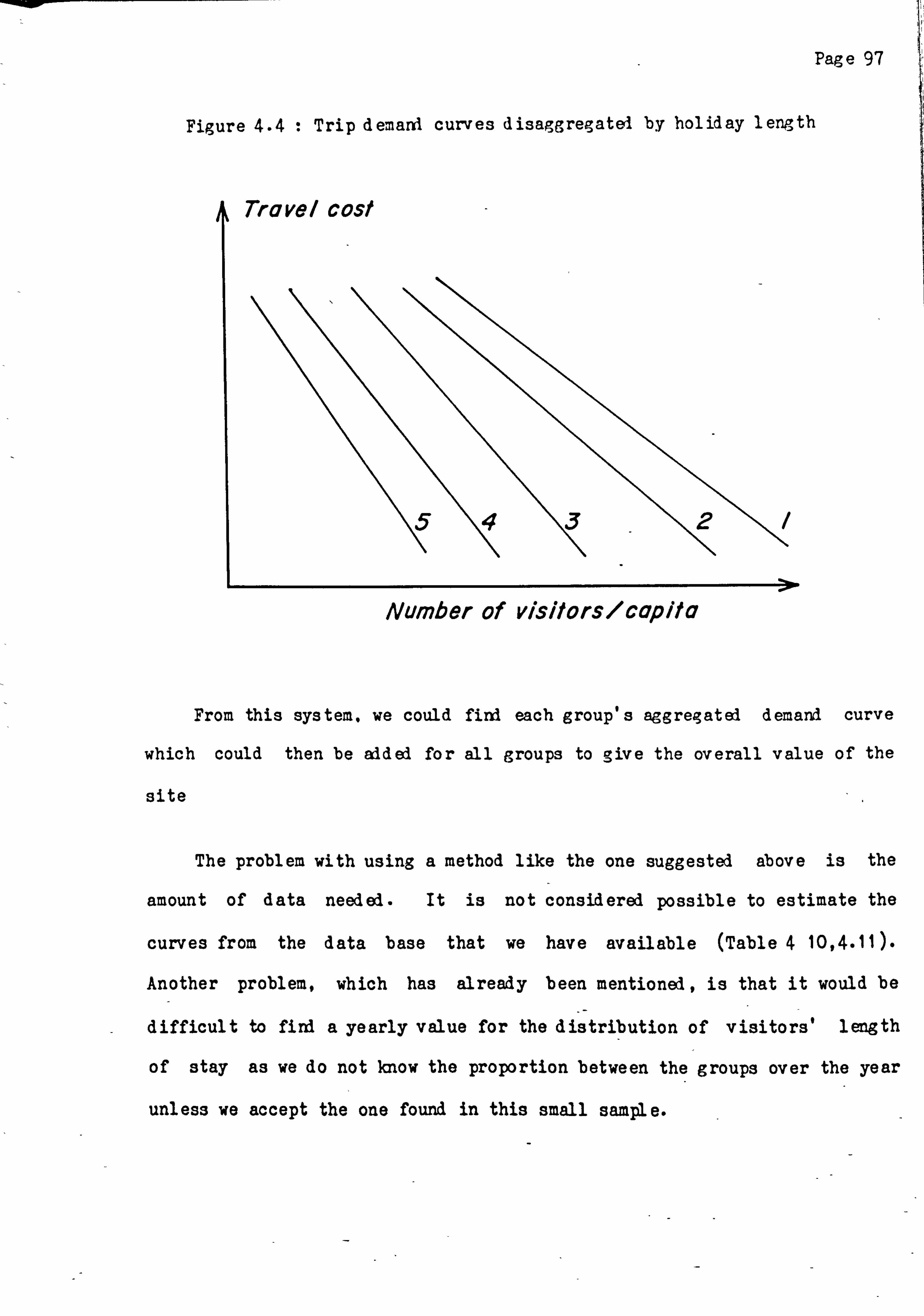
Page 97
Figure 4.4 : Trip demanI curves disaggregatel by holiday length
rrovel cost
/
From this system. we could find each group's aggregated demard curve
which could then be added for all groups to give the overall value of the
site
The problem with using a method like the one suggested above is the
amount of data needed. It is not considered possible to estimate the
curves from the data base that we have available (Table 4 10,4.11).
An other problem, which has already been mentioned, is that it would be
difficult to fird a yearly value for the distribution of visitors' 1 eng th
of stay as we do not know the proportion between the groups over the year
unless we accept the one found in this small sample.
Number of visitorsleapita

Page 98--
4.2 2.2. A Traditional Clawson Method
In addition to the revised Clawson analysis (4-2-2.1), it was decided
to carry out a traditional Clawson analysis on the data to identify the
differences which might occur between the two methods. The travel cost for
each zone was calculated according to the following formula-
Ci - 2*D i *CM (31)
where Ci = travel cost from zone i to visited area
Di - average distance from zone i to the visited
area (in miles)
CM - travel cost per mile
The Di term could be based on an unweighted middle distance to the
zone. For example, when the zones are concentric and Bi is the distance
from the visited area to the nearest border of zone i. then
Di - Bi+(Bi+, -Bi)/2 (32)
It would. however. be better if we could identify the gravity point for the
population density, i. e. the distance to the centre of the population
As a compromise, we have, in this-study, used a zone distance as if
the zone population was uniformly distributed over each zone. This leads
to the followir)g formula for Xi (for the median)9-
9. The true mean is- Di - 2/3 (B(i+i)3 -Bi 3)/(B(i+i)2
- B12)

Page 99
Di = (33)
The formula (33) gives slightly bigger distances than (32).
For the weighting of the points of the trip demar-d curve the same
methods as for the revised Clawson analysis were employed (see 4.2-2.1-2. ).
The consumer's surplus can be calculated either zonewise or zonewise
with visitor numbers regulated to- those observed, i. e. methods 1-3 as
described in Section 4 2.2.1.6.
4.2 2 3. The Computer Programme
To analyze the data as described in the previous sections using, both
the revised and the traditional Clawson methods, a programme was written in
FORTRANIO using the NAG-lib routines and the GINO-F subroutines for
plotting
The intention was to make the programme as general as possible and
more or less to create an interactive package which allows the user the
possibility of changirg zoning. types of curve fits, weightings, plotst
etc. The programme can accomplish the modified analysis with all of its
described options and a traditional Clawson analysis where the travel cost
for each zone is given. The zoning can be by distance or by zone
identifier. The latter is necessary when. for example, post codes are used
to identify visitors -
Page 100
The programme automatically does scaling etc. and takes an unlimited
number of observations and up to 20 zones. It carries out the plotting of
the trip demani curve and fits the described models either weighted or
unweighte, i. In addition, it calculates the consumer's surplus from the
trip demand curve either on a zone basis or using individuals The
aggregated demaM curve can also be plotted - The programme together with
the necessary modification of the data files are shown in Appendix A4.1 and
A4.2.
4.2-3. Total Willingness to Pay
In order to compare the consumer's surplus derived from the Clawson
analysis with the stated willingness to pay as given on the questionnaire.
a programme, TES2 FOR was written. This programme simply sorts willingness
to pay by increasing size, plots the curve of statel willingness to pay ard
numbers of persons and finally, sums the statei willingness to pay.
The total willingness to pay calculatei as above ought to be
comparable to the consumer's surplus if both were correctly estimated.
That is, the additional sum, after travel costs, that people are willing to
pay should equal the consumer's surplus derived from the Clawson analysis.
Unfortunately, it is difficult to reveal people's preferences without
the people behaving strategically (see Chapter 3). As described in
4.3.1-1, we have found a rather discouraging result in that those
interviewed appeared to be responding to the interviewer's prompt-
Therefore, the e%ercise of asking for people's preferences may be rather
futile in this context.

Page 101
4.3. Resul ts
4 3-1 The Descriptive Statistics
In this stuly, only a few of the analyses carrie4 out will be referred
to as much of the information gathered is not considered relevant to this
discussion.
4 3.1 -I .- Statel Willingness to Pay
In orler to reveal whether there was any relationship between statel
willingness to pay (FEES) ard prompting method (Q17) four different
prompting ., methods were testel.
The question asked was:
"Free access is the policy of the Forestry Commission to
State owned forests but to help me assess how much you value Gwyiyr as a
recreational area. I would like to ask you what you personally would be
willing to pay as an entry fee-"
Option I- open (nothing stated from the interviewer)
Option 2 - would you be willing to pay 25 pence?
Option 3! would you be willing to pay I pound ?
Option 4, would you be willing to pay 2 pounds ?
Options 2-4 were followed by the ques-tion "How much? " and the answer was
written down 10
10 This was only done for the questionnaires on sites 1-4. The stude4its (site 5) used a hierarchical approach. Their results are not included here in order not to bias the test. The questionnaires here (sites 1-4) were done primarily by the same interviewer.

Pag e 102
'When the interviews were carried out, it would have been desirable
that a uniform distribution of prompting methods at each site was
attempted The d istribution in Table 4.11 was presented -
Table 4.11 - Distribution of prompts on sites
OPTION S ITE 1 2 3 4 (sum)
I. LLYN CRAFNANT 15 11 12 6 44 2-LLYN GEIRI03YDD 15 10 13 3 41 3 DIOSGYDD 23 3 16 2 44 4 TYN LLYN 18 6 11 13 48
(SUM) 71 30 52 24 177
The first model tried was a simple one-way analysis of variance (ANOVA)*
Yij = ai+eij
where
(34)
Yij - the willingness to pay of individual j w'. Iien
prompted by method i
ai - coefficient for promptirg method ii- 1-4
eij - the random error, leijl N(O. 2)
The model was highly significant (p<O . 001 ) which is very interesting as it
means that these results directly contradict Bohm (1972) (see Chapter 3).
In contrast to Bohm's, this stuly shows that people do not seem to have a
clear idea about. their willingness to pay and instead. let themselves be
guided by the interviewer.
The means for the four options were
Open- 44.6 pence 25 pence: 38.5 pence I pound 85-1 pence 2 pounds 139.6 pence.

Pag, e 103
There is no reason to believe that because options 1 and 2 are very
close. that option I the "open" option is the most valid This
underlines the point that although consistent methods can be found. this
does not necessarily prove that the methods are correct.
In order to find out whether we had interviewed different kinds of
groups of people or if there were differences between sites. we carried out
a 4-way ANOVA without interactions. The model wast
Yijkl, = ai+b +ck+ll+eijklm (35) .? I i
where in addition to the ; ariables in (34),
bj - site for interview -i=1 -4
Ck ý income group,. k- 1-6
d1- holilay, 1- 1-2, (l = yes. 2= no)
There were 134 cases where all the data were available These were
processed and the only variable found to be significant was the prompting
method (07) where p<0.001. Income was the next most important (p<0.098)
According to the interviewer. a number of respondents interrupted
before she had finished the prompt to say they would not pay on principle.
Unfortunately, these cases were recorded under prompt I (open) and cannot
be identified They should rightly- either all have been omitted or
recorded under the prompt that she intended to use at the beginning of the
interview.
1-1 -

Pag e 104
To try ani correct for flaws in the interview proceiure, the 4-way
ANOVA as in (35) was done but omitting both student questionnaires (SITEE
- 5) and promptirg method 1 (Q17 -1). However. this 4id not change the
result of the ANOVA. The prompting method was still significant (p<0.00i
and the next most important factor was income (p<0.096).
Thus. there seems to be no reason to object to the model described in
equation (34) and the conclusion must be that in an attempt to estimate the
socioeconomic value of the forest visits. it is preferable to use methods
based on actual behaviour rather than a questionnaires trying explicitly to
reveal willingness to pay.
As income had some importance. it would be interesting to inclule this
variable in a travel cost molel when the distribution of income is not the
same for each zone.
It would also be interesting to test stated willingness to pay against
actual behaviour when a fee was introduced. The fee would increase the
total travel cost and it should be possible to see whether people reactel
according to their stated willingness to pay. As the actual observed
behaviour is the correct measure. it might be possible to derive conversion
factors between the "true" consumer's surplus and the total stated
willingness to pay for each of the different prompting methods.

Page 105
4.3-1-2. Estimatel Running Costs for Cars
As with the willingness to pay question. four different prompting
methods were used when asking about the running costs (in pence per mile)
for the car visitors. The question was (Ql2b)-
"Can you tell me how much it (the car) costs to run? "
Option 1: open (nothing statei from interviewer)
Option 2: Does it cost you 10 pence per mile?
Option 3. Does it cost you 20 pence per mile?
Option 47 Does it cost you 30 pence per mile?
options 2-4 were followe4 by the question "How much? " if the answer was no
to the first promDt.
The result from a one-way ANOVA was that running costs variel highly
significantly with the prompting method (p<0.001 ) for a molel similar to
(34).
The questionnaire should probably have clarified more prec, isely
whether it was the average cost (i. e. including interest depreciation,
maintenance, etc. ) or the marginal cost (fuel consumption) that we wanted
them to estimate. For an economic analysis of the social value it would be
ideal if we could establish a trip demand curve from people's perceived
costs and then use average costs when calculating the consumer's surplus.
It could be argued that the average cost which is then wanted is not
the same as the average cost that a visitor faces. This is due to the
inclusion of taxes aM it might be more correct if we had a shadow price
free of taxes and incluling the externalities of drivirg

Page 106
If we were to reduce use to a certain level. ard we wantei to do it by
charging, visitors. the marginal costs should be used to establish the fee
as we must expect marginal costs to be close to perceived costs.
4.3.2 Results from a Clawson Analysis
In the following discussion, the names in brackets. e. g. [CLAW2]
refer to the files for a particular run of the computer programme described
in 4.2.2 3. Files which have been usel to generate results are input files
with the extension -INP. e. g. CLAW2-INP- The corresponding output files
have the ectension -OUT. e. g. CLAW2. OUT.
4-3.2 1 Results from a Revised Clawson Method
The first run [CLAWI] of the model was carried out using the zoning
shown in Table 4.8 in Section 4.2.2.1-5. This zoning resulted in one of
the zones (Zone 2) contributing zero visitors which led to the point. (O, -).
This was then excluied as discussed earlier (section 4.2.2. ). Due to the
lack of visitors from Zone 2 in this zoning pattern, the population zones
were changed so that Zone I was extended to 8 miles and Zone 2 went from
9-20 miles.
With this change includel [CLAW2], the following results we re
obtained:

Pag e 107
Table 4.12 Points for the trip demard curve
Number of Visitors/100000 Inhabitants in Zone-
Zone 1 28-7604 Average cost 6 penc e Zone 2 16-3281 Average cost 112 pence Zone 3 18-6334 Average cost 221 pence Zone 4 15-7440 Average cost 294 pence Zone 5 6.1634 Average cost 362 pence Zone 6 0.6296 Average cost 398 pence Zone 7 1.1055 Average cost 345 pence Zone 8 0 8400 Average cost 261 pence Zone 9 2.9993 Average cost 417 pence Zone 10 0 0370 Average cost 548 pence
8 observations (3 43%) of all observations are outside the outer Zone and are excluded
Although excluded here. the 8 observations outside the furthest Zone
are included in a later run [CLA"W11]. The 10 pairs of values in the Table
4.12 are the points upon which the trip demanl curve is estimated -
The results from the three different curvefits and various summation
methods are summarised. in Table 4.13 but are discussed here as well. The
regression fit without weighting gave the line
Yj - 25 223 - 0.054*Xi
where -
(36)
Yi number of visitor groups per 100000 inhabitants in zone
xi average travel cost in pence for zone i
This led to a consumer's surplus of 669 pounds when the integration
was 4one by the traditional zone based method (hereafter abbreviated as
CSZ). A consumer's surplus of 211 pounds was obtained when the integrating
was done irdividually (CSI) as described in Section 4.2.2.1.6. Finally, a
consumer Is surplus of 135 poundu resulted when each zone was regulated to
actual observed number of visitor groups (CSR). The model (36) predicts

> CL - (\j M CM tl- --T M%OM 00 Ln -T (n %0 m 11*1 t- C\l %D 0 Lr) 0 0 Lr% 0 00 - t, - %0 Ln - 00 CYN 00 OD (31% co
I
E0
br, cý a) u; uý tý LA oý t-: Cý Lý Lý t-: 8 LA t, m Ln > (n t- - M OD CIJ C\j CO C\j 0 t- ý III III - (3*% C\j C\j (n ON C\j CO C3% C\j CL C3, % - C\j C\j C\j - C\j CO - C\J 0 C\j C\j C\j C\J
C\j r- m C\j ýT co r-
I
co 0 m co Lr% co 01
LA Cý M m m CV) Lf', I I CY\ co 0 E/) C\j C\j M C\j L)
Cý C% -T C\j t-
Cl\ a", 0 1 1 -T C3 co CIO C\j N N C\j C\; L)
0
%. D 0 cn C, 0 m m (n %D -7
Cý 1: tý Cý I'D -Z 01, Lrlý I I r- col: ko - C\. %D Ol r-
-T Cl\ Ul% C\j ON c
l Cýl Cý I L ý t-- I
c GO C\J, cr, co I C/i r- co
0 -r-4 > > > 0 IN 0 1-1 0
cl cl CL CL tc (1) 13) a) la) a) 0) f-4 C C C C C rl:
0 0 0 0 0 0 0 0 0 C C N t1l N N
0 C: f- CL :3
4-4 S.
IV a) cc P-4 r--4
> f-
cr, N,
0 E-

Pag e 108
937 visitor- groups compared with the actual 225 observed
For the individual integration 173 observations contributed to the
calculation of consumer's surplus. For the third method, 214 observations
contributed. This higher value with the thirl method results from the fact
that Zone 10 has an average travel cost bigger than the value 467 pence
where the line from (36) and the X-axis (price) intercept
The linear regression weighted by zone population/visit rate decreased
the consumer's surplus to 140 pounis for CSZ ard 2q4 pounds for the CSI
method while the CSR method gave a result for consumer's surplus of 235
pounds. Usima, this weighted linear regression the predicted number of
visitor groups was only 138 by the CSZ method. Weighting by zone
population gave a consumer's surplus of 231 pounds for CSZ . 291 pounds for
CSI and, finally. 231 pounds when regulated. When this weighting was
employed. the CSZ method gave the correct prediction of 225 visitor groups
as Expected
At first glance there seems to be some difference between the two
weighting methods. However, when we introduce the measure of consumer's
surplus per predicted visitor group (CSP), the two weighting methods give
very similar results12. In this case, they both give 103 pence per predicted
visitor group.
11 See discussion in 4 2.2.1-3.
12. This measure is discussed in 4.2.2.1 6.

Page 109
The CSI method gives a higher consurier's surplus than the two other
integration methods. This is lue to the fact that for the CSI method the
trip demard curve is estimated on the basis of average values with a
considerable variance within the zone. As a resul t, the CSI method
integrates some extremely low values while ignoring all of the values
greater than the intercept between the demard curve and the price-axis. 13
It can be seen from the following Table 4.14 that the unweighted model
for calculating consumer's surplus is unsuitable-
Table 4 14 Number of visitor groups distribute4 to zones
Number from Zone I Number from Zone 2 Number from Zone 3 Number from Zone 4 Number from Zone 5 Number from Zone 6 Number from Zone 7 Number from Zone 8 Number from Zone 9 Number from Zone 10
2 Visitor groups 7 Visitor groups
17 Visitor groups 13 Visitor groups 17 Visitor groups 45 Visitor groups 31 Visitor groups 31 Visitor groups 51 Visitor groups 11 Visitor groups
In the unweighted method. equal reliance is placed upon a point which is
based on 2 visitor groups (as in Zone 1) as on a point based on 51 visitor
groups (as in Zone 9). 14
13- See also Section 4.2.2 1.6. ,
14. See 4.2.2.1.2

Page 110
The seconi curvefit a second degree polynomial, gave in the
unweighted version a very similar result to that generatei by the linear
model (here, 657 pounds). The model was estimated as:
yi- 28-7333 - 0-0920*%i + 0.0007*Xi 2 (37)
where
Yi ard Xi are the same as in equation (36)
Unfortunately, the two weighted models did not. using a 2nd degree
polynomial. give any curvefit from which a consumer's surplus could be
d eriv ed -
The third curvefit the log-linear model, gave the following line for
the unweighted situation:
ln(Yi +1)-5.1726 - 0.6442*ln(Xi +I) (38)
where:
Yi ani Xi are the same as in Equation (36)
This gave a consumer$ s surplus of 7280 pounds for 1092 visitor groups
with the CSZ method which is equal to 6.67 pounds per predicted visitor
group. Weighted according to zone population/visit rate. this model gave a
result of 114 pounds for 137 visitor groups and of 0.84 pounds per
predicted visitor group -The same result was found when adjusting to the
actual observed number of visitor groups. Weighting by the zone population
gave a consumer's surplus of 154 pounds for 187 visitor - groups azid 0.83
pounds per predicted visitor group.

Page 111
The trend seen earlier in the application of the linear regression
model where the two weighting methods give similar results for consumer's
surplus per prelicted visitor group is also apparent in the application of
the log-linear model.
The disadvantage of the log-linear malel is that points are weightei
accordirg to the transformation as discussed in Section 4.2.2.1.6. In our
case, we could say. have use4 number of visitors per 4 million inhabitants
in ýthe zone insteal of number of visitor per 100,000 inhabitants. Th is
, would have preventel any of the visit rates being less than I and resu I tell
in a completely different "weighting" pattern
An attempt was m&ie to run the programme with the transformation ln(X)
instead of ln(X + 1). In the unweightel model, this lei to a result where
the consumer's surplus was equal to 1099 pounds for 659 visitor groups or
1.67 pounds per predicted visitor group. In the two weighted models, a
consumer $s surplus of 0.27 pounds per predictei visitor group was found
The above example underlines the problems of using ., a log-linear
transformation, anI users would be advised to rely instead on the results
from the linear regression model and the second degree polynomial.
In the examples dealt with so far , no consideration was given to the
fact that a bias in estimating the average travel costs had occured owing
to'differences in the length of stay of the sampled visitor groups The
problem is explained in section 4 2.2-1-4. Run number 3 (CLAW61 corrected
for this via an option in the programme The result of this correction was
much lower average travel co3ts as shown in Table 4.7 in Section 4.2.2.1-4.
When these lower values were used for estimating the trip demard curve.

Page 112
this again led to a decrease in consuner' s surplus as shown in the results
in Table 4.15.
Again. it must be emphasisei how relatively consistent the results are
when it is the consumer's surplus per predictel visitor group which is
being considered. For the linear regression model (when individual
integration is ignored) the weighted cases yield a consumer's surplus per
predicted visitor group of about 0.40 pounds. Values in the same range are
obtained by using the log-linear transformed model in the two weighted
cases. In this run [CLAW61 it was again impossible to derive any results
from the second degree polynomial when trying; to weight.
In the above run, the 8 observations outside the furthest zone were
ex clud ed - The followir)g run [CLAW151 included these observations as a
point (0.287), where 287 was the average weighted travel cost in pence as
described in Section 4 2-2 1.5. For the unweighted linear regression, this
changed the consumer's surplus from 398 pounds to 350 pounds and the number
of predicted visitor groups from 1032 to 865 which resulted in a consumer's
surplus per predictei visitor group equal to approximately 0.40 pounis.
The weighted models cannot be carried out without modification of the
weighting procedures as the zone population is not defined for this new
observation and neither is the visit rate. A modification was built in
which automatically sets the weightings to I when this happens. This did
not lead to results different from the ones already obtained in [CLAW61.
This is because the weightings for some of the bigger zones are in the
range of 109, and a new point with the weighting of i does not affect the
results.

'T 0 0- C, % Lr% 0 C\j C', Ln (1) %D r- %. o a) vs N Ln M 'T , 'T t- (W) LI- M ýr ko -T N -T CY) -. T -Z V% -Z
, * , 1 , U o0 0 0 C4 r4 8 0
6L Cý rý Cý tl: 1; Uý Cý Cý Lý Lý > M --T 00 \. o M OD C\j 'T CO ý Ln C\j III III co C\j N Lr) -Z CO %D Lr% C\; 0 C\j C\J ý (\j N C\j C\j
ýo 0 C31% 00 C\. Ln t-- a) \. D C\j 00 m Cý t- OD 0 00
%. D m \. O -T CO %Z CN k4o t- 0
1-4 a:. ký Cý 1ý I I rý c"j, C31% ON 0 0 C\. cc L)
V) CC) m cr)
co 0ý 0ý I I Cý V) C31% C\J, co 0 CIA N t-0 L) Cý)
-T Lf) t-- co 0 (1) C\j Cl\ U% CV) 0 M
I (n M \0 I cc 0 %D Eý C/I C\j Ln N C\j t- 0
,3 C/)
0 "A i
> > c > 11% 0
CL a in. a a a
-&-) b1c 0) V 4) Q) (1) W W 0) 0)
r-i r-I z r_ r_ c C r_ C r_ C: 0 (1) 0 0 0 0 0 0 0 0 V) N N c N
Ln bc (U
V 4) (13 *a H r-4 :> 0) 0 C-4 0 V tit
. Cis 0 -H -
C 0 E C. ) IJ -
C\j 0-3 -

cl 00 000 Cl% UIN CN (3-, () 0 OD 'T co C\J, Ln E-- IT ýr r- IT m E-- -T
U) ... ... ... U _0 00 000 000 8ý8 ý88
bL LA ý: Cý Cý 0ý Cý 8
0ý > %D IT co %0 -T co c\; n a) III C\j -T 00 C\i U'% m L-- 00 0. OC) C\j CNQI
cc,
clý t-- t- cl% C- 0 co L)
--T ON t- 0 I'D -4* U*ý
OC. CN Cý cr GIN C% 10 N 0
0 co t- ON 1ý0 Lr- L, - co (n
Vý 8 ý r-- N C Cý 0ý : 3-1 0 n C\j cc
cx u m
L)
10 r- cz %D cr% -T rn (n tl- ýT
co C31\ 0 ko CC) Lr\ co W ý ý S.. C C *
N cri C\j Lf % C\j Ll- (n
C/)
L)
0
> > > 0 0 0 a 0. CL a
bf a) Q) 0) 0) 0 W "4 C r- C r- r_ C
a) 0 0 0 00 0 0 N ba N
0 br bL tic +
L) Q) a) I CY\ m +
CC)
0- 0 0 co ca a ca > (1) 4) C\j (D 0) 0 a) 0 0)
0 rý r_ C V4 -- r. r_ 0 c V. c . cd :3 rq 00 "-4 0 00
L) NN

Page 113
Insteal, the built-in subjective weighting feature. was used in an
attempt to make use of the observations outside the furthest zone. Two
different methods were used [CLAW15B]. The first one gave Zone 11 the same
weighting -as Zone 10 and the second gave Zone IIa weighting equal to the
average of Zone 8 9. and 10. The results are summarised in Table 4.16 for
the linear regression model.
In the first case. no result could be obtained for the linear
regression when weighted by zone population/ visit rate In every other
case, the results obtained for consumer's surplus per predicted visitor
group were very similar to the results obtained without the inclusion of
the new point. This is hardly surprising as the value, 287. is in the same
range as the rest of the further zones, i. e zoned with low visit rates.
To test the sensitivity due to zoning, the next run [CLAW171 of the
model was done with the zones popled into equidistant zones of 50 miles as
shown below in Table 4.17-
Table 4.17 - Equi(listant zoning system
Zone 1 0 - 50 miles Population- 223630 Zone 2 51 - 100 mil es Population- 7422858 Zone3 10, -150 miles Population- 2804152 Zone 4 151 - 200 miles Population: 3690580 Zone 5 201 - 250 miles Population- 1700105 Zone 6 251 - 300 mil. es Population: 29696401
This gave as a result the 6 points for the trip demand curve shown in the
following Table 4.18:

Page l14
Table 4.18 - Average travel costs with equidistant zoning,
Number of Visitor Groups/ 100000 Inhabitants in Zone:
- Zone 1 17-4395 Average cost (weighted): 148-10 Zone 2 0.8353 Average cost (weighted)- 335-37 Zone 3 1.1055 Average cost (weighted): 223.23 Zone 4 0.8400 Average cost (weighted): 206.63 Zone 5 2-9998 Average cost (weighted) - 293.19 Zone 6 0-0370 Average cost (weighted) i 311 . 46
8 observ ations (3.43% of all observations) are outside the outer zone and are excluierl.
The results from the calculation of consumer's surplus are summarised
in Table 4 19 The consumer's surpluses are generally smaller when
calculated by CSZ. CSI. ard CSR but are about the same value as in [CLA361
when we consider -only consumer's surplus per predicted visitor group (CSP).
The second degrde polynomial yields a smaller value for consumer's surplus
in the case of the unweighted model than it did in [CLAW6] ard yielded no
results for the weighted cases. The log-linear model behaves better here
than in [CLAW6] ard gives results in the same range as the linear
regression.
Another run [CLAW161 where the zones were pooled to 20,50.100.200. and
300 miles gave results in the same range as above for the weighted models.
For the unweighted models. all results varied considerably except for the
consumer Is surplus per predicted visitor group.
4.3.2 2. Results from a Traditional Clawson Method
A traditional Clawson analysis was carried out by using constant
travel cost for each -zone. The travel costs were based on the formula
(31).

> a
Cl) 0
cri llý* ý C-)
cr, L)
C/) U
C/: cr,
tic
z V
FS
.0 0
>
C. :5
c3. % N Ln C7N -Z C% ý. - %ýo - L: 11 0 -, ") ý- -1) r`ý 9r ri -e m ý- r1) (n N r) Z rl
0 0-000000ý0000 0* ýý I-:,
C4 Lý
ý; Lý ý: C-:, -: ý ý-: Lý Cý Cý C4 Clýj Lý Lý
"D t. 0 C\. <, C\., - 00 N L") N ý10 m ý-o Q0 Lr% C\j - 0. - C\, C\. ýý -. z - N, -- -- C\j
CN 0 Ol 0
cl, Zl- C\.
C\.
VIA r-- oc,
0
cr,
C4 cc
U-% C\j U') .
r-- cc
-%D -T
0ý t:. Lý C\j C\j cc M C\:
ýlo cc
r- C\l N m r-
n U'ý cl%: co t--
r- C\j C\j \D cn C\j C\j C\j C\j
> > 0 0 0 CL CL a., CL
0 0 0 N
>1 tkr r-I
0
ca 10 CU r. . br
. rj 0 C\j

Page 115
The fomula is discussed in Section 4.2-2-2. The value of CM is
calculatel from the petrol price which was valii at the time of the surrey
(136 pence/gallon) and from the average mileage per car (29 miles/gallon).
The following result, Table 4.20 was obtained [CLXW141 for the trip demand
curve of the number of visitors per 100000 inhabitants in the zone and the
new travel cost.
Table 4.20 - Points for the trip demand curve
Number of Visitor Groups/100000 Inhabitants in Zone-
Zone 1 28.7604 T rav el costs 53 pence Zone 2 16-3281 T rav el costs 143 pence Zone 3 18-6334 T rav el costs' 239 pence Zone 4 15-7440 T rav el costs 387 pence Zone 5 6.1634 T rav el costs 571 pence Zone 6 0.6296 T rav el costs 810 pence Zone 7 1.1055 T rav el costs 1196 pence Zone 13 0.8400 T rav el costs 165 3 Dence Zone 9 2.9993 T rav el costs 2123- pence Zone 10 0 0370 Travel costs 2590 Dence
8 observations (3-43% of all observations) are outside the outer zone and 'are ec clud ed .
The distribution of willingness to pay is very wide. that is, there is
a high maximum value. Therefore, the prog-ramme automatically increases the
increment in price in the calculation of the consumer Is surplus as there
are only approximately 200 steps allowed in the procedures.
The results obtained using the above travel costs are summarised in
Table 4.21. Notice that the results from the two methods of calculating
consumer Is surplus do not differ considerably when the consumer's surplus
per predicted visitor group is being considered.

U
a
xý
N
cI ci
C,! ) Cl)
br
C4.4
CO
4-)
V) V
P:,.
.0f. cli E4
ý CC) C3N N U% CYN 131 00 CYN ITI 0-ý, D (ýI N 00 Ch cm N0
oý cý
Uý C4 Lý I;. Lý 8 Cý U; Cý Lý Oý Lý Cý Lý T ko C\j C\j C\j rl- m C\j C\j 0 C\j \ýo C\. l
C\j C\j C\j 'T CTN N Lrv C\j -N cn
LI- C71% ON C\ý
Cý 1; cc Lr, ý
"0 cl Cl% (n
00
u*ý cm N t- Ln Co
%0 -: r ri Ln _T
r- r-
m r-
C*l (n
Cý -Z cn Lr)
0 0 Lr, U'ý
ký M co Lr% V-
>
CL 4) C 0
>1 br bc r-4 W
ca
bc -. ri
r_

>
Cl) 0
CL
0
Cl) 0
a, i.
Cl) Cl)
PZ
CM
Co
(31%(7% -: r 0 00-N Z0 ý %, 0 (\. N Nl - ri 0- 00 C% N C\ý 0
Ln Lý tl: t_: t-- Lý Uý
Lý C4 (ý, Lý tý Lý 8 (ý Uý Oý Lý Oý Lý Cý U4 -7 ko ý C\j C\j C\j Lý- mII C\j C\j 0 C\j %. o C\lj ý C\j C\j C\j -T a, \ C\; UN C\j - C\j C\j
M
�Z (n t- CN n (V) `T 10
Lý cý j rý (11;
ON %0 %. D ON Vý Ln C\ý
Cý Cý C"% co
%. D (n CN ri _T Co -7 LN
cý J j rý t-- 0 OD 0
Cl%j N E-- 00
Lý
r, )
1 \Z -Z (VI Ul- U'% r, ýi
Ln r- U*ý 0
I Lr) co --T 1.0 M
V-4 >
1-1 a 0. M CL CL CL 0 (1) W C C r. 0 0 0 W
br br (D (D 0
CL
"A co
br -m cli ýl

CL "I
r_r_
N
cr, cri
cc
C-)
r: w- 0 t.
CO-4
CO
4j r-I :5 0 w
tx_
C\j C\j
co
C\ 000 Lrý -Z L"i %ýo or) ko -0- C\j UN 0 -47 IT co cN GN CT\ 0 C\ C\j IL- (1)
tý t-* r_: t: Cýl Cý -II 1ý 1ý ký t44 Lý \ý ýI
ý 1; 8 Lý L4 Lý Cý Cý
r-: Lý -: Lý W" Lý 12, Lý N, - -T C\; N C\j C-- m I Lrl% C\j t-- N C\l C\" C. - C\., 00 C\j L"N N -T C\. C\.
m -0 (n 0 co 0 CT\ --T
1ý rý, `ý cc cn 0 C\j co cc -Z Lý rý I Lý . Z-* Cý ON t- \D or" \Z \. D \. Cl C\l 0 LrI \. 3 rl,
%Z N.
J Lrý r1. LP
C C 0 C'
0 C' C' N-
Cl
m Ln cc 0 CDN m
(w) %. o -. T tl- 0.1 C\.
r-- LCI% tl- C\. co
1.4 a:. Cý I ýT cc M, Cl%. -T C\j C\. M
Co U) " "r4
0. 0 0
0. 0. 0. 0. 1) C) C) C) C) C) C)
0 0 0 0 0 0 0 N N N N
bf tr
0
C%j
Cc 00 t1l N

Pag e
The consumer's surpluses are bigger overall when using this method
rather than the revised Clawson method- This applies for any model of
curvefit ani weighting.; method This is what we would have expecterl as the
traditional' Clawson method in fact attributes the main holiday travel costs
to the visit area under concern. The revisei method only attributes a
proportion of the total experditures as a measure of willingness to pay.
The same rezoning as shown in Table 4.17 was tried with the
traditional Clawson method [CLAW18]'to test how-sensitive this model was to
rezonirg. The results are summarisei in Table 4 22 It can be seen that
rezoning in this case results in higher values than in [CLAW141 when the
consumer's surplus on a zone basis is being, considere-i Howev er. ý, hen we
consider the consumer's surplus per predicted visitor group, the results
are quite similar to those obtained in [CLAW141.
The traditional Clawson method is not very sensitive to the described
rezoning because of the extraordinarily heavy weighting of the most distant
zones which does not change in the rezoning. If, however, we rezone in
such a way (Table 4.23) that the zones farthest from the forest are
increased in size then we will fini that the consumer's surplus decreases.
Table 4.23 Rezoned zoning system
Zone 10 20 mil es Population: 49825 T rav el costs- 133 Zone 2- 21 50 mil es Population- 173805 Travel costs! 357 Zone 3- 51 70 mil es Populationý 275824 T rav el costs 571 Zone 4- 71 100 mil es Population- 7147034 T rav el costs! 8io Zone 5- 101 - 200 mil, es Population- 6494732 Travel costs! 1483 Zone 6 201 - 300 miles Population: 31396506 T rav el costs: 2391
The results from the run using this -. -ezoning pattern [CLAW19] are
summarised in Table 4 24 Except in the case of the-transformed linear
model when weighted ._ the consumer's surpluses are smaller than those

>
Cl) C-)
c=I o C-)
N cr, u
cr; C/I
0
V)
4-)
d) m
C\j
.0C. - co :s E-4 L)
mM %. D t- co 00 00 M C\j 00 t-- - ý-- 1: 7 C\j CO Ln 0-7 t-- zl--
* co 0 N N,
Cý rý Cý 4- r4 Cý cý r: _
ý (ý fý Lý j. j j. -: rý rý oý J lý Lý ý Lý 110110 %10 NNN %m 011 IZ %Z - 01: Ln cm (: CM CD -, -NN Ný cli - %Z, ý (VA N- (NJ - CM
%. D CYN CTI,
Cý 0 CN Ul. 00 C\.
0 %10
oc 0 C\j
CIN oc
-T 10
C\; cc C"% m
cc cc m m
N %M VN Ln -Z %. 0 cc (7 U-11 0 C% 0 (D - ýID CYN CD, %
ý ' lý f cý cr. Lý
lý rý 31 CO -: r cc r- _T _T
> 0 1., 0 CL CL CL
r. r. r_ r_ r. a r_ C C 0 0 0 0 N
-C: N N
bc
-H m
10 r-4
bý 0

Page 117
obtained in [CUW141. This is due to the lower travel costs from the
furthest away zones
4.4 Summary of Methods and Results
The preceding sections in this Chapter have emphasised various
problems which should be considered when the task of producing a measure of
the benefits from recreation is un4ertaken. In this section, the major
problems will be summarised and discussed.
Questionnaire design- The fact that our analysis was based on
secondary data of variable quality has been useful in that it highlighted
some problems. In particular for the Clawson analysis the meaning of the"
cost we wanted was not clear to the visitors. Also missing values reduceI
the size of the data-set. We will discuss more the probl3m of
questionnaire design in Chapter 6. Some of the problems we have been able
to solve with statistical methods, however.
Survey methods vs. Travel cost methods: The results from a
questionnaire conducted in Gwydyr Forest clearly indicated a correlation
between prompting method and stated willingness to pay. In addition, some
visitors would not be willing to pay on principle, even though they place a
large value on the opportunity for free access. This led us to believe
that in this case the survey method would be unreliable and that the best
way to proceed in the estimation of recreational benefits was to undertake
a travel cost method (Clawson method) in which the benefit is derived from
observations of actual behaviour. Even then. it has become clear that
prompting method has influenced people's response to questions about the
cost of running their car.

Page 118
Traditional vs. Revisei Clawson method- The traditional Clawson
method was f ound to be unsatisfactory in this case-. it greatly
overestimated the consumer's surplus. This was due to the fact that 73% of
the visitor groups interviewed were on holiday at the time of their forest
visit; it would be wrong to attribute all the cost of travel from home as
willingness to pay for the forest visit. The revised Clawson method takes
this into consideration by basing the visitor group's travel cost (imputed
willingness to pay) on a formula based on mileage cost, home distance,
holiday length, and length of stay in the forest. This results in smaller
travel costs than the traditional method ani, thus. a smaller consumer's
surplus. The revised method also has the a4vantage that it can combine
different means of transportation into one stuly: in this and other
stulies the data-set is too small to give useful results if it is split UD
for separate analysis. The method is further discussed in Christensen,
Humphreys ani Price (* 1985 -).
Length of stay in the foresti When randomly sampling on a site
interviewers will get an ov erre presentation of those visitor groups who are
staying in the area for the longest periods of time We found a
correlation between the length of stay and the travel cost used in the
revised model. Therefore, it was considered necessary (as suggested by
Luc as, 1963) to weight the travel cost by the reciprocal of the length of
stay. An option was therefore built into, the developed programme which
weighted the travel . cost when we calculated the average from each zon6.
This led to a decrease in the consumer's surplus.

Page 119
Curve fitting Three models were used in this part of the stuiy, a
linear regression, a second degree polynomial, and a log transformed linear
regression. The l as the og-linear model is not recommended points are
actually weighted by the transformation process. Also, considerable
variation results from the units used for the visit rate (e. g. visits per
thousand contra visits per million) when this arbitrary weighting is
employed.
The secord degree polynomial was, in some instances, unable to yield a
result partly because our sample was not as good as expected. This model
can, like the log-linear model, give us infinite consumer's surplus. The
normal linear regrassion model in most cases was able to yield a result.
Despite the traditional interpretation of a demand curve as bei ng'
non-linear, application of the linear regression model proved useful in
this stuly.
In an early stage of the stuly, an eximential curve fit was inclui ed
However, its use was abandoned as it could not be weighted in a
satisfactory way. This problem has later been solved (See 5.4-9).
The task of deciding which model is "best" in this case is not easy.
The SS-residuals have been calculated and so have the PRESS values. The
SS-residuals can be used to compare different models if they. are weighted
equally. In this instance, the second degree polynomial will always give_
the smallest value indicating the best fit but this is simply due to the
fact that it has one more degree of freedom to describe the data. The
PRESS value which iMicates how good the model is as a predictor can give
some guidance on the choice of model because we car, justify selecting a
good predictor which has some importance when we are calculating the

Pag e 120
consumer, s surplus. The PRESS values are often lower for the linear
regressions than for the second degree polynomials. However. this can also
be caused by an uneven distribution of points. The SS-residuals for the
weighted models cannot be compared wit h the -SS-residuals for the unweighted
models as we have deliberately forced the curve to go closer to some points
and to ignore others in the weighting procedures. The topic of functional
form is discussed further in Chapters 5 and
Weighting of points for the trip demand curve- It is shown that
considerable variation can be obtained in the results as a consequence of
the weighting system employed. It is not considered to be appropriate to
use an unweighted model as equal weight is then attributed to all zones
despite a wide variety in the number of 'visitor groups and in zone
populations. The weighting which we consider most appropriate is zone
population/ visit rate. This might not lead to the predicted number of
visitor groups being equal to the observed number but the right number of
total predicted visitor groups is not a goal in itself. Weighting by zone
population does give the correct number of visitor groups if negative
visits are includel. but it is not considered to be statistically correct
(4.2.2.1 2).
The right zoning: It has been shown that the zoning pattern can
influence the consumer's surplus and it is recommerded to try different
zoning systems. Ideally, zones with a small range of travel cost should be
used) but this is not usually possible with the revised Clawson method.
Ev en in the trad itional method where average travel costs per mile are
used, narrow zor.. es lead to problems because the number of visits from each
zone can be too small. As a compromise consumer's surplus could be taken
'Fsoe 121
as an average value of the consumer's surpluses ierived from different
zonir4a, systems.
Integration of Consumer s surplus- Three different integration methods
were tested for the revised method. Method a/ is the normal method based
on zones. M-ethod b/ is a method based on irdividuals ar)d method c/ is a
method based on zones but regulated to actual observed number of visitor
groups for each zone, The methods did not give the same result. "his was
primarily due to the fact that they predicted different numbers of visitor
groups.. In some cases, method a/ gave a consumer's surplus basel on a
prediction of more than 1000 visit or groups compared with the actual number
of 1-25 observed - This lei to the belief that. rather than co-. centrate on
total consumer's surplus, we should focus on the consumer' s surplus per
predicted visitor group. By doing so. quite consistent results were
obtained using methods a/ and c/ even for different curve fits. Method b/
terded to overestimate the consumer's surplus even when we concentratel on
the consumer's surplus per predictel visitor group- the reasons were
explained in Section 4 2.2-1-6. This method will be further discussed in
Chapter
This study has yielded a consumer's surplus per visitor group's visit
to Gwyiyr Forest Our estimated trip demand curve could be overestimated
due to the perceived cost being smaller than the actual. On the other
hanIq as-a lot of demand has not been observed due to substitute areas the
demand curve could be overestimated. Our data do not allow us to decide
which effect will be stronger.

Page 122
To obtain an overall consumer's surplus, we wouli need. the number of
visitor groups per year. Then, proviied our sample is a good
representation of the population of forest visitors over the year. we could
multiply our consumer's surplus per predictel visitor group by this yearly
Value. (It would also be necessary to adjust for the 3.43% of the visitor
groups that we excluded from the stuly). This yearly value could be
capitalized in the normal way if the government's (society's) discount rate
is known,

THE ECONOMICS OF FORESTRY RECREATION IN A REGION OF DENMARK.
5.1 Introduction
A research project, " Project Forest and Folk (PFAF) " was set up in
1975 funded by the Danish Agricultural and Veterinary Research Council -
The project's aim was to provide a better basis for decisions in the field
of forestry recreation. This has, so far, resulted in two reports being
published (Koch 1978,1980) giving a description of the population's use of
forests and the use of the forests considered regionally. The two reports
give no economic measures. but a further report (Part VII) is planned in
which economic measure3 will be considered.
The present study should yield some ideas as to how a better basis for
economic decisions concerning forestry recreation can be achieved - It is
the aim of this work to present some of the data from the above project aril
show the measures which can be derived as future guidelines for PFAF.
5.2 Previous Work in the Field of Forestry Recreation Economics in
I Scandinavia
The first major important work on recreation economics was by Strand
0967), who discussed different theoretical problems such as collective
consumption, non-tradeability ard joint public and pri, ýate supply of
recreational goods, as well as the possibilities of a better allocation in
i- Section 5.29 5.3 ard 5.4.1 have been partly published in Christensen (1981). Section 5.2 is based on the author's contribution to Kaiser and Marchetta (1981 ).

Al Page 124
the production of recreational. goods.
The most interesting part, though, in relation to the development of
recreation economics in Scandinavia, is probably the section on 'Measures
for describing recreation' where a very critical discussion of the travel
cost method ard the assumptions behind it is presented. Strand opposed,
among other things, the assumption that the only benefit from the travel is
gained inside the visited area, and he concluded:
" for individual problems one will probably not be able to
inlicate practicable methods with such properties that they
might lead towards an optimum of social welfare
(Ib id p. 180).
Instead, the applied works carried out in both Norway and Sweden
developed along the line of the opportunity cost method, that is,
estimating the loss to production forestry through providing recreational
facilities. In this way Haakansson and Haegglund 0969) estimated thd
costs of preserving the objects of scientific, aesthetic and social
importance in a forest area (2105 hec. ) SE of Stockholm. They separated
costs into three groups:
Costs due to the fact that restrictions inhibited
management to maximize gains (Forgone revenues)
2. Investment costs*
- Maintenance costs

AO
Pag e 12 5
It was found that' 10% of the total cost was due to category I above,
and a net present value (NPV) of costs was calculated as 526 Sw. Cr. per
hectare using a discount rate of 4% p. a. (Approx $ iOO/hec. ).
In the same way Johannesen 0 970) applied an opportunity cost approach
to a forest area (407 hec. ) near Oslo. He found the difference between NPV
when a production management plan was undertaken and NPV from practising
the proposed recreation plan worked out as 1830 N-Cr. per hectare using a
discount rate of 3.5% p. a. (approx. $360/hec. ). Most of the decline in
NPV was due to extension of the rotation age beyond optimum.
Hoejer (1971 ), like Strand, argues against quantitative evaluation of
recreation unless the area concerned has intensive use as a recreation
area, so actual or derived visit frequency can be used as a base for
calculazions. However, it is suggcsted that a calculation should always be
underzaken of the opportunity costs which co=ercial forestry has to face.
(Ibid. p. 263)
Kardell (1973) applied eight different evaluation methods to two areas
near Stockholm, incluling a method based on physical use, Clawson's zone
method, and an opportunity cost method. He follows Strand in the criticism
of the Clawson method, especially on the assumption that 'all visitors
despite travel distance have identical preferences' (Ibid. P-31 That
is, Kard ell seems to bel_ieve that - the Clawson method. is based on each
visitor having identical willingness to pay. But what the zone method
ac tually requires is that each zone has the same distribution of
Ereferences within its population not identical preferencea. His
conclusion is that none of the methods are generally applicable and 'Most of
the discussed methods suffer from theoretical shortcomings. -- Finally, 'a-

Page 126
method based on more qualitative measures is suggestei -
Conflicts between recreational and commercial groups over land use
are, according to Qvigstad (1974), - to be solved by establishing a
Is market ". In this " market of . restrictions on use of zones can be
priced A model applied to an area of Oslomarka finds that the
recreational value has to be equal to at least 50-60,000 N-Cr. per year to
justify the area as it is today (approx. $11 000). The idea behind the
method used can still be described as an opportunity cost approach.
Kardell and Ericson (1975) have evaluated three different management
plans for an area outside Stockholm, using an opportunity cost method. The
three alternatives were:
I- Production forestry
2. Extensive recreation
Intensive recreation
The extensive programme was estimated to cost approx. 40 Sw-Cro. per
hectare per year, (approx. $10 /hec/year) or about 1 Sw-Cr- (approx. 25
cents) per visit. The more intensive recreation plan increased losses to
50-100 Sw. Cr. per hectare per year (approx. $13-25/hee/year). The
largest amount (60%) was due to lowered yield values-and retention costs.
The
gover=ei
Linigren
affected
1 .4 mil 1
result of forestry management restrictions proposed by the
a t's physical planning schemes of 1975 has been evaluated by
0 976). It has been estimated that 1 .9 mill hectares will b_e
and that annual yield from that area-'wili have to be lowered 1. by
m3. Due to lack of data it was found impossible to calculate the
benefit of - recreation and the report is, therefore, mainly concerned with

Page 127
the costs accruing to the forestry sector. Two extreme cases have been
considered
I. When only primary forestry is influenced
2. When external effects are spread to the rest of the
forest irdustries
The first alternative is estimated to cost 90-180 mill. Sw. Cr. per
year (approx. $25-45 mill ) and the second_ alternative will cost 200-500
mill Sw. Cr- (approx. $50-125 mill ). The real costs are believed to be
in the rar)ge of 200-400 mill Sw-Cr- per year before tax (approx. $50-80
mill )-
The general theoretical problems behind multiple use have been
described by Joergensen (1974), Loennstedt (1975) and Helles (1977). The
theory has been applied to Katnosa-Spaalen, a part of Oslomarka (Hofstad
1976), where a number of restrictions were put-on-timber production in
order to increase the recreational value of the area. The restrictions
were chosen from the results of interviews and behavioural studiesO No
quantitative recreation benefits were estimated and the political decisions
were to be based on the estimated opportunity cost values.
In Finlard 2, Mikola (1973) discusses the economic consequences of
recreation and Saastamoinen 0972) has measured visitor expenditures. The
same author (Saastamoinen 1978) estimated the value of mushrooms. ard
2. Based on RE, unala's 0979) work for the "Worldwide annotated bibliography concerning the economics of recreation".

Page 128
berries gathered in the period 1860-1965. Vesikallio (1974) applied an
opportunity cost approach to timber harvesting in' an area, when
restrictions were put on due to recreation. He found timber harvesting on
average 30% more expensive in the recreation area than in production
forest.
Most recently, Strand (1981 ) has used a traditional- Clawson analysis
for calculating the socioeconomic value of sport-fishing in the Gauls.
river-syszem in florway for the year, 1979. He found the consumer's surplus
for the fishing to be 7.5 million N-Cr. (approx. f 1.25 million ). This
is Approx. 1150 N. Cr. (approx. $190 ) for the 'average fisherman'.
With a basis of the estimated number of trips to Gaula in 1979 (approx. *
31,200), he found that the 'average trip' contained a willingness to pay
equal to 240 N. Cr. (approx. $60 ).
5.3 Project Forest and Folk
"Project Forest ard Folk" was set up in 1975. The Project's aim was
to provide a better basis for decisions in the field of forestry
recreation.
Part I (Koch 1978) is based on a mailed questionnaire survey spread
over the period June 1976 to June 1977. The sample size was 3087 persons
(age 15-76 years) selected in a random way* using the Central Person
Register, and the response was 2807 persons (91.4%).
The main results in the report include:
The number of forest visits per year per capita.
The length- of stay - group size - activities.

Page 129
Percentage who arrive by car for a given travel distance.
Differences between motorists' and non-motorists' use of the
forest.
Name of the forest last visited.
Part II (Koch 1980) is based on the followirg:
1. Counting of parked cars on 318 different counting areas, -
divided into W9 subareas makirg up 446 forest areas with a
total area of approx. 187,000 hec. (approx. 40 % of all
forest area in Denmark). Counts were carried out at all
counting areas at the same 22 points in time distributed over
the period April 1976 to May 19T7.
2. At each counting a questionnaire was attached to the
windscreen of parked cars or a sample of the parked cars. In
this manner 44,846 questionnaires were handed out. The
response was 24,076 (53.7%) as it was impossible to use
follow-ups. (The effect of the non-response was estimated a rd
partly corrected for using three different methods. )
The above information was combined with part I and with automatic
recordings at 4 counting stations of the number of cars present every 15
min. over the period August 1976 until October 1979 (planned to be
published-An a forthcoming part III).
The main results presented are:
Total use in visitor hours and visits for the 446 forest areas
including non-motorists.
For each forest area the number of car visitor hours per year, for

Pag e 130
peak periods, different seasons of the year and for weekdays arA
weekends.
In addition, average group size, length of stay, activities, travel
time and travel distance for the car-borne visitors are given.
By using data from part I and a further questionnaire survey (a
forthcoming part IV), the relative use intensity has been established for
230 forest districts. This, in combination with the above results, has
been used to estimate the absolute use intensity for approx. 274.000 hec.
or 3/4 of the area of all forest properties of 50 hec. or more.
5.4 Methodology
5.4.1 Aims of this Stuly
The following is a brief introduction and all the topics incluled will
be discussed in greater detail in subsequent sections.
The method suggested is a travel cost method mainly based on the
questionnaire information -from part II (Koch 1980). This means that it is
only benefits accruing to the car visitors which will be estimated in this
preliminary stuly.
The region chosen is North Zealani, which has the advantage that
nearly all forests in the region are investigated, aid that the relatively
dense population produced many responses to the questionnaires.
The unit of visitation will be household visitst hereby assuming that
each car visiting is coming from- one household, and the value is not
distributed across individuals.. Using that method it can be assumed that

Pag e 131
travel cost from each zone to each forest is relatively constant for all
visitor groups coming, from the zone.
As a zoning unit, post codes are used. These were given on the
questionnaires. A cross- tabulation giving average distance from each
forest to each post zone can be constructed.
The following analyses can be carried out:
I- Clawson analysis for a particular forest based on the actual
number of visitors.
2. Clawson analysis for a particular forest based on the
visitors for whom that is the nearest forest.
An integrated Clawson analysis, i. e. first find the gross
demard curve for all forests as one, then simultaneously apply
this to all the forests.
Clawson analysis for a particular forest, when alternative
areas are taken into consideration, i. e. using diversion of
demand as the "entry charge" is raised.
Use of the overall gross demand curve estimated in 3 to
calculate the value of a new hypothetical forest. 3.
The validity of the relatively simple models suggested depends on the
use of the measures: Is it the overall social value for all forests in the_
region, or the value of one particular forest that is wanted ? The- main
3. There will naturally be aesthetic differences between the foreats and differences in facilities, etc. which more refined methods might take into account.

Page 132
intention in this preliminary stuly is to show the kinds of results which
can be obtained from the available data. Hopefully this can give ideas on
the direction in which to proceed and provide the decision - makers with
information such as:
1. An economic measure of the additional benefits accruing- to
the society due to the Forestry Commission's provision of
forestry recreational facilities.
2. The social value of establishing a new forest in a particular
area.
The loss to society by closing a forest in the area.
The above information will provide the kind of measures searched for
in -the introduction, and will also be of use in the local planning
procedures.
If there are any opportunity costs these should naturally be deductel
as mentioned in Section 1.2.
It might also be possible to extract information such as : What fee
should be introduced in a forest X to keep use down to a certain carrying
capacity ? However this raises the question of perceived costs contra
actual costs. It would, thereforev be interesting through further research
to analyse the relationship between consumer's surplus found by -this
measure and actual behaviour when a--charge is introduced e. g. -at a new car
park.

Page 133
More complicated models could have been suggested but as qualitative 4 data on both forests and socioeconomic factors have not been gathered,
this is not directly possible without further expensive surveys.
Nevertheless, the data base on actual visitors is large and very
thorough. It is not the aim of this study to describe the number of
visitors so much as simply to estimate the value of the actual visits
recorded from the available data.
5.4.2 The Region Investigated
The area chosen in which the forests are situated is North Zealand
including Hornsherred peninsula and the island Amager. To the southwest
the border is a line from Greve north of Roskilde up to Skibby.
The reasons for chosing this area are .
It is well defined as it is surrounded, by water except for the
southwestern borderline. The total area is approx. 1966 km2 and
the population approximately 1.54 million (Damarks Statistik
1981 It is divided into two counties
County of Copenhagen (KBH)
County of Frederiksborg (FRB)
Occupation is available and might provide a guide. -

Table 5.1: The Investigated Forests
County of Copenhagen (KBH):
1 Trorod_Hegn 7 Geel Skov 2 Kohaven m. v. 8 Norreskoven
---3 Jwgersborg Dyrehave og Hegn m. v. 9 Asevang m. v. ---4 Charlottenlund Skov 10 Hareskovene og Jonstrup Vang
5 Kongelunden 11 Vestskoven Vest 6 Sollerod Kirkeskov
County of Frederiksborg (FRB):
1 Horneby Sand 2 HornbEpk Plantage 3 Teglstrup Hegn og Hellebmk Skov 4 Klosterris og Horserod Hegn m. v. 5 Gurrevang 6 Nyrup Hegn 7 Egebaksvang 8 Danstrup og Krogenberg Hegn 9 Munkegärds Hegn
jo Kelleris Hegn 11 Krogerup og Babylone Skov 12 Snevret 13 Gribskov op- Stenholt Vanz 14 Sorup 15 Aggebo og Grmsted Hegn 16 Valby Hegn 17 Hobjerg Hegn 18 Tisvilde Hegn m. v. 19 Brodemose Skov 20 Avderod Skov 21 Nejede Vesterskov 22 Ullerup Skoir
23 Gronnwsse m. v. 24 Sonnerup Skov 25 Lyngby Skov 26 Fr,. -. erslev Hegn 27 Brode Skov 28 St. Dyrehave og Tokkekob Hegn m. v. 29 Gronholt Vang m. v. 3o Knorrenborg Vang 31 Gronholt Hegn 32 Lave Skov 33 Stasevang 34 Sjmlsolund 35 Folehave 36 Rude Skov 37 Bistrup Hegn 38 Lystrup Skov 39 Ravnsholt og Sonderskov 4o Uggelose Skov 41 Slagslunde 42 Krogelund 43 Ganlose Eget 44 Ganlose Ore o. gý Farum LlvaRg m. v.

Page 134
2. Most forests in the region are included in the study. In the area
55 forests are investigated directly :
11 in KBH ard 44 in FRB
These forests are the primary outdoor recreation facilities
(except sea-shore) and the total area of the directly investigated
forests is approximately 22700 hec. which is approximately 80% of
the total forest area in North Zealand - (Damarks Statistik 1979,
Danske Forstkandidaters Forening 1979)5
The region is densely populated, resulting in many visits ard,
therefore, many questionnaires (approximately 30% of The
population of Denmark lives in this area). 6 The total number of
questionnaires for all parts of Denmark was 44846 with a response
of 24076 equal to 53.7 %. The number of questionnaires in the
above region was 16512 ard the response 8758, equal to 53.0 %
(Koch 1980, p. 270-273). The above figures show that although the
area of North Zealard is only approximately 4.6 % of the total
area of Denmark, it is by far the best investigated area.
One of the permanent and automatic counting stations (See 5-3) was
situated in the area in forest no. 28 in FRB, (Koch 1976).
Table 5.1 contains a list of all the investigated forests aid in Figure 5.1
a map is shown of the investigated area on which the forests are marked
5. The figures have been reduced by the area of four lakes. 6. The figures are excluding Greenlaid and tho-Faroe Islands.

Fi re 5.1 gu
Map of North Zealand with investigated fores/sMGrked
N
42
15
@lip 8 13 9 10 7
30 29 32
. All liff-,
FRB 41P n-ml IPFF Nz. ý/ ug qo
-
5b v * 5b
37 si,
.9 (3) d
44 -0
00 9)
I '*% ssl '. *-% / 0-0 .
le", /4P%
KBH
Copen agen
1 40
40% 0*0 - L Oft Ono %a
- Nt
50"0) -
10 km

Page 135.
according to Table 5.1 -
5.4.3 Unit of Visitation
The unit of visitation used is visitor groups per household and not,
as usual, visits per capita. This is done for the following reasons: H
I. One car-borne visitor group is probably one household coming to
the forest.
2. The decision to come to the forest is probably made on the
assumption that it costs the family x amount to drive to the
forest and not that it costs x' amount per member of the visitor
group.
3. This will lead to less variability in the travel cost, as it now
is the cost per car which is the travel cost, despite the fact
that some cars bring 5 persons ard some bring 1 person, which
would give higher variability in the travel cost within a'given
zone.
4. The number of households is accessible for each postal area, while
it would be more difficult to find the number of inhabitants for
each postal area (See 5.4-4).
-/

Page 136
5.4.4 Zoning Unit
The postal codes were used for grouping visitor groups into population
zones instead of the traditional method of concentric zones. The postcodes
were chosen becausei
I. The postal codes for startpoint (Koch 1980, P. 38i ) were given on
all questionnaires, which made it a very easy measure to obtain.
2. The Post and Telegraph service could provide a booklet (Postaeog
Telegrafvaesenet 1976 ) with the number of households within each
postal area.
The above mentioned booklet defines all households as All private
residences, apartments, rooms with name sign and individual letterbox or
other separate delivery possibility. It includes apartments in blocks,
houses, terraced houses and farms, but" noz* summerhouses and weekend
cottages. ' (Ibid., P. 14)7
The problem with summerhouses could bias the result as some people at e. g.
'Hornbaek - Plantage' (Forest no-2 in FRB) have presumably started out from
their summerhouses a few kms away , ard the visit rate for that postal area
will then be overestimated. The problem cannot be overcome by asking
whether visitors are on holiday because many people live more or less
permanently in their summerhouses' over the summer and probably would
respond-- negatively to the question.
Author's translation

Table 5.2: Postal Areas and Number of Households
Postal code No. of househ. Postal code No. of househ.
1000 Kobenhavn K 22424 '
3ooo -
Helsingor 14191 15oo Kobenhavn V 39361 3o5o Humlebwk 3382 2ooo Kobenhavn F 29628 3o6o Espergwrde 3869 21oo Kobenhavn 0 47598 3o7o Snekkersten 1389 22oo Kobenhavn 11 43698 3o8o Tikob 444
----23oo Kobenhavn S 52995 310o Hornbmk 16o4 24oo Kobenhavn
, NV 26948 312o Dronningmolle 389
2450 Kobenhavn SV lo4lo 314o AlsgArde 1269 25oo Valby 27546 315o Hellebmk 234 26oo Glostrup 13498 3200 Helsinge 4492 261o Rodovre 17963 321o Vejby 768 262o Albertslund 12148 322o Tisvildeleje 52o 263o TAstrup 112og 323o Grzested 2697 2635 Ishoj 6794 325o Gilleleje 22o8 264o Hedehusene 4472 33oo FrederiksvT. rk 537o 265o Hvidovre 236oo 331o Olsted 631 266o Brondby Strand 658o 3320 Skmvinge 1176 2670 Greve Strand 8385 333o Gorlose 37o 268o Solrod Strand 3578 334o Brodeskov 232 269o Karlslunde 2362 336o Liseleje 413 27oo Bronshoj 22949 3370 Melby 27o 272o Vanlose 16789 339o Hundested 2967 273o Herlev 139o5 34oo Hillerod 11545 274o Skovlunde 53o9 345o Allerod 56oo 275o Ballerup 12223 346o Birkerod 7751 276o MA1av 4294 3471 Hovelte 45 2770 Kastrup 16413 348o Fredensborg 3937 2791 Dragor 5731 349o KvistgArd 53o 2800 Lyngby 18161 35oo VF-rlose 6368 282o Gentofte 10000 352o Farum 582o 2830 Virum 844o 353o ý Farum Kaserne 35 284o Holte 6o55 354o Lynge 14o7 2850 Nwrum 3125 355o Slangerup 2442 286o SoborR 171o8 36oo Frederikssund 5544 288o Ragsv, -. rd 7488 363o Ja! gerspris 23o6 2900 Hellerup lo488 365o Olstykke 3759
ý 292o Charlottenlund lo634 366o Stenlose 2288 293o Klampenborg 2o88 367o. Vekso Simlland 733
-2942 Skodsborg 8o4 4ooo Roskilde 27o5l 2950 Vedbmk 2697 4o5o Skibby 2228 2980 Rungsted Kyst 2171 4070 Kirke-Hyllinge 1478 297o Horsholm 6419 4621 Gadstrup 1o41 2980 Kokkedal 3549 4622 Havdrup 12o6 2990 NivA 1567

Page 137
To make a more well defined border than the one defined in 5.4-2, five
postal areas on the southwestern borderline are included although they are
not actually in either of -
the iwo counties. These zones have few
households and no forests.
In Table 5.2 is a list of postal areas and the number of households.
Figure 5.2 shows the postal areas, and the population densities. The data
are stored in PSOF-BB-
5.4.5 Unit of Travel Costs
The primary unit of the calculations will be kilometres. - This-is done
in order not to introduce another source of inaccuracy. It was felt that
it was easier to calculate all consumer's surpluses in -the unit of
kilometres and then finally show what a given kilometre price would mean to
the surplus. The inaccuracy occurs for two mai n reasons: (1) The means of
transport differ and (2) the perception of costs differs. This last point
is especially difficult to harAle. However, as it is the visitors'
willingness to pay that we want to measure, it is considered that it should
be the perceived costs that we use. But, are perceived cosis the marginal
costs or the average costs? It is assumed here that most visitors, when
considering making a trip, consider their marginal costs or variable cost.
The variable costs for driving a car during the period 1'976 --1977 can
be taken to vary from approximately 44 oere to 76 oere per kilometre
(approx. 3-3.5 pence per kilometre) depending on the size of the - car
(Truelsen 19T,? ). A good average would be 60, oere per kilometre (approx. 4.
pence/km). The price if -fixed
costs and depreciation were included could.

F0 igure 5-2
North Zealand: Postal areas and Population Density
Households per kmp-
50
50-200
200-500
500-1000
)0-4000 .... .......
4000
(Within the areu-of Copenhagen there 'are'several postal- areas)

0 "' * .... .......
... .... ...
2 .... ....... ............ 3ý60 3300
3370
i will 39
3320. *. * ...........
3,
(00 355CI
0
3140 10 0 1.5
323
. 3ý 00ý
............ ............. 308 :3490::
........... ... ...... 30 .......... ......
3060
30
12990 lu llwl
2 loý: P-:
I M-
; Illillllllllli#2960 2970
36T
2942
2750 2700
2720
2610 2630 CQpenha e 6
1 2600
2650
4000 635 20
2670
2690
462 2680 Approx. 1: 300000
10 km

Page 138
vary from approximately 78 oere to 372 oere per kilometre (approx. 6- 26
pence per kilometre) all depending upon the make of the car and yearly use
(Truelsen 19T7)8. -
The Directorate of Roads gives a cost as of I July 1977 of 52.1
oere/km (approx. 3.5 pence/km). This price is the variable cost ard based
.- on weighted costs for different cars according to the amount sold in the
year, 1976 (Vejdirekzoratet 1977).
5.4.6 The Data from PFAF
In Denmark the data from -PFAF are analysed mainly by using a
statistical package, SAS (Barjr et al. 1976) ard the data made available
for this study were produced by a programme using SAS (prg Al 711 )- For
each forest investigated, it gives a frequency distribution of the yearly
number of car-borne visitor groups distributed according to postal codes.
The data have been created in the following manner as shown in Figure 5-3:
On the 20 stratified sampling occasions, -the number of parked cars were
counted in each of the investigated forests. By using the sample weights
accordirg to the stratification (Koch 1980, Table A. 1-3), the yearly
numbers of car-borne visitor groups have been estimated. On each sampling
8. For a car in the price range of 51 - 659000 D. kr. (approx. 3,600 - -4,600 pounds) and running 15,000 kilometres per year, the marginal Posts are 56.8 ore/km (4 pence/km) - -if fixed costs are added, 90.9 ore/km (6-5 pence/km) and if interest and depreciation are included, 165.5 ore/km (12 pence/km) (Truelsen 1977, P. 47).

Fj f gure 5-3 The Dc7tG from PFA F
1. Manual bounting of parked cars on 20 different occasions between 1/4/1976 and 1/4/1977.
4. Handed out questionnaires 3. Total number of on the 20 different occasions carborne visitor groups described in 1 asking for the to each forest per year. postal code of the visitor
group's starting point.
5. For each forest, a frequency distribution of the yearly number of carborne visitor groups distributed to postal codes.
PSOF. AA I
2. The sample weights according to the stratification.

Pag e 13 9
occasion, questionnaires were harded out. These have given a percentage
frequency distribution for each forest of visitor groups according to
postal areas. Combining these two data sets has, for each forest, given a
frequency distribution of the yearly number of visitor groups according to
postal codes.
The above data are not correcte4 for any missing samples, which were
very few (Koch 1980, Appendix B. 4). However, this means that for some
forests, the total number of visitor groups may have been slightly
underestimalted.
One way to correct for this is to use the regression estimate for the
yearly - number of forest visitor groups. ? or each forest, this is basei on
a multiple linear regression of the number of cars counted on each of the
four permanent sample plots. 9 The follow-.. ng model has been used (Koch 1980,
p. 205 and 230 -233). 10
Yi - bo+bl *XI +b2*X2+b3*X3+b4*X4 +ei (1 )
9. There are 22 observations, i. e. the 20 sampling occasions and 2 additional countings.
10. A slightly different model was used including two dummy variables in cases where a forest had been closed due to a fire risk (Koch 1980, p. 233).

Page 140
where: Xi X2, X3, X4 the 4 permanent and automatic counting
stations
Yi - the number of cars counted in the forest
bo, bl, b2, b3, b4 parameters
On these permanent sample plots, the numbers of parked cars were
measured every 15 minutes between 1/8/1975 and 1/10/1979. When the
regression coefficients were estimated, the average values for the whole
11 period were used to find the value for the investigated period. The
regression estimate is thus dependent upon any trends during the period
1976 to 1979. The regression as shown in (I ) is not weighted with relation
to the number of cars or -the sample weights. Therefore, in -this study, -the
main base will be the sample estimate which covers the same period as the
one in which the distribution according to postal areas was obtained.
However, comparisons will be carried out with analysis done on The
regression estimate for some of the forests.
In Appenlix A5.1 both estimates are given for the investigated
forests.
II- The automatic counters did not work consistently until the spring of 1977 (Koch MO, p. 111).
S-

Pag e 141
5.4.7 Distances
5.4-7.1 Distances for Visitor Groups
The forests and the postal areas were identified on maps on the scale
of 1: 50000 (Geodaetisk Institut 1514 I, II, III, IV and IM I and IV). A
gravity point for each forest and postal area was determined. For the
forests, it was chosen on basis of knowledge of accessibility, parking
places etc., and for the postal areas it was selected by judging between
the number of households in town and countryside as given in the booklet
(Ib id -, 1976 ).
As some forests only had observed visitor groups coming from the
nearest zones surrounding them, not all distances from each forest to each
postal area were measured. Instead the following procedure was adopted
I. The distances were measured with a" Curvimeter Map Measurer "
along the most obvious road choice from each forest to each postal
area from which visitor groups were observed
The above distances are in file PSOF-CC-
2. Then the maximum distance for each forest to a postal area with
number of visitor groups >0 was found. Distances were then
measured to postal zones from which no visitor groups were
observed if the postal zone lies within a circle where r the
maximum distance as defined above. These distances -are in file
PSOF. EE.
Afterwards some distances were randomly chosen for control measure and it

Page 142
was found that repeat measurements were always within 5% of the first.
5.4-7.2 Logical Distances
When measuring the distances above on. 'the maps from where visitor
groups had come it became clear that the forests could be divided into 3
groups as follows :
Forests of national interest
2. Forests of regional interest
Forests of local interest
An example of I could be taken as 'Jaegersborg Dyrehave og Hegn,
(Forest no-3 in KBH), which is a famous forest park just north of
Copenhagen. People would come from more or less all over the region to
this forest.
Examples of 2 could be taken as 'Sz. Dyrehave og Tokkekoeb Hegn 1ý. v. '
(Forest no. 28 in FRB) or 'Rude Skov' (Forest no-36 in FRB), which are both
well known forests of medium size. People will travel quite a bit, but it
seems as if they are indifferent to which of them they go to. That is,
they travel to the nearest, - i. e. the forests can substitute for each
othbr.
This means that in 'St. Dyrehave og Tokkekoeb Hegn m. v. ' one will find
visitors from Hilleroed (postal code 3400) and Alleroed (postal code 3450),
but not any from the postal areas around 'Rude Skov'.

Page 143
An example of 3 could be 'Groenholz Hegn' (Forest no-31 in FRB) which
is an example of the smaller local forest type, which serves the local
re sid ents,
To be able to distinguish these forest types it was decided to
identify an approximate distance to the nearest forest(s) from the postal
areas and a distance from postal areas within which people would find a
reasonable variety of forests incluling at least one of type 2. These
distances (two for each postal area) are stored in PSOF. DD
In This manner, it is possible to select observations so we, for
example , can do an analysis for a particular forest based only on the
visitors for whom that is the nearest forest etc.
5.4.8 WeightiAgg
The weighting described in 4.2.2.1.2 is also believed to be the
correct weighting to use in this analysis. The argument was that the
number of visitor groups ni from a given zone of origin observed within a
given forest was assumed to be Poisson distributed with parameter Ajo
Then the variance of the visit rate will be :
. .1
Var(V, ) - Ai/Ni 2 (2)
where :
-Vi estimated visit rate from zone -i
Ni zonepopulation in zone i
In order to balance the variances when estimating- the trip demanj. curve
each obE-ervation should be weighted by

Page 144
Ni 2/ý, = Ni/E(Vi)
In Chapter 4 equation (3) was set approximately equal to
Ni/Vi
This is not assumed to be correct in this section as some of the observed
values are zero (See 5.4-7.1 In these cases the weighting factor (4) is
not defined. Instead of joining postal areas so all Vi >0 it was decided
to keep the zoning system. This was particularly important as we believed
that an observation of one zone having a visit rate of 0% should have more
weight than one zone having a visit rate of 4%, ceteribus paribus, - dnd
a conglomerate zone with visit rate of 2% if the zone populations were of
equal size would thus not be acceptable. Therefore it was found
appropriate to apply a two stage model as
On the basis of all observations (including the zeros) a model was
fitted using ordinary least squares. From the estimated
parameters the predicted visit rate could be calculated. The
weights W. can then be calculated :
Ni/E(Vi): IwNi/Vi
2. The model was fitted again and this time each point was weighted
by Wi
The assumption that the observation of number of visitor g'roups are Poisson

Page 145
distributed is still valid despite the transformation described in 5.4.5 to
number of yearly visitor groups.
5.4.9 Selecting a Model for the Trip Demand Curve
5.4-9.1 Models of Interest
Three models were considered of general interest to be used fo r
estimating the trip demani curve. They were :
A linear regression :
yi- a+b*Xi+e i (6)
2. A 2nd dg polynomial
Yi - a+b, *Xi+b2*Xi 2+ei
A negative exponential curvefit :.
yi. Oe b*Xi +e1, (8)
These three models were chosen'because they could all be expected to hav e
an acceptable form. Especially interesting though is the exponential
curvefit, which ensures that no negative visit rates will be-predicied for
any given cost.
In order to select the best model of these three. a programme was
written in GENSTAT (Alvey et al., 1977) using the two stage model . described
in 5.4.8 - The programme worked in the following manner
An exponential model was fitted to all observations (unweighted)
to giv 8 the predicted values to be used as weights in step 20

Page 146
2. The three models were fitted using the weights from 1.
The above procedure using an exponential model in the first step was
chosen in order not to get 'negative' ard infinite weights which could have
been the case using the two other models. Furthermore a comparison of the
models using different weights would not have been meaningful.
The test described above has been applied to some of the forests and
to all the observations together, i. e. for an overall demand curve (See
5.4-10)
In all the ca-ses the exponential model was found to have the smallest
SS-residual and this model was chosen for the analysis in the rest of this
study.
Possibly other nonlinear models could have been tried, but the reason for
choosing the exponential will be explained below.
5.4-9.2 The Advantages of Using Exponential Curvefits
The advantages of using an exponential model are several:
At no price is a negative visit rate predicted and neither,
therefore. is a negative consumer's surplus. This is a very
important feature; other works have used linear regression and
have had to ignore negative visit rates or else they have. used
negative visit rates when calculating total number of predicted
visitors for zero additional entrance fee, but ignoring the
Inegative' consumer's surplus (Bowes. and Loomis, 1980).

Pag e 147
(The logical argument)
2. It also has the smallest SS-residual for the models compared. in
this study (5-4.9-1). Other models could have been tried and,
using more variables, we could have got a smaller SS-residuals.
(The numerical argument)
3. Also the calculation of consumer's surplus gets simplified
For zone i with travel cost ci the coasumerls surplus is
00
Csi Ni A* e b*x dx =N i*a/b
[e b*x] (9)
ci Ci
But as ex--*O for% )-o0ard b <0 (9) caabe reduced to
cs ia -"i*a/b*eb*ci 00)
The number of predicted visitor groups Qi from zone i is :
-
Qj - Ni*a*e b*c
From (10) and (11), it follows that the measure CS/(predicted visitor
group)- which was introduced in 4.2-2-1.6 is
CSi/Qi -i /b (12)
Equation (12. ) means further that in most cases where the total number of

Page 148
predicted visitor groups is close to total number of observed visitor
groups an easily obtained measure for the consumer's surplus for an area
is :
CS = -ni/b
where : ni - total number of observed visitor groups
5.4-10 Methods
5.4-10.1 Database
(13)
The data described in the previous sections were combined into one
file PFAFOI -RES to be used as a database for the analysis to follow. The
procedure for this is shown in Figure 5.4. The programme which combines
the infomation is PFAFOI. FOR shown in App-A5-2.
The working file gives for each forest a heading with county, forest
number in county, forest name, number of postal areas which are included
for the forest, global forest number, average staytime in forest, total
number of yearly visitor groups, the number, of excluded visitor groups and
maximum distance from which a visitor group has been observed; then for
each postal area a line with postal code, the yearly number of visitor
groups to the forest, the zone population, the visit rate, cost of travel,
ar, d the two logical variables concerning distance as described in 5.4.6.2.
Berjides the working file, the programme produced various control files
checking that all the needed information was available, and it produced one
plot for each forest with all-the available points for the trip demand

Figure 5.4
The Creation of the Database
Data from PFAF: For each forest, a frequency Data from P. & T.: distribution-of yearly number List of postal areas and of visitor groups distributed number of households in each to postal areas'(See 5.4.5. ). area (See 5.4.4. )_
PSOF. AA PSOF. BB
Distances from forest to postal areas for whých a positive number of visitor groups has 'been observed (See 5.4.6.1. ) N/ F1
PSOF. CC For each postal area, PROGRAMME: distance to nearest forest and acceptable PFAFOI FOR
D
distance (See 5.4.6.2. ). . Distances from forest to all
pSOF. DD postal areas within maximum distance from PSOF. DD when the number of visitor groups observed is equal to zero (See 5.4.6.1. ).
PSOF. EE
For each forest in the region: postal codes of the visitor groups, the number of visitor groups from each area expressed both as the - total and as a% of the households in the area, the distance (cost) from each area to the forest, and logical variables: whether the visited forest is the nearest facility of this type to the postal area and whether it is within an acceptable distance
PFU01. RES
dp

Page 149
curve. An example of such a plot is shown in Figure 5.5 for 'Hareskovene
og Jonstrup Vang' and 'Sz. Dyrehave og Tokkekoeb Hegn' -
5.4-10.2 Clawson Analysis
As mentioned in the introduction to this chapt er the aim of this stuly
is to give guidance on how the available data from PFAF can be used,
Therefore different models have been applied.
For each forest the following Clawson analysis can be carried out
based on the zoning system described in 5.4.4 :
1. A Clawson analysis using, all the postal areas within The distance
up to ard incluling the one zone furthest away from which visitor
groups have been observed.
2. A Clawson analysis using all the postal areas for which the forest
investigated is within an 'acceptable' distance as described in
5.4.6-2.
A Clawson analysis using all the postal areas for which the forest
investigated is the nearest forest.
A rezoned Clawson analysis rezoned in the traditional manner of
concentric zones.
For all the forests as one forest, i. e. aggregating all . forests
observations as if they were all from the same fores-c, the same analysis as
above can be done. From this we would expect a general demard curve for
recreation.

Figure 5.5 An example of trip demand curves
HARESKOVENE OG JONSTRUP VANG OIKBH 10 ZONES # 70
70
60 2
so
w cz 0. -
20
10 -++
0 0.0 0.2 0.4 0.6 0.8 1.0 1.2 1.4 1.6
VISIT RATE
ST. DYREHAVE OG TOKKEK@B HEGN M. V 02FRB 28 ZONES 81
90
2 70 V m- 60 (M c2
so
ui > 40
cr 30
20
10
0.0 0.9 1.8 2.? 3.6 4.5 SA 6.3 7.2 8.1 9.0
_VISIT RATE i (rl

Page 150
5.4-10.3 Computer Programmes
The computer programmes for undertaking the analysis above in 5.4-9.2
are written in FORTRAN using GHOST plotting routines and the curvefits are
done with the use of GENSTAT. The programmes are linked together via MIC
files and the following are being used :
1. PFAFI-MIC for Clawson analysis for separate foreszs
2. PFAF2-MIC for rezoned Clawson analysis
PFAF3-MIC for analysingg all forest as one
The programmes calculate the consumer's surplus and plot the trip
demand curves. All programs are in Appendix A5.3.
5.5 Results
For the economic analyses of the individual forests. only those
forests with more than 5000 estimated car-borne visitor groups annually
have been selectei. This procedure leaves us with 25 forests and is d one
in order to get a reliable distribution as in many of the other cases,
visitors from only 2 postal areas have been observed - This criterion may,
in future calculations, be changed as some of the local forests of type I
(See 5.4-7-2) can be expecte-I only to have visitor groups from the nearest
- one or two postal areas. Thus, for example, an estimated 4000 visitor
groups to a forest of type I might give a more reliable distribution than
8000 visitor groups to a type 2 forest coming from 6 zones. In that case,
a selection on the basis of the number of questionnaires returned in
lit
proportion to the estimated - number might be more appropriate. When the"
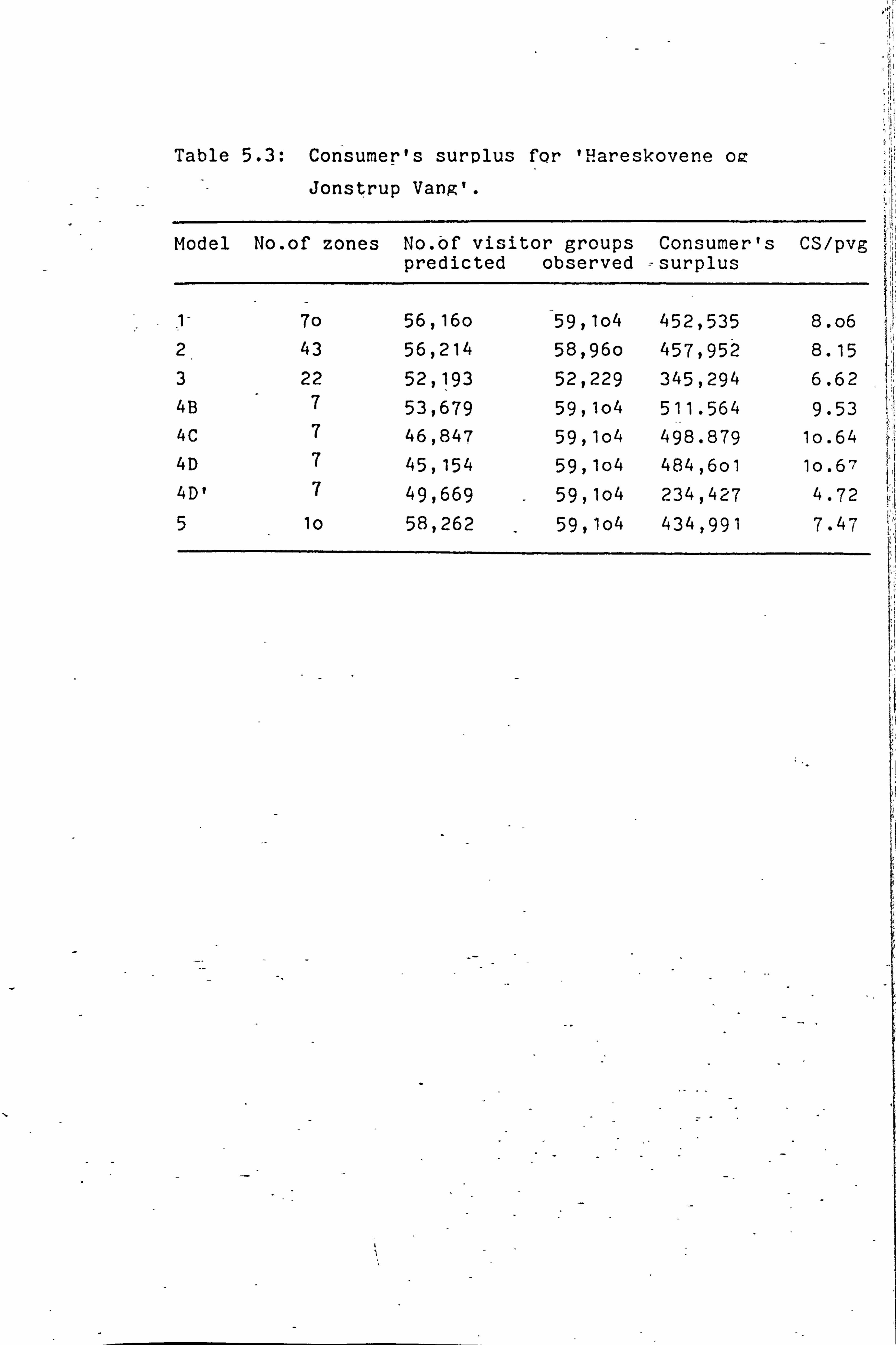
Table 5.3: Consumer's surplus for 'Hareskovene oz
Jonstrup Vang'.
Model No. of zones No. 6f visitor groups Consumer's CS/pvg predicted observed ýsurplus
7o 56,16o 59, lo4 452,535 8. o6 2. 43 56,214 58,96o 457,952 8.15 3 22
7 52,193 52,229 345,294 6.62
4B 53,679 59, lo4 511-564 9.53 4C 7 46,847 59, lo4 498.879 lo. 64 4D 7 45,154 59, lo4 484,6ol lo. 67 4D' 7 49,669 59, lo4 2349427 4.72 5 lo 58,262 59, lo4 434,991 7.4-(

Pag e 151
demar, d for all of the forests as one is calculated, all 52 forests are
included despite the above criterion.
As described in Section 5.4-5, travel costs are calculatel in
kilometres which are, in the following, referred to as units'.
5.5.1 A Comparison of Mezhods
In the following, the results for two forest areas in particular will
be describel: 'Hareskovene og Jonstrup Vang' (Forest No. 10 in County of
Copenhagen) and 'Jaegersborg Dyrehave og Hegn m. v. ' (Forest No-3 in County
of Copenhagen). This is done in order to clarify the difference between
the variations of the applied method.
'Hareskovene og Jonstrup Vang'
All the results from this forest are summarised in Table 5.3 and
Figuie 5.6 shows the trip demand curves and The aggregate demand curves for
the three basic models discussed below.
Basic Models.
I- When all the zones are used (in total 70) the consumer's surplus
is calculated to 452,535 units for a predicted number of visitor groups of
56,160. The ac-tual, number of visitor -groups (i. e. the- sample- estimate
from PFAF) was 59,104. The consumer's surplus per predicted visitor group
(pvg) is 8.06 units. (Figure 5.6 a)
2. When only the postal zones for which - the forest was within an,
acceptable range - (See 5.4-7.2), 17 zones were excluled thus leaving 43,

0
(n c: 0 MD tyl 0
G)
0 LW
in
5 a)
N4 m t31 tu
(0
rcj 124
. ri 14 Eri
0*
PW
U
-c >
(x -,
;; >- 12Z6 in Z f4 0
L2 CD
w Z w
CD lz
in w (x
IM) ISM 13AY7J1
z E ri a -j
I- j h C, ) - I
z .. I _�
Lu z
UJ > 0 v
LU
cx 5t v2-. aK 2- T2
ISM MAYU
0 z >
J
cr Z j
z 0 I
U 0 Lu z
ui 0 Id
in L LJ a0
I- st I It -2
am M MAYM
ui lz
!Z
ui 0. - .c at S. -
'U
t
0 z >
M: I. - -i in z C: ) f4 5 C4
Lu z LLJ
LLJ cr-
(w)D 334 NOISSlwaV
0
Ub
6-
0 z
D
in z
ui z ui
tu Cý
Ic,
6-
A es rcj
a 88 0
O1 33I NOISS WaY
z >
b. - a V) z 0
LU
LLJ M
ro Q) (D 41 ro ra Q)
4j
ty,
C: Q) t- I
OW 33-J -NOISSIWav

Page 152
observations for estimating the demand curve. The consumer's surplus was
calculated to 457,952 units or 8.15 units/pvg for the 56,214 visitor groups
predicted. The difference between model I and model 2 is not very big.
From Figure 5.6, it can be seen that it is mainly the furthest distances-
which have been omitted. (Figure 5.6 b)
3. When only %hose postal areas for which the forest is within the
distance to the nearest forest are selected, we are left with-22 zones. In
this case, the consumer's surplus is 345,294 units or 6.61 units/Pvg, which
is approximately 28% less than the results derived above.
It should be noted how well the predicted number of visitor groups in
the three models matches the actual number of visitor groups. This is even
true for the individual zones as can be seen in Appendix A5.4 where output
from the model is shown. (Figure 5.6 c)
Rezoned Models
In the rezoned models, -the postal areas are rezoned according to a
chosen zone width in more or less concentric zones and, in this way, the
method becomes very similar to the traditional Clawson analysis. .
The
rezoning works in the following way: the maximum distance, i. e. the
distance to the postal area furthest away from which a positive number of
visitor groups has been observed is found. For 'Haveskovene og Jonstrup
Vang', this is equal to 34.8 km. -
The width of the zone interval is chosen
and the number of zones is calculated as:
Number of zones ROUND (mmc D, /z, + 0-5) 04)
where
ROUND a function which rounds the argument to the nearest integer.

Page 153
zi = width of the zone interval.
If the width of the zone interval is chosen to be 5.0 km, the above
equation gives the number of zones to be 7 which means that all postal
areas up to a distance of 35.0 km are used in -the analysis. For each of
the 7 new zones, the cumulated number of visitor groups and zone population
will be calculated and from those figures, the visit rate can be found.
The travel costs can be calculated using one of the following three
mod el s:
B) 'Normal costs' which is the distance to the middle of the zone.
C) 'Uniform costs' which is the distance calculated with the assumption
that the population is uniformly distributed over the zone (For B and C see
also 4.2-2-2).
D) 'Weighted costs' which is the average distance to the postal areas
within the zone weighted according to the number of households (zone
population) in each postal area.
For model 4B, a consumer's surplus of 511 564 units is calculated fo r
53,679 visitor groups which
give similar results. C gives
10.64 units/pvg and D give
JO. 67 units/pvg. Models C arA
similar to models I and 2.
groups are smaller for C and
slightly bigger*
is equal to. 9.53 units/pvg. Models C and D
493,879 units for 46,847 visitor groups or
s 484.601 units for 45,154 visitor groups or
D are, for the total consumer surplus, quite
However, as the predicted nfimbers of visitor
D, it makes the consume r's surplus/lvg

Page 154
It should be noted that these models are still weighted similarly to
the individual models by zone population/visit rate. If we did not weight,
the consumer Is surplus would decrease as shown in model 4D' which consists
of - the same data as 4D but where no weighting has been applied - This
results in a consumer's surplus of 234,427 units for 49,669 visitor groups
or 4.72 units/pvg.
If, instead of using a zone width of 5.0 km-, we used 3.5 km, thereby
eszablishirig 10 zones, we will gez-the results shown in model 5. This
gives a total consumer's surplus of 434,991 units for 58,262 visitor groups
or 7.47 units/pvg.
Which model is, then, the 'right' one? This forest can be taken as an
example of a type 2 forest i. e. a forest of regional interest. Therefore,
model 2 ought 'to be the most representative although, in this case, the
difference between models 2 and 3 is very small and the number of visitor
groups declines by only approximately 6000 when the postal areas nearest
the forest are used.
5.5-1.2 'Jaegersborg Dyrehave og Hegn m. v. '
This forest, on the outskirts of Copenhagen, is by far the most
important recreational area in North Zealard and is the most frequently
visited with an estimated- -annual number of visitor groups of 381 685.12
This is a forest of national importance (See 5.4.7.2_). A"ll of the 'results
for this forest are summarised in Table 5.4.
12. See Apperdix A5.2. The regression estimate is' 515,236 and the sample estimate 398,324 (before exclusion of zones).

Table 5.4: Consumer's surplus for 'Ja! gersborg Dyrehave
og Hegn m. v.
Model No. of No. of visitor groups Consumer's CS/pvg zones predicted observed surplus
1 87 375j789 3812685 12,573j819 33.46
2 42 27o, 696 357v775 15,299,526 56-52
3 19 262,32o 262,53o 21385,562 9.09
4B 12 341,685 3319685 11,822,6ol 34.6o
4C 12 318,629 381,685 12,896,367 4o. 47
4D 12 245,748 381,685 15,3819372 62.59
4E 4 262,3o2 262,53o 2,363, o33 9.01
4F 8 . 31o, 33o 357,775 11,128,336 35.86

Page 155
Basic models
1. When it was attempted to include all of the 87 zones, no
convergence in the non-linear procedure was obtained. This was due to the
inelasticity of the exponential curve as this forest had some recorded
visit rates with very high travel costs. Later in this study, the data for
this case were divided into two groups and an exponential curve fitted to
each group. The consumer's surplus was then calculated on these combined.
This was accomplished using a non-linear procedure in SAS (Barr et al.
1976, Secondary Appendix PSOF. PF04). The result was a consumer's surplus
of 12,573,819 units for a predictel number of 375,789 visitor 'groups which
gives a CS/pvg equal to 33-46 units. However, since this result was not
derived in the manner of all of the others, it should be regarded with some
care. In future research, it should be investigated whether this
inelasticity is a major disadvantage in using the exponential curvefit.
2. When all the zones for which the forest was within an acceptable range
ifere selected, a consumer's surplus of 15,299,526 units was found for a
predicted number of visitor groups of 270,696 or 56-52 units/pvg.
3- When only the zones for which the forest is the nearest are considered,
we are left with 19 zones. This gives us a result of 2,385,562 units for
262,320 visitor groups or a CS/pvg equal to 9.09 units.
Rezoned models
The different methods of calculating the costs are discussed in
5.5.1.1.

Page 156
When we use the same zones as in model I but rezone in 5 km intervals, _
we get 12 zones and the consumer's surplus is 11 822,601 units for 341,685
visitor groups or 34-60 units/pvg. This was with the 'normal costs' (0)
but if we weight the costs according to zone population ' (0), the
consumer's surplus increases to 15,381,372 units ard the number of
predicted visitor groups decreases to 245,748 leading to a consumer s
surplus/pvg of 62-59 units. If we rezone model 3 with 10 km intervals and
use weighted costs* (4E) we get a CS/pvg of 9.01 units which is very
similar to what was found using model 3.
If we rezone model 2 with a zone interval of 7.5 km (4F) and again use
'weighted costs' , we get a consumer Is surplus of 11 128,336 units for
320,330 predicted visitor groups or a CS/PV9 Of 35.86 units.
summary
The results from 'Jaegersborg Dyrehave og Hegn m. v. ' show that this
forest area is more important than 'Hareskovene og Jon'strup Vang' . It is
interesting to see that, at a national level, it has a much higher value
than when it is simply considered as a local forest, The rezoned models
give results similar to models 1,2, and 3 but it should be remembered that
they arer in fact, quite similar as the points are still weighted according
to Section 5.4.8.
A reasonable value -to put on this forest would be in the range of 35
-60 units per predicted v isitor group.

Pag e 157
5.5.2 Comparison of the Forests
Table 5.5 summarizes the results from the 25 forests with more than
5000 estimated yearly visitor groups (as explained in Section 5-5). Those
which are left blank are the ones for which no convergence could be
obtained - For those forests, a consumer Is surplus could probably have been
derived if a rezoned model had been used. However, this was not attempted
in this study. Instead, it was considered more interesting to concentrate
on looking at the differences between some of the forests.
'Troeroed Hegn I
This forest is a typical small local forest ard only when the two
zones for which the forest is nearest are considered do we get a result.
This result yields a low value for CS/pvg.
'Jaegersborg Dyrehave og Hegn m. v. '.
This forest has already been described in detail in Section 5.5-1.2.
It should be noted that, as expected, we derive a very high value for
Cslpvg for this forest except when only the nearest zones are considered.
'Charlottenlund Skov' .I
This forest has slightly higher values for- CS/pvg than the average for
this type of local forest. - However, this may be due' to the fact that there
: Ls a museum and a beach adjoining the forest.

fall r--i Co 0N CYN "0 rl 0 c3-% %ýo :r ý
Ln 0 OD OD Ln cm ý J l
cm
%0 cy% %. D N CO T -, 0 t- t-- CIN N OD e- N %D N cm n t. - 0 N 00 00 CO U-1 Lr% CO CO ON 0 ý t-- Co G) ul
r= :3 r-i L-- (: CD ri 0 0 CL Uý Z.
0Z cm Ln u
ul ta v) CL a) ri N Ln zi > 0 Co t- ri IID Uý t- 0 %m 0 N oL , CO %, 0 t, - U'ý cr, LN %M t, - Ln ý Z J. i
L. (D -i -- - cl (n i t- (M cý: ' ý j C
, CC) L-1 %0 NZ %-0 wý CM N t. 0 cl Cl N 0
Co
(Z .. 1
tz: > 4-4 41
"u -ZT c% %0 0 (n ri OD 0 41 vi 0., 4 1 1
01 Co
Co ON
1- %0 cm C) cr%, %JD
cy, IT
Cr. rl
0 CM
(n
G) 10 ,
t - -- 1
- - > . G) uý j CN7 1; 0 ': r r- CM 0 L. %D OD n u--t N CM Z CL rl N C\j
-- Co - 4.2 (6ý Co 00 (L) %D %I0 CM t- N c31. e C3N %Z C\i ý c
o . r- t- ri CD t %D M -T CM . f4-. 00
tli r-i
fý v r- cm ri e- N (n v-- N (n r- - N (1 1- cm fi 0
:i » v- (1 .t U'% %D H 4-) 0 0 0, 0 0
0 Co rn m L) b4 bd
E
V,
tic r. 0 41. », r_
9) IG L. (L) r-i - C) - 9) - - r-4 0 f
Lo i
(U m L- -, , tic
l - r-1
(13 04 0 G ho
83 l
c: , >Z 0
0-

br > r- N Co Lr% IT %D LN (N. LI- c31% CL Ul% %D P-4 -ý %D UN IT 0 %D i. T Co ý %D 0 Co Co VD (ý) m ri L)
(V M cm 00 %D 0 tr% N uý N IT cn r- U-1
EZ CM CY% 0 %M N N m Uý CN 0 m t- zi r--4 t- t- ýT 0 o Ul% CY% C\i 0 0 Co CL . - 1 1
cL 0 Co t- 0 t- t- N r- ulý (n n Uli 0 :1 OD m _T Ln ýT ri LN Uý IT -: r m (n C-) ci U'% _T -: r ri
v2 v CL a) "> t- CO - t-- C% m -T 0 c3"% -: r t- - 0 L. %z %D %z Lr% (n n 0 -, D CI%., m N cn f- (L) C% cc CIN CM, Co ci CM
: Uli 0 %D ýz r u; az
j cz
9.0 Uý U'ý LII, 0
41 4ý U r) N CY% C% ci %Z 0T (n ON 0 : - 0., 1 c31% 0 (n ri OD ON N Z cn
v C\j :r OD ý 0 r- CO (V) N
ýL (M Co UIN ri t- t- %Z ýlo N j
c; j n UN n
0 u) C t 0 9- t- - %C 0 c31% %10 0 0 (n CI%i 00 t- 0
>b t- Co CY% 0 v- . b. ) 0 0 0 0
r_ 0
0
0 tü
>
> 12. X X 0 :3 0 rn 02 x 94 --54 0) cu 41 M - LO > Co - 41 l '
Le 0 L 4) 94 r_ - 0 4) G vi tu ýo CZ4 0 Z - -: c = b12

v
L
rL
t
I
4
(
4. )
G)
0 £14
n Lr% M
C\i
Ln N 10
(n Ln CO ý
t- ýlo
Co
UN N
ri ýT
J Co
(n N
Co Co ri
r\j 0
m cr.
tu
r: - 94 0
- :Z
N0r: 71 %0 -: r (n
rý
-T 0 "D C\j 0 Ln Lr)
Lr) M Ln IT C\j ON
C\j 0- C\j CYN r-
IT C\j
m C\j C\j
ý 17 a, %
Ln Mm Ln tl- IT
(n ý, c - co C\i I C\j
r- r- (n CC)
T- C\j m
(W) 0
tto 0
Z to > Q) 0
R3
40 0 r-i r-1
III
III
III
C\j
0 a:
tko 0
-ri tko 94 a)
41 v V) GI 0 LO
, r, -, -. , 1 C\i Ull
cý 1;
t-- 0 OD Ln
Ln cm
0
%D Ln
Ln N 00 c31%
%M Ln
0
Lid
tko C C13
tio
94
co I CN I
CY) C\j
co
101
Ln 0
1-I 110
C\j CY) CC) r-
I- N CY)
co 0
44
W
bjO 0
bo 0 0. tko
:3 (D
-W tz
ca W Cý ýo

tic > ýT %. 0 CT% ýT CIN C7, r-p ýr m %ýD *- CL CYN Cl% L"N n - N, m co CN o
ýo o : ý 4 ý ; co t- C L t- 1 0ý Uý ý; Cý C% Ln
(L) co %0 0 0 %D 0 CT% m C\j m ON -r a :3 IT co t- co 0 m (1) Lr) (Y) co ko :3 r-4 t- 0 M ý 0 El- co M C\j ýT \. o 0
- c , C\7 j Cý j Cý C-7 rl: Cý Cý 0 :3 V- %. D V-- IT fn I C\j E-- %10- (n C\j IT C-) V) -T C\J, 0 m C\j ýT
:5> Cl% (7% m 00 ON C\l (n cn ý Cl\ ! I- 0 9. co 0 Llý IT cc -7 00 to cc n \ýo cl% t. (1) C\j C", Cl% CIN C\j M N tc CO ;, ý : ý I : ý I I : .C 'T C ý C t L Cý t- :ý L: ý r- 0 C\. t 0 4-)
>
0 0 %D C\l co 0 0 o 0 r- r- C\l U') C\l U'% ko L-- t-
10 'T ý -zr* - El- 0 UIN C\j t-- -Z cy, m
- ý : : 0 (n -T 0 C t r Lfý Cý CL C\j V. 0 IT I C\l
0 U)
0) to t- 0 -T
0m cy\ C\j %. 0 fn M C\j m
. r- 00 r- CO ý 00 C\. l \D C\l co ýT ýT r- 00 z
C\j M C\j M C\j cn C\j C, C\j cn C\j CY) o
>-, CY) co CC) n %D co 4. ) . r- T- C\j m Cl) oo =s z M cm o
ELI EX4 CLI 44
be bo r_ 0 r_ r. tkc bc >
tio C13 4) 4) 0 0> > X
(is V) > 41 W = . 10 4) OH *a Q)G
4. ) _x 0 H _x ca C/3 :3 17) 0) a -f-4 0 = (D Dc > a 44 - (D (D L -4 (D 0) 0ý ý4 C-4 IC to 0 L -4. ) 4-) 0 0
0 CO 0 E-4 EZ4

ttc
(1)
S :: $ Ea CL C: S. 0 :3
0 co
co a CL a) :3> 0
tic (1) .0 2.. 0
0 4-)
. r-I a >
C6.4 U
0
Q)
0 r-
z CL
C6.4
0 Ell
00
= t-I
r-A Q)
1ý 0
r. 0 :3z 0
0
. 4-, Cl, 1)
0
IIII
IIII
IIII
III
r- ON N r- CY)
r- C\j cn
CTN m
ELI
bo 0
0 r-4 44 0 0)
> ca 6
= C/)
C\j 'n rN-1 n0
Cý rý
co C\j co -T C\J 0 CC)
Lr% cv)
0 co 0 000
cy% ON 0ý Co 00 C% LN Ln IT fi
t--i
Co C% Ul%
CL4
0)
(-4
bC C3
r-1
Lrý Cýl
CO C)N M C\j \0
Lr% cc C\Jl C\j C\. m
- co Ll- C\j cc 0 Cl) 0 1.0
Lfl% Lr- C\j
LfN ý, o C\j Cl\ cc Lr%
0 \D
Lf; C\7
%0 C\.
r- C\j M
cz
(D bc
El:
4)
m
Cl) 0
t-- Co Co N1 CO %Z
- CO ý
0 Ln t-- OC
j
cm N
tt. 0 cu
00
la rz r-1 :i
r_ z4
cu cu ý
0 CIW --

Page 158
I 'Kongelunden .
This a forest of regional importance and, as such, is similar to
'Hareskovene og Jonstrup Vang' Iz has a smaller 'catchment' area but this
inight, to some extent, be counteracted by its I traditional' use as a
recreation area.
I 'Soelleroed Kirkeskov
This is a small local forest ard no result is obtained until model 2
is applied, i. e., selecting the zones for which that forest is within an
acceptable distance. The CS/pvg value is, as expected. quite low.
'Geel Skov' -
This is a forest of regional interest. The upward tendency in CSlpvg
when applying model 3 could be caused by the fact that here we are
e]ccludirg zones from which we get small visit rates due to a large number
of recreational alternatives in the area (See 3.2.2).
'Noerreskoven'.
When model 2 is applied, this forest yields a value for. CS/pVg around
the average for a forest of regional importance.
'Aasevang M. V. '
Neither model I nor model 2 worked for this forest and it would, seem
that model 3 has overestimated the CS/pvg.

Page 159
'Ha'reskovene og Jonstrup Varg'
This forest has already been described in detail in Section 5.5.1 . 1.
It is a forqst of regional importance.
'Vestskoven Vest'
Although this forest might one day be of regional interest, it is
still so new that no long-term use pattern has developed.
'Hornbaek Plantage'
This forest is located near the sea and is used as a beaýh resort.
Therefore, we get a high value for CS/pvg using model i If we select the
zones for which the forest is within an acceptable distance, i. e. use
model 2, the value for CS/pvg drops. However, -it should be noted that, in
a way, it is not the same product because the visitors may be coming, -for
The beach.
'Teglstrup Hegn og Hellebaek Skov'.
The value for CS/pvg'for this forest is similar to oth'ers of regional
to local interest. Model 3 yields a high value 'for CS/pvg but it is only
based on 3 zones.
ýKlosterris og Horseroea Hegn' .
No results were obtained for this forest. A rezoned model could be
-attempted -

Pag e 160
*Egeb. aeksvang I-
For this forest, no result is obtained for CS/pvg until we use model 2
when the calculated value of CS/pvg is within the expected range for a
forest of this type.
'Danstrup og Krogenberg Hegn'.
Model 1 did not work. However, model 2 gave a result for CS/pvg which
was similar to that for other forests of regional to local interest. For
model 3, only one observation was left.
I 'Gribskov og Stenholt Vang .
This forest should probably be ranked as b_eing of regional to national
importance and the CS/pvg value is higher, than the average for regional
forests. For model 3, only one observation was left.
'Tisvilde Hegn'.
This forest is also of special interest due to its popular beaches.
As for Hornbaek Plantage, we notice a drop in CS/pvg when using model 2.
Tjje discussion under Hornbaek Plantage applies here as well.
, St. Dyrehave og Tokkekoeb Hegn m. v. '.
-Here, only model 2 yields a result. *_ This resul t is surprisingly high
for a forest of regional interest.
(I

Page 161
'Folehave'.
This is a forest of local interest and the values found for CS/pvg are
consistent with those found for other local forests.
I 'Rude Skov
As with 'St. Dyrehave og Tokkekoeb Hegn m. v. ', only model 2 yields a
result and, again, this leads to a surprisingly high value for CS/pvg.
This may be due to an underestimation of the number of visitor groups to
the forest.
'Lys truP Skov'
This is a typical local forest which the results also, show. Mod el 3
is only based on 3 zones and, therefore, should not be given, much weight.
'Ravnsholt og Soerderskov
No results were obtained for this forest. A rezoned model could lie
tested -
#Slagslunde'. ."z
This is a local forest but the values for CS/pvg are slightly -higher
-than for other local forests-, This may be caused by the fact that Burre
Lake is. next to the forest.
r

-Page 162
'Ganloese Eget' .
This a for est of local interest and the values for CS/pvg are as
expected for such a forest.
'Ganloese Ore og Farum Lillevang
This is a forest of mainly local interest and, again, the CS/pvg
values found are typical of such a forest.
5.5.3 All Forests as One.
The results from the model as explained in 5.4-10.2 using all of the
available points will be described here. The results are summarized in
Table 5.6. When model 1 is applied, we get a very high CSlpvg (76-92
units). This is' probably due to the fact that there are some very long
distances included in this model -which affect the shape of the trip demand
curve. High visit rates at low cost benefit from this. Model 2 gives a
much lower value for CS/pvg 00.17 units). Model 3 yields a result similar
to model 2.
If we rezone all of the points (4), we get a result similar to model 1
but if we do not weight these points (4') the CS/pvg decreases to 8.90
units (5 km zone intervals and normal costs).
If -we
rezone model 2, we get CS1pvg equal to 12.90 units (0) and if
that one is not weighted (4B'), the value for CS/pvg again decreases (9-02
units (5 km and normal costs). When model 3 is rezoned (41)), we get a
CS/pvg of il-80 units and if the points are not weighted (411) , CS/pvg
equals 10-37 units.

Table 5.6: Consumer's surplus for 'all forests aýs onev.
Mod el No. of zones
No. of visi tor groups predicted observed
Consumer's - surplus
CS/pvg
1 19o2 4o6,273 958,138 31,251,7o5 76.92
2 '1167 825,162 825,9o4 81391,778 lo-17
.3 2o8 593,663 595, o16 6,11o, 862 lo. 29
4 14 4o8,859 95F3,138 32,131,75o 78-59
41 14 798,191 958,138 IT , 2o 11 cro9 8.90
49 8 795, o46 825,9o4 lo, 253, Boo 12.9o
49, 8 7629921 825,9o4 6,879, o77 9. o2
4D 6 594,527 595, o16 7, ol5, o63 11.80
4DI 6 582,674 595, o16 6, o4o, 552 lo. 37
Page 163
5.6 Summary
In Chapter 5, a Clawson analysis' has been applied to 'data from
Denmark. This section will summarise and discuss the major_problems I
encountered and the findings of the study. Some of the assumptions used in 11
the application of the Clawson method to this data result from the findings
discussed in Chapter 4.
Previous works: Most workers in Scandinavia who have tried to estimate the
recreational value of forest areas have used the opportunity costs method.
However, it is not logical to consider that the benefit of iecreation is
always equal to cost of providing it. For reasons explained in Chapter 3,
this author considers the Clawson method more appropriate and its
application in Denmark has been attempted in this work. Recently, a
Clawson analysis has been used for estimating the value of sport-fishing in
the Gaula River system in Norway.
Project Forestry ard Folk: Data pertaining to visits to forest areas have
been collected during the study period April, 1976 to April, 1977. For
this study, data from the region of North Zealaýd have been made available.
For each forest, the data relating to the annual number of car-borne
visitors to postal areas are investigated. As with the Owydyr data
(Chapter 4), the visitor group was chosen as the- visit unit,
Zoning system: Postal areas were used -as the basic zoning system,
especially because this information war, coded on the data-base. Also, the
number of households in each zone was available*

Page 164
Distances: It was decided to attribute 'logical' variables to the
observations on visit rate arA price in order to distinguish between
visitor groups. In this way, it becomes possible, for each forest, to do a
Clawson analysis 1) using all- postal areas up to the furthest zone from
which visitors were observed, 2) using postal areas for which the forest
area is within an 'acceptable ' 'distance, 3) using the postal areas for
which the forest is the nearest forest.
Cost function: the cost function was simply determined by measuring the
distance on a map from the forest to each postal area. In this way, no
allowance was made for time costs. However, no long time- periods are
involved in travelling within this area and if a time cost was to be
included, it would have to be approximately proportional to the distance.
This means that we can always mAtiply -the final consumer's surplus by a
constant in order to include time costs. 13
ý
Curve fitting: Three different models for the trip demand curve were were
testell -a linear regression, a2 r" degree polynomial and a negative
exponential curvefit. The negative exponential model was found to have the
smallest SS-residuals and it was also considered to be the most 'logical'
as it has some important advantages which will be discussed in Chapter 6.
13. The Directorate of Roads uses as time costs 20% of the average hourly wage for trips from the home to somewhere else and 10% if the d, riving is considered to be a part of the purpose of the trip (Vejdirektoratet- 1977, P. 9. ).

Page 165
Weighting of points for the trip demand curve: The weighting used is
discussed in Chapter 4 (zone population/visit rate). As there were some
zones with an observed visit rate of zero, a two stage model was applied -
First, an unweighted model was fitted to the data ard, in the second stage,
the predicted values from this curvefir. were used to calculate the weights.
Methods: the data were organized in a data base on which several
programmes could be used. It was possible to do a Clawson analysis on each
forest individually in three different ways dependent on which zones were
selected as explained above. It was also possible to rezone for an
individual forest. Finally it was possible to calculate a consumer's
surplus for 'all forests as one' , i. e. using all possible information.
Results Comparisons have been done between the different variants of the
Clawson method in detail on two forest areas. The result for 'Jaegersborg
Dyrehave og Hegn m. v. ' varied quite considerably according to the model
used
For all forests with an estimated number of yearly visitor group of
more than 5000 it has _been
attempted to calculate the consumer's surplus.
The values obtained for the different forests vary accordir)g to what one
would expect from knowledge of the forests. In fact the subjective
classification of forests given in 5.4-7.2 seems to be confirmed. For
forests of local interest, . values for Model 3 terA to be- higher than those
for Models I ard 2, while the reverse is true for forests of regional or
national interest. This is because of the way zones are excluded or
included in the models. For local forests, no visits are - expected from
zones for which it is not the-nearest forest. Therefore, including such-

Page 166
zones will bias the demazil curve to the left, especially as these zero or
small values will be heavily weighted by the procedure described above.
Using only zones for which the forest investigated is the nearest one helps
us to correct for the effect of substitute opportunities in depressing the
apparent value of the forest.
On the other hand, for forests of national interest, inclusion of the
more distant zones, from which many visits are recorded, puts emphasis on
the really high values which may be experienced in these forests. Omitting
these zones leads to underestimation of value.
The best known forest of national interest has a consumer's surplus
(CS/pvg) in the range of 30-60 units which is equal to approximately 18-36
Dkr- or 120-140 pence per visitor group. This makes a value of around 10
million Dkr- (approximately 1666,000) for the total number )f annual
car-borne visitor groups. It should be emphasised that these values do not
include time costs and only car-borne visitor groups have been considered.
In addition, no expenditures for maintaining such a high visitor rate have
been deducted. It would be possible to calculate the NPV by dividing'by
the proper discount rate in order to get a value for the forest use as a
recreational facility. 14 Most forests of regional interest have a CS/pvg of
around 10 units which is around 6 Dkr. or -40 pence per visitor group.
Forests of local interest have CS/pvg values of less than 10 units.
14. See also the general discussion in Chapter 1.

Page 167
When calculating the consumer's surplus for 'all forests as one' the
results vary considerably dependent on the model used. A reasonable value
for the average visitor group (CS/pvg) would be about 10 units, which is
-equal to approximately 6 D. Cr. (approx. 40 -pence ). However, the large
variation in value between individual forests casts doubt on- the idea of a
Ogeneral forest recreation value'. We need at least to classify forests,
as has been done here, in order to set an approximate value for consumer's
surplus per predictel visitor group.
The results presented in this chapter were based on data collected in
Denmark from 1976 to 1977. The data only took car-borne visitor groups
into consideration and in order to get the right valuation. non-car-borne
visitor groups should also be considered. It should be investigated
whether or not the non-car-borne visitor groups have the same demand curve
as the car-borne -visitor groups, i. e. the same willingness to pay, or
whether we are dealing with another group of users who have a different
consumption pattern.
The results from this study present a static pijature of the situation
in 1976-77. The rate of visits might have changed. According to Koch
(personal communication) the number of cars on the permanent sample plots
has gone down by approximately 24% between 1976 and 1982. This is mainly
due to the steady increase in travel costs during this period. It should
be investigated whether this has resulted in an increase in'the-number of
persons per car and also - whether the visitor groups have the same
distribution by postal areas as in 1976-77 or if the the visit habits have
changed to become more local.

6. FINAL'CONC LUS IONS AND RECOMMENDATIONS
In the conclusion to Chapter 3, several problems of the Clawson method
were identified for investigation and treatment. In this chapter, the
findings of this investigation will be drawn together in recommendations
for the way in which future analyses of forest recreation might be carried
out. At the same time the findings are assessed in relation to other work
in the general field of recreation economics. Topics are highlighted which
have been identified in the course of the investigation as requiring
further research. Finally implications for forest decision-making are
reviewed.
6.1 Multi-site visits
Where a recreation site is visited as part of a recreation trip which
includes m any sites, the traditional Clawson-method cannot give a realistic
value to the site. In general it will greatly overestimate benefit of an
individual site, especially if the visit is part of a long holiday. Apart
from the discussion of benefit from travel as was described in 3.2-3, the
literature does not make much reference to this practically important
problem. However, after the work in Chapter 4 had been completed, Haspel
and Johnson (1982) described an approach to allocating values for
multi-, site visits in North American National Parks. They tested several
jaultiple regressions in which total trip distance was comt-ined'in various
formulations with number of trip destinations. On this basis they-obtainea
a better estimate of participation ' rates ', than was given by simple

Pag e 169
regression of participation rate on total trip distance. This approach has
been criticized as follows by Christensen, Humphreys and Price 0985).
"First, testing a n=ber of alternative regressions, each containing
several variables, increases the probability that an apparently significant
regression will be generated by chance. Second, multiple linear regression
requires that the influence of inlependent variables upon dependent
variable is additive and separable. In fact on P-369 Haspel and Johnson
give reason to suspect some degree of collinearity between three of the
variables incluled in their most successful regression, but they offer no
indication of why the separable influences of these variables should be
additive. Thus, while each variable in this regression would be expected
to affect participation rate in some way, there is no a priori
justification for the functional form of the relationship tested. "
The revised Clawson method described in Chapter 4 should be used in
preference to the traditional Clawson method for forests (or recreation
sites of other types) in holiday areas, because here many, or probably most
visits will be made not from home but from the holiday base. In addition,
as shown in Christensen, Humphreys and Price 0 985), the ' revised Clawson
method enables us to account for travel modes having different costs.
6.2 Substitution between sites
In the results of Chapter 5- it has been shown to be incorrect to take
a general value for "forest recreation", as has ', ieen done in one study of
British forestry (Treasury 1972). On the contrary,, the value of a forest

Page 170
visit depends on the individual character of the forest. For forests of
national importance, the value of a visit seems to be several times the
value' of a' forest which does not provide any special experience. Our
subjective classification of the importance of forests in North Zealand
seems to have been confirmed by values calculated for them.
On the other hand all forests can be to some extent a substitute for
others, and this explains why few or no visits from long distances have
been recorded to forests of only local interest in North Zealand. The
effect of substitution is to bias the upper parts of the demani curve
strongly to the left, indicating that no visitor is ever deriving great
value from local forests.
No really satisfactory solutions to the substitutes problem have so
far been offered, though as described in 3.2.6 many authors have proposed
methods. As a result of this work, it is recommended that logical
distances as defined in 5.4-7.2 are used to define the limit of zones to be
used in deriving the demand function for a site: when a forest is sim P1 Y'
of local interest, only those zones are inclijded for which the forest is
the closest one, whereas for forests of national importance all zones
should be used. However, applicatio n of all the different models can give
some indication of which type of forest we are dealing with since for
forests of national importance we expect a higher value using all zones.
The different models (i. e. models 1,2 anid 3) used in the Danish
study can be viewed as a way of classifying the visits. For example, many
visits to a specific area might be due to an adjacent beach and not to the
forest itself where the cars are parked: this was the case in some areas
of North Zealand. But by using a model where only zones for which that

Page 171
forest is the nearest (i. e. only local visits) will filter out the
long-distance beach visitors, and in that way yield a more accurate value
of consumer's surplus per predicted visitor-group for the forest itself.
The above classification could have been carried out more. explicitly if we
had divided the visitors into groups according to what activity they
pursued from the parking area where they were counted, but this was not
possible with the secondary data available.
6.3 Weighting of data
It has been shown that not all points for the demand . regre. ssion are
equally reliable The solution to this problem given by Bowes and Loomis
0980) is not generally correct, as pointed out by Christensen and Price
0 982 The correct weighting is visit rate/zone population. But sampled
visit rate is not the best estimate of this variable. The visit rate
should be estimated first from an unweighted regression, ard the first
estimate of visit rate used in weighting the second-stage regression. This
has the advantage that zones with a recorded zero visit rate can be used in
the analysis which -would otherwise be -impossible
due to -their
infinite
weighting - It is important that such zones should be able to be included
and not completely ignored, since they represent valid data on the
d is tribution -of
willir)gness to pay within the population.

Page 172
6.4 Aggregation of data
In this- study it has been shown with both British and Danish data that
can affect the calculated consumer's surplus. different zonings
Accordingly, it is recommended that different zonings shoul d be - tried and
an average taken. When analysis is performed by means of computer,
rezoning can be done very easily.
As for Flegg'-s claim (1976) that heteroscedasticity problems may arise
from certain aggregations of origins, this has been solved by the weighting
procedures in least-squares regression, as have been described.
As for the suggestion that a high degree of disaggregation of origins
leads to better statistical estimates, we eventually encounter the problem
that origins may not supply any visits at all. This can give a statistical
problem when we weight by zone population, but we believe we have solved
this through the two-stage estimation process.
6.5 Functional form of the demand regression
Comments on this important matter have already been given in 4.4 and
5.6. The results from different forms do vary, ard the conclusions can be
summarized thus.
Linear form: This often appears to fit the data well, -there are-, no.
problems 'with transformation of residuals and it is easy to use. Howevert
the form of the relationship is not logical because it implies that there
I should be negative visit-rates above a certain cost; Not only can this not
happen in practice,, it also can create statistical problems in tw. o-siage

Page 173
weighting of data points.
Second degree polynomial: This is a more flexible curve-fit, which can
represent the data more exactly than the linear form. However, there are
different problems here when the curve is extrapolated. For example, when
the curve is convex to origin, the area below the curve, which shows gross
benefit, may be undefined. Therefore this form cannot be recommerded.
Log-linear form: This form also yields indefinite gross benefits.
The demand curve does not intersect either axis, implying there is not a
limit to visit rate at zero cost or to the distance visitors are prepared
to travel. These problems can be overcome by aiding arbitrary constants to
the variables, but then the answer is very sensitive to the chosen constant
and this is not very satisfactory. Also the distribution of the residuals
and the weighting of the data-points is changed during transformation of
the data to logarithmic form.
Negative exponential form: In spite of somn initial problems with
fitting a regression line. this functional form was found to have important
advantages. Unlike the log-linear form, the curve can be fitted without
affecting the distribution of residuals. Unlike the linear form, it does
not predict negative visit-rates: this is logical. and it also makes sure
that positive weightings can be given in two-stage estimation procedures
for the demand curve. Unlike log-linear and 2nd degree polynomial forms, a
finite gross benefit is given by integration under the curve. In
statistical tests also this -curve-f it gave th e smallest residual. sum of
squares and it was very successful in correctly estimating the total number
of visitor-groups. Using the exponential function however implies, as
pointed out by Cheshire and Stabler (1976), that there are " visitors

Page 174
travelling impossible distances " (Ibid., p. 374). We do not believe zhat
this is an overwhelming criticism. On the contrary, because there is no
intersection of the demand curve with the cost axis we do not have the
problem of negative visit rates. The absence of visitors from very long
distances can-be explained by substitution effects. On the other hard, if
there were not any substitutes, a small proportion of visitors would be
prepared to travel very long distances. Thus the very large consumer's
surplus for a small proportion of visits is not at all impossible, ard in
fact reflects the reality of recreational experiences. If it was wanted, a
maximum willingness to pay could be defined arbitrarily, although this
actually makes the integration under the demand curve somewhat more
difficult to handle.
In summary, either the functional form reaches and crosses the cost
axis, in which case illogical negative visits are predicted and correct
weighting cannot be achieved, or it does not reach the axis, in which case
for a small proportion of visits a very high value is predicted. We
believe the second case is more realistic, ' provided the functional form
does not lead to indefinite consumer's surplus.
The negative exponential form is recommended on these grounds, but
with the caution that not all statistical packages are able to provide an
untransformed negative exponential curve-fit. Also, as mentioned in
Chapter 5, it seems that the exponential curve fit does not produce a
result in all situations, and further research might invest igate whether
this is a general problem, aid if so. whether it is due to the data or
whether it is because of the particular curve-fit.

Page 175
6-6: Integration of consumer's surplus
In connection with the revised Clawson method, the integration of
consumer Is surplus was attempted with three different methods. If the
revised Clawson method is used, it can be argued that integration of the
individual's consumer's surplus is most valid, since each consumer faces
different costs. The problem is that the various methods of integration
often lead to very different results for the total value of the site. To
overcome this problem, the measure consumer's surplus per predicted visitor I
group was introduced. This was found to produce much more consistent
results. In the case of the negative exponential, this measure was found
to be tery simply related to the parameter of the exponeatial,
independently of the cost of visiting. Extending this result to the
revised Clawson method, we should expect identical value for consumer's
surplus per predicted visitor group whichever integration method we have
used
It is recommended that consumer's surplus per predicted visitor group
is used in evaluation of sampled visits, and that this figure is multiplied
by the recorded or the predicted number of visits -to give an annual value
of recreation.
6.7 Some outstandirg problems.
Many of the problems described in Chapter 3 have not been investigated
in this thesis. Where we have investigatea probiems, we have shown that
there are needs for further "research in certain identified areas. It would
be useful. to repeat the studies described in Chapter 4 ard Chapter 5 to see
if- similar results were found for other data. In addition, it would be

Page 176
interesting in future research if a 'quality value' for the different
forests obtained from a preference study could be included with the
behaviour study and the population densities. Some problems identified in
the course of the studies neel to be addressed. For example, --the whole
basis of the Clawson method is travel cost, but it is not agreed which
definition of cost should be. used. It is argued that perceived cost is_
relevant in determining willipgness to pay, but visitors do not clearly
perceive their costs of travel by car, as was shown by the bias in response
-to the Gwydyr questionnaire. Most often people estimate their costs as
being petrol costs only, but this is different both from average and
marginal costs of running a car. Also in this study it was assumed that
people consider their costs as a group, not as individuals, which is why we
used visitor-group as the unit of visitation. Considering the central
importance of this figurq in outdoor recreation evaluation, it has not
received much attention from recreation researchers. The traditional
Clawson method has always had the problem that a uniform travel cost from
each zone must be used. The revised Clawson method does not have thiý
restriction and therefore can inclule variation in perceptions.
In future research, the problem of the survey method -versus the
i Clawson method should also receive more attention. In the case of the
Danish study, no data were available which would enable the survey method
to be used - However, as discussed in Chapter 3, there are situations where
the Clawson method is inappropriate and the only possible way to yield an
estimate is by the survey method.

Pag e 177 -
It would be interesting to test the hypothesis of people's willingness
to pay, i. e. do they react in the same way to an increase in fee as to an
increase in travel costs? Charging would be a useful tool in managing
congestel areas but it would be a rather discouraging measure as we do not
have a tradition of paying fees in order to visit forest recreational areas
and we might, therefore, e%perience a reluctance to pay for the use of such
areas.
6.8 The evaluation of forest recreation
In spite of some deficiencies. it proved possible to use. secondary
data sets in this study. By their use. problems relating to the evaluation
of recreation forestry have been dealt with. In particular, we have
discussed the necessity for an economic evaluation in order to compare
recreation with other sources of benefit - from a 'multiple-use managed
forest.
Recreation, being one of many outputs from forestry, might affect the
utility of the other outputs. In this study, we have tried to derive
demand curves for forests as recreational goods and, thereby, estimate the
value of the consumer's surplus. This has been done in a static situation
giving us an idea about how people would react to an increase in travel
costs and fees. However, further research is still needed on the
substitutional effects between recreation and the other outputs. from
forestry. -
Ideally, we would estimate the transformation curves between all
the output. 3 -involved ard then, given the right price curvet we -could
optimise the mixture of outputs if we had established this n-dimensional

Page 178
trade-off space. Although a lot of data is required to investigate ani
establish the transformation curves exactly, it would nevertheless be of
importance just to know about the curve shapes to get an idea of th_e
relationship between different parameters.
The presenzei study has shown that it is possible to get estimates of
the value of recreation ani it is our belief that it is important to have-
these values or, as discussed earlier, curves for the demard for recreation
in these forests. Not only are the absolute values necessary when we wish
to compare recreation with other *investment' alternatives but also the
relative values are important to the state forestry administration in
deciding where to expard its services.

190
LITERATURE CITED
Anon., . 1977: FORTRAIT -10. Language Manual (Version 5). - Digital Corp.
Alvey, IN. G. C.?. Banfield, R. I. Baxter, J. C. P-W Lane, P. K. Leech, J. A. Nelder, R. W. Rogers, G-J-S- Ross, H. R. Simpson, Wedderburn, G. N. Wilkinson, 1977! Statistical Program (4.01). -Lawes Ag-ricul Experimenzal Station)
Gower, W. J. - Krzanowski, Payne, K. M Phelps, C; E
A. D. Todd, R. W-M, Genstat- A General
tural Trust ýRothamstea3,
Banford, N. D. , J-L Knetsch and G. A. Mauser, 1977: Compensating ani equivalent variation measures of consumer's surplus: Further survey resalts. Unpublished paper, Department of Economics anI Commerce, Sinon Fraser University.
'Barr, A. J., J. H. Goodnight, J. P. Sall and J. T. Helwig, 976: A User' s Gui, 4
efzo 3-'S 76-SAS Institute Inc., Raleigh, North
Carolina 5., 32-9 pp-. -
Baxter, M. J., 1979a; 7-Teasuring the benefits of recreational size provision- X review of techýTýues relazei to the Clawson method. 47pp.
Baxter, 14. J., 1979b; The interpretation of the distance anI attractiveness componets in models of recreational trips. - G'. 2 OLj: Eý. PhLe 2L ýýýis , 11 : 311 -3115.
Becker, G. S., 1965; A theory of the allocation of time. - The Economic Journal, 75: 439-517.
Beesley, M. E., 1965: The value of time spent in zr. aV ell ing --Economics, 32: 174-175.
Binkley, C., 1977: Estimating Recreation Benefits: A Critical Review and Bibliography. 7ExchaMe BibliogLapýy No. 1219, Council of Planning Librarians.
Bockstael, N. E. ard K. E. McConnell, 1980- Tquivalent ard compensating variation for natural Resources. -Lard Economics, 56: 56-63.
Bohm, P. , 1971 : An approach to the problem of estimating d emard for public goods. - Swedish Journal of Economics. 73 : 94-105,
Bohm, P. , 1972: Estimating. demanI for public goods An experiment. -European Eýonomic Review, 3 : 111-130-.
_- Bouma, S. t 1976: Some models for determining the value 'of recreation
areaa. - in; Environmental Economics, Volume. TI, -Methods, editdd by P. Nijkamp. -Nijhoff, Leiden.
Bowes, M. D. and J. B. Loomis, 1980: --A note on the use of travel cost
mo(fels -with
unequal zone populationi. -Land Economics,, 56 (4):

Page 118'.
465-470
Brookshire, D S., B. C. Ives and W. D. Schulze, 1976 - The valuation of aesthetic preferences. - Journal of Environmental Economics and Management, 3 : 325-346.
Brown, W. G., A. Singh and E. N. Castle, 1964: An economic evaluation of the Oregon salmon and Shetland sport fishery. -Technical 0 Bulletin, No. 78, Oregon State Agricultural Research Station, Corvallis.
Burt, O. R. and D. Brewer, 1971: Estimation of net social benefits from outdoor recreation. - Econometrica, 39 -. 813-827.
Burton, R. C. J. 1973: A new approach to perceptual capacity. -Recreation Lews ýýnplemenz, 10: 31-36.
Cesario, F. J., 1976: Value of time in recreation benefit stulies. -Lard Economics 52: 32-41.
Cesario, F. J. anl J. L. Knetsch, 1970: Time bias in recreation benefit estimates. -Yater Resources Research, 6(3): 730-704.
Cesario. F. J. ad J. L. Knetsch, 1976 A Recreation Site DemanI and Benefiz Estimation Model. - Regional Szulies, 10 : 97-104.
Cheshire, P. C. ani I. I. J. Stabler, 1976: Joint consumption benefits in recreational site 'surplus'; An empirical estimate. - Reýional Stulies, 10 343-351.
Christensen, J. E. , 1980: A second look at the informal interview as a technique for recreation research. - Journal of Leisure Research, 12 -. 183-166.
Christensen, J-B., 1931: Economics of recreation- forestry in Scandinavia. -Proceed ings, Division IV, XVI IUFRO World Congress, Kyoto, Japan, pp. 481-4ý4-
Christensen, J. B. ard C. Price, 19EQ: Weighting observations in the derivation of recreation trip demanl regressions -A comment on Bowes ard Loomis. -Land Economics , 58(3): 395-399.
Christensen, J. B., S. K. Humphreys Clawson method: one disaggregation problems in Environmental Management, 20
Cicchetti, C. J. - and V. K. Smith$ Ballinger, Cambridge, Mass.
and C. Price, 1985: A revised part-solution to multidimensional recreation evaluation. - Journal of
: 333-346.
1976: The Costs of Congestion,!,
Clawson, M., . 1959: MethodF. of measuring the demand for- and value - of - outdoor recreation. -12pLintt No. 10, Resources for the Future,
Washington, D. C. 37pp.
Clawson, - M. ard J. L.. Knetsch, 1966: ' - Economics of Outdoor

Page 182
Recreation. -Johns Hopkins University Press for Resources for- the Future, Baltimore, 323pp.
Colenutt, R. J., 1969; Modelling 'travel patterns of day visitors to the cotmuyside, Area,
- 1: 4ý47-
Collings, J. J. , 1974; The'valuation of leisure travel time a note. Regional ard Urban Stalies, 4: 65-67.
Common, M. S., 1973;, A note. on -the use of the Clawson method for the evaluation, of recreation size benefits. Regional Stulies, 7: 401-406.
Couch, J. D., 1975: Recreation with neoclassical economics. - in- Searle, G. A. C. el Recreational Economics and Lnalysi: ý Longman, Harlow.
Crutchfield, J. A., 1962: Valuatioa of fishery resources. -Lard Econor-iies (May): 145-154.
Currie, N. , 1980; A review of cost-benefit techniques in rural recreation planning. - Gloucestershire pý! pers in local and rural pLannia. 7: 26pp.
Currie, J. M. , J. A. Murphy and A. Smith, 1971 - The Concept of Economic Surplus ani its Use in Economic Analysis. -The Economic Journal, 81: 741-799.
Dasgupta, A. K. ard D. W. Pearce. 1978! Cosz-Benefit Lnýjysis-- theory ITý. 2ractice -Macmillan, London, 2C9--pp.
Davis, R. K. , 1963: The Value of Outdoor Recreation : An Economic Stuly of the Maine Woods. - Ph. D. diss. , Harvard University.
DeGroot, X. H. , 1970: Optimal Statistical Decision. -McGraw-Hill, Inc., New York.
_ Deyak, T. A. ant V. K. Smith, 1978; Congestion and participation in
outdoor recreation: A household production function approach. - Journal of Environmental Economics and Management, 5: 63-80.
Dupui t, J. , 1844: On the measurement of the utility of puplic works. -Translated in: International Economics Pape rs, 2(1952): 83-ilO.
Dwyer, J. F., J. R. Kelly and M. D. Bowes, -1977: Improved Procedures for Valuation. of ý the ContributioA to- National Economic Development. -a2rrý No. 128, Water Resources, Center, -University of Illinois at Urbana-Chamraign, 218pp.
Edwards, J. A., K. C. Gibbs, L. J. Guedry and H. H. Stoevener,, 1976: _
The demand fo r non-Unique outdoor recreational- . services: methodological- issues. -Technical Bulletin, - 133--. 60pp. Ag ricul tural . Ex pe rim e nt al Station, q; egon. -State-
Universityp Corvalis, Ordg-on, 60ppe

Page 1,83
Elson, M. J., 1975; Some fectors affecting the incli ence and distribution of week-end recreation trips
Fisher, A. C. and J. V. Krutilla, 1972: Determination of optimal capacity of resource-basal recreation facilities. - in: Krutilla, J. V. [ed. ]: Natural Environments, Studies in Theoretical and ATjI n ýjy s i! j. Johns Hopkins University Press for Resources
_Lc! j L
for the Future, Baltimore, 352 pp.
Flegg, M. J., 1975; Methodological problems in estimating recreational demard functions anI evaluazin, -, -recreational benefits. - Regional szulies, 10: 353-362.
Freeman, A. M. , 1979: The Benefits. of Environmental Im rovement. Johns Hopkins University Press for Resources for the Future, Baltimore, 272 pp.
Gordon, M. I. ard J. L. Knezsch, 1979: Consumer's surplus measures ard The evaluation of resources. -Lard Economics, 550 ): 1-10'.
Groes, N. , 1979: Skoven er ikke bare zraeer. (Woods are more than trees). - Dansk Skovforenings Tidsskrift, 64(4): 260-275.
Gundermann, E., 1976: Economic procelures used in outdoor recreation evaluations throughout The world. - Proceedings, Division IV, XVI IUFRO World Congress, Oslo, Norway, pp. 122-142.
Haakansson, H. and Bj. Haegglurul , 1969: Et eksempel paa v ad naturvarden kan kosta skogsbruket. (An example of how much nature conservatioa can cost forestry). -Sveriges Skogvaardsfoerbunds Tidsskrift. 67: 459-480.
Hammack, J. and G. M. Brown, 1974: Waterfowl and Wetlands : Towa zd Bioeconomic ýji! jysjs. - Johns Hopkins University Press for Resources for the Future, Baltimore
Harrison, A. J. M. ard M. J. Stabler, 1981 ; An analysis of Journeys for canal-based recreation. - Regional Studies, 15: 345-358.
Helles, F. , 1977: Om teorien bag flersidig produktion i skovbruget. On the Theory Behind Multiple-Use in Forestry Dansk Skovforenin&s Tidsskrift, 62 : 179-198.
Helliwell, D. R., J969: Valuation of wildl ife resources. -Regional Studies, 3: 41-47.
Henderson, A., 1941: . Consumer's surplus aid .
the compensating variation --Review of Economic Studies, VIII, 117-121.
Hicks, J. R., 1939: Value and Capital . -Clarendon Press, Oxford.
Hicks, J. R., 1943% The four consumer's surpluses. -Review Of Economic Studies XI, 3i-4i.
Hicks,, J. R., 1946: Value and Capital (2nd edition). - Clarendon -Press,

Page 184
Oxforl.
Hicks, J. R., 1956: 'A
Revision of Demard 1ý1=. -Clarendon Press, Oxford, 194 pp.
Hockirg, R. R. , 1976: The analysis ani selection of v-ariables in - linear. regression. - Biometrics, 32: 1-49.
Hoejer, E. 1971: Vaerdering av rekreationsskog. (Evaluation of recreation forestry) --ýýen, 8: 262-263.
Hofstal - 0. . pp. Economic and Sociological Analysis as a Basis of the Multiple-Use Planning fd7r Oslomarka. - ProceediL), qs, Division IV, XVI IUFRO World Congress, Oslo, Norway, pp. 143-152.
Howe, C. W., 19T7; " Displaced facilities and benefit calculations": commnet. - Land Economics, 53: 496-493.
Humphreys, K., 1981: The socio-economic characteristics of respondents to recreation questionnaires in GýXr Forest, North Wles. -UnpublEs-hed project, Departm'Ent 6f forestry ani Wood Science, University College of North Wales.
Iljew, L. I. ard R. N. Gordienko, 1973: Ekonomitscheskoe Snatschenie Lesow Selenoj zoni. - Lesnoj shurnal, 16(3): 137-140.
Joergensen, F., 1974: Flersidig bruk av skogsarealene. ( Multiple-Use of Forest Areas ). - Norsk Skogsbruk, (10): 9-15.
Johannesen, T. , 1970: Nedgangen i bruksverd i ved gjennomfoeringen av en rekreasjonsplan i Tryvannsaasen. (The Decline in Capital Value
'ryvannsaasen due to the Accomplishment of a for the Area rL Recreation Management Plan). - Melding, No. 14: 80-89, Institutt for Skogstaksasjon, Norges Lardbrukshoegskole, Aas.
Kaiser, H. F. ard J. S. Marchezta (comp. ), 1981: Outdoor Recreation Economics-. - Methods of Valui% Recreation Resources -ý-IUFRO anl George Washington University, USDA Forest Service, 151pp.
Kaldor, N. , 1939: Welfare propositions in economics - Economic Journal, MIX
Kaidell, L. , 1973: Ekonomisk vaerdering av rekreation i -skogsmark. - Assessment of Forestry Resources Potential for Recreational -
Uses Lverip,. es. Skogvaardsfoerbunds Tidskrift, 71, : 15-02.
Kardell, 14. and 0. -- Ericson, .
1975: -En ' stud ie av det rekreationsanpassade -skogsbrukets - eko. nomiska konsekwenser. ( Economic Consequenc-es of Managing a Forest for Recreation Sveriges Skogvaardsfoerbunds Tidskrift, 73 : 339-ý37i -
Knýtsch, J. L. - 1963: 'Outdoor Recreation Demands and Benefits. Land
Economics, 39 -. 387-396.
Knetsch, J L. . -1964: Economic-s of inclul ing recreation as a purpose of

Page 185
eastern water projects. -Journal of Farm Economic s 46(5)-1148-1.157.
Knetsch, J. L., 1977: Displacal facilities a rd benefiz calculations. -Land Economics, 53: 123-129.
Knight, F., 1944: Realism and relevance in the theory of demard. -Journal of Political, E! jonomy, LII (December).
Koch, N. E. , 1976: PSOF-Anverdelsemaaling pa. fast proeveflade paa Freleriksborg StatsskovdistrikT,, af(i. 189. - ýPFAF- use measurement on permanent sample plot on campartment 189 in Prederiksborg State forest d iStric: z) . -ELqjeýt Skov og Folk, Anlaegsrapport Lo. i., Starens Forstlige Forsoegsvaesen, dop4ý Yagen.
Koch, N. E., 1978: Skovenes friluftsfunkzion i Damarlic. I. d el . Befolkningens anvendelse af landets skove. ( Forest Recreation in Denmark. Part I: The Use of the Country's Forests by the Population Forstlige ForsoNsvaesen Danmark, Copenhagen, 35 : 285-451.
Koch, N. E., 1930: Skovenes friluftsfunktion i Damark. II. del. Anvendelsen af skovene, regionalt bjtragtet. Forest Recreation in Denmark. Part II: The Use of the Forests Considered Regionally). - Forstlige Forsoeisvaesen Damark, Copenhagen, 37 : 73-383.
Kurz, M.. 1974: An Experimental Approach to the Determination of the DemanI fo r Public Goods. - Journal of Public Economics, 3: 329-348.
LeA3, R- Co ard M. C. Whitby, 1972: Recreation benefits from a Reservoir, A%ricLillurý11 ij, ý Výsiaiýnt lit Research Monograph 2, University of Newcastle-upon-Tyne.
Lindgren, J-E. , 1976: Rekreationsanpassat skogsbruk - en ekonomisk bedoemning. (Recreation Fitted Forestry - An Economic Evaluation). - Raport, No. i, Troedssonska Forskningskuratoriet foer Skogsbrukets Utvecklin, -,,, , Skogshoegskolan Sweden.
Little, I. M. D., 1957 :A Criti ue of Welfare Economics. - Ox fo rd -nd University Press, (2 300pp.
Little, I. M. D. ard J. A. Mirless, 1974: Project Appraisal and Planning for Developing Countries. - Heinemann, London*
Lucas, R. C. _,
1963: Bias in estimating' recreati6nists' length of stay from sampling interviews. - lournal of Forestry, 61 : 912-914.
Loennstelt, L. 0 1975: Haangsidigt skogsbruk - En ekonomisk modell. Multiple-Use Forestry - An Economic Model Sveri2as
Skogvaardsfoerbunds Tidakrift, 73 : 559-563.
Long, M. F. 1967: Collective consumption services of irA iv id ual consumtption goods:
_ _a comment. - Quarterly Journal of Economicst
81: 351-2.

Page 11-16
Mansfield, N. W., 1969; 'Recreational trip generation -A cross section I analysis of weekeni pleasure trips to the Lake District National Park. - Journal of Transport POUCY, 3(2).
Mansfield, N. W., 1971 ; The estimation of benefits from recreation sizes anI provision of a new recreation facility. - Regional Stuties, 5-55-69.
Marshall, A., 1924: Principles of Economics. - MacMillan, London.
McConnell, K. E. , 1975: Some problems in the demanI for outdoor recreation. - American Journal of Agricultural. Economics, 57: 330-4.
McConnell, K. E. ard V. Duff, 1976: Estimating, net benefits of recreation under conditions of excess demand. - Journal of Environmental Economics ani Management, 2: 24-30.
Mikola, P., 1973: Metsaetaloulen Ympaeristoevaikurukseic ja Niiden Merkitys MeZ31en 'r%'Aeyzoen Suunnittelussa. ( Environmental Effects of Forestry ani their Role in the Planning of Forest Use )-- Research Notes,, No. 9: 1-52, Dept. of Silviculture, University of Helsinki -
Mishan, E. J., 1948: Realism and relevance in consumer's surplus. - Review of Economic Stulies, XV: 27-33.
Mishan, E. J., 1960- A survey of welfare economics, 1939-59-- I. Economic Journal 70: 197-256.
Mishan, E. J., 1975- Cost-Benefiz ýnalZsis-- George Allen arA Unwin, London. 454pp.
Mishan, E. J., 1976: The use of compensating and equivalent variations in cosz-benefit analysis. - Economica, 43: 185-197.
Moeller, G. H., M. A. Mescher, Th-A. More ard E. L. Schafer, 1980: The Informal Interview as a Technique for Recreation Research. - Journal of Leisure Research, 12074-182.
Nie, N. H. and C. H. Hullt 1977: SPSS Batch Release 7.0. UEdate Manual, March. - Chicagot 135 pp.
Nie, N. H., C. H. Hull, J. G. Jenkins, K. Steinbrenner and D. H. Bent, 1975: SPSS: Statistical Pacýage for the Social Sciences. McGraw-Hill, Inc. , New York, (2'- UFitlo_ný _'67_5-pj_-
Nie, N-H-t C. H. Hull, M. N. Franklin, J. C.. Jenkins, -K. J. Pours, M. J. Norusis, V. Beadle, 1980: SCSS: A User's Guide to -the SCSS Conversational SLstem. - McGraw-Iiill, New York, 595pp.
Pearse, P. H. t 1968: A new approach to the -ý evaluation of non-priced recreational resources. - Lant Economics, 44.
Pearce, D. W.. anl CA. Nash, -198i-; _--
The Social Appraisal of Projects: -_A Text in Cost-Benefit Analysis - MacMillan, London, 221 pp.

Page 137
Post og Telegrafvae3enet, 1976: Postomdelirýj af reklamer. (Postal delivery of advertising -literature - )-Pos tens Kundetjeneste, Copenhagen.
Prewitz, R. A. , 1949! The Economics, of Public Recreation: An Economic Stul, y of the Monetary Evaluation of Recreation in
' the National
Parks - National Park Service, U. S. Department of the Interior, Washing ton, D. C.
Price, C., 1978: Landscape Economics. -MacMillan Press, London, 168pp.
Price, C. , 1979a: ChaEginj versus Exclusion: Choice between recrea'Cion
. management rools. -Mimeo., U. C. N. W. Bangor, Gwynedd, U. K.
Price, C., 1979b: Estimating net benefit of recreation under conditions of excess demand., simplification, revislon, extension. -Mimeo. ,
Bargor, Gwynecid. U. K.
Price. C. , 1979 c: Interpreting, the Clawson Demand Curve : Some Philosophical Problems In Evaluating Alditional Facilities. - in: Proc)edings for IUFRO Meeting Economics of Recreation, (March 11-15,1979). Wislifiýzon, D. C..
Price, C., 1931. Charging versus exclusion: cho ice between recreational management tools. - Environmental 'ýanageFient, 5: 161-175.
Price, C. . 1983: Evaluation of congestion ani other social coszs: implications for systems of recreation parks. - Sistemi Urbani, 5: 119-139.
Price, C. M., 19T7: Welfare Economics in TheoU and Practice. MacMillan, Lonlon.
Qvigstad, J. F., 1974: Naturinngrep i ez skogomraade. ( Nature Interference in a Forest Area ). - Re2rint Series, -no. 124, Inst. of Economics, University of Oslo.
Randall, A., 0. Grunewald, S. Johnson, R. Ausness, A. Pagoulatos, 1978: Reclaiming coal surface mines in central Appalachia: a case study of the benefits and. costs. - Land Economics, 54: 472-489.
Reunala, Aa., 1979: Recreation in Forests- in Finlard An Annotatel Bibliography 1970-1979. comp. for )'IUFRO Working ýaLtZ P4.03.
Saastamoinen, 0. -, -1972: Saariselaen -- Itaekairan Alueen VirkisIZakaeyttoe CT-. Recreational Use
' of the Saariselkae
Itaekaira Area Unpubl Licentiate Thesist Dept. of Forestry Economics, University of Helsinki*
-- Saastamoinen, 0. t 1978: - Havaintoja Marjastuksen . ja_ Sienestyksen Taloulesta. Observations on the-Economics of Gaihe'ring Berries ard Mushrooms ReE2ii, 16-1-2j, Forestry Research Institute. Research Station of Rovaniemi.

Pat, e 188 a
Scitovsky, T., 1941-2: A note on welfare propositions in economics. -Review of Economic Stalies, IX: 77-88-
Searle, G. A. C. (ed) 1975; Recreational Economics and Analysis. - Longman Group, Harloe, Essex, 190pp.
Seckler, D. W., 1966-, On the use and abuse of economic science in evaluating public outdoor recreation. - Lard. Economibs, 42: 485-449
Seckler, D. W. 1968; Analytical issues in demard analysis for outdoor recreation! Comment. American Journal of Agricultural Economics, 50: 147-151.
Shelby, B. 1930: Crowding models for backcountry recreation. - Lard Economics, 56: 43-55.
Smith, R. J. . 1971 ; The evaluation of recreation benefits: The Clawson method in praczice. - Urban Szudies, 8: 89-102.
Smith, R. J. ard N. J. Kavanagh, 1969; The measurement of the benefits of trout fishing. - Journal of Dýisure Research, 1: 316-332.
Snedecor, G. W. ard W. G. Cochran, 1967: Statistical Methods (6 T, h Edition). - The Iowa State'University Press, Ames, Iowa, 5§73ip.
Squire, L. ani H. G. van der Tak, 1976: Economic An. Llyý. is of Projects. - Johns Hopkins University Press, timore, 153pp.
Stankey, G. , 1972* A strategy for the definitions and management of wilderness quality. -in: Krutilla, J. V. [Ed]: Natural Environments Stulles in Theoretical trd Ap. p1LLxL LnaLlaýis- - Johns- Hopkins University Press for Resources for the Future Baltimore, 352 pp.
Strard, H., 1967: Oekonomiske synspunkter paa rekreasjon. ( Outdoor Recreation from an Economic Viewpoint Medd. fra det Norske Skogsforsoeksvaesen, nr. 84: 157-187.
Strard, J., 1931: Beregning av samfunnsokonomisk verdi av fisket i Gaula-Vassdraget. (Calculating the socioeconomic value of fishing in the Gaula. River System). - Memorandum, Institute of Economics, University of Oslo, 91pp.
Sugd en, R. , 1981 : The political - Economy of Public Choice. -Martin Robertson and Co. Ltd., oxford, 217 pp.
Talhelm, D. R., 1980; -Defining Angling SuPPIY: The key to' , recreational
fishery resource evaluation. - Prepa-red for the International Symposium on Fishery Resource Allocation, European Inland Fisjeries Advisory Committee, Vichy, France, 19pp.
Tideman. - T. N. , 1972: The Efficient Provision of Public -- Goods. - in: Mushkin, S. J. Public Prices for. Public Produe tst The- Urban Inst. Washington D. C.

I
Page 189
Treasury, 1972: Forestry in Great Britain: an Interdepartmental THMSO, London. Cost/Benefit
Trice, k-H. and S. E. Wood, 1953: Measurement of Recreation Benefits. - Lard Economics, 34 : 195-207.
Truelsen, E. , 1977: Dyre spor: Bilens driftsoekonomi 1977. (Expensive Tracks: The Car* s Economy 1977). Motor, 2: 44-49, Copenhagen.
-Tucker, J. C., 1933: An Estimation of the Use and. Social Benefit from Urban Parks. - Uýpubl- M. Sc 0
ýhesls '
fe Ta ent of Forestry ail Wod Science, University College of North Wales, Bangor.
UNIDO, 1972: Guidelines for ýoLec t Evaluation. -United . Nations
Induszrialý Development Organisation, New York, 383 pp.
Vaux, H. J. ard N. A. Williams, 1977: The Costs of Congestion and Wilderness Recreation. - Enviro=ental Marvigement. 1: 495-503.
Vejdirti', ctorazez, 1977: Trafikoekonomiske enhedspriser 2r. 1. jul i L977 (Traffic economic unitprices on I S-t Tf July 1977). -Oekonomisk-statistisk Afleling.
Vejdirekzorazet, 1982: Trafikoekonomiske enhedspriser pr. 1. Jul i 1931 (Traffic economic unitprices on lut 0f July T9F).
-Oekonomisk-szazistisk Afdeling. -
Vesikallio, H., 1974- Rezkeilymetsaen Mezsaenkaeyttoerajoitusten Aiheuttarnal Puunkojuun Lisaekustanmu3kset- ( The Increase in Timber Harvesting Costs as a Result of Forest Utilization Limitations in a Forest usecl for Recreational Purposes ). - Research Reports, no. 1: 1-66, Dept. of Lana Use Econ., University of Helsinki.
Vickerman, R. W., 1975; The Economics of Leisure and Recreation. MacMillan Press, London, 229pp.
Weisbrod, B. A., -1964: Collective Consumption Services of Individual Consumption Goods. - Quarterlj Journal of Economics, 78: 471-477.
Willig, R. D. , 1976: Consumer Is surplus without apology. -American Economic Review, 66: 589-597.
Willigo -R. D., 1979: Consumer's surplus without apology: Reply. -American Economic Review 69: 469-474,

ACKNOWLEDGMENTS
The work presented here could not have been accomplished without. help and support from many sources:
Lecturer Finn Helles (Royal Veterinary and Agriculture Universi. ty, Copenhagen) who suggested and supported the idea of a Ph. D. stulys
The Royal Veterinary and Agriculture University, Copenhagen -and The Danish' Social Science Research Council, Copenhagen who financed the- 6-tudy.
Dr. Colin Price (University College of North Wales) who supervised the study and the staff of the Department of Forestry and Wood Science who made my stay pleasant.
Katharine Humphreys (B-Sc. ) who collected and punched the data from Gwydyr Forest.
Project Leader Niels Elers Koch (The Danish Forest Experiment Station) who supplied tLe Danish data.
'Phe staff of the Computing Laboratory (U. C. N. W. ) especially: I. q. Jones, M. D. Williams, D. Roberts, and T. G. Gwynne.
Dr. J. Kassab at the Department of Mathematics and Statistics (U. C. N. W. ).
Kath Richardson who typed most of the thesis, drew the figures, and corrected the worst parts of my English.
The manuscript was critically read and commented upon by Prof. I Risvand_ (R. V. A. U. ) , Finn Helles, and, in part, by Niels E. Koch.
The postgaduates at the Department who created the nice environment and took part in the many seminars from which I. benefited, especially Dr. C. T. S Nair, with whom I shared an office.
Thanks to my family and friends.
A special thanks to Colin Price.
Copenhagen, December 1985--z
Jens lijerregaard Christensen

Appendix A3.1
Calculating Clawsonss surplus from recreation
As described in Section 3-1t Clawson (1959) recommended a
non-discriminating monopolist's maximum possible profit as a measure-for.
the value of a recreational area.
This value is found using a normal optimization approach, i. e., -the
quantity to be 'sold' is that which makes the marginal costs (MC) equal to
the marginal revenue (MR). If MC is assumed to be zero, the problem can be
illustrated as in Figure I for the data shown in Table 3.2:
0
401 Price (pence)
30
20
10
0

The profit is equal to the hatched area. A numerical solution of the
problem is found by solving the line equations.
The equation'section 3 of the fractured demand curve is:
y- 340/11 - 1/il x
Then the equation for-the MR i must be:
Y- 340/il -2/11 x (2)
As the equationfor-the marginal costs is:
Y-0 (3)
we find the intercept to be:
x- 170 (4)
If we insert (4) into (i), we find the price:
v 170/11-405.45 (5)
and then the total revenue is:
170/11 * 170 - 28900/11,4- 2627-27 pence.
1. For linear. equations, MR curves have the double slope of the demand curve as: q k+ oq
Revenue k+ k+ pq-

Appendix A3.2
Calculating consumer's surplus for R
The equation for consumer's surplus is given in Chapter 3 (3).
From. the trip demand curve Fig. 3.2 we find the rate of visits V per
1000 inhabitants to be:
V 12 - 0.2-g( P+ t(r i)
and we find: 5= 60
The integral from Equation 3(3):
60-t(r i) f( p+ t(ri) )dp
0
can be solved as 60-t(r i) I
12p O. Ip 2 _- 0.2p, *t(r i)]
0
and hence
4 60-t(r. ) 1
CS Ni 12p O. 1P 2 0.2p*t(r i 62oo 0
For zone 1N 15000
F-t(ri) = 60 - 20 = 40
CS 15000(12*40-0.1*1600-0.2*40420)/1000 2400
Zone 2 to 4 are calculated in the same way, and the total CS is 62 pounds,

Appendix A3.3
A mathetical approach to consumer's surplus measure in recreation
-The following is mainly Wilt on McConnell & Duff (1976) and
Couch (1975).
The utility function for an individual consumer can-be expres-
sed as:
U=X0xI- (1) - 12 U ordinal utility function
x number of visits to recreation area x2 quantity of all other goods 6,7 parameters
The budget constraint can be expressed as:
E= (Pl+ Ptw )xl +P2x2 (2)
where: E the allocated proportion of income, - here it is all income
as x2 represents all Other goods P, admission fee to the area
Pt travel expenditure p er distance unit
W distance from home to recreation area
P2 price of all other goods
Then (1) can be maximized under constraint (2) using the Langrangian
multiplier method. The expression to maximize is:
Wx0 xV + A(E-(pl+ptw 12 )xl-P2x2)-
dW O. j y -1 - _. jX-1 x1 x. 2- -'(Pf+Ptuy) Optimum when
dW dW dW a=0 T=X yxý 2P2 TX_ =6F ; XF2 112
ex X, - A(p +)- 12--1 -Ptoj xa .
11 -. --
1yX ýP2

xe-1 A(pl+ptw x2
x PIX
x 2
x Ap, 04 0 P2 X; 2 rl X2 2(P 1 +Pe (P, +P tW
(pl+ptw)x -0 I+ P2x2 p2X2 + P2X2 ('+Y )P2X2
E (1+ E P2X2 1+
Y
xE 'E (1*0)3-(Pl+ptuj) 1+ (p +Ptw Ya
which is the demand of x1 for the individual. If the population distribution N(w ) is known, the number of visits X, demanded by people living in a narrow band of width dw at distance w will be:
x N(w)x 1 dw-
and k- xD JN(w-)xldw
0
k
xDf N(w)E 1 ( 1+ X-) (P, +ýtw )
0

Appendix A3.4
The value of R, and R. together.
If we evaluate R and R together, i. e., impute entrance-fees on both 12
areas at the same time, then the initia 1 travel costs to the'nearest area
are: Zone ABCD
Initial travel costs 10- 30 30 20 (pence)
We are now able to calculate the values for the aggregate demand curve.
Number of visitors from zone Entrance fee
(pence) ABCD Total
0 150 180 60 560 950 10 120 120 40 420 700 20 90 60 20
-280 450
30 60 -- 140 200 40 30- 30 50 --
504
40
'30
20
10
0 0 100 200 300 400 500 600--- 700 800 900.1000
-ffumbor of-- -Wsltors
and the cons=ers's su rplus is 185-50.
The aggregate demand curve looks like this:

Appendix A3.5
The value of R. wheft R, is closed.
Zone A BCD
Initial travel costs 10 40 30 20 (pence)
Number of visitors from zone Entrance fee
(pence) - A BC D Total
0 150 120 60 560 890 10 120 60 40 420 640 20 90 - 20 280 390 30 60 - 140 200 40 30 30 50 - -
The aggregate demand curve looks like this:
-Price (pence)
50 4
40
30
20
10
0 0 100 -2-00 300 400 500
- . 900 700 80b
Number of Visitors
and the consumerýs surplus is- 170- 50.

Appendix A3.6
The value of R , when R. is introduced.
Zone AB- C D
Will go to R, + ---
-
--------
-Population 15,000 30,000 10,000 70,000
Travel cost to R (20) 30- (40Y (50)_
Travel cost to R2 (10) 40 (30) (20)
Will shift to R when entrance
2 fee (-10) 10 (-10) (-30) at R1 is
Number of visitors fro m zone
Entrance fee ABC D Total (pence)
0 ISO 180 10 120 120
>10 - -
The aggregate demand curve looks like this:
20
10
0
0 100 200 Number of VIsItors
and the consumer's surplus is 15-00.

Appendix A3.7
Including the cost of time in the valuation of R
The new trip demand curve based on Table-3.5 is:
rO/O/ COS/S (pence)
904
80
70
60
50
40
30
20
10
0L 0 2468 10
Number of v1sils per /000- inhobilonts
Number of visitors from zone
Entrance fee ABC D Total (pence)
0 120 180 40 140 480 15 90 120 20 - 230 30 60 60 - 120'- 45 30 - 30 60 -
12

The aggregate demand curve looks like this:
PrIce (pence)
6041
50 - 40 - 30 - 20 - 10 - 0 t- II
o 100 200 300 400 500
Number of v1sitors
and the consumer's surplus is-4 93-00.

Appendix A3.8
The value of R under excess demand. =4-
The data from Table 3.6 are assumed to be obtained and qr the perceived chance of being admitted is assumed to be 0.8.
Price (pence)
100
80 c< =-6-25
60 0.16
40
20
0 02468 10 12 14 16
N, vmbe, r Of Visitors per /000 inhabitants
Number of visitors from zone
Entrance fee ABCD (pence)
0 120 180 40 140 480 io 96 132 24 28 280 20 72 84 8- 164 30 48 36 - 84 40 24 - 24 50

50t
40 -
30-
20 -
10 -
0 L. 0 100 200 300
Number of visitors
400 500
and the consumer's surplus is X 77-50.
The aggregate demand curve becomes:

Appendix A. I
. -. Computer_ Progra, =e Clawson.
The appendix is separately bound with the other programmes.,

A4.2. Modification of the Data Files
The raw data base stored in GWYD. DTA was examined and modified for use
in the Clawson analysis. For that purpose, the programme GWTR-FOR was
written. The programme shown in Appendix B-P creates 3 new
files, HOMI. DTA, HOM2. DTA and HOM3-DTA all described below.
GWTR. FOR-
This program has been written to select the observations which can be
used in the Clawson analysis and for each of these observations to
calculate the travel cost according to the model in Section 4.2-2-1.
An observation is deleted if at least one of the following statements
is true-:
Home distance (HOMED): kissing
On holiday? (Q9): Missing
Means of transport (Q12): Missing
Somewhere else today? (Q6): Missing
Correct mileage/gal (CMILEC): Missing
By the above procedure, 4 observations were excluded; 233 observations
remained to be used in the analysis.
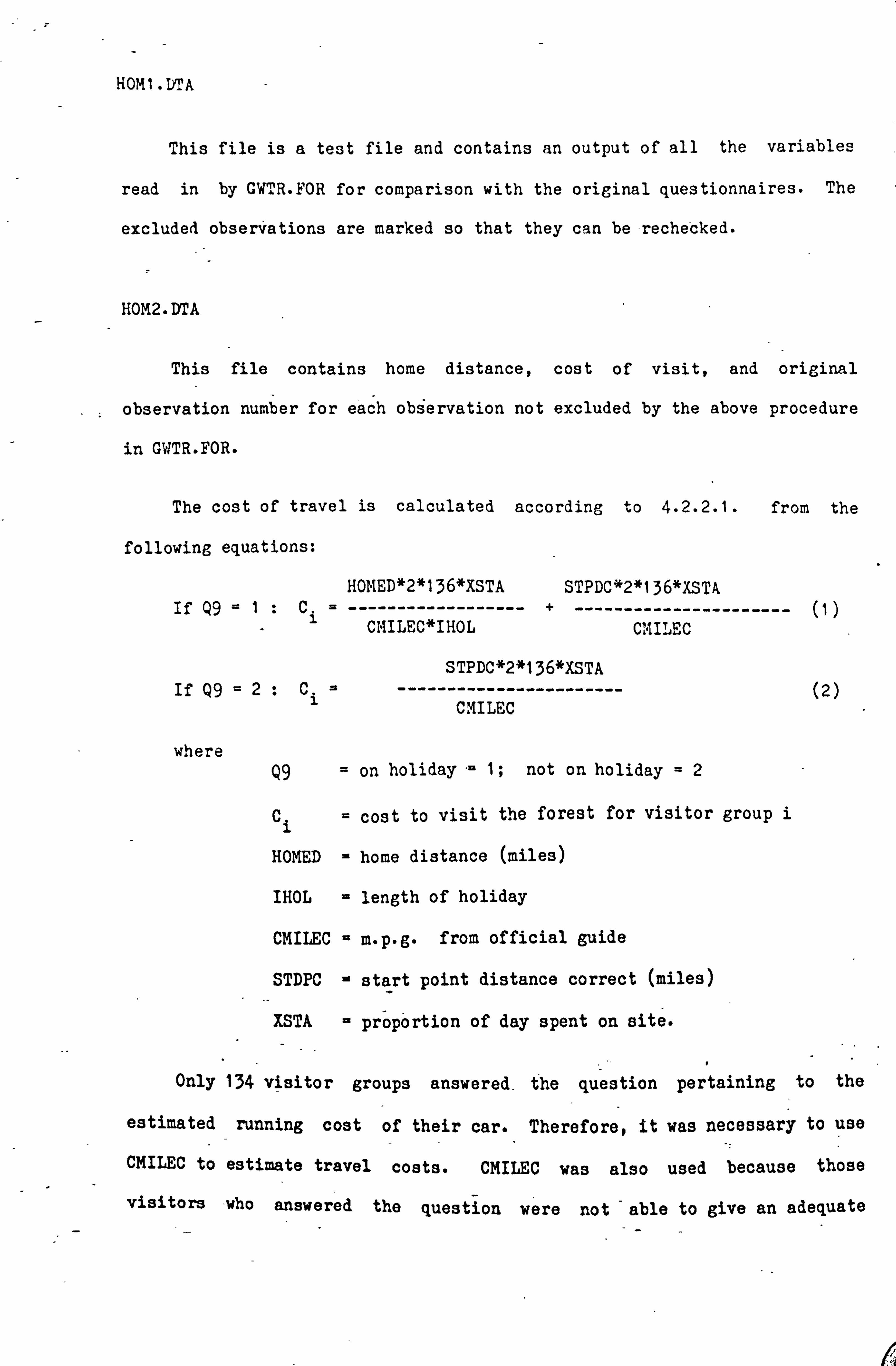
HOMI DTA
This file is a test file and contains an output of all the variables
read in by GWII. 'R-FOR for comparison with the original questionnaires. The
excluded observations are marked so that they can be-rechecked.
HOM2. DTA
This file contains home distance, cost of visit, and original
observation number for each observation not excluded by the above procedure
in GWTR-FOR-
The cost of travel is calculated according to 4.2.2.1. from the
following equations:
HOMED*2*136*XSTA STPDC*2*136*XSTA If Q9 =1: C ------------------ - ---------------------- (1)
CMILEC*IHOL CMILEC
STPDC*2*136*XSTA If Q9 =2: C ----------------------- (2)
CMILEC
where Q9 = on holiday-- 1; not on holiday =2
Ci= cost to visit the forest for visitor group i
HOMED - home distance (miles)
IHOL - length of holiday
CMILEC - m. p. g. from official guide
STDPC - start point distance correct (miles)
XSTA proportion of day spent on site.
Only 134 visitor groups answered- the question pertaining to the
estimated running cost of their car. Therefore, it was necessary to use
CMILEC to estimate travel costs. CMILEC was also used because those
visit Ors -who answered the question were not -able to give an adequate

estimate of the cost of running their cars. For the . 134 valid cases, a
one-way ANOVA for estimated running cost (CMILE1 ) on'prompting method
(CMILEM) was carried out' and was found significant at -p<0.001 -(see 4.3-1.2. ). For this reason also, values for travel cost were taken from an
official" list: What car, October, 1980, Fuel consumption list m. p. g. (An.
1980).
When we want to find the social value of the forest it must be the
actual cost of travel that we are interested in and not the perceived cost.
The perceived cost is important, however, when we want to find the fee
required to keep use of the site down to a certain level.
Ideally, a demand curve based on perceived cost should be used and
then integrated for the actual cost in order to find the social benefit.
This would probably be very small as the actual cost is generally higher
than the perceived cost.
STDPC, start point distance correct, is measured on a map and is used
instead of the one estimated on the questionnaire as it was found (Appendix
G-R) that:
STPDC 2.69 + 0.83*STPDE (3)
2 p<0.001, r 90
where STPDE estimated start distance.
Thus, if we used_STPDE, we would get an overestimation of the start point
distance. STPDEIshould have been used if we wanted the perceived cost.

PCOST, the petrol price, is set to 136 pence/gallon which was the
average price at the_time of the s urvey. To get the return cost the one
way travel cost was multiplied by 2.
XSTA, the proportion of the day spent on the site, is modified from
the variable staytime (STAYT) according to the. following procedure in Table
A4.1
Table A4.1 Conversion of staytime to proportion of day costs
If Q6 1 (Visitor group somewhere else today)
staying for the day XSTA = 1.0
staying for 1/2 day : XSTA = 0.7
staying 2-3 hours : XSTA = 0.5
staying 1-2 hours : XSTA = 0.4
staying <1 hour : XSTA = 0.3
If Q6 2 (Visitor group not somewhere else today)
XSTA - 1.0
See also Sdetion 4.2.2.1-4.
HOM3. DTA
This file contains two variables; the stated willingness to ' pay
(FEES) and the observation ýumber. The observations excluded by the-
procedure in GWTR. FOR are excluded here as well. The file is des igned to
be used for comparison with the results from the Clawson analysis via the
programme TES2. FOR (see 4.2-3)

Appendix A5.1
Comparison of Sample Estimate and Regression Estimate.
A comparison of yearly carbo rne visitor groups estimated by the sample
estimate and the regression esti mate is presented here. The estimates are
explained in Section 5.4-5. The regression estimate is calc ulated using
Part II (Koch 1980, -Appeiidix B. 2) from which the yearly number of forest
car visitor hours hours can be found (line 5 * line 22). This is divided
by the average stay length per car visitor group which is calculated in a
special programme (prg A 1811).
Only the forests investigated in Section 5.5 are included .
County of Copenhagen: Number of yearly carborne visitor groups
Forest C no. Sample Regression Estimate Estimate
'Troeroed Hegn' 1 6.612 6.664
IJaegersborg Dyrehavn og Hegn m. v*9 3 398-324 515.236
'Charlottenlund Skov' 4 65.828 97-069
'Kongelunden' 5 25-383 27-548
'Soelleroed Kirkeskov' 6 5.752 7.382
'Geel Skov' 7 15-167 15-840
'Noerreskoven' 8 15-197 22.115
'Aasevang mov. ' 9-* 31-884 36.650
'Hareskovene og Jonstrup Vang' 10 61-. 010 76-916
'Vestskoven Vest' 11 li. 50R-- 8.021..

County of Frederiksborg:
'Hombaek Plantage' 2 56-323 50-053.
'Teglstrup og -- Hellebaek Skov' 3 35-565 38-906
'Klosterris og Horseroed Hegn M-V., 4 10-427 8.687
'Egebaeksvang' 7- -7.633 10-115
'Danstrup og Krogenberg Hegn' 8 8.371 9-500
'Gribskov og Stenholt Vang' 13 24-916 37-199
'Tisvilde Hegn m. v. ' 18 71-893 102-582
'St. Dyrehavn og Tokkekoeb Hegn m. v. ' 28 32-068 36-398
'Folehave' 35 19-641 21-325
'Rude Skov' 36 8.821 11-887
'Lystrup Skov' 38 7.532 8.920
'Ravnsholt og Soenderskov' 39 9.234 10-749
'Slagslunde' 41 6.344 15.259
'Ganloese Eget' 43 5.445 7.169
'Ganloese ore og - Farum Lillevang m. v. ' 44 17.608 19-032

Appendix A5-L
Computer Progra=e PFAFOl. FOR
The appendix is separately-bound with the other programmes.

Appendix A5.3
Computer Programme PFAF02. FOR and PFAF03. FOR
The appendix is separately bound with the other programmes. -.

Appendix A5.4
Example of Out2ut
. The appendix is bound separately with the prograirraes.

Appendix B. Q
GWY. DY. R R-E. C. R. "ATIO QUý; 3'-: 'ION1-1AIRE 1980
C. an you spare five minutes to-answer a few-questions aboutyour visit to-
- this forest, Gwydyr? This'is part of a research project carried out
-bythe Dept. of Forestry & WoodScience, - U. C. 11.1d. 9 Bangor. -
-(J) Have. y, )u been interviewei before about a visit -to Gw-j%Iyr? -
(2) Hav-e you come speciall*1 to visit. the forest?
(3) Is this your whoýe party?
What are you going to do during your visit? Go for a walk., Sit ýo enjoy the view, 'Obsezýye the wildlifeg Fishing, Sailing, Canoeing,.
(5) How long do you intend staying here?
(6) Have you/will'-you visit somewhere else today? Where?,
(7)Have you been here before? How many times in the last year?
<8) Where'do you live?
(9: 0) Are you on holiday? For how long?
(10) Where did you start from today?
(11) About how far is that from here?
(12) How did you travel here?: Car, Bus, Train, Motorbiket Minibus, Bike, Walk.
(a) Can you tell me the make, engine size, and age of the vehicle?
(b) Can you tell. me how much per mile it costs you to run?
plot P209 P309
(13) Have recent increases in ; etrol prices/pub lic transpo"rt affected the no. of trips you make?
(14) If travel costs were to double in relation to wages would you make -the 'same no. of trips?, or reduce the-trips to
3 in 4,2 in 4,1 in 4, or stop almost all trips?
(15)How long ap; rox did the journey'here take today?
(16) If it took you*2/3-of the present time to get here would you; Make the same no. of trips to Gwydyr? Make the same no. of trips further afield? Nalke r-ore tr4-, -. s'to Gwydyr ? How many more?