University of Dundee DOCTOR OF PHILOSOPHY Fabrication ...

University of Dundee

DOCTOR OF PHILOSOPHY

Fabrication of Ultrasound Transducers and Arrays Integrated within Needles forImaging Guidance and Diagnosis

McPhillips, Rachael

Award date:2017

Link to publication

General rightsCopyright and moral rights for the publications made accessible in the public portal are retained by the authors and/or other copyright ownersand it is a condition of accessing publications that users recognise and abide by the legal requirements associated with these rights.

• Users may download and print one copy of any publication from the public portal for the purpose of private study or research. • You may not further distribute the material or use it for any profit-making activity or commercial gain • You may freely distribute the URL identifying the publication in the public portal

Take down policyIf you believe that this document breaches copyright please contact us providing details, and we will remove access to the work immediatelyand investigate your claim.

Download date: 22. Mar. 2022

https://discovery.dundee.ac.uk/en/studentTheses/741bf40f-6b2b-4e16-bf89-5b180ed5d67e

Fabrication of Ultrasound Transducers and Arrays

Integrated within Needles for Imaging Guidance and

Diagnosis

Rachael McPhillips

Doctoral thesis submitted in fulfilment of the requirements for the

degree of Doctor of Philosophy to the School of Medicine, University

of Dundee, Scotland, UK

2017

I

DECLARATION

I, Rachael McPhillips, hereby declare that this thesis entitled, “Fabrication of Ultrasound

Transducers and Arrays Integrated within Needles for Imaging Guidance and Diagnosis”

submitted to University of Dundee for the degree of Doctor of Philosophy represents my own work.

Unless otherwise stated, all references cited have been consulted by me; the work of which the thesis

is a record has been done by me and it has not been previously accepted for a higher degree: provided

that if the thesis is based upon joint research, the nature and extent of my individual contribution shall

be defined.

Signed: Date:

This is to certify that Miss Rachael McPhillips has done this research under my supervision and

complied with all the requirements for the submission of this Doctor of Philosophy thesis to the

University of Dundee.

Signed: Date:

II

ACKNOWLEDGEMENTS

I wish to express my sincere gratitude to my supervisors Dr. Christine Démoré and Dr. Sarah

Vinnicombe. Their dedicated support, patience, encouragement and advice has been unwavering and

inspirational throughout my work and is greatly appreciated.

I would also like to thank Professor Sandy Cochran for his support throughout the project, along with

the valued advice and help from Dr. Zhen Qiu and Dr. Yongqiang Qiu. Dr. Zhen Qiu’s patience with

my endless questions during the start of my project will always be remembered and appreciated. I am

also extremely grateful for the incredible source of fabrication advice that was provided by Dr.

Yongqiang Qiu.

I would like to extend my thanks to the collaborators, Dr. Yun Jiang from the University of

Birmingham, Dr. Giuseppe Schiavone and Dr. David Watson from Heriot Watt University, and Dr.

Osama Syed Mahboob. Each of whom provided their expertise and valuable assistance to my project.

I would like to express my thanks to my other colleagues and friends, Anu Chandra, Dr. Joyce Joy,

Miriam Jimenez Garcia, Dr. Vipin Seetohul, Dr Holly Lay, Dr. Ben Cox, Fraser Stewart, Ciaran

Connor and Zhailu Zhu.

Finally, I cannot possibly stress enough, my love and gratitude to my Mam and Dad, my sister Leah

and my brother Seán for your limitless encouragement, support and love throughout this experience.

III

TABLE OF CONTENTS

DECLARATION I

ACKNOWLEDGEMENTS II

TABLE OF CONTENTS III

GLOSSARY VIII

LIST OF FIGURES IX

LIST OF TABLES X

ABSTRACT XI

CHAPTER 1 INTRODUCTION 1

1.1 Overview of High Frequency Ultrasound Imaging 1

1.2 Rationale and Objective 2

1.2.1 Quality Control 2

1.3 Thesis Structure 3

1.4 Contribution to Knowledge 4

1.5 Publications 5

1.6 References 7

CHAPTER 2 CLINICAL BACKGROUND AND MOTIVATION 9

2.1 Aim of Chapter 9

2.2 Medical Imaging Modalities 9

2.2.1 Radiography 10

2.2.2 Positron Emission Tomography 10

2.2.3 Magnetic Resonance Imaging 11

2.2.4 Ultrasound 11

2.2.5 Optical Coherence Tomography 14

2.2.6 Multimodality Imaging 14

2.2.7 Image Guidance 15

2.3 Current Clinical Procedures used for Brain Imaging and Neuronavigation 16

2.3.1 Conventional Imaging Approaches 16

2.3.2 Current Navigation Techniques 17

2.3.3 Intraoperative Ultrasound in Neurosurgery 18

2.3.4 Brain Shift 19

IV

2.3.5 Clinical Need for Improved Imaging in Neurosurgery 20

2.3.6 Proposed Neurosurgical Application 21

2.4 Current Clinical Modalities and Procedures used for Breast Imaging and Breast

Cancer 22

2.4.1 Breast Cancer 22

2.4.2 Conventional Imaging Approaches 23

2.4.3 Image Guided Biopsies 26

2.4.4 Axillary Lymph Nodes 26

2.4.5 Conventional Imaging Approaches in the Axilla 28

2.4.6 Intervention 30

2.4.7 Remaining Challenges 31

2.4.8 Ductal Carcinoma In-Situ 32

2.4.9 Conventional Imaging Approaches for Detection of DCIS 32

2.4.10 Remaining Challenges 35

2.4.11 Clinical Need for Improved Imaging in the Breast and Axilla 35

2.4.12 Proposed Breast Application 36

2.5 Thiel Embalmed Cadavers 37

2.6 References 38

CHAPTER 3 TECHNICAL BACKGROUND 42


3.2 Medical Ultrasound 42

3.3 Piezoelectricity and Ultrasound Generation 43

3.4 Ultrasound Behaviour 44

3.4.1 Wave Propagation 44

3.4.2 Attenuation 45

3.5 Piezoelectric Materials 47

3.5.1 Material Properties 47

3.5.2 Ceramics 50

3.5.3 Single Crystals 51

3.5.4 Composite Materials 52

3.6 Medical Imaging Transducers 53

3.7 Design Considerations for Transducers 54

3.7.1 Passive Layers 54

3.7.2 Matching Layer 55

V

3.7.3 Backing Layer 55

3.7.4 Active Layer 56

3.7.5 Axial Resolution 57

3.7.6 Lateral Resolution 58

3.7.7 Sensitivity 60

3.8 Medical Ultrasound Transducer Arrays 60

3.9 Diagnostic Ultrasound 62

3.10 Transducer Fabrication and Technology 63

3.10.1 Lapping and Polishing 63

3.10.2 Precision Dicing 65

3.10.3 Electrical Interconnects 69

3.10.4 Packaging 72

3.11 Conclusions 74

3.12 References 74

CHAPTER 4 FABRICATION 79


4.2 Introduction to Micromachining Techniques 81

4.2.1 Lapping and Polishing 81

4.2.2 Precision Dicing Saw 82

4.3 Single Element Transducers 83

4.3.1 Device Design 83

4.3.2 Single Element Bulk Ceramic Transducers 85

4.3.3 Single Element Micromoulded 1-3 Piezocomposite Transducers 90

4.3.4 Single Element Single Crystal Dice-and-Fill Composite Transducer 92

4.4 Array Transducers 93

4.4.1 Device Design 94

4.4.2 Fabrication Process for the Production of 15 MHz Arrays 95

4.4.3 Active Layer – 15 MHz Piezocomposite Material 99

4.4.4 Machining of the Transducer Stack 105

4.4.5 Electrode Layer 107

4.4.6 Interconnects 108

4.4.7 Needle Package 116

4.5 Future Work 118

4.6 Discussion 119

VI

4.7 References 120

CHAPTER 5 FUNCTIONAL CHARACTERISATION RESULTS OF IMAGING

PROBES 122


5.2 Single Element Transducer Characterisation 122

5.2.1 Electrical Impedance Measurements 123

5.2.2 Pulse-Echo Response Measurements 125

5.2.3 Insertion Loss 128

5.2.4 Beam Profile 128

5.2.5 Wire Phantom Scan 131

5.3 Discussion of Single Element Transducer Characterisation Results 132

5.4 15 MHz 16 Element Array Characterisation Results 133

5.4.1 Electrical Impedance Measurements 133

5.4.2 Pulse-Echo Response Measurements 137

5.4.3 Wire Phantom Imaging 139

5.4.4 Crosstalk and Insertion Loss Measurements 140

5.5 Discussion of 16 Element Array Characterisation Results 141

5.6 References 142

CHAPTER 6 NEEDLE IMAGING PROBES FOR NEUROSURGICAL GUIDANCE 144


6.2 Clinical Need 144

6.3 Image Acquisition Methods 145

6.4 B-mode Imaging 145

6.4.1 B-mode Imaging Experimental Set-up 145

6.4.2 B-mode Imaging Results of Resected Lamb Brain 147

6.5 M-mode Imaging 149

6.5.1 M-mode Imaging Experimental Set-up 149

6.5.2 M-mode Imaging Results of Thiel Embalmed Cadaveric Brain 153

6.5.3 MRI Pre and Post Intervention 156

6.5.4 M-mode Imaging of Ex-Vivo Porcine brain 156

6.5.5 MRI Pre and Post Intervention 158

6.6 Discussion and Conclusions 159

6.7 References 161

CHAPTER 7 BREAST IMAGING 162

VII


7.2 Thiel Embalmed Cadavers 163

7.3 Identification of Breast Anatomy in Thiel Embalmed Cadavers 163

7.3.1 Ducts 164

7.3.2 Lymph Nodes 165

7.3.3 Thiel Cadaver Imaging Results 165

7.4 Imaging of Resected Breast using Range of Frequencies 167

7.5 Ductography Procedure 169

7.6 Conclusions 171

7.7 References 172

CHAPTER 8 CONCLUSIONS AND FUTURE WORK 174


8.2 Conclusions 174

8.2.1 Single Element Transducers 174

8.2.2 Array Transducers 175

8.2.3 Applications 178

8.3 Future Work 180

8.3.1 Higher Frequency Devices 180

8.3.2 In-vivo Tissue Characterisation 181

8.3.3 Multi-Modality Devices and Other Applications 182

8.3.4 Implementation of a Quality Management System 183

8.4 References 183

APPENDIX

VIII

GLOSSARY

A list of symbols and abbreviations used in this Thesis is given below. Additional expressions

are defined in the text as necessary

IOUS Intraoperative Ultrasound

HIFU High Intensity Focused Ultrasound

CT Computed Tomography

PET Positron Emission Tomography

MRI Magnetic Resonance Imaging

IVUS Intravascular Ultrasound

OCT Optical Coherence Tomography

CNB Core Needle Biopsy

FNAC Fine Needle Aspiration Technology

DCIS Ductal Carcinoma In-Situ

c Speed of sound in a medium

f Frequency

λ Wavelength

α Attenuation coefficient

keff Effective coupling factor

kt Electromechanical coupling coefficient

εr Dielectric constant

f# F-number

IPB Interdigital Pair Bonding

ACA Anisotropic Conductive Adhesive

PZT Lead Zirconate Titanate

PIN PMN-PT Lead Indium Niobate-Lead Magnesium Niobate Lead Titanate

VPP Viscous Polymer Processing

FPCB Flexible Printed Circuit Board

DRIE Deep Reactive Ion Etching

IX

LIST OF FIGURES

Figure 2.1 Illustration of brain anatomy………………………………………………………...16

Figure 2.2 Comparison of images from the same individual using A) T2 Weighted MRI B)

Intraoperative Ultrasound and C) CT from a study by Cheon et al (Cheon 2015). These images

present a 16-year-old female with left frontal lobe epilepsy. The MRI image shows a high signal

intensity lesion in the left frontal precentral cortex. The ultrasound image displays a well-defined

hyperechoic lesion confined to the precentral cortex. An arc-like dense hyperechogenicity within the

lesion (arrowheads) is shown. C. The hyperechoic arc corresponds to calcification on the preoperative

brain CT (arrow) (Cheon 2015)……………………………………………………………………….17

Figure 2.3 Image showing potential solution - the use of a miniature ultrasound transducer at the

tip of a neurosurgical needle for imaging and diagnosis……………………………………………...22

Figure 2.4 Illustration of breast anatomy, including ducts and lymph nodes…………………...23

Figure 2.5 Illustration of the axilla and surrounding anatomy. Image adapted from (Dialani,

James, and Slanetz 2015)…………………………………………………………………………..….27

Figure 2.6 a) Image of lymph node anatomy, highlighting the cortex and hilum (Whitman, Lu,

and Adejolu 2011). The hypoechoic cortex, made up of the marginal sinus and lymphoid follicles is

thin with smooth edges, and the hyperechoic hilum is as a result of the scattering from the blood

vessels, fat, and the central sinus (Whitman, Lu, and Adejolu 2011). An ultrasound representation of a

lymph node is shown in b), where the cortex and hilum can be identified (Rahbar et al. 2012)……...27

Figure 2.7 Illustration of breast ducts showing the ducts radiating from the mammary glands

towards the nipple……………………………………………………………………………………..33

Figure 2.8 Image of proposed use of microultrasound device in a needle to aid breast imaging

and diagnosis………………………………………………………………………………………….37

Figure 3.1 Pulse echo technique used for ultrasound imaging. Transmitted ultrasound pulse is

reflected and scattered from tissue structures, with receive echoes detected by the transducer

converted to electrical voltage………………………………………………………………………...43

Figure 3.2 Illustration indicating the operation of an imaging transducer via the Piezoelectric

Effect and Inverse Piezoelectric Effect………………………………………………………………..44

Figure 3.3 Image showing approximate attenuation coefficient values for a variety of materials

and how these vary with increasing frequency (USRA, 2008). For each of these materials, as the

frequency of the ultrasound increases, the attenuation also increases………………………………...46

Figure 3.4 Example of an electrical impedance profile showing impedance magnitude and phase

spectra of a transducer………………………………………………………………………………...48

Figure 3.5 Piezoelectric pillars surrounded by a passive polymer material……………………..52

Figure 3.6 Components which make up a transducer stack……………………………………..54

Figure 3.7 Depiction of axial resolution…………………………………………………………58

Figure 3.8 Near field and far field of ultrasound beam………………………………………….59

Figure 3.9 Depiction of lateral resolution……………………………………………………….60

Figure 3.10 Multiple elements in a linear transducer array……………………………………….61

Figure 3.11 Illustration of lapping machine set up………………………………………………..64

Figure 3.12 Image from Bezanson et al showing the front face of a 64 element array with

patterned electrode tracks and wire bonds forming connections from the electrode tracks to two flex-

circuit boards, one on each side of the array (Bezanson et al., 2012)…………………………………70

Figure 3.13 Photograph of 5 MHz array fabricated by R.T. Ssekitoleko, using conductive silver

epoxy to attach and connect an 8 element array to a flexible printed circuit board. A dicing blade is

then used to dice and separate the elements and silver epoxy to establish individual connection

between each element and its corresponding track on the circuit (Ssekitoleko, 2013; Ssekitoleko et al.,

2011)…………………………………………………………………………………………………..71

Figure 3.14 Image by Manian Ramkumar et al illustrating conductive particles within an ACA

forming conductive columns in one direction following the curing process within a magnetic field

(Manian Ramkumar & Srihari, 2005)…………………………………………………………………72

Figure 4.1 Schematic diagram of primary lapping equipment………………………………….82

X

Figure 4.2 Design and imaging orientation of single element transducers…………………...…85

Figure 4.3 (a) Sample(s) orientated off centre to glass substrate as shown to ensure surface

contact of the sample is spread evenly over entire plate during lapping. This helps maintain lapping

plate flatness therefore improving uniformity of sample surface. The red arrow indicates the rotation

of the samples when mounted on the lapping jig. 4.3(b) An illustration showing the significance of

sample placement on glass plate to maintain uniform lapping plates…………………………………87

Figure 4.4 Lapped and Diced Octagons. (a) Indicates the octagon dimensions. (b) Image

showing the 6 dicing passes made by the dicing machine. The images on the right show the waste

material has been washed away to reveal the octagons for use……………………………………….88

Figure 4.5 Micromoulded Composite Pillars (a) showing their hexagonal arrangement, and (b),

showing the matrix of pillars produced through viscous polymer processing………………………..90

Figure 4.6 Forward and Side facing needle prototypes, the side window for the side facing

transducer is highlighted………………………………………………………………………………91

Figure 4.7 Lenses on forward facing and side facing devices………………………………….92

Figure 4.8 (a) A vice is used to secure the wire connection in place as it is attached to the back of

the transducer using conductive epoxy (b) Assembly and connection of SET_SC_FF single element

transducer……………………………………………………………………………………………..93

Figure 4.9 Layout of the FPCB interconnections to connect the electronic driving system with

the ultrasound transducer array……………………………………………………………………….95

Figure 4.10 Design of array transducer within biopsy needle package……..................................95

Figure 4.11 Examples of collapsed pillars (a) collapsed pillars in a sample after one dicing pass of

cuts and (b) in a sample after dicing two orthogonal passes…………………………………………102

Figure 4.12 Piezoceramic composite dicing cuts made in two passes, (a) the first dicing pass, and

(b) following the second dicing pass, showing minimal pillar damage. Pillars of 50 µm pitch with a 13

µm kerf are created…………………………………………………………………………………..102

Figure 4.13 Single crystal composite dicing cuts made in two passes, with minimal pillar

damage. Pillars of 50 µm pitch created……………………………………………………………...104

Figure 4.14 Epoxy plate with three transducer workpieces. These three test transducers were

initially part of one plate of material, with shallow cuts made around their perimeter which allowed

the plate to be machined as one piece but then separated the devices once they were lapped to final

thickness……………………………………………………………………………………………...107

Figure 4.15 Finished array tracks scratch diced to create elements 50 µm width tracks at 100 µm

pitch at the rear of the transducer stack. The area outlined in red shows the active composite area,

which is surrounded by a frame of epoxy……………………………………………………………108

Figure 4.16 Photographs showing (a) manual alignment of array elements and FPCB, with the

addition of conductive silver epoxy and tape to hold the FPCB in place in (b)……………………..109

Figure 4.17 Damage to silver epoxy and frayed FPCB tracks following dicing………………..110

Figure 4.18 (a) Shows the tracks of the FPCB and array connected via conductive silver epoxy.

As this is isotropic conductive paste, the adjacent tracks are therefore also connected to each other and

require separation. (b) A blade has been used to cut through the silver epoxy to separate this

connection (c) Glue is deposited in the resulting track to ensure that the FPCB does not fray away

from the array as a result of the cutting (d) A narrower blade is then used to cut through the glue in the

track to ensure separation, while the narrower blade retains some glue on either side of the track to

reinforce adhesion of the FPCB to the array…………………………………………………………111

XI

Figure 4.19 Image of 16 element array after connection to FPCB and dicing of tracks to separate

individual elements…………………………………………………………………………………..112

Figure 4.20 ACA is dispensed evenly along the top of the FCB. The array is then placed track

side down such that the element tracks of the array align with the element tracks of the FPCB

(Schiavone et al., 2016)………………………………………………………………………………112

Figure 4.21 (a) MAT 6400 flip chip bonding machine for assembly of array and FPCB connection

(b) Stage on MAT 6400 to secure FPCB in place for alignment and bonding (c) Image on MAT 6400

showing dispensed paste across bonding area of FPCB……………………………………………..113

Figure 4.22 Test arrays made for testing automated bonding process………………………….114

Figure 4.23 The test array and FPCB assembly was encapsulated in bulk epoxy and diced in half

in order to obtain a cross section of the connections between the two. Pillars of conductive particles

have been formed in the adhesive paste to make connection in the vertical direction only, between the

FPCB and array, but not between adjacent element electrode tracks i.e. anisotropic conduction…...116

Figure 4.24 A 16 element flexible circuit twisted into a helix to demonstrate it fitting within a

needle case of inner diameter 1.8 mm……………………………………………………………….116

Figure 4.25 (a) Biopsy needle used as device casing (b) FPCB within the core of the biopsy

needle case (c) SMA connector board for connection to elements from FPCB to enable testing and

measurements from elements (d) FPCB connected to connectors on this board (e) Finished device of

15 MHz 16 element array within a biopsy needle with SMA connectors for characterisation and

functional testing…………………………………………………………………………………….117

Figure 4.26 Pillars of DRIE composite………………………………………………………….118

Figure 5.1 Impedance and phase measurements of single element transducers integrated within

needles. Figure a) and b) show the results from bulk piezoceramic transducers, a) forward facing

(SET_BULK_FF), and b) side facing (SET_BULK_SF) orientation. Figure c) and d) show the results

from micromoulded PZT composite transducers, a) forward facing (SET_MM_FF), and b) side facing

(SET_MM_SF) orientation…………………………………………………………………………..124

Figure 5.2 Impedance and phase measurement of single element single crystal composite

transducer integrated within a needle of forward facing orientation (SET_SC_FF)………………...125

Figure 5.3 Pulse echo responses of single element transducers SET_BULK_FF,

SET_BULK_SF, SET_MM_FF and SET_MM_SF. The energy set for the pulse was 12.4 µJ with 0

gain given to the acquired signal…………………………………………………………………….126

Figure 5.4 Pulse echo response of the needle with active material composed of single crystal

composite…………………………………………………………………………………………….127

Figure 5.5 (a) Set-up used to obtain beam scans of single element transducers using needle

hydrophone (b) The position of the hydrophone from the forward facing transducer face

SET_MM_FF at start of scan (c) The position of the hydrophone from the forward facing transducer

face SET_MM_SF at start of scan…………………………………………………………………..129

Figure 5.6 (a) Beam scan showing lateral beam profile b) Beam scan to show cross section slice

of the forward facing transducer SET_MM_FF…………………………………………………….130

Figure 5.7 (a) Beam scan showing lateral beam profile b) Beam scan to show cross section slice

of the side facing transducer SET_MM_SF………………………………………………………….131

Figure 5.8 Wire Phantom images acquired using the single element transducers. A linear B- scan

using the SET_MM_FF and a radial B-scan using the SET_MM_SF………………………………132

Figure 5.9 Electrical impedance measurements for 15 MHz dice-and-fill composite active layer

material (a) prior to integration with the layers of the transducer stack in the graph and (b) with the

addition of quarter wavelength matching layer………………………………………………………134

Figure 5.10 a) Impedance and b) phase measurements for transducer array 16 elements with

matching layer connected to flexible circuit before addition of backing layer………………………135

XII

Figure 5.11 a) Impedance and b) phase of transducer array stack of 16 elements connected to a

flexible circuit, with a backing layer and integrated into a needle package…………………………136

Figure 5.12 Pulse-echo response of element number 6 from 15 MHz transducer array………...137

Figure 5.13 An example of 16 elements from the 15 MHz array transmitting and receiving

simultaneously using a quartz flat as the echo target………………………………………………..138

Figure 5.14 An image generated from 16 adjacent elements from the 15 MHz array with a 5 mm

thick quartz flat as the echo target using the FI Toolbox……………………………………………138

Figure 5.15 16 elements used to image a series of 7 wires 20 μm in diameter separated by 1 mm.

The wires appear as lines due to side lobes and constructive interference producing image artefacts

across the 16 elements………………………………………………………………………………..139

Figure 5.16 Indication of a circular cross section of a 20 μm tungsten wire visualised using

elements 6, 7, 8 and 9 as a preliminary test of introducing a small beam steer to the array using the FI

toolbox……………………………………………………………………………………………….140

Figure 5.17 Transmit signal shown on element 6, while element 7 is operating in receive to

display the crosstalk between adjacent elements…………………………………………………….141

Figure 6.1 Experiment Set-up for B-mode Imaging…………………………………………...146

Figure 6.2 B-mode image of lamb brain with forward facing needle………………………….147

Figure 6.3 B-mode image of lamb brain with side facing needle……………………………...148

Figure 6.4 Experiment Set-up for M-mode Imaging…………………………………………..150

Figure 6.5 Screen shot of real-time M-mode image feedback using the forward facing

transducer…………………………………………………………………………………………….151

Figure 6.6 Position of Kocher’s Point in human skull…………………………………………152

Figure 6.7 M-mode image of Thiel embalmed brain with forward facing needle……………..154

Figure 6.8 M-mode image of Thiel embalmed brain with side facing needle…………………155

Fig 6.9 MRI (a) before and (b) after Thiel embalmed cadaver experiment………………...156

Figure 6.10 M-mode image of fresh porcine brain with forward facing needle………………...157

Figure 6.11 M-mode image of fresh porcine brain with side facing needle…………………….157

Figure 6.12 MRI (a) before and (b) after fresh porcine brain experiment………………………158

Figure 7.1 a) Cross sections of breast ducts shown as oval hypoechoic structures b) Ducts shown

branching downwards from the nipple (Sencha et al., 2013)………………………………………..164

Figure 7.2 Images of normal appearing lymph nodes with recognisable cortex and central

echogenic hilum shown. Images adapted from (a) Dudea et al (Dudea, 2012) and (b) Rahbar et al

(Rahbar, 2012)……………………………………………………………………………………….165

Figure 7.3 Images showing (a) breast ducts and (b) lymph node from a Thiel embalmed cadaver

(Subject 3). Images acquired are shown at a depth of 2.0 cm and were taken at a frequency of 12

MHz………………………………………………………………………………………………….166



MHz………………………………………………………………………………………………….166

Figure 7.5 Images of ducts from resected breast at a) 6 MHz, b) 14 MHz, c) 20 MHz and d) 40

MHz………………………………………………………………………………………………….168

Figure 7.6 Images of lymph node from resected breast at a) 6 MHz, b) 14 MHz, c) 20 MHz and

d) 40 MHz……………………………………………………………………..…………………….169

XIII

Figure 7.7 Images showing stages of injection of fluid into duct; a) location of duct is shown b)

insertion of needle into duct wall c) insertion of needle into duct and d) injection of fluid into duct.171

Figure 8.1 (a) Reverse side of proposed 50 MHz array where bonding of interconnects is carried

out. The flexible circuit will bend back and be fed down the body of the case. The distance required to

allow the flexible circuit to have sufficient room to bend will affect the final overall diameter of the

device. A backing layer will be deposited onto the rear of the transducer across the surface of the

interconnects (b) The proposed 50 MHz device with interconnects established for assembly into a

needle device…………………………………………………………………………………………181

XIV

LIST OF TABLES

Table 3.1 Example of Curie temperatures in a variety of piezoelectric materials (K. K. Shung et

al., 2007)………………………………………………………………………………………………50

Table 4.1 List of prototype transducers and their applications………………………………...80

Table 4.2 Dimensions of octagons to fit within 1.8 mm inner diameter of needle……………..89

Table 4.3 Wafer-scale fabrication process steps for the production of multiple transducer array

stacks for 15 MHz operation…………………………………………………………………………..95

Table 4.4 Dicing program parameters for creation of 1 – 3 composites in 3203 HD and PIN

PMN PT single crystal piezoelectric material……………………………………………………….103

Table 5.1 Transducer materials, thicknesses and their corresponding acoustic impedances….123

Table 5.2 Characteristics of Single Element Transducers calculated from Figure 5.3………..127

Table 5.3 Pulser Settings for Set-Up of Beam Scans………………………………………….129

Table 7.1 Table indicating details of Thiel embalmed cadavers used in this study…………...163

XV

ABSTRACT

As opposed to current Intraoperative Ultrasound (IOUS) systems and their relatively large probes and

limited superficial high frequency imaging, the use of a biopsy needle with an integrated transducer

that is capable of minimally invasive and high-resolution ultrasound imaging is proposed. Such a

design would overcome the compromise between resolution and penetration depth which is associated

with the use of a probe on the skins surface. It is proposed that during interventional procedures, a

transducer array positioned at the tip of a biopsy needle could provide real-time image guidance to the

clinician with regards to the needle position within the tissue, and aid in the safe navigation of needles

towards a particular target such as a tumour in tissues such as the breast, brain or liver, at which point

decisions surrounding diagnosis or treatment via in vivo tissue characterisation could be made. With

this objective, challenges exist in the manufacturing these miniature scale devices and their

incorporation into needle packages. The reliable realisation of miniature ultrasound transducer arrays

on fine-scale piezoelectric composites, and establishing interconnects to these devices which also fit

into suitably sized biopsy needles are two such hurdles.

In this thesis, the fabrication of miniature 15 MHz ultrasound transducers is presented. The first stage

of development involved the production of single element transducers in needles ~2 mm inner

diameter, using various piezoelectric materials as the active material. These devices were tested and

characterised, and the expertise developed during their fabrication was used as the foundation upon

which to design a wafer-scale fabrication process for the production of multiple 15 MHz transducer

arrays. This process resulted in a 16 element 15 MHz array connected to a flexible printed circuit

board and integrated into a breast biopsy needle. Characterisation tests demonstrated functionality of

each of the 16 elements, both individually and combined as an array.

To explore potential applications for these devices, the single element transducers were tested in fresh

and Thiel embalmed cadaveric brain tissue. Plasticine targets were embedded in these brain models

and the needle transducers were tested as navigational real-time imaging tools to detect these targets

within the brain tissue. The results demonstrated feasibility of such devices to determine the location

XVI

of the target as the needle devices were advanced or withdrawn from the tissue, showing promise for

future devices enabling neurosurgical guidance of interventional tools in the brain.

The application of breast imaging was also considered. Firstly, Thiel embalmed cadaveric breasts

were assessed as viable breast models for ultrasound imaging. Following this, anatomical features,

with diagnostic significance in relation to breast cancer i.e. axillary lymph nodes and milk ducts, were

imaged using a range of ultrasound frequencies (6 – 40 MHz). This was carried out to determine

potential design parameters (i.e. operational frequency) of an interventional transducer in a biopsy

needle probe which would best visualise these features and aid current breast imaging and diagnosis

procedures.

1

CHAPTER 1

INTRODUCTION

1.1 Overview of High Frequency Ultrasound Imaging

Ultrasound describes mechanical waves which propagate at frequencies greater than the range of

human hearing i.e. 20 kHz. The use of ultrasound as an imaging modality has been explored

extensively since the 1950s (KK Shung 2011). Due to its safe nonionizing nature, portability, and

ability to image in real time, ultrasound imaging is one of the most significant tools for clinical

diagnosis, second only to conventional X-ray radiography (KK Shung 2011) (Szabo 2014).

Technical advances in ultrasound technology have led to developments such as enabling the

measurement of tissue elastic properties, known as elastography, while therapeutic functions have

been explored using ultrasound for drug delivery and high-intensity focused ultrasound (HIFU)

surgery (KK Shung 2011) (Szabo 2014). High frequency ultrasound, also known as Microultrasound,

generates images using frequencies greater than 15 MHz with improved resolution (~200 μm at 15

MHz), opening the potential for an even larger scope of applications (K Shung et al. 2009). To date,

high frequency ultrasound systems have been utilised for the imaging of eye, skin, intravascular and

small animal imaging. A limitation with high frequency ultrasound exists in that attenuation of the

ultrasound energy increases proportionally with frequency. As a result, the improved spatial

resolution comes at the expense of penetration depth. To overcome this challenge, the miniaturization

of ultrasound transducers and their incorporation into interventional probes to access the region of

interest within tissue has become a necessary field of research (Cannata and Zhao 1999; Bezanson et

al. 2012; Cummins, Eliahoo, and Shung 2016). The design and construction of high frequency

transducer arrays has been shown to be highly challenging due to the miniature scale of these devices

(Lockwood et al. 1996; Zhou et al. 2009; Ssekitoleko et al. 2011).

2

1.2 Rationale and Objective

Micromachining methods used to realise high frequency ultrasound devices include lapping and

polishing, precision dicing and various means of establishing miniature interconnects in smaller

packages. Fabrication at this scale however renders the materials used for transducer construction

extremely fragile, difficult to handle, making fabrication procedures time consuming and costly. A

significant challenge persists in the objective of creating electrical interconnects to arrays at a scale

that remains suitable for assembly within interventional devices such as biopsy needles. As a result of

these challenges, the objectives in this thesis are as follows:

Demonstrate feasibility of fabrication processes for the production of 15 MHz single element

transducers within needle cases ~2 mm in diameter

Develop use of the micromachining techniques to create repeatable practices for the

production of piezocomposite active layers for operation at high frequencies

Design a wafer-scale fabrication process which limits handling of devices during production

and realises multiple devices from a single process

Investigate achievable methods for establishing interconnects to miniature ultrasound arrays

for integration into interventional tools

Demonstrate that the fabrication processes produced functional imaging transducers capable

of indicating potential for applications such as image guidance and diagnosis

Explore potential for clinical adoption of miniature ultrasound probes within neurosurgery

and interventional breast radiology

1.2.1 Quality Control

Throughout this project, a consistent objective was to employ the standards of a Quality Management

System ISO 13485 (International Standard for Medical Devices) to each of the processes used for the

production of the devices fabricated in this project. These controls were implemented on all

equipment used to drive quality and consistency in the processes developed, to maintain the machine

calibration and maintenance to minimise inaccuracies and encourage repeatability similar to that of

industrial scale manufacture.

3

1.3 Thesis Structure

Chapter 2 provides an overview of the background to the clinical applications discussed in this thesis

with focus on the brain and breast applications in particular. Conventional methods for imaging and

diagnosis in the brain and breast are presented with an emphasis on the use of ultrasound in current

practice. The chapter outlines the clinical motivation behind the proposed ultrasound devices, and

where the use of such devices can address current clinical needs.

Chapter 3 presents a background to the technical work carried out in this thesis. An overview of the

theory which defines ultrasound and its application in medical imaging is given. This is followed by

the current developments in fabrication of ultrasound transducers, in particular high frequency

ultrasound and the micromachining techniques used to realise such devices.

Chapter 4 discusses the fabrication processes designed to produce single element transducers and 15

MHz arrays incorporated into needles. Each transducer that has been developed as part of this project

is discussed in detail, outlining the micromachining methods used and the challenges experienced and

overcome. Emphasis is given to producing fabrication processes suitable for waferscale manufacture

of high frequency ultrasound arrays.

Chapter 5 presents the characterisation tests and measurements acquired for each of the produced

needle devices. Results such as electrical impedance tests, pulse-echo response measurements and

preliminary imaging of wire phantoms are reported to demonstrate and assess the functionality of the

fabricated transducers.

Chapter 6 explores the application of the single element transducers as interventional imaging tools

for neurosurgical guidance. Imaging experiment results are shown using the devices to identify targets

within Thiel embalmed cadaveric brain and fresh porcine brain tissue.

Chapter 7 examines ultrasound imaging of the breast. Thiel embalmed breast tissue is assessed as an

effective breast model for ultrasound imaging. This breast tissue is then examined with a range of

ultrasound frequencies to determine potential miniature device specifications for improving

ultrasound imaging for the visualisation of breast ducts and axillary lymph nodes.

4

Chapter 8 presents the conclusions drawn from the work presented in this thesis. This discussion

highlights the various accomplishments and challenges experienced throughout the project and what

elements of future work and development could be taken on to further improve the devices and

achieve the imaging objectives.

1.4 Contribution to Knowledge

This thesis presents the following contributions to knowledge:

Fabrication of 15 MHz single element transducers and their assembly into needles and

demonstrating their use as real-time M-mode imaging devices

Design of a wafer-scale fabrication process for the production of multiple 15 MHz arrays

from one plate of piezoelectric material and their connection to flexible printed circuit boards

and incorporation into needle cases.

The creation of dicing programs which enable the repeatable production of 1 – 3

piezocomposites from both ceramic and single crystal material with a pillar pitch of 50 μm,

suitable for 15 MHz operation.

Exploration of methods using both isotropic and anisotropic adhesives to establish

interconnects to array devices suitable for integration into biopsy needles.

The realisation of a 15 MHz 16 element array, with individual connections made to each

element, and with dimensions small enough to fit within a 2 mm diameter biopsy needle.

Each element was shown to be operational via electrical impedance measurements and pulse-

echo response tests.

The assessment of single element transducers for image guidance in neurosurgery using fresh

porcine and Thiel embalmed cadaver brain tissue

The assessment of Thiel embalmed cadavers as breast models suitable for ultrasound imaging

The assessment of anatomical features of the breast with a range of ultrasound frequencies

from 6 MHz – 40 MHz to evaluate the best frequency appropriate for potentially improving

breast imaging and diagnosis.

5

1.5 Publications

Rachael McPhillips, Zhen Qiu, Yun Jiang, Syed O Mahboob, Han Wang, Carl Meggs,

Giuseppe Schiavone, Daniel Rodriguez Sanmartin, Sam Eljamel, Marc PY Desmulliez, Tim

Button, Sandy Cochran, Christine E M Démoré 2015. “Ex-Vivo Navigation of Neurosurgical

Biopsy Needles Using Microultrasound Transducers with M-Mode Imaging.” IEEE

International Ultrasonics Symposium (IUS), 2015 3–6.

Syed O Mahboob, Rachael McPhillips, Zhen Qiu, Yun Jiang, Carl Meggs, Giuseppe

Schiavone, Tim Button, Marc Desmulliez, Christine Demore, Sandy Cochran, Sam Eljamel

2016 “Intraoperative Ultrasound-Guided Resection of Gliomas: A Meta-Analysis and Review

of the Literature.” World Neurosurgery 92. Elsevier Inc: 255–63.

doi:10.1016/j.wneu.2016.05.007.

Giuseppe Schiavone, Thomas Jones, Dennis Price, Rachael McPhillips, Yun Jiang, Zhen

Qiu, Carl Meggs, Syed O. Mahboob, Sam Eljamel, Tim W. Button, Christine E M Demore,

Sandy Cochran, Marc P Y Desmulliez 2016. “A Highly Compact Packaging Concept for

Ultrasound Transducer Arrays Embedded in Neurosurgical Needles.” Microsystem

Technologies. Springer Berlin Heidelberg, 1–11. doi:10.1007/s00542-015-2775-1.

Yun Jiang, Zhen Qiu, Rachael McPhillips, Carl Meggs, Syed Osama Mahboob, Han Wang,

Robyn Duncan, Daniel Rodriguez-Sanmartin, Ye Zhang, Giuseppe Schiavone, Roos Eisma,

Marc P Y Desmulliez, Sam Eljamel, Sandy Cochran, Tim W. Button, Christine E M Demore

2016. “Dual Orientation 16-MHz Single-Element Ultrasound Needle Transducers for Image-

Guided Neurosurgical Intervention.” IEEE Transactions on Ultrasonics, Ferroelectrics, and

Frequency Control 63 (2): 233–44. doi:10.1109/TUFFC.2015.2506611.

6

Schiavone, Giuseppe, Thomas Jones, Dennis Price, Rachael McPhillips, Zhen Qiu, Christine

E M Demore, Carl Meggs, Syed O Mahboob, Sam Eljamel, Tim W. Button, Sandy Cochran,

Marc P Y Desmulliez 2014. “Advanced Electrical Array Interconnections for Ultrasound

Probes Integrated in Surgical Needles.” IEEE 16th Electronics Packaging Technology

Conference (EPTC), 88–93.

Yun Jiang, Carl Meggs, Tim Button, Giuseppe Schiavone, Marc P Y Desmulliez, Zhen Qiu,

Syed Mahboob, Rachael McPhillips, Christine E M Demore, Graeme Casey, Sam Eljamel,

Sandy Cochran, Daniel Rodriguez Sanmartin 2014. “15 MHz Single Element Ultrasound

Needle Transducers for Neurosurgical Applications.” In IEEE International Ultrasonics

Symposium, IUS, 687–90. doi:10.1109/ULTSYM.2014.0169.

Conference Presentations

9th - 11th December 2015 British Medical Ultrasound Society (BMUS) Ultrasound 2015 City

Hall Cardiff Oral Presentation "Ex-vivo navigation of neurosurgical biopsy needles using

microultrasound transducers with M-mode imaging"

21 - 25 October 2015 IEEE International Ultrasonics Symposium Taipei, Taiwan Oral

Presentation (Presented by Christine Demore on behalf of RMP) "Ex-vivo navigation of

neurosurgical biopsy needles using microultrasound transducers with M-mode imaging"

15th-16th March 2015 Oncological Engineering Conference Leeds UK: Poster Presentation

"Interventional Micro-Ultrasound imaging devices established within biopsy needles for in-

vivo pathology and needle guidance"

7

28th September – 1st October 2014 Ultrasonic Biomedical Microscanning Conference,

Peebles, Scotland: Oral Presentation “Ultrasound probes integrated into biopsy needles for

improved diagnosis and guided intervention"

3rd – 6th September 2014 IEEE IUS Conference, Chicago, United States: Oral Presentation

“15-20MHz Single Element Ultrasound Transducers in a Needle for Neurological

Applications”

15th-16th September 2013 Oncological Engineering Conference Leeds UK: Poster

Presentation “Development of Miniaturised Linear Arrays for Integration in Biopsy Needles”

1.6 References

Bezanson, A., P. Garland, R. Adamson, and J. a. Brown. 2012. “Fabrication of a Miniaturized 64-

Element High-Frequency Phased Array.” 2012 IEEE International Ultrasonics Symposium,

October. Ieee, 2114–17. doi:10.1109/ULTSYM.2012.0528.

Cannata, JM, and JZ Zhao. 1999. “Fabrication of High Frequency (25-75 MHz) Single Element

Ultrasonic Transducers.” IEEE Ultrasonics Symposium, 1099–1103.

http://ieeexplore.ieee.org/xpls/abs_all.jsp?arnumber=849191.

Cummins, Thomas, Payam Eliahoo, and K. Kirk Shung. 2016. “High-Frequency Ultrasound Array

Designed for Ultrasound-Guided Breast Biopsy.” IEEE Transactions on Ultrasonics,

Ferroelectrics, and Frequency Control 63 (6): 817–27. doi:10.1109/TUFFC.2016.2548993.

Lockwood, G. R., D. H. Turnbull, D. a. Christopher, and F. S. Foster. 1996. “Beyond 30 MHz -

Applications of High-Frequency Ultrasound Imaging.” IEEE Engineering in Medicine and

Biology Magazine 15: 60–71. doi:10.1109/51.544513.

Shung, K, Jonathan Cannata, Member Qifa Zhou, and Jungwoo Lee. 2009. “High Frequency

Ultrasound: A New Frontier for Ultrasound.” Conference Proceedings : ... Annual International

Conference of the IEEE Engineering in Medicine and Biology Society. IEEE Engineering in

Medicine and Biology Society. Conference 2009 (January): 1953–55.

doi:10.1109/IEMBS.2009.5333463.

Shung, KK. 2011. “Diagnostic Ultrasound: Past, Present, and Future.” Journal of Medical and

Biological Engineering 31 (6): 371–74. doi:10.5405/jmbe.871.

Ssekitoleko, R.T., C.E.M. Demore, D. Flynn, J.H.G. Ng, and M.P.Y. Desmulliez. 2011. “Design and

Fabrication of PM MN-PT Based High Frequency Ultrasound Imaging Devices Integrated into

Medical Interventional Tools.” IEEE International Ultrasonics Symposium Proceedings, 2345–

48.

Szabo, Thomas L. 2014. “Diagnostic Ultrasound Imaging: Inside Out.” Diagnostic Ultrasound

Imaging: Inside Out 787: 735–63. doi:10.1016/B978-0-12-396487-8.00017-3.

Zhou, Qifa, Jung Hyui Cha, Yuhong Huang, Rui Zhang, Wenwu Cao, and K. Kirk Shung. 2009.

8

“Alumina/epoxy Nanocomposite Matching Layers for High-Frequency Ultrasound Transducer

Application.” IEEE Transactions on Ultrasonics, Ferroelectrics, and Frequency Control 56 (1):

213–19. doi:10.1109/TUFFC.2009.1021.

9

CHAPTER 2

CLINICAL BACKGROUND AND MOTIVATION

2.1. Aim of Chapter

The clinical motivation of this project lies in developing and improving the use of microultrasound as

a tool for high resolution imaging for diagnosis and guiding interventional procedures. The potential

benefits of this technology for brain and breast applications are explored, in particular. The objective

is to fabricate microultrasound transducers and integrate this technology into a miniature and

potentially interventional probe for exploration of the potential benefits such a tool could bring to the

clinical workflows for each of these areas.

This chapter begins by providing an overview of the current imaging modalities available in clinical

practice. With a focus on ultrasound, a review is carried out on how it is presently used in the field of

brain and breast imaging and the status of the research that aims to overcome remaining drawbacks

and challenges in these clinical applications.

2.2. Medical Imaging Modalities

Medical imaging uses the interaction of energy with biological tissue in order to acquire spatially

resolved information about the physical properties of the underlying biological structure to

characterise tissues inside the body in a non-invasive manner. In diagnostic imaging, we consider the

detection of different physical signals that arise from the patient and their transformation into medical

images.

Recently, advances in medical imaging modalities mean that they no longer operate within the

conventional boundaries of diagnostic imaging. Imaging technology is increasingly used for

monitoring progression or treatment of disease, and for navigating interventional tools. Consequently,

the deployment of such techniques ranges from radiologists to surgeons using real time imaging

during their interventional procedures (Sakas 2002).

10

2.2.1. Radiography

Radiography began following the discovery of X-Rays by Röntgen in 1895 (Röntgen 1896). X-Ray

imaging uses the transmission of ionising radiation through the body where is it absorbed by tissues.

Contrast is created by differential absorption of photons according to tissue characteristics such as

density (e.g. dense structures such as bones absorb many more photons than aerated lung), making the

signal received at a detector non-uniform. While this modality has limited soft tissue contrast and uses

ionising radiation, with current safety precautions, it is a low cost and efficient imaging method.

Computed Tomography (CT) imaging also uses X-rays and produces an image of the distribution of

density in the body (Sakas 2002). In CT, the attenuation characteristics for each small volume of

tissue in the patient slice are determined through reconstructive techniques and composed to produce

an image with spatial resolution of <0.5 mm and much greater contrast than that of a regular x-ray

radiograph (Sakas 2002). However, like conventional X-ray imaging, CT imaging uses ionising

radiation and is both expensive and not portable (Leiserson 2010). Despite radiation associated with

this imaging method, its use to render 3D images of organs, tissue and bone for image diagnosis and

to aid navigation of procedures is heavily and increasingly relied on in general medical practice

(Sakas 2002).

2.2.2. Positron Emission Tomography

Positron Emission Tomography (PET) is a form of Nuclear Medicine whereby a tracer labelled with a

positron emitting isotope is administered to the patient. A whole-body image of the distribution of the

radio-labelled tracer is then acquired post injection. Due to relatively poor spatial resolution, PET is

mainly used for functional information, to give for example, information about physiological

processes such as glucose metabolism, cell membrane turnover and hypoxia. As a result this can be

used to identify and quantify tumour activity or the effect of therapy amongst many other applications

(Sakas 2002). PET is usually combined with other imaging modalities such as CT to combine the

functional image with a high spatial resolution anatomical image. The advantage of PET/CT over PET

alone is that by combining anatomical and functional information, it provides an anatomical substrate

for the functional information, hence greatly improving the specificity of the images over PET alone.

11

2.2.3. Magnetic Resonance Imaging

Magnetic resonance imaging (MRI) is an imaging technique based on the absorption and emission of

energy in the radiofrequency range of the electromagnetic spectrum. This imaging modality uses

signal from the magnetisation of hydrogen in water molecules, found in the majority of tissues.

Resonances of these atomic nuclei are translated into a grey scale image (Meinzer et al. 2002).

Popular due to its use of non-ionising energy, it is predominantly used to image soft tissue, for

example marrow, brain tissue, musculoskeletal, cardiac and vascular tissue (Meinzer et al. 2002).

While this imaging modality is notably costly in both installation and maintenance of the machine, it

generates images non-invasively with excellent spatial (~ 1mm (Szabo 2014)) and contrast resolution.

Over the last 40 years, MRI as a clinical modality has advanced to become a powerful imaging tool

(Sakas 2002).

2.2.4. Ultrasound

Medical ultrasound has been adopted as a common diagnostic imaging tool since its beginnings in the

1950’s. Following radiography, ultrasound is the next most commonly used imaging modality.

Clinical diagnosis by ultrasound depends upon measuring the physical interactions which take place

between ultrasonic waves and biological materials. Ultrasound waves propagate through tissue as

longitudinal waves and reflect or scatter from tissue interfaces and structures. The time delay between

the emission of the pulse and echo received by the ultrasound probe enables the depth of the reflecting

structure to be deduced (Szabo 2014).

Due to the non-ionising nature of ultrasound and the ability to image in real time, ultrasound is used in

a large range of applications. While ultrasound has the potential to heat tissues or create pockets of

gas known as cavitation, when used appropriately for each application by trained personnel, this

modality is considered safe. Its use is prevalent in imaging the major internal organs and all of the soft

tissues, and it is the imaging modality of choice in obstetrics due to its lack of ionising radiation

(Szabo 2014). In addition to imaging for diagnosis, ultrasound is also used for real time guidance of

minimally invasive procedures, such as percutaneous needle biopsy (Szabo 2014). Developments in

ultrasound technologies have been advancing its imaging and diagnostic capabilities.

12

B-mode Imaging

B-mode (Brightness-mode) ultrasound is the most commonly utilised mode in the clinical

environment. B-mode imaging is the production of 2D ultrasound images made up of bright spots on a

grey-scale image. Each bright spot represents an ultrasound echo signal which has reflected from a

boundary of different acoustic impedances within a tissue medium, its brightness governed by the

amplitude of the received echo. The resulting 2D images enable visualisation of anatomical structures,

from which diagnostic and navigational information can be determined.

3D ultrasound is achieved either by recording the placement of the imaging transducer with a

magnetic sensor and merging multiple 2D image slices to form volumes, or by using a 2D array that

can electronically scan a volume of tissue, so that whole organs can be visualised as opposed to just

one 2D plane of view. The 3D function can increase a clinician’s ability to refine their diagnosis from

2D ultrasound information, such as the examination of foetal anomalies of the heart during pregnancy

(Gururaja and Panda 1998).

M-mode Imaging

M-mode (Movement-mode) imaging involves demonstrating the movement of structures with respect

to time. Using a single scan line transmitted from a single element transducer, M-mode imaging can

show echo signals from structures which are intersected by the field of view of that scan line, and

indicate movement of these structures towards or away from the face of the transducer probe as it

varies with time. The resulting image displays a time history of the scan line and the echoes received

within its spatial position over time (Szabo 2014).

Colour Doppler Ultrasound

In using Colour Doppler mode, pulsed wave Doppler signals create a colour map representing the

velocity and direction of blood flow, which is shown superimposed over a grey-scale 2D image.

Utilising this mode provides real-time blood flow information (Sakas 2002).

13

Contrast Agents

In contrast-enhanced ultrasound imaging, microbubbles which are gas filled microspheres, are used as

effective acoustic backscatterers. The injection of microbubbles intravenously enhances identification

of blood flow by acting as red blood cell tracers, and scatter ultrasound more strongly than blood.

Real time imaging of blood flow can provide significant diagnostic information, such as assessment of

cardiac function, liver lesion detection and characterisation, and stroke evaluation. (Gururaja and

Panda 1998) (Goertz et al. 2005).

Harmonic and subharmonic contrast imaging are techniques that use the signals produced from gas

microbubbles to improve visualisation of blood flow within tissue. Harmonic imaging monitors the

non-linear propagation of acoustic energy through these tissues and contrast agents when ultrasound is

delivered. These non-linear signals are integer multiples of the exciting ultrasound frequency.

Microbubble contrast agents introduced to vasculature are stimulated by the ultrasound wave

transmitted from the probe, at a fundamental frequency. Vibrations of the microbubbles generate a

non-linear response to the ultrasound wave, and produce harmonics and subharmonics of the

delivered ultrasound frequency well as subharmonic signals. As the tissue around the vasculature does

not produce a subharmonic signal, the blood flow containing the microbubbles can be delineated from

the surrounding tissue by filtering and identifying the sub-harmonic signal. Similarly, the harmonic

signals from the microbubbles within the vasculature can be filtered and therefore visualised

(Choudhry et al. 2000).

Elastography

Elastography measures the elastic properties of tissues and generally involves the application of

pressure to tissue while imaging. Using the elastography function then determines the relative

displacements caused by static or dynamic deformation, while also producing a strain amplitude

image (Szabo 2014). The results enable tissue characterisation through providing distinction between

stiff and soft tissue. This mode of imaging serves an important application for example; differentiating

a fibrous scar from a tumour often cannot be distinguished using B-mode imaging alone (Szabo 2014)

(Shung 2011) (Evans et al. 2010). Shear wave elastography derives from the acoustic radiation force,

14

where an ultrasound probe generates transversely orientated shear waves within the tissue. As shear

waves travel at a higher velocity in stiff tissue than normal soft tissue, the system measures the speed

of these shear waves to give a value of tissue elasticity measured in meters per second or kilopascals

(Sencha et al. 2013) (Hooley, Scoutt, and Philpotts 2013).

Microultrasound/High Frequency Imaging

Ultrasound imaging technology conventionally operates in the 2 – 15 MHz range. Limitations in the

resolution of ultrasound imaging systems are being overcome presently through the use of high

frequencies, also known as Microultrasound (Szabo 2014) (Gururaja and Panda 1998) (Shung 2011).

In recent years, high frequency probes operating above 15 MHz have been developed for eye, skin

and intravascular imaging applications in particular. Devices operating above 15 MHz transmit

ultrasonic pulses with wavelength below 100 μm can potentially resolve features below 200 μm in

contrast to lower frequencies such as 2 – 5 MHz where resolution can be ~2 mm. This high resolution

enables the visualisation of detailed tissue structure; however this is at the expense of loss of depth

penetration due to increased attenuation of the ultrasound beam at high frequencies. The increased

device operating frequency offers the potential for an even larger scope of applications beyond current

clinical applications (Szabo 2014)(Gururaja and Panda 1998).

Presently, a variety of ultrasound probe types are employed in clinical practice, depending on the

application, accessibility, penetration depth and resolution required.

Intravascular Ultrasound (IVUS) for example, employs transducers mounted onto catheters and

enables the imaging of intraluminal coronary arteries. M-mode imaging is commonly used for this

application, along with transducer arrays within catheters providing an ability to achieve high quality

B-scans for investigating cardiac disease (O’Donnell et al. 1997) (Meyer et al. 1988).

Unlike modalities such as MRI, ultrasound is portable, and relatively low cost. Continued

developments in ultrasound imaging systems and transducers aim to advance clinical practice by

15

improving resolution, sensitivity and tissue contrast, plus adding tissue property or functional

information which can be extracted from the acquired ultrasound echoes (Gururaja and Panda 1998).

2.2.5. Optical Coherence Tomography

First used in the 1990s, Optical Coherence Tomography (OCT) detects back-scattered light from a

tissue sample similar to determining the depth of a structure in ultrasound by measuring the echo

delay times (Fercher et al. 2003). Due to its excellent resolution (standard ~ 10 μm) and low cost,

OCT is a promising means of imaging with significant potential in ophthalmology, gastroenterology,

dermatology and cardiology (Gabriele et al. 2011). This method obtains a cross sectional image of the

microstructure of biological tissue and allows for the visualisation of tissue structures at greater

depths than bright-field and confocal microscopes. Transparent tissues such as frog embryos can be

imaged at depths greater than 2 cm, while in more scattering tissues such as skin and blood vessels,

image depths are limited to 1 – 2mm (Schmitt 1999).

2.2.6. Multimodality Imaging

Combining image modalities has the potential to greatly improve the diagnostic information collected.

In clinical practice, the combinations of PET/CT and recently, PET/MRI and are used frequently;

functional information is produced from the PET and spatial resolution and detail from the MRI or

CT, providing complementary information for diagnosis of disease (McRobbie et al. 2007). There

have been continued attempts to merge different imaging systems, each offering different strengths,

which when combined, result in enhanced images, refining areas where one modality alone may fall

short. An example of such attempts is a hybrid system of both US and MR imaging discussed by

Curiel et al. The MRI offers the function of multiplanar imaging, good signal-to-noise ratio and

sensitivity to changes in soft tissue while the ultrasound offers high temporal resolution and the ability

to detct acoustic scatterers such as calcifications while being cost effective and portable. By

performing imaging with both techniques simultaneously, assessment of unique physiological

16

parameters can be made with each imaging modality to fully characterize the tissue being examined

(Curiel, 2007).

2.2.7. Image Guidance

The importance of controlling and tracking interventional tools during minimally invasive procedures

has grown in recent years to improve positioning accuracy and optimise patient outcomes.

Neurosurgery, in particular, relies on meticulous navigation as the risk of brain injury using invasive

instruments can be substantial (Sakas 2002).

In oncological practice, navigation and guidance for visceral surgery is often required. In this

situation, the volume of diseased tissue to be resected and the volume of functional healthy tissue to

remain must be estimated. The care in carrying out such evaluations relies largely on the location of

the tumour. Excision of tumours adjacent to or amidst vasculature presents greater complications and

necessitates meticulous planning, often with the help of 3D imaging formed from a combination of

2D images (Meinzer et al. 2002).

In general, obtaining 2D slices from one of CT, MR, tomography and US images, remains the

standard for guidance of interventional procedures. The integration of changes and improvements to

imaging procedures into common clinical practice continues to be challenging. Advantages brought

by new technology or techniques must not only benefit patients by improving the outcomes of

procedures, but also the clinicians themselves as end users by improving the diagnostic information

provided and enhancing the clinical workflow (Meinzer et al. 2002).

2.3. Current Clinical Procedures used for Brain Imaging and Neuronavigation

2.3.1. Conventional Imaging Approaches

Imaging techniques such as CT, MRI, PET and ultrasound are vital in neurosurgical practice to obtain

spatial and functional information in the brain in order to accurately identify the borders of tumours

and other significant structures in the brain. These methods are used prior, during and following

17

surgical procedures to help predict and minimise damage or injuries as a result of intervention

(Belsuzarri, Sangenis, and Araujo 2016). Intervention is required in procedures such as external

ventricular drain (EVD) and ventriculoperitoneal (VP) shunt placement, lumbar drain placement, deep

brain electrode insertion and biopsy or resection of various lesions e.g. gliomas and meningiomas.

Effective image guidance is critical in these procedures, which involve insertion of interventional

needles, shunts and resecting tools into the brain tissue (Sosna et al. 2005). Figure 2.1 shows an

illustration of general brain anatomy for reference during discussion of the brain in this chapter.

Figure 2.1 Illustration of brain anatomy

Figure 2.2 Comparison of images from the same individual using A) T2 Weighted MRI B)

Intraoperative Ultrasound and C) CT from a study by Cheon et al (Cheon 2015). These images

present a 16-year-old female with left frontal lobe epilepsy. The MRI image shows a high signal

intensity lesion in the left frontal precentral cortex. The ultrasound image displays a well-defined

18

hyperechoic lesion confined to the precentral cortex. An arc-like dense hyperechogenicity within the

lesion (arrowheads) is shown. C. The hyperechoic arc corresponds to calcification on the preoperative

brain CT (arrow) (Cheon 2015).

2.3.2. Current Navigation Techniques

Orringer et al (Orringer, Golby, and Jolesz 2012) outlines the present and developing multimodality

techniques used as a means of enhancing neuronavigation during the examination and resection of

brain tumours. The use of a stereotactic frame for guidance of interventional tools into the brain is

presented by Spiegel (Spiegel, Lee, and Neter 1947) and Leksell (Leksell et al. 1987) . The

attachment of stereotactic frames to the patient’s skull to accurately guide tools to a particular region

of interest improved in vivo guidance significantly. Although these frame based procedures are still

used in clinical practice, the frame structures restrict tool positioning and surgical mobility.

Frameless assemblies for navigation have been introduce to overcome this challenge while

maintaining the precision of a stereotactic frame, reducing restrictions caused by the frame structures

with the aim of increasing system sensitivity to changes within the brain tissue during surgery (Peters

2001). Successful, frameless stereotactic surgery requires a system which can effectively monitor

probe position during intervention with respect to anatomical targets calculated from pre-operative

cross sectional imaging. Currently, frameless systems use either cameras which track probe position

with respect to fiducial markers or electromagnetic navigational probes. Many studies indicate that the

use of frameless stereotactic navigation offers equivalent accuracy to frame systems, down to between

2 – 3 mm (Peters 2001).

2.3.3. Intraoperative Ultrasound in Neurosurgery

Ultrasound has the ability to visualise tissue in real time during surgical procedures, supporting

decisions made by surgeons during the procedure (Sosna et al. 2005). At present, procedures that use

intraoperative ultrasound for the brain also use preoperative CT and MRI imaging. The preoperative

images are examined prior to the surgical procedure to provide an indication of the target’s expected

position which can then be tracked in real time with ultrasound imaging (Letteboer et al. 2005).

19

A craniotomy is carried out in order for the ultrasound transducer to access the brain tissue. With

saline used as coupling, the probe is placed on the surface of the brain. The ultrasound system is

usually set to the highest frequency (typically 15 MHz) and the largest image depth possible for the

probe. Pulsed colour Doppler can be used to visualise vasculature (Sosna et al. 2005). The surface

gyri and sulci of the brain, the ridges and grooves of the brain tissue, are shown as echogenic in

ultrasound images. The parenchyma beneath, i.e. the functional brain tissue, appears homogeneously

hypoechoic. Masses such as meningiomas and gliomas are usually hyperechoic when compared to

healthy brain parenchyma. Cystic tumours, however, can present as anechoic areas.

It is important to note that occasionally what appears to be a concise tumour boundary in an

ultrasound image may not correspond with boundaries shown on CT or MRI, particularly in more

aggressive tumours (Sosna et al. 2005).

Preoperative CT and MRI have been shown to detect the form of tumours, however may not have the

capability to distinguish microscopic malignant infiltration beyond the tumour margin, and so the

precise margins of such cancers cannot be explicitly defined from pre-operative imaging. Studies have

demonstrated the potential which intraoperative ultrasound presents to neurosurgeons in defining the

boundaries of cancerous lesions by following the echogenic margin between the hyperechoic tumour

and normal tissue (Hammoud et al. 1996). Similarly, Enchev et al have also shown the advantages of

overlaying intraoperative ultrasonography with pre-operative MRI to improve differentiation of solid

and cystic areas and therefore more accurately remove recurrent gliomas.

Having the ability to monitor, in real time, the resection of gliomas during the procedure and helping

to avoid damage to proximate tissue is of great importance and intraoperative ultrasound proves to be

a potential method to achieve this in this report (Enchev et al. 2006).

In the papers presented by Enchev, Hammoud and Sosna, it was shown that ultrasound was used as an

effective real-time method of monitoring boundaries of brain lesions during resection, although the

need for improved resolution of ultrasound remains. It has been found that in cases where gliomas are

surrounded with extensive oedema, it becomes difficult to accurately identify and define the tumour

border using conventional ultrasound (Erdogan N. et al. 2005). Preoperative MRI and CT was shown

to require the addition of the real-time imaging to visualise changes in tissue position during these

20

procedures. In addition to resection, Sosna et al discussed the use of intraoperative ultrasound to

observe the drainage of cerebrospinal fluid, which requires careful insertion of catheters or shunts into

affected regions as when the dura is penetrated, further loss of cerebrospinal fluid, swelling or

bleeding can result, again shifting brain tissue from its pre-operative location . This movement of

tissue is known as “Brain Shift” and continues to be a challenge for surgeons during interventional

neurosurgical procedures (Sosna et al. 2005) (Hammoud et al. 1996) (Enchev et al. 2006).

2.3.4. Brain Shift

Limitations remain with stereotactic navigation, due to the continued reliance on pre-operative MRI

and CT imaging, which may have been acquired hours or days before the procedure. The accuracy of

preoperative imaging is questionable when a phenomenon known as brain shift occurs during surgery

(Peters 2001).

Brain shift occurs as a result of craniotomy procedures, displacement of cerebrospinal fluid, tumour

removal and swelling intraoperatively and is one of the principle challenges in neurosurgery and

navigation. This brain deformation is one of the most important causes limiting the overall accuracy

of image-guided neurosurgical procedures, with displacements of the cortex reported to vary from 5 –

10 mm, and maximum displacement found to be over 20 mm (Letteboer et al. 2005). Such errors have

been reported as being an order of magnitude greater than discrepancies as a result of surgical

navigation systems (Hastreiter et al. 2004).

In the work presented in the papers by Hill and Hastreiter (Hill et al. 1998) (Hastreiter et al. 2004),

brain shift during surgeries was examined and measured. Hill et al looked in particular at deformation

at the dural layer and brain surface during the period of imaging until the beginning of surgery in

cases of patients who required craniotomies for the removal of cerebral lesions. It was deduced from

measuring the extent of deformation of the brain surface before and after the opening of the dura, that

significant errors are introduced during the insertion of intraoperative tools (Hill et al. 1998).

Hastreiter et al, acquired MR scans before and during surgery to assess the extent of deformation of

21

the brain tissue and the deep tumour margin, with results indicating brain shift in multiple directions,

further demonstrating the need to monitor intraoperative brain shift in real-time for safe and precise

interventional neurosurgery (Hastreiter et al. 2004).

2.3.5. Clinical Need for Improved Imaging in Neurosurgery

An unmet clinical need has been shown to exist for development of real-time intraoperative imaging

techniques in order to overcome the challenges presented by brain shift. Brain biopsy is one example

of an application which currently depends largely on preoperative images. As explained, relying on

these images can result in significant error in biopsy needle placement, which diminishes the success

and usefulness of the biopsy procedure. While greater dependence on intraoperative modalities is

needed to improve the efficacy of a biopsy, logistical challenges remain (Orringer, Golby, and Jolesz

2012). Although MRI and CT can be used intraoperatively to improve precision, drawbacks exist due

to the high cost and requirement for a neurosurgical theatre to be adjacent to an imaging suite. In

addition when using intraoperative MRI for tumour resection, it significantly lengthens the surgical

procedure, requiring extended patient sedation, increasing costs, and mandating the use of MRI

compatible infrastructure and tools (Orringer, Golby, and Jolesz 2012). Pressure to develop

intraoperative ultrasound tools as a portable, cost effective and real-time alternative has increased as a

result (Sosna et al. 2005) (Orringer, Golby, and Jolesz 2012).

2.3.6. Proposed Neurosurgical Application

It has been shown from the discussion above that a need exists in the field of neurosurgery for a

modality to provide consistent, real time, and accurate feedback to improve neurosurgical procedures.

Ideally, such a modality would enable meticulous, real-time corrections to be made to the navigation

of interventional tools to account for brain shift following the opening of the skull. To date, a

combination of intraoperative MRI, CT and ultrasound remain options.

Theoretically, ultrasound represents a cost effective, real-time imaging neuronavigation modality and

could successfully detect movement of anatomical structures. However, due to the aforementioned

requirement for craniotomy and relatively poor resolution when detecting in-depth lesion boundaries

22

within brain tissue from the brain surface, current ultrasound methodologies are still used in

combination with pre-operative MRI and CT, which are expensive and require specific infrastructure

(Belsuzarri 2016) (Letteboer et al. 2005) (Orringer 2012).

To overcome these drawbacks and challenges, it is proposed in this thesis that by integrating a

microultrasound transducer into a neurosurgical biopsy needle, effective, real-time navigation of the

biopsy needle within the tissue would be possible. By designing the device to operate at

approximately 15 MHz, a field of view ~20 mm in depth would be possible. When using an

ultrasound transducer of this frequency via a probe on the surface of the brain, imaging of deep brain

structures would be limited due to the shallow penetration depth. However, with an interventional

needle transducer, the user would be guided to region of interest within the tissue, overcoming

limitations of image depth. The constant image feedback would allow a surgeon to manipulate the

interventional tool amidst brain-shift, maintaining accurate positioning, reducing length of procedures

and reducing risk to the patient.

Figure 2.3 Image showing potential solution - the use of a miniature ultrasound transducer at the tip of

a neurosurgical needle for imaging and diagnosis.

23

2.4. Current Clinical Modalities and Procedures used for Breast Imaging and

Breast Cancer

2.4.1. Breast Cancer

Breast tissue is made up of fat, connective tissue and glandular tissue which is divided into lobes.

From the lobes, a network of ducts radiate towards the nipple. A network of lymph nodes are located

underneath the arm (i.e. the axilla), as shown in Figure 2.4. The lymphatic vessels in the breast drain

into the axillary lymph nodes. In the assessment of breast disease with ultrasound the axillary nodes

are always assessed along with examination of the breast. The lymph nodes make up part of the

lymphatic system which functions to rid the body of toxins, waste and other such unwanted materials.

Therefore when cancer cells start to break away from a tumour established in the breast, they can

often be carried to the nearest lymph node. As a result, in cases of breast cancer, the lymph nodes are

examined using ultrasound to determine whether a cancer has spread. Symptoms often associated with

breast cancer include: change in shape of or pulling of the nipple, pathological discharge from nipples,

and palpable lesions within the breast or in the axillary areas (Sencha et al. 2013; Cancer Research

UK 2014). Breast cancer is the most prevalent cancer in the UK, accounting for 15% of all new cases

(Cancer Research UK 2014).

Further emphasis in this thesis has being given to axillary lymph nodes and the issue of ductal

carcinoma in situ. These remain two areas in which improvements can be made in relation to imaging

and diagnosis. Metastatic deposits which measure between 0.2 mm and 2.0 mm are known as

“micrometastases” (Edge and Compton 2010). At present, this level of disease is not detectable via

imaging alone. Studies show that no combination of physical examination or imaging can provide a

sensitivity or accuracy rate to rival, and certainly not exclude, the standard of interventional

assessment, such as sentinel lymph node biopsy (SLNB) and axillary lymph node dissection (ALND)

(Valente et al. 2012). Efforts in developing imaging modalities to characterise abnormal nodes as

early as possible are therefore required (Ecanow et al. 2013).

24

Duct size and the intraductal proliferation affects the visualisation of DCIS using mammography.

Papillomas often cannot be characterised by using mammography alone, and a suspicion of papilloma

calls for further investigations, such as ultrasound imaging (Ballesio et al. 2007). Studies have shown

that in using ultrasound to acquire high resolution images of the breast, the modality can reveal

microcalcifications within masses. However, ultrasound remains unreliable in comparison to the

detection levels provided with mammography in depicting and characterising the morphology and

distribution of microcalcifications, particularly when in isolation (Yang and Tse 2004). Improvements

in the imaging and diagnostic performance of ultrasound for this application are needed as a result.

General imaging of breast cancer along with the current status of applications for image guidance and

diagnosis, with a focus on ultrasound is presented in the following sections.

Figure 2.4 Illustration of breast anatomy, including ducts and lymph nodes

2.4.2. Conventional Imaging Approaches

In routine practice, when patients present with a symptom, a mammogram is carried out, followed by

an ultrasound exam for elucidation of the mammographic findings. The combination of

25

mammography and ultrasound imaging detect most symptomatic cancers (Hooley, Scoutt, and

Philpotts 2013) (Sencha et al. 2013).

Mammography

X-ray mammography is conventionally accepted as one of the most informative methods for imaging

and diagnosis of breast cancer. Mammography provides a two-dimensional image of the breast. It

enables analysis of density of glandular tissue and can identify and examine the position, shape,

boundaries, and dimensions of lesions. The advantages of employing mammography include the

detection of breast lesions that cannot be identified via palpation. It is also deemed the gold standard

for the identification and classification of microcalcifications i.e. Ductal Carcinoma In-Situ (DCIS)

(Nagashima et al. 2005). Disadvantages include the fact that it uses ionizing radiation (Bartella et al.

2007).

MRI

MRI is often employed to screen women deemed as being at very high risk of breast cancer or to

provide additional evaluation of patients recently diagnosed with breast cancer. Lesions identified

using MRI can signify either invasive cancers or ductal carcinoma in situ, DCIS (McRobbie et al.

2007).

Ultrasound

Ultrasonography is a crucial modality in the breast imaging pathway and fits effectively into the

clinical workflow to complement both mammography and MR imaging (Sencha et al. 2013). Initially

it was used to differentiate between cystic and solid masses, and with earlier technology (mechanical

sector probes) it was difficult to use ultrasound to further characterise solid masses as benign or

malignant, with a biopsy being necessary for definitive diagnosis. However, developments in

ultrasound technology such as those discussed in Chapter 3, have enabled significant advancements to

be made in its ability to characterise solid lesions. Conventional practices regularly employ ultrasound

to guide biopsy procedures (Hooley, Scoutt, and Philpotts 2013). Ultrasound procedures are, more

26

often than not, preferred by patients in place of mammography as the breast does not require

compression and the procedure is considerably less time consuming with the patient in a comfortable

supine position.

Developments in ultrasound technology include the introduction of Doppler Ultrasound, high

resolution transducers, elastography and 3D ultrasound. Such advances greatly increase the diagnostic

capability of ultrasound in a wide variety of applications (Hooley, Scoutt, and Philpotts 2013) (Sencha

et al. 2013).

Ultrasound Elastography

During physical examination, or palpation, it is consistently reported that malignant lesions feel

harder than benign lesions. This has been the basis of using ultrasound elastography for diagnostic

imaging in the breast, as it enables the evaluation of tissue stiffness for the characterisation of breast

tumours. Elastography measures acoustic data from both strain and shear waves within lesions and

can display this information via a colour-scaled image overlain onto the regular B-mode grey-scale

image captured (Hooley, Scoutt, and Philpotts 2013). Strain elastography involves putting a slight

pressure onto the tissue, often using an ultrasound transducer to cause tissue displacement. Strain

ratios can be calculated by comparing the strain of a lesion to adjacent healthy tissue. Malignant

breast tumours tend to have higher ratios than benign lesions (Sencha et al. 2013) (Hooley, Scoutt,

and Philpotts 2013). Shear wave elastography employs the acoustic radiation force produced by a

focused ultrasound beam to quantify the shear velocity of waves in tissue. This enables measurement

of the tissue stiffness and therefore characterisation between stiff and normal tissue via a value of

tissue elasticity, as the shear waves propagate faster in stiff tissue. (Sencha et al. 2013) (Hooley,

Scoutt, and Philpotts 2013).

Zhi et al (Zhi, Ou, and Luo 2007) found that ultrasound elastography showed comparable success to

mammography in its ability to characterise benign and malignant tumours in the breast. Merging

conventional ultrasound and the elastography demonstrated effective results in detecting malignancy

and indicate the potential in using these modalities to reduce the need for biopsy dependent diagnosis

(Zhi, Ou, and Luo 2007). Work by Giannotti et al has shown that by using a combination of both

27

greyscale ultrasound and ultrasound elastography to characterise tissue, no cancers would have been

missed if biopsy had not been performed on soft lesions that looked completely benign on greyscale

ultrasound (Giannotti et al. 2016). Skerl et al have also shown further developments in shear wave

elastography by developing a preliminary algorithm to automatically provide qualitative assessment

of solid breast lesions when using shear wave elastography in conjunction with B-mode ultrasound

examination; early results indicated diagnostic capabilities which are comparable to that of manual

evaluation of the images (Skerl et al. 2016).

2.4.3. Image Guided Biopsies

Ultrasound remains the principal biopsy guidance method for lesions identified during

mammography, MRI, or ultrasound examination as it is significantly more cost effective, results in a

much shorter procedure and is more comfortable for the patient than MRI guided procedures. In most

ultrasound guided biopsies, ~14 gauge (~2 mm diameter) core needle biopsy (CNB) devices are used.

The CNB devices are usually chosen over fine needle aspiration cytology (FNAC) (~23 – 25 gauge)

of breast lesions due to the greater sensitivity and accuracy they offer, with FNAC often not collecting

enough tissue for conclusive diagnosis in certain cases. Using tissue collected with CNB, ductal

carcinoma in situ (DCIS), the presence of invasive disease and hormone receptor status of breast

cancers can be diagnosed, this is, however, not possible with FNAC (Pagni et al. 2014). Vacuum

assisted biopsy systems are an additional option, (~8 – 14 gauge) which, although more invasive,

reduce the number of samples necessary due to the larger amount of tissue collected per sample

(Pagni et al. 2014).

2.4.4. Axillary Lymph Nodes

The axilla contains the axillary artery and vein, brachial plexus, lymph nodes, fat, accessory breast

tissue, skin and subcutaneous glands. In patients diagnosed with breast cancer, imaging is carried out

to examine the lymph nodes in the axillary area. The area in which the lymph nodes are located is

28

classified into the following three sections, which are illustrated in Figure 2.5 (Dialani, James, and

Slanetz 2015).

Level I: Lymph nodes lateral and inferior to the pectoralis minor muscle

Level II: Lymph nodes under the pectoralis minor muscle

Level III: Lymph nodes deep and medial to the medial border of the pectoralis minor muscle

Figure 2.5 Illustration of the axilla and surrounding anatomy. Image adapted from (Dialani, James,

and Slanetz 2015)

Figure 2.6 a) Image of lymph node anatomy, highlighting the cortex and hilum (Whitman, Lu, and

Adejolu 2011). The hypoechoic cortex, made up of the marginal sinus and lymphoid follicles is thin

with smooth edges, and the hyperechoic hilum is as a result of the scattering from the blood vessels,

fat, and the central sinus (Whitman, Lu, and Adejolu 2011). An ultrasound representation of a lymph

node is shown in b), where the cortex and hilum can be identified (Rahbar et al. 2012).

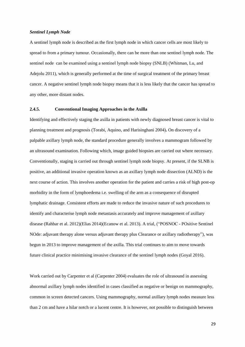
29

Sentinel Lymph Node

A sentinel lymph node is described as the first lymph node in which cancer cells are most likely to

spread to from a primary tumour. Occasionally, there can be more than one sentinel lymph node. The

sentinel node can be examined using a sentinel lymph node biopsy (SNLB) (Whitman, Lu, and

Adejolu 2011), which is generally performed at the time of surgical treatment of the primary breast

cancer. A negative sentinel lymph node biopsy means that it is less likely that the cancer has spread to

any other, more distant nodes.

2.4.5. Conventional Imaging Approaches in the Axilla

Identifying and effectively staging the axilla in patients with newly diagnosed breast cancer is vital to

planning treatment and prognosis (Torabi, Aquino, and Harisinghani 2004). On discovery of a

palpable axillary lymph node, the standard procedure generally involves a mammogram followed by

an ultrasound examination. Following which, image guided biopsies are carried out where necessary.

Conventionally, staging is carried out through sentinel lymph node biopsy. At present, if the SLNB is

positive, an additional invasive operation known as an axillary lymph node dissection (ALND) is the

next course of action. This involves another operation for the patient and carries a risk of high post-op

morbidity in the form of lymphoedema i.e. swelling of the arm as a consequence of disrupted

lymphatic drainage. Consistent efforts are made to reduce the invasive nature of such procedures to

identify and characterise lymph node metastasis accurately and improve management of axillary

disease (Rahbar et al. 2012)(Elias 2014)(Ecanow et al. 2013). A trial, (“POSNOC - POsitive Sentinel

NOde: adjuvant therapy alone versus adjuvant therapy plus Clearance or axillary radiotherapy”), was

begun in 2013 to improve management of the axilla. This trial continues to aim to move towards

future clinical practice minimising invasive clearance of the sentinel lymph nodes (Goyal 2016).

Work carried out by Carpenter et al (Carpenter 2004) evaluates the role of ultrasound in assessing

abnormal axillary lymph nodes identified in cases classified as negative or benign on mammography,

common in screen detected cancers. Using mammography, normal axillary lymph nodes measure less

than 2 cm and have a hilar notch or a lucent centre. It is however, not possible to distinguish between

30

benign lymphadenopathy and metastatic lymphadenopathy or lymphoma via mammography. In

general, only the bottom part of the axilla can be seen, and during mammography positioning, axillary

nodes may be pushed out of the field of the image. Mammography is not considered a dependable

method for axillary lymph node imaging and in lymphadenopathy found on mammography, there are

no consistent criteria for classifying a lymph node as abnormal. As a result, ultrasound has been

deemed valuable in evaluating axillary lymph nodes for metastatic involvement in patients with breast

cancer (Carpenter 2004).

Ultrasound

Ultrasound imaging of the axilla tends to be carried out using a transducer array probe at frequencies

from 7.5 – 17 MHz. For larger patients, the frequency may need to be reduced in order to increase the

image penetration depth, at the expense of resolution. Mammography is not regarded as a good

technique for assessment of axillary nodes as it only reliably identifies gross nodal metastatic spread.

Ultrasound however, remains the more favourable method to examine the axillary lymph nodes due to

its real time function allowing for sensitive and thorough assessment. From the ultrasound image, the

cortex of the node should be relatively hypoechoic and with a maximum thickness of 2.3 mm – 2.5

mm (Dialani, James, and Slanetz 2015). The inner structures of a lymph node are shown in Figure 2.6.

The echogenic hilum should make up the majority of the node. Morphologic gauges, such as cortical

thickening, hilar effacement and non-hilar cortical blood flow, are of greater significance than size

criteria in the classification of metastases in cases where the metastases are of small volume. Features

of lymph nodes that may indicate malignancy apart from overall size and cortical thickness include a

round shape and absence of the fatty hilum. Should part or the entire node be filled with a mass with

irregular margins, a greater likely of malignancy is predicted (Dialani, James, and Slanetz 2015).

Nodal calcifications are also identified on occasion, using high frequency ultrasound probes.

A study by Abe et al (Abe et al. 2007), presented the use of colour Doppler ultrasound to aid

characterisation of lymph nodes. The colour Doppler function can indicate increased blood flow in the

hilum and central cortex. In metastatic lymph nodes, this non-hilar cortical blood flow is likely due to

31

angiogenesis of the tumour, with the vascular network of the cortex is enlarged. (Abe et al. 2007)

(Dudea et al. 2012).

Alternative applications for high frequency ultrasound in breast cancer diagnosis are continuously

being developed. Mamou has examined high frequency ultrasound transducers (>15 MHz) as a means

of quantitatively characterising biological tissue at microscopic levels via processing of back scattered

echo signals (Mamou et al. 2011) (Mamou et al. 2012). The study takes excised lymph nodes from

cancer patients and evaluates them using 3D high frequency quantitative ultrasound techniques,

analysing scatterer size, acoustic concentration, intercept and slope of the tissue microstructure via the

received backscatter spectrum. The results showed potential for the detection of small metastatic foci

in the dissected lymph nodes and contributes to a future goal of further 3D quantitative high

frequency ultrasound methods for characterising lymph node metastases to provide information for

staging, treatment and optimising diagnostic outcomes (Mamou et al. 2012).

2.4.6. Intervention

If these imaging techniques yield a suspicious result, interventional investigation, such as ultrasound-

guided FNAC or ultrasound-guided CNB of the sentinel lymph node may be required. A sentinel

lymph node biopsy is not without drawbacks, however. Radioisotopes are administered to the patient

to help locate the sentinel lymph node, and the process can be timely as many microscopic sections

are required via ultrasound guided biopsy for histological analysis and in certain circumstances, the

sentinel lymph node is not identifiable. If lymph node metastases are confirmed, standard practice

outwith clinical trials is to carry out a dissection of the entire axilla (Dialani, James, and Slanetz

2015).

Most interventional biopsy procedures of the breast and axilla are conventionally guided by

ultrasound (Chung et al. 2008). The paper by Kim et al (Kim et al. 2008) speaks of the advantages of

ultrasound as an image guided tool for breast biopsy, mentioning the lack of ionizing radiation, real-

time accessibility to all areas of the breast and the axilla, uninterrupted visualization of the needle,

32

multidirectional sampling, and low cost. While ultrasound guided FNAC has been an initial procedure

to detect the lymph node metastasis in the axilla, this method can often produce a high false negative

rate mostly due to inadequate volume sampling. Thus, Kim et al found that by replacing ultrasound

guided FNAC of axillary lymph nodes with CNB in the preoperative staging of breast cancer patients,

with larger volumes of tissue obtained , greater sensitivity is achievable (Kim et al. 2008).

It is emphasised that various complications of the percutaneous core biopsy such as bleeding or

infection have been associated with this procedure and that as a result, care should be employed for

reducing complications by recognising detailed anatomy including vessels and nerves in the axilla.

Nerves tend not to be visible on ultrasound, however, the axillary vein and artery can be identified. As

it is accepted that the main nerves are found between the vein and artery, the path of the nerves can be

predicted through imaging the vessels. Lymph nodes lie more superficially than the neurovascular

structures. Therefore, correct positioning of patients and perfect guiding by ultrasound is critical to

avoid traumatic injuries during CNB of the axilla (Kim et al. 2008).

2.4.7. Remaining Challenges

Understanding of the principal anatomic features of the axilla is vital in identifying and classifying

suspect lymph nodes. Ultrasound guided biopsy procedures, in particular core biopsy, are critical in

diagnosing axillary metastasis. In the research arena, MRI can be utilised for examination, often

valuable due to the possibility of viewing both axillae in a scan. Computed tomography and

radionuclide imaging are also options, but are less commonly used.

Challenges remain whereby when using CNB, sensitivity is remains low and, in some cases, is no

better than FNAC. The sentinel node might not be the one that has been biopsied and if the sentinel

node is the node which has been biopsied there can still be sampling error and the portion of the node

with the metastasis could be missed. Metastatic deposits measuring less than 0.2 mm are called

isolated tumor cells, and deposits between 0.2 and 2.0 mm are called “micrometastases” (Edge and

Compton 2010). This level of disease is not presently detectable at imaging.

33

Studies indicate that at present, no combination of physical examination or imaging can provide a

sensitivity or accuracy rate to rival , and certainly not exclude, the standard of interventional

assessment, such as SLNB and ALND (Valente et al. 2012). However as further growth at this

location can result in a focal cortical bulge or cortical thickening identifiable at imaging, efforts in

developing imaging modalities to characterise abnormal nodes as early as possible continues (Ecanow

et al. 2013).

2.4.8. Ductal Carcinoma In-Situ

Ductal carcinoma in situ (DCIS) is a malignant proliferation of ductal epithelium confined by the

basement membrane of the affected ducts. The probable invasiveness of DCIS and its behavior post

treatment varies greatly and depends on its architectural structure and histopathologic grade (Yang

and Tse 2004). Recent studies have been examined for this thesis to explore the current role,

challenges associated with sonography and its potential in the detection and evaluation of

microcalcifications associated with DCIS.

2.4.9. Conventional Imaging Approaches for Detection of DCIS

DCIS is associated with microcalcifications usually identified at mammography. The incidence of

DCIS has increased due to mammographic screening (Moss et al. 2015). These microcalcifications

may also be found via ultrasound if they are associated with a subtle hypoechoic mass. The location

of the ducts within the breast are shown in Figure 2.7.

The majority of ductal diseases are benign and include duct ectasia, solitary intraductal papilloma,

multiple papillomas, nipple papillomatosis and juvenile papillomatosis. Duct size and the intraductal

proliferative process affect the visualisation of these diseases: papillomas often cannot be

characterised by using mammography alone, and a suspicion of papilloma calls for further

investigations, such as ultrasound imaging (Ballesio et al. 2007). Clinical signs or symptoms which

are cause for imaging evaluation include identification of spontaneous or induced single duct nipple

discharge along with indication of palpable nodules in the areolar region on clinical examination

(Ballesio et al. 2007).

34

Figure 2.7 Illustration of breast ducts showing the ducts radiating from the mammary glands towards

the nipple

Nagashima et al (Nagashima et al. 2005) refers to mammography as the gold standard for the

identification and classification of microcalcifications. Following identification by mammography,

suspect microcalcifications are generally diagnosed by means of stereotactic guided core needle

biopsy or vacuum assisted biopsy. Ultrasound examination, in contrast, has been regarded as less

effective for the detection of microcalcifications. It is reported that microcalcifications, when

localised within echogenic and fibroglandular breast tissue, are challenging to detect amongst the

echogenic structures within the breast tissue. This challenge has, until recently, limited ultrasound as a

screening device for early breast cancer. Developments in ultrasound technology have, however,

greatly advanced the resolution and sensitivity of transducer probes providing improved visualisation

of microcalcifications in the breast. Nagashima noted that microcalcifications were not easily detected

using ultrasound, however that their preliminary results show that an ultrasound probe 7 – 13 MHz

showed promise for detecting non palpable microcalcifications in the breast and with further

improvements, could potentially be employed to localise microcalcifications in patients with early

stages of breast cancer (Nagashima et al. 2005).

35

Ballesio et al also showed that ultrasound has the ability to identify ductal disease which has been

flagged as suspicious during mammographic examination and to differentiate between suspicious

lesions needing follow-up or surgical intervention (Ballesio et al. 2007).

Ultrasound can portray microcalcifications, most commonly those in clusters more than 10 mm in size

and located in a hypoechoic mass or a duct-like structure. Malignant calcifications are more likely to

be detected with ultrasound than are benign calcifications, which may be concealed by surrounding

echogenic breast tissue. It is reported by Hooley et al that ultrasound features linked with DCIS tend

to include a hypoechoic mass with an irregular shape, microlobulated margins, no posterior acoustic

features, and no internal vascularity. Ductal abnormalities, intracystic lesions, and architectural

distortions may also be present (Hooley, Scoutt, and Philpotts 2013).

Galactography is a procedure which is employed to assist the diagnosis of DCIS or papillomas in

cases where patients present with a bloody nipple discharge The procedure involves injecting contrast

fluid into the ducts by cannulating one of the ductal orifices on the nipple surface to enable

identification of dilated and blocked lactiferous ducts with mammography (Yang and Tse 2004). It

has been proposed that ultrasound can be used as a complementary imaging method to galactography

procedures, or as a valuable alternative when galactography is not available (Ballesio et al. 2007).

Microultrasound

Following the introduction and development of higher frequency ultrasound transducers, it is evident

that the potential application of breast ultrasound has broadened considerably (Hooley, Scoutt, and

Philpotts 2013) (Mainiero et al. 2005) (Graf et al. 2007). Studies by Stavros, Stöblen and Ballesio,

report that ultrasound transducer technology is advancing to the point that an operating frequency

greater than 13 MHz may be deemed reliable in its ability to detect mammographically suspicious

microcalcifications, along with playing a role in the detection of benign ductal disease, both for the

diagnosis and characterisation of focal masses and duct ectasia. However, various papers report

different level of success when comparing results to histology and mammography, the standard

practices used (Stavros et al. 1995) (Stöblen et al. 2011) (Ballesio et al. 2007).

36

2.4.10. Remaining Challenges

It was suggested by Hooley et al, that in patients with small breasts with a supine thickness less than

3 cm, or when dealing with a superficial target, a higher frequency transducer such as a linear 7 - 17

MHz probe, could be utilised to deliver images of excellent spatial resolution, margin distinction and

lesion visibility. The compromise of using high frequency ultrasound is however the loss of

penetration depth due to an increase in attenuation of the ultrasound signal, rendering visualisation of

tissue at a depth of greater than 3 cm difficult (Hooley, Scoutt, and Philpotts 2013). Similarly, in

research by Yang et al (Yang and Tse 2004) the aim was to establish characteristic elements of DCIS

in the breast visible with high resolution ultrasound. From the high resolution images acquired it was

concluded that while the modality can reveal microcalcifications within masses, it remains unreliable

in comparison to the detection levels provided with mammography in depicting and characterising the

morphology and distribution of microcalcifications, particularly when in isolation.

2.4.11. Clinical Need for Improved Imaging in the Breast and Axilla

Ultrasound guided biopsy is regarded as both a cost effective and time efficient means to obtain

histopathological samples. To carry out these guided procedures in the breast, an accurate sonographic

representation of the region of interest is a vital requirement. Consequently, tumour margins and

tumour associated microcalcifications must be identifiable by ultrasound (Stöblen et al. 2011). As

highlighted above, the value of ultrasound for the identification of mammary microcalcifications has

been debated in past literature. Conclusions vary from claiming that the success and sensitivities of

ultrasound detection are comparable to other effective modalities such as mammography, while

further studies describe it as a supplementary tool to complement mammography, the undisputed gold

standard in identifying these calcifications. It is apparent from this range of results that the primary

clinical need from the use of ultrasound is to be able to show ductal pathology, which is not associated

with masses. As a result, it is suggested that, rather than a replacement to mammography for the

characterisation of DCIS at present, ultrasound should be employed as a complimentary, adjunctive

tool to guide biopsy procedures and improve the sensitivity and precision of mammography in early

breast cancer diagnosis (Yang and Tse 2004) (Hooley, Scoutt, and Philpotts 2013).

37

2.4.12. Proposed Breast Application

As discussed above it is evident that challenges remain in the use of ultrasound in the diagnosis of low

volume axillary nodal metastatic disease and evaluation of ductal pathology. With DCIS being the

earliest form of breast cancer, its accurate detection and sampling is crucial. Similarly, effective

characterisation of axillary lymph nodes is vital for determining cancer staging and prognosis. As a

means to improve clinical practice in both these areas, it is proposed in this thesis that a miniature

high frequency ultrasound transducer array at the tip of a needle has potential to firstly provide

precision guidance for biopsy needle insertion into the breast tissue to maximise efficacy of sampling.

Secondly, such a device could serve as a minimally invasive means of in-vivo tissue characterisation.

Using a minimally invasive, high frequency (> 15 MHz) device to visualise and characterise

micrometastases within lymph nodes could greatly aid diagnosis and management of the axillary

nodes. If micrometastases could be identified the need for SLNB could be obviated or potentially

avoid unnecessary invasive clearance of the axilla. In terms of the diagnosis of DCIS, a device of

appropriately high frequency has the potential to image internal calcifications of ducts and also

increase accuracy in which the ducts could be biopsied. With the transducer based on a needle, high

frequency ultrasound could be utilised to achieve these images by easily accessing the region of

interest with the needle, enabling high resolution imaging regardless of the depth of these features

below the skin.

Demonstration of the feasibility of such applications could greatly enhance diagnostic capability,

breast cancer detection and prognostication, along with being cost effective and reducing patient

discomfort. Imaging studies in this project aim to determine an optimum operating frequency for such

a device.

38

Figure 2.8 Image of proposed use of microultrasound device in a needle to aid breast imaging and

diagnosis

2.5. Thiel Embalmed Cadavers

For examination of both the brain and breast application in this project, Thiel embalmed human

cadavers were used as respective models, acquired through ethical approval from the Centre of

Anatomy and Human Identification at the University of Dundee in conjunction with the Human

Tissue (Scotland) Act, 2006. Thiel embalming refers to an embalming process designed to preserve

lifelike properties of tissue, demonstrated by W. Thiel in 1992 (Thiel 1992). The method was

developed in order to create lifelike research models for the design and development of medical

procedures and devices and enabling effective training in various interventional procedures (Eisma

and Wilkinson 2014). To date, the use of these cadavers as models has been explored for numerous

applications as the entire anatomy of the human body can be utilised. Examples of such research

includes investigation of their use for minimally invasive surgical procedures (Eisma et al. 2013), for

the ultrasound guidance of the delivery of anaesthesia (McLeod et al. 2010) and as models for MR-

guided focused ultrasound surgery (Karakitsios et al. 2016).

For the purposes of this project, Thiel embalmed brain tissue will be used to evaluate the function and

demonstrate the potential of the designed and fabricated miniature ultrasound transducer in a needle.

Thiel embalmed breast tissue will be assessed as being a viable breast model for imaging ducts and

39

subsequently, be used to test the ability of a range of ultrasound frequencies to identify and

characterise ducts and axillary lymph nodes.

2.6. References

Abe, Hiroyuki, Robert A Schmidt, Charlene A Sennett, Akiko Shimauchi, and Gillian M Newstead.

2007. “US-Guided Core Needle Biopsy of Axillary Lymph Nodes in Patients with Breast

Cancer : Why and How to Do It 1.” RadioGraphics 27: 91–100.

Ballesio, L, C Maggi, S Savelli, M Angeletti, P Rabuffi, L Manganaro, and L.M. Porfiri. 2007.

“Adjunctive Diagnostic Value of Ultrasonography Evaluation in Patients with Suspected Ductal

Breast Disease Contributo Diagnostico Della Valutazione Ecografica Nelle Pazienti Con

Sospetta Patologia Duttale Della Mammella.” Radiol Med 112: 354–65. doi:10.1007/s11547-

007-0146-4.

Bartella, Lia, Clare S. Smith, D. David Dershaw, and Laura Liberman. 2007. “Imaging Breast

Cancer.” Radiologic Clinics of North America. doi:10.1016/j.rcl.2006.10.007.

Belsuzarri, TelmoAugusto Barba, RaphaelMartinelli Anson Sangenis, and JoãoFlavio Mattos Araujo.

2016. “Brain Tumor Surgery: Supplemental Intra-Operative Imaging Techniques and Future

Challenges.” Journal of Cancer Metastasis and Treatment 2 (0): 70–79. doi:10.4103/2394-

4722.172249.

Cancer Research UK. 2014. “Breast Cancer Statistics.” Cancer Research UK.

http://www.cancerresearchuk.org/health-professional/cancer-statistics/statistics-by-cancer-

type/breast-cancer#heading-Zero.

Carpenter, Wendy S. 2004. “Sonographic Evaluation of Isolated Abnormal Axillary Lymph Nodes

Identified on Mammograms.” Journal of Ultrasound in Medicine 23: 63–71.

Cheon, Jung-Eun. 2015. “Intraoperative Neurosonography Revisited: Effective Neuronavigation in

Pediatric Neurosurgery.” Ultrasonography (Seoul, Korea) 34 (2): 79–87.

doi:10.14366/usg.14054.

Chung, Maureen A, Martha B Mainiero, Margaret M Steinhoff, and Blake Cady. 2008. “Axillary

Lymph Nodes : US-Guided Fine-Needle Aspiration for Initial Staging of Breast Cancer —

Correlation with Primary Tumor Size.” Radiology 246 (1): 81–89.

Dialani, V, D F James, and P J Slanetz. 2015. “A Practical Approach to Imaging the Axilla.” Insights

Imaging 6: 217–29. doi:10.1007/s13244-014-0367-8.

Dudea, Sorin M, Manuela Lenghel, Carolina Botar-jid, Dan Vasilescu, and Magdalena Duma. 2012.

“Ultrasonography of Superficial Lymph Nodes : Benign vs . Malignant.” Med Ultrason 14 (4):

294–306.

Ecanow, Jacob S, Hiroyuki Abe, Gillian M Newstead, David B Ecanow, and Jan M Jeske. 2013.

“Axillary Staging of Breast Cancer : What the Radiologist Should Know.” RadioGraphics 33

(6): 1589–1613.

Edge, Stephen B, and Carolyn C Compton. 2010. “The American Joint Committee on Cancer: The 7th

Edition of the AJCC Cancer Staging Manual and the Future of TNM.” Annals of Surgical

Oncology 17 (6): 1471–74. doi:10.1245/s10434-010-0985-4.

Eisma, Roos, Mariana Gueorguieva, Erwin Immel, Rachel Toomey, Graeme McLeod, Roger Soames,

and Andreas Melzer. 2013. “Liver Displacement during Ventilation in Thiel Embalmed Human

Cadavers - a Possible Model for Research and Training in Minimally Invasive Therapies.”

Minimally Invasive Therapy & Allied Technologies 22 (5): 291–96.

doi:10.3109/13645706.2013.769451.

Eisma, Roos, and Tracey Wilkinson. 2014. “From ‘Silent Teachers’ to Models.” PLoS Biology 12

(10). doi:10.1371/journal.pbio.1001971.

Elias, Simone. 2014. “Axillary Lymph Nodes in Breast Cancer Patients : Sonographic Evaluation.”

Radiology Brasil 47 (6): 240–44.

Enchev, Y., O. Bozinov, D. Miller, W. Tirakotai, S. Heinze, L. Benes, H. Bertalanffy, and U. Sure.

2006. “Image-Guided Ultrasonography for Recurrent Cystic Gliomas.” Acta Neurochirurgica

148 (10): 1053–63. doi:10.1007/s00701-006-0858-6.

40

Evans, Andrew, Patsy Whelehan, Kim Thomson, Denis McLean, Katrin Brauer, Colin Purdie, Lee

Jordan, Lee Baker, and Alastair Thompson. 2010. “Quantitative Shear Wave Ultrasound

Elastography: Initial Experience in Solid Breast Masses.” Breast Cancer Research 12 (6): R104.

doi:10.1186/bcr2787.

Fercher, Adolf Friedrich, W Drexler, C K Hitzenberger, and T Lasser. 2003. “Optical Coherence

Tomography – Development, Principles, Applications.” Reports on Progress in Physics 66:

239–303. doi:http://dx.doi.org/10.1016/j.zemedi.2009.11.002.

Gabriele, Michelle L, Gadi Wollstein, Hiroshi Ishikawa, Larry Kagemann, Juan Xu, Lindsey S Folio,

and Joel S Schuman. 2011. “Optical Coherence Tomography: History, Current Status, and

Laboratory Work.” Invest Ophthalmol Vis Sci 52: 2425–36. doi:10.1167/iovs.10-6312.

Giannotti, Elisabetta, Sarah Vinnicombe, Kim Thomson, Dennis McLean, Colin Purdie, Jordan Lee,

and Andrew Evans. 2016. “Shear Wave Elastography and Grey Scale Assessment of Palpable

Probably Benign Masses: Is Biopsy Always Required?” The British Journal of Radiology 89

(1062). doi:10.1259/bjr.20150865.

Goertz, David E., Emmanuel Cherin, Andrew Needles, Raffi Karshafian, Allison S. Brown, Peter N.

Burns, and F. Stuart Foster. 2005. “High Frequency Nonlinear B-Scan Imaging of Microbubble

Contrast Agents.” IEEE Transactions on Ultrasonics, Ferroelectrics, and Frequency Control 52

(1): 65–79. doi:10.1109/TUFFC.2005.1397351.

Goyal, Amit. 2016. “POSNOC - POsitive Sentinel NOde: Adjuvant Therapy Alone versus Adjuvant

Therapy plus Clearance or Axillary Radiotherapy. A Randomised Controlled Trial of Axillary

Treatment in Women with Early Stage Breast Cancer Who Have Metastases in One or Two

Sentinel.” Accessed September 15. http://www.posnoc.co.uk/wp-

content/uploads/2014/09/POSNOC-Protocol-21-Nov-2013_NETSCC.pdf.

Graf, Oswald, Thomas H Helbich, Gottfried Hopf, Claudia Graf, and Edward a Sickles. 2007.

“Probably Benign Breast Masses at US: Is Follow-up an Acceptable Alternative to Biopsy?”

Radiology 244 (1): 87–93. doi:10.1148/radiol.2441060258.

Gururaja, T.R., and R.K. Panda. 1998. “Current Status and Future Trends in Ultrasonic Transducers

for Medical Imaging Applications.” Proceedings of the Eleventh IEEE International Symposium

on Applications of Ferroelectrics, 1998., 223–28. doi:10.1109/ISAF.1998.786675.

Hammoud, M a, B L Ligon, R elSouki, W M Shi, D F Schomer, and R Sawaya. 1996. “Use of

Intraoperative Ultrasound for Localizing Tumors and Determining the Extent of Resection: A

Comparative Study with Magnetic Resonance Imaging.” Journal of Neurosurgery 84 (5): 737–

41. doi:10.3171/jns.1996.84.5.0737.

Hastreiter, Peter, Christof Rezk-Salama, Grzegorz Soza, Michael Bauer, G??nther Greiner, Rudolf

Fahlbusch, Oliver Ganslandt, and Christopher Nimsky. 2004. “Strategies for Brain Shift

Evaluation.” Medical Image Analysis 8 (4): 447–64. doi:10.1016/j.media.2004.02.001.

Hill, Derek L G, Calvin R. Maurer, Robert J. Maciunas, John A. Barwise, J. Michael Fitzpatrick, and

Matthew Y. Wang. 1998. “Measurement of Intraoperative Brain Surface Deformation under a

Craniotomy.” Neurosurgery 43 (3): 514–26. doi:10.1007/BFb0056187.

Hooley, Regina J, Leslie M Scoutt, and Liane E Philpotts. 2013. “Breast Ultrasonography : State of

the Art.” Radiology 268 (3): 642–59.

Karakitsios, Ioannis, Senay Mihcin, Timur Saliev, and Andreas Melzer. 2016. “Feasibility Study of

Pre-Clinical Thiel Embalmed Human Cadaver for MR-Guided Focused Ultrasound of the

Spine.” Minimally Invasive Therapy & Allied Technologies 5706 (March): 1–8.

doi:10.3109/13645706.2016.1150297.

Kim, Ki Hong, Eun Ju Son, Eun-kyung Kim, Kyung Hee Ko, Haeyoun Kang, and Ki Keun Oh. 2008.

“The Safety and Efficiency of the Ultrasound-Guided Large Needle Core Biopsy of Axilla

Lymph Nodes” 49 (2): 249–54. doi:10.3349/ymj.2008.49.2.249.

Laura Curiel; Rajiv Chopra; Kullervo Hynynen. 2007. “Progress in Multimodality Imaging: Truly

Simultaneous IEEE Trans Med Imaging Ultrasound and Magnetic Resonance Imaging.” IEEE

Transactions on Medical Imaging 26 (12): 1740–46. doi:10.1109/TMI.2007.903572.

Leiserson, Mark. 2010. “The Future of Medical Imaging.” Tuftscope 9 (2): 17–18.

Leksell, L, C Lindquist, J R Adler, D Leksell, B Jernberg, and L Steiner. 1987. “A New Fixation

Device for the Leksell Stereotaxic System. Technical Note.” Journal of Neurosurgery 66 (4):

626–29. doi:10.3171/jns.1987.66.4.0626.

41

Letteboer, Marloes M J, Peter W A Willems, Max A. Viergever, and Wiro J. Niessen. 2005. “Brain

Shift Estimation in Image-Guided Neurosurgery Using 3-D Ultrasound.” IEEE Transactions on

Biomedical Engineering 52 (2): 268–76. doi:10.1109/TBME.2004.840186.

Mainiero, Martha B, Allison Goldkamp, Elizabeth Lazarus, Linda Livingston, Susan L Koelliker,

Barbara Schepps, and William W Mayo-Smith. 2005. “Characterization of Breast Masses with

Sonography: Can Biopsy of Some Solid Masses Be Deferred?” Journal of Ultrasound in

Medicine 24 (2): 161–67. http://www.ncbi.nlm.nih.gov/pubmed/15661946.

Mamou, Jonathan, Alain Coron, Michael L. Oelze, Emi Saegusa-Beecroft, Masaki Hata, Paul Lee,

Junji Machi, Eugene Yanagihara, Pascal Laugier, and Ernest J. Feleppa. 2011. “Three-

Dimensional High-Frequency Backscatter and Envelope Quantification of Cancerous Human

Lymph Nodes.” Ultrasound in Medicine and Biology 37 (3): 345–57.

doi:10.1016/j.ultrasmedbio.2010.11.020.

Mamou, Jonathan, Alain Coron, Emi Saegusa-beecroft, Masaki Hata, Eugene Yanagihara, Tadashi

Yamaguchi, Pascal Laugier, et al. 2012. “Quantification of Freshly-Excised Human Lymph

Node Tissue Using High-Frequency Ultrasound.” Societe Francaise d’Acoustique. Acoustics

2012. https://hal.archives-ouvertes.fr/hal-00811216.

McLeod, Graeme, Roos Eisma, Andreas Schwab, George Corner, Roger Soames, and Sandy Cochran.

2010. “An Evaluation of Thiel-Embalmed Cadavers for Ultrasound-Based Regional Anaesthesia

Training and Research.” Ultrasound 18 (July): 125–29. doi:10.1258/ult.2010.010016.

McRobbie, Donald W, Elizabeth A Moore, Martin J Graves, and Martin R Prince. 2007. Radiology

MRI : From Picture to Proton. Cambridge University Press.

doi:http://dx.doi.org/10.1017/CBO9780511545405.

Meinzer, H. P., M. Thorn, M. Vetter, P. Hassenpflug, M. Hastenteufel, and I. Wolf. 2002. “Medical

Imaging: Examples of Clinical Applications.” ISPRS Journal of Photogrammetry and Remote

Sensing 56 (5–6): 311–25. doi:10.1016/S0924-2716(02)00072-2.

Meyer, C R, E H Chiang, K P Fechner, D W Fitting, D M Williams, and A J Buda. 1988. “Feasibility

of High-Resolution, Intravascular Ultrasonic Imaging Catheters.” Radiology 168 (1): 113–16.

doi:10.1148/radiology.168.1.3289084.

Moss, Sue M., Christopher Wale, Robert Smith, Andrew Evans, Howard Cuckle, and Stephen W.

Duffy. 2015. “Effect of Mammographic Screening from Age 40 Years on Breast Cancer

Mortality in the UK Age Trial at 17 Years’ Follow-up: A Randomised Controlled Trial.” The

Lancet Oncology 16 (9): 1123–32. doi:10.1016/S1470-2045(15)00128-X.

Nagashima, Takeshi, Hideyuki Hashimoto, Keiko Oshida, Shigeharu Nakano, Naoto Tanabe, Takashi

Nikaido, Keiji Koda, and Masaru Miyazaki. 2005. “Ultrasound Demonstration of

Mammagraphically Detected Microcalcifications in Patients with Ductal Carcinoma in Situ of

the Breast.” Breast Cancer 12 (3): 2–6.

O’Donnell, M, M J Eberle, D N Stephens, J L Litzza, B M Shapo, J R Crowe, C D Choi, et al. 1997.

“Catheter Arrays: {C}an Intravascular Ultrasound Make a Difference in Managing Coronary

Artery Disease.” IEEE Ultrasonics Symposium, 1447–56.

Orringer, Daniel A, Alexandra Golby, and Ferenc Jolesz. 2012. “Neuronavigation in the Surgical

Management of Brain Tumors: Current and Future Trends.” Expert Review of Medical Devices 9

(5): 491–500. doi:10.1586/erd.12.42.

Pagni, Paola, Flaminia Spunticchia, Simona Barberi, Giuliana Caprio, and Carlo Paglicci. 2014. “Use

of Core Needle Biopsy rather than Fine-Needle Aspiration Cytology in the Diagnostic Approach

of Breast Cancer.” Case Reports in Oncology 7 (2): 452–58. doi:10.1159/000365141.

Peters, Terry M. 2001. “Image-Guided Surgery: From X-Rays to Virtual Reality.” Computer Methods

in Biomechanics and Biomedical Engineering 4 (1): 27–57. doi:10.1080/10255840008907997.

Rahbar, Habib, Savannah C Partridge, Sara H Javid, and Constance D Lehman. 2012. “Imaging

Axillary Lymph Nodes in Patients with Newly Diagnosed Breast Cancer.” Curr Probl Diagn

Radiol 41 (5). Elsevier Inc.: 149–58. doi:10.1067/j.cpradiol.2011.08.002.

Röntgen, W. C. 1896. “On a New Kind of Rays.” Science 3 (59): 274–77.

doi:10.1126/science.3.59.227.

Sakas, Georgios. 2002. “Trends in Medical Imaging: From 2D to 3D.” Computers & Graphics 26 (4):

577–87. doi:10.1016/S0097-8493(02)00103-6.

Schmitt, J.M. 1999. “Optical Coherence Tomography (OCT): A Review.” IEEE Journal of Selected

42

Topics in Quantum Electronics 5 (4): 1205–15. doi:10.1109/2944.796348.

Sencha, Alexander N, Elena V Evseeva, Mikhail S Mogutov, and Yury N Patrunov. 2013. Breast

Ultrasound. Springer-Verlag Berlin Heidelberg. doi:10.1007/978-3-642-36502-7.

Shung, KK. 2011. “Diagnostic Ultrasound: Past, Present, and Future.” Journal of Medical and

Biological Engineering 31 (6): 371–74. doi:10.5405/jmbe.871.

Skerl, Katrin, Sarah Vinnicombe, Stephen Mckenna, Kim Thomson, and Andrew Evans. 2016. “First

Step for Computer Assisted Evaluation of Qualitative Supersonic Shear Wave Elastography

Characteristics in Breast Tissue.” International Symposium on Biomedical Imaging (ISBI), 481–

84.

Sosna, Jacob, Mara M Barth, Jonathan B Kruskal, and Robert a Kane. 2005. “Intraoperative

Sonography for Neurosurgery.” Journal of Utrasound in Medicine 24 (12): 1671–82.

doi:24/12/1671 [pii].

Spiegel, E.A, J Lee, and Erwin Neter. 1947. “Stereotaxic Apparatus for Operations on the Human

Brain.” Science 106 (2754): 349–50. doi:10.1126/science.106.2754.349.

Stavros, A T, D Thickman, C L Rapp, Mark A Dennis, Steve H Parker, and Gale A Sisney. 1995.

“Solid Breast Nodules: Use of Sonography to Distinguish between Benign and Malignant

Lesions.” Radiology 196 (1): 123–34. doi:10.1148/radiology.196.1.7784555.

Stöblen, Frank, Solveig Landt, Rami Ishaq, Ruth Stelkens-gebhardt, and Mahdi Rezai. 2011. “High-

Frequency Breast Ultrasound for the Detection of Microcalcifications and Associated Masses in

BI-RADS 4a Patients” 2582: 2575–81.

Szabo, Thomas L. 2014. “Diagnostic Ultrasound Imaging: Inside Out.” Diagnostic Ultrasound

Imaging: Inside Out 787: 735–63. doi:10.1016/B978-0-12-396487-8.00017-3.

Thiel, Walter. 1992. “Die Konservierung Ganzer Leichen in Natürlichen Farben [The Preservation of

the Whole Corpse with Natural Color].” Annals of Anatomy - Anatomischer Anzeiger 174 (3):

185–95.

Torabi, Maha, Suzanne L Aquino, and Mukesh G Harisinghani. 2004. “Current Concepts in Lymph

Node Imaging.” The Journal of Nuclear Medicine 45 (9): 1509–19.

Valente, Stephanie A, Gary M Levine, Melvin J Silverstein, Jessica A Rayhanabad, Janie G Weng-

grumley, Lingyun Ji, Dennis R Holmes, Richard Sposto, and Stephen F Sener. 2012. “Accuracy

of Predicting Axillary Lymph Node Positivity by Physical Examination , Mammography ,

Ultrasonography , and Magnetic Resonance Imaging.” Annals of Surgical Oncology 19 (6):

1825–30. doi:10.1245/s10434-011-2200-7.

Whitman, Gary J, Tracy J Lu, and Margaret Adejolu. 2011. “Lymph Node Sonography.” Ultrasound

Clinics 6. Elsevier Inc: 369–80. doi:10.1016/j.cult.2011.05.005.

Yang, Wei Tse, and Gary M K Tse. 2004. “Sonographic, Mammographic, and Histopathologic

Correlation of Symptomatic Ductal Carcinoma In Situ,” no. January: 101–10.

Zhi, Hui, Bing Ou, and Bao-ming Luo. 2007. “Comparison of Ultrasound Elastography,

Mammography, and Sonography in the Diagnosis of Solid Breast Lesions.” Journal of

Ultrasound in Medicine 26: 807–15.

43

CHAPTER 3

TECHNICAL BACKGROUND

3.1 Aim of Chapter

As discussed in Chapter 2, ultrasound as a medical imaging modality has been explored extensively

since the 1950s. Due to its safe nonionizing nature and its ability to image in real time, it has become

used in a large range of applications from obstetrics, cardiology, and vascular disease, to real time

biopsy guidance and minimally invasive surgery (Szabo, 2014).

The aim of this literature review is to give an overview of the technological background to ultrasound

and the fabrication methods employed for the development of ultrasound devices. Established and

ongoing research in these areas is presented to provide the foundation of the theory upon which the

device development work in this thesis is based.

3.2 Medical Ultrasound

Medical Ultrasound has been adopted as a common diagnostic imaging tool for more than 40 years

(K. Shung, 2011). Clinical diagnosis with ultrasound depends upon measuring the interactions

between transmitted ultrasonic waves and tissues. Ultrasound imaging uses the pulse-echo technique,

where an ultrasonic pulse transmitted from a transducer is reflected or scattered by the tissues. By

measuring the time delay, T, between the emission of the pulse and echo received, the depth, D, and

position of the reflecting tissue boundaries or scattering structure can be calculated by:

In this equation c is the speed of sound in the medium i.e. tissue, and the factor of two is required to

account for the ultrasound pulse travelling to and from the target and returning to the transducer face.

44

In most medical imaging systems, the same transducer is used to transmit and receive these pulse-

echo signals (Hunt, Arditi, & Foster, 1983).

Figure 3.1 Pulse echo technique used for ultrasound imaging. Transmitted ultrasound pulse is

reflected and scattered from tissue structures, with receive echoes detected by the transducer

converted to electrical voltage.

3.3 Piezoelectricity and Ultrasound Generation

Piezoelectricity is the reversible conversion between mechanical and electrical energy, first

discovered by the Curie brothers in 1880 (Szabo, 2014). It was found that certain crystalline materials

had a property due to crystal asymmetry and polarity whereby when the crystal is put under

mechanical stress; a proportional electrical charge is produced. This is termed the Piezoelectric Effect.

Similarly, when voltage is put across a face of these materials, the crystal will be deformed via

expansion and contraction, therefore converting the electrical energy to mechanical energy and

producing what is known as the Inverse Piezoelectric Effect.

The materials in which this behaviour is observed are known as piezoelectric materials. These

materials expand and contract in response to an applied AC voltage and a resonant mechanical

vibration is produced in the material.

As a result, medical ultrasound transducers generate ultrasound energy via mechanical vibrations

induced in piezoelectric material by applying a voltage through the inverse piezoelectric effect. These

45

ultrasound waves propagate into tissues until a boundary, where there is a change in acoustic

impedance of the tissue reflects the ultrasound, or a small structure scatters the wave. The echoes of

the ultrasound energy from these boundaries and scatterers are incident on the transducer surface, and

the mechanical waves are converted to an electric potential difference and translated into an image via

the piezoelectric effect as per Figure 3.2 (Mason, 1981). The location of the source of the echo is

determined by its acoustic transit time and beam direction in the plane. Post processing functions are

carried out on the signals to map the received echoes into a grey scale image. The display of grey-

scale dots is made up of time traces running vertically (top to bottom) to indicate depth. The

brightness along each trace is proportional to the echo amplitude and as a result such an image is

known as a B-mode image where the ‘B’ refers to brightness (Szabo, 2014).

Figure 3.2 Illustration indicating the operation of an imaging transducer via the Piezoelectric Effect

and Inverse Piezoelectric Effect

3.4 Ultrasound Behaviour

3.4.1 Wave Propagation

Acoustic energy generated by a transducer propagates through a medium via the vibrations of the

medium particles. The speed at which the ultrasound travels within this medium is equal to the

product of its frequency, f, and wavelength, λ. The thickness of the piezoelectric material is equal to

46

half of this wavelength. The equation below shows that frequency and wavelength are interdependent

and inversely proportional.

The velocity of sound, c, is a constant within a medium at constant temperature. While the value for c

varies widely for various biological materials e.g. Bone ~4000 ms-1, Fat ~1450 ms-1, In the case of the

work presented in this thesis, soft tissue is the material of interest, of which the average sound

velocity is taken to be 1540 m/s (Cobbold, 2007).

The two main types of ultrasound wave used in medical imaging are longitudinal and shear waves.

Longitudinal waves are due to particle vibration which oscillates in the same direction as the wave

propagation. Shear waves occur due to particle oscillation perpendicular to this direction. Both

longitudinal and shear waves are found in tissue, however shear waves are usually negated for

standard B-mode imaging as their speeds are much smaller than the longitudinal speeds and are highly

attenuated at high frequencies (Cobbold, 2007).

When an ultrasound wave propagates through a material where a boundary exists of varying acoustic

impedance or acoustic velocity, reflection of the ultrasound wave will occur at this boundary.

Specular reflections result in materials where the boundary is smooth and the sizes of irregularities at

a tissue boundary are much smaller than the wavelength of the ultrasound beam. Diffuse reflections

are observed when the ultrasound wave meets a rough boundary while scattering reflects ultrasound

waves into various directions as a result of irregularities within the medium material (Blackstock &

Atchley, 2001) (Cheeke & Zagzebski, 2004).

3.4.2 Attenuation

As ultrasound energy propagates through a material, energy is lost to the medium (Cheeke &

Zagzebski, 2004). This reduction in acoustic energy is called attenuation, which arises as a result of

absorption, reflections and scattering (Cobbold, 2007). The rate at which an ultrasound pulse is

absorbed is dependent on the medium it propagates through and the frequency of the ultrasound. The

47

attenuation rate is specified in terms of an attenuation coefficient in the units of decibels (dB) per

centimetre (cm-1). Attenuation coefficients are used to quantify different materials in terms of how

much the amplitude of an ultrasound beam decreases as a function of frequency. The higher the

attenuation coefficient, the more attenuated the ultrasound wave is by that particular tissue, e.g. bone

with a large attenuation coefficient significantly reduces beam transmission. The attenuation

coefficient (α) can be used to determine total attenuation in dBcm-1 in the medium using the following

formula:

In this equation, the attenuation coefficient is denoted as α (in dBcm-1 at 1 MHz), f is the ultrasound

frequency (MHz), and d is the thickness of the medium. This formula indicates that in addition to the

thickness of the medium and the attenuation coefficient, attenuation varies linearly with frequency of

the propagating beam (Sprawls, 1993). Figure 3.3 below shows how attenuation in different materials

changes as the ultrasound frequency increases.

.

Figure 3.3 Image showing approximate attenuation coefficient values for a variety of materials and

how these vary with increasing frequency (USRA, 2008). For each of these materials, as the

frequency of the ultrasound increases, the attenuation also increases.

It is shown from the figure that attenuation increases with higher frequencies. As a result, the depth of

penetration of the ultrasound energy decreases when using high frequencies. Therefore, high

resolution, i.e. the ability of the ultrasound to distinguish between two close structures, at greater

deeper depths in tissue is difficult to realise using surface probes.

48

3.5 Piezoelectric Materials

3.5.1 Material Properties

Piezoelectric materials can be categorised into classes based on their varying properties for example,

polymers, ceramics, single crystals and composites (W.A. Smith, 1986) (K. K. Shung, Cannata, &

Zhou, 2007). The electromechanical properties of these materials determine their characteristics.

Stress tensor T and strain tensor S are the mechanical considerations, which are related to the

electrical parameters electric displacement vector D and the electric field vector E (“IEEE Standard

on Piezoelectricity,” 1988) (Smits, 1976). The relationship between these variables can be described

through the standard piezoelectric equations and matrices below (Equation 3.4 – 3.7). In these

equations, sE and sD are the specific elastic compliance tensors at constant electric field and electric

displacement,εis the permittivity and β the inverse permittivity, indicated at constant stress and

strain with the suffix T and S respectively, while t indicates that it is the transpose of the tensor

(“IEEE Standard on Piezoelectricity,” 1988) (Smits, 1976).

The standard piezoelectric equations and matrices are shown to display the relationship between the

electromechanical properties in piezoelectric materials. The variables e and h are stress constants and

d and g are strain constants for piezoelectric materials (Smits, 1976).

When considering piezoelectric materials for medical imaging applications, particular characteristics

are required.

49

Acoustic impedance is a property of a material which describes how much resistance the propagating

ultrasound energy encounters as it travels through the material. Ideally, materials with acoustic

impedance near to the value of that in tissue are preferred, to allow for efficient energy transfer

between the transducer and tissue medium; materials with a high electromechanical coupling

coefficient (kt) are also desired for efficient conversion between electrical and mechanical energy. The

electromechanical coupling coefficient indicates the conversion efficiency of the piezoelectric

material as it changes between electrical and mechanical energy. A high coefficient value specifies a

material with greater efficiency.

Many properties of piezoelectric materials can be obtained from an electrical impedance measurement

using an impedance analyser, which provides the impedance magnitude and phase spectra over a

range of driving frequencies. An example of an electrical impedance profile is displayed in the Figure

3.4 below.

Figure 3.4 Example of an electrical impedance profile showing impedance magnitude and phase

spectra of a transducer

The spectrum shows the normal resonant response of a piezoelectric material. The electrical resonant

frequency, fr, is at a minimum when the piezoelectric material vibrates with the minimum impedance

and is called the electrical resonant frequency. The frequency at the point of maximum impedance is

the anti-resonant frequency, fa, and is also known as the mechanical resonant frequency. The anti-

50

resonant frequency is related to the thickness, T, and the longitudinal velocity of sound, vL, of the

material by (“IEEE Standard on Piezoelectricity,” 1988):

The relative difference in the frequencies fr and fa is effected by the material coupling factor and the

resonator geometry. As a result, a quantity called the effective coupling factor has been used as a

convenient measure of this difference. The effective coupling factor, keff, can be defined in terms of

the characteristic frequencies as per the equation below (Jaffe & Berlincourt, 1965) (“IEEE Standard

on Piezoelectricity,” 1988)

The electromechanical coupling coefficient, also known as the electromechanical coupling factor, kt,

of a thickness mode material such as the piezoelectric ceramic plate in a simple transducer, denotes

the conversion efficiency between electrical and mechanical energy. This is defined in terms of the

following equation (R. Liu, Harasiewicz, & Stuart Foster, 2001) (“IEEE Standard on

Piezoelectricity,” 1988):

The Curie temperature, Tc, which is the temperature at which the properties of the piezoelectric

material degrade, should also be taken into account as various fabrication processes involve heat

applied to the transducer material (K. K. Shung et al., 2007).

51

Table 3.1 Example of Curie temperatures in a variety of piezoelectric materials (K. K. Shung et al.,

2007)

Piezoelectric

Material PVDF PZT-5H PbTiO3

PMN-PT

Crystal

Curie Temperature

(ᵒC) 100 200 260 130

Permittivity, or the dielectric constant, is a property which defines the relative strain a piezoelectric

active element experiences under electronic excitation. The dielectric constant of a material is

inversely proportional to electrical impedance, which means materials with a high dielectric constant

are more easily matched to the system electronics and result in efficient signal transfer. Therefore,

materials with a high dielectric constant are required for the purpose of fabricating imaging arrays

(Waller, Chen, & Gururaja, 1996).

Ceramics and single crystals are most commonly used for medical imaging, usually in the form of

composite materials (K. K. Shung et al., 2007). Piezoelectric polymer materials such as PVDF

(polyvinylidene difluoride) are used in ultrasound transducers typically in applications which tend to

be employed for imaging above 15 MHz. PVDF has a low electromechanical coupling coefficient,

resulting in decreased efficiency, but also has a very low acoustic impedance, and as a result, is a

good match to tissue and therefore an efficient receiver (Jeong & Shung, 2013).

3.5.2 Ceramics

Lead zirconate titanate, Pb (Zr, Ti) O3 or PZT ceramics, are the most widely used piezoelectric materials

in medical imaging transducers. The advantage of using piezoelectric ceramic materials can be

attributed in most part to their high piezoelectric and electromechanical coupling coefficients (Hunt et

al., 1983). These conventional ceramics are made up of crystalline grains sized 5 – 10 μm, which are

randomly arranged together. The ceramic material must undergo a process known as poling to align and

polarise the individual grain effects. A high strength electric field is applied to orientate the polarisation

vector to the crystallographic direction nearest to the direction of the electric field. When the field is

52

removed the dipoles are retained in this position and the ceramic possesses a permanent polarisation

and demonstrates piezoelectricity (Newnham, 1989). Once poled, the piezoceramic material is

anisotropic, whereby the piezoelectric dielectric and elastic characteristics are different along different

axes.

The acoustic impedance of piezoceramic material tends to be approximately 30 MRayl with a Curie

temperature of up to 200 °C. The smaller the grain size of these materials, the more suitable they are

for small elements of high frequency transducer arrays. As a result, finer grain materials are being

manufactured; the smaller grain size improves the materials performance when undergoing fine scale

dicing, and maintains the parameters found in its bulk form, such as high dielectric permittivity which

enables better matching to the systems electronics and therefore optimises signal transfer efficiency (K.

K. Shung et al., 2007).

3.5.3 Single Crystals

In contrast to the ceramics, single crystal piezoelectric materials do not consist of grains, but are

obtained from a grown crystal boule. For years, single crystal piezoelectrics such as quartz (Si02) and

lithium niobate (LiNbO) have been used in applications such as oscillators and surface acoustic wave

devices. Advancements in the production of single crystal relaxor-based materials such as PMN-PT

offer considerable improvements in transducer performance (Gururaja & Panda, 1998). While the

absence of grain boundaries can make single crystal piezoelectric materials quite brittle, and therefore

difficult to handle, their properties include a higher electromechanical coupling coefficient (kt), and

permittivity coefficient than piezoceramics (Sun et al., 2009) (Marin-Franch, Cochran, & Kirk, 2004)

(Q. F. Zhou et al., 2008). These characteristics result in a better performance, however, temperature

restrictions exist in PMN PT single crystals where their properties degrade at high temperatures, due

to the Curie temperature of these materials being less than 130°C (Sun et al., 2009). With these

temperature constraints come fabrication restrictions, therefore significant efforts have been put into

the development of single crystal materials with increased Curie temperature. The incorporation of

lead indium niobate (PIN ) to PMN–PT materials to generate ternary PIN-PMN-PT single crystals has

resulted in a higher Curie temperature, up to 160°C. The properties of this material create greater

53

potential for the production of high frequency transducers and arrays for medical applications with

single crystal materials.

3.5.4 Composite Materials

Piezoelectric composite materials have pillars of piezoelectric materials encapsulated with passive

polymers. A piezocomposite with 1 – 3 connectivity, depicted in Figure 3.5, has piezoelectric pillars

connected in one dimension, that is, through the thickness, and the polymer is connected in all three

orthogonal dimensions.

Figure 3.5 Piezoelectric pillars surrounded by a passive polymer material

Because of the tall, thin pillars, a piezocomposite possesses an efficient length-extensional mode (k33)

with higher electromechanical coupling coefficient than the thickness extensional mode (kt) of a plate

of bulk piezoelectric material. This is maintained while functional in a plate thickness kt, mode. A

high thickness mode electromechanical coupling coefficient is obtained due to a reduction in lateral

clamping of the pillars when they are surrounded with a passive polymer, which is soft relative to

piezoelectric ceramic or single crystal material. This characteristic is an advantageous feature of the

composite materials over its bulk counterparts. In addition, the composite material has lower acoustic

impedance. This is due to the inclusion of the polymer which reduces the overall material density, and

in turn, the acoustic impedance, providing superior acoustic matching to tissue. By incorporating the

polymer with the piezoelectric material, the acoustic impedance can be lowered to below 17 MRayl.

This value varies based on the volume fraction of the piezoelectric pillars used, albeit, permittivity is

also reduced (W. A. Smith, 1989) (K. K. Shung et al., 2007) (C. Liu, Djuth, Zhou, & Shung, 2011).

Greater electromechanical coupling and lower acoustic impedance result in improved sensitivity and

54

broader bandwidth. The effective properties of a composite can be expressed as a function of the

ceramic volume fraction (Smith & Auld, 1991). Volume fractions of 40% - 70% are most commonly

used for a range of applications, the fraction varied to adjust acoustic impedance and the dielectric

constant. The composite is designed in terms of a compromise between the volume fraction, the pillar

to pillar pitch, and the pillar aspect ratio, i.e. the ratio of height to width of the pillars. It is suggested

that the design of a composite feature pillars with an aspect ratio close to 3:1, where possible, to

minimise extraneous intra-pillar acoustic modes (W. A. Smith, 1989).

Due to the advantages discussed, 1-3 composites have been used as the main material of choice for

the array devices in this thesis fabricated via ‘dice and fill’ techniques along with Micromoulded 1 – 3

piezocomposites, the use of which will be presented in Chapter 4.

3.6 Medical Imaging Transducers

The device used by clinicians to generate, transmit and detect ultrasound is called a transducer.

Depending on the application, different variations of design of transducer are used. Structures of a

transducer vary from simple plate of piezoelectric material known as a single element, to a transducer

array made up of a series of independent transducer elements. The fundamental components of a

medical imaging transducer are together known as the transducer stack, and can be broken down into

the following parts, also illustrated in Figure 3.6.

Active Element

The active element is made up of a piezoelectric material which generates and receives

ultrasound energy.

Passive Layers

a. Matching Layer

A passive material at the front face of the transducer, used to improve the efficiency of energy

transfer from the active layer into the medium i.e. tissue.

b. Backing Material

A passive material at the back of the transducer stack which is used to dampen continued

vibration (ringing) of the transducer element and achieve short pulses.

55

Electrical Connections

The connections to the active elements deliver the excitation voltage to the piezoelectric

material and collect received information.

Transducer Casing

The casing contains the transducer assembly and can also be used to provide electrical

shielding.

The design considerations for each of these components are discussed in the following section 3.6.1.

Figure 3.6 Components which make up a transducer stack

3.7 Design Considerations for Transducers

3.7.1 Passive Layers

Matching and backing layers are developed using passive polymer materials in order to improve the

imaging performance of the transducer (Kossoff, 1966) (Q. Zhou et al., 2009) (Webster, 2009). When

designed correctly, passive layers can optimise energy transducer and minimise unwanted resonances

in a transducer.

56

3.7.2 Matching Layer

Matching layers can be constructed as one or multiple layers at the front face of a transducer, usually

made up of a polymer combined with alumina particles. The role of the matching layer is to enable

efficient energy transfer between the transducer and medium being imaged by minimising the acoustic

impedance difference between the two, thus minimising reflection from the boundary. A reduced

acoustic mismatch is achieved by designing the matching layer to have an intermediate acoustic

impedance value between the transducer element and the imaging medium (Kossoff, 1966). For

example, using a piezoceramic of acoustic impedance of ~30 MRayl, to image a tissue medium of

~1.5 MRayl, by the equation below a matching layer with impedance of ~6.7 MRayl would be

required. The chosen material must also exhibit low loss properties because high attenuation would

limit effective transmission between the transducer and medium. The required acoustic impedance of

the matching layer can be determined by calculating the geometric mean of the impedance values , Z,

of the transducer active material and the medium, e.g. Tissue (Draheim & Cao, 1996), as shown in the

equation:

The thickness of the matching layer is also important. A thickness equal to integer multiples of a quarter

of the wavelength improves the intensity of the ultrasound propagated into the tissue (Wang & Cao,

2004). A one quarter wavelength layer is generally chosen as layers which are thicker result in greater

attenuation (Wang & Cao, 2004).

3.7.3 Backing Layer

The main purpose of a backing layer is to enhance the performance of the transducer by absorbing the

transmission of ultrasound energy propagating into the back of the transducer. As with the matching

layers, a polymer with a particle filler, often tungsten, tends to be used. When the backing layer has an

acoustic impedance significantly less than the transducer active material, greater sensitivity results as

less energy transmitted into the backing. In this case, however, the pulse duration is longer due to

continued vibration of the active material following excitation because of the reflection of waves at

57

the interface. When the backing material has an acoustic impedance close to that of the active

element, a large part of the ultrasound energy is coupled into the backing, which reduces reverberation

and shortens pulse duration. The shorter pulse improves resolution but decreases the sensitivity,

therefore, a compromise between resolution and sensitivity is required (Webster, 2009) (Gururaja &

Panda, 1998). The backing material should also have a high absorption coefficient (attenuation) to

prevent ultrasonic energy from returning to the piezoelectric element (Grewe, Gururaja, Shrout, &

Newnham, 1990).

3.7.4 Active Layer

The properties of the active material used in a transducer determine the transducer performance

(“IEEE Standard on Piezoelectricity,” 1988; Jaffe & Berlincourt, 1965). These properties include the

electromechanical coupling coefficient, kt, dielectric constant εr, and acoustic impedance, Z (Waller et

al., 1996).

A material with a high electromechanical coupling coefficient, where kt approaches the value of 1, is

preferred to enable efficient conversion between mechanical and electrical energy.

A large dielectric constant is particularly important when dealing with electrical impedance matching

to small piezoelectric elements used in arrays. Correctly matched electrical impedance to an imaging

system (~50Ω) optimises efficient signal transfer and minimises reflections within the circuit.

Electrical impedance magnitude is inversely proportional to the surface area of the transducer and as a

result, in cases where arrays are made up of miniature elements, the electrical impedance of these

elements can be high. This electrical impedance is inversely proportional to the dielectric constant of

the transducer material (Waller et al., 1996).

The acoustic impedance, Z, affects the propagation of energy across the boundaries from the

transducer stack through to the tissue medium. Ideally, the specific acoustic impedance of the active

element would be similar to tissue where Z = 1.5 MRayl. This mismatch between Z value of the

active layer and the medium is addressed via the addition of a matching layer as described in the

Matching Layer section 3.7.2 above.

58

As shown in Section 3.5.1, the thickness of the piezoelectric material is related to the anti-resonant

frequency and the longitudinal sound velocity. It should be considered that when the thickness of the

active layer is similar to the length of the piezoelectric material, an additional resonance is observed

which interferes with the thickness mode resonance, reducing sensitivity. As a result, it is suggested

that having a length to thickness aspect ratio which is less than 0.6 for a composite pillar or greater

than 3 for a simple piezoelectric plate will avoid this problem by maintaining thickness mode

resonance only (R. Liu et al., 2001)

In addition to material considerations, performance criteria such as axial and lateral resolution and

dynamic range should be taken into account in order to achieve an effective image. These factors can

be enhanced via careful design and fabrication of the transducer layers and geometry.

3.7.5 Axial Resolution

Axial resolution of a transducer is the ability to differentiate between two reflecting targets which are

positioned close to one another along the wave propagation direction. The axial resolution, RA,

depends on the length of the pulse-echo response of the transducer and can be described by the

following:

In this equation, v is the acoustic velocity in the medium being imaged and tp is the time duration for

the pulse amplitude to decay to -6 dB of its maximum amplitude. The axial resolution is influenced by

the resonance frequency and damping of a transducer. Higher frequencies result in shorter pulse

lengths. The properties of a backing layer, as discussed in section 3.7.3, can be adjusted to vary its

damping ability in order to shorten pulse lengths and improving the transducers resolution and

bandwidth (Webster, 2009).

59

Figure 3.7 Depiction of axial resolution

3.7.6 Lateral Resolution

The lateral resolution is the ability of a transducer to distinguish between two closely positioned

targets perpendicular to the ultrasound beam. At the focal point of an ultrasound beam, the lateral

resolution of the transducer is optimised, where the beam is at its narrowest. The area of the beam

between the face of a flat, unfocused transducer and the focal point is defined as the near field

(Fresnel region), and the far field (Fraunhofer region) denotes the region beyond the focal point. The

intensity of the near field area of the ultrasound beam is affected by wave interference and diffraction,

while the far field features a uniform decrease in intensity. The distance from the transducer face to

the area between the near field and far field sections of a beam, i.e. near field length, NFL, can be

defined using the equation:

Where D is the diameter of the transducer aperture, and λ is the wavelength in the medium.

60

Figure 3.8 Near field and far field of ultrasound beam

The aperture of a transducer can be described as the dimension of its physical footprint. For a single

element transducer, the dimensions of its aperture are that of the active element, while for an array,

the aperture includes the combined dimensions of all the active elements together. The size of the

aperture is significant in its effect on the lateral resolution of the transducer. Larger apertures which

measure greater than the ultrasound wavelength of the transducer yield a narrow ultrasound beam and

result in improved resolution.

Focusing of a transducer can improve lateral resolution; this can be achieved by fabricating

transducers with spherical curvature to focus the beam at a specific depth, or with the addition of a

focusing lens, where at the focused area of the beam, the lateral resolution is improved.

The focusing power of a transducer is described by the f-number (f #), as per the equation below,

where r is the focal length and D is the diameter of the transducer aperture:

The diameter of the aperture, D, affects the lateral resolution, RL, by the equation:

In this equation, λ is the wavelength in the medium, and r is the focal length. In contrast, the smaller

the aperture, the more the beam will diverge. Side lobes occur when beams are created off-axis from

the primary beam and result in ultrasound echoes being received by the transducer which indicate

their origin from false positions within the transducer footprint and therefore create image artefacts

(Barthez, Léveillé, & Scrivani, 1996; Hindi, Peterson, & Barr, 2013).

61

Figure 3.9 Depiction of lateral resolution

3.7.7 Sensitivity

The proficiency in which a transducer can detect targets can be described as its sensitivity. Greater

sensitivity signifies an increased penetration depth and a high signal to noise ratio (SNR) which

results in greater dynamic range. The dynamic range of an image is the ratio of maximum to

minimum signal intensity, displayed as shades of grey in an image. For transducer performance, a

compromise must be made between sensitivity and resolution; this can be varied and determined

during the fabrication processes via the matching and backing layers and the electromechanical

coupling coefficient, kt, of the piezoelectric material which influences sensitivity. Sensitivity can be

improved through use of good quality electrode layers and cabling in the transducer assembly.

3.8 Medical Ultrasound Transducer Arrays

Ultrasound transducers used in medical imaging are most often transducer arrays, made up of a series

of multiple transducer elements. As opposed to the single element transducers, multiple elements in

an array broaden the transducer applications. An array configuration enables independent control of

each element to facilitate electronic beam focusing and steering. This improves the devices imaging

and measurement potential.

62

Figure 3.10 Multiple elements in a linear transducer array

The linear array consists of a number of identical transducer elements arranged in a row. Each

element is separated by a space called a kerf, and the distance between the centre points of two

neighbouring elements is known as the pitch. In linear arrays the pitch measures about one

wavelength of sound in tissue. To form a 2D, B-scan image using a linear array, a pulse echo line is

created across each element or group of elements and the set of lines are interpolated to create a

rectangular shaped image.

.

Linear phased arrays tend to have a pitch which is ½ of the wavelength of sound in tissue. During

transmit and receive operation of these elements, images are acquired by activating the elements in

turn. A linear phased array introduces a delay to the electronic signal activating the elements in order

to steer and enable focusing of the ultrasound beam. By varying the excitation delay of elements the

beam direction and focus can be steered electronically, enabling multiple angles to be inspected by an

individual probe in a single position While the field of view generated by a linear array tends to be

presented in a rectangular format, phased arrays allow sector scans to be produced via this beam

steering.

63

Curved arrays are comparable to linear arrays with the composition of the elements curved in convex

configuration which results in a sector beam shape and enables focusing of the beam.

Annular arrays are constructed of a central circular element, surrounded by consecutive ring elements

with equal surface area in order to maintain comparable electrical impedance. Annular arrays have the

ability to introduce dynamic phase delays which can be manipulated to realise a focused beam, where

the depth of focus can be controlled. However, they must be mechanically scanned to produce an

image.

Multi-dimensional arrays have similar composition to linear arrays, however with multiple elements

arranged in both the x and y direction. Phased delays can be introduced to the elements in both

directions to focus and steer the beam. The drawback usually associated with these arrays is cost due

to fabrication, the challenge of connecting to large numbers of elements and the operation systems

required.

3.9 Diagnostic Ultrasound

In routine practice, ultrasound for medical imaging and diagnosis operates at frequencies up to ~15

MHz (K. Shung, 2011; Szabo, 2014). At 15 MHz, the corresponding wavelength is about 100 μm in a

tissue medium. As per Section 3.4.1, frequency and wavelength are inversely proportional, while the

thickness of the active piezoelectric material is equal to half of the wavelength. Therefore, the scale of

ultrasound devices are miniaturised with higher frequencies. This allows them to be integrated into

smaller probes. Devices operating above 15 MHz have the potential of resolving features below 200

μm ( Foster, 1996; Ritter, 2001; Ssekitoleko, 2011). In recent years, such high frequency probes have

been developed to advance image quality in eye, skin and intravascular applications in particular (K.

Shung, 2011). This high resolution enables the visualization of detailed tissue structure at the expense

of penetration depth due to increased attenuation, as shown in Section 3.4.2. This can often be

considered one of the disadvantages of high frequency ultrasound, for example, transducers which

operate at 50 MHz are limited to a image penetration depth of approximately 20 mm whereas

transducers at 5 MHz can visualise areas up to 130 mm in depth.

64

In this project, a miniaturized high frequency ultrasound linear array is integrated into an

interventional tool i.e. a biopsy needle, in order to place the ultrasound array at the region of interest

and acquire high resolution images while overcoming the constraint of decreased penetration depth.

3.10 Transducer Fabrication Technology

Array fabrication increases in complexity during development of high frequency ultrasound arrays.

The miniature scale of these devices creates a significant challenge to integrate electrical connections

to each element of the array within the structure of active, matching and backing layers. Using careful

manipulation of fabrication techniques and parameters, research is continuously adapting processes to

overcome these difficulties in order to assemble miniature high frequency ultrasound arrays.

The primary fabrication processes used to produce transducers and arrays include micromachining

and microfabrication techniques including;

Lapping and polishing – thinning of material and surface preparation

Dicing – Cutting lateral dimensions, separating and defining array elements and for the

production of dice and fill composites

Electrode deposition – Various methods for electrode deposition such as Photolithography

3.10.1 Lapping and Polishing

This method is used to control the thickness of active and passive layers and prepare the surface for

deposition and adhesion of electrode layers. The thickness of these layers is critical to the

performance of the transducer, determining factors including the operation frequency, transducer

efficiency and damping.

The lapping process controls the thickness of the layers of a transducer or array stack via pushing

abrasive slurry between the surface of the material and a lapping plate. This process can be carefully

controlled with careful consideration of abrasive particle size, plate rotation speeds and pressure at

which the material sample is subjected to.

65

The particle size used in the abrasive slurry determines the smoothness of the surface achieved. While

larger particles e.g. 20 μm remove material at a faster rate, smaller particles such as 1 μm – 3 μm yield

smoother results, at a slower removal rate.

The rate at which material is removed in order to flatten surfaces is also influenced by the plate

rotation speed selected and the pressure at which the sample is placed against the plate surface. As it

rotates, the lapping plate is pulling the abrasive material across the face of the sample (~30 – 50 rpm).

Therefore, the quicker this rotation speed is, more particles pass over the sample to wear away the

material over a shorter period of time. Similarly, a force can be applied to the sample to increase the

pressure in which the sample surface is being pressed into the abrasive during the rotation, increasing

the material removal rate. Consideration must be given to rotation speed and force when machining a

fragile sample.

The precision this method offers makes it an effective technique for achieving miniature thicknesses

of piezoelectric layers for higher resonant frequencies. In addition to controlling thickness, the quality

of the surface finish of these layers is significant and must be considered for successful adhesion of

other layers of the transducer array stack, and electrode deposition.

Figure 3.11 Illustration of lapping machine set up

Detailed studies by Bernassau et al. have examined lapping for effectively thinning high frequency

composite materials (A.L. Bernassau et al., 2007) (A. L. Bernassau et al., 2008). The results presented

66

in this work provide best practice guidelines and processes for the machining of high frequency

piezocomposites and signify the effect of the variable lapping components such as abrasive size and

lapping plate material. From particle sizes of 9 μm, 3 μm and 1 μm Al2O3 slurry examined in their

performance of flattening a piezocomposite sample, the 9 μm and 3 μm were found to be most

effective in obtaining a uniform surface finish and minimum height difference between the

piezocomposite pillars and the surrounding polymer. These results were particularly true when used

with a glass lapping plate as opposed to a cast iron plate. Interestingly, using a particle size of 1 μm

was found to scratch and therefore damage the material surface. Following the lapping, the samples

underwent mechanical polishing, and the height difference between composite pillar and surrounding

polymer was reduced to 1 μm , with a surface finish roughness of 12 nm and 7 nm for the ceramic

and polymer respectively (A.L. Bernassau et al., 2007). This surface flatness and finish was suitable

for the deposition and adhesion of electrode patterns using photolithography (Bernassau et al., 2012).

Ultra-precision grinding has been presented as an alternative to lapping for the production of high

frequency transducers (S. Cochran et al., 2006). Piezocomposite samples were thinned to less than

100 μm, with a surface roughness of less than 1 μm in a single process, proving potential as a cost

effective method to mass produce such material. While this was shown as a viable process, a

drawback exists in terms of the high cost of such a machine. As a result sample thinning processes in

this project were completed using a lapping and polishing machine.

3.10.2 Precision Dicing

Fine scale dicing is used to define the lateral dimensions of piezoelectric active layers, produce dice-

and-fill piezocomposites, and can be used to define the connections in an array by creating the kerf

between elements, forming independent interconnects to each element.

For both the application of dicing to the separation of array elements and the production of dice-and-

fill piezocomposites, considerations for dicing parameters change and become more challenging as

the frequency of ultrasound devices increase. As the wavelength and dimensions of ultrasound arrays

scale inversely proportional to frequency (as shown in equation 3.2). As a result, the size of cuts to

create kerfs between elements and composite pillars are miniaturised and the remaining material

67

becomes more fragile due to its fine dimensions e.g. for 15 MHz, wavelength element spacing is 100

μm pitch, and composite pillar pitch for this frequency is ~50 μm. Studies in literature have reported

that spindle rotation speed, blade feed rate along with coolant flow all affect the outcome of the dicing

process used, depending on the application, and especially at high frequencies (Michau, Mauchamp,

& Dufait, 2004; Ritter et al., 2001).

Spindle rotation speed determines the speed in which the blade rotates while feed rate is how fast the

blade advances through material. Fragile materials such as single crystal samples require these

parameters to be reduced in comparison to what would be suitable for piezoceramics to avoid

cracking along the kerf of the cut due to their brittle nature. Coolant flow is important to wash away

debris and cool the blade during the dicing process. Consideration must be given to the extent of the

coolant flow when dicing small features such as pillars in a material as the water flow has the

potential to break and wash the delicate pillars from the sample.

Array Element Definition

Linear kerfless arrays have been produced by numerous research groups to achieve arrays without the

requirement to dice between elements (Démoré, Brown, & Lockwood, 2006) (Zhu et al., 2013). This

simplified method enables the development of high frequency arrays where the required kerf width

between elements becomes increasingly minute, the dimensions of which can be challenging to

achieve with a dicing saw. Performance constraints exist in kerfless arrays however, as acoustic beam

steering is not possible due to considerable electromechanical cross-talk which results between the

array elements. A paper by Bezanson et al. has investigated the potential of using a micro dicing saw

to produce “semi-kerfs”, whereby for the production of a high frequency 64 element array with 38 μm

element pitch, the kerfs were kept to a maximum depth of 20 μm into the substrate which was 47 μm

thick, to increase element directivity while on the other side of the array photolithography electrode

patterns were unaffected (Bezanson, Garland, Adamson, & Brown, 2012). R.T. Ssekitoleko has

employed dicing as a means to separate array elements, where a 6 MHz, 8 element array was attached

using a conductive adhesive to a flexible circuit board with electrode tracks at a pitch of 300 μm.

68

A 100 µm blade was used at this pitch to dice through the array stack and separate the elements

(Ssekitoleko et al., 2011).

Production of Piezocomposite Materials

Where dicing is employed to create kerf cuts to separate adjacent array elements and to create

piezocomposite materials via the “dice and fill” method, a high precision dicing saw has been used

extensively in the literature.

Cannata et al. for example, employed a 13 µm hubbed nickel/diamond blade to produce a 35 MHz 2 -

2 piezoceramic composite. The average kerf produced by this blade was 14 µm with a volume

fraction of 44%, and in this method, 1 - 5 μm alumina loaded epoxy was deposited into the kerfs

between the first and second set of cuts made into the material to minimise pillar breakage at such

small kerf and pillar dimensions (J. M. Cannata, 2006). A kerf of 8 µm however was achieved by

Bantignies et al (Bantignies, 2011) using a fine grain ceramic material for the fabrication of a 40 MHz

composite dice and fill array. As mentioned earlier, the higher the frequency desired, the smaller the

kerfs needed to separate the neighbouring pillars. The capability of the dicing machine to create these

high frequency composite materials is therefore constrained by the minimum blade thickness

available which, from the current research literature shows to be approximately 10 µm. In addition,

the fabrication of fine-scale composites without the effects of lateral resonances due to the miniature

pillars is increasingly challenging. As a result, further developments in dicing must be realised and

alternative methods are required for composite materials operating at 20 MHz and above. Numerous

research groups have been working to address this requirement.

Adjusting composite pillar geometry has been an area of interest as an alternative to the conventional

orthogonal dicing cuts. A paper by Brown et al has shown the fabrication of a 40 MHz transducer

using a piezocomposite with triangular shaped pillars (JA Brown & Cherin, 2007). The aim of using

triangular shaped pillars is to minimise lateral resonances associated with pillars required for high

frequency substrates, due to difficulties getting the pillar width to scale with pillar length. The

piezoceramic material was diced into a series of isosceles triangle pillars with a 15 µm blade. A single

element 3 mm diameter, curved transducer (JA Brown & Cherin, 2007) was built using this material.

69

Similarly, the papers by Yang and Cannata et al (Yang, Cannata, Williams, & Shung, 2012) (Jonathan

Cannata, Williams, & Shung, 2011), have presented developments of new diced 1 – 3 piezocomposite

geometry to minimise acoustic cross talk between high frequency transducer array elements. In this

work, 10 MHz and 15 MHz 1 – 3 piezocomposite substrates were fabricated using a variety of pillar

geometers in order to compare their performance. Square, triangle and pseudo-random were the

variations of pillars created using a 12 µm blade and 50 % volume fraction. It is postulated in this

study that the greater the geometric complexity of the pillars in the composite, the more suppressed

the coupling between lateral and thickness mode resonances would become. It was found that between

adjacent elements in an array at 15 MHz, the pseudo-random composites performed best, resulting in

the lowest measured crosstalk in comparison to the square and triangle pillars.

Interdigital pair bonding (IPB) has been explored and applied to the fabrication of high frequency

composites as the technique can create a smaller kerf between elements than is possible by the

smallest dicing blade (~10 µm) and have the potential to create substrates for operation up to 85 MHz.

This method involves taking two plates of piezoelectric substrate which are partially diced with a

series of cuts to create a linear pattern of “teeth” connected by the bulk material. The cuts in the

material are wider than the width of the pillars which remain. The two piezoelectric plates are then

interdigitated whereby the pillars from one plate slot into the cuts made on the other plate. The

remaining kerfs between the integrated pillars are filled with epoxy and the bulk material on each side

is removed (Ritter et al., 2001). Ultrafine piezoelectric composites were manufactured using this

method by Yin et al (Yin, Lukacs, Harasiewicz, & Foster, 2005) where single element transducers at

frequencies of 50 – 60 MHz were developed and when tested, showed no lateral resonances in the

frequency range of 55 – 150 MHz. IPB has also been used by Chabok et al to produce a 1- 3

composite with pillars 19 µm wide, with 6 µm kerf, operational at 35 MHz in a 8 element kerfless

annular array (Chabok et al., 2011). This method however involves timely processing due to lapping

required of material stock on both sides of the substrate. Alignment of the pillars of the two

piezoelectric plates is challenging and involves the use of more material than the conventional dicing

and filling methods using one plate of material.

70

Additional Methods for the Production of Piezocomposites

To further overcome the limitations presented by standard fabrication procedures during the

manufacture of 1 – 3 piezocomposites, a gel-casting process was used by Garcia-Gancedo et al

(García-Gancedo et al., 2012). A PZT ceramic paste was pressed into a mould to achieve a series of

micro-pillars with a minimum separation between features of 4 µm. Following a process of

demoulding, drying and sintering, an epoxy was cast over the ceramic, encapsulating the pillars. The

material was then lapped to produce a thickness resonance mode at 70 MHz and a keff of ~0.51, the

results of which indicate potential for use of this method for the production of piezocomposite

substrates for high frequency ultrasound devices.

Deep Reactive Ion Etching (DRIE) is an additional method which has demonstrated as an effective

technique to etch ultra-fine composite pillars using ceramic and single crystal materials (Jiang et al.,

2006)(Shrout, 2008). The photolithographic based micromachining method enables submicron

machining precision, mass production with minimal handling and damage to the material. It is

apparent that this is a process which could potentially be integrated into a wafer-scale transducer array

production process. This method is not without drawbacks however, as it is time consuming and the

dimensions which can be etched are limited to about ~50 µm.

3.10.3 Electrical Interconnects

One of the greatest challenges for the construction of high frequency transducers remains the

establishment of electrical interconnects. The miniature scale of the high frequency array elements

call for interconnects scaled to match and to be integrated into the compact package of the array stack.

Many research groups concentrate on developing and improving the yield and performance of

interconnects at these dimensions.

To establish connections to an array, an electrode layer must be deposited on the array surface. To

ensure individual connection to each element, blanket electrode connections can be separated

manually via dicing or individual element connections can be created by various methods.

Wire bonding has been shown as a possible means of connection to elements, demonstrated by Brown

et al (Jeremy a Brown, Démoré, & Lockwood, 2004) where 25 µm aluminium wires were bonded to

71

7 elements on a 2 mm diameter 50 MHz annular array. Bezanson et al presented a novel method of

establishing interconnects to a 64 element array through dicing solid vias on a multilayer flex circuit

and using aluminium wire bonds to connect these vias to bonding pads on the side of the array, shown

in Figure 3.12. The resulting assembly was packaged into a 2.5mm by 3.1mm endoscopic form factor

(Bezanson et al., 2012).

Figure 3.12 Image from Bezanson et al showing the front face of a 64 element array with patterned

electrode tracks and wire bonds forming connections from the electrode tracks to two flex-circuit

boards, one on each side of the array (Bezanson et al., 2012)

.

Recently, an interconnect solution was presented by Cummins et al where it is proposed that a 64

element array could be connected to a compact micro-strip glass transmission line and impedance

matching printed circuit board (Cummins, Eliahoo, & Shung, 2016).

R.T. Ssekitoleko has used conductive silver epoxy to form connection between array elements and

elements on flexible circuit boards where the silver epoxy was then diced through a 5 MHz array at

300 µm pitch to establish separate connections to 8 individual elements (Ssekitoleko, 2013).

72

Figure 3.13 Photograph of 5 MHz array fabricated by R.T. Ssekitoleko, using conductive silver epoxy

to attach and connect an 8 element array to a flexible printed circuit board. A dicing blade is then used

to dice and separate the elements and silver epoxy to establish individual connection between each

element and its corresponding track on the circuit (Ssekitoleko, 2013; Ssekitoleko et al., 2011).

The potential of integrating arrays with flexible circuit boards connected with anisotropic conductive

adhesive films and pastes has also been presented (Ng et al., 2011) (Ssekitoleko, 2013) (A. L.

Bernassau, 2009). Anisotropic conduction forms connections in one direction only via these

anisotropic conductive adhesives (ACA). Variations of ACA have been developed to enable

electrical isolation between closely spaced elements, for example the Anisotropic Conductive

Adhesive, ZTACH™ by SunRay Scientific (SunRay Scientific, NJ, USA) (Manian Ramkumar &

Srihari, 2005). ACA is made up of particles which have a paramagnetic centre and are coated with a

conductive shell. The particles can measure from ~1 μm to 3 μm in diameter. When these particles are

subjected to a magnetic field, they align to form pillars parallel to the direction of the field. As a

result, these pillars establish conduction in just one direction. This ACA paste can be cured in the

magnetic field under various conditions, such as low temperature (70 ᵒC to 150 ᵒC) or through UV

exposure (Manian Ramkumar & Srihari, 2005). These options enable curing of the paste when using

materials such as single crystal piezoelectric materials which have relatively low Curie temperatures,

as shown in Table 3.1 (Ng et al., 2011) (Ssekitoleko, 2013) (A. L. Bernassau, 2009). Due to these

promising characteristics, the potential of using ACA is included in the fabrication process designed

for the production of arrays in this thesis.

73

Figure 3.14 Image by Manian Ramkumar et al illustrating conductive particles within an ACA

forming conductive columns in one direction following the curing process within a magnetic field

(Manian Ramkumar & Srihari, 2005)

It is consistently apparent from the literature that continued development in increasing integration of

high frequency arrays with micro-electronics is an ongoing requirement in order to effectively realise

the production of miniature ultrasound devices (Cochran et al., 2010).

3.10.4 Packaging

As with the aim of this project, developments in achieving smaller ultrasound transducer array

packages have been underway by numerous groups for various applications.

Due to the significant potential applications for high frequency ultrasound, in particular bringing high

frequency ultrasound to the region of interest within the body to overcome limitations of penetration

depth, much research and development has been completed in relation to integrating high frequency

ultrasound arrays into interventional devices. Efforts have been made to construct transducers which

can be incorporated into catheters, needles and capsules, pushing the boundaries of the

aforementioned fabrication and interconnect techniques. Significant advancements in both academic

and industry groups make this a competitive area of interest.

74

Single element transducers incorporated into miniature packages have indicated useful functionality in

intravascular ultrasound (IVUS) and other catheter based applications. Various single element devices

have been fabricated operating at frequencies generally ranging from 25 – 75 MHz shown in literature

by Cannata, Snook and Zhou et al, for example. These transducers build up an image via rotating

around a fixed point (JM Cannata & Zhao, 1999; Snook et al., 2002; Q. F. Zhou et al., 2008). The

medical device industry also drives the research and development in the use of interventional

ultrasound array devices in the clinical environment. Boston Scientific Corporation has numerous

products using IVUS in catheters using techniques combining both intravascular ultrasound and OCT.

Similarly, in the application of imaging vasculature, Volcano Corporation has made numerous

advancements. Their technology includes developing high resolution IVUS transducer assemblies

along with catheters combined with a rotatable transducer.

Miniature, high frequency annular arrays also feature heavily in the literature, designed for medical

imaging applications, at frequencies up to 50 MHz by groups such as Brown and Snook et al (Brown

et al., 2004; Snook, Hu, Shrout, & Shung, 2006). Although single element and annular arrays are less

challenging to incorporate into miniature devices, they require mechanical scanning across the region

of interest to create an image, and as a result, concentration continues on achieving high frequency

linear arrays. For visualisation of skin structures, a 40 MHz 128 element array was manufactured by

Bantignies et al (Bantignies, Mauchamp, Dufait, et al., 2011), while Cannata et al have produced a 64

element 35 MHz array for ocular imaging applications. Liu et al has also presented high frequency

arrays 50 – 100 MHz destined for medical applications (C. Liu et al., 2011; C. G. Liu, Wu, Zhou,

Djuth, & Shung, 2008). A surface probe by Michau et al utilising a 128 element array has been built

for evaluation with a commercial ultrasound system (Michau et al., 2004). Visualsonics are known for

their development of commercial high frequency array transducers which operate up to 70 MHz but as

these are surface probes, they are limited to small animal and superficial imaging.

Each of these arrays are designed for external use, on the surface of the skin, and are not miniaturised

to fit into assemblies scaled for interventional imaging to reach regions of interest within tissue at

high frequencies.

75

Construction of arrays specifically for the realisation of their integration into smaller packages has

been discussed by Bezanson, Ssekitoleko, and Cummins. In these studies, efforts have been

presented in incorporating a functional array within an endoscopic form factor and biopsy

needles, respectively (Bezanson et al., 2012; Cummins et al., 2016; Ssekitoleko et al., 2011).

In addition to needles, miniature arrays within capsules are also being considered, for

example the paper by Lay et al. proposes the potential of an ultrasonic endoscopic capsule for

imaging of the gastrointestinal tract using a high frequency ultrasound array (Lay, Seetohul,

Cox, Démoré, & Cochran, 2014).

3.11 Conclusions

A review of the literature concerning the ultrasound theory and work completed to date in relation to

the design and fabrication of miniature, high frequency transducer arrays has been presented in this

chapter. Using this review as a foundation of fabrication and technical knowledge, wafer-scale

processes for the design and construction of single element and array transducers were realised. The

objective guiding this study has been to drive the improvement and optimisation of the discussed

fabrication techniques and create solutions to overcome the challenges outlined which are faced when

incorporating a high frequency ultrasound array into an interventional package.

Utilising the micromachining techniques to create waferscale manufacturing procedures would enable

the production of multiple devices from the one process. Lapping, polishing and precision dicing are

suitable to apply to such a process, and this will be explored further in this thesis. To date, most

interconnect solutions such as wire bonding, are not suitable for waferscale manufacture. As a result,

a challenge remains to implement an interconnect solution which is applicable. Overcoming this

challenge will also be an aim undertaken in this project.

Should this be realised, production of miniature high frequency transducers would become more

reproducible, consistent and cost effective.

3.12 References

Bantignies, C., Mauchamp, P., & Dufait, R. (2011). 40 MHz piezo-composite linear array for medical

76

imaging and integration in a high resolution system. Vermon.com, 226–229. Retrieved from

http://www.vermon.com/vermon/PDF_Biblio../40MHz-piezo-composite-linear-array-

IEEE2011.pdf

Bantignies, C., Mauchamp, P., Dufait, R., Levassort, F., Mateo, T., Gregoire, J.-M., & Ossant, F.

(2011). 40 MHz piezo-composite linear array and integration in a high resolution system. In

2011 IEEE International Ultrasonics Symposium (pp. 226–229). IEEE.

http://doi.org/10.1109/ULTSYM.2011.0055

Barthez, P. Y., Léveillé, R., & Scrivani, P. V. (1996). Side lobes and grating lobes artifacts in

ultrasound imaging. Veterinary Radiology & Ultrasound : The Official Journal of the American

College of Veterinary Radiology and the International Veterinary Radiology Association, 38(5),

387–93. http://doi.org/10.1111/j.1740-8261.1997.tb02104.x

Bernassau, A. L., Flynn, D., Amalou, F., Desmulliez, M. P. Y., & Cochran, S. (2009). Techniques for

wirebond free interconnection of piezoelectric ultrasound arrays operating above 50 MHz. In

Proceedings - IEEE Ultrasonics Symposium. http://doi.org/10.1109/ULTSYM.2009.5441700

Bernassau, A. L., García-Gancedo, L., Hutson, D., Démoré, C. E. M., McAneny, J. J., Button, T. W.,

& Cochran, S. (2012). Microfabrication of electrode patterns for high-frequency ultrasound

transducer arrays. IEEE Transactions on Ultrasonics, Ferroelectrics, and Frequency Control,

59(8), 1820–1829. http://doi.org/10.1109/TUFFC.2012.2387

Bernassau, A. L., McAneny, J. J., McGroggan, T., Button, T. W., Hughes, H., Meggs, C., & Cochran,

S. (2008). Comparison of Wax and Wax-free Mounting of Irregular Piezocomposite Materials

for Thinning for High-frequency Medical Devices. 2008 IEEE/SEMI Advanced Semiconductor

Manufacturing Conference, 100–104. http://doi.org/10.1109/ASMC.2008.4529018

Bernassau, A. L., McKay, S., Hutson, D., Demore, C. E. M., Garcia-Gancedo, L., Button, T. W., …

Cochran, S. (2007). 2F-5 Surface Preparation of 1-3 Piezocomposite Material for

Microfabrication of High Frequency Transducer Arrays. In 2007 IEEE Ultrasonics Symposium

Proceedings (pp. 96–99). IEEE. http://doi.org/10.1109/ULTSYM.2007.37

Bezanson, A., Garland, P., Adamson, R., & Brown, J. a. (2012). Fabrication of a miniaturized 64-

element high-frequency phased array. 2012 IEEE International Ultrasonics Symposium, 2114–

2117. http://doi.org/10.1109/ULTSYM.2012.0528

Blackstock, D. T., & Atchley, A. a. (2001). Fundamentals of Physical Acoustics. The Journal of the

Acoustical Society of America, 109(4), 1274. http://doi.org/10.1121/1.1354982

Brown, J. a, Démoré, C. E. M., & Lockwood, G. R. (2004). Design and fabrication of annular arrays

for high-frequency ultrasound. IEEE Transactions on Ultrasonics, Ferroelectrics, and

Frequency Control, 51(8), 1010–7. Retrieved from

http://www.ncbi.nlm.nih.gov/pubmed/15344406

Brown, J., & Cherin, E. (2007). 2F-1 Fabrication and Performance of a High-Frequency

Geometrically Focussed Composite Transducer with Triangular Pillar Geometry. … Symposium,

2007. IEEE, 80–83. Retrieved from

http://ieeexplore.ieee.org/xpls/abs_all.jsp?arnumber=4409606

Cannata, J. M., Williams, J. a, Zhou, Q., Ritter, T. a, & Shung, K. K. (2006). Development of a 35-

MHz piezo-composite ultrasound array for medical imaging. IEEE Transactions on Ultrasonics,

Ferroelectrics, and Frequency Control, 53(1), 224–36. Retrieved from


Cannata, J., Williams, J., & Shung, K. K. (2011). A study of 1–3 pseudo-random pillar

piezocomposites for ultrasound transducers. 2011 IEEE International Ultrasonics Symposium,

(c), 1743–1746. http://doi.org/10.1109/ULTSYM.2011.0435

Cannata, J., & Zhao, J. (1999). Fabrication of high frequency (25-75 MHz) single element ultrasonic

transducers. IEEE Ultrasonics Symposium, 1099–1103. Retrieved from


Chabok, H. R., Cannata, J. M., Kim, H. H., Williams, J. a, Park, J., & Shung, K. K. (2011). A high-

frequency annular-array transducer using an interdigital bonded 1-3 composite. IEEE

Transactions on Ultrasonics, Ferroelectrics, and Frequency Control, 58(1), 206–14.

http://doi.org/10.1109/TUFFC.2011.1787

Cheeke, J. D., & Zagzebski, J. (2004). Fundamentals and Applications of Ultrasonic Waves.

American Journal of Physics. http://doi.org/10.1119/1.1645288

77

Cobbold, R. S. C. (2007). Foundations of Biomedical Ultrasound. Oxford University Press, 45–51.

Cochran, S., Bernassau, A., Cumming, D., Demoré, C. E. M., Desmulliez, M. P. Y., & Sweet, J.

(2010). Future integration of silicon electronics with miniature piezoelectric ultrasonic

transducers and arrays. … (IUS), 2010 IEEE, 1108–1116. Retrieved from


Cochran, S., MacLennan, D., Button, T. W., Hughes, H., Ponting, M., & Sweet, J. (2006). P3Q-1

Ultra Precision Grinding in the Fabrication of High Frequency Piezocomposite Ultrasonic

Transducers. 2006 IEEE Ultrasonics Symposium, 2353–2356.


Cummins, T., Eliahoo, P., & Shung, K. K. (2016). High-Frequency Ultrasound Array Designed for

Ultrasound-Guided Breast Biopsy. IEEE Transactions on Ultrasonics, Ferroelectrics, and

Frequency Control, 63(6), 817–827. http://doi.org/10.1109/TUFFC.2016.2548993

Démoré, C. E. M., Brown, J. a, & Lockwood, G. R. (2006). Investigation of cross talk in Kerfless

annular arrays for high-frequency imaging. IEEE Transactions on Ultrasonics, Ferroelectrics,

and Frequency Control, 53(5), 1046–56. Retrieved from


Draheim, M. R., & Cao, W. (1996). Finite element analysis on impedance matching layer thickness.

Applications of Ferroelectrics, 1996. ISAF ’96., Proceedings of the Tenth IEEE International

Symposium on, 1015–1018. http://doi.org/10.1109/ISAF.1996.598201

García-Gancedo, L., Olhero, S. M., Alves, F. J., Ferreira, J. M. F., Demoré, C. E. M., Cochran, S., &

Button, T. W. (2012). Application of gel-casting to the fabrication of 1–3 piezoelectric ceramic–

polymer composites for high-frequency ultrasound devices. Journal of Micromechanics and

Microengineering, 22(12), 125001. http://doi.org/10.1088/0960-1317/22/12/125001

Grewe, M. G., Gururaja, T. R., Shrout, T. R., & Newnham, R. E. (1990). Acoustic properties of

particle/polymer composites for ultrasonic transducer backing applications. IEEE Transactions

on Ultrasonics, Ferroelectrics, and Frequency Control, 37(6), 506–14.

http://doi.org/10.1109/58.63106

Gururaja, T. R., & Panda, R. K. (1998). Current Status and Future Trends in Ultrasonic Transducers

for Medical Imaging Applications. Applications of Ferroelectrics, 1998. ISAF 98. Proceedings

of the Eleventh IEEE International Symposium on, 223–228.

http://doi.org/10.1109/ISAF.1998.786675

Hindi, A., Peterson, C., & Barr, R. G. (2013). Artifacts in diagnostic ultrasound. Reports in Medical

Imaging. http://doi.org/10.2147/RMI.S33464

Hunt, J. W., Arditi, M., & Foster, F. S. (1983). Ultrasound Transducers for Pulse-Echo Medical

Imaging. IEEE Transactions on Biomedical Engineering, BME-30(8), 453–481.

http://doi.org/10.1109/TBME.1983.325150

IEEE Standard on Piezoelectricity. (1988). ANSI/IEEE Std, 176–1987.

http://doi.org/10.1109/IEEESTD.1988.79638

Jaffe, H., & Berlincourt, D. A. (1965). Piezoelectric Transducer Materials. Proceedings of the IEEE,

53(10), 1372–1386. http://doi.org/10.1109/PROC.1965.4253

Jeong, J. S., & Shung, K. K. (2013). Improved fabrication of focused single element P(VDF-TrFE)

transducer for high frequency ultrasound applications. Ultrasonics, 53(2), 455–8.

http://doi.org/10.1016/j.ultras.2012.08.013

Jiang, X., Yuan, J. R., Cheng, A., Snook, K., Cao, P. J., Rehrig, P. W., … Shrout, T. R. (2006).

Microfabrication of piezoelectric composite ultrasound transducers (PC-MUT). In Proceedings -

IEEE Ultrasonics Symposium (Vol. 1, pp. 918–921). http://doi.org/10.1109/ULTSYM.2006.246

Kossoff, G. (1966). The Effects of Backing and Matching on the Performance of Piezoelectric

Ceramic Transducers. IEEE Transactions on Sonics and Ultrasonics, 13(1), 20–30.

http://doi.org/10.1109/T-SU.1966.29370

Lay, H. S., Seetohul, V., Cox, B., Démoré, C. E. M., & Cochran, S. (2014). Design and simulation of

a high-frequency ring-shaped linear array for capsule ultrasound endoscopy. In IEEE

International Ultrasonics Symposium, IUS (pp. 683–686).


Liu, C., Djuth, F. T., Zhou, Q. F., & Shung, K. K. (2011). Micromachining Techniques in Developing

High Frequency Piezoelectric Composite Ultrasound Array Transducers. IEEE International

78

Ultrasonics Symposium Proceedings, 1747–1750. Retrieved from


Liu, C. G., Wu, D. W., Zhou, Q. F., Djuth, F. T., & Shung, K. K. (2008). High-frequency (50-

100MHz) medical ultrasound transducer arrays produced by micromachining bulk PZT

materials. In Proceedings - IEEE Ultrasonics Symposium (pp. 690–693).


Liu, R., Harasiewicz, K. A., & Stuart Foster, F. (2001). Interdigital pair bonding for high frequency

(20-50 MHz) ultrasonic composite transducers. IEEE Transactions on Ultrasonics,

Ferroelectrics, and Frequency Control, 48(1), 299–306. http://doi.org/10.1109/58.896143

Lockwood, G. R., Turnbull, D. H., Christopher, D. a., & Foster, F. S. (1996). Beyond 30 MHz -

applications of high-frequency ultrasound imaging. IEEE Engineering in Medicine and Biology

Magazine, 15, 60–71. http://doi.org/10.1109/51.544513

Manian Ramkumar, S., & Srihari, K. (2005). Novel Anisotropic Conductive Adhesive For Lead-Free

Surface Mount Electronics Packaging. In ASME International Mechanical Engineering

Congress and Exposition. Orlando, Florida. Retrieved from

http://www.sunrayscientific.com/wp-content/uploads/2013/Novel Anisotropic Conductive

Adhesive For Lead-Free Surface Mount Electronics Packaging.pdf

Marin-Franch, P., Cochran, S., & Kirk, K. (2004). Progress towards ultrasound applications of new

single crystal materials. Journal of Materials Science: Materials in Electronics, 15(11), 715–

720. http://doi.org/10.1023/B:JMSE.0000043418.10953.38

Mason, W. P. (1981). Piezoelectricity, its history and applications. The Journal of the Acoustical

Society of America, 70(6), 1561–1566. http://doi.org/10.1121/1.387221

Michau, S., Mauchamp, P., & Dufait, R. (2004). Piezocomposite 30MHz linear array for medical

imaging: design challenges and performances evaluation of a 128 elements array. IEEE

Ultrasonics Symposium, 0(c), 898–901.

Newnham, R. E. (1989). Electroceramics. Reports on Progress in Physics, 52(2), 123.

http://doi.org/10.1088/0034-4885/52/2/001

Ng, J. H. G., Ssekitoleko, R. T., Flynn, D., Kay, R. W., Démoré, C. E. M., Cochran, S., & Desmulliez,

M. P. Y. (2011). Design, manufacturing and packaging of high frequency micro ultrasonic

transducers for medical applications. In 2011 IEEE 13th Electronics Packaging Technology

Conference, EPTC 2011 (pp. 93–98). http://doi.org/10.1109/EPTC.2011.6184393

Ritter, T. a., Shrout, T. R., & Shung, K. K. (2001). Development of high frequency medical

ultrasound arrays. 2001 IEEE Ultrasonics Symposium. Proceedings. An International

Symposium (Cat. No.01CH37263), 2, 1127–1133.


Shrout, T. R. (2008). Innovations in piezoelectric materials for ultrasound transducers. 2008 17th

IEEE International Symposium on the Applications of Ferroelectrics, 1–4.

http://doi.org/10.1109/ISAF.2008.4693822

Shung, K. (2011). Diagnostic ultrasound: past, present, and future. Journal of Medical and Biological

Engineering, 31(6), 371–374. http://doi.org/10.5405/jmbe.871

Shung, K. K., Cannata, J. M., & Zhou, Q. F. (2007). Piezoelectric materials for high frequency

medical imaging applications: A review. Journal of Electroceramics, 19(1), 141–147.

http://doi.org/10.1007/s10832-007-9044-3

Smith, W. a. (1989). The role of piezocomposites in ultrasonic transducers. Proceedings., IEEE

Ultrasonics Symposium, 755–766. http://doi.org/10.1109/ULTSYM.1989.67088

Smith, W. A. (1986). Composite Piezoelectric Materials for Medical Ultrasonic Imaging Transducers

-- A Review. Sixth IEEE International Symposium on Applications of Ferroelectrics, 249–256.

http://doi.org/10.1109/ISAF.1986.201136

Smith, W. A., & Auld, B. A. (1991). Modeling 1–3 Composite Piezoelectrics: Thickness-Mode

Oscillations. IEEE Transactions on Ultrasonics, Ferroelectrics, and Frequency Control, 38(1),

40–47. http://doi.org/10.1109/58.67833

Smits, J. G. (1976). Iterative Method for Accurate Determination of the Real and Imaginary Parts of

the Materials Coefficients of Piezoelectric Ceramics. IEEE Transactions on Sonics and

Ultrasonics, 23(6), 393–401. http://doi.org/10.1109/T-SU.1976.30898

Snook, K. a, Hu, C.-H., Shrout, T. R., & Shung, K. K. (2006). High-frequency ultrasound annular-

79

array imaging. Part I: array design and fabrication. IEEE Transactions on Ultrasonics,



Snook, K. a, Zhao, J.-Z., Alves, C. H. F., Cannata, J. M., Chen, W.-H., Meyer, R. J., … Shung, K. K.

(2002). Design, fabrication, and evaluation of high frequency, single-element transducers

incorporating different materials. IEEE Transactions on Ultrasonics, Ferroelectrics, and



Sprawls, P. (1993). Physical Principles of Medical Imaging (2nd ed.). University of Michigan: Aspen

Publishers. Retrieved from http://www.sprawls.org/ppmi2/

Ssekitoleko, R. T. (2013). Design and Fabrication of micro-scale high frequency ultrasonic

diagnostic devices for in-vivo pathology. University of Strathclyde.

Ssekitoleko, R. T., Demore, C. E. M., Flynn, J.H.G. Ng, D., & Desmulliez, M. P. Y. (2011). Design

and Fabrication of PM MN-PT Based High Frequency Ultrasound Imaging Devices Integrated

into Medical Interventional Tools. IEEE International Ultrasonics Symposium Proceedings,

2345–2348.

Sun, P., Zhou, Q., Zhu, B., Wu, D., Hu, C., Cannata, J. M., … Shung, K. K. (2009). Design and

fabrication of PIN-PMN-PT single-crystal high-frequency ultrasound transducers. IEEE



Szabo, T. L. (2014). Diagnostic Ultrasound Imaging: Inside Out. Diagnostic Ultrasound Imaging:

Inside Out, 787, 735–763. http://doi.org/10.1016/B978-0-12-396487-8.00017-3

USRA. (2008). Ultrasound Tissue Interaction. Retrieved December 21, 2016, from

http://usra.ca/tissue.php

Waller, D., Chen, J., & Gururaja, T. R. (1996). Requirements of piezoelectric materials for medical

ultrasound transducers. Applications of Ferroelectrics, 565–568.

Wang, H., & Cao, W. (2004). Characterizing Ultra-Thin Matching Layers of High-Frequency

Ultrasonic Transducer Based on Impedance Matching Principle. IEEE Transactions on

Ultrasonics, Ferroelectrics, and Frequency Control, 51(2), 211–215.


Webster, R. A. (2009). Passive Materials for High Frequency Piezocomposite Ultrasonic Transducers.

University of Birmingham.

Yang, H., Cannata, J., Williams, J., & Shung, K. K. (2012). Crosstalk Reduction for High-Frequency

Linear-Array Ultrasound Transducers Pseudo-Random Pillars. IEEE Transactions on

Ultrasonics, Ferroelectrics and Frequency Control, 59(10), 2312–2321.

Yin, J., Lukacs, M., Harasiewicz, K. a., & Foster, F. S. (2005). Design and Fabrication of Ultrafine

Piezoelectric Composites. Ultrasonic Imaging, 27(1), 54–64.

http://doi.org/10.1177/016173460502700104

Zhou, Q., Cha, J. H., Huang, Y., Zhang, R., Cao, W., & Shung, K. K. (2009). Alumina/epoxy

nanocomposite matching layers for high-frequency ultrasound transducer application. IEEE



Zhou, Q. F., Zhu, B. P., Wu, D. W., Hu, C. H., Cannata, J. M., Tian, J., … Shung, K. K. (2008). PIN-

PMN-PT Single Crystal High Frequency Ultrasound Transducers for Medical Applications.

Vasa, (11), 1433–1436. Retrieved from

http://medcontent.metapress.com/index/A65RM03P4874243N.pdf

Zhu, B., Chan, N. Y., Dai, J., Shung, K. K., Takeuchi, S., & Zhou, Q. (2013). New fabrication of

high-frequency (100-MHz) ultrasound PZT film kerfless linear array. IEEE Transactions on

Ultrasonics, Ferroelectrics, and Frequency Control, 60(4), 854–7.


80

CHAPTER 4

FABRICATION

4.1 Aim of Chapter

The intention of the microultrasound needle devices presented in this project is to demonstrate their

potential as in vivo imaging tools. This chapter outlines the examination, design and development of

wafer scale fabrication processes for the production of these miniature microultrasound transducer

devices. The micromachining technology used to realise this includes lapping and polishing for

thinning and surface preparation of material, precision dicing for cutting and development of

piezocomposite substrates, and investigation into various manual and automated methods of

establishing interconnects to miniature transducers. Numerous prototypes were created to gradually

progress and optimise the technical capability of the microfabrication methods used towards

achieving the high frequency transducer arrays incorporated into needle packages.

The ultimate target is to achieve a reliable, reproducible procedure for the fabrication of a 15 MHz

transducer array, along with its connection and integration into a biopsy needle package. This process

was also developed with the future aim of fabrication of arrays which operate up to 50 MHz

considered; details on this will be discussed further in Section 4.5 of this Chapter. The production of

arrays of these frequencies and miniature dimensions presents numerous challenges, in particular,

incorporating the entire package within a needle suitable for minimally invasive procedures. As a

result, the assembly of basic single element transducers, both forward and side facing, within a needle

case was first undertaken in collaboration with the University of Birmingham, to test and evolve the

fabrication methods required for transducer array construction, as presented in the paper (Jiang et al.,

2016). In developing these transducers, bulk piezoceramic material and 1-3 piezocomposites

developed via both micro-moulding and conventional dice-and-fill methods were used as the active

material. The critical aim of these single element transducer devices was to establish the feasibility of

designing a process for fabricating composites and building arrays suitable for wafer scale

81

manufacturing at these device dimensions. A second aim was to identify and overcome difficulties

encountered and to realistically consider the potential applications of such tools in practice.

Neurosurgical intervention was chosen as the application to investigate the use of using single

element transducers as it was believed that the single element devices themselves would be a useful

device in this surgical area in their own right while forming the foundations of the possibilities of

imaging with arrays in various other applications such as the breast (McPhillips et al., 2015). The

table below, Table 4.1, identifies the various prototypes created including their reason for

development. All are used for evaluating fabrication and characterisation with some also employed

for pre-clinical imaging.

Table 4.1 List of prototype transducers and their applications

Transducer Type Piezoelectric

Substrate

Probe Configuration Application

15 MHz Single

Element Transducer

(SET_BULK_FF)

Bulk Piezoceramic Forward Facing Transducer Assess fabrication

methods

15 MHz Single

Element Transducer

(SET_BULK_SF)

Bulk Piezoceramic Side Facing Transducer Assess fabrication

methods

15 MHz Single

Element Transducer

(SET_MM_FF)

Micromoulded

Piezoceramic 1-3

Composite

Forward Facing Transducer Assess fabrication

methods

Neurosurgical

guidance

15 MHz Single

Element Transducer

(SET_MM_SF)

Micromoulded

Piezoceramic 1-3

Composite

Side Facing Transducer Assess fabrication

methods

Neurosurgical

guidance

15 MHz Single

Element Transducer

(SET_SC_FF)

Single Crystal 1-3

Composite

Forward Facing Transducer Assess fabrication

methods

15 MHz composite

array

Single Crystal 1-3

Composite

Side Facing Transducer

(Designed for both Forward

and Side Facing

Transducer)

Refine fabrication

processes

Imaging of breast

tissue

50 MHz composite

array

Single Crystal 1-3

Composite

Designed for Forward /

Side Facing Transducer Refine fabrication

processes for

higher frequency

operation

82

For all of these devices, micromachining methods were used for fabrication. The fabrication

techniques used to realise these devices are discussed in the following sections.

4.2 Introduction to Micromachining Techniques

4.2.1 Lapping and Polishing

Lapping is a process used to reduce the thickness of a material and control the materials surface

finish. The material for processing is mounted upon a glass plate using wax. This glass plate is then

held on a lapping jig. This lapping jig holds the material sample downwards onto a large lapping

plate, and rotates this material at a controlled speed with a controlled load while an abrasive slurry is

pushed between the lapping plate and material surface. The lapping plates used for these devices were

made of glass, however iron plates can also be used for a greater rate of material removal. The

abrasive particles used are alumina powder (Crystapol Ltd. Glasgow, UK) and generally vary in size

from 3 µm to 20 µm, depending on the desired roughness of the sample surface. Polishing is also

possible using this machine for materials which require a particularly fine, smooth finish for certain

electrode deposition methods eg. Photolithography. The lapping machine used in this project was a

Logitech PM5 lapping machine (Logitech, Glasgow UK). An illustration of the set-up is shown in

Figure 4.1 below. The variable parameters which can be altered depending on material and

application are as follows:

Lapping rate – impacts processing speed

Load Force – impacts pressure on sample and affects processing speed

Abrasive particle size – impacts processing speed, surface uniformity and surface finish

Abrasive slurry feed rate – impacts processing speed, surface uniformity and surface finish

83

Figure 4.1 Schematic diagram of primary lapping equipment

4.2.2 Precision Dicing Saw

Dicing is a method to make precise cuts into and define the size and shape of material plates. The

dicing saw used in this project was the MicroAce 66 automatic dicing saw (Loadpoint, UK). This fine

scale dicing saw uses blades with kerf sizes as low as 10 – 15 µm. The samples are mounted onto a

vacuum chuck using adhesive tape (Universal Tape, Loadpoint Ltd). Careful manipulation of the

dicing parameters allows the machine to be used for the production of dice-and-fill composites

(Smith, 1989). The parameters chosen greatly depend on the material used and will be discussed in

detail with examples below. Single crystal piezoelectric material is significantly more brittle and

fragile than piezoceramic and so careful consideration must be given to the control of the saw to avoid

damage to the material. The parameters include:

Spindle speed – impacts quality of cut into material i.e. the edge of the kerf

Feed rate – impacts quality of cut into material and processing speed

Dicing Depth – impacts quality of cut into material and blade wear

Material thickness – impacts dicing parameters required

Cut length – impacts quality of cut into material and processing speed

84

Coolant flow – impacts maintenance of blade, removal of debris and quality of cut into

material

4.3 Single Element Transducers

4.3.1 Device Design

The target application was first studied for the design of single element transducers. As mentioned in

Section 4.1, the intended use for these devices was neurosurgical intervention. As a result the device

design must have similar dimensions to interventional tools used in neurosurgery. After surveying

biopsy needles (See Appendix) used in the brain, a 2.3 mm outer diameter 1.8 mm inner diameter,

commercially available cannula from Pajunk UK was chosen as an appropriate needle size for

integration with a transducer. The 1.8 mm inner diameter of the needle determined the required

diameter of the transducer element that must fit within this package. The transducers were machined

for ~15 MHz operation for comparison with the fabrication of 15 MHz arrays, the frequency chosen

based on the capability of the electronic systems available for array control. The needle transducers

were designed in both a forward and side facing orientation to allow investigation of imaging in both

directions. For these first prototypes, no matching layer was added as assessing the basic feasibility of

fabrication rather than evaluating imaging performance was the primary aim in their construction

Forward Facing Needle

It was thought in this exploratory phase of creating the first prototypes of single element transducers,

that a transducer element facing directly forward from the tip of a needle would best provide basic

image guidance for navigation of the needle as it was advanced within tissue. This navigation would

be enabled by the ultrasound beam enabling a field of view outward from the tip of the needle, with

echoes from tissue boundaries providing information to the user as to what tissue layers lay ahead of

the needle. Using a forward facing orientation required a disc of a transducer element to fit inside the

needle inner diameter with a connection directly from the back of the element fed down the body of

the needle. Backing material can be cast at the rear of the transducer, both securing the electrical

85

connection and damping the resonance to achieve good resolution, as discussed in Chapter 3 Section

3.7.3.

Side Facing Needle

In addition to the forward facing function, side facing needle transducers were designed and

fabricated. This was carried out with the intention that a side facing transducer could provide an

alternative orientation for examination of a target, and have potential value for aiding in vivo tissue

characterisation. The transducer discs fabricated for the forward facing needles fit within the inner

diameter of the needle, however, the transducer is places in a window at the side of the needle near the

tip. The electrical connection would be made to the back of the transducer as with the forward facing

transducer, with the connective wire bending from the back of the active material down through the

inside of the needle. Backing material thickness would be limited due to the physical constraint of the

needle diameter.

Electrical Connections and Packaging

The wires connected to both orientation of transducer were fed down the body of the needle cases and

connected to SMA or MCX connectors in order to easily connect these to the scanning system used.

Since ultrasound imaging may be carried out in conjunction with MRI in a clinical setting, an MRI

compatible needle would be preferable for future prototype devices. Brass tubes (Speciality Metals,

UK) of the same inner diameter (1.8 mm) as the Pajunk needle (OD 2.4 mm, Length 80 mm), were

obtained and used for the bulk PZT side facing needle and the devices fabricated thereafter as only a

minimum number of samples of the commercial needle were obtained. An MCX connector was

soldered onto the wire at the rear of the needles and secured into place to enable experimental

measurements to be taken.

For some of the single element transducers (SET_MM_FF and SET_MM_SF), a lens was used to

improve the imaging performance by focusing the transmitted ultrasound beam. The lenses were

constructed with a diameter of 1.8 mm and a radius of curvature of 4.37 mm. This radius of curvature

was determined by the requirement of a focal length to be approximately 10 mm, this was calculated

86

using the standard lens equation (Cannata, 2006) and subsequently defining the focal length (f) to be

10mm.

In this equation, c1 is the acoustic velocity in the epoxy and c2 the acoustic velocity in the medium,

with δ as the radius of curvature. In order to keep internal reflection to a minimum, the thickness of

the centre of the lens was designed to be a quarter of the transducers wavelength in epoxy, 43.8 μm

while the edge thickness was 127 μm. These lenses were degassed to remove any air bubbles during

curing.

Figure 4.2 Design and imaging orientation of single element transducers

4.3.2 Single Element Bulk Ceramic Transducers

Commercial CTS 3203HD monolithic lead zirconate titanate (PZT) wafers (CTS Corporation, IL,

USA) provided in a poled condition was the active material used for the bulk single element

transducers (SET_BULK_FF and SET_BULK_SF). The material was supplied in large plates at a

thickness of 1 mm and so the microfabrication techniques of lapping and dicing were utilised to

machine the active material into the required dimensions. Efforts were made to use the fabrication

techniques to produce multiple, uniform, single element samples at a time, as discussed below.

87

Lapping of Bulk Piezoceramic Transducers

A 10 x 10 x 1 mm plate of the bulk material was lapped to 0.148 mm thickness for 15 MHz operation

using the Logitech PM5 lapping machine (Logitech, Glasgow, UK). The lapping machine was

equipped with glass lapping plates and alumina oxide powder for abrasive slurries with a range of

abrasive particle sizes (Crystapol Ltd, Glasgow UK). The plate was mounted onto a glass substrate,

~8 cm in diameter, and secured using a wax which has melting at temperatures of 65 °C (Crystapol

Ltd, Glasgow UK). The sample was positioned off-centre on the glass substrate to ensure surface

contact with the entire lapping plate during lapping. This helps to maintain both the sample and the

lapping plate’s flatness as per Figure 4.3. When positioning the sample upon melted wax, pressure

was applied to the PZT plate. This pressure was maintained while heat was continuously applied to

the sample and wax to guarantee that a thin, flat layer of wax melted and spread beneath the sample

prior to cooling. The pressure was sustained while the wax then cooled, hardened and secured the

sample in place. This ensures the workpiece is parallel to the glass substrate and glass lapping plate,

avoiding lapping at a tapered angle. A 15 µm abrasive slurry was first used to quickly remove 300 µm

from each side of the material. The material was lapped on both sides using the same size of abrasive

to ensure the sides were parallel. This was followed by 100 µm of material removed from each side

by a 9 µm slurry at a rotation speed of 20 rpm, lapping both sides in each step. The smaller particle

size was chosen to provide a slower removal rate of material for more precise thinning and to give the

surface a smoother finish. Each time the sample was removed from the glass substrate, the uniformity

of the thickness achieved at each stage was measured on a precision thickness gauge and calibrated

flat surface (Logitech, Glasgow UK). A uniformity of +/- 0.001 mm (the minimum limit of

measurement of the thickness gauge used) was possible across the 10 x 10 mm lapping area with this

lapping process. For the careful removal of the final 0.052 mm, the 9 µm abrasive was used with the

rotation speed reduced to 10 rpm, and gradually decreased further to 8 rpm as the sample neared its

final thickness. The reduction in the rotation speed allowed accurate control of the thickness and such

fragile dimensions and maintained uniform removal of material across the entire area of the sample.

To remove the sample at its final thickness from the glass substrate required substantial care using an

IPA solvent to gently release the melting wax from beneath as the substrate was heated to ~65 ᵒC. It is

88

suggested that when dealing with thin fragile samples e.g. <200 μm, that a shallow cut (~100 µm)

could be made into the substrate, to provide a channel for the IPA solvent to flow beneath the PZT

plate to help remove the wax. This reduces the amount of contact needed with the sample itself.

Cotton swabs are used to gently wipe IPA over the sample area, with contact as light as possible to

avoid cracking the material. Swabbing the material was preferred to soaking as soaking was found to

remove the wax however surface tension of a bath of IPA solvent can often adhere a thin sample to

the glass substrate, the lifting of which can result in cracking of the material.

(a)

(b)

Figure 4.3(a) Sample(s) orientated off centre to glass substrate as shown to ensure surface

contact of the sample is spread evenly over entire plate during lapping. This helps maintain

lapping plate flatness therefore improving uniformity of sample surface. The red arrow indicates

the rotation of the samples when mounted on the lapping jig. 4.3(b) An illustration showing the

significance of sample placement on glass plate to maintain uniform lapping plates

89

Dicing of Bulk Piezoceramic Transducers

The fabrication techniques are optimised with the aim of achieving small wafer scale processing,

meaning multiple transducer samples are produced from the one workpiece. Therefore, a precision

dicing saw (MicroAce 66 Dicing Machine Loadpoint Ltd., UK), was designed to produce a series of

octagon transducers suitable for insertion into the 1.8 mm inner diameter of the needle from the entire

10 x 10 x 0.160 mm plate of bulk PZT. Using 6 dicing passes at calculated distances and angles

shown in the Table 4.2 below, the plate of material was cut into a grid of octagons. The details of the

octagons along with the dicing cuts producing multiple samples from plates of material are shown in

Figure 4.4 where 20 octagons were produced from the one plate of material.

Figure 4.4 Lapped and Diced Octagons. (a) Indicates the octagon dimensions. (b) Image showing

the 6 dicing passes made by the dicing machine. The images on the right show the waste material

has been washed away to reveal the octagons for use.

90

Table 4.2 Dimensions of octagons to fit within 1.8 mm inner diameter of needle

Dimension Measurement

Diameter 1.768 mm

Thickness 0.160 mm

Area 2.209 mm

Perimeter 5.411 mm

Interior Angle 135 ᵒ

Incircle Radius 0.817 mm

Exterior Angle 45 ᵒ

Excircle Radius 0.884 mm

A cast-in-place method used by the University of Birmingham was employed to attach a tungsten

epoxy backing layer to the forward facing transducer element, while for the side facing orientation, a

10% volume of tungsten epoxy backing was moulded to slot within the side facing window of the

needle. Piercing a small hole about 300 µm in diameter through the backing insert allowed the wire

connection to be made to the rear of the transducer element when attached to the backing material.

Electrical Connection and Packaging

The electrical connections to the bulk PZT single element transducer in the forward and side facing

needles was carried out in the University of Birmingham (Jiang et al., 2016). An electrode was

deposited on each side of the bulk transducer elements via a sputter coater, where a 10 nm layer of CR

and 200 nm layer of Au were applied. An enamelled copper wire was then attached to the element

using a conductive silver epoxy (RS Components, U.K.). This wire was fed down the body of the

needle case and secured to a MCX connector at the end of the needle.

For these transducers which were made from an octagon shape, the angular edges within the circular

diameter of the needle left minute spaces at the face of the transducers which required filling. Once

the transducer, wire connection and backing material assemblies were cured at room temperature, any

remaining space surrounding the face of the single element transducers when secured within the

needle casing was sealed using a non-conductive Epofix epoxy (Struers, UK). A gold coating was

then deposited on the front face of the transducer and the surrounding needle case for the ground

connection. The non-conductive epoxy which was used to seal the transducers in place also ensured

insulation around the edge of the elements to separate the back electrode from this ground connection.

91

For the needle casing itself, the size of an outer cannula of a stainless steel stereotactic neurosurgical

biopsy needle (Pajunk, UK) was chosen with inner diameter (ID) 1.8 mm, outer diameter (OD) 2.3

mm and length 80 mm, which was used for the forward facing bulk PZT transducer.

4.3.3 Single Element Micromoulded 1-3 Piezocomposite Transducers

The fabrication of the single element composite transducers, SET_MM_FF and SET_MM_SF,

follows the same approach as that of the bulk PZT transducers and uses the same design. However,

micromoulded 1 – 3 piezocomposites were used as the active material. Composite piezoelectric

substrates are generally favoured as the active material for ultrasound imaging transducers owing to

its higher electromechanical coupling and low acoustic impedance as compared to the bulk PZT

material.

A micromoulding technique using viscous polymer processing (VPP), in collaboration with the

University of Birmingham and Applied Functional Materials Corp, (Jiang et al., 2016), was employed

for the fabrication of the 1-3 piezocomposites for the active material of these transducers in place of

standard dice-and-fill practices.

A dough-like paste combining PZT ceramic powder is pressed into a mould to produce a matrix of

PZT pillars as shown in the Figure below. After demoulding, drying and sintering, an Epofix epoxy

(Struers, UK), was cast over the ceramic, encapsulating the pillars. Once the epoxy was cured, the

substrate was lapped to ~115 μm for 15 MHz resonance.

Figure 4.5 Micromoulded Composite Pillars (a) showing their hexagonal arrangement, and (b),

showing the matrix of pillars produced through viscous polymer processing

92

After poling of the material, chrome-gold electrodes were deposited on both sides of the substrate. 1.7

mm diameter discs were laser cut from the composite plate in order to fit within the 1.8 mm inner

diameter of the needle case.


The incorporation of the backing layer and electrical connection process described in Section 4.3.2

which was used for the bulk ceramic single element transducers was also used for the VPP

composites. These electrical connections and the packaging of the needles were carries out by the

University of Birmingham (Jiang et al., 2016)

Figure 4.6 Forward and Side facing needle prototypes, the side window for the side facing

transducer is highlighted.

Addition of Lens

Lenses were attached to the single element micromoulded composite devices. Lenses of the calculated

dimensions were achieved by the University of Birmingham (Jiang et al., 2016) by first obtaining a

ball bearing with the required radius of curvature, 4.37 mm. Taking a sample of the needle, a ring

section was then cut from the casing and lapped such that is height corresponded to the edge thickness

of the lens. The ball bearing and machined ring were used as the mould to create the desired

dimension of the epoxy lenses. Once formed and inspected, they were attached to the faces of the

transducers using a drop of epoxy.

93

Figure 4.7 Lenses on forward facing and side facing devices

4.3.4 Single Element Single Crystal Dice-and-Fill Composite Transducer

A single element transducer in a needle was also fabricated using a dice-and-fill composite which was

designed to operate at 15 MHz. This device was a forward facing transducer within a needle, designed

to be 1 mm in diameter for fast production in order to carry out feasibility testing. Fabrication of this

device was completed in order to have an additional device to support tests on the production of 1 – 3

piezocomposite production which was the material of choice for the fabrication of arrays of the same

PIN-PMN-PT single crystal ternary material (SET_SC_FF). The details of the dice-and-fill composite

development and processes are given in Section 4.4.3.


For the dice-and-fill 1-3 single crystal composite transducers SET_SC_FF, the connections were

carried out in Dundee via conductive epoxy as described in further detail in the images in Figure 4.8

(b) below. The wire was held in position using a small vice until the conductive epoxy had cured as

per Figure 4.8 (a). The conductive epoxy was left to cure at room temperature for 24 hours. The

SET_SC_FF transducer backing was a 15% volume fraction alumina loaded epoxy. The backing

material was used to insulate the silver epoxy connection on the wire from the inside of the needle

case and to also secure the transducer assembly at the top of the needle. The wire was fed down the

needle case and attached to a SMA connector for measurements and testing presented in Chapter 5.

94

(a)

(b)

Figure 4.8 (a) A vice is used to secure the wire connection in place as it is attached to the back of the

transducer using conductive epoxy (b) Assembly and connection of SET_SC_FF single element

transducer

4.4 Array Transducers

Following the production of single element transducer devices to evaluate and demonstrate the

feasibility of miniature transducer fabrication processes, the design and development of processes

suitable for the production of miniaturised linear arrays for integration within biopsy needles was

undertaken. Microfabrication and micromachining techniques have been investigated to establish a

fabrication process which minimises manual handling of the devices, and produces multiple devices

from a single process, reducing fabrication costs and complexity.

95

4.4.1 Device Design

The linear arrays have been designed for operation at 15 MHz, with 100 µm pitch between elements,

equivalent to the wavelength at that frequency. The array element elevation was determined by the

smallest needle which was aimed to feasibly integrate the needle into. The minimum biopsy needle

size for the entire package was that with an inner diameter of ~2 mm.

The material used for the array was PIN24% PMN-PT single crystal ternary material from CTS

Corporation (Illinois, USA). This material was developed into a 1-3 composite via the conventional

“dice-and-fill” method. Piezocomposites of this PIN PMN PT material was chosen as they offer

higher coupling coefficients in comparison to their PZT ceramic counterparts. This active material

was then lapped to a thickness of ~117 µm for 15 MHz operation. A quarter wavelength matching

layer, ~57 µm, and a backing layer, both made from 15% volume fraction alumina loaded epoxy was

also included in the array transducer stack as per equation 4.2 below for reference (also described in

Chapter 3 Section 3.4.1) where c is the speed of sound in the material, f is its frequency, and λ the

wavelength.

It was intended that the 15 MHz array would be made up of 16 elements, connections to which would

be made using a conductive adhesive to connect a flexible printed circuit board (FPCB) (Merlin

Circuit Technology Ltd, Falcon Group). The FPCB was patterned with 100 µm pitch conductive

tracks, defined using an ultrasonic etching technique. The flexible cable was designed to twist into a

helical structure in order that the array and cabling could fit within the core of the biopsy needle.

As with the single element transducers, the device design was created to accommodate biopsy needles

which could be orientated with either forward facing or side facing array transducers. For the

production of the array device in this project, a side facing orientation was chosen. Variation in

fabrication to accommodate different device orientations involves tweaks to the FPCB design used. A

forward facing transducer array would require the end of the FPCB to have a slight difference in

96

geometry to that of the side facing equivalent in order to twist the flex down the needle core in both

cases. The angle of the FPCB which is effected is shown in Figure 4.9 below (Schiavone et al., 2014).

Figure 4.9 Layout of the FPCB interconnections to connect the electronic driving system with the

ultrasound transducer array

Figure 4.10 Design of array transducer within biopsy needle package

4.4.2 Fabrication Process for the Production of 15 MHz Arrays

Table 4.3 Wafer-scale fabrication process steps for the production of multiple transducer array stacks

for 15 MHz operation

Process Step Cross Section of Transducer

Plate Surface of Transducer

A: Dicing cuts are made in two

orthogonal directions using a 13 μm

blade at 50 μm pitch into a single

crystal material plate to produce a

series of pillars. The pillars at this

pitch are 37 μm wide separated by a

kerf of 15 μm. The first series of cuts

are made at a depth of 250 μm, the

second series of cuts in an orthogonal

direction were made at a depth of 230

μm

97

B: Dicing cuts are made into the plate

of material to define the lateral

dimensions of multiple arrays from

the one plate. The dimensions of these

cuts are determined based on the

required lateral dimensions for the

application (i.e. 1 x 1.6 mm for 16

element array), and how many devices

are required for production. The depth

of this cut was designed to be half the

depth of the plate (i.e. ~400 μm into a

plate ~ 800 μm thick) in order to

retain material stock at the base for as

long as possible throughout the

process to give structural support to

the plate during micromachining. This

also minimised handling required to

the array stacks being formed from the

one plate of material.

C: Pillars of composite are

encapsulated into an epoxy surround.

The depth of epoxy above the surface

of the pillars was >2 mm in order to

insure that the epoxy spread

sufficiently into the bottom of the

diced kerfs. The epoxy is then cured

for 24 hours at room temperature and

for a further 3 hours at 50 ᵒC

D: The stock epoxy is lapped to

expose the top of the diced composite

pillars

E: A chrome-gold electrode layer is

sputtered across the composite

surface. Silver epoxy bumps are cast

across the surface of the plate in order

to provide ground connections on the

front of the transducer device.

98

F: A 15% volume fraction of alumina

loaded epoxy (3 μm particles) is

spread across the surface of the plate.

To reduce lapping process time, this

layer is made ~300 μm thick. The

matching layer is cured for

approximately 24 hours at room

temperature and for a further 3 hours

at 50 ᵒC.

G: The matching layer is then lapped

to ¼ wavelength thickness for 15

MHz operation (~58 μm). This

lapping also exposes silver epoxy

pads from the silver epoxy bumps

along the plate for ground connection

for each of the array stacks.

H: The plate is flipped 180ᵒ. Damage

to the plate of transducer array stacks

is limited as the bulk material stock

has been retained at the back of the

plate up to this step which has kept the

stack thickness ~0.9 mm. This bulk

material is lapped to produce the

composite layer of ½ wavelength

thickness for 15 MHz operation ~117

μm. This lapping exposes the pillars

and the cuts which define the

dimensions of the arrays on the rear of

the stack.

I: A chrome gold electrode is

sputtered across the exposed pillars of

the rear of the stack.

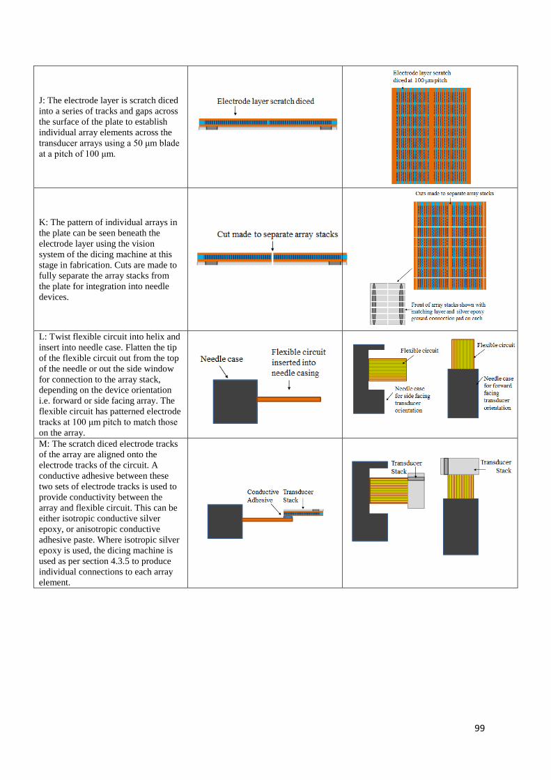
99

J: The electrode layer is scratch diced

into a series of tracks and gaps across

the surface of the plate to establish

individual array elements across the

transducer arrays using a 50 μm blade

at a pitch of 100 μm.

K: The pattern of individual arrays in

the plate can be seen beneath the

electrode layer using the vision

system of the dicing machine at this

stage in fabrication. Cuts are made to

fully separate the array stacks from

the plate for integration into needle

devices.

L: Twist flexible circuit into helix and

insert into needle case. Flatten the tip

of the flexible circuit out from the top

of the needle or out the side window

for connection to the array stack,

depending on the device orientation

i.e. forward or side facing array. The

flexible circuit has patterned electrode

tracks at 100 μm pitch to match those

on the array.

M: The scratch diced electrode tracks

of the array are aligned onto the

electrode tracks of the circuit. A

conductive adhesive between these

two sets of electrode tracks is used to

provide conductivity between the

array and flexible circuit. This can be

either isotropic conductive silver

epoxy, or anisotropic conductive

adhesive paste. Where isotropic silver

epoxy is used, the dicing machine is

used as per section 4.3.5 to produce

individual connections to each array

element.

100

N: The connected array is then

secured into the needle casing using a

backing layer of alumina loaded

epoxy. An electrode layer is then

deposited across the face of the

transducer array to connect the silver

epoxy pad for ground connection to

the needle casing.

Key for diagrams:

Throughout this fabrication process, waferscale production of multiple devices from the one plate was

an important objective. Process steps from A – K were designed to enable the application of

microfabrication techniques to realise this, with multiple arrays produced and retained on the one

plate from the one fabrication process before the final stage of separating them into individual devices

for connection and integration into needles in steps K – N. This process is designed to be easily

adapted depending on the amount of devices required, to be reproducible, along with time and cost

effective. The specific details of the microfabrication processes used and challenges encountered are

discussed in the following sections.

4.4.3 Active Layer - 15 MHz Piezocomposite Material

Precision Dicing

As mentioned above, PIN24% PMN-PT single crystal piezocomposite material was the active layer of

choice for the devices. For the 15 MHz transducer, the composite development involved use of the

“dice and fill” method as mentioned in Chapter 3 (Smith, 1989). The dicing of which was carried out

using the precision dicing saw (MicroAce 66, Loadpoint, Swindon, UK), and a 13 μm blade (Disco

HI-TEC Europe, Munich, Germany). The pillars of the composite were diced using this blade at a

pitch of 50 μm to produce a composite with volume fraction of 57%.

101

Factors Affecting the Dicing Process

The miniature dimensions and fragile pillar sizes required resulted in significant challenges to

effectively create a dicing program to result in 100% yield of pillars without collapse or damage. The

variables described in Section affected the success of the dicing program i.e. spindle speed, feed rate,

coolant flow and cut length. In order to methodically find the best possible program for the repeatable

production of these composites, development was carried out initially on CTS 3203 HD piezoceramic.

This ceramic material was less brittle to the single crystal material and provided a basis for the initial

teasing out of problems from the process, before fine tuning to suit the more fragile requirements of

the PIN24% PMN-PT.

On securing the plate of piezoelectric material to the dicing tape, it should be noted that sample set up

could have the potential to adversely affect the fine dicing practices of composites. An unstable

sample had the potential to vibrate or shift during the passing of the blade which would cause pillar

breakage. This was observed where the size of samples had a relatively low contact area with the

adhesive on the dicing tape (Universal Tape, Loadpoint, Swindon, UK) used to hold the sample in

place on the vacuum jig. The larger the surface area in contact with the dicing tape, the fewer issues

resulted. In cases where due to the samples aspect ratio, this was a problem, scrap material would be

used to surround the sample and provide support. Tape was preferred than the use of wax for adhesion

of the sample in place during dicing, as it allowed epoxy to be deposited to encapsulate and surround

the sample without disturbing its position on the tape. This minimised handling required while the

sample had the series of pillars diced into it, rendering it extremely fragile. Once the epoxy has been

applied over and around the composite sample, handling then becomes much easier. Using wax at this

stage, the plate of material would need to be removed from the wax after dicing and before epoxy

deposition as the layer of wax beneath the plate would introduce a step between the epoxy surround

and piezoelectric material, causing difficulties when monitoring thicknesses of layers during lapping.

The major sources of pillar breakage initially proved to be spindle speed and the rate at which the

blade was fed through the material. A higher spindle speed was possible in the ceramic than that of

the single crystal material. The blade feed rate needed to be adjusted between the first and second

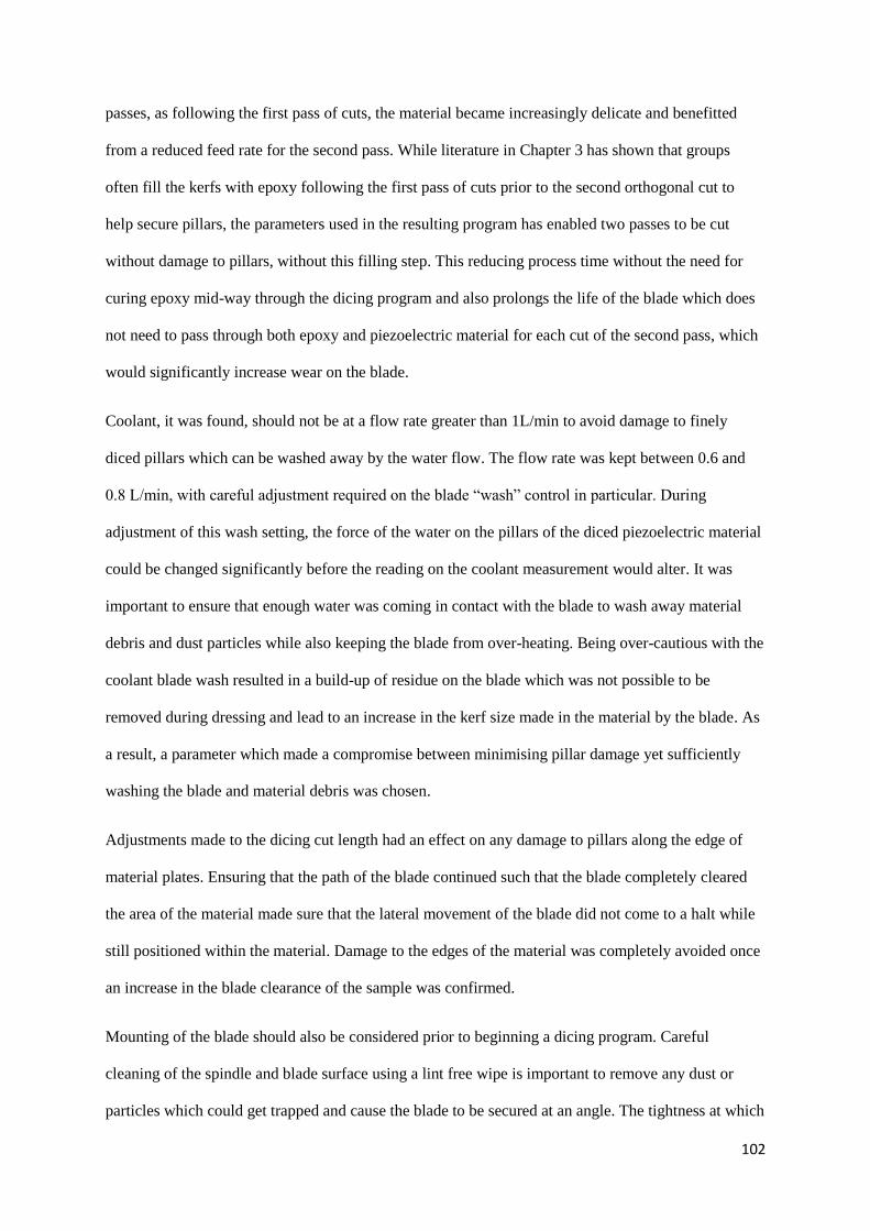
102

passes, as following the first pass of cuts, the material became increasingly delicate and benefitted

from a reduced feed rate for the second pass. While literature in Chapter 3 has shown that groups

often fill the kerfs with epoxy following the first pass of cuts prior to the second orthogonal cut to

help secure pillars, the parameters used in the resulting program has enabled two passes to be cut

without damage to pillars, without this filling step. This reducing process time without the need for

curing epoxy mid-way through the dicing program and also prolongs the life of the blade which does

not need to pass through both epoxy and piezoelectric material for each cut of the second pass, which

would significantly increase wear on the blade.

Coolant, it was found, should not be at a flow rate greater than 1L/min to avoid damage to finely

diced pillars which can be washed away by the water flow. The flow rate was kept between 0.6 and

0.8 L/min, with careful adjustment required on the blade “wash” control in particular. During

adjustment of this wash setting, the force of the water on the pillars of the diced piezoelectric material

could be changed significantly before the reading on the coolant measurement would alter. It was

important to ensure that enough water was coming in contact with the blade to wash away material

debris and dust particles while also keeping the blade from over-heating. Being over-cautious with the

coolant blade wash resulted in a build-up of residue on the blade which was not possible to be

removed during dressing and lead to an increase in the kerf size made in the material by the blade. As

a result, a parameter which made a compromise between minimising pillar damage yet sufficiently

washing the blade and material debris was chosen.

Adjustments made to the dicing cut length had an effect on any damage to pillars along the edge of

material plates. Ensuring that the path of the blade continued such that the blade completely cleared

the area of the material made sure that the lateral movement of the blade did not come to a halt while

still positioned within the material. Damage to the edges of the material was completely avoided once

an increase in the blade clearance of the sample was confirmed.

Mounting of the blade should also be considered prior to beginning a dicing program. Careful

cleaning of the spindle and blade surface using a lint free wipe is important to remove any dust or

particles which could get trapped and cause the blade to be secured at an angle. The tightness at which

103

the blade is screwed onto the spindle is also significant, too tight or too loose can cause the blade to

vibrate and damage pillars in the material.

Figure 4.11 Examples of collapsed pillars (a) collapsed pillars in a sample after one dicing pass of

cuts and (b) in a sample after dicing two orthogonal passes

Figure 4.12 Piezoceramic composite dicing cuts made in two passes, (a) the first dicing pass, and

(b) following the second dicing pass, showing minimal pillar damage. Pillars of 50 µm pitch with

a 13 µm kerf are created.

104

Once a repeatable process was established for the piezoceramic material, dicing trials using the single

crystal material was used. Due to this material being considerably more brittle to that of the ceramic,

using the ceramic program caused significant damage to the pillars. Plates of the material used for

testing measured 3 x 1 mm. Approximately 15 plates of this material were used to evaluate various

combinations of the following dicing parameters.

Spindle speed was set first at 35,000 rpm and reduced in 5000 rpm intervals to find a more suitable

range, after which smaller adjustments were made in steps of 1000 rpm. Critically, the feed rate of the

blade needed to be reduced further. This made a significant improvement and reduced pillar damage

by about 80%, and limiting damage to pillars around the edge of the plate. Damage around the edges

of the material was reduced further by increasing the path length, producing almost 100% yield of

undamaged pillars. The final program employed which could be used with no alterations or

interruption was made up of the following parameters:

Table 4.4 Dicing program parameters for creation of 1 – 3 composites in 3203 HD and PIN PMN PT

single crystal piezoelectric material

105

Figure 4.13 Single crystal composite dicing cuts made in two passes, with minimal pillar

damage. Pillars of 50 µm pitch created.

Filling of Composite Material

The next stage in the development of the composite material is the filling of the matrix of pillars with

a passive material. Epofix (Struers, UK), a low shrinkage epoxy was used. The epoxy was prepared

and placed in a vacuum chamber to remove air bubbles. Using a needle tip, the epoxy was then slowly

poured over the active material to encapsulate the pillars. Extremely slow and gentle pouring is

essential to avoid knocking down pillars and also to avoid trapping bubbles within the kerfs. It is

advised that pouring is carried out from a consistent direction at a pace which allows the epoxy to

flow and settle throughout the pillar and kerf matrix. Depositing this from one direction is useful to

“push” out air from the kerfs rather than trap the air. A minimum depth of 2 mm above the surface of

the pillars is required in order to ensure the epoxy infiltrates to the bottom of the kerf cuts. Once the

epoxy had been deposited to encapsulate the pillars, the entire assembly was placed into the vacuum

chamber once more for approximately 30 minutes. The epoxy was then left to cure at room

temperature for 24 hours followed by an additional 3 hour cure in an oven at 50 ᵒC to further harden

106

the material. This curing process was chosen as opposed to a shorter cure time at a high temperature

which could potentially reach the Curie Temperature of the single crystal material.

For this device design, an epoxy surround is also formed to reduce risk of damage to the active

composite material during machining, and to provide an area for the connections which do not overlap

and therefore potentially affect the acoustic behaviour of the transducer stack as per Figure 4.15.

4.4.4 Machining of the Transducer Stack

Lapping and Polishing

Lapping was carried out at to thin the active and matching layers of the transducer stack. The main

objective of the process was to keep the stack resilient during handling for as long as possible, to

improve yield of the processes and reduce risk of damaging the devices. Lapping of the piezoelectric

composite layers required careful control of the lapping equipment to maintain uniformity. As with

the fabrication of the single element transducers, the samples were mounted off centre as per Figure

4.3, where, as explained in Section, helps to maintain flatness across the layer surfaces along with the

lapping plates themselves. One matching layer was used for the arrays. This layer was made up of 3

µm alumina particles at 15% volume fraction in Epofix epoxy (Struers, UK). Approximately 300 µm

of the matching layer material was slowly applied to the face of the transducers using a needle tip, to

minimise the amount of air trapped in the mixture. Once deposited, the stack was put in a vacuum

chamber to de-gas the material before curing at room temperature for 24 hours, followed by a 3 hour

post cure at 50 °C. The matching layer was then lapped down to ¼ wavelength thickness ~57 µm of

the operating frequency for each the 15 MHz and 50 MHz array stacks.

Factors Affecting the Lapping Process

The primary challenge was met when lapping bulk material from the composite in order to expose the

surface of the pillars. It was pertinent to reduce the removal rate of material the closer to the pillars

came to the surface. In a case where 500 µm of stock material lay above the pillars surface, the

lapping process would begin by removing approximately 200 µm of the 500 µm thick bulk material

using 15 µm abrasive powder at a glass plate rotation speed of 30 rpm. For the final 200 µm, left to

107

remove, it was found the best results are achieved by firstly reducing the abrasive particle size to 9

µm and the rotation speed to between 15 and 20 rpm, for the removal of a further 100 µm. For the fine

removal of the last 100 µm of material to achieve the required accuracy and uniformity of thickness

across the substrate, the particle size can be then reduced further to 3 µm, with a plate rotation of 8 –

10 rpm with minimal loading on the lapping jig. Using this process and the gradual reduction of

particle size, enabled quick removal of much of the bulk material initially, and following this, greater

precision of material removal in smaller increments is achieved using the smaller particle size to

expose the top of the pillars. Parallelism was also maintained such that the top of the composite pillars

were exposed across the entire surface of the plate simultaneously. A matching layer at ¼ wavelength

thickness meant that the final thickness (Step G in Table 4.3) was less than 60 µm. As a result, had the

composite surface not been maintained uniformly parallel a significant taper in the layers could

become apparent at this stage. A taper greater than 50 µm could result in the removal of part of the

matching layer material from the surface of the pillars completely.

As a means to further control the lapping speed and uniformity, along with reducing stress on the face

of the composite or lapping materials, blocks of alumina loaded epoxy of the same thickness were

used to surround the transducer stacks to provide mechanical support and increase the surface area to

be lapped. Loaded epoxy was used such that it was the same material was the lapping layer and

therefore removal rate across the entire lapped surface was uniform. While this method increased

lapping time, the result was that the ability to maintain a uniform, parallel surface with minimal

damage to composite pillars, significantly improved as the larger surface area spread the abrasive

slurry evenly across the surface of the composite.

With the aim to create processes which are as repeatable and cost effective as possible, it was

investigated if a series of transducers could be machined in the one lapping process for future

production of multiple devices as shown in the fabrication process Table 4.3. Mock transducers made

of bulk ceramic 3 x 8 mm encapsulated in epoxy were used to mimic production of a transducer stack.

While the stack was at a thickness which could be comfortably handled, a shallow dicing cut was

made around the perimeter of the transducers at a depth of the final transducer thickness to mimic

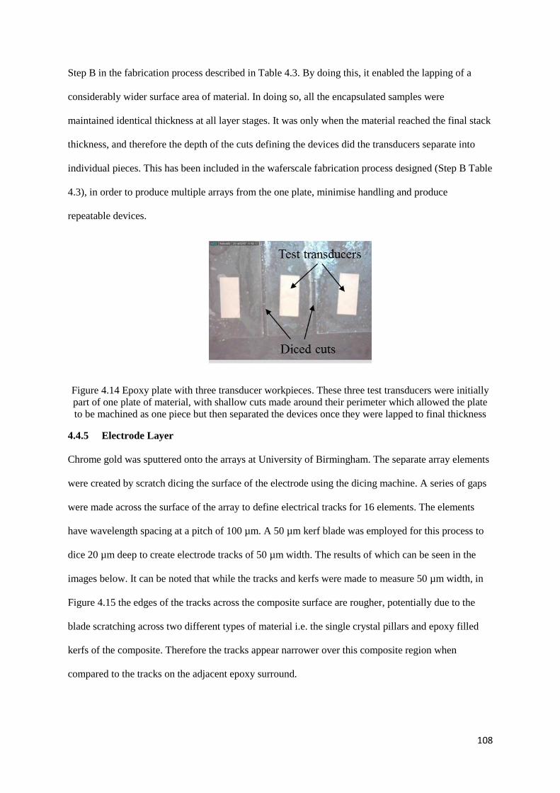
108

Step B in the fabrication process described in Table 4.3. By doing this, it enabled the lapping of a

considerably wider surface area of material. In doing so, all the encapsulated samples were

maintained identical thickness at all layer stages. It was only when the material reached the final stack

thickness, and therefore the depth of the cuts defining the devices did the transducers separate into

individual pieces. This has been included in the waferscale fabrication process designed (Step B Table

4.3), in order to produce multiple arrays from the one plate, minimise handling and produce

repeatable devices.

Figure 4.14 Epoxy plate with three transducer workpieces. These three test transducers were initially

part of one plate of material, with shallow cuts made around their perimeter which allowed the plate

to be machined as one piece but then separated the devices once they were lapped to final thickness

4.4.5 Electrode Layer

Chrome gold was sputtered onto the arrays at University of Birmingham. The separate array elements

were created by scratch dicing the surface of the electrode using the dicing machine. A series of gaps

were made across the surface of the array to define electrical tracks for 16 elements. The elements

have wavelength spacing at a pitch of 100 µm. A 50 µm kerf blade was employed for this process to

dice 20 µm deep to create electrode tracks of 50 µm width. The results of which can be seen in the

images below. It can be noted that while the tracks and kerfs were made to measure 50 µm width, in

Figure 4.15 the edges of the tracks across the composite surface are rougher, potentially due to the

blade scratching across two different types of material i.e. the single crystal pillars and epoxy filled

kerfs of the composite. Therefore the tracks appear narrower over this composite region when

compared to the tracks on the adjacent epoxy surround.

109

Figure 4.15 Finished array tracks scratch diced to create elements 50 µm width tracks at 100 µm

pitch at the rear of the transducer stack. The area outlined in red shows the active composite area,

which is surrounded by a frame of epoxy

4.4.6 Interconnects

The connection of the flexible circuit to the array proved to be the most challenging stage in the

fabrication process. Two methods of connection were explored using flexible printed circuit boards

(FPCB), using a) Isotropic adhesive, and b) Anisotropic adhesive.

a) Isotropic Adhesive

The first method aimed to manually align the FPCB tacks to the tracks scratch diced onto the array,

and connect these electrodes using silver conductive epoxy. As this conductive epoxy would connect

across all elements, the dicing machine would be used to dice through both the FPCB and silver

epoxy connection in order to create 16 individual elements across the array at 100 µm spacing.

The technique involves manually aligning the element electrode tracks on the FPCB with the tracks

on the array and securing this in place with some tape. The FPCB is then gently pulled back,

maintaining the alignment and the conductive epoxy is deposited between the two. The FPCB is then

110

rested back on top of the array, where the conductive epoxy cures and secures it in place, before the

dicing saw is used to dice through the adjacent connected tracks to establish separate connections for

each array element.

Challenges

The initial challenge in this manual process was firstly the alignment of the array elements to the

FPCB tracks. This was carried out by securing the array with the defined electrode tracks facing

upwards, to the dicing tape. This keeps the array fixed in place for the entire connection, bonding and

dicing phases. Using a DinoCapture 2.0 USB microscope, the FPCB was placed with tracks facing

down, towards the array, onto the array elements. As the FPCB is transparent, the tracks could be

overlapped with the array elements using this set-up. It was important to ensure alignment was as

accurate as possible to avoid any additive angular error across the area of overlap which could

potentially cause shorting between elements.

Figure 4.16 Photographs showing (a) manual alignment of array elements and FPCB, with the

addition of conductive silver epoxy and tape to hold the FPCB in place in (b)

When the conductive epoxy has been deposited, checking the alignment becomes increasingly

difficult. Time is also limited before the assembly with silver epoxy must be placed into the oven for

effective curing. Once the placement of the FPCB was deemed satisfactory, this was gently tacked in

place along its length using tape. Using a tweezers to gently peel back the top of the FPCB, a needle

tip was used to spread a layer of silver epoxy (RS Components, UK) across the overlap area. The

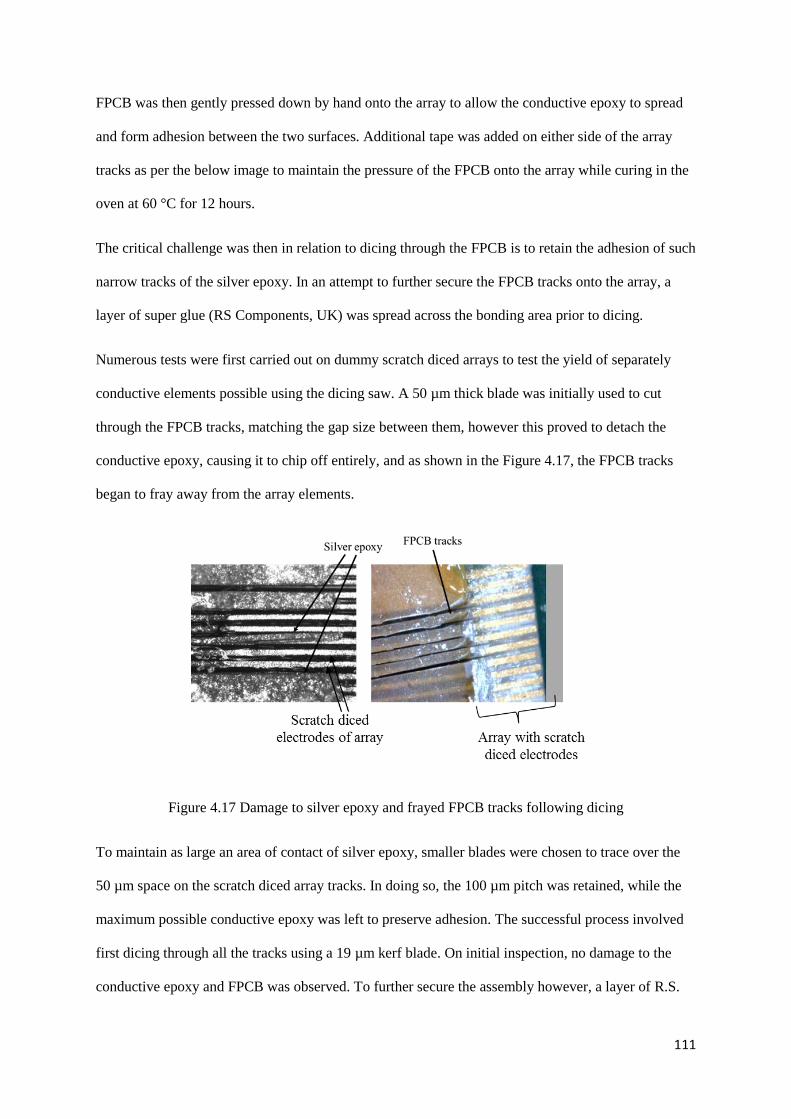
111

FPCB was then gently pressed down by hand onto the array to allow the conductive epoxy to spread

and form adhesion between the two surfaces. Additional tape was added on either side of the array

tracks as per the below image to maintain the pressure of the FPCB onto the array while curing in the

oven at 60 °C for 12 hours.

The critical challenge was then in relation to dicing through the FPCB is to retain the adhesion of such

narrow tracks of the silver epoxy. In an attempt to further secure the FPCB tracks onto the array, a

layer of super glue (RS Components, UK) was spread across the bonding area prior to dicing.

Numerous tests were first carried out on dummy scratch diced arrays to test the yield of separately

conductive elements possible using the dicing saw. A 50 µm thick blade was initially used to cut

through the FPCB tracks, matching the gap size between them, however this proved to detach the

conductive epoxy, causing it to chip off entirely, and as shown in the Figure 4.17, the FPCB tracks

began to fray away from the array elements.

Figure 4.17 Damage to silver epoxy and frayed FPCB tracks following dicing

To maintain as large an area of contact of silver epoxy, smaller blades were chosen to trace over the

50 µm space on the scratch diced array tracks. In doing so, the 100 µm pitch was retained, while the

maximum possible conductive epoxy was left to preserve adhesion. The successful process involved

first dicing through all the tracks using a 19 µm kerf blade. On initial inspection, no damage to the

conductive epoxy and FPCB was observed. To further secure the assembly however, a layer of R.S.

112

superglue was spread such that it ran between the diced tracks. Subsequently, an additional series of

cuts were made using a 12 µm kerf blade at a depth 5 µm deeper than the original cuts. This allowed

any conductive debris to be cleared from the tracks and to provide a means to confirm separation of

the tracks. By applying the addition of the glue between the tracks and then cutting with a smaller

blade, a portion of adhesive would be left on either side of the 13 µm kerf, along the length of the

FPCB track, securing it in place, while completely ensuring that the connection between two adjacent

tracks were separated.

Figure 4.18 (a) Shows the tracks of the FPCB and array connected via conductive silver epoxy. As

this is isotropic conductive paste, the adjacent tracks are therefore also connected to each other and

require separation. (b) A blade has been used to cut through the silver epoxy to separate this

connection (c) Glue is deposited in the resulting track to ensure that the FPCB does not fray away

from the array as a result of the cutting (d) A narrower blade is then used to cut through the glue in the

track to ensure separation, while the narrower blade retains some glue on either side of the track to

reinforce adhesion of the FPCB to the array.

This method proved successful and was used to bond two 15 MHz arrays. The first array resulted in

16 elements individually connected to the FPCB, while in the second array, elements 1 – 16 were

individually connected apart from shorting between element 11 and 12. The image below in Figure

4.19 shows an example of the final result.

113

Figure 4.19 Image of 16 element array after connection to FPCB and dicing of tracks to separate

individual elements

b) Anisotropic Adhesive

The second method targeted a more automated technique working in collaboration with, and on site at

Heriot Watt University (Edinburgh, UK) (Schiavone et al., 2016). It was planned that connection

could be made by automatically positioning and aligning the array onto the FPCB using a MAT 6400

die attach system in flip-chip configuration. This machine would deposit a SunRay Scientific

ZTACH™ magnetically aligned anisotropic conductive paste (ACP) or anisotropic conductive

adhesive (ACA) containing ferromagnetic conductive particles 1 µm in diameter. When cured within

a magnetic field, these particles align to form pillars parallel to the field, making the paste conductive

in just one direction.

Figure 4.20 ACA is dispensed evenly along the top of the FCB. The array is then placed track side

down such that the element tracks of the array align with the element tracks of the FPCB (Schiavone

et al., 2016).

114

The conductivity in one direction creates connection between the array and FPCB. Using this paste

would provide individual connections to the array elements without the need for further machining to

separate the tracks. Unfortunately, within the time constraints of this PhD, the full automated process

was not completed, however, multiple steps have been established and it is intended that in future

work this processes will be employed for the effective connection of arrays.

The pick-and-place die attach system enables the placement of the array on the flexible interconnects

with a precision of 3 µm. The imaging system of the MAT 6400 records the patterns on both the front

and back of the array and defines a reference point for bonding. The same procedure is followed to

define a reference point on the FPCB onto which the array will be placed. Following deposition of the

paste along the defined bonding area at the top of the FPCB using the bonding machines paste

dispenser syringe, the array is then picked and placed on the FPCB by superimposing the two

reference points previously defined. This allows the tracks on both sides to be accurately aligned.

Figure 4.21 (a) MAT 6400 flip chip bonding machine for assembly of array and FPCB connection (b)

Stage on MAT 6400 to secure FPCB in place for alignment and bonding (c) Image on MAT 6400

showing dispensed paste across bonding area of FPCB

115

Challenges

Uniformity of the array samples was required to allow for successful programing of the visual system

to recognise and implement the correct bonding area and alignment. This proved challenging as the

arrays themselves were in development stages also. As a result, dummy test arrays were fabricated to

mimic the process, these dummy arrays were stock piezoelectric material, with scratch diced electrode

tracks at the same pitch, 100 µm, as the final array devices.

Figure 4.22 Test arrays made for testing automated bonding process

Alignment was completed by programming the vision system to use the edges and scratch diced

tracks as reference points for alignment and placement upon the tracks of the FPCB. Once alignment

was achieved, the next difficulty was depositing the paste. The paste deposition involved careful

programming of pressure, dispense height, speed, and pattern parameters of the paste dispenser

integrated with the bonding machine. The thickness of paste was critical for successful electrical

conduction via the formation of pillars of conductive particles and so this was a significant challenge

to overcome. The viscous nature of the paste made it difficult to fill the dispensing syringe without

trapping air within the paste, and to get it to settle sufficiently into the needle. As a result, during

dispensing, obtaining a uniform line of paste was difficult and not repeatable. Different dispense

patterns were explored to try get uniform spread of paste such as in drops or separate lines across the

bonding area of the FPCB which would spread across the tracks once the transducer was placed on

top of the dispensed pattern. If the paste was too thin or indeed too thick, conduction did not occur

due to insufficient or too great a density of pillars i.e. forming lateral connection. Thinning of the

paste using a solvent would not create successful connection. The ideal thickness to achieve was

116

recommended to be approximately 50 µm. It was hypothesised that screen printing could be

incorporated into the bonding process to provide greater controls to this ACP thickness dimension,

and preliminary investigation has begun employing this solution.

Following deposition of the paste and alignment of the array onto the FPCB, the entire assembly had

to be transferred into an oven with magnets placed on top and bottom of the bonding area to provide

the magnetic field via which the conductive particles align. It was noted however, that during this

particle alignment, that the paste spread due to the magnetic field and resulted in the movement of the

array, therefore ruining the alignment between the tracks, causing elements to short circuit. To

overcome this issue, various holders were designed to hold the array in place, however misalignment

persisted. It was apparent that a layer of adhesive tape to secure the array once placed would be the

solution to this problem. Varying the magnet strength was also explored, with reduction in the

magnetic strength showing preliminary promising results. Future tests using tape to secure the array or

to create more suitable holders must be completed.

As a contingency plan during investigation into the use of the ACP for bonding a FPCB to an array,

manual alignment of the array upon the flexible circuit was demonstrated as an option, using a

DinoCapture 2.0 USB microscope in the same procedure as with the isotropic adhesive except with

deposition of the ACP using stencil printing. While alignment and deposition were shown with this

method, the problem of the array shifting during the curing of the paste remained.

While successful, automated, individual connection to each element of an array was not achieved with

the ACP during the duration of this project, the formation of the conductive particle pillars in the ACP

was observed by taking cross section cuts of bonded samples. The image in Figure 4.23 shows the

pillars formed in one direction, connecting the tracks of the FPCB to a sample silicon dummy array.

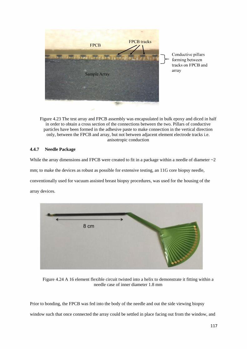
117

Figure 4.23 The test array and FPCB assembly was encapsulated in bulk epoxy and diced in half

in order to obtain a cross section of the connections between the two. Pillars of conductive

particles have been formed in the adhesive paste to make connection in the vertical direction

only, between the FPCB and array, but not between adjacent element electrode tracks i.e.

anisotropic conduction

4.4.7 Needle Package

While the array dimensions and FPCB were created to fit in a package within a needle of diameter ~2

mm; to make the devices as robust as possible for extensive testing, an 11G core biopsy needle,

conventionally used for vacuum assisted breast biopsy procedures, was used for the housing of the

array devices.

Figure 4.24 A 16 element flexible circuit twisted into a helix to demonstrate it fitting within a

needle case of inner diameter 1.8 mm

Prior to bonding, the FPCB was fed into the body of the needle and out the side viewing biopsy

window such that once connected the array could be settled in place facing out from the window, and

118

secured in place using backing material. The backing material of chose was 15% VF alumina loaded

epoxy. Although tungsten loaded polymers are often the backing material of choice, it has been

reported that certain concentrations of tungsten can become conductive (Webster, 2009). This was

undesirable as the biopsy needle itself was conductive and was being used to ground the device. Any

conduction in the backing layer would short circuit the entire array. The backing layer material was

slowly built up to fill the entire biopsy window so that the back of the array could be secured onto it,

with the front of the array facing outward. The backing material was left to cure at room temperature

for 24 hours. The resulting devices are displayed in the images below in Figure 4.25, the testing and

performance of which has been shown and discussed in Chapter 5.

Figure 4.25 (a) Biopsy needle used as device casing (b) FPCB within the core of the biopsy

needle case (c) SMA connector board for connection to elements from FPCB to enable testing

and measurements from elements (d) FPCB connected to connectors on this board (e) Finished

device of 15 MHz 16 element array within a biopsy needle with SMA connectors for

characterisation and functional testing.

119

4.5 Future Work

15 MHz was the chosen frequency initially based on the electronics available to operate at high

frequencies. Clinicians require a compromise between resolution and penetration depth during

diagnostic imaging. As a result, consideration was given to how the developed fabrication processes

could be scaled for higher frequency operation, with 50 MHz devices also designed to explore the

trade-off between resolution and image depth. Piezoelectric single crystal composites that operate at

50 MHz can be fabricated using DRIE rather than dicing. The 50 MHz device fabrication methods

were developed using a Deep Reactive-Ion Etching (DRIE) composite from CTS Corporation

(Illinois, USA). Using this material, a trial fabrication process was explored for the production of 50

MHz devices. By carrying this out, experience of using the micromachining techniques such as dicing

and lapping for this higher frequency application was gathered.

In order to suit the array fabrication processes designed, the material was received with bulk material

still attached to allow the stack to be more easily handled. As per the image in Figure 4.26 the

composition of the material was made up of ~25 µm with approximately 700 µm stock material left

behind it. The pillars of this composite were measured to be ~13 µm in width with a kerf of

approximately ~2 µm, arranged in a hexagonal pattern. As the composite was produced by CTS

Corporation, the first stage of this process was to dice the lateral dimensions of this material and

embed the plate into a surround of epoxy for the next fabrication stage.

Figure 4.26 Pillars of DRIE composite

120

Lapping of the 50 MHz pillars in the DRIE composite was challenging, due to the thickness of the

composite section of the material provided, as per the image Figure 4.27

Here it can be seen that the height of the pillars

were measured to be ~25 µm, leaving little to

no room for error in removing the bulk

material behind it. Such a thin layer of

composite material could potentially

disintegrate when subjected to stress during

lapping and while heating the sample when

using wax to attach it to glass lapping slides.

While testing these fabrication methods on the DRIE material, six 50 MHz transducer stacks from the

one plate of material were produced up to the stage of being prepared for photolithography patterning

of electrodes. Advancing the production of these trial devices will be one of the first tasks in the

future work in this project, the objectives with these devices are discussed further in Chapter 8.

4.6 Discussion

Employing the discussed fabrication methods to develop these needle transducer devices have

demonstrated the feasibility of integrating ultrasound transducers into packages of this size for various

applications, from single element transducers to arrays. During this project, the 15 MHz arrays were

completed and tested. The 50 MHz array stacks have been realised up to the point of electrode and

element definition, and their completion will form part of this projects future work, with the intention

of carrying out their connection via the automated bonding process.

It was clear from the development of the dicing and lapping processes for array production that

controls to ensure consistently correct use of these machines was extremely important in order to

maintain repeatable processes. To introduce such controls on the use of the fabrication equipment,

equipment standards required by the International Standards Organisation (ISO) for the Design and

Figure 4.27 Pillars of DRIE

composite ~25 µm tall

121

Development of Medical Devices ISO 13485 were implemented. Strict training requirements and

competency levels were established and standardised and work instruction procedures were developed

for all personnel to follow. User logs monitored use and any changes or issues found related to

equipment to ensure calibration and maintenance remained current and effective. The range of

paperwork developed and audited by the Quality Management System to administer these standards in

equipment training, supervision, operation, calibration and maintenance can be seen in the Appendix

of this thesis such as Work Instructions, User Logs, and Skills Requirements. The strict adherence to

the quality controls implemented enabled the production of these devices to be feasible and indicates

potential for commercialisation. An example of the positive effects these controls had on production is

demonstrated in the production of the dice and fill 1 – 3 composite material. As discussed in Chapter

3, a common method used for the production of dice and fill composites is to dice a series of cuts in

one direction and fill the gaps with epoxy before dicing in the other direction and filling again. The

method presented in this chapter whereby two orthogonal cuts can be made consecutively before

filling with epoxy and yield almost 100% pillars without breakage signifies the impact of the quality

controls made around the process. The result means that a dicing procedure which is faster,

reproducible and therefore has commercial potential has been presented.

4.7 References

Cannata, J. M., Williams, J. a, Zhou, Q., Ritter, T. a, & Shung, K. K. (2006). Development of a 35-

MHz piezo-composite ultrasound array for medical imaging. IEEE Transactions on Ultrasonics,



Jiang, Y., Qiu, Z., McPhillips, R., Meggs, C., Mahboob, S. O., Wang, H., … Demore, C. E. M.

(2016). Dual Orientation 16-MHz Single-Element Ultrasound Needle Transducers for Image-

Guided Neurosurgical Intervention. IEEE Transactions on Ultrasonics, Ferroelectrics, and


McPhillips, R., Qiu, Z., Jiang, Y., Mahboob, S. O., Wang, H., Meggs, C., … Démoré, C. E. M.

(2015). Ex-vivo navigation of neurosurgical biopsy needles using microultrasound transducers

with M-mode imaging. IEEE International Ultrasonics Symposium (IUS), 3–6.

Schiavone, G., Jones, T., Price, D., McPhillips, R., Jiang, Y., Qiu, Z., … Desmulliez, M. P. Y. (2016).

A highly compact packaging concept for ultrasound transducer arrays embedded in

neurosurgical needles. Microsystem Technologies, 1–11. http://doi.org/10.1007/s00542-015-

2775-1

Schiavone, G., Jones, T., Price, D., McPhillips, R., Qiu, Z., Demore, C. E. M., … Desmulliez, M. P.

Y. (2014). Advanced electrical array interconnections for ultrasound probes integrated in

122

surgical needles. IEEE 16th Electronics Packaging Technology Conference (EPTC), 88–93.

Smith, W. a. (1989). The role of piezocomposites in ultrasonic transducers. Proceedings., IEEE

Ultrasonics Symposium, 755–766. http://doi.org/10.1109/ULTSYM.1989.67088

Webster, R. A. (2009). Passive Materials for High Frequency Piezocomposite Ultrasonic Transducers.

University of Birmingham.

123

CHAPTER 5

FUNCTIONAL CHARACTERISATION RESULTS OF

IMAGING PROBES

5.1 Aim of Chapter

The aim of this chapter is to present characterisation measurements of the fabricated transducers

constructed as explained in Chapter 4. These measurements serve to assess the success of the

fabrication methods used, compare the component materials and the functionality of the resulting

transducers and to examine potential imaging performance of these devices.

Electrical and acoustic characterisation was performed on all the single element transducers

fabricated. The results of these provided information such as the active material performance, and

aided the design of the transducer stack and the characterisation measurements for the 15 MHz array.

5.2 Single Element Transducer Characterisation

As shown in Chapter 4, five single element transducers within needles were developed using different

active materials; bulk piezoceramic, micromoulded PZT composite, and single crystal dice and fill

composite. The variations in single element transducer and the names of which they will be referred to

in this chapter are defined in Table 4.1, Chapter 4.

For each of these devices, impedance spectra and pulse echo responses have been acquired. Based on

the results of these characterisation tests, the forward and side facing micromoulded composite

needles SET_MM_FF and SET_MM_SF were taken forward for further tests and experiments to

explore feasibility and function of such transducers (Jiang et al., 2016).

124

Table 5.1 Transducer materials, thicknesses and their corresponding acoustic impedances

Material Thickness

(μm)

Acoustic

Impedance, Z

(MRayl)

Bulk Piezoceramic

CTS3203 HD

160 34

Micromoulded

Composite

115 14

Single Crystal PIN-

PMN PT Composite

(57% VF)

117 22

Tungsten loaded

backing material (Used

in SET_BULK and

SET_MM transducers)

Forward facing

transducers:

~5 mm

Side facing

transducers:

~1 mm

5

Alumina loaded

backing material (Used

in SET_SC transducer)

5 4

5.2.1 Electrical Impedance Measurements

The electrical impedance response of each fabricated single element transducer in a needle was

determined by a precision impedance analyser (4395A, Agilent Technologies UK Ltd., UK),

connected to a PC.

The electrical impedance spectra of the bulk ceramic and micro-moulded composite needle

transducers, of both forward and side facing orientation are presented in Figures 5.1 and 5.2. It can be

seen from the figure that the resonance frequency is present at ~15 MHz for all four transducers. It is

noted that small resonances between 5 and 10 MHz outside the primary resonance peak can be

observed in the case of the side facing transducers in particular. It is thought that this is due to the

thickness of the backing material being limited in the side facing transducer orientation by the needle

casing.

From the impedance measurements, the effective electromechanical coupling factors (Chapter 3

Section 3.5.1 Equation 3.9) 𝑘𝑒𝑓𝑓, were determined from the impedance curves for each transducer.

SET_BULK_FF, SET_BULK_SF, SET_MM_FF and SET_MM_SF were found to have, 𝑘𝑒𝑓𝑓 values

of 0.55, 0.53, 0.68, and 0.62 respectively. Higher electromechanical coupling factors were observed in

125

the transducers with piezocomposite active layers, demonstrating a more efficient transducer material

when compared to the bulk piezoceramic material. The impedance magnitude however is higher for

the transducers made using the piezocomposite and therefore makes electrical impedance matching to

cables more difficult.

Figure 5.1 Impedance and phase measurements of single element transducers integrated within

needles. Figure a) and b) show the results from bulk piezoceramic transducers, a) forward facing

(SET_BULK_FF), and b) side facing (SET_BULK_SF) orientation. Figure c) and d) show the results

from micromoulded PZT composite transducers, a) forward facing (SET_MM_FF), and b) side facing

(SET_MM_SF) orientation.

The same set-up was employed for the impedance measurement of the single element single crystal

composite forward facing needle SET_SC_FF. This transducer was made of an active single crystal

material PIN PMN PT, fabricated via the conventional dice-and-fill method. From the impedance

curve in Figure 15.3, the electromechanical coupling factor was calculated to be 0.37, unusually low,

particularly for a composite material. It is speculated that perhaps a certain amount of de-poling of the

126

piezoelectric material may have occurred during the fabrication process, perhaps due to temperatures

at heating stages during the lapping process. In future work, the material in this transducer could be

re-poled to test if performance improved, this was not possible within the time constraints of this PhD

project. The high electrical impedance in the figure below indicates that electrical coupling will be

difficult and as a result may produce a poor pulse echo response.

Figure 5.2 Impedance and phase measurement of single element single crystal composite transducer

integrated within a needle of forward facing orientation (SET_SC_FF).

5.2.2 Pulse-Echo Response Measurements

To acquire a pulse-echo response of the single element transducers, a high frequency pulser-receiver

(DPR 500, JSR Ultrasonics, Pittsford, NY, USA) was used. The energy set for the pulse was 12.4 µJ

at a pulse repetition frequency of 1 kHz with 0 gain given to the acquired signal. The needle

transducers were placed in a water bath with the transducer face facing an aluminium plate used as an

echo target. The aluminium plate was placed approximately 5 mm from the face of the transducers.

The pulse-echo results were then used to determine the operational frequency, bandwidth and axial

resolution of these devices.

127

Figure 5.3 Pulse echo responses of single element transducers SET_BULK_FF, SET_BULK_SF,

SET_MM_FF and SET_MM_SF. The energy set for the pulse was 12.4 µJ with 0 gain given to the

acquired signal

From the results presented in Figure 5.3, each of the transducers indicates a central frequency of

approximately 15 MHz. However, the transducers with a composite active layer yielded considerably

broader -6 dB bandwidth than the bulk piezoelectric devices. The bandwidth values for SET_MM_FF

and SET_MM_SF were found to be 85.7% and 73.7%, while the bandwidth of SET_BULK_FF and

SET_BULK_SF was 24.5% and 21.1% respectively. The broader bandwidth in the case of the

piezocomposite transducers is expected due to their higher electromechanical coupling factors, which

lead to greater sensitivity and broader bandwidth. The -20 dB pulse lengths were also obtained from

these results to indicate the axial resolution of the transducers, with 0.498 µs for SET_BULK_FF,

0.524 µs for SET_BULK_SF, 0.115 µs for SET_MM_FF and 0.148 µs for SET_MM_SF. It is worth

noting that when examining the results from the transducers made from the same active material and

128

taking into account their forward and side facing orientation, the forward facing transducers indicate

greater bandwidth and shorter pulse length than their side facing counterparts. It is expected that this

is again due to a thicker backing layer being present in the forward facing transducers, which was

approximately 5 mm in depth. The thickness of the tungsten backing layer in the side facing

transducers was limited to approximately 1 mm and fit within the constraints of the fixed size of the

needle diameter. The same backing layer was used, i.e. tungsten loaded epoxy, for each of these four

devices. Alumina loaded epoxy was used for the single element single crystal device, fabricated in

Dundee. Details of the fabrication process can be found in Chapter 4.

Table 5.2 Characteristics of Single Element Transducers calculated from Figure 5.3

Transducer Type Centre

Frequency

(MHz)

-6dB Bandwidth -20dB Pulse Length

(μs)

Single Element

Transducer

(SET_BULK_FF)

~15 24.5% 0.498

Single Element

Transducer

(SET_BULK_SF)

~15 21.1% 0.524

Single Element

Transducer

(SET_MM_FF)

~15 85.7% 0.115

Single Element

Transducer

(SET_MM_SF)

~15 73.7% 0.148

Figure 5.4 Pulse echo response of the needle with active material composed of single crystal

composite

129

The same set-up described for the earlier single element tests was employed for the acquisition of the

pulse-echo response from the SET_SC_FF. The amplitude of this response was firstly significantly

lower to the other devices due to the aperture of the transducer face in this transducer being less than

those examined previously (1.0 mm diameter vs. 1.7 mm respectively).

Following these results the performance of the SET_MM_FF and SET_MM_SF , as shown in table

5.2, were deemed most promising and these devices were taken forward for use in further

characterisation tests and imaging experiments.

5.2.3 Insertion Loss

The two way insertion loss of the transducers was each device was determined to be 38.5 dB and 30.5

dB for SET_MM_FF and SET_MM_SF respectively following compensation for loss due to

attenuation in water and reflection from the aluminium plate (Cannata & Zhao, 1999). While the

calculated figures are greater than those typically reported for some similar transducers, in the range

of 15 - 25 dB (Zhou et al., 2008) (Cannata & Zhao, 1999)(Snook et al., 2002), the performance of

these transducers was considered appropriate for further tests and experimentation.

5.2.4 Beam Profile

Beam profile scans were carried out on each of the forward and side facing micro-moulded transducer

SET_MM_FF and SET_MM_SF using a needle hydrophone integrated in the set-up shown in Figure

5.6, where the transducers were connected to a pulser-receiver (DPR 300, JSR Ultrasonics, Pittsford,

NY, USA) and a pressure map of the resultant beam was acquired by the needle hydrophone. The

position of the needle hydrophone relative to the face of the transducer is shown in Figures 5.5. To

obtain a beam scan, the hydrophone was scanned a distance 3 mm laterally across the centre of

transducer and 16 mm away from its surface, while to acquire a cross section scan of the beam, the

hydrophone was located at the focal distance and a slice scan approximately 3 x 3 mm in area was

carried out.

130

Table 5.3 Pulser Settings for Set-Up of Beam Scans

DPR Pulser Settings

Pulse Voltage 71.63 V with -20dB (attenuation) 716.3 V

PRF Rate 100 Hz

Pulse Amplitude Scale – 16 (max)

Pulse Energy Low Z scale – 4 (max)

Damping Scale – 1 (min)

Receiver Through

REL Gain (dB) 70.0 dB

HP Filter Scale – out

LP Filter Scale – 22.5 MHz

Figure 5.5 (a) Set-up used to obtain beam scans of single element transducers using needle

hydrophone (b) The position of the hydrophone from the forward facing transducer face

SET_MM_FF at start of scan (c) The position of the hydrophone from the forward facing transducer

face SET_MM_SF at start of scan

From the beam profiles shown in Figure 5.6 and 5.7, the hydrophone measures the pressure field of

the transducers and outputs the beam profile, illustrating the depth of field along with the focal point

at the position of maximum pressure. For both transducers it is apparent from the lateral beam profile

that the focus is at a distance of approximately 4 – 5 mm from the face of the transducer.

131

Figure 5.6 (a) Beam scan showing lateral beam profile b) Beam scan to show cross section slice of the

forward facing transducer SET_MM_FF

132

Figure 5.7 (a) Beam scan showing lateral beam profile b) Beam scan to show cross section slice of the

side facing transducer SET_MM_SF

5.2.5 Wire Phantom Scan

To assess the imaging performance of the SET_MM_FF and SET_MM_SF transducers, the needles

were used to carry out B-scans of wire phantoms. A scanning system with mechanical stages was used

in conjunction with LabVIEW software (National Instruments, Newbury, UK) to control the

movement of the transducers across an array of wires in a water bath. As the transducers were pulsed

133

by the pulser-receiver (DPR 500, JSR Ultrasonics, Pittsford, NY, USA), an oscilloscope was used to

observe and gather the resultant echoes received from the wires. The data was then analysed using

MATLAB (The MathWorks Inc., Cambridge, U.K.). Two set-ups were assembled for each needle

orientation. For the forward facing needle SET_MM_FF, a wire phantom with a series of eight 20 µm

diameter tungsten wires, separated in a step sequence 1 mm apart in both the axial and lateral

directions, was placed below the transducer face. The face of the transducer was positioned such that

the fourth wire was placed approximately in its focus. The transducer was then linearly scanned

across the wire phantom in steps of 0.02 mm. For the side facing transducer, a wire phantom using

nylon wires 0.7 mm in diameter was mounted on a rotation stage (TDC001 T-Cube DC Servo Motor

Controller, Thorlab, NJ, USA) and positioned such that when motorized it rotated about the face of

the transducer which remained in a fixed position. The stage rotated the wires 120◦ in steps of 0.2

degrees. The images acquired are shown in Figure 5.8 with a dynamic range of 35 dB, showing good

resolution from both transducers, particularly in the axial direction.

Figure 5.8 Wire Phantom images acquired using the single element transducers. A linear B- scan

using the SET_MM_FF and a radial B-scan using the SET_MM_SF.

5.3 Discussion of Single Element Transducer Characterisation Results

The series of characterisation measurements carried out on the single element transducers indicated

the potential and feasibility of fabricating a functional single element transducer within a needle sized

housing. Broad bandwidth, short pulse length and good axial resolution were shown in particular in

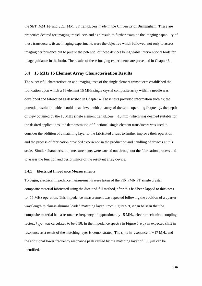
134

the SET_MM_FF and SET_MM_SF transducers made in the University of Birmingham. These are

properties desired for imaging transducers and as a result, to further examine the imaging capability of

these transducers, tissue imaging experiments were the objective which followed, not only to assess

imaging performance but to pursue the potential of these devices being viable interventional tools for

image guidance in the brain. The results of these imaging experiments are presented in Chapter 6.

5.4 15 MHz 16 Element Array Characterisation Results

The successful characterisation and imaging tests of the single element transducers established the

foundation upon which a 16 element 15 MHz single crystal composite array within a needle was

developed and fabricated as described in Chapter 4. These tests provided information such as; the

potential resolution which could be achieved with an array of the same operating frequency, the depth

of view obtained by the 15 MHz single element transducers (~15 mm) which was deemed suitable for

the desired applications, the demonstration of functional single element transducers was used to

consider the addition of a matching layer to the fabricated arrays to further improve their operation

and the process of fabrication provided experience in the production and handling of devices at this

scale. Similar characterisation measurements were carried out throughout the fabrication process and

to assess the function and performance of the resultant array device.

5.4.1 Electrical Impedance Measurements

To begin, electrical impedance measurements were taken of the PIN PMN PT single crystal

composite material fabricated using the dice-and-fill method, after this had been lapped to thickness

for 15 MHz operation. This impedance measurement was repeated following the addition of a quarter

wavelength thickness alumina loaded matching layer. From Figure 5.9, it can be seen that the

composite material had a resonance frequency of approximately 15 MHz, electromechanical coupling

factor,, 𝑘𝑒𝑓𝑓, was calculated to be 0.58. In the impedance spectra in Figure 5.9(b) an expected shift in

resonance as a result of the matching layer is demonstrated. The shift in resonance to ~17 MHz and

the additional lower frequency resonance peak caused by the matching layer of ~58 μm can be

identified.

135

Figure 5.9 Electrical impedance measurements for 15 MHz dice-and-fill composite active layer

material (a) prior to integration with the layers of the transducer stack in the graph and (b) with the

addition of quarter wavelength matching layer.

The next stage of measurements was carried out following the formation of 16 individual array

elements and their connection to a flexible printed circuit board. At this stage in the process, while a

matching layer was on the front face of the transducer, no backing layer was included in the array

stack. The electrical impedance measurements of the device at this stage are presented in Figure 5.10

a) and b). The impedance curves for each element are very flat with a resonance only visible in

element 1. Once the transducer array was integrated with a backing layer and incorporated into the

needle package, 1.0 m coaxial cables were attached to the flexible circuit and the measurements were

repeated, as shown in Figure 5.11 a) and b). In contrast, the electrical impedance matching effect of

the addition of the coaxial cables to each element has reduced the impedance magnitude significantly,

with no resonance visible. The resonances of each element are further damped in this case due to the

array being heavily backed. As stated in chapter 4, the backing material for the array was 15% VF

alumina loaded (3μm particle size) backing, which corresponds to an acoustic impedance of

approximately 4 MRayl. The thickness of this was approximately 3.5 mm, as the backing material

was used to fill the diameter of the 11 G breast biopsy needle used as casing and secure the side

facing array in place. The impedance phase below 90ᵒ could potentially be attributed to an artefact

caused by a capacitive effect from the addition of the length of the flexible circuit board being secured

within the needle casing.

136

Figure 5.10 a) Impedance and b) phase measurements for transducer array 16 elements with matching

layer connected to flexible circuit before addition of backing layer

137

Figure 5.11 a) Impedance and b) phase of transducer array stack of 16 elements connected to a

flexible circuit, with a backing layer and integrated into a needle package

138

5.4.2 Pulse-Echo Response Measurements

To obtain a pulse echo response from the array elements, element 1 through 16 were individually

connected one at a time to a high frequency pulser-receiver (DPR 500, JSR Ultrasonics, Pittsford, NY,

USA), The energy set for the pulse was 12.4 µJ at a pulse repetition frequency of 1 kHz with a gain of

30 dB. The response was recorded using an oscilloscope. A plate of quartz flat 5 mm thick was

submerged in front of the array elements in a water bath as the echo target ~5 mm from the face of the

array. An echo response was acquired for each of the individual 16 elements using this set up.

Element number six is shown in Figure 5.12 below as an example.

Figure 5.12 Pulse-echo response of element number 6 from 15 MHz transducer array

From this figure, a central frequency of ~14 MHz is shown with a -6dB fractional bandwidth of 78%.

The -20 dB pulse length for this element is approximately 0.09 µs which corresponds to an axial

resolution of approximately 69 µm. These pulse-echo response tests were carried out for all 16

elements and each of which were shown to be functional.

The array was connected to a Diagnostic Sonar FI Toolbox (Diagnostic Sonar Ltd. Livingston, UK) to

attempt to activate all 16 elements simultaneously and obtain an image.

To begin, four elements were tested at once as a 4 element array to establish the functional settings to

transmit and receive on multiple elements. A-voltage of 80 V with a pulse repetition frequency of 5

kHz and gain of 30 dB was used for the set-up. Figure 5.13 illustrates 16 elements receiving an echo

139

from a plate of quartz flat simultaneously i.e. parallel receive, while Figure 5.14 shows a preliminary

beam from elements 1 through to 16, creating an image of the surface of this target, placed 4 - 5 mm

from the face of the array.

Figure 5.13 An example of 16 elements from the 15 MHz array transmitting and receiving

simultaneously using a quartz flat as the echo target

Figure 5.14 An image generated from 16 adjacent elements from the 15 MHz array with a 5 mm thick

quartz flat as the echo target using the FI Toolbox

140

5.4.3 Wire Phantom Imaging

Using the same set-up as the pulse echo measurement above, an image was acquired of a cross section

of a stepped wire phantom made up of 7 wires 20 μm in diameter separated by 1 mm. Side lobes,

unwanted regions of the ultrasound beam emitted off axis as a result of constructive interference have

produced image artefacts and caused the wires to appear as lines. Each of the 7 wires can be identified

in the 1 mm intervals.

Figure 5.15 16 elements used to image a series of 7 wires 20 μm in diameter separated by 1 mm. The

wires appear as lines due to side lobes and constructive interference producing image artefacts across

the 16 elements.

Although beam steering is not possible using linear arrays, the program on the FI toolbox enabled a

small degree of steering which was tested with a 5° beam steer introduced to elements 6 through to 9

as a preliminary test. The result of which reduced the presence of the artefacts when visualising the

wire and enabled identification of an improved circular cross section within the beam path, as shown

by the Figure 5.16 below.

141

Figure 5.16 Indication of a circular cross section of a 20 μm tungsten wire visualised using elements

6, 7, 8 and 9 as a preliminary test of introducing a small beam steer to the array using the FI toolbox

5.4.4 Crosstalk and Insertion Loss Measurements

Adjacent element crosstalk was measured between element 6 and 7 in the array via transmitting a

signal on element 6 and receiving on element 7, illustrated in Figure 5.17 below. The crosstalk was

calculated to be -12 dB between the two adjacent elements.

The two way insertion loss measurement was carried out as per the set up in (Cannata & Zhao, 1999)

and (Liu, Wu, Zhou, Djuth, & Shung, 2008), the result of which was 39.1 dB following compensation

for attenuation in a water bath (2×10−4 dB/mm−MHz). This is a value which can be compared to

similar devices produced in the literature (Cummins, Eliahoo, & Shung, 2016).

142

Figure 5.17 Transmit signal shown on element 6, while element 7 is operating in receive to display the

crosstalk between adjacent elements

5.5 Discussion of 16 Element Array Characterisation Results

The electrical characterisation measurements have shown the impedance spectra throughout the

fabrication process indicating the effects of adding the multiple layers of the transducer stack. It is

shown how the electrical impedance of piezoelectric materials is impacted by changes to its acoustic

load. The presence of a matching layer was indicated on the electrical impedance spectra by the shift

in resonance and the additional resonance curve in Figure 5.9 (b). While the addition of the backing

layer resulted in damping of the resonance peaks in the electrical impedance magnitude spectrum i.e.

Figure 5.11. The pulse-echo results have shown functionality in all 16 elements. The elements have

shown excellent fractional bandwidth and good short pulse lengths. Once the array was connected to

the FI toolbox, preliminary tests were carried out to investigate performance characteristics and

challenges of operating the entire array further. One of the most significant results is that of crosstalk

between the elements whereby an array element receives a signal that is not reflected from its

intended target but generated by adjacent elements. The design and constraints in fabricating an array

device of a miniature scale means that there is often a path for electrical or acoustic signal between

elements. The result indicated a crosstalk value less than -12 dB between elements 6 and 7, with

143

-20dB an acceptable crosstalk value for linear arrays, this level of crosstalk was deemed adequate.

Additional shielding to the flexible circuit board may be an option to help improve this. The entire

size of a 16 element aperture also limits imaging potential, with a footprint of just 1.6 mm. However

from these results, fabrication processes have been shown to yield a functioning array and therefore

larger arrays can be constructed to increase imaging potential. Using the 16 elements, an image of a

20 µm tungsten wire target was attempted. It is apparent from Figure 5.15 that side lobes and

constructive interference contributed to artefacts when imaging the cross section of the 20 µm wires,

as the cross sections appear as lines across the array aperture as opposed to circular cross sections.

This could perhaps be improved with the introduction of a lens to aid focusing of the beam.

Considerable scope for future work exists in optimising the operation of this array using the F1

Toolbox array controller, with further examination of the operation of this system required. The next

steps include additional imaging tests such as optimising the functionality of the array for effective

imaging of phantoms and targets. Crosstalk across all elements will also be measured. The results

presented indicate that the fabrication processes detailed in Chapter 4 have produced a 16 element 15

MHz functional array and future tests on this, and improved devices will exhibit the imaging potential

of such a device as an interventional imaging tool in the clinical field.

5.6 References

Cannata, J., & Zhao, J. (1999). Fabrication of high frequency (25-75 MHz) single element ultrasonic

transducers. IEEE Ultrasonics Symposium, 1099–1103. Retrieved from


Cummins, T., Eliahoo, P., & Shung, K. K. (2016). High-Frequency Ultrasound Array Designed for

Ultrasound-Guided Breast Biopsy. IEEE Transactions on Ultrasonics, Ferroelectrics, and






Liu, C. G., Wu, D. W., Zhou, Q. F., Djuth, F. T., & Shung, K. K. (2008). High-frequency (50-

100MHz) medical ultrasound transducer arrays produced by micromachining bulk PZT

materials. In Proceedings - IEEE Ultrasonics Symposium (pp. 690–693).


Snook, K. a, Zhao, J.-Z., Alves, C. H. F., Cannata, J. M., Chen, W.-H., Meyer, R. J., … Shung, K. K.

(2002). Design, fabrication, and evaluation of high frequency, single-element transducers

incorporating different materials. IEEE Transactions on Ultrasonics, Ferroelectrics, and



Zhou, Q., Wu, D., Jin, J., Hu, C., Xu, X., Williams, J., … Shung, K. K. (2008). Design and fabrication

144

of PZN-7%PT single crystal high frequency angled needle ultrasound transducers. IEEE



145

CHAPTER 6

NEEDLE IMAGING PROBES FOR NEUROSURGICAL

GUIDANCE

6.1 Aim of Chapter

This chapter considers the single element transducers developed in Chapters 4 and 5, and their

potential as image guidance tools for neurosurgical interventional procedures. Simple B-mode scans

are first carried out to assess their imaging performance, followed by the use of M-mode imaging in a

simulated surgical setting using Thiel cadaveric and porcine brain models. The results of this chapter

will not only postulate that significant potential exists in fabricating transducer arrays within needle

packages, but also propose the use of the single element transducers themselves as useful, cost

effective, imaging probes.

6.2 Clinical Need

The clinical application explored in this study is interventional neurosurgical procedures using tools

such as biopsy needles. It is evident that conventional practice calls for an increase in cost effective,

real-time image guidance modalities for aiding such procedures. At present, pre-operative Magnetic

Resonant Imaging (MRI) and Computed Tomography (CT) are utilised to image the patient and plan

the surgical procedure by mapping the route to the region of interest from these images. Stereotactic

frames secured to the patient’s skull are then employed to navigate the interventional tool to this

location based on the predetermined coordinates. These techniques, however, do not account for a

phenomenon known as Brain Shift, which involves the movement of brain tissue following the

opening of the skull, as described in Chapter 2. This movement can be on the scale of 1 – 20 mm and

can cause significant inaccuracies in relation to the positioning of the invasive tools as it renders the

calculated position of targets inexact.

The use of intraoperative MRI and CT can address this issue, however these modalities require

expensive and specific infrastructure, while their set-up can also cause interruptions to the surgical

146

procedure and their size makes access to the brain tissue difficult for the surgeon. These drawbacks

have driven the development of intraoperative ultrasound due to its ability to deliver real-time images

on a portable imaging system and cost effective basis. The use of external intraoperative ultrasound as

a reliable imaging modality for the visualisation of tumours during neurosurgery continues to be

assessed and evaluated. It has been reported that delineation of tumour margins using intraoperative

ultrasound probes is less effective in certain circumstances to CT or MRI due to relatively poor

resolution of the imaging probes (LeRoux et al. 1994) (Hammoud et al 1996). Intraoperative

ultrasound images of gliomas and metastases have been evaluated in comparison to preoperative CT

and MRI images. From the results, it indicated that good correlation was found in most instances for

superficial tumours, apart from previously treated patients who had recurrent gliomas and had

undergone radiation therapy. In these cases intraoperative ultrasound appeared to overestimate the

tumour volume and the tumour margin was not as accurate. The tissue characterisation performance

of ultrasound, however, has the potential to be improved greatly by using higher frequencies to

enhance the resolution (i.e. > 15 MHz). Utilising intraoperative ultrasound in its current state involves

the use of standard ultrasound probes with relatively large footprints and as a result, an undesirably

large craniotomy is required to enable imaging to a useful depth with high frequencies within the

brain tissue. The trade-off between imaging resolution and penetration depth of the intraoperative

ultrasound images must also be considered in these studies. The intraoperative probes have the ability

to visualise superficial tumours, however the potential for imaging deeper targets effectively is

reduced due to poor resolution. . As an alternative, it is proposed that the use of high frequency

miniature transducers at the tip of the interventional tools, in this case, a biopsy needle. This could

instead provide minimally invasive, real- time guidance to the region of interest for the neurosurgeon,

improving the safety and efficacy of the procedure for the patient (Mcphillips et al., 2015) (Jiang et

al., 2016).

6.3 Image Acquisition Methods

An image acquisition system was assembled in-house which consisted of a high frequency pulser

receiver (DPR 500, JSR Ultrasonics, Pittsford, NY, USA), an oscilloscope (MDO3024, Tektronix,

147

Oregon, United States) and a PC which utilised LabVIEW software (National Instruments, Newbury,

UK) for data collection and real-time image feedback.

Using this set-up, both B-mode and M-mode scans were acquired of plasticine (Play Doh™) targets

within brain tissue using the single element composite devices. Based on advice from the

neurosurgeon associated with this project, the material of brain tumours can vary from hard, stony

material to a much softer texture. As a result, plasticine was used to resemble a tumour-like target in

this context. This material was used with consideration that this was MRI compatible, provided

constrast on MRI scans, and could be quickly acquired and moulded to size as needed throughout the

experimental procedures. The forward and side facing devices used were denoted SET_MM_FF and

SET_MM_SF respectively, as per Chapter 4. Once the data was acquired, the images created were

processed for presentation and mapped to grey-scale or colour output images.

6.4 B-mode Imaging

6.4.1 B-mode Imaging Experimental Set-up

a) Imaging System

To acquire linear B-mode images, the forward facing composite transducer was connected to a

mechanical linear scanning stage operated via a SHOT-602 stage controller (Sigma Koki, Tokyo,

Japan). The stage controller moves the transducer across controlled distances in specified step

intervals to scan areas of tissue. Linear scans were carried out using the forward facing device over

defined paths of the tissue, moving in lateral steps of 0.020 mm as per Figure 6.1. This step distance is

smaller than half the lateral resolution of the transmitted beam.

The side facing transducer was used to obtain sector scans via a similar experimental set-up but with a

rotational stage rather than a linear stage. In this case, the needle was fastened in a rigid position and

the tissue container was secured onto a mechanical rotation stage (PRM1Z8 mount with TDC001 T-

Cube DC Servo Motor Controller, Thorlabs, New Jersey, USA). With the transducer fixed in a central

location relative to the tissue, the tissue was rotated through a span of 120 degrees in steps of 0.2

148

degrees, once more the size of these step increments were selected to be less than half the angular

resolution of the ultrasound beam.

Figure 6.1 Experiment Set-up for B-mode Imaging

b) Tissue Set up

The B-mode experimental tissue set-up incorporated a plasticine target implanted within lamb brain

tissue. This tissue had previously been frozen for storage and then thawed ahead of the imaging

procedure. When thawed, the tissue appeared to have similar texture to fresh brain tissue. A plasticine

target approximately 20 mm in diameter was obtained and inserted into the brain tissue via a lateral

incision away from the intended imaging location. The entire specimen was then encapsulated into

1%wt agar phantom to retain its shape and position. The process of surrounding the tissue with agar

involved first casting a layer of agar at the bottom of a plastic container (20 cm x 15 cm), onto which

the lamb brain with embedded target was placed. Further agar was then cast and cured around the

tissue to secure its position. As a means of preventing thermal damage to the tissue, the temperature of

the agar was precisely controlled to avoid exceeding 40°C before putting into container. Once filled,

the container was then placed in a water bath to speed up the cooling and solidification of the

surrounding agar. While the use of the agar was retained the form of the brain tissue sample, an

additional purpose was also to show that the transducer had enough sensitivity to identify a soft tissue

149

to soft tissue interface. This can be seen from the image in Figure 6.2, where the contour of the brain

tissue is visible along with the base layer of agar in the container.

6.4.2 B-mode Imaging Results of Resected Lamb Brain

Using both the forward and side facing composite transducer needle devices, B-mode scans were

performed by Dr. Zhen Qiu, obtaining linear and radial sector images respectively. These results are

presented here to demonstrate the imaging capability of the transducers.

a) Forward Facing Needle

Figure 6.2 B-mode image of lamb brain with forward facing needle

The forward facing needle was positioned over the surface of the brain tissue and scanned, via the

precision step stage controller, for a distance of 60 mm. As the target was inserted from the top

surface of the brain, the point of incision and insertion could be identified. From this point, the scan

line was chosen such that the transducer would traverse across the area of tissue in which the target

had been embedded.

The resulting image is displayed in Figure 6.2. It is possible to recognise the contour of the brain

tissue along with the plasticine target located within it, ~5 mm below the brain tissue surface. In

addition, the incision which was made in the tissue to slide the target into position can be identified,

while the boundary between the layer of agar at the base of the container and the agar layer

surrounding the brain tissue can also be distinguished.

150

b) Side Facing Needle

Figure 6.3 B-mode image of lamb brain with side facing needle

To acquire the radial scan using the side facing transducer, the needle was inserted into the brain

tissue and orientated such that the side window of the transducer was approximately 5 mm from the

plasticine targets location. By programming the rotational stage on which the tissue container was

mounted, the brain was rotated in an arc of 120 degrees with the needle remaining stationary. The

image which was obtained is displayed in Figure 6.3. From this image, the plasticine target can be

observed, however, unlike the linear scan, it is not possible to identify the contour of the brain tissue

as the transducer was inserted below the surface contours. The curvature of the image makes the

shape of the target less distinct, with poorer spatial resolution than observed in the image obtained

with the forward facing transducer. There are also some reverberations which makes the boundary of

the target within the agar less visible. This corresponds to the quality of wire phantom image shown

by the same transducer in Chapter 5, Figure 5.11 and could be attributed to the limited amount of

backing material in the side facing transducer due to the physical size constraint of the needle

diameter.

6.5 M-mode Imaging

The M-mode scanning enabled a 2D representation of the distance between the transducer and

structures in the tissue. This 2D representation can therefore show changes in position of the

151

transducer relative to the target. Critically, using the set-up, this variance could be monitored in real-

time, giving the user effective information in terms of the navigation of the needle within the tissue.

6.5.1 M-mode Imaging Experimental Set-up

a) Imaging System

The M-mode imaging set-up employed the same image acquisition equipment as used for the B-mode

scanning with the exception of the stage controllers. For the M-mode scans, the needle transducers

were manoeuvred into the brain tissue by hand in order to imitate the anticipated use of such a device

in the operating theatre. Syed Osama Mahboob, a neurosurgeon working on this project was

instructed on and trialled the use of the device.

The transducers were driven by the remote pulser at a pulse repetition frequency (PRF) of 6Hz. The

received RF data was processed with amplitude scan (A-scan) data and displayed at a rate of six lines

per second.

As the forward facing transducer was advanced into the brain and the side facing transducer was

rotated within the tissue, the distance between the transducer and the target location in both cases was

varied while singular scan (A-scan) lines were captured at a rate of six lines per second. The

individual scan lines were merged in real time and presented as a continuously updating 2D image via

the LabVIEW software on the PC screen. The reflecting and scattering targets visible on the A-scan

and M-mode image indicated the varying distance of the target from the face of the transducers as

they were moved within the tissue during their respective experimental tests, providing real-time

feedback to the user.

152

Figure 6.4 Experiment Set-up for M-mode Imaging

In the case of the M-mode experiments, the neurosurgeon was instructed and guided as a user to

locate the target with the needle to obtain an evaluation of how a clinician would use such a device.

Real-time video of the RF waveform showing the echo received from the plasticine target, in

conjunction with a grey-scale M-mode representation of these echo signals indicating the distance at

which the target was located from the face of the transducer, was used to give feedback to the user. A

screen shot of this real-time feedback is shown in Figure 6.5. The neurosurgeon used this

continuously updating signal and image to understand where the face of the transducer was relative to

the target surface at any one time. The images which are presented in Section 6.5.2 (Figure 6.7 and

6.8) and Section 6.5.4 (Figure 6.10 and 6.11) show how the transducer face varied in distance from

the plasticine target during the complete M-mode scan duration, i.e. 30 seconds.

153

Figure 6.5 Screen shot of real-time M-mode image feedback using the forward facing transducer

b) Tissue Set up

For M-mode imaging experiments, both a Thiel embalmed human cadaveric brain and a fresh ex vivo

porcine brain were used in conjunction with plasticine insertions as targets.

The first model utilised was the Thiel embalmed brain. The Thiel embalmed cadaver was utilised

following approval of the experiment by the Thiel Cadaver Facility which enabled use of a Thiel

embalmed cadaver from the Centre of Anatomy and Human Identification at the University of

Dundee, donated in accordance with the Human Tissue (Scotland) Act, 2006 (Eisma & Wilkinson,

2014; Thiel, 1992). While preservation of Thiel brain tissue has been reported to be poor (Eisma &

Wilkinson, 2014), the use of the Thiel embalmed cadaver brains remained useful for establishing

experimental set-up, configuration of the needles and for the surgeon to become familiarised with the

apparatus in a comparable model to a clinical setting, with less emphasis on the device testing. The

device testing was then the experimental focus for the fresh porcine brain tissue.

154

Plasticine ball targets of 10 mm in diameter were prepared. To access the brain tissue, a burr hole was

created in the skull at a standard position in interventional neurosurgery known as Kocher's point, as

per Figure 6.7.

Figure 6.6 Position of Kocher’s Point in human skull.

Once the dura layer was penetrated, the plasticine target was gently inserted into the brain tissue via

the opening. The low viscosity and lack of structural integrity of the tissue resulted in the first target

sinking to the bottom of the ventricle. A second target was inserted via the same insertion path and in

this case, it did not sink. It was assumed that due to the low viscosity of the brain tissue, it was

possible that the movement of the tissue pushed in front of the second target during insertion perhaps

caused the surrounding tissue to settle in a slightly different position and thus managed to hold it in

place. Although a second target was successfully implanted and M-mode imaging was carried out, it

was because of the poor preservation of the Thiel brain tissue and therefore the uncertainty that the

target remained in position that the use of fresh porcine brain tissue, was also considered as an

experimental model.

Fresh ex vivo porcine brain for the subsequent M-mode imaging experiment was accessed at the

Roslin Institute, University of Edinburgh, UK. In this instance, two burr holes were formed in the

frontal bone of the skull, the first allocated to target insertion into the brain tissue and the second

retained for the needle intervention. The additional burr hole provided separate access points for the

155

imaging needle penetration of the brain tissue. The tissue being imaged was, as a result, undisturbed

by the target insertion. This minimised tissue damage in the field of view and better mimicked

conditions of authentic neurosurgical practice. As per the previous tissue set-ups, a small ball (10 mm

diameter) of plasticine was used as the target material.

c) Procedure Training

As this was the first time the neurosurgeon used the device in the set-up for the Thiel cadaver brain

imaging, it should be noted that understanding and interpretation of what the signal was showing and

how manoeuvring of the needle affected the results took some time. For the experiment with the Thiel

cadaveric brain, approximately 10 scans each were carried out with both the forward and side facing

device, in order to find and maintain echo signal within view of the transducer for a prolonged period

of time, so that the M-mode images shown in Section 6.5.2 could be produced. The poor preservation

of the Thiel embalmed brain tissue also added to difficulty in keeping the needle steady within the

tissue.

Following this experience however, along with post analysis of the acquired images, the second set of

M-mode imaging experiments were carried out using the porcine models. In this case, the surgeon

displayed a considerable improvement in control and knowledge of the equipment, as well as ability

to navigate the device relative to the target while monitoring the real-time RF signal as per Figure 6.5.

This is evident in the images shown in Section 6.5.4, where the transducer face maintains the target in

view with a strong signal, as the user then knew how to attempt to retain the echo in the RF display

visible, while varying the distance between the transducer and target. Therefore the porcine images

were gathered with ease, with echo from the target acquired upon the first insertion of the needle.

6.5.2 M-mode Imaging Results of Thiel Embalmed Cadaveric Brain

Utilising the forward and side facing single element composite needle devices characterised in

Chapter 5, their potential as an image guidance tool was first explored with M-mode imaging in a

Thiel embalmed cadaveric brain.

156

a) Forward Facing needle

Figure 6.7 M-mode image of Thiel embalmed brain with forward facing needle

The M-mode image captured using the forward facing transducer in the Thiel embalmed brain is

shown in Figure 6.7. In the grey scale image, the white speckle indicates the target position, and how,

as the needle is pushed further into the tissue the distance between the transducer and the target

surface decreases. Looking at the depth and time scales it can be seen that initially, at the beginning of

the scan, the face of the transducer was 6 mm from the target. From 1 – 7 seconds, the needle was

advanced into the tissue. From 8 – 15 seconds the target is no longer visible, indicating the transducer

has passed the target. At the 15 second point the needle has gradually been withdrawn from the tissue

and the target appears back into the field of view, until approximately 17 seconds. The signal from 1 –

7 seconds appears greater than the latter as the transducer face was more in parallel with the surface of

the target. As the brain tissue preservation was poor, and therefore very soft, it was difficult to

maintain the needle in a straight and steady position and path during movement. During withdrawal of

the needle in this instance, with little to no tactile feedback from the liquid like surrounding tissue, the

direction the needle was facing was changed slightly due to the pulling motion when moving it away

from the target.

157


Figure 6.8 M-mode image of Thiel embalmed brain with side facing needle

Figure 6.8 presents the M-mode imaging result achieved using the side facing transducer in the Thiel

embalmed cadaver brain model. In this experiment, the transducer, once inserted into the brain, was

kept at a relatively constant depth within the tissue and rotated about this point to identify the target

when in the field of view of the side transducer window, and demonstrate how it disappears from

view as the needle was rotated. From the image, it can be seen that, from 0 – 5 seconds, the target can

be identified by the transducer, as the needle is turned, the signal from the target is no longer detected

until 15 seconds later where the transducer has rotated back towards the plasticine and now faces the

target surface once more. It can be noted from the image that in the instances where the target is

identifiable, the echoes received appear noisy; this could be attributed to the fact that the needle is

being held by hand and the user is attempting to maintain the needle at a uniform, steady depth while

rotating the device. Reverberations are also evident due to the minimal backing layer in the side

facing transducer, as mentioned in Chapter 5, which results in increased ringing of the received signal

into the back of the transducer.

158

6.5.3 MRI Pre and Post Intervention

Fig 6.9 MRI (a) before and (b) after Thiel embalmed cadaver experiment

In order to assess the state, structure and volume of the Thiel embalmed brain before and after

intervention, MRI imaging was carried out in each case. The sagittal T2 weighted image before and

after intervention is displayed in Figure 6.9. In Figure 6.9 (a), prior to the opening of the skull, the

brain appears to have maintained good volume, with the ventricle evident and the white and grey

matter clearly distinguishable. The MRI image in Figure 6.9 (b) was taken following the experimental

intervention. The burr hole in the skull as a point of entry is distinctly visible, as is the target located

in the ventricle. On inspection of the insertion path, it was apparent that some damage to the tissue

had occurred. As the quality of brain tissue preservation proved to be very poor, it was deemed that

the act of pushing the target into the brain tissue prior to the needle insertion was likely the cause of

this damage. As a result, for the fresh porcine brain experiment which followed, it was decided that

two burr holes would be created in the skull to enable different points of access for each the target and

transducer device.

6.5.4 M-mode Imaging of Ex-Vivo Porcine Brain

Following the B-mode imaging experiments in Section 6.4, using fresh brain tissue as an experimental

model was deemed practical and potentially more comparable to authentic properties of human brain

tissue due to the poor quality of the Thiel embalmed brain. With the exception of the additional burr

hole, the overall conditions and set up of the experiment remained the same as the Thiel embalmed

159

brain experiment to again explore the forward and side facing transducers ability as devices for

providing effective image guidance.

a) Forward Facing Needle

Figure 6.10 M-mode image of fresh porcine brain with forward facing needle

Figure 6.10 displays a strong signal received from the target in the resulting grey scale image as the

forward facing needle was manoeuvred towards and away from the target. During 0 – 7 seconds into

the scan, the tip of the needle has been withdrawn from within the tissue, increasing the distance

between the face of the transducer to approximately 10 mm. The needle can be seen to have then been

pushed back into the tissue towards the target from 7 – 13 seconds until the target is located 2 mm

from the transducer, when the needle is retracted once more for the remainder of the scan.


Figure 6.11 M-mode image of fresh porcine brain with side facing needle

160

In the case of the side facing needle transducer, the device was positioned within the brain tissue at a

depth where the target was within the field of view of the transducer face. As with the Thiel

embalmed cadaveric brain experiment, it can be observed from Figure 6.11 that the target appears and

disappears from the image as the transducer is rotated. It is apparent that the transducer is at a constant

lateral distance of about 10 mm from the plasticine throughout the entire scan. The plasticine is within

the field of view from 0 – 3.5 seconds. As the window containing the transducer is turned away from

the target from 4 – 10 seconds, it is absent from view, and finally can be seen once more at the end of

the scan at 10 seconds and 15 seconds at the same depth, during which the transducer is facing it

again.

The signal is stronger in this image to those of the Thiel embalmed brain in Figure 6.7 and 6.8,

Section 6.5.2. The better preservation of the porcine tissue made it possible to obtain proprioceptive

feedback from the tissues around the needle, and therefore made it easier to keep the shaft of the

needle steady with minimal movement aside from the required forward and backward motion of the

forward facing needle and the rotation of the side facing needle.

6.5.5 MRI Pre and Post Intervention

Figure 6.12 MRI (a) before and (b) after fresh porcine brain experiment

To examine the effect the procedure had on the porcine brain tissue, and compare to the effect on the

Thiel embalmed brain tissue, MRI scans were carried out of the porcine model before and after the

161

procedure. The coronal plane images of which are shown in Figure 6.11. In Figure 6.11 (a), the fresh,

undisturbed brain tissue is shown prior to intervention. In Figure 6.11 (b), the two burr holes in the

skull and the plasticine target can be identified, the opening on the left used for the target insertion,

leaving some notable damage from doing so. The opening on the right for needle insertion, however,

shows minimal destruction of tissue occurred, which corresponded to what would be expected as the

needles are designed and scaled based on commercially available neurosurgical needles (Pajunk UK)

used in current practice. In the “Burr hole 2”, the bright signal shown can be attributed to the opening

being flushed with ultrasound gel as couplant for the transducer. This result suggests that it was

indeed the target insertion though the burr hole of the Thiel embalmed brain in combination with the

poor preservation of the tissue which caused the tissue damage, rather than the needle device itself.

6.6 Discussion and Conclusions

The potential of both the forward and side facing composite transducers as image guidance tools in

conjunction with B-mode and M-mode imaging was investigated through a number of experiments.

Initially, the function of the transducers was assessed via rudimentary B-mode linear and radial scans

of resected lamb brain tissue with a plasticine target, embedded in agar. In the images which resulted

from both the linear and radial scans, the target position could clearly be seen, with the contour of the

brain visible in the case of the forward facing transducer. Following these feasibility tests, it was

decided that the application of these tools could be explored further using M-mode imaging, to

provide real-time feedback of the needle movements relative to a target location within brain tissue.

The first model for M-mode imaging was that of a Thiel embalmed cadaver with a plasticine target

inserted deep into the brain tissue. It was found upon immediate entry to the brain tissue that tissue

preservation of the brain was poor with the in-vivo tissue properties not maintained. This was to be

expected as per the study by Eisma et al (Eisma & Wilkinson, 2014). The tissue had a liquid-like

consistency and it proved difficult even to maintain the target position in the ventricle, without it

sinking to the bottom of the skull. This consistency of tissue does not accurately replicate fresh brain

162

tissue. Nonetheless, the M-mode imaging was completed using a second target as the device’s

imaging performance could still be assessed.

The control of the needle in the experiment was given to a neurosurgeon on the team, to observe how

easily the device could be handled by a clinician who would use it in real practice and to assess if they

could interpret the results from the front panel designed with the LabVIEW software. It is important

to note that during the experiment, a live real-time video of the RF signal waveform and M-mode

image was providing image feedback to the surgeon of how the distance between the needle and

target changed. The Figures 6.7 and 6.8 in Section 6.5.2 and Figures 6.10 and 6.11 in Section 6.5.4

demonstrate that the target was distinguishable during the each of the needles movement, indicating

that the real-time feedback was successful in enabling the neurosurgeon to know where the needle

was relative to the target.

Based on the promising performance of the needle devices during this evaluation but having the

drawback of the poor quality of Thiel embalmed brain tissue, it was determined that using a fresh

porcine model would be worthwhile.

The fresh porcine brain tissue retained significantly more structural integrity than the Thiel embalmed

brain for this M-mode experiment. The amendment made to the procedure by adding the second burr

hole as a separate means of entry for the transducer was also very helpful in enabling assessment of

damage caused by the imaging needle alone. Figures 6.10 and 6.11 indicate substantial improvement

in the signal from the plasticine target received due to better positioning and knowledge from the

surgeon, with the movement of the needle relative to the target clearly discernible. The superior

results in this case was noted to be largely due to the surgeon’s increased familiarity with the

equipment and understanding of the real-time feedback provided on the screen following the previous

experiments.

To conclude, it was evident that both the forward and side facing devices enabled the collection of

real-time positional feedback relative to the targets within the brain tissue. While this study was

initially carried out as a feasibility test to assess the basis of using transducer arrays for such an

163

application, it was found that these single element devices could be effective tools in their own right.

With these single element transducers the target could easily be detected and the real-time image

feedback acquired enabled the surgeon to navigate the needle in relation to this. In addition, the

improvement of the surgeon’s use of the tool during the experiments also proves promising for

introducing such a device as a useful image guidance tool. To further improve and investigate the

potential of single element transducers in needles as neurosurgical navigation tools, a broad selection

of lifelike targets are required to be tested to more accurately mimic real neurosurgical targets with

diseased animal or ex-vivo tissue potential options for the next stage of testing.

6.7 References

Eisma, R., & Wilkinson, T. (2014). From “Silent Teachers” to Models. PLoS Biology, 12(10).

http://doi.org/10.1371/journal.pbio.1001971





Mcphillips, R., Qiu, Z., Jiang, Y., Mahboob, S. O., Wang, H., Meggs, C., … Démoré, C. E. M.

(2015). Ex-vivo navigation of neurosurgical biopsy needles using microultrasound transducers

with M-mode imaging. Ultrasonics Symposium (IUS), 2015 IEEE Internationa, 3–6.

Thiel, W. (1992). Die Konservierung ganzer Leichen in natürlichen Farben [The preservation of the

whole corpse with natural color]. Annals of Anatomy - Anatomischer Anzeiger, 174(3), 185–195.

164

CHAPTER 7

BREAST IMAGING

7.1 Aim of Chapter

As discussed in Chapter 2, the use of ultrasound for imaging the breast is widespread in clinical

practice and it plays a significant role in the characterisation of breast lesions and diagnosis of breast

cancer. Although ultrasound technology has advanced in terms of providing images of higher

resolution, with supplemental colour Doppler and elastography, some limitations remain in its value

for certain clinical and imaging scenarios. The aim of this chapter is to investigate the use of

ultrasound for imaging of the mammary ducts and axillary lymph nodes in particular.

Improvements in imaging could be made firstly, in providing reliable assessment of ducts in the

subareolar regions. This could for example help differentiate between intraductal proliferations such

as DCIS, and inspissated ductal secretions or debris and could aid in the identification of papillomas.

In addition, the ability to distinguish microcalcifications within ducts would be a valuable addition to

the role of ultrasound in facilitating targeted biopsy. A second potential improvement could be made

in the reliable assessment of axillary lymph nodes. The visualisation and assessment of these lymph

nodes provides valuable information in relation to cancer prognosis in the breast. At present,

ultrasound is effective in the identification of large volume or extensive nodal disease but less good in

identification of small volume disease especially if there is minimal effect on the morphology of the

node. Refining the use of ultrasound to aid clinicians in recognizing when a lymph node needs to be

biopsied or removed under image guidance could further refine the role of ultrasound in the

management of breast cancer.

It is proposed that the development of a miniature, microultrasound device could address these

requirements, with the use of high frequency ultrasound providing enhanced resolution for effective

tissue characterisation. In order to develop an appropriate device design, the use of Thiel embalmed

cadavers as a suitable breast tissue model has been explored. The anatomy of Thiel embalmed breasts

165

have been examined using commercial systems and assessed as a means to provide comparable

anatomical and structural detail to that of real patients. Once established as a viable breast model,

ultrasound imaging experiments have been completed to ascertain design considerations for the

creation of a clinical microultrasound device for these applications; evaluating the optimum

frequency, resolution and penetration depth trade-offs to best image these anatomical features.

7.2 Thiel Embalmed Cadavers

The imaging in this study used Thiel embalmed cadavers donated to the Centre of Anatomy and

Human Identification at the University of Dundee in accordance with the Human Tissue (Scotland)

Act, 2006. The Thiel embalming process results in the retention of lifelike flexibility, tissue quality

and colour (Thiel, 1992). The fluid used in this method consists of salts and glycol in a water-based

solution and uses considerably less formalin than conventional embalming techniques. The cadavers

can be used for multiple procedures and are considered a better research model than animals and

tissue for the design and development of medical procedures and devices, thanks to their accurate

anatomy (Eisma & Wilkinson, 2014). Four cadavers were utilised in this project, the details of which

are given in Table 7.1 below.

Table 7.1 Table indicating details of Thiel embalmed cadavers used in this study

Thiel Embalmed Cadaver Reference Cadaver ID #, Gender, Age

Subject 1 # 1238, Female, 55




7.3 Identification of Breast Anatomy in Thiel Embalmed Cadavers

To evaluate the potential for using Thiel embalmed cadavers as suitable breast tissue models for

ultrasound imaging, a series of scans were carried out on four cadavers. These scans were acquired

using a Zonare scanner (Z. One, Zonare Medical Systems Inc.) with probe L14-5 at 12 MHz. The

ultrasound system at this frequency provided images of the Thiel cadaver breasts with a penetration

166

depth of approximately 2 - 3 cm. During the scans, attempts were made to specifically identify the

subareolar ducts and axillary lymph nodes in the Thiel cadaveric breasts and axillae. The images were

assessed as to whether the visualisation of these anatomical features was comparable to those in live

patients. Conclusions were drawn based on how well the appearance, structure and relative

dimensions of the ducts and lymph nodes agreed with what would be considered normal. Expertise

from a consultant radiologist was also sought. Images are shown from two of the subjects imaged,

subject 3 and subject 4 for discussion. Although little difference existed between the acquired images

in terms of image quality, it was thought that images from these subjects best represented the

visualisation of subareolar ducts and axillary lymph nodes.

7.3.1 Ducts

In conventional ultrasound images, ducts in the sub-areolar breast tissue present as hypoechoic tubular

branches within echogenic glandular tissue. The image in Figure 7.1 is that of a lactating breast,

showing a cross section of ductal branches in a) and the branching structures radiating out from the

nipple in Figure 7.1 image b). It should also be noted that the shape of the ducts can appear

increasingly oval depending on compression of the ultrasound transducer on the tissue surface

(Sencha, 2013).

Figure 7.1 a) Cross sections of breast ducts shown as oval hypoechoic structures b) Ducts shown

branching downwards from the nipple (Sencha et al., 2013).

167

7.3.2 Lymph Nodes

Changes in the size, shape and morphology of axillary lymph nodes can be indicative of disease. As

explained in Chapter 2, visualisation of their structure is of great diagnostic value. The main

characteristics of a lymph node are generally an oval shape with an internal echogenic fatty hilum

bordered by a hypoechoic, nearly transonic cortex. A normal lymph node can measure up to 10 mm in

width although it is agreed that this can vary significantly from patient to patient. The cortex should

be hypoechoic and uniformly thick, measuring ~2.5 mm or less. Cortical thickness greater than ~2.5

mm, a round shape, hilar effacement and non-hilar cortical blood flow are some of the characteristics

that can be predictors of metastases. Of these, a cortical thickness greater than ~2.5 mm is one of the

earliest detectable signs (Dialani, James, & Slanetz, 2015).

Figure 7.2 Images of normal appearing lymph nodes with recognisable cortex and central echogenic

hilum shown. Images adapted from (a) Dudea et al (Dudea, 2012) and (b) Rahbar et al (Rahbar,

2012).

7.3.3 Thiel Cadaver Imaging Results

Subject 3

In Figure 7.3, images from subject 3 are shown; in Figure 7.3 (a) the ducts from this examination are

evident approximately 1.5 mm below the skin, radiating downwards from the nipple which is out of

frame to the top right hand side of the image. These appear virtually transonic with a definite margin

showing the edge of the tubular wall. The width of the ducts ranges from 1 – 2 mm, their diameter

largest close to the nipple. In Figure 7.3 (b) the lymph node of this subject has a width of 10 mm. The

hilum is clearly visible, with a cortex 2 -3 mm thick.

168



MHz.

Subject 4

Images obtained from Subject 4 also allowed the ducts and axillary lymph nodes to be successfully

distinguished from surrounding tissue. Figure 7.4 (a) shows the nipple visible at the top left of the

image, below which the ducts are evident up to 1 mm below the surface of the skin. The ducts in this

breast measure ~1 mm in diameter. A lymph node clearly identified in image (b), shows the node at

0.8 mm below the skin, with a cortical thickness 1 – 2.5 mm, with a distinct hilum visible.



MHz.

Following breast and axillary ultrasound imaging of these four Thiel embalmed cadavers, it was

169

determined that these tissues were indeed suitable breast imaging models. The Thiel embalmed breast

tissue preserved imaging characteristics comparable to that of live subjects. In terms of the evaluation

of the target features, it is evident from the range of images acquired that the ducts and lymph nodes

in the Thiel embalmed cadavers retain life-like characteristics, with comparable structures and

measurements to normal breast tissue. It was possible to carry out a resection of the axillary lymph

node on this subject (subject 4) and, as the subareolar tissues were well visualised, a simple

mastectomy was carried out so that imaging experiments of the resected breast and axillary tissue

could be used to help develop specifications for the design of a microultrasound device with the

application of improving the imaging of ducts and lymph nodes.

7.4 Imaging of Resected Breast using Range of Frequencies

Using the resected Thiel embalmed breast a set of imaging experiments was carried out, the objective

of which was to image the ducts and lymph nodes at a range of frequencies to determine which

frequency best presented these features such that the most diagnostically significant information could

be extracted. The ultrasound machine used to obtain these images was the SonixTablet (Ultrasonix

Medical Corporation, Canada). The frequencies used were 6 MHz, 14 MHz, 20 MHz and 40 MHz.

The transducer L14-5/38 was used to acquire the images at 6 and 14 MHz at a gain of 58% and

dynamic range of ~72dB, while transducer L40-8/12 was employed for the images at 20 and 40 MHz

with a gain of 60% and a dynamic range of ~68%. Figure 7.5 presents the imaging results at these

frequencies of ducts while Figure 7.6 shows the corresponding images of lymph nodes.

170

Figure 7.5 Images of ducts from resected breast at a) 6 MHz, b) 14 MHz, c) 20 MHz and d) 40 MHz.

From Figure 7.5, the breast duct can be recognised in all the images as a hypoechoic tubular feature

which radiates downwards 1 cm from the nipple positioned at the top left corner of the frame. A

notable difference can be seen firstly in relation to how well the wall of the duct has been resolved

from image a) at 6 MHz to image b) at 14 MHz. At 14 MHz, the duct has been more clearly

distinguished. Images c) and d) detect the duct easily also, however it can be seen that the inside of

the duct is more visible in d) at 40 MHz in particular. From these four images, it is concluded that the

higher frequency range of ultrasound probe best portrays the breast ducts and has a greater chance of

indicating the presence of debris or microcalcifications within their lumina.

Figure 7.6 shows an axillary lymph node at each of the frequencies, with a hypoechoic cortex

surrounding an echogenic hilum. The node is positioned at ~8 mm below the surface of the skin and

measures approximately 10 mm in width with a cortex thickness around 2 to 3 mm. Comparing first,

the image a) at 6 MHz versus image b) at 14 MHz, the border of the cortex is more distinct in b), and

171

this is further resolved as the frequency increases to 20 MHz and, especially, at 40 MHz, where the

boundary between the hypoechoic cortex and hyperechoic hilum is very clearly seen.

Figure 7.6 Images of lymph node from resected breast at a) 6 MHz, b) 14 MHz, c) 20 MHz and d) 40

MHz

The higher frequencies allow for considerably resolved detail within the cortex, enabling more

accurate measurements of the cortex thickness and evaluation of the size of the hilum than the 6 MHz

and 14 MHz images shown. Effective visualisation of within the cortex and accurate measurements

could deliver significant diagnostic and prognostic information for patients, provided, in future work,

it can be shown that these high frequencies can identify lymphoid follicles within the cortex. If the

follicles can be identified, the potential exists for detection of small metastases that don’t deform the

cortex.

7.5 Ductography Procedure

As detailed in Chapter 2, ductography (also termed “galactography”) conventionally involves the

injection of a contrast agent into the ducts of the breast in cases where patients present with

172

spontaneous unilateral bloody discharge from the nipple. The dispersion of the contrast agent is then

monitored via mammography to investigate the presence of intraductal papilloma, atypical ductal

hyperplasia, or ductal carcinoma in-situ, for example (Lamont 2000). In this experiment, the objective

of carrying out a mock-ductography procedure using ultrasound was to confirm that the hypoechoic

tubular structures identified on ultrasound of the Thiel cadavers were indeed ductal in nature, by

observing dilatation in response to injection of fluid into the lumina of the ducts. This was important,

as it was found that the differentiation of ducts from the layers of surrounding tissue was often more

difficult than lymph nodes for example, which have a distinct, characteristic shape e.g. Figure 7.4.

The imaging system used was the SonixTablet (Ultrasonix Medical Corporation , Canada) with the

L14-5/38 probe at 13.3 MHz, 3mm depth with a gain of 46% and dynamic range of 75 dB.

Injection of a dyed saline solution into a duct was attempted using both a cannula and needle attached

to a syringe. Initially, cannulation of a ductal orifice on the surface of the nipple was attempted. This

was found to be challenging as orifices of the ducts were difficult to identify in the absence of

discharge. Gentle probing in steps across the surface of the nipple was carried out at varying angles in

an attempt to cannulate a duct orifice, however this was unsuccessful. As an alternative method, a

putative duct was first localised using guidance from the ultrasound probe. A needle attached to a

syringe filled with the dyed saline solution was then advanced to the duct wall under ultrasound

guidance and fluid was injected once the needle tip could be seen within the lumen of the duct. This

was monitored in real time using the ultrasound probe and representative images of the recorded

procedure are shown in Figure 7.9. In image a) of this figure, the duct has been identified. Image b)

shows the needle positioned for insertion, the needle visible pushing the wall in order to perforate it.

In image c) the needle tip was pushed inside the duct and injection of the fluid is shown to perfuse the

duct in image d), dilating it. Despite numerous injections of fluid into the duct, it was not possible to

get dyed liquid to emerge from any of the nipple orifices. Although the needle was seen to be within

the duct lumen, upon injection the motion of fluid could be seen to travel up the duct at first; however

once filled the injected fluid back-tracked around the needle and spread into the surrounding tissue.

173

Figure 7.7 Images showing stages of injection of fluid into duct; a) location of duct is shown b)

insertion of needle into duct wall c) insertion of needle into duct and d) injection of fluid into duct.

7.6 Conclusions

The initial results in this study have indicated that Thiel embalmed cadavers are a valuable resource

for the practice of breast imaging, as their anatomy and tissue characteristics retain the properties

associated with ultrasound imaging of a normal breast. Once the Thiel embalmed cadavers were

shown to be a viable breast model, the experiments which followed focused on the visualisation of

breast ducts in the retro-areolar region and axillary lymph nodes using ultrasound. The objective of

this was to determine design criteria for a miniature ultrasound device which could potentially

improve diagnostic capabilities of conventional ultrasound systems.

174

It is apparent that the high frequency probe used i.e. 40 MHz enabled detailed visualisation of ductal

structures and lymph nodes. Therefore the next step in assessing the diagnostic capability of this

would be to obtain samples of diseased tissue in order to ascertain if ultrasound at this frequency

could identify and characterise the presence of malignant cells inside the ducts and lymph nodes.

Acquiring biopsy samples of the Thiel embalmed breast ducts could also be undertaken for

comparison of characteristics such as the duct lumen diameter measured in histopathology versus

those measured in the high frequency images obtained. Based on the resolution evident in the images

gathered in this study, the potential of in-vivo characterisation can be considered possible, these tests

will be realised in future work, detailed further in Chapter 8.

It can be seen that while 40 MHz yields very high resolution images; this is limited to tissue within

approximately 1 cm below the surface of the skin when using a conventional external probe. It

follows that a miniature ultrasound array with a frequency >40 MHz, integrated into an interventional

needle could access tissue at any depth within the breast and therefore has the potential to improve

and broaden the imaging detail and diagnostic capability of ultrasound in the breast. In particular, in

real-life cases, the depth of the axillary lymph nodes could vary significantly from patient to patient.

As a result, an interventional array in a needle may serve better than a surface probe to access these

for imaging at frequencies >40 MHz.

The transducer fabrication process for the production of 50 MHz transducer arrays within such

miniature interventional probes, outlined in Chapter 4, will be developed to further explore this

application in addition to the possibility of in-vivo tissue characterisation.

7.7 References

Dialani, V., James, D. F., & Slanetz, P. J. (2015). A practical approach to imaging the axilla. Insights

Imaging, 6, 217–229. http://doi.org/10.1007/s13244-014-0367-8

Dudea, S. M., Lenghel, M., Botar-jid, C., Vasilescu, D., & Duma, M. (2012). Ultrasonography of

superficial lymph nodes : benign vs . malignant. Med Ultrason, 14(4), 294–306.

Eisma, R., & Wilkinson, T. (2014). From “Silent Teachers” to Models. PLoS Biology, 12(10).

http://doi.org/10.1371/journal.pbio.1001971

Lamont, J. P., Dultz, R. P., Kuhn, J. A., Grant, M. D., & Jones, R. C. (2000). Galactography in

patients with nipple discharge. Proceedings (Baylor University. Medical Center), 13(3), 214–6.

Retrieved from

175

http://www.pubmedcentral.nih.gov/articlerender.fcgi?artid=1317042&tool=pmcentrez&renderty

pe=abstract

Rahbar, H., Partridge, S. C., Javid, S. H., & Lehman, C. D. (2012). Imaging Axillary Lymph Nodes in

Patients with Newly Diagnosed Breast Cancer. Curr Probl Diagn Radiol, 41(5), 149–158.

http://doi.org/10.1067/j.cpradiol.2011.08.002

Sencha, A. N., Evseeva, E. V, Mogutov, M. S., & Patrunov, Y. N. (2013). Breast Ultrasound.

Springer-Verlag Berlin Heidelberg. http://doi.org/10.1007/978-3-642-36502-7

Thiel, W. (1992). Die Konservierung ganzer Leichen in natürlichen Farben [The preservation of the

whole corpse with natural color]. Annals of Anatomy - Anatomischer Anzeiger, 174(3), 185–195.

176

CHAPTER 8

CONCLUSIONS AND FUTURE WORK

8.1 Aim of Chapter

This chapter presents an overview of the conclusions drawn from the work presented in this thesis.

The production of both the single element transducers and arrays are discussed from the challenges

incurred during their fabrication through to their characterisation and testing. The application of high

frequency ultrasound in the brain and breast is also reviewed with an outlook given on what could

improve imaging and diagnosis in these particular fields following the conclusions obtained from the

completed experiments. Potential future aims which could be pursued following the conclusions made

from the results in this thesis are considered, with the objective to further improve devices, push

fabrication technology to realise higher frequencies, develop their application and performance in

characterising tissue along with the possibility of combining ultrasound with other modalities.

8.2 Conclusions

8.2.1 Single Element Transducers

Methods for the fabrication of single element transducers were shown for a variety of piezoelectric

materials. Transducers operating at ~15 MHz using bulk piezoceramic, micro-moulded ceramic

composite, and diced 1-3 single crystal composite were constructed in a combination of forward and

side facing orientations. The size of the elements was chosen such that they would fit within a

commercially available biopsy needle i.e. 2.3 mm outer diameter. To characterise the performance of

these devices, a series of tests were carried out. Pulse echo responses, impedance spectra, wire

phantom images were amongst the measurements completed. Devices have shown good axial and

lateral resolution while results indicated that the side facing transducers were affected by limitations

to the thickness of the backing layer, restricted to the physical diameter of the needle. Ringing in the

signal of these transducers was observed as a result. The forward and side facing micro-moulded

177

composite transducers manufactured by the University of Birmingham were taken forward for

imaging experiments (Jiang et al. 2016).

Lapping and dicing fabrication processes used in the development of these devices were used to

provide the foundation upon which to design and develop the more challenging techniques for the

production of transducer array devices. Fabrication processes for single element transducers proved

possible to apply to produce multiple transducers at once in the future. This was demonstrated in the

lapping of larger plates of material for the production of a series of octagon shaped discs of

piezoelectric material for incorporation into single element devices. Such wafer-scale production

processes have the potential to be translated into production suitable for larger scaled manufacture in a

cost effective manner.

Imaging using these single element devices was explored with images of fresh animal and Thiel

embalmed cadaveric brain tissue obtained via B-mode and M-mode imaging. In the imaging

experiments, plasticine targets were inserted into the brain tissue with the aim to identify these targets

using the needle transducers. In all images, echo signal from the targets were effectively detected. In

the M-mode imaging experiments in both porcine and Thiel embalmed brain tissue, real-time RF-

signal feedback allowed the target signal to be monitored while the needle was manoeuvred within the

tissue, enabling the distance between the transducer face and the target surface to be measured at any

one time. In carrying out these imaging experiments, it was considered that single element transducers

may potentially have function as useful devices in the brain imaging application.

8.2.2 Array Transducers

The micromachining methods used to build the single element transducers were adapted for array

production. The objective was to construct a 16 element, 15 MHz array and integrate the entire

assembly within an 11G breast biopsy needle (~4 mm in diameter). With this brought great

challenges, in particular the manufacturing of the 1 – 3 piezocomposite PIN PMN-PT single crystal

active layer, along with establishing individual connections to each element in the array and

incorporating this package into the needle case.

178

Careful consideration of dicing machine parameters for the production of 15 MHz 1 - 3 composites

was required. The miniature pitch and kerf size of the composite pillars called for each dicing

parameter to be optimised in order to result in as little damage as possible. Meticulous testing of these

programs were carried out firstly on piezoceramics, which due to their material properties, were able

to withstand the machining better than their single crystal counterparts, and the material was less

expensive for testing. Using the piezoceramic materials allowed investigation into which program

settings had the greatest effects on the outcome of the dicing process on the resulting pillars. The

critical parameters proved to be; spindle speed, coolant flow, feed rate and cut length. Once successful

values were determined for these settings for the piezoceramic material, the same testing process was

carried out using the single crystal material. While the experience built up during the testing of the

piezoceramic was valuable to apply to the single crystal material, this material was significantly more

brittle and prone to pillar damage. As a result, to ascertain values which gave a maximum yield of

pillars, a much greater length of time was spent in varying the parameters in smaller intervals until the

dicing program was finalised. The resulting program required a much slower spindle speed for the

single crystal material (~12,000 rpm), in comparison to that for the ceramic (~35,000 rpm), similarly a

slower feed rate of the blade was necessary. Other careful parameter selection involved noting that it

was necessary to set the cut length long enough to clear the plate of material to avoid hitting the plate

with the blade as the spindle was raised before beginning the next cut.

For the dicing saw used, the MicroAce 66 (Loadpoint, UK), the created programs for the production

of 1-3 composites suitable for 15 MHz were saved, and throughout this project, these programs were

repeatedly employed for the creation of composites using both ceramic and single crystal material

without the need to interrupt or vary any factors in their production. The lab technician also used these

programs for composite production with success.

Establishing interconnects to the transducer array stack was the most challenging task of this

objective. The flexible circuit board was designed for connections at 100 μm pitch made up of 50 μm

electrode tracks separated by 50 μm gaps to match the pitch of the array elements. A method had to be

designed to make electrical connection between the tracks on the array and those on the flexible

179

circuit such that the adhesion between the two would withstand stress incurred while being integrated

into the needle package and maintaining strong electrical contact to each individual element without

shorting the circuit. The ultimate goal to achieve this was to use a MAT6400 flip chip bonding

machine in collaboration with Heriot Watt University, Edinburgh UK, which ideally would carry out

automatic alignment of the array and circuit tracks using its imaging system; deposit a layer of

anisotropic conductive adhesive (Sunray Scientific ZTACH™) onto the circuit substrate; and position

the array upon the bonding site. Following a curing process, the conductive particles would align in

the direction of a magnetic field only, forming connection between the two sets of tracks while

avoiding connection of adjacent elements. While extensive work was carried out with the machine to

in an attempt to achieve this automated process, the process could not be fully optimised within the

time restraints of this PhD project. Therefore, an alternative approach had to be undertaken in order to

achieve a connected array within a needle.

The alternative approach was to use silver epoxy as an isotropic conductive adhesive and then use the

dicing saw to separate the elements. Alignment between the electrode tracks of the array and circuit

was carried out manually using a DinoCapture 2.0 USB microscope. Conductive silver epoxy was

deposited by hand with a needle tip and cured, which resulted in electrical connection and shorting

across all 16 elements. To separate these elements the dicing saw was employed. A number of test

processes on dummy samples were carried out in order to acquire the optimum dicing program which

could separate the connections between neighbouring tracks of the array while maintaining adhesion

between the array and the flexible circuit board. Using a process involving two series of cuts using

two sizes of blades and with the addition of a super glue to aid adhesion throughout the process, a

procedure and program was designed to achieve individual connections to each of the 16 array

elements with no shorting. This dicing process was applied to a second fabricated array and proved

repeatable in this case with 16 elements connected to the flexible circuit and shorting measured

between element 11 and 12 only.

The entire fabrication process used to produce the 15 MHz 16 element array was designed to optimise

the machining and minimise the handling of such thin and delicate samples. This has been

180

demonstrated in the wafer scale fabrication process designed as per Chapter 4 Table 4.3. This process

has presented a means to produce multiple transducer stacks using dice and fill 1 – 3 piezocomposite

from the one plate of material, up to the point where separation of the array transducers from the plate

is required for connection to the flexible circuit and integration into the needle package. This wafer

scale procedure could be adapted for various frequencies for the cost and time effective manufacture

of multiple high frequency ultrasound arrays for incorporation into miniature devices.

Multiple characterisation tests were carried out to demonstrate the operation of each of the individual

16 elements from the 15 MHz array developed, and the operation of the array as a whole. The tests

carried out included electrical impedance tests, pulse-echo response measurements and 20 μm wire

target imaging.

The same approaches to fabrication were adapted and applied to produce multiple 50 MHz arrays up

to the stage of photolithography and will be taken forward to realise 50 MHz transducers within a

needle package.

8.2.3 Applications

Brain Imaging

The single element transducers fabricated for this project were used to image and attempt to identify

plasticine targets within fresh porcine and Thiel embalmed brain tissue. While it was noted that the

tissue preservation of the brain following the Thiel embalming process was poor, as expected (Eisma

and Wilkinson 2014), in both experimental configurations the position of the target relative to the face

of the single element transducer within the needle could be determined. The M-mode imaging

application using these devices was of particular interest as the signal received from the target was

easily monitored in real-time. The most promising conclusion taken from these experiments was the

enthusiasm the collaborating neurosurgeons had for such a device, and despite the relatively basic

information acquired from the single element, they concluded that the navigational information it

provided was still very useful. As a result it is determined that to further evolve this potential

application, more in-vivo imaging experiments are required using a range of targets which can more

181

accurately depict the properties of those found in brain tumours. Should this be successful it is

proposed that such a device could be integrated with a biopsy procedure as a cost effective aid to the

real-time guidance of a biopsy needle toward a tumour for accurate sampling.

Going forward, incorporating an array in a needle device for the brain application could widen the

potential applications for this device in this field, for example; guiding the placement of

ventriculoperitoneal shunts to relieve pressure on the brain. The use of the fabricated 15 MHz array

could be tested with Doppler ultrasound feedback following adaptation to electrical drive and signal

analysis. The application of such a device may be used to provide information for navigation near

vessels, potentially increasing the safety of interventional procedures for the patient.

Breast Imaging

The aim for the breast imaging experiments carried out was two-fold; to assess if Thiel embalmed

breast tissue was comparable to real patient tissue when imaged using ultrasound and to image milk

ducts and axillary lymph nodes with a range of ultrasound frequencies to determine which frequency

could best portray the most valuable diagnostic information for potential application in the design of

an interventional needle with a high frequency array.

From the images acquired, it was determined that Thiel embalmed breasts were suitable breast models

for use with ultrasound imaging with good tissue preservation observed with anatomy in the images

comparable to those shown of patients in the literature. The breast ducts and axillary lymph nodes of

the Thiel embalmed cadaver breasts were examined using ultrasound frequencies 6 MHz, 14 MHz, 20

MHz and 40 MHz. It was shown that the high frequency (40 MHz) indicated the best resolution and

detail.

While it was shown via a mock-ductography procedure that what appeared in the acquired images as

ducts were indeed ducts, additional experimentation is required to distinguish the margins of the duct

walls from surrounding hypoechoic tissue in a Thiel embalmed breast. To examine this, the next steps

required are to take a biopsy of a Thiel embalmed breast duct to compare the duct characteristics

shown in histology with ultrasound examination at frequencies of 40 MHz and above. Ideally, this

182

would be compared to image results from the 50 MHz array stacks currently designed and built for

integration in a needle. Should the high resolution images of the duct be shown to be comparable to

the histology, further imaging could be carried out of breast ducts containing microcalcifications to

ascertain the potential for such a device to reliably diagnose microcalcifications within the duct

boundaries.

In terms of management of the axilla, a current clinical need exists in being able to resolve 2 – 3 mm

metastases within the cortex of the axillary lymph nodes. From the 40 MHz images of the Thiel

embalmed cadaveric breast, the lymph nodes were shown with good resolution at a depth of up to 2

cm, providing the foundation upon which to start tests to determine if ultrasound at this frequency

could identify metastases within the cortex of this size. If successful, diagnosis could be carried out

via scanning the axilla with high resolution ultrasound, providing information as to whether invasive

clearance of the axilla is required. It should also be considered that in real clinical practice, axillary

lymph nodes can be found at depths greater than 2 cm in larger patients. By integrating a transducer

array within a needle probe ~2 mm in diameter would overcome any limitations in penetration depth

when imaging with higher frequencies in cases such as these. As a result, it is proposed that the use of

arrays within needle packages operating at a frequency > 40 MHz could be valuable for this

application. In addition, for the breast imaging application, limitations to the diameter are less

significant, with vacuum core biopsy needles of 7-gauge diameter (~4 mm) available for use in

routine practice. As a result, a higher number of interconnects could be incorporated into such a

package, to connect to an array with higher element density (i.e. 32, 64, 128… element arrays). This

would have the potential to improve imaging performance and diagnostic capability. Using these

developed devices, the next stage of testing required would be examination of freshly excised nodes

and samples of tissue with DCIS. Such tests would provide proof of concept data for an in-vivo study.

183

8.3 Future Work

8.3.1 Higher Frequency Devices

The next step in this project is to move forward with completing the fabrication of the 50 MHz

transducer array stacks and integrating these within needle packages. The 50 MHz array stacks had

been brought as far as the photolithography stage. The photolithography masks were designed with

the help of Dr. Yongqiang Qiu. While it is intended that the automated bonding process would be

functional for these devices, the more manual based, dicing of the interconnects would also be an

applicable option for these arrays as the photolithography pattern is designed to fan out and be bonded

to the 100 μm flexible circuit boards.

(a)

(b)

184

Figure 8.1 (a) Reverse side of proposed 50 MHz array where bonding of interconnects is carried out.

The flexible circuit will bend back and be fed down the body of the case. The distance required to

allow the flexible circuit to have sufficient room to bend will affect the final overall diameter of the

device. A backing layer will be deposited onto the rear of the transducer across the surface of the

interconnects (b) The proposed 50 MHz device with interconnects established for assembly into a

needle device

8.3.2 In-vivo Tissue Characterisation

Once functional high frequency arrays are established, greater investigation is needed in terms of

assessing the potential for in-vivo tissue characterisation. Healthy tissue samples are required initially

to determine what detail the fabricated high frequency arrays can resolve. The results could then be

used to compare with equivalent diseased samples. Should effective tissue characterisation be

possible, potential lies in making diagnostic decisions using such interventional high frequency

imaging devices, and perhaps in the future, reducing the amount of tissue resection needed to make a

diagnosis in certain diseases.

8.3.3 Multi-Modality Devices and Other Applications

Following the demonstration of a functional ultrasound array within a needle, the future potential of a

device such as this could be significantly broadened with the integration of additional modalities to

aid and improve the level of diagnostic information which could be extracted from tissues.

With limited change to the design of the current ultrasound array in a needle, the incorporation of a

specific drive for elastography function could be employed to enhance imaging of the device. With

adjustments to the device design, the addition of fibre optics for photoacoustic illumination or optical

coherence tomography could be considered. Photoacoustic technology could be employed to obtain

structural, functional and molecular imaging of tissues, while Optical Coherence Tomography can

obtain excellent resolution (standard ~10 – 15 μm). Both are examples of modalities which could

compliment ultrasound in an interventional needle probe (Schmitt 1999).

Numerous biopsy needles and other functional needles exist varying in design to cater for all

applications and tissue types in addition to the brain and breast, for example; the kidney, liver,

prostate, and for the delivery of anaesthesia. Integrating ultrasound arrays into these needles could

provide real time image guidance to improve their placement in each these applications, reducing the

185

amount of needle insertions or sampling required minimising tissue damage and therefore enhancing

patient recovery from such procedures.

An additional option is the incorporation of a therapeutic function to the ultrasound in a needle device.

It is proposed that while an imaging array could enable a clinician to navigate to a particular region of

interest and carry out in-vivo diagnosis, a High Intensity Focused Ultrasound (HIFU) transducer could

then be employed to precisely treat cancerous lesions following identification and diagnosis with

immediate effect.

8.3.4 Implementation of a Quality Management System

Throughout the fabrication processes used and developed in this project, a strong emphasis was given

to the implementation of ISO13485 controls to the equipment used with the support of the Quality

Manager at the Institute of Medical Science and Technology (IMSAT), Dundee UK. The ISO 13485

is an international standard which outlines Quality Management System (QMS) requirements for

producers of medical devices. Detailed work instructions, skills requirements and competency

matrices were established across all fabrication equipment in accordance to this standard to ensure:

Calibration and service status of equipment was monitored and up to date

Problems with equipment were tracked and recorded

Sufficient training was defined and provided for all users of critical equipment

All users were trained and competent on using the relevant equipment

Changes to settings were recorded

It was found that this had a positive impact on the performance of the machines and the quality of

their outputs and as a result confidence was established in the measurements and results obtained.

Examples of the extensive documents created and maintained are shown in the Appendix.

It is proposed that upon future manufacture of high frequency array devices where the intention is to

eventually realise mass production in an industry environment, that these controls could be

implemented from the design and development stage right through to the production of the final

186

device prototype. This process would help enable an efficient research approach along with a smooth

transition of the device production from a research facility through to industrial manufacturing.

8.4 References

Eisma, Roos, and Tracey Wilkinson. 2014. “From ‘Silent Teachers’ to Models.” PLoS Biology 12

(10). doi:10.1371/journal.pbio.1001971.

Jiang, Yun, Zhen Qiu, Rachael McPhillips, Carl Meggs, Syed Osama Mahboob, Han Wang, Robyn

Duncan, et al. 2016. “Dual Orientation 16-MHz Single-Element Ultrasound Needle Transducers

for Image-Guided Neurosurgical Intervention.” IEEE Transactions on Ultrasonics,

Ferroelectrics, and Frequency Control 63 (2): 233–44. doi:10.1109/TUFFC.2015.2506611.

Schmitt, J.M. 1999. “Optical Coherence Tomography (OCT): A Review.” IEEE Journal of Selected

Topics in Quantum Electronics 5 (4): 1205–15. doi:10.1109/2944.796348.

APPENDIX

BIOPSY NEEDLE INFORMATION & SUPPLIERS

1.0 Types of Biopsy Procedures

1.1 Fine Needle Aspiration Biopsy

Thin needle attached to a syringe to withdraw a small amount of tissue.

1.2 Core Needle Biopsy

Larger, Hollow needle is used to withdraw small cylinders of tissue.

1.3 Vacuum-assisted Core Biopsy

Tissue is pulled into probe through a hole in its side, a rotating knife inside the probe cuts the tissue sample

from the rest of the breast

2.0 Biopsy Needle Suppliers (See corresponding tabs for further details)

Biopsy Needle Suppliers Used in Ninewells Application

B.Braun Yes - - Liver -

Bard Biopsy Systems Yes Breast Prostate Liver -

Pajunk Yes Breast Prostate Liver Brain

Medtronic TBC - - - Brain

Elekta TBC - - - Brain

Scanlon International TBC - - - Brain

Surgimedik TBC - Prostate Liver -

Needle Tech Products Inc TBC - Prostate Liver -

3.0 Gauge System

The 'Gauge' System for Medical Use

Copyright © 2013 by the International Anesthesia Research Society

The 'Gauge' System for Medical Use

Copyright © 2013 by the International Anaesthesia Research Society

Gauge*

Range of outside diameters (mm) Minimum inside diameter of tubing (mm)

Minimum Maximum Normal-walled Thinwalled Extra-

thinwalled

29 0.324 0.351 0.133 0.19 —

27 0.4 0.42 0.184 0.241 —

26 0.44 0.47 0.232 0.292 —

25 0.5 0.53 0.232 0.292 —

22 0.698 0.73 0.39 0.44 0.522

20 0.86 0.92 0.56 0.635 0.687

19 1.03 1.1 0.648 0.75 0.85

18 1.2 1.3 0.79 0.91 1.041

17 1.4 1.51 0.95 1.156 1.244

16 1.6 1.69 1.1 1.283 1.39

14 1.95 2.15 1.5 1.6 1.727

* Needle gauge selection is based on the commonly used medical products of large market share.

4.0 Summary

Application Minimum OD Maximum OD Length Range

Breast 20G 10G 70mm - 140mm

Prostate 22G 14G 50mm - 250mm

Liver 22G 14G 50mm - 250mm

Brain 1.5mm 2.5mm 110mm -

250mm

A survey of biopsy needle suppliers was carried out: The detailed results documented for the brain and breast applications are below:

IMSaT

WORK INSTRUCTION DOCUMENT AUTHOR TITLE DOCUMENT NUMBER

NAME: Rachael McPhillips Work Instruction Set-Up of Dicing Machine in Ultrasound Lab

WI 301

REVISION: 01

APPROVAL DATE: XXX EFFECTIVE DATE: XXXX

WI 301, Revision 01 Page 1 of 16

Overview Purpose The Purpose of this work instruction is to document a standard operating

procedure for the step up of the Dicing Machine in the Ultrasound Lab Responsibilities

and Authority

Contents

The ‘Responsible Person’ defined on Equipment Register for this apparatus

is responsible for ensuring that training of this procedure has been carried

out correctly and only personnel with the relevant Skills Requirements may

perform these tasks.

1. Sample Preparation

2. Turning On Dicing Machine

3. Dicing Machine Set-Up

3.1 Machine Warm-Up

3.2 Blade Dressing

4 Dicing Machine Operation

5 Turning Off Dicing Machine

6 General Information & Useful Parameters

6.1 General Information

6.2 Useful Parameters

1 Sample Preparation

Step 1: Separate and lay out black and white dicing rings

IMSaT



WI 301

REVISION: 01



Step 2: Cut sheet of blue plastic and spread over inner white ring, with adhesive side facing upwards

Step 3: Press outer black ring down over tape and inner white ring to fix plastic tape between rings,

ensuring plastic has no creases.

Step 4: Trim excess tape around edge of rings

IMSaT



WI 301

REVISION: 01



2 Turning On Dicing Machine

Note: Steps must be carried out in this order

Step 5: Apply green tape with adhesive side facing upwards and fix sample onto green tape ensuring there

are no air bubbles. Align green tape and sample in centre of ring.

Step 1: Turn on Drier switch

IMSaT



WI 301

REVISION: 01



Step 2: Turn on air by turning handle upwards

Step 3: When air handle is in on position (Step 2), Turn on valve of regulator

Step 4: Turn on Water by turning handle upwards

IMSaT



WI 301

REVISION: 01



Step 5: Turn on Fan switch

Step 6: Turn on Coolant Chiller System

Step 7: Turn on Dicing Machine. A high pitched tone will sound until the operating system has completed

its boot up sequence

IMSaT



WI 301

REVISION: 01



Step 8: Log in screen will appear. Using scroll wheel and button at RIGHT side of panel click OK.

Step 9: ‘Press Machine Start’ will appear – Press green button at front of panel

Step 10: Observe bottom of screen until it reads – Status: Machine Idle, Information: Axis Parked

IMSaT



WI 301

REVISION: 01



3 Dicing Machine Set-Up

3.1 Machine Warm-Up

The machine Warm-Up must be carried out when machine has been turned on. The

Warm-Up is a “dummy” cut whereby the dicing saw will move as though a cut is being

made however the thickness and depth of cut parameters will be set such that the blade

will not penetrate any material. The purpose of this is to warm-up the spindle and

mechanical movements of the saw. It is not necessary to repeat the Warm-Up program

between jobs / samples while the machine has been turned on continuously.

Step 11: Check that air and water come out of gun at side of machine

Step 1: Open door and place dresser board on ring onto vacuum.

Step 2: Using scroll wheel and button at right side of panel, click on Program tab and select predefined

Warm Up program from list

Step 3: Information screen will appear stating camera wheel and blade offset. Always select ‘Use Current

Value’

IMSaT



WI 301

REVISION: 01



Step 4: Press Water button on panel to turn on water flow (red light will indicate water is on)

Step 5: Open door and adjust cooling water flow – important to ensure water is running on blade

Step 6: Adjust Blade Main and Blade Wash controls at side of machine to adjust strength of flow

Step 7: Turn on Spindle by pressing Spindle button on panel (red light will indicate spindle is on)

Step 8: Turn on Vacuum by pressing VAC button on panel (red light will indicate Vac is on)

IMSaT



WI 301

REVISION: 01



Step 9: Note Air (left) and Water (right) indicators at each side of screen. These must be blue

Step 10: Turn on Spindle by pressing Spindle button on panel (red light will indicate spindle is on)

Step 11: Check parameters inserted on program by selecting Align/Edit tab using scroll wheel and button

at right side of panel. In particular pay attention to component thickness value.

Step 12: Select height sense by pressing height sense button on panel (continuous red light will indicate

height sense is complete and up to date). A height sense must be completed every time component

thickness value is updated.

Step 13: On completion of the height sense, a Height Sense information window will appear. Double check

these values. Open up Wheel tab and select Dimensions using scroll wheel and button at right side of

panel. Ensure parameters are correct. In particular pay attention to Flange Clearance.

Step 14: Press Auto Cut button on panel to begin warm up. Warm – Up is complete once cut has finished.

IMSaT



WI 301

REVISION: 01



Step 1: On completion of warm up, Go to program tab using scroll wheel and button at right side of panel.

Select “Dress-Hub” or “Dress” Program, depending on whether a hubbed blade or hubless blade is being

used respectively.

Step 2: Insert dresser board into Dicing machine. It is important to choose correct dicing board according

to blade size used. Dresser board with finer grit size is required for blades <20 µm. Check with Trainer if

unsure which board to use.

Step 3: Check Program details. Check Component Thickness and Cut Depth in particular. Component

Thickness (Dressing board with Green and Blue tape thickness: 1.135mm)

Step 4: Open up Wheel tab and select Dimensions using scroll wheel and button at right side of panel .

Ensure parameters are correct. In particular pay attention to Flange Clearance and Thickness.

Step 5: Select height sense by pressing height sense button on panel (continuous red light will indicate

height sense is complete and up to date). A height sense must be completed every time component

thickness value is updated.

Step 6: Yellow lines indicate where blade will cut. Using scroll wheel and button at right side of panel

select Camera tab and click on Graticules. Change Graticule Spacing parameter to adjust thickness of cut

according to blade kerf size used. Click OK and close.

Step 7: To move field of view, press button on LEFT side of panel and rotate scroll wheel. Alternatively,

use arrow buttons on panel. Using these controls, choose point of reference aligning edge of dressing

board with yellow lines. Use scroll wheel and button at right side of panel to click on ‘1st Point’.

3.2 Blade Dressing

IMSaT



WI 301

REVISION: 01



4 Dicing Machine Operation

Step 8: Move camera field of view to align across edge of dressing board and choose second point of

reference aligning edge of dressing board with yellow lines. Use scroll wheel and button at right side of

panel to click on ‘2nd Point’. Note information at base of screen will display “Two-Point alignment Done”.

Step 9: Alignment of camera and blade must be completed every time you run program. Using camera

movement controls described in Step 7, pick a position on the dressing board near previous cuts.

Step 10: Using scroll wheel and button at right side of panel, select Align/Edit tab to double check all

parameters. It is good practice to complete a cut at both slow and fast speed of Feed Rate. Begin with Slow

Feed Rate eg: enter 0.5mm/s into Program. Enter “1” for number of cuts on program. Press Cut Auto on

panel to begin.

Step 11: On completion of single cut, observe cut using air jet button on panel to remove water and allow

for a clearer view. Observe offset between cut and yellow graticule lines. Using camera movement controls

described in step 7, move yellow graticule lines to align exactly with cut. Using scroll wheel and button at

right side of panel, select Camera tab and Offset. Select Update and Close.

Step 12: Repeat steps 9 - 11 for faster Feed Rate. Eg: 1.0 mm/s

Step 13: When offset has been updated, press Vac button on panel and open door to remove dresser

board. Dressing of blade is complete.

Step 1: Measure thickness of sample prior to attaching to tape and positioning ring

Step 2: Prepare sample as per Section 1

Step 3: Select Program tab on screen and select predefined program or select New to create a new

program. On creation of new program, the format INITIALS_PROGRAM DESCRIPTION must be

followed e.g. RM_SGLCUT. A detailed description explaining blade used, material used, and description

of run must be given in description box e.g “150µm blade multiple single cuts in CTS3203HD ceramic for

USINN project”. The program name and description of use must be recorded in User Log.

IMSaT



WI 301

REVISION: 01



5 Turning off Dicing Machine

Step 4: Information screen will appear stating camera wheel and blade offset. Always select ‘Use Current

Value’

Step 5: Enter parameters on program as per job requirements. Ensure that spindle speed is suitable for

type of blade used. Add Component thickness as per thickness of sample and tape combined.

Step 6: Position graticules at desired point where cut is to be made. Before beginning complete run using

multiple cuts a single cut can be made to examine result. Single Cut can be selected on front keyboard

panel. Select Cut Auto to run entire program.

Step 7: On completion of program, complete height sense to note blade exposure after run. Note in user

log.

Step 8: On completion of program, redress blade using dresser board and process described in Section

3.2, ensuring wash rinses any residue which may be left upon blade.

Step 9: Complete User Log.

Step 1: Select User tab at base of screen. Select Shut down. Save program if required.

Step 2: Allow Machine to shut down. It is useful at this stage to open the machine doors to allow access to

blades when machine is powered off. A high pitched tone will sound to indicate the machine is finished

shutting down.

Step 3: Turn off Dicing Machine

IMSaT



WI 301

REVISION: 01



Step 4: Turn off Coolant Chiller system

Step 5: Turn off Fan switch

IMSaT



WI 301

REVISION: 01



Step 6: Turn off Water

Step 7: Turn off Air by turning handle down

Step 8: Wait for 2 mins. Turn off valve of regulator

IMSaT



WI 301

REVISION: 01



6 General Information & Useful Parameters

6.1 General Information

Always consult lab Technician in relation to blade choices prior to blade installation.

Diamond grit and Resin blades, hubbed and hubless blades are available to use but

material and cutting depth are a significant factor on blade choice and must be taken

into account.

Important! When ordering spacers / flanges / blades, please note:

The MicroAce66 in the Ultrasound Lab is a one of a kind machine which has a low

power / high speed spindle that requires non-standard thicknesses of spacers / flanges.

When installing a blade, note the max Spindle Speed (rpm) which will be indicated on

the blade for hubless blades or on the hub of hubbed blades. When entering parameters

into Warm-Up, Blade Dressing and Dicing programs, the Spindle Speed MUST NOT be

greater than this value.

When using blades of different sizes / outer diameters, please note that the coolant

nozzle position can be adjusted to correct position according to blade size. It is

important that coolant is always running onto blade. The force of coolant onto the

sample however, can be an important factor depending on how delicate the material of

the sample is. Should the force be too great, the coolant may wash sample away during

cutting.

6.2 Useful Parameters

Current spacers in use for Hubless Blades: 69 mm OD and 52 mm OD.

Ceramic Materials

For ceramic materials, when choosing parameters, a slow feed rate (e.g. 15 mm/s /

20 mm/s) and fast spindle speed (e.g. 40,000 rpm) would be recommended.

Step 9:Turn off Drier switch

IMSaT



WI 301

REVISION: 01



Single Crystal Materials

For single crystal materials, when choosing parameters, both a very slow feed rate (e.g.

15mm/s) and a slow spindle speed (e.g. 10,000 rpm) would be recommended.

Reference documents

QF 301.01 Rev 01 Dicing Machine Log Book

QF 301.02 Rev 01 Dicing Machine Troubleshooting Log Book

QF 04 06 rev01 Skills Requirements for Dicing Machine

DOCUMENT AMENDMENT RECORD

Issue Issue Date Change Request Reason For Change

01 Draft N/A, new document New document

IM IMSaT SKILLS REQUIREMENT

SOP Ref: 04 QF 04/06

Revision : 01 Effective 10TH October 2011

Page 1 of 2

Prepared By: C Whipps, Regulatory Compliance Consultant

Approved By: S Smith, Quality Management Representative

Task: Set-up, handling, and operation of dicing machine and accessories

Requirement:

Initial Training – Minimum half a day training and read manual instructions Training will include the following steps:

1. Introduction to Dicing Machine and what it can be used for

2. Sample preparation – using ring fixture 3. Introduction to blade types and handling 4. Consulting Technician or expert user in

relation to type of blade required 5. Overview of program selection and layout –

explanation of key terms and key parameters 6. Naming program 7. Machine Warm Up 8. Alignment of Sample 9. Blade Dressing 10. General / required key parameters 11. Using program to achieve cuts.

Can perform task, but only with supervision

Requirement:

Advanced Training and Practice – Additional full day of supervised training and practice Training will include the following steps: (Some steps repeated for reiteration and confirmation of competency by trainer)

1. Sample preparation – using ring fixture 2. Turning on / off machine 3. Machine start-up operation 4. Alignment of sample 5. Blade installation 6. Blade dressing 7. General / required key parameters, the

effects of these parameters on different materials

8. Using program to achieve required cuts 9. Using program to complete multiple passes

Can perform task without supervision




Page 2 of 2



Requirement:

Meet the above training requirements and perform consistent work using the machine, building experience using different blades, materials for a range of fabrication requirements (i.e. single dice cuts, scratch dicing etc.), while following manufacturer requirements and work instructions

Is sufficiently competent to train others

Requirement prepared By

Print Name:

Date:

Signed:

Approved By:

Print name:

Date:

Signed:

IMSaT


NAME: Rachael McPhillips Work Instruction for use of Lapping Machine in Ultrasound lab

WI 302

REVISION: 01



Overview

Purpose The Purpose of this work instruction is to document a standard operating

procedure for the use of Lapping Machine in the Ultrasound Lab Responsibilities

and Authority

Contents

The ‘Responsible Person’ defined on the Equipment Register for this

apparatus is responsible for ensuring that training of this procedure has been

carried out correctly and only personnel with the relevant Skills

Requirements may perform these tasks.

1. General Information

2. Machine Maintenance

2.1 Maintenance of Lapping Plates

3. Sample Preparation

4. Lapping Procedure

4.1 Machine Set-Up

4.2 Machine Operation

1 General Information

The careful cleaning and handling of equipment used in the process of lapping is extremely

significant in order to achieve accurate, consistent results. Gloves are to be worn during all

handling of sample and equipment to avoid dirt / grease from fingertips on sample surface

2 Machine Maintenance

Before and after use, please ensure that the following components are / have been cleaned.

Slurry chute and drip wire

Removable drip tray

Lapping plate

Slurry scraper assembly

Roller arm assembly

Plate flatness monitor

Glass surfaced test block (grooved)

Lapping jig

Machine body

2.1 Maintenance of lapping plates

Iron Lapping Plates

When iron lapping plates are not in use, it is important to keep them clean and

dry to prevent rust and contamination to sample

Range of iron lapping plate rotation speed: 0 – 70 rpm

IMSaT



WI 302

REVISION: 01



Glass Lapping Plates

Do not start plate rotation without ensuring plate surface has been sprayed with

water to prevent scratching

Range of glass lapping plate rotation speed: 0 – 50 rpm

Maximum abrasive size: 15 µm

Lapping plate flatness

The flatness of the lapping plate is indicated via the Plate flatness monitor on the

operating screen. Should the plate become concave or convex during the lapping

process, a grooved glass surface test block should be allowed to rotate on lapping plate

in place of the lapping jig until the flatness of the plate has been sufficiently corrected.

Flatness of the test block can be measured using height gauge and results recorded on

the User Log.

3 Sample Preparation

Step 1: Put on gloves

Step 2: Clean sample

Step 3: Measure and record initial thickness of sample using height gauge

Directions

i. Zero height gauge

ii. Place sample under pin of height gauge

iii. Record reading shown on digital display

iv. Calculate amount of material required to be removed

Step 4: Obtain glass substrate and clean using IPA, ensure surface is free from contamination

Step 5: Check flatness of glass substrate is flat using height gauge

Insert Sample

under pin

IMSaT



WI 302

REVISION: 01



Step 6: Place pressure fixture onto hotplate

Step 7: Gently place glass substrate onto base of pressure fixture and set temperature of hotplate to

approx 80 °C

Step 8: Carefully melt a thin film of wax onto glass substrate suitable for sample surface area

Step 9: Gently press sample onto wax and ensure an even layer is spread underneath.

Step 10: Use pressure fixture to distribute pressure evenly across sample and leave on heat for 5 minutes

Sample(s) orientated off centre as shown to ensure surface spread evenly over entire plate. This helps maintain lapping plate flatness therefore improving uniformity of sample surface

IMSaT



WI 302

REVISION: 01



4 Lapping Procedure

4.1 Machine Set-Up (See Lapping Manual for further detail)

Step 1: Select abrasive cylinder according to size of abrasive required, fill 1 cup of abrasive powder and

deposit into cylinder using funnel. Fill cylinder with water up to half way mark at centre.

Step 2: Attach abrasive cylinder to machine with slurry chute and drip wire assembly

Step 3: Attach drip tray, lapping plate and slurry scraper

Step 4: Press vacuum switch

Step 5: Turn on lapping machine, observe operating screen

Step 6: Press centre of control to begin set-up

Step 7: Ensure jigs are removed from machine. Press centre of control to confirm jigs removed when

Step 11: Lift entire fixture from hotplate and cool by running cold water over base

Step 12: After a few minutes lift pressure from substrate and double check that wax has cooled and

hardened

Step 13(a): After making sure no wax is on surface of sample, measure and record height of sample while

attached to wax and substrate using top of clean glass substrate as zero point.

Step 13(b): Important Notes:

i: Careful handling and cleaning of glass substrates is a must, each time samples are removed, glass plates

must be thoroughly cleaned

ii: The flat surface of the height gauge must be carefully cleaned during each use

IMSaT



WI 302

REVISION: 01



“Please remove jigs” is displayed on operating screen

Step 8: Select OK to centre arms

Step 9: Set jig positions with roller arms and setting tool. Select OK to continue

Step 10: Attach cable and weight to plate flatness monitor

Step 11: Place glass substrate with sample onto lapping jig

Step 12: Attach vacuum to lapping jig to fix glass substrate with sample on lapping jig

4.2 Machine Operation (See Lapping Manual for further detail)

Reference documents

QF 302.01 Rev 01 Lapping Machine Log Book

QF 302.02 Rev 01 Lapping Machine Troubleshooting Log Book

QF 04 06 rev01 Skills Requirements for Lapping Machine

DOCUMENT AMENDMENT RECORD

Issue Issue Date Change Request Reason For Change

01 Draft N/A, new document New document

Step 1: Spray lapping plate with water

Step 2: Begin plate and abrasive rotation by selecting START to spread even layer of abrasive onto plate

surface. Approx. 1 drop per sec should be sufficient.

Step 3: Adjust plate rotation to desired speed

Step 4: Stop plate rotation

Step 5: Place lapping jig with attached sample into position in roller arm

Step 6: Allow lapping jig to settle into place and zero thickness meter (ensure correct units are selected)

Step 7: Select START to begin plate and abrasive rotation and removal of material.

Step 8: (Optional) Select TIMER to automatically stop plate rotation after desired / calculated time

Step 9: Continue a process of monitoring material removal, and measuring sample thickness until desired

thickness is achieved. For a smoother finish, reduce abrasive size.

Step 10: Once desired thickness is achieved, remove abrasive cylinder. Disassemble and clean all

components as per Section 2.

Step 11: Fill out User Log




Page 1 of 3



Task: Set-up, maintenance, and operation of lapping machine and accessories

Requirement:

Initial Training – Minimum half a day training and read Work Instructions Training will include the following steps: 1. Basic machine operation – power on, machine functions, e-stop etc… 2. Accessories for thinning: Lapping plate choice; jig operation and set up etc… 3. Lapping plate flatness check and control/conditioning 3. Glass substrate check and use 4. Wax mounting, measurement and transducer material preparation 5. Choosing the thinning process parameters: abrasive type, flow rate, jig force, plate speed and practical procedure implementation 6. Post process evaluation and measurement of results 7. Assessment of results on transducer material

Can perform task, but only with supervision




Page 2 of 3



Requirement:

Advanced Training and Practice – Additional full day of supervised training and practice Training will include the following steps: (Some steps repeated for reiteration and confirmation of competency by trainer) 1. Basic machine operation – power on, machine functions, e-stop etc… 2. Accessories for thinning: Lapping plate choice; jig operation and set up etc… 3. Lapping plate flatness check and control/conditioning 3. Glass substrate check and use 4. Wax mounting, measurement and transducer material preparation 5. Choosing the thinning process parameters: abrasive type, flow rate, jig force, plate speed and practical procedure implementation 6. Post process evaluation and measurement of results 7. Discuss possible process adjustments/improvements 8. Demonstration of polishing accessories; process and implementation 9. Assessment of results on transducer material 10. Maintenance of equipment and accessories 11. Choosing the correct accessories for each new process

Can perform task without supervision

Requirement:

Meet the above training requirements and perform consistent work using the machine, building experience on different materials while following manufacturer requirements and work instructions

Is sufficiently competent to train others

Requirement prepared By

Print Name: Rachael McPhillips

Date:

Signed:




Page 3 of 3



Approved By:

Print name:

Date:

Signed:

University of Dundee DOCTOR OF PHILOSOPHY Fabrication ...

Documents

Transcript of University of Dundee DOCTOR OF PHILOSOPHY Fabrication ...