1

GEORGIA INSTITUTE OF TECHNOLOGY – INTRODUCTION TO ROBOTICS RESEARCH REPORT

Automated Tracking and Estimation for Control of

Non-rigid Cloth

Author: Marc Killpack

Advisors: Dr. Wayne Book and Dr. Frank Dellaert

2

Table of Contents Preface .......................................................................................................................................................... 2

Introduction .................................................................................................................................................. 3

Background on Problem ..................................................................................................................... 3

Overview of Cloth Tracking Algorithm ................................................................................................ 4

Development, Testing, and Results for Part 1 ...................................................................................... 9

Development, Testing, and Results for Part 2 .................................................................................... 16

Related Works ................................................................................................................................. 24

References .................................................................................................................................................. 31

Preface (November 2012)

This report is a summary of research conducted on cloth tracking for automated textile manufacturing

during a two semester long research course at Georgia Tech. This work was completed in 2009. Advances

in current sensing technology such as the Microsoft Kinect would now allow me to relax certain

assumptions and generally improve the tracking performance. This is because a major part of my

approach described in this paper was to track features in a 2D image and use these to estimate the cloth

deformation. Innovations such as the Kinect would improve estimation due to the automatic depth

information obtained when tracking 2D pixel locations. Additionally, higher resolution camera images

would probably give better quality feature tracking. However, although I would use different technology

now to implement this tracker, the algorithm described and implemented in this paper is still a viable

approach which is why I am publishing this as a tech report for reference. In addition, although the related

work is a bit exhaustive, it will be useful to a reader who is new to methods for tracking and estimation as

well as modeling of cloth.

3

Introduction

Recent work on the modeling and tracking of cloth is focused primarily either on realistic recreation of

cloth geometry and behavior or being able to simulate cloth in real-time. Research in the area of the

fashion or movie industries has focused on the accuracy of cloth data capture in being able to accurately

represent clothing and even replace it in post-production of a film [8][26][28]. Often this kind of work

requires extensive setup, perhaps numerous cameras and does not run in near real-time. On the other

hand, the emphasis in the video game industry is to model or simulate cloth in real-time. However most

of these implementations or applications are focused on being aesthetically pleasing rather than physically

accurate [30]. This means that although some aspects of cloth parameter estimation and tracking have

become highly developed, the ability to control a piece of cloth using these models in real time with

current methods is infeasible. In this work I developed an Extended Kalman filter cloth tracker that can

run in near real-time (4-20 Hz) and accurately represent the state of the cloth for translations and rotations

involving minor deformations. In addition I implement an EKF with a mesh model for the cloth,

borrowing from finite element methods and show some promising initial results for tracking of large scale

bending or folding in the cloth.

Background

In this paper I describe my implementation of a tracking algorithm in order to track and control non-rigid

cloth on a system with steerable conveyors, (as can be seen in Figure 1).

Figure 1 Example of what a possible single steerable conveyor will look like.

In our application we use two different models for the cloth. The first is the 2-dimensional x, y, and theta

displacements and their derivatives of the center of mass of the cloth. The second model includes a 2-

dimensional finite element mesh where the nodes represent the states of the cloth. The cloth to be used for

this research is denim. Although for denim, the assumption of a rigid object for tracking will perhaps be

sufficient, it is not general enough for other types of material or even extreme cases where the cloth

moves rapidly or non-rigidly. For this reason a completely rigid model and a mesh model of the cloth will

be considered.

4

Despite there being numerous methods for object tracking the technique of feature point tracking is most

applicable for this project. This is because the cloth is non-rigid and the actuators in our system will

require a model that can relate the states of the cloth to measureable feature points on the cloth.

We present the development of a cloth tracker using a mathematical cloth model, extracted 2D feature

tracks from an image sequence and an Extended Kalman Filter formulation. This research extends current

state of the art methods in non-rigid tracking and cloth modeling to a control application with the

opportunity to help automate textile manufacturing in the future.

Future work should include completion of the automatic non-rigid cloth tracker by combining the more

realistic cloth model and automatic 2D feature tracker in an Extended Kalman Filter. Implementation on

the experimental setup for the steerable conveyors (which is an array of stepper motors, see Figure 1) will

allow verification of accurate tracking and the development of a regulator scheme to keep the cloth flat.

This work has provided the components for a viable non-rigid cloth tracking and control scheme. It has

also extended current state of the art methods in non-rigid cloth tracking and modeling to a control

application with the opportunity to automate textile manufacturing in the future.

Overview of Cloth Tracking Algorithm

The tracking process involves four distinct events of 1) initialization, 2) state prediction, 3) measurement

with data association and 4) state correction. The initialization stage concerns only the initial frames of

the sequence. Background subtraction would be used to identify the cloth (foreground) from the

background of the conveyor system except in the case where only the cloth is visible in the field of view

of the camera. This work is done under the assumption of background subtraction for identifying the

region of interest (ROI) and it is currently identified manually.

In order to effectively describe the algorithm three distinct spaces are defined. The first is the cloth space

which is a two dimensional surface and is defined by variables s and t. The second space is the three

dimensional real world space and is defined by Euclidean x, y and z coordinates. Finally, the third space

is the image space and can be defined by u and v which describe the locations of pixels in a given frame

during the tracking process. Space-mappings are defined such that we can move between the spaces.

Suppose that:

[

]

Where K is the ideal camera calibration matrix and f is the focal length. We can also say that:

[

] [

] [

]

Where R is the camera rotation matrix with respect to the global coordinate system and t is the translation

of the camera away from the global coordinate system. Let u and v represent the pixel coordinates in

image space then the following is true:

5

[ ] [

]

This leads to:

[

] [ ] [

]

Since the cloth is assumed to be flat in the initial frame the scalar which satisfies the following can be

approximated:

Then we make the approximation that:

[ ] [

]

All of this can be done to give the 3 space coordinates of the original feature points which we represent as

follows:

( ) ( )

The mapping from the real world space to the camera space can be defined as:

( ) ( ) ( ( ))

This is essentially the inverse of the mapping from image space to world space and can be found as

follows:

( ) [

]

Where K and M are the camera calibration matrices defined above.

The definition of these spaces is necessary because the measurement is done in the image space whereas

the object exists in real space and the features exist in cloth space and the three must be related. State

prediction and correction steps will take place in the real world space. For the rest of the algorithm these

mappings remain defined as above except if an estimate of Z in world space were available in which case

this would slightly modify the approximation of alpha in the development above.

During the initialization stage the cloth position is set in both cloth and real-world space coordinate

systems.

6

In the first frame “features” within the perimeter of the cloth are identified in the image using feature

extractors. Those points are projected into the cloth space. If q is a 2 by n matrix containing the pixel

coordinates of the n features, then the cloth coordinates can be found as follows:

( ) ( )

Where w is the mapping between image and real world space and the values of 320 and 240 are used to

center the image coordinates at zero for a 640x480 pixel image.

These points are then projected onto the cloth space or coordinate system where essentially:

[ ] [

]

This being completely valid only for the initial frame unless we assume that the cloth always behaves as a

rigid plate. Once these points are identified and mapped to the cloth space, the initialization stage is

completed.

The rest of the process is a repeating cycle which can be seen as follows:

The cloth has been represented in one of two ways. In initial development the cloth was modeled as a

rigid object for simple validation purposes and has since been replaced by the mass-spring model

developed by Provot [50]. The cloth is assumed to be flat in the initial frames and the camera calibrated.

For the mass-spring model a square mesh is mapped onto the cloth. The nodes of this mesh represent the

state of the cloth.

The prediction of the states of the cloth at each time step is done using the Nvidia physics engine called

PhysX. Once the initial mesh and cloth parameters are defined, a prediction can be made for a given time

step using only the previous locations and an estimated applied force.

Measurements are taken from the current frame in order to re-identify the locations of the originally

identified feature points whose coordinates were stored in qo in the initialization stage. We associate the

newly detected feature points with the points that have been tracked up until qk-1 at time k.

After having resolved the data correspondence problem in the current step, the original estimate of the

states at the current time step can then be corrected.

7

For the formulation of the Extended Kalman Filter we follow the formulation by Welch and Bishop [71].

The Jacobian matrix J of the homogenous state matrix is calculated using complex step differentiation.

This numerical Jacobian is a mxm matrix where m is the number of states.

We can then calculate our a priori estimate error covariance as:

Q is defined as the covariance matrix for the process noise and the integer k represents the current time

step.

For the two different cloth models (rigid and mesh model) there are two different measurement functions.

The measurement function for the rigid model involves simply rotating the original set of feature points q

in cloth space by the current estimate for theta and then translating them.

[ ( ) ( ) ( ) ( )

] [

] [

]

Where X,Y, and, are three of the estimated states of the cloth at each step.

Using the same K and M matrices that were defined earlier the following defines the measurement

function given the current prediction of the states X,Y, and for each feature point i:

( ) [

] [

]

( )

[

]

[

] ( )

The measurement function for the mesh formulation uses the concept of shape functions from finite

element methods. The general idea is to weight the corners of a mesh square according to where the

feature point is found within that square. Each square in the mesh is initially mapped to a square centered

at zero and with a width and length of two. This can be seen in Figure 2.

Figure 2 Schematic of mapping from original mesh to square used for shape functions in FEM.

The corners of the square are then weighted according to the location of the feature point within the

square as follows:

34

1 2

1-1

1

-1

x0y0

8

( )( )

( )( )

( )( )

( )( )

This allows estimation of the location of the feature at any time with only the state estimates that are

calculated anyway. A representation of this mapping can be seen below in Figure 3.

Figure 3 Mapping from original mesh to location of new coordinate still relative to original nodes.

Given one of the two described measurement methods, the Jacobian of the measurement function can now

be calculated as the state variables are varied and call this matrix F. As each measurement is two

dimensional (u and v coordinates) we stack the total measurement vector as a single column vector of all

the u’s and then the v’s. This means that the measurement vector is 2*n where n is the number of

measurements. This also means that F is 2*n by m where m is the number of states.

The gain matrix which weights the residual error between the measurement function and the actual

measurements (W) is then found as follows:

(

)

The current state estimate is then calculated by using the original prediction for the time step and adding

the quantity of the gain matrix times the residual:

( ( ))

Where W is the actual measurement performed by the 2D point tracking algorithm. Finally, the a

posteriori estimate error covariance can be calculated:

34

1 2

3

4

1

2

9

( )

At this point the next prediction is made and stages two through four of the algorithm are repeated in an

effort to continuously track the non-rigid cloth. There are obvious limitations as the model and tracking

will likely fail for extreme deformations or tangling of cloth, but the assumption of application is

extremely important. As this tracking method is to be used in a control scheme, initial wrinkling or

folding that is detected should be smoothed by the actuators.

Development, Testing, and Results for Part 1

The work described in this section is the result of the first semester of a two semester research course.

Experimental Setup

My cloth tracking algorithm was initially implemented in Matlab and three cloth movement tests were

chosen. The first is the simple translation of the cloth in a single direction with one applied force in that

direction. The second test is a rotation and translation of the cloth induced by a force with a moment arm.

The third test is the compression and tension of the cloth from both sides causing a folding and unfolding

in the middle. These tests permit us to test the limits of our current implementation and look for

improvements.

In order to test the basic procedure as previously noted, the cloth in the image as well as twenty features

were manually identified across a certain number of frames containing motion of the cloth. Since feature

extraction is a fairly developed field, we focus instead on the cloth tracking problem. We use an idealized

camera calibration matrix and set the camera directly above the cloth in order to make assumptions about

R and t in the camera matrices as described above. The cloth was filmed using a 640x480 resolution

camera at 30 fps. This data was then imported into Matlab. For the real application of control, this would

obviously need to be done in real-time.

Results and Discussion

For each of the three tests described above the same variations were used. Once the frames were read into

Matlab, we ran the algorithm with:

-no assumed model or force

-only the assumed force

-an assumed force and the Extended Kalman Filter for the rigid model only

-no assumed force and the Extended Kalman Filter for the rigid model only

-an assumed force and the Extended Kalman Filter for the mesh model

-no assumed force and the Extended Kalman filter for the mesh model

The results for each part and each test are not included below. However, those thought to illustrate a point

or give insight into the performance of our algorithm have been included. In the frames showing the

algorithm’s progression, the green x’s are the predicted features, the red x’s are the measured ones and the

yellow line is the error between them. For the error graphs also shown below, we used the magnitude of

the distance between the predicted feature location and its measured location to quantify error. Since the

measured features were extracted manually, this seemed to be a logical baseline for error comparison.

10

Y-direction applied force

The images in Figure 4 are for no assumed force or cloth model and show how the error progresses from

the 1st, 20

th and 30

th frames.

Figure 4 Frames 1, 20 and 30 for sequence with no assumed cloth model or force.

The images in Figure 5 shows the progression of the algorithm for the case where the Extended Kalman

Filter is used with the rigid cloth model.

Figure 5 Frames 1, 20 and 30 for the sequence using the EKF rigid cloth model implementation.

The error graphs below show the comparison when only the force is assumed versus when we use the

Extended Kalman Filter. This intial result is encouraging as we have only a single pixel average error for

the twenty measurements over most of the frames in the sequence for the EFK implementation.

11

Figure 6 Left: error for assume force only model. Right: Error for EKF rigid cloth model.

Applied Moment:

The images in Figure 7 again show the progression of the cloth and the error through the sequence of

frames with no assumed force or model.

Figure 7 Frames 1, 20 and 30 for sequence with no assumed cloth model or force.

In Figure 8 top and bottom we can see the progression of the algorithm using the mesh model and the

EKF. For the first figure we have assumed an applied force that is not included for the second. As the

nodes of the mesh represent the states of the cloth, it is clear that the second figure, which assumes no

applied force, is qualitatively less accurate.

12

Figure 8 Above: EKF mesh model with assumed force, Below: EKF mesh model with no assumed force for frames 1, 20

and 30.

The error graphs in Figure 9 make it clear that for the rigid cloth model, the EKF implementation with an

assumed force easily outperforms the one with no assumed force. However, although obvious by

observation in the frames above, the error graphs make the EKF mesh model with and without force look

comparable. The reason for this is because we are only comparing the error in the measurements and not

in the actual state estimates. The main limiting factor in our algorithm is that although the shape functions

for the mesh currently work to push the nodes or states into positions so that the measurements will

match, there is no physical phenomenon keeping the nodes in likely relationships with each other. This is

abundantly clear in the next test.

13

Figure 9 Top left: Error for the EKF model with no assumed force. Top Right: Error for EKF model with assumed force.

Bottom left: Error for EKF Mesh model with no assumed force. Bottom right: Error for EKF mesh model with assumed

force.

Applied Compression and then Tension :

In this test we applied an approximately equal force to each side of the cloth first pushing and then pulling

it back into place. The frames shown below were frames 1, 30 and 45. This means that the entire sequence

occurs within a second and a half since the camera is filming at 30 frames per second. Figure 10 again

simply shows the progression of the cloth and the error without any model or filter for the given

sequence.

14

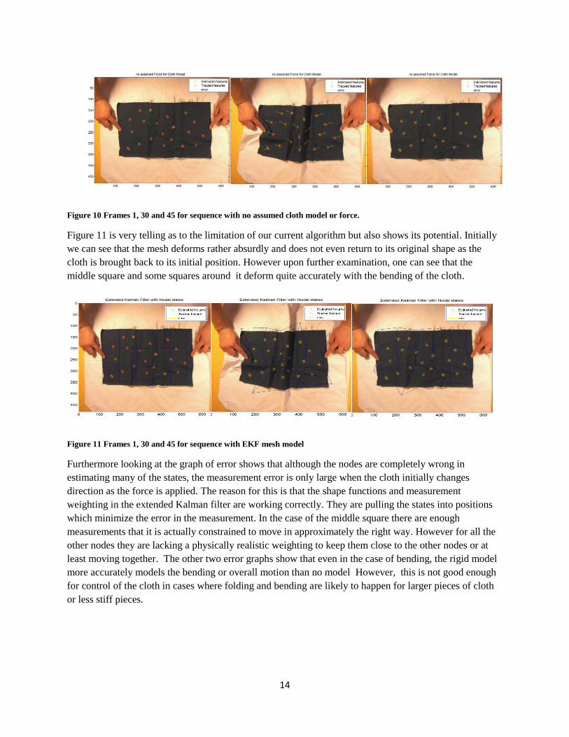
Figure 10 Frames 1, 30 and 45 for sequence with no assumed cloth model or force.

Figure 11 is very telling as to the limitation of our current algorithm but also shows its potential. Initially

we can see that the mesh deforms rather absurdly and does not even return to its original shape as the

cloth is brought back to its initial position. However upon further examination, one can see that the

middle square and some squares around it deform quite accurately with the bending of the cloth.

Figure 11 Frames 1, 30 and 45 for sequence with EKF mesh model

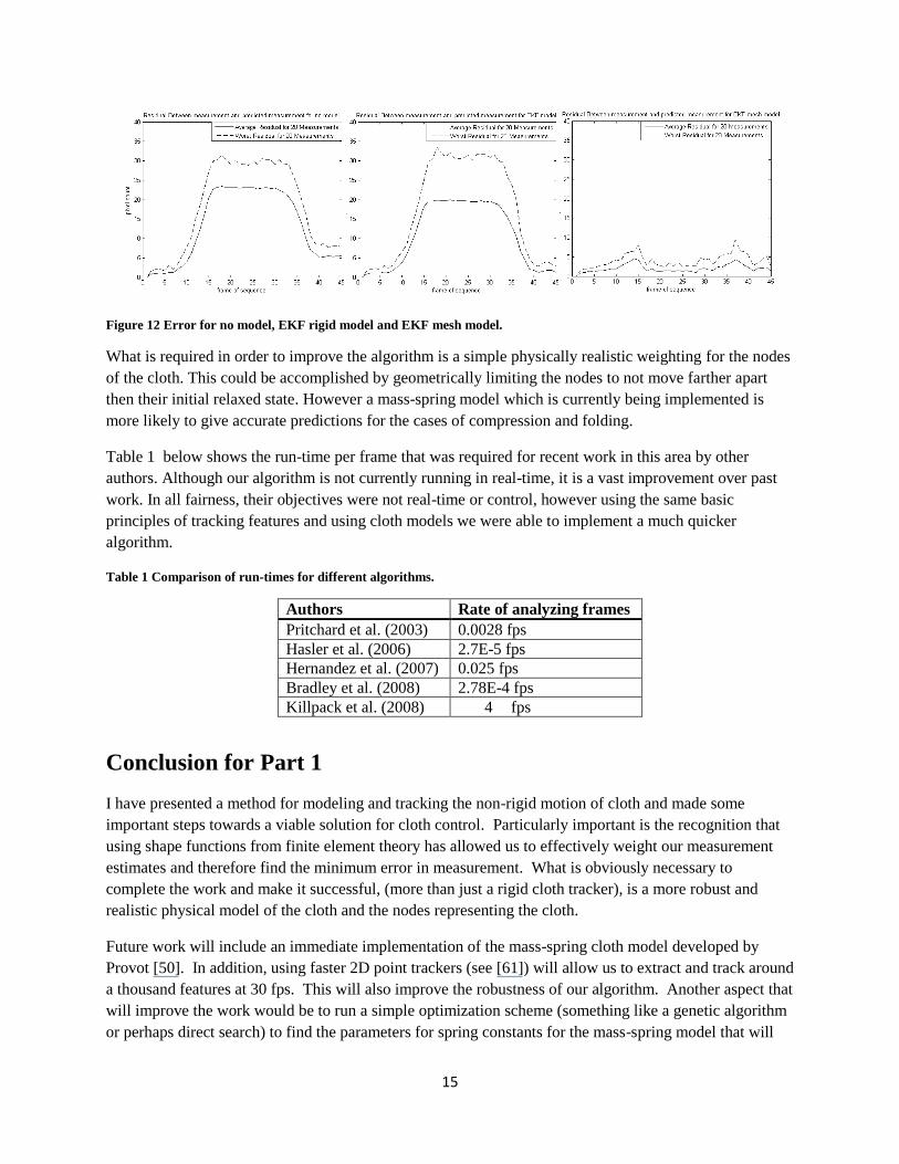
Furthermore looking at the graph of error shows that although the nodes are completely wrong in

estimating many of the states, the measurement error is only large when the cloth initially changes

direction as the force is applied. The reason for this is that the shape functions and measurement

weighting in the extended Kalman filter are working correctly. They are pulling the states into positions

which minimize the error in the measurement. In the case of the middle square there are enough

measurements that it is actually constrained to move in approximately the right way. However for all the

other nodes they are lacking a physically realistic weighting to keep them close to the other nodes or at

least moving together. The other two error graphs show that even in the case of bending, the rigid model

more accurately models the bending or overall motion than no model However, this is not good enough

for control of the cloth in cases where folding and bending are likely to happen for larger pieces of cloth

or less stiff pieces.

15

Figure 12 Error for no model, EKF rigid model and EKF mesh model.

What is required in order to improve the algorithm is a simple physically realistic weighting for the nodes

of the cloth. This could be accomplished by geometrically limiting the nodes to not move farther apart

then their initial relaxed state. However a mass-spring model which is currently being implemented is

more likely to give accurate predictions for the cases of compression and folding.

Table 1 below shows the run-time per frame that was required for recent work in this area by other

authors. Although our algorithm is not currently running in real-time, it is a vast improvement over past

work. In all fairness, their objectives were not real-time or control, however using the same basic

principles of tracking features and using cloth models we were able to implement a much quicker

algorithm.

Table 1 Comparison of run-times for different algorithms.

Authors Rate of analyzing frames

Pritchard et al. (2003) 0.0028 fps

Hasler et al. (2006) 2.7E-5 fps

Hernandez et al. (2007) 0.025 fps

Bradley et al. (2008) 2.78E-4 fps

Killpack et al. (2008) 4 fps

Conclusion for Part 1

I have presented a method for modeling and tracking the non-rigid motion of cloth and made some

important steps towards a viable solution for cloth control. Particularly important is the recognition that

using shape functions from finite element theory has allowed us to effectively weight our measurement

estimates and therefore find the minimum error in measurement. What is obviously necessary to

complete the work and make it successful, (more than just a rigid cloth tracker), is a more robust and

realistic physical model of the cloth and the nodes representing the cloth.

Future work will include an immediate implementation of the mass-spring cloth model developed by

Provot [50]. In addition, using faster 2D point trackers (see [61]) will allow us to extract and track around

a thousand features at 30 fps. This will also improve the robustness of our algorithm. Another aspect that

will improve the work would be to run a simple optimization scheme (something like a genetic algorithm

or perhaps direct search) to find the parameters for spring constants for the mass-spring model that will

16

give the least amount of error for a baseline sequence of the cloth moving. Finally the code can be

optimized and embedded in order to attain real-time cloth tracking and the control law to control the cloth

on our given conveyor system can be developed.

Development, Testing, and Results for Part 2

The work described in this section is the result of the second semester of a two semester research course.

Proof of concept had been shown from results in Part 1. This section outlines results relating to

improvements in the cloth model and implementation for tracking using the LabVIEW software and

camera.

Experimental Design and Simulation

Cloth Model

Originally a two degree of freedom mass-spring model was formulated in Matlab according to the model

in [50]. This was done as a replacement for a rigid plate cloth model. The choice of two degrees of

freedom was an attempt to reduce the computation time and complexity of the algorithm. By assuming

the cloth deformed in the plane, the z-component could be ignored and collision detection with the ground

(which can be computationally costly) could be avoided. However upon initial implementation and

experimentation it was seen that a non-linear spring model would be required in order to accurately

predict the motion of the cloth. Figure 13 shows a result that was not unexpected. Due to the nature of

numerical integration and since the cloth is constrained to the plane, the resulting movement of the cloth

was a total acceleration either downwards or upwards when put in compression in the x-direction.

Figure 13 Deformation and translation of representative mass nodes of a cloth when in compression.

In addition to being inaccurate, this initial implementation was also computationally slow. Since the cloth

and the differential equations governing the cloth are both stiff, the ODE solver in Matlab was extremely

slow. Such that, even if a non-linear spring model was developed, the overall mass-spring model would

have required implementation in a different programming language in order to run at acceptable frame

rates.

These initial results led to an implementation of Nvidia's physics engine as a viable alternative. This is

preferable for a number of reasons. The first is that the code for PhysX (the commercially developed

physics engine for Nvidia) has already been highly optimized to run in real-time and includes collision

detection and three degrees of freedom in the model. Secondly, it permits a user-defined mesh size and

simulation time step as well as the ability to change numerous cloth parameters such as damping and

x-direction (meters)

y-d

irecti

on

(m

ete

rs)

17

stiffness in order to match physical cloth behavior. In addition to position variables being returned for the

mesh nodes, the program can also estimate velocities which could be useful for control. Finally, it allows

the representation of the conveyors which will control the cloth as spherical force fields rather than forces

acting at specific nodes of the cloth mesh.

In order to evaluate the effectiveness of the tracker a brief discussion of how error will be measured is

necessary. Since the nodes of the cloth are imposed and not true physical locations on the cloth, it is

difficult to measure the actual error between the states and their estimates. An alternative is instead to

measure the error between measured features on the cloth and their estimated locations as given by the

estimated states. In order to assign an actual value with the error of the tracking method, the absolute

distance between the measurement’s pixel values and its estimate are calculated. In initial tuning, features

can be manually identified and this measure can then be accurately termed error. However, in subsequent

testing with the automatic 2D point tracker, this measure is referred to as pixel residual since it is the

difference between the measured and predicted features. The average is recorded as well as the worst

pixel error for each frame. As the distance error is already an absolute measure, there is no need for an

RMS sort of calculation. One final note is that although the error between manually extracted feature

locations and their estimates in the image is a generally effective measure, it is not definitive. Early tests

have already shown that an observer can see estimates of states that give good feature estimates but very

poor error qualitatively (see Figure 14 below). This means that at least in initial testing, in addition to the

average pixel error and the worst pixel error there will need to be a physical observation of the estimates

of the state to verify accuracy. Further work could involve using another calibrated camera as a static

observer from a different angle to verify the estimated states of the cloth.

Figure 14 Example of state estimates that give good measurement estimate but are qualitatively poor.

The first step in developing the new cloth model was to tune the parameters of the physics engine cloth

model in order to match as much as possible the behavior of the denim cloth to be tracked and controlled.

Parameters of dynamic and static friction coefficients, stiffness, damping and bending are all tunable in

the PhysX SDK. Using a set of video sequences typical of cloth motion (translation, rotation, bending and

folding), a set of manually extracted features for each frame was used to minimize the measurement

estimate error. The average pixel error for a sequence of frames was weighted with the worst pixel error

and combined as a cost function. This was done, because although we want to reduce the worst error over

all of the frames, it is also important to have a generally low overall average error.

This cost function was minimized using a genetic algorithm [29] that varied the parameters of the

simulation to change the value of the cost function as follows:

( ) ( ) ( )

18

Where f(x) is the cost function, xi’s are the cloth parameters and ai and bi define reasonable constraints on

the parameters. Although genetic algorithms do not necessarily find a global optimum, they have been

shown to effectively search large and complex solution spaces to find acceptable solutions. An acceptable

solution in this case is one that reduces the simulation error in pixel measurement estimate to values that

correspond to noise levels in the measurement technique (on the order of 1-2 pixels). As can be seen in

Figure 15, error values near one pixel for a sequence of cloth translation were easily obtained.

Figure 15 Example of parameter identification using a genetic algorithm on a cloth translation video sequence.

In addition to the simplicity of implementing genetic algorithms, another benefit of using an evolutionary

type algorithm is that the result is a population of solutions. This allows the user or engineer to make

practical and physically meaningful decisions based on a population of best designs. One example of this

principle can be seen for the cloth model in Table 2 below. The values are for the best design in the given

generation. Nvidia’s PhysX engine only gives some parameters as a value from 0 to 1 which is why

gravity was added as a variable to give more flexibility in the model.

Table 2 Parameter and fitness values for two different generations.

Generation 87 Generation 89 Lower Limit Upper Limit

Bending stiffness 0.94 0.26 0 1

Stretching stiffness 0.74 0.74 0 1

Density of Cloth 0.036 0.036 0.02 2

Thickness of Cloth 0.0032 0.0032 0.0005 0.01

Damping of Particles 0.49 0.49 0 1

Iterations of Solver 4 4 1 5

Friction Coefficients 0.079 0.079 0 1

Gravity Value

(to induce stiffer cloth) 12 12 5 15

Fitness Value -0.89 -0.89

19

The two designs from different generations given in Table 2are almost identical except for the Bending

Stiffness value. Their fitness values differ only in the fifth significant digit. However, generation 89’s

value for bending stiffness being so low would be physically inaccurate for denim when the cloth is put in

tension. This “family” of solutions allows the use of good physical judgment in addition to the

optimization routine.

Cloth Results

Using the genetic algorithm and manually identified features, the cloth model was tuned to give

acceptable performance. Of particular importance was the ability of the cloth model to predict bending

and folding of the cloth. In Figure 16, on the left is the image of the real piece of denim in compression.

On the right is the simulated piece of cloth that was solved for using Nvidia’s physics engine and

displayed using OpenGL.

Figure 16 Bending deformation of cloth in compression, on the left is real image; on the right is simulated image using

OpenGL and Nvidia physics engine.

It is important that for different types of cloth or thickness of cloth, the model must still be accurate. For

this reason, another video was taken using a thicker piece of cloth placed under the first. In

Figure 17, it can be seen that it was also possible to simulate the real physical behavior.

Figure 17 Real and simulated bending deformation of a thicker piece of cloth.

These two figures, although not conclusively, show the specific ability of the cloth model to accurately

predict certain motions with given force inputs. The image on the left in Figure 17 shows the error that

was associated when tracking with the previous rigid plate model for the cloth. This new cloth model

should address this issue sufficiently well.

20

As speed was an issue for the initial Matlab implementation of the cloth model, this Nvidia cloth model

was tested for speed. On an Intel Quad-core 2.33 GHz desktop computer, the model was able to simulate

one time step of 1/30th of a second at or under 15 ms. This is an acceptable speed for the cloth model.

2D feature tracking

The next stage was to implement a 2D point tracker. Although the GPU KLT tracker [61] purportedly

tracks near 1000 features at around 30 fps there were two major reasons to not use their method in this

application. The first was that it required a specialized and expensive Nvidia or ATI GPU. In addition,

although it claims to track 1000 features, most of their demo work showed only an average of around 300

features being tracked. One important note however, is that using the GPU unloads the CPU and would

allow a speedup for the total cloth tracker system. For this reason, using the GPU KLT tracker will be

considered in future work if this initial implementation of the cloth tracker is considered successful

enough.

Instead, the OpenCV implementation of Bouguet’s work [6][9] was used to do pyramidal Lucas-Kanade

tracking. Following the general OpenCV implementation, Shi and Tomasi’s work [60] was used to find

the initial features that were then tracked from frame to frame.

This algorithm, as well as the cloth model simulation was compiled into dynamically linked libraries in

order to communicate with a National Instruments Smart Camera. The architecture for the experimental

setup is shown below in Figure 18.

Figure 18 Architecture of experimental setup for cloth tracking tests.

Intel Core2 Duo Host Computer

LabVIEWhost program

PhysX .dll

OpenCV .dll

NI Smart Camera

Ethernet

Connection

21

The Smart Camera from LabVIEW can take 640x480 resolution images at between 30 and 60 fps. Each

frame can then be passed back to a host computer where a LabVIEW host application is running and

handles communication with the camera. The current and previous frames as well as a 2D array of

features from the previous frame are then sent to the OpenCV .dll. The OpenCV .dll does pyramidal

Lucas-Kanade tracking and returns the tracked feature locations to the host program. The PhysX .dll

meanwhile, takes the previous state estimates and any inputs from the stepper motors and passes back a

prediction of the state estimates at the next time step. The rest of the cloth tracking algorithm proceeds as

outlined in the Appendix.

Initial Results from Smart Camera

In order to test the 2D point tracker implementation, translation and then a shearing motion were used to

check the accuracy of the tracker. Initial results were encouraging. Figure 19 shows the feature tracking

working in real-time with the NI smart camera between 10-15 fps when a shearing force is applied.

Figure 19 Frame on the left shows initial features that were extracted, frame on the right shows features after cloth has

deformed.

Upon further testing, however, the features seemed to drift over time and large-scale translation. In order

to test if this was a problem with the algorithm or with the LabVIEW setup, initial feature locations were

extracted and saved for later use. Offline, the same frames were run with the given initial features. One

can see in figure Figure 20 that the initial frames and features for the two methods are indeed the same.

22

Figure 20 Starting frames for offline and real-time feature tracking test, (on the left is the offline image, on the right is the

real-time image).

However, it is clear from Figure 21 that the features in the real-time frame on the right have begun to

drift. By running the exact same frames with the same initial features offline, it is clear that the error in

the real-time feature tracking is not with the OpenCV code.

Figure 21 Frames of offline and real-time tracking test after some displacement of the cloth (on the left is the offline

image, on the right is the real-time image).

The probable cause of this error is either network latency or errors in the real-time timing loop

implementation in LabVIEW. The two processors on the host machine are only ever running at about

20% capacity during the experiment, which means that it is not likely an issue of processor power.

Interestingly enough, even when the frames of the video sequence are processed offline on a quad-core

2.33 GHz desktop, the average processing time per frame was the same as the processing rate of the frame

in the real-time implementation (around 15 fps). This likely means that the limiting factor on the speed of

the complete cloth tracker is the speed of the 2D point tracker and not the network latency. The most

likely cause for this error is unintentional asynchronous processing of frames due to errors in timing loops

in the LabVIEW code.

23

Conclusions and Future Work from Part 2

Although the tracker has not been fully integrated, both of the limiting issues from Part 1 have been

addressed. First, a more robust, quick and accurate cloth model has been developed and proven useful in

initial testing. Secondly, a real-time 2D point tracker has been implemented with minor errors and proof

that the tracker itself is capable at tracking robustly at a fairly high frame rate.

Future work includes tying together existing components and reducing error. Of particular importance is

the debugging of the 2D point tracker on the real-time system shown in Figure 18. In addition, tuning of

parameters of the Extended Kalman filter including covariance matrices for the process and measurement

are still required. Finally the Extended Kalman filter will need to be modified for every feature that is

dropped and added from frame to frame. One option is to drop the number of points tracked every time a

feature is lost until a critical level is reached and then resample the image for more features. The other

option would be to resample certain regions on the fly when a number of features have been lost or the

quality of those features has degraded. Finally, the forces applied to the cloth by conveyor motion will

need to be estimated and serial communication with the stepper motors will need to be incorporated into

the LabVIEW real-time system that has already been developed.

The experiments and implementations as well as future work will allow the validation and development

of a fully automatic non-rigid cloth tracker. This tracker which will be able to run in real-time will allow

the control of non-rigid cloth on a system with steerable conveyors.

24

Related Work

Cloth model

Past work in simulating or modeling cloth behavior can be largely divided into geometrical or physical

techniques or a hybrid of both. Ng et al. [48] summarized the initial work in this field. They explained

that geometrical techniques do not consider properties of cloth but focus on appearance, especially folds

and creases represented by geometrical equations. Physical techniques generally use triangular or

rectangular grids with points of finite mass at the intersections.

The majority of physically based modeling techniques since the work described by Ng et al. [48] has been

based around the methods developed by Baraff et al. in [3]. This work addressed the limitation of using

small time steps to avoid numerical instability in numerical integration. Using the common mass-spring

model, with a triangular mesh, they used a new technique for enforcing constraints on individual cloth

particles with an implicit integration method. This meant that their method was always stable even for

large time steps. Although much work since then has modified the method of constraints or the method of

solving the linear system, their work was the seminal work in terms of cloth simulation using implicit

integration. Desbrun et al. [19], [41] addressed the speed of Baraff’s algorithm [3] by modifying the

original implicit integration method in different ways. In [41] the authors used a hybrid explicit-implicit

method in order to implement a stable real-time animation of textiles still based on a mass-spring model

for a VR environment. Although it ran at a high frame rate its accuracy in comparison to real world cloth

dynamics was never addressed. Work by Bridson et al. [10] is fairly representative of work that followed

Barraf et al. [3] which focused on more realistic wrinkles or folds instead of speed of computation. In

addition to using an explicit-implicit time integration scheme and mass-spring model, they introduced a

physically correct bending model to better model wrinkles.

Work by Provot [50] uses the general mass-spring model and explicit integration techniques as well as

limiting the elastic deformation arbitrarily when there is high stress in small areas. This allows for a more

realistic modeling of real cloth without having to increase spring stiffness between the masses. Rudomin

et al. [55] represent pieces of clothing using a mass-spring particle system implemented in real time. They

point out that Euler or Runge-Kutta methods are fast and easy to implement, but require small steps.

Whereas implicit integration can take much larger time steps but requires more computations to resolve

the system at every step. According to their work, real time applications, where the time step is small and

the regularity of the system cannot be determined, are best addressed using an explicit first or second

order integration method. Bridson et al. [11] use the mass-spring model by Provot as the basis for an

algorithm that deals robustly with collisions, contact and friction in cloth simulation by focusing on the

internal dynamics of the cloth.

Another strain of work in the cloth modeling field that is much less common but is finding more

popularity due to an increase in computational power and efficient formulations is that of a finite element

formulation for deformable bodies. Eischen et al. [20] present a fairly representative survey of finite

element methods for cloth modeling and develop their own algorithm based on nonlinear shell theory.

Their motivation was to successfully simulate fabric drape and manipulation for use in textile and apparel

manufacture. Most similar finite element methods were fairly slow in terms of run-time until the work of

Etzmuss et al. [21]. They sped up the process by reducing the nonlinear elasticity problem to a planar

25

linear problem for each implicit time integration step. Their algorithm was able to compute frames for a

0.02 second time step at an average rate of three seconds per frame for a simple shirt simulation and 16-

21 seconds for a man walking in a shirt and trousers. Although still not real-time, this was a vast

improvement on previous finite element methods with apparently little loss in accuracy although they

include no proof of error measurement or validation. One other important and interesting point that they

made is that from a finite element stand point, spring-mass systems should only use quadrilateral meshes

as triangle meshes tend to show a larger shear resistance than real textiles. Their main criticism of work

like Provot’s was not its lack of accuracy compared to their algorithm but difficulty in applying it to

garment construction for linking multiple pieces of simulated cloth. Finally, Garcia et al. [25] were able to

sacrifice a very small amount of accuracy in order to make a finite element formulation for deformable

bodies run at near 30 frames per second. They did this by estimating an initial solution and then only

iterating on equations showing large error.

A succinct and current summary of the advantages and disadvantages among the different currently used

methods of cloth simulation is found in work by Nealen et al. [47]. They discuss specifically the current

deformable models that are all physically based, giving numerous examples at the end of their work.

2D point tracking

Among the numerous forms of tracking, (i.e. kernel tracking, contour tracking, active shape models,

snakes), the most useful type for this specific application is point tracking. As the cloth’s state will be

represented using nodes, 2D feature tracks provide an obvious way to relate the motion of the feature

points to the motion and velocity of the nodes of the cloth.

Feature points

The first step in feature tracking is being able to identify interest points in initial frames of the image or

video sequence. An effective feature tracker therefore obviously depends on identifying “good features.”

Generally, feature point detectors that have proven effective in other applications are those that are

insensitive to illumination variance and affine transformations. Mikolajczyk et al. [42][45] compared

numerous scale and affine invariant point detectors and concluded that the SIFT detector by Lowe [34]

performed the best in matching tests where images underwent affine and scale transformations. When the

performance measure included changes in illumination, defocus and image compression as well they

concluded that the MSER feature detector by Matas et al. [38] performed the best, with the Hessian affine

detector being the next best [43]. They also concluded that for point tracking applications with occlusion

or clutter, the Harris and Hessian affine feature detectors [43][45] were the most useful as they extracted

more overall features than the other detectors. In work by Tissainayagam et al. [64] a number of different

feature detectors ([32][67][62][43]) were implemented in order to track extracted points and compare the

performance of the feature finders. It was shown that the two most effective types of feature points for

tracking are Harris affine feature points [43] and KLT points (which were developed specifically for

tracking purposes, see [67] and [60]). Some of the most recent work in feature extraction is focused on the

speed and efficiency of extraction. Rosten and Drummond [54] (FAST) use machine learning to derive a

feature detector that can run in real-time and is very competitive with other robust feature extractors. We

will therefore be using KLT points or FAST feature points in our application since the SIFT feature

extractor is generally much slower in running time than the other two methods.

26

The second aspect of point tracking is efficiently and effectively matching these feature points through

progressive frames in order to produce 2D image tracks that can be used to update the estimate of the

states from the cloth model. Many methods for this data correspondence problem have been proposed.

Included here is a brief summary of the general areas and trends in feature tracking in relation to solving

the data association problem.

Kalman filtering

Broida et al. [12] used a Kalman filter to track an object in noisy images. While Rosales et al. [53] used

an extended Kalman filter in order to estimate a bounding box for position and velocity of multiple points

which were then used in a larger scheme to estimate relative 3D motion trajectories. The major drawback

with using a simple Kalman filter is that even though it provides optimal state estimates, it is only optimal

for unimodal Gaussian distributions over the state to be estimated. In addition, the Kalman filter by itself

does not solve the data correspondence problem. The authors Forsyth and Ponce [23] present a simple

example of using the Kalman filter with a global nearest neighbor approach to solve the data

correspondence problem.

JPDA

The joint probability distribution association (JPDA) addresses the data correspondence problem by

computing a Bayesian estimate of the correspondence between features detected by the “sensor” and the

different objects to be tracked. Fortmann et al. [24] first introduced this method with an application to a

passive sonar tracking problem with multiple sensors and targets. The algorithm was also reviewed and

evaluated by Cox [17] and a simple version of it is presented by Forsyth and Ponce [23]. The original

JPDA still uses a Kalman filter and therefore is only optimal for Gaussian distributions over the state to

be estimated. In addition, the JPDA algorithms fails to handle objects entering or exiting the scene. This

is particularly a problem because the JPDA only associates the data over two frames which can lead to

major errors if the number of objects changes. Schulz et al. [58] addressed the limiting factor of the JPDA

only describing a Gaussian probability distribution function by presenting a sample-based JPDA filter to

track multiple objects. This method then combines the advantages of sample-based density

approximations with the generally efficient JPDA. This does not however resolve the problem of objects

entering or leaving the scene or at least being occluded in the two frame interval. Because the JPDA is not

formulated to handle objects entering or leaving the scene and because for point tracking, sample-based

density approximations seem irrelevant, this method is a less likely candidate for a cloth control problem.

MHT

As an alternative to the JPDA method of data correspondence, Reid [52] proposed the multiple hypothesis

tracking algorithm (MHT). The underlying principle of the MHT algorithm is maintaining multiple

hypotheses about a single object in order to obtain optimal data correspondence. He also incorporated the

ability to initiate tracks, account for false or missing objects and process sets of dependent reports in one

algorithm. One major drawback is the obvious combinatorial explosion that takes place as all hypotheses

are explored. Cox et al. [16][18] updated the original MHT algorithm to run more efficiently and applied

it to feature point tracking. They tracked the features using a simple linear Kalman filter and kept only the

k-best hypothesis. They used Murti’s algorithm [46] to solve the problem and additionally addressed track

initiation, termination and low-level support for temporary track occlusion. This work has been used more

recently by Tissainayagam et al. [63][65]. The authors use the MHT method twice in a framework where

they both segment contours and track selected key points using the MHT algorithm for both parts.

27

However they make no claim about being able to run in real-time which is clearly important in being able

to use the tracking in any kind of a control application. In addition, the authors explain that the tracking

process can breakdown on the contour segmentation side for occlusion or possibly deforming objects

which is clearly a problem as our objective is to track and control non-rigid cloth. Veenman et al. [70]

have shown that tuning parameters for the MHT algorithm tends to be tricky as it is extremely sensitive to

its parameter settings. Finally, the complexity of the algorithm still grows exponentially with the number

of points making the MHT algorithm a less effective feature tracker in non-rigid tracking applications

which are facilitated by a larger number of 2D point tracks.

Deterministic Algorithms

Deterministic algorithms are another class of feature trackers that have seen quite a bit of success using

qualitative motion heuristics instead of probability density functions and distributions. Salari et al. [56]

formulated the data correspondence problem as a minimization problem for extracting globally smooth

trajectories that are not necessarily complete but satisfy certain local smoothness constraints. Their work

involved an iterated optimization procedure. They were followed by the work of Rangarajan et al. [51]

who defined a proximal uniformity constraint which said that most objects in the real world follow

smooth paths and cover small distances in a small amount of time. They also minimized a cost function

that described such a constraint and used gradient based optical flow to establish correspondence in the

initial frames. Their algorithm was a non-iterative greedy algorithm. Veenman et al. [70] built on this

previous work and developed what they call a qualitative motion modeling framework. Their algorithm

was less sensitive to parameter changes than the previous deterministic algorithms and outperformed

them as well as outperforming the most recent MHT algorithms at the time despite running in real-time.

They also included error and occlusion handling and did automatic initialization of tracks. The limitations

however were that this method addressed no track initiation or termination during the image sequence and

optimized only over two frames. Shafique et al. [59] developed another non-iterative greedy algorithm

that presented a framework for finding the correspondence over multiple frames using a single pass

greedy algorithm. Their method handles object entry or exiting of the frame as well as occlusion. Their

results show that the algorithm can run at 17 Hz for the tracking of 50 separate points on a 2.4 GHz Intel

Pentium 4 CPU although they do not mention for what resolution this measurement is given. Their

method automatically initializes the tracks using the Shi-Tomasi-Kanade tracker [60]. Finally showing

that the algorithm of Shafique et al. was useful in tracking non-rigid objects, Mathes and Piater [39]

developed 2D point distribution models using the automatically tracked points from [59] to track non-

rigid motion of football (soccer) players. The real-time implementation of these deterministic algorithms

as well as their current application in other non-rigid tracking problems makes them a candidate for our

application.

Optical flow estimation

One of the most popular methods for point tracking is based on the two-frame differential method for

optical flow estimation. Lucas and Kanade [35] first presented an iterative approach that measured the

match between fixed-size feature windows in past and current frames as the sum of squared intensity

differences of the windows. The track or correspondence was then defined as the one that minimized the

sum between two frames. Tomasi and Kanade [67] re-derived the same method in a more intuitive

fashion and then addressed how to define feature windows that were best suited for tracking. Shi and

Tomasi[60] continued this work by proposing a feature selection criterion based on how the tracker works

so as to pick “good features” for this tracking method. They also proposed a feature monitoring method

28

(i.e. better addressing the correspondence problem) that can handle occlusions, disocclusions and features

that do not correspond to points in the real world (noise). Finally they extended previous Newton-

Rapshon style search methods to work under affine image transformations. Their work was extended by

Tommasini et al. [68] who introduced an automatic scheme for rejecting spurious features by using a

simple outlier rejection rule. Zinsser et al. [73] proposed two ameliorations to the Shi-Tomasi-Kanade

tracker which dealt with affine motion estimation and feature drift. In addition their algorithm ran in real-

time and was specifically formulated to run well over long image sequences. Sinha et al. [61]

implemented the KLT tracker [67] on the graphics processing unit (GPU) instead of the CPU. Two

examples of work that have successfully used the implementation by Sinha et al. is the work by

Akbarzadeh et al. in 3D urban reconstruction [2] and Andreasson et al. in a real-time SLAM application

[1]. They were able to track about a thousand features in real-time at 30 Hz on 1024x768 resolution video.

An alternative to the implementation of the Lucas Kanade tracker by Sinha is the pyramidal method

developed by Bouguet [6] and implemented in the computer vision library OpenCV [9]31. Because of the

wide use of this approach and its implementation in real-time, this method is one of the best candidates

for being able to track the non-rigid cloth.

Cloth tracking

Non-rigid tracking is not a new topic in research and is fairly well developed for some applications.

However, algorithms such as the one found in the work by Comaniciu et al. [14] is not acceptable for a

cloth tracking application. This is because only a bounding box or contour of the non-rigid object is

tracked which is useful for a cloth tracking application since we want to track and control within the

perimeter of the cloth as well.

In terms of actual tracking or parameter estimation of cloth from real video, most current methods use

implicit integration for their cloth model. Bhat et al. [4] used the general method proposed by Baraff et al.

[3] to present an algorithm for estimating the parameters for cloth simulation from video data of real

fabric. Simulated annealing was used to minimize the frame by frame error between a given simulation

and the real-world footage. Pritchard et al. [49] instead used the fairly well developed methods of rigid

body motion capture systems to estimate the geometry of a non-rigid textile. They pointed out that

methods proposed by Bridson and Baraff are still too demanding for real-time applications. Instead, they

proposed using feature matching techniques and a multi-baseline stereo camera setup with 10fps to

recover geometry and parameterize a moving sheet of cloth. Scholz et al. [57] also used a multi-camera

setup but used optical flow between frames to model the deformable surface. They included a silhouette

matching procedure which is required to correct the tracking errors that occur in long video sequences.

Similar work was done by Hasler et al. [24][25] in terms of cloth parameter estimation for a tracking

application using analysis-by-synthesis. Their method consisted of optimizing a set of parameters of a

mass-spring model that were used to simulate the textile. The fabric properties and the positions of a

limited number of constrained points of the simulated cloth were found during the optimization. However,

in order to improve tracking accuracy, nonphysical forces were introduced to bias the simulation towards

following the observed real world behavior. Due to the optimization scheme used and the fact that they

estimated all parameters for every frame, their algorithm took 10 to 30 hours on 7 AMD Opteron

processors at 2.2GHz to converge for their experiments. Where the work by Hasler et al. was based on

29

surface features of the cloth, White et al. [72] use painted markers of constant color. They used multiple

cameras which allowed them to compute the markers’ coordinates in world space using correspondence.

They also addressed a data driven hole-filling technique for occluded regions by using previous frames

where the occluded regions were visible.

One area of cloth tracking that has been steadily growing is the use of garment capture for use with

augmented reality, post production of films or even avatars. Bradley and Roth [7] were able to track non-

rigid cloth and insert virtual images on the non-rigid cloth in real-time. However, they required special

patterns in specific locations to be on the cloth. In similar work, Bradley et al. [8] were able to

successfully capture complicated garment motion with a sixteen camera array and then insert images or

change the clothing completely in post-production. The disadvantages were the complicated setup and the

fact that processing times for each frame were approximately one hour. Another approach to the same

problem was presented by Hernandez et al. [28] who used multispectral photometric stereo to recreate 3D

data for a moving non-rigid object. Although they obtain impressive results, their processing time of 40

seconds per frame for a 1280x720 resolution image with a 2.8 Ghz processor is too slow for a control

application. In addition the method is perhaps too restrictive for textile manufacturing in requiring

specific lighting conditions that may not be possible in a factory setting.

Visual tracking and control

Recent work on combining the aspects of visual tracking and control focuses on robustness and speed.

Work by Comport et al. [15] developed a 3D model-based tracking method with a focus on trying to more

robustly handle natural scenes without fiducial markers. In [37], Marchand et al. gave a review of

effective 2D feature-based or motion-based tracking methods that have been used over the past 10 years

in addition to reviewing their formulation of the 3D model-based tracking method. Malis et al. [36]

developed a combined visual tracking and control system similar to our objective. However, they

proposed a template matching algorithm based on second-order minimization in an effort to avoid design

of feature dependent visual tracking algorithms. Although clearly important for more broad applications,

template based tracking is inadequate to be able to measure the states of a non-rigid textile to be tracked.

Kumar et al. [33] developed visual servoing strategies that involved robustness to non-rigid deformation.

However, the non-rigid deformation is assumed to be part of the environment of the robot and not the

object to be controlled per se. Finally, Tran et al. [69] developed a tracking algorithm for visual servoing

which most resembles our proposed plan. However, even using a fast corner detector, a corner descriptor

based on Principal Component Analysis and an efficient matching scheme using approximate nearest

neighbor technique they were only able to achieve tracking at 10-14 fps. This is sluggish in terms of

desired control rates.

Stepper motors and control

Although both servo and stepper motors are a possibility for controlling the cloth on an array, stepper

motors offer a generally more accurate solution. The behavior and capabilities of stepper motors have

been extensively studied. Numerous control schemes including linear and non-linear methods have been

proposed , [74][40][5]. Frequency response, stability and nonlinear behavior of stepper motors were

30

studied by Cao and Schwartz [13]. Most recently, Ferrah et al. [22] presented a clear and simple stepper

motor model and developed an extended Kalman Filter to improve the control over the already accurate

stepper motor.

Although much work has been done in terms of visual servoing and tracking of rigid objects, tracking and

control of a non-rigid object like cloth has not been addressed. It can be seen from the review above that

combining techniques from the well-developed field of cloth simulation as well as the field of feature

tracking will allow us to further develop work in real-time textile tracking as well as textile control.

31

References

[1] H. Andreasson, T. Duckett and A. Lilienthal. “Mini-SLAM: Minimalistic Visual SLAM in Large-

Scale Environments Based on a New Interpretation of Image Similarity.” Int. Conf. on Robotics

and Automation, pages 4096-4101, 2007.

[2] A. Akbarzadeh, J.M. Frahm, P. Mordohai, B. Clipp, C. Engels, D. Gallup, P. Merrell, M. Phelps,

S. Sinha and B. Talton. “Towards Urban 3D Reconstruction From Video.” Int. Symp. on 3D Data

Processing Visualization and Transmission, Vol. 4, 2006.

[3] D. Baraff and A. Witkin. Large steps in cloth simulation. Proceedings of the 25th annual

conference on Computer graphics and interactive techniques, pages 43-54, 1998.

[4] K.S. Bhat, C.D. Twigg, J.K Hodgins, P.K. Khosla, Z. Popovic and S.M. Seitz. Estimating cloth

simulation parameters from video. Proceedings of ACM SIGGRAPH/Eurographics Symposium

on Computer Animation, 2003.

[5] M. Bodson, J.N. Chiasson, R.T. Novotnak and R.B. Rekowski. “High-performance nonlinear

feedback control of a permanent magnet stepper motor,” IEEE Transactions on Control Systems

Technology, 1(1):5-14, 1993.

[6] J.-Y. Bouguet, “Pyramidal implementation of Lucas Kanade feature tracker description of the

algorithm,” http://robots.stanford.edu/cs223b04/algo_tracking.pdf.

[7] D. Bradley and G. Roth. “Augmenting Non-Rigid Objects with Realistic Lighting,” Technical

Report NRC/ERB-1116, Oct. 2004.

[8] D. Bradley, T. Popa, A. Sheffer, W. Heidrich, T. Boubekeur. "Markerless Garment Capture,"

SIGGRAPH 2008, pg 1-8, 2008.

[9] G. Bradski and A. Kaehler, Learning OpenCV: Computer Vision with the OpenCV Library,

O’Reilly Media, October 3, 2008.

[10] R. Bridson, S. Marino and R. Fedkiw. Simulation of clothing with folds and wrinkles.

Proceedings of the 2003 ACM SIGGRAPH/Eurographics symposium on Computer animation,

pages 28-36, 2003.

[11] R. Bridson, R. Fedkiw and J. Anderson. “Robust Treatment of Collisions, Contact and Friction

for Cloth Animation,” Int. Conf. on Computer Graphics and Interactive Techniques, 2005.

[12] T. Broida and R. Chapella. “Estimation of object motion parameters from noisy images,” IEEE

Trans. Patt. Analy. Mach. Intell., 8 (1): 90–99. 1986.

[13] L. Cao and H.M. Schwartz. “Oscillation, Instability and Control of Stepper Motors,” Nonlinear

Dynamics, 18(4):383-404, 1999.

[14] D. Comaniciu, V. Ramesh and P. Meer. “Real-time tracking of non-rigid objects using mean

shift,” Computer Vision and Pattern Recognition, Vol. 2, 2000.

32

[15] A.I. Comport, E. Marchand and F. Chaumette, “Robust model-based tracking for robot vision,”

Intelligent Robots and Systems, vol. 1, 2004.

[16] I.J. Cox and J.J. Leonard, “Modeling a dynamic environment using a Bayesian multiple

hypothesis approach,” Artificial Intelligence, 66:311-344, 1994.

[17] I.J. Cox, “A review of statistical data association techniques for motion correspondence,” Int. J.

Comput. Vision, 10 (1):53–66, 1993.

[18] I.J. Cox, S.L. Hingorani, “An efficient implementation of Reid’s multiple hypothesis tracking

algorithm and its evaluation for the purpose of visual tracking,” IEEE Trans. on Pattern Anal.

Machine Intell., 18 (2): 138–150, 1996.

[19] M. Desbrun, P. Schröder, and A. H. Barr, “Interactive Animation of Structured Deformable

Objects,” Graphics Interface, pages 1–8, June 1999.

[20] J.W. Eischen, S. Deng and T.G. Clapp. “Finite-Element Modeling and Control of Flexible Fabric

Parts.” Computer Graphics and Applications, 5(16):71-80, 1996.

[21] O. Etzmuss, M. Keckeisen, W. Strasser, I.V. Concepts and G. Berlin. “A Fast Finite Element

Solution For Cloth Modeling,” Proceedings 11th Pacific Conf. on Computer Graphics and

Applications, pages 244-251, 2003.

[22] A. Ferrah, J.A.K. Bani-Younes, M. Bouzguenda and A. Tami. “Sensorless speed and position

estimation in a stepper motor,” Int. Aegean Conf. on Electrical Machines and Power Electronics,

pages 297-302, 2007.

[23] D.A. Forsyth and J. Ponce. Computer Vision: A Modern Approach. Prentice Hall Professional

Technical Reference. 2002.

[24] T.E. Fortmann, Y. Bar-Shalom, and M.Sheffe, “Sonar tracking of multiple targets using joint

probabilistic data association,” IEEE J. Oceanic Eng., 8 (3):173–184, 1983.

[25] M. Garcia, O.D. Robles, L. Pastor and A. Rodriguez. “MSRS: A fast linear solver for the real-

time simulation of deformable objects,” Computers and Graphics, 3(32):293-306, 2008.

[26] N. Hasler, B. Rosenhahn, M. Asbach, J.R. Ohm, and H.P. Seidel, “An analysis-by-synthesis

approach to tracking of textiles,” Proc. of Int. Workshop on Motion and Video Computing, 2007.

[27] N. Hasler, M. Asbach, B. Rosenhahn, J.R. Ohm and H.P. Seidel. Physically based tracking of

cloth. Vision, Modeling, and Visualization 2006: Proceedings, November 22-24, 2006.

[28] C. Hernandez, G. Vogiatzis, G.J. Brostow, B. Stenger, R. Cipolla, "Non-rigid Photometric Stereo

with Colored Lights," ICCV 2007, pg (1-8), October 2007.

[29] C.R. Houck, J.Joines and M.Kay, “A genetic algorithm for function optimization: A Matlab

implementation, ACM Transactions on Mathematical Software.

[30] T. Jakobsen, “Advanced Character Physics,” Gamasutra-gamasutra physics resource guide, 2003.

33

[31] M. Killpack, F. Dellaert and W. Book, Cloth Modeling and Tracking with future application for

control. 11 Dec. 2008. Georgia Institute of Technology.

[32] L. Kitchen, A. Rosenfeld, “Gray level corner detection,” Pattern Recognition Letters, pages 95–

102, 1982.

[33] D.S. Kumar and C.V. Jawahar, “Visual servoing in presence of non-rigid motion,” ICPR 2006,

vol 4, 2006.

[34] D.G. Lowe, “Object Recognition from local scale–invariant features,” International Conference

on Computer Vision, 1999.

[35] B.D. Lucas and T. Kanade, “An iterative image registration technique with an application to

stereo vision,” In Proceedings of the 7th International Joint Conference on Artificial Intelligence,

1981.

[36] E. Malis and S. Benhimane, “A unified approach to visual tracking and servoing,” Robotics and

Autonomous Systems, 52(1):39-52, 2005.

[37] E. Marchand and F.Chaumette, “Feature tracking for visual servoing purposes,” Robotics and

Autonomous Systems, 52(1):53-70, 2005.

[38] J. Matas, O. Chum, M. Urban and T. Pajdla, “Robust wide-baseline stereo from maximally stable

extremal regions,” Image and Vision Computing, 22(10):761–767, 2004.

[39] T. Mathes and J. H. Piater, “Robust non-rigid object tracking using point distribution models,” In

British Machine Vision Conference 2005, 2005.

[40] H. Melkote, F. Khorrami, S. Jain and M.S. Mattice. “Robust adaptive control of variable

reluctance stepper motors,” IEEE Transactions on Control Systems Technology, 7(2):212-221,

1999.

[41] M. Meyer, G. Debunne, M. Desbrun and A. Barr, “Interactive animation of cloth-like objects in

virtual reality,” Journal of Visualization and Computer Animation, 12(1):1-12, 2001.

[42] K. Mikolajczyk and C. Schmid. “A performance evaluation of local descriptors,” In Proceedings

of IEEE Conference on Computer Vision and Pattern Recognition, Wisconsin, USA, 2003.

[43] K. Mikolajczyk and C. Schmid. “An affine invariant interest point detector,” ECCV, 2002.

[44] K. Mikolajczyk and C. Schmid. “Scale and affine invariant interest point detectors,” International

Journal of Computer Vision, 60 (1): 63 – 86, 2004.

[45] K. Mikolajczyk, T. Tuytelaars, C. Schmid, A. Zisserman, J. Matas, F. Schaffalitzky, T. Kadir and

L. Van Gool, “A comparison of affine region detectors,” In International Journal of Computer

Vision, 65(1/2):43-72, 2005.

[46] K.G. Murty, “An algorithm for ranking all the assignments in order of increasing cost,”

Operations research, 16:682-687, 1968.

34

[47] A. Nealen, M. Muller, R. Keiser, E. Boxerman and M. Carlson. “Physically Based Deformable

Models in Computer Graphics,” Computer Graphics Forum, 4(25):809-836, 2006.

[48] H.N. Ng and R.L. Grimsdale. Computer graphics techniques for modeling cloth. IEEE Comp.

Graphics and Applications, 16(5):28-41, 1996.

[49] D. Pritchard and W. Heidrich, “Cloth Motion Capture,” Computer Graphics Forum, 22(3):263-

271, 2003.

[50] X. Provot. Constraints in a Mass-Spring Model to Describe Rigid Cloth Behavior. Graphics

Interface, pg 147-154, 1995.

[51] K. Rangarajan and M. Shah, “Establishing motion correspondence,” Conference Vision Graphics

Image Process, 54 (1):56–73, 1991.

[52] D.B. Reid, “An algorithm for tracking multiple targets,” IEEE Trans. Automatic Control,

24(6):843–854, 1979.

[53] R. Rosales and S. Sclaroff, “3D Trajectory Recovery For Tracking Multiple Objects and

Trajectory Guided Recognition of Actions,” In IEEE Conference on Computer Vision and

Pattern Recognition (CVPR), pages 117–123. 1999.

[54] E. Rosten and T. Drummond. “Machine Learning for High-Speed Corner Detection,” Lecture

Notes in Computer Science,” Vol. 3951, page 430, 2006.

[55] I. Rudomin and J. Castillo. Real-time clothing: Geometry and Physics. WSCG, February 2002.

[56] V. Salari and I.K. Sethi, “Feature point correspondence in the presence of occlusion,” IEEE

Trans. Patt. Analy. Mach. Intell., 12 (1):87–91, 1990.

[57] V. Scholz and M.A. Magnor, “Cloth motion from optical flow,” Proc. Vision, Modeling and

Visualization, pages 117-124, 2004.

[58] D. Schulz, W. Burgard and D. Fox, “People tracking with mobile robots using sample-based joint

probabilistic data association filters,” International Journal of Robotics Research, 22(2), 2003.

[59] K. Shafique and M. Shah. “A noniterative greedy algorithm for multiframe point

correspondence,” IEEE Trans. on Pattern Analysis and Machine Intelligence, 27(1), January

2005.

[60] J. Shi, C. Tomasi. “Good Features to Track,” In CVPR, pages 593–600, June 1994.

[61] S. Sinha, J.-M. Frahm, M. Pollefeys and Y. Genc, “GPU-based video feature tracking and

matching,” Technical Report TR 06-012, University of North Carolina at Chapel Hill, May 2006,

http://cs.unc.edu/_ssinha/Research/GPU KLT/.

[62] S.M. Smith, J.M. Brady, “SUSAN—a new approach to low level image processing,”

International Journal of Computer Vision, 23 (1): 45–78, 1997.

35

[63] P. Tissainayagam and D. Suter, “Object tracking in image sequences using point features,”

Pattern Recognition, 38(1):105–113, 2005.

[64] P. Tissainayagam, D. Suter, “Assessment of corner detectors for point feature tracking

applications,” Image and Vision Comput. J. (IVC), 22 (8):663–679, 2004.

[65] P. Tissainayagam, D. Suter, “Visual tracking with automatic motion model switching,” Int. J.

Pattern Recogn, 34:641–660, 2001.

[66] C. Tomasi and T. Kanade, “Shape and motion from image streams under orthography: a

factorization method,” Int. J. of Computer Vision, 9(2):137–154, 1992.

[67] C. Tomasi, T. Kanade, “Detection and Tracking of Point Features,” Carnegie Mellon University,

Tech. Report CMU-CS-91-132, April 1991.

[68] T. Tommasini, A. Fusiello, E. Trucco, V. Roberto. Making Good Features Track Better. In

Computer Vision Pattern Recognition (CVPR ’98), pages 178-183, June 1998.

[69] T.T.H. Tran and E. Marchand, “Real-time key points matching: application to visual servoing,”

2007 Int. Conf. on Robotics and Automation, pages 3787-3792, 2007.

[70] C. Veenman, M. Reinders and E. Backer, “Resolving motion correspondence for densely moving

points,” IEEE Trans. Patt. Analy. Mach. Intell., 23 (1):54–72, 2001.

[71] G. Welch, G. Bishop, “An Introduction to the Kalman Filter,” Technical Report TR 95-041,

University of North Carolina at Chapel Hill, July 2006.

[72] R. White, K. Crane and D.A. Forsyth, “Capturing and animating occluded cloth,” Int. Conf. on

Computer Graphics and Interactive Techniques, 2007.

[73] T. Zinßer, C. Gräßl, and H. Niemann, “Efficient feature tracking for long video sequences,” in

Proceedings of the 26th DAGM Symposium, pp. 326–333, Tübingen, Germany, August-

September 2004.

[74] M. Zribi and J. Chiasson. “Position control of a PM stepper motor by exact linearization,” IEEE

Transactions on Automatic Control, 36(5):620-625, 1991.

All in-text references underlined in blue are linked to publications on ResearchGate, letting you access and read them immediately.