Assessing the Dynamic Viscosity of Na–K–Ca–Cl–H2O Aqueous Solutions at High-Pressure and...

Assessing the Dynamic Viscosity of Na−K−Ca−Cl−H2O AqueousSolutions at High-Pressure and High-Temperature ConditionsHossein Safari,*,† Sahand Nekoeian,‡ Mohammad Reza Shirdel,§ Hossein Ahmadi,† Alireza Bahadori,*,⊥

and Sohrab Zendehboudi¶

†Department of Petroleum Engineering and ‡Department of Chemical Engineering, Petroleum University of Technology,Ahwaz 63431, Iran§Schlumberger Stimulation and Cementing Services, Kish Island 79417, Iran⊥School of Environment, Science, & Engineering, Southern Cross University, Lismore, NSW 2480, Australia¶Department of Chemical Engineering, Massachusetts Institute of Technology (MIT), Cambridge, Massachusetts 02139,United States

ABSTRACT: Most industrial areas, especially oilfield operations and geothermal reservoirs, deal with varying viscosities inmulticomponent electrolyte solutions. An accurate estimate of this property as a function of pressure, temperature, and varyingsalt concentrations is highly desirable. Although a number of empirical correlations have already been developed, they are stilllimited to single electrolyte solutions and can only operate over specified temperature and pressure ranges. In this study, a highlyaccurate model based on an adaptive network-based fuzzy inference system was developed, mainly devoted to dynamic viscosityprediction in aqueous multicomponent chloride solutions. Crisp input data were transformed into fuzzy sets employing thesubtractive clustering algorithm with an effective radius optimized by a hybrid of genetic algorithm and particle swarmoptimization technique. Comparing the model with thousands of experimental data concluded in squared correlation coefficient(R2) of 0.9986 and an average absolute error of 1.59%. The developed model was also found to outperform a number ofempirical correlations that are employed for the viscosity determination of single electrolyte solutions.

1. INTRODUCTION

Knowledge of the thermo-physical and transport properties ofaqueous electrolyte solutions is considered of paramount im-portance in a variety of applications in chemical, mechanical,and petroleum engineering. As a crucially important transportproperty, viscosity plays a vital role in geothermal applications,oilfield operations, desalination units, and many other industrialprocesses that deal with fluid−rock interactions, fluid-flowsimulations, material transport, fluid-inclusion studies, andliquid-dominated systems.1−3

Geothermal heat and power plants employ hot geothermalfluids as transport media for extracting energy from under-ground formations.1 The complex nature of the fluids ingeothermal reservoirs and the presence of different ions inwater as a result of water−rock interactions necessitate thecontribution of many disciplines in science and engineering forthe numerical or analytical modeling of fluid flow throughporous media. Efficient development of geothermal reservoirsrelies on the accurate measurement of reservoir rock and fluidproperties together with the interpretation of methods for im-plementation of measured data.Because of the temperature degradations of fluids from

higher degrees existing in underground formations to lowerdegrees at the surface either around production or injectionwells or in surface facilities, no uniform viscosity could beassumed in engineering calculations of well productivity orflowline computations.4 A literature survey by Ophori5 showsthat most numerical models have considered the impact ofdensity while the variation in the viscosity of underground

formation water is neglected. Yet, other studies suggest thatthere is a strong relationship between viscosity and densityand therefore assuming a constant viscosity is highly prone tocause incorrect simulation results.6 The significance of viscosityhas also been highlighted in the works of Magri et al.,7 Yidana,8

and Mark Yidana et al.9

Proper knowledge of the relationship between the viscosityof aqueous solutions and important thermodynamic character-istics (e.g., temperature, pressure, and composition) happens tobe extremely important in petroleum engineering calculationsas well. The recovery of hydrocarbons in an undergroundreservoir is usually accompanied by the production of watertrapped in rock pores. The density and salinity of this watercould be comparably higher than those of seawater.10 Anaccurate estimate of the water dynamic viscosity under wideranges of temperature, pressure, and ionic compositions isindispensible in optimal production design and reservoirengineering calculations.4

Most petroleum reservoirs are generally surrounded by salineaquifers, which may act as their driving forces during the primarystages of production. Secondary recovery techniques, the mostimportant of which is water flooding, are usually implementedafter the reservoir is depleted and natural production mecha-nisms are no longer active.11 Likewise, the transport properties of

Received: April 25, 2014Revised: June 6, 2014Accepted: June 10, 2014

Article

pubs.acs.org/IECR

© 2014 American Chemical Society A dx.doi.org/10.1021/ie501702z | Ind. Eng. Chem. Res. XXXX, XXX, XXX−XXX

pubs.acs.org/IECR

aqueous solutions including viscosity are undoubtedly requisitefor simulating the phase behaviors and possible interactions ofinjected water and indigenous formation water under reservoirconditions.Experimentalists have carried out a large number of

laboratory work and over thousands of dynamic viscosity mea-surements have been reported by different researchers. Wehave collected the viscosity data of (NaCl+H2O), (KCl+H2O),(CaCl2+H2O) systems. The authors’ names, published year,and uncertainty values together with the operating ranges aresummarized in Table 1. The available databases for NaCl andKCl solutions are quite large compared to the other electrolytesolutions, and Kestin and co-workers12,13 had the most con-tribution to these viscosity measurements. The gatheredexperimental data are still scattered and only cover certainranges of temperature, pressure, and salt concentration. To thisend, a number of researchers have devoted extensive attemptsto providing theoretical models so as to interpolate the datapoints among these ranges.Numbere et al.14 proposed an empirical correlation for the

dynamic viscosity of the salt-containing water phase, which isonly applicable to sodium chloride solutions and requires theviscosity of pure water to be known at the same operatingconditions. It appears that this correlation might not be asuitable choice for engineering calculations and has not beenemployed much by researchers. Ershaghi, Abdassah, Bonakdar,and Ahmad4 also developed an empirical correlation for thedynamic viscosity of NaCl containing solutions using the datameasured in their own work. Nevertheless, this correlation doesnot account for the effect of pressure and only covers a tem-perature range of 50−275 °C.The most exhaustive equation for the prediction of the

dynamic viscosity of single electrolyte solutions could be foundin the study of Kestin and colleagues.12,13 This correlation takesinto account the influence of pressure as well as temperature forNaCl+H2O and KCl+H2O binary systems. In the following,some of the important dynamic viscosity correlations will bedescribed in detail.1.1. Dynamic Viscosity Correlations. 1.1.1. Ershaghi,

Abdassah, Bonakdar, and Ahmad.4 In their attempt tomeasure the dynamic viscosity of NaCl, KCl, and CaCl2aqueous solutions at elevated temperatures, Ershaghi, Abdassah,Bonakdar, and Ahmad4 presented an analytical expression todescribe the viscosity data of NaCl containing solutions. Thiscorrelation is written as follows:

μ α β γ δ= + + +

+ ×

−

−

T T T10 [

241.4 10 ]T

4 2 3

247.8/( 140) (1)

in which T is the temperature in K, and α, β, γ, and δ areconcentration-dependent constants that are described asfollows:

α = × + ×− × + ×

CC C

0.7543564 10 0.1585416 100.2153238 10 0.1311786 10

4 4

3 2 2 3 (2)

β = − × − ×

+ × − × −

C

C C

0.4203004 10 0.8313187 10

0.1260422 10 0.7739334 10

2 1

1 2 1 3 (3)

γ = × + ×

− × + ×

− −

− −

C

C C

0.81770676 10 0.1507287 10

0.2354586 10 0.1479379 10

1 1

2 2 3 3 (4)

and

δ = − × − ×+ × − ×

− −

− −C

C C0.5509047 10 0.8906202 100.1396191 10 0.9156521 10

4 5

5 2 7 3 (5)

where C is the concentration of NaCl salt in weight percentage.The developed model is applicable within the temperatureinterval of 50−275 °C. This equation can be also applied togeothermal brines that contain other salts provided that theirequivalent NaCl concentration is calculated using the multi-pliers given in the work by Ershaghi, Abdassah, Bonakdar, andAhmad4. However, these multipliers are only limited to certainranges of temperature and concentration.

1.1.2. Kestin and Co-Workers.12,13 The viscosity correlationproposed by Kestin et al.12,13 is presented by the followingform:

μ μ β= +P T C T C T C P( , , ) ( , )[1 ( , ) ]o(6)

where μ stands for the dynamic viscosity in μPa·s, P is pressurein MPa, T is temperature in °C, and C refers to the salt con-centration (either NaCl or KCl) in molality (m). The hypo-thetical zero-pressure viscosity (μ°) is given by

∑ ∑μ μ= += =

+T C T A C T( , ) ( )[1 ]i j

ijj io

wo

0

2

0

21

(7)

where μw° is the hypothetical zero-pressure dynamic viscosityintroduced by Kestin et al.:15

μ μα

° =∑ −

+=T

T

Tlog [ ( )/ (20 C)]

(20 )

90i i

i

10 wo

wo 1

4

(8)

where α1−α4 are equal to 1.2378, 1.303 × 10−3, 3.06 × 10−6,and 2.55 × 10−8, respectively. The measurement of viscosities isalmost universally based on the absolute value of water visco-sity at 20 °C as a primary standard.16 This parameter was

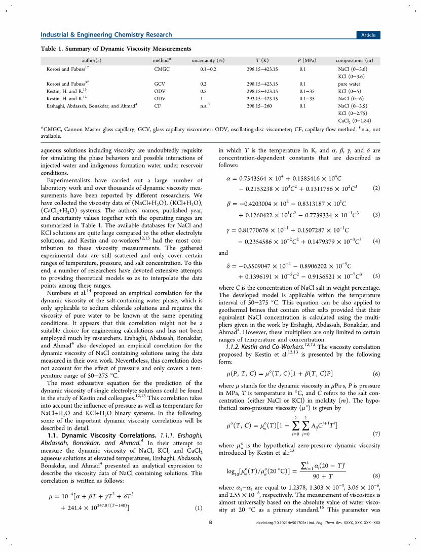
Table 1. Summary of Dynamic Viscosity Measurements

author(s) methoda uncertainty (%) T (K) P (MPa) compositions (m)

Korosi and Fabuss17 CMGC 0.1−0.2 298.15−423.15 0.1 NaCl (0−3.6)KCl (0−3.6)

Korosi and Fabuss37 GCV 0.2 298.15−423.15 0.1 pure waterKestin, H. and R.13 ODV 0.5 298.15−423.15 0.1−35 KCl (0−5)Kestin, H. and R.12 ODV 1 293.15−423.15 0.1−35 NaCl (0−6)Ershaghi, Abdassah, Bonakdar, and Ahmad4 CF n.a.b 298.15−260 0.1 NaCl (0−3.5)

KCl (0−2.75)CaCl2 (0−1.84)

aCMGC, Cannon Master glass capillary; GCV, glass capillary viscometer; ODV, oscillating-disc viscometer; CF, capillary flow method. bn.a., notavailable.

Industrial & Engineering Chemistry Research Article

dx.doi.org/10.1021/ie501702z | Ind. Eng. Chem. Res. XXXX, XXX, XXX−XXXB

determined by Swindells, Coe, and Godfrey16 to be around1002 μPa·s.The pressure coefficient (β) in eq 6 appears as a linear factor,

which can be calculated according to the following formula:

β β β β= * +T C C C T( , ) ( / ) ( )sE

s w (9)

where the pressure coefficient of water (βw) is defined by

∑β =−

=

T b T( ), GPai

ii

w1

0

4

(10)

The excess pressure coefficient (βsE) at salt saturation is only a

function of temperature and can be computed using thefollowing expression:

β λ λ β= + −−T T T( ), GPa ( )sE 1

1 2 w (11)

The concentration of salts at their saturation is expressed by

∑ θ==

C T T( )i

ii

s0

2

(12)

In addition, the reduced excess pressure coefficient (β*) isobtained by the following equation:

∑β γ* =−

=

C C GPa C C( / ), ( / )i

ii

s1

1

3

s(13)

In these equations, A, α, b, λ, θ, and γ are all constantsor vectors of constant parameters that are specific to a certainsingle electrolyte system, which can be obtained throughmultiple regression analyses. These parameters for KCl andNaCl were determined in the research study of Kestin, H. andR.12,13 Although this correlation takes into account the pressureeffect as compared to the correlation of Ershaghi, Abdassah,Bonakdar, and Ahmad,4 the results obtained in the work ofKorosi and Fabuss17 suggest that pressure has a rather negligibleeffect on the dynamic viscosity as long as the pressure is lowerthan 200 psig. This is probably the most comprehensive dynamicviscosity correlation presented so far, which can be extended toany electrolyte system aside from KCl and NaCl under thecircumstances that enough experimental data are available;however, for some specific salts such as MgSO4, the experi-mental data reported in the open sources are scarce and theaforementioned parameters are rather unidentifiable consideringthis data shortage.18

The methodologies introduced so far appear to work wellwithin wide temperature and pressure ranges but are stilllimited to single electrolyte systems. This fact could beattributed to the high costs associated with the design ofexperiments for measuring the dynamic viscosity in complex

systems in which a large number of components may exist. Toaddress these problems, new methodologies must be developedthat are capable of modeling precise viscosity values and take intoconsideration the concentrations of different salts in solution.Inductive machine learning algorithms as branches of

artificial intelligence have already been applied in providingapplicable solutions to a wide variety of industrial and scientificproblems.19,20 This study employs a fusion of two softcomputing techniques, namely artificial neural networks andfuzzy logic (FL), which is generally referred to as an adaptivenetwork based fuzzy inference system (ANFIS). The notionbehind this methodology lies in the fact that artificial neuralnetworks can learn the patterns within data, whereas fuzzy logiccan turn the observed patterns into linguistic if−then rules thatare more comprehensible than the patterns observed by neuralnetworks. Information regarding the fuzzy systems and theANFIS structure will be described shortly within this study. Thedeveloped model is capable of accurately determining thedynamic viscosity in multicomponent (Na, K, or Ca)Cl−H2Osystems over temperatures varying between 293.15 and 533.15 Kand pressure ranging from 0.1 to 35 MPa.

2. ADAPTIVE NETWORK BASED FUZZY INFERENCESYSTEM (ANFIS)

The complexity and heterogeneity of real systems haverendered the call for more sophisticated and more errortolerant modeling techniques.21 Modeling complicated systemswith exact and conventional mathematical tools may not bevery well suited considering the natural uncertainties associatedwith these systems.21−23 In recent years, soft computingtechniques such as artificial neural networks (ANNs) and fuzzysystems have successfully been applied in the robust modelingof complex real world problems.22,24,25

While debate exists regarding the precise definition of softcomputing, the stance adopted in this paper is that given byZadeh as follows:21 “Soft computing differs from conventional(hard) computing in that, unlike hard computing, it is tolerantof imprecision, uncertainty, and partial truth”. The concept offuzzy logic was introduced by Zadeh26 for modeling uncertainsystems. In contrast to classical logic, which is based on crispsystems of true and false, fuzzy logic perceives the problems as adegree of truth (defined as the membership degree in fuzzysets) or fuzzy sets of true and false.26

Modeling based on fuzzy logic is carried out using linguisticfuzzy if−then rules which provide an extraordinary methodfor qualitative process description without implementingprecise quantitative measures; however, designing such modelsrequires the proper and adequate knowledge about the problembeing considered.23

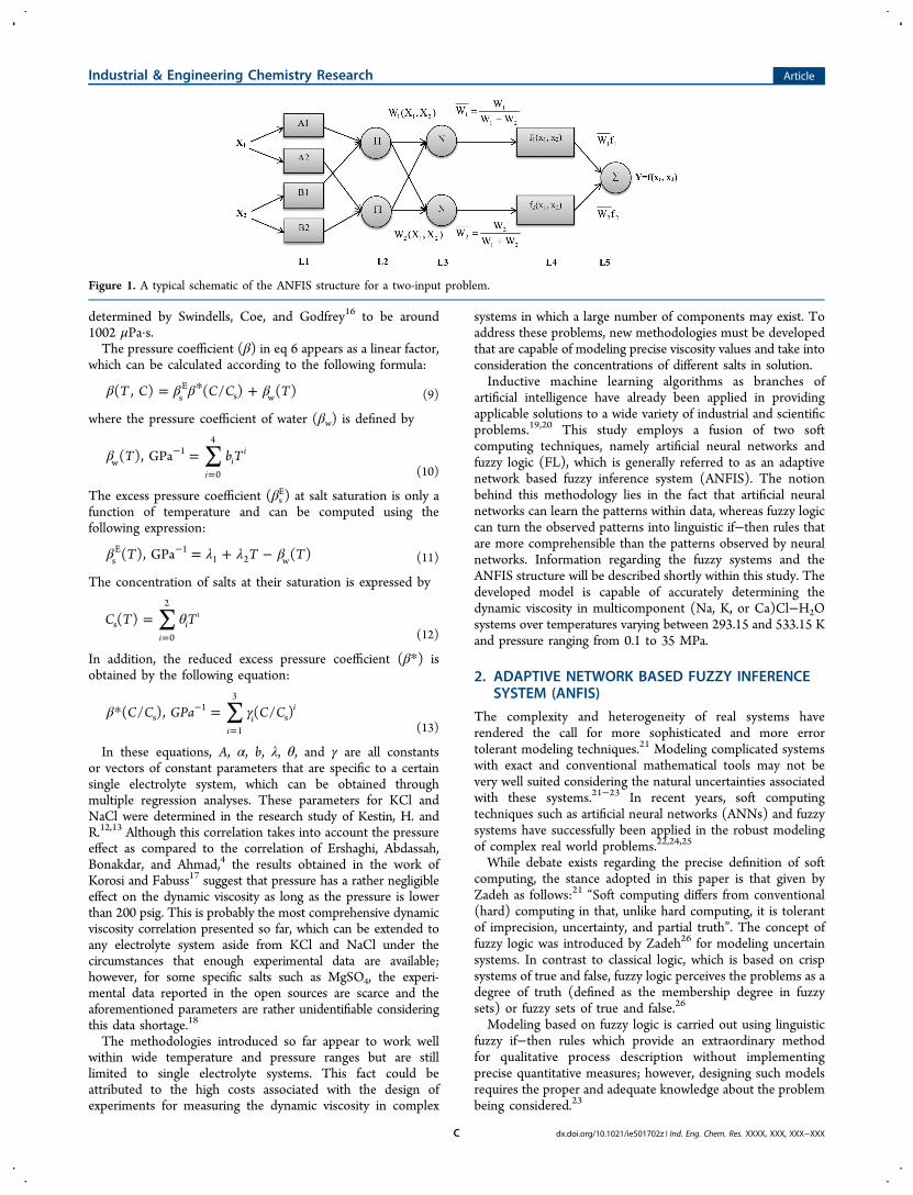
Figure 1. A typical schematic of the ANFIS structure for a two-input problem.


dx.doi.org/10.1021/ie501702z | Ind. Eng. Chem. Res. XXXX, XXX, XXX−XXXC

In most cases, the expert knowledge used as the basis ofdesigning fuzzy systems is inadequate or uncertain, mainlyowing to an incompleteness of existing knowledge and differentbiases of human experts. This is where data-driven soft com-puting techniques such as ANNs may be thought of as greatalternatives since they can learn the required knowledge fromavailable databases.23 Fuzzy logic can be subsequently imple-mented to describe the learned patterns in linguistic if−thenrules that are easy to comprehend. In fact, ANN and FL canbe looked upon as complementary methods.The cardinal part of ANFIS comes from a common frame-

work referred to as adaptive networks, which combines bothfuzzy models and neural networks. Fuzzy inference systems(FISs) can serve as the basis for defining a set of fuzzy if−thenrules and membership functions (MFs), which are then fine-tuned using the learning capabilities of intelligence systems(e.g., ANNs).22,23 Owing to the fact that ANFIS can achieve asuccessful nonlinear mapping of input−output data pairs, it isthen very well suited for the problem of modeling the viscosityfor multicomponent aqueous mixtures.Two types of FIS structures have been proposed in the

literature, namely Mamdani and Takagi−Sugeno−Kang(TSK).23 While the former deals with a subjective definitionof fuzzy if−then rules using expert statements, the latterprovides a framework for generating these rules from input andoutput numerical data. Owing to the fact that a subjectivedefinition of fuzzy rules may bring in vagueness and impre-cision, ANFISs utilize the TSK fuzzy structures for successfulnonlinear mapping of input and output patterns.21−23

Figure 1 represents a constructed ANFIS for a two-inputsystem. In this figure, β functions represent the degrees ofmembership of each variable in the constructed fuzzy sets, X1and X2 indicate the inputs, and Y is the output. Assuming a firstorder TSK FIS, a fuzzy model can be generated according tothe following rules:23

Rule I:

= + +X A X B f m X n X rIF is and is THEN1 1 2 1 1 1 1 1 2 1

(14)

Rule II:


(15)

Rule III:


(16)

Rule IV:


(17)

where A1,2 and B1,2 are respective fuzzy sets of X1 and X2.Conditions stipulated in the IF part are generally known asantecedent, and those in the THEN part are called theconsequence. According to Lee,23 a typical ANFIS is normallycomposed of five different layers.Layer 1. In this layer, crisp input data given into the system

are converted into fuzzy numbers or linguistic terms. Forexample, in the schematic diagram shown in Figure 1, X1 and X2are both connected to two nodes, meaning that two linguisticterms or fuzzy sets have been defined for each of these inputs.

This step, which is also referred to as the fuzzification layer,constructs fuzzy sets based on predefined MFs. Althoughthe selection of the MF is not limited and is more of a case-dependent issue, Gaussian MFs are more preferred fornonlinear regression problems because they lead to a smoothmodel behavior. Gaussian MFs implemented in this study aredefined according to the following expression:

βσ

= = − −⎛⎝⎜

⎞⎠⎟O X

X Z( ) exp

12

( )i1

2

2(18)

in which O represents the layer outputs, Z defines the Gaussiancenter, and σ2 stands for the variance. Gaussian parameters arefinally tuned by the ANFIS to obtain more robust and accuratepredictions.

Layer 2. This layer calculates the degree of correctness orapplicability of the statements stipulated in antecedent parts,which is also called the firing strength, according to thefollowing relationship:23

β β= = ·O W X X( ) ( )i i i i2

A B (19)

Layer 3. Each of the firing strengths calculated in theprevious layer (Wi), are normalized in this layer to make adistinction between the firing strength of each rule and theentire firing strengths of all rules as given below:

=∑

OW

Wii

i i

3

(20)

Layer 4. Like the first layer, nodes of this layer (also knownas the consequent layer) represent the linguistic terms of theoutput variable (which is the viscosity of aqueous solutions inthe current study). The contribution of each rule toward thetotal output is described as

= = + +O Wf W m X n X r( )i i i i i i i4

1 2 (21)

where mi, ni, and ri are called consequent or linear param-eters. These parameters, along with the parameters men-tioned in the first layer, are tuned during the learning processto attain a better match between real targets and ANFISoutputs.

Layer 5. This layer is called the defuzzification layer wherethe total number of rules defined for one output are aggregatedand defuzzified into numerical outputs through a weightedaverage sum given below:

∑= = = + =∑∑

O Y Wf W f W fWf

Wii

i ii i i

i i

51 1 2 2

(22)

3. BUILDING THE ANFIS MODEL FOR DYNAMICVISCOSITY PREDICTION3.1. Data Acquisition and Statistical Summary. To

build a reliable and accurate model capable of predicting theviscosity of aqueous electrolyte solutions at high temperaturesand pressures, comprehensive (covering wide ranges of opera-tional conditions) and accurate experimental data are required.To this end, an aggregate number of 5537 published data weregathered from the open literature to assemble an exhaustivedatabase. According to the references provided in Table 1,water viscosity appears to be a function of temperature, pres-sure, and strong electrolyte concentrations in water as ex-pressed below:


dx.doi.org/10.1021/ie501702z | Ind. Eng. Chem. Res. XXXX, XXX, XXX−XXXD

μ = f T P C C C( , , , , )w NaCl KCl CaCl2 (23)

The assembled data set was initially divided by performing arandom permutation into three subsets, namely “train,” “check,”and “test”. To increase the model applicability and robustnessand to reduce the chance of bias in the connectionist model,the collected database was divided randomly into 70%, 15%,and 15% fractions for the train set (3876), check set (831), andtest set (830), respectively. The train set was used to train themodel to capture the dominant patterns among the data; theseries of check data was used to evaluate the model perfor-mance during the learning process to ascertain that overfittingwould not occur; and finally, the test phase was conducted toevaluate the model generalization capability for unseen dataafter its successful training process. The statistical information

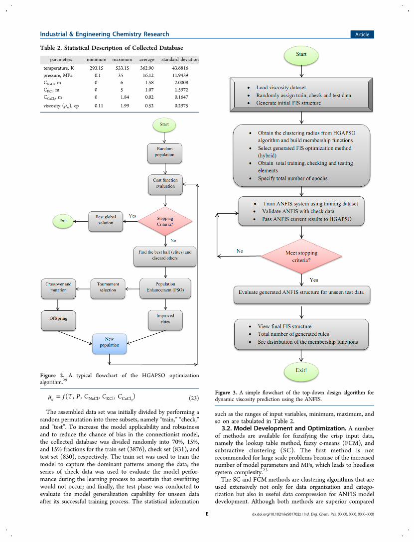
such as the ranges of input variables, minimum, maximum, andso on are tabulated in Table 2.

3.2. Model Development and Optimization. A numberof methods are available for fuzzifying the crisp input data,namely the lookup table method, fuzzy c-means (FCM), andsubtractive clustering (SC). The first method is notrecommended for large scale problems because of the increasednumber of model parameters and MFs, which leads to heedlesssystem complexity.23

The SC and FCM methods are clustering algorithms that areused extensively not only for data organization and catego-rization but also in useful data compression for ANFIS modeldevelopment. Although both methods are superior compared

Table 2. Statistical Description of Collected Database

parameters minimum maximum average standard deviation

temperature, K 293.15 533.15 362.90 43.6816pressure, MPa 0.1 35 16.12 11.9439CNaCl, m 0 6 1.58 2.0008CKCl, m 0 5 1.07 1.5972CCaCl2, m 0 1.84 0.02 0.1647

viscosity (μw), cp 0.11 1.99 0.52 0.2975

Figure 2. A typical flowchart of the HGAPSO optimizationalgorithm.29

Figure 3. A simple flowchart of the top-down design algorithm fordynamic viscosity prediction using the ANFIS.


dx.doi.org/10.1021/ie501702z | Ind. Eng. Chem. Res. XXXX, XXX, XXX−XXXE

to lookup table methodology, most studies have preferred SCover the FCM method.21−23

FCM is a clustering method in which each data belongs to acluster with a degree specified by its MF. The center of theclusters is found in an iterative process during which the valueof an objective function known as mountain function is mini-mized within a number of epochs. Nevertheless, computationsgrow exponentially with the increasing dimension of the problem,mainly because the algorithm evaluates the mountain functionover all of the grid points.22 The SC method proposed by Chiu27

was utilized in this study because of its simple calculation proce-dure and its independence of the problem dimensionality.Despite FCM, the SC method considers the data points as

cluster centers instead of grid points with an effective clusterradius.22 This effective radius was optimized in this work by theemployment of the hybrid of the genetic algorithm (GA) and

particle swarm optimization (PSO), generally known as theHGAPSO algorithm.

3.3. Hybrid of Genetic Algorithm and Particle SwarmOptimization (HGAPSO). 3.3.1. Genetic Algorithm (GA).The GA is one of the evolutionary optimization techniquesdeveloped by John Holland over the course of the 1960s and1970s and is based on the genetic theory and natural selection.28

In a search for the optimum solution, the GA constructs a candi-date list of solutions to the problem, which are referred to asindividuals or chromosomes. Each individual represents a point inthe search domain and thus holds a list of candidate solutions.29

Each solution could be encoded as a binary string of real-valued coefficients, which are then evaluated using a perfor-mance function (or objective function). Wright30 claimed thatthe use of real-valued genes offers a number of advantages innumerical function optimizations over binary encodings. In fact,

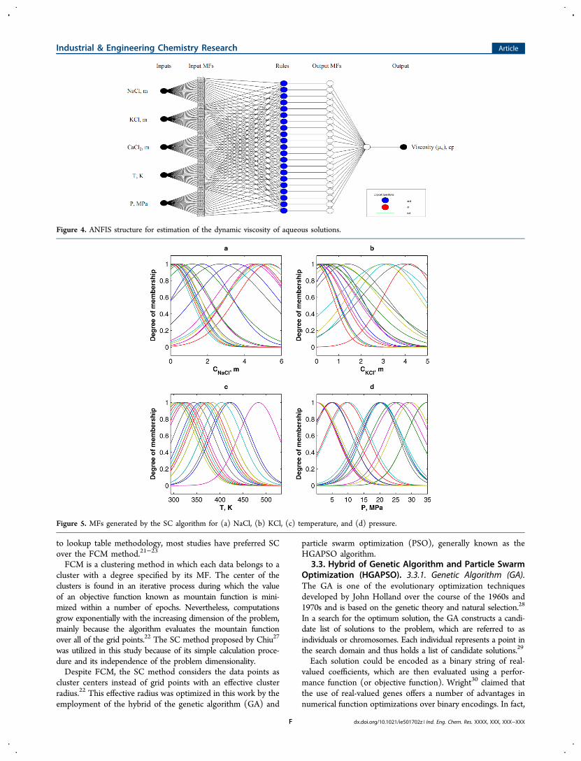
Figure 4. ANFIS structure for estimation of the dynamic viscosity of aqueous solutions.

Figure 5. MFs generated by the SC algorithm for (a) NaCl, (b) KCl, (c) temperature, and (d) pressure.


dx.doi.org/10.1021/ie501702z | Ind. Eng. Chem. Res. XXXX, XXX, XXX−XXXF

the real-valued GA tends to be inherently faster than the binaryGA because the chromosomes do not need to be decoded priorto the objective function (or cost function in minimizationproblems) evaluation.28 Individuals in the population are thensorted according to their costs and then, usually with the use ofa selection algorithm, random pairs of better individuals areselected and a new population is reproduced using GA basiccrossover and mutation operators.The crossover operator produces two offspring (two new

individuals) through recombining the genetic information ofthe parents.29 The mutation is applied to alter the geneticstructure of the individuals within chromosomes and to avoidthe problem of fast convergence to local minima by introducingsome changes to the genes or variables.28,31

3.3.2. Particle Swarm Optimization (PSO). Particle swarmoptimization is one of the latest evolutionary optimizationtechniques, developed by Eberhart and Kennedy,32 which isinspired by the coordinated motion of animals such as birdflocking or fish schooling. Like the GA, PSO is a population-based stochastic algorithm that is initialized with random initialpopulations possessing random positions and random velocitiesin a multidimensional search space.The particles, which are also the candidate solutions to the

optimization problem, fly around in the search space inan effort to find the optimum solution. The theory of PSOdescribes an iterative solution process in which each particle’svelocity and position in space is constantly updated accordingto previous best performance of the particle or its neigh-borhood (i.e., cognitive behavior), as well as the best per-formance of the particles in the entire population (i.e., socialbehavior). The PSO algorithm can be formulated as follows:33

α α= + − + −+v w v c x c x(Pb ) (Gb )ij j

ij j

ij

ij j

ij

ij1

1 1 2 2 (24)

= ++ +x x vij

ij

ij1 1

(25)

where vij and xi

j represent velocity and position vectors of the ithparticle at iteration j, respectively. Pbi is the personal best ofeach individual in the population, while Gbi is the global bestposition found in the entire population. The parameters α1,2 ∈[0,1] are vectors of uniformly distributed random numbers, α1,2are acceleration constants, and w is called the inertia weight.Inertia weight was introduced by Shi and Eberhart34 into

eq 24 in order to dampen the natural tendency of standard PSOto explode at higher oscillations. Reducing w over time resultsin a shift from an exploratory to an exploitative search furtherguaranteeing convergence toward the global minima. Ingeneral, w reduces linearly with the iteration number, fromwinitial to wfinal:

34

=− × −

+wj j w w

jw

( ) ( )j max initial final

maxfinal

(26)

in which jmax indicates the maximum number of iterationsperformed. A good starting point would be to set winitial to0.9 and wfinal to 0.4.33

3.3.3. HGAPSO Algorithm. Compared to the GA, PSO has anumber of appealing characteristics. PSO is probably the onlyevolutionary algorithm that does not employ survival of thefittest;33 therefore, both low- and high-value individuals surviveduring the search and could explore any point in the featurespace.35 Thus, in PSO, knowledge of good solutions is retainedby all particles during the construction of several genera-tions, and no information is discarded as compared to GA.

Information sharing mechanisms are also completely differ-ent.35,36 Information in PSO is only disseminated by a globalbest particle and thus is directional; nevertheless, in the GA,this information is shared among all chromosomes and thewhole population moves toward the optimum solution.29

In general, all individuals in PSO belong to the samegeneration, and optimization proceeds on the basis of the socialadaptation of knowledge. On the other hand, the GA operateson the basis of evolution from one generation to the other, andindividual adaptations in a single generation are not con-sidered.29 It appears that a hybridization of the GA and PSOcould compensate for the deficiencies associated with eachalgorithm. In the GA, individuals are reproduced or selected aselite parents for the next generation without being enhanced;however, all of the individuals in nature adapt to thesurrounding environment as they grow up prior to producing

Figure 6. Plot of ANFIS errors versus total number of epochs.

Figure 7. Regression plot of ANFIS predictions of viscosity valuesversus observed values.


dx.doi.org/10.1021/ie501702z | Ind. Eng. Chem. Res. XXXX, XXX, XXX−XXXG

any offspring.29 Individuals improved by the knowledge sharingproperty of PSO tend to produce better offspring than the originalones. Furthermore, computations of PSO are easy and add a slightcomputational burden when coupled with the GA, which in turnmight also obviate the premature convergence of the individualPSO algorithm by mutating the stagnant particles.29

Taking into account the previous discussion on the meritsand demerits of both algorithms, the hybrid of the GA and PSOappears to introduce a maturing property into the populationfrom the GA perspective and increase diversity among theindividuals from the PSO perspective so that the evolution ofindividuals is no longer restricted to be in the same generation.

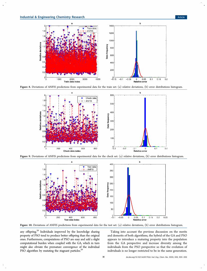
Figure 8. Deviations of ANFIS predictions from experimental data for the train set: (a) relative deviations, (b) error distributions histogram.

Figure 9. Deviations of ANFIS predictions from experimental data for the check set: (a) relative deviations, (b) error distributions histogram.

Figure 10. Deviations of ANFIS predictions from experimental data for the test set: (a) relative deviations, (b) error distributions histogram.


dx.doi.org/10.1021/ie501702z | Ind. Eng. Chem. Res. XXXX, XXX, XXX−XXXH

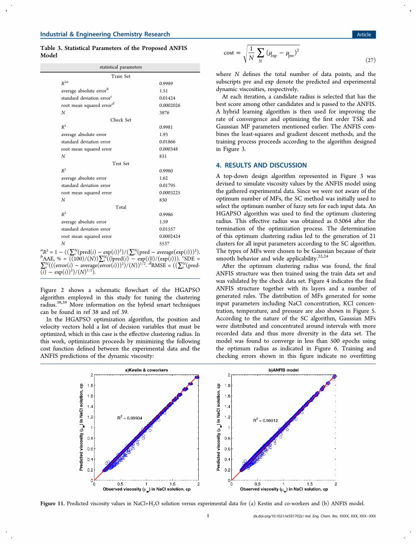
Figure 2 shows a schematic flowchart of the HGAPSOalgorithm employed in this study for tuning the clusteringradius.38,39 More information on the hybrid smart techniquescan be found in ref 38 and ref 39.In the HGAPSO optimization algorithm, the position and

velocity vectors hold a list of decision variables that must beoptimized, which in this case is the effective clustering radius. Inthis work, optimization proceeds by minimizing the followingcost function defined between the experimental data and theANFIS predictions of the dynamic viscosity:

∑ μ μ= −N

cost1

( )N

exp pre2

(27)

where N defines the total number of data points, and thesubscripts pre and exp denote the predicted and experimentaldynamic viscosities, respectively.At each iteration, a candidate radius is selected that has the

best score among other candidates and is passed to the ANFIS.A hybrid learning algorithm is then used for improving therate of convergence and optimizing the first order TSK andGaussian MF parameters mentioned earlier. The ANFIS com-bines the least-squares and gradient descent methods, and thetraining process proceeds according to the algorithm designedin Figure 3.

4. RESULTS AND DISCUSSION

A top-down design algorithm represented in Figure 3 wasdevised to simulate viscosity values by the ANFIS model usingthe gathered experimental data. Since we were not aware of theoptimum number of MFs, the SC method was initially used toselect the optimum number of fuzzy sets for each input data. AnHGAPSO algorithm was used to find the optimum clusteringradius. This effective radius was obtained as 0.5064 after thetermination of the optimization process. The determinationof this optimum clustering radius led to the generation of 21clusters for all input parameters according to the SC algorithm.The types of MFs were chosen to be Gaussian because of theirsmooth behavior and wide applicability.22,24

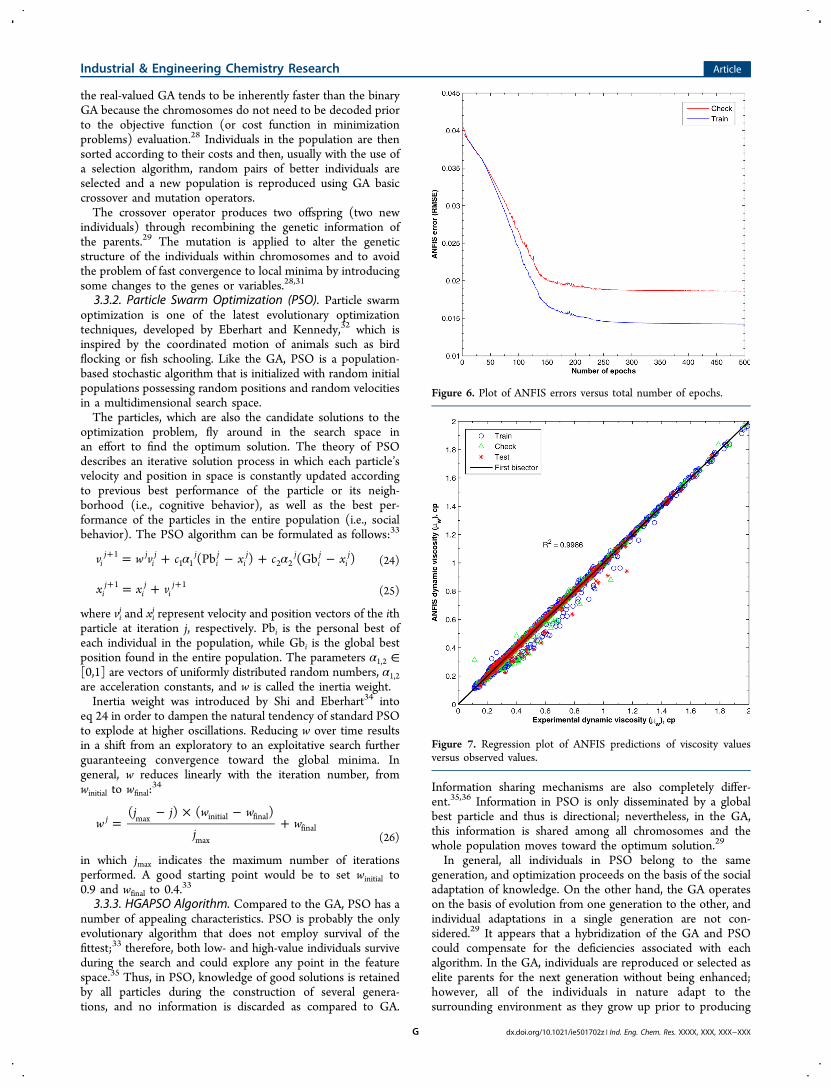
After the optimum clustering radius was found, the finalANFIS structure was then trained using the train data set andwas validated by the check data set. Figure 4 indicates the finalANFIS structure together with its layers and a number ofgenerated rules. The distribution of MFs generated for someinput parameters including NaCl concentration, KCl concen-tration, temperature, and pressure are also shown in Figure 5.According to the nature of the SC algorithm, Gaussian MFswere distributed and concentrated around intervals with morerecorded data and thus more diversity in the data set. Themodel was found to converge in less than 500 epochs usingthe optimum radius as indicated in Figure 6. Training andchecking errors shown in this figure indicate no overfitting

Table 3. Statistical Parameters of the Proposed ANFISModel

statistical parameters

Train SetR2a 0.9989average absolute errorb 1.51standard deviation errorc 0.01424root mean squared errord 0.0002026N 3876

Check SetR2 0.9981average absolute error 1.93standard deviation error 0.01866root mean squared error 0.000348N 831

Test SetR2 0.9980average absolute error 1.62standard deviation error 0.01795root mean squared error 0.0003225N 830

TotalR2 0.9986average absolute error 1.59standard deviation error 0.01557root mean squared error 0.0002424N 5537

aR2 = 1 − ((∑iN(pred(i) − exp(i))2)/(∑i

N(pred − average(exp(i)))2).bAAE, % = ((100)/(N))∑i

N((|pred(i) − exp(i)|)/(exp(i))). cSDE =∑i

N(((error(i) − average(error(i)))2)/(N))1/2. dRMSE = ((∑iN(pred-

(i) − exp(i))2)/(N)1/2).

Figure 11. Predicted viscosity values in NaCl+H2O solution versus experimental data for (a) Kestin and co-workers and (b) ANFIS model.


dx.doi.org/10.1021/ie501702z | Ind. Eng. Chem. Res. XXXX, XXX, XXX−XXXI

during the training process as both follow approximately thesame trends.The constructed model for viscosity prediction was also

compared to the experimental values for the train, check, andtest sets shown in Figure 7. The concentration of points alongthe 45° line shows an excellent accordance between the modelpredictions and the observed experimental values. Figures 8−10indicate the relative deviations and error distributions of thetrain, check, and test sets, respectively. Predicted viscosityvalues almost overlap with the experimentally recorded data,revealing a satisfactory agreement. Error distribution histogramsalso corroborate this accordance by showing a Gaussian normaldistribution around zero. Statistical parameters showing modelaccuracy and robustness were also calculated. These parame-ters, which are the squared correlation coefficient (R2), averageabsolute error (AAE), root mean squared error (RMSE), andstandard deviation error (SDE) are summarized in Table 3. Anoverall correlation coefficient of 0.9986 and an average absoluteerror of 1.59% indicate excellent accordance between viscosityvalues predicted by the ANFIS and their respectiveexperimental values. The overall RMSE value of 0.0002424and SDE value of 0.01557 also support this acceptable match.The dynamic viscosity values predicted by the ANFIS model

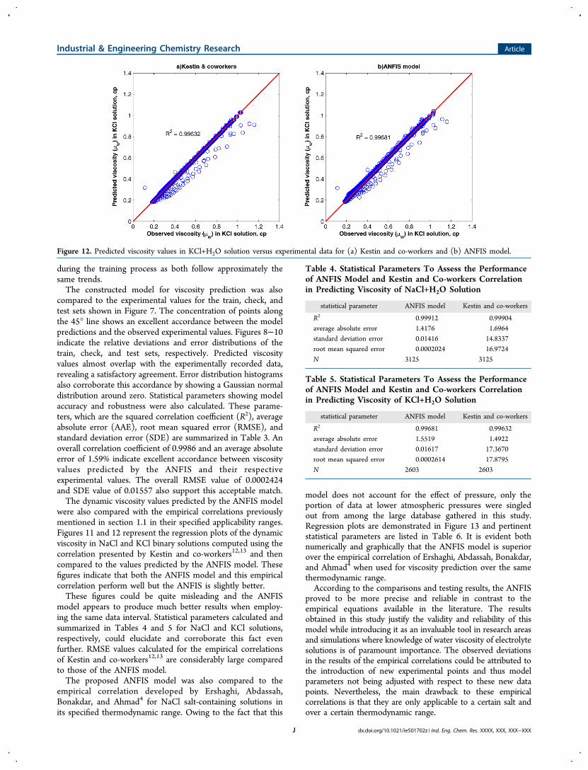
were also compared with the empirical correlations previouslymentioned in section 1.1 in their specified applicability ranges.Figures 11 and 12 represent the regression plots of the dynamicviscosity in NaCl and KCl binary solutions computed using thecorrelation presented by Kestin and co-workers12,13 and thencompared to the values predicted by the ANFIS model. Thesefigures indicate that both the ANFIS model and this empiricalcorrelation perform well but the ANFIS is slightly better.These figures could be quite misleading and the ANFIS

model appears to produce much better results when employ-ing the same data interval. Statistical parameters calculated andsummarized in Tables 4 and 5 for NaCl and KCl solutions,respectively, could elucidate and corroborate this fact evenfurther. RMSE values calculated for the empirical correlationsof Kestin and co-workers12,13 are considerably large comparedto those of the ANFIS model.The proposed ANFIS model was also compared to the

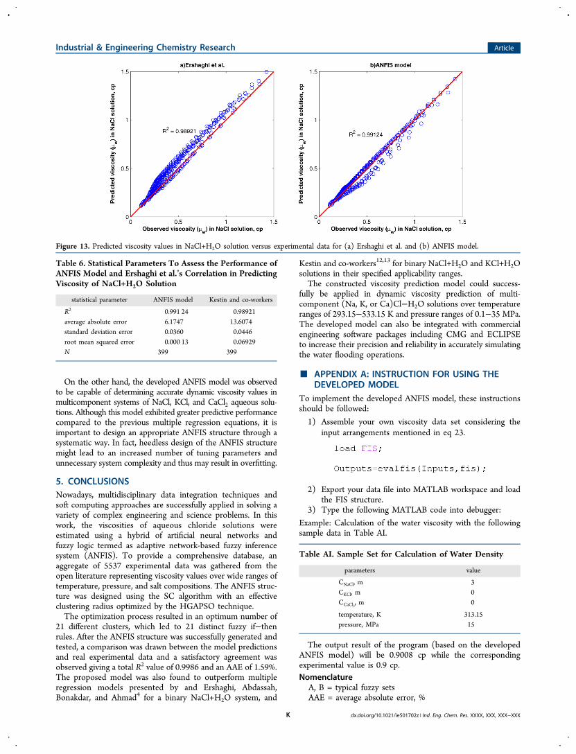
empirical correlation developed by Ershaghi, Abdassah,Bonakdar, and Ahmad4 for NaCl salt-containing solutions inits specified thermodynamic range. Owing to the fact that this

model does not account for the effect of pressure, only theportion of data at lower atmospheric pressures were singledout from among the large database gathered in this study.Regression plots are demonstrated in Figure 13 and pertinentstatistical parameters are listed in Table 6. It is evident bothnumerically and graphically that the ANFIS model is superiorover the empirical correlation of Ershaghi, Abdassah, Bonakdar,and Ahmad4 when used for viscosity prediction over the samethermodynamic range.According to the comparisons and testing results, the ANFIS

proved to be more precise and reliable in contrast to theempirical equations available in the literature. The resultsobtained in this study justify the validity and reliability of thismodel while introducing it as an invaluable tool in research areasand simulations where knowledge of water viscosity of electrolytesolutions is of paramount importance. The observed deviationsin the results of the empirical correlations could be attributed tothe introduction of new experimental points and thus modelparameters not being adjusted with respect to these new datapoints. Nevertheless, the main drawback to these empiricalcorrelations is that they are only applicable to a certain salt andover a certain thermodynamic range.

Figure 12. Predicted viscosity values in KCl+H2O solution versus experimental data for (a) Kestin and co-workers and (b) ANFIS model.

Table 4. Statistical Parameters To Assess the Performanceof ANFIS Model and Kestin and Co-workers Correlationin Predicting Viscosity of NaCl+H2O Solution

statistical parameter ANFIS model Kestin and co-workers

R2 0.99912 0.99904average absolute error 1.4176 1.6964standard deviation error 0.01416 14.8337root mean squared error 0.0002024 16.9724N 3125 3125

Table 5. Statistical Parameters To Assess the Performanceof ANFIS Model and Kestin and Co-workers Correlationin Predicting Viscosity of KCl+H2O Solution


R2 0.99681 0.99632average absolute error 1.5519 1.4922standard deviation error 0.01617 17.3670root mean squared error 0.0002614 17.8795N 2603 2603


dx.doi.org/10.1021/ie501702z | Ind. Eng. Chem. Res. XXXX, XXX, XXX−XXXJ

On the other hand, the developed ANFIS model was observedto be capable of determining accurate dynamic viscosity values inmulticomponent systems of NaCl, KCl, and CaCl2 aqueous solu-tions. Although this model exhibited greater predictive performancecompared to the previous multiple regression equations, it isimportant to design an appropriate ANFIS structure through asystematic way. In fact, heedless design of the ANFIS structuremight lead to an increased number of tuning parameters andunnecessary system complexity and thus may result in overfitting.

5. CONCLUSIONSNowadays, multidisciplinary data integration techniques andsoft computing approaches are successfully applied in solving avariety of complex engineering and science problems. In thiswork, the viscosities of aqueous chloride solutions wereestimated using a hybrid of artificial neural networks andfuzzy logic termed as adaptive network-based fuzzy inferencesystem (ANFIS). To provide a comprehensive database, anaggregate of 5537 experimental data was gathered from theopen literature representing viscosity values over wide ranges oftemperature, pressure, and salt compositions. The ANFIS struc-ture was designed using the SC algorithm with an effectiveclustering radius optimized by the HGAPSO technique.The optimization process resulted in an optimum number of

21 different clusters, which led to 21 distinct fuzzy if−thenrules. After the ANFIS structure was successfully generated andtested, a comparison was drawn between the model predictionsand real experimental data and a satisfactory agreement wasobserved giving a total R2 value of 0.9986 and an AAE of 1.59%.The proposed model was also found to outperform multipleregression models presented by and Ershaghi, Abdassah,Bonakdar, and Ahmad4 for a binary NaCl+H2O system, and

Kestin and co-workers12,13 for binary NaCl+H2O and KCl+H2Osolutions in their specified applicability ranges.The constructed viscosity prediction model could success-

fully be applied in dynamic viscosity prediction of multi-component (Na, K, or Ca)Cl−H2O solutions over temperatureranges of 293.15−533.15 K and pressure ranges of 0.1−35 MPa.The developed model can also be integrated with commercialengineering software packages including CMG and ECLIPSEto increase their precision and reliability in accurately simulatingthe water flooding operations.

■ APPENDIX A: INSTRUCTION FOR USING THEDEVELOPED MODEL

To implement the developed ANFIS model, these instructionsshould be followed:

1) Assemble your own viscosity data set considering theinput arrangements mentioned in eq 23.

2) Export your data file into MATLAB workspace and loadthe FIS structure.

3) Type the following MATLAB code into debugger:

Example: Calculation of the water viscosity with the followingsample data in Table AI.

The output result of the program (based on the developedANFIS model) will be 0.9008 cp while the correspondingexperimental value is 0.9 cp.Nomenclature

A, B = typical fuzzy setsAAE = average absolute error, %

Figure 13. Predicted viscosity values in NaCl+H2O solution versus experimental data for (a) Ershaghi et al. and (b) ANFIS model.

Table 6. Statistical Parameters To Assess the Performance ofANFIS Model and Ershaghi et al.’s Correlation in PredictingViscosity of NaCl+H2O Solution


R2 0.991 24 0.98921average absolute error 6.1747 13.6074standard deviation error 0.0360 0.0446root mean squared error 0.000 13 0.06929N 399 399

Table AI. Sample Set for Calculation of Water Density

parameters value

CNaCl, m 3CKCl, m 0CCaCl2, m 0

temperature, K 313.15pressure, MPa 15


dx.doi.org/10.1021/ie501702z | Ind. Eng. Chem. Res. XXXX, XXX, XXX−XXXK

ANFIS = adaptive network-based fuzzy inference systemANN = artificial neural networkC = concentration, mFCM = fuzzy c-meansFIS = fuzzy inference systemFL = fuzzy logicGbi

j = global best of particle i at iteration jMF = membership functionP = pressure, MPaPbi

j = personal best of particle i at iteration jR2 = squared correlation coefficientRMSE = root mean squared errorSC = subtractive clusteringSDE = standard deviation errorT = temperature, Kv = velocity vectorW = weight associated with each rulew = inertia weightX = input patternsx = position vectorY = output patternsZ = Gaussian centers

Greek Symbolsβ = membership degreesμ = dynamic viscosity, cpσ = standard deviation in Gaussian functions

■ AUTHOR INFORMATION

Corresponding Authors*E-mail: [email protected].*E-mail: [email protected].

NotesThe authors declare no competing financial interest.

■ REFERENCES(1) Francke, H.; Thorade, M. Density and Viscosity of Brine: AnOverview from a Process Engineers Perspective. Chem. Erde 2010, 70(Suppl. 3, (0)), 23−32.(2) Konigsberger, E.; Konigsberger, L. C.; May, P.; Harris, B.Properties of Electrolyte Solutions Relevant to High ConcentrationChloride Leaching. II. Density, Viscosity, and Heat Capacity of MixedAqueous Solutions of Magnesium Chloride and Nickel ChlorideMeasured to 90 °C. Hydrometallurgy 2008, 90 (2−4), 168−176.(3) Abdulagatov, I. M.; Zeinalova, A.; Azizov, N. D. Viscosity ofAqueous Na2SO4 Solutions at Temperatures from 298 to 573 K and atPressures up to 40 MPa. Fluid Phase Equilib. 2005, 227 (1), 57−70.(4) Ershaghi, I.; Abdassah, D.; Bonakdar, M.; Ahmad, S. Estimationof Geothermal Brine Viscosity. J. Pet. Technol. 1983, 35, 621−628.(5) Ophori, D. U. Flow of Groundwater with Variable Density andViscosity, Atikokan Research Area, Canada. Hydrogeol. J. 1998, 6 (2),193−203.(6) Kestin, J.; Wang, H. Corrections for the Oscillating DiskViscometer. J. Appl. Mech. 1957, 79, 197−206.(7) Magri, F.; Bayer, U.; Clausnitzer, V.; Jahnke, C.; Diersch, H. J.;Fuhrmann, J.; Moller, P.; Pekdeger, A.; Tesmer, M.; Voigt, H. DeepReaching Fluid Flow Close to Convective Instability in the NEGerman BasinResults from Water Chemistry and NumericalModelling. Tectonophysics 2005, 397 (1−2), 5−20.(8) Yidana, M. S. Groundwater Flow Modeling and Particle Trackingfor Chemical Transport in the Southern Voltaian Aquifers. Environ.Earth Sci. 2011, 63 (4), 709−721.(9) Yidana, M. S.; Ophori, D.; Alo, C. A. HydrogeologicalCharacterization of a Tropical Crystalline Aquifer System. J. Appl.Water Eng. Res. 2014, 1−12.

(10) Jamialahmadi, M.; Muller-Steinhagen, H. Mechanisms of ScaleDeposition and Scale Removal in Porous Media. Int. J. Oil, Gas CoalTechnol. 2008, 1, 81−108.(11) Safari, H.; Jamialahmadi, M. Thermodynamics, Kinetics, andHydrodynamics of Mixed Salt Precipitation in Porous Media: ModelDevelopment and Parameter Estimation. Transp. Porous Media 2014,101 (3), 477−505.(12) Kestin, J.; Khalifa, H. E.; Correia, R. J. Tables of Dynamic andKinematic Viscosity of Aqueous NaCl Solutions in the TemperatureRange 20−150 °C and the Pressure Range 0.1−35 MPa. Phys. Chem.1981, 10 (1), 71−87.(13) Kestin, J.; Khalifa, H. E.; Correia, R. J. Tables of Dynamic andKinematic Viscosity of Aqueous KCl Solutions in the TemperatureRange 25−150 °C and the Pressure Range 0.1−35 MPa. Phys. Chem.1981, 10 (1), 57−70.(14) Numbere, D.; Bringham, W. E.; Standing, M. B. Correlations forthe Physical Properties of Petroleum Reservoir Brines; StanfordUniversity: Stanford, CA, 1977.(15) Kestin, J.; Sokolov, M.; Wakeham, W. A. Viscosity of LiquidWater in the Range −8 to 150 °C. J. Phys. Chem. Ref. Data 1978, 7,941.(16) Swindells, J. F.; Coe, J. R.; Godfrey, T. B. Absolute Viscosity ofWater at 20 °C. J. Res. Natl. Bur. Stand. 1952, 48 (1), 1−31.(17) Korosi, A.; Fabuss, B. M. Viscosities of Binary AqueousSolutions of Sodium Chloride, Potassium Chloride, Sodium Sulfate,and Magnesium Sulfate at Concentrations and Temperatures ofInterest in Desalination Processes. J. Chem. Eng. Data 1968, 13 (4),548−552.(18) Bedrikovetsky, P.; Siqueira, F.; Furtado, C.; Souza, A. ModifiedParticle Detachment Model for Colloidal Transport in Porous Media.Transp. Porous Media 2011, 86 (2), 353−383.(19) Safari, H.; Gharagheizi, F.; Lemraski, A.; Jamialahmadi, M.;Mohammadi, A.; Ebrahimi, M. Rigorous Modeling of GypsumSolubility in Na-Ca-Mg-Fe-Al-H-Cl-H2O System at Elevated Temper-atures. Neural Comput. Appl. 2014, 1−11.(20) Eslamimanesh, A.; Gharagheizi, F.; Mohammadi, A. H.; Richon,D. Assessment Test of Sulfur Content of Gases. Fuel Process. Technol.2013, 110 (0), 133−140.(21) Nikravesh, M.; Aminzadeh, F.; Zadeh, L. A. Soft Computing andIntelligent Data Analysis in Oil Exploration; Elsevier: Amsterdam, TheNetherlands, 2003; Vol. 51, pp 3−724, http://www.sciencedirect.com/science/book/9780444506856.(22) Jang, J. S. R.; Sun, C. T.; Mizutani, E. Neuro-Fuzzy and SoftComputing: A Computational Approach to Learning and MachineIntelligence; Prentice Hall: Upper Saddle River, New Jersey, 1997.(23) Lee, K. H. First Course on Fuzzy Theory and Applications;Springer: New York, 2005.(24) Dursun, O. F.; Kaya, N.; Firat, M. Estimating DischargeCoefficient of Semi-elliptical Side Weir Using ANFIS. J. Hydrol. 2012,426−427 (0), 55−62.(25) Tahseen, T. A.; Ishak, M.; Rahman, M. M. PerformancePredictions of Laminar Heat Transfer and Pressure Drop in an In-LineFlat Tube Bundle Using an Adaptive Neuro-Fuzzy Inference System(ANFIS) Model. Int. Commun. Heat Mass Transfer 2014, 50 (0), 85−97.(26) Zadeh, L. A. Fuzzy Sets. Inf. Control 1965, 8 (3), 338−353.(27) Chiu, S. Fuzzy Model Identification Based on ClusterEstimation. J. Intell. Fuzzy Syst. 1994, 2, 267−278.(28) Haupt, R. L.; Haupt, S. E. Practical Genetic Algorithms; Wiley:New York, 2004.(29) Juang, C.-F. A Hybrid of Genetic Algorithm and Particle SwarmOptimization for Recurrent Network Design. Trans. Syst. Man Cybern.,Part B 2004, 34 (2), 997−1006.(30) Wright, A. H. Genetic Algorithms for Real ParameterOptimization. Found. Genet. Algorithms 1991, 1, 205−218.(31) Safari, H.; Jamialahmadi, M. Estimating the Kinetic ParametersRegarding Barium Sulfate Deposition in Porous Media: A GeneticAlgorithm Approach. Asia-Pac. J. Chem. Eng. 2014, 9 (2), 256−264.


dx.doi.org/10.1021/ie501702z | Ind. Eng. Chem. Res. XXXX, XXX, XXX−XXXL

mailto:[email protected]

mailto:[email protected]

http://www.sciencedirect.com/science/book/9780444506856

http://www.sciencedirect.com/science/book/9780444506856

(32) Eberhart, R.; Kennedy, J. In A New Optimizer Using ParticleSwarm Theory, Proceedings of the Sixth International Symposium onMicro Machine and Human Science, 1995, MHS ’95, 4−6 Oct 1995;IEEE: New York, 1995; pp 39−43.(33) Poli, R.; Kennedy, J.; Blackwell, T. Particle Swarm Optimization.Swarm Intell. 2007, 1 (1), 33−57.(34) Shi, Y.; Eberhart, R. In A Modified Particle Swarm Optimizer,Evolutionary Computation Proceedings, 1998. IEEE World Congresson Computational Intelligence, The 1998 IEEE International Confer-ence, 4−9 May 1998; IEEE: New York, 1998; pp 69−73.(35) Shi, W.; Kan, A. T.; Fan, C.; Tomson, M. B. Solubility of Bariteup to 250 °C and 1500 bar in up to 6 M NaCl Solution. Ind. Eng.Chem. Res. 2012, 51 (7), 3119−3128.(36) Van den Bergh, F.; Engelbrecht, A. P. A Cooperative Approachto Particle Swarm Optimization. IEEE Trans. Evol. Comput. 2004, 8(3), 225−239.(37) Korosi, A.; Fabuss, B. M. Viscosity of Liquid Water from 25 to150 Degree Measurements in Pressurized Glass Capillary Viscometer.Anal. Chem. 1968, 40 (1), 157−162.(38) Ahmadi, M. A.; Zendehboudi, S.; Lohi, A.; Elkamel, A.; Chatzis,I. Reservoir Permeability Prediction by Neural Networks combinedwith Hybrid Genetic Algorithm and Particle Swarm Optimization.Geophys. Prospect. 2013, 61 (3), 582−598.(39) Zendehboudi, S.; Ahmadi, M. A.; Mohammadzadeh, O.;Bahadori, A.; Chatzis, I. Thermodynamic Investigation of AsphaltenePrecipitation During Primary Oil Production: Laboratory and SmartTechnique. Ind. Eng. Chem. Res. 2013, 52 (17), 6009−6031.


dx.doi.org/10.1021/ie501702z | Ind. Eng. Chem. Res. XXXX, XXX, XXX−XXXM

Assessing the Dynamic Viscosity of Na–K–Ca–Cl–H2O Aqueous Solutions at High-Pressure and...

Documents

Transcript of Assessing the Dynamic Viscosity of Na–K–Ca–Cl–H2O Aqueous Solutions at High-Pressure and...