ANNALS OF GEOPHYSICS, 60, 6, S0658, 2017; doi: 10.4401/ag-7353

S0658

Artificial neural networks (ANN) and stochastic techniques toestimate earthquake occurrences in Northeast region of India

Amit Zarola1 and Arjun Sil1,*

1 Department of Civil Engineering, NIT Silchar, Assam, India

ABSTRACT

The paper presents the probability of earthquake occurrences and forecast-ing of earthquake magnitudes size in northeast India, using four stochas-tic models (Gamma, Lognormal, Weibull and Log-logistic) and artificialneural networks, respectively considering updated earthquake catalogue ofmagnitude Mw ≥ 6.0 that occurred from year 1737 to 2015 in the study area.On the basis of past seismicity of the region, the conditional probabilities forthe identified seismic source zones (12 sources) have been estimated using theirbest fit model and respective model parameters for various combinations ofelapsed time (T) and time interval (t). It is observed that for elapsed time T=0years, EBT and Kabaw zone shows highest conditional probability and itreaches 0.7 to 0.91 after about small time interval of 3-6 years (2014-2017;since last earthquake of Mw ≥ 6.0 occurred in the year 2011) for an earth-quake magnitude Mw ≥ 6.0.Whereas, Sylhet zone shows lowest value of con-ditional probability among all twelve seismic source zones and it reaches 0.7after about large time interval of 48 years (year 2045, since last event of Mw≥ 6.0 occurred in the year 1999). While for elapsed time up to 2016 from theoccurrence of the last earthquake of magnitude Mw ≥ 6.0, the MBT and MCTregion shows highest conditional probability among all twelve seismic sourcezones and it reaches 0.88 to 0.91 after about 6-7 (2022-2023) years and in thesame year (2022-2023) Sylhet zone shows lowest conditional probability andit reaches 0.14-0.17. However, we have proposed Artificial Neural Network(ANN) technique, which is based on feedforward backpropagation neural net-work model with single hidden layer to estimate the possible magnitude of fu-ture earthquake in the identified seismic source zones. For conditionalprobability of earthquake occurrence above 0.8, the neural network gives theprobable magnitude of future earthquake as Mw 6.6 in Churachandpur-Maofault (CMF) region in the years 2014 to 2017, Mw 6.8 in Myanmar CentralBasin (MCB) region in the years 2013 to 2016, Mw 6.5 in Eastern BoundaryThrust (EBT) and Kabaw region in the years 2015-2018, respectively. The epi-centre of recently occurred 4 January 2016 Manipur earthquake (M 6.7), 13April 2016 Myanmar earthquake (M 6.9) and the 24 August 2016 Myanmarearthquake (M 6.8) are located in Churachandpur-Mao fault (CMF) regionMyanmar Central Basin (MCB) region and EBT and Kabaw region, respec-tively and that are the identified seismic source zones in the study area whichshow that the ANN model yields good forecasting accuracy.

1. IntroductionThe earthquake forecasting gives the probability of

time, location and magnitude of occurrence of nextearthquake, which is necessary to understand the seis-mic hazard of any region [Parvez and Ram, 1997]. Anearthquake is one of the most precarious natural haz-ards, which causes the sudden violent movement of theearth’s crust, resulting in huge damage to structures andloss of human lives [Milne 1896]. The statistical approachbased on trends of earthquake such as seismicity pat-terns, seismic gaps, and characteristics of earthquake isthe most appropriate and widely used method for esti-mation of the seismic hazard in any region. The reliableestimation of seismic hazard requires the prediction oftime, location and magnitude of future earthquakeevents [Anagnos and Kiremidjian, 1988].

The probabilities of occurrence of future earth-quake can be estimated by using the different stochas-tic models. Utsu [1972], Hagiwara [1974], and Rikitake[1974] have proposed a statistical probabilistic approachfor forecasting of future earthquake for a particular re-gion. Their models are based on the concept that theearthquake is a renewal process, in which just after anearthquake event the probability of occurrences ofnext earthquake is initially low. And it goes on increas-ing over a long period of time until the occurrence ofany next earthquake event. Over this long period oftime the accumulation of strain energy prepares thefault to release energy in the next earthquake. How-ever, the Poisson distribution model is more appropri-ate and widely used for seismicity studies [Cornell 1968,Caputo 1974, Gardner and Knopoff 1974, Shah andMovassate 1975, Cluff et. al. 1980] with assumptionthat the earthquake occurrences are independent inspace and time. But the probabilities of occurrence aredependent on the size and time elapsed since the lastmajor earthquake. In the past, several statistical distri-

Article historyReceived January 10, 2017; accepted July 29, 2017. Subject classification:Forecasting, Seismicity, ANN, Seismic source, Hazard, Probability.

bution models have been proposed for forecasting offuture earthquakes including double exponential [Utsu1972b], Gaussian [Rikitake 1974], Weibull [Hagiwara1974, Rikitake 1974], Gamma [Utsu 1984] and Lognor-mal [Nishenko and Buland 1987]. This type of studyhas been carried by many researchers for different areas[Parvez and Ram 1997, 1999; Yilmaz et al. 2004, Yilmazand Celik 2008, Yadav et al. 2008, 2010, Sil et al. 2015].

Recently, Sil et al. [2015] have estimated condi-tional probabilities for forecasting of future earth-quakes (Mw > 6.0) in the northeast region of Indiausing earthquake catalogue from year 1737 to 2011.They have divided their study area (longitudes 86.20° E-97.30° E and latitudes 18.40° N-29.00° N) into six re-gions based on seismic event distribution pattern andorientation of all seismic sources or faults. They havesuggested lognormal model is the most suitable modelfor analyzing earthquake occurrence in northeast India.In their study Indo-Burma Range (IBR) and Eastern Hi-malaya (EH) show > 90 % chances of occurrence foran earthquake Mw > 6.0 in the 5 years period (2012-2017). Hence, it needs to be reworked precisely with anupdated earthquake catalogue occurred after year 2011.

However, the earthquake magnitude is the mostimportant parameter which describes the severity of anearthquake. It has been observed that higher magni-tude earthquakes cause greater amount of fatalities, in-juries and devastations. Therefore, estimation ofmagnitude size of future earthquake is important.Many researchers [Wong et al. 1992, Alarifi et al. 2012,Niksarlioglu and Kulahci 2013, Mahmoudi et al. 2016,Narayanakumar and Raja 2016] have used ArtificialNeural Network (ANN) technique to estimate the in-tensity and magnitude of earthquakes because of its ca-pability of providing higher forecasting accuracy andcapturing non-linear relationship than other proposedmodels. Wong et al. [1992] have presented ModifiedMercalli Intensity (MMI) forecast model for regionalseismic hazard assessment in California using ArtificialNeural Network (ANN) method. The authors haveused ‘three-layer’ back propagation neural networkwith Hyperbolic Tangent Sigmoid transfer functionand Normalized Cumulative-Delta learning rule. Onthe other hand, Alarifi et al. [2012] have used ArtificialNeural Network (ANN) method to estimate the mag-nitude of future earthquakes in northern Red Sea area.The authors have used different feed forward neuralnetwork configurations with multi-hidden layers alongwith two transfer functions namely Log sigmoid andHyperbolic Tangent Sigmoid. To measure the perfor-mance of the neural networks, authors have estimatedMean Absolute Error (MAE) and Mean Squared Error

(MSE). Niksarlioglu and Kulahci [2013] have proposeda ‘three-layer’ neural network model with Levenberg-Marquardt learning to estimate the earthquake magni-tude for East Anatolian Fault Zone (EAFZ), Turkiyeusing location, radon emission and environmental pa-rameters as input neurons for the neural network. Simi-larly, Narayanakumar and Raja [2016] have proposed a‘three-layer’ feedforward backpropagation neural net-work model to predict magnitude of earthquakes in theregion of Himalayan belt. Location, energy released andseismicity parameters have been taken as input elementsand magnitude as an output element to prepare the ar-chitecture of neural network.

In the present study, the North East India is beingconsidered to forecast the future earthquake occurrencesconsidering the past historical event data collected since1737-2015 from available national and international vari-ous seismological agencies such as USGS, NGRI, andIMD. In the present work, the study area has been dividedinto 29 active seismic source zones based on seismicityconsidering the latest catalogue, distribution pattern ofseismic events and orientation of seismic sources orfaults. In this work probabilistic recurrence of earthquake(Mw > 6.0) has been estimated using four probability dis-tribution models, namely, Gamma, Lognormal, Weibulland Log-logistic in northeast India. However, we haveused the Artificial Neural Network (ANN) technique toestimate the magnitude of future earthquakes in thestudy region. Future earthquakes have been estimatedusing different stochastic models for different seismicsource zones in this research work. The proposed Artifi-cial Neural Network (ANN) technique is based on feed-forward backpropagation neural network model withsingle hidden layer. The results presented in this studywould be helpful for long-term disaster mitigation plan-ning of the region in future.

2. Study areaFor forecasting of future earthquakes, the study area

has been chosen between latitudes 19.345° to 29.431°and longitudes 87.590° to 98.461°. However, the north-east region of the India is the most seismically active re-gion in the world. This region is situated in the zone-Vwith a zone factor 0.36g on the latest version of seismiczoning map of India, given in the earthquake resistantdesign code of India [IS 1893:2002 (Part 1)], which expectsthe highest level of seismicity in the country. There aremany identified geologically active faults in this region,whose activities make the region seismically vulnerableand cause huge destruction of buildings and other struc-tures referred as seismic risk. To overcome the seismicrisk first the systematic evaluation of the seismic hazard

ZAROLA AND SIL

2

3

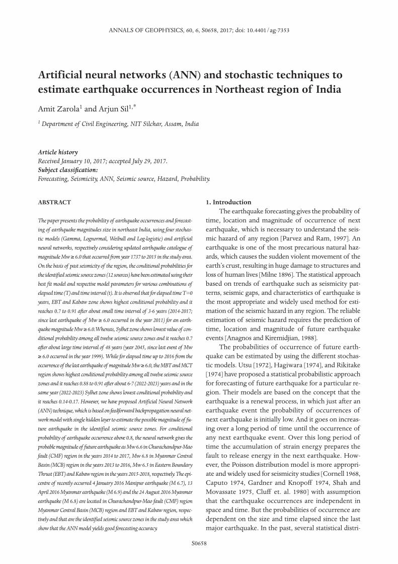
is necessary [Parvez and Ram 1997]. The term seismichazard indicates the estimation of the probability of oc-currences of seismic event in a given region, within agiven time window and with magnitude larger or equalthan a threshold value, which was first formulated byCornell in 1968. Within this study area, total 29 seismicsources (shown in Figure 1.a and 1.b) including linearsources, thrusts, lineaments and area sources have beenidentified from different literatures, SEISAT 2000, and re-mote sensing images. In the past years, the study area hasexperienced some great and major earthquakes such as in1869 Cachar Earthquake, Mw=7.5; 1897 Great ShillongEarthquake, Mw=8.1; 1943 Assam Earthquake, Ms=7.2;1950 Great Assam Earthquake, Mw=8.7 and most recentJanuary 3, 2016 Manipur Earthquake, Mw=6.7.

3. Earthquake dataA well assessed earthquake catalogue of magni-

tude ≥ 4.0 has been taken from Sil et al. [2015], fromyear 1737 to 2011 (274 years) in the study area withinEast longitudes 87.590° to 98.461° and North lati-

tudes 19.345° to 29.431°. Sil et al. [2015] have col-lected preinstrumental (historic) seismic events fromdifferent literatures [Oldham 1883, Basu 1964, Rastogi1974, Chandra 1977, Dunbar et al. 1992, Bilham 2004]and instrumental data from various national and in-ternational seismological agencies, such as IMD,BARC, NGRI (National agencies) and USGS, ISC,COSMO Virtual Data Center (International agencies).They have removed all the repeated events (from dif-ferent seismological agencies) and declustered theforeshocks and aftershocks using methodology givenby Gardner and Knopoff [1974] and modified byUhrhammer [1986]. This methodology assumes thatthe temporal and spatial distribution of foreshocksand aftershocks are dependent on the size of the mainevent. The size of space and time window to declus-ter foreshocks and aftershocks are given ase-1.024+0.804*Mw (km) and e-2.87+1.235*Mw (days) respec-tively. Sil et al. [2015] have converted different types ofmagnitude scale into a common magnitude scale i.e.moment magnitude (Mw) using relationships proposed

FORECASTING OF EARTHQUAKE IN NER, INDIA

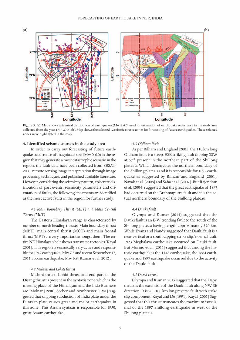
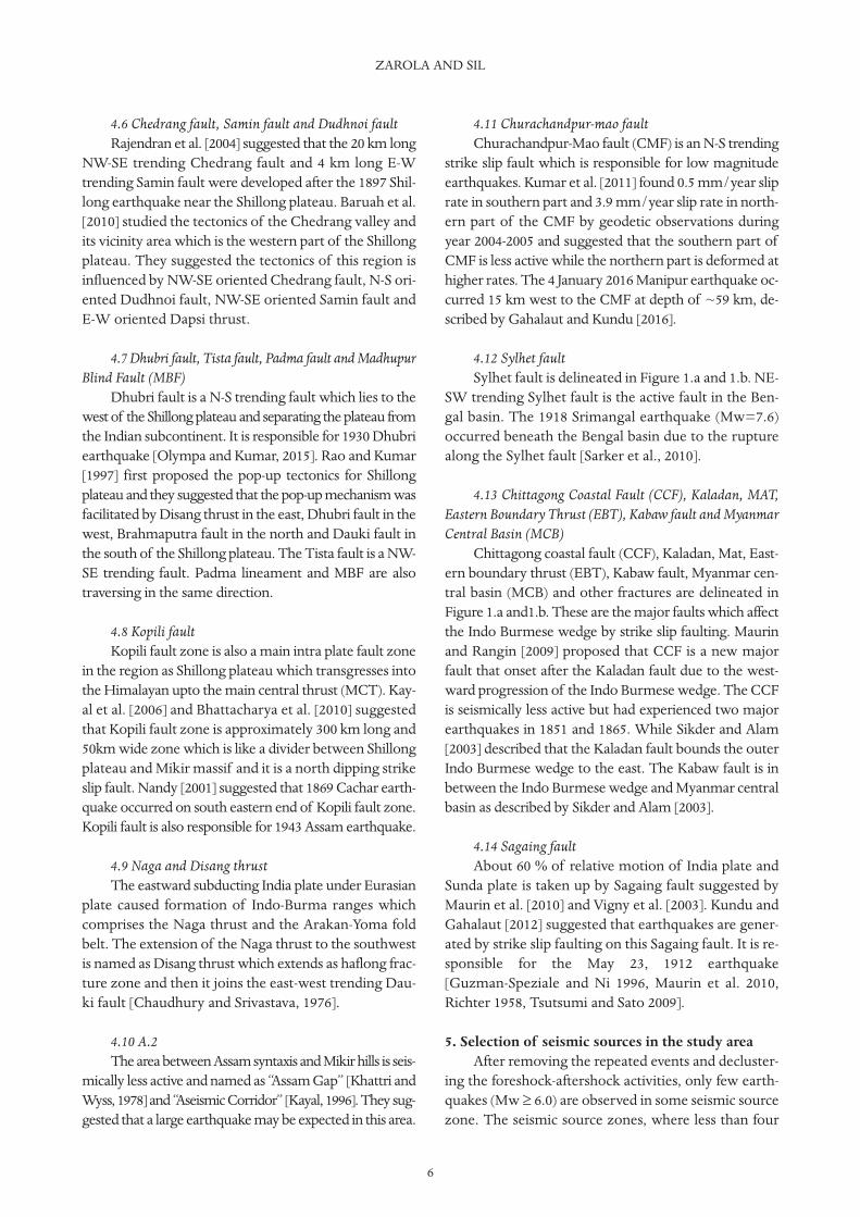
Figure 1. .(a) Delineated seismic source zones of northeast India: Main central thrust (MCT), Main boundary thrust (MBT), Oldham fault(OF), Dapsi thrust (DT), Samin fault (SF), Dudhoni fault (DhF), Naga thrust(NT), Disang thrust(DsT), Chedrang fault (CF), Churachand-pur Mao fault (CMF), Chittagong coastal fault (CCF), Eastern boundary thrust (EBT), Kabaw faut, Dauki fault (DF), Barapani shear zone(BS), Kopili fault, Tista fault, Padma fault, Dhubri fault, Madhupur blind fault (MBF), F.2, F.3, F.4, A.1, A.2, Kaladan fault, Mat fault, Myan-mar central basin (MCB), Sagaing fault, Lohiti thrust, Mishmi thrust. (b) Delineated seismic source zones of northeast India: Main centralthrust (MCT), Main boundary thrust (MBT), Oldham fault (OF), Dapsi thrust (DT), Samin fault (SF), Dudhoni fault (DhF), Naga thrust(NT),Disang thrust(DsT), Chedrang fault (CF), Churachandpur Mao fault (CMF), Chittagong coastal fault (CCF),Eastern boundary thrust (EBT),Kabaw faut, Dauki fault (DF),Barapani shear zone (BS), Kopili fault, Tista fault, Padma fault, Dhubri fault, Madhupur blind fault (MBF), F.2,F.3, F.4, A.1, A.2, Kaladan fault, Mat fault, Myanmar central basin (MCB), Sagaing fault, Lohiti thrust, Mishmi thrust. The earthquake dis-tribution (Mw ≥ 4.0) collected from the year 1737-2015 is also shown in the figure.

(a) (b)

by Sitharam and Sil [2014]. With addition to this earth-quake data base, we have collected earthquake events(magnitude ≥ 4.0) from year 2012 to 2015 (4 years) inthe study area from U.S. Geological Survey. All col-lected events (from year 2012-2015) have been homog-enized using the relationships proposed by Sitharamand Sil [2014].

Mw=0.862Mb+1.034 (R2 =0.782) (1)

Mw=0.673Ml+1.730 (R2 =0.852) (2)

Mw=0.625Ms+2.350 (R2 =0.782) (3)

Where Mw is the moment magnitude, Mb is thebody wave magnitude, Ml is the local magnitude and Msis the surface wave magnitude.

This newly collected data set (from year 2012-2015)has been declustered using the same method as used bySil et al. [2015]. A complete earthquake catalogue fromyear 1737 to 2015 has been prepared after adding twoearthquake catalogues, first from year 1737 to 2011 [Silet al. 2015] and second from year 2012 to 2015 (preparedin this study). Some scattered events are outside the pro-posed source zones and study area and hence are nottaken into account for further study. Total 2508 earth-quake events (Mw ≥ 4.0) with range of longitudes87.599° to 97.918° and latitudes 19.392° to 29.026° havebeen compiled in data base.

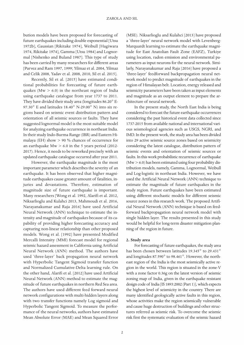
A histogram of earthquake data (Mw ≥ 4.0) that oc-curred from year 1737 to 2015 in the study area has beenprepared (see Figure 2). The study area has been dividedinto 29 seismic source zones (see Figure 1.a and 1.b ) onthe basis of distribution patterns of seismic events (Mw

≥ 4.0) and orientation of seismic sources or faults after su-perimposing of total 2508 earthquake events (Mw ≥ 4.0)on the digitized tectonic map (Seismotectonic Atlas ofIndia [SEISAT], 2000). A total of 52 scattered events areoutside the proposed source zones but within the studyarea, hence are not taken into account for further study.

The general property of the size distribution ofearthquakes that smaller earthquakes occur more fre-quently than the bigger earthquakes is well known. It isobserved that model parameters give a higher probabil-ity of occurrence caused by an extremely short recur-rence interval (for smaller earthquakes). Therefore, forlong term forecasting only main events of magnitudeMw ≥ 6.0 have been taken.

After declustering the catalog, Sil et al. [2015] haveobserved that some of the main shock events (Mw ≥ 6.0)are available in the same year (only there is a month’s dif-ference) in the same identified seismic source zone. Thus,an extremely short recurrence interval makes the sameproblem as a problem of higher probability of occur-rence. Hence, in the same year only the earthquake eventhaving the highest magnitude amongst all has been con-sidered for further study and all other events have beenremoved from the data base.

Therefore, for further study, they used total 148events (Mw ≥ 6.0) that occurred from 1737 to 2011. Butin the present study, after declustering the catalog, with-out deleting any real data (even if, there is a month’s dif-ference), all the mainshocks (Mw ≥ 6.0) have beenconsidered for further study. Therefore, total 191 earth-quake events (Mw ≥ 6.0) that occurred from 1737 to 2015have been used in this study and superimposed on thedigitized tectonic map (Seismotectonic Atlas of India[SEISAT], 2000; shown in Figure 3a).

ZAROLA AND SIL

4

Figure 2. .The figure shows a histogram of earthquakes (Mw ≥ 4.0) that occurred from year 1737-2015 in the study area.

5

FORECASTING OF EARTHQUAKE IN NER, INDIA

4. Identified seismic sources in the study areaIn order to carry out forecasting of future earth-

quake occurrence of magnitude size (Mw ≥ 6.0) in the re-gion that may generate a most catastrophic scenario in theregion, the fault data have been collected from SESAT-2000, remote sensing image interpretation through imageprocessing techniques, and published available literature.However, considering the seismicity pattern, epicentre dis-tribution of past events, seismicity parameters and ori-entation of faults, the following lineaments are identifiedas the most active faults in the region for further study.

4.1 Main Boundary Thrust (MBT) and Main CentralThrust (MCT)

The Eastern Himalayan range is characterized bynumber of north heading thrusts. Main boundary thrust(MBT), main central thrust (MCT) and main frontalthrust (MFT) are very important amongst them. The en-tire NE Himalayan belt shows transverse tectonics [Kayal2001]. This region is seismically very active and responsi-ble for 1947 earthquake, Mw 7.8 and recent September 17,2011 Sikkim earthquake, Mw 6.9 [Kumar et al. 2012].

4.2 Mishmi and Lohiti thrustMishmi thrust, Lohiti thrust and end part of the

Disang thrust is present in the syntaxis zone which is themeeting place of the Himalayan and the Indo-Burmesearc. Molnar [1990], Seeber and Armbruster [1981] sug-gested that ongoing subduction of India plate under theEurasian plate causes great and major earthquakes inthis zone. This Assam syntaxis is responsible for 1950,great Assam earthquake.

4.3 Oldham faultAs per Bilham and England [2001] the 110 km long

Oldham fault is a steep, ESE striking fault dipping SSWat 57° present in the northern part of the Shillongplateau. Which demarcates the northern boundary ofthe Shillong plateau and it is responsible for 1897 earth-quake as suggested by Bilham and England [2001],Nayak et al. [2008] and Saha et al. [2007]. But Rajendranet al. [2004] suggested that the great earthquake of 1897had occurred on the Brahmaputra fault and it is the ac-tual northern boundary of the Shillong plateau.

4.4 Dauki faultOlympa and Kumar [2015) suggested that the

Dauki fault is an E-W trending fault to the south of theShillong plateau having length approximately 320 km.While Evans and Nandy suggested that Dauki fault is anear vertical or a south dipping strike slip/normal fault.1923 Meghalaya earthquake occurred on Dauki fault.But Morino et al. [2011] suggested that among the his-toric earthquakes the 1548 earthquake, the 1664 earth-quake and 1897 earthquake occurred due to the activityof the Dauki fault.

4.5 Dapsi thrustOlympa and Kumar, 2015 suggested that the Dapsi

thrust is the extension of the Dauki fault along NW-SEdirection. It is 90~100 km long reverse fault with strikeslip component. Kayal and De [1991], Kayal [2001] Sug-gested that this thrust truncates the maximum isoseis-mal of the 1897 Shillong earthquake in west of theShillong plateau.

Figure 3. (a). Map shows epicentral distribution of earthquakes (Mw ≥ 6.0) used for estimation of earthquake recurrence in the study areacollected from the year 1737-2015. (b). Map shows the selected 12 seismic source zones for forecasting of future earthquakes. These selectedzones were highlighted in the map.

(a) (b)

4.6 Chedrang fault, Samin fault and Dudhnoi faultRajendran et al. [2004] suggested that the 20 km long

NW-SE trending Chedrang fault and 4 km long E-Wtrending Samin fault were developed after the 1897 Shil-long earthquake near the Shillong plateau. Baruah et al.[2010] studied the tectonics of the Chedrang valley andits vicinity area which is the western part of the Shillongplateau. They suggested the tectonics of this region isinfluenced by NW-SE oriented Chedrang fault, N-S ori-ented Dudhnoi fault, NW-SE oriented Samin fault andE-W oriented Dapsi thrust.

4.7 Dhubri fault, Tista fault, Padma fault and MadhupurBlind Fault (MBF)

Dhubri fault is a N-S trending fault which lies to thewest of the Shillong plateau and separating the plateau fromthe Indian subcontinent. It is responsible for 1930 Dhubriearthquake [Olympa and Kumar, 2015]. Rao and Kumar[1997] first proposed the pop-up tectonics for Shillongplateau and they suggested that the pop-up mechanism wasfacilitated by Disang thrust in the east, Dhubri fault in thewest, Brahmaputra fault in the north and Dauki fault inthe south of the Shillong plateau. The Tista fault is a NW-SE trending fault. Padma lineament and MBF are alsotraversing in the same direction.

4.8 Kopili faultKopili fault zone is also a main intra plate fault zone

in the region as Shillong plateau which transgresses intothe Himalayan upto the main central thrust (MCT). Kay-al et al. [2006] and Bhattacharya et al. [2010] suggestedthat Kopili fault zone is approximately 300 km long and50km wide zone which is like a divider between Shillongplateau and Mikir massif and it is a north dipping strikeslip fault. Nandy [2001] suggested that 1869 Cachar earth-quake occurred on south eastern end of Kopili fault zone.Kopili fault is also responsible for 1943 Assam earthquake.

4.9 Naga and Disang thrustThe eastward subducting India plate under Eurasian

plate caused formation of Indo-Burma ranges whichcomprises the Naga thrust and the Arakan-Yoma foldbelt. The extension of the Naga thrust to the southwestis named as Disang thrust which extends as haflong frac-ture zone and then it joins the east-west trending Dau-ki fault [Chaudhury and Srivastava, 1976].

4.10 A.2The area between Assam syntaxis and Mikir hills is seis-

mically less active and named as “Assam Gap” [Khattri andWyss, 1978] and “Aseismic Corridor” [Kayal, 1996]. They sug-gested that a large earthquake may be expected in this area.

4.11 Churachandpur-mao faultChurachandpur-Mao fault (CMF) is an N-S trending

strike slip fault which is responsible for low magnitudeearthquakes. Kumar et al. [2011] found 0.5 mm/year sliprate in southern part and 3.9 mm/year slip rate in north-ern part of the CMF by geodetic observations duringyear 2004-2005 and suggested that the southern part ofCMF is less active while the northern part is deformed athigher rates. The 4 January 2016 Manipur earthquake oc-curred 15 km west to the CMF at depth of ~59 km, de-scribed by Gahalaut and Kundu [2016].

4.12 Sylhet faultSylhet fault is delineated in Figure 1.a and 1.b. NE-

SW trending Sylhet fault is the active fault in the Ben-gal basin. The 1918 Srimangal earthquake (Mw=7.6)occurred beneath the Bengal basin due to the rupturealong the Sylhet fault [Sarker et al., 2010].

4.13 Chittagong Coastal Fault (CCF), Kaladan, MAT,Eastern Boundary Thrust (EBT), Kabaw fault and MyanmarCentral Basin (MCB)

Chittagong coastal fault (CCF), Kaladan, Mat, East-ern boundary thrust (EBT), Kabaw fault, Myanmar cen-tral basin (MCB) and other fractures are delineated inFigure 1.a and1.b. These are the major faults which affectthe Indo Burmese wedge by strike slip faulting. Maurinand Rangin [2009] proposed that CCF is a new majorfault that onset after the Kaladan fault due to the west-ward progression of the Indo Burmese wedge. The CCFis seismically less active but had experienced two majorearthquakes in 1851 and 1865. While Sikder and Alam[2003] described that the Kaladan fault bounds the outerIndo Burmese wedge to the east. The Kabaw fault is inbetween the Indo Burmese wedge and Myanmar centralbasin as described by Sikder and Alam [2003].

4.14 Sagaing faultAbout 60 % of relative motion of India plate and

Sunda plate is taken up by Sagaing fault suggested byMaurin et al. [2010] and Vigny et al. [2003]. Kundu andGahalaut [2012] suggested that earthquakes are gener-ated by strike slip faulting on this Sagaing fault. It is re-sponsible for the May 23, 1912 earthquake[Guzman-Speziale and Ni 1996, Maurin et al. 2010,Richter 1958, Tsutsumi and Sato 2009].

5. Selection of seismic sources in the study area After removing the repeated events and decluster-

ing the foreshock-aftershock activities, only few earth-quakes (Mw ≥ 6.0) are observed in some seismic sourcezone. The seismic source zones, where less than four

ZAROLA AND SIL

6

7

FORECASTING OF EARTHQUAKE IN NER, INDIA

ZAROLA AND SIL

8

95.36 24.92 25/04/1981 11:32 1.91 6.4

95.12 24.55 23/08/1983 12:12 2.33 6.0

95.56 21.09 18/01/1986 6:25 2.40 6.1

95.50 20.90 15/07/1989 6:25 3.49 6.1

95.26 24.76 09/01/1990 6:25 0.48 6.9

95.40 22.50 05/01/1991 6:25 0.99 6.9

94.91 24.29 15/04/1992 6:25 1.28 6.4

95.20 24.73 08/08/1994 6:25 2.31 6.7

95.42 24.88 06/05/1995 6:25 0.74 6.9

95.00 23.00 19/11/1996 6:25 1.54 6.0

94.84 21.76 11/07/1997 6:25 0.64 6.2

95.31 24.97 02/05/1998 6:25 0.81 6.2

94.93 23.94 11/10/2000 6:25 2.44 6.2

95.32 20.19 21/9/2003 6:25 2.94 6.6

94.73 24.60 18/9/2005 6:25 1.99 6.3

94.64 23.58 27/7/2008 6:25 2.86 6.0

94.79 20.40 21/9/2009 6:25 1.15 6.0

7 EBT and KABAW 96.00 27.00 10/05/1926 8:18 0.00 6.1

95.57 25.93 14/08/1932 4:39 6.26 7.2

94.25 23.50 16/08/1938 4:27 6.01 7.2

94.25 23.75 11/05/1940 21:0 1.74 6.4

94.70 24.90 18/11/1950 0:44 10.52 6.5

94.00 23.00 21/01/1956 17:35 5.18 6.2

95.03 25.42 28/05/1957 5:31 1.35 6.0

93.80 23.53 22/03/1958 10:11 0.82 6.5

93.59 22.35 22/01/1964 15:58 5.83 6.7

94.45 22.00 15/12/1965 6:25 1.90 6.0

94.42 21.51 15/12/1966 6:25 1.00 6.2

95.36 26.03 29/07/1970 6:25 3.62 7.0

94.71 25.17 29/12/1971 22:27 1.42 6.3

94.50 23.30 27/07/1973 20:23 1.58 6.1

94.69 21.47 08/07/1975 6:25 1.95 6.9

94.00 20.00 19/11/1980 6:25 5.36 6.6

94.67 21.45 24/01/1982 6:25 1.18 6.1

94.69 25.06 30/08/1983 10:39 1.60 6.4

94.64 24.53 05/03/1984 21:26 0.52 6.0

94.22 23.71 26/07/1986 6:25 2.39 6.3

94.42 23.09 24/08/1987 9:24 1.08 6.0

95.13 25.16 06/08/1988 6:25 0.95 7.5

93.76 21.19 08/12/1989 6:25 1.34 6.4

93.90 23.40 20/12/1991 6:25 2.03 6.0

94.60 20.89 27/03/1992 6:25 0.27 6.3

94.47 23.21 01/04/1993 16:30 1.01 6.2

94.18 20.60 29/05/1994 6:25 1.16 7.0

95.12 25.29 09/05/1995 6:25 0.95 6.0

94.40 23.27 07/07/2002 6:25 7.16 6.0

94.49 24.43 15/02/2005 6:25 2.61 6.0

94.28 23.32 11/05/2006 6:25 1.24 6.8

94.68 24.62 04/02/2011 13:54 4.73 6.2

8 CCF 92.00 22.00 02/04/1762 7:30 0.00 7.2

91.80 24.00 29/12/1950 22:35 188.74 6.5

9

FORECASTING OF EARTHQUAKE IN NER, INDIA

92.70 21.60 14/12/1955 10:51 4.96 6.5

91.69 23.73 02/02/1971 7:59 15.13 6.1

91.55 23.69 21/05/1984 9:59 13.30 6.1

92.00 22.00 21/11/1997 6:25 13.50 6.1

91.92 21.56 22/07/1999 6:25 1.67 6.1

9 KALADAN 92.50 24.50 10/01/1869 6:25 0.00 7.2

92.80 24.80 20/04/1898 6:25 29.28 6.1

92.98 21.73 12/05/1977 6:25 79.06 6.1

92.90 24.69 30/12/1984 6:25 7.63 6.4

93.00 23.88 08/02/1986 6:25 1.11 6.0

92.00 24.30 06/02/1988 6:25 1.99 6.3

92.44 24.45 13/04/1989 6:25 1.19 6.1

92.98 23.85 15/11/1990 6:25 1.59 6.0

93.13 24.67 20/12/1991 6:25 1.10 6.3

92.67 24.49 19/11/1996 6:25 4.91 6.3

92.71 22.27 21/11/1997 6:25 1.01 6.9

92.48 22.86 26/07/2003 6:25 5.68 6.8

92.51 24.78 09/12/2004 6:25 1.37 6.4

10 MBT and MCT 89.27 28.77 21/05/1935 4:22 0.00 6.5

92.00 27.20 21/01/1941 12:41 5.67 6.6

93.85 28.65 29/07/1947 13:43 6.52 7.7

93.70 28.10 14/04/1951 23:40 3.71 6.5

91.70 27.80 23/02/1954 6:40 2.86 6.3

90.30 26.90 29/07/1960 10:42 6.43 6.3

93.76 28.06 21/10/1964 6:25 4.23 6.5

92.61 27.49 26/09/1966 6:25 1.93 6.1

91.84 27.41 15/09/1967 10:32 0.97 6.5

93.99 27.40 19/02/1970 6:25 2.43 6.3

88.75 27.33 19/11/1980 6:25 10.75 6.9

92.88 26.90 02/02/1983 20:44 2.21 6.0

91.98 27.15 07/01/1985 6:25 1.93 6.3

88.33 27.18 27/09/1988 6:25 3.72 6.0

88.80 27.30 09/01/1990 6:25 1.28 6.5

92.39 27.63 17/02/1995 6:25 5.11 6.2

92.82 27.73 26/09/1998 6:25 3.61 6.3

92.56 27.77 25/01/2000 6:25 1.33 6.2

91.69 26.92 23/02/2006 6:25 6.08 6.2

88.05 27.37 02/12/2008 6:25 2.78 6.0

91.44 27.33 21/09/2009 6:25 0.80 6.4

88.16 27.73 18/09/2011 12:41 1.99 6.9

11 A.2 94.00 26.80 23/10/1943 17:23 0.00 6.9

93.18 26.43 17/07/1971 15:0 27.73 6.1

93.30 26.40 05/03/1984 6:25 12.63 6.3

93.42 26.63 06/09/1987 6:25 3.50 6.2

93.20 26.61 23/06/1991 10:4 3.80 6.1

12 SAGAING 96.00 22.00 23/03/1839 6:25 0.00 7.5

97.00 26.50 12/12/1908 12:54 69.72 7.6

97.00 21.00 23/05/1912 2:24 3.45 7.6

97.00 26.00 10/05/1926 8:19 13.97 6.7

96.00 26.00 15/03/1927 16:56 0.85 6.1

96.80 25.40 27/01/1931 20:9 3.87 7.3

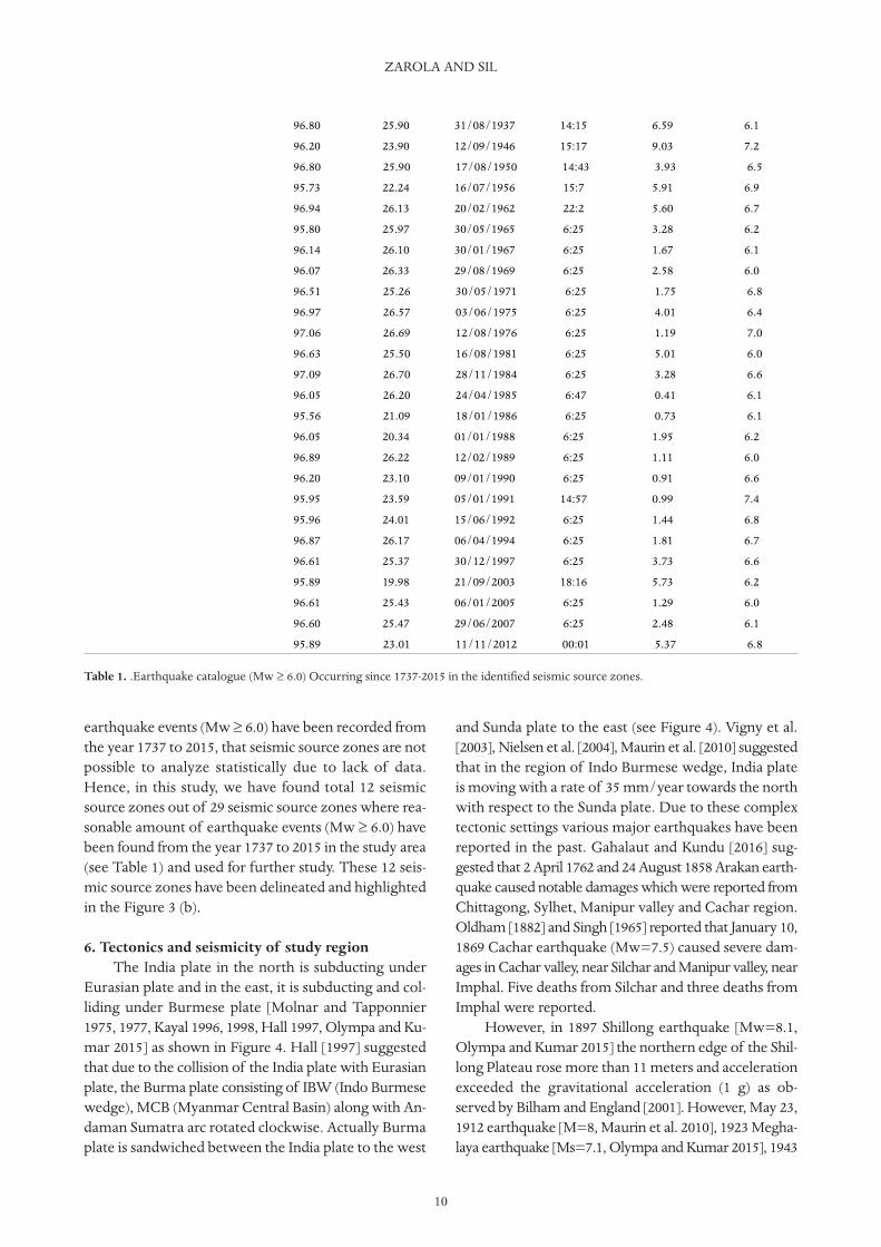
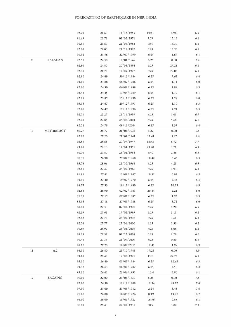
earthquake events (Mw ≥ 6.0) have been recorded fromthe year 1737 to 2015, that seismic source zones are notpossible to analyze statistically due to lack of data.Hence, in this study, we have found total 12 seismicsource zones out of 29 seismic source zones where rea-sonable amount of earthquake events (Mw ≥ 6.0) havebeen found from the year 1737 to 2015 in the study area(see Table 1) and used for further study. These 12 seis-mic source zones have been delineated and highlightedin the Figure 3 (b).

6. Tectonics and seismicity of study regionThe India plate in the north is subducting under

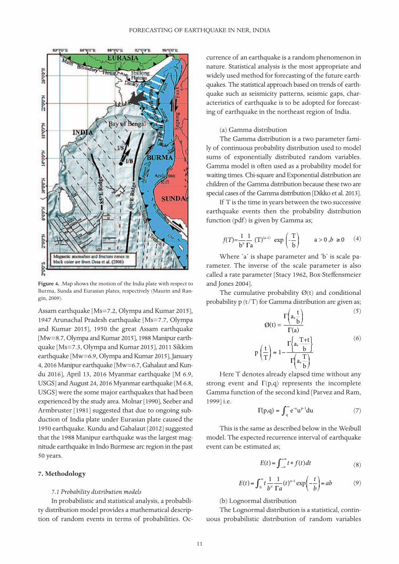
Eurasian plate and in the east, it is subducting and col-liding under Burmese plate [Molnar and Tapponnier1975, 1977, Kayal 1996, 1998, Hall 1997, Olympa and Ku-mar 2015] as shown in Figure 4. Hall [1997] suggestedthat due to the collision of the India plate with Eurasianplate, the Burma plate consisting of IBW (Indo Burmesewedge), MCB (Myanmar Central Basin) along with An-daman Sumatra arc rotated clockwise. Actually Burmaplate is sandwiched between the India plate to the west

and Sunda plate to the east (see Figure 4). Vigny et al.[2003], Nielsen et al. [2004], Maurin et al. [2010] suggestedthat in the region of Indo Burmese wedge, India plateis moving with a rate of 35 mm/year towards the northwith respect to the Sunda plate. Due to these complextectonic settings various major earthquakes have beenreported in the past. Gahalaut and Kundu [2016] sug-gested that 2 April 1762 and 24 August 1858 Arakan earth-quake caused notable damages which were reported fromChittagong, Sylhet, Manipur valley and Cachar region.Oldham [1882] and Singh [1965] reported that January 10,1869 Cachar earthquake (Mw=7.5) caused severe dam-ages in Cachar valley, near Silchar and Manipur valley, nearImphal. Five deaths from Silchar and three deaths fromImphal were reported.

However, in 1897 Shillong earthquake [Mw=8.1,Olympa and Kumar 2015] the northern edge of the Shil-long Plateau rose more than 11 meters and accelerationexceeded the gravitational acceleration (1 g) as ob-served by Bilham and England [2001]. However, May 23,1912 earthquake [M=8, Maurin et al. 2010], 1923 Megha-laya earthquake [Ms=7.1, Olympa and Kumar 2015], 1943

ZAROLA AND SIL

10

96.80 25.90 31/08/1937 14:15 6.59 6.1

96.20 23.90 12/09/1946 15:17 9.03 7.2

96.80 25.90 17/08/1950 14:43 3.93 6.5

95.73 22.24 16/07/1956 15:7 5.91 6.9

96.94 26.13 20/02/1962 22:2 5.60 6.7

95.80 25.97 30/05/1965 6:25 3.28 6.2

96.14 26.10 30/01/1967 6:25 1.67 6.1

96.07 26.33 29/08/1969 6:25 2.58 6.0

96.51 25.26 30/05/1971 6:25 1.75 6.8

96.97 26.57 03/06/1975 6:25 4.01 6.4

97.06 26.69 12/08/1976 6:25 1.19 7.0

96.63 25.50 16/08/1981 6:25 5.01 6.0

97.09 26.70 28/11/1984 6:25 3.28 6.6

96.05 26.20 24/04/1985 6:47 0.41 6.1

95.56 21.09 18/01/1986 6:25 0.73 6.1

96.05 20.34 01/01/1988 6:25 1.95 6.2

96.89 26.22 12/02/1989 6:25 1.11 6.0

96.20 23.10 09/01/1990 6:25 0.91 6.6

95.95 23.59 05/01/1991 14:57 0.99 7.4

95.96 24.01 15/06/1992 6:25 1.44 6.8

96.87 26.17 06/04/1994 6:25 1.81 6.7

96.61 25.37 30/12/1997 6:25 3.73 6.6

95.89 19.98 21/09/2003 18:16 5.73 6.2

96.61 25.43 06/01/2005 6:25 1.29 6.0

96.60 25.47 29/06/2007 6:25 2.48 6.1

95.89 23.01 11/11/2012 00:01 5.37 6.8

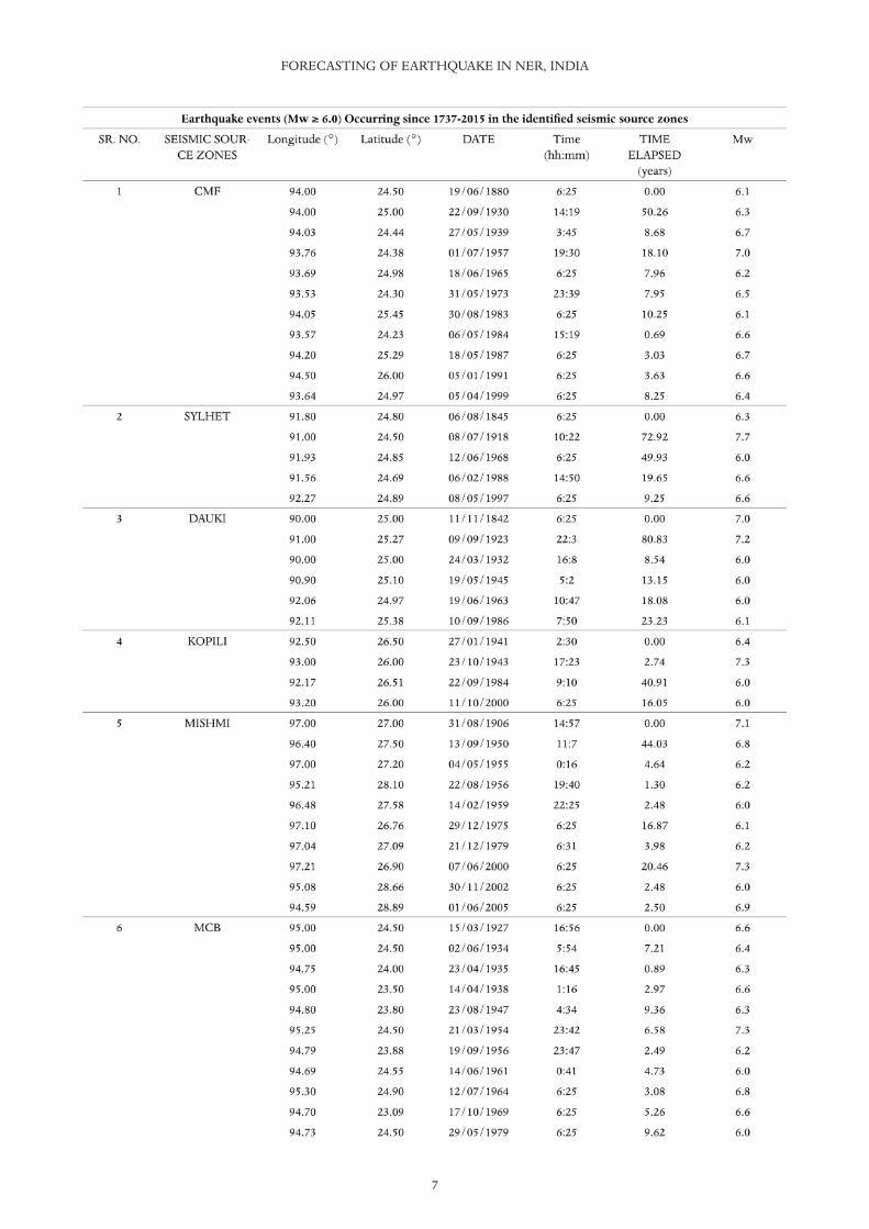
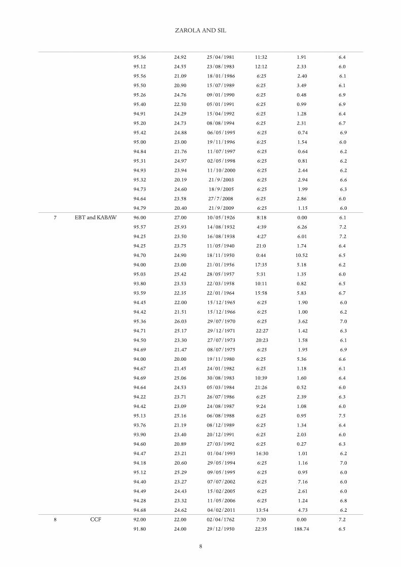
Table 1. .Earthquake catalogue (Mw ≥ 6.0) Occurring since 1737-2015 in the identified seismic source zones.

11

Assam earthquake [Ms=7.2, Olympa and Kumar 2015],1947 Arunachal Pradesh earthquake [Ms=7.7, Olympaand Kumar 2015], 1950 the great Assam earthquake[Mw=8.7, Olympa and Kumar 2015], 1988 Manipur earth-quake [Ms=7.3, Olympa and Kumar 2015], 2011 Sikkimearthquake [Mw=6.9, Olympa and Kumar 2015], January4, 2016 Manipur earthquake [Mw=6.7, Gahalaut and Kun-du 2016], April 13, 2016 Myanmar earthquake [M 6.9,USGS] and August 24, 2016 Myanmar earthquake [M 6.8,USGS] were the some major earthquakes that had beenexperienced by the study area. Molnar [1990], Seeber andArmbruster [1981] suggested that due to ongoing sub-duction of India plate under Eurasian plate caused the1950 earthquake. Kundu and Gahalaut [2012] suggestedthat the 1988 Manipur earthquake was the largest mag-nitude earthquake in Indo Burmese arc region in the past50 years.

7. Methodology

7.1 Probability distribution modelsIn probabilistic and statistical analysis, a probabili-

ty distribution model provides a mathematical descrip-tion of random events in terms of probabilities. Oc-

currence of an earthquake is a random phenomenon innature. Statistical analysis is the most appropriate andwidely used method for forecasting of the future earth-quakes. The statistical approach based on trends of earth-quake such as seismicity patterns, seismic gaps, char-acteristics of earthquake is to be adopted for forecast-ing of earthquake in the northeast region of India.

(a) Gamma distributionThe Gamma distribution is a two parameter fami-

ly of continuous probability distribution used to modelsums of exponentially distributed random variables.Gamma model is often used as a probability model forwaiting times. Chi-square and Exponential distribution arechildren of the Gamma distribution because these two arespecial cases of the Gamma distribution [Dikko et al. 2013].

If T is the time in years between the two successiveearthquake events then the probability distributionfunction (pdf ) is given by Gamma as;

(4)

Where ‘a’ is shape parameter and ‘b’ is scale pa-rameter. The inverse of the scale parameter is alsocalled a rate parameter [Stacy 1962, Box-Steffensmeierand Jones 2004].

The cumulative probability Ø(t) and conditionalprobability p (t/T) for Gamma distribution are given as;

(5)

(6)

Here T denotes already elapsed time without anystrong event and Γ(p,q) represents the incompleteGamma function of the second kind [Parvez and Ram,1999] i.e.

(7)

This is the same as described below in the Weibullmodel. The expected recurrence interval of earthquakeevent can be estimated as;

(8)

(9)

(b) Lognormal distributionThe Lognormal distribution is a statistical, contin-

uous probabilistic distribution of random variables

FORECASTING OF EARTHQUAKE IN NER, INDIA

Figure 4. .Map shows the motion of the India plate with respect toBurma, Sunda and Eurasian plates, respectively (Maurin and Ran-gin, 2009).

f(T)= 1ba

1Γa

(T)(a-1) exp -Tb

⎛⎝⎜

⎞⎠⎟

a > 0 ,b ≥ 0

Ø(t) =Γ a, t

b⎛⎝⎜

⎞⎠⎟

Γ(a)

p tT

⎛⎝⎜

⎞⎠⎟

= 1−Γ a, T+t

b{ }Γ a, T

b⎛⎝⎜

⎞⎠⎟

Γ(p,q) = e-uq

∞∫ up-1du

E(t)= t ∗ f (t)dt−∞

+∞∫

E(t)= t 1ba0

∞∫ 1Γa

(t)a−1 exp − tb

⎛⎝⎜

⎞⎠⎟

= ab

which have a normally distributed logarithm. So this dis-tribution is useful for representing quantities that can’thave negative values, since log(x) exists only when x ispositive. Actually x is the multiplicative product of manyindependent random variables, each of which is positive[Heyde 1963, Barakat 1976].

Probability density function (pdf ), cumulativeprobability of the next earthquake event Ø(t) , and con-ditional probability p (t/T) of the two parameters log-normal distribution [Nishenko and Buland 1987, Yadavet al. 2008] are given as;

(10)

Where, T is the time between two successiveevents. On a logarithmic scale m and σ are termed as lo-cation and scale parameters of lognormal distribution.

cumulative probability (11)

cumulative probability (12)

Here T denotes already elapsed time without anystrong event and Ø(y) represents the error integralgiven as;

(13)

The expectation of the earthquake in period t iscalculated with the expected value

(14)

(15)

(c) Weibull distributionWeibull distribution is a continuous probability dis-

tribution. The Weibull distribution with two parameters(shape, scale) is the most widely used stochastic modelfor earthquake data analysis [Utsu 1984, 2002, Sil et al.2015] If T is the time in years between the two succes-sive earthquake events then the probability distributionfunction (pdf ) is given by Weibull [1951] as:

(16)

Where, β is the shape parameter and θ is the scaleparameter of Weibull distribution.The Weibull cumu-lative distribution function (cdf ) is expressed as;

(17)

The conditional probability p(t/T) that the nextearthquake will occur during the time interval betweenT and T+t can be expressed as

(18)

Where, T denotes already elapsed time withoutany strong event. In quality control engineering thisconditional probability is called hazard rate [Wes-nousky et al. 1984 and Rikitake 1991].

The expected recurrence interval of earthquakeevent can be estimated as [Hagiwara 1974, Yilmaz andCelik 2008]:

(19)

(20)

(d) Log-logistic distribution [Yilmaz et al. 2004, Yil-maz and Celik 2008]

Loglogistic distribution is a probability distributionof random variables, if logarithm of the random vari-able is logistically distributed. The loglogistic distribu-tion is generally used to model events that experiencean initial increase, followed by a rate decrease. If T isthe time in years between the two successive earth-quake events then the probability distribution function(pdf ), cumulative probability or cumulative distributionfunction (cdf ) are given by log-logistic [Ashkar andMahdi 2006] as:

(21)

where, (22)

cumulative probability; (23)

(24)

conditional probability; (25)

Where m and σ are the model parameters ofLoglogistic distribution.On a logarithmic scale m and σare termed as location and scale parameters of Loglo-gistic distribution. In conditional probability T denotesalready elapsed time without any strong event.

The expected or mean interval of earthquake oc-currence time can be estimated as;

(26)

(27)

For σ ≥1.0,E(t) doesn’t exist.

ZAROLA AND SIL

12

f (T)= 1Tσ 2π2π

exp −(lnT −μ )2

2⎧⎨⎩

⎫⎬⎭

μ > 0, σ > 0

= ln(t)−μ⎛⎝⎜

⎞⎠⎟Ø(t) σφ

p tT

⎛⎝⎜

⎞⎠⎟

=1−1−φ ln(T +t)−μ⎛

⎝⎜⎞⎠⎟

⎧⎨⎩

⎫⎬⎭

1−φ ln(T)−μ⎛⎝⎜

⎞⎠⎟

⎧⎨⎩

⎫⎬⎭

σ

σ

φ(y)= 12p

exp−u2/2 du−∞

y∫

E(t)= t ∗ f (t)dt−∞

+∞∫E(t)= t 1

tσ σ2p0

∞∫ exp −(ln(t)−m )2

2 2

⎧⎨⎩

⎫⎬⎭dt = emeσ 2/2

f (T)= βθ

Tθ

⎛⎝⎜

⎞⎠⎟(β −1)

exp − T θ⎛⎝⎜

⎞⎠⎟

β⎧⎨⎪⎩⎪

⎫⎬⎪⎭⎪

> 0, > 0θ

β

f (T)=1−exp − T⎛⎝⎜

⎞⎠⎟

⎧⎨⎪⎩⎪

⎫⎬⎪⎭⎪θ

β

p tT

⎛⎝⎜

⎞⎠⎟

=1−exp − T +t⎛⎝⎜

⎞⎠⎟

β

− T⎛⎝⎜

⎞⎠⎟

⎧⎨⎪⎩⎪

⎫⎬⎪⎭⎪

⎡

⎣⎢⎢

⎤

⎦⎥⎥θ

β

θ

E(t)= t ∗ f (t)dt−∞

+∞∫E(t)= t β

θ0

∞∫ tθ

⎛⎝⎜

⎞⎠⎟(β −1)

exp − tθ

⎛⎝⎜

⎞⎠⎟

β⎧⎨⎪⎩⎪

⎫⎬⎪⎭⎪dt = Γ(1+ 1 )θ

β

Pdf ; f (T)= 1 1T

ez

(1+ez )2σ

z = ln(T)−σ

−∞ < < ∞ and 0 < < ∞m m σ

= 11+ez

Ø(t)

cdf ; F(T)= ez

1+ez

p tT

⎛⎝⎜

⎞⎠⎟

= ∅(T)−∅(T +t)∅(T)

E(t)= t ∗ f (t)dt−∞

+∞∫

E(t)= t 1σ0

∞∫ 1t

ez

(1+ez )2dt = em Γ(1+ ) Γ(1− )σ σ

13

7.2 Logarithm likelihood function and maximum like-lihood estimation method

The logarithm likelihood function of the parame-ter ‘a’ given the observed data ‘t’, is presented bylnL(a ⁄ t). The logarithm likelihood function lnL(a ⁄ t) isnot a probability density function. It is an important com-ponent of both frequentist and Bayesian analyses. If wecompare the logarithm likelihood function at two pa-rameter points and find that lnL(a1 ⁄ t) > lnL(a2 ⁄ t) thenthe sample we actually observed is more likely to haveoccurred if a=a1 than a= a2 . This could be interpretedas ‘a1’ is more suitable value for ‘a’ than 'a2’. A higher val-ue of this function suggests a better (or more suitable)model and lower shows worse [Sil et al. 2015]. The log-likelihood function has the particularly simple form;

(28)

Thus, lnL(a ⁄ t) represents the log-likelihood of theparameter ‘a’ given the observed data ‘t’, and as such isa function of ‘a’. And f(ti;a) represents the probabilitydistribution function of the random variables‘t’ giventhe parameter ‘a’.

However, in this work maximum likelihood esti-mation has been done using the data statistics. In thiscase of the maximum likelihood estimation, let wehave a probability distribution function (pdf ) f(ti;a) ofrandom variables t and we are interested in estimating‘a’ parameter. amle is the value of ‘a’ that maximizesvalue of likelihood function L(a ⁄ t). It is very difficult tomaximize L(a ⁄ t) directly but it is much easier to maxi-mize the log-likelihood function lnL(a ⁄ t).Since ln(∙) isa monotonic function. The value of the ‘a’ that maxi-mizes lnL(a ⁄ t) will also maximizeL(a ⁄ t). Therefore wemay also define amle as the value of ‘a’ that solvesMAXalnL(a ⁄ t). We may find the Maximum likelihood esti-mate by differentiating lnL(a ⁄ t) with respect to param-eter ‘a’ and equating zero [Myung 2003].

(29)

7.3 Artificial Neural Network (ANN)A neural network is a computing system inspired

by biological neural network. In an Artificial NeuralNetwork (ANN), the processing elements called neu-rons are connected together to form a network, whereevery link that connects neurons has a numeric weight.This numeric weight refers to the strength or amplitudeof a connection between neurons. The output fromeach processing element is calculated by applying anactivation function to the sum of inputs multiple by theweight vector [Alarifi et al. 2012]. The Artificial NeuralNetworks support number of activation functions,

such as linear function, non-linear function, sign func-tion, step function [Alarifi et al. 2012].

There are many kinds of neural networks de-pending on their structure, function, and their trainingmethod. In this study, we used a feedforward neuralnetwork with a backpropagation learning algorithm totrain the network. A typical neural network in feedfor-ward direction is given by [Bichkule 2014]:

(30)

Where ai is the input vector, Oj is the output vec-tor, wij is a weight factor between two neurons, bj is thebias weight vector. Among the different kinds of acti-vation function, the Log-sigmoid function and the rec-tifier linear function have been adopted in this study.These activation functions were applied to the neuronsin hidden and output layers, whereas Input layer neu-rons are linear. The Log-Sigmoid function is consideredthe most popular activation function used in multilayernetworks that are trained using backpropagation algo-rithm because this function is differentiable [Alarifi etal. 2012]. This function [Wong et al. 1992] is defined as:

(31)

The rectifier activation function [Maas et al. 2013]is defined as:

(32)

A neuron employing the rectifier function is alsocalled rectified linear neuron, which is neither fully dif-ferentiable (not at zero) nor bounded [Glorot et al.2011]. However, its derivative can take only two valueszero or one and it can be represented as;

(33)

(34)

The backpropagation learning algorithm is basedon a generalized delta-rule, accelerated by a momen-tum term. The momentum term is added to acceleratethe convergence of error during the training, with goodlearning rate. The weight factors and bias are adjustedby using the following equations [Bichkule 2014]:

(35)

(36)

FORECASTING OF EARTHQUAKE IN NER, INDIA

lnL(a / t)= ln Πi=1n f (ti ;a){ } = ln f (tii=1

n∑ ;a)

∂lnL(amle / t)∂a

Oj = f ( (wiji=1

n∑ ai )+bj )

f (x)= 11+e−x

y =max 0, (wij aj )+bji=1

n∑( ){ }

f (x)=x,x > 00,x ≤ 0

⎧⎨⎩

f '(x)=1,x > 00,x ≤ 0

⎧⎨⎩

(wijk+1)= (wij

k )+ Δ(wijk )

Δ(wijk )=η(δ j

k )Oi + ∗Δ(wijk−1)α

(37)

(38)Where ‘η’ is the learning rate, ‘α’ is the momen-

tum coefficient, ‘wij’ is the weight factor associated be-tween two neurons ‘bj’ is the bias weight, ‘O’ is theoutput, ‘δ’ is the gradient descent correction term and‘k’ stands for number of pattern. Each pattern presen-tation represents an iteration and a presentation of theentire training set is called an epoch. The performanceof the trained network was checked by estimating thesum of squared error (SSE) using eq. (39) [Prabhakarand Dutta 2013].

(39)

Where; T = the target value of output variables.O = the estimated value of output variables.Nk= the total number of training data sets.Nj = the total number of output variables.

7.3.1 K-Fold cross validationThis test is performed to validate the estimated

values in the neural networks. In k-fold cross valida-tion, the dataset ‘D’ is randomly split into approxi-mately equal size of ‘k’ subsets (‘D1’, ‘D2’,‘D3’,…,’Dk’). The training and testing iterations areperformed ‘k’ times and in each iteration i ε (1, 2,3,….., k) and the dataset is tested on D \ Di and testedon Di [Kohavi 1995]. In this way, in k-fold cross vali-dation, every data point would be part of trainingsample and part of validation sample.

The estimated results are validated by calculat-ing the average error (in this study, ‘SSE’). To calcu-

late the average SSE, the sum of all the SSE of thetesting subsets is divided by ‘k’.8. Theory and analysis

8.1 Estimation of logarithm likelihood function andmodel parameters

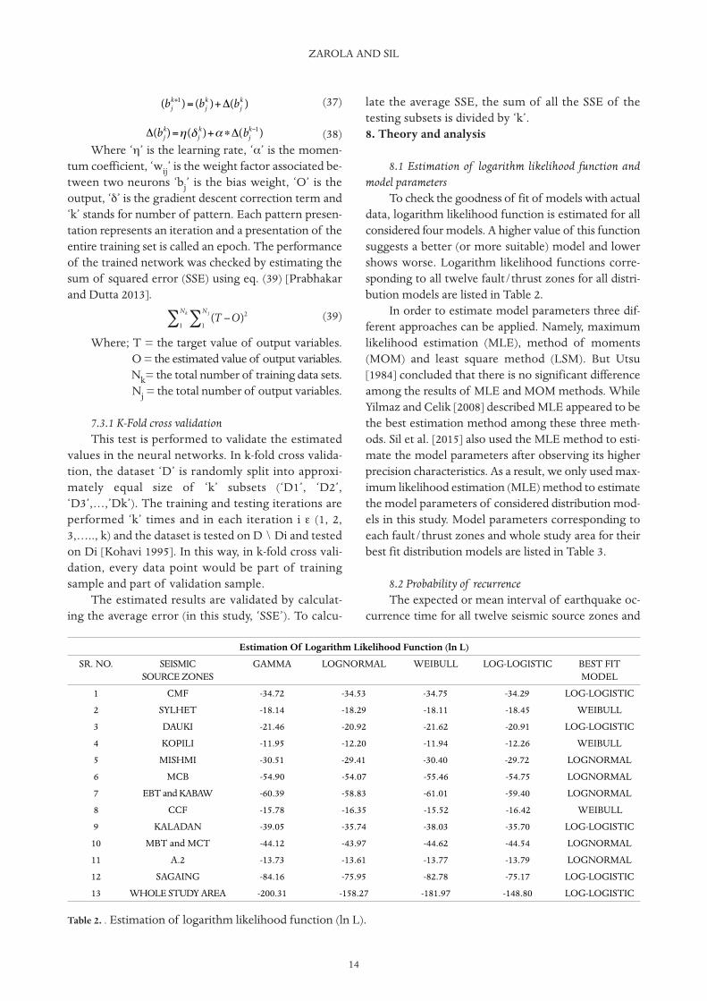
To check the goodness of fit of models with actualdata, logarithm likelihood function is estimated for allconsidered four models. A higher value of this functionsuggests a better (or more suitable) model and lowershows worse. Logarithm likelihood functions corre-sponding to all twelve fault/thrust zones for all distri-bution models are listed in Table 2.

In order to estimate model parameters three dif-ferent approaches can be applied. Namely, maximumlikelihood estimation (MLE), method of moments(MOM) and least square method (LSM). But Utsu[1984] concluded that there is no significant differenceamong the results of MLE and MOM methods. WhileYilmaz and Celik [2008] described MLE appeared to bethe best estimation method among these three meth-ods. Sil et al. [2015] also used the MLE method to esti-mate the model parameters after observing its higherprecision characteristics. As a result, we only used max-imum likelihood estimation (MLE) method to estimatethe model parameters of considered distribution mod-els in this study. Model parameters corresponding toeach fault/thrust zones and whole study area for theirbest fit distribution models are listed in Table 3.

8.2 Probability of recurrenceThe expected or mean interval of earthquake oc-

currence time for all twelve seismic source zones and

ZAROLA AND SIL

14

(bjk+1)= (bj

k )+ Δ(bjk )

Δ(bj )= ( jk )+ ∗Δ(bj

k−1)η δ k α

(T !O)21

N j"1

Nk"

Estimation Of Logarithm Likelihood Function (ln L)

SR. NO. SEISMICSOURCE ZONES

GAMMA LOGNORMAL WEIBULL LOG-LOGISTIC BEST FITMODEL

1 CMF -34.72 -34.53 -34.75 -34.29 LOG-LOGISTIC

2 SYLHET -18.14 -18.29 -18.11 -18.45 WEIBULL

3 DAUKI -21.46 -20.92 -21.62 -20.91 LOG-LOGISTIC

4 KOPILI -11.95 -12.20 -11.94 -12.26 WEIBULL

5 MISHMI -30.51 -29.41 -30.40 -29.72 LOGNORMAL

6 MCB -54.90 -54.07 -55.46 -54.75 LOGNORMAL

7 EBT and KABAW -60.39 -58.83 -61.01 -59.40 LOGNORMAL

8 CCF -15.78 -16.35 -15.52 -16.42 WEIBULL

9 KALADAN -39.05 -35.74 -38.03 -35.70 LOG-LOGISTIC

10 MBT and MCT -44.12 -43.97 -44.62 -44.54 LOGNORMAL

11 A.2 -13.73 -13.61 -13.77 -13.79 LOGNORMAL

12 SAGAING -84.16 -75.95 -82.78 -75.17 LOG-LOGISTIC

13 WHOLE STUDY AREA -200.31 -158.27 -181.97 -148.80 LOG-LOGISTIC

Table 2. . Estimation of logarithm likelihood function (ln L).

15

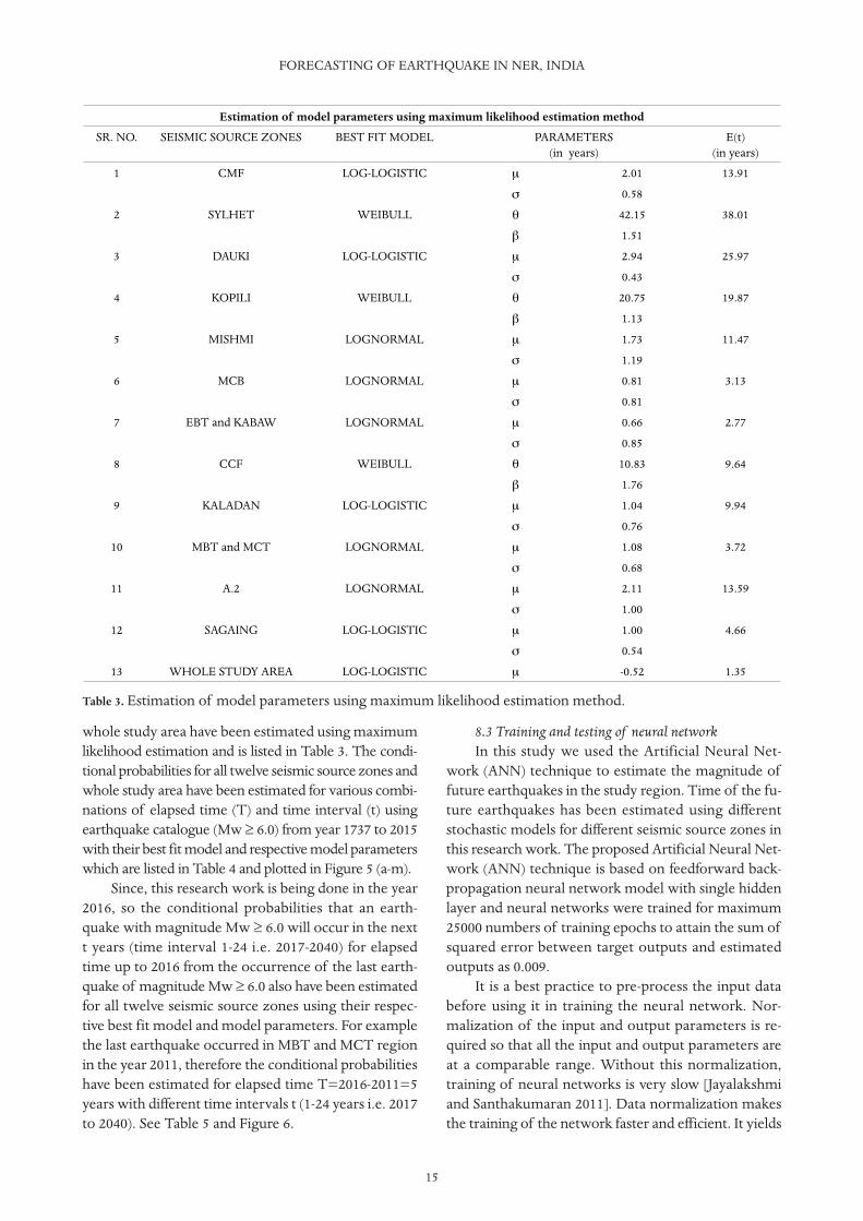
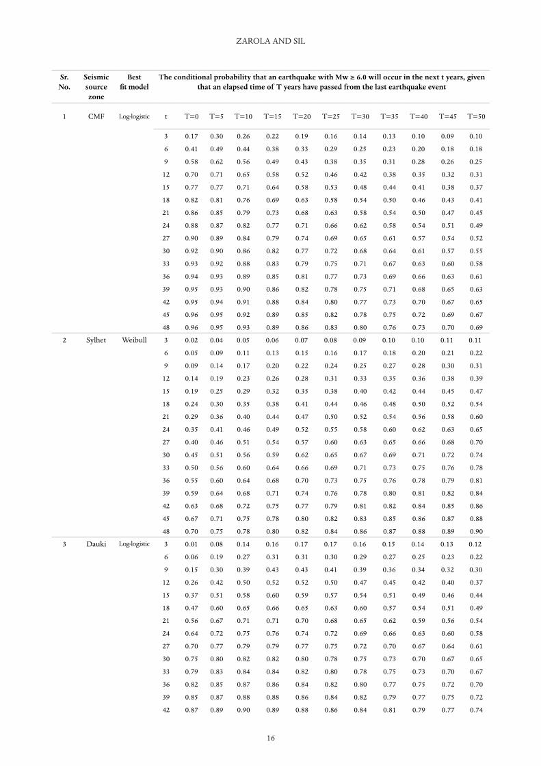
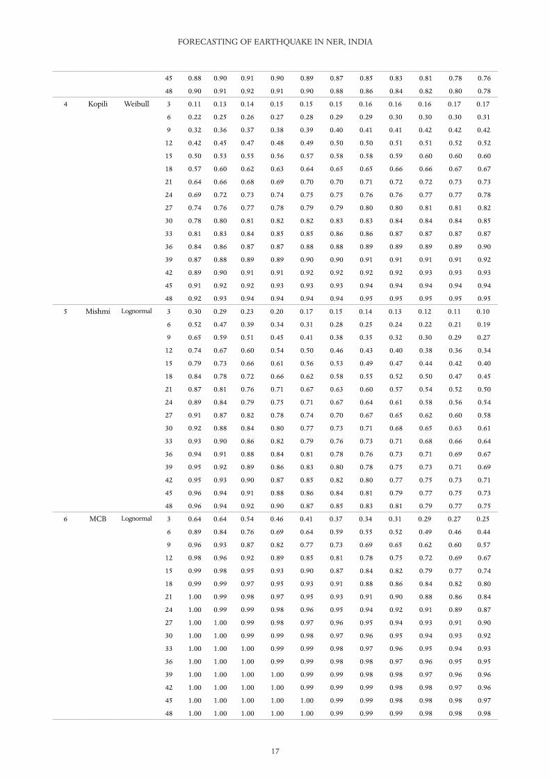
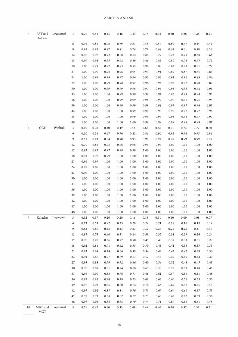
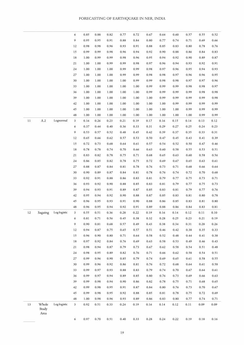
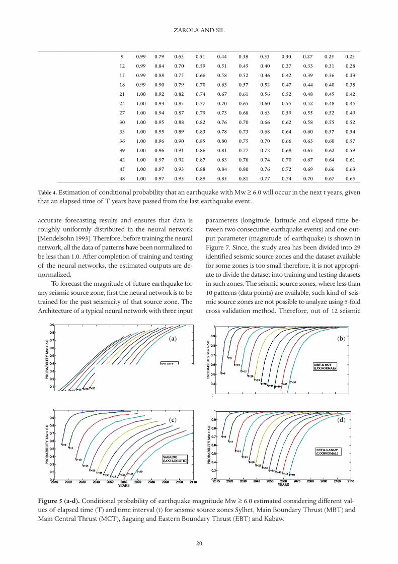
whole study area have been estimated using maximumlikelihood estimation and is listed in Table 3. The condi-tional probabilities for all twelve seismic source zones andwhole study area have been estimated for various combi-nations of elapsed time (T) and time interval (t) usingearthquake catalogue (Mw ≥ 6.0) from year 1737 to 2015with their best fit model and respective model parameterswhich are listed in Table 4 and plotted in Figure 5 (a-m).

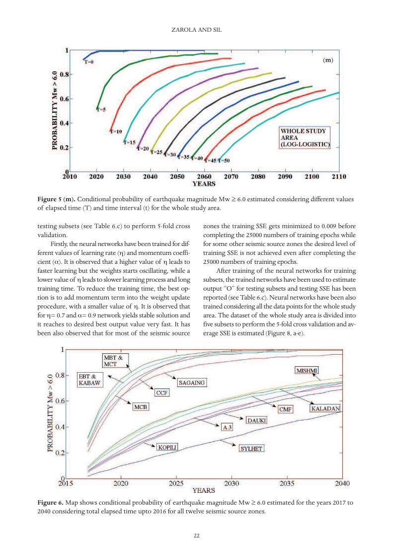
Since, this research work is being done in the year2016, so the conditional probabilities that an earth-quake with magnitude Mw ≥ 6.0 will occur in the nextt years (time interval 1-24 i.e. 2017-2040) for elapsedtime up to 2016 from the occurrence of the last earth-quake of magnitude Mw ≥ 6.0 also have been estimatedfor all twelve seismic source zones using their respec-tive best fit model and model parameters. For examplethe last earthquake occurred in MBT and MCT regionin the year 2011, therefore the conditional probabilitieshave been estimated for elapsed time T=2016-2011=5years with different time intervals t (1-24 years i.e. 2017to 2040). See Table 5 and Figure 6.

8.3 Training and testing of neural networkIn this study we used the Artificial Neural Net-

work (ANN) technique to estimate the magnitude offuture earthquakes in the study region. Time of the fu-ture earthquakes has been estimated using differentstochastic models for different seismic source zones inthis research work. The proposed Artificial Neural Net-work (ANN) technique is based on feedforward back-propagation neural network model with single hiddenlayer and neural networks were trained for maximum25000 numbers of training epochs to attain the sum ofsquared error between target outputs and estimatedoutputs as 0.009.

It is a best practice to pre-process the input databefore using it in training the neural network. Nor-malization of the input and output parameters is re-quired so that all the input and output parameters areat a comparable range. Without this normalization,training of neural networks is very slow [Jayalakshmiand Santhakumaran 2011]. Data normalization makesthe training of the network faster and efficient. It yields

FORECASTING OF EARTHQUAKE IN NER, INDIA

Estimation of model parameters using maximum likelihood estimation method

SR. NO. SEISMIC SOURCE ZONES BEST FIT MODEL PARAMETERS(in years)

E(t)(in years)

1 CMF LOG-LOGISTIC μ 2.01 13.91

σ 0.58

2 SYLHET WEIBULL θ 42.15 38.01

β 1.51

3 DAUKI LOG-LOGISTIC μ 2.94 25.97

σ 0.43

4 KOPILI WEIBULL θ 20.75 19.87

β 1.13

5 MISHMI LOGNORMAL μ 1.73 11.47

σ 1.19

6 MCB LOGNORMAL μ 0.81 3.13

σ 0.81

7 EBT and KABAW LOGNORMAL μ 0.66 2.77

σ 0.85

8 CCF WEIBULL θ 10.83 9.64

β 1.76

9 KALADAN LOG-LOGISTIC μ 1.04 9.94

σ 0.76

10 MBT and MCT LOGNORMAL μ 1.08 3.72

σ 0.68

11 A.2 LOGNORMAL μ 2.11 13.59

σ 1.00

12 SAGAING LOG-LOGISTIC μ 1.00 4.66

σ 0.54

13 WHOLE STUDY AREA LOG-LOGISTIC μ -0.52 1.35

Table 3. Estimation of model parameters using maximum likelihood estimation method.

ZAROLA AND SIL

16

Sr. No.

Seismic source zone

Bestfi t model

The conditional probability that an earthquake with Mw ≥ 6.0 will occur in the next t years, given that an elapsed time of T years have passed from the last earthquake event

1 CMF Log-logistic t T=0 T=5 T=10 T=15 T=20 T=25 T=30 T=35 T=40 T=45 T=50

3 0.17 0.30 0.26 0.22 0.19 0.16 0.14 0.13 0.10 0.09 0.10

6 0.41 0.49 0.44 0.38 0.33 0.29 0.25 0.23 0.20 0.18 0.18

9 0.58 0.62 0.56 0.49 0.43 0.38 0.35 0.31 0.28 0.26 0.25

12 0.70 0.71 0.65 0.58 0.52 0.46 0.42 0.38 0.35 0.32 0.31

15 0.77 0.77 0.71 0.64 0.58 0.53 0.48 0.44 0.41 0.38 0.37

18 0.82 0.81 0.76 0.69 0.63 0.58 0.54 0.50 0.46 0.43 0.41

21 0.86 0.85 0.79 0.73 0.68 0.63 0.58 0.54 0.50 0.47 0.45

24 0.88 0.87 0.82 0.77 0.71 0.66 0.62 0.58 0.54 0.51 0.49

27 0.90 0.89 0.84 0.79 0.74 0.69 0.65 0.61 0.57 0.54 0.52

30 0.92 0.90 0.86 0.82 0.77 0.72 0.68 0.64 0.61 0.57 0.55

33 0.93 0.92 0.88 0.83 0.79 0.75 0.71 0.67 0.63 0.60 0.58

36 0.94 0.93 0.89 0.85 0.81 0.77 0.73 0.69 0.66 0.63 0.61

39 0.95 0.93 0.90 0.86 0.82 0.78 0.75 0.71 0.68 0.65 0.63

42 0.95 0.94 0.91 0.88 0.84 0.80 0.77 0.73 0.70 0.67 0.65

45 0.96 0.95 0.92 0.89 0.85 0.82 0.78 0.75 0.72 0.69 0.67

48 0.96 0.95 0.93 0.89 0.86 0.83 0.80 0.76 0.73 0.70 0.69

2 Sylhet Weibull 3 0.02 0.04 0.05 0.06 0.07 0.08 0.09 0.10 0.10 0.11 0.11

6 0.05 0.09 0.11 0.13 0.15 0.16 0.17 0.18 0.20 0.21 0.22

9 0.09 0.14 0.17 0.20 0.22 0.24 0.25 0.27 0.28 0.30 0.31

12 0.14 0.19 0.23 0.26 0.28 0.31 0.33 0.35 0.36 0.38 0.39

15 0.19 0.25 0.29 0.32 0.35 0.38 0.40 0.42 0.44 0.45 0.47

18 0.24 0.30 0.35 0.38 0.41 0.44 0.46 0.48 0.50 0.52 0.54

21 0.29 0.36 0.40 0.44 0.47 0.50 0.52 0.54 0.56 0.58 0.60

24 0.35 0.41 0.46 0.49 0.52 0.55 0.58 0.60 0.62 0.63 0.65

27 0.40 0.46 0.51 0.54 0.57 0.60 0.63 0.65 0.66 0.68 0.70

30 0.45 0.51 0.56 0.59 0.62 0.65 0.67 0.69 0.71 0.72 0.74

33 0.50 0.56 0.60 0.64 0.66 0.69 0.71 0.73 0.75 0.76 0.78

36 0.55 0.60 0.64 0.68 0.70 0.73 0.75 0.76 0.78 0.79 0.81

39 0.59 0.64 0.68 0.71 0.74 0.76 0.78 0.80 0.81 0.82 0.84

42 0.63 0.68 0.72 0.75 0.77 0.79 0.81 0.82 0.84 0.85 0.86

45 0.67 0.71 0.75 0.78 0.80 0.82 0.83 0.85 0.86 0.87 0.88

48 0.70 0.75 0.78 0.80 0.82 0.84 0.86 0.87 0.88 0.89 0.90

3 Dauki Log-logistic 3 0.01 0.08 0.14 0.16 0.17 0.17 0.16 0.15 0.14 0.13 0.12

6 0.06 0.19 0.27 0.31 0.31 0.30 0.29 0.27 0.25 0.23 0.22

9 0.15 0.30 0.39 0.43 0.43 0.41 0.39 0.36 0.34 0.32 0.30

12 0.26 0.42 0.50 0.52 0.52 0.50 0.47 0.45 0.42 0.40 0.37

15 0.37 0.51 0.58 0.60 0.59 0.57 0.54 0.51 0.49 0.46 0.44

18 0.47 0.60 0.65 0.66 0.65 0.63 0.60 0.57 0.54 0.51 0.49

21 0.56 0.67 0.71 0.71 0.70 0.68 0.65 0.62 0.59 0.56 0.54

24 0.64 0.72 0.75 0.76 0.74 0.72 0.69 0.66 0.63 0.60 0.58

27 0.70 0.77 0.79 0.79 0.77 0.75 0.72 0.70 0.67 0.64 0.61

30 0.75 0.80 0.82 0.82 0.80 0.78 0.75 0.73 0.70 0.67 0.65

33 0.79 0.83 0.84 0.84 0.82 0.80 0.78 0.75 0.73 0.70 0.67

36 0.82 0.85 0.87 0.86 0.84 0.82 0.80 0.77 0.75 0.72 0.70

39 0.85 0.87 0.88 0.88 0.86 0.84 0.82 0.79 0.77 0.75 0.72

42 0.87 0.89 0.90 0.89 0.88 0.86 0.84 0.81 0.79 0.77 0.74

17

FORECASTING OF EARTHQUAKE IN NER, INDIA

45 0.88 0.90 0.91 0.90 0.89 0.87 0.85 0.83 0.81 0.78 0.76

48 0.90 0.91 0.92 0.91 0.90 0.88 0.86 0.84 0.82 0.80 0.78

4 Kopili Weibull 3 0.11 0.13 0.14 0.15 0.15 0.15 0.16 0.16 0.16 0.17 0.17

6 0.22 0.25 0.26 0.27 0.28 0.29 0.29 0.30 0.30 0.30 0.31

9 0.32 0.36 0.37 0.38 0.39 0.40 0.41 0.41 0.42 0.42 0.42

12 0.42 0.45 0.47 0.48 0.49 0.50 0.50 0.51 0.51 0.52 0.52

15 0.50 0.53 0.55 0.56 0.57 0.58 0.58 0.59 0.60 0.60 0.60

18 0.57 0.60 0.62 0.63 0.64 0.65 0.65 0.66 0.66 0.67 0.67

21 0.64 0.66 0.68 0.69 0.70 0.70 0.71 0.72 0.72 0.73 0.73

24 0.69 0.72 0.73 0.74 0.75 0.75 0.76 0.76 0.77 0.77 0.78

27 0.74 0.76 0.77 0.78 0.79 0.79 0.80 0.80 0.81 0.81 0.82

30 0.78 0.80 0.81 0.82 0.82 0.83 0.83 0.84 0.84 0.84 0.85

33 0.81 0.83 0.84 0.85 0.85 0.86 0.86 0.87 0.87 0.87 0.87

36 0.84 0.86 0.87 0.87 0.88 0.88 0.89 0.89 0.89 0.89 0.90

39 0.87 0.88 0.89 0.89 0.90 0.90 0.91 0.91 0.91 0.91 0.92

42 0.89 0.90 0.91 0.91 0.92 0.92 0.92 0.92 0.93 0.93 0.93

45 0.91 0.92 0.92 0.93 0.93 0.93 0.94 0.94 0.94 0.94 0.94

48 0.92 0.93 0.94 0.94 0.94 0.94 0.95 0.95 0.95 0.95 0.95

5 Mishmi Lognormal 3 0.30 0.29 0.23 0.20 0.17 0.15 0.14 0.13 0.12 0.11 0.10

6 0.52 0.47 0.39 0.34 0.31 0.28 0.25 0.24 0.22 0.21 0.19

9 0.65 0.59 0.51 0.45 0.41 0.38 0.35 0.32 0.30 0.29 0.27

12 0.74 0.67 0.60 0.54 0.50 0.46 0.43 0.40 0.38 0.36 0.34

15 0.79 0.73 0.66 0.61 0.56 0.53 0.49 0.47 0.44 0.42 0.40

18 0.84 0.78 0.72 0.66 0.62 0.58 0.55 0.52 0.50 0.47 0.45

21 0.87 0.81 0.76 0.71 0.67 0.63 0.60 0.57 0.54 0.52 0.50

24 0.89 0.84 0.79 0.75 0.71 0.67 0.64 0.61 0.58 0.56 0.54

27 0.91 0.87 0.82 0.78 0.74 0.70 0.67 0.65 0.62 0.60 0.58

30 0.92 0.88 0.84 0.80 0.77 0.73 0.71 0.68 0.65 0.63 0.61

33 0.93 0.90 0.86 0.82 0.79 0.76 0.73 0.71 0.68 0.66 0.64

36 0.94 0.91 0.88 0.84 0.81 0.78 0.76 0.73 0.71 0.69 0.67

39 0.95 0.92 0.89 0.86 0.83 0.80 0.78 0.75 0.73 0.71 0.69

42 0.95 0.93 0.90 0.87 0.85 0.82 0.80 0.77 0.75 0.73 0.71

45 0.96 0.94 0.91 0.88 0.86 0.84 0.81 0.79 0.77 0.75 0.73

48 0.96 0.94 0.92 0.90 0.87 0.85 0.83 0.81 0.79 0.77 0.75

6 MCB Lognormal 3 0.64 0.64 0.54 0.46 0.41 0.37 0.34 0.31 0.29 0.27 0.25

6 0.89 0.84 0.76 0.69 0.64 0.59 0.55 0.52 0.49 0.46 0.44

9 0.96 0.93 0.87 0.82 0.77 0.73 0.69 0.65 0.62 0.60 0.57

12 0.98 0.96 0.92 0.89 0.85 0.81 0.78 0.75 0.72 0.69 0.67

15 0.99 0.98 0.95 0.93 0.90 0.87 0.84 0.82 0.79 0.77 0.74

18 0.99 0.99 0.97 0.95 0.93 0.91 0.88 0.86 0.84 0.82 0.80

21 1.00 0.99 0.98 0.97 0.95 0.93 0.91 0.90 0.88 0.86 0.84

24 1.00 0.99 0.99 0.98 0.96 0.95 0.94 0.92 0.91 0.89 0.87

27 1.00 1.00 0.99 0.98 0.97 0.96 0.95 0.94 0.93 0.91 0.90

30 1.00 1.00 0.99 0.99 0.98 0.97 0.96 0.95 0.94 0.93 0.92

33 1.00 1.00 1.00 0.99 0.99 0.98 0.97 0.96 0.95 0.94 0.93

36 1.00 1.00 1.00 0.99 0.99 0.98 0.98 0.97 0.96 0.95 0.95

39 1.00 1.00 1.00 1.00 0.99 0.99 0.98 0.98 0.97 0.96 0.96

42 1.00 1.00 1.00 1.00 0.99 0.99 0.99 0.98 0.98 0.97 0.96

45 1.00 1.00 1.00 1.00 1.00 0.99 0.99 0.98 0.98 0.98 0.97

48 1.00 1.00 1.00 1.00 1.00 0.99 0.99 0.99 0.98 0.98 0.98

ZAROLA AND SIL

18

7 EBT and Kabaw

Lognormal 3 0.70 0.64 0.53 0.46 0.40 0.36 0.33 0.30 0.28 0.26 0.25

6 0.91 0.85 0.76 0.69 0.63 0.58 0.54 0.50 0.47 0.45 0.42

9 0.97 0.93 0.87 0.81 0.76 0.72 0.68 0.64 0.61 0.58 0.56

12 0.98 0.96 0.92 0.88 0.84 0.80 0.77 0.74 0.71 0.68 0.65

15 0.99 0.98 0.95 0.92 0.89 0.86 0.83 0.80 0.78 0.75 0.73

18 1.00 0.99 0.97 0.95 0.92 0.90 0.88 0.85 0.83 0.81 0.79

21 1.00 0.99 0.98 0.96 0.95 0.93 0.91 0.89 0.87 0.85 0.83

24 1.00 0.99 0.99 0.97 0.96 0.95 0.93 0.91 0.90 0.88 0.86

27 1.00 1.00 0.99 0.98 0.97 0.96 0.95 0.93 0.92 0.90 0.89

30 1.00 1.00 0.99 0.99 0.98 0.97 0.96 0.95 0.93 0.92 0.91

33 1.00 1.00 1.00 0.99 0.98 0.98 0.97 0.96 0.95 0.94 0.93

36 1.00 1.00 1.00 0.99 0.99 0.98 0.97 0.97 0.96 0.95 0.94

39 1.00 1.00 1.00 0.99 0.99 0.99 0.98 0.97 0.97 0.96 0.95

42 1.00 1.00 1.00 1.00 0.99 0.99 0.98 0.98 0.97 0.97 0.96

45 1.00 1.00 1.00 1.00 0.99 0.99 0.99 0.98 0.98 0.97 0.97

48 1.00 1.00 1.00 1.00 1.00 0.99 0.99 0.99 0.98 0.98 0.97

8 CCF Weibull 3 0.10 0.28 0.40 0.49 0.56 0.62 0.66 0.71 0.74 0.77 0.80

6 0.30 0.54 0.67 0.76 0.82 0.86 0.90 0.92 0.94 0.95 0.96

9 0.51 0.73 0.84 0.90 0.93 0.96 0.97 0.98 0.99 0.99 0.99

12 0.70 0.86 0.93 0.96 0.98 0.99 0.99 1.00 1.00 1.00 1.00

15 0.83 0.93 0.97 0.99 0.99 1.00 1.00 1.00 1.00 1.00 1.00

18 0.91 0.97 0.99 1.00 1.00 1.00 1.00 1.00 1.00 1.00 1.00

21 0.96 0.99 1.00 1.00 1.00 1.00 1.00 1.00 1.00 1.00 1.00

24 0.98 1.00 1.00 1.00 1.00 1.00 1.00 1.00 1.00 1.00 1.00

27 0.99 1.00 1.00 1.00 1.00 1.00 1.00 1.00 1.00 1.00 1.00

30 1.00 1.00 1.00 1.00 1.00 1.00 1.00 1.00 1.00 1.00 1.00

33 1.00 1.00 1.00 1.00 1.00 1.00 1.00 1.00 1.00 1.00 1.00

36 1.00 1.00 1.00 1.00 1.00 1.00 1.00 1.00 1.00 1.00 1.00

39 1.00 1.00 1.00 1.00 1.00 1.00 1.00 1.00 1.00 1.00 1.00

42 1.00 1.00 1.00 1.00 1.00 1.00 1.00 1.00 1.00 1.00 1.00

45 1.00 1.00 1.00 1.00 1.00 1.00 1.00 1.00 1.00 1.00 1.00

48 1.00 1.00 1.00 1.00 1.00 1.00 1.00 1.00 1.00 1.00 1.00

9 Kaladan Log-logistic 3 0.52 0.37 0.26 0.20 0.16 0.13 0.11 0.10 0.09 0.08 0.07

6 0.73 0.55 0.42 0.33 0.28 0.24 0.21 0.18 0.16 0.15 0.14

9 0.82 0.66 0.53 0.43 0.37 0.32 0.28 0.25 0.23 0.21 0.19

12 0.87 0.73 0.60 0.51 0.44 0.39 0.35 0.31 0.29 0.26 0.24

15 0.90 0.78 0.66 0.57 0.50 0.45 0.40 0.37 0.33 0.31 0.29

18 0.92 0.81 0.71 0.62 0.55 0.50 0.45 0.41 0.38 0.35 0.33

21 0.93 0.84 0.74 0.66 0.59 0.54 0.49 0.45 0.42 0.39 0.36

24 0.94 0.86 0.77 0.69 0.63 0.57 0.53 0.49 0.45 0.42 0.40

27 0.95 0.88 0.79 0.72 0.66 0.60 0.56 0.52 0.48 0.45 0.43

30 0.96 0.89 0.81 0.74 0.68 0.63 0.59 0.55 0.51 0.48 0.45

33 0.96 0.90 0.83 0.76 0.71 0.66 0.61 0.57 0.54 0.51 0.48

36 0.97 0.91 0.84 0.78 0.73 0.68 0.63 0.60 0.56 0.53 0.50

39 0.97 0.92 0.86 0.80 0.74 0.70 0.66 0.62 0.58 0.55 0.53

42 0.97 0.92 0.87 0.81 0.76 0.71 0.67 0.64 0.60 0.57 0.55

45 0.97 0.93 0.88 0.82 0.77 0.73 0.69 0.65 0.62 0.59 0.56

48 0.98 0.94 0.88 0.83 0.79 0.74 0.71 0.67 0.64 0.61 0.58

10 MBT and MCT

Lognormal 3 0.51 0.67 0.60 0.53 0.48 0.44 0.40 0.38 0.35 0.33 0.31

19

FORECASTING OF EARTHQUAKE IN NER, INDIA

6 0.85 0.88 0.82 0.77 0.72 0.67 0.64 0.60 0.57 0.55 0.52

9 0.95 0.95 0.91 0.88 0.84 0.80 0.77 0.74 0.71 0.69 0.66

12 0.98 0.98 0.96 0.93 0.91 0.88 0.85 0.83 0.80 0.78 0.76

15 0.99 0.99 0.98 0.96 0.94 0.92 0.90 0.88 0.86 0.84 0.83

18 1.00 0.99 0.99 0.98 0.96 0.95 0.94 0.92 0.90 0.89 0.87

21 1.00 1.00 0.99 0.99 0.98 0.97 0.96 0.94 0.93 0.92 0.91

24 1.00 1.00 1.00 0.99 0.99 0.98 0.97 0.96 0.95 0.94 0.93

27 1.00 1.00 1.00 0.99 0.99 0.98 0.98 0.97 0.96 0.96 0.95

30 1.00 1.00 1.00 1.00 0.99 0.99 0.98 0.98 0.97 0.97 0.96

33 1.00 1.00 1.00 1.00 1.00 0.99 0.99 0.99 0.98 0.98 0.97

36 1.00 1.00 1.00 1.00 1.00 0.99 0.99 0.99 0.99 0.98 0.98

39 1.00 1.00 1.00 1.00 1.00 1.00 0.99 0.99 0.99 0.99 0.98

42 1.00 1.00 1.00 1.00 1.00 1.00 1.00 0.99 0.99 0.99 0.99

45 1.00 1.00 1.00 1.00 1.00 1.00 1.00 1.00 0.99 0.99 0.99

48 1.00 1.00 1.00 1.00 1.00 1.00 1.00 1.00 1.00 0.99 0.99

11 A.2 Lognormal 3 0.16 0.26 0.23 0.21 0.19 0.17 0.16 0.15 0.14 0.13 0.12

6 0.37 0.44 0.40 0.36 0.33 0.31 0.29 0.27 0.25 0.24 0.23

9 0.53 0.57 0.52 0.48 0.45 0.42 0.39 0.37 0.35 0.33 0.31

12 0.65 0.66 0.62 0.57 0.53 0.50 0.47 0.45 0.43 0.41 0.39

15 0.72 0.73 0.68 0.64 0.61 0.57 0.54 0.52 0.50 0.47 0.46

18 0.78 0.78 0.74 0.70 0.66 0.63 0.60 0.58 0.55 0.53 0.51

21 0.83 0.82 0.78 0.75 0.71 0.68 0.65 0.63 0.60 0.58 0.56

24 0.86 0.85 0.82 0.78 0.75 0.72 0.69 0.67 0.65 0.63 0.61

27 0.88 0.87 0.84 0.81 0.78 0.76 0.73 0.71 0.68 0.66 0.64

30 0.90 0.89 0.87 0.84 0.81 0.78 0.76 0.74 0.72 0.70 0.68

33 0.92 0.91 0.88 0.86 0.83 0.81 0.79 0.77 0.75 0.73 0.71

36 0.93 0.92 0.90 0.88 0.85 0.83 0.81 0.79 0.77 0.75 0.73

39 0.94 0.93 0.91 0.89 0.87 0.85 0.83 0.81 0.79 0.77 0.76

42 0.95 0.94 0.92 0.90 0.88 0.87 0.85 0.83 0.81 0.80 0.78

45 0.96 0.95 0.93 0.91 0.90 0.88 0.86 0.85 0.83 0.81 0.80

48 0.96 0.95 0.94 0.92 0.91 0.89 0.88 0.86 0.84 0.83 0.81

12 Sagaing Log-logistic 3 0.55 0.51 0.36 0.28 0.22 0.19 0.16 0.14 0.12 0.11 0.10

6 0.81 0.71 0.56 0.45 0.38 0.32 0.28 0.25 0.23 0.21 0.19

9 0.90 0.81 0.68 0.57 0.49 0.43 0.38 0.34 0.31 0.28 0.26

12 0.94 0.87 0.75 0.65 0.57 0.51 0.46 0.42 0.38 0.35 0.33

15 0.96 0.90 0.80 0.71 0.64 0.58 0.52 0.48 0.44 0.41 0.38

18 0.97 0.92 0.84 0.76 0.69 0.63 0.58 0.53 0.49 0.46 0.43

21 0.98 0.94 0.87 0.79 0.73 0.67 0.62 0.58 0.54 0.51 0.48

24 0.98 0.95 0.89 0.82 0.76 0.71 0.66 0.62 0.58 0.54 0.51

27 0.99 0.96 0.90 0.85 0.79 0.74 0.69 0.65 0.61 0.58 0.55

30 0.99 0.96 0.92 0.86 0.81 0.76 0.72 0.68 0.64 0.61 0.58

33 0.99 0.97 0.93 0.88 0.83 0.79 0.74 0.70 0.67 0.64 0.61

36 0.99 0.97 0.94 0.89 0.85 0.80 0.76 0.73 0.69 0.66 0.63

39 0.99 0.98 0.94 0.90 0.86 0.82 0.78 0.75 0.71 0.68 0.65

42 0.99 0.98 0.95 0.91 0.87 0.84 0.80 0.76 0.73 0.70 0.67

45 0.99 0.98 0.95 0.92 0.88 0.85 0.81 0.78 0.75 0.72 0.69

48 1.00 0.98 0.96 0.93 0.89 0.86 0.83 0.80 0.77 0.74 0.71

13 Whole StudyArea

Log-logistic 3 0.92 0.51 0.33 0.24 0.19 0.16 0.14 0.12 0.11 0.09 0.09

6 0.97 0.70 0.51 0.40 0.33 0.28 0.24 0.22 0.19 0.18 0.16

accurate forecasting results and ensures that data isroughly uniformly distributed in the neural network[Mendelsohn 1993]. Therefore, before training the neuralnetwork, all the data of patterns have been normalized tobe less than 1.0. After completion of training and testingof the neural networks, the estimated outputs are de-normalized.

To forecast the magnitude of future earthquake forany seismic source zone, first the neural network is to betrained for the past seismicity of that source zone. TheArchitecture of a typical neural network with three input

parameters (longitude, latitude and elapsed time be-tween two consecutive earthquake events) and one out-put parameter (magnitude of earthquake) is shown inFigure 7. Since, the study area has been divided into 29identified seismic source zones and the dataset availablefor some zones is too small therefore, it is not appropri-ate to divide the dataset into training and testing datasetsin such zones. The seismic source zones, where less than10 patterns (data points) are available, such kind of seis-mic source zones are not possible to analyze using 5-foldcross validation method. Therefore, out of 12 seismic

ZAROLA AND SIL

20

9 0.99 0.79 0.63 0.51 0.44 0.38 0.33 0.30 0.27 0.25 0.23

12 0.99 0.84 0.70 0.59 0.51 0.45 0.40 0.37 0.33 0.31 0.28

15 0.99 0.88 0.75 0.66 0.58 0.52 0.46 0.42 0.39 0.36 0.33

18 0.99 0.90 0.79 0.70 0.63 0.57 0.52 0.47 0.44 0.40 0.38

21 1.00 0.92 0.82 0.74 0.67 0.61 0.56 0.52 0.48 0.45 0.42

24 1.00 0.93 0.85 0.77 0.70 0.65 0.60 0.55 0.52 0.48 0.45

27 1.00 0.94 0.87 0.79 0.73 0.68 0.63 0.59 0.55 0.52 0.49

30 1.00 0.95 0.88 0.82 0.76 0.70 0.66 0.62 0.58 0.55 0.52

33 1.00 0.95 0.89 0.83 0.78 0.73 0.68 0.64 0.60 0.57 0.54

36 1.00 0.96 0.90 0.85 0.80 0.75 0.70 0.66 0.63 0.60 0.57

39 1.00 0.96 0.91 0.86 0.81 0.77 0.72 0.68 0.65 0.62 0.59

42 1.00 0.97 0.92 0.87 0.83 0.78 0.74 0.70 0.67 0.64 0.61

45 1.00 0.97 0.93 0.88 0.84 0.80 0.76 0.72 0.69 0.66 0.63

48 1.00 0.97 0.93 0.89 0.85 0.81 0.77 0.74 0.70 0.67 0.65

Table 4.Estimation of conditional probability that an earthquake with Mw ≥ 6.0 will occur in the next t years, giventhat an elapsed time of T years have passed from the last earthquake event.

Figure 5 (a-d). Conditional probability of earthquake magnitude Mw ≥ 6.0 estimated considering different val-ues of elapsed time (T) and time interval (t) for seismic source zones Sylhet, Main Boundary Thrust (MBT) andMain Central Thrust (MCT), Sagaing and Eastern Boundary Thrust (EBT) and Kabaw.

(a) (b)

(c) (d)

21

source zones only 6 zones have been considered for fur-ther study to perform 5-fold cross validation.

The feedforward backpropagation learning algo-rithm based on generalized delta rule and accelerated bymomentum term has been used to train the neural net-work with single hidden layer. Before starting the train-ing, data of the patterns were normalized by any factorto be less than 1.0. It can be seen in table 6.a, in which the

dataset for all considered 6 zones has been shown, where“T” is the target output (magnitude of earthquakes, nor-malized by factor 8.0) and I1, I2, I3 (longitude, latitude,elapsed time between two consecutive seismic events,normalized by 100, 30, and 100 respectively) are input pa-rameters, which indicate the past seismicity of a particu-lar seismic source zone. After that, dataset of each zonehas been divided into training subsets (see Table 6.b) and

FORECASTING OF EARTHQUAKE IN NER, INDIA

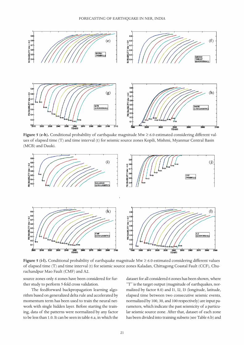
Figure 5 (e-h). Conditional probability of earthquake magnitude Mw ≥ 6.0 estimated considering different val-ues of elapsed time (T) and time interval (t) for seismic source zones Kopili, Mishmi, Myanmar Central Basin(MCB) and Dauki.

Figure 5 (i-l). Conditional probability of earthquake magnitude Mw ≥ 6.0 estimated considering different valuesof elapsed time (T) and time interval (t) for seismic source zones Kaladan, Chittagong Coastal Fault (CCF), Chu-rachandpur Mao Fault (CMF) and A2.

(e) (f )

(g) (h)

(i) ( j)

(k) (l)

testing subsets (see Table 6.c) to perform 5-fold crossvalidation.

Firstly, the neural networks have been trained for dif-ferent values of learning rate (η) and momentum coeffi-cient (α). It is observed that a higher value of η leads tofaster learning but the weights starts oscillating, while alower value of η leads to slower learning process and longtraining time. To reduce the training time, the best op-tion is to add momentum term into the weight updateprocedure, with a smaller value of η. It is observed thatfor η= 0.7 and α= 0.9 network yields stable solution andit reaches to desired best output value very fast. It hasbeen also observed that for most of the seismic source

zones the training SSE gets minimized to 0.009 beforecompleting the 25000 numbers of training epochs whilefor some other seismic source zones the desired level oftraining SSE is not achieved even after completing the25000 numbers of training epochs.

After training of the neural networks for trainingsubsets, the trained networks have been used to estimateoutput “O” for testing subsets and testing SSE has beenreported (see Table 6.c). Neural networks have been alsotrained considering all the data points for the whole studyarea. The dataset of the whole study area is divided intofive subsets to perform the 5-fold cross validation and av-erage SSE is estimated (Figure 8, a-e).

ZAROLA AND SIL

22

Figure 5 (m). Conditional probability of earthquake magnitude Mw ≥ 6.0 estimated considering different valuesof elapsed time (T) and time interval (t) for the whole study area.

Figure 6. Map shows conditional probability of earthquake magnitude Mw ≥ 6.0 estimated for the years 2017 to2040 considering total elapsed time upto 2016 for all twelve seismic source zones.

(m)

23

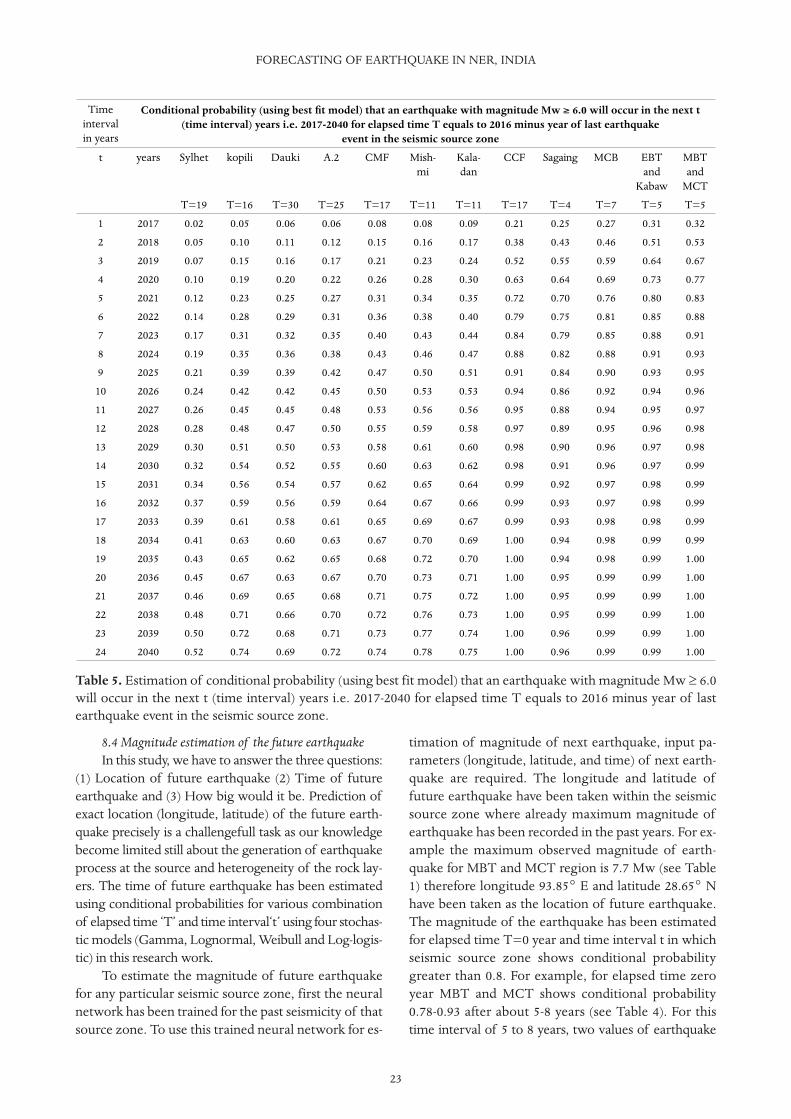
8.4 Magnitude estimation of the future earthquakeIn this study, we have to answer the three questions:

(1) Location of future earthquake (2) Time of futureearthquake and (3) How big would it be. Prediction ofexact location (longitude, latitude) of the future earth-quake precisely is a challengefull task as our knowledgebecome limited still about the generation of earthquakeprocess at the source and heterogeneity of the rock lay-ers. The time of future earthquake has been estimatedusing conditional probabilities for various combinationof elapsed time ‘T’ and time interval‘t’ using four stochas-tic models (Gamma, Lognormal, Weibull and Log-logis-tic) in this research work.

To estimate the magnitude of future earthquakefor any particular seismic source zone, first the neuralnetwork has been trained for the past seismicity of thatsource zone. To use this trained neural network for es-

timation of magnitude of next earthquake, input pa-rameters (longitude, latitude, and time) of next earth-quake are required. The longitude and latitude offuture earthquake have been taken within the seismicsource zone where already maximum magnitude ofearthquake has been recorded in the past years. For ex-ample the maximum observed magnitude of earth-quake for MBT and MCT region is 7.7 Mw (see Table1) therefore longitude 93.85° E and latitude 28.65° Nhave been taken as the location of future earthquake.The magnitude of the earthquake has been estimatedfor elapsed time T=0 year and time interval t in whichseismic source zone shows conditional probabilitygreater than 0.8. For example, for elapsed time zeroyear MBT and MCT shows conditional probability0.78-0.93 after about 5-8 years (see Table 4). For thistime interval of 5 to 8 years, two values of earthquake

FORECASTING OF EARTHQUAKE IN NER, INDIA

Time interval in years

Conditional probability (using best fi t model) that an earthquake with magnitude Mw ≥ 6.0 will occur in the next t (time interval) years i.e. 2017-2040 for elapsed time T equals to 2016 minus year of last earthquake

event in the seismic source zone

t years Sylhet kopili Dauki A.2 CMF Mish-mi

Kala-dan

CCF Sagaing MCB EBT and

Kabaw

MBT and

MCT

T=19 T=16 T=30 T=25 T=17 T=11 T=11 T=17 T=4 T=7 T=5 T=5

1 2017 0.02 0.05 0.06 0.06 0.08 0.08 0.09 0.21 0.25 0.27 0.31 0.32

2 2018 0.05 0.10 0.11 0.12 0.15 0.16 0.17 0.38 0.43 0.46 0.51 0.53

3 2019 0.07 0.15 0.16 0.17 0.21 0.23 0.24 0.52 0.55 0.59 0.64 0.67

4 2020 0.10 0.19 0.20 0.22 0.26 0.28 0.30 0.63 0.64 0.69 0.73 0.77

5 2021 0.12 0.23 0.25 0.27 0.31 0.34 0.35 0.72 0.70 0.76 0.80 0.83

6 2022 0.14 0.28 0.29 0.31 0.36 0.38 0.40 0.79 0.75 0.81 0.85 0.88

7 2023 0.17 0.31 0.32 0.35 0.40 0.43 0.44 0.84 0.79 0.85 0.88 0.91

8 2024 0.19 0.35 0.36 0.38 0.43 0.46 0.47 0.88 0.82 0.88 0.91 0.93

9 2025 0.21 0.39 0.39 0.42 0.47 0.50 0.51 0.91 0.84 0.90 0.93 0.95

10 2026 0.24 0.42 0.42 0.45 0.50 0.53 0.53 0.94 0.86 0.92 0.94 0.96

11 2027 0.26 0.45 0.45 0.48 0.53 0.56 0.56 0.95 0.88 0.94 0.95 0.97

12 2028 0.28 0.48 0.47 0.50 0.55 0.59 0.58 0.97 0.89 0.95 0.96 0.98

13 2029 0.30 0.51 0.50 0.53 0.58 0.61 0.60 0.98 0.90 0.96 0.97 0.98

14 2030 0.32 0.54 0.52 0.55 0.60 0.63 0.62 0.98 0.91 0.96 0.97 0.99

15 2031 0.34 0.56 0.54 0.57 0.62 0.65 0.64 0.99 0.92 0.97 0.98 0.99

16 2032 0.37 0.59 0.56 0.59 0.64 0.67 0.66 0.99 0.93 0.97 0.98 0.99

17 2033 0.39 0.61 0.58 0.61 0.65 0.69 0.67 0.99 0.93 0.98 0.98 0.99

18 2034 0.41 0.63 0.60 0.63 0.67 0.70 0.69 1.00 0.94 0.98 0.99 0.99

19 2035 0.43 0.65 0.62 0.65 0.68 0.72 0.70 1.00 0.94 0.98 0.99 1.00

20 2036 0.45 0.67 0.63 0.67 0.70 0.73 0.71 1.00 0.95 0.99 0.99 1.00

21 2037 0.46 0.69 0.65 0.68 0.71 0.75 0.72 1.00 0.95 0.99 0.99 1.00

22 2038 0.48 0.71 0.66 0.70 0.72 0.76 0.73 1.00 0.95 0.99 0.99 1.00

23 2039 0.50 0.72 0.68 0.71 0.73 0.77 0.74 1.00 0.96 0.99 0.99 1.00

24 2040 0.52 0.74 0.69 0.72 0.74 0.78 0.75 1.00 0.96 0.99 0.99 1.00

Table 5. Estimation of conditional probability (using best fit model) that an earthquake with magnitude Mw ≥ 6.0will occur in the next t (time interval) years i.e. 2017-2040 for elapsed time T equals to 2016 minus year of lastearthquake event in the seismic source zone.

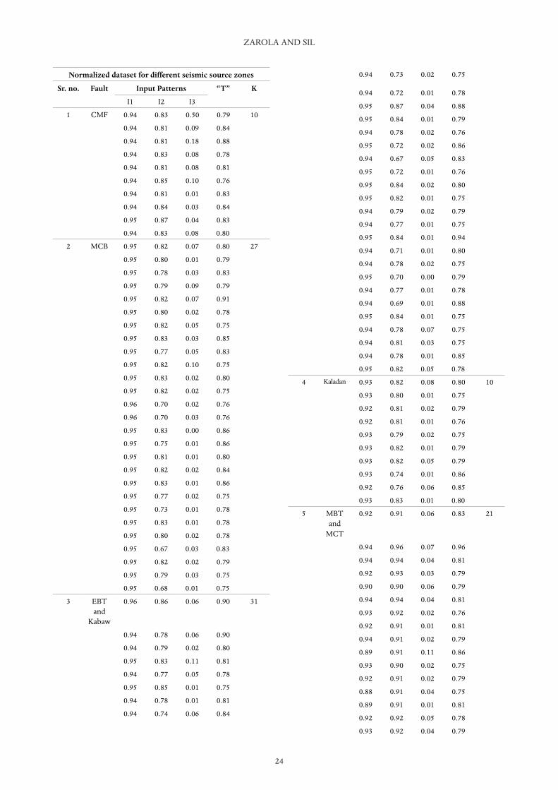
ZAROLA AND SIL

24

Normalized dataset for different seismic source zones

Sr. no. Fault Input Patterns “T” K

I1 I2 I3

1 CMF 0.94 0.83 0.50 0.79 10

0.94 0.81 0.09 0.84

0.94 0.81 0.18 0.88

0.94 0.83 0.08 0.78

0.94 0.81 0.08 0.81

0.94 0.85 0.10 0.76

0.94 0.81 0.01 0.83

0.94 0.84 0.03 0.84

0.95 0.87 0.04 0.83

0.94 0.83 0.08 0.80

2 MCB 0.95 0.82 0.07 0.80 27

0.95 0.80 0.01 0.79

0.95 0.78 0.03 0.83

0.95 0.79 0.09 0.79

0.95 0.82 0.07 0.91

0.95 0.80 0.02 0.78

0.95 0.82 0.05 0.75

0.95 0.83 0.03 0.85

0.95 0.77 0.05 0.83

0.95 0.82 0.10 0.75

0.95 0.83 0.02 0.80

0.95 0.82 0.02 0.75

0.96 0.70 0.02 0.76

0.96 0.70 0.03 0.76

0.95 0.83 0.00 0.86

0.95 0.75 0.01 0.86

0.95 0.81 0.01 0.80

0.95 0.82 0.02 0.84

0.95 0.83 0.01 0.86

0.95 0.77 0.02 0.75

0.95 0.73 0.01 0.78

0.95 0.83 0.01 0.78

0.95 0.80 0.02 0.78

0.95 0.67 0.03 0.83

0.95 0.82 0.02 0.79

0.95 0.79 0.03 0.75

0.95 0.68 0.01 0.75

3 EBT and

Kabaw

0.96 0.86 0.06 0.90 31

0.94 0.78 0.06 0.90

0.94 0.79 0.02 0.80

0.95 0.83 0.11 0.81

0.94 0.77 0.05 0.78

0.95 0.85 0.01 0.75

0.94 0.78 0.01 0.81

0.94 0.74 0.06 0.84

0.94 0.73 0.02 0.75

0.94 0.72 0.01 0.78

0.95 0.87 0.04 0.88

0.95 0.84 0.01 0.79

0.94 0.78 0.02 0.76

0.95 0.72 0.02 0.86

0.94 0.67 0.05 0.83

0.95 0.72 0.01 0.76

0.95 0.84 0.02 0.80

0.95 0.82 0.01 0.75

0.94 0.79 0.02 0.79

0.94 0.77 0.01 0.75

0.95 0.84 0.01 0.94

0.94 0.71 0.01 0.80

0.94 0.78 0.02 0.75

0.95 0.70 0.00 0.79

0.94 0.77 0.01 0.78

0.94 0.69 0.01 0.88

0.95 0.84 0.01 0.75

0.94 0.78 0.07 0.75

0.94 0.81 0.03 0.75

0.94 0.78 0.01 0.85

0.95 0.82 0.05 0.78

4 Kaladan 0.93 0.82 0.08 0.80 10

0.93 0.80 0.01 0.75

0.92 0.81 0.02 0.79

0.92 0.81 0.01 0.76

0.93 0.79 0.02 0.75

0.93 0.82 0.01 0.79

0.93 0.82 0.05 0.79

0.93 0.74 0.01 0.86

0.92 0.76 0.06 0.85

0.93 0.83 0.01 0.80

5 MBT and

MCT

0.92 0.91 0.06 0.83 21

0.94 0.96 0.07 0.96

0.94 0.94 0.04 0.81

0.92 0.93 0.03 0.79

0.90 0.90 0.06 0.79

0.94 0.94 0.04 0.81

0.93 0.92 0.02 0.76

0.92 0.91 0.01 0.81

0.94 0.91 0.02 0.79

0.89 0.91 0.11 0.86

0.93 0.90 0.02 0.75

0.92 0.91 0.02 0.79

0.88 0.91 0.04 0.75

0.89 0.91 0.01 0.81

0.92 0.92 0.05 0.78

0.93 0.92 0.04 0.79

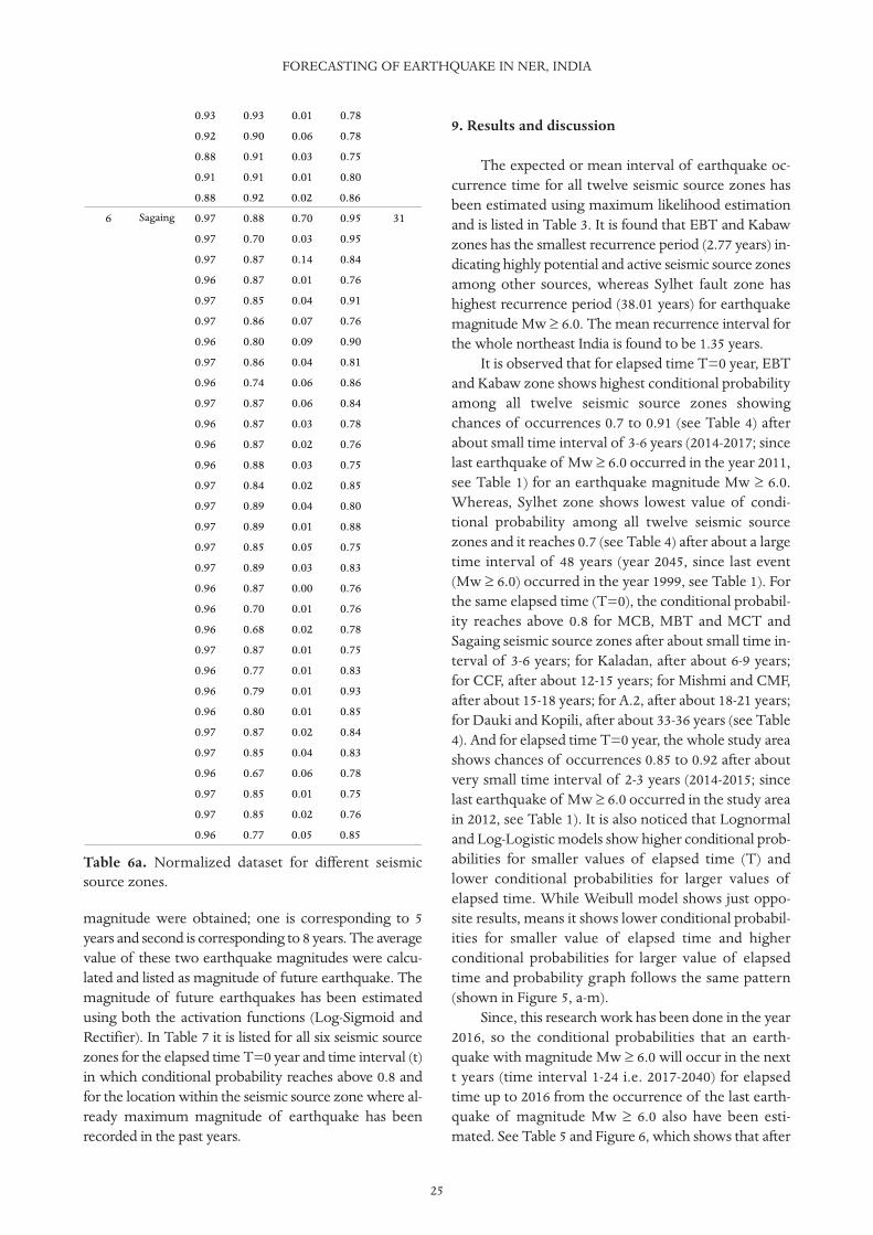
25

magnitude were obtained; one is corresponding to 5years and second is corresponding to 8 years. The averagevalue of these two earthquake magnitudes were calcu-lated and listed as magnitude of future earthquake. Themagnitude of future earthquakes has been estimatedusing both the activation functions (Log-Sigmoid andRectifier). In Table 7 it is listed for all six seismic sourcezones for the elapsed time T=0 year and time interval (t)in which conditional probability reaches above 0.8 andfor the location within the seismic source zone where al-ready maximum magnitude of earthquake has beenrecorded in the past years.

9. Results and discussion

The expected or mean interval of earthquake oc-currence time for all twelve seismic source zones hasbeen estimated using maximum likelihood estimationand is listed in Table 3. It is found that EBT and Kabawzones has the smallest recurrence period (2.77 years) in-dicating highly potential and active seismic source zonesamong other sources, whereas Sylhet fault zone hashighest recurrence period (38.01 years) for earthquakemagnitude Mw ≥ 6.0. The mean recurrence interval forthe whole northeast India is found to be 1.35 years.

It is observed that for elapsed time T=0 year, EBTand Kabaw zone shows highest conditional probabilityamong all twelve seismic source zones showingchances of occurrences 0.7 to 0.91 (see Table 4) afterabout small time interval of 3-6 years (2014-2017; sincelast earthquake of Mw ≥ 6.0 occurred in the year 2011,see Table 1) for an earthquake magnitude Mw ≥ 6.0.Whereas, Sylhet zone shows lowest value of condi-tional probability among all twelve seismic sourcezones and it reaches 0.7 (see Table 4) after about a largetime interval of 48 years (year 2045, since last event(Mw ≥ 6.0) occurred in the year 1999, see Table 1). Forthe same elapsed time (T=0), the conditional probabil-ity reaches above 0.8 for MCB, MBT and MCT andSagaing seismic source zones after about small time in-terval of 3-6 years; for Kaladan, after about 6-9 years;for CCF, after about 12-15 years; for Mishmi and CMF,after about 15-18 years; for A.2, after about 18-21 years;for Dauki and Kopili, after about 33-36 years (see Table4). And for elapsed time T=0 year, the whole study areashows chances of occurrences 0.85 to 0.92 after aboutvery small time interval of 2-3 years (2014-2015; sincelast earthquake of Mw ≥ 6.0 occurred in the study areain 2012, see Table 1). It is also noticed that Lognormaland Log-Logistic models show higher conditional prob-abilities for smaller values of elapsed time (T) andlower conditional probabilities for larger values ofelapsed time. While Weibull model shows just oppo-site results, means it shows lower conditional probabil-ities for smaller value of elapsed time and higherconditional probabilities for larger value of elapsedtime and probability graph follows the same pattern(shown in Figure 5, a-m).

Since, this research work has been done in the year2016, so the conditional probabilities that an earth-quake with magnitude Mw ≥ 6.0 will occur in the nextt years (time interval 1-24 i.e. 2017-2040) for elapsedtime up to 2016 from the occurrence of the last earth-quake of magnitude Mw ≥ 6.0 also have been esti-mated. See Table 5 and Figure 6, which shows that after

FORECASTING OF EARTHQUAKE IN NER, INDIA

0.93 0.93 0.01 0.78

0.92 0.90 0.06 0.78

0.88 0.91 0.03 0.75

0.91 0.91 0.01 0.80

0.88 0.92 0.02 0.86

6 Sagaing 0.97 0.88 0.70 0.95 31

0.97 0.70 0.03 0.95

0.97 0.87 0.14 0.84

0.96 0.87 0.01 0.76

0.97 0.85 0.04 0.91

0.97 0.86 0.07 0.76

0.96 0.80 0.09 0.90

0.97 0.86 0.04 0.81

0.96 0.74 0.06 0.86

0.97 0.87 0.06 0.84

0.96 0.87 0.03 0.78

0.96 0.87 0.02 0.76

0.96 0.88 0.03 0.75

0.97 0.84 0.02 0.85

0.97 0.89 0.04 0.80

0.97 0.89 0.01 0.88

0.97 0.85 0.05 0.75

0.97 0.89 0.03 0.83

0.96 0.87 0.00 0.76

0.96 0.70 0.01 0.76

0.96 0.68 0.02 0.78

0.97 0.87 0.01 0.75

0.96 0.77 0.01 0.83

0.96 0.79 0.01 0.93

0.96 0.80 0.01 0.85

0.97 0.87 0.02 0.84

0.97 0.85 0.04 0.83

0.96 0.67 0.06 0.78

0.97 0.85 0.01 0.75

0.97 0.85 0.02 0.76

0.96 0.77 0.05 0.85

Table 6a. Normalized dataset for different seismicsource zones.

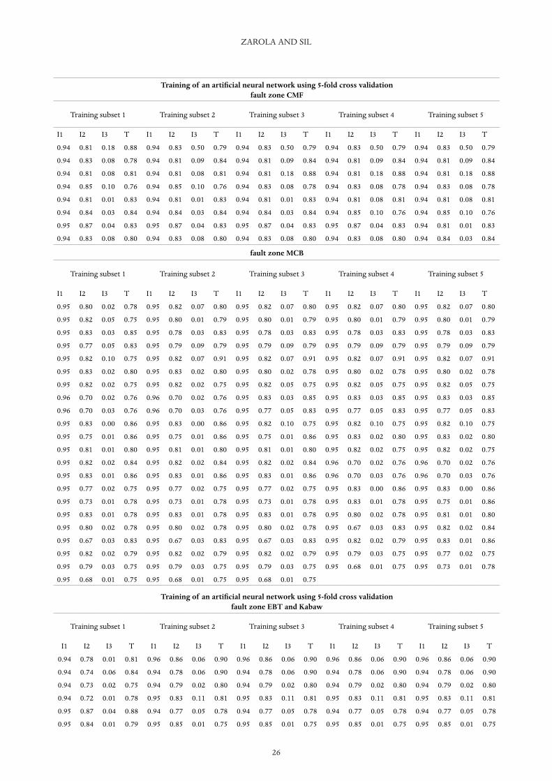
ZAROLA AND SIL

26

Training of an artifi cial neural network using 5-fold cross validation fault zone CMF

Training subset 1 Training subset 2 Training subset 3 Training subset 4 Training subset 5

I1 I2 I3 T I1 I2 I3 T I1 I2 I3 T I1 I2 I3 T I1 I2 I3 T

0.94 0.81 0.18 0.88 0.94 0.83 0.50 0.79 0.94 0.83 0.50 0.79 0.94 0.83 0.50 0.79 0.94 0.83 0.50 0.79

0.94 0.83 0.08 0.78 0.94 0.81 0.09 0.84 0.94 0.81 0.09 0.84 0.94 0.81 0.09 0.84 0.94 0.81 0.09 0.84

0.94 0.81 0.08 0.81 0.94 0.81 0.08 0.81 0.94 0.81 0.18 0.88 0.94 0.81 0.18 0.88 0.94 0.81 0.18 0.88

0.94 0.85 0.10 0.76 0.94 0.85 0.10 0.76 0.94 0.83 0.08 0.78 0.94 0.83 0.08 0.78 0.94 0.83 0.08 0.78

0.94 0.81 0.01 0.83 0.94 0.81 0.01 0.83 0.94 0.81 0.01 0.83 0.94 0.81 0.08 0.81 0.94 0.81 0.08 0.81

0.94 0.84 0.03 0.84 0.94 0.84 0.03 0.84 0.94 0.84 0.03 0.84 0.94 0.85 0.10 0.76 0.94 0.85 0.10 0.76

0.95 0.87 0.04 0.83 0.95 0.87 0.04 0.83 0.95 0.87 0.04 0.83 0.95 0.87 0.04 0.83 0.94 0.81 0.01 0.83

0.94 0.83 0.08 0.80 0.94 0.83 0.08 0.80 0.94 0.83 0.08 0.80 0.94 0.83 0.08 0.80 0.94 0.84 0.03 0.84

fault zone MCB

Training subset 1 Training subset 2 Training subset 3 Training subset 4 Training subset 5

I1 I2 I3 T I1 I2 I3 T I1 I2 I3 T I1 I2 I3 T I1 I2 I3 T

0.95 0.80 0.02 0.78 0.95 0.82 0.07 0.80 0.95 0.82 0.07 0.80 0.95 0.82 0.07 0.80 0.95 0.82 0.07 0.80

0.95 0.82 0.05 0.75 0.95 0.80 0.01 0.79 0.95 0.80 0.01 0.79 0.95 0.80 0.01 0.79 0.95 0.80 0.01 0.79

0.95 0.83 0.03 0.85 0.95 0.78 0.03 0.83 0.95 0.78 0.03 0.83 0.95 0.78 0.03 0.83 0.95 0.78 0.03 0.83

0.95 0.77 0.05 0.83 0.95 0.79 0.09 0.79 0.95 0.79 0.09 0.79 0.95 0.79 0.09 0.79 0.95 0.79 0.09 0.79

0.95 0.82 0.10 0.75 0.95 0.82 0.07 0.91 0.95 0.82 0.07 0.91 0.95 0.82 0.07 0.91 0.95 0.82 0.07 0.91

0.95 0.83 0.02 0.80 0.95 0.83 0.02 0.80 0.95 0.80 0.02 0.78 0.95 0.80 0.02 0.78 0.95 0.80 0.02 0.78

0.95 0.82 0.02 0.75 0.95 0.82 0.02 0.75 0.95 0.82 0.05 0.75 0.95 0.82 0.05 0.75 0.95 0.82 0.05 0.75

0.96 0.70 0.02 0.76 0.96 0.70 0.02 0.76 0.95 0.83 0.03 0.85 0.95 0.83 0.03 0.85 0.95 0.83 0.03 0.85

0.96 0.70 0.03 0.76 0.96 0.70 0.03 0.76 0.95 0.77 0.05 0.83 0.95 0.77 0.05 0.83 0.95 0.77 0.05 0.83

0.95 0.83 0.00 0.86 0.95 0.83 0.00 0.86 0.95 0.82 0.10 0.75 0.95 0.82 0.10 0.75 0.95 0.82 0.10 0.75

0.95 0.75 0.01 0.86 0.95 0.75 0.01 0.86 0.95 0.75 0.01 0.86 0.95 0.83 0.02 0.80 0.95 0.83 0.02 0.80

0.95 0.81 0.01 0.80 0.95 0.81 0.01 0.80 0.95 0.81 0.01 0.80 0.95 0.82 0.02 0.75 0.95 0.82 0.02 0.75

0.95 0.82 0.02 0.84 0.95 0.82 0.02 0.84 0.95 0.82 0.02 0.84 0.96 0.70 0.02 0.76 0.96 0.70 0.02 0.76

0.95 0.83 0.01 0.86 0.95 0.83 0.01 0.86 0.95 0.83 0.01 0.86 0.96 0.70 0.03 0.76 0.96 0.70 0.03 0.76

0.95 0.77 0.02 0.75 0.95 0.77 0.02 0.75 0.95 0.77 0.02 0.75 0.95 0.83 0.00 0.86 0.95 0.83 0.00 0.86

0.95 0.73 0.01 0.78 0.95 0.73 0.01 0.78 0.95 0.73 0.01 0.78 0.95 0.83 0.01 0.78 0.95 0.75 0.01 0.86

0.95 0.83 0.01 0.78 0.95 0.83 0.01 0.78 0.95 0.83 0.01 0.78 0.95 0.80 0.02 0.78 0.95 0.81 0.01 0.80

0.95 0.80 0.02 0.78 0.95 0.80 0.02 0.78 0.95 0.80 0.02 0.78 0.95 0.67 0.03 0.83 0.95 0.82 0.02 0.84

0.95 0.67 0.03 0.83 0.95 0.67 0.03 0.83 0.95 0.67 0.03 0.83 0.95 0.82 0.02 0.79 0.95 0.83 0.01 0.86

0.95 0.82 0.02 0.79 0.95 0.82 0.02 0.79 0.95 0.82 0.02 0.79 0.95 0.79 0.03 0.75 0.95 0.77 0.02 0.75

0.95 0.79 0.03 0.75 0.95 0.79 0.03 0.75 0.95 0.79 0.03 0.75 0.95 0.68 0.01 0.75 0.95 0.73 0.01 0.78

0.95 0.68 0.01 0.75 0.95 0.68 0.01 0.75 0.95 0.68 0.01 0.75

Training of an artifi cial neural network using 5-fold cross validationfault zone EBT and Kabaw

Training subset 1 Training subset 2 Training subset 3 Training subset 4 Training subset 5

I1 I2 I3 T I1 I2 I3 T I1 I2 I3 T I1 I2 I3 T I1 I2 I3 T

0.94 0.78 0.01 0.81 0.96 0.86 0.06 0.90 0.96 0.86 0.06 0.90 0.96 0.86 0.06 0.90 0.96 0.86 0.06 0.90

0.94 0.74 0.06 0.84 0.94 0.78 0.06 0.90 0.94 0.78 0.06 0.90 0.94 0.78 0.06 0.90 0.94 0.78 0.06 0.90

0.94 0.73 0.02 0.75 0.94 0.79 0.02 0.80 0.94 0.79 0.02 0.80 0.94 0.79 0.02 0.80 0.94 0.79 0.02 0.80

0.94 0.72 0.01 0.78 0.95 0.83 0.11 0.81 0.95 0.83 0.11 0.81 0.95 0.83 0.11 0.81 0.95 0.83 0.11 0.81

0.95 0.87 0.04 0.88 0.94 0.77 0.05 0.78 0.94 0.77 0.05 0.78 0.94 0.77 0.05 0.78 0.94 0.77 0.05 0.78

0.95 0.84 0.01 0.79 0.95 0.85 0.01 0.75 0.95 0.85 0.01 0.75 0.95 0.85 0.01 0.75 0.95 0.85 0.01 0.75

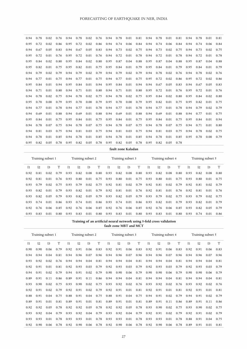
27

FORECASTING OF EARTHQUAKE IN NER, INDIA

0.94 0.78 0.02 0.76 0.94 0.78 0.02 0.76 0.94 0.78 0.01 0.81 0.94 0.78 0.01 0.81 0.94 0.78 0.01 0.81

0.95 0.72 0.02 0.86 0.95 0.72 0.02 0.86 0.94 0.74 0.06 0.84 0.94 0.74 0.06 0.84 0.94 0.74 0.06 0.84

0.94 0.67 0.05 0.83 0.94 0.67 0.05 0.83 0.94 0.73 0.02 0.75 0.94 0.73 0.02 0.75 0.94 0.73 0.02 0.75

0.95 0.72 0.01 0.76 0.95 0.72 0.01 0.76 0.94 0.72 0.01 0.78 0.94 0.72 0.01 0.78 0.94 0.72 0.01 0.78

0.95 0.84 0.02 0.80 0.95 0.84 0.02 0.80 0.95 0.87 0.04 0.88 0.95 0.87 0.04 0.88 0.95 0.87 0.04 0.88

0.95 0.82 0.01 0.75 0.95 0.82 0.01 0.75 0.95 0.84 0.01 0.79 0.95 0.84 0.01 0.79 0.95 0.84 0.01 0.79

0.94 0.79 0.02 0.79 0.94 0.79 0.02 0.79 0.94 0.79 0.02 0.79 0.94 0.78 0.02 0.76 0.94 0.78 0.02 0.76

0.94 0.77 0.01 0.75 0.94 0.77 0.01 0.75 0.94 0.77 0.01 0.75 0.95 0.72 0.02 0.86 0.95 0.72 0.02 0.86

0.95 0.84 0.01 0.94 0.95 0.84 0.01 0.94 0.95 0.84 0.01 0.94 0.94 0.67 0.05 0.83 0.94 0.67 0.05 0.83

0.94 0.71 0.01 0.80 0.94 0.71 0.01 0.80 0.94 0.71 0.01 0.80 0.95 0.72 0.01 0.76 0.95 0.72 0.01 0.76

0.94 0.78 0.02 0.75 0.94 0.78 0.02 0.75 0.94 0.78 0.02 0.75 0.95 0.84 0.02 0.80 0.95 0.84 0.02 0.80

0.95 0.70 0.00 0.79 0.95 0.70 0.00 0.79 0.95 0.70 0.00 0.79 0.95 0.82 0.01 0.75 0.95 0.82 0.01 0.75

0.94 0.77 0.01 0.78 0.94 0.77 0.01 0.78 0.94 0.77 0.01 0.78 0.94 0.77 0.01 0.78 0.94 0.79 0.02 0.79

0.94 0.69 0.01 0.88 0.94 0.69 0.01 0.88 0.94 0.69 0.01 0.88 0.94 0.69 0.01 0.88 0.94 0.77 0.01 0.75

0.95 0.84 0.01 0.75 0.95 0.84 0.01 0.75 0.95 0.84 0.01 0.75 0.95 0.84 0.01 0.75 0.95 0.84 0.01 0.94

0.94 0.78 0.07 0.75 0.94 0.78 0.07 0.75 0.94 0.78 0.07 0.75 0.94 0.78 0.07 0.75 0.94 0.71 0.01 0.80

0.94 0.81 0.03 0.75 0.94 0.81 0.03 0.75 0.94 0.81 0.03 0.75 0.94 0.81 0.03 0.75 0.94 0.78 0.02 0.75

0.94 0.78 0.01 0.85 0.94 0.78 0.01 0.85 0.94 0.78 0.01 0.85 0.94 0.78 0.01 0.85 0.95 0.70 0.00 0.79

0.95 0.82 0.05 0.78 0.95 0.82 0.05 0.78 0.95 0.82 0.05 0.78 0.95 0.82 0.05 0.78

fault zone Kaladan

Training subset 1 Training subset 2 Training subset 3 Training subset 4 Training subset 5

I1 I2 I3 T I1 I2 I3 T I1 I2 I3 T I1 I2 I3 T I1 I2 I3 T

0.92 0.81 0.02 0.79 0.93 0.82 0.08 0.80 0.93 0.82 0.08 0.80 0.93 0.82 0.08 0.80 0.93 0.82 0.08 0.80

0.92 0.81 0.01 0.76 0.93 0.80 0.01 0.75 0.93 0.80 0.01 0.75 0.93 0.80 0.01 0.75 0.93 0.80 0.01 0.75

0.93 0.79 0.02 0.75 0.93 0.79 0.02 0.75 0.92 0.81 0.02 0.79 0.92 0.81 0.02 0.79 0.92 0.81 0.02 0.79

0.93 0.82 0.01 0.79 0.93 0.82 0.01 0.79 0.92 0.81 0.01 0.76 0.92 0.81 0.01 0.76 0.92 0.81 0.01 0.76

0.93 0.82 0.05 0.79 0.93 0.82 0.05 0.79 0.93 0.82 0.05 0.79 0.93 0.79 0.02 0.75 0.93 0.79 0.02 0.75

0.93 0.74 0.01 0.86 0.93 0.74 0.01 0.86 0.93 0.74 0.01 0.86 0.93 0.82 0.01 0.79 0.93 0.82 0.01 0.79

0.92 0.76 0.06 0.85 0.92 0.76 0.06 0.85 0.92 0.76 0.06 0.85 0.92 0.76 0.06 0.85 0.93 0.82 0.05 0.79

0.93 0.83 0.01 0.80 0.93 0.83 0.01 0.80 0.93 0.83 0.01 0.80 0.93 0.83 0.01 0.80 0.93 0.74 0.01 0.86

Training of an artifi cial neural network using 5-fold cross validationfault zone MBT and MCT

Training subset 1 Training subset 2 Training subset 3 Training subset 4 Training subset 5

I1 I2 I3 T I1 I2 I3 T I1 I2 I3 T I1 I2 I3 T I1 I2 I3 T

0.90 0.90 0.06 0.79 0.92 0.91 0.06 0.83 0.92 0.91 0.06 0.83 0.92 0.91 0.06 0.83 0.92 0.91 0.06 0.83

0.94 0.94 0.04 0.81 0.94 0.96 0.07 0.96 0.94 0.96 0.07 0.96 0.94 0.96 0.07 0.96 0.94 0.96 0.07 0.96

0.93 0.92 0.02 0.76 0.94 0.94 0.04 0.81 0.94 0.94 0.04 0.81 0.94 0.94 0.04 0.81 0.94 0.94 0.04 0.81

0.92 0.91 0.01 0.81 0.92 0.93 0.03 0.79 0.92 0.93 0.03 0.79 0.92 0.93 0.03 0.79 0.92 0.93 0.03 0.79

0.94 0.91 0.02 0.79 0.94 0.91 0.02 0.79 0.90 0.90 0.06 0.79 0.90 0.90 0.06 0.79 0.90 0.90 0.06 0.79

0.89 0.91 0.11 0.86 0.89 0.91 0.11 0.86 0.94 0.94 0.04 0.81 0.94 0.94 0.04 0.81 0.94 0.94 0.04 0.81

0.93 0.90 0.02 0.75 0.93 0.90 0.02 0.75 0.93 0.92 0.02 0.76 0.93 0.92 0.02 0.76 0.93 0.92 0.02 0.76

0.92 0.91 0.02 0.79 0.92 0.91 0.02 0.79 0.92 0.91 0.01 0.81 0.92 0.91 0.01 0.81 0.92 0.91 0.01 0.81

0.88 0.91 0.04 0.75 0.88 0.91 0.04 0.75 0.88 0.91 0.04 0.75 0.94 0.91 0.02 0.79 0.94 0.91 0.02 0.79

0.89 0.91 0.01 0.81 0.89 0.91 0.01 0.81 0.89 0.91 0.01 0.81 0.89 0.91 0.11 0.86 0.89 0.91 0.11 0.86

0.92 0.92 0.05 0.78 0.92 0.92 0.05 0.78 0.92 0.92 0.05 0.78 0.93 0.90 0.02 0.75 0.93 0.90 0.02 0.75

0.93 0.92 0.04 0.79 0.93 0.92 0.04 0.79 0.93 0.92 0.04 0.79 0.92 0.91 0.02 0.79 0.92 0.91 0.02 0.79

0.93 0.93 0.01 0.78 0.93 0.93 0.01 0.78 0.93 0.93 0.01 0.78 0.93 0.93 0.01 0.78 0.88 0.91 0.04 0.75

0.92 0.90 0.06 0.78 0.92 0.90 0.06 0.78 0.92 0.90 0.06 0.78 0.92 0.90 0.06 0.78 0.89 0.91 0.01 0.81

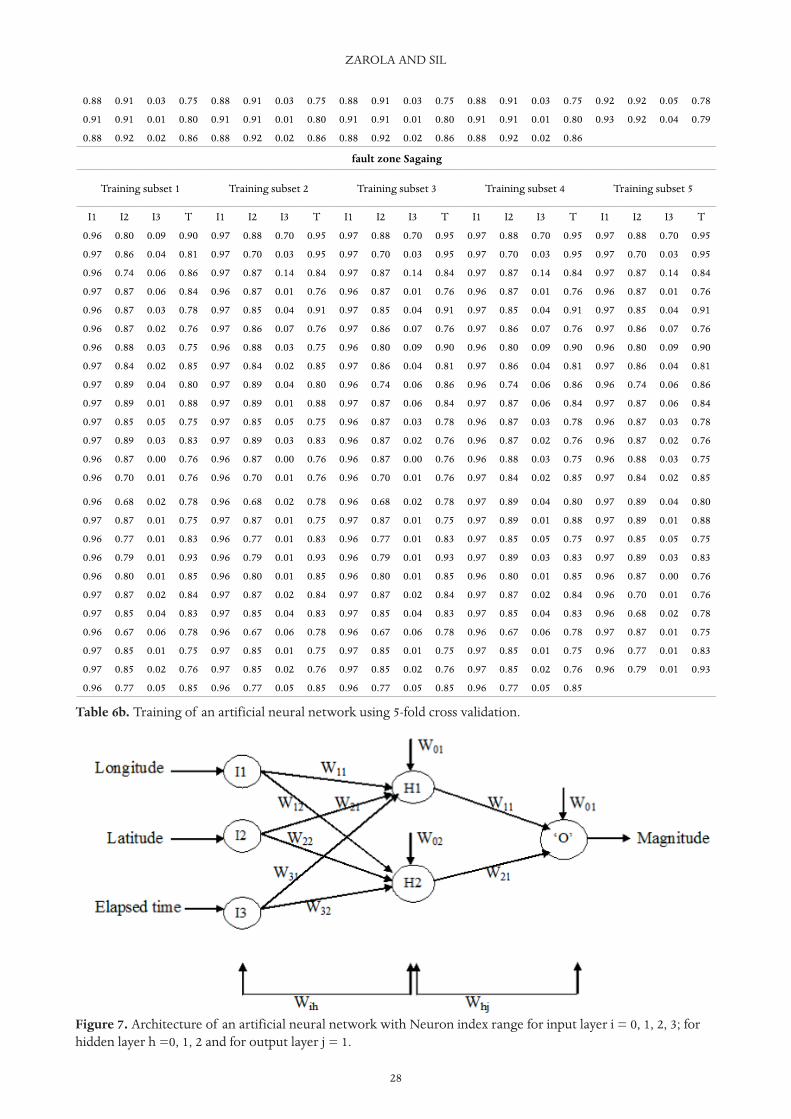
ZAROLA AND SIL

28

0.88 0.91 0.03 0.75 0.88 0.91 0.03 0.75 0.88 0.91 0.03 0.75 0.88 0.91 0.03 0.75 0.92 0.92 0.05 0.78

0.91 0.91 0.01 0.80 0.91 0.91 0.01 0.80 0.91 0.91 0.01 0.80 0.91 0.91 0.01 0.80 0.93 0.92 0.04 0.79

0.88 0.92 0.02 0.86 0.88 0.92 0.02 0.86 0.88 0.92 0.02 0.86 0.88 0.92 0.02 0.86

fault zone Sagaing

Training subset 1 Training subset 2 Training subset 3 Training subset 4 Training subset 5

I1 I2 I3 T I1 I2 I3 T I1 I2 I3 T I1 I2 I3 T I1 I2 I3 T

0.96 0.80 0.09 0.90 0.97 0.88 0.70 0.95 0.97 0.88 0.70 0.95 0.97 0.88 0.70 0.95 0.97 0.88 0.70 0.95

0.97 0.86 0.04 0.81 0.97 0.70 0.03 0.95 0.97 0.70 0.03 0.95 0.97 0.70 0.03 0.95 0.97 0.70 0.03 0.95

0.96 0.74 0.06 0.86 0.97 0.87 0.14 0.84 0.97 0.87 0.14 0.84 0.97 0.87 0.14 0.84 0.97 0.87 0.14 0.84

0.97 0.87 0.06 0.84 0.96 0.87 0.01 0.76 0.96 0.87 0.01 0.76 0.96 0.87 0.01 0.76 0.96 0.87 0.01 0.76

0.96 0.87 0.03 0.78 0.97 0.85 0.04 0.91 0.97 0.85 0.04 0.91 0.97 0.85 0.04 0.91 0.97 0.85 0.04 0.91

0.96 0.87 0.02 0.76 0.97 0.86 0.07 0.76 0.97 0.86 0.07 0.76 0.97 0.86 0.07 0.76 0.97 0.86 0.07 0.76

0.96 0.88 0.03 0.75 0.96 0.88 0.03 0.75 0.96 0.80 0.09 0.90 0.96 0.80 0.09 0.90 0.96 0.80 0.09 0.90

0.97 0.84 0.02 0.85 0.97 0.84 0.02 0.85 0.97 0.86 0.04 0.81 0.97 0.86 0.04 0.81 0.97 0.86 0.04 0.81

0.97 0.89 0.04 0.80 0.97 0.89 0.04 0.80 0.96 0.74 0.06 0.86 0.96 0.74 0.06 0.86 0.96 0.74 0.06 0.86

0.97 0.89 0.01 0.88 0.97 0.89 0.01 0.88 0.97 0.87 0.06 0.84 0.97 0.87 0.06 0.84 0.97 0.87 0.06 0.84

0.97 0.85 0.05 0.75 0.97 0.85 0.05 0.75 0.96 0.87 0.03 0.78 0.96 0.87 0.03 0.78 0.96 0.87 0.03 0.78

0.97 0.89 0.03 0.83 0.97 0.89 0.03 0.83 0.96 0.87 0.02 0.76 0.96 0.87 0.02 0.76 0.96 0.87 0.02 0.76

0.96 0.87 0.00 0.76 0.96 0.87 0.00 0.76 0.96 0.87 0.00 0.76 0.96 0.88 0.03 0.75 0.96 0.88 0.03 0.75

0.96 0.70 0.01 0.76 0.96 0.70 0.01 0.76 0.96 0.70 0.01 0.76 0.97 0.84 0.02 0.85 0.97 0.84 0.02 0.85

0.96 0.68 0.02 0.78 0.96 0.68 0.02 0.78 0.96 0.68 0.02 0.78 0.97 0.89 0.04 0.80 0.97 0.89 0.04 0.80

0.97 0.87 0.01 0.75 0.97 0.87 0.01 0.75 0.97 0.87 0.01 0.75 0.97 0.89 0.01 0.88 0.97 0.89 0.01 0.88

0.96 0.77 0.01 0.83 0.96 0.77 0.01 0.83 0.96 0.77 0.01 0.83 0.97 0.85 0.05 0.75 0.97 0.85 0.05 0.75

0.96 0.79 0.01 0.93 0.96 0.79 0.01 0.93 0.96 0.79 0.01 0.93 0.97 0.89 0.03 0.83 0.97 0.89 0.03 0.83

0.96 0.80 0.01 0.85 0.96 0.80 0.01 0.85 0.96 0.80 0.01 0.85 0.96 0.80 0.01 0.85 0.96 0.87 0.00 0.76

0.97 0.87 0.02 0.84 0.97 0.87 0.02 0.84 0.97 0.87 0.02 0.84 0.97 0.87 0.02 0.84 0.96 0.70 0.01 0.76

0.97 0.85 0.04 0.83 0.97 0.85 0.04 0.83 0.97 0.85 0.04 0.83 0.97 0.85 0.04 0.83 0.96 0.68 0.02 0.78

0.96 0.67 0.06 0.78 0.96 0.67 0.06 0.78 0.96 0.67 0.06 0.78 0.96 0.67 0.06 0.78 0.97 0.87 0.01 0.75

0.97 0.85 0.01 0.75 0.97 0.85 0.01 0.75 0.97 0.85 0.01 0.75 0.97 0.85 0.01 0.75 0.96 0.77 0.01 0.83

0.97 0.85 0.02 0.76 0.97 0.85 0.02 0.76 0.97 0.85 0.02 0.76 0.97 0.85 0.02 0.76 0.96 0.79 0.01 0.93

0.96 0.77 0.05 0.85 0.96 0.77 0.05 0.85 0.96 0.77 0.05 0.85 0.96 0.77 0.05 0.85

Table 6b. Training of an artificial neural network using 5-fold cross validation.

Figure 7. Architecture of an artificial neural network with Neuron index range for input layer i = 0, 1, 2, 3; forhidden layer h =0, 1, 2 and for output layer j = 1.

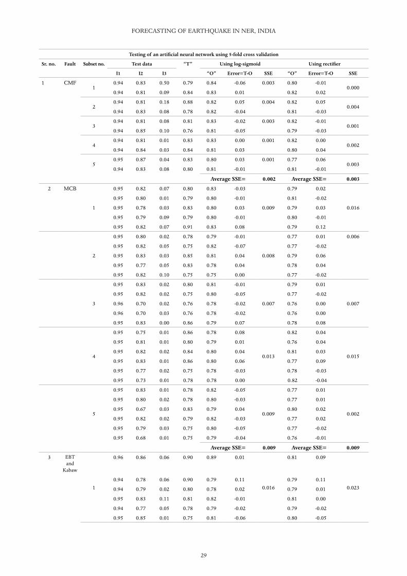
29

FORECASTING OF EARTHQUAKE IN NER, INDIA

Testing of an artifi cial neural network using 5-fold cross validation

Sr. no. Fault Subset no. Test data “T” Using log-sigmoid Using rectifi er

I1 I2 I3 “O” Error=T-O SSE “O” Error=T-O SSE

1 CMF1

0.94 0.83 0.50 0.79 0.84 -0.06 0.003 0.80 -0.010.000

0.94 0.81 0.09 0.84 0.83 0.01 0.82 0.02

20.94 0.81 0.18 0.88 0.82 0.05 0.004 0.82 0.05

0.0040.94 0.83 0.08 0.78 0.82 -0.04 0.81 -0.03

30.94 0.81 0.08 0.81 0.83 -0.02 0.003 0.82 -0.01

0.0010.94 0.85 0.10 0.76 0.81 -0.05 0.79 -0.03

40.94 0.81 0.01 0.83 0.83 0.00 0.001 0.82 0.00

0.0020.94 0.84 0.03 0.84 0.81 0.03 0.80 0.04

50.95 0.87 0.04 0.83 0.80 0.03 0.001 0.77 0.06

0.0030.94 0.83 0.08 0.80 0.81 -0.01 0.81 -0.01

Average SSE= 0.002 Average SSE= 0.003

2 MCB

1

0.95 0.82 0.07 0.80 0.83 -0.03

0.009

0.79 0.02

0.016

0.95 0.80 0.01 0.79 0.80 -0.01 0.81 -0.02

0.95 0.78 0.03 0.83 0.80 0.03 0.79 0.03

0.95 0.79 0.09 0.79 0.80 -0.01 0.80 -0.01

0.95 0.82 0.07 0.91 0.83 0.08 0.79 0.12

2

0.95 0.80 0.02 0.78 0.79 -0.01

0.008

0.77 0.01 0.006

0.95 0.82 0.05 0.75 0.82 -0.07 0.77 -0.02

0.95 0.83 0.03 0.85 0.81 0.04 0.79 0.06

0.95 0.77 0.05 0.83 0.78 0.04 0.78 0.04

0.95 0.82 0.10 0.75 0.75 0.00 0.77 -0.02

3

0.95 0.83 0.02 0.80 0.81 -0.01

0.007

0.79 0.01

0.007

0.95 0.82 0.02 0.75 0.80 -0.05 0.77 -0.02

0.96 0.70 0.02 0.76 0.78 -0.02 0.76 0.00

0.96 0.70 0.03 0.76 0.78 -0.02 0.76 0.00

0.95 0.83 0.00 0.86 0.79 0.07 0.78 0.08

4

0.95 0.75 0.01 0.86 0.78 0.08

0.013

0.82 0.04

0.015

0.95 0.81 0.01 0.80 0.79 0.01 0.76 0.04

0.95 0.82 0.02 0.84 0.80 0.04 0.81 0.03

0.95 0.83 0.01 0.86 0.80 0.06 0.77 0.09

0.95 0.77 0.02 0.75 0.78 -0.03 0.78 -0.03

0.95 0.73 0.01 0.78 0.78 0.00 0.82 -0.04

5

0.95 0.83 0.01 0.78 0.82 -0.05

0.009

0.77 0.01

0.002

0.95 0.80 0.02 0.78 0.80 -0.03 0.77 0.01

0.95 0.67 0.03 0.83 0.79 0.04 0.80 0.02

0.95 0.82 0.02 0.79 0.82 -0.03 0.77 0.02

0.95 0.79 0.03 0.75 0.80 -0.05 0.77 -0.02

0.95 0.68 0.01 0.75 0.79 -0.04 0.76 -0.01

Average SSE= 0.009 Average SSE= 0.009

3 EBT and

Kabaw

1

0.96 0.86 0.06 0.90 0.89 0.01

0.016

0.81 0.09

0.0230.94 0.78 0.06 0.90 0.79 0.11 0.79 0.11

0.94 0.79 0.02 0.80 0.78 0.02 0.79 0.01

0.95 0.83 0.11 0.81 0.82 -0.01 0.81 0.00

0.94 0.77 0.05 0.78 0.79 -0.02 0.79 -0.02

0.95 0.85 0.01 0.75 0.81 -0.06 0.80 -0.05

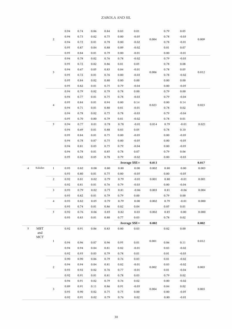
ZAROLA AND SIL

30

2 0.004 0.009

0.94 0.74 0.06 0.84 0.83 0.01 0.79 0.05

0.94 0.73 0.02 0.75 0.80 -0.05 0.78 -0.03

0.94 0.72 0.01 0.78 0.80 -0.02 0.78 -0.01

0.95 0.87 0.04 0.88 0.89 -0.02 0.81 0.07

0.95 0.84 0.01 0.79 0.80 -0.01 0.80 -0.01

3

0.94 0.78 0.02 0.76 0.78 -0.02

0.006

0.79 -0.03

0.012

0.95 0.72 0.02 0.86 0.81 0.05 0.78 0.08

0.94 0.67 0.05 0.83 0.84 -0.01 0.78 0.05

0.95 0.72 0.01 0.76 0.80 -0.03 0.78 -0.02

0.95 0.84 0.02 0.80 0.80 0.00 0.80 0.00

0.95 0.82 0.01 0.75 0.79 -0.04 0.80 -0.05

4

0.94 0.79 0.02 0.79 0.78 0.00

0.023

0.79 0.00

0.023

0.94 0.77 0.01 0.75 0.78 -0.03 0.79 -0.04

0.95 0.84 0.01 0.94 0.80 0.14 0.80 0.14

0.94 0.71 0.01 0.80 0.81 -0.01 0.78 0.02

0.94 0.78 0.02 0.75 0.78 -0.03 0.79 -0.04

0.95 0.70 0.00 0.79 0.81 -0.02 0.78 0.01

5 0.94 0.77 0.01 0.78 0.78 -0.01 0.014 0.79 -0.01 0.021

0.94 0.69 0.01 0.88 0.83 0.05 0.78 0.10

0.95 0.84 0.01 0.75 0.80 -0.05 0.80 -0.05

0.94 0.78 0.07 0.75 0.80 -0.05 0.80 -0.05

0.94 0.81 0.03 0.75 0.79 -0.04 0.80 -0.05

0.94 0.78 0.01 0.85 0.78 0.07 0.79 0.06

0.95 0.82 0.05 0.78 0.79 -0.02 0.80 -0.03

Average SSE= 0.013 0.017

4 Kaladan 1 0.93 0.82 0.08 0.80 0.80 0.00 0.002 0.80 0.00 0.003

0.93 0.80 0.01 0.75 0.80 -0.05 0.80 -0.05

2 0.92 0.81 0.02 0.79 0.79 -0.01 0.001 0.80 -0.01 0.001

0.92 0.81 0.01 0.76 0.79 -0.03 0.80 -0.04

3 0.93 0.79 0.02 0.75 0.81 -0.06 0.003 0.81 -0.06 0.004

0.93 0.82 0.01 0.79 0.79 0.00 0.79 0.00

4 0.93 0.82 0.05 0.79 0.79 0.00 0.002 0.79 -0.01 0.000

0.93 0.74 0.01 0.86 0.82 0.04 0.85 0.01

5 0.92 0.76 0.06 0.85 0.82 0.03 0.002 0.85 0.00 0.000

0.93 0.83 0.01 0.80 0.77 0.03 0.78 0.02

Average SSE= 0.002 0.002

5 MBT and

MCT1

0.92 0.91 0.06 0.83 0.80 0.03

0.001

0.82 0.00

0.0120.94 0.96 0.07 0.96 0.95 0.01 0.86 0.11

0.94 0.94 0.04 0.81 0.82 -0.01 0.83 -0.02

0.92 0.93 0.03 0.79 0.78 0.01 0.81 -0.03

2

0.90 0.90 0.06 0.79 0.76 0.03

0.002

0.81 -0.02

0.0030.94 0.94 0.04 0.81 0.82 -0.01 0.83 -0.02

0.93 0.92 0.02 0.76 0.77 -0.01 0.81 -0.04

0.92 0.91 0.01 0.81 0.78 0.03 0.79 0.02

3

0.94 0.91 0.02 0.79 0.76 0.02

0.004

0.80 -0.02

0.0030.89 0.91 0.11 0.86 0.91 -0.05 0.84 0.02

0.93 0.90 0.02 0.75 0.75 0.00 0.80 -0.05

0.92 0.91 0.02 0.79 0.76 0.02 0.80 -0.01

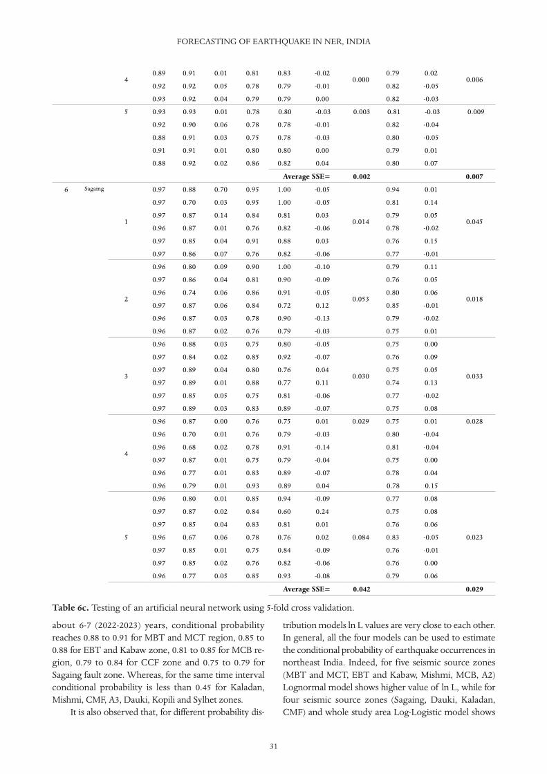
31

about 6-7 (2022-2023) years, conditional probabilityreaches 0.88 to 0.91 for MBT and MCT region, 0.85 to0.88 for EBT and Kabaw zone, 0.81 to 0.85 for MCB re-gion, 0.79 to 0.84 for CCF zone and 0.75 to 0.79 forSagaing fault zone. Whereas, for the same time intervalconditional probability is less than 0.45 for Kaladan,Mishmi, CMF, A3, Dauki, Kopili and Sylhet zones.

It is also observed that, for different probability dis-

tribution models ln L values are very close to each other.In general, all the four models can be used to estimatethe conditional probability of earthquake occurrences innortheast India. Indeed, for five seismic source zones(MBT and MCT, EBT and Kabaw, Mishmi, MCB, A2)Lognormal model shows higher value of ln L, while forfour seismic source zones (Sagaing, Dauki, Kaladan,CMF) and whole study area Log-Logistic model shows

FORECASTING OF EARTHQUAKE IN NER, INDIA

4 0.000 0.0060.89 0.91 0.01 0.81 0.83 -0.02 0.79 0.02

0.92 0.92 0.05 0.78 0.79 -0.01 0.82 -0.05

0.93 0.92 0.04 0.79 0.79 0.00 0.82 -0.03

5 0.93 0.93 0.01 0.78 0.80 -0.03 0.003 0.81 -0.03 0.009

0.92 0.90 0.06 0.78 0.78 -0.01 0.82 -0.04

0.88 0.91 0.03 0.75 0.78 -0.03 0.80 -0.05

0.91 0.91 0.01 0.80 0.80 0.00 0.79 0.01

0.88 0.92 0.02 0.86 0.82 0.04 0.80 0.07

Average SSE= 0.002 0.007

6 Sagaing

1

0.97 0.88 0.70 0.95 1.00 -0.05

0.014

0.94 0.01

0.045

0.97 0.70 0.03 0.95 1.00 -0.05 0.81 0.14

0.97 0.87 0.14 0.84 0.81 0.03 0.79 0.05

0.96 0.87 0.01 0.76 0.82 -0.06 0.78 -0.02

0.97 0.85 0.04 0.91 0.88 0.03 0.76 0.15

0.97 0.86 0.07 0.76 0.82 -0.06 0.77 -0.01

2

0.96 0.80 0.09 0.90 1.00 -0.10

0.053

0.79 0.11

0.018

0.97 0.86 0.04 0.81 0.90 -0.09 0.76 0.05

0.96 0.74 0.06 0.86 0.91 -0.05 0.80 0.06

0.97 0.87 0.06 0.84 0.72 0.12 0.85 -0.01

0.96 0.87 0.03 0.78 0.90 -0.13 0.79 -0.02

0.96 0.87 0.02 0.76 0.79 -0.03 0.75 0.01

3

0.96 0.88 0.03 0.75 0.80 -0.05

0.030

0.75 0.00

0.033

0.97 0.84 0.02 0.85 0.92 -0.07 0.76 0.09

0.97 0.89 0.04 0.80 0.76 0.04 0.75 0.05

0.97 0.89 0.01 0.88 0.77 0.11 0.74 0.13

0.97 0.85 0.05 0.75 0.81 -0.06 0.77 -0.02

0.97 0.89 0.03 0.83 0.89 -0.07 0.75 0.08

4

0.96 0.87 0.00 0.76 0.75 0.01 0.029 0.75 0.01 0.028

0.96 0.70 0.01 0.76 0.79 -0.03 0.80 -0.04

0.96 0.68 0.02 0.78 0.91 -0.14 0.81 -0.04

0.97 0.87 0.01 0.75 0.79 -0.04 0.75 0.00

0.96 0.77 0.01 0.83 0.89 -0.07 0.78 0.04

0.96 0.79 0.01 0.93 0.89 0.04 0.78 0.15

5

0.96 0.80 0.01 0.85 0.94 -0.09

0.084

0.77 0.08

0.023

0.97 0.87 0.02 0.84 0.60 0.24 0.75 0.08

0.97 0.85 0.04 0.83 0.81 0.01 0.76 0.06

0.96 0.67 0.06 0.78 0.76 0.02 0.83 -0.05

0.97 0.85 0.01 0.75 0.84 -0.09 0.76 -0.01

0.97 0.85 0.02 0.76 0.82 -0.06 0.76 0.00

0.96 0.77 0.05 0.85 0.93 -0.08 0.79 0.06

Average SSE= 0.042 0.029

Table 6c. Testing of an artificial neural network using 5-fold cross validation.

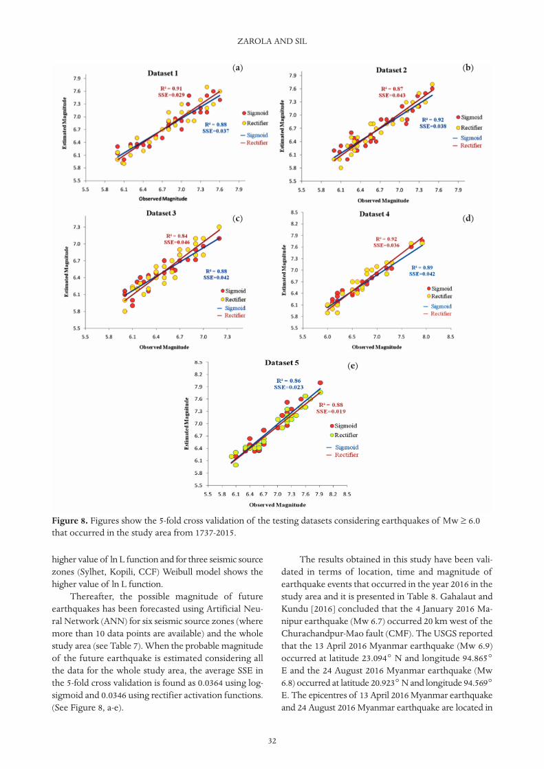
higher value of ln L function and for three seismic sourcezones (Sylhet, Kopili, CCF) Weibull model shows thehigher value of ln L function.

Thereafter, the possible magnitude of futureearthquakes has been forecasted using Artificial Neu-ral Network (ANN) for six seismic source zones (wheremore than 10 data points are available) and the wholestudy area (see Table 7). When the probable magnitudeof the future earthquake is estimated considering allthe data for the whole study area, the average SSE inthe 5-fold cross validation is found as 0.0364 using log-sigmoid and 0.0346 using rectifier activation functions.(See Figure 8, a-e).

The results obtained in this study have been vali-dated in terms of location, time and magnitude ofearthquake events that occurred in the year 2016 in thestudy area and it is presented in Table 8. Gahalaut andKundu [2016] concluded that the 4 January 2016 Ma-nipur earthquake (Mw 6.7) occurred 20 km west of theChurachandpur-Mao fault (CMF). The USGS reportedthat the 13 April 2016 Myanmar earthquake (Mw 6.9)occurred at latitude 23.094° N and longitude 94.865°E and the 24 August 2016 Myanmar earthquake (Mw6.8) occurred at latitude 20.923° N and longitude 94.569°E. The epicentres of 13 April 2016 Myanmar earthquakeand 24 August 2016 Myanmar earthquake are located in

ZAROLA AND SIL

32

Figure 8. Figures show the 5-fold cross validation of the testing datasets considering earthquakes of Mw ≥ 6.0that occurred in the study area from 1737-2015.

(a) (b)

(c) (d)

(e)

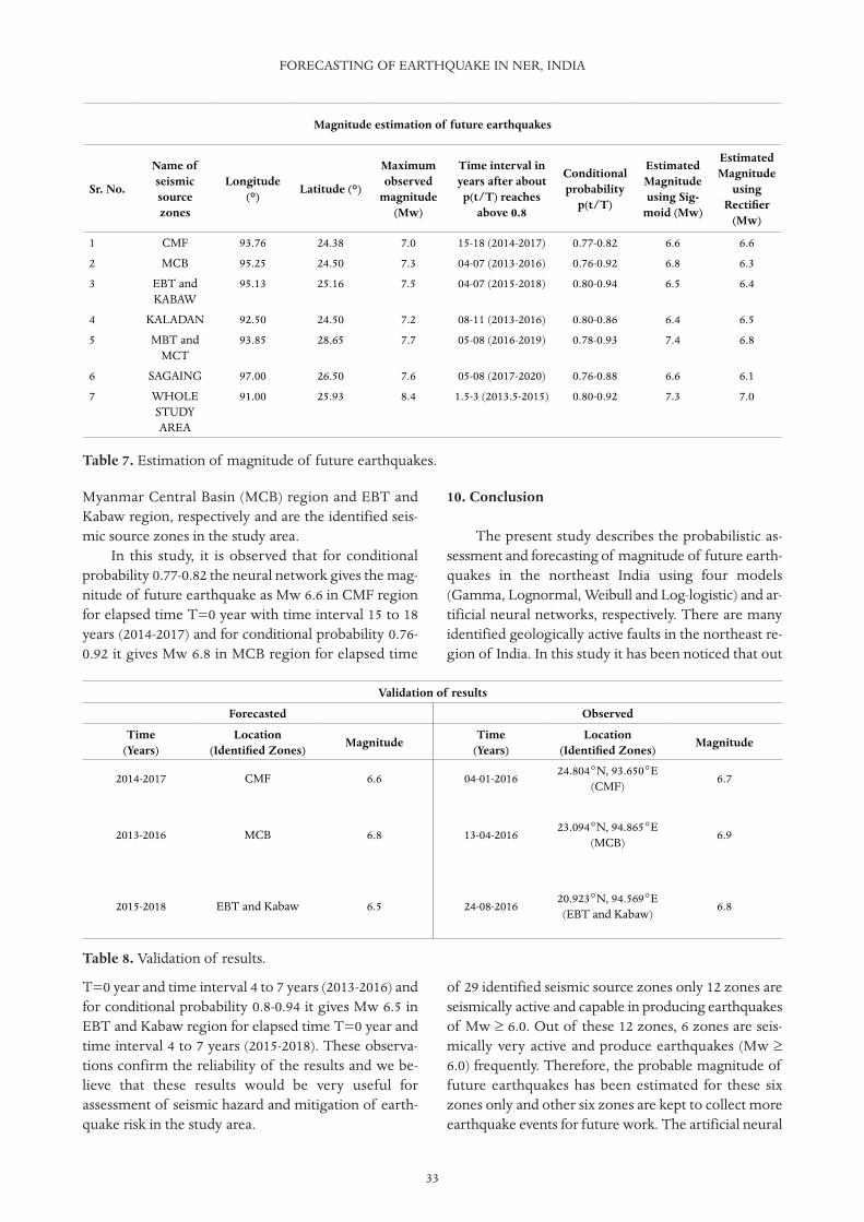
33

Myanmar Central Basin (MCB) region and EBT andKabaw region, respectively and are the identified seis-mic source zones in the study area.

In this study, it is observed that for conditionalprobability 0.77-0.82 the neural network gives the mag-nitude of future earthquake as Mw 6.6 in CMF regionfor elapsed time T=0 year with time interval 15 to 18years (2014-2017) and for conditional probability 0.76-0.92 it gives Mw 6.8 in MCB region for elapsed time

T=0 year and time interval 4 to 7 years (2013-2016) andfor conditional probability 0.8-0.94 it gives Mw 6.5 inEBT and Kabaw region for elapsed time T=0 year andtime interval 4 to 7 years (2015-2018). These observa-tions confirm the reliability of the results and we be-lieve that these results would be very useful forassessment of seismic hazard and mitigation of earth-quake risk in the study area.

10. Conclusion

The present study describes the probabilistic as-sessment and forecasting of magnitude of future earth-quakes in the northeast India using four models(Gamma, Lognormal, Weibull and Log-logistic) and ar-tificial neural networks, respectively. There are manyidentified geologically active faults in the northeast re-gion of India. In this study it has been noticed that out

of 29 identified seismic source zones only 12 zones areseismically active and capable in producing earthquakesof Mw ≥ 6.0. Out of these 12 zones, 6 zones are seis-mically very active and produce earthquakes (Mw ≥6.0) frequently. Therefore, the probable magnitude offuture earthquakes has been estimated for these sixzones only and other six zones are kept to collect moreearthquake events for future work. The artificial neural

FORECASTING OF EARTHQUAKE IN NER, INDIA

Magnitude estimation of future earthquakes

Sr. No.

Name of seismic source zones

Longitude (°)

Latitude (°)

Maximum observed

magnitude (Mw)

Time interval in years after about p(t/T) reaches

above 0.8

Conditional probability

p(t/T)

Estimated Magnitude using Sig-

moid (Mw)

Estimated Magnitude

usingRectifi er

(Mw)

1 CMF 93.76 24.38 7.0 15-18 (2014-2017) 0.77-0.82 6.6 6.6

2 MCB 95.25 24.50 7.3 04-07 (2013-2016) 0.76-0.92 6.8 6.3

3 EBT and KABAW

95.13 25.16 7.5 04-07 (2015-2018) 0.80-0.94 6.5 6.4

4 KALADAN 92.50 24.50 7.2 08-11 (2013-2016) 0.80-0.86 6.4 6.5

5 MBT and MCT

93.85 28.65 7.7 05-08 (2016-2019) 0.78-0.93 7.4 6.8

6 SAGAING 97.00 26.50 7.6 05-08 (2017-2020) 0.76-0.88 6.6 6.1

7 WHOLE STUDY AREA

91.00 25.93 8.4 1.5-3 (2013.5-2015) 0.80-0.92 7.3 7.0

Validation of results

Forecasted Observed

Time(Years)

Location(Identifi ed Zones)

MagnitudeTime

(Years)Location

(Identifi ed Zones)Magnitude

2014-2017 CMF 6.6 04-01-2016 24.804°N, 93.650°E (CMF) 6.7

2013-2016 MCB 6.8 13-04-2016 23.094°N, 94.865°E (MCB) 6.9

2015-2018 EBT and Kabaw 6.5 24-08-2016 20.923°N, 94.569°E (EBT and Kabaw) 6.8

Table 7. Estimation of magnitude of future earthquakes.

Table 8. Validation of results.

network model presented in this study yields higherforecasting accuracy for magnitude of earthquakes inthe northeast region of India because of its capabilityof capturing non linear relationship. It is observed that,for most of the seismic source zones the rectifier func-tion increases the training speed of the neural networkand the sum of squared error gets minimized to 0.009very fast. The results show that the seismic sourcezones CMF, MCB, EBT and Kabaw, Kaladan, MBT andMCT and Sagaing fault zone are highly potential seis-mic source zones having very small recurrence intervaland capable in producing the significant earthquakes innortheast region of India. Therefore, earthquake fore-casting and the proper seismic microzonation projectsare required for such regions which would help in riskassessment, disaster mitigation and also in designing ofsafe structures to reduce loss of human lives.

Acknowledgments. The authors acknowledge the support ofSERB-DST (ECR/2016/001329) to carry out the research studies.

ReferencesAlarifi, A. S. N., Alarifi, N. S. N. & Humidan, S. A., 2012.

Earthquake magnitude prediction using artificialneural network in northern red sea area, Journal ofKing Saud University Science, 24, 301-313.

Anagnos, T. & Kiremidjian A. S., 1988. A review of earth-quake occurrence models for seismic hazard analysis,Probabilistic Engineering Mechanics, vol. 3, no. 1, 3-11.

Ashkar, F. & Mahdi, S., 2006. Fitting the log-logistic dis-tribution by generalized moments, Journal of Hy-drology 328, 694-703.

Barakat, R., 1976. Sums of independent lognormallydistributed random variables, J. Opt. Soc. Am. 66,no. 3, 211-216, doi: 10.1364/JOSA.66.000211.

Baruah, S., Hazarika, D., Kalita, A. & Goswami, S., 2010.Intrinsic and scattering attenuation in Chedrangfault and its vicinity - the rupture area of greatAssam earthquake of 12 June 1897 (M = 8.7), Cur-rent Science, Vol. 99, No. 6, 775-784.

Basu, K. L., 1964. A note on the Coimbatore earthquake8th Februrary 1900, Indian J. Meteorol. Geophys. 15,no. 2, 281-286.

Bhattacharya, P. M., Kayal, J. R., Baruah, S. & Arefiev, S.S., 2010. Earthquake source zones in northeast India:seismic tomography, fractal dimension and b-valuemapping, Pure and Applied Geophysics, 167 (8), 999-1012, doi: 10.1007/s00024-010-0084-2.

Bichkule, K., 2014. Advanced neural network algo-rithms for prediction applications, InternationalJournal of Science and Research, vol. 3, 441-444.

Bilham R. & England P., 2001. Plateau pop-up during

the 1897 Assam earthquake, Nature, 410, 806-809.Bilham, R., 2004. Earthquakes in India and the Hi-

malaya: Tectonics, geodesy and history, Ann. Geo-phys., 47, 839–858.

Box-Steffensmeier, J. M. & Jones, B. S., 2004. Event His-tory Modeling: A Guide for Social Scientists, Cam-bridge University Press, Cambridge, New York,41-43, ISBN 0-521-54673-7.

Bureau of Indian Standards, 2002. IS 1893 (Part I): In-dian Standard Criteria for Earthquake Resistant De-sign of Structures, Bureau of Indian Standards, NewDelhi, India.

Caputo, M., 1974. Analysis of seismic risk, EngineeringSeismology and Earthquake Engineering: NATOAdvanced Study Institutes Series, Series E: AppliedSciences, 3, 55-86.

Chandra, U., 1977. Earthquakes of peninsula India - Aseismotectonic study, Bull. Seismol. Soc. Am. 67,1387-1413.

Chaudhury, H. M. & Srivastava, H. N., 1976. Seismicityand focal mechanism of some recent earthquakes innortheast India and neighbourhood, Ann. Geofis., 29(1-2), 41-56

Cluff, L. S., Patwardhan, A. S. & Coppersmith, K. J., 1980.Estimating the probability of occurrence of surfacefaulting earthquakes on the Wasatch fault zone, Utah,Bull. Seismol. Soc. Am. 70, 463-478.

Cornell, C. A., 1968. Engineering Seismic risk analysis,Bull. Seismol. Soc. Am. 58, 1583-1606.

Dikko, H. G., David, I. J. & Bakari, H. R., 2013. Modellingthe distribution of rainfall intensity using quarterlydata. IOSR Journal of Mathematics, vol. 9, 11-16.

Dunbar, P. K., Lockridge, P. A. & Whiteside, L. S., 1992.Catalogue of Significant Earthquakes, 2150 B. C. -1991 A. D., NOAA/NGDC Report SE-49, Boulder,Colorado, 320 pp.

Gahalaut, V. K. & Kundu, B., 2016. The 4 January 2016Manipur earthquake in the Indo-Burmese wedge, anintra-slab event, Geomatics, Natural Hazards Risk,7:5, 1506-1512, doi: 10.1080/19475705.2016.1179686.

Gardner, J. K. & Knopoff, L., 1974. Is the sequence ofearthquakes in southern California with aftershocksremoved, Poissonian? Bull. Seismol. Soc. Am. 64, no.5, 1363-1367.

Glorot, X., Bordes, A. & Bengio, Y., 2011. Deep sparserectifier neural networks, The 14th InternationalConference on Artificial Intelligence and Statistics(AISTATS), Fort Lauderdale, FL, USA,Vol. 15 ofJMLR.

Guzman-Speziale, M. & Ni, J. F., 1996. Seismicity andactive tectonics of the western Sunda Arc. In: Yin,A., Harrison, T. M. (Eds.), The Tectonic Evolution

ZAROLA AND SIL

34

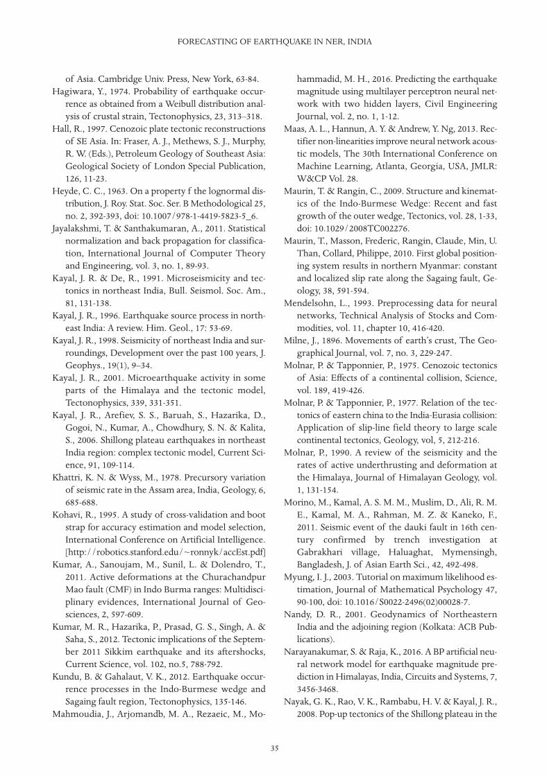
35

of Asia. Cambridge Univ. Press, New York, 63-84.Hagiwara, Y., 1974. Probability of earthquake occur-

rence as obtained from a Weibull distribution anal-ysis of crustal strain, Tectonophysics, 23, 313–318.

Hall, R., 1997. Cenozoic plate tectonic reconstructionsof SE Asia. In: Fraser, A. J., Methews, S. J., Murphy,R. W. (Eds.), Petroleum Geology of Southeast Asia:Geological Society of London Special Publication,126, 11-23.

Heyde, C. C., 1963. On a property f the lognormal dis-tribution, J. Roy. Stat. Soc. Ser. B Methodological 25,no. 2, 392-393, doi: 10.1007/978-1-4419-5823-5_6.

Jayalakshmi, T. & Santhakumaran, A., 2011. Statisticalnormalization and back propagation for classifica-tion, International Journal of Computer Theoryand Engineering, vol. 3, no. 1, 89-93.

Kayal, J. R. & De, R., 1991. Microseismicity and tec-tonics in northeast India, Bull. Seismol. Soc. Am.,81, 131-138.

Kayal, J. R., 1996. Earthquake source process in north-east India: A review. Him. Geol., 17: 53-69.

Kayal, J. R., 1998. Seismicity of northeast India and sur-roundings, Development over the past 100 years, J.Geophys., 19(1), 9–34.

Kayal, J. R., 2001. Microearthquake activity in someparts of the Himalaya and the tectonic model,Tectonophysics, 339, 331-351.

Kayal, J. R., Arefiev, S. S., Baruah, S., Hazarika, D.,Gogoi, N., Kumar, A., Chowdhury, S. N. & Kalita,S., 2006. Shillong plateau earthquakes in northeastIndia region: complex tectonic model, Current Sci-ence, 91, 109-114.

Khattri, K. N. & Wyss, M., 1978. Precursory variationof seismic rate in the Assam area, India, Geology, 6,685-688.

Kohavi, R., 1995. A study of cross-validation and bootstrap for accuracy estimation and model selection,International Conference on Artificial Intelligence.[http://robotics.stanford.edu/~ronnyk/accEst.pdf]

Kumar, A., Sanoujam, M., Sunil, L. & Dolendro, T.,2011. Active deformations at the ChurachandpurMao fault (CMF) in Indo Burma ranges: Multidisci-plinary evidences, International Journal of Geo-sciences, 2, 597-609.

Kumar, M. R., Hazarika, P., Prasad, G. S., Singh, A. &Saha, S., 2012. Tectonic implications of the Septem-ber 2011 Sikkim earthquake and its aftershocks,Current Science, vol. 102, no.5, 788-792.

Kundu, B. & Gahalaut, V. K., 2012. Earthquake occur-rence processes in the Indo-Burmese wedge andSagaing fault region, Tectonophysics, 135-146.

Mahmoudia, J., Arjomandb, M. A., Rezaeic, M., Mo-

hammadid, M. H., 2016. Predicting the earthquakemagnitude using multilayer perceptron neural net-work with two hidden layers, Civil EngineeringJournal, vol. 2, no. 1, 1-12.

Maas, A. L., Hannun, A. Y. & Andrew, Y. Ng, 2013. Rec-tifier non-linearities improve neural network acous-tic models, The 30th International Conference onMachine Learning, Atlanta, Georgia, USA, JMLR:W&CP Vol. 28.

Maurin, T. & Rangin, C., 2009. Structure and kinemat-ics of the Indo-Burmese Wedge: Recent and fastgrowth of the outer wedge, Tectonics, vol. 28, 1-33,doi: 10.1029/2008TC002276.

Maurin, T., Masson, Frederic, Rangin, Claude, Min, U.Than, Collard, Philippe, 2010. First global position-ing system results in northern Myanmar: constantand localized slip rate along the Sagaing fault, Ge-ology, 38, 591-594.

Mendelsohn, L., 1993. Preprocessing data for neuralnetworks, Technical Analysis of Stocks and Com-modities, vol. 11, chapter 10, 416-420.

Milne, J., 1896. Movements of earth’s crust, The Geo-graphical Journal, vol. 7, no. 3, 229-247.

Molnar, P. & Tapponnier, P., 1975. Cenozoic tectonicsof Asia: Effects of a continental collision, Science,vol. 189, 419-426.

Molnar, P. & Tapponnier, P., 1977. Relation of the tec-tonics of eastern china to the India-Eurasia collision:Application of slip-line field theory to large scalecontinental tectonics, Geology, vol, 5, 212-216.

Molnar, P., 1990. A review of the seismicity and therates of active underthrusting and deformation atthe Himalaya, Journal of Himalayan Geology, vol.1, 131-154.

Morino, M., Kamal, A. S. M. M., Muslim, D., Ali, R. M.E., Kamal, M. A., Rahman, M. Z. & Kaneko, F.,2011. Seismic event of the dauki fault in 16th cen-tury confirmed by trench investigation atGabrakhari village, Haluaghat, Mymensingh,Bangladesh, J. of Asian Earth Sci., 42, 492-498.

Myung, I. J., 2003. Tutorial on maximum likelihood es-timation, Journal of Mathematical Psychology 47,90-100, doi: 10.1016/S0022-2496(02)00028-7.

Nandy, D. R., 2001. Geodynamics of NortheasternIndia and the adjoining region (Kolkata: ACB Pub-lications).

Narayanakumar, S. & Raja, K., 2016. A BP artificial neu-ral network model for earthquake magnitude pre-diction in Himalayas, India, Circuits and Systems, 7,3456-3468.

Nayak, G. K., Rao, V. K., Rambabu, H. V. & Kayal, J. R.,2008. Pop-up tectonics of the Shillong plateau in the

FORECASTING OF EARTHQUAKE IN NER, INDIA

great 1897 earthquake (Ms 8.7), Insight from thegravity in conjunction with the recent seismologicalresults, Tectonics, 27, TC 1018.

Nielsen, C., Chamot-Rooke, N., Rangin, C., The An-daman Cruise Team, 2004. From partial to fullstrain partitioning along the Indo-Burmese hyper-oblique subduction, Marine Geology 209, 303-327.

Niksarlioglu, S. & Kulahci, F., 2013. An artificial neuralnetwork model for earthquake prediction and rela-tions between environmental parameters and earth-quakes, International Journal of Environmental,Chemical, Ecological, Geological and GeophysicalEngineering, 7(2).

Nishenko, S. P. & Buland, R. A., 1987. Generic recur-rence interval distribution for earthquake forecast-ing, Bull. Seism. Soc. Am., 77, 1382-1399.

Oldham, R. D., 1882. The Cachar earthquake of 10thJanuary, 1869, Memoirs of the Geological Societyof India, vol 19, 1-98.

Oldham, T., 1883. A catalogue of Indian earthquakesfrom the earliest time to the end of A. D. 1869,Memoir. Geol. Surv. India 29, 163-215.

Olympa, B. & Kumar A., 2015. A review on the tecton-ics setting and seismic activity of the ShillongPlateau in the light of past studies, Disaster Ad-vances, 8(7), 34-45.

Parvez, I. A. & Ram, A., 1997. Probabilistic assessmentof earthquake hazards in the northeast Indianpeninsula and Hindukush regions, Pure Appl. Geo-phys., 149, 731–746.

Parvez, I. A. & Ram A., 1999. Probabilistic assessmentof earthquake hazards in the Indian subcontinent,Pure Appl. Geophys., 154, 23–40.

Prabhakar & Dutta, M., 2013. Prediction of softwareeffort using artificial neural network and supportvector machine, International Journal of AdvancedResearch in Cmputer Science and Software Engi-neering, vol. 3, 40-46.

Rajendran, C. P., Rajendran, K., Duarah, B. P., Baruah,S. & Earnest A., 2004. Interpreting the style of fault-ing and paleoseismicity associated with the 1897Shillong, northeast India, earthquake: Implicationsfor regional tectonism, Tectonics, 23, TC4009, doi:10.10 29/2003 TC 001605.

Rao, N. P. & Kumar, M. R.,1997. Uplift and tectonics ofthe Shillong plateau, northeast India, J. Phys. Earth,45, 167-176.

Rastogi, B. K., 1974. Earthquake mechanisms and platetectonics in the Himalayan region, Tectonophysics,21, 47-56.

Richter, C. F., 1958. Elementary Seismology, Freeman,San Francisco, pp. 768.

Rikitake, T., 1974. Probability of an earthquake occur-rence as estimated from crustal strain, Tectono-physics, 23, 299-312.

Rikitake, T,, 1991. Assessment of earthquake hazard inthe Tokyo area, Japan, Tectonophysics 199, 121-131.

Saha, D. K., Naskar, D. C., Bhattacharya, P. M. & Kayal,J. R., 2007. Geophysical and seismological investin-gations for the hidden Oldham fault in the Shillongplateau and Assam valley of northeast India, J. Geol.Soc. India, 69, 359-372.

Sarker, J. K., Ansary, M. A., Islam, M. R. & Safiullah, A.M. M., 2010. Potential losses for Sylhet, Bangladeshin a repeat of the 1918 Srimangal earthquake, Envi-ronmental Economics, 1(1), 12-31.

Seeber, L. & Armbruster, J., 1981. Great detachmentearthquakes along the Himalayan Arc and long-term forecasting. In: Simpson, D. W., Richards, P. G.(Eds.), Earthquake Prediction: An International Re-view. Maurice Ewing Series: American GeophysicalUnion, vol. 4, 259-277.

Shah, HC. & Movassate, M., 1975. Seismic risk analysisof California state water project: Proc. of the 5thEuropean Conf. on Earthquake Engineering,10/156, Istanbul.

Sikder, A. M. & Alam, M. M., 2003. 2-D modelling ofthe anticlinal structures and structural developmentof the eastern fold belt of the Bengal Basin,Bangladesh, Sediment, Geol., 155, 209-226,doi:10.1016/S0037-0738(02)00181-1.

Sil, A., Sitharam, T. G. & Haider S. T. 2015. Probabilis-tic models for forecasting earthquakes in the north-east region of India, BSSA, 105(6), 2910-2927.

Singh, R. K. Jhaljit, 1965. A short history of Manipur,Manipur Sahitya Parishad, Imphal, India, p. 365.

Sitharam, T. G. & Sil, A., 2014. Comprehensive seismichazard assessment of Tripura & Mizoram states, J.Earth Syst. Sci., 123(4), 837–857.

Stacy, E. W., 1962. A generalization of the gamma dis-tribution, Ann. Math. Stat. 33, no. 3, 1187-1192.

Tsutsumi, H. & Sato, Takayuki, 2009. Tectonic geo-morphology of the Southernmost Sagaing fault andsurface rupture associated with the May 1930 pegu(Bago) earthquake, Myanmar, Bull. Seismol. Soc.Am. 99, 2155-2168. doi: 10.1785/0120080113.

Uhrhammer, R. A., 1986. Characteristics of northernand central California seismicity, Earthq. Notes 1,21.

Utsu, T., 1972b. Aftershocks and earthquake statistics(IV), Journal of the Faculty of Science, HokkaidoUniversity Series VII Geophysic, 4, 1-42.

Utsu, T., 1984. Estimation of parameters for recurrencemodels of earthquakes, Bull. Earthq. Res. Inst. Univ.

ZAROLA AND SIL

36

37

Tokyo, 59, 53–66.Utsu, T., 2002. Statistical features of seismicity, in In-

ternational Handbook of Earthquake & Engineer-ing Seismology, W. H. K. Lee, H. Kanamori, P. C.Jennings and C. Kisslinger (Editors), vol. 81A, Aca-demic Press, New York, 719-732.

Vigny, C., Socquet, A., Rangin, C., Chamot-Rooke, N.,Pubellier, M., Bouin, M., Bertrand, G. & Becker, M.,2003. Present-day crustal deformation aroundSagaing fault, Myanmar, Journal of Geophysical Re-search 108 (B11), 2533. doi: 10.1029/2002JB001999.

Weibull, W., 1951. A statistical distribution function ofwide applicability, J. Appl. Mech. Trans. ASME 18,no. 3, 293-297.

Wesnousky, S. G., Scholz, C. H., Shimazaki, K. & Mat-suda, T., 1984. Integration of geological and seis-mological data for the analysis of seismic hazard: Acase study of Japan, Bull. Seismol. Soc. Am., 74, 687-708.

Wong, F. S., Tung, A. T. Y. & Dong, W., 1992. Seismichazard prediction using neural nets, Earthquake En-gineering, Tenth world Conference Balkema, Rot-terdam, ISBN, 90 5410 060 5.

Yadav, R. B. S., Tripathi, J. N., Rastogi, B. K. & ChopraS., 2008. Probabilistic assessment of earthquake haz-ard in Gujarat and adjoining region of India, PureAppl. Geophys., 165, 1813-1833.

Yadav, R. B. S., Tripathi, J. N., Rastogi, B. K., Das, M. C.& Chopra S., 2010. Probabilistic assessment ofearthquake recurrence in northeast India and ad-joining regions, Pure Appl. Geophys., 167, 1331-1342.

Yilmaz V., Erisoglu M. & Celik H. E., 2004. Probabilis-tic prediction of the next earthquake in the NAFZ(north Anatolian fault zone), turkey, Dogus Univer-sitesi Dergisi, 5(2), 243-250.

Yilmaz, V. & Celik, H. E., 2008. A statistical approachfor estimating the probability of occurrence ofearthquake on the northern Anatolian fault zone,IJNES, 2(2), 81-86.

*Corresponding author: Arjun Sil,Department of Civil Engineering, NIT Silchar, Assam, India;email: silarjun@gmail.com.

© 2017 by the Istituto Nazionale di Geofisica e Vulcanologia. Allrights reserved.

FORECASTING OF EARTHQUAKE IN NER, INDIA