Artemis User's Guide
148
ARTEMIS User’s Guide Bruce Ravel [email protected] http://bruceravel.github.io/demeter/ Document version 0.2 for artemis version 0.9.19 January 9, 2014
-
Upload
khangminh22 -
Category
Documents
-
view
4 -
download
0
Transcript of Artemis User's Guide

ARTEMIS User’sGuideBruce Ravel
[email protected]://bruceravel.github.io/demeter/
Document version 0.2
for artemis version 0.9.19
January 9, 2014

I sing of Artemis, whose shafts are of gold, who cheers onthe hounds, the pure maiden, shooter of stags, who delightsin archery, own sister to Apollo with the golden sword. Overthe shadowy hills and windy peaks she draws her golden bow,rejoicing in the chase, and sends out grievous shafts. The topsof the high mountains tremble and the tangled wood echoesawesomely with the outcry of beasts: earthquakes and the seaalso where fishes shoal. But the goddess with a bold heartturns every way destroying the race of wild beasts: and whenshe is satisfied and has cheered her heart, this huntress whodelights in arrows slackens her supple bow and goes to thegreat house of her dear brother Phoebus Apollo, to the richland of Delphi, there to order the lovely dance of the Musesand Graces. There she hangs up her curved bow and herarrows, and heads and leads the dances, gracefully arrayed,while all they utter their heavenly voice, singing how neat-ankledLeto bare children supreme among the immortals both inthought and in deed. Hail to you, children of Zeus and rich-haired Leto! And now I will remember you and another song also.
Homeric Hymns XXVIITranslated by H. G. Evelyn-White
athena is copyright c© 2001–2014 Bruce Ravel
This document is copyright c© 2007–2014 Bruce Ravel.
This work is licensed under the Creative Commons Attribution-ShareAlike License. To view a copy of thislicense, visit
http://creativecommons.org/licenses/by-sa/3.0/
or send a letter to Creative Commons, 559 Nathan Abbott Way, Stanford, California 94305, USA.
You are free:
• to Share – to copy, distribute, and transmit the work
• to Remix – to adapt the work
Under the following conditions:
• Attribution. You must attribute the work in the manner specified by the author or licensor (but notin any way that suggests that they endorse you or your use of the work).
• Share Alike. If you alter, transform, or build upon this work, you may distribute the resulting workonly under the same, similar or a compatible license.
• Any of these conditions can be waived if you get permission from the author.
• For any reuse or distribution, you must make clear to others the license terms of this work.
• Any of the above conditions can be waived if you get permission from the copyright holder.
• Nothing in this license impairs or restricts the author’s moral rights.
Your fair dealing and other rights are in no way affected by the above.
This is a human-readable summary of the Legal Code (the full license).

4 This work is licensed under the Creative Commons Attribution-ShareAlike License.

Contents
1 Introduction 91.1 Using this document . . . . . . . . . . . . . . . . . . . . . . . . . . . . . . . . . . . . . . . . . 9
1.1.1 Typesetting . . . . . . . . . . . . . . . . . . . . . . . . . . . . . . . . . . . . . . . . . . 91.2 The technology behind Artemis . . . . . . . . . . . . . . . . . . . . . . . . . . . . . . . . . . . 10
1.2.1 perl . . . . . . . . . . . . . . . . . . . . . . . . . . . . . . . . . . . . . . . . . . . . . . 101.2.2 wxWidgets and wxPerl . . . . . . . . . . . . . . . . . . . . . . . . . . . . . . . . . . . 101.2.3 Moose . . . . . . . . . . . . . . . . . . . . . . . . . . . . . . . . . . . . . . . . . . . . . 101.2.4 Templates, backends, and other tools . . . . . . . . . . . . . . . . . . . . . . . . . . . . 10
1.3 Folders and log files . . . . . . . . . . . . . . . . . . . . . . . . . . . . . . . . . . . . . . . . . 11
2 Starting Artemis 132.1 The main window . . . . . . . . . . . . . . . . . . . . . . . . . . . . . . . . . . . . . . . . . . . 13
2.1.1 Main menu bar . . . . . . . . . . . . . . . . . . . . . . . . . . . . . . . . . . . . . . . . 152.1.2 The File menu . . . . . . . . . . . . . . . . . . . . . . . . . . . . . . . . . . . . . . . . 152.1.3 The Monitor menu . . . . . . . . . . . . . . . . . . . . . . . . . . . . . . . . . . . . . . 162.1.4 The Plot menu . . . . . . . . . . . . . . . . . . . . . . . . . . . . . . . . . . . . . . . . 162.1.5 The Main help menu . . . . . . . . . . . . . . . . . . . . . . . . . . . . . . . . . . . . . 172.1.6 Status bar . . . . . . . . . . . . . . . . . . . . . . . . . . . . . . . . . . . . . . . . . . . 172.1.7 The Data list . . . . . . . . . . . . . . . . . . . . . . . . . . . . . . . . . . . . . . . . . 172.1.8 The Athena project selection dialog . . . . . . . . . . . . . . . . . . . . . . . . . . . . 182.1.9 The recent data dialog . . . . . . . . . . . . . . . . . . . . . . . . . . . . . . . . . . . . 182.1.10 The Feff list . . . . . . . . . . . . . . . . . . . . . . . . . . . . . . . . . . . . . . . . . . 182.1.11 Fit information . . . . . . . . . . . . . . . . . . . . . . . . . . . . . . . . . . . . . . . . 192.1.12 Fit and log buttons . . . . . . . . . . . . . . . . . . . . . . . . . . . . . . . . . . . . . . 19
2.2 The plot window . . . . . . . . . . . . . . . . . . . . . . . . . . . . . . . . . . . . . . . . . . . 20
3 The Data window 233.1 Special plots . . . . . . . . . . . . . . . . . . . . . . . . . . . . . . . . . . . . . . . . . . . . . 253.2 Data menu bar . . . . . . . . . . . . . . . . . . . . . . . . . . . . . . . . . . . . . . . . . . . . 28
3.2.1 The Data menu . . . . . . . . . . . . . . . . . . . . . . . . . . . . . . . . . . . . . . . . 283.2.2 The Path menu . . . . . . . . . . . . . . . . . . . . . . . . . . . . . . . . . . . . . . . . 293.2.3 The Marks menu . . . . . . . . . . . . . . . . . . . . . . . . . . . . . . . . . . . . . . . 303.2.4 The Actions menu . . . . . . . . . . . . . . . . . . . . . . . . . . . . . . . . . . . . . . 313.2.5 The Debug menu . . . . . . . . . . . . . . . . . . . . . . . . . . . . . . . . . . . . . . . 313.2.6 The Data help menu . . . . . . . . . . . . . . . . . . . . . . . . . . . . . . . . . . . . . 31
4 The Atoms and Feff Window 334.0.7 Crystal data . . . . . . . . . . . . . . . . . . . . . . . . . . . . . . . . . . . . . . . . . 334.0.8 Atoms tool bar . . . . . . . . . . . . . . . . . . . . . . . . . . . . . . . . . . . . . . . . 36
4.1 The Feff tab . . . . . . . . . . . . . . . . . . . . . . . . . . . . . . . . . . . . . . . . . . . . . . 36
5

CONTENTS
4.1.1 Feff documentation . . . . . . . . . . . . . . . . . . . . . . . . . . . . . . . . . . . . . . 364.1.2 Feff input templates . . . . . . . . . . . . . . . . . . . . . . . . . . . . . . . . . . . . . 38
4.2 The Paths tab . . . . . . . . . . . . . . . . . . . . . . . . . . . . . . . . . . . . . . . . . . . . 384.2.1 Path plotting and path geometry . . . . . . . . . . . . . . . . . . . . . . . . . . . . . . 404.2.2 Path ranking . . . . . . . . . . . . . . . . . . . . . . . . . . . . . . . . . . . . . . . . . 41
4.3 The Path-like tab . . . . . . . . . . . . . . . . . . . . . . . . . . . . . . . . . . . . . . . . . . . 434.3.1 Single Scattering Paths . . . . . . . . . . . . . . . . . . . . . . . . . . . . . . . . . . . 434.3.2 FSPaths . . . . . . . . . . . . . . . . . . . . . . . . . . . . . . . . . . . . . . . . . . . . 454.3.3 Histogram paths . . . . . . . . . . . . . . . . . . . . . . . . . . . . . . . . . . . . . . . 45
4.4 The Console tab . . . . . . . . . . . . . . . . . . . . . . . . . . . . . . . . . . . . . . . . . . . 45
5 The Path page 475.1 Setting math expressions . . . . . . . . . . . . . . . . . . . . . . . . . . . . . . . . . . . . . . . 485.2 Marking and Plotting . . . . . . . . . . . . . . . . . . . . . . . . . . . . . . . . . . . . . . . . 52
5.2.1 Moving paths to the Plotting list . . . . . . . . . . . . . . . . . . . . . . . . . . . . . . 535.2.2 Phase corrected plots . . . . . . . . . . . . . . . . . . . . . . . . . . . . . . . . . . . . 53
5.3 Using path-like objects . . . . . . . . . . . . . . . . . . . . . . . . . . . . . . . . . . . . . . . . 545.3.1 SSPaths . . . . . . . . . . . . . . . . . . . . . . . . . . . . . . . . . . . . . . . . . . . . 545.3.2 Quick first shell paths . . . . . . . . . . . . . . . . . . . . . . . . . . . . . . . . . . . . 545.3.3 Empirical paths . . . . . . . . . . . . . . . . . . . . . . . . . . . . . . . . . . . . . . . . 54
6 The GDS window 556.1 Parameter types . . . . . . . . . . . . . . . . . . . . . . . . . . . . . . . . . . . . . . . . . . . 556.2 User interaction . . . . . . . . . . . . . . . . . . . . . . . . . . . . . . . . . . . . . . . . . . . . 57
6.2.1 Button bar . . . . . . . . . . . . . . . . . . . . . . . . . . . . . . . . . . . . . . . . . . 576.2.2 Keyboard shortcuts . . . . . . . . . . . . . . . . . . . . . . . . . . . . . . . . . . . . . 586.2.3 Context menu . . . . . . . . . . . . . . . . . . . . . . . . . . . . . . . . . . . . . . . . . 58
7 Running a fit 617.1 Sanity checking your fitting model . . . . . . . . . . . . . . . . . . . . . . . . . . . . . . . . . 627.2 The heuristic happiness parameter . . . . . . . . . . . . . . . . . . . . . . . . . . . . . . . . . 63
7.2.1 Evaluation of the happiness parameter . . . . . . . . . . . . . . . . . . . . . . . . . . . 647.2.2 Configuring the happiness evaluation . . . . . . . . . . . . . . . . . . . . . . . . . . . . 64
7.3 Using path-like objects . . . . . . . . . . . . . . . . . . . . . . . . . . . . . . . . . . . . . . . . 65
8 Plotting data 678.0.1 The plotting list . . . . . . . . . . . . . . . . . . . . . . . . . . . . . . . . . . . . . . . 678.0.2 Populating the plotting list manually . . . . . . . . . . . . . . . . . . . . . . . . . . . . 688.0.3 Refreshing the plotting list after a fit . . . . . . . . . . . . . . . . . . . . . . . . . . . . 68
8.1 Stacked plots . . . . . . . . . . . . . . . . . . . . . . . . . . . . . . . . . . . . . . . . . . . . . 698.1.1 Stacked plot . . . . . . . . . . . . . . . . . . . . . . . . . . . . . . . . . . . . . . . . . . 698.1.2 Inverted plot . . . . . . . . . . . . . . . . . . . . . . . . . . . . . . . . . . . . . . . . . 698.1.3 Data stack plot . . . . . . . . . . . . . . . . . . . . . . . . . . . . . . . . . . . . . . . . 70
8.2 Plot Indicators . . . . . . . . . . . . . . . . . . . . . . . . . . . . . . . . . . . . . . . . . . . . 708.3 Creating and plotting VPaths . . . . . . . . . . . . . . . . . . . . . . . . . . . . . . . . . . . . 71
9 The Log and Journal windows 759.1 The Log window . . . . . . . . . . . . . . . . . . . . . . . . . . . . . . . . . . . . . . . . . . . 759.2 The Journal window . . . . . . . . . . . . . . . . . . . . . . . . . . . . . . . . . . . . . . . . . 76
10 The History window 7710.1 Reports on fits . . . . . . . . . . . . . . . . . . . . . . . . . . . . . . . . . . . . . . . . . . . . 7810.2 Plotting fits . . . . . . . . . . . . . . . . . . . . . . . . . . . . . . . . . . . . . . . . . . . . . . 79
6 This work is licensed under the Creative Commons Attribution-ShareAlike License.

CONTENTS
11 Monitoring things 8111.1 Command and status buffers . . . . . . . . . . . . . . . . . . . . . . . . . . . . . . . . . . . . 81
11.1.1 The Command buffer . . . . . . . . . . . . . . . . . . . . . . . . . . . . . . . . . . . . 8111.1.2 The Status buffer . . . . . . . . . . . . . . . . . . . . . . . . . . . . . . . . . . . . . . . 81
11.2 Interacting with Ifeffit . . . . . . . . . . . . . . . . . . . . . . . . . . . . . . . . . . . . . . . . 8211.3 Debugging Demeter . . . . . . . . . . . . . . . . . . . . . . . . . . . . . . . . . . . . . . . . . 82
12 Managing preferences 85
13 Worked examples 8713.1 Example 1: FeS2 . . . . . . . . . . . . . . . . . . . . . . . . . . . . . . . . . . . . . . . . . . . 87
13.1.1 Import data . . . . . . . . . . . . . . . . . . . . . . . . . . . . . . . . . . . . . . . . . . 8713.1.2 Examine the scattering paths . . . . . . . . . . . . . . . . . . . . . . . . . . . . . . . . 9013.1.3 Fit to the first coordination shell . . . . . . . . . . . . . . . . . . . . . . . . . . . . . . 9513.1.4 Extending the fit to higher shells . . . . . . . . . . . . . . . . . . . . . . . . . . . . . . 9513.1.5 The final fitting model . . . . . . . . . . . . . . . . . . . . . . . . . . . . . . . . . . . . 9513.1.6 Additional questions . . . . . . . . . . . . . . . . . . . . . . . . . . . . . . . . . . . . . 95
13.2 Example 1: Methyltin . . . . . . . . . . . . . . . . . . . . . . . . . . . . . . . . . . . . . . . . 95
14 Crystallography for EXAFS 9914.1 Understanding and denoting space groups . . . . . . . . . . . . . . . . . . . . . . . . . . . . . 99
14.1.1 Notation conventions . . . . . . . . . . . . . . . . . . . . . . . . . . . . . . . . . . . . . 9914.1.2 Unique Crystallographic Positions . . . . . . . . . . . . . . . . . . . . . . . . . . . . . 10014.1.3 Specially Recognized Lattice Types . . . . . . . . . . . . . . . . . . . . . . . . . . . . . 10014.1.4 Bravais Lattice Conventions . . . . . . . . . . . . . . . . . . . . . . . . . . . . . . . . . 10014.1.5 Low Symmetry Space Groups . . . . . . . . . . . . . . . . . . . . . . . . . . . . . . . . 10114.1.6 Rhombohedral Space Groups . . . . . . . . . . . . . . . . . . . . . . . . . . . . . . . . 10214.1.7 Multiple Origins and the Shift Keyword . . . . . . . . . . . . . . . . . . . . . . . . . . 10214.1.8 Denoting Space Groups . . . . . . . . . . . . . . . . . . . . . . . . . . . . . . . . . . . 10314.1.9 A Quick Review of Crystallography . . . . . . . . . . . . . . . . . . . . . . . . . . . . 10314.1.10 Decoding the Hermann-Maguin Notation . . . . . . . . . . . . . . . . . . . . . . . . . 10514.1.11 Decoding the Schoenflies Notation . . . . . . . . . . . . . . . . . . . . . . . . . . . . . 10614.1.12 The Hermann-Maguin Notation . . . . . . . . . . . . . . . . . . . . . . . . . . . . . . . 10614.1.13 The Schoenflies Notation . . . . . . . . . . . . . . . . . . . . . . . . . . . . . . . . . . 110
14.2 Absorption calculations and experimental corrections . . . . . . . . . . . . . . . . . . . . . . . 11114.2.1 Absorption Calculation . . . . . . . . . . . . . . . . . . . . . . . . . . . . . . . . . . . 11214.2.2 McMaster Correction . . . . . . . . . . . . . . . . . . . . . . . . . . . . . . . . . . . . 11214.2.3 I0 Correction . . . . . . . . . . . . . . . . . . . . . . . . . . . . . . . . . . . . . . . . . 11214.2.4 Self-Absorption Correction . . . . . . . . . . . . . . . . . . . . . . . . . . . . . . . . . 113
14.3 A worked example (in text!) . . . . . . . . . . . . . . . . . . . . . . . . . . . . . . . . . . . . . 11314.3.1 The Atoms input file . . . . . . . . . . . . . . . . . . . . . . . . . . . . . . . . . . . . . 11314.3.2 The Feff input file . . . . . . . . . . . . . . . . . . . . . . . . . . . . . . . . . . . . . . 11314.3.3 Modifying the Feff input file . . . . . . . . . . . . . . . . . . . . . . . . . . . . . . . . . 116
15 Extended discussions 11915.1 Understanding the quick first shell tool in Artemis . . . . . . . . . . . . . . . . . . . . . . . . 120
15.1.1 Using the quick first shell tool to model first shell data . . . . . . . . . . . . . . . . . . 12015.1.2 (Mis)Using the quick first shell tool beyond the first shell . . . . . . . . . . . . . . . . 12115.1.3 Executive summary . . . . . . . . . . . . . . . . . . . . . . . . . . . . . . . . . . . . . 12215.1.4 So, what should you do? . . . . . . . . . . . . . . . . . . . . . . . . . . . . . . . . . . . 12215.1.5 Reproducing the images above . . . . . . . . . . . . . . . . . . . . . . . . . . . . . . . 123
15.2 Using a data group’s characteristic value . . . . . . . . . . . . . . . . . . . . . . . . . . . . . . 125
This work is licensed under the Creative Commons Attribution-ShareAlike License. 7

CONTENTS
15.2.1 The CV token . . . . . . . . . . . . . . . . . . . . . . . . . . . . . . . . . . . . . . . . 12615.2.2 Use in lguess parameters . . . . . . . . . . . . . . . . . . . . . . . . . . . . . . . . . . . 127
15.3 Geometric parametrization of bond length . . . . . . . . . . . . . . . . . . . . . . . . . . . . . 12815.3.1 Volumetric expansion coefficient . . . . . . . . . . . . . . . . . . . . . . . . . . . . . . 12815.3.2 Propagating crystal distortion parameters . . . . . . . . . . . . . . . . . . . . . . . . . 12915.3.3 Parametrizations of distance in non-crystalline materials . . . . . . . . . . . . . . . . . 131
15.4 Modeling disorder . . . . . . . . . . . . . . . . . . . . . . . . . . . . . . . . . . . . . . . . . . 13215.4.1 Debye and Einstein models . . . . . . . . . . . . . . . . . . . . . . . . . . . . . . . . . 13215.4.2 Collinear multiple scattering paths . . . . . . . . . . . . . . . . . . . . . . . . . . . . . 13315.4.3 Sensible approximations for triangular multiple scattering paths . . . . . . . . . . . . 133
15.5 Constraints and restraints . . . . . . . . . . . . . . . . . . . . . . . . . . . . . . . . . . . . . . 13415.6 Using bond valence sums in Artemis . . . . . . . . . . . . . . . . . . . . . . . . . . . . . . . . 135
15.6.1 Computing a bond valence sum from a fit . . . . . . . . . . . . . . . . . . . . . . . . . 13515.6.2 Using a bond valance sum as a restraint . . . . . . . . . . . . . . . . . . . . . . . . . . 136
15.7 Fitting with empirical standards . . . . . . . . . . . . . . . . . . . . . . . . . . . . . . . . . . 13615.7.1 Preparing the empirical standard . . . . . . . . . . . . . . . . . . . . . . . . . . . . . . 13715.7.2 Using the empirical standard . . . . . . . . . . . . . . . . . . . . . . . . . . . . . . . . 139
15.8 Unique potential styles . . . . . . . . . . . . . . . . . . . . . . . . . . . . . . . . . . . . . . . . 14115.8.1 Each element gets a unique potential . . . . . . . . . . . . . . . . . . . . . . . . . . . . 14115.8.2 Each tag gets a unique potential . . . . . . . . . . . . . . . . . . . . . . . . . . . . . . 14215.8.3 Each site gets a unique potential . . . . . . . . . . . . . . . . . . . . . . . . . . . . . . 143
15.9 The pathfinder and fuzzy degeneracy . . . . . . . . . . . . . . . . . . . . . . . . . . . . . . . . 14415.9.1 How the path finder works . . . . . . . . . . . . . . . . . . . . . . . . . . . . . . . . . 14415.9.2 The pathfinder in Feff and Artemis . . . . . . . . . . . . . . . . . . . . . . . . . . . . . 14515.9.3 An example of using fuzzy degeneracy . . . . . . . . . . . . . . . . . . . . . . . . . . . 146
8 This work is licensed under the Creative Commons Attribution-ShareAlike License.

Chapter 1
Introduction
feff and ifeffit are amazing tools, but they can be somewhat hard to use. feff requires the use of clunkytext files with confusing syntax as its input. ifeffit has a wordy, finicky syntax. Both benefit by beingwrapped up inside of something easier to use. Hopefully, artemis is that something.
1.1 Using this document
1.1.1 Typesetting
I use some typesetting conventions to convey certain kinds of information in this manual.
1. The names of programs look like this: artemis, feff
2. The names of files look like this: ‘atoms.inp’
3. Configuration parameters (i.e. preferences) for artemis and demeter look like this: § Artemis →plot after fit
4. Verbatim text, such as represent specific input to or output from artemis or text typed into a computer,looks like this:
This is verbatim text!
Caution: Words of caution intended to point out some specific pitfall of the useor artemis are found in boxes that look like this.
To Do: Aspects of this document, or possibly of artemis itself, which areincomplete are indicated with boxes like this.
9

1.2. THE TECHNOLOGY BEHIND ARTEMIS
1.2 The technology behind Artemis
1.2.1 perl
demeter uses perl. This is, I suppose, an unsexy choice these days. All the cool kids are, after all, usingpython or ruby. I like perl. I can think in perl. And I can code quickly and fluently in perl. What’s more,perl has CPAN, the worlds largest repository of language extensions. CPAN means that I have far fewerwheels to recreate (and probably get wrong). Virtually any language extension I need in pursuit of makingdemeter awesome probably already exists.
1.2.2 wxWidgets and wxPerlartemis uses wxWidgets and its perl wrapper wxPerl as its graphical toolkit. This cross-platform tool
gives artemis a truly native look and feel because it uses the platform’s native API rather than emulatingthe GUI. Using wx’s rich set of graphical tools, artemis strives to provide a powerful yet user-friendlyenvironment in which to perform EXAFS data analysis.
1.2.3 Moose
demeter uses Moose. This is, on the balance, a very good thing, indeed. Moose brings many powerfulcapabilities to the programming table. When I was about halfway through writing demeter, I paused fora bit less than a month to rewrite everything I had thus far created to use Moose. This left me with about2/3 as many lines of code and a code base that was more robust and more featureful. Neat-o!
For the nerdly, Moose is an implementation of a meta-object protocol. This interesting and powerful toolallows for the semantics of the object system to be modified at either compile or run time. The problem ofadding features and functionality to the object system is therefore pushed downstream from the developersof the language to the users of the language. In good CPAN fashion, a healthy and robust ecosystem hasevolved around Moose producing a whole host of useful extensions.
Moose offers lots of great features, including an extremely powerful attribute system, a type attribute system,method modifiers, an ability to mix object and aspect orientation, and a wonderfully deep set of automatedtests. I am confident that simply by using Moose, my code is better code and, because Moose testing is sodeep, I am confident that any bugs in demeter are my fault and not the fault of the people whose work Idepend on.
For all the wonderfulness of Moose, it does have one big wart that I need to be up-front about. Moose isslow at start-up. Since demeter is big and Moose starts slowly, any program using demeter will takeabout 2 extra second to start. For a long-running program like a complicated fitting script or a GUI, anadditional couple of seconds at start-up is no big deal. For quick-n-dirty or one-off application, that maya bit annoying. The Moose folk claim to be working on start-up issues. I am keeping my fingers crossed.Until then, I live with the slow start-up, confident that the rest of demeter is worth the wait.
1.2.4 Templates, backends, and other tools
All of artemis’ interactions with feff, ifeffit, and its plotting tools use a templating library. Along with
10 This work is licensed under the Creative Commons Attribution-ShareAlike License.

CHAPTER 1. INTRODUCTION
a clean separation between function within the demeter code base and syntax of the various tools used bydemeter, the use of templated interactions provides a clear upgrade path for all parts of artemis.
FeffAlthough demeter ships with a freely redistributable version of feff6, it is possible to upgrade to uselater versions of feff by providing an appropriate set of templates. At this time, feff8 is partiallysupported, with better support coming soon.
Ifeffit and LarchMatt Newville, the author of ifeffit, is hard at work on ifeffit’s successor, called larch. The pathto supporting larch will be relatively shallow, requiring only authorship of a new set of templates.
plottingdemeter currently supports two plotting backends: PGPLOT, which is the native plotting tool inifeffit, and gnuplot. New plotting backends can be supported, again simply by creation of new setof templates.
For numerically intensive parts of the code, artemis relies on the Perl Data Language, a natively vector-oriented numerical language.
artemis makes use a host of other tools from CPAN, the online perl library, including tools for date andtime manipulation; heap and tree data structures; tools for formal graph theory; tools for manipulating zip,INI, and yaml files; and many others. These tools from CPAN are extensively tested and highly reliable.
1.3 Folders and log files
On occasion, it is helpful to know something about how artemis writes information to disk during itsoperations.
working folderMany of artemis’ chores involve writing temporary files. Project files are unpacked in tempo-rary folders. gnuplot writes temporary files as part of its plot creation. These files are storedin the “stash folder”. On linux (and other unixes) this is ‘/.horae/stash/’. On Windows this is‘%APPDATA%\demeter\stash’.
log filesWhen artemis runs into problems, it attempts to write enough information to the screen that theproblem can be addressed. This screen information is what Bruce needs to troubleshoot bugs. On alinux (or other unix) machine, simply run artemis from the command line and the informative screenmessages will be written to the screen.
On a Windows machine, it is uncommon to run the software from the command line, so artemis hasbeen instrumented to write a run-time log file. This log file is called ‘dartemis.log’ and can be foundin the ‘%APPDATA%\demeter’ folder.
‘%APPDATA%’ is ‘C:\Users\<username>\AppDataRoaming\’ on Windows 7.
It is ‘C:\Documents and Settings\<username>\Application Data\’ on Windows XP and Vista.
In either case, ‘username’ is your log-in name.
This work is licensed under the Creative Commons Attribution-ShareAlike License. 11

1.3. FOLDERS AND LOG FILES
12 This work is licensed under the Creative Commons Attribution-ShareAlike License.

Chapter 2
Starting Artemis
artemis is launched on Windows by double-clicking the Artemis icon on the desk top, by selecting Artemisfrom the Demeter menu in the Start Menu, or by typing dartemis (with a d) at the command prompt.If you installed demeter using the standard installer package, you can also double click on an artemisproject file (i.e. one with a ‘.fpj’ extension) to open it in artemis.
On a unix computer, artemis is launched by typing dartemis in the shell. Depending on how demeterwas installed on your computer, there may be some kind of application launcher, such as a desktop icon, apanel or dashboard launcher, or an entry in some kind of application menu.
To Do: Describe how this is done on a Mac once the Mac installer exists....
Once started, artemis displays two windows, as shown below.
Everything will certainly look a little different on your computer. This and all other screenshots in this doc-ument were taken on an Ubuntu Linux computer running KDE with custom window decorations. Althoughthe details of the appearance may differ, all functionality is the same on all platforms. (You may not havea cool insect as the background image. Your loss.)
The window across the top of your screen is the “Main window”. It provides an overview of the state of theprogram and of your fitting project. The window along the left side of the screen is the “Plot window”. Itis used to control how certain plots of your data, fits, paths, and other things are displayed.
The plot window can be hidden by clicking the “Plot” button on the left side of the main window. Clickingthat button again will make the plot window reappear in the same place on your screen.
The following two sections provide an overview of the functionality in these two windows. We will returnthese many times throughout this document.
2.1 The main window
The main window provides an overview of the state of artemis as well as of your current fitting project.
13

2.1. THE MAIN WINDOW
Figure 2.1: Artemis, as it appears immediately after starting.
14 This work is licensed under the Creative Commons Attribution-ShareAlike License.

CHAPTER 2. STARTING ARTEMIS
This window is divided into 7 areas.
Figure 2.2: The main Artemis window.
1. At the top is a menu bar. We will examine the contents of each menu below.
2. At the bottom is the status bar. This area is used to convey messages to you during the course ofoperating the program.
3. On the left is a stack of buttons used to show and hide various parts of artemis. Each of these willbe described in detail later in the document.
4. To the right is the listing of data groups. The “Add” button is used to import a new data set intoartemis. As data are imported, they will listed as a stack of buttons below the “Add” button.
5. Next comes the listing of feff calculations. The “Add” button is used to import new structural dataset into artemis. This may be input data for feff, an ‘atoms.inp’ file, or a CIF file containingcrystal structure data. As feff calculations are started, they will listed as a stack of buttons belowthe “Add” button.
6. The wide area to the right of the feff calculations contains several controls for the current fittingproject. The “Name” and “Description” boxes are used to describe the current state of your fittingproject. The name should be a concise description of the current fit and is used as a label identifyinga specific fit. The description is a lengthier, free-form bit of text describing the current fit in moredetail. This text will; be written to log files. artemis does a decent job of automatically generatingtext for both of these boxes, but providing your own text will help you to document the progression ofyour fitting project. This section also has controls for selecting the space in which your fit is evaluatedand for saving a project file in a single click.
7. On the far right is the “Fit” button. As you might guess, this button is clicked to initiate a fit. Thecolor of this button will change to provide a heuristic evaluation (Sec. 7.2 on page 63) of the qualityof each fit. Below the Fit button is a button used to show or hide a window containing the log fromthe most recent fit.
2.1.1 Main menu bar
2.1.2 The File menu
Clicking on “File” displays this menu, which is mostly used for various kinds of input and output. Note thatsome menu items that have keyboard shortcuts attached and that these shortcuts are shown in the menu.
• The first option is used to import any kind of data into artemis, including artemis or athenaproject files, ASCII files containing χ(k) data, feff or atoms input files, CIF files, or a few otherthings. artemis is usually good about properly identifying the type of input file and doing the rightthing with it. In the rare situation where this doesn’t work, try the “import” submenu.
• The second option provides a submenu of recently imported files broken down by file type, includingartemis projects, athena projects, structure data for atoms or feff, and a couple of other more
This work is licensed under the Creative Commons Attribution-ShareAlike License. 15

2.1.3 The Monitor menu
obscure file types.
• The next three items are used to save artemis project files. “Save project” saves the current stateof the project to its current, prompting for a name if it does not yet have one. “Save project as” willprompt for the name to which to save the current state of the project. “Save current fit” will save aproject file containing only the current fit, without any of the history.
• The “import” submenu is used to specify the file type to import. Typically, this is not necessary andis only provided for the rare situation when artemis fails to recognize one of its standard input datatypes.
• The “export” submenu is used to generate files in the format of an ifeffit script or a perl script usingdemeter. These files attempt to capture the current state of your fitting project. It is unlikely thatthe output of either of these export options will be immediately useful without some editing. Thepurpose of these export options is to allow you to use artemis to develop a fitting model, then usethe exported file in some other way, for instance as part of a script for automated batch processing.
• The next menu item displays a window used to set program preferences. (Sec. 12 on page 85)
• Finally, there are menu items for closing the current fitting project and for exiting the program. Eachof these will prompt you to save your fitting option if you have not recently done so.
Figure 2.3:
2.1.3 The Monitor menu
Figure 2.4:
This menu provides several options for monitoring the state of artemis, ifeffit, and theplotting backend (usually gnuplot).
• The command buffer contains a record of every data processing command sent toifeffit and every plotting command sent to the plotting backend. Bruce uses thesebuffers to debug the prgram as he implements new features. You may want to usethese buffers to learn the details of interacting directly with ifeffit or with theplotting backend.
• The status bar buffer contains a record of every message sent the status bar in themain window as well as those messages displayed in the status bars of other windows in artemis. Allmessages are time stamped.
• The “Show Ifeffit” menu will cause ifeffit to display detailed information in thecommand buffer about the internal state of different kind of data. This is anotherthing Bruce uses to debug program issues.
• The “Debug options” menu contains several items used to display technical infor-mation about the current state of artemis. Again, this is a tool Bruce uses whendeveloping the program. After reporting a bug to the ifeffit mailing list, Brucemay ask for information obtained using these menu items. This submenu is onlydisplayed if the § Artemis → debug menus configuration parameter is set to a truevalue.
• “Show Ifeffit’s memory use” item displays a crude, somewhat unreliable calculationof the resources still available to ifeffit.
2.1.4 The Plot menu
When using gnuplot as the plotting backend, you have an option to direct plots to multiple windows, thusallowing you to plot something new without removing an existing plot. This menu controls which of foursuch plot displays is active.
16 This work is licensed under the Creative Commons Attribution-ShareAlike License.

CHAPTER 2. STARTING ARTEMIS
Figure 2.5:
2.1.5 The Main help menu
Figure 2.6:
This menu is used to display this document or to display information about artemis,including its open source licensing terms.
2.1.6 Status bar
This area in the main window is used to display various kinds of messages, includingupdates on long-running tasks, hints about controls underneath the mouse, and otherannouncements.
On some platforms, the status bar is able to display color. If you are one one of thoseplatforms, the status bar will display with a green background during a long runningtask and with a red background when an error has occured or when something needs your immediateattention.
Many controls in the main window and elsewhere have hints attached to them which will be displayed inthis status bar when the mouse passes over. These hints are intended to teach about the functionality of thecontrol beheath the mouse. Hints are not recorded in the status bar buffer.
Many short and long running tasks display updates of various kinds. Many of these are recorded in thestatus bar buffer. Messages displayed in the status bar with a green or red background are recorded in thestatus bar buffer with green or red text. Messages which only indicate the progress of a long running taskare not recorded in the buffer.
2.1.7 The Data list
Figure 2.7:
The data list starts off with a single control, which is used toimport data into your fitting project. Clicking the “Add” buttonwill open the standard file selection dialog for your platform. Thatis, on Windows, the standard Windows file selection dialog is used;on Linux, the standard Gnome file selection dialog is used; and soon.
The standard manner of importing data into artemis is to use anathena project file. Thus the file selection dialog will, by default,look for files with the ‘.prj’ extension.
As you import data, a stack of buttons – one for each data group– is made. These buttons are used to show or hide the windowsassociated with each data group. In this example, a multiple data set fit (i.e. one in which models for morethan one data set are co-refined) is shown. One of the associated data windows is displayed on screen, asindicated by the depressed state of the button labeled “Dimethyltin dichloride”. The other data window ishidden. See the Data window chapter. (Sec. 3 on page 23)
This work is licensed under the Creative Commons Attribution-ShareAlike License. 17

2.1.8 The Athena project selection dialog
Caution: artemis has a very different relationship to your data than athena.The very purpose of athena is to process large quantities of data, thus a typicalathena project will contain many – perhaps dozens – of data groups. artemisexpects that you will import only that data whose EXAFS you intend to analyze. Ifyou doing a single-data-set analysis, the Data list will contain only that item. If youimport many data sets without actually using them in the fitting model, artemiswill get confused. And so will you.
2.1.8 The Athena project selection dialog
Figure 2.8:
When importing data from an athena project file, the project selectiondialog is shown. It presents you with a list of all data groups from theproject file. The file listing is configured such that only one item can beselected at a time. The selected data group is also plotted. Any titlelines from that data group are displayed in the text box on the upperright.
Beneath that is a series of radio buttons for selecting how the data areplotted. Each time you click on a data group from the list, it will beplotted as selected.
The next set of radio buttons selects what set of Fourier transform andfitting parameters will be used. The first choice says to use the val-ues found in the athena project file. The second choice says to useartemis’s default values. The third choice is only relevant when replac-ing the data in a current fitting project. In that case, the values currentlyselected for the data being replaced will be retained.
To continue importing data, click the “Import” button. The “Cancel”button dismisses this dialog without importing data.
2.1.9 The recent data dialog
You can access a list of recently imported data by right clicking on the “Add” button. This presents a dialogwith a selection list. Click on one of your recent files, then click “OK”. Alternately, double click on yourchoice in the list of recent files.
2.1.10 The Feff list
The feff list starts off with a single control, which is used to import structural data into your fittingproject. Clicking the “Add” button will open the standard file selection dialog for your platform. That is,on Windows, the standard Windows file selection dialog is used; on Linux, the standard Gnome file selectiondialog is used; and so on.
18 This work is licensed under the Creative Commons Attribution-ShareAlike License.

CHAPTER 2. STARTING ARTEMIS
Figure 2.9:
Figure 2.10:
The standard manner of importing structural data into artemisis to import an input file for atoms or feff or to import a CIFfile containing crystal data. Thus the file selection dialog will, bydefault, look for files with the ‘.inp’ or ‘.cif’ extension.
As you import structural data, a stack of buttons – one for eachfeff calculation – is made. These buttons are used to showor hide the windows associated with each data group. In thisexample, two feff calculations have been made. Neither is beingdisplayed on screen. See the Atoms/Feff chapter. (Sec. 4 onpage 33)
Right clicking on the “Add” button will present the same recentfile selection dialog as for the data list. In this case, the list will contain recetnly imported atoms, feff, orCIF files.
2.1.11 Fit information
Figure 2.11:
This section of the main window is used to specifyproperties of the fit. The name is a short bit of textthat will be used as a label for each fit. The numberwill be auto-incremented unless you explicitly set it.
The description is a longer bit of text which you canuse to describe the current fitting model. Here, too,the number is auto-incremented unless you explcitlyset it. The text from this box is written to the logfile, thus can be used to document your fitting model.
The set of radio buttons is used to select the spacein which the fit will be evaluated. The default is toevaluate the fit in R space.
Finally, the “Save” button is used to quickly save your fitting model to a project file. If you model is alreadyassociated with a file, this is a quick one-click saving tool. If no project file is associated, the file selectiondialog will prompt you for a file. The default is to use the ‘.fpj’ extension.
2.1.12 Fit and log buttons
All the way to the right of the main window are the “Fit” and “log” buttons. Click the Fit button to initiate
This work is licensed under the Creative Commons Attribution-ShareAlike License. 19

2.2. THE PLOT WINDOW
the fit. The log button is used to show and hide a window which displays the log from the most recentfit. See the chapter on the Log and Journal windows. (Sec. 9 on page 75) In the event of a fit that exitsabnormally, error messages explaining the problems will be show in the log window.
Figure 2.12:
At start-up the Fit button is yellow. After each fit, the color of this button will range fromred to green as a heuristic indication of the fit quality. See the happiness chapter for moredetails. (Sec. 7.2 on page 63)
2.2 The plot window
The second window that appears when artemis starts is the Plot window. An overviewof the functionality of this window will be presented here, but the full picture of how plotsare made in artemis will have to wait until the Data and Path windows are explained.
At the top of the Plot window is a row of three buttons used to make plots in k, R, or qspace. These plots will be made using the contents of the “Plotting list” near the bottomof the Plot window. The plotting list gets populated with data, paths, and other plottable items. The detailsof how the plotting list gets populated will be discussed later in the document.
Figure 2.13:
Beneath that is a set of radio buttons for setting the k-weighting to be used in manyof the kinds of plots that artemis makes, including those made when pressingt hebuttons above. Note that these k-weight values are only used for making plots. Thek-weight values used to evaluate fits are set in the Data window. The “kw” option usesthe arbitrary (possibly non-integer) k-weighting value specified in the Data window.
Beneath the k-weight buttons is a set of tabs used to control different aspects of plots.The “limits” tab provides controls for the most commonly used plotting options.
• Because we use a complex Fourier transform, χ(R) and χ(q) are complex func-tions. The two sets of radio buttons at the top of the limits tab are used tospecify how χ(R) and χ(q) are displayed. Becasue a typical plot in artemisinvolves many traces, artemis does not allow over-plotting of the various partsof the complex functions in the manner of athena.
• Beneath the χ(R) and χ(q) radio buttons are a set of check buttons used todisplay additional functions related to the data. These are:
Fitplotted, the most recent fit will be plotted.
Backgroundfunction will be plotted, but only if it was refined in the most recent fit.
Windowwill be plotted over the data. The window will be scaled appropriately forthe current k-weight value. When plotting in q, the k-space window will beused.
Residualbetween the data and the fit will be plotted.
Running R-factorsum of the residual will be plotted, providing another way of visualizing themisfit.
• The last thing on the limits tab is a series of text entry boxes for setting theplotting range in each of the three spaces.
20 This work is licensed under the Creative Commons Attribution-ShareAlike License.

CHAPTER 2. STARTING ARTEMIS
The other tabs will explained in the plotting chapter (Sec. 8 on page 67).
The last item on the Plot window is a button labeled “Save next plot to a file”. When depressed, the nextplot made will write a column data file with columns representing the traces as they would have been plotted.The plot will not be shown on the screen. The purpose of this file is to reproduce a plot from artemis asclosely as possible using some other plotting program.
This work is licensed under the Creative Commons Attribution-ShareAlike License. 21

2.2. THE PLOT WINDOW
22 This work is licensed under the Creative Commons Attribution-ShareAlike License.

Chapter 3
The Data window
After importing data from an athena project file, several things happen:
1. A new Data window is created for interacting with that data set and the various controls are set tovalues taken from the athena project file or from artemis’ defaults.
2. A message is written to the status bar in the Main window.
3. The data are plotted in k-space.
4. The data are transferred to the plotting list in the Plot window.
5. An entry is placed in the Data list on the main window.
Here is the Plot window as it initially appears:
Figure 3.1: The Artemis data window, immediately after data import.
1. This button is used to transfer this data set into the plotting list in the Plot window (Sec. 8 on page 67).
2. This is the characteristic value (Sec. 15.2 on page 125) of this data set. Typically, this is just in-cremented for each data set as it is imported. The CV can be used as a special parameter in mathexpressions.
23

3. This text box shows where this data set came from. Typically, this shows the fully resolved file namefor an athena project file, followed by the index of the data from that project file.
4. These five buttons generate special plots using this data set. Each of the special plots types is explainedbelow. Like the Fit button from the main window, these buttons are recolored after a fit according tothe value of the fit’s happiness parameter (Sec. 7.2 on page 63).
5. This text box contains any title lines associated with the data.
6. These controls are used to set the functional form of the windows for forward and backward Fouriertransforms. The Rmin and Rmax values are also used as the fitting range. The menus for selecting thewindows functions are only displayed when the § Artemis → window function is set to “user”.
7. These check buttons are used to set the k-weight values used to evaluate the fit. Note that these arecheck buttons and radio buttons not – more than one can be selected at a time. The default is thatall of 1, 2, and 3 checked, resulting in a multiple k-weight fit. The default can be changed by editingthe § Fit → k1, § Fit → k2, and § Fit → k3 parameters.
8. This area contains several other parameters related to this data set. When the first check button ischecked, this data will be included in the fitting model. Unchecking it is a way of removing a data setfrom a multiple data set fit without actually disposing of the data. The second check button instructsartemis to automatically transfer this data set to the plotting list (Sec. 8 on page 67) at the end of afit. The third check button turns on background co-refinement. The ε text box allows you to specifya measurement error fit this data set. Finally, the last check button turns phase corrected plotting onand off. See the discussion of phase corrected plots (Sec. 5.2.2 on page 53).
9. This status bar is used to display messages specifically related to this data set. These messages arelogged in the status buffer (Sec. 11.1.2 on page 81).
10. The paths list will become populated as paths are associated with this data set. How that works willbe explained in the next chapter (Sec. 5 on page 47).
11. When no paths have yet been associated with a data set, this default page is displayed. The lines ofblue text are sensitive to mouse clicks and initiate the import of certain kinds of data. All of thoseimport options will be explained elsewhere in this document.
After one or more paths have been associated with this data set, the Data window looks something like this.
Figure 3.2: The Artemis data window, with imported paths.
Note that the paths list is populated with the paths assigned to these data and that the right hand side of
24 This work is licensed under the Creative Commons Attribution-ShareAlike License.

CHAPTER 3. THE DATA WINDOW
the Data window displays the details about a particular path. Clicking on an item in the paths list causesthat path to be displayed on the right.
Note that each path in the path list has a check button associated with it. These check buttons are involvedin much of the functionality described below.
Some vocabulary: The highlighted path is displayed on the right and is said to be selected. When a pathscheck button is checked, it is said to be marked. In this example, the first path is selected and no paths haveyet been marked.
3.1 Special plots
The five plot buttons on the Data window make special plots of that data set along with its fit (if a fit hasbeen run). Each of these is an elaborate, multi-component plot that cannot be made using the tools on thePlot window. The examples shown here are for a fit to gold metal out to the fourth coordination shell.
The k123 plot
Figure 3.3: k123 plot
This is the “k123” plot. It shows the data and fit as χ(k). Each k-weighting from 1 to 3 is shown. The datawith k-weighting of 2 is plotted normally. The other two k-weightings are scaled by the appropriate numbersuch that all three k-weighting appear to be about the same size in the plot. The Fourier transform windowfunction is drawn over the k-weight of 1 spectrum.
The R123 plot
This is the “R123” plot. It shows the data and fit as χ(R). The Fourier transform has been done with eachk-weighting from 1 to 3. The data with k-weighting of 2 is plotted normally. The other two k-weightings arescaled by the appropriate number such that all three k-weighting appear to be about the same size in theplot. The back-Fourier transform window function is drawn over the k-weight of 1 spectrum to indicate therange over which the fit was evaluated (assuming the fit space is R, as is the default). The radio button inthe Plot window (Sec. 8 on page 67) for selecting the part of χ(R) is respected when this plot is made.
The Rmr plot
The “Rmr” plot is the plot displayed by default after a fit. It shows the magnitude and real part of χ(R)using the value of k-weighting selected in the Plot window. The back-Fourier transform window function is
This work is licensed under the Creative Commons Attribution-ShareAlike License. 25

3.1. SPECIAL PLOTS
Figure 3.4: R123 plot
Figure 3.5: Rmr plot
26 This work is licensed under the Creative Commons Attribution-ShareAlike License.

CHAPTER 3. THE DATA WINDOW
drawn over the magnitude spectrum to indicate the range over which the fit was evaluated (assuming the fitspace is R, as is the default).
The Rk plot
Figure 3.6: Rk plot
The “Rk” plot is a stacked plot with the “Rmr” on the bottom and χ(k) on the top. The value of k-weightingselected in the Plot window (Sec. 8 on page 67) is used. Fourier transform windows are drawn over the χ(k)and |χ(R)| spectra.
This is Bruce’s favorite way of presenting data for publication. It is a compact representation of the dataand the fit. All the interesting ways of visualizing the data and fit are presented on equal footing.
The kq plot
Figure 3.7: kq plot
The “kq” plot shows the data and fit as χ(k) and χ(q). The value of k-weighting selected in the Plot window(Sec. 8 on page 67) is used. The Fourier transform windows are drawn over the χ(k) spectra.
This work is licensed under the Creative Commons Attribution-ShareAlike License. 27
3.2. DATA MENU BAR
3.2 Data menu bar
3.2.1 The Data menu
Figure 3.8:
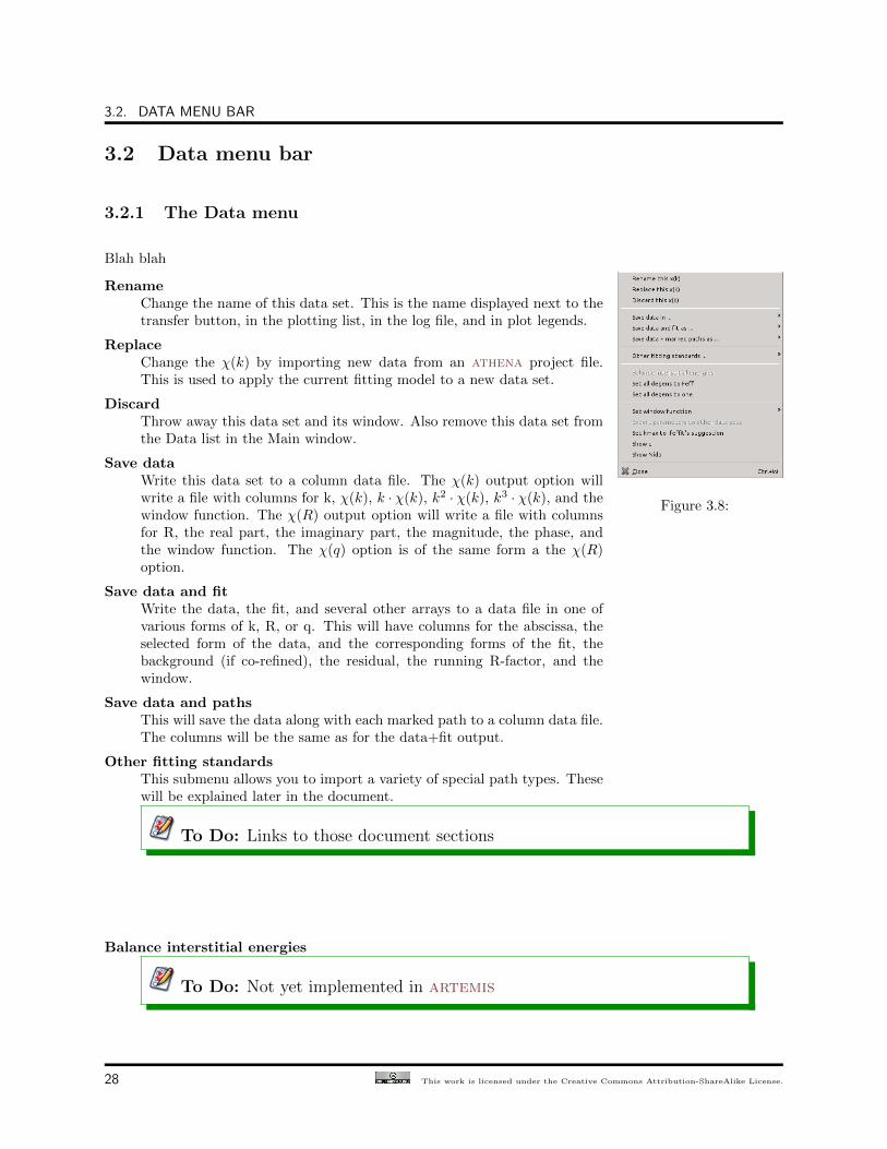
Blah blah
RenameChange the name of this data set. This is the name displayed next to thetransfer button, in the plotting list, in the log file, and in plot legends.
ReplaceChange the χ(k) by importing new data from an athena project file.This is used to apply the current fitting model to a new data set.
DiscardThrow away this data set and its window. Also remove this data set fromthe Data list in the Main window.
Save dataWrite this data set to a column data file. The χ(k) output option willwrite a file with columns for k, χ(k), k · χ(k), k2 · χ(k), k3 · χ(k), and thewindow function. The χ(R) output option will write a file with columnsfor R, the real part, the imaginary part, the magnitude, the phase, andthe window function. The χ(q) option is of the same form a the χ(R)option.
Save data and fitWrite the data, the fit, and several other arrays to a data file in one ofvarious forms of k, R, or q. This will have columns for the abscissa, theselected form of the data, and the corresponding forms of the fit, thebackground (if co-refined), the residual, the running R-factor, and thewindow.
Save data and pathsThis will save the data along with each marked path to a column data file.The columns will be the same as for the data+fit output.
Other fitting standardsThis submenu allows you to import a variety of special path types. Thesewill be explained later in the document.
To Do: Links to those document sections
Balance interstitial energies
To Do: Not yet implemented in artemis
28 This work is licensed under the Creative Commons Attribution-ShareAlike License.
CHAPTER 3. THE DATA WINDOW
Set all degeneraciesThese two options allow you to control the degeneracy values of all thepaths in the fit. The choices are to set them all to 1 or to have them alluse their degeneracies from their respective feff calculations.
Set window functionWhen the § Artemis → window function parameter is not set to “user”,this submenu will be displayed. It allows the user to change the windowfunction to be used for both forward and backward Fourier transforms.Note that setting the window function in this way uses the same func-tional form for transforms in both directions. If you want to control thetwo functions independently (for some inscrutable reason), you must set§ Artemis → window function to “user”.
Export parametersIn a multiple data set fit, this allows you to constrain the data sets to havethe same choice of Fourier transform parameters.
To Do: Not yet implemented in artemis
Set kmax to Ifeffit’s suggestionUse ifeffit’s suggestion for an appropriate value of kmax.
Show epsilonShow the value of ε computed from the noise in this data set. The valuewill be displayed in the Data window status bar.
Show NidpShow the number of independent points computed from the Fourier trans-form and fitting range. The will be displayed in the Data window statusbar.
3.2.2 The Path menu
Figure 3.9:
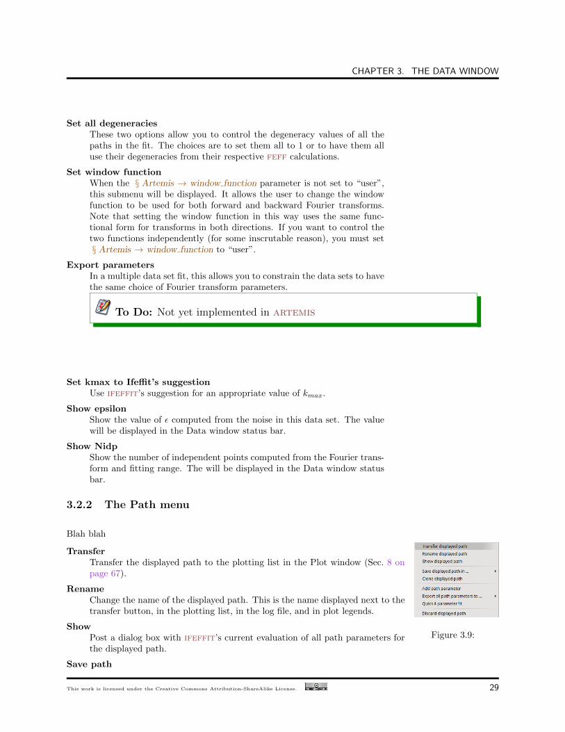
Blah blah
TransferTransfer the displayed path to the plotting list in the Plot window (Sec. 8 onpage 67).
RenameChange the name of the displayed path. This is the name displayed next to thetransfer button, in the plotting list, in the log file, and in plot legends.
ShowPost a dialog box with ifeffit’s current evaluation of all path parameters forthe displayed path.
Save path
This work is licensed under the Creative Commons Attribution-ShareAlike License. 29

3.2.3 The Marks menu
Write the displayed path to a column data file. The χ(k) output option will write a file with columnsfor k, χ(k), k ·χ(k), k2 ·χ(k), k3 ·χ(k), and the window function. The χ(R) output option will write afile with columns for R, the real part, the imaginary part, the magnitude, the phase, and the windowfunction. The χ(q) option is of the same form as the χ(R) option.
CloneMake a copy of the displayed path and insert it into the path list. The degen-eracies of the original and cloned path will be half the original degeneracy.
Add path parameterPost the dialog on the right, which is used to add a path parameter mathexpression to multiple paths associated with this or other data sets. This is aconvenience allowing you to edit the path parameters for many paths at thesame time.
Export path parametersPush the math expressions of each path parameter from the displayed path toother paths. This submenu has options for pushing these values to the otherpaths from the same feff calculation, to the marked paths, to all paths in thisdata set, or to all paths in all data sets.
Quick 4 parameter fitThis is a convenience function for setting up a simple, one-shell fit. Selectingthis menu item will create 4 parameters in the GDS window and use thosefour parameters as the math expressions for S2
0 , E0, ∆R, and σ2 for each pathassigned to this data set. This is intended only for a one-path, one-shell fit.While it may be tempting to expect broader utility out of this function – don’t.It really only serves this narrow purpose.
DiscardDiscard the displayed path, removing its window, and removing it from thepath list.
Figure 3.10:
3.2.3 The Marks menu
Figure 3.11:
Much of artemis’ functionality revolves around groups of marked paths. This menucontains a number of shortcuts for marking paths. Note that each of these has akeyboard shortcut given on the right side of the menu. Learning the shortcuts formarking functions that you use frequently is key to the effective use of artemis.
Marking via these functions is cumulative. That is, most of them only add to the setof marked paths. Choosing to mark, say, all single scattering paths will not unmarkany marked multiple scattering paths.
Several of these functions will post a dialog for receiving input. Marking by regularexpression (regex) will prompt for a perl-style regular expression to match againstthe labels in the path list. The pattern you provide will be used only if it can besuccessfully parsed as a valid perl regular expression.
Marking either greater than or less than an R value will prompt for that R value.
Marking before or after the current path will mark those above or below the displayedpath in the path list. Included and excluded refers to whether a path is selected asbeing included in a fit. Importance refers to the heuristic importance of the path,which is represented by the green (high), yellow (medium), or grey (low) color of thelabel at the top of the path page.
30 This work is licensed under the Creative Commons Attribution-ShareAlike License.

CHAPTER 3. THE DATA WINDOW
Caution: When using regular expression marking, you haveaccess to perl’s entire regular expression functionality. If you knowwhat a “(? code )” extended expression is and you use it foolishly,you only have yourself to blame.
To Do: Mark by path ranking
3.2.4 The Actions menu
Figure 3.12:
Every item in this menu operates on the set of marked paths. Again, keyboardshortcuts are given in the menu.
The first option is used to make a VPath (Sec. 8.3 on page 71) from the markedpaths. The second option will transfer all marked paths to the plotting list in thePlot window (Sec. 8 on page 67).
The next two options will cause the set of marked paths to be included in or excludedfrom the fit. The next item causes all marked paths to be discarded from your fittingproject and removed from the path list.
The final two items are about controlling what gets transferred into the plotting listafter a fit. The next to last item causes all marked paths to be transferred. Thelast item removes all paths from the list of things transferred
3.2.5 The Debug menu
Figure 3.13:
This menu displays various dialog boxes showing aspects of the current state if ifeffitor artemis. These are mostly used for debugging purposes. This menu is only displayedif the § Artemis → debug menus configuration parameter is set to a true value.
3.2.6 The Data help menu
This menu is used to display the sections on the Data window or the Path page fromthe document.
Figure 3.14:
This work is licensed under the Creative Commons Attribution-ShareAlike License. 31

3.2.6 The Data help menu
32 This work is licensed under the Creative Commons Attribution-ShareAlike License.
Chapter 4
The Atoms and Feff Window
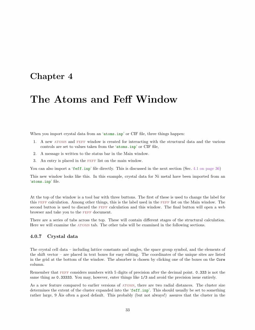
When you import crystal data from an ‘atoms.inp’ or CIF file, three things happen:
1. A new atoms and feff window is created for interacting with the structural data and the variouscontrols are set to values taken from the ‘atoms.inp’ or CIF file,
2. A message is written to the status bar in the Main window.
3. An entry is placed in the feff list on the main window.
You can also import a ‘feff.inp’ file directly. This is discussed in the next section (Sec. 4.1 on page 36)
This new window looks like this. In this example, crystal data for Ni metal have been imported from an‘atoms.inp’ file.
At the top of the window is a tool bar with three buttons. The first of these is used to change the label forthis feff calculation. Among other things, this is the label used in the feff list on the Main window. Thesecond button is used to discard the feff calculation and this window. The final button will open a webbrowser and take you to the feff document.
There are a series of tabs across the top. These will contain different stages of the structural calculation.Here we will examine the atoms tab. The other tabs will be examined in the following sections.
4.0.7 Crystal data
The crystal cell data – including lattice constants and angles, the space group symbol, and the elements ofthe shift vector – are placed in text boxes for easy editing. The coordinates of the unique sites are listedin the grid at the bottom of the window. The absorber is chosen by clicking one of the boxes on the Core
column.
Remember that feff considers numbers with 5 digits of precision after the decimal point. 0.333 is not thesame thing as 0.33333. You may, however, enter things like 1/3 and avoid the precision issue entirely.
As a new feature compared to earlier versions of atoms, there are two radial distances. The cluster sizedetermines the extent of the cluster expanded into the ‘feff.inp’. This should usually be set to somethingrather large, 9 Ais often a good default. This probably (but not always!) assures that the cluster in the
33

4.0.7 Crystal data
Figure 4.1: The atoms and feff window in artemis.
34 This work is licensed under the Creative Commons Attribution-ShareAlike License.

CHAPTER 4. THE ATOMS AND FEFF WINDOW
‘feff.inp’ file is adequately large to include all unique potentials and has all atom types sufficiently wellbounded that the muffin tin potentials are likely to be be computed reasonably well.
The second distance will set the value of RMAX in the ‘feff.inp’ file. In general, you do not want this tobe much larger than the extent of the data you intend to analyze. 5 Aor 6 Ais usually the largest sensiblevalue for longest path. The reason for this is that the pathfinder part of feff has been rewritten for thisversion of artemis. While the new pathfinder implementation offers a number of useful new features, it issubstantially slower than feff’s native pathfinder. In any case, there is no benefit to computing paths thatyou will never use in your fit.
The absorption edge for the calculation is chosen from the menu to the left of the lattice constant area.This is usually determined from the input data, but may need to be explicitly selected. If not specified inthe ‘atoms.inp’ file, the edge will be set to K for element lighter than Ce (Z=58), and to LIII for heavierelements.
The style menu is another new feature in this version of Atoms. It is used to set how the list of uniquepotentials is determined from the elements in the atoms list. The choices are
elementsEach unique element species is assigned a potential number.
tagsEach unique tag is assigned a potential number.
sitesEach crystallographic site is assigned a potential number.
Remember that feff only allows for 7 unique potentials other than the absorber. The tags and sites optionscan often result in more than 7 potnatials, which will result in an unrunnable ‘feff.inp’ file. Specifyingunique potentials by tags is a good way of differentiating between dissimilar atoms of the same species. Forexample, in an oxygenyl species, it is often useful to give the axial oxygen atoms a different potential fromthe remaining oxygens by using the tags option.
Here is an example of an ‘atoms.inp’ file for sodium uranyl acetate, which contains two very short axialoxygen atoms double bonded to the uranium atoms at about 1.8 Aand a number of equatorial oxygen atomsat a much longer distance. The axial and equatorial oxygen positions are distinguished by their tags andwill given separate unique potentials when using the tags style.
The assignment of potential indeces is explained in detail and with examples in the extended explanationschapter (Sec. 15.8 on page 141).
title Templeton et al.
title Redetermination and Absolute configuration of Sodium Uranyl(VI) triacetate.
title Acta Cryst 1985 C41 1439-1441
space = P 21 3
a = 10.6890 b = 10.6890 c = 10.6890
alpha = 90.0 beta = 90.0 gamma = 90.0
core = U edge = L3
atoms
! elem x y z tag occ
U 0.42940 0.42940 0.42940 U 1.00000
Na 0.82860 0.82860 0.82860 Na 1.00000
O 0.33430 0.33430 0.33430 Oax 1.00000
O 0.52420 0.52420 0.52420 Oax 1.00000
O 0.38340 0.29450 0.61100 Oeq 1.00000
O 0.54640 0.24430 0.50070 Oeq 1.00000
C 0.47860 0.22600 0.59500 C 1.00000
C 0.50880 0.12400 0.68620 C 1.00000
This work is licensed under the Creative Commons Attribution-ShareAlike License. 35

4.0.8 Atoms tool bar
4.0.8 Atoms tool bar
The toolbar across the top of the atoms tab offers several functions.
Clicking the open button will post the standard file selection dialog for importing a new ‘atoms.inp’ or CIFfile. This is more useful in the stand-along version of atoms than in artemis where the crystal data fileimported in other ways. Right clicking this button will post the recent files dialog populated with recentlyimported ‘atoms.inp’, ‘feff.inp’, and CIF files.
Figure 4.2:
The save button will prompt you for a filename for an output ‘atoms.inp’saving the current state of the tab.
Clicking the export button will post dialog on the right, which offers severaldifferent kinds of output files based on the crystal data. The “Feff6” and“Feff8” options will write input files for feff6 and feff8. The “Atoms”option write the same file as the save button. The “P1” option writes thecyrstal data using the P 1 space group and with a fully decorated unit cell.The “Spacegroup” option writes a file that fully describes the space group. the“Absorption” option writes a file containing some calculations based on tablesof X-ray absorption coefficients.
The clear button is used to clear all data from all controls on the atoms tab.
Finally the run button is pressed to convert the crystal data into input datafor feff. Pressing this displays the next tab (Sec. 4.1).
4.1 The Feff tab
The feff6 document can be found here.
The feff9 document can be found here.
When you click the “Run Atoms” button on the atoms tab, the resulting input data for feff, whichconstists of a list of Cartesian coordinates for the atoms in the cluster, is written to the feff tab. The fefftab is then displayed.
The box containing the feff input data is a simple text entry box. If you wish to make any modificationsto the input data for the feff calculation, you can edit the text directly. Although it is most common torun the feff calculation straight away, there are a number of situations where directly editing the inputdata prior to running feff is desirable.
The “Open” button can be used to import a different ‘feff.inp’ file. Right clicking that button posts therecently used file dialog. The “Save” button will post the standard column selection dialog for choosing afile name for saving the current feff input data. The “Clear” button will remove all text from the big textbox.
The feff calculation is started by clicking the w“Run Feff” button.
4.1.1 Feff documentation
This page allows you to link directly to feff’s documentation. Right clicking on the text window containingthe ‘feff.inp’ usually posts the standard “cut/copy/paste” menu. However, if you right click on one of
36 This work is licensed under the Creative Commons Attribution-ShareAlike License.

CHAPTER 4. THE ATOMS AND FEFF WINDOW
Figure 4.3: The feff tab.
This work is licensed under the Creative Commons Attribution-ShareAlike License. 37
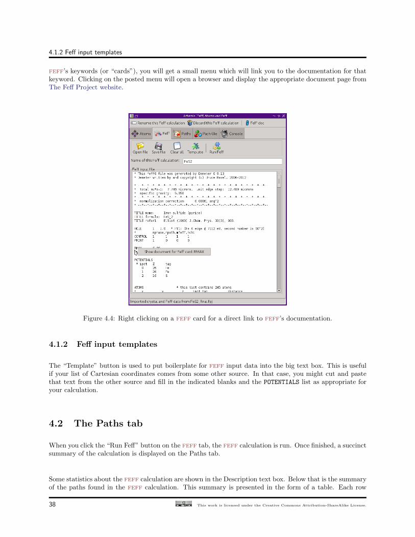
4.1.2 Feff input templates
feff’s keywords (or “cards”), you will get a small menu which will link you to the documentation for thatkeyword. Clicking on the posted menu will open a browser and display the appropriate document page fromThe Feff Project website.
Figure 4.4: Right clicking on a feff card for a direct link to feff’s documentation.
4.1.2 Feff input templates
The “Template” button is used to put boilerplate for feff input data into the big text box. This is usefulif your list of Cartesian coordinates comes from some other source. In that case, you might cut and pastethat text from the other source and fill in the indicated blanks and the POTENTIALS list as appropriate foryour calculation.
4.2 The Paths tab
When you click the “Run Feff” button on the feff tab, the feff calculation is run. Once finished, a succinctsummary of the calculation is displayed on the Paths tab.
Some statistics about the feff calculation are shown in the Description text box. Below that is the summaryof the paths found in the feff calculation. This summary is presented in the form of a table. Each row
38 This work is licensed under the Creative Commons Attribution-ShareAlike License.

CHAPTER 4. THE ATOMS AND FEFF WINDOW
Figure 4.5: A feff template.
Figure 4.6: The Paths tab.
This work is licensed under the Creative Commons Attribution-ShareAlike License. 39

4.2.1 Path plotting and path geometry
describes a scattering path. The columns contain the following information:
1. The first column shows a path index, similar to the index that feff uses when run by hand from thecommand line.
2. The second column shows the degeneracy of the path.
3. The third column shows its nominal path length, Reff . That is value that will be used in any pathparameter math expression (Sec. 5.1 on page 48) containing the reff token.
4. The fourth column shows a simple view of the scattering path. The @ token represents the absorber,thus appears as the first and last token in each description. The tokens representing the scatteringatoms are taken from the tags on the feff tab. You can change the absorber token by setting the§ Pathfinder → token configuration parameter.
5. The fifth column contains the rank of the path. This is an attempt to predict how important of eachpath will be to your fitting model. Paths with large spectral weight have a large rank and pathswith little spectral weight have small rank. Highly ranked paths are colored green, mid-rank paths arecolored yellow, and low-rank paths are grey. Don’t put too much faith in this assessment of importance.You should explicitly check all paths to decide if they should be included in a fit.
6. The sixth column gives the number of legs in each path.
7. The final column is a simple explanation of the shape of the scattering geometry.
The rows in this table are selectable by mouse click. Left clicking on a row selects that row. Control clickingon another row adds it to the selection. Shift clicking adds to the selection all rows between the one clickedupon and the previously clicked upon row.
Much of the functionality of this page rests upon the set of selected paths. Most importantly, selecting pathsis the first step to using paths in a fitting model. This will be explained in the next chapter (Sec. 5 onpage 47).
At the top of the page is a bar of buttons used to perform tasks specific to the path list. The “Doc”button will open a browser displaying this documentation for the interpretation page. The “Rank” buttonis described below. The remaining buttons are related to making plots of the selected paths.
4.2.1 Path plotting and path geometry
This is a plot of paths from the raw feff calculation. In this example, the first three single scattering pathsfrom the sodium uranyl triacetate calculation were selected along with a low-rank multiple scattering path.Then the “Plot selection” button was pressed. In this plot, we see that the three single scattering pathsare, indeed, quite large. The multiple scattering path can barely be seen on this scale. It truly is a lowimportance path.
The meaning of a “raw” feff calculation is that it is displayed as χ(k) with S20 set to 1.0 and each of E0,
∆R, and set to 0. A plot of χ(R) for the “raw” feff calculation, then, displays the Fourier transform ofχ(k) parameterized with those values.
It is, therefore, very quick and easy to examine the results of a feff calculation. The other four buttons areused to select how the plot of paths is made. The options are χ(k), |χ(R)|, Re[χ(R)], and Im[χ(R)]. Thek-weight selected in the Plot window is used to make the plot of paths.
Right clicking on an entry in the paths list will post a menu. The first item on the menu opens a dialogwindow with more details about the geomtery of the selected scattering path. In the following figure, theselected path (0006) was right-clicked on, opening the dialog depicted below.
The other context menu options are used to set the path select on the basis of distance, ranking, or scattering
40 This work is licensed under the Creative Commons Attribution-ShareAlike License.

CHAPTER 4. THE ATOMS AND FEFF WINDOW
geometry. These options are useful for selecting groups of paths to drag and drop onto the Data window.
Figure 4.7:
Figure 4.8: Information about the geometry of a scattering path.
The contents of the path interpretation can be fil-tered after running the feff calculation by settingthe § Pathfinder → postcrit parameter. By default,it is set to 3, which means that only paths with aranking above 3 will be displayed in the path inter-pretation. Resetting this parameter allows you tunehow many paths get displayed after the calculation.
4.2.2 Path ranking
feff provides a crude evaluation of the importance of each path called the “curved wave importance factor”.This is computed as a very sparse – computed at four points between 0 A−1 and 20 A−1 – trapezoidalintegration of |χ(k)|. This amplitude is then expressed as a percentage with the largest path having anamplitude of 100.
There are a few shortcomings of feff’s amplitudefactor. First, the percentages are computed serially.So the frist path is always given as 100path, it, so,
will be given as 100scaled to size of the later path. This is somewhat confusing.
This work is licensed under the Creative Commons Attribution-ShareAlike License. 41

4.2.2 Path ranking
Second, the integration is very sparse. This made sense back in the mid-90s, when computers were slowerand had less memory. But it means the amplitude is not very accurate.
Finally, the integration is over a much wider range in k-space than is typically measured in a real experiment.It would make more sense to evaluate a measure of the importance of a path over a range in k that is expressedin a real measurement or, at least, a range that is more typical of a normal experiment.
To this end, artemis offers a variety of new ways to rank the importance of a path. Some use χ(k) andsome use χ(R) of the paths. All are evaluated over a restricted range in k or R. By default, the range in kis 3 A−1 and 12 A−1 and in R it is 1 Aand 4 A. All are evaluated using the full k or R grid which is usedinternally. Some consider k-weighting.
They all have funny acronyms:
akcThis is the sum over the k-range of the absolute value of k·χ(k).
akncThis is the sum over the k-range of the absolute value of kn·χ(k) where the plotting k-weight is usedfor n.
sqkcThis is the square root of the sum over the k-range of the square of k·χ(k).
sqkncThis is the square root of the sum over the k-range of the square of kn·χ(k) where the plotting k-weightis used for n.
mkcThis is the sum over the k-range of k·|χ(k)|.
mkncThis is the sum over the k-range of kn·|χ(k)| where the plotting k-weight is used for n.
mftThis is the maximum value of |χ(R)| within the R-range where the plotting k-weight is used for theFourier transform.
sftThis is the sum over the R-range of |χ(R)| where the plotting k-weight is used for the Fourier transform.
These new ranking criteria tend to do a better job of correctly predicting which paths are important to afit. That’s a good thing. The bad thing is that they take quite a bit longer to compute than simply relyingon feff’s amplitude ratios.
The full suite of options are provided in order to replicate the analysis shown in the paper by K. Provost, etal. The “akc” and “aknc” choices tend to be reliable.
You can select which criterion to use on the interpretation page by setting the § Pathfinder → rank config-uration parameter to “feff” or to one of the acronyms above.
You can compare the evaluations of the ranking criteria by pressing the “Rank” button in the toolbar. Thiscalculation takes about a third of a second per path. If there are a lot of paths in the interpretation, thiscan be a bit time consuming. At the end, a text dialog with the various rankings for each path is displayed.As can be seen in the figure below, there is some variation between the criteria, but all of them differsubstantially from feff’s importance factors.
This improvement upon feff’s path selection tool is adapted from K. Provost et al., J. Synchrotron Radiat.,
42 This work is licensed under the Creative Commons Attribution-ShareAlike License.

CHAPTER 4. THE ATOMS AND FEFF WINDOW
Figure 4.9: The report on the path ranking calculation.
(2014), submitted.
None of the path ranking criteria currently use σ2 when they are being evaluated, but that would be aninteresting consideration.
4.3 The Path-like tab
One of the powerful new features in artemis is the ability to define “path-like” objects. A path-like objectis one which can be treated like a normal path from feff. It can be used in a fit and it can be plotted. Itis not, however, the result of a normal feff calculation. Instead, feff has been run in some special way togenerate a theoretical χ(k) spectrum for something different from all the items listed on the Paths tab.
artemis defines a number of kinds of path-like objects. Controls for generating these things are dividedinto different pages accessible by the menu at the top of the Path-like tab. The first item in that menu isfor defining “SSPaths”.
4.3.1 Single Scattering Paths
The concept of a Single Scattering Path (or SSPath) is that it uses the potentials from a feff calculationto compute the single scattering contribution from an atom that exists in that feff calculation but at adistance not represented in the list of cartesian coordinates.
In the example show, a feff calculation has been run on , a trigonal perovskite-like material with 6 oxygenscatterers at 1.93 A, 8 La scatterers at 3.28 Aor 3.34 A, and 6 Co scatterers at 3.83 A.
Suppose we had some reason to wonder what a Co scatterer at a distance of 3 Awould look like in a fit. (Forexample, we might suspect that some phase segregation happened during synthesis, resulting in some CoO.)In that case, the distance on the SSPath page would be set to 3.0 and the Co scatterer would be selectedfrom the group of radio buttons. This group of radio buttons corresponds to the list of unique potentials in
This work is licensed under the Creative Commons Attribution-ShareAlike License. 43

4.3.1 Single Scattering Paths
Figure 4.10: The Pathlike tab.
44 This work is licensed under the Creative Commons Attribution-ShareAlike License.

CHAPTER 4. THE ATOMS AND FEFF WINDOW
the input data for feff.
Figure 4.11:
The method for associating this SSPath with data willbe explained in the next chapter (Sec. 5 on page 47).For now, we simply jump ahead and compare the nor-mal Co scatterer at 3.83 A(blue) with the SSPathcomputed at 3 A(red).
Use of SSPath for modeling scatterers at such a longdistance is much superior to using a quick first shelltheory (Sec. 5.3 on page 54). The advantage of thisapproach is that it uses well constructed scatteringpotentials – i.e. potentials from a real structure –to make the special path. Using the quick first shelltechnique on a path this long results in poorly con-structed potentials. This is explained in detail in theextended discussions chapter (Sec. 15.1 on page 120).
4.3.2 FSPaths
Model the effect of variable forward scattering angle in nearly collinear multiple scattering paths.
To Do: FSPaths have not yet been implemented.
4.3.3 Histogram paths
To Do: Document the histogram system.
4.4 The Console tab
Any messages from the atoms and feff runs are displayed in this windows, including error messages. Ifyou suspect something has gone wrong in your feff calculation, check this tab. If the problem is one thatis recognized by artemis, you will a helpful diagnostic suggestion.
This work is licensed under the Creative Commons Attribution-ShareAlike License. 45

4.4. THE CONSOLE TAB
Figure 4.12: The Console tab.
46 This work is licensed under the Creative Commons Attribution-ShareAlike License.

Chapter 5
The Path page
In this chapter, the method for associating paths with data sets is explained. We will also see how to beginconstructing a fitting model.
Shown below is the Data window, which we have already seen (Sec. 3 on page 23), with some data from agold foil already imported. I have passed the cursor over the active text which says “Import crystal data ora Feff calculation”. Clicking will open the standard file selection dialog, prompting you for an ‘atoms.inp’,‘feff.inp’ or CIF file. The same thing can be done by clicking the “Add” button above the Feff list in theMain window, by selecting “Open project of data” from the File menu in the Main window, or by using theControl-o keyboard shortcut.
Figure 5.1: The Data window with no paths associated.
From the file dialog, I select an ‘atoms.inp’ file containing these crystal data:
title gold
space f m 3 m
a = 4.08 rmax = 6.00 core = Au1
atoms
Au 0.00000 0.00000 0.00000 Au1
47

5.1. SETTING MATH EXPRESSIONS
This crystal data is entered in a feff window and posted to the screen.
Figure 5.2: The atoms and feff window containing gold metal crystal data.
Running atoms then feff results in this path list:
By clicking on path 0000 in the list then shift-clicking on path 0012, the first 13 paths are selected
Now click on any of the selected paths. While holding down the left mouse button, drag those paths over tothe right side of the Data window and drop them by releasing the mouse button. This will place all 13 ofthose paths in the path list on the Data window containing the data on the gold foil.
At this point we can begin examining the paths by plotting them along with the data. The path plottingtools are explained in the chapter on the Plot window (Sec. 8 on page 67).
Also at this point, we can begin creating a fitting model to fit the gold foil data using these paths from thefeff calculation.
5.1 Setting math expressions
48 This work is licensed under the Creative Commons Attribution-ShareAlike License.

CHAPTER 5. THE PATH PAGE
Figure 5.3: The path list for the gold metal calculation.
This work is licensed under the Creative Commons Attribution-ShareAlike License. 49

5.1. SETTING MATH EXPRESSIONS
Figure 5.4: The first 13 paths have been selected.
Figure 5.5: The Data window has been populated with the 13 paths from the Feff calculation.
50 This work is licensed under the Creative Commons Attribution-ShareAlike License.

CHAPTER 5. THE PATH PAGE
Once some paths have been dragged from the feff window onto the Data window containing the gold foildata, it is time to begin defining math expressions for the path parameters. In the following figure, the pathcorresponding to the first coordination shell has been selected from the path list. A path is selected by leftclicking on its label in the path list. Doing so, displays that path on the right side of the Data window.
At the top of the Path page are two checkboxes. One is used to include and exclude a path from the fittingmodel. In this way, you can control which paths are used in a fit without having to remove them from thepath list. The other check box is used to indicate if the current path should be transfered to the plottinglist in the Plot window at the end of a fit.
To Do: Implement and explain the two items in the “other path options” pane.
The text box contains a brief description of the geometry of the scattering path. For a path with degeneracygreater than 1, the scattering geometry of one of the degenerate paths is shown. The simple explanation ofthe shape of the path and its heuristic importance are also given in the text box.
To Do: Implement a way to display a text box which shows all the pathscontributing to the degeneracy + report on fuzziness of the degeneracy.
Beneath the scattering geometry is a table of path parameters labels and text boxes. Math expressions areentered into these text boxes.
Figure 5.6: Math expressions have been set for the first shell path.
In the preceding image, a simple fitting model appropriate for a cubic, monoatomic material like our goldfoil has been entered for the first shell path. This includes simple expressions for S2
0 and E0 consisting ofvariables that will be floated in the fit. A model of isotropic expansion (Sec. 15.3 on page 128) is provided
This work is licensed under the Creative Commons Attribution-ShareAlike License. 51

5.2. MARKING AND PLOTTING
for ∆R. The σ2 path parameter is expressed using the correlated Debye model (Sec. 15.4 on page 132). Theother path parameter text boxes have been left blank and will not be modified in the fit.
This, of course, establishes the parameterization only for the first path. The same editing of path parametermath expressions must happen for all the other paths used in the fit.
The most straightforward way to do this editing chore is to click on each successive path in the path list, thenclick into each text box, then type in the math expressions. That, however, is both tedious and error-prone.
Figure 5.7:
For math expressions that are the same for every path – E0 is a commonexample – artemis provides some automation tools. Each of the path param-eter labels on the Path page is sensitive to either left or right click. Eitherkind of click posts a menu like the one of the right. The top option is used toerase the contents of the associated text both, but only on this path.
The next four options are used to push the math expression for the associatedpath parameter onto other paths. These four options allow some control overthe paths that are targeted to receive the pushed path parameter values.
The last two options are used to grab the math expression from one of thesurrounding paths.
The menu that pops up for the σ2 parameter has two additional options. One inserts a math expression forusing the correlated Debye function for σ2, the other inserts the math expression for an Einstein model. Boththe Debye and Einstein functions (Sec. 15.4 on page 132) depend on the measurement temeprature and acharacteristic temperature. Typically, the measurement temperature is a set variable and the characteristictemperature is a guess. When either function is inserted into the text box, parameters are automaticallycreated on the GDS page (Sec. 6 on page 55).
The Path menu on the Data page offers a way of pushing all the path parameters from the displayed pathto other paths. The same options for targeting other paths are presented.
Figure 5.8: Push all path parameters to other paths.
5.2 Marking and Plotting
The check buttons next to each path in the path list are central to many features in artemis related toplotting and other tasks. Along with all of the tools in the Mark menu, you can mark a group of paths byclicking elsewhere on the path list while holding down the shift key. Doing so marks all paths between theselected one and the one shift-clicked upon.
52 This work is licensed under the Creative Commons Attribution-ShareAlike License.

CHAPTER 5. THE PATH PAGE
Control-clicking on the path list is also a special function used for two purposes. Doing a control-click startsa drag-and-drop with the path you click on. Dropping the path on another data window, copies If you dropthe path on the same path list, that path to that Data set. Dropping the path on the same path list isequivalent to cloning the dragged path, with the clone being appended to the end of the path list.
Caution: Mistakenly control-clicking rather than shift-clicking will likely resultin a path being cloned. This can be surprising and confusing, so take care!
To Do: Write a page about tools for building MDS fits
5.2.1 Moving paths to the Plotting list
artemis has no special plot types involving individual paths like those for the data sets (Sec. 3.1 on page 25).Any plots with paths are constructed using the Plotting list on the Plot window (Sec. 8 on page 67). Thereare three ways of moving individual paths to the Plotting list.
1. The blue button with the squiggly line in the upper left corner of the Path page transfers that path tothe Plotting list.
2. A path will be transferred automatically after a fit if its “Plot after fit” button is checked.
3. The set of marked groups will be transferred when “Transfer marked” is selected from the Actionsmenu. This is probably the most common way of constructing plots involving paths.
Another new feature in this version of artemis related to plotting is called a “virtual path”, or a “VPath”.A VPath is an ensemble of normal paths which are summed. The sum is then plotted in k-, R-, or q-space.A VPath is made by marking a set of paths then selecting “Make VPath from marked” from the Actionsmenu. VPaths are discussed in more detail the chapter on the Plot window (Sec. 8.3 on page 71).
When the VPath is created, it is placed in the VPath tab in the Plot window and in the Plotting list.The VPath list contains tools for renaming and discarding VPaths, displaying its constituants in the Mainwindow status bar, and a VPath onto the Plotting list. (Remember that, unless the “Freeze” button isclicked, the Plotting list is cleared and repopulated after each fit.)
5.2.2 Phase corrected plots
When the Data page button labeled “Plot with phase correction”, plots using that data set and/or any of itspaths will be plotted with phase correction. This means that the contributions of the central and scatteringatom phase shifts will be removed before the Fourier transform. This has the effect of shifting the peaks inχ(R) by about +0.5A, such that the first shell peaks at an R value close to the physical interatomic distancebetween the absorber and first shell scatterer.
This work is licensed under the Creative Commons Attribution-ShareAlike License. 53

5.3. USING PATH-LIKE OBJECTS
Figure 5.9: Here is an example of a VPath. On the left is data on a gold foil plotted as Re[χ(R)] withthe fourth shell single scattering path and the two collinear multiple scattering paths involving the fourthneighbor and the intervening first shell neighbor. This is a rather cluttered plot due to the phase relationshipbetween these three paths. On the right, the VPath composed of those three paths is plotted along with thedata. This is a much cleaner plot and gives you a sense of the net impact of the fourth neighbor on the fit.
The phase information is taken from one of the paths. Each path has a button labeled “Use this path forphase corrected plotting”. These buttons are exclusive – only one path per data set can have its buttonticked on. The phase information from that path is used for the phase corrected plots.
If you turn on phase corrected plotting without having selected a path to use, artemis will issue a warningin te status bar and turn phase corrected plotting back off. You must select a path to use as the source ofthe phase information.
Note that, when making a phase corrected plot, the window function in R is not corrected in any way.
Also note that the phase correction propagates through to χ(q). While the window function will displaysensibly with the central atom phase corrected χ(q), a “kq” plot will be somewhat less insightful becausephase correction is not performed on the original χ(k) data.
5.3 Using path-like objects
5.3.1 SSPaths
5.3.2 Quick first shell paths
5.3.3 Empirical paths
54 This work is licensed under the Creative Commons Attribution-ShareAlike License.

Chapter 6
The GDS window
This is the big trick in artemis:
The parameters of the EXAFS equation are not the parameters of thefit. The parameters of the EXAFS equation are written in terms of theparameters of the fit.
As a consequence, path parameter values are math expressions. These math expressions are functions of theactual fitting parameters.
Some of these math expressions are quite simple. For example, in the gold metal example in the previouschapter (Sec. 5.1 on page 48), the math expressions for S2
0 and E0 were simple function of a single parameter.The math expression for ∆R, however, was a function of alpha and reff, while the σ2 math expressionused the debye function and two parameters.
All of these parameters must be defined in the GDS window. This window contains a grid with a seriesof buttons down the right side. It is displayed and hidden using the GDS button on the left side of theMain window. Here are the contents of the GDS window from the gold metal example. The four variableparameters in the fit along with the fixed sample temperature needed by the debye function are shown. Anew variable parameter is being defined in line 6.
The second, third, and fourth columns in the grid are filled by simple text boxes. The first column containsa drop down menu from which the parameter types can be chosen.
6.1 Parameter types
Every parameter of any type used in any math expression must be defined on the GDS widow. Any variableparameter defined on the GDS window must be used in a math expression.
There are 9 types of parameters in artemis. They are color coded in the grid to give you a visual indicationof each parameter’s type.
55

6.1. PARAMETER TYPES
Figure 6.1: The artemis GDS window.
guess(purple) This is a parameter of the fit. Its value will be adjusted to find the best fit of the model toyour data.
def(green) This is a parameter that is defined as a math expression dependent upon other guess, def,or set parameters. Its value is updated throughout the fit. As discussed elsewhere in this manual,sophisticated use of def parameters is key to successful model building and effective use of artemis.
set(black) A set parameter is one that is evaluated at the beginning of the fit, but not evaluated subse-quently. Although a set parameter can take a math expression as its value, it is more typically usedto represent a constant value used elsewhere in the fitting model.
lguess(dark purple) An lguess parameter is a tool used to simplify model creation for a multiple data set fit.It can be used in math expressions for two or more data sets. When the fit started, an actual guessparameter will be created for each data set in which the lguess is used. As an example, suppose yourmultiple data set fit includes data on a series of binary alloys. If x is a mixing parameter betweenthe two alloys and is different for each sample, you might then use math expressions containing x and(1-x) for S2
0 parameters of paths representing the two metallic species in each fit. With x an lguessparameter, independent mixing parameters will be floated for each data set. The point, then, of anlguess is to facilitate the chore of editing path parameter math expressions using artemis’ tools forpushing path parameter values across paths. This is discussed in more detail in the discussion of thecharacteristic value (Sec. 15.2.2 on page 127).
skip(gray) A skip parameter is one that is not used in any capacity in the fit, but which you do not wantto discard from your fitting project.
restrain(darkyellow) A restraint is a math expression that is evaluated and added in quadrature to χ2 toevaluate the fit. That is, the fit is optimized in the presence of the restraint. The point of this is toadd prior knowledge to a fit. Restraints will be discussed in more detail later in this document.
after(blue) An after parameter is very similar to a def parameter in that it takes a math expression thatdepends on other parameters. It is not, however, used in any way in the fit. Instead, it is evaluated atthe end of the fit and reported to the log file. This is used to make interesting calculations based onother parameters as part of the record of the fit.
penalty
56 This work is licensed under the Creative Commons Attribution-ShareAlike License.

CHAPTER 6. THE GDS WINDOW
(brown) This takes a math expression representing a user defined penalty to the happiness calculation.This feature has not yet been implemented in artemis.
merge(XSwhite on red) A merge parameter is a parameter which has been multiply defined under the samename as part of combining fitting projects or importing structural units. A fit cannot proceed withany parameters in this state. This feature has not yet been implemented in artemis.
To Do: Penalty and merge parameters have not been implemented.
6.2 User interaction
To Do: Explain drag and drop
6.2.1 Button bar
The stack of buttons on the right side of the GDS window contains many of the main functions of the GDSwindow.
Use best fitThis button makes the most recent best fit value into the initial guess for every guess parameter in thegrid.
Reset allThis button tells ifeffit to reset all parameters to their initial values.
HighlightThis button prompts you for a string. All parameters with names or math expressions matching thestring provided will be highlighted with a yellow background. This feature is particularly useful in largefitting models with many parameters. In the image above, you can see that all parameters matching“brc1” have been highlighted. The string to match can actually be any valid Perl regular expression.
EvaluateClicking this button will evaluate all parameters and insert their evaluations into the fourth columnof the grid. This is used to “spell-check” your math expressions for def and other parameters. Inthe image above, this button has been clicked and the evaluations have been inserted into the fourthcolumn.
Import/exportThe next two buttons are used to import or export a simple text file with the names and definitionsof all the parameters.
Discard allThis button does just that, after prompting to be sure that is what you want to do.
This work is licensed under the Creative Commons Attribution-ShareAlike License. 57

6.2.2 Keyboard shortcuts
Add a siteThis button appends a blank row to the end of the grid.
6.2.2 Keyboard shortcuts
When one or more rows are selected, you can use the following keyboard shortcuts to change the parametertype of that set of parameters.
• Alt - g : convert to guess
• Alt - d : convert to def
• Alt - s : convert to set
• Alt - l : convert to lguess
• Alt - k : convert to skip
• Alt - r : convert to restrain
• Alt - a : convert to after
• Alt - p : convert to penalty
6.2.3 Context menu
Figure 6.2:
Clicking on a line in the grid selects the entire line. Control clicking of a line adds thatline to the selection. Shift clicking adds all lines between the selected and clicked uponlines.
Right clicking on any line in the grid, including the label containing the line number, willpost the menu shown on the right.
Copy, cut, pasteThese three options copy, cut, and paste lines from or to the GDS grid. The cutfunction is one way of discarding a parameter. Another is to simply delete thename in the second column.
Insert blank linesThe insertion options complement the “Add a site” button by adding blank rowsto the middle of the grid.
Change parameter type of selected linesThis sub-menu provides yet another way of changing the parameter type of theselected lines of the grid. If you have more than one line selected, they will all getchanged to the option you choose from the submenu.
Grab best fitThis changes theinitial guess of the selected lines to the most recent best fit value(s).
Build restraintThis posts a dialog that helps you name and define a restraint based upon the valueof the parameter in the line clicked upon. This will use ifeffit’s penalty functionwith the lower and upper bounds as its arguments and multiplied by the scalingfactor. The example shown will make this restraint:
restrain res_enot = 1000 * penalty(enot, -5, 5)
58 This work is licensed under the Creative Commons Attribution-ShareAlike License.

CHAPTER 6. THE GDS WINDOW
and add it to the end of the grid. The penalty function will evaluate to 0 when enotstays between -5 and 5. As the value of enot strays outside that range, the restraintwill evaluate to a value of 100 times the distance outside the range. This, then, isadded in quadrature to χ2 when the fit is minimized. You can read more aboutthis, including how to choose the value of the scaling parameter, in the discussionof restraints (Sec. 15.5 on page 134).
AnnotateThis prompts you for a text string to describe the parameter in the line clickedupon. The intent is to allow you document the role of the parameter in your fittingmodel. This annotation is displayed in the GDS window’s status bar when thatline is selected.
Find parameterThis posts a small window with a text box reporting all GDS parameters and pathparameters which have math expressions containing this parameter.
Rename parameter globallyThis allows you to rename a parameter and have its new name inserted every placein the fit where that parameter is used. All instances in other parameters on theGDS page and in the math expressions for parameters of all paths will be changed.Essentially, this is a global search and replace.
ExplainFinally, the items in this submenu write a short text to the status bar explainingthe various parameter types.
Figure 6.3:
This work is licensed under the Creative Commons Attribution-ShareAlike License. 59

6.2.3 Context menu
60 This work is licensed under the Creative Commons Attribution-ShareAlike License.

Chapter 7
Running a fit
artemis is, admittedly, a complex and non-intuitive program. There are good reasons for artemis beingthe way it is, although those reasons may not be clear if you are coming to the program for the first time.While it is important that easy things be easy in artemis, letting hard things be possible is central to theintent of the program.
Most of the complexity revolves around the central premise in ifeffit and artemis:
The parameters of the EXAFS equation are not the parameters of thefit. The parameters of the EXAFS equation are written in terms of theparameters of the fit.
As a consequence, we have the GDS window where the parameters of the fit are defined and the variousPath pages where those parameters are used.
It is instructive to understand a little bit about how the fitting model is structured internally. The basicdefinition of a fit consists of three things: (1) a list of one or more GDS parameters, (2) a list of one or moredata sets, and (3) a list of one or more paths. To make a fit, all three of those lists must somehow be defined.
The list of data sets is taken from the Data list in the Main window. All data sets in the Data list whichhave the “Include in fit” button checked on will be used in the fit.
Each data set has a list of one or more paths associated with it. In artemis a path is associated with a dataset by dragging and dropping it onto a data set’s path list. The contrapositive is also true. All paths usedin a fit must be associated with a Data set.
Paths typically come from a feff calculation explicitly initiated by the user. That is, the user imports anatoms input file, a feff input file, or a CIF file. feff is run and the interpretation list is displayed inthe feff window. Paths are dragged from that list and dropped on a Data set. Thus paths are not onlyassociated with a Data set, they are also associated with a specific feff calculation.
Each path must have its path parameters set in some manner, even if they are merely set to 0 or some otherconstant. Typically, path parameters are set to math expressions which depend functionally upon one ormore parameters from the GDS page. Every GDS parameter used in a path parameter math expression
61

7.1. SANITY CHECKING YOUR FITTING MODEL
must be defined on the GDS window. Similarly, every guess or def parameter from the GDS window mustbe used in at least one math expression in your fitting model.
All paths which have their “Include in fit” button checked on will be used in the fit.
When the fit begins, artemis digs through all the windows, finding all data sets, paths, and GDS parameters.It runs a number of sanity checks to avoid certain obvious situations which will result in an unsuccessful fit.It then makes sure that all of ifeffit’s data structure are up to date with respect to your current settingsin artemis. The fit is run. Statistics, including error bars and correlations, are calculated. A log file iswritten, a plot is made, and the various colored buttons are set according to the fit happiness.
That’s a fit!
There are some details of the fitting process that are configurable (Sec. 12 on page 85). For instance, thelog file can be displayed in either the Log window or in the History window after the fit finishes. You canalso choose not to have it display automatically. This is set by § Artemis → show after fit.
The plot that is made upon completion of the fit is also configurable. The default is to have an Rmr plot(Sec. 3.1 on page 25) made containing the data and the fit. Any of the five plot types from the Data windowcan be chosen as the after-fit plot. You may also choose to have the contents of the plotting list plotted in k-,R-, or q-space. This adds value to the “Plot after fit” buttons on the Data window and Path pages. You mayalso choose to have no plot displayed automatically after the fit. This is set by § Artemis → plot after fit.
The fit name and fit description text boxes from the Main window are also useful for customizing your fitas well as the course of a fitting project. The fit name is used in many places – most notably in the legendsof plots. Thus you may find it useful to select descriptive names for each of your fits. The fit descriptionis written to every log file and can be used to document features of your current fitting model and how itrelates to the development of your fitting project.
7.1 Sanity checking your fitting model
artemis is complex and it is quite easy to make mistakes. Many common mistakes are obvious and dis-coverable by automated analysis of the fitting model. Before running a fit, artemis applies each of thefollowing test to your fitting model. If any of them are triggered, the fit is halted and a (hopefully) usefulerror message is posted in the Log window. Think of this like artemis’ spell checker!
Any problems that are found must be corrected before artemis will allow the fit to proceed.
1. Check that any files associated with the data or the feff calculations exist.
2. Check that all guess parameters are used in at least one def parameter or path parameter.
3. Check that no def parameter or path parameter uses an undefined parameter.
4. Check that none of these typos – “++”, “–”, “//”, or “***” – appear in any math expressions.
5. Check that all function names used in math expression (i.e. a word followed by parentheses) are validfunctions in ifeffit.
6. Check that all GDS parameters have unique names.
7. Check that parentheses match in all math expressions, i.e. that every open penthesis has a matchingclose paremthesis.
8. Check that Fourier transform and fit parameters are sensible (for example Rmin ¡ Rmax) for all datasets.
9. Check that the number of guess parameters is less than .
62 This work is licensed under the Creative Commons Attribution-ShareAlike License.

CHAPTER 7. RUNNING A FIT
10. Verify that Rmin≥Rbkg for data imported from an athena project file.
11. Verify that Reff for each path is not well beyond Rmax. The margin beyond Rmax that a value ofReff is acceptable is set by Rmax+0.2 plus the val §Warnings → reff margin.
12. Check that various compiled-in limits (e.g. maximum number of paths or maximum number of setparameters) in ifeffit are not exceeded.
13. Check that parameters do not have the same names as ifeffit program variables. For example, thingslike pi or dr1 are not allowed since ifeffit uses those strings for other purposes.
14. Check that there are no unresolved merge parameters.
15. Check that GDS math expressions do not have loops or cycles in their definitions. For example, eitherof the following would trigger this error.
guess x = x # with apologies to Laurie Anderson fans....
guess a = b
def b = c
def c = a
16. Check for obvious cases of a data set used more than once.
17. Check that each data set used in the fit has at least one path assigned to it.
As a side note, item 15 is particularly interesting. demeter does a simple lexical analysis on the ensembleof math expressions defined on the GDS window, then uses a formal graph theory tool to develop a graphdepiction of the parameters. Loops (like the first example) and cycles (like the second) a trivially evidentwhen the parameters are viewed as a formal graph. That was a really fun part of demeter to write.
7.2 The heuristic happiness parameter
artemis evaluates a variety of statistical parameters relevant to the evaluation of your fit. These includethe fitting metric χ2, the fitting metric normalized by the degrees of freedom in the fit χ2
ν , an R-factor, anduncertainties on and correlations between the variable parameters.
In a formal sense, the most important of these parameters is χ2ν , which is the statistical parameter allowing
you to distinguish between different fitting models applied to the same data. Unfortunately, χ2ν is difficult
to interpret directly. In practice, the EXAFS analysis problem using feff is not a well-posed problem inthe sense required by Gaussian statistics. This is true for a variety of reasons. In EXAFS, the signal is notideally packed – that is, the signal is not composed of pure sine waves. In general, you cannot guaranteethat errors in your fitting parameters are normally distributed. In general, we cannot actually identify andenumerate all sources of measurement error, many of which are complex and systematic, such as sampleinhomogeneity, detector non-linearity, and so on. Finally, we do not know the true line shape of our signal– instead we use feff to approximate the lineshape.
For all those reasons, χ2ν is rarely – if ever – close to 1 as expected for a good fit. Although χ2
ν for differentfitting models can be compared effectively, it is, generally speaking, not a sufficient criterion for evaluatingthe quality of an individual fit.
Happily, this is not an insolvable problem. After decades of analyzing EXAFS data, using feff, and usingifeffit, we know a lot about what constitutes a good fit. For instance, a good fit has a small R-factor,which is a measure of the percentage misfit between the data and theory. We know things about individualparameter types, e.g. that an E0 is rarely more than 10 eV or less than -10 eV, that S2
0 and σ2 should neverbe negative. We know that a robust fit does not have excessive correlation between variable parameters.
This work is licensed under the Creative Commons Attribution-ShareAlike License. 63

7.2.1 Evaluation of the happiness parameter
artemis offers a heuristic tool called “happiness” which is an attempt to enumerate the knowledge andexperience we bring to a fit. After a fit, this heuristic parameter is evaluated and reported in the log file. Ithas no meaning other that to give you a general sense of how the fit came out.
Caution: The word “happiness” was chosen for this parameter because it is asilly word in a statistics context. Happiness is an ad-hoc, semantic metric. It hasno basis in formal statistics. It is essentially meaningless and should NEVER bepublished. NEVER!
7.2.1 Evaluation of the happiness parameter
The happiness parameter begins with a value of 100, indicating complete happiness. After the fit is evaluated,a series of tests are run against the fitting results. If a test hits, it removes points from the happiness. Thefinal evaluation is reported in the log file and used to color the Fit and plot buttons.
R-factorAssess a penalty for an R-factor that is larger than 0.02. That is, any fit which has 2assessed a penalty.Above that, the penalty scales linearly in R-factor up to a maximum penalty of 40.
Parameter valuesAfter every path parameter for every path is evaluated, assess a penalty of 2 for each path parameterthat fails a sanity check. The sanity checks include checking that E0 is not too large either positivelyor negatively, checking that neither of S2
0 or σ2 is negative, and checking that neither of σ2 or ∆R istoo large.
RestraintsIf any restraints are placed upon the fit, assess a penalty for every restraint which evaluates to somethingnon-zero. The penalty scales linearly with the size of the evaluated restraint.
Number of independent pointsAssess a penalty if the number of guess parameters is larger than 2/3 of the total number of independentpoints as evaluated by the Nyquist criterion. Above the 2/3 threshold, the penalty scales linearly.
CorrelationsAssess a penalty for each correlation that exceeds a cutoff value.
Penalty parametersAssess a penalty equal to the evaluation of a penalty parameter.
To Do: Penalty parameters have not yet been implemented.
7.2.2 Configuring the happiness evaluation
Note that everything above is something that Bruce made up out of whole cloth, inlcuding the parametriza-
64 This work is licensed under the Creative Commons Attribution-ShareAlike License.

CHAPTER 7. RUNNING A FIT
tion. That said, every part of the happiness calculation is configurable. That means that you, the user, cantune the happiness evaluation to report on fit quality in a way that is meaningful and useful for your dataand your fits.
The configuration parameters are spread over two configuration groups (Sec. 12 on page 85). The parametersin the Happiness group control the evaluation of the penalties. Those in the Warning group control theassessment of path parameter values.
For example, to tune the assessment of the penalty for an excessive number of guess parameters, you canchange two configuration parameters. § Happiness → nidp cutoff default to 2/3 and sets the cutoff belowwhich no penalty is assessed. This parameter is interpreted as a fraction of total number of independent pointsin the fit. § Happiness → nidp scale sets the maximum penalty to assess for using up all the independentpoints.
The path parameter penalties can also be fine tuned. A couple examples: the value above which a penaltyis assessed for an excessively large E0 is set with §Warnings → e0 max and the assessment of a penalty fora negative σ2 can be turned off by toggling §Warnings → ss2 neg .
Since this happiness thing is an artificial and statistically meaningless creation, it can be changed as youlike. Do you have any ideas for penalty assessments? Let Bruce know! Do you have a suggestion for howthe existing penalties should be tuned? Send your configuration parameter values to Bruce!
7.3 Using path-like objects
Another of the new features in the version of artemis is the ability to make interesting things that areconstructed from tools that feff provides, but which are not paths in the traditional sense of being strictlyassociated with one of the ‘feffNNNN.dat’ files that comes from a normal execution of feff.
Some of these path-like objects are directly associated with a particular feff calculation. For example,an SSPath created on the Path-like tab on the feff window is created directly from the scattering poten-tials from that feff calculation. Similarly, a histogram-based path-like object also uses a particular feffcalculation.
Other path-like objects either have a hidden relationship with a feff calculation or none at all. The pathfrom a quick first shell theory calculation does have a feff calculation associated with it, but it is done ina way that the user never interacts with that calculation. The quick first shell path does not have an entryin the feff list on the Main window. An empirical standard, as the name implies, is derived from data andtherefor is not associated with any feff calculation.
Although each of these path-like objects derives from a different place than a typical path, artemis presentsthem to the user identically. Each kind of path-like object is displayed using all the same controls as anormal path and each is parametered and used in a fit in the same way.
• For information about SSPaths, see Chapter XXX
• For information about histograms, see Chapter XXX
• For information about the quick first shell theory, see Chapter XXX
• For information about empirical standards, see Chapter XXX
To Do: Make these links
This work is licensed under the Creative Commons Attribution-ShareAlike License. 65

7.3. USING PATH-LIKE OBJECTS
66 This work is licensed under the Creative Commons Attribution-ShareAlike License.

Chapter 8
Plotting data
Figure 8.1:
You have already been introduced (Sec. 2.2 on page 20) to the basic functionality ofthe Plot window. In this chapter, all the details of artemis’ plotting system will beexplained. While artemis does not provide all the plotting capabilities offered by realplotting tools like Gnuplot, Origin, Excel, Kaleidagraph, and others, it does provideenough options to create interesting and instructive visualization of your EXAFS fittingproject.
Let’s briefly go over the basic features of the Plot window. The buttons at the top areused to make plots of data and paths in one of the three spaces. The data listed inthe plotting list at the bottom of the Plot window will be included in the plots madewith those three buttons.
The part of the complex χ(R) or χ(q) functions is controled by the two sets of ra-diobuttons at the top of the “limits” tab. Additional traces – the fit, the window, andso on – can be included by clicking on their check buttons. Finally, the plotting rangealong the x-axis can be set for each of the three spaces. At the top of the Plot windoware a series of radio buttons used to set the k-weighting used in plots. A plot of χ(k)will be weighted by the specified factor of k. Plots of χ(R) or χ(q) will use that valuleof k-weighting for the forward Fourier transform.
The “kw” option for k-weighting will use the user-specified value of k-weight for eachdata set included in the plot. That value will also be used for any paths associatedwith that data set.
Please note that the value of k-weight selected for plotting has no bearing on how thefit is performed. The k-weighting specified on the Data window is used to evaluate thefit. Fit evaluation and visualization are different tasks, each with their own value ofk-weight.
8.0.1 The plotting list
The contents of the plotting list are included in a plot made from the Plot window. There are a number ofways of populating the plotting list manually and there are tools for repopulating the list upon completionof a fit.
67

8.0.2 Populating the plotting list manually
8.0.2 Populating the plotting list manually
The most basic way of moving a data set or a path to the plotting list is to click on a plot transfer button.These are the light blue buttons, , at the top of the Data window. There is one to the left of the name ofthe data set. Clicking on this button inserts that data at the end of the plotting list. There is also a transferbutton on each Path page to the left of the path’s name.
Figure 8.2: The plot transfer buttons on the Data window and Path page
Clicking on any of the path transfer buttons inserts that path at the end of the plotting list.
In this way, the plotting list can be built up item by item. The order in which items are inserted into theplotting list is the order in which they are displayed in the plot. An item can be removed from a plot withoutremoving it from the plotting list by unchecking its check box.
Of course, adding a number of paths to the plotting list by checking on their individual transfer buttons canbe quite tedious. Transfering of items into the plotting list is another of the many chores that use the set ofmarked paths. Marking a path is done is by checking its check box in the Path list or by using one of thehandy options in the Marks menu (Sec. 3.2.3 on page 30). Once a set of paths is marked, selecting “Transfermarked” from the Actions menu (Sec. 3.2.4 on page 31) will move that set in order to the end of the plottinglist. By learning to use path marks effectively, you can quickly build interesting plots which include dataalong with many paths. Note that keyboard shortcuts exist for everything in the Mark and Actions menus.These are shown in the menus themselves. Learning these shortcuts makes setting up interesting plots muchfaster and easier.
The “Clear” button at the bottom of the Plot window is used to remove all content from the plotting list.
Items in the list can be reordered by dragging and dropping while holding down the control key. Note thatan item will be placed after the item on which it is dropped.
Right clicking on an item will post a pop-up button for removing that item from the list. Selecting more thanone path then right-clicking will post a menu with options for removing the selected paths or for alteringtheir check buttons.
8.0.3 Refreshing the plotting list after a fit
After a fit finishes, the plotting list will be populated with all of the data sets and paths which have their“Plot after fit” button checked. On the Data window, this checkbutton is found in the “Other parameters”section at the bottom of the page. On the Path page, this checkbutton is directly below the name of thepath at the top of the page.
Upon completion of the fit, the plotting list is cleared the repopulated with all the items selected for plottingafter the fit. The data are inserted in the order they appear in the Data sets list in the Main window. Pathsassociated with that data set are inserted after their data set in the order they appear in that data set’spath list.
The refreshing of the plotting list can be turned off by checking the “Freeze” button below the plotting list.
68 This work is licensed under the Creative Commons Attribution-ShareAlike License.

CHAPTER 8. PLOTTING DATA
This will preserve the state of the plotting list as it appeared before starting the fit.
8.1 Stacked plotsWith a large number of items in the plotting list, a plot may become quite hard to understand due to the
large number of overlapping traces.
Figure 8.3:
The “stack” tab holds controls for providing vertical offset between traces in a plot.The top set of controls works very similarly to the stacking feature in athena. Whenthe check button is clicked on, paths will be offset vertically as indicated by the thetwo values. The initial value is the offset applied to the data. All parts of the data(fit, window, etc) will also be plotrted with that offset. The second value is a verticaldisplacement between successive paths. Note that the displacement is downward –that is, a value of +2 means to displace each path by -2 on the y-axis. In this way,traces appear in the same top-to-bottom order as the plot legend when a positive valueis chosen.
The second group of controls is used to multiply paths by -1 before plotting. Thisresults in the data pointing up and the individual paths pointing down. This featureis turned off when the check button for a stacked plot is clicked on.
The last control is used to specify a vertical offset between data sets when plottingmore than one data set from a multiple data set fit. Note that this stacking parameterand the individual data set stacking parameters will each provide some vertical offset,requiring careful consideration for an attractive plot.
8.1.1 Stacked plot
Figure 8.4: A stacked plot
Here is an example of a stacked plot. Shown are Co foil data, the fit function, and the fitting window. Offsetdownward are the paths from the first two coordination shells as evaluated in the fit. Note that the size ofan appropriate offset depends on the k-weighting and on the space the plot is made it. artemis does notattempt to compute a sensible value – that is up to you.
8.1.2 Inverted plot
This work is licensed under the Creative Commons Attribution-ShareAlike License. 69

8.1.3 Data stack plot
Figure 8.5: Plotting with inversion
Here we see a plot with inversion. This is the same fit as in the stacked plot above, except that the first twocoordination shells as evaluated in the fit are pointing downward.
8.1.3 Data stack plot
Figure 8.6: A data stack plot
Finally, here is an example of stacked data sets. This is a multiple data set fit to dimethytin dichloride andmonomethyltin trichloride. The visualize both parts of this fit, it is convenient offset the monomethyltintrichloride data and paths downward by enough to completely separate the traces associated with each dataset. Again, the value of the offset depends on the k-weighting and on the sapce in which the plot is made.
8.2 Plot Indicators
In demeter, an indicator is a vertical line used to mark a specific position on the x-axis. In this example,it is the dotted pink line at 2.067 A. An indicator for a position in R is not plotted in k or q. An indicatorfor a position in k or q is not plotted in R. Inidactors for positions in k or q are also plotted in q or k.
To set an indicator, click the target button, then click on a point in the current plot. Once set, the positionand space can be edited using the associated choice menu and text control. The check button turns theindicator on or off in subsequent plots. The buttons at the bottom toggle the check buttons for each indicator.
70 This work is licensed under the Creative Commons Attribution-ShareAlike License.

CHAPTER 8. PLOTTING DATA
Figure 8.8: Plot with indicator
Figure 8.7:
8.3 Creating and plotting VPaths
A common problem with visualizing the paths that contribute to a fit occurs whenseveral single and multiple scatteriung paths contribute spectral wieght in the sameregion of R spadce. In a well-ordered material like these data on a cobalt foil, adistant single scattering path may be of the same length as two or more importantcollinear multiple scattering paths. The fit involves a subtle superposition of all thepaths in the fit. This single scattering path and its related multiple scattering pathsall contribute spectral weight in the same region of R-space.
Figure 8.9: A plot of overlapping paths
Plotting them together results in a complicated figure with lots of overlapping traces.It is hard to see how each path contributes to the fit. Indeed, it is hard to ascertainmuch beyond the fact that these three paths have a complicated phase relationshipbetween them.
artemis offers a handy visualization tool called a virtual path, or VPath. A VPath is simply a group of
This work is licensed under the Creative Commons Attribution-ShareAlike License. 71

8.3. CREATING AND PLOTTING VPATHS
paths which are added together after being evaluated in a fit. The sum of these paths is then plotted as asingle item in a fit. Here is the plot made with the VPath constructed from the three paths in the previousfigure. While this plot hides the individual contributions of the three path, it shows how those three affectthe fit when added together.
Figure 8.10: A plot with the overlapping paths made into a single VPath
Figure 8.11:
The VPath is made by marking the contributing paths and choosing“Make VPath” from the Actions menu. You will be prompted for aname for the VPath. This name will be used to identify the VPath ina plot. The VPath is then inserted into the list of the VPaths tab.
Here is another example of how a VPath can help visualize the components ofa fit. The data in the follow two figures are of uranium LIII edge EXAFS ofuranyl acetate in solution. Uranyl compounds are notable for having two, very short double-bonded oxygenatoms in a trans configuration and at a distance of about 1.78 A. The remaining oxygen atoms lie in anequatorial plane. These are single-bonded and at a distance of around 2.4 A.
Figure 8.12:
The two axial oxygen atoms usually have a rather small and contribute very stronglyat low R in the Fourier transform. Because those oxygen atoms are at such ashort distance, there are a few multiple scattering paths that contribute significantspectral weight just beyond the region dominated by single scattering from theequatorial oxygen atoms.
Here is the plot the fit to the uranyl acetate data along with each of the single andmultiple scattering paths that involve the axial oxygen atoms. Again, it is ahrd toappreciate how the various multiple scattering paths contribute to the fit.
In this case, it is nice to combine all these paths into a VPath which represents theentire contribution to the EXAFS from the axial oxygen atoms.
72 This work is licensed under the Creative Commons Attribution-ShareAlike License.

CHAPTER 8. PLOTTING DATA
Figure 8.13: A plot of the axial oxygen paths in uranyl acetate
Figure 8.14: A plot with the axial oxygen paths made into a VPath
This work is licensed under the Creative Commons Attribution-ShareAlike License. 73

8.3. CREATING AND PLOTTING VPATHS
74 This work is licensed under the Creative Commons Attribution-ShareAlike License.
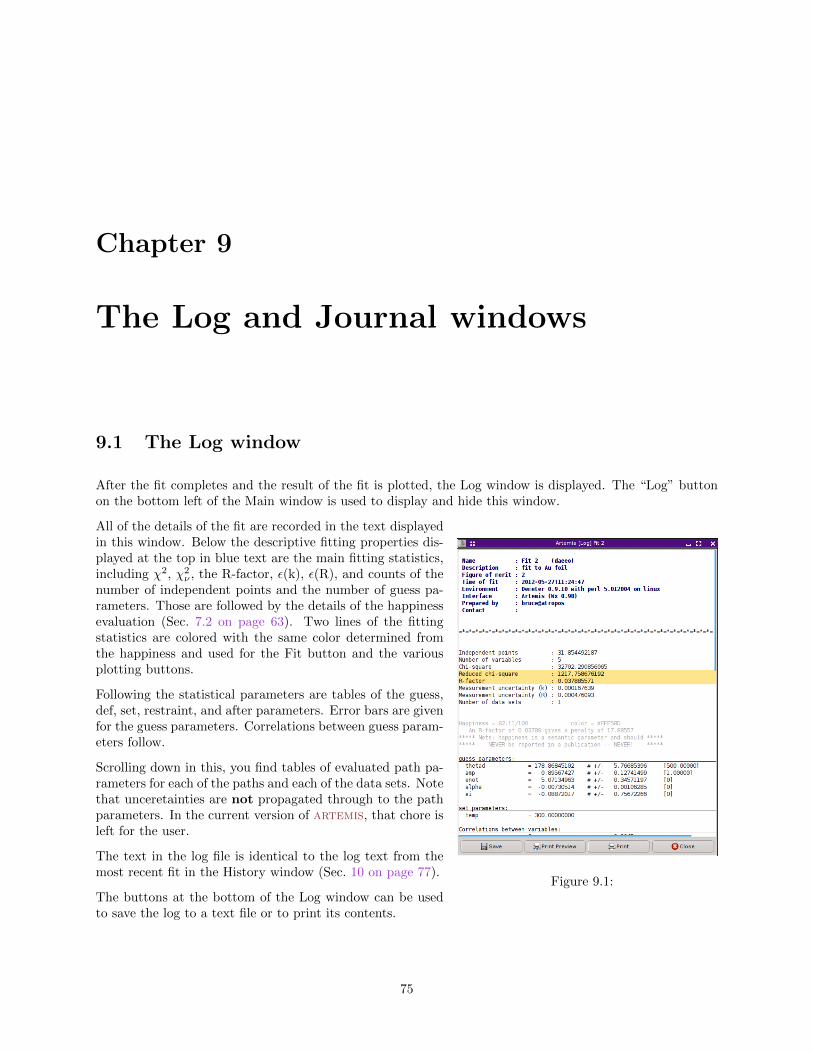
Chapter 9
The Log and Journal windows
9.1 The Log window
After the fit completes and the result of the fit is plotted, the Log window is displayed. The “Log” buttonon the bottom left of the Main window is used to display and hide this window.
Figure 9.1:
All of the details of the fit are recorded in the text displayedin this window. Below the descriptive fitting properties dis-played at the top in blue text are the main fitting statistics,including χ2, χ2
ν , the R-factor, ε(k), ε(R), and counts of thenumber of independent points and the number of guess pa-rameters. Those are followed by the details of the happinessevaluation (Sec. 7.2 on page 63). Two lines of the fittingstatistics are colored with the same color determined fromthe happiness and used for the Fit button and the variousplotting buttons.
Following the statistical parameters are tables of the guess,def, set, restraint, and after parameters. Error bars are givenfor the guess parameters. Correlations between guess param-eters follow.
Scrolling down in this, you find tables of evaluated path pa-rameters for each of the paths and each of the data sets. Notethat unceretainties are not propagated through to the pathparameters. In the current version of artemis, that chore isleft for the user.
The text in the log file is identical to the log text from themost recent fit in the History window (Sec. 10 on page 77).
The buttons at the bottom of the Log window can be usedto save the log to a text file or to print its contents.
75

9.2. THE JOURNAL WINDOW
9.2 The Journal window
Figure 9.2:
Clicking the “Journal” button on the right side of the Mainwindow displays and hides the Journal window. This issimply a blank text box in which you can write notes aboutyour fitting project or love letters to your collaborators. Thetext found in this box will be saved to and restored from theproject file.
The buttons at the bottom of the Log window can be usedto save the journal to a text file or to print its contents.
76 This work is licensed under the Creative Commons Attribution-ShareAlike License.
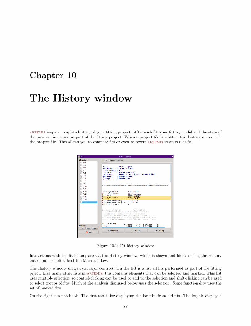
Chapter 10
The History window
artemis keeps a complete history of your fitting project. After each fit, your fitting model and the state ofthe program are saved as part of the fitting project. When a project file is written, this history is stored inthe project file. This allows you to compare fits or even to revert artemis to an earlier fit.
Figure 10.1: Fit history window
Interactions with the fit history are via the History window, which is shown and hidden using the Historybutton on the left side of the Main window.
The History window shows two major controls. On the left is a list all fits performed as part of the fittingprject. Like many other lists in artemis, this contains elements that can be selected and marked. This listuses multiple selection, so control-clicking can be used to add to the selection and shift-clicking can be usedto select groups of fits. Much of the analysis discussed below uses the selection. Some functionality uses theset of marked fits.
On the right is a notebook. The first tab is for displaying the log files from old fits. The log file displayed
77

10.1. REPORTS ON FITS
when the most recent fit is clicked upon is identical to the log file displayed in the Log window.
You may find that there is a short pause between clicking on a fit and seeing its log file displayed. Whenimporting a project file, artemis delays importing the fits until one is explicitly needed. For a large projectfile, this greatly speeds up import at the small cost of a pause when examining log files.
Figure 10.2:
Each fit in the list will display a context menu when right clicked. Again, there maybe a short pause before the menu gets posted. In that menu are a variety of functionsrelated to the fit history.
Restore fitting modelAn prior fitting model can be restored. This will clear all of artemis’s windowsand replace them with content from that fit.
Save log fileThe log file displayed can be written to a text file. You will be prompted for afile name and location.
Export fitThe fit can be exported to an artemis project file containing only that fit inthe fit history.
Discard fit(s)The current or the set of marked fits can be discarded from the project.
Show YAMLThe last item is a tool used to help debug problems in artemis. It displaysartemis’s internal representation of the fit in a text window.
10.1 Reports on fits
The second tab is used to analyze groups of fits. In the example shown above, the progression of χ2ν values
throughout the development of the fitting model is shown both as a textual report and as a plot. Similarplots can be made for individual parameter values.
Figure 10.3:
78 This work is licensed under the Creative Commons Attribution-ShareAlike License.

CHAPTER 10. THE HISTORY WINDOW
Only the marked fits are included in the report. If no fits are marked, then all fits will be marked beforethe report is generated. Simple controls for setting the marks are at the bottom of the list. The buttonsmarked “All” and “None” set and clear all marks. The “Regexp” button will prompt you for a pattern tomatch against all fit names.
When a fit is selected from the list, the “Select parameter” menu is populated with the names of theparameters used in that fit. All parameter types are included. Selecting a new item from the menu orclicking the “Write report” button will generate a new report and its plot.
For statistics, all of χ2, χ2ν , R-factor, and the happiness are reported. You can choose which of χ2
ν , R-factor,and happiness to have displayed in the resulting plot. Clicking the “Show y=0” button forces the plot to bescaled of the y-axis such that y=0 is shown.
Buttons at the bottom of this tab allow you to save the report as a text file or to send it to the printer.
10.2 Plotting fits
The plot tool tab is used to place old fits in the Plotting list for comparison with data and with the currentfit. As you perform fits (or when a project file is imported), an entry on the “Plot tool” page is made foreach fit. Within the box associated with each fit is one button for each data set included in the fit. Theexample below is of a single data set fit to Co metal, thus each fit has a single button associated with it.
Figure 10.4: Fit history plotting tool
Clicking one of the buttons on the “Plot tool” page makes an entry in the plotting list. These will then beplotted just like any other item in the plotting list (Sec. 8 on page 67). Note that it is usually not necessaryto put the most recent plot in the plotting list in this way. If the “Plot fit” button is checked on and a datagroup is in the plotting list, the most recent will be plotted by default. Fit items in the plotting list will bestacked (Sec. 8.1 on page 69) when the stacking option is in play.
This work is licensed under the Creative Commons Attribution-ShareAlike License. 79

10.2. PLOTTING FITS
Figure 10.5: Historical fits placed in the plotting list
80 This work is licensed under the Creative Commons Attribution-ShareAlike License.

Chapter 11
Monitoring things
artemis provides a number of tools for keeping track of things going on behind the scenes. These tools arefound either in the Monitor menu on the Main window or the Debug menu on the Data window.
In the normal course of operations, consulting the monitoring tools should not be necessary. But if somethingis not working quite right, they can be invaluable for diagnosing the problem.
11.1 Command and status buffers
11.1.1 The Command buffer
The command buffer window contains a record of every data processing and fitting command sent to ifeffit.At the bottom of this window is the plotting buffer, which contains every command sent to the plottingbackend (usually Gnuplot).
These are very useful both for diagnosing problems and for learning the details of how ifeffit and Gnuplotwork.
At the bottom of the window is a simple command line for sending instructions directly to ifeffit.
11.1.2 The Status buffer
81

11.2. INTERACTING WITH IFEFFIT
Figure 11.1:
Figure 11.2:
Every message sent to any of the status bars inartemis is time-stamped and logged in the statusbuffer. This provides a sort of record of the majoractions taken during your current artemis session.The contents of this buffer can be saved to a file.
11.2 Interacting with Ifeffit
One of the submenus in the Monitor menu on theMain window allows you to examine ifeffit datastructures. The results of these examination com-mands are displayed in the command buffer. In thisexample, all arrays currently defined in ifeffit havebeen shown.
Options exist for showing specific ifeffit datagroup, all arrays, all scalars, all strings, all paths,or all feff paths. The last one is simply a listing all‘feffNNNN.dat’ files imported into ifeffit.
You can also inquire about how much of ifeffit’s statically allocated memory is in use and whether youare in danger of exceeding capacity. This information is displayed in the Main window status bar.
11.3 Debugging Demeter
82 This work is licensed under the Creative Commons Attribution-ShareAlike License.

CHAPTER 11. MONITORING THINGS
Several additional menu items are turned on when § Artemis → debug menus is set to a true value. Theitems in these menus provide tools for debugging artemis by showing the current state of demeter and itsdata structures. These tools are invaluable for developing the software, but are probably of limited value tothe general user.
Figure 11.3:
This work is licensed under the Creative Commons Attribution-ShareAlike License. 83

11.3. DEBUGGING DEMETER
84 This work is licensed under the Creative Commons Attribution-ShareAlike License.

Chapter 12
Managing preferences
demeter has a mountain of preferences available for the user to tinker with. This may, I suppose, be aproblem. There is a school of thought in user interface design that asserts that a program should be simple,offering the user a small number of carefully considered configurable options, all of which have sensibledefaults. That sort of thing is usually considered “user friendly”, while a dizzying array of configrableoptions if conisdered to be hostile to the user.
I don’t disagree with that. However, I am not so lucky as to have teams dedicated to user interface designand product testing. I don’t have the luxury of testing design decisions to determine if they are successful.
Unfortunately, there are a lot of aspects of the software that need sensible default values. In general, I havea good idea what a sensible value might be, but I am rarely certain. My solution for any option or parameterwhose sensible default is open to interpretation is to make it configurable. As a result, there are almost 300aspects of demeter that can be configured, ranging from default parameter values to the colors of thingsthat get plotted.
Figure 12.1:
artemis presents all of demeter’s configuration options in the Preferences window, which can be displayedfrom the File Menu. Shown here, the “artemis” group has been opened and the § Artemis → plot after fitoption has been selected. Since it takes one of predefined list of possible values, you are presented with anoption menu for selecting among the possibilities. The default value can be restored by pressing the buttonlabeled as demeter’s default. In the text area, the option is described. Once you change an option, youcan apply it to the current session or apply it and save its value to demeter’s initialization file.
Different configuration options take different kindsof values. For example, some are filenames, strings,real numbers, integers, colors, and so on. Controlsappropriate to the value type will be provided whenthe option is clicked on.
85

86 This work is licensed under the Creative Commons Attribution-ShareAlike License.

Chapter 13
Worked examples
This section presents some worked examples of EXAFS data analysis using artemis. These should give asense of the work flow of a typical analysis project.
Iron pyriteThis is Bruce’s favorite teaching example, . This is a cubic crystal, not too structurall complicated,but with enough interesting features to make it a good teaching tool. The data and crystal structurefor this example can be found here.
MethyltinThis demonstrates a multiple data set fit using Sn K edge data on dimethyl tin dichloride andmonomethyl tin trichloride. The data and crystal structure for this example can be found here.
13.1 Example 1: FeS2
Introduction, blah blah, known crystal structure, blah blah, learn the mechanics of the program, blah blah
13.1.1 Import data
After starting artemis, click on the “Add” button at the top of the “Data sets” list in the Main window.This will open a file selection dialog. Click to find the athena project file containing the data you want toanalyze. Opening that project file displays the project selection dialog.
The project file used here has several iron standards. Select from the list. That data set gets plotted whenselected.
Now click the “Import” button. That data set gets imported into artemis. An entry for the is created inthe Data list, a window for interacting with the data is created, and the data are plotted as χ(k).
The next step is to prepare for the feff calculation using the known crystal structure. Clicking on the linein the Data window that says “Import crystal data or a Feff calculation” will post a file selection ddialog.Click to find the ‘atoms.inp’ file containing the crystal structure.
With the crystal data imported, run atoms by clicking the “Run Atoms” button on the Atoms tab of thefeff windows. That will display the Feff tab containing the feff input data. Click the “Run Feff” button
87

13.1.1 Import data
Figure 13.1: Import data into Artemis
88 This work is licensed under the Creative Commons Attribution-ShareAlike License.

CHAPTER 13. WORKED EXAMPLES
Figure 13.2: Import crystal data into Artemis
This work is licensed under the Creative Commons Attribution-ShareAlike License. 89

13.1.2 Examine the scattering paths
to compute the scattering potentials and to run the pathfinder.
Once the feff calculation is finished, the path intepretation list is shown in the Paths tab. This is the listof scattering paths, sorted by increasing path length. Select the first 11 paths by clicking on the path 0000,then shift-clicking on path 0010. These group of selected paths will be highlighted. Click on one of thehighlighted paths and, without letting go of the mouse button, drag the paths over to the Data winodw.Drop the paths on the empty Path list.
Figure 13.3: Drag and drop paths onto a data set
Dropping the paths on the Path list will associate those paths with that data set. That is, that group ofpaths is now available to be used in the fitting model for understanding the data.
Each path will get its own Path page. The Path page for a path is displayed when that path is clicked uponin the Path list. Shown below is the data with its 11 paths. The first path in the list, the one representingthe contribution to the EXAFS from the S single scattering path at 2.257 A, is currently displayed.
13.1.2 Examine the scattering paths
The first chore is to understand how the various paths from the feff calculation relate to the data. To thisend, we need to populate the Plotting list with data and paths and make some plots.
90 This work is licensed under the Creative Commons Attribution-ShareAlike License.

CHAPTER 13. WORKED EXAMPLES
Figure 13.4: Paths associated with a data set
This work is licensed under the Creative Commons Attribution-ShareAlike License. 91

13.1.2 Examine the scattering paths
First let’s examine how the single scattering paths relate to the data. Mark each of the first four singlescattring paths – the ones labeled “S.1”, “S.2”, “S.3”, and “Fe.1” – by clicking on their check buttons.Transfer those four paths to the Plotting list by selecting “Transfer marked” from the Actions menu.
With the Plotting list poluated as shown below, click on the “R” plot button in the Plot window to makethe plot shown.
Figure 13.5: FeS2 data plotted with the first four single scattering paths
The first interesting thing to note is that the first peak in the data seems to be entirely explained by thepath from the S atom at 2.257 A. None of the other single scattering paths contribute significantly to theregion of R-space.
The second interesting thing to note is that the next three single scattering paths are not so well separatedfrom one another. While it may be tempting to point at the peaks at 2.93 Aand 3.45 Aand assert that theyare due to the second shell S and the fourth shell Fe, it is already clear that the situation is more complicated.Those three single scattering paths overlap one another. Each contriobutes at least some spectral weight toboth of the peaks at 2.93 Aand 3.45 A.
The first peak shold be reather simple to interpret, but higher shells are some kind of superposition of manypaths.
92 This work is licensed under the Creative Commons Attribution-ShareAlike License.

CHAPTER 13. WORKED EXAMPLES
What about the multiple scattering paths?
To examine those, first clear the Plotting list by clicking the “Clear” button at the bottom of the Plotwindow. Transfer the data back to the Plotting list by clicking its transfer button, . Mark the first threemultiple scattering paths by clicking their mark buttons. Select “Transfer marked” from the Actions menu.
With the Plotting list newly populated, make a new plot of |χ(R)|.
Figure 13.6: FeS2 data plotted with the first three multiple scattering paths
The two paths labeled “S.1 S.1”, which represent two different ways for the photoelectron to scatter froma S atom in the first coordination shell then scatter from another S atom in the first coordination shell,contribute rather little spectra weight. Given their small size, it seems possible that we may be able toignore those paths when we analyze our data.
The “S.1 S.2” path, which first scatters from a S in the first coordination shell then from a S in the secondcoordination shell, contributes significantly to the peak at 2.93 A. It seems unlikely that we will be able toignore that path.
To examine the next three multiple scattering paths, clear the Plotting l ist, mark those paths, and repopulatethe Plotting lilst.
The “S.1 Fe.1” path, which scatters from a S atom in the first coordination shell then scatters from an Fe
This work is licensed under the Creative Commons Attribution-ShareAlike License. 93
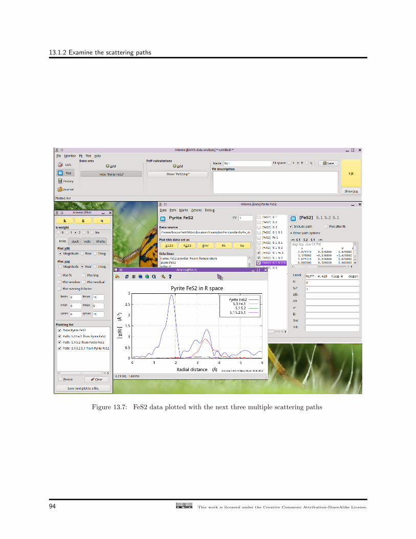
13.1.2 Examine the scattering paths
Figure 13.7: FeS2 data plotted with the next three multiple scattering paths
94 This work is licensed under the Creative Commons Attribution-ShareAlike License.

CHAPTER 13. WORKED EXAMPLES
atom in the fourth coordination shell, is quite substantial. It will certainly need to be considered in our fit.The other two paths are tiny.
13.1.3 Fit to the first coordination shell
We begin by doing an analysis of the first shell. As we saw above, we only need the first path in the pathlist. To prepare for the fit, we do the following:
1. Exclude all but the first path from the fit. With the first path selected in the path list and displayed,select “Mark after current” from the Marks menu. This will mark all paths except for the first one.Then select “Exclude marked” from the Actions menu. This will exclude those paths from the fit.That is indicated by the triple parentheses in the path list.
2. Set the values of Rmin and Rmax to cover just the first peak.
3. For this simple first shell fit, we set up a simple, four-parameter model. The parameters amp, enot,delr, and ss are defined in the GDS window and given sensible initial guess values.
4. The path parameters for the first shell path are set. S20 is set to amp, E0 is set to enot, ∆R is set to
delr, and σ2 is set to ss.
Note that the current settings for k- and R-range result in a bit more than 7 independent points, as computedfrom the Nyquist criterion. With only 4 guess parameters, this should be a reasonable fitting model.
Now hit the “Fit” button. Upon completion of the fit, the following things happen:
1. An Rmr plot is made of the data and the fit.
2. The log Window is displayed with the results of the fit
3. The Fit and plot buttons are recolored according to the evaluation of the happiness parameter.
4. The Plotting list is cleared and repopulated with the data.
5. The fit is entered into the History window (which is not in the screenshot below).
This is not a bad result. The value of enot is small, indicatng that a reasonable value of E0 was chosen backin athena. delr is small and consistent with 0, as we should expect for a known crystal. ss is a reasonablevalue with a reasonable error bar. The only confusing parameter is amp, which is a bit smaller than we mightexpect for a S2
0 value.
The correlations between parameters are of a size that we expect. The R-factor evaluates to about 2thatlikely means that ε was not evaluated correctly. All in all, this is a reasonable fit.
13.1.4 Extending the fit to higher shells
13.1.5 The final fitting model
13.1.6 Additional questions
13.2 Example 1: Methyltin
This work is licensed under the Creative Commons Attribution-ShareAlike License. 95

13.2. EXAMPLE 1: METHYLTIN
Figure 13.8: Setting up for a first shell fit
96 This work is licensed under the Creative Commons Attribution-ShareAlike License.

CHAPTER 13. WORKED EXAMPLES
Figure 13.9: Results of the first shell fit
This work is licensed under the Creative Commons Attribution-ShareAlike License. 97

13.2. EXAMPLE 1: METHYLTIN
Methyltin blah blah
98 This work is licensed under the Creative Commons Attribution-ShareAlike License.

Chapter 14
Crystallography for EXAFS
This chapter provides an overview of crystallography tools as implemented in artemis. Crystallographicdata is provided either in the form of a CIF file or in a simpler format that has long been the input formatfor my atoms program.
Compared to other crystallography codes, the crystallography capabilities in artemis are, perhaps, a littlecrude and incomplete. The goal is to provide enough functionality to support the needs of the X-rayabsorption spectroscopist.
This section discussed conventions for denoting space groups (Sec. ?? on page ??), the details of calculationsusing tables of absorption coefficients (Sec. ?? on page ??), and provides a worked example (Sec. ?? onpage ??).
14.1 Understanding and denoting space groups
14.1.1 Notation conventions
The two most commonly used standards for the designation of three dimensional space groups are theHermann-Maguin and Schoenflies conventions. atoms recognizes both conventions. Each of the 230 spacegroups as designated in each convention is listed later in this chapter.
The Hermann-Maguin system uses four symbols to uniquely specify the group properties of each of the 230space groups. The first symbol is a single letter P, I, R, F, A, B, or C which refers to the Bravais lattice type.The remaining three letters refer to the point group of the crystal.
Some modifications to the notation convention are made for use with a keyboard. Spaces must separate eachof the four symbols. Subscripted numbers are printed next to the number being modified (e.g. 63 is printedas 63). A bar above a number is entered with a minus sign.
Occasionally there are variations in how space groups are referenced. For example, the hausmannite structureof Mn3 O4 is placed in space group I 41/A M D by the conventions laid out in . In v. 3, Wyckoff denotesthis space group as I 4/A M D. This sort of incongruity is unfortunate. The list of Hermann-Maguin spacegroup designations as recognized by atoms is shown below. If you cannot resolve the incongruity using thislist, try using the Schoenflies notation.
99

14.1.2 Unique Crystallographic Positions
The Schoenflies conventions are also recognized by atoms. In the literature there is less variation in theapplication of these conventions. The Schoenflies convention is, in fact, less precise than the Hermann-Maguinin that the complete symmetry characteristics of the crystal are not encoded in the space group designation.Adaptations to the keyboard have been made here as well. Subscripts are denoted with an underscore ( )and superscripts are denoted with a caret (^. Spaces are not allowed in the keyboard designation. A coupleof examples: d 4^8, and O 5. The underscore does not need to precede to superscript. C 2^V9 can also bewritten C V9^2. Each of the 230 space groups as designated by the Schoenflies notation is listed below inthe same order as the listing of the Hermann-Maguin notation. The two conventions are equally supportedin the code.
14.1.2 Unique Crystallographic Positions
The atoms list in ‘atoms.inp’ is a list of the unique crystallographic sites in the unit cell. A unique site isone (and only one) of a group of equivalent positions. The equivalent positions are related to one anotherby the symmetry properties of the crystal. atoms determines the symmetry properties of the crystal fromthe name of the space group and applies those symmetry operations to each unique site to generate all ofthe equivalent positions.
If you include more than one of a group of equivalent positions in the atom list, then a few odd things willhappen. A series of run-time messages will issued telling you that atom positions were found that werecoincident in space. This is because each of the equivalent positions generated the same set of points inthe unit cell. atoms removes these redundancies from the atom list. The atom list and the potentials listwritten to ‘feff.inp’ will be correct and feff can be run correctly using this output. However, the site tagsand the indexing of the atoms will certainly make no sense. Also the density of the crystal will be calculatedincorrectly, thus the absorption calculation and the self-absorption correction will be calculated incorrectlyas well. The McMaster correction is unaffected.
14.1.3 Specially Recognized Lattice Types
For some common crystal types it is convenient to have a shorthand way of designating the space group.For instance, one might remember that copper is an fcc crystal, but not that it is in space group F M 3 M
(or O H^5). In this spirit, atoms will recognize the following words for common crystal types. These wordsmay be used as the value of the keyword space and atoms will supply the correct space group. Note thatseveral of the common crystal types are in the same space groups. For copper it will still be necessary tospecify that an atom lies at (0,0,0), but it isn’t necessary to remember that the space group is F M 3 M.
_______________________________________________________
cubic | cubic | P M 3 M
body-centered cubic | bcc | I M 3 M
face-centered cubic | fcc | F M 3 M
halite | salt or nacl | F M 3 M
zincblende | zincblende or zns | F -4 3 M
cesium chloride | cscl | P M 3 M
perovskite | perovskite | P M 3 M
diamond | diamond | F D 3 M
hexagonal close pack | hex or hcp | P 63/M M C
graphite | graphite | P 63 M C
-------------------------------------------------------
When space is set to hex or graphite, γ is automatically set to 120.
14.1.4 Bravais Lattice Conventions
100 This work is licensed under the Creative Commons Attribution-ShareAlike License.
CHAPTER 14. CRYSTALLOGRAPHY FOR EXAFS
atoms assumes certain conventions for each of the Bravais lattice types. Listed here are the labelingconventions for the axes and angles in each Bravais lattice.
• Triclinic: All axes and angles must be specified.
• Monoclinic: B is the perpendicular axis, thus β is the angle not equal to 90.
• Orthorhombic: A, B, and C must all be specified.
• Tetragonal: The C axis is the unique axis in a tetragonal cell. The A and B axes are equivalent.Specify A and C in ‘atoms.inp’.
• Trigonal: If the cell is rhombohedral then the three axes are equivalent as are the three angles. SpecifyA and α. If the cell has hexagonal axes, specify A and C. γ will be set to 120 by the program.
• Hexagonal: The equivalent axes are A and B. Specify A and C in ‘atoms.inp’. γ will be set to 120 bythe program.
• Cubic: Specify A in ‘atoms.inp’. The other axes will be set equal to A and the angles will all be setto 90.
14.1.5 Low Symmetry Space Groups
In three dimensional space there is an ambiguity in choice of right handed coordinate systems. Given aset of mutually orthogonal axes, there are six choices for how to label the positive x, y, and z directions.For some specific physical problem, the crystallographer might choose a non-standard setting for a crystal.The choice of standard setting is described in detail in The International Tables. The Hermann-Maguinsymbol describes the symmetries of the space group relative to this choice of coordinate system.
The symbols for triclinic crystals and for crystals of high symmetry are insensitive to choice of axes. Mon-oclinic and orthorhombic notations reflect the choice of axes for those groups that possess a unique axis.Tetragonal crystals may be rotated by 45 degrees about the z axis to produce a unit cell of doubled volumeand of a different Bravais type. Alternative symbols for those space groups that have them are listed inAppendix A.
atoms recognizes those non-standard notations for these crystal classes that are tabulated in The International
Tables. ‘atoms.inp’ may use any of these alternate notations so long as the specified cell dimensions andatomic positions are consistent with the choice of notation. Any notation not tabulated in chapter 6 of the1969 edition of The International Tables will not be recognized by atoms.
This resolution of ambiguity in choice of coordinate system is one of the main advantages of the Hermann-Maguin notation system over that of Shoenflies. In a situation where a non-standard setting has been chosenin the literature, use of the Schoenflies notation will, for many space groups, result in unsatisfactory outputfrom atoms. In these situations, atoms requires the use of the Hermann-Maguinn notation to resolve thechoice of axes.
Here is an example. In the literature, La2CuO4 was given in the non-standard b m a b setting rather thanthe standard c m c a. As you can see from the axes and coordinates, these settings differ by a 90 degreerotation about the A axis. The coordination geometry of the output atom list will be the same with eitherof these input files, but the actual coordinates will reflect this 90 degree rotation.
This work is licensed under the Creative Commons Attribution-ShareAlike License. 101

14.1.6 Rhombohedral Space Groups
title La2CuO4 structure at 10K from Radaelli et al.
title standard setting
space c m c a
a= 5.3269 b= 13.1640 c= 5.3819
rmax= 8.0 core= la
atom
la 0 0.3611 0.0074
Cu 0 0 0
O 0.25 -0.0068 -0.25 o1
O 0 0.1835 -0.0332 o2
--------------------------------------
title La2CuO4 structure at 10K from Radaelli et al.
title non standard setting, rotated by 90 degrees about A axis
space b m a b
a= 5.3269 b= 5.3819 c= 13.1640
rmax= 8.0 core= la
atom
la 0 -0.0074 0.3611
Cu 0 0 0
O 0.25 0.25 -0.0068 o1
O 0 0.0332 0.1835 o2
--------------------------------------
14.1.6 Rhombohedral Space Groups
There are seven rhombohedral space groups. Crystals in any of these space groups that may be representedas either monomolecular rhombohedral cells or as trimolecular hexagonal cells. These two representationsare entirely equivalent. The rhombohedral space groups are the ones beginning with the letter R in theHermann-Maguin notation. atoms does not care which representation you use, but a simple conventionmust be maintained. If the rhombohedral representation is used then the keyword α must be specified in‘atoms.inp’ to designate the angle between the rhombohedral axes and the keyword a must be specified todesignate the length of the rhombohedral axes. If the hexagonal representation is used, then a and c mustbe specified in ‘atoms.inp’. γ will be set to 120 by the code. Atomic coordinates consistent with the choiceof axes must be used.
14.1.7 Multiple Origins and the Shift Keyword
Some space groups in The International Tables are listed with two possible origins. The difference is only inwhich symmetry point is placed at (0,0,0). atoms always wants the orientation labeled “origin-at-centre”.This orientation places (0,0,0) at a point of highest crystallographic symmetry. Wyckoff and other authorshave the unfortunate habit of not choosing the “origin-at-centre” orientation when there is a choice. AgainMn3 O4 is an example. Wyckoff uses the “origin at -4m2” option, which places one Mn atom at (0,0,0)and another at (0,1/4,5/8). atoms wants the “origin-at-centre” orientation which places these atoms at(0,3/4,1/8) and (0,0,1/2). Admittedly, this is an arcane and frustrating limitation of the code, but it is notpossible to conclusively check if the “origin-at-centre” orientation has been chosen.
Twenty one of the space groups are listed with two origins in The International Tables. atoms knows whichgroups these are and by how much the two origins are offset, but cannot know if you chose the correctone for your crystal. If you use one of these groups, atoms will print a run-time message warning you ofthe potential problem and telling you by how much to shift the atomic coordinates in ‘atoms.inp’ if theincorrect orientation was used. This warning will also be printed at the top of the ‘feff.inp’ file. If youuse the “origin-at-center” orientation, you may ignore this message.
102 This work is licensed under the Creative Commons Attribution-ShareAlike License.

CHAPTER 14. CRYSTALLOGRAPHY FOR EXAFS
If you use one of these space groups, it usually isn’t hard to know if you have used the incorrect orientation.Some common problems include atoms in the atom list that are very close together (less than 1 A), unphys-ically large densities (see section 4.1), and interatomic distances that do not agree with values published inthe crystallography literature. Because it is tedious to edit the atomic coordinates in the input file everytime this problem is encountered and because forcing the user to do arithmetic invites trouble, there is auseful keyword called shift. For the Mn3 O4 example discussed above, simply insert this line in atoms.inp
if you have supplied coordinates referenced to the incorrect origin:
shift = 0.0 0.25 -0.125
This vector will be added to all of the coordinates in the atom list after the input file is read.
Here is the input file for Mn3O4 using the shift keyword:
title Mn3O4, hausmannite structure, using the shift keyword
a 5.75 c 9.42 core Mn2
rmax 7.0 Space i 41/a m d
shift 0.0 0.25 -0.125
atom
* At x y z tag
Mn 0.0 0.0 0.0 Mn1
Mn 0.0 0.25 0.625 Mn2
O 0.0 0.25 0.375
The above input file gives the same output as the following. Here the shift keyword has been removed andthe shift vector has been added to all of the fractional coordinates. These two input files give equivalentoutput.
title Mn3O4, hausmannite structure, no shift keyword
a 5.75 c 9.42 core Mn2
rmax 7.0 Space i 41/a m d
atom
* At x y z tag
Mn 0.0 0.25 -0.125 Mn1
Mn 0.0 0.50 0.50 Mn2
O 0.0 0.50 0.25
14.1.8 Denoting Space Groups
The following is my attempt to demystify the crazy symbolism used by the Hermann-Maguin and Schoenfliesconventions. This is by no means an adequate explanation of the rich and beautiful field of crystallography.For that, I recommend a real crystallography text.
An important part of the demystification process is to define some of the important terms used to describecrystal symmetries. The words system, Bravais lattice, crystal class, and space group have well-definedmeanings. The symbols used in each of the notation conventions specifically relate the various symmetriesof crystals. In crystallography, a symmetry operation is defined as a sequence of reflections, translations,and/or rotations that map the crystal back onto itself in such a way that the crystal after the mapping isindistinguishable from the crystal before the mapping.
14.1.9 A Quick Review of Crystallography
To start, here are some definitions. These will be elaborated below.
• System: The undecorated shape of the unit cell.
This work is licensed under the Creative Commons Attribution-ShareAlike License. 103

14.1.9 A Quick Review of Crystallography
• Bravais Lattice: An undecorated lattice of equivalent points.
• Crystal Class: The description of the symmetries about a point.
• Space Group: The complete description of three dimensional crystal symmetries.
There are seven systems of crystals. The system refers to the shape of the undecorated unit cell. They are:
• Triclinic: a 6= b 6= c, α 6= β 6= γ 6= 90◦
• Monoclinic: a 6= b 6= c, α=γ=90◦, β 6= 90◦
• Orthorhombic: a 6= b 6= c, α=β=γ=90◦
• Tetragonal: a = b 6= c, α=β=γ=90◦
• Hexagonal: a = b 6= c, α=β=90◦, γ=120◦
• Trigonal: (rhombohedral axes): a = b = c, α=β=γ < 120◦ 6= 90◦
(hexagonal axes): a = b 6= c, α=β=90◦, γ=120◦
• Cubic: a = b = c, α=β=γ=90◦
There are fourteen Bravais lattices. The Bravais lattices are constructed from the simplest translationalsymmetries applied to the seven crystal systems. A P lattice has decoration only at the corners of the unitcell. An I lattice has decoration at the body center of the cell as well as at the corners. An F lattice hasdecoration at the face centers as well as at the corners. A C lattice has decoration at the center of the (001)face as well as at the corners. Likewise A and B lattices have decoration at the centers of the (100) and (010)faces respectively. R lattices are a special type in the trigonal system which possess rhombohedral symmetry.
All seven crystal systems have P lattices, but not all the classes have the other type of Bravais lattices. Thisis because there is degeneracy when all the Bravais lattice types are applied to all the crystal systems. Forexample, a face centered tetragonal cell can be expressed as a body centered tetragonal cell by rotating thetwo equivalent axes by 45◦ and shortening them by a factor of square root of 2. Considering such degeneraciesreduces the possible decorations of the seven systems to these 14 unique three dimensional lattices:
Triclinic P
Monoclinic P, C
Orthorhombic P, C, I, F
Tetragonal P, I
Hexagonal P
Trigonal P, R
Cubic P, I, F
For historic reasons, hexagonal cells are sometimes called C lattices. atoms will recognize hexagonal P cellsdenoted in ‘atoms.inp’ by the letter C. Modern literature usually uses the P designation.
The decorations placed on the Bravais lattices come in 32 flavors called classes or point groups which representthe possible symmetries within the decorations. Each type of symmetry is defined either by a reflection plane,a rotation axis, or a rotary inversion axis. A reflection plane can either be a simple mirror plane or a glideplane, which defines the symmetry operation of reflecting through a mirror followed by translating along adirection in the plane. A rotation axis can either define a simple rotation or a screw rotation, which is thesymmetry operation of rotating about the axis followed by translating along that axis. A rotary inversionaxis defines the symmetry operation of reflecting through a plane followed by rotating about an axis in thatplane.
These three symmetry types, reflection plane, rotation axis, and rotary inversion axis, can be combined in32 non-degenerate ways. (An example degeneracy: the symmetry operation of combining a 180◦ rotaryinversion with a mirror reflection is identical to the operation of a simple 180◦ rotation.) It would seemthat the 32 classes could decorate the 14 Bravais lattices in 458 ways. In fact, the number might be largeras there are numerous types of screw axes and glide planes. Again, considering degeneracies reduces the
104 This work is licensed under the Creative Commons Attribution-ShareAlike License.

CHAPTER 14. CRYSTALLOGRAPHY FOR EXAFS
total number of combinations, leaving 230 unique decorations of the Bravais lattices. These are called spacegroups. The 230 space groups are a rigorously complete set of descriptions of crystal symmetries in threedimensional space. That is, there may be new crystals but there are no new space groups. Here I am onlyconsidering space-filling crystals with translational periodicity. 3-D Penrose structures and quasi-crystalsare outside the realm of this appendix and of the code.
14.1.10 Decoding the Hermann-Maguin Notation
The Hermann-Maguin notation uses a set of two to four symbols to completely specify the symmetries of aspace group. The first symbol is always a single letter specifying the Bravais lattice. The next three symbolsspecify the class of the space group. These three symbols are some combination of the following characters:
1 2 3 4 5 6 A B C D M N / -
These are sufficient to completely specify the various planar and axial symmetries of the classes and sub-classes. The following is a discussion of the most important rules of this convention. Some details areneglected but sufficient information is provided to appreciate the information contained in the notation.
The second symbol in the Hermann-Maguin notation, i.e. the one after the Bravais lattice symbol, tellsabout symmetries involving the primary axis of the cell and/or of the plane normal to the primary axis. Theprimary axis is defined as follows:
• Triclinic: none
• Monoclinic: the B axis
• Orthorhombic: the C axis
• Tetragonal: the C axis
• Hexagonal: the C axis
• Trigonal: the A axis
• Cubic: the A axis
In cubic or rhombohedral lattices the axes are equivalent, thus the primary axis is arbitrary. For orthorhombiclattices the third and fourth symbols specify the symmetries of the a and b axes respectively. In other lattices,the last two symbols encode the remaining symmetries as described below.
A space filling crystal will always show a symmetry when rotated through (360/n) degrees, where n is oneof 1, 2, 3, 4, or 6. The second symbol often tells the rotational symmetry properties of the primary axis.Notice that all trigonal, tetragonal, and hexagonal groups have a 3, 4, or 6 respectively in their designations.Many orthorhombic and monoclinic groups have a 2, which is the highest degree of rotational symmetryavailable to those lattices. Cubic groups may possess 2- or 4-fold rotational symmetry about the cell axes,thus have 2 or 4 in the second symbol.
Many second symbols contain a second number. This is the subscripted number when the Hermann-Maguinnotation is typeset. This refers to the type of screw symmetry associated with the axis. A screw symmetriclattice is mapped onto itself by an anti-clockwise rotation through m*(360/n) degrees and a translation of1/n up the primary axis. Here n is the degree of rotational symmetry, m is the type of screw, and thedefinition of rotation and direction is right-handed. Two types of screw symmetry that are different only inhandedness of rotation are called enantiomorphous. The enantiomorphous pairs are 31 and 32, 41 and 43,61 and 65, and 62 and 64.
Several of the second symbols are one or two numbers followed by a slash and a letter, e.g. P 63/M M C.The letter specifies the type of reflection plane that is normal to the rotation axis.
This work is licensed under the Creative Commons Attribution-ShareAlike License. 105

14.1.11 Decoding the Schoenflies Notation
There are several types of reflection planes. The simplest is a mirror plane, denoted by the letter M. This saysthe crystal is mapped onto itself by reflecting all atoms through a mirror placed in an appropriate plane inthe crystal. The letters A, B, or C denote glide planes. These map the crystal onto itself by reflecting throughthe plane then translating elements of the crystal by half the length of the cell axis normal to the reflectionplane. A D glide plane is similar but involves translations of a quarter of the cell axis length. Finally, theletter N denotes a diagonal glide plane, which is a reflection through a plane followed by a translation in thesame plane of half the length of both cell axes in that plane.
The symbol - before a number indicates a rotary inversion axis. This maps the crystal back onto itself byrotating through (360/n) degrees then reflecting through a plane parallel to the rotation axis.
A final word about the Hermann-Maguin notation, all cubic space groups have four three-fold rotationalaxes through the body diagonals. Thus all cubic groups have the number 3 as the third symbol, e.g. F M 3
M.
14.1.11 Decoding the Schoenflies Notation
The Schoenflies notation uses a set of three symbols to classify sets of space groups by their dominantsymmetry features. The letters C, D, S, T, and O denote the character of the center of symmetry. The symbolafter the underscore (the subscript when typeset) indicates the presence of symmetry planes and additionalsymmetry axes. The number after the caret (the superscript when typeset) is simply an indexing of all thedistinct space groups that share major symmetry properties. In the older literature, D symmetry centers areoccasionally referred to as V. atoms will probably understand a space group referred to by the letter V, butusing the D notation is recommended.
The letter C indicates an rotation axis where the crystal is mapped onto itself when rotated by (360/n) deg,where n is the number after the underscore. An H after the underscore indicates the presence of a plane ofsymmetry normal to the rotation axis. A V after the underscore indicates one or two planes of symmetryparallel to the rotation axis. The letter S after the underscore indicates a normal plane of symmetry in acrystal where the degree of rotational symmetry is 1. The letter I after the underscore indicates the presenceof a point center of symmetry.
The letter S indicates a rotary inversion axis. The degree of rotation is the number after the underscore.
The letter D denotes a primary rotation axis with another rotation axis normal to it. The degree of rotationof both axes is the number after the underscore. The letters H and V have the same meanings as they did ingroups beginning with the letter C. The letter D indicates the presence of a diagonal symmetry plane.
Cubic groups are all specified by the letters T and O. T indicates tetrahedral symmetry, that is, the presenceof the four three-fold axes and three two-fold axes. O indicates octahedral symmetry, i.e. four three-fold axeswith three four-fold axes. H and D after the underscore carry the same meaning as before.
14.1.12 The Hermann-Maguin Notation
Notation for the Standard Settings
2 Triclinic and 13 Monoclinic Space Groups
P 1 P -1 P 2 P 21 C 2 P M
P C C M C C P 2/M P 21/M C 2/M
P 2/C P 21/C C 2/C
59 Orthorhombic Space Groups
106 This work is licensed under the Creative Commons Attribution-ShareAlike License.

CHAPTER 14. CRYSTALLOGRAPHY FOR EXAFS
P 2 2 2 P 2 2 21 P 21 21 2 P 21 21 21 C 2 2 21 C 2 2 2
F 2 2 2 I 2 2 2 I 21 21 21 P M M 2 P M C 21 P C C 2
P M A 2 P C A 21 P N C 2 P M N 21 P B A 2 P N A 21
P N N 2 C M M 2 C M C 21 C C C 2 A M M 2 A B M 2
A M A 2 A B A 2 F M M 2 F D D 2 I M M 2 I B A 2
I M A 2 P M M M P N N N P C C M P B A N P M M A
P N N A P M N A P C C A P B A M P C C N P B C M
P N N M P M M N P B C N P B C A P N M A C M C M
C M C A C M M M C C C M C M M A C C C A F M M M
F D D D I M M M I B A M I B C A I M M A
68 Tetragonal Space Groups
P 4 P 41 P 42 P 43 I 4 I 41
P -4 I -4 P 4/M P 42/M P 4/N P 42/N
I 4/M I 41/A P 4 2 2 P 4 21 2 P 41 2 2 P 41 21 2
P 42 2 2 P 42 21 2 P 43 2 2 P 43 21 2 I 4 2 2 I 41 2 2
P 4 M M P 4 B M P 42 C M P 42 N M P 4 C C P 4 N C
P 42 M C P 42 B C I 4 M M I 4 C M I 41 M D I 41 C D
P -4 2 M P -4 2 C P -4 21 M P -4 21 C P -4 M 2 P -4 C 2
P -4 B 2 P -4N2 I -4 M 2 I -4 C 2 I -42 M I -42 D
P 4/M M M P 4/M C C P 4/N B M P 4/N N C P 4/M B M P 4/M N C
P 4/N M M P 4/N C C P 42/M M C P 42/M C M P 42/N B C P 42/N N M
P 42/M B C P 42/M N M P 42/N M C P 42/N C M I 4/M M M I 4/M C M
I 41/A M D I 41/A C D
25 Trigonal Space Groups
P 3 P 3 1 P 32 R3 P -3 R -3
P 3 1 2 P 3 2 1 P 31 1 2 P 31 2 1 P 32 1 2 P 32 2 1
R 32 P 3 M 1 P 3 1 M P 3 C 1 P 3 1 C R 3 M
R 3C P -3 1 M P -3 1 C P -3 M 1 P -3 C 1 R -3 M
R -3 C
27 Hexagonal Space Groups
P 6 P 61 P 65 P 62 P 64 P 63
P -6 P 6/M P 63/M P 62 2 P 61 2 2 P 65 2 2
P 62 2 2 P 64 2 2 P 63 2 2 P 6 M M P 6 C C P 63 C M
P 63 M C P -6 M 2 P -6 C 2 P -6 2 M P -62 C P 6/M M M
P 6/M C C P 63/M C M P 63/M M C
36 Cubic Space Groups
P 2 3 F 2 3 I 2 3 P 21 3 I 21 3 P M 3
P N 3 F M 3 F D 3 I M 3 P A 3 I A 3
P 4 3 2 P 42 3 2 F 4 3 2 F 41 3 2 I 4 3 2 P 43 3 2
P 41 3 2 I 41 3 2 P -4 3 M F -4 3 M I -4 3 M P -4 3 N
F -4 3 C I -4 3 D P M 3 M P N 3 N P M 3 N P N 3 M
F M 3 M F M 3 C F D 3 M F D 3 C I M 3 M I A 3 D
Non-Standard Settings
Here are the notations for the alternate settings of the monoclinic and orthorhombic space groups. Alsopresented are the notations for tetragonal space groups that have been rotated by 45 degrees resulting in aunit cell of doubled volume and of a different Bravais type.
In an monoclinic or orthorhombic space group, the Hermann-Maguin symbols are identical for the varioussettings if none of the three axes possess special symmetry properties. In this case the three axes aredistinguished only by length and the symbol is the same for all settings.
The column headings below indicate the orientations of the alternative settings relative to the standard
This work is licensed under the Creative Commons Attribution-ShareAlike License. 107

14.1.12 The Hermann-Maguin Notation
setting. For instance, cab is a setting with axes and coordinates cyclically permuted from the standardsetting. This is equivalent to a rotation of 120 degrees about an axis in a ¡111¿ direction relative to theCartesian axes. The setting a-cb is rotated by 90 degrees about the A axis. Thus the B and C axesare swapped and the y and z coordinates in the standard setting map onto the z and -y coordinates of thealternate setting. In atoms, when an alternative setting is specified in ‘atoms.inp’, the axes and coordinatesare multiplied by the appropriate permutation matrix onto the standard setting. The positions in the unitcell are expanded according to the Hermann-Maguin symbol for the standard setting. The contents of theunit cell are then permuted back to the specified setting.
Symbols for Monoclinic Groups of Various Settings
standard | standard
abc bca | abc bca
-----------------------------------------------------------------
P 2 both settings | P 21 both settings
B 2 or C 2 | P M both settings
P B or P C | B M or C M
B B or C C | P 2/M both settings
P 21/M both settings | B 2/M or C 2/M
P 2/B or P 2/C | P 21/B or P 2/C
B 2/B or C 2/C |
Symbols for Orthorhombic Groups of Various Settings
standard
abc cab bca a-cb ba-c -cab
-----------------------------------------------------------------
P 2 2 2 each setting
P 2 2 21 P 21 2 2 P 2 21 2 P 2 21 2 P 2 2 21 P 21 2 2
P 21 21 2 P 2 21 21 P 21 2 21 P 21 2 21 P 21 21 2 P 2 21 21
P 21 21 21 each setting
C 2 2 21 A 21 2 2 B 2 21 2 B 2 21 2 C 2 2 21 A 21 2 2
C 2 2 2 A 2 2 2 B 2 2 2 B 2 2 2 C 2 2 2 A 2 2 2
F 2 2 2 each setting
I 2 2 2 each setting
I 21 21 21 each setting
P M M 2 P 2 M M P M 2 M P M 2 M P M M 2 P 2 M M
P M C 21 P 21 M A P B 21 M P M 21 B P C M 21 P 21 A M
P C C 2 P 2 A A P B 2 B P B 2 B P C C 2 P 2 A A
P M A 2 P 2 M B P C 2 M P M 2 A P B M 2 P 2 C M
P C A 21 P 21 A B P C 21 B P B 21 A P B C 21 P 21 C A
P N C 2 P 2 N A P B 2 N P N 2 B P C N 2 P 2 A N
P M N 21 P 21 M N P N 21 M P M 21 N P N M 21 P 2 N M
P B A 2 P 2 C B P C 2 A P C 2 A P B A 2 P 2 C B
P N A 21 P 21 N B P C 21 N P N 21 A P B N 21 P 2 C N
P N N 2 P 2 N N P N 2 N P N 2 N P N N 2 P 2 N N
C M M 2 A 2 M M B M 2 M B M 2 M C M M 2 A 2 M M
C M C 21 A 21 M A B B 21 M B M 21 B C C M 21 A 21 A M
C C C 2 A 2 C A B B 2 C B B 2 B C C C 2 A 2 A A
A M M 2 B 2 M M C M 2 M A M 2 M B M M 2 C 2 M M
A B M 2 B 2 C M C M 2 A A C 2 M B M A 2 C 2 M B
A M A 2 B 2 M B C C 2 M A M 2 A B B M 2 C 2 C M
A B A 2 B 2 C B C C 2 A A C 2 A B B A 2 C 2 C B
108 This work is licensed under the Creative Commons Attribution-ShareAlike License.

CHAPTER 14. CRYSTALLOGRAPHY FOR EXAFS
standard
abc cab bca a-cb ba-c -cab
-----------------------------------------------------------------
F M M 2 F 2 M M F M 2 M F M 2 M F M M 2 F 2 M M
F D D 2 F 2 D D F D 2 D F D 2 D F D D 2 F 2 D D
I M M 2 I 2 M M I M 2 M I M 2 M I M M 2 I 2 M M
I B A 2 I 2 C B I C 2 A I C 2 A I B A 2 I 2 C B
I M A 2 I 2 M B I C 2 M I M 2 A I B M 2 I 2 C M
P M M M each setting
P N N N each setting
P C C M P M A A P B M B P B M B P C C M P M A A
P B A N P N C B P C N A P C N A P B A N P N C B
P M M A P B M M P M C M P M A M P M M B P C M M
P N N A P B N N P N C N P N A N P N N B P C N N
P M N A P B M N P N C M P M A N P N M B P C N M
P C C A P B A A P B C B P B A B P C C B P C A A
P B A M P M C B P C M A P C M A P B A M P M C B
P C C N P N A A P B N B P B N B P C C N P N A A
P B C M P M C A P B M A P C M B P C A M P M A B
P N N M P M N N P N M N P N M N P N N M P M N N
P M M N P N M M P M N M P M N M P M M N P N M M
P B C N P N C A P B N A P C N B P C A N P N A B
P B C A P B C A P B C A P C A B P C A B P C A B
P N M A P B N M P M C N P N A M P M N B P C M N
C M C M A M M A B B M M B M M B C C M M A M A M
C M C A A B M A B B C M B M A B C C M B A C A M
C M M M A M M M B M M M B M M M C M M M A M M M
C C C M A M A A B B M B B B M B C C C M A M A A
C M M A A B M M B M C M B M A M C M M B A C M M
C C C A A B A A B B C B B B A B C C C B A C A A
F M M M each setting
F D D D each setting
I M M M each setting
I B A M I M C B I C M A I C M A I B A M I M C B
I B C A I B C A I B C A I C A B I C A B I C A B
I M M A I B M M I M C M I M A M I M M B I C M M
Symbols for Tetragonal Groups of Various Orientations
This work is licensed under the Creative Commons Attribution-ShareAlike License. 109
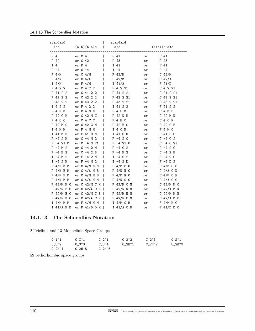
14.1.13 The Schoenflies Notation
standard | standard
abc (a+b)(b-a)c | abc (a+b)(b-a)c
----------------------------------------------------------------------
P 4 or C 4 | P 41 or C 41
P 42 or C 42 | P 43 or C 43
I 4 or F 4 | I 41 or F 41
P -4 or C -4 | I -4 or F -4
P 4/M or C 4/M | P 42/M or C 42/M
P 4/N or C 4/A | P 42/M or C 42/A
I 4/M or F 4/M | I 41/A or F 41/D
P 4 2 2 or C 4 2 2 | P 4 2 21 or C 4 2 21
P 41 2 2 or C 41 2 2 | P 41 2 21 or C 41 2 21
P 42 2 2 or C 42 2 2 | P 42 2 21 or C 42 2 21
P 43 2 2 or C 43 2 2 | P 43 2 21 or C 43 2 21
I 4 2 2 or F 4 2 2 | I 41 2 2 or F 41 2 2
P 4 M M or C 4 M M | P 4 B M or C 4 M B
P 42 C M or C 42 M C | P 42 N M or C 42 M N
P 4 C C or C 4 C C | P 4 N C or C 4 C N
P 42 M C or C 42 C M | P 42 B C or C 42 C B
I 4 M M or F 4 M M | I 4 C M or F 4 M C
I 41 M D or F 41 D M | I 41 C D or F 41 D C
P -4 2 M or C -4 M 2 | P -4 2 C or C -4 C 2
P -4 21 M or C -4 M 21 | P -4 21 C or C -4 C 21
P -4 M 2 or C -4 2 M | P -4 C 2 or C -4 2 C
P -4 B 2 or C -4 2 B | P -4 N 2 or C -4 2 N
I -4 M 2 or F -4 2 M | I -4 C 2 or F -4 2 C
I -4 2 M or F -4 M 2 | I -4 2 D or F -4 D 2
P 4/M M M or C 4/M M M | P 4/M C C or C 4/M C C
P 4/N B M or C 4/A M B | P 4/N N C or C 4/A C N
P 4/M B M or C 4/M M B | P 4/M N C or C 4/M C N
P 4/N M M or C 4/A M M | P 4/N C C or C 4/A C C
P 42/M M C or C 42/M C M | P 42/M C M or C 42/M M C
P 42/N B C or C 42/A C B | P 42/N N M or C 42/A M N
P 42/M B C or C 42/M C B | P 42/M N M or C 42/M M N
P 42/N M C or C 42/A C M | P 42/N C M or C 42/A M C
I 4/M M M or F 4/M M M | I 4/M C M or F 4/M M C
I 41/A M D or F 41/D D M | I 41/A C D or F 41/D D C
14.1.13 The Schoenflies Notation
2 Triclinic and 13 Monoclinic Space Groups
C_1^1 C_I^1 C_2^1 C_2^2 C_2^3 C_S^1
C_S^2 C_S^3 C_S^4 C_2H^1 C_2H^2 C_2H^3
C_2H^4 C_2H^5 C_2H^6
59 orthorhombic space groups
110 This work is licensed under the Creative Commons Attribution-ShareAlike License.

CHAPTER 14. CRYSTALLOGRAPHY FOR EXAFS
D_2^1 D_2^2 D_2^3 D_2^4 D_2^5 D_2^6
D_2^7 D_2^8 D_2^9 C_2V^1 C_2V^2 C_2V^3
C_2V^4 C_2V^5 C_2V^6 C_2V^7 C_2V^8 C_2V^9
C_2V^10 C_2V^11 C_2V^12 C_2V^13 C_2V^14 C_2V^15
C_2V^16 C_2V^17 C_2V^18 C_2V^19 C_2V^20 C_2V^21
C_2V^22 D_2H^1 D_2H^2 D_2H^3 D_2H^4 D_2H^5
D_2H^6 D_2H^7 D_2H^8 D_2H^9 D_2H^10 D_2H^11
D_2H^12 D_2H^13 D_2H^14 D_2H^15 D_2H^16 D_2H^17
D_2H^18 D_2H^19 D_2H^20 D_2H^21 D_2H^22 D_2H^23
D_2H^24 D_2H^25 D_2H^26 D_2H^27 D_2H^28
68 Tetragonal space groups
C_4^1 C_4^2 C_4^3 C_4^4 C_4^5 C_4^6
S_4^1 S_4^2 C_4H^1 C_4H^2 C_4H^3 C_4H^4
C_4H^5 C_4H^6 D_4^1 D_4^2 D_4^3 D_4^4
D_4^5 D_4^6 D_4^7 D_4^8 D_4^9 D_4^10
C_4V^1 C_4V^2 C_4V^3 C_4V^4 C_4V^5 C_4V^6
C_4V^7 C_4V^8 C_4V^9 C_4V^10 C_4V^11 C_4V^12
D_2D^1 D_2D^2 D_2D^3 D_2D^4 D_2D^5 D_2D^6
D_2D^7 D_2D^8 D_2D^9 D_2D^10 D_2D^11 D_2D^12
D_4H^1 D_4H^2 D_4H^3 D_4H^4 D_4H^5 D_4H^6
D_4H^7 D_4H^8 D_4H^9 D_4H^10 D_4H^11 D_4H^12
D_4H^13 D_4H^14 D_4H^15 D_4H^16 D_4H^17 D_4H^18
D_4H^19 D_4H^20
25 Trigonal space groups
C_3^1 C_3^2 C_3^3 C_3^4 C_3I^1 C_3I^2
D_3^1 D_3^2 D_3^3 D_3^4 D_3^5 D_3^6
D_3^7 C_3V^1 C_3V^2 C_3V^3 C_3V^4 C_3V^5
C_3V^6 D_3D^1 D_3D^2 D_3D^3 D_3D^4 D_3D^5
D_3D^6
27 Hexagonal space groups
C_6^1 C_6^2 C_6^3 C_6^4 C_6^5 C_6^6
C_3H^1 C_6H^1 C_6H^2 D_6^1 D_6^2 D_6^3
D_6^4 D_6^5 D_6^6 C_6V^1 C_6V^2 C_6V^3
C_6V^4 D_3H^1 D_3H^2 D_3H^3 D_3H^4 D_6H^1
D_6H^2 D_6H^3 D_6H^4
36 Cubic space groups
T^1 T^2 T^3 T^4 T^5 T_H^1
T_H^2 T_H^3 T_H^4 T_H^5 T_H^6 T_H^7
O^1 O^2 O^3 O^4 O^5 O^6
O^7 O^8 T_D^1 T_D^2 T_D^3 T_D^4
T_D^5 T_D^6 O_H^1 O_H^2 O_H^3 O_H^4
O_H^5 O_H^6 O_H^7 O_H^8 O_H^9 O_H^10
14.2 Absorption calculations and experimental corrections
Included in atoms is absorption data for the elements from various sources. Using this and the crystallo-graphic information from ‘atoms.inp’, atoms is able to make several calculations useful for XAFS analysis.It approximates the absorption depth and edge step size of the material at the edge energy of the core atomand estimates three corrections needed for the analysis of XAFS data. These corrections are the “McMastercorrection”, the energy response of the I0 chamber in a fluorescence experiment, and the self-absorption ofa thick material in a fluorescence experiment. All of these numbers are written at the top of the output file.For more information on these calculations consult Chapter 10 of Handbook of Synchrotron Radiation, v.1.
This work is licensed under the Creative Commons Attribution-ShareAlike License. 111
14.2.1 Absorption Calculation
14.2.1 Absorption Calculation
Proper sample preparation for an XAFS experiment requires knowledge of the absorption depth and edgestep size of the material of interest. The statistics of data collection can be optimized by choosing the correctsample thickness. It is also necessary to avoid distortions to the data due to thickness and large particle sizeeffects.
atoms calculates the total cross section of the material above the edge energy of the central atom and dividesby the unit cell volume. The number obtained, µtotal, has units of cm−1. Thus, if x is the thickness of thesample in cm, the x-ray beam passing through the sample will be attenuated by exp(µtotal * x).
atoms also calculates the change in cross section of the central atom below and above the absorption edgeand divides by the unit cell volume. This number, ∆µ, multiplied by the sample thickness in cm gives theapproximate edge step in a transmission experiment.
The density of the material is also reported. This number assumes that the bulk material will have the samedensity as the unit cell. It is included as an aid to sample preparation.
14.2.2 McMaster Correction
Typically, XAFS data is normalized to a single number representing the size of the edge step. While thereare compelling reasons to use this simple normalization, it can introduce an important distortion to theamplitude of the χ(k) extracted from the absorption data. This distortion comes from energy response ofthe bare atom absorption of the central atom. This is poorly approximated away from the edge by a singlenumber. Because this affects the amplitude of χ(k) and not the phase, it can be corrected by including aDebye-Waller factor and a fourth cumulant in the analysis of the data. These two “McMaster corrections”are intended to be additive corrections to any thermal or structural disorder included in the analysis of theXAFS.
atoms uses data from McMaster to construct the bare atom absorption for the central atom. atomsthen regresses a quadratic polynomial in energy to the natural logarithm of the constructed central atomabsorption. Because energy and photo-electron wave number are simply related, E is proportional to k2, thecoefficients of this regression can be related to the XAFS Debye-Waller factor and fourth cumulant. Thecoefficient of the term linear in energy equals sigma MM^2 and the coefficient of the quadratic term equals4/3 * sigma MM^4. The values of sigma MM^2 and sigma MM^4 are written at the top of the output file.
14.2.3 I0 Correction
The response of the I0 chamber varies with energy during an XAFS experiment. In a fluorescence experiment,the absorption signal is obtained by normalizing the If signal by the I0 signal. There is no energy responsein the If signal since all atoms fluoresce at set energies. The energy response of I0 is ignored by thisnormalization. At low energies this can be a significant effect. Like the McMaster correction, this effectattenuates the amplitude of χ(k) and is is well approximated by an additional Debye-Waller factor andfourth cumulant.
atoms uses the values of the nitrogen, argon and krypton keywords in ‘atoms.inp’ to determine the contentof the I0 chamber by pressure. It assumes that the remainder of the chamber is filled with helium. It thenuses McMaster’s data to construct the energy response of the chamber and regresses a polynomial to it inthe manner described above. sigma I0^2 and are also written at the top of the output file and intended asadditive corrections in the analysis.
112 This work is licensed under the Creative Commons Attribution-ShareAlike License.

CHAPTER 14. CRYSTALLOGRAPHY FOR EXAFS
14.2.4 Self-Absorption Correction
If the thickness of a sample is large compared to absorption length of the sample and the absorbing atom issufficiently concentrated in the sample, then the amplitude of the χ(k) extracted from the data taken on itin fluorescence will be distorted by self-absorption effects in a way that is easily estimated. The absorptiondepth of the material might vary significantly through the absorption edge and the XAFS wiggles. Thecorrection for this effect is well approximated as
1 + mu_abs / (mu_background+mu_fluor)
where µbackground is the absorption of the non-resonant atoms in the material and µfluo is the total absorptionof the material at the fluorescent energy of the absorbing atom. atoms constructs this function using theMcMaster tables then regresses a polynomial to it in the manner described above. sigma self^2 andsigma self^4 are written at the top of the output file and intended as additive corrections in the analysis.Because the size of the edge step is affected by self-absorption, the amplitude of χ(k) is attenuated whennormalized to the edge step. Since the amplitude is a measure of S2
0 , this is an important effect. The numberreported in ‘feff.inp’ as the amplitude factor is intended to be a multiplicative correction to the data orto the measured S2
0 .
14.3 A worked example (in text!)
14.3.1 The Atoms input file
Here is an example of atoms in action. The material is Lead Titanate, PbTiO3. The crystallographicliterature places this material in the tetragonal space group P 4 M M. Let’s suppose tha the data were takenin fluorescence at the titanium K-edge. Since the edge energy is around 5 KeV and the sample was verythick, the I0 and self-absorption corrections are expected to be significant. That titanium is the centralatom is indicated by the keyword core. atoms assumes the K-edge of the titanium was probed because theatomic number of titanium is less than 57 and the edge was not otherwise chosen with the edge keyword.The I0 chamber was filled with 50is indicated by the nitrogen keyword. The size of the cluster to be printedin ‘feff.inp’ is chosen with the rmax keyword. The rpath keyword is used to set the value of RMAX in the‘feff.inp’ file, which indicates the length of the longest path to be calculated.
title PbTiO3 10K,a=3.885,c=4.139
space P 4 m m
a=3.885 c=4.139 nitrogen = 0.5
rmax=6.0 rpath=4.2 core=ti
atom
* At x y z tag
Pb 0.0 0.0 0.0
Ti 0.5 0.5 0.5377
O 0.5 0.5 0.1118 axial
O 0.0 0.5 0.6174 planar
Note that CIF files can also be used as the input to atoms and will, in many cases, work just fine. Thecode that reads the CIF files is rather incomplete and a bit buggy, though. Also, demeter will refuse toattempt to import data from a CIF file that contains multiple occupancy for a crystallographic cite.
14.3.2 The Feff input file
This work is licensed under the Creative Commons Attribution-ShareAlike License. 113

14.3.2 The Feff input file
atoms produces the output reproduced below. The absorption and correction calculations are at the top ofthe file. All the CONTROL cards are set to 1 and the PRINT cards are set to 0. This will run all four modules offeff and produce the default output files. Several other useful feff cards are printed but commented outby an asterisk (*). The unique potential list is constructed in a simple fashion – the core atom is potential 0and each different atomic species has a single potential. The atom list is printed in the format required byfeff. The atom list has two comment columns. The indexed atomic symbol and radial distance are writtenby atoms for your use when reading ‘feff.inp’ and are ignored by feff.
feff will run to completion using the input file generated by atoms. It is still likely that the user will wantto edit ‘feff.inp’. Several assumptions are made by atoms that might not hold true. The assignment ofunique potentials is made by a simple algorithm and may not adequately reflect the physics of the problem.The CONTROL cards are such that all four modules of feff will be run. The feff user might want to runthe modules separately. Values for other cards have been assumed and might not be desired. Other cardshave been left out entirely. Always check your ‘feff.inp’ file to be sure it is just what you want.
* This feff6 file was generated by Demeter 0.9.13
* Demeter written by and copyright (c) Bruce Ravel, 2006-2012
* --*--*--*--*--*--*--*--*--*--*--*--*--*--*--*--*--*--*--*--*--*--*--*--
* title = PbTiO3 10K,a=3.885,c=4.139
* space = P 4 m m
* a = 3.88500 b = 3.88500 c = 4.13900
* alpha = 90.00000 beta = 90.00000 gamma = 90.00000
* rmax = 5.0 core = ti
* shift =
* atoms
* # el. x y z tag
* Pb 0.00000 0.00000 0.00000 Pb
* Ti 0.50000 0.50000 0.53770 Ti
* O 0.50000 0.50000 0.11180 axial
* O 0.00000 0.50000 0.61740 planar
* --*--*--*--*--*--*--*--*--*--*--*--*--*--*--*--*--*--*--*--*--*--*--*--
TITLE PbTiO3 10K,a=3.885,c=4.139
HOLE 1 1.0 * FYI: (Ti K edge @ 4966 eV, second number is S0^2)
* mphase,mpath,mfeff,mchi
CONTROL 1 1 1 1
PRINT 1 0 0 0
RMAX 4.2
*NLEG 4
POTENTIALS
* ipot Z tag
0 22 Ti
1 82 Pb
2 22 Ti
3 8 O
114 This work is licensed under the Creative Commons Attribution-ShareAlike License.

CHAPTER 14. CRYSTALLOGRAPHY FOR EXAFS
ATOMS * this list contains 94 atoms
* x y z ipot tag distance
0.00000 0.00000 0.00000 0 Ti 0.00000
0.00000 0.00000 -1.76280 3 axial.1 1.76280
1.37355 1.37355 0.32988 3 planar.1 1.97031
-1.37355 1.37355 0.32988 3 planar.1 1.97031
1.37355 -1.37355 0.32988 3 planar.1 1.97031
-1.37355 -1.37355 0.32988 3 planar.1 1.97031
0.00000 0.00000 2.37620 3 axial.2 2.37620
2.74711 0.00000 1.91346 1 Pb.1 3.34783
-2.74711 0.00000 1.91346 1 Pb.1 3.34783
0.00000 2.74711 1.91346 1 Pb.1 3.34783
0.00000 -2.74711 1.91346 1 Pb.1 3.34783
2.74711 0.00000 -2.22554 1 Pb.2 3.53548
-2.74711 0.00000 -2.22554 1 Pb.2 3.53548
0.00000 2.74711 -2.22554 1 Pb.2 3.53548
0.00000 -2.74711 -2.22554 1 Pb.2 3.53548
2.74711 2.74711 0.00000 2 Ti.1 3.88500
-2.74711 2.74711 0.00000 2 Ti.1 3.88500
2.74711 -2.74711 0.00000 2 Ti.1 3.88500
-2.74711 -2.74711 0.00000 2 Ti.1 3.88500
0.00000 0.00000 4.13900 2 Ti.2 4.13900
0.00000 0.00000 -4.13900 2 Ti.2 4.13900
2.74711 2.74711 -1.76280 3 axial.3 4.26623
-2.74711 2.74711 -1.76280 3 axial.3 4.26623
2.74711 -2.74711 -1.76280 3 axial.3 4.26623
-2.74711 -2.74711 -1.76280 3 axial.3 4.26623
1.37355 1.37355 -3.80912 3 planar.2 4.27583
-1.37355 1.37355 -3.80912 3 planar.2 4.27583
1.37355 -1.37355 -3.80912 3 planar.2 4.27583
-1.37355 -1.37355 -3.80912 3 planar.2 4.27583
4.12066 1.37355 0.32988 3 planar.3 4.35607
-4.12066 1.37355 0.32988 3 planar.3 4.35607
1.37355 4.12066 0.32988 3 planar.3 4.35607
-1.37355 4.12066 0.32988 3 planar.3 4.35607
4.12066 -1.37355 0.32988 3 planar.3 4.35607
-4.12066 -1.37355 0.32988 3 planar.3 4.35607
1.37355 -4.12066 0.32988 3 planar.3 4.35607
-1.37355 -4.12066 0.32988 3 planar.3 4.35607
2.74711 2.74711 2.37620 3 axial.4 4.55407
-2.74711 2.74711 2.37620 3 axial.4 4.55407
2.74711 -2.74711 2.37620 3 axial.4 4.55407
-2.74711 -2.74711 2.37620 3 axial.4 4.55407
1.37355 1.37355 4.46888 3 planar.4 4.87280
-1.37355 1.37355 4.46888 3 planar.4 4.87280
1.37355 -1.37355 4.46888 3 planar.4 4.87280
-1.37355 -1.37355 4.46888 3 planar.4 4.87280
END
14.3.3 Modifying the Feff input file
There are many reasons why you may want to edit the ‘feff.inp’ before running feff. Here are someexamples.
Change the absorber
This work is licensed under the Creative Commons Attribution-ShareAlike License. 115

14.3.3 Modifying the Feff input file
Suppose your absorber is a very dilute dopant such that you do not expect, on the average, thatanother example of the dopant resides anywhere near the absorber. In that case, you would want toleave the atoms list untouched but change the atomic species of the absorber.
In the example above, let’s consider that the dilute absorber is Nb. To make it the absorber, we mustmodify the ‘feff.inp’ file like so:
POTENTIALS
* ipot Z tag
0 41 Nb
1 82 Pb
2 22 Ti
3 8 O
ATOMS * this list contains 94 atoms
* x y z ipot tag distance
0.00000 0.00000 0.00000 0 Nb 0.00000
Note that the labels (i.e. the instances of the string “Nb”) are for the benefit of the human reader ofthe file and are also used by demeter to provide some information for the user. The essential edit isto change the Z number of the absorber in the POTENTIALS list.
Change a scattererAgain, consider the situation of a Nb dopant in this crystal. With Ti as the absorber, we need toconsider the possibility of a Nb atom in the third coordination shell. To do this, we must adit thePOTENTIALS list to include Nb:
POTENTIALS
* ipot Z tag
0 22 Ti
1 82 Pb
2 22 Ti
3 8 O
4 41 Nb
We must then replace one or more of the atoms in the third coordination shell with the new uniquepotential. Here is one example:
2.74711 2.74711 0.00000 4 Nb 3.88500
Again, the “Nb” label is not used by feff in any capacity, but is used by demeter.
Add an unique potentialYou may choose to consider the possibility that the feff calculation might be improved by allowingthe axial and planar oxygen atoms to have their own unique potentials. This probably won’t makemuch of a difference in this case, but in the case of an double bonded oxygenyl ligand (as in a uranylor vanadyl species), it almost certainly will.
First you must add a unique potential
116 This work is licensed under the Creative Commons Attribution-ShareAlike License.

CHAPTER 14. CRYSTALLOGRAPHY FOR EXAFS
POTENTIALS
* ipot Z tag
0 22 Ti
1 82 Pb
2 22 Ti
3 8 axial
4 8 planar
Then you must modify the potential indeces in the to use the new potential index: ATOMS list:
0.00000 0.00000 -1.76280 4 axial.1 1.76280
1.37355 1.37355 0.32988 3 planar.1 1.97031
-1.37355 1.37355 0.32988 3 planar.1 1.97031
1.37355 -1.37355 0.32988 3 planar.1 1.97031
-1.37355 -1.37355 0.32988 3 planar.1 1.97031
0.00000 0.00000 2.37620 4 axial.2 2.37620
Modify feff’s parametersfeff has lots of options that can be used to control the calculation of the muffin tin potentials, toalter the self-energy model, or to enable other features of the code. atoms directly supports few ofthese additional features. Should you wish to use them, you must edit the ‘feff.inp’ accordingly.
This work is licensed under the Creative Commons Attribution-ShareAlike License. 117

14.3.3 Modifying the Feff input file
118 This work is licensed under the Creative Commons Attribution-ShareAlike License.

Chapter 15
Extended discussions
This section is a catch-all for topics of data analysis and the operation of artemis that simply did not fit inother parts of this users’ guide.
Topics related to fitting EXAFS data
Quick first shell theoryAn in-depth discussion of how the quick first shell theory tool (Sec. 15.1 on the next page) works, whatit is used for, and how it can be misused.
Characteristic valuesAn explanation of the characteristic value (Sec. 15.2 on page 125), or CV, Data attribute. This is atool for building expressive, flexible, and powerful models for multiple data set fitting problems.
Geometric parametrization of bond lengthA discussion of parametrizations of bond length (Sec. 15.3 on page 128).
Modeling the disorder parameterA discussion of parametrizations of the disorder parameter (Sec. 15.4 on page 132), σ2.
Using constraints and restraintsA discussion of model building (Sec. 15.5 on page 134) in ifeffit and artemis.
Using empirical standardsA discussion of the use of empirical standards (Sec. 15.7 on page 136) is implemented in artemis.
Topics related to Feff
Unique potentialsThe Atoms page (Sec. 4 on page 33) offers three ways of styling the potential indeces of the feff inputdata. They are explained (Sec. 15.8 on page 141) by example using crystal data.
The pathfinder and fuzzy degeneracyAn explanation (Sec. 15.8 on page 141) of the pathfinder and of the concept of fuzzy degeneracy.
119

15.1. UNDERSTANDING THE QUICK FIRST SHELL TOOL IN ARTEMIS
To Do: Pages for
* Histograms,* background co-refinement* dealing with dopants* constraints and restraints
15.1 Understanding the quick first shell tool in Artemis
artemis offers several ways to get information from feff into a fitting model. One of these is called a quickfirst shell path. It’s purpose is to provide a model-free way of computing the scattering amplitude and phaseshift well enough to be used for a quick analysis of the first coordination shell.
The way it works is quite simple. Given the species of the absorber and the scatterer, the absorption edge(usually K or LIII), and a nominal distance between the absorber and the scatterer, artemis constructsinput for feff. This input data assumes that the absorber and scatterer are present in a rock salt structuredcrystal. The lattice constant of this notional cubic crystal is such that the nearest neighbor distance is thenominal distance supplied by the user. feff is run and the scattering path for the nearest neighbor isretained. The rest of the feff calculation is discarded. The nearest neighbor path is imported into artemiswith the degeneracy set to 1.
The assumption here is that the notional crystal will produce a scattering amplitude and phase shift for thenearest neighbor path that is close enough to what would be calculated by feff were the local structureactually known. Does this really work?
15.1.1 Using the quick first shell tool to model first shell data
To demonstrate what QFS does and to explain the constraints on the situations in which it can be expectedto work, let’s take a look at my favorite teaching example, . Anyone who has attended one of my XAStraining courses has seen this example.
These three figures show the S atom in the 1st coordination shell computed using the known crystal structurefor . This calculation is the blue trace. The red trace is the contribution from a S atom at the same distanceas computed using the quick first shell tool. These calculations are plotted as χ(k), |χ(R)|, and Re[χ(R)].
Figure 15.1: Using the quick first shell tool to model first shell data
120 This work is licensed under the Creative Commons Attribution-ShareAlike License.
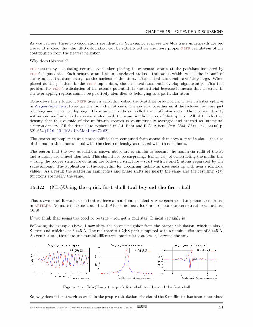
CHAPTER 15. EXTENDED DISCUSSIONS
As you can see, these two calculations are identical. You cannot even see the blue trace underneath the redtrace. It is clear that the QFS calculation can be substituted for the more proper feff calculation of thecontribution from the nearest neighbor.
Why does this work?
feff starts by calculating neutral atoms then placing these neutral atoms at the positions indicated byfeff’s input data. Each neutral atom has an associated radius – the radius within which the “cloud” ofelectrons has the same charge as the nucleus of the atom. The neutral-atom radii are fairly large. Whenplaced at the positions in the feff input data, these neutral-atom radii overlap significantly. This is aproblem for feff’s calculation of the atomic potentials in the material because it means that electrons inthe overlapping regions cannot be positively identified as belonging to a particular atom.
To address this situation, feff uses an algorithm called the Mattheis prescription, which inscribes spheresin Wigner-Seitz cells, to reduce the radii of all atoms in the material together until the reduced radii are justtouching and never overlapping. These smaller radii are called the muffin-tin radii. The electron densitywithin one muffin-tin radius is associated with the atom at the center of that sphere. All of the electrondensity that falls outside of the muffin-tin spheres is volumetrically averaged and treated as interstitialelectron density. All the details are explained in J.J. Rehr and R.A. Albers, Rev. Mod. Phys., 72, (2000) p.621-654 (DOI: 10.1103/RevModPhys.72.621).
The scattering amplitude and phase shift is then computed from atoms that have a specific size – the sizeof the muffin-tin spheres – and with the electron density associated with those spheres.
The reason that the two calculations shown above are so similar is because the muffin-tin radii of the Feand S atoms are almost identical. This should not be surprising. Either way of constructing the muffin tins– using the proper structure or using the rock-salt structure – start with Fe and S atoms separated by thesame amount. The application of the algorithm for producing muffin-tin sizes ends up with nearly identicalvalues. As a result the scattering amplitudes and phase shifts are nearly the same and the resulting χ(k)functions are nearly the same.
15.1.2 (Mis)Using the quick first shell tool beyond the first shell
This is awesome! It would seem that we have a model independent way to generate fitting standards for usein artemis. No more mucking around with Atoms, no more looking up metalloprotein structures. Just useQFS!
If you think that seems too good to be true – you get a gold star. It most certainly is.
Following the example above, I now show the second neighbor from the proper calculation, which is also aS atom and which is at 3.445 A. The red trace is a QFS path computed with a nominal distance of 3.445 A.As you can see, there are substantial differences, particularly at low k, between the two.
Figure 15.2: (Mis)Using the quick first shell tool beyond the first shell
So, why does this not work so well? In the proper calculation, the size of the S muffin-tin has been determined
This work is licensed under the Creative Commons Attribution-ShareAlike License. 121

15.1.3 Executive summary
in large part by the Fe-S nearest neighbor distance. This same muffin-tin radius is used for all the S atomsin the cluster. Thus, in the real calculation, the contribution from the second neighbor S atom is determinedusing the same well-constrained S muffin-tin radius as in the 1st shell calculation.
In contrast, the QFS calculation has been made with an unphysically large Fe-S nearest neighbor distance.Remember, the QFS algorithm works by putting the absorber and scatterer in a rock-salt crystal with alattice constant such that the nearest neighbor distance is equal to the distance supplied by the user. In thiscase, that nearest neighbor distance is 3.445 A!
The algorithm for constructing the muffin tins requires that the muffin-tin spheres touch. Supplied with adistance of 3.445 A, the muffin-tin radii are much too large, the electron density within the muffin tins ismuch too small, and the scattering amplitude and phase shift are calculated wrongly.
The central problem here is not that the red line is different from the blue line – although that is certainlythe case and it is certainly a problem. The central problem is that, by misusing the QFS tool in this way,you introduce a large systematic error into your data analysis. This systematic error affects both amplitudeand phase (as you can clearly see in the figures above). What’s worse, you have no way of quantifying thissystematic error. Your results for coordination number, ∆R, and σ2 will be wrong. And you have no wayof knowing by how much.
Caution: In short, if you misuse the QFS tool in this way, you cannot possiblyreport a defensible analysis of your data.
To add even more ill cheer to this discussion, the problem gets worse and worse as the nominal distance ofthe QFS calculation gets larger. Here I show the same comparison, this time for the fifth coordination shellin , another S scatterer at 4.438 A:
Figure 15.3: (Mis)Using the quick first shell tool beyond the first shell
15.1.3 Executive summary
The quick first shell tool is given that name because it is only valid for first shell analysis.
If you attempt to use the QFS tool at larger distances, you introduce large systematic error into your dataanalysis. Don’t do that!
15.1.4 So, what should you do?
Presumably, you have measured EXAFS on your sample because you because you do not know its structure.
122 This work is licensed under the Creative Commons Attribution-ShareAlike License.

CHAPTER 15. EXTENDED DISCUSSIONS
The point of the EXAFS analysis is to determine the structure. The upshot of this discussion would seemto be that you need to know the structure in order to measure the structure. That’s a catch-22, right?
Not really. As I often say in my lectures during XAS training courses: you never know nothing. It is rarethat you cannot make an educated guess about what your unknown material might resemble. With thatguess, you can run feff, parameterize your fitting model, and determine the extent to which that guess isconsistent with your data.
Crystalline analogsIn this paper, Shelly Kelly demonstrates how to use feff calculations on crystalline materials as thebasis for interpreting the EXAFS of uranyl ions adsorbed onto biomass. In that paper, she showsthe pH dependence of the fractionation of the uranyl ions among phosphoryl, carboxyl, and hydroxylbinding sites. Obviously, there is no way to make feff input data for uranyl ions on organic goo.However, Shelly realized that the basic structure of the uranyl-phosphoryl or uranyl-carboxyl ligandsare very similar in the organic and inorganic cases. Thus she ran feff on the inorganic structure andpulled out those paths that describe the uranyl ion in its similar ligation environment in the organiccase.
The great advantage of using the inorganic structures is that the muffin-tin radii are very likely tobe computed well. The paths that describe the uranyl ligation environment have thus been computedreliably and with good muffin tin radii.
There is yet another advantage to this over attempting to use QFS for higher shells – considerationof multiple scattering paths. In the example from Shelly’s paper, there are several small but non-negligible MS paths to be considered for both carboxyl and phosphoryl ligands. Neglecting those infavor of a single-scattering-only model introduces further systematic uncertainty into the determinationof coordination number, ∆R, and σ2.
SSPathsartemis offers another tool called an SSPath (Sec. 5.3.1 on page 54). An SSPath is a way of usingwell-constructed muffin tins to compute a scattering path that is not represented in the input structureprovided for the feff calculation. For example, suppose you run a feff calculation on , a trigonalperovskite-like material with 6 oxygen scatterers at 1.93 A, 8 La scatterers at 3.28 Aor 3.34 A, and 6Co scatterers at 3.83 A. Suppose you have some reason to consider a Co scatterer at 3 A. You can tellartemis to compute that using the muffin-tin potentials from the calculation, but with a Co scattererat that distance, which is not represented in the structure. Unlike an attempt to use a QFS Co pathat that distance, the SSPath uses a scattering potential with a properly calculated muffin tin.
The advantage of the SSPath is that it it results in a much more accurate calculation than QFS. Thedisadvantage is that it can only be calculated on a scattering element already present in the feffcalculation.
15.1.5 Reproducing the images above
To start, I imported the FeS2 data and crystal structure into artemis. (You can find them here.) I ranatoms, then feff. I then dragged and dropped the nearest neighbor path onto the Data page. At thisstage, artemis looks like this:
I begin a QFS calculation by selecting that option from the menu on the Data page:
The nearest neighbor path in is a S atom at 2.257 A.
This work is licensed under the Creative Commons Attribution-ShareAlike License. 123

15.1.5 Reproducing the images above
Figure 15.4: Getting started with the comparison
Figure 15.5: Go compute the QFS path
124 This work is licensed under the Creative Commons Attribution-ShareAlike License.

CHAPTER 15. EXTENDED DISCUSSIONS
Clicking OK, the QFS path is generated. I set the degeneracy of the QFS path to 6 so that I can directlycompare the normally calculated path (there are 6 nearest neighbor S atoms in ) to the QFS path. I markboth paths and transfer them to the plotting list. I am now ready to compare these two calculations. Toexamine another single scattering path, I drag and drop that path from the feff page to the Data page andredo the QFS calculation at that distance.
Figure 15.7: Ready to plot the comparison
15.2 Using a data group’s characteristic value
At the top of the Data window (Sec. 3 on page 23) is the control for setting the characteristic value, or CV,of a data group. In this section, the purpose and use of the CV is explained.
The CV is a user-defined number which is associated with the data set and is used for special purposes whenevaluating the math expressions associated with def and path parameters. By default, artemis simplyincrements the CV value for each data set imported – the first is set to 1, the second to 2, and so on. Thesevalues can be changed, but should always be integer-valued.
The CV value is used in two ways to construct rich math expressions and expressive fitting models.
This work is licensed under the Creative Commons Attribution-ShareAlike License. 125

15.2.1 The CV token
15.2.1 The CV token
Consider a multiple data set fit to a material measured at various temperatures. For this discussion, let’sconsider a rock salt structured metal oxide, for instance ZnO. Let’s also suppose that we have measureddata at three temperatures, 10 K, 300 K, and 500 K.
In a multiple data set fit, you may choose to model the σ2 of the first shell Zn-O bond using an Einstein model.This allows you to parameterize the σ2 at each temperature as a function of a single variable parameter, theEinstein temperature. To do this, you must define a guess parameter to represent the Einstein temperaturelike so:
guess thetae = 500
The functional form of the Einstein model takes the variable Einstein temperature and the sample’s mea-surement temperature as its arguments.
path
sigma2 = eins(temp, thetae)
where temp represents the sample temparature. The pseudo-syntax used here is simply meant to representthe σ2 parameter on a the Path page (Sec. 5 on page 47).
In a multiple data set fit, you would have to take care that temp is replaced each time it is used. That couldbe done in two ways. You could use various set parameters:
set temp1 = 10
set temp2 = 300
set temp3 = 500
path for data set 1
sigma2 = eins(temp1, thetae)
path for data set 2
sigma2 = eins(temp2, thetae)
path for data set 3
sigma2 = eins(temp3, thetae)
Or you could simply state the temperature explicitly in the path parameter math expressions:
path for data set 1
sigma2 = eins(10, thetae)
path for data set 2
sigma2 = eins(300, thetae)
path for data set 3
sigma2 = eins(500, thetae)
Both of those solutions work. But neither make effective use of the model building automation in artemis.In the chapter on the Path window (Sec. 5.1 on page 48), you learned about various ways of pushing pathparameter values onto other paths. One efficient way of setting up a multiple data set fit would be to editthe path parameters for one of the data sets, then push the path parameters onto the other data sets.
Using the two strategies summarized above, you would need to do considerable editing after pushing thepath parameter values. That sort of editing is often error-prone.
126 This work is licensed under the Creative Commons Attribution-ShareAlike License.

CHAPTER 15. EXTENDED DISCUSSIONS
Here is a third way of solving this problem.
1. Set the CV for the three data sets to the temperature at which the data were measured. In ourexample, the three data sets would get CV values of 10, 300, and 500.
2. Next, edit the σ2 path parameter for one of the data sets to read
path for data set 1
sigma2 = eins([CV], thetae)
3. Finally, push this σ2 value on the other data sets without editing those to which it is pushed.
When artemis evaluates the fitting model, it will replace the [CV] token with the appropriate characteristicvalue. In short, the computer handles the error-prone (for a human) task of editing the many σ2 pathparameters.
While this may seem like a small improvement over handling the editing chores yourself, use of the CV reallypays off for large or complicated fitting models. For a multiple data set fit with many data sets, use of theCV saves quite a bit of editing. Furthermore, you can use the CV value in many path parameter mathexpressions. For example, suppose you were to model the ∆R values with a temperature-dependent, linearexplansion coefficient. The use of the CV in those math expressions saves even more error-prone, manualediting!
15.2.2 Use in lguess parameters
The second use of the CV is along with lguess parameters. These parameters are an eficient way of generatingper-data-set guess parameters in a multiple data set fit while still making good use of the automation inartemis for pushing path parameter math expressions between data sets.
Let’s again consider the ZnO sample measured at the same three temparatures. This time, however, wechoose to float an independent parameter at each temperature.
The straightforward way of doing this would be something like
guess ss1 = 0.002
guess ss2 = 0.004
guess ss3 = 0.006
path for data set 1
sigma2 = ss1
path for data set 2
sigma2 = ss2
path for data set 3
sigma2 = ss3
Here is how this can be done using the CV and an lguess parameter. First, set the CV values to thetemperature values, as before. Next, do the following:
This work is licensed under the Creative Commons Attribution-ShareAlike License. 127

15.3. GEOMETRIC PARAMETRIZATION OF BOND LENGTH
lguess ss = 0.002
path for data set 1
sigma2 = ss
path for data set 2
sigma2 = ss
path for data set 3
sigma2 = ss
artemis will notice that ss is an lguess parameter. For each data set in which it is used, artemis willcreate a guess parameters named ss [CV], where, as before, the [CV] is replaced by the CV value.
In the case of our example, three guess parameters will be created called ss 10, ss 300, and ss 500. Eachof those will be given the initial value of the coresponding lguess parameter (0.002 in this case). The lguessparameter will not be used in the fit, but each of the generated guess parameters will be floated. At the endof the fit, the log file will report on each as for any other guess parameter.
The utility of the lguess parameter is that it allows you to define a common fitting model used across manydata sets. You can use the automation built into artemis to push those path parameter math expressionsbetween paths and data sets. Without further editing, the desired fitting model – with one guess parameterfor each data set – is correctly made.
15.3 Geometric parametrization of bond length
15.3.1 Volumetric expansion coefficient
is a cubic crystal. Here is the crystal data
title name: Iron sulfide (pyrite)
title formula: FeS_2
title refer1: Elliot (1960) J.Chem. Phys. 33(3), 903.
space P a 3
a = 5.404
rmax = 9.00 rpath = 6.00
core = Fe
atoms
Fe 0.00000 0.00000 0.00000 Fe
S 0.38400 0.38400 0.38400 S
In this case, there are only two parameters that determine the locations of all the atoms in the cluster – thelattice constant a and the position of the S atom in the unit cell. For now, we’ll neglect the effect of theposition of the S atom.
In the FeS2 worked example (Sec. 13.1 on page 87), a parameterization was used which related ∆R for allthe paths to a volumetric expansion coefficient, ∆R=α·Reff . Why does this work?
The distance deff between any two atoms in a cubic crystal is some geometrical factor multiplied by thelattice constant. That factor depends on the positions of the atoms in the unit cell, but is a pure number.
Thus, from the FEFF calculation, deff (i, j) = ci,j ·a0 for any two atoms i and j. For any two pairs of atoms,ci,j is a different number, but the distances between all pairs of atoms are related by simple geometry andthe value of the lattice constant.
128 This work is licensed under the Creative Commons Attribution-ShareAlike License.

CHAPTER 15. EXTENDED DISCUSSIONS
We consider an isotropic expansion (or contraction, if α is negative) of the unit, which is reasonable for acubic lattice that does not undergo a phase transition. So a = (1 + α)·a0 .
The distance between any two atoms, after accounting for the isotropic expansion (or contraction) is
di,j = deff (i,j) + ∆d(i,j)di,j = ci,j · adi,j = ci,j · (1+α)·a0
di,j = ci,j ·a0 + ci,j ·α·a0
∴ ∆d(i,j) = ci,j ·α·a0
∆d(i,j) = α·deff (i,j)
The expression α·deff works for all legs of any SS or MS path in a cubic crystal (assuming that there areno internal degrees of freedom, like the parameter for the position of the S atom in ). The length of a path,then, is the sum of the length of each leg. ∆R for a path is the sum of ∆d for each leg. The sum of the deffvalues is Reff , thus ∆R=α·Reff .
While this trick is only valid for a cubic crystal, it does ilustrate two important points about artemis. First,it is an example of an interesting math expression relating a path’s ∆R value to a fitting parameter. The∆R of the path is not itself a variable of the fit, rather it is written in terms of α, which is a variable of thefit.
Second, it is an example of a constrain which uses the information content of the data very well. We caninclude any number of paths with introducing new parameters for their ∆R values. α is a robust fittingparameter in the sense that every path is involved in its determination.
15.3.2 Propagating crystal distortion parameters
The room temperature structure of PbTiO3 is a tetragonal modification of the perovskite structure. The caxis is considerably longer than the a axis. The Pb atoms lie at the corners of the tetragonal cell, the Tiatom lies near the center of the cell, and the O atoms lie near the centers of the faces.
In a setting which places the Pb atoms at positions of high symmetry, i.e. right on the cell corners, the otheratoms are displaced from sites of symmetry c direction. Here is the crystal data:
title PbTiO3 25C
title Glazer and Mabud, Acta Cryst. B34, 1065-1070 (1978)
core = ti Space = P 4 m m
a = 3.905 c = 4.156
rmax=3.6
atoms
! At.type x y z tag
Pb 0.0 0.0 0.0
Ti 0.5 0.5 0.539
O 0.5 0.5 0.1138 axial
O 0.0 0.5 0.6169 planar
There are 5 parameters that detrmine the positions of all the atoms in the crystal, thus there are 5 parametersthat determine the lengths of all scattering paths. They are the two lattice constants, the z displacement ofthe Ti away from z=0, the z displacement of the axial oxygen atom away from z=0.5, and the z displacementof the planar oxygen atom away from z=0.5.
We set up a set of guess, def, and set parameters to encode this:
This work is licensed under the Creative Commons Attribution-ShareAlike License. 129

15.3.2 Propagating crystal distortion parameters
set a0 = 3.905
guess dela = 0
def a = a0 + dela
set c0 = 4.156
guess delc = 0
def c = c0 + delc
guess dti = 0.039
guess doax = 0.1138
guess dopl = 0.1169
after volume = a*a*c
Figure 15.8:
I have also defined an after parameter which computes the volume of the unitcell. While this will not serve a purpose in the fitting model, it is useful infor-mation to report to the log file.
A 2-dimensional cut through this distorted perovskite is shown to the right.The Pb atoms are above and below this plane, the axial oxygen atoms arein line with the titanium atoms. The planar oxygen atoms are in a slightlynon-collinear, buckled alignment with the Ti atoms.
The distortions of the Ti and O atoms split the first coordination shell intothree distance. Along the z direction, there is a short Ti-O distance and longone. In the buckled plane, there are four equivalent Ti-O distances.
Computing these distances requires some simple geometry, with the planardistance being just a bit more complicated.
def rtio_sh = (0.5 - (doax-dti)) * c
def rtio_lo = (0.5 - (doax+dti)) * c
def rtio_pl = sqrt( (a/2)^2 + ((dopl+dti)*c)^2 )
The second shell Pb atoms are similarly computed using trigonometry and theappropriate structural parameters.
def rtipb_sh = sqrt( (a/2)^2 + c^2*(0.5 - dti)^2 )
def rtipb_lo = sqrt( (a/2)^2 + c^2*(0.5 + dti)^2 )
Finally, the Ti-Ti distances in the thrid coordination shell are comparatively trivial. This shell is split bythe tetragonal disortion into two subshells. The distances are the lattice constants, as you can be seen inthe schematic above.
We now have math expressions for the interatomic distances between the Ti absorber and each type ofscatterer up to the third coordination shell. These math expressions for these 7 paths are expressed in termsof the 5 guess parameters above. The nice thing about these expressions is that the interatomic distancesare expressed in terms of easily intepretable parameters of the crystal structure.
Now, encoding the ∆R path parameter for each of these paths is simple. We just subtract Reff from thecorresponding math expression.
130 This work is licensed under the Creative Commons Attribution-ShareAlike License.

CHAPTER 15. EXTENDED DISCUSSIONS
path short axial oxygen:
delr = rtio_sh - reff
path planar oxygen:
delr = rtio_pl - reff
path long axial oxygen:
delr = rtio_lo - reff
path short lead:
delr = rtipb_sh - reff
path long lead:
delr = rtipb_lo - reff
path short titanium:
delr = a - reff
path long titanium:
delr = c - reff
There are important collinear or nearly-collinear multiple scattering paths at the distance of the third shellTi atom. These are shown in the yellow and green shaded areas of the schematic above.
The ∆R parameters for the axial multiple scattering paths are simply the same as for the correspondingsingle scattering path. This is the case because the distortions in PbTiO3 are all in the z direction, so thoseMS paths must have the same length as the corresponding SS paths.
In the planar direction, you need to add up the lengths of the legs and subtract Reff for their ∆R parameters:
path planar double scattering:
delr = (a + 2*rtio_pl)/2 - reff
path planar triple scattering:
delr = 2*rtio_pl - reff
This strategy of adding up leg lengths works for any kind of multiple scattering path you include in this fit.
This is lovely! With 5 guess parameters and some well-considered math expressions, we are able to encode∆R parameters for all the paths in the fit. As more scattering paths are considered for the fit, it is notnecessary to include any more guess parameters for ∆R.
15.3.3 Parametrizations of distance in non-crystalline materials
Interesting geometrical constraints on distance are not the sole province of crystalline materials. In thefollowing two papers, I show the details of an analysis of Hg bound to the pyrimidine ring of a nucleotidein a synthetic DNA structure. To cope with severe information limits in my data, I made some simplifyingassumptions about the structure of the Hg/DNA complex. I then employed a bit of trigonometry to expressall the absorber-scatterer distances as functions of a small number of guess parameters.
• B. Ravel et al., Rad. Phys. Chem., 78:10, (2009) p. S75-S79 (DOI: 10.1016/j.radphyschem.2009.05.024)
• B. Ravel, J. Phys. Conf. Series, 190, (2009) p. 012026 (DOI: 10.1088/1742-6596/190/1/012026)
To Do: Need more examples
This work is licensed under the Creative Commons Attribution-ShareAlike License. 131

15.4. MODELING DISORDER
15.4 Modeling disorder
The σ2 term in the EXAFS equation accounts for the mean square variation in path length. This variationcan be due to thermal or structural disorder. Even in a well-ordered material, like Cu or another FCC metal,data are measured at finite temperature. The absorber and scatterer are both in motion due to the finitetemperature. Each interaction of the incident X-ray and the absorber is like a femtosecond snapshot of thecoordination environment. As those snapshots are averaged in the EXAFS measurement, σ2 is non-zero,even in the well-ordered material.
A structural disordered contributes another term to σ2. Due to structural disorder, the scatterers whichare nominally contained in a scattering shell may be centered around somehwat different distances. Whenthe contributions from those scatterers are considered, σ2 will be larger than what is expected from purelythermal effects.
Consequently, σ2 is always non-zero in an EXAFS fit and a proper interpretation of the fitted value of σ2
will take into account both the thermal and structural component.
It is usually a challenge to distinguish the thermal and structural contributions to σ2. As with any highlycorrelated effects, the only way to disentangle the two contributions is to do something in the experimentwhich is sensitive to one or both.
One common approach for understanding the thermal part of σ2 is to measure the sample at two or moretemperatures. Assuming the material does not change phase in that temperature range, we expect thethermal part of σ2 to have a temperature dependence while the structural part may reman fixed (or at leastchange much less). Another possible way to disentangle the two contributions is to measure EXAFS data asa function of pressure. In that case the thermal contribution can be modeled as a function of pressure anda Gruneisen parameter.
15.4.1 Debye and Einstein models
ifeffit provides two bult-in functions for modeling σ2 as a function of temperature.
Einstein modelThe Einstein model assumes that the absorber and scatter are balls connected by a quantum spring.They oscillate with a single frequency and the low-temperature motion saturates to a zero-point motion.The function for computing σ2 from the Einstein is a function of the measurement temperature, anEinstein temperature, and the reduced mass of the absorber/scatterer pair. In artemis one writes:
path:
sigma2 = eins(temperature, thetae)
Typically, temeprature is a set parameter whise value is the mesurement tempreature of the data andthetae is a guess parameter representing the Einstein temprature – i.e. the characteristic frequencyof vibration expressed in temeprature units – of the absorber-scatterer pair. The reduced mass iscomputed by ifeffit from the information provided by feff about the scattering path.
The Einstein function is most useful as part of a multiple data set fit. In that case, a path can have itsσ2 parametrized using the eins function and a single ΘE guess parameter is used for all temperatures.
Correlated Debye model
132 This work is licensed under the Creative Commons Attribution-ShareAlike License.

CHAPTER 15. EXTENDED DISCUSSIONS
The correlated Debye model assumes that the σ2 for any pair of atoms can be computed from theacoustic phonon spectrum. That is, a single charcteristic energy – the same Debye temperature, , thatis determined from the heat capacity of the material – can be used to compute σ2 for any path in thematerial. In artemis one writes:
path:
sigma2 = debye(temperature, thetae)
This is a very powerful concept. All σ2 parameters in the fit are determined from a single variableΘD. The caveat is that the correlated Debye model is only strictly valid for a monoatomic material. Inpractice, the Debye model works well for metals like Cu, Au, and Pt. It works poorly for any materialthat has two or more atomic species.
Both models are described in S. Sevillano, H. Meuth, and J.J. Rehr, Phys. Rev., B20:12, (1979) p. 4908-4911(DOI: 10.1103/PhysRevB.20.4908).
15.4.2 Collinear multiple scattering paths
Figure 15.9:
This valuable paper by E.A. Hudson et al., Phys. Rev., B54:1, (1996) p. 156-165(DOI: 10.1103/PhysRevB.54.156) explains the relationships between σ2 parame-ters for single scattering paths and certain multiple scattering paths.
The diagram to the right demonstrates the various kinds of collinear MS pathsand how they relate to the corresponding SS path.
To begin, we define guess parameters for the σ2 of the SS paths to atoms 1 and2.
guess ss1 = 0.003
guess ss2 = 0.003
The next two paths are double and triple scattering paths that scatter in the for-ward direction from atom 1, then in the backward direction atom 2. As explainedby Hudson, et al., these paths have the same σ2 as the SS path to atom 2, i.e.σ2=ss2 for both these paths.
The next three paths involve scattering from the absorber. The collinear DS andTS paths simply have σ2=2*ss1. The path in which the photoelectron rattles back and forth between theabsorber and atom 1 has σ2=4*ss1.
The caveat to these relationships is that the motion of the intervening atom in the perpendicular direction ispresumed to be a negligible contribution to the mean square variation in path length. This is, of course, notstrictly true. In very high quality data, you may see deviations from the expressions presented by Hudson,et al., but in most cases they are an excellent approximation and a powerful constraint that you can applyto the paths in your fit.
15.4.3 Sensible approximations for triangular multiple scattering paths
In the FeS2 example (Sec. 13.1 on page 87), we saw that a couple of non-collinear multiple scattering pathscontributed significantly to the EXAFS. For these triangular paths, unlike for collinear paths, there is noobvious relationship between their σ2 parameters and the σ2 for the SS paths.
One of the triangular paths in the fit was of the form Abs→Fe→S→Abs. The S→Abs leg is like half thefirst neighbor path. The Fe→S is also like half the first neighbor path. The mean square vairation in pathlength along those two legs of the path is the σ2 for the first path. FinallyThe Abs→Fe leg is like half the
This work is licensed under the Creative Commons Attribution-ShareAlike License. 133

15.5. CONSTRAINTS AND RESTRAINTS
fourth shell path.
The math epression for the σ2 of this triangle path was set as
path Fe-S triangle:
sigma2 = ss1 + ss_fe/2
This approximation of σ2 has the great virtue of not introducing a new parameter to the fit. It neglectsany attenutation to the path due to thermal variation in sattering angle. While that is an important effect,there is no simple and accurate way to model it.
This example demonstrates the decision that must be made every time a non-collinear multiple scatteringpath is considered for a fitting model. In short, you have three choices:
1. Do nothing, leave the MS path out of the fit.
2. Include the MS path, but allow it to have it’s own σ2 parameter.
3. Include the MS path, but approximate it’s σ2 in terms of parameters which are already part ofthefitting model, presumably the parameters of the SS σ2 values.
The Abs→Fe→S→Abs path in was really quite large. Going for choice number 1 and leaving it out of thefit is clearly a poor choice.
Number 2 is, in principle, the best choice. As an independently floated parameter, it’s σ2 will account forthe mean square vriation in path length and the effect of variation in t he scattering angle. Unfortunately,this parameter is likely not to be highly robust because it is only used for this one path. There just is notmuch information available to determine its proper value. And if the fit includes several triangle paths, eachof which has a σ2 parameter of similarly weak robustness, the problem becomes amplified.
In almost all cases, option number 3 is the best choice. The approximation is not horribly wrong, thusit introduces only a little bit of systematic error into the fitting model. Including the Fourier componentsfrom the path is better than neglecting the path. Since a reasonable approximation can be made withoutintroducing new variable parameters to the fit, the triangle path should be included.
The Abs→Fe→S→Abs path had the virtue that all of its legs were represented by SS paths already includedin the fit. Another triangle path was included: Abs→S→S→Abs. In this case, the first and last legs arerelated to the first coordination shell. The middle leg, S→S, has no corresponding SS path. In the FeS2example (Sec. 13.1 on page 87), this triangle path was given a σ2 math expression of 1.5 times the first shellσ2.
This is obviously not accurate. Like all such triangle paths, the decision outlined above must be workedthrough. In this case, the fit benefits by including this triangle path, but it does not merit having its ownfloating parameter. I assert that value of σ2 that is “a bit more than the first shell” is reasonable.
This is discussed in more detail in Scott Calvin’s book, XAFS for Everyone.
15.5 Constraints and restraints
To Do: Write me!
134 This work is licensed under the Creative Commons Attribution-ShareAlike License.
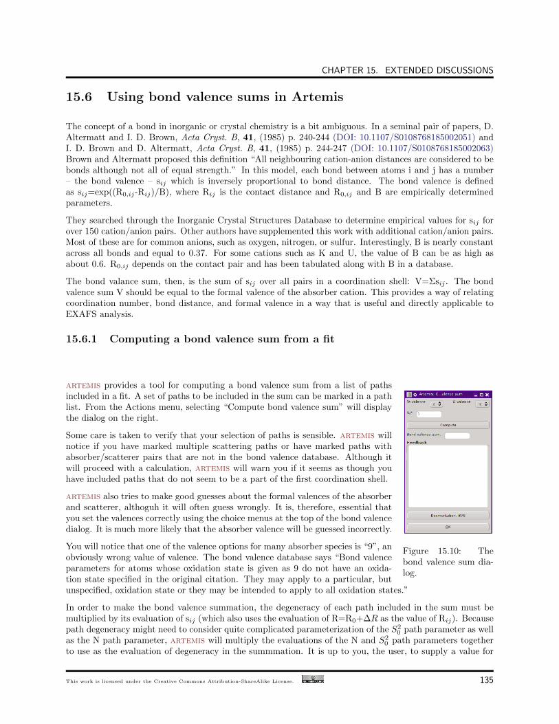
CHAPTER 15. EXTENDED DISCUSSIONS
15.6 Using bond valence sums in Artemis
The concept of a bond in inorganic or crystal chemistry is a bit ambiguous. In a seminal pair of papers, D.Altermatt and I. D. Brown, Acta Cryst. B, 41, (1985) p. 240-244 (DOI: 10.1107/S0108768185002051) andI. D. Brown and D. Altermatt, Acta Cryst. B, 41, (1985) p. 244-247 (DOI: 10.1107/S0108768185002063)Brown and Altermatt proposed this definition “All neighbouring cation-anion distances are considered to bebonds although not all of equal strength.” In this model, each bond between atoms i and j has a number– the bond valence – sij which is inversely proportional to bond distance. The bond valence is definedas sij=exp((R0,ij-Rij)/B), where Rij is the contact distance and R0,ij and B are empirically determinedparameters.
They searched through the Inorganic Crystal Structures Database to determine empirical values for sij forover 150 cation/anion pairs. Other authors have supplemented this work with additional cation/anion pairs.Most of these are for common anions, such as oxygen, nitrogen, or sulfur. Interestingly, B is nearly constantacross all bonds and equal to 0.37. For some cations such as K and U, the value of B can be as high asabout 0.6. R0,ij depends on the contact pair and has been tabulated along with B in a database.
The bond valance sum, then, is the sum of sij over all pairs in a coordination shell: V=Σsij . The bondvalence sum V should be equal to the formal valence of the absorber cation. This provides a way of relatingcoordination number, bond distance, and formal valence in a way that is useful and directly applicable toEXAFS analysis.
15.6.1 Computing a bond valence sum from a fit
artemis provides a tool for computing a bond valence sum from a list of paths
Figure 15.10: Thebond valence sum dia-log.
included in a fit. A set of paths to be included in the sum can be marked in a pathlist. From the Actions menu, selecting “Compute bond valence sum” will displaythe dialog on the right.
Some care is taken to verify that your selection of paths is sensible. artemis willnotice if you have marked multiple scattering paths or have marked paths withabsorber/scatterer pairs that are not in the bond valence database. Although itwill proceed with a calculation, artemis will warn you if it seems as though youhave included paths that do not seem to be a part of the first coordination shell.
artemis also tries to make good guesses about the formal valences of the absorberand scatterer, althoguh it will often guess wrongly. It is, therefore, essential thatyou set the valences correctly using the choice menus at the top of the bond valencedialog. It is much more likely that the absorber valence will be guessed incorrectly.
You will notice that one of the valence options for many absorber species is “9”, anobviously wrong value of valence. The bond valence database says “Bond valenceparameters for atoms whose oxidation state is given as 9 do not have an oxida-tion state specified in the original citation. They may apply to a particular, butunspecified, oxidation state or they may be intended to apply to all oxidation states.”
In order to make the bond valence summation, the degeneracy of each path included in the sum must bemultiplied by its evaluation of sij (which also uses the evaluation of R=R0+∆R as the value of Rij). Becausepath degeneracy might need to consider quite complicated parameterization of the S2
0 path parameter as wellas the N path parameter, artemis will multiply the evaluations of the N and S2
0 path parameters togetherto use as the evaluation of degeneracy in the summmation. It is up to you, the user, to supply a value for
This work is licensed under the Creative Commons Attribution-ShareAlike License. 135

15.6.2 Using a bond valance sum as a restraint
the actual amplitude reduction factor, S20 to be divided out of the summation.
Pressing the “Compute” button will make the bond valence sum, reporting its value in the box so labeled.Any feedback will be written in the larger text control. For a successful calculation, the values of Rij and Bobtained from the database will be displayed. Any warnings about the path selection will be printed in thefeedback box in bold red text.
15.6.2 Using a bond valance sum as a restraint
The bond valence sum can be used a restraint on a fit. That is, the relationship between formal valence, coor-dination number, and bond distance can be used as prior knowledge guiding the fit. If the absorber/scattererpair are in the bond valence database, values for R0,ij , B, and the formal valence of the obsorber can bedefined as set parameters. The bond valence sum is expressed as a def parameter. Finally, the differencebetween the bond valence sum and the formal valence are expressed as a restrain parameter. These areshown below for the Fe-O bond in FeO. In FeO the iron atom is of valence 2+ and the oxygen is 2-.
When the fit is evaluated, the restrain parameter will be added in quadrature to the evaluation of χ2. Thissum will be minimized in the fit. In a fit to FeO, the coordination number is fixed to 6, the value known fromcyrstallography. By using this restraint, the value of ∆R will be encouraged to assume a value that resultsin a bond valence sum of 2. By increasing the value of the scale parameter, the strength of the restraint isincreased. For a very large value of scale, ∆R will constrained to a value that forces the bond valence sum to2. For a very small value of scale, the restraint will be weak and ∆R will be given more freedom to deviatefrom a value that casues a bond valence sum of 2.
This example shows the simplest case of a single scattering path contributing to the bond valence sum. Themath expressions to establish the restraint would be more complicated for a more disrodered first shell, butthose math expressions would follow the same pattern as this example.
15.7 Fitting with empirical standards
Let me just say up front that artemis is intended as a front-end to feff for the problem of EXAFS analysis.In almost all cases, feff is the right tool for that job and there are extremely few cases where the use ofempirical standards is preferable to using feff. As discussed elsewhere in this manual, there are a situationswhere the application of feff to a particular problem may not be obvious. Any situation for which thechoice of a starting configuration of atomic coordinates, as needed for feff’s input data, is not obvious mightfall into that category. In one of those situations, you might be tempted to puruse empirical standards. Youwould, however, usually be better served by adopting one of the strategies that have been developed for
136 This work is licensed under the Creative Commons Attribution-ShareAlike License.

CHAPTER 15. EXTENDED DISCUSSIONS
applying feff calculations to unknown structures.
That said, there are a small handful of situations where the use of empirical standards is justified. In fact,I can think of two. The situation where an absorber and a scatterer are bound by a hydrogen atom – i.e.there is a hydrogen atom in the space between the absorber and scatterer from which the photoelectronmight scatter – is poorly handled by feff. In that case, finding a suitable empirical standard will likely bean improvement over the systematic error introduced by feff’s poor handlng of the hydrogen. The secondexample would be a heterogeneous sample – like a soil – which contains a component which varies littlefrom sample to sample. In that case, using an emirical standard to represent the unchanging component andusing feff to model the behavior of the component(s) which do change across the ensemble of measurementsmight be a fruitful strategy.
To this end, demeter offers a mechanism for generating an empirical standard from measured data. This issaved in a form that can be used by artemis as if it were a normal path imported into the fit in the normalway.
My example will use the copper foil data at 10 K and 150 K, which can be found at at my Github site. Inorder to demonstrate the gneration and use of an empirical standard, I will use the uncomplicated exampleof using the low temperature data as the standard for the analysis of the higher temperature data. Ofcourse, a real-world scenario will be much more complicated that this example, but it should demonstratethe mechanics of making and using the empirical standard.
15.7.1 Preparing the empirical standard
It starts by processing the data properly. First, import the two data sets into athena. Take care that thedata are aligned and have the same values for E0. Choose a k-range over which both data sets are of goodquality. I have chosen a range of 3A−1 to 12 A−1. Then choose an R-range to enclose and isolate the firstpeak, which corresponds to the first coordination shell. Here, I chose 1.8 Ato 2.8 A.
Figure 15.11: The Cu foil data at two temperatures have been imported into athena, aligned, and processed.
This work is licensed under the Creative Commons Attribution-ShareAlike License. 137
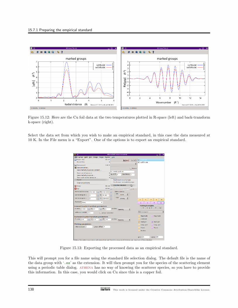
15.7.1 Preparing the empirical standard
Figure 15.12: Here are the Cu foil data at the two temperatures plotted in R-space (left) and back-transformk-space (right).
Select the data set from which you wish to make an empirical standard, in this case the data measured at10 K. In the File menu is a “Export”. One of the options is to export an empirical standard.
Figure 15.13: Exporting the processed data as an empirical standard.
This will prompt you for a file name using the standard file selection dialog. The default file is the name ofthe data group with ‘.es’ as the extension. It will then prompt you for the species of the scattering elementusing a periodic table dialog. athena has no way of knowing the scatterer species, so you have to providethis information. In this case, you would click on Cu since this is a copper foil.
138 This work is licensed under the Creative Commons Attribution-ShareAlike License.

CHAPTER 15. EXTENDED DISCUSSIONS
Figure 15.14: Select the species of the scatterer from the periodic table interface.
15.7.2 Using the empirical standard
Now fire up artemis and import the 150 K data from the athena project file you saved before closingathena. (You did save your work, didn’t you?!) The k- and R-ranges will be imported as they were set inathena. To begin the analysis using the empirical standard, click on the hot text indicated in the figurebelow. You can also import this sort of standard from the “Data-¿Other fitting standards...” menu.
Figure 15.15: The 150 K data have been imported into artemis and we are ready to import the preparedempirical standard.
Once the empirical standard is imported, it will be displayed just like a normal path. You can tell it is anempirical standard because its label contains the token “[Emp.]”.
Here I have set up a 4-parameter fit typical for a first shell analysis, except that I have set the E0 parameterto 0. The amplitude, σ2, and ∆R are guess parameters.
We are now ready to hit the Fit button. Shown below are the results of the fit with the fitting space chosenfirst as R, then as q.
The results fitting in R or q are pretty similar, which is reassuring.
This work is licensed under the Creative Commons Attribution-ShareAlike License. 139

15.7.2 Using the empirical standard
Figure 15.16: The 150 K data and the empirical standard have been imported into artemis.
Figure 15.17: The results of the fit with the fitting space selected as R and the plot displayed in R.
Figure 15.18: The results of the fit with the fitting space selected as q and the plot displayed in q.
140 This work is licensed under the Creative Commons Attribution-ShareAlike License.

CHAPTER 15. EXTENDED DISCUSSIONS
The value for the amplitude is consistent with and close to 1, which is should be since the copper metal is12-fold coordinate at both temperatures.
The value for the change in σ2 is 0.0017±3, which seems reasonable for this change in temperature.
The value for ∆R fitted in q space is 0.001±1. Fitted in R space, the uncertainty is 0.002. That’s kind ofinteresting. In either case, the uncertainty in R is smaller than for a Feff-based fit for a number of reasons.Probably the most significant is that both standard and data are of excellent quality. Were the data the sortof marginal data that comes from most research problems on difficult materials, the effects of statistical andsystematic noise would be much more dramatic. Also relevant to the small uncertainty is that this fittingproblem has been contrived (by virtue of careful alignment and choice of E0 back in Athena) to remove thefitted change in E0 from the problem. By removing the parameter most correlated with ∆R, we significantlyreduces the uncertainty in ∆R.
I would not interpret all of this to mean that use of empirical standards is superior to the use of Feff. Inthe specific case where the first coordination shell is of known contents and can be well isolated from highershells and where you are confident that your unknown is identical to your standard except for small changesin N, R, or σ2, then empirical standards are a useful tool for your EXAFS toolbox.
15.8 Unique potential styles
Consider this ‘atoms.inp’ file for sodium uranyl triacetate:
title = Templeton et al.
title = Redetermination and Absolute configuration of Sodium Uranyl(VI) triacetate.
title = Acta Cryst 1985 C41 1439-1441
space = P 21 3
a = 10.6890 b = 10.6890 c = 10.6890
alpha = 90.0 beta = 90.0 gamma = 90.0
core = U edge = L3 rmax = 7.0
shift 0.00000 0.00000 0.00000
atoms
! elem x y z tag occ.
U 0.42940 0.42940 0.42940 U 1.00000
Na 0.82860 0.82860 0.82860 Na 1.00000
O 0.33430 0.33430 0.33430 Oax 1.00000
O 0.52420 0.52420 0.52420 Oax 1.00000
O 0.38340 0.29450 0.61100 Oeq 1.00000
O 0.54640 0.24430 0.50070 Oeq 1.00000
C 0.47860 0.22600 0.59500 C 1.00000
C 0.50880 0.12400 0.68620 C 1.00000
This crystal has 4 elemental species distributed over 8 crystallographic positions. Two of the oxygen sitesare the two oxygenyl sites with U-O double bond distance of about 1.76 A. The remaining oxygen sites aresingle bonded at a distance of about 2.46 A.
In the Atoms and Feff chapter (Sec. 4 on page 33), the concept of unique potential styles was introduced.Here we show examples of how these work using sodium uranyl triacetate.
15.8.1 Each element gets a unique potential
Choosing the “elements” style assigns a unique potenitial to each atomic species in the crystal. Using thisstyle results in the following ‘feff.inp’ file:
This work is licensed under the Creative Commons Attribution-ShareAlike License. 141

15.8.2 Each tag gets a unique potential
TITLE Templeton et al.
TITLE Redetermination and Absolute configuration of Sodium Uranyl(VI) triacetate.
TITLE Acta Cryst 1985 C41 1439-1441
HOLE 4 1.0 * FYI: (U L3 edge @ 17166 eV, second number is S0^2)
* mphase,mpath,mfeff,mchi
CONTROL 1 1 1 1
PRINT 1 0 0 0
RMAX 5.0
*NLEG 4
POTENTIALS
* ipot Z tag
0 92 U
1 92 U
2 11 Na
3 8 O
4 6 C
ATOMS * this list contains 81 atoms
* x y z ipot tag distance
0.00000 0.00000 0.00000 0 U 0.00000
1.01332 1.01332 1.01332 3 Oax.1 1.75512
-1.01652 -1.01652 -1.01652 3 Oax.2 1.76067
1.25061 -1.97853 0.76213 3 Oeq.1 2.46160
-1.97853 0.76213 1.25061 3 Oeq.1 2.46160
... (more atoms follow)
This is reasonable input for feff. Indeed, for many crystals, the elements style is exactly what you want.With four elements in the cyrstal, five unique potentials are made. The absorber is always potential index0. The remaining uranium atoms are given potential index 1.
For this material, it is probably a poor idea to give the axial (double bonded, distance 1.76 A) and equatorial(single bonded, distance 2.46 A) the same potential index. Doing so forces their muffin tin radii to be thesame. Given this substantial difference in distance, it is probably a good idea to let the two types of oxygenatoms have different muffin tin radii so that their scattering amplitudes and phase shifts can be computeddifferently. That introduces a more chemically reasonable potential model.
15.8.2 Each tag gets a unique potential
The two oxygen types can get differnt unique potentials by choosing the “tags” style. Note that in the‘atoms.inp’ pairs of oxygen sites were given the tags “Oax” and “Oeq”. Also note that the two carbon siteswere given the same tag. With all this, we get the following ‘feff.inp’ file:
142 This work is licensed under the Creative Commons Attribution-ShareAlike License.

CHAPTER 15. EXTENDED DISCUSSIONS
TITLE Templeton et al.
TITLE Redetermination and Absolute configuration of Sodium Uranyl(VI) triacetate.
TITLE Acta Cryst 1985 C41 1439-1441
HOLE 4 1.0 * FYI: (U L3 edge @ 17166 eV, second number is S0^2)
* mphase,mpath,mfeff,mchi
CONTROL 1 1 1 1
PRINT 1 0 0 0
RMAX 5.0
*NLEG 4
POTENTIALS
* ipot Z tag
0 92 U
1 92 U
2 11 Na
3 8 O
4 8 O
5 6 C
ATOMS * this list contains 81 atoms
* x y z ipot tag distance
0.00000 0.00000 0.00000 0 U 0.00000
1.01332 1.01332 1.01332 3 Oax.1 1.75512
-1.01652 -1.01652 -1.01652 3 Oax.2 1.76067
1.25061 -1.97853 0.76213 4 Oeq.1 2.46160
-1.97853 0.76213 1.25061 4 Oeq.1 2.46160
... (more atoms follow)
Note that potential indeces 3 and 4 are both for oxygen atoms. 3 is for the short, axial oxygens and 4 is forthe longer, equatorial oxygens.
15.8.3 Each site gets a unique potential
Figure 15.19:
The final option for potential assignement is the “sites” style. In thisstyle, each crystallographic position gets its own potential index.
This is a somewhat dangerous option because feff only allows up to7 potentials beyond the absorber (for a total of 8). In this crystal,we have 8 sites which results in 8 unique potentials. The softwaredutifully writes out the ‘feff.inp’ file, but it also issues the warningshown on the right.
This work is licensed under the Creative Commons Attribution-ShareAlike License. 143

15.9. THE PATHFINDER AND FUZZY DEGENERACY
TITLE Templeton et al.
TITLE Redetermination and Absolute configuration of Sodium Uranyl(VI) triacetate.
TITLE Acta Cryst 1985 C41 1439-1441
HOLE 4 1.0 * FYI: (U L3 edge @ 17166 eV, second number is S0^2)
* mphase,mpath,mfeff,mchi
CONTROL 1 1 1 1
PRINT 1 0 0 0
RMAX 5.0
*NLEG 4
POTENTIALS
* ipot Z tag
0 92 U
1 92 U
2 11 Na
3 8 O
4 8 O
5 8 O
6 8 O
7 6 C
8 6 C
ATOMS * this list contains 81 atoms
* x y z ipot tag distance
0.00000 0.00000 0.00000 0 U 0.00000
1.01332 1.01332 1.01332 4 Oax.1 1.75512
-1.01652 -1.01652 -1.01652 3 Oax.2 1.76067
1.25061 -1.97853 0.76213 6 Oeq.1 2.46160
-1.97853 0.76213 1.25061 6 Oeq.1 2.46160
... (more atoms follow)
Figure 15.20:
If you attempt to run feff with this input data, artemis willcomplain with the rather repetitious error message shown tothe right and not run feff. You have to fix the feff inputdata either by hand-editing or by re-running atoms with adifferent potentials style.
15.9 The pathfinder and fuzzy de-generacy
15.9.1 How the path finder works
Given a list of atomic coordinates for a cluster of atoms:
A heap is a tree-shaped data structure. Each node is guaran-teed to represent a shorter path length than all nodes below it. The top node is, thus, guaranteed to bethe shortest path. See S.I. Zabinsky, et al., Phys. Rev., B66:22, (1995) p. 2995-3009 (DOI: 10.1103/Phys-RevB.52.2995) for more details.
1. Find all paths (0i0), i6=0 in the cluster. These paths are represented by the two-leg diagram to the
144 This work is licensed under the Creative Commons Attribution-ShareAlike License.

CHAPTER 15. EXTENDED DISCUSSIONS
right. Put each such path in a heap.
2. For each such path, add a leg with j6=i, j6=0. Put all (0ij0) in the heap. These paths are representedby the three-leg diagram to the right.
3. Up to some order of scattering, populate the heap with (0i...x0).
4. Test each path (0i...x0) for magnitude. If small, discard and do not consider any (0i...xy0).
5. Use up all atoms in the cluster and up to some order of scattering (feff’s default is 7 legs).
Figure 15.21:
Figure 15.22:
Construct the path list by repeatedly pulling the top path from the heap untilthe heap is empty. When the top node is removed, the remaining nodes rear-range themselves such that heap retains the property that each node representsa shorter path than all those below it.
The resulting path list is guaranteed to be sorted by increasing path length.The list is then examined to find “degenerate” paths. Degenerate paths areones that contribute identically to the EXAFS. A simple example owuld bethe single scattering paths from the various atoms in the first coordinationshell. Since each atom is the same distance away from the absorber, eachcontributes identically to the EXAFS. Thus these paths are degenerate. Afterbeing screened for degeneracy, the path list is presented to the user.
15.9.2 The pathfinder in Feff and Artemis
One of the features of artemis is a rewrite of feff’s pathfinder.
The new path finder has two huge advantages over feff’s:
1. User configurable fuzzy degeneracy. feff considers paths that differ in length by 0.00001 Ato benon-degenerate. artemis can group together these nearly degenerate paths.
2. The scattering geometries of the degenerate paths are stored and are available for use and examination.feff discards the details of the degenerate paths.
The first point – the use of fuzzy degneracy – is the topic of this section.
feff’s path finder, however, has its advantages over artemis’:
1. As it is written in a compiled language, it is considerably faster. Fortunately, the path finder does notneed to be run very often.
This work is licensed under the Creative Commons Attribution-ShareAlike License. 145

15.9.3 An example of using fuzzy degeneracy
2. feff uses its fast plane wave calculation to approximate the importance of path. Low importancepaths can be removed from consideration, as can all higher order paths built from that path. artemisdoes not have access to the plane wave calculation, so it must consider rather more paths than feff’spathfinder. artemis relies instead on some simple heuristics to trim the tree of paths.
3. feff’s path finder considers up to seven-legged paths. artemis currently stops at four-legged paths.This could be fixed in artemis, but without feff’s plane wave approximation, the cost of computingso many paths would be prohibitive. In any case, it is rather unusual to need more than four-leggedpaths in an EXAFS analysis. (Cubic metals analyzed beyond about 6 Aand cyanide bridged structureslike prussian blue are two examples.)
To Do: artemis’ path finder does not currently handle polarization andellipticity. So that’s another advantage at the moment for feff’s path finder.
As for the speed issue, I have some ideas for improving artemis’ performance.While it will never be as fast as feff, I should be able to close the gap somewhat.
15.9.3 An example of using fuzzy degeneracy
As the path finder organizes all the scattering geometries it finds among the atoms in the input atoms list, itwill make a fuzzy comparison to sort the paths into nearly-degenerate bins. That is, all paths whose lengthsare within a small margin will be considered degenerate. The width of this bin is set by the § Pathfinder→ fuzz preference.
Consider this ‘feff.inp’ file (made from this crystal data):
146 This work is licensed under the Creative Commons Attribution-ShareAlike License.

CHAPTER 15. EXTENDED DISCUSSIONS
TITLE magnetoplumbite PbFe_12O_19
HOLE 4 1.0 * FYI: (Pb L3 edge @ 13035 eV, second number is S0^2)
* mphase,mpath,mfeff,mchi
CONTROL 1 1 1 1
PRINT 1 0 0 0
RMAX 5.0
*NLEG 4
POTENTIALS
* ipot Z tag
0 82 Pb
1 82 Pb
2 26 Fe
3 8 O
ATOMS * this list contains 84 atoms
* x y z ipot tag distance
0.00000 0.00000 0.00000 0 Pb1 0.00000
1.65468 0.00003 2.30070 3 O.1 2.83394
-0.82737 -1.43298 2.30070 3 O.1 2.83394
1.65468 0.00003 -2.30070 3 O.1 2.83394
-0.82737 -1.43298 -2.30070 3 O.1 2.83394
-0.82737 1.43304 2.30070 3 O.1 2.83397
-0.82737 1.43304 -2.30070 3 O.1 2.83397
2.63123 -1.31552 0.00000 3 O.2 2.94176
-0.17634 -2.93647 0.00000 3 O.2 2.94176
2.63123 1.31558 0.00000 3 O.2 2.94179
-2.45494 -1.62092 0.00000 3 O.2 2.94179
-2.45494 1.62098 0.00000 3 O.2 2.94182
-0.17634 2.93653 0.00000 3 O.2 2.94182
1.69537 -2.93647 0.00000 2 Fe2.1 3.39074
-3.39080 0.00003 0.00000 2 Fe2.1 3.39079
1.69537 2.93653 0.00000 2 Fe2.1 3.39079
0.83581 -1.44767 3.24399 2 Fe5.1 3.64935
0.83581 -1.44767 -3.24399 2 Fe5.1 3.64935
-1.67167 0.00003 3.24399 2 Fe5.1 3.64937
0.83581 1.44772 3.24399 2 Fe5.1 3.64937
-1.67167 0.00003 -3.24399 2 Fe5.1 3.64937
0.83581 1.44772 -3.24399 2 Fe5.1 3.64937
3.39074 0.00006 1.38042 2 Fe4.1 3.66097
-1.69542 -2.93644 1.38042 2 Fe4.1 3.66097
3.39074 0.00006 -1.38042 2 Fe4.1 3.66097
-1.69542 -2.93644 -1.38042 2 Fe4.1 3.66097
-1.69542 2.93656 1.38042 2 Fe4.1 3.66107
-1.69542 2.93656 -1.38042 2 Fe4.1 3.66107
... (more atoms follow)
END
Using the default § Pathfinder → fuzz parameter of 0.03 A, will give these paths. Note that the Fe4 andFe5 scatterers, which differ by about 0.11 A, get merged into a single scattering path. This path has a valueof Reff that is the average of the constituent paths and a degenaracy that is the sum of the constituentpaths.
This work is licensed under the Creative Commons Attribution-ShareAlike License. 147

15.9.3 An example of using fuzzy degeneracy
# degen Reff scattering path I Rank legs type
0001 6 2.834 ---- @ O.1 @ 2 100.00 2 single scattering
0002 6 2.942 ---- @ O.2 @ 2 89.88 2 single scattering
0003 3 3.391 ---- @ Fe2.1 @ 2 34.83 2 single scattering
0004 12 3.655 ---- @ Fe5.1 @ 2 100.00 2 single scattering
Resetting the § Pathfinder → fuzz to 0.01 separates those two nearly degenerate paths into separate scat-tering paths.
# degen Reff scattering path I Rank legs type
0001 6 2.834 ---- @ O.1 @ 2 100.00 2 single scattering
0002 6 2.942 ---- @ O.2 @ 2 89.88 2 single scattering
0003 3 3.391 ---- @ Fe2.1 @ 2 34.83 2 single scattering
0004 6 3.649 ---- @ Fe5.1 @ 2 57.63 2 single scattering
0005 6 3.661 ---- @ Fe4.1 @ 2 57.15 2 single scattering
To make the pathfinder neglect fuzzy degeneracy, thus behaving like feff’s pathfinder, set § Pathfinder →fuzz to 0.
148 This work is licensed under the Creative Commons Attribution-ShareAlike License.