DSP Blockset User's Guide
738
Modeling Simulation Implementation User’s Guide Version 4 For Use with Simulink ® DSP Blockset
-
Upload
khangminh22 -
Category
Documents
-
view
0 -
download
0
Transcript of DSP Blockset User's Guide

Modeling
Simulation
Implementation
User’s GuideVersion 4
For Use with Simulink®
DSPBlockset
How to Contact The MathWorks:
www.mathworks.com Webcomp.soft-sys.matlab Newsgroup
[email protected] Technical [email protected] Product enhancement [email protected] Bug [email protected] Documentation error [email protected] Order status, license renewals, [email protected] Sales, pricing, and general information
508-647-7000 Phone
508-647-7001 Fax
The MathWorks, Inc. Mail3 Apple Hill DriveNatick, MA 01760-2098
For contact information about worldwide offices, see the MathWorks Web site.
DSP Blockset User’s Guide COPYRIGHT 1995 - 2001 by The MathWorks, Inc. The software described in this document is furnished under a license agreement. The software may be used or copied only under the terms of the license agreement. No part of this manual may be photocopied or repro-duced in any form without prior written consent from The MathWorks, Inc.
FEDERAL ACQUISITION: This provision applies to all acquisitions of the Program and Documentation by or for the federal government of the United States. By accepting delivery of the Program, the government hereby agrees that this software qualifies as "commercial" computer software within the meaning of FAR Part 12.212, DFARS Part 227.7202-1, DFARS Part 227.7202-3, DFARS Part 252.227-7013, and DFARS Part 252.227-7014. The terms and conditions of The MathWorks, Inc. Software License Agreement shall pertain to the government’s use and disclosure of the Program and Documentation, and shall supersede any conflicting contractual terms or conditions. If this license fails to meet the government’s minimum needs or is inconsistent in any respect with federal procurement law, the government agrees to return the Program and Documentation, unused, to MathWorks.
MATLAB, Simulink, Stateflow, Handle Graphics, and Real-Time Workshop are registered trademarks, and Target Language Compiler is a trademark of The MathWorks, Inc.
Other product or brand names are trademarks or registered trademarks of their respective holders.
Printing History: April 1995 First printing DSP Blockset 1.0May 1997 Second printing DSP Blockset 2.0January 1998 Third printing DSP Blockset 2.2 (Release 10)January 1999 Fourth printing DSP Blockset 3.0 (Release 11)November 2000 Fifth printing DSP Blockset 4.0 (Release 12)June 2001 (Online only) DSP Blockset 4.1 (Release 12.1)

i
Contents
1Introduction
Welcome to the DSP Blockset . . . . . . . . . . . . . . . . . . . . . . . . . . 1-2
What Is the DSP Blockset? . . . . . . . . . . . . . . . . . . . . . . . . . . . . . 1-3Key Features . . . . . . . . . . . . . . . . . . . . . . . . . . . . . . . . . . . . . . . . 1-3
What Is in the DSP Blockset? . . . . . . . . . . . . . . . . . . . . . . . . . . 1-6Installation . . . . . . . . . . . . . . . . . . . . . . . . . . . . . . . . . . . . . . . . . . 1-7
Getting Started with the DSP Blockset . . . . . . . . . . . . . . . . . 1-8How to Get Help Online . . . . . . . . . . . . . . . . . . . . . . . . . . . . . . . 1-8How to Use This Guide . . . . . . . . . . . . . . . . . . . . . . . . . . . . . . . . 1-9Technical Conventions . . . . . . . . . . . . . . . . . . . . . . . . . . . . . . . 1-10Typographical Conventions . . . . . . . . . . . . . . . . . . . . . . . . . . . 1-12
R12 Related Products . . . . . . . . . . . . . . . . . . . . . . . . . . . . . . . . 1-13
2Simulink and the DSP Blockset
Overview . . . . . . . . . . . . . . . . . . . . . . . . . . . . . . . . . . . . . . . . . . . . 2-2
The Simulink Environment . . . . . . . . . . . . . . . . . . . . . . . . . . . . 2-3Starting Simulink . . . . . . . . . . . . . . . . . . . . . . . . . . . . . . . . . . . . 2-3Getting Started with Simulink . . . . . . . . . . . . . . . . . . . . . . . . . . 2-5Learning More About Simulink . . . . . . . . . . . . . . . . . . . . . . . . 2-10
Configuring Simulink for DSP Systems . . . . . . . . . . . . . . . . 2-11Using dspstartup.m . . . . . . . . . . . . . . . . . . . . . . . . . . . . . . . . . . 2-12Customizing dspstartup.m . . . . . . . . . . . . . . . . . . . . . . . . . . . . 2-12Performance-Related Settings . . . . . . . . . . . . . . . . . . . . . . . . . 2-13Miscellaneous Settings . . . . . . . . . . . . . . . . . . . . . . . . . . . . . . . 2-15

ii Contents
3Working with Signals
Overview . . . . . . . . . . . . . . . . . . . . . . . . . . . . . . . . . . . . . . . . . . . . . 3-2
Signal Concepts . . . . . . . . . . . . . . . . . . . . . . . . . . . . . . . . . . . . . . . 3-3Discrete-Time Signals . . . . . . . . . . . . . . . . . . . . . . . . . . . . . . . . . 3-3Continuous-Time Signals . . . . . . . . . . . . . . . . . . . . . . . . . . . . . . 3-9Multichannel Signals . . . . . . . . . . . . . . . . . . . . . . . . . . . . . . . . . 3-11Benefits of Frame-Based Processing . . . . . . . . . . . . . . . . . . . . . 3-14
Sample Rates and Frame Rates . . . . . . . . . . . . . . . . . . . . . . . . 3-16Sample Rate and Frame Rate Concepts . . . . . . . . . . . . . . . . . . 3-16Inspecting Sample Rates and Frame Rates . . . . . . . . . . . . . . . 3-17Converting Sample Rates and Frame Rates . . . . . . . . . . . . . . 3-20Changing Frame Status . . . . . . . . . . . . . . . . . . . . . . . . . . . . . . 3-31
Creating Signals . . . . . . . . . . . . . . . . . . . . . . . . . . . . . . . . . . . . . 3-33Creating Signals Using Constant Blocks . . . . . . . . . . . . . . . . . 3-33Creating Signals Using Signal Generator Blocks . . . . . . . . . . 3-36Creating Signals Using the Signal From Workspace Block . . 3-38
Constructing Signals . . . . . . . . . . . . . . . . . . . . . . . . . . . . . . . . . 3-42Constructing Multichannel Sample-Based Signals . . . . . . . . . 3-42Constructing Multichannel Frame-Based Signals . . . . . . . . . . 3-45
Deconstructing Signals . . . . . . . . . . . . . . . . . . . . . . . . . . . . . . . 3-54Deconstructing Multichannel Sample-Based Signals . . . . . . . 3-54Deconstructing Multichannel Frame-Based Signals . . . . . . . . 3-57
Importing Signals . . . . . . . . . . . . . . . . . . . . . . . . . . . . . . . . . . . . 3-62Importing a Multichannel Sample-Based Signal . . . . . . . . . . . 3-62Importing a Multichannel Frame-Based Signal . . . . . . . . . . . 3-68Importing WAV Files . . . . . . . . . . . . . . . . . . . . . . . . . . . . . . . . . 3-71
Exporting Signals . . . . . . . . . . . . . . . . . . . . . . . . . . . . . . . . . . . . 3-72Exporting Multichannel Signals . . . . . . . . . . . . . . . . . . . . . . . . 3-72Exporting and Playing WAV Files . . . . . . . . . . . . . . . . . . . . . . 3-79
Viewing Signals . . . . . . . . . . . . . . . . . . . . . . . . . . . . . . . . . . . . . . 3-80

iii
Displaying Signals in the Time-Domain . . . . . . . . . . . . . . . . . . 3-80Displaying Signals in the Frequency-Domain . . . . . . . . . . . . . 3-82Displaying Matrices . . . . . . . . . . . . . . . . . . . . . . . . . . . . . . . . . . 3-83
Delay and Latency . . . . . . . . . . . . . . . . . . . . . . . . . . . . . . . . . . . 3-85Computational Delay . . . . . . . . . . . . . . . . . . . . . . . . . . . . . . . . . 3-85Algorithmic Delay . . . . . . . . . . . . . . . . . . . . . . . . . . . . . . . . . . . 3-86
4DSP Operations
Overview . . . . . . . . . . . . . . . . . . . . . . . . . . . . . . . . . . . . . . . . . . . . . 4-2
Filters . . . . . . . . . . . . . . . . . . . . . . . . . . . . . . . . . . . . . . . . . . . . . . . 4-3Adaptive Filters . . . . . . . . . . . . . . . . . . . . . . . . . . . . . . . . . . . . . . 4-3Filter Designs . . . . . . . . . . . . . . . . . . . . . . . . . . . . . . . . . . . . . . . . 4-4Multirate Filters . . . . . . . . . . . . . . . . . . . . . . . . . . . . . . . . . . . . . 4-9
Transforms . . . . . . . . . . . . . . . . . . . . . . . . . . . . . . . . . . . . . . . . . . 4-10Using the FFT and IFFT Blocks . . . . . . . . . . . . . . . . . . . . . . . . 4-10
Power Spectrum Estimation . . . . . . . . . . . . . . . . . . . . . . . . . . 4-15
Linear Algebra . . . . . . . . . . . . . . . . . . . . . . . . . . . . . . . . . . . . . . . 4-16Solving Linear Systems . . . . . . . . . . . . . . . . . . . . . . . . . . . . . . . 4-16Factoring Matrices . . . . . . . . . . . . . . . . . . . . . . . . . . . . . . . . . . . 4-17Inverting Matrices . . . . . . . . . . . . . . . . . . . . . . . . . . . . . . . . . . . 4-19
Statistics . . . . . . . . . . . . . . . . . . . . . . . . . . . . . . . . . . . . . . . . . . . . 4-21Basic Operations . . . . . . . . . . . . . . . . . . . . . . . . . . . . . . . . . . . . 4-21Running Operations . . . . . . . . . . . . . . . . . . . . . . . . . . . . . . . . . . 4-23
DSP Blockset Demos Overview . . . . . . . . . . . . . . . . . . . . . . . . 4-24Adaptive Processing Demos . . . . . . . . . . . . . . . . . . . . . . . . . . . . 4-24Audio Processing Demos . . . . . . . . . . . . . . . . . . . . . . . . . . . . . . 4-24Communications Demos . . . . . . . . . . . . . . . . . . . . . . . . . . . . . . 4-25Filtering Demos . . . . . . . . . . . . . . . . . . . . . . . . . . . . . . . . . . . . . 4-25

iv Contents
Queues Demo . . . . . . . . . . . . . . . . . . . . . . . . . . . . . . . . . . . . . . . 4-26Sigma-Delta A/D Conversion Demo . . . . . . . . . . . . . . . . . . . . . 4-26Sine Wave Generation Demo . . . . . . . . . . . . . . . . . . . . . . . . . . . 4-26Spectral Analysis Demos . . . . . . . . . . . . . . . . . . . . . . . . . . . . . . 4-26Statistical Functions Demo . . . . . . . . . . . . . . . . . . . . . . . . . . . . 4-26Wavelets Demos . . . . . . . . . . . . . . . . . . . . . . . . . . . . . . . . . . . . . 4-26
5DSP Block Reference
Features of the Online DSP Block Reference . . . . . . . . . . . . 5-2Main Sections of a Block Reference Page . . . . . . . . . . . . . . . . . . 5-2Ways to Access Online DSP Block Reference Pages . . . . . . . . . 5-4Running Example Code in the MATLAB Help browser . . . . . . 5-4Running Example Models in the MATLAB Help browser . . . . . 5-4
Blocks Supporting Code Generation . . . . . . . . . . . . . . . . . . . 5-6
Block Library List . . . . . . . . . . . . . . . . . . . . . . . . . . . . . . . . . . . . . 5-9Block Library Hierarchy . . . . . . . . . . . . . . . . . . . . . . . . . . . . . . . 5-9Block Library Contents . . . . . . . . . . . . . . . . . . . . . . . . . . . . . . . 5-10Analog Filter Design . . . . . . . . . . . . . . . . . . . . . . . . . . . . . . . . . 5-18Analytic Signal . . . . . . . . . . . . . . . . . . . . . . . . . . . . . . . . . . . . . . 5-22Autocorrelation . . . . . . . . . . . . . . . . . . . . . . . . . . . . . . . . . . . . . . 5-24Autocorrelation LPC . . . . . . . . . . . . . . . . . . . . . . . . . . . . . . . . . 5-26Backward Substitution . . . . . . . . . . . . . . . . . . . . . . . . . . . . . . . 5-30Biquadratic Filter . . . . . . . . . . . . . . . . . . . . . . . . . . . . . . . . . . . 5-32Buffer . . . . . . . . . . . . . . . . . . . . . . . . . . . . . . . . . . . . . . . . . . . . . 5-36Burg AR Estimator . . . . . . . . . . . . . . . . . . . . . . . . . . . . . . . . . . 5-43Burg Method . . . . . . . . . . . . . . . . . . . . . . . . . . . . . . . . . . . . . . . . 5-45Check Signal Attributes . . . . . . . . . . . . . . . . . . . . . . . . . . . . . . 5-49Chirp . . . . . . . . . . . . . . . . . . . . . . . . . . . . . . . . . . . . . . . . . . . . . . 5-56Cholesky Factorization . . . . . . . . . . . . . . . . . . . . . . . . . . . . . . . 5-73Cholesky Inverse . . . . . . . . . . . . . . . . . . . . . . . . . . . . . . . . . . . . 5-75Cholesky Solver . . . . . . . . . . . . . . . . . . . . . . . . . . . . . . . . . . . . . 5-77Complex Cepstrum . . . . . . . . . . . . . . . . . . . . . . . . . . . . . . . . . . . 5-79Complex Exponential . . . . . . . . . . . . . . . . . . . . . . . . . . . . . . . . . 5-81

v
Constant Diagonal Matrix . . . . . . . . . . . . . . . . . . . . . . . . . . . . . 5-82Constant Ramp . . . . . . . . . . . . . . . . . . . . . . . . . . . . . . . . . . . . . 5-84Contiguous Copy . . . . . . . . . . . . . . . . . . . . . . . . . . . . . . . . . . . . 5-86Convert 1-D to 2-D . . . . . . . . . . . . . . . . . . . . . . . . . . . . . . . . . . . 5-88Convert 2-D to 1-D . . . . . . . . . . . . . . . . . . . . . . . . . . . . . . . . . . . 5-90Convert Complex DSP To Simulink . . . . . . . . . . . . . . . . . . . . . 5-91Convert Complex Simulink To DSP . . . . . . . . . . . . . . . . . . . . . 5-93Convolution . . . . . . . . . . . . . . . . . . . . . . . . . . . . . . . . . . . . . . . . 5-95Correlation . . . . . . . . . . . . . . . . . . . . . . . . . . . . . . . . . . . . . . . . . 5-97Counter . . . . . . . . . . . . . . . . . . . . . . . . . . . . . . . . . . . . . . . . . . . . 5-99Covariance AR Estimator . . . . . . . . . . . . . . . . . . . . . . . . . . . . 5-106Covariance Method . . . . . . . . . . . . . . . . . . . . . . . . . . . . . . . . . 5-108Create Diagonal Matrix . . . . . . . . . . . . . . . . . . . . . . . . . . . . . . 5-110Cumulative Sum . . . . . . . . . . . . . . . . . . . . . . . . . . . . . . . . . . . 5-111dB Conversion . . . . . . . . . . . . . . . . . . . . . . . . . . . . . . . . . . . . . 5-113dB Gain . . . . . . . . . . . . . . . . . . . . . . . . . . . . . . . . . . . . . . . . . . . 5-115DCT . . . . . . . . . . . . . . . . . . . . . . . . . . . . . . . . . . . . . . . . . . . . . . 5-117Delay Line . . . . . . . . . . . . . . . . . . . . . . . . . . . . . . . . . . . . . . . . 5-119Detrend . . . . . . . . . . . . . . . . . . . . . . . . . . . . . . . . . . . . . . . . . . . 5-123Difference . . . . . . . . . . . . . . . . . . . . . . . . . . . . . . . . . . . . . . . . . 5-124Digital Filter Design . . . . . . . . . . . . . . . . . . . . . . . . . . . . . . . . 5-126Direct-Form II Transpose Filter . . . . . . . . . . . . . . . . . . . . . . . 5-129Discrete Impulse . . . . . . . . . . . . . . . . . . . . . . . . . . . . . . . . . . . 5-133Downsample . . . . . . . . . . . . . . . . . . . . . . . . . . . . . . . . . . . . . . . 5-136DSP Constant . . . . . . . . . . . . . . . . . . . . . . . . . . . . . . . . . . . . . . 5-143Dyadic Analysis Filter Bank . . . . . . . . . . . . . . . . . . . . . . . . . . 5-146Dyadic Synthesis Filter Bank . . . . . . . . . . . . . . . . . . . . . . . . . 5-154Edge Detector . . . . . . . . . . . . . . . . . . . . . . . . . . . . . . . . . . . . . . 5-161Event-Count Comparator . . . . . . . . . . . . . . . . . . . . . . . . . . . . 5-163Extract Diagonal . . . . . . . . . . . . . . . . . . . . . . . . . . . . . . . . . . . 5-165Extract Triangular Matrix . . . . . . . . . . . . . . . . . . . . . . . . . . . 5-166FFT . . . . . . . . . . . . . . . . . . . . . . . . . . . . . . . . . . . . . . . . . . . . . . 5-168Filter Realization Wizard . . . . . . . . . . . . . . . . . . . . . . . . . . . . 5-178FIR Decimation . . . . . . . . . . . . . . . . . . . . . . . . . . . . . . . . . . . . 5-188FIR Interpolation . . . . . . . . . . . . . . . . . . . . . . . . . . . . . . . . . . . 5-195FIR Rate Conversion . . . . . . . . . . . . . . . . . . . . . . . . . . . . . . . . 5-202Flip . . . . . . . . . . . . . . . . . . . . . . . . . . . . . . . . . . . . . . . . . . . . . . 5-206Forward Substitution . . . . . . . . . . . . . . . . . . . . . . . . . . . . . . . . 5-208Frame Status Conversion . . . . . . . . . . . . . . . . . . . . . . . . . . . . 5-210From Wave Device . . . . . . . . . . . . . . . . . . . . . . . . . . . . . . . . . . 5-212

vi Contents
From Wave File . . . . . . . . . . . . . . . . . . . . . . . . . . . . . . . . . . . . 5-217Histogram . . . . . . . . . . . . . . . . . . . . . . . . . . . . . . . . . . . . . . . . . 5-219IDCT . . . . . . . . . . . . . . . . . . . . . . . . . . . . . . . . . . . . . . . . . . . . . 5-223Identity Matrix . . . . . . . . . . . . . . . . . . . . . . . . . . . . . . . . . . . . . 5-225IFFT . . . . . . . . . . . . . . . . . . . . . . . . . . . . . . . . . . . . . . . . . . . . . 5-227Inherit Complexity . . . . . . . . . . . . . . . . . . . . . . . . . . . . . . . . . . 5-234Integer Delay . . . . . . . . . . . . . . . . . . . . . . . . . . . . . . . . . . . . . . 5-236Kalman Adaptive Filter . . . . . . . . . . . . . . . . . . . . . . . . . . . . . . 5-244LDL Factorization . . . . . . . . . . . . . . . . . . . . . . . . . . . . . . . . . . 5-249LDL Inverse . . . . . . . . . . . . . . . . . . . . . . . . . . . . . . . . . . . . . . . 5-252LDL Solver . . . . . . . . . . . . . . . . . . . . . . . . . . . . . . . . . . . . . . . . 5-254Least Squares Polynomial Fit . . . . . . . . . . . . . . . . . . . . . . . . . 5-256Levinson-Durbin . . . . . . . . . . . . . . . . . . . . . . . . . . . . . . . . . . . 5-259LMS Adaptive Filter . . . . . . . . . . . . . . . . . . . . . . . . . . . . . . . . 5-263LU Factorization . . . . . . . . . . . . . . . . . . . . . . . . . . . . . . . . . . . 5-267LU Inverse . . . . . . . . . . . . . . . . . . . . . . . . . . . . . . . . . . . . . . . . 5-269LU Solver . . . . . . . . . . . . . . . . . . . . . . . . . . . . . . . . . . . . . . . . . 5-270Magnitude FFT . . . . . . . . . . . . . . . . . . . . . . . . . . . . . . . . . . . . 5-272Matrix 1-Norm . . . . . . . . . . . . . . . . . . . . . . . . . . . . . . . . . . . . . 5-275Matrix Multiply . . . . . . . . . . . . . . . . . . . . . . . . . . . . . . . . . . . . 5-277Matrix Product . . . . . . . . . . . . . . . . . . . . . . . . . . . . . . . . . . . . . 5-279Matrix Scaling . . . . . . . . . . . . . . . . . . . . . . . . . . . . . . . . . . . . . 5-281Matrix Square . . . . . . . . . . . . . . . . . . . . . . . . . . . . . . . . . . . . . 5-283Matrix Sum . . . . . . . . . . . . . . . . . . . . . . . . . . . . . . . . . . . . . . . 5-285Matrix Viewer . . . . . . . . . . . . . . . . . . . . . . . . . . . . . . . . . . . . . 5-287Maximum . . . . . . . . . . . . . . . . . . . . . . . . . . . . . . . . . . . . . . . . . 5-293Mean . . . . . . . . . . . . . . . . . . . . . . . . . . . . . . . . . . . . . . . . . . . . . 5-298Median . . . . . . . . . . . . . . . . . . . . . . . . . . . . . . . . . . . . . . . . . . . 5-302Minimum . . . . . . . . . . . . . . . . . . . . . . . . . . . . . . . . . . . . . . . . . 5-304Modified Covariance AR Estimator . . . . . . . . . . . . . . . . . . . . 5-309Modified Covariance Method . . . . . . . . . . . . . . . . . . . . . . . . . . 5-311Multiphase Clock . . . . . . . . . . . . . . . . . . . . . . . . . . . . . . . . . . . 5-314Multiport Selector . . . . . . . . . . . . . . . . . . . . . . . . . . . . . . . . . . 5-317N-Sample Enable . . . . . . . . . . . . . . . . . . . . . . . . . . . . . . . . . . . 5-320N-Sample Switch . . . . . . . . . . . . . . . . . . . . . . . . . . . . . . . . . . . 5-322Normalization . . . . . . . . . . . . . . . . . . . . . . . . . . . . . . . . . . . . . . 5-324Overlap-Add FFT Filter . . . . . . . . . . . . . . . . . . . . . . . . . . . . . . 5-326Overlap-Save FFT Filter . . . . . . . . . . . . . . . . . . . . . . . . . . . . . 5-329Pad . . . . . . . . . . . . . . . . . . . . . . . . . . . . . . . . . . . . . . . . . . . . . . 5-332Permute Matrix . . . . . . . . . . . . . . . . . . . . . . . . . . . . . . . . . . . . 5-334

vii
Polynomial Evaluation . . . . . . . . . . . . . . . . . . . . . . . . . . . . . . 5-338Polynomial Stability Test . . . . . . . . . . . . . . . . . . . . . . . . . . . . 5-340Pseudoinverse . . . . . . . . . . . . . . . . . . . . . . . . . . . . . . . . . . . . . . 5-342QR Factorization . . . . . . . . . . . . . . . . . . . . . . . . . . . . . . . . . . . 5-344QR Solver . . . . . . . . . . . . . . . . . . . . . . . . . . . . . . . . . . . . . . . . . 5-346Queue . . . . . . . . . . . . . . . . . . . . . . . . . . . . . . . . . . . . . . . . . . . . 5-348Random Source . . . . . . . . . . . . . . . . . . . . . . . . . . . . . . . . . . . . 5-353Real Cepstrum . . . . . . . . . . . . . . . . . . . . . . . . . . . . . . . . . . . . . 5-360Reciprocal Condition . . . . . . . . . . . . . . . . . . . . . . . . . . . . . . . . 5-362Repeat . . . . . . . . . . . . . . . . . . . . . . . . . . . . . . . . . . . . . . . . . . . . 5-364RLS Adaptive Filter . . . . . . . . . . . . . . . . . . . . . . . . . . . . . . . . . 5-370RMS . . . . . . . . . . . . . . . . . . . . . . . . . . . . . . . . . . . . . . . . . . . . . 5-374Sample and Hold . . . . . . . . . . . . . . . . . . . . . . . . . . . . . . . . . . . 5-378Short-Time FFT . . . . . . . . . . . . . . . . . . . . . . . . . . . . . . . . . . . . 5-380Signal From Workspace . . . . . . . . . . . . . . . . . . . . . . . . . . . . . . 5-383Signal To Workspace . . . . . . . . . . . . . . . . . . . . . . . . . . . . . . . . 5-387Sine Wave . . . . . . . . . . . . . . . . . . . . . . . . . . . . . . . . . . . . . . . . . 5-393Singular Value Decomposition . . . . . . . . . . . . . . . . . . . . . . . . 5-400Sort . . . . . . . . . . . . . . . . . . . . . . . . . . . . . . . . . . . . . . . . . . . . . . 5-402Spectrum Scope . . . . . . . . . . . . . . . . . . . . . . . . . . . . . . . . . . . . 5-404Stack . . . . . . . . . . . . . . . . . . . . . . . . . . . . . . . . . . . . . . . . . . . . . 5-408Standard Deviation . . . . . . . . . . . . . . . . . . . . . . . . . . . . . . . . . 5-413Submatrix . . . . . . . . . . . . . . . . . . . . . . . . . . . . . . . . . . . . . . . . . 5-417SVD Solver . . . . . . . . . . . . . . . . . . . . . . . . . . . . . . . . . . . . . . . . 5-425Time Scope . . . . . . . . . . . . . . . . . . . . . . . . . . . . . . . . . . . . . . . . 5-427Time-Varying Direct-Form II Transpose Filter . . . . . . . . . . . 5-428Time-Varying Lattice Filter . . . . . . . . . . . . . . . . . . . . . . . . . . 5-433Toeplitz . . . . . . . . . . . . . . . . . . . . . . . . . . . . . . . . . . . . . . . . . . . 5-437To Wave Device . . . . . . . . . . . . . . . . . . . . . . . . . . . . . . . . . . . . 5-439To Wave File . . . . . . . . . . . . . . . . . . . . . . . . . . . . . . . . . . . . . . . 5-444Transpose . . . . . . . . . . . . . . . . . . . . . . . . . . . . . . . . . . . . . . . . . 5-446Triggered Delay Line . . . . . . . . . . . . . . . . . . . . . . . . . . . . . . . . 5-448Triggered Signal From Workspace . . . . . . . . . . . . . . . . . . . . . 5-451Triggered To Workspace . . . . . . . . . . . . . . . . . . . . . . . . . . . . . 5-455Unbuffer . . . . . . . . . . . . . . . . . . . . . . . . . . . . . . . . . . . . . . . . . . 5-458Uniform Decoder . . . . . . . . . . . . . . . . . . . . . . . . . . . . . . . . . . . 5-461Uniform Encoder . . . . . . . . . . . . . . . . . . . . . . . . . . . . . . . . . . . 5-465Unwrap . . . . . . . . . . . . . . . . . . . . . . . . . . . . . . . . . . . . . . . . . . . 5-469Upsample . . . . . . . . . . . . . . . . . . . . . . . . . . . . . . . . . . . . . . . . . 5-479Variable Fractional Delay . . . . . . . . . . . . . . . . . . . . . . . . . . . . 5-486

viii Contents
Variable Integer Delay . . . . . . . . . . . . . . . . . . . . . . . . . . . . . . 5-491Variable Selector . . . . . . . . . . . . . . . . . . . . . . . . . . . . . . . . . . . 5-499Variance . . . . . . . . . . . . . . . . . . . . . . . . . . . . . . . . . . . . . . . . . . 5-502Vector Scope . . . . . . . . . . . . . . . . . . . . . . . . . . . . . . . . . . . . . . . 5-506Wavelet Analysis . . . . . . . . . . . . . . . . . . . . . . . . . . . . . . . . . . . 5-524Wavelet Synthesis . . . . . . . . . . . . . . . . . . . . . . . . . . . . . . . . . . 5-530Window Function . . . . . . . . . . . . . . . . . . . . . . . . . . . . . . . . . . . 5-536Yule-Walker AR Estimator . . . . . . . . . . . . . . . . . . . . . . . . . . . 5-541Yule-Walker Method . . . . . . . . . . . . . . . . . . . . . . . . . . . . . . . . 5-544Zero Pad . . . . . . . . . . . . . . . . . . . . . . . . . . . . . . . . . . . . . . . . . . 5-547
6DSP Function Reference
DSP Blockset Utility Functions . . . . . . . . . . . . . . . . . . . . . . . . . 6-2dsp_links . . . . . . . . . . . . . . . . . . . . . . . . . . . . . . . . . . . . . . . . . . . . 6-3dsplib . . . . . . . . . . . . . . . . . . . . . . . . . . . . . . . . . . . . . . . . . . . . . . . 6-4dspstartup . . . . . . . . . . . . . . . . . . . . . . . . . . . . . . . . . . . . . . . . . . 6-5liblinks . . . . . . . . . . . . . . . . . . . . . . . . . . . . . . . . . . . . . . . . . . . . . 6-7rebuffer_delay . . . . . . . . . . . . . . . . . . . . . . . . . . . . . . . . . . . . . . . 6-8

1
Introduction
Welcome to the DSP Blockset . . . . . . . . . . . . 1-2
What Is the DSP Blockset? . . . . . . . . . . . . . 1-3Key Features . . . . . . . . . . . . . . . . . . . . 1-3
What Is in the DSP Blockset? . . . . . . . . . . . . 1-6Installation . . . . . . . . . . . . . . . . . . . . . 1-7
Getting Started with the DSP Blockset . . . . . . . . 1-8How to Get Help Online . . . . . . . . . . . . . . . . 1-8How to Use This Guide . . . . . . . . . . . . . . . . 1-9Technical Conventions . . . . . . . . . . . . . . . . 1-10Typographical Conventions . . . . . . . . . . . . . . 1-12R12 Related Products . . . . . . . . . . . . . . . . 1-13

1 Introduction
1-2
Welcome to the DSP BlocksetWelcome to the DSP Blockset, the premier tool for digital signal processing (DSP) algorithm simulation and code generation. This section contains the following topics, which help introduce you to the DSP Blockset:
• “What Is the DSP Blockset?”
• “What Is in the DSP Blockset?”
• “Getting Started with the DSP Blockset”
• “R12 Related Products”
The DSP Blockset brings the full power of Simulink® to DSP system design and prototyping by providing key DSP algorithms and components in Simulink’s adaptable block format. From buffers to linear algebra solvers, from dyadic filter banks to parametric estimators, the blockset gives you all the core components to rapidly and efficiently assemble complex DSP systems.
Use the DSP Blockset and Simulink to develop your DSP concepts, and to efficiently revise and test until your design is production-ready. Use the DSP Blockset together with the Real-Time Workshop® to automatically generate code for real-time execution on DSP hardware.
We hope you enjoy using the DSP Blockset, and we look forward to hearing your comments and suggestions.
[email protected] Technical [email protected] Product enhancement [email protected] Bug [email protected] Documentation error reports
Visit the MathWorks Web site at www.mathworks.com for complete contact information.

What Is the DSP Blockset?
1-3
What Is the DSP Blockset?The DSP Blockset is a collection of block libraries for use with the Simulink dynamic system simulation environment.
The DSP Blockset libraries are designed specifically for digital signal processing (DSP) applications, and include key operations such as classical, multirate, and adaptive filtering, matrix manipulation and linear algebra, statistics, time-frequency transforms, and more.
Key FeaturesThe DSP Blockset extends the Simulink environment by providing core components and algorithms for DSP systems. You can use blocks from the DSP Blockset in the same way that you would use any other Simulink blocks, combining them with blocks from other libraries to create sophisticated DSP systems.
A few of the important features are described in the following sections:
• “Frame-Based Operations”
• “Matrix Support”
• “Adaptive and Multirate Filtering”
• “Statistical Operations”
• “Linear Algebra”
• “Parametric Estimation”
• “Real-Time Code Generation”
Frame-Based OperationsMost real-time DSP systems optimize throughput rates by processing data in “batch” or “frame-based” mode, where each batch or frame is a collection of consecutive signal samples that have been buffered into a single unit. By propagating these multisample frames instead of the individual signal samples, the DSP system can best take advantage of the speed of DSP algorithm execution, while simultaneously reducing the demands placed on the data acquisition (DAQ) hardware.
The DSP Blockset delivers this same high level of performance for both simulation and code generation by incorporating frame-processing capability

1 Introduction
1-4
into all of its blocks. A completely frame-based model can run several times faster than the same model processing sample-by-sample; faster still if data sources are frame based.
See “Sample Rates and Frame Rates” on page 3-16 for more information.
Matrix SupportThe DSP Blockset takes full advantage of Simulink’s matrix format. Some typical uses of matrices in DSP simulations are:
• General two-dimensional array
A matrix can be used in its traditional mathematical capacity, as a simple structured array of numbers. Most blocks for general matrix operations are found in the Matrices and Linear Algebra library.
• Factored submatrices
A number of the matrix factorization blocks in the Matrix Factorizations library store the submatrix factors (i.e., lower and upper submatrices) in a single compound matrix. See the LDL Factorization and LU Factorization blocks for examples.
• Multichannel frame-based signal
The standard format for multichannel frame-based data is a matrix containing each channel’s data in a separate column. A matrix with three columns, for example, contains three channels of data, one frame per channel. The number of rows in such a matrix is the number of samples in each frame.
See the following sections for more information about working with matrices:
• “Multichannel Signals” on page 3-11
• “Creating Signals” on page 3-33
• “Constructing Signals” on page 3-42
• “Importing Signals” on page 3-62
Adaptive and Multirate FilteringThe Adaptive Filters and Multirate Filters libraries provide key tools for the construction of advanced DSP systems. Adaptive filter blocks are parameterized to support the rapid tailoring of DSP algorithms to application-specific environments, and effortless “what if” experimentation.

What Is the DSP Blockset?
1-5
The multirate filtering algorithms employ polyphase implementations for efficient simulation and real-time code execution.
Statistical OperationsUse the blocks in the Statistics library for basic statistical analysis. These blocks calculate measures of central tendency and spread (e.g., mean, standard deviation, and so on), as well as the frequency distribution of input values (histograms).
Linear AlgebraThe Matrices and Linear Algebra library provides a wide variety of matrix factorization methods, and equation solvers based on these methods. The popular Cholesky, LU, LDL, and QR factorizations are all available.
Parametric EstimationThe Parametric Estimation library provides a number of methods for modeling a signal as the output of an AR system. The methods include the Burg AR Estimator, Covariance AR Estimator, Modified Covariance AR Estimator, and Yule-Walker AR Estimator, which allow you to compute the AR system parameters based on forward error minimization, backward error minimization, or both.
Real-Time Code GenerationYou can also use the separate Real-Time Workshop product to generate optimized, compact, C code for models containing blocks from the DSP Blockset.

1 Introduction
1-6
What Is in the DSP Blockset?The DSP Blockset contains a collection of blocks organized in a set of nested libraries. The best way to explore the blockset is to expand the DSP Blockset entry in the Simulink Library Browser. The fully expanded library list is shown below.
See the Simulink documentation for complete information about the Library Browser. To access the blockset through its own window (rather than through the Library Browser), type
dsplib
in the command window. Double-click on any library in the window to display its contents. The Demos block opens the MATLAB® Demos utility with the DSP Blockset demos selected.

What Is in the DSP Blockset?
1-7
Double-click on a demo in the list to open that model, and select Start from the model window’s Simulation menu to run it.
For a complete list of all the blocks in the DSP Blockset by library, see “Block Library Contents” on page 5-10.
InstallationThe DSP Blockset follows the same installation procedure as the MATLAB toolboxes. See the MATLAB Installation Guide for your platform.

1 Introduction
1-8
Getting Started with the DSP BlocksetTo get started with the DSP Blockset, open the Simulink Library Browser by pressing the button on the MATLAB toolbar, or by typing
simulink
at the command line. Expand the DSP Blockset library tree in the Simulink Library Browser by clicking the symbol next to the DSP Blockset entry. You can drag blocks directly from the Library Browser into a Simulink model.
Alternatively, you can open the DSP Blockset in its own window by typing
dsplib
at the MATLAB command line. Double-click on any library in the DSP Blockset window to view its contents, and double-click on a block to access its parameter dialog box.
The following sections provide additional information to help get you started with the DSP Blockset:
• “How to Get Help Online”
• “How to Use This Guide”
• “Technical Conventions”
• “Typographical Conventions”
How to Get Help OnlineThere are a number of easy ways to get help on the DSP Blockset while you’re working at the computer:
• Block Help – Press the Help button in any block dialog box to view the online reference documentation for that block.
• Simulink Library Browser – Right-click on a block to access the help for that block.

Getting Started with the DSP Blockset
1-9
• Help browser – Select Full Product Family Help from the Help menu, or type doc or helpdesk at the command line to display the Help browser. Select DSP Blockset in the Contents pane.
• Command Line – Type doc('block name') at the command line to access the help for a block with the name block name. Spaces and capitalization in the block name are ignored.
• Help Desk (remote) – Use a Web browser or the Help browser to connect to the MathWorks Web site at www.mathworks.com. Follow the Documentation link on the Support Web page for remote access to the documentation.
• Release Information – Select Full Product Family Help from the Help menu, or type whatsnew at the MATLAB command line and select the DSP Blockset Release Notes from the Contents pane of the Help browser. The Release notes contain information about new features and recent changes to the version of the DSP Blockset that you are using. You can also type info dspblks at the MATLAB command line to view detailed release information related to bug fixes and enhancements.
How to Use This GuideThis guide contains tutorial sections that are designed to help you become familiar with using Simulink and the DSP Blockset, as well as a reference section for finding detailed information on particular blocks in the blockset:
• Read Chapter 2, “Simulink and the DSP Blockset,” to get an overview of fundamental Simulink and DSP Blockset concepts. Also see the Simulink documentation for more information on the Simulink environment.
• Read Chapter 3, “Working with Signals,” for details on key operations common to many signal processing tasks.
• Read Chapter 4, “DSP Operations,” for a discussion of important block applications.
• Read Chapter 5, “DSP Block Reference,” for a description of each block’s operation, parameters, and characteristics.
• Read the “DSP Blockset” sections of R12.1 Release Notes and to learn about enhancements made to the blockset in the current version.
Use this guide in conjunction with the software to learn about the powerful features that the DSP Blockset provides.

1 Introduction
1-10
Technical ConventionsThe following sections provides a brief overview of the technical conventions used in this guide, and provides pointers to more detailed information:
• “Signal Dimension Nomenclature”
• “Frame-Based Signal Nomenclature”
• “Sampling Nomenclature”
Signal Dimension NomenclatureThe DSP Blockset fully supports Simulink’s matrix format, which is described in “Working with Signals” in the Simulink documentation. The nomenclature used for vectors and matrices in the DSP Blockset is described below.
Matrices. A Simulink matrix is the same as a MATLAB matrix, a two-dimensional (2-D) array of values, organized as rows and columns. As in MATLAB, a matrix can be indexed by one or two values. The size of a matrix is described by the number of rows M and the number of columns N. In the DSP Blockset, matrix size is usually denoted by the compact expression M-by-N or M×N, and occasionally by the MATLAB notation [M N].
For instance, a 2-by-3 matrix, like matrix u below, has two rows and three columns.
This matrix can be represented in MATLAB notation as
u = [1 2 3;4 5 6] % A 2-by-3 matrix
In the online help, matrix elements are indexed using either subscript notation or MATLAB notation. For example, u23 and u(2,3) both refer to the element in the third column of the second row. The number of channels in a frame-based matrix is the number of columns, N. More information about matrices can be found in “Multichannel Signals” on page 3-11.
Vectors. Strictly speaking, a Simulink vector is a one-dimensional (1-D) array of values, an ordered list that has no row or column orientation. For convenience, the DSP Blockset help uses the plain term vector to refer to any of the following three entities:
u 1 2 34 5 6
=

Getting Started with the DSP Blockset
1-11
• One-dimensional array, also called a 1-D vector
• 1-by-N matrix, also called a row vector
• M-by-1 matrix, also called a column vector
The size or length of a vector, M for a column vector or N for a row vector, is the number of elements that it contains. There is no MATLAB equivalent for a 1-D Simulink vector (i.e., all MATLAB vectors have either a row or column orientation), and most blocks in the DSP Blockset treat a 1-D vector as a column vector.
Arrays. The number of pages, P, of a three-dimensional array in the MATLAB workspace refers to the size of its third dimension
A(:,:,1) = [1 2 3;4 5 6] % The first page of a 3-page arrayA(:,:,2) = [7 8 9;0 1 2] % The second pageA(:,:,3) = [3 4 5;6 7 8] % The last page
Array size is frequently denoted by the compact expression M-by-N-by-P or M×N×P.
Frame-Based Signal NomenclatureA frame of data is a collection of sequential samples from a single channel. In Simulink, a length-M frame of data is represented by an M-by-1 matrix (column vector). A multichannel signal with N channels and M samples per frame is represented as an M-by-N matrix. See “Multichannel Signals” on page 3-11 for more about multichannel signals.
Signals in Simulink can be either frame-based or sample-based. You can typically specify the frame status (frame-based or sample-based) of any signal that you generate using a source block (from the DSP Sources library). Most other DSP blocks generally preserve the frame status of an input signal, but some do not. See “Creating Signals” on page 3-33 for more information.
Sampling NomenclatureImportant sampling-related notational conventions are listed in “Sample Rates and Frame Rates” on page 3-16.

1 Introduction
1-12
Typographical ConventionsThis manual uses some or all of these conventions.
Item Convention to Use Example
Example code Monospace font To assign the value 5 to A, enter
A = 5
Function names/syntax Monospace font The cos function finds the cosine of each array element.
Syntax line example is
MLGetVar ML_var_name
Keys Boldface with an initial capital letter
Press the Return key.
Literal strings (in syntax descriptions in Reference chapters)
Monospace bold for literals
f = freqspace(n,'whole')
Mathematicalexpressions
Italics for variables
Standard text font for functions, operators, and constants
This vector represents the polynomial
p = x2 + 2x + 3
MATLAB output Monospace font MATLAB responds with
A = 5
Menu names, menu items, and controls
Boldface with an initial capital letter
Choose the File menu.
New terms Italics An array is an ordered collection of information.
String variables (from a finite list)
Monospace italics sysc = d2c(sysd,’method’)

R12 Related Products
1-13
R12 Related ProductsThe MathWorks provides several products that are especially relevant to the kinds of tasks you can perform with the DSP Blockset.
For more information about any of these products, see either:
• The online documentation for that product if it is installed or if you are reading the documentation from the CD
• The MathWorks Web site, at http://www.mathworks.com; see the “products” section
Note The toolboxes listed below all include functions that extend MATLAB’s capabilities. The blocksets all include blocks that extend Simulink’s capabilities. The DSP Blockset requires MATLAB, Simulink, and Signal Processing Toolbox.
Product Description
Communications Blockset
Simulink block libraries for modeling the physical layer of communications systems
Developer’s Kit for Texas Instruments™ DSP
Developer’s kit that unites MATLAB, Simulink, and Real-Time Workshop code generation with the Texas Instruments Code Composer Studio™ to provide DSP software/systems architects with suite of tools for DSP development, from simulating signal processing algorithms to optimizing and running code on Texas Instruments DSPs
Filter Design Toolbox Advanced filter design and analysis methods for real-world systems with stringent specifications, including support for bit-true simulation and analysis of quantized filters, signals, and FFTs

1 Introduction
1-14
Motorola DSP Developer’s Kit
Developer's kit for co-simulating and verifying Motorola 56300 and 56600 fixed-point DSP code. Combines the algorithm development, simulation, and verification capabilities of the MathWorks system-level design tools with the Motorola Suite 56® assembly language development and debugging tools
Real-Time Workshop Tool that generates customizable C code from Simulink models and automatically builds programs that can run in real time in a variety of environments
Signal Processing Toolbox
Tool for algorithm development, signal and linear system analysis, and time-series data modeling
Simulink Interactive, graphical environment for modeling, simulating, and prototyping dynamic systems
Product Description

2 Simulink and the DSP Blockset
Overview . . . . . . . . . . . . . . . . . . . . . 2-2
The Simulink Environment . . . . . . . . . . . . . 2-3Starting Simulink . . . . . . . . . . . . . . . . . . 2-3Getting Started with Simulink . . . . . . . . . . . . . 2-5Learning More About Simulink . . . . . . . . . . . . . 2-10
Configuring Simulink for DSP Systems . . . . . . . . 2-11Using dspstartup.m . . . . . . . . . . . . . . . . . 2-12Customizing dspstartup.m . . . . . . . . . . . . . . . 2-12Performance-Related Settings . . . . . . . . . . . . . 2-13
Miscellaneous Settings . . . . . . . . . . . . . . . . 2-15

2 Simulink and the DSP Blockset
2-2
OverviewThis chapter will help you get started building DSP models with Simulink and the DSP Blockset. It contains the following sections:
• “The Simulink Environment”
• “Configuring Simulink for DSP Systems”
The first section provides a brief overview of the Simulink environment. The second section provides guidance in tailoring the environment for DSP system simulation.

The Simulink Environment
2-3
The Simulink EnvironmentSimulink is an environment for simulating dynamic systems. It provides a modeling and simulation “foundation” on which you can build digital signal processing applications. All of the blocks in the DSP Blockset are designed for use together with the blocks in the Simulink libraries.
This section includes the following topics:
• “Starting Simulink”
• “Getting Started with Simulink”
• “Learning More About Simulink”
Starting SimulinkTo start Simulink, click the icon in the MATLAB toolbar, or type
simulink
at the command line.
Simulink on PC Platforms On PC platforms, the Simulink Library Browser opens when you start Simulink. The left pane contains a list of all of the blocksets that you currently have installed.

2 Simulink and the DSP Blockset
2-4
The first item in the list is the Simulink blockset itself, which is already expanded to show the available Simulink libraries. Click the symbol to the left of any blockset name to expand the hierarchical list and display that blockset’s libraries within the browser.
See the Simulink documentation for a complete description of the Library Browser.
Simulink on UNIX Platforms On UNIX platforms, the Simulink window below opens when you start Simulink. To view other installed blocksets, double-click the Blocksets & Toolboxes button.

The Simulink Environment
2-5
The following tutorial makes use of the Simulink Library Browser, available only on PC platforms. If you are working on a UNIX platform, instead of clicking the symbol in the Library Browser to open a library, simply double-click the appropriate library in the main Simulink or DSP Blockset windows. To open the DSP Blockset window from the MATLAB command line, type dsplib.
The Simulink LibrariesThe eight libraries in the Simulink window contain all of the basic elements you need to construct a model. Look here for basic math operations, switches, connectors, simulation control elements, and other items that do not have a specific DSP orientation.
To create a new model, select New from the Simulink File menu or press Ctrl+N. Then simply drag a block from one of the Simulink libraries into the new model window to begin building a system.
Getting Started with SimulinkIf you have never used Simulink before, take some time to get acquainted with its features. You can begin by learning the two basic stages in model construction, discussed in the following sections:
• “Model Definition”
• “Model Simulation”
Model DefinitionSimulink is a model definition environment. You define a model by creating a block diagram that represents the computations and data flow of your system or application. Try building a simple model that adds two sine waves and displays the result.

2 Simulink and the DSP Blockset
2-6
1 Type dspstartup at the MATLAB command line to configure Simulink for DSP simulation (optional).
One of the things that dspstartup does is set the Stop time value in the Simulation parameters dialog box to inf for all new models. The inf setting instructs Simulink to run the model until you click the simulation stop button. You can access this dialog box and enter a different Stop time value by selecting Simulation parameters from the model window’s Simulation menu.
2 Start Simulink by clicking the button in the MATLAB toolbar. The Library Browser appears.
3 Select New > Model from the File menu in the Library Browser. A new model window appears on your screen.
4 Add a Sine Wave block to the model.
a In the Library Browser, click the symbol next to DSP Blockset to expand the hierarchical list of DSP libraries.
b In the expanded list, click DSP Sources to view the blocks in the DSP Sources library.
c Drag the Sine Wave block into the new model window.
5 Add a Matrix Sum block to the model.
a Click the symbol next to Math Functions to expand the Math Functions library.
b Click the symbol next to Matrices and Linear Algebra to expand the Matrices and Linear Algebra sublibrary.
c In the expanded list, click Matrix Operations to view the blocks in the Matrix Operations library.
d Drag the Matrix Sum block into the model window.

The Simulink Environment
2-7
6 Add a Scope block to the model.
a Click Sinks (in the Simulink tree) to view the blocks in the Simulink Sinks library.
b Drag the Scope block from the Sinks library into the model window. (The Simulink Scope block is the same as the Time Scope block in the DSP Sinks library.)
7 Connect the blocks.
a Position the pointer near the output port of the Sine Wave block. Hold down the mouse button (the left button for a multibutton mouse) and drag the line that appears until it touches the input port of the Matrix Sum block. Release the mouse button.
b Using the same technique, connect the output of the Matrix Sum block to the input port of the Scope block.
8 Set the block parameters.
a Double-click on the Sine Wave block. The dialog box that appears allows you to set the block’s parameters. Parameters are defining values that tell the block how to operate.
For this example, configure the block to generate a 10 Hz sine wave and a 20 Hz sine wave by entering [10 20] for the Frequency parameter. Both sinusoids will have the default amplitude of 1 and phase of 0 specified by the Amplitude and Phase offset parameters. They also both share the default sample period of 0.001 seconds specified by the Sample time parameter, which represents a sample rate of 1000 Hz.

2 Simulink and the DSP Blockset
2-8
Close the dialog box by clicking on the OK button or by pressing Enter on the keyboard.
b Double-click on the Matrix Sum block. Select Rows from the Sum along parameter, and close the dialog box.
You can now move on to the model simulation phase.
Model SimulationSimulink is also a model simulation environment. You can run the simulation block diagram that you have built to see how the system behaves. To do this:
1 Select Signal dimensions from the Format menu (optional). The symbol “[1x2]” appears on the output line from Sine Wave indicating that the output is a 1-by-2 matrix.
At each sample time, the output matrix contains one sample from each of the two sinusoids. The Matrix Sum block adds the two matrix elements together

The Simulink Environment
2-9
to produce a scalar output. Thus, the input to the Scope block is the point-by-point sum of the two sinusoids.
2 Double-click on the Scope block if the Scope window is not already open on your screen. The scope window appears.
3 Select Start from the Simulation menu in the block diagram window. The signal containing the summed 10 Hz and 20 Hz component sinusoids is plotted on the scope.
4 Adjust the Scope block’s display.
a While the simulation is running, right-click on the y-axis of the scope and select Autoscale. The vertical range of the scope is adjusted to better fit the signal.
b Click the Properties button on the scope, , and enter 0.1 for Time range. This resizes the scope’s time axis to display only one cycle of the signal.
5 Vary the Sine Wave block parameters.
a While the simulation is running, double-click on the Sine Wave block to open it.
b Change the frequencies of the two sinusoids. Try entering [1 5] or [100 400] in the Frequency field. Press Apply after entering each new value, and observe the changes on the scope.
Note that the sample rate of both sinusoids is 1000 Hz, so aliasing will occur for sinusoid frequencies above 500 Hz. You can increase the sample rate by entering a smaller value in the Sine Wave block’s Sample time parameter. This parameter is not tunable (see below), so you will need to stop the simulation before making any adjustment.
6 Select Stop from the Simulation menu to stop the simulation.
Many parameters cannot be changed while a simulation is running. This is usually the case for parameters that directly or indirectly alter a signal’s dimensions or sample rate. There are some parameters, however, like the Sine Wave Frequency parameter, that you can tune without terminating the simulation. In the online “DSP Block Reference” these parameters are marked “Tunable,” indicating that they are tunable while the simulation runs.

2 Simulink and the DSP Blockset
2-10
Running a Simulation from an M-File. You can also modify and run a Simulink simulation from within a MATLAB M-file. By doing this, you can automate the variation of model parameters to explore a large number of simulation conditions rapidly and efficiently. For information on how to do this, see “Delay and Latency” on page 3-85 and “Running a Simulation from the Command Line” in the Simulink documentation.
Learning More About SimulinkHere are a few more suggestions to help you get started with Simulink:
• Browse through the Simulink documentation to get complete exposure to all of Simulink’s capabilities.
• Open the Simulink library as described in “Starting Simulink” on page 2-3. Build a few simple models using blocks from the Simulink and DSP Blockset libraries.
• Open some of the models in the DSP Blockset Demos library. Most of the advanced demos have blocks that you can double-click to get information about the algorithm or implementation. The Demos library also contains easy-to-understand models that demonstrate some of the blockset’s elementary math and statistics blocks. In each case, just select Start from the Simulation menu to run the simulation.

Configuring Simulink for DSP Systems
2-11
Configuring Simulink for DSP SystemsWhen you create a new DSP model, you may want to adjust certain Simulink settings to suit your own needs. A typical change, for example, is to adjust the Stop time parameter (in the Simulation Parameters dialog box) to a different value. Another common change is to specify the Fixed-step option in the Solver options panel to reflect the discrete-time nature of the DSP model.
The DSP Blockset provides an M-file, dspstartup, that lets you automate this configuration process so that every new model you create is preconfigured for DSP simulation. The M-file executes the following commands.
set_param(0, ...'SingleTaskRateTransMsg','error', ...'Solver', 'fixedstepdiscrete', ...'SolverMode', 'SingleTasking', ...'StartTime', '0.0', ...'StopTime', 'inf', ...'FixedStep', 'auto', ...'SaveTime', 'off', ...'SaveOutput', 'off', ...'AlgebraicLoopMsg', 'error', ...'InvariantConstants', 'on', ...'ShowInportBlksSampModeDlgField','on', ...'RTWOptions', [get_param(0,'RTWOptions')
' -aRollThreshold=2']);
The following sections provide information about dspstartup:
• “Using dspstartup.m”
• “Customizing dspstartup.m”
• “Performance-Related Settings”
• “Miscellaneous Settings”
For complete information on any of the settings, see the Simulink documentation.

2 Simulink and the DSP Blockset
2-12
Using dspstartup.mThere are two ways to use the dspstartup M-file to preconfigure Simulink for DSP simulations:
• Run it from the MATLAB command line, by typing dspstartup, to preconfigure all of the models that you subsequently create. Existing models are not affected.
• Place a call to dspstartup within the startup.m file. This is an efficient way to use dspstartup if you would like these settings to be in effect every time you start Simulink.
If you do not have a startup.m file on your path, you can create one from the startupsav.m template in the toolbox/local directory.
To edit startupsav.m, simply replace the load matlab.mat command with a call to dspstartup, and save the file as startup.m. The result should look like something like this.
%STARTUP Startup file% This file is executed when MATLAB starts up, % if it exists anywhere on the path.
dspstartup;
The default settings in dspstartup will now be in effect every time you launch Simulink.
For more information about performing automated tasks at startup, see the documentation for the startup command in the “MATLAB Function Reference.”
Customizing dspstartup.mYou can edit the dspstartup M-file to change any of the settings above or to add your own custom settings. For example, you can change the 'StopTime' option to a value that is better suited to your particular simulations, or set the 'SaveTime' option to 'on' if you prefer to record the simulation sample times.

Configuring Simulink for DSP Systems
2-13
Performance-Related SettingsA number of the settings in the dspstartup M-file are chosen to improve the performance of the simulation:
• 'SaveTime' is set to 'off'
When 'SaveTime' is set to 'off', Simulink does not save the tout time-step vector to the workspace. The time-step record is not usually needed for analyzing discrete-time simulations, and disabling it saves a considerable amount of memory, especially when the simulation runs for an extended period of time. To enable time recording for a particular model, select the Time check box in the Workspace I/O panel of the Simulation Parameters dialog box (shown below).
• 'SaveOutput' is set to 'off'
When 'SaveOutput' is set to 'off', Simulink Outport blocks in the top level of a model do not generate an output (yout) in the workspace. To reenable output recording for a particular model, select the Output check box in the Workspace I/O panel of the Simulation Parameters dialog box (above).
• 'InvariantConstants' is set to 'on'
When 'InvariantConstants' is set to 'on', Simulink precomputes the values of all constant blocks (e.g., DSP Constant, Constant Diagonal Matrix) at the start of the simulation, and does not update them again for the

2 Simulink and the DSP Blockset
2-14
duration of the simulation. Simulink additionally precomputes the outputs of all downstream blocks driven exclusively by constant blocks.
In the example below, the input to the top port (U) of the Matrix Multiply block is computed only once, at the start of the simulation.
This eliminates the computational overhead of continuously reevaluating these constant branches, which in turn results in faster simulation, and smaller and more efficient generated code.
Note, however, that when 'InvariantConstants' is set to 'on', changes that you make to parameters in a constant block while the simulation is running are not registered by Simulink, and do not affect the simulation. If you would like to adjust the model constants while the simulation is running, you can turn off 'InvariantConstants' by deselecting the Inline Parameters check box in the Advanced panel of the Simulation Parameters dialog box.
• 'RTWOptions' sets loop-rolling threshold to 2
By default, the Real-Time Workshop “unrolls” a given loop into inline code when the number of loop iterations is less than five. This avoids the overhead
precomputed

Configuring Simulink for DSP Systems
2-15
of servicing the loop in cases when inline code can be used with only a modest increase in the file size.
However, because typical DSP processors offer zero-overhead looping, code size is the primary optimization constraint in most designs. It is therefore more efficient to minimize code size by generating a loop for every instance of iteration, regardless of the number of repetitions. This is what the 'RTWOptions' loop-rolling setting in dspstartup accomplishes.
Miscellaneous SettingsThe dspstartup M-file adjusts several other parameters to make it easier to run DSP simulations. Two of the important settings are:
• 'StopTime' is set to 'inf', which allows the simulation to run until you manually stop it by selecting Stop from the Simulation menu, or by pressing the Stop Simulation button on the toolbar. To set a finite stop time, enter a value for the Stop time parameter in the Simulation Parameters dialog box.
• 'Solver' is set to 'fixedstepdiscrete', which selects the fixed-step solver option instead of Simulink’s default variable-step solver (this mode enables code generation from the model using the Real-Time Workshop). See “Discrete-Time Signals” on page 3-3 for more information about the various solver settings.

2 Simulink and the DSP Blockset
2-16

3
Working with Signals
Overview . . . . . . . . . . . . . . . . . . . . . 3-2
Signal Concepts . . . . . . . . . . . . . . . . . . 3-3
Sample Rates and Frame Rates . . . . . . . . . . . 3-16
Creating Signals . . . . . . . . . . . . . . . . . . 3-33
Constructing Signals . . . . . . . . . . . . . . . . 3-42
Deconstructing Signals . . . . . . . . . . . . . . . 3-54
Importing Signals . . . . . . . . . . . . . . . . . 3-62
Exporting Signals . . . . . . . . . . . . . . . . . 3-72
Viewing Signals . . . . . . . . . . . . . . . . . . 3-80
Delay and Latency . . . . . . . . . . . . . . . . . 3-85

3 Working with Signals
3-2
OverviewThe first part of this chapter will help you understand how signals are represented in Simulink. It covers a number of topics that are especially important in DSP simulations, such as sample rates and frame-based processing:
• “Signal Concepts”
• “Sample Rates and Frame Rates”
The second part of the chapter explains the practical aspects of how to create, construct, import, export, and view signals:
• “Creating Signals”
• “Constructing Signals”
• “Deconstructing Signals”
• “Importing Signals”
• “Exporting Signals”
• “Viewing Signals”
The last part of the chapter deals with the advanced topic of delay and latency:
• “Delay and Latency”

Signal Concepts
3-3
Signal ConceptsSimulink models can process both discrete-time and continuous-time signals, although models that are built with the DSP Blockset are often intended to process only discrete-time signals. The next few sections cover the following topics:
• “Discrete-Time Signals” – A brief introduction to some of the common terminology used for discrete-time signals, and a discussion of how discrete-time signals are represented within Simulink
• “Continuous-Time Signals” – An explanation of how continuous-time signals are treated by various blocks in the DSP Blockset
• “Multichannel Signals” – A description of how multichannel signals are represented in Simulink
• “Benefits of Frame-Based Processing” – An explanation of how frame-based processing achieves higher throughput rates
Discrete-Time SignalsA discrete-time signal is a sequence of values that correspond to particular instants in time. The time instants at which the signal is defined are the signal’s sample times, and the associated signal values are the signal’s samples. Traditionally, a discrete-time signal is considered to be undefined at points in time between the sample times. For a periodically sampled signal, the equal interval between any pair of consecutive sample times is the signal’s sample period, Ts. The sample rate, Fs, is the reciprocal of the sample period, or 1/Ts. The sample rate is the number of samples in the signal per second.
For example, the 7.5-second triangle wave segment below has a sample period of 0.5 seconds, and sample times of 0.0, 0.5, 1.0, 1.5, ...,7.5. The sample rate of the sequence is therefore 1/0.5, or 2 Hz.
time (s)
Ts
1 2 3 4 5 6 70

3 Working with Signals
3-4
The following sections provide definitions for a number of terms commonly used to describe the time and frequency characteristics of discrete-time signals, and explain how these characteristics relate to Simulink models:
• “Time and Frequency Terminology”
• “Discrete-Time Signals in Simulink”
Time and Frequency TerminologyA number of different terms are used to describe the characteristics of discrete-time signals found in Simulink models. These terms, which are listed in the table below, are frequently used in Chapter 5, “DSP Block Reference,” to describe the way that various blocks operate on sample-based and frame-based signals.
Term Symbol Units Notes
Sample period TsTsiTso,
Seconds The time interval between consecutive samples in a sequence, as the input to a block (Tsi) or the output from a block (Tso).
Frame period TfTfiTfo
Seconds The time interval between consecutive frames in a sequence, as the input to a block (Tfi) or the output from a block (Tfo).
Signal period T Seconds The time elapsed during a single repetition of a periodic signal.
Sample rate, orSample frequency
Fs Hz (samples per second)
The number of samples per unit time,Fs = 1/Ts.
Frequency f Hz (cycles per second)
The number of repetitions per unit time of a periodic signal or signal component, f = 1/T.
Nyquist rate Hz (cycles per second)
The minimum sample rate that avoids aliasing, usually twice the highest frequency in the signal being sampled.
Nyquist frequency fnyq Hz (cycles per second)
Half the Nyquist rate.

Signal Concepts
3-5
Note In the block dialog boxes, the term sample time is used to refer to the sample period, Ts. An example is the Sample time parameter in the Signal From Workspace block, which specifies the imported signal’s sample period.
Discrete-Time Signals in Simulink Simulink allows you to select from among several different simulation solver algorithms through the Solver options controls of the Solver panel in the Simulation Parameters dialog box. The selections that you make here determine how discrete-time signals are processed in Simulink.
Normalized frequency
fn Two cycles per sample
Frequency (linear) of a periodic signal normalized to half the sample rate,fn = ω/π = 2f/Fs.
Angular frequency Ω Radians per second
Frequency of a periodic signal in angular units, Ω = 2πf.
Digital (normalized angular) frequency
ω Radians per sample
Frequency (angular) of a periodic signal normalized to the sample rate, ω = Ω/Fs = πfn.
Term Symbol Units Notes

3 Working with Signals
3-6
The following sections explain the parameters available in this dialog box:
• “Recommended Settings for Discrete-Time Simulations”
• “Sample Time Offsets”
• “Cross-Rate Operations in Variable-Step and Fixed-Step SingleTasking Modes”
• “Sample Time Offsets”
Recommended Settings for Discrete-Time Simulations. The recommended Solver options settings for DSP simulations are:
• Type = Fixed-step discrete
• Fixed step size = auto
• Mode = SingleTasking
You can automatically set the above solver options for all new models by running the dspstartup M-file. See “Configuring Simulink for DSP Systems” on page 2-11 for more information.
In Fixed-step SingleTasking mode, discrete-time signals differ from the prototype described in “Discrete-Time Signals” on page 3-3 by remaining defined between sample times. For example, the representation of the discrete-time triangle wave looks like this.
The above signal’s value at t=3.112 seconds is the same as the signal’s value at t=3 seconds. In Fixed-step SingleTasking mode, a signal’s sample times are the instants where the signal is allowed to change values, rather than where the signal is defined. Between the sample times, the signal takes on the value at the previous sample time.
As a result, in Fixed-step SingleTasking mode, Simulink permits cross-rate operations such as the addition of two signals of different rates. This is explained further in “Cross-Rate Operations in Variable-Step and Fixed-Step SingleTasking Modes” on page 3-7.
time (s)1 2 3 4 5 6 70
Ts

Signal Concepts
3-7
Additional Settings for Discrete-Time Simulations. It is worthwhile to know how the other solver options available in Simulink affect discrete-time signals. In particular, you should be aware of the properties of discrete-time signals under the following settings:
• Type = Fixed-step, Mode = MultiTasking
• Type = Variable-step (Simulink’s default solver)
• Type = Fixed-step, Mode = Auto
When the Fixed-step MultiTasking solver is selected, discrete signals in Simulink most accurately model the prototypical discrete signal described in “Discrete-Time Signals” on page 3-3. In particular, when these settings are in effect, discrete signals are undefined between sample times. Simulink generates an error when operations attempt to reference the undefined region of a signal, as, for example, when signals with different sample rates are added.
To perform cross-rate operations like the addition of two signals with different sample rates, you must explicitly convert the two signals to a common sample rate. There are several blocks provided for precisely this purpose in the Signal Operations and Multirate Filters libraries. See “Converting Sample Rates and Frame Rates” on page 3-20 for more information. By requiring explicit rate conversions for cross-rate operations in discrete mode, Simulink helps you to identify sample rate conversion issues early in the design process.
When the Variable-step solver is selected, discrete time signals remain defined between sample times, just as in the Fixed-step SingleTasking setting previously described in “Recommended Settings for Discrete-Time Simulations”. In this mode, cross-rate operations are allowed by Simulink.
In the Fixed-step Auto setting, Simulink automatically selects a tasking mode (single-tasking or multitasking) that is best suited to the model. See “Simulink Tasking Mode” on page 3-91 for a description of the criteria that Simulink uses to make this decision. For the typical model containing multiple rates, Simulink selects the multitasking mode.
Cross-Rate Operations in Variable-Step and Fixed-Step SingleTasking Modes. In Simulink’s Variable step and Fixed-step SingleTasking modes, a discrete-time signal is defined between sample times. Therefore, if you sample the signal with a rate or phase that is different from the signal’s own rate and phase, you will still measure meaningful values.

3 Working with Signals
3-8
Note In the recommended dspstartup settings, SingleTask rate transition is set to Error in the Diagnostics pane in the Simulation Parameters dialog box. Thus, in the dspstartup configurations, cross-rate operations will generate errors even though the solver is in fixed-step single-tasking mode.
Example: Cross-Rate Operations. Consider the model below, which sums two signals having different sample periods. The fast signal (Ts=1) has sample times 1, 2, 3, ..., and the slow signal (Ts=2) has sample times 1, 3, 5, ....
This example will generate an error under the dspstartup settings, as explained in the previous Note.
The output, yout, is a matrix containing the fast signal (Ts=1) in the first column, the slow signal (Ts=2) in the second column, and the sum of the two in the third column.
yout =
1 1 2 2 1 3 3 2 5 4 2 6 5 3 8 6 3 9 7 4 11 8 4 12 9 5 14 10 5 15
As expected, the slow signal (second column) changes once every two seconds, half as often as the fast signal. Nevertheless, it has a defined value at every
Ts = 2
Ts = 1

Signal Concepts
3-9
moment inbetween because Simulink implicitly auto-promotes the rate of the slower signal to match the rate of the faster signal before the addition operation is performed.
In general, for Variable-step and Fixed-step SingleTasking modes, when you measure the value of a discrete signal between sample times, you are observing the value of the signal at the previous sample time.
Sample Time Offsets. Simulink offers the ability to shift a signal’s sample times by an arbitrary value, which is equivalent to shifting the signal’s phase by a fractional sample period. However, sample-time offsets are rarely used in DSP systems, and blocks from the DSP Blockset do not support them.
Continuous-Time SignalsMost signals in a DSP model are discrete-time signals, and all of the blocks in the DSP Blockset accept discrete-time inputs. However, many blocks can also operate on continuous-time signals, whose values vary continuously with time. Similarly, most blocks generate discrete-time signals, but some also generate continuous-time signals.
The sampling behavior of a particular block (continuous or discrete) determines which other blocks you can connect as an input or output. The following sections describe the behavior for two types of blocks:
• “Source Blocks”
• “Nonsource Blocks”
See Chapter 5, “DSP Block Reference,” for information about the particular sample characteristics of each block in the blockset.
Source BlocksSource blocks are those blocks that generate or import signals in a model. Most source blocks appear in the DSP Sources library. See section “Importing Signals” on page 3-62 to fully explore the features of these blocks.
Continuous-Time Source Blocks. The sample period for continuous-time source blocks is set internally to zero, which indicates a continuous-time signal. Simulink’s Signal Generator block is an example of a continuous-time source block. Continuous-time signals are rendered in black when Sample time colors is selected from the Format menu. When connecting such blocks to

3 Working with Signals
3-10
discrete-time blocks, you may need to interpose a Zero-Order Hold block to discretize the signal (see the following diagram). Specify the desired sample period for the signal in the Sample time parameter of the Zero-Order Hold block.
The Triggered Signal From Workspace block is also a continuous-time block.
Discrete-Time Source Blocks. Discrete-time source blocks such as Signal From Workspace require a discrete (nonzero) sample period to be specified in the block’s Sample time parameter. Simulink generates an error if a zero value is specified for the Sample time parameter of a discrete-time source block.
Nonsource BlocksAll nonsource blocks in the DSP Blockset accept discrete signals, and inherit the sample period of the input. Others additionally accept continuous-time discrete signals.
Discrete-Time Nonsource Blocks. Discrete-time nonsource blocks can accept only discrete-time inputs, and generate only discrete-time outputs. Examples are all of the resampling and delay blocks, including Upsample and Integer Delay. A discrete-time nonsource block inherits the sample period and sample rate of its driving block (the block supplying its input). For example, if the driving block’s sample period is 0.5 seconds, the inheriting block also executes at 0.5 second intervals. Simulink generates an error if a continuous input is connected to a discrete-only block.
Continuous/Discrete Nonsource Blocks. In the continuous/discrete blocks, continuous-time inputs generate continuous-time outputs, and discrete-time inputs generate discrete-time outputs. Examples are Complex Exponential and dB Gain. The nonsource triggered blocks such as Triggered Delay Line are also in this category.
Correct:
Wrong: Error: Continuous sample times not allowed for upsample blocks.
Signal Concepts
3-11
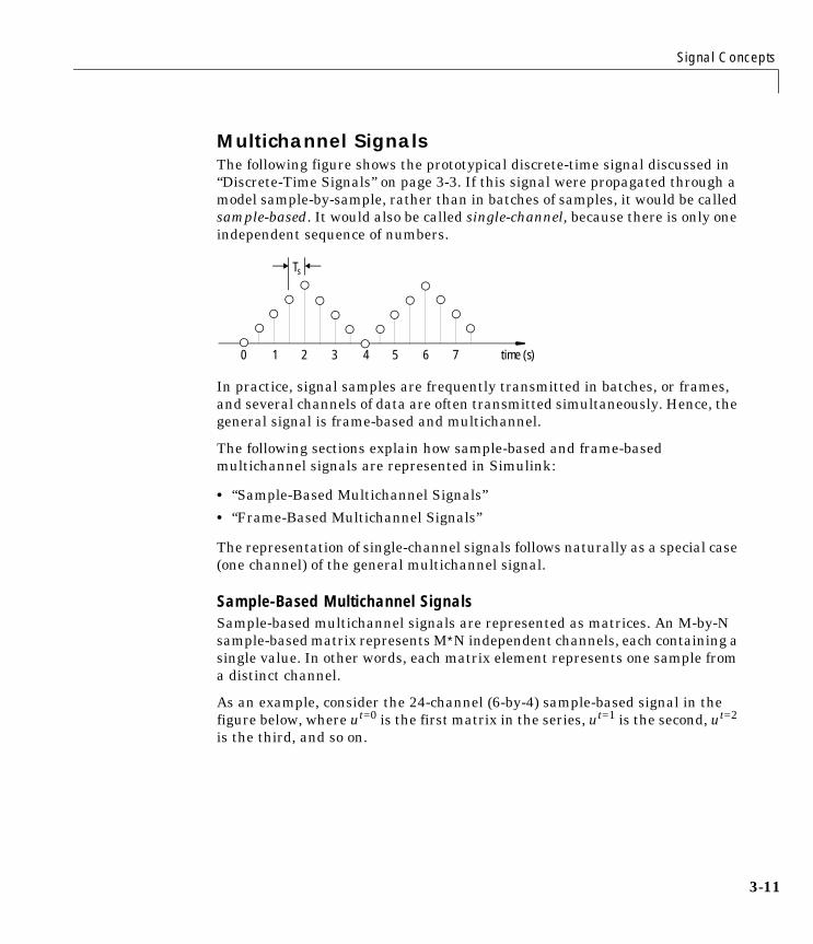
Multichannel SignalsThe following figure shows the prototypical discrete-time signal discussed in “Discrete-Time Signals” on page 3-3. If this signal were propagated through a model sample-by-sample, rather than in batches of samples, it would be called sample-based. It would also be called single-channel, because there is only one independent sequence of numbers.
In practice, signal samples are frequently transmitted in batches, or frames, and several channels of data are often transmitted simultaneously. Hence, the general signal is frame-based and multichannel.
The following sections explain how sample-based and frame-based multichannel signals are represented in Simulink:
• “Sample-Based Multichannel Signals”
• “Frame-Based Multichannel Signals”
The representation of single-channel signals follows naturally as a special case (one channel) of the general multichannel signal.
Sample-Based Multichannel SignalsSample-based multichannel signals are represented as matrices. An M-by-N sample-based matrix represents M∗N independent channels, each containing a single value. In other words, each matrix element represents one sample from a distinct channel.
As an example, consider the 24-channel (6-by-4) sample-based signal in the figure below, where ut=0 is the first matrix in the series, ut=1 is the second, ut=2 is the third, and so on.
time (s)
Ts
1 2 3 4 5 6 70
3 Working with Signals
3-12
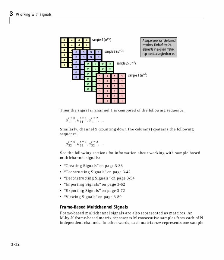
Then the signal in channel 1 is composed of the following sequence.
Similarly, channel 9 (counting down the columns) contains the following sequence.
See the following sections for information about working with sample-based multichannel signals:
• “Creating Signals” on page 3-33
• “Constructing Signals” on page 3-42
• “Deconstructing Signals” on page 3-54
• “Importing Signals” on page 3-62
• “Exporting Signals” on page 3-72
• “Viewing Signals” on page 3-80
Frame-Based Multichannel SignalsFrame-based multichannel signals are also represented as matrices. An M-by-N frame-based matrix represents M consecutive samples from each of N independent channels. In other words, each matrix row represents one sample
A sequence of sample-based matrices. Each of the 24 elements in a given matrix represents a single channel.
sample 4 (u t=3)
sample 3 (u t=2)
sample 2 (u t=1)
sample 1 (u t=0)
4
4
2
2
2
2
4
4
2
2
2
2
4
4
4
4
4
4
4
4
4
4
4
4
3
3
2
2
2
2
3
3
2
2
2
2
3
3
3
3
3
3
3
3
3
3
3
3
2
2
2
2
2
2
2
2
2
2
2
2
2
2
2
2
2
2
2
2
2
2
2
2
1
1
1
1
1
1
1
1
1
1
1
1
1
1
1
1
1
1
1
1
1
1
1
1
u11t 0= u11
t 1= u11t 2= …, , ,
u32t 0= u32
t 1= u32t 2= …, , ,

Signal Concepts
3-13
(or time slice) from N distinct signal channels, and each matrix column represents M consecutive samples from a single channel.
This is a simple structure, as illustrated below for a sample 6-by-4 frame matrix.
Consider a sequence of frame matrices, where ut=0 is the first matrix in a series, ut=1 is the second, ut=2 is the third, and so on.
Then the signal in channel 1 is the following sequence.
Similarly, the signal in channel 3 is the following sequence.
See the following sections for information about working with frame-based multichannel signals:
• “Creating Signals” on page 3-33
• “Constructing Signals” on page 3-42
• “Deconstructing Signals” on page 3-54
ch1 ch2 ch3 ch4
Frame matrix:4 channels, 1 frame per channel,6 samples per frame
1
2
3
4
5
6
1
2
3
4
5
6
1
2
3
4
5
6
1
2
3
4
5
6
sample 5sample 6
ch1 ch2 ch3 ch4
1
2
1
2
1
2
1
2
3
4
3
4
3
4
3
4
5
6
5
6
5
6
5
6
sample 3sample 4
sample 1sample 2
A sequence of frame-based matrices. Each column in a given matrix represents a single channel.
frame 1 (u t=0)
frame 2 (u t=1)
frame 3 (u t=2)
u11t 0= u21
t 0= u31t 0= … uM1
t 0= u11t 1= u21
t 1= u31t 1= … uM1
t 1= u11t 2= u21
t 2= …, , , , , , , , , , , ,
u13t 0= u23
t 0= u33t 0= … uM3
t 0= u13t 1= u23
t 1= u33t 1= … uM3
t 1= u13t 2= u23
t 2= …, , , , , , , , , , , ,

3 Working with Signals
3-14
• “Importing Signals” on page 3-62
• “Exporting Signals” on page 3-72
• “Viewing Signals” on page 3-80
Benefits of Frame-Based ProcessingFrame-based processing is an established method of accelerating both real-time systems and simulations.
Accelerating Real-Time SystemsFramed-based data is a common format in real-time systems. Data acquisition hardware often operates by accumulating a large number of signal samples at a high rate, and propagating these samples to the real-time system as a block of data. This maximizes the efficiency of the system by distributing the fixed process overhead across many samples; the “fast” data acquisition is suspended by “slow” interrupt processes after each frame is acquired, rather than after each individual sample.
The figure below illustrates how throughput is increased by frame-based data acquisition. The thin blocks each represent the time elapsed during acquisition of a sample. The thicker blocks each represent the time elapsed during the interrupt service routine (ISR) that reads the data from the hardware.
In this example, the frame-based operation acquires a frame of 16 samples between each ISR. The frame-based throughput rate is therefore many times higher than the sample-based alternative.

Signal Concepts
3-15
It’s important to note that frame-based processing will introduce a certain amount of latency into a process due to the inherent lag in buffering the initial frame. In many instances, however, it is possible to select frame sizes that improve throughput without creating unacceptable latencies.
Accelerating SimulationsSimulation also benefits from frame-based processing. In this case, it is the overhead of block-to-block communications that is reduced by propagating frames rather than individual samples.
acquire 16 samples ISR
time
timelatency
acquire sample
ISR
Sample-based operation
Frame-based operation

3 Working with Signals
3-16
Sample Rates and Frame Rates Sample rates are an important issue in most DSP models, especially in systems incorporating rate conversions. Fortunately, in most cases, when you build a Simulink model you only need to worry about setting sample rates in the source blocks, such as Signal From Workspace; Simulink automatically computes the appropriate sample rates for all downstream blocks.
Nevertheless, it is important to become familiar with the concepts of “sample rate” and “frame rate” as they apply in the Simulink world. The next sections cover the following important topics:
• “Sample Rate and Frame Rate Concepts”
• “Inspecting Sample Rates and Frame Rates”
• “Converting Sample Rates and Frame Rates”
• “Changing Frame Status”
Sample Rate and Frame Rate ConceptsThe input frame period (Tfi) of a frame-based signal is the time interval between consecutive vector or matrix inputs to a block. This interval is what the Probe block displays when you connect it to a frame-based input line. Similarly, the output frame period (Tfo) is the time interval at which the block updates the frame-based vector or matrix value at the output port. This interval is what the Probe block displays when you connect it to a frame-based output line. (See “Inspecting Sample Rates and Frame Rates” on page 3-17 for more about using the Probe block.)
In contrast, the sample period, Ts, is the time interval between individual samples in a frame, which is necessarily shorter than the frame period when the frame size is greater than 1. The sample period of a frame-based signal is the quotient of the frame period and the frame size, M.
More specifically, the sample periods of inputs (Tsi) and outputs (Tso) are related to their respective frame periods by
Ts Tf M⁄=
Tsi Tfi Mi⁄=
Tso Tfo Mo⁄=

Sample Rates and Frame Rates
3-17
where Mi and Mo are the input and output frame sizes, respectively.
The illustration below shows a one-channel frame-based signal with a frame size (Mi) of 4 and a frame period (Tfi) of 1. The sample period, Tsi, is therefore 1/4, or 0.25 seconds. A Probe block connected to this signal would display the frame period Tfi = 1.
In most cases, the sequence sample period Tsi is of primary interest, while the frame rate is simply a consequence of the frame size that you choose for the signal. For a sequence with a given sample period, a larger frame size corresponds to a slower frame rate, and vice versa.
For information on converting a signal from one sample rate or frame rate to another, see “Converting Sample Rates and Frame Rates” on page 3-20.
Inspecting Sample Rates and Frame RatesWhen constructing a frame-based or multirate model, it is often helpful to check the rates that Simulink computes for different signals. There are two basic ways to inspect the sample rates and frame rates in a model. These are described in the following sections:
• “Using the Probe Block to Inspect Rates”
• “Using Sample Time Color Coding to Inspect Sample Rates”
Using the Probe Block to Inspect RatesConnect Simulink’s Probe block to any line to display the period of the signal on that line. The period is displayed in the block icon itself (together with the line width and data type, if desired), making it easy to verify that the sample rates in the model are what you expect them to be. When the line width and data type displays are suppressed (by deselecting the appropriate check boxes in the block dialog box), the Probe block looks like this.
13141516
9101112
5678
1234
t=0t=1t=2t=3
first input frameTfi = 1
Tsi = 0.25

3 Working with Signals
3-18
The block displays the label Ts or Tf, followed by a two-element vector. The first (left) element is the period of the signal being measured. The second (right) is the signal’s sample time offset, which is usually 0, as explained in “Sample Time Offsets” on page 3-9.
For sample-based signals, the value shown in the Probe block icon is the sample period of the sequence, Ts. For frame-based signals, the value shown in the Probe block icon is the frame period, Tf. The difference between sample rates and frame rates is explained in “Sample Rate and Frame Rate Concepts” on page 3-16.
Probe Block Example: Sample-Based. The three Probe blocks in the sample-based model below verify that the signal’s sample period is halved with each upsample operation: The output from the Signal From Workspace block has a sample period of 1 second, the output from the first Upsample block has a sample period of 0.5 seconds, and the output from the second Upsample block has a sample period of 0.25 seconds.
Probe Block Example: Frame-Based. The three Probe blocks in the frame-based model below again verify that the signal’s sample period is halved with each upsample operation: The output from the Signal From Workspace block has a frame period of 16 seconds, the output from the first Upsample block has a frame period of 8 seconds, and the output from the second Upsample block has a sample period of 4 seconds.

Sample Rates and Frame Rates
3-19
Note that the sample rate conversion is implemented through a change in the frame period rather than the frame size. This is because the Frame-based mode parameter in the Upsample blocks is set to Maintain input frame size rather than Maintain input frame rate. See “Converting Sample Rates and Frame Rates” on page 3-20 for more information.
Using Sample Time Color Coding to Inspect Sample RatesTurn on Simulink’s sample time color coding option by selecting Sample time colors from the Format menu. For sample-based signals, this assigns each sample rate a different color. For frame-based signals, this assigns each frame rate a different color.
Sample Time Color Coding Example: Sample-Based. Here is the sample-based model from “Probe Block Example: Sample-Based” on page 3-18 with the Probe blocks removed and sample time color coding turned on.
Since every sample-based signal in this model has a different sample rate, each signal is assigned a different color.
Sample Time Color Coding Example: Frame-Based. Here’s the frame-based model from “Probe Block Example: Frame-Based” on page 3-18 with the Probe blocks removed and sample time color coding turned on.
Red = fastest sample rate
Green = second fastest sample rate
Blue = third fastest sample rate

3 Working with Signals
3-20
Because the Frame-based mode parameter in the Upsample blocks is set to Maintain input frame size rather than Maintain input frame rate, each Upsample block changes the frame rate. Therefore, each frame-based signal in the model is assigned a different color.
If the Upsample blocks are instead set to Maintain input frame rate, then every signal in the model shares the same frame rate, and as a result, every signal is coded with the same color.
For more information about sample time color coding, see “Sample Time Colors” in the Simulink documentation.
Converting Sample Rates and Frame RatesIn a DSP Blockset model, there are two types of periods that you will commonly be concerned with: sample periods and frame periods. The input and output sample periods of a block (Tsi and Tso, respectively) are related to the input and output frame periods (Tfi and Tfo, respectively) by
where Mi and Mo are the input and output frame sizes, respectively.
The buffering and rate-conversion capabilities of the DSP Blockset generally allow you to independently vary any two of the three parameters (Tso, Tfo, Mo). In most cases, the sample period and the frame size are the two parameters of primary interest; the frame period is simply a consequence of your choices for the other two.
There are two common types of operations that impact the frame and sample rates of a signal:
Tsi Tfi Mi⁄=
Tso Tfo Mo⁄=

Sample Rates and Frame Rates
3-21
• Direct rate conversions
Direct rate conversions, such as upsampling and downsampling, are a feature of most DSP systems, and can be implemented by altering either the frame rate or the frame size of a signal.
• Frame rebuffering
The principal purpose of frame rebuffering is to alter the frame size of a signal, usually to improve simulation throughput. By redistributing the signal samples to frames of a new size, rebuffering usually changes either the sample rate or frame rate of the signal.
Both operations are discussed in the following sections, along with ways to avoid unintentional rate conversions:
• “Direct Rate Conversion”
• “Frame Rebuffering”
• “Avoiding Unintended Rate Conversions”
You may also want to look at the Sample Rate Conversion demo, dspsrcnv.mdl.
Note Technically, when a Simulink model contains signals with various frame rates, the model is called multirate. You can find a discussion of multirate models in “Delay and Latency” on page 3-85 and in the “Discrete Time Systems” section of the Simulink documentation.
Direct Rate ConversionRate conversion blocks accept an input signal at one sample rate, and propagate the same signal at a new sample rate. Several of these blocks contain a Frame-based mode parameter offering two options for adjusting the sample rate of the signal:
• Maintain input frame rate: Change the sample rate by changing the frame size (i.e., Mo ≠ Mi), but keep the frame rate constant (i.e., Tfo = Tfi)
• Maintain input frame size: Change the sample rate by changing the output frame rate (i.e., Tfo ≠ Tfi), but keep the frame size constant (i.e., Mo = Mi)
The setting of this parameter does not affect sample-based inputs.

3 Working with Signals
3-22
Rate Conversion Blocks. The following table lists the principal rate conversion blocks in the DSP Blockset. Blocks marked with an asterisk (*) offer the option of changing the rate by either adjusting the frame size or frame rate.
The following examples illustrate the two sample rate conversion modes:
• “Example: Rate Conversion by Frame-Rate Adjustment”
• “Example: Rate Conversion by Frame-Size Adjustment”
Example: Rate Conversion by Frame-Rate Adjustment. A common example of direct rate conversion is shown in the model below, where the signal is directly downsampled to half its original rate by a Downsample block. The values next to input and output ports are the signal dimensions, displayed by selecting Signal dimensions from the model window’s Format menu.
Block Library
Downsample * Signal Operations
Dyadic Analysis Filter Bank Filtering / Multirate Filters
Dyadic Synthesis Filter Bank Filtering / Multirate Filters
FIR Decimation * Filtering / Multirate Filters,
FIR Interpolation * Filtering / Multirate Filters
FIR Rate Conversion Filtering / Multirate Filters
Repeat * Signal Operations
Upsample * Signal Operations
Wavelet Analysis Filtering / Multirate Filters
Wavelet Synthesis Filtering / Multirate Filters

Sample Rates and Frame Rates
3-23
The sample period and frame size of the original signal are set to 0.125 seconds and 8 samples per frame, respectively, by the Sample time and Samples per frame parameters in the Signal From Workspace block. This results in a frame rate of 1 second (0.125∗8), as shown by the first Probe block.
The Downsample block is configured to downsample the signal by changing the frame rate rather than the frame size. The dialog box with this setting is shown below.
The second Probe block in the model verifies that the output from the Downsample block has a frame period of 2, twice that of the input (i.e., half the rate). As a result, the sequence sample period is doubled to 0.25 seconds without any change to the frame size.
Example: Rate Conversion by Frame-Size Adjustment. The model from “Example: Rate Conversion by Frame-Rate Adjustment” on page 3-22 is shown again below, but this time with the rate conversion implemented by adjusting the frame size, rather than the frame rate.
Maintain input frame size: Downsample the signal by changing the frame rate.

3 Working with Signals
3-24
As before, the frame rate of the original signal is 1 second (0.125∗8), shown by the first Probe block. Now the Downsample block is configured to downsample the signal by changing the frame size rather than the frame rate. The dialog box with this setting is shown below.
The line width display on the Downsample output port verifies that the downsampled output has a frame size of 4, half that of the input. As a result, the sequence sample period is doubled to 0.25 seconds without any change to the frame rate.
Frame RebufferingBuffering operations provide another mechanism for rate changes in DSP models. The purpose of many buffering operations is to adjust the frame size of the signal, M, without altering the sequence sample rate Ts. This usually results in a change to the signal’s frame rate, Tf, according to the relation
Maintain input frame rate: Downsample the signal by changing the frame size.
Tf MTs=

Sample Rates and Frame Rates
3-25
However, this is only true when the original signal is preserved in the buffering operation, with no samples added or deleted. Buffering operations that generate overlapping frames, or that only partially unbuffer frames, alter the data sequence by adding or deleting samples. In such cases, the above relation is not valid.
Buffering Blocks. The following table lists the principal buffering blocks in the DSP Blockset.
The following sections discuss two general classes of buffering operations:
• “Buffering with Preservation of the Signal”
• “Buffering with Alteration of the Signal”
Buffering with Preservation of the Signal. There are various reasons that you may need to rebuffer a signal to a new frame size at some point in a model. For example, your data acquisition hardware may internally buffer the sampled signal to a frame size that is not optimal for the DSP algorithm in the model. In this case, you would want to rebuffer the signal to a frame size more appropriate for the intended operations, but without introducing any change to the data or sample rate.
There are two blocks in the Buffers library that can be used to change a signal’s frame size without altering the signal itself:
• Buffer – redistributes signal samples to a larger or smaller frame size
• Unbuffer – unbuffers a frame-based signal to a sample-based signal (frame size = 1)
Block Library
Buffer Signal Management / Buffers
Delay Line Signal Management / Buffers
Unbuffer Signal Management / Buffers
Variable Selector Signal Management / Indexing
Zero Pad Signal Operations

3 Working with Signals
3-26
The Buffer block preserves the signal’s data and sample period only when its Buffer overlap parameter is set to 0. The output frame period, Tfo, is
where Tfi is the input frame period, Mi is the input frame size, and Mo is the output frame size specified by the Buffer size parameter.
The Unbuffer block is specialized for completely unbuffering a frame-based signal to its sample-based equivalent, and always preserves the signal’s data and sample period:
where Tfi and Mi are the period and size, respectively, of the frame-based input.
Both the Buffer and Unbuffer blocks preserve the sample period of the sequence in the conversion (Tso = Tsi).
Example: Buffering with Preservation of the Signal. In the model below, a signal with a sample period of 0.125 seconds is rebuffered from a frame size of 8 to a frame size of 16. This doubles the frame period from 1 to 2 seconds, but does not change the sample period of the signal (Tso = Tsi = 0.125).
Buffering with Alteration of the Signal. Some forms of buffering alter the signal’s data or sample period, in addition to adjusting the frame size. There are many instances when this type of buffering is desirable, for example when creating sliding windows by overlapping consecutive frames of a signal, or selecting a subset of samples from each input frame for processing.
The blocks that alter a signal while adjusting its frame size are listed below. In this list, Tsi is the input sequence sample period, and Tfi and Tfo are the input and output frame periods, respectively.
Tfo
MoTfiMi
----------------=
Tso Tfi M⁄ i=
Sample Rates and Frame Rates
3-27
• Buffer adds duplicate samples to a sequence when the Buffer overlap parameter, L, is set to a nonzero value. The output frame period is related to the input sample period by
where Mo is the output frame size specified by the Buffer size parameter. As a result, the new output sample period is
• Delay Line adds duplicate samples to the sequence when the Delay line size parameter, Mo, is greater than 1. The output and input frame periods are the same, Tfo = Tfi = Tsi, and the new output sample period is
• Variable Selector can remove, add, and/or rearrange samples in the input frame when Select is set to Rows. The output and input frame periods are the same, Tfo = Tfi, and the new output sample period is
where Mo is the length of the block’s output, determined by the Elements vector.
• Zero Pad adds samples to the sequence by appending zeros to each frame when Zero pad along is set to Columns. The output and input frame periods are the same, Tfo = Tfi, and the new output sample period is
where Mo is the length of the block’s output, determined by the Number of output rows parameter.
In all of these cases, the sample period of the output sequence is not equal to the sample period of the input sequence.
Tfo Mo L–( )Tsi=
TsoMo L–( )Tsi
Mo-------------------------------=
TsoTsiMo--------=
Tso
MiTsiMo
----------------=
Tso
MiTsiMo
----------------=

3 Working with Signals
3-28
Example: Buffering with Alteration of the Signal. In the model below, a signal with a sample period of 0.125 seconds is rebuffered from a frame size of 8 to a frame size of 16 with an overlap of 4.
The relation for the output frame period for the Buffer block is
which indicates that Tfo should be (16-4)∗0.125, or 1.5 seconds, as confirmed by the second Probe block. The sample period of the signal at the output of the Buffer block is no longer 0.125 seconds, but rather 0.0938 seconds (i.e., 1.5/16). Thus, both the signal’s data and the signal’s sample period have been altered by the buffering operation.
Avoiding Unintended Rate ConversionsThe previous sections discussed a number of the blocks that are responsible for rate conversions. It is important to be aware of where in a model these rate conversions are taking place; in a few cases, unintentional rate conversions can produce misleading results. The following pair of examples illustrate how unintended rate conversion can occur:
• “Example 1: No Rate Conversion”
• “Example 2: Unintended Rate Conversion”
Example 1: No Rate Conversion. The model below plots the magnitude FFT of a signal composed of two sine waves, with frequencies of 1 Hz and 2 Hz.
Tfo Mo L–( )Tsi=

Sample Rates and Frame Rates
3-29
To build the model, configure one Sine Wave block with Frequency = 1, and the other with Frequency = 2. In addition, both Sine Wave blocks should have the following settings:
• Sample time = 0.1
• Samples per frame = 128
The frame period of the resulting summed sinusoid is 12.8 seconds (i.e., 128∗0.1), which is confirmed by the Probe block when the model is updated.
Select Inherit FFT length from input dimensions in the Magnitude FFT block. This setting instructs the block to use the input frame size (128) as the FFT length (which is also the output size).
Configure the Vector Scope block as follows:
• Select Frequency from the Input domain parameter.
• Select the Axis properties check box to expose the Axis properties panel.
• Set Minimum Y-limit to -10.
• Set Maximum Y-limit to 40.
The plot generated by the Vector Scope block is shown below.

3 Working with Signals
3-30
The Vector Scope block uses the input frame size (128) and period (12.8) to deduce the original signal’s sample period (0.1), which allows it to correctly display the peaks at 1 Hz and 2 Hz.
Example 2: Unintended Rate Conversion. Now alter the previous example by setting the Magnitude FFT block parameters as follows:
• Deselect the Inherit FFT length from input dimensions check box.
• Set the FFT length parameter to 256.
This setting instructs the block to zero-pad the length-128 input frame to a length of 256 before performing the FFT. The signal dimension display on the new version of the model shows that the output of the Magnitude FFT block is now a length-256 frame.
The plot generated by the Vector Scope block is shown below.

Sample Rates and Frame Rates
3-31
In this case, based on the input frame size (256) and period (12.8), the Vector Scope block calculates the original signal’s sample period to be 0.05 seconds (12.8/256), which is wrong. As a result, the spectral peaks appear at the incorrect frequencies, 2 Hz and 4 Hz rather than 1 Hz and 2 Hz.
The problem is that the zero-pad operation performed by the Magnitude FFT block halves the sample period of the sequence by appending 128 zeros to each frame. The Vector Scope block, however, needs to know the sample period of the original signal. The problem is easily solved by changing the Sample time of original time series setting in the Axis properties panel of the Vector Scope block to the actual sample period of 0.1. The plot generated with this setting is identical to the first Vector Scope plot above.
In general, be aware that when you do zero-padding or overlapping buffering you are changing the sample period of the signal. As long as you keep this in mind, you should be able to anticipate and correct problems like the one above.
Changing Frame StatusThe frame status of a signal refers to whether the signal is sample-based or frame-based. In a Simulink model, the frame status is symbolized by a single line, →, for a sample-based signal and a double line, ⇒, for a frame-based signal.
In most cases, the appropriate way to convert a sample-based signal to a frame-based signal is by using the Buffer block, and the appropriate way to

3 Working with Signals
3-32
convert a frame-based signal to a sample-based signal is by using the Unbuffer block. See the following sections for more information about these methods:
• “Buffering Sample-Based and Frame-Based Signals” on page 3-47
• “Unbuffering a Frame-Based Signal into a Sample-Based Signal” on page 3-60
On occasion it may be desirable to change the frame status of a signal without performing a buffering operation. You can do this by using the Frame Status Conversion block in the Signal Attributes library.
The Output signal parameter (or the signal at the optional Ref input port) determines the frame status of the output If the frame status of the input differs from the Output signal setting, then the frame status is altered as specified. If the frame status of the input is the same as that specified by the Output signal parameter, then no change is made to the signal.
The block’s input and output port rates are the same, and because the block does not make any sample rate accommodation, the sample rate of the signal is generally not preserved under a change of frame status. (The exception to this rule occurs when a sample-based signal is converted to a frame-based signal with frame size 1, or vice versa.)
See the Frame Status Conversion block’s reference page for complete information.

Creating Signals
3-33
Creating SignalsThere are a variety of different ways to create signals using Simulink and DSP blocks. The following sections explore the most common techniques:
• “Creating Signals Using Constant Blocks” on page 3-33
• “Creating Signals Using Signal Generator Blocks” on page 3-36
• “Creating Signals Using the Signal From Workspace Block” on page 3-38
The above sections discuss creating signals (single-channel and multichannel) using source blocks. For information about constructing multichannel signals from existing single-channel signals, see the following sections:
• “Constructing Multichannel Sample-Based Signals” on page 3-42
• “Constructing Multichannel Frame-Based Signals” on page 3-45
Creating Signals Using Constant BlocksA constant signal is a sample-based signal in which successive samples are identical, or a frame-based signal in which successive frames are identical. The DSP Sources library provides the following blocks for creating sample-based and frame-based constant signals:
• Constant Diagonal Matrix
• Constant Ramp
• DSP Constant
• Identity Matrix
• Window Function
Although some of these blocks generate continuous-time outputs and some generate discrete-time outputs, in each case the output of the block remains constant throughout the simulation.
The most versatile of these blocks is the DSP Constant, which is discussed further in the following example. See Chapter 5, “DSP Block Reference,” for complete explanation of all the constant blocks.
For information about creating signals with other types of blocks, see the following sections:
• “Creating Signals Using Signal Generator Blocks” on page 3-36

3 Working with Signals
3-34
• “Creating Signals Using the Signal From Workspace Block” on page 3-38
For information about importing signals, see the following sections:
• “Importing a Multichannel Sample-Based Signal” on page 3-62
• “Importing a Multichannel Frame-Based Signal” on page 3-68
Example: Creating Signals with the DSP Constant BlockThe DSP Constant block has the following parameters:
• Constant value• Interpret vector parameters as 1-D• Sample mode• Sample time• Frame-based output
To generate a constant matrix signal, simply enter the desired matrix in the Constant value parameter using standard MATLAB notation. Some common examples of MATLAB’s matrix notation are shown below.
[1 2 3;4 5 6] % A 2-by-3 matrix
[1 2 3;4 5 6]' % The transpose, a 3-by-2 matrix
randn(2,3) % A 2-by-3 matrix with random elements
[1 2 3] % A 1-by-3 row vector
[1 2 3]' % The transpose, a 3-by-1 column vector
As with all numerical parameters, you can also enter any valid MATLAB variable or expression that evaluates to a matrix. See the MATLAB documentation for a thorough introduction to constructing and indexing matrices.
The Interpret vector parameters as 1-D and Frame-based output parameters are discussed following the example below. See the DSP Constant block’s reference page for information about the Sample mode and Sample time parameters.
The model below shows five DSP Constant blocks, each generating one of the constant signals listed above. Two of the blocks have non-default settings for the other parameters: The third block (DSP Constant2) has the Frame-based

Creating Signals
3-35
output check box selected, and the fourth block (DSP Constant3) has the Interpret vector parameters as 1-D check box selected.
In addition to the various output dimensions in the model, you can observe three different kinds of signals:
• Sample-based matrix signal – The DSP Constant and DSP Constant1 blocks generate sample-based matrices (2-by-3 and 3-by-2, respectively) because the Frame-based output check box in those blocks is not selected. The sample-based matrices can each be considered to each have six independent channels.
• Frame-based matrix signal – The DSP Constant2 and DSP Constant4 blocks generate frame-based matrices (2-by-3 and 3-by-1, respectively, and represented by double lines) because the Frame-based output check box in those blocks is selected. The 2-by-3 frame-based matrix is considered to have three independent channels, each containing two consecutive samples. The 3-by-1 frame-based matrix (column vector) is considered to have one independent channel, containing three consecutive samples.
• 1-D vector signal – The DSP Constant3 block generates a length-3 1-D vector signal because the Interpret vector parameters as 1-D check box in that
Sample-based matrix (6 channels)
Sample-based matrix (6 channels)
Frame-based matrix (3 channels)
1-D vector
Frame-based matrix (1 channel)

3 Working with Signals
3-36
block is selected. This means that the output is not a matrix. However, most nonsource DSP blocks interpret a length-M 1-D vector as an M-by-1 matrix (column vector).
Note A 1-D vector signal must always be sample-based. The Interpret vector parameters as 1-D parameter is ignored when Frame-based output is selected, or when a matrix is specified for the Constant value parameter.
See “Multichannel Signals” on page 3-11 for more information about the representation of sample-based and frame-based data.
Creating Signals Using Signal Generator BlocksThe DSP Sources library provides the following blocks for automatically generating common sample-based and frame-based signals:
• Chirp
• Counter
• Discrete Impulse
• Multiphase Clock
• N-Sample Enable
• Sine Wave
One of the most commonly used of these is the Sine Wave block, which is discussed further in the example below. See Chapter 5, “DSP Block Reference,” for a complete explanation of the other signal generation blocks. The Simulink Sources library offers a collection of continuous-time signal generation blocks that you may also find useful. Consult the Simulink documentation for more information.
For more information about creating signals, see the following sections:
• “Creating Signals Using Constant Blocks” on page 3-33
• “Creating Signals Using the Signal From Workspace Block” on page 3-38
Example: Creating Signals with the Sine Wave BlockThe Sine Wave block dialog box contains the following key parameters.

Creating Signals
3-37
• Amplitude• Frequency• Phase offset• Sample time• Samples per frame
In the model below, a Sine Wave block generates a frame-based (multichannel) matrix containing three independent signals:
• Sine wave of amplitude 1 and frequency 100 Hz
• Sine wave of amplitude 3 and frequency 250 Hz
• Sine wave of amplitude 2 and frequency 500 Hz
Each channel has a frame size of 64 samples. The three signals are summed point-by-point by a Matrix Sum block, and exported to the workspace.
To build the model, set the Sum along parameter of the Matrix Sum block to Rows, and make the following parameter settings in the Sine Wave block:
• Set Amplitude to [1 3 2]. This specifies the amplitudes for three independent sinusoids (and therefore dictates a three-column output).
• Set Frequency to [100 250 500]. This specifies the frequency for each of the output sinusoids.
• Set Sample time to 1/5000. (This is ten times the highest sinusoid frequency, and so satisfies the Nyquist criterion.)
• Set Samples per frame to 64. This specifies a frame size of 64 for all sinusoids (and therefore dictates a 64-row output).
After running the model, you can look at a portion of the resulting summed sinusoid by typing
plot(yout(1:100))
at the command line.

3 Working with Signals
3-38
See “Multichannel Signals” on page 3-11 for more information about the representation of sample-based and frame-based data.
Creating Signals Using the Signal From Workspace BlockYou can easily create custom signals using the Signal From Workspace block.
This block allows you to generate arbitrary sample-based and frame-based signals, as illustrated in the following examples:
• “Example 1: Generating Sample-Based Output” on page 3-39
• “Example 2: Generating Frame-Based Output” on page 3-39
As the name implies, the Signal From Workspace block is more commonly used to import custom signals from the workspace. See the following sections for more information:
• “Importing a Multichannel Sample-Based Signal” on page 3-62
• “Importing a Multichannel Frame-Based Signal” on page 3-68
0 20 40 60 80 100−6
−4
−2
0
2
4
6

Creating Signals
3-39
For more information about creating signals, see the following sections:
• “Creating Signals Using Constant Blocks” on page 3-33
• “Creating Signals Using Signal Generator Blocks” on page 3-36
Example 1: Generating Sample-Based OutputIn the model below, the Signal From Workspace creates a four-channel sample-based signal with the following data:
• Channel 1: 1, 2, 3, 0, 0,...
• Channel 2: -1, -2, -3, 0, 0,...
• Channel 3: 0, 0, 0, 0, 0,...
• Channel 4: 5, 5, 5, 0, 0,...
To create the model, specify the following parameter values in the Signal From Workspace block:
• Signal = cat(3,[1 -1;0 5],[2 -2;0 5],[3 -3;0 5])
• Sample time = 1
• Samples per frame = 1
• Form output after final data value = Setting to zero
The Sample time setting of 1 yields a sample-based output with sample period of 1 second. Each of the four elements in the matrix signal represents an independent channel (the channel numbering is arbitrary). The Form output after final data value parameter setting specifies that all outputs after the third are zero.
Example 2: Generating Frame-Based Output In the model below, the Signal From Workspace creates a two-channel frame-based signal with the following data:
1 1–
0 52 2–
0 5
first matrix output
t=0t=1
3 3–
0 5
t=2
0 00 0
t=3

3 Working with Signals
3-40
• Channel 1: 1, 2, 3, 4, 5, 6, 7, 8, 9, 10, 0, 0,...
• Channel 2: 1, 1, 0, 0, 1, 1, 0, 0, 1, 1, 0, 0,...
To create the model, specify the following parameter values in the Signal From Workspace block:
• Signal = [1 2 3 4 5 6 7 8 9 10;1 1 0 0 1 1 0 0 1 1]'
• Sample time = 1
• Samples per frame = 4
• Form output after final data value = Setting to zero
The Sample time setting of 1 and the Samples per frame setting of 4 yield a frame-based output with a frame size of 4 samples and a frame period of 4 seconds. The Form output after final data value parameter setting specifies that all outputs after the third frame are zero.
Note that the output of the To Workspace block, yout, is the original signal with appended zeros in each channel.
1 12 13 04 0
5 16 17 08 0
first matrix output
t=0t=4
ch2
ch1
ch2
ch1
9 110 10 00 0
ch2
ch1
t=8
0 00 00 00 0
ch2
ch1
t=12

Creating Signals
3-41
yout =
1 1 2 1 3 0 4 0 5 1 6 1 7 0 8 0 9 1 10 1 0 0 0 0

3 Working with Signals
3-42
Constructing SignalsWhen you want to perform a given sequence of operations on several independent signals, it is frequently very convenient to group those signals together as a multichannel signal. Most DSP blocks accept multichannel signals, and process each channel independently. By taking advantage of this capability, you can do the same job with fewer blocks and have a cleaner, leaner model.
For example, if you need to filter each of four independent signals using a direct-form II transpose filter with the same coefficients, combine the signals into a multichannel signal, and run that multichannel signal into a Direct-Form II Transpose Filter block. The block will apply the filter to each channel independently.
The following sections explain how to construct multichannel signals from existing independent signals:
• “Constructing Multichannel Sample-Based Signals” on page 3-42
• “Constructing Multichannel Frame-Based Signals” on page 3-45
For information about creating multichannel signals using source blocks, see the following sections:
• “Creating Signals Using Constant Blocks” on page 3-33
• “Creating Signals Using Signal Generator Blocks” on page 3-36
• “Creating Signals Using the Signal From Workspace Block” on page 3-38
Constructing Multichannel Sample-Based SignalsA sample-based signal with M∗N channels is represented by a sequence of M-by-N matrices. (The special case of M = N = 1 represents a single-channel signal.) Multiple individual signals can be combined into a multichannel matrix signal using the Matrix Concatenation block. Individual signals can be added to an existing multichannel signal in the same way. The following sections explain how to do this:
• “Constructing Sample-Based Multichannel Signals from Independent Sample-Based Signals” on page 3-43
• “Constructing Sample-Based Multichannel Signals from Existing Sample-Based Multichannel Signals” on page 3-44

Constructing Signals
3-43
Constructing Sample-Based Multichannel Signalsfrom Independent Sample-Based SignalsYou can combine individual sample-based signals into a multichannel signal by using the Matrix Concatenation block in Simulink’s Sources library.
Example: Concatenating Single-Channel Signals. In the model below, four independent sample-based signals are combined into a 2-by-2 multichannel matrix signal.
To build the model, make the following parameter settings:
• In Signal From Workspace, set Signal = 1:10
• In Signal From Workspace1, set Signal = -1:-1:-10
• In Signal From Workspace2, set Signal = zeros(10,1)
• In Signal From Workspace3, set Signal = 5*ones(10,1)
• In Matrix Concatenation, set:
- Number of inputs = 4
- Concatenation method = Vertical
• In Reshape, set:
- Output dimensionality = Customize
- Output dimensions = [2,2]
Four single-channel signals Multichannel signals

3 Working with Signals
3-44
Each 4-by-1 output from the Matrix Concatenation block contains one sample from each of the four input signals. All four samples in the output correspond to the same instant in time. The Reshape block simply rearranges the samples into a 2-by-2 matrix. Note that the Reshape block works columnwise, so that a column vector input is reshaped as shown below.
The 4-by-1 matrix and the 2-by-2 matrix in the above model represent the same sample-based four-channel signal. In some cases one representation may be more useful than the other. See “Sample-Based Multichannel Signals” on page 3-11 for more about sample-based signals.
Constructing Sample-Based Multichannel Signalsfrom Existing Sample-Based Multichannel SignalsYou can combine existing multichannel sample-based signals into a larger multichannel signal by using the Matrix Concatenation block in Simulink’s Sources library.
Example: Concatenating Multichannel Signals. The model below shows two two-channel sample-based signals (four channels total) being combined into a 2-by-2 multichannel matrix signal.
To build the model, make the following parameter settings:
• In Signal From Workspace, set Signal = [1:10;-1:-1:-10]'
1234
1 32 4
Two 2-channel signals,Four distinct channels
4-channel signal

Constructing Signals
3-45
• In Signal From Workspace1, set Signal = [zeros(10,1) 5*ones(10,1)]
• In Matrix Concatenation, set:
- Number of inputs = 2
- Concatenation method = Vertical
Each 2-by-2 output from the Matrix Concatenation block contains both samples from each of the two input signals, so that all four samples in the output correspond to the same instant in time. See “Sample-Based Multichannel Signals” on page 3-11 for more about sample-based signals.
Constructing Multichannel Frame-Based SignalsA frame-based signal with N channels and frame size M is represented by a sequence of M-by-N matrices. (The special case of N = 1 represents a single-channel signal.) There are two basic ways to construct a multichannel frame-based signal from existing signals:
• By horizontally concatenating existing frame-based signals – Multiple individual frame-based signals (with the same frame rate and size) can be combined into a multichannel frame-based signal using the Simulink Matrix Concatenation block. Individual signals can be added to an existing multichannel signal in the same way.
• By buffering existing sample-based or frame-based signals – Multichannel sample-based and frame-based signals can be buffered into multichannel
ch1 ch2 ch3 ch4
1
2
3
4
5
6
1
2
3
4
5
6
1
2
3
4
5
6
1
2
3
4
5
6
1
2
3
4
5
6
1
2
3
4
5
6
1
2
3
4
5
6
1
2
3
4
5
6
sig1 sig2 sig3 sig4
Four frame-based signals:1 channel each, 6 samples per frame
Multichannel frame-based signal:4 channels, 6 samples per frame

3 Working with Signals
3-46
frame-based signals using the Buffer block in the Buffers library (in Signal Management).
The following sections explain the two methods of constructing multichannel frame-based signals:
• “Concatenating Independent Frame-Based Signals into Multichannel Signals” on page 3-46
• “Buffering Sample-Based and Frame-Based Signals” on page 3-47
Concatenating Independent Frame-Based Signalsinto Multichannel SignalsYou can combine existing frame-based signals into a larger multichannel signal by using the Matrix Concatenation block in Simulink’s Sources library. All signals must have the same frame rate and frame size.
Example: Concatenating Frame-Based Signals. In the model below, a single-channel frame-based signal is combined with a two-channel frame-based signal to produce a three-channel frame-based signal.
sample 1
sample 2
sample 3
sample 4
sample 5
ch1 ch2 ch3 ch4
1
2
3
4
5
6
1
2
3
4
5
6
1
2
3
4
5
6
1
2
3
4
5
6
Multichannel sample-based signal:4 channels
Multichannel frame-based signal:4 channels, 6 samples per frame
ch1 ch2 ch3 ch4
1111
2222
3333
4444
5555
6666sample 6

Constructing Signals
3-47
To build the model, make the following parameter settings:
• In Signal From Workspace, set Signal = [1:10;-1:-1:-10]'
• In Signal From Workspace1, set Signal = 5*ones(10,1)
• In Matrix Concatenation, set:
- Number of inputs = 2
- Concatenation method = Horizontal
The 4-by-3 matrix output from the Matrix Concatenation block contains all three input channels, and preserves their common frame rate and frame size. See “Frame-Based Multichannel Signals” on page 3-12 for more about frame-based signals.
Note that you could also create or import the three-channel signal using just one Signal From Workspace block. See the following sections for more information:
• “Creating Signals Using the Signal From Workspace Block” on page 3-38
• “Importing a Multichannel Frame-Based Signal” on page 3-68
Buffering Sample-Based and Frame-Based SignalsYou can buffer a multichannel sample-based or frame-based signal into a multichannel frame-based signal by using the Buffer block in the Buffers library (in Signal Management). The Buffer block has the following key parameters:
2-channel frame-based signal (top) and 1-channel frame-based signal (bottom)
3-channel frame-based signal
1 1– 52 2– 53 3– 54 4– 5
1 1–
2 2–
3 3–
4 4–
5555

3 Working with Signals
3-48
• Output buffer size (per channel), Mo
• Buffer overlap, L
• Initial conditions
Buffering an N-channel (1-by-N or N-by-1) sample-based signal produces a Mo-by-N frame-based signal. Buffering an Mi-by-N frame-based signal (N channels and Mi samples per frame) results in an Mo-by-N output frame-based signal.
For each output buffer, the block acquires the number of new input samples specified by the difference between the Buffer size (Mo) and Buffer overlap (L) parameters. Each new input sample enters at the bottom of the buffer, and is pushed upwards as later samples enter. The first row in the output therefore corresponds to the earliest input sample. Because the block can buffer a signal to a larger or smaller frame size, the number of samples acquired from the input can be greater or less than the number of samples in an individual input frame.
In general, the output frame period, Tfo, is related to the input sample period, Tsi, by
where Mo is the Output buffer size (per channel), and L is the Buffer overlap.
As a result, the new output sample period, Tso, is
Clearly, this is equal to the input sample period only when the Buffer overlap is zero. See “Converting Sample Rates and Frame Rates” on page 3-20 for more information about rate conversions.
The following sections provide examples of buffering, and explore related buffering issues:
• “Example: Buffering Sample-Based Signals without Overlap” on page 3-49
• “Overlapping Buffers” on page 3-50
• “Example: Buffering Sample-Based Signals with Overlap” on page 3-50
Tfo Mo L–( )Tsi=
TsoMo L–( )Tsi
Mo-------------------------------=

Constructing Signals
3-49
• “Example: Buffering Frame-Based Signals with Overlap” on page 3-52
• “Buffering Delay and Initial Conditions” on page 3-53
Example: Buffering Sample-Based Signals without Overlap. In the model below, a two-channel sample-based signal is buffered into a two-channel frame-based signal.
To build the model, make the following parameter settings:
• In Signal From Workspace:
- Signal = [1:10;-1:-1:-10]'
- Sample time = 1
- Samples per frame = 1
• In Buffer
- Output buffer size = 4
- Buffer overlap = 0
- Initial conditions = 0
The Signal From Workspace block generates one two-channel sample at each sample time due to the Samples per frame parameter setting of 1. The Buffer size setting of 4 in the Buffer block results in a frame-based output with frame size 4.
A much better way to create the frame-based signal shown above is to set the Samples per frame parameter of the Signal From Workspace block to 4. The Signal From Workspace block then performs the buffering internally, and directly generates the two-channel frame-based signal; the separate Buffer block is not needed. See the following sections for more information:
• “Creating Signals Using the Signal From Workspace Block” on page 3-38
Four consecutive samples from a 2-channel sample-based signal
2-channel frame-based signal
1 1–
2 2–
3 3–
4 4–
[1 -1][2 -2][3 -3][4 -4]
t=0t=1t=2t=3

3 Working with Signals
3-50
• “Importing a Multichannel Frame-Based Signal” on page 3-68
Overlapping Buffers. In some cases it is useful to work with data that represents overlapping sections of an original sample-based or frame-based signal. In estimating the power spectrum of a signal, for example, it is often desirable to compute the FFT of overlapping sections of data. Overlapping buffers are also needed in computing statistics on a sliding window, or for adaptive filtering. The Buffer overlap parameter of the Buffer block specifies the number of overlap points, L.
In the overlap case (L > 0), the frame period for the output is (Mo-L)∗Tsi, where Tsi is the input sample period and Mo is the Buffer size.
Note Set the Buffer overlap parameter to a negative value to achieve output frame rates slower than in the nonoverlapping case. The output frame period is still Tsi∗(Mo-L), but now with L < 0. Only the Mo newest inputs are included in the output buffer; the previous L inputs are discarded.
Example: Buffering Sample-Based Signals with Overlap. In the following model, a four-channel sample-based signal with sample period 1 is buffered to a frame-based signal with frame size 3 and frame period 2. Because of the overlap, the input sample period is not conserved, and the output sample period is 2/3.

Constructing Signals
3-51
To build the model, define the following variable in the MATLAB workspace.
A = [1 1 5 -1;2 1 5 -2;3 0 5 -3;4 0 5 -4;5 1 5 -5;6 1 5 -6];
Connect the Buffer block to a Signal From Workspace source and a To Workspace sink with the following parameter settings:
• In the Signal From Workspace block, set:
- Signal = A
- Sample time = 1
- Samples per frame = 1
• In the Buffer block, set:
- Output buffer size (per channel) = 3
- Buffer overlap = 1
- Initial conditions = 0
Note that the inputs do not begin appearing at the output until the second row of the second matrix. This is due to the block’s latency. See “Delay and Latency” on page 3-85 for general information about algorithmic delay, and see “Buffering Delay and Initial Conditions” on page 3-53 for instructions on how to calculate buffering delay.
4 0 5 4–
5 1 5 5–
6 1 5 6–
6 1 5 6–
t=0
t=2
t=5
t=4
t=3
t=1
first frame-based output
Tsi = 15 1 5 5–
3 0 5 3–
4 0 5 4–
2 1 5 2–
1 1 5 1–
(Mo=3, L=1)
0 0 0 01 1 5 1–
2 1 5 2–
0 0 0 00 0 0 00 0 0 0
2 1 5 2–
3 0 5 3–
4 0 5 4–
first sample-based input
t=0t=4t=6 t=2
ch4ch3
ch1ch2
ch4
ch3
ch2
ch1
Sample-based input, sample period = Tsi
Frame-based output,frame period = (Mo-L)∗Tsi
ch4
ch3
ch2
ch1
ch4
ch3
ch2
ch1
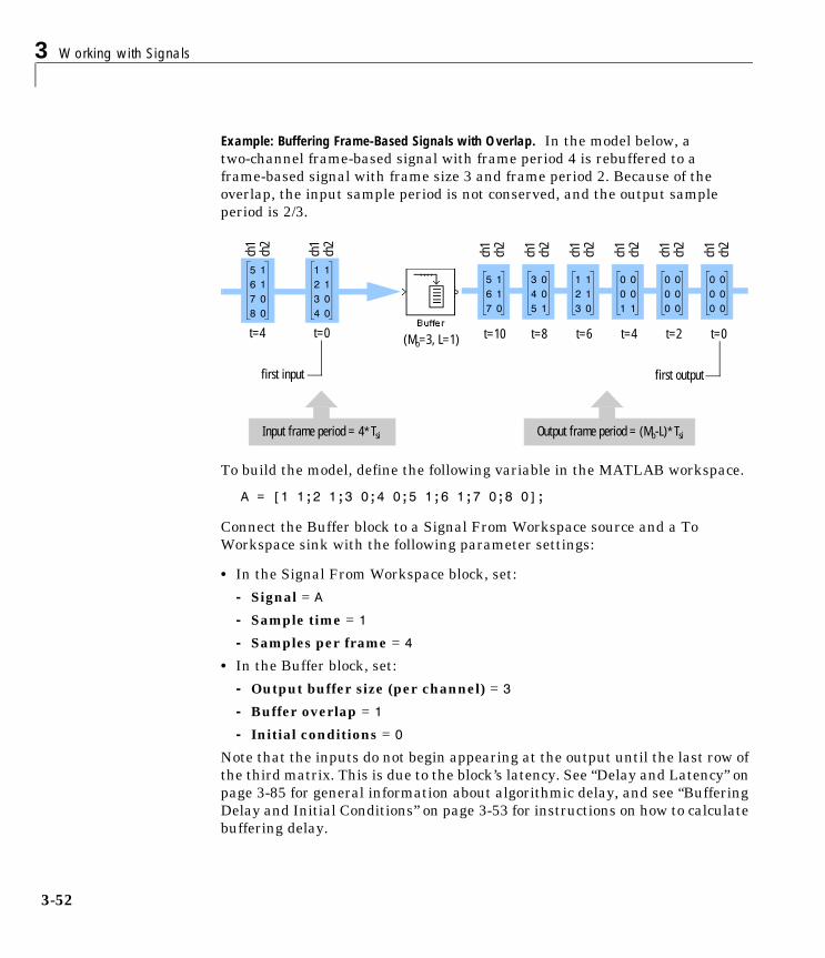
3 Working with Signals
3-52
Example: Buffering Frame-Based Signals with Overlap. In the model below, a two-channel frame-based signal with frame period 4 is rebuffered to a frame-based signal with frame size 3 and frame period 2. Because of the overlap, the input sample period is not conserved, and the output sample period is 2/3.
To build the model, define the following variable in the MATLAB workspace.
A = [1 1;2 1;3 0;4 0;5 1;6 1;7 0;8 0];
Connect the Buffer block to a Signal From Workspace source and a To Workspace sink with the following parameter settings:
• In the Signal From Workspace block, set:
- Signal = A
- Sample time = 1
- Samples per frame = 4
• In the Buffer block, set:
- Output buffer size (per channel) = 3
- Buffer overlap = 1
- Initial conditions = 0
Note that the inputs do not begin appearing at the output until the last row of the third matrix. This is due to the block’s latency. See “Delay and Latency” on page 3-85 for general information about algorithmic delay, and see “Buffering Delay and Initial Conditions” on page 3-53 for instructions on how to calculate buffering delay.
1 12 13 04 0
5 16 17 08 0
(Mo=3, L=1)
first input
t=0t=4
Output frame period = (Mo-L)∗Tsi
ch2
ch1
ch2
ch1
Input frame period = 4∗Tsi
1 12 13 0
5 16 17 0
3 04 05 1
first output
t=0t=10 t=2
ch2
ch1
ch2
ch1
ch2
ch1
0 00 01 1
0 00 00 0
0 00 00 0
ch2
ch1
ch2
ch1
ch2
ch1
t=4t=6t=8

Constructing Signals
3-53
Buffering Delay and Initial Conditions. In both of the previous buffering examples the input signal is delayed by a certain number of samples. In “Example: Buffering Sample-Based Signals with Overlap” the delay is four samples. In “Example: Buffering Frame-Based Signals with Overlap” the delay is eight samples. The initial output samples adopt the value specified for the Initial condition parameter, which is zero in both examples above.
In fact, under most conditions the Buffer and Unbuffer blocks have some amount of latency. This latency depends on both the block parameter settings and Simulink’s tasking mode. You can use the rebuffer_delay function to determine the length of the block’s latency for any combination of frame size and overlap.
The syntax rebuffer_delay(f,n,m) returns the delay (in samples) introduced by the buffering and unbuffering blocks in multitasking operations, where f is the input frame size, n is the Buffer size parameter setting, and m is the Buffer overlap parameter setting.
For example, if you had run the frame-based example model in multitasking mode, you could compute the latency by entering the following command at the MATLAB command line.
d = rebuffer_delay(4,3,1)
d = 8
This agrees with the block’s output in that example. See “Delay and Latency” on page 3-85 and the “Latency” section on each block reference page for more information.

3 Working with Signals
3-54
Deconstructing SignalsMultichannel signals, represented by matrices in Simulink, are frequently used in DSP models for efficiency and compactness. An M-by-N sample-based multichannel signal represents M*N independent signals (one sample from each), whereas an M-by-N frame-based multichannel signal represents N independent channels (M consecutive samples from each). See “Multichannel Signals” on page 3-11 for more information about the matrix format.
Even though most of the DSP blocks can process multichannel signals, you may sometimes need to access just one channel or a particular range of samples in a multichannel signal. There are a variety of ways to deconstruct multichannel signals, the most common of which are explained in the following sections:
• “Deconstructing Multichannel Sample-Based Signals” on page 3-54
• “Deconstructing Multichannel Frame-Based Signals” on page 3-57
For information about constructing multichannel signals from individual sample-based or frame-based signals, see the following sections:
• “Constructing Multichannel Sample-Based Signals” on page 3-42
• “Constructing Multichannel Frame-Based Signals” on page 3-45
Deconstructing Multichannel Sample-Based SignalsA sample-based signal with M∗N channels is represented by a sequence of M-by-N matrices. (The special case of M = N = 1 represents a single-channel signal.) You can access individual channels of the multichannel signal by using the blocks in the Indexing library (in Signal Management). The following sections explain how to do this:
• “Deconstructing a Sample-Based Multichannel Signal into Multiple Independent Signals” on page 3-54
• “Deconstructing a Sample-Based Multichannel Signal into a Related Multichannel Signal” on page 3-55
Deconstructing a Sample-Based Multichannel Signalinto Multiple Independent SignalsYou can split a multichannel sample-based signal into individual sample-based signals (single-channel or multichannel) by using the Multiport Selector block

Deconstructing Signals
3-55
in the Indexing library (in Signal Management). Any subset of rows or columns can be selected for propagation to a given output port.
Example: Deconstructing to Independent Signals. In the model below, a six-channel sample-based signal (3-by-2 matrix) is deconstructed to yield three independent sample-based signals. Two of the output signals have four channels, and the third signal has two channels.
To build the model, make the following parameter settings:
• In Signal From Workspace, set Signal = randn(3,2,10)
• In Multiport Selector, set:
- Select = Rows
- Indices to output = [1 2],[1 3],3
The Indices to output setting specifies that rows 1 and 2 of the input should be reproduced at output 1, that rows 1 and 3 of the input should be reproduced at output 2, and that row 3 of the input should be reproduced alone at output 3.
See “Sample-Based Multichannel Signals” on page 3-11 for more about sample-based signals.
Deconstructing a Sample-Based Multichannel Signalinto a Related Multichannel SignalYou can select a subset of channels from a multichannel sample-based signal by using one of the following blocks in the Indexing library (in Signal Management):
• Selector (Simulink)
• Submatrix

3 Working with Signals
3-56
• Variable Selector
The next section provides an example of using the Submatrix block to extract a portion of a multichannel sample-based signal. The Submatrix block is the most versatile of the above blocks in that it allows you to make completely arbitrary channel selections.
Example: Deconstructing to a Multichannel Signal. In the model below, a 35-channel sample-based signal (5-by-7 matrix) is deconstructed to yield a sample-based signal containing only six of the original channels.
To build the model, make the following parameter settings:
• In DSP Constant, set Constant value = rand(5,7)
• In Submatrix, set:
- Row span = Range of rows
- Starting row = Index
- Starting row index = 3
- Ending row = Last
- Column span = Range of columns
- Starting column = Offset from last
- Starting column index = 1
- Ending column = Last
See “Sample-Based Multichannel Signals” on page 3-11 for more about sample-based signals.

Deconstructing Signals
3-57
Deconstructing Multichannel Frame-Based SignalsA frame-based signal with N channels and frame size M is represented by a sequence of M-by-N matrices. (The special case of N = 1 represents a single-channel signal.) There are two basic ways to deconstruct a multichannel frame-based signal:
• Split the channels into independent signals – The constituent channels of a multichannel frame-based signal can be extracted to form individual frame based signals (with the same frame rate and size) by using the Multiport Selector block in the Indexing library (in Signal Management).
• Unbuffer the samples – Multichannel frame-based signals can be unbuffered into multichannel sample-based signals using the Unbuffer block in the Buffers library (in Signal Management).
ch1 ch2 ch3 ch4
1
2
3
4
5
6
1
2
3
4
5
6
1
2
3
4
5
6
1
2
3
4
5
6
Four frame-based signals:1 channel each, 6 samples per frame
Multichannel frame-based signal:4 channels, 6 samples per frame
1
2
3
4
5
6
1
2
3
4
5
6
1
2
3
4
5
6
1
2
3
4
5
6
sig1 sig2 sig3 sig4

3 Working with Signals
3-58
The following sections explain the two methods of deconstructing multichannel frame-based signals:
• “Splitting a Multichannel Signal into Individual Signals” on page 3-58
• “Unbuffering a Frame-Based Signal into a Sample-Based Signal” on page 3-60
The final section explains how to reorder the channels in a frame-based signal without splitting the channels apart:
• “Reordering Channels in a Frame-Based Multichannel Signal” on page 3-61
Splitting a Multichannel Signal into Individual SignalsYou can split a frame-based multichannel signal into its constituent frame-based signals by using the Multiport Selector block in the Indexing library (in Signal Management).
Example: Splitting a Multichannel Frame-Based Signal. In the model below, a three-channel frame-based signal is split into a single-channel frame-based signal and a two-channel frame-based signal.
sample 6
sample 5
sample 4
sample 3
sample 2
Multichannel sample-based signal:4 channels
Multichannel frame-based signal:4 channels, 6 samples per frame
ch1 ch2 ch3 ch4
2222
3333
4444
5555
sample 1
ch1 ch2 ch3 ch4
1
2
3
4
5
6
1
2
3
4
5
6
1
2
3
4
5
6
1
2
3
4
5
6
6666
1111

Deconstructing Signals
3-59
To build the model, make the following parameter settings:
• In Signal From Workspace, set:
- Signal = [1:10;-1:-1:-10;5*ones(1,10)]'
- Samples per frame = 4
• In Multiport Selector, set:
- Select = Columns
- Indices to output = [1 3],2
The top (4-by-2) output from the Multiport Selector block contains the first and third input channels, and the bottom output contains the second input channel. The Multiport Selector block preserves the frame rate and frame size of the input as long as Select is set to Columns. See “Frame-Based Multichannel Signals” on page 3-12 for more about frame-based signals.
Note that you could also create or import the two signals by using two distinct Signal From Workspace blocks. See the following sections for more information:
• “Creating Signals Using the Signal From Workspace Block” on page 3-38
• “Importing a Multichannel Frame-Based Signal” on page 3-68
2-channel frame-based signal (top) and 1-channel frame-based signal (bottom)3-channel frame-based signal
1 1– 52 2– 53 3– 54 4– 5
1 52 53 54 5
1–
2–
3–
4–

3 Working with Signals
3-60
Unbuffering a Frame-Based Signal into a Sample-Based SignalYou can unbuffer a multichannel frame-based signal into a multichannel sample-based signal by using the Unbuffer block in the Buffers library (in Signal Management).
The Unbuffer block performs the inverse operation of the Buffer block’s “sample-based to frame-based” buffering process, and generates an N-channel sample-based output from an N-channel frame-based input. The first row in each input matrix is always the first sample-based output. In other words, the Unbuffer block unbuffers each input frame from the top down.
The sample period of the sample-based output, Tso, is related to the input frame period, Tfi, by the input frame size, Mi.
The Unbuffer block always preserves the signal’s sample period (Tso = Tsi). See “Converting Sample Rates and Frame Rates” on page 3-20 for more information about rate conversions.
Example: Unbuffering a Frame-Based Signal. In the model below, a two-channel frame-based signal is unbuffered into a two-channel sample-based signal.
To build the model, make the following parameter settings:
• In Signal From Workspace:
- Signal = [1:10;-1:-1:-10]'
- Sample time = 1
- Samples per frame = 4
Tso Tfi Mi⁄=
Four consecutive samples from a 2-channel sample-based signal
2-channel frame-based signal
1 1–
2 2–
3 3–
4 4–
[1 -1][2 -2][3 -3][4 -4]
t=4t=5t=6t=7

Deconstructing Signals
3-61
The Signal From Workspace block generates a two-channel frame based-signal with frame size 4 (because the Samples per frame parameter is set to 4). The Unbuffer block unbuffers this signal to a two-channel sample-based signal.
Note The Unbuffer block generates initial conditions (not shown in the figure above) with the value specified by the Initial conditions parameter. See the Unbuffer reference page for information about the number of initial conditions that appear in the output.
Reordering Channels in a Frame-Based Multichannel SignalUse the Permute Matrix block to swap channels in a frame-based signal.

3 Working with Signals
3-62
Importing SignalsAlthough a number of signal generation blocks are available in Simulink and the DSP Blockset, it is very common to import custom signals from the MATLAB workspace as well. The following sections explain how to do this:
• “Importing a Multichannel Sample-Based Signal” on page 3-62
• “Importing a Multichannel Frame-Based Signal” on page 3-68
• “Importing WAV Files” on page 3-71
For information about creating signals, see the following sections:
• “Creating Signals Using Constant Blocks” on page 3-33
• “Creating Signals Using Signal Generator Blocks” on page 3-36
• “Creating Signals Using the Signal From Workspace Block” on page 3-38
Importing a Multichannel Sample-Based SignalThe Signal From Workspace block in the DSP Sources library is the key block for importing sample-based signals of all dimensions from the MATLAB workspace.
The dialog box has the following parameters:
• Signal• Sample time• Samples per frame• Form output after final data value by
Use the Signal parameter to specify the name of a variable (vector, matrix, or 3-D array) in the MATLAB workspace. You can also enter any valid MATLAB expressions involving workspace variables, as long as the expressions evaluate to a vector, matrix, or 3-D array.
The Samples per frame parameter must be set to 1 for sample-based output; any value larger that 1 produces a frame-based output. See “Importing a Multichannel Frame-Based Signal” on page 3-68 for more information. The

Importing Signals
3-63
Sample-time parameter specifies the sample period of the sample-based output. See “Sample-Based Multichannel Signals” on page 3-11 for general information about sample-based signals.
The following sections explain how the Signal From Workspace generates its output:
• “Importing a Sample-Based Vector Signal” on page 3-63
• “Importing a Sample-Based Matrix Signal” on page 3-65
Importing a Sample-Based Vector SignalThe Signal From Workspace block generates a sample-based vector signal when the variable (or expression) in the Signal parameter is a matrix and Samples per frame = 1. Beginning with the first row of the matrix, the block releases a single row of the matrix to the output at each sample time. Therefore, if the Signal parameter specifies an M-by-N matrix, the output of the Signal From Workspace block is a 1-by-N matrix (row vector), representing N channels.
The figure below illustrates this for a 6-by-4 workspace matrix, A.
As the figure above suggests, the output of the Signal From Workspace block can only be a valid sample-based signal (having N independent channels) if the M-by-N workspace matrix A in fact represents N independent channels, each
sample 6
sample 5
sample 4
sample 3
sample 2
Sample-based vector signal:4 channels
MATLAB workspace matrix, A:4 channels, 6 samples each
ch1 ch2 ch3 ch4
2222
3333
4444
5555
sample 1
ch1 ch2 ch3 ch4
1
2
3
4
5
6
1
2
3
4
5
6
1
2
3
4
5
6
1
2
3
4
5
6
6666
1111

3 Working with Signals
3-64
containing M consecutive samples. In other words, the workspace matrix must be oriented so as to have the independent channels as its columns.
When the block has output all of the rows available in the specified variable, it can start again at the beginning of the signal, or simply repeat the final value (or generate zeros) until the end of the simulation. This behavior is controlled by the Form output after final data value by parameter. See the Signal From Workspace reference page for more information.
The following example illustrates how the Signal From Workspace block can be used to import a sample-based vector signal into a model.
Example: Importing a Sample-Based Vector Signal. In the model below, the Signal From Workspace creates a three-channel sample-based signal with the following data:
• Channel 1: 1, 2, 3, 4, 5,..., 100, 0, 0, 0,...
• Channel 2: -1, -2, -3, -4, -5,..., -100, 0, 0, 0,...
• Channel 3: 5, 5, 5, 5, 5,..., 0, 0, 0,...
To create the model, define the following variables at the MATLAB command line
A = [1:100;-1:-1:-100]'; % 100-by-2 matrixB = 5*ones(100,1); % 100-by-1 column vector
Matrix A represents a two-channel signal with 100 samples, and matrix B represents a one-channel signal with 100 samples.
Specify the following parameter values in the Signal From Workspace block:
• Signal = [A B]
• Sample time = 1
• Samples per frame = 1
Four consecutive samples from a 3-channel sample-based signal
[1 -1 5][2 -2 5][3 -3 5][4 -4 5]
t=0t=1t=2t=3

Importing Signals
3-65
• Form output after final data value = Setting to zero
The Signal expression [A B] uses the standard MATLAB syntax for horizontally concatenating matrices and appends column vector B to the right of matrix A. Equivalently, you could set Signal = C, and define C at the command line by
C = [A B]
The Sample time setting of 1 yields a sample-based output with sample period of 1 second. The Form output after final data value parameter setting specifies that all outputs after the third are zero.
Importing a Sample-Based Matrix SignalThe Signal From Workspace block generates a sample-based matrix signal when the variable (or expression) in the Signal parameter is a three-dimensional array and Samples per frame = 1. Beginning with the first page of the array, the block releases a single page (i.e., matrix) of the array to the output at each sample time. Therefore, if the Signal parameter specifies an M-by-N-by-P array, the output of the Signal From Workspace block is an M-by-N matrix, representing M∗N channels.
The figure below illustrates this for a 6-by-4-by-5 workspace array A.

3 Working with Signals
3-66
As the figure above suggests, the output of the Signal From Workspace block can only be a valid sample-based signal (having M∗N independent channels) if the M-by-N-by-P workspace array A in fact represents M∗N independent channels, each having P samples. In other words, the workspace array must be oriented to have time running along its third (P) dimension.
When the block has output all of the pages available in the specified array, it can start again at the beginning of the array, or simply repeat the final page (or generate zero-matrices) until the end of the simulation. This behavior is controlled by the Form output after final data value by parameter. See the Signal From Workspace reference page for more information.
The following example illustrates how the Signal From Workspace block can be used to import a sample-based matrix signal into a model.
Example: Importing a Sample-Based Matrix Signal. In the model below, the Signal From Workspace imports a four-channel sample-based signal with the following data:
• Channel 1: 1, 2, 3, 4, 5,..., 100, 0, 0, 0,...
• Channel 2: -1, -2, -3, -4, -5,..., -100, 0, 0, 0,...
5
2
2
2
2
2
5
2
2
2
2
2
5
2
2
2
2
2
5
5
5
5
5
5
4
2
2
2
2
2
4
2
2
2
2
2
4
2
2
2
2
2
4
4
4
4
4
4
3
2
2
2
2
2
3
2
2
2
2
2
3
2
2
2
2
2
3
3
3
3
3
3
2
2
2
2
2
2
2
2
2
2
2
2
2
2
2
2
2
2
2
2
2
2
2
2
sample 4
sample 3
sample 2
Sample-based matrix signal:24 channels
MATLAB workspace array, A:24 channels, 1 sample each
sample 1
1
1
1
1
1
1
1
1
1
1
1
1
1
1
1
1
1
1
1
1
1
1
1
1
4
4
2
2
2
2
4
4
2
2
2
2
4
4
4
4
4
4
4
4
4
4
4
4
3
3
2
2
2
2
3
3
2
2
2
2
3
3
3
3
3
3
3
3
3
3
3
3
2
2
2
2
2
2
2
2
2
2
2
2
2
2
2
2
2
2
2
2
2
2
2
2
1
1
1
1
1
1
1
1
1
1
1
1
1
1
1
1
1
1
1
1
1
1
1
1

Importing Signals
3-67
• Channel 3: 0, 0, 0, 0, 0,...
• Channel 4: 5, 5, 5,..., 0, 0, 0,...
To create the model, define the following variables at the MATLAB command line.
sig1 = reshape(1:100,[1 1 100]) % 1-by-1-by-100 arraysig2 = reshape(-1:-1:-100,[1 1 100]) % 1-by-1-by-100 arraysig3 = zeros(1,1,100) % 1-by-1-by-100 arraysig4 = 5*ones(1,1,100) % 1-by-1-by-100 arraysig12 = cat(2,sig1,sig2) % 1-by-2-by-100 arraysig34 = cat(2,sig3,sig4) % 1-by-2-by-100 array
A = cat(1,sig12,sig34) % 2-by-2-by-100 array
Array A represents a 4-channel signal with 100 samples.
Specify the following parameter values in the Signal From Workspace block:
• Signal = A
• Sample time = 1
• Samples per frame = 1
• Form output after final data value = Setting to zero
The Sample time and Samples per frame settings of 1 yield a sample-based output with sample period of 1 second. Each of the four elements in the matrix represents an independent channel. The Form output after final data value parameter setting specifies that all outputs after the one-hundredth are zero.
The following two sections may also be of interest:
• “Creating Signals Using the Signal From Workspace Block” on page 3-38
Four consecutive samples from a 4-channel sample-based signal
1 1–
0 52 2–
0 5
first matrix output
t=0t=1
3 3–
0 5
t=2t=3
4 4–
0 5

3 Working with Signals
3-68
• “Constructing Multichannel Sample-Based Signals” on page 3-42
Importing a Multichannel Frame-Based SignalThe Signal From Workspace in the DSP Sources library is the key block for importing frame-based signals from the MATLAB workspace.
The dialog box has the following parameters:
• Signal• Sample time• Samples per frame• Form output after final data value by
Use the Signal parameter to specify the name of a variable (vector or matrix) in the MATLAB workspace. You can also enter any valid MATLAB expressions involving workspace variables, as long as the expressions evaluate to a vector or matrix.
The Samples per frame parameter must be set to a value greater than 1 for frame-based output; a value of 1 produces sample-based output. See “Importing a Multichannel Sample-Based Signal” on page 3-62 for more information.
The Sample-time parameter specifies the sample period, Ts, of the frame-based output. The frame period of the signal is M∗Ts, where M is the value of the Samples per frame parameter. See “Frame-Based Multichannel Signals” on page 3-12 for general information about frame-based signals.
The following section explains how the Signal From Workspace generates its frame-based output.
Importing a Frame-Based Signal withthe Signal From Workspace Block The Signal From Workspace block generates a frame-based multichannel signal when the variable (or expression) in the Signal parameter is a matrix, and the Samples per frame parameter specifies a value M greater than 1.

Importing Signals
3-69
Beginning with the first M rows of the matrix, the block releases M rows of the matrix (i.e., one frame from each channel) to the output every M∗Ts seconds. Therefore, if the Signal parameter specifies a W-by-N workspace matrix, the output of the Signal From Workspace block is an M-by-N matrix representing N channels.
The figure below illustrates this for a 6-by-4 workspace matrix, A, and a frame size of 2.
As the figure above suggests, the output of the Signal From Workspace block can only be a valid frame-based signal (having N independent channels) if the W-by-N workspace matrix A in fact represents N independent channels. In other words, the workspace matrix must be oriented so as to have the independent channels as its columns.
Note Although independent channels are generally represented as columns, a single-channel signal can be represented in the workspace as either a column vector or row vector. The output from the Signal From Workspace block is a column vector in both cases.
When the block has output all of the rows available in the specified variable, it can start again at the beginning of the signal, or simply repeat the final value (or generate zeros) until the end of the simulation. This behavior is controlled
sample 5sample 6
Frame-based signal:4 channels, 2 samples per frame
MATLAB workspace matrix, A:4 channels, 6 samples each
ch1 ch2 ch3 ch4ch1 ch2 ch3 ch4
1
2
3
4
5
6
1
2
3
4
5
6
1
2
3
4
5
6
1
2
3
4
5
61
2
1
2
1
2
1
2
3
4
3
4
3
4
3
4
5
6
5
6
5
6
5
6
sample 3sample 4
sample 1sample 2

3 Working with Signals
3-70
by the Form output after final data value by parameter. See the Signal From Workspace reference page for more information.
The following example illustrates how the Signal From Workspace block is used to import a frame-based multichannel signal into a model.
Example: Importing a Frame-Based Signal. In the model below, the Signal From Workspace creates a three-channel frame-based signal with the following data:
• Channel 1: 1, 2, 3, 4, 5,..., 100, 0, 0, 0,...
• Channel 2: -1, -2, -3, -4, -5,..., -100, 0, 0, 0,...
• Channel 3: 5, 5, 5, 5, 5,..., 0, 0, 0,...
The frame size is four samples.
To create the model, define the following variables at the MATLAB command line.
A = [1:100;-1:-1:-100]'; % 100-by-2 matrixB = 5*ones(100,1); % 100-by-1 column vector
Matrix A represents a two-channel signal with 100 samples, and matrix B represents a one-channel signal with 100 samples.
Specify the following parameter values in the Signal From Workspace block:
• Signal = [A B]
• Sample time = 1
• Samples per frame = 4
• Form output after final data value = Setting to zero
Three consecutive frames from a 3-channel frame-based signal
1 1– 52 2– 53 3– 54 4– 5
9 9– 510 10– 511 11– 512 12– 5
5 5– 56 6– 57 7– 58 8– 5
t=0t=4t=8

Importing Signals
3-71
The Signal expression [A B] uses the standard MATLAB syntax for horizontally concatenating matrices and appends column vector B to the right of matrix A. Equivalently, you could set Signal = C, and define C at the command line by
C = [A B]
The Sample time setting of 1 and Samples per frame setting of 4 yield a frame-based output with sample period of 1 second and frame period of 4 seconds. The Form output after final data value parameter setting specifies that all samples after the hundredth are zero.
Importing WAV FilesThe key blocks for importing WAV audio files are:
• From Wave Device
• From Wave File
See the reference pages for complete information.

3 Working with Signals
3-72
Exporting SignalsThe To Workspace and Triggered To Workspace blocks are the primary conduits for exporting signals from a Simulink model to the MATLAB workspace. The following sections explain how to use these important blocks:
• “Exporting Multichannel Signals” on page 3-72
• “Exporting and Playing WAV Files” on page 3-79
Exporting Multichannel SignalsThe To Workspace block in the Simulink Sources library is the key block for exporting signals of all dimensions to the MATLAB workspace.
The dialog box has the following parameters:
• Variable name• Limit data points to last• Decimation• Sample time• Save format
Use the Variable name parameter to specify the workspace variable in which the output should be saved. (An existing output with the same name is overwritten.)
The Limit data points to last parameter specifies how many of the most recent output samples should be retained in the specified workspace variable. For example, if you specify Limit data points to last = 100, then even if the simulation propagates thousands of samples to the To Workspace block, only the most recent 100 samples will actually be saved in the workspace. By setting a limit on the number of saved samples, you can prevent out-of-memory errors for long-running simulations. Note, however, that the default setting for Limit data points to last is inf, which allows the workspace variable to grow indefinitely large.
The default values of 1 and -1 for the Decimation and Sample time parameters (respectively) are generally adequate for DSP models. If you want

Exporting Signals
3-73
to downsample a signal before exporting to the workspace, consider using the Downsample or FIR Decimation blocks. See “Converting Sample Rates and Frame Rates” on page 3-20 for more information about rate conversion.
The Save format parameter allows you to save the output in a variety of formats. The default is Array, which is also generally the most accessible output format. Although this format does not save a record of the sample times corresponding to the output samples, you can create such a record for a given model by selecting the Time option in the Workspace I/O panel of the Simulation Parameters dialog box. See “Performance-Related Settings” on page 2-13 for more information.
The following sections explain how the To Workspace block generates its output:
• “Exporting a Sample-Based Signal Using the To Workspace Block” on page 3-73
• “Exporting a Frame-Based Signal Using the To Workspace Block” on page 3-76
The following two sections may also be of interest:
• “Creating Signals Using the Signal From Workspace Block” on page 3-38
• “Constructing Multichannel Sample-Based Signals” on page 3-42
Exporting a Sample-Based Signal Using the To Workspace BlockRecall that a sample-based signal with M∗N channels is represented by a sequence of M-by-N matrices. (The special case of M = N = 1 represents a single-channel signal.) When the input to the To Workspace block is a sample-based signal (and the Save format parameter is set to Array), the block creates an M-by-N-by-P array in the MATLAB workspace containing the P most recent samples from each channel. The number of pages, P, is specified by the Limit data points to last parameter. The newest samples are added at the back of the array.
The figure below illustrates this for a 6-by-4 sample-based signal exported to workspace array A.

3 Working with Signals
3-74
The workspace array always has time running along its third (P) dimension. Samples are saved along the P dimension whether the input is a matrix, vector, or scalar (single channel).
The following example illustrates how the To Workspace block can be used to export a sample-based matrix signal to the MATLAB workspace.
Example: Exporting a Sample-Based Matrix Signal. In the model below, the To Workspace block exports a four-channel sample-based signal with the following data:
• Channel 1: 1, 2, 3, 4, 5,..., 100, 0, 0, 0,...
• Channel 2: -1, -2, -3, -4, -5,..., -100, 0, 0, 0,...
• Channel 3: 0, 0, 0, 0, 0,...
• Channel 4: 5, 5, 5,..., 0, 0, 0,...
The first four consecutive samples are shown in the figure.
4
2
2
2
4
4
4
2
2
2
4
4
4
4
4
4
4
4
4
4
4
4
4
4
5
2
2
2
2
2
5
2
2
2
2
2
5
2
2
2
2
2
5
5
5
5
5
5
4
2
2
2
2
2
4
2
2
2
2
2
4
2
2
2
2
2
4
4
4
4
4
4
3
2
2
2
2
2
3
2
2
2
2
2
3
2
2
2
2
2
3
3
3
3
3
3
2
2
2
2
2
2
2
2
2
2
2
2
2
2
2
2
2
2
2
2
2
2
2
2
sample 2
sample 3
1
1
1
1
1
1
1
1
1
1
1
1
1
1
1
1
1
1
1
1
1
1
1
1
3
2
2
2
3
3
3
2
2
2
3
3
3
3
3
3
3
3
3
3
3
3
3
3
2
2
2
2
2
2
2
2
2
2
2
2
2
2
2
2
2
2
2
2
2
2
2
2
1
1
1
1
1
1
1
1
1
1
1
1
1
1
1
1
1
1
1
1
1
1
1
1
sample 4
sample 1
MATLAB workspace array, A:6-by-4-by-P (24 channels)
Sample-based matrix signal:6-by-4 (24 channels)

Exporting Signals
3-75
To create the model, define the following variables at the MATLAB command line.
sig1 = reshape(1:100,[1 1 100]) % 1-by-1-by-100 arraysig2 = reshape(-1:-1:-100,[1 1 100]) % 1-by-1-by-100 arraysig3 = zeros(1,1,100) % 1-by-1-by-100 arraysig4 = 5*ones(1,1,100) % 1-by-1-by-100 arraysig12 = cat(2,sig1,sig2) % 1-by-2-by-100 arraysig34 = cat(2,sig3,sig4) % 1-by-2-by-100 array
A = cat(1,sig12,sig34) % 2-by-2-by-100 array
Array A represents a four-channel signal with 100 samples.
Specify the following parameter values in the Signal From Workspace block:
• Signal = A
• Sample time = 1
• Samples per frame = 1
• Form output after final data value = Setting to zero
Specify the following parameter values in the To Workspace block:
• Variable name = yout
• Limit data points to last = inf
• Decimation = 1
• Sample time = -1
• Save format = Array
Run the model, and look at output yout. The first four samples (pages) are shown below.
Four consecutive samples from a 4-channel sample-based signal
1 1–
0 52 2–
0 5
first matrix output
t=0t=1
3 3–
0 5
t=2t=3
4 4–
0 5

3 Working with Signals
3-76
yout(:,:,1:4)
ans(:,:,1) =
1 -1 0 5
ans(:,:,2) =
2 -2 0 5
ans(:,:,3) =
3 -3 0 5
ans(:,:,4) =
4 -4 0 5
Exporting a Frame-Based SignalUsing the To Workspace BlockRecall that a frame-based signal with N channels and frame size M is represented by a sequence of M-by-N matrices. (The special case of N = 1 represents a single-channel signal.) When the input to the To Workspace block is a frame-based signal (and the Save format parameter is set to Array), the block creates an P-by-N array in the MATLAB workspace containing the P most recent samples from each channel. The number of rows, P, is specified by the Limit data points to last parameter. The newest samples are added at the bottom of the matrix.
The figure below illustrates this for three consecutive frames of a frame-based signal (two samples per frame) exported to matrix A.

Exporting Signals
3-77
The workspace matrix always has time running along its first (P) dimension. Samples are saved along the P dimension whether the input is a matrix, vector, or scalar (single channel).
The following example illustrates how the To Workspace block can be used to export a frame-based multichannel signal to the MATLAB workspace.
Example: Exporting a Frame-Based Signal. In the model below, the To Workspace block exports a three-channel frame-based signal with the following data:
• Channel 1: 1, 2, 3, 4, 5,..., 100, 0, 0, 0,...
• Channel 2: -1, -2, -3, -4, -5,..., -100, 0, 0, 0,...
• Channel 3: 5, 5, 5, 5, 5,..., 0, 0, 0,...
sample 5sample 6
Frame-based signal:4 channels, 2 samples per frame
MATLAB workspace matrix, A:4 channels
ch1 ch2 ch3 ch4ch1 ch2 ch3 ch4
1
2
3
4
5
6
1
2
3
4
5
6
1
2
3
4
5
6
1
2
3
4
5
6
3
4
3
4
3
4
3
4
sample 3sample 4
sample 1sample 2
1
2
1
2
1
2
1
2
5
6
5
6
5
6
5
6
Three consecutive frames from a 3-channel frame-based signal
1 1– 52 2– 53 3– 54 4– 5
9 9– 510 10– 511 11– 512 12– 5
5 5– 56 6– 57 7– 58 8– 5
t=0t=4t=8

3 Working with Signals
3-78
To create the model, define the following variables at the MATLAB command line.
A = [1:100;-1:-1:-100]'; % 100-by-2 matrixB = 5*ones(100,1); % 100-by-1 column vector
Matrix A represents a two-channel signal with 100 samples, and matrix B represents a one-channel signal with 100 samples.
Specify the following parameter values in the Signal From Workspace block:
• Signal = [A B]
• Sample time = 1
• Samples per frame = 4
• Form output after final data value = Setting to zero
The Sample time setting of 1 and Samples per frame setting of 4 yield a frame-based output with sample period of 1 second and frame period of 4 seconds.
Specify the following parameter values in the To Workspace block:
• Variable name = yout
• Limit data points to last = inf
• Decimation = 1
• Sample time = -1
• Save format = Array
Run the model, and look at output yout. The first 10 samples (rows) are shown.
yout =
1 -1 5 2 -2 5 3 -3 5 4 -4 5 5 -5 5 6 -6 5 7 -7 5 8 -8 5 9 -9 5 10 -10 5

Exporting Signals
3-79
The following two sections may also be of interest:
• “Creating Signals Using the Signal From Workspace Block” on page 3-38
• “Constructing Multichannel Sample-Based Signals” on page 3-42
Exporting and Playing WAV FilesThe key blocks for exporting and playing WAV audio files are:
• To Wave Device
• To Wave File
The To Wave Device and To Wave File blocks are limited to one-channel (mono) or two-channel (stereo) inputs, selectable in the Stereo check box. See the reference pages for complete information.
The following demos may also be of interest:
• Audio Flanger – PC/Windows
• Demonstration of Audio Reverberation
• Basic LPC Speech Coding - PC/Windows

3 Working with Signals
3-80
Viewing SignalsThe following blocks in the DSP Sinks library are the key blocks for displaying signals:
• Matrix Viewer
• Spectrum Scope
• Time Scope (Simulink Scope)
• Vector Scope
The following sections provide an introduction to how these blocks are commonly used:
• “Displaying Signals in the Time-Domain” on page 3-80
• “Displaying Signals in the Frequency-Domain” on page 3-82
• “Displaying Matrices” on page 3-83
Displaying Signals in the Time-DomainThe Vector Scope block can display both time-domain and frequency-domain data. It differs from the Spectrum Scope in that it does not compute the FFT of inputs.
Example: Displaying Time-Domain DataIn the model below, two frame-based signals are simultaneously displayed on the scope.
To create the model, first load the mtlb signal.
load mtlb % Contains variables 'mtlb' and 'Fs'

Viewing Signals
3-81
Specify the following parameter values in the Signal From Workspace block:
• Signal = mtlb
• Sample time = 1
• Samples per frame = 16
• Form output after final data value = Cyclic Repetition
Specify the following parameter values in the Digital Filter Design block:
• Filter Type = Lowpass
• Design Method = FIR (Window)
• Filter Order (Specify order) = 22
• Window Specifications (Window) = Hamming
• Frequency Specifications (wc) = 0.25
• Frequency Specifications (Units) = Normalized (0 to 1)
• Magnitude Specifications (Units) = dB
Specify the following parameter values in the Scope properties pane of the Vector Scope block:
• Input domain = Time
• Time display span (number of frames) = 2
When you run the model, the Vector Scope block plots two consecutive frames of each channel at each update. You may want to set the Stop time in the Simulation Parameters dialog box to inf to allow the simulation to run longer. The following section provides a few tips for improving the display.
Improving the Appearance of the Display. You may want to alter the appearance of the scope display by making some of the following adjustments from the right-click popup menu. To access the right-click menu, click with the right mouse button anywhere in the plot region. These options are also available from the Axes and Channels menus that are visible at the top of the window when Compact display is not selected. You can make all of these changes while the simulation is running:
• Select Autoscale at any time from the right-click menu to rescale the vertical axis to best fit the most recently displayed data.

3 Working with Signals
3-82
• Select Compact display from the right-click menu to allow the scope to use all the available space in the window.
• Select CH 1 from the right-click menu, and then select Marker and “o” from the submenus, to mark the data points on the channel 1 signal with circles.
• Select CH 1 from the right-click menu, and then select Color and Blue from the submenus, to code the channel 1 signal with the color blue.
• Select CH 2 from the right-click menu, and then select Marker and Diamond from the submenus, to mark the data points on the channel 2 signal with diamonds.
Displaying Signals in the Frequency-DomainThe Spectrum Scope block can display the frequency spectra of time-domain input data. It differs from the Vector Scope by computing the FFT of inputs to transform them to the frequency domain.
Example: Displaying Frequency-Domain DataIn the model below, the frequency content of two frame-based signals is simultaneously displayed on the scope.
To create the model, first load the mtlb signal.
load mtlb % Contains variables 'mtlb' and 'Fs'
Specify the following parameter values in the Signal From Workspace block:
• Signal = mtlb
• Sample time = 1
• Samples per frame = 16
• Form output after final data value = Cyclic Repetition
Specify the following parameter values in the Digital Filter Design block:

Viewing Signals
3-83
• Filter Type = Lowpass
• Design Method = FIR (Window)
• Filter Order (Specify order) = 22
• Window Specifications (Window) = Hamming
• Frequency Specifications (wc) = 0.25
• Frequency Specifications (Units) = Normalized (0 to 1)
• Magnitude Specifications (Units) = dB
Specify the following parameter values in the Scope properties pane of the Spectrum Scope block:
• Buffer input =
• Buffer size = 128
• Buffer overlap = 64
• Specify FFT length =
• Number of spectral averages = 2
With these settings, the Spectrum Scope block buffers each input channel to a new frame size of 128 (from the original frame size of 16) with an overlap of 64 samples between consecutive frames. Because Specify FFT length is not selected, the frame size of 128 is used as the number of frequency points in the FFT. This is the number of points plotted for each channel every time the scope display is updated.
You may want to set the Stop time in the Simulation Parameters dialog box to inf to allow the simulation to run longer. See “Improving the Appearance of the Display” on page 3-81 for some tips on improving the scope display.
Displaying MatricesThe Matrix Viewer block provides general matrix display capabilities that can be used with all matrix signals (frame-based and sample-based).
Example: Displaying MatricesIn the model below, a matrix of shifted sinusoids is displayed with the Matrix Viewer block.

3 Working with Signals
3-84
To build the model, specify the following parameter values in the Sine Wave block:
• Amplitude = 1
• Frequency = 100
• Phase offset = 0:pi/64:pi
Specify the following parameter values in the Submatrix block:
• Row span = All rows
• Column span = Range of columns
• Starting column = First
• Ending column = Offset from last
• Ending column offset = 1
Specify the following parameter values in the Reshape block:
• Output dimensionality = Customize
• Output dimensions = [8,8]
Specify Colormap matrix = bone(256) in the Image properties pane of the Matrix Viewer block.
When you run the model, the Matrix Viewer displays each 8-by-8 matrix as it is received. The 256 shades in the specified bone colormap are mapped to the range of values specified by the Minimum input value and Maximum input value parameters; see colormap for more information. In this example, these values are -1.0 and 1.0 respectively, which are appropriate for the sinusoids of amplitude 1 that compose the input signal.

Delay and Latency
3-85
Delay and LatencyThere are two distinct types of delay that affect Simulink models:
• Computational delay
• Algorithmic delay
The following sections explain how you can configure Simulink to minimize both varieties of delay and increase simulation performance.
Computational DelayThe computational delay of a block or subsystem is related to the number of operations involved in executing that component. For example, an FFT block operating on a 256-sample input requires Simulink to perform a certain number of multiplications for each input frame. The actual amount of time that these operations consume (as measured in a benchmark test, for example) depends heavily on the performance of both the computer hardware and underlying software layers, such as MATLAB and the operating system. Computational delay for a particular model therefore typically varies from one computer platform to another.
The simulation time represented on a model’s status bar (which can be accessed via Simulink’s Digital Clock block) does not provide any information about computational delay. For example, according to the Simulink timer, the FFT mentioned above executes instantaneously, with no delay whatsoever. An input to the FFT block at simulation time t=25.0 is processed and output at time t=25.0, regardless of the number of operations performed by the FFT algorithm. The Simulink timer reflects only algorithmic delay (described below), not computational delay.
The next section discussed methods of reducing computational delay.
Reducing Computational DelayThere are a number of ways to reduce computational delay without actually running the simulation on faster hardware. To begin with, you should familiarize yourself with “Improving Simulation Performance and Accuracy” in the Simulink documentation, which describes some basic strategies. The section below supplements that information with several additional options for improving performance.

3 Working with Signals
3-86
A first step in improving performance is to analyze your model, and eliminate or simplify elements that are adding excessively to the computational load. Such elements might include scope displays and data logging blocks that you had put in place for debugging purposes and no longer require. In addition to these model-specific adjustments, there are a number of more general steps you can take to improve the performance of any model:
• Use frame-based processing wherever possible. It is advantageous for the entire model to be frame-based. See “Benefits of Frame-Based Processing” on page 3-14 for more information.
• Use the dspstartup file to tailor Simulink for DSP models, or manually make the adjustments described in “Performance-Related Settings” on page 2-13.
• Turn off the Simulink status bar by deselecting the Status bar option in the View menu. Simulation speed will improve, but the time indicator will not be visible.
• Run your simulation from the MATLAB command line by typing sim(gcs)
This method of launching a simulation can greatly increase the simulation speed, but also has several limitations:
- You cannot interact with the simulation (to tune parameters, for instance).
- You must press Ctrl+C to stop the simulation, or specify start and stop times.
- There are no graphics updates in M-file S-functions, which include blocks such as the frame scopes (Vector Scope, etc.).
• Use the Real-Time Workshop to generate generic real-time (GRT) code targeted to your host platform, and simulate the model using the generated executable file. See the Real-Time Workshop documentation for more information.
Algorithmic DelayAlgorithmic delay is delay that is intrinsic to the algorithm of a block or subsystem, and is independent of CPU speed. In Chapter 5, “DSP Block Reference,” and elsewhere in this guide, the algorithmic delay of a block is referred to simply as the block’s delay. It is generally expressed in terms of the number of samples by which a block’s output lags behind the corresponding

Delay and Latency
3-87
input. This delay is directly related to the time elapsed on the Simulink timer during that block’s execution.
The algorithmic delay of a particular block may depend on both the block’s parameter settings and the general Simulink settings. To simplify matters, it is helpful to categorize a block’s delay using the following levels:
• Zero algorithmic delay
• Basic algorithmic delay
• Excess algorithmic delay (tasking latency)
The following sections explain the different levels of delay, and how the simulation and parameter settings can affect the level of delay that a particular block experiences.
Zero Algorithmic DelayThe FFT block is an example of a component that has no algorithmic delay; the Simulink timer does not record any passage of time while the block computes the FFT of the input, and the transformed data is available at the output in the same time step that the input is received. There are many other blocks that have zero algorithmic delay, such as the blocks in the Matrices and Linear Algebra libraries. Each of those blocks processes its input and generates its output in a single time step.
In Chapter 5, “DSP Block Reference,” blocks are assumed to have zero delay unless otherwise indicated. In cases where a block has zero delay for one combination of parameter settings but nonzero delay for another, this is noted on the block’s reference page.
Example: Zero Algorithmic Delay. Create the model below to observe the operation of the zero-delay Normalization block.

3 Working with Signals
3-88
Use the default settings for the Normalization, Digital Clock, Mux, and To Workspace blocks, and adjust the Signal From Workspace block parameters as follows:
• Signal = 1:100
• Sample time = 1/4
• Samples per frame = 4
Select Sample-based from the Output signal menu in the Frame Status Conversion block.
Note that the current value of the Simulink timer (from the Digital Clock block) is prepended to each output frame. The frame-based signal is converted to a sample-based signal by the Frame Status Conversion so that the output in the command window will be more easily readable.
In the example, the Signal From Workspace block generates a new frame containing four samples once every second (Tfo = ¼∗4). The first few output frames are shown below.
(t=0) [ 1 2 3 4]'(t=1) [ 5 6 7 8]'(t=2) [ 9 10 11 12]'(t=3) [13 14 15 16]'(t=4) [17 18 19 20]'
When you run the simulation, the normalized output, yout, is saved in a workspace array. To convert the array to an easier-to-read matrix format, type
squeeze(yout)'
The first few samples of the result, ans, are shown below.
ans =
0 0.0333 0.0667 0.1000 0.1333 1.0000 0.0287 0.0345 0.0402 0.0460 2.0000 0.0202 0.0224 0.0247 0.0269 3.0000 0.0154 0.0165 0.0177 0.0189 4.0000 0.0124 0.0131 0.0138 0.0146
time

Delay and Latency
3-89
The first column of ans is the Simulink time provided by the Digital Clock block. You can see that the squared 2-norm of the first input,
[1 2 3 4]' ./ sum([1 2 3 4]'.^2)
appears in the first row of the output (at time t=0), the same time step that the input was received by the block. This indicates that the Normalization block has zero algorithmic delay.
Zero Algorithmic Delay and Algebraic Loops. When several blocks with zero algorithmic delay are connected in a feedback loop, Simulink may report an algebraic loop error and performance may generally suffer. You can prevent algebraic loops by injecting at least one sample of delay into a feedback loop (for example, by including an Integer Delay block with Delay > 0). See the Simulink documentation for more information about algebraic loops.
Basic Algorithmic DelayA typical example of a block that does have algorithmic delay is the Variable Integer Delay block.
The input to the Delay port of the block specifies the number of sample periods that should elapse before an input to the In port is released to the output. This value represents the block’s algorithmic delay. For example, if the input to the Delay port is a constant 3, and the sample period at both ports is 1, then a sample that arrives at the block’s In port at time t=0 is released to the output at time t=3.
Example: Basic Algorithmic Delay. Create the model shown below to observe the operation of a block with basic delay.

3 Working with Signals
3-90
Use the default settings for the Digital Clock, Mux, and To Workspace blocks, and adjust the Signal From Workspace block’s parameters to the values below:
• Signal = 1:100
• Sample time = 1
• Samples per frame = 1
Set the DSP Constant block’s Constant value parameter to 3, and set the Variable Integer Delay block’s Initial conditions parameter to -1.
Now run the simulation and look at the output, yout. The first few samples are shown below.
The first column of yout is the Simulink time provided by the Digital Clock block, and the second column is the delayed input. As expected, the input to the block at t=0 is delayed three samples, and appears as the fourth output sample, at t=3. You can also see that the first three outputs from the Variable Integer Delay block inherit the value of the block’s Initial conditions parameter, -1. This period of time, from the start of the simulation until the first input is propagated to the output, is sometimes called the initial delay of the block.
Many blocks in the DSP Blockset have some degree of fixed or adjustable algorithmic delay. These include any blocks whose algorithms rely on delay or storage elements, such as filters or buffers. Often (but not always), such blocks provide an Initial conditions parameter that allows you to specify the output values generated by the block during the initial delay. In other cases, the initial conditions are internally fixed at 0.
Consult “DSP Block Reference” on page 5-1 for the delay characteristics of particular DSP blocks.
yout =
0 -1 1 -1 2 -1 3 1 4 2 5 3
time

Delay and Latency
3-91
Excess Algorithmic Delay (Tasking Latency)Under certain conditions, Simulink may force a block to delay inputs longer than is strictly required by the block’s algorithm. This excess algorithmic delay is called tasking latency, because it arises from synchronization requirements of Simulink’s tasking mode. A block’s overall algorithmic delay is the sum of its basic delay and tasking latency.
Algorithmic delay = Basic algorithmic delay + Tasking latency
The tasking latency for a particular block may be dependent on the following block and model characteristics:
• Simulink tasking mode
• Block rate type
• Model rate type
• Block sample mode
Simulink Tasking Mode. Simulink has two tasking modes:
• Single-tasking
• Multitasking
Select a mode by choosing SingleTasking or MultiTasking from the Mode pop-up menu in the Solver panel of the Simulation Parameters dialog box. The Mode pop-up menu is only available when the Fixed-step option is selected from the Type pop-up menu. (When the Variable-step option is selected from the Type pop-up menu, Simulink always operates in single-tasking mode.) The Auto option in the Mode pop-up menu automatically selects single-tasking operation if the model is single-rate (see below), or multitasking operation if the model is multirate.
Many multirate blocks have reduced latency in Simulink’s single-tasking mode; check the “Latency” section of a multirate block’s reference page for details. Also see “The Simulation Parameters Dialog Box” in the Simulink documentation for more information about the tasking modes and other simulation options.
Block Rate Type. A block is called single-rate when all of its input and output ports operate at the same frame rate (as indicated by identical Probe block measurements or sample time color coding on the input and output lines). A

3 Working with Signals
3-92
block is called multirate when at least one input or output port has a different frame rate than the others.
Many blocks are permanently single-rate, which means that all input and output ports always have the same frame rate. For other blocks, the block parameter settings determine whether the block is single-rate or multirate. Only multirate blocks are subject to tasking latency.
Note Simulink may report an algebraic loop error if it detects a feedback loop composed entirely of multirate blocks. To break such an algebraic loop, insert a single-rate block with nonzero delay, such as a Unit Delay block. For more information about algebraic loops, see “Algebraic Loops” in the Simulink documentation.
Model Rate Type. When all ports of all blocks in a model operate at a single frame rate, the model is called single-rate. When the model contains blocks with differing frame rates, or at least one multirate block, the model is called multirate. Note that Simulink prevents a single-rate model from running in multitasking mode by generating an error.
Block Sample Mode. Many blocks can operate in either sample-based or frame-based modes. In source blocks, the mode is usually determined by the Samples per frame parameter; a value of 1 for this parameter indicates sample-based mode, while a value greater than 1 indicates frame-based mode. In nonsource blocks, the sample mode is determined by the input signal. See Chapter 5, “DSP Block Reference,” for additional information on particular blocks.
Predicting Tasking LatencyThe specific amount of tasking latency created by a particular combination of block parameter and simulation settings is described in the “Latency” section of the reference page for the block in question. The following examples show how to use Chapter 5, “DSP Block Reference,” to predict tasking latency:
• “Example: Nonzero Tasking Latency” on page 3-93
• “Example: Zero Tasking Latency” on page 3-95

Delay and Latency
3-93
Example: Nonzero Tasking Latency. Most multirate blocks experience tasking latency only in Simulink’s multitasking mode. As an example, consider the following model.
To engage Simulink’s multitasking mode, adjust the following settings in the Solver panel of the Simulation Parameters dialog box:
• Type = Fixed-step
• Mode = MultiTasking
Use the default settings for the Mux and To Workspace blocks. Adjust the other blocks’ parameter settings as follows:
• Set the Signal From Workspace block’s parameters to the values below.
- Signal = 1:100
- Sample time = 1/4
- Samples per frame = 4
• Set the Upsample block’s parameters to the values below. The Maintain input frame size setting of the Frame-based mode parameter makes the block (and model) multirate since the input and output frame rates will not be equal.
- Upsample factor = 4
- Sample offset = 0
- Initial condition = -1
- Frame-based mode = Maintain input frame size
• Set the Sample time parameter of the Digital Clock block to 0.25 to match the sample period of the Upsample block’s output.

3 Working with Signals
3-94
• Set the Output signal parameter of the Frame Status Conversion block to Sample-based.
Notice that the current value of the Simulink timer (from the Digital Clock block) is prepended to each output frame. The frame-based signal is converted to a sample-based signal by the Frame Status Conversion block so that the output in the command window will be easily readable.
In the example, the Signal From Workspace block generates a new frame containing four samples once every second (Tfo = ¼∗4). The first few output frames are shown below.
(t=0) [ 1 2 3 4](t=1) [ 5 6 7 8](t=2) [ 9 10 11 12](t=3) [13 14 15 16](t=4) [17 18 19 20]
The Upsample block upsamples the input by a factor of 4, inserting three zeros between each input sample. The change in rates is confirmed by the Probe blocks in the model, which show a decrease in the frame period from Tfi = 1 to Tfo = 0.25.
Question: When does the first input sample appear in the output?
The “Latency and Initial Conditions” section of the reference page for the Upsample block indicates that when Simulink is in multitasking mode, the first sample of the block’s frame-based input appears in the output as sample MiL+D+1, where Mi is the input frame size, L is the Upsample factor, and D is the Sample offset. This formula therefore predicts that the first input in this example should appear as output sample 17 (i.e., 4∗4+0+1).
To verify this, look at the output from the simulation, saved in the workspace array yout. To convert the array to a easier-to-read matrix format, type
squeeze(yout)'
The first few samples of the result, ans, are shown below.

Delay and Latency
3-95
The first column of yout is the Simulink time provided by the Digital Clock block. The four values to the right of each time are the values in the output frame at that time. You can see that the first sample in each of the first four output frames inherits the value of the block’s Initial conditions parameter. As a result of the tasking latency, the first input value appears only as the first sample of the 5th output frame (at t=1), which is sample 17.
Example: Zero Tasking Latency. Now try the previous example in Simulink’s single-tasking mode. The model and all of the block parameter settings are the same.
To engage Simulink’s single-tasking mode, adjust the following settings in the Solver panel of the Simulation Parameters dialog box:
• Type = Fixed-step
• Mode = SingleTasking
When does the first input sample appear in the output?
time
ans =
0 -1.0000 0 0 0 0.2500 -1.0000 0 0 0 0.5000 -1.0000 0 0 0 0.7500 -1.0000 0 0 0 1.0000 1.0000 0 0 0 1.2500 2.0000 0 0 0 1.5000 3.0000 0 0 0 1.7500 4.0000 0 0 0 2.0000 5.0000 0 0 0
1st output frame
5th output frame

3 Working with Signals
3-96
The “Latency and Initial Conditions” section of the reference page for Upsample indicates that the block has zero latency for all multirate operations in Simulink’s single-tasking mode. To verify this, look at the output from the simulation, squeeze(yout)'. The first few samples are shown below.
The first column of yout is the Simulink time provided by the Digital Clock block. The four values to the right of each time are the values in the output frame at that time.
You can see that the first input value appears as the first sample of the first output frame (at t=0), as expected for zero-latency operation. Running this model under Simulink’s single-tasking mode therefore eliminates the 17-sample delay that the model experiences under Simulink’s multitasking mode (for the particular parameter settings in the example).
time
ans =
0 1.0000 0 0 0 0.2500 2.0000 0 0 0 0.5000 3.0000 0 0 0 0.7500 4.0000 0 0 0 1.0000 5.0000 0 0 0 1.2500 6.0000 0 0 0 1.5000 7.0000 0 0 0 1.7500 8.0000 0 0 0 2.0000 9.0000 0 0 0
1st output frame
5th output frame
4
DSP Operations
Overview . . . . . . . . . . . . . . . . . . . . . 4-2
Filters . . . . . . . . . . . . . . . . . . . . . . . 4-3
Transforms . . . . . . . . . . . . . . . . . . . . 4-10
Power Spectrum Estimation . . . . . . . . . . . . . 4-15
Linear Algebra . . . . . . . . . . . . . . . . . . . 4-16
Statistics . . . . . . . . . . . . . . . . . . . . . 4-21DSP Blockset Demos Overview . . . . . . . . . . . 4-24

4 DSP Operations
4-2
OverviewThis chapter discusses some basic DSP operations, and how they can be implemented using the DSP Blockset. The following topics are covered:
• “Filters”
• “Transforms”
• “Power Spectrum Estimation”
• “Linear Algebra”
• “Statistics”
The discussion and examples included in these sections should help you become familiar with the standard operations involved in simulating DSP models. See Chapter 3, “Working with Signals” for more basic information on sample rates, matrices, and frame-based processing.
A final section, “DSP Blockset Demos Overview” on page 4-24, provides a look at the demonstration models that accompany the DSP Blockset.

Filters
4-3
Filters Filtering is one of the most important operations in signal processing, and is supported in the DSP Blockset with three libraries of filtering blocks. The following sections present a brief overview of these libraries:
• “Adaptive Filters” on page 4-3
• “Filter Designs” on page 4-4
• “Multirate Filters” on page 4-9
All libraries are located within the top-level Filtering library.
Adaptive FiltersAdaptive filters are filters whose transfer function coefficients or taps change over time in response to an external error signal. The Adaptive Filters library contains the following blocks:
• Kalman Adaptive Filter
• LMS Adaptive Filter
• RLS Adaptive Filter
The DSP Blockset provides a collection of adaptive filtering demos to illustrate typical applications of these blocks:
• LMS Adaptive Equalization (lmsadeq)
• LMS Adaptive Linear Prediction (lmsadlp)
• LMS Adaptive Noise Cancellation (lmsdemo)
• LMS Adaptive Time-Delay Estimation (lmsadtde)
• Nonstationary Channel Estimation (kalmnsce)
• RLS Adaptive Noise Cancellation (rlsdemo)
Open the demos by clicking on the demo names above in the MATLAB Help browser. Alternatively, open the demos by typing the demo name (provided in parentheses above) at the MATLAB command line.

4 DSP Operations
4-4
Filter DesignsFilter Designs library blocks apply specified filters to an input signal and output the result. Depending on the block, you specify a filter with its filter coefficients, or by setting filter specification parameters. The following table categorizes Filter Designs library blocks by the types of filters they implement.
Filter Designs Library Blocks: Categorization and Description
Analog Filter Blocks
Analog Filter Design Implements a variety of non-time-varying time-domain analog filters.
Digital Non-Time-Varying Time-Domain Filter Blocks
Digital Filter Design Implements a variety of digital FIR and IIR filters. You specify the filter using the Filter Design and Analysis Tool (FDATool) graphical user interface.
Filter Realization Wizard Implements custom digital non-time-varying time-domain filters.
Biquadratic Filter and Direct-Form II Transpose Filter
These blocks are included in the library for backward compatibility of models using blocks from pervious DSP Blockset versions. To implement biquadratic and direct-form II transpose filters in new models, use the Digital Filter Design block.
Digital Time-Varying Time-Domain Filter Blocks
Time-Varying Direct-Form II Transpose Filter
Implements a direct-form II transpose whose filter coefficients can be updated during the simulation.
Time-Varying Lattice Filter
Implements a moving average or autoregressive lattice filter whose filter reflection coefficients can be updated during the simulation.
Digital Frequency-Domain Filter Blocks
Overlap-Add FFT Filter Implements frequency-domain filters with the overlap-add method.
Overlap-Save FFT Filter Implements frequency-domain filters with the overlap-save method.

Filters
4-5
For details about a particular block, consult its reference page. Also see the rest of this section, which discuss the following topics in detail:
• “Designing Digital Filters with Direct-Form II Transposed Structures” on page 4-5
• “Designing Filters with Various Filter Structures” on page 4-6
• “Designing Continuous-Time Classical IIR Filters” on page 4-7
Designing Digital Filters with Direct-Form II Transposed StructuresThe Digital Filter Design block in the Filter Designs library integrates the Filter Design and Analysis Tool (FDATool) graphical user interface with the DSP Blockset. Double-licking this block opens the FDATool GUI, which you can use to quickly design, import, or directly specify the coefficients of a digital FIR or IIR filter. Using these coefficients, the block filters the input signal and outputs the result within Simulink.
To design a filter in FDATool, you enter the desired filter response characteristics, such as cutoff frequency and bandwidth. You can also enter the filter coefficients directly. As soon as you apply your filter changes in FDATool, the Digital Filter Design block automatically updates to implement the filter.
To learn more about the Digital Filter Design block, see the Digital Filter Design block reference page. To learn how to use FDATool, see the FDATool section of the Signal Processing Toolbox documentation.

4 DSP Operations
4-6
The FDATool GUI Opened from the Digital Filter Design Block
Designing Filters with Various Filter StructuresAny realizable filter can be represented in the time domain by a difference equation of the form
y k( ) b1u k( ) b2u k 1–( ) L bmu k m– 1–( )
a2y k 1–( )– …– any k n– 1–( )–
+ + +=

Filters
4-7
where y(k) and u(k) are, respectively, the output and input at the current time step, y(k-1) and u(k-1) are the output and input at the previous time step, and so on. The values b1, b2, ..., bm, and a2, ..., an are the filter coefficients, or taps.
Every realizable filter is therefore fundamentally a collection of multiplications, additions, and delays. The order in which these assorted operations are implemented in practice determines the filter structure (also known as the filter realization, architecture, or implementation). Implementations may differ from each other in terms of speed, memory requirements, delay, and quantization error. See “Linear System Models” in the Signal Processing Toolbox documentation for more information about common filter structures.
The Filter Designs library provides a number of blocks for designing filters with various filter structures:
• Digital Filter Design
• Filter Realization Wizard
• Overlap-Add FFT Filter
• Overlap-Save FFT Filter
• Time-Varying Direct-Form II Transpose Filter
• Time-Varying Lattice Filter
See the following demos, which make use of many of the filter structure blocks:
• Frequency Domain Filtering (olapfilt)
• LPC Analysis and Synthesis of Speech (dsplpc)
• Sample Rate Conversion (dspsrcnv)
Open the demos by clicking on the demo names above in the MATLAB Help browser. Alternatively, open the demos by typing the demo name (provided in parentheses above) at the MATLAB command line.
Designing Continuous-Time Classical IIR Filters The Analog Filter Design block designs and implements continuous-time IIR filters with standard band configurations. All of the analog filter designs let

4 DSP Operations
4-8
you specify a filter order. The other available parameters depend on the filter type and band configuration, as shown in the table below.
where:
For all of the analog filter designs, frequency parameters are in units of radians per second.
The block uses a state-space filter representation, and applies the filter using the State-Space block in the Simulink Continuous library. All of the design methods use Signal Processing Toolbox functions to design the filter:
• The Butterworth design uses the toolbox function butter.
• The Chebyshev type I design uses the toolbox function cheby1.
• The Chebyshev type II design uses the toolbox function cheby2.
• The elliptic design uses the toolbox function ellip.
The Analog Filter Design block is built on the filter design capabilities of the Signal Processing Toolbox. For more information on the filter design algorithms, see the Filter Designs section of the Signal Processing Toolbox documentation.
Configuration Butterworth Chebyshev I Chebyshev II Elliptic
Lowpass Ωp Ωp, Rp Ωs, Rs Ωp, Rp, Rs
Highpass Ωp Ωp, Rp Ωs, Rs Ωp, Rp, Rs
Bandpass Ωp1, Ωp2 Ωp1, Ωp2, Rp Ωs1, Ωs2, Rs Ωp1, Ωp2, Rp, Rs
Bandstop Ωp1, Ωp2 Ωp1, Ωp2, Rp Ωs1, Ωs2, Rs Ωp1, Ωp2, Rp, Rs
Ωp = passband edge frequencyΩp1 = lower passband edge frequencyΩp2 = upper cutoff frequencyΩs = stopband edge frequencyΩs1 = lower stopband edge frequencyΩs2 = upper stopband edge frequencyRp = passband ripple in decibelsRs = stopband attenuation in decibels

Filters
4-9
Note The Analog Filter Design block does not work with Simulink’s discrete solver, which is enabled when the discrete option is selected in the Solver panel of the Simulation Parameters dialog box. Select one of the continuous solvers (e.g., ode4) instead.
Multirate FiltersMultirate filters are those which alter the sample rate of the input signal during the filtering process. Such filters are useful in both rate conversion and filter bank applications.
The Multirate Filters library provides a number of blocks for multirate applications:
• Dyadic Analysis Filter Bank
• Dyadic Synthesis Filter Bank
• FIR Decimation
• FIR Interpolation
• FIR Rate Conversion
• Wavelet Analysis
• Wavelet Synthesis
The DSP Blockset additionally provides a number of demos that make use of the multirate filter blocks:
• Denoising (dspwdnois)
• Multistage Multirate Filtering Suite (dspmrf_menu)
• Interpolation of a Sinusoidal Signal (dspintrp)
• Sample Rate Conversion (dspsrcnv)
• Sigma-Delta A/D Converter (dspsdadc)
• Three-Channel Wavelet Transmultiplexer (dspwvtrnsmx)
• Wavelet Perfect Reconstruction Filter Bank (dspwpr1)
• Wavelet Reconstruction (dspwlet)
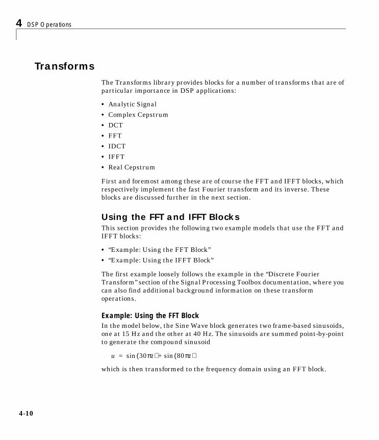
4 DSP Operations
4-10
TransformsThe Transforms library provides blocks for a number of transforms that are of particular importance in DSP applications:
• Analytic Signal
• Complex Cepstrum
• DCT
• FFT
• IDCT
• IFFT
• Real Cepstrum
First and foremost among these are of course the FFT and IFFT blocks, which respectively implement the fast Fourier transform and its inverse. These blocks are discussed further in the next section.
Using the FFT and IFFT BlocksThis section provides the following two example models that use the FFT and IFFT blocks:
• “Example: Using the FFT Block”
• “Example: Using the IFFT Block”
The first example loosely follows the example in the “Discrete Fourier Transform” section of the Signal Processing Toolbox documentation, where you can also find additional background information on these transform operations.
Example: Using the FFT BlockIn the model below, the Sine Wave block generates two frame-based sinusoids, one at 15 Hz and the other at 40 Hz. The sinusoids are summed point-by-point to generate the compound sinusoid
which is then transformed to the frequency domain using an FFT block.
u 30πt( ) 80πt( )sin+sin=

Transforms
4-11
To build the model, make the following parameter settings:
• In the Sine Wave block, set:
- Amplitude = 1
- Frequency = [15 40]
- Phase offset = 0
- Sample time = 0.001
- Samples per frame = 128
• In the Matrix Sum block, set Sum along = Rows.
• In the Complex to Magnitude-Angle block, set Output = Magnitude.
• In the Vector Scope block, set:
- Input domain = Frequency in the Scope properties panel
- Amplitude scaling = Magnitude in the Axis properties panel
• Set the Stop time in the Parameters dialog box to inf, and start the simulation by selecting Start from the Simulation menu.
The scope shows the two peaks at 0.015 and 0.04 kHz, as expected.

4 DSP Operations
4-12
Note that the three-block sequence of FFT, Complex to Magnitude-Angle, and Vector Scope could be replaced by a single Spectrum Scope block, which computes the magnitude FFT internally.
Other blocks that compute the FFT internally are the blocks in the Power Spectrum Estimation library. See “Power Spectrum Estimation” on page 4-15 for more information about these blocks.
Example: Using the IFFT BlockIn the model below, the Sine Wave block again generates two frame-based sinusoids, one at 15 Hz and the other at 40 Hz. The sinusoids are summed point-by-point to generate the compound sinusoid
which is transformed to the frequency domain using an FFT block. The frequency-domain signal is then immediately transformed back to the time domain by the IFFT block, and the difference between the original time-domain signal and transformed time-domain signal is plotted on the scope.
To build the model, make the following parameter settings (leave unlisted parameters in their default settings):
• In the Sine Wave block, set:
- Amplitude = 1
- Frequency = [15 40]
- Phase offset = 0
- Sample time = 0.001
- Samples per frame = 128
• In the Matrix Sum block, set Sum along = Rows.
• In the FFT block, set Output in bit-reversed order =
• In the IFFT block, set:
u 30πt( ) 80πt( )sin+sin=

Transforms
4-13
- Input is in bit-reversed order = - Input is conjugate symmetric =
• In the Sum block, set List of signs = |++.
• In the Gain block, set Gain = -1.
• In the Scope properties panel of the Vector Scope block, set Input domain = Time
• Set the Stop time in the Parameters dialog box to inf, and start the simulation by selecting Start from the Simulation menu.
The flat line on the scope suggests that there is no difference between the two signals, and that the IFFT block has perfectly reconstructed the original time-domain signal from the frequency-domain input.
More precisely, the two signals are identical to within round-off error, which can be seen by selecting Autoscale from the right-click menu on the scope. The enlarged trace shows that the differences between the two signals are on the order of 10-15.

4 DSP Operations
4-14

Power Spectrum Estimation
4-15
Power Spectrum EstimationThe Power Spectrum Estimation library provides a number of blocks for spectral analysis. Many of them have correlates in the Signal Processing Toolbox, which are shown in parentheses:
• Burg Method (pburg)
• Covariance Method (pcov)
• Magnitude FFT (periodogram)
• Modified Covariance Method (pmcov)
• Short-Time FFT
• Yule-Walker Method (pyulear)
See “Spectral Analysis” in the Signal Processing Toolbox documentation for an overview of spectral analysis theory and a discussion of the above methods.
The DSP Blockset provides two demos that illustrate the spectral analysis blocks:
• A Comparison of Spectral Analysis Techniques (dspsacomp)
• Spectral Analysis: Short-Time FFT (dspstfft)

4 DSP Operations
4-16
Linear AlgebraThe Matrices and Linear Algebra library provides three large sublibraries containing blocks for linear algebra:
• Linear System Solvers
• Matrix Factorizations
• Matrix Inverses
A third library, Matrix Operations, provides other essential blocks for working with matrices. See “Multichannel Signals” on page 3-11 for more information about matrix signals.
The following sections provide examples to help you get started with the linear algebra blocks:
• “Solving Linear Systems”
• “Factoring Matrices”
• “Inverting Matrices”
Solving Linear SystemsThe Linear System Solvers library provides the following blocks for solving the system of linear equations AX = B:
• Autocorrelation LPC
• Cholesky Solver
• Forward Substitution
• LDL Solver
• Levinson-Durbin
• LU Solver
• QR Solver
• SVD Solver
Some of the blocks offer particular strengths for certain classes of problems. For example, the Cholesky Solver block is particularly adapted for a square Hermitian positive definite matrix A, whereas the Backward Substitution block is particularly suited for an upper triangular matrix A.

Linear Algebra
4-17
Example: LU SolverIn the model below, the LU Solver block solves the equation Ax = b, where
and finds x to be the vector [-2 0 1]'.
To build the model, set the following parameters:
• In the DSP Constant block, set Constant value = [1 -2 3;4 0 6;2 -1 3].
• In the DSP Constant1 block, set Constant value = [1 -2 -1]'.
You can verify the solution by using the Matrix Multiply block to perform the multiplication Ax, as shown in the model below.
Factoring MatricesThe Matrix Factorizations library provides the following blocks for factoring various kinds of matrices:
• Cholesky Factorization
• LDL Factorization
• LU Factorization
A1 2– 34 0 62 1– 3
= b12–
1–
=

4 DSP Operations
4-18
• QR Factorization
• Singular Value Decomposition
Some of the blocks offer particular strengths for certain classes of problems. For example, the Cholesky Factorization block is particularly suited to factoring a Hermitian positive definite matrix into triangular components, whereas the QR Factorization is particularly suited to factoring a rectangular matrix into unitary and upper triangular components.
Example: LU FactorizationIn the model below, the LU Factorization block factors a matrix Ap into upper and lower triangular submatrices U and L, where Ap is row equivalent to input matrix A, where
To build the model, in the DSP Constant block, set the Constant value parameter to [1 -2 3;4 0 6;2 -1 3].
The lower output of the LU Factorization, P, is the permutation index vector, which indicates that the factored matrix Ap is generated from A by interchanging the first and second rows.
The upper output of the LU Factorization, LU, is a composite matrix containing the two submatrix factors, U and L, whose product LU is equal to Ap.
A1 2– 34 0 62 1– 3
=
Ap
4 0 61 2– 32 1– 3
=

Linear Algebra
4-19
You can check that LU = Ap with the Matrix Multiply block, as shown in the model below.
Inverting MatricesThe Matrix Inverses library provides the following blocks for inverting various kinds of matrices:
• Cholesky Inverse
• LDL Inverse
• LU Inverse
• Pseudoinverse
Example: LU InverseIn the model below, the LU Inverse block computes the inverse of input matrix A, where
and then forms the product A-1A, which yields the identity matrix of order 3, as expected.
U4 0 60 2– 1.50 0 0.75–
= L1 0 0
0.25 1 00.5 0.5 1
=
A1 2– 34 0 62 1– 3
=

4 DSP Operations
4-20
To build the model, in the DSP Constant block, set the Constant value parameter to [1 -2 3;4 0 6;2 -1 3].
As shown above, the computed inverse is
A 1–1– 0.5– 20 0.5 1–
0.6667 0.5 1.333–
=

Statistics
4-21
StatisticsThe Statistics library provides fundamental statistical operations such as minimum, maximum, mean, variance, and standard deviation. Most blocks in the Statistics library support two types of operations:
• Basic operations
• Running operations
The blocks listed below toggle between basic and running modes using the Running check box in the parameter dialog box:
• Histogram
• Mean
• RMS
• Standard Deviation
• Variance
An unchecked Running box means that the block is operating in basic mode, while a checked Running box means that the block is operating in running mode.
The Maximum and Minimum blocks are slightly different from the blocks above, and provide a Mode parameter in the block dialog box to select the type of operation. The Value and Index, Value, and Index options in the Mode menu all specify basic operation, in each case enabling a different set of output ports on the block. The Running option in the Mode menu selects running operation.
The following sections explain how basic mode and running mode differ:
• “Basic Operations”
• “Running Operations”
The statsdem demo illustrates the operation of several blocks from the Statistics library.
Basic OperationsA basic operation is one that processes each input independently of previous and subsequent inputs. For example, in basic mode (with Value and Index

4 DSP Operations
4-22
selected, for example) the Maximum block finds the maximum value in each column of the current input, and returns this result at the top output (Val). Each consecutive Val output therefore has the same number of columns as the input, but only one row. Furthermore, the values in a given output only depend on the values in the corresponding input. The block repeats this operation for each successive input.
This type of operation is exactly equivalent to the MATLAB command
val = max(u) % Equivalent MATLAB code
which computes the maximum of each column in input u.
The next section provides an example of a basic statistical operation.
Example: Sliding WindowsYou can use the basic statistics operations in conjunction with the Buffer block to implement basic sliding window statistics operations. A sliding window is like a stencil that you move along a data stream, exposing only a set number of data points at one time.
For example, you may want to process data in 128-sample frames, moving the window along by one sample point for each operation. One way to implement such a sliding window is shown in the model below.
The Buffer block’s Buffer size (Mo) parameter determines the size of the window. The Buffer overlap (L) parameter defines the “slide factor” for the window. At each sample instant, the window slides by Mo-L points. The Buffer overlap is often Mo-1 (the same as the Delay Line block), so that a new statistic is computed for every new signal sample.
To build the model, make the following settings:
• In the Signal From Workspace block, set:
- Signal = 1:256
- Sample time = 0.1
- Samples per frame = 1

Statistics
4-23
• In the Buffer block, set:
- Output buffer size (per channel) = 128
- Buffer overlap = 127
Running OperationsA running operation is one that processes successive sample-based or frame-based inputs, and computes a result that reflects both present and past inputs. A reset port enables you to restart this tracking at any time. The running statistic is computed for each input channel independently, so the block’s output is the same size as the input.
For example, in running mode (Running selected from the Mode parameter) the Maximum block outputs a record of the input’s maximum value over time.
The figure below illustrates how a Maximum block in running mode operates on a frame-based 3-by-2 (two-channel) matrix input, u. The running maximum is reset at t=2 by an impulse to the block’s optional Rst port.
7– 22 45 1
8 60 21– 5
3– 02 41 17
ch1
6 11 33 9
Simul
atio
n tim
e
In
ch2
Rst
0
0
1
0
ch1 ch2
Reset
Output
First outputFirst input
t=0
t=1
t=2
t=3
6 96 96 9
8 68 68 6
8 68 68 17
6 16 36 9

4 DSP Operations
4-24
DSP Blockset Demos OverviewYou can access the DSP Blockset demos by typing
demos
at the MATLAB command line. In the Demos window that opens, expand the Blocksets entry by double-clicking, and then click DSP to see the demos.
Explore all the demos to see how you can implement both basic and advanced DSP algorithms with the DSP Blockset. You can also use the demos as a base for building your own models. Simply select the section of the demo that you want to build on and copy it into your own model.
The available demos are listed below by category.
Adaptive Processing Demos• Equalization: Demonstrates adaptive channel equalization by using the
LMS algorithm to adaptively compute an estimate of an FIR equalization filter.
• Noise canceller (using either LMS or RLS): These demos use either the LMS or RLS algorithm to subtract noise from an input signal.
• Linear prediction: Uses the LMS adaptive FIR algorithm to adaptively compute the linear prediction coefficients for a noisy input signal.
• Time-delay estimation: Uses the LMS adaptive FIR algorithm to adaptively estimate the time delay for a noisy input signal.
• Tracking filter: Uses a Kalman filter to track the time-varying weights of a nonstationary fifth order FIR filter.
Audio Processing Demos• Dynamic range compression: Compresses the dynamic range of a signal by
modifying the range of the magnitude at each frequency bin. This nonlinear spectral modification is followed by an overlap-add FFT algorithm for reconstruction.
• Flanging: Introduces a “flanging” effect into a short segment of music.
• Reverberation: Uses the Integer Delay block to demonstrate the popular reverberation audio effect.

DSP Blockset Demos Overview
4-25
• LPC analysis and synthesis: Uses the Levinson solver and Time-Varying Lattice Filter for low-bandwidth transmission of speech.
• Waveform coding: This set of demos uses a variety of modulation methods to code a waveform using one bit per message sample:
- ADPCM (Adaptive Differential Pulse Code Modulation)
- CVSD (Continuously Variable Slope Delta-modulation)
- LDM (Linear Delta Modulation)
- Comparison of LDM, CVSD, and ADPCM
Communications Demos• SSB modulation: Demonstrates single sideband (SSB) modulation in
sample-based and frame-based modes.
• WWV digital receiver: WWV is the call sign of a US Government radio station that transmits frequency reference standards and time code information with a timing accuracy of 10 microseconds and a frequency accuracy of 1 part in 100 billion. This demo simulates the transmission of a WWV signal and demonstrates implementation of the subsequent receiver and decoder blocks. The receiver design serves as a simple example of the use of Simulink, DSP Blockset, Stateflow® and Real-Time Workshop.
Filtering Demos• Multirate filtering suite: Uses FIR decimation blocks in multiple stages to
filter with very short bandwidths and low computational loads.
• FIR interpolation: Uses the FIR Interpolation block to demonstrate interpolation of a delayed sine wave signal.
• Overlap add/save: Demonstrates filtering of a sinusoid using the Overlap-Add and Overlap-Save FFT blocks.
• Sample rate conversion: Illustrates the efficiency of the FIR rate conversion block by comparing the block with the equivalent process of separate upsampling, FIR filtering, and downsampling.

4 DSP Operations
4-26
Queues Demo• Demo uses a Queue block with a system of selection switches to illustrate
pushing and popping elements from a queue.
Sigma-Delta A/D Conversion Demo• Demo illustrates analog-to-digital conversion using a sigma-delta algorithm
implementation.
Sine Wave Generation Demo• Demo compares different sine wave generation systems.
Spectral Analysis Demos• Short-time FFT: Uses the Short-Time FFT block to compute and display a
spectrogram.
• Comparison of techniques: Uses the Vector Scope block to simultaneously display spectral estimates computed by the Short-Time FFT, Burg Method, and Modified Covariance Method blocks.
Statistical Functions Demo• Demo illustrates the behavior of several running-statistics blocks that are
periodically reset every 100 input samples.
Wavelets Demos• One-level PR filter bank: Uses the Dyadic Analysis and Dyadic Synthesis
blocks to implement a perfect reconstruction filter bank.
• Wavelet function: Uses a sequence of FIR interpolation blocks to reconstruct a wavelet function from filter coefficients.
• Denoising: Uses Analysis and Synthesis blocks to remove noise from an input signal.
• Wavelet transmultiplexer (WTM): Illustrates the perfect reconstruction property of the discrete wavelet transform (DWT) by using a WTM to reconstruct three independent combined signals transmitted over a single communications link.

5
DSP Block Reference
Features of the Online DSP Block Reference . . . . . 5-2Main Sections of a Block Reference Page . . . . . . . . . 5-2Ways to Access Online DSP Block Reference Pages . . . . . 5-4Running Example Code in the MATLAB Help browser . . . 5-4Running Example Models in the MATLAB Help browser . . 5-4
Blocks Supporting Code Generation . . . . . . . . . 5-6
Block Library List . . . . . . . . . . . . . . . . . 5-9Block Library Hierarchy . . . . . . . . . . . . . . . . 5-9
Block Library Contents . . . . . . . . . . . . . . . . 5-10

5 DSP Block Reference
5-2
Features of the Online DSP Block ReferenceThe online DSP Blockset block reference section contains complete information on every block in the DSP Blockset in a structured, accessible format. Use this reference section when you need to find detailed information on a particular block. See the following sections for more information:
• “Main Sections of a Block Reference Page”
- “About Tunable Parameters”
- “About Supported Data Types”
• “Ways to Access Online DSP Block Reference Pages”
• “Running Example Code in the MATLAB Help browser”
• “Running Example Models in the MATLAB Help browser”
To learn the basic concepts behind building DSP models with Simulink, see Chapter 2, “Simulink and the DSP Blockset.” To find out about using blocks together for common DSP tasks, see Chapter 3, “Working with Signals.”
Main Sections of a Block Reference PageThe block reference entries appear in alphabetical order and each contains most of the following sections.
Section Description
“Purpose” The purpose of the block.
“Library” The library or libraries where the block can be found.
“Description” A description of the block’s use.
“Dialog Box” The block’s dialog box and parameters. Tunable parameters are labeled “Tunable”. See the next section, “About Tunable Parameters” for more information.
“Supported Data Types”
The data types supported by the block. See the following section, “About Supported Data Types” for more information.
“See Also” A list of related blocks and functions.

Features of the Online DSP Block Reference
5-3
About Tunable ParametersTunable parameters are block parameters whose settings you can change or tune during a simulation. In the “Dialog Box” section of the block reference pages, these parameters are marked “Tunable” in the parameter descriptions. To tune a tunable parameter during a simulation, open the block parameters dialog, change the parameter to the desired setting, then press the OK or Apply button.
Parameters that are not labeled “Tunable” are not tunable. During a simulation, the fields, pull-down menus, and check boxes of nontunable parameters become gray and cannot be edited.
About Supported Data TypesMany DSP Blockset blocks can support all built-in data types, as well as custom data types and the fixed-point data type. To see which data types a particular block supports, check the “Supported Data Types” section of its reference page.
Note that not all blocks support all of the following data types.
Correctly Defining Custom Data Types. Custom data types are user-defined data types. You must define your custom data types by following the guidelines in the Custom Data Types section in the “Implementing Block Features” section of the “Writing S-Functions” Simulink documentation. If you do not follow the Simulink guidelines for creating custom data types, the DSP Blockset blocks will not support your custom data types.
Data Types Supported by the DSP Blockset:
• Fixed-point data type
• Custom data types
• Simulink built-in data types (and commands for casting values to these data types):
- Boolean — boolean
- Integer (8-,16-, or 32-bits) — int8, int16, int32
- Unsigned integer (8-,16-, or 32-bits) — uint8, uint16, uint32
- Single-precision floating point — single
- Double-precision floating point — double

5 DSP Block Reference
5-4
Ways to Access Online DSP Block Reference PagesThere are several ways to access the reference pages:
• Click Help in a block dialog box.
• Right-click a block in a model, and select Help from the pop-up menu.
• Right-click a block in the Simulink Library Browser, and select Help from the pop-up menu. (Open the library browser by typing simulink at the MATLAB command line.)
• Type doc('block name') at the MATLAB command line.
• Expand the DSP Blockset entry in the Help browser, and select DSP Block Reference, which is under Reference. (Open the Help browser by typing doc at the MATLAB command line.)
Running Example Code in the MATLAB Help browserWhen viewing online reference pages in the MATLAB Help browser, you can run example code without retyping it:
• Highlight the code.
• Right-click on the selection.
• Choose Evaluate Selection from the drop-down menu.
Running Example Models in the MATLAB Help browserWhen viewing online reference pages in the MATLAB Help browser, you can run example models without rebuilding them (note the models may create new variables in your workspace):

Features of the Online DSP Block Reference
5-5
• Click on indicated links to bring up example models.
• Run the models as you would run any other model.
Open the following model by clicking here in the MATLAB Help browser.

5 DSP Block Reference
5-6
Blocks Supporting Code GenerationYou can generate C code from models containing DSP Blockset blocks by using the Real-Time Workshop. All DSP Blockset blocks support generic real-time (GRT) code generation. Many blocks also support embedded real-time (ERT) code generation, as indicated in the following table. See the Real-Time Workshop documentation for more information on generating code from Simulink models.
Note All DSP Blockset blocks support generic real-time (GRT) code generation.
DSP Blockset Blocks Supporting ERT Code Generation:
Analytic Signal Autocorrelation
Biquadratic Filter Buffer
Check Signal Attributes Chirp
Complex Cepstrum Complex Exponential
Constant Diagonal Matrix Constant Ramp
Contiguous Copy Convert 1-D to 2-D
Convert 2-D to 1-D Convolution
Correlation Counter
Create Diagonal Matrix Cumulative Sum
dB Conversion dB Gain
DCT Delay Line
Difference Digital Filter Design
Direct-Form II Transpose Filter Discrete Impulse

Blocks Supporting Code Generation
5-7
Display Downsample
DSP Constant Dyadic Analysis Filter Bank
Dyadic Synthesis Filter Bank Edge Detector
Event-Count Comparator Extract Diagonal
Extract Triangular Matrix FFT
Filter Realization Wizard FIR Decimation
FIR Interpolation FIR Rate Conversion
Flip Frame Status Conversion
Histogram Identity Matrix
IFFT Inherit Complexity
Integer Delay Kalman Adaptive Filter
LMS Adaptive Filter Magnitude FFT
Matrix 1-Norm Matrix Concatenation
Matrix Multiply Matrix Product
Matrix Scaling Matrix Square
Matrix Sum Maximum
Mean Median
Minimum Multiport Selector
N-Sample Switch Normalization
Overlap-Add FFT Filter Overlap-Save FFT Filter
Pad Permute Matrix
Polynomial Evaluation Polynomial Stability Test
Quantizer Random Source
DSP Blockset Blocks Supporting ERT Code Generation:

5 DSP Block Reference
5-8
Real Cepstrum Repeat
RLS Adaptive Filter RMS
Sample and Hold Selector
Short-Time FFT Signal From Workspace
Signal To Workspace Sine Wave
Sort Standard Deviation
Submatrix Time Scope
Time-Varying Direct-Form II Transpose Filter
Time-Varying Lattice Filter
Toeplitz Transpose
Triggered Delay Line Triggered Signal From Workspace
Triggered To Workspace Unbuffer
Uniform Decoder Uniform Encoder
Unwrap Upsample
Variable Fractional Delay Variable Integer Delay
Variable Selector Variance
Wavelet Analysis Wavelet Synthesis
Window Function Zero Pad
DSP Blockset Blocks Supporting ERT Code Generation:

Block Library List
5-9
Block Library ListThis section contains the following two subsections:
• “Block Library Hierarchy” – a structured list of the DSP Blockset libraries
• “Block Library Contents” – a listing of all DSP blocks, arranged by library
See “Alphabetical List of Blocks” on page 5-18 for an alphabetical listing of blocks. The pages that follow that section contain reference information for all blocks in the DSP Blockset, arranged in alphabetical order by block name.
Block Library HierarchyThe DSP Blockset contains the following libraries and sublibraries:
• DSP Sinks
• DSP Sources
• Estimation
- Estimation: Linear Prediction
- Estimation: Parametric Estimation
- Estimation: Power Spectrum Estimation
• Filtering
- Filtering: Adaptive Filters
- Filtering: Filter Designs
- Filtering: Multirate Filter
• Math Functions
- Matrices and Linear Algebra
• Linear System Solvers
• Matrix Factorizations
• Matrix Inverses
• Matrix Operations
- Math Functions: Math Operations
- Math Functions: Polynomial Functions
• Quantizers
• Signal Management

5 DSP Block Reference
5-10
- Signal Management: Buffers
- Signal Management: Indexing
- Signal Management: Signal Attributes
- Signal Management: Switches and Counters
• Signal Operations
• Statistics
• Transforms
Use the Simulink Library Browser to access the blockset directly through the above hierarchical library list.
Block Library ContentsThe DSP blocks in each of these libraries are listed below. Simulink blocks that appear in DSP Blockset libraries (such as the Display block in DSP Sinks) are followed by the phrase “Simulink block” in parentheses.
DSP Sinks
Display (Simulink block) To Wave Device
Matrix Viewer To Wave File
Signal To Workspace Triggered To Workspace
Spectrum Scope Vector Scope
Time Scope (Simulink Block)
DSP Sources
Chirp Identity Matrix
Constant Diagonal Matrix Multiphase Clock
Constant Ramp N-Sample Enable
Counter Random Source
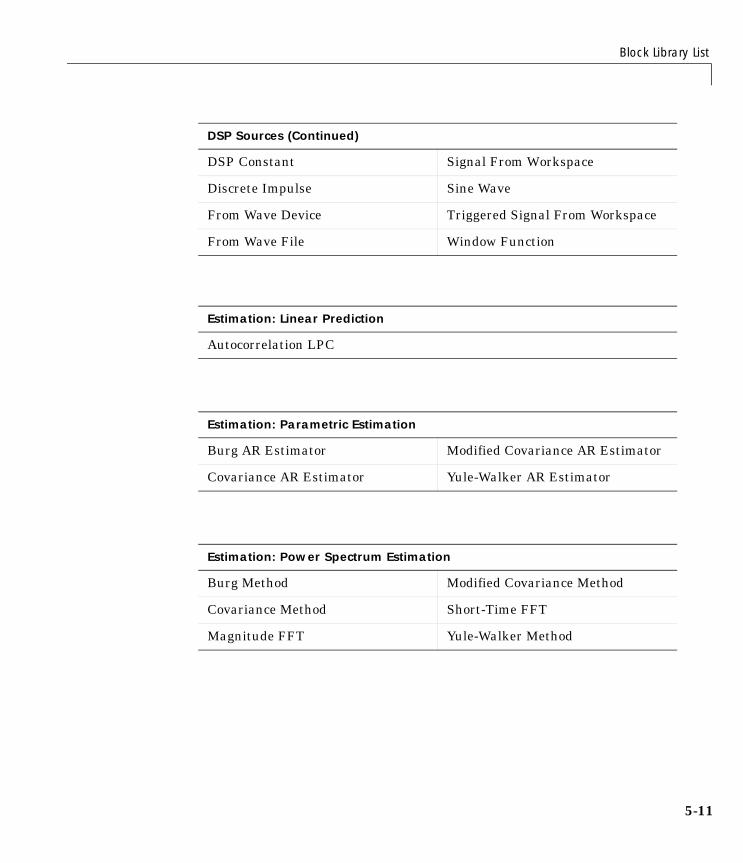
Block Library List
5-11
DSP Constant Signal From Workspace
Discrete Impulse Sine Wave
From Wave Device Triggered Signal From Workspace
From Wave File Window Function
Estimation: Linear Prediction
Autocorrelation LPC
Estimation: Parametric Estimation
Burg AR Estimator Modified Covariance AR Estimator
Covariance AR Estimator Yule-Walker AR Estimator
Estimation: Power Spectrum Estimation
Burg Method Modified Covariance Method
Covariance Method Short-Time FFT
Magnitude FFT Yule-Walker Method
DSP Sources (Continued)

5 DSP Block Reference
5-12
Filtering: Adaptive Filters
Kalman Adaptive Filter RLS Adaptive Filter
LMS Adaptive Filter
Filtering: Filter Designs
Analog Filter Design Overlap-Add FFT Filter
Biquadratic Filter Overlap-Save FFT Filter
Digital Filter Design Direct-Form II Transpose Filter
Filter Realization Wizard Time-Varying Direct-Form II Transpose Filter
Time-Varying Lattice Filter
Filtering: Multirate Filter
Dyadic Analysis Filter Bank FIR Rate Conversion
Dyadic Synthesis Filter Bank Wavelet Analysis
FIR Decimation Wavelet Synthesis
FIR Interpolation

Block Library List
5-13
Math Functions: Matrices and Linear AlgebraLinear System Solvers
Autocorrelation LPC Levinson-Durbin
Cholesky Solver LU Solver
Forward Substitution QR Solver
LDL Solver SVD Solver
Math Functions: Matrices and Linear AlgebraMatrix Factorizations
Cholesky Factorization QR Factorization
LDL Factorization Singular Value Decomposition
LU Factorization
Math Functions: Matrices and Linear AlgebraMatrix Inverses
Cholesky Inverse LU Inverse
LDL Inverse Pseudoinverse

5 DSP Block Reference
5-14
Math Functions: Matrices and Linear AlgebraMatrix Operations
Constant Diagonal Matrix Matrix Scaling
Create Diagonal Matrix Matrix Square
Extract Diagonal Matrix Sum
Extract Triangular Matrix Permute Matrix
Identity Matrix Reciprocal Condition
Matrix Concatenation (Simulink block)
Submatrix
Matrix 1-Norm Toeplitz
Matrix Multiply Transpose
Matrix Product
Math Functions: Math Operations
Complex Exponential dB Gain
Cumulative Sum Normalization
dB Conversion Difference
Math Functions: Polynomial Functions
Least Squares Polynomial Fit Polynomial Stability Test
Polynomial Evaluation

Block Library List
5-15
Quantizers
Quantizer (Simulink block) Uniform Encoder
Uniform Decoder
Signal Management: Buffers
Buffer Stack
Delay Line Triggered Delay Line
Queue Unbuffer
Signal Management: Indexing
Flip Submatrix
Multiport Selector Variable Selector
Selector (Simulink block)
Signal Management: Signal Attributes
Check Signal Attributes Convert 2-D to 1-D
Contiguous Copy Frame Status Conversion
Convert 1-D to 2-D Inherit Complexity

5 DSP Block Reference
5-16
Signal Management: Switches and Counters
Counter Multiphase Clock
Edge Detector N-Sample Enable
Event-Count Comparator N-Sample Switch
Signal Operations
Convolution Unwrap
Downsample Upsample
Integer Delay Variable Fractional Delay
Pad Variable Integer Delay
Repeat Window Function
Sample and Hold Zero Pad
Statistics
Autocorrelation Median
Correlation Minimum
Detrend RMS
Histogram Sort
Maximum Standard Deviation
Mean Variance

Block Library List
5-17
Transforms
Analytic Signal IDCT
Complex Cepstrum IFFT
DCT Real Cepstrum
FFT

Analog Filter Design
5-23
5Analog Filter DesignPurpose Design and implement an analog filter.
Library Filtering / Filter Designs
Description The Analog Filter Design block designs and implements a Butterworth, Chebyshev type I, Chebyshev type II, or elliptic filter in a highpass, lowpass, bandpass, or bandstop configuration.
The input must be a sample-based scalar signal.
The design and band configuration of the filter are selected from the Design method and Filter type pop-up menus in the dialog box. For each combination of design method and band configuration, an appropriate set of secondary parameters is displayed.
The table below lists the available parameters for each design/band combination. For lowpass and highpass band configurations, these parameters include the passband edge frequency Ωp, the stopband edge frequency Ωs, the passband ripple Rp, and the stopband attenuation Rs. For bandpass and bandstop configurations, the parameters include the lower and upper passband edge frequencies, Ωp1 and Ωp2, the lower and upper stopband edge frequencies, Ωs1 and Ωs2, the passband ripple Rp, and the stopband
Filter Design Description
Butterworth The magnitude response of a Butterworth filter is maximally flat in the passband and monotonic overall.
Chebyshev type I
The magnitude response of a Chebyshev type I filter is equiripple in the passband and monotonic in the stopband.
Chebyshev type II
The magnitude response of a Chebyshev type II filter is monotonic in the passband and equiripple in the stopband.
Elliptic The magnitude response of an elliptic filter is equiripple in both the passband and the stopband.

Analog Filter Design
5-24
attenuation Rs. Frequency values are in rad/s, and ripple and attenuation values are in dB.
The analog filters are designed using the Signal Processing Toolbox’s filter design commands buttap, cheb1ap, cheb2ap, and ellipap, and are implemented in state-space form. Filters of order 8 or less are implemented in controller canonical form for improved efficiency.
Supported Data Types
Dialog Box
The parameters displayed in the dialog box vary for different design/band combinations. Only a portion of the parameters listed below are visible in the dialog box at any one time.
Design methodThe filter design method: Butterworth, Chebyshev type I, Chebyshev type II, or Elliptic. Tunable.
Lowpass Highpass Bandpass BandstopButterworth Order, Ωp Order, Ωp Order, Ωp1, Ωp2 Order, Ωp1, Ωp2Chebyshev Type I Order, Ωp, Rp Order, Ωp, Rp Order, Ωp1, Ωp2, Rp Order, Ωp1, Ωp2, RpChebyshev Type II Order, Ωs, Rs Order, Ωs, Rs Order, Ωs1, Ωs2, Rs Order, Ωs1, Ωs2, RsElliptic Order, Ωp, Rp, Rs Order, Ωp, Rp, Rs Order, Ωp1, Ωp2, Rp, Rs Order, Ωp1, Ωp2, Rp, Rs
Double-precision floating point

Analog Filter Design
5-25
Filter typeThe type of filter to design: Lowpass, Highpass, Bandpass, or Bandstop. Tunable.
Filter orderThe order of the filter, for lowpass and highpass configurations. For bandpass and bandstop configurations, the order of the final filter is twice this value.
Passband edge frequencyThe passband edge frequency, in rad/s, for the highpass and lowpass configurations of the Butterworth, Chebyshev type I, and elliptic designs.
Lower passband edge frequencyThe lower passband frequency, in rad/s, for the bandpass and bandstop configurations of the Butterworth, Chebyshev type I, and elliptic designs.
Upper passband edge frequencyThe upper passband frequency, in rad/s, for the bandpass and bandstop configurations of the Butterworth, Chebyshev type I, or elliptic designs.
Stopband edge frequencyThe stopband edge frequency, in rad/s, for the highpass and lowpass band configurations of the Chebyshev type II design.
Lower stopband edge frequencyThe lower stopband edge frequency, in rad/s, for the bandpass and bandstop configurations of the Chebyshev type II design.
Upper stopband edge frequencyThe upper stopband edge frequency, in rad/s, for the bandpass and bandstop filter configurations of the Chebyshev type II design.
Passband ripple in dBThe passband ripple, in dB, for the Chebyshev Type I and elliptic designs.
Stopband attenuation in dBThe stopband attenuation, in dB, for the Chebyshev Type II and elliptic designs. Tunable.
Analog Filter Design
5-26
References Antoniou, A. Digital Filters: Analysis, Design, and Applications. 2nd ed. New York, NY: McGraw-Hill, 1993.
Supported Data Types
See Also
See the following sections for related information:
• “Filter Designs” on page 4-4
• “Designing Continuous-Time Classical IIR Filters” on page 4-7
Double-precision floating point
Digital Filter Design DSP Blocksetbuttap Signal Processing Toolboxcheb1ap Signal Processing Toolboxcheb2ap Signal Processing Toolboxellipap Signal Processing Toolbox

Analytic Signal
5-27
5Analytic SignalPurpose Compute the analytic signal of a discrete-time input.
Library Transforms
Description The Analytic Signal block computes the complex analytic signal corresponding to each channel of the real M-by-N input, u.
where and H⋅ denotes the Hilbert transform. The real part of the output in each channel is a replica of the real input in that channel; the imaginary part is the Hilbert transform of the input. In the frequency domain, the analytic signal retains the positive frequency content of the original signal while zeroing-out negative frequencies and doubling the DC component.
The block computes the Hilbert transform using an equiripple FIR filter with the order specified by the Filter order parameter, n. The linear phase filter is designed using the Remez exchange algorithm, and imposes a delay of n/2 on the input samples.
The output has the same dimension and frame status as the input.
Sample-Based OperationWhen the input is sample-based, each of the M∗N matrix elements represents an independent channel. Thus, the block computes the analytic signal for each channel (matrix element) over time.
Frame-Based OperationWhen the input is frame-based, each of the N columns in the matrix contains M sequential time samples from an independent channel, and the block computes the analytic signal for each channel over time.
Dialog Box
y u jH u +=
j 1–=

Analytic Signal
5-28
Filter orderThe length of the FIR filter used to compute the Hilbert transform.
Supported Data Types
Double-precision floating point

Autocorrelation
5-29
5AutocorrelationPurpose Compute the autocorrelation of a vector input.
Library Statistics
Description The Autocorrelation block computes the autocorrelation of each column (channel) in an M-by-N input matrix u. Matrix inputs must be frame-based. The result, y, is a frame-based (l+1)-by-N matrix whose jth column has elements
where ∗ denotes the complex conjugate, and l represents the maximum lag. Note that y1,j is the zero-lag element in the jth column. When All positive lags is selected, l=M. Otherwise, l is specified as a nonnegative integer by the Maximum positive lag parameter.
Input u is zero when indexed outside of its valid range. When the input is real, the output is real; otherwise, the output is complex. If the input is a sample-based vector (row, column, or 1-D), the output is sample-based, with the same shape as the input and length l+1. The Autocorrelation block does not accept a sample-based full-dimension matrix input.
The Scaling parameter controls the scaling that is applied to the output. The following options are available:
• None – Generates the raw autocorrelation, yi,j, without normalization.
• Biased – Generates the biased estimate of the autocorrelation.
• Unbiased – Generates the unbiased estimate of the autocorrelation.
• Unity at zero-lag – Normalizes the estimate of the autocorrelation for each channel so that the zero-lag sum is identically 1.
yi j, uk j,* u k i 1–+( ) j, 1 i l 1+( )≤ ≤
k 1=
M
∑=
yi j,biased yi j,
M--------=
yi j,unbiased yi j,
M i–-------------=
y1 j, 1=

Autocorrelation
5-30
Dialog Box
All positive lagsWhen selected, computes the autocorrelation over all M+1 positive lags.
Maximum positive lagThe maximum positive lag, l, for the autocorrelation. This parameter is enabled when the All positive lags check box is unselected.
ScalingThe type of scaling for the autocorrelation: None, Biased, Unbiased, or Unity at zero-lag. Tunable, except in Simulink’s external mode.
Supported Data Types
See Also
Double-precision floating point
Correlation DSP Blocksetxcorr Signal Processing Toolbox

Autocorrelation LPC
5-31
5Autocorrelation LPCPurpose Determine the coefficients of an Nth-order forward linear predictor.
Library Estimation / Linear Prediction
Description The Autocorrelation LPC block determines the coefficients of an N-step forward linear predictor for the time-series in length-M input vector, u, by minimizing the prediction error in the least-squares sense. A linear predictor is an FIR filter that predicts the next value in a sequence from the present and past inputs. This technique has applications in filter design, speech coding, spectral analysis, and system identification.
The Autocorrelation LPC block can output the prediction error as polynomial coefficients, reflection coefficients, or both. It can also output the prediction error power. The length-M input, u, can be a scalar, 1-D vector, frame- or sample-based column vector, or a sample-based row vector. Frame-based row vectors are not valid inputs.
When Inherit prediction order from input dimensions is selected, the prediction order, N, is inherited from the input dimensions. Otherwise, the Prediction order parameter sets the value of N.
When Output(s) is set to A, port A is enabled. Port A outputs an (N+1)-by-1 column vector, a = [1 a2 a3 … aN+1]T, containing the coefficients of an Nth-order moving average (MA) linear process that predicts the next value, ûM+1, in the input time-series.
When Output(s) is set to K, port K is enabled. Port K outputs a length-N column vector whose elements are the prediction error reflection coefficients. When Output(s) is set to A and K, both port A and K are enabled, and each port outputs its respective column vector of prediction coefficients. The outputs at both port A and K are always 1-D vectors.
When Output prediction error power (P) is selected, port P is enabled. The prediction error power, a scalar, is output at port P.
uM 1+ a2uM( )– a3uM 1–( )– L– aN 1+ uM N– 1+( )–=

Autocorrelation LPC
5-32
Algorithm The Autocorrelation LPC block computes the least-squares solution to
where indicates the 2-norm and
Solving the least-squares problem via the normal equations
leads to the system of equations
where r = [r1 r2 r3 … rn+1]T is an autocorrelation estimate for u computed using the Autocorrelation block, and * indicates the complex conjugate transpose. The normal equations are solved in O(n2) operations by the Levinson-Durbin block.
Ua b–a ℜn∈min
⋅
U
u1 0 L 0
u2 u1 O M
M u2 O 0
M M O u1
M M M u2
M M M M
uM M M M
0 O M M
M O O M
0 L 0 uM
, aa2
M
an 1+
, b
u2
u3
M
uM
0M
0
= = =
U*Ua U*b=
r1 r2* L rn
*
r2 r1 O M
M O O r2*
rn L r2 r1
a2
a3
M
an 1+
r2–
r3–
M
rn 1+–
=

Autocorrelation LPC
5-33
Note that the solution to the LPC problem is very closely related to the Yule-Walker AR method of spectral estimation. In that context, the normal equations above are referred to as the Yule-Walker AR equations.
Dialog Box
Output(s)The type of prediction coefficients output by the block. The block can output polynomial coefficients (A), reflection coefficients (K), or both (A and K).
Output prediction error power (P)When selected, enables port P, which outputs the output prediction error power.
Inherit prediction order from input dimensionsWhen selected, the block inherits the prediction order from the input dimensions.
Prediction order (N)The prediction order, N. This parameter is disabled when Inherit prediction order from input dimensions is selected.
References Haykin, S. Adaptive Filter Theory. 3rd ed. Englewood Cliffs, NJ: Prentice Hall, 1996.
Ljung, L. System Identification: Theory for the User. Englewood Cliffs, NJ: Prentice Hall, 1987. Pgs. 278-280.

Autocorrelation LPC
5-34
Proakis, J. and D. Manolakis. Digital Signal Processing. 3rd ed. Englewood Cliffs, NJ: Prentice-Hall, 1996.
Supported Data Types
See Also
Double-precision floating point
Autocorrelation DSP BlocksetLevinson-Durbin DSP BlocksetYule-Walker Method DSP Blocksetlpc Signal Processing Toolbox

Backward Substitution
5-35
5Backward SubstitutionPurpose Solve the equation UX=B for X when U is an upper triangular matrix.
Library Math Functions / Matrices and Linear Algebra / Linear System Solvers
Description The Backward Substitution block solves the linear system UX=B by simple backward substitution of variables, where U is the upper triangular M-by-M matrix input to the U port, and B is the M-by-N matrix input to the B port. The output is the solution of the equations, the M-by-N matrix X, and is always sample-based.
The block uses only the elements in the upper triangle of input U; the lower elements are ignored. When Force input to be unit-upper triangular is selected, the block replaces the elements on the diagonal of U with ones. This is useful when matrix U is the result of another operation, such as an LDL decomposition, that uses the diagonal elements to represent the D matrix.
A length-M vector input at port B is treated as an M-by-1 matrix.
Dialog Box
Force input to be unit-upper triangularReplaces the elements on the diagonal of U with 1s when selected. Tunable.
Supported Data Types
See Also
Double-precision floating point
Cholesky Solver DSP BlocksetForward Substitution DSP BlocksetLDL Solver DSP BlocksetLevinson-Durbin DSP BlocksetLU Solver DSP BlocksetQR Solver DSP Blockset

Backward Substitution
5-36
See “Solving Linear Systems” on page 4-16 for related information.

Biquadratic Filter
5-37
5Biquadratic FilterPurpose Apply a cascade of biquadratic (second-order section) filters to the input.
Library Filtering / Filter Designs
Description The Biquadratic Filter block applies a cascade of biquadratic filters independently to each input channel. Biquadratic filters are useful for reduced precision implementations because the coefficients are bounded between ±2 for typical minimum-phase designs. This may reduce scaling and coefficient sensitivity problems.
The filter is constructed from L second-order sections, each having a quadratic numerator and denominator.
The figure below illustrates the structure of a 4th-order biquadratic filter (L=2) with states vik, where k is the section number.
An M-by-N sample-based matrix input is treated as M∗N independent channels, and an M-by-N frame-based matrix input is treated as N independent channels. In both cases, the block filters each channel independently over time, and the output has the same size and frame status as the input.
H z( ) Hk z( )
k 1=
L
∏b1k b2kz 1– b3kz 2–+ +
a1k a2kz 1– a3kz 2–+ +----------------------------------------------------------
k 1=
L
∏= =
u(nTs)
z-1
Σ
a31
a21
b11
b21
b31
y(nTs)
Section 1, H1(z) Section 2, H2(z)
Σ
Σ
z-1
z-1
Σ
a32
a22b22
b32
Σ
Σ
z-1
v11
v21
v12
v22
b12

Biquadratic Filter
5-38
The SOS matrix parameter specifies the filter coefficients as a second-order section matrix of the type produced by the ss2sos and tf2sos functions in the Signal Processing Toolbox.
This is an L-by-6 matrix whose rows contain the numerator and denominator coefficients bik and aik of each second-order section in H(z). Use the ss2sos and tf2sos functions to convert a state-space or transfer-function description of the filter into the second-order section description used by this block. Note that the filter uses a value of 1 for the zero-delay denominator coefficients (a11 to a1L) regardless of the value specified in the SOS matrix parameter.
The Initial conditions parameter sets the initial filter states, and can be specified in the following different forms:
• Scalar to be used for all filter states (v11, v12, ..., v1L, v21 v22, ..., v2L) in all channels. An empty vector, [], is the same as the scalar value 0.
• Vector of length 2∗L (row or column) to initialize the filter states for all channels.
Each pair of elements specifies v1k and v2k for second-order section k in every channel.
• Matrix of dimension (2∗L)-by-N containing the initial filter states for each of the N channels.
b11 b21 b31 a11 a21 a31
b12 b22 b32 a12 a22 a32
M M M M M M
b1L b2L b3L a1L a2L a3L
a11 a12 …= a1L 1= = =
v11 v21 v12 v22 … v1L v2L
H1(z) H2(z) HL(z)
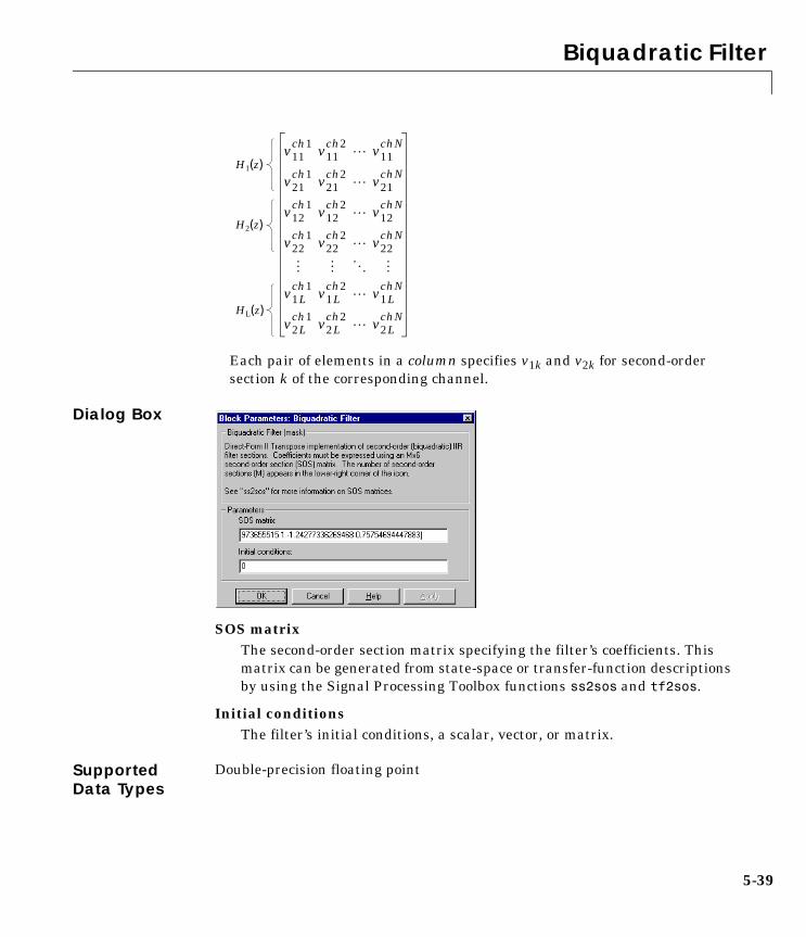
Biquadratic Filter
5-39
Each pair of elements in a column specifies v1k and v2k for second-order section k of the corresponding channel.
Dialog Box
SOS matrixThe second-order section matrix specifying the filter’s coefficients. This matrix can be generated from state-space or transfer-function descriptions by using the Signal Processing Toolbox functions ss2sos and tf2sos.
Initial conditionsThe filter’s initial conditions, a scalar, vector, or matrix.
Supported Data Types
v11ch1 v11
ch2L v11
chN
v21ch1 v21
ch2L v21
chN
v12ch1 v12
ch2L v12
chN
v22ch1 v22
ch2L v22
chN
M M O M
v1Lch1 v1L
ch2L v1L
chN
v2Lch1 v2L
ch2L v2L
chN
H1(z)
H2(z)
HL(z)
Double-precision floating point

Biquadratic Filter
5-40
See Also
See “Designing Filters with Various Filter Structures” on page 4-6 for related information.
Direct-Form II Transpose Filter DSP BlocksetFilter Realization Wizard DSP BlocksetTime-Varying Direct-Form II Transpose Filter DSP Blocksetfilter MATLABsosfilt Signal Processing Toolboxss2sos Signal Processing Toolboxtf2sos Signal Processing Toolbox

Buffer
5-41
5BufferPurpose Buffer the input sequence to a smaller or larger frame size.
Library Signal Management / Buffers
Description The Buffer block redistributes the input samples to a new frame size, larger or smaller than the input frame size. Buffering to a larger frame size yields an output with a slower frame rate than the input, as illustrated below for scalar input.
Buffering to a smaller frame size yields an output with a faster frame rate than the input, as illustrated below for scalar output.
The block coordinates the output frame size and frame rate of nonoverlapping buffers so that the sample period of the signal is the same at both the input and output, Tso = Tsi.
Sample-Based OperationSample-based inputs are interpreted by the Buffer block as independent channels of data. Thus, a sample-based length-N vector input is interpreted as N independent samples.
In sample-based operation, the Buffer block creates frame-based outputs from sample-based inputs. A sequence of sample-based length-N vector inputs (1-D, 2-D row, or 2-D column) is buffered into an Mo-by-N matrix, where Mo is specified by the Output buffer size parameter (Mo > 1). That is, each input vector becomes a row in the N-channel frame-based output matrix. When
“fast-time” input “slow-time” output(frame size = 1, sample period = Tsi) (frame size = 3, frame period = 3∗Tsi)
123456789789
456
123
“fast-time” output“slow-time” input(frame size = 1, sample period = Tsi)(frame size = 3, frame period = 3∗Tsi)
123456789789
456
123

Buffer
5-42
Mo=1, the input is simply passed through to the output, and retains the same dimension.
Sample-based full-dimension matrix inputs are not accepted.
The Buffer overlap parameter, L, specifies the number of samples (rows) from the current output to repeat in the next output, where L < Mo. For 0 ≤ L < Mo, the number of new input samples that the block acquires before propagating the buffered data to the output is the difference between the Output buffer size and Buffer overlap, Mo-L.
The output frame period is (Mo-L)∗Tsi, which is equal to the input sequence sample period, Tsi, when the Buffer overlap is Mo-1. For L < 0, the block simply discards L input samples after the buffer fills, and outputs the buffer with period (Mo-L)∗Tsi, which is longer than the zero-overlap case.
In the model below, the block buffers a four-channel sample-based input using a Output buffer size of 3 and a Buffer overlap of 1.
Note that the input vectors do not begin appearing at the output until the second row of the second matrix. This is due to the block’s latency (see “Latency” below). The first output matrix (all zeros in this example) reflects the block’s Initial conditions setting, while the first row of zeros in the second output is a result of the one-sample overlap between consecutive output frames.
4 0 5 4–
5 1 5 5–
6 1 5 6–
6 1 5 6–
t=0
t=2
t=5
t=4
t=3
t=1
first frame-based output
Tsi = 15 1 5 5–
3 0 5 3–
4 0 5 4–
2 1 5 2–
1 1 5 1–
(Mo=3, L=1)
0 0 0 01 1 5 1–
2 1 5 2–
0 0 0 00 0 0 00 0 0 0
2 1 5 2–
3 0 5 3–
4 0 5 4–
first sample-based input
t=0t=4t=6 t=2
ch4ch3
ch1ch2
ch4
ch3
ch2
ch1
Sample-based input, sample period = Tsi
Frame-based output,frame period = (Mo-L)∗Tsi
ch4
ch3
ch2
ch1
ch4
ch3
ch2
ch1

Buffer
5-43
You can use the rebuffer_delay function with a frame size of 1 to precisely compute the delay (in samples) for sample-based signals. For the above example,
d = rebuffer_delay(1,3,1)
d = 4
This agrees with the four samples of delay (zeros) per channel shown in the figure above.
Frame-Based OperationIn frame-based operation, the Buffer block redistributes the samples in the input frame to an output frame with a new size and rate. A sequence of Mi-by-N matrix inputs is buffered into a sequence of Mo-by-N frame-based matrix outputs, where Mo is the output frame size specified by the Output buffer size parameter (i.e., the number of consecutive samples from the input frame to buffer into the output frame). Mo can be greater or less than the input frame size, Mi. Each of the N input channels is buffered independently.
The Buffer overlap parameter, L, specifies the number of samples (rows) from the current output to repeat in the next output, where L < Mo. For 0 ≤ L < Mo, the number of new input samples the block acquires before propagating the buffered data to the output is the difference between the Output buffer size and Buffer overlap, Mo-L.
The input frame period is Mi∗Tsi, where Tsi is the sample period. The output frame period is (Mo-L)∗Tsi, which is equal to the sequence sample period when the Buffer overlap is Mo-1. The output sample period is therefore related to the input sample period by
Negative Buffer overlap values are not permitted.
In the model below, the block buffers a two-channel frame-based input using a Output buffer size of 3 and a Buffer overlap of 1.
TsoMo L–( )Tsi
Mo-------------------------------=

Buffer
5-44
Note that the sequence is delayed by eight samples, which is the latency of the block in Simulink’s multitasking mode for the parameter settings of this example (see “Latency” below). The first eight output samples therefore adopt the value specified for the Initial conditions, which is assumed here to be zero. Use the rebuffer_delay function to determine the block’s latency for any combination of frame size and overlap.
Latency Zero LatencyThe Buffer block has zero tasking latency in Simulink’s single-tasking mode for the following special cases:
• Scalar input and output (Mo = Mi = 1) with zero or negative Buffer overlap (L ≤ 0)
• Scalar output (Mo = 1) with zero Buffer overlap (L = 0) for any input frame size Mi
• Equal input and output frame sizes (Mo = Mi) with zero Buffer overlap (L = 0)
• Input frame size an integer multiple of the output frame size (Mi/Mo = k, for an integer value of k) with zero Buffer overlap (L = 0)
Zero tasking latency means that the first input sample (received at t=0) appears as first output sample.
1 12 13 04 0
5 16 17 08 0
(Mo=3, L=1)
first input
t=0t=4
Output frame period = (Mo-L)∗Tsi
ch2
ch1
ch2
ch1
Input frame period = 4∗Tsi
1 12 13 0
5 16 17 0
3 04 05 1
first output
t=0t=10 t=2
ch2
ch1
ch2
ch1
ch2
ch1
0 00 01 1
0 00 00 0
0 00 00 0
ch2
ch1
ch2
ch1
ch2
ch1
t=4t=6t=8

Buffer
5-45
Nonzero Latency
Sample-Based Operation. For all cases of sample-based single-tasking operation other than those listed above, the Buffer block’s buffer is initialized to the value(s) specified by the Initial conditions parameter, and the block reads from this buffer to generate the first D output samples, where
If the Buffer overlap, L, is zero, the Initial conditions parameter can be a scalar to be repeated across the first Mo output samples, or a length-Mo vector containing the values of the first Mo output samples. For nonzero Buffer overlap, the Initial conditions parameter must be a scalar.
Frame-Based Operation. For frame-based single-tasking operation and all multitasking operation, use the rebuffer_delay function to compute the exact delay (in samples) that the Buffer block introduces for a given combination of buffer size and buffer overlap.
For general buffering between arbitrary frame sizes, the Initial conditions parameter must be a scalar value, which is then repeated across all elements of the initial output(s). However, in the special case where the input is 1-by-N (and the block’s output is therefore an Mo-by-N matrix), Initial conditions can be:
• An Mo-by-N matrix
• A length-Mo vector to be repeated across all columns of the initial output(s)
• A scalar to be repeated across all elements of the initial output(s)
In the special case where the output is 1-by-N (the result of unbuffering an Mi-by-N frame-based matrix), Initial conditions can be:
• A vector containing Mi samples to output sequentially for each channel during the first Mi sample times
• A scalar to be repeated across all elements of the initial output(s)
DMo L+ L 0≥( )
Mo L 0<( )
=

Buffer
5-46
See “Excess Algorithmic Delay (Tasking Latency)” on page 3-91 and “The Simulation Parameters Dialog Box” in the Simulink documentation for more information about block rates and Simulink’s tasking modes.
Dialog Box
Output buffer sizeThe number of consecutive samples, Mo, from each channel to buffer into the output frame.
Buffer overlapThe number of samples, L, by which consecutive output frames overlap.
Initial conditionsThe value of the block’s initial output for cases of nonzero latency; a scalar, vector, or matrix.
Supported Data Types
Fixed-pointCustom data typesBoolean8-, 16-, and 32-bit signed integer 8-, 16-, and 32-bit unsigned integerSingle-precision floating point Double-precision floating point

Buffer
5-47
See Also
See “Buffering Sample-Based and Frame-Based Signals” on page 3-47 for related information.
Delay Line DSP BlocksetUnbuffer DSP Blocksetrebuffer_delay DSP Blockset

Burg AR Estimator
5-48
5Burg AR EstimatorPurpose Compute an estimate of AR model parameters using the Burg method.
Library Estimation / Parametric Estimation
Description The Burg AR Estimator block uses the Burg method to fit an autoregressive (AR) model to the input data by minimizing (least squares) the forward and backward prediction errors while constraining the AR parameters to satisfy the Levinson-Durbin recursion.
The input is a sample-based vector (row, column, or 1-D) or frame-based vector (column only) representing a frame of consecutive time samples from a single-channel signal, which is assumed to be the output of an AR system driven by white noise. The block computes the normalized estimate of the AR system parameters, A(z), independently for each successive input frame.
When Inherit estimation order from input dimensions is selected, the order, p, of the all-pole model is one less that the length of the input vector. Otherwise, the order is the value specified by the Estimation order parameter
The Output(s) parameter allows you to select between two realizations of the AR process:
• A – The top output, A, is a column vector of length p+1 with the same frame status as the input, and contains the normalized estimate of the AR model polynomial coefficients in descending powers of z,[1 a(2) ... a(p+1)]
• K – The top output, K, is a column vector of length p with the same frame status as the input, and contains the reflection coefficients (which are a secondary result of the Levinson recursion).
• A and K – The block outputs both realizations.
The scalar gain, G, is provided at the bottom output (G).
H z( ) GA z( )------------
G
1 a 2( )z 1– … a p 1+( )z p–+ + +
-------------------------------------------------------------------------------= =

Burg AR Estimator
5-49
Dialog Box
Output(s)The realization to output, model coefficients, reflection coefficients, or both.
Inherit estimation order from input dimensionsWhen selected, sets the estimation order p to one less than the length of the input vector.
Estimation orderThe order of the AR model, p. This parameter is enabled when Inherit estimation order from input dimensions is not selected.
References Kay, S. M. Modern Spectral Estimation: Theory and Application. Englewood Cliffs, NJ: Prentice-Hall, 1988.
Marple, S. L., Jr., Digital Spectral Analysis with Applications. Englewood Cliffs, NJ: Prentice-Hall, 1987.
Supported Data Types
See Also
Double-precision floating point
Burg Method DSP BlocksetCovariance AR Estimator DSP BlocksetModified Covariance AR Estimator DSP BlocksetYule-Walker AR Estimator DSP Blocksetarburg Signal Processing Toolbox

Burg Method
5-50
5Burg MethodPurpose Compute a parametric spectral estimate using the Burg method.
Library Estimation / Power Spectrum Estimation
Description The Burg Method block estimates the power spectral density (PSD) of the input frame using the Burg method. This method fits an autoregressive (AR) model to the signal by minimizing (least-squares) the forward and backward prediction errors while constraining the AR parameters to satisfy the Levinson-Durbin recursion.
The input is a sample-based vector (row, column, or 1-D) or frame-based vector (column only) representing a frame of consecutive time samples from a single-channel signal. The block’s output (a column vector) is the estimate of the signal’s power spectral density at Nfft equally spaced frequency points in the range [0,Fs), where Fs is the signal’s sample frequency.
When Inherit estimation order from input dimensions is selected, the order of the all-pole model is one less that the input frame size. Otherwise, the order is the value specified by the Estimation order parameter. The spectrum is computed from the FFT of the estimated AR model parameters.
When Inherit FFT length from input dimensions is selected, Nfft is specified by the frame size of the input, which must be a power of 2. When Inherit FFT length from input dimensions is not selected, Nfft is specified as a power of 2 by the FFT length parameter, and the block zero pads or truncates the input to Nfft before computing the FFT. The output is always sample-based.
The Burg Method and Yule-Walker Method blocks return similar results for large frame sizes. The following table compares the features of the Burg Method block to the Covariance Method, Modified Covariance Method, and Yule-Walker Method blocks.

Burg Method
5-51
Burg Covariance Modified Covariance Yule-Walker
Characteristics Does not apply window to data
Does not apply window to data
Does not apply window to data
Applies window to data
Minimizes the forward and backward prediction errors in the least-squares sense, with the AR coefficients constrained to satisfy the L-D recursion
Minimizes the forward prediction error in the least-squares sense
Minimizes the forward and backward prediction errors in the least-squares sense
Minimizes the forward prediction error in the least-squares sense(also called “Autocorrelation method”)
Advantages High resolution for short data records
Better resolution than Y-W for short data records (more accurate estimates)
High resolution for short data records
Performs as well as other methods for large data records
Always produces a stable model
Able to extract frequencies from data consisting of p or more pure sinusoids
Able to extract frequencies from data consisting of p or more pure sinusoids
Always produces a stable model
Does not suffer spectral line-splitting
Disadvantages Peak locations highly dependent on initial phase
May produce unstable models
May produce unstable models
Performs relatively poorly for short data records
May suffer spectral line-splitting for sinusoids in noise, or when order is very large
Frequency bias for estimates of sinusoids in noise
Peak locations slightly dependent on initial phase
Frequency bias for estimates of sinusoids in noise
Frequency bias for estimates of sinusoids in noise
Minor frequency bias for estimates of sinusoids in noise
Conditions for Nonsingularity
Order must be less than or equal to half the input frame size
Order must be less than or equal to 2/3 the input frame size
Because of the biased estimate, the autocorrelation matrix is guaranteed to positive-definite, hence nonsingular

Burg Method
5-52
Examples The dspsacomp demo compares the Burg method with several other spectral estimation methods.
Dialog Box
Inherit estimation order from input dimensionsWhen selected, sets the estimation order to one less than the length of the input vector. Tunable.
Estimation orderThe order of the AR model. This parameter is enabled when Inherit estimation order from input dimensions is not selected.
Inherit FFT length from input dimensionsWhen selected, uses the input frame size as the number of data points, Nfft, on which to perform the FFT. Tunable.
FFT lengthThe number of data points, Nfft, on which to perform the FFT. If Nfft exceeds the input frame size, the frame is zero-padded as needed. This parameter is enabled when Inherit FFT length from input dimensions is not selected.
References Kay, S. M. Modern Spectral Estimation: Theory and Application. Englewood Cliffs, NJ: Prentice-Hall, 1988.
Orfanidis, J. S. Optimum Signal Processing: An Introduction. 2nd ed. New York, NY: Macmillan, 1985.

Burg Method
5-53
Supported Data Types
See Also
See “Power Spectrum Estimation” on page 4-15 for related information.
Double-precision floating point
Burg AR Estimator DSP BlocksetCovariance Method DSP BlocksetModified Covariance Method DSP BlocksetShort-Time FFT DSP BlocksetYule-Walker Method DSP Blocksetpburg Signal Processing Toolbox

Check Signal Attributes
5-54
5Check Signal AttributesPurpose Generate an error when the input signal does or does not match selected attributes exactly.
Library Signal Management / Signal Attributes
Description The Check Signal Attributes block terminates the simulation with an error when the input characteristics differ from those specified by the block parameters.
When the Error if input parameter is set to Does not match attributes exactly, the block generates an error only when the input possesses none of the attributes specified by the other parameters. Signals that possess at least one of the specified attributes are propagated to the output unaltered, and do not generate an error.
When the Error if input parameter is set to Matches attributes exactly, the block generates an error only when the input possesses all attributes specified by the other parameters. Signals that do not possess all of the specified attributes are propagated to the output unaltered, and do not generate an error.
Signal AttributesThe Check Signal Attributes block can test for up to five different signal attributes, as specified by the following parameters. When Ignore is selected in any parameter, the block does not check the signal for the corresponding attribute. For example, when Complexity is set to Ignore, neither real nor complex inputs cause the block to generate an error. The attributes are:
• Complexity
Checks whether the signal is real or complex. (Note that this information can also be displayed in a model by attaching a Probe block with Probe complex signal selected, or by selecting Port data types from the model window’s Format menu.)
• Frame status
Checks whether the signal is frame-based or sample-based. (Note that Simulink displays sample-based signals using a single line, →, and frame-based signals using a double line, ⇒.)

Check Signal Attributes
5-55
• Dimensionality
Checks the dimension of signal for compliance (Is...) or noncompliance (Is not...) with the attributes in the subordinate Dimension menu, which are shown in the table below. See“Signal Dimension Nomenclature” on page 1-10 for a description of Simulink signal dimensions. M and N are positive integers unless otherwise indicated below.

Check Signal Attributes
5-56
Dimensions Is... Is not...
1-D 1-D vector,1-D scalar
M-by-N matrix,1-by-N matrix (row vector),M-by-1 matrix (column vector),1-by-1 matrix (2-D scalar)
2-D M-by-N matrix,1-by-N matrix (row vector),M-by-1 matrix (column vector),1-by-1 matrix (2-D scalar)
1-D vector,1-D scalar
Scalar
(1-D or 2-D)
1-D scalar,1-by-1 matrix (2-D scalar)
1-D vector with length>1, M-by-N matrix with M>1 and/or N>1
Vector
(1-D or 2-D)
1-D vector,1-D scalar,1-by-N matrix (row vector),M-by-1 matrix (column vector),1-by-1 matrix (2-D scalar)Vector (1-D or 2-D) or scalar
M-by-N matrix with M>1 and N>1
Row Vector
(2-D)
1-by-N matrix (row vector),1-by-1 matrix (2-D scalar)Row vector (2-D) or scalar
1-D vector,1-D scalar,M-by-N matrix with M>1
Column
Vector
(2-D)
M-by-1 matrix (column vector),1-by-1 matrix (2-D scalar)Column vector (2-D) or scalar
1-D vector,1-D scalar,M-by-N matrix with N>1

Check Signal Attributes
5-57
Note that when Signal dimensions is selected from the model window Format menu, Simulink displays the size of a 1-D vector signal as an unbracketed integer, and displays the dimension of a 2-D signal as a pair of bracketed integers, [MxN]. Simulink does not display any size information for a 1-D or 2-D scalar signal. Dimension information for a signal can also be displayed in a model by attaching a Probe block with Probe signal dimensions selected.
• Data type
Checks the signal data type for compliance (Is...) or noncompliance (Is not...) with the attributes in the subordinate General data type menu, which are shown in the table below. Any of the specific data types listed in the Is...
Full matrix M-by-N matrix with M>1 and N>1
1-D vector,1-D scalar,1-by-N matrix (row vector),M-by-1 matrix (column vector),1-by-1 matrix (2-D scalar)
Square
matrix
M-by-N matrix with M=N,1-D scalar,1-by-1 matrix (2-D scalar)
M-by-N matrix with M≠N,1-D vector,1-by-N matrix (row vector),M-by-1 matrix (column vector)
Dimensions (Continued)
Is... Is not...

Check Signal Attributes
5-58
column below can be individually selected from the subordinate Specific data type menu.
Note that data type information can also be displayed in a model by selecting Port data types from the model window’s Format menu.
• Sample mode
Checks whether the signal is discrete-time or continuous-time. (Note that when Sample time colors is selected from the Format menu, Simulink displays continuous-time signal lines in black or grey and discrete-time signal lines in colors corresponding to the relative rate. When a Probe block with Probe sample time enabled is attached to a continuous-time signal, the block icon displays the string Ts:[0 x], where x is the sample time offset. When a Probe block is attached to a discrete-time signal, the block icon displays the string Ts:[t 0] for a sample-based signal or Tf:[t 0] for a frame-based signal, where t is the nonzero sample period or frame period, respectively. Frame-based signals are almost always discrete-time.)
General data type Is... Is not...
Boolean boolean single, double, uint8, int8, uint16, int16, uint32, int32, fixed-point
Floating-point single, double boolean, uint8, int8, uint16, int16, uint32, int32, fixed-point
Fixed-point fixed-point boolean, uint8, int8, uint16, int16, uint32, int32, single, double
Integer Signed integerint8, int16, int32Unsigned integeruint8, uint16, uint32
boolean, single, double

Check Signal Attributes
5-59
Dialog Box
Error if inputSpecifies whether the block generates an error when the input possesses none of the required attributes (Does not match attributes exactly), or when the input possesses all of the required attributes (Matches attributes exactly).
ComplexityThe complexity for which the input should be checked, Real or Complex.
Frame statusThe frame status for which the input should be checked, Sample-based or Frame-based.
DimensionalitySpecifies whether the input should be checked for compliance (Is...) or noncompliance (Is not...) with the attributes in the subordinate Dimension menu.
DimensionsThe dimensions for which the input should be checked. This parameter is available when Is... or Is not... is selected in the Dimensionality menu.

Check Signal Attributes
5-60
Data typeSpecifies whether the input should be checked for compliance (Is...) or noncompliance (Is not...) with the attributes in the subordinate General data type menu.
General data typeThe general data type for which the input should be checked. This parameter is available when Is... or Is not... is selected in the Data type menu, and enables the subordinate Specific data type parameter in most cases.
Specific data typeThe specific data type for which the input should be checked. This parameter is available when Floating-point, Fixed-point, or Integer is selected in the General data type menu.
Sample modeThe sample mode for which the input should be checked, Discrete or Continuous.
Supported Data Types
See Also
Fixed-pointCustom data typesBoolean8-, 16-, and 32-bit signed integer 8-, 16-, and 32-bit unsigned integerSingle-precision floating point Double-precision floating point
Buffer DSP BlocksetConvert 1-D to 2-D DSP BlocksetConvert 2-D to 1-D DSP BlocksetData Type Conversion SimulinkFrame Status Conversion DSP BlocksetInherit Complexity DSP BlocksetProbe SimulinkReshape SimulinkSubmatrix DSP Blockset

Chirp
5-61
5ChirpPurpose Generate a swept-frequency cosine (chirp) signal.
Library DSP Sources
Description The Chirp block outputs a swept-frequency cosine (chirp) signal with unity amplitude and continuous phase. To specify the desired output chirp signal, you must define its instantaneous frequency function, also known as the output frequency sweep. The frequency sweep can be linear, quadratic, or logarithmic, and repeats once every Sweep time by default. See the following sections of this reference page for more details:
• “Variables Used in This Reference Page” on page 5-61
• “Setting the Output Frame Status” on page 5-62
• “Shaping the Frequency Sweep by Setting Frequency Sweep and Sweep Mode” on page 5-62
• “Unidirectional and Bidirectional Sweep Modes” on page 5-63
• “Setting Instantaneous Frequency Sweep Values” on page 5-64
• “Block Computation Methods” on page 5-65
• “Cautions Regarding the Swept Cosine Sweep” on page 5-67
• “Examples” on page 5-68
Variables Used in This Reference PageRefer to the following list for definitions of variables used in this reference page.
f0 Initial frequency parameter (Hz)fi(tg) Target frequency parameter (Hz)tg Target time parameter (seconds)Tsw Sweep time parameter (seconds)
Initial phase parameter (radians)Phase of the chirp signal (radians)
fi(t) User-specified output instantaneous frequency function (Hz); user-specified sweep
fi(actual)(t) Actual output instantaneous frequency function (Hz); actual output sweep
ychirp(t) Output chirp function
φ0ψ t( )
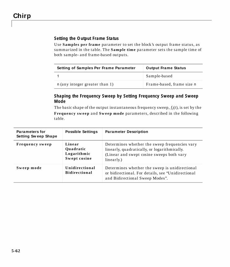
Chirp
5-62
Setting the Output Frame StatusUse Samples per frame parameter to set the block’s output frame status, as summarized in the table. The Sample time parameter sets the sample time of both sample- and frame-based outputs.
Shaping the Frequency Sweep by Setting Frequency Sweep and Sweep ModeThe basic shape of the output instantaneous frequency sweep, fi(t), is set by the Frequency sweep and Sweep mode parameters, described in the following table.
Setting of Samples Per Frame Parameter Output Frame Status
1 Sample-based
n (any integer greater than 1) Frame-based, frame size n
Parameters for Setting Sweep Shape
Possible Settings Parameter Description
Frequency sweep LinearQuadraticLogarithmicSwept cosine
Determines whether the sweep frequencies vary linearly, quadratically, or logarithmically. (Linear and swept cosine sweeps both vary linearly.)
Sweep mode UnidirectionalBidirectional
Determines whether the sweep is unidirectional or bidirectional. For details, see “Unidirectional and Bidirectional Sweep Modes”.

Chirp
5-63
The following diagram illustrates the possible shapes of the frequency sweep that you can obtain by setting the Frequency sweep and Sweep mode parameters.
For information on how to set the frequency values in your sweep, see “Setting Instantaneous Frequency Sweep Values”.
Unidirectional and Bidirectional Sweep ModesThe Sweep mode parameter determines whether your sweep is unidirectional or bidirectional, which affects the shape of your output frequency sweep (see “Shaping the Frequency Sweep by Setting Frequency Sweep and Sweep Mode”
...time
fi(t)
Negative Sweeps
Quadratic and Logarithmic Sweeps
Un
idir
ecti
onal
( fi(tg) < f0 )
...time
fi(t)
...time
fi(t)
...time
fi(t)
...time
fi(t)
...time
fi(t)
...time
fi(t)
...time
fi(t)
(Logarithmic sweeps cannot be negative.)
These diagrams applyonly to quadratic sweeps.
Possible Shapes of the Output Instantaneous Frequency Sweep
Positive Sweeps( fi(tg) > f0 )
Sw
eep
sB
idir
ecti
onal
Sw
eep
s
Negative SweepsPositive Sweeps
Swept Cosine and Linear Sweeps
Tsw Tsw Tsw
Tsw Tsw
Tsw
TswTsw

Chirp
5-64
on page 5-62). The following table describes the characteristics of unidirectional and bidirectional sweeps.
The following diagram illustrates a linear sweep in both sweep modes. For information on setting the frequency values in your sweep, see “Setting Instantaneous Frequency Sweep Values”.
Setting Instantaneous Frequency Sweep ValuesSet the following parameters to tune the frequency values of your output frequency sweep:
• Initial frequency (Hertz), f0
Sweep mode Parameter Settings
Sweep Characteristics
Unidirectional • Lasts for one Sweep time, Tsw
• Repeats once every Tsw
Bidirectional • Lasts for twice the Sweep time, 2*Tsw
• Repeats once every 2*Tsw
• First half is identical to its unidirectional counterpart.
• Second half is a mirror image of the first half.
0
fi(t)
f0Tsw
...
Unidirectional Linear Sweep
0
fi(t)
f0
...
Bidirectional Linear Sweep
fi(tg)tg
fi(tg)
2Tsw
tg Tsw 2Tsw 3Tsw 4Tsw
time
time
Lasts for 2*TswLasts for Tsw
Repeats every Tsw
Repeats every 2*Tsw
Second half is mirror image of first half.
First half is identical to its unidirectional counterpart.

Chirp
5-65
• Target frequency (Hertz), fi(tg)• Target time (seconds), tg
The following table summarizes the sweep values at specific times for all Frequency sweep settings. For information on the formulas used to compute sweep values at other times, see “Block Computation Methods”.
Block Computation MethodsThe Chirp block uses one of two formulas to compute the block output, depending on the Frequency Sweep parameter setting. For details, see the following sections:
• “Equations for Output Computation”
• “Output Computation Method for Linear, Quadratic, and Logarithmic Frequency Sweeps”
• “Output Computation Method for Swept Cosine Frequency Sweep”
Equations for Output Computation. The following table shows the equations used by the block to compute the user-specified output frequency sweep, fi(t), the block output, ychirp(t), and the actual output frequency sweep, fi(actual)(t). The only time the user-specified sweep is not the actual output sweep is when the Frequency sweep parameter is set to Swept cosine.
Note The following equations apply only to unidirectional sweeps in which fi(0) < fi(tg). To derive equations for other cases, you may find it helpful to
Table 5-1: Instantaneous Frequency Sweep Values
Frequency Sweep
Sweep Value at t = 0 Sweep Value at t = tg Time When Sweep Value is Target Frequency, fi(tg)
Linear f0 fi(tg) tg
Quadratic f0 fi(tg) tg
Logarithmic f0 + 1 fi(tg) tg
Swept cosine f0 2fi(tg) - f0 tg/2

Chirp
5-66
examine the following table and the diagram in “Shaping the Frequency Sweep by Setting Frequency Sweep and Sweep Mode” on page 5-62.
Table 5-2 contains the following variables:
• fi(t) — the user-specified frequency sweep
• fi(actual)(t) — the actual output frequency sweep, usually equal to fi(t)
• ychirp(t) — the Chirp block output
• — the phase of the chirp signal, where , and is the derivative of the phase
• — the Initial phase parameter value, where
.
Output Computation Method for Linear, Quadratic, and Logarithmic Frequency Sweeps.The derivative of the phase of a chirp function gives the instantaneous frequency of the chirp function. The Chirp block uses this principle to calculate
ψ t( ) ψ 0( ) 0= 2πfi t( )
fi t( ) 12π------
dψ t( )dt
---------------⋅=
φ0 ychirp 0( ) φ0( )cos=
Table 5-2: Equations Used by the Chirp Block for Unidirectional Positive Sweeps
Frequency Sweep
Block Output Chirp Signal User-Specified Frequency Sweep, fi(t)
Actual Frequency Sweep, fi(actual)(t)
Linear
Quadratic Same as Linear
Logarithmic Same as Linear
Note fi(0) = f0 + 1Where fi(tg) > f0
Swept cosine Same as Linear Same as Linear
β
ychirp t( ) ψ t( ) φ0+( )cos= fi t( ) f0 βt+=
βfi tg( ) f0–
tg--------------------------=
fi actual( ) t( ) fi t( )=
fi t( ) f0 βt2+=
βfi tg( ) f0–
tg2
--------------------------=
fi actual( ) t( ) fi t( )=
fi t( ) f0 10βt+=β
fi tg( ) f0–[ ]log
tg----------------------------------------=
fi actual( ) t( ) fi t( )=
ychirp t( ) 2πfi t( )t φ0+( )cos= fi actual( ) t( ) fi t( ) βt+=

Chirp
5-67
the chirp output when the Frequency Sweep parameter is set to Linear, Quadratic, or Logarithmic.
For instance, if you want a chirp signal with a linear instantaneous frequency sweep, you should set the Frequency Sweep parameter to Linear, and tune the linear sweep values by setting other parameters appropriately. The block will output a chirp signal, the phase derivative of which is the specified linear sweep. This ensures that the instantaneous frequency of the output is the linear sweep you desired. For equations describing the linear, quadratic, and logarithmic sweeps, see “Equations for Output Computation” on page 5-65.
Output Computation Method for Swept Cosine Frequency Sweep. To generate the swept cosine chirp signal, the block sets the swept cosine chirp output as follows.
Note that Equation 5-1 does not hold for the swept cosine chirp, so the user-defined frequency sweep, fi(t), is not the actual output frequency sweep, fi(actual)(t), of the swept cosine chirp. Thus, the swept cosine output may not behave as you expect. To learn more about swept cosine chirp behavior, see “Cautions Regarding the Swept Cosine Sweep” on page 5-67 and “Equations for Output Computation” on page 5-65.
Cautions Regarding the Swept Cosine SweepIf you want a linearly swept chirp signal, we recommend you use a linear frequency sweep. Though a swept cosine frequency sweep also yields a linearly swept chirp signal, the output may have unexpected frequency content. For details, see the following two sections.
Linear, quadratic, or logarithmic chirp signal with phase
Phase derivative is instantaneous frequency (5-1)
Swept cosine chirp output (Equation 5-1 does not hold.)
ychirp t( ) ψ t( ) φ0+( )cos=ψ t( )
fi t( ) 12π------
dψ t( )dt
---------------⋅=
ychirp t( ) ψ t( ) φ0+( )cos 2πfi t( )t φ0+( )cos= =

Chirp
5-68
Swept Cosine Instantaneous Output Frequency at the Target Time is not the Target Frequency.The swept cosine sweep value at the Target time is not necessarily the Target frequency. This is because the user-specified sweep is not the actual frequency sweep of the swept cosine output, as noted in “Output Computation Method for Swept Cosine Frequency Sweep” on page 5-67. See Table 5-1, Instantaneous Frequency Sweep Values, for the actual value of the swept cosine sweep at the Target time.
Swept Cosine Output Frequency Content May Greatly Exceed Frequencies in the Sweep. In Swept cosine mode, you should not set the parameters so that 1/Tsw is very large compared to the values of the Initial frequency and Target frequency parameters. In such cases, the actual frequency content of the swept cosine sweep may be closer to 1/Tsw, far exceeding the Initial frequency and Target frequency parameter values.
Examples The first few examples demonstrate how to use the Chirp block’s main parameters, how to view the output in the time domain, and how to view the output spectrogram:
• “Example 1: Setting a Final Frequency Value for Unidirectional Sweeps”
• “Example 2: Bidirectional Sweeps”
• “Example 3: When Sweep Time is Greater Than Target Time”
Examples 4 and 5 illustrate Chirp block settings that may produce unexpected outputs:
• “Example 4: Output Sweep with Negative Frequencies”
• “Example 5: Output Sweep with Frequencies Greater Than Half the Sampling Frequency”
Example 1: Setting a Final Frequency Value for Unidirectional Sweeps. Often times, you may want a unidirectional sweep for which you know the initial and final frequency values. You can specify the final frequency of a unidirectional sweep by setting Target time equal to Sweep time, in which case the Target frequency becomes the final frequency in the sweep. The following model demonstrates this method.
This technique may not work for swept cosine sweeps. For details, see “Cautions Regarding the Swept Cosine Sweep” on page 5-67.

Chirp
5-69
Open the Example 1 model by clicking here in the MATLAB Help Browser. You can also rebuild the model yourself; see the following list for model parameter settings (leave unlisted parameters in their default states).
Since Target time is set to equal Sweep time (1 second), the Target frequency (25 Hertz) is the final frequency of the unidirectional sweep.
Run your model to see the time domain output, and then type the following command to view the chirp output spectrogram.
TIME (s)
FR
EQ
UE
NC
Y
0 1 2 3 4 50
5
10
15
20
25
30
35
40
0 1 2 3 4 5 6−10
−5
0
5
10
Frame: 6 TIME (s)
AM
PLI
TU
DE

Chirp
5-70
specgram(dsp_examples_yout,[0:.01:40],400,hamming(128),110)
Example 2: Bidirectional Sweeps. Change the Sweep mode parameter in the Example 1 model to Bidirectional, and leave all other parameters the same to view the following bidirectional chirp. Note that in the bidirectional sweep, the period of the sweep is twice the Sweep time (2 seconds), whereas it was one Sweep time (1 second) for the unidirectional sweep in Example 1.
Chirp Block Parameters for Example 1Frequency sweep LinearSweep mode UnidirectionalInitial frequency 0
Target frequency 25
Target time 1
Sweep time 1
Initial phase 0
Sample time 1/400
Samples per frame 400
Vector Scope Block Parameters for Example 1Input domain TimeTime display span 6
Signal To Workspace Block Parameters for Example 1Variable name dsp_examples_yout
Simulation Parameters Dialog Parameters for Example 1Stop time 5

Chirp
5-71
Open the Example 2 model by clicking here in the MATLAB Help Browser.
Run your model to see the time domain output, and then type the following command to view the chirp output spectrogram.
specgram(dsp_examples_yout,[0:.01:40],400,hamming(128),110)
Example 3: When Sweep Time is Greater Than Target Time. Setting Sweep time to 1.5 and leaving the rest of the parameters as in the Example 1 model gives the following output. The sweep still reaches the Target frequency (25 Hertz) at the Target time (1 second), but since Sweep time is greater than Target time, the sweep continues on its linear path until one Sweep time (1.5 seconds) is traversed.
Unexpected behavior may arise when you set Sweep time greater than Target time; see “Example 4: Output Sweep with Negative Frequencies” for details.
TIME (s)
FR
EQ
UE
NC
Y
0 1 2 3 4 50
5
10
15
20
25
30
35
40
0 1 2 3 4 5 6−10
−5
0
5
10
Frame: 6 TIME (s)
AM
PLI
TU
DE

Chirp
5-72
Open the Example 3 model by clicking here in the MATLAB Help Browser.
Run your model to see the time domain output, and then type the following command to view the chirp output spectrogram.
specgram(dsp_examples_yout,[0:.01:40],400,hamming(128),110)
Example 4: Output Sweep with Negative Frequencies. Modify the Example 1 model by changing Sweep time to 1.5, Initial frequency to 25, and Target frequency to 0. The output chirp of this example may not behave as you expect because the sweep contains negative frequencies between 1 and 1.5 seconds. The sweep reaches the Target frequency of 0 Hertz at one second, then continues on its negative slope, taking on negative frequency values until it traverses one Sweep time (1.5 seconds).
The spectrogram may reflect negative sweep frequencies along the x-axis so they appear to be positive, as in the one below. If you unexpectedly get a chirp output with a spectrogram resembling the one following, your chirp’s sweep may contain negative frequencies. See the next example for another possible unexpected chirp output.
Time (s)
FR
EQ
UE
NC
Y
0 1 2 3 4 50
5
10
15
20
25
30
35
40
0 1 2 3 4 5 6−10
−5
0
5
10
Frame: 6 TIME (s)
AM
PLI
TU
DE

Chirp
5-73
Open the Example 4 model by clicking here in the MATLAB Help Browser.
Run your model to see the time domain output, and then type the following command to view the chirp output spectrogram.
specgram(dsp_examples_yout,[0:.1:30],400,hamming(128),110);
Example 5: Output Sweep with Frequencies Greater Than Half the Sampling Frequency.Modify the Example 1 model by changing the Target frequency parameter to 275. The output chirp of this model may not behave as you expect because the sweep contains frequencies greater than half the sampling frequency (200 Hertz), which causes aliasing. If you unexpectedly get a chirp output with a spectrogram resembling the one following, your chirp’s sweep may contain frequencies greater than half the sampling frequency. See the previous example for another possible unexpected chirp output.
TIME (s)
FR
EQ
UE
NC
Y
0 1 2 3 4 50
5
10
15
20
25
30
0 1 2 3 4 5 6−10
−5
0
5
10
Frame: 6 TIME (s)
AM
PLI
TU
DE

Chirp
5-74
Open the Example 5 model by clicking here in the MATLAB Help Browser.
Run your model to see the time domain output, and then type the following command to view the chirp output spectrogram.
specgram(dsp_examples_yout,256,400,hamming(64),60)
TIME (s)
FR
EQ
UE
NC
Y
0 1 2 3 4 50
20
40
60
80
100
120
140
160
180
200
0 1 2 3 4 5 6−10
−5
0
5
10
Frame: 6 TIME (s)
AM
PLI
TU
DE

Chirp
5-75
Dialog Box
Frequency sweepThe type of output instantaneous frequency sweep, fi(t): Linear, Logarithmic, Quadratic, or Swept cosine. Tunable.
Sweep modeThe directionality of the chirp signal: Unidirectional or Bidirectional. Tunable.
Initial frequency (Hz)For Linear, Quadratic, and Swept cosine sweeps, the initial frequency, f0, of the output chirp signal. For Logarithmic sweeps, Initial frequency is one less than the actual initial frequency of the sweep. Also, when the sweep is Logarithmic, you must set the Initial frequency to be less than the Target frequency. Tunable.
Chirp
5-76
Target frequency (Hz)For Linear, Quadratic, and Logarithmic sweeps, the instantaneous frequency, fi(tg), of the output at the Target time, tg. For a Swept cosine sweep, Target frequency is the instantaneous frequency of the output at half the Target time, tg/2. When Frequency sweep is Logarithmic, you must set the Target frequency to be greater than the Initial frequency. Tunable.
Target time (sec)For Linear, Quadratic, and Logarithmic sweeps, the time, tg, at which the Target frequency, fi(tg), is reached by the sweep. For a Swept cosine sweep, Target time is the time at which the sweep reaches 2fi(tg) - f0. You must set Target time to be no greater than Sweep time, . Tunable.
Sweep time (sec)In Unidirectional Sweep mode, the Sweep time, Tsw, is the period of the output frequency sweep. In Bidirectional Sweep mode, the Sweep time is half the period of the output frequency sweep. You must set Sweep time to be no less than Target time, . Tunable.
Initial phase (radians)The phase, , of the cosine output at t=0; . Tunable.
Sample timeThe sample period, Ts, of the output. The output frame period is Mo∗Ts.
Samples per frameThe number of samples, Mo, to buffer into each output frame.
Supported Data Types
See Also
Tsw tg≥
Tsw tg≥
φ0 ychirp t( ) φ0( )cos=
Double-precision floating point
Signal From Workspace DSP BlocksetSignal Generator SimulinkSine Wave DSP Blocksetchirp Signal Processing Toolboxspecgram Signal Processing Toolbox

Chirp
5-77
See “Creating Signals Using Signal Generator Blocks” on page 3-36 for related information.

Cholesky Factorization
5-78
5Cholesky FactorizationPurpose Factor a square Hermitian positive definite matrix into triangular components.
Library Math Functions / Matrices and Linear Algebra / Matrix Factorizations
Description The Cholesky Factorization block uniquely factors the square Hermitian positive definite input matrix S as
where L is a lower triangular square matrix with positive diagonal elements and L* is the Hermitian (complex conjugate) transpose of L. Only the diagonal and upper triangle of the input matrix are used, and any imaginary component of the diagonal entries is disregarded.
The block’s output is a composite matrix with lower triangle elements from L and upper triangle elements from L*, and is always sample-based.
Note that L and L* share the same diagonal in the output matrix. Cholesky factorization requires half the computation of Gaussian elimination (LU decomposition), and is always stable.
The algorithm requires that the input be square and Hermitian positive definite. When the input is not positive definite, the block reacts with the behavior specified by the Non-positive definite input parameter. The following options are available:
• Ignore – Proceed with the computation and do not issue an alert. The output is not a valid factorization. A partial factorization will be present in the upper left corner of the output.
S LL*=
9 1– 21– 8 5–
2 5– 7
3.00 0.33– 0.670.33– 2.81 1.70–
0.67 1.70– 1.91
L3.00 0 00.33– 2.81 00.67 1.70– 1.91
=

Cholesky Factorization
5-79
• Warning – Display a warning message in the MATLAB command window, and continue the simulation. The output is not a valid factorization. A partial factorization will be present in the upper left corner of the output.
• Error – Display an error dialog box and terminate the simulation.
Dialog Box
Non-positive definite inputResponse to non-positive definite matrix inputs. Tunable.
References Golub, G. H., and C. F. Van Loan. Matrix Computations. 3rd ed. Baltimore, MD: Johns Hopkins University Press, 1996.
Supported Data Types
See Also
See “Factoring Matrices” on page 4-17 for related information.
Double-precision floating point
Autocorrelation LPC DSP BlocksetCholesky Inverse DSP BlocksetCholesky Solver DSP BlocksetLDL Factorization DSP BlocksetLU Factorization DSP BlocksetQR Factorization DSP Blocksetchol MATLAB

Cholesky Inverse
5-80
5Cholesky InversePurpose Compute the inverse of a Hermitian positive definite matrix using Cholesky factorization.
Library Math Functions / Matrices and Linear Algebra / Matrix Inverses
Description The Cholesky Inverse block computes the inverse of the Hermitian positive definite input matrix S by performing Cholesky factorization.
L is a lower triangular square matrix with positive diagonal elements and L* is the Hermitian (complex conjugate) transpose of L. Only the diagonal and upper triangle of the input matrix are used, and any imaginary component of the diagonal entries is disregarded. Cholesky factorization requires half the computation of Gaussian elimination (LU decomposition), and is always stable. The output is always sample-based.
The algorithm requires that the input be Hermitian positive definite. When the input is not positive definite, the block reacts with the behavior specified by the Non-positive definite input parameter. The following options are available:
• Ignore – Proceed with the computation and do not issue an alert. The output is not a valid inverse.
• Warning – Display a warning message in the MATLAB command window, and continue the simulation. The output is not a valid inverse.
• Error – Display an error dialog box and terminate the simulation.
Dialog Box
Non-positive definite inputResponse to non-positive definite matrix inputs. Tunable.
S 1– LL*( )1–
=

Cholesky Inverse
5-81
References Golub, G. H., and C. F. Van Loan. Matrix Computations. 3rd ed. Baltimore, MD: Johns Hopkins University Press, 1996.
Supported Data Types
See Also
See “Inverting Matrices” on page 4-19 for related information.
Double-precision floating point
Cholesky Factorization DSP BlocksetCholesky Solver DSP BlocksetLDL Inverse DSP BlocksetLU Inverse DSP BlocksetPseudoinverse DSP Blocksetinv MATLAB

Cholesky Solver
5-82
5Cholesky SolverPurpose Solve the equation SX=B for X when S is a square Hermitian positive definite matrix.
Library Math Functions / Matrices and Linear Algebra / Linear System Solvers
Description The Cholesky Solver block solves the linear system SX=B by applying Cholesky factorization to input matrix at the S port, which must be square (M-by-M) and Hermitian positive definite. Only the diagonal and upper triangle of the matrix are used, and any imaginary component of the diagonal entries is disregarded. The input to the B port is the right-hand side M-by-N matrix, B. The output is the unique solution of the equations, M-by-N matrix X, and is always sample-based.
When the input is not positive definite, the block reacts with the behavior specified by the Non-positive definite input parameter. The following options are available:
• Ignore – Proceed with the computation and do not issue an alert. The output is not a valid solution.
• Warning – Proceed with the computation and display a warning message in the MATLAB command window. The output is not a valid solution.
• Error – Display an error dialog box and terminate the simulation.
A length-M vector input for right-hand side B is treated as an M-by-1 matrix.
Algorithm Cholesky factorization uniquely factors the Hermitian positive definite input matrix S as
where L is a lower triangular square matrix with positive diagonal elements.
The equation SX=B then becomes
which is solved for X by making the substitution Y = L*X, and solving the following two triangular systems by forward and backward substitution, respectively.
S LL*=
LL*X B=

Cholesky Solver
5-83
Dialog Box
Non-positive definite inputResponse to non-positive definite matrix inputs. Tunable.
Supported Data Types
See Also
See “Solving Linear Systems” on page 4-16 for related information.
LY B=
L*X Y=
Double-precision floating point
Autocorrelation LPC DSP BlocksetCholesky Factorization DSP BlocksetCholesky Inverse DSP BlocksetLDL Solver DSP BlocksetLU Solver DSP BlocksetQR Solver DSP Blocksetchol MATLAB

Complex Cepstrum
5-84
5Complex CepstrumPurpose Compute the complex cepstrum of an input.
Library Transforms
Description The Complex Cepstrum block computes the complex cepstrum of each channel in the real-valued M-by-N input matrix, u. For both sample-based and frame-based inputs, the block assumes that each input column is a frame containing M consecutive samples from an independent channel. The block does not accept complex-valued inputs.
The input is altered by the application of a linear phase term so that there is no phase discontinuity at ±π radians. That is, each input channel is independently zero padded and circularly shifted to have zero phase at π radians.
The output is a real Mo-by-N matrix, where Mo is specified by the FFT length parameter. Each output column contains the length-Mo complex cepstrum of the corresponding input column.
y = cceps(u,Mo) % Equivalent MATLAB code
When the Inherit FFT length from input port dimensions check box is selected, the output frame size matches the input frame size (Mo=M). In this case, a sample-based length-M row vector input is processed as a single channel (i.e., as an M-by-1 column vector), and the output is a length-M row vector. A 1-D vector input is always processed as a single channel, and the output is a 1-D vector.
The output is always sample-based, and the output port rate is the same as the input port rate.
Dialog Box

Complex Cepstrum
5-85
Inherit FFT length from input port dimensionsWhen selected, matches the output frame size to the input frame size.
FFT lengthThe number of frequency points at which to compute the FFT, which is also the output frame size, Mo. This parameter is available when Inherit FFT length from input port dimensions is not selected.
Supported Data Types
See Also
Double-precision floating point
DCT DSP BlocksetFFT DSP BlocksetReal Cepstrum DSP Blocksetcceps Signal Processing Toolbox

Complex Exponential
5-86
5Complex ExponentialPurpose Compute the complex exponential function.
Library Math Functions / Math Operations
Description The Complex Exponential block computes the complex exponential function for each element of the real input, u.
where . The output is complex, with the same size and frame status as the input.
Dialog Box
Supported Data Types
See Also
y e ju ucos j usin+= =
j 1–=
Double-precision floating point
Math Function SimulinkSine Wave DSP Blocksetexp MATLAB

Constant Diagonal Matrix
5-87
5Constant Diagonal MatrixPurpose Generate a square, diagonal matrix.
Library DSP Sources,Math Functions / Matrices and Linear Algebra / Matrix Operations
Description The Constant Diagonal Matrix block outputs a square diagonal matrix constant. The Constant along diagonal parameter determines the values along the matrix diagonal. This parameter can be a scalar to be repeated for all elements along the diagonal, or a vector containing the values of the diagonal elements. To generate the identity matrix, set the Constant along diagonal to 1, or use the Identity Matrix block.
The output is frame-based when the Frame-based output check box is selected; otherwise, the output is sample-based.
Dialog Box
Constant(s) along diagonalThe values of the elements along the diagonal, as a scalar or vector. Tunable.
Frame-based outputSpecifies frame-based output when selected. Tunable.
MATLAB commands for casting values to certain data types are provided parentheses:

Constant Diagonal Matrix
5-88
Supported Data Types
(
See Also
See “Creating Signals Using Constant Blocks” on page 3-33 for related information.
(MATLAB commands for casting values to certain data types are provided in parentheses.)Boolean (boolean)8-, 16-, and 32-bit signed integer (int8, int16, int32)8-, 16-, and 32-bit unsigned integer (uint8, uint16, uint32)Single-precision floating point (single)Double-precision floating point (double)
Create Diagonal Matrix DSP BlocksetDSP Constant DSP BlocksetIdentity Matrix DSP Blocksetdiag MATLAB

Constant Ramp
5-89
5Constant RampPurpose Generate a ramp signal with length based on input dimensions.
Library DSP Sources
Description The Constant Ramp block generates the constant ramp signal
y = (0:L-1)*m + b
where m is the slope specified by the scalar Slope parameter, b is the y-intercept specified by the scalar Offset parameter.
For a matrix input, the length L of the output ramp is equal to either the number of rows or the number of columns in the input, as determined by the Ramp length equals number of parameter. For a 1-D vector input, L is equal to the length of the input vector. The output, y, is always a 1-D vector.
Dialog Box
Ramp length equals number ofThe dimension of the input matrix that determines the length of the output ramp, Rows or Columns.
SlopeThe slope of the ramp, a scalar.
OffsetThe y-intercept of the ramp, a scalar.
Supported Data Types
Double-precision floating point

Constant Ramp
5-90
See Also
See “Creating Signals Using Constant Blocks” on page 3-33 for related information.
Create Diagonal Matrix DSP BlocksetIdentity Matrix DSP BlocksetDSP Constant DSP Blockset
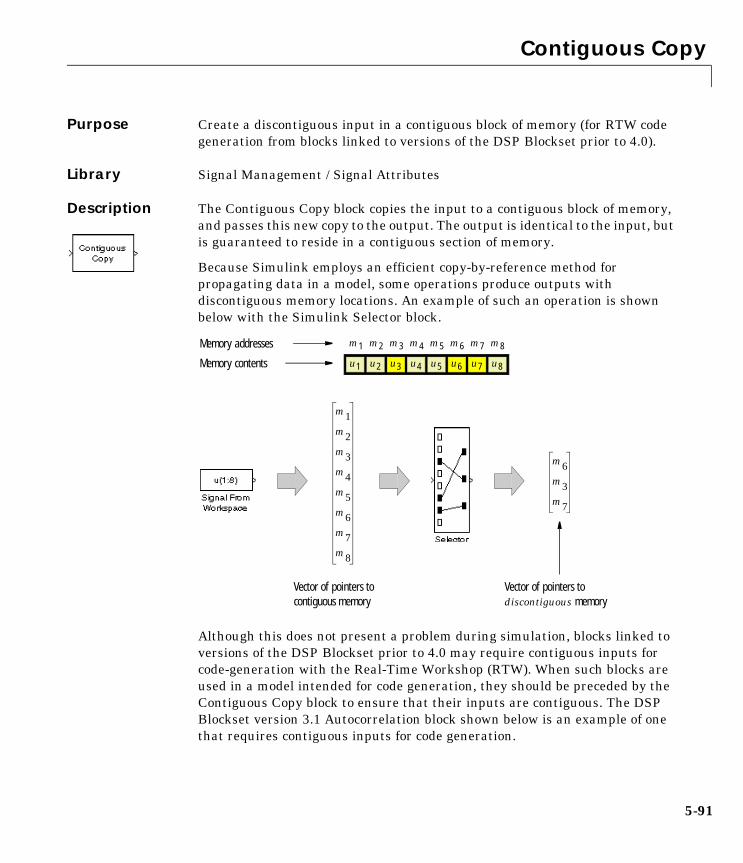
Contiguous Copy
5-91
5Contiguous CopyPurpose Create a discontiguous input in a contiguous block of memory (for RTW code generation from blocks linked to versions of the DSP Blockset prior to 4.0).
Library Signal Management / Signal Attributes
Description The Contiguous Copy block copies the input to a contiguous block of memory, and passes this new copy to the output. The output is identical to the input, but is guaranteed to reside in a contiguous section of memory.
Because Simulink employs an efficient copy-by-reference method for propagating data in a model, some operations produce outputs with discontiguous memory locations. An example of such an operation is shown below with the Simulink Selector block.
Although this does not present a problem during simulation, blocks linked to versions of the DSP Blockset prior to 4.0 may require contiguous inputs for code-generation with the Real-Time Workshop (RTW). When such blocks are used in a model intended for code generation, they should be preceded by the Contiguous Copy block to ensure that their inputs are contiguous. The DSP Blockset version 3.1 Autocorrelation block shown below is an example of one that requires contiguous inputs for code generation.
u1 u2 u3 u4 u5 u6 u7 u8
m1 m2 m3 m4 m5 m6 m7 m8
m1m2m3m4m5m6m7m8
m6m3m7
Memory addresses
Memory contents
Vector of pointers to contiguous memory
Vector of pointers to discontiguous memory

Contiguous Copy
5-92
Dialog Box
Supported Data Types
u1 u2 u3 u4 u5 u6 u7 u8
m1 m2 m3 m4 m5 m6 m7 m8
m6m3m7
Memory addresses
Memory contents
Vector of pointers to new contiguous memory
Vector of pointers to discontiguous memory
m9m10m11
u6 u3 u7
Original memory allocation New memory allocation
m9 m10 m11
v3.1
Fixed-pointCustom data typesBoolean8-, 16-, and 32-bit signed integer 8-, 16-, and 32-bit unsigned integerSingle-precision floating point Double-precision floating point

Convert 1-D to 2-D
5-93
5Convert 1-D to 2-DPurpose Reshape a 1-D or 2-D input to a 2-D matrix with the specified dimensions.
Library Signal Management / Signal Attributes
Description The Convert 1-D to 2-D block reshapes a length-Mi 1-D vector or an Mi-by-Ni matrix to an Mo-by-No matrix, where Mo is specified by the Number of output rows parameter, and No is specified by the Number of output columns parameter.
y = reshape(u,Mo,No) % Equivalent MATLAB code
The input is reshaped columnwise, as shown in the two cases below. The length-6 vector and the 2-by-3 matrix are both reshaped to the same 3-by-2 output matrix.
An error is generated if (Mo∗No) ≠ (Mi∗Ni). That is, the total number of input elements must be conserved in the output.
The output is frame-based if the Frame-based output check box is selected; otherwise, the output is sample-based.
Dialog Box
u1 u4
u2 u5
u3 u6u1 u3 u5
u2 u4 u6
(u1 u2 u3 u4 u5 u6)

Convert 1-D to 2-D
5-94
Number of output rowsThe number of rows, Mo, in the output matrix. Tunable.
Number of output columnsThe number of rows, No, in the output matrix. Tunable.
Frame-based outputCreates a frame-based output when selected. Tunable.
Supported Data Types
See Also
Fixed-pointCustom data typesBoolean8-, 16-, and 32-bit signed integer 8-, 16-, and 32-bit unsigned integerSingle-precision floating point Double-precision floating point
Buffer DSP BlocksetConvert 2-D to 1-D DSP BlocksetFrame Status Conversion DSP BlocksetReshape SimulinkSubmatrix DSP Blockset

Convert 2-D to 1-D
5-95
5Convert 2-D to 1-DPurpose Convert a 2-D matrix input to a 1-D vector.
Library Signal Management / Signal Attributes
Description The Convert 2-D to 1-D block reshapes an M-by-N matrix input to a 1-D vector with length M∗N.
y = u(:) % Equivalent MATLAB code
The input is reshaped columnwise, as shown below for a 3-by-2 matrix.
The output is always sample-based.
Dialog Box
Supported Data Types
See Also
u1 u4
u2 u5
u3 u6
(u1 u2 u3 u4 u5 u6)
Fixed-pointCustom data typesBoolean8-, 16-, and 32-bit signed integer 8-, 16-, and 32-bit unsigned integerSingle-precision floating point Double-precision floating point
Buffer DSP BlocksetConvert 1-D to 2-D DSP BlocksetFrame Status Conversion DSP BlocksetReshape SimulinkSubmatrix DSP Blockset
Convert Complex DSP To Simulink
5-96
5Convert Complex DSP To SimulinkPurpose Convert complex data from the DSP Blockset Version 2.2 format to the Simulink Version 3 format.
Library Elementary Functions, in Math Functions
Description The Convert Complex DSP To Simulink block accepts complex data (scalar, vector, matrix) in the DSP Blockset Version 2.2 format, and outputs the same data in the Simulink Version 3 complex format. Only complex data should be supplied to this block.
Blocks provided in Release 11 and later blocksets (e.g., Simulink Version 3.0, DSP Blockset Version 3.0, Fixed Point Blockset Version 2.0) use the Simulink Version 3 complex format, which is not compatible with the DSP Blockset Version 2.2 complex format. To add a new block or subsystem (Release 11 and later) to an existing model that uses the DSP Blockset Version 2.2 complex data format, precede it with the Convert Complex DSP To Simulink block. If the new block or subsystem’s output is complex, you should follow it with the complementary Convert Complex Simulink To DSP block (unless the downstream blocks have already been updated to their Release 11 counterparts).
These convertor blocks are only needed for interfacing Version 3.0 blocks to the complex-data section of a Version 2.2 or earlier model. Version 3.0 blocks can be added to real-data sections of older models without any data format conversion.
Note Within a section of model that uses the Version 2.2 complex format, you should continue to use the complex port identifier (∗) as a guide to wiring blocks. Outputs ports labeled with the ∗ symbol should only be connected to input ports labeled with the ∗ symbol.
The following figure shows how you can use these two convertor blocks to migrate part of a complex-data model to the Version 3.0 complex format while letting other components continue to use the Version 2.2 complex-data format.

Convert Complex DSP To Simulink
5-97
Dialog Box
Supported Data Types
See Also
Existing (Version 2.2) complex-data
Subsystem B upgraded to Version 3.0 complex-data
Subsystem A upgraded to Version 3.0 complex-data
(Subsystem A remains a Version 2.2 implementation)
(Subsystem B remains a Version 2.2 implementation)
Double-precision floating point
Convert Complex Simulink To DSP DSP Blockset

Convert Complex Simulink To DSP
5-98
5Convert Complex Simulink To DSPPurpose Convert complex data from the Simulink Version 3 format to the DSP Blockset Version 2.2 format.
Library Elementary Functions, in Math Functions
Description The Convert Complex Simulink To DSP block accepts complex data (scalar, vector, matrix) in the Simulink Version 3 format, and outputs the same data in the DSP Blockset Version 2.2 complex format. Only complex data should be supplied to this block.
Blocks provided in Release 11 and later blocksets (e.g., Simulink Version 3.0, DSP Blockset Version 3.0, Fixed Point Blockset Version 2.0) use the Simulink Version 3 complex format, which is not compatible with the DSP Blockset Version 2.2 complex format. To add a new block or subsystem (Release 11 and later) to an existing model that uses the DSP Blockset Version 2.2 complex data format, precede it with the Convert Complex DSP To Simulink block. If the new block’s output is complex, you should then follow it with the Convert Complex Simulink To DSP block (unless the downstream blocks have already been updated to their Release 11 counterparts).
These convertor blocks are only needed for interfacing Version 3.0 blocks to the complex-data section of a Version 2.2 or earlier model. Version Version 3.0 blocks can be added to real-data sections of older models without any data format conversion.
Note Within a section of model that uses the Version 2.2 complex format, you should continue to use the complex port identifier (∗) as a guide to wiring blocks. Outputs ports labeled with the ∗ symbol should only be connected to input ports labeled with the ∗ symbol.
The following figure shows how you can use these two convertor blocks to migrate part of a complex-data model to the Version 3.0 complex format while letting other components continue to use the Version 2.2 complex-data format.

Convert Complex Simulink To DSP
5-99
Dialog Box
Supported Data Types
See Also
Existing (Version 2.2) complex-data
Subsystem B upgraded to Version 3.0 complex-data
Subsystem A upgraded to Version 3.0 complex-data
(Subsystem A remains a Version 2.2 implementation)
(Subsystem B remains a Version 2.2 implementation)
Double-precision floating point
Convert Complex DSP To Simulink DSP Blockset

Convolution
5-100
5ConvolutionPurpose Compute the convolution of two inputs.
Library Signal Operations
Description The Convolution block convolves corresponding columns (channels) of Mu-by-N input matrix u and Mv-by-N input matrix v.
Frame-Based InputsMatrix inputs must be frame-based. The output, y, is a frame-based (Mu+Mv-1)-by-N matrix whose jth column has elements
where ∗ denotes the complex conjugate. Inputs u and v are zero when indexed outside of their valid ranges. When both inputs are real, the output is real; when one or both inputs are complex, the output is complex.
When one input is a column vector (single channel) and the other is a matrix (multiple channels), the single-channel input is independently convolved with each channel of the multichannel input. For example, if u is a Mu-by-1 column vector and v is an Mv-by-N matrix, the output is an (Mu+Mv-1)-by-N matrix whose jth column has elements
Sample-Based InputsIf u and v are sample-based vectors with lengths Mu and Mv, the Convolution block performs the vector convolution
yi j, uk j, v i k– 1+( ) j,* 1 i Mu Mv 1–+( )≤ ≤
k 1=
max Mu Mv,( )
∑=
yi j, ukv i k– 1+( ) j,* 1 i Mu Mv 1–+( )≤ ≤
k 1=
max Mu Mv,( )
∑=
yi ukv i k– 1+( )* 1 i Mu Mv 1–+( )≤ ≤
k 1=
max Mu Mv,( )
∑=
Convolution
5-101
The dimensions of the sample-based output vector are determined by the dimensions of the input vectors:
• When both inputs are row vectors, or when one input is a row vector and the other is a 1-D vector, the output is a 1-by-(Mu+Mv-1) row vector.
• When both inputs are column vectors, or when one input is a column vector and the other is a 1-D vector, the output is a (Mu+Mv-1)-by-1 column vector.
• When both inputs are 1-D vectors, the output is a 1-D vector of length Mu+Mv-1.
The Convolution block does not accept sample-based full-dimension matrix inputs, or mixed sample-based row vector and column vector inputs.
Dialog Box
Supported Data Types
See Also
Double-precision floating point
Correlation DSP Blocksetconv MATLAB

Correlation
5-102
5CorrelationPurpose Compute the correlation along the columns of two inputs.
Library Statistics
Description The Correlation block computes the cross-correlation of corresponding columns (channels) of the Mu-by-N input matrix u and Mv-by-N input matrix v. The frame status of both inputs must be the same. The block does not accept sample-based full-dimension matrix inputs or 2-D row vector inputs.
Frame-Based InputsMatrix inputs must be frame-based. The output, y, is a frame-based (Mu+Mv-1)-by-N matrix whose jth column has elements
where ∗ denotes the complex conjugate. Inputs u and v are zero when indexed outside of their valid ranges. When both inputs are real, the output is real; when one or both inputs are complex, the output is complex.
When one input is a column vector (single channel) and the other is a matrix (multiple channels), the single-channel input is independently cross-correlated with each channel of the multichannel input. For example, if u is a Mu-by-1 column vector and v is an Mv-by-N matrix, the output is an (Mu+Mv-1)-by-N matrix whose jth column has elements
Sample-Based InputsMatrix inputs cannot be sample based, so all sample-based inputs are column vectors or 1-D vectors. (the block does not support 2-D row vector inputs.) If u and v are sample-based vectors with lengths Mu and Mv, the Correlation block performs the vector cross-correlation
yi j, uk j, v k i Mv–+( ) j,* 1 i Mu Mv 1–+( )≤ ≤
k 1=
max Mu Mv,( )
∑=
yi j, ukv k i– Mv+( ) j,* 1 i Mu Mv 1–+( )≤ ≤
k 1=
max Mu Mv,( )
∑=

Correlation
5-103
The dimensions of the sample-based output vector are determined by the dimensions of the input vectors:
• When both inputs are column vectors, or when one input is a column vector and the other is a 1-D vector, the output is a (Mu+Mv-1)-by-1 column vector.
• When both inputs are 1-D vectors, the output is a 1-D vector of length Mu+Mv-1.
The Correlation block does not accept sample-based full-dimension matrix inputs or 2-D row vector inputs.
Dialog Box
Supported Data Types
See Also
yi ukv k i– Mv+( )* 1 i Mu Mv 1–+( )≤ ≤
k 1=
max Mu Mv,( )
∑=
Double-precision floating point
Autocorrelation DSP BlocksetConvolution DSP Blocksetxcorr Signal Processing Toolbox

Counter
5-104
5CounterPurpose Count up or down through a specified range of numbers.
Library Signal Management / Switches and Counters
Description The Counter block increments or decrements an internal counter each time it receives a trigger event at the Clk port. A trigger event at the Rst port resets the counter to its initial state.
The input to the Rst port must be a real sample-based scalar. The input to the Clk port can be a real sample-based scalar, or a real frame-based vector (i.e., single channel). If both inputs are sample-based, they must have the same sample period. If the Clk input is frame-based, the frame period must equal the sample period of the Rst input.
The trigger event for both inputs is specified by the Count event pop-up menu, and can be one of the following:
• Rising edge triggers a count or reset operation when the Clk or Rst input rises from a negative value to zero or a positive value, or from zero to a positive value.
• Falling edge triggers a count or reset operation when the Clk or Rst input falls from a positive value to zero or a negative value, or from zero to a negative value.
• Either edge triggers a count or reset operation when either a rising or falling edge (as described above) occurs.
• Nonzero sample triggers a count or reset operation at each sample time that the Clk or Rst input is not zero.
• Free running disables the Clk port, and enables the Samples per output frame and Sample time parameters. The block increments or decrements the counter at a constant interval, Ts, specified by the Sample time parameter. See “Free-Running Operation” below.
At the start of the simulation, the block sets the counter to the value specified by the Initial count parameter, which can be any integer in the range defined by the Counter size parameter. The Counter size parameter allows you to choose from three standard counter ranges, or to specify an arbitrary counter limit:
• 8 bits specifies a counter with a range of 0 to 255.

Counter
5-105
• 16 bits specifies a counter with a range of 0 to 65535.
• 32 bits specifies a counter with a range of 0 to 232-1.
• User defined enables the supplementary Maximum count parameter, which allows you to specify an arbitrary integer as the upper count limit. The range of the counter is then 0 to the Maximum count value.
Sample-Based OperationThe block operates in sample-based mode when the Clk input is a sample-based scalar. Sample-based vectors and matrices are not accepted.
When the Count direction parameter is set to Up, a sample-based trigger event at the Clk input causes the block to increment the counter by one. The block continues incrementing the counter when triggered until the counter value reaches the upper count limit (e.g., 255 for an 8-bit counter). At the next Clk trigger event, the block resets the counter to 0, and resumes incrementing the counter with the subsequent Clk trigger event.
When the Count direction parameter is set to Down, a sample-based trigger event at the Clk input causes the block to decrement the counter by one. The block continues decrementing the counter when triggered until the counter value reaches 0. At the next Clk trigger event, the block resets the counter to the upper count limit (e.g., 255 for an 8-bit counter), and resumes decrementing the counter with the subsequent Clk trigger event.
Between triggering events the block holds the output at its most recent value. The block resets the counter to its initial state when the trigger event specified in the Count event menu is received at the optional Rst input. When trigger events are received simultaneously at the Clk and Rst ports, the block first resets the counter, and then increments or decrements appropriately. (If you do not need to reset the counter during the simulation, you can disable the Rst port by deselecting the Reset input check box.)
The Output pop-up menu provides three options for the output port configuration of the block icon:
• Count configures the block icon to show a Cnt port, which produces the current value of the counter as a sample-based scalar with the same sample period as the inputs.
• Hit configures the block icon to show a Hit port. The Hit port produces zeros while the value of the counter does not equal the integer Hit value

Counter
5-106
parameter setting. When the counter value does equal the Hit value setting, the block generates a value of 1 at the Hit port. The output is sample-based with the same sample period as the inputs.
• Count and Hit configures the block icon with both ports.
Frame-Based OperationThe block operates in frame-based mode when the Clk input is a frame-based vector (i.e., single channel). Multichannel frame-based inputs are not accepted.
Frame-based operation is the same as sample-based operation, except that the block increments or decrements the counter by the total number of trigger events contained in the Clk input frame. A trigger event that is split across two consecutive frames is counted in the frame that contains the conclusion of the event. When a trigger event is received at the Rst port, the block first resets the counter, and then increments or decrements the counter by the number of trigger events contained in the Clk frame.
The Cnt and Hit outputs are sample-based scalars with sample period equal to the Clk input frame period.
Free-Running OperationThe block operates in free-running mode when Free running is selected from the Count event menu.
The Clk input port is disabled in this mode, and the block simply increments or decrements the counter using the constant sample period specified by the Sample time parameter, Ts. The Cnt output is a frame-based M-by-1 matrix containing the count value at each of M consecutive sample times, where M is specified by the Samples per output frame parameter. The Hit output is a frame-based M-by-1 matrix containing the hit status (0 or 1) at each of those M consecutive sample times. Both outputs have a frame period of M∗Ts.
Example In the model below, the Clk port of the Counter block is driven by Simulink’s Pulse Generator block, and the Rst port is triggered by an N-Sample Enable block. All of the Counter block’s inputs and outputs are multiplexed into a single To Workspace block using a 4-port Mux block.

Counter
5-107
To run the model, first select Simulation Parameters from the Simulation menu, and set the Stop time to 30. Then adjust the block parameters as described below. (Use the default settings for the Pulse Generator and To Workspace blocks.)
• Set the N-Sample Enable block parameters as follows:
- Trigger count = 6
- Active level = High (1)
• Set the Counter block parameters as follows:
- Count direction = Down
- Count event = Rising edge
- Counter size = User defined
- Maximum count = 20
- Initial count = 5
- Output = Count and Hit
- Hit value = 4
- Reset input
• Set the Number of inputs parameter of the Mux block to 4.
The figure below shows the first 22 samples of the model’s four-column output, yout. The first column is the Counter block’s Clk input, the second column is the block’s Rst input, the third column is the block’s Cnt output, and the fourth column is the block’s Hit output.

Counter
5-108
You can see that the seventh input samples to both the Clk and Rst ports of the Counter block represent trigger events (rising edges), so at this time step the block first resets the counter to its initial value of 5, and then immediately decrements the count to 4. When the counter reaches its minimum value of 0, it rolls over to its maximum value of 20 with the following trigger event at the Cnt port.
[1]
[0]
[1]
[0]
[1]
[0]
[1]
[0]
[1]
[0]
[1]
[0]
[1]
[0]
[1]
[0]
[1]
[0]
[1]
[0]
[1]
[0]
Clk Rst
...
...
Simul
atio
n tim
e
Cnt Hit
...
...
[0]
[0]
[0]
[0]
[0]
[0]
[1]
[1]
[1]
[1]
[1]
[1]
[1]
[1]
[1]
[1]
[1]
[1]
[1]
[1]
[1]
[1]
[5]
[5]
[4]
[4]
[3]
[3]
[4]
[4]
[3]
[3]
[2]
[2]
[1]
[1]
[0]
[0]
[20]
[20]
[19]
[19]
[18]
[18]
[0]
[0]
[1]
[1]
[0]
[0]
[1]
[1]
[0]
[0]
[0]
[0]
[0]
[0]
[0]
[0]
[0]
[0]
[0]
[0]
[0]
[0]
reset
initial value
max value
hit
hit

Counter
5-109
Dialog Box
Count directionThe counter direction, Up or Down. Tunable, except in Simulink’s external mode.
Count eventThe type of event that triggers the block to increment, decrement, or reset the counter when received at the Clk or Rst ports. Free running disables the Clk port, and counts continuously with the period specified by the Sample time parameter.
Counter sizeThe range of integer values the block should count through before recycling to zero.
Maximum countThe counter’s maximum value when Counter size is set to User defined. Tunable.

Counter
5-110
Initial countThe counter’s initial value at the start of the simulation and after reset. Tunable, except in Simulink’s external mode.
OutputSelects the output port(s) to enable: Cnt, Hit, or both.
Hit valueThe scalar value whose occurrence in the count should be flagged by a 1 at the (optional) Hit output. This parameter is available when Hit or Count and Hit are selected in the Output menu. Tunable, except in Simulink’s external mode.
Reset inputEnables the Rst input port when selected.
Samples per output frameThe number of samples, M, in each output frame. This parameter is available when Free running is selected in the Count event menu.
Sample timeThe output sample period, Ts, in free-running mode. This parameter is available when Free running is selected in the Count event menu.
Supported Data Types
See Also
Double-precision floating point
Edge Detector DSP BlocksetN-Sample Enable DSP BlocksetN-Sample Switch DSP Blockset

Covariance AR Estimator
5-111
5Covariance AR EstimatorPurpose Compute an estimate of AR model parameters using the covariance method.
Library Estimation / Parametric Estimation
Description The Covariance AR Estimator block uses the covariance method to fit an autoregressive (AR) model to the input data. This method minimizes the forward prediction error in the least-squares sense.
The input is a sample-based vector (row, column, or 1-D) or frame-based vector (column only) representing a frame of consecutive time samples from a single-channel signal, which is assumed to be the output of an AR system driven by white noise. The block computes the normalized estimate of the AR system parameters, A(z), independently for each successive input frame.
The order, p, of the all-pole model is specified by the Estimation order parameter.
The top output, A, is a column vector of length p+1 with the same frame status as the input, and contains the normalized estimate of the AR model coefficients in descending powers of z,
[1 a(2) ... a(p+1)]
The scalar gain, G, is provided at the bottom output (G).
Dialog Box
Estimation orderThe order of the AR model, p.
H z( ) GA z( )------------
G
1 a 2( )z 1– … a p 1+( )z p–+ + +
-------------------------------------------------------------------------------= =

Covariance AR Estimator
5-112
References Kay, S. M. Modern Spectral Estimation: Theory and Application. Englewood Cliffs, NJ: Prentice-Hall, 1988.
Marple, S. L., Jr., Digital Spectral Analysis with Applications. Englewood Cliffs, NJ: Prentice-Hall, 1987.
Supported Data Types
See Also
Double-precision floating point
Burg AR Estimator DSP BlocksetCovariance Method DSP BlocksetModified Covariance AR Estimator DSP BlocksetYule-Walker AR Estimator DSP Blocksetarcov Signal Processing Toolbox

Covariance Method
5-113
5Covariance MethodPurpose Compute a parametric spectral estimate using the covariance method.
Library Estimation / Power Spectrum Estimation
Description The Covariance Method block estimates the power spectral density (PSD) of the input using the covariance method. This method fits an autoregressive (AR) model to the signal by minimizing the forward prediction error in the least-squares sense. The order of the all-pole model is the value specified by the Estimation order parameter, and the spectrum is computed from the FFT of the estimated AR model parameters.
The input is a sample-based vector (row, column, or 1-D) or frame-based vector (column only) representing a frame of consecutive time samples from a single-channel signal. The block’s output (a column vector) is the estimate of the signal’s power spectral density at Nfft equally spaced frequency points in the range [0,Fs), where Fs is the signal’s sample frequency.
When Inherit FFT length from input dimensions is selected, Nfft is specified by the frame size of the input, which must be a power of 2. When Inherit FFT length from input dimensions is not selected, Nfft is specified as a power of 2 by the FFT length parameter, and the block zero pads or truncates the input to Nfft before computing the FFT. The output is always sample-based.
See the Burg Method block reference for a comparison of the Burg Method, Covariance Method, Modified Covariance Method, and Yule-Walker Method blocks.
Dialog Box
Estimation orderThe order of the AR model.

Covariance Method
5-114
Inherit FFT length from input dimensionsWhen selected, uses the input frame size as the number of data points, Nfft, on which to perform the FFT. Tunable.
FFT lengthThe number of data points, Nfft, on which to perform the FFT. If Nfft exceeds the input frame size, the frame is zero-padded as needed. This parameter is enabled when Inherit FFT length from input dimensions is not selected.
References Kay, S. M. Modern Spectral Estimation: Theory and Application. Englewood Cliffs, NJ: Prentice-Hall, 1988.
Marple, S. L., Jr., Digital Spectral Analysis with Applications. Englewood Cliffs, NJ: Prentice-Hall, 1987.
Supported Data Types
See Also
See “Power Spectrum Estimation” on page 4-15 for related information.
Double-precision floating point
Burg Method DSP BlocksetCovariance AR Estimator DSP BlocksetShort-Time FFT DSP BlocksetModified Covariance Method DSP BlocksetYule-Walker Method DSP Blocksetpcov Signal Processing Toolbox

Create Diagonal Matrix
5-115
5Create Diagonal MatrixPurpose Create a square diagonal matrix from diagonal elements.
Library Math Functions / Matrices and Linear Algebra / Matrix Operations
Description The Create Diagonal Matrix block populates the diagonal of the M-by-M matrix output with the elements contained in the length-M vector input, D. The elements off the diagonal are zero.
A = diag(D) Equivalent MATLAB code
The output is always sample-based.
Dialog Box
Supported Data Types
See Also
Double-precision floating point
Constant Diagonal Matrix DSP BlocksetExtract Diagonal DSP Blocksetdiag MATLAB

Cumulative Sum
5-116
5Cumulative SumPurpose Compute the cumulative sum of row or column elements.
Library Math Functions / Math Operations
Description The Cumulative Sum block computes the cumulative sum of the row or column elements in the M-by-N input matrix u.
Columnwise SummingWhen the Cumulative Sum along parameter is set to Columns, the block computes the cumulative sum of the column elements.
y = cumsum(u) % Equivalent MATLAB code
The output is an M-by-N matrix whose jth column has elements
The frame status of the output is the same as the input. For sample-based inputs, the first row of each successive output is the same as that of the corresponding input. For convenience, length-M 1-D vector inputs are treated as M-by-1 column vectors for column-wise summation, and the output is a length-M 1-D vector.
For frame-based inputs, the first row of the first output is the same as that of the first input, and the first row of each subsequent output contains the sum of the first row of the current input (time t) and the last row of the previous output (time t-Tf).
Rowwise SummingWhen the Cumulative Sum along parameter is set to Rows, the block computes the cumulative sum of the row elements.
y = cumsum(u,2) % Equivalent MATLAB code
The output is an M-by-N matrix whose ith row has elements
yi j, uk j, 1 i M≤ ≤k 1=
i
∑=
y1 j, t( ) u1 j, t( ) yM j, t Tf–( )+=

Cumulative Sum
5-117
The frame status of the output is the same as the input. For both sample-based and frame-based inputs, the first column of each successive output is the same as that of the corresponding input. For convenience, length-N 1-D vector inputs are treated as 1-by-N row vectors for row-wise summation, and the output is a length-N 1-D vector.
Dialog Box
Cumulative Sum alongThe dimension along which to compute the cumulative summations. Columns specifies columnwise summation, while Rows specifies rowwise summation.
Supported Data Types
See Also
yi j, ui k, 1 j N≤ ≤k 1=
j
∑=
Double-precision floating point
Difference DSP BlocksetMatrix Sum DSP Blocksetcumsum MATLAB

dB Conversion
5-118
5dB ConversionPurpose Convert magnitude data to decibels (dB or dBm).
Library Math Functions / Math Operations
Description The dB Conversion block converts a linearly scaled power or amplitude input to dB or dBm. The Input signal parameter specifies whether the input is a power signal or a voltage signal, and the Convert to parameter controls the scaling of the output. When selected, the Add eps to input to protect against “log(0) = -inf” parameter adds a value of eps to all power and voltage inputs. When this option is not enabled, zero-valued inputs produce -inf at the output. The size and frame status of the output are the same as the input.
Power InputsSelect Power as the Input signal parameter when the input, u, is a real, nonnegative, power signal (units of watts). When the Convert to parameter is set to dB, the block performs the dB conversion
y = 10*log10(u) % Equivalent MATLAB code
When the Convert to parameter is set to dBm, the block performs the dBm conversion
y = 10*log10(u) + 30
The dBm conversion is equivalent to performing the dB operation after converting the input to milliwatts.
Voltage InputsSelect Amplitude as the Input signal parameter when the input, u, is a real voltage signal (units of volts). The block uses the scale factor specified in ohms by the Load resistance parameter, R, to convert the voltage input to units of power (watts) before converting to dB or dBm. When the Convert to parameter is set to dB, the block performs the dB conversion
y = 10*log10(abs(u)^2/R)
When the Convert to parameter is set to dBm, the block performs the dBm conversion
y = 10*log10(abs(u)^2/R) + 30

dB Conversion
5-119
The dBm conversion is equivalent to performing the dB operation after converting the (abs(u)^2/R) result to milliwatts.
Dialog Box
Convert toThe logarithmic scaling to which the input is converted, dB or dBm. Tunable.
Input signalThe type of input signal, Power or Amplitude. Tunable.
Load resistanceThe scale factor used to convert voltage inputs to units of power. Tunable.
Add eps to input to protect against “log(0) = -inf”When selected, adds eps to all input values (power or voltage). Tunable.
Supported Data Types
See Also
Double-precision floating point
dB Gain DSP BlocksetMath Function Simulinklog10 MATLAB

dB Gain
5-120
5dB GainPurpose Apply a gain specified in decibels.
Library Math Functions / Math Operations
Description The dB Gain block multiplies the input by the decibel values specified in the Gain parameter. For an M-by-N input matrix u with elements uij, the Gain parameter can be a real M-by-N matrix with elements gij to be multiplied element-wise with the input, or a real scalar.
The value of k is 10 for power signals (select Power as the Input signal parameter) and 20 for voltage signals (select Amplitude as the Input signal parameter).
The value of the equivalent linear gain
is displayed in the block icon below the dB gain value. The size and frame status of the output are the same as the input.
Dialog Box
GainThe dB gain to apply to the input, a scalar or a real M-by-N matrix. Tunable.
Input signalThe type of input signal: Power or Amplitude. Tunable.
yij 10uijgij k⁄( )
=
gijlin 10
gij k⁄( )=

dB Gain
5-121
Supported Data Types
See Also
Single-precision floating pointDouble-precision floating point
dB Conversion DSP BlocksetMath Function Simulinklog10 MATLAB

DCT
5-122
5DCTPurpose Compute the DCT of the input.
Library Transforms
Description The DCT block computes the unitary discrete cosine transform (DCT) of each channel in the M-by-N input matrix, u.
y = dct(u) % Equivalent MATLAB code
For both sample-based and frame-based inputs, the block assumes that each input column is a frame containing M consecutive samples from an independent channel. The frame size, M, must be a power of two. To work with other frame sizes, use the Zero Pad block to pad or truncate the frame size to a power-of-two length.
The output is an M-by-N matrix whose lth column contains the length-M DCT of the corresponding input column.
where
The output is always sample-based, and the output port rate and data type (real/complex) are the same as those of the input port.
For convenience, length-M 1-D vector inputs and sample-based length-M row vector inputs are processed as single channels (i.e., as M-by-1 column vectors), and the output has the same dimension as the input.
y k l,( ) w k( ) u m l,( ) π 2m 1–( ) k 1–( )2M
--------------------------------------------, kcos
m 1=
M
∑ 1 … M, ,= =
w k( )
1M
--------- , k 1=
2M----- , 2 k M≤ ≤
=

DCT
5-123
Dialog Box
Supported Data Types
See Also
Double-precision floating point
Complex Cepstrum DSP BlocksetFFT DSP BlocksetIDCT DSP BlocksetReal Cepstrum DSP Blocksetdct Signal Processing Toolbox

Delay Line
5-124
5Delay LinePurpose Rebuffer a sequence of inputs with a one-sample shift.
Library Signal Management / Buffers
Description The Delay Line block buffers the input samples into a sequence of overlapping or underlapping matrix outputs. In the most typical use (sample-based inputs), each output differs from the preceding output by only one sample, as illustrated below for scalar input.
Note that the first output of the block in the example above is all zeros; this is because the Initial Conditions parameter is set to zero. Due to the latency of the Delay Line block, all outputs are delayed by one frame, the entries of which are defined by the Initial Conditions parameter.
Sample-Based OperationIn sample-based operation, the Delay Line block buffers a sequence of sample-based length-N vector inputs (1-D, row, or column) into a sequence of overlapping frame-based Mo-by-N matrix outputs, where Mo is specified by the Delay line size parameter (Mo>1). That is, each input vector becomes a row in the frame-based output matrix.
At each sample time the new input vector is added in the last row of the output, so each output overlaps the previous output by Mo-1 samples. Therefore, the output sample period and frame period is the same as the input sample period (Tso=Tsi, and Tfo=Tsi). When Mo=1, the input is simply passed through to the output and retains the same dimension, but becomes frame-based. The latency of the block always causes an initial delay in the output; the value of the first output is specified by the Initial conditions parameter (see “Initial Conditions” below). Sample-based full-dimension matrix inputs are not accepted.
The Delay Line block’s sample-based operation is similar to that of a Buffer block with Buffer size equal to Mo and Buffer overlap equal to Mo-1, except that the Buffer block has a different latency.
123456789456
012
(input sample period = Tsi) (output sample period = Tsi)
123
234
345
001
000

Delay Line
5-125
In the model below, the block operates on a sample-based input with a Delay line size of 3.
The input vectors in the example above do not begin appearing at the output until the second row of the second matrix due to the block’s latency (see “Initial Conditions” below). The first output matrix (all zeros in this example) reflects the block’s Initial conditions setting. As for any sample-based input, the output frame rate and output sample rate are both equal to the input sample rate.
Frame-Based OperationIn frame-based operation, the Delay Line block rebuffers a sequence of frame-based Mi-by-N matrix inputs into a sequence of frame-based Mo-by-N matrix outputs, where Mo is the output frame size specified by the Delay line size parameter. Depending on whether Mo is greater than, less than, or equal to the input frame size, Mi, the output frames can be underlapped or overlapped. Each of the N input channels is rebuffered independently.
When Mo > Mi, the output frame overlap is the difference between the output and input frame size, Mo-Mi. When Mo < Mi, the output is underlapped; the Delay Line block discards the first Mi-Mo samples of each input frame so that only the last Mo samples are buffered into the corresponding output frame.
6 1 5 6–
t=0
t=2
t=5
t=4
t=3
t=1
first frame-based output
Tsi = 15 1 5 5–
3 0 5 3–
4 0 5 4–
2 1 5 2–
1 1 5 1–
(Mo=3)
0 0 0 00 0 0 00 0 0 0
first sample-based input
t=0t=2t=3 t=1
ch4ch3
ch1ch2
ch4
ch3
ch2
ch1
Sample-based input, sample period = Tsi
Frame-based output,sample period = Tsi
ch4
ch3
ch2
ch1
ch4
ch3
ch2
ch1
0 0 0 00 0 0 01 1 5 1–
0 0 0 01 1 5 1–
2 1 5 2–
1 1 5 1–
2 1 5 2–
3 0 5 3–
Tso = 1

Delay Line
5-126
When Mo = Mi, the output data is identical to the input data, but is delayed by the latency of the block. Due to the block’s latency, the outputs are always delayed by one frame, the entries of which are specified by the Initial conditions (see “Initial Conditions” below).
The output frame period is equal to the input frame period (Tfo=Tfi). The output sample period, Tso, is therefore equal to Tfi/Mo, or equivalently, Tsi(Mi/Mo)
In the model below, the block rebuffers a two-channel frame-based input with a Delay line size of 3.
The first output frame in the example is a product of the latency of the Delay Line block; it is all zeros because the Initial conditions is set to be zero. Since the input frame size, 4, is larger than the output frame size, 3, only the last three samples in each input frame are propagated to the corresponding output frame. The frame periods of the input and output are the same, and the output sample period is Tsi(Mi/Mo), or 4/3 the input sample period.
Initial ConditionsThe Delay Line block’s buffer is initialized to the value specified by the Initial condition parameter. The block outputs this buffer at the first simulation step (t=0). If the block’s output is a vector, the Initial condition can be a vector of the same size, or a scalar value to be repeated across all elements of the initial output. If the block’s output is a matrix, the Initial condition can be a matrix of the same size, a vector (of length equal to the number of matrix rows) to be repeated across all columns of the initial output, or a scalar to be repeated across all elements of the initial output.
(Mo=3)
Output frame period = TsiInput frame period = 4∗Tsi
1 12 13 04 0
5 16 17 08 0
first input
t=0t=4
ch2
ch1
ch2
ch1
9 110 111 012 0
t=8
ch2
ch1
first output
t=8
ch2
ch1
ch2
ch1
ch2
ch1
t=0t=4
6 17 08 0
2 13 04 0
0 00 00 0

Delay Line
5-127
Dialog Box
Delay line sizeThe number of rows in output matrix, Mo.
Initial conditionsThe value of the block’s initial output, a scalar, vector, or matrix.
Supported Data Types
See Also
See “Buffering Sample-Based and Frame-Based Signals” on page 3-47 for related information.
Fixed-pointCustom data typesBoolean8-, 16-, and 32-bit signed integer 8-, 16-, and 32-bit unsigned integerSingle-precision floating point Double-precision floating point
Buffer DSP BlocksetTriggered Delay Line DSP Blockset

Detrend
5-128
5DetrendPurpose Remove a linear trend from a vector.
Library Statistics
Description The Detrend block removes a linear trend from the length-M input vector, u, by subtracting the straight line that best fits the data in the least-squares sense.
The least-squares line, û = ax + b, is the line with parameters a and b that minimizes the quantity
for M evenly-spaced values of x, where ui is the ith element in the input vector. The output, y = u–û, is an M-by-1 column vector (regardless of the input vector dimension) with the same frame status as the input.
Dialog Box
Supported Data Types
See Also
ui ui–( )2
i 1=
M
∑
Double-precision floating point
Cumulative Sum DSP BlocksetDifference DSP BlocksetLeast Squares Polynomial Fit DSP BlocksetUnwrap DSP Blocksetdetrend MATLAB

Difference
5-129
5DifferencePurpose Compute the element-to-element difference along rows or columns.
Library Math Functions / Math Operations
Description The Difference block computes the difference between adjacent elements in rows or columns of the M-by-N input matrix u.
Columnwise DifferencingWhen the Difference along parameter is set to Columns, the block computes differences between adjacent column elements.
y = diff(u) % Equivalent MATLAB code
For sample-based inputs, the output is a sample-based (M-1)-by-N matrix whose jth column has elements
For convenience, length-M 1-D vector inputs are treated as M-by-1 column vectors for columnwise differencing, and the output is 1-D.
For frame-based inputs, the output is a frame-based M-by-N matrix whose jth column has elements
The first row of the first output contains the difference between the first row of the first input and zero. The first row of each subsequent output contains the difference between the first row of the current input (time t) and the last row of the previous input (time t-Tf).
Rowwise DifferencingWhen the Difference along parameter is set to Rows, the block computes differences between adjacent row elements.
y = diff(u,[],2) % Equivalent MATLAB code
yi j, ui 1+ j, ui j, 1 i M 1–( )≤ ≤–=
yi j, ui 1+ j, ui j, 2 i M≤ ≤–=
y1 j, t( ) uM j, t Tf–( ) u1 j, t( )–=

Difference
5-130
The output is an M-by-(N-1) matrix whose ith row has elements
The frame status of the output is the same as the input. For convenience, length-N 1-D vector inputs are treated as 1-by-N row vectors for rowwise differencing, and the output is 1-D.
Dialog Box
Difference alongThe dimension along which to compute element-to-element differences. Columns specifies columnwise differencing, while Rows specifies rowwise differencing. Tunable.
Supported Data Types
See Also
yi j, ui j 1+, ui j, 1 j N 1–( )≤ ≤–=
Double-precision floating point
Cumulative Sum DSP Blocksetdiff MATLAB

Digital Filter Design
5-131
5Digital Filter DesignPurpose Design and implement a variety of digital FIR and IIR filters.
Library Filtering / Filter Designs
Description The Digital Filter Design block implements a digital FIR or IIR filter that you design using the Filter Design and Analysis Tool graphical user interface, referred to as FDATool. The block applies the filter to a discrete-time input signal and outputs the resulting signal.
To learn how to use FDATool, see the FDATool section of the Signal Processing Toolbox documentation.
Input and Output CharacteristicsThe block filters each input channel independently over time, preserving the input size, frame status, and dimension (1-D or 2-D). Depending on input characteristics, the block considers the input’s channels as the input columns or individual input elements:
• Sample-based input matrix — Each matrix element is a channel
• Frame-based input matrix — Each matrix column is a channel
• Unoriented 1-D input vector — Each vector element is a channel
Designing the FilterDouble-click the Digital Filter Design block to open FDATool. Use FDATool to design or directly specify the filter coefficients of a digital FIR or IIR filter. See the FDATool section of the Signal Processing Toolbox documentation to learn how to use FDATool.
Tuning the Filter During SimulationYou can tune the filter specifications in FDATool during simulations as long as your changes do not modify the filter length or filter order. The block’s filter updates as soon as you apply any filter changes in FDATool.

Digital Filter Design
5-132
Dialog Box Double-click the block to open FDATool.
Supported Data Types
Double-precision floating point

Digital Filter Design
5-133
See Also Analog Filter Design DSP BlocksetWindow Function DSP Blocksetfdatool Signal Processing Toolboxfvtool Signal Processing Toolboxsptool Signal Processing Toolbox

Direct-Form II Transpose Filter
5-134
5Direct-Form II Transpose Filter Purpose Apply an IIR filter to the input.
Library Filtering / Filter Designs
Description The Direct-Form II Transpose Filter block applies a transposed direct-form II IIR filter to the input.
This is a canonical form that has the minimum number of delay elements. The filter order is max(m,n)-1.
An M-by-N sample-based matrix input is treated as M∗N independent channels, and an M-by-N frame-based matrix input is treated as N independent channels. In both cases, the block filters each channel independently over time, and the output has the same size and frame status as the input.
The filter is specified in the parameter dialog box by its transfer function,
where the Numerator parameter specifies the vector of numerator coefficients,
[b(1) b(2) ... b(m)]
and the Denominator parameter specifies the vector of denominator coefficients,
[a(1) a(2) ... a(n)]
The filter coefficients are normalized by a1.
y(k)
u(k)
ΣΣ z-1 Σ z-1 Σ z-1zn-1(k) z2(k) z1(k)
. . .
b(m) b(2)b(3) b(1)
-a(n) -a(2)-a(3)
. . .
. . .
H z( ) B z( )A z( )------------
b1 b2z 1– … bm 1+ z m 1–( )–+ + +
a1 a2z 1– … an 1+ z n 1–( )–+ + +
-----------------------------------------------------------------------------------= =

Direct-Form II Transpose Filter
5-135
Initial ConditionsIn its default form, the filter initializes the internal filter states to zero, which is equivalent to assuming past inputs and outputs are zero. The block also accepts optional nonzero initial conditions for the filter delays. Note that the number of filter states (delay elements) per input channel is
max(m,n)-1
The Initial conditions parameter may take one of four forms:
• Empty matrix
The empty matrix, [], causes a zero (0) initial condition to be applied to all delay elements in each filter channel.
• Scalar
The scalar value is copied to all delay elements in each filter channel. Note that a value of zero is equivalent to setting the Initial conditions parameter to the empty matrix, [].
• Vector
The vector has a length equal to the number of delay elements in each filter channel, max(m,n)-1, and specifies a unique initial condition for each delay element in the filter channel. This vector of initial conditions is applied to each filter channel.
• Matrix
The matrix specifies a unique initial condition for each delay element, and can specify different initial conditions for each filter channel. The matrix must have the same number of rows as the number of delay elements in the filter, max(m,n)-1, and must have one column per filter channel.

Direct-Form II Transpose Filter
5-136
Dialog Box
NumeratorThe filter numerator vector. Tunable; the numerator coefficients can be adjusted while the simulation runs, but the vector length (i.e., the filter order) must remain the same.
DenominatorThe filter denominator vector. Tunable; the denominator coefficients can be adjusted while the simulation runs, but the vector length (i.e., the filter order) must remain the same.
Initial conditionsThe filter’s initial conditions, a scalar, vector, or matrix.
References Oppenheim, A. V. and R. W. Schafer. Discrete-Time Signal Processing. Englewood Cliffs, NJ: Prentice Hall, 1989.
Proakis, J. and D. Manolakis. Digital Signal Processing. 3rd ed. Englewood Cliffs, NJ: Prentice-Hall, 1996.
Supported Data Types
Double-precision floating point

Direct-Form II Transpose Filter
5-137
See Also
See “Designing Filters with Various Filter Structures” on page 4-6 for related information.
Biquadratic Filter DSP BlocksetDiscrete Filter SimulinkFilter Realization Wizard DSP BlocksetTime-Varying Direct-Form II Transpose Filter DSP Blocksetfilter MATLAB

Discrete Impulse
5-138
5Discrete ImpulsePurpose Generate a discrete impulse.
Library DSP Sources
Description The Discrete Impulse block generates an impulse (the value 1) at output sample D+1, where D is specified by the Delay parameter (D ≥ 0). All output samples preceding and following sample D+1 are zero.
When D is a length-N vector, the block generates an M-by-N matrix output representing N distinct channels, where frame size M is specified by the Samples per frame parameter. The impulse for the ith channel appears at sample D(i)+1. For M=1, the output is sample-based; otherwise, the output is frame-based.
The Sample time parameter value, Ts, specifies the output signal sample period. The resulting frame period is M∗Ts.
The Data type parameter allows you to specify an output precision of double, single, or Boolean. Note, however, that most of the blocks in the DSP Blockset accept only double precision inputs. Use the Simulink Data Type Conversion block to convert integer data types to double precision. See “Working with Data Types” in the Simulink documentation for a complete discussion of data types, as well as a list of Simulink blocks capable of reduced-precision operations.
Example Construct the model below.
Configure the Discrete Impulse block to generate a frame-based three-channel output of type double, with impulses at samples 1, 4, and 6 of channels 1, 2, and 3, respectively. Use a sample period of 0.25 and a frame size of 4. The corresponding settings should be as follows:
• Delay = [0 3 5]
• Sample time = 0.25
• Samples per frame = 4
• Data type = Double

Discrete Impulse
5-139
Run the model and look at the output, yout. The first few samples of each channel are shown below.
yout(1:10,:)ans =
1 0 0 0 0 0 0 0 0 0 1 0 0 0 0 0 0 1 0 0 0 0 0 0 0 0 0 0 0 0
The block generates an impulse at sample 1 of channel 1 (first column), at sample 4 of channel 2 (second column), and at sample 6 of channel 3 (third column).
Dialog Box
DelayThe number of zero-valued output samples, D, preceding the impulse. A length-N vector specifies an N-channel output. Tunable.

Discrete Impulse
5-140
Sample timeThe sample period, Ts, of the output signal. The output frame period is M∗Ts. Tunable.
Samples per frameThe number of samples, M, in each output frame. Tunable.
Data typeThe precision of the output. Tunable.
Supported Data Types
See Also
See “Creating Signals Using Signal Generator Blocks” on page 3-36 for related information.
Single-precision floating pointDouble-precision floating point
Data Type Conversion SimulinkDSP Constant DSP BlocksetMultiphase Clock DSP BlocksetN-Sample Enable DSP BlocksetSignal From Workspace DSP Blocksetimpz Signal Processing Toolbox

Downsample
5-141
5DownsamplePurpose Resample an input at a lower rate by deleting samples.
Library Signal Operations
Description The Downsample block resamples each channel of the Mi-by-N input at a rate K times lower than the input sample rate by discarding K-1 consecutive samples following each sample passed through to the output. The integer K is specified by the Downsample factor parameter.
The Sample offset parameter delays the output samples by an integer number of sample periods, D, where 0 ≤ D < (K-1), so that any of the K possible output phases can be selected. For example, when you downsample the sequence 1, 2, 3, ... by a factor of 4, you can select from the following four phases.
The initial zero in each output sequence above is a result of the default zero Initial condition parameter setting for this example. See “Latency” on page 5-143 for more on the Initial condition parameter.
Sample-Based OperationWhen the input is sample-based, the block treats each of the M∗N matrix elements as an independent channel, and downsamples each channel over time. The input and output sizes are identical.
The Sample-based mode parameter determines how the block represents the new rate at the output. There are two available options:
• Allow multirate
When Allow multirate is selected, the sample period of the sample-based output is K times longer than the input sample period (Tso = KTsi). The block is therefore multirate.
Input Sequence Sample Offset, D Output Sequence (K=4)
1,2,3,... 0 0,1,5,9,13,17,21,25,...
1,2,3,... 1 0,2,6,10,14,18,22,26,...
1,2,3,... 2 0,3,7,11,15,19,23,27,...
1,2,3,... 3 0,4,8,12,16,20,24,28,...

Downsample
5-142
• Enforce single rate
When Enforce single rate is selected, the block forces the output sample rate to match the input sample rate (Tso = Tsi) by repeating every Kth input sample K times at the output. The block is therefore single-rate. (The block’s operation when Enforce single rate is selected is similar to the operation of a Sample and Hold block with a repeating trigger event of period KTsi.)
The setting of the Frame-based mode popup menu does not affect sample-based inputs.
Frame-Based InputsWhen the input is frame-based, the block treats each of the N input columns as a frame containing Mi sequential time samples from an independent channel. The block downsamples each channel independently by discarding K-1 rows of the input matrix following each row that it passes through to the output.
The Frame-based mode parameter determines how the block adjusts the rate at the output to accommodate the reduced number of samples. There are two available options:
• Maintain input frame size
The block generates the output at the slower (downsampled) rate by using a proportionally longer frame period at the output port than at the input port. For downsampling by a factor of K, the output frame period is K times longer than the input frame period (Tfo = KTfi), but the input and output frame sizes are equal.
The model below shows a single-channel input with a frame period of 1 second being downsampled by a factor of 4 to a frame period of 4 seconds. The input and output frame sizes are identical.

Downsample
5-143
• Maintain input frame rate
The block generates the output at the slower (downsampled) rate by using a proportionally smaller frame size than the input. For downsampling by a factor of K, the output frame size is K times smaller than the input frame size (Mo = Mi/K), but the input and output frame rates are equal.
The model below shows a single-channel input of frame size 64 being downsampled by a factor of 4 to a frame size of 16. The input and output frame rates are identical.
The setting of the Sample-based mode popup menu does not affect frame-based inputs.
Latency
Zero Latency. The Downsample block has zero tasking latency for the special combinations of input signal sampling and parameter settings shown in the table below. In all of these cases the block has single-rate operation.
Zero tasking latency means that the block propagates input sample D+1 (received at t=0) as the first output sample, followed by input sample D+1+K, input sample D+1+2K, and so on. The Initial condition parameter value is not used.
Input Sampling Parameter Settings
Sample-basedDownsample factor parameter, K, is 1, orEnforce single rate is selected (with D=0)
Frame-basedDownsample factor parameter, K, is 1, orMaintain input frame rate is selected

Downsample
5-144
Nonzero Latency. The Downsample block is multirate for most settings other than those in the above table. The amount of latency for multirate operation depends on input signal sampling and Simulink’s tasking mode, as shown in the table below.
The only case of nonzero single-rate latency occurs in sample-based mode, when Enforce single rate is selected with D > 0. The latency in this case is one sample.
In all cases of one-sample latency, the initial condition for each channel appears as the first output sample. Input sample D+1 appears as the second output sample for each channel, followed by input sample D+1+K, input sample D+1+2K, and so on. The Initial condition parameter can be an Mi-by-N matrix containing one value for each channel, or a scalar to be applied to all signal channels.
In all cases of one-frame latency, the Mi rows of the initial condition matrix appear in sequence as the first Mi output rows. Input sample D+1 (i.e, row D+1 of the input matrix) appears in the output as sample Mi+1, followed by input sample D+1+K, input sample D+1+2K, and so on. The Initial condition value can be an Mi-by-N matrix, or a scalar to be repeated across all elements of the Mi-by-N matrix. See the example below for an illustration of this case.
See “Excess Algorithmic Delay (Tasking Latency)” on page 3-91 and “The Simulation Parameters Dialog Box” in the Simulink documentation for more information about block rates and Simulink’s tasking modes.
Example Construct the frame-based model shown below.
Multirate... Sample-Based Latency Frame-Based Latency
Single-taskingNone, for D=0One sample, for D>0
One frame (Mi samples)
Multitasking One sample One frame (Mi samples)

Downsample
5-145
Adjust the block parameters as follows:
• Configure the Signal From Workspace block to generate a two-channel signal with frame size of 4 and sample period of 0.25 seconds. This represents an output frame period of 1 second (0.25∗4). The first channel should contain the positive ramp signal 1, 2, ..., 100, and the second channel should contain the negative ramp signal -1, -2, ..., -100. The settings are:
- Signal = [(1:100)' (-1:-1:-100)']
- Sample time = 0.25
- Samples per frame = 4
• Configure the Downsample block to downsample the two-channel input by decreasing the output frame rate by a factor of 2 relative to the input frame rate. Set a sample offset of 1, and a 4-by-2 initial condition matrix of
- Downsample factor = 2
- Sample offset = 1
- Initial condition = [11 -11;12 -12;13 -13;14 -14]
- Frame-based mode = Maintain input frame size
• Configure the Probe blocks by deselecting the Probe width and Probe complex signal check boxes (if desired).
This model is multirate because there are at least two distinct frame rates, as shown by the two Probe blocks. To run this model in Simulink’s multitasking mode, select Fixed-step and discrete from the Type controls in the Solver
11 11–
12 12–
13 13–
14 14–

Downsample
5-146
panel of the Simulation Parameters dialog box, and select MultiTasking from the Mode parameter. Additionally, set the Stop time to 30.
Run the model and look at the output, yout. The first few samples of each channel are shown below.
yout =
11 -11 12 -12 13 -13 14 -14 2 -2 4 -4 6 -6 8 -8 10 -10 12 -12 14 -14
Since we ran this frame-based multirate model in multitasking mode, the first row of the initial condition matrix appears as the first output sample, followed by the other three initial condition rows. The second row of the first input matrix (i.e., row D+1, where D is the Sample offset) appears in the output as sample 5 (i.e., sample Mi+1, where Mi is the input frame size).
Dialog Box

Downsample
5-147
Downsample factorThe integer factor, K, by which to decrease the input sample rate.
Sample offsetThe sample offset, D, which must be an integer in the range [0, K-1].
Initial conditionThe value with which the block is initialized for cases of nonzero latency; a scalar or matrix.
Sample-based modeThe method by which to implement downsampling for sample-based inputs: Allow multirate (i.e, decrease the output sample rate), or Force single-rate (i.e., force the output sample rate to match the input sample rate by repeating every Kth input sample K times at the output).
Frame-based modeThe method by which to implement downsampling for frame-based inputs: Maintain input frame size (i.e., decrease the frame rate), or Maintain input frame rate (i.e., decrease the frame size).
Supported Data Types
See Also
Fixed-pointCustom data typesBoolean8-, 16-, and 32-bit signed integer 8-, 16-, and 32-bit unsigned integerSingle-precision floating point Double-precision floating point
FIR Decimation DSP BlocksetFIR Rate Conversion DSP BlocksetRepeat DSP BlocksetSample and Hold DSP BlocksetUpsample DSP Blockset

DSP Constant
5-148
5DSP ConstantPurpose Generate a discrete-time or continuous-time constant signal.
Library DSP Sources
Description The DSP Constant block generates a signal whose value remains constant throughout the simulation. The Constant value parameter specifies the constant to output, and can be any valid MATLAB expression that evaluates to a scalar, vector, or matrix.
When a row vector or column vector is specified for the Constant value parameter, and the Interpret vector parameters as 1-D check box is selected, the dimension of the Constant value vector is disregarded, and the output is a 1-D vector. When the Interpret vector parameters as 1-D check box is not selected, the output dimension is constrained to match the Constant value dimension (row or column). When the Constant value is an M-by-N matrix with M > 1 and N > 1, the output is always M-by-N.
When Sample mode is set to Continuous, the output is a continuous-time signal. When Sample mode is set to Discrete, the Sample time and Frame-based output parameters are enabled, and signal has the discrete output period specified by the Sample time parameter.
When the Frame-based output check box is selected, the output is frame-based; otherwise, the output is sample-based. Because a 1-D vector signal cannot be frame-based, an active Frame-based output setting overrides an active Interpret vector parameters as 1-D setting, and the output is a frame-based column vector (regardless of the actual Constant value vector dimension).

DSP Constant
5-149
Dialog Box
Constant valueThe constant to generate. Tunable; values entered here can be tuned, but their dimensions must remain fixed.
Interpret vector parameters as 1-DWhen selected, generates 1-D vector outputs for Constant value settings with vector dimension; when unselected, generates 2-D vector outputs for Constant value settings with vector dimension. An active Interpret vector parameters as 1-D setting is overridden by an active Frame-based output setting.
Sample modeThe sample mode of the output, Discrete for a discrete-time signal or Continuous for a continuous-time signal.
Sample timeThe discrete sample period for sample-based outputs. When the Frame-based output parameter is checked, this parameter is named Frame period, and is the discrete frame period for the frame-based output. This parameter is enabled when Discrete is selected in the Sample mode menu.
Frame-based outputSpecifies frame-based output when selected. This parameter is enabled when Discrete is selected in the Sample mode menu

DSP Constant
5-150
Supported Data Types
See Also
See “Creating Signals Using Constant Blocks” on page 3-33 for related information.
(MATLAB commands for casting values to certain data types are provided in parentheses.)Boolean (boolean)8-, 16-, and 32-bit signed integer (int8, int16, int32)8-, 16-, and 32-bit unsigned integer (uint8, uint16, uint32)Single-precision floating point (single)Double-precision floating point (double)
Constant SimulinkSignal From Workspace DSP Blockset

Dyadic Analysis Filter Bank
5-151
5Dyadic Analysis Filter BankPurpose Decompose a signal into components of equal or logarithmically decreasing frequency intervals and sample rates.
Library Filtering / Multirate Filters
Description The Dyadic Analysis Filter Bank block decomposes a broadband signal into a collection of successively more bandlimited components by repeatedly dividing the frequency range. The typical (asymmetric) n-level filter bank structure is shown below.
At each level, the low-frequency output of the previous level is decomposed into adjacent high- and low-frequency subbands by a highpass (HP) and lowpass (LP) filter pair. Each of the two output subbands is half the bandwidth of the input to that level (hence “dyadic”). The bandlimited output of each filter is maximally decimated by a factor of 2 to preserve the bit rate of the original signal. In wavelet applications (see below) the aliasing introduced by the decimation stage can be exactly canceled in reconstruction.
The Lowpass FIR filter coefficients and Highpass FIR filter coefficients parameters specify (respectively) the filter coefficients to be used for every lowpass and highpass direct-form II transpose filter in the filter bank. The values of these coefficients are typically computed using the wavelet family
HP
LP ↓2
↓2
HP ↓2
LP ↓2 HP ↓2
LP ↓2
u
HP: highpass filter with fc ≈ 1/2 NyquistLP: lowpass filter with fc ≈ 1/2 Nyquist↓2: downsample by 2
y1
y2
y3
ynHP ↓2
LP ↓2
. . .
yn+1
Asymmetric Filter Bank, n Levels
2Ts
4Ts
8Ts
Tso = (2k)Ts for output yk, 1 ≤ k ≤ n
Tso = (2n)Ts for output yn+1
Tsi = Ts

Dyadic Analysis Filter Bank
5-152
functions in the Wavelet Toolbox (see the Wavelet Toolbox documentation for more information).
Tree StructureThe Tree structure parameter specifies an asymmetric (or wavelet) tree, as shown above, or a symmetric structure, as shown below. Note that the symmetric structure decomposes both the high- and low-frequency subbands at each level, whereas the asymmetric structure only decomposes the low-frequency bands.
Asymmetric Tree. The asymmetric structure in the first figure (Tree structure set to Asymmetric) has n+1 outputs, where n is the Number of levels parameter value. The sample rate and bandwidth of the top output are half the input sample rate and bandwidth. The sample rate and bandwidth of each additional output (except the last) are half that of the output from the previous level. In general, for an input with sample period Tsi = Ts, and bandwidth BW, output yk has sample period Tso,k and bandwidth BWk.
Note that in frame-based mode, the change in the sample period of output yk is reflected by its frame size, Mo,k, rather than by its frame rate.
Tso k,2k( )Ts 1 k n≤ ≤( )
2n( )Ts k n 1+=( )
=
BWk
BW
2k---------- 1 k n≤ ≤( )
BW
2n---------- k n 1+=( )
=
Mo k,
Mi
2k------- 1 k n≤ ≤( )
Mi
2n------- k n 1+=( )
=

Dyadic Analysis Filter Bank
5-153
The bottom two outputs (yn and yn+1) share the same sample period, bandwidth, and frame size because they originate at the same tree level.
Symmetric Tree. The symmetric structure shown below (Tree structure set to Symmetric) has 2n outputs, where n is the Number of levels parameter value.
The sample rate and bandwidth of every output are reduced by a factor of 2n from the input sample rate and bandwidth. For an input with sample period Tsi = Ts, and bandwidth BW, output yk has sample period Tso,k and bandwidth BWk.
HP
LP ↓2
↓2
HP ↓2
LP ↓2
HP ↓2
LP ↓2
u
HP: highpass filter with fc ≈ 1/2 NyquistLP: lowpass filter with fc ≈ 1/2 Nyquist↓2: downsample by 2
y1
y2
y3
y7
y2n
HP ↓2
LP ↓2
HP ↓2
LP ↓2
HP ↓2
LP ↓2
HP ↓2
LP ↓2
. . .
. . .
. . .
. . .
y4
y5
y6
Symmetric Filter Bank, n Levels
Tsi = Ts
Tso = (2n)Ts for all 2n outputs
Tso k, 2n( )Ts 1 k 2n≤ ≤( )=
BWkBW
2n---------- 1 k 2n≤ ≤( )=

Dyadic Analysis Filter Bank
5-154
In frame-based mode, the sample period of output yk is reflected by its frame size, Mo,k, rather than by its frame rate.
Sample-Based OperationAn M-by-N sample-based matrix input is treated as M∗N independent channels, and the block filters each channel independently over time. The output at each port is the same size as the input, one output channel for each input channel. As described earlier, for the asymmetric tree structure, each output port has a different sample period.
The figure below shows the input and output sample periods for a 64-channel sample-based input to a three-level filter bank. The input has a period of 1, so the fastest output has a period of 2.
Frame-Based OperationAn Mi-by-N frame-based matrix input is treated as N independent channels, and the block filters each channel independently over time. The input frame size Mi must be a multiple of 2n, and n is the number of filter bank levels. For example, a frame size of 8 would be appropriate for a three-level tree (23=8). The number of columns in each output is the same as the number of columns in the input.
Each output port has the same frame period as the input. The reduction in the output sample rates results from the smaller output frame sizes, as shown in the example below for a four-channel input to a three-level asymmetric tree.
Mo k,Mi
2n------- 1 k 2n≤ ≤( )=
Tsi = 1
Tso = 2
Tso = 4
Tso = 8
Tso = 8

Dyadic Analysis Filter Bank
5-155
Applications
Wavelets. The primary application for dyadic analysis filter banks is coding for data compression using wavelets.
At the transmitting end, the output of the dyadic analysis filter bank is fed to a lossy compression scheme, which typically assigns the number of bits for each filter bank output in proportion to the relative energy in that frequency band. This represents the more powerful signal components by a greater number of bits than the less powerful signal components.
At the receiving end, the transmission is decoded and fed to a dyadic synthesis filter bank to reconstruct the original signal. The filter coefficients of the complementary analysis and synthesis stages are designed to cancel aliasing introduced by the filtering and resampling.
Scalograms. When the magnitudes in each of the subband signals yk, 1 ≤ k ≤ n, are plotted across the full bandwidth of the original signal, the result is a scalogram. This is the equivalent of a spectrogram with constant Q, where
and is the midpoint frequency of the band occupied by output yk. The frequency axis of a scalogram therefore has logarithmic divisions like those shown below, where Fs is the sample rate (1/Ts).
Tfi = 1Tsi = 1/64
Tso = 1/32)
Tso = 1/16)
Tso = 1/8)
Tso = 1/8)
Tfo = 1
lossy coding decoding
Qfyk
BWyk
--------------=
fyk

Dyadic Analysis Filter Bank
5-156
Latency
Zero Latency. The Dyadic Analysis Filter Bank block has no tasking latency for frame-based operation, which is always single-rate. The block therefore analyzes the first input sample (received at t=0) to produce the first output sample at each port.
Nonzero Latency. The Dyadic Analysis Filter Bank block has tasking latency only for sample-based operation, which is always multirate. As shown in the table below, the amount of latency, D, depends on the structure (symmetric or asymmetric) of the n-level tree used by the block.
In the above cases, the block repeats a zero initial condition in each channel for the first D output samples. For example, in single-tasking mode, the asymmetric tree structure generates 2n-1 zero-valued output samples at each port in each channel before propagating the first analyzed input sample (computed from the input received at t=0).
See “Excess Algorithmic Delay (Tasking Latency)” in Chapter 3 and “The Simulation Parameters Dialog Box” in the Simulink documentation for more information about block rates and Simulink’s tasking modes.
Multirate... Symmetric Tree Asymmetric Tree
Single-tasking One sample 2n-1 samples
Multitasking One sample 2n-1 samples
Fs/2Fs/4Fs/8Fs/16
Fs/32Fs/64
Fs/128Fs/256
0
Fs

Dyadic Analysis Filter Bank
5-157
Dialog Box
Lowpass FIR filter coefficientsA vector of filter coefficients (descending powers of z) to be shared by all the lowpass filters in the filter bank.
Highpass FIR filter coefficientsA vector of filter coefficients (descending powers of z) to be shared by all the highpass filters in the filter bank.
Number of levelsThe number of filter bank levels. An n-level asymmetric structure has n+1 outputs; an n-level symmetric structure has 2n outputs.
Tree structureThe structure of the filter bank, Asymmetric (wavelet) or Symmetric.
References Fliege, N. J. Multirate Digital Signal Processing: Multirate Systems, Filter Banks, Wavelets. West Sussex, England: John Wiley & Sons, 1994.
Strang, G. and T. Nguyen. Wavelets and Filter Banks. Wellesley, MA: Wellesley-Cambridge Press, 1996.
Vaidyanathan, P. P. Multirate Systems and Filter Banks. Englewood Cliffs, NJ: Prentice Hall, 1993.

Dyadic Analysis Filter Bank
5-158
Supported Data Types
See Also
See the following sections for related information:
• “Converting Sample Rates and Frame Rates” on page 3-20
• “Multirate Filters” on page 4-9
Double-precision floating point (double)
Dyadic Synthesis Filter Bank DSP BlocksetWavelet Analysis DSP Blockset

Dyadic Synthesis Filter Bank
5-159
5Dyadic Synthesis Filter BankPurpose Reconstruct a signal from its multirate bandlimited components.
Library Filtering / Multirate Filters
Description The Dyadic Synthesis Filter Bank block typically reconstructs a signal that was decomposed by the Dyadic Analysis Filter Bank block. The reconstruction or synthesis process is the inverse of the analysis process, and restores the original signal by upsampling, filtering, and summing the bandlimited inputs in stages corresponding to the analysis process. The typical (asymmetric) n-level filter bank structure is shown below.
At each level, the two bandlimited inputs (one low-frequency, one high-frequency, both with the same sample rate) are upsampled by a factor of 2 to match the sample rate of the input to the next stage. They are then filtered by a highpass (HP) and lowpass (LP) filter pair with coefficients calculated to cancel (in the subsequent summation) the aliasing introduced in the corresponding dyadic analysis filter stage. The output from each (upsample-filter-sum) level has twice the bandwidth and twice the sample rate of the input to that level (hence “dyadic”).
The Lowpass FIR filter coefficients and Highpass FIR filter coefficients parameters specify (respectively) the filter coefficients to be used for every
HP
LP↑2
↑2
HP↑2
LP↑2HP↑2
LP↑2
y
HP: highpass filter with fc ≈ 1/2 NyquistLP: lowpass filter with fc ≈ 1/2 Nyquist↑2: upsample by 2
u1
u2
u3
un HP↑2
LP↑2
. . .
un+1
Asymmetric Filter Bank, n Levels
Σ
Σ
Σ
Σ
2Ts
4Ts
8Ts
Tsi = (2k)Ts for input uk, 1 ≤ k ≤ n
Tsi = (2n)Ts for input un+1
Tso = Ts

Dyadic Synthesis Filter Bank
5-160
highpass and lowpass direct-form II transpose filter in the filter bank. The values of these coefficients are typically computed together with the dyadic analysis coefficients using the wavelet family functions in the Wavelet Toolbox (see the Wavelet Toolbox documentation for more information).
Tree StructureThe Tree structure parameter specifies an asymmetric (or wavelet) tree, as shown above, or a symmetric structure, as shown below. Note that the symmetric structure reconstructs a signal that was symmetrically decomposed by the Dyadic Analysis Filter Bank block (i.e., both the high- and low-frequency subbands were divided at each level). The asymmetric structure reconstructs a signal that was asymmetrically decomposed by the Dyadic Analysis Filter Bank block (i.e., only the low-frequency subbands were divided at each level).
Asymmetric Tree. The asymmetric structure in the first figure (Tree structure set to Asymmetric) has n+1 inputs, where n is the Number of levels parameter value. The sample rate and bandwidth of the output are twice the sample rate and bandwidth of the top input. The sample rate and bandwidth of each additional input (except the last) should be half that of the input to the previous level.
The bottom two inputs (un and un+1) should have the same sample rate and bandwidth since they are processed by the same level.
Note that in frame-based mode, the change in the sample period of input uk is reflected by its frame size, Mi,k, rather than by its frame rate.
Tsi k 1+, 2Tsi k,= 1 k n<≤
BWk 1+
BWk2
-------------= 1 k n<≤
Tsi n 1+, Tsi n,=
BWn 1+ BWn=
Mi k 1+,Mi k,
2------------= 1 k n<≤

Dyadic Synthesis Filter Bank
5-161
Symmetric Tree. The symmetric structure shown below (Tree structure set to Symmetric) has 2n inputs, where n is the Number of levels parameter value.
The sample rate and bandwidth of the output are a factor of 2n higher than the sample rate and bandwidth of the inputs, which are all equal.
Sample-Based OperationAn M-by-N sample-based matrix input is treated as M∗N independent channels, and the block filters each channel independently over time. The output is the same size as the input at each port, one output channel for each input channel. As described earlier, for the asymmetric tree structure, each input port has a different sample period.
Mi n 1+, Mi n,=
HP
LP↑2
↑2
HP↑2
LP↑2
HP↑2
LP↑2
y
HP: highpass filter with fc ≈ 1/2 NyquistLP: lowpass filter with fc ≈ 1/2 Nyquist↑2: upsample by 2
u1
u2
u3
u7
u2n
HP↑2
LP↑2
HP↑2
LP↑2
HP↑2
LP↑2
HP↑2
LP↑2
. . .
. . .
. . .
. . .
u4
u5
u6
Symmetric Filter Bank, n Levels
Σ
Σ
Σ
Σ
Σ
Σ
Σ
Tsi = (2n)Ts for all 2n inputs
Tso = Ts

Dyadic Synthesis Filter Bank
5-162
The figure below shows the input and output sample periods for the four 64-channel sample-based inputs to a three-level filter bank. The fastest input has a period of 2, so the output period is 1.
Frame-Based OperationAn Mi-by-N frame-based matrix input is treated as N independent channels, and the block filters each channel independently over time. The number of columns in the output is the same as the number of columns in the input.
All inputs must have the same frame period, which is also the output frame period. The different input sample rates should be represented by the input frame sizes: If the input to the top port has frame size Mi, the input to the second-from-top port should have frame size Mi/2, the input to the third-from-top port should have frame size Mi/4, and so on. The input to the bottom port should have the same frame size as the second-from-bottom port. The increase in the sample rate of the output is also represented by its frame size, which is twice the largest input frame size.
The relationship between sample periods, frame periods, and frame sizes is shown below for a four-channel frame-based input to a three-level filter bank.
Tso = 1
Tsi = 2
Tsi = 4
Tsi = 8
Tsi = 8
Tfo = 1Tso = 1/64
(Tsi=1/32)
(Tsi=1/16)
(Tsi=1/8)
(Tsi=1/8)
Tfi = 1

Dyadic Synthesis Filter Bank
5-163
ApplicationsThe primary application for asymmetric dyadic synthesis filter banks is coding for compression using wavelets.
At the transmitting end, the output of a dyadic analysis filter bank is fed to a lossy compression scheme, which typically assigns the number of bits for each filter bank output in proportion to the relative energy in that frequency band. This represents the more powerful signal components by a greater number of bits than the less powerful signal components.
At the receiving end, the transmission is decoded and fed to the dyadic synthesis filter bank to reconstruct the original signal. The filter coefficients of the complementary analysis and synthesis stages are designed to cancel aliasing introduced by the filtering and resampling.
Latency
Zero Latency. The Dyadic Synthesis Filter Bank block has no tasking latency for frame-based operation, which is always single-rate. The block therefore uses the first input samples (received at t=0) to synthesize the first output sample.
Nonzero Latency. The Dyadic Synthesis Filter Bank block has tasking latency only for sample-based operation, which is always multirate. As shown in the table below, the amount of latency, D, depends on the structure (symmetric or asymmetric) of the n-level tree used by the block.
In the above cases, the block repeats a zero initial condition in each channel for the first D output samples. For example, in single-tasking mode the
Multirate... Symmetric Tree Asymmetric Tree
Single-tasking None 2n-2 samples
Multitasking 2n samples 2n samples
lossy coding decoding

Dyadic Synthesis Filter Bank
5-164
asymmetric tree structure generates 2n-2 zero-valued output samples in each channel before propagating the first synthesized output sample (computed from the inputs received at t=0).
See “Excess Algorithmic Delay (Tasking Latency)” in Chapter 3 and “The Simulation Parameters Dialog Box” in the Simulink documentation for more information about block rates and Simulink’s tasking modes.
Dialog Box
Lowpass FIR filter coefficientsA vector of filter coefficients (descending powers of z) to be shared by all the lowpass filters in the filter bank.
Highpass FIR filter coefficientsA vector of filter coefficients (descending powers of z) to be shared by all the highpass filters in the filter bank.
Number of levelsThe number of filter bank levels. An n-level asymmetric structure has n+1 inputs; an n-level symmetric structure has 2n inputs.
Tree structureThe structure of the filter bank, Asymmetric (wavelet) or Symmetric.
References Fliege, N. J. Multirate Digital Signal Processing: Multirate Systems, Filter Banks, Wavelets. West Sussex, England: John Wiley & Sons, 1994.

Dyadic Synthesis Filter Bank
5-165
Strang, G. and T. Nguyen. Wavelets and Filter Banks. Wellesley, MA: Wellesley-Cambridge Press, 1996.
Vaidyanathan, P. P. Multirate Systems and Filter Banks. Englewood Cliffs, NJ: Prentice Hall, 1993.
Supported Data Types
See Also
See the following sections for related information:
• “Converting Sample Rates and Frame Rates” on page 3-20
• “Multirate Filters” on page 4-9
Double-precision floating point (double)
Dyadic Analysis Filter Bank DSP BlocksetWavelet Synthesis DSP Blockset

Edge Detector
5-166
5Edge DetectorPurpose Detect a transition of the input from zero to a nonzero value.
Library Signal Management / Switches and Counters
Description The Edge Detector block generates an impulse (the value 1) in a given output channel when the corresponding channel of the input transitions from zero to a nonzero value. Otherwise, the block generates zeros in each channel.
The output has the same dimension and sample rate as the input. If the input is frame-based, the output is frame-based; otherwise, the output is sample-based. For frame-based input, an edge that is split across two consecutive frames (i.e., a zero at the bottom of the first frame, and a nonzero value at the top of the following frame) is counted in the frame that contains the nonzero value.
Example In the model below, the Edge Detector block locates the edges (zero to nonzero transitions) in a two-channel frame-based input with frame size 3. The two input channels are horizontally concatenated with the two output channels to create the four-channel workspace variable yout.
Adjust the block parameters as described below. (Use the default settings for the To Workspace block.)
• Set the Signal From Workspace block parameters as follows:
- Signal = [(-5:5) ; 0 1 0 0 2 0 0 0 3 0 0]'
- Sample time = 1
- Samples per frame = 3
• Set the Matrix Concatenation block parameters as follows:
- Number of inputs = 2
- Concatenation method = Horizontal
As shown below, the block finds edges at sample 7 in channel 1, and at samples 2, 5, and 9 in channel 2.

Edge Detector
5-167
Dialog Box
Supported Data Types
See Also
Input
Simul
atio
n tim
e
Output
5– 04– 1
3– 02– 0
1– 20 0
1 02 0
3 34 0
5 00 0
0 00 1
0 00 0
0 10 0
1 00 0
0 10 0
0 00 0
First input First output
ch1 ch2 ch1 ch2
ch2 edge
ch2 edge
ch1 edge
ch2 edge
Double-precision floating point
Counter DSP BlocksetEvent-Count Comparator DSP Blockset

Event-Count Comparator
5-168
5Event-Count ComparatorPurpose Detect threshold crossing of accumulated nonzero inputs.
Library Signal Management / Switches and Counters
Description The Event-Count Comparator block records the number of nonzero inputs to the Data port during the period that the block is enabled by a high signal (the value 1) at the interval (Int) port. Both inputs must be scalars, and the Int input must be sample-based.
When the number of accumulated nonzero inputs first equals the Event threshold setting, the block waits one additional sample interval, and then sets the output high (1). The block holds the output high until recording is restarted by a low-to-high (0-to-1) transition at the Int port.
If the input to the Data port is frame-based, the output is frame-based; otherwise, the output is sample-based.
Example In the model below, the Event-Count Comparator block (Event threshold = 3) detects two threshold crossings in the input to the Data port, one at sample 4 and one at sample 12.
All inputs and outputs are multiplexed into the workspace variable yout, whose contents are shown in the figure below. The two left columns in the illustration show the inputs to the Data and Int ports, the center column shows the state of the block’s internal counter, and the right column shows the block’s output.

Event-Count Comparator
5-169
Dialog Box
Event thresholdThe value against which to compare the number of nonzero inputs. Tunable.
Supported Data Types
See Also
[0]
[1]
[2]
[3]
[4]
[5]
[0]
[0]
[0]
[5]
[4]
[3]
[2]
[1]
[0]
Data Int
...
...
Output
...
[0]
[1]
[1]
[1]
[1]
[1]
[0]
[0]
[1]
[1]
[1]
[1]
[1]
[1]
[0]
[0]
[0]
[0]
[0]
[1]
[1]
[1]
[1]
[0]
[0]
[0]
[0]
[1]
[1]
[1]
start count
exceeds threshold
Nonzero count
...
[0]
[1]
[2]
[3]
[4]
[5]
[5]
[5]
[0]
[1]
[2]
[3]
[4]
[5]
[5]
equals threshold
restart count,
exceeds thresholdequals threshold
stop count
stop count
Double-precision floating point
Counter DSP BlocksetEdge Detector DSP Blockset

Extract Diagonal
5-170
5Extract Diagonal
Purpose Extract the main diagonal of the input matrix.
Library Math Functions / Matrices and Linear Algebra / Matrix Operations
Description The Extract Diagonal block populates the 1-D output vector with the elements on the main diagonal of the M-by-N input matrix A.
D = diag(A) Equivalent MATLAB code
The output vector has length min(M,N), and is always sample-based.
Dialog Box
Supported Data Types
See Also
Fixed-pointCustom data typesBoolean8-, 16-, and 32-bit signed integer 8-, 16-, and 32-bit unsigned integerSingle-precision floating point Double-precision floating point
Constant Diagonal Matrix DSP BlocksetCreate Diagonal Matrix DSP BlocksetExtract Triangular Matrix DSP Blocksetdiag MATLAB

Extract Triangular Matrix
5-171
5Extract Triangular MatrixPurpose Extract the lower or upper triangle from an input matrix.
Library Math Functions / Matrices and Linear Algebra / Matrix Operations
Description The Extract Triangular Matrix block creates a triangular matrix output from the upper or lower triangular elements of an M-by-N input matrix. A length-M 1-D vector input is treated as an M-by-1 matrix.
The Extract parameter selects between the two components of the input:
• Upper – Copies the elements on and above the main diagonal of the input matrix to an output matrix of the same size. The first row of the output matrix is therefore identical to the first row of the input matrix. The elements below the main diagonal of the output matrix are zero.
• Lower – Copies the elements on and below the main diagonal of the input matrix to an output matrix of the same size. The first column of the output matrix is therefore identical to the first column of the input matrix. The elements above the main diagonal of the output matrix are zero.
The output has the same frame status as the input.
Example The example below shows the extraction of upper and lower triangles from a 5-by-3 input matrix.
1 2 34 5 67 8 910 11 1213 14 15
1 2 30 5 60 0 90 0 00 0 0
1 2 34 5 67 8 910 11 1213 14 15
1 0 04 5 07 8 910 11 1213 14 15

Extract Triangular Matrix
5-172
Dialog Box
ExtractThe component of the matrix to copy to the output, upper triangle or lower triangle. Tunable, except in Simulink’s external mode.
Supported Data Types
See Also
Fixed-pointCustom data typesBoolean8-, 16-, and 32-bit signed integer 8-, 16-, and 32-bit unsigned integerSingle-precision floating point Double-precision floating point
Autocorrelation LPC DSP BlocksetCholesky Factorization DSP BlocksetConstant Diagonal Matrix DSP BlocksetExtract Diagonal DSP BlocksetForward Substitution DSP BlocksetLDL Factorization DSP BlocksetLU Factorization DSP Blocksettril MATLABtriu MATLAB

FFT
5-173
5FFTPurpose Compute the FFT of the input.
Library Transforms
Description The FFT block computes the fast Fourier transform (FFT) of each channel in the M-by-N or length-M input, u, where M must be a power of two. To work with other input sizes, use the Zero Pad block to pad or truncate the length-M dimension to a power-of-two length. The output is always complex-valued and sample-based (it is unoriented 1-D vectors for unoriented inputs).
y = fft(u,M) % Equivalent MATLAB code
The kth entry of the lth output channel, y(k, l), is the kth point of the M-point discrete Fourier transform (DFT) of the lth input channel.
(5-2)
For information on block output characteristics and how to configure the block computation methods, see the following sections:
• “Input and Output Characteristics” on page 5-173
• “Ordering Output Column Entries (Output in bit-reversed order Parameter)” on page 5-176
• “Selecting the Twiddle Factor Computation Method” on page 5-177
• “Optimizing the Table of Trigonometric Values” on page 5-178
• “Algorithms Used for FFT Computation” on page 5-179
• “Example” on page 5-179
Input and Output CharacteristicsThe following table describes all valid block input types, their corresponding outputs, and the dimension along which the block computes the DFT.
Note For M-by-N and length-M inputs, M must be a power of two. To work with other input sizes, use the Zero Pad block to pad or truncate the length-M
y k l,( ) u m l,( )e j– 2π m 1–( ) k 1–( ) M⁄
m 1=
M
∑= k 1 … M, ,=

FFT
5-174
dimension to a power-of-two length. Also, to get valid outputs, your inputs must be in linear order.
Valid Block Inputs
• Real- or complex-valued
• Must be in linear order
• M must be a power of two
Dimension Along Which Block Computes DFT
Corresponding Block Output CharacteristicsOutput port rate = input port rate
Frame-based M-by-N matrix
Column • Sample-based
• Complex-valued
• Same dimensions as input
• Each column (each row for sample-based row inputs) contains the M-point DFT of the corresponding input channel in linear or bit-reversed order.
Sample-based M-by-N matrix,
Column
Sample-based 1-by-M row vector
Row
Unoriented length-M 1-D vector
Vector Unoriented, length-M, complex-valued 1-D vector containing M-point DFT of input in linear or bit-reversed order
M 1≠
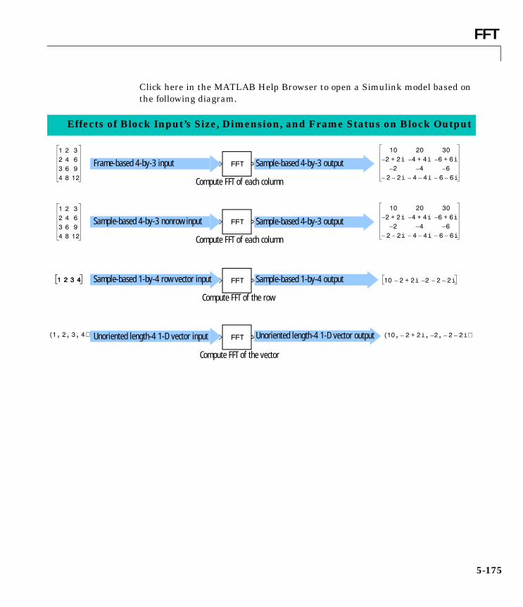
FFT
5-175
Click here in the MATLAB Help Browser to open a Simulink model based on the following diagram.
1 2 32 4 63 6 94 8 12
10 20 302 2i+– 4 4i+– 6 6i+–
2– 4– 6–
2– 2i– 4– 4i– 6– 6i–
1 2 3 4 10 2– 2i+ 2– 2– 2i–
1 2 3 4, , ,( )
1 2 32 4 63 6 94 8 12
10 20 302 2i+– 4 4i+– 6 6i+–
2– 4– 6–
2– 2i– 4– 4i– 6– 6i–
1 2 3 4
Unoriented length-4 1-D vector input
Sample-based 4-by-3 output
Sample-based 4-by-3 output
Sample-based 1-by-4 output
Frame-based 4-by-3 input
Sample-based 4-by-3 nonrow input
Sample-based 1-by-4 row vector input
Compute FFT of the row
Compute FFT of the vector
Compute FFT of each column
Compute FFT of each column
Effects of Block Input’s Size, Dimension, and Frame Status on Block Output
10 2– 2i+ 2– 2– 2i–, , ,( )Unoriented length-4 1-D vector output

FFT
5-176
Ordering Output Column Entries (Output in bit-reversed order Parameter)Set the Output in bit-reversed order parameter as follows to indicate the ordering of the output’s column elements. For a definition of bit-reversed ordering, see “Description of Bit-Reversed Ordering” on page 5-177.
Note Linearly ordering the output requires extra data sorting manipulation, so in some situations it may be better to output in bit-reversed order as illustrated in the example, “Use of Outputs in Bit-Reversed Order” on page 5-179.
The next diagram illustrates the difference between linear and bit-reversed outputs. Note that output values in linear and bit-reversed order are the same; only the order in which they appear in the columns differs.
Parameter Setting Ordering of Output Channel Elements
Output Column Entries
Linear order(See the following note.)
kth column element is the DFT of the corresponding input column at the kth frequency.
Bit-reversed order kth column element is the DFT of the corresponding input column at the rth frequency, where r is the bit reversed value of k.
12345678
364– 9.7i+4– 4i+4– 1.7i+
4–
4– 1.7i–
4– 4i–
4– 9.7i–
364–
4– 4i+4– 4i–
4– 9.7i+4– 1.7i–
4– 1.7i+4– 9.7i–
w1w2w3w4w5w6w7
w0
Output in bit-reversed order
Output in linear order
Output can be ordered in two ways
wk is the kth frequency at which the block computes the FFT. For an N-point FFT,
wk = 2πk/N k = 0, 1, ..., N-1
w4w2w6w1w5w3w7
w0
Bit reverse the frequency indices
and indicate the frequencies at which the block computes the FFT to get the output
Input must be in linear order

FFT
5-177
Description of Bit-Reversed Ordering. Two numbers are bit-reversed values of each other when the binary representation of one is the mirror image of the binary representation of the other. For example, in a three-bit system, one and four are bit-reversed values of each other, since the three-bit binary representation of one, 001, is the mirror image of the three-bit binary representation of four, 100.
The sequence 0, 1, 2, 3, 4, 5, 6, 7, is in linear order. To put the sequence in bit-reversed order, replace each element in the linearly ordered sequence with its bit-reversed counterpart. You can do this by translating the sequence into its binary representation (with the minimum number of bits), then finding the mirror image of each binary entry, and translating the sequence back to its decimal representation. The resulting sequence is the original linearly ordered sequence in bit-reversed order.
Selecting the Twiddle Factor Computation MethodThe Twiddle factor computation parameter determines how the block computes the necessary sine and cosine terms to calculate the term
01234567
04261537
Find mirror image of each entry
Translate to binary representation
Translate back to decimal representation
000001010011100101110111
000100010110001101011111
Linear Order Bit-Reversed Order (In a three-bit system)

FFT
5-178
in Equation 5-2. This parameter has two settings, each with its advantages and disadvantages, as described in the following table.
Optimizing the Table of Trigonometric ValuesWhen you set the Twiddle factor computation parameter to Table lookup, you need to set the Optimize table for parameter. This parameter optimizes
e j– 2π m 1–( ) k 1–( ) M⁄
Twiddle factor computation Parameter Setting
Sine and Cosine Computation Method
Effect on Block Performance
Table lookup The block computes and stores the trigonometric values before the simulation starts, and retrieves them during the simulation. When you generate code from the block, the processor running the generated code stores the trigonometric values computed by the block, and retrieves the values during code execution.
The block usually runs much more quickly, but requires extra memory for storing the precomputed trigonometric values. You can optimize the table for memory consumption or speed, as described in “Optimizing the Table of Trigonometric Values” below.
Trigonometric fcn The block computes sine and cosine values during the simulation. When you generate code from the block, the processor running the generated code computes the sine and cosine values while the code runs.
The block usually runs more slowly, but does not need extra data memory. For code generation, the block requires a support library to emulate the trigonometric functions, increasing the size of the generated code.

FFT
5-179
the table of trigonometric values for speed or memory by varying the number of table entries as summarized in the following table.
Algorithms Used for FFT ComputationDepending on whether the block input is real- or complex-valued, and whether you want the output in linear or bit-reversed order, the block uses one or more of the following algorithms as summarized in the next table:
• Radix-2 decimation-in-time (DIT) algorithm
• Radix-2 decimation-in-frequency (DIF) algorithm
• Half-length algorithm
• Double-signal algorithm
Example Use of Outputs in Bit-Reversed Order. The FFT block runs more quickly when it outputs in bit-reversed order. You can often use an output in bit-reversed order when your model also uses the IFFT block (the IFFT block allows you to indicate whether its input is in bit-reversed or linear order). For instance, set the FFT block to output in bit-reversed order when you want to filter or
Optimize table for Parameter Setting
Number of Table Entries for N-Point FFT
Memory Required for Single-Precision 512-Point FFT
Speed 3N/4 1536 bytes
Memory N/4 + 1 516 bytes
Input Complexity Output Ordering Algorithms Used for FFT Computation
Complex Linear or bit-reversed
Radix-2 DIT
Real Linear Radix-2 DIT in conjunction with the half-length and double-signal algorithms when possible
Real Bit-reversed Radix-2 DIF in conjunction with the half-length and double-signal algorithms when possible
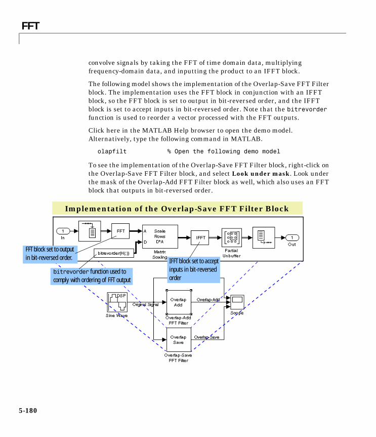
FFT
5-180
convolve signals by taking the FFT of time domain data, multiplying frequency-domain data, and inputting the product to an IFFT block.
The following model shows the implementation of the Overlap-Save FFT Filter block. The implementation uses the FFT block in conjunction with an IFFT block, so the FFT block is set to output in bit-reversed order, and the IFFT block is set to accept inputs in bit-reversed order. Note that the bitrevorder function is used to reorder a vector processed with the FFT outputs.
Click here in the MATLAB Help browser to open the demo model. Alternatively, type the following command in MATLAB.
olapfilt % Open the following demo model
To see the implementation of the Overlap-Save FFT Filter block, right-click on the Overlap-Save FFT Filter block, and select Look under mask. Look under the mask of the Overlap-Add FFT Filter block as well, which also uses an FFT block that outputs in bit-reversed order.
Implementation of the Overlap-Save FFT Filter Block
FFT block set to output in bit-reversed order. IFFT block set to accept
inputs in bit-reversed order
bitrevorder function used to comply with ordering of FFT output

FFT
5-181
Dialog Box
Twiddle factor computationComputation method of the term in Equation 5-2. In Table lookup mode, the block computes and stores the sine and cosine values before the simulation starts. In Trigonometric fcn mode, the block computes the sine and cosine values during the simulation. See “Selecting the Twiddle Factor Computation Method” on page 5-177.
Optimize table forOptimization of the table of sine and cosine values for Speed or Memory. Active only when Twiddle factor computation is set to Table lookup. See “Selecting the Twiddle Factor Computation Method” on page 5-177.
Output in bit-reverse orderOrder of the output channel elements relative to the ordering of the input elements. When checked, the output channel elements are in bit-reversed order relative to the input ordering. Otherwise, the output column elements are linearly ordered relative to the input ordering. See “Ordering Output Column Entries (Output in bit-reversed order Parameter)” on page 5-176.
Supported Data Types
e j– 2π m 1–( ) k 1–( ) M⁄
Single-precision floating point Table lookup mode onlyDouble-precision floating point All modes

FFT
5-182
See Also Complex Cepstrum DSP BlocksetDCT DSP BlocksetIFFT DSP BlocksetPad DSP BlocksetZero Pad DSP Blocksetbitrevorder Signal Processing Toolboxfft Signal Processing Toolboxifft Signal Processing Toolbox

Filter Realization Wizard
5-183
5Filter Realization WizardPurpose Automatically construct filter realizations using Sum, Gain, and Unit Delay blocks.
Library Filtering / Filter Designs
Description The Filter Realization Wizard is a tool for automatically creating filter realizations with specific architectures. The Wizard’s interface allows you to specify the filter’s structure and coefficients, the type of data to be filtered, and optimization criteria for the design. The Wizard then builds the specified filter as a subsystem composed of Sum, Gain, and Unit Delay blocks. You can specify the name of the subsystem (“Filter” is the default) and whether it is placed in the current model or in a new model.
The Architecture panel in the Wizard’s interface allows you to select from the following realizations.
The Optimization panel in the Wizard’s interface lets you choose to optimize for zero and unity gains. Zero-gain optimization removes zero-gain paths from the filter structure, and unity-gain optimization substitutes a wire (short circuit) for unity gains.
Type a name for the new filter block in the Block Name text field, and select where the block should be placed from the Destination pop-up menu. Within a model, the Filter subsystem operates on a sample-based signal (similar to Simulink’s Discrete Filter block), filtering each channel over time. Double-click on the subsystem to open it; you can then modify the gains or the filter structure to suit your needs.
Architecture Parameters
Direct-Form I Numerator, denominator
Direct-Form II Numerator, denominator
Symmetric FIR Coefficients
Lattice (AR) Lattice coefficients
Lattice (MA) Lattice coefficients
Lattice (ARMA) Lattice coefficients, ladder coefficients

Filter Realization Wizard
5-184
Fixed-Point OptionsBy default, the filter constructed by the Filter Realization Wizard operates using the Simulink standard double-precision arithmetic. If you have the Fixed-Point Blockset installed on your system, you have the additional option of building the filter to operate using single-precision or fixed-point arithmetic. Select the option you want from the Data Type panel:
• Built-in data types
The filter is constructed using the standard Simulink Sum, Gain, and Unit Delay blocks, and operates in any precision supported by Simulink (e.g., double-precision, single-precision, Boolean, etc.). This is the default.
• Single
The filter is constructed using the Sum, Gain, and Unit Delay blocks from the Fixed-Point Blockset. The blocks are configured for single-precision arithmetic.
• Fixed-Point
The filter is constructed using the Sum, Gain, and Unit Delay blocks from the Fixed-Point Blockset. The Sum and Gain blocks are configured for fixed-point arithmetic using the options specified in the Fixed-Point panel of the Filter Realization Wizard. These options include:
- Format (Signed or Unsigned)
- Word size- Radix pos
- Overflow (Wrap or Saturate)
- Rounding (Zero, Nearest, Ceiling, or Floor)
For information on these parameters, see the Fixed-Point Blockset documentation.
Examples The examples below illustrate some of the common architectures available through the Filter Realization Wizard:
• Example 1: Direct Form II
• Example 2: Second Order Sections
• Example 3: Nth Order Sections
• Example 4: ARMA Lattice

Filter Realization Wizard
5-185
Example 1: Direct Form IIDesign an fourth-order, quarter-band, lowpass Butterworth filter:
1 At the MATLAB command line, compute the filter coefficients by entering[b,a] = butter(4,.25);
2 Launch the Filter Realization Wizard by double-clicking on the icon in the Filter Realizations library.
3 Configure the Wizard to use b and a as the numerator and denominator of a Direct-Form II structure:
- Select Direct-Form II from the Type menu.
- Type b in the Numerator text field.
- Type a in the Denominator text field.
4 Type a name for the new filter subsystem in the Block Name field. The example uses Butter LPF.
The GUI with these settings is shown below.
5 Press the Build button to create the specified filter subsystem in a new model window.

Filter Realization Wizard
5-186
6 Double-click the new Butter LPF block to see the Direct-Form II filter realization that the Wizard created.
Example 2: Second Order SectionsDesign an eighth-order, quarter-band, lowpass Butterworth filter using second-order sections (SOS):
1 At the MATLAB command line, compute the second-order sections by entering[a,b,c,d] = butter(4,.25);sos = ss2sos(a,b,c,d);
2 Configure the Wizard to use sos as the numerator of a Direct-Form II structure:
- Select Direct-Form II from the Type menu.
- Type sos in the Numerator text field.
- Leave the Denominator text field blank.

Filter Realization Wizard
5-187
3 Type a name for the new filter subsystem in the Block Name field. The example uses Butter SOS.
4 Press the Build button to create the specified filter subsystem in a new model window.
5 Double-click the new Butter SOS block to see the Direct-Form II filter realization that the Wizard created.
Note that in a subsystem with the Direct-Form I or II architecture, the filter sections are connected using From and Goto blocks rather than being directly wired together. This makes it easier to recognize and move filter sections in the model window independently of each other.
Example 3: Nth Order SectionsDesign a lowpass Butterworth filter using Nth order cascades:
1 At the MATLAB command line, compute the coefficients for the Nth order sections by entering[b1,a1] = butter(4,.25);[b2,a2] = butter(3,.25);
2 Configure the Wizard to use these coefficient vectors as the numerator and denominator of a Direct-Form II structure:
- Select Direct-Form II from the Type menu.
- Type b1,b2 in the Numerator text field. Note that the numerator coefficient vector for each section is entered as an element in a cell array. Since this is a two-section filter, a two-cell array is specified in the
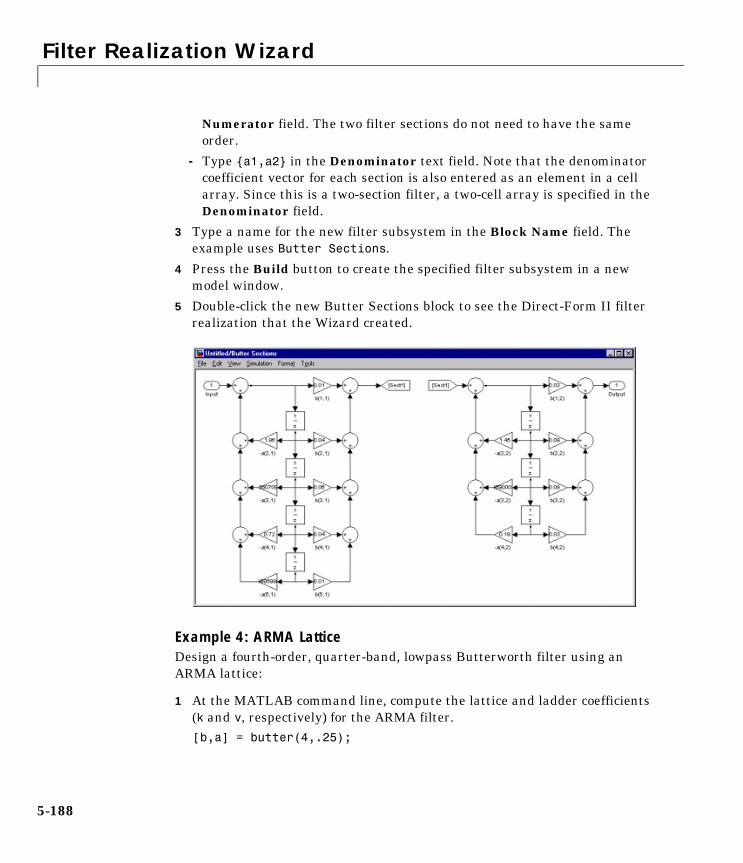
Filter Realization Wizard
5-188
Numerator field. The two filter sections do not need to have the same order.
- Type a1,a2 in the Denominator text field. Note that the denominator coefficient vector for each section is also entered as an element in a cell array. Since this is a two-section filter, a two-cell array is specified in the Denominator field.
3 Type a name for the new filter subsystem in the Block Name field. The example uses Butter Sections.
4 Press the Build button to create the specified filter subsystem in a new model window.
5 Double-click the new Butter Sections block to see the Direct-Form II filter realization that the Wizard created.
Example 4: ARMA LatticeDesign a fourth-order, quarter-band, lowpass Butterworth filter using an ARMA lattice:
1 At the MATLAB command line, compute the lattice and ladder coefficients (k and v, respectively) for the ARMA filter.[b,a] = butter(4,.25);

Filter Realization Wizard
5-189
[k,v] = tf2latc(b,a);
Configure the Wizard to use k and v as the coefficients of the lattice design:
- Select Lattice (ARMA) from the Type menu.
- Type k in the Lattice Coeffs text field.
- Type v in the Ladder Coeffs text field.
2 Type a name for the new filter subsystem in the Block Name field. The example uses Butter Lattice.
3 Press the Build button to create the specified filter subsystem in a new model window.
4 Double-click the new Butter Lattice block to see the ARMA filter realization that the Wizard created.

Filter Realization Wizard
5-190
Dialog Box
The parameters displayed in the Architecture panel vary for different selections in the Type menu. Only a portion of the parameters listed below are visible in the wizard at any one time.
TypeThe filter architecture: Direct-Form I, Direct-Form II, Symmetric FIR, Lattice (MA), Lattice (AR), Lattice (ARMA).
NumeratorThe numerator coefficients for the direct-form I and II structures, specified as a vector or variable name.
DenominatorThe denominator coefficients for the direct-form I and II structures, specified as a vector or variable name.
CoefficientsThe coefficients for the symmetric FIR structure, specified as a vector or variable name.

Filter Realization Wizard
5-191
Lattice CoeffsThe lattice coefficients for the lattice MA/AR/ARMA structures, specified as a vector or variable name.
Ladder CoeffsThe ladder coefficients for the lattice ARMA structure, specified as a vector or variable name.
Optimize for zero gainsEnables zero-gain optimization (when checked) by removing zero-gain paths from the filter structure.
Optimize for unity gainsEnables unity-gain optimization (when checked) by substituting a wire (short circuit) for unity gains.
DestinationThe location where the new filter block should be created.
Block nameThe name of the new filter block.
BuildGenerate the filter.
Data typeThe precision of the data that the filter will process. Built-in data types, when selected, configures the block to build the filter using double-precision Simulink blocks. Single precision and Fixed-point configure the block to build the filter using Fixed-Point Blockset blocks.
Fixed-pointOptions for fixed-point filter construction. See the Fixed-Point Blockset documentation.
References Oppenheim, A. V. and R. W. Schafer. Discrete-Time Signal Processing. Englewood Cliffs, NJ: Prentice Hall, 1989.
Proakis, J. and D. Manolakis. Digital Signal Processing. 3rd ed. Englewood Cliffs, NJ: Prentice-Hall, 1996.

Filter Realization Wizard
5-192
Supported Data Types
See Also
See “Designing Filters with Various Filter Structures” on page 4-6 for related information.
Fixed-point Supported only when you install the Fixed-Point Blockset
Single-precision floating point Supported only when you install the Fixed-Point Blockset
Double-precision floating point
Biquadratic Filter DSP BlocksetDirect-Form II Transpose Filter DSP BlocksetDiscrete Filter SimulinkTime-Varying Direct-Form II Transpose Filter DSP BlocksetTime-Varying Lattice Filter DSP Blocksetfilter MATLAB

FIR Decimation
5-193
5FIR DecimationPurpose Filter and downsample an input signal.
Library Filtering / Multirate Filters
Description The FIR Decimation block resamples the discrete-time input at a rate K times slower than the input sample rate, where the integer K is specified by the Decimation factor parameter. This process consists of two steps:
• The block filters the input data using a direct-form II transpose FIR filter.
• The block downsamples the filtered data to a lower rate by discarding K-1 consecutive samples following every sample retained.
The FIR Decimation block implements the above FIR filtering and downsampling steps together using a polyphase filter structure, which is more efficient than straightforward filter-then-decimate algorithms. The output of the decimator is the first phase of the polyphase filter.
The FIR filter coefficients parameter specifies the numerator coefficients of the FIR filter transfer function H(z).
The length-m coefficient vector, [b(1) b(2) ... b(m)], can be generated by one of the filter design functions in the Signal Processing Toolbox, such as the fir1 function used in the example below. The filter should be lowpass with normalized cutoff frequency no greater than 1/K. All filter states are internally initialized to zero.
Sample-Based OperationAn M-by-N sample-based matrix input is treated as M∗N independent channels, and the block decimates each channel over time. The output sample period is K times longer than the input sample period (Tso = KTsi), and the input and output sizes are identical.
Frame-Based OperationAn Mi-by-N frame-based matrix input is treated as N independent channels, and the block decimates each channel over time. The Framing parameter determines how the block adjusts the rate at the output to accommodate the reduced number of samples. There are two available options:
H z( ) B z( ) b1 b2z 1– … bmz m 1–( )–+ + += =

FIR Decimation
5-194
• Maintain input frame size
The block generates the output at the slower (decimated) rate by using a proportionally longer frame period at the output port than at the input port. For decimation by a factor of K, the output frame period is K times longer than the input frame period (Tfo = KTfi), but the input and output frame sizes are equal.
The example below shows a single-channel input with a frame period of 1 second (Sample time = 1/64 and Samples per frame = 64 in the Signal From Workspace block) being decimated by a factor of 4 to a frame period of 4 seconds. The input and output frame sizes are identical.
• Maintain input frame rate
The block generates the output at the slower (decimated) rate by using a proportionally smaller frame size than the input. For decimation by a factor of K, the output frame size is K times smaller than the input frame size (Mo = Mi/K), but the input and output frame rates are equal. The input frame size, Mi, must be a multiple of the decimation factor, K.
The example below shows a single-channel input of frame size 64 being decimated by a factor of 4 to a frame size of 16. The block’s input and output frame rates are identical.

FIR Decimation
5-195
Latency
Zero Latency. The FIR Decimation block has zero tasking latency for all single-rate operations. The block is single-rate for the particular combinations of sampling mode and parameter settings shown in the table below.
Note that in sample-based mode, single-rate operation occurs only in the trivial case of factor-of-1 decimation.
The block also has zero latency for sample-based multirate operations in Simulink’s single-tasking mode. Zero tasking latency means that the block propagates the first filtered input sample (received at t=0) as the first output sample, followed by filtered input samples K+1, 2K+1, and so on.
Nonzero Latency. The FIR Decimation block is multirate for all settings other than those in the above table. The amount of latency for multirate operation depends on Simulink’s tasking mode and the block’s sampling mode, as shown in the table below.
In cases of one-sample latency, a zero initial condition appears as the first output sample in each channel. The first filtered input sample appears as the second output sample, followed by filtered input samples K+1, 2K+1, and so on.
In cases of one-frame latency, the first Mi output rows contain zeros, where Mi is the input frame size. The first filtered input sample (first filtered row of the input matrix) appears in the output as sample Mi+1, followed by filtered input
Sampling Mode Parameter Settings
Sample-based Decimation factor parameter, K, is 1.
Frame-based Decimation factor parameter, K, is 1, or Framing parameter is Maintain input frame rate.
Multirate... Sample-Based Latency Frame-Based Latency
Single-tasking None One frame (Mi samples)
Multitasking One sample One frame (Mi samples)

FIR Decimation
5-196
samples K+1, 2K+1, and so on. See the example below for an illustration of this case.
See “Excess Algorithmic Delay (Tasking Latency)” on page 3-91 and “The Simulation Parameters Dialog Box” in the Simulink documentation for more information about block rates and Simulink’s tasking modes.
Examples Example 1Construct the frame-based model shown below.
Adjust the block parameters as follows:
• Configure the Signal From Workspace block to generate a two-channel signal with frame size of 4 and sample period of 0.25. This represents an output frame period of 1 (0.25∗4). The first channel should contain the positive ramp signal 1, 2, ..., 100, and the second channel should contain the negative ramp signal -1, -2, ..., -100.
- Signal = [(1:100)' (-1:-1:-100)']
- Sample time = 0.25
- Samples per frame = 4
• Configure the FIR Decimation block to decimate the two-channel input by decreasing the output frame rate by a factor of 2 relative to the input frame rate. Use a third-order filter with normalized cutoff frequency, fn0, of 0.25. (Note that fn0 satisfies fn0 ≤ 1/K.)
- FIR filter coefficients = fir1(3,0.25)
- Downsample factor = 2
- Framing = Maintain input frame size

FIR Decimation
5-197
The filter coefficient vector generated by fir1(3,0.25) is[0.0386 0.4614 0.4614 0.0386]
or, equivalently,
• Configure the Probe blocks by deselecting the Probe width, Probe complex signal, and Probe signal dimensions check boxes (if desired).
This model is multirate because there are at least two distinct sample rates, as shown by the two Probe blocks. To run this model in Simulink’s multitasking mode, select Fixed-step and discrete from the Type controls in the Solver panel of the Simulation Parameters dialog box, and select MultiTasking from the Mode parameter. Also set the Stop time to 30.
Run the model and look at the output, yout. The first few samples of each channel are shown below.
yout =
0 0 0 0 0 0 0 0 0.0386 -0.0386 1.5000 -1.5000 3.5000 -3.5000 5.5000 -5.5000 7.5000 -7.5000 9.5000 -9.5000 11.5000 -11.5000
Since we ran this frame-based multirate model in multitasking mode, the first four (Mi) output rows are zero. The first filtered input matrix row appears in the output as sample 5 (i.e., sample Mi+1).
Example 2The dspmrf_menu demo illustrates the use of the FIR Decimation block in a number of multistage multirate filters.
H z( ) B z( ) 0.0386 0.04614z 1– 0.04614z 2– 0.0386z 3–+ + += =

FIR Decimation
5-198
Dialog Box
FIR filter coefficientsThe lowpass FIR filter coefficients, in descending powers of z.
Decimation factorThe integer factor, K, by which to decrease the sample rate of the input sequence.
FramingFor frame-based operation, the method by which to implement the decimation; reduce the output frame rate, or reduce the output frame size.
Supported Data Types
See Also
See the following sections for related information:
• “Converting Sample Rates and Frame Rates” on page 3-20
Double-precision floating point
Direct-Form II Transpose Filter DSP BlocksetDownsample DSP BlocksetFIR Interpolation DSP BlocksetFIR Rate Conversion DSP Blocksetdecimate Signal Processing Toolboxfir1 Signal Processing Toolboxfir2 Signal Processing Toolboxfirls Signal Processing Toolboxremez Signal Processing Toolbox

FIR Decimation
5-199
• “Multirate Filters” on page 4-9

FIR Interpolation
5-200
5FIR InterpolationPurpose Upsample and filter an input signal.
Library Filtering / Multirate Filters
Description The FIR Interpolation block resamples the discrete-time input at a rate L times faster than the input sample rate, where the integer L is specified by the Interpolation factor parameter. This process consists of two steps:
• The block upsamples the input to a higher rate by inserting L-1 zeros between samples.
• The block filters the upsampled data with a direct-form II transpose FIR filter.
The FIR Interpolation block implements the above upsampling and FIR filtering steps together using a polyphase filter structure, which is more efficient than straightforward upsample-then-filter algorithms.
The FIR filter coefficients parameter specifies the numerator coefficients of the FIR filter transfer function H(z).
The coefficient vector, [b(1) b(2) ... b(m)], can be generated by one of the filter design functions in the Signal Processing Toolbox (such as fir1), and should have a length greater than the interpolation factor (m>L). The filter should be lowpass with normalized cutoff frequency no greater than 1/L. All filter states are internally initialized to zero.
Sample-Based OperationAn M-by-N sample-based matrix input is treated as M∗N independent channels, and the block interpolates each channel over time. The output sample period is L times shorter than the input sample period (Tso = Tsi/L), and the input and output sizes are identical.
Frame-Based OperationAn Mi-by-N frame-based matrix input is treated as N independent channels, and the block decimates each channel over time. The Framing parameter determines how the block adjusts the rate at the output to accommodate the added samples. There are two available options:
H z( ) B z( ) b1 b2z 1– … bmz m 1–( )–+ + += =

FIR Interpolation
5-201
• Maintain input frame size
The block generates the output at the faster (interpolated) rate by using a proportionally shorter frame period at the output port than at the input port. For interpolation by a factor of L, the output frame period is L times shorter than the input frame period (Tfo = Tfi/L), but the input and output frame sizes are equal.
The example below shows a single-channel input with a frame period of 1 second (Sample time = 1/64 and Samples per frame = 64 in the Signal From Workspace block) being interpolated by a factor of 4 to a frame period of 0.25 seconds. The input and output frame sizes are identical.
• Maintain input frame rate
The block generates the output at the faster (interpolated) rate by using a proportionally larger frame size than the input. For interpolation by a factor of L, the output frame size is L times larger than the input frame size (Mo = Mi∗L), but the input and output frame rates are equal.
The example below shows a single-channel input of frame size 16 being interpolated by a factor of 4 to a frame size of 64. The block’s input and output frame rates are identical.

FIR Interpolation
5-202
Latency
Zero Latency. The FIR Interpolation block has zero tasking latency for all single-rate operations. The block is single-rate for the particular combinations of sampling mode and parameter settings shown in the table below.
Note that in sample-based mode, single-rate operation occurs only in the trivial case of factor-of-1 interpolation.
The block also has zero latency for sample-based multirate operations in Simulink’s single-tasking mode. Zero tasking latency means that the block propagates the first filtered input (received at t=0) as the first input sample, followed by L-1 interpolated values, the second filtered input sample, and so on.
Nonzero Latency. The FIR Interpolation block is multirate for all settings other than those in the above table. The amount of latency for multirate operation depends on Simulink’s tasking mode and the block’s sampling mode, as shown in the table below.
In cases of one-sample latency, a zero initial condition appears as the first output sample in each channel, followed immediately by the first filtered input sample, L-1 interpolated values, and so on.
In cases of one-frame latency, the first Mi output rows contain zeros, where Mi is the input frame size. The first filtered input sample (first filtered row of the
Sampling Mode Parameter Settings
Sample-based Interpolation factor parameter, L, is 1.
Frame-based Interpolation factor parameter, L, is 1, or Framing parameter is Maintain input frame rate.
Multirate... Sample-Based Latency Frame-Based Latency
Single-tasking None One frame (Mi samples)
Multitasking One sample One frame (Mi samples)

FIR Interpolation
5-203
input matrix) appears in the output as sample Mi+1, followed by L-1 interpolated values, the second filtered input sample, and so on. See the example below for an illustration of this case.
See “Excess Algorithmic Delay (Tasking Latency)” on page 3-91 and “The Simulation Parameters Dialog Box” in the Simulink documentation for more information about block rates and Simulink’s tasking modes.
Example Example 1Construct the frame-based model shown below.
Adjust the block parameters as follows.
• Configure the Signal From Workspace block to generate a two-channel signal with frame size of 4 and sample period of 0.25. This represents an output frame period of 1 (0.25∗4). The first channel should contain the positive ramp signal 1, 2, ..., 100, and the second channel should contain the negative ramp signal -1, -2, ..., -100.
- Signal = [(1:100)' (-1:-1:-100)']
- Sample time = 0.25
- Samples per frame = 4
• Configure the FIR Interpolation block to interpolate the two-channel input by increasing the output frame rate by a factor of 2 relative to the input frame rate. Use a third-order filter (m=3) with normalized cutoff frequency, fn0, of 0.25. (Note that fn0 and m satisfy fn0 ≤ 1/L and m > L.)
- FIR filter coefficients = fir1(3,0.25)
- Interpolation factor = 2
- Framing = Maintain input frame size

FIR Interpolation
5-204
The filter coefficient vector generated by fir1(3,0.25) is[0.0386 0.4614 0.4614 0.0386]
or, equivalently,
• Configure the Probe blocks by deselecting the Probe width, Probe complex signal, and Probe signal dimensions check boxes (if desired).
This model is multirate because there are at least two distinct sample rates, as shown by the two Probe blocks. To run this model in Simulink’s multitasking mode, select Fixed-step and discrete from the Type controls in the Solver panel of the Simulation Parameters dialog box, and select MultiTasking from the Mode parameter. Also set the Stop time to 30.
Run the model and look at the output, yout. The first few samples of each channel are shown below.
yout =
0 0 0 0 0 0 0 0 0.0386 -0.0386 0.4614 -0.4614 0.5386 -0.5386 0.9614 -0.9614 1.0386 -1.0386
Since we ran this frame-based multirate model in multitasking mode, the first four (Mi) output rows are zero. The first filtered input matrix row appears in the output as sample 5 (i.e., sample Mi+1). Every second row is an interpolated value.
Example 2The dspintrp demo provides another simple example, and the dspmrf_menu demo illustrates the use of the FIR Interpolation block in a number of multistage multirate filters.
H z( ) B z( ) 0.0386 0.04614z 1– 0.04614z 2– 0.0386z 3–+ + += =

FIR Interpolation
5-205
Dialog Box
FIR filter coefficientsThe FIR filter coefficients, in descending powers of z.
Interpolation factorThe integer factor, L, by which to increase the sample rate of the input sequence.
FramingFor frame-based operation, the method by which to implement the interpolation: increase the output frame rate, or increase the output frame size.
Supported Data Types
See Also
See the following sections for related information:
• “Converting Sample Rates and Frame Rates” on page 3-20
Double-precision floating point
FIR Decimation DSP BlocksetFIR Rate Conversion DSP BlocksetUpsample DSP Blocksetfir1 Signal Processing Toolboxfir2 Signal Processing Toolboxfirls Signal Processing Toolboxinterp Signal Processing Toolboxremez Signal Processing Toolbox

FIR Interpolation
5-206
• “Multirate Filters” on page 4-9

FIR Rate Conversion
5-207
5FIR Rate ConversionPurpose Upsample, filter, and downsample an input signal.
Library Filtering / Multirate Filters
Description The FIR Rate Conversion block resamples the discrete-time input to a period K/L times the input sample period, where the integer K is specified by the Decimation factor parameter and the integer L is specified by the Interpolation factor parameter. The resampling process consists of the following steps:
• The block upsamples the input to a higher rate by inserting L-1 zeros between input samples.
• The upsampled data is passed through a direct-form II transpose FIR filter.
• The block downsamples the filtered data to a lower rate by discarding K-1 consecutive samples following each sample retained.
K and L must be relatively prime integers; that is, the ratio K/L cannot be reducible to a ratio of smaller integers. The FIR Rate Conversion block implements the above three steps together using a polyphase filter structure, which is more efficient than straightforward upsample-filter-decimate algorithms. The output of the interpolator is the first filter phase, while the output of the decimator is the last filter phase. When both K and L are greater than 1, the resulting output is the last decimation phase from the first interpolation phase.
The FIR filter coefficients parameter specifies the numerator coefficients of the FIR filter transfer function H(z).
The coefficient vector, [b(1) b(2) ... b(m)], can be generated by one of the filter design functions in the Signal Processing Toolbox (such as fir1), and should have a length greater than the interpolation factor (m>L). The filter should be lowpass with normalized cutoff frequency no greater than min(1/L,1/K). All filter states are internally initialized to zero.
H z( ) B z( ) b1 b2z 1– … bmz m 1–( )–+ + += =

FIR Rate Conversion
5-208
Frame-Based OperationThis block accepts only frame-based inputs. An Mi-by-N frame-based matrix input is treated as N independent channels, and the block resamples each channel independently over time.
The Interpolation factor, L, and Decimation factor, K, must satisfy the relation
for an integer output frame size Mo. The simplest way to satisfy this requirement is to let the Decimation factor equal the input frame size, Mi. The output frame size, Mo, is then equal to the Interpolation factor. This change in the frame size, from Mi to Mo, produces the desired rate conversion while leaving the output frame period the same as the input (Tfo = Tfi).
LatencyThe FIR Rate Conversion block has no tasking latency. The block propagates the first filtered input (received at t=0) as the first output sample.
Examples The dspsrcnv demo compares sample rate conversion performed by the FIR Rate Conversion block with the same conversion performed by a cascade of Upsample, Direct-Form II Transpose Filter, and Downsample blocks.
KL----
MiMo--------=
17181920
13141516
9101112
5678
1234
t=0t=6t=12 t=9 t=3
first input frame
Tfi = 3
first non-zero output
3.844.304.72
2.502.943.39
1.171.612.05
0.040.290.72
t=0t=6t=9 t=3
Tfo = 3
5.175.616.05
t=12
FIR Rate Conversion (One-channel input)
Decimation factor: 4Interpolation factor: 3
Input:
4-by-1Tfi = 3
Output:
3-by-1Tfo = 3

FIR Rate Conversion
5-209
Diagnostics An error is generated if the relation between K and L shown above is not satisfied.
(Input port width)/(Output port width) must equal the(Decimation factor)/(Interpolation factor).
A warning is generated if L and K are not relatively prime; that is, if the ratio L/K can be reduced to a ratio of smaller integers.
Warning: Integer conversion factors are not relatively prime in block 'modelname/FIR Rate Conversion (Frame)'. Converting ratio L/M to l/m.
The block scales the ratio to be relatively prime, and continues the simulation.
Dialog Box
Interpolation factorThe integer factor, L, by which to upsample the signal before filtering.
FIR filter coefficientsThe FIR filter coefficients, in descending powers of z.
Decimation factorThe integer factor, K, by which to downsample the signal after filtering.
References Fliege, N. J. Multirate Digital Signal Processing: Multirate Systems, Filter Banks, Wavelets. West Sussex, England: John Wiley & Sons, 1994.

FIR Rate Conversion
5-210
Supported Data Types
See Also
See the following sections for related information:
• “Converting Sample Rates and Frame Rates” on page 3-20
• “Multirate Filters” on page 4-9
Double-precision floating point
Downsample DSP BlocksetFIR Decimation DSP BlocksetFIR Interpolation DSP BlocksetUpsample DSP Blocksetfir1 Signal Processing Toolboxfir2 Signal Processing Toolboxfirls Signal Processing Toolboxremez Signal Processing Toolboxupfirdn Signal Processing Toolbox

Flip
5-211
5FlipPurpose Flip the input vertically or horizontally.
Library Signal Management / Indexing
Description The Flip block vertically or horizontally reverses the M-by-N input matrix, u. The output always has the same dimension and frame status as the input.
When Columns is selected from the Flip along menu, the block vertically flips the input so that the first row of the input is the last row of the output.
y = flipud(u) % Equivalent MATLAB code
For convenience, length-M 1-D vector inputs are treated as M-by-1 column vectors for vertical flipping.
When Rows is selected from the Flip along menu, the block horizontally flips the input so that the first column of the input is the last column of the output.
y = fliplr(u) % Equivalent MATLAB code
For convenience, length-N 1-D vector inputs are treated as 1-by-N row vectors for horizontal flipping. The output always has the same dimension and frame status as the input.
Dialog Box
Flip alongThe dimension along which to flip the input. Columns specifies vertical flipping, while Rows specifies horizontal flipping. Tunable

Flip
5-212
Supported Data Types
See Also
Fixed-pointCustom data typesBoolean8-, 16-, and 32-bit signed integer 8-, 16-, and 32-bit unsigned integerSingle-precision floating point Double-precision floating point
Selector SimulinkTranspose DSP BlocksetVariable Selector DSP Blocksetflipud MATLABfliplr MATLAB

Forward Substitution
5-213
5Forward SubstitutionPurpose Solve the equation LX=B for X when L is a lower triangular matrix.
Library Math Functions / Matrices and Linear Algebra / Linear System Solvers
Description The Forward Substitution block solves the linear system LX=B by simple forward substitution of variables, where L is the lower triangular M-by-M matrix input to the L port, and B is the M-by-N matrix input to the B port. The output is the solution of the equations, the M-by-N matrix X, and is always sample-based.
The block only uses the elements in the lower triangle of input L; the upper elements are ignored. When Force input to be unit-lower triangular is selected, the block replaces the elements on the diagonal of L with ones. This is useful when matrix L is the result of another operation, such as an LDL decomposition, that uses the diagonal elements to represent the D matrix.
A length-M vector input at port B is treated as an M-by-1 matrix.
Dialog Box
Force input to be unit-lower triangularReplaces the elements on the diagonal of L with 1s when selected. Tunable.
Supported Data Types
See Also
Double-precision floating point
Autocorrelation LPC DSP BlocksetCholesky Solver DSP BlocksetLDL Solver DSP BlocksetLevinson-Durbin DSP BlocksetLU Solver DSP BlocksetQR Solver DSP Blockset

Forward Substitution
5-214
See “Solving Linear Systems” on page 4-16 for related information.

Frame Status Conversion
5-215
5Frame Status ConversionPurpose Specify the frame status of the output, sample-based or frame-based.
Library Signal Management / Signal Attributes
Description The Frame Status Conversion block passes the input through to the output, and sets the output frame status to the Output signal parameter, which can be either Frame-based or Sample-based. The output frame status can also be inherited from the signal at the Ref (reference) input port, which is made visible by selecting the Inherit output frame status from Ref input port check box.
If the Output signal parameter setting or the inherited signal’s frame status differs from the input frame status, the block changes the input frame status accordingly, but does not otherwise alter the signal. In particular, the block does not rebuffer or resize 2-D inputs. Because 1-D vectors cannot be frame-based, if the input is a length-M 1-D vector, and the Output signal parameter is set to Frame-based, the output is a frame-based M-by-1 matrix (i.e., a single channel).
If the Output signal parameter or the inherited signal’s frame status matches the input frame status, the block passes the input through to the output unaltered.
Dialog Box
Inherit output frame status from Ref input portWhen selected, enables the Ref input port from which the block inherits the output frame status. Tunable.
Output signalThe output frame status, Frame-based or Sample-based. Tunable.

Frame Status Conversion
5-216
Supported Data Types
See Also
Fixed-pointCustom data typesBoolean8-, 16-, and 32-bit signed integer 8-, 16-, and 32-bit unsigned integerSingle-precision floating point Double-precision floating point
Check Signal Attributes DSP BlocksetConvert 1-D to 2-D DSP BlocksetConvert 2-D to 1-D DSP BlocksetInherit Complexity DSP Blockset

From Wave Device
5-217
5From Wave DevicePurpose Read audio data from a standard audio device in real-time. (Windows 95/98/NT only)
Library DSP Sources
Description The From Wave Device block reads audio data from a standard Windows audio device in real-time. It is compatible with most popular Windows hardware, including Sound Blaster cards. (Models that contain both this block and the To Wave Device block require a duplex-capable sound card.)
The Use default audio device parameter allows the block to detect and use the system’s default audio hardware. This option should be selected on systems that have a single sound device installed, or when the default sound device on a multiple-device system is the desired source. In cases when the default sound device is not the desired input source, deselect Use default audio device, and enter the desired device identification number in the Audio device ID parameter. The device ID is an integer value that the block associates with the sound device. A three-device system, for example, has device ID numbers of 1, 2, and 3.
If the audio source contains two channels (stereo), the Stereo check box should be selected. If the audio source contains a single channel (mono), the Stereo check box should be deselected. For stereo input, the block’s output is an M-by-2 matrix containing one frame (M consecutive samples) of audio data from each of the two channels. For mono input, the block’s output is an M-by-1 matrix containing one frame (M consecutive samples) of audio data from the mono input. The frame size, M, is specified by the Samples per frame parameter. For M=1, the output is sample-based; otherwise, the output is frame-based.
The amplitude of the input from the sound device should be in the range ±1. Values outside this range are clipped to the nearest allowable value. If the audio signal is saturating at ±1, you can reduce the microphone gain from the Multimedia Properties window (available through the Windows 95/98/NT Control Panel). The audio data is processed in uncompressed PCM (pulse code modulation) format, and should typically be sampled at one of the standard Windows audio device rates: 8000, 11025, 22050, or 44100 Hz. You can select one of these rates from the Sample rate parameter. To specify a different rate, select the User-defined option and enter a value in the User-defined sample rate parameter.

From Wave Device
5-218
The Sample Width (bits) parameter specifies the number of bits used to represent the signal samples read by the audio device. Two settings are available:
• 8 – allocates 8 bits to each sample, allowing a resolution of 256 levels
• 16 – allocates 16 bits to each sample, allowing a resolution of 65536 levels
The 16-bit sample width setting requires more memory but yields better fidelity. The output from the block is independent of the Sample Width (bits) setting, and is always double precision.
BufferingSince the audio device accepts real-time audio input, Simulink must read a continuous stream of data from the device throughout the simulation. Delays in reading data from the audio hardware can result in hardware errors or distortion of the signal. This means that the From Wave Device block must in principle read data from the audio hardware as quickly as the hardware itself acquires the signal. However, the block often cannot match the throughput rate of the audio hardware, especially when the simulation is running from within Simulink rather than as generated code. (Simulink operations are generally slower than comparable hardware operations, and execution speed routinely varies during the simulation as the host operating system services other processes.) The block must therefore rely on a buffering strategy to ensure that signal data can be read on schedule without losing samples.
At the start of the simulation, the audio device begins writing the input data to a (hardware) buffer with a capacity of Tb seconds. The From Wave Device block immediately begins pulling the earliest samples off the buffer (first in, first out) and collecting them in length-M frames for output. As the audio device continues to append inputs to the bottom of the buffer, the From Wave Device block continues to pull inputs off the top of the buffer at the best possible rate.
The following figure shows an audio signal being acquired and output with a frame size of 8 samples. The buffer of the sound board is approaching its five-frame capacity at the instant shown, which means that the hardware is adding samples to the buffer more rapidly than the block is pulling them off. (If

From Wave Device
5-219
the signal sample rate was 8 kHz, this small buffer could hold approximately 0.005 second of data.)
If the simulation throughput rate is higher than the hardware throughput rate, the buffer remains empty throughout the simulation. If necessary, the From Wave Device block simply waits for new samples to become available on the buffer (the block does not interpolate between samples). More typically, the simulation throughput rate is lower than the hardware throughput rate, and the buffer tends to fill over the duration of the simulation.
TroubleshootingIf the buffer size is too small in relation to the simulation throughput rate, the buffer may fill before the entire length of signal is processed. This usually results in a device error or undesired device output. When this problem occurs, you can choose to either increase the buffer size or the simulation throughput rate:
• Increase the buffer size
The Queue duration parameter specifies the duration of signal, Tb (in real-time seconds), that can be buffered in hardware during the simulation. Equivalently, this is the maximum length of time that the block’s data acquisition can lag the hardware’s data acquisition. The number of frames buffered is approximately
where Fs is the sample rate of the signal and M is the number of samples per frame. The required buffer size for a given signal depends on the signal
boar
dHardware buffer with 5-frame capacity
Simulink execution rate varies.Hardware execution rate is
No delays Simulation delay
TbFsM
-------------

From Wave Device
5-220
length, the frame size, and the speed of the simulation. Note that increasing the buffer size may increase model latency.
• Increase the simulation throughput rate
Two useful methods for improving simulation throughput rates are increasing the signal frame size and compiling the simulation into native code:
- Increase frame sizes (and convert sample-based signals to frame-based signals) throughout the model to reduce the amount of block-to-block communication overhead. This can drastically increase throughput rates in many cases. However, larger frame sizes generally result in greater model latency due to initial buffering operations.
- Generate executable code with Real Time Workshop. Native code runs much faster than Simulink, and should provide rates adequate for real-time audio processing.
More general ways to improve throughput rates include simplifying the model, and running the simulation on a faster PC processor. See “Delay and Latency” on page 3-85 of this book, and “Improving Simulation Performance and Accuracy” in the Simulink documentation, for other ideas on improving simulation performance.
Dialog Box

From Wave Device
5-221
Sample rate (Hz)The sample rate of the audio data to be acquired. Select one of the standard Windows rates or the User-defined option.
User-defined sample rate (Hz)The (nonstandard) sample rate of the audio data to be acquired.
Sample width (bits)The number of bits used to represent each signal sample.
StereoSpecifies stereo (two-channel) inputs when checked, mono (one-channel) inputs when unchecked. Stereo output is M-by-2; mono output is M-by-1.
Samples per frameThe number of audio samples in each successive output frame, M.
Queue duration (seconds)The length of signal (in seconds) to buffer to the hardware at the start of the simulation.
Use default audio deviceReads audio input from the system’s default audio device when selected. Deselect to enable the Audio device ID parameter and manually enter a device ID number. Tunable.
Audio device IDThe number of the audio device from which to read the audio output. In a system with several audio devices installed, a value of 1 selects the first audio card, a value of 2 selects the second audio card, and so on. Select Use default audio device if the system has only a single audio card installed. Tunable.
Supported Data Types
See Also
See “Importing WAV Files” on page 3-71 for related information.
Double-precision floating point
From Wave File DSP BlocksetTo Wave Device DSP Blockset

From Wave File
5-222
5From Wave FilePurpose Read audio data from a Microsoft Wave (.wav) file. (Windows 95/98/NT only)
Library DSP Sources
Description The From Wave File block reads audio data from a Microsoft Wave (.wav) file and generates a double-precision signal with amplitudes in the range ±1. The audio data must be in uncompressed PCM (pulse code modulation) format.
y = wavread('filename') % Equivalent MATLAB code
The File name parameter can specify an absolute or relative path to the file. If the file is on the MATLAB path or in the current directory (the directory returned by typing pwd at the MATLAB command line), you need only specify the file’s name. You do not need to specify the.wav extension in either case.
If the audio file contains two channels (stereo), the block’s output is an M-by-2 matrix containing one frame (M consecutive samples) of audio data from each of the two channels. If the audio file contains a single channel (mono), the block’s output is an M-by-1 matrix containing one frame (M consecutive samples) of mono audio data. The frame size, M, is specified by the Samples per frame parameter. For M=1, the output is sample-based; otherwise, the output is frame-based.
The output frame period, Tfo, is
,
where Fs is the data sample rate in Hz.
To reduce the required number of file accesses, the block acquires L consecutive samples from the file during each access, where L is specified by the Minimum number of samples for each read from file parameter (L ≥ M). For L < M, the block instead acquires M consecutive samples during each access. Larger values of L result in fewer file accesses, which reduces run-time overhead.
The block icon shows the name, sample rate (in Hz), number of channels (1 or 2), and sample width (in bits) of the data in the specified audio file. All sample rates are supported; the sample width must be either 8 or 16 bits.
TfoMFs------=
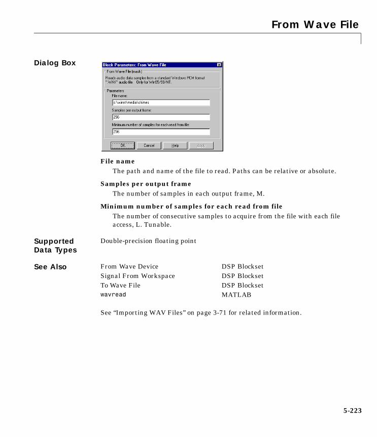
From Wave File
5-223
Dialog Box
File nameThe path and name of the file to read. Paths can be relative or absolute.
Samples per output frameThe number of samples in each output frame, M.
Minimum number of samples for each read from fileThe number of consecutive samples to acquire from the file with each file access, L. Tunable.
Supported Data Types
See Also
See “Importing WAV Files” on page 3-71 for related information.
Double-precision floating point
From Wave Device DSP BlocksetSignal From Workspace DSP BlocksetTo Wave File DSP Blocksetwavread MATLAB

Histogram
5-224
5HistogramPurpose Generate the histogram of an input or sequence of inputs.
Library Statistics
Description The Histogram block computes the frequency distribution of the elements in each column of the input, or tracks the frequency distribution in a sequence of inputs over a period of time. The Running histogram parameter selects between basic operation and running operation, described below.
The block sorts the elements of each column into the number of discrete bins specified by the Number of bins parameter, n.
y = hist(u,n) % Equivalent MATLAB code
Complex inputs are sorted by their magnitudes.
The histogram value for a given bin represents the frequency of occurrence of the input values bracketed by that bin. The upper-boundary of the highest-valued bin is specified by the Maximum value of input parameter, BM, and the lower-boundary of the lowest-valued bin is specified by the Minimum value of input parameter, Bm. The bins have equal width of
and centers located at
Input values that fall on the border between two bins are sorted into the lower-valued bin; that is, each bin includes its upper boundary. For example, a bin of width 4 centered on the value 5 contains the input value 7, but not the input value 3. Input values greater than the Maximum value of input parameter or less than Minimum value of input parameter are sorted into the highest-valued or lowest-valued bin, respectively.
Basic OperationWhen the Running histogram check box is not selected, the block computes the frequency distribution of each column in the M-by-N input u independently at each sample time.
∆BM Bm–
n-----------------------=
Bm k 12---+
∆ k+ 0 1 2 … n 1–, , , ,=

Histogram
5-225
For convenience, length-M 1-D vector inputs and sample-based length-M row vector inputs are both treated as M-by-1 column vectors.
The output, y, is a sample-based n-by-N matrix whose jth column is the histogram for the data in the jth column of u. When the Normalized check box is selected, the block scales each column of the output so that sum(y(:,j)) is 1.
Running OperationWhen the Running histogram check box is selected, the block computes the frequency distributions in a time-sequence of M-by-N inputs by creating N persistent histograms to which successive inputs are continuously added. For frame-based inputs, this is equivalent to a persistent histogram for each independent channel.
As in basic operation, length-M 1-D vector inputs and sample-based length-M row vector inputs are both treated as M-by-1 column vectors.
The output is a sample-based n-by-N matrix whose jth column reflects the current state of the jth histogram. The block resets the running histogram (by emptying all bins of all histograms) when the scalar input at the optional Rst port is nonzero. (The Rst port can be disabled by deselecting the Reset port check box.)
Example The model below illustrates the Histogram block’s basic operation for a single-channel input, u, where
u = [0 -2 6 -12 2 5 4 3 0 4 3 -2 -3 -2 -9]'
The parameter settings for the Histogram block are:
• Minimum value of input = -10
• Maximum value of input = 10
• Number of bins = 5

Histogram
5-226
• Normalized =
• Running histogram =
The resulting bin width is 4, as shown below.
Dialog Box
Minimum value of inputThe lower boundary, Bm, of the lowest-valued bin.
02–
612–
25430432–
3–
2–
9–
Input Minimum value of input = -10Maximum value of input = 10Number of bins = 5
-8 -4 0 4 8
# of
occ
urre
nces
24360
Output
-9-12
-2
-2-2
-3 002
654
33
4

Histogram
5-227
Maximum value of inputThe upper boundary, BM, of the highest-valued bin.
Number of binsThe number of bins, n, in the histogram.
NormalizedNormalizes the output vector (1-norm) when selected. Tunable, except in Simulink’s external mode.
Running histogramEnables running operation when selected.
Reset portEnables the Rst input port when selected.
Supported Data Types
See Also
Double-precision floating point
Sort DSP Blocksethist MATLAB

IDCT
5-228
5IDCTPurpose Compute the IDCT of the input.
Library Transforms
Description The IDCT block computes the inverse discrete cosine transform (IDCT) of each channel in the M-by-N input matrix, u.
y = idct(u) % Equivalent MATLAB code
For both sample-based and frame-based inputs, the block assumes that each input column is a frame containing M consecutive samples from an independent channel. The frame size, M, must be a power-of-two. To work with other frame sizes, use the Zero Pad block to pad or truncate the frame size to a power-of-two length.
The output is an M-by-N matrix whose lth column contains the length-M IDCT of the corresponding input column.
where
The output is always frame-based, and the output sample rate and data type (real/complex) are the same as those of the input.
For convenience, length-M 1-D vector inputs and sample-based length-M row vector inputs are processed as single channels (i.e., as M-by-1 column vectors), and the output has the same dimension as the input.
y m l,( ) w k( )u k l,( ) π 2m 1–( ) k 1–( )2M
--------------------------------------------, mcos
k 1=
M
∑ 1 … M, ,= =
w k( )
1M
--------- , k 1=
2M----- , 2 k M≤ ≤
=

IDCT
5-229
Dialog Box
Supported Data Types
See Also
Double-precision floating point
DCT DSP BlocksetIFFT DSP Blocksetidct Signal Processing Toolbox

Identity Matrix
5-230
5Identity MatrixPurpose Generate a matrix with ones on the main diagonal and zeros elsewhere.
Library DSP Sources,Math Functions / Matrices and Linear Algebra / Matrix Operations
Description The Identity Matrix block generates a rectangular matrix with ones on the main diagonal and zeros elsewhere.
When the Inherit input port attributes from input port check box is selected, the input port is enabled, and an M-by-N matrix input generates a sample-based M-by-N matrix output with the same sample period. The values in the input matrix are ignored.
y = eye([M N]) % Equivalent MATLAB code
When the Inherit input port attributes from input port check box is not selected, the input port is disabled, and the dimensions of the output matrix are determined by the Matrix size parameter. A scalar value, M, specifies an M-by-M identity matrix, while a two-element vector, [M N], specifies an M-by-N unit-diagonal matrix. The output is sample-based, and has the sample period specified by the Sample time parameter.
Example Set Matrix size to [3 6] to generate the 3-by-6 unit-diagonal matrix below.
1 0 0 0 0 00 1 0 0 0 00 0 1 0 0 0

Identity Matrix
5-231
Dialog Box
Inherit input port attributes from input portEnables the input port when selected. The output inherits its dimensions and sample period from the input.
Matrix sizeThe number of rows and columns in the output matrix: a scalar M for a square M-by-M output, or a vector [M N] for an M-by-N output. This parameter is disabled when Inherit input port attributes from input port is selected.
Sample timeThe discrete sample period of the output. This parameter is disabled when Inherit input port attributes from input port is selected.
Supported Data Types
See Also
See “Creating Signals Using Constant Blocks” on page 3-33 for related information.
Double-precision floating point
Constant Diagonal Matrix DSP BlocksetDSP Constant DSP Blockseteye MATLAB

IFFT
5-232
5IFFTPurpose Compute the IFFT of the input.
Library Transforms
Description The IFFT block computes the inverse fast Fourier transform (IFFT) of each channel in the M-by-N or length-M input, u, where M must be a power of two. To work with other input sizes, use the Zero Pad block to pad or truncate the length-M dimension to a power-of-two length. The output is always frame-based, and each output column contains the M-point inverse discrete Fourier transform (IDFT) of the corresponding input channel.
y = ifft(u,M) % Equivalent MATLAB code
The kth entry of the lth output channel, y(k, l), is the kth point of the M-point IDFT of the lth input channel.
(5-3)
You can choose to output a scaled version of the input’s IDFT, , by setting the parameter Skip normalization by transform length, N.
(5-4)
For information on block output characteristics and how to configure the block computation methods, see the following sections:
• “Input and Output Characteristics” on page 5-233
• “Conjugate Symmetric Input” on page 5-235
• “Inputs in Bit-Reversed Order” on page 5-236
• “Selecting the Twiddle Factor Computation Method” on page 5-236
• “Optimizing the Table of Trigonometric Values” on page 5-236
• “Algorithms Used for IFFT Computation” on page 5-236
• “Example” on page 5-237
y k l,( )1M----- u m l,( )ej2π m 1–( ) k 1–( ) M⁄
m 1=
M
∑= k 1 … M, ,=
M y k l,( )⋅
M y k l,( )⋅ u m l,( )ej2π m 1–( ) k 1–( ) M⁄
m 1=
M
∑= k 1 … M, ,=

IFFT
5-233
Input and Output CharacteristicsThe following table describes all valid block input types, their corresponding outputs, and the dimension along which the block computes the IDFT.
Note For M-by-N and length-M inputs, M must be a power of two. To work with other input sizes, use the Zero Pad block to pad or truncate the length-M dimension to a power-of-two length. To get valid outputs, you must correctly set the Input is in bit-reversed order parameter to indicate the ordering of the block input. When the input is conjugate symmetric and you want to get a real-valued output, set the Input is conjugate symmetric parameter.

IFFT
5-234
Valid Block Inputs
• Must be complex-valued
• M must be a power of two
• In linear or bit-reversed order
Dimension Along Which Block Computes IDFT
Corresponding Block Output CharacteristicsOutput port rate = input port rate
Frame-based M-by-N matrix Column The following output characteristics apply to all valid block inputs:
• Frame-based
• Complex-valued unless you set the Input is conjugate symmetric parameter when your input is conjugate-symmetric, in which case the output is real-valued
• Same dimension as input (for 1-D inputs, output is a length-M column)
• Each column (each row for sample-based row inputs) contains the M-point IDFT of the corresponding input channel in linear order. If the parameter Skip normaliza-tion by transform length, N is set, rath-er than computing the IDFT, the block computes a scaled version of the IDFT given by Equation 5-4.
Sample-based M-by-N matrix,
Column
Sample-based 1-by-M row vector
Row
1-D length-M vector Vector
M 1≠

IFFT
5-235
Click here in the MATLAB Help Browser to open a Simulink model based on the following diagram.
Conjugate Symmetric InputWhen the block input is conjugate symmetric and you want real-valued outputs, set the Input is conjugate symmetric parameter, which also optimizes the block’s computation method. A common source of conjugate symmetric data is the FFT block, which yields conjugate symmetric output when its input is real-valued.
Note If the IFFT block input is conjugate symmetric but you do not set the Input is conjugate symmetric parameter, you do not get a real-valued output. Instead, you get a complex-valued output with small imaginary parts.
1 2 32 4 63 6 94 8 12
2.5 5 7.50.5– 0.5i– 1– i– 1.5– 1.5i–
0.5– 1– 1.5–
0.5– 0.5i+ 1– i+ 1.5– 1.5i+
1 2 3 4 2.5 0.5– 0.5i– 0.5– 0.5– 0.5i+
1 2 3 4, , ,( )
2.50.5– 0.5i–
0.5–
0.5– 0.5i+
1 2 32 4 63 6 94 8 12
2.5 5 7.50.5– 0.5i– 1– i– 1.5– 1.5i–
0.5– 1– 1.5–
0.5– 0.5i+ 1– i+ 1.5– 1.5i+
Unoriented length-4 1-D vector input
Frame-based 4-by-3 output
Frame-based 4-by-3 output
Frame-based 1-by-4 output
Frame-based 4-by-1 output
Frame-based 4-by-3 input
Sample-based 4-by-3 nonrow input
Sample-based 1-by-4 row vector input
Compute IFFT of the row
Compute IFFT of the vector
Compute IFFT of each column
Compute IFFT of each column
Effects of Block Input Size, Dimension, and Frame Status on Block Output

IFFT
5-236
The block output is invalid if you set this parameter when the input is not conjugate symmetric.
Inputs in Bit-Reversed OrderWhen the block input is in bit-reversed order, you must set the parameter Input is in bit-reversed order to get a valid output. The block output is invalid if you set this parameter when the input is not in bit-reversed order. A common source of bit-reversed inputs is the FFT block, as illustrated in the FFT block example, “Use of Outputs in Bit-Reversed Order” on page 5-179.
For a definition of bit-reversed and linear order, see the FFT block reference page section, “Description of Bit-Reversed Ordering” on page 5-177.
Selecting the Twiddle Factor Computation MethodThe FFT block and IFFT block both have a parameter, Twiddle factor computation. Setting this parameter in the IFFT block is very similar to setting it in the FFT block. For details, see the FFT block reference page section, “Selecting the Twiddle Factor Computation Method” on page 5-177.
Optimizing the Table of Trigonometric ValuesThe FFT block and IFFT block both have a parameter, Optimize table for. Setting this parameter in the IFFT block is very similar to setting it in the FFT block. For details, see the FFT block reference page section, “Optimizing the Table of Trigonometric Values” on page 5-178.
Algorithms Used for IFFT ComputationDepending on whether the block input is real- or complex-valued and conjugate symmetric, the block uses one or more of the following algorithms as summarized in the next table:
• Radix-2 decimation-in-time (DIT) algorithm
• Half-length algorithm
• Double-signal algorithm

IFFT
5-237
Example For an example of how to optimize computations when using both the IFFT block and FFT block in the same model, see the FFT block reference page example, “Use of Outputs in Bit-Reversed Order” on page 5-179.
Dialog Box
Twiddle factor computationComputation method of the term in Equation 5-3. In Table lookup mode, the block computes and stores the sine and cosine
Input Complexity Other Parameter Settings
Algorithms Used for FFT Computation
Complex not applicable Radix-2 DIT
Real Radix-2 DIT
Real Radix-2 DIT in conjunction with the half-length and double-signal algorithms when possible
ej2π m 1–( ) k 1–( ) M⁄

IFFT
5-238
values before the simulation starts. In Trigonometric fcn mode, the block computes the sine and cosine values during the simulation.
Optimize table forOptimization of the table of sine and cosine values for Speed or Memory. Active only when Twiddle factor computation is set to Table lookup.
Input is in bit-reversed orderSet when the input is in bit-reversed order, and clear when the input is in linear order. The block yields invalid outputs if you do not set this parameter correctly.
Input is conjugate symmetricSet when the block input is conjugate symmetric and you want real-valued outputs. The block output is invalid if you set this parameter when the input is not conjugate symmetric.
Skip normalization by transform length, NWhen set, rather than computing the IDFT, the block computes a scaled version of the IDFT given by Equation 5-4.
Supported Data Types
See Also
Single-precision floating point Table lookup mode onlyDouble-precision floating point All modes
FFT DSP BlocksetIDCT DSP BlocksetPad DSP BlocksetZero Pad DSP Blocksetbitrevorder Signal Processing Toolboxfft Signal Processing Toolboxifft Signal Processing Toolbox

Inherit Complexity
5-239
5Inherit ComplexityPurpose Change the complexity of the input to match that of a reference signal.
Library Signal Management / Signal Attributes
Description The Inherit Complexity block alters the input data at the Data port to match the complexity of the reference input at the Ref port. If the Data input is real, and the Ref input is complex, the block appends a zero-valued imaginary component, 0i, to each element of the Data input.
If the Data input is complex, and the Ref input is real, the block outputs the real component of the Data input.
If both the Data input and Ref input are real, or if both the Data input and Ref input are complex, the block propagates the Data input with no change.
Ref
5+ i3-2i0+ i2-5i2-5i
Data Output
Simul
atio
n tim
e
...
01234.
..
0+0i1+0i2+0i3+0i4+0i.
..
RefData Output
Simul
atio
n tim
e
553
-2-2.
..
i1-2i2+ i3-5i4-5i.
..
01234.
..

Inherit Complexity
5-240
Dialog Box
Supported Data Types
See Also
Fixed-pointCustom data typesBoolean8-, 16-, and 32-bit signed integer 8-, 16-, and 32-bit unsigned integerSingle-precision floating point Double-precision floating point
Check Signal Attributes DSP BlocksetComplex to Magnitude-Angle SimulinkComplex to Real-Imag SimulinkMagnitude-Angle to Complex SimulinkReal-Imag to Complex Simulink

Integer Delay
5-241
5Integer DelayPurpose Delay an input by an integer number of sample periods.
Library Signal Operations
Description The Integer Delay block delays a discrete-time input by the number of sample intervals specified in the Delay parameter. Noninteger delay values are rounded to the nearest integer, and negative delays are clipped at 0.
Sample-Based OperationWhen the input is a sample-based M-by-N matrix, the block treats each of the M∗N matrix elements as an independent channel. The Delay parameter, v, can be an M-by-N matrix of positive integers that specifies the number of sample intervals to delay each channel of the input, or a scalar integer by which to equally delay all channels.
For example, if the input is M-by-1 and v is the matrix [v(1) v(2) ... v(M)]', the first channel is delayed by v(1) sample intervals, the second channel is delayed by v(2) sample intervals, and so on. Note that when a channel is delayed for sample-time units, the output sample at time
is the input sample at time . If is negative, then the output is the corresponding value specified by the Initial conditions parameter.
A 1-D vector of length M is treated as an M-by-1 matrix, and the output is 1-D.
The Initial conditions parameter specifies the output of the block during the initial delay in each channel. The initial delay for a particular channel is the time elapsed from the start of the simulation until the first input in that channel is propagated to the output. Both fixed and time-varying initial conditions can be specified in a variety of ways to suit the dimensions of the input.
Fixed Initial Conditions. A fixed initial condition in sample-based mode can be specified as one of the following:
• Scalar value to be repeated at each sample time of the initial delay (for every channel). For a 2-by-2 input with the parameter settings below,
∆t t ∆– t ∆–

Integer Delay
5-242
the block generates the following sequence of matrices at the start of the simulation,
where is the i,jth element of the kth matrix in the input sequence.
• Array of size M-by-N-by-d. In this case, you can set different fixed initial conditions for each element of a sample-based input. This setting is explained further in the Array bullet in “Time-Varying Initial Conditions” below.
Initial conditions cannot be specified by full matrices.
Time-Varying Initial Conditions. A time-varying initial condition in sample-based mode can be specified in one of the following ways:
• Vector of length d, where d is the maximum value specified for any channel in the Delay parameter. The vector can be a L-by-d, 1-by-d, or 1-by-1-by-d. The d elements of the vector are output in sequence, one at each sample time of the initial delay.
For a scalar input and the parameters shown below,
the block outputs the sequence -1, -1, -1, 0, 1,... at the start of the simulation.
• Array of dimension M-by-N-by-d, where d is the value specified for the Delay parameter (the maximum value if the Delay is a vector) and M and N are the number of rows and columns, respectively, in the input matrix. The d pages
1– 1–
1– 1–
u111 1–
1– 1–
u112
u121
1– 1–
u113 u12
2
u211 1–
u114 u12
3
u212 u22
1…, , , , ,
uijk

Integer Delay
5-243
of the array are output in sequence, one at each sample time of the initial delay. For a 2-by-3 input, and the parameters below,
the block outputs the matrix sequence
at the start of the simulation. Note that setting Initial conditions to an array with the same matrix for each entry implements constant initial conditions; a different constant initial condition for each input matrix element (channel).
Initial conditions cannot be specified by full matrices.
Frame-Based OperationWhen the input is a frame-based M-by-N matrix, the block treats each of the N columns as an independent channel, and delays each channel as specified by the Delay parameter.
For frame-based inputs, the Delay parameter can be a scalar integer by which to equally delay all channels. It can also be a 1-by-N row vector, each element of which serves as the delay for the corresponding channel of the N-channel input. Likewise, it can also be an M-by-1 column vector, each element of which serves as the delay for one of the corresponding M samples for each channel. The Delay parameter can be an M-by-N matrix of positive integers as well; in this case, each element of each channel is delayed by the corresponding element in the delay matrix. For instance, if the fifth element of the third column of the delay matrix was 3, then the fifth element of the third channel of the input matrix is always delayed by three sample-time units.
When a channel is delayed for sample-time units, the output sample at time is the input sample at time . If is negative, then the output is the
corresponding value specified in the Initial conditions parameter.
1 2 34 5 6
2 4 61 3 5
3 6 90 4 8
, ,
∆t t ∆– t ∆–

Integer Delay
5-244
The Initial conditions parameter specifies the output during the initial delay. Both fixed and time-varying initial conditions can be specified. The initial delay for a particular channel is the time elapsed from the start of the simulation until the first input in that channel is propagated to the output.
Fixed Initial Conditions. The settings shown below specify fixed initial conditions. The value entered in the Initial conditions parameter is repeated at the output for each sample time of the initial delay. A fixed initial condition in frame-based mode can be one of the following:
• Scalar value to be repeated for all channels of the output at each sample time of the initial delay. For a general M-by-N input with the parameter settings below,
the first five samples in each of the N channels are zero. Note that if the frame size is larger than the delay, all of these zeros are all included in the first output from the block.
• Array of size 1-by-N-by-D. In this case, you can also specify different fixed initial conditions for each channel. See the Array bullet in “Time-Varying Initial Conditions” below for details.
Initial conditions cannot be specified by full matrices.
Time-Varying Initial Conditions. The following settings specify time-varying initial conditions. For time-varying initial conditions, the values specified in the Initial conditions parameter are output in sequence during the initial delay. A time-varying initial condition in frame-based mode can be specified in the following ways:
• Vector of length D, where each of the N channels have the same initial conditions sequence specified in the vector. D is defined as follows:
- When an element of the delay entry is less than the frame size, D = d + 1
where d is the maximum delay.

Integer Delay
5-245
- When the all elements of the delay entry are greater than the input frame size,
D = d + input frame size - 1
Only the first d entries of the initial condition vector will be used; the rest of the values are ignored, but you must include them nonetheless. For a two-channel ramp input [1:100; 1:100]' with a frame size of 4 and the parameter settings below,
the block outputs the following sequence of frames at the start of the simulation.
Note that since one of the delays, 2, is less than the frame size of the input, 4, the length of the Initial conditions vector is the sum of the maximum delay and 1 (5+1), which is 6. The first five entries of the initial conditions vector are used by the channel with the maximum delay, and the rest of the entries are ignored. Since the first channel is delayed for less than the maximum delay (2 sample time units), it only makes use of two of the initial condition entries.
• Array of size 1-by-N-by-D, where D is defined in the Vector bullet above in “Time-Varying Initial Conditions” on page 5-244. In this case, the kth entry of each 1-by-N entry in the array corresponds to an initial condition for the kth channel of the input matrix. Thus, a 1-by-N-by-D initial conditions input allows you to specify different initial conditions for each channel. For instance, for a two-channel ramp input [1:100; 1:100]' with a frame size of 4 and the parameter settings below,
4– 1–5– 2–1 3–2 4–
3 5–4 15 26 3
7 48 59 610 7
…, , ,
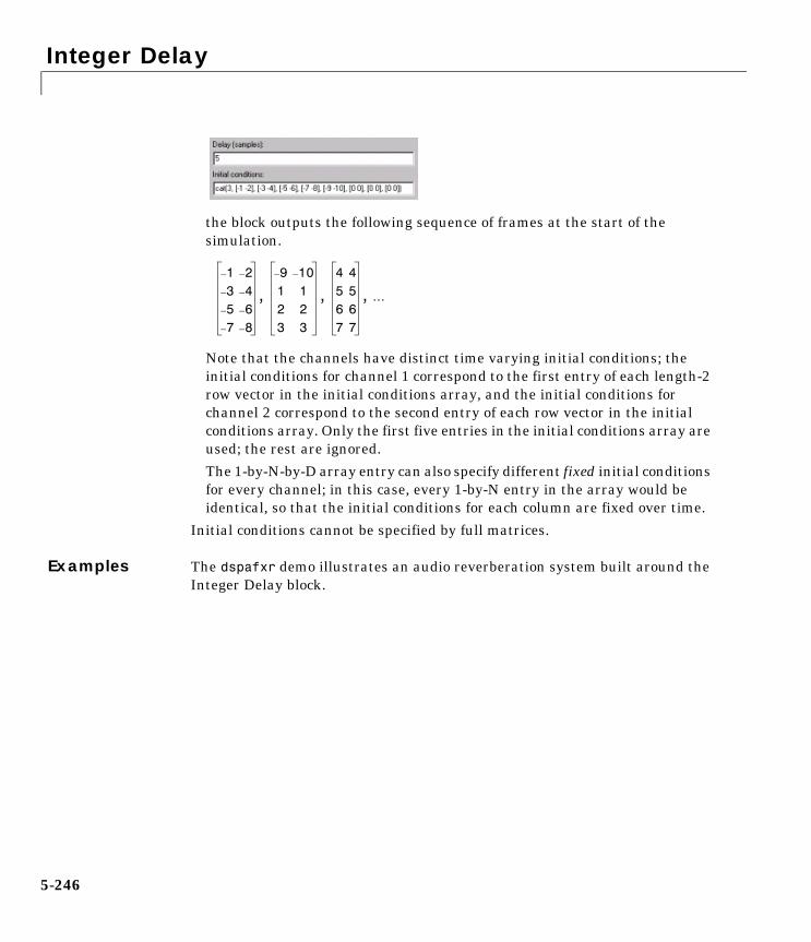
Integer Delay
5-246
the block outputs the following sequence of frames at the start of the simulation.
Note that the channels have distinct time varying initial conditions; the initial conditions for channel 1 correspond to the first entry of each length-2 row vector in the initial conditions array, and the initial conditions for channel 2 correspond to the second entry of each row vector in the initial conditions array. Only the first five entries in the initial conditions array are used; the rest are ignored.
The 1-by-N-by-D array entry can also specify different fixed initial conditions for every channel; in this case, every 1-by-N entry in the array would be identical, so that the initial conditions for each column are fixed over time.
Initial conditions cannot be specified by full matrices.
Examples The dspafxr demo illustrates an audio reverberation system built around the Integer Delay block.
1– 2–3– 4–5– 6–7– 8–
9– 10–
1 12 23 3
4 45 56 67 7
…, , ,

Integer Delay
5-247
Dialog Box
DelayThe number of sample periods to delay the input signal.
Initial conditionsThe value of the block’s output during the initial delay.
[1 1 1][2 2 2][3 3 3][4 4 4][5 5 5][6 6 6][7 7 7][8 8 8][9 9 9]
[0 1 0][0 2 0][1 3 0][2 4 0][3 5 0][4 6 1][5 7 2][6 8 3][7 9 4]
Input Output
First output
...
Simul
atio
n tim
e...
ch1
ch3
ch2
ch1
ch3
ch2
Delay: [2 0 5]Initial conditions: 0
First input (sample-based)

Integer Delay
5-248
Supported Data Types
See Also
Fixed-pointCustom data typesBoolean8-, 16-, and 32-bit signed integer 8-, 16-, and 32-bit unsigned integerSingle-precision floating point Double-precision floating point
Unit Delay SimulinkVariable Fractional Delay DSP BlocksetVariable Integer Delay DSP Blockset

Kalman Adaptive Filter
5-249
5Kalman Adaptive FilterPurpose Compute filter estimates for an input using the Kalman adaptive filter algorithm.
Library Filtering / Adaptive Filters
Description The Kalman Adaptive Filter block computes the optimal linear minimum mean-square estimate (MMSE) of the FIR filter coefficients using a one-step predictor algorithm. This Kalman filter algorithm is based on the following physical realization of a dynamical system.
The Kalman filter assumes that there are no deterministic changes to the filter taps over time (i.e., the transition matrix is identity), and that the only observable output from the system is the filter output with additive noise. The corresponding Kalman filter is expressed in matrix form as
g n( ) K n 1–( )u n( )
uH n( )K n 1–( )u n( ) QM+--------------------------------------------------------------------=
y n( ) uH n( )w n( )=
e n( ) d n( ) y n( )–=
w n 1+( ) w n( ) e n( )g n( )+=
K n( ) K n 1–( ) g n( )uH n( )K n 1–( ) QP+–=

Kalman Adaptive Filter
5-250
The variables are as follows.
The correlation matrices, QM and QP, are specified in the parameter dialog box by scalar variance terms to be placed along the matrix diagonals, thus ensuring that these matrices are symmetric. The filter algorithm based on this constraint is also known as the random-walk Kalman filter.
The implementation of the algorithm in the block is optimized by exploiting the symmetry of the input covariance matrix K(n). This decreases the total number of computations by a factor of two.
The block icon has port labels corresponding to the inputs and outputs of the Kalman algorithm. Note that inputs to the In and Err ports must be sample-based scalars. The signal at the Out port is a scalar, while the signal at the Taps port is a sample-based vector.
Variable Description
n The current algorithm iteration
u(n) The buffered input samples at step n
K(n) The correlation matrix of the state estimation error
g(n) The vector of Kalman gains at step n
The vector of filter-tap estimates at step n
y(n) The filtered output at step n
e(n) The estimation error at step n
d(n) The desired response at step n
QM The correlation matrix of the measurement noise
QP The correlation matrix of the process noise
w n( )

Kalman Adaptive Filter
5-251
An optional Adapt input port is added when the Adapt input check box is selected in the dialog box. When this port is enabled, the block continuously adapts the filter coefficients while the Adapt input is nonzero. A zero-valued input to the Adapt port causes the block to stop adapting, and to hold the filter coefficients at their current values until the next nonzero Adapt input.
The FIR filter length parameter specifies the length of the filter that the Kalman algorithm estimates. The Measurement noise variance and the Process noise variance parameters specify the correlation matrices of the measurement and process noise, respectively. The Measurement noise variance must be a scalar, while the Process noise variance can be a vector of values to be placed along the diagonal, or a scalar to be repeated for the diagonal elements.
The Initial value of filter taps specifies the initial value as a vector, or as a scalar to be repeated for all vector elements. The Initial error correlation matrix specifies the initial value K(0), and can be a diagonal matrix, a vector of values to be placed along the diagonal, or a scalar to be repeated for the diagonal elements.
Block Ports Corresponding Variables
In u, the scalar input, which is internally buffered into the vector u(n)
Out y(n), the filtered scalar output
Err e(n), the scalar estimation error
Taps , the vector of filter-tap estimates w n( )
w 0( )

Kalman Adaptive Filter
5-252
Dialog Box
FIR filter lengthThe length of the FIR filter.
Measurement noise varianceThe value to appear along the diagonal of the measurement noise correlation matrix. Tunable.
Process noise varianceThe value to appear along the diagonal of the process noise correlation matrix. Tunable.
Initial value of filter tapsThe initial FIR filter coefficients.
Initial error correlation matrixThe initial value of the error correlation matrix.
Adapt inputEnables the Adapt port.
References Haykin, S. Adaptive Filter Theory. 3rd ed. Englewood Cliffs, NJ: Prentice Hall, 1996.

Kalman Adaptive Filter
5-253
Supported Data Types
See Also
See “Adaptive Filters” on page 4-3 for related information.
Double-precision floating point
LMS Adaptive Filter DSP BlocksetRLS Adaptive Filter DSP Blockset

LDL Factorization
5-254
5LDL FactorizationPurpose Factor a square Hermitian positive definite matrix into lower, upper, and diagonal components.
Library Math Functions / Matrices and Linear Algebra / Matrix Factorizations
Description The LDL Factorization block uniquely factors the square Hermitian positive definite input matrix S as
where L is a lower triangular square matrix with unity diagonal elements, D is a diagonal matrix, and L* is the Hermitian (complex conjugate) transpose of L. Only the diagonal and lower triangle of the input matrix are used, and any imaginary component of the diagonal entries is disregarded.
The block’s output is a composite matrix with lower triangle elements lij from L, diagonal elements dij from D, and upper triangle elements uij from L*. It is always sample-based. The output format is shown below for a 5-by-5 matrix.
LDL factorization requires half the computation of Gaussian elimination (LU decomposition), and is always stable. It is more efficient that Cholesky factorization because it avoids computing the square roots of the diagonal elements.
The algorithm requires that the input be square and Hermitian positive definite. When the input is not positive definite, the block reacts with the behavior specified by the Non-positive definite input parameter.
S LDL*=
d11 u12 u13 u14 u15
l21 d22 u23 u24 u25
l31 l32 d33 u34 u35
l41 l42 l43 d44 u45
l51 l52 l53 l54 d55
uij lji*
=

LDL Factorization
5-255
The following options are available:
• Ignore – Proceed with the computation and do not issue an alert. The output is not a valid factorization. A partial factorization will be present in the upper left corner of the ouput.
• Warning – Display a warning message in the MATLAB command window, and continue the simulation. The output is not a valid factorization. A partial factorization will be present in the upper left corner of the ouput.
• Error – Display an error dialog box and terminate the simulation.
Example LDL decomposition of a 3-by-3 Hermitian positive definite matrix:
Dialog Box
Non-positive definite inputResponse to non-positive definite matrix inputs. Tunable.
References Golub, G. H., and C. F. Van Loan. Matrix Computations. 3rd ed. Baltimore, MD: Johns Hopkins University Press, 1996.
Supported Data Types
9 1– 21– 8 5–
2 5– 7
9.00 0.11– 0.220.11– 7.89 0.61–
0.22 0.61– 3.66
L1 0 0
0.11– 1 00.22 0.61– 1
= L'1 0.11– 0.220 1 0.61–
0 0 1
=D9.00 0 00 7.89 00 0 3.66
=
Double-precision floating point

LDL Factorization
5-256
Supported Data Types
See Also
See “Factoring Matrices” on page 4-17 for related information.
Double-precision floating point
Cholesky Factorization DSP BlocksetLDL Inverse DSP BlocksetLDL Solver DSP BlocksetLU Factorization DSP BlocksetQR Factorization DSP Blockset

LDL Inverse
5-257
5LDL InversePurpose Compute the inverse of a Hermitian positive definite matrix using LDL factorization.
Library Math Functions / Matrices and Linear Algebra / Matrix Inverses
Description The LDL Inverse block computes the inverse of the Hermitian positive definite input matrix S by performing an LDL factorization.
L is a lower triangular square matrix with unity diagonal elements, D is a diagonal matrix, and L* is the Hermitian (complex conjugate) transpose of L. Only the diagonal and lower triangle of the input matrix are used, and any imaginary component of the diagonal entries is disregarded. The output is always sample-based.
LDL factorization requires half the computation of Gaussian elimination (LU decomposition), and is always stable. It is more efficient than Cholesky factorization because it avoids computing the square roots of the diagonal elements.
The algorithm requires that the input be Hermitian positive definite. When the input is not positive definite, the block reacts with the behavior specified by the Non-positive definite input parameter. The following options are available:
• Ignore – Proceed with the computation and do not issue an alert. The output is not a valid inverse.
• Warning – Display a warning message in the MATLAB command window, and continue the simulation. The output is not a valid inverse.
• Error – Display an error dialog box and terminate the simulation.
Dialog Box
S 1– LDL*( )1–
=

LDL Inverse
5-258
Non-positive definite inputResponse to non-positive definite matrix inputs. Tunable.
References Golub, G. H., and C. F. Van Loan. Matrix Computations. 3rd ed. Baltimore, MD: Johns Hopkins University Press, 1996.
Supported Data Types
See Also
See “Inverting Matrices” on page 4-19 for related information.
Double-precision floating point
Cholesky Inverse DSP BlocksetLDL Factorization DSP BlocksetLDL Solver DSP BlocksetLU Inverse DSP BlocksetPseudoinverse DSP Blocksetinv MATLAB

LDL Solver
5-259
5LDL SolverPurpose Solve the equation SX=B for X when S is a square Hermitian positive definite matrix.
Library Math Functions / Matrices and Linear Algebra / Linear System Solvers
Description The LDL Solver block solves the linear system SX=B by applying LDL factorization to the matrix at the S port, which must be square (M-by-M) and Hermitian positive definite. Only the diagonal and lower triangle of the matrix are used, and any imaginary component of the diagonal entries is disregarded. The input to the B port is the right-hand side M-by-N matrix, B. The output is the unique solution of the equations, M-by-N matrix X, and is always sample-based.
A length-M 1-D vector input for right-hand side B is treated as an M-by-1 matrix.
When the input is not positive definite, the block reacts with the behavior specified by the Non-positive definite input parameter. The following options are available:
• Ignore – Proceed with the computation and do not issue an alert. The output is not a valid solution.
• Warning – Proceed with the computation and display a warning message in the MATLAB command window. The output is not a valid solution.
• Error – Display an error dialog box and terminate the simulation.
Algorithm The LDL algorithm uniquely factors the Hermitian positive definite input matrix S as
where L is a lower triangular square matrix with unity diagonal elements, D is a diagonal matrix, and L* is the Hermitian (complex conjugate) transpose of L.
The equation
is solved for X by the following steps:
S LDL*=
LDL*X B=

LDL Solver
5-260
1 Substitute
2 Substitute
3 Solve one diagonal and two triangular systems.
Dialog Box
Non-positive definite inputResponse to non-positive definite matrix inputs. Tunable.
Supported Data Types
See Also
See “Solving Linear Systems” on page 4-16 for related information.
Y DL*X=
Z L*X=
LY B=
DZ Y=
L*X Z=
Double-precision floating point
Autocorrelation LPC DSP BlocksetCholesky Solver DSP BlocksetLDL Factorization DSP BlocksetLDL Inverse DSP BlocksetLevinson-Durbin DSP BlocksetLU Solver DSP BlocksetQR Solver DSP Blockset

Least Squares Polynomial Fit
5-261
5Least Squares Polynomial FitPurpose Compute the coefficients of the polynomial that best fits the input data in a least-squares sense.
Library Math Functions / Polynomial Functions
Description The Least Squares Polynomial Fit block computes the coefficients of the nth order polynomial that best fits the input data in the least-squares sense, where n is specified by the Polynomial order parameter. A distinct set of n+1 coefficients is computed for each column of the M-by-N input, u.
For a given input column, the block computes the set of coefficients, c1, c2, …, cn+1, that minimizes the quantity
where ui is the ith element in the input column, and
The values of the independent variable, x1, x2, …, xM, are specified as a length-M vector by the Control points parameter. The same M control points are used for all N polynomial fits, and can be equally or unequally spaced. The equivalent MATLAB code is shown below.
c = polyfit(x,u,n) % Equivalent MATLAB code
Inputs can be frame-based or sample-based. For convenience, a length-M 1-D vector input is treated as an M-by-1 matrix.
Each column of the (n+1)-by-N output matrix, c, represents a set of n+1 coefficients describing the best-fit polynomial for the corresponding column of the input. The coefficients in each column are arranged in order of descending exponents, c1, c2, …, cn+1. The output is always sample-based.
Example In the model below, the Polynomial Evaluation block uses the second-order polynomial
ui ui–( )2
i 1=
M
∑
ui f xi( ) c1xin c2xi
n 1–L cn 1++ + += =
y 2– u2 3+=

Least Squares Polynomial Fit
5-262
to generate four values of dependent variable y from four values of independent variable u, received at the top port. The polynomial coefficients are supplied in the vector [-2 0 3] at the bottom port. Note that the coefficient of the first-order term is zero.
The Control points parameter of the Least Squares Polynomial Fit block is configured with the same four values of independent variable u that are used as input to the Polynomial Evaluation block, [1 2 3 4]. The Least Squares Polynomial Fit block uses these values together with the input values of dependent variable y to reconstruct the original polynomial coefficients.
Dialog Box
Control pointsThe values of the independent variable to which the data in each input column correspond. For an M-by-N input, this parameter must be a length-M vector. Tunable.
Polynomial orderThe order, n, of the polynomial to be used in constructing the best fit. The number of coefficients is n+1. Tunable.

Least Squares Polynomial Fit
5-263
Supported Data Types
See Also
Double-precision floating point
Detrend DSP BlocksetPolynomial Evaluation DSP BlocksetPolynomial Stability Test DSP Blocksetpolyfit MATLAB

Levinson-Durbin
5-264
5Levinson-DurbinPurpose Solve a linear system of equations using Levinson-Durbin recursion.
Library Math Functions / Matrices and Linear Algebra / Linear System Solvers
Description The Levinson-Durbin block solves the nth-order system of linear equations
for the particular case where R is a Hermitian, positive-definite, Toeplitz matrix and b is identical to the first column of R shifted by one element and with the opposite sign.
The input to the block, r = [r(1) r(2) ... r(n+1)], can be a 1-D or 2-D vector (row or column). It contains lags 0 through n of an autocorrelation sequence, which appear in the matrix R.
The block can output the polynomial coefficients, A, the reflection coefficients, K, and the prediction error power, P, in various combinations. The Output(s) parameter allows you to enable the A and K outputs by selecting one of the following settings:
• A – Port A outputs A=[1 a(2) a(3) ... a(n+1)], the solution to the Levinson-Durbin equation. A has the same dimension as the input. The elements of the output can also be viewed as the coefficients of an nth-order autoregressive (AR) process (see below).
• K – Port K outputs K=[k(1) k(2) ... k(n)], which contains n reflection coefficients, and has the same dimension as the input, less one element. (A scalar input causes an error when K is selected.) Reflection coefficients are useful for realizing a lattice representation of the AR process described below.
• A and K – The block outputs both representations at their respective ports. (A scalar input causes an error when A and K is selected.)
Both A and K are always 1-D vectors.
Ra b=
r 1( ) r* 2( ) L r* n( )
r 2( ) r 1( ) L r* n 1–( )M M O M
r n( ) r n 1–( ) L r 1( )
a 2( )a 3( )M
a n 1+( )
r 2( )–
r 3( )–
M
r n 1+( )–
=

Levinson-Durbin
5-265
The prediction error power, P, (a scalar), is output when the Output prediction error power (P) check box is selected. P represents the power of the output of an FIR filter with taps A and input autocorrelation described by r, where A represents a prediction error filter and r is the input to the block. (In this case, A is a whitening filter).
When If the value of lag 0 is zero, A=[1 zeros], K=[zeros], P=0 is selected (default), an input whose r(1) element is zero generates a zero-valued output. When this check box is not selected, an input with r(1) = 0 generates NaNs in the output. In general, an input with r(1) = 0 is invalid because it does not construct a positive-definite matrix R; however, it is common for blocks to receive zero-valued inputs at the start of a simulation. The check box allows you to avoid propagating NaNs during this period.
ApplicationsOne application of the Levinson-Durbin formulation above is in the Yule-Walker AR problem, which concerns modeling an unknown system as an autoregressive process. Such a process would be modeled as the output of an all-pole IIR filter with white Gaussian noise input. In the Yule-Walker problem, the use of the signal’s autocorrelation sequence to obtain an optimal estimate leads to an Ra = b equation of the type shown above, which is most efficiently solved by Levinson-Durbin recursion. In this case, the input to the block represents the autocorrelation sequence, with r(1) being the zero-lag value. The output at the block’s A port then contains the coefficients of the autoregressive process that optimally models the system. The coefficients are ordered in descending powers of z, and the AR process is minimum phase. The prediction error, G, defines the gain for the unknown system, where .
The output at the block’s K port contains the corresponding reflection coefficients, [k(1) k(2) ... k(n)], for the lattice realization of this IIR filter. The Yule-Walker AR Estimator block implements this autocorrelation-based method for AR model estimation, while the Yule-Walker Method block extends the method to spectral estimation.
Another common application of the Levinson-Durbin algorithm is in linear predictive coding, which is concerned with finding the coefficients of a moving
G P=
H z( ) GA z( )------------
G
1 a 2( )z 1– … a n 1+( )z n–+ + +
--------------------------------------------------------------------------------= =

Levinson-Durbin
5-266
average (MA) process (or FIR filter) that predicts the next value of a signal from the current signal sample and a finite number of past samples. In this case, the input to the block represents the signal’s autocorrelation sequence, with r(1) being the zero-lag value, and the output at the block’s A port contains the coefficients of the predictive MA process (in descending powers of z).
These coefficients solve the optimization problem below.
Again, the output at the block’s K port contains the corresponding reflection coefficients, [k(1) k(2) ... k(n)], for the lattice realization of this FIR filter. The Autocorrelation LPC block in the Linear Prediction library implements this autocorrelation-based prediction method.
Algorithm The algorithm requires O(n2) operations, and is thus much more efficient for large n than standard Gaussian elimination, which requires O(n3) operations.
Dialog Box
Output(s)The solution representation of Ra = b to output: model coefficients (A), reflection coefficients (K), or both (A and K). For scalar inputs, this parameter must be set to A.
H z( ) A z( ) 1 a 2( )z 1– … a n 1+( )z n–+ + += =
minai E xn aixn i–
i 1=
N
∑–
2

Levinson-Durbin
5-267
Output prediction error power (P)When selected, the block outputs the prediction error at port P.
If the value of lag 0 is zero, A=[1 zeros], K=[zeros], P=0When selected, the block outputs a zero-vector for inputs having r(1) = 0. When unselected, the block outputs NaNs for these inputs.
References Golub, G. H., and C. F. Van Loan. Sect. 4.7 in Matrix Computations. 3rd ed. Baltimore, MD: Johns Hopkins University Press, 1996.
Ljung, L. System Identification: Theory for the User. Englewood Cliffs, NJ: Prentice Hall, 1987. Pgs. 278-280.
Kay, Steven M., Modern Spectral Estimation: Theory and Application. Englewood Cliffs, NJ: Prentice Hall, 1988.
Supported Data Types
See Also
See “Solving Linear Systems” on page 4-16 for related information.
Double-precision floating point
Cholesky Solver DSP BlocksetLDL Solver DSP BlocksetAutocorrelation LPC DSP BlocksetLU Solver DSP BlocksetQR Solver DSP BlocksetYule-Walker AR Estimator DSP BlocksetYule-Walker Method DSP Blocksetlevinson Signal Processing Toolbox
LMS Adaptive Filter
5-268
5LMS Adaptive FilterPurpose Compute filter estimates for an input using the LMS adaptive filter algorithm.
Library Filtering / Adaptive Filters
Description The LMS Adaptive Filter block implements an adaptive FIR filter using the stochastic gradient algorithm known as the normalized Least Mean-Square (LMS) algorithm.
The variables are as follows.
To overcome potential numerical instability in the tap-weight update, a small positive constant (a = 1e-10) has been added in the denominator.
To turn off normalization, deselect the Use normalization check box in the parameter dialog box. The block then computes the filter-tap estimate as
The block icon has port labels corresponding to the inputs and outputs of the LMS algorithm. Note that inputs to the In and Err ports must be sample-based
Variable Description
n The current algorithm iteration
u(n) The buffered input samples at step n
The vector of filter-tap estimates at step n
y(n) The filtered output at step n
e(n) The estimation error at step n
d(n) The desired response at step n
µ The adaptation step size
y n( ) wH n 1–( )u n( )=
e n( ) d n( ) y n( )–=
w n( ) w n 1–( ) u n( )
a uH n( )u n( )+---------------------------------------µe∗ n( )+=
w n( )
w n( ) w n 1–( ) u n( )µe∗ n( )+=

LMS Adaptive Filter
5-269
scalars. The signal at the Out port is a scalar, while the signal at the Taps port is a sample-based vector.
An optional Adapt input port is added when the Adapt input check box is selected in the dialog box. When this port is enabled, the block continuously adapts the filter coefficients while the Adapt input is nonzero. A zero-valued input to the Adapt port causes the block to stop adapting, and to hold the filter coefficients at their current values until the next nonzero Adapt input.
The FIR filter length parameter specifies the length of the filter that the LMS algorithm estimates. The Step size parameter corresponds to µ in the equations. Typically, for convergence in the mean square, 0<µ<2. The Initial value of filter taps specifies the initial value as a vector, or as a scalar to be repeated for all vector elements. The Leakage factor specifies the value of the leakage factor, , in the leaky LMS algorithm below. This parameter must be between 0 and 1.
Examples The lmsdemo demo illustrates a noise cancellation system built around the LMS Adaptive Filter block.
Block Ports Corresponding Variables
In u, the scalar input, which is internally buffered into the vector u(n)
Out y(n), the filtered scalar output
Err e(n), the scalar estimation error
Taps , the vector of filter-tap estimates w n( )
w 0( )
1 µα–
w n 1+( ) 1 µα–( )ω n( ) u n( )
uH n( )u n( )-----------------------------µe∗ n( )+=

LMS Adaptive Filter
5-270
Dialog Box
FIR filter lengthThe length of the FIR filter.
Step-sizeThe step size, usually in the range (0, 2). Tunable.
Initial value of filter tapsThe initial FIR filter coefficients.
Leakage factorThe leakage factor, in the range [0, 1]. Tunable.
Use normalizationSelect or deselect normalization.
Adapt inputEnables the Adapt port.
References Haykin, S. Adaptive Filter Theory. 3rd ed. Englewood Cliffs, NJ: Prentice Hall, 1996.
Supported Data Types
Double-precision floating point

LMS Adaptive Filter
5-271
See Also
See “Adaptive Filters” on page 4-3 for related information.
Kalman Adaptive Filter DSP BlocksetRLS Adaptive Filter DSP Blockset

LU Factorization
5-272
5LU FactorizationPurpose Factor a square matrix into lower and upper triangular components.
Library Math Functions / Matrices and Linear Algebra / Matrix Factorizations
Description The LU Factorization block factors a row permutation of the square input matrix A as
where L is a lower-triangular square matrix with unity diagonal elements, and U is an upper-triangular square matrix. The row-pivoted matrix Ap contains the rows of A permuted as indicated by the permutation index vector P.
Ap = A(P,:) % Equivalent MATLAB code
The output at the LU port is a composite matrix with lower subtriangle elements from L and upper triangle elements from U, and is always sample-based.
Example The row-pivoted matrix Ap and permutation index vector P computed by the block are shown below for 3-by-3 input matrix A.
The LU output is a composite matrix whose lower subtriangle forms L and whose upper triangle forms U.
Ap LU=
A1– 8 5–
9 1– 22 5– 7
= Ap
9 1– 21– 8 5–
2 5– 7
=P = (2 1 3)
1– 8 5–
9 1– 22 5– 7
9.00 1.00– 2.000.11– 7.89 4.78–
0.22 0.61– 3.66
L1 0 0
0.11– 1 00.22 0.61– 1
= U9.00 1.00– 2.000 7.89 4.78–
0 0 3.66
=
(2 1 3)

LU Factorization
5-273
Dialog Box
References Golub, G. H., and C. F. Van Loan. Matrix Computations. 3rd ed. Baltimore, MD: Johns Hopkins University Press, 1996.
Supported Data Types
See Also
See “Factoring Matrices” on page 4-17 for related information.
Double-precision floating point
Autocorrelation LPC DSP BlocksetCholesky Factorization DSP BlocksetLDL Factorization DSP BlocksetLU Inverse DSP BlocksetLU Solver DSP BlocksetPermute Matrix DSP BlocksetQR Factorization DSP Blocksetlu MATLAB

LU Inverse
5-274
5LU InversePurpose Compute the inverse of a square matrix using LU factorization.
Library Math Functions / Matrices and Linear Algebra / Matrix Inverses
Description The LU Inverse block computes the inverse of the square input matrix A by factoring and inverting row-pivoted variant Ap.
L is a lower-triangular square matrix with unity diagonal elements, and U is an upper-triangular square matrix. The block’s output is A-1, and is always sample-based.
Dialog Box
References Golub, G. H., and C. F. Van Loan. Matrix Computations. 3rd ed. Baltimore, MD: Johns Hopkins University Press, 1996.
Supported Data Types
See Also
See “Inverting Matrices” on page 4-19 for related information.
Ap1– LU( ) 1–
=
Double-precision floating point
Cholesky Inverse DSP BlocksetLDL Inverse DSP BlocksetLU Factorization DSP BlocksetLU Solver DSP Blocksetinv MATLAB

LU Solver
5-275
5LU SolverPurpose Solve the equation AX=B for X when A is a square matrix.
Library Math Functions / Matrices and Linear Algebra / Linear System Solvers
Description The LU Solver block solves the linear system AX=B by applying LU factorization to the M-by-M matrix at the A port. The input to the B port is the right-hand side M-by-N matrix, B. The output is the unique solution of the equations, M-by-N matrix X, and is always sample-based.
A length-M 1-D vector input for right-hand side B is treated as an M-by-1 matrix.
Algorithm The LU algorithm factors a row-permuted variant (Ap) of the square input matrix A as
where L is a lower-triangular square matrix with unity diagonal elements, and U is an upper-triangular square matrix.
The matrix factors are substituted for Ap in
where Bp is the row-permuted variant of B, and the resulting equation
is solved for X by making the substitution Y = UX, and solving two triangular systems.
Dialog Box
Ap LU=
ApX Bp=
LUX Bp=
LY Bp=
UX Y=

LU Solver
5-276
Supported Data Types
See Also
See “Solving Linear Systems” on page 4-16 for related information.
Double-precision floating point
Autocorrelation LPC DSP BlocksetCholesky Solver DSP BlocksetLDL Solver DSP BlocksetLevinson-Durbin DSP BlocksetLU Factorization DSP BlocksetLU Inverse DSP BlocksetQR Solver DSP Blockset

Magnitude FFT
5-277
5Magnitude FFTPurpose Compute a nonparametric estimate of the spectrum using the periodogram method.
Library Estimation / Power Spectrum Estimation
Description The Magnitude FFT block computes a nonparametric estimate of the spectrum using the periodogram method. When the Output parameter is set to Magnitude squared, the block output for an input u is equivalent to
y = abs(fft(u,nfft)).^2 % Equivalent MATLAB code
When the Output parameter is set to Magnitude, the block output for an input u is equivalent to
y = abs(fft(u,nfft)) % Equivalent MATLAB code
Both an M-by-N frame-based matrix input and an M-by-N sample-based matrix input are treated as M sequential time samples from N independent channels. The block computes a separate estimate for each of the N independent channels and generates an Nfft-by-N matrix output. When Inherit FFT length from input dimensions is selected, Nfft is specified by the frame size of the input, which must be a power of 2. When Inherit FFT length from input dimensions is not selected, Nfft is specified as a power of 2 by the FFT length parameter, and the block zero pads or truncates the input to Nfft before computing the FFT.
Each column of the output matrix contains the estimate of the corresponding input column’s power spectral density at Nfft equally spaced frequency points in the range [0,Fs), where Fs is the signal’s sample frequency. The output is always sample-based.
Example The dspsacomp demo compares the periodogram method with several other spectral estimation methods.

Magnitude FFT
5-278
Dialog Box
OutputDetermines whether the block computes the magnitude FFT (Magnitude) or magnitude-squared FFT (Magnitude squared) of the input. Tunable.
Inherit FFT length from input dimensionsWhen selected, uses the input frame size as the number of data points, Nfft, on which to perform the FFT.
FFT sizeThe number of data points on which to perform the FFT, Nfft. If Nfft exceeds the input frame size, the frame is zero-padded as needed. This parameter is enabled when Inherit FFT length from input dimensions is not selected.
References Oppenheim, A. V. and R. W. Schafer. Discrete-Time Signal Processing. Englewood Cliffs, NJ: Prentice Hall, 1989.
Proakis, J. and D. Manolakis. Digital Signal Processing. 3rd ed. Englewood Cliffs, NJ: Prentice-Hall, 1996.
Supported Data Types
Double-precision floating point

Magnitude FFT
5-279
See Also
See “Power Spectrum Estimation” on page 4-15 for related information.
Burg Method DSP BlocksetShort-Time FFT DSP BlocksetSpectrum Scope DSP BlocksetYule-Walker Method DSP Blocksetpwelch Signal Processing Toolbox

Matrix 1-Norm
5-280
5Matrix 1-NormPurpose Compute the 1-norm of a matrix.
Library Math Functions / Matrices and Linear Algebra / Matrix Operations
Description The Matrix 1-Norm block computes the 1-norm, or maximum column-sum, of an M-by-N input matrix, A.
This is equivalent to
y = max(sum(abs(A))) % Equivalent MATLAB code
A length-M 1-D vector input is treated as an M-by-1 matrix. The output, y, is always a scalar.
Dialog Box
References Golub, G. H., and C. F. Van Loan. Matrix Computations. 3rd ed. Baltimore, MD: Johns Hopkins University Press, 1996.
y A 1 aij
i 1=
M
∑1 j N≤ ≤max= =
a11 a12 a13
a21 a22 a23
a31 a32 a33
a13 a23 a33+ + A3=
a12 a22 a32+ + A2=
a11 a21 a31+ + A1=
A 1 A1 A2 A3, ,( )max=

Matrix 1-Norm
5-281
Supported Data Types
See Also
Double-precision floating point
Normalization DSP BlocksetReciprocal Condition DSP Blocksetnorm MATLAB

Matrix Multiply
5-282
5Matrix MultiplyPurpose Multiply input matrices.
Library Math Functions / Matrices and Linear Algebra / Matrix Operations
Description The Matrix Multiply block multiplies n input matrices, A, B, C, ..., Un, in the forward direction, where n is specified by the Number of input ports parameter and Un is the input at the nth port.
Y = ((((A*B)*C)*D) ... Un) % Equivalent MATLAB code
All inputs must have sizes compatible for matrix multiplication; that is, size(A,2) = size(B,1), size(B,2) = size(C,1), and so on. Inputs can be real, complex, sample-based, or frame-based in any combination, but all inputs must have the same precision, single or double. A length-M 1-D vector input at any port is treated as an M-by-1 matrix.
The size of sample-based output Y is [size(A,1) size(Un,2)]. That is, Y is MA-by-NUn.
Algorithm The Matrix Multiply block is optimized to use at most two temporary variables for storage of intermediate results.
Dialog Box
Number of input portsThe number of inputs to the block.
Supported Data Types
Single-precision floating pointDouble-precision floating point

Matrix Multiply
5-283
See Also Dot Product SimulinkMatrix Product DSP BlocksetMatrix Scaling DSP BlocksetProduct Simulink

Matrix Product
5-284
5Matrix ProductPurpose Multiply the elements of a matrix along rows or columns.
Library Math Functions / Matrices and Linear Algebra / Matrix Operations
Description The Matrix Product block multiplies the elements of an M-by-N input matrix u along either the rows or columns.
When the Multiply along parameter is set to Rows, the block multiplies across the elements of each row and outputs the resulting M-by-1 matrix. A length-N 1-D vector input is treated as a 1-by-N matrix.
This is equivalent to
y = prod(u,2) % Equivalent MATLAB code
When the Multiply along parameter is set to Columns, the block multiplies down the elements of each column and outputs the resulting 1-by-N matrix. A length-M 1-D vector input is treated as a M-by-1 matrix.
This is equivalent to
y = prod(u) % Equivalent MATLAB code
The output has the same frame status as the input.
u11 u12 u13
u21 u22 u23
u31 u32 u33
y1
y2
y3
u11u12u13( )
u21u22u23( )
u31u32u33( )
=
u11 u12 u13
u21 u22 u23
u31 u32 u33
y1 y2 y3 u11u21u31( ) u12u22u32( ) u13u23u33( )=

Matrix Product
5-285
Dialog Box
Multiply alongThe dimension of the matrix along which to multiply, row or column.
Supported Data Types
See Also
Double-precision floating point
Matrix Multiply DSP BlocksetMatrix Square DSP BlocksetMatrix Sum DSP Blocksetprod MATLAB

Matrix Scaling
5-286
5Matrix ScalingPurpose Scale the rows or columns of a matrix by a specified vector.
Library Math Functions / Matrices and Linear Algebra / Matrix Operations
Description The Matrix Scaling block scales the rows or columns of the M-by-N input matrix A by the values in input vector D.
When the Mode parameter is set to Scale Rows (D*A), input D can be a 1-D or 2-D vector of length M, and the block multiplies each element of D across the corresponding row of matrix A.
This is equivalent to premultiplying A by a diagonal matrix with diagonal D.
y = diag(D)*A % Equivalent MATLAB code
When the Mode parameter is set to Scale Columns (A*D), input D can be a 1-D or 2-D vector of length N, and the block multiplies each element of D across the corresponding column of matrix A.
This is equivalent to postmultiplying A by a diagonal matrix with diagonal D.
y = A*diag(D) % Equivalent MATLAB code
The output is the same size as the input matrix, A. If both inputs are sample-based, the output is sample-based; otherwise, the output is frame-based.
d1
d2
d3
a11 a12 a13
a21 a22 a23
a31 a32 a33
d1a11 d1a12 d1a13
d2a21 d2a22 d2a23
d3a31 d3a32 d3a33
×
×
×
d1 d2 d3
a11 a12 a13
a21 a22 a23
a31 a32 a33
d1a11 d2a12 d3a13
d1a21 d2a22 d3a23
d1a31 d2a32 d3a33
× × ×

Matrix Scaling
5-287
Dialog Box
ModeThe mode of operation, row scaling or column scaling. Tunable.
Supported Data Types
See Also
Single-precision floating pointDouble-precision floating point
Matrix Multiply DSP BlocksetMatrix Product DSP BlocksetMatrix Sum DSP Blockset

Matrix Square
5-288
5Matrix SquarePurpose Compute the square of the input matrix.
Library Math Functions / Matrices and Linear Algebra / Matrix Operations
Description The Matrix Square block computes the square of an M-by-N input matrix, u, by premultiplying with the Hermitian transpose.
y = u' * u % Equivalent MATLAB code
A length-M 1-D vector input is treated as an M-by-1 matrix. For both sample-based and frame-based inputs, output y is sample-based with dimension N-by-N.
ApplicationsThe Matrix Square block is useful in a variety of applications:
• General matrix squares – The Matrix Square block computes the output matrix, y, without explicitly forming u'. It is therefore more efficient than other methods for computing the matrix square.
• Sum of squares – When the input is a column vector (N=1), the block’s operation is equivalent to a multiply-accumulate (MAC) process, or inner product. The output is the sum of the squares of the input, and is always a real scalar.
• Correlation matrix – When the input is a row vector (M=1), the output, y, is the symmetric autocorrelation matrix, or outer product.
Dialog Box
Supported Data Types
Double-precision floating point

Matrix Square
5-289
See Also Matrix Multiply DSP BlocksetMatrix Product DSP BlocksetMatrix Sum DSP BlocksetTranspose DSP Blockset

Matrix Sum
5-290
5Matrix SumPurpose Sum the elements of a matrix along rows or columns.
Library Math Functions / Matrices and Linear Algebra / Matrix Operations
Description The Matrix Sum block sums the elements of an M-by-N input matrix u along either the rows or columns.
When the Sum along parameter is set to Rows, the block sums across the elements of each row and outputs the resulting M-by-1 matrix. A length-N 1-D vector input is treated as a 1-by-N matrix.
This is equivalent to
y = sum(u,2) % Equivalent MATLAB code
When the Sum along parameter is set to Columns, the block sums down the elements of each column and outputs the resulting 1-by-N matrix. A length-M 1-D vector input is treated as a M-by-1 matrix.
This is equivalent to
y = sum(u) % Equivalent MATLAB code
The output has the same frame status as the input.
u11 u12 u13
u21 u22 u23
u31 u32 u33
y1
y2
y3
u11 u12 u13+ +
u21 u22 u23+ +
u31 u32 u33+ +
=
u11 u12 u13
u21 u22 u23
u31 u32 u33
y1 y2 y3 ui1i 1=
3
∑ ui2i 1=
3
∑ ui3i 1=
3
∑=
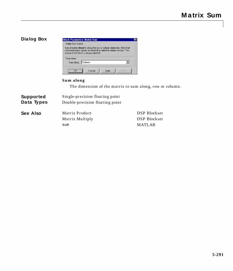
Matrix Sum
5-291
Dialog Box
Sum alongThe dimension of the matrix to sum along, row or column.
Supported Data Types
See Also
Single-precision floating pointDouble-precision floating point
Matrix Product DSP BlocksetMatrix Multiply DSP Blocksetsum MATLAB

Matrix Viewer
5-292
5Matrix ViewerPurpose Display a matrix as a color image.
Library DSP Sinks
Description The Matrix Viewer block displays an M-by-N matrix input by mapping the matrix element values to a specified range of colors. The display is updated as each new input is received. (A length-M 1-D vector input is treated as an M-by-1 matrix.)
Image PropertiesClick on the Image properties check box to expose the image property parameters, which control the colormap and display.
The mapping of matrix element values to colors is specified by the Colormap matrix, Minimum input, and Maximum input parameters. For a colormap with L colors, the colormap matrix has dimension L-by-3, with one row for each color and one column for each element of the RGB triple that defines the color. Examples of RGB triples are
[ 1 0 0 ] (red)[ 0 0 1 ] (blue)[0.8 0.8 0.8] (light gray)
See ColorSpec in the MATLAB documentation for complete information about defining RGB triples.
MATLAB provides a number of functions for generating predefined colormaps, such as hot, cool, bone, and autumn. Each of these functions accepts the colormap size as an argument, and can be used in the Colormap matrix parameter. For example, if you specify gray(128) for the Colormap matrix parameter, the matrix is displayed in 128 shades of gray. The color in the first row of the colormap matrix is used to represent the value specified by the Minimum input parameter, and the color in the last row is used to represent the value specified by the Maximum input parameter. Values between the minimum and maximum are quantized and mapped to the intermediate rows of the colormap matrix.
The documentation for MATLAB’s colormap function provides complete information about specifying colormap matrices, and includes a complete list of the available colormap functions.

Matrix Viewer
5-293
Axis PropertiesClick on the Axis properties check box to expose the axis property parameters, which control labeling and positioning.
The Axis origin parameter determines where the first element of the input matrix, U(1,1), is displayed. When Upper left corner is specified, the matrix is displayed in matrix orientation, with U(1,1) in the upper-left corner.
When Lower left corner is specified, the matrix is flipped vertically to image orientation, with U(1,1) in the lower-left corner.
Axis zoom, when selected, causes the image display to completely fill the figure window. Menus and axis titles are not displayed. This option can also be selected from the right-click pop-up menu in the figure window.
When Axis zoom is deselected, the axis labels and titles are displayed in a gray border surrounding the image axes, and the window’s menus (including Axes) and toolbar are visible. The Plot Editor tools allow you to annotate and customize the image display. Select Help Plot Editor from the figure’s Help menu for more information about using these tools. For information on printing or saving the image, or on the other options found in the generic figure menus (File, Edit, Window, Help), see the MATLAB documentation.
Figure WindowThe image title (in the figure title bar) is the same as the block title. The axis tick marks reflect the size of the input matrix; the x-axis is numbered from
U11 U12 U13 U14
U21 U22 U23 U24
U31 U32 U33 U34
U41 U42 U43 U44
U41 U42 U43 U44
U31 U32 U33 U34
U21 U22 U23 U24
U11 U12 U13 U14

Matrix Viewer
5-294
1 to N (number of columns), and the y-axis is numbered from 1 to M (number of rows).
In addition to the standard MATLAB figure window menus (File, Edit, Window, Help), the Matrix Viewer window has an Axes menu containing the following items:
• Refresh erases all data on the scope display, except for the most recent image.
• Autoscale recomputes the Minimum input and Maximum input parameter values to best fit the range of values observed in a series of 10 consecutive inputs. The numerical limits selected by the autoscale feature are shown in the Minimum input and Maximum input parameters, where you can make further adjustments to them manually.
• Axis zoom, when selected, causes the image to completely fill the containing figure window. Menus and axis titles are not displayed. When Axis zoom is deselected, the axis labels and titles are displayed in a gray border surrounding the scope axes, and the window’s menus (including Axes) and toolbar are visible. This option can also be set in the Axis properties panel of the parameter dialog box.
• Colorbar, when selected, displays a bar with the specified colormap to the right of the image axes.
• Save Position automatically updates the Figure position parameter in the Axis properties field to reflect the figure window’s current position and size on the screen. To make the scope window open at a particular location on the screen when the simulation runs, simply drag the window to the desired location, resize it as needed, and select Save Position. Note that the parameter dialog box must be closed when you select Save Position in order for the Figure position parameter to be updated.
Many of these options can also be accessed by right-clicking with the mouse anywhere on the displayed image. The right-click menu is very helpful when the scope is in zoomed mode and the Axes menu is not visible.
Examples See the demo dspstfft.mdl for an example of using the Matrix Viewer block to create a moving spectrogram (time-frequency plot) of a speech signal by updating just one column of the input matrix at each sample time.

Matrix Viewer
5-295
Dialog Box
Image propertiesSelect to expose the image property parameters. Tunable.
Colormap matrixA 3-column matrix defining the colormap as a set of RGB triples, or a call to a colormap-generating function such as hot or spring. See the ColorSpec property for complete information about defining RGB triples, and the colormap function for a list of colormap-generating functions. Tunable.
Minimum input valueThe input value to be mapped to the color defined in the first row of the colormap matrix. Select Autoscale from the right-click pop-up menu to set this parameter to the minimum value observed in a series of 10 consecutive matrix inputs. Tunable.

Matrix Viewer
5-296
Maximum input valueThe input value to be mapped to the color defined in the last row of the colormap matrix. Select Autoscale from the right-click pop-up menu to set this parameter to the maximum value observed in a series of 10 consecutive matrix inputs. Tunable.
Display colorbarSelect to display a bar with the selected colormap to the right of the image axes. Tunable.
Axis propertiesSelect to expose the axis property parameters. Tunable.
Axis originThe position within the axes where the first element of the input matrix, U(1,1), is plotted; bottom left or top left. Tunable.
X-axis titleThe text to be displayed below the x-axis. Tunable.
Y-axis titleThe text to be displayed to the left of the y-axis. Tunable.
Colorbar titleThe text to be displayed to the right of the color bar, if Display colorbar is currently selected. Tunable.
Figure positionA 4-element vector of the form [left bottom width height] specifying the position of the figure window, where (0,0) is the lower-left corner of the display. Tunable.
Axis zoomResizes the image to fill the figure window. Tunable.

Matrix Viewer
5-297
Supported Data Types
See Also
See “Viewing Signals” on page 3-80 for related information.
Fixed-pointCustom data typesBoolean8-, 16-, and 32-bit signed integer 8-, 16-, and 32-bit unsigned integerSingle-precision floating point Double-precision floating point
Spectrum Scope DSP BlocksetVector Scope DSP Blocksetcolormap MATLABColorSpec MATLABimage MATLAB

Maximum
5-298
5MaximumPurpose Find the maximum values in an input or sequence of inputs.
Library Statistics
Description The Maximum block identifies the value and position of the largest element in each column of the input, or tracks the maximum values in a sequence of inputs over a period of time. The Mode parameter specifies the block’s mode of operation and can be set to Value, Index, Value and Index, or Running.
Value ModeWhen Mode is set to Value, the block computes the maximum value in each column of the M-by-N input matrix u independently at each sample time.
val = max(u) % Equivalent MATLAB code
For convenience, length-M 1-D vector inputs and sample-based length-M row vector inputs are both treated as M-by-1 column vectors.
The output at each sample time, val, is a 1-by-N vector containing the maximum value of each column in u. For complex inputs, the block selects the value in each column that has the maximum magnitude, max(abs(u)), as shown below.
The frame status of the output is the same as that of the input.
Index ModeWhen Mode is set to Index, the block computes the maximum value in each column of the M-by-N input matrix u,
[val,idx] = max(u) % Equivalent MATLAB code
abs(u)Complex
Output (val)
4 2i+3– i–
4 4i+1 4+– i4– i–
4.473.165.664.124.12
4 4i+

Maximum
5-299
and outputs the sample-based 1-by-N index vector, idx. Each value in idx is an integer in the range [1 M] indexing the maximum value in the corresponding column of u.
As in Value mode, length-M 1-D vector inputs and sample-based length-M row vector inputs are both treated as M-by-1 column vectors.
If a maximum value occurs more than once in a particular column of u, the computed index corresponds to the first occurrence. For example, if the input is the column vector [3 2 1 2 3]', the computed index of the maximum value is 1 rather than 5.
Value and Index ModeWhen Mode is set to Value and Index, the block outputs both the vector of minima, val, and the vector of indices, idx.
Running ModeWhen Mode is set to Running, the block tracks the maximum value of each channel in a time-sequence of M-by-N inputs. For sample-based inputs, the output is a sample-based M-by-N matrix with each element yij containing the maximum value observed in element uij for all inputs since the last reset. For frame-based inputs, the output is a frame-based M-by-N matrix with each element yij containing the maximum value observed in the jth column of all inputs since the last reset, up to and including element uij of the current input.
The block resets the running maximum whenever a reset event is detected at the optional Rst port. The reset event is specified by the Reset port menu, and can be one of the following:
• Rising edge triggers a reset operation when the Rst input rises from a negative value to zero or a positive value, or from zero to a positive value.
• Falling edge triggers a reset operation when the Rst input falls from a positive value to zero or a negative value, or from zero to a negative value.
• Either edge triggers a reset operation when either a rising or falling edge (as described above) occurs.
• Non-zero sample triggers a reset operation at each sample time that the Rst input is not zero.

Maximum
5-300
For sample-based inputs, a reset event causes the running maximum for each channel to be initialized to the value in the corresponding channel of the current input. For frame-based inputs, a reset event causes the running maximum for each channel to be initialized to the earliest value in each channel of the current input. The Rst port can be disabled by selecting None from the Reset port menu.
As in the other modes, length-M 1-D vector inputs and sample-based length-M row vector inputs are both treated as M-by-1 column vectors.
Example The Maximum block in the model below calculates the running maximum of a frame-based 3-by-2 (two-channel) matrix input, u. The running maximum is reset at t=2 by an impulse to the block’s Rst port.
The Maximum block has the following settings:
• Mode = Running
• Reset port = Non-zero signal
The Signal From Workspace block has the following settings:
• Signal = u
• Sample time = 1/3
• Samples per frame = 3
where
u = [6 1 3 -7 2 5 8 0 -1 -3 2 1;1 3 9 2 4 1 6 2 5 0 4 17]'
The Discrete Impulse block has the following settings:
• Delay (samples) = 2
• Sample time = 1
• Samples per frame = 1

Maximum
5-301
The block’s operation is shown in the figure below.
The statsdem demo illustrates the operation of several blocks from the Statistics library.
Dialog Box
ModeThe block’s mode of operation: Output the maximum value of each input (Value), the index of the maximum value (Index), both the value and the
7– 22 45 1
8 60 21– 5
3– 02 41 17
ch1
6 11 33 9
Simul
atio
n tim
e
In
ch2
Rst
0
0
1
0
ch1 ch2
Reset
Output
First outputFirst input
t=0
t=1
t=2
t=3
6 96 96 9
8 68 68 6
8 68 68 17
6 16 36 9

Maximum
5-302
index (Value and index), or track the maximum value of the input sequence over time (Running).
Reset portSpecifies the reset event detected at the Rst input port when Running is selected as the Mode parameter. The reset operation can be set to occur when a rising and/or falling edge is detected at the Rst port, (Rising edge, Falling edge, Either Edge), or when a non-zero sample is detected at the Rst port (Non-zero sample). The Rst port can be disabled by selecting None.
Supported Data Types
See Also
Double-precision floating point
Mean DSP BlocksetMinimum DSP BlocksetMinMax Simulinkmax MATLAB

Mean
5-303
5MeanPurpose Find the mean value of an input or sequence of inputs.
Library Statistics
Description The Mean block computes the mean of each column in the input, or tracks the mean values in a sequence of inputs over a period of time. The Running mean parameter selects between basic operation and running operation.
Basic OperationWhen the Running mean check box is not selected, the block computes the mean of each column of M-by-N input matrix u independently at each sample time.
y = mean(u) % Equivalent MATLAB code
For convenience, length-M 1-D vector inputs and sample-based length-M row vector inputs are both treated as M-by-1 column vectors.
The output at each sample time, y, is a 1-by-N vector containing the mean value for each column in u. The mean of a complex input is computed independently for the real and imaginary components, as shown below.
The frame status of the output is the same as that of the input.
Running OperationWhen the Running mean check box is selected, the block tracks the mean value of each channel in a time-sequence of M-by-N inputs. For sample-based inputs, the output is a sample-based M-by-N matrix with each element yij containing the mean value of element uij over all inputs since the last reset. For frame-based inputs, the output is a frame-based M-by-N matrix with each
Complex input (u)
Output (y)4 2i+3 i––
4 4i+1 4+– i4– i–
0 1.6i+

Mean
5-304
element yij containing the mean value of the jth column over all inputs since the last reset, up to and including element uij of the current input.
If the Reset port parameter is set to Non-zero sample, the optional Rst port is enabled and the block resets the running mean when the scalar input at the Rst port is nonzero. (The Rst port can be disabled by setting the Reset port parameter to None.) For sample-based inputs, the running mean for each channel is initialized to the value in the corresponding channel of the current input. For frame-based inputs, the running mean for each channel is initialized to the earliest value in each channel of the current input.
As in basic operation, length-M 1-D vector inputs and sample-based length-M row vector inputs are both treated as M-by-1 column vectors.
Example The Mean block in the model below calculates the running mean of a frame-based 3-by-2 (two-channel) matrix input, u. The running mean is reset at t=2 by an impulse to the block’s Rst port.
The Mean block has the following settings:
• Running mean =
• Reset port = Non-zero sample
The Signal From Workspace block has the following settings:
• Signal = u
• Sample time = 1/3
• Samples per frame = 3
where
u = [6 1 3 -7 2 5 8 0 -1 -3 2 1;1 3 9 2 4 1 6 2 5 0 4 17]'

Mean
5-305
The Discrete Impulse block has the following settings:
• Delay (samples) = 2
• Sample time = 1
• Samples per frame = 1
The block’s operation is shown in the figure below.
The statsdem demo illustrates the operation of several blocks from the Statistics library.
Dialog Box
7– 22 45 1
8 60 21– 5
3– 02 41 17
ch1
6.00 1.003.50 2.003.33 4.33
6 11 33 9
Simul
atio
n tim
eIn
ch2
Rst
0
0
1
0
Reset
Output
First outputFirst input
t=0
t=1
t=2
t=3
ch1 ch2
0.75 3.751.00 3.801.67 3.33
8.00 6.004.00 4.002.33 4.33
1.00 3.251.20 3.401.17 5.67

Mean
5-306
Running meanEnables running operation when selected.
Reset portEnables the Rst input port when set to Non-zero sample, and disables the Rst input port when set to None.
Supported Data Types
See Also
Double-precision floating point
Maximum DSP BlocksetMedian DSP BlocksetMinimum DSP BlocksetStandard Deviation DSP Blocksetmean MATLAB

Median
5-307
5MedianPurpose Find the median value of an input.
Library Statistics
Description The Median block computes the median value of each column in an M-by-N input matrix.
y = median(u) % Equivalent MATLAB code
For convenience, length-M 1-D vector inputs and sample-based length-M row vector inputs are both treated as M-by-1 column vectors.
The output at each sample time, y, is a sample-based 1-by-N vector containing the median value for each column in u.
When M is odd, the block sorts the column elements by value, and outputs the central row of the sorted matrix.
s = sort(u);y = s((M+1)/2,:)
When M is even, the block sorts the column elements by value, and outputs the average of the two central rows in the sorted matrix.
s = sort(u);y = mean([s(M/2,:);s(M/2+1,:)])
Complex inputs are sorted by magnitude, and the real and imaginary components are averaged independently (for even M).
Dialog Box
Supported Data Types
Double-precision floating point

Median
5-308
See Also Maximum DSP BlocksetMean DSP BlocksetMinimum DSP BlocksetSort DSP BlocksetStandard Deviation DSP BlocksetVariance DSP Blocksetmedian MATLAB

Minimum
5-309
5MinimumPurpose Find the minimum values in an input or sequence of inputs.
Library Statistics
Description The Minimum block identifies the value and position of the smallest element in each column of the input, or tracks the minimum values in a sequence of inputs over a period of time. The Mode parameter specifies the block’s mode of operation, and can be set to Value, Index, Value and Index, or Running.
Value ModeWhen Mode is set to Value, the block computes the minimum value in each column of the M-by-N input matrix u independently at each sample time.
val = min(u) % Equivalent MATLAB code
For convenience, length-M 1-D vector inputs and sample-based length-M row vector inputs are both treated as M-by-1 column vectors.
The output at each sample time, val, is a 1-by-N vector containing the minimum value of each column in u. For complex inputs, the block selects the value in each column that has the minimum magnitude, min(abs(u)), as shown below.
The frame status of the output is the same as that of the input.
Index ModeWhen Mode is set to Index, the block computes the minimum value in each column of the M-by-N input matrix u,
[val,idx] = min(u) % Equivalent MATLAB code
abs(u)Complex Input (u) Output (val)
4 2i+3– i–
4 4i+1– 4i+4– i–
4.473.165.654.124.12
3– i–

Minimum
5-310
and outputs the sample-based 1-by-N index vector, idx. Each value in idx is an integer in the range [1 M] indexing the minimum value in the corresponding column of u.
As in Value mode, length-M 1-D vector inputs and sample-based length-M row vector inputs are both treated as M-by-1 column vectors.
If a minimum value occurs more than once in a particular column of u, the computed index corresponds to the first occurrence. For example, if the input is the column vector [-1 2 3 2 -1]', the computed index of the minimum value is 1 rather than 5.
Value and Index ModeWhen Mode is set to Value and Index, the block outputs both the vector of minima, val, and the vector of indices, idx.
Running ModeWhen Mode is set to Running, the block tracks the minimum value of each channel in a time-sequence of M-by-N inputs. For sample-based inputs, the output is a sample-based M-by-N matrix with each element yij containing the minimum value observed in element uij for all inputs since the last reset. For frame-based inputs, the output is a frame-based M-by-N matrix with each element yij containing the minimum value observed in the jth column of all inputs since the last reset, up to and including element uij of the current input.
If the Reset port parameter is set to Non-zero sample, the optional Rst port is enabled and the block resets the running minimum when the scalar input at the Rst port is nonzero. (The Rst port can be disabled by setting the Reset port parameter to None.) For sample-based inputs, the running minimum for each channel is initialized to the value in the corresponding channel of the current input. For frame-based inputs, the running minimum for each channel is initialized to the earliest value in each channel of the current input.
As in the other modes, length-M 1-D vector inputs and sample-based length-M row vector inputs are both treated as M-by-1 column vectors.
Example The Minimum block in the model below calculates the running minimum of a frame-based 3-by-2 (two-channel) matrix input. The running minimum is reset at t=2 by an impulse to the block’s Rst port.

Minimum
5-311
The Minimum block has the following settings:
• Mode = Running
• Reset port = Non-zero sample
The Signal From Workspace block has the following settings:
• Signal = u
• Sample time = 1/3
• Samples per frame = 3
where
u = [6 1 3 -7 2 5 8 0 -1 -3 2 1;1 3 9 2 4 2 6 2 5 0 4 17]'
The Discrete Impulse block has the following settings:
• Delay (samples) = 2
• Sample time = 1
• Samples per frame = 1
The block’s operation is shown in the figure below.

Minimum
5-312
Dialog Box
ModeThe block’s mode of operation: Output the minimum value of each input (Value), the index of the minimum value (Index), both the value and the index (Value and Index), or track the minimum values in the input sequence over time (Running).
Reset portEnables the Rst input port when set to Non-zero sample, and disables the Rst input port when set to None.
7– 22 45 2
8 60 21– 5
3– 02 41 17
ch1
6 11 33 9
Simul
atio
n tim
e
In
ch2
Rst
0
0
1
0
ch1 ch2
Reset
Output
First outputFirst input
t=0
t=1
t=2
t=3
7– 17– 17– 1
8 60 21– 2
3– 03– 03– 0
6 11 11 1

Minimum
5-313
Supported Data Types
See Also
Double-precision floating point
Maximum DSP BlocksetMean DSP BlocksetMinMax SimulinkHistogram DSP Blocksetmin MATLAB

Modified Covariance AR Estimator
5-314
5Modified Covariance AR EstimatorPurpose Compute an estimate of AR model parameters using the modified covariance method.
Library Estimation / Parametric Estimation
Description The Modified Covariance AR Estimator block uses the modified covariance method to fit an autoregressive (AR) model to the input data. This method minimizes the forward and backward prediction errors in the least-squares sense. The input is a frame of consecutive time samples, which is assumed to be the output of an AR system driven by white noise. The block computes the normalized estimate of the AR system parameters, A(z), independently for each successive input.
The order, p, of the all-pole model is specified by the Order parameter.
The top output, A, contains the normalized estimate of the AR model coefficients in descending powers of z,
[1 a(2) ... a(p+1)]
The scalar gain, G, is provided at the bottom output (G).
Dialog Box
Estimation orderThe order of the AR model, p.
References Kay, S. M. Modern Spectral Estimation: Theory and Application. Englewood Cliffs, NJ: Prentice-Hall, 1988.
H z( ) GA z( )------------
G
1 a 2( )z 1– … a p 1+( )z p–+ + +
-------------------------------------------------------------------------------= =
Modified Covariance AR Estimator
5-315
Marple, S. L., Jr., Digital Spectral Analysis with Applications. Englewood Cliffs, NJ: Prentice-Hall, 1987.
Supported Data Types
See Also
Double-precision floating point
Burg AR Estimator DSP BlocksetCovariance AR Estimator DSP BlocksetModified Covariance Method DSP BlocksetYule-Walker AR Estimator DSP Blocksetarmcov Signal Processing Toolbox

Modified Covariance Method
5-316
5Modified Covariance MethodPurpose Compute a parametric spectral estimate using the modified covariance method.
Library Estimation / Power Spectrum Estimation
Description The Modified Covariance Method block estimates the power spectral density (PSD) of the input using the modified covariance method. This method fits an autoregressive (AR) model to the signal by minimizing the forward and backward prediction errors in the least-squares sense. The order of the all-pole model is the value specified by the Estimation order parameter, and the spectrum is computed from the FFT of the estimated AR model parameters.
The input is a sample-based vector (row, column, or 1-D) or frame-based vector (column only) representing a frame of consecutive time samples from a single-channel signal. The block’s output (a column vector) is the estimate of the signal’s power spectral density at Nfft equally spaced frequency points in the range [0,Fs), where Fs is the signal’s sample frequency.
When Inherit FFT length from input dimensions is selected, Nfft is specified by the frame size of the input, which must be a power of 2. When Inherit FFT length from input dimensions is not selected, Nfft is specified as a power of 2 by the FFT length parameter, and the block zero pads or truncates the input to Nfft before computing the FFT. The output is always sample-based.
See the Burg Method block reference for a comparison of the Burg Method, Covariance Method, Modified Covariance Method, and Yule-Walker Method blocks.
Examples The dspsacomp demo compares the modified covariance method with several other spectral estimation methods.

Modified Covariance Method
5-317
Dialog Box
Estimation orderThe order of the AR model.
Inherit FFT length from input dimensionsWhen selected, uses the input frame size as the number of data points, Nfft, on which to perform the FFT. Tunable.
FFT lengthThe number of data points, Nfft, on which to perform the FFT. If Nfft exceeds the input frame size, the frame is zero-padded as needed. This parameter is enabled when Inherit FFT length from input dimensions is not selected.
References Kay, S. M. Modern Spectral Estimation: Theory and Application. Englewood Cliffs, NJ: Prentice-Hall, 1988.
Marple, S. L., Jr., Digital Spectral Analysis with Applications. Englewood Cliffs, NJ: Prentice-Hall, 1987.
Supported Data Types
See Also
Double-precision floating point
Burg Method DSP BlocksetCovariance Method DSP BlocksetModified Covariance AR Estimator DSP BlocksetShort-Time FFT DSP BlocksetYule-Walker Method DSP Blocksetpmcov Signal Processing Toolbox

Modified Covariance Method
5-318
See “Power Spectrum Estimation” on page 4-15 for related information.

Multiphase Clock
5-319
5Multiphase ClockPurpose Generate multiple binary clock signals.
Library Signal Management / Switches and Counters
Description The Multiphase Clock block generates a sample-based 1-by-N vector of clock signals, where the integer N is specified by the Number of phases parameter. Each of the N phases has the same frequency, f, specified in hertz by the Clock frequency parameter.
The clock signal indexed by the Starting phase parameter is the first to become active, at t=0. The other signals in the output vector become active in turn, each one lagging the preceding signal’s activation by 1/(N∗f) seconds, the phase interval. The period of the sample-based output is therefore 1/(N∗f) seconds.
The active level can be either high (1) or low (0), as specified by the Active level (polarity) parameter. The duration of the active level, D, is set by the Number of phase intervals over which the clock is active. This value, which can be an integer value between 1 and N-1, specifies the number of phase intervals that each signal should remain in the active state after becoming active. The active duty cycle of the signal is D/N.
Example Configure the Multiphase Clock block in the model below to generate a 100 Hz five-phase output in which the third signal is first to become active. Use a high active level with a duration of one interval.
The corresponding settings are as follows:
• Clock frequency = 100
• Number of phases = 5
• Starting phase = 3
• Number of phase intervals over which the clock is active = 1
• Active level (polarity) = High (1)

Multiphase Clock
5-320
The Scope window below shows the Multiphase Clock block’s output for these settings. Note that the first active level appears at t=0 on y(3), the second active level appears at t=0.002 on y(4), the third active level appears at t=0.004 on y(5), the fourth active level appears at t=0.006 on y(1), and the fifth active level appears at t=0.008 on y(2). Each signal becomes active 1/(5∗100) seconds after the previous signal.
To experiment further, try changing the Number of phase intervals over which clock is active setting to 3 so that the active-level duration is three phase intervals (60% duty cycle).
Signal 1
Signal 2
Signal 3
Signal 4
Signal 5
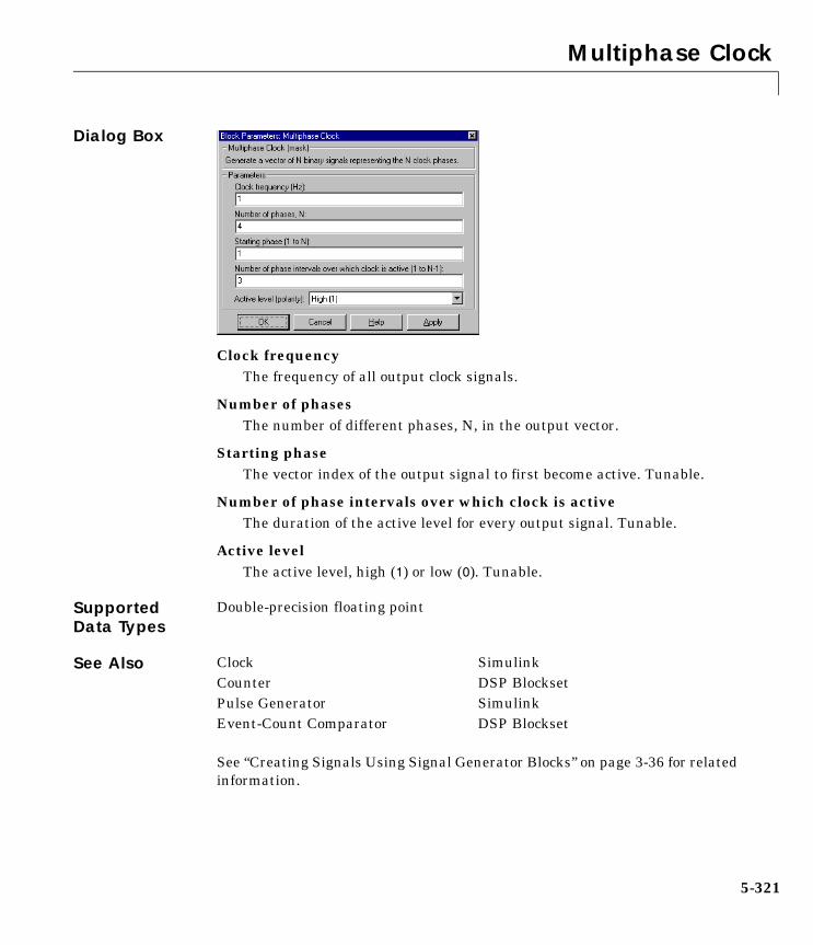
Multiphase Clock
5-321
Dialog Box
Clock frequencyThe frequency of all output clock signals.
Number of phasesThe number of different phases, N, in the output vector.
Starting phaseThe vector index of the output signal to first become active. Tunable.
Number of phase intervals over which clock is activeThe duration of the active level for every output signal. Tunable.
Active levelThe active level, high (1) or low (0). Tunable.
Supported Data Types
See Also
See “Creating Signals Using Signal Generator Blocks” on page 3-36 for related information.
Double-precision floating point
Clock SimulinkCounter DSP BlocksetPulse Generator SimulinkEvent-Count Comparator DSP Blockset

Multiport Selector
5-322
5Multiport SelectorPurpose Distribute arbitrary subsets of input rows or columns to multiple output ports.
Library Signal Management / Indexing
Description The Multi-port Selector block extracts multiple subsets of rows or columns from M-by-N input matrix u, and propagates each new submatrix to a distinct output port. A length-M 1-D vector input is treated as an M-by-1 matrix.
The Indices to output parameter is a cell array whose kth cell contains a one-dimensional indexing expression specifying the subset of input rows or columns to be propagated to the kth output port. The total number of cells in the array determines the number of output ports on the block.
When the Select parameter is set to Rows, the specified one-dimensional indices are used to select matrix rows, and all elements on the chosen rows are included. When the Select parameter is set to Columns, the specified one-dimensional indices are used to select matrix columns, and all elements on the chosen columns are included. A given input row or column can appear any number of times in any of the outputs, or not at all.
The Indices to output parameter is tunable, so you can change the values of the indices at any time during the simulation; however, the number of cells in the array (i.e., the number of output ports) and the size of each submatrix in the output must remain the same while the simulation is running.
When an index references a nonexistent row or column of the input, the block reacts with the behavior specified by the Invalid index parameter. The following options are available:
• Clip index – Clip the index to the nearest valid value, and do not issue an alert.
Example: For a 64-by-4 input with Select = Rows, an index of 72 is clipped to 64; with Select = Columns, an index of 72 is clipped to 4. In both cases, an index of -2 is clipped to 1.
• Clip and warn – Display a warning message in the MATLAB command window, and clip as above.
• Generate error – Display an error dialog box and terminate the simulation.

Multiport Selector
5-323
Example Consider the following Indices to output cell array:
4,[1:2 5],[7;8],10:-1:6
This is a four-cell array, which requires the block to generate four independent outputs (each at a distinct port). The table below shows the dimensions of these outputs when Select = Rows and the input dimension is M-by-N.
Dialog Box
Select The dimension of the input to select, Rows or Columns.
Indices to outputA cell array specifying the row- or column-subsets to propagate to each of the output ports. The number of cells in the array determines the number of output ports on the block. This parameter is tunable, but the size of the cell array (i.e., the number of output ports) and the size of each submatrix in the output must remain the same while the simulation is running.
Cell Expression Description Output size
1 4 Row 4 of input 1-by-N
2 [1:2 5] Rows 1, 2, and 5 of input 3-by-N
3 [7;8] Rows 7 and 8 of input 2-by-N
4 10:-1:6 Rows 10, 9, 8, 7, and 6 of input 5-by-N

Multiport Selector
5-324
Invalid indexResponse to an invalid index value. Tunable.
Supported Data Types
See Also
Fixed-pointCustom data typesBoolean8-, 16-, and 32-bit signed integer 8-, 16-, and 32-bit unsigned integerSingle-precision floating point Double-precision floating point
Permute Matrix DSP BlocksetSelector SimulinkSubmatrix DSP BlocksetVariable Selector DSP Blockset

N-Sample Enable
5-325
5N-Sample EnablePurpose Output ones or zeros for a specified number of sample times.
Library DSP Sources,Signal Management / Switches and Counters
Description The N-Sample Enable block outputs the inactive value (0 or 1, whichever is not selected in the Active level parameter) during the first N sample times, where N is the Trigger count value. Beginning with output sample N+1, the block outputs the active value (1 or 0, whichever is selected in the Active level parameter) until a reset event occurs or the simulation terminates.
The Reset input check box enables the Rst input port. At any time during the count, a trigger event at the input port resets the counter to its initial state. The triggering event is specified by the Trigger type pop-up menu, and can be one of the following:
• Rising edge triggers the reset when the trigger input rises from a negative value to zero or a positive value, or from zero to a positive value.
• Falling edge triggers the reset when the trigger input falls from a positive value to zero or a negative value, or from zero to a negative value.
• Either edge triggers the reset when either a rising or falling edge (as described above) occurs.
The output is always sample-based.
Dialog Box

N-Sample Enable
5-326
Trigger countThe number of samples for which the block outputs the active value. Tunable.
Active levelThe value to output after the first N sample times, 0 or 1. Tunable.
Reset inputEnables the Rst input port.
Trigger typeThe type of event that triggers a reset when the Rst port is enabled. Tunable.
Sample timeThe sample period, Ts, for the block’s counter. The block switches from the active value to the inactive value at t=Ts∗(N+1).
Supported Data Types
See Also
See “Creating Signals Using Signal Generator Blocks” on page 3-36 for related information.
Double-precision floating point
Counter DSP BlocksetN-Sample Switch DSP Blockset

N-Sample Switch
5-327
5N-Sample SwitchPurpose Switch between two inputs after a specified number of sample periods.
Library Signal Management / Switches and Counters
Description The N-Sample Switch block outputs the signal connected to the top input port during the first N sample times after the simulation begins or the block is reset, where N is specified by the Switch count value. Beginning with output sample N+1, the block outputs the signal connected to the bottom input until the next reset event or the end of the simulation.
The sample period of the output is specified by the Sample time parameter (i.e., the output sample period is not inherited from the sample period of either input). The block applies a zero-order hold at the input ports, so the value the block reads from a given port between input sample times is the value of the most recent input to that port.
Both inputs must have the same dimension, except in the following two cases:
• When one input is a scalar, the block expands the scalar input to match the size of the other input.
• When one input is a 1-D vector and the other input is a row or column vector with the same number of elements, the block reshapes the 1-D vector to match the dimension of the other input.
The inputs must either both be frame-based or both be sample-based.
The Reset input check box enables the Rst input port. At any time during the count, a trigger event at the Rst port resets the counter to zero. The triggering event is specified by the Trigger type pop-up menu, and can be one of the following:
• Rising edge triggers the reset when the trigger input rises from a negative value to zero or a positive value, or from zero to a positive value.
• Falling edge triggers the reset when the trigger input falls from a positive value to zero or a negative value, or from zero to a negative value.
• Either edge triggers the reset when either a rising or falling edge (as described above) occurs.

N-Sample Switch
5-328
Dialog Box
Switch countThe number of sample periods, N, for which the output is connected to the top input before switching to the bottom input. Tunable.
Reset inputEnables the Rst input port when selected.
Trigger typeThe type of event at the Rst port that resets the block’s counter. This parameter is enabled when Reset input is selected. Tunable.
Sample timeThe sample period, Ts, for the block’s counter. The block switches inputs at t=Ts∗(N+1).
Supported Data Types
See Also
Double-precision floating point
Counter DSP BlocksetN-Sample Enable DSP Blockset

Normalization
5-329
5NormalizationPurpose Normalize an input by its 2-norm or squared 2-norm.
Library Math Functions / Math Operations
Description The Normalization block independently normalizes each column of the M-by-N matrix input, u.
2-NormWhen the Norm parameter specifies 2-norm, the block normalizes the jth input column as follows.
where b is specified by the Normalization bias parameter, and is the 2-norm (or Euclidean norm) of the jth input column.
Equivalently,
y = u ./ (norm(u) + b) % Equivalent MATLAB code
The normalization bias, b, is typically chosen to be a small positive constant (e.g., 1e-10) that prevents potential division by zero.
Squared 2-NormWhen the Norm parameter specifies Squared 2-norm, the block normalizes the jth input column as follows.
where
Equivalently,
y = u ./ (norm(u).^2 + b) % Equivalent MATLAB code
yijuij
u j b+---------------------=
u j
u j u12 u2
2L uM
2+ + +=
yijuij
u j2 b+
----------------------=
u j2 u1
2 u22
L uM2
+ + +=

Normalization
5-330
The output has the same dimension and frame status as the input. For convenience, length-M 1-D vector inputs and sample-based length-M row vector inputs are both treated as M-by-1 column vectors, and the output retains the dimensions of the input.
Dialog Box
NormThe type of normalization to apply, 2-norm or Squared 2-norm. Tunable.
Normalization biasThe value b to be added in the denominator to avoid division by zero. Tunable.
Supported Data Types
See Also
Double-precision floating point
Matrix Scaling DSP BlocksetReciprocal Condition DSP Blocksetnorm MATLAB

Overlap-Add FFT Filter
5-331
5Overlap-Add FFT FilterPurpose Implement the overlap-add method of frequency-domain filtering.
Library Filtering / Filter Designs
Description The Overlap-Add FFT Filter block uses an FFT to implement the overlap-add method, a technique that combines successive frequency-domain filtered sections of an input sequence.
Valid inputs to this block are 1-D vectors, sample-based vectors, frame-based vectors, and frame-based full matrices. All outputs are unbuffered into sample-based row vectors. The length of the output vector is equal to the number of channels in the input vector. An M-by-1 sample-based input has M channels, so it would result in a length-M sample-based output vector. An M-by-1 frame-based input has only one channel, so would result in a 1-by-1 (scalar) output.
The block’s data output rate is M times faster than its data input rate, where M is the input frame-size. Thus, the block’s data input and output rates are the same when the inputs are 1-D vectors, sample-based vectors, or frame-based row vectors. For frame-based column and frame-based full-matrix inputs, the block’s data output rate is M times greater than the block’s data input rate.
1-D vectors are treated as length-N sample-based vectors, and result in sample-based length-N row vectors.
The block breaks the scalar input sequence u, of length nu, into length-L nonoverlapping data sections,
which it linearly convolves with the filter’s FIR coefficients,
The numerator coefficients for H(z) are specified as a vector by the FIR coefficients parameter. The coefficient vector, b = [b(1) b(2) ... b(n+1)], can be generated by one of the filter design functions in the Signal Processing Toolbox, such as fir1. All filter states are internally initialized to zero.
. . .u
2LL 3L ceil(nu/L)*L
H z( ) B z( ) b1 b2z 1– … bn 1+ z n–+ + += =

Overlap-Add FFT Filter
5-332
If either the filter coefficients or the inputs to the block are complex, the Output parameter should be set to Complex. Otherwise, the default Output setting, Real, instructs the block to take only the real part of the solution.
The block’s overlap-add operation is equivalent to
y = ifft(fft(u(i:i+L-1),nfft) .* fft(b,nfft))
where nfft is specified by the FFT size parameter as a power-of-two value greater (typically much greater) than n+1. Values for FFT size that are not powers of two are rounded upwards to the nearest power-of-two value to obtain nfft.
The block overlaps successive output sections by n points and sums them.
The first L samples of each summation are output in sequence. The block chooses the parameter L based on the filter order and the FFT size.
L = nfft - n
LatencyIn single-tasking operation, the Overlap-Add FFT Filter block has a latency of nfft-n+1 samples. The first nfft-n+1 consecutive outputs from the block are zero; the first filtered input value appears at the output as sample nfft-n+2.
In multitasking operation, the Overlap-Add FFT Filter block has a latency of 2*(nfft-n+1) samples. The first 2*(nfft-n+1) consecutive outputs from the block are zero; the first filtered input value appears at the output as sample 2*(nfft-n)+3.
See “Excess Algorithmic Delay (Tasking Latency)” on page 3-91 and “The Simulation Parameters Dialog Box” in the Simulink documentation for more information about block rates and Simulink’s tasking modes.
L L+n
2L 2L+n
3L 3L+n. . .

Overlap-Add FFT Filter
5-333
Dialog Box
FFT sizeThe size of the FFT, which should be a power-of-two value greater than the length of the specified FIR filter.
FIR coefficientsThe filter numerator coefficients.
OutputThe complexity of the output; Real or Complex. If the input signal or the filter coefficients are complex, this should be set to Complex.
References Oppenheim, A. V. and R. W. Schafer. Discrete-Time Signal Processing. Englewood Cliffs, NJ: Prentice Hall, 1989.
Proakis, J. and D. Manolakis. Digital Signal Processing. 3rd ed. Englewood Cliffs, NJ: Prentice-Hall, 1996.
Supported Data Types
See Also
See “Designing Filters with Various Filter Structures” on page 4-6 for related information.
Double-precision floating point
Direct-Form II Transpose Filter DSP BlocksetOverlap-Save FFT Filter DSP Blockset

Overlap-Save FFT Filter
5-334
5Overlap-Save FFT FilterPurpose Implement the overlap-save method of frequency-domain filtering.
Library Filtering / Filter Designs
Description The Overlap-Save FFT Filter block uses an FFT to implement the overlap-save method, a technique that combines successive frequency-domain filtered sections of an input sequence.
Valid inputs to this block are 1-D vectors, sample-based vectors, frame-based vectors, and frame-based full matrices. All outputs are unbuffered into sample-based row vectors. The length of the output vector is equal to the number of channels in the input vector. An M-by-1 sample-based input has M channels, so it would result in a length-M sample-based output vector. An M-by-1 frame-based input has only one channel, so would result in a 1-by-1 (scalar) output.
The block’s data output rate is M times faster than its data input rate, where M is the input frame-size. Thus, the block’s data input and output rates are the same when the inputs are 1-D vectors, sample-based vectors, or frame-based row vectors. For frame-based column and frame-based full-matrix inputs, the block’s data output rate is M times greater than the block’s data input rate.
1-D vectors are treated as length-N sample-based vectors, and result in sample-based length-N row vectors.
Overlapping sections of input u are circularly convolved with the FIR filter coefficients
The numerator coefficients for H(z) are specified as a vector by the FIR coefficients parameter. The coefficient vector, b = [b(1) b(2) ... b(n+1)], can be generated by one of the filter design functions in the Signal Processing Toolbox, such as fir1. All filter states are internally initialized to zero.
If either the filter coefficients or the inputs to the block are complex, the Output parameter should be set to Complex. Otherwise, the default Output setting, Real, instructs the block to take only the real part of the solution.
H z( ) B z( ) b1 b2z 1– … bn 1+ z n–+ + += =

Overlap-Save FFT Filter
5-335
The circular convolution of each section is computed by multiplying the FFTs of the input section and filter coefficients, and computing the inverse FFT of the product.
y = ifft(fft(u(i:i+(L-1)),nfft) .* fft(b,nfft))
where nfft is specified by the FFT size parameter as a power-of-two value greater (typically much greater) than n+1. Values for FFT size that are not powers of two are rounded upwards to the nearest power-of-two value to obtain nfft.
The first n points of the circular convolution are invalid and are discarded. The Overlap-Save FFT Filter block outputs the remaining nfft-n points, which are equivalent to the linear convolution.
LatencyIn single-tasking operation, the Overlap-Save FFT Filter block has a latency of nfft-n+1 samples. The first nfft-n+1 consecutive outputs from the block are zero; the first filtered input value appears at the output as sample nfft-n+2.
In multitasking operation, the Overlap-Save FFT Filter block has a latency of 2*(nfft-n+1) samples. The first 2*(nfft-n+1) consecutive outputs from the block are zero; the first filtered input value appears at the output as sample 2*(nfft-n)+3.
See “Excess Algorithmic Delay (Tasking Latency)” on page 3-91 and “The Simulation Parameters Dialog Box” in the Simulink documentation for more information about block rates and Simulink’s tasking modes.
Dialog Box

Overlap-Save FFT Filter
5-336
FFT sizeThe size of the FFT, which should be a power-of-two value greater than the length of the specified FIR filter.
FIR coefficientsThe filter numerator coefficients.
OutputThe complexity of the output; Real or Complex. If the input signal or the filter coefficients are complex, this should be set to Complex.
References Oppenheim, A. V. and R. W. Schafer. Discrete-Time Signal Processing. Englewood Cliffs, NJ: Prentice Hall, 1989.
Proakis, J. and D. Manolakis. Digital Signal Processing. 3rd ed. Englewood Cliffs, NJ: Prentice-Hall, 1996.
Supported Data Types
See Also
See “Designing Filters with Various Filter Structures” on page 4-6 for related information.
Double-precision floating point
Direct-Form II Transpose Filter DSP BlocksetOverlap-Add FFT Filter DSP Blockset

Pad
5-337
5PadPurpose Alter the input size by padding or truncating rows and/or columns.
Library Signal Operations
Description The Pad block changes the size of the input matrix from Mi-by-Ni to Mo-by-No by padding or truncating along the rows, the columns, or both dimensions. The dimensions of the output, Mo and No, are specified by the Number of output rows and Number of output columns parameters, respectively. The value with which to pad the input is set by the Value parameter.
The behavior of the Pad block and Zero Pad block are identical, with the exception that the Pad block can pad the input matrix with values other than zero. See the Zero Pad block reference for more information on the behavior of the Pad block.
Dialog Box
ValueThe scalar value with which to pad the input matrix. Tunable.
Pad alongThe direction along which to pad or truncate. Columns specifies that the row dimension should be changed to Mo. Rows specifies that the column dimension should be changed to No. Columns and rows specifies that both column and row dimensions should be changed. None disables padding and truncation and passes the input through to the output unchanged.

Pad
5-338
Number of output rowsThe desired number of rows in the output, Mo. This parameter is enabled when Columns or Columns and rows is selected in the Pad along menu.
Number of output columnsThe desired number of columns in the output, No. This parameter is enabled when Rows or Columns and rows is selected in the Pad along menu.
Supported Data Types
See Also
Fixed-pointCustom data typesBoolean8-, 16-, and 32-bit signed integer 8-, 16-, and 32-bit unsigned integerSingle-precision floating point Double-precision floating point
Matrix Concatenation SimulinkRepeat DSP BlocksetSubmatrix DSP BlocksetUpsample DSP BlocksetVariable Selector DSP BlocksetZero Pad DSP Blockset

Permute Matrix
5-339
5Permute MatrixPurpose Reorder the rows or columns of a matrix.
Library Math Functions / Matrices and Linear Algebra / Matrix Operations
Description The Permute Matrix block reorders the rows or columns of M-by-N input matrix A as specified by indexing input P.
When the Permute parameter is set to Rows, the block uses the rows of A to create a new matrix with the same column dimension. Input P is a length-L vector whose elements determine where each row from A should be placed in the L-by-N output matrix.
% Equivalent MATLAB codey = [A(P(1),:) ; A(P(2),:) ; A(P(3),:) ; ... ; A(P(end),:)]
For row permutation, a length-M 1-D vector input at the A port is treated as a M-by-1 matrix.
When the Permute parameter is set to Columns, the block uses the columns of A to create a new matrix with the same row dimension. Input P is a length-L vector whose elements determine where each column from A should be placed in the M-by-L output matrix.
% Equivalent MATLAB codey = [A(:,P(1)) A(:,P(2)) A(:,P(3)) ... A(:,P(end))]
For column permutation, a length-N 1-D vector input at the A port is treated as a 1-by-N matrix.
When an index value in input P references a nonexistent row or column of matrix A, the block reacts with the behavior specified by the Invalid permutation index parameter. The following options are available:
• Clip index – Clip the index to the nearest valid value (1 or M for row permutation, and 1 or N for column permutation), and do not issue an alert. Example: For a 3-by-7 input matrix, a column index of 9 is clipped to 7, and a row index of -2 is clipped to 1.
• Clip and warn – Display a warning message in the MATLAB command window, and clip the index as described above.
• Generate error – Display an error dialog box and terminate the simulation.

Permute Matrix
5-340
When length of the permutation vector P is not equal to the number of rows or columns of the input matrix A, you can choose to get an error dialog box and terminate the simulation by checking Error when length of P is not equal to Permute dimension size.
If input A is frame-based, the output is frame-based; otherwise, the output is sample-based.
Example In the model below, the top Permute Matrix block places the second row of the input matrix in both the first and fifth rows of the output matrix, and places the third row of the input matrix in the three middle rows of the output matrix. The bottom Permute Matrix block places the second column of the input matrix in both the first and fifth columns of the output matrix, and places the third column of the input matrix in the three middle columns of the output matrix.
As shown in the example above, rows and columns of A can appear any number of times in the output, or not at all.
4 5 67 8 97 8 97 8 94 5 6
2 3 3 3 25 6 6 6 58 9 9 9 8

Permute Matrix
5-341
Dialog Box
PermuteMethod of constructing the output matrix; by permuting rows or columns of the input.
Invalid permutation indexResponse to an invalid index value. Tunable, except in Simulink’s external mode.
Error when length of P is not equal to Permute dimension sizeOption to display an error dialog box and terminate the simulation if the length of the permutation vector P is not equal to the number of rows or columns of the input matrix A.
Supported Data Types
See Also
Fixed-point Only supported by input port A Custom data types Only supported by input port A Boolean8-, 16-, and 32-bit signed integer 8-, 16-, and 32-bit unsigned integerSingle-precision floating point Double-precision floating point
Submatrix DSP BlocksetTranspose DSP BlocksetVariable Selector DSP Blocksetpermute MATLAB

Permute Matrix
5-342
See “Reordering Channels in a Frame-Based Multichannel Signal” on page 3-61 for related information.
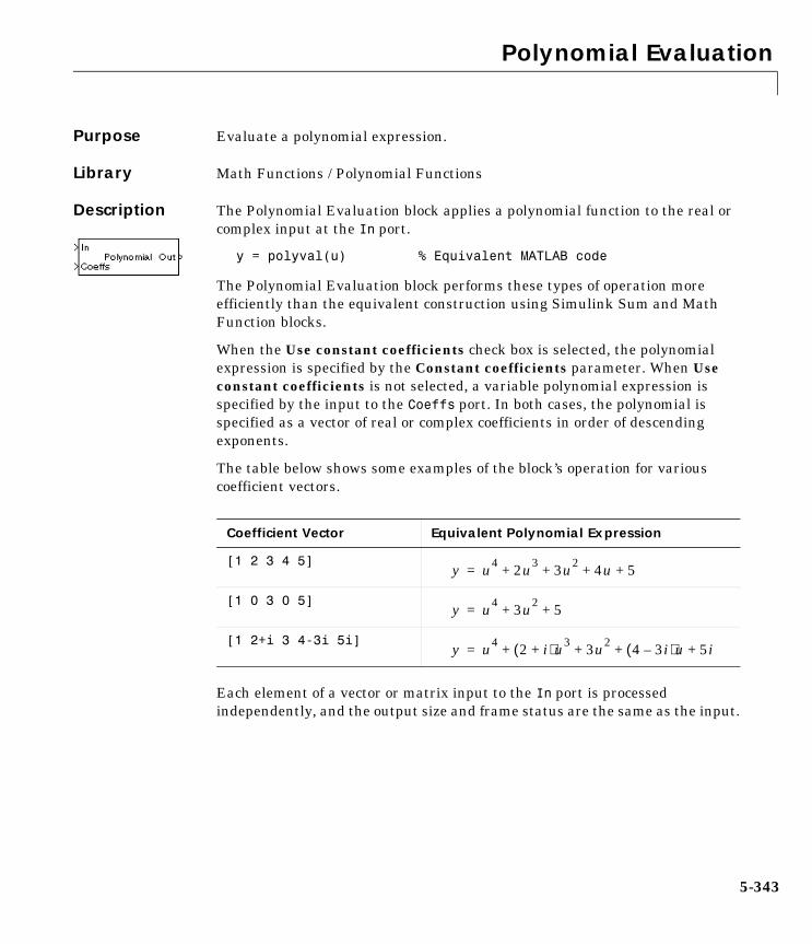
Polynomial Evaluation
5-343
5Polynomial EvaluationPurpose Evaluate a polynomial expression.
Library Math Functions / Polynomial Functions
Description The Polynomial Evaluation block applies a polynomial function to the real or complex input at the In port.
y = polyval(u) % Equivalent MATLAB code
The Polynomial Evaluation block performs these types of operation more efficiently than the equivalent construction using Simulink Sum and Math Function blocks.
When the Use constant coefficients check box is selected, the polynomial expression is specified by the Constant coefficients parameter. When Use constant coefficients is not selected, a variable polynomial expression is specified by the input to the Coeffs port. In both cases, the polynomial is specified as a vector of real or complex coefficients in order of descending exponents.
The table below shows some examples of the block’s operation for various coefficient vectors.
Each element of a vector or matrix input to the In port is processed independently, and the output size and frame status are the same as the input.
Coefficient Vector Equivalent Polynomial Expression
[1 2 3 4 5]
[1 0 3 0 5]
[1 2+i 3 4-3i 5i]
y u4 2u3 3u2 4u 5+ + + +=
y u4 3u2 5+ +=
y u4 2 i+( )u3 3u2 4 3i–( )u 5i+ + + +=

Polynomial Evaluation
5-344
Dialog Box
Use constant coefficientsWhen selected, enables the Constant coefficients parameter and disables the Coeffs input port.
Constant coefficientsThe vector of polynomial coefficients to apply to the input, in order of descending exponents. This parameter is enabled when the Use constant coefficients check box is selected.
Supported Data Types
See Also
Double-precision floating point
Least Squares Polynomial Fit DSP BlocksetMath Function SimulinkSum Simulinkpolyval MATLAB

Polynomial Stability Test
5-345
5Polynomial Stability TestPurpose Determine whether all roots of the input polynomial are inside the unit circle using the Schur-Cohn algorithm.
Library Math Functions / Polynomial Functions
Description The Polynomial Stability Test block uses the Schur-Cohn algorithm to determine whether all roots of a polynomial are within the unit circle.
y = all(abs(roots(u)) < 1) % Equivalent MATLAB code
Each column of the M-by-N input matrix u contains M coefficients from a distinct polynomial,
arranged in order of descending exponents, u1, u2, …, uM. The polynomial has order M-1 and positive integer exponents.
Inputs can be frame-based or sample-based, and both represent the polynomial coefficients as shown above. For convenience, a length-M 1-D vector input is treated as an M-by-1 matrix.
The output is a 1-by-N matrix with each column containing the value 1 or 0. The value 1 indicates that the polynomial in the corresponding column of the input is stable; i.e., the magnitudes of all solutions to f(x) = 0 are less than 1. The value 0 indicates that the polynomial in the corresponding column of the input may be unstable; i.e., the magnitude of at least one solution to f(x) = 0 is greater than or equal to 1.
The output is always sample-based.
ApplicationsThis block is most commonly used to check the pole locations of the denominator polynomial, A(z), of a transfer function, H(z).
The poles are the n-1 roots of the denominator polynomial, A(z). If any poles are located outside the unit circle, the transfer function H(z) is unstable. As is
f x( ) u1xM 1– u2xM 2–L uM+ + +=
H z( ) B z( )A z( )------------
b1 b2z 1– … bmz m 1–( )–+ + +
a1 a2z 1– … anz n 1–( )–+ + +
---------------------------------------------------------------------------= =

Polynomial Stability Test
5-346
typical in DSP applications, the transfer function above is specified in descending powers of z-1 rather than z.
Dialog Box
Supported Data Types
See Also
Single-precision floating point Double-precision floating point
Least Squares Polynomial Fit DSP BlocksetPolynomial Evaluation DSP Blocksetpolyfit MATLAB

Pseudoinverse
5-347
5PseudoinversePurpose Compute the Moore-Penrose pseudoinverse of a matrix.
Library Math Functions / Matrices and Linear Algebra / Matrix Inverses
Description The Pseudoinverse block computes the Moore-Penrose pseudoinverse of input matrix A.
[U,S,V] = svd(A,0) % Equivalent MATLAB code
The pseudoinverse of A is the matrix A+ such that
where U and V are orthogonal matrices, and S is a diagonal matrix. The pseudoinverse has the following properties:
• AA+ = (AA+)*
• A+A = (A+A)*
• AA+A = A
• A+AA+ = A+
The output is always sample-based.
Dialog Box
References Golub, G. H., and C. F. Van Loan. Matrix Computations. 3rd ed. Baltimore, MD: Johns Hopkins University Press, 1996.
Supported Data Types
A+ VS+U*=
Double-precision floating point

Pseudoinverse
5-348
See Also
See “Inverting Matrices” on page 4-19 for related information.
Cholesky Inverse DSP BlocksetLDL Inverse DSP BlocksetLU Inverse DSP BlocksetSingular Value Decomposition DSP Blocksetinv MATLAB

QR Factorization
5-349
5QR FactorizationPurpose Factor a rectangular matrix into unitary and upper triangular components.
Library Math Functions / Matrices and Linear Algebra / Matrix Factorizations
Description The QR Factorization block uses modified Gram-Schmidt iteration to factor a column permutation of the M-by-N input matrix A as
where Q is an M-by-min(M,N) unitary matrix, and R is a min(M,N)-by-N upper-triangular matrix. A length-M vector input is treated as an M-by-1 matrix, and is always sample-based.
The column-pivoted matrix Ae contains the columns of A permuted as indicated by the contents of length-N permutation vector E.
Ae = A(:,E) % Equivalent MATLAB code
The block selects a column permutation vector E, which ensures that the diagonal elements of matrix R are arranged in order of decreasing magnitude.
QR factorization is an important tool for solving linear systems of equations because of good error propagation properties and the invertability of unitary matrices.
Unlike LU and Cholesky factorizations, the matrix A does not need to be square for QR factorization. Note, however, that QR factorization requires twice as many operations as Gaussian elimination.
Example A sample factorization is shown below. The input to the block is matrix A, which is permuted according to vector E to produce matrix Ae. Matrix Ae is factored to produce the Q and R output matrices.
Ae QR=
ri 1 j 1+,+ ri j, i j=>
Q 1– Q*=

QR Factorization
5-350
Dialog Box
References Golub, G. H., and C. F. Van Loan. Matrix Computations. 3rd ed. Baltimore, MD: Johns Hopkins University Press, 1996.
Supported Data Types
See Also
See “Factoring Matrices” on page 4-17 for related information.
9 1– 21– 8 5–
2 5– 7
Ae
1– 9 28 1– 5–
5– 2 7
=
0.105– 0.986– 0.131–
0.843 0.159– 0.5140.527– 0.057– 0.848
9.487 2.846– 8.117–
0 8.826– 1.575–
0 0 3.105
(2 1 3)
Double-precision floating point
Cholesky Factorization DSP BlocksetLU Factorization DSP BlocksetQR Solver DSP BlocksetSingular Value Decomposition DSP Blocksetqr MATLAB

QR Solver
5-351
5QR SolverPurpose Find a minimum-norm-residual solution to the equation AX=B.
Library Math Functions / Matrices and Linear Algebra / Linear System Solvers
Description The QR Solver block solves the linear system AX=B, which can be overdetermined, underdetermined, or exactly determined. The system is solved by applying QR factorization to the M-by-N matrix, A, at the A port. The input to the B port is the right-hand-side M-by-L matrix, B. A length-M 1-D vector input at either port is treated as an M-by-1 matrix.
The output at the x port is the N-by-L matrix, X. X is always sample based, and is chosen to minimize the sum of the squares of the elements of B-AX. When B is a vector, this solution minimizes the vector 2-norm of the residual (B-AX is the residual). When B is a matrix, this solution minimizes the matrix Frobenius norm of the residual. In this case, the columns of X are the solutions to the L corresponding systems AXk=Bk, where Bk is the kth column of B, and Xk is the kth column of X.
X is known as the minimum-norm-residual solution to AX=B. The minimum-norm-residual solution is unique for overdetermined and exactly determined linear systems, but it is not unique for underdetermined linear systems. Thus when the QR Solver is applied to an underdetermined system, the output X is chosen such that the number of nonzero entries in X is minimized.
Algorithm QR factorization factors a column-permuted variant (Ae) of the M-by-N input matrix A as
where Q is a M-by-min(M,N) unitary matrix, and R is a min(M,N)-by-N upper-triangular matrix.
The factored matrix is substituted for Ae in
,
and
Ae QR=
AeX Be=
QRX Be=

QR Solver
5-352
is solved for X by noting that Q-1 = Q* and substituting Y = Q*Be. This requires computing a matrix multiplication for Y and solving a triangular system for X.
Dialog Box
Supported Data Types
See Also
See “Solving Linear Systems” on page 4-16 for related information.
RX Y=
Double-precision floating point
Levinson-Durbin DSP BlocksetLDL Solver DSP BlocksetLU Solver DSP BlocksetQR Factorization DSP BlocksetSVD Solver DSP Blockset

Queue
5-353
5QueuePurpose Store inputs in a FIFO register.
Library Signal Management / Buffers
Description The Queue block stores a sequence of input samples in a FIFO (first in, first out) register. The register capacity is set by the Register size parameter, and inputs can be scalars, vectors, or matrices.
The block pushes the input at the In port onto the end of the queue when a trigger event is received at the Push port. When a trigger event is received at the Pop port, the block pops the first element off the queue and holds the Out port at that value. The first input to be pushed onto the queue is always the first to be popped off.
A trigger event at the optional Clr port (enabled by the Clear input check box) empties the queue contents. If Clear output port on reset is selected, then a trigger event at the Clr port empties the queue and sets the value at the Out port to zero. This setting also applies when a disabled subsystem containing
register size
Pushing the queue1101
0101
0000
1001
1111
1100
empt
y
empt
y
empt
y
first in
0101
0000
1001
1111
1100
empt
y
empt
y
empt
y
first out
Popping the queue
1101
1101
0101
0000
1001
1111
empt
y
empt
y 1100

Queue
5-354
the Queue block is reenabled; the Out port value is only reset to zero in this case if Clear output port on reset is selected.
When two or more of the control input ports are triggered at the same time step, the operations are executed in the following order:
1 Clr
2 Push
3 Pop
The triggering event for the Push, Pop, and Clr ports is specified by the Trigger type pop-up menu, and can be one of the following:
• Rising edge triggers execution of the block when the trigger input rises from a negative value to zero or a positive value, or from zero to a positive value.
• Falling edge triggers execution of the block when the trigger input falls from a positive value to zero or a negative value, or from zero to a negative value.
• Either edge triggers execution of the block when either a rising or falling edge (as described above) occurs.
The Push onto full register parameter specifies the block’s behavior when a trigger is received at the Push port but the register is full. The Pop empty register parameter specifies the block’s behavior when a trigger is received at the Pop port but the register is empty. The following options are available for both cases:
• Ignore – Ignore the trigger event, and continue the simulation.
• Warning – Ignore the trigger event, but display a warning message in the MATLAB command window.
• Error – Display an error dialog box and terminate the simulation.
The Push onto full register parameter additionally offers the Dynamic reallocation option, which dynamically resizes the register to accept as many additional inputs as memory permits. To find out how many elements are on the queue at a given time, enable the Num output port by selecting the Output number of register entries option.

Queue
5-355
Examples Example 1The table below illustrates the Queue block’s operation for a Register size of 4, Trigger type of Either edge, and Clear output port on reset enabled. Because the block triggers on both rising and falling edges in this example, each transition from 1 to 0 or 0 to 1 in the Push, Pop, and Clr columns below represents a distinct trigger event. A 1 in the Empty column indicates an empty queue, while a 1 in the Full column indicates a full queue.
Note that at the last step shown, the Push and Clr ports are triggered simultaneously. The Clr trigger takes precedence, and the queue is first cleared and then pushed.
Example 2The dspqdemo demo provides another example of Queue operation.
In Push Pop Clr Queue Out Empty Full Num
1 0 0 0 0 1 0 0
2 1 0 0 0 0 0 1
3 0 0 0 0 0 0 2
4 1 0 0 0 0 0 3
5 0 0 0 0 0 1 4
6 0 1 0 2 0 0 3
7 0 0 0 3 0 0 2
8 0 1 0 4 0 0 1
9 0 0 0 5 1 0 0
10 1 0 0 5 0 0 1
11 0 0 0 5 0 0 2
12 1 0 1 0 0 0 1
top bottom
top bottom2
top bottom3 2
top bottom3 24
top bottom3 245
top bottom345
top bottom5 4
top bottom5
top bottom
top bottom10
top bottom11 10
top bottom12

Queue
5-356
Dialog Box
Register sizeThe number of entries that the FIFO register can hold.
Trigger typeThe type of event that triggers the block’s execution. Tunable.
Push onto full registerResponse to a trigger received at the Push port when the register is full.
Pop empty registerResponse to a trigger received at the Pop port when the register is empty. Tunable.
Empty register outputEnable the Empty output port, which is high (1) when the queue is empty, and low (0) otherwise.
Full register outputEnable the Full output port, which is high (1) when the queue is full, and low (0) otherwise. The Full port remains low when Dynamic reallocation is selected from the Push onto full register parameter.
Output number of register entriesEnable the Num output port, which tracks the number of entries currently on the queue.

Queue
5-357
Clear inputEnable the Clr input port, which empties the queue when the trigger specified by the Trigger type is received.
Clear output port on resetReset the Out port to zero (in addition to clearing the queue) when a trigger is received at the Clr input port. Tunable.
Supported Data Types
See Also
Double-precision floating point
Buffer DSP BlocksetDelay Line DSP BlocksetStack DSP Blockset

Random Source
5-358
5Random SourcePurpose Generate randomly distributed values.
Library DSP Sources
Description The Random Source block generates a frame of M values drawn from a uniform or Gaussian pseudorandom distribution, where M is specified by the Samples per frame parameter.
This reference page contains a detailed discussion of the following Random Source block topics:
• “Distribution Type” on page 5-358
• “Output Data Type” on page 5-359
• “Output Repeatability” on page 5-360
• “Specifying the Initial Seed” on page 5-360
• “Sample Period” on page 5-361
Distribution TypeWhen the Source type parameter is set to Uniform, the output samples are drawn from a uniform distribution whose minimum and maximum values are specified by the Minimum and Maximum parameters, respectively. All values in this range are equally likely to be selected. A length-N vector specified for one or both of these parameters generates an N-channel output (M-by-N matrix) containing a unique random distribution in each channel.
For example, specify
• Minimum = [ 0 0 -3 -3]
• Maximum = [10 10 20 20]
to generate a four-channel output whose first and second columns contain random values in the range [0, 10], and whose third and fourth columns contain random values in the range [-3, 20]. When only one of the Minimum and Maximum parameters is specified as a vector, the other is scalar expanded to the same length.
When the Source type parameter is set to Gaussian, the output samples are drawn from the normal distribution defined by the Mean and Variance parameters. A length-N vector specified for one or both of the Mean and

Random Source
5-359
Variance parameters generates an N-channel output (M-by-N frame matrix) containing a distinct random distribution in each column. When only one of these parameters is specified as a vector, the other is scalar expanded to the same length.
Output Data TypeThe block’s output can be either real or complex, as selected by the Real and Complex options in the Output complexity parameter. (These settings control all channels of the output, so real and complex data cannot be combined in the same output.) For complex output with a Uniform distribution, the real and imaginary components in each channel are both drawn from the same uniform random distribution, defined by the Minimum and Maximum parameters for that channel.
For complex output with a Gaussian distribution, the real and imaginary components in each channel are drawn from normal distributions with different means. In this case, the Mean parameter for each channel should specify a complex value; the real component of the Mean parameter specifies the mean of the real components in the channel, while the imaginary component specifies the mean of the imaginary components in the channel. If either the real or imaginary component is omitted from the Mean parameter, a default value of 0 is used for the mean of that component.
For example, a Mean parameter setting of [5+2i 0.5 3i] generates a three-channel output with the following means.
For complex output, the Variance parameter, σ2, specifies the total variance for each output channel. This is the sum of the variances of the real and imaginary components in that channel.
Channel 1 mean real = 5 imaginary = 2
Channel 2 mean real = 0.5 imaginary = 0
Channel 3 mean real = 0 imaginary = 3
σ2 σRe2 σIm
2+=

Random Source
5-360
The specified variance is equally divided between the real and imaginary components, so that
Output RepeatabilityThe Repeatability parameter determines whether or not the block outputs the same signal each time you run the simulation. You can set the parameter to one of the following options:
• Repeatable — The block outputs the same signal each time you run the simulation. The first time you run the simulation, the block randomly selects an initial seed. The block reuses these same initial seeds every time you rerun the simulation.
• Specify seed — The block outputs the same signal each time you run the simulation. Every time you run the simulation, the block uses the initial seed(s) specified by the Initial seed parameter. Also see the next section, “Specifying the Initial Seed”.
• Not repeatable — The block does not output the same signal each time you run the simulation. Every time you run the simulation, the block randomly selects an initial seed.
Specifying the Initial SeedWhen you set the Repeatability parameter to Specify seed, you must set the Initial seed parameter. The Initial seed parameter specifies the initial seed for the pseudorandom number generator. The generator produces an identical sequence of pseudorandom numbers each time it is executed with a particular initial seed.
For real outputs (Output complexity parameter set to Real), a length-N seed vector can be specified to set a distinct initial generator seed for each individual channel. When a scalar seed is specified for a multichannel output, the block uses the specified seed for the first channel, and increments the seed by 2 for each additional channel. For example, specifying an Initial seed value of 10 for
σRe2 σ2
2------=
σIm2 σ2
2------=

Random Source
5-361
a five-channel output is equivalent to specifying an Initial seed vector of [10 12 14 16 18].
For complex outputs (Output complexity parameter set to Complex), a length-N seed vector can be specified to set a distinct initial generator seed to be used for the real components of each individual channel. The block increments these values by 1 to determine the initial seeds used for the imaginary components of the corresponding channels.
When a scalar seed is specified for a multichannel complex output, the block uses the specified seed for the real components of the first channel, and increments the seed by 2 for the real components of each additional channel. The block increments the specified seed by 1 for the imaginary components of the first channel, and increments the first channel’s imaginary seed by 2 for the imaginary components of each additional channel. For example, specifying an Initial seed value of 10 for a five-channel complex output is equivalent to specifying an Initial seed vector of [10 12 14 16 18]. These values are used to seed the real-component generator for each channel; the vector [11 13 15 17 19] is used to seed the imaginary-component generator for each channel.
Sample PeriodThe Sample time parameter value, Ts, specifies the random sequence sample period when the Sample mode parameter is set to Discrete. In this mode, the block generates the number of samples specified by the Samples per frame parameter value, M, and outputs this frame with a period of M∗Ts. For M=1, the output is sample-based; otherwise, the output is frame-based.
When Sample mode is set to Continuous, the block is configured for continuous-time operation, and the Sample time and Samples per frame parameters are disabled. Note that many blocks in the DSP Blockset do not accept continuous-time inputs.

Random Source
5-362
Dialog Box
Source typeThe distribution from which to draw the random values, Uniform or Gaussian.
MinimumThe minimum value in the uniform distribution. This parameter is only enabled when Uniform is selected from the Source type parameter. Tunable.

Random Source
5-363
MaximumThe maximum value in the uniform distribution. This parameter is only enabled when Uniform is selected from the Source type parameter. Tunable.
MeanThe mean of the Gaussian (normal) distribution. This parameter is only enabled when Gaussian is selected from the Source type parameter. Tunable.
VarianceThe variance of the Gaussian (normal) distribution. This parameter is only enabled when Gaussian is selected from the Source type parameter. Tunable.
RepeatabilityThe repeatability of the block output: Not repeatable, Repeatable, or Specify seed. In the Repeatable and Specify seed settings, the block outputs the same signal every time you run the simulation. For details, see “Output Repeatability” on page 5-360.
Initial seedThe initial seed(s) to use for the random number generator when you set the Repeatability parameter to Specify seed. For details, see “Specifying the Initial Seed” on page 5-360.
Inherit output port attributesWhen selected, allows the block to inherit the sample mode, sample period, and complexity of a downstream block. (The Sample mode, Sample time, Samples per frame, and Output complexity parameters are disabled.) The output is a length-M sample-based 1-D vector, where length M is inherited from the downstream block. If the Minimum, Maximum, Mean, or Variance parameter specifies N channels, the 1-D vector output contains M/N samples from each channel. An error occurs in this case if M is not an integer multiple of N.
Sample modeThe sample mode, Continuous or Discrete. This parameter is enabled when the Inherit output port attributes check box is deselected.

Random Source
5-364
Sample timeThe sample period, Ts, of the random output sequence. The output frame period is M∗Ts. This parameter is enabled when the Inherit output port attributes check box is deselected.
Samples per frameThe number of samples, M, in each output frame. This parameter is enabled when the Inherit output port attributes check box is deselected.
Output complexityThe data type of the output, Real or Complex. This parameter is enabled when the Inherit output port attributes check box is deselected.
Supported Data Types
See Also
See “Creating Signals Using Signal Generator Blocks” on page 3-36 for related information.
Double-precision floating point
Discrete Impulse DSP BlocksetDSP Constant DSP BlocksetMaximum DSP BlocksetMinimum DSP BlocksetRandom Number SimulinkSignal From Workspace DSP BlocksetSignal Generator SimulinkStandard Deviation DSP BlocksetVariance DSP Blocksetrand MATLABrandn MATLAB

Real Cepstrum
5-365
5Real CepstrumPurpose Compute the real cepstrum of an input.
Library Transforms
Description The Real Cepstrum block computes the real cepstrum of each channel in the real-valued M-by-N input matrix, u. For both sample-based and frame-based inputs, the block assumes that each input column is a frame containing M consecutive samples from an independent channel. The block does not accept complex-valued inputs.
The output is a real Mo-by-N matrix, where Mo is specified by the FFT length parameter. Each output column contains the length-Mo real cepstrum of the corresponding input column.
y = real(ifft(log(abs(fft(u,Mo))))) % Equivalent MATLAB code
or, more compactly,
y = rceps(u,Mo)
When the Inherit FFT length from input port dimensions check box is selected, the output frame size matches the input frame size (Mo=M). In this case, a sample-based length-M row vector input is processed as a single channel (i.e., as an M-by-1 column vector), and the output is a length-M row vector. A 1-D vector input is always processed as a single channel, and the output is a 1-D vector.
The output is always sample-based, and the output port rate is the same as the input port rate.
Dialog Box

Real Cepstrum
5-366
Inherit FFT length from input port dimensionsWhen selected, matches the output frame size to the input frame size.
FFT lengthThe number of frequency points at which to compute the FFT, which is also the output frame size, Mo. This parameter is available when Inherit FFT length from input port dimensions is not selected.
Supported Data Types
See Also
Double-precision floating point
Complex Cepstrum DSP BlocksetDCT DSP BlocksetFFT DSP Blocksetrceps Signal Processing Toolbox

Reciprocal Condition
5-367
5Reciprocal ConditionPurpose Compute the reciprocal condition of a square matrix in the 1-norm.
Library Math Functions / Matrices and Linear Algebra / Matrix Operations
Description The Reciprocal Condition block computes the reciprocal of the condition number for a square input matrix A.
y = rcond(A) % Equivalent MATLAB code
or
where κ is the condition number (κ ≥ 1), and y is the scalar sample-based output (0 ≤ y < 1).
The matrix 1-norm, , is the maximum column-sum in the M-by-M matrix A.
For a 3-by-3 matrix:
y 1κ---
1
A 1–1 A 1
-------------------------------= =
A 1
A 1 aij
i 1=
M
∑1 j M≤ ≤max=
a11 a12 a13
a21 a22 a23
a31 a32 a33
a13 a23 a33+ + A3=
a12 a22 a32+ + A2=
a11 a21 a31+ + A1=
A 1 A1 A2 A3, ,( )max=

Reciprocal Condition
5-368
Dialog Box
References Golub, G. H., and C. F. Van Loan. Matrix Computations. 3rd ed. Baltimore, MD: Johns Hopkins University Press, 1996.
Supported Data Types
See Also
Double-precision floating point
Matrix 1-Norm DSP BlocksetNormalization DSP Blocksetrcond MATLAB

Repeat
5-369
5RepeatPurpose Resample an input at a higher rate by repeating values.
Library Signal Operations
Description The Repeat block upsamples each channel of the Mi-by-N input to a rate L times higher than the input sample rate by repeating each consecutive input sample L times at the output. The integer L is specified by the Repetition count parameter.
Sample-Based OperationWhen the input is sample-based, the block treats each of the M∗N matrix elements as an independent channel, and upsamples each channel over time. The Frame-based mode parameter must be set to Maintain input frame size. The output sample rate is L times higher than the input sample rate (Tso = Tsi/L), and the input and output sizes are identical.
Frame-Based OperationWhen the input is frame-based, the block treats each of the N input columns as a frame containing Mi sequential time samples from an independent channel. The block upsamples each channel independently by repeating each row of the input matrix L times at the output. The Frame-based mode parameter determines how the block adjusts the rate at the output to accommodate the repeated rows. There are two available options:
• Maintain input frame size
The block generates the output at the faster (upsampled) rate by using a proportionally shorter frame period at the output port than at the input port. For L repetitions of the input, the output frame period is L times shorter than the input frame period (Tfo = Tfi/L), but the input and output frame sizes are equal.
The model below shows a single-channel input with a frame period of 1 second being upsampled through 4-times repetition to a frame period of 0.25 seconds. The input and output frame sizes are identical.

Repeat
5-370
• Maintain input frame rate
The block generates the output at the faster (upsampled) rate by using a proportionally larger frame size than the input. For L repetitions of the input, the output frame size is L times larger than the input frame size (Mo = Mi∗L), but the input and output frame rates are equal.
The model below shows a single-channel input of frame size 16 being upsampled through 4-times repetition to a frame size of 64. The input and output frame rates are identical.
Latency
Zero Latency. The Repeat block has zero tasking latency for all single-rate operations. The block is single-rate for the particular combinations of sampling mode and parameter settings shown in the table below.
Sampling Mode Parameter Settings
Sample-based Repetition count parameter, L, is 1.
Frame-based Repetition count parameter, L, is 1, or Frame-based mode parameter is Maintain input frame rate.

Repeat
5-371
The block also has zero latency for all multirate operations in Simulink’s single-tasking mode.
Zero tasking latency means that the block repeats the first input (received at t=0) for the first L output samples, the second input for the next L output samples, and so on. The Initial condition parameter value is not used.
Nonzero Latency. The Repeat block has tasking latency only for multirate operation in Simulink’s multitasking mode:
• In sample-based mode, the initial condition for each channel is repeated for the first L output samples. The channel’s first input appears as output sample L+1. The Initial condition value can be an Mi-by-N matrix containing one value for each channel, or a scalar to be applied to all signal channels.
• In frame-based mode, the first row of the initial condition matrix is repeated for the first L output samples, the second row of the initial condition matrix is repeated for the next L output samples, and so on. The first row of the first input matrix appears in the output as sample MiL+1. The Initial condition value can be an Mi-by-N matrix, or a scalar to be repeated across all elements of the Mi-by-N matrix. See the example below for an illustration of this case.
See “Excess Algorithmic Delay (Tasking Latency)” on page 3-91 and “The Simulation Parameters Dialog Box” in the Simulink documentation for more information about block rates and Simulink’s tasking modes.
Example Construct the frame-based model shown below.
Adjust the block parameters as follows.
• Configure the Signal From Workspace block to generate a two-channel signal with frame size of 4 and sample period of 0.25. This represents an

Repeat
5-372
output frame period of 1 (0.25∗4). The first channel should contain the positive ramp signal 1, 2, ..., 100, and the second channel should contain the negative ramp signal -1, -2, ..., -100.
- Signal = [(1:100)' (-1:-1:-100)']
- Sample time = 0.25
- Samples per frame = 4
• Configure the Repeat block to upsample the two-channel input by increasing the output frame rate by a factor of 2 relative to the input frame rate. Set an initial condition matrix of
- Repetition count = 2
- Initial condition = [11 -11;12 -12;13 -13;14 -14]
- Frame-based mode = Maintain input frame size
• Configure the Probe blocks by deselecting the Probe width and Probe complex signal check boxes (if desired).
This model is multirate because there are at least two distinct sample rates, as shown by the two Probe blocks. To run this model in Simulink’s multitasking mode, select Fixed-step and discrete from the Type controls in the Solver panel of the Simulation Parameters dialog box, and select MultiTasking from the Mode parameter. Also set the Stop time to 30.
Run the model and look at the output, yout. The first few samples of each channel are shown below.
yout =
11 -11 11 -11 12 -12 12 -12 13 -13 13 -13 14 -14
11 11–
12 12–
13 13–
14 14–

Repeat
5-373
14 -14 1 -1 1 -1 2 -2 2 -2 3 -3 3 -3 4 -4 4 -4 5 -5 5 -5
Since we ran this frame-based multirate model in multitasking mode, the block repeats each row of the initial condition matrix for L output samples, where L is the Repetition count of 2. The first row of the first input matrix appears in the output as sample 9 (i.e., sample MiL+1, where Mi is the input frame size).
Dialog Box
Repetition countThe integer number of times, L, that the input value is repeated at the output. This is the factor by which the output frame size or sample rate is increased. Tunable.
Initial conditionsThe value with which the block is initialized for cases of nonzero latency; a scalar or matrix. Tunable.

Repeat
5-374
Frame-based modeFor frame-based operation, the method by which to implement the repetition (upsampling): Maintain input frame size (i.e., increase the frame rate), or Maintain input frame rate (i.e., increase the frame size). The Frame-based mode parameter must be set to Maintain input frame size for sample-base inputs. Tunable.
Supported Data Types
See Also
Fixed-pointCustom data typesBoolean8-, 16-, and 32-bit signed integer 8-, 16-, and 32-bit unsigned integerSingle-precision floating point Double-precision floating point
FIR Interpolation DSP BlocksetUpsample DSP BlocksetZero Pad DSP Blockset

RLS Adaptive Filter
5-375
5RLS Adaptive FilterPurpose Compute filter estimates for an input using the RLS adaptive filter algorithm.
Library Filtering / Adaptive Filters
Description The RLS Adaptive Filter block recursively computes the least squares estimate (RLS) of the FIR filter coefficients.
The corresponding RLS filter is expressed in matrix form as
where λ-1 denotes the reciprocal of the exponential weighting factor. The variables are as follows.
Variable Description
n The current algorithm iteration
u(n) The buffered input samples at step n
P(n) The inverse correlation matrix at step n
k(n) The gain vector at step n
The vector of filter-tap estimates at step n
y(n) The filtered output at step n
e(n) The estimation error at step n
d(n) The desired response at step n
λ The exponential memory weighting factor
k n( ) λ 1– P n 1–( )u n( )
1 λ 1– u+H
n( )P n 1–( )u n( )-----------------------------------------------------------------------=
y n( ) wH n 1–( )u n( )=
e n( ) d n( ) y n( )–=
w n( ) w n 1–( ) k n( )e∗ n( )+=
P n( ) λ 1– P n 1–( ) λ 1– k n( )uH n( )– P n 1–( )=
w n( )

RLS Adaptive Filter
5-376
The block icon has port labels corresponding to the inputs and outputs of the RLS algorithm. Note that inputs to the In and Err ports must be sample-based scalars. The signal at the Out port is a scalar, while the signal at the Taps port is a sample-based vector.
An optional Adapt input port is added when the Adapt input check box is selected in the dialog box. When this port is enabled, the block continuously adapts the filter coefficients while the Adapt input is nonzero. A zero-valued input to the Adapt port causes the block to stop adapting, and to hold the filter coefficients at their current values until the next nonzero Adapt input.
The implementation of the algorithm in the block is optimized by exploiting the symmetry of the inverse correlation matrix P(n). This decreases the total number of computations by a factor of two.
The FIR filter length parameter specifies the length of the filter that the RLS algorithm estimates. The Memory weighting factor corresponds to λ in the equations, and specifies how quickly the filter “forgets” past sample information. Setting λ=1 specifies an infinite memory; typically, 0.95 ≤ λ ≤ 1.
The Initial value of filter taps specifies the initial value as a vector, or as a scalar to be repeated for all vector elements. The initial value of P(n) is
where is specified by the Initial input variance estimate parameter.
Example The rlsdemo demo illustrates a noise cancellation system built around the RLS Adaptive Filter block.
Block Ports Corresponding Variables
In u, the scalar input, which is internally buffered into the vector u(n)
Out y(n), the filtered scalar output
Err e(n), the scalar estimation error
Taps , the vector of filter-tap estimates w n( )
w 0( )
I 1
σ2
------
σ2

RLS Adaptive Filter
5-377
Dialog Box
FIR filter lengthThe length of the FIR filter.
Memory weighting factorThe exponential weighting factor, in the range [0,1]. A value of 1 specifies an infinite memory. Tunable.
Initial value of filter tapsThe initial FIR filter coefficients.
Initial input variance estimateThe initial value of 1/P(n).
Adapt inputEnables the Adapt port.
References Haykin, S. Adaptive Filter Theory. 3rd ed. Englewood Cliffs, NJ: Prentice Hall, 1996.
Supported Data Types
See Also
Double-precision floating point
Kalman Adaptive Filter DSP BlocksetLMS Adaptive Filter DSP Blockset

RLS Adaptive Filter
5-378
See “Adaptive Filters” on page 4-3 for related information.

RMS
5-379
5RMSPurpose Compute the root-mean-square (RMS) value of an input or sequence of inputs.
Library Statistics
Description The RMS block computes the RMS value of each column in the input, or tracks the RMS value of a sequence of inputs over a period of time. The Running RMS parameter selects between basic operation and running operation.
Basic OperationWhen the Running RMS check box is not selected, the block computes the RMS value of each column in M-by-N input matrix u independently at each sample time.
y = sqrt(sum(u.^2)/size(u,1)) % Equivalent MATLAB code
For convenience, length-M 1-D vector inputs and sample-based length-M row vector inputs are both treated as M-by-1 column vectors.
The output at each sample time, y, is a 1-by-N vector containing the RMS value for each column in u. The RMS value of the jth column is
The frame status of the output is the same as that of the input.
Running OperationWhen the Running RMS check box is selected, the block tracks the RMS value of each channel in a time-sequence of M-by-N inputs. For sample-based inputs, the output is a sample-based M-by-N matrix with each element yij containing the RMS value of element uij over all inputs since the last reset. For frame-based inputs, the output is a frame-based M-by-N matrix with each element yij containing the RMS value of the jth column over all inputs since the last reset, up to and including element uij of the current input.
If the Reset port parameter is set to Non-zero sample, the optional Rst port is enabled and the block resets the running RMS when the scalar input at the Rst port is nonzero. (The Rst port can be disabled by setting the Reset port
yj
uij2
i 1=
M
∑M
------------------=

RMS
5-380
parameter to None.) For sample-based inputs, the running RMS for each channel is initialized to the value in the corresponding channel of the current input. For frame-based inputs, the running RMS for each channel is initialized to the earliest value in each channel of the current input.
As in basic operation, length-M 1-D vector inputs and sample-based length-M row vector inputs are both treated as M-by-1 column vectors.
Example The RMS block in the model below calculates the running RMS of a frame-based 3-by-2 (two-channel) matrix input, u. The running RMS is reset at t=2 by an impulse to the block’s Rst port.
The RMS block has the following settings:
• Running RMS =
• Reset port = Non-zero sample
The Signal From Workspace block has the following settings:
• Signal = u
• Sample time = 1/3
• Samples per frame = 3
where
u = [6 1 3 -7 2 5 8 0 -1 -3 2 1;1 3 9 2 4 1 6 2 5 0 4 17]'
The Discrete Impulse block has the following settings:
• Delay (samples) = 2
• Sample time = 1
• Samples per frame = 1
The block’s operation is shown in the figure below.

RMS
5-381
Dialog Box
Running RMSEnables running operation when selected.
Reset portEnables the Rst input port when set to Non-zero sample, and disables the Rst input port when set to None.
Supported Data Types
7– 22 45 1
8 60 21– 5
3– 02 41 17
ch1
6.00 1.004.30 2.243.92 5.51
6 11 33 9
Simul
atio
n tim
e
In
ch2
Rst
0
0
1
0
Reset
Output
First outputFirst input
t=0
t=1
t=2
t=3
4.87 4.874.45 4.714.55 4.32
8.00 6.005.66 4.474.65 4.65
4.30 4.033.95 4.023.63 7.85
ch1 ch2
Double-precision floating point

RMS
5-382
See Also Mean DSP BlocksetVariance DSP Blockset

Sample and Hold
5-383
5Sample and HoldPurpose Sample and hold an input signal.
Library Signal Operations
Description The Sample and Hold block acquires the input at the signal port whenever it receives a trigger event at the trigger port (marked by ). The block then holds the output at the acquired input value until the next triggering event occurs. If the acquired input is frame-based, the output is frame-based; otherwise, the output is sample-based.
The trigger input must be a sample-based scalar with sample rate equal to the input frame rate at the signal port. The trigger event is specified by the Trigger type pop-up menu, and can be one of the following:
• Rising edge triggers the block to acquire the signal input when the trigger input rises from zero to a positive value.
• Falling edge triggers the block to acquire the signal input when the trigger input falls from zero to a negative value.
• Either edge triggers the block to acquire the signal input when the trigger input either rises from zero to a positive value or falls from zero to a negative value.
The block’s output prior to the first trigger event is specified by the Initial condition parameter. If the acquired input is an M-by-N matrix, the Initial condition can be an M-by-N matrix, or a scalar to be repeated across all elements of the matrix. If the input is a length-M 1-D vector, the Initial condition can be a length-M row or column vector, or a scalar to be repeated across all elements of the vector.
Dialog Box
Trigger typeThe type of event that triggers the block to acquire the input signal.

Sample and Hold
5-384
Initial conditionThe block’s output prior to the first trigger event.
Supported Data Types
See Also
Fixed-pointCustom data typesBoolean8-, 16-, and 32-bit signed integer 8-, 16-, and 32-bit unsigned integerSingle-precision floating point Double-precision floating point
Downsample DSP BlocksetN-Sample Switch DSP Blockset

Short-Time FFT
5-385
5Short-Time FFTPurpose Compute a nonparametric estimate of the spectrum using the short-time, fast Fourier transform (ST-FFT) method.
Library Estimation / Power Spectrum Estimation
Description The Short-Time FFT block computes a nonparametric estimate of the spectrum. The block averages the squared magnitude of the FFT computed over windowed sections of the input, and normalizes the spectral average by the square of the sum of the window samples.
Both an M-by-N frame-based matrix input and an M-by-N sample-based matrix input are treated as M sequential time samples from N independent channels. The block computes a separate estimate for each of the N independent channels and generates an Nfft-by-N matrix output. When Inherit FFT length from input dimensions is selected, Nfft is specified by the frame size of the input, which must be a power of 2. When Inherit FFT length from input dimensions is not selected, Nfft is specified as a power of 2 by the FFT length parameter, and the block zero pads or truncates the input to Nfft before computing the FFT.
Each column of the output matrix contains the estimate of the corresponding input column’s power spectral density at Nfft equally spaced frequency points in the range [0,Fs), where Fs is the signal’s sample frequency. The output is always sample-based.
The Number of spectral averages specifies the number of spectra to average. Setting this parameter to 1 effectively disables averaging.
The Window type, Stopband ripple, Beta, and Window sampling parameters all apply to the specification of the window function; see the reference page for the Window Function block for more details on these four parameters.
Example The dspstfft demo provides an illustration of using the Short-Time FFT and Matrix Viewer blocks to create a spectrogram. The dspsacomp demo compares the ST-FFT with several other spectral estimation methods.

Short-Time FFT
5-386
Dialog Box
Window typeThe type of window to apply. (See the Window Function block reference.) Tunable.
Stopband attenuation in dBThe level (dB) of stopband attenuation, Rs, for the Chebyshev window. Disabled for other Window type selections. Tunable.
BetaThe β parameter for the Kaiser window. Disabled for other Window type selections. Increasing Beta widens the mainlobe and decreases the amplitude of the window sidelobes in the window’s frequency magnitude response. Tunable.
Window samplingThe window sampling, symmetric or periodic. Tunable.
Inherit FFT length from input dimensionsWhen selected, uses the input frame size as the number of data points, Nfft, on which to perform the FFT.
FFT lengthThe number of data points, Nfft, on which to perform the FFT. If Nfft exceeds the input frame size, the frame is zero-padded as needed. This

Short-Time FFT
5-387
parameter is enabled when Inherit FFT length from input dimensions is not selected.
Number of spectral averagesThe number of spectra to average; setting this parameter to 1 effectively disables averaging.
References Oppenheim, A. V. and R. W. Schafer. Discrete-Time Signal Processing. Englewood Cliffs, NJ: Prentice Hall, 1989.
Proakis, J. and D. Manolakis. Digital Signal Processing. 3rd ed. Englewood Cliffs, NJ: Prentice-Hall, 1996.
Supported Data Types
See Also
See “Power Spectrum Estimation” on page 4-15 for related information.
Double-precision floating point
Burg Method DSP BlocksetMagnitude FFT DSP BlocksetWindow Function DSP BlocksetSpectrum Scope DSP BlocksetYule-Walker Method DSP Blocksetpwelch Signal Processing Toolbox

Signal From Workspace
5-388
5Signal From WorkspacePurpose Import a signal from the MATLAB workspace.
Library DSP Sources
Description The Signal From Workspace block imports a signal from the MATLAB workspace into the Simulink model. The Signal parameter specifies the name of a MATLAB workspace variable containing the signal to import, or any valid MATLAB expression defining a matrix or 3-D array.
When the Signal parameter specifies an M-by-N matrix (M≠1), each of the N columns is treated as a distinct channel. The frame size is specified by the Samples per frame parameter, Mo, and the output is an Mo-by-N matrix containing Mo consecutive samples from each signal channel. The output sample period is specified by the Sample time parameter, Ts, and the output frame period is Mo∗Ts. For Mo=1, the output is sample-based; otherwise the output is frame-based. For convenience, an imported row vector (M=1) is treated as a single channel, so the output dimension is Mo-by-1.
When the Signal parameter specifies an M-by-N-by-P array, each of the P pages (an M-by-N matrix) is output in sequence with period Ts. The Samples per frame parameter must be set to 1, and the output is always sample-based.
Initial and Final ConditionsUnlike Simulink’s From Workspace block, the Signal From Workspace block holds the output value constant between successive output frames (i.e., no linear interpolation takes place). Additionally, the initial signal values are always produced immediately at t=0.
When the block has output all of the available signal samples, it can start again at the beginning of the signal, or simply repeat the final value or generate zeros until the end of the simulation. (The block does not extrapolate the imported signal beyond the last sample.) The Form output after final data value by parameter controls this behavior:
• If Setting To Zero is specified, the block generates zero-valued outputs for the duration of the simulation after generating the last frame of the signal.
• If Holding Final Value is specified, the block repeats the final sample for the duration of the simulation after generating the last frame of the signal.

Signal From Workspace
5-389
• If Cyclic Repetition is specified, the block repeats the signal from the beginning after generating the last frame. If there are not enough samples at the end of the signal to fill the final frame, the block zero-pads the final frame as necessary to ensure that the output for each cycle is identical (e.g., the ith frame of one cycle contains the same samples as the ith frame of any other cycle).
Examples Example 1In the first model below, the Signal From Workspace imports a two-channel signal from the workspace matrix A. The Sample time is set to 1 and the Samples per frame is set to 4, so the output is frame-based with a frame size of 4 and a frame period of 4 seconds. The Form output after final data value by parameter specifies Setting To Zero, so all outputs after the third frame (at t=8) are zero.
Example 2In the second model below, the Signal From Workspace block imports a sample-based matrix signal from the 3-D workspace array A. Again, the Form output after final data value by parameter specifies Setting To Zero, so all outputs after the third (at t=2) are zero.
1 12 13 04 0
5 16 17 08 0
(Ts=1, Mo=4)
first matrix output
t=0t=4
Matrix output, frame period = Mo∗Ts
ch2
ch1
ch2
ch1
Ch 1 Ch 2
MATLAB Workspace
A
1 12 13 04 05 16 17 08 09 110 1
=9 110 10 00 0
ch2
ch1
t=8
0 00 00 00 0
ch2
ch1
t=12

Signal From Workspace
5-390
The Samples per frame parameter is set to 1 for 3-D input.
Dialog Box
SignalThe name of the MATLAB workspace variable from which to import the signal, or a valid MATLAB expression specifying the signal.
Sample timeThe sample period, Ts, of the output. The output frame period is Mo∗Ts.
Samples per frameThe number of samples, Mo, to buffer into each output frame. This value must be 1 if a 3-D array is specified in the Signal parameter.
1 11 1
2 22 2
(Ts=1, Mo=1)first matrix output
t=0t=1
Matrix output, frame period = TsMATLAB Workspace
3 33 3
t=2
0 00 0
t=3
A : : 1, ,( ) 1 11 1
=
A : : 2, ,( ) 2 22 2
=
A : : 3, ,( ) 3 33 3
=

Signal From Workspace
5-391
Form output after final data value bySpecifies the output after all of the specified signal samples have been generated. The block can output zeros for the duration of the simulation (Setting to zero), repeat the final data sample (Holding Final Value) or repeat the entire signal from the beginning (Cyclic Repetition). Tunable.
Supported Data Types
See Also
See the sections below for related information:
• “Discrete-Time Signals” on page 3-3
• “Multichannel Signals” on page 3-11
• “Benefits of Frame-Based Processing” on page 3-14
• “Creating Signals Using the Signal From Workspace Block” on page 3-38
“Importing Signals” on page 3-62
(MATLAB commands for casting values to certain data types are provided in parentheses.)Boolean (boolean)8-, 16-, and 32-bit signed integer (int8, int16, int32)8-, 16-, and 32-bit unsigned integer (uint8, uint16, uint32)Single-precision floating point (single)Double-precision floating point (double)
From Wave Device DSP BlocksetFrom Wave File DSP BlocksetSignal From Workspace DSP BlocksetTo Workspace SimulinkTriggered Signal From Workspace DSP Blockset

Signal To Workspace
5-392
5Signal To WorkspacePurpose Write simulation data to an array in MATLAB’s main workspace.
Library DSP Sinks
Description The Signal To Workspace block writes data from your simulation into an array in MATLAB’s main workspace. The output array can be 2-D or 3-D, depending on whether the data is 1-D, sample-based, or frame-based. The Signal To Workspace block and Simulink’s To Workspace block can output the same arrays if their parameters are set appropriately.
For more information on the Signal To Workspace block, see the following sections of this reference page:
• “Parameter Descriptions” on page 5-392
• “Output Dimension Summary” on page 5-393
• “Matching the Outputs of Signal To Workspace and To Workspace Blocks” on page 5-394
• “Examples” on page 5-394
Parameter DescriptionsThe Variable name parameter is the name of the array in the MATLAB workspace into which the block logs the simulation data. The array is created in the workspace only after the simulation stops running. If you enter the name of an existing workspace variable, the block overwrites the variable with an array of simulation data after the simulation stops running.
When the block input is sample-based or 1-D, the Limit data points to last parameter indicates how many samples of data to save. If the block input is frame-based, this parameter indicates how many frames of data to save. If the simulation generates more than the specified maximum number of samples or frames, the simulation saves only the most recently generated data. To capture all data, set Limit data points to last to inf.
The Decimation parameter is the decimation factor. It can be set to any positive integer d, and allows you to write data at every dth sample. The default decimation, 1, writes data at every time step.

Signal To Workspace
5-393
The Frames parameter sets the dimension of the output array to 2-D or 3-D for frame-based inputs. The block ignores this parameter for 1-D and sample-based inputs. The Frames parameter has the following two settings:
• Log frames separately (3-D array): Given an M-by-N frame-based input signal, the block outputs an M-by-N-by-K array, where K is the number of frames logged by the end of the simulation. (K is bounded above by the Limit data points to last parameter.) Each input frame is an element of the 3-D array. (See “Example 2: Frame-Based Inputs” on page 5-395.)
• Concatenate frames (2-D array): Given an M-by-N frame-based input signal with frame size f, the block outputs a (K∗f)-by-N matrix, where K∗f is the number of samples acquired by the end of the simulation. Each input frame is vertically concatenated to the previous frame to produce the 2-D array output. (See “Example 2: Frame-Based Inputs” on page 5-395.)
Signal to Workspace always logs sample-based input data as 3-D arrays, regardless of the Frame parameter setting. Given an M-by-N sample-based signal, the block outputs an M-by-N-by-L array, where L is the number of samples logged by the end of the simulation (L is bounded above by the Limit data points to last parameter). Each sample-based matrix is an element of the 3-D array. (See “Example 1: Sample-Based Inputs” on page 5-394.)
For 1-D vector inputs, the block outputs a 2-D matrix regardless of the setting of Frame. For a length-N 1-D vector input, the block outputs an L-by-N matrix. Each input vector is a row of the output matrix, vertically concatenated to the previous vector.
Output Dimension SummaryThe following table summarizes the output array dimensions for various block inputs. In the table, f is the frame size of the input, K is the number of frames acquired by the end of the simulation, and L is the number of samples acquired by the end of the simulation (K and L are bounded above by the Limit data points to last parameter).
Input Signal Type Signal To Workspace Output Dimension
Sample-based M-by-N matrix M-by-N-by-L array
Length-N 1-D vector L-by-N matrix

Signal To Workspace
5-394
Matching the Outputs of Signal To Workspace and To Workspace BlocksThe To Workspace block in Simulink’s Sinks Library and the Signal To Workspace block can output the same array if they are given the same inputs. To match the blocks’ outputs, set their parameters as follows.
Examples Example 1: Sample-Based Inputs. In the following Example 1 model, the input to the Signal To Workspace block is a 2-by-2 sample-based matrix signal with a sample time of 1 (generated by a Signal From Workspace block). The Signal To Workspace block logs 11 samples by the end of the simulation, and creates a 2-by-2-by-11 array, A, in the MATLAB workspace.
Frame-based M-by-N matrix; Frame set to Log frames separately (3-D array)
M-by-N-by-K array
Frame-based M-by-N matrix; Frame set to Concatenate frames (2-D array)
(K∗f)-by-N matrixK∗f is the number of samples acquired by the end of the simulation.
Block Parameters Signal To Workspace To Workspace
Limit data points to last x (any positive integer or inf)
x
Decimation y (any positive integer, not inf)
y
Sample Time No such parameter -1
Save format No such parameter Array
Frames Concatenate frames (2-D array)
No such parameter
Input Signal Type Signal To Workspace Output Dimension

Signal To Workspace
5-395
The Example 1 block settings are as follows.
input1 = cat(3, [1 1; -1 0], [2 1; -2 0],...,[11 1; -11 0])
Example 2: Frame-Based Inputs. In the following Example 2 model, the input to the Signal To Workspace block is a 2-by-4 frame-based matrix signal with a frame period of 1 (generated by a Signal From Workspace block). The block logs 11
Signal To Workspace Block ParametersVariable name yout
Limit data points to last inf
Decimation 1
Frames ignored since block input is not frame-based
Simulation Parameters Dialog ParametersStart time 0
Stop time 10
Signal From Workspace Parameters (provides Signal To Workspace input)Signal input1 (defined below)Sample time 1
Samples per frame 1
Form output after final data value by
Setting to zero
t=0t=1t=2t=10
2-by-2 sample-based input
1 11– 0
2 12– 0
3 13– 0
11 111– 0
. . .
. . .
First SampleSample 1
Last SampleSample 11
MATLAB Workspace
A : : 1, ,( ) 1 11– 0
=
A : : 2, ,( ) 2 12– 0
=
A : : 3, ,( ) 3 13– 0
=
A : : 11, ,( ) 11 111– 0
=
…

Signal To Workspace
5-396
frames (two samples per frame) by the end of the simulation. The frames are concatenated to create a 22-by-4 matrix, A, in the MATLAB workspace.
The block settings for the following Example 2 model are similar to the Example 1 block settings, except Frames is set to Concatenate frames (2-D array) and the Signal From Workspace parameter, Signal, is set to input2, where
input2 = [1 -1 1 0; 2 -2 1 0; 3 -3 1 0;...; 22 -22 1 0]
In the 2-D output, there is no indication of where one frame ends and another begins. By setting Frames to Log frames separately (3-D array) in the Example 2 model, you can easily see each frame in the MATLAB workspace, as illustrated in the following model. Each of the 11 frames is logged separately to create a 2-by-4-by-11 array, A, in the MATLAB workspace.
t=0t=1t=10
1 1– 1 02 2– 1 0
. . .
. . . 3 3– 1 04 4– 1 0
21 21– 1 022 22– 1 0
2-by-4 frame-based input
Concatenate Frames
First FrameFrame 1
Last FrameFrame 11
MATLAB Workspace
A
1 1– 1 02 2– 1 03 3– 1 04 4– 1 0M M M M
21 21– 1 022 22– 1 0
=
t=0t=1t=10
1 1– 1 02 2– 1 0
. . .
. . . 3 3– 1 04 4– 1 0
21 21– 1 022 22– 1 0
2-by-4 frame-based input
Log frames separately
MATLAB Workspace
First FrameFrame 1
Last FrameFrame 11
A : : 1, ,( ) 1 1– 1 02 2– 1 0
=
A : : 2, ,( ) 3 3– 1 04 4– 1 0
=
A : : 3, ,( ) 5 5– 1 06 6– 1 0
=
A : : 11, ,( ) 21 21– 1 022 22– 1 0
=
…

Signal To Workspace
5-397
Dialog Box
Variable nameThe name of the array that holds the input data. Tunable.
Limit data points to lastThe maximum number of input samples (for sample-based inputs) or input frames (for frame-based inputs) to be saved. Tunable.
DecimationThe decimation factor, d. Data is written at every dth sample. Tunable.
FramesThe output dimensionality for frame-based inputs. Frames can be set to Concatenate frames (2-D array) or Log frames separately (3-D array). This parameter is ignored when inputs are not frame-based. Tunable.
Supported Data Types
See Also
Fixed-pointCustom data typesBoolean8-, 16-, and 32-bit signed integer 8-, 16-, and 32-bit unsigned integerSingle-precision floating point Double-precision floating point
Triggered To Workspace DSP BlocksetTo Workspace Simulink

Sine Wave
5-398
5Sine WavePurpose Generate a continuous or discrete sine wave.
Library DSP Sources
Description The Sine Wave block generates a multichannel real or complex sinusoidal signal, with independent amplitude, frequency, and phase in each output channel. A real sinusoidal signal is generated when the Output complexity parameter is set to Real, and is defined by an expression of the type
where A is specified by the Amplitude parameter, f is specified in hertz by the Frequency parameter, and φ is specified in radians by the Phase parameter. A complex exponential signal is generated when the Output complexity parameter is set to Complex, and is defined by an expression of the type
Each parameter value (A, f, φ) for real and complex sinusoids can be a scalar or length-N vector, where N is the desired number of channels in the output. If at least one parameter is specified as a length-N vector, scalar values specified for the other parameters are scalar expanded to length N (i.e., they are applied to every channel).
For example, specify
• Amplitude = [1 2 3]
• Frequency = [1000 500 250]
• Phase = [0 0 pi/2]
with Output complexity set to Real to generate a three-channel output containing the real sinusoids below.
y A 2πft φ+( )sin=
y Ae j 2πft φ+( ) A 2πft φ+( )cos j 2πft φ+( )sin+ = =

Sine Wave
5-399
In all discrete modes (see below), the block buffers the sampled sinusoids into frames of size M, where M is specified by the Samples per frame parameter. The output is a frame-based M-by-N matrix with frame period M∗Ts, where Ts is specified by the Sample time parameter. For M=1, the output is sample-based.
The Sample mode parameter specifies the block’s sampling property, which can be Continuous or Discrete, described below:
• Continuous
In continuous mode, the sinusoid in the ith channel, yi, is computed as a continuous function,
or
and the block’s output is continuous. In this mode, the block’s operation is the same as that of a Simulink Sine Wave block with Sample time set to 0. This mode offers high accuracy, but requires trigonometric function evaluations at each simulation step, which is computationally expensive. Additionally, because this method tracks absolute simulation time, a discontinuity will eventually occur when the time value reaches its maximum limit.
Note also that many blocks in the DSP Blockset do not accept continuous-time inputs.
y
2000πt( )sin channel 1( )
2 1000πt( )sin channel 2( )
3 500πt π2---+
sin channel 3( )
=
yi Ai 2πfit φi+( )sin= real( )
yi Aiej 2πfit φi+( )
= complex( )

Sine Wave
5-400
• Discrete
In discrete mode, the block’s discrete-time output can be generated by directly evaluating the trigonometric function, by table look-up, or by a differential method. The three options are explained below.
Discrete Computational MethodsWhen Discrete is selected from the Sample mode parameter, the secondary Computation method parameter provides three options for generating the discrete sinusoid:
• Trigonometric Fcn• Table Lookup• Differential
Trigonometric Fcn. The trigonometric function method computes the sinusoid in the ith channel, yi, by sampling the continuous function
or
with a period of Ts, where Ts is specified by the Sample time parameter. This mode of operation shares the same benefits and liabilities as the Continuous sample mode described above.
If the period of every sinusoid in the output is evenly divisible by the sample period, meaning that 1/(fiTs) = ki is an integer for every output yi, then the sinusoidal output in the ith channel is a repeating sequence with a period of ki samples. At each sample time, the block evaluates the sine function at the appropriate time value within the first cycle of the sinusoid. By constraining trigonometric evaluations to the first cycle of each sinusoid, the block avoids the imprecision of computing the sine of very large numbers, and eliminates the possibility of discontinuity during extended operations (when an absolute time variable might overflow). This method therefore avoids the memory demands of the table look-up method at the expense of many more floating-point operations.
yi Ai 2πfit φi+( )sin= real( )
yi Aiej 2πfit φi+( )
= complex( )

Sine Wave
5-401
Table Lookup. The table look-up method precomputes the unique samples of every output sinusoid at the start of the simulation, and recalls the samples from memory as needed. Because a table of finite length can only be constructed if all output sequences repeat, the method requires that the period of every sinusoid in the output be evenly divisible by the sample period. That is, 1/(fiTs) = ki must be an integer value for every channel i = 1, 2, ..., N. When the Optimize table for parameter is set to Speed, the table constructed for each channel contains ki elements. When the Optimize table for parameter is set to Memory, the table constructed for each channel contains ki/4 elements.
For long output sequences, the table look-up method requires far fewer floating-point operations than any of the other methods, but may demand considerably more memory, especially for high sample rates (long tables). This is the recommended method for models that are intended to emulate or generate code for DSP hardware, and that therefore need to be optimized for execution speed.
Differential. The differential method uses an incremental (differential) algorithm rather than one based on absolute time. The algorithm computes the output samples based on the output values computed at the previous sample time (and precomputed update terms) by making use of the following identities.
The update equations for the sinusoid in the ith channel, yi, can therefore be written in matrix form (for real output) as
where Ts is specified by the Sample time parameter. Since Ts is constant, the right-hand matrix is a constant and can be computed once at the start of the simulation. The value of Aisin[2πfi(t+Ts)+φi] is then computed from the values of sin(2πfit+φi) and cos(2πfit+φi) by a simple matrix multiplication at each time step.
t Ts+( )sin t( ) Ts( )cossin t( )cos Ts( )sin+=
t Ts+( )cos t( ) Ts( )coscos t( ) Ts( )sinsin–=
2πfi t Ts+( ) φi+ sin
2πfi t Ts+( ) φi+ cos
2πfiTs( )cos 2πfiTs( )sin
2πfiTs( )sin– 2πfiTs( )cos
2πfit φi+( )sin
2πfit φi+( )cos=

Sine Wave
5-402
This mode offers reduced computational load, but is subject to drift over time due to cumulative quantization error. Because the method is not contingent on an absolute time value, there is no danger of discontinuity during extended operations (when an absolute time variable might overflow).
Examples The dspsinecomp demo provides a comparison of all the available sine generation methods.
Dialog Box
AmplitudeA length-N vector containing the amplitudes of the sine waves in each of N output channels, or a scalar to be applied to all N channels. The vector

Sine Wave
5-403
length must be the same as that specified for the Frequency and Phase parameters. Tunable; the amplitude values can be altered while a simulation is running, but the vector length must remain the same.
FrequencyA length-N vector containing the frequencies, in rad/s, of the sine waves in each of N output channels, or a scalar to be applied to all N channels. The vector length must be the same as that specified for the Amplitude and Phase parameters. Tunable; the frequency values can be altered while a simulation is running, but the vector length must remain the same. Not tunable in Simulink’s external mode when using the differential method.
PhaseA length-N vector containing the phase offsets, in radians, of the sine waves in each of N output channels, or a scalar to be applied to all N channels. The vector length must be the same as that specified for the Amplitude and Frequency parameters. Tunable; the phase values can be altered while a simulation is running, but the vector length must remain the same. Not tunable in Simulink’s external mode when using the differential method.
Sample modeThe block’s sampling behavior, Continuous or Discrete.
Output complexityThe type of waveform to generate: Real specifies a real sine wave, Complex specifies a complex exponential. Tunable.
Computation methodThe method by which discrete-time sinusoids are generated: Trigonometric fcn, Table lookup, or Differential. This parameter is disabled when Continuous is selected from the Sample mode parameter. For details, see “Discrete Computational Methods” on page 5-400.
Optimize table forOptimizes the table of sine values for Speed or Memory (this parameter is enabled only when the Computation method parameter is set to Table lookup). When optimized for speed, the table contains k elements, and when optimized for memory, the table contains k/4 elements, where k is the number of input samples in one full period of the sine wave.
Sine Wave
5-404
Sample timeThe period with which the sine wave is sampled, Ts. The block’s output frame period is M∗Ts, where M is specified by the Samples per frame parameter. This parameter is disabled when Continuous is selected from the Sample mode parameter.
Samples per frameThe number of consecutive samples from each sinusoid to buffer into the output frame, M. This parameter is disabled when Continuous is selected from the Sample mode parameter.
State when re-enabledThe behavior of the block when a disabled subsystem containing it is reenabled. The block can either reset itself to its starting state (Restart at time zero), or resume generating the sinusoid based on the current simulation time (Catch up to simulation time). This parameter is disabled when Continuous is selected from the Sample mode parameter.
Supported Data Types
See Also
See “Creating Signals Using Signal Generator Blocks” on page 3-36 for related information.
Double-precision floating point
Chirp DSP BlocksetComplex Exponential DSP BlocksetSignal From Workspace DSP BlocksetSignal Generator SimulinkSine Wave Simulinksin MATLAB

Singular Value Decomposition
5-405
5Singular Value DecompositionPurpose Factor a matrix using singular value decomposition.
Library Math Functions / Matrices and Linear Algebra / Matrix Factorizations
Description The Singular Value Decomposition block factors the M-by-N input matrix A such that
where U is an M-by-P matrix, V is an N-by-P matrix, S is a length-P vector, and P is defined as min(M,N).
When M = N, U and V are both M-by-M unitary matrices. When M > N, V is an N-by-N unitary matrix, and U is an M-by-N matrix whose columns are the first N columns of a unitary matrix. When N > M, U is an M-by-M unitary matrix, and V is an M-by-N matrix whose columns are the first N columns of a unitary matrix. In all cases, S is a 1-D vector of positive singular values having length P. The output is always sample-based.
Length-N row inputs are treated as length-N columns.
[U,S,V] = svd(A,0) % Equivalent MATLAB code for M > N
Note that the first (maximum) element of output S is equal to the 2-norm of the matrix A.
You can enable the U and V output ports by selecting the Output the singular vectors parameter.
Dialog Box
Compute singular vectorsEnables the U and V output ports when selected.
A U∗diag S( ) VT⋅=

Singular Value Decomposition
5-406
References Golub, G. H., and C. F. Van Loan. Matrix Computations. 3rd ed. Baltimore, MD: Johns Hopkins University Press, 1996.
Supported Data Types
See Also
See “Factoring Matrices” on page 4-17 for related information.
Double-precision floating point
Autocorrelation LPC DSP BlocksetCholesky Factorization DSP BlocksetLDL Factorization DSP BlocksetLU Inverse DSP BlocksetPseudoinverse DSP BlocksetQR Factorization DSP BlocksetSVD Solver DSP Blocksetsvd MATLAB

Sort
5-407
5SortPurpose Sort the elements in the input by value.
Library Statistics
Description The Sort block sorts the elements in each column of the input using a Quicksort algorithm. The Mode parameter specifies the block’s mode of operation, and can be set to Value, Index, or Value and Index.
Value ModeWhen Mode is set to Value, the block sorts the elements in each column of the M-by-N input matrix u in order of ascending or descending value, as specified by the Sort order parameter.
val = sort(u) % Equivalent MATLAB code (ascending)val = flipud(sort(u)) % Equivalent MATLAB code (descending)
For convenience, length-M 1-D vector inputs and sample-based length-M row vector inputs are both treated as M-by-1 column vectors.
The output at each sample time, val, is a M-by-N matrix containing the sorted columns of u. Complex inputs are sorted by magnitude, and the output has the same frame status as the input.
Index ModeWhen Mode is set to Index, the block sorts the elements in each column of the M-by-N input matrix u,
[val,idx] = sort(u) % Equivalent MATLAB code (ascending)[val,idx] = flipud(sort(u))% Equivalent MATLAB code (descending)
and outputs the sample-based M-by-N index matrix, idx. The jth column of idx is an index vector that permutes the jth column of u to the desired sorting order:
val(:,j) = u(idx(:,j),j)
As in Value mode, length-M 1-D vector inputs and sample-based length-M row vector inputs are both treated as M-by-1 column vectors.

Sort
5-408
Value and Index ModeWhen Mode is set to Value and Index, the block outputs both the sorted matrix, val, and the index matrix, idx.
Dialog Box
ModeThe block’s mode of operation: Output the sorted matrix (Value), the index matrix (Index), or both (Value and Index).
Sort orderThe order in which to sort the input values, Descending or Ascending. Tunable, except in Simulink’s external mode.
Supported Data Types
See Also
Double-precision floating point
Histogram DSP BlocksetMedian DSP Blocksetsort MATLAB

Spectrum Scope
5-409
5Spectrum ScopePurpose Compute and display the short-time FFT of each input signal.
Library DSP Sinks
Description The Spectrum Scope block computes and displays the magnitude-squared FFT of the input. The input be a 1-D vector or a 2-D matrix of any frame status.
When the input is a 1-by-N sample-based vector or M-by-N sample-based matrix, you must select the Buffer input check box. Each of the N vector elements (or M∗N matrix elements) is then treated as an independent channel, and the block buffers and displays the data in each channel independently.
When the input is frame-based, you can leave the input as is, or rebuffer data by checking the Buffer input check box and specifying the new buffer size. In the latter case, you can also specify an optional Buffer overlap.
Buffering 1-D vector inputs is recommended. In this case, the inputs are buffered into frames (the length of which are specified in the Buffer size parameter), where each 1-D input vector becomes a row in the buffered outcome. If a 1-D vector input is left unbuffered, you will get a warning because the block is computing the FFT of a scalar; though the scope window appears, it is unlikely you will be able to see the plot, and a warning is also displayed on the scope itself. It is not recommended that you leave 1-D inputs unbuffered.
The number of input samples that the block buffers before computing and displaying the magnitude FFT is specified by the Buffer size parameter, Mo. The Buffer overlap parameter, L, specifies the number of samples from the previous buffer to include in the current buffer. The number of new input samples the block acquires before computing and displaying the magnitude FFT is the difference between the Buffer size and Buffer overlap, Mo-L.
The display update period is (Mo-L)∗Ts, where Ts is the input sample period, and is equal to the input sample period when the Buffer overlap is Mo-1. For negative Buffer overlap values, the block simply discards the appropriate number of input samples after the buffer fills, and updates the scope display at a slower rate than the zero-overlap case.
When the FFT length check box is deselected and the input is buffered, the block uses the buffer size as the FFT size. If the check box is deselected and the input is not buffered, the block uses the input size as the FFT size. When the check box is selected, the FFT length parameter, Nfft, is enabled, and specifies

Spectrum Scope
5-410
the number of samples on which to perform the FFT. The block zero pads or truncates every channel’s buffer to Nfft before computing the FFT.
The number of spectra to average is set by the Number of spectral averages parameter. Setting this parameter to 1 effectively disables averaging; See Short-Time FFT for more information.
In order to correctly scale the frequency axis (i.e., to determine the frequencies against which the transformed input data should be plotted), the block needs to know the actual sample period of the time-domain input. This is specified by the Sample time of original time series parameter, Ts.
When the Inherit sample time from input check box is selected, the block computes the frequency data from the sample period of the input to the block. This is valid when the following conditions hold:
• The input to the block is the original signal, with no samples added or deleted (by insertion of zeros, for example).
• The sample period of the time-domain signal in the simulation is equal to the period with which the physical signal was originally sampled.
One example when these conditions do not hold, is such as when the input to the block is not the original signal, but a zero-padded or otherwise rate-altered version. In such cases, you should specify the appropriate value for the Sample time of original time-series parameter.
The Frequency units parameter specifies whether the frequency axis values should be in units of Hertz or rad/s, and the Frequency range parameter specifies the range of frequencies over which the magnitudes in the input should be plotted. The available options are [0..Fs/2], [-Fs/2..Fs/2], and [0..Fs], where Fs is the time-domain signal’s actual sample frequency. If the Frequency units parameter specifies Hertz, the spacing between frequency points is 1/(NfftTs). For Frequency units of rad/sec, the spacing between frequency points is 2π/(NfftTs).
Note that all of the FFT-based blocks in the DSP Blockset, including those in the Power Spectrum Estimation library, compute the FFT at frequencies in the range [0,Fs). The Frequency range parameter controls only the displayed range of the signal.
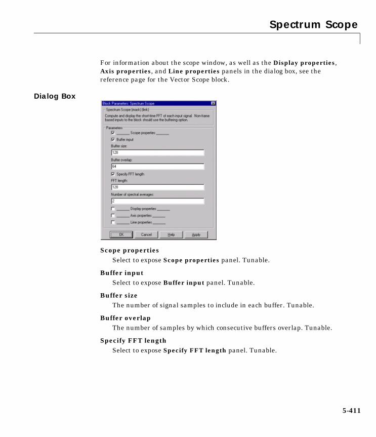
Spectrum Scope
5-411
For information about the scope window, as well as the Display properties, Axis properties, and Line properties panels in the dialog box, see the reference page for the Vector Scope block.
Dialog Box
Scope propertiesSelect to expose Scope properties panel. Tunable.
Buffer inputSelect to expose Buffer input panel. Tunable.
Buffer sizeThe number of signal samples to include in each buffer. Tunable.
Buffer overlapThe number of samples by which consecutive buffers overlap. Tunable.
Specify FFT lengthSelect to expose Specify FFT length panel. Tunable.

Spectrum Scope
5-412
FFT lengthThe number of samples on which to perform the FFT. If the FFT length differs from the buffer size, the data is zero-padded or truncated as needed. Tunable.
Number of spectral averagesThe the number of spectra to average. Setting this parameter to 1 effectively disables averaging. See Short-Time FFT for more information. Tunable.
Display propertiesSelect to expose the Display properties panel. See Vector Scope for more information. Tunable.
Axis propertiesSelect to expose the Axis properties panel. See Vector Scope for more information. Tunable.
Line propertiesSelect to expose the Line properties panel. See Vector Scope for more information. Tunable.
Supported Data Types
See Also
See “Viewing Signals” on page 3-80 for related information.
Fixed-pointCustom data typesBoolean8-, 16-, and 32-bit signed integer 8-, 16-, and 32-bit unsigned integerSingle-precision floating point Double-precision floating point
FFT DSP BlocksetVector Scope DSP Blockset

Stack
5-413
5StackPurpose Store inputs into a LIFO register.
Library Signal Management / Buffers
Description The Stack block stores a sequence of input samples in a LIFO (last in, first out) register. The register capacity is set by the Stack depth parameter, and inputs can be scalars, vectors, or matrices.
The block pushes the input at the In port onto the top of the stack when a trigger event is received at the Push port. When a trigger event is received at the Pop port, the block pops the top element off the stack and holds the Out port at that value. The last input to be pushed onto the stack is always the first to be popped off.
A trigger event at the optional Clr port (enabled by the Clear input check box) empties the stack contents. If Clear output port on reset is selected, then a trigger event at the Clr port empties the stack and sets the value at the Out port to zero. This setting also applies when a disabled subsystem containing the Stack block is re-enabled; the Out port value is only reset to zero in this case if Clear output port on reset is selected.
0 1 0 1
0 0 0 0
1 0 0 1
1 1 1 1
1 1 0 1
empty
empty
empty
1 1 0 0
stack depth0 1 0 1
0 0 0 0
1 0 0 1
1 1 1 1
1 1 0 1
empty
empty
empty
1 1 0 0
oldest input
Pushing the stack Popping the stack
last in first out
0 1 0 1
0 0 0 0
1 0 0 1
1 1 1 1
1 1 0 1
empty
empty
1 1 0 0

Stack
5-414
When two or more of the control input ports are triggered at the same time step, the operations are executed in the following order:
1 Clr
2 Push
3 Pop
The triggering event for the Push, Pop, and Clr ports is specified by the Trigger type pop-up menu, and can be one of the following:
• Rising edge triggers execution of the block when the trigger input rises from a negative value to zero or a positive value, or from zero to a positive value.
• Falling edge triggers execution of the block when the trigger input falls from a positive value to zero or a negative value, or from zero to a negative value.
• Either edge triggers execution of the block when either a rising or falling edge (as described above) occurs.
The Push full stack parameter specifies the block’s behavior when a trigger is received at the Push port but the register is full. The Pop empty stack parameter specifies the block’s behavior when a trigger is received at the Pop port but the register is empty. The following options are available for both cases:
• Ignore – Ignore the trigger event, and continue the simulation.
• Warning – Ignore the trigger event, but display a warning message in the MATLAB command window.
• Error – Display an error dialog box and terminate the simulation.
The Push full stack parameter additionally offers the Dynamic reallocation option, which dynamically resizes the register to accept as many additional inputs as memory permits. To find out how many elements are on the stack at a given time, enable the Num output port by selecting the Output number of stack entries option.
Examples Example 1The table below illustrates the Stack block’s operation for a Stack depth of 4, Trigger type of Either edge, and Clear output port on reset enabled. Because the block triggers on both rising and falling edges in this example, each transition from 1 to 0 or 0 to 1 in the Push, Pop, and Clr columns below

Stack
5-415
represents a distinct trigger event. A 1 in the Empty column indicates an empty buffer, while a 1 in the Full column indicates a full buffer.
Note that at the last step shown, the Push and Clr ports are triggered simultaneously. The Clr trigger takes precedence, and the stack is first cleared and then pushed.
Example 2The dspqdemo demo provides an example of the related Queue block.
In Push Pop Clr Stack Out Empty Full Num
1 0 0 0 0 1 0 0
2 1 0 0 0 0 0 1
3 0 0 0 0 0 0 2
4 1 0 0 0 0 0 3
5 0 0 0 0 0 1 4
6 0 1 0 5 0 0 3
7 0 0 0 4 0 0 2
8 0 1 0 3 0 0 1
9 0 0 0 2 1 0 0
10 1 0 0 2 0 0 1
11 0 0 0 2 0 0 2
12 1 0 1 0 0 0 1
top bottom
2top bottom
top bottom3 2
top bottom3 24
top bottom3 245
top bottom3 24
top bottom3 2
top bottom2
top bottom
10top bottom
11top bottom10
top bottom12

Stack
5-416
Dialog Box
Stack depthThe number of entries that the LIFO register can hold.
Trigger typeThe type of event that triggers the block’s execution. Tunable.
Push full stackResponse to a trigger received at the Push port when the register is full.
Pop empty stackResponse to a trigger received at the Pop port when the register is empty. Tunable.
Empty stack outputEnable the Empty output port, which is high (1) when the stack is empty, and low (0) otherwise.
Full stack outputEnable the Full output port, which is high (1) when the stack is full, and low (0) otherwise. The Full port remains low when Dynamic reallocation is selected from the Push full stack parameter.
Output number of stack entriesEnable the Num output port, which tracks the number of entries currently on the stack.

Stack
5-417
Clear inputEnable the Clr input port, which empties the stack when the trigger specified by the Trigger type is received.
Clear output port on resetReset the Out port to zero (in addition to clearing the stack) when a trigger is received at the Clr input port. Tunable.
Supported Data Types
See Also
Double-precision floating point
Buffer DSP BlocksetDelay Line DSP BlocksetQueue DSP Blockset

Standard Deviation
5-418
5Standard DeviationPurpose Find the standard deviation of an input or sequence of inputs.
Library Statistics
Description The Standard Deviation block computes the standard deviation of each column in the input, or tracks the standard deviation of a sequence of inputs over a period of time. The Running standard deviation parameter selects between basic operation and running operation.
Basic OperationWhen the Running standard deviation check box is not selected, the block computes the standard deviation of each column in M-by-N input matrix u independently at each sample time.
y = std(u) % Equivalent MATLAB code
For convenience, length-M 1-D vector inputs and sample-based length-M row vector inputs are both treated as M-by-1 column vectors. (A scalar input generates a zero-valued output.)
The output at each sample time, y, is a 1-by-N vector containing the standard deviation for each column in u. For purely real or purely imaginary inputs, the standard deviation of the jth column is the square root of the variance
where µj is the mean of jth column. For complex inputs, the output is the total standard deviation for each column in u, which is the square root of the total variance for that column.
Note that the total standard deviation is not equal to the sum of the real and imaginary standard deviations. The frame status of the output is the same as that of the input.
yj σj
uij µj–2
i 1=
M
∑M 1–
-----------------------------------= = 1 j N≤ ≤
σj σj Re,2 σj Im,
2+=

Standard Deviation
5-419
Running OperationWhen the Running standard deviation check box is selected, the block tracks the standard deviation of each channel in a time-sequence of M-by-N inputs. For sample-based inputs, the output is a sample-based M-by-N matrix with each element yij containing the standard deviation of element uij over all inputs since the last reset. For frame-based inputs, the output is a frame-based M-by-N matrix with each element yij containing the standard deviation of the jth column over all inputs since the last reset, up to and including element uij of the current input.
If the Reset port parameter is set to Non-zero sample, the optional Rst port is enabled and the block resets the running standard deviation when the scalar input at the Rst port is nonzero. (The Rst port can be disabled by setting the Reset port parameter to None.)
As in basic operation, length-M 1-D vector inputs and sample-based length-M row vector inputs are both treated as M-by-1 column vectors.
Example The Standard Deviation block in the model below calculates the running standard deviation of a frame-based 3-by-2 (two-channel) matrix input, u. The running standard deviation is reset at t=2 by an impulse to the block’s Rst port.
The Standard Deviation block has the following settings:
• Running standard deviation =
• Reset port = Non-zero sample
The Signal From Workspace block has the following settings:
• Signal = u
• Sample time = 1/3
• Samples per frame = 3

Standard Deviation
5-420
where
u = [6 1 3 -7 2 5 8 0 -1 -3 2 1;1 3 9 2 4 1 6 2 5 0 4 17]'
The Discrete Impulse block has the following settings:
• Delay (samples) = 2
• Sample time = 1
• Samples per frame = 1
The block’s operation is shown in the figure below.
7– 22 45 1
8 60 21– 5
3– 02 41 17
ch1
0 03.54 1.412.52 4.16
6 11 33 9
Simul
atio
n tim
e
In
ch2
Rst
0
0
1
0
Reset
Output
First outputFirst input
t=0
t=1
t=2
t=3
ch1 ch2
5.56 3.594.85 3.114.63 3.01
0 05.66 2.834.93 2.08
4.83 2.754.21 2.413.76 5.96

Standard Deviation
5-421
Dialog Box
Running standard deviationEnables running operation when selected.
Reset portEnables the Rst input port when set to Non-zero sample, and disables the Rst input port when set to None.
Supported Data Types
See Also
Double-precision floating point
Mean DSP BlocksetRMS DSP BlocksetVariance DSP Blocksetstd MATLAB

Submatrix
5-422
5SubmatrixPurpose Select a subset of elements (submatrix) from a matrix input.
Library Math Functions / Matrices and Linear Algebra / Matrix Operations,Signal Management / Indexing
Description The Submatrix block extracts a contiguous submatrix from the M-by-N input matrix u. A length-M 1-D vector input is treated as an M-by-1 matrix. The Row span parameter provides three options for specifying the range of rows in u to be retained in submatrix output y:
• All rows
Specifies that y contains all M rows of u.
• One row
Specifies that y contains only one row from u. The Starting row parameter (described below) is enabled to allow selection of the desired row.
• Range of rows
Specifies that y contains one or more rows from u. The Row and Ending row parameters (described below) are enabled to allow selection of the desired range of rows.
The Column span parameter contains a corresponding set of three options for specifying the range of columns in u to be retained in submatrix y: All columns, One column, or Range of columns. The One column option enables the Column parameter, and Range of columns options enable the Starting column and Ending column parameters.
The output has the same frame status as the input.
Range Specification OptionsWhen One row or Range of rows is selected from the Row span parameter, the desired row or range of rows is specified by the Row parameter, or the Starting row and Ending row parameters. Similarly, when One column or Range of columns is selected from the Column span parameter, the desired column or range of columns is specified by the Column parameter, or the Starting column and Ending column parameters.

Submatrix
5-423
The Row, Column, Starting row or Starting column can be specified in six ways:
• First
For rows, this specifies that the first row of u should be used as the first row of y. If all columns are to be included, this is equivalent to y(1,:) = u(1,:).
For columns, this specifies that the first column of u should be used as the first column of y. If all rows are to be included, this is equivalent to y(:,1) = u(:,1).
• Index
For rows, this specifies that the row of u, firstrow, forward-indexed by the Row index parameter or the Starting row index parameter, should be used as the first row of y. If all columns are to be included, this is equivalent to y(1,:) = u(firstrow,:).
For columns, this specifies that the column of u, forward-indexed by the Column index parameter or the Starting column index parameter, firstcol, should be used as the first column of y. If all rows are to be included, this is equivalent to y(:,1) = u(:,firstcol).
• Offset from last
For rows, this specifies that the row of u offset from row M by the Row offset or Starting row offset parameter, firstrow, should be used as the first row of y. If all columns are to be included, this is equivalent to y(1,:) = u(M-firstrow,:).
For columns, this specifies that the column of u offset from column N by the Column offset or Starting column offset parameter, firstcol, should be used as the first column of y. If all rows are to be included, this is equivalent to y(:,1) = u(:,N-firstcol).
• Last
For rows, this specifies that the last row of u should be used as the only row of y. If all columns are to be included, this is equivalent to y = u(M,:).
For columns, this specifies that the last column of u should be used as the only column of y. If all rows are to be included, this is equivalent to y = u(:,N).
• Offset from middle
For rows, this specifies that the row of u offset from row M/2 by the Starting row offset parameter, firstrow, should be used as the first row of y. If all

Submatrix
5-424
columns are to be included, this is equivalent to y(1,:) = u(M/2-firstrow,:).
For columns, this specifies that the column of u offset from column N/2 by the Starting column offset parameter, firstcol, should be used as the first column of y. If all rows are to be included, this is equivalent to y(:,1) = u(:,N/2-firstcol).
• Middle
For rows, this specifies that the middle row of u should be used as the only row of y. If all columns are to be included, this is equivalent to y = u(M/2,:).
For columns, this specifies that the middle column of u should be used as the only column of y. If all rows are to be included, this is equivalent to y = u(:,N/2).
The Ending row or Ending column can similarly be specified in five ways:
• Index
For rows, this specifies that the row of u forward-indexed by the Ending row index parameter, lastrow, should be used as the last row of y. If all columns are to be included, this is equivalent to y(end,:) = u(lastrow,:).
For columns, this specifies that the column of u forward-indexed by the Ending column index parameter, lastcol, should be used as the last column of y. If all rows are to be included, this is equivalent to y(:,end) = u(:,lastcol).
• Offset from last
For rows, this specifies that the row of u offset from row M by the Ending row offset parameter, lastrow, should be used as the last row of y. If all columns are to be included, this is equivalent to y(end,:) = u(M-lastrow,:).
For columns, this specifies that the column of u offset from column N by the Ending column offset parameter, lastcol, should be used as the last column of y. If all rows are to be included, this is equivalent to y(:,end) = u(:,N-lastcol).

Submatrix
5-425
• Last
For rows, this specifies that the last row of u should be used as the last row of y. If all columns are to be included, this is equivalent to y(end,:) = u(M,:).
For columns, this specifies that the last column of u should be used as the last column of y. If all rows are to be included, this is equivalent to y(:,end) = u(:,N).
• Offset from middle
For rows, this specifies that the row of u offset from row M/2 by the Ending row offset parameter, lastrow, should be used as the last row of y. If all columns are to be included, this is equivalent to y(end,:) = u(M/2-lastrow,:).
For columns, this specifies that the column of u offset from column N/2 by the Ending column offset parameter, lastcol, should be used as the last column of y. If all rows are to be included, this is equivalent to y(:,end) = u(:,N/2-lastcol).
• Middle
For rows, this specifies that the middle row of u should be used as the last row of y. If all columns are to be included, this is equivalent to y(end,:) = u(M/2,:).
For columns, this specifies that the middle column of u should be used as the last column of y. If all rows are to be included, this is equivalent to y(:,end) = u(:,N/2).
Example To extract the lower-right 3-by-2 submatrix from a 5-by-7 input matrix, enter the following set of parameters:
• Row span = Range of rows
• Starting row = Index
• Starting row index = 3
• Ending row = Last
• Column span = Range of columns
• Starting column = Offset from last
• Starting column offset = 1
• Ending column = Last
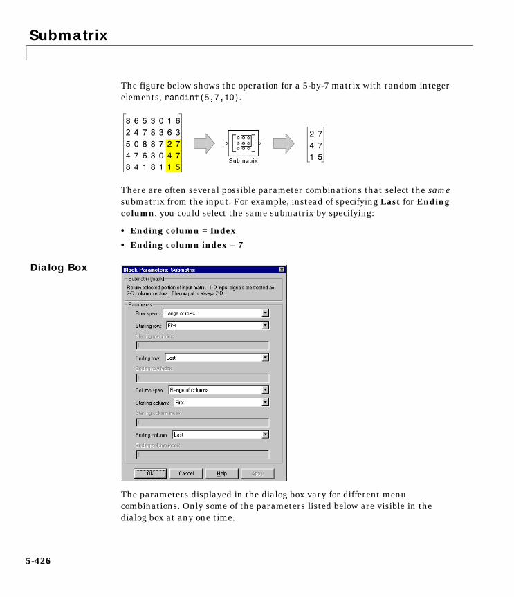
Submatrix
5-426
The figure below shows the operation for a 5-by-7 matrix with random integer elements, randint(5,7,10).
There are often several possible parameter combinations that select the same submatrix from the input. For example, instead of specifying Last for Ending column, you could select the same submatrix by specifying:
• Ending column = Index
• Ending column index = 7
Dialog Box
The parameters displayed in the dialog box vary for different menu combinations. Only some of the parameters listed below are visible in the dialog box at any one time.
8 6 5 3 0 1 62 4 7 8 3 6 35 0 8 8 7 2 74 7 6 3 0 4 78 4 1 8 1 1 5
2 74 71 5

Submatrix
5-427
Row spanThe range of input rows to be retained in the output. Options are All rows, One row, or Range of rows.
Row/Starting rowThe input row to be used as the first row of the output. Row is enabled when One row is selected from Row span, and Starting row when Range of rows is selected from Row span.
Row index/Starting row indexThe index of the input row to be used as the first row of the output. Row index is enabled when Index is selected from Row, and Starting row index when Index is selected from Starting row.
Row offset/Starting row offsetThe offset of the input row to be used as the first row of the output. Row offset is enabled when Offset from middle or Offset from last is selected from Row, and Starting row offset is enabled when Offset from middle or Offset from last is selected from Starting row.
Ending rowThe input row to be used as the last row of the output. This parameter is enabled when Range of rows is selected from Row span and any option but Last is selected from Starting row.
Ending row indexThe index of the input row to be used as the last row of the output. This parameter is enabled when Index is selected from Ending row.
Ending row offsetThe offset of the input row to be used as the last row of the output. This parameter is enabled when Offset from middle or Offset from last is selected from Ending row.
Column spanThe range of input columns to be retained in the output. Options are All columns, One column, or Range of columns.

Submatrix
5-428
Column/Starting columnThe input column to be used as the first column of the output. Column is enabled when One column is selected from Column span, and Starting column is enabled when Range of columns is selected from Column span.
Column index/Starting column indexThe index of the input column to be used as the first column of the output. Column index is enabled when Index is selected from Column, and Starting column index is enabled when Index is selected from Starting column.
Column offset/Starting column offsetThe offset of the input column to be used as the first column of the output. Column offset is enabled when Offset from middle or Offset from last is selected from Column. Starting column offset is enabled when Offset from middle or Offset from last is selected from Starting column.
Ending columnThe input column to be used as the last column of the output. This parameter is enabled when Range of columns is selected from Column span and any option but Last is selected from Starting column.
Ending column indexThe index of the input column to be used as the last column of the output. This parameter is enabled when Index is selected from Ending column.
Ending column offsetThe offset of the input column to be used as the last column of the output. This parameter is enabled when Offset from middle or Offset from last is selected from Ending column.
Supported Data Types
Fixed-pointCustom data typesBoolean8-, 16-, and 32-bit signed integer 8-, 16-, and 32-bit unsigned integerSingle-precision floating point Double-precision floating point

Submatrix
5-429
See Also
See “Deconstructing Signals” on page 3-54 for related information.
Reshape SimulinkSelector SimulinkVariable Selector DSP Blocksetreshape MATLAB

SVD Solver
5-430
5SVD SolverPurpose Solve the equation AX=B using singular value decomposition.
Library Math Functions / Matrices and Linear Algebra / Linear System Solvers
Description The SVD Solver block solves the linear system AX=B, which can be overdetermined, underdetermined, or exactly determined. The system is solved by applying SVD factorization to the M-by-N matrix, A, at the A port. The input to the B port is the right hand-side M-by-L matrix, B. A length-M 1-D vector input at either port is treated as an M-by-1 matrix.
The output at the x port is the N-by-L matrix, X. X is always sample based, and is chosen to minimize the sum of the squares of the elements of B-AX. When B is a vector, this solution minimizes the vector 2-norm of the residual (B-AX is the residual). When B is a matrix, this solution minimizes the matrix Frobenius norm of the residual. In this case, the columns of X are the solutions to the L corresponding systems AXk=Bk, where Bk is the kth column of B, and Xk is the kth column of X.
X is known as the minimum-norm-residual solution to AX=B. The minimum-norm-residual solution is unique for overdetermined and exactly determined linear systems, but it is not unique for underdetermined linear systems. Thus when the SVD Solver is applied to an underdetermined system, the output X is chosen such that the number of nonzero entries in X is minimized.
Dialog Box
Supported Data Types
Double-precision floating point

SVD Solver
5-431
See Also
See “Solving Linear Systems” on page 4-16 for related information.
Autocorrelation LPC DSP BlocksetCholesky Solver DSP BlocksetLDL Solver DSP BlocksetLevinson-Durbin DSP BlocksetLU Inverse DSP BlocksetPseudoinverse DSP BlocksetQR Solver DSP BlocksetSingular Value Decomposition DSP Blockset

Time Scope
5-432
5Time Scope
The Time Scope block is the same as the Scope block in Simulink. To learn how to use the Time Scope block, see the Scope block reference page in the Simulink documentation.
Library DSP Sinks
Supported Data Types
Fixed-pointCustom data typesBoolean8-, 16-, and 32-bit signed integer 8-, 16-, and 32-bit unsigned integerSingle-precision floating point Double-precision floating point
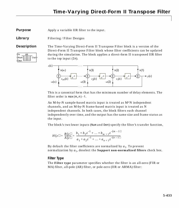
Time-Varying Direct-Form II Transpose Filter
5-433
5Time-Varying Direct-Form II Transpose FilterPurpose Apply a variable IIR filter to the input.
Library Filtering / Filter Designs
Description The Time-Varying Direct-Form II Transpose Filter block is a version of the Direct-Form II Transpose Filter block whose filter coefficients can be updated during the simulation. The block applies a direct-form II transposed IIR filter to the top input (In).
This is a canonical form that has the minimum number of delay elements. The filter order is max(m,n)-1.
An M-by-N sample-based matrix input is treated as M∗N independent channels, and an M-by-N frame-based matrix input is treated as N independent channels. In both cases, the block filters each channel independently over time, and the output has the same size and frame status as the input.
The block’s two lower inputs (Num and Den) specify the filter’s transfer function,
By default the filter coefficients are normalized by a1. To prevent normalization by a1, deselect the Support non-normalized filters check box.
Filter TypeThe Filter type parameter specifies whether the filter is an all-zero (FIR or MA) filter, all-pole (AR) filter, or pole-zero (IIR or ARMA) filter:
y(k)
x(k)
ΣΣ z-1 Σ z-1 Σ z-1zn-1(k) z2(k) z1(k)
. . .
b(m) b(2)b(3) b(1)
-a(n) -a(2)-a(3)
. . .
. . .
H z( ) B z( )A z( )------------
b1 b2z 1– … bm 1+ z m 1–( )–+ + +
a1 a2z 1– … an 1+ z n 1–( )–+ + +
-----------------------------------------------------------------------------------= =

Time-Varying Direct-Form II Transpose Filter
5-434
• Pole-zero
The block accepts inputs for both the numerator (Num) and denominator (Den) vectors.
Input Num is a vector of numerator coefficients,[b(1) b(2) ... b(m)]
and input Den is a vector of denominator coefficients,[a(1) a(2) ... a(n)]
• All-zero
The block accepts only the numerator vector (Num). The denominator of the all-zero filter is 1.
• All-pole
The block accepts only the denominator vector (Den). The numerator of the all-pole filter is 1.
For any of these designs, the coefficient vector inputs can change over time to alter the filter’s response characteristics during the simulation.
Initial ConditionsIn its default form, the filter initializes the internal filter states to zero, which is equivalent to assuming past inputs and outputs are zero. The block also accepts optional nonzero initial conditions for the filter delays. Note that the number of filter states (delay elements) per input channel is
max(m,n)-1
The Initial conditions parameter may take one of four forms:
• Empty matrix
The empty matrix, [], causes a zero (0) initial condition to be applied to all delay elements in each filter channel.
• Scalar
The scalar value is copied to all delay elements in each filter channel. Note that a value of zero is equivalent to setting the Initial conditions parameter to the empty matrix, [].

Time-Varying Direct-Form II Transpose Filter
5-435
• Vector
The vector has a length equal to the number of delay elements in each filter channel, max(m,n)-1, and specifies a unique initial condition for each delay element in the filter channel. This vector of initial conditions is applied to each filter channel.
• Matrix
The matrix specifies a unique initial condition for each delay element, and can specify different initial conditions for each filter channel. The matrix must have the same number of rows as the number of delay elements in the filter, max(m,n)-1, and must have one column per filter channel.
Filter Update RateIn frame-based operation, the Filter update rate parameter determines how frequently the block updates the filter coefficients (i.e., how often it checks the Num and Den inputs). There are two available options:
• One filter per sample time
The block updates the filter coefficients (from inputs Num and Den) for each individual scalar sample in the frame-based input. This means that each output sample could potentially be computed by a different filter (assuming that Num and Den inputs are updated frequently enough).
• One filter per frame time
The block updates the filter coefficients (from inputs Num and Den) for each new input frame, rather than at each sample in the frame. This means that each output sample in a given frame is a result of an identical filtering process.

Time-Varying Direct-Form II Transpose Filter
5-436
Dialog Box
Filter typeThe type of filter to apply: Pole-Zero (IIR), All-Zero (FIR), or All-Pole (AR). The Num and Den input ports are enabled or disabled as appropriate.
Initial conditionsThe filter’s initial conditions, a scalar, vector, or matrix.
Support non-normalized filtersNormalizes the filter by a1 when selected.
Filter update rateThe frequency with which the block updates the filter coefficients; once per sample, or once per frame.
References Oppenheim, A. V. and R. W. Schafer. Discrete-Time Signal Processing. Englewood Cliffs, NJ: Prentice Hall, 1989.
Proakis, J. and D. Manolakis. Digital Signal Processing. 3rd ed. Englewood Cliffs, NJ: Prentice-Hall, 1996.
Supported Data Types
Double-precision floating point

Time-Varying Direct-Form II Transpose Filter
5-437
See Also
See “Designing Filters with Various Filter Structures” on page 4-6 for related information.
Discrete Filter SimulinkFilter Realization Wizard DSP BlocksetDirect-Form II Transpose Filter DSP BlocksetTime-Varying Lattice Filter DSP Blocksetfilter MATLAB

Time-Varying Lattice Filter
5-438
5Time-Varying Lattice FilterPurpose Apply a variable lattice filter to the input.
Library Filtering / Filter Designs
Description The Time-Varying Lattice Filter block applies a moving average (MA) or autoregressive (AR) lattice filter to the top input (In). The filter reflection coefficients are specified by the vector input to the MA or AR port, and can vary with time.
An M-by-N sample-based matrix input to the In port is treated as M∗N independent channels, and an M-by-N frame-based matrix input is treated as N independent channels. In both cases, the block filters each channel independently over time, and the output has the same size and frame status as the input.
Filter TypeThe Filter type parameter specifies whether the filter is an all-zero (FIR or MA) filter or all-pole (AR) filter.
• All-zero
The block constructs an nth order MA filter using the n reflection coefficients contained in the vector input to the MA port. k = [k(1) k(2) ... k(n)]
• All-pole
The block constructs an nth order AR filter using the n reflection coefficients contained in the vector input to the AR port. k = [k(1) k(2) ... k(n)]
For both designs, the coefficient vector inputs can change over time to alter the filter’s response characteristics during the simulation.
Initial ConditionsIn its default form, the filter initializes the internal filter states to zero, which is equivalent to assuming past inputs and outputs are zero. The block also accepts optional nonzero initial conditions for the filter delays. Note that the number of filter states (delay elements) per input channel is
length(k)

Time-Varying Lattice Filter
5-439
The Initial conditions parameter may take one of four forms:
• Empty matrix
The empty matrix, [], causes a zero (0) initial condition to be applied to all delay elements in each filter channel.
• Scalar
The scalar value is copied to all delay elements in each filter channel. Note that a value of zero is equivalent to setting the Initial conditions parameter to the empty matrix.
• Vector
The vector has a length equal to the number of delay elements in each filter channel, length(k), and specifies a unique initial condition for each delay element in the filter channel. This vector of initial conditions is applied to each filter channel.
• Matrix
The matrix specifies a unique initial condition for each delay element, and can specify different initial conditions for each filter channel. The matrix must have the same number of rows as the number of delay elements in the filter, length(k), and must have one column per filter channel.
Filter Update RateIn frame-based operation, the Filter update rate parameter determines how frequently the block updates the filter coefficients (i.e., how often it checks the MA or AR input). There are two available options:
• One filter per sample time
The block updates the filter coefficients (from input MA or AR) for each individual scalar sample in the framed input. This means that each output sample could potentially be computed by a different filter (assuming that the MA or AR input is updated frequently enough).
• One filter per frame time
The block updates the filter coefficients (from input MA or AR) for each new input frame, rather than at each sample in the frame. This means that each output sample in a given frame is a result of an identical filtering process.

Time-Varying Lattice Filter
5-440
Dialog Box
Filter typeThe type of filter to apply: MA or AR. The MA or AR input port is enabled or disabled appropriately.
Initial conditionsThe filter’s initial conditions.
Filter update rateThe frequency with which the block updates the filter coefficients; once per sample, or once per frame.
References Oppenheim, A. V. and R. W. Schafer. Discrete-Time Signal Processing. Englewood Cliffs, NJ: Prentice Hall, 1989.
Proakis, J. and D. Manolakis. Digital Signal Processing. 3rd ed. Englewood Cliffs, NJ: Prentice-Hall, 1996.
Supported Data Types
See Also
Double-precision floating point
Discrete Filter SimulinkDirect-Form II Transpose Filter DSP BlocksetFilter Realization Wizard DSP BlocksetTime-Varying Direct-Form II Transpose Filter DSP Blocksetfilter MATLAB

Time-Varying Lattice Filter
5-441
See “Designing Filters with Various Filter Structures” on page 4-6 for related information.

Toeplitz
5-442
5ToeplitzPurpose Generate a matrix with Toeplitz symmetry.
Library Math Functions / Matrices and Linear Algebra / Matrix Operations
Description The Toeplitz block generates a Toeplitz matrix from inputs defining the first column and first row. The top input (Col) is a vector containing the values to be placed in the first column of the matrix, and the bottom input (Row) is a vector containing the values to be placed in the first row of the matrix.
y = toeplitz(Col,Row) % Equivalent MATLAB code
The other elements of the matrix obey the relationship
y(i,j) = y(i-1,j-1)
and the output has dimension [length(Col) length(Row)]. The y(1,1) element is inherited from the Col input. For example, the following inputs
Col = [1 2 3 4 5]Row = [7 7 3 3 2 1 3]
produce the Toeplitz matrix
If both of the inputs are sample-based, the output is sample-based. Otherwise, the output is frame-based.
When the Symmetric check box is selected, the block generates a symmetric (Hermitian) Toeplitz matrix from a single input, u, defining both the first row and first column of the matrix.
y = toeplitz(u) % Equivalent MATLAB code
The output has dimension [length(u) length(u)]. For example, the Toeplitz matrix generated from the input vector [1 2 3 4] is
1 7 3 3 2 1 32 1 7 3 3 2 13 2 1 7 3 3 24 3 2 1 7 3 35 4 3 2 1 7 3

Toeplitz
5-443
The output has the same frame status as the input.
Dialog Box
SymmetricWhen selected, enables the single-input configuration for symmetric Toeplitz matrix output.
Supported Data Types
See Also
1 2 3 42 1 2 33 2 1 24 3 2 1
Fixed-pointCustom data typesBoolean8-, 16-, and 32-bit signed integer 8-, 16-, and 32-bit unsigned integerSingle-precision floating point Double-precision floating point
Constant Diagonal Matrix DSP Blocksettoeplitz MATLAB

To Wave Device
5-444
5To Wave DevicePurpose Send audio data to a standard audio device in real-time (Windows only).
Library DSP Sinks
Description The To Wave Device block sends audio data to a standard Windows audio device in real-time. It is compatible with most popular Windows hardware, including Sound Blaster cards. (Models that contain both this block and the From Wave Device block require a duplex-capable sound card.) The data is sent to the hardware in uncompressed PCM (pulse code modulation) format, and should typically be sampled at one of the standard Windows audio device rates: 8000, 11025, 22050, or 44100 Hz. Some hardware may support other rates in addition to these.
The Use default audio device parameter allows the block to detect and use the system’s default audio hardware. This option should be selected on systems that have a single sound device installed, or when the default sound device on a multiple-device system is the desired target. In cases when the default sound device is not the desired output device, deselect Use default audio device, and enter the desired device identification number in the Audio device ID parameter. The device ID is an integer value that the block associates with the sound device. A 3-device system, for example, has device ID numbers of 1, 2, and 3.
The input to the block, u, can contain audio data from a mono or stereo signal. A mono signal is represented as either a sample-based scalar or frame-based length-M vector, while a stereo signal is represented as a sample-based length-2 vector or frame-based M-by-2 matrix. If the input data type is double, single, or int16, the block conveys the signal samples to the audio device using 16 bits. If the input data type is uint8, the block conveys the signal samples to the audio device using 8 bits.
sound(u,Fs,bits) % Equivalent MATLAB code
Note that the block does not support uint16 or int8 data types. The 16-bit sample width requires more memory but in general yields better fidelity. The amplitude of the input should be in the range ±1. Values outside this range are clipped to the nearest allowable value.

To Wave Device
5-445
BufferingBecause the audio device generates real-time audio output, Simulink must maintain a continuous flow of data to the device throughout the simulation. Delays in passing data to the audio hardware can result in hardware errors or distortion of the output. This means that the To Wave Device block must in principle supply data to the audio hardware as quickly as the hardware reads the data. However, the To Wave Device block often cannot match the throughput rate of the audio hardware, especially when the simulation is running from within Simulink rather than as generated code. (Simulink execution speed routinely varies during the simulation as the host operating system services other processes.) The block must therefore rely on a buffering strategy to ensure that signal data is accessible to the hardware on demand.
At the start of the simulation, the To Wave Device block writes Td seconds worth of signal data to the device (hardware) buffer, where Td is specified by the Initial output delay parameter. When this initial data is loaded into the buffer, the audio device begins processing the buffered data, and continues at a constant rate until the buffer empties. The size of the buffer, Tb, is specified by the Queue duration parameter. As the audio device reads data from the front of the buffer, the To Wave Device block continues appending inputs to the back of the buffer at the rate they are received.
The following figure shows an audio signal with 8 samples per frame. The buffer of the sound board has a five-frame capacity, not fully used at the instant shown. (If the signal sample rate was 8kHz, for instance, this small buffer could hold approximately 0.005 seconds of data.)
If the simulation throughput rate is higher than the hardware throughput rate, the buffer remains at a constant level throughout the simulation. If necessary, the To Wave Device block buffers inputs until space becomes available in the hardware buffer (i.e., data is not thrown away). More typically,
boar
d
Hardware buffer with 5-frame capacity
Simulink execution rate varies Hardware execution rate is constant
no delaysSimulation delay

To Wave Device
5-446
the hardware throughput rate is higher than the simulation throughput rate, and the buffer tends to empty over the duration of the simulation.
Under normal operation, an empty buffer indicates that the simulation is finished, and the entire length of the audio signal has been processed. However, if the buffer size is too small in relation to the simulation throughput rate, the buffer may also empty before the entire length of signal is processed. This usually results in a device error or undesired device output.
When the device fails to process the entire signal length because the buffer prematurely empties, you can choose to either increase the buffer size or the simulation throughput rate.
• Increase the buffer size. The Queue duration parameter specifies the length of signal, Tb (in real-time seconds), to buffer to the audio device during the simulation. The number of frames buffered is approximately
where Fs is the sample rate of the signal and Mo is the number of samples per frame. The optimal buffer size for a given signal depends on the signal length, the frame size, and the speed of the simulation. The maximum number of frames that can be buffered is 1024.
• Increase the simulation throughput rate. Two useful methods for improving simulation throughput rates are increasing the signal frame size and compiling the simulation into native code.
- Increase frame sizes (and convert sample-based signals to frame-based signals) throughout the model to reduce the amount of block-to-block communication overhead. This can drastically increase throughput rates in many cases. However, larger frame sizes generally result in greater model latency due to initial buffering operations. (Note that increasing the audio signal frame size does not affect the number of samples buffered to the hardware since the Queue duration is specified in seconds.)
- Generate executable code with Real-Time Workshop. Native code runs much faster than Simulink, and should provide rates adequate for real-time audio processing.
Audio problems at startup can often be corrected by entering a larger value for the Initial output delay parameter, which allows a greater portion of the
TbFsMo
-------------

To Wave Device
5-447
signal to be preloaded into the hardware buffer. A value of 0 for the Initial output delay parameter specifies the smallest possible initial delay, which is one frame.
More general ways to improve throughput rates include simplifying the model, and running the simulation on a faster PC processor. See the Simulink documentation and “Delay and Latency” on page 3-85 for other ideas on improving simulation performance.
Dialog Box
Queue duration (seconds)The length of signal (in seconds) to buffer to the hardware at the start of the simulation.
Initial output delay (seconds)The amount of time by which to delay the initial output to the audio device. A value of 0 specifies the smallest possible initial delay, a single frame.
Use default audio deviceDirects audio output to the system’s default audio device when selected. Deselect to enable the Audio device ID parameter and manually enter a device ID number.
Audio device IDThe number of the audio device to receive the audio output. In a system with several audio devices installed, a value of 1 selects the first audio card,

To Wave Device
5-448
a value of 2 selects the second audio card, and so on. Select Use default audio device if the system has only a single audio card installed.
Supported Data Types
See Also
See “Exporting and Playing WAV Files” on page 3-79 for related information.
Double-precision floating point
From Wave Device DSP BlocksetTo Wave File DSP Blocksetsound MATLAB

To Wave File
5-449
5To Wave FilePurpose Write audio data to file in the Microsoft Wave (.wav) format (Windows only).
Library DSP Sinks
Description The To Wave File block writes audio data to a Microsoft Wave (.wav) file in the uncompressed PCM (pulse code modulation) format. For compatibility reasons, the sample rate of the discrete-time input signal should typically be one of the standard Windows audio device rates (8000, 11025, 22050, or 44100 Hz), although the block supports arbitrary rates.
The input to the block, u, can contain audio data from a mono or stereo signal. A mono signal is represented as either a sample-based scalar or frame-based length-M vector, while a stereo signal is represented as a sample-based length-2 vector or frame-based M-by-2 matrix. The amplitude of the input should be in the range ±1. Values outside this range are clipped to the nearest allowable value.
wavwrite(u,Fs,bits,'filename') % Equivalent MATLAB code
The Sample Width (bits) parameter specifies the number of bits used to represent the signal samples in the file. Two settings are available:
• 8 – allocates 8 bits to each sample, allowing a resolution of 256 levels
• 16 – allocates 16 bits to each sample, allowing a resolution of 65536 levels
The 16-bit sample width setting requires more memory but yields better fidelity for double-precision inputs.
The File name parameter can specify an absolute or relative path to the file. You do not need to specify the.wav extension. To reduce the required number of file accesses, the block writes L consecutive samples to the file during each access, where L is specified by the Minimum number of samples for each write to file parameter (L ≥ M). For L < M, the block instead writes M consecutive samples during each access. Larger values of L result in fewer file accesses, which reduces run-time overhead.

To Wave File
5-450
Dialog Box
File nameThe path and name of the file to write. Paths can be relative or absolute. Tunable.
Sample width (bits)The number of bits used to represent each signal sample. Tunable.
Minimum number of samples for each write to fileThe number of consecutive samples to write with each file access, L. Tunable.
Supported Data Types
See Also
See “Exporting and Playing WAV Files” on page 3-79 for related information.
Double-precision floating point
From Wave File DSP BlocksetTo Wave Device DSP BlocksetTo Workspace Simulinkwavwrite MATLAB

Transpose
5-451
5TransposePurpose Compute the transpose of a matrix.
Library Math Functions / Matrices and Linear Algebra / Matrix Operations
Description The Transpose block transposes the M-by-N input matrix to size N-by-M. When the Hermitian check box is selected, the block performs the Hermitian (complex conjugate) transpose
y = u' % Equivalent MATLAB code
When the Hermitian check box is not selected, the block performs the nonconjugate transpose
y = u.' % Equivalent MATLAB code
A length-M 1-D vector input is treated as an M-by-1 matrix. The output is always sample-based.
Dialog Box
HermitianWhen selected, specifies the complex conjugate transpose. Tunable, except in Simulink’s external mode.
u11 u12 u13
u21 u22 u23
u11* u21
*
u12* u22
*
u13* u23
*
u'
u11 u12 u13
u21 u22 u23
u11 u21
u12 u22
u13 u23
u.'

Transpose
5-452
Supported Data Types
See Also
Fixed-pointCustom data typesBoolean8-, 16-, and 32-bit signed integer 8-, 16-, and 32-bit unsigned integerSingle-precision floating point Double-precision floating point
Permute Matrix DSP BlocksetReshape SimulinkSubmatrix DSP Blockset

Triggered Delay Line
5-453
5Triggered Delay LinePurpose Buffer a sequence of inputs into a frame-based output.
Library Signal Management / Buffers
Description The Triggered Delay Line block acquires a collection of Mo input samples into a frame, where Mo is specified by the Delay line size parameter. The block buffers a single sample from input 1 whenever it is triggered by the control signal at input 2 ( ). The newly acquired input sample is appended to the output frame (in the same simulation step) so that the new output overlaps the previous output by Mo-1 samples. Between triggering events the block ignores input 1 and holds the output at its last value.
The triggering event at input 2 is specified by the Trigger type pop-up menu, and can be one of the following:
• Rising edge triggers execution of the block when the trigger input rises from a negative value to zero or a positive value, or from zero to a positive value.
• Falling edge triggers execution of the block when the trigger input falls from a positive value to zero or a negative value, or from zero to a negative value.
• Either edge triggers execution of the block when either a rising or falling edge (as described above) occurs.
The Triggered Delay Line block has zero latency, so the new input appears at the output in the same simulation time step. The output frame period is the same as the input sample period, Tfo=Tsi.
Sample-Based OperationIn sample-based operation, the Triggered Delay Line block buffers a sequence of sample-based length-N vector inputs (1-D, row, or column) into a sequence of overlapping sample-based Mo-by-N matrix outputs, where Mo is specified by the Delay line size parameter (Mo>1). That is, each input vector becomes a row in the sample-based output matrix. When Mo=1, the input is simply passed through to the output, and retains the same dimension. Sample-based full-dimension matrix inputs are not accepted.
Frame-Based OperationIn frame-based operation, the Triggered Delay Line block rebuffers a sequence of frame-based Mi-by-N matrix inputs into an sequence of overlapping

Triggered Delay Line
5-454
frame-based Mo-by-N matrix outputs, where Mo is the output frame size specified by the Delay line size parameter (i.e., the number of consecutive samples from the input frame to rebuffer into the output frame). Mo can be greater or less than the input frame size, Mi. Each of the N input channels is rebuffered independently.
Initial ConditionsThe Triggered Delay Line block’s buffer is initialized to the value specified by the Initial condition parameter. The block always outputs this buffer at the first simulation step (t=0). If the block’s output is a vector, the Initial condition can be a vector of the same size, or a scalar value to be repeated across all elements of the initial output. If the block’s output is a matrix, the Initial condition can be a matrix of the same size, a vector (of length equal to the number of matrix rows) to be repeated across all columns of the initial output, or a scalar to be repeated across all elements of the initial output.
Dialog Box
Trigger typeThe type of event that triggers the block’s execution. Tunable.
Delay line sizeThe length of the output frame (number of rows in output matrix), Mo.
Initial conditionThe value of the block’s initial output, a scalar, vector, or matrix.
Triggered Delay Line
5-455
Supported Data Types
See Also
Fixed-pointCustom data typesBoolean8-, 16-, and 32-bit signed integer 8-, 16-, and 32-bit unsigned integerSingle-precision floating point Double-precision floating point
Buffer DSP BlocksetDelay Line DSP BlocksetUnbuffer DSP Blockset

Triggered Signal From Workspace
5-456
5Triggered Signal From WorkspacePurpose Import signal samples from the MATLAB workspace when triggered.
Library DSP Sources
Description The Triggered Signal From Workspace block imports signal samples from the MATLAB workspace into the Simulink model when triggered by the control signal at the input port ( ). The Signal parameter specifies the name of a MATLAB workspace variable containing the signal to import, or any valid MATLAB expression defining a matrix or 3-D array.
When the Signal parameter specifies an M-by-N matrix (M≠1), each of the N columns is treated as a distinct channel. The frame size is specified by the Samples per frame parameter, Mo, and the output when triggered is an Mo-by-N matrix containing Mo consecutive samples from each signal channel. For Mo=1, the output is sample-based; otherwise the output is frame-based. For convenience, an imported row vector (M=1) is treated as a single channel, so the output dimension is Mo-by-1.
When the Signal parameter specifies an M-by-N-by-P array, the block generates a single page of the array (an M-by-N matrix) at each trigger time. The Samples per frame parameter must be set to 1, and the output is always sample-based.
Trigger EventThe triggering event at the input port is specified by the Trigger type pop-up menu, and can be one of the following:
• Rising edge triggers execution of the block when the trigger input rises from a negative value to zero or a positive value, or from zero to a positive value.
• Falling edge triggers execution of the block when the trigger input falls from a positive value to zero or a negative value, or from zero to a negative value.
• Either edge triggers execution of the block when either a rising or falling edge (as described above) occurs.
Initial and Final ConditionsThe Initial output parameter specifies the output of the block from the start of the simulation until the first trigger event arrives. Between trigger events, the block holds the output value constant at its most recent value (i.e., no linear

Triggered Signal From Workspace
5-457
interpolation takes place). For single-channel signals, the Initial output parameter value can be a vector of length Mo or a scalar to repeat across the Mo elements of the initial output frames. For matrix outputs (Mo-by-N or M-by-N), the Initial output parameter value can be a vector of length N to repeat across all rows of the initial outputs, or a scalar to repeat across all elements of the initial matrix outputs.
When the block has output all of the available signal samples, it can start again at the beginning of the signal, or simply repeat the final value or generate zeros until the end of the simulation. (The block does not extrapolate the imported signal beyond the last sample.) The Form output after final data value by parameter controls this behavior:
• If Setting To Zero is specified, the block generates zero-valued outputs for the duration of the simulation after generating the last frame of the signal.
• If Holding Final Value is specified, the block repeats the final sample for the duration of the simulation after generating the last frame of the signal.
• If Cyclic Repetition is specified, the block repeats the signal from the beginning after generating the last frame. If there are not enough samples at the end of the signal to fill the final frame, the block zero-pads the final frame as necessary to ensure that the output for each cycle is identical (e.g., the ith frame of one cycle contains the same samples as the ith frame of any other cycle).

Triggered Signal From Workspace
5-458
Dialog Box
SignalThe name of the MATLAB workspace variable from which to import the signal, or a valid MATLAB expression specifying the signal.
Trigger typeThe type of event that triggers the block’s execution. Tunable, except in Simulink’s external mode.
Initial outputThe value to output until the first trigger event is received.
Samples per frameThe number of samples, Mo, to buffer into each output frame. This value must be 1 if a 3-D array is specified in the Signal parameter.
Form output after final data value bySpecifies the output after all of the specified signal samples have been generated. The block can output zeros for the duration of the simulation (Setting to zero), repeat the final data sample (Holding Final Value) or repeat the entire signal from the beginning (Cyclic Repetition).
Triggered Signal From Workspace
5-459
Supported Data Types
See Also
See the sections below for related information:
• “Discrete-Time Signals” on page 3-3
• “Multichannel Signals” on page 3-11
• “Benefits of Frame-Based Processing” on page 3-14
• “Creating Signals Using the Signal From Workspace Block” on page 3-38
• “Importing Signals” on page 3-62
(MATLAB commands for casting values to certain data types are provided in parentheses.)Boolean (boolean)8-, 16-, and 32-bit signed integer (int8, int16, int32)8-, 16-, and 32-bit unsigned integer (uint8, uint16, uint32)Single-precision floating point (single)Double-precision floating point (double)
From Wave Device DSP BlocksetFrom Wave File DSP BlocksetSignal To Workspace DSP BlocksetSignal From Workspace DSP BlocksetTriggered To Workspace DSP Blockset

Triggered To Workspace
5-460
5Triggered To WorkspacePurpose Write the input sample to the workspace when triggered.
Library DSP Sinks
Description The Triggered To Workspace block creates a matrix or array variable in the workspace, where it stores the acquired inputs at the end of a simulation. An existing variable with the same name is overwritten.
For an M-by-N frame-based input, the block creates an N-column workspace matrix in which each group of M rows represents a single input frame from each of N channels (the most recent frame occupying the last M rows). The maximum size of this workspace variable is limited to P-by-N, where P is the Maximum number of rows parameter. (If the simulation progresses long enough for the block to acquire more than P samples, it stores only the most recent P samples.) The Decimation factor, D, allows you to store only every Dth input frame.
For an M-by-N sample-based input, the block creates a three-dimensional array in which each M-by-N page represents a single sample from each of M∗N channels (the most recent input matrix occupying the last page). The maximum size of this variable is limited to M-by-N-by-P, where P is the Maximum number of rows parameter. (If the simulation progresses long enough for the block to acquire more than P inputs, it stores only the last P inputs.) The Decimation factor, D, allows you to store only every Dth input matrix.
The block acquires and buffers a single frame from input 1 whenever it is triggered by the control signal at input 2 ( ). At all other times, the block ignores input 1. The triggering event at input 2 is specified by the Trigger type pop-up menu, and can be one of the following:
• Rising edge triggers execution of the block when the trigger input rises from a negative value to zero or a positive value, or from zero to a positive value.
• Falling edge triggers execution of the block when the trigger input falls from a positive value to zero or a negative value, or from zero to a negative value.
• Either edge triggers execution of the block when either a rising or falling edge (as described above) occurs.
To save a record of the sample time corresponding to each sample value, check the Time box in the Save to workspace parameters list of the Simulation

Triggered To Workspace
5-461
Parameters dialog. You can access these parameters by selecting Parameters from the Simulation menu, and clicking on the Workspace I/O tab.
The nontriggered version of this block is To Workspace.
Dialog Box
Trigger typeThe type of event that triggers the block’s execution. Tunable.
Variable nameThe name of the workspace matrix in which to store the data.
Maximum number of rowsThe maximum number of rows (one row per time step) to be saved, P. The default is 100 rows.
DecimationThe decimation factor, D. The default is 1.
Supported Data Types
Fixed-pointCustom data typesBoolean8-, 16-, and 32-bit signed integer 8-, 16-, and 32-bit unsigned integerSingle-precision floating point Double-precision floating point

Triggered To Workspace
5-462
See Also
See “Exporting Signals” on page 3-72 for related information.
Signal From Workspace DSP BlocksetTo Workspace Simulink

Unbuffer
5-463
5UnbufferPurpose Unbuffer a frame input to a sequence of scalar outputs.
Library Signal Management / Buffers
Description The Unbuffer block unbuffers an Mi-by-N frame-based input into a 1-by-N sample-based output. That is, inputs are unbuffered row-wise so that each matrix row becomes an independent time-sample in the output. The rate at which the block receives inputs is generally less than the rate at which the block produces outputs.
The block adjusts the output rate so that the sample period is the same at both the input and output, Tso=Tsi. Therefore, the output sample period for an input of frame size Mi and frame period Tfi is Tfi/Mi, which represents a rate Mi times higher than the input frame rate. In the example above, the block receives inputs only once every three sample periods, but produces an output once every sample period. To rebuffer frame-based inputs to a larger or smaller frame size, use the Buffer block.
In the model below, the block unbuffers a four-channel frame-based input with frame size 3. The Initial conditions parameter is set to zero and the tasking mode is set to multitasking, so the first three outputs are zero vectors (see “Latency” below).
“fast-time” output“slow-time” input(frame size = 1, sample period = Tsi)(frame size = 3, frame period = 3∗Tsi)
123456789123
456
789

Unbuffer
5-464
Latency
Zero Latency. The Unbuffer block has zero tasking latency in Simulink’s single-tasking mode. Zero tasking latency means that the first input sample (received at t=0) appears as the first output sample.
Nonzero Latency. For multitasking operation, the Unbuffer block’s buffer is initialized with the value specified by the Initial condition parameter, and the block begins unbuffering this frame at the start of the simulation. Inputs to the block are therefore delayed by one buffer length, or Mi samples.
The Initial condition parameter can be one of the following:
• A scalar to be repeated for the first Mi output samples of every channel
• A length-Mi vector containing the values of the first Mi output samples for every channel
• An Mi-by-N matrix containing the values of the first Mi output samples in each of N channels
0 0 0 0
t=0
t=6
t=3
Tfi = 3
1 0 1 1–
3 0 0 3–
2 0 1 2–
4 0 0 4–
5 0 1 5–
7 0 0 7–
8 0 0 8–
9 0 1 9–
4 0 0 4–
5 0 1 5–
6 0 1 6–
1 0 1 1–
2 0 1 2–
3 0 0 3–first matrix input
t=0
t=1
ch4ch3
ch1ch2
Frame-based input, frame period = Tfi
Sample-based output, sample period = Tfi/Mi
Tso = Tsi = 1
0 0 0 0
0 0 0 0 t=2
t=3
t=4
t=5
t=7
t=6
ch4ch3
ch1ch2
initial condition(multitasking delay)

Unbuffer
5-465
See “Excess Algorithmic Delay (Tasking Latency)” on page 3-91 and “The Simulation Parameters Dialog Box” in the Simulink documentation for more information about block rates and Simulink’s tasking modes.
Dialog Box
Initial conditionsThe value of the block’s initial output for cases of nonzero latency; a scalar, vector, or matrix.
Supported Data Types
See Also
See “Unbuffering a Frame-Based Signal into a Sample-Based Signal” on page 3-60 for related information.
Fixed-pointCustom data typesBoolean8-, 16-, and 32-bit signed integer 8-, 16-, and 32-bit unsigned integerSingle-precision floating point Double-precision floating point
Buffer DSP Blockset

Uniform Decoder
5-466
5Uniform DecoderPurpose Decode an integer input to a floating-point output.
Library Quantizers
Description The Uniform Decoder block performs the inverse operation of the Uniform Encoder block, and reconstructs quantized floating-point values from encoded integer input. The block adheres to the definition for uniform decoding specified in ITU-T Recommendation G.701.
Inputs can be real or complex values of the following six integer data types: uint8, uint16, uint32, int8, int16, or int32.
The block first casts the integer input values to floating-point values, and then uniquely maps (decodes) them to one of 2B uniformly spaced floating point values in the range [-V, (1-21-B)V], where B is specified by the Bits parameter (as an integer between 2 and 32) and V is a floating-point value specified by the Peak parameter. The smallest input value representable by B bits (0 for an unsigned input data type; -2B-1 for a signed input data type) is mapped to the value -V. The largest input value representable by B bits (2B-1 for an unsigned input data type; 2B-1-1 for a signed input data type) is mapped to the value (1-21-B)V. Intermediate input values are linearly mapped to the intermediate values in the range [-V, (1-21-B)V].
To correctly decode values encoded by the Uniform Encoder block, the Bits and Peak parameters of the Uniform Decoder block should be set to the same values as the Bits and Peak parameters of the Uniform Encoder block. The Overflow mode parameter specifies the Uniform Decoder block’s behavior when the integer input is outside the range representable by B bits. If Saturate is selected, unsigned input values greater than 2B-1 saturate at 2B-1; signed input values greater than 2B-1-1 or less than -2B-1 saturate at those limits. The real and imaginary components of complex inputs saturate independently.
If Wrap is selected, unsigned input values, u, greater than 2B-1 are wrapped back into the range [0, 2B-1] using mod-2B arithmetic.
u = mod(u,2^B) % Equivalent MATLAB code

Uniform Decoder
5-467
Signed input values, u, greater than 2B-1-1 or less than -2B-1 are wrapped back into that range using mod-2B arithmetic.
u = (mod(u+2^B/2,2^B)-(2^B/2)) % Equivalent MATLAB code
The real and imaginary components of complex inputs wrap independently.
The Output type parameter specifies whether the decoded floating-point output is single or double precision. Either level of output precision can be used with any of the six integer input data types.
Example Consider a Uniform Decoder block with the following parameter settings:
• Peak = 2
• Bits = 3
The input to the block is the uint8 output of a Uniform Encoder block with comparable settings: Peak = 2, Bits = 3, and Output type = Unsigned. (Comparable settings ensure that inputs to the Uniform Decoder block do not saturate or wrap. See the example on the Uniform Encoder reference page for more about these settings.)
The real and complex components of each input are independently mapped to one of 23 distinct levels in the range [-2.0,1.5].
0 is mapped to -2.01 is mapped to -1.52 is mapped to -1.03 is mapped to -0.54 is mapped to 0.05 is mapped to 0.56 is mapped to 1.07 is mapped to 1.5

Uniform Decoder
5-468
Dialog Box
PeakThe largest amplitude represented in the encoded input. To correctly decode values encoded with the Uniform Encoder block, set the Peak parameters in both blocks to the same value.
BitsThe number of input bits, B, used to encode the data. (This can be less than the total number of bits supplied by the input data type.) To correctly decode values encoded with the Uniform Encoder block, set the Bits parameters in both blocks to the same value.
Overflow modeThe block’s behavior when the integer input is outside the range representable by B bits. Out-of-range inputs can either saturate at the extreme value, or wrap back into range.
Output typeThe precision of the floating-point output, single or double.
References General Aspects of Digital Transmission Systems: Vocabulary of Digital Transmission and Multiplexing, and Pulse Code Modulation (PCM) Terms, International Telecommunication Union, ITU-T Recommendation G.701, March, 1993
Supported Data Types
Single-precision floating point Double-precision floating point

Uniform Decoder
5-469
See Also Data Type Conversion SimulinkQuantizer SimulinkUniform Encoder DSP Blocksetudecode Signal Processing Toolboxuencode Signal Processing Toolbox

Uniform Encoder
5-470
5Uniform EncoderPurpose Quantize and encode a floating-point input to an integer output.
Library Quantizers
Description The Uniform Encoder block performs the following two operations on each floating-point sample in the input vector or matrix:
1 Quantizes the value using the same precision
2 Encodes the quantized floating-point value to an integer value
In the first step, the block quantizes an input value to one of 2B uniformly spaced levels in the range [-V, (1-21-B)V], where B is specified by the Bits parameter and V is specified by the Peak parameter. The quantization process rounds both positive and negative inputs downward to the nearest quantization level, with the exception of those that fall exactly on a quantization boundary. The real and imaginary components of complex inputs are quantized independently.
The number of bits, B, can be any integer value between 2 and 32, inclusive. Inputs greater than (1-21-B)V or less than -V saturate at those respective values. The real and imaginary components of complex inputs saturate independently.
In the second step, the quantized floating-point value is uniquely mapped (encoded) to one of 2B integer values. If the Output type is set to Unsigned integer, the smallest quantized floating-point value, -V, is mapped to the integer 0, and the largest quantized floating-point value, (1-21-B)V, is mapped to the integer 2B-1. Intermediate quantized floating-point values are linearly (uniformly) mapped to the intermediate integers in the range [0, 2B-1]. For efficiency, the block automatically selects an unsigned output data type (uint8, uint16, or uint32) with the minimum number of bits equal to or greater than B.
If the Output type is set to Signed integer, the smallest quantized floating-point value, -V, is mapped to the integer -2B-1, and the largest quantized floating-point value, (1-21-B)V, is mapped to the integer 2B-1-1. Intermediate quantized floating-point values are linearly mapped to the intermediate integers in the range [-2B-1, 2B-1-1]. The block automatically selects a signed output data type (int8, int16, or int32) with the minimum number of bits equal to or greater than B.

Uniform Encoder
5-471
Inputs can be real or complex, double or single precision. The output data types that the block uses are shown in the table below. Note that most of the blocks in the DSP Blockset accept only double precision inputs. Use the Simulink Data Type Conversion block to convert integer data types to double precision. See “Working with Data Types” in the Simulink documentation for a complete discussion of data types, as well as a list of Simulink blocks capable of reduced-precision operations.
The Uniform Encoder block operations adhere to the definition for uniform encoding specified in ITU-T Recommendation G.701.
Example The figure below illustrates uniform encoding with the following parameter settings:
• Peak = 2
• Bits = 3
• Output type = Unsigned
Bits Unsigned Integer Signed Integer
2 to 8 uint8 int8
9 to 16 uint16 int16
17 to 32 uint32 int32
−3 −2 −1 0 1 2 3−1
0
1
2
3
4
5
6
7
8
Input Value (real or imaginary component)
Out
put V
alue
(re
al o
r im
agin
ary
com
pone
nt)

Uniform Encoder
5-472
The real and complex components of each input (horizontal axis) are independently quantized to one of 23 distinct levels in the range [-2,1.5] and then mapped to one of 23 integer values in the range [0,7].
-2.0 is mapped to 0-1.5 is mapped to 1-1.0 is mapped to 2-0.5 is mapped to 30.0 is mapped to 40.5 is mapped to 51.0 is mapped to 61.5 is mapped to 7
The table below shows the results for a few particular inputs.
The output data type is automatically set to uint8, the most efficient format for this input range.
Input Quantized Input Output Notes
1.6 1.5+0.0i 7+4i
-0.4 -0.5+0.0i 3+4i
-3.2 -2.0+0.0i 4i Saturation (real)
0.4-1.2i 0.0-1.5i 4+i
0.4-6.0i 0.0-2.0i 4 Saturation (imaginary)
-4.2+3.5i -2.0+2.0i 7i Saturation (real and imag)

Uniform Encoder
5-473
Dialog Box
PeakThe largest input amplitude to be encoded, V. Real or imaginary input values greater than (1-21-B)V or less than -V saturate (independently for complex inputs) at those limits.
BitsThe number of levels at which to quantize the floating-point input. (Also the number of bits needed to represent the integer output.)
Output typeThe data type of the block’s output, Unsigned integer or Signed integer. Unsigned outputs are uint8, uint16, or uint32, while signed outputs are int8, int16, or int32.
References General Aspects of Digital Transmission Systems: Vocabulary of Digital Transmission and Multiplexing, and Pulse Code Modulation (PCM) Terms, International Telecommunication Union, ITU-T Recommendation G.701, March, 1993
Supported Data Types
See Also
Single-precision floating point Double-precision floating point
Data Type Conversion SimulinkQuantizer SimulinkUniform Decoder DSP Blocksetudecode Signal Processing Toolboxuencode Signal Processing Toolbox

Unwrap
5-474
5UnwrapPurpose Unwrap the phase of a signal.
Library Signal Operations
Description The Unwrap block unwraps each input channel by adding or subtracting appropriate multiples of to each channel element. The input can be any matrix or 1-D vector, and must have radian phase entries. The block recognizes phase discontinuities larger than the Tolerance parameter setting.
The block preserves the input size, dimension, and frame status, and the output port rate equals the input port rate.
For a detailed discussion of the Unwrap block, see the following sections:
• “Acceptable Inputs and Corresponding Output Characteristics” on page 5-474
• “The Two Unwrap Modes” on page 5-475
• “Unwrap Method” on page 5-479
• “Definition of Phase Unwrap” on page 5-479
Acceptable Inputs and Corresponding Output CharacteristicsThe Unwrap block preserves the input size, dimension, and frame status, and the output port rate equals the input port rate.
Characteristics of Valid Input Characteristics of Corresponding Output
• Input elements must be phase values in radians.
• Sample- or frame-based
• M-by-N 2-D matrix or a 1-D vector
• Output elements are phase values in radians.
• Same frame status as input
• Same size and dimension as input
• Output port rate = input port rate
2π

Unwrap
5-475
The Two Unwrap ModesYou must specify the unwrap mode by setting the parameter, Do not unwrap phase discontinuities between successive frames. The unwrap modes are summarized in the next table.

Unwrap
5-476
Two Unwrap Modes
In both unwrap modes, the block adds to each input channel’s elements, where it updates k at each phase discontinuity. (For more on the updating of k, see “Unwrap Method” on page 5-479.) The number of times that k is reset to 0 depends on the unwrap mode.
Default Unwrap Mode:Initialize k to 0 For Only the First Input Frame
Nondefault Unwrap Mode:Set k to 0 For Each Successive Input Matrix or Input Vector
In this mode, k is initialized to 0 for only the first input matrix or input vector. As k gets updated, the value of k is retained between successive input matrices or input vectors. That is, the block unwraps each input’s channel by considering phase discontinuities in all previous frames and the current frame.
Depending on input characteristics, the block unwraps the columns or each individual element of the input:
• Frame-based inputs — unwrap columns
• Sample-based inputs — unwrap each element of the input.
• 1-D vector inputs — treat as frame-based column
See the following diagrams.
In this mode, k is reset to 0 for each successive input matrix or input vector. As k gets updated, the value of k is only retained within the current input matrix or vector. That is, the block unwraps each input’s channel by considering phase discontinuities in the current input matrix or input vector only, ignoring discontinuities in previous inputs.
Depending on input characteristics, the block unwraps the columns or rows of the input:
• Frame-based inputs — unwrap columns
• Sample-based nonrow inputs — unwrap columns
• Sample-based row vector inputs — unwrap the row.
• 1-D vector inputs — treat as frame-based column
See the following diagrams.
2πk

Unwrap
5-477
The following diagrams illustrate how the two unwrap modes operate on various inputs.
0 02π3---- 0
2– π3----- 0
0 02π3---- 0
4π3---- 0
6π3---- 0
8π3---- 0
10π3
------ 0
12π3
------ 0
14π3
------ 0
16π3
------ 0
Default Unwrap Mode Operation:
Frame 1
Channel 2Channel 1
Phase discontinuity (jump in adjacent phase values greater than the value of the Tolerance parameter)
The block treats each input column as an independent channel. It unwraps by treating Channel 1 of Frame 2 as a continuation of Channel 1 of Frame 1.
0 02π3---- 0
2– π3----- 0
Frame 2
0 02π3---- 0
2– π3----- 0
Frame 3
Tolerance parameter = π
0 00 0
2π3---- 0
0 0
2π–3----- 0
0 0
0 00 0
2π3---- 0
0 0
Channel 1
Sample 1
Sample 2
Sample 3
Sample 4
Sample 5
Tolerance parameter = π
Ch 3Ch 4 0 0
0 0
2π3---- 0
0 0
4π3---- 0
0 0
6π3---- 0
0 0
8π3---- 0
0 0
The block treats each element of the input matrix as an independent channel. (The first sample in Channel 1 is in the upper left corner of the Sample 1 matrix. The second sample of Channel 1 is in the corresponding corner of the Sample 2 matrix, and so on.)
Frame-Based Inputs Sample-Based Inputs
Phase discontinuity

Unwrap
5-478
The block unwraps each row, treating each input row vector as completely independent of the other input row vectors.
0 02π3---- 0
4π3---- 0
0 02π3---- 0
4π3---- 0
The block unwraps each column, treating each input matrix as completely unrelated to the other input matrices.
0 02π3---- 0
4π3---- 0
Nondefault Unwrap Mode Operation:
Frame-Based Inputs and Sample-Based Row Vector InputsSample-Based (Nonrow) Inputs
0 02π3---- 0
2– π3----- 0
Input 1
0 02π3---- 0
2– π3----- 0
Input 2
0 02π3---- 0
2– π3----- 0
Input 3
0 2π3---- 2– π
3----- 0 2π
3---- 2– π
3----- 0 2π
3---- 4π
3---- 6π
3---- 8π
3---- 10π
3------
Tolerance parameter = π
0 2π3---- 4π
3---- 6π
3---- 8π
3---- 10π
3------
0 2π3---- 4π
3---- 6π
3---- 8π
3---- 10π
3------
Input 1
Input 2
Input 3
0 2π3---- 2– π
3----- 0 2π
3---- 2– π
3-----
0 2π3---- 2– π
3----- 0 2π
3---- 2– π
3-----
Tolerance parameter = π
Phase discontinuity (jump in adjacent phase values greater than the value of the Tolerance parameter)

Unwrap
5-479
Unwrap MethodThe Unwrap block unwraps each channel of its input matrix or input vector by adding to each successive channel element, and updating k at each phase jump. See the following steps to the unwrap method for details.
Definition of Phase UnwrapAlgorithms that compute the phase of a signal often only output phases between and . For instance, such algorithms compute the phase of
to be 3, since , and since the actual phase, , is not between and . Such algorithms compute the phases of
and to be 3 as well.
Phase unwrap or unwrap is a process often used to reconstruct a signal’s original phase. Unwrap algorithms add appropriate multiples of to each phase input to restore original phase values, as illustrated in the following
Relevant Unwrap Terms:• ui — ith element of the input channel on which the algorithm operates
• — Tolerance parameter value
• phase jump or phase discontinuity — difference between phase values of two adjacent channel entries that exceeds . The diagram in the next section indicates phase jumps with red arrows.
Steps to the Unwrap Method:1 Set k to 0 (See “The Two Unwrap Modes” on page 5-475 for more on how
often this step occurs.)
2 Check for a phase jump between adjacent channel elements ui and ui+1:
- If there is no phase jump between ui and ui+1 , add to ui, and then repeat step 2 to continue checking for phase jumps.
- If there is a phase jump between ui and ui+1 , add to ui, and then go to step 3 to update k.
3 Update k as follows when there is a phase jump between ui and ui+1. Then go back to step 2 to add the updated value to ui+1 and succeeding channel elements until the next phase jump:
- If (phase jump is negative), increment k.
- If (phase jump is positive), decrement k.
2πk
α
α
ui 1+ ui– α≤( ) 2πk
ui 1+ ui– α>( ) 2πk
2πk
ui 1+ ui<ui 1+ ui>
π– π2π 3+( )sin 3( ) 2π 3+( )sin=sin
2π 3+ π– π4– π 3+( )sin 16π 3+( )sin
2π

Unwrap
5-480
diagram. For more on phase unwrap, see the previous section, “Unwrap Method” on page 5-479.

Unwrap
5-481
0
5
10
15
20
25
30
0 2 4 6 8 10 12 14 16−5
0
5
10
15
20
25
30
0 pi 2pi 3pi 4pi 5pi 6pi0( )sin 2π
5------
4π5
------ 6π
5------
… 28π5
---------- sin, ,sin,sin,sin[ , ]
Unwrap Restricted Phases:
Input:
Output:
where
Update the value of k after every large jump in phase value, indicated by .
θn θn′ 2πk+=
Calculate Phases of Signal Data:
Input:
Output:
where
and
θn′( )sin θn( )sin=
π θn′ π≤<–
θ0( )sin θ1( )sin … θN( )sin, , ,[ ]
θ0′ θ1
′ … θN′, , ,[ ]
θ0′ θ1
′ … θN′, , ,[ ]
θ0 θ1 … θN, , ,[ ]
Signal data with instantaneous phase values that range over all numbers
Unwrapping Phase Data Ranging Between π and -π
0 2π5
------4π5
------4– π5
----------2π–5
---------- 0 2π5
------4π5
------4– π5
----------2π–5
---------- 0 2π5
------4π5
------4– π5
----------2π–5
----------, , , , , , , ,, , , , ,[ , ]
0 2π5
------4π5
------6π5
------8π5
------ 2π 12π5
----------14π
5----------
16π5
----------18π
5---------- 4π 22π
5----------
24π5
----------26π
5----------
28π5
----------, , , , , , , ,, , , , ,[ , ]
Unwrapped phase data ranging over all numbers.
Add Add 6πAdd 4π
2π 5⁄4π 5⁄
2– π 5⁄4π 5⁄–
0
2π 5⁄
28π 5⁄
2π
4π
Phase data of the signal restricted to range between π and -π.
Restr
icted
Pha
ses (
Radi
ans)
Time
Unwr
appe
d Ph
ases
(Rad
ians
)
Time
2π
0

Unwrap
5-482
Limitations The Unwrap block detects branch cut crossings, but can be fooled by sparse, rapidly changing phase values.
Dialog Box
0 2π 4π …,, ,
2π5
------12π
5----------
22π5
---------- …, , ,4π5
------14π
5----------
24π5
---------- …, , ,
6π5
------16π
5----------
26π5
---------- …, , ,
θ
θ( )sin
θ( )cos
8π5
------18π
5----------
28π5
---------- …, , ,
0
2π5
------4π5
------
4π–5
----------
θ′
θ′( )sin
θ′( )cos
2π–5
----------
ππ–( )
Range of unwrapped phase data: all numbersRange of restricted phase data: π θ′ π≤<–
Large jump in phase value

Unwrap
5-483
Do not unwrap phase discontinuities between successive framesWhen this parameter is cleared, the block unwraps each input’s channels (the input channels are the columns of frame-based inputs and each element of sample-based inputs). When this parameter is set, the block unwraps each row of sample-based row vector inputs, and unwraps the columns of all other inputs, where each input matrix or input vector is treated as completely unrelated to the other input matrices or input vectors. 1-D vector inputs are always treated as frame-based column vectors. See “The Two Unwrap Modes” on page 5-475.
ToleranceThe jump size that the block recognizes as a true phase discontinuity. The default is set to π (rather than a smaller value) to avoid altering legitimate signal features. To increase the block’s sensitivity, set Tolerance to a value slightly less than π.
Supported Data Types
See Also
Double-precision floating point
unwrap MATLAB

Upsample
5-484
5UpsamplePurpose Resample an input at a higher rate by inserting zeros.
Library Signal Operations
Description The Upsample block resamples each channel of the Mi-by-N input at a rate L times higher than the input sample rate by inserting L-1 zeros between consecutive samples. The integer L is specified by the Upsample factor parameter. The Sample offset parameter delays the output samples by an integer number of sample periods D, where 0 ≤ D < (L-1), so that any of the L possible output phases can be selected.
Sample-Based OperationWhen the input is sample-based, the block treats each of the M∗N matrix elements as an independent channel, and upsamples each channel over time. The Frame-based mode parameter must be set to Maintain input frame size. The output sample rate is L times higher than the input sample rate (Tso = Tsi/L), and the input and output sizes are identical.
Frame-Based OperationWhen the input is frame-based, the block treats each of the N input columns as a frame containing Mi sequential time samples from an independent channel. The block upsamples each channel independently by inserting L-1 rows of zeros between each row in the input matrix. The Frame-based mode parameter determines how the block adjusts the rate at the output to accommodate the added rows. There are two available options:
• Maintain input frame size
The block generates the output at the faster (upsampled) rate by using a proportionally shorter frame period at the output port than at the input port. For upsampling by a factor of L, the output frame period is L times shorter than the input frame period (Tfo = Tfi/L), but the input and output frame sizes are equal.
The model below shows a single-channel input with a frame period of 1 second being upsampled by a factor of 4 to a frame period of 0.25 seconds. The input and output frame sizes are identical.

Upsample
5-485
• Maintain input frame rate
The block generates the output at the faster (upsampled) rate by using a proportionally larger frame size than the input. For upsampling by a factor of L, the output frame size is L times larger than the input frame size (Mo = Mi∗L), but the input and output frame rates are equal.
The model below shows a single-channel input of frame size 16 being upsampled by a factor of 4 to a frame size of 64. The input and output frame rates are identical.

Upsample
5-486
Latency and Initial Conditions
Zero Latency. The Upsample block has zero tasking latency for all single-rate operations. The block is single-rate for the particular combinations of sampling mode and parameter settings shown in the table below.
The block also has zero latency for all multirate operations in Simulink’s single-tasking mode.
Zero tasking latency means that the block propagates the first input (received at t=0) immediately following the D consecutive zeros specified by the Sample offset parameter. This output (D+1) is followed in turn by the L-1 inserted zeros and the next input sample. The Initial condition parameter value is not used.
Nonzero Latency. The Upsample block has tasking latency only for multirate operation in Simulink’s multitasking mode:
• In sample-based mode, the initial condition for each channel appears as output sample D+1, and is followed by L-1 inserted zeros. The channel’s first input appears as output sample D+L+1. The Initial condition value can be an Mi-by-N matrix containing one value for each channel, or a scalar to be applied to all signal channels.
• In frame-based mode, the first row of the initial condition matrix appears as output sample D+1, and is followed by L-1 inserted rows of zeros, the second row of the initial condition matrix, and so on. The first row of the first input matrix appears in the output as sample MiL+D+1. The Initial condition value can be an Mi-by-N matrix, or a scalar to be repeated across all elements of the Mi-by-N matrix. See the example below for an illustration of this case.
Sampling Mode Parameter Settings
Sample-based Upsample factor parameter, L, is 1.
Frame-based Upsample factor parameter, L, is 1, or Frame-based mode parameter is Maintain input frame rate.

Upsample
5-487
See “Excess Algorithmic Delay (Tasking Latency)” on page 3-91 and “The Simulation Parameters Dialog Box” in the Simulink documentation for more information about block rates and Simulink’s tasking modes.
Example Construct the frame-based model shown below.
Adjust the block parameters as follows:
• Configure the Signal From Workspace block to generate a two-channel signal with frame size of 4 and sample period of 0.25. This represents an output frame period of 1 (0.25∗4). The first channel should contain the positive ramp signal 1, 2, ..., 100, and the second channel should contain the negative ramp signal -1, -2, ..., -100.
- Signal = [(1:100)' (-1:-1:-100)']
- Sample time = 0.25
- Samples per frame = 4
• Configure the Upsample block to upsample the two-channel input by increasing the output frame rate by a factor of 2 relative to the input frame rate. Set a sample offset of 1, and an initial condition matrix of
- Upsample factor = 2
- Sample offset = 1
- Initial condition = [11 -11;12 -12;13 -13;14 -14]
- Frame-based mode = Maintain input frame size
11 11–
12 12–
13 13–
14 14–
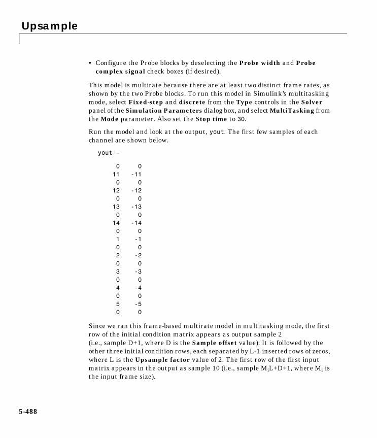
Upsample
5-488
• Configure the Probe blocks by deselecting the Probe width and Probe complex signal check boxes (if desired).
This model is multirate because there are at least two distinct frame rates, as shown by the two Probe blocks. To run this model in Simulink’s multitasking mode, select Fixed-step and discrete from the Type controls in the Solver panel of the Simulation Parameters dialog box, and select MultiTasking from the Mode parameter. Also set the Stop time to 30.
Run the model and look at the output, yout. The first few samples of each channel are shown below.
yout =
0 0 11 -11 0 0 12 -12 0 0 13 -13 0 0 14 -14 0 0 1 -1 0 0 2 -2 0 0 3 -3 0 0 4 -4 0 0 5 -5 0 0
Since we ran this frame-based multirate model in multitasking mode, the first row of the initial condition matrix appears as output sample 2 (i.e., sample D+1, where D is the Sample offset value). It is followed by the other three initial condition rows, each separated by L-1 inserted rows of zeros, where L is the Upsample factor value of 2. The first row of the first input matrix appears in the output as sample 10 (i.e., sample MiL+D+1, where Mi is the input frame size).

Upsample
5-489
Dialog Box
Upsample factorThe integer factor, L, by which to increase the input sample rate.
Sample offsetThe sample offset, D, which must be an integer in the range [0,L-1].
Initial conditionThe value with which the block is initialized for cases of nonzero latency, a scalar or matrix. This value (first row in frame-based mode) appears in the output as sample D+1.
Frame-based modeFor frame-based operation, the method by which to implement the upsampling: Maintain input frame size (i.e., increase the frame rate), or Maintain input frame rate (i.e., increase the frame size). The Framing parameter must be set to Maintain input frame size for sample-base inputs.
Supported Data Types
Fixed-pointCustom data typesBoolean8-, 16-, and 32-bit signed integer 8-, 16-, and 32-bit unsigned integerSingle-precision floating point Double-precision floating point

Upsample
5-490
See Also Downsample DSP BlocksetFIR Interpolation DSP BlocksetFIR Rate Conversion DSP BlocksetRepeat DSP Blockset
Variable Fractional Delay
5-491
5Variable Fractional DelayPurpose Delay an input by a time-varying fractional number of sample periods.
Library Signal Operations
Description The Variable Fractional Delay block delays each channel of the Mi-by-N input matrix, u, by a variable (possibly noninteger) number of sample intervals.
The block computes the value for each channel of the output based on the stored samples in memory most closely indexed by the Delay input, v, and the interpolation method specified by the Mode parameter. In Linear Interpolation mode, the block stores the D+1 most recent samples received at the In port for each channel, where D is the Maximum delay. In FIR Interpolation mode, the block stores the D+P+1 most recent samples received at the In port for each channel, where P is the Interpolation filter half-length.
See the Variable Integer Delay block for further discussion of how input samples are stored in the block’s memory. The Variable Fractional Delay block differs only in the way that these stored sample are accessed; a fractional delay requires the computation of a value by interpolation from the nearby samples in memory.
Sample-Based OperationWhen the input is sample-based, the block treats each of the Mi∗N matrix elements as an independent channel. The input to the Delay port, v, is an Mi-by-N matrix of floating-point values in the range 0 ≤ v ≤ D that specifies the number of sample intervals to delay each channel of the input.
A 1-D vector input is treated as an Mi-by-1 matrix, and the output is 1-D.
The Initial conditions parameter specifies the values in the block’s memory at the start of the simulation in the same manner as for the Variable Integer Delay block. See the section on sample-based initial conditions there for complete information.
Frame-Based OperationWhen the input is frame-based, the block treats each of the N input columns as a frame containing Mi sequential time samples from an independent channel.

Variable Fractional Delay
5-492
The input to the Delay port, v, contains floating-point values in the range 0 ≤ v ≤ D specifying the number of sample intervals to delay the current input. The input to the Delay port can be:
• An Mi-by-N matrix containing the number of sample intervals to delay each sample in each channel of the current input
• An Mi-by-1 matrix containing the number of sample intervals to delay each sample in every channel of the current input
• A 1-by-N matrix containing the number of sample intervals to delay every sample in each channel of the current input
For example, if v is the Mi-by-1 matrix [v(1) v(2) ... v(Mi)]', the earliest sample in the current frame is delayed by v(1) fractional sample intervals, the following sample in the frame is delayed by v(2) fractional sample intervals, and so on. The set of fractional delays contained in v is applied identically to every channel of a multichannel input.
The Initial conditions parameter specifies the values in the block’s memory at the start of the simulation in the same manner as for the Variable Integer Delay block. See the section on frame-based initial conditions there for complete information.
Interpolation ModesThe delay value specified at the Delay port is used as an index into the block’s memory, U, which stores the D+1 most recent samples received at the In port for each channel. For example, an integer delay of 5 on a scalar input sequence retrieves and outputs the fifth most recent input sample from the block’s memory, U(6). Fractional delays are computed by interpolating between stored samples; the two available interpolation modes are described below.
Linear Interpolation Mode. For noninteger delays, at each sample time the Linear Interpolation mode uses the two samples in memory nearest to the specified delay to compute a value for the sample at that time. If v is the specified fractional delay for a scalar input, the output sample, y, is computed as follows.
vi = floor(v) % vi = integer delayvf = v-vi % vf = fractional delayy = (1-vf)*U(vi) + vf*U(vi+1)

Variable Fractional Delay
5-493
Delay values less than 0 are clipped to 0, and delay values greater than D are clipped to D, where D is the Maximum delay. Note that a delay value of 0 causes the block to pass through the current input sample, U(1), in the same simulation step that it is received.
FIR Interpolation Mode. In FIR Interpolation mode, the block computes a value for the sample at the desired delay by applying an FIR filter of order 2P to the stored samples on either side of the desired delay, where P is the Interpolation filter half-length. For periodic signals, a larger value of P (i.e., a higher order filter) yields a better estimate of the sample at the specified delay. A value between 4 and 6 for this parameter (i.e. a 7th to 11th order filter) is usually adequate.
A vector of 2P filter tap weights is precomputed at the start of the simulation for each of Q-1 discrete points between input samples, where Q is specified by the Interpolation points per input sample parameter. For a delay corresponding to one of the Q interpolation points, the unique filter computed for that interpolation point is applied to obtain a value for the sample at the specified delay. For delay times that fall between interpolation points, the value computed at the nearest interpolation point is used. Since Q controls the number of locations where a unique interpolation filter is designed, a larger value results in a better estimate of the sample at a given delay.
Note that increasing the Interpolation filter half length (P) increases the number of computations performed per input sample, as well as the amount of memory needed to store the filter coefficients. Increasing the Interpolation points per input sample (Q) increases the simulation’s memory requirements but does not affect the computational load per sample.
The Normalized input bandwidth parameter allows you to take advantage of the bandlimited frequency content of the input. For example, if you know that the input signal does not have frequency content above Fs/4, you can specify a value of 0.5 for the Normalized input bandwidth to constrain the frequency content of the output to that range.
(Each of the Q interpolation filters can be considered to correspond to one output phase of an “upsample-by-Q” FIR filter. In this view, the Normalized input bandwidth value is used to improve the stopband in critical regions, and to relax the stopband requirements in frequency regions where there is no signal energy.)

Variable Fractional Delay
5-494
For delay values less than P/2-1, the output is computed using linear interpolation. Delay values greater than D are clipped to D, where D is the Maximum delay.
The block uses the intfilt function in the Signal Processing Toolbox to compute the FIR filters.
Note When the Variable Fractional Delay block is used in a feedback loop, at least one block with nonzero delay (e.g., an Integer Delay block with Delay > 0) should be included in the loop as well. This prevents the occurrence of an algebraic loop if the delay of the Variable Fractional Delay block is driven to zero.
Examples The dspafxf demo illustrates an audio flanger system built around the Variable Fractional Delay block.
Dialog Box
ModeThe method by which to interpolate between adjacent stored samples to obtain a value for the sample indexed by the input at the Delay port.

Variable Fractional Delay
5-495
Maximum delayThe maximum delay that the block can produce, D. Delay input values exceeding this maximum are clipped at the maximum.
Interpolation filter half-lengthHalf the number of input samples to use in the FIR interpolation filter.
Interpolation points per input sampleThe number of points per input sample, Q, at which a unique FIR interpolation filter is computed.
Normalized input bandwidthThe bandwidth to which the interpolated output samples should be constrained. A value of 1 specifies half the sample frequency.
Initial conditionsThe values with which the block’s memory is initialized. See the Variable Integer Delay block for more information.
Supported Data Types
See Also
Double-precision floating point
Integer Delay DSP BlocksetUnit Delay SimulinkVariable Integer Delay DSP Blockset

Variable Integer Delay
5-496
5Variable Integer DelayPurpose Delay the input by a time-varying integer number of sample periods.
Library Signal Operations
Description The Variable Integer Delay block delays the discrete-time input at the In port by the integer number of sample intervals specified by the input to the Delay port. The Delay port input rate must be an integer multiple of the In port input rate. The delay for a sample-based input sequence is a scalar value to uniformly delay every channel. The delay for a frame-based input sequence can be a scalar value to uniformly delay every sample in every channel, a vector containing one delay value for each sample in the input frame, or a vector containing one delay value for each channel in the input frame.
The delay values should be in the range of 0 to D, where D is the Maximum delay. Delay values greater than D or less than 0 are clipped to those respective values and noninteger delays are rounded to the nearest integer value.
The Variable Integer Delay block differs from the Integer Delay block in the following ways.
Sample-Based OperationWhen the input is an M-by-N sample-based matrix, the block treats each of the M∗N matrix elements as an independent channel, and applies the delay at the Delay port to each channel.
Variable Integer Delay Integer Delay
Delay is provided as an input to the Delay port.
Delay is specified as a parameter setting in the dialog box.
Delay can vary with time; for example, for a frame-based input, the nth element’s delay in the first input frame can differ from the nth element’s delay in the second input frame.
Delay cannot vary with time; for example, for a frame-based input, the nth element’s delay is the same for every input frame.

Variable Integer Delay
5-497
The Variable Integer Delay block stores the D+1 most recent samples received at the In port for each channel. At each sample time the block outputs the stored sample(s) indexed by the input to the Delay port.
For example, if the input to the In port, u, is a scalar signal, the block stores a vector, U, of the D+1 most recent signal samples. If the current input sample is U(1), the previous input sample is U(2), and so on, then the block’s output is
y = U(v+1); % Equivalent MATLAB code
where v is the input to the Delay port. Note that a delay value of 0 (v=0) causes the block to pass through the sample at the In port in the same simulation step that it is received. The block’s memory is initialized to the Initial conditions value at the start of the simulation (see below).
The figure below shows the block output for a scalar ramp sequence at the In port, a Maximum delay of 5, an Initial conditions of 0, and a variety of different delays at the Delay port.
Note that the current input at each time-step is immediately stored in memory as U(1). This allows the current input to be available at the output for a delay of 0 (v=0).
The Initial conditions parameter specifies the values in the block’s memory at the start of the simulation. Unlike the Integer Delay block, the Variable
012345678910
00213344855
Simul
atio
n tim
e
In Delay Output
310212
2.33–1410
[0 0 0 0 0 0][1 0 0 0 0 0][2 1 0 0 0 0][3 2 1 0 0 0][4 3 2 1 0 0][5 4 3 2 1 0][6 5 4 3 2 1][7 6 5 4 3 2][8 7 6 5 4 3][9 8 7 6 5 4][10 9 8 7 6 5].
..
...
Memory (U)
...
...
i.c.
rounded to 2
clipped to 0
clipped to 5

Variable Integer Delay
5-498
Integer Delay block does not have a fixed initial delay period during which the initial conditions appear at the output. Instead, the initial conditions are propagated to the output only when they are indexed in memory by the value at the Delay port. Both fixed and time-varying initial conditions can be specified in a variety of ways to suit the dimensions of the input sequence.
Fixed Initial Conditions. The settings shown below specify fixed initial conditions. For a fixed initial condition, the block initializes each of D samples in memory to the value entered in the Initial conditions parameter. A fixed initial condition in sample-based mode can be specified in one of the following ways:
• Scalar value with which to initialize every sample of every channel in memory. For a general M-by-N input and the parameter settings below,
the block initializes 100 M-by-N matrices in memory with zeros.
• Array of size M-by-N-by-D. In this case, you can specify different fixed initial conditions for each channel. See the Array bullet in “Time-Varying Initial Conditions” below for details.
Initial conditions cannot be specified by full matrices.
Time-Varying Initial Conditions. The following settings specify time-varying initial conditions. For a time-varying initial condition, the block initializes each of D samples in memory to one of the values entered in the Initial conditions parameter. This allows you to specify a unique output value for each sample in memory. A time-varying initial condition in sample-based mode can be specified in one of the following ways:
• Vector containing D elements with which to initialize memory samples U(2:D+1), where D is the Maximum delay. For a scalar input and the parameters shown below,

Variable Integer Delay
5-499
the block initializes U(2:6) with values [-1, -1, -1, 0, 1].
• Array of dimension M-by-N-by-D with which to initialize memory samples U(2:D+1), where D is the Maximum delay and M and N are the number of rows and columns, respectively, in the input matrix. For a 2-by-3 input and the parameters below,
the block initializes memory locations U(2:5) with values
An array initial condition can only be used with matrix inputs.
Initial conditions cannot be specified by full matrices.
Frame-Based OperationWhen the input is an M-by-N frame-based matrix, the block treats each of the N input columns as a frame containing M sequential time samples from an independent channel.
In frame-based mode, the input at the Delay port can be a scalar value to uniformly delay every sample in every channel. It can also be a length-M vector, v = [v(1) v(2) ... v(M)], containing one delay for each sample in the input frame(s). The set of delays contained in vector v is applied identically to every channel of a multichannel input. The Delay port entry can also be a length-N vector, containing one delay for each channel.
Vector v does not specify when the samples in the current input frame will appear in the output. Rather, v indicates which previous input samples (stored in memory) should be included in the current output frame. The first sample in the current output frame is the input sample v(1) intervals earlier in the
U 2( ) 1 1 1
1 1 1U 3( ), 2 2 2
2 2 2U 4( ), 3 3 3
3 3 3U 5( ), 4 4 4
4 4 4= = = =

Variable Integer Delay
5-500
sequence, the second sample in the current output frame is the input sample v(2) intervals earlier in the sequence, and so on.
The illustration below shows how this works for an input with a sample period of 1 and frame size of 4. The Maximum delay (Dmax) is 5, and the Initial conditions parameter is set to -1. The delay input changes from [1 3 0 5] to [2 0 0 2] after the second input frame. Note that the samples in each output frame are the values in memory indexed by the elements of v.
y(1) = U(v(1)+1)y(2) = U(v(2)+1)y(3) = U(v(3)+1)y(4) = U(v(4)+1)
The Initial conditions parameter specifies the values in the block’s memory at the start of the simulation. Both fixed and time-varying initial conditions can be specified.
Simul
atio
n tim
e
Delay (v) OutMemory (U)
5678
In
(t=0)
9101112
13141516
1234
1305
2002
2002
1305
(t=4)
(t=8)
(t=12)
4373
7101110
11141514
1–
1–
31–
U(2)U(4)U(1)U(6)
U(2)U(4)U(1)U(6)
U(3)U(1)U(1)U(3)
U(3)U(1)U(1)U(3)
[ 1 -1 -1 -1 -1 -1]
[ 3 2 1 -1 -1 -1][ 2 1 -1 -1 -1 -1]
[ 4 3 2 1 -1 -1]
[ 5 4 3 2 1 -1][ 6 5 4 3 2 1][ 7 6 5 4 3 2][ 8 7 6 5 4 3]
[ 9 8 7 6 5 4][10 9 8 7 6 5][11 10 9 8 7 6][12 11 10 9 8 7]
[13 12 11 10 9 8][14 13 12 11 10 9][15 14 13 12 11 10][16 15 14 13 12 11]

Variable Integer Delay
5-501
Fixed Initial Conditions. The settings shown below specify fixed initial conditions. For a fixed initial condition, the block initializes each of D samples in memory to the value entered in the Initial conditions parameter. A fixed initial condition in frame-based mode can be one of the following:
• Scalar value with which to initialize every sample of every channel in memory. For a general M-by-N input with the parameter settings below,
the block initializes five samples in memory with zeros.
• Array of size 1-by-N-by-D. In this case, you can specify different fixed initial conditions for each channel. See the Array bullet in “Time-Varying Initial Conditions” below for details.
Initial conditions cannot be specified by full matrices.
Time-Varying Initial Conditions. The following setting specifies a time-varying initial condition. For a time-varying initial condition, the block initializes each of D samples in memory to one of the values entered in the Initial conditions parameter. This allows you to specify a unique output value for each sample in memory. A time-varying initial condition in frame-based mode can be specified in the following way:
• Vector of dimensions 1-by-D. In this case, all channels have the same set of time-varying initial conditions specified by the entries of the vector. For the ramp input [100; 100]' with a frame size of 4, delay of 5, and the parameter settings below,
the block outputs the following sequence of frames at the start of the simulation.

Variable Integer Delay
5-502
• Array of size 1-by-N-by-D. In this case, you can specify different time-varying initial conditions for each channel. For the ramp input [100; 100]' with a frame size of 4, delay of 5, and the parameter settings below,
the block outputs the following sequence of frames at the start of the simulation.
Note that by specifying a 1-by-N-by-D initial condition array such that each 1-by-N vector entry is identical, you can implement different fixed initial conditions for each channel.
Initial conditions cannot be specified by full matrices.
Dialog Box
1– 1–
2– 2–
3– 3–
4– 4–
5– 5–
1 12 23 3
4 45 56 67 7
…, , ,
1– 11–
2– 22–
3– 33–
4– 44–
5– 55–
1 12 23 3
4 45 56 67 7
…, , ,

Variable Integer Delay
5-503
Maximum delayThe maximum delay that the block can produce for any sample. Delay input values exceeding this maximum are clipped at the maximum.
Initial conditionsThe values with which the block’s memory is initialized.
Supported Data Types
See Also
Fixed-pointCustom data typesBoolean8-, 16-, and 32-bit signed integer 8-, 16-, and 32-bit unsigned integerSingle-precision floating point Double-precision floating point
Integer Delay DSP BlocksetVariable Fractional Delay DSP Blockset

Variable Selector
5-504
5Variable SelectorPurpose Select a subset of rows or columns from the input.
Library Signal Management / Indexing
Description The Variable Selector block extracts a subset of rows or columns from the M-by-N input matrix at the In port, u.
When the Select parameter is set to Rows, the Variable Selector block extracts rows from the input matrix, while if the Select parameter is set to Columns, the block extracts columns.
When the Selector mode parameter is set to Variable, the length-L vector input to the Idx port selects L rows or columns of u to pass through to the output. The elements of the indexing vector can be updated at each sample time, but the vector length must remain the same throughout the simulation.
When the Selector mode parameter is set to Fixed, the Idx port is disabled, and the length-L vector specified in the Elements parameter selects L rows or columns of u to pass through to the output. The Elements parameter is tunable, so you can change the values of the indexing vector elements at any time during the simulation; however, the vector length must remain the same.
For both variable and fixed indexing modes, the row selection operation is equivalent to
y = u(idx,:) % Equivalent MATLAB code
and the column selection operation is equivalent to
y = u(:,idx) % Equivalent MATLAB code
where idx is the length-L indexing vector. The row selection output size is L-by-N and the column selection output size is M-by-L. Input rows or columns can appear any number of times in the output, or not at all.
When the input is a 1-D vector, the Select parameter is ignored; the output is a 1-D vector of length L containing those elements specified by the length-L indexing vector.
When an element of the indexing vector references a nonexistent row or column of the input, the block reacts with the behavior specified by the Invalid index parameter. The following options are available:

Variable Selector
5-505
• Clip index – Clip the index to the nearest valid value, and do not issue an alert. Example: For a 64-by-N input, an index of 72 is clipped to 64; an index of -2 is clipped to 1.
• Clip and warn – Display a warning message in the MATLAB command window, and clip as above.
• Generate error – Display an error dialog box and terminate the simulation.
Note The Variable Selector block always copies the selected input rows to a contiguous block of memory (unlike the Simulink Selector block).
Dialog Box
SelectThe dimension of the input to select, Rows or Columns. Tunable.
Selector modeThe type of indexing operation to perform, Variable or Fixed. Variable indexing uses the input at the Idx port to select rows or columns from the input at the In port. Fixed indexing uses the Elements parameter value to select rows from the input at the In port, and disables the Idx port.

Variable Selector
5-506
ElementsA vector containing the indices of the input rows or columns that will appear in the output matrix. This parameter is available when Fixed is selected in the Selector mode parameter. Tunable.
Invalid indexResponse to an invalid index value. Tunable.
Supported Data Types
See Also
Fixed-point Only supported by input port In Custom data types Only supported by input port In Boolean8-, 16-, and 32-bit signed integer 8-, 16-, and 32-bit unsigned integerSingle-precision floating point Double-precision floating point
Multiport Selector DSP BlocksetPermute Matrix DSP BlocksetSelector SimulinkSubmatrix DSP Blockset

Variance
5-507
5VariancePurpose Compute the variance of an input or sequence of inputs.
Library Statistics
Description The Variance block computes the variance of each column in the input, or tracks the variance of a sequence of inputs over a period of time. The Running variance parameter selects between basic operation and running operation.
Basic OperationWhen the Running variance check box is not selected, the block computes the variance of each column in M-by-N input matrix u independently at each sample time.
y = var(u) % Equivalent MATLAB code
For convenience, length-M 1-D vector inputs and sample-based length-M row vector inputs are both treated as M-by-1 column vectors. (A scalar input generates a zero-valued output.)
The output at each sample time, y, is a 1-by-N vector containing the variance for each column in u. For purely real or purely imaginary inputs, the variance of the jth column is the square of the standard deviation:
where µj is the mean of the jth column. For complex inputs, the output is the total variance for each column in u, which is the sum of the real and imaginary variances for that column:
The frame status of the output is the same as that of the input.
Running OperationWhen the Running variance check box is selected, the block tracks the variance of each channel in a time-sequence of M-by-N inputs. For sample-based inputs, the output is a sample-based M-by-N matrix with each
yj σj2
uij µj–2
i 1=
M
∑M 1–
-----------------------------------= = 1 j N≤ ≤
σj2 σj Re,
2 σj Im,2
+=

Variance
5-508
element yij containing the variance of element uij over all inputs since the last reset. For frame-based inputs, the output is a frame-based M-by-N matrix with each element yij containing the variance of the jth column over all inputs since the last reset, up to and including element uij of the current input.
If the Reset port parameter is set to Non-zero sample, the optional Rst port is enabled and the block resets the running variance when the scalar input at the Rst port is nonzero. (The Rst port can be disabled by setting the Reset port parameter to None.)
As in basic operation, length-M 1-D vector inputs and sample-based length-M row vector inputs are both treated as M-by-1 column vectors.
Example The Variance block in the model below calculates the running variance of a frame-based 3-by-2 (two-channel) matrix input, u. The running variance is reset at t=2 by an impulse to the block’s Rst port.
The Variance block has the following settings:
• Running variance =
• Reset port = Non-zero sample
The Signal From Workspace block has the following settings:
• Signal = u
• Sample time = 1/3
• Samples per frame = 3
where
u = [6 1 3 -7 2 5 8 0 -1 -3 2 1;1 3 9 2 4 1 6 2 5 0 4 17]'
The Discrete Impulse block has the following settings:
• Delay (samples) = 2

Variance
5-509
• Sample time = 1
• Samples per frame = 1
The block’s operation is shown in the figure below.
The statsdem demo illustrates the operation of several blocks from the Statistics library.
Dialog Box
Running varianceEnables running operation when selected.
7– 22 45 1
8 60 21– 5
3– 02 41 17
ch1
0 012.50 2.006.33 17.33
6 11 33 9
Simul
atio
n tim
e
In
ch2
Rst
0
0
1
0
Reset
Output
First outputFirst input t=0
t=1
t=2
t=3
ch1 ch2
30.92 12.9223.50 9.7021.47 9.07
0 032.00 8.0024.33 4.33
23.33 7.5817.70 5.8014.17 35.47

Variance
5-510
Reset portEnables the Rst input port when set to Non-zero sample, and disables the Rst input port when set to None.
Supported Data Types
See Also
Double-precision floating point
Mean DSP BlocksetRMS DSP BlocksetStandard Deviation DSP Blocksetvar MATLAB

Vector Scope
5-511
5Vector ScopePurpose Display a vector or matrix of time-domain, frequency-domain, or user-defined data.
Library DSP Sinks
Description The Vector Scope block is a comprehensive tool, similar to a digital oscilloscope, for displaying time-domain, frequency-domain, or user-defined signals. The scope window, display-property settings, axis-property settings, and line-property settings are shared with the Spectrum Scope block.
The input to this block can be any M-by-N matrix or 1-D vector, where 1-D vectors are treated as column vectors. The frame-status for inputs are ignored; the input to the block is always assumed to be a data frame, even if the input is not identified as a frame. Thus, any M-by-N matrix input is interpreted as having N independent channels of data, each with M consecutive samples to be plotted sequentially across the horizontal axis of the plot.
The Vector Scope is most commonly used to plot consecutive time samples (from a frame-based vector). However, it is just as appropriate to use the Vector Scope to plot vectors containing data such as filter coefficients or spectral magnitudes.
Displaying DataThe domain of the data is specified by the Input domain parameter under the Scope properties check box, and can be Time, Frequency, or User-defined.
When displaying an M-by-N matrix containing time-domain data, the block assumes that each of the N input frames (columns) represent a succession of M consecutive samples taken from a time-series. That is, each data point in the input frame is assumed to correspond to a unique time value.
When displaying an N-by-M matrix of frequency-domain data, the block assumes that each of the N input frames (columns) is a vector of spectral magnitude data corresponding to M consecutive ascending frequency indices. That is, if the input is a single column vector, u, each value in the input frame, u(i), is assumed to correspond to a unique frequency value, f(i), where f(i+1)>f(i).
When displaying user-defined data, the block does not make any assumptions about the nature of the data in the input frame. In particular, it does not

Vector Scope
5-512
assume that it is time-domain or frequency-domain data. The dialog box parameters give you complete freedom to plot the data in the most appropriate manner.
The scope updates the display for each new input frame. The number of sequential frames displayed on the scope is specified by the Time display span parameter for time-domain signals, and the Horizontal display span parameter for user-defined signals. Setting either parameter to 1 plots the current input frame’s data across the entire width of the scope. Setting these display-span parameters to larger numbers allows you to see a broader section of the signal by fitting more frames of data into the display region. A single frame is the smallest unit that can be displayed, so neither parameter can be less than 1.
Scaling the Horizontal Axis for Time-Domain SignalsScaling of the horizontal (time) axis for time-domain signals is automatic. The range of the time axis is [0,S∗Tfi], where Tfi is the input frame period, and S is the Time display span parameter. The spacing between time points is Tfi/(M-1).
➀ ➁ ➂ ➃
Time display span = 4

Vector Scope
5-513
Scaling the Horizontal Axis for User-Defined SignalsTo correctly scale the horizontal axis for user-defined signals, the block needs to know the spacing of the data in the input. This is specified by the Increment per sample in input frame parameter, Is. This parameter represents the numerical interval between adjacent x-axis points corresponding to the input data. For example, an input signal sampled at 500 Hz has an increment per sample of 0.002 second. The actual units of this interval (seconds, meters, Volts, etc.) are not needed for axis scaling.
When the Inherit sample increment from input check box is selected, the block scales the horizontal axis by computing the horizontal interval between samples in the input frame from the frame period of the input. For example, if the input frame period is 1, and there are 64 samples per input frame, the interval between samples is computed to be 1/64. Computing the interval this way is usually only valid if the following conditions hold:
• The input is a nonoverlapping time-series; the x-axis on the scope represents time.
• The input’s sample period (1/64 in the above example) is equal to the period with which the physical signal was originally sampled.
In other cases, the frame rate and frame size do not provide enough information for the block to correctly scale the horizontal axis, and you should specify the appropriate value for the Increment per sample in input frame parameter. The range of the horizontal axis is [0,M∗Is∗S], where M is the number of samples in each consecutive input frame, and S is the Horizontal display span parameter.
Scaling the Horizontal Axis for Frequency-Domain SignalsIn order to correctly scale the horizontal (frequency) axis for frequency-domain signals, the Vector Scope block needs to know the sample period of the original time-domain sequence represented by the frequency-domain data. This is specified by the Sample time of original time series parameter.
When the Inherit sample time from input check box is selected, the block scales the frequency axis by reconstructing the frequency data from the frame-period of the frequency-domain input. This is valid when the following conditions hold:

Vector Scope
5-514
• Each frame of frequency-domain data shares the same length as the frame of time-domain data from which it was generated; for example, when the FFT is computed on the same number of points as are contained in the time-domain input.
• The sample period of the time-domain signal in the simulation is equal to the period with which the physical signal was originally sampled.
• Consecutive frames containing the time-domain signal do not overlap each other; that is, a particular signal sample does not appear in more than one sequential frame.
In cases where not all of these conditions hold, you should specify the appropriate value for the Sample time of original time-series parameter.
The Frequency units parameter specifies whether the frequency axis values should be in units of Hertz or rad/sec, and the Frequency range parameter specifies the range of frequencies over which the magnitudes in the input should be plotted. The available options are [0..Fs/2], [-Fs/2..Fs/2], and [0..Fs], where Fs is the original time-domain signal’s sample frequency.
The Vector Scope block assumes that the input data spans the range [0,Fs), as does the output from an FFT. To plot over the range [0..Fs/2] the scope truncates the input vector leaving only the first half of the data, then plots these remaining samples over half the frequency range. To plot over the range [-Fs/2..Fs/2], the scope reorders the input vector elements such that the last half of the data becomes the first half, and vice versa; then it relabels the x-axis accordingly.
If the Frequency units parameter specifies Hertz, the spacing between frequency points is 1/(M∗Ts). For Frequency units of rad/sec, the spacing between frequency points is 2π/(M∗Ts). The Amplitude scaling parameter allows you to select Magnitude or dB scaling along the y-axis.
Scope PropertiesThe Vector Scope block allows you to plot time-domain, frequency-domain, or user-defined data, and adjust the frame span of the plot. Selecting the Scope Properties check box displays the Input domain parameter, which specifies the domain of the input data. In addition, for time-domain data, a Time display span parameter allows you to specify the number of frames to be displayed across the width of the scope window at any given time. For

Vector Scope
5-515
user-defined data, a Horizontal display span parameter serves the same function. Both of these parameters must be 1 or greater. See “Displaying Data” on page 5-511 for more information.
Display PropertiesThe Vector Scope and Spectrum Scope blocks offer a similar collection of display property settings. These can be exposed in the parameter dialog box by selecting the Display properties check box. Many of the properties can be accessed under the Axes menu in the unzoomed scope view (when Compact display is deselected), or by right-clicking on the scope window.
The Show grid parameter toggles the background grid on and off. This option can also be set in the Axes menu of the scope window.
When Persistence is selected, the window maintains successive displays. That is, the scope does not erase the display after each frame (or collection of frames), but overlays successive input frames in the scope display. This option can also be set in the Axes menu of the scope window.
When Frame number is selected, the number of the current frame in the input sequence is displayed on the scope window, incrementing the count as each new input is received. Counting starts at 1 with the first input frame, and continues until the simulation stops.
When Channel legend is selected, a legend indicating the line color, style, and marker of each channel’s data is added. If the input signal is labeled, that label is displayed in the channel legend. If the input signal is not labeled, but comes from a Matrix Concatenation block with labeled inputs, those labels are displayed in the channel legend. Otherwise, each channel in the legend is labeled with the channel number (CH 1, CH 2, etc.). Click and drag on the legend

Vector Scope
5-516
to reposition it in the scope window; double click on the line label to edit the text. Note that when the simulation is rerun, the new edits are lost and the labels revert to the defaults. The Channel legend option can also be set in the Axes menu of the scope window.
When Compact display is selected, the scope completely fills the containing figure window. Menus and axis titles are not displayed, and the numerical axis labels are shown within the axes. When Compact display is deselected, the axis labels and titles are displayed in a gray border surrounding the scope axes, and the window’s menus (including Axes and Channels) and toolbar are visible. This option can also be set in the Axes menu of the scope window.
When Open scope at start of simulation is selected, the scope opens at the start of the simulation. When this parameter is deselected, the scope does not open automatically during the simulation. To view the scope, double-click on the Vector Scope block, which brings up the scope as well as the block parameter dialog box. This feature is useful when you have several scope blocks in a model, and you do not want to view all the associated scopes during the simulation.
Open scope immediately allows you to open the scope from the Vector Scope parameters dialog box while the simulation is running. If the simulation is running and the scope window is not visible, you can double-click on the scope block to expose the scope window and the parameters dialog box. If you close the scope window during simulation, you can make it visible again by checking the Open scope immediately check box as long as the simulation is running. The check box will become deselected as soon as the scope opens.
The Scope position parameter specifies a four-element vector of the form
[left bottom width height]
specifying the position of the scope window on the screen, where (0,0) is the lower-left corner of the display. See the MATLAB figure command for more information.
Axis PropertiesThe Vector Scope and Spectrum Scope blocks also share a similar collection of axis property settings. For the Vector Scope, the parameters listed under the Axis properties check box vary with the domain of the input. The dialogue box below shows the parameters available for frequency-domain data.

Vector Scope
5-517
Minimum Y-limit and Maximum Y-limit set the range of the vertical axis. If Autoscale is selected from the right-click pop-up menu or from the Axes menu option, the Minimum Y-limit and Maximum Y-limit values are automatically recalculated to best fit the range of the data on the scope. Both of these parameters are available for all input domains.
Y-axis title is the text to be displayed to the left of the y-axis. This parameter is available for all input domains. X-axis title is an analogous parameter available only when plotting user-defined data (this parameter is not visible in the dialog box shown).
Frequency-domain and user-defined data need extra information to scale the horizontal axis. For user-defined data, the parameters that provide this information are Inherit sample increment from input and Increment in sample in input frame. See “Scaling the Horizontal Axis for User-Defined Signals” on page 5-513 for more information. For frequency-domain data, an analogous pair of parameters, Inherit sample time from input and Sample time of original time series, must be specified. See “Scaling the Horizontal Axis for Frequency-Domain Signals” on page 5-513 for more information.
Three other parameters related to scaling the x-axis for frequency-domain signals are Frequency units, Frequency range, and Amplitude scaling. These are also described in “Scaling the Horizontal Axis for Frequency-Domain Signals” on page 5-513.

Vector Scope
5-518
Line PropertiesBoth the Vector Scope and Spectrum scope also offer a similar collection of line property settings. These can be exposed in the parameter dialog box by selecting the Line properties check box. These properties can also be accessed under the Channels menu in the unzoomed scope view (when Compact display is deselected), or by right-clicking on the scope window.
The Line properties setting are typically used to help distinguish between two or more independent channels of data on the scope.
The Line visibilities parameter specifies which channels’ data is displayed on the scope, and which is hidden. The syntax specifies the visibilities in list form, where the term on or off as a list entry specifies the visibility of the corresponding channel’s data. The list entries are separated by the pipe symbol, |.
For example, a five-channel signal would ordinarily generate five distinct plots on the scope. To disable plotting of the third and fifth lines, enter the following visibility specification.
Note that the first (leftmost) list item corresponds to the first signal channel (leftmost column of the input matrix).
The Line styles parameter specifies the line style with which each channel’s data is displayed on the scope. The syntax specifies the channel line styles in list form, with each list entry specifying a style for the corresponding channel’s data. The list entries are separated by the pipe symbol, |.
➄➃➂➁➀
on | on | off | on | off

Vector Scope
5-519
For example, a five-channel signal would ordinarily generate all five plots with a solid line style. To instead plot each line with a different style, enter
These settings plot the signal channels with the following styles.
Note that the first (leftmost) list item, '-', corresponds to the first signal channel (leftmost column of the input matrix). See LineStyle property of the line function in the MATLAB documentation for more information about the style syntax. To specify a marker for the individual sample points, use the Line markers parameter, described below.
The Line markers parameter specifies the marker style with which each channel’s samples are represented on the scope. The syntax specifies the channels’ marker styles in list form, with each list entry specifying a marker for the corresponding channel’s data. The list entries are separated by the pipe symbol, |.
For example, a five-channel signal would ordinarily generate all five plots with no marker symbol (i.e., the individual sample points are not marked on the scope). To instead plot each line with a different marker style, you could enter
Line Style Appearance
Solid
Dashed
Dotted
Dash-dot
Solid
➄➃➂➁➀
- | -- | : | -. | -
➄➃➂➁➀
* | . | x | s | d

Vector Scope
5-520
These settings plot the signal channels with the following styles.
Note that the first (leftmost) list item, '*', corresponds to the first signal channel (leftmost column of the input matrix). See the Marker property of the line function in the MATLAB documentaion for more information about the available markers.
Type the word stem instead of one of the basic Marker shapes to produce a stem plot for the data in a particular channel.
The Line colors parameter specifies the color in which each channel’s data is displayed on the scope. The syntax specifies the channel colors in list form, with each list entry specifying a color (in one of MATLAB’s ColorSpec formats) for the corresponding channel’s data. The list entries are separated by the pipe symbol, |.
For example, a five-channel signal would ordinarily generate all five plots in the color black. To instead plot the lines with the color order below, enter
or
Marker Style Appearance
Asterisk
Point
Cross
Square
Diamond
➄➃➂➁➀
[0 0 0] | [0 0 1] | [1 0 0 ] | [0 1 0] | [.7529 0 .7529]
➄➃➂➁➀
'k' | 'b' | 'r' | 'g' | [.7529 0 .7529]

Vector Scope
5-521
These settings plot the signal channels in the following colors (8-bit RGB equivalents shown in the center column).
Note that the first (leftmost) list item, 'k', corresponds to the first signal channel (leftmost column of the input matrix). See ColorSpec in the online MATLAB documentaion for more information about the color syntax.
Scope WindowThe scope title (in the window title bar) is the same as the block title. The axis scaling is set by parameters listed under the Axis properties check box in the dialog box.
In addition to the standard MATLAB figure window menus (File, Edit, Window, Help), the Vector Scope window has an Axes and a Channels menu.
The properties listed in the Axes menu apply to all channels. Many of the parameters in this menu are also accessible through the block parameter dialog box. These are Persistence, Show grid, Compact display, Frame number, and Channel legend; see “Display Properties” on page 5-515 for more information. Below are descriptions of the other parameters listed in the Axes menu:
• Refresh erases all data on the scope display, except for the most recent trace. This command is useful in conjunction with the Persistence setting.
• Autoscale resizes the y-axis to best fit the vertical range of the data. The numerical limits selected by the autoscale feature are displayed in the Minimum Y-limit and Maximum Y-limit parameters in the parameter dialog box. You can change them by editing those values.
Color RGB Equivalent Appearance
Black (0,0,0)
Blue (0,0,255)
Red (255,0,0)
Green (0,255,0)
Dark purple (192,0,192)

Vector Scope
5-522
• Save Position automatically updates the Scope position parameter in the Axis properties field to reflect the scope window’s current position and size. To make the scope window open at a particular location on the screen when the simulation runs, simply drag the window to the desired location, resize it as needed, and select Save Position. Note that the parameter dialog box must be closed when you select Save Position in order for the Scope position parameter to be updated.
The properties listed in the Channels menu apply to a particular channel. The parameters listed in this menu are Visible, Style, Marker, and Color; they correspond to the parameters listed in the dialog box under the Line properties check box. See “Line Properties” on page 5-518 for more information.
Many of these options can also be accessed by right-clicking with the mouse anywhere on the scope display. The menu that pops up contains a combination of the options available in both the Axes and Channels menus. The right-click menu is very helpful when the scope is in zoomed mode, when the Axes and Channels menus are not visible.

Vector Scope
5-523
Dialog Box Scope Properties Dialog Box
Scope propertiesSelect to expose Scope properties panel. Tunable.
Input domainThe domain of the input; Time, Frequency, or User-defined. Tunable.
Time display spanThe number of consecutive frames to display (horizontally) on the scope at any one time. (Visible when the Input domain parameter is Time.)
Horizontal display span(Not visible in the dialog box shown; appears under Scope properties when the Input domain parameter is User-defined.) The number of consecutive frames to display (horizontally) on the scope at any one time.

Vector Scope
5-524
Display Properties Dialog Box
Display propertiesSelect to expose Display properties panel. Tunable.
Show gridToggles the scope grid on and off. Tunable.
PersistenceCauses the window to maintain successive displays. That is, the scope does not erase the display after each frame (or collection of frames), but overlays successive input frames in the scope display. Tunable.
Frame numberDisplays the number of the current frame in the input sequence, when selected with Compact display off. The frame number is not shown when Compact display is selected. Tunable.
Channel legendToggles the legend on and off. Tunable.
Compact displayResizes the scope to fill the window. Tunable.
Open scope at start of simulationOpens the scope at the start of the simulation. When this parameter is deselected, the scope will not open automatically during the simulation; to view the scope, double click on the Vector Scope block during the simulation. This will bring up the scope as well as the block parameter dialog box. Tunable.

Vector Scope
5-525
Open scope immediatelyOpens the scope from the Vector Scope parameters dialog box while the simulation is running. The check box becomes deselected automatically after use. Tunable.
Scope positionA four-element vector of the form [left bottom width height] specifying the position of the scope window. (0,0) is the lower-left corner of the display. Tunable.
Axis properties Dialog Box
Axis propertiesSelect to expose the Axis Properties panel. Tunable.
Frequency unitsThe frequency units for the x-axis, Hertz or rad/sec. (Visible when the Input domain parameter is Frequency.) Tunable.
Frequency rangeThe frequency range over which to plot the data, [0..Fs/2], [-Fs/2..Fs/2], or [0..Fs], where Fs is the sample frequency of the original time-domain signal, 1/Ts. (Visible when the Input domain parameter is Frequency.) Tunable.
Inherit sample time from inputComputes the time-domain sample period from the frame period and frame size of the frequency-domain input; use only if the length of the each frame

Vector Scope
5-526
of frequency-domain data is the same as the length of the frame of time-domain data from which is was generated. (Visible when the Input domain parameter is Frequency.) Tunable.
Sample time of original time seriesThe sample period of the original time-domain signal, Ts. (Visible when the Input domain parameter is Frequency.) Tunable.
Inherit sample increment from input(Not visible in the dialog box shown; appears under Axis properties when the Input domain parameter is User-defined.) Scales the horizontal axis by computing the horizontal interval between samples in the input frame from the frame period of the input; use only if the input’s sample period is equal to the period with which the physical signal was originally sampled. Tunable.
Increment per sample in input frame(Not visible in the dialog box shown; appears under Axis properties when the Input domain parameter is User-defined.) The numerical interval between adjacent x-axis points corresponding to the user-defined input data. Tunable.
Amplitude scalingThe scaling for the y-axis, dB or Magnitude. (Visible when the Input domain parameter is Frequency.) Tunable.
Minimum Y-limitThe minimum value of the y-axis. Tunable.
Maximum Y-limitThe maximum value of the y-axis. Tunable.
Y-Axis titleThe text to be displayed to the left of the y-axis. Tunable.
X-Axis title(Not visible in the dialog box shown; appears under Axis properties when the Input domain parameter is User-defined.) The text to be displayed below the x-axis. Tunable.

Vector Scope
5-527
Line Properties Dialog Box
Line propertiesSelect to expose the Line Properties panel. Tunable.
Line visibilitiesThe visibility of the various channels’ scope traces, on or off. Channels are separated by a pipe (|) symbol. Tunable.
Line stylesThe line styles of the various channels’ scope traces. Channels are separated by a pipe (|) symbol. Tunable.
Line markersThe line markers of the various channels’ scope traces. Channels are separated by a pipe (|) symbol. Tunable.
Line colorsThe colors of the various channels’ scope traces, in one of the ColorSpec formats. Channels are separated by a pipe (|) symbol. Tunable.
Supported Data Types
Fixed-pointCustom data typesBoolean8-, 16-, and 32-bit signed integer 8-, 16-, and 32-bit unsigned integerSingle-precision floating point Double-precision floating point

Vector Scope
5-528
See Also
See “Viewing Signals” on page 3-80 for related information.
Matrix Viewer DSP BlocksetSpectrum Scope DSP Blockset

Wavelet Analysis
5-529
5Wavelet AnalysisPurpose Decompose a signal into components of logarithmically decreasing frequency intervals and sample rates (requires the Wavelet Toolbox).
Library Filtering / Multirate Filters
Description The Wavelet Analysis block uses the wfilters function from the Wavelet Toolbox to construct a dyadic analysis filter bank that decomposes a broadband signal into a collection of successively more bandlimited components. An n-level filter bank structure is shown below, where n is specified by the Number of levels parameter.
At each level, the low-frequency output of the previous level is decomposed into adjacent high- and low-frequency subbands by a highpass (HP) and lowpass (LP) filter pair. Each of the two output subbands is half the bandwidth of the input to that level. The bandlimited output of each filter is maximally decimated by a factor of 2 to preserve the bit rate of the original signal.
HP
LP ↓2
↓2
HP ↓2
LP ↓2 HP ↓2
LP ↓2
u
HP: highpass filter with fc ≈ 1/2 NyquistLP: lowpass filter with fc ≈ 1/2 Nyquist↓2: downsample by 2
y1
y2
y3
ynHP ↓2
LP ↓2
. . .
yn+1
Wavelet Analysis Filter Bank, n Levels
Tsi = Ts
Tso = (2k)Ts for output yk, 1 ≤ k ≤ n
Tso = (2n)Ts for output yn+1
2Ts
4Ts
8Ts

Wavelet Analysis
5-530
Filter CoefficientsThe filter coefficients for the highpass and lowpass filters are computed by the Wavelet Toolbox function wfilters, based on the wavelet specified in the Wavelet name parameter. The table below lists the available options.
The Daubechies, Symlets, and Coiflets options enable a secondary Wavelet order parameter that allows you to specify the wavelet order. For example, if you specify a Daubechies wavelet with Wavelet order equal to 6, the Wavelet Analysis block calls the wfilters function with input argument 'db6'.
The Biorthogonal and Reverse Biorthogonal options enable a secondary Filter order [synthesis / analysis] parameter that allows you to independently specify the wavelet order for the analysis and synthesis filter stages. For example, if you specify a Biorthogonal wavelet with Filter order [synthesis / analysis] equal to [2 / 6], the Wavelet Analysis block calls the wfilters function with input argument 'bior2.6'.
See the Wavelet Toolbox decantation for more information about the wfilters function. If you want to explicitly specify the FIR coefficients for the analysis filter bank, use the Dyadic Analysis Filter Bank block.
Tree StructureThe wavelet tree structure has n+1 outputs, where n is the number of levels. The sample rate and bandwidth of the top output are half the input sample rate and bandwidth. The sample rate and bandwidth of each additional output
Wavelet Name Sample Wavelet Function Syntax
Haar wfilters('haar')
Daubechies wfilters('db4')
Symlets wfilters('sym3')
Coiflets wfilters('coif1')
Biorthogonal wfilters('bior3.1')
Reverse Biorthogonal wfilters('rbio3.1')
Discrete Meyer wfilters('dmey')

Wavelet Analysis
5-531
(except the last) are half that of the output from the previous level. In general, for an input with sample period Tsi = Ts, and bandwidth BW, output yk has sample period Tso,k and bandwidth BWk.
Note that in frame-based mode, the change in the sample period of output yk is reflected by its frame size, Mo,k, rather than by its frame rate.
The bottom two outputs (yn and yn+1) share the same sample period, bandwidth, and frame size because they originate at the same tree level.
Sample-Based OperationAn M-by-N sample-based matrix input is treated as M∗N independent channels, and the block filters each channel independently over time. The output at each port is the same size as the input, one output channel for each input channel. As described earlier, each output port has a different sample period.
The figure below shows the input and output sample periods for a 64-channel sample-based input to a three-level filter bank. The input has a period of 1, so the fastest output has a period of 2.
Tso k,2k( )Ts 1 k n≤ ≤( )
2n( )Ts k n 1+=( )
=
BWk
BW
2k---------- 1 k n≤ ≤( )
BW
2n---------- k n 1+=( )
=
Mo k,
Mi
2k------- 1 k n≤ ≤( )
Mi
2n------- k n 1+=( )
=

Wavelet Analysis
5-532
Frame-Based OperationAn Mi-by-N frame-based matrix input is treated as N independent channels, and the block filters each channel independently over time. The input frame size Mi must be a multiple of 2n, and n is the number of filter bank levels. For example, a frame size of 8 would be appropriate for a three-level tree (23=8). The number of columns in each output is the same as the number of columns in the input.
Each output port has the same frame period as the input. The reduction in the output sample rates results from the smaller output frame sizes, as shown in the example below for a four-channel input to a three-level filter bank.
Latency
Zero Latency. The Wavelet Analysis block has no tasking latency for frame-based operation, which is always single-rate. The block therefore analyzes the first input sample (received at t=0) to produce the first output sample at each port.
Nonzero Latency. For sample-based operation, the Wavelet Analysis block is multirate and has 2n-1 samples of latency in both Simulink tasking modes. As a result, the block repeats a zero initial condition in each channel for the first
Tsi = 1
Tso = 2
Tso = 4
Tso = 8
Tso = 8
Tfi = 1Tsi = 1/64
Tso = 1/32)
Tso = 1/16)
Tso = 1/8)
Tso = 1/8)
Tfo = 1

Wavelet Analysis
5-533
2n-1 output samples, before propagating the first analyzed input sample (computed from the input received at t=0).
See “Excess Algorithmic Delay (Tasking Latency)” on page 3-91 and “The Simulation Parameters Dialog Box” in the Simulink documentation for more information about block rates and Simulink’s tasking modes.
Dialog Box
The parameters displayed in the dialog box vary for different wavelet types. Only some of the parameters listed below are visible in the dialog box at any one time.
Wavelet nameThe wavelet used in the analysis.
Wavelet orderThe order for the Daubechies, Symlets, and Coiflets wavelets. This parameter is available only when one of these wavelets is selected in the Wavelet name menu.
Filter order [synthesis / analysis]The filter orders for the synthesis and analysis stages of the Biorthogonal and Reverse Biorthogonal wavelets. For example, [2 / 6] selects a second-order synthesis stage and a sixth-order analysis stage. The Filter order parameter is available only when one of the above wavelets is selected in the Wavelet name menu.
Number of levelsThe number of filter bank levels. An n-level structure has n+1 outputs.

Wavelet Analysis
5-534
References Fliege, N. J. Multirate Digital Signal Processing: Multirate Systems, Filter Banks, Wavelets. West Sussex, England: John Wiley & Sons, 1994.
Strang, G. and T. Nguyen. Wavelets and Filter Banks. Wellesley, MA: Wellesley-Cambridge Press, 1996.
Vaidyanathan, P. P. Multirate Systems and Filter Banks. Englewood Cliffs, NJ: Prentice Hall, 1993.
Supported Data Types
See Also
See the following sections for related information:
• “Converting Sample Rates and Frame Rates” on page 3-20
• “Multirate Filters” on page 4-9
Double-precision floating point
Dyadic Analysis Filter Bank DSP BlocksetWavelet Synthesis DSP Blocksetwfilters Wavelet Toolbox

Wavelet Synthesis
5-535
5Wavelet SynthesisPurpose Reconstruct a signal from its multirate bandlimited components (requires the Wavelet Toolbox).
Library Filtering / Multirate Filters
Description The Wavelet Synthesis block uses the wfilters function from the Wavelet Toolbox to reconstruct a signal that was decomposed by the Wavelet Analysis block. The reconstruction or synthesis process is the inverse of the analysis process, and restores the original signal by upsampling, filtering, and summing the bandlimited inputs in stages corresponding to the analysis process. An n-level synthesis filter bank structure is shown below, where n is specified by the Number of levels parameter.
At each level, the two bandlimited inputs (one low-frequency, one high-frequency, both with the same sample rate) are upsampled by a factor of 2 to match the sample rate of the input to the next stage. They are then filtered by a highpass (HP) and lowpass (LP) filter pair with coefficients calculated to cancel (in the subsequent summation) the aliasing introduced in the corresponding analysis filter stage. The output from each (upsample-filter-sum) level has twice the bandwidth and twice the sample rate of the input to that level.
HP
LP↑2
↑2
HP↑2
LP↑2HP↑2
LP↑2
y
HP: highpass filter with fc ≈ 1/2 NyquistLP: lowpass filter with fc ≈ 1/2 Nyquist↑2: upsample by 2
u1
u2
u3
un HP↑2
LP↑2
. . .
un+1
Wavelet Synthesis Filter Bank, n Levels
Σ
Σ
Σ
Σ
Tsi = (2k)Ts for input uk, 1 ≤ k ≤ n
Tsi = (2n)Ts for input un+1
Tso = Ts
2Ts
4Ts
8Ts

Wavelet Synthesis
5-536
For perfect reconstruction, the Wavelet Synthesis and Wavelet Analysis blocks must have the same parameter settings.
Filter CoefficientsThe filter coefficients for the highpass and lowpass filters are computed by the Wavelet Toolbox function wfilters, based on the wavelet specified in the Wavelet name parameter. The table below lists the available options.
The Daubechies, Symlets, and Coiflets options enable a secondary Wavelet order parameter that allows you to specify the wavelet order. For example, if you specify a Daubechies wavelet with Wavelet order equal to 6, the Wavelet Synthesis block calls the wfilters function with input argument 'db6'.
The Biorthogonal and Reverse Biorthogonal options enable a secondary Filter order [synthesis / analysis] parameter that allows you to independently specify the wavelet order for the analysis and synthesis filter stages. For example, if you specify a Biorthogonal wavelet with Filter order [synthesis / analysis] equal to [2 / 6], the Wavelet Synthesis block calls the wfilters function with input argument 'bior2.6'.
See the Wavelet Toolbox documentation for more information about the wfilters function. If you want to explicitly specify the FIR coefficients for the synthesis filter bank, use the Dyadic Synthesis Filter Bank block.
Wavelet Name Sample Wavelet Function Syntax
Haar wfilters('haar')
Daubechies wfilters('db4')
Symlets wfilters('sym3')
Coiflets wfilters('coif1')
Biorthogonal wfilters('bior3.1')
Reverse Biorthogonal wfilters('rbio3.1')
Discrete Meyer wfilters('dmey')

Wavelet Synthesis
5-537
Tree StructureThe wavelet tree structure has n+1 inputs, where n is the number of levels. The sample rate and bandwidth of the output are twice the sample rate and bandwidth of the top input. The sample rate and bandwidth of each additional input (except the last) are half that of the input to the previous level.
The bottom two inputs (un and un+1) should have the same sample rate and bandwidth since they are processed by the same level.
Note that in frame-based mode, the sample period of input uk is reflected by its frame size, Mi,k, rather than by its frame rate.
Sample-Based OperationAn M-by-N sample-based matrix input is treated as M∗N independent channels, and the block filters each channel independently over time. The output is the same size as the input at each port, one output channel for each input channel. As described earlier, each input port has a different sample period.
Tsi k 1+, 2Tsi k,= 1 k n<≤
BWk 1+
BWk2
-------------= 1 k n<≤
Tsi n 1+, Tsi n,=
BWn 1+ BWn=
Mi k 1+,Mi k,
2------------= 1 k n<≤
Mi n 1+, Mi n,=

Wavelet Synthesis
5-538
The figure below shows the input and output sample periods for the four 64-channel sample-based inputs to a three-level filter bank. The fastest input has a period of 2, so the output period is 1.
Frame-Based OperationAn Mi-by-N frame-based matrix input is treated as N independent channels, and the block filters each channel independently over time. The number of columns in the output is the same as the number of columns in the input.
All inputs must have the same frame period, which is also the output frame period. The different input sample rates should be represented by the input frame sizes: If the input to the top port has frame size Mi, the input to the second-from-top port should have frame size Mi/2, the input to the third-from-top port should have frame size Mi/4, and so on. The input to the bottom port should have the same frame size as the second-from-bottom port. The increase in the sample rate of the output is also represented by its frame size, which is twice the largest input frame size.
The relationship between sample periods, frame periods, and frame sizes is shown below for a four-channel frame-based input to a 3-level filter bank.
Tso = 1
Tsi = 2
Tsi = 4
Tsi = 8
Tsi = 8
Tfo = 1Tso = 1/64
(Tsi=1/32)
(Tsi=1/16)
(Tsi=1/8)
(Tsi=1/8)
Tfi = 1

Wavelet Synthesis
5-539
Latency
Zero Latency. The Wavelet Synthesis block has no tasking latency for frame-based operation, which is always single-rate. The block therefore uses the first input samples (received at t=0) to synthesize the first output sample.
Nonzero Latency. For sample-based operation, the Wavelet Synthesis block is multirate and has the following tasking latencies:
• 2n-2 samples in Simulink’s single-tasking mode
• 2n samples in Simulink’s multitasking mode
In the above cases, the block repeats a zero initial condition in each channel for the first D output samples, where D is the latency shown above. For example, in single-tasking mode the block generates 2n-2 zero-valued output samples in each channel before propagating the first synthesized output sample (computed from the inputs received at t=0).
See “Excess Algorithmic Delay (Tasking Latency)” on page 3-91 and “The Simulation Parameters Dialog Box” in the Simulink documentation for more information about block rates and Simulink’s tasking modes.
Dialog Box
The parameters displayed in the dialog box vary for different wavelet types. Only some of the parameters listed below are visible in the dialog box at any one time.
Wavelet nameThe wavelet used in the synthesis.

Wavelet Synthesis
5-540
Wavelet orderThe order for the Daubechies, Symlets, and Coiflets wavelets. This parameter is available only when one of these wavelets is selected in the Wavelet name menu.
Filter order [synthesis / analysis]The filter orders for the synthesis and analysis stages of the Biorthogonal and Reverse Biorthogonal wavelets. For example, [2 / 6] selects a second-order synthesis stage and a sixth-order analysis stage. The Filter order parameter is available only when one of the above wavelets is selected in the Wavelet name menu.
Number of levelsThe number of filter bank levels. An n-level structure has n+1 outputs.
References Fliege, N. J. Multirate Digital Signal Processing: Multirate Systems, Filter Banks, Wavelets. West Sussex, England: John Wiley & Sons, 1994.
Strang, G. and T. Nguyen. Wavelets and Filter Banks. Wellesley, MA: Wellesley-Cambridge Press, 1996.
Vaidyanathan, P. P. Multirate Systems and Filter Banks. Englewood Cliffs, NJ: Prentice Hall, 1993.
Supported Data Types
See Also
See the following sections for related information:
• “Converting Sample Rates and Frame Rates” on page 3-20
• “Multirate Filters” on page 4-9
Double-precision floating point
Dyadic Synthesis Filter Bank DSP BlocksetWavelet Analysis DSP Blocksetwfilters Wavelet Toolbox

Window Function
5-541
5Window FunctionPurpose Compute a window, and/or apply a window to an input signal.
Library DSP Sources, Signal Operations
Description The Window Function block has three modes of operation, selected by the Operation parameter as described below.
Operation ModesIn each mode, the block first creates a window vector, w, by sampling the window specified in the Window type parameter at M discrete points. The Operation modes are:
• Apply window to input
In this mode the block computes an M-by-1 window vector, w, and multiplies the vector element-wise with each of the N channels in the M-by-N input matrix u.y = repmat(w,1,N) .* u % Equivalent MATLAB code
A length-M 1-D vector input is treated as an M-by-1 matrix. The output, y, always has the same dimension as the input. If the input is frame-based, the output is frame-based; otherwise, the output is sample-based.
• Generate window
In this mode the block generates a sample-based 1-D window vector, w, with length M specified by the Window length parameter. The In port is disabled.
• Generate and apply window
In this mode the block computes an M-by-1 window vector, w, and multiplies the vector element-wise with each of the N channels in the M-by-N input matrix u.y = repmat(w,1,N) .* u % Equivalent MATLAB code
A length-M 1-D vector input is treated as an M-by-1 matrix. The block produces two outputs:
- At the Out port, the block produces the result of the multiplication, y, which has the same dimension as the input. If the input is frame-based, output y is frame-based; otherwise, output y is sample-based.
- At the Win port, the block produces the M-by-1 window vector, w. Output w is always sample-based.

Window Function
5-542
Window SamplingFor the generalized-cosine windows (Blackman, Hamming, and Hann), the Sampling parameter determines whether the window samples are computed in a periodic or a symmetric manner. For example, if Sampling is set to Symmetric, a Hamming window of length M is computed as
w = hamming(M) % Symmetric (aperiodic) window
If Sampling is set to Periodic, the same window is computed as
w = hamming(M+1) % Periodic (asymmetric) windoww = w(1:M)
Window TypeThe available window types are shown in the table below. The Stopband attenuation in dB and Beta parameters specify the characteristics of the Chebyshev and Kaiser windows, respectively, and are only available when those window designs are selected.
When Window type is set to User defined, the Window function block computes the user-defined window specified by the Window function name parameter. If the user-defined window requires parameters other than the window length, select the Additional parameters for user defined window check box. The cell array entered in Window function parameters determines the values of the additional parameters.
For complete information about the other window functions, consult the Signal Processing Toolbox documentation.
Window Type
Description
Bartlett Computes a Bartlett window.
w = bartlett(M)
Blackman Computes a Blackman window.
w = blackman(M)

Window Function
5-543
Rectangular Computes a rectangular window.
w = rectwin(M)
Chebyshev Computes a Chebyshev window with stopband ripple R.
w = chebwin(M,R)
Hamming Computes a Hamming window.
w = hamming(M)
Hann Computes a Hann window (also known as a Hanning window).
w = hann(M)
Hanning Obsolete. This window option is included only for compatibility with older models. Use the Hann option instead of Hanning whenever possible.
Kaiser Computes a Kaiser window with Kaiser parameter beta.
w = kaiser(M,beta)
Triang Computes a triangular window.
w = triang(M)
User Defined Computes the user-defined window function specified by the entry in the Window function name parameter, usrwin.
w = usrwin(M) % window takes no extra parametersw = usrwin(M,x1,...,xn) % window takes extra parameters x1 ... xn
Window Type
Description

Window Function
5-544
Dialog Box
OperationThe block’s operation: Apply window to input, Generate window, or Generate and apply window. The input/output port configuration is updated to match the parameter setting.
Window typeThe type of window to apply. Tunable.
Window lengthThe length of the window to apply. This parameter is available only when Generate window is selected in the Operation menu. Otherwise, the window vector length is computed to match the input frame size, M.
SamplingThe window sampling for generalized-cosine windows, Symmetric or Periodic. Tunable.
Stopband attenuation in dB(Not shown in dialog above. Visible for the Chebyshev window.) The level (dB) of stopband attenuation, Rs. Tunable.
Beta(Not shown in dialog above. Visible for the Kaiser window.) The Kaiser window β parameter. Increasing β widens the mainlobe and decreases the amplitude of the window sidelobes in the window’s frequency magnitude response. Tunable.

Window Function
5-545
Window function name(Not shown in dialog above. Visible for User defined windows.) The name of the user-defined window function to be calculated by the block.
Additional parameters for user defined window(Not shown in dialog above. Visible for User defined windows.) Enables the Window function parameters when selected. Select when the user-defined window requires parameters other than the window length.
Window function parameters(Not shown in dialog above.Visible for User defined windows.) The extra parameters required by the user-defined window function (besides the window length), enabled when Additional parameters for user defined window is selected. The entry must be a cell array.
Supported Data Types
See Also
Single-precision floating point Double-precision floating point
FFT DSP Blocksetbartlett Signal Processing Toolboxblackman Signal Processing Toolboxrectwin Signal Processing Toolboxchebwin Signal Processing Toolboxhamming Signal Processing Toolboxhann Signal Processing Toolboxkaiser Signal Processing Toolboxtriang Signal Processing Toolbox

Yule-Walker AR Estimator
5-546
5Yule-Walker AR EstimatorPurpose Compute an estimate of AR model parameters using the Yule-Walker method.
Library Estimation / Parametric Estimation
Description The Yule-Walker AR Estimator block uses the Yule-Walker AR method, also called the autocorrelation method, to fit an autoregressive (AR) model to the windowed input data by minimizing the forward prediction error in the least-squares sense. This formulation leads to the Yule-Walker equations, which are solved by the Levinson-Durbin recursion.
The Yule-Walker AR Estimator block can output the AR model coefficients as polynomial coefficients, reflection coefficients, or both. The input is a sample-based vector (row, column, or 1-D) or frame-based vector (column only) representing a frame of consecutive time samples from a single-channel signal, which is assumed to be the output of an AR system driven by white noise. The block computes the normalized estimate of the AR system parameters, A(z), independently for each successive input frame.
When Inherit estimation order from input dimensions is selected, the order, p, of the all-pole model is one less that the length of the input vector. Otherwise, the order is the value specified by the Estimation order parameter. The Yule-Walker AR Estimator and Burg AR Estimator blocks return similar results for large frame sizes.
When Output(s) is set to A, port A is enabled. Port A outputs a column vector of length p+1 that contains the normalized estimate of the AR model coefficients in descending powers of z,
[1 a(2) ... a(p+1)]
When Output(s) is set to K, port K is enabled. Port K outputs a length-p column vector whose elements are the AR model reflection coefficients. When Output(s) is set to A and K, both port A and K are enabled, and each port outputs its respective column vector of AR model coefficients. The outputs at both ports A and K are always 1-D vectors.
The square of the model gain, G (a scalar), is provided at port G.
H z( ) GA z( )------------
G
1 a 2( )z 1– … a p 1+( )z p–+ + +
-------------------------------------------------------------------------------= =

Yule-Walker AR Estimator
5-547
Dialog Box
Output(s)The type of AR model coefficients output by the block. The block can output polynomial coefficients (A), reflection coefficients (K), or both (A and K). Tunable.
Inherit estimation order from input dimensionsWhen selected, sets the estimation order p to one less than the length of the input vector. Tunable.
Estimation orderThe order of the AR model, p. This parameter is enabled when Inherit estimation order from input dimensions is not selected.
References Kay, S. M. Modern Spectral Estimation: Theory and Application. Englewood Cliffs, NJ: Prentice-Hall, 1988.
Marple, S. L., Jr., Digital Spectral Analysis with Applications. Englewood Cliffs, NJ: Prentice-Hall, 1987.
Supported Data Types
Double-precision floating point

Yule-Walker AR Estimator
5-548
See Also Burg AR Estimator DSP BlocksetCovariance AR Estimator DSP BlocksetModified Covariance AR Estimator DSP BlocksetYule-Walker Method DSP Blocksetaryule Signal Processing Toolbox

Yule-Walker Method
5-549
5Yule-Walker MethodPurpose Compute a parametric estimate of the spectrum using the Yule-Walker AR method.
Library Estimation / Power Spectrum Estimation
Description The Yule-Walker Method block estimates the power spectral density (PSD) of the input using the Yule-Walker AR method. This method, also called the autocorrelation method, fits an autoregressive (AR) model to the windowed input data by minimizing the forward prediction error in the least-squares sense. This formulation leads to the Yule-Walker equations, which are solved by Levinson-Durbin recursion.
The input is a sample-based vector (row, column, or 1-D) or frame-based vector (column only) representing a frame of consecutive time samples from a single-channel signal. The block’s output (a column vector) is the estimate of the signal’s power spectral density at Nfft equally spaced frequency points in the range [0,Fs), where Fs is the signal’s sample frequency.
When Inherit estimation order from input dimensions is selected, the order of the all-pole model is one less that the input frame size. Otherwise, the order is the value specified by the Estimation order parameter. The spectrum is computed from the FFT of the estimated AR model parameters.
When Inherit FFT length from estimation order is selected, Nfft is specified by (estimation order + 1), which must be a power of 2. When Inherit FFT length from estimation order is not selected, Nfft is specified as a power of 2 by the FFT length parameter, and the block zero pads or truncates the input to Nfft before computing the FFT. The output is always sample-based.
See the Burg Method block reference for a comparison of the Burg Method, Covariance Method, Modified Covariance Method, and Yule-Walker AR Estimator blocks. The Yule-Walker AR Estimator and Burg Method blocks return similar results for large buffer lengths.

Yule-Walker Method
5-550
Dialog Box
Inherit estimation order from input dimensionsWhen selected, sets the estimation order to one less than the length of the input vector.
Estimation orderThe order of the AR model. This parameter is enabled when Inherit estimation order from input dimensions is not selected.
Inherit FFT length from estimation orderWhen selected, uses the estimation order to determine the number of data points, Nfft, on which to perform the FFT. Sets Nfft equal to (estimation order + 1). Note that Nfft must be a power of 2, so (estimation order + 1) must be a power of 2.
FFT lengthThe number of data points, Nfft, on which to perform the FFT. If Nfft exceeds the input frame size, the frame is zero-padded as needed. This parameter is enabled when Inherit FFT length from estimation order is not selected.
References Kay, S. M. Modern Spectral Estimation: Theory and Application. Englewood Cliffs, NJ: Prentice-Hall, 1988.
Marple, S. L., Jr., Digital Spectral Analysis with Applications. Englewood Cliffs, NJ: Prentice-Hall, 1987.
Supported Data Types
Double-precision floating point

Yule-Walker Method
5-551
Supported Data Types
See Also
See “Power Spectrum Estimation” on page 4-15 for related information.
Double-precision floating point
Burg Method DSP BlocksetCovariance Method DSP BlocksetLevinson-Durbin DSP BlocksetAutocorrelation LPC DSP BlocksetShort-Time FFT DSP BlocksetYule-Walker AR Estimator DSP Blocksetpyulear Signal Processing Toolbox

Zero Pad
5-552
5Zero PadPurpose Alter the input size by zero-padding or truncating rows and/or columns.
Library Signal Operations
Description The Zero Pad block changes the size of the input matrix from Mi-by-Ni to Mo-by-No by zero-padding or truncating along the rows, the columns, or both dimensions. The dimensions of the output, Mo and No, are specified by the Number of output rows and Number of output columns parameters, respectively. You can set Action when truncation occurs so that the block gives a warning or an error when truncation occurs.
The Zero pad along parameter specifies how the input should be altered. The options are:
• Columns
When Columns is selected, the Number of output rows parameter (Mo) is enabled, and the block pads or truncates each input column by an equal amount. If Mo>Mi, the block pads by adding Mo-Mi rows of zeros to the bottom of the matrix. If Mo<Mi, the block truncates by deleting Mi-Mo rows from the bottom of the matrix. In both cases, the number of columns is unchanged (No=Ni). A 1-D vector input is zero padded or truncated at the “bottom,” and the output is a 1-D vector.
• Rows
When Rows is selected, the Number of output columns parameter (No) is enabled, and the block pads or truncates each input row by an equal amount. If No>Ni, the block pads by adding No-Ni columns of zeros to the right side of the matrix. If No<Ni, the block truncates by deleting Ni-No columns from the right side of the matrix. In both cases, the number of rows is unchanged (Mo=Mi). A 1-D vector input is zero padded or truncated at the “bottom,” and the output is a 1-D vector.
• Columns and rows
When Columns and rows is selected, both the Number of output rows parameter (Mo) and the Number of output columns parameter (No) are enabled, and the block pads or truncates rows and columns as specified. A length-Mi 1-D vector input is treated as an Mi-by-1 matrix and the output is an Mo-by-No matrix.

Zero Pad
5-553
• None
When None is selected, the input is passed through to the output without padding or truncation.
Example In the model below, the 3-by-3 input is zero-padded along the column dimension to 5-by-3. The parameter settings in the Zero Pad block are:
• Zero pad along = Columns
• Number of output rows = 5
Dialog Box
Zero pad alongThe direction along which to pad or truncate. Columns specifies that the row dimension should be changed to Mo; Rows specifies that the column dimension should be changed to No; Columns and rows specifies that both

Zero Pad
5-554
column and row dimensions should be changed; None disables padding and truncation and passes the input through to the output unchanged.
Number of output rowsThe desired number of rows in the output, Mo. This parameter is enabled when Columns or Columns and rows is selected in the Zero pad along menu.
Number of output columnsThe desired number of columns in the output, No. This parameter is enabled when Rows or Columns and rows is selected in the Zero pad along menu.
Action When Truncation OccursThe block’s behavior when the input matrix is truncated. It gives a Warning, an Error, or gives no indication of the truncation when set to None.
Supported Data Types
See Also
Fixed-pointCustom data typesBoolean8-, 16-, and 32-bit signed integer 8-, 16-, and 32-bit unsigned integerSingle-precision floating point Double-precision floating point
Matrix Concatenation SimulinkPad DSP BlocksetRepeat DSP BlocksetSubmatrix DSP BlocksetUpsample DSP BlocksetVariable Selector DSP Blockset

6
DSP Function Reference
DSP Blockset Utility Functions . . . . . . . . . . . 6-2

6 DSP Function Reference
6-2
DSP Blockset Utility FunctionsIn addition to the blocks contained in the DSP Blockset libraries, a number of utility functions and scripts are provided in the toolbox\dspblks\dspblks directory. The key functions are listed below and described on the following pages:
• dsp_links• dsplib• dspstartup• liblinks• rebuffer_delay

dsp_links
6-3
6dsp_linksPurpose Display library link information for blocks linked to the DSP Blockset.
Syntax dsp_linksdsplinks(sys)dsplinks(sys,mode)
Description dsp_links displays library link information for blocks linked to the DSP Blockset. For each block in the current model, dsp_links replaces the block name with the full pathname to the block’s library link in the DSP Blockset. Blocks linked to v4 or later DSP Blockset blocks are highlighted in green while blocks linked to v3 DSP Blockset blocks are highlighted in yellow. Blocks at all levels of the model are analyzed.
A summary report indicating the number of blocks linked to each blockset version is also displayed in the MATLAB command window. The highlighting and link display is disabled when the model is executed or saved, or when dsp_links is executed a second time from the MATLAB command line.
dsp_links(sys) toggles the display of block links in system sys. If sys is the current model (gcs), this is the same as the plain dsp_links syntax.
dsp_links(sys,mode) directly sets the link display state, where mode can be 'on', 'off', or 'toggle'. The default is 'toggle'.
See Also liblinks DSP Blockset
dsplib
6-4
6dsplibPurpose Open the main DSP Blockset library.
Syntax dsplibdsplib ver
Description dsplib opens the current version of the main DSP Blockset library.
dsplib ver opens version ver of the DSP Blockset library, where ver can be 2, 3, or 4.
When you launch an older version of the DSP Blockset, MATLAB displays a message reminding you that a newer version exists.

dspstartup
6-5
6dspstartupPurpose Configure the Simulink environment for DSP systems.
Syntax dspstartup
Description dspstartup configures a number of Simulink environment parameters with settings appropriate for a typical DSP project. When the Simulink environment has successfully been configured, the function displays the following message in the command window.
Changed default Simulink settings for DSP systems (dspstartup.m).
To automatically configure the Simulink environment at startup, add a call to dspstartup.m from your startup.m file. If you do not have a startup.m file on your path, you can create one from the startupsav.m template in the toolbox/local directory.
To edit startupsav.m, simply replace the load matlab.mat command with a call to dspstartup.m, and save the file as startup.m. The result should look like this.
%STARTUP Startup file% This file is executed when MATLAB starts up, % if it exists anywhere on the path.
dspstartup;
For more information, see the description for the startup command in the MATLAB documentation, “Using dspstartup.m” on page 2-12.
The dspstartup.m script sets the following Simulink environment parameters. See Appendix A, “Model and Block Parameters,” in the Simulink documentation for complete information about a particular setting.
Parameter Setting
SingleTaskRateTransMsg
error
Solver fixedstepdiscrete
SolverMode SingleTasking

dspstartup
6-6
See Also
StartTime 0.0
StopTime inf
FixedStep auto
SaveTime off
SaveOutput off
AlgebraicLoopMsg error
InvariantConstants on
RTWOptions [get_param(0,'RTWOptions')', -aRollThreshold=2']
Parameter Setting
startup MATLAB

liblinks
6-7
6liblinksPurpose Display library link information for blocks linked to the DSP Blockset.
Syntax liblinksliblinks(sys)liblinks(sys,mode,lib)liblinks(sys,mode,lib,clrs)blks = liblinks(...)
Description Please see the command line help for liblinks. Type
help liblinks
in the MATLAB command window.
See Also dsp_links DSP Blockset

rebuffer_delay
6-8
6rebuffer_delayPurpose Compute the number of samples of delay introduced by buffering and unbuffering operations.
Syntax d = rebuffer_delay(f,n,m)d = rebuffer_delay(f,n,m,'singletasking')
Description d = rebuffer_delay(f,n,m) returns the delay (in samples) introduced by the buffering and unbuffering blocks in multitasking operations, where f is the input frame size, n is the Buffer size parameter setting, and m is the Buffer overlap parameter setting.
The blocks whose delay can be computed by rebuffer_delay are:
• Buffer
• Unbuffer
d = rebuffer_delay(f,n,m,'singletasking') returns the delay (in samples) introduced by these blocks in single-tasking operations.
The table below shows the appropriate rebuffer_delay parameter values to use in computing delay for the two blocks.
See Also
Block Parameter Values
Buffer f = input frame size (f=1 for sample-based mode)n = Buffer size m = Buffer overlap
Unbuffer f = input frame sizen = 1m = 0
Buffer DSP BlocksetUnbuffer DSP Blockset

I-1
Index
Symbols
f (linear frequency). See frequenciesfnyq (Nyquist frequency). See frequenciesFs (sample frequency or rate)
See sample periodsM (frame size). See frame sizes and matricesMi (input frame size). See frame sizesMo (output frame size). See frame sizesN (number of channels)
See sample vectors and matricesω (digital frequency). See frequenciesΩ (angular frequency). See frequenciesΩp (passband edge frequency)
See edge frequenciesΩp1 (lower passband edge frequency)
See edge frequenciesΩp2 (upper passband edge frequency)
See edge frequenciesΩs (stopband edge frequency)
See edge frequenciesΩs1 (lower stopband edge frequency)
See edge frequenciesΩs2 (upper stopband edge frequency)
See edge frequenciesRp (passband ripple). See passband rippleRs (stopband attenuation)
See stopband attenuationT (signal period). See periodsT (tunable parameter). See tuning parametersTf (frame period). See frame periodsTfi (input frame period). See frame periodsTfo (output frame period). See frame periodsTs (sample period). See sample periodsTsi (input sample period). See sample periodsTso (output sample period). See sample periods
Numerics0s
inserting 5-200, 5-207, 5-484outputting
Counter block 5-105Discrete Impulse block 5-138Integer Delay block 5-244N-Sample Enable block 5-325Signal From Workspace block 5-388, 5-457
padding with 3-27, 3-311s, outputting 5-3252-norm 5-405
Aacquiring data, blocks for 5-10adaptive filter designs
blocks for 1-4FIR 5-268Kalman 5-249LMS 5-268RLS 5-375
adaptive filters 4-3Adaptive Filters library 5-9addition, cumulative 5-116algebraic loop errors 3-92algorithmic delay 3-86
adjustable 3-90and initial conditions 3-90basic 3-89excess 3-91relation to latency 3-91zero 3-87
Analog Filter Design block 4-7, 5-23analog filter designs 5-23, 5-24
See also filter designs, continuous-time

Index
I-2
analytic signal 5-27Analytic Signal block 5-27angular frequency
defined 3-5See also periods
arraysexporting matrix data to 3-73importing 3-65
attenuation, stopband 4-8audio
exporting 3-79, 5-444, 5-449importing 5-217, 5-222
autocorrelationand Levinson-Durbin recursion 5-265of a real vector 5-29sequence 5-549
Autocorrelation block 5-29Autocorrelation LPC block 5-31autocorrelation method 5-546auto-promoting rates 3-9autoregressive models
using Burg AR Estimator block 5-48using Burg Method block 5-50using the Covariance AR Estimator block
5-111using the Covariance Method block 5-113using the Modified Covariance AR Estimator
block 5-314using the Modified Covariance Method block
5-316using the Yule-Walker AR Estimator block
5-546using the Yule-Walker Method block 5-549
BBackward Substitution block 5-35
band configurationsSee filter band configurations
bandpass filter designsanalog, available parameters 4-8using Analog Filter Design block 5-23
bandstop filter designsanalog, available parameters 4-8using Analog Filter Design block 5-23
Bartlett windows 5-542basic operations 4-21batch processing 1-3binary clock signals 5-319bins, histogram 5-224Biquadratic Filter block 5-37bit-reversed order 5-177Blackman windows 5-542block diagrams, creating 2-5, 2-6blocks
connecting 2-7multirate 3-92parameters for 2-7single-rate 3-91
Buffer block 3-25, 3-27, 5-41initial state of 5-45
Buffer overlap parameter 3-48negative values for 3-50
buffering 3-24, 3-47, 5-41and rate conversion 3-47blocks for 3-25causing unintentional rate conversions 3-31example 3-47FIFO (first input, first output) register 5-353internally 3-49LIFO (last input, first output) register 5-413overlapping 3-25, 3-50to create a frame-based signal 3-47with alteration of the signal 3-26, 3-28

Index
I-3
with Delay Line block 5-124with preservation of the signal 3-25with Queue block 5-353with Stack block 5-413with Triggered Delay Line block 5-453
Buffers library 5-10Burg AR Estimator block 5-48Burg Method block 5-50butter 4-8Butterworth filter designs
analog 4-8band configurations for 4-8using Analog Filter Design block 5-23
CC code, generating 1-5canonical forms 5-134, 5-433channels
in a frame-matrix 1-10of a sample-based signal 3-11
cheby1 4-8cheby2 4-8Chebyshev type I filter designs
analog 4-8band configurations for 4-8using Analog Filter Design block 5-23
Chebyshev type II filter designsanalog 4-8band configurations for 4-8using Analog Filter Design block 5-23
Chebyshev windows 5-542, 5-543Check Signal Attributes block 5-54Chirp block 5-61Cholesky Factorization block 5-78Cholesky Inverse block 5-80Cholesky Solver block 5-82
clocksbinary 5-319multiphase 5-319
code generation 5-6and contiguous memory 5-91generic real-time (GRT) 3-86minimizing size of 2-15using Real Time Workshop (RTW) 1-5
code generation in the DSP Blocksetembedded real-time (ERT), generic real-time
(GRT) 5-6color coding sample periods 3-19complex analytic signal 5-27Complex Cepstrum block 5-84Complex Exponential block 5-86complex exponentials 5-86, 5-398computational delay 3-85concatenating
to create multichannel signals 3-43, 3-54Constant Diagonal Matrix block 5-87Constant Ramp block 5-89constants
generating 3-33invariant (non-tunable) 2-13matrix 5-87, 5-230precomputing 2-13ramp 5-89
Contiguous Copy block 5-91contiguous memory
defined 5-91continuous-time signals 3-9continuous-time source blocks 3-9control signals
for Triggered Shift Register block 5-453for Triggered Signal From Workspace block
5-456

Index
I-4
for Triggered Signal To Workspace block 5-460
controller canonical forms 5-24conventions
technical 1-10time and frequency 3-4
conventions in our documentation (table) 1-12Convert 1-D to 2-D block 5-93Convert 2-D to 1-D block 5-95Convert Complex DSP To Simulink block 5-96Convert Complex Simulink To DSP block 5-98converting
frame rates. See rate conversionsample rates. See rate conversion
convolutionof two real vectors 5-100
Convolution block 5-100correlation
of two real vectors 5-102Correlation block 5-102correlation matrices 5-250Counter block 5-104Covariance AR Estimator block 5-111Covariance Method block 5-113Create Diagonal Matrix block 5-115creating signals 3-33Cumulative Sum block 5-116
Ddata types
customizing 5-3fixed-point 5-3supported by DSP Blockset 5-3
dB Conversion block 5-118dB Gain block 5-120dB, converting to 5-118
dBm, converting to 5-118DC component of an analytic signal 5-27DCT block 5-122DCTs
computing 5-122decimation
process of 5-193using FIR Decimation block 5-193using FIR Rate Conversion block 5-207
default settings, Simulink 2-11delay
algorithmic 3-86computational 3-85fractional 5-491, 5-496generating 5-241, 5-491, 5-496integer 5-241rebuffering 3-53, 6-8relation to latency 3-91types of 3-85
Delay Line block 3-25, 3-27, 5-124demos
MATLAB 4-24running 1-7
Demos library 1-6Detrend block 5-128diagonal matrix constants 5-87dialog boxes, opening 1-8Difference block 5-129difference, between elements in a vector 5-129Digital Filter Design block 5-131digital frequency
defined 3-5See also periods
Direct-Form II Transpose Filter block 5-134initial conditions for 5-135
discrete cosine transforms. See DCTsDiscrete Impulse block 5-138

Index
I-5
discrete sample time, defined 3-10discrete-time blocks
nonsource 3-10source 3-10
discrete-time signalscharacteristics 3-4defined 3-3terminology 3-4, 3-5See also signals
discretizing a continuous-time signal 3-10Display block 5-10displaying
blocks for 5-10frame-based data 5-511matrices as images 5-292
doc 1-8documentation
Signal Processing Toolbox 5-542Downsample block 3-22, 3-23, 5-141downsampling 5-141, 5-193, 5-207
See also rate conversionDSP Blockset
accessing 1-8documentation 1-9features 1-3getting started with 1-8installation 1-7organization 1-6overview 1-3required products 1-13
DSP Constant block 5-148DSP Sinks library 5-9DSP Sources library 5-9dsp_links 6-3dsplib 1-6, 1-8, 6-4dspstartup M-file 2-11, 2-15, 6-5
editing 2-12
Dyadic Analysis Filter Bank block 3-22, 5-151Dyadic Synthesis Filter Bank block 3-22, 5-159
EEdge Detector block 5-166edge frequencies
of analog filters 4-8edge frequencies, of analog filters 4-8ellip 4-8elliptic filter designs
analog 4-8band configurations for 4-8using Analog Filter Design block 5-23
errorsalgebraic loop 3-92discrete-time source block 3-10due to continuous-time input to a discrete-time
block 3-10due to insufficient audio buffer size 5-446sample-rate mismatch 3-7
ERT 5-6estimation
nonparametric 5-277, 5-385parametric 1-5
using Burg AR Estimator block 5-48using Burg Method block 5-50using Covariance AR Estimator block 5-111using Covariance Method block 5-113using Modified Covariance AR Estimator
block 5-314using Modified Covariance Method block
5-316using Yule-Walker AR Estimator block
5-546using Yule-Walker Method block 5-549
Estimation library 5-9
Index
I-6
Event-Count Comparator block 5-168events, triggering
for N-Sample Enable block 5-325, 5-327for Sample and Hold block 5-383for Stack block 5-354, 5-414for Triggered Shift Register block 5-453for Triggered Signal From Workspace block
5-456for Triggered Signal To Workspace block
5-460exponentials, complex 5-86, 5-398exporting
blocks for 3-72, 5-10sample-based signals 3-73using Triggered Signal To Workspace block
5-460exporting signals 3-72Extract Diagonal block 5-170Extract Triangular Matrix block 5-171
Ff (linear frequency)
defined 3-4See also frequencies
fast Fourier transform (FFT) 5-173FDATool
and the Digital Filter Design block 5-131using with DSP Blockset 5-131
features of DSP Blockset 1-3FFT block 5-173FFT length parameter 3-30FFTs
and overlap-add filtering 5-331and overlap-save filtering 5-334computing 5-173
filter architectures. See filter realizations
filter band configurationsbandpass 4-8
using Analog Filter Design block 5-23bandstop 4-8
using Analog Filter Design block 5-23highpass 4-8
using Analog Filter Design block 5-23lowpass 4-8
using Analog Filter Design block 5-23filter designs
analog. See filter designs, continuous-timeButterworth 4-8
using Analog Filter Design block 5-23using butter 4-8
Chebyshev type Iband configurations for 4-8using Analog Filter Design block 5-23using cheby1 4-8
Chebyshev type IIband configurations for 4-8using Analog Filter Design block 5-23using cheby2 4-8
continuous-time 4-8, 5-23available parameters 4-8band configurations for 4-8edge frequency for 4-8passband ripple for 4-8stopband attenuation for 4-8
ellipticband configurations for 4-8using Analog Filter Design block 5-23using ellip 4-8
FIRusing Levinson-Durbin block 5-266with prescribed autocorrelation sequence
5-266IIR

Index
I-7
continuous-time 4-7working with 4-3
Filter Designs library 4-4, 5-9designing digital filters 4-5designing filters with various filter structures
4-6Filter Realization Wizard 5-183filter realizations
canonical forms 5-134, 5-433lattice 5-438transposed direct-form II IIR 5-134, 5-433using Filter Realization Wizard 5-183
filteringadaptive. See adaptive filter designsby overlap-add method 5-331by overlap-save method 5-334multirateusing Direct-Form II Transpose Filter block
5-134, 5-433using Time-Varying Lattice Filter block 5-438
Filtering library 5-9filters
adaptive 4-3FIR Decimation block 3-22, 5-193FIR filter designs
using Levinson-Durbin block 5-266with prescribed autocorrelation sequence
5-266FIR Interpolation block 3-22, 5-200FIR Rate Conversion block 3-22, 5-207first-input, first-output (FIFO) registers 5-353fixed-step solvers 2-15, 3-7Flip block 5-211fn (normalized frequency)
defined 3-5See also frequencies
fnyq (Nyquist frequency)
defined 3-4See also frequencies
Forward Substitution block 5-213frame
defined 1-11See also frame-based signals
frame periodsaltered by buffering 3-47altered by unbuffering 3-60constant 3-21, 3-23converting. See rate conversiondefined 3-4, 3-20inspecting 3-17inspecting, using the Simulink Probe block
3-18multiple 3-21related to sample period and frame size 3-16,
3-20frame rates
auto-promoting 3-9See also frame periods
frame sizesconstant 3-21, 3-23converting 3-47
by direct rate conversion 3-21by rebuffering 3-21to maintain constant frame rate 3-21, 3-23to maintain constant sample rate 3-24, 3-25See also rate conversion
definedrelated to sample period and frame period
3-16frame status
converting 3-31Frame Status Conversion block 5-215frame-based processing 1-3
and latency 3-15

Index
I-8
benefits 3-86frame-based signals
benefits of 3-14changing frame size 3-47converting to sample-based signals 3-31, 3-60creating 3-47creating from sample-based signals 3-47unbuffering 3-60
frame-matricesformat of 3-12
frameschanging size of 5-41unbuffering to scalars 5-463
Framing parameter 3-21frequencies
normalized 4-8normalized linear 3-5terminology 3-4See also periods
frequency distributions 5-224computing 5-224
From Wave Device block 5-217From Wave File block 5-222Fs (sample frequency or rate)
defined 3-4See also sample periods
functions, utility 6-2dsp_links 6-3dsplib 6-4dspstartup 2-11, 2-15, 6-5rebuffer_delay 6-8startup 2-12startupsav 2-12
Ggain, applying in dB 5-120
generated codeand contiguous memory 5-91generic real-time (GRT) 3-86size of 2-15
generating signals 3-33GRT 5-6
HHamming windows 5-543Hann windows 5-543help
accessing block reference pages online 5-2Help Browser, accessing 1-8help, accessing 1-8, 1-9helpdesk 1-8highpass filter designs
continuous-time 4-8using Analog Filter Design block 5-23
Hilbert transformer filter designs 5-27Histogram block 4-21, 5-224histograms, computing 5-224Hz (Hertz)
defined 3-4See also sample periods
IIDCT block 5-228IDCTs 5-228
computing 5-228identity matrices 5-230Identity Matrix block 5-230IFFT block 5-232IFFTs
computing 5-232IIR filter designs

Index
I-9
continuous-time 4-7images, displaying matrices as 5-292importing
arrays 3-65blocks for 5-10frame-based signals 3-68pages of an array 3-65sample-based matrices 3-65sample-based signals 3-63, 3-65, 3-68sample-based vectors 3-63scalars 5-222signals 3-62, 5-388, 5-456vectors 5-222
indexingto deconstruct multichannel signals 3-55
Indexing library 5-10inf parameter setting 2-6info 1-9Inherit Complexity block 5-239inheriting sample periods 3-10initial conditions, with basic algorithmic delay
3-90Inline Parameters check box 2-14input frame periods
defined 3-16See also frame periods
input frame sizes. See frame sizesinput periods. See also frame periodsinput sample periods. See sample periodsinstalling the DSP Blockset 1-7Integer Delay block 5-241
initial conditions for 5-241, 5-244interpolating 5-200, 5-207
procedure 5-200InvariantConstants parameter 2-13inverse discrete cosine transforms. See IDCTs
KKaiser windows 5-542, 5-543Kalman Adaptive Filter block 5-249
Llast-input, first-output (LIFO) registers 5-413latency 3-91
due to frame-based processing 3-15example 3-93predicting 3-92reducing 3-91relation to delay 3-91
lattice filters 5-438LDL Factorization block 5-254LDL Inverse block 5-257LDL Solver block 5-259least mean-square algorithm 5-268Least Squares Polynomial Fit block 5-261length of a vector
defined 1-11See also frame sizes
Levinson-Durbin block 5-264libraries
Adaptive Filters 5-9Buffers 5-10Demos 1-6displaying link information 6-3DSP Sinks 5-9DSP Sources 5-9Estimation 5-9Filter Designs 5-9Filtering 5-9Indexing 5-10Linear Prediction 5-9Linear System Solvers 5-9listed 5-9

Index
I-10
Math Functions 5-9Math Operations 5-9Matrices and Linear Algebra 5-9Matrix Factorizations 5-9Matrix Functions 5-9Matrix Inverses 5-9Matrix Operations 5-9Multirate Filters 5-9opening 1-8Parametric Estimation 5-9Polynomial Functions 5-9Power Spectrum Estimation 5-9Quantizers 5-9Signal Attributes 5-10Signal Management 5-9Signal Operations 5-10Simulink 2-3, 2-5Statistics 4-21, 5-10Switches and Counters 5-10Transforms 5-10
Library Browser, using 2-4line widths
displaying 3-22linear algebra 1-5Linear Prediction library 5-9linear prediction, using LPC block 5-31Linear System Solvers library 5-9LMS Adaptive Filter block 5-268LMS algorithm 5-268loop-rolling 2-14lowpass filter designs
continuous-time 4-8using Analog Filter Design block 5-23
LU Factorization block 5-272LU Inverse block 5-274LU Solver block 5-275
MM (frame size). See frame sizes and matricesMagnitude FFT block 5-277magnitude response
of Butterworth filters 5-23of Chebyshev type I filters 5-23of Chebyshev type II filters 5-23of elliptic filters 5-23
magnitudesconverting to dB 5-118
Math Functions library 5-9Math Operations library 5-9MATLAB
Demos window 1-6, 4-24matrices
2-norm 5-405diagonal 5-87, 5-115dimensions
defined 1-10displaying
as images 5-292extracting diagonal of 5-170extracting triangle from 5-171frame-based
format of 3-12generated by buffering 3-47identity 5-87, 5-230multiplying 5-282multiplying within 5-284normalizing 5-280number of channels in 1-10permuting 5-339scaling 5-286selecting elements from 5-422summing 5-290support for 1-4Toeplitz 5-442

Index
I-11
transposing 5-451Matrices and Linear Algebra library 5-9Matrix 1-Norm block 5-280Matrix Concatenation block 5-14Matrix Factorizations library 5-9Matrix Functions library 5-9Matrix Inverses library 5-9Matrix Multiply block 5-282Matrix Operations library 5-9Matrix Product block 5-284Matrix Scaling block 5-286Matrix Square block 5-288Matrix Sum block 5-290
in tutorial 2-6Matrix Viewer block 3-83, 5-292maximum 4-21Maximum block 5-298mean 4-21
computing 5-303Mean block 4-21, 5-303Median block 5-307memory
conserving 2-13contiguous 5-91
M-filesdspstartup 2-11, 2-15, 6-5running simulations from 2-10startup 2-12startupsav 2-12
Mi (input frame size). See frame sizesminimum 4-21Minimum block 5-309MMSE 5-249Mo (output frame size). See frame sizesmodels
building 2-5defining 2-5
multirate 3-21simulating 2-8
modes, tasking 3-91Modified Covariance AR Estimator block 5-314Modified Covariance Method block 5-316mono inputs 3-79multichannel signals
constructing 3-43, 3-54deconstructing 3-55See also signals
Multiphase Clock block 5-319multiplying
by dB gain 5-120matrices 5-282
Multi-port Selector block 5-322multirate blocks 3-92multirate filteringMultirate Filters library 5-9multirate models 3-21, 3-92multi-tasking mode 3-7multitasking mode 3-91
NN (number of channels)
See sample vectors and matrices 1-10Normalization block 5-329normalized frequencies
definedSee also frequencies
norms, 2-norm 5-405N-Sample Enable block 5-325N-Sample Switch block 5-327n-step forward linear predictors 5-31Nyquist frequency
defined 3-4Nyquist rate
Index
I-12
defined 3-4
Oω (digital frequency)
defined 3-5See also frequencies
Ω (angular frequency)defined 3-5See also frequencies
Ωp (passband edge frequency)See edge frequencies
Ωp1 (lower passband edge frequency)See edge frequencies
Ωp2 (upper passband edge frequency)See edge frequencies
Ωs (stopband edge frequency)See edge frequencies
Ωs1 (lower stopband edge frequency)See edge frequencies
Ωs2 (upper stopband edge frequency)See edge frequencies
ones, outputting 5-325online help 1-8Out block, suppressing output 2-13Output check box 2-13output frame periods
defined 3-16See also frame periods
output frame sizes. See frame sizesoutput periods. See frame periodsoutput sample periods. See sample periodsOverlap-Add FFT Filter block 5-331, 5-332overlap-add method 5-331overlapping buffers 3-25, 3-50
causing unintentional rate conversions 3-31Overlap-Save FFT Filter block 5-334, 5-335
overlap-save method 5-334overview of DSP Blockset 1-3
PPad block 5-337pages of an array
defined 1-11exporting 3-73
pages of an array, importing 3-65parameters
Buffer overlap, negative values for 3-50continuous-time filter 4-8definition of 2-7InvariantConstants 2-13normalized frequency 4-8RTWOptions 2-15SaveOutput 2-13SaveTime 2-13setting 2-7Simulink 2-11Solver 2-15StopTime 2-15tuning 2-9, 5-3with T symbol 5-3
parametric estimation 1-5Parametric Estimation library 5-9Partial Unbuffer block 3-27partial unbuffering 3-25passband ripple
analog filter 4-8performance, improving 2-13, 3-14, 3-86periodograms 5-277periods
defined 3-4See sample periods and frame periods
Permute Matrix block 5-339

Index
I-13
phase angles, unwrapping 5-474phase unwrap 5-474Polynomial Evaluation block 5-343Polynomial Functions library 5-9Polynomial Stability Test block 5-345polyphase filter structures 5-193, 5-200, 5-207ports, connecting 2-7power spectrum estimation
using the Burg method 5-50, 5-113, 5-316using the short-time, fast Fourier transform
(ST-FFT) 5-385using the Yule-Walker AR method 5-549
Power Spectrum Estimation library 5-9prediction, linear 5-31predictor algorithm 5-249Probe block 3-17
example 3-18Pseudoinverse block 5-347
QQR Factorization block 5-349QR Solver block 5-351Quantizer block 5-15Quantizers library 5-9Queue block 5-353Quicksort algorithm 5-407
Rradians 3-5ramp signal 5-89random signals 5-358Random Source block 5-358random-walk Kalman filter 5-250rate conversion 3-21, 3-23
blocks for 3-22
by buffering 3-47by unbuffering 3-60direct 3-21, 3-22overview 3-20to avoid rate-mismatch errors 3-7unintentional 3-21, 3-28
rate typesblock 3-91model 3-92
ratesauto-promoting 3-9See also sample periods and frame periods
Real Cepstrum block 5-365Real-Time Workshop
and contiguous memory 5-91and loop-rolling 2-14generating generic real-time (GRT) code 3-86
Real-Time Workshop panel 2-14rebuffer_delay 3-53, 6-8rebuffering 3-21, 3-24, 5-41
blocks for 3-25causing unintentional rate conversions 3-31delay 3-53, 6-8
computing 3-53procedure 3-48with alteration of the signal 3-26, 3-28with preservation of the signal 3-25, 3-26
Reciprocal Condition block 5-367rectangular windows 5-543recursive least-squares (RLS) algorithm 5-375Remez exchange algorithm 5-27Repeat block 3-22, 5-369resampling 5-141, 5-193, 5-200, 5-207, 5-369
by inserting zeros 5-484procedure 5-207
ripple, passband 4-8RLS (recursive least-squares) algorithm 5-375

Index
I-14
RLS Adaptive Filter block 5-375RMS block 4-21, 5-379RMS, computing 5-379root-mean-square. See RMSRp (passband ripple)
See passband rippleRs (stopband attenuation)
See stopband attenuationRTW. See Real-Time WorkshopRTWOptions parameter 2-15running operations 4-23
SSample and Hold block 5-383sample frequency
definition 3-4See also sample periods
sample modes 3-92sample periods
altered by buffering 3-47altered by unbuffering 3-60color coding 3-19continuous-time 3-9converting 3-26, 3-28
See also rate conversiondefined 3-3, 3-4, 3-5, 3-20discrete-time 3-10for Buffer block 3-27for frame-based signals 3-16for nonsource blocks 3-10for Rebuffer block 3-27inherited 3-10input, defined 3-4inspecting 3-17
using color coding 3-19using the Simulink Probe block 3-17, 3-18
maintaining constant 3-24, 3-25of source blocks 3-9output, defined 3-4related to frame period and frame size 3-16,
3-20See also frame periods and sample times
sample ratesauto-promoting 3-9changing 5-141, 5-369defined 3-3, 3-4inherited 3-10overview 3-16See also sample periods
Sample time colors option 3-19Sample time of original time series parameter
3-31Sample time parameter 3-10sample times
color coding 3-19defined 3-3, 3-5, 3-6shifting with sample-time offsets 3-9See also sample periods and frame periods
sample-based signals 3-11, 3-12converting to frame-based signals 3-47creating from frame-based signals 3-60importing 3-63, 3-68
samplesadding 3-25, 3-27defined 3-3deleting 3-25, 3-27rearranging 3-27
sampling 5-383See also sample periods and frame periods
SaveOutput parameter 2-13SaveTime parameter 2-13scalars
converting to vectors 5-124, 5-453

Index
I-15
creating from vectors 5-463exporting 5-460importing 5-222, 5-388
Scope block 2-7scopes 3-80scripts 6-2seconds 3-4selecting
elements of a vector 5-504Selector block 5-15sequences
defining a discrete-time signal 3-3settings, Simulink 2-11Shift Register block
initial state of 5-126Short-Time FFT block 5-385short-time, fast Fourier transform (ST-FFT)
method 5-385Signal Attributes library 5-10Signal dimensions 2-8Signal From Workspace block 5-388
compared to Simulink To Workspace block 5-388
Signal Management library 5-9Signal Operations library 5-10Signal Processing Toolbox
documentation 5-542Signal To Workspace block 5-392signals
continuous-time 3-9control 5-453, 5-456, 5-460discrete-time
characteristics 3-4defined 3-3inspecting the sample period of 3-17terminology 3-4, 3-5
exporting 3-72
frame-basedbenefits 3-14converting to sample-based 3-31, 3-60multichannel 3-12
frequency of, defined 3-4, 3-5generating 3-33importing 3-62, 5-456
sample-based 3-65multichannel 3-11, 3-12Nyquist frequency, defined 3-4Nyquist rate, defined 3-4period of, defined 3-4random 5-358sample-based 3-11, 3-12
converting to frame-based 3-47Simulation Parameters dialog box 2-6, 2-13, 2-14,
3-5accessing 2-6
simulationsaccelerating 2-13, 3-14, 3-86running 2-8
from M-file 2-10from the command line 3-86
size of generated code 2-15stopping 2-15
Simulinkaccessing 2-3configuring for DSP 2-11default settings 2-11description 2-1learning 1-9, 2-10libraries 2-3, 2-5parameters 2-11
simulink 2-3Sine Wave block 3-29, 5-398
in tutorial 2-6single-rate blocks 3-91

Index
I-16
single-rate models 3-92single-tasking mode 3-6, 3-91Singular Value Decomposition block 5-405size
of a frameSee also frame sizes
of a matrix 1-10of an array 1-11
size of a vectordefined 1-11See also frame sizes
sliding windowsexample 4-22
Solver options panel, recommended settings 3-5Solver parameter 2-15solvers
fixed-step 3-7variable-step 3-7
Sort block 5-407sound
exporting 3-79, 5-444, 5-449importing 5-217, 5-222
source blocksdefined 3-9sample periods of 3-9
sourcesdiscrete-time 3-10sample periods of 3-9
spectral analysisBurg method 5-50covariance method 5-113magnitude FFT method 5-277modified covariance method 5-316See also power spectrum estimationshort-time FFT method 5-385Yule-Walker method 5-549
Spectrum Scope block 3-82, 5-409
speed, improving 2-13, 3-14, 3-86Stack block 5-413stack events 5-354, 5-414standard deviation 4-21
computing 5-418Standard Deviation block 4-21, 5-418startup M-file 2-12startupsav M-file 2-12
editing 2-12state-space forms 4-8, 5-24statistics
operations 1-5, 4-21RMS 5-379standard deviation 5-418variance 5-507
Statistics library 4-21, 5-10stereo inputs 3-79Stereo parameter 3-79ST-FFT method 5-385stopband, attenuation 4-8stopping a simulation 2-15StopTime parameter 2-15Submatrix block 5-422SVD Solver block 5-430swept cosine 5-67swept-frequency cosine 5-61Switches and Counters library 5-10switching
between two inputs 5-327symbols, time and frequency 3-4
TT (signal period)
defined 3-4See also sample periods and frame periods
T (tunable) icon 5-3

Index
I-17
tasking latencydefined 3-91example 3-93predicting 3-92
tasking modes 3-91technical conventions 1-10terminology, time and frequency 3-4, 3-5Tf (frame period)
defined 3-4See also frame periods
Tfi (input frame period)defined 3-4See also frame periods
Tfo (output frame period)defined 3-4See also frame periods
throughput rates, increasing 3-14Time check box 2-13Time Scope Block 5-10Time Scope block 5-432time-step vector, saving to workspace 2-13Time-Varying Direct-Form II Transpose Filter
initial conditions for 5-434Time-Varying Direct-Form II Transpose Filter
block 5-433Time-Varying Lattice Filter block 5-438
initial conditions for 5-439To Wave Device block 3-79, 5-444To Wave File block 3-79, 5-449Toeplitz block 5-442tout vector, suppressing 2-13transforms
discrete cosine 5-122Fourier 5-173
Transforms library 5-10Transpose block 5-451transposed direct-form II IIR filter 5-134, 5-433
transposingmatrices 5-451
trends, removing 5-128triangular windows 5-543triggered blocks 3-10Triggered Delay Line block 5-453Triggered Shift Register block
initial state of 5-454Triggered Signal From Workspace block 5-456Triggered Signal To Workspace block 5-460triggering
for N-Sample Enable block 5-325, 5-327for Sample and Hold block 5-383for Triggered Shift Register block 5-453for Triggered Signal From Workspace block
5-456for Triggered Signal To Workspace block
5-460Ts (sample period)
defined 3-3, 3-4See also sample periods
Tsi (input sample period)defined 3-4See also sample periods
Tso (output sample period)defined 3-4See also sample periods
tuning parameters 2-9, 5-3typographical conventions (table) 1-12
UUnbuffer block 3-25, 3-26, 5-463
initial state of 5-464unbuffering 3-60, 5-41, 5-463
and rate conversion 3-60frame-based signals 3-25

Index
I-18
partial 3-25to a sample-based signal 3-26
Uniform Decoder block 5-466Uniform Encoder block 5-470, 5-471units of time and frequency measures 3-4Unwrap block 5-474unwrapping radian phase angles 5-474Upsample block 3-22, 5-484, 5-486upsampling 3-21, 5-200, 5-207, 5-369
by inserting zeros 5-484See also rate conversion
utility functions 6-2dsp_links 6-3dsplib 6-4dspstartup 6-5rebuffer_delay 6-8
VVariable Fractional Delay block 5-491
initial conditions for 5-491, 5-492Variable Integer Delay block 5-496
initial conditions for 5-497, 5-500Variable Selector block 3-25, 3-27, 5-504, 5-505variable-step solver 2-15, 3-7variance 4-21, 5-507
tracking 5-507Variance block 4-21, 5-507Vector Scope block 3-29, 3-80, 5-511vectors
1-D 1-10, 1-11converting to scalars 5-463creating
by buffering 3-47from scalars 5-453
defined 1-10displaying 5-511, 5-512
exporting 5-460importing 5-222, 5-388
versionsdisplaying information about 6-3opening 6-4
viewing datawith scopes 3-80
viewing in a model 2-8
WWavelet Analysis block 3-22, 5-529Wavelet Synthesis block 3-22, 5-535Window Function block 5-541windows
applying 5-541Bartlett 5-542Blackman 5-542Chebyshev 5-542, 5-543computing 5-541Hamming 5-543Hann 5-543Kaiser 5-542, 5-543rectangular 5-543triangular 5-543
workspaceimporting data from 3-62suppressing output to 2-13
Workspace I/O panel 2-13
Yyout, suppressing 2-13Yule-Walker Estimator block 5-546Yule-Walker Method block 5-549

Index
I-19
ZZero Pad block 3-25, 3-27, 5-552Zero-Order Hold block 3-10zero-padding 3-30, 5-337, 5-552
causing unintentional rate conversions 3-31zeros
inserting 5-200, 5-207, 5-484outputting
Counter block 5-105Discrete Impulse block 5-138Integer Delay block 5-244N-Sample Enable block 5-325Signal From Workspace block 5-388, 5-457
padding with 3-27, 3-31