
Sage User's Guide - CiteSeerX
436
. . . for Solving and Optimizing Engineering Models Sage User’s Guide Stirling, Pulse-Tube and Low-T Cooler Model Classes David Gedeon Electronic Version for Acrobat Reader Sage v10 Edition Gedeon Associates 16922 South Canaan Road Athens, OH 45701 June 20, 2014 Copyright c 1999–2014 by Gedeon Associates Typeset with the L A T E X document preparation system under pcT E X software Hyperlinks produced with L A T E X Hyperref package
-
Upload
khangminh22 -
Category
Documents
-
view
1 -
download
0
Transcript of Sage User's Guide - CiteSeerX

. . . for Solving and Optimizing Engineering Models
SageUser’s GuideStirling, Pulse-Tube and Low-T Cooler Model Classes
David Gedeon
Electronic Version for Acrobat Reader
Sage v10 Edition
Gedeon Associates
16922 South Canaan RoadAthens, OH 45701
June 20, 2014
Copyright c© 1999–2014 by Gedeon AssociatesTypeset with the LATEX document preparation system under pcTEX softwareHyperlinks produced with LATEX Hyperref package

ii

Preface
Combined User’s Guide and Model Classes
This manual combines into a single volume the Sage User’s Guide and Model-Class Reference Guide for the stirling-cycle, pulse-tube and low-T cooler modelclasses. Combining them under one cover simplifies the printing process andalso makes it easier for you to find things in one place. Note that the softwareyou are running may not contain all the model components documented in thismanual because the three model classes are licensed separately.
Manual Divisions
Parts I and II document the Sage software distribution files and the graphicaluser interface and general structure common to all model componentsrunning under the Sage modeling and optimization framework.
Part III documents the stirling-cycle model class, which forms the basis forthe other two model classes. The stirling model class is designed to modelmost instances of what are generally known as stirling-cycle machines,whether free-piston or kinematically driven, engines or coolers.
Part IV documents the pulse-tube model class, which is extends the stirlingmodel class with certain components required for modeling pulse-tubecoolers and other thermoacoustic devices containing thermal buffer tubes,orifi, valves, pumps, etc. All model components available to the stirling-cycle model class are also available to the pulse-tube model class.
Part V documents the low-T cooler model class, which extends the pulse-tubemodel class with a special gas type having an equation of state designedfor accuracy at extremely low temperatures (near the working gas criticaltemperature) and some model components designed for modeling Joule-Thomson coolers.
iii
iv PREFACE
New in Version 10
On the software side, the Sage user interface and model components have con-tinued to evolve since the previous version. Changes since version 9 documentedin this manual are:
Connector Hints The GUI now displays connector values when you hover themouse over a connection arrow. Chapter 8
Multi-Select Model Components You can now copy and paste more thanone component at a time. Chapter 4
Improved Bar Conductor The thermal conduction calculation now consid-ers the variation of thermal conductivity over the conductor length. Chap-ter 20
New Electromagnetic Components Power probe, ideal transformer, electrically-conductive magnetic path. Chapter 26
New Motion Snubber Components Limit the motion of free-piston com-ponents. Chapter 19
An exhaustive list of software improvements, starting from the earliest daysof Sage, is found in the file UpgradeHistory.pdf. This file is located in theDocs\UpgradeHistory subdirectory under your Sage installation directory (de-fault c:\Program Files\Gedeon\Sage[x]) or may be downloaded from the Sagewebsite at www.sageofathens.com. Each software improvement documentedthere is generally associated with a revision in this reference manual.

Part I
Getting Started with SageSoftware
1


Chapter 1
Installation
1.1 Computer Requirements
Sage runs under the Microsoft Windows operating system, including XP andWindows 7, 32 and 64 bit. A high resolution (≥ 17 in) display monitor isconvenient for editing complex models.
1.2 Installing
The correct installation procedure will update the Windows Registry and ensurethat you can easily un-install your application later. As of version 7, Sagesoftware is distributed as a single executable setup file (e.g. SageStirlx.exe).You can run the setup file using the Add/Remove Programs utility locatedin the Windows Control Panel. Or just double-click on the file in WindowsExplorer or the equivalent. Then follow the on-screen instructions.
The Sage files that are installed on your computer are selected accordingto the license ID and product key you enter in the “enter license information”dialog that pops up during the installation process.
1.3 Un-Installing
The automatic un-installing process will remove all installed files and update theWindows Registry. Files created by you, either knowingly (data files) or invisibly(program initialization files) will remain in place. So afterwards, you might wantto use Windows Explorer to manually delete files from the installation directoryor whatever directory you stored data files in.
Removal Activate Add/Remove Programs in the Control Panel, select theSage application from the listbox and follow the prompts.
3

4 CHAPTER 1. INSTALLATION
1.4 Files
The default installation directory is c:\Program Files\Gedeon\Sage[x]. Withinthe installation directory are a number of subdirectories. The first two listedbelow are part of the normal executable software distribution. The last two arepart of the DLL or source-code distribution, licensed separately.
\Apps Contains executable program files and sample data files in subdirecties[ModelClass]\Bin and [ModelClass]\Data, where [ModelClass] refers to Stir-ling, Ptube, etc. You can and should store your own data files in what-ever directory you choose. For example, you might use a main directory..\Sagework, with subdirectories as needed to keep things organized.
\Docs contains document files (generally in Adobe Acrobat pdf format) includ-ing manual, technical notes, source-code instructions, the Sage upgradehistory, and so forth.
\DLL Contains dynamic-link libraries and documentation in the [ModelClass]subdirectories.
\Source Contains source code common to all Sage applications in the Dialogs,Models, and Units subdirectories and for particular model classes in theSageApps\[ModelClass] subdirectories.
Each Sage application remembers from session to session such things as windowdimensions, scroll positions, disk directories. Some of this information is storedin an application-specific file named gizmo.ini, stirling.ini, etc. Some is stored ina project-specific file named something like AName.gin, AName.sin, . . . , whereAName is the name of your input file and .gin stands for ”gizmo initialization”,.sin stands for stirling initialization”, and so forth. Such files appear automat-ically in your Local Settings \Gedeon \Sage directory or the directory whereyour data file is stored. The application-specific file is updated whenever theprogram closes. The project-specific file when you save the data file. Both areregenerated automatically with default values if they are lost.

Chapter 2
Overview
2.1 What is Sage
Sage is a graphical interface that supports simulation and optimization of anunderlying class of engineering models. The underlying model class representssomething like a spring-mass-damper resonant system, a stirling-cycle machine,or anything else that has been properly coded to work with Sage.
The model classes of Sage are not just fixed-geometry models. Each maycontain an unlimited number of variations or instances. A model instance,or just plain model for short, is a particular collection of component buildingblocks, connected and assembled in a particular way, with particular data values,forming a complete system representing whatever it is you are trying to simulate.In other words, you don’t just add numerical data values within the confinesof a presumed geometry. You may modify the geometry too. Each particularinstance of a given model class resides in its own disk file with a unique namebut common file extension (such as .stl for stirling models).
Each model class comes with its own executable file for dealing with its owninstances. The resonant-system model class (gizmo.exe) is common to all Sagedistributions. Other model classes (stirling.exe, etc.) are distribution dependent.Running a model-class executable file brings up the common Sage graphicalinterface which allows you to:
• create new or read existing model files
• enter numerical data
• edit model geometry
• specify optimization problems
• solve, map or optimize the model
• view, save or print a listing
These functions are all controlled by menu commands.
5

6 CHAPTER 2. OVERVIEW
2.2 What are Models
Models are more than the sum of their component building blocks. The waythe components are organized and connected together is important too.
2.2.1 Models as Trees
Within Sage, model components are organized logically in a hierarchical treestructure. For example, the root model-component of a stirling machine con-tains a number of sub-components representing pistons, heat exchangers, andthe like. These sub-components may themselves contain sub-sub-components.And so forth. The natural way to organize this in terms of child (sub) compo-nents branching off of their parent components — as trees in computer-scienceparlance — not unlike the directory structure on your hard drive.
The tree-structured point of view is especially convenient for organizing amodel’s disk file or output listing. It does not tell us much, however, aboutthe boundary-interconnections among model components, which are crucial tounderstanding the functioning of the model as a whole.
2.2.2 Models as Interconnected Systems
An alternate way to present models is through their boundary interconnections,which are the abstractions by which quantities like fluid flow, force, heat flux,etc., pass from one model component to another. A special form, known as theedit form, presents the model from this point of view. In the edit form, eachmodel component is represented by an icon, with sibling components (belong-ing to a common parent component) grouped on the same page of the form.Boundary connections among components are indicated graphically by match-ing numbered arrows attached to the individual model components. In thisway it is possible to understand the physical connections among components.An analogy would be this: A catalog of parts, even if tree-structured, tells uslittle about how an automobile works. We also need to know that the wheelsare connected to the engine through clutch, gearbox and differential, before webegin to understand the whole machine. So it is with Sage. To understand yourmodel you must take some time to delve through its interconnections.
2.3 Numerical Input and Output
Model components are self-contained entities. As such they manage their owninputs and outputs. Continuing with the automobile analogy: If you want toknow what a wheel is doing, ask the wheel.
In Sage, if you want to specify input data for a model component, you do sodirectly within that model component. And if you want to find the output fora model component, you look within that same component. One ramificationof this is that output listings are organized differently than you may be used to.
2.4. SOLVING, MAPPING AND OPTIMIZING 7
Instead of finding all similar quantities from the whole model listed together, youfind a sequence of component sub-listings following each other in hierarchicalorder. A table of contents at the beginning makes it easy to navigate throughthe listing. Once you get the hang of it you will find it quite easy to home inon a particular component of interest and ignore the rest.
2.4 Solving, Mapping and Optimizing
An important thing to do with models is solve them. After you modify a model’snumerical inputs, some of its numerical outputs may no longer be valid. Thisis because models are defined in terms of implicit relationships among variableswhich must be iteratively solved. Solving is a menu activated process that bringsnumerical outputs back into sync for the whole model hierarchy simultaneously.
You can also map your model, another menu-activated process available afteryou have selected a number of input variables to be automatically stepped overa range of values. The stepping sequence is that which would be produced bya nested loop structure. After each step, the model is automatically solved andselected outputs are stored in a disk file for later inspection. More details onmapping are in chapter 6.
Yet another menu-activated process is optimization, which is what you do af-ter you have specified an optimization problem — involving optimized variables,constraints and an objective function. Unlike mapping, which is an exhaustiveinvestigation of a broad area, an optimization is more like a locally-guided walkto the top of a hill. At each step of the way the model is solved and selectedoutputs are stored in a disk file. More details on optimization are in chapter 7
You can find out more about what’s going on behind the scenes duringsolving and optimizing in chapter 13.

8 CHAPTER 2. OVERVIEW

Chapter 3
Exploring a Gizmo
A good way to orient yourself with Sage is to play around with a simple resonantsystem, or gizmo for short. To get started, click on the icon labeled resonantsystem modeler in the Sage program group. Once the program is loaded youmay either create a new file from scratch or modify any of the *.giz files, whichare distributed with Sage.
Presuming you have some windows experience, you will already understanda good bit of the Sage interface. Go ahead and experiment.
Your objective should be to put together or modify a resonant system com-prising some combination of springs, dampers, reciprocating masses, which arethe basic gizmo model components. Each component comes in phasor and time-ring (time-grid) versions, corresponding to the type of its solution scheme. Ineither case the solution found will be the steady periodic solution. No transientsolutions are available in gizmo-class models. Once you have assembled sucha system you may specify a forcing function and solve for reciprocating massamplitude and various forces, power flows, etc. A worthy exercise would beto set up an optimization problem whereby you solve for (optimize) frequencyto maximize reciprocating-mass amplitude, given a fixed forcing function. Youmust include a damper in your system, though, to prevent infinite amplitudeat resonance. Hint 1: Amplitude may be referenced as X.amp within the recip-rocator model component. Hint 2: This very problem is solved for you in fileop1.giz.
Besides chapter 4 on menu commands, you may also want to refer to subse-quent chapters which discuss how you work with models in general and chapter12 which discusses the resonant-system model class in particular.
9

10 CHAPTER 3. EXPLORING A GIZMO

Part II
Sage General Reference
11

Chapter 4
Menu Commands
The important thing to know about menu commands is that they are often keyedto the model component currently active. An active model component is theone currently selected in the display or edit form, or whose caption within theedit form is highlighted. You can select multiple model components in the editform by holding down the shift key while mouse clicking on them or dragging aselection rectangle over them. In that case the active model component is theone most recently selected.
Summarized in this chapter are only those menu commands unique to Sage.Common Windows menu commands are not listed.
4.1 File
The file commands generally have something to do with operations involvingdisk files, generally for the entire model as a whole.
4.1.1 File|New
Creates a new model instance belonging to a particular model class and putsup an empty edit form ready to accept components from the palette.
4.1.2 File|Open
Opens a existing model instance file.
4.1.3 File|Save
Saves the current model instance under the existing file name.
13

14 CHAPTER 4. MENU COMMANDS
4.1.4 File|Save As
Allows you to change the file name of the current model instance before saving.Generally used when you want to make a change but save the old model too.As of version 8 the “Save as type” selection list in the save-as dialog allowsyou to save under a previous stream format, currently limited to version 7.The resulting output file can be read by the previous version of Sage but anynew model component classes or variables added since that version will not beincluded in the stream. If your model contains components not supported in theprevious version you will be asked to manually remove them before continuing.Once saved as a previous version subsequent saves will also be in that previousversion until you change the type selection in the save-as dialog.
4.1.5 File|Save Listing
Save the model listing to a file. The model listing file is an ASCII file, not thesame as the model data file.
4.1.6 File|Print Listing
Sends the model listing to the printer.
4.1.7 File|Listing Preview
Displays the model listing in a window and allows you to select various categoriesto appear in the listing.
4.1.8 File|Save Solution Grid
Creates a file containing detailed solution variables for any computational gridsused by the model focused in the display or edit form and its connectors. In-cludes the grids of child model components (components that appear in lower-level windows of the edit form) and their connectors.
4.1.9 File|Save Tagged Variables
Creates a file containing all user-defined outputs selected to appear in log files.You so designate a user variable by checking the Write to Log file check-boxin the user-variable input dialog. (Click on the Specify|User Variables menucommand then select a user variable from the list box and click the Change orNew buttons.) Log-file tagged user-variables are indicated with an asterisk inthe selection dialog list box.
4.1.10 File|Save Embedded Property
Displays a selection list of all properties (those with unique names) embeddedin the entire model and allows you to save the selected property to an individual

4.2. DISPLAY 15
data file. This is useful if your gas.dta or solid.dta property file (see chapter28) does not contain that particular property. You can then use the PropBaseutility to append the saved data file to your gas.dta or solid.dta file where itwill then be available in the input selection list for any gas or solid variable ofthe model.
4.2 Display
The display commands pertain to the display form which appears separatelyfrom the main Sage form. The display form shows textual information forselected model components.
4.2.1 Display|Show Window
Shows the display form. If showing for the first time adds the root-model page.
4.2.2 Display|Add Page
Adds to the display form a page (or pages) for an particular model componentselected from a model-tree selection dialog.
4.2.3 Display|Remove Page
Removes the currently selected page from the display form. Removing a pagedoes not affect the underlying model component that was displayed.
4.2.4 Display|Remove All
Clears all pages in the display form.
4.2.5 Display|Print Display
Prints the contents of the currently selected page in the display form.
4.3 Edit
The edit commands pertain to the edit form which appears separately from themain Sage form.
4.3.1 Edit|Show Window
Shows the edit form with the root-model page selected. You can open lower-level pages by double-clicking on the appropriate model-component icon. Orclick on the page tabs. See chapter 8.

16 CHAPTER 4. MENU COMMANDS
4.3.2 Edit|Select All
Selects all model components in the edit form.
4.3.3 Edit|Up Connector
Moves up the highlighted connector arrow(s) one level in the model hierarchytoward the root, enabling you to connect it to a mate at that level. To highlighta connector arrow click on it. Hold down the shift key to highlight many.
4.3.4 Edit|Down Connector
Opposite of the up command.
4.3.5 Edit|Cut Model(s)
Removes the currently selected model components from the edit form to a clip-board of sorts, as a means of deleting them with undo capability. Availableonly if the selected components are not connected to other model componentsoutside the group. Only the most recently cut model components can be pastedback.
4.3.6 Edit|Copy Model(s)
Copies the currently selected model components to the clip-board but does notremove them from the edit form. Useful for cloning model components, includingtheir child components.
4.3.7 Edit|Paste Model(s)
Pastes model components, including child components, from the clip board tothe edit form. Multiple pastings are possible to undelete or clone model compo-nents. The paste function works for pasting model components into the parentcomponent originally copied from or a different parent — possibly in a differentmodel file. This allows you to create a new model file by copying componentsfrom one or more existing model files. The only restriction is that the pasteparent be capable of supporting the copy. In other words, the paste parentmust contain seeds in its child-creation palette of the same class types as thecomponents to be pasted.
4.3.8 Edit|Delete Model(s)
Deletes the currently selected model components in the edit form. Availableonly if the selected components are not connected to other model componentsoutside the group.

4.4. SCAN 17
4.3.9 Edit|Change Bitmap
Launches a dialog that permits loading a new bitmap image for the active modelcomponent from a disk file or restoring the default image.
4.3.10 Edit|Print Form
Prints the edit form as it appears on the display monitor.
4.4 Scan
For reviewing or specifying information for the whole model sub-tree beginningwith the active model component. If the root model component is active thenScan includes the whole model hierarchy.
4.4.1 Scan|Input Values
Scans and allows modification of numerical inputs.
4.4.2 Scan|User Variables
Scans and allows modification of user-defined outputs.
4.4.3 Scan|User Inputs
Scans and allows modification of user-defined inputs.
4.4.4 Scan|Recast Variables
Scans and allows modification of recast inputs.
4.4.5 Scan|Mapped Variables
Scans and allows modification of variables stepped in the map process.
4.4.6 Scan|Optimized Variables
Scans and allows modification variables solved in the optimize process.
4.4.7 Scan|Constraints
Scans and allows modification of constraints.
4.4.8 Scan|Comments
Scans and allows modification of comments.

18 CHAPTER 4. MENU COMMANDS
4.5 Specify
For specifying information for the active model component only.
4.5.1 Specify|Input Values
For numerical data input or modification.
4.5.2 Specify|User Variables
For creating and modifying special user-defined outputs. See chapter 5. In thedefinition dialog, checking the ”write to log file” box tags the variable so it willappear in mapping or optimization log files.
4.5.3 Specify|User Inputs
For creating and modifying special user-defined inputs. See chapter 5.
4.5.4 Specify|Recast Variables
For recasting independent input variables as dependent variables, defined interms of an algebraic expression involving other model variables. See chapter 5.
4.5.5 Specify|Mapped Variables
For selecting variables to be stepped in the map process.
4.5.6 Specify|Optimized Variables
For selecting variables to be solved in the optimize process.
4.5.7 Specify|Constraints
For specifying equality or inequality constraints for the optimize process.
4.5.8 Specify|Objective Function
For specifying the objective function for the optimize process.
4.5.9 Specify|Rename
For changing the name of a model component.
4.5.10 Specify|Comment
For entering an optional comment for a model component. A comment is a textstring of arbitrary length, possibly containing multiple lines. Comments appearin the display window or listing.

4.6. PROCESS 19
4.5.11 Specify|Child-Model Order
For changing the order in which sibling model components appear in the modellisting and certain dialog boxes.
4.6 Process
4.6.1 Process|Solve
Brings numerical outputs up to date with numerical inputs that may have beenchanged.
4.6.2 Process|Map
Carries out the mapping sequence specified by the mapped variables.
4.6.3 Process|Optimize
Carries out the optimization problem specified by the optimized variables, con-straints and objective function, if any.
4.6.4 Process|Parse Solution
Parses or compiles the evaluation expressions in user-defined variables, alongwith other model setup tasks, without actually solving the model.
4.6.5 Process|Parse Mapping
Parses or compiles the evaluation expressions for mapped variables, withoutactually mapping the model.
4.6.6 Process|Parse Optimization
Parses or compiles the evaluation expressions in constraints and the objectivefunction, along with other optimization setup tasks, without actually optimizingthe model.
4.6.7 Process|Reinitialize
Resets all implicitly solved model variables to their initial values. Helpful whena change to a numerical input or model structure causes the model solver to failto converge.
20 CHAPTER 4. MENU COMMANDS
4.7 Tools
4.7.1 Tools|Explore Optimization
Lists all optimized variables in a model, grouped by model component, withsubject-to constraints listed in a parallel column. Useful for understanding theoptimization structure of complicated models and for finding over-constrainedor infeasible optimization specifications.
4.7.2 Tools|Explore Custom Variables
Displays an interactive form containing a tree-structured view of all user-definedinputs, outputs and recast inputs in the whole model. You may click on avariable identifier in the tree view to display its value and defining informationor use the Find button to locate a variable anywhere in the model by matchingits identifier against the one you type in the identifier box. Other buttons allowyou to trace which variables reference or depend on other user-defined variablesand make editing changes. A submenu that pops up after clicking the rightmouse button supports copy and paste operations. See section 5.10.2
4.8 Options
4.8.1 Options|Sage
Activates a self-explanatory dialog for setting options pertaining to all Sageapplications.
4.8.2 Options|Model Class
Activates a self-explanatory dialog for setting options pertaining to a particularmodel class.
4.9 Popup Menus
The Specify menu items are also available under popup menus on clicking theright mouse button when positioned on the selected model component in thedisplay window or edit window. The popup menu also includes an item fortoggling the view of the selected model component from the edit window to thedisplay window and vice-versa.

Chapter 5
Working with Models
5.1 Data Files
Use the File|New menu command to create a new model or the File|Open com-mand to open an existing model file. Creating a new model opens an emptyedit form and fills the model-component palette within the main Sage form withpotential model components. See chapter 8 for what to do after that. Open-ing an existing model file restores a model to its numerical state and displayappearance at the time the model was last saved.
You are responsible for saving a model when you have made changes to it.Use the File|Save command or the File|Save As command if you want to saveit to a new file and simultaneously change the file name for subsequent Saves.It is always a good idea to save your model before making a lot of changes toit, in case you want to revert back to the old file. Otherwise, undoing modelchanges is a manual process. The one undo feature in Sage is to re-paste adeleted (cut) model component back into the edit form, but it works only forthe most recently deleted component.
When you save a model file, there are actually two files saved, a model-specific file and a Windows initialization file containing the state of the modelWindows interface. The files have the same name but different file extensions,such as *.giz and *.gin for gizmo files. Other extensions are used for other modelclasses. You will normally not be aware of the Windows initialization file andit will be regenerated if lost.
5.2 Viewing Model Structure
The edit form, displayed with the Edit|Show Window menu command, shows thechild model components within a given parent model component, along with theconnections among them. If the parent component is the root-level component,you are looking at the whole model at the highest level of abstraction. Thename of the current parent component is on the selected tab at the bottom of
21

22 CHAPTER 5. WORKING WITH MODELS
the form. You can move up and down in the parent-child hierarchy in one oftwo ways: Double-clicking on a component icon in the window will activate thatchild as the new parent component. Or clicking on a tab will change that modelcomponent to the parent component. The tabs are designed to hold only onepathway (from root to terminal component) of the model tree at a time.
Keep in mind that many menu commands are keyed to the model componentthat is currently active. Within the edit form, the active model componentis the one whose icon caption bar is highlighted. Or, if no component iconsare highlighted, it is the parent model component itself. Highlighting a modelcomponent is just a matter of clicking on its icon. Click in the form client areabetween child-component icons to activate the parent component. Or click onthe parent’s tab.
There are two purposes for the edit form. The first is passive display of theexisting model structure to help you understand what the model is all about.You may print the edit form as it appears on your display monitor, with theEdit|Print command. The second purpose is to support interactive modificationof the model structure. This is the subject of chapter 8.
5.3 Viewing Model Data
Proceeding from the general to the specific, you may view your model’s datawith listings, display-form pages or solution-grid files.
5.3.1 Listings
The format in which model files are stored on disk is a special binary codeunderstood by Sage alone. It is not appropriate for human readable hard copy.For readable copy, you will need an output listing which you may either preview,print or save-to-file using menu sub-commands Listing Preview, Print Listing orSave Listing under the File main menu item. An output listing contains currentnumerical inputs and outputs for the entire model hierarchy. There is a table-of-contents header at the beginning of an output listing which numbers its varioussections (one for each model component) using a notation that conveys themodel-tree hierarchy. Using this identification number it is easy to scan throughthe listing to the location of the model-component you are interested in.
You can select among various categories of display using the File|Listing Pre-view command, then checking the appropriate boxes at the top of the previewdialog. For example, to display a model’s inputs only, check the inputs box. Todisplay a model’s optimization structure only, check the optimized, constraintsand objective function boxes. And so forth.
The File|Print Listing command produces a non-formatted printout withoutmargins or intelligent page breaks. For a formatted printout you should insteadsave the listing to a file using the File|Save Listing command. The result is anASCII text file which you may then format and print as you see fit with yourfavorite word processor or text printer.

5.3. VIEWING MODEL DATA 23
5.3.2 Display Form
The display form contains the same textual information as a listing except youinclude in the form only those model components you are interested in. Thedisplay for a single model component is known as a page, and each page hasa corresponding tab at the bottom of the form. You display different pagesby clicking on the corresponding tab. To add a new page to the form use theDisplay|Add Page command. To remove a page, select that page then use theDisplay|Remove Page command. To print a page use the Display|Print command.A display-form page contains the complete textual output for a model compo-nent. There is no way to restrict the display by categories.
The display form as a whole behaves like any other window. To make theform visible in the first place use the Display|Show Window command. Afterthat you can close the form by clicking on the window close box in the formcaption bar. Closing has the side effect of removing all the pages from the form.
Although the pages of the display form are passive, in that they do notsupport direct editing operations, the Scan and Specify menu items are keyedto the model component that is currently active — the one whose display pageis selected.
5.3.3 Solution Grid Variables
The standard numerical outputs that appear in the listing or display form areusually single numerical values representing discrete quantities — integrals oraverages, that sort of thing. Often, a model component has an underlyingcomputational solution grid behind the outputs. You can inspect this grid viathe File|Save Solution Grid command which produces an ASCII format disk filecontaining all the numerical solution grids for the model component currentlyactive in the edit form or display form and all its child model components.
You should keep in mind that not all model components contain solutiongrids. Generally, the highest level components (those visible in the root pageof the edit form) do not. Solution grids are usually found only in lower-levelcomponents of a model class. To see which components contain grids you willhave to read the documentation for the model class you are working with.
An output file may contain several grids each containing several individualstate variables. The easiest way to explain this is with an actual example, suchas the following which show the solution grid for a time-ring reciprocating massof the gizmo model class:
Sage version 1.0 --- 5/28/96 10:05:30 AM
noname.giz
resonant system | reciprocator
position displacement grid
X: displacement (m)
-7.569E-04 -3.784E-04 3.784E-04 7.569E-04 3.784E-04 -3.784E-04
Xd: velocity (m/s)
-1.720E-20 2.471E-01 2.471E-01 1.668E-20 -2.471E-01 -2.471E-01

24 CHAPTER 5. WORKING WITH MODELS
Xdd: acceleration (m/s2)
1.076E+02 5.378E+01 -5.378E+01 -1.076E+02 -5.378E+01 5.378E+01
After the header information the solution values for the three state variables ofthe position displacement grid are listed. The individual variable values appearas tab-delimited fields within a line or record. For the present case — a puretime grid — the entire grid of values fits in a single record, starting at timezero and equal-spaced throughout the periodic interval. For a pure space grid itwould be much the same, starting at the negative domain endpoint and endingat the positive domain endpoint, also equal-spaced. For a space-time grid, therewould be a sequence of records, each record corresponding to the time nodes ata fixed spatial position. The first record would consist of the time nodes at thenegative domain endpoint, and so forth. In this example there is only one grid,the position displacement grid.
You can inspect a solution grid file with any text editor or word processor.Or you can open it with a spreadsheet program, such as Excel, where the tab-delimited fields should arrange themselves into neat rows and columns. Besideslooking at your data, you can then plot it or operate upon it in other ways asyou see fit.
5.4 Numerical Input
Once you have created a model structure or read an existing model file, you willgenerally want to change one or more numerical inputs.
To change a numerical input, first activate the model component in whichit resides by mouse-clicking the appropriate tab in the display or edit form,or clicking the appropriate icon in the edit form. Then select Specify|InputVariables from the main menu. You will be presented with a list of input variablespertaining to that particular model component only. To change a variable valueclick on that variable and an appropriate input dialog will appear, geared to theformat of the individual variable. It is here that you actually enter the value.Sorry, but you cannot directly edit a variable value within the display form.
Sometimes you want to change or inspect numerical inputs for more thanjust a single model component. This is possible with the Scan|Input Variablesmenu command. Using this option you are presented with a list of all model-component names requiring numerical input for the active model and its entiresub-tree. Clicking on a model-component name brings up the appropriate input-specifying dialog. Often, scanning input variables this way will be much moreconvenient than individually selecting model components one at a time. Whenyou want to inspect input variables for the entire model hierarchy, just scan theroot model component.

5.5. SYSTEM OF UNITS 25
5.5 System of Units
It is possible to change the dimensional units displayed for the variables of yourmodel. To do so, make the appropriate selections in the dimensions page ofthe model-class options dialog available under the Options|Model Class menuitem. For example, if you change the length dimension from m (meters) toin (inches), all variables whose dimensions were previously listed as (m) areimmediately converted to (in). Also affected are any variables with deriveddimensions involving length. For example, variables in (m/s) are converted to(in/s).
Changing dimensional units does not affect your model’s solution, nor doesaffect the internally-stored values for any built-in variables, which are alwaysin SI units (International System) or dimensionless. It merely changes yourmodel’s appearance by means of a value-conversion layer of software built intothe visual interface. So it is safe to change dimensions back and forth as oftenas required. No information will be lost.
But, changing dimensions is not entirely without subtle consequences. Thisis because the value-conversion layer of software also affects the internal val-ues of any user-defined variable (section 5.8), constraint or objective function(chapter 7) whose value derives from a string expression referencing a dimen-sional variable. For example, if you have defined a constraint like X ≥ 0.04,its value is based on the current dimensional value of X. Anything else wouldbe confusing. But as a result, the constraint may be satisfied if X has unitsof (m) and violated if it has units of (in)! Similarly, in a mapping specifica-tion (chapter 6), the range you specify applies to the dimensional value of themapped variable, as you would expect. So the consequences of mapping X overa range [0.010, 0.020], depend on the current dimensions of X. Sage gives youthe responsibility for making sure that your mapping and optimization specifi-cations survive a dimensional change. To be safe, it is a good idea to settle ona system of units at the beginning of a project and stick with it, only changingit from time to time to compare with engineering drawings in other units orcommunicate with actual engineers who prefer to speak in other units.
The state of your model’s dimensional units is saved in the project-specificinitialization file logically paired with your model’s input file (same name). Thisinitialization file is updated whenever you save your model and read wheneveryou load your model. So exiting Sage without saving your model, or just re-loading it, will abandon any temporary dimensional changes you might havemade.
5.6 Solving
After you have modified the model structure or changed numerical inputs, youwill notice that the warning not solved appears after the Outputs heading in thedisplay form. This means you can no longer trust the values displayed. Theyare displayed anyway as an aid to diagnostics during the solution process.
26 CHAPTER 5. WORKING WITH MODELS
To re-validate numerical outputs you must solve the model with the Process|Solve menu command. This command initiates an iterative process that maytake a significant amount of time to finish. In some cases the solver may noteven converge.
To keep you informed during the solving process, Sage puts up a statusdialog which displays useful information and allows you to stop or pause theprocess if things are not going well. The goal is for the solver to drive themodel’s RMS error function (measure of how close the model’s implicit functionvalues are to zero) to some target value. When the RMS error fails to go downafter a reasonable number of iterations (30–40 or so), you have trouble. Youcan inspect the individual components of the RMS error function and possiblydiagnose problems using the techniques described in section 5.7.
Sometimes a model will not converge for a good physical reason, such asa missing boundary condition or bad initial conditions. The first and easiestthing to try is to stop the current solving process, re-initialize all variableswith the Process|Reinitialize command then try again. This often works if theproblem is due to remnants of a previous solution being incompatible with adrastic change in model structure or numerical input. Sage never throws awaysolution information unless you tell it to. It assumes previous solutions arereasonable initial conditions for subsequent solutions, which pays big dividendswhen you or its optimizer make only small changes to numerical inputs. Ifre-initializing doesn’t work, it may be that the initial values are too far fromthe converged solution. Most model classes give you some control over this byincluding a number of constant inputs which are used to set initial conditions.These range from normalization values for key physical dimensions (usually inthe root model component) to initial temperature distributions and the like.The idea is to set any such constants to reasonable values for your particularmodel-class instance. Documentation for individual model classes should offerhints about setting these constants.
If converge continues to fail, it may be that you have a physically absurdmodel. Helping you to understand why, is the reason Sage displays numericaloutputs, even if not solved. In fact, after each solver iteration, sage updates itsnumerical outputs. Variables tending to zero or infinity will often give you vitalclues about why your model is not converging. A good physical understandingof your model is important here. If all else fails, you may have to throw awayyour recent changes and resort to the last working version of your model file.You did save one, right?
5.7 Solver Diagnostics
In the event Sage’s solver fails to converge and the methods discussed in section5.6 don’t help, you may want to take a look behind the scenes by checking thesolver diagnostic dialog box under the Options|Sage menu command.
The result is a diagnostic dialog displayed after each Jacobian-matrix factor-ization, usually every solution iteration for a non-converging model. This dialog

5.8. USER VARIABLES 27
allows you to inspect implicit variable values, variable steps, system functionvalues and Jacobian matrix terms. You are looking for function values that failto get small, variable steps that are large or hunt around back and forth, or ∂F
∂Vvalues that change significantly from one iteration to the next. Since there areoften upward of a thousand variables in the solution, this can be like lookingfor a needle in a haystack. But there are some filters available to restrict thedisplay to manageable chunks. Keep in mind that except for V values, the valuesdisplayed in the dialog are dimensionless and normalized (scaled to a range ofvalues on the order of one). V values are true SI dimensioned values.
In your model, each function component F is associated with an implicitvariable V . For example the residual of Newton’s second law of motion “mass× acceleration − summation of forces”, at some particular time, is the functioncomponent for the state variable Xddot (acceleration) within the reciprocatingmass solution grid, at the same time. While each F is always associated withexactly one V for data-structure purposes, it generally depends on many V ’s— typically neighboring values in a computational grid. The partial derivatives∂F (row)
∂V (col)are the coefficients of the Jacobian matrix, the central data structure
for the iterative solution process (see Chapter 13). The V steps displayed in thedialog are those requested (but not necessarily taken) by the previous iterationof the nonlinear solver in its attempt to simultaneously zero all the F ’s.
So, for example, if in the diagnostic dialog the step dV(999) is large, orotherwise suspicious, set Col = 999 and display V(col). This should in mostcases identify what V is and in which model component it is located, oftenenabling you immediately locate the problem. You can find out how V(999)affects various function components by selecting dF/dV(col) for display.
Function components are identified through their associated variables. So,if you want to identify F(999), you must display V(999) as before. After that,you could delve into which V’s are affecting that particular F by setting Row= 999, then selecting dF(row)/dV for display. You could then delve further byidentifying individually any V’s that look suspicious.
If you isolate the problem to a computational grid you may want to explorethat grid in detail using the File|Save Solution Grid command.
5.8 User Variables
Sometimes the numerical outputs programmed into model components may notbe sufficient for your needs. You may find you are always having to add togethera number of individual outputs, from one or more model components, to getthe answer you are interested in. User-defined variables can help.
User-defined variables are special output variables that you yourself add tomodel components and define by entering algebraic expressions in terms of othervariables known to that model component. They become part of the model com-ponent and appear in the display window and output listing. They may alsoappear in log files that accompany mappings or optimizations. Variables refer-enceable in the defining expression are any of a component’s own input or output

28 CHAPTER 5. WORKING WITH MODELS
variables, provided they have a numerical type, as well as any user-defined vari-ables in its model sub-tree, provided their export level is high enough. Soundscomplicated but it really isn’t. You just have to be a bit organized.
For example, you may want to define a variable named Qin (net heat input)whose value is Qh + Qparasitic, where Qh and Qparasitic are names of tworeferenceable variables, in this case other user-defined variables. All you dois activate the model component in which you want your variable to resideand select the Specify|User Variables menu command. A dialog will then open,allowing you to create a New variable, Change an existing one, and so forth.Like this:
With this dialog you can also set the selected user-variable’s display order (MoveUp, Move Dn buttons) and Increase or Decrease its export level (visibility forpurposes of referencing by other user-defined algebraic expressions, see below).When you click on the New or Change buttons A sub-dialog prompts you for

5.8. USER VARIABLES 29
the vital information that defines the variable:
Within the sub-dialog you have the opportunity to enter your variable’s identi-fier, a defining comment and an algebraic expression. The identifier is the nameused to reference the variable in other algebraic expressions of your model, simi-lar to the variable identifier in a programming language. The defining commentis only for human use, to help you, and others who might read it, keep trackof the variables purpose. More information about referenceable variables andacceptable syntax for the algebraic expression can be found in chapters 9 and10. You may also designate your variable to appear in mapping or optimizationlog files by checking the write to log file box.
The export level, defined in the second dialog above, is the highest-levelparent model component in which the variable will be referenceable. It is notautomatically as high as possible to avoid potential name conflicts with variablesin other branches of the model tree. Variables are automatically referenceablein the model component in which they are defined and any lower-level childmodel.
Writing algebraic expressions for user variables is a bit like programming ina typical computer language. It is possible to make grammatical syntax errorsthat render your expression unreadable by Sage. To see if you have done this,you may use the Process|Parse Solution menu command. Or you may just try tosolve the model without taking this step. If Sage cannot parse your algebraicexpression it will put up a dialog box showing your expression with the cursorat the offending location, giving you an opportunity to change it. You will finda terse comment describing the problem within the status bar at the bottom ofthe dialog box.

30 CHAPTER 5. WORKING WITH MODELS
5.9 Recast Variables
Sage model components are designed for general use within a number of pos-sible different hardware configurations. For example, a “piston-and-cylinder”component may represent a piston within a stand-alone pressure wall or a dis-placer within a cylinder that is the inner wall of an annular regenerator. In thelater case the length of the displacer is related to the length of the regeneratorbut the two lengths are specified independently in the Sage model. You caneliminate the need for entering both inputs independently by recasting the dis-placer length as a dependent variable, defined in terms of regenerator length.In general you can recast any real-valued independent input variable (or vari-able with real parts) as a dependent variable so that Sage calculates its valueduring the solution process in terms of a user-defined expression involving othermodel variables. Recast variables appear in the Sage listing or display windowsunder the heading Recasts and their calculated values appear under the Outputsheading.
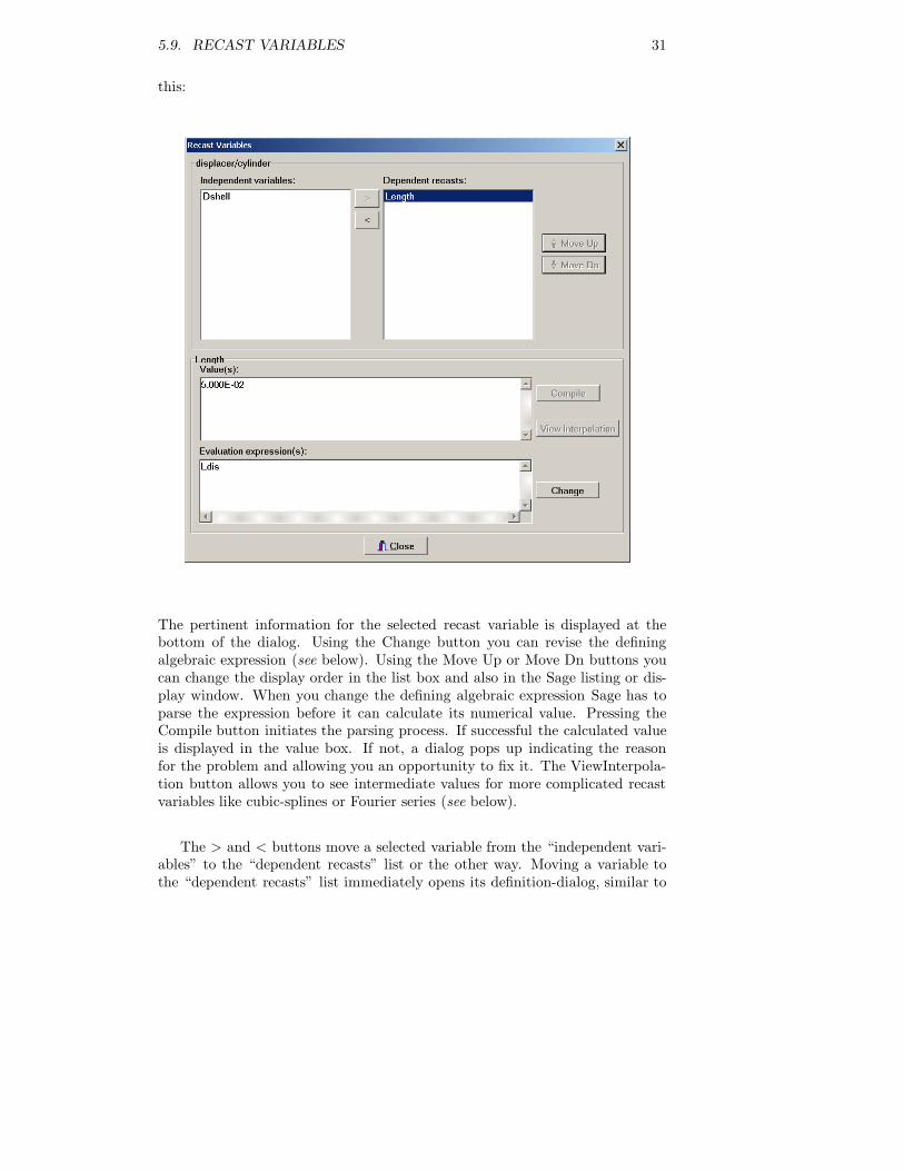
To recast an independent input variable, activate the model component inwhich it reside and select the Specify|Recast Variables menu command. A dialogopens, showing variables eligible for recasting and those already recast. Like
5.9. RECAST VARIABLES 31
this:
The pertinent information for the selected recast variable is displayed at thebottom of the dialog. Using the Change button you can revise the definingalgebraic expression (see below). Using the Move Up or Move Dn buttons youcan change the display order in the list box and also in the Sage listing or dis-play window. When you change the defining algebraic expression Sage has toparse the expression before it can calculate its numerical value. Pressing theCompile button initiates the parsing process. If successful the calculated valueis displayed in the value box. If not, a dialog pops up indicating the reasonfor the problem and allowing you an opportunity to fix it. The ViewInterpola-tion button allows you to see intermediate values for more complicated recastvariables like cubic-splines or Fourier series (see below).
The > and < buttons move a selected variable from the “independent vari-ables” to the “dependent recasts” list or the other way. Moving a variable tothe “dependent recasts” list immediately opens its definition-dialog, similar to

32 CHAPTER 5. WORKING WITH MODELS
the dialog used to specify user-defined variables:
Moving a variable to the “independent variables” list restores it to its originalstate, except that its value becomes the most recent value it had as a recastvariable.
In the above example the displacer Length is recast to equal Ldis, which is auser-defined input defined at the root level (see section 5.10).
Recasting is not the only way to implement geometric model constraints. Itis also possible to do so during the optimization process. Using recast variableshowever, eliminates explicit constraints and associated variables from an opti-mization structure, making it easier to understand and run faster. Moreover,recast variables are updated as part of the solution process and do not require re-optimizing the model each time you change an associated input variable. Thereare also advantages for the mapping process because a single mapped variablecan affect other inputs that you have recast as dependents, allowing you tomap along a curve in model space rather than just along the input coordinatedirections.
5.9.1 What Variables are Recastable?
In addition to recasting single-valued real input variables, you can also recastthe real-valued parts of more complicated variable types like Fourier series andcubic-splines data pairs. Provided they are what Sage recognizes as true inde-pendent variables rather than constants. Constants are not recastable becausethey used for normalizing variables during solving and optimizing and must notchange during either process. Constants are usually single-valued real inputs
5.9. RECAST VARIABLES 33
(e.g. Tnorm) although some cubic-spline variables (e.g. Tinit of heat exchangers)are also implemented as constants.
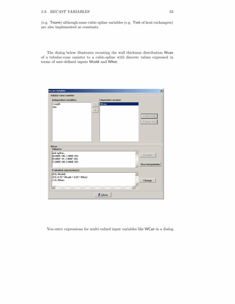
The dialog below illustrates recasting the wall thickness distribution Wcanof a tubular-cone canister to a cubic-spline with discrete values expressed interms of user-defined inputs Wcold and Whot.
You enter expressions for multi-valued input variables like WCan in a dialog

34 CHAPTER 5. WORKING WITH MODELS
like this:
Expressions for the independent and dependent parts of discrete interpola-tion points are entered in the cells of the string grid control of the dialog. Justmouse-click on the desired cell to make changes, taking care, in this case, thatthe independent values are entered in increasing order from 0 to 1.
The Delete Row, Insert Row, Move Up and Move Dn buttons act on bothindependent and dependent cells simultaneously for the selected row of the stringgrid. The selected row is the one you have most recently edited or clicked onwith the mouse.
5.10. USER INPUTS 35
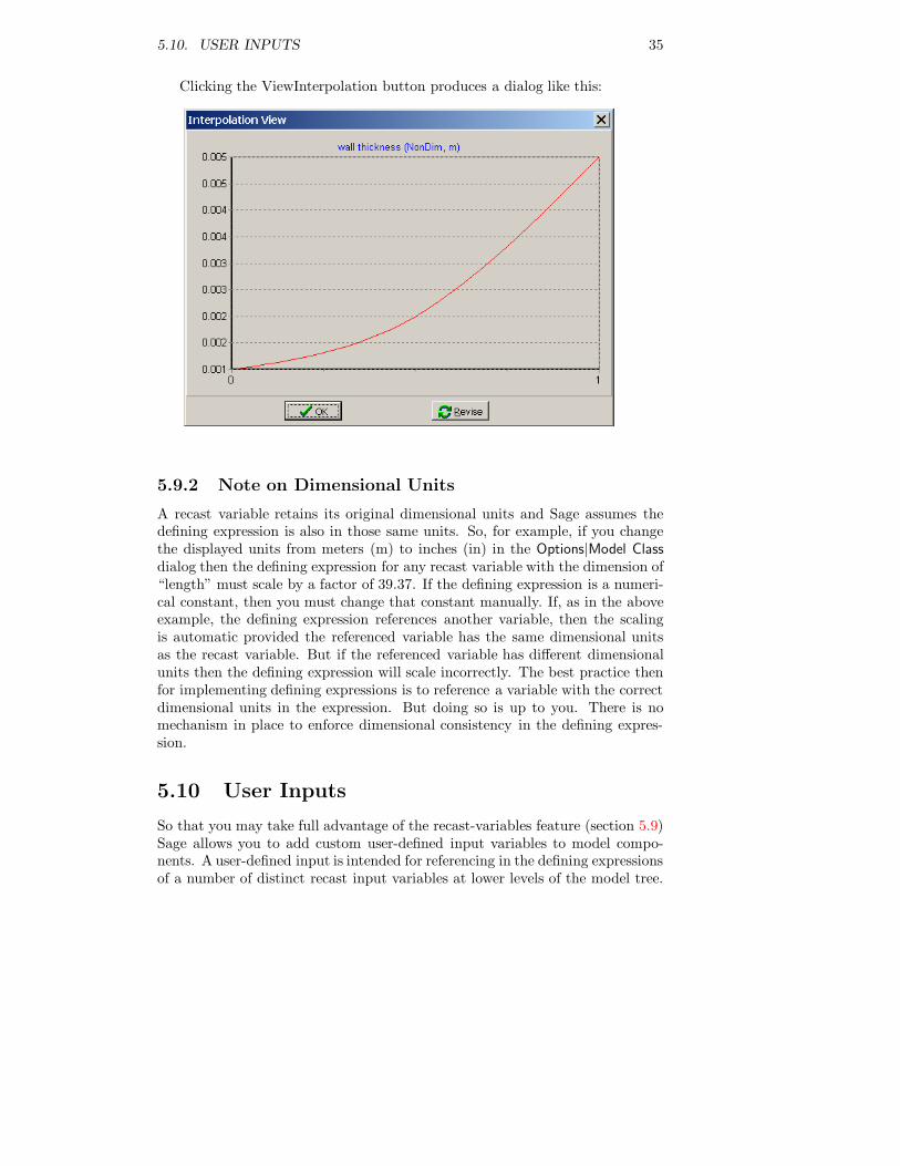
Clicking the ViewInterpolation button produces a dialog like this:
5.9.2 Note on Dimensional Units
A recast variable retains its original dimensional units and Sage assumes thedefining expression is also in those same units. So, for example, if you changethe displayed units from meters (m) to inches (in) in the Options|Model Classdialog then the defining expression for any recast variable with the dimension of“length” must scale by a factor of 39.37. If the defining expression is a numeri-cal constant, then you must change that constant manually. If, as in the aboveexample, the defining expression references another variable, then the scalingis automatic provided the referenced variable has the same dimensional unitsas the recast variable. But if the referenced variable has different dimensionalunits then the defining expression will scale incorrectly. The best practice thenfor implementing defining expressions is to reference a variable with the correctdimensional units in the expression. But doing so is up to you. There is nomechanism in place to enforce dimensional consistency in the defining expres-sion.
5.10 User Inputs
So that you may take full advantage of the recast-variables feature (section 5.9)Sage allows you to add custom user-defined input variables to model compo-nents. A user-defined input is intended for referencing in the defining expressionsof a number of distinct recast input variables at lower levels of the model tree.

36 CHAPTER 5. WORKING WITH MODELS
That way a single user-defined input value can directly assign the values of whatwere previously several independent inputs. A user-defined input becomes partof the model component it is defined in and behaves just any other input forpurposes of model solving, mapping or optimizing. Currently Sage allows onlysingle-valued real user-defined inputs.
To create a user-defined input variable, activate the model component inwhich it is to reside and select the Specify|User Inputs menu command. A dialogopens, showing any user-defined inputs already present with buttons for creatingnew ones or modifying existing ones:
The New button creates a new input. The Change button allows you to revisethe defining properties of an existing input (the one selected) or the Deletebutton allows you to remove it from the model component. The Move Up orMove Dn buttons change the display order in the list box and also in the Sagelisting or display window. Pressing the Change or New buttons opens the dialogfor setting the defining fields:
The Identifier field is the name that will appear in the listing and displaywindow and by which the input may be referenced in algebraic expressions

5.10. USER INPUTS 37
within your model. The Definition field is a short description of what the inputmeans. It also appears in the listing and display window but only for yourconvenience. The Value field is the numerical value that propagates throughthe model solution according to the other variables that reference the input.This is the value you normally see in the listing and display windows for aninput variable. You can also assign it with the Specify|Input Values dialog justas for a built-in input variable. The normalization field supplies the scale of theinput. It is used for setting step size during numerical differencing operationsin the solution or optimization processes. The Dimensional Units are selectedfrom a list and tie the value and normalization fields to the current dimensionsselected in the Options|Model Class dialog. For example, if you change thedisplayed units from meters (m) to inches (in), the Value and Normalizationfields automatically scale by a factor of 39.37. When you reference a user-defined input in the defining expression of a recast input variable (or any otheralgebraic expression) the referenced value also automatically scales according tothe currently selected dimensional units.
5.10.1 Identifier Visibility
As with a built-in input, the identifier of a user-defined input is visible from anylower-level child component in the model tree and may be referenced there inany algebraic expression. There is no provision for increasing the visibility toa higher level (parent model component) as there is for user-defined dependentvariables. If you need to reference a user-defined input at a higher level thenjust define it at that level or higher in the first place.
5.10.2 Exploring Custom Variables
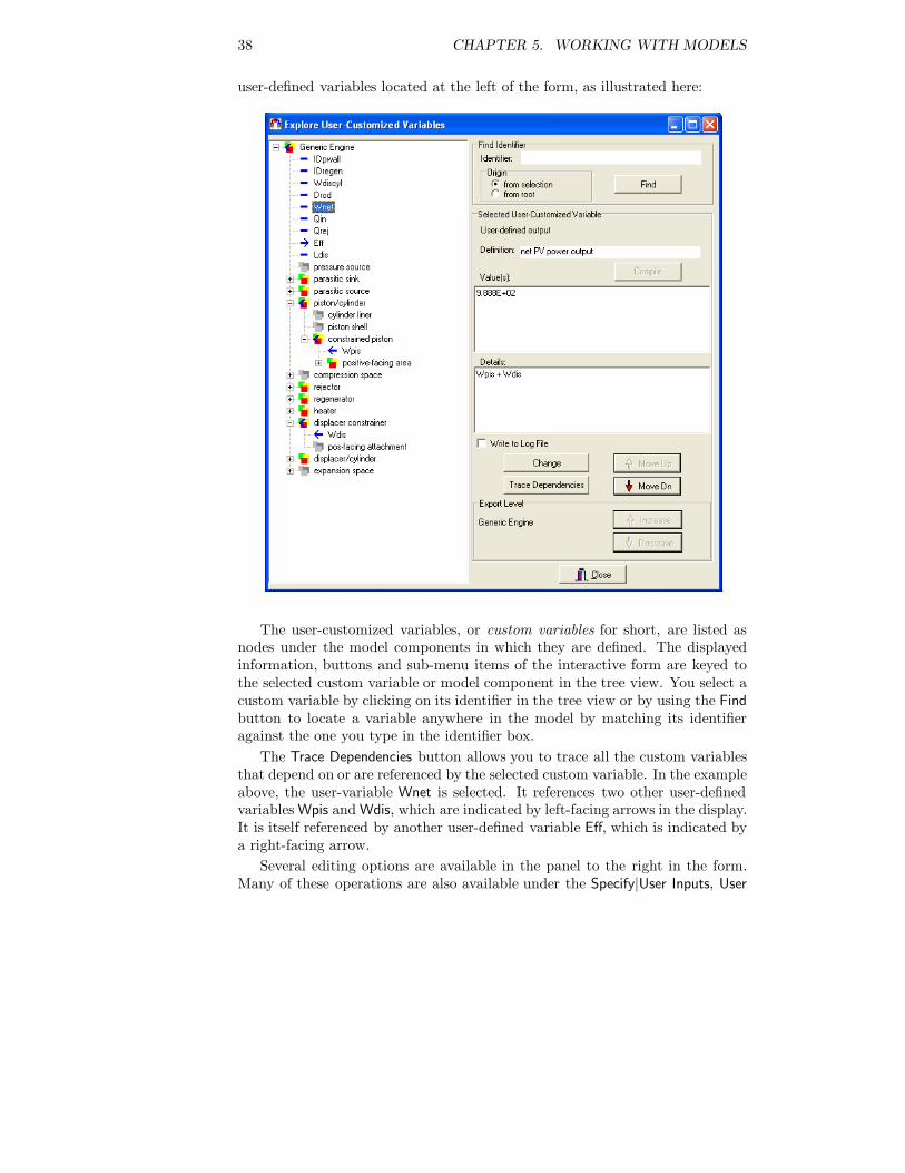
The Tools|Explore Custom Variables menu command opens up an interactivevisual form where you can work with all the user-customized variables (uservariables, recast variables and user inputs) in your entire model simultaneously.The key to doing this is a tree-structured listing of model components and
38 CHAPTER 5. WORKING WITH MODELS
user-defined variables located at the left of the form, as illustrated here:
The user-customized variables, or custom variables for short, are listed asnodes under the model components in which they are defined. The displayedinformation, buttons and sub-menu items of the interactive form are keyed tothe selected custom variable or model component in the tree view. You select acustom variable by clicking on its identifier in the tree view or by using the Findbutton to locate a variable anywhere in the model by matching its identifieragainst the one you type in the identifier box.
The Trace Dependencies button allows you to trace all the custom variablesthat depend on or are referenced by the selected custom variable. In the exampleabove, the user-variable Wnet is selected. It references two other user-definedvariables Wpis and Wdis, which are indicated by left-facing arrows in the display.It is itself referenced by another user-defined variable Eff, which is indicated bya right-facing arrow.
Several editing options are available in the panel to the right in the form.Many of these operations are also available under the Specify|User Inputs, User

5.10. USER INPUTS 39
Variables, or Recast Variables menu items but they are repeated here for conve-nience. You can change a variables identifier, definition or expression. You canchange the order in which it is listed and for user variables change its exportlevel. The export level is the level above the parent model component in whichthe variable identifier may be referenced by an expression in another customvariable, constraint or whatever.
After you change a custom variable all custom variables that may reference itare disabled for evaluation purposes and the value box displays “not compiled”.The Compile button allows you re-parse all the custom variables, after whichthe value box once again displays numerical values.
There is also a submenu available that supports new, delete, cut, copy andpaste operations. The submenu pops up by positioning the mouse cursor withinthe tree view then clicking the right button. When a model component isselected the New submenu item, allows you to insert a new user input, variableor recast variable. When a user input or variable is selected the Cut or Copyoperations are available. Recast variables are not copyable because they aretied to specific built-in variables of the model. Copy and paste operations usethe Windows clipboard by encoding a user input or variable defining data as atab-delimited text string. It is possible to copy user inputs or variables fromone model to another model running under a second Sage application. In orderto paste a user input or variable that has been cut or copied it is necessary tofirst select the model component in the tree view into which the variable will bepasted.

40 CHAPTER 5. WORKING WITH MODELS

Chapter 6
Mapping
There are times when you may want to investigate a sequence of solutions overa discrete range of one or more input variables. This is the process of mapping.Mapping is something you might want to do to achieve a better understanding ofyour model’s sensitivity to various inputs. But it is not the same as optimization,the topic of the next chapter.
Anyone with any programming experience will understand the sequence ofsolutions generated in a mapping as the result of a nested loop structure. Exceptno programming is required (on your part) to do a mapping in Sage. All youdo is select one or more input variables to be mapped using the Specify|MappedVariables command then run the mapping with the Process|Map command. Therest is automatic.
Prior to specifying a mapped variable you must first activate the modelcomponent containing the variable by clicking its tab in the display or editform, or clicking on its edit-form icon. Mappable variables are selected froma list of any drivable variable within the model component as described inchapter 11 — usually a real-valued independent variable, rarely the real partof a composite variable. For each mapped variable selected, you also specifythe first and last values the variable will take, the number of iterations to bemade within the mapping interval and whether the variable should be mappedin equal steps or equal ratios. The total number of solutions performed in thewhole mapping process is the product of the iteration counts for the individualmapped variables. Evidently, for complicated models that take a long time tosolve, you will want to think carefully about how many variables to map andtheir iteration counts.
When mapping initiates you are prompted for the name of a disk file inwhich the mapping results will be stored in ASCII format. This file will containa sequence of lines or records containing tab-delimited values for the mappedvariables as well as any user-defined variables tagged for appearance in log files.You select such user-defined variables by checking the ”write to log file” boxin the user-variable definition dialog available under the Specify|User Variablescommand.
41

42 CHAPTER 6. MAPPING
During the mapping process, solutions are generated automatically until themapping is finished. A mapping status dialog shows you the current mappingiteration and solution progress within that iteration. Using the buttons of thestatus dialog you can abort the mapping at any time, after which the mappinglog file is closed with the results so far. You can also view the mapping progressin the display form, as usual, while the mapping is in progress.
A sample gizmo mapping that maps the amplitude (user-variable) of aspring-mass-damper system as a function of frequency (mapped) produces alog file that looks like this:
Sage version 1.0 --- 5/28/96 2:30:44 PM
Mapping For: C:\SAGE\GIZ\OP1.GIZ
Omega resonant system Amplitude
5.000E+01 1.109E-02
6.000E+01 1.140E-02
7.000E+01 1.155E-02
8.000E+01 1.140E-02
9.000E+01 1.087E-02
1.000E+02 1.000E-02
After the two header lines comes the line identifying the mapped and uservariables whose tab-delimited values appear in the remainder of the file. Thevariable-identification line is also tab-delimited which is more apparent if youopen the map file with a spreadsheet program such as Excel. Viewing map fileswithin a spreadsheet, or similar program, is not required but recommended fordealing with the results of complex mappings.
Chapter 7
Optimizing
The standard mathematical definition of a general nonlinear programming prob-lem looks like this:
minimize a real-valued objective function F (x), where x is a vectorof n real variables, subject to the equality or inequality constraints
ci(x) = 0, i ∈ E (7.1)
ci(x) ≥ 0, i ∈ N (7.2)
where E and N are disjoint index sets.
which may leave you cold. In Sage you deal with optimization as a naturalextension of the engineering model you already understand, in terms of thingsyou quite naturally want to do. The objective function and any constraints fallout naturally. And after you have specified a few optimization problems youmight want to note that they can, after all, be cast into the above rigorousmathematical form.
7.1 Sample Resonant System Optimizations
Every mechanical engineering student learns about spring-mass-damper reso-nant systems of the type embodied in Sage’s resonant-system model class. Ifyou plot response amplitude in such a system when driven by a fixed-amplitude,variable-frequency forcing function you get a curve that looks something like
43

44 CHAPTER 7. OPTIMIZING
this:
What if you want to find the frequency that maximizes the amplitude, with-out actually plotting every point? This is an unconstrained optimization prob-lem, already set up for you in sample file op1.giz. There you find Omega, (an-gular frequency) an input variable in the root model component, flagged as anoptimization variable and objective function “maximize X.amp” specified in thereciprocator model component. Beware though of setting the damping coefficientbeyond the critical-damping value (2
√km). For then the maximum amplitude
occurs at zero frequency.A somewhat contrived example of a constrained optimization problem would
be to optimize both frequency (Omega) and reciprocating mass (Mass) in orderto maximize response amplitude, subject to the equality constraint that “Mass= Omega / 100”. This problem is worked out in sample file op2.giz.
The previous two examples should be enough to get you started. The restof this chapter is for your reference when the going gets tough. One word ofwarning though: always try to understand the physical principles behind youroptimizations. It is much easier to specify an ill-defined problem without asolution than a well behaved one. If there is no good physical reason why anoptimization should converge to a solution, then it probably won’t. We mustnot always be blaming Sage.
7.2 Specifying Optimization Variables
Although optimization variables pertain to the model as a whole, you specifythem one group at a time within each model component. To flag a variable

7.3. SPECIFYING CONSTRAINTS 45
as an optimization variable, first activate the model component containing it(click its tab in the display or edit form, or click on its edit-form icon), thenselect Specify|Optimized Variables from the menu. As with mappable variables,optimizable variables are selected from a list of any drivable variable within themodel component as described in chapter 11 — usually a real-valued indepen-dent variable, rarely the real part of a composite variable.
7.3 Specifying Constraints
Constraints, too, pertain to the model as a whole but are specified individuallywithin a particular model component. To specify a constraint, first activate themodel component that will contain it (click its tab in the display or edit form,or click on its edit-form icon), then select Specify|Constraints from the menu.Constraints are specified in the form E1 ≤ E2, E1 = E2, E1 ≥ E2, where E1and E2 are two algebraic expressions you enter, similar to those entered foruser-defined variables. More information about entering algebraic expressioncan be found in chapter 10.
Satisfying your constraints is the job of Sage’s optimization driver. It doesthis by tweaking the optimization variables to force the left-hand-side expres-sion minus the right-hand-side expression (E1 − E2) to be zero, in the case ofan equality constraint, or merely non-negative or non-positive in the case ofan inequality constraint. Equality constraints are always said to be active —meaning in force or to be reckoned with. Inequality constraints are active onlywhen they start out violated or the optimization driver tends to violate theconstraint during the course of the optimization. A useful rule of thumb is thateach active constraint reduces by one the degrees of freedom available in thesearch domain to minimize or maximize the objective function.
Constraints are very useful things. You can invoke simple inequality con-straints to keep an optimized variable in bounds — such as “X ≤ C” or “X≥ C”. Or, you can invoke more complicated constraints — such as PowerOut= 100, where PowerOut is a user-defined variable you have defined in terms ofbuilt-in outputs. You can even invoke constraints without an objective functionpresent. However, when you do this it is necessary to specify the same numberof optimization variables as active constraints. Go ahead and be liberal impos-ing constraints. Create as many as you feel you need. If physically sensible andreasonably linear, they are no great burden on Sage’s optimizer.
7.4 Specifying the Objective Function
Like all the other elements of an optimization problem, the objective functionpertains to the model as a whole but is specified within a particular modelcomponent. There can be only one objective function, which means that if youcreate a new one, the old one disappears. To specify the objective function, firstactivate the model component in which it is to appear (click its tab in the display

46 CHAPTER 7. OPTIMIZING
or edit form, or click on its edit-form icon), then select Specify|Objective Functionfrom the menu. You will be presented with dialog containing information aboutthe existing objective function, if any, and the means to change it. The objectivefunction is specified in the form “minimize E” or “maximize E”, where E isan algebraic expression similar to those entered for user-defined variables orconstraints. More information about entering algebraic expression can be foundin chapter 10.
In the objective-function dialog box, the existing objective function is dis-played even if it is in another model component. Where it presently residesappears in the dialog box labeled Currently In Model Component. Where anewly created or changed objective function will reside appears in the dialogbox labeled New Model Component. The component in which the objectivefunction belongs is the one where it is most natural to reference the variablesin its defining expression, usually, but not always, the root model component.
As with satisfying constraints, Sage maximizes or minimizes your objec-tive function by tweaking optimization variables according to its built-in logic.The objective function often represents some model output such as power, heatinput, efficiency — typically, something that arises as the end result of a con-siderable amount of computation. As such, objective functions can be highlynon quadratic (the ideal) and require many iterations for Sage to minimize ormaximize. On the other hand, they may be relatively simple, as in the sampleproblems concocted at the beginning of this chapter.
7.5 Running An Optimization
Once you have specified the optimization problem, you initiate the optimizationprocess with the Process|Optimize menu command. When optimization beginsyou are prompted for the name of a disk file in which the optimization results willbe stored in ASCII format. This file will contain a sequence of lines or recordscontaining tab-delimited values for the optimized variables, constraints and ob-jective function, as well as any user-defined variables tagged for appearance inlog files. You select such user-defined variables by checking the ”write to logfile” box in the user-variable definition dialog available under the Specify|UserVariables command.
A status dialog box then appears, giving you a blow-by-blow account of theprocess and an opportunity to stop or pause if the need should arise. You canuse the pause option to inspect the current solution state or save the modelbetween iterations. The status dialog itself contains a good deal of informationdesigned to keep you somewhat informed and entertained while you are sippingyour coffee, or doing whatever you do to kill time. The goal of the optimizeris to drive the so-called pseudo-Lagrangian step change to a small but negativevalue.
The pseudo-Lagrangian step-change is a measure of the relative change overthe current step of the objective function plus a weighted sum of violated con-straints. The value should start out large and negative and grow ever smaller

7.5. RUNNING AN OPTIMIZATION 47
(but still always negative) as the optimization converge to the minimizer. Forour present purposes, it is sufficient to think of the pseudo-Lagrangian as anapproximation to the classical Lagrangian function of constrained optimizationtheory, which has an extreme point at the minimizer or maximizer.
One thing to keep in mind is that values printed in the status dialog pertainto the optimization problem at a somewhat higher level of abstraction thanyour original specification. The objective function and constraint violationsdisplayed are normalized values. And if you have chosen to maximize ratherthan minimize your objective function, its sign is switched. This is because theoptimizer always minimizes objective functions. Minimizing −f is equivalent tomaximizing f .
After some up-front work to estimate evaluation precision in the objectivefunction and constraints and to initialize the Hessian (second-derivative matrix),an optimization is carried out as a sequence of iterations. Each iteration requiresa small step of each optimization variable in order to perform numerical partialderivatives of the objective function and its constraints, followed by a line search(all variables stepped simultaneously) along a direction defined by the solution toa quadratic-programming subproblem the optimizer maintains as it goes along.You can follow this in the status dialog box labeled stepping. Each step requiresanother model solution.
If all goes well, Sage will converge to a unique solution within a reasonableperiod of time. Satisfying any violated constraints usually requires only a fewiterations, say less than ten. After that, Sage seems to concentrate more onminimizing or maximizing the objective function, which may take a good deallonger, say up to forty iterations — maybe more in some cases. After conver-gence you should inspect the state of your model then save it using the File|Savecommand if all is well.
Sometimes, due to noise in the model, the optimizer will never reach itstarget pseudo-Lagrangian step change. It will achieve a small value in the rangeof, say, (−10−5) to (−10−8 and never get lower. This is generally good enoughand you should feel free to stop the optimizer whenever you think it is done.After all, you are a good deal more intelligent than Sage’s optimizer and shouldbe able to sense when your model is as optimized as it is ever likely to get. Theoptimizers main advantage over you is superior diligence.
When your optimization is finished you may want to take a look at the logfile. The sample op1.giz gizmo optimization mentioned earlier, produces a logfile that looks like this:
Sage version 1.0 --- 5/28/96 3:37:22 PM
Optimization For: C:\SAGE\GIZ\OP1.GIZ
Omega resonant system Maximize X.amp
5.000E+01 1.109E-02
7.902E+01 1.143E-02
6.560E+01 1.151E-02
6.992E+01 1.155E-02
7.082E+01 1.155E-02

48 CHAPTER 7. OPTIMIZING
7.071E+01 1.155E-02
7.071E+01 1.155E-02
After the two header lines comes the line identifying the optimized variable andobjective function whose tab-delimited values appear in the remainder of thefile. The identification line is also tab-delimited which is more apparent if youopen the map file with a spreadsheet program such as Excel. Viewing map fileswithin a spreadsheet, or similar program, is not required but recommended fordealing with the results of complex optimizations.
7.6 Diagnostics
The most obvious symptom of a failing optimization is when the magnitude ofthe pseudo-Lagrangian step change fails to decrease, or even increases duringthe optimization process. There are other signs to look for that may help youpinpoint the problem.
7.6.1 Variable Step Limits
Keep an eye on the status-dialog box labeled step limit for. Ideally it shoulddisplays none, which is a sign that all is going smoothly and the optimizer’squadratic approximation to your optimization problem is reasonably valid. Ifit displays the name of one of your optimization variables instead, then theoptimizer is having trouble with that variable. It has tried to step it to aforbidden value. If the problem does not clear up after a few iterations, it maybe a good idea to stop and restart the optimization after a careful review of thecurrent state of the optimization variables.
7.6.2 Line-Search Step Reductions
Another think to look for is two successive model solutions, instead of one, dur-ing the line search. You may have to be quick to notice this, depending onthe time the solver spends solving your model. The first step of the line searchis with the increment returned by the quadratic programming subproblem. Ifthat step fails to produce the expected decrease in the pseudo-Lagrangian func-tion, then a second, reduced, step is taken. When a failed search step happensnear the beginning of an optimization, it usually means that either the Hes-sian (second-derivative) matrix, which is internally maintained and updated bySage’s optimizer, has not yet had time to fully evolve, or the pseudo-Lagrangianfunction is nowhere near quadratic. Usually the problem is self-correcting aftera few iterations as the quadratic approximation begins to better fit the non-linear pseudo-Lagrangian. If the problem does not go away it may indicate anill-conditioned optimization as described below. Sometimes it helps to restartthe optimization.

7.6. DIAGNOSTICS 49
7.6.3 Ill-Conditioned Problems
When Sage absolutely fails to converge, it is probably suffering from an ill-conditioned optimization problem. You will want to be on guard for some ofthe following cases.
The most obvious example of ill-conditioning is a problem without a min-imum or maximum. An example might be maximizing heat lift in a stirlingcooler but forgetting to constrain input power. The size and power of the ma-chine may go up forever. It is usually not difficult to avoid this problem, butsometimes the interaction of objective function and constraints is subtle. Thesymptom of a problem without a minimum or maximum is optimization vari-ables drifting off to infinity or zero while the objective function keeps decreasingsteadily.
A similar problem, but not as easy to spot, is the problem of weakly-determined optimization variables — subsets of variables with more degreesof freedom than required to solve the problem. Say, for example, you are op-timizing a rectangular-channel heat exchanger with three pertinent physicalvariables: channel number, width and gap. And assume your objective functionand constraints depend only on the two derived variables: hydraulic diameterand wetted perimeter. Then there would be no way you could optimize all threephysical variables simultaneously. Nor could Sage. The best you could hope todo would be to optimize two physical variables, fixing the third. If Sage wereto attempt to solve for all three, it would probably do its best, but wind updrifting around inconclusively. Whenever you select an optimization variable,take time to think of how the objective function and constraints depend uponit. There is no point adding a variable if it has no bearing on either. And ifa variable is present solely to satisfy a constraint, be sure it is the only suchvariable.
The most ill-conditioned problem of all is one with infeasible or overdeter-mined constraints — constraints that cannot possibly be satisfied. A simpleexample might be a problem with the two inequality constraints “pressure ≥10.0E5” and “pressure ≤ 5.0E5”. No one would be that foolish, but when con-straints get complicated, incompatibilities become less glaring. Sage has bigtrouble when faced with such constraints. The main symptoms are very largepseudo-Lagrangian step changes but no real improvement in constraint viola-tions or the objective function. The objective function may increase dramat-ically (wrong way) as it takes a back seat to Sage’s attempt to satisfy yourconstraints. If you have any experience running Sage with a well-behaved prob-lem, you will immediately recognize the symptoms of infeasible constraints.
If the optimizer feels the problem is bad enough it will terminate the op-timization process with a message box containing some information about thenature of the problem. Always check for the possibility that you have moreequality constraints (plus active inequality constraints) than optimization vari-ables. Otherwise, because of small numerical differences in the linear constraintapproximations, it is rare for constraints to be truly infeasible. More likely, youwill see the weird behavior described earlier than any error messages.

50 CHAPTER 7. OPTIMIZING
Occasionally Sage may suggest that your inequality constraints are infeasible,even though you have specified no inequality constraints. This is not an error.It merely reflects the status of two hidden inequality constraints added to yourproblem by Sage’s optimizer. When this happens, you should infer that yourequality constraints are really the infeasible ones.
If all else fails, after 100, or so, iterations — more than enough for all fore-seeable well-conditioned optimizations — Sage’s optimizer is programmed togive up, displaying its reason in a message box. The exact number of iterationsbefore this happens may be model-class specific.
7.6.4 Multiple Extreme Points
Unconstrained optimizations generally lead to a unique solution — independentof starting conditions. There are two reasons for this: First, in most engineeringmodels, optimization variables tend to cluster themselves into weakly coupledsubsets (within model components or component subtrees). And second, withineach of these subsets model outputs tend to vary smoothly, or at least withoutmultiple peaks and valleys.
Add constraints and all bets are off. Constraints, especially nonlinear in-equality constraints, tend to carve up the search domain into weird shaped,possibly disjoint, regions, with multiple local extreme points potentially foundon the boundaries. Moreover, these regions are in n-dimensional space (wheren is usually greater than 3) and are extremely difficult to visualize.
The problem is that Sage will happily converge to any local minimum withcomplete disregard for a better local minima lurking in some other corner of thesearch domain. This is a problem with any gradient-based search algorithm.The only way to find multiple solutions is to restart Sage from several differentpoints in the search domain. But the problem is, how do you pick these startingpoints?
The most satisfactory approach to finding a global optimum is by way of suc-cessive approximation, building intuition about your problem as you go. Startout by solving a problem with as few constraints as possible, then add con-straints one by one and see what happens. Save the data files from intermediateresults in case you need to return to them as future starting points. As you addconstraints you will be able to develop some intuition about where that con-straint drives the solution, why it does so, whether or not there might be otherlocal extrema, and where to look for them. Eventually you will accumulate anumber of good starting points from which to start Sage for the final case whereall constraints are simultaneously present.
7.6.5 Normalization Values
When specifying an optimized variable, constraint or the objective function, youcan change its normalization value using an edit box in the specification dialog.Actually, what you can change is the scale factor which multiplies the default
7.6. DIAGNOSTICS 51
normalization value. But first, what is a normalization value and why mightyou need to change it?
A normalization value establishes a representative size for a dimensionedvalue, providing the necessary information to convert it to a uniform sized di-mensionless value. A dimensioned value may be a very small number or a verylarge number, depending on physical units. For example, the value of a clear-ance seal gap might be of the order of 10−5 m while the value of charge pressuremight be of the order 106 Pa. A dimensionless value is always of uniform size,on the order of one.
The way Sage converts a dimensioned value to a dimensionless one is bydividing by the normalization value. Sage automatically maintains a defaultnormalization value for each optimized variable, constraint or objective function.The basis for these normalization values are special input constants, usuallydefined in the top-level model component and usually with the suffix “norm”in the variable name, as in Lnorm. So, for example, a gap of 10−5 m becomes,in dimensionless form, gap / Lnorm. Normalization constants for the more-complicated expressions found in constraints and objective functions are builtup as similar expressions involving basic normalization constants.
The good news is that you need not be concerned about normalization valuesin most cases. As long as the normalized values of all optimized variables,constraints and the objective function are within an order of magnitude or twoof each other, the optimizer can successfully complete the optimization. Onrare occasions, however, a normalization value can be too small or too large.If too small, then the optimizer is fooled into stepping farther than necessarywhen making finite-difference approximations to partial derivatives. Sometimesstepping so far that the model solution fails to converge. If the normalizationvalue is too large, then the optimizer may not step far enough to get an accuratefinite-difference result. Or it may be lulled into thinking that the optimizationhas converged because the objective function is changing by what it things is avery small amount.
To allow you to diagnose this sort of problem, the value displays of optimizedvariables, constraints and the objective function (visible in display windowsduring optimization or after Process|Compile Optimization) include the normal-ization value in parenthesis, as in (norm = 1.654E-2), or some such. So, forexample, if your objective is to maximize Wpv (where Wpv might be a user-defined variable for stirling-engine PV power output), you might expect troubleif Wpv is of the order 10 W, and norm is of the order 104. To remedy the prob-lem, you would set the normalization scale factor for the objective function to10−3, using the edit box in the specification dialog. This would correct the valueof norm to 10 (visible after another Process|Compile Optimization), resulting ina better conditioned optimization problem.

52 CHAPTER 7. OPTIMIZING

Chapter 8
Editing Model Structure
In Sage, you edit (create or modify) a model’s structure within a graphicalinterface known as the edit form, separate from the main Sage form. To openthe edit form use the Edit|Show Window menu command. The edit form containsa number of pages at different levels of the model hierarchy. These pages arecreated as explained below and selected by mouse-clicking on the tabs at thebottom of the edit form. The leftmost page always shows the child componentsof the root-level model component.
The edit-form root page for the resonant-system sample model phasor.giz,looks like this:
Visible in the window are graphical icons representing child model compo-nents of the root model. Attached to the child-model icons are arrows corre-sponding to their boundary connections. An arrow with a number beside it
53

54 CHAPTER 8. EDITING MODEL STRUCTURE
indicates an active connection to another model icon within the same window.Active connections are identified by matching numbers. Arrows without num-bers indicate potential connections, as yet unmade. The reason connections areindicated with numbers rather than attachment lines is to avoid cluttering upthe window in complicated models.
Boundary connections can be made freely, but only among similar type con-nectors. Similar type connectors are indicated by the symbolic code next to thearrows. In the above example, the arrows labeled Fphsr indicate phasor forces.Phasor (complex-number) amplitudes are the way the resonant-system modelclass represents sinusoidally time-varying quantities.
8.1 Basic Operations
The edit form has a basic mouse interface for certain common operations.
8.1.1 Selecting Components
Each model-component icon in the edit form has a caption bearing the nameof the model component it belongs to. Clicking on a component icon highlightsits caption bar, which activates that model component for pertinent menu op-erations. You can select multiple model components by holding down the shiftkey while mouse clicking on them or dragging a selection rectangle over them.In that case the active model component is the one most recently selected.
8.1.2 Positioning Icons
Holding down the left mouse button while the mouse cursor is on a componenticon allows you to drag the icon anywhere within the edit form. Releasing themouse button drops the icon at its new position. Continuing to hold down theshift key after selecting multiple model components allows you to move them asa group. You can also use the arrow keys to move selected model components.
8.1.3 Navigating the Model Tree
Model components can have child components, and so on for several generations.To display a component’s children just double-click on its icon. This adds a newpage to the edit form and a new tab at the bottom. You can re-display the parentcomponent by clicking on its tab.
The tabs hold only a single branch pathway from the root to some lower-level component. When you change the tail of a path, by double clicking on adifferent component icon, the tabs corresponding to the old tail disappear.

8.2. COMPONENT PALETTE 55
8.2 Component Palette
When the edit form is active, a model-component palette appears in the mainSage form. This palette contains buttons representing the seeds for new modelcomponents which can germinate in the current page of the edit form. Thecomponent palette for the previous example looks like this
The buttons of the palette are themselves arranged in tab-selected pagescorresponding to different categories of model components. The available com-ponents in the palette are those which make sense in the context of the parentcomponent, generally a small subset of the total number of components in themodel class.
To create a new model component click a button in the component palette,then click again in the edit form at the position you want the component toreside. Once you’ve created a model component you can drag it around the editform with the mouse, as describe above.
Considerably more difficult than the problem of creating model componentsis deciding which ones to create in the first place. For help with this you mightwant to look at the sample data files distributed with your particular modelclass. You can also find detailed information about each model component inother sections of this user’s guide.
8.3 Connections
Making or breaking connections between model components is simply a matterof drag-and-dropping a connector to its mate.
To connect together two compatible boundary connectors, click on the firstconnector arrow with the left mouse button, then with the button held downposition the mouse cursor on the second connector arrow and release the button.The first-clicked connector arrow establishes the type of the connection, andlocks it in. The connector arrow you drag to must then be a mating arrow(opposite sense) of the same type (label).
Breaking connections is just like making them. Click on the first connectorarrow with the left mouse button, then with the button held down position themouse cursor on the mating connector arrow and release the button.
Clicking on a connection arrow for an active connection highlights the mat-ing connector arrow at the other end of the connection. Hovering the mouseover a connection arrow displays a popup window that traces the source of the

56 CHAPTER 8. EDITING MODEL STRUCTURE
connection within the model component and also shows the current value of thequantity flowing through the connection if the connection is active.
8.4 Changing Connector Level
Often, the desired mate to a boundary connector resides at another location inthe model tree, not displayed on the same page of the edit form. So the twoboundary connectors are not immediately connectable. In this case it is alwayspossible to trace up the model tree (toward the root) from each boundary-connector’s model component to find two ancestor model components that ap-pear within a common page. This is useful because, in Sage, you are allowed tomove boundary connector arrows up the model hierarchy. Connector arrows somoved appear attached to the ancestor model-component icon. Once they arethere they may be attached to any compatible boundary connector at the newlevel. By doing this for our original two star-crossed connector arrows, they canbe eventually joined.
To move a boundary-connector arrow up the model tree (toward the root)first highlight the arrow by clicking on it then click on the Inc connector levelspeed button in the main Sage form (red up-directed arrow) or use the Edit|UpConnector menu command. If you hold-down the shift key, you can highlightseveral connector arrows at the same time, after which you can move them as agroup. But you can only highlight an arrow that is not already connected.
To move a boundary-connector down the model tree, first highlight one (orseveral) disconnected arrows then click on the Dec connector level speed buttonin the main Sage form (red down-directed arrow) or use the Edit|Down Connectormenu command.
The notions of up and down may or may not make sense to you, dependingon your mental picture of a model tree. For purpose of moving connectors youmight want to visualize the model tree with the root at the top and branchesextending downward.
8.5 Cut and Pasting Model Components
The standard Window’s conventions for cutting and pasting blocks of text in atext editor apply to model components in the edit form. Cut and copy operateon the currently selected model components and insert those component into aclipboard-like temporary storage area. The clipboard is the source for one ormore subsequent paste operations.
This clipboard is not the same as the standard Window’s clipboard for tex-tual information. So you will not be able to paste into another Windows appli-cation a model component cut from Sage.

8.6. CHANGING MODEL COMPONENT BITMAPS 57
8.5.1 Copy
First highlight a model component by clicking on its icon or select multiplemodel components by holding down the shift key while clicking on them ordragging a selection rectangle over them. Then click on the Copy speed buttonin the main Sage form (overlapped pages) or use the Edit|Copy Model(s) menucommand. The model components, including all generations of child compo-nents, are now copied into the clipboard for subsequent pasting. Copying doesnot affect the existing model components so it is useful for cloning or duplicatingthose model component as sibling components.
This only works for model components that are not connected to other modelcomponents outside the selection group. If you want to copy model componentsconnected externally first break any boundary connections to components out-side the group (possibly at a higher level in the model tree) using the drag-and-drop techniques described above.
8.5.2 Cut
First select model components as for copying. Then click on the Cut speedbutton in the main Sage form (scissors) or use the Edit|Cut Model(s) menucommand. This is just like the copy operation except the model component isdeleted from the edit form.
8.5.3 Delete
First select model components as for copying. Then press the delete key or usethe Edit|Delete Model(s) menu command. There is no undo option after deletingmodel components.
8.5.4 Paste
Following a copy or cut operation, click on the Paste speed button in the mainSage form or use the Edit|Paste Model(s) menu command to clone new modelcomponents into the edit form. Model components can only be pasted intothe same parent model component they were copied from or to compatibleparent having seeds in its child-creation palette of the same class types as thecomponents to be pasted.
8.6 Changing Model Component Bitmaps
The Edit|Change Bitmap menu command allows you to change the bitmap imagesused to represent model components in the edit window. The command is keyedto the model component currently focused in the edit window. When you select

58 CHAPTER 8. EDITING MODEL STRUCTURE
this command a dialog pops up, like this:
Pressing the “Load From File” button allows you to load a new image fromany bitmap file (*.bmp) that you have previously created using some graphicalediting software. Pressing the “Restore Default” button restores the bitmaporiginally assigned to the model component by Sage when it was first created.
The default bitmaps for Sage model components are all 64x64 pixel black-and-white bitmaps that were originally created with an early Borland appli-cation called Resources Workshop. Borland has stopped actively promotingResources Workshop, but any other graphics editing software should do aswell, provided it supports creating Windows compatible bitmap files (*.bmp).Bitmaps do not have to adhere to the 64x64 black-and-white format. You canload any size bitmap and even in color. You may use a bitmap rendered byCAD software or captured from a computer screen image. But keep in mindthat the bitmap image will become embedded in your model file and affect itsstorage size accordingly.
The change-bitmap feature gives you control over the illusion of what themodel component is intended to do. Do not underestimate this illusion. Ap-propriate bitmap images go a long way toward making a Sage model compre-hensible. You may not want to change the default bitmaps for any of Sage’sindividual model components but submodels are another matter. If you havea model containing submodels you might find it useful to change their defaultimages to something representative of what they actually do.

Chapter 9
Variable Types
Sage models employ a number variable types that you need to be aware of.These include the common integer and real (floating-point) variables but go onquite a bit beyond that.
9.1 Integers
Integer variables display as numerals without decimal points like this:
NCell number spatial cells 2
Sometimes integer variable inputs are restricted to a range of values.You may reference integer variables directly by name in user-defined alge-
braic expressions. They are converted to real values when you do this.
9.2 Reals
Real variables display in exponential format like this:
Freq frequency (Hz) 5.500E+01
Sometimes real variable inputs are restricted to non-negative, strictly positiveor values within some prescribed closed interval. You may enter real values indialog boxes with or without decimal points or the E suffix.
Real variables may be referenced directly by name in user-defined algebraicexpressions.
9.3 Complex
Complex variables display in an extended exponential format like this:
59

60 CHAPTER 9. VARIABLE TYPES
F boundary force (N) (-9.466, 7.633)E+01
The numbers in parenthesis are the real and imaginary parts and the E+01 isthe common power-of-ten multiplier. The above example is equivalent to thecomplex number (−94.66, 76.33) or −94.66 + 76.33i, where i is the imaginaryunit (i =
√−1).
In model components with an underlying basis in linear differential equa-tions, complex amplitudes are often used to represent sinusoidal time-varyingquantities. Presuming this to be the case in the above example, physical bound-ary force would actually be understood as the real-part of Feiωt, or
physical boundary force = −94.66 cosωt − 76.33 sinωt
If we look at this as just the first-harmonic terms in a Fourier-series expansion∑
(an cosnωt + bn sinnωt), we note that a1 = <F and b1 = −=F , where <Fand =F are the real and imaginary parts of complex amplitude F .
Complex variables are not directly referenceable in user-defined algebraicexpressions. However for a complex variable X, the following subfields are ref-erenceable:
X.real real partX.imag imaginary partX.amp amplitude or modulusX.arg argument or phase angle
9.4 Phasors
Phasors are just complex numbers displayed in polar form. A typical phasorvariable would be displayed like this:
F boundary force (N) 1.216E+02 cis(2.463)
The leading coefficient (1.216E+02 in this case) is the complex magnitude oramplitude — the length of the phasor. The number in parenthesis (2.463) isthe phase angle in radians measured counterclockwise from the positive realaxis. The notation “cis” reads “cosine plus i sine”, where i is the complexunit. In other words, the above variable is equal to the complex number121.6 cos(2.463) + 121.6i sin(2.463), which is the same as the number in theprevious example.
Under the convention that boundary force actually represents a complexamplitude for a sinusoidal time-varying quantity, we would now have
physical boundary force = 121.6 cos(ωt + 2.463)
If we look at this as just the first-harmonic term in a Fourier-series cosineexpansion
∑(cn cos(nωt + rn), we have c1 = |F | and r1 = 6 F , where |F | and
6 F are the magnitude and phase angle of phasor amplitude F .

9.5. FOURIER SERIES 61
Phasors are indirectly referenceable in user-defined algebraic expressionsthrough the same subfield identifiers as for complex numbers.
9.5 Fourier Series
Fourier-series variables have a multi-line display like this:
FTmean x-mean temperature (K) 2.990E+02...
( 1.597, 0.428, 0.301)E+01 Amp
(-2.894, -0.431, 3.142)E+00 Arg
The number to the right on the first line is the time-mean value and numbersin the subsequent two lines are the common-exponent amplitudes and phasesof the first three harmonics in the Fourier-series cosine expansion. The aboveexample is an abbreviation for
T = 299
+ 15.97 cos(ωt− 2.849)
+ 4.28 cos(2ωt− 0.431)
+ 3.01 cos(3ωt+ 3.142)
where t is time and ω is angular frequency. The amplitude and phase of thefirst harmonic in a Fourier cosine series correspond to the amplitude and phaseof a complex or phasor-type variable.
An alternate, though less common, format is in terms of coefficients in acosine-sine expansion like this
FTmean x-mean temperature (K) 2.990E+02...
(-1.529, 0.389, -0.163)E+01 Cos
( 0.461, 0.179, -0.253)E+01 Sin
which would be an abbreviation for
T = 299
− 15.29 cosωt+ 4.61 sinωt
+ 3.89 cos2ωt+ 1.79 sin2ωt
− 1.63 cos3ωt− 2.53 sin3ωt
The two representations are completely equivalent, as can be seen by applyingthe cosine angle-addition formula to the cosine series
∞∑
n=1
cn cos(nωt+ rn) =
∞∑
n=1
(cn cos rn) cosnωt −∞∑
n=1
(cn sin rn) sinnωt
=
∞∑
n=1
an cos nωt+
∞∑
n=1
bn sinnωt

62 CHAPTER 9. VARIABLE TYPES
Evidently, one can convert from cosine-only to cosine-sine series using the rela-tionships
an = cn cos rn
bn = −cn sin rn
or conversely
tan rn = −bn/an
c2n = a2n + b2n
However, one must use caution if the need arises to shift the reference phasein an amplitude-phase expansion. Each harmonic shifts phase by a differentamount. To see this let θ = ωt − r0 denote a phase shifted time where r0 issome fixed phase angle. Then
cos(nωt+ rn) = cos(nθ + rn + nr0)
from which it is clear that the n-th harmonic in a θ cosine series is phase-shiftedby an amount nr0 compared to the original ωt series.
The number of harmonics displayed is automatic in the case of an outputvariable. It is generally half the number of time nodes specified in the underlyingcomputational grid, the maximum resolvable amount according to the Nyquistsampling theorem.
For an input variable, the number of harmonics is up to the user, althoughhigher harmonics are not resolvable, and in fact will cause aliasing errors, inany computational grid containing fewer than twice as many time nodes as thenumber of the harmonic. Amplitudes and phases for individual harmonics arechanged via dialog-box commands.
The higher-frequency harmonics in a Fourier-series output variable shouldbe small compared to the lower-frequency harmonics. When this is the case, itsuggests that the number of time nodes in your model’s time grid is sufficient toresolve the solution and all is well. If this is not the case, then you may be foolingyourself. At best, the higher-frequency harmonics are simply missing from theoutput. At worst, they are actually showing up as erroneous contributions tolow-frequency harmonics, in which case you may be in for a rude awakening inthe test cell. So keep an eye on those high-frequency coefficients and increasethe time nodes in your solution grid if necessary.
Fourier-series variables are not directly referenceable in user-defined alge-braic expressions. However for a Fourier-series variable X, the following subfieldsare referenceable:
X.mean time-mean valueX.cos.n nth-harmonic cosine coefficientX.sin.n nth-harmonic sine coefficientX.amp.n nth-harmonic amplitudeX.arg.n nth-harmonic phase angle
In the last four cases, n is an integer, ranging from 1 up to the maximumavailable harmonic index.

9.5. FOURIER SERIES 63
Interpolation You may also reference the evaluated result of a Fourier-seriesvariable by following the variable name with an argument enclosed in parenthe-sis. For example, if X is a Fourier-series variable then X(0.5) returns X evaluatedat ωt = 0.5. The argument can be any valid expression as defined in chapter10, not just a simple constant. The dimensional units of the argument arepresumed to be the same as the current dimensional units in effect for angles(Options|Model Class dialog).
9.5.1 Discrete Representations
There are some subtle differences between Fourier-series representations of con-tinuous functions and representations of discrete functions defined only at thenodes of a time grid. You should be aware of these in case you plan to workout the Fourier coefficients of a special function defined in terms of a tableof values. The general formulation for a function f(τj), defined at points{τj = 2πj/N : j = 0 . . .N − 1} is
f(τj) = fm +
M∑
n=1
(an cos nτj + bn sinnτj)
In the above formula, N corresponds to the Sage input variable NTnode and Mis either N/2, if N is even, or (N − 1)/2, if N is odd. Variable τ substitutes forωt. The Fourier-series coefficient are
mean value
fm =1
N
N−1∑
j=0
f(τj )
cosine coefficients n = 1..M
an =2
N
N−1∑
j=0
f(τj) cos nτj
sine coefficients n = 1..M
bn =2
N
N−1∑
j=0
f(τj) sinnτj
Except for the case N even, where aM is half the above value and bM = 0(technically, bM is half the above value too, however it evaluates to zero becausesinMτj is always zero). For Sage input variables in terms of cosine-coefficientsonly, the previous conversion equations can be used to convert the an and bncoefficients to cn and rn.

64 CHAPTER 9. VARIABLE TYPES
The above formulation is the real equivalent of the complex discrete Fouriertransform, which says for a complex-valued function F
F (τj) =
N−1∑
n=0
cneinτj
if and only if
cn =
N−1∑
j=0
F (τj)einτj
The real equivalent follows after substituting (an,−bn)/2 for cn, assuming F isreal and making some simplifications.
Case: Impulse Function
A simple example should make it clear how to use the above definitions totranslate a tabular function to Sage inputs. In this case, the tabular function isthe impulse function which takes the value N at τ0 = 0 and zero for all otherτj . When plotted out, the impulse function looks like this:
τ0 τ1 . . . τN−1
c
c c c c c
N
impulse function f(τj)
Since this is an even function (f(τj ) = f(τN−j )), only the cosine coefficientsare nonzero. And even then, most of the terms in the above summations dropout because f(τj ) = 0 for j ≥ 1. So with a little thought, it is clear that theexpansion for the impulse function for the case of N (NTnode) even is
f(τj) = 1 + 2 cos τj + 2 cos 2τj + . . .+ 1 cosN/2 τj
The impulse function phase-shifted by α would be
f(τj) = 1 + 2 cos(τj + α) + 2 cos(2τj + 2α) + . . .+ 1 cos(N/2 τj +N/2α)
For the case of N odd, the coefficient of the last term would be 2, rather than1 and its order would be (N − 1)/2, rather than N/2.
9.6 Data Pairs
Data-pair variables have a multi-line display like this:
9.7. CUBIC SPLINES 65
ExtrmT temperature extremes (NonDim, K) data pairs...
( 0.000E+00, 3.000E+02)
( 2.500E-01, 4.000E+02)
( 1.000E+00, 2.000E+02)
Within the parenthesis, the left number represents the independent variableand the right number the dependent variable. In this example we have theextreme temperature values occurring at dimensionless positions 0, 0.25 and1.0, respectively. Generally speaking, data-pair variables are used as outputs.
Data-pair variables are not directly referenceable in user-defined algebraicexpressions. However for a data-pair variable X, the following subfields arereferenceable:
X.TData.n nth independent value in X’s defining dataX.FData.n nth dependent value in X’s defining data
where n ranges from 1 to the number of interpolation pairs defining X. Forexample ExtrmT.FData.2 in the above example would be 4.0E2.
The notation TData and FData to denote independent and dependent valuesrequires some explanation. Sage’s original purpose for data pairs was to storephysical properties F (T ) as a function of temperature T . In that context thenotation TData and FData makes perfect sense. Later on data pairs were usedto represent other independent variables as well but the designation TData forthe independent value was retained.
9.7 Cubic Splines
Cubic-spline variables are similar in outward appearance to data-pair variables.They have a multi-line display like this:
Tinit initial temperature (NonDim, K) unit spline..
( 0.000E+00, 3.000E+02)
( 5.000E-01, 6.000E+02)
( 1.000E+00, 9.000E+02)
What you see are interpolation pairs through which a cubic-spline curve willbe fit, with the left number representing the independent variable and the rightnumber the dependent variable. In this example we have the specificationsfor a cubic spline passing through the temperatures 300K, 600K and 900K atdimensionless positions 0, 0.5 and 1.0, respectively. The number of interpolationpairs is arbitrary so long as there are at least two. Changing them is easily donevia dialog box commands.
Generally speaking, cubic spline variables are used to specify things likeinitial temperature profiles or interpolation data for material properties. Theindependent variable may be dimensionless, as in this example, or itself a dimen-sioned quantity. This is generally clear from context. Further information for

66 CHAPTER 9. VARIABLE TYPES
specific variables can be found in the documentation for the model componentin which it resides.
There are variations of cubic splines for data that vary over several ordersof magnitude, such as is the case for most material properties. The log-logspline, for example, log-transforms both independent and dependent variablesbefore curve fitting — as if curve-fitting to the data on a log-log plot. The so-called semi-log variation log-transforms only the dependent variable. The useof un-transformed vs. log-log or semi-log splines is entirely transparent to theuser.
Cubic-spline variables are not directly referenceable in user-defined algebraicexpressions. However for a cubic-spline variable Y, the following subfields arereferenceable:
Y.TData.n nth independent value in Y’s defining dataY.FData.n nth dependent value in Y’s defining data
where n ranges from 1 to the number of interpolation pairs defining Y. Forexample Tinit.FData.2 in the above example would be 6.0E2;
Interpolation You may also reference the interpolated value of a cubic-splinevariable by following the variable name with an argument enclosed in parenthe-sis. For example, if Y is a cubic-spline variable then Y(0.25) returns Y interpo-lated at x = 0.25, where x is the independent variable. The argument can beany valid expression as defined in chapter 10, not just a simple constant. Thedimensional units of the argument are presumed to be the same as the currentdimensional units in effect for the independent variable (Options|Model Classdialog).
TBelow Operator The TBelow operator evaluates the total duration of theindependent variable T for which the dependent interpolation function F isbelow a given value. For example if Y(t) is a time-function cubic-spline variablethen Y.TBelow(1.0) returns the total time duration for which Y is below 1.0.The TBelow operator works even if the independent variable is not time. Forexample, if Y(x) is a function of position then Y.TBelow has the units of length.In general, TBelow has the units currently in effect for the spline’s independentvariable (Options|Model Class dialog). The dimensional units of the argumentare presumed to be the same as the current dimensional units in effect for thedependent variable.
9.8 Enumerated
Enumerated variables display like this:
Solid wall material SS304...

9.8. ENUMERATED 67
where the identifier on the right is one of several discrete alternatives selectedin a dialog box. If you select the “name only” display option within the Sageoptions dialog (Options|Sage menu command) this is all you will see. If you selectthe “full detail” display option, enumerated variables are followed by additionaldisplay lines containing further information. For example, the above variable isfollowed by
Rhos = 7.800E+03 (kg/m3)
(T, Ks(T))... (K, W/(m K))
(3.000E+00, 1.800E-01)
(6.000E+00, 4.800E-01)
(1.000E+01, 9.000E-01)
(2.000E+01, 2.200E+00)
(4.000E+01, 4.600E+00)
(1.000E+02, 8.100E+00)
(3.000E+02, 1.470E+01)
(1.500E+03, 3.000E+01)
(T, Cs(T))... (K, J/(kg K))
(3.000E+00, 1.500E+00)
(6.000E+00, 3.000E+00)
(1.000E+01, 5.300E+00)
(2.000E+01, 1.340E+01)
(4.000E+01, 5.700E+01)
(1.000E+02, 2.210E+02)
(3.000E+02, 4.850E+02)
(1.000E+03, 6.100E+02)
(1.500E+03, 6.600E+02)
which define its density and cubic-spline interpolation pairs used for its conduc-tivity and specific heat. Values are displayed in the current dimensional unitsset in the Model Class | Options dialog. You cannot directly change any of thisdefining data from within Sage. If you want to change defining data you mustcreate a new enumerated variable instance with some unique identifier nameand add it to the data file from which Sage reads its enumerated variables. Theenumerated-variable data file you will have to modify depends on the particulartype of enumerated variable you are concerned about. More information on thistopic can be found in chapters 28 and 34.
9.8.1 Referencable Properties
As of Sage v7 you may reference the individual properties of Gas and Solid vari-ables in user-defined algebraic expressions. As with other referenced variables,these properties are returned in the current dimensional units. Some propertiesrequire one or more arguments like temperature, pressure, etc. These argumentsare also assumed to be in current dimensional units (see below).

68 CHAPTER 9. VARIABLE TYPES
Referencable Solid Properties
For the thermal solid variables Solid defined within various subcomponents youmay reference:
Solid.Rhos Density ρs.Solid.Ks(T) Thermal conductivity ks as a function of temper-
ature T.Solid.Cs(T) Specific heat cs as a function of temperature T.Solid.Diffusivity(T) Thermal diffusivity ks/(ρscs) as a function of tem-
perature T.
The value of the T argument can be an explicit numerical constant or anotherreferenceable variable. Numerical constants are not recommended because theydo not change if you change the current dimensional units. For example, theexpression Solid.Ks(300) will return the thermal conductivity at 300 K if thecurrent units for temperature are Kelvin and 300 C if centigrade. To avoidthis problem it is better to reference a temperature whose value automaticallychanges along with current dimensional units. For example in a thermal-solidmodel component, Solid.Ks(TsNeg) will return the thermal conductivity at thetemperature of the negative component boundary. TsNeg is the built-in outputfor the temperature at the negative boundary.
Referencable Gas Properties
For the working gas variable Gas defined at the root model level you may refer-ence:

9.8. ENUMERATED 69
Gas.T0 Representative temperature (relevant only forideal and Redlich-Kwong gases).
Gas.Rgas Gas constant R.Gas.Cp0(T) Zero-pressure limit of specific heat cp0 as a func-
tion of temperature T.Gas.mu0(T) Zero-pressure limit of viscosity µ0 as a function of
temperature T.Gas.K0(T) zero-pressure limit of thermal conductivity k0 as
a function of temperature T.Gas.Vsound(T) Zero-pressure limit speed of sound
√γ0RTas as
a function of temperature T, where γ0 = 1/(1 −R/cp0)).
Gas.Cp(Rho, T) Specific heat cp as a function of density Rho andtemperature T.
Gas.mu(Rho, T) Viscosity µ as a function of density Rho and tem-perature T.
Gas.K(Rho, T) Thermal conductivity k as a function of densityRho and temperature T.
Gas.Prandtl(Rho, T) Prandtl number cpµ/k as a function of density Rhoand temperature T.
Gas.P(Rho, T) Pressure P as a function of density Rho and tem-perature T.
Gas.s(Rho, T) Mass-specific entropy s as a function of densityRho and temperature T.
Gas.EOSErr(Rho, T) Relative error of equation of state as a function ofdensity Rho and temperature T (relevant only forRedlich-Kwong gases).
Gas.Z(T, P) Compressibility Pv/(RT ) as a function of temper-ature T and pressure P.
Gas.v(T, P) Specific volume 1/ρ as a function of temperatureT and pressure P.
Gas.T(Rho, RhoE, U) Temperature T as a function of density Rho,volume-specific energy density RhoE and flow ve-locity U.
Gas.RhoE(Rho, T, U) Volume-specific energy density ρe as a function ofdensity Rho, temperature T and flow velocity U.
The values for arguments T, Rho, RhoE, P must be in current dimensionalunits. See guidelines above for Solid property argument T. For the case ofa TBSpline3Gas instance (section 34.2) available in the Low-T Cooler modelclass you may reference the additional properties below:

70 CHAPTER 9. VARIABLE TYPES
Gas.Tc The temperature Tc above which there is no two-phase state at any pressure. For a pure fluid thisis the critical temperature. For a fluid mixtureit is the temperature at the critical-condensationpoint, known in chemical engineering parlance asthe cricondentherm.
Gas.Rhoc Density ρc corresponding to Tc. For a pure fluidthis is the critical density. For a fluid mixture itis the density at the critical-condensation point.
Gas.RhoD(T) Dew-point vapor density ρd as a function of tem-perature T. Valid only for T below Tc where twophases are possible.
Gas.RhoB(T) Bubble-point liquid density ρb as a function oftemperature T. Same restrictions as RhoDew.
Gas.Qual(Rho, T) Pseudo vapor quality (mass fraction) as a functionof bulk density Rho and temperature T, defined byequation (34.3) of section 34.2.2.
Gas.CpL(Rho, T) Liquid-phase specific heat cp as a function of den-sity Rho and temperature T. Valid only for T be-low Tc and Rho above the dew-point density RhoDwhere the liquid phase is present. To access thevapor-phase specific heat use the inherited identi-fier Cp(Rho, T). It has no restrictions other thanthat T and Rho must be in the tabulated range.Inside the two-phase region Cp(Rho, T) returnsthe vapor-phase value. Outside the two-phase re-gion it returns the appropriate single-phase value,which may be either liquid or vapor.
Gas.MuL(Rho, T) Liquid-phase viscosity µ as a function of densityRho and temperature T. Same restrictions as CpL.
Gas.KL(Rho, T) Liquid-phase thermal conductivity k as a functionof density Rho and temperature T. Same restric-tions as CpL.

Chapter 10
Entering AlgebraicExpressions
Algebraic expressions are the common element of constraints, objective func-tions and user-defined variables. You enter them as ordinary strings of textwithin Windows edit controls. Then, at the appropriate time, Sage reads andinterprets (parses) them and converts them to meaningful calculations. A typ-ical dialog box in which you are asked to enter an expression is the one for
71

72 CHAPTER 10. ENTERING ALGEBRAIC EXPRESSIONS
user-defined variables which looks like this:
In all cases, the expression you enter is the basis for Sage to calculate somenew value in terms of other variable values in the model. But there are rules ofsyntax to follow.
Programmers will have an advantage here because the expressions under-stood by Sage follow the common rules of syntax for most programming lan-guages — particularly Pascal. For example, if A, B, and C are valid variableidentifier names, then the following are all valid expressions:
A + B - C
A + 2*B
((A+B)/C + 3.0E-2) / 5.0
Of course, most variable names are longer than a single character.Sage does not get around to actually parsing your expression until you tell
it to, by selecting the Process|Solve, Process|Parse Solution, Process|Optimize orProcess|Parse Optimization menu commands. This allows you to reference iden-tifiers not yet created and otherwise get away with anything in your expression.

10.1. GROUND RULES 73
If, after you have entered your expression and closed its dialog box, you wantSage to check it for errors, just select Process|Parse Solution in the case of auser-defined variable or Process|Parse Optimization in the case of a constraint orobjective function. These commands are equivalent to the compile step in a con-ventional computer language. If you are pretty sure your expressions are correctyou can omit this step and proceed directly to Process|Solve or Process|Optimize.In this case, compiling, if successful, will be immediately followed by execution.
10.1 Ground Rules
Sage expressions are not case sensitive. That is, upper and lower case lettersare equivalent within identifiers or constants. (Although there is only one validletter for constants: E or its lower-case equivalent e used in an exponentialformat like 1.0E-2).
Generally speaking, Sage ignores blank spaces, whether leading, trailing orembedded within your expression. You are welcome to use them, though, to sep-arate variable identifiers from numerical constants or operators, thereby makingyour expressions more readable. However, blank spaces do connote separation.So you must not embed them within identifiers or constants, otherwise Sage willmisunderstand your meaning.
10.2 Identifiers
The identifiers used in expressions are the variable names already in use in themodel or those you create yourself for user-defined variables. All must beginwith a letter, followed by one or more letters or digits. The following are allvalid identifiers
x
Y1
Aardvark
PowerOutput
Some variable types have sub-fields that are accessed by appending a perioddirectly after an identifier name, followed by the appropriate qualifier. Forexample, if Aardvark is a phasor-type variable, then
Aardvark.amp
Aardvark.arg
are valid identifiers. Aardvark alone, although valid as an identifier, will gener-ate an error at compile time because it cannot be resolved into a floating-pointtype. See chapter 9 for the subfield qualifiers for the various types of variables.
10.3 Operators
The list of valid operators is

74 CHAPTER 10. ENTERING ALGEBRAIC EXPRESSIONS
+ add- negate or subtract* multiply/ divide
Parenthesis may be used in the usual way to control operator precedence,and they may be nested to any level. Lacking parentheses, operations occurin the usual pecking order. That is, multiplication and division come beforeaddition and subtraction. For example, (3 + 4 / 2) evaluates to 5 not 7/2.
10.4 Constants
Numerical constants are also allowed in expressions. They are always under-stood as floating-point numbers, rather than integers. The following are all validrepresentations for the same constant:
234
2.34E+02
234.0
Constants may not begin with a period. In other words, .234 is not a validconstant. The reason for this rule is to avoid confusion with periods as subfieldqualifiers in identifiers.
Constants in algebraic expressions require the period as the decimal separa-tor character regardless of the Windows operating system regional setting forthat character. In Sage algebraic expressions special characters like ’.’ and ’,’have precise meanings depending on the context in which they occur. Thesemeanings cannot change depending on regional settings lest algebraic expres-sions created under one set of regional settings be invalid when parsed underanother.
10.5 Built-In Functions
Sage has a number of built-in functions you can use in expressions. Theserequire either zero, one or two arguments following the function identifier, en-closed within parentheses. In the following table, the first argument is indicatedby x, the second by y and either one may be another expression, perhaps in-volving a nested function. For example Sqrt( 10 * Abs( ArcSin(Pi) ) ) isa legitimate construct.

10.6. MODEL-SPECIFIC FUNCTIONS 75
function meaning restrictions
Pi π (3.14159. . . )Abs(x) absolute value of xSqrt(x) square root of x x ≥ 0Sqr(x) square of xExp(x) exponential function of xLn(x) natural logarithm of x x > 0Sin(x) sine of xArcSin(x) inverse sine of x x in [−1,1]; result in [−π/2, π/2]Cos(x) cosine of xArcCos(x) inverse cosine of x x in [−1,1]; result in [0, π]Tan(x) tangent of xArcTan(x) inverse tangent of x result in [−π/2, π/2]Sinh(x) hyperbolic sine of xArcSinh(x) inverse hyperbolic sine of xCosh(x) hyperbolic cosine of xArcCosh(x) inverse hyperbolic cosine of x x ≥ 1; result ≥ 0Tanh(x) hyperbolic tangent of xArcTanh(x) inverse hyperbolic tangent of x result in (−1, 1)Max(x, y) larger of x and yMin(x, y) smaller of x and yPower(x, y) exponentiation (xy) x > 0Amp(x, y) magnitude of complex number (x, y)Arg(x, y) phase of complex number (x, y) result in [−π, π]
The arguments of the trigonometric functions are in radians. The Power func-tion is mainly intended for raising positive arguments to fractional powers. Forpolynomial expressions using integer powers it is faster and less restrictive (canuse a negative x) to use direct multiplication, perhaps in conjunction with theSqr function — for example, x*Sqr(x) to represent x3.
10.6 Model-Specific Functions
In addition to the built-in functions, any referenceable cubic-spline or Fourier-series variable in your model may also be used as a function by following itsidentifier name with an argument enclosed in parentheses. For example, if Areais a cubic-spline variable, then
Area(0.5)
is a valid expression that returns the interpolated value of Area at x = 0.5,where x is the independent variable. The argument can be any valid expression,not just a simple constant.
In general, the units of the argument are dimensional according to the unitsin effect for the independent-variable part of the underlying cubic-spline orFourier-series variable. In the case of Fourier-series variables, the argument is al-ways an angle with units of radians or degrees as specified in the Options|Model

76 CHAPTER 10. ENTERING ALGEBRAIC EXPRESSIONS
Class dialog. In the case of cubic-spline variables, the argument is often di-mensionless but not always. If not dimensionless, its units are listed after thevariable definition in the display window or output listing. Argument units maymatter if you specify an argument as a simple constant then change the unitssetting that applies to the argument. For example, if P is a Fourier-series vari-able then P(45) will mean one thing if the units for the argument are degreesand quite another if radians.
10.7 Referenceable Variables and Qualifiers
You may not just include any old identifier name in the expression you enter.It must be the name of a referenceable identifier. That is, an identifier knownto exist at the current level within the model structure and, if it is not a realor integer type variable, with potential to be converted to a floating-point valuethrough a subfield qualifier, as noted above. For your convenience, identifiers forall currently referenceable variables are presented in a list box at the bottom leftof any dialog requiring you to enter an expression. Clicking on an identifier inthe list will display its possible subfield qualifiers, if any, in the box to the right(see the above illustration). You cannot drag and drop identifiers and qualifiersinto your expression. You must type them in, with a period separating the two(if a qualifier is required). Be alert for qualifiers requiring sub-qualifiers, such asmost Fourier-series qualifiers and cubic-spline qualifiers as explained in chapter9. Sub-qualifiers are generally integer indices and you must remember to typethem in yourself.
The rule about only using referenceable identifiers from the list box is nota hard and fast rule. You may reference other identifiers in your expression aswell, if you want. But before you actually compile your expression you mustcreate a user-defined variable having that name and whose scope includes themodel level in which your expression resides.
10.8 Variable Scope
The default scope of a variable is the model component in which it resides andall generations of its child models. Looking at it another way, you may referencefrom a child model component any variable defined in a Parent model, or anancestor any number of generations back. But you cannot reference the otherway. At least not usually. The reason for this is to prevent variable nameconflicts from the point of view of a parent model component looking at two ormore children with the same variable identifier.
There is a way around this restriction, though, in the case of user-definedvariables. For these, the default variable scope applies at the moment of cre-ation, but may be manually extended to include any number of generations backby clicking on the Increase button located at the bottom of the Specify|User Vari-ables dialog box. The so-called export level may be reduced again by clicking on

10.8. VARIABLE SCOPE 77
the Decrease button. This scope extending feature is very useful when you needto compute big-picture quantities in terms of variables localized in a numberof distinct model components. You simply export the various local variables tosome common level, say the root model, then reference them there in constraints,the objective function or other user-defined variables.
One final note: problems of self-reference will cause a runtime error as thenumerical co-processor stack overflows. Self reference will occur if a variablenamed A references a variable named B in its defining expression while at thesame time B references A. While such referencing may be allowed in computerlanguages that assign values in strict sequential order, this does not apply toSage.

78 CHAPTER 10. ENTERING ALGEBRAIC EXPRESSIONS

Chapter 11
Specifying DrivableVariables
Drivable variables are those whose values are automatically assigned by a Sagedriver, such as the mapper or optimizer. Generally speaking, drivable variablesmust be real-valued independent inputs. However, they may also be real partsof certain complex (phasor), splines or Fourier-series variables, provided theyare independent inputs. Dependent (output) variables are not drivable, forobvious reasons. Nor are constants (certain inputs) because of assumptionsabout constants made by the optimizer – namely, that they be constant.
Drivable variables are specified by their identifier name along with an op-tional subfield qualifier, similar to the way variables are referenced in algebraicexpressions. But when specifying drivable variables there is no need to manu-ally type in identifier + qualifier. You just select the two from combo-box listswithin the selection dialog. For example, the selection dialog for an optimizedvariable (Specify|Optimized Variables) might look like this:
If there is no qualifier required for a selected identifier you will not even see
79

80 CHAPTER 11. SPECIFYING DRIVABLE VARIABLES
the qualifier list.The above selection process applies in most cases. However, for Fourier-
series or cubic-spline variables, where the qualifier requires a subqualifier, asexplained in chapter 9, you must manually append the sub-qualifier to the qual-ifier. The sub-qualifier is generally an integer index which you type directly intothe qualifier combo-box as an edit control. Be sure to separate qualifier fromsub-qualifier with a period.
Chapter 12
Resonant-System ModelClass
A good way to get acquainted with Sage is by running some simple spring-mass-damper resonant system models. This is the purpose of the so-called gizmomodel class. You run gizmo.exe by clicking on the Resonant System icon in theSage program group window, which launches the program.
A typical thing you might do with a gizmo-class spring-mass-damper systemis specify a fixed-frequency forcing function as an input and solve for responseamplitude of a reciprocating mass as output. There are other things you mightdo as well, depending on the individual model components you select into yourmodel. Generally speaking, the main model components within gizmo are vari-ations of moving parts, a general class including reciprocating masses as well asvarious types of springs and dampers.
Most gizmo model components come in both phasor and time-ring varieties.In either case, the motion is assumed periodic in time. But in the phasor case,motion and forces are assumed sinusoidal so they can be represented by theircomplex amplitudes (see chapter 9), while in the time-ring case, model variablesare solved on a periodic time-grid — a so-called time ring.
12.1 Boundary Connections
Gizmo model components communicate with each other in one of two ways.Either via forces acting on points of attachment or pressures acting on areafaces. After model solution, two attachments points connected together willshare the same motion, whereas two area faces connected together will sharethe same displaced volume, much as two pistons connected by an incompressiblehydraulic circuit would. Connected faces need not have the same area. In eithercase there is a positive or negative orientation to the connection. Positive-facingconnectors show up as labeled arrows on the right edge of model components.Negative-facing connectors show up on the left. Only opposite-facing connectors
81

82 CHAPTER 12. RESONANT-SYSTEM MODEL CLASS
may be connected together. This is Sage’s equivalent of Newton’s law, whichsays (sort of): a force may only mate with an equal but opposite reaction.Although the real world admits forces directed arbitrarily in three-dimensionalspace, gizmo models confine forces to lie along a one-dimensional axis.
In the edit form, force connectors are arrows labeled either Fphsr or FGt,depending on whether the connecting force is a phasor or time ring. Pressureconnectors are arrows labeled either Pphsr or PGt. You are only allowed toconnect a force to a force and a pressure to a pressure, and only when bothhave the same solution structure. That is, you cannot connected phasors totime rings.
12.2 Moving-Part Attachments
All gizmo moving parts have the ability to produce child model componentsrepresenting points of attachment and area faces. When you drop a moving-part component from the gizmo component palette into the edit form, it startsout with no connector arrows whatsoever. That is, you cannot connect it toanything, initially. In order to make connections, you must first create one ormore attachment child model components. To do this you first double-click theleft mouse button on the model-component icon, which displays its child-modelpage in the edit form. Then, in the Sage component palette you will find asubset of the following point attachment and area-face attachment child modelcomponents available for dropping into the edit form:

12.2. MOVING-PART ATTACHMENTS 83
Icon Purpose
phasor negative-facing force attachment
phasor positive-facing force attachment
phasor negative-facing area attachment
phasor positive-facing area attachment
time-ring negative-facing force attachment
time-ring positive-facing force attachment
time-ring negative-facing area attachment
time-ring positive-facing area attachment
When you drop one of these into the edit form, it is born with a connection arrowwhich you can then move up one level to the parent-model page for connectionthere to a mate with another moving-part model component.
Generally speaking you will want to create exactly one connector child com-ponent for each moving part you want to connect to. But you must not makeduplicate connections between the same moving parts. Doing so will cause asingular equation system at solving time.
This business of using child model components to customize boundary con-nections is a typical Sage convention for all model classes, not just Gizmos. Itallows you to create exactly as many connections as your model componentsrequire without presuming any minimum or maximum amount. However, theidea may be a bit confusing to new users of Sage. Keep this in mind: Modelcomponents get boundary connectors in one of two ways. Either they are bornwith them right out of the palette. Or they are hidden in potential child modelcomponents in the palette of a lower-level page, there to be user-created andelevated to the proper level by mouse operations. The first behavior is appro-priate when one and only one boundary connection makes sense for that typeof component. In our gizmo example, exactly one force boundary connection isappropriate for a force-attachment component. The second behavior is appro-priate when any number of boundary connections make sense. As is the casefor the number of connectors attached to a reciprocating mass component.

84 CHAPTER 12. RESONANT-SYSTEM MODEL CLASS
12.3 Moving-Part Variables
Moving parts also have a number of output variable found in all descendants.Phasor moving-parts have variables:
F : (phasor, N) Net boundary force acting on the component resulting fromall connections. A negatively directed boundary force cancels a positivelydirected force.
Wnet : (real, W) Time-averaged power delivered by all boundary forces. Themean value of net force times velocity.
And time-ring moving-parts have variables:
F : (Fourier series, N) Net boundary force acting on the component resultingfrom all connections.
W : (Fourier series, W) Power delivered by all boundary forces. Net force timesvelocity. The mean value is equivalent to Wnet in the TPhsrMov modelcomponent.
12.4 Generic Springs
Generic springs are moving-part descendants that come in a phasor version anda time-ring version. Both introduce a new input variable:
K : (real, N/m) Spring stiffness.
In either case, the mathematics behind the scene solves displacement x fromnet applied boundary force F and stiffness K using the equation
F = Kx (12.1)
For the phasor spring, variables F and x are complex numbers and solution forx is straight-forward in terms of complex algebra. For the time-ring spring Fand x are discrete real values on a grid and the solution is even easier.
You may think of Sage springs as having one end fixed to ground andthe other subject to any number of attachment points or faces for connec-tion to other model components — generally to reciprocating-mass components.Generic springs have no mass.

12.5. GENERIC DAMPERS 85
12.5 Generic Dampers
Generic dampers are moving part descendants that also come in phasor andtime-ring versions. Both introduce a new input variable:
D : (real, N/(m/s)) Damping coefficient.
This time, the mathematics behind the scenes solves displacement x from netapplied boundary force F and damping coefficient D using the equation
F = Dx (12.2)
where x is velocity. For the phasor damper, we may write iωx for x so it iseasy to solve for x explicitly. For the time-ring damper, solving for x is lessdirect. Time-ring moving-part model components maintain a computationalgrid containing, not just displacement x, but velocity x and acceleration x aswell, as individual solution variables. We may call these variables x, xd and xdd.The above equation determines xd explicitly, time-differentiating xd determinesxdd explicitly and the defining condition x = xd determines x implicitly.
Like springs, you may think of Sage dampers as having one end fixed toground and the other subject to any number of attachment points or faces forconnection to other model components. You will usually be connecting them toreciprocating mass components. They, too, are massless.
12.6 Reciprocating Masses
Reciprocating masses, or reciprocators for short, are moving part descendantsthat come in both phasor and time-ring versions. Mathematically, they bothsolve displacement x from the net resultant force F and mass M using Newton’sequation of motion
F = Mx (12.3)
where x is acceleration. This time, F includes an internally-specified body forc-ing function in addition to applied boundary forces. For the phasor reciprocator,we may write −ω2x for x so it is easy to solve for x explicitly. For the time-ring damper, solving for x in the grid of solution variables x, xd and xdd goeslike this: The above equation determines xdd explicitly, the defining conditionxd = xdd determines xd implicitly and defining condition x = xd determines ximplicitly.
One may think of Sage reciprocators as masses that move back and forth ac-cording to Newton’s law of motion. For phasor reciprocators, mean position andvelocity are both zero. All that matters is displacement from some fixed meanposition. For time-ring reciprocators, mean velocity is zero as a requirementof periodic motion, but mean position may be nonzero, depending on possibleposition-dependent boundary forces or pressures.
The phasor reciprocator introduces new variables:
Mass : (real, kg) Reciprocating mass.

86 CHAPTER 12. RESONANT-SYSTEM MODEL CLASS
FF : (phasor, N) Forcing function. An applied body force specified within themodel component itself rather than arising as a boundary force.
X : (phasor, m) Displacement from mean position.
The time-ring reciprocator introduces similar new variables, except Fourier se-ries replace phasors:
Mass : (real, kg) Reciprocating mass.
FF : (Fourier series, N) Forcing function.
FX : (Fourier series, m) Displacement from mean position.
You can optimize any of the drivable real-parts of either the phasor or Fourier-series forcing function if you choose (see chapter 11).
12.7 Constrained Pistons
These model components descend from the reciprocator components previouslydiscussed. Except they switch the role of forcing function and displacement,so that now displacement is the input and required forcing function, to achievethat displacement, is the solved quantity. Generally, you will only want toconnect a constrained motion reciprocator to model components like springsand dampers that can accommodate the irresistible displacement provided bythese components. You should never directly connect together two constrainedmotion reciprocators.
Mathematically, these components solve required forcing function Ff fromnet applied boundary force Fb, displacement x and mass M , using Newton’sequation of motion
Ff = Mx− Fb (12.4)
where x is acceleration.The phasor constrained piston introduces new variables:
Xamp : (real, m) Displacement amplitude.
Xphase : (real, radians) Displacement phase angle.
FF : (phasor, N) Required forcing function to achieve Xamp and Xphase in lightof applied boundary forces.
Displacement is given by two real variables rather than a single phasor so thatamplitude or phase may be more conveniently optimized if need be. Physicaldisplacement is
x = Xamp cos(ωt + Xphase) (12.5)
The time-ring constrained piston introduces similar new variables, exceptFourier series replace phasors.
12.8. RELATIVE MOVING PARTS 87
FX : (Fourier series, m) Displacement from mean position.
FF : (Fourier series, N) Required forcing function.
You can optimize any of the drivable real-parts of displacement if you choose(see chapter 11).
12.8 Relative Moving Parts
The preceding springs and dampers are referenced to ground (fixed inertialframe) at the end opposite the connection. So, for example, there is no way toconnect one between two reciprocating masses. Relative springs and damperssolve this problem. Relative springs and dampers descend from the commonabstract class of relative moving parts.
Relative moving parts contain two position coordinates instead of one —the coordinates of the positive and negative boundaries. Before, all connectionswere thought of as made to the same boundary, which was represented by asingle coordinate. Now, positive connections are thought of as made to thepositive boundary and negative connections to the negative boundary.
Relative moving parts are born with exactly two force connectors, with noprovision for additional connectors. You may connect these built-in connectorsto opposite force connectors in any of the previous moving parts (such as re-ciprocating masses). In any event, you must connect them to something, lest asingular solution result.
Like the previous moving parts, relative moving parts come in phasor andtime-ring variations. All phasor relative moving parts have the variables:
Fneg : (phasor, N) Force acting on the component negative boundary.
Fpos : (phasor, N) Force acting on the component positive boundary. By de-fault, Fpos is equal and opposite Fneg, or 180 degrees out of phase. (seeequation (12.6))
Wnet : (real, W) Time-averaged power delivered by the boundary forces. Fora relative spring, this is zero. For a relative damper this is the powerabsorbed by the damper.
All time-ring relative moving parts have the variables:
Fneg : (Fourier series, N) Force acting on the component negative boundary.
Fpos : (Fourier series, N) Force acting on the component positive boundary.As for the phasor counterparts, Fpos is equal and opposite Fneg. But thistime for each component of the Fourier series.
W : (Fourier series, W) Power delivered by the boundary forces. The meanvalue is equivalent to Wnet in the phasor counterpart.

88 CHAPTER 12. RESONANT-SYSTEM MODEL CLASS
Unless overridden in some future descendant class, Sage assumes all relativemoving parts are massless. As such, the dynamic force balance may be writtenin terms of the negative and positive boundary forces as
Fneg + Fpos = 0 (12.6)
Sage uses this condition to implicitly solve the negative coordinate xneg for allrelative moving parts.
12.9 Relative Springs
Relative springs, just like generic (absolute) springs, are massless springs definedin terms of the input variable:
K : (real, N/m) Spring stiffness.
Sage solves the negative coordinate xneg as above and the positive coordinatexpos from the applied boundary force Fpos and stiffness K using the equation
Fpos = K(xpos − xneg) (12.7)
12.10 Relative Dampers
Relative dampers, just like generic (absolute) dampers, are massless dampersdefined in terms of the input variable:
D : (real, N/(m/s)) Damping coefficient.
This time, Sage solves the positive coordinate xpos from the applied boundaryforce Fpos and damping coefficient D using the equation
Fpos = D(xpos − xneg) (12.8)

Chapter 13
Behind the Scenes
Sage model components and their variables are nothing at all like the constructsfound in a typical scientific programming language like FORTRAN. They are,instead, examples of software objects which may be loosely defined as encap-sulated data structures with built-in methods (functions and procedures) tomanipulate their data. If this has you curious then by all means read thischapter. Otherwise you may skip it. You can run Sage perfectly well withoutknowing anything about its computer-science architecture.
13.1 Smart Variables
A good place to start is with the fundamental building blocks of Sage models:the variables. These are much more than named memory locations. As softwareobjects they have some useful behaviors as well. For example, they know theirnames. They know how to format themselves for input and output. They knowwhen their stored value is valid, or if it is not, how to call the proper evaluationfunction to make it valid. And they have a context within an overall solutionscheme.
All variables are created either constant, independent, dependent or im-plicit. A constant is a variable whose value you may set via menu command atany time but remains fixed thereafter. An example of a constant would be areal-valued normalization quantity. An independent variable is like a constantexcept its value may also be set by an external driver, such as the mapper oroptimizer. Collectively, constants and independent variables form the inputs ofa model component. A dependent variable is one whose value depends on othervariables, possibly other dependent variables, but eventually on non-dependentvariables. Sage models contain mechanisms to invalidate dependent variableswhen the variables upon which they depend change. After invalidation, a de-pendent variable re-evaluates itself the next time it is needed. It does this bycalling a function, whose address is stored locally within the variable, and wait-ing for the return value. An executing evaluation function may, in turn, call
89
90 CHAPTER 13. BEHIND THE SCENES
upon other variables, some of which may turn out to be other invalid depen-dents. This process may go on for a while, cascading throughout a vast networkof variables, until eventually the first evaluation function returns. In a sense,dependent variables struggling to keep themselves valid is what Sage models areall about. Finally, an implicit variable is one whose value is set by a nonlinearequation solver on the basis of zeroing a real-valued function whose address is,again, stored locally within the variable. Like independent variables, implicitvariables are real valued. The implicit-variable evaluation function is much likea dependent-variable evaluation function, calling upon other variable values asneeded, possibly giving more grief to the dependent variables who are constantlyhaving to re-evaluate themselves. Collectively, the dependent and implicit vari-ables form the outputs of a model component, although some are invisible tothe user.
13.2 Smart Models
As you may have surmised by now, models in Sage are just collections of smartvariables organized to exhibit some required behavior. But specific behaviorspertaining to physical phenomena occur in the high-level cerebral cortex of amodel. Deep in the reptilian brain stem, common to all models, are a numberof fundamental behaviors.
At the lowest level of awareness, models maintain a number of data structureswhich help them to manage their variables and any child models they mighthave. Thus they are able on demand to load and store themselves, their variablesand their children to and from a disk file. They know how to invalidate anyof their dependent variables currently valid and which models are affected bytheir non-dependent variables so they may ask them, in turn, to invalidate theirdependent variables when required. And they are able to interface with Sage’sI/O routines, its mapping and optimization drivers and its nonlinear solver inorder to count, collect together or otherwise deal with variables that are eitherinputs, outputs, mapped, optimized or solved.
13.3 Grids
At a slightly higher level of awareness, some models know how, when asked, todeal with the various computational grids common to numerical analysis. Thereis a split in the model evolutionary tree here with one branch knowing aboutgrids and the other not. The knowing branch is further divided according tothe type of grid it understands. Presently supported are one-dimensional spatialgrids, periodic one-dimensional time rings and two-dimensional space-time grids,denoted respectively by Gx, Gt and Gxt. All grids maintain nodes of real-valued variables (smart ones) at discrete spatial positions or times and supportthe common operations on grids such as numerical differencing, integrating andaveraging. A periodic time ring is a grid where the nodes may be thought of as

13.3. GRIDS 91
equally spaced on the perimeter of a circle, so that there is no actual first or lastnode, except as a computer-storage convenience. Time rings are appropriate formodeling time-periodic phenomena.
13.3.1 Spatial Grids
Spatial grids are compatible with staggered-grid, also known as control-volume,solution methods. That is, they may be thought of as containing an integernumber of control volumes or cells, with nodes falling at the boundaries andcenters of each cell, so the total number of nodes is always odd. They do spatialdifferencing according to the central formula
∂f
∂x(i) =
f(i+ 1) − f(i − 1)
2 dx(13.1)
where i is the spatial index. For integration, spatial grids use a variationof Euler’s rule, sampling only every other spatial index, at cell midpoints,thereby guaranteeing a global conservation property with staggered-grid so-lution schemes. This follows because when one integrates a term ∂f
∂x across acomputational domain there is a pair-wise cancellation of f values, except atthe two endpoints. In physical terms the global conservation property may bestated as “what flows out of one computational cell enters the next”. The rea-son higher order differentiation is not used is that it would destroy this globalconservation property, or complicate it greatly.
Spatial grids interpolate between neighboring solved values using Lagrangepolynomial interpolation. Staggered-grid solutions generally alternate betweensolved and interpolated values. In the case of interpolation there is no globalconservation property to worry about so, in principle, the order of interpolationcan be as high as required. The current limit is set to cubic (third order) becauseof concerns that higher order will only cause numerical trouble due to the ten-dency of higher-order polynomials to produce wildly oscillating values betweentabulated values. The order of interpolation may be set in the Options|ModelClass dialog as either linear or cubic for those models using grids.
When possible, the neighboring solved values used in interpolation are dis-tributed equally on either side of the interpolation point with the interpolationpoint at the center. For example, linear interpolation amounts to the averagingthe values of the surrounding two solved variables.
f(i) =f(i − 1) + f(i + 1)
2(13.2)
Cubic interpolation involves the weighted average of four neighboring values.
f(i) = −0.0625f(i−3)+0.5625f(i−1)+0.5625f(i+1)−0.0625f(i+3) (13.3)
When neighboring values fall outside the computational domain they are shiftedtoward one side or the other, as required. For example, linear interpolation at

92 CHAPTER 13. BEHIND THE SCENES
the negative and positive domain endpoints become
f(i) =3
2f(i+ 1) − 1
2f(i+ 3) (13.4)
f(i) =3
2f(i− 1) − 1
2f(i− 3) (13.5)
unless the computational domain contains only one cell, in which case nodesi + 3 or i− 3 lie outside the computational domain and the interpolated valueis just the cell-center value.
In general, spatial interpolation is carried out according to the formula
f(xi) =
N∑
k=1
Akf(xp) (13.6)
where N is an even number corresponding to the number of points in the set ofneighboring solved points xp used for the interpolation. The neighboring pointsxp are a set of consecutive staggered locations in the neighborhood of the pointof interpolation xi, with index p given by
p(k) = (i− 1) + 2(k − ki) (13.7)
ki is the offset (0 to N) of the point of interpolation relative to the xp. ki = 0corresponds to the xp beginning at xi+1 (i.e. interpolating at the negativeendpoint), ki = N/2 corresponds to the xp distributed equally on either side ofxi (i.e. central interpolation) and ki = N corresponds to the xp ending at xi−1
(i.e. interpolating at the positive endpoint). The coefficients Ak are tabulateddepending on N and ki using a variation of Neville’s recursive algorithm, asfollows. Start with
Fl,0 = δkl l = 1, . . . , N (13.8)
where δkl is the Kronecker delta function (0 if l 6= k, 1 if l = k). Then compute
Fl,m =DlFl+1,m−1 −Dl+mFl,m−1
2m
m = 1, . . . , N−1l = 1, . . . , N−m (13.9)
where the Dl are the offsets of the lth p index relative to i.
Dl = 2(ki − l) + 1 (13.10)
and finallyAk = F1,N−1 (13.11)
This requires some explanation. Neville’s recursive algorithm (see section 3.1of [47]) obtains the unique N − 1 order polynomial approximation at an inter-polation point xi to the function with values fp at the points xp. If the pointxi and the xp always remain the same, the interpolation may be represented inthe form of equation (13.6) where the Ak values need to be calculated only onceand then saved for subsequent use. The way to calculate the Ak’s is to trace

13.3. GRIDS 93
the contribution of each fp component through the interpolation process. Thisis easily done by applying the Neville algorithm with all fp values zero exceptfor fp = 1 for p corresponding to the index k. This is exactly what the abovealgorithm does by interpolating the set of basis functions δk
l . The one confusingpoint is that for purposes of the algorithm the tabulated xp and fp points areindexed sequentially using what is denoted above by the l index, as xp(l) andfp(l) for l = 1, . . .N .
13.3.2 Time Grids
Time grids, or rings in Sage parlance, assume a periodic solution. They dotime differencing using a scheme with its roots in the three-point backwarddifferencing method attributed to Richtmyer and Morton [49]. Letting j denotethe time index, this method is
∂f
∂t(j) =
3f(j) − 4f(j − 1) + f(j − 2)
2 dt(13.12)
While this is a starting point for the method in Sage, it is not the actual methodused. The method was originally improved by re-deriving it to “get the rightanswer for” or annihilate periodic sinusoidal functions rather than the first fewterms of a polynomial, as the method was originally conceived. This was merelya matter of replacing the integer coefficients in the above formula with coeffi-cients β0, β1, β2 solved to annihilate test functions f = 1, f = sin and f = cos.The result was a three-point backward differencing formula that served Sagewell for several years.
But the problem was that although the method gave exact results for time-derivatives of purely sinusoidal functions, it introduced progressively increasingerrors for higher harmonics, depending on the number of nodes in the grid.So the method was extended to annihilate as many harmonics as possible, byincreasing the number of backward sampling points, according to the formula
∂f
∂t(j) =
2M∑
k=0
βkf(j − k)) (13.13)
where M is the order of the highest harmonic annihilated — in practice limitedto (N−1)div 2, where N is the number of nodes in the grid. (“div” is the divideoperator that rounds down to the next lowest integer) With this value of M ,all available harmonics are annihilated when N is odd and all but the highestwhen N is even.
By requiring that formula (13.13) hold for the first M Fourier-series basisfunctions, it is straight-forward to show that the required βk coefficients must

94 CHAPTER 13. BEHIND THE SCENES
solve the following linear equation system
sin ∆τ sin 2∆τ . . . sin 2M∆τ1 − cos ∆τ 1 − cos 2∆τ . . . 1 − cos 2M∆τ
sin 2∆τ sin 4∆τ . . . sin 4M∆τ1 − cos 2∆τ 1 − cos 4∆τ . . . 1 − cos 4M∆τ
...sinM∆τ sin 2M∆τ . . . sin 2M2∆τ
1 − cosM∆τ 1 − cos 2M∆τ . . . 1 − cos 2M2∆τ
β1
β2
β3
β4
...β2M−1
β2M
=
−10
−20...
−M0
(13.14)with ∆τ the dimensionless time step
∆τ =2π
N(13.15)
and the zeroth coefficient computed explicitly as
β0 = −2M∑
k=1
βk (13.16)
once those for k ≥ 1 are available. This implicit formulation is no problemcomputationally. It just means that Sage must invoke a linear solver object tocompute the βk’s, rather than evaluate some, perhaps, complicated expressionsinvolving sine and cosine functions. This is required only once upon creation ofthe computational grid.
For integration, time grids use Euler’s rule without modification — samplingand giving equal weight to every time index. This is the only possibility, sincelogically time grids have no beginning or end indices, or any other basis, todistinguish one node from another for weighting purposes.
13.4 Connecting Things Together
So just what it does it mean to connect two model components together acrossa boundary? And how is it that information passes between the two compo-nents? Whenever you make a connection there is actually a third invisible objectcreated, a boundary connector. This object is a close relative of a model compo-nent in that it is a collection of smart variables organized for a specific behavior.The behavior in this case is to provide a common boundary-value variable (orvariables) to be used by the adjoining models as part of their solution and toreceive from those models, in exchange, sufficient information to establish thevalidity of the boundary variable. This information generally takes the form ofsome quantity that must be conserved across the connection.
Take steady heat flow for example. We might imagine two thin heat-conductingrods connected in series between an isothermal source and an isothermal sink.Each rod is a separate model component and the connection in the middle isthe current point of interest. The physical principle governing heat flow is this:
13.4. CONNECTING THINGS TOGETHER 95
Heat flows across the connection until the rod endpoint temperatures are equal.Simple. The Sage equivalent goes like this: Heat flow is an implicit variablemanaged by a boundary-connector object in the middle. Each rod maintainsits own independent solution, producing an axial temperature distribution asa function of connector heat flow. When the user connects the two rod endstogether, each rod receives a pointer to the connector object which it can callupon to read the current value of heat flow. Meanwhile, the connector ob-ject receives pointers to the appropriate endpoint-temperature variables withinboth rod models. It evaluates the difference of these two temperatures as theto-be-zeroed function component associated its implicit heat flow variable. Anonlinear solver object in the background sees all this as just another equationto be solved in its equation system, and iterates the value of heat flow untiltemperature continuity is achieved. This is essentially how most Sage connectorobjects work.
As a matter of notational convenience, we could denote the previous heat-flow boundary-connector example as Q(T ) where Q represents the implicit heat-flow variable in the connector and T represents endpoint temperatures in theadjoining rods, continuity of which determines Q. Using this notation we canquickly summarize the basic types of boundary connectors available in Sage:
F (∆X) — Force determined by positional displacement continuity.
P (∆V ) — Pressure determined by volumetric displacement continuity.
T (θ) — Torque determined by rotation angle continuity.
Q(T ) — Heat flow determined by temperature continuity.
ρ(P ) — Density determined by pressure continuity.
m(s) — Gas mass flow rate determined by state-variable continuity. Actually,m symbolizes combined mass flow rate, mass-density jump and energy-density jump, while s symbolizes, momentum flow, energy flow and amomentum equation.
I(V ) — Electrical current determined by voltage continuity.
φ(Ψ) — magnetic flux determined by magnetic potential continuity.
R(B) — Thermal radiation flow determined by radiosity continuity (combinedemitted plus reflected radiation per unit area of surfaces exchanging radi-ation).
Not very many connector types, really. However, as with models, connectorsare further subdivided according to the numerical representation of the solvedvariables within themselves and in the models to be joined. For each basictype there may be variations for steady-valued solutions, complex or phasorsolutions and the various types of grid solutions. But the basic types of boundaryconnectors are those listed.

96 CHAPTER 13. BEHIND THE SCENES
13.5 Solving
When you elect to solve the model hierarchy you have specified, you are reallycalling into play another software object: a nonlinear solver. The purpose ofthis object is to orchestrate the iterative solution of a large system of nonlin-ear equations — one equation (setting the evaluation function to zero) for eachimplicit variable in the model hierarchy. Although often numbering in the hun-dreds, these implicit variables are generally invisible to the user. They comeabout automatically, as computational grid variables and the like.
The nonlinear solver does its job by solving a sequence of linear approxi-mations to the nonlinear equations. The coefficients of the linearized equationsresult from numerical partial derivatives of the evaluation functions taken withrespect to the model’s implicit variables. The result is a sparse matrix, solvedwith a special sparse-matrix solver. The solution becomes a search directionalong which to seek the nonlinear solution. This process repeats until the non-linear model equations are all satisfied within some prescribed tolerance.
Mathematically, each iteration takes the form of solving the equation
J∆V = −F (13.17)
for the step ∆V , where J is the Jacobian (partial-derivative) matrix and F isthe to-be-zeroed function vector. This is Newton’s method. While Newton’smethod works well for nearly linear system functions, it can fail to converge fornonlinear ones, especially when the starting value for V is far from the finalsolution. In particular, discontinuities of implicit-variable initial values acrossconnections have been observed to be a chief cause of non-convergence in Sage.The implicit function components corresponding to these discontinuities are ofthe form F = V+ − V−, where V+ and V− are the implicit variable values oneither side of the connection. Newton’s method tries to zero the discontinuityin one step, which tends to destabilize the solution. It is not too difficult toavoid this problem by relaxing variable discontinuities more slowly, which iswhat Sage’s nonlinear solver does.
The idea is to replace F on the right-hand side of (13.17) by ∆F , the desiredchange in F . For most components, ∆Fj is just −Fj , meaning that Fj isallowed to step all the way to zero. But for key components (those of theform F = V+ − V−), ∆Fj is some smaller amount — small enough to avoiddestabilizing the solution. The maximum allowable ∆Fj is something that isleft to smart variables to decide.
13.6 Optimizing
Likewise, when you elect to optimize your model, you are calling into play yet an-other software object: an optimization driver. The nonlinear optimizer in Sageemploys a variation of Powell’s sequential-quadratic-programming method [46]which locally approximates the nonlinear optimization problem by a successionof quadratic sub-problems (quadratic objective function and linear constraints)

13.7. DELPHI SPOKEN HERE 97
each of which is readily solved. The idea is that by doing this often enoughand searching along the direction from where you are to where the quadraticminimizer lies, you will eventually converge to the actual nonlinear minimizer —or rather a minimizer if there happens to be more than one. Powell’s algorithmbuilds up its quadratic programming problems as it steps along by accumulatingsecond derivative information about the objective function and constraints. Itthen turns to a separate quadratic optimizer for the sub-problem solution — inthe Sage implementation, a convex method suited to Powell’s method, reportedby Goldfarb and Idnani [25]. Complicated as this may seem, it really does work.
13.7 Delphi Spoken Here
Sage is a Delphi application (Borland International, Inc.) running under Mi-crosoft Windows. So why not C++, some might ask, which seems to be thecurrent language of fashion, at least in the United States. Partly for continu-ity’s sake, since the solving and optimization engines of Sage were originallywritten in Pascal (the underlying language of Delphi). But also, Delphi’s visualcomponent library has taken much of the drudgery out of programming theWindows interface, a considerable part of Sage. And the inherent structure andreadability of the underlying Pascal language seem to make for more reliable,maintainable code.
At any rate, the object-oriented philosophy pervades Sage. Almost every-thing is an object of one sort or another. This makes some things easier thanbefore, some things harder. Easier are creating and maintaining reliable modelsfor complicated phenomena. A new model can inherit its basic behaviors from anearlier model then add new behaviors as needed. Thus, it is straight-forward tocreate from a generic gas domain, three variations each with its own turbulence-transition model. Debugging is easier too, because it is a snap to isolate andtest model components one at a time. Harder is realizing global connectivityfrom a bunch of separate objects. Seemingly little things like summing massesof different components or imposing dimensional stack-up constraints can bevexing problems in the object-oriented world. As programmed, objects are selfcontained entities that know nothing of the larger context of the model theyfind themselves in. Sage’s answer to this is to provide such things as connectorobjects, user defined variables and recastable inputs which were expensive inprogrammer time to conceive of and implement, but allow the user to play anactive role in defining high-level model structure.

98 CHAPTER 13. BEHIND THE SCENES

Part III
Stirling Cycle Model Class
99

Chapter 14
Overview
The stirling model class allows you to model a wide variety of stirling-cyclecoolers and engines within the Sage modeling framework. A stirling machine isbuilt up from component parts of your choosing representing thermal solids, gasdomains, canisters, heat exchangers, piston-cylinder pairs, and so forth. Theparts function as a whole by virtue of their interconnections — heat and gasflows through appropriate boundaries, forces acting on appropriate attachmentpoints and pressures on appropriate area faces. Add to this the possibility foruser-defined variables and custom optimization specifications and you can seethat the possible combinations are endless.
The distribution CD comes with a number of stirling-instance sample files toget you started (in the Apps\Stirling\Data sub-directory under the installationdirectory). These are accessible from Sage with the File|Open menu command.There may well be a sample file very close to the stirling geometry you areinterested in. All you have to do is save it with another name (File|Save As) andedit the model to your liking. Each sample file also comes with documentation ina companion file in Adobe PDF format with the same name but file extensionpdf. These are installed in the same directory as the sample files. Use yourfavorite word processor to read them.
The remainder of this guide will help you answer detailed questions you mayhave about what a particular model component does, its inner details and howit fits into the grand scheme of things.
101

102 CHAPTER 14. OVERVIEW

Chapter 15
How Do I Model. . .
In case you are starting from scratch, these step-by-step instructions show youhow to create some common elements of stirling machines from Sage modelcomponents and illustrate some of the finer points of the Sage interface. Someof the basic concepts introduced in the early examples are not repeated inlater examples, so if you are new to Sage you might want to work throughthe first few examples in order. Input files for all examples are found in theApps\Stirling\Data\Elements sub-directory under the installation directory.
You can use the copy-and-paste function of Sage’s Edit menu (or the toolbuttons) to copy model components from the sample files into your data file.You can only copy single, disconnected, model components this way (althoughany child components are copied too). After you copy a model component youhave to first open the model you wish to paste it into. It is not possible to copyand paste between two separate Sage applications using the Windows clipboard.
15.1 A Variable-Volume Space
Compression spaces or expansion spaces are examples of variable-volume spaces.From a modeling point of view both are essentially identical. This examplecorresponds to sample file vvspace.stl
• From the Basic page of the component palette for the root-level edit form,click on the generic cylinder, position the mouse cursor in the edit formand click again to drop the generic cylinder into the edit window. Theconnector arrows will appear later.
103
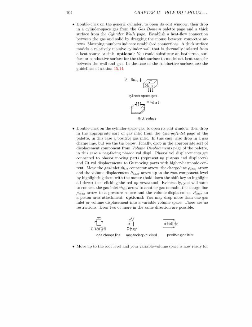
104 CHAPTER 15. HOW DO I MODEL. . .
• Double-click on the generic cylinder, to open its edit window, then dropin a cylinder-space gas from the Gas Domain palette page and a thicksurface from the Cylinder Walls page. Establish a heat-flow connectionbetween the gas and solid by dragging the mouse between connector ar-rows. Matching numbers indicate established connections. A thick surfacemodels a relatively massive cylinder wall that is thermally isolated froma heat source or sink. optional: You could substitute an isothermal sur-face or conductive surface for the thick surface to model net heat transferbetween the wall and gas. In the case of the conductive surface, see theguidelines of section 15.14.
• Double-click on the cylinder-space gas, to open its edit window, then dropin the appropriate sort of gas inlet from the Charge/Inlet page of thepalette, in this case a positive gas inlet. In this case, also drop in a gascharge line, but see the tip below. Finally, drop in the appropriate sort ofdisplacement component from Volume Displacements page of the palette,in this case a neg-facing phasor vol displ. Phasor vol displacements getconnected to phasor moving parts (representing pistons and displacers)and Gt vol displacements to Gt moving parts with higher-harmonic con-tent. Move the gas-inlet mGt connector arrow, the charge-line ρstdy arrowand the volume-displacement Pphsr arrow up to the root-component levelby highlighting them with the mouse (hold down the shift key to highlightall three) then clicking the red up-arrow tool. Eventually, you will wantto connect the gas-inlet mGt arrow to another gas domain, the charge-lineρstdy arrow to a pressure source and the volume-displacement Pphsr toa piston area attachment. optional: You may drop more than one gasinlet or volume displacement into a variable volume space. There are norestrictions. Even two or more in the same direction are possible.
• Move up to the root level and your variable-volume space is now ready for

15.2. A ROTATING MECHANISM 105
connection to other model elements.
Tip: You may drop a charge line component into any gas domain for con-nection to a pressure source. But only one gas domain in an interconnectednetwork of gas domains can have a charge line. Otherwise a solution singularitywill result. Generally, the compression-space gas domain is a good place for thecharge line.
15.2 A Rotating Mechanism
Stirling machine rotating mechanisms are broken down into separate compo-nents representing the flywheel, kinematic linkage and reciprocating piston ordisplacer. This example corresponds to sample file RotMech.stl. See also thecomplete engine example AlphaEngineFlywheel.stl
• From the Gt Moving Parts tab of the Sage form drag a flywheel andsimple-crank linkage into the edit form. Or another type of linkage if youprefer. Then from the Composite tab drag in a free-piston and cylinder(Gt version). Position the components as shown below. The connectorarrows will appear later.
• Double-click on the flywheel, to open its child component edit window,then drop in a pos-facing torque attachment. Move the TGt connectorarrow up to the root component and connect it to the matching connectorin the simple-crank linkage. Similarly, double-click on the simple-cranklinkage, then drop in a pos-facing force attachment. Move the FGt con-nector arrow up to the root component for connection to the reciprocatingmass within the free-piston and cylinder. Before you do that you mustadd a matching connector to that reciprocating mass. Double click on the

106 CHAPTER 15. HOW DO I MODEL. . .
free-piston and cylinder to see the child components within:
• The reciprocater represent a piston or displacer with associated recipro-cating mass. Double-click on it, then drop in a neg-facing attachment anda pos-facing area, moving both connector arrows up to the root level. Inthe root model connect the FGt connector to the simple-crank linkage.The PGt connector arrow remains unconnected in this example. It repre-sents the volume displaced by the reciprocator piston face. In a completestirling machine model it would be connected to a volume displacementin a variable volume space.
15.3 A Regenerator
This example corresponds to sample file regen.stl
• From the component palette of the Sage form, drop an appropriate can-ister component into the edit form, in this case a tubular canister. Theconnector arrows will appear later.
• Double-click on the canister to open its child-component edit-window thendrop in an appropriate matrix component from the Matrices page of thepalette and an appropriate wall-conduction component (optional) fromthe Heat Flows page. In this case the matrix is woven screen and the wall
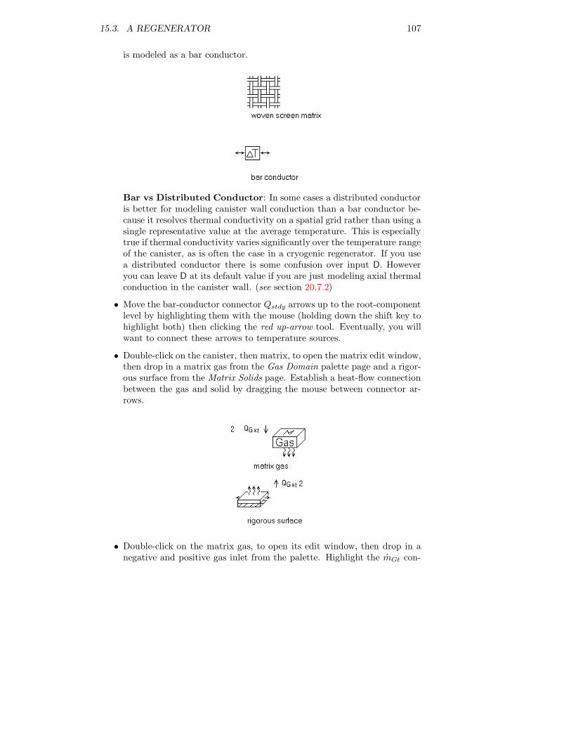
15.3. A REGENERATOR 107
is modeled as a bar conductor.
Bar vs Distributed Conductor: In some cases a distributed conductoris better for modeling canister wall conduction than a bar conductor be-cause it resolves thermal conductivity on a spatial grid rather than using asingle representative value at the average temperature. This is especiallytrue if thermal conductivity varies significantly over the temperature rangeof the canister, as is often the case in a cryogenic regenerator. If you usea distributed conductor there is some confusion over input D. Howeveryou can leave D at its default value if you are just modeling axial thermalconduction in the canister wall. (see section 20.7.2)
• Move the bar-conductor connector Qstdy arrows up to the root-componentlevel by highlighting them with the mouse (holding down the shift key tohighlight both) then clicking the red up-arrow tool. Eventually, you willwant to connect these arrows to temperature sources.
• Double-click on the canister, then matrix, to open the matrix edit window,then drop in a matrix gas from the Gas Domain palette page and a rigor-ous surface from the Matrix Solids page. Establish a heat-flow connectionbetween the gas and solid by dragging the mouse between connector ar-rows.
• Double-click on the matrix gas, to open its edit window, then drop in anegative and positive gas inlet from the palette. Highlight the mGt con-

108 CHAPTER 15. HOW DO I MODEL. . .
nector arrows and move them up to the root-component level by clickingthe red up-arrow tool. Eventually, you will want to connect these arrowsto other gas domains.
Optional: Within the rigorous surface, you could create negative and pos-itive heat-flow ends for axial matrix conduction, then move the resulting Qstdy
connection arrows up to the root-component level for connection to temperaturesources. This would make sense if the ends of your regenerator matrix were ingood thermal contact with some sort of solid conduction paths. Otherwise gasheat transfer will couple internal matrix axial conduction to the enthalpy flowcarried by the gas.
You can model thermal conduction between the matrix rigorous surface andthe canister wall by following the examples for porous matrix heat exchangersin section 15.14.
Tip: Change the names of the components displayed in the edit form to cor-respond with their function, using the Specify|Component Name menu commandwhen the component is highlighted. For example, you might want to changethe generic name tubular canister to regenerator, or whatever. This will helpyou understand the purpose of your model components and is especially usefulwhen there is more than one component present with the same generic name.
15.4 An Isothermal Heat Exchanger
This example corresponds to sample file hxiso.stl
• From the component palette of the Sage form, drag an appropriate heat-exchanger component into the edit form, in this case a tube bundle. Theconnector arrows will appear later.
• Double-click on the tube-bundle to open its child-component edit-windowthen drop in an isothermal surface from the Duct Walls page of the paletteand a duct gas from the Gas Domain page. Establish a heat-flow connec-tion between the gas and solid by dragging between connector arrows. The

15.5. AN INTERNALLY-FINNED HEAT EXCHANGER 109
isothermal-surface temperature distribution becomes that specified for theTinit input variable of the tube bundle.
• Double-click on the duct gas, then drop in a negative and positive gasinlet from the palette. Move the mGt connector arrows up to the root-component and your heat exchanger is now ready for connection to othermodel elements.
15.5 An Internally-Finned Heat Exchanger
This example corresponds to sample file hxfin.stl
• From the component palette of the Sage form, drag a rectangular fins heat-exchanger into the edit form. The connector arrows will appear later.
• Double-click on the rectangular fins to open its child-component edit-window then drop in a conductive surface and line heat source from theDuct Walls page of the palette and a duct gas from the Gas Domainpage. Similarly, within the conductive surface and line heat source, dropin negative and positive heat flow faces from the palette and move the QGx
connector arrows up to the rectangular-fins level. Establish the heat-flowconnections as indicated. The conductive surface represents the metallicconduction path of the fins. Its input D is the fin conduction length andthe fin base temperature is anchored to that of the line-heat-source whichin turn comes from the Tinit input variable of the rectangular fins. See

110 CHAPTER 15. HOW DO I MODEL. . .
section 15.14 for specific geometric examples of the fin conduction path.
• Double-click on the duct gas, then drop in a negative and positive gasinlet from the palette. Move the mGt connector arrows up to the root-component and your heat exchanger is now ready for connection to othermodel elements.
15.6 An Isothermal Matrix Heat Exchanger
Heat exchangers can also be made from canister components. Many variationsare possible. The simplest is this example where the matrix surface is presumedisothermal. This example corresponds to sample file hxpori.stl
• From the component palette of the Sage form, drag an appropriate canisterinto the edit form, in this case a tubular canister. The connector arrowswill appear later.
• Double-click on the canister to open its child-component edit-window thendrop in an appropriate matrix from the Matrices page of the palette, inthis case a random-fiber matrix.
• Double-click on the random-fiber matrix to open its child-component edit-window then drop in an isothermal surface from the Matrix Solids page of
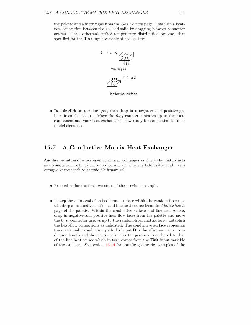
15.7. A CONDUCTIVE MATRIX HEAT EXCHANGER 111
the palette and a matrix gas from the Gas Domain page. Establish a heat-flow connection between the gas and solid by dragging between connectorarrows. The isothermal-surface temperature distribution becomes thatspecified for the Tinit input variable of the canister.
• Double-click on the duct gas, then drop in a negative and positive gasinlet from the palette. Move the mGt connector arrows up to the root-component and your heat exchanger is now ready for connection to othermodel elements.
15.7 A Conductive Matrix Heat Exchanger
Another variation of a porous-matrix heat exchanger is where the matrix actsas a conduction path to the outer perimeter, which is held isothermal. Thisexample corresponds to sample file hxporc.stl
• Proceed as for the first two steps of the previous example.
• In step three, instead of an isothermal surface within the random-fiber ma-trix drop a conductive surface and line heat source from the Matrix Solidspage of the palette. Within the conductive surface and line heat source,drop in negative and positive heat flow faces from the palette and movethe QGx connector arrows up to the random-fiber matrix level. Establishthe heat-flow connections as indicated. The conductive surface representsthe matrix solid conduction path. Its input D is the effective matrix con-duction length and the matrix perimeter temperature is anchored to thatof the line-heat-source which in turn comes from the Tinit input variableof the canister. See section 15.14 for specific geometric examples of the

112 CHAPTER 15. HOW DO I MODEL. . .
matrix conduction path.
The effective matrix conduction length is just 1/4 the canister diameter fora cylindrical canister. Why? The exact solution governing temperature dropfor radial heat flow in a porous circular cylinder with a uniformly distributedsource or sink is:
Q = 8π(1 − β)kL∆T (15.1)
where Q is the total heat flow passing through the outer boundary, (1 − β)kis the effective solid conductivity and L is cylinder length (see [28], example2-3, p. 35). The effective conductivity is written as the product of the solidfraction 1−β (β is porosity) and non-porous conductivity k in a crude attemptto account for the void part of the solid, which is presumed insulating. ∆T isthe outer-boundary temperature minus the cross-section average temperature.
For the conductive-surface model, on the other hand, (see section 20.7.3) they directed temperature drop is governed by
Q = k(As/D)
D/2L∆T (15.2)
where factor As/D is the solid z-thickness and D/2 is the y-directed conductionlength. Equating the two Q’s and canceling obvious factors gives
D2 =As
4π(1 − β)(15.3)
But As/(1− β) is just the total canister cross section area πD2c/4. Making this
substitution givesD = Dc/4 (15.4)
So all one has to do is set the effective conduction length D to 1/4 the canisterdiameter and the y-directed temperature drop in the conductive surface will bea good approximation to the radial temperature drop in the porous solid.
15.8 An External Conduction Path or Busbar
In all the previous examples, the heat exchanger was anchored to an isothermaltemperature distribution modeled by an isothermal surface or line heat source.

15.8. AN EXTERNAL CONDUCTION PATH OR BUSBAR 113
Sometimes it is desirable to replace the isothermal component with a solid con-duction path to an external temperature source or sink at the root-componentlevel. This conduction path might be a physical part of the model, such asthe canister wall in a porous-matrix heat exchanger. It might also be a ficti-tious component introduced solely for convenience, a thermal busbar if you will.Whatever it is, it can simplify energy-flow accounting by forcing all heat flowsto terminate in a point temperature source at the root level and it is possibleto optimize or map that temperature through a single variable.
The idea is illustrated here as a modification to the above internally-finnedheat-exchanger example. This example corresponds to sample file busbar.stl
• Proceed as for the first step of internally-finned heat-exchanger example.
• In step two, instead of the line heat source within the rectangular fins,drop in a distributed conductor from the Duct Walls page of the palette.Within the distributed conductor, drop in a negative (or positive) heat-flow end and a positive heat flow face from the palette. Move the Qstdy
connector arrow from the heat-flow end up to the root-component levelfor connection there to a point temperature source or sink. Move the QGx
connector arrow from the heat-flow face up to the random-fiber matrixlevel and establish the heat-flow connection to the conductive surface asindicated.
• Input variable W of the distributed conductor should be set to the perime-ter in contact with the heat exchanger — the heat-exchanger circumfer-ence in a cylindrical arrangement. (See specific examples in section 15.14)Input variable D is the busbar thickness — the radial depth in a cylin-drical arrangement. Input variable Solid is the busbar material. Cop-per gives the least temperature drop. Heat-flow in the above example istwo-dimensional changing from the y-direction at the conductive-surfaceinterface to the x-direction along the busbar to the ultimate source orsink.
• Optional: You could also replace the heat-flow end of the distributedconductor with a negative heat flow face for connection to an isothermal
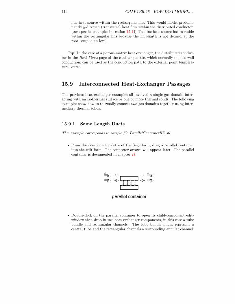
114 CHAPTER 15. HOW DO I MODEL. . .
line heat source within the rectangular fins. This would model predomi-nantly y-directed (transverse) heat flow within the distributed conductor.(See specific examples in section 15.14) The line heat source has to residewithin the rectangular fins because the fin length is not defined at theroot-component level.
Tip: In the case of a porous-matrix heat exchanger, the distributed conduc-tor in the Heat Flows page of the canister palette, which normally models wallconduction, can be used as the conduction path to the external point tempera-ture source.
15.9 Interconnected Heat-Exchanger Passages
The previous heat exchanger examples all involved a single gas domain inter-acting with an isothermal surface or one or more thermal solids. The followingexamples show how to thermally connect two gas domains together using inter-mediary thermal solids.
15.9.1 Same Length Ducts
This example corresponds to sample file ParallelContainerHX.stl
• From the component palette of the Sage form, drag a parallel containerinto the edit form. The connector arrows will appear later. The parallelcontainer is documented in chapter 27.
• Double-click on the parallel container to open its child-component edit-window then drop in two heat exchanger components, in this case a tubebundle and rectangular channels. The tube bundle might represent acentral tube and the rectangular channels a surrounding annular channel.
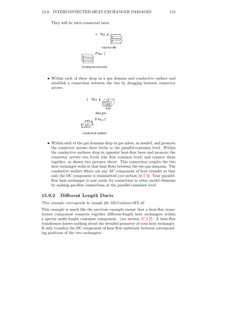
15.9. INTERCONNECTED HEAT-EXCHANGER PASSAGES 115
They will be inter-connected later.
• Within each of these drop in a gas domain and conductive surface andestablish a connection between the two by dragging between connectorarrows.
• Within each of the gas domains drop in gas inlets, as needed, and promotethe connector arrows three levels to the parallel-container level. Withinthe conductive surfaces drop in opposite heat-flow faces and promote theconnector arrows two levels (the first common level) and connect themtogether, as shown two pictures above. This connection couples the twoheat exchanger walls so that heat flows between the two gas domains. Theconductive surface filters out any AC component of heat transfer so thatonly the DC component is transmitted (see section 20.7.3). Your parallel-flow heat exchanger is now ready for connection to other model elementsby making gas-flow connections at the parallel container level.
15.9.2 Different Length Ducts
This example corresponds to sample file MLContainerHX.stl
This example is much like the previous example except that a heat-flux trans-former component connects together different-length heat exchangers withina special multi-length container component. (see section 27.2.2). A heat-fluxtransformer knows nothing about the detailed geometry of your heat exchanger.It only transfers the DC component of heat flow uniformly between correspond-ing positions of the two exchangers.

116 CHAPTER 15. HOW DO I MODEL. . .
• From the component palette of the Sage form, drag a multi-length con-tainer into the edit form. The connector arrows will appear later.
• Double-click on the multi-length container to open its child-componentedit-window then drop in two heat exchanger components, in this casetwo tube bundles, one representing a straight central tube and the other alonger outer tube spiral-wrapped around the outside. The lengths are inde-pendent inputs for each tube bundle. Also drop in a heat-flux transformerfrom the basic page of the component palette. The heat flux transformeris born with two QGx heat-connection arrows. The arrows attached to thetwo tubes will be promoted from conductive surfaces within.
• Within each of the tube bundles drop in a gas domain and conductivesurface with gas inlets and heat-flow faces as in the previous example.Promote the heat-flux connection arrows to the same level as the heat-flux transformer and connect them together, as shown above. Promote thegas-flow connection arrows up to the multi-length heat exchanger level forsubsequent connection to other model elements.
15.10 A Piston with Seal Leakage
A stand alone piston can be modeled with one of the piston components in theMoving Parts page of the component palette. To model the combination of apiston and seal leakage, use one of the components on the Composite page. Thisexample corresponds to sample file piscyl.stl

15.10. A PISTON WITH SEAL LEAKAGE 117
• From the Composite page in the component palette of the Sage form, dropan appropriate piston/cylinder component into the edit form, in this casea constrained piston and cylinder. The connector arrows will appear later.
• Double-click on the piston and cylinder to open its child-component edit-window, revealing three built-in child components: the cylinder liner, pis-ton shell and constrained piston. The normal purpose of the liner andshell components is to model thermal conduction. But the presumptionof this example is that there is no significant temperature gradient alongthe shell and liner so that thermal conduction is negligible. That beingthe case the shell and liner inputs are irrelevant and may be left at theirdefault values. From the Inter-Gap page of the palette, drop in an op-tional annulus and re-name it “clearance seal”. Child components withinthis component will model the actual gas leakage. The component itselfestablishes the radial gap between shell and liner and also models shut-tle heat transfer between the liner and shell, which is implemented bythe built Qstdy connector arrows. For this example you can move theseconnector arrows up to the root-component level for connection there tothe same temperature source, consistent with the assumption of negligibletemperature gradient within the seal.
• Within the seal, drop in a matrix gas and an isothermal surface and con-nect them. The isothermal surface anchors the gas temperature in theseal in this example. An isothermal surface is recommended because it iseasiest to implement, well behaved from a solution convergence point of

118 CHAPTER 15. HOW DO I MODEL. . .
view and there is usually a negligible amount of heat transferred in theseal anyway. For more realism or other reasons you can instead anchorthe gas with a conductive surface, following the geometric guidelines ofsection 15.14.
Within the matrix gas drop in negative and positive gas inlets. Move thetwo mGt connector arrows up to a higher level for connection there to thetwo gas domains at either end of the leak path.
• Within the constrained piston drop in positive and negative facing areaattachments and move the Pphsr connector arrows up to a higher level forconnection there to variable-volume gas domains, such as the expansionand compression spaces.
• Optional: Within the constrained piston drop in positive and negativefacing force attachments for connection to other moving parts and movethe Fphsr connector arrows up to the appropriate level.
15.11 A Displacer and Cylinder
Like a piston, a stand alone displacer can be modeled with one of the pistoncomponents in the Moving Parts page of the component palette. To model adisplacer moving within a cylinder, use one of the components on the Compositepage. The main distinction between a piston and a displacer in these examples isthat a displacer generally has a significant temperature gradient along its lengthso that shuttle heat transfer and solid conduction down the cylinder liner andpiston shell are important. This example corresponds to sample file discyl.stl
• From the Composite page in the component palette of the Sage form, dropan appropriate piston/cylinder component into the edit form, in this case

15.11. A DISPLACER AND CYLINDER 119
a constrained piston and cylinder. The connector arrows will appear later.
• Double-click on the piston and cylinder to open its child-component edit-window, revealing three built-in child components: the cylinder liner, pis-ton shell and constrained piston. From the Inter-Gap page of the palette,drop in an optional annulus whose purpose in this case is to model shuttleheat transfer between the liner and shell. Move the annulus Qstdy connec-tor arrows up to the root-component level for connection there to pointtemperature sources.
• Within the cylinder liner (double-click), drop in a bar conductor (or dis-tributed conductor) from the Heat Flows page of the component paletteand move the Qstdy connector arrows up to the root-component level forconnection there to point temperature sources. See the discussion in sec-tion 15.3 regarding bar vs distributed conductors.
• Similarly, within the piston shell, drop in a bar conductor (or distributedconductor) for purposes of modeling thermal conduction and a radiationtransport path for modeling radiation heat transfer down the presumablyhollow shell. Move the Qstdy connector arrows up to the root-componentlevel.
• Within the constrained piston drop in positive and negative facing areaattachments and optional force attachments as in the previous piston-and-leakage example.

120 CHAPTER 15. HOW DO I MODEL. . .
15.12 A Regenerative Displacer and Cylinder
In stirling refrigerators, the displacer often houses the regenerator. This examplecorresponds to sample file disreg.stl
• Proceed as for the previous displacer and cylinder example, except omit-ting the radiation transport path within the piston shell.
• Within the piston shell drop in a matrix from the Matrices page of thepalette, in this case a woven screen matrix.
• At this point proceed as for the previous regenerator example, except thatthe regenerator is now contained in the piston-shell canister instead of astand-alone canister at the root-component level.
• Set the displacer area attachments based on the frontal areas of the dis-placer shell the same as though the displacer were impervious. Effectivelythe regenerator matrix is modeled as a parallel gas-flow path even thoughit is physically within the displacer shell.
15.13 Displacer Appendix and Seal Leakage
Like the earlier example of a piston leak, this example considers the gas flow inthe annular region between the displacer shell and cylinder liner. In addition toan isothermal seal part there is an annular “appendix” as well, in general, havinga larger gap and significant temperature gradient. This example corresponds tosample file disleak.stl
• Proceed as for either previous displacer and cylinder example, in this casethe displacer-and-cylinder example.
• Within the displacer and cylinder, rename the existing annulus as “seal”and drop in a second annulus, renamed “appendix”. The seal and ap-pendix model the two parts of the displacer leak in series. The relativepositions of the seal and appendix are defined by their XNeg and XPosinput variables and their radial gaps by the Gap input variable. To cor-rectly model shuttle heat transfer, connect the Qstdy arrows between theseal and appendix and move the arrows at the far ends up to the root-
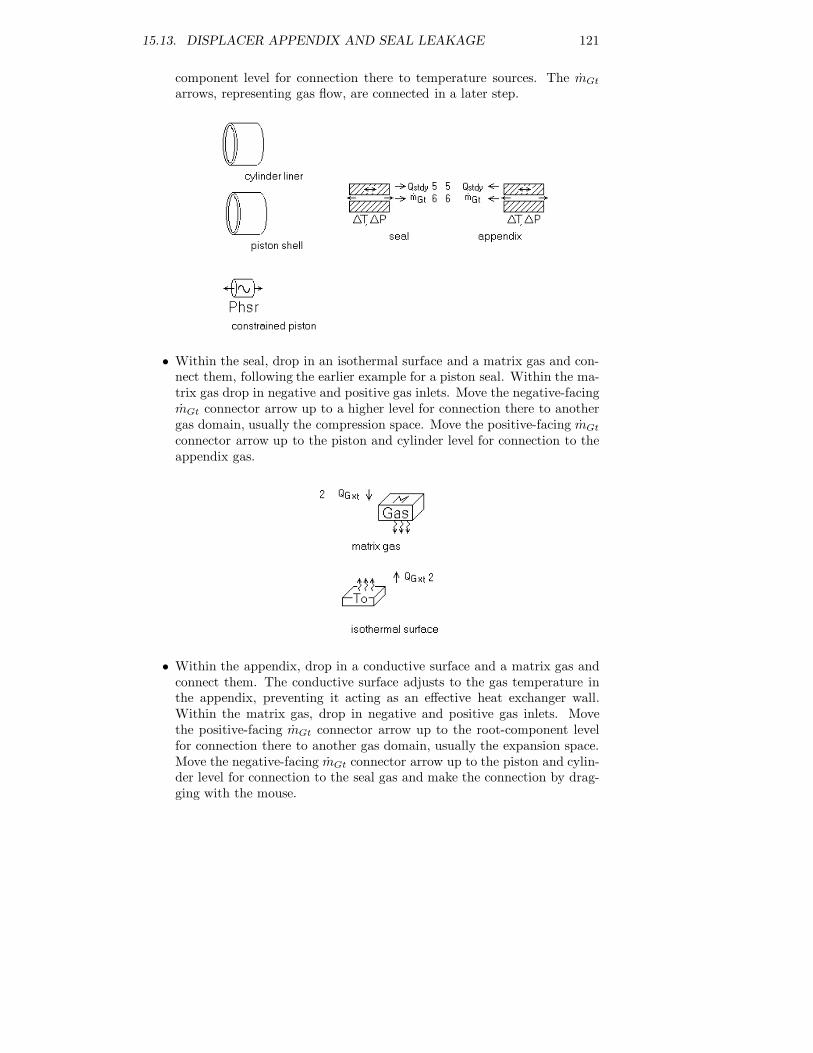
15.13. DISPLACER APPENDIX AND SEAL LEAKAGE 121
component level for connection there to temperature sources. The mGt
arrows, representing gas flow, are connected in a later step.
• Within the seal, drop in an isothermal surface and a matrix gas and con-nect them, following the earlier example for a piston seal. Within the ma-trix gas drop in negative and positive gas inlets. Move the negative-facingmGt connector arrow up to a higher level for connection there to anothergas domain, usually the compression space. Move the positive-facing mGt
connector arrow up to the piston and cylinder level for connection to theappendix gas.
• Within the appendix, drop in a conductive surface and a matrix gas andconnect them. The conductive surface adjusts to the gas temperature inthe appendix, preventing it acting as an effective heat exchanger wall.Within the matrix gas, drop in negative and positive gas inlets. Movethe positive-facing mGt connector arrow up to the root-component levelfor connection there to another gas domain, usually the expansion space.Move the negative-facing mGt connector arrow up to the piston and cylin-der level for connection to the seal gas and make the connection by drag-ging with the mouse.

122 CHAPTER 15. HOW DO I MODEL. . .
The conductive surface within the appendix inherits solid material andcross-sectional area information from the cylinder liner and piston shell.So you can and should use it to model the axial conduction in the appendixliner and shell. To do this just drop negative and positive heat-flow endsinto the distributed conductor and move their Qstdy arrows up to theroot component level for connection there to temperature sources. Theconduction so modeled corresponds to that in the combined cylinder linerand piston shell over that portion of the length specified by the XNeg andXPos input variables.
NOTE: When modeling appendix wall conduction this way do not alsouse bar conductors within the cylinder liner or piston shell to do the samething. You do not want to model the same conduction paths twice.
Tip: Use at least 2 cells (NCell) in the seal component lest frictional pressuredrop not be modeled.
15.14 Thermal Conductors in Heat Exchangers
Some of the previous examples used the conductive surface and distributed con-ductor components for modeling solid thermal conduction paths in heat ex-changers. Applying these examples to actual heat exchanger geometries hasoften been a point of confusion because it is not always clear which dimensionsin the actual geometry correspond to the inputs of the Sage model.
This section attempts to shed more light on the matter by showing a numberof specific heat exchanger cross-sections with appropriate dimensions for equiv-alent Sage components noted below each one. Before getting into that, somegeneral guidelines:
15.14.1 Guidelines
First, keep in mind that you do not always need to use thermal conductorswithin heat exchangers. You can just anchor the gas component within the heatexchanger directly to a line heat source, as many of the previous examples do,which then provides an isothermal surface boundary condition at the specified
15.14. THERMAL CONDUCTORS IN HEAT EXCHANGERS 123
temperature. This approach effectively puts any parts of the heat exchangerbeyond the wetted gas surface outside the scope of the Sage model.
When you do need to model solid conduction paths think of them this way:The conductive surface within a heat exchanger models the solid material whosesurface exchanges heat directly with the gas within the heat exchanger while thedistributed conductor allows you to model a secondary solid conduction path rep-resenting a container wall or other structure outside the primary heat exchangermaterial. Both components have an input D which specifies the distance alongthe direction of heat flow through the solid cross section. D only matters inthe event the distributed conductor is thermally connected along its length. Ifonly connected at the ends then the solid cross-section area by itself governsheat flow, independent of D. When possible, both components calculate theircross-section area based on information inherited from their parent component.The exception is a stand-alone distributed conductor used for a secondary con-duction path which requires a second input W and calculates cross-section areaas the product W × D. You can find a detailed discussion of Sage’s thermalconductor components in chapter 20.
15.14.2 Tubes with Conductive Walls
These examples below are for heat exchanger comprising individual tubes whereyou want to model the heat transfer (and temperature drop) across the tubewall to an external medium or axial heat flows within the tube walls to a sourceor sink at either end. They are one step more complicated than the isothermalheat exchanger example in section 15.6. You might, for example, connect theouter tube walls (conductive surface QGx connectors) to an isothermal line heatsource to represent the temperature of a secondary heat transfer fluid, althoughthe examples do not show that. Or you might make a connection to the wallsof another heat exchanger component, as shown in section 15.9.

124 CHAPTER 15. HOW DO I MODEL. . .

15.14. THERMAL CONDUCTORS IN HEAT EXCHANGERS 125
15.14.3 Drilled Hole Heat Exchangers
Imagine individual tubes with combined wall cross-sections swaged together intoa single contiguous solid conduction path. That is the idea behind using Sage’stube-bundle component to model drilled holes in a block of solid conductivematerial. The parent tube diameter, wall thickness and tube number inputsproduce a total solid cross section area given by equation (23.31) of chapter 23.You need to specify wall thickness to make this total solid cross section (heatexchanger output Asec) come out right. Either by hand or automatically byrecasting input Twall in terms of actual solid area, Am, which to equal the solid

126 CHAPTER 15. HOW DO I MODEL. . .
area calculated by Sage must satisfy
Am = nπ
4
((di + 2tw)2 − d2
i
)(15.5)
where n is tube number, di tube inner diameter and tw wall thickness. Solvingthis for wall thickness requires that
tw =1
2
(√
d2i +
4Am
nπ− di
)
(15.6)
The examples below illustrate several possible arrangements of drilled-hole heatexchangers. For the cylindrical case see the explanation in section 15.7 for whythe matrix conductive surface D input should be half the radius.

15.14. THERMAL CONDUCTORS IN HEAT EXCHANGERS 127
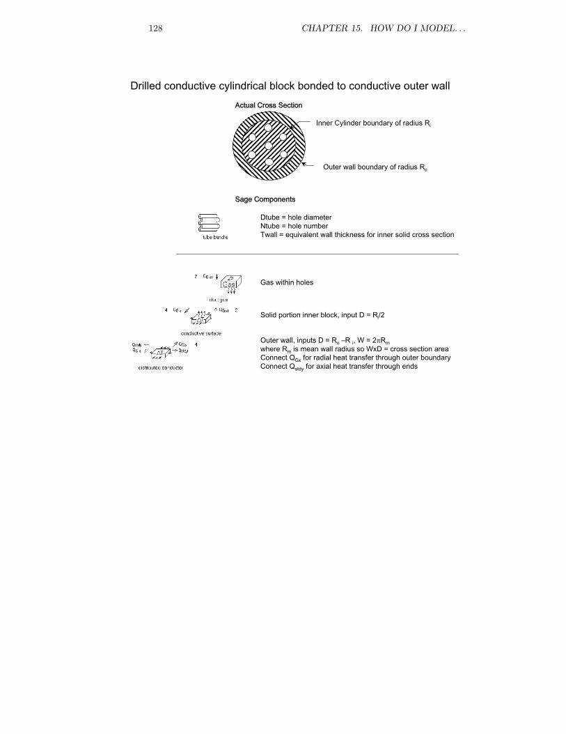
128 CHAPTER 15. HOW DO I MODEL. . .

15.14. THERMAL CONDUCTORS IN HEAT EXCHANGERS 129
15.14.4 Rectangular Finned Heat Exchangers
The rectangular-fins component can model heat exchangers comprising radialrectangular channels cut in a conductive material. The parent channel height,fin thickness and channel number inputs produce a total solid cross sectionarea given by equation (23.56) of chapter 23. Again, you need to specify finthickness (input Tfin) to make the total solid cross section calculated by Sage(output Asec) equal the actual solid area Am. This will be so when
tf =Am
nhi(15.7)

130 CHAPTER 15. HOW DO I MODEL. . .
where tf is fin thickness, n is the number of channels and hi is the channelheight. The examples below illustrate only the annular variations of this typeof heat exchanger.

15.14. THERMAL CONDUCTORS IN HEAT EXCHANGERS 131
15.14.5 Porous Matrix Heat Exchangers
In the example of section 15.7 conductive screens were anchored to a line heatsource. The conductive matrix (screens, random fibers or packed spheres) canalso be anchored to the wall(s) of a conductive canister. The modeling is a bitdifferent from the above heat-exchanger examples because the porous-matrixmodel components are not stand-alone components but rather reside only withincanister components. This means you do not have to calculate an equivalenttube wall or fin thickness according to overall solid cross section. The porosityinput takes care of that.
The examples below illustrate cylindrical and annular variations of porous

132 CHAPTER 15. HOW DO I MODEL. . .
matrix heat exchangers. Generally you will want to connect the conductivesurface representing the matrix itself to the distributed conductor representingthe canister wall by moving the QGx connector for the conductive surface upone level. The examples mention this possibility but do not specifically show it.It does not matter if you use negative-facing or positive-facing QGx connectorsfor this purpose. Use whichever fits your mental image of the geometry.
Annular Confusion
For the annular case there is some confusion because a single distributed con-ductor represents both inner and outer canister walls. This is fine for modelingaxial conduction. The confusion sets in for radial conduction because the in-ward direction for the inner wall and the outward direction for the outer wallcorrespond to the same direction in the distributed conductor. Some mentalunwrapping is required. It is least confusing if you are willing to assume thatonly one of the two walls is thermally connected to the matrix (QGx connection)and the other insulated. In that case you are justified in setting the insulatedwall thickness to a very-small value, perhaps including it in another componentof your overall model for purposes of calculating axial conduction (e.g. an innerregenerator wall modeled as a displacer cylinder wall). Then you should setdistributed conductor input D to the thickness of the active wall.
If both walls are thermally connected to the matrix, then for the model tomake sense, both must be connected to the same external temperature sourceor sink with a single QGx connection, reserving the opposite-facing connectionfor connecting to the matrix. In that case set distributed conductor input D tosome representative mean value for the two wall thicknesses.
The value of conductive surface input D, representing the matrix conductionpath length, also differs for the two cases, as noted in the example. When thematrix conducts heat to both walls the actual radial conduction path is roughlyhalf as long as when conducting heat to only one wall, depending on the exactlocation of the point where radial heat flow reverses direction. So you shouldset D half as long as well.

15.14. THERMAL CONDUCTORS IN HEAT EXCHANGERS 133
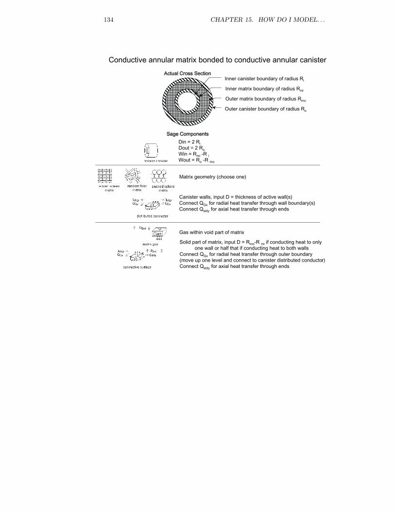
134 CHAPTER 15. HOW DO I MODEL. . .

Chapter 16
Boundary Connections
Stirling model components communicate with each other using the followingboundary connections. As usual you may only connect together like connectorsof opposite sign (opposite-facing arrows).
16.1 Force Connections
Fphsr or FGt
These represent either phasor or time ring forces acting on points of attachment.The points of attachment will share the same motion when connected together.Force connections are used primarily for connecting springs and dampers tomoving parts, as in the Gizmo (resonant system) model class documented inchapter 12.
16.2 Pressure Connections
Pphsr or PGt
These represent either phasor or time ring pressure variations acting on areafaces. The area faces share the same volume displacement when connectedtogether. They are used primarily for connecting pistons and the like to gasdomains.
16.3 Heat Flow Connections
Qstdy, QGx or QGxt
These represent either steady, spatial grid, or space-time grid heat flows actingon thermal boundaries. Boundaries share the same temperature when connectedtogether. Steady heat flows are useful for time-averaged parasitic conductionlosses. Spatial grid heat flows are useful for steady but distributed heat flows,
135

136 CHAPTER 16. BOUNDARY CONNECTIONS
such as occurs two dimensional fins. Space-time heat flows are for connectingthermal solids to gas domains.
16.4 Gas Flow Connections
mGt
These represent the flow of gas from one gas domain inlet into another. Twoinlets conserve mass flow rate, energy and momentum when connected together.
16.5 Density Connections
ρstdy
This represents the common mass density between a gas domain and a pressurereservoir. The two share the same mean pressure when connected together.Density connections are used to connect the stirling working gas to a fixed-pressure source in order to establish charge pressure. This connection type isgenerally used only once per stirling model instance, but its use is criticallyimportant.
16.6 Electrical Current Connections
IGt
These represent the flow of electrical current from one electrical component intoanother. Electrical boundaries share the same voltage when connected together.
16.7 Magnetic Flux Connections
φGt
These represent the flow of magnetic flux from one magnetic component into an-other. Magnetic boundaries share the same magnetic potential when connectedtogether.

Chapter 17
Entropy Generation
Many stirling model components involve irreversible entropy-generating pro-cesses and keep tabs of entropy generation in terms available energy outputvariables. Available energy or availability for short is just entropy multipliedby the negative of ambient temperature T0, which is really just input Tnorm inthe stirling root model component. A loss in availability equates to a decrease(in an engine) or increase (in a cooler) of PV power.
17.1 Lost Available Energy
The concept of availability arises from the net mechanical work Wr availablefrom a reversible heat engine with a net inflow of heat Q (positive) at a tem-perature T and outflow Q0 (negative) at a sink temperature T0:
Wr = Q+Q0 = Q(1 − T0/T ) (17.1)
In contrast, an irreversible-cycle might produce work Wi < Wr obtained fromthe same input Q. According to the first law of thermodynamics, and in termsof heat rejected Q∗
0
Wi = Q+Q∗0 (17.2)
where Q∗0 is no longer equal to −QT0/T . The lost available energy is just
Wr −Wi = −QT0/T −Q∗0 = −T0(Q/T +Q∗
0/T0) (17.3)
Evidently, this is just −T0 times the net entropy increase of the surroundinguniverse as a result of the heat flows into and out-of the system. This leads usto generally characterize all internal entropy generations in the stirling modelclass in terms of losses in availability according to the definition
Availability Loss = −T0 × Entropy Generation (17.4)
The value of the availability-loss concept is that it allows us to think aboutentropy generation in terms of the more concrete notion of lost mechanicalwork.
137

138 CHAPTER 17. ENTROPY GENERATION
It is important to note that availability losses vary with the sink temperatureT0, which is given by input variable Tnorm in the stirling root model component.Therefore, availability losses really equate to lost PV powers only when all pointsof heat rejection are indeed at the temperature Tnorm. See reference [4] for astandard treatment of available-energy accounting.
17.2 Second-Law Balance
Entropy generation (or available energy loss) may be measured in one of twoways: by entropy flow across the external boundaries of a stirling model instanceor by entropy generated by internal processes. The previous example accountsfor entropy generation in the first way. The surrounding universe suffers a loss ofavailable energy due to heat flow through the boundaries of a stirling machine.When we get specific about individual stirling model components we will alsobe able to account for entropy generation in the second way — by tallying upthe individual entropy generations in all internal processes.
In principle, the two methods of accounting should give the same answer.But often they do not. This is because there is no conservation-of-entropy-generation principle built into the stirling model components, as there is forconservation of energy. Discrepancies arise, usually attributable to numeri-cal artifacts in the computational solution. These include finite-differencingtruncation errors, for both spatial and temporal partial derivatives, as wellas interpolation errors needed to obtain solution variables at off-solution gridpoints. So model components that tally available energy losses generally havean available-energy discrepancy output, as well, that monitors the differencebetween external-boundary and internal-process accounting.
It is tempting to look at the relative magnitude of the availability accountingdiscrepancy as a measure of the solution accuracy. Large discrepancies may beproduced by difficult to model features such as heat exchangers with highlynonlinear axial temperature distributions, large pressure ratios, etc. In suchcases it is usually helpful to refine the computational grid — that is, add moretime nodes (NTnode) or more control volumes (NCell).

Chapter 18
Stirling Root Component
The highest level stirling model component, and the only model component yousee when you create a new model instance, is the root model. Its purpose is todefine a few global variables and some normalization constants as a frameworkfor all its children which you create, or someone created before, by selectingfrom the component palette. Its variables are:
NTnode : (dimensionless) The number of time nodes in the computational gridsof all underlying model components having such grids. NTnode is impor-tant because it dramatically affects the solution time and memory require-ments, not to mention solution accuracy. Treat it gingerly by making onlygradual, small changes. Changing this variable re-creates all time grids inthe model and initializes solution values by interpolating between solvedvalues of the previous grid.
You can get an idea if the solution grid is too coarse (NTnode too small) byinspecting the various Fourier series output variables produced by individ-ual model components. If the highest harmonic is not small compared tothe lower harmonics then you might want to increase NTnode to improvesolution accuracy. You should also increase it to an odd number becauseNTnode must be odd to resolve the mean value plus both componentsof all harmonics available in the grid. When NTnode is even the highestharmonic is not fully determined. This leads to finite differencing errorsin addition to the inaccuracy produced by not resolving all the significantharmonics in the solution.
It is a good idea to always set NTnode to an odd value, although evenvalues are allowed by Sage. When NTnode is odd the highest harmonicavailable in the grid is (NTnode - 1) / 2.
Lnorm : (real, m) Length scale normalization constant. The value of this inputmay make the difference between a solution that converges and one thatdoesn’t. As a rule of thumb, Lnorm should be, roughly, the cube root of thelargest swept volume amplitude in the underlying stirling model. Some
139
140 CHAPTER 18. STIRLING ROOT COMPONENT
fiddling around may be required to achieve optimal solution convergencerate. Keep in mind that a small change may have a big effect, since manyquantities are normalized by the cube of Lnorm.
FreqNorm : (real, Hz) Frequency scale normalization constant. This one is notas critical as Lnorm. Generally, set it to the actual operating frequencyFreq. It is a separate constant because Freq may change during optimiza-tion.
Pnorm : (real, Pa) Pressure scale normalization constant. Again, not as criticalas Lnorm, but important because it establishes the initial pressure in allunderlying gas domains. It should be close to the charge pressure Pchargein the pressure-source component. Otherwise, the pressure solutions ingas domains may go unstable.
Tnorm : (real, K) Temperature scale normalization constant. Usually the am-bient temperature, or about 300 K. Keep in mind that it scales availableenergy outputs in certain model components (see chapter 17).
Qnorm : (real, W) Heat flow normalization constant. Generally, set it to themagnitude of the total heat rejection expected for the stirling model. In-creasing Qnorm can sometimes help a solution converge when the conver-gence error is hovering near the target error and the problem is due tosurface heat flux stiffness (small temperature fluctuation producing largeheat flux fluctuation) as can happen, for example, with a particularlyeffective regenerator matrix.
Freq : (real, Hz) The actual operating frequency for the stirling machine. Al-though it is set as an input, it may be optimized to satisfy an objectivefunction or constraints.
Omega : (real, radians/s) A convenience output that converts Freq to angularfrequency by multiplying by 2π.
Gas : (enumerated) The working gas type (see below).
18.1 Working Gas
The gas variable is deceptively simple. It is an enumerated-type variable thatselects the working gas from a list of choices. Each available gas is itself asoftware object with sufficient data encapsulated within it to know its importantproperties.
ideal If the gas is an ideal gas, these properties are:
T0 : (K) Representative temperature T0.
Rgas : (J/(kg K)) Gas constant R.
18.1. WORKING GAS 141
Specific heat : (J/(kg K)) A cubic spline variable with temperature vszero-pressure specific heat (T, cp(T )) data pairs covering a broadrange of temperatures.
Viscosity : (kg/(m s)) A cubic spline variable with temperature vs viscos-ity (T, µ(T )) data pairs.
Conductivity : (W/(m K)) A cubic spline variable with temperature vsconductivity (T, k(T )) data pairs.
Redlich-Kwong If it is a Redlich-Kwong gas then it has additional properties:
Tcrit : (K) Critical temperature Tc
Pcrit : (Pa) Critical pressure Pc
C1 : (dimensionless) Redlich-Kwong constant c1
C2 : (dimensionless) Redlich-Kwong constant c2
BVirialErr : (dimensionless) Overall RMS error B in the second virialcoefficient.
tabular If it is a tabular gas then a table of state values takes the place ofRedlich-Kwong properties.
Z(v, T) : (dimensionless) a rectangular table of Z(vj , Tk) values whereZ = Pv/RT is compressibility, v is specific volume and T is tem-perature. The first (left) column contains the Tk values and the first(top) row the vj values. The corresponding Z values lie in the bodyof the table.
The values of the individual properties, including cubic-spline interpolationpairs or state table, appear after the enumerated identifier in display windowsand the output listing. The gas choices come from a default database file gas.dta,or a data base file customized by you. (see chapter 28)
An instance of a gas object has methods (subroutines) that can be calledupon to return various properties, as functions of temperature, or various statevariables, as functions of other state variables. The underlying gas-domainmodel components call upon these methods when needed. Sometimes, thisrequires only cubic-spline interpolation using the appropriate set of data pairs.Sometimes, it gets a little more complicated.
18.1.1 Conductivity k(T ) and Viscosity µ(T )
All gas objects calculate conductivity and viscosity from cubic-spline interpo-lation as a function of T , without any pressure dependence. In most cases,ignoring pressure dependence is reasonable. Even when it is not reasonable, itwill cause no great harm because k and µ are only used for calculating suchthings as Reynolds, Valensi and Prandtl numbers which, in turn, are used forcalculating viscous friction, surface heat transfer and axial gas conduction. And

142 CHAPTER 18. STIRLING ROOT COMPONENT
correlating expressions for such phenomena are not extremely accurate in thefirst place.
One way to achieve some pressure dependence would be to insert additionalgases into a customized database file, each one a reasonably good approximationin some pressure range. For example, you might define gas named “TabularHelium 5 MPa”, valid only in the vicinity of 5 MPa, and so forth.
18.1.2 Ideal Gas Objects
As the name implies, ideal-gas objects presume the ideal gas equation of state
Pv = RT (18.1)
Available methods are presented below in functional notation. For example,cp(T ) is the heading for the method that returns cp as a function of T .
Specific Heat Ratio γ
This is actually a data field, not a method, initialized as
γ =1
1 − R/cp(18.2)
where cp is the zero-pressure limit at reference temperature T0. This is theonly reason for the existence of T0 as a data field. It is important that γ be aconstant, rather than a function of T , because internal energy and entropy bothdepend on γ (cv = R/(γ − 1)) as does sonic velocity.
Specific Heat cp(T )
Zero-pressure cp limit, that is. This is just a matter of cubic-spline interpolationfrom the specific-heat data pairs.
Prandtl Number Pr(T )
Calculated as a function of temperature as Pr = k/(µcp).
Viscosity µ(T )
Molecular viscosity interpolated from viscosity-temperature data pairs.
Conductivity k(T )
Molecular conductivity interpolated from conductivity-temperature data pairs.
Sonic Velocity us(T )
Returns the isentropic, small amplitude, phase velocity of an acoustical wave
us =√
γRT (18.3)

18.1. WORKING GAS 143
Compressibility Z(T, P )
Returns compressibility, defined as
z =Pv
RT(18.4)
which equals one, by definition, for an ideal gas.
Temperature T (ρ, ρe, u)
Returns temperature as function of mass density, volume-specific energy densityand velocity
T =γ − 1
R
((ρe)/ρ− u2/2
)(18.5)
Pressure P (ρ, T )
Returns pressure as function of mass density and temperature
P = ρRT (18.6)
Energy Density ρe(ρ, T, u)
Returns volume-specific energy density as function of mass density, temperatureand velocity
ρe = ρ(R/(γ − 1)T + u2/2
)(18.7)
where R/(γ − 1) = cv.
Entropy s(ρ, T )
Returns mass-specific entropy as function of mass density and temperature
s = R (ln(T )/(γ − 1) + ln(1/ρ)) (18.8)
Equation of State Error Z(ρ, T )
Returns zero because the ideal equation of state relative error is zero by as-sumption.
18.1.3 Redlich-Kwong Gas Objects
Redlich-Kwong gas objects employ the real-gas equation of state by the samename. They were originally intended for use in low-temperatures cryocoolersand high pressures engines where ideal gas properties no longer apply. But sub-sequent development of so-called tabular gas objects (tabulated state properties)has essentially eliminated the need for Redlich-Kwong gases. Tabular gas objectscontain more accurate gas properties with negligible impact on computationalperformance. So the use of Redlich-Kwong gases is no longer recommended butthey are still documented here for completeness.
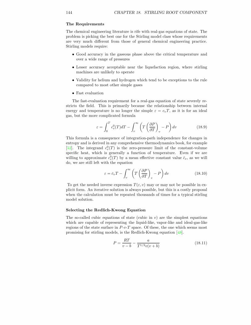
144 CHAPTER 18. STIRLING ROOT COMPONENT
The Requirements
The chemical engineering literature is rife with real-gas equations of state. Theproblem is picking the best one for the Stirling model class whose requirementsare very much different from those of general chemical engineering practice.Stirling models require:
• Good accuracy in the gaseous phase above the critical temperature andover a wide range of pressures
• Lesser accuracy acceptable near the liquefaction region, where stirlingmachines are unlikely to operate
• Validity for helium and hydrogen which tend to be exceptions to the rulecompared to most other simple gases
• Fast evaluation
The fast-evaluation requirement for a real-gas equation of state severely re-stricts the field. This is primarily because the relationship between internalenergy and temperature is no longer the simple ε = cvT , as it is for an idealgas, but the more complicated formula
ε =
∫ T
0
c0v(T )dT −∫ ∞
v
(
T
(∂P
∂T
)
v
− P
)
dv (18.9)
This formula is a consequence of integration-path independence for changes inentropy and is derived in any comprehensive thermodynamics book, for example[52]. The integrand c0v(T ) is the zero-pressure limit of the constant-volumespecific heat, which is generally a function of temperature. Even if we arewilling to approximate c0v(T ) by a mean effective constant value cv, as we willdo, we are still left with the equation
ε = cvT −∫ ∞
v
(
T
(∂P
∂T
)
v
− P
)
dv (18.10)
To get the needed inverse expression T (ε, v) may or may not be possible in ex-plicit form. An iterative solution is always possible, but this is a costly proposalwhen the calculation must be repeated thousands of times for a typical stirlingmodel solution.
Selecting the Redlich-Kwong Equation
The so-called cubic equations of state (cubic in v) are the simplest equationswhich are capable of representing the liquid-like, vapor-like and ideal-gas-likeregions of the state surface in P -v-T space. Of these, the one which seems mostpromising for stirling models, is the Redlich-Kwong equation [48].
P =RT
v − b− a
T 1/2v(v + b)(18.11)

18.1. WORKING GAS 145
Parameter b pertains to the volume of the molecules and a to the forces ofcohesion between them. They are typically given as
a = c1R2T 2.5
c
Pc(18.12)
b = c2RTc
Pc(18.13)
where c1 = 0.42748 and c2 = 0.08664, which are derived by the condition thatthe critical-temperature isotherm in the P -v plane have an inflection point at
Pc and vc — namely, that at Pc and vc,∂P∂v = 0 and ∂2P
∂v2 = 0.The Redlich-Kwong equation enjoys an honored position in the chemical
engineering literature because of its reasonable accuracy over a wide range ofdensities and temperatures. For simple gases like Ar, Kr, and Xe, Abbott [1]demonstrates the superiority of the Redlich-Kwong equation over some other cu-bic equations of state in tracking experimental temperature dependence at lowdensity and specific-volume dependence along critical-temperature isotherms.To the extent that pressure dependence and temperature dependence are sep-arable, one infers that the Redlich-Kwong equation is pretty good for all tem-peratures and pressures.
Low-density temperature dependence of an equation of state may be evalu-ated by first putting it in the standard virial form
Pv
RT= 1 +B(T )/v +C(T )/v2 + · · · (18.14)
and then comparing the predicted second virial coefficient B(T ) against experi-mental data. The Redlich-Kwong equation can be put into virial form by usinga Taylor power-series expansion in 1/v (density) about the point 1/v = 0
Pv
RT= 1 +
(
b− a
RT 3/2
)
/v +
(
b2 +ab
RT 3/2
)
/v2 + · · · (18.15)
One infers from this that B(T ) = b−a/(RT 3/2) for the Redlich-Kwong equation.Tables of B(T ) tabulated for a large number of gases are found in [8]. The
gases of most importance to stirling models are helium, hydrogen and nitrogen.Unfortunately, the Redlich-Kwong second virial coefficient agreement with he-lium and hydrogen leaves much to be desired, although agreement with nitrogenis quite good.
One can attempt to correct for this disagreement by using data modelingtechniques to pick the numerical coefficients c1 and c2 in the expressions for aand b to best fit the tabulated data. The default gas-property data base fileincorporates best-fit values for c1’s and c2’s (see chapter 28).
The overall RMS error in second virial coefficient B, over the range of sam-ples considered, is the data field B in the gas object. It may be used as arough measure of the inaccuracy of the Redlich-Kwong equation for a particu-lar gas in question. Specifically, for low to moderate densities, the error Z incompressibility is just
Z ≈ B/v (18.16)

146 CHAPTER 18. STIRLING ROOT COMPONENT
This result follows directly from the virial expansion (18.14). Note that thepreceding error estimate ignores errors in third and higher virial coefficientswhich become important at high densities. However for our purposes, it will dojust fine.
The property methods for Redlich-Kwong gases are the same as for idealgases. But The state-variable methods and the equation of state error are quitedifferent.
Compressibility Z(T, P )
Compressibility is now Pv/(RT ) based on algebraic solution of cubic Redlich-Kwong equation of state. The crucial part is solving specific volume v as afunction of T and P .
Computing v(T, P ) is not always as easy as it might sound. You can appre-ciate why by imagining isotherms on a P -v plot. For T > Tc or P > Pc, theisotherms are nearly hyperbolas with a single value for v(T, P ). No problem.But if T < Tc and P < Pc one may be in the liquefaction zone where real-life∂P∂v = 0 along an isotherm — in other words, where there is no unique solution tov(P, T ). Redlich-Kwong isotherms, as those of all cubic equations of state, arenot flat in the liquefaction zone, but they do wiggle in such a way that there arethree real solutions to v(P, T ). Furthermore, the Redlich-Kwong equation suf-fers from physically meaningless negative-v solutions at high pressures. Whensolving v(T, P ), one must always be aware of these possibilities. My strategyfor dealing with multiple solutions is to always take the largest one. In theliquefaction zone, this corresponds to the most gas-like state. When there aremeaningless solutions present, the largest one is always meaningful with v > b.
Because of the possibility of multiple solutions, and the need to distinguishthe largest one from the others, I prefer an algebraic solution to v(T, P ) overan iterative one. The Redlich-Kwong equation (18.11) can be put into standardcubic form by multiplying through by v(v − b)(v + b). Collecting terms andintroducing v0 = RT/P one obtains
v3 − v0v2 +
( a
PT 1/2− b2 − v0b
)
v − ab
PT 1/2= 0 (18.17)
Although the above cubic equation can be solved for v, there is some advantageto re-writing it with dimensionless compressibility z = v/v0 as the independentvariable and solving directly for z. This is easily done by multiplying throughby 1/v3
0 :
z3 − z2 +
(a
PT 1/2v20
− b2
v20
− b
v0
)
z − ab
PT 1/2v30
= 0 (18.18)
Again, from [47], the solution proceeds in terms of
Q =1 − 3a2
9(18.19)
S =−2 + 9a2 − 27ab
PT 1/2v30
54(18.20)

18.1. WORKING GAS 147
where
a2 =a
PT 1/2v20
− b2
v20
− b
v0(18.21)
If S2 −Q3 > 0 then there is a single solution given by
z = −sgn(S)
(
(√
S2 −Q3 + |S|)1/3 +Q
(√
S2 −Q3 + |S|)1/3
)
+ 1/3 (18.22)
Otherwise, there are three roots, namely:
z = −2√
Q cos(θ/3 + 2nπ/3) + 1/3 (18.23)
θ = arccos(S/√
Q3) (18.24)
where n = 0, 1, or 2. Since θ is between 0 and π, it follows that θ/3 is between0 and π/3 and the largest solution we are seeking occurs for n = 1.
Temperature T (ρ, ρe, u)
Unfortunately, the internal energy formulation for the Redlich-Kwong equationis rather expensive to invert for the temperature. We first note that mass specificinternal energy is always
ε = (ρe)/ρ− u2/2 (18.25)
Then, evaluating energy equation (18.10) produces
ε = cvT − 3
2
a
b
ln(1 + b/v)
T 1/2(18.26)
which can be solved for T either analytically or iteratively, by Newton’s method.To solve it analytically one can multiply through by T 1/2 which results in acubic equation in T 1/2. The general solution of a cubic equation involves twoquantities Q and S (see [47]), which in the present case amount to Q = ε/(3cv)and S = −3a ln(1 + b/v)/(4b). if Q3 − S2 ≥ 0 then the equation has threereal roots, otherwise it has only one. In the present case, Q3 − R2 may beeither positive or negative. When it is negative the solution involves evaluatingthe cosine function and its inverse. This is a rather expensive proposition torepeat thousands of times per stirling solution. Alternately, to employ Newton’smethod, one can define the function
F (T ) = ε− cvT +3
2
a
b
ln(1 + b/v)
T 1/2(18.27)
which takes on the value zero at the required solution. So long as ε > 0, thesequence starting with T0 = ε/cv and with general term
Tn+1 = Tn − F (Tn)/F ′(Tn) (18.28)
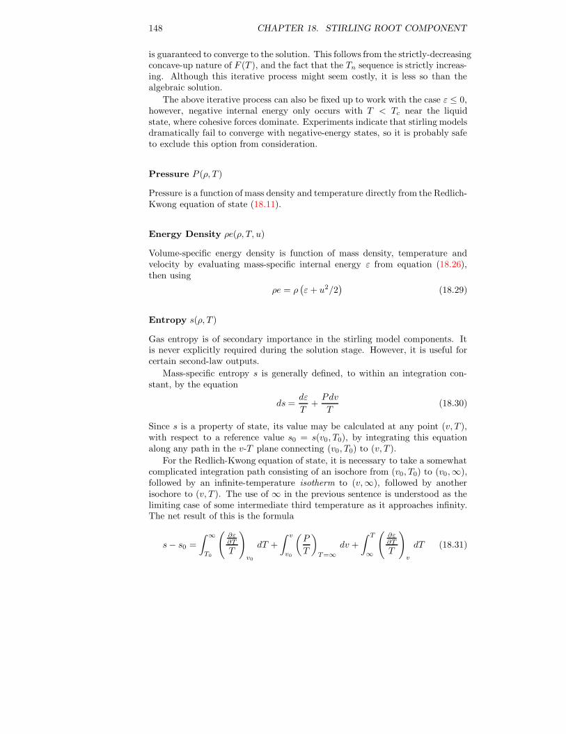
148 CHAPTER 18. STIRLING ROOT COMPONENT
is guaranteed to converge to the solution. This follows from the strictly-decreasingconcave-up nature of F (T ), and the fact that the Tn sequence is strictly increas-ing. Although this iterative process might seem costly, it is less so than thealgebraic solution.
The above iterative process can also be fixed up to work with the case ε ≤ 0,however, negative internal energy only occurs with T < Tc near the liquidstate, where cohesive forces dominate. Experiments indicate that stirling modelsdramatically fail to converge with negative-energy states, so it is probably safeto exclude this option from consideration.
Pressure P (ρ, T )
Pressure is a function of mass density and temperature directly from the Redlich-Kwong equation of state (18.11).
Energy Density ρe(ρ, T, u)
Volume-specific energy density is function of mass density, temperature andvelocity by evaluating mass-specific internal energy ε from equation (18.26),then using
ρe = ρ(ε+ u2/2
)(18.29)
Entropy s(ρ, T )
Gas entropy is of secondary importance in the stirling model components. Itis never explicitly required during the solution stage. However, it is useful forcertain second-law outputs.
Mass-specific entropy s is generally defined, to within an integration con-stant, by the equation
ds =dε
T+Pdv
T(18.30)
Since s is a property of state, its value may be calculated at any point (v, T ),with respect to a reference value s0 = s(v0, T0), by integrating this equationalong any path in the v-T plane connecting (v0, T0) to (v, T ).
For the Redlich-Kwong equation of state, it is necessary to take a somewhatcomplicated integration path consisting of an isochore from (v0, T0) to (v0,∞),followed by an infinite-temperature isotherm to (v,∞), followed by anotherisochore to (v, T ). The use of ∞ in the previous sentence is understood as thelimiting case of some intermediate third temperature as it approaches infinity.The net result of this is the formula
s− s0 =
∫ ∞
T0
(∂ε∂T
T
)
v0
dT +
∫ v
v0
(P
T
)
T=∞
dv +
∫ T
∞
(∂ε∂T
T
)
v
dT (18.31)

18.1. WORKING GAS 149
The above equation uses the fact that dε = ∂ε∂T dT along an isochore. For the
Redlich-Kwong equation, the integrands in the above integrals work out to
∂ε
∂T/T =
cvT
+3
4
a
b
ln(1 + b/v)
T 5/2(18.32)
P
T=
R
v − b− a
T 3/2v(v + b)(18.33)
Carrying out the integrations and simplifying produces the final entropy formula
s = cv lnT +R ln(v − b) − 1
2
a
b
ln(1 + b/v)
T 3/2(18.34)
Equation of State Error Z(ρ, T )
This is just Bρ according to the virial equation of state.
18.1.4 Tabular Gas Objects
Tabular gas objects abandon the idea of an algebraic equation of state in favorof an interpolation approach. As a result, tabular gases are more accurate andversatile than Redlich-Kwong gases.
Creating a good table of compressibility values Z(vj , Tk) may be somewhatdelicate and time consuming. Chapter 28 covers this issue in some detail. Ofcourse, once a data table exists, it is easy to use.
Computational Issues
The essential idea is to interpolate the equation of state P (v, T ) from a tableof known values, using bicubic spline interpolation (see section 3.6 of [47]).However, the values P (vj, Tk) are likely to vary over a large range, which mightlead to data input errors and interpolation errors. So instead of tabulating Pdirectly, it is better to tabulate the compressibility Z = Pv/(RT ), which hasthe value one in the ideal-gas range. It is easy enough to recover P (vj , Tk) fromZ(vj , Tk).
It is also possible to recover volume-specific internal energy ε(v, T ) and mass-specific entropy s(v, T ) from the state table Z(vj , Tk), although the calculationsinvolve computationally expensive path integrations. So it is best to do thesecalculations only once and then store ε(v, T ) and s(v, T ) as derived interpolationtables. But how does one calculate ε(v, T ) and s(v, T )?
Internal Energy According to reference [52] (equation (232), p. 285), thedifferential of mass-specific internal energy is
dε = cvdT +
[
T
(∂P
∂T
)
v
− P
]
dv (18.35)

150 CHAPTER 18. STIRLING ROOT COMPONENT
In terms of compressibility Z, one can substitute RρTZ for P andRρ[Z + T
(∂Z∂T
)
v
]
for(
∂P∂T
)
vso that the internal energy differential becomes
dε = cvdT +
[
RρT 2
(∂Z
∂T
)
v
]
dv (18.36)
Then one can build a table of ε values as follows:First build the vmax row of the table by temporarily assigning the corner
point ε(vmax, Tmin) the value zero, then calculating the remaining points in therow by integrating (18.36) with respect to T only, from one point to the next.Assuming ideal-gas conditions at vmax, it is valid to substitute the zero-pressurelimit cv0(T ) for cv(T ), then cp0(T ) − R for cv0(T ), since cv0(T ) is not directlytabulated. cp0(T ), on the other hand (the zero-pressure limit of cp), is availableas a cubic-spline data object.
Then, in a similar point-by-point process, complete the columns of the tableby integrating equation (18.36) with respect to v only, starting at each of the(vmax, Tk) points already calculated and using bicubic-spline routines operatingon the Z table to calculate the value of
(∂Z∂T
)
v.
The process so far does not establish an appropriate constant of integration.Usually this is done to give a particular reference value for internal energy atsome state point (v0, T0). In principle, this is not a problem since the equationsin Sage’s gas domains are affected only by changes in internal energy, not abso-lute values. On the other hand, some built-in solution convergence safeguardsprevent internal energy values from going negative, which might be the case inthe low T and low v portion of the table. So, to avoid this, an integration-constant offset is added to the entire table so that the minimum energy value isat least cv0Tmin.
Entropy The calculation of the entropy table proceeds along similar lines,except the differential of mass-specific entropy is
ds =dε
T+P
Tdv (18.37)
again according to reference [52] (equation (103), p. 102). By substituting(
∂ε∂T
)
vdT +
(∂ε∂v
)
Tdv for dε this becomes
ds = cvdT
T+
[(∂ε
∂v
)
T
+ P
]dv
T(18.38)
As before, the vmax row of the table is produced by integrating equation(18.38) with respect to T only, point-by-point, starting with a temporary valueof zero for s(vmax, Tmin), and substituting cp0(T ) − R for cv(T ). Then thecolumns of the table are completed by integrating equation (18.38) with respectto v only, starting at each of the (vmax, Tk) points just calculated.
As for the energy table, this approach may lead to negative values in the lowT , low v corner of the table. This is not a problem for Sage gas domains, but

18.1. WORKING GAS 151
more of a problem with human perception. So an integration-constant offset isadded to the entire table so that the minimum entropy value is some convenientvalue, such as gas constant R.
Derived Properties All of the gas properties Sage requires can be calculatedin terms of the above Z(v, T ), ε(v, T ) and s(v, T ) tables. The property methodsthat perform these calculations are the same as those for the other gases, exceptthe internal calculation details are entirely different. Interpolation replaces al-gebraic calculation and the specific volume v and mass-specific internal energyε used in the state-table formulation are converted back and forth into Sagevariables density ρ and volume-specific total energy ρe.
Compressibility Z(T, P )
For this method the independent variables are (T, P ) instead of (T, v), so itis not possible to interpolate the result directly from the table of Z values.Instead, Sage finds the appropriate v(T, P ), then returns Z = Pv(T, P )/(RT ),according to its definition. Finding v(T, P ) is a matter of using Newton’s methodto iteratively solve
F (v) = Pin − P (v, T ) = 0 (18.39)
Where Pin is the given pressure input and P (v, T ) is the pressure interpolatedfrom the table of Z values. Required in the process is ∂P
∂v , which is supplied bybicubic spline routines operating on the Z table.
Newton’s method requires a good starting value for v, otherwise it maynot converge. This starting value comes from a binary search in the Z tableto find the v-indices that bracket Pin (the indices jlo and jhi = jlo + 1 sothat P (vjlo, T ) ≥ Pin ≥ P (vjhi , T )) followed by a linear interpolation betweenthe bracketing values. The bracketing technique is reliable because P alwaysdecreases with increasing v for all gases. Pressure may remain constant duringthe liquid to vapor transition but it never increases.
Temperature T (ρ, ρe, u)
Sage uses temperature in the solution process so this is a critical method. Thefirst step is to convert volume-specific total energy ρe to mass-specific internalenergy ε using
ε = (ρe)/ρ− u2/2 (18.40)
then finding T (ρ, ε) is once again a matter of using Newton’s method, this timeto iteratively solve
F (T ) = εin − ε(1/ρ, T ) (18.41)
Where εin is the given energy input and ε(1/ρ, T ) is the energy interpolatedfrom the table of ε values. Required in the process is ∂ε
∂T , which is supplied bybicubic spline routines operating on the ε table.
The initial guess at T comes from a binary search in the ε table to find theT -indices that bracket εin (similar to above) followed by a linear interpolation

152 CHAPTER 18. STIRLING ROOT COMPONENT
between the bracketing values. The bracketing technique is reliable because εalways increases with increasing T for all gases.
Pressure P (ρ, T )
This is directly available by interpolation in the Z table as
P = Z(1/ρ, T )RρT (18.42)
Energy Density ρe(ρ, T, u)
This is directly available by interpolation in the ε table as
ρe = ρ(ε(1/ρ, T ) + u2/2) (18.43)
Entropy s(ρ, T )
This is directly available by interpolation in the s table.
Equation of State Error Z(ρ, T )
This could be based on some measure of error in the actual tabulated values ofZ(vj , Tk) as well as some estimate of the cubic spline interpolation error. But
it is not worth the bother since Z is required only for an output variable in theSage listing. So Z is presumed zero until further notice.

Chapter 19
Moving Parts
Stirling-class moving parts are additions to the generic resonant-system modelcomponents already documented in chapter 12. Generally they are more phys-ically specific yet remain connector compatible with their generic counterparts.
19.1 Rotary Mechanisms
The components in this section model the various rotary mechanisms often usedto drive the pistons and displacers of stirling-cycle machines. There are actuallytwo types of rotary components, one representing various kinematic linkages andthe other representing the flywheel.
19.1.1 Flywheel
A flywheel is used to drive one or more of the kinematic linkage componentsbelow. Its child-model palette allows you to create any number of steady-torqueattachments, each born with a positive-facing torque connector designed to at-tach to the negative-facing torque connector of a kinematic linkage. In physicalterms a flywheel behaves like a constant torque drive or motor with angularmomentum. It supplies exactly the torque required to balance the rotationalenergy input or output from any torque connections while its rotation speedfluctuates in response to those torque connections. The input and outputs fora flywheel are:
IMoment : (real, kg m2) Moment of inertia I, including the moments of inertiaof any rotating parts in attached kinematic linkages. For a disk flywheelof uniform thickness I = 1/2MR2, where M is the mass and R is the diskradius. For a flywheel where all of the mass is concentrated in the outerrim I = MR2.
FTorque : (Fourier series, N m) Total Torque T applied to the flywheel by alltorque connections as a function of time.
153

154 CHAPTER 19. MOVING PARTS
FOmega : (Fourier series, radians/s) Rotation angular velocity θ as a functionof time.
FW : (Fourier series, W) Power delivered to the flywheel from all torque con-nections.
Rotational Realism The rotational angular velocity θ fluctuates accordingto the applied torque and moment of inertia I, which is an input. Except thatthe mean value of angular velocity is constrained so that the rotational period isalways consistent with the root model Frequency input. In other words the crankmechanism always rotates Frequency times per second although the rotationalspeed fluctuates somewhat as it does in an actual machine.
If the flywheel moment of inertia (input Imoment) is too small the flywheelrotation may stall as in an actual machine. To avoid numerical problems duringdesign work it is best to start with a high moment of inertia and reduce it lateron if necessary.
Torque Attachments There is only one type of torque-attachment availablewithin the flywheel component:
Icon Purpose
time-ring positive-facing torque attachment
Create as many as you need. Then move the connection arrows up one leveland connect them to the kinematic linkages in your model.
19.1.2 Kinematic Linkages
Kinematic linkages implement the math required to convert a rotary motion intoa back and forth reciprocating motion. The rotary motion comes from attach-ment to a flywheel component via a torque connection. The torque connectionlocks together the rotation of the flywheel and linkage. The back and forthmotion is coupled to one or more reciprocating masses that model the pistonand displacer components of stirling cycle machines (see chapter 12). Attachinga kinematic linkage to a reciprocating mass with a force connection cause thekinematic linkage to drive the reciprocating mass according to the linear motionof its specific linkage geometry.
Inputs and outputs common to all kinematic linkages are:
Rcrank : (real, m) Crank-throw radius r.
Phase : (real, radians) Initial crank-angle ρ at time zero. Time zero is whenthe attached flywheel rotation angle θ is zero.
FTorque : (Fourier series, N m) Torque T applied by the linkage geometry tothe crank pin as a function of time.

19.1. ROTARY MECHANISMS 155
Mandatory Flywheel Connection All kinematic linkages contain built-innegative-facing torque connectors for mandatory connection to a flywheel com-ponent (section 19.1.1) which defines the rotational angular momentum coupledto the mechanism. Without a flywheel connection a kinematic linkage will beunable to balance the torque on the crank pin produced by the linear forcesacting on the linkage geometry and the solve process will fail. The angular mo-mentum is defined in a separate component so more than one mechanism canshare the same flywheel and combine together to produce a single rotation an-gle solution. In the physical world this simulates having two or more kinematiclinkages geared together and coupled to the same flywheel.
Reciprocating Motion All kinematic linkage components produce a linkagelinear motion x as a function of crank angle and define the torque T appliedto the crank pin as a function of the applied force to the reciprocating linkage.Crank angle is the flywheel rotational angle θ plus the phase offset ρ providedby input Phase. When calculating torque the reciprocating mass of the linkageand its rotational moment of inertia are presumed to be zero. Any actualreciprocating mass must be included in the attached reciprocating mass andany rotational moment of inertia in the attached flywheel.
Beware Aliasing Errors Higher harmonics in the reciprocating linkage mo-tion can produce significant solution errors if the time grid is too coarse — e.g.root-model input NTnode is too small — and even lead to energy conservationerrors in attached reciprocator or spring components if NTnode is even.
Higher harmonics are produced by the nonlinear relationship between crankrotation and linkage reciprocating motion. These harmonics are compounded ifthe rotational angular velocity is itself fluctuating because the flywheel momentof inertia (input Imoment) is small. If the highest harmonic resolved by thegrid is significant (e.g. amplitude of highest harmonic in FX output not smallcompared to other harmonics) then you might want to increase NTnode to im-prove solution accuracy. You should also increase it to an odd number becauseNTnode must be odd to resolve the mean value plus both components of allharmonics. When NTnode is even the highest harmonic is not fully determined.This leads to finite differencing errors in the time grids for reciprocators andsprings which may produce time-average energy dissipation or production inviolation of physical principles. When NTnode is odd there are no finite differ-encing errors and energy conservation is numerically exact, although there canstill be solution errors if NTnode is too small.
Failure to conserve energy in springs and reciprocators is especially bad be-cause it can mislead you about the power delivered to the kinematic linkage(output W). For example the PV power delivered by the working gas to a re-ciprocator driven by a kinematic linkage will show up partly in the reciprocatorand partly in the kinematic linkage if there is an energy conservation error.

156 CHAPTER 19. MOVING PARTS
Scotch Yoke Linkage
The drawing below shows the kinematic linkage geometry for a Scotch yoke:
Ra
xR cos a
+-
The linkage linear displacement is just the x-component of crank pin motion
x = R cosα (19.1)
Simple Crank Linkage
Note: A simple crank mechanism supersedes the simple crank pistoncomponent (see below). It provides the same linear motion as afunction of crank angle with the realism of an attached flywheel.
A simple crank mechanism adds the input:
Lratio : (real, dimensionless) Connecting-rod length divided by crank-throwradius L/R. The linkage geometry requires that L/R > 1 (L > R).
The kinematic linkage geometry is shown in this drawing:
R L
ab
xR cos a
+-L cos b
The linkage linear displacement is the sum of the x-components of crank pinmotion and connecting rod displacement. Referring to the above drawing andsubtracting the constant length L the linkage displacement may be written
x = R cosα+ L cos β − L (19.2)

19.1. ROTARY MECHANISMS 157
where angle β is:
β = arcsin
(R sinα
L
)
(19.3)
The reason for subtracting L is so the linear displacement ranges above andbelow zero according to Sage’s convention for moving parts. The extreme dis-placements are x = R and −R at α = 0 and π. The displacements at α = π/2and 3π/2 are both negative, not zero which has the implication that the time-average displacement is also negative. Time-average displacement is zero onlyin the limit of infinite connecting rod length L.
Rhombic Drive Linkage
A rhombic drive mechanism has a different pedigree from previous rotatingmechanisms. It descends from the relative moving parts documented in chapter12. Because of that a rhombic drive mechanism is born with positive and neg-ative facing force connectors and does not support connections via child-modelforce attachments like previous rotating mechanisms.
In the physical world a rhombic drive has two counter-rotating crankshaftsand four equal-length connecting rods, connected in pairs to the two crank pins(see drawing below). The connecting rods produce two linkage motions xp andxn. The Sage convention is that the xp motion is transmitted through thepositive facing force connection and the xn motion through the negative facingforce connection. The rhombic mechanism adds two inputs:
Eratio : (real, dimensionless) Rhombic eccentricity divided by crank-throw ra-dius E/R (see drawing). Mathematics requires only that E/R be non-negative (E/R ≥ 0). The drawing shows the typical case E/R > 1. Thecase E/R = 0 corresponds to the simple crank piston.
Lratio : (real, dimensionless) Connecting-rod length divided by crank-throwradius L/R. The linkage geometry requires that L/R > E/R + 1 (L >E + R).
The drawing below shows only the kinematic linkage geometry and appliedforces for half of the mechanism, cut along the center-line (plane of symmetry)at the top of the drawing:

158 CHAPTER 19. MOVING PARTS
R
L
a
b
xp
R cos a
R sin a
+-CL
L
xn +-
E
L sin b
L cos b
b
The linkage linear displacements are the sum of the x-component of crank pinmotion plus-or-minus the connecting rod displacement. Referring to the abovedrawing and including a constant offset x0 the linkage displacements may bewritten
xp = R cosα+ L cos β − x0 (19.4)
xn = R cosα− L cos β + x0 (19.5)
where angle β is:
β = arcsin
(E −R sinα
L
)
(19.6)
The purpose for x0 is so the linear displacements range equally above and belowzero according to Sage’s convention for moving parts. In terms of the abovedrawing x0 is the average of the max and min horizontal displacements betweenxp (or xn) and the crank circle center. These max and min displacementsoccur when the connecting rod L is directly in-line and directly opposite theconnecting rod radius R. The drawing shows the crank angle near the time ofmaximum xp displacement
√
(L +R)2 − E2, which is the horizontal leg of theright triangle with hypotenuse L+R and vertical leg E. Similarly the minimumxp displacement is
√
(L −R)2 − E2. The average displacement is one-half thesum, or
x0 =1
2
(√
(L +R)2 − (E)
2+
√
(L− R)2 − (E)
2
)
(19.7)
19.1.3 Rotary Mechanism Theory
The physics of rotary mechanisms is relatively simple with the roles of kinemat-ics and rotational inertia handled by distinct model components. Kinematiclinkage components handle the kinematic part. They derive from the time-gridmoving-part components of chapter 12. The inherited displacement variable x

19.1. ROTARY MECHANISMS 159
represents the linear back and forth motion of the linkage solved as an explicitfunction of crank angle. More on crank angle later. The flywheel componenthandles the rotational inertia part. It implements a time grid with three statevariables θ, θd and θdd, corresponding to the rotation angle as a function oftime, angular velocity (first time derivative θ) and angular acceleration (secondtime derivative θ).
Flywheel Angular Acceleration
Flywheels solve state variable θdd (angular acceleration) explicitly from the ro-tary equivalent of Newton’s equation of motion written in the form:
θdd =TE + Ts
I(19.8)
where moment of inertia I is an input and TE is the net applied torque byexternal torque connections. Indirectly TE comes from the forces acting onthe reciprocating mass (or masses) attached to the kinematic linkages that areattached to the flywheel. In addition to inertial forces the reciprocating masstransmits whatever other forces might be attached to it (e.g. pressure forcesacting on piston frontal areas). TS is the internal torque applied to the flywheelrequired to keep it rotating at an average angular velocity of ω (root modelvariable Omega).
TS is an invisible implicit variable needed for the mathematical solution. Itspurpose is to offset any time-average of the external applied torque TE thatwould otherwise tend to increase or decrease the rotation speed with time. As ifthe output shaft is internally connected to a constant torque motor or alternatorthat regulates the speed. TS is not a grid state variable but rather solved as asingle implicit variable of the flywheel component itself. While the solved valueof TS is not displayed as an output variable its valued can be inferred as thenegative of the mean value of the FTorque Fourier series output. More on thesolution of TS below.
Flywheel Angular Velocity
Flywheels solve state variable θd (angular velocity) implicitly from
dθd/dt− θdd = 0 (19.9)
In other words, the time derivative of solution variable θd equals the solutionvariable θdd.
Flywheel Crank Angle
In the limit of infinite moment of inertia the flywheel rotation angle approachesθ = ωt. But because the moment of inertia is finite flywheels must solve crankangle implicitly from
dθ/dt− θd = 0 (19.10)
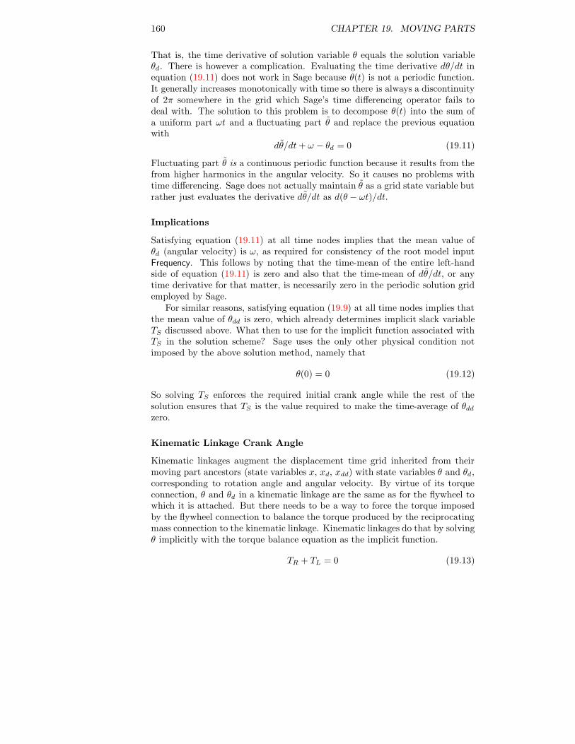
160 CHAPTER 19. MOVING PARTS
That is, the time derivative of solution variable θ equals the solution variableθd. There is however a complication. Evaluating the time derivative dθ/dt inequation (19.11) does not work in Sage because θ(t) is not a periodic function.It generally increases monotonically with time so there is always a discontinuityof 2π somewhere in the grid which Sage’s time differencing operator fails todeal with. The solution to this problem is to decompose θ(t) into the sum ofa uniform part ωt and a fluctuating part θ and replace the previous equationwith
dθ/dt+ ω − θd = 0 (19.11)
Fluctuating part θ is a continuous periodic function because it results from thefrom higher harmonics in the angular velocity. So it causes no problems withtime differencing. Sage does not actually maintain θ as a grid state variable butrather just evaluates the derivative dθ/dt as d(θ− ωt)/dt.
Implications
Satisfying equation (19.11) at all time nodes implies that the mean value ofθd (angular velocity) is ω, as required for consistency of the root model inputFrequency. This follows by noting that the time-mean of the entire left-handside of equation (19.11) is zero and also that the time-mean of dθ/dt, or anytime derivative for that matter, is necessarily zero in the periodic solution gridemployed by Sage.
For similar reasons, satisfying equation (19.9) at all time nodes implies thatthe mean value of θdd is zero, which already determines implicit slack variableTS discussed above. What then to use for the implicit function associated withTS in the solution scheme? Sage uses the only other physical condition notimposed by the above solution method, namely that
θ(0) = 0 (19.12)
So solving TS enforces the required initial crank angle while the rest of thesolution ensures that TS is the value required to make the time-average of θdd
zero.
Kinematic Linkage Crank Angle
Kinematic linkages augment the displacement time grid inherited from theirmoving part ancestors (state variables x, xd, xdd) with state variables θ and θd,corresponding to rotation angle and angular velocity. By virtue of its torqueconnection, θ and θd in a kinematic linkage are the same as for the flywheel towhich it is attached. But there needs to be a way to force the torque imposedby the flywheel connection to balance the torque produced by the reciprocatingmass connection to the kinematic linkage. Kinematic linkages do that by solvingθ implicitly with the torque balance equation as the implicit function.
TR + TL = 0 (19.13)

19.2. SIMPLE CRANK PISTON 161
where TR is the torque supplied by the flywheel via the torque connection andTL is the torque applied to the crank pin via force connections to reciprocatingmasses.
The kinematic linkage crank angle α is offset from the flywheel rotation angleθ by a fixed phase angle offset ρ (input Phase)
α = θ + ρ (19.14)
The phase offset ρ allows the crank angle to differ from the flywheel rotationangle so two or more mechanisms connected to the same flywheel can havedifferent phases.
Kinematic Linkage Torque
Kinematic linkages calculate the torque T applied to crank pin from the energyconservation principle
T θ = F x (19.15)
where θ is state variable θd, F is the sum of applied boundary forces and x isstate variable xd. In English, the rate of rotational work done by the torqueacting on the crank pin equals the rate of work done by the applied forces actingon the reciprocating linkages. This principle holds because there is no mass ormoment of inertia in a kinematic linkage to store energy.
This way is much simpler than calculating torque directly as a functionof applied boundary force and crank angle (using force-balance diagrams andtrigonometry). It also guarantees that global energy conservation holds. Anymechanical energy that enters or leaves through the reciprocating linkage nec-essarily equals the mechanical energy transmitted to the flywheel.
19.2 Simple Crank Piston
Note: This is a depreciated component. It has been superseded bythe combination of a flywheel, simple crank linkage and reciprocatingmass which together provide greater functionality.
A simple crank piston is a descendant of the time-ring constrained piston whereFourier-series displacement is now calculated as a dependent variable in termsof geometrical input variables pertaining to a simple crankshaft and connecting-rod kinematic mechanism.
Mathematically, displacement is given by
x = r(
cos θ+√
cos2 θ+ L2/r2 − 1)
− L (19.16)
where r is crank-throw radius, L is connecting-rod length and θ is crank angle,defined in terms of angular frequency ω and a fixed phase angle ρ as
θ = ωt + ρ (19.17)
In Sage, the above variables become:

162 CHAPTER 19. MOVING PARTS
Rcrank : (real, m) Crank-throw radius r.
Lratio : (real, dimensionless) Connecting-rod length divided by crank-throwradius L/r.
Phase : (real, radians) Crank-angle phase shift ρ.
Any or all of these may be optimized if need be.
19.3 Flexure Springs
These model components descend from the spring components documented inchapter 12. Except linear spring stiffness is now calculated as a dependentvariable in terms of physical dimensions for spiral-arm flexure springs. And themass of the spring is reflected in its attachment force. Displacement x is nowsolved from net applied boundary force F , stiffness K and effective mass me
using the equation
F = Kx+mex (19.18)
There are two phasor versions. The first version represents a stack of flexureelements located at one point. The second represents a stack of flexure elementsseparated into two parts by some axial distance, acting as a couple. There areno time-ring flexures.
The theory behind Sage spiral arm flexures is an extrapolated case of helicalcoil spring theory. It applies, more or less, to flexures having spiral arms ofuniform width and thickness. Since the analysis is only approximate, a numberof calibration constants are included in the model. The idea is that you can resettheir default values, if you want, based on a separate finite-element analysis ofyour particular geometry.
19.3.1 Flexure Stack
This component is intended as a plug-compatible replacement for a genericphasor spring in a resonant-system model. You would use this component duringan advanced stage of design where you wanted to actually design and optimize aspiral-arm flexure spring, rather than just work with its generic spring stiffnesswithin a larger system. The flexure-stack component introduces new variables:
Ca, Cr, Cs, Cw, Cm : (real, dimensionless) Empirical calibration constants ac-cording to following theory.
E : (real, N/m2) Elastic modulus E of spring material.
Rho : (real, N/m2) Density ρ of spring material.
T : (real,m) Thickness t of a single flexure.
W : (real, m) Spiral arm width w.

19.3. FLEXURE SPRINGS 163
D : (real, m) Active diameter D. Defined by circle where arms attach to outerrim.
M : (real, dimensionless) Number k of arms per flexure.
N : (real, dimensionless) Number n of flexures in stack.
Kr : (real, N/m) Radial stiffness Kr . Spring stiffness for deflection transverseto spring axis.
Sm : (real, N/m2) Peak torsional stress τm.
Ws : (real, 1/s) Surge angular frequency ωs. The operating frequency at orabove which the analysis breaks down due to internal resonance.
Me : (real, kg) Effective mass Me. That mass which moving with the samedisplacement amplitude as the flexure central attachment point producesthe same reaction force.
Tn : (real, radians) Spiral arm total turning angle θT . The angle through whicha radius vector rotates as it traverses a spiral arm from its inner to outerattachment points.
19.3.2 Flexure-Stack Couple
This component is a minor variation of the above flexure component (a descen-dant actually) that presumes the stack of flexures is divided into two groupsspaced by some distance along the central axis, so as to produce a restoring mo-ment to a tilting moment load. It, too, is a plug-compatible replacement for thegeneric phasor spring component. The angular stiffness within this componentis intended for use in optimization constraints rather than some sort of trans-verse force connection to other model components. New variables introducedby the flexure-stack couple are:
Sc : (real, m) Couple separation distance S.
Ka : (real, N m / radian) Angular stiffness Ka.
You could optimize one of these subject to a constraint on the other.
Angular stiffness, defined as the restoring moment produced per unit tiltangle in radians, may be expressed in the form
Ka =1
4KrS
2 (19.19)
where Kr is the total radial stiffness of both groups of flexures combined and Sis the distance separating the groups. A simple force diagram will convince youthis is so.

164 CHAPTER 19. MOVING PARTS
19.3.3 Theory
The principle assumption is that spiral flexure arms behave at each point likethe coils in a helical spring with the same radius of curvature. This is reasonableprovided that (1) the arms actually turn through some minimum angle as theyspiral out from the center (so as to produce load moments similar to those inhelical springs), (2) they are longer than some minimum length (so that we mayignore the stresses due to slope and roll constraints at the end attachments) and(3) the radius of curvature does not change too abruptly.
Spiral Geometry
A spiral flexure may be geometrically characterized by four independent vari-ables:
D active diametert thicknessw arm widthk number of arms
If we take r(θ) to be the radius (distance from center to spiral-arm neutralaxis) as a function of turning angle, then the spiral arm shape is defined by thegeometrical requirement that ∆r/∆θ = k(1 + ε)w/2π. In English: r increasesby k arm widths for each turn. Factor (1 + ε) accounts for the gap betweenarms and the fact that the radial distance between edge-bounding involutesprogressively deviates from perpendicular arm width as r decreases. If dr/dθ isas above then arm shape r(θ) must be
r(θ) = r0 +k(1 + ε)w
2πθ (19.20)
where r0 is the inner radius. The total turn angle for each spiral arm is thatangle θT for which r(θT ) = D/2. If we ignore r0 then total turn angle isapproximately
θT ≈ πD
k(1 + ε)w(19.21)
In the following analysis, we will require that θT should always be at least π/2or so. And we shall assume that ε is a design constant of minor consequence tobe subsumed by calibration constants.
Axial Spring Stiffness
From Wahl’s classic tome of spring design (reference [64], equation 10-9, p.129), we find the formula for axial deflection x per unit coil turning angle in arectangular-bar helical spring under applied load Fx
dx
dθ≈ 8.3
Fx
wt3Er3 (19.22)
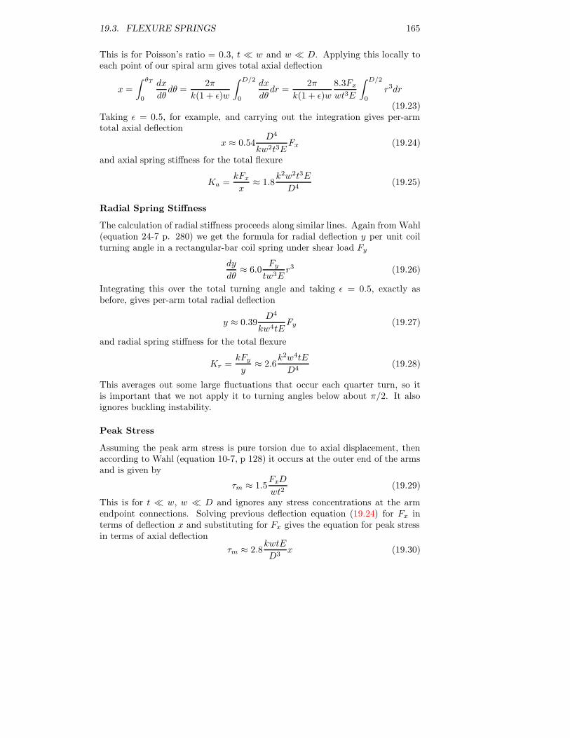
19.3. FLEXURE SPRINGS 165
This is for Poisson’s ratio = 0.3, t � w and w � D. Applying this locally toeach point of our spiral arm gives total axial deflection
x =
∫ θT
0
dx
dθdθ =
2π
k(1 + ε)w
∫ D/2
0
dx
dθdr =
2π
k(1 + ε)w
8.3Fx
wt3E
∫ D/2
0
r3dr
(19.23)Taking ε = 0.5, for example, and carrying out the integration gives per-armtotal axial deflection
x ≈ 0.54D4
kw2t3EFx (19.24)
and axial spring stiffness for the total flexure
Ka =kFx
x≈ 1.8
k2w2t3E
D4(19.25)
Radial Spring Stiffness
The calculation of radial stiffness proceeds along similar lines. Again from Wahl(equation 24-7 p. 280) we get the formula for radial deflection y per unit coilturning angle in a rectangular-bar coil spring under shear load Fy
dy
dθ≈ 6.0
Fy
tw3Er3 (19.26)
Integrating this over the total turning angle and taking ε = 0.5, exactly asbefore, gives per-arm total radial deflection
y ≈ 0.39D4
kw4tEFy (19.27)
and radial spring stiffness for the total flexure
Kr =kFy
y≈ 2.6
k2w4tE
D4(19.28)
This averages out some large fluctuations that occur each quarter turn, so itis important that we not apply it to turning angles below about π/2. It alsoignores buckling instability.
Peak Stress
Assuming the peak arm stress is pure torsion due to axial displacement, thenaccording to Wahl (equation 10-7, p 128) it occurs at the outer end of the armsand is given by
τm ≈ 1.5FxD
wt2(19.29)
This is for t � w, w � D and ignores any stress concentrations at the armendpoint connections. Solving previous deflection equation (19.24) for Fx interms of deflection x and substituting for Fx gives the equation for peak stressin terms of axial deflection
τm ≈ 2.8kwtE
D3x (19.30)

166 CHAPTER 19. MOVING PARTS
Effective Mass
Based on kinetic and potential energy arguments the spiral-arm effective recip-rocating mass as a fraction of actual mass is the area-weighted displacement-squared divided by the center displacement squared, or
Me/M =
∫ 1
0x2(r)2πr dr
πx20
(19.31)
The above equation presumes a spiral arm of unit outer radius and center de-flection x0. From the previous axial-deflection formula (19.24) we may take,x(r) = x0(1 − r4) — highly nonlinear with most of the drop-off near the outerradius. Substituting into the previous equation and integrating gives the result
Me/M = 0.53 (19.32)
Actual mass M is just density ρ multiplied by the part of flexure disk areaoccupied by spiral arms, or M = ρ(1/(1 + ε))tπD2/4. Taking ε = 0.5, effectivemass works out to
Me = 0.28ρtD2 (19.33)
Surge Frequency
Once we know axial spring stiffness and effective reciprocating mass, we mayapproximate surge frequency as
ωs ∝√
Ka/Me ≈ 2.5kwt
D3
√
E/ρ (19.34)
which is just the resonant frequency of the flexure with no attached mass. Thisis not quite correct, for surge frequency is the frequency of a standing wave(half-wave) in the spiral arms with inner and outer ends clamped — not thesame waveform used in deriving effective mass or axial spring stiffness. However,with the way these things usually go, the above formula is off by no more thana constant of proportionality which can be calibrated out with finite-elementanalysis.
Calibrated Formulae
Introducing into our equations the effect of n, the number of flexures stackedtogether, the above formulae become:
axial stiffness
Ka = Cank2w2t3E
D4(19.35)
radial stiffness
Kr = Crnk2w4tE
D4(19.36)

19.4. NONLINEAR SPRING 167
peak stress
τm = CτkwtE
D3x (19.37)
effective reciprocating mass
Me = CmnρtD2 (19.38)
surge angular frequency
ωs = Cωkwt
D3
√
E/ρ (19.39)
19.4 Nonlinear Spring
A nonlinear spring is a generic spring where the spring stiffness K varies asa quadratic function of position x. Most actual springs are nonlinear to someextent, depending on how far extended from their rest position x = 0. Thiscomponent allows you to model the effects of operating a spring beyond itslinear range. The stiffness function is defined by four inputs:
K0 : (real, n/m) Stiffness K0 at x = 0.
Xm : (real, m) Reference extension xm.
Rp : (real, dimensionless) Stiffness ratio Rp = K/K0 at x = xm.
Rn : (real, dimensionless) Stiffness ratio Rn = K/K0 at x = −xm.
You can read these, more-or-less directly, from a plot of local spring stiffnessK vs x generated either experimentally or computationally. In terms of therestoring force F (x), the spring stiffness is K(x) = −dF/dx. A more preciseapproach would involve finding the best-fit parabola (not necessarily symmetricabout the rest position) to the function K(x) over the intended operating rangeand then defining K0, Xm, Rp, Rn consistent with the parabola.
For internal processing, Sage translates the above inputs into a quadraticspring stiffness in the form
K(x) = K0
(1 + a(x/xm) + b(x/xm)2
)(19.40)
Coefficients a and b come from substituting xm and −xm for x in equation(19.40), which results in the equation system
Rp = 1 + a+ b (19.41)
Rn = 1 − a+ b (19.42)
with the solution
a = (Rp −Rn)/2 (19.43)
b = (Rp +Rn)/2 − 1 (19.44)

168 CHAPTER 19. MOVING PARTS
The restoring force provided by a nonlinear spring is
F (x) = −K0x
(
1 +a
2(x/xm) +
b
3(x/xm)2
)
(19.45)
The position x = 0 is the neutral force position.You can attach a nonlinear spring to a time-ring reciprocating mass (not
a phasor reciprocating mass) for modeling the resultant motion of nonlinearspring-mass systems. Even when driven by a sinusoidal forcing function, sucha system will produce a reciprocating motion with higher harmonics. And theresonant frequency will change, depending on amplitude.
19.5 Relative Nonlinear Spring
A relative nonlinear spring is just like the above nonlinear spring, except itis connected between two moving parts instead of between a moving part andground (fixed inertial frame). The same input variables and governing equationsapply except that position coordinate x is replaced by the difference of theendpoint coordinates xpos − xneg. The relative nonlinear spring descends fromthe relative moving parts documented in chapter 12.
19.6 Motion Snubber
Something between a nonlinear spring and damper, a motion snubber imposesdisplacement limits on an attached reciprocating mass by generating a forcethat approximates an energy dissipating collision when the motion exceeds thoselimits. Otherwise this component produces essentially zero force on whatever itmay be attached to. Simulating a collision is not an easy task for Sage becauseactual collision forces tend to be abrupt and dependent on the elasticity andrestitution coefficient of the materials at the impact point. This component onthe other hand produces a collision force that is smooth enough to resolve withinSage’s coarse time-grid and distributed over the entire solution period. Becausecollision forces are inherently non-sinusoidal, this component only comes in atime-ring version and supports only time-ring force connections (FGt) to time-ring moving parts.
Because of the non-sinusoidal motions likely to result when using this com-ponent you may have to increase the number of time nodes in the solution gridabove the default NTnode = 7 (NTnode is a root component input). You mayneed NTnode = 9, 11 or even higher to adequately resolve the motion. Experi-ment! When using this component it is a good idea inspect the actual solutiongrid of the snubbed component (menu: File|Save Solution Grid) because it isdifficult to visualize the solved motion from the Fourier series output FX.
The motion snubber has five inputs and one output:
Mscale : (real, kg) snubbed mass scale. The approximate mass ms of the recip-rocating mass or combined reciprocating masses the snubber is connected
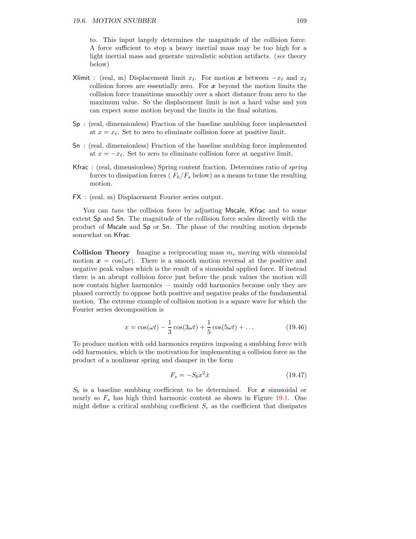
19.6. MOTION SNUBBER 169
to. This input largely determines the magnitude of the collision force.A force sufficient to stop a heavy inertial mass may be too high for alight inertial mass and generate unrealistic solution artifacts. (see theorybelow)
Xlimit : (real, m) Displacement limit x`. For motion x between −x` and x`
collision forces are essentially zero. For x beyond the motion limits thecollision force transitions smoothly over a short distance from zero to themaximum value. So the displacement limit is not a hard value and youcan expect some motion beyond the limits in the final solution.
Sp : (real, dimensionless) Fraction of the baseline snubbing force implementedat x = x`. Set to zero to eliminate collision force at positive limit.
Sn : (real, dimensionless) Fraction of the baseline snubbing force implementedat x = −x`. Set to zero to eliminate collision force at negative limit.
Kfrac : (real, dimensionless) Spring content fraction. Determines ratio of springforces to dissipation forces ( Fk/Fs below) as a means to tune the resultingmotion.
FX : (real, m) Displacement Fourier series output.
You can tune the collision force by adjusting Mscale, Kfrac and to someextent Sp and Sn. The magnitude of the collision force scales directly with theproduct of Mscale and Sp or Sn. The phase of the resulting motion dependssomewhat on Kfrac.
Collision Theory Imagine a reciprocating mass ms moving with sinusoidalmotion x = cos(ωt). There is a smooth motion reversal at the positive andnegative peak values which is the result of a sinusoidal applied force. If insteadthere is an abrupt collision force just before the peak values the motion willnow contain higher harmonics — mainly odd harmonics because only they arephased correctly to oppose both positive and negative peaks of the fundamentalmotion. The extreme example of collision motion is a square wave for which theFourier series decomposition is
x = cos(ωt) − 1
3cos(3ωt) +
1
5cos(5ωt) + . . . (19.46)
To produce motion with odd harmonics requires imposing a snubbing force withodd harmonics, which is the motivation for implementing a collision force as theproduct of a nonlinear spring and damper in the form
Fs = −Sbx2x (19.47)
Sb is a baseline snubbing coefficient to be determined. For x sinusoidal ornearly so Fs has high third harmonic content as shown in Figure 19.1. Onemight define a critical snubbing coefficient Sc as the coefficient that dissipates

170 CHAPTER 19. MOVING PARTS
-1.50
-1.00
-0.50
0.00
0.50
1.00
1.50
0.00 1.00 2.00 3.00 4.00 5.00 6.00 7.00ωt
Snubbing Force for Sinsuoidal Motion
x = cos(ωt)
Fs = -x2 dx/dt
Figure 19.1: Sinusoidal piston motion x and snubbing force produced by func-tion (19.47) with unit snubbing coeffient. The force for the positive-displacementhalf cycle cancels that of the negative half cycle, so the time average force andnet spring content is zero. But the force shifts with velocity so it dissipatesenergy.
the peak kinetic energy of the moving mass msv2/2 over half the cycle period.
If the motion is x = x` cos(ωt) the peak kinetic energy is msx`2ω2/2. For
that same motion the average power dissipated by the snubbing force is thetime-average of Sc(xx)2 which evaluates to Scx`
4ω2/4, so the energy dissipatedover half the cycle period π/ω is Scx`
4ωπ/4. Equating the two dissipations andsolving gives
Sc =2
π
msω
x`2
(19.48)
The baseline snubbing coefficient Sb used in Sage’s motion snubber componentis somewhat higher than Sc, based on numerical experiments of actual collisionsimulations.
The above snubbing force is the basis for Sage’s motion snubber componentbut there are also some practical refinements. First of all the snubbing force isnot active unless the motion actually exceeds the allowable limits. Beyond thelimits there is a smooth transition to full force rather than an abrupt change.Abrupt changes are bad because they may cause solution instability. The forcetransition is implemented in terms of a weight factor W that multiplies theforce. The weight factor depends on the instantaneous displacement x andcyclic peak values xm ± x1 where xm is the time-average displacement andx1 is the amplitude of the first harmonic in its Fourier series expansion. Theweight factor is near zero when the cyclic peak values are within limits, althoughnot exactly zero to avoid solution indeterminacy. When instantaneous position

19.7. RELATIVE MOTION SNUBBER 171
is positive and its Fourier-series peak value exceeds the limit, the the weightfunction increases smoothly but rapidly to the value of input Sp. When theinstantaneous position is negative and its Fourier-series negative peak valueexceeds the negative limit, the weight function increases smoothly but rapidlyto the value of input Sn. In this way the force can simulate a single-endedcollision if Sp or Sn are zero.
It is also useful to provide some degree of spring component to the snubbingforce to prevent the motion from drifting off center if there are no externalsprings attached to the snubbed reciprocator and also to provide a means totune the the resulting motion so it is more realistic. So the actual force producedby the motion snubber component is the sum of a dissipative component Fs anda spring component Fk of the form
F = −W (Fs + Fk) = −W(Sbx
2x+Kbx)
(19.49)
The motion snubber component does not specify Kb as an input but rathercalculates it from input Kfrac, which is the ratio Fk/Fs. Ignoring fluctuatingquantities this is the ratio of spring force (Kbx`) to snubbing force (Sbωx`
3) or
Fk
Fs=
Kb
ωxb2Sb
(19.50)
Solving for Kb, the spring stiffness is Kfrac times ωxb2Sb.
19.7 Relative Motion Snubber
A relative motion snubber is just like the above motion snubber, except it isconnected between two moving parts instead of between a moving part andground (fixed inertial frame). The same input variables and governing equationsapply except that position coordinate x is replaced by the difference of theendpoint coordinates xpos − xneg. The relative motion snubber descends fromthe relative moving parts documented in chapter 12.
19.8 Linear Motors
A linear motor provides a reciprocating force as a function of electrical current,which is an input. There is no detailed analysis of electromagnetic fields inphysical geometries — all the physics is collapsed into a single electromagneticforce coefficient input. There are phasor and time-ring versions.
You can connect a linear motor to a reciprocating mass through a standardforce connection, just like you would a spring or damper. The motor will drivethe mass according to the current and force-coefficient inputs. In the time-ring case, a spring is mandatory to determine the equilibrium position of thereciprocating mass. Otherwise the solver will tend to drift around withoutconverging. Generally, even a very weak spring will do.

172 CHAPTER 19. MOVING PARTS
In a full-fledged stirling model, a linear motor can drive a reciprocating masswhich, in turn, has a face area attached to the compression space gas. In thetime-ring case, besides a spring attached to the reciprocating mass, there mustalso be a balancing area face on the other side of the reciprocating mass (oppositethe compression-space attachment), attached to a buffer space. Otherwise therewould be a great pressure-force imbalance on the piston which the spring wouldhave difficulty offsetting. This inconvenience is the price for realism.
19.8.1 Phasor Motor
In the phasor motor, the current and resultant force are sinusoidal. Its effectscan be produced by the built-in forcing function input of a reciprocating mass,although the motor component also calculates the electrical resistance (I2R)losses in the coil. The motor is defined by four inputs:
Icoil : (phasor, A) Electrical current I in the coil.
Cf : (real, N/A) Force coefficient Cf produced by electromagnetic interaction.
Rcoil : (real, ohm) Electrical resistance R of the coil.
Inorm : (real, A) Current scale used to normalize Icoil for internal Sage purposes.
with a new output variable (besides those inherited from the ancestral movingpart component):
Wcoil : (real, W) Electrical resistance I2R losses in the coil.
The force produced by the motor is just the product of force coefficient andcurrent
F = CfI (19.51)
19.8.2 Time-Ring Motor
In the time-ring motor the current is a Fourier series input and the force coeffi-cient is a quadratic function of position. It can produce forces beyond the scopeof even a Fourier series forcing function. One option would be to play aroundwith the interaction between a nonlinear current and a nonlinear force coeffi-cient, perhaps canceling each other out. Replacing the phasor-motor inputs Icoiland Cf, the time-ring motor has the following inputs:
FIcoil : (Fourier series, A) Electrical current I in the coil.
Cf0 : (real, N/A) Force coefficient Cf0 at x = 0.
Xm : (real, m) Reference extension xm.
Rp : (real, dimensionless) Force-coefficient ratio Rp = Cf/Cf0 at x = xm.
Rn : (real, dimensionless) Force-coefficient ratio Rn = Cf/Cf0 at x = −xm.
19.9. FREE DRIVER 173
As with the analogous inputs for a nonlinear spring, you can read Cf0, Xm, Rp,Rn more-or-less directly, from a plot of Cf vs x generated either experimentallyor computationally, or more precisely from a best-fit parabola to the functionCf(x) over the intended operating range.
The force produced by the motor is still the product of force coefficient andcurrent, as in equation (19.51), but now Cf is the quadratic function of position
Cf(x) = Cf0
[1 + a(x/xm) + b(x/xm)2
](19.52)
where coefficients a and b are formulated in terms of inputs as
a = (Rp −Rn)/2 (19.53)
b = (Rp +Rn)/2 − 1 (19.54)
just as for the nonlinear spring stiffness function.
19.8.3 Relative Motors
The above linear motor components also come in relative-position versions —a relative phasor motor and relative time-ring motor. They are just like theirabsolute counterparts above, except they are connected between two movingparts instead of between a moving part and ground (fixed inertial frame). Thesame input variables and governing equations apply except that instead of ap-plying a single force to one or more moving parts attached to a single positioncoordinate x they apply the force given by equation 19.51 to the moving partattached to endpoint coordinate xpos and the negative of that force to the mov-ing part attached to xneg. The relative motor components descend from therelative moving parts documented in chapter 12.
19.9 Free Driver
A free driver is similar to a time-ring generic damper (chapter 12) except itprovides a negative damping effect so as to simulate a driver that adds, ratherthan absorbs, mechanical power to whatever it is attached to. It provides aforce in proportion to velocity. You might think of it as providing somethinglike the force of a free piston in a free-piston stirling engine except without allthe physics.
Like a damper, this component does not determine the phase of the forcebut rather adjusts to the phase of the moving object to which it is attached.The phase of that moving object must be determined by some other componentof the overall model which provides a controlling phase input. So you might usea free driver to model a load, such as a linear alternator, subject to a controlvoltage or current that specifies the reference phase angle. The driving forcedepends on the input variable:
D : (real, N/(m/s)) Driving coefficient.

174 CHAPTER 19. MOVING PARTS
Sage solves displacement x from net applied boundary force F and drivingcoefficient D using the equation
F = −Dx (19.55)
where x is velocity. Under Sage force sign conventions this always produces anequal and opposite force on the attached object that provides mechanical powerinput.
A free driver has one end fixed to ground and the other subject to any numberof attachment points or faces for connection to other model components.

19.10. MOTION FILTERS 175
19.10 Motion Filters
There may be times when you want to connect a phasor moving part to atime-ring moving part and vice-versa. Normally that is impossible because theforce connectors for the two are incompatible. Motion filters make it possiblealthough there is some loss of physical realism as a result.
There are two classes of motion filters. They both have built-in phasor andtime-ring force connections facing opposite directions but the orientations arereversed. There are no input or output variables.
A motion filter forces the displacement grid of the time-ring moving compo-nent it is attached to to have a sinusoidal displacment. To make that happenit provides to that component whatever time-average or higher harmonic forcecomponents are required to make it so. The phasor moving component attachedto the other side sees only the sinusoidal component of that force. In effect thetime-mean and higher harmonic force components are filtered out and do notpass through a motion filter.
In physical terms a motion filter behaves like an infinitely heavy inertial masswhen it comes to higher harmonics of force but like an infinitely light inertialmass when it comes to the fundamental sinusoidal force component. Obviouslythat is not physically realistic but it may be a convenient simplification pro-vided it is a reasonable approximation to assume that the moving componentconnected to the phasor side moves sinusoidally.
These components are found in the Phsr Moving Parts component palette ofthe root model and also the Springs and Dampers component palette of phasorcomposite (piston-cylinder) components. This allows phasor moving parts inthese locations to be connected to time-ring components in other parts of themodel without the bother of replacing the phasor moving parts with time-ringcounterparts.
19.10.1 Usage Restrictions
There are some things you cannot do with motion filters.You cannot connect a time-ring constrained piston to a phasor reciprocator.
That is because a time-ring constrained piston allows you to explicitly specifynon-zero higher harmonics for the motion. But that conflicts with the sinusoidaldisplaement forced by a motion filter. On the other hand it is perfectly okay toconnect a phasor constrained piston to a time-ring reciprocator.
If you connect a time-ring reciprocator driven by non-sinusoidal forces to aphasor reciprocator you must make sure the forces acting on the former deter-mine its mean position. Generally that requires it to be anchored by a springcomponent.

176 CHAPTER 19. MOVING PARTS
Chapter 20
Thermal Solids
Thermal solids represent the solid heat flow pathways found in stirling machines.Some are designed to be connected to the gas model components within heatexchangers. Some are designed to be connected only to other thermal solidcomponents. The boundary connections to thermal solids may represent pointcontacts or line (surface) contacts carrying steady or time-varying heat flows.Some thermal solids are born with their boundary connectors while others getthem via palette-created child model components. Ultimately your job is toconnect the thermal solids in your stirling machine to form pathways from theworking gas to a number of isothermal temperature sources or sinks.
This chapter provides detailed documentation for individual components.For usage suggestions and examples in specific model settings see chapter 15.
20.1 Attachment Child Components
There are several types of thermal solids, with mathematical representationsinvolving anything from single points, to space grids, to space-time grids. Someof these are born with appropriate heat-flow connectors, intended for connectionto a gas component or another thermal solid component. Others have optionalconnections depending on which of the following child-model components youdrag and drop into your edit form:
177

178 CHAPTER 20. THERMAL SOLIDS
Icon Purpose
steady negative heat-flow end
steady positive heat-flow end
space-grid negative heat-flow face
space-grid positive heat-flow face
space-grid negative heat-flow end
space-grid positive heat-flow end
When you drop one of these into the edit form, it is born with a connection arrowwhich you can then move up one level to the parent-model page for connectionthere to a mate, perhaps originating in another thermal solid component. Thetype of heat-flow connector arrow you get depends on the individual child com-ponent you create. You should have no trouble sorting out which connectorsget connected where from the context of your problem and subsequent docu-mentation.
20.2 Coordinate Conventions
All of the thermal solids attempt to adhere to a coordinate convention, both intheir underlying model and their icon representation. A typical thermal soliddomain is a rectangular solid that looks like this:

20.3. ENTROPY GENERATION 179
- x
6
z
���
y��
��
��
��
��
����� ��� ���
q(x)
6 6 6
q(x, t)
-q
Generally speaking, the space-time varying q(x, t) heat flow on the upperz face (with unit normal z) is reserved for connection to a gas domain, thesteady but spatially-distributed q(x) heat flow on either y face is for connectionto another a mating y face, while the steady single-point q heat flow on eitherx face is for connection to a mating x face. Generally, one or two, but notall, of these heat flow connections are available in any given thermal solid.Computationally, we discretize our solid in the x direction only — never they or z directions. That is, we slice it into a stack of wafers rather than diceit into tiny cubes. Individual thermal solid model components make differentassumptions about the physics within the volume elements. Sometimes there istime variation, sometimes there is not.
20.3 Entropy Generation
Most thermal solids involve the conduction of heat across finite temperaturedifferences and therefore represent irreversible entropy-generating processes (seechapter 17).
The second law of thermodynamics applied to the external surface of ourthermal solid, over a full periodic cycle is
External Entropy Generation =
∮
dt
∫
ds
n · qT
(20.1)
where n · q is the surface normal heat flux and T is the surface absolute tem-perature. Entropy generation defined this way refers to the increase in entropyin the universe surrounding the thermal solid domain as a result of internalirreversibilities.

180 CHAPTER 20. THERMAL SOLIDS
The internal generation of entropy may be calculated as
Internal Entropy Generation = −∮
dt
∫
dv
q · ∇TT 2
(20.2)
where the integrand is the local rate of entropy production due to heat flow ina temperature gradient. Since this is the only irreversible process in a thermalsolid, its integral must equal the external entropy generation. We can prove thisis so by applying Gauss’s theorem to the external entropy generation formula,obtaining
External Entropy Generation =
∮
dt
∫
dv
∇ · q
T(20.3)
which can be simplified by substituting the vector identity 1T ∇·q+q ·∇(1/T ) for
∇ · qT
, then ignoring the first term because ∇ · q ∝ ∂T∂t
, which gives∮
dt1T∇ · q ∝
∮
dTdT/T = 0. Then substituting −∇T/T 2 for ∇(1/T ) in the second term, we
wind up with the above internal generation formula. This simplification holdsonly approximately when we substitute finite differences for exact derivatives.
Entropy generations are presented as available-energy outputs by multiply-ing the entropy integrals by Tnorm, the normalization temperature of the rootstirling model component. Each model component evaluates its entropy inte-grals in a manner appropriate to the physics and temperature discretizationembodied within it.
20.4 Solid Material
Certain thermal solid model components have an enumerated-type variablewhich selects the solid type from a list of choices. Each available solid is it-self a software object with sufficient data encapsulated within it to know itsimportant properties. These properties are.
Density : (kg/m3) Constant mass density ρs.
Conductivity : (K, W/(m K)) A cubic spline variable with temperature vs con-ductivity (T, ks(T )) data pairs covering a broad range of temperatures.
Specific heat : (K, J/(Kg K)) A cubic spline variable with temperature vsspecific-heat (T, cs(T )) data pairs covering a broad range of temperatures.
The values of density and the cubic-spline interpolation pairs appear after theenumerated identifier in display windows and the output listing. The solidchoices come from a default data base file solid.dta, or a data base file customizedby you. (see chapter 28)
An instance of a solid object has methods (subroutines) that can be calledupon to return conductivity ks, specific heat cs or thermal diffusivity α asfunctions of temperature T , whenever needed by the model component. Thisis, essentially, just a matter of cubic-spline interpolation using the appropriateset of data pairs.

20.5. FIXED TEMPERATURE HEAT SOURCES 181
20.5 Fixed Temperature Heat Sources
These components may serve as either heat sources or sinks with a fixed temper-ature that you specify as an input. The heat flow in any connection is supposedto be regulated by the physics of the adjoining model component which, in ef-fect, sees a fixed temperature boundary. Connecting together two heat sourcesis likely to result in a singular solution.
20.5.1 Point Heat Source
This component allows any number of steady point heat-flow connections to thepositive or negative x ends of adjoining thermal solids. Its variables are:
T : (real, K) Source temperature.
QNeg : (real, W) Net heat flow through negative x end.
QPos : (real, W) Net heat flow through positive x end.
20.5.2 Line Heat Source
This component allows any number of steady distributed heat-flow connectionsto the positive or negative y faces of adjoining thermal solids. Its variables are:
QyNeg : (real, W) Net (x integrated) heat flow through negative y face.
QyPos : (real, W) Net heat flow through positive y face.
Since a line source is always created as a child component to a parent, it alwaysgets its temperature distribution T (x) from that parent, in the form of a cubicspline variable.
20.5.3 Isothermal Surface
This component allows a single time-varying distributed heat-flow connection tothe negative z face of a gas domain. It functions as an isothermal heat exchangersurface. Its variables are:
QwNet : (real, W) Net (t averaged and x integrated) heat flow through positivez face.
In principle, the source temperature could have x and t variation, but it doesn’t.Temperature is constant with time. Only x variation is allowed much like thepreceding component. Also, like a line source, this component always gets itstemperature distribution T (x) from a cubic spline constant in a parent modelcomponent. Heat flow generally varies both in x and t on a space-time gridaccording to the heat flow to or from the attached gas domain.

182 CHAPTER 20. THERMAL SOLIDS
20.6 Fixed Heat Flow Sources
These components are similar to the fixed-temperature heat source componentsof section 20.5 except the roles of temperature and heat flow are reversed —heat flow is input and temperature is solved. They can be used to model elec-trical resistance heating (cryocooler loads or engine heaters) or other situationswhere heat flow is a more appropriate boundary condition than temperature.Beware though that using heat flow rather than temperature as a boundarycondition may destabilize your model. It may lead to diverging-temperaturenon-converging solutions if your model cannot accommodate the specified heatflows. Especially when solving from initial conditions.
20.6.1 Point Heater
This component allows any number of steady point heat-flow connections to thepositive or negative x ends of adjoining thermal solids. Its variables are:
Qhtr : (real, W) Heat production.
T : (real, K) Solved temperature.
QNeg : (real, W) Net heat flow through negative x end.
QPos : (real, W) Net heat flow through positive x end.
On solving, the temperature T adjusts until the heat flow to external modelcomponents QPos – QNeg equals heat production Qhtr.
20.6.2 Line Heater
This component allows any number of steady distributed heat-flow connectionsto the positive or negative y faces of adjoining thermal solids. Its variables are:
Qhtr : (cubic spline, W) Heat production distribution Q(x) where x = 0 isthe negative endpoint and x = 1 is the positive endpoint. The units areW (watts per dimensionless length) rather than W/m (watts per actuallength). The average value of Qhtr is the total heat production.
QyNeg : (real, W) Net (x integrated) heat flow through negative y face.
QyPos : (real, W) Net heat flow through positive y face.
A line heater is always created as a child component to a parent and gets itsinitial temperature distribution T (x) from that parent. On solving, T (x) adjustsuntil the heat flow to external model components QyPos – QyNeg equals heatthe average value of the heat production distribution Qhtr

20.7. HEAT CONDUCTORS 183
20.6.3 Surface Heater
This component allows a single time-varying distributed heat-flow connectionto the negative z face of a gas domain. Its variables are:
Qhtr : (cubic spline, W) Heat production distribution Q(x) (see Line Heaterabove).
QwNet : (real, W) Net (t averaged and x integrated) heat flow through positivez face.
This component also gets its initial temperature distribution T (x) from a parentcomponent. On solving, T (x) adjusts until the heat flow to the connected gasdomain QwNet equals heat the average value of the heat production distributionQhtr. The solved temperature T (x) is constant with time and regulates only thetime-average heat flow to the gas domain. There is generally a time dependentheat flow to the gas domain but it is regulated by the time-varying physicswithin the gas domain.
20.7 Heat Conductors
These are intended as parasitic conduction paths or intermediate paths fromprimary surfaces in contact with a gas component to heat sources or sinks. Aregenerator pressure wall or a heat exchanger fin would be good examples.
20.7.1 Bar Conductor
This component models a simple linear solid conduction path with built-insteady heat-flow connectors at the positive and negative x ends. Heat flowis governed by
Q =A
L
∫
ksdT (20.4)
where area A and length L are specified directly and conductivity ks is atemperature-dependent property of the solid material. The integration lim-its are two hidden internal variables Tp and Tn, at the positive and negative xends. The integration is accomplished without a spatial grid using a cubic-splineintegration method available for solid properties. Displayed variables are:
A : (real, m2) Cross section area A.
L : (real, m) conduction length L.
Solid : (enumerated) Solid material.
TsNeg : (real, K) Temperature Tn at negative x end.
TsPos : (real, K) Temperature Tp at positive x end.
QNeg : (real, W) Net heat flow Qn through negative x end.

184 CHAPTER 20. THERMAL SOLIDS
QPos : (real, W) Net heat flow Qp through positive x end.
AEQ : (real, W) Available energy loss to heat flow.
QNeg and QPos are necessarily equal after solution, but they are listed as sep-arate outputs because, logically, they are.
There is a variation of this component where variables A, L and Solid donot appear in the display. They are instead inherited from the parent modelcomponent. This type of conductor is typically used as a child component toa parent model component whose main purpose is not heat conduction butin whom heat conduction needs to be tagged on as an independent parasiticphenomenon. For example, a conductive-surface component within a canister(see chapter 22). All this is completely transparent to the user so there shouldbe no confusion.
20.7.2 Distributed Conductor
This component models a rudimentary two-dimensional solid conduction pathwith any number of steady point heat-flow connections to the positive or neg-ative x ends of adjoining thermal solids and any number of steady distributedconnections to the positive or negative y faces. A typical use would be for an in-termediate conduction path between a fixed-temperature heat source (sink) andone of the subsequent heat-exchanger surface components. A thermal busbar,if you will.
The thermal solid domain now has an axial center-line temperature distri-bution Ts(x), discretized on a spatial grid, beginning at the negative x end andending at the positive x end. It also has two additional discretized temperaturedistributions Tn(x) and Tp(x), parallel to T (x), centered in the negative andpositive y faces. Axial (x directed) heat flux is given by
qx = ks∂Ts
∂x(20.5)
with ∂Ts
∂x being replaced by the finite-difference equivalent. Transverse (y di-rected) heat flux at the negative and positive y faces are given by
qn = ksTn(x) − Ts(x)
D/2(20.6)
and
qp = ksTs(x) − Tp(x)
D/2(20.7)
where D is the solid depth in the y direction. The governing equation forthe interrelationship among qx, qn and qp is the heat-flow continuity equation∇ · q = 0 which may be written in the form
∂qx
∂x+qp − qn
D= 0 (20.8)
20.7. HEAT CONDUCTORS 185
Actual heat flow per unit length in the y direction is either qnW or qpW , whereW is the solid thickness in the z direction. Actual heat flow in the x directionis qxAs where As = WD is the cross-sectional area.
Distributed conductor variables are:
W : (real, m) Solid thickness in z direction. Increasing this dimension givesmore y heat flow for a given temperature drop.
D : (real, m) Solid depth D in y direction. Increasing this dimension gives lessy heat flow for a given temperature drop.
Solid : (enumerated) Solid material.
Mass : (real, Kg) Solid mass, provided for use in constraints in case it is partof a reciprocating mass system.
QyNeg : (real, W) Net (x integrated) heat flow through negative y face.
QyPos : (real, W) Net heat flow through positive y face.
QxNeg : (real, W) Net heat flow through negative x end.
QxPos : (real, W) Net heat flow through positive x end.
AEQy : (real, W) Available energy loss to y directed heat flow, according tointernal generation formula (20.2).
AEQx : (real, W) Available energy loss to x directed heat flow, according tointernal generation formula (20.2).
AEdiscr : (real, W) Available energy discrepancy of above two losses comparedto external generation as calculated by (20.1). (see section 20.3)
TsNeg : (real, K) Temperature Ts at negative x end.
TsPos : (real, K) Temperature Ts at positive x end.
The initial temperature distribution and length of a distributed conductor comefrom the parent model component.
There is a variation of this component which inherits its conduction-pathcross-section area As and solid properties (Solid variable) from a parent com-ponent. Cross sectional area typically comes from a variable like Asolid in acanister component (see chapter 22) which may be either real or cubic-splinevalued. Solid z-thickness W then becomes a dependent variable according to
W = As/D (20.9)
W is either real or cubic-spline valued depending on the type of As in the parent.D remains an independent input, although its value is irrelevant (provided non-zero) if the component is used only to model axial heat flow (no y-face heat-flowconnections). Otherwise, D may be used to control the y temperature differencefor distributed heat flow, as described above.

186 CHAPTER 20. THERMAL SOLIDS
zy
x
W (wall thickness)
qn
qz
qp
gas facing surface
D
D
Wgas facing surface
gas facing surface
fin base
flipped element
Sx (wetted perimeter)
L
Figure 20.1: For illustration purposes, a conductive surface morphed into heatexchanger fins. The top picture corresponds to the basic thermal solid domain ofthickness W broken into 2n pieces of widthD (D is independent input variable).In the bottom picture the individual pieces are re-arranged into n heat exchangerfins, each of height D and thickness 2W . Only one fin is shown. The same one-dimensional solution grid applies to all the fins together.
20.7.3 Conductive Surface
This component is similar to the previous distributed conductor except it alsoallows a single time-varying distributed heat-flow connection from its positivez face to the negative z face of a gas domain. In other words, the positivez face models the wetted surface of a heat exchanger. The interior models aconduction pathway to the ultimate source or sink, which may be connectedthrough either x end or y face. A typical use would be for a rectangular heat-exchanger fin, although it is adaptable to any geometry. Like a distributedconductor, a conductive surface inherits its initial temperature distribution andlength from a parent model component.
A conductive surface also inherits cross-section area As and wetted perimeterSx from its parent component, typically from variables Asec and Pwet in a heat-exchanger component (see chapter 23), which may be either real or cubic-splinevalued. This information is translated into 2n rectangular solid domains of z-thickness W and y depth D as shown in figure 20.1. W is a dependent variable

20.7. HEAT CONDUCTORS 187
calculated asW = As/Sx (20.10)
W is always a reasonable approximation of the parent heat exchanger wall thick-ness. D is an independent input variable. The implied number of rectangulardomains is just the quotient of As and WD or
2n =Sx
D(20.11)
In the event the conductive surface represents rectangular fins n correspondsto the fin number. The assumption is that these rectangular domains act inparallel. The y-depth D is up to you. As you reduce D you are making y-directed heat flow easier by effectively breaking the total wetted perimeter ofthe heat-exchanger wall into more parallel segments, as illustrated in figure20.1. Although this may seem complicated, most of the complexity is man-aged internally, Your only responsibility is to enter the correct value for D,the conduction-segment y-length, based on your understanding of the heat ex-changer geometry.
In effect the heat flows a distance W/2 from z face to fin center through aconductor of area LSx (wetted surface exposed to gas) then turns direction andflows to either y face (or both if both connected) over distance D/2 through aconductor of area L2nW = LAs/D (total fin cross section). For the special casewhere you set D = W (wall thickness) the conductor area in the y directionworks out to LSx (same as z direction) and the total conduction length isthe wall thickness W , in effect modeling heat flow directly through the heatexchanger wall. Then the z surface represents the inside tube surface and theconnected y face (either one but not both) represents the outside tube surface(see the examples of section 15.14).
Although the gas-surface heat flux may have a time-varying component,only the steady component contributes to the interior solid solution. In otherwords, the solid filters out any AC heat flow components, passing only the DCcomponent to the source or sink. This is appropriate where the net steadycomponent of gas-surface heat transfer dominates the time-varying component— as in a heat rejector or acceptor. Otherwise, in a regenerator for example,one of the quasi-adiabatic surface components might be more appropriate.
In the conductive surface the thermal solid domain has an axial temperaturedistribution Tw(x) centered in the positive z face (serving all 2n fin faces of finmorphing in figure 20.1), in addition to Ts(x), Tn(x) and Tp(x) as previouslydescribed for the distributed conductor. Gas surface heat flux at the positive zface is given by
〈qw〉 = ksTs(x) − Tw(x)
W/2(20.12)
where W is the solid thickness in the z direction and 〈〉 symbolizes the time-average operator. The equations for axial and transverse heat fluxes qx, qn andqp are the same as those given previously for the distributed conductor, exceptthat qx includes a tortuosity factor as explained below. The governing equation

188 CHAPTER 20. THERMAL SOLIDS
for the interrelationship among heat fluxes is again the heat-flow continuityequation ∇ · q = 0 which may now be written in the form
∂qx
∂x+qp − qn
D+
〈qw〉W
= 0 (20.13)
The y-directed heat fluxes qn and qp are always based on the total z thicknessAs/D. The z-directed heat flux qw is always based on the total wetted perimeterSx. So, even if the parent geometry is not rectangular fins, the model continuesto make sense because variables As and Sx are always defined.
Because a conductive surface can represent the solid surface of a matrix-type heat exchanger the axial heat flow qx is discounted by a possible tortuosityfactor fs < 1 (see section 23.0.1). Axial heat flow qx is calculated as
qx = −ksAe∂Ts
∂x(20.14)
where ks is solid conductivity and Ae is the effective solid conduction area. Foraxially-uniform regenerator matrices, such as wrapped foil, Ae is just the meansolid area As. For axially-irregular matrices like stacked screens, Ae is the meansolid area reduced by a tortuosity factor fs to account for the small contactareas between wires (see section 23.0.1). Sage does not apply the tortuosityfactor to thermal conduction in the z or y directions because the first generallypertains to conduction normal to the surface of individual matrix particles andthe second pertains to bulk conduction out of the matrix perpendicular to theflow direction, which may be along a continuous path (e.g. stacked screens inplane of screens). If it is necessary to model some tortuosity in the y directionyou can always increase the D input.
Conductive surface variables are:
D : (real, m) Individual fin depth D. Often thought of as the fin conductionlength in a typical sectional view. In general, the conduction path length(of one or more parallel segments) from the wetted surface of the heat-exchanger wall to the point(s) where heat is added or removed at the outerperimeter.
Solid : (enumerated) Solid material.
Mass : (real, Kg) Total solid mass, provided for use in constraints in case it ispart of a reciprocating mass system.
W : (real, m) Effective heat-exchanger wall thickness. Half the thickness ofa symmetrically-heated fin. In general, As/Sx, where cross-section As
and wetted perimeter Sx come from a parent model component. Spatialaverage value if As and Sx are cubic-spline valued.
Tortuosity : (real, dimensionless) Mean (x average) solid axial conduction multi-plier fs (see section 23.0.1). fsAs is the effective area Ae for thermal-solidaxial conduction (see equation (20.14)). So named because of the tortuoussolid conduction path in porous materials.

20.7. HEAT CONDUCTORS 189
QwNet : (real, W) Net (t averaged and x integrated) heat flow through positivez gas-facing surface.
QyNeg : (real, W) Net (x integrated) heat flow through negative y face.
QyPos : (real, W) Net heat flow through positive y face.
QxNeg : (real, W) Net heat flow through negative x end.
QxPos : (real, W) Net heat flow through positive x end.
AEQw : (real, W) Available energy loss to z directed gas-surface heat flow,according to internal generation formula (20.2).
AEQy : (real, W) Available energy loss to y directed heat flow, according tointernal generation formula (20.2).
AEQx : (real, W) Available energy loss to x directed heat flow, according tointernal generation formula (20.2).
AEdiscr : (real, W) Available energy discrepancy of above three losses comparedto external generation as calculated by (20.1). (see section 20.3)
TsNeg : (real, K) Temperature Ts at negative x end.
TsPos : (real, K) Temperature Ts at positive x end.
20.7.4 Line Temperature Drop
This component is a bit like a distributed conductor (section 20.7.2) exceptinstead of solving a temperature distribution as a function of heat flux, physicaldimensions and solid properties it simply imposes a fixed temperature dropbetween negative and positive y-faces, regardless of heat flux. For example,between a line heat source (section 20.5.2) and a distributed conductor. Thetemperature drop is specified by independent cubic-spline input DeltaT.
It was created in order to provide a framework for including the temperaturedrop of an external fluid in a stirling-cycle heat exchanger. For example, inputTinit in a heat exchanger might specify the fixed temperature of a line heatsource attached to a distributed conductor representing the tube wall. The linesource temperature then anchors the outer tube wall temperature (see examplesin section 15.14). Inserting a line temperature drop between the line heat sourceand the distributed conductor imposes an additional temperature drop betweenthe heat source and the wall. The reason for using this component, rather thanjust manually adjusting heat-exchanger input Tinit to reflect the external-fluidtemperature drop, is that Tinit is a constant and cannot be adjusted automati-cally during optimization or recast as a dependent variable. Tinit is a constantbecause it is used for normalization purposes in child components (e.g. gas do-mains). Input DeltaT on the other hand is an independent variable so it has nosuch restrictions. For example, it may be recast as a dependent variable based

190 CHAPTER 20. THERMAL SOLIDS
on external heat-transfer analysis implemented in terms of user-defined inputsand variables.
A line temperature drop is born with two y-face heat-flow connectors andhas no provision for customizing the connectors via child-model attachments.
The solution domain has an axial center-line temperature distribution Ts(x),discretized on a spatial grid, beginning at the negative x end and ending at thepositive x end. It also has two additional discretized temperature distributionsTn(x) and Tp(x), parallel to T (x), centered in the negative and positive y faces.There is no axial (x directed) heat flux. Transverse (y directed) heat fluxes qn
and qp at the negative and positive y faces are determined by adjoining compo-nents. The center-line temperature distribution is implicitly solved accordingto the condition that qn and qp are the same
qp − qn = 0 (20.15)
which is the equivalent of a steady solid energy equation ignoring axial conduc-tion. Temperatures Tn and Tp are explicitly solved as
Tn = Ts −∆T
2(20.16)
and
Tp = Ts +∆T
2(20.17)
where ∆T is input DeltaT, interpolated to the location in the grid where ∆T isevaluated.
Distributed conductor variables are:
Delta : (cubic spline, K) y-face temperature drop Tp − Tn.
QyNeg : (real, W) Net (x integrated) heat flow through negative y face.
QyPos : (real, W) Net heat flow through positive y face.
AEQy : (real, W) Available energy loss to y directed heat flow, according tointernal generation formula (20.2).
AEdiscr : (real, W) Available energy discrepancy of above two losses comparedto external generation as calculated by (20.1). (see section 20.3)
The sign of DeltaT is important. It should be positive for negative directedheat flow and vice-versa. In physical terms this means heat flows from hot tocold. If you get it backwards then this component will violate the second lawof thermodynamics and produce a negative available energy loss AEQy.
20.8 Quasi-Adiabatic Surfaces
These thermal solids all presume the positive z surface is subject to time-varyingsinusoidal heat flux, with zero or near zero mean, usually as the primary surface

20.8. QUASI-ADIABATIC SURFACES 191
in contact with the gas within a regenerator or variable-volume space. Accord-ingly they are born with a surface heat-flow connector, intended for connectionto a gas model component. The presumed zero-mean heat flow is where theterm quasi-adiabatic comes from.
Aside from that they are in many respects similar to the previous conductivesurface component. You may connect either x-end or y-face to other thermalsolids via optional steady point or distributed heat-flow connections. But onlythe DC (steady) component of heat-flow passes through such connections. Heat-flow connections are made via optional negative or positive heat-flow ends orfaces available on the Thermal Attachments page of the child-model creationpalette.
As with a conductive surface the actual solid geometry, which may be anextremely complicated porous structure, is shoe-horned into an equivalent rect-angular solid based on the cross-section area As and wetted perimeter Sx in-herited from the parent component. Independent input variable D defines theeffective depth for any y directed heat flows you may wish to model.
The thermal solid domain has an axial center-line temperature distributionTs(x, t) and a temperature distribution Tw(x, t) centered in the positive z face.Both are discretized on a space-time grid, beginning at the negative x end andending at the positive x end. In support of y-directed heat flows there are alsotwo time-independent temperature distributions Tn(x) and Tp(x) centered inthe negative and positive y-faces, similar to those of a distributed conductor.These are discretized on a separate spatial grid.
The governing equation for the thermal solid is now the time-dependentenergy equation ∂es
∂t + ∇ · q = 0 where es is the volume-specific solid energy. Ifwe section-average this equation through the entire z depth of the solid we maywrite it in the form
ρscsAs∂Ts
∂t+∂qx
∂x+Qw +Qp −Qn = 0 (20.18)
where
As = mean solid cross sectioncs = solid specific heatqx = solid-mode axial heat flowQw = z surface heat transfer per unit lengthQp = positive y face heat flow per unit lengthQn = negative y face heat flow per unit lengthρs = solid density
The purpose of the solid energy equation is to determine Ts as an implicitvariable.
Equation (20.18) is not in conservative form (energy conserving) becausefactor cs is not time-constant. As it stands, numerical differencing errors wouldresult in
∮ρscsAs
∂Ts
∂tdt not quite zero, as it should be. To avoid this problem,
Sage replaces cs(Ts) with cs(〈Ts〉), where 〈Ts〉 is time-mean Ts.
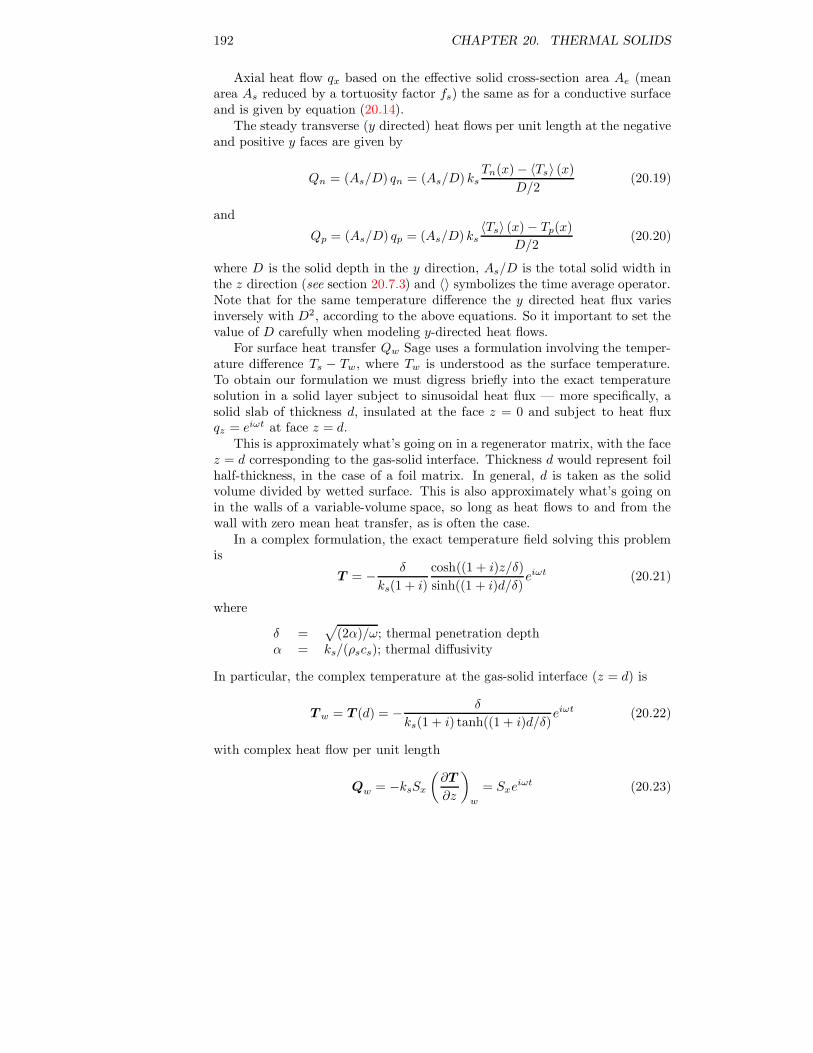
192 CHAPTER 20. THERMAL SOLIDS
Axial heat flow qx based on the effective solid cross-section area Ae (meanarea As reduced by a tortuosity factor fs) the same as for a conductive surfaceand is given by equation (20.14).
The steady transverse (y directed) heat flows per unit length at the negativeand positive y faces are given by
Qn = (As/D) qn = (As/D) ksTn(x) − 〈Ts〉 (x)
D/2(20.19)
and
Qp = (As/D) qp = (As/D) ks〈Ts〉 (x) − Tp(x)
D/2(20.20)
where D is the solid depth in the y direction, As/D is the total solid width inthe z direction (see section 20.7.3) and 〈〉 symbolizes the time average operator.Note that for the same temperature difference the y directed heat flux variesinversely with D2, according to the above equations. So it important to set thevalue of D carefully when modeling y-directed heat flows.
For surface heat transfer Qw Sage uses a formulation involving the temper-ature difference Ts − Tw, where Tw is understood as the surface temperature.To obtain our formulation we must digress briefly into the exact temperaturesolution in a solid layer subject to sinusoidal heat flux — more specifically, asolid slab of thickness d, insulated at the face z = 0 and subject to heat fluxqz = eiωt at face z = d.
This is approximately what’s going on in a regenerator matrix, with the facez = d corresponding to the gas-solid interface. Thickness d would represent foilhalf-thickness, in the case of a foil matrix. In general, d is taken as the solidvolume divided by wetted surface. This is also approximately what’s going onin the walls of a variable-volume space, so long as heat flows to and from thewall with zero mean heat transfer, as is often the case.
In a complex formulation, the exact temperature field solving this problemis
T = − δ
ks(1 + i)
cosh((1 + i)z/δ)
sinh((1 + i)d/δ)eiωt (20.21)
where
δ =√
(2α)/ω; thermal penetration depthα = ks/(ρscs); thermal diffusivity
In particular, the complex temperature at the gas-solid interface (z = d) is
T w = T (d) = − δ
ks(1 + i) tanh((1 + i)d/δ)eiωt (20.22)
with complex heat flow per unit length
Qw = −ksSx
(∂T
∂z
)
w
= Sxeiωt (20.23)

20.8. QUASI-ADIABATIC SURFACES 193
where Sx = As/d is wetted perimeter. The section-average temperature is
T s =iδ2
2ksdeiωt (20.24)
which is also the solution of our mean-parameter solid energy equation (20.18)with ∂qx
∂x = 0 and Qw = (As/d)eiωt.
Complex heat flux may be written as
Qw =ks
dSxN s(T s − T w) (20.25)
where N s is a dimensionless number not unlike the Nusselt number of gas heattransfer. Solving equation (20.25) for Ns and substituting the above solutions(20.22), (20.23) and (20.24) for T w, Qw and T s gives
Ns =2i(d/δ)2
(1+i)d/δtanh((1+i)d/δ)
− 1(20.26)
Interesting are the limiting cases for d/δ → ∞ (thick wall, high frequency, lowconductivity) and for d/δ → 0 (thin wall, low frequency, high conductivity).These are
N s =
{(1 + i)d/δ if d/δ → ∞3 if d/δ → 0
(20.27)
For thick solids, where thermal activity is confined to a layer roughly δ thick,surface heat flux is phase-shifted 45 degrees ahead of temperature differenceT s − T w. For thin solids, where the entire solid is thermally active, there is nophase shift.
In practice, the physical heat flux we are interested in is the real part of Qw
Qw =ks
dSx<(Ns(T s − T w)) (20.28)
The complex temperature difference T s − T w required for the right side isformulated in terms of the physical real temperature difference Ts − Tw as
T s − T w = (Ts − Tw) − ∂
∂ωt(Ts − Tw) (20.29)
This is valid so long as the temperature difference varies sinusoidally, becauseif Ts − Tw = <(T s − T w) = <(Ceiωt), then − ∂
∂ωt(Ts − Tw) = <(−iCeiωt) ==(Ceiωt) = =(T s −T w). And it is not Qw that is solved from equation (20.28)but, rather, the other way around. Sage solves the two variables Ts and Tw
implicitly using equations (20.18) and (20.28), considering sinusoidal heat fluxQw as given.
There are quasi-adiabatic model components for Ns computed rigorously,according to equation (20.26), as well as the thick- and thin-wall approximationsaccording to (20.27). They all descend from a common ancestor which has thefollowing variables:

194 CHAPTER 20. THERMAL SOLIDS
Kmult : (real, dimensionless) Empirical multiplier for axial conduction qx.
D : (real, m) Effective solid-conduction distance between the center line andthe surface where any y face heat flow is extracted. The value of D onlymatters when there is a distributed heat-flow connection made at either yface.
Solid : (enumerated) Solid material.
Mass : (real, Kg) Solid mass, provided for use in constraints in case it is partof a reciprocating mass system.
Dskin : (real, m) Skin thickness d in z direction, calculated as solid volumedivided by wetted perimeter (As/Sx).
Lambda : (real, m) Mean thermal wavelength λ in z direction, calculated as(2π√
2α/ω).
Tortuosity : (real, dimensionless) Mean (x, t average) solid axial conductionmultiplier fs (see section 23.0.1). fsAs is the effective area Ae for thermal-solid axial conduction (see equation (20.14)). So named because of thetortuous solid conduction path in porous materials.
FQwNet : (Fourier series, W) Net (x integrated) heat flow through positive zgas-facing surface.
QxNeg : (real, W) Net heat flow through negative x end.
QxPos : (real, W) Net heat flow through positive x end.
AEQw : (real, W) Available energy loss to z directed gas-surface heat flow,according to internal generation formula (20.2).
AEQx : (real, W) Available energy loss to x directed heat flow, according tointernal generation formula (20.2).
AEdiscr : (real, W) Available energy discrepancy of above two losses comparedto external generation as calculated by (20.1). (see section 20.3)
TsNeg : (real, K) Temperature Ts at negative x end.
TsPos : (real, K) Temperature Ts at positive x end.
FTsMean : (Fourier series, K) Spatial averaged (x average) temperature Ts.
Length l, cross sectional area As, z surface wetted perimeter Sx and initialtemperature distribution Ts all come from the parent model component.
20.8.1 Thick Surface
This quasi-adiabatic surface presumes the skin thickness d is much larger thanthe thermal wavelength λ. It is intended for modeling something like a thermallymassive cylinder space wall, where the time-varying heat flux is confined to athin layer near the surface.

20.9. FLOATING ISOTHERMAL SURFACE 195
20.8.2 Thin Surface
This quasi-adiabatic surface presumes the skin thickness d is much smaller thanthe thermal wavelength λ. It is intended as a fast alternative to the followingrigorous surface for modeling something like a regenerator matrix when the wirediameter, particle size, foil thickness, or whatever, is very small. If you use thiscomponent, you should check that output variable Dskin is indeed smaller thanLambda. If not, then you should use the rigorous surface component instead.
20.8.3 Rigorous Surface
This quasi-adiabatic surface presumes the skin thickness d is on the same orderas the thermal wavelength Lambda. It is intended for modeling any sort ofregenerator matrix or duct wall, although the slightly-faster thin-surface modelcomponent may be justified for finely divided matrices. A rigorous surface calcu-lates the Nusselt-like number Ns from equation (20.26) which takes a bit moretime than the thick- or thin-surface approximations.
20.9 Floating Isothermal Surface
This component was originally intended to be a faster version (in computationaltime) of the above quasi-adiabatic surfaces for use as the primary surface an-choring the gas temperature within a variable-volume space when the thermalsolution within the solid was not important. It is equivalent to the thin-surfacequasi-adiabatic model component in the limit of infinite thermal mass and zeroaxial conduction. It presumes the positive z surface is subject to time-varyingsinusoidal heat flux, with zero mean. The negative z surface along with bothx and y surfaces are presumed insulated. It has a discretized temperaturedistribution Ts(x) with no time variation. Ts serves as both the solid interiortemperature and the temperature at the positive zsurface. Sage implicitly solvesTs to achieve zero net (time-mean) surface heat flux.
As it turned out, floating isothermal surfaces were not noticeably faster thanother quasi-adiabatic solids and the solid temperature would often drift to phys-ically unrealistic values because of the lack of solid axial conduction. In somecases this led to convergence problems. So the use of floating isothermal surfacesis no longer recommended but they are still documented here for completenessand available in the software for special purposes.
A floating isothermal surface receives its initial temperature distribution Ts
from its parent model component, but has no variables of its own to appear indisplay windows or output listings. Everything you need to know about surfaceheat transfer and temperature is available from the gas-domain component it isconnected to.

196 CHAPTER 20. THERMAL SOLIDS
Chapter 21
Gas Domains
The gas-domain model components are at the heart of the stirling model class.Because of their complicated mathematical structure, they are also the mosttime consuming to solve and prone to convergence problems. From your pointof view, they appear simply as palette-created child model components withinheat-exchanger geometries. There are gas-domain variations for all of the basictypes of fluid flow: duct flow, porous matrix flow and flow into a variable-volumespace (formed by a piston in its cylinder) through an inlet. All gas domains areborn with a thermal boundary connector intended for connection to a thermalsolid of your choice. Gas domains, being one dimensional, admit to flow connec-tions with other gas domains at either their positive or negative ends. Since youmay want to have flow connections at only one end, at both ends, or multipleconnections at one end, flow connectors are palette-created child-model com-ponents. Variable-volume gas domains have palette-created displaced-volumeconnectors intended for connection to area faces of moving parts.
There remains one more gas-domain connection: the charge line. Exactly onegas domain model component must have a charge-line connection to a pressure-source component to establish the amount of working gas in the sum-total of allinterconnected gas domains. This is very important. Without a pressure-sourceconnection there will be no way for Sage to determine the amount of workinggas in your system and solving will not converge. Charge-line connectors arepalette created because there is no way for Sage to decide which gas componentshould get it.
21.1 Attachment Child Components
All gas domains have the ability to produce child model components represent-ing charge-line connectors and flow inlets. Some can also produce volumetricdisplacements.
When you drop a gas domain model component from the stirling palette intothe edit form, it starts out with only a thermal connector arrow, intended for
197

198 CHAPTER 21. GAS DOMAINS
connection to a thermal solid component. In order to make additional connec-tions, you must first drop in one or more of the following child model componentsfrom the palette.
Icon Purpose
gas charge line
negative gas inlet
positive gas inlet
phasor negative-facing volume displacement
phasor positive-facing volume displacement
time-ring negative-facing volume displacement
time-ring positive-facing volume displacement
When you drop one of these into the edit form, it is born with a connectionarrow which you can then move up one level to the parent-component page ofthe edit form for connection there to a mate, perhaps originating in another gasdomain.
The gas charge line is for connection to a pressure-source component. It isrequired for exactly one gas domain component in your total interconnected gasdomain, as explained above.
The two types of gas inlets are for connection to other gas domains as yousee fit. Generally you will want zero or one flow inlets at each end, dependingon whether your component is functioning as a dead-ended passage or throughpassage. In some instances you will create two (or more) flow inlets at the endof a gas component which enables it to act as a T or Y component.
The volume displacements are available only in variable-volume gas domains.They are intended for connection to area faces of moving parts like the recipro-cator or constrained piston components documented in chapters 12 and 19.
21.2 Coordinate Conventions
A gas domain may be thought of as a one-dimensional rectangular region likethis:

21.3. ENTROPY GENERATION 199
- x
6
z
���
y
((((((((((((((((((((((
��
��
��
��
��
��
((((((((((((((((((((((
6 6 6
q(x, t)
-m(t)
Gas flow m(t) may pass through either the positive or negative x boundaries,but nowhere else. Heat flux q(x, t), generally to a thermal solid, may passthrough the negative z boundary, but nowhere else. Discretization is in the xdirection only, similar to a thermal solid. In principle, the cross-sectional areamay vary with x, as drawn. It may even vary with time, as if the upper z surfacewere moving in accordance with a volume displacement.
21.3 Entropy Generation
Gas domains involve the conduction of heat across finite temperature differencesas well as irreversible flow processes. Both generate entropy (see chapter 17).
The second law of thermodynamics applied to the external surface of ourgas domain, over a full periodic cycle is
External Entropy Generation =
∮
dt
∫
ds
n · qT
+
[∮
dt
ms
]x=b
x=a
(21.1)
where n · q and T are the z-surface normal heat flux and absolute temperature,and m and s are the x-end mass flow rate and mass-specific entropy. The [·]x=b
x=a
notation means the difference of the enclosed expression evaluated a the twoendpoints. Entropy generation defined this way refers to the increase in entropyin the universe surrounding the gas domain as a result of internal irreversibilities.
There are two internal entropy generating mechanisms, heat flow and viscousfriction. There are actually two distinct heat-flow mechanisms, axial conductionand film heat transfer, but at this level of generality the entropy generated byeither is covered by the formula
Conductive Entropy Generation = −∮
dt
∫
dv
q · ∇TT 2
(21.2)

200 CHAPTER 21. GAS DOMAINS
where the integrand is the local rate of entropy production due to heat flowin a temperature gradient. And the entropy generation of viscous friction, inone-dimensional flow, may be calculated as
Viscous Entropy Generation = −∮
dt
∫
dx
uAF
T(21.3)
where uA is volumetric flow rate and F represents that part of the pressuregradient due to viscous friction. The numerator in the integrand is the pumpingdissipation per unit length.
Entropy generations are presented as available-energy outputs by multiply-ing the entropy integrals by Tnorm, the normalization temperature of the rootstirling model component. Each model component evaluates its entropy inte-grals in a manner appropriate to the physics and solution-variable discretizationembodied within it.
21.4 Pressure Source Component
The pressure source component establishes the charge pressure for your stirlingmodel. You must have exactly one pressure source, connected to some gasdomain. A pressure source acts as an infinite isobaric gas reservoir. Its onlyvariable is
Pcharge : (real, Pa) Charge pressure.
The result of connecting a pressure source to a gas domain is that the density inthe gas domain adapts itself so that t average pressure is continuous across theconnection — so that the time-average pressure at the negative end of the gasdomain becomes Pcharge. This is explained mathematically in section (21.6).
21.5 Gas Domain Components
There are three distinct variations of gas domains, distinguished primarily by themethod by which they track the onset of turbulence. They all come with a largeassortment of variables, mostly outputs, sufficient for most of your needs but nottoo numerous to unduly clutter your output listings. For more information youcan always dump the solution grid with the File|Save Solution Grid command.The following list includes all possible variables in all types of gas domains. Somevariables may be missing from individual gas domains, depending on what makessense. Mathematical symbols, as yet undefined, will be found in the subsequentsections on theory at the end of this chapter.
Fmult : (real, dimensionless) Empirical multiplier for viscous pressure drop F .
Hmult : (real, dimensionless) Empirical multiplier for z-surface heat transferQw.

21.5. GAS DOMAIN COMPONENTS 201
Kmult : (real, dimensionless) Empirical multiplier for axial conduction q indomain interior.
KmultBnd : (real, dimensionless) Empirical multiplier for axial conduction q atdomain endpoints. Default is 0 which blocks thermal conduction betweengas domains. Set to 1 in both gas domains on either side of a flow connectorto allow continuous thermal conduction across the flow connector.
UpwindFrac : (real, dimensionless) The relative weight factor for upwind influ-ence in density (temperature) interpolation between control volumes inthe computational grid (see section 21.6.6). Increasing the value will helpsmooth out a jagged axial temperature profile at some cost in reducedaccuracy. Based on computational experiments, the default of 1.0E-2 pro-vides sufficient stability for almost all situations with a negligible effect onaccuracy. In the event of temperature instability (which you can see byplotting a file of computational solution variables), increasing the value to1.0E-1 should stabilize almost any gas domain. Poor convergence may bea sign of temperature instability. Inputs are restricted to the range zeroto one.
Klocal : (real, dimensionless) Local frictional pressure-drop loss coefficient K(see equation (21.14). Used for including entrance, exit and bend effectsonly in duct-type gas domains.
TbInNeg : (real, dimensionless) Incoming relative turbulence T at the positiveend of a duct-type gas domain. The default is 1, corresponding to a sharpentrance where flow separation is expected or the upstream turbulencelevel is high. A value of 0 implies completely smooth incoming flow corre-sponding to a continuous flow area or a perfectly diffused transition andlow upstream turbulence level.
TbInPos : (real, dimensionless) Like TbInNeg except at the duct-gas negativeend.
FQcombust : (Fourier series, W) Combustion firing rate as a function of time.Available as an input variable only in the combustion-space gas componentwithin a generic-cylinder component. It directly determines the combus-tion heating term Qc in the gas energy equation. (see section 21.6.3).
PV : (Fourier series, W) Net (x integrated) PV power output (∫
dxP ∂A
∂t). Avail-
able only in variable-volume gas domains where flow area A is a functionof time. The mean value is the t-average PV power which most peoplethink of when they think of PV power. A positive value indicates workdone by the gas on the walls. The higher harmonics are available if youare interested.
FQwNet : (Fourier series, W) Net (x integrated) heat flow through negative zsolid-facing surface (positive is from solid to gas).

202 CHAPTER 21. GAS DOMAINS
HNeg : (real, W) t average stagnation enthalpy flow through negative x in-let. Stagnation enthalpy uA(ρe+ P ) includes all forms of energy flow —internal, PV and kinetic.
HPos : (real, W) t average stagnation enthalpy flow through positive x inlet.
AEfric : (real, W) Available energy loss to viscous flow friction, according tointernal generation formula (21.3).
AEQw : (real, W) Available energy loss to z directed solid-surface heat flow,according to internal generation formula (21.2).
AEQx : (real, W) Available energy loss to x directed heat flow, according tointernal generation formula (21.2).
AEdiscr : (real, W) Available energy discrepancy of above losses compared toexternal generation as calculated by (21.1). (see section 21.3)
QwNeg : (real, W/m) t average heat flow per unit length through negative zsolid-facing surface, at negative x end. Gives insight into surface heat flowdistribution.
QwPos : (real, W/m) Same as QwNeg except at positive x end.
QxMean : (real, W) t and x averaged axial heat flow q.
TNeg : (real, K) t average temperature T at negative x end.
TPos : (real, K) t average temperature T at positive x end.
Vmean : (real, m3) Gas domain volume. Provided for fixed as well as time-varying volumes, although in that case Vmean is the t average volume.See also: FV for variable-volume gas domains.
FTMean : (Fourier series, K) Spatial averaged (x average) temperature T .
FPMean : (Fourier series, Pa) Spatial averaged (x average) pressure P .
FPNeg : (Fourier series, Pa) Pressure P at negative boundary.
FPPos : (Fourier series, Pa) Pressure P at positive boundary.
FDP : (Fourier series, Pa) Pressure difference across domain (positive − nega-tive x ends).
FV : (Fourier series, m3) Domain volume for a variable-volume gas domain.The mean value (t average) and first harmonic are generally of the mostinterest.

21.5. GAS DOMAIN COMPONENTS 203
FM : (Fourier series, kg) Total mass in a gas domain. The sum of all meanvalues (t averages) over all gas domains is the total gas mass in the system.The time derivatives of the first and higher harmonics are theoretically thesame as the difference of inlet mass flow rates (FRhoUAPos - FRhoUANeg).But due to inaccuracies of finite time-differencing, this is exact only for thefirst harmonic and in the limit of large time nodes for higher harmonics.
FHmean : (Fourier series, W) Spatial averaged (x average) stagnation enthalpyflow uA(ρe+ P ).
FRhoUAmean : (Fourier series, kg/s) Spatial averaged (x average) mass flowrate ρuA.
FRhoUANeg : (Fourier series, kg/s) Mass flow rate ρuA through negative xinlet.
FRhoUAPos : (Fourier series, kg/s) Mass flow rate ρuA through positive x inlet.
MachMean : (real, dimensionless) t and x averaged Mach number.
TdMean : (real, dimensionless) t and x averaged tidal amplitude divided bylength L. Total tidal displacement is computed as the mean absolutevelocity multiplied by half a cycle period. Tidal amplitude is half that.Only available in duct or matrix gas domains.
ReMean : (real, dimensionless) t and x average Reynolds number Re in matrixor duct gas domains or turbulent Reynolds number Rt in variable-volumegas domains.
VaMean : (real, dimensionless) t and x averaged Valensi number Va in duct gasdomains.
TbMean : (real, dimensionless or J/m3) t and x averaged relative turbulenceT in duct gas domains or turbulence intensity ρκ in variable-volume gasdomains.
ZMean : (real, dimensionless) t and x averaged gas compressibility P/(ρRT )as returned by the gas property variable Gas selected in the stirling rootcomponent. This is always one for an ideal gas. A Redlich-Kwong gasreturns a more realistic value.
EOSErrMean : (real, dimensionless) t and x averaged equation of state relativeerror as returned by the gas property variable Gas selected in the stirlingroot component. This is always zero for an ideal gas. A Redlich-Kwonggas returns a more realistic estimate.
Coming from the parent component are the length L, mean flow area A, wettedperimeter Sx, initial axial temperature distribution T (x) in the form of a cubicspline variable and working gas (properties).

204 CHAPTER 21. GAS DOMAINS
A primary purpose of a gas domain is to calculate the empirical relation-ships for friction factor f , Nusselt number Nu and axial conductivity ratio Nk
appropriate for the flow geometry in which it finds itself (see section (21.6).Accordingly, there is a gas-domain variation for each individual type of heatexchanger geometry. But they all fit into one of the following three classes.
21.5.1 Matrix Gas Domains
A matrix gas domain is used within a porous matrix or within uniform channelsof tiny hydraulic diameter. A matrix gas domain knows about Reynolds number,defined as
Re =ρ|u|dh
µ(21.4)
where u is mean-flow velocity and dh is hydraulic diameter defined as
dh =4A
Sx(21.5)
It also knows about matrix porosity, which is a variable imported from theparent component.
Wetted perimeter is the wetted surface area per unit length. The notationSx is shorthand for ∂S
∂x , where S(x) is the cumulative wetted surface between po-sition zero and x. For domains where S varies linearly with x, wetted perimeteris just the total wetted surface divided by domain length.
21.5.2 Duct Gas Domains
A duct gas domain is used within relatively short flow ducts (generally tubesor rectangular channels) with not so tiny hydraulic diameters. A duct gas do-main knows about Reynolds number, Valensi number and turbulence intensity.Reynolds number Re is defined as in equation (21.4). Valensi number is
Va =ρωd2
h
4µ(21.6)
It is related to the ratio of hydraulic diameter to viscous penetration depthδν =
√
2µ/(ωρ)) according to
dh/δν =√
2Va (21.7)
Turbulence intensity T is discussed in detail in section 21.8. Duct domainsalso know about aspect ratio, which is a variable imported from the parentcomponent. And they introduce the local-loss pressure-drop coefficient K (inputvariable Klocal), used in frictional pressure-drop equation (21.14).

21.6. GAS DOMAIN THEORY 205
21.5.3 Variable-Volume Gas Domains
A variable-volume gas domain is used within the generic-cylinder model com-ponent for modeling piston-cylinder spaces of stirling models — i.e. the volumebetween the pistons and the cylinders in which they ride. A variable-volume gasdomain knows about turbulent Reynolds number and Valensi number. Valensinumber Va is the same as in equation (21.6) and turbulent Reynolds number Rt
is defined in section 21.8. Flow area A is no longer constant. Rather, it varieswith time in accordance with palette-generated volume displacements connectedto the area faces of moving-part components.
21.5.4 Combustion-Space Gas Domains
A combustion-space gas domain is alternative to the above variable-volume gasdomain, also available within the generic-cylinder model component. It is in-tended for modeling internal-combustion spaces in a simplified way. Input vari-able FQcombust specifies the combustion firing rate independently of fuel or airflow rates or combustion chemistry. You are responsible for ensuring the con-ditions for combustion are actually met. The combustion firing rate directlydetermines source term Qc in the gas energy equation (see section 21.6.3)).
Combustion heating is modeled as a completely reversible process that doesnot involve entropy generation. It is perfectly feasible to specify a negative firingrate, in which case it amounts to a reversible cooling process.
As a software object, this component descends from the above variable-volume gas domain. This means it inherits all of the physics of the variable-volume gas domain in regard to turbulent Reynolds number, etc.
21.6 Gas Domain Theory
The following equations are somewhat nonstandard in the computational fluiddynamics literature because they are designed specifically for one-dimensionalinternal flows with space- and time-variable flow area. Most CFD textbookstake a more general world view. So, rather than just quote the equations, weare forced to do a bit of derivation — as concisely as possible. Our startingpoint is the general Navier-Stokes equations in integral form, as found in Peyretand Taylor [45], except that we shall neglect body forces and relax the prevailingconvention that control volume v be fixed. We shall assume that v has fixedinlet and exit boundaries, but allow moving side boundaries — time-variableflow area. The side boundaries are impermeable so that flow enters and leavesonly through the inlet and exit boundaries. A rubber tube with space- andtime-variable cross section is a useful thought picture. The principle flow axisis the tube axis. In this control volume the integral gasdynamic equations are:
continuityd
dt
∫
v
ρ dv +
∫
s
ρn · V r ds = 0 (21.8)

206 CHAPTER 21. GAS DOMAINS
momentumd
dt
∫
v
ρV dv +
∫
s
[(n · V r)ρV − nσ]ds = 0 (21.9)
energyd
dt
∫
v
ρe dv +
∫
s
n · (ρeV r − σV − q) ds = 0 (21.10)
where
e = ε+ u2/2; mass-specific total gas energyn = unit outward normal of sq = heat flux vectors = surface of vt = timev = control volumeV = Newtonian-frame flow velocity vectorV r = boundary-relative flow velocity vectorε = mass-specific internal gas energyρ = gas densityσ = stress tensor
The continuity equation states, in English, that the time rate of change ofmass in the control volume equals the rate at which mass leaves through itssurface boundaries. By definition, n · V r is zero along the side surfaces, so themass enters and leaves only through the inlet and exit boundaries.
The momentum equation is a statement of Newton’s second law of motion— the time rate of change of control-volume momentum, less the momentumleaving through its surface boundaries, equals the net force acting on all surfaces.We must be a bit more careful here because momentum (velocity) must bemeasured in reference to a fixed Galilean frame for Newton’s second law to bevalid. So the “V ” in ρV must continue to be absolute, not relative velocity.We will keep this distinction in mind but, fortunately, it will not affect us muchbecause it applies only to the transverse velocity components (associated withconverging, diverging or moving side boundaries) and we are necessarily ignoringtransverse components in the momentum equation in a one-dimensional model.
The energy equation states that the time rate of change of control-volumeinternal plus kinetic energy, less that leaving through its surface boundariesequals the net heat flux through its boundaries plus the mechanical work doneon its boundaries. Mechanical work, like momentum, must be measured in aninertial frame so the “V ” in the tensor product σV must also remain absolute,not relative.
We now convert our equations to one-dimensional differential equations inconservative form.
In all equations we replace dv in the time integrals with Adx, where A is flowarea and x is the principle flow direction, take the limit as ∆x→ dx then dividethrough by dx. For example, the term d
dt
∫
vρ dv in the momentum equation will
transform to ∂∂t
(ρA), and so forth.

21.6. GAS DOMAIN THEORY 207
((((((((((((((((((((((
x x+ dx
PA - PA �
P dA -
FA�
Figure 21.1: Axial surface forces∫
s−Nσ resolved into pressure and empirical
flow-friction terms
For the surface integrals, we must consider the inlet and outlet boundariesseparately from the side boundaries on a case-by-case basis.
Continuity Equation Surface integral∫
sρn · V r ds in the continuity equa-
tion, after taking the limit as ∆x → 0 and dividing out dx, becomes ∂∂x
(ρuA),where u is mean-flow velocity in the x direction.
Momentum Equation Surface integral∫
s(n · V r)ρV ds in the momentum
equation becomes, simply, ∂∂x (uρuA) because there is no momentum flux through
the side boundaries.
Integral∫
s−nσds, representing the forces applied to the surface, is more
involved. Straight off, since this is a one-dimensional model, we will empiricisethe stress tensor σ into thermodynamic pressure P and a viscous flow resistanceterm F which we may think of as the force per unit length per unit flow areadue to surface shear stress. F amounts to a frictional pressure gradient. Then,pressure forces on the inlet and exit boundaries transform to ∂
∂x(PA)−P ∂A∂x =
A∂P∂x . Viscous forces on the side boundaries transform into just −FA. The
sketch in figure 21.1 may help make this clear:
Energy Equation Surface integral∫
sn · (ρeV r)ds in the energy equation
becomes, simply, ∂∂x
(uρeA) because there is no energy flux through the sideboundaries.
Integral∫
s−n·σV ds for the inlet and exit boundaries transforms to ∂
∂x(uPA).No F term is involved since F is applied to the side walls. For the side walls theintegral transforms to P ∂A
∂t, the PV work done on the wall. ∂A
∂tderives from
the transverse velocity component of the moving walls. Once again, there is no

208 CHAPTER 21. GAS DOMAINS
((((((((((((((((((((((
x x+ dx
uPA - uPA -
P ∂A∂t dx ?
Figure 21.2: Surface work∫
s−n · σV resolved into pressure terms
F term. The reason is because axial velocity is zero at the walls where F isapplied. See figure 21.2:
Integral∫
s −n · qds transforms to a term ∂∂x (qA) for the end boundaries,
where q is axial heat flux. For the negative z boundary we introduce empiricalfilm heat transfer per unit length Qw to represent the integral.
In terms of these simplifications our equation set becomes:
continuity∂ρA
∂t+∂ρuA
∂x= 0 (21.11)
momentum∂ρuA
∂t+∂uρuA
∂x+∂P
∂xA − FA = 0 (21.12)
gas energy
∂ρeA
∂t+ P
∂A
∂t+
∂
∂x(uρeA + uPA+ q) −Qw = 0 (21.13)
The purpose of these gasdynamic equations is to determine three implicit solu-tion variables, which we hereby choose to be ρ, ρuA and ρe. The reason for thischoice is that all are roughly continuous across area discontinuities and, exceptfor the factor A in the second, are standard in the field. Empirical terms F , Qw
and q are explained further below.
21.6.1 Viscous Pressure Gradient F
The term F in the momentum equation takes the place of the viscous terms inthe Stokes stress tensor, which cannot be resolved directly in a one-dimensionalmodel. The units of F are force per unit length, per unit flow area (same as

21.6. GAS DOMAIN THEORY 209
∂P∂x ). F may be formulated in terms of Darcy friction factor f and total localloss coefficient K in a heat exchanger of hydraulic diameter dh and length L as:
F = − (f/dh +K/L) ρu|u|/2 (21.14)
Friction factor may be calculated as an empirical function of instantaneouslocal flow conditions, according to some published correlation. Loss coefficientis generally a fixed constant, equal to the sum of local loss coefficients for sharp-edged area changes, bends, etc.
Complex Formulation for Ducts
In the case of laminar flow in duct gas domains (see section 21.5.2), Sage allowsfor a phase shift between viscous pressure gradient and velocity by formulat-ing F in terms of a complex wall-shear-stress function s = sr + isi insteadif a conventional friction factor. The following formulation also accounts forthe contribution of any time-mean (DC) velocity that may be present, whichsometimes happens in novel Sage applications:
F = −(K/L)ρu|u|/2 − (8µ/d2h)sr0um − (8µ/d2
h)<(su) (21.15)
Here, µ is viscosity and sr0 is the steady-flow limit for sr . The factor 8µ/d2h
may also be written 2ρω/Va. The first term on the right is a smeared-out local-loss per unit length carried over from the previous formulation. The last twoterms amount to the superposition of the frictional pressure gradient solutionsfor a laminar steady-flow momentum equation and an laminar oscillating-flowmomentum equation. Both equations are linear in u, so the superposition isvalid.
In this formulation Sage’s section-mean velocity u(t) is broken into the time-mean value um plus a fluctuating component u− um considered to be the realpart of the complex-valued velocity
u(t) ≈ (u− um) − i∂u
∂ωt(21.16)
This is valid so long as velocity varies sinusoidally, because if u − um = <u =<(Ceiωt), then − ∂u
∂ωt= <(−iCeiωt) = =(Ceiωt) = =u.
The oscillating-flow wall-shear-stress function s is not a standard conceptlike friction factor. It is defined in reference [12], for incompressible laminarflow between parallel plates, as −f ′
wall/ 〈f〉 where f is the complex velocityprofile function (u(y) = f(y)eiωt). For other channel shapes, it can be relatedto the somewhat more standard fν functions used in thermoacoustic theory [61]using
s =iVa
2
(fν
1 − fν
)
(21.17)
Both s and f ν are functions of Valensi number, or, as thermoacoustic practition-ers prefer to say, functions of the ratio of some characteristic channel dimension

210 CHAPTER 21. GAS DOMAINS
to viscous penetration depth. (Viscous penetration depth is δ =√
2µ/(ρω),which is related to Valensi number by
√2Va = dh/δ.)
The steady-flow (low-Va) limit sr0 is related to the conventional Darcy fric-tion factor by
f =16sr0
Re(21.18)
In other words, 16sr0 is the constant factor that appears in the numerator ofthe laminar friction factor correlation. This relation can be used to cross-checks calculations against the laminar steady-flow friction-factor literature.
21.6.2 Film Heat Transfer Qw
The term Qw in the energy equation is the heat flow per unit length, throughthe negative z surface, due to film heat transfer. The normal way to formulatethis is
Qw = hSx(Tw − T ) = Nu(k/dh)Sx(Tw − T ) (21.19)
where Nu is a Nusselt number, k is gas conductivity, dh is hydraulic diameter, Sx
is the wetted perimeter (wetted surface area per unit length) and Tw − T is thetemperature difference between the negative z surface and section-average. Thisis appropriate for heat transfer in phase with the film temperature difference.Matrix gas domains (see section 21.5.1) use this approach.
Complex Formulation for Cylinders
Variable-volume gas domains (see section 21.5.3), allow for a phase shift betweenheat transfer and film temperature difference by using a complex Nusselt numberformulation
Qw = (k/dh)Sx [Nu0(Tw − Tm) −<(NuT )] (21.20)
In this formulation Sage’s gas temperature T (t) is broken into the time-meanvalue Tm plus a fluctuating component T − Tm considered to be the real partof the complex-valued temperature
T (t) ≈ (T − Tm) − i∂T
∂ωt(21.21)
This is valid so long as temperature varies sinusoidally, because if T − Tm =<T = <(Ceiωt), then − ∂T
∂ωt = <(−iCeiωt) = =(Ceiωt) = =T . The complex-valued Nusselt number Nu generally comes from some linear time-varying lam-inar theory [35]. The reason behind the form of equation (21.20) is that theterms (1/dh)Nu0(Tw − Tm) and −(1/dh)NuT are, because of the way the Nus-selt numbers are defined in such theories, just the normal temperature gradients( ∂
∂y ) at the wall for the steady and time-varying components of the theoreti-cal temperature solution, which are additive. Complex Nusselt numbers havea significant imaginary component only for high Valensi number laminar flows,when hydraulic diameter is large compared to thermal diffusion length. In thiscase, the quantity −(k/dh)Sx<(NuT ) in equation (21.20), which represents the

21.6. GAS DOMAIN THEORY 211
physical component of the complex heat flow per unit length, may be phaseshifted ahead of Tm − T by as much as 45 degrees. For turbulent flows or forlow Valensi numbers the complex heat-flow formulation essentially reduces tothe conventional real formulation (21.19).
Complex Formulation for Ducts
Duct gas domains (see section 21.5.2), attempt to improve upon the complex for-mulation by breaking the fluctuating complex temperature T into compression-driven and advection-driven components T c + T a, arising from pressure vari-ations and temperature gradients carried along by the flow, the two being in-dependent mechanisms. The reason for decomposing temperature like this isthat the Nusselt numbers for the two sources of temperature variation differ,compression-driven temperature variations being roughly twice as effective atdriving wall heat transfer as advection-driven temperature variations in thehigh Valensi-number limit — according to first-order oscillating-flow solutions[15, 60]. So to be as accurate as possible, duct gas domains formulate wall heattransfer as
Qw = (k/dh)Sx [Nu0(Tw − Tm) − <(NucT c) − <(NuaT a)] (21.22)
where Nuc is the compression-driven complex Nusselt number and Nua is theadvection-driven complex Nusselt number. The importance of this formulationis mainly for high Valensi number laminar flows. For turbulent flows or for lowValensi numbers, Nuc and Nua are equal, or nearly equal, and real-valued so theheat-flow formulation essentially reduces to the previous complex formulation(21.20) or the real formulation (21.19).
Of course, the trick is how to evaluate T c and T a, given that the onlytemperature available directly from the Sage solution is the combined result T .This goes roughly as follows:
• Take T c = scT∞c where sc is some complex scale factor which varies with
Valensi number Va and T∞c is the high Va limit of the compression-driven
temperature variation
T∞c =
1
ρmCpP1 (21.23)
according to Swift’s first-order acoustic solution [60]. P 1 is the complexpressure variation, which may be calculated as P 1 = (P − Pm) − i ∂P
∂ωt .
• Similarly, take T a = saT∞a where sa is another complex scale factor and
T∞a is the high Va limit of Swift’s advection-driven temperature variation
T∞a =
1
ω
∂T
∂xi 〈u1〉 (21.24)
〈u1〉 is the complex section-average velocity 〈u1〉 = u− i ∂u∂ωt
.

212 CHAPTER 21. GAS DOMAINS
• Assume the same scale factor s serves for both sc and sa, which is jus-tified by examination of Swift’s exact solution for temperature (section-averaged) over the entire range of Va.
• Calculate this common scale factor as
s =T
T∞c + T ∞
a
(21.25)
except when the denominator is zero or close to zero — whenever T∞c
and T∞a are nearly equal and opposite. When this happens calculate s
directly from an approximation based on Swift’s theory, then T c = sT∞c
as above, but T a = T − T c so the sum T a + T c is always T .
Explicit Surface Temperature
Although we might tend to think of Tw as the independent variable in the pre-ceding heat-flow equations, from the point of view of Sage’s solver it is actuallyQw that is the independent variable; implicitly solved so that Tw is continu-ous across the gas-solid connection at the negative z surface. Given Qw, gasdomains explicitly calculate negative z surface temperature as either
Tw = T +
(dh
k
Qw
SxNu
)
(21.26)
or
Tw = Tm +1
Nu0
(dh
k
Qw
Sx+ <(NuT )
)
(21.27)
or
Tw = Tm +1
Nu0
(dh
k
Qw
Sx+ <(NucT c) + <(NuaT a)
)
(21.28)
depending on which heat-transfer formulation is used.
21.6.3 Combustion Heating Qc
In rare instances where it may be appropriate to consider an internal heatingsource within the gas (see the combustion-space gas domain of section 21.5.4),an energy source Qc is added into energy equation (21.13), on the same footingas the above film heat transfer term, except it represents internally generatedheat per unit length. This energy input is treated as a simple energy sourceindependent of any actual combustion chemistry.
21.6.4 Gas Axial-Conduction Heat Flux q
Term q in the gas energy equation is instantaneous axial heat flux which wemay formulate as
q = −ke∂T
∂xA (21.29)

21.6. GAS DOMAIN THEORY 213
where ke is the effective gas conductivity — which may exceed molecular con-ductivity due to turbulent enhancement. This may be formulated in terms ofan axial-conductivity enhancement ratio Nk as:
q = −Nkk∂T
∂xA (21.30)
21.6.5 Equations of State
Tying the gasdynamic equations together is an equation of state which serves toformulate the dependent variables P and T as functions of independent variablesρ, ρuA and ρe — specifically as P (ρ, T ) and T (ρ, ρe, ρuA). The gas-propertyobjects defined in the stirling root model provide these functions (see chapter18).
21.6.6 Solution Method
The gasdynamic equations are discretized over a grid of points (xi, tj) uniformlyspaced throughout the domain and over the cycle period. Upon this grid, vari-ables ρ, ρuA and ρe, are solved implicitly or interpolated explicitly according tothe logic of a staggered-grid formulation. The essential idea is to solve ρuA atalternate nodes from ρe and ρ to avoid solution instability and produce globalconservation of mass, momentum and energy. Solution staggering is with respectto the spatial direction only.
The concept of control volumes is helpful for keeping things straight in thestaggered-grid scheme. Control volume boundaries can be thought of as lyingon alternate spatial nodes. One can think of it this way: ρuA is solved at thecontrol volume boundaries, while ρ and ρe are solved at the midpoints. Theentire domain comprises an integral number of control volumes or, includingendpoints, an odd number of nodes greater than or equal to three. Globalconservation of energy and mass automatically hold for the solved variables ρand ρe if one is careful to use first-order central differencing in the continuityand energy equations so that, in effect, quantities leaving one control volumeenter the adjacent one.
Interior Points
Those nodes lying strictly within the domain interior give rise to implicit finite-difference equations for the solved variables ρuA, ρ and ρe. Variables thatare not solved at interior nodes are interpolated. In the case of ρuA and ρe,interpolation takes the form of a central polynomial interpolation of neighboringsolved values. The degree of the interpolation (linear or cubic) can be specifiedin the Options|Sage dialog. In the case of ρ, interpolation is a weighted averageof central interpolation and interpolation with the set of interpolation pointsshifted toward the upwind direction. This weights the interpolation toward thecurrently upwind direction in order to stabilize the solution. You can specifythe relative fraction of upwind interpolation with input variable UpwindFrac,

214 CHAPTER 21. GAS DOMAINS
should the default value be too small. Without the upwind weighting, densityand temperature profiles can sometimes show a static zig-zag instability in gasdomains where there is not a lot of thermal diffusion to dampen the effect.
Endpoint Boundary Points
These are the nodes lying at the negative and positive domain boundaries —the flow inlets. Solved variables ρ, ρuA, ρe get special treatment at such nodes,depending on whether or not there is a flow connection to an adjoining gasdomain or not. This is explained fully in the following section. Other variablesare simply extrapolated from the interior.
Minimal Requirement for Resolving Pressure Drop
One idiosyncrasy of the solution method is worthy of note: Pressure-drop,whether due to flow resistance or acceleration, will be ignored in any gas domaincontaining only one control volume. According to the staggered-grid solutionscheme of the gas domain, the momentum equation will never be invoked whenonly one cell is present, leaving mass flow rate determined solely by Bernoulli’slaw in adjacent flow connectors. This behavior is not necessarily bad. It mayeven be desirable in some cases. But it is something to keep in mind.
The Mean Pressure Constraint
Although it may not be immediately apparent, the solution scheme so far out-lined will result in a singular system of implicit equations. In physical terms,there is no mechanism to establish the mean pressure.
Resolving this dilemma requires a close inspection of the mass-continuityequations enforced in the gas domain interior. Taken together, these equationsimply that the cyclic-net mass passing through the endpoint boundaries is zero,meaning that we cannot independently set boundary mass flow rate at bothendpoint boundaries for all time nodes. Looking at this in another way, if we dospecify boundary mass flow rates at all time nodes (such that cyclic-net massthrough boundaries is zero) and enforce the mass-continuity equation at all butone interior cell, say (i0, j0), then mass continuity is automatically guaranteedfor (i0, j0). This frees us to replace the mass continuity equation at (i0, j0) witha mean-pressure constraint instead — which is what we do.
The penultimate sentence in the preceding paragraph is really a mathe-matical theorem that follows from the conservation property of central spatialdifferencing in our staggered-grid scheme and the time-ring-differencing prop-erty
∑
j
∂f
∂t(i, j) = 0 (21.31)
which holds no matter what. To show the mass-continuity equation indeed holds

21.7. FLOW CONNECTOR THEORY 215
at (i0, j0) we first use the time ring differencing property to conclude that
∂ρA
∂t(i0, j0) = −
∑
j 6=j0
∂ρA
∂t(i0, j) (21.32)
we immediately replace the right-hand side using
−∑
j 6=j0
∂ρA
∂t(i0, j) =
∑
j 6=j0
∂ρuA
∂x(i0, j) (21.33)
=∑
j
∂ρuA
∂x(i0, j) −
∂ρuA
∂x(i0, j0) (21.34)
the first part of the above equation follows from the presumed local mass conti-nuity for all nodes but (i0, j0) and the second part is just regrouping. The firstterm on the right may be further resolved into
∑
j
∂ρuA
∂x(i0, j) ∝
∑
j
ρuA(i0 + 1, j) −∑
j
ρuA(i0 − 1, j) (21.35)
∝∑
j
ρuA(2M, j) −∑
j
ρuA(0, j) (21.36)
(21.37)
which follows from central differencing formula used in the computational grid,then summing the local mass-continuity equations over j at successive columnsin the grid from i0 + 2 to the positive boundary i = 2M and from i0 − 2 to thenegative boundary i = 0. Combining the above results we are left with
∂ρA
∂t(i0, j0) +
∂ρuA
∂x(i0, j0) ∝
∑
j
ρuA(2M, j) −∑
j
ρuA(0, j) (21.38)
which is the mass-continuity equation at (i0, j0) we are after, provided the right-hand side evaluates to zero, which it will if the net mass flow through theendpoint boundaries is zero.
In a system comprising many gas domains joined by flow connectors, theabove result still applies to the system as a whole. So long as zero net massflows through the ultimate boundaries of the system, we are free to replace alocal mass-continuity equation at exactly one node (i0, j0) with a mean-pressureconstraint. In a Sage model the gas domain to which the mean-pressure con-straint applies is the one attached to the pressure-source component (see section21.4).
21.7 Flow Connector Theory
Flow area may change abruptly between adjacent gas domains, requiring specialconsideration in Sage’s one-dimensional formulation. Between every two gas
216 CHAPTER 21. GAS DOMAINS
domains that are connected together there is a special flow connector objectthat manages the connection behind the scenes. There are three conditions tosatisfy: conservation of mass, momentum and energy. Conservation of mass isautomatic because of the choice of mass flow rate ρuA as a solution variable.Sage uses momentum continuity (Bernoulli’s law) as the implicit equation forsolving mass flow rate in flow connectors. This is entirely consistent with thestaggered-grid treatment for ρuA in the bounding gas domains. This leavesonly energy conservation. Here Flow connectors pass responsibility back to thebounding gas domains but help them out by keeping track of the enthalpy on theother side of the connector and the thermal conduction through the connector.The bottom line is that because of a Bernoulli pressure change, mass densityρ and energy density ρe may jump slightly across the connector, but energyis always conserved. The inter-domain flow connector model resides in unitFlowCnct.
21.7.1 Bernoulli’s Law
Momentum flow continuity is a limiting case of the integral-form momentumequation applied to the connector volume itself when the − boundary approachesthe + boundary in the stream tube V shown in figure 21.3. The only terms thatsurvive in the limit are the net momentum flow leaving through the boundaries[uρuA]+ − [uρuA]− = ρuA(u+ − u−) and the net pressure force acting on theboundaries P−A− + Pm(A+ − A−) − P+A+, the middle term being the axialcomponent of force on the side walls with Pm some intermediate pressure. Tak-ing Pm = (P− + P+)/2, expanding pressure terms and simplifying yields thefollowing momentum flow continuity condition
ρuA(u+ − u−) + (P+ − P−)Am = 0 (21.39)
where Am = (A− + A+)/2. This can be put in the more familiar form ofBernoulli’s law by using the previous mass flow continuity condition to replaceρuA with ρmumAm, where um = (u− + u+)/2 and ρm is some intermediatedensity, leaving
P+ − P− = ρmum(u− − u+) = ρmu2− − u2
+
2(21.40)
Flow connectors use this equation to implicitly determine mass flow rate ρuAthrough the connector, thereby ensuring that Bernoulli’s law governs the pres-sure change across the connector.
21.7.2 Energy Continuity
Energy flow continuity is similarly derived by integrating the gas energy equationacross a transition volume between adjacent components and then taking thelimit as volume approaches zero. The result is
[(ρe + P )uA+ q]+ − [(ρe+ P )uA+ q]− = 0 (21.41)
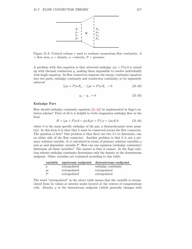
21.7. FLOW CONNECTOR THEORY 217
HHHH
����
A−ρ−u−P−
V
A+ρ+u+
P+
Figure 21.3: Control volume v used to evaluate momentum flow continuity; A= flow area, ρ = density, u =velocity, P = pressure.
A problem with this equation is that advected enthalpy (ρe + P )uA is mixedup with thermal conduction q, making them impossible to resolve individuallywith single equation. So flow connectors separate the energy continuity equationinto two parts, enthalpy continuity and conduction continuity, to be separatelyenforced
[(ρe+ P )uA]+ − [(ρe + P )uA]− = 0 (21.42)
q+ − q− = 0 (21.43)
Enthalpy Part
How should enthalpy continuity equation (21.42) be implemented in Sage’s so-lution scheme? First of all it is helpful to write stagnation enthalpy flow in theform
H = (ρe+ P )uA = ρuA(ρe + P )/ρ = (ρuA)h (21.44)
where h is the mass specific enthalpy of the gas, a thermodynamic state prop-erty. In this form it is clear that h must be conserved across the flow connector.The question is how? One problem is that there are two h’s to determine, oneon either side of the flow connector. Another problem is that h is not a pri-mary solution variable. It is calculated in terms of primary solution variables ρand ρe and dependent variable P . How can one equation (enthalpy continuity)determine all these variables? The answer is that it cannot. In the Sage solu-tion scheme enthalpy continuity determines only the density at the downstreamendpoint. Other variables are evaluated according to this table:
variable upstream endpoint downstream endpoint
ρ extrapolated enthalpy continuityρe extrapolated extrapolatedP extrapolated extrapolated
The word “extrapolated” in the above table means that the variable is extrap-olated from its values at interior nodes located at the centers of computationscells. Density ρ at the downstream endpoint (which generally changes with

218 CHAPTER 21. GAS DOMAINS
time) is chosen as the variable used to enforce enthalpy continuity because den-sity is a property carried with the flow and the principle of upstream causalitysuggests that upstream conditions determine downstream conditions, not vice-versa. In the case of pressure P it makes sense to extrapolate its value at theendpoints regardless of flow direction because pressure information propagatesat sonic velocity which is not carried with the flow in the low subsonic flowrange where all good stirling machines operate. In the case of volumetric en-ergy density ρe it makes sense to extrapolate both endpoint values because thatis consistent with Sage’s staggered-grid solution scheme and also because ρe isdirectly proportional to pressure for ideal-gas conditions so it should be treatedsimilarly.
Endpoint Temperature Glitch Sage calculates temperature at gas domainendpoints from the equation of state T (ρ, ρe, u). Under ideal gas conditions theabove endpoint solution scheme produces continuous temperature across flowconnectors. Under non-ideal conditions there may be a slight discontinuity oftemperature due to the fact all three variables ρ, ρe and P are extrapolatedat the upstream endpoint and, according to the equation of state, only twoare generally independent. In other words it is not guaranteed that extrapo-lated pressure is consistent with the equation of state as a function of ρ andρe, except under ideal-gas conditions where P is essentially equivalent to ρe.Attempting to correct this problem by simply evaluating pressure according tothe equation of state at the endpoint does not work because doing so tends todecouple the interior pressure solution (based on the momentum equation) fromthe enforcement of Bernoulli’s law across the flow connector.
So the values of dependent solution variables P and T at domain endpoints(in fact at all computational cell boundaries) may be slightly inconsistent withthe equation of state and primary solution variables ρ and ρe, as a result ofinterpolation. In the case of T this is more of an apparent problem than a realproblem because none of the governing equations depends on T values at cellboundaries. In the case of P it is a real problem, though generally a slight one,because pressure values at cell boundaries affect the enthalpy flows (computedaccording to equation (21.44)) entering the computational cells, thereby affect-ing their energy equations. In principle any cell-boundary inconsistencies in Pwill vanish as the number of computational cells (NCell) increases.
There is a way around the problem by evaluating ρe at cell boundariesimplicitly so that ρ, ρe and P are consistent with the equation of state. Howeverdoing so is inconsistent with the principles of the staggered-grid solution schemeand also slows down the solving time significantly, so it was judged not worththe bother.
Complication of Multiple Connections
Gas domains support multiple connections at their endpoint boundaries. Thesimplest such case is a Y-branch where one domain splits into two or two domains

21.7. FLOW CONNECTOR THEORY 219
converge to one, although more complicated connections are possible. Gas do-mains manage this complexity by logically breaking their endpoint boundariesinto a number of distinct flow inlets, one for each flow connector. The flow con-nectors communicate with the individual flow inlets which then communicatewith the gas domain. Flow inlets are software objects encapsulated togetherwith the gas domain.
Under this scheme, gas domains obtain their endpoint mass flow rate bypolling all flow inlets to return the mass flow rate from their associated flowconnectors and summing the results. Since mass is a conserved quantity andmass flow rate is a solution variable this is completely straight forward.
It is more complicated for gas domains to evaluate the correct density which,according to the above logic, must be based on enthalpy continuity when the gasdomain is downstream of the flow connector. The problem is that a gas domainwith multiple inlets can be simultaneously downstream of one flow connectorwhile upstream of another. In other words, one inlet can see incoming flow whilethe other sees outgoing flow. The way gas domains manage this is by defininga separate mixed density ρm at each endpoint to be passed by flow inlets totheir flow connectors. This mixed density is in-turn used by the gas domain todetermine its endpoint density, consistent with upstream causality and enthalpycontinuity.
At this point it is convenient to denote variables at the gas domain endpointby the subscript e and those within the individual flow inlets by subscript i.
Enthalpy conservation requires that the sum-total of stagnation enthalpyflows passing through the inlets must equal the stagnation enthalpy flow com-puted at the gas-domain endpoint and used in its interior solution. This latterquantity is always calculated from gas-domain endpoint variables as
He = [ρuA]e[ρe+ P ]e
ρe(21.45)
In particular, ρe is extrapolated from the interior gas domain solution for outgo-ing mass flow rate [ρuA]e and taken as the above mixed density ρm for incoming[ρuA]e. Enthalpy flows Hi through the individual flow inlets are imported fromthe associated flow connector whenever the individual inlet mass flow rate [ρuA]iis directed into the gas domain. For [ρuA]i directed out of the gas domain theyare calculated as
Hi = [ρuA]i[ρe+ P ]e
ρm(21.46)
Under these assumptions the condition of enthalpy-flow continuity may be writ-ten
0 = He −∑
i
Hi (21.47)
= [ρe+ P ]e
(ρuA)e
ρe− 1
ρm
∑
out
(ρuA)i
−∑
in
Hi (21.48)

220 CHAPTER 21. GAS DOMAINS
where designations in (in-flowing) and out (out-flowing) are relative to the gasdomain. We may write this as
1
[ρe+ P ]e
∑
in
Hi =(ρuA)e
ρe− 1
ρm
∑
out
(ρuA)i (21.49)
This equation can be solved explicitly for ρm. For incoming (ρuA)e one maysubstitute ρm for ρe (according to the above conventions) and
∑
in(ρuA)i +∑
out(ρuA)i for (ρuA)e, in which case the solution becomes
ρm = [ρe+ P ]e∑
in
(ρuA)i /∑
in
Hi (21.50)
To avoid a division by zero this equation applies only to strictly non-zero in-coming flow. For outgoing or zero (ρuA)e no such simplification is possiblebecause ρe is extrapolated from the interior gas domain solution. In this casethe solution of equation (21.49) is
ρm =∑
out
(ρuA)i /
(ρuA)e
ρe− 1
[ρe+ P ]e
∑
in
Hi
(21.51)
In the case where both (ρuA)e and∑
inHi are both zero gas domains assignρm = ρe, to avoid an indeterminate form.
Note that ρe may take a sudden jump at (ρuA)e flow reversal, an eventworthy of note to all practitioners of iterative nonlinear equation solving. Dis-continuities like this have been known to slow down the rate of convergence oreven force the solver to hunt back and forth near the discontinuity. Fortunately,in this case, ρe only affects interior gas-domain solution variables by amountsscaled in proportion to (ρuA)e which is zero at flow reversal. Therefore thediscontinuity is conveniently wiped out. On the other hand, ρm (which is ex-ported to flow connectors) is continuous at (ρuA)e flow reversal, as can be seenby substituting zero for (ρuA)e in equation (21.51) after which it reduces toequation (21.50).
Thermal Conduction Part
Thermal conduction continuity is much easier than enthalpy continuity since itdoes not involve so many solution variables or change with flow direction. Flowconnectors look at the conductance (conductivity times area kA) and tempera-ture gradients of the adjoining gas domains in order to decide the appropriatevalue of q allowed to “pass through” the connection. That is, flow connectorsexplicitly calculate q which adjoining gas domains use at their endpoints.
This approach differs from the way solid domains are connected in Sage. Insolid domains the connector calculates q implicitly according to the requirementthat temperature is continuous across the connection. In gas domains this isnot necessary because temperature continuity is already established by enthalpy
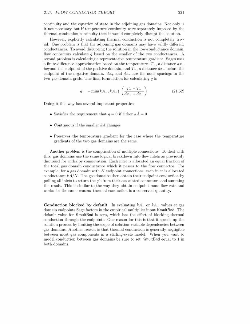
21.7. FLOW CONNECTOR THEORY 221
continuity and the equation of state in the adjoining gas domains. Not only isit not necessary but if temperature continuity were separately imposed by thethermal-conduction continuity then it would completely disrupt the solution.
However, explicitly calculating thermal conduction is not completely triv-ial. One problem is that the adjoining gas domains may have wildly differentconductances. To avoid disrupting the solution in the low-conductance domain,flow connectors calculate q based on the smaller of the two conductances. Asecond problem is calculating a representative temperature gradient. Sages usesa finite-difference approximation based on the temperatures T+, a distance dx+
beyond the endpoint of the positive domain, and T−, a distance dx− before theendpoint of the negative domain. dx+ and dx− are the node spacings in thetwo gas-domain grids. The final formulation for calculating q is
q = −min(kA−, kA+)
(T+ − T−dx+ + dx−
)
(21.52)
Doing it this way has several important properties:
• Satisfies the requirement that q = 0 if either kA = 0
• Continuous if the smaller kA changes
• Preserves the temperature gradient for the case where the temperaturegradients of the two gas domains are the same.
Another problem is the complication of multiple connections. To deal withthis, gas domains use the same logical breakdown into flow inlets as previouslydiscussed for enthalpy conservation. Each inlet is allocated an equal fraction ofthe total gas domain conductance which it passes to the flow connector. Forexample, for a gas domain with N endpoint connections, each inlet is allocatedconductance kA/N . The gas domains then obtain their endpoint conduction bypolling all inlets to return the q’s from their associated connectors and summingthe result. This is similar to the way they obtain endpoint mass flow rate andworks for the same reason: thermal conduction is a conserved quantity.
Conduction blocked by default In evaluating kA− or kA+ values at gasdomain endpoints Sage factors in the empirical multiplier input KmultBnd. Thedefault value for KmultBnd is zero, which has the effect of blocking thermalconduction through the endpoints. One reason for this is that it speeds up thesolution process by limiting the scope of solution-variable dependencies betweengas domains. Another reason is that thermal conduction is generally negligiblebetween most gas components in a stirling-cycle model. When you want tomodel conduction between gas domains be sure to set KmultBnd equal to 1 inboth domains.

222 CHAPTER 21. GAS DOMAINS
21.8 Turbulence Models
Knowing the state of turbulence is critical for computing the empirical rela-tionships for friction factor f , Nusselt number Nu and axial conductivity ratioNk used in the various gas-domain model components, of which there are threebasic types: matrix, duct and variable-volume.
21.8.1 Matrix Gas Domains
Matrix gas domains presume quasi-steady flow, meaning that local Reynoldsnumber Re completely characterizes the turbulence state. Entrance effects andtime-constants for boundary-layer growth are neglected. In most porous mate-rials, the issue of turbulence is moot anyway since relatively simple formulationsfor friction factor f , Nusselt number Nu and enhanced axial conductivity ra-tio Nk typically apply over the entire Reynolds number range of interest. Innon-porous matrix materials, though, (notably wrapped foils) the state of turbu-lence does matter because formulations for f , Nu, and Nk tend to be completelydifferent for laminar vs turbulent flow.
When turbulence matters, matrix gas domains correlate dimensionless groupsas a weighted average of the laminar and turbulent cases. For example frictionfactor is computed from a laminar value fl and a turbulent value ft as
f = (1 −W )fl +Wft (21.53)
The idea is that weight function W varies smoothly between 0 and 1 as flowgoes from laminar to turbulent. Smooth is better than abrupt for numericalconvergence reasons.
The weight function is formulated in terms of a normalized and zero-shiftedReynolds number R∗
e defined as
R∗e ≡ Re − Rl
Rt − Rl(21.54)
Here Rl = 2300 and Rt = 10, 000 are the critical below-which-is-laminar andabove-which-is-turbulent Reynolds numbers, conventional in the steady flowliterature. Note that R∗
e varies from 0 to 1 in the transitional Reynolds-numberrange. The turbulence weight function is now defined as
W (R∗e) =
0 if R∗e ≤ 0
2R∗2e if 0 < R∗
e ≤ 1/21 − 2(1 − R∗
e)2 if 1/2 < R∗
e ≤ 11 if 1 < R∗
e
(21.55)
This formulation is first-derivative continuous everywhere, which should besmooth enough for Sage.

21.8. TURBULENCE MODELS 223
21.8.2 Duct Gas Domains
In duct gas domains we no longer have the luxury of neglecting entrance effectsor time constants for boundary-layer growth. In addition to Reynolds numberRe, the state of turbulence depends on Valensi number Va, elapsed time sinceflow reversal and convective triggering, which is turbulence triggered by a slugof turbulent fluid that enters through one of the inlets and is carried to the pointof observation by the mean flow.
Modeling turbulence in such ducts is a tall order for a one-dimensional model.Our goal is keep things as simple as possible, relying heavily on empirical ob-servation. Researchers Terry Simon, Joerg Seume and others at the Universityof Minnesota [54], [56], [55], [57] have observed that transition to turbulence isdelayed in proportion to
√Va for large Valensi numbers and that flow is always
laminar according to:
always laminar if Re/Rl < max(√
Va/Vc, 1) (21.56)
where Rl ≈ 2300 is a critical Reynolds number and Vc ≈ 10 is a critical Valensinumber, below which flow is essentially similar to steady flow. Above the alwayslaminar condition, the Minnesota researchers observed turbulence transition duemainly to convective triggering, with turbulence persisting until the time of flowreversal, but generally not beyond, leaving the velocity profile uniformly zeroacross the tube cross-section at the time of flow reversal. The Minnesota obser-vations were generally confined to mean-flow tidal displacements greater thanthe tube length. University of Michigan and MIT researchers R. Akhavan, R.D. Kamm and A.H. Shapiro, [3], support these conclusions and make additionalobservations pertaining to the spontaneous transition to turbulence of fluid inthe duct interior, not affected by disturbances propagating from the inlets. Theyobserved that turbulence was generally delayed during most of the accelerationphase of the cycle but exploded suddenly near the end of this phase (just beforeor just after the time of peak velocity), with turbulent flow persisting throughoutthe deceleration phase, until the time of flow reversal. They saw no turbulencefor peak Re/
√Va less than about 700 – 800, or so, consistent with the above
always laminar condition for Va > Vc. And when turbulence was present, they,like the Minnesotans, observed that the velocity profile was uniformly zeroedout at the time of flow reversal. Then during the following acceleration phasethe velocity profile was very close to the exact solution for start-up from rest oflaminar flow in a tube, until the time of turbulence transition. They attributedthe delay in turbulence transition to the stabilizing effects of fluid acceleration,although the viewpoint here (and of the Minnesota researchers) is that it justa matter of the time required for the boundary layer to grow to an unstablethickness.
To attempt to capture all these effects, in duct gas domains there is a specialturbulence intensity variable T added to the set of state variables and solvedimplicitly from its own partial differential equation. This turbulence variableT functions much like the weight function W in the matrix gas-domain model.Again using friction factor as an example, we compute local instantaneous fric-

224 CHAPTER 21. GAS DOMAINS
tion factor from the weighted average of a laminar value fl and a turbulent valueft
f = (1 − T )fl + T ft (21.57)
Turbulence intensity T is to vary smoothly between 0 and 1 as flow goes fromlaminar to turbulent.
We may think of T as a normalized version of ρκ, where κ is the time-averaged turbulence kinetic energy per unit mass
κ = 1/2⟨u′2 + v′2 +w′2
⟩(21.58)
More precisely, we might think of T as roughly proportional to ρκ/(ρ0u2) ∝
κ/u2, where u(x, t) is the mean-flow velocity. We can estimate the constant ofproportionality by noting that for the fully turbulent state (T = 1), the RMSvelocity fluctuation (
√2κ) is about 0.08u, according to [57]. So a reasonable
estimate for T would be
T ≈ 2κ
(0.08u)2(21.59)
Because of the variable nature of the normalization quantity u2, T is not, strictlyspeaking, a tangible quantity carried along with the flow (like ρκ itself is).Nonetheless, it is convenient to overlook this for the moment and presume that Tis governed by a one dimensional differential equation like our other gasdynamicequations
∂T A∂t
+∂T uA∂x
︸ ︷︷ ︸
convection
= G(Re, Va)︸ ︷︷ ︸
generation
−D(Re, Va)︸ ︷︷ ︸
decay
(21.60)
The only problems are deciding on inlet boundary conditions and decay andgeneration terms to impart the desired properties to the solution T — namely,that T be 0 when flow is to be laminar, 1 when flow is be turbulent and some-where in between during transition. The convection term automatically takescare of convective triggering.
Inlet Boundary Conditions
The University of Minnesota work suggests that incoming fluid is always turbu-lent. This turbulence is either the result of high upstream turbulence level orcontinuously generated by separation of incoming flow at the inlet. Denotingthe incoming turbulence level by Tin, it appears then that a value Tin = 1 isreasonable, although the value is adjustable to any value between 0 and 1 withinput variables TbInNeg and TbInPos, which define the incoming turbulencelevel at the two ends of the duct. For outgoing flow, it makes physical senseto extrapolate T at the end boundary from interior values, denoted by E(T ).There is no problem with T discontinuity at flow reversal since only the productT uA (always zero at flow reversal) affects the interior solution. The value of Tat either inlet boundary is computed as
T =
{Tin inflowE(T ) outflow
(21.61)

21.8. TURBULENCE MODELS 225
Generation
The universal observation seems to be that in turbulent oscillating flow thesteady velocity profile zeros out uniformly across the duct cross-section at flowreversal. Essentially, each half cycle begins anew from rest. Simon et. al. arguein [57] that under these conditions transition should occur when the momentum-thickness Reynolds number
Rδ =uδ
ν(21.62)
reaches a critical value. u is the instantaneous mean flow velocity, ν = µ/ρis kinematic viscosity and δ is the so-called momentum thickness, roughly theboundary-layer thickness, but defined more precisely in Schlichting ([51], equa-tion 7.38, p. 141) for a flat plate as
δ =
∫ ∞
y=0
u
U∞
(
1 − u
U∞
)
dy (21.63)
Here, y is the normal distance from the wall and u(y) is velocity. Reference [2]shows that for undisturbed flow, Rδ may range between 1200 and 3000 from thestart to end of transition, while the range of transition drops to Rδ between 200and 400 with as little as 4% free-stream turbulence level.
The boundary-layer growth for a flat plate accelerated sinusoidally from restcan be seen in the velocity profiles shown in figure 21.4. In the figure the fluidis initially at rest with the wall suddenly started moving with velocity u(0, t) =sinωt at ωt = 0. This is equivalent to the present problem of interest, whichis a fixed wall with free-stream velocity suddenly started moving with velocityu(∞, t) = − sinωt at ωt = 0 (driven by a sinusoidal pressure gradient ∂P
∂x), by
the addition of − sinωt to the velocity solution everywhere. The advantage ofthe velocity profiles shown is that they better show the viscous boundary layerthickness.
The momentum thickness for the case of flow accelerated sinusoidally fromrest is shown in figure 21.5. Except for a brief time at the beginning of the flowand lasting until well after the time of peak velocity, the momentum thicknessgrows linearly with time in close approximation to
δ =√
ν/ω(0.15 + 0.225ωt) if 0.3 ≤ ωt ≤ 2.3 (21.64)
So for sinusoidal flow starting from rest the momentum-thickness Reynolds num-ber, and hence the point of turbulence transition, may be easily calculated.Transition so predicted is probably valid for 0 ≤ ωt ≤ 2.3, because in thisrange the velocity profiles qualitatively resemble those of suddenly-acceleratedflow (u(∞, t) = u0 for ωt ≥ 0), the conditions for which the correlation be-tween momentum-thickness Reynolds number and turbulence transition wereoriginally established. Beyond ωt = 2.3, though, the velocity profile beginsto show a pronounced maximum at some distance from the wall which, dueto a mathematical technicality, has the effect of producing diminishing, thennegative, momentum thicknesses even though the actual viscous-layer thickness

226 CHAPTER 21. GAS DOMAINS
Figure 21.4: Velocity profiles at equally-spaced times 0 ≤ ωt ≤ π for viscous
flow governed by ∂u∂t = ν ∂2u
∂y2 . Fluid initially at rest (u(y, t) = 0, for t < 0) with
wall boundary condition u(0, t) = sinωt for 0 ≤ ωt ≤ π. From a numericalsolution based on the Crank-Nicolson implicit method.
continues to grow, as can be seen in figure 21.4. So the momentum-thicknessReynolds number cannot be used as a predictor of transition during the laterstages of the flow half-cycle.
In order to discover critical value of the momentum-thickness Reynolds num-ber, first write it in terms of the usual hydraulic-diameter Reynolds number as
Rδ = Re δ/dh (21.65)
Then replace factor δ/dh by substituting approximation (21.64) for δ and expandinto dimensionless variables, leaving
Rδ ≈ 0.075 + 0.112ω(t− t0)√Va
Re (21.66)
To avoid confusion, the elapsed time since flow reversal is written above andhereafter as (t− t0). And to save time, the numerator of the coefficient of Re ishereafter written
F (t− t0) ≡ 0.075 + 0.112ω(t− t0) (21.67)
At this point, there is no need to work with Rδ directly at all. Taking thecritical value of Rδ as an unknown constant Rδc, the turn-on time for turbulencegeneration may be stated
laminar until Re > Rδc
√Va
F (t− t0)(21.68)

21.8. TURBULENCE MODELS 227
Figure 21.5: Growth of dimensionless momentum thickness√
ω/νδ with timeωt for flow accelerated sinusoidally from rest. Calculated according to formaldefinition (21.63) with integration performed numerically based on a finite dif-ference solution of the velocity profile.
Even though approximation F (t − t0) is not valid for ω(t − t0) > 2.3, it willdo no harm because transition will always occur before this, if at all, before orslightly after the time of peak velocity at ω(t− t0) = π/2.
The constant Rδc may be evaluated according to the observed always-laminarcondition (21.56) for high Valensi numbers (Va > Vc), which states that fora cycle with peak Reynolds number Rem below about 730
√Va, the flow re-
mains laminar for the whole cycle, whereas for any higher Rem, flow becomesat least partly turbulent. On the other hand, substituting Rem sin(ω(t − t0))for Re in momentum-thickness condition (21.68), the implication is that flowremains laminar until Rem(sin(ω(t − t0))F (t − t0)) exceeds Rδc
√Va. So, the
largest Rem for which flow remains always laminar may be evaluated by settingω(t − t0) ≈ 1.937, where sin(ω(t − t0))F (t − t0) ≈ 0.274 attains its maximumvalue. It follows that 730
√Va must equal Rδc
√Va/0.274, so that
Rδc ≈ 200 (21.69)
which is in reasonable agreement with the value reported in [2] for disturbedinitial flow.
Transition criterion (21.68) applies only when Valensi number is above somelower limit because for
√Va/(F (t− t0)) too low, the growth of the momentum-
thickness will be limited by the duct dimensions. Below this, turbulence onsetmay be characterized by the well-known steady-flow criterion; namely, that flowis laminar until Re rises above Rl. Just when this lower limit of
√Va/(F (t−t0))
occurs may be taken as a constant c1, conveniently determined as the value that

228 CHAPTER 21. GAS DOMAINS
makes the low- and high-Valensi number branches continuous in the followinguniversal condition for the time of turbulence onset:
if
√Va
F (t− t0)≥ c1 then laminar until Re = Rδc
√Va
F (t− t0)(21.70)
if
√Va
F (t− t0)< c1 then laminar until Re > Rl (21.71)
The value of c1 is evidently Rl/Rδc ≈ 2300/200 or about 11.5. So the universalturbulence onset condition may be collapsed into the single condition
laminar until Re > Rt (21.72)
where Rt is the critical Reynolds number
Rt = 200 max(
√Va
F (t− t0), 11.5) (21.73)
Required in evaluating Rt within a computational solution is the currentvalue of ω(t− t0), the dimensionless time since the previous flow reversal. Thisis not as easy as it may first sound because times of past events such as flowreversal are not usually available at any given time. The proposed method isone that works well enough whenever the velocity u is close to sinusoidal. Themethod is best illustrated by considering u = sinωt, for which the times of flowreversal are ωt0 = {0, π . . .}. Acceleration is then u = ω cosωt and the ratioωu/u is just tanωt. A formula for flow-reversal time that always works is
ω(t− t0) =
{arctan(ωu/u) if ωu/u ≥ 0π − arctan(−ωu/u) if ωu/u < 0
(21.74)
The advantage of this formulation is that both u and u are generally computable.For a coarser but faster approximation the arctan function may be approximatedfor non-negative arguments (the only arguments required) by
arctan x ≈ π
2
(
1 − 1
x+ 1
)
if x ≥ 0 (21.75)
the approximation being within about 0.08 rad (5 degrees) for any positive x.Criterion (21.72) establishes the time when turbulence generation begins,
but more useful in a computational model is the criterion for the entire timeturbulence generation is active. Presumably, this is from the time of transitionuntil the Reynolds number once again drops below the steady-flow relaminar-ization value Re = Rl. The value Rl makes sense because, once turbulence ispresent, the velocity profile becomes similar to steady turbulent flow, no matterwhat the Valensi number, due to the mixing effects of the turbulent eddies. Butfor flows with large peak Reynolds numbers, the time at which Re drops belowRl may be relatively close to the time of flow reversal, and entirely missed in a

21.8. TURBULENCE MODELS 229
coarse computational grid! This problem can be remedied by slightly modifyingthe transitional Reynolds number to
R∗t = max(Rt, Rc) (21.76)
where Rc is the value of Reynolds number at some cutoff time ω(tc − t0). Thecondition of turbulence duration may now be stated
turbulent while Re > R∗t (21.77)
A cutoff time of ω(tc−t0) = 3/4π, for example, would leave the last π/4 radians(45 degrees) prior to flow reversal available for relaminarization. (This followsbecause Re < Rc after the cutoff time and Rc ≤ R∗
t .) The cost is a possibleslight delay in turbulence onset and slight advance in decay onset.
There is, of course, the problem of estimating the cutoff Reynolds numberRc at a current time, not the cutoff time. There is no need to get too fancy here.Essentially, what is required is that the current value of Re exceed Rc beforethe cutoff time, equal Rc at the cutoff time and be less than Rc after the cutofftime. So, presuming Re varies as sinω(t − t0) and using the approximationsin(π−τ ) ≈ τ , a reasonable approximation for cutoff Reynolds number in termsof the current Reynolds number is
Rc = Reπ − ω(tc − t0)
π − ω(t − t0)(21.78)
The numerator on the right side is simply a constant, like π/4, than need becalculated only once. The value ω(t−t0) in the denominator is already availablein the calculation ofRt. This approximation also has the advantage of producingRe > Rc for any time prior to the cutoff time so turbulence onset will alwaysbe governed by Rt, as it should.
But what is the rate of turbulence growth, during the transition period?Theoretical turbulence modelers (see Patankar [44]) suggest that this rate shouldbe proportional to ∂u
∂r , which scales as u/dh, or in dimensionless terms ωRe/Va.A pragmatic approach can be used to decide the constant of proportionality. Itshould be large enough so that, for relatively high values of Re/Va, turbulencewill be generated quickly, but not too quickly lest the solution become unstableor too difficult to properly resolve in the computational grid. The followingsteady generation term will produce an initial growth of turbulence ∂τ
∂ωt at τ =0 of about 4 (same growth rate as the maximum rate of change of the 4thharmonic) for a value Re/Va = 500, which is near the high end of known stirlingpractice according to the survey published in [53]:
G =
{0.008ωARe
VaS(1 − T ) if Re > R∗
t
0 otherwise(21.79)
Smoothing function S, defined to be W (Re/R∗t − 1), where W is the weight
function (21.55), makes the generation term come in smoothly at Re = R∗t .
The factor 1 − T serves to limit growth to T = 1.

230 CHAPTER 21. GAS DOMAINS
Decay
The simplest formulation is to have the decay term active whenever the gener-ation term is inactive — whenever Re < R∗
t . For calculating the actual rate ofturbulence decay we can turn to a two-dimensional κ transport equation suchas the one recommended in Launder and Spaulding ([34], p. 77). Simplified toits bare essentials by neglecting the diffusion and production terms, taking theLagrangian point of view where Dκ/Dt = dκ/dt and dividing out density, theresulting equation is
dκ
dt∝ −1
`κ
32 (21.80)
where the constant of proportionality is to be determined from pragmatic rea-soning, as usual, and ` is a length scale proportional to the Prandtl mixinglength `m. (Prandtl mixing length is the length that makes turbulent shear
stress come out right in the expression τ = ρ`2m∂u∂y
2.) Assuming that mixing
length scales with hydraulic diameter we have
dκ
dt∝ − 1
dhκ
32 (21.81)
We can write this in terms of T by substituting 0.0032u2T for κ (from equa-tion (21.59)) and taking normalization velocity u to be the constant value ul
corresponding to Re = Rl. Then replacing ul/dh by ωRl/(4Va), we have
dTdt
≈ −cdωRl
VaT 3
2 (21.82)
Even though decay is active whenever Re is below R∗t (which may be much
higher than the physically-correct value Rl), the rate of decay is taken as thatappropriate for Re = Rl to avoid artificially increasing the rate of decay due toa computational artifact. The value of cd should be chosen high enough thatrelaminarization takes place for all but the very highest values of Rem/Va. Agood calibration case is case b of [55] where relaminarization occurs for Rem =47, 000 and Va = 29. The time for of relaminarization in this case is ωδt =arcsin(Rl/Rem) ≈ 0.05. Under these conditions, a value of cd ≈ 0.25 willproduce an initial decay rate ∂τ
∂ωt at τ = 1 of about 20, which is the desiredvalue. To avoid numerical difficulty with a discontinuous decay term, it is agood idea to smooth the above rate by a transition function S which smoothlyvaries from zero to one as Re drops below R∗
t . A convenient smoothing functionis W (1−Re/R
∗t ), where W is the weight function (21.55). The final decay term
in equation (21.60) is then
D =
{0.25ωARl
VaST 3
2 if Re < R∗t
0 otherwise(21.83)
Of some concern is how long it takes incoming turbulence to decay to zerofrom the worst-case inlet value of Tin = 1, for flow with low Reynolds number(Re < Rl). A long delay would be unrealistic. The time for the mean flow to

21.8. TURBULENCE MODELS 231
travel from the inlet to x = dh is dh/u and the change in turbulence over thistime is ∆T ≈ dT
dtdh
u≈ −Rl/Re, from equation (21.82) with cd = 0.25. Even
considering smoothing function S, It follows that relaminarization occurs withinabout 1 pipe diameter of the inlet, at Re = Rl/2, and proportionately less thanthis for lower Re. This seems fast enough.
21.8.3 Variable Volume Gas Domains
In variable-volume gas domains, incoming flow separation produces turbulencewhich mixes throughout the cylinder space uniformly and dominates all othersources of turbulence. At least, that is the assumption.
In addition to the main x−t solution grid, variable volume gas domains havea special t-only grid that maintains volume V and turbulence kinetic energy ρκas state variables. Volume is just
V (t) = A(t)L (21.84)
κ is again the time-averaged turbulence kinetic energy per unit mass defined byequation (21.58).
According to Gedeon [13] and [14], correlations for Nusselt number Nu andenhanced axial conduction ratio Nk may be formulated directly in terms of theturbulent Reynolds number Rt defined as
Rt = ρ√κdh/µ (21.85)
Volume-specific turbulence kinetic energy is just ρκ. Because of the uniformmixing assumption there is no spatial variation in ρκ. Therefore, a time ring(special time grid for periodic solutions where the first index is logically identi-fied as the successor to the last index) rather than a space-time grid suffices forits storage and an ordinary time-differential equation suffices for its solution
∂ρκV
∂t+ [ρuAκ]
outin
︸ ︷︷ ︸
inflow
+ D︸︷︷︸
decay
= 0 (21.86)
Compared to the duct turbulence equation, we have replaced the convectionterm by the net turbulence kinetic energy entering through the flow inlet(s) andneglected the generation term.
Inlet Boundary Conditions
We assume that for incoming flow, the inlet mean-flow kinetic energy is con-verted entirely to turbulence kinetic energy — that is, κi = 1/2u2
i , where thei subscript denotes an inlet value. Velocity ui is just the mean-flow velocityin the upstream gas duct. For outgoing flow we naturally assume κi takes theinterior value κ. We do not need to worry about the discontinuity in κi atthe time of flow reversal because we are interested only in the product ρuAκi,
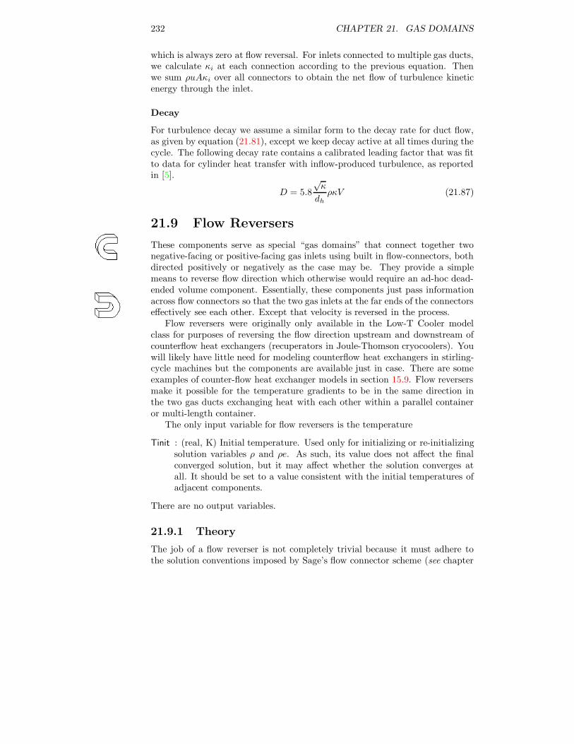
232 CHAPTER 21. GAS DOMAINS
which is always zero at flow reversal. For inlets connected to multiple gas ducts,we calculate κi at each connection according to the previous equation. Thenwe sum ρuAκi over all connectors to obtain the net flow of turbulence kineticenergy through the inlet.
Decay
For turbulence decay we assume a similar form to the decay rate for duct flow,as given by equation (21.81), except we keep decay active at all times during thecycle. The following decay rate contains a calibrated leading factor that was fitto data for cylinder heat transfer with inflow-produced turbulence, as reportedin [5].
D = 5.8
√κ
dhρκV (21.87)
21.9 Flow Reversers
These components serve as special “gas domains” that connect together twonegative-facing or positive-facing gas inlets using built in flow-connectors, bothdirected positively or negatively as the case may be. They provide a simplemeans to reverse flow direction which otherwise would require an ad-hoc dead-ended volume component. Essentially, these components just pass informationacross flow connectors so that the two gas inlets at the far ends of the connectorseffectively see each other. Except that velocity is reversed in the process.
Flow reversers were originally only available in the Low-T Cooler modelclass for purposes of reversing the flow direction upstream and downstream ofcounterflow heat exchangers (recuperators in Joule-Thomson cryocoolers). Youwill likely have little need for modeling counterflow heat exchangers in stirling-cycle machines but the components are available just in case. There are someexamples of counter-flow heat exchanger models in section 15.9. Flow reversersmake it possible for the temperature gradients to be in the same direction inthe two gas ducts exchanging heat with each other within a parallel containeror multi-length container.
The only input variable for flow reversers is the temperature
Tinit : (real, K) Initial temperature. Used only for initializing or re-initializingsolution variables ρ and ρe. As such, its value does not affect the finalconverged solution, but it may affect whether the solution converges atall. It should be set to a value consistent with the initial temperatures ofadjacent components.
There are no output variables.
21.9.1 Theory
The job of a flow reverser is not completely trivial because it must adhere tothe solution conventions imposed by Sage’s flow connector scheme (see chapter

21.9. FLOW REVERSERS 233
21). Basically there needs to be a way to force incoming mass flow rate (ρuA)to equal outgoing mass flow rate. So flow reversers must implement at-least oneimplicit solution grid variable for this purpose. Having done that they must takeadditional steps to ensure energy continuity (because local solution values arenow decoupled from the incoming values). In the end, flow reversers implementa simplified version of the solution scheme used in flow restrictors (see chapter32). They contain a time grid with state variables ρ, ρe, and P , governed byequations of mass continuity and energy continuity.
ρ
Mass density ρ is computed implicitly from the zero-volume mass-continuityequation
(ρuA)1 + (ρuA)2 = 0 (21.88)
where (ρuA)1 and (ρuA)2 are the values imported from flow connectors 1 and2. This forces mass flow rate in two flow connectors to be equal but opposite.Implicit functions used for solving ρe also help to determine ρ.
ρe
Basically, energy density ρe is computed implicitly from the energy continuityequation written in the form
ρe+ P
ρ= hi (21.89)
where ρe and P on the left are internal state variables while hi on the right is themass-specific enthalpy evaluated using variables imported from the componentacross the incoming flow connection. For an ideal gas h reduces to cpT in thezero-velocity limit where kinetic energy may be neglected.
For numerical reasons it is convenient to separate ρe into two variables ρe1and ρe2 . ρe1 is exported to flow connector 1 and ρe2 to flow connector 2.Each is guaranteed valid at the right time — ρe1 whenever flow is incomingfrom connector 2 and vice-versa for ρe2 . The reason for this formulation isbecause the implicit function determining either can be formulated without adiscontinuity at flow reversal, as would otherwise be the case. That is, theequation for determining ρe1 is always that local mass-specific enthalpy ρe1+P1
ρequals the hi value imported across connector 2. this enforces energy continuitywhen flow is incoming from connector 2 and otherwise does no harm. A similarequation determines ρe2. The meaning of P1 and P2 is similar to the meaningof ρe1 and ρe2, and is explained below.
It might be tempting to use these continuity conditions instead to calculateρe1 and ρe2 explicitly. This will not work because of a circular reference whenaccessing P , which itself depends on ρe.

234 CHAPTER 21. GAS DOMAINS
P
Pressure is also broken into two components P1 and P2, similar to the treatmentfor ρe. P1 is exported to the flow connector 1 and P2 to flow connector 2.Both are calculated explicitly from the equation of state P (ρ, T ). This requirestemperature which is calculated from the zero-velocity equation of state. Forevaluating P1 the temperature is calculated as T (ρ, ρe1, 0). For evaluating P2 itis calculated as T (ρ, ρe2, 0). (The 0’s in the argument lists are velocity) Pressuresis required in the solution grid so that the flow connectors can properly enforceBernoulli’s law across the connections.
Why zero velocity? Basically, velocity is irrelevant to mass or energy con-servation. The only thing velocity determines is the pressure shift across theflow connectors, according to Bernoulli’s law. But any pressure shift across theincoming-flow connector, produced by the velocity in the flow reverser, is can-celed by an opposite pressure shift across the outgoing-flow connector. So flowreverser velocity does not matter and it is convenient to assume the simplestthing: zero velocity.

Chapter 22
Canisters
Canisters are the containers into which you normally put a matrix-type heat-exchanger. But you can fill them with more than that. You can drop in aradiation transport path for modeling radiant heat transport from one end tothe other, which makes sense if the contents are sufficiently transparent. Or,you can drop in a bar or distributed conductor for modeling axial conductionin the canister walls. Some canisters even allow you to nest other canisterswithin them, which can be useful for modeling pistons or displacers withincylinders (see chapter 25). All of these attributes arise as toolbox-created childcomponents, at your discretion. The main purpose of canisters is to pass oncritical geometry-dependent information to these child components when youcreate them. The child components within canisters and they way they areconnected to the outside world are what really matters.
All canisters are high level components that appear in the toolbox of theroot-level stirling model component. They are born without connectors of anysort. To get connectors at this level you must move them up from the variouschild components you create within. Variables common to all canisters are:
NCell : (dimensionless) The number of spatial nodes in the computational gridsof all underlying model components having such grids. Changing thisvariable causes these computational grids to re-initialize themselves. NCellwill affect the solution time and memory requirements, not to mentionsolution accuracy. Treat it gingerly by making only gradual, small changes.
Length : (real, m) Canister length L in x direction.
Avoid : (real or cubic spline, m2) Canister void cross sectional (x-normal) areaAc.
Asolid : (real or cubic spline, m2) Canister solid (wall) cross sectional area As.
Mass : (real, kg) Canister mass m, provided for use in constraints in case it ispart of a reciprocating mass system.
235

236 CHAPTER 22. CANISTERS
Solid : (enumerated) Solid (wall) material.
Tinit : (cubic spline, W) Axial temperature distribution T (x) where x = 0 isthe negative endpoint and x = 1 is the positive endpoint.
The working gas type (properties) comes from the parent model component.All canister types calculate mass as
m = ρs
∫
dx
As (22.1)
where ρs is the solid density. Dependent variables Avoid and Asolid are calcu-lated differently for each of the descendant canister types below, in terms ofgeometrical inputs. When they do not vary with x (axial coordinate) they aresingle-valued real variables. When x variation is allowed they are cubic splines.
22.1 Tubular Canister
A tubular canister is a right circular cylinder, just as its icon suggests. Itsadditional variables are:
Din : (real, m) Canister internal diameter di.
Wcan : (real, m) Wall thickness w.
It calculates void cross-section area as
Ac =π
4d2
i (22.2)
and solid cross-section area as
As =π
4(d2
o − d2i ) (22.3)
where do = di + 2w is outer diameter.There is a close descendant of a tubular canister known as a nested tubular
canister. It shares the same icon as a tubular canister but is intended for nestingwithin another canister so that variables NCell, Length, and Tinit come from theparent canister and do not appear in its variable list. Its inner diameter Dinbecomes a dependent variable based on the assumption that its outer diameterequals the inner diameter of the parent canister. In other words, a nestedcanister always fits snugly within its parent canister.
22.2 Annular Canister
An annular canister is the volume enclosed by two concentric right circularcylinders. Its additional variables are:
Din : (real, m) Inner-wall internal diameter di.

22.3. TUBULAR-CONE CANISTER 237
Dout : (real, m) Outer-wall outside diameter do.
Win : (real, m) Inner-wall thickness wi.
Win : (real, m) Outer-wall thickness wo.
It calculates void cross-section area as
Ac =π
4
((do − 2wo)
2 − (di + 2wi)2)
(22.4)
and solid cross-section area as
As =π
4
(d2
o − (do − 2wo)2 + (di + 2wi)
2 − d2i
)(22.5)
There is a close descendant of an annular canister known as a nested annularcanister. It shares the same icon as an annular canister but is intended fornesting within another canister so that variables NCell, Length, Dout and Tinitcome from the parent canister and do not appear in its variable list. A nestedcanister always fits snugly within its parent canister
22.3 Tubular-Cone Canister
A tubular-cone canister is similar to an ordinary tubular canister except itsinternal diameter and wall thickness are specified by cubic splines. In otherwords, both may vary with axial position. The variation may be a good dealmore complex than linear, depending on the number of interpolation pairs youspecify for the variables:
Din : (cubic spline, m) Canister internal diameter di.
Wcan : (cubic spline, m) Wall thickness w.
A powerful option now presents itself: Din and Wcan, may be optimized! At leastany data value in any of their defining interpolation pairs may be optimized.Say, for example, you want to find the optimum diameter profile for a tubular-cone regenerator canister specified by three interpolation pairs. Then you wouldselect as optimized variables Din.FData.1, Din.FData.2 and Din.FData.3. Like-wise, you may also map either variable.
Tubular-cone canisters calculate void cross-section area Ac and solid cross-section area As using equations (22.2) and (22.3), similar to ordinary tubecanisters, except di and do are taken as functions of axial position. Whatactually happens is that tubular cones override variables Avoid and Asolid asdependent cubic splines. These splines are each defined by n data pairs (x, A(x))equal spaced in x within the interval [0, 1], where n is the larger of the numberof data pairs in the specification of Din or Wcan. This is self-evident in thedisplay form or listing.
There is a subtlety here worth noticing: The resolution of Avoid or Asolid areonly as good as the resolution of Din or Wcan. If you specify a linear diameter

238 CHAPTER 22. CANISTERS
profile (a true cone) by the interpolation pairs (0, 0.05) and (1, 0.10) for Din, forexample, you might think that Ac would then have a quadratic profile since itdepends on d2
i . You might be wrong. If the Avoid cubic spline is also definedby only two interpolation pairs, it will also have a linear profile. This is of someconcern because the solutions of child model components within the canister(gas and solid domains) generally regard area as the fundamental quantity, notdiameter. So your linear diameter profile is actually modeled as if it were asquare-root profile. To increase accuracy you might want to specify Din withthree, or more interpolation points, even though it may be linear.
22.4 Annular-Cone Canister
An annular-cone canister is an extension of an ordinary annular canister in thesame way a tubular cone was an extension of an ordinary cone. Now all of thefollowing inputs are specified as cubic splines:
Din : (cubic spline, m) Inner-wall internal diameter di.
Dout : (cubic spline, m) Outer-wall outside diameter do.
Win : (cubic spline, m) Inner-wall thickness wi.
Win : (cubic spline, m) Outer-wall thickness wo.
Any or all of these may be mapped or optimized by specifying the appropriateFData.n qualifier as discussed above.
Annular cones calculate void cross-section area Ac and solid cross-sectionarea As using equations (22.4) and (22.5), similar to ordinary annular canisters,except all the d’s and w’s are taken as functions of axial position. This takes theform of overriding Avoid and Asolid as dependent cubic splines using the samelogic as for tubular cones, discussed above. And the same cautionary remarksapply as well. Namely, that two-point linear diameter profiles may producelinear, not quadratic, area profiles.

Chapter 23
Heat Exchangers
Heat exchangers are the containers — or sub-containers if they are themselvesfound within a canister — into which you normally put a gas-domain and oneor more thermal-solid model components. Their main purpose is to pass oncritical geometry-dependent information to these child components when youcreate them. Stand-alone heat exchangers appear in the toolbox of the root-level stirling model component, while those needing containers appear in canistertoolboxes. They are born without connectors of any sort. To get connectorsyou must move them up from the various child components you create within.Variables common to all heat exchangers are:
NCell : (dimensionless) The number of spatial nodes in the computational gridsof all underlying model components having such grids. Changing thisvariable causes these computational grids to re-initialize themselves. NCellwill affect the solution time and memory requirements, not to mentionsolution accuracy. Treat it gingerly by making only gradual, small changes.
Length : (real, m) Heat exchanger length L in x direction. For a variable-volume heat exchanger this is a rough estimate of the mean flow-pathlength of a typical fluid particle — the path length from the inlet to a wallboundary. No need to be overly exact because thermal performance is notvery sensitive to L in variable-volume heat exchangers.
Roughness : (dimensionless) Relative roughness of the surface in contact withthe gas, defined as the average height ε of surface irregularities divided bythe hydraulic diameter dh (i.e. tube diameter or twice the gap for parallelplates). Required as an input only for heat-exchangers having uniform flowpassages, where it is important for determining turbulent flow resistance.According to [29], the height ε is the average distance between low and highpoints on the surface, rather than the average distance from high points tothe mean surface. Multiplying Machinery’s Handbook [42] peak-to-meanroughness values by two suggests the following absolute roughness valuesfor various manufacturing processes:
239

240 CHAPTER 23. HEAT EXCHANGERS
Process ε (microns)cold-rolling 2 to 6drawing 2 to 6extruding 2 to 6drilling 3 to 13
So for example, a drawn seamless tube with 3 mm ID could be expectedto have a relative roughness in the range of 0.001 to 0.002. A drilled holeof the same diameter as much as 0.004.
Aflow : (real, m2) Mean flow cross sectional (x-normal) area Af . Void volumedivided by length.
Asec : (real, m2) Mean solid cross sectional area As. (see equation (20.18) inchapter 20)
Pwet : (real, m2) Wetted perimeter Sx. The surface area per unit length forgas-to-solid heat transfer.
Tinit : (cubic spline, W) Axial temperature distribution T (x) where x = 0 isthe negative endpoint and x = 1 is the positive endpoint.
Matrix type heat exchangers have the additional variable
Porosity : (real, dimensionless) Porosity β. Void volume divided by total vol-ume. Total volume is void plus solid volume.
Matrix heat exchangers calculate mean-flow cross section area Af as the productof porosity and canister cross-sectional area Ac.
Af = βAc (23.1)
Duct and variable-volume type heat exchangers have the additional variable:
Twall : (real, m) Wall thickness tw. Usually a non-critical variable used indetermining solid cross-sectional area for some thermal-solid child compo-nent.
Every heat exchanger component comes with a unique gas-domain component inits toolbox. This domain is a descendant of either the matrix, duct or variable-volume type of gas domain and shares an icon with its ancestor object. The gas-domain is unique because it knows the specific correlations for friction factor,Nusselt number and axial conductivity ratio appropriate for the parent heatexchanger type. These correlations are documented below as part of the heat-exchanger documentation. Correlations are in terms of the following variables:

241
dh hydraulic diameter defined by equation (21.5)β porosity; void / total volumeε average height of surface irregularities (see Roughness
above)Va Valensi number defined by equation (21.6)Re Reynolds number defined by equation (21.4)Pr cpµ/k; Prandtl numberPe RePr; Peclet numberRt turbulent Reynolds number defined by equation (21.85)
23.0.1 Solid Tortuosity
Matrix type heat exchangers implement a tortuosity function for solid-modeaxial thermal conduction. This function accounts for the possibility of a com-plicated solid conduction path which typically zig-zags through the matrix andbridges a number of contact points between particles or wires. The tortuosityfunction is inherited by the wall-surface child component within the porous ma-trix. The child component calls the tortuosity function from within its compu-tational grid and uses the result to correctly model solid-mode axial conduction.The wall-surface child component displays the average tortuosity as an output(see sections 20.7.3 and 20.8). The discussion below is a condensed version of amore detailed account in memorandum [20].
Definitions
Static conduction down a porous matrix (total inside the canister, not includingthe canister) can be represented in terms of an average matrix conductivity kav
Qt = kavAcdT
dx(23.2)
where Ac is the matrix canister frontal area. Compare this to the static conduc-tions down gas and solid uniform bars of cross-section areas βAc and (1−β)Ac,corresponding to the void and filled parts of the matrix in the simplest of models
Qg = kgβAcdT
dx(23.3)
and
Qs = ks(1 − β)AcdT
dx(23.4)
kg and ks are the gas and solid conductivities and β is matrix porosity (voidfraction). Generally the total matrix conduction is less than the sum Qg +Qs.Sage models the static gas conduction according to the first equation (23.3) butdiscounts solid conduction by a tortuosity factor to make the total conductioncome out right. The tortuosity factor is defined as
fs ≡ Qt −Qg
Qs≡ kav − kgβ
ks(1 − β)(23.5)

242 CHAPTER 23. HEAT EXCHANGERS
Calibrated Formulation
The difficult thing is figuring out the average matrix conductivity kav. Sagestarts with a basic formula for the average thermal conduction of a matrixconsisting of spheres embedded in a medium of different conductivity, basedon an example in Carslaw and Jaeger ([6], pp. 426–428). Victorian physicistJames Clerk Maxwell (of Maxwell’s equations) actually derived the formula forinduced magnetization in a sphere placed in a uniform external field but thegoverning equations are the same for heat flow. When reduced to the form ofa tortuosity factor according to the above definition (23.5) and multiplied by acalibration factor of the form (ks/kg)
m the final tortuosity formulation is
fs =
(ks
kg
)m−1 [3(ks/kg − β) + (2 + ks/kg)β
3(1− β) + (2 + ks/kg)β
]
(23.6)
The above equation with m = 0 corresponds to the original Maxwell conductionmodel. For particular matrices Sage uses calibration exponents fit to NISTdata in [37] (see below under particular matrix heat exchanger types). TheMaxwell conduction model assumes high contact resistance between individualsolid elements of a matrix. So it is not suitable for wrapped-foil matrices or anymatrix with continuous solid elements in the axial direction.
23.0.2 Gas Axial-Conduction Enhancement
For complicated gas flows with microscopic details smaller than a computationalgrid can resolve Sage resorts to the mechanism of enhanced gas conduction tomodel at least some of the macroscopic thermal energy transport (the remain-der being modeled as bulk enthalpy transport, based on the section-mean gastemperature and mass flow rate). Enhanced gas conduction is represented interms of a dimensionless ratio
Nk ≡ ke/kg (23.7)
where ke is the effective gas conductivity and kg is the molecular conductivity.Sage resorts to enhanced gas conduction for turbulent flows and also for flowsthrough porous material. The former is typically known as turbulent conductionand the latter as thermal dispersion. Of the two, thermal dispersion is probablythe more unfamiliar concept.
The limiting value ofNk for zero flow velocity isNk0 = 1.0. This is consistentwith the above tortuosity formulation for solid-mode conduction and results inthe correct overall matrix static conduction (gas + solid).
Thermal Dispersion
One way to think about thermal dispersion is in terms of a experiment for ananalogous phenomenon in mass diffusion. Take a screen matrix filled with fluid(say water) initially at rest and with a segment near the middle (bounded by

23.1. WOVEN SCREEN MATRIX 243
two planes) colored differently from the surrounding fluid. If you were to swimthrough the matrix in the axial direction you would swim through clear water,then suddenly enter colored water, then emerge a short time later into clearwater again. Now you can do two things. Thing one is to just let the experimentsit there with the fluid at rest. The colored and clear water will gradually diffuseinto each other, smoothing out the sharp-edged color boundary. This is themass-transfer analog of molecular conduction. Thing two is to start oscillatingthe fluid back and forth through the matrix in the axial direction. In this casethe color boundary diffuses much faster than before due to the interaction ofhigh-velocity flow channels between the wires and low-velocity wakes behind thewires. This is the analog of thermal dispersion.
23.1 Woven Screen Matrix
The woven screen matrix component adds input variable:
Dwire : (real, m) Wire diameter dw.
It calculates wetted perimeter Sx as
Sx = 4(1 − β)Ac/dw (23.8)
where Ac is canister cross-section area. The following correlations are fromNASA Contractor Report [17] which documents oscillating-flow regeneratortests made at Ohio University for the following stainless-steel woven-screen sam-ples, over a range of peak Reynolds numbers from 1 to 3400:
200 mesh per inch wire diameter 53.3 microns (0.0021 in), porosity 0.6232
100 mesh per inch wire diameter 55.9 microns (0.0022 in), porosity 0.7810
80 mesh per inch wire diameter 94.0 microns (0.0037 in), porosity 0.7102
23.1.1 Friction Factor
The screen friction factor is a variation of the Ergun equation [40] with theconstant term replace by a term proportional to Reynolds number raised to anegative but small exponent to better track observed reality at high Re.
f = 129/Re + 2.91R−0.103e (23.9)
23.1.2 Nusselt Number
Nu = (1 + 0.99P 0.66e )β1.79 (23.10)

244 CHAPTER 23. HEAT EXCHANGERS
23.1.3 Axial-Conduction Enhancement
Nk = 1.0 + 0.50P 0.66e β−2.91 (23.11)
23.1.4 Tortuosity
Solid-mode tortuosity is calculated from equation (23.6) with calibration expo-nent m = 0.165, based on fitting to data for stainless-steel and phosphor bronzescreens in [37].
23.2 Random Fiber Matrix
The random fiber matrix component adds input variable:
Dfiber : (real, m) Fiber diameter dw.
It calculates wetted perimeter using the same formula (23.8) as for wovenscreens, presuming circular cross-section fibers. For non-circular fibers the wet-ted perimeter and the following correlations will probably be wrong. As theywill if the fibers are not oriented perpendicular to the axial flow direction. Thecorrelations are based on oscillating-flow regenerator tests and data-reductionprocedures reported in NASA Contractor Report [17] along with more recenttests for higher porosity matrices reported in memorandum [21]. The correla-tions are derived from porosity-dependence curve fits to the best-fit modelingparameters for the following round-wire test samples:
2 mil Brunswick inconel, wire diameter 52.5 micron, porosity 0.688
1 mil Brunswick stainless steel, wire diameter 27.4 micron, porosity 0.820
12 micron Bekaert stainless steel, wire diameter 13.4 micron, porosity 0.897
30 micron Bekaert stainless steel, wire diameter 31.0 micron, porosities 0.85,0.90, 0.93, 0.96 (samples cut from same sheet of material and pressed todifferent porosities)
24 micron Bekaert Fecralloy, wire diameter 24.3 micron, porosity 0.909
Wire diameters are typically mean effective values based on electron micro-scope image measurements. The two Brunswick samples were tested in 1992–03as documented in NASA Contractor report [17]. The 12 micron Bekaert samplewas tested under DOE funding in 2003. “Bekaert” refers to Bekaert Corpo-ration, the company who made the random fibers and continues to do so asof 2008. (Brunswick Corporation no longer is in the random fiber business.)The 30 and 24 micron Bekaert samples were tested in 2006–2008 under fund-ing provided by the NASA Headquarters Science Mission Directorate (via aNASA Glenn Research Center Grant to Cleveland State University). The peak

23.2. RANDOM FIBER MATRIX 245
Reynolds numbers for the combined test ranged from about 1 to 3500. In thecorrelations below porosity dependence is correlated in terms of
α ≡ β
1 − β
The correlations have been most recently updated in November 2008 (Sageversion 6) based on re-tests of high porosity samples as documented in [22] and[23].
23.2.1 Friction Factor
f = a1/Re + a2Ra3e (23.12)
where
a1 = 25.7α+ 79.8
a2 = 0.146α+ 3.76
a3 = −0.00283α− 0.0748
23.2.2 Nusselt Number
Nu = 1 + b1Pb2e (23.13)
where
b1 = 0.186α
b2 = 0.55
23.2.3 Axial-Conduction Enhancement
Nk = 1.0 + b3Pb2e (23.14)
where
b2 = same as above
b3 = 1.0
23.2.4 Tortuosity
Solid-mode tortuosity is calculated the same as for screens, namely from equa-tion (23.6) with calibration exponent m = 0.165. There is no data to back thisup but the wires in random-fibers matrices are typically oriented perpendicularto the axial flow direction, similar to screens.

246 CHAPTER 23. HEAT EXCHANGERS
23.3 Packed Sphere Matrix
The packed sphere matrix component adds input variable:
Dsphere : (real, m) Sphere or particle diameter ds.
It calculates wetted perimeter Sx as
Sx = 6(1 − β)Ac/ds (23.15)
where Ac is canister cross-section area, presuming spherical particles. For non-spherical particles the wetted perimeter and the following correlations will prob-ably be wrong.
The following correlations are based on unpublished oscillating-flow regen-erator tests using essentially the same hardware and procedures as documentedin NASA Contractor Report [17]. The material tested was 173 micron diame-ter spherical lead particles (173 micron mean diameter ± 14 micron standarddeviation) packed to porosities in the range 0.38 to 0.43.
23.3.1 Friction Factor
f =(157/Re + 5.15R−0.137
e
)(β/0.39)
3.48(23.16)
23.3.2 Nusselt Number
Nu = 1 + 0.48P 0.65e (23.17)
23.3.3 Axial-Conduction Enhancement
Nk = 1.0 + 3.00P 0.65e (23.18)
23.3.4 Tortuosity
Solid-mode tortuosity is calculated from equation (23.6) with calibration expo-nent m = 0.145, based on fitting to data for lead, stainless-steel and copperspheres in [37].
23.4 Wrapped Foil Matrix
The wrapped foil matrix component adds input variables:
Gap : (real, m) Gap g between foil layers.
Thk : (real, m) Foil thickness b.

23.4. WRAPPED FOIL MATRIX 247
It calculates wetted perimeter Sx as
Sx = 2Af/g (23.19)
where Af is flow cross-section area according to equation (23.1). It calculatesporosity as
β =1
1 + b/g(23.20)
23.4.1 Friction Factor
The laminar case is based on exact theory for fully-developed flow and theturbulent case is the Altshul approximation to the Colebrook formula with ashape correction factor of 1.1, as recommended in [29] (pp. 8, 22).
• Case laminarf = 96R−1
e (23.21)
• Case turbulentf = 0.121 (ε/dh + 68/Re)
0.25(23.22)
23.4.2 Nusselt Number
The laminar case is based on exact theory for fully-developed flow, uniform heatflux, and the turbulent case is from figure 7.4 p. 146 of reference [32].
• Case laminarNu = 8.23 (23.23)
• Case turbulentNu = 0.025R0.79
e P 0.33r (23.24)
23.4.3 Axial-Conduction Enhancement
Same as equations (23.42) and (23.43) for tubular ducts since the flow micro-structure is likely to be similar.
23.4.4 Tortuosity
Solid-mode tortuosity is taken as fs = 1 (no tortuosity at all) which correspondsto an uninterrupted solid conduction path.

248 CHAPTER 23. HEAT EXCHANGERS
23.5 Generic Matrix
A generic matrix component allows you to specify your own coefficients andexponents within generic formulations for friction factor, Nusselt number, axialconduction enhancement and tortuosity. The generic matrix component addsinput variables:
Dhyd : (real, m) Hydraulic diameter dh as in equation (21.5).
FsC1 : (real, dimensionless) c1 in tortuosity formulation (23.29).
FsC2 : (real, dimensionless) c2 in tortuosity factor formulation (23.29).
FdM : (real, dimensionless) m in tortuosity formulation (23.29).
It calculates wetted perimeter Sx as
Sx = 4Af/dh (23.25)
where Af is mean flow area βAc (porosity × canister area). Its associated gasdomain adds input variables:
FdC1 : (real, dimensionless) c1 in friction factor formulation (23.26).
FdC2 : (real, dimensionless) c2 in friction factor formulation (23.26).
FdC3 : (real, dimensionless) c3 in friction factor formulation (23.26).
FdM : (real, dimensionless) m in friction factor formulation (23.26).
NuC1 : (real, dimensionless) c1 in Nusselt number formulation (23.27).
NuC2 : (real, dimensionless) c2 in Nusselt number formulation (23.27).
NuM : (real, dimensionless) m in Nusselt number formulation (23.27).
NuN : (real, dimensionless) n in Nusselt number formulation (23.27).
KrC1 : (real, dimensionless) c1 in axial conduction enhancement formulation(23.28).
KrC2 : (real, dimensionless) c2 in axial conduction enhancement formulation(23.28).
KrM : (real, dimensionless) m in axial conduction enhancement formulation(23.28).
KrN : (real, dimensionless) n in axial conduction enhancement formulation(23.28).

23.6. TUBE BUNDLE 249
23.5.1 Friction Factor
The generic matrix friction factor is
f = c1 + c2Rme + c3/Re (23.26)
where c1, c2, c3 and m are input variables.
23.5.2 Nusselt Number
The generic matrix Nusselt number is
Nu = c1 + c2Rme P
nr (23.27)
where c1, c2, m, n are input variables.
23.5.3 Axial-Conduction Enhancement
The generic matrix axial conductivity enhancement ratio is
Nk = c1 + c2Rme P
nr (23.28)
where c1, c2, m, n are input variables.
23.5.4 Tortuosity
The generic matrix tortuosity factor is
fs = c1 + c2
(ks
kg
)m−1 [3(ks/kg − β) + (2 + ks/kg)β
3(1 − β) + (2 + ks/kg)β
]
(23.29)
where c1, c2 and m are input variables. This reduces to the Maxwell tortuosityfactor of equation (23.6) for c1 = 0 and c2 = 1. If that is not appropriate youcan specify specify a constant tortuosity with c1 > 0 and c2 = 0.
23.6 Tube Bundle
The tubular heat exchanger adds input variables:
Dtube : (real, m) Tube internal diameter di.
Ntube : (real, m) Tube number n. This can take on non-integer values so thatit can be optimized.
It calculates flow area as
Af = nπ
4d2
i (23.30)

250 CHAPTER 23. HEAT EXCHANGERS
It calculates solid cross-section area in terms of outside diameter do (do = di +2tw where tw is wall thickness) as
As = nπ
4(d2
o − d2i ) (23.31)
And it calculates wetted perimeter as
Sx = nπdi (23.32)
23.6.1 Friction Factor
The laminar case is formulated in terms of the real and imaginary componentsof the oscillating-flow wall-shear-stress function as discussed in section (21.6.1)with s derived from the thermoacoustic function fν for circular tubes in ref-erence [61]. The approximations below are defined piecewise from low-Va andhigh-Va asymptotic limits, with the Valensi number dividing one branch fromthe other chosen to make the two branches continuous. These approximationsare much easier to compute than the exact functions (complex Bessel functions)and are accurate to within a worst-case relative error on the order of 25%. Thelow Va laminar equivalent friction factor is f = 64/Re, according to equation(21.18). The turbulent case is the Altshul approximation to the Colebrookformula as recommended in [29] (p. 8).
• Case laminar
sr =
{4 if Va ≤ 32√
Va/2 if Va > 32(23.33)
si =
{Va/6 if Va ≤ 18√
Va/2 if Va > 18(23.34)
• Case turbulent
f = 0.11 (ε/dh + 68/Re)0.25
(23.35)
23.6.2 Nusselt Number
The laminar case is broken into separate parts Nu0, Nuc and Nua — real andcomplex Nusselt numbers that apply respectively to the steady, compression-driven and advection-driven components of the gas-to-wall temperature differ-ence, as discussed in section (21.6.2). These are based on piecewise-continuousblended averages of low and high Valensi-number solutions presented in [15]and also derived from [60]. The real-valued turbulent case is based on reference[26] and there is no distinction made for the various components of temperaturedifference.

23.7. RECTANGULAR CHANNELS 251
• Case laminar
Nu0 = 6.0 (23.36)
<(Nuc) =
{6.0 if
√2VaPr < 6.0√
2VaPr otherwise(23.37)
=(Nuc) =
{15VaPr if VaPr < 5
√2VaPr√
2VaPr otherwise(23.38)
<(Nua) =
{4.2 if
√2VaPr < 8.4
12
√2VaPr otherwise
(23.39)
=(Nua) =
{110VaPr if VaPr < 5
√2VaPr
12
√2VaPr otherwise
(23.40)
• Case turbulent
Nu = 0.036R0.8e (L/dh)−0.055P 0.33
r (23.41)
23.6.3 Axial-Conduction Enhancement
The laminar case assumes no enhancement beyond molecular conduction. Theturbulent case is based on a theoretical analysis that goes roughly as follows: Inturbulent flow the total fluid shear stress can be represented as τ = (µ+ µt)
∂u∂y
where µ is the molecular viscosity, µt is the so-called turbulent viscosity andy is the coordinate normal to the wall. For turbulent tube flow, µt can bedetermined from the Blasius friction factor (f = 0.316R−0.25
e ) and the knownvelocity profile. Then, using a Reynolds-analogy type of argument, the enhanced(turbulent) axial conductivity ratio (Nk) can be equated with Prµt/µ. Afterthe details have been worked out the resulting correlation is
• Case laminar
Nk = 1 (23.42)
• Case turbulent
Nk = 0.022R0.75e Pr (23.43)
23.7 Rectangular Channels
The rectangular channel heat exchanger adds input variables:
Wchan : (real, m) Channel inner width wi.
Hchan : (real, m) Channel inner height hi.
Nchan : (real, m) Channel number n. This can take on non-integer values sothat it can be optimized.

252 CHAPTER 23. HEAT EXCHANGERS
It calculates flow area as
Af = nwihi (23.44)
It calculates solid cross-section area in terms of outer channel width wo andheight ho (wo = wi + 2b, ho = hi + 2tw, where tw is wall thickness) as
As = n(woho −wihi) (23.45)
And it calculates wetted perimeter as
Sx = 2n(wi + hi) (23.46)
Aspect ratio a is defined to be the smaller of wi/hi or hi/wi. In terms of a,there are two geometrical parameters used in the following correlations
b = 1.47− 1.48a+ 0.92a2
c = 0.438 + 0.562(1− a)3
23.7.1 Friction Factor
The laminar case is similar to the case for tubes, with the factor b representingthe continuum between parallel plates and rectangular channels. The value ofb is about 1.5 (1.47 actually) for an aspect ratio of zero (parallel plates) and0.91 for an aspect ratio of one (square channels). The approximations belowreduce to the above tube approximations for b = 1.0 and to the approximationsfor parallel plates for b = 1.5 (except for a 10% error in the low-Va branch forSi). The turbulent case is the Altshul equation, the same as for tubes.
• Case laminar
sr =
{4b if Va ≤ 32b2√
Va/2 if Va > 32b2(23.47)
si =
{Va/(6b) if Va ≤ 18b2√
Va/2 if Va > 18b2(23.48)
• Case turbulent
f = 0.11 (ε/dh + 68/Re)0.25
(23.49)
Factor b is the result of a curve-fitting process for laminar friction factors, trace-able to Terry Heames and associates at the Argonne National Laboratory [26].The fact that b is not quite 1.0 for square channels is, perhaps, a reasonable ac-counting of the differences between square channels and circular tubes. The factthat b is not exactly 1.5 in the parallel-plate limit is likely a minor curve-fittingerror.

23.8. RECTANGULAR FINS 253
23.7.2 Nusselt Number
The laminar case is similar to that for tubes with different low-Valensi limits.The turbulent case comes from reference [26].
• Case laminar
Nu0 = 10.0 c (23.50)
<(Nuc) =
{10.0 c if
√2VaPr < 10.0 c√
2VaPr otherwise(23.51)
=(Nuc) =
{15VaPr if VaPr < 5
√2VaPr√
2VaPr otherwise(23.52)
<(Nua) =
{8.1 c if
√2VaPr < 16.2 c
12
√2VaPr otherwise
(23.53)
=(Nua) =
{110VaPr if VaPr < 5
√2VaPr
12
√2VaPr otherwise
(23.54)
• Case turbulentNu = 0.035R0.75
e P 0.33r (23.55)
In the laminar case, 10.0 and 8.1 are the recommended steady-flow compression-driven and advection-driven values for parallel plates in [15] and scale factor c isthe above function of aspect ratio, which was obtained by curve fitting to datain Kays and London [32] (fig 6-1, p. 120) for laminar rectangular-tube Nusseltnumbers, expressed as a fraction of the parallel-plate value, under constantheat-flux boundary conditions.
23.7.3 Axial-Conduction Enhancement
Same as equations (23.42) and (23.43) for tubular ducts since the flow micro-structure is likely to be similar.
23.8 Rectangular Fins
The rectangular fin heat exchanger is a minor variation of the rectangular ductheat exchanger that uses the same type of gas domain but alters the solid vari-ables passed to any child thermal-solid components. It presumes the rectangularpassages are formed by alternating rectangular fins. Accordingly, it adds theinput variable:
Tfin : (real, m) Fin thickness tf .
and overrides wall thickness tw (Twall) to be a dependent variable, calculatedas tf/2. That is, half the fin thickness is presumed to belong to the side-wallof the adjacent duct. It calculates solid cross-section area as the fin-only crosssection
As = ntfhi (23.56)

254 CHAPTER 23. HEAT EXCHANGERS
where hi (Hchan) is the fin height. This gives any distributed-conductor childmodel components the appropriate cross-section area for modeling fin conduc-tion (see chapter 20). Note that solid cross section area does not include endwalls and fin height is presumed equal to channel height.
The correlations for f , Nu and Nk are the same as for rectangular channelheat exchangers.
23.9 Generic Cylinder
The generic-cylinder variable-volume component adds variables:
Swet : (real, m2) Time-mean wetted surface S0. Not extremely critical since ithas only a secondary effect on the cycle pressure through the heat transferbetween the gas and wall. But there is also a thermodynamic irreversibilityassociated with this heat transfer which affects overall efficiency somewhat.As a rule of thumb, a value of Swet within fifty percent is good enough.Too much accuracy is not justified because of the relatively large errorband for the Nusselt number correlation.
Volume : (real, m3) Baseline volume V0 when all volume-displacement attach-ments are zero. Each volume displacement adds to the baseline volume. Ifall volume displacements are phasors (attached to sinusoidal moving partwith zero mean) then V0 is the same as the time-mean cylinder volume.Of primary importance since it directly effects the pressure ratio of themachine. Relative accuracy within a few percent is recommended.
Sratio : (real, m) An output variable which expresses the time-mean surfacearea S0 as a fraction of the surface area of a minimal-surface right-circular
cylinder with the same V0 (Smin = 5.54V2/30 ). Useful for seeing if the Swet
you have entered is reasonable compared to the Volume, or for constrainingwhen optimizing Swet and Volume. If Sratio � 1, then your Swet is toosmall. If Sratio � 1, then either your Swet is too large or your volumehas a lot of extra wetted surface area within it. Sratio has no effect on thenumerical solution so you may safely ignore it if you want.
Generic cylinders calculate time-mean flow area as
Af = V0/L (23.57)
They calculate solid cross-section area for use in thermal-solid child model com-ponents as
As = twS0/L (23.58)
where tw is the wall thickness input and L is the length input.The time-varying part of volume comes from volume-displacement child
model components of the associated variable-volume gas domain. The assump-tion is that the length remains fixed but the flow area varies as a function of timeto produce the required volume variation. This makes the equations simpler.

23.9. GENERIC CYLINDER 255
23.9.1 Length
So what is the length anyway? There are two ways to look at it.
The first is in terms of the underlying gas domain model which consists of aone dimensional passage of some length and cross-sectional flow area, as shownin section 21.2. So the problem is how to represent a variable volume space as aone dimensional passage? Here is one way: You specify the length as an inputvariable — say the average length of a streamline between the entrance to thespace and its stagnation point on the opposite wall or moving piston face. Sagethen computes the cross-sectional area from the above formula. Although thismay seem somewhat arbitrary, it does not matter much. The length may varyby an order of magnitude or so without producing much effect on the simulationoutputs. This is because nothing much in the variable-volume gas domain modeldepends on length or flow area. Volume and wetted surface are the main thingsthat matter. So the recommendation is to pick a rough value of Length scaledto the machine you are modeling and then forget about it.
The second way to look at length is in terms of the underlying solid wallmodel. In the event the wall models an external conduction path where axialconduction is an important feature, then this length might override the gasdomain length in modeling importance. In most cases, though, the solid wallis thermally isolated from everything except the gas, in which case the solidconduction length is irrelevant.
23.9.2 Friction Factor
The friction factor is set to f = 0 as a reasonable approximation for all likelyapplications.
23.9.3 Nusselt Number
This correlation is taken from personal memoranda [13, 14, 16] which derived aformulation for Nusselt number in stirling cylinder spaces, based on an analyticexpression for wall heat flux in a gas undergoing compression and expansionbetween parallel walls. In place of molecular conductivity, the derivation useda turbulent conductivity, assumed to increase linearly with distance from thewall. Flow into the cylinder was the source of turbulence.
The correlation is broken into real and complex parts Nu0, and Nu thatapply to the steady and fluctuating components of the gas-to-wall temperaturedifference, as discussed in section (21.6.2). The steady part is, for lack of anycompelling evidence to the contrary, just the steady laminar Nusselt numberfor tubes scaled by the spatial-mean ratio of turbulent to molecular conductiv-ity Nk. The complex part reflects a calibration of the analytic expression forfluctuating wall heat flux on the basis of experimental data for cylinders withinflow produced turbulence reported in [5].
Nu0 = 6.0Nk (23.59)
256 CHAPTER 23. HEAT EXCHANGERS
<(Nu) =
√2VaPr if Rt ≤ 7.7
√2VaPr
0.13Rt
ln
(0.35Rt√2VaPr
) otherwise (23.60)
=(Nu) =tanh(0.40/η)
1 + 3 η<(Nu) (23.61)
where
η =
√
Rt
7.8VaPr(23.62)
23.9.4 Axial-Conduction Enhancement
According to a variation of the Prandtl mixing length hypothesis, turbulentviscosity may be expressed in terms of turbulent Reynolds number as
µt
µ= Rt
`
dh(23.63)
where ` is a mixing length scale. Based on personal memorandum [16], a meanrepresentative value for `/dh in cylinder spaces is
< ` >
dh≈ 0.014 (23.64)
Assuming that the turbulent Prandtl number is unity, the equation for enhanced(turbulent) conductivity ratio becomes simply
Nk = 1 + 0.014Rt (23.65)
The leading constant covers the limiting case of Rt = 0.
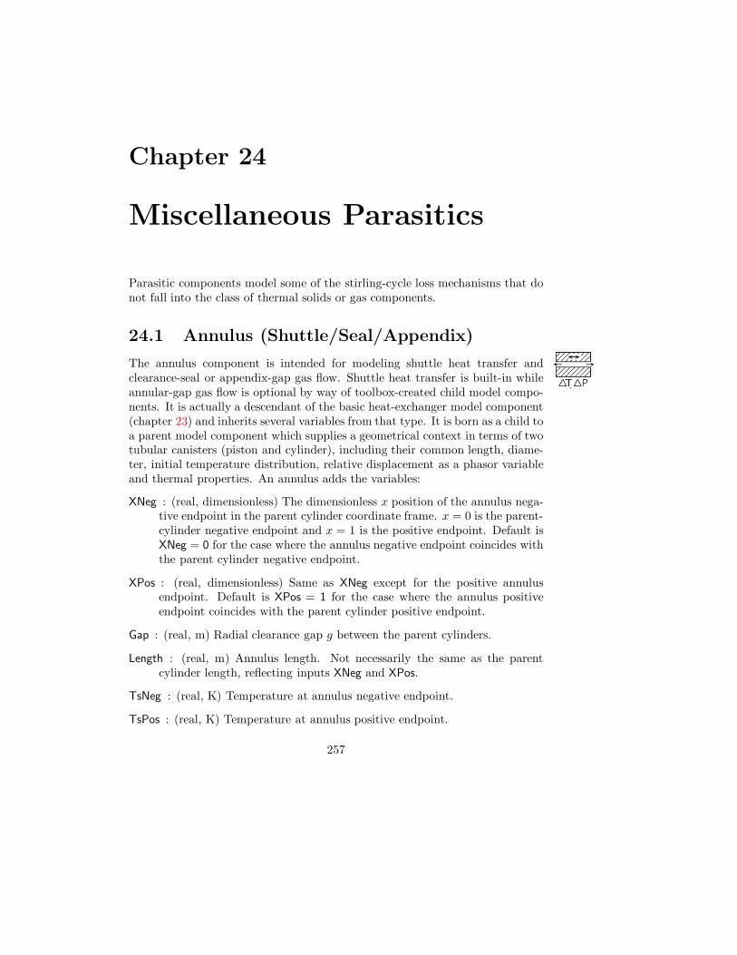
Chapter 24
Miscellaneous Parasitics
Parasitic components model some of the stirling-cycle loss mechanisms that donot fall into the class of thermal solids or gas components.
24.1 Annulus (Shuttle/Seal/Appendix)
The annulus component is intended for modeling shuttle heat transfer andclearance-seal or appendix-gap gas flow. Shuttle heat transfer is built-in whileannular-gap gas flow is optional by way of toolbox-created child model compo-nents. It is actually a descendant of the basic heat-exchanger model component(chapter 23) and inherits several variables from that type. It is born as a child toa parent model component which supplies a geometrical context in terms of twotubular canisters (piston and cylinder), including their common length, diame-ter, initial temperature distribution, relative displacement as a phasor variableand thermal properties. An annulus adds the variables:
XNeg : (real, dimensionless) The dimensionless x position of the annulus nega-tive endpoint in the parent cylinder coordinate frame. x = 0 is the parent-cylinder negative endpoint and x = 1 is the positive endpoint. Default isXNeg = 0 for the case where the annulus negative endpoint coincides withthe parent cylinder negative endpoint.
XPos : (real, dimensionless) Same as XNeg except for the positive annulusendpoint. Default is XPos = 1 for the case where the annulus positiveendpoint coincides with the parent cylinder positive endpoint.
Gap : (real, m) Radial clearance gap g between the parent cylinders.
Length : (real, m) Annulus length. Not necessarily the same as the parentcylinder length, reflecting inputs XNeg and XPos.
TsNeg : (real, K) Temperature at annulus negative endpoint.
TsPos : (real, K) Temperature at annulus positive endpoint.
257

258 CHAPTER 24. MISCELLANEOUS PARASITICS
QNeg : (real, W) Shuttle heat flow at annulus negative endpoint.
QPos : (real, W) Shuttle heat flow at annulus positive endpoint.
AEQ : (real, W) Available energy loss to shuttle heat flow.
Within the annulus toolbox are tools for creating an optional foil-matrixgas-domain with one of three wall models: isothermal, conductive surface orfloating. The isothermal wall is for modeling thermally-anchored seals (such aspiston seals), although you must remember to account for any wall heat flowin your overall energy balance. The conductive surface is for thermally-isolatedwalls, such as appendix-gap walls. It inherits solid material and cross-sectionalarea information from the parent canisters and models the solid conductionpath corresponding to their combined cross sections over that portion of theirlength specified by the XNeg and XPos input variables. The floating model isalso an option for thermally-isolated walls, except that it does not model axialconduction. It can be useful on occasion to avoid for double-accounting forsolid axial heat flows when they are separately considered in the parent canistermodels. However, floating walls with NCell > 2 often converge to unrealistictemperature distributions due to poor thermal anchoring.
You connect the shuttle-heat-transfer part of an annulus into the grandscheme of your stirling model much like you would a simple bar conductor— typically, at both ends to a temperature source (sink) objects via built-insteady-heat-flow boundary connectors. If you create a child gas domain, itsflow connectors are connected to other gas domains as is appropriate in yourmodel scheme. Two annulus instances may be ganged together in series tomodel a seal-appendix combination.
24.1.1 Theory
Shuttle heat transfer is a somewhat complicated process whereby, in the presenceof a temperature gradient, the moving wall of an annulus alternately picks upfrom and deposits heat to the stationary wall, with the net effect of transportingheat in the axial direction. This picking up and depositing of heat is governed bythe time-varying heat conduction in the transverse direction across the gas-filledannular gap, between and into the two walls. The shuttle heat transfer loss qs
may be presented in the form of an enhancement to molecular gas conductionqm within the clearance gap, although it is implemented separately from the gasin Sage. The following formula is due to Rios [50]:
qs
qm=
1
2(x/g)
2 1 + λ
1 + λ2(24.1)
where

24.2. RADIATION TRANSPORT PATH 259
g = radial clearance gapk = molecular gas conductivityks = wall solid conductivityqm = −k ∂T
∂x molecular conduction heat fluxx = relative displacement amplitudeλ = 1 + (k/g)[(δs/ks)1 + (δs/ks)2]; the subscripts refer
to the inner and outer walls
δs =√
2ks/(ωρscs); thermal penetration depthcs = wall solid specific heatρs = wall solid densityω = angular frequency
The above formula applies to the case of thick walls, where the wall thicknessw is larger than the thermal penetration depth δs, for each wall. When this isnot the case, shuttle heat transfer is reduced, because a thin wall cannot holdas much heat as a thick wall in the transverse heat-flow part of the shuttlemechanism. In fact a thin wall can hold only about w/δs as much heat. So,whenever one of the walls is thin (w/δs < 1), Sage scales the above formula bythe ratio of the smaller of w/δs for the two walls.
24.2 Radiation Transport Path
The radiation transport path embodies a simple model of radiant heat transferbetween two gray bodies. It is plug-compatible with a simple bar conductorand comes with two built-in steady heat flow connectors at either x end forconnection to a point temperature source and sink. It is born as a child to aparent model component which supplies the radiation frontal area. A radiationtransport path has variables:
Emmis : (real, dimensionless) Gray-body emissivity ε. A number between 0 and1. ε = 1 for an ideal black body. ε ≈ 0 for a silvered surface.
TsNeg : (real, K) Temperature Tn of negative x surface.
TsPos : (real, K) Temperature Tp of positive x surface.
QNeg : (real, W) Radiation heat flow at negative x surface.
QPos : (real, W) Radiation heat flow at positive x surface.
AEQ : (real, W) Available energy loss to radiation heat flow.
24.2.1 Theory
A radiation transport path models in-vacuum radiation energy transport be-tween two gray body surfaces with same area and emissivity, presuming all the
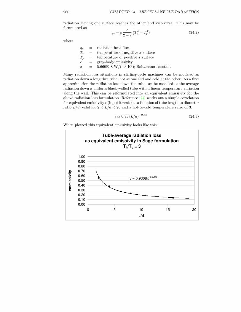
260 CHAPTER 24. MISCELLANEOUS PARASITICS
radiation leaving one surface reaches the other and vice-versa. This may beformulated as
qr = σε
2 − ε
(T 4
n − T 4p
)(24.2)
where
qr = radiation heat fluxTn = temperature of negative x surfaceTp = temperature of positive x surfaceε = gray-body emissivityσ = 5.669E–8 W/(m2 K4); Boltzmann constant
Many radiation loss situations in stirling-cycle machines can be modeled asradiation down a long thin tube, hot at one end and cold at the other. As a firstapproximation the radiation loss down the tube can be modeled as the averageradiation down a uniform black-walled tube with a linear temperature variationalong the wall. This can be reformulated into an equivalent emissivity for theabove radiation-loss formulation. Reference [24] works out a simple correlationfor equivalent emissivity ε (input Emmis) as a function of tube length to diameterratio L/d, valid for 2 < L/d < 20 and a hot-to-cold temperature ratio of 3.
ε ' 0.93 (L/d)−0.68
(24.3)
When plotted this equivalent emissivity looks like this:
Tube-average radiation loss
as equivalent emissivity in Sage formulation
Th/Tc = 3
y = 0.9308x-0.6798
0.00
0.10
0.20
0.30
0.40
0.50
0.60
0.70
0.80
0.90
1.00
0 5 10 15 20
L/d
em
mis
siv
ity

Chapter 25
Composite ModelComponents
Composite model components are high level components that work like othermodel components except that they have built in child models that you cannotdestroy. They automatically take care of some of the geometrical relationshipsamong these built-in components that would otherwise prove bothersome toyou.
25.1 Piston-Cylinder Composites
Piston-cylinder composites appear in the root-level stirling model toolbox. Theyall represent some form of piston within a cylinder, with capability to model theinteraction between the two. Built-in are two nested tubular canister child com-ponents serving as the moving piston (shell) and the fixed cylinder (liner). Thedescendants below also build-in various types of moving-part child components.
You treat these built-in components just as if you had created them yourself.For example, you may put a regenerator matrix and gas domain within themoving shell, to serve as a regenerative displacer (chapter 22). Or you may addarea attachments to the moving part (chapter 19) for connection to variable-volume gas domains (chapter 21).
Piston-cylinder composites also come with a toolbox with which you maycreate your own custom child model components. Available are springs anddampers for attachment to the moving part and a shuttle-heat-transfer annulusfor modeling the interaction between the shell and liner, including possible gasflow.
Piston-cylinder composites are born without connectors of any sort. Any andall connectors come from the child components within and must be moved up tothe top level if you wish to connect them to other root-level model components.
Variables common to all piston-cylinder composites are:
261

262 CHAPTER 25. COMPOSITE MODEL COMPONENTS
NCell : (dimensionless) The number of spatial nodes in the computational gridsof all underlying model components having such grids. Changing thisvariable causes these computational grids to re-initialize themselves. NCellwill affect the solution time and memory requirements, not to mentionsolution accuracy. Treat it gingerly by making only gradual, small changes.
Length : (real, m) Shell and liner length in x direction.
Dliner : (real, m) Cylinder liner outside diameter, reflecting wall thickness ofliner
Dshell : (real, m) Moving shell outside diameter.
Tinit : (cubic spline, W) Axial temperature distribution T (x) where x = 0 isthe negative endpoint and x = 1 is the positive endpoint.
The working gas type (properties) comes from the root model component.
25.1.1 Phasor Free-Piston and Cylinder
This component adds a built-in phasor reciprocating mass intended as the basisfor free-piston or free-displacer modeling. Choose this composite model whenyou want to solve for the limit-cycle sinusoidal response according to Newton’sequation of motion. Since overstroking is a distinct possibility, with potentialnegative volumes in variable-volume gas domains, you will want to make sureyou know the proper combination of area attachments, springs, etc., beforechoosing this model component.
25.1.2 Time-Ring Free-Piston and Cylinder
Similar to the above except with a time-ring reciprocating mass. This allowsyou to resolve higher harmonics in the resulting motion which may be of interestin certain cases. The number of nodes in the ring is according to the root-modelinput variable NTnode.
25.1.3 Phasor Constrained Piston and Cylinder
This component adds a built-in phasor constrained piston (or displacer) in-tended for first-approximation kinematic modeling or free-piston design work.The sinusoidal piston motion is now specified as input. Overstroking is no longera problem with this option. And by proper use of constraints you can set up anoptimization problem to solve for the proper combination of area attachments,springs, etc., to make the piston run properly when you switch to free-pistonmode.
For example, you could attach a spring to the piston and set up one areaattachment to represent a drive rod. You could then optimize the spring stiffnessand rod area subject to the constraints that the real and imaginary parts of therequired boundary force (F.real and F.imag) are both zero. You could chose to

25.1. PISTON-CYLINDER COMPOSITES 263
optimize other combinations of free-piston variables as well, provided you windup with two independent degrees of freedom.
25.1.4 Time-Ring Constrained Piston and Cylinder
Similar to the above except with a time-ring constrained piston. This modelcomponent is mainly intended for modeling the higher harmonics of kinematicmotion, provided you know the correct Fourier-series coefficients. You couldalso use it for free-piston design work, as above, except there is no easy way tobalance the higher harmonics within the equation of motion.
25.1.5 Simple-Crank Piston and Cylinder
This component adds a built-in simple-crank kinematic piston intended for mod-eling a kinematically driven piston using geometrical mechanism inputs. Withthese inputs you have a handle on optimizing the mechanism or introducingconstraints in terms of them.
25.1.6 Phasor Free-Piston and Free-Cylinder
This component is similar to the phasor free-piston component except it addsanother built-in phasor reciprocating mass representing the moving cylinder orcasing of a so-called “free cylinder” machine. The main reason for includingthe moving cylinder in this component is so it can pass the relative motionbetween the piston and cylinder to any annulus child components (see chapter24) for purposes of calculating shuttle heat transfer. In free-cylinder machinesthe cylinder and piston can both have large amplitudes with respect to a fixedreference frame yet be moving almost in parallel so that the relative amplitudebetween them is small. So it is important to calculate shuttle heat transferbased on the relative piston motion, not absolute motion.
The mass of the cylinder reciprocator should include all the mass rigidlyattached to the cylinder. If you want to allocate some of the mass to an externalreciprocating mass you can do so provided you connect the two reciprocatingmasses together with a force connection, which will force them to move togetherwith the same amplitude and phase. Generally the cylinder reciprocator willhave area attachments representing volume displacements to other gas spaces inyour model and be connected to ground with a spring and damper, representingthe suspension and load.
Keep in mind that in a free-cylinder model, both piston and cylinder motionsare understood as being relative to a fixed coordinate frame. This is differentthan the usual mind-set when thinking about stirling-cycle thermodynamicswhere the displacer amplitude, say, really refers to the amplitude of the dis-placer relative to the cylinder. When working with a free-cylinder model youmust make all such implicit understandings explicit in the model by providingappropriate volume displacements to any affected variable-volume gas spacesvia area attachments to the moving cylinder.

264 CHAPTER 25. COMPOSITE MODEL COMPONENTS
There is no corresponding constrained-cylinder variation of this component.If you want to constrain the cylinder motion, or the piston motion for thatmatter, you can just connect it to an external constrained piston componentusing a force connection. The two components will then move together withthe same motion. During the solution process, the force between them willautomatically accommodate to produce whatever force is necessary to drive thereciprocating mass. You can always break the connection later to implement“free” motion.
25.1.7 Time-Ring Free-Piston and Free-Cylinder
Similar to the above except with time-ring reciprocating masses representingboth the piston and cylinder motion. This allows you to resolve higher harmon-ics in the resulting motion which may be of interest in certain cases. The numberof nodes in the ring is according to the root-model input variable NTnode.
Chapter 26
ElectromagneticComponents
As of version 9 Sage offers electromagnetic component in the stirling, pulse-tubeand Low-T cooler model classes. The ultimate purpose of electromagnetic com-ponents is to model linear motors and alternators from first principles as partof an overall model for a stirling-cycle engine or cooler. Available componentsrange from simple electrical components like resistors or capacitors to compo-nents representing moving magnets or coils in interacting with time-varyingelectro-magnetic fields. Linear motors constructed from these components su-persede the elementary linear-motor components of section 19.8 offered in earlierSage version.
Electromagnetic components are connected to each other with current andmagnetic flux connections representing time-ring (periodic time grid) values atthe terminals or end poles of the component. They also sometimes have me-chanical force connections for attachment to moving parts (chapter 19). Currentand magnetic flux connections were introduce for version 9 in 2012
26.1 Sample Electromagnetic Models
You can find a number of electrical and magnetic circuit models as well as anumber of linear actuator models in the Apps\Stirling \Data\E-M sub-directoryunder the installation directory. Each Sage model file has a companion docu-ment in pdf format.
26.2 Connection Child Components
Electromagnetic components have two ends corresponding to the two leads ona resistor or capacitor or the two poles of a permanent bar magnet. Some comewith built-in electrical current or magnetic-flux connections at the two ends (see
265

266 CHAPTER 26. ELECTROMAGNETIC COMPONENTS
section 13.4). Others allow you to create any number of such connections ateither end using terminal or pole child models, which you drag and drop intoyour edit form.
Icon Purpose
time-ring negative terminal
time-ring positive terminal
time-ring negative pole
time-ring positive pole
When you drop one of these into the edit form, it is born with a connectionarrow which you can then move up one level to the parent-model page forconnection there to a mating connector in another component. You decidewhich connectors get connected where from the context of your problem andsubsequent documentation.
26.3 Simple Electrical Components
Simple electrical components can model stand-alone elementary electrical cir-cuits or serve as circuit elements that regulate voltage and current in morecomplicated electromagnetic models involving the electrical coil components ofsection 26.4.
26.3.1 Common Variables
Simple electrical components share some common output variables although notall are present, depending on the component:
FVneg : (Fourier series, V) Voltage at left (negative oriented) end V−.
FVpos : (Fourier series, V) Voltage at right (positive oriented) end V+.
FV : (Fourier series, V) Uniform voltage Vo.
FDeltaV : (Fourier series, V) Voltage drop ∆V = V+ − V−.
FI : (Fourier series, A) Average of the electrical currents at the two ends (I− +I+)/2, same comments as for phasor Icur above.
FWe : (Fourier series, W) Electrical power delivered to the component. Theinstantaneous electrical power delivered to component is W = −I∆V .Output FWe is just the Fourier series representation of W as a functionof time.

26.3. SIMPLE ELECTRICAL COMPONENTS 267
Positives and Negatives In the context of electrical components the termsnegative and positive can refer to two distinct things, the sign of the electricalcharge or the physical orientation of the Sage component. So to minimize con-fusion the terms left end and right end are used to refer to the negative-orientedand positive-oriented ends of components. This terminology is consistent withthe way components are displayed in the edit window.
However in mathematical symbols the left and right ends are still denotedwith − and + subscripts because there are no conventional symbol for right andleft. So for example, V− refers to voltage at the left end of a component and V+
to voltage at the right end.
Electrical current sign convention Sage follows the unfortunate conven-tion that electrical current represents a flow of positive charges. Together withthe general Sage convention that positive flows are reckoned from the left tothe right component ends, this means that a positive current flow correspondsto positive charges flowing in the positive direction or negative charges flowingin the negative direction. So in the case of a simple electrical resistor a nega-tive voltage drop ∆V (voltage at right end lower than at left end) produces apositive current flow, which actually corresponds to a flow of electrons in thenegative direction.
26.3.2 Connection Block
This component functions like a conduction path on a printed circuit boardthat connects together the leads of several electrical components. Within aconnection block you can drop in any number of negative or positive terminalsdepending on which components you are interconnecting. All leads attached toa connection block share a common voltage which is solved as part of the overallmodel so as to zero the net current flow, summed over all connections. Thereare no required inputs for a connection block.
26.3.3 Voltage References
This component is similar to the above connection block except you explicitly setthe voltage. It functions something like a ground connection. In any electricalcircuit the voltage is indeterminate unless you specify the absolute voltage (usu-ally zero) at least one point. Otherwise adding an arbitrary constant offset Vo toall the voltages of the circuit would produce an equivalent circuit (same voltagedrops and currents). This component allows you to specify reference voltagesas an arbitrary periodic time grid if you should want to do that. Generallyyou will connect a voltage reference to one point of an electrical circuit using apositive or negative facing terminal. You may ground a circuit at more than onepoint using voltage references with different voltages to simulate ground currentloops.
Additional inputs compared to the variables listed above are:

268 CHAPTER 26. ELECTROMAGNETIC COMPONENTS
FV : (Fourier series, V) Voltage offset Vo.
A voltage reference is the only electrical component where the net current flowinto or out of the component can be non-zero — where the current flow neednot be the same at both ends.
26.3.4 Voltage Source
This component establishes the voltage drop ∆V across two terminals of anelectrical circuit as an input. The voltages and currents in the rest of the circuitrespond accordingly. A sinusoidal voltage source is a good representation of thesinusoidal power grid in that it provides whatever current necessary to producethe required voltage drop across the terminals. With the addition of higherharmonics a voltage source might represent the output of an inverter.
Additional inputs compared to the variables listed above are:
FDeltaV : (Fourier series, V) Fixed ∆V overriding above dependent variable.
26.3.5 Current Source
This component establishes the current flow I between two terminals of anelectrical circuit as an input. It supplies whatever voltage drop is necessaryto produce the required current. The voltages and currents in the rest of thecircuit respond accordingly.
Additional inputs compared to the variables listed above are:
FI : (Fourier series, A) Fixed current I overriding above dependent variable.
26.3.6 Resistor
This component represents a simple resistor with input
R : (real, Ohms) Electrical resistance R.
It imposes a voltage drop between the negative and positive terminals accordingto Ohm’s law
∆V = −IR (26.1)
Where I is the electrical current. The minus sign is justified because a positivecurrent flow I > 0 implies voltage at the left end V− is higher than voltage atthe right end V+, so ∆V = V+ − V− < 0.
26.3.7 Capacitor
This component represents a simple capacitor with input
C : (real, Farads) Electrical capacitance C.

26.3. SIMPLE ELECTRICAL COMPONENTS 269
It is governed by this relationship between current I and voltage drop ∆V :
I = −C d
dt(∆V ) (26.2)
The minus sign is justified because a positive current flow I > 0 implies voltageincreasing at the left end V− (positive charge accumulating) and decreasing atthe right end V+ (negative charge accumulating), so d/dt(∆V ) < 0.
26.3.8 Inductor
This components represents a simple inductor with input
L : (real, Henries) Electrical inductance L.
It is governed by this relationship between voltage drop ∆V and current I:
∆V = −LdIdt
(26.3)
The minus sign is justified because a voltage higher at the left end than theright end (∆V < 0) accelerates current in the positive direction (dI/dt > 0).
26.3.9 Power Probe
This components represents a power flow meter. It is functionally equivalentto a short wire with zero resistance. Use it to monitor voltage, current and,more importantly, power flow at any point in an electrical circuit. There are noinputs required.
Other electrical components measure power dissipated within the compoent.This compnent overrides the FWe output to show the power flowing through thecomponent, evaluated as a function of time from
We = IV (26.4)
26.3.10 Ideal Transformer
Use this component to model an off-the-shelf transformer of adequate currentrating for your application. For actually designing a transformer see the samplemodel Transformer.stl installed in a subdirectory of the Sage program directory.This ideal transformer assumes zero resistance in the windings and zero reluc-tance in the iron path. It just steps up voltage and steps down current (orvice-versa) according to the single input:
TurnRatio : (real, dimensionless) Ratio secondary/primary winding turn num-bers N2/N1.
There are two built-in electrical circuit child components corresponding to theprimary winding and secondary winding, each with the usual electrical-component

270 CHAPTER 26. ELECTROMAGNETIC COMPONENTS
outputs. Ideal transformers are born with four current connectors, correspond-ing to the ends of the primary and secondary windings.
In transformers both coils are wound around a common magnetic flux path.If subscript 1 denotes the primary winding and 2 the secondary winding thenFaraday’s law (equation (26.24) ) gives the voltage induced in each winding interms of the rate of change of linked magnetic flux as
∆V1 = N1dφ
dt(26.5)
∆V2 = N2dφ
dt(26.6)
With zero wire resistance, ∆V1 and ∆V2 are the actual voltages at the trans-former terminals. Eliminating the common dφ/dt gives the well known voltagestep-up equation for a transformer
∆V2
∆V1=N2
N1(26.7)
Regarding the magnetic flux, it is related to the magnetic potential differencearound the flux path according the the magnetic circuit relationship
φ =µA
`∆Ψ (26.8)
where µ is the magnetic permeability, A is the effective magnetic path crosssection area and ` is the length. The magnetic potential difference is producedby the combined electrical current flows in the two coils according to Ampere’slaw (equation (26.27))
∆Ψ = N1I1 +N2I2 (26.9)
From the previous two equations it follows that
φ =µA
`(N1I1 +N2I2) (26.10)
For an ideal transformer the assumption is that µA/` → ∞ while φ remainsfinite (according to (26.5) or (26.6), so that
N1I1 +N2I2 = 0 (26.11)
orI1I2
= −N2
N1(26.12)
In other words the currents are opposite and stepped down by the same ratiothat the voltages are stepped up. In an actual transformer N1I1 and N2I2 arenot quite equal and opposite.
In energy flow terms, the above equations imply that
∆V2I2 + ∆V1I1 = 0 (26.13)
There is energy flow through an ideal transformer but no net energy dissipatedwithin it.

26.3. SIMPLE ELECTRICAL COMPONENTS 271
26.3.11 Solution Method
All simple electrical components share a common computational frameworkwhich may be represented abstractly in terms of a discrete component withnegative facing and positive facing ends to which voltage is applied and throughwhich current flows, as shown in this diagram:
V– V+
I–I+Vo
In some components there are two primary solution variables, voltage offsetVo and voltage drop ∆V = V+ − V− with voltages at the two ends evaluatedexplicitly as
V− = Vo − ∆V/2 (26.14)
V+ = Vo + ∆V/2 (26.15)
In other components there is only one primary solution variable Vo, presumeduniform throughout the component with no need to define ∆V . Electrical cur-rent I is a secondary variable evaluated as the average of the currents flowingthrough the negative and positive ends.
I =I− + I+
2(26.16)
Generally, the current is forced to be the same at the two ends (no net chargeaccumulation within) so I is the uniform current flowing through the component.In the case of a capacitor the current includes the so-called displacement currentof the time-varying electric field between the plates.
Current determines voltage offset Generally the condition of uniform cur-rent (I− = I+) determines the voltage offset Vo implicitly. The exception beingthe voltage reference components where the voltage offset is set by inputs andthe current can be different at the two ends.
Component physics determines voltage drop Generally the voltage drop∆V is evaluated explicitly as a function of current according to the physics forthe particular component (see above for each component class). The exceptionbeing the current source component where ∆V is solved implicitly from thecurrent input.
Current based on voltage continuity Connections between terminals pro-vide current I solved implicitly from the condition that the voltage is the sameacross the connection. When there are multiple terminal connections at oneor both ends of a component, the voltages are all the same. Each component

272 CHAPTER 26. ELECTROMAGNETIC COMPONENTS
is responsible for enforcing the requirement that the sum of currents flowingthrough the negative boundary equals the sum of currents flowing through thepositive boundary.
Solved by Sage Taken together in the Sage solution framework the implicitvariables identified above suffice for Sage to solve for voltages and currentseverywhere in a circuit comprising any number of simple electrical componentsconnected together in ways that make physical sense.
26.4 Coil Components
Coil components are electromagnetic components that implement Faraday’s lawof induction and Ampere’s law relating electric current to magnetic field. In asoftware sense they descend from the above simple electrical components andborrow the concept of magnetic potential and magnetic flux connections fromthe magnetic components to follow.
Physically, they represent coils of wire consisting of one or more turns woundon a cylindrical form (not necessarily circular). Each turn is insulated from thenext and an electrical current flow through the wire from one end to the other.
Magnetic effects occurring within the coil core (inside of the cylinder onwhich it is wound) are communicated to other magnetic model components(e.g. ferromagnetic materials) via magnetic flux connections at the ends ofthe coil core cylinder — the coil end boundaries. Generally in a Sage modelthere will be an external closed-loop magnetic flux path originating at one coilboundary and terminating at the other. Physically this flux path representsthe ferromagnetic or air path inside the coil core as well as the external path.The electrical current flowing in the coil winding generates a magnetic potentialdifference ∆Ψ between the two ends of the coil core (Ampere’s law). A changingmagnetic flux φ flowing through the coil core as a result of the magnetic fluxconnections generates a potential difference in the coil winding (Faraday’s law).All Coil components share these variables:
Inputs
Dwire : (real, m) Wire diameter dw not including insulation. If the wire crosssection is not circular this should be the effective diameter for a circu-lar wire with the same area. For example,
√
4/π b for a square wire ofdimension b × b.
Nturns : (real, dimensionless) Number of wire turns in coil N .
Dcentroid : (real, m) Diameter of coil centroid Dc. In the case of a circular coilof rectangular or circular cross section Dc is the average of the coil innerand outer diameters. Generally, defined by πDcAc = Vc, where Vc is thetotal coil volume and Ac is the coil section area. In other words so thatthe coil volume equals the coil area swept over the linear distance πDc.
26.4. COIL COMPONENTS 273
Alpha : (real, dimensionless) Coil packing factor α, (conductive material volume/ total volume), a number between 0 and 1. For close-packed circularwires (centers on vertices of equilateral triangular grid) the packing factoris π/(2
√3) ≈ 0.91. For rectangular packing (non-nested annular layers)
the packing factor is π/4 ≈ 0.79. Insulation thickness lowers the packingfactor by the square of the core to insulated diameter ratio.
Tcoil : (real, K) Coil temperature T at which electrical conductivity is evalu-ated.
LinkMult : (real, dimensionless) An empirical multiplier FL (range 0 to 1) usedto account for any magnetic fringing flux leakage through the coil vol-ume that subtracts from the flux passing through the inner core. Theeffective linked flux (average flux circumscribed by all windings) is takenas FLφ, where φ is the magnetic flux passing through the magnetic fluxconnections. (see discussion below)
Conductor : (selection list) Wire conductor material.
Outputs
Wdissip : (real, W) Coil time average electrical resistance I2R loss.
Rcoil : (real, Ohms) Coil resistance.
Lcoil : (real, Henries) Coil effective inductance L calculated from voltage drop
∆V and current time derivative I as L = −∮
∆V I∮
I2. For a pure inductor
this give the correct value as you can see by substituting the definingrelationship −LI for ∆V . Essentially in this formulation L is a coefficientin an orthogonal function expansion with I the orthogonal function.
Acoil : (real, m2) Total cross section area Ac of the coil winding normal towires. The cross section area into which the coil is wound.
Awire : (real, m2) Wire conductor cross section area Aw not including insula-tion.
Vcoil : (real, m3) Total volume of the coil winding Vc. The volume of the entiretoroidal envelope with cross section Ac enclosing the coil.
Vwire : (real, m3) Wire conductor total volume Vw. The volume of conductivematerial in the winding not including insulation.
Lwire : (real, m) Wire total length Lw.
Mwire : (real, kg) Wire mass ρsVw, where ρs is conductive material density.
FVneg : (Fourier series, V) Voltage at left (negative oriented) end of windingV−.

274 CHAPTER 26. ELECTROMAGNETIC COMPONENTS
x
yz
Ac
Aw
Dc
dw
I+
H
Figure 26.1: Coil geometry with arrows pointing in the direction of positive co-ordinate directions and current flow. According to the right-hand rule for mag-netic fields a positive current produces a positive z-directed (upward)magneticfield H in the coil core.
FVpos : (Fourier series, V) Voltage at right (positive oriented) end of windingV+.
FDeltaV : (Fourier series, V) Voltage drop ∆V = V+ − V−.
FI : (Fourier series, A) Electrical current in winding.
FW : (Fourier series, W) Electrical power delivered to the winding.
FDeltaPsi : (Fourier series, A) Induced magnetic potential ∆Ψ from Ampere’slaw (26.27).
FBflux : (Fourier series, Wb) Total linked magnetic flux φ through coil core.
FWm : (Fourier series, W) Magnetic power delivered to component −φ∆Ψ.
26.4.1 Fixed Coil
A fixed coil is one that does not move relative to the other magnetic componentsin the model. It does not consider the forces on the coil generated by theinteraction of the coil magnetic field with an external magnetic field or thevelocity of the coil winding through that magnetic field
Figure 26.1 shows the coil geometry. The input wire diameter dw determinesthe conductive material cross section area of a single wire as
Aw =π
4d2
w (26.17)
Additional inputs, number of turns N and coil packing factor α determine thecross section area of the total coil as
Ac =NAw
α(26.18)

26.4. COIL COMPONENTS 275
The final geometric input, centroid diameter Dc determines total coil volume as
Vc = πDcAc (26.19)
The total volume of conductive material in the coil is the total volume multipliedby the packing factor
Vw = αVc (26.20)
The overall wire length is the total conductive material volume divided by thewire cross section area
Lw =Vw
Aw(26.21)
Magnetic Field The current I flowing through the wire and the number ofturns N in the coil winding determine the magnetic potential difference accord-ing to Ampere’s law
∆Ψ = −NI (26.22)
This is a well-known result that derives from the Maxwell equation relatingcurrent density Jn normal to the coil cross section and the magnetic field H inintegral form:
∫
A
JndA =
∮
H · ds (26.23)
In this case integration surface A on the left side includes the currents of theindividual wires in the coil cross section Ac and the path of integration on theright side can be any path that includes Ac. In particular it can be axiallyupward through the coil inner cylinder then diverting radially to somewhereoutside the coil (where H is negligible) then downward axially, then convergingradially inward to the other end of the coil. Symmetry arguments for the tworadial legs and the arbitrariness of the inner axial leg leads to the conclusionthat the H field is uniform in the axial direction within the coil inside cylinderand that is the only part that contributes to the loop integral. So the right sidemay be written as
∫H · d` over the length ` of the inner cylinder. But by the
definition of magnetic potential this is just −∆Ψ.
Because of the formulation in terms of magnetic potential difference ∆Ψneither the value of the magnetic field H nor length of the coil cylinder ` areimportant individually. This explains why the coil axial length is not a requiredinput variable.
Why can’t the path of integration on the right side of the equation (26.23)include the external magnetic flux path, you ask, leading to a different con-clusion. The reason is that the magnetic flux path includes its own electricalcurrents associated with the magnetic domains of ferromagnetic materials andthese would have to be considered in the bounding surface integral of electricalcurrent density on the left side.

276 CHAPTER 26. ELECTROMAGNETIC COMPONENTS
Induced Voltage The rate of change of magnetic flux dφ/dt through thecoil inner core and the number of turns N determine the zero-current inductivevoltage difference across the coil terminals according to Faraday’s law
∆VL = Ndφ
dt(26.24)
This is another well-known result that derives from the Maxwell equation relat-ing the rate of change of magnetic flux density in the coil inner cylinder to theelectrical field E loop tension in integral form:
d
dt
∫
A
BndA = −∮
E · ds (26.25)
In this case the integration surface A on the left side is the coil inner cylindercross section and in terms of the magnetic flux through that cross section isjust dφ/dt. The path of integration on the right side applies to each turn ofthe winding separately. When added together for the total number of turns Nthe integral on the right amount to the total voltage difference across the coilterminals ∆V .
Because of the changing magnetic field produced by a time-varying currentvia Ampere’s law there is some degree of self induction that tends to counterthe current change by an opposing voltage change. The degree of this selfinduction depends on the properties of the magnetic flux path to which the coilis connected because that determines the size of the magnetic flux variation.
Flux Linkage Multiplier The above account assumes all of the magneticflux passes through the coil core and returns by some path entirely outsidethe coil volume. This is usually a good approximation to reality because themagnetic flux is contained within a ferromagnetic material of very high magneticpermeability compared to the coil or surrounding air. But not always. Inmoving-magnet linear motor applications, for example, there is generally a gapof low magnetic permeability in the ferromagnetic flux path in the vicinity ofthe coil. So some fringing magnetic flux may pass through parts of the coilwith the direction of flux opposite to that in the core. To account for this Sageincludes the empirical multiplier input FL (LinkMult) and modifies the inducedvoltage calculation of equation (26.24) to
∆VL = FLNdφ
dt(26.26)
to account for the fact that the linked flux is FLφ. In order to conserve energyit is also necessary to modify the magnetic potential difference calculation ofequation (26.27) to
∆ψ = −FLNI (26.27)
This follows from an energy conservation principle. The electrical energy flowassociated with the induced voltage ∆VL is
dEe
dt= −∆VLI = −FLN
dφ
dtI (26.28)

26.5. MAGNETIC COMPONENTS 277
The magnetic energy flow associated with the changing magnetic potential dif-ference ∆ψ is, according to equation (26.32)
dEm
dt= H
dB
dt= −∆ψ
dφ
dt= FLNI
dφ
dt(26.29)
so that the changes of electrical and magnetic energy are equal and oppositeand energy is conserved.
Resistance The electrical resistance in the wire creates a separate resistivevoltage drop whenever electrical current I is flowing according to
∆Vr = −IR = −Iσ Lw
Aw(26.30)
Where σ is the electrical resistivity (Ohm-m).
Total Voltage Difference The total voltage difference across the coil termi-nals is the sum of the part due to time-varying magnetic flux and the componentdue to resistance
∆V = ∆VL + ∆Vr (26.31)
26.5 Magnetic Components
Magnetic components form the basic elements of magnetic circuits. They in-clude air gaps, permanent magnets and ferromagnetic flux paths. All magneticcomponents define a scalar magnetic potential Ψ at each end of the componentand a magnetic flux φ that is a function of the magnetic potential difference ∆Ψacross the component. The negative potential difference −∆Ψ = Ψ− − Ψ+ isthe so-called magnetomotive force. Magnetic flux φ may be a function of timebut is presumed uniform in space throughout the component. Each componentdefines a different functional relation ship φ(∆Ψ) between magnetic flux andmagnetic potential difference. This is equivalent to a functional relationshipB(H) between magnetic flux density and magnetic field strength.
Energy and magnetic fields This manual does not go into the basic theoryof electromagnetism. But it does have an axe to grind about the way that the-ory is generally presented in terms of Maxwell’s equations involving a magneticfield and flux H and B. Maxwell’s equations, beautiful though they are, do notsay anything about the physical nature of H and B and what is the differencebetween them. It doesn’t help that the two are directly proportional in a vac-uum. What are the natures of two invisible quantities that are proportional toeach other?
So the Sage manual offers a mental crutch for the abstractly impaired. Amental picture that comes from taking the definition of magnetic energy as a
278 CHAPTER 26. ELECTROMAGNETIC COMPONENTS
fundamental concept along with Maxwell’s equations. By taking as axiomaticthis differential relationship for the change in magnetic energy per unit volume
dEm ≡ H · dB (26.32)
assumed to apply universally in vacuum or in a solid material — no exceptions.In this form the roles of H and B are seen to be fundamentally different. Infact they are similar to the roles of force to force F and displacement dx in theequation for the work done on a simple mechanical spring
dEs ≡ F · dx (26.33)
By analogy it is clear that H is something like a force and B something like adisplacement. In fact H is the gradient of a magnetic potential much like F isthe gradient of a mechanical potential (spring potential energy). In the case ofB in is not clear exactly what is being displaced from its equilibrium value butstill the idea that B is a displacement provides a useful mental image. Whateveris being displaced, it is displaced even in a vacuum. So it is some property ofspace itself outside our usual sensory perceptions. In these terms the fact thatB and H are proportional in a vacuum may be understood to mean that B isstretching like a spring in response to an increasing H force.
Conventional terminology that B is a magnetic flux is misleading. It sug-gests B is something flowing through space rather than a displacement froman equilibrium value. It would be better to call B the magnetic displacementand if anything is to be called the magnetic flux it should be the rate of changedB/dt.
26.5.1 Common Variables
For software design reasons magnetic components are subdivided into a parentcomponent that manages the solution grid and a child object component withvariables specific to a particular magnetic material.
Magnetic parent components share some common variables although notall are present, depending on the component:
Inputs
Lpath : (real, m) Magnetic path length `.
Apath : (real, m2) Magnetic path area A.
Outputs
Mmag : (real, kg) Mass of magnetic material.
FPsiNeg : (Fourier series, A) Magnetic potential at negative pole Ψ−.

26.5. MAGNETIC COMPONENTS 279
FPsiPos : (Fourier series, A) Magnetic potential at positive pole Ψ+.
FH : (Fourier series, A/m) Magnetic field H = −∆Ψ/`.
FB : (Fourier series, C) Magnetic flux density B = φ/A.
FWm : (Fourier series, W) Magnetic power delivered to the component.
From magnetic energy formulation (26.32) The instantaneous magnetic powerdelivered to a magnetic component of volume v = A` isW =
∫
vHBdv. In terms
of magnetic flux φ = BA and potential difference −∆Ψ =∫Hd` this works out
to W = −φ∆Ψ. Output FWm is just the Fourier series representation of W asa function of time.
Magnetic child objects share these common inputs:
Material : (selection list) The magnetic material selected by name from a list offerromagnetic or permanent magnet materials, depending on the compo-nent.
Tm : (real, K) Material temperature T at which magnetic properties are eval-uated.
ThkLam : (real, m) Lamination thickness a. To minimize eddy current lossesmagnetic materials typically comprise multiple layers or laminations withthe layers parallel to the magnetic field direction (section 26.7.3). If thereare no layers this input is still important because it affects the eddy currentmagnetic field and I2R loss, both of which are modeled in Sage. It shouldbe set to the minimum dimension of the material when viewed from the zdirection parallel to the magnetic field.
Meaning of lamination thickness For un-laminated magnetic materialsthe lamination thickness input ThkLam may be approximated according to thistable:
material shape lamination thickness a
Rectangle with B perpendicular to sec-tion
minimum rectangular dimension
Closed annular ring with radial B smaller of height or circumferenceAnnular ring with radial B, ring brokeninto rectangular sections
minimum rectangular dimension
26.5.2 Magnetic Connection Block
A component of zero magnetic reluctance that allows you to connect two or moremagnetic components together. Once connected the magnetic potentials Ψ ineach component adjust so all the connected poles share a common magnetic

280 CHAPTER 26. ELECTROMAGNETIC COMPONENTS
potential and the net magnetic flux flowing into the connection block is zero(∇ · B = 0). This is the magnetic analog of an electronic connection terminalexcept in magnetic circuits it is usually impossible to implement a magnetic fluxpath with negligible reluctance compared to the other circuit elements. It maybe useful to think of this component as representing a physical contact betweentwo or more magnetic poles where there is a negligible impedance of magneticflux among them.
26.5.3 Magnetic Potential Reference
This component is similar to the above magnetic connection block except youexplicitly set the magnetic potential Ψ. It functions something like a groundconnection in an electrical circuit. In any magnetic circuit the magnetic po-tential is indeterminate unless you specify the absolute value (usually zero) atleast one point. Otherwise adding an arbitrary constant offset Ψo to all themagnetic potentials of the circuit would produce an equivalent circuit (samemagnetic potential drops and magnetic fluxes). Generally you will connect amagnetic potential reference to one point of a magnetic circuit using a upwardor downward facing pole. In principle it is possible to ground a magnetic circuitat more than one point using different potentials although there is a more phys-ical way to do that using a permanent magnet component.The one additionalinput compared to the inputs listed above is:
FPsi : (Fourier series, A) Magnetic potential offset Ψo.
Magnetic potential references are the only magnetic components where thenet magnetic flux flowing into the component can be non-zero.
26.5.4 Magnetic Field Source
This component specifies the magnetic field magnitudeH between two poles of amagnetic circuit as an input. It produces a magnetic potential difference ∆Ψ =−H`, where ` is the magnetic path length (Lpath). The magnetic potentialsand fluxes in the rest of the circuit respond accordingly.
In effect it models a coil (section 26.4) with zero magnetic reluctance wherethe current is automatically adjusted to produce the required magnetic field.You might use this component to approximate such a coil or to provide boundaryconditions to evaluate other magnetic circuit elements.
Additional inputs compared to the variables listed above are:
FH : (Fourier series, A/m) Fixed magnetic field H overriding above dependentvariable.
26.5.5 Magnetic Flux Source
This components is similar to the above magnetic field source except the rolesof B and H are reversed. It specifies the magnetic flux density B between two

26.5. MAGNETIC COMPONENTS 281
poles of a magnetic circuit as an input. It supplies whatever magnetic potentialdrop is necessary to produce the required flux density. The magnetic potentialsand fluxes in the rest of the circuit respond accordingly.
Additional inputs compared to the variables listed above are:
FB : (Fourier series, V) Fixed magnetic flux density B overriding above depen-dent variable.
26.5.6 Air Gap
This component represents simple magnetic air gap with gap length and areainputs Lpath and Apath (above). It forces a relationship between magnetic fluxφ and magnetic potential drop ∆Ψ equivalent to the vacuum relationship
B = µ0H (26.34)
Where µ0 = 4π10−7 (H/m) is the permeability of free space.
The term air gap is traditional based on common usage in Earth’s atmo-sphere and has nothing to do with the actual gas that may be in the gap. Itwould be more accurate to call this component an empty gap.
26.5.7 Permanent Magnet
This component provides a magnetic flux φ as a function of magnetic potentialdifference ∆Ψ according to a fixed demagnetization curve B(H) = µ0H +J(H)as described in section 26.7.2. In addition to Material and Tm listed above apermanent magnet has these inputs:
Jmult : (real, dimensionless) Scale factor used to change the direction or mag-nitude of magnetic polarization J(H). A value +1 corresponds to a northpole at the positive end. A value −1 to a south pole at the positive end.Other values may be used to effectively weakening or strengthening themagnet relative to the Material data.
DemagLimit : (real, dimensionless) The external magnetic field beyond whichsignificant demagnetization occurs, expressed as a fraction of HcB. Thedefault value is 1. Sage will warn you if the external field exceeds thisvalue, otherwise it has no effect on the solution.
And adds this output:
FUtilization : (Fourier series, dimensionless) Utilization factor defined as theBH energy product along the demagnetization curve as a fraction of themaximum value. Small values for the time-mean and harmonic amplitudessuggest the magnet may be too large or too small. See section 26.7.2

282 CHAPTER 26. ELECTROMAGNETIC COMPONENTS
No Hysteresis In solutions with time varying H permanent magnets do nottraverse any minor hysteresis loops when traversing back and forth along de-magnetization curve. This is a reasonable approximation to reality providedthe external magnetic field is well below the coercive force limit HcJ . It alsoavoids the problem of solution transients demagnetizing the magnet and leadingto an unexpected solution — possibly multiple solutions depending on initialconditions and the path to the solution. In other words permanent magnets arereally permanent in Sage.
But this is not always a good thing. If you impose a high demagnetizingfield on a permanent magnet in Sage it will always recover its magnetizationwhen the field returns to a low value. A real magnet on the other hand may bepermanently demagnetized and never recover. Therefore the inputs for a perma-nent magnet include the value DemagLimit, the relative fraction of the coerciveforce HcB above which the magnet undergoes significant demagnetization. Thedefault value is 1. The Sage solver will warn you whenever |H |/HcB exceedsDemagLimit. If this warning occurs during the solution process as a result oftransient values then you can probably ignore it. If it occurs on re-opening amodel in the solved state and HcB and DemagLimit are set correctly then youignore it at your peril.
26.5.8 Soft Ferromagnetic Material
Soft ferromagnetic materials are generally used to conduct a cyclically reversingmagnetic flux with as little material as possible. So peak flux densities are gen-erally high (near saturation). Compared to a permanent magnet the coerciveforce required to change the direction of magnetization is relatively low. Butstill there is some coercive force required, which produces an energy dissipatinghysteresis loop B(H) as the H field varies back and forth. Sage captures thisenergy dissipation by solving the Magnetization M(H) as a function of both Hand dH/dt formulated in terms of the magnetic properties usually available forsoft iron materials. To help you keep an eye out for saturation a soft ferromag-netic material adds this output:
FJ : (Fourier series, T) Magnetic polarization J = µ0M .
The output is magnetic polarization rather than magnetization because thesaturation value Js is more commonly available in material property tablesthan Ms and it is also a number on the order of 1 rather than 106 (in SI units).
Pseudo-Hysteresis Formulation Since magnetization M depends on theprevious history as well as the current magnetic state it should, in principle,be solved as a differential equation (see section 26.7.1). One of the false startsof Sage development was to actually solve M as a differential equation but itwas soon apparent that doing so led to unacceptable numerical errors in Sage’scoarse time grid and also convergence problems. So instead of that, Sage solvesM using a simplified formulation motivated by the observation that all minor

26.5. MAGNETIC COMPONENTS 283
hysteresis loops fall between the two limiting curves of the outer hysteresis loop,produced by driving the magnetization to saturation in one direction then theother. Referring to figure 26.10 in section 26.7.1, the two limiting magnetizationcurves are roughly separated horizontally from each other by the distance 2Hc,where Hc is the coercive force (M = 0 intercept. In other words, the dH > 0branch is approximately Ma(H −Hc) and the dH < 0 branch Ma(H +Hc). Inparticular Sage formulates a shift value Hs that varies smoothly between ±Hc
Hs =
{dHdτ
Hc
H1if H1 > Hc
dHdτ otherwise
(26.35)
where H1 is the amplitude of the H and τ = ωt is the dimensionless cycleangle. The formulation is based on the observation that for sinusoidally varyingquantities the value dH/dτ takes its extreme values 90 degrees out of phasewith the extreme values of H . Since the amplitude of dH/dτ is also H1, thefirst branch amounts to a sinusoidal function with amplitude Hc. The secondbranch applies to low amplitude H solutions and scales down the shift Hs inproportion to the H amplitude. To deal with the possibility of non-sinusoidalH the value Hs is truncated to lie within the limits ±Hc.
Sage estimates the amplitude H1 using local solution information using aformulation that is valid provided the variation of H is sinusoidal or nearly sobut reasonable in any case.
H1 ≈√(dH
dτ
)2
+
(d2H
dτ2
)2
(26.36)
This may make more sense if you think of dH/dτ = H1 sin τ and d2H/dτ2 =H1 cos τ .
The value of M is then defined implicitly as
M = Ma(xs) (26.37)
where Ma is the function (26.93) and xs is the shifted dimensionless magneticfield
xs =H −Hs + αM
αMs(26.38)
Hysteresis loops for this pseudo-hysteresis approximation are illustrated in figure(26.10) of section 26.7.1 for the case of purely sinusoidal H variation. Forlarge H amplitudes (M near saturation) the pseudo-hysteresis loops appearquite reasonable compared to those calculated with the hysteresis differentialequation. For small H amplitudes the differences are more noticeable with thehysteresis loss is somewhat overestimated — the price for reliable convergence.
26.5.9 Non Magnetic Material
This component models the magnetic flux path within a non-magnetic electri-cally conductive material. It has the same free-space magnetic permeability as

284 CHAPTER 26. ELECTROMAGNETIC COMPONENTS
an air gap, µ0 = 4π10−7 (H/m). But unlike an air gap it models eddy currentlosses according to the formulation of section 26.7.3. Any time-varying magneticflux generates an opposing magnetic field, depending on material electrical con-ductivity and effective lamination thickness (ThkLam input).
The reason for this component is that some electro-magnetic devices imposea pressure wall between internal and external parts of the magnetic flux path.For example, a linear motor design may locate the coil outside a pressure wallto minimize internal volume, avoid contamination issues and avoid the need forwire feed thrus. Often this pressure wall must be a metal (electrically conduc-tive) for strength purposes.
If you want to model a pressure wall made from a ferromagnetic materialuse the Soft Ferromagnetic Material component instead. That component alsomodels eddy current losses but also includes the increased magnetic permeabilityof a ferromagnetic material and magnetic hysteresis.
For the present component the selection list for the Material input comesfrom the electrical materials data file. For the Soft Ferromagnetic Materialcomponent it comes from the soft ferromagnetic materials data file (see section28.5).
26.5.10 Solution Method
All magnetic components share a common computational framework based on alumped magnetic circuit approach. A magnetic component may be representedabstractly in terms of a solid of length ` and cross section area A with uniformmagnetic potentials Ψ+ and Ψ− on the upward and downward facing ends. Thepotential difference drives a uniform magnetic flux φ through the component,as shown in this diagram:
Y+
Y–
f
l
Ax
yz
Potential difference ∆Ψ and magnetic flux φ may vary with time.
The magnetic field within the component is presumed uniform (only a func-tion of time) and broken into two parts, H+Heddy , where H is the net magneticfield that determines the magnetic flux and magnetization and Heddy is the op-posing field due to eddy currents (see section 26.7.3 for details). The magneticflux and potential difference are related to the magnetic fields H , Heddy andmagnetic flux density B through these defining equations:
B = φ/A k (26.39)

26.5. MAGNETIC COMPONENTS 285
− ∆Ψ =
∫
(H + Heddy) · d` = (H +Heddy)` (26.40)
where k is the unit vector in along the component z axis. So the net scalarmagnetic field is
H = −∆Ψ/`−Heddy (26.41)
Implementation Details
In some components both magnetic potential offset Ψo and potential drop ∆Ψ =Ψ+ − Ψ− are solved in the computational grid with the magnetic potentials atthe two ends evaluated explicitly as
Ψ− = Ψo − ∆Ψ/2 (26.42)
Ψ+ = Ψo + ∆Ψ/2 (26.43)
In other components only Ψo is solved, presuming ∆Ψ = 0. Magnetic flux φ isevaluated explicitly as the average of the magnetic fluxes flowing through thenegative and positive ends.
φ =φ− + φ+
2(26.44)
Generally, the magnetic flux is forced to be the same at the two ends (∇·B = 0)so φ is the uniform magnetic flux flowing through the component.
Magnetic flux determines magnetic potential offset Generally the con-dition of uniform magnetic flux (φ− = φ+) determines the magnetic potentialoffset Ψo implicitly. The exception being the magnetic potential reference com-ponents where the Magnetic potential offset is set by inputs and the magneticflux can be different at the two ends.
Component physics determines magnetic potential drop The mag-netic potential drop ∆Ψ is evaluated implicitly as a function of magnetic flux φaccording to the physics for the particular component.
The objective is to adjust ∆Ψ so that φ(∆Ψ) demanded by the physicsequals the actual value of φ. Except for most components it is more convenientto formulate the relationship B(H) rather than the relationship φ(∆Ψ), theequivalence between the two being
φ(∆Ψ) ≡ A B(−∆Ψ/` −Heddy) (26.45)
Magnetic flux based on Magnetic potential continuity Connections be-tween poles provide magnetic flux φ solved implicitly from the condition that themagnetic potential is the same across the connection. When there are multiplepole connections at one or both ends of a component, the magnetic potentialsare all the same. Each component is responsible for enforcing the requirementthat the sum of magnetic fluxes flowing through the negative boundary equalsthe sum of magnetic fluxes flowing through the positive boundary.

286 CHAPTER 26. ELECTROMAGNETIC COMPONENTS
Solved by Sage Taken together in the Sage solution framework the implicitvariables identified above suffice for Sage to solve for magnetic potentials andmagnetic fluxes everywhere in a circuit comprising any number of magneticcomponents connected together in ways that make physical sense.
Validity of Scalar Potential with Eddy Currents
Technically the validity of a scalar potential formulation depends on the path-independence of
∫(H + Heddy) · ds between any two points in the magnetic
solid, or equivalently∮(H + Heddy) · ds = 0 for any closed path. For the net
field H this is the case because, by definition, H is the field that would bepresent in the absence of eddy currents and only electrical currents can disruptthe path independence of
∮H · ds.1 But this is not the case for the eddy field
Heddy. According to section 26.7.3 it varies from zero at the outer surface of themagnetic material to maximum at the center. But it is the case for the sectionaverage of Heddy (averaged in any x-y plane), which is what is important fora lumped parameter analysis. So there is really no difference between the eddyfield Heddy and the net magnetic field H when it comes to representation by ascalar magnetic potential. Both vary locally within the magnetic component andthe only assumption is that the scalar magnetic potential difference between thecomponent z ends represents the integral of the section averages of H + Heddy
along the z axis.
26.6 Linear Motors, Alternators, Actuators
Electromagnetic transduction components model the conversion of electricalpower to mechanical power or vice-versa via the interaction of components likepermanent magnets or coils moving through an air gap between magnetic polepieces.
26.6.1 Simple Transducer
But first there is a simple transducer component that functions as a bridgebetween the electrically-challenged linear motors of section 19.8 and the compo-nents below that model detailed electromagnetic physics. A transducer compo-nent is born with electrical current and force connectors for connecting to othercomponents of your model. There is only a time-ring version. It is a relativemoving part, which means that each end (xneg and xpos) should be connectedto a different moving part, one of which may be stationary.
A simple transducer throws to the dogs any electromagnetic physics thatmight be behind the conversion of electrical current to mechanical force and
1According to Maxwell’s equations the integral∮
H · ds around a closed path equals the
integral∫
Cndσ over any surface bounded by that path, where Cn is the electrical currentflow normal to surface element dσ.

26.6. LINEAR MOTORS, ALTERNATORS, ACTUATORS 287
instead simply assumes a linear relationship between the two
F = CfI (26.46)
The only physics this component implements is to produce a voltage drop acrossits electrical terminals according to an energy conservation principle — namely,that the mechanical power input equals the electrical power output:
Fdx
dt= ∆V I (26.47)
Solving for ∆V and using the definition of Cf , the energy conservation principleimplies that the voltage drop across the transducer terminals must be
∆V = Cfdx
dt(26.48)
This voltage drop is an output of the transduction voltage child componentbuilt into the linear transducer component. Resistive, inductive and capacitivecircuit elements are not included. They are to be implemented as separatecircuit elements connected to this component by current connections.
The force given by equation (26.47) acts on the moving part attached toendpoint coordinate xpos and the negative of that force on the moving partattached to xneg. The x in velocity dx/dt refers to the relative position xpos −xneg. Whether a transducer functions as a motor or alternator depends on therelative phase between current I and relative velocity dx/dt and also the signof Cf . If Cf is positive and I and dx/dt are in phase within 90 degrees thenthe mechanical power output is positive, otherwise it is negative.
The force or transduction coefficient Cf is a quadratic function of positionaccording to the inputs:
Cf0 : (real, N/A) Force or transduction coefficient Cf0 at x = 0.
Xm : (real, m) Reference extension xm.
Rp : (real, dimensionless) Force-coefficient ratio Rp = Cf/Cf0 at x = xm.
Rn : (real, dimensionless) Force-coefficient ratio Rn = Cf/Cf0 at x = −xm.
These are the same as for the relative linear motor component of section 19.8,which this component replaces. If you already know something about the physicsbehind the transducer you are modeling you may be able to read Cf0, Xm, Rp,Rn more-or-less directly, from a plot of Cf vs x generated either experimentallyor computationally, or more precisely from a best-fit parabola to the functionCf(x) over the intended operating range.
The force produced by the motor is still the product of force coefficient andcurrent, as in equation (26.46), but now Cf is the quadratic function of position
Cf(x) = Cf0
[1 + a(x/xm) + b(x/xm)2
](26.49)

288 CHAPTER 26. ELECTROMAGNETIC COMPONENTS
where coefficients a and b are formulated in terms of inputs as
a = (Rp −Rn)/2 (26.50)
b = (Rp +Rn)/2 − 1 (26.51)
This component will drive any attached reciprocating masses according to theforce-coefficient inputs and electrical current flow. It is important that thecomponents a transducer is connected to be capable of determining an absolutemean position (e.g. a constrained piston or connect to a spring to ground).Otherwise the solver will tend to drift around without converging.
26.6.2 Magnetic Gaps
These components represent the air gap between magnetic pole pieces. Eventhough the pole geometry is depicted as rectangular, these components canmodel concentric cylindrical pole geometries that are typically found in linearmotors or generators. The magnetic potential on each pole face is assumeduniform along the length and width (x and y) dimensions but variable withtime. The magnetic flux emerging from or entering the upper and lower z facesof the poles may be connected to other magnetic model components via built-inmagnetic flux connectors.
A single-pole magnetic gap (top icon in margin) represents a single opposedpair of parallel rectangular magnetic pole faces of length L (x-direction), widthW (y-direction) and separated by a gap gz (z-direction) through which magneticflux flows. The left-turned and right-turned magnetic gaps (second and thirdicons in margin) are sub-types of single-pole gaps. They are intended for usewith moving voice coils and deal with the special physics where the magneticflux path of the inner (lower) pole first turns toward the left or right (x direction)for the coil extend before turning again to the z direction.
A two-pole magnetic gap (bottom icon in margin) represents two pairs ofsuch pole faces separated in the x direction by a gap gx. (See figure 26.2).
The same set of input variables serves for all magnetic gap components:
Zgap : (real, m) Total z-directed air gap gz.
Wpole : (real, m) Common pole width W , or circumference in a cylindricalarrangement. In that case Wpole should be set to the effective pole cir-cumference that gives the correct air-gap volume. For example, if the innerand outer pole faces are located on circles of diameters Din and Din +2gz
respectively then the effective pole circumference is the mid-circle circum-ference W = π(Din + gz).
FringeMult : (real, dimensionless) An empirical multiplier used to scale thefringing flux outside the gap as a means to calibrate models. The 1-DSage model employs an idealized calculation of the fringing flux basedon the similarity of an electric field outside a parallel-plate capacitor (seesection 26.6.7). Depending on the actual magnetic gap you are modeling

26.6. LINEAR MOTORS, ALTERNATORS, ACTUATORS 289
pole pair 1
W
pole pair 2x
yz
L1 L2gx
gz
Figure 26.2: Two-pole magnetic gap geometry. The model assumes spatially-uniform, time-varying magnetic potentials on the inner faces of each pole and az-directed magnetic flux between the poles that may vary with both x positionand time.
the fringing flux may be more or less than that. The modeled fringingflux scales directly with FringeMult. It is still calculated from the idealizedformulation but for an effective gap equal to FringeMult times the actualgap.
Lpole1 : (real, m) Pole 1 length L1.
Xgap : (real, m) x-directed separation gx between poles 1 and 2.
Lpole2 : (real, m) Pole 2 length L2.
In the case of the two-pole magnetic gap the flux leakage between poles 1 and 2across the gap gx is presumed negligible, consistent with good design practices.But there is nothing in the software to prevent you from specifying a gap thatis in fact too small.
Air Gap Physics Magnetic gaps defer most of the electromagnetic physics toa built-in container and its components as discussed below. But they do handlethe physics for that part of the pole area not covered by the built-in containerat any particular time. For this they use the same principles as the magneticair gap discussed in section 26.5 based on the vacuum relationship betweenmagnetic flux and potential of equation (26.34). See section 26.6.7 below formore discussion on this topic. In addition, the left-turned and right-turned gapsalso deal with the variation of magnetic potential in the x direction induced byvoice coils. See section 26.6.5.
There are two outputs associated with the poles of magnetic gaps. They areavailable within the pole pair child component(s) built into every magnetic gapcomponent:
FBfluxAir : (Fourier series, Wb) Magnetic flux flowing through the part of themagnetic gap not covered by the moving electromagnetic container, if any,as a function of time. The uncovered part of the magnetic gap may be

290 CHAPTER 26. ELECTROMAGNETIC COMPONENTS
on one or both sides of the moving container or neither, depending on thecontainer length and offset.
FWm : (Fourier series, W) Magnetic power inflow into the total magnetic gapcalculated as −φ∆Ψ, where φ is the total pole magnetic flux and ∆Ψ isthe potential difference.
In the absence of a moving container the time-average magnetic power inflowwould be zero because there are no energy dissipating mechanisms in an airgap (φ and ∆Ψ are proportional). But with a moving container present, themagnetic energy flows to the components embedded in the container producepower flows at the poles. The magnetic energy flows to the components em-bedded in the container go to energy dissipations (hysteresis and eddy-current),mechanical power flows and in the case of coils electrical energy inputs anddissipations.
For pole in left or right-turned magnetic gaps there is a third output:
FWmLinked : (Fourier series, W) Magnetic power inflow linked to the embeddedvoice coil or coils.
As illustrated in figure 26.4 a voice coil produces a magnetic potential differencein the uncovered region of the air gap between the moving container end andpole end. The magnetic flux in this region is linked through the coil becauseof the way the inner pole is presumed to turn the flux. So the magnetic powerinflow to this uncovered region must be included in the total power inflow tothe coil or coils embedded in the container. Therefore output FWmLinked mustbe included when calculating the overall energy balance within a left or right-turned magnetic gap.
26.6.3 Moving Electromagnetic Container
This component is found in every magnetic gap component as a built-in childcomponent. Its purpose is to house and manage a series arrangement of oneor more moving electromagnetic components that move along together in the xdirection. For example: a coil, a moving magnet polarized in the z direction ora stack of several such magnets polarized in opposite directions as is sometimesused to modulate force versus position characteristics.
The container component defines the overall length (x-direction) of the inter-nal component stackup and descends from the relative moving part component(section 12.8) with built-in connectors at each end. The force connector at thepositive end is logically associated with the moving container and the force con-nection at the negative end with the outer pole pieces. The idea is that byconnecting these connectors to other moving parts of your model you can sim-ulate the relative motion of the electromagnetic container. Normally the polepieces are fixed and the container moving but depending on how you configureyour model it can be the other way around or both can be moving. Because ofthis flexibility the container component provides only the electromagnetic force

26.6. LINEAR MOTORS, ALTERNATORS, ACTUATORS 291
between the inner container and outer poles leaving any inertial forces to becalculated by reciprocating mass components to which the force connectors areconnected. In addition to the variables inherited from the relative moving partancestor component moving electromagnetic containers have these variables:
Length : (real, m) Container length.
Offset : (real, m) x-directed offset of the container at its rest position. Variablexo in figure 26.7.
Mass : (real, kg) Total mass of all electromagnetic components inside the con-tainer. An output variable.
Fscale : (real, dimensionless) Magnetic force correction factor applied to thecalculated force in order to achieve time-average global energy balance(see section 26.6.7). An output variable.
26.6.4 Moving Electromagnetic Components
All moving electromagnetic components are implemented in terms of a wrappercomponent that manages a space-time (x, t) solution grid with magnetic fluxdistribution variables φx+ and φx− (see figure 26.9). This wrapper componentdefines common inputs pertaining to the component grid, z-thickness, positionrelative to the parent container and also a few common outputs. These commoninputs and outputs are:
NCell : (dimensionless) The number of spatial cells in the computational grid.The higher the number the more accurate will be the magnetic flux dis-tributions φx+ and φx− between the outer poles and the electromagneticcomponent as it moves between the poles.
XnegRel : (real, dimensionless) The dimensionless x position of the componentnegative endpoint relative to the parent container. A number between 0and 1, with 0 corresponding to the container negative endpoint and 1 tothe container positive endpoint. The default value is 0.
XposRel : (real, dimensionless) Like XnegRel except for the component positiveendpoint relative to the parent container. The default value is 1. (seebelow)
ZthkRel : (real, dimensionless) Component thickness as a fraction of the z-directed air gap gz between the outer poles. A number between 0 and 1.The default value is 1. A number less than 1 corresponds to a sub-gap∆Z between the outer poles and component on each side (see figure 26.8)with ∆Z = (1 - ZthkRel) gz/2.
Length : (real, m) Dimensional component length L. An output calculated frominputs XnegRel, XposRel and the parent container length.
FFm : (Fourier series, N) Magnetic force acting on the component.

292 CHAPTER 26. ELECTROMAGNETIC COMPONENTS
FBflux : (Fourier series, Wb) Spatial average magnetic flux through the movingcomponent,
∫
dxφx, where φx is the component magnetic flux distribution.
Important When the container has more than one electromagnetic compo-nent the first must have the value XnegRel = 0 and the last XposRel = 1.subsequent components must have XnegRel equal to XposRel for the precedingcomponent. In other words the container components must completely fill thecontainer with no gaps or overlaps. Sage makes this assumption when allocatingthe magnetic flux between the outer poles not covered by the moving container.If there is a gap then magnetic flux will be zero in that gap making it a mag-netic insulator in effect with zero permeability, lower than the permeability ofa vacuum. If there is an overlap then both components will see the same mag-netic potential difference in the overlap as if they were connected in a parallelmagnetic circuit instead of in series.
Embedded Objects The actual moving electromagnetic component embed-ded within the wrapper is implemented as a separate built-in child componentwith its own inputs, outputs and physics. For example, the coil objects in themoving coil components below. Such embedded components and their governingphysical principles is the main topic of discussion in the following sections.
Generally speaking, moving electromagnetic components are similar to theirstationary counterparts except the physics is refined to include a spatial distri-bution of magnetic flux density B depending on where a point x in the gridfinds itself relative to the outer magnetic pole potentials. The quantity BWsymbolized by φx is the magnetic flux per unit length (Wb/m). The total fluxpassing through the moving component is just φ = BWL = φxL.
Warning about pole spacing Even though the magnetic flux density mayvary in the x direction, the flux direction itself is always presumed in the z di-rection (across the magnetic gap). This approximation is always reasonable forsingle-pole magnetic gaps but for multiple pole gaps there can be an issue in theregion between one pole and the next, or near, if the pole-to-pole potential gra-dient (in the x direction) is not small compared to across-gap potential gradient(in the z direction). This can happen if the pole-to-pole spacing is smaller thanthe magnetic gap or the pole-to-pole potential difference larger than the across-gap potential difference. In that case the accuracy of the Sage solution willsuffer. The problem is worse for coils or soft ferromagnetic materials where themagnetic flux direction is always proportional to the magnetic field direction.For permanent magnets — especially rare-earth magnets — it is less of an issuebecause the magnetic flux direction is mainly determined by the magnetizationdirection, which is locked into the material during fabrication.

26.6. LINEAR MOTORS, ALTERNATORS, ACTUATORS 293
Fa
Fb
x
yz
I+
B
L
W
hC
x=a x=a+c x=b-c x=b
Figure 26.3: Rectangular coil normal to z-directed magnetic field. Positivecurrent and coordinates in the direction of the arrows produce opposed forcesFa and Fb on the legs at a < x < a + c and b − c < x < b. A variation ofmagnetic B field in the x direction produces a net x-directed force on the coil.
26.6.5 Moving Coils
Moving coils implement the physics of non-moving coils discussed in section26.4 except in the context of the flux distribution and coil orientation withinthe parent magnetic gap and including the mechanical force on the coil producedby the interaction with the magnetic flux. The inputs and outputs basically thesame except for changes imposed by the magnetic gap geometry.
Transverse Coil
This component represents a rectangular coil of dimensions L × W movingbetween magnetic pole faces as illustrated in figure 26.3. The coil moves inthe x direction, parallel to the magnetic pole faces and perpendicular to thez-directed magnetic field between the poles. This arrangement is used for hard-drive head-positioning actuators but unlike the typical voice-coil orientation ina loudspeaker where the coil axis is parallel to the direction of motion and thepole faces.
The side legs of the coil (parallel to the direction of motion) do not interactwith the magnetic field so they are presumed to lie outside the pole gap. All themagnetic field interaction is produced by the two legs normal to the directionof motion.
Sage calculates the coil volume Vcoil according to the presumed rectangulargeometry of figure 26.3 assuming the coil side legs (parallel to x direction) liejust outside poles:
Vc = 2Ac(W + L − 2c) + πc2hc (26.52)
The number of turns in the coil (Nturns) remains an independent input, howeverthere is a new output:

294 CHAPTER 26. ELECTROMAGNETIC COMPONENTS
FillFac : (real, dimensionless) The fraction of coil length filled by the cross legs2c/L.
Cross leg x extent c is just the coil cross section area divided by the coil heightAc/hc. The coil height hc is a specified fraction of the parent magnetic gap(input ZthkRel). The Sage interface raises an exception whenever FillFac exceeds1, indicating the coil cross legs overfill the available volume.
Magnetic Field The electrical current flowing through the coil produces az-directed magnetic potential difference ∆Ψc according to Ampere’s law (26.27)of section 26.4. But unlike a non-moving coil, the total potential difference ∆Ψnow includes the potential drop due to magnetic flux across the coil air gap∆Ψa = −Bhc/µ0. So ∆Ψ = ∆Ψc + ∆Ψa.
The potential difference also varies as a function of x. It has the full valueof equation (26.27) only when x lies completely within the coil. Otherwise themagnetic potential
∮H · ds varies with the number of coil turns n(x) enclosed
by the integration path, which ranges from zero at the outer winding of the coilto N at the inner winding.
∆Ψc(x) = −n(x)I (26.53)
The assumption is that n(x) varies linearly so that ∆Ψc(x) also varies linearlyfrom zero at the outer winding to the full value at the inner winding.
Induced Voltage The rate of change of magnetic flux dφ/dt linked throughthe coil core induces a voltage difference across the coil terminals according toFaraday’s law (26.24) of section 26.4. Except now the total linked flux φ is theintegral of a flux distribution
∫φxdx over the distance x between windings. The
linked flux varies from the extreme outer winding to the extreme inner winding.The average value determines the total coil voltage drop.
Magnetic Force Something new for a moving coil is the magnetic force be-tween the coil and outer magnetic poles. Referring to figure 26.3 the net x-directed force on the coil is the difference between the forces Fa and Fb actingon the legs at x = a and x = b. The force arises as the summation of Lorentzforces acting on individual charge carriers moving through the coil wires.
If the magnetic flux density B were uniform throughout the coil there wouldbe no net force because the forces on opposite legs would exactly cancel. But ifB varies in the x direction there is a net force in the x direction produced bythe coil legs normal to the x direction. In general the differential force on anywire segment of length ds is
dF = ds(I × B) (26.54)
where I is the current vector in the coil reference frame2. For those familiarwith screw threads, the force direction is the direction of advance of a right-hand screw normal to the plane containing I and B rotating in the direction
2In the coil reference frame the current flow I is the number of charges per unit length of

26.6. LINEAR MOTORS, ALTERNATORS, ACTUATORS 295
from I to B. Under the assumption that I and B are always aligned with thecoordinate directions, then only the magnitudes I and B matter with positivevalues corresponding to the directions drawn. With B a function of x and tonly the total x-directed force on a single winding of the coil crossing the gapat a+ x and b− x is simply
Fw = I
(∫
b−x
Bds−∫
a+x
Bds
)
= IW [B]b−xa+x = I [φx]b−x
a+x (26.55)
where φx is just BW . Assuming there are N windings (turns) in the coil ex-tending across the magnetic gap from a to a + c on one end and b − c to b onthe other the total force on the coil is
F = NI(
〈φx〉bb−c − 〈φx〉a+ca
)
(26.56)
where 〈φx〉x2
x1denotes the average flux distribution between x1 and x2. This
equation is fine but for reasons that will be clear later it is possible to write itin a form that does not directly involve the electrical current by replacing NIwith the magnetic potential difference generated by the coil −∆Ψc. The resultafter also replacing φx with WB is
F = −W∆Ψc
(
〈B〉bb−c − 〈B〉a+ca
)
(26.57)
Voice Coils
These components represent circular coils moving in the direction of the coilaxis in the typical arrangement used for loudspeaker voice coils. The lower polecorresponds to the inner cylindrical pole piece. The magnetic flux turns axiallywithin the inner pole toward either left (negative x-direction) or right (positivex-direction) flux-path components to complete the external magnetic circuit.Hence there are two orientations of this component, depending on which side ofthe inner pole connects to the external magnetic path. Each exists only withina special magnetic gap parent, either a left-turned or right-turned magnetic gap.
Sage calculates the coil volume Vcoil assuming pole width W represents thecoil centroid circumference and the coil thickness hc is a specified fraction of theparent magnetic gap (ZthkRel).
Vc = Lπ
4
[
(W/π + hc)2 − (W/π − hc)
2]
(26.58)
wire drifting with velocity ud in the wire direction, which is actually quite small for typicalcurrents. What affect does the coil velocity have on the magnetic force? In the pole referenceframe the charges are moving with velocity ud plus the velocity of the moving wire uc. Butin this frame both negative and positive charges are moving and the magnetic forces on thepositive charges due to the uc velocity component cancel the magnetic forces on the negativecharges. Even if the wire is not exactly electrically neutral the net excess charge one way orthe other is small compared to the total number of charge carriers. Besides, whatever netforce due to uc there may be is of no concern because it is always directed perpendicular tothe direction of coil motion.

296 CHAPTER 26. ELECTROMAGNETIC COMPONENTS
coil center axis
x
H . sd
Figure 26.4: Left-directed voice coil cross section showing how the number ofturns in the coil inducing a magnetic potential difference
∮H · ds varies with
the position x where the path intersects the coil.
fx
x
zcoil center axis
x=b
I F
Figure 26.5: Left-directed voice coil cross section showing how the magnetic fluxlinked through the coil core varies with position due to the continuous upwarddiversion into the air gap. A positive z-directed magnetic flux distribution φx
produces a negative x-directed force F on the coil for an electrical current I inthe direction drawn.

26.6. LINEAR MOTORS, ALTERNATORS, ACTUATORS 297
The coil cross-section area Ac (normal to wires) is simply
Ac = Lhc (26.59)
Since the coil cross section is now specified by the external geometry the previousinput Nturns (number of wire turns in the coil) is now a output. It is calculatedaccording to the number of wires of individual cross section Aw that will fit intothe available cross section Ac given the specified packing factor α.
N = αAc
Aw(26.60)
Magnetic Field The electrical current flowing through a voice coil producesa magnetic potential difference per Ampere’s law as discussed in section 26.4except because the coil axis is along the x direction instead of the z directionthere are differences, as illustrated for a left-turning inner pole in figure 26.4.The magnetic potential
∮H · ds varies with the number of coil turns n(x)
enclosed by the integration path, depending on the position x where the pathintersects the coil. In the Sage solution the magnetic potential induced by thecoil is presumed concentrated across the air gap between poles but it is notlocalized to the coil. The potential varies from zero a any pole point to the leftof the coil to the full potential ∆Ψ = −NI at any point to the right of the coil.At points within the coil the potential varies linearly between the two. The caseof a right-turning inner pole is similar except the integration path encloses thecoil turns to the right of point x.
Induced Voltage The rate of change of magnetic flux dφ/dt passing throughthe coil core (the linked flux) still induces a voltage difference across the coilterminals according to Faraday’s law (26.24) of section 26.4. But now the linkedflux varies with position. Referring to figure 26.5 for the case of a left-turninginner pole piece, the linked flux at a point x in the coil is the total z directed(radial) flux crossing the magnetic gap between x and the pole endpoint, or
φL(x) =∫ b
xφx, where x is a point within the coil and b is the pole endpoint.
The flux change that determines the voltage difference is d 〈φL〉 /dt where 〈φL〉is the average linked flux over the coil length. The case of a right-turning innerpole piece is similar except the pole endpoint is reversed.
Magnetic Force Unlike a transverse coil, each turn of a voice coil createsan x directed force in the same direction. For a voice coil of circumference Wmoving through an external magnetic flux density B the differential force on asingle turn of wire carrying current I is
dF = W (I × B) (26.61)
Under the assumption that I and B are perpendicular and give rise to a forcein the x direction, only the magnitudes I and B matter and the x-directed force

298 CHAPTER 26. ELECTROMAGNETIC COMPONENTS
on the i-th turn of wire for current in the direction shown in figure 26.5 is
Fi = −WIB (26.62)
Noting that WB is just the flux distribution φx and that the number of wiresper unit length is N/L, where N is the number of turns in the coil and L is thecoil length, the differential force acting on a coil segment of length dx is
dF = −IφxN
Ldx (26.63)
So the total force acting on the coil is
F = −NIL
∫
x
φx (26.64)
26.6.6 Moving Magnetic Components
Moving magnetic components implement the physics of their non-moving coun-terparts discussed in section 26.5 except resolve the magnetic flux and field inthe x direction and override the Lpath and Apath inputs in terms of the parentmagnetic gap dimensions. Fourier series outputs for magnetic potentials, fieldsand flux densities are omitted because they would not capture the variation ofthese quantities with x. For detailed information about such things you canrefer directly to the solution grid.
For software design reasons the embedded objects representing magneticcomponents are subdivided into a parent embedment piece with variables com-mon to all components and a child object piece with variables specific to theparticular component. The graphical-interface icons for the embedment pieceare all similar to icon shown in the margin for the case of a permanent magnet.The icons for the child object piece appear in the margins under the individualsections below describing particular components.
Air Gap
This component represents an empty gap that may be used as an axial spacer(parallel to magnetic gap) between other magnetic components.
Permanent Magnet
This component represents a rectangular magnet of dimensions L ×W (lengthtimes width) moving between magnetic pole faces or a radially magnetized ringof magnets moving between cylindrical pole faces where W corresponds to theaverage of the inner and outer pole circumferences. The magnetization is pre-sumed parallel to the z-axis (across magnetic gap).
Fourier series output FUtilization representing magnet utilization factor doesmake sense for a moving magnet and is included. The same definition appliesas for a stationary permanent magnet, namely the BH energy product alongthe demagnetization curve as a fraction of the maximum value. Except now thevalue is an x-spatial average.

26.6. LINEAR MOTORS, ALTERNATORS, ACTUATORS 299
x
yz
dx
dy
dzI
m
Figure 26.6: Magnetic domain represented by a single effective current loop Ienclosing area dx dy in a differential volume dx dy dz. The current induces amagnetic dipole moment m oriented in the z direction with magnitude m =Idx dy and average volumetric density −M .
B H Relationship The B(H) functional relationship is the same as describedin section 26.5 for a stationary magnet except based on an x-distribution ofmagnetic flux φx as described above.
Magnetic Force The total magnetic potential difference across a magnetwith z thickness hm may be broken into two terms
∆Ψ ≡ ∆ΨM − hmB/µ0 (26.65)
in effect defining ∆ΨM , the component of the potential difference driving themagnetization.3 In terms of ∆ΨM and pole width W the x-component of forceacting on the moving magnet is
F = −W∫
x
∆ΨM∂B
∂x(26.66)
This follows as a generalization of equation (26.57) derived above for transversemoving coils except applied the individual magnetic domains in a permanentmagnet. For example, applied to the current loop I within the differential vol-ume dx dy dz illustrated in figure 26.6. Current I produces a magnetic potentialdifference ∆ΨI = −I. So substituting ∆ΨI for ∆Ψc, and dy for W in equation(26.57) gives
dF = −dy∆ΨI [B]x+dxx (26.67)
Taking the limit as dx→ 0 gives
dF = −∆ΨI∂B
∂xdx dy (26.68)
Integrating over the total magnet volume assuming uniform ∆ΨI and B in they direction, the dy integral reduces to the integrand times W so that the totalforce is
F = −W∫
x
∫
z
∆ΨI∂B
∂x(26.69)
3B ≡ µ0(H + M ) ⇔ B/µ0 ≡ M + H ⇔ hmB/µ0 ≡ ∆ΨM − ∆Ψ

300 CHAPTER 26. ELECTROMAGNETIC COMPONENTS
Assuming B does not depend on z, ∂B∂x factors out of the z integral and then
∫
z∆ΨI = ∆ΨM , resulting in equation (26.66). The same derivation also applies
to the case when eddy currents are present in the magnet. Then ∆ΨM isthe component of the magnetic potential difference driving both magnetization(magnetic domain currents) and eddy currents.
Force by Energy Conservation The force on a magnet can also be derivedfrom energy considerations. Think of the total force on the magnet as thesum of a large number of force elements acting on the individual magneticdomains moving through the external magnetic field. Referring to figure 26.6each domain has an associated magnetic dipole moment mi (not necessarilyin the z direction) with a volumetric moment density −M i (i is the domainindex). By the nature of permanent magnets, or any ferromagnetic material forthat matter, the magnitude of each magnetic dipole remains constant and onlythe angle of alignment with an external magnetic field H changes.
Mechanical energy input Fi · dx resulting from force Fi acting on M i in-creases the magnetic energy H ·dB within the volume element, but only the partassociated with the magnetization component of the magnetic field −M i · dB.More on this later but for now it follows that the x component of force actingon the magnetic domain is
Fi = −M i ·∂B
∂x(26.70)
Summing this over all the domains in the magnet amounts to an integral overthe magnet volume. In the one-dimensional Sage formulation the B field ispresumably directed along the z axis and varies only in the x direction. So in
integrating M · ∂B∂x
over any y-z plane, the vector ∂B∂x
factors out leaving onlythe integral of M which may be replace by the integral of the average magne-tization in the y-z plane. In the Sage formulation the average magnetization ispresumed oriented along the z axis with the scalar magnitude M , which maybe replaced with the equivalent ∆ΨI/dz. Likewise B can be replaced with itsscalar magnitude B. So the integrand reduces to the same one above in equation(26.68) and likewise the total force reduces to the same equation (26.66).
Returning to the justification for only −M i · dB balancing the mechanicalenergy change, equation (26.70) is equivalent to
Fi = (H − B/µ0) ·∂B
∂x(26.71)
which follows from the definition H ≡ B/µ0−M i. Arguing as before it followsthat in the one-dimensional Sage formulation the x-component of force actingon the moving magnet may be written as
F = hmW
∫
x
(H −B/µ0)∂B
∂x(26.72)
In this form the equation reveals something about global energy conservation. Inthe total electromagnetic model it is necessary that Fdx energy changes balance

26.6. LINEAR MOTORS, ALTERNATORS, ACTUATORS 301
pole pair 1
F-
pole pair 2
F+
x +pos xo
xneg
moving magnetic container
Figure 26.7: Side view of two-pole magnetic gap with moving magnetic containerinside. The magnetic force between the poles and moving container producesequal and opposite forces F+ and F− transmitted to other moving componentsof the model, or vice-versa. The magnetic container is a member of the relativemoving part family defining two position coordinates xneg and xpos. The left(negative) end of pole pair 1 is identified with xneg and the left end of themoving container with xpos + xo where xo is a fixed offset.
∆V I energy changes in electrical coils. For that to be the case the change inmagnetic energy resulting from the two must be the same. Taking the case ofan air-core solenoid for example, the change in magnetic energy in the core as aresult of coil electrical work dEc is (H −B/µ0)dB.4 So the change in magneticenergy associated with mechanical energy input must be likewise.
Soft Ferromagnetic Material
This component represents a rectangular piece of soft ferromagnetic material ofdimensions L ×W (length times width) moving between magnetic pole facesor a radially magnetized ring of material moving between cylindrical pole faceswhere W corresponds to the average of the inner and outer pole circumferences.
The magnetic energy and force relationships are the same as for a permanentmagnet. The only difference is that the functional relationship between magneticflux density B and magnetic field H is governed by the hysteresis formulationdescribed in section 26.5 for a stationary soft ferromagnetic material except interms of an x-distributed of magnetic flux φx.
26.6.7 Solution Method
The geometrical layout and solution method for the combination of a magneticgap, moving magnetic container and electromagnetic components within areillustrated starting with figure 26.7, which shows a top-level side view (y-axisinto page).
The interesting magnetic physics begins with figure 26.8. The magnetic polefaces are presumed to have uniform magnetic potentials Ψ1+, Ψ1−, Ψ2+, Ψ2−.
4This follows because the voltage drop induced in the coil is ∆V = NA dB/dt, where Nis the number of winding turns and A is the core section area. The core magnetic field isH = NI/` − B/µ0, where ` is the flux path length in the core. So I = (H − B/µo)`/N andthe coil energy works out to dEc/dt = A`(H − B/µ0)dB/dt

302 CHAPTER 26. ELECTROMAGNETIC COMPONENTS
Magnetic flux is presumed to flow in the z direction between the pole faces,passing through the total air gap gz or through an electromagnetic componentof some thickness lying between the pole faces, in series with air gaps ∆z oneach side. A relatively small fringing magnetic flux also flows between the polefaces and points on the surface of the electromagnetic component lying outsidethe pole faces, in which case the flux passes through an additional effective airgap gf as illustrated for the point x. Likewise for points lying to the left of polepair 1 or to the right of pole pair 2. For such calculations the outer magneticpotential is presumed to be that of the nearest pole face, or in the case of theregion between poles a smooth transition between the potentials of the polefaces on either side. Points on the faces of the electromagnetic component tothe left of the mid-plane between the poles are assumed to transfer magneticflux to pole pair 1 and those to the right to pole pair 2.
Fringe Field The effective air gap gf for the fringe region beyond the polefaces is based on an approximation to the field solution for a magnetic dipole(formed by the pole faces) in vacuum (air). This is a reasonable assumptionif something like a voice coil occupies the fringe region but not so reasonableif there is a ferromagnetic material or another pole face there. In those casesthe model underestimates the fringing flux to some extent but it is hard todo better in a one-dimensional solution. For a magnetic dipole the magneticpotential variation in the z direction along the plane of symmetry equidistantfrom the two poles (plane midway between pole faces) varies with distance xfrom the pole, for x� gz as
∂Ψ
∂z≈ 1
8
g3z
x3
(∂Ψ
∂z
)
x=0
(26.73)
where gz is the pole separation distance. In terms of the Sage solution theeffective pole separation s = gz + 2gf in the fringe region that gives the samemagnetic flux distribution for a given pole-to-pole potential difference, again forx � gz, is
s
gz≈ 8
x3
g3z
(26.74)
But s/gz must approach unity for x = 0 and also a magnetic gap is not quiteas simple as a magnetic dipole. In fact by similarity of governing equations themagnetic field between magnetic pole faces is similar to the electric field in aparallel plate capacitor. This is useful because fringe fields in capacitors hasbeen well studied. So the approach to approximating flux fringing in Sage is tostart with a formulation involving an unknown parameter a that has the correctx variation for x� gz
s
gz= 1 + a
x3
g3z
(26.75)
and then fit a so the resulting fringing flux is consistent with published capacitordata. The baseline formula for capacitance per unit length in terms of plate
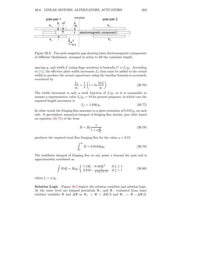
26.6. LINEAR MOTORS, ALTERNATORS, ACTUATORS 303
Y1+
Y1-
pole pair 1gz
Y1+
pole pair 2
Y2-
DZ
x electromagnetic component
mid-plane
x
yz
gf
Figure 26.8: Two-pole magnetic gap showing inner electromagnetic componentsof different thicknesses, arranged in series to fill the container length.
spacing gz and width L (using Sage notation) is basically C ∝ L/gz. Accordingto [39], the effective plate width increment Lf that must be added to the actualwidth to produce the actual capacitance using the baseline formula is accuratelycorrelated by
Lf
gz=
1
π
(
1 + ln2πL
gz
)
(26.76)
The width increment is only a week function of L/gz so it is reasonable toassume a representative value L/gz = 10 for present purposes, in which case therequired length increment is
Lf = 1.636 gz (26.77)
In other words the fringing flux amounts to a plate extension of 0.818 gz on eachside. A spreadsheet numerical integral of fringing flux density (per side) basedon equation (26.75) of the form
B = B01
1 + ax3
g3z
(26.78)
produces the required total flux fringing flux for the value a = 3.15.
∫ ∞
0
B = 0.818B0gz (26.79)
The indefinite integral of fringing flux at any point x beyond the pole end isapproximately correlated as
∫
B dξ = B0gz
{1.13ξ − 0.443ξ2 if ξ ≤ 10.818− 1
6.3(ξ+0.1)2if ξ > 1
(26.80)
where ξ = x/gz
Solution Logic Figure 26.9 depicts the solution variables and solution logic.At the outer level are lumped potentials Ψ+ and Ψ− evaluated from innersolution variables Ψ and ∆Ψ as Ψ+ = Ψ + ∆Ψ/2 and Ψ− = Ψ - ∆Ψ/2.
304 CHAPTER 26. ELECTROMAGNETIC COMPONENTS
Ψ and ∆Ψ are solved much like the solution for an ordinary air gap. Potentialoffset Ψ is solved implicitly in terms of the total pole magnetic fluxes φ+ andφ− from the continuity condition
φ+ = φ− (26.81)
Potential difference ∆Ψ is solved implicitly from the condition that the totalmagnetic flux φ (evaluated as (φ+ + φ−)/2) is the sum of the part through theair gap φair (to the left of the dotted line) plus the part through the embeddedmagnetic component φe.
φ = φair + φe (26.82)
The magnetic flux through the air gap is evaluated explicitly from the vacuumrelationship
φair = −µ0∆Ψ
gzAair (26.83)
Where µ0 = 4π1.0−7 (H/m) is the permeability of free space and Aair is theuncovered area of the pole (to the left of the dotted line). The embeddedcomponent magnetic flux φe is the integral of the magnetic flux distributionφx (evaluated as (φx+ + φx−)/2) for that part of the embedded componentexchanging flux with the outer poles (the whole component for a single-polegap or that part on one side or the other of the mid-pole position for a two polegap).
Within the embedded magnetic component flux distribution φx is solvedindependently as a function of the outer potentials Ψ+ and Ψ−. The solutionoccurs in a spatial grid so as to capture the changing flux with position xwhile moving through the gap. The potential offset Ψe is solved implicitly ateach point of the grid in terms of the magnetic flux distributions φx+ and φx−
(Wb/m) from the continuity condition
φx+ = φx− (26.84)
At this point there is a twist in the solution logic required because there is noexternal connector object to enforce magnetic potential continuity. So insteadof solving magnetic potential continuity from continuity of magnetic flux distri-bution it is the other way around. Flux distributions φx+ and φx− are solvedimplicitly from the conditions that the outer potential difference equals the sumof the potential difference across the inner component plus that across the airgaps on either side, namely
Ψ+ − Ψe+ = ∆Ψz (26.85)
andΨ− − Ψe− = −∆Ψz (26.86)
where ∆Ψz is the potential difference for flux φx flowing across the air gap ∆z (or∆z+∆x for points outside the pole boundaries). In the above equations Ψ+ andΨ− come from the previous air-gap solution so they may be taken as given and

26.6. LINEAR MOTORS, ALTERNATORS, ACTUATORS 305
fx+
Ye+
Ye-
fx-
fe+
fe-
f+
Y+
Y-
fair
DY
electromagneticcomponent
Y
DYe
Ye
pole pair
f-
Figure 26.9: Solution schematic for electromagnetic component located at thenegative end of the container between and offset from magnetic pole faces. Thearrows indicate the direction of information flow, not magnetic flux direction.The gap between the poles is expanded for clarity.
Ψe+ is evaluated as Ψe + ∆Ψe/2 and Ψe− as Ψe - ∆Ψe/2. Potential difference∆Ψe comes from the internal physics of the electromagnetic component as afunction of flux distribution φx.
Energy Leakage Normally the principle of global energy conservation is builtinto the numerical differencing methods used for Sage’s model components. Theenergy flowing out of one computational cell is exactly balanced by the energyentering another. But this is not so simple for electromagnetic componentsmoving between fixed poles. The grid of the embedded magnetic componentmoves relative to the poles and the boundaries of the computational cells donot always line up with the pole endpoints. The magnetic flux from the polesis apportioned into the moving grid so as to conserve magnetic flux but themagnetic potential across the grid computational cells and the magnetic forcecalculation are not guaranteed 100% accurate. In effect there may be a smallamount of energy leakage between the outer poles and the embedded movingcomponent.
But global energy conservation is too important to abandon. Without itSage’s optimizer might take advantages of any errors in a model. So Sagecalculates magnetic force so as to always preserve at least the time average ofglobal energy conservation. The moving electromagnetic container contains animplicitly solved variable kF (output Fscale). The force seen by any componentconnected to the moving electromagnetic container is kFF , where F is themagnet force calculated explicitly from physical principles. kF is adjusted as

306 CHAPTER 26. ELECTROMAGNETIC COMPONENTS
part of the solution so that the time-average power output conserves energyrelative to the magnetic energy flow into the pole gaps. Except that kF isnot allowed to deviate too much from one to avoid unrealistic forces when theenergy balance is not affected by kF (e.g. when magnetic force is uniformly zeroor produces negligible power because it is in phase with displacement or thedisplacement is very small). In that case some numerical energy leakage doesoccur.
26.7 Magnetic Material Physics
In a vacuum the magnetic flux displacement resulting from a magnetic field His simply
B ≡ µ0H (26.87)
where µ0 ≈ 1.257E-6 (H/m) is the permeability of free space. In ferromagneticmaterials, including permanent magnets, magnetic domains align in responseto a magnetic field, increasing the magnetic flux displacement. The domainalignment is characterized by the so-called magnetization Mdefined by
B ≡ µ0(H +M) (26.88)
The relative permeability µr is the factor by which the vacuum permeabilitymust be multiplied to account for the magnetization. It is defined by
µr ≡ H +M
H(26.89)
Domain alignment may also be characterized in terms of the magnetic polariza-tion J defined by
B ≡ µ0H + J (26.90)
In this form it is clear that the residual magnetic flux Br at H = 0 is the sameas the residual magnetic polarization Jr.
26.7.1 Soft Ferromagnetic Materials
Soft ferromagnetic materials are characterized by high relative magnetic perme-ability µr and relatively low coercive force (H at M = 0 intercept) compared toa permanent magnet. In typical usage the magnetization alternates from nearsaturation in one direction to near saturation in the other so that magnetichysteresis losses may be significant.
Hysteresis Model
Jiles and Atherton [30] in 1986 laid out the mathematical underpinnings ofmagnetic hysteresis in the form of a differential equation. The primary variableto be determined is the magnetization M in the defining relationship B ≡

26.7. MAGNETIC MATERIAL PHYSICS 307
-1.0
0.0
1.0
-20 -15 -10 -5 0 5 10 15
Re
lati
ve
Ma
gn
eti
zati
on
M/M
s
Relative Magnetic Field H/HcB
solved from hysteresis model
20 -15 -10 -5 0 5 10 15 20
Relative Magnetic Field H/HcB
from pseudo-hysteresis model
Figure 26.10: Excel spreadsheet solutions of differential equation (26.91) for Hcycling back and forth between positive and negative limits over six differentranges, decreasing in powers of two. Compared to curves from pseudo-hysteresisequation (26.37) on the right. The curves calculated from the differential equa-tion overestimate coercive force Hc slightly. Parameter α = 1.49E-4, based onproperties for non-oriented silicon steel (2.9%): µr = 8000, Ms = 1.59E6 A/m,Hc = 40 A/m.
µ0(H + M). In the Jiles and Atherton formulation M is the solution of adifferential equation. The underlying differential equation for M is:
dM
dH=
{(Ma−M)∨0
Hcif dH > 0
(M−Ma)∨0Hc
if dH < 0(26.91)
The ∨ operator on the right side is the max operator (i.e. ∆M ∨ 0 means thelarger of ∆M and 0). Ma(H) is the so-called anhysteretic magnetization — theaverage of the upper and lower branches of the actual hysteresis curve shownin figure (26.10). Hc is the coercive force (point where the lower branch of thehysteresis curve crosses the H axis).
Compared to the formulation used in Jiles and Atherton the above equationomits a relatively small term α(Ma −M) in the denominator on the right side.The idea is that the solution M(H) approaches asymptotically the anhystereticmagnetization Ma(H) for large negative and positive values of H but typicallyfalls somewhat above or below Ma depending on the direction H is changing.The purpose of the ∨ operator is to avoid a non-physical behavior in the Msolution when dH changes sign. For example just before a maximum-H reversalpoint where dH goes from positive to negative the M value is always slightlybelow Ma. So just after flow reversal M − Ma is negative and without the∨ operator M would continuing to increase ((M −Ma)dH > 0). With the ∨operator the M value instead remains constant until H decrease to the pointwhere Ma(H) again drops below M (or dH reverse direction again).

308 CHAPTER 26. ELECTROMAGNETIC COMPONENTS
In solving the above differential equation there is a complication because theanhysteretic magnetization is defined in terms of an effective magnetic field He
related to magnetic domain coupling. This effective magnetic field is
He = H + αM (26.92)
where α is the inter-domain coupling coefficient. The anhysteretic magnetizationis taken to be a function that varies smoothly between saturation values −Ms
and Ms:
Ma(x) = Ms(coth(x) − 1/x) (26.93)
The independent variable is the dimensionless effective magnetic field
x ≡ He
αMs(26.94)
This differs from the Jiles & Atherton formulation which defines x as He dividedby another parameter. But it will turn out that the above formulation sufficesfor the M solution to have the correct slope near M = 0, which is good enoughfor Sage.
To speed up computation Sage approximates the function coth(x) − 1/x onthe right side by a function
f(x) =
{
sign(x) − 14/15x if |x| > 2
x3 − x3
60 otherwise(26.95)
The factor 14/15 makes the branches of the approximation continuous at x =±2. Both original and approximate functions are shown in figure 26.11.
M intercept Hc Referring to the lower branch of the major hysteresis loop infigure 26.10), the M intercept of the magnetization solutionM(H) starting froma large negative H is Hc. This is already built into the governing differentialequation (26.91). To see this it is helpful to simplify the dH > 0 branch of thatequation to
dM
dH=Ma −M
Hc(26.96)
So the slope of M at Hc is (Ma(Hc)−M(Hc))/Hc. On the other hand the slopeof the anhysteretic magnetization curve Ma (curve midway between upper andlower branches of the major hysteresis loop) at Hc is approximatelyMa(Hc)/Hc
(since Ma(0) = 0). For the two slopes to be equal requires M(Hc) = 0. In otherwords that the M intercept is Hc. This conclusion applies to all useful softferromagnetic materials where the curves M(H) and Ma(H) are nearly linearand parallel in the range (−Hc, Hc).
Determining α So the slope of M and Ma are the same near M = 0 butwhat determines the steepness? Parameter α does. To see this start with the

26.7. MAGNETIC MATERIAL PHYSICS 309
-1
-0.8
-0.6
-0.4
-0.2
0
0.2
0.4
0.6
0.8
1
-5 -4 -3 -2 -1 0 1 2 3 4 5M
a(x
) /
Ms
x
Dimensionless Anhysteretic Magnetization Function
coth(x) - 1/x
1 - (14/15)/x
x/3 - x /603
Figure 26.11: Dimensionless anhysteretic magnetization function (26.93) andpiecewise approximation (26.95).
definition of magnetic susceptibility κ = µr−1. It follows from equation (26.88)and the definition of relative permeability B = µoµrH that
κ = dMa/dH (26.97)
Using the above approximation (26.95) (namely, f(x) ≈ x/3 near x = 0), itfollows that
κ =dMa
dH He=0=
d
dH
(1
3α(H + αM)
)
=1
3α
(
1 + αdM
dH
)
(26.98)
But since the M and Ma are close it is reasonable to approximate dM/dH onthe right side with dMa/dH = κ, obtaining
κ =1
3α(1 + ακ) (26.99)
or solving for α:
α =1
2κ(26.100)
In other words, this is the value of inter-domain coupling coefficient α in thedefinition of effective magnetic field (26.92) required for the solution to have thecorrect magnetic susceptibility κ.
At this point parameter α is specified in terms of bulk material properties andthe solutionM(H) to differential equation (26.91) can in principal be calculated.Except under the coarse time grid employed in Sage and the nonlinearity ofM(H) coupled with possible non-sinusoidal variations inH produce convergenceissues and numerical artifacts in the solution. So the Sage formulation uses thepseudo-hysteresis approximation discussed in section 26.5.8.

310 CHAPTER 26. ELECTROMAGNETIC COMPONENTS
Js
J = Br r
-HcJ
H
J
(JH)max
J(H)
Figure 26.12: The approximate demagnetization curve given by equations(26.104) and (26.105) determined by parameters Jr, HcJ and Kjh.
26.7.2 Permanent Magnets
Permanent magnets are characterized by high coercive forces and are suppliedin a magnetized state. Unlike soft ferromagnetic materials they are never, bydesign, subject to a high enough demagnetizing field to change the magneti-zation. Rather the magnetization varies only slightly and nearly reversibly sothat hysteresis losses can be neglected. For practical purposes they are definedaccording to a fixed demagnetization curve B(H) that can be formulated asfollows.
Permanent magnets like other ferromagnetic materials have a saturationmagnetic polarization Js where all the magnetic domains align with the externalmagnetic field. As the external magnetic field varies from a positive high valueto a negative high value the magnetic polarization follows the upper branch ofa hysteresis loop which always looks something like the approximation shownin figure (26.12). The saturation and residual magnetic polarizations Js and Jr
and the coercive force HcJ are all labeled on the curve. The exact shape of thedemagnetization curve is not important so Sage approximates it in a simple butgeneral way. Sage formulates the part of the hysteresis curve for J > 0 as thesimple hyperbola J ∝ −1/H with the origin displaced to the second quadrant.The part for J < 0 is a linear continuation of that function, which is physicallyincorrect for H � HcJ but moot since permanent magnet are demagnetized ifthey operate below HcJ . In Sage, the linear continuation facilitates the implicitsolution of H .
The shape of this function in the second quadrant (upper half of figure 26.12)is determined by how close Jr is to Js. If Jr is near the asymptotic value Js
then there will be a pronounced knee in the curve. If Jr is small comparedto Js then the curve will be approximately linear. The (JH)max point (whereJdH + HdJ = 0) occurs at the knee of the curve so the shape of the curve is

26.7. MAGNETIC MATERIAL PHYSICS 311
0.0
0.1
0.2
0.3
0.4
0.5
0.6
0.7
0.8
0.9
1.0
-1 -0.9 -0.8 -0.7 -0.6 -0.5 -0.4 -0.3 -0.2 -0.1 0
Dim
en
sio
nle
ss M
ag
ne
tic
Po
lari
zati
on
J /
Jr
Dimensionless Magnetic Field H / HcJ
permanent magnet demagnetization curves
for different Kjh values
K =0.6jh
K =0.7jh
K =0.8jh
K =0.9jh
K =0.95jh
K =0.51jh
Figure 26.13: Permanent magnet demagnetization curves for different values ofshape parameter Kjh. Curves generated using equation (26.104).
also determined by the (JH)max value compared to the product JrHcJ . It isconvenient to define the dimensionless shape factor Kjh by
K2jh ≡ (JH)max
JrHcJ(26.101)
For a nearly linear J(H) demagnetization curve the (JH)max point falls nearthe point (−HcJ/2, Jr/2), so the value of Kjh is close to 1/2. For a curve with apronounced knee the (JH)max point falls near (−HcJ , Jr), so the value of Kjh
is close to 1.It is straight forward but a bit tedious to work out the approximate de-
magnetization function in terms of Br , HcB and K. It is useful to define aconstant
C ≡ 1/K + 1
1/K2 − 1(26.102)
and then
D ≡ C
C2 − 1(26.103)
in terms of which the approximate demagnetization function turns out to be
J(H) = Br
[
CD − D2
CD + HHcJ
]
if H ≥ −HcJ (26.104)
For H < HcJ the demagnetization function is just the linear continuation
J(H) = BrC2
[H
HcJ+ CD− D
C
]
(26.105)

312 CHAPTER 26. ELECTROMAGNETIC COMPONENTS
The demagnetization curves resulting from different values of K are shown infigure 26.13.
Maximum Energy Product
Permanent magnets are often characterized by their so-called maximum energyproduct BH along the demagnetization curve. AlthoughH is negative along thedemagnetization curve and B positive so it is really −BH that has a maximum.
What is the significance of the maximum energy product? Given a simplemagnetic circuit consisting of a permanent magnet of length Lm in series witha linear magnetic material (B = µH) of length Lg and cross section Ag, themagnet energy product −BH is proportional to the total energy stored in themagnetic material. This follows because the total energy stored in the magneticmaterial is 1/2BgHgLgAg. But B and H in the two materials are related byBmAm = BgAg and −HmLm = HgLg , so that the total energy stored in themagnetic material is −1/2BmHmLmAm — in other words, proportional to themagnet BH product and the magnet volume.
In a magnetic circuit application the actual magnet −BH product as a frac-tion of the maximum value can be viewed as a magnet utilization factor. InSage permanent magnet components it is represented by the output FUtilizationwhere the maximum value (BH)max is evaluated numerically for each perma-nent magnet instance because it is complicated to find an analytic expressionin terms of the above magnetization formulation (BH ≡ JH + µ0H
2). If theutilization factor is low then the permanent magnet may not being used to itsfull potential. It may be low because H is small (magnet driving flux throughthe circuit with minimal effort) in which case you might get by with a smallermagnet. Or it may be low because B is small (magnet too weak to drive fluxthrough the circuit) in which case you may need a larger magnet. Because Band H vary with time in most applications the magnet utilization factor alsovaries with time so it is output as a Fourier series. Generally speaking the meanvalue and harmonic amplitudes should not all be small.
26.7.3 Eddy Currents
Magnetic materials are usually also electrical conductors and a changing mag-netic flux induces an electrical current flow just like in a wire coil. Except thecurrent flow is in the form of a current distribution within the bulk material.The current flows along the electric field induced by the changing magnetic fluxin the form of simply-connected closed loops as depicted by loop J in this sketch.(note: The symbol J denotes current density here but is also used to denote themagnetic polarization elsewhere.)

26.7. MAGNETIC MATERIAL PHYSICS 313
x
yy = a/2
y = -a/2
a
L
J
Figure 26.14: Cross section of a single lamination of magnetic material show-ing eddy current distribution J resulting from changing magnetic flux dB/dtdirected into the page and uniform within the lamination. A typical currentstreamline follows the dotted line, which is somewhat idealized near the end-points.
Y+
Y–
l
J
Heddyx
yz
Heddy
But there are no net voltage differences within the material — the electric fieldproduces a voltage gradient along the field direction that is canceled exactly byan opposite voltage gradient due to electrical resistance to the current flow. Allother things being equal, materials with low resistivity tend to have large eddycurrents in order to create sufficient large opposing voltage gradients. Exceptthe eddy currents themselves produce magnetic fields (Heddy of illustration)that oppose the changing magnetic flux so materials with low resistivity reducethe changing magnetic flux somewhat. In the case of a superconductor theeddy currents are always exactly enough to completely cancel any changingmagnetic flux. So you would not want to use a superconducting material in anAC magnetic circuit.
To minimize electrical dissipation, the eddy currents are confined in practicalmagnetic circuits to thin layers within laminations. The lamination layers arealways parallel to the magnetic field direction, which is the z direction in Sage.Figure 26.14 shows a typical lamination with the z direction into the page. Thefigure depicts the current distribution J(y) flowing in any x − y plane of thematerial. It is uniform in the x direction and symmetrical about the x axis.This is reasonable (e.g. satisfies solution boundary conditions) except for smallregions near the x endpoints where the current reverses direction. The analysisbelow ignores these end effects.
Consider the current path indicated by the dotted line in figure 26.14. FromFaraday’s law the total change of magnetic flux enclosed by the current path(d/dt
∫BdA) induces a voltage drop ∆VL equal to the negative of the line-
integral∮
E · ds along the path. Presuming B is uniform within the enclosed

314 CHAPTER 26. ELECTROMAGNETIC COMPONENTS
area of approximately 2yL the total inductive voltage change around the loopis
∆VL = 2LdB
dty (26.106)
Applying Ohm’s law to the same current loop and approximating the pathlength as 2L the total resistive voltage drop is
∆VR = −2LσJ(y) (26.107)
where σ is the electrical resistivity. Adding these two equations and using thefact that ∆VL +∆VR = 0 in a closed loop, the result is a simple formulation forthe current density in a lamination
J(y) =1
σ
dB
dty (26.108)
The eddy current distribution produces a magnetic field that opposes the ex-ternal magnetic field. Looking at the current streamlines as windings in a coilthe field within the region between (−y, y) results from the current streamlinesoutside that region, according to Ampere’s law. The magnetic field varies fromzero at the outer surface to maximum along the x axis. For any y > 0 themagnetic field is
HJ(y) =
∫ a/2
y
J(y)dy (26.109)
Substituting the right side of equation (26.108) for J(y) gives
HJ(y) =1
σ
dB
dt
(a2
4− y2
)
(26.110)
Omitting some details the average magnetic field over the range 0, a/2 is
Heddy =a2
12
1
σ
dB
dt(26.111)
In the superconductor limit σ → 0 the two previous equations are singular unlessdB/dt = 0. That is interesting but Sage does not deal with that possibility andwould produce a divide-by-zero error. The net magnetic fieldH that determinesthe magnetic flux and magnetization usually associated with ferromagnetic ma-terials (e.g. B = µ0(H +M)) is defined in terms of the external magnetic fieldHext and the mean eddy field as
H = Hext −Heddy (26.112)
The electrical dissipation produced by the eddy current distribution can becalculated in one of two ways. First by analogy with a bundle of wires. Imaginethe eddy currents flow in rectangular wire elements of length L and area `dy,where ` is the z thickness of the magnetic material. The loss in such a wireelement is
dWeddy = I2R = (J`dy)2(
σL
`dy
)
= σL`J2dy (26.113)

26.7. MAGNETIC MATERIAL PHYSICS 315
Substituting the right side of equation (26.108) for J and integrating over thelamination limits (−a/2, a/2) gives the total eddy current instantaneous powerdissipation
Weddy =1
12
a3L`
σ
(dB
dt
)2
(26.114)
or power dissipation per unit volume
weddy =1
12
a2
σ
(dB
dt
)2
(26.115)
Another way to calculate the magnetic power dissipation per unit volume isdirectly from the rate of change of magnetic energy per unit volume
weddy = HeddydB
dt(26.116)
According to equation (26.111) both give the same result. The important thingto note is that the loss scales with the square of the lamination thickness a andinversely with the resistivity σ.

316 CHAPTER 26. ELECTROMAGNETIC COMPONENTS
Chapter 27
Submodels and Containers
The components in this section allow you to group other model componentstogether under a separate window.
27.1 Submodels
A submodel allows you to create all the child model components available in theroot model, except organized one level deeper in the model tree and displayed ina separate window. This is handy for organizing large models, multi-stage mod-els, managing display screen clutter and copy/pasting of groups of componentssimultaneously. You may promote connector arrows from within a submodelup to the root model level for connection there to other submodels or modelcomponents at the root level.
All of the input variables of the root model are inherited by a submodel andpassed to any child model components created within the submodel. There areno new input or output variables introduced by a submodel. So whether or nota model component resides at the root level or in a submodel does not affectthe model solution.
Using the cut and paste tools it is possible to move model components fromthe root model to a submodel and vice-versa. So long as the model componentis not externally connected.
27.2 Containers
Container components are similar to submodel components except not all childcomponents available in the root model are available in the container and newinput variables are introduced.
The main reason for the existence of containers is to support heat exchangermodeling. For example, you might want to model the transverse heat flow (dis-tributed between y-faces) between separate heat-exchanger components repre-senting the two legs of a counterflow heat exchanger. Sage normally does not
317

318 CHAPTER 27. SUBMODELS AND CONTAINERS
allow this because the components might have different lengths, which wouldrequire the heat flux value (W/m) to change discontinuously across the bound-ary.
There are two ways to escape Sage’s normal restrictions against such inter-component heat-flow connections. The first is create the components togetherwithin a parallel container. The second is to create them within a multi-lengthcontainer.
Section 15.9 gives specific examples of interconnected equal-length and different-length heat exchangers.
27.2.1 Parallel Container
A parallel container defines a common length, number of computational cells(NCell) and initial temperature distribution (Tinit) inherited by all child com-ponents. Any canister or heat-exchanger child components created within theparallel container inherits these same values. This permits you to make trans-verse heat-transfer connections from the thermal solid components within thecanisters or heat exchangers by promoting their connector arrows to a commonlevel and connected them.
The only variables in parallel containers are the following inputs:
NCell : (dimensionless) The number of spatial nodes in the computational gridsof all underlying model components having such grids.
Length : (real, m) Common length of all underlying model components.
Tinit : (cubic spline, W) Axial temperature distribution T (x) where x = 0 isthe negative endpoint and x = 1 is the positive endpoint. Underlyingmodel components use Tinit as a fixed boundary condition or just aninitial value, depending on whether the temperature of the component isfixed or solved.
The available model components in the parallel-container child-model cre-ation palette are essentially all those available at the root-model level. So inaddition to creating parallel canisters and heat exchangers you can also createmoving parts and composite (piston/cylinder) components that might be asso-ciated with those components. In other words, a parallel container may be usedas an organizational convenience to group together related components of largemodels, thereby simplifying the top-level edit window.
Also in the parallel-container child-model creation palette are the line heatsource and distributed conductor components. A line heat source may be usedto provide temperature boundary conditions to other components defined withinthe parallel container. The temperature so provided is that defined by the Tinitinput variable of the parallel container. A distributed conductor may be usedto provide a solid conduction path between other components. In either casethe thermal connections are made via Gx heat-flow connections of negativeor positive heat flow faces available on the Thermal Attachments page of thecomponents to be connected.

27.2. CONTAINERS 319
27.2.2 Multi-Length Container
A multi-length container permits a different approach to transverse heat-flowconnections, the result of which is to allow different-length components to beconnected together. You might want to do this, for example, to connect togetherthe walls of a tube spiral-wrapped around a straight central tube, as the iconicrepresentation suggests. A special heat-flux transformer component, available inthe basic page of the multi-length container child-model creation palette makesthis possible (see below). Any components created as child models of a multi-length container can be interconnected via heat-flux transformers.
A multi-length container defines a number of computational cells (NCell)and initial temperature distribution (Tinit) that are inherited by all child com-ponents. It is similar to the above parallel container except that a commonlength is not defined. The only variables in parallel containers are the followinginputs:
NCell : (dimensionless) As above.
Tinit : (cubic spline, W) As above.
Heat-Flux Transformer
A heat-flux transformer is the essential component available within a multi-length container for making transverse heat flow connections between compo-nents of different length. It overrides Sage’s usual connection compatibility testand permits you to inter-connect thermal solids within any two heat exchangers(conductors or quasi-adiabatic surfaces) by connecting their negative or positiveheat flow arrows to one of its two built-in connector arrows, via Gx or Gxt y-faceheat-flow connections.
A heat-flux transformer works by changing the heat flux value (W/m) fromone face to the other by the ratio of lengths for the two interconnected thermalsolids. This conserves the total heat energy flow (W) across the boundary. Theactual implementation does this by way of a temperature grid whose values aredefined implicitly by the following energy equation.
QnLn = QpLp (27.1)
where Qn and Qp denote the heat fluxes at the negative and positive y-faceboundaries and Ln and Lp are the lengths of the components connected acrossthe two boundaries.
Warning about Convergence and Energy Conservation
A heat-flux transformer is designed to be interconnected only to componentscreated within a multi-length container. But there are no software restrictionsenforcing this rule. You can, in principle, connect it between higher-level com-ponents by promoting connection arrows to a higher level in the model. But if

320 CHAPTER 27. SUBMODELS AND CONTAINERS
you do so there is no guarantee that the solution will converge or that Sage’sglobal energy conservation principle will hold.
If the NCell value for the heat flux transformer (inherited from multi-lengthcontainer) is greater than for both higher level models then the solution willnot converge. This is because a heat-flux transformer does not correspond toa physical object. Its defining energy equation only matches up boundary heatflows. If there are more T’s in the heat-flux transformer grid than Q’s in theconjoined model grids, there will be too many implicit function elements tosatisfy simultaneously, given number of Q’s available to do so. (This would notbe a problem if there were a real solid energy equation present because then theinternal temperature solution could adapt to any boundary condition by way ofappropriate internal energy flows.)
A more subtle problem occurs if the NCell values differ for the two inter-connected components: Global energy conservation will not hold. Grid interpo-lation methods, which are used to exchange solution information across connec-tions, produce numerical truncation errors in the case when NCell values differ.This leads to slightly differ values for the total heat flow leaving one componentdomain and entering the other (
∫
nQdx 6=
∫
pQdx). Small energy conservation
errors might not seem so bad but there is always the danger that the optimizercould exploit them and find a way to extract a large amount of “free”energy inorder to boost power or efficiency.

Chapter 28
Material Property Files
Some stirling model components use selection-list variables to define thermo-physical properties for the working gas or some solid material. These variableseach contain a number of defining data fields. When you change the value ofsuch a variable, you do not directly enter the values for its individual data fields.Rather, you select the appropriate material, by name, from a list box. Whilethere are enough named materials available for many needs, there is the distinctpossibility that you will want to specify some material not in the list. Anticipat-ing this, Sage fills its property-selection list boxes from customizable propertydata files.
28.1 Changing Properties with PropBase
The default property files are located in your program directory (default c:\ProgramFiles\Gedeon \Sage x\Apps). You can create a custom property file using thePropBase program distributed with the stirling model class. This program islabeled “property database editor” in your Window’s program group. WithPropBase running, File|Open the property file you want to start from, modifythe data using the self-evident program dialogs, then File|Save As under a newname. Saving under a new name is important to avoid future conflicts with anupgrade distribution file of the same name. With PropBase it is easy to changeproperties of an existing material or create an entirely new one. Note: Allproperty values must be entered in SI units.
To use your custom property file in Sage simply change the corresponding filename in the dialog that opens under the Options|Model Class menu command.The values you set are stored in the program initialization file (e.g. stirling.ini),so they will be in effect for the current session as well as future sessions.
Sage reads data from property files whenever you change the value of a gasor solid variable selected from a list. This data becomes part of your modelwhile Sage is executing and is stored in its input data file when your model isinactive. The next time you open the model, Sage automatically compares the
321

322 CHAPTER 28. MATERIAL PROPERTY FILES
data of any such variables with data by the same name, if any, in the currentproperty files. You are ordinarily not aware of this unless there is a discrepancy,in which case Sage will put up a dialog giving you the option to update yourmodel’s data according to the property files or ignore the discrepancy.
28.2 Cubic Splines
Many properties are temperature dependent and represented by a discrete setof samples. When non-sampled values are needed, they are interpolated usingstandard cubic spline techniques, essentially fitting a piecewise-defined cubicpolynomial to data (see chapter 3 of reference [47]). Standard cubic splinesare defined so that first and second derivatives are continuous throughout theinterpolation domain. This can lead to wiggles and over-shoots at corners,where the slope of the data changes abruptly. To avoid this problem Sage usesso-called constrained cubic splines that sacrifice second-derivative continuity inorder to minimize overshoot at corners [33].
28.3 Solid Properties
The enumerated solid-material data base file is named solid.dta. The source fordefault solid data was mainly reference [62] and to a lesser degree reference [31].
In critical applications you should check over the conductivity and specificheat data pairs that appear in the display windows or output listing. In manycases, solid conductivity is not very predictable below 100K. Data from differentsources for the same nominal material can differ by orders of magnitude pre-sumably due to small variations in alloy composition. Solid specific heats, likeconductivities, vary dramatically with temperature. However, there is much lessscatter in the data as reported from several sources. Apparently, specific heatis not quite as sensitive to variations in material composition as is conductivity.The moral is that if you have good data available for your material, check itagainst the Sage values.
28.4 Gas Properties
The enumerated gas material data base file is named gas.dta. The sourcesfor default gas data were thermophysical properties and P -v-T tabulations inreferences [62], [9], [63] and [41]. The value for R is simply the universal gasconstant R = 8.314E3 J/(kmol K) divided by the molecular weight of the gas.
28.4.1 Redlich-Kwong Fitting
For Redlich-Kwong gases, theoretical values for parameters c1 and c2 are c1 =0.42748 and c2 = 0.08664 (see chapter 18). The default gas-property data basedoes not use these values because they are not especially accurate for helium

28.4. GAS PROPERTIES 323
or hydrogen. Rather, it attempts to best-fit c1 and c2 to the second virialcoefficient published in [8]. The following tables show an independent check ofthe accuracy of the fit by comparing compressibility calculated from tabulateddata against values calculated by the best-fit Redlich-Kwong equation. The datasource for this comparison is the compilation of Vargaftic [63]. Specific volumeor density is presented there for various gases over a wide range of temperaturesand pressures. This can be most lucidly cast in terms of compressibility Z =Pv/(RT ) as a function of temperature and pressure. In general, agreement isgood. The most demanding conditions, and the largest errors, occur at thelowest temperatures and highest pressures.
Helium
This gas is likely to be used over the widest range of conditions of any stirlingworking gas because it is suitable for both engines and cryocoolers. Data for18K and 300K are summarized in the following tables.
T (K) P (bar) Zexper Zcalc
18 0.1 0.999 0.99918 1 0.996 0.99718 2 0.993 0.99418 4 0.989 0.99018 8 0.986 0.98418 15 0.995 0.98518 30 1.058 1.02618 60 1.285 1.20618 100 1.661 1.506
T (K) P (bar) Zexper Zcalc
300 1 1.000 1.000300 2 1.001 1.001300 4 1.001 1.002300 8 1.004 1.003300 15 1.007 1.007300 30 1.015 1.013300 60 1.029 1.026300 100 1.049 1.044303 200 1.090 1.087
Data for helium: Redlich-Kwong c1 = 0.5338, c2 = 0.05886
Hydrogen
With a critical temperature of 33K (versus 5.2K for helium) hydrogen is lesslikely to be a cryocooler working gas than it is an engine gas. Nevertheless, theattached data at 50K and that at 200K should cover all bases.
T (K) P (bar) Zexper Zcalc
50 1 0.992 0.99250 4 0.968 0.96850 10 0.919 0.92050 20 0.841 0.84650 40 0.726 0.75350 100 0.918 0.92050 200 1.451 1.39950 400 2.437 2.332
T (K) P (bar) Zexper Zcalc
200 1 1.001 1.001200 4 1.003 1.003200 10 1.006 1.007200 20 1.013 1.014200 40 1.027 1.028200 100 1.074 1.075200 200 1.162 1.164200 400 1.357 1.360

324 CHAPTER 28. MATERIAL PROPERTY FILES
Data for hydrogen: Redlich-Kwong c1 = 0.4442, c2 = 0.08207
Nitrogen and Air
With critical temperatures about 130K, these gases apply exclusively to stirlingengines or, perhaps, low-lift heat pumps. The tabulated data at 200K show goodagreement at pressures below 100 bar but moderate error at higher pressures,notably 200 bar and above. This seems to be due to a dip in experimental Zvs P near 100 bar. Evidently the Redlich-Kwong fails to track this dip, whichaccounts for the rather significant discrepancy. However, at 400K and above,agreement is much better.
The data for nitrogen and air at 200K and 400K are summarized in thefollowing tables. The c1 and c2 values for air are a weighed average of those fornitrogen and oxygen, based on their respective volumetric fractions in air.
T (K) P (bar) Zexper Zcalc
200 1 0.998 0.998200 2 0.996 0.996200 4 0.991 0.992200 10 0.979 0.980200 20 0.959 0.962200 40 0.921 0.933200 100 0.845 0.918200 200 0.907 1.064200 400 1.268 1.496
T (K) P (bar) Zexper Zcalc
400 1 1.000 1.000400 2 1.001 1.001400 4 1.001 1.001400 10 1.002 1.003400 20 1.006 1.006400 40 1.012 1.014400 100 1.038 1.045400 200 1.093 1.114400 400 1.238 1.292
Data for nitrogen: Redlich-Kwong c1 = 0.4456, c2 = 0.1102
T (K) P (bar) Zexper Zcalc
200 1 0.998 0.998200 2 0.995 0.995200 4 0.991 0.991200 10 0.977 0.978200 20 0.954 0.957200 40 0.910 0.922200 100 0.814 0.881200 200 0.855 0.996200 400 1.205 1.389
T (K) P (bar) Zexper Zcalc
400 1 1.000 1.000400 2 1.000 1.000400 4 1.001 1.001400 10 1.002 1.002400 20 1.004 1.005400 40 1.010 1.010400 100 1.031 1.034400 200 1.079 1.092400 400 1.212 1.247
Data for air: Redlich-Kwong c1 = 0.4372, c2 = 0.1063
28.4.2 Entering Tables of State
For gases defined in terms of a table of state, the data-entry process is compli-cated by the need to enter an entire table of compressibility values Z(vj , Tk).

28.4. GAS PROPERTIES 325
This compressibility table is visible in the scroll box titled Properties of SelectedItem at the right of the form, when you highlight a tabular equation-of-stategas type. For example, the database file gas.dta contains a gas named TabularHelium. Highlighting this gas shows its properties in the scroll box.
To change the compressibility table, click on the Edit Properties buttonbelow the scroll box, then on the Compressibility button of the sub-dialog box.You should now see a file-open dialog enabling you to load a file containingthe appropriate data table. You do not enter values one by one as you do forsingle-valued data or cubic-spline interpolation pairs. You load an entire file ofvalues all at once. This is to allow you to create the property table(s) using aspreadsheet program like Excel or by some other automatic means that mightbe easier and more reliable than entering each value by hand. For symmetrysake, there is also a provision for saving the a gas’s property data to a separatefile, although you will probably not need to do this very often.
Compressibility Data Format
The PropBase program expects to load a tab-delimited file of compressibilityvalues. Excel normally produces such a format when saving as a text file (*.txt).The file must contain a rectangular table of data fields as follows:
first row a label such as “T \ v” identifying the nature of the first columnand row of the table, followed by a number of specific volume v values inincreasing order (important) with units (m3/kg)
subsequent rows a temperature value T with units (K) followed by a numberof property values under each v of the first row. The temperature valuesmust be increasing in subsequent rows.
There is no limit to the number of v columns or T rows in the table. The easiestway to understand this is probably from the following, rather short, example —roughly what you might see on your Excel screen:
T \ v 0.005 0.006 0.007 0.008 0.009 0.013 5.8909 1.6582 9.11E-02 3.09E-02 3.47E-02 3.86E-023.5 5.2087 1.5932 0.26822 5.18E-02 5.82E-02 6.47E-024 4.7152 1.5693 0.42009 7.86E-02 8.84E-02 9.82E-024.5 4.3514 1.5679 0.54942 0.18123 0.12542 0.139355 4.0773 1.5788 0.66019 0.31901 0.20832 0.188725.5 3.8661 1.5964 0.75589 0.43549 0.32443 0.295516 3.7001 1.6174 0.8393 0.5353 0.42366 0.389456.5 3.5671 1.6397 0.91255 0.62182 0.50954 0.4708
You must adhere to this format closely, otherwise PropBase may squawk at you.
What Values?
As far as the property values themselves, you will probably want to producethem automatically using some sort of thermophysical-property software, such

326 CHAPTER 28. MATERIAL PROPERTY FILES
as the NIST database [41] or commercial HePak software (for helium). Obvi-ously, the T -range must cover the entire temperature range you are interestedin — with a bit of overlap margin for interpolation safety. The v range is deter-mined from the desired pressure range and the available formulation for v(T, P )(as a first approximation, v = RT/P for an ideal gas). So the minimum andmaximum v values would be:
vmin = v(Tmin , Pmax) (28.1)
vmax = v(Tmax, Pmin) (28.2)
(28.3)
As far as computational time goes, the smaller the compressibility table,the less memory consumed and the faster the state-property interpolation rou-tines will work. Tables on the order of 32 × 32 (rows × columns) are entirelyreasonable. Tables on the order 100 × 100 would probably slow things downnoticeably.
However, too small a table will reduce accuracy. So you will want to makesure there is enough resolution in your table to capture the non-ideal regions ofv−T space, where Z 6= 1. This is especially important at temperatures below thecritical temperature where specific volume passes through the saturation curve(from gas to mixed liquid-vapor) and the liquid curve (from mixed liquid-vaporto pure liquid). There are sharp corners in Z(v, T ) at these phase-transitionpoints, which leads to over and under-shoot of the interpolating polynomials oneither side of the boundary. Figure 28.1 shows the compressibility values forhelium in the mixed liquid-vapor region between 3 K and 5.25 K, which is justabove the critical temperature.
Choosing vj and Tk Values Here is a strategy for choosing vj and Tk valuesfor any gas modeled after the successful strategy used for Tabular Helium in thegas.dta database.
First, pick a set of temperatures Tk in the range of interest and spaced closeenough together to acceptably resolve the abrupt changes in compressibilitywhen crossing into or out of the condensation region below Tcrit,. For TabularHelium, these temperatures were 3.0, 3.25, 3.5, 3.75, 4.0, 4.25, 4.50, 4.75, 5.0,5.25, 6.0, 6.5, 7.0, 7.5, 8, 10, 12, 15, 20, 25, 30, 40, 50, 70, 100, 150, 200, 250,300, 400, 500. Above Tcrit (5.2 K), the spacing increased gradually to largevalues because compressibility is better behaved.
Then, the choice of vj’s proceeds as follows. For each of the Tk temperaturesbelow Tcrit, calculate (with suitable property software) the liquid and saturated-vapor endpoint of the mixed liquid-vapor isobars — the specific volumes vL andvG where the fluid is completely condensed and completely evaporated. Thesevalues must be well resolved in your vj values. A good way to do this is by listingthe vL and vG in order and picking a vj value midway between each. Choosing vj
values exactly equal to any vL or vG value is probably a bad idea because theseare values where the derivatives of Z change discontinuously, which will lead tointerpolating polynomial overshoot and undershoot. Having done this, you still

28.4. GAS PROPERTIES 327
Figure 28.1: Compressibility of helium 4 in the mixed liquid-vapor region. Thevolume scale is nonlinear to better resolve the liquid and saturated-vapor curves.So the compressibility values between liquid and saturated vapor appear assmoothly increasing curves rather than straight lines, even though they actuallyare linear in v, due to pressure being constant during evaporation.
have a number of gaps in the specific-volume range to be filled in. Specificallythe region below the liquid curve, above the saturation curve and between thetwo above the highest vL and the lowest vG. Z is changing smoothly in theseregions so the choice of vj is less critical. Spacing the vj’s by uniform incrementsor ratios with enough points that there are no large gaps in coverage seems togive good results.
The following table illustrates the entire process of choosing the vj for TabularHelium given the above set of Tk’s:
vj’s (m3/kg)0.004500.004750.005000.005250.005500.005750.006000.006250.006500.00675
Equal spaced values below the liquid curve with thelowest value corresponding to 150 bar at 4 K.
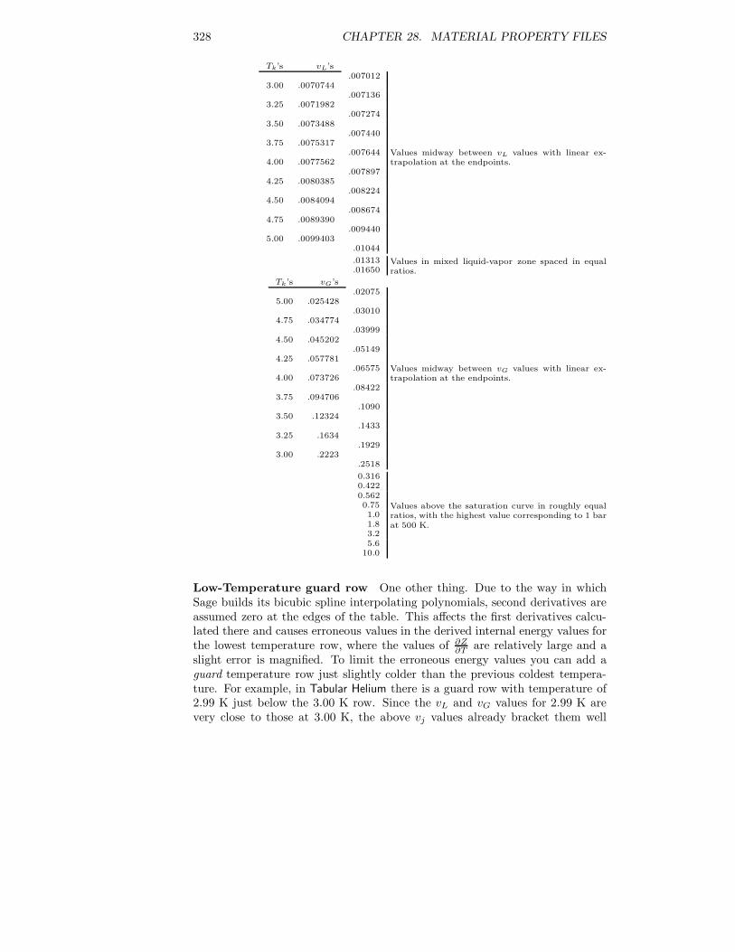
328 CHAPTER 28. MATERIAL PROPERTY FILES
Tk’s vL’s.007012
3.00 .0070744.007136
3.25 .0071982.007274
3.50 .0073488.007440
3.75 .0075317.007644
4.00 .0077562.007897
4.25 .0080385.008224
4.50 .0084094.008674
4.75 .0089390.009440
5.00 .0099403.01044
Values midway between vL values with linear ex-trapolation at the endpoints.
.01313
.01650Values in mixed liquid-vapor zone spaced in equalratios.
Tk’s vG’s.02075
5.00 .025428.03010
4.75 .034774.03999
4.50 .045202.05149
4.25 .057781.06575
4.00 .073726.08422
3.75 .094706.1090
3.50 .12324.1433
3.25 .1634.1929
3.00 .2223.2518
Values midway between vG values with linear ex-trapolation at the endpoints.
0.3160.4220.5620.751.01.83.25.6
10.0
Values above the saturation curve in roughly equalratios, with the highest value corresponding to 1 barat 500 K.
Low-Temperature guard row One other thing. Due to the way in whichSage builds its bicubic spline interpolating polynomials, second derivatives areassumed zero at the edges of the table. This affects the first derivatives calcu-lated there and causes erroneous values in the derived internal energy values forthe lowest temperature row, where the values of ∂Z
∂T are relatively large and aslight error is magnified. To limit the erroneous energy values you can add aguard temperature row just slightly colder than the previous coldest tempera-ture. For example, in Tabular Helium there is a guard row with temperature of2.99 K just below the 3.00 K row. Since the vL and vG values for 2.99 K arevery close to those at 3.00 K, the above vj values already bracket them well

28.5. ELECTROMAGNETIC PROPERTIES 329
enough and there is no need to introduce more.
Interpolation Details
One way you can see if the resolution of your table is adequate is by creating afile of interpolated values by clicking the interpolation details button below thescroll box in the PropBase form. When you click this button, a dialog opensallowing you to specify a range of v and T and number of points. The result isa tab-delimited file of values, similar to your original compressibility table. Youcan inspect this file with Excel.
Note that the interpolation values produced are the values interpolated be-tween your data points, which may or may not include the original data points.So, for example, by interpolating a bunch of points in a small region of v − Tspace you can see exactly how the bicubic spline routines are interpolating be-tween your Z values in a small region of your original table.
In addition to interpolated Z values, you also get interpolated values formass-specific internal energy ε and entropy s. Because of arbitrary constantsof integration these values may be offset somewhat from values you might becomparing them against. Constant offsets do not matter. Any other differencesdo matter. You should, at least, examine the internal energy values for accu-racy because they are the basis for enthalpy flows and temperature calculationsin subsequent gas-domain solutions. Entropy values are of lesser importancebecause they are only used for some available-energy outputs, not the basicsolution variables.
28.5 Electromagnetic Properties
As of Sage version 9 there are three new data files distributed with Sage —ESolid.dta for electrical materials, FMSolid.dta for soft ferromagnetic materialsand PMSolid.dta for permanent magnet materials. The selection lists for elec-tromagnetic component input variables Conductor and Material are populatedfrom these data files.
Electrical Conductor Properties There are only two properties:
Density mass density ρs (kg/m3)Rs(T) resistivity σ (Ohm-m) as a function of temperature T
Density is a single value for each material. Rs is defined by a set of cubic splinedata pairs (T, Rs(T)).
Soft Ferromagnetic Material Properties include the above electrical prop-erties in addition to:
Mur(T) maximum relative permeability µr (dimensionless)Jsat(T) saturation magnetic polarization Js (T)Hcb(T) induction coercive force HcB (A/m)

330 CHAPTER 28. MATERIAL PROPERTY FILES
All are defined by a set of cubic spline data pairs. These properties are generallyavailable in the magnetic material literature or supplier data sheets, althoughusually not directly. It is rare to find these properties tabulated over a rangeof temperatures, in which case it is reasonably to assume that they all droplinearly to zero at the Curie temperature. Actually the relative permeabilitydrops to the value one at the Curie temperature but that is essentially zero forpractical purposes. Values are often reported in CGS rather than SI units, inwhich case the following conversion table may be useful.
1 T = 104 Gauss1 A/m = 0.01257 Oersted
Often instead of saturation magnetization Js a vendor will provide the valueof the magnetic flux B at some large value of applied field H . The hope isthat magnetization J is close to the saturation value Js at the max B valuereported. Note that the magnetic flux B is larger than the magnetization bythe term µ0H , which amounts to an extra 0.0126 T for every 10,000 A/m. Forlarge applied fields this extra µ0H should be subtracted from the max B valuewhen setting the value Js.
Maximum relative permeability µr may be called many things and the valuereported may not be the appropriate value for Sage. In Sage, the combinationof µr and Js determine the anhysteretic magnetization function Ma shown infigure 26.11. In the product literature if a B-H curve is also available it is agood idea to use any reported value of µr as an initial value and adjust it sothe B-H curve produced by Sage matches the data over the entire range of H .You can do this by using a simple Sage model consisting of a soft ferromagneticbar bounded by magnetic potential references to generate a set of B vs H datapoints over a range of steady (DC) H fields values. Sample model SoftFerroB-Hmap.stl shows how to generate such a map which is used to produce a plot likethe one below:

28.5. ELECTROMAGNETIC PROPERTIES 331
0.0
0.5
1.0
1.5
2.0
2.5
0.0E+00 2.0E+03 4.0E+03 6.0E+03 8.0E+03 1.0E+04 1.2E+04
B (
T)
H (A/m)
DC Magnetic flux as function of magnetic field strengthSiliconSteel(3%)_2T_7A/m
Permanent Magnet Properties include the above electrical properties butreplace the above ferromagnetic properties with these properties particular topermanent magnets:
Kjh magnetization curve J(H) shape parameter Kjh (0.5 < Kjh < 1)Br(T) residual magnetic flux density Br (T) at H = 0Hcj(T) magnetization coercive force HcJ (A/m)
Kjh is a single value. Br and Hcj are defined by cubic spline data pairs. PropertiesBr and HcJ can be found in supplier data sheets. The J(H) demagnetizationcurve shape parameter Kjh is unique to Sage and is entered according to avisual comparison of the actual demagnetization curve and the approximatecurves shown in figure 26.13 of section 26.7.2.
Coercive Forces In the above properties there are two coercive forces HcJ
and HcB both positive numbers, defined as follows. Start from a high positivemagnetic field H where the polarization is near saturation. Then graduallyreduce H to zero and below. HcB is the absolute value of H at the point whenthe magnetic flux density B falls to zero. HcJ is the absolute value of H at thepoint when the magnetic polarization J falls to zero. HcB is always the smallerof the two because at H = −HcB the polarization is still positive at the valueJ = µ0HcB (from definition (26.90) above).
For a soft ferromagnetic material HcJ and HcB are essentially the same. Thedifference between HcJ and HcB can be estimated by from the Taylor expansionapproximation HcB/(HcJ −HcB) ≈ dM/dH where dM/dH = µr − 1 is usuallya very large number for a soft ferromagnetic material. So (HcJ −HcB) is verysmall compared to HcB.

332 CHAPTER 28. MATERIAL PROPERTY FILES

Part IV
Pulse-Tube Model-ClassExtension
333


Chapter 29
Overview
The pulse-tube model class is an extension of the stirling model class. It incor-porates all of the stirling-cycle model components plus a few additions requiredfor modeling so-called pulse-tube coolers. The principle new component is thepulse-tube itself, herein known as the compliance tube. This is the empty tubethat serves as a compliant displacer of sorts. The naming reflects its function-ality. Since Sage adopted this name the term thermal buffer tube seems to begaining common acceptance and is also descriptive of functionality. However,no-one talks about “compliance-tube coolers” or “thermal-buffer-tube coolers”so the model class continues to be known as the pulse-tube model class. At anyrate, the compliance tube component comes with a new gas model designed toincorporate some of the convective loss mechanisms peculiar to oscillating flowin the wall boundary layer. Other new components are flow restrictors, intendedfor representing orifi, valves and mass-flow pumps.
Sample pulse-tube input files and companion documentation files in AdobePDF format are in the Apps\Ptube\Data sub-directory under the installationdirectory.
The input file extension for the pulse-tube model class is .ptb. The software iscapable of reading and converting existing .stl (stirling) data files automaticallyto the pulse-tube format. Once converted a .ptb file cannot be demoted to a .stlfile.
335

336 CHAPTER 29. OVERVIEW

Chapter 30
Compliance Duct GasDomains
The compliance-duct type of gas domain descends from the duct-type gas do-main documented in the chapter 21. The major difference is the special treat-ment of the convective losses that arise in the wall boundary layer in the presenceof an axial temperature gradient. These losses are critical because they carrythermal energy from the warm to the cold end of the compliance duct anddegrade heat lift.
The gas axial conduction term q now comprises molecular conduction qm,turbulent conduction qt, free convection qf , boundary convection qb and stream-ing convection qs, all considered in detail below. We can write this in dimen-sionless form as
q
qm= 1 +
qt
qm+qf
qm+qb
qm+qs
qm(30.1)
where q/qm on the left is just the axial conductivity enhancement ratio Nk andthe terms on the right may be viewed as its component parts.
The variables of a compliance-duct gas domain are mostly the same as thosein any gas domain documented in 21. New variables are:
Tmult : (real, dimensionless) Empirical multiplier for turbulent conduction qt.
Gmult : (real, dimensionless) Adverse gravitational field multiplier for free con-vection qf .
Bmult : (real, dimensionless) Empirical multiplier for boundary convection qb.
Smult : (real, dimensionless) Empirical multiplier for streaming convection qt.
QmolMean : (real, W) t and x averaged molecular conduction flow qm.
QturbMean : (real, W) t and x averaged turbulent conduction flow qt.
QfreeMean : (real, W) t and x averaged free convection qf .
337

338 CHAPTER 30. COMPLIANCE DUCT GAS DOMAINS
QoscMean : (real, W) t and x averaged boundary convection qb.
QstrMean : (real, W) t and x averaged streaming convection qs.
The empirical multiplier inputs give you free reign to scale any of the enhancedaxial conduction mechanisms individually. They may still be scaled all-togetherby the inherited duct-gas input Kmult. Outputs QmolMean, . . . , QstrMean arecomponents of the inherited output QxMean, not additional losses. Their sumequals QxMean.
Just as for the ancestor duct gas domain, there is a compliance-duct gasdomain for each individual type of compliance duct geometry.
30.1 Theory
The role of the compliance tube is to transfer the PV work of expansion fromthe cold end of the compliance tube to the warm end, thereby sucking heatout of the cold source, according to a first-law energy balance. Ideally thishappens in the absence of any wall heat transfer or fluid mixing and the gaswithin the compliance tube oscillates back and forth with a uniform velocityprofile across the tube cross section. Of course, in reality, there is wall heattransfer, fluid mixing and a non-uniform velocity profile. There may even beturbulence in ill-designed compliance tubes. All these real-world phenomenabuck the ideal enthalpy flow with oppositely-directed convective losses. In anyparticular design instance, some may be small and some may be large, butprudent analysis demands we evaluate them all. That way none are liable togrow out of bounds during optimizations.
30.1.1 Turbulent Conduction
Turbulent conduction qt is the same as that reported for axial-conduction en-hancement in tube-bundle heat exchangers in chapter 23. Repeated here forconvenience, the correlating expression is
qt
qm= 0.022R0.75
e Pr (30.2)
30.1.2 Free Convection
The presence of an adverse gravitational field acting upon the temperature-induced density gradient within a compliance tube can produce buoyant insta-bility that leads to free convection cells. Free convection is only a problem incompliance tubes oriented cold end up.
Free convection in vertically-oriented closed cylinders heated from belowseems to lie in the unfashionable end of the free-convection universe. Mostheat transmission textbooks ignore it entirely. However, Edwards and Cattonin reference [10] are right on target, offering experimental data and a correlat-ing expression for this very thing. Unfortunately, their correlating expression

30.1. THEORY 339
involves a messy sum of tabulated coefficients. In another paper, consideringconvection across honeycomb panels comprising many convection ducts in par-allel, Hollands [27] gives a correlating expression, still applicable to our case, butmuch easier to compute. The Hollands correlation in terms of a free-convectionenhancement normalized by molecular conduction is:
qf
qm= 0.076X
(
1 − e1.19(Xc−X)
Xc
)
(30.3)
whereX = R1/3
a (30.4)
and Xc is the critical value of X, to be explained shortly. The enhancementis zero (molecular conduction only) for X ≤ Xc. Rayleigh number Ra is theproduct of Grashof and Prandtl numbers
Ra = GrPr (30.5)
A useful definition of Grashof number based on cylinder length L is
Gr =gρ2L4
µ2
|Tx|T
(30.6)
Here, g = 9.8N/kg stands for Earth’s gravitational field strength, Tx is themean axial temperature gradient and T is the mean absolute temperature. Inthe above definition, the coefficient of fluid thermal expansion β = −1/ρ ∂ρ
∂T |P ,which normally appears in the definition of Grashof number, has been replacedby its ideal-gas value 1/T . The Grashof number measures the ratio of buoyantto viscous forces.
The critical Rayleigh number, used to calculate Xc = Ra1/3c , is computed as
Rac =(a2
1 + 15.9)3
a21
(30.7)
wherea21 = a2
0 + 1.99 (30.8)
and
a0 = 5.75L
d(30.9)
The value a1 is the so-called horizontal wave number for the first-mode con-vection cell within the tube. It is, essentially, a theoretical dimensionless wavenumber a0 corrected for end effects by term 15.9. Theoretical wave number a0
depends on the thermal boundary condition assumed at the wall. The abovevalue applies to the case of an adiabatic wall boundary, which I felt made themost sense for us from the viewpoint of modeling free-convection as a decoupledloss mechanism.
The correlation (30.3) is not exactly the correlation Hollands recommends.His correlation contains a leading coefficient of 0.0585 instead of 0.076. I fudged

340 CHAPTER 30. COMPLIANCE DUCT GAS DOMAINS
the leading coefficient to better agree with the experimental data of Edwardsand Catton, published in [10], for heat transfer in a cylinder with adiabatic walls.My justification was that adiabatic-wall cylinders are more like compliance tubesthan square-celled honeycombs — both because of the circular geometry andthe lack of thermal interaction among adjacent cells. Correlation (30.3) agreeswith the data to within 10% at L/d = 2.5, the highest aspect ratio considered.
In arguing for the form of his correlating expression, Hollands presents aninformative and convincing case, worth repeating. It goes something like this:For very small L/d we have essentially convection in an infinite horizontal fluidlayer heated from below. In such a geometry the top-heavy fluid layer be-comes unstable at some critical Rayleigh number at which point convectioncells appear, causing an enhancement to molecular-conduction heat transfer.As Rayleigh number increases, additional smaller-scale cells appear, furtherenhancing heat transfer. Finally, turbulence ensues at high-enough Rayleighnumber. When vertical walls interrupt the horizontal layer, they suppress anyconvection cells smaller than the wall spacing, or tube diameter in our case.Thus the critical Rayleigh number at which the first convection cell occursincreases with reducing diameter (increasing L/d). Eventually though, at suffi-ciently high Rayleigh numbers, the conduction enhancement approaches that ofan unobstructed horizontal layer, which is correlated by the Globe and Drop-
kin expression qf/qm = 0.069G1/3r P 0.407
r . Hollands correlation captures boththe critical Rayleigh number at which convection first appears and the high-Rayleigh-number limit.
30.1.3 Boundary Convection
Boundary convection is a sort of shuttle heat transfer produced by the convolutednear-wall velocity profile of oscillating flow. It is the analog of displacer shut-tle heat transfer in a conventional stirling machine. At high Valensi numbers,the convoluted velocity and temperature profiles within the viscous and ther-mal boundary layer of oscillating flow interact to produce a convective thermalenergy transport beyond that produced by the complex-valued Nusselt numbermodel in Sage. Reference [12], which applies to laminar incompressible flow be-tween parallel plates with an axial temperature gradient, shows that the effectis small so long as Valensi number remains below about 100. However, typicalcompliance tubes involve Valensi numbers significantly higher than 100.
Figure 6 of that paper shows a curve A, corresponding to the exact-solutionenthalpy transport, and a curve B, corresponding to that of a solution basedon complex-valued Nusselt number, like that of Sage’s duct-gas model. Thedifference between these curves is the boundary convection qb we are lookingfor. Taking the high Valensi number limits of the equations for these curves(equations (65) for Pr = 0.7, σ = ∞ ) and normalizing by molecular axialconduction qm gives normalized boundary convection in the form
qb
qm= 0.159
√
Va(2δ/d)2 (30.10)

30.1. THEORY 341
where δ is the section-mean flow tidal amplitude. Rewriting 2δ/d = 2(L/d)(δ/L),the final boundary convection formula becomes
qb
qm= 0.64
√
Va(L/d)2(δ/L)2 (30.11)
Although the above results were derived for parallel-plate flow, cast as theyare in terms of hydraulic diameter, they apply to tubes as well as to narrowchannels or annuli. This follows because boundary convection, in the high-Valensi-number limit, occurs entirely within a thin layer (thickness on the orderd/
√Va) near the wall. As such, the phenomena is insensitive to the exact shape
of the duct and amounts to a convective energy flow per unit wetted perimeter.The actual value of this energy flow per unit wetted perimeter could be obtainedby multiplying either previous expression by the molecular conduction per unitarea q = −kTx, then by the ratio of flow area to wetted perimeter d/4. Asexpected, in the high-Valensi limit (neglecting the Nu term), the result wouldbe seen to be independent of d or any other geometrical parameter. Assuming,in particular, it would be applicable to tubes, we could then convert it back tothe original form by dividing by the area-to-perimeter ratio (d/4, same as forplates) and then again by q.
There remains the question of what happens in turbulent flow. Evidencesuggest we might then base our boundary convection equation on an effectiveValensi number where molecular viscosity is replaced by turbulent viscosity —which is generally very much higher. Thus, effective Valensi number is generallygreatly reduced for turbulent flow and qb would not be as large as predicted byequation (30.11). However, since enhanced axial conduction is likely to prohibitany reasonable compliance tube from operating in the turbulent flow regime inthe first place, the issue is probably moot. We might as well ignore any turbulentcorrection to qb, thereby giving added incentive for flow to remain laminar.
30.1.4 Streaming Convection
Streaming convection is a second-order steady flow circulation, within the wholetube interior, superimposed on the main oscillating-flow velocity field. It hasno counterpart in displacer-type stirling machines. In the high Valensi-numberlimit (viscous and thermal boundary layer thicknesses small compared to tubediameter) the second-order terms of an oscillating velocity field produce aneffective wall-velocity boundary condition replacing the usual no slip condition.This effective wall velocity uw may be calculated using the formulation belowderived by Olson and Swift [43]. Note: prior to Sage version 7 the formulationomitted some of the smaller terms — effectively assuming C1 = C2 = 3/4,C3 = 0.
uw =|P − P0||u|
γP0[C1 cos θ +C2 sin θ] +
|u|2ω
[3
4
dA/dx
A+ C3
dTm/dx
Tm
]
(30.12)

342 CHAPTER 30. COMPLIANCE DUCT GAS DOMAINS
where
C1 =3
4+
(γ − 1)(1 − bP 2r )
2Pr(1 + Pr)
C2 =3
4+
(γ − 1)(1 − b)√Pr
2(1 + Pr)
C3 =(1 − b)(1 −√
Pr)
4(1 + Pr)(1 +√Pr)
|P − P0| is the pressure-fluctuation amplitude, P0 is time-mean pressure, |u| isthe section-mean velocity amplitude, θ is the phase angle between them (velocityphase minus pressure phase) and A is the flow area. γ is the ratio of specificheats, Pr the Prandtl number and b represents the temperature dependence ofviscosity, assumed to be of the form
µ(T ) = µ(T0)
(T
T0
)b
(30.13)
Sage calculates the b exponent at each point of evaluation based on the viscosityvariation around Tm using a central finite differencing of the Sage gas-stateviscosity function µ(T )
b =Tm
µ(Tm)
dµ
dT≈ µ(Tm + εTm) − µ(Tm − εTm)
2εµ(Tm)
The fluid in the central part of the compliance tube (away from the wallboundary layer) must satisfy the uw boundary condition while maintaining zerosection-mean flow. This results in a zero-shifted parabolic velocity profile. Inthe presence of a temperature gradient, a central stream, brings fluid from onedirection and exchanges heat with a near-wall stream which brings fluid fromthe opposite direction. This, results in a transverse temperature profile whichinteracts with the velocity profile to produce a net (section-average) thermalstreaming convection [18].
For correlating the streaming convection loss there are two dimensionlessgroups of interest. The first is a Reynolds number based on effective wall velocityand hydraulic diameter
Rew =ρuwd
µ(30.14)
The second is the dimensionless wall mass-velocity gradient
Gw =d2
µ
∂ρuw
∂x(30.15)
Tubes
In the case of a tubular geometry, streaming convection may be calculated fromthe approximate formula
qs
qm=
1
4|RewPr|L/d
(
1 − e−148
dL |RewPr |
)
F (PrGw) (30.16)

30.2. NUMERICAL DIFFUSION 343
where Pr is Prandtl number, L/d is length to hydraulic-diameter ratio and Fis a function defined by
F (B) =
{1 + 1
64B + 14096B
2 if B > −56144B3
(B(eB/32 + 1
)− 64
(eB/32 − 1
))if B ≤ −5
(30.17)
Narrow Slots or Annuli
In the case of a parallel-plate-like geometry the formula is
qs
qm= 0.193|RewPr|L/d
(
1 − e−1
162dL |RewPr |
)
F (PrGw/32) (30.18)
where
F (B) =
{1 + 7
60B + 1
96B2 + 1
1920B3 if B > −10
64B4
(B2(eB/4 + 2
)+ 24B − 96
(eB/4 − 1
))if B ≤ −10
(30.19)
The above are approximations derived in [18] and [19]. However, the expo-nential formulations for large positive values of PrGw, which are likely to beinaccurate anyway, are replaced with the small PrGw approximations so theydo not blow-up to absurd values in some cases.
30.2 Numerical Diffusion
Properly modeling, of even an ideal compliance tube, requires quite a few controlvolumes (NCell) to reduce numerical truncation errors to an acceptable level —typically about 7 or 8 in Sage. The problem is that the temperature field ismostly carried with the flow (rather than fixed to the matrix as in the caseof a regenerator) which is a non-optimal state of affairs for the spatially fixed(Eulerian) solution framework of Sage.
The problem grows with increasing flow amplitude so that the error in pre-dicted net enthalpy flux generally becomes quite significant when the tidal am-plitude of the mean flow is more than about 25% of the duct length, or wheneverthe flow amplitude is high enough that a fluid particle at the inlet at the timeof flow reversal travels more than about half way down the duct. The errortends to reduce the net refrigeration power, much as an increased gas thermaldiffusion would, hence the name numerical diffusion.
Experience suggests that numerical diffusion is something to keep in mindbut not worry about too much. It is generally not a problem during optimiza-tions because there is usually no compelling reason for the optimizer to drive acompliance duct into the region of significant numerical diffusion. So, the errortends to be self limiting. The main problem is reduced simulation accuracywhen validating experimental data at large compliance-duct tidal amplitudes.

344 CHAPTER 30. COMPLIANCE DUCT GAS DOMAINS
NCell = 6 NCell = 8 NCell = 10 NCell = 12δ/L NTnode = 6 NTnode = 8 NTnode = 10 NTnode = 120.1 0.0009 0.005 0.0004 0.00030.2 0.0061 0.0046 0.0036 0.00270.3 0.0184 0.0156 0.0127 0.01030.4 0.0387 0.0360 0.0315 0.0272
Table 30.1: Numerical diffusion error h/h0 for different values of tidal amplituderatio δ/L and grid cell numbers.
30.2.1 Quantitative Estimates
The actual amount of numerical diffusion can be measured by comparing Sagesimulated results against an exact analytic solution for which enthalpy transportis zero. Such a solution is that of an ideal adiabatic compliance tube filledwith non-axially-conductive gas moving back and forth with uniform sinusoidalvelocity, as would be produced by two parallel-moving pistons within cylinderspaces attached to either end. If the piston cylinders are each held at differenttemperatures (say by means of two heat exchangers positioned between themand the compliance tube) then an equilibrium temperature profile will establishitself within the compliance tube. Provided the tidal amplitude remains lowenough, this temperature profile will consist of two isothermal legs from eitherinlet up to the maximum penetration depth (of a fluid particle that was atthe inlet at the time of last flow reversal) with a continuous linear variation inbetween. The linear variation is not strictly-speaking necessary but it is onevalid solution. This temperature profile will merely slosh back and forth withthe mean flow, the net enthalpy flow down the tube will be zero and there willbe no pressure variation. This happy state of affairs continues until the tidalamplitude increases to the point where gas from one end reaches the other. Atthis point warm gas is suddenly cooled, or vice-versa, with the result that netenthalpy transport is no longer zero.
When modeled by Sage, the idealized compliance-tube produces a net en-thalpy transport h as given by table 30.1. The results are normalized by theworst-case enthalpy transport h0 that would occur in the case of zero tube length
h0 =cpπm1(Th − Tc)
where m1 is the average mass flow rate amplitude (it varies with temperature)and (Th − Tc) is the temperature difference. Theoretically h/h0 should be zeroup to the point where the tidal amplitude ratio δ/L reaches 1/2.
The results shown that h/h0 grows quickly as tidal amplitude ratio ap-proaches the critical value of 1/2. This is to be expected since the finite-difference solution for the pulse-tube tends to round out the corners of a temper-ature profile that is theoretically approaching a step function as tidal amplituderatio approaches 1/2. But below a tidal amplitude ratio of about 0.25, erroneousenthalpy transport h/h0 is less than 0.01.

30.2. NUMERICAL DIFFUSION 345
30.2.2 Interpretation in terms of Refrigeration Power
So how significant is an erroneous enthalpy transport of h/h0 = 0.01? This ishard to say since worst-case enthalpy transport h0 is not something we usuallythink about. Instead we usually think about the ideal refrigeration power of apulse tube which is
hpv =1
2P1V1
assuming pressure amplitude P1 and volumetric flow rate amplitude V1 are inphase. But if we substitute m1/ρ0 for V1, then 2P0/(R(Th +Tc)) for ρ0, we canformulate the ratio of ideal refrigeration power to worst-case enthalpy transportas
hpv
h0=π
4(1 − 1/γ)
P1
P0
(Th + Tc)
(Th − Tc)
So, for example, in a helium pulse tube with (1 − 1/γ) = 0.4, pressure ratioP1/P0 = 0.15 (somewhat on the high side), Th = 300 and Tc = 75, we havehpv/h0 = 0.079. Therefore, an erroneous enthalpy transport of h/h0 = 0.01corresponds to 0.01/0.079 = 0.13 of ideal refrigeration power — a significantamount. But the error quickly drops off as tidal amplitudes decreases. So, fortidal amplitude ratios on the order of 0.10, the error would only be of the order1% of ideal refrigeration power.

346 CHAPTER 30. COMPLIANCE DUCT GAS DOMAINS

Chapter 31
Compliance DuctGeometries
Compliance duct geometries are the containers that house compliance gas do-mains and provide to them certain geometrical information. They are analogousto the heat-exchanger geometries documented in chapter 23. They occur in thetoolbox of the root-level pulse-tube model component and you use them formodeling that empty-tube part of a pulse-tube cooler, commonly known as thepulse tube.
31.1 Compliance Tube
The compliance tube is a descendant of the stirling-class tube-bundle heat ex-changer. The main difference is that it substitutes a compliance-duct gas domainin its toolbox and adds a radiation-transport model component, in case you wantto model radiation transport along the tube. Wall conduction is available in thethick-wall toolbox component already present.
From your point of view, you may think of a compliance tube as a specialsort of tubular container. Its variables are the same as those the tube-bundleheat-exchanger model component. Most of the interesting stuff belongs to thecompliance-duct gas domain child component (see chapter 30), which you dropin from the component palette.
31.2 Tapered Compliance Tube
A tapered compliance tube is similar to an ordinary compliance tube except itsinternal diameter and wall thickness are specified by cubic splines:
Dtube : (cubic spline, m) Tube internal diameter.
Twall : (cubic spline, m) Wall thickness.
347

348 CHAPTER 31. COMPLIANCE DUCT GEOMETRIES
The main reason for using a tapered compliance tube is to reduce or elim-inate streaming convection by taking advantage of the dA/dx dependence ofthe effective wall-velocity uw, according to equation (30.12). The proper choiceof dA/dx will cancel the other term, thereby leading to zero streaming convec-tion. Locally, at least. There may still be some variation of uw along the tubelength but it can generally be reduced compared to the case for uniform flowarea. The demonstrated reduction of streaming convection by compliance-tubetapering has been reported by Olson and Swift in reference [43].
The implementation of the tapered compliance tube is similar to that of thetubular-cone canister reported in chapter 22. Dependent variables Aflow, Asecand Pwet (flow area, solid cross-sectional area and wetted perimeter also becomecubic spline variables instead of uniform values. These splines are each definedby n data pairs (x, A(x)) equal spaced in x within the interval [0, 1], where nis the larger of the number of data pairs in the specification of Dtube or Twall.So, the resolution of the dependent variables is only as good as the resolutionof Dtube or Twall. In particular, if your intent is a nonlinear variation in flowarea (as in a simple conical tube) you must specify more than the endpointdiameters in Dtube, even though it varies linearly with axial position. SpecifyingDtube interpolation pairs at the relative x coordinates 0, 0.25, 0.5 and 1.0 wouldprobably be sufficiently.
The turbulence transition model along with the heat-transfer and flow-friction correlations are unchanged from those of uniform area ducts. Thisis probably incorrect to some degree, with the result that heat transfer andflow friction will probably be off a bit. This should not pose a problem forcompliance-tube modeling because these terms are generally small.

Chapter 32
Flow Restrictors
Flow restrictors are composite geometry and gas-domain components that modelzero-volume adiabatic flow restrictions. They are intended for modeling the orififound in pulse-tube coolers. They are found in the toolbox of the root-levelpulse-tube model component and are born with gas flow connectors at eitherx end intended for connection to stirling-class gas domain model components.While you could also model orifi using a stirling-class heat exchanger geometriesand child-model gas domains, the use of flow restrictors is easier and shouldimprove solution speed and convergence stability. Keep in mind, though, thatflow restrictors are not appropriate where the volume of the orifice is significantor where there might be a significant amount of heat transfer to or from thegas. Variables common to all flow restrictors are:
Aflow : (real, m2) mean-flow cross sectional area A.
Pwet : (real, m) Wetted perimeter w.
Fmult : (real, dimensionless) Empirical multiplier for viscous pressure drop.
Tinit : (real, K) Initial temperature. Used only for initializing or re-initializingsolution variables ρ and ρe. As such, its value does not affect the finalconverged solution, but it may affect whether the solution converges atall. It should be set to a value consistent with the initial temperatures ofadjacent components.
AEfric : (real, W) Available energy loss to viscous flow friction.
FT : (Fourier series, K) Gas temperature T .
FP : (Fourier series, Pa) Gas pressure P .
FDP : (Fourier series, Pa) Pressure difference across restrictor (positive − neg-ative ends).
FH : (Fourier series, W) Stagnation enthalpy flow uA(ρe+ P ).
349
350 CHAPTER 32. FLOW RESTRICTORS
FRhoUA : (Fourier series, kg/s) Mass flow rate ρuA.
MachMean : (real, dimensionless) Time-averaged Mach number. Keep an eyeon this. If it gets near unity Sage may not converge.
ReMean : (real, dimensionless) Time-average Reynolds number Re.
When needed, flow restrictors calculate hydraulic diameter in terms of flow areaA and wetted perimeter w as
dh = 4A/w (32.1)
and Reynolds number as
Re =|ρu|dh
µ(32.2)
Flow restrictors calculate gasdynamic variables at each end with the same flowarea A. So the product of density and velocity ρu is proportional to massflow rate and is the same at either end of the flow restictor. Flow is assumedisenthalpic which means that the temperature T is also the same, at least to theextent the gas state is ideal. But density may differ at the two ends, especiallyif the pressure drop across the flow restrictor is large. It is important to keepthis in mind in formulating the pressure drop across the flow restrictor.
32.1 Sintered Powder Plug
The sintered powder plug adds input variables:
Length : (real, m) Flow length L.
Dcan : (real, m) Diameter Dc of plug or internal diameter of canister holdingplug.
Dsphere : (real, m) Powder sphere or particle diameter ds.
Porosity : (real, m) Plug porosity β (void volume / total volume).
It calculates flow area asA = β
π
4D2
c (32.3)
and wetted perimeter as
w = 6(1 − β)π
4D2
c/ds (32.4)
presuming spherical particles. It calculates Darcy friction factor using the samecorrelation as for the stirling-class packed-sphere matrix heat exchanger geom-etry, namely:
f = (79/Re+ 1.1)β−0.6 (32.5)
and computes viscous pressure drop as
∆P = −1
2fL
dhρmu|u| = −1
2fL
dh(ρu)|ρu|/ρm (32.6)

32.2. SHARP-EDGED ORIFICE 351
Density ρm is the average of density at the two ends but calculating it is abit convoluted because the solution formulation maintains only the downstreamvalue, denoted by ρ, without a subscript. For purpose of pressure drop calcu-lations then, Sage calculates mean density from the average pressure Pm of thegas domains on either side of the flow restrictor, the flow-restrictor downstreamtemperature T and the gas equation of state.
32.2 Sharp-Edged Orifice
The sharp-edged orifice adds input variables:
Dorf : (real, m) Diameter Do of orifice.
Cd : (real, dimensionless) Discharge coefficient Cd.
Areduc : (real, dimensionless) Ratio Ao/Ah of orifice area Ao to housing areaAh. Must be > 0 and should be < 1.0. Affects the orifice pressure drop(see below) and also the Bernoulli pressure change between the ends ofthe flow restrictor and adjoining gas domains, which see gas entering orleaving the flow restrictor at the velocity in the housing rather than in theorifice itself.
A sharp-edged orifice is defined primarily by the orifice diameter but also bythe housing duct in which it is contained. To avoid trouble with high velocitiesin the flow-restrictor gas kinetic energy term the mean flow area A is taken tobe the housing area Ah (upstream and downstream flow area), calculated frominputs Do and (Ao/Ah) as.
Ah =π
4D2
o/(Ao/Ah) (32.7)
The cross-section area of the orifice itself is calculated as
Ao = Ah(Ao/Ah) (32.8)
According to the conventional formulation for positive-directed flow through asharp-edged orifice, the mass flow rate m is governed by
m = −CdAo
√
ρe∆P
(1 − Ao/Ah)2(32.9)
where Cd is the discharge coefficient and ρe is a representative density, whichSage takes as the downstream density provided pressure drop does not get toolarge (see below). Solving for ∆P , the explicit equation for pressure-drop in asharp-edged orifice is
∆P = − 2
C2d
(1 −Ao/Ah)2 m|m|
2ρeA2o
(32.10)

352 CHAPTER 32. FLOW RESTRICTORS
The final factor on the right is the velocity head 12ρeuo|uo| reckoned at the orifice
velocity uo = m/(ρeAo). Discharge coefficient Cd accounts for the actual orificevelocity being somewhat higher than uo due to the flow stream in the orificebeing somewhat contracted below Ao. According to Idelchik ([29], p. 90), Cd
ranges from about 0.84 for a thin sharp-edged orifice to 1.14 for a drilled holein a thick plate (L/d ≥ 2, sharp edged).
32.2.1 Low-Reynolds Linearization
In the Sage formulation a term 50/Re is added to the factor (2/C2d)(1−Af /Ah)2
in equation (32.10) to improve solution stability when starting from zero-velocityinitial values. The added term is reminiscent of the Darcy-flow part of the Ergunfriction factor for porous materials. It is significant only for small Re and servesto linearize ∆P as a function of ρu. For purposes of calculating Reynolds numberthe wetted perimeter is taken to be that of the housing, calculated as
w = πDo/√
Ao/Ah (32.11)
32.2.2 Choked Flow
Equation (32.10) is fine for relatively low pressure drops. But when downstreampressure P drops to about half the upstream pressure Pu the velocity in the ori-fice reaches the speed of sound and a further reduction in downstream pressurehas no affect on the flow through the orifice. The flow is said to be choked atthat point. The critical downstream pressure Pc at which this happens is givenby Schmidt ([52], p. 337), for the case of frictionless ideal-gas flow as
Pc = Pu
(2
γ − 1
)γ/(γ−1)
(32.12)
where γ is the ratio of specific heats. For all gases the factor on the right isnear 0.5 so Sage simply takes Pc as half the upstream pressure. For the caseof choked flow (i.e. P < Pc) Sage calculates the pressure drop from equation(32.10) evaluated at effective density ρe equal to the choke density ρc and addsto it the choked pressure drop ±(Pc − P ), where the positive sign applies tonegative directed flow and vice-versa. The choked density ρc is calculated fromthe equation of state as ρ(Pc, T ). Essentially, equation (32.10) takes care ofthe expansion loss as the jet at the orifice throat dissipates in the downstreamhousing and (Pc − P ) takes care of any additional pressure drop beyond thechoke point.
32.3 Asymmetric Sharp-Edged Orifice
The asymmetric sharp-edged orifice is a variation of a sharp-edged orifice witha pressure recovery diffuser in one direction or the other defined by new inputvariable:

32.4. CHECK VALVE 353
Recov : (real, dimensionless) Recovery area ratio R.
You might, for example, use such an orifice in a model having a closed flow loopwhere you need a way to cancel unwanted DC (time averaged) flow circulation.You would do this by optimizing Recov subject to a constraint like FRhoUA.mean= 0.
Asymmetric flow is implemented in terms of two areas A+ and A−, theformer being the effective orifice flow area for positive flow and the later theeffective area for negative flow. The two areas are related by the formula
A+ − A−
Amin= R (32.13)
where R is the recovery area ratio and Amin, the smaller of the two areas,is the orifice flow area inherited from the parent object. In other words, forR = 0 there is no recovery and flow is that of the parent sharp-edged orifice.For R > 0 there is a recovery channel in the positive direction with exit areaA+ = (1 + R)Amin. And for R < 0 there is a recovery channel in the negativedirection with exit area A− = (1 − R)Amin. The succinct way to say all this isthat the orifice flow area Ao is always given by
Ao =
{(1 + max(R, 0))Amin if u > 0(1 − min(R, 0))Amin otherwise
(32.14)
At the root of the DC flow phenomenon are ill-phased density and velocityfluctuations in the gas which tend to produce DC pressure gradients. The issueis whether or not DC pressure gradients produced by various flow resistances inthe closed loop completely cancel each other. If they do not, then DC flow is theconsequence. Enthalpy flow in components like the regenerator and compliancetube can be extremely sensitive to DC flow. So, one symptom of DC flow isextreme sensitivity of heat lift to small changes in input variables or grid nodecounts.
32.4 Check Valve
The check valve is a variation of a sharp-edged orifice that behaves like an orificein one direction but essentially blocks flow in the other direction. New inputvariables are:
Aratio : (real, dimensionless) Ratio of fully-closed to fully-open flow area R.Generally a positive number � 1.0. A value of 1.0E–2 is a reasonablevalue. Backflow leakage increases as Aratio increases and decreases asAratio decreases. But too small a value may cause convergence problems.
Popen : (real, Pa) Pressure difference ∆Pc required to open the valve. A pos-itive value means positive flow opens the valve. A negative value meansnegative flow opens the valve. At pressures above ∆Pc flow resistancechanges smoothly but rapidly to the fully-open value. A zero value meansthe valve is always open.

354 CHAPTER 32. FLOW RESTRICTORS
Instead of modulating flow by changing the actual flow area, like the asym-metric orifice, a check valve simply adjusts the flow friction to have the sameeffect. This avoids instabilities due to high gas flow velocities when the areasuddenly goes from large to small. In the open position, check valves calculatepressure drop as the orifice pressure drop from equation (32.10), for the fullopen area, plus the opening pressure difference ∆Pc. In the closed position,pressure drop is the full-open orifice pressure drop increased by a factor 1/R2,where R is the closed-to-open area ratio. So even though actual flow area doesnot change, the effect on pressure drop is the same as if it had.
Check valves decide whether they are fully closed, fully open or somewherein between, based on the current mass flow rate m compared to the mass flowrate mc when the valve begins to open, which is reckoned as the mass flow ratethat produces a closed-position pressure drop of −∆Pc. At twice mc the valveis presumed fully open. No valve inertia is modeled.
In mathematical terms, this is succinctly stated in the formula for calculatingpressure drop, which for positive flow is
∆P =
∆P0/R2 if m < mc
∆P0 − ∆Pc if m > 2mc
smooth transition otherwise(32.15)
where ∆P0 is the pressure drop calculated from orifice equation (32.10) as afunction of current mass flow rate, at full open area. For negative flow a similarequation applies except the signs of the inequalities are reversed.
So why can’t a check valve seal perfectly in the back direction? The reasonhas to do with the way gas domains are set up and connected together. Es-sentially, a check valve receives mass flow rate as an input and must calculatean appropriate pressure drop as an output. And a pressure drop of infinity isnot a mathematically proper value. So all a check valve can do is supply alarge pressure drop for a small amount of backflow. But too large and solutionnon-convergence may be the result, which is why the Aratio input cannot be toosmall.
32.5 Time-Dependent Valve
The time-dependent valve is a variation of a sharp-edged orifice that behavesas if the inherited flow area (that given by input Dorf) is reduced (or increased)by a time-varying multiplier factor
F (t) = max(R(t), Rmin) (32.16)
The time-varying factor R(t) comes from the Fourier-series input variable FRe-strict and the minimum allowed value Rmin from the real input MinRestrict,which must always be positive. A time-dependent valve is intended for model-ing such things as the pressurization valve in a Gifford-McMahon cooler. Newinput variables are:

32.6. DC FLOW BLOCKING RESTRICTORS 355
FRestrict : (Fourier series, dimensionless) Flow area multiplier R(t) above.Keep in mind that valves that open or close abruptly are difficult to re-solve in the coarse computational grid employed by Sage. Better to modela more smoothly varying equivalent valve, if possible. Either that or in-crease the number of time nodes in the computational grid (input variableNTnode). For more information on how you might specify FRestrict toaccomplish your objectives, see the section on Fourier Series in chapter 9.
MinRestrict : (real, dimensionless) Minimum flow area multiplier Rmin above.Generally a positive number � 1.0. A value of 1.0E–2 is reasonable. Toosmall a value may cause convergence problems.
Like a check valve, this object does not change the actual flow area, but onlyadjusts the pressure drop to have the same effect, by calculating it as
∆P = ∆P0/F (t)2 (32.17)
where ∆P0 is the pressure drop calculated from orifice equation (32.10) as afunction of current mass flow rate, at inherited flow area. This prevents insta-bilities due to high gas flow velocities when the area is small.
32.6 DC Flow Blocking Restrictors
Another way to cancel DC flow is to use one of these flow-restrictor variations,which descend from the sintered powder plug or the sharp-edged orifice com-ponents, respectively. They automatically block DC flow by imposing on topof the pressure drop inherited from the parent component an implicitly-solvedDC pressure-drop sufficient to exactly cancel any DC mass flow rate. This DCflow blocking behavior is built into the model solution and does not require anoptimization constraint to solve, as in the case of the asymmetric sharp-edgedorifice. The amount of DC pressure-drop required appears as output variableDPstdy.
In some cases you may want to regulate the DC flow to some desired set-point rather than canceling it entirely. You can do this by changing the value ofinput variable DCRhoUA from its default value of zero to the desired set-point.
The additional variables for this component are:
DCRhoUA : (real, Kg/s) set-point for DC (time-average) mass flow rate.
DPstdy : (real, Pa) pressure drop required to achieve the DC mass flow rateset-point.
Variable DPstdy is not the same as the time-mean value of the pressure-dropFourier series FDP because FDP includes the pressure drop of the ancestor com-ponent, which may have its own DC component for reasons outlined above.
While very convenient from a modeling point of view, these componentssuffer from the disadvantage that they do not specify the mechanism by which

356 CHAPTER 32. FLOW RESTRICTORS
DPstdy is to be generated. This is partly a good thing, because the value ofDPstdy is subject to considerable numerical error. Changing the number of timeor spatial nodes in the computational grid, or even the time-grid orientation withrespect to the solution (by changing compressor piston phase), can dramaticallyaffect DPstdy. This is because the time-average pressure drop is the residual ofsome much larger time-varying pressure drops.
Orifice designers, then, have two choices. Either they ignore DPstdy, hopingthat the any DC flow effect will be too small to matter, or they deal with it.Dealing with it might involve designing-in some sort of mechanism to producethe a DC pressure drop bias of the predicted magnitude (allowing time in thetest cell to calibrate it). Or it might involve eliminating DC flow by some othermeans — by means of an impermeable membrane, for example. In fact, it isuseful to think of these components as impermeable membranes in series withan orifice.
Another disadvantage of these components is that they must only be usedin situations where DC flow is possible (closed loop flow paths, not otherwiseDC-flow restricted) lest a solver singularity result. In other words, if DC flowis already implied to be zero, then any DC pressure-drop imposed by thesecomponents will have no affect — and may result in a singular solution. Thisfact places an added burden on the model designer to recognize when DC flowis a problem and to correct it, but not over-correct it. For example, placing twoDC-flow canceling components in series, is taboo.
32.7 Mass-Flow Pump
The universe of modeling options admits to another possibility — one whereDC flow is desirable. To model an open thermodynamic cycle, for example. Orto investigate the effect of a prescribed amount of DC flow. This componentallows you to model a mass-flow pump by recasting the mass-flow-rate Fourierseries FRhoUA as an independent input variable rather than an output. Whathappens is the pressure drop across the component is solved implicitly in orderto make the mass flow rate come out right. You can see what this pressure dropis by inspecting output variable FDP.
You can specify the mass flow rate to be anything you desire — includingsinusoidal terms and higher harmonics. This means you can model much morethan merely a DC flow generator. You can model the perfect flow restrictor.One that gives any desired mass flow and phasing without regard to the physicalmeans for achieving it. And the subfields of the mass flow rate can be optimizedor referenced in constraints, as discussed under the topic of Fourier-series vari-ables in chapter 9. One warning though: If you specify a nonzero DC part ofthe mass flow rate, the mass-flow pump should be located within a closed loopcapable of supporting DC flow, otherwise the mean pressure drop will be inde-terminate and the solution will not converge — if DC flow is impossible, thenthere is no amount of pressure drop that will force the required value.
The flow area Aflow is another input. It is present in order to define flow

32.8. MASS-FLOW DRIVER 357
velocity in the pump, but normally its value does not matter much. However,it should be large enough that the mean Mach number (output MachMean) issubstantially below one.
When starting from initial values or a re-initialized solution, a mass flowpump in your model can slow down convergence, depending on the magnitude ofthe flow specified. The DC component of FRhouUA seems especially troublesomein this regard. If this is a problem, try starting with a small mass flow rateinitially and increase it gradually over the course of several solutions.
32.8 Mass-Flow Driver
This is a phasor version of the previous mass-flow pump. It specifies massflow rate as a phasor input variable, having sinusoidal time variation. You canoptimize the subfields of the mass flow rate, or reference them in constraints, asdiscussed under the topics of Complex and Phasor variables in chapter 9.
Why would you want to use a mass-flow driver since you can specify all ofthe Fourier-series components, not just the sinusoidal part, with the previousmass-flow pump? Because this component allows the DC part and all higherharmonics to pass unobstructed. So there is no requirement that it be placedin a closed flow loop, as is the case with the mass-flow pump. Mass-flow driversare perfectly happy as components in either closed or dead-ended flow loops.The DC flow component cannot be over-constrained. You can even connectmass-flow drivers at both ends of a duct, for example, to achieve a desiredpressurization within the duct, provided the physics is reasonable.
The way the mass-flow driver works is by defining the desired mass flowrate as an independent phasor input variable PhsrRhoUA and implicitly solvingfor the phasor pressure drop that will bring this about. The phasor pressuredrop is actually implemented as two implicit real variables corresponding to thereal and imaginary parts. Although these variables are invisible, they give theirvalues to the solution grid and you can monitor them in the first harmonic ofoutput variable FDP.
As with the mass-flow pump, the flow area Aflow does not affect the pressuredrop but it does affect the gas velocity. So it should be large enough that themean Mach number (output MachMean) is substantially below one.
32.9 Flow Restrictor Theory
To be connection-compatible with the gas-domains of the stirling model classrequires two things: flow restrictors must maintain a time-ring that includesstate variables P, u, ρ, ρe for export to flow connectors. And they must importmass flow rate ρuA and upwind mass-specific enthalpy h from flow connectorsfor use in their own internal solution. ρuA must be taken as the boundary massflow rate, at all times, and H as incoming energy, only when flow is into therestrictor domain. Other state variables may be included for convenience.

358 CHAPTER 32. FLOW RESTRICTORS
The solution grid for flow restrictors is a single time ring containing statevariables A, ρ, ρuA, ρe, u, T, P . These are in the same order and have the samemeanings as in the stirling-class gas domains, except there are a few omissionsfor state variables no longer required. Generally, the variables in the grid areunderstood as downwind values, except for ρe and P which are separated intonegative- and positive-boundary values to allow for an entropy-generating pres-sure drop. Aside from that, the variables are designed to maintain mass andenergy continuity across the flow restriction. Neither space nor time differencingis required anywhere. Exact meaning and method of calculation for all variablesare explained in detail below.
A
Flow area A is computed explicitly from geometrical inputs appropriate to thespecific type of flow restrictor. The reason for including it as a state variableis so time-dependent flow areas may be specified, as is convenient in the imple-mentation of the time-dependent valve component.
ρ
Mass density ρ is computed implicitly from the zero-volume mass-continuityequation
(ρuA)+ − (ρuA)− = 0 (32.18)
where (ρuA)+ and (ρuA)− are the values imported from the positive and nega-tive flow connectors. This forces mass flow rate in the adjoining flow connectorsto be equal. Implicit functions used for solving ρe also help to determine ρ. Theusage in these other implicit functions is consistent with ρ being the downwindvalue.
ρuA
Mass flow rate ρuA is computed explicitly as the average of the values in theadjoining flow connectors:
ρuA =1
2[(ρuA)+ + (ρuA)−] (32.19)
This fulfills the requirement that the flow restrictor use imported (ρuA)’s in itsinterior solution.
ρe
Downwind energy density ρe is computed implicitly by solving the energy con-tinuity equation written in the form
ρe+ P
ρ= hi (32.20)

32.9. FLOW RESTRICTOR THEORY 359
where ρe and P on the left are downwind state variables while hi on the rightis the mass-specific enthalpy evaluated using variables imported from the com-ponent across the flow connection in the upstream direction. For an ideal gas hreduces to cpT in the zero-velocity limit where kinetic energy may be neglected.
For numerical reasons it is convenient to separate ρe into two variables ρe−and ρe+, thought of as lying at the negative and positive boundaries of theflow restrictor. The downwind value is ρe+ when flow is positive and ρe−when flow is negative. ρe− is exported to the negative flow connector and ρe+to the positive flow connector. The reason this makes sense is because theimplicit function determining either can be formulated without a discontinuityat flow reversal, as would otherwise be the case. That is, the equation fordetermining ρe− is always that local mass-specific enthalpy ρe
−+P
−
ρ equals thevalue imported across the positive flow boundary, which is valid when flow isin the negative direction and does no harm otherwise. A similar but oppositeequation determines ρe+. The meaning of P− and P+ is similar to the meaningof ρe− and ρe+, and is explained further below.
It might be tempting to use these continuity conditions instead to calculateρe− and ρe+ explicitly. This will not work because of a circular reference whenaccessing P , which itself depends on ρe.
u
Velocity u is computed explicitly in terms of other state variables as
u =(ρuA)
ρA(32.21)
The parenthesis in the numerator indicate that (ρuA) is a single state variable.Since ρ is understood to be a downwind value so u is a downwind value.
T
Temperature T is computed explicitly in terms of other state variables from theequation of state function
T = T (ρ, ρe, u) (32.22)
The value of ρe is taken as ρe− for negative directed flow and ρe+ for positivedirected flow. In other words, the downwind value. Since ρ and u are alsodownwind values the value of T is a downwind value.
P
Pressure P is a bit tricky. The first thought that comes to mind is to calculateit explicitly in terms of other state variables according to the equation of state.But then how would pressure drop be imposed on the solution?
The answer is to break down pressure into two components P− and P+,similar to the treatment for ρe. P− is exported to the negative flow connector

360 CHAPTER 32. FLOW RESTRICTORS
and P+ to the positive flow connector. The idea is to calculate them explicitly,in terms of the thermodynamic pressure, calculated from the equation of stateP (ρ, T ), plus or minus the pressure drop. For the case of P− the equation of stateis valid for the negative flow direction because of the downwind interpretationalready given to ρ and T . For the positive flow direction P (ρ, T ) may be offsetby the required pressure drop to produce the correct pressure. If this is also donesimilarly but oppositely for P+ then the components across the flow connectorsat either end see the correct pressure drop at all times. This can be writtenmathematically as:
P− =
{P (ρ, T ) if ρuA ≤ 0P (ρ, T ) − ∆P otherwise
(32.23)
and
P+ =
{P (ρ, T ) if ρuA > 0P (ρ, T ) + ∆P otherwise
(32.24)
Note that P+ − P− is always the pressure drop ∆P .

Part V
Low-T Cooler Model-ClassExtension
361

Chapter 33
Overview
The low-T cooler model class is an extension of the stirling and pulse-tubemodel classes. It incorporates all of the model components in these predecessorclasses plus additional features and components required for modeling coolersat extremely low temperatures, near or below the critical temperature of theworking gas. The low-T cooler model class extends Sage modeling capacity toinclude Joule-Thomson (J-T) cooling loops.
Sample low-T cooler input files and companion documentation files in AdobePDF format in the Apps\LowTCooler\Data sub-directory under the installationdirectory.
The input file extension for the low-T cooler model class is .ltc. The softwareis capable of reading and converting existing .stl (stirling) and .ptb (pulse-tube)data files automatically to the low-T cooler format. Once converted a .ltc filecannot be demoted to a .stl or .ptb file.
363

364 CHAPTER 33. OVERVIEW

Chapter 34
Working Gas
The low-T cooler model class supports two new working gas formulations, bothwith improved-accuracy tabular equation of state, known as TBSpline2Gas andTBSpline3Gas in the Sage source code. The “BSpline” in the names refersto bicubic-spline interpolation, which is a way of fitting a piecewise-definedcubic polynomial to two-dimensional data (specific volume v and temperatureT being the two dimension) so that first and second derivatives are continuousthroughout the interpolation domain (see chapter 3 of reference [47]). BothTBSpline2Gas and TBSpline3Gas are evolutionary advancements compared tothe tabular gas formulation available in the stirling and pulse-tube model classes.In the case of TBSpline2Gas, the table of internal energy interpolation valuesis read as an input, rather than generated internally as it was in the originalTBSplineGas, with the result that accuracy and numerical stability is increased.In the case of TBSpline3Gas viscosity and thermal conductivity are tabulatedover a range of both pressures and temperature, instead of just temperature atsome fixed pressure as they are in TBSpline2 gases.
Both gas types may be available in the gas-property data file you are cur-rently using (Options|model class, properties tab). They are selected by namefrom a list when specifying the ”gas” input at the root-model level. GenerallyTBSpline2 gases contain a reference pressure in the name while TBSpline3 gasesdo not. You can tell for sure which gas type is in your model by inspecting theinputs in the root-model display page with the ”full detail” option set in the”enumerated variable display detail” selection box of the Options|Sage dialog.
TBSpline3 gases are the most recent addition to the Low-T Cooler modelclass and are expected to eventually supersede TBSpline2 gases because of theirincrease accuracy over a wide range of pressures. For backward compatibility,TBSpline2 gases continue to be supported and documented although they arebeing phased out of the default gas property file LowTGases distributed withthe Low-T Cooler software.
365

366 CHAPTER 34. WORKING GAS
34.1 TBSpline2Gas
A TBSpline2Gas is defined by the following values:
T0 : (K) Representative temperature T0.1
Rgas : (J/(kg K)) Gas constant R.
Specific heat : (J/(kg K)) A cubic spline variable with temperature vs zero-pressure specific heat (T, cp(T )) data pairs covering a broad range of tem-peratures.
Viscosity : (kg/(m s)) A cubic spline variable with temperature vs viscosity(T, µ(T )) data pairs.
Conductivity : (W/(m K)) A cubic spline variable with temperature vs conduc-tivity (T, k(T )) data pairs.
Z(v, T) : (dimensionless) A rectangular table of Z(vj , Tk) values where Z =Pv/RT is compressibility, v is specific volume and T is temperature. Thefirst (left) column contains the Tk values and the first (top) row the vj
values. The corresponding Z values lie in the body of the table.
ε(v, T) : (J/kg) A rectangular table of mass-specific internal energy valuesε(vj , Tk), structurally similar to the Z(vj , Tk) table.
The values of the individual properties, including cubic-spline interpolationpairs or state tables, appear after the enumerated identifier in display windowsand the output listing. The choices available when specifying the Gas inputvariable in the root-level model component come from the default database fileLowTGases.dta, or a data base file customized by you using the property data-base editor LTCProp.exe.
34.1.1 Benefits of TBSpline2Gas
The previous tabular-state gas class TBsplineGas derived state tables for mass-specific internal energy ε(v, T ) and mass-specific entropy s(v, T ) from the com-pressibility state table Z(vj , Tk), which was provided as input. This approachworked reasonably well above the critical temperature Tcrit. At lower tempera-tures, however, integrating Z across phase-change boundaries (where derivativesare discontinuous) resulted in noise in the derived ε table. One effect of thisnoise was to create high-frequency wiggles in curves of cp(T ) at constant pressurebelow Tcrit. The resulting wiggles caused d(cpT )/dT < 0 at some temperatures,leading to solution convergence instability. This can be understood by notingthat mcpT is the enthalpy flow rate (ignoring any pressure-dependent part). So
d(CpT )/dT < 0 is equivalent to d(H)/dT < 0 for fixed m. It is not to hard
1A vestige of the ancestor ideal gas class used only as the temperature at which cp wasevaluated in returning the ratio of specific heats γ = cp/cv. T0 is of no consequence in tabulargas classes.
34.1. TBSPLINE2GAS 367
to convince oneself that d(H)/dT < 0 produces a destabilizing enthalpy flowfor a perturbation in upstream T . An enthalpy flow that tends to amplify anyperturbation in upstream T .
To increase accuracy below Tcrit the TBSpline2Gas class reads the ε(vj , Tk)table as input, leaving s(vj , Tk) as the only derived table. The procedure forgenerating the s(vj , Tk) table from the Z(vj , Tk) and ε(vj , Tk) tables is the sameas that documented previously under the Stirling-Cycle Model Class in chapter28.
34.1.2 Entering Tables of State
For TBSpline2Gas gases the procedure for entering gas properties and state ta-bles is similar to the procedure documented in chapter 28 except that there aretwo state tables to enter, Z(vj , Tk) and ε(vj , Tk). TBSpline2Gas gases are iden-tified by the name BSpline2 Gas in the Add menu item of the Propbase programLTCProp.exe. The two tables are visible in the scroll box titled Properties ofSelected Item at the right of the form, when you highlight a tabular equation-of-state gas type. When such a gas is selected, the property display windowcontains a ε(v, T ) table following the Z(v, T ) table, although the energy tableis labeled E(v, T ) due to the lack of a ”ε” character in the available windowsfont.
To change the compressibility or internal-energy table, click on the EditProperties button below the scroll box, then on the appropriate button of thesub-dialog box. You should now see a file-open dialog enabling you to load afile containing the appropriate data table. You do not enter values one by oneas you do for single-valued data or cubic-spline interpolation pairs. You load anentire file of values all at once. This is to allow you to create the property tablesusing spreadsheet program like Excel in conjunction with a third-party propertydatabase or a commercial software package like HePak (Horizon Technologies)or REFPROP (NIST).
The strategy for choosing (vj , Tk) values is similar to the strategy reportedin section 28.4.2. Except more widely spaced values are now preferred, sincewide spacings promote smoothness in the derived cp(T, P ) data and there isno need to use fine spacings to increase accuracy in the ε table. Nor is thereany need for a temperature guard row (a row of temperatures slightly colderthan the previous coldest temperatures). Essentially, choose enough v’s andT ’s to adequately resolve the non-ideal part of the state space at or near thecondensation region below Tcrit. A reasonable set of T values below Tcrit forhelium-4 is something like (3.25, 3.75, 4.25, 4.75). Above Tcrit something like (6,7.5, 10, 14, 20, 30, 45, 75, 120, 200, 350, 700, 1500). For specific-volume valuesin the phase transition region, it is reasonable to use midpoints of the phase-transition specific-volume values corresponding to the T values below Tcrit.
Once the data is loaded you can inspect it in detail by clicking the Inter-polation Details button. Selecting this option will produce a ASCII text file ofdata tables similar to the actual data except focusing on any particular range ofthe data you wish, possibly with higher resolution (more data points) than the
368 CHAPTER 34. WORKING GAS
actual data so that you can evaluate the bicubic spline interpolation accuracy.You can produce interpolated data files arranged in columns of constant specificvolume or constant pressure, over any range you wish, so long as it falls withinthe range of the original data.
34.2 TBSpline3Gas
TBSpline3Gases are designed for use where pressure changes significantly withinthe model scope (J-T coolers) or where the working fluid may be in a two-phasestate.
TBSpline3Gas is a descendant of TBSpline2Gas with specific heat cp, viscos-ity µ and conductivity k now defined using (v, T ) interpolation tables rather thanT -only interpolation pairs. Previous cubic-spline data-pairs (T, Cp), (T, µ) and(T, k) are still present but are now all understood as zero-pressure limits. Theyare automatically generated on input from the high-v column of the correspond-ing data table without any additional user input required (in the LTCProp.exeproperty management software). Previously only Cp was a zero-pressure limit,the other two properties were tabulated for a representative pressure. The onlyreason cp is included as a (v, T ) table is for the calculation of Prandtl numberused in certain heat-transfer formulations.
In support of modeling within the two-phase region TBSpline3Gases containtwo new cubic spline variables ρd(T ) and ρb(T ), representing the densities ofthe vapor at the dew point and liquid at the bubble point (see below).
TBSpline3Gases suffer a slight performance penalty compared to TBSpline2-Gases because of the increased computation overhead of two-dimensional inter-polation over one-dimensional interpolation when accessing cp, µ and k and anincrease in the total number of interpolation points needed to better cover thenon-ideal fluid conditions near the critical temperature and density. A TB-Spline3Gas is defined by the following values:
T0 : (K) Representative temperature T0. A vestige inherited from the originalideal gas class, used only as the temperature for calculating the zero-pressure ratio of specific heats γ = cp/cv.
Z(v, T) : (dimensionless) Rectangular table of Z(vj , Tk) values where Z =Pv/RT is compressibility, v is specific volume and T is temperature. Thefirst (left) column contains the Tk values and the first (top) row the vj
values. The corresponding Z values lie in the body of the table.
ε(v, T) : (J/kg) Rectangular table of mass-specific internal energy values ε(vj , Tk),structurally similar to the Z(vj , Tk) table.
Cp(v, T) : (J/(kg K)) Rectangular table of constant-pressure specific heat val-ues cp(vj , Tk), structurally similar to the Z(vj , Tk) table.
Mu(v, T) : (kg/(m s)) Rectangular table of viscosity values µ(vj , Tk), struc-turally similar to the Z(vj , Tk) table.

34.2. TBSPLINE3GAS 369
K(v, T) : (W/(m K)) Rectangular table of thermal conductivity values k(vj , Tk),structurally similar to the Z(vj , Tk) table.
ρd(T) : (kg/m3) Cubic spline data pairs of dew-point density values (Tk, ρd(Tk)),with temperature values covering the lower range of the other tables upto critical temperature Tc. Usage within the TBSpline3Gas class requiresthat the final data pair be (Tc, ρc), where ρc is the critical density. Thedew-point density ρd(T ) is the vapor density where liquid condensate firstappears for vapor compressed at a fixed temperature T .
ρb(T) : (kg/m3) Cubic spline data pairs of bubble-point density values (Tk, ρb(Tk)),with temperature data requirements same as for the ρd(T ) data pairs. Thebubble-point density ρb(T ) is the liquid density where vapor bubbles firstappear for liquid expanded at fixed temperature T ).
The data values of the individual properties appear after the name identifierfor the Gas input variable in display windows and the output listing. Theselection-list choices available when specifying the Gas input variable in theroot-level model component come from the default database file LowTGases.dta,or a data base file customized by you.
34.2.1 Critical Point Meaning
For low-temperature cooler modeling and in the TBSpline3Gas framework theboundary of the two-phase region is of fundamental importance. That boundaryis defined by the bubble-point and dew-point curves which when plotted ona T -v diagram meet at the top at a so-called critical-condensation point, orcriconden point for short. For a pure fluid the criconden point is the sameas the thermodynamic critical point defined by the isotherm Tc in a P -v plotwhere there is an inflection point, i.e. where (dP/dv)Tc = 0 and (d2P/dv2)Tc =0. But for a mixture the criconden point may differ significantly from thethermodynamic critical point as illustrated in figure 34.1 for a 50-50 mixture ofmethane and butane.
For the above reason all critical values in the context of a TBSpline3Gasrefer to the values at the criconden point. In particular the critical temperatureTc is the temperature known to chemical engineers as the cricodentherm.
34.2.2 Vapor Quality
It is sometimes useful to know the vapor quality (vapor mass fraction) for fluidin the two-phase region. For a given quantity of fluid containing vapor mass mv
and liquid mass ml , the quality is defined as
X ≡ mv
mv +ml(34.1)
The total volume occupied by the two states is the sum mv/ρv +ml/ρl, whereρv and ρl are the vapor and liquid densities. This same total volume may also

370 CHAPTER 34. WORKING GAS
Figure 34.1: refprop produced T -v plot for a 50-50 mixture of methane andbutane showing the critical-condensation point separate from the thermody-namic critical point. The critical-condensation point theoretically lies at theintersection of the bubble and dew-point curves although the two curves do notquite meet at the top in refprop.
be represented in terms of a bulk density ρ as (mv +ml)/ρ. Equating these tworepresentations of volume, dividing through by mv + ml and using the abovedefinition of quality gives an equivalent definition of quality in terms of the threedensities
X ≡ 1/ρ− 1/ρl
1/ρv − 1/ρl(34.2)
However, TBSpline3Gases do not separately tabulate the vapor and liquid den-sities ρv and ρl (as a function of v, T ) so they define instead a pseudo qualityin terms of dew-point and bubble-point densities ρd and ρb as
Q ≡ 1/ρ− 1/ρb
1/ρd − 1/ρb≡ v − vb
vd − vb(34.3)
For pure fluids Q and X are the same thing because the equilibrium pressureremains constant along an isotherm so ρv and ρl are always the same as ρd andρb. In mixtures the pressure varies so Q and X are not quite the same. But Qis a reasonable approximation to the true vapor quality for many purposes andapproaches the correct values of Q = 0 as ρ→ ρb and Q = 1 as ρ→ ρd.
34.2.3 Transport Property Encoding in Two-Phase Re-gion
In the two-phase region the values of transport properties cp, µ and k in the in-terpolation tables are not the bulk values (mass weighted liquid/vapor average)

34.2. TBSPLINE3GAS 371
as they are for the thermal properties Z and ε. Rather the TBSpline3Gas classstores separate liquid and vapor phase values in a special format so that theymay be recovered individually. TBSpline3Gases override the inherited transportproperty evaluation functions to decode the vapor values within the two-phaseregion and define new functions to decode the liquid values. In doing so thetransport properties for the separate liquid and gas phases are available forheat transfer and flow resistance calculations.
Essentially, the property values for the liquid phase are stored between thebubble-point and critical specific volumes vb and vc and values for the vaporphase between the critical and dew-point specific volumes vc and vd, for eachtemperature Tk. To be more precise it is useful to normalize the specific volumerange between vb and vd to the range 0 to 1 using the function Q(v) definedby equation 34.3. The value F stored in the two-phase region of the propertytable is either the liquid value FL or vapor value FV according to the followingformula in which F , FL and FV are understood to be functions of Q:
F (Q) =
FL
(QQc
)
if Q < Qc
FV
(Q−Qc
1−Qc
)
if Q > Qc
(34.4)
where Qc is the pseudo-quality evaluated at the critical specific volume
Qc ≡ vc − vb
vd − vb(34.5)
For any sub-critical temperature vc is always somewhere between vb and vd soQc always lies between 0 and 1. As tabulated above the property value F iscontinuous across the bubble line (F (0) = FL(0)) and also across the dew line(F (1) = FV (1)) but is discontinuous at Q = Qc (FL(1) 6= FV (0)).2
TBSpline3Gases decode the separate liquid and vapor phase properties forany x in the range 0 to 1 as
FL(x) = F (xQc) (34.6)
FV (x) = F (Qc + [1 −Qc]x) (34.7)
Except that in the FL evaluation x is truncated to no more than (1−ε), where εis some small positive number, to avoid liquid/vapor property crosstalk when in-terpolating near the discontinuity at x = 1. In the FV evaluation x is truncatedto no less than ε for the same reason near the discontinuity at x = 0.3 Currentlyε = 0.05 which requires a reasonably close spacing of the vj data points aroundthe critical density vc (controlled by configuration constant VptsInMixed in theRefpropToSage utility below).
2 As Q ranges from 0 → Qc, Q/Qc ranges from 0 → 1 and as Q ranges from Qc → 1,(Q − Qc)/(1− Qc) also ranges from 0 → 1.
3 As x ranges from 0 → 1, xQc ranges from 0 → Qc and Qc + [1 − Qc]x ranges fromQc → 1, compatible with the piecewise definition of F .
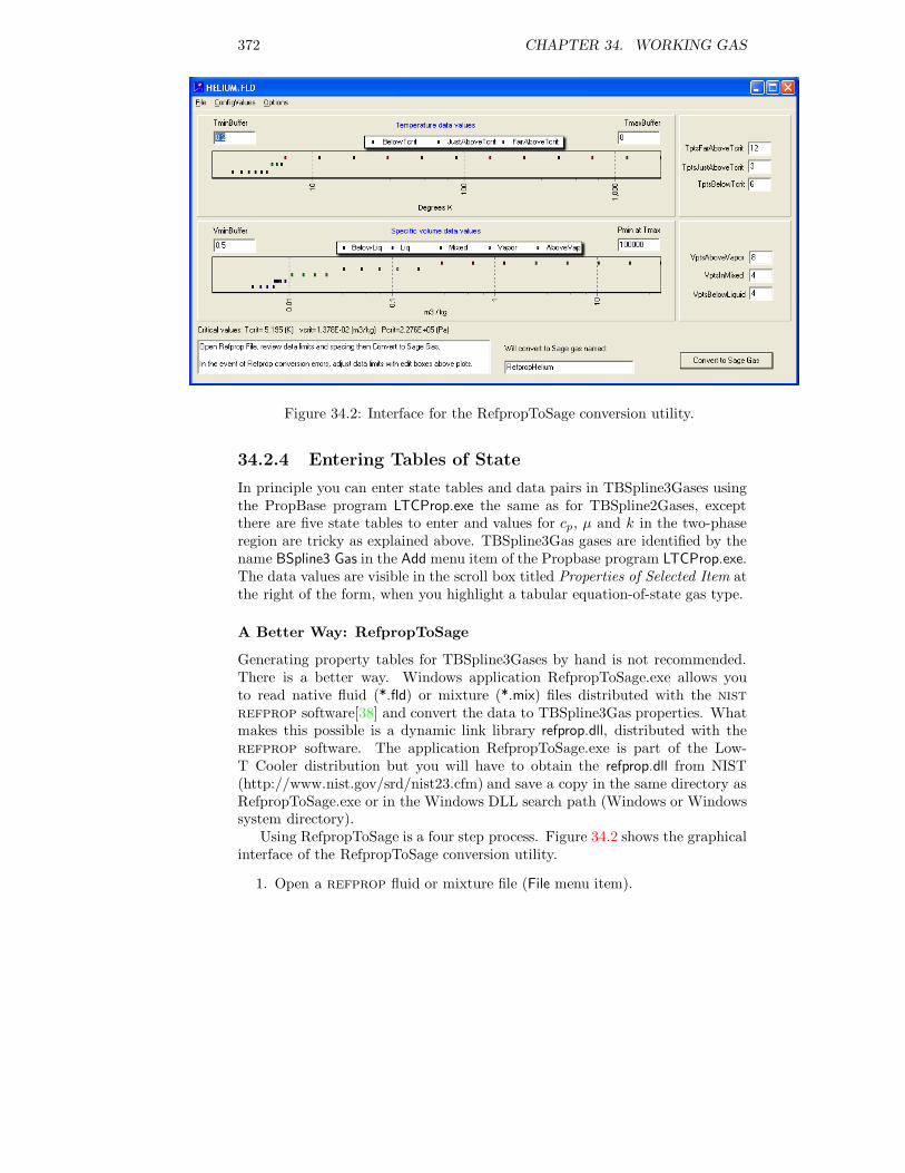
372 CHAPTER 34. WORKING GAS
Figure 34.2: Interface for the RefpropToSage conversion utility.
34.2.4 Entering Tables of State
In principle you can enter state tables and data pairs in TBSpline3Gases usingthe PropBase program LTCProp.exe the same as for TBSpline2Gases, exceptthere are five state tables to enter and values for cp, µ and k in the two-phaseregion are tricky as explained above. TBSpline3Gas gases are identified by thename BSpline3 Gas in the Add menu item of the Propbase program LTCProp.exe.The data values are visible in the scroll box titled Properties of Selected Item atthe right of the form, when you highlight a tabular equation-of-state gas type.
A Better Way: RefpropToSage
Generating property tables for TBSpline3Gases by hand is not recommended.There is a better way. Windows application RefpropToSage.exe allows youto read native fluid (*.fld) or mixture (*.mix) files distributed with the nist
refprop software[38] and convert the data to TBSpline3Gas properties. Whatmakes this possible is a dynamic link library refprop.dll, distributed with therefprop software. The application RefpropToSage.exe is part of the Low-T Cooler distribution but you will have to obtain the refprop.dll from NIST(http://www.nist.gov/srd/nist23.cfm) and save a copy in the same directory asRefpropToSage.exe or in the Windows DLL search path (Windows or Windowssystem directory).
Using RefpropToSage is a four step process. Figure 34.2 shows the graphicalinterface of the RefpropToSage conversion utility.
1. Open a refprop fluid or mixture file (File menu item).

34.2. TBSPLINE3GAS 373
Figure 34.3: Dialog for interactively plotting gas properties after conversion toSage format (TBSpline3Gas).
2. Review and adjust the plots at the top of the form showing temperatureand specific volume data values. These are the (vj , Tk) interpolation datapoints at which Sage gas properties will match refprop values. Youcan make adjustments by changing the configuration constants in the editboxes. Constants TminBuffer, TmaxBuffer, VminBuffer, VmaxBuffer ad-just the spacing between the first and last vj and Tk data values andthe minumum and maximum refprop values. Constants TptsBelowTcrit,TptsAboveTcrit, TptsFarAboveTcrit control the number of points in threeregions relative to the critical temperature, as explained below. Con-stants VptsBelowLiquid, VptsInMixed, VptsAboveVapor control the numberof points in the liquid single phase region at the lowest temperature, thetwo-phase region just below the critical temperature and the vapor single-phase region at the lowest temperature, as explained below.
3. Click the Convert To Sage Gas button and inspect the plots in the inter-active plotting dialog that pops up (Figure 34.3) to make sure there areno anomalies. The Convert To Sage Gas disappears after the conversionprocess to declutter the form.
4. When you are satisfied with the result click the SaveBSpline3Gas.Databutton in the bottom right corner to save the converted data to a Sage-format dta file. You may then use the LTCProp.exe program to appendthe resulting file to the gas-property data base file you use with the Low-T Cooler application (the one selected in the Options|Model Class dialog,Properties tab.
374 CHAPTER 34. WORKING GAS
Plot Interaction For the dialog shown in Figure 34.3 mouse clicking on plotlines or T , v data points displays the numerical value of the isotherm or in-dividual T , v value. Resize the plot by holding the left mouse button downand dragging between the upper left and lower right corners of a rectangle ofinterest. Undo by dragging in the opposite direction. Reposition the plot byholding the right mouse button down and dragging.
The edit boxes v-interval subdivisions and T-interval subdivisions to the rightof the property values plot allow you to inspect interpolated values betweentabulated data points. With zero subdivisions the plots just connect the tab-ulated data points. With subdivisions greater than zero the plots also showvalues interpolated between the data points. It is a good idea to set subdivisionvalues to at least 1 so you can spot any spurious wiggles or other anomalies andpossibly correct them by modifying the configuration constants (e.g. increasingthe number of T or v data points).
Configuration constants (set in edit boxes) are automatically saved when-ever you save the BSpline3Gas data to a file. The constants are saved as acompanion to the original refprop fluid or mixture file in the form of a tab-delimited text file with with the suffix Config appended to refprop file nameand file extension .tab. For example, HeliumConfig.tab.
The ConfigValues menu item allows you to load configuration constants fromany previously saved configuration file. You can also independently save a con-figuration constant file or restore default values.
Gas Mixtures are defined in refprop mixture files (.mix file extension). Therefprop software contains a number of pre-defined mixtures and also allowsyou to define your own custom mixtures and save them to .mix files (Storebutton of the Specify Mixture Composition dialog). A refprop mixture file onlycontains information about the molar fractions of the mixture components andfile names where their properties are stored. The RefpropToSage utility mustbe able to locate the individual fluids specified in a mixture file. It will lookfor them first in the same directory as the mixture file and then in one or moresearch paths specified in the Options menu item.
Mixture component fractions apply to the bulk fluid in a homogeneous state(e.g. all vapor or all liquid). But there is some confusion in the two-phase statewhere at a given temperature the fluid fractions in liquid and vapor phasesgenerally differ from the bulk fractions. This two-stage variability limits Sagemodels using gas mixtures to processes where there is no significant separationof the vapor and liquid downstream of the point where they are generated. Sagecan model vapor condensation or liquid boiling in a flow process as long as bothphases flow together. Sage cannot model processes like fractional distillationwhere separating the vapor from the liquid is a fundamental part of the process.In fractional distillation the vapor of a two-phase equilibrium state is physicallyseparated to a different location and condensed at a lower temperature. Thatphysical separation resets the baseline component fractions.

34.2. TBSPLINE3GAS 375
a a a a a a a a a a a a a a a a a aaaaaaaaaaaaaa
aa
aa
a
aa
aa
a
aa
aa
a
aa
aa
a
+
+
+
+
+
+
+
+
+
+
��
��
��
��
@@
@@
@@
@@
Tmin
Tc
Tmax
Tk
6
vmin vmax
vj -
bubble-point curve
@@@R
dew-point curve
���
a = (vj , Tk)
+ =
{vl(Tk − ∆T/2)vv(Tk − ∆T/2)
Figure 34.4: BSpline3Gas interpolation points.
Implementation Details The implementation of the RefpropToSage pro-gram is straight forward but not completely trivial. Special considerations arerequired for some properties in the two-phase region and sometimes at low-volume (high density) points out of refprop’s range.
Interpolation Points To avoid problems it is necessary to choose the (vj , Tk)interpolation points with care near the boundaries of the two-phase region.These boundaries are defined by the values of saturated vapor and liquid volumesvd(T ) and vb(T ) at the dew and bubble points available in refprop. The waythis is done is illustrated somewhat abstractly in figure 34.4. vj and Tk valuesare drawn in non-linear scale so the saturation curves vd(T ) and vb(T ) appearas straight lines. The temperature points Tk are chosen as follows:
• First a number of points spaced by ∆T from Tmin + ∆T/2 to just belowthe critical temperature Tc − ∆T/2. Tmin is near the minimum valuesupported by refprop for the particular fluid.
• Followed by a number N points spaced by ∆T from Tc + ∆T/2 to Tc +(N − 1
2)∆T .
• Followed by a number of points spaced in equal ratios from Tc+(N+ 12)∆T
up to Tmax (the maximum value supported by refprop)

376 CHAPTER 34. WORKING GAS
The specific volume points vj are then chosen with reference to the saturatedliquid and vapor densities vb and vd tabulated at points offset by ∆T/2 fromthe above Tk values, at the points T = Tmin, . . . , Tc − ∆T :
• First a number of equal spaced points between a minimum value vmin andthe lowest liquid volume vb(Tmin).
• Followed by the vb(T ) values, T = Tmin + ∆T, . . . , Tc − ∆T
• Followed by a number of points spaced in equal ratios between vb(Tc −∆T/4) to just below the critical volume vc and the same number of pointsfrom just above vc to vd(Tc − ∆T/4)
• Followed by the vd(T ) values, T = Tc − ∆T, . . . , Tmin + ∆T
• Followed by a number of points spaced in equal ratios from vd(Tmin) upto vmax, where vmax is the greater of twice vd(Tmin) and RTmax/Pmin,for Pmin a reasonable minimum pressure such as 1 atmosphere
Chosen in this way it is a simple matter to know which k correspond to tem-peratures below Tc and which j, k indices correspond to points in the two-phaseregion.
Saturation Pressure In theory and in refprop the slope of saturation pres-sure (dP
dv )T in the two-phase region is much smaller than the slope in the liq-uid or vapor single-phase regions. For a pure fluid at a given temperature Tthe pressure remains constant as specific volume goes from the saturated liquidvalue vb(T ) (liquid bubble point) to the saturated vapor value vd(T ) (vapor dewpoint), as illustrated in figure 34.5. From the point of view of Sage convergencethis is bad — for two reasons. First because Sages cubic-spline interpolationfunctions tend to overshoot or undershoot the value P (v) near the corners P (vb)and P (vd) where the slope changes discontinuously. Second because the suddencondensation or evaporation of fluid that results from a small change in pressurein the saturation region might play havoc with the numerical solution.
To remedy these problems the RefpropToSage program takes some libertieswith pressure in the saturation region. It eliminates the abrupt corners. Thisis illustrated in figure 34.6 which shows a smoothed pressure isotherm Ps(X)between a dimensionless specific-volume X = 0 at liquid volume vl just belowthe bubble point and X = 1 at vapor volume vv just above the dew point.For any given isotherm, the smoothed pressure exponentially decays inward atboth ends of the interval 0 < X < 1, from endpoint values P(0) and P(1) toasymptotically approach in the interior the correct value P (X), a constant valuefor pure fluids but generally a nonlinear decreasing function for mixtures. Thesmoothing function is
Ps(X) = P (X) + [P (0) − Pb)] e−X/δb + [P (1) − Pd] e(X−1)/δd (34.8)
where Pb is the bubble-point pressure at X = δb (dimensionless value of bubble-point volume vb) and Pd is the dew-point pressure at X = 1− δd (dimensionless

34.2. TBSPLINE3GAS 377
EEEEEEEEE
P
v
bubble-point boundary
��
��
dew-point boundary
��
Figure 34.5: Typical pressure isotherm below Tc for a pure fluid.
P
X0 1
Figure 34.6: Smoothed pressure isotherm between X = 0 (last liquid volume vl
before the bubble point) and X = 1(first vapor volume vv above the dew point).X is just the specific volume relative to the interval over which the smoothingoccurs.

378 CHAPTER 34. WORKING GAS
value of dew-point volume vd). The 1/e decay half lives for the exponentialparts are δb at the negative end of the interval and δv at the positive end. δband δd are both positive number less than one. Because the spacing of thespecific volume data points vj near the bubble point is typically very muchsmaller than near the dew point, the decay at the liquid end of the smoothinginterval is very rapid compared to the other end (δb � δd), which is goodbecause the pressure difference between P (0) and Pb is typically quite large.The resulting pressure Ps(X) varies smoothly in the two-phase region but is nottoo far from the correct value. A small inaccuracy in the service of numericalstability. This pressure smoothing is embedded in the compressibility data tableZ(vj , Tk) because pressure itself is not directly tabulated.
Internal Energy refprop calculates fluid internal energy ε in both single-phase and two-phase regions and RefpropToSage uses the refprop values di-rectly except shifted by a constant offset to make the value always positive, asrequired by Sage. The offset is chosen so the minimum energy value is at leastcv0T (ideal gas value), where cv0 is the zero-pressure limit of the specific heatat constant volume. This energy offset amounts to an integration constant anddoes not affect the mathematical solution in Sage. It is strictly a convenienceso that solution outputs like enthalpy flows always have the expected sign andso energy values appear reasonable when plotted on a log scale.
Transport Properties in the Two-Phase Region RefpropToSage encodesvalues for transport properties k, µ and cp (conductivity, viscosity and specificheat at constant pressure) in the two-phase region according to the schemeoutlined in section 34.2.4. In the single-phase region RefpropToSage records therefproptransport-property values directly.
in the interactive plotting dialog (Figure 34.3) you can plot the vapor andliquid transport properties separately. Vapor properties are defined for temper-atures above the critical temperature or sub-critical temperatures with volumesabove the bubble line. Liquid properties are defined only for temperatures belowthe critical temperature and volumes below the dew line. Because of the waythe properties are stored you may see anomalies in the values of vapor propertiesnear the bubble line or liquid properties near the dew line. You should be ableto remove these anomalies by increasing the VptsInMixed configuration constantwhich has the effect of refining the v-grid near the critical specific volume.
Out-of-Range Single-Phase Properties In the single-phase region ref-
prop defines all required properties in theory but can sometimes fail to returnvalid results at extremely high temperatures and low volumes (corresponding toextremely high pressure). When refprop fails RefpropToSage linearly extrap-olates the failed property from previously calculated values at higher volumes.The assumption is that refprop is more likely to fail at low rather than highspecific volumes so RefpropToSage tabulates properties in order of decreasingspecific volume with the likelyhood that values that may be needed for extrapo-

34.2. TBSPLINE3GAS 379
lation will be available. RefpropToSage warns you when property extrapolationoccurs. The hope is that the extrapolated values will fall at temperatures orpressures outside the range of interest.
If property extrapolation fails (no values available to extrapolate from) thenthe BSpline3Gas conversion will fail. Reducing the maximum tabulated tem-perature (increasing TmaxBuffer) or increasing the minimum tabulated specificvolume (increasing VminBuffer) may solve the problem.
Mixture Difficulties Not all gas mixtures are equal when it comes to ref-
prop. Property calculations in the two-phase region can fail to converge, espe-cially if the component fluids have wildly different critical points. There may betemperatures in the two-phase region for which one or more of the componentfluids is always in a supercritical single-phase state. For example, a mixture ofnitrogen and water (humid air), where water can condense from vapor to mostlyliquid at an elevated temperature where nitrogen remains always in the vaporphase, well above its critical temperature. On the other hand a fluid mixturecan behave almost like a pure fluid. For example, an 80-20 nitrogen-oxygenmixture (dry air) where the two components condense more-or-less together.
Keep this in mind when running the RefpropToSage utility for gas mixtures.Success is not always guaranteed. You may have to play around with the con-figuration constants to avoid errors in the two-phase region or abandon yourefforts entirely, hoping that a future release of the refprop dll will solve theproblem.

380 CHAPTER 34. WORKING GAS
Chapter 35
Low T Components
35.1 Adiabatic Compressor
This component descends from the mass-flow pump component documentedin chapter 32. Like the mass-flow pump it provides a mass flow rate, usuallyin a closed flow-loop, with the pressure rise (or drop) across the componentestablished by the flow characteristics of the overall flow loop. You can seewhat this pressure rise is by inspecting output variable FDP. As with the mass-flow pump you can uses Sage’s optimizer to solve for the resistance of the flowloop to adjust FDP to a predetermined value.
Unlike the mass-flow pump the adiabatic compressor adds the compressorPV power input to the enthalpy flow stream. The ancestor mass-flow pumpimplemented an isenthalpic flow stream as if compressor PV power input wasalways balanced internally by an equal but opposite heat flow out of the pump.The present compressor requires an aftercooler or other type of heat exchangerin the flow loop to remove the heat of compression. The required PV powerinput is a virtual part of the model and is indicated only as an output variable(FWc). There is no actual PV power connection required to the compressorfrom an external Sage component.
As Expander It is also possible to run the compressor backwards (e.g. reversethe pressure change for the same mass flow rate) to model an adiabatic expander.In this case there is enthalpy removed from the flow stream by the amount ofthe expander PV power. In physical terms there must be something in the flowloop to boost the pressure upstream of the expander. This might be anotheradiabatic-compressor component acting as a true compressor upstream of theexpander.
Two in Series In other words, two adiabatic compressor components may bearranged in series within a flow loop with the upstream component serving as thecompressor and the downstream component serving as the expander. However,
381

382 CHAPTER 35. LOW T COMPONENTS
since the time-mean flow of both components is specified as input they mustboth be exactly equal unless there is someplace for the excess mean flow to go.Into a bypass flow path for example. Otherwise the solution will not converge.
Pressure Reference As with all Sage models, one pressure source is requiredto establish the mean pressure. If a model contains one compressor then thatone pressure source suffices so long as the other components in the flow loopdetermine the pressure change across the compressor. If a model contains twocompressors forming a closed flow loop then the pressure-drop across one ofthem is indeterminate unless there are two pressure sources, attached to thetwo flow flow segments between the two compressors. And so forth. See exam-ple file JetEngine.ltc (in the Apps\LowTCooler \Data sub-directory under theinstallation directory.)
In addition to the variables inherited from the mass-flow-pump, the adiabaticcompressor components adds the new variables:
Efficiency : (real, dimensionless) Adiabatic efficiency η, an input. For a com-pressor the PV power input (−Wc) will be greater than the ideal isentropicadiabatic power input by the factor 1/η. For an expander the PV poweroutput (Wc) will be less than the ideal adiabatic power output by thefactor η.
FWc : (Fourier series, W) PV power output Wc. The sign reflects the Sageconvention that positive numbers indicate energy flows out of the gas. Soa negative value indicates work flow into a compressor. A positive valueindicates work flow out of an expander. Usually the mean value (time-mean power) is the only part of concern, but in some applications thetime-varying components may also be of interest.
FHneg, FHpos : (Fourier series, W) Stagnation enthalpy flows uA(ρe + P ) atthe component neg and pos boundaries. These two replace output FHinherited from the mass-flow pump.
The output AEfric inherited from the flow restrictor components remainsvalid except instead of measuring the available energy loss due to flow resistanceit measures the available energy loss (T0 x entropy generation) due to compressorinefficiency, from whatever cause.
The formulation for adding the PV power input to the enthalpy flow stream iscompletely general and remains valid no matter what the mass-flow-rate lookslike. The enthalpy flow increment is evaluated each node of the time grid,implicitly, based on the increase of entropy across the compressor consistentwith the input efficiency η. Entropy calculations use a general formulation thatdoes not assume ideal gas properties.
A few items documented previously under the mass-flow pump componentbear repeating here:
Because the set-point mass flow rate is a Fourier series input, it is possible toproduce pulsatile flows — including sinusoidal terms and higher harmonics —

35.1. ADIABATIC COMPRESSOR 383
H–
H = H - W+ – c
S–
S = S +(W -W )/ T =+ -- a c
S + (1- )W / T– c
h
Compressor
W = W / < 0c a
h
H–
H = H - W+ c–
S–
S = S +(W -W )/ T =+ -- a c
S + (1-1/ )W / Thc–
Expander
W = W > 0c a
h
Figure 35.1: Enthalpy and entropy flows in compressor and expander modesas determined by the sign of PV power output Wc. For positive flow enthalpyflow always changes by −Wc according to a first-law energy balance; entropyflow changes by the amount dQ/T where dQ is the difference between ideal andactual PV powers Wa−Wc. Flow is isentropic (S+ = S−) when efficiency η = 1.
as well as steady flows with the adiabatic compressor component. The subfieldsof the mass flow rate can be optimized or referenced in constraints, as discussedunder the topic of Fourier-series variables in chapter 9. If you specify a nonzeroDC part of the mass flow rate, the mass-flow pump should be located within aclosed loop capable of supporting DC flow, otherwise the mean pressure drop willbe indeterminate and the solution will not converge — if DC flow is impossible,then there is no amount of pressure drop that will force the required value.
The flow area Aflow is another input. It is present in order to define flowvelocity in the pump and normally its value does not matter much. However,it should be large enough that the mean Mach number (output MachMean) issubstantially below one.
When starting from initial values or a re-initialized solution, an adiabaticcompressor in your model can slow down convergence, depending on the mag-nitude of the flow specified. If this is a problem, try starting with a small orzero DC component of mass flow rate initially and increase it gradually over thecourse of several solutions. Also be sure to check that the initial temperaturevalue (Tinit) is close to the initial temperatures of the components to which itis connected.
35.1.1 Theory
Figure 35.1 illustrates the enthalpy flow and entropy flow relationships thatdefine the adiabatic compressor. The flow restrictor theory outlined in chapter
384 CHAPTER 35. LOW T COMPONENTS
9 remains the same except for two changes:
1. The governing equations determining downwind energy densities ρe+ andρe− are revised to include the compressor PV work input to the enthalpyflow stream.
2. A new state variable is added to the solution grid, corresponding to thechange of mass-specific enthalpy ∆h across the component due to PVpower output. This variable is solved implictly according to the entropyflow change illlustrated in figure 35.1
Energy densities ρe+ and ρe− at the negative and positive component bound-aries are computed implicitly according to an energy balance equation involvingincoming and outgoing enthalpy flows and compressor PV work input. Forpositive mass flow rate this energy balance equation takes the form
H+ −Wc −H− = 0 (35.1)
where the H ’s are the enthalpy flows through the positive and negative bound-aries and Wc is the PV power flow (positive for outgoing). Energy conservationrequires that the PV power output equals the product of mass flow rate andmass-specific enthalpy change, or
Wc = −(ρuA)∆h (35.2)
Enthalpy flows may be represented in terms of state variables as
H =ρuA
ρ(ρe+ P ) (35.3)
In the case of ρe+ , the enthalpy flow at the positive boundary H+ is takenfrom local solution variables (including ρe+ itself) and the enthalpy flow at thenegative boundary H− is imported from the component across from the flowconnector at the negative boundary. The case for ρe− is similar, except theinternal and external enthalpy flows come from opposite boundaries. To avoidthe energy balance equation becoming indeterminate at zero mass flow rate, themass flow rate ρuA is divided out leaving the energy balance equation used fordetermining ρe+ in the form
ρe+ + P+
ρ+ ∆h−
(ρe+ P
ρ
)
−
= 0 (35.4)
The solution variable ∆h (cp∆T for an ideal gas) is determined implicitly bythe mass-specific entropy change ∆s produced by compressor inefficiency.
∆s =
{(1 − 1/η)∆h/T if (ρuA)∆h < 0 (expander)(1 − η)∆h/T otherwise (compressor)
(35.5)
The governing equation for solving dh takes in the form
s+ − s− − ∆s = 0 (35.6)

35.2. PRESSURE-REGULATED COMPRESSOR 385
The values of mass-specific entropies s+ and s− are calculated from solutionvariables ρ and T at the component boundaries. Downwind values of ρ and T arealready part of the solution. Upwind values are imported from the componentsacross from the flow connectors at each boundary. In the case of an ideal gas andideal efficiency, entropy continuity leads to the well known adiabatic compressorpower equation
Wc = cp(ρuA)Tin
(
1 −(Pout
Pin
)γ−1γ
)
(35.7)
where γ is the ratio of specific heats cp/cv.
35.2 Pressure-Regulated Compressor
This component descends from the previous adiabatic compressor componentexcept that the roles of pressure rise FDP and mass flow rate FRhoUA are re-versed. It specifies pressure rise as an input and produces whatever mass flowrate is required to achieve that pressure rise.
A pressure-regulated compressor is handy for those situations where thepressures at the intake and discharge of the compressor are known. One ofthese pressures must be established by a pressure source (pressure bottle icon).To do that just connect an appropriate gas domain near the inlet or dischargeto the pressure source. Then the pressure rise FDP specified for the compres-sor determines the other pressure according to the convention that FDP is thedifference (P+ − P−), where P+ is the pressure attached to the positive end ofthe compressor (right-pointing arrow) and P− is the pressure attached to thenegative end (left-pointing arrow).
For this component to work properly it must be located in a flow loop forwhich mass flow rate is free to vary and that can produce an equal but oppositepressure drop for some reasonable mass flow rate.
35.3 Flow Separator
This component separates a supersaturated incoming flow stream into distinctvapor-phase and liquid-phase streams. It is designed for positive flow only, withthe supersaturated flow stream entering through the negative (left) boundaryand the vapor and liquid streams exiting through two positive (right) bound-aries. The upper right flow connector is reserved for the vapor stream andthe lower right boundary is reserved for the liquid stream. The working gastype must be TBSpline3Gas (Chapter 34) for this component to work prop-erly. Otherwise there will always be zero flow directed to the liquid stream.BSpline3Gases are available in the default gas property file LowTGases.dta.
A flow separator is useful for modeling J-T coolers operating as gas liquefiers,where some of the flow stream liquefies after expansion and is no longer availableto return through the recuperative counterflow heat exchanger. A flow separator
386 CHAPTER 35. LOW T COMPONENTS
may be inserted into the Sage model just after the J-T expansion orifice. SinceSage can only model continuous closed flow loops that do not abruptly end orbegin, the separated vapor and liquid streams must ultimately join togetheragain somewhere downstream of the flow separator. For example, the liquidstream might pass through a vaporizing heat exchanger then merge with thevapor stream at the warm end of the counterflow heat exchanger and re-enterthe compressor intake.
The supersaturated stream condenses inside a flow separator and somethingmust regulate the flow to the vapor and liquid exit streams consistent with thevapor mass fraction of the condensate. What does this is a pressure drop (orrise) ∆P introduced in the outgoing liquid stream, which regulates the flowleaving through the liquid line. This corresponds to the physical reality of aregulated pump of some sort. The flow through this pump is assumed to beincompressible, which means that the fluid density and internal energy do notchange but there is an external pumping power input or output required equalto the pressure change ∆P multiplied by the liquid-line volumetric flow rate((ρUA)b+/ρb+). This pumping power appears as an output variable FWc.
A flow separator is designed to work with any incoming fluid state, not justsupersaturated. In the event the incoming fluid is a pure vapor (quality X = 1)the flow just passes through unaltered from the incoming flow line (left) to theoutgoing vapor line (upper right), with zero flow out the outgoing liquid line(lower left). Actually the liquid-line flow is never allowed to be exactly zero toprevent solution convergence problems in downstream components. In the eventthe incoming fluid is a pure liquid (unlikely) the flow passes through unalteredto the outgoing liquid line.
A flow separator will work with flow in the reverse direction although it isnot clear what physical reality such operation corresponds to.
The input and output variables for a flow separator are:
Tinit : (real, K) Initial temperature. Used only for initializing or re-initializingsolution variables ρ and ρe. As such, its value does not affect the finalconverged solution, but it may affect whether the solution converges atall. It should be set to a value consistent with the initial temperatures ofadjacent components.
FWc : (FourierSeries, W) Pumping power done on the liquid flow stream bythe control pressure drop ∆P . The sign reflects the Sage convention thatpositive numbers indicate energy flows out of the fluid. So a positive valueindicates expansion work leaving the flow separator. A negative valueindicates compression work entering the separator. No problem if smallbut beware the Sage optimizer relying on such things to boost efficiency.
FT : (Fourier series, K) Gas temperature T .
FP : (Fourier series, Pa) Gas pressure P .
FDP : (Fourier series, Pa) Liquid-line control pressure rise (positive) or drop(negative).

35.3. FLOW SEPARATOR 387
�
(ρUA)−-supersaturated
(ρUA)a+-vapor
(ρUA)b+
-liquid
ρXTP
ρe− ρe+
ρa+ρea+
ρb+ρeb+
ρb+ρeb+
P + ∆P
Figure 35.2: State variables for flow separator
FH : (Fourier series, W) Stagnation enthalpy flow uA(ρe+ P ).
FRhoUA : (Fourier series, kg/s) Mass flow rate ρuA.
FX : (Fourier series, dimensionless) Quality (vapor mass fraction) of internalstate.
35.3.1 Theory
Flow separator analysis starts out similar to that of the flow reverser compo-nent (section 21.9) with the implementation of internal state variables ρ (massdensity) and ρe (energy density) based on conservation of mass and energy fora zero-volume component. Separating the presumed supersaturated incomingfluid stream in to liquid and vapor parts is something new and requires a newstate variable X (vapor mass fraction or quality) and some help from the gasequation of state as to the values of mass densities ρv and ρl and internal ener-gies ev and el appropriate for saturated vapor and liquid phases at the prevailingtemperature and pressure. The diagram in figure 35.2 illustrates the key statevariables within a flow separator.
ρ
Mass density ρ is computed implicitly from the zero-volume mass-continuityequation
(ρuA)a+ + (ρuA)b+ − (ρuA)− = 0 (35.8)
where the ρuA’s are the mass flow rates imported from flow connectors at thethree flow boundaries. Subscript a+ denotes the positive vapor-phase exit (up-per right), subscript b+ denotes the positive liquid-phase exit (lower right) andsubscript − denotes the negative inlet (left). Implicit functions used for solv-ing ρe also help to determine ρ. The usage in these other implicit functions is

388 CHAPTER 35. LOW T COMPONENTS
consistent with ρ being consistent with the incoming flow state no matter whatthe flow direction.
ρe
Energy density ρe is computed implicitly from an energy continuity equation.For numerical reasons, it is broken into two distinct parts ρe+ and ρe−. Thefirst, used for the presumed case of positive flow, is implicitly solved by theequation
ρe+ + P
ρ= h− (35.9)
The second, used for the unanticipated but possible case of negative flow, isimplicitly solved by the equation
ρe− + P
ρ= Xha+ + (1 −X)hb+ (35.10)
Separating ρe into two parts like this avoids the difficulty of using a singlemixed equation that changes right-hand sides on flow reversal. Pressures Pis explicitly calculated as explained below. The h’s in the above equationsdenote the incoming mass-specific enthalpies evaluated using variables importedfrom the associated flow connectors. The subscripts have the same meaning asabove. The quality X used as a weight factor in equation (35.10) is appropriatebecause the mass flow rates through connectors a+ and b+ are always held inthe proportions of X to 1 −X.
Mass and energy densities ρ and ρe− are exported directly to the negativeflow connector while ρ and ρe+ form the basis of the mass and energy densitiesexported to the two positive flow connectors, but are not directly used for thatpurpose. They must be first broken down into vapor and liquid values ρa+, ρb+,ρea+ , ρeb+.
P , T
The pressure P appearing in equations (35.9) and 35.10) is calculated explicitlyfrom the equation of state P (ρ, T ). This requires temperature which is calcu-lated from the zero-velocity equation of state, as T (ρ, ρe−, 0) or T (ρ, ρe+ , 0).(The 0 in the argument list is velocity. See section 21.9 on flow reversers fora justification of the zero-velocity assumption.) The formulation T (ρ, ρe+ , 0) isused when flow is positive and the formulation T (ρ, ρe−, 0) in the event flowis negative. The implication, based on the way ρe+ and ρe− are calculated,is that P and T are consistent with the incoming flow state no matter whatthe flow direction. Pressures is required in the solution grid so that the flowconnectors can properly enforce Bernoulli’s law across the connections. P isdirectly exported to the negative flow connector and the positive vapor-onlyflow connector a+, but the pressure exported to the liquid-only connector b+ isP + ∆P , where the ∆P is used to control the mass flow rate ratios for the twostreams, as noted above.

35.3. FLOW SEPARATOR 389
X (Quality)
The vapor mass fractionX is defined in terms of vapor density ρv, liquid densityρl and bulk density ρ as (see section 34.2.2)
X ≡ 1/ρ− 1/ρl
1/ρv − 1/ρl(35.11)
In the flow separator model ρ is understood as that of the density state variableas determined by equations (35.8), (35.9), (35.10), and ρv and ρl are taken to bedew-point and bubble point values ρd and ρb, respectively, which come directlyfrom the equation state as a functions of T . Evidently one of the things a flowseparator has to do maintain mass balance is pass X mass units of vapor atdensity ρv to the vapor flow connector a+ and 1 −X units of liquid at densityρl to the liquid flow connector b+. To avoid problems when ρ is not strictlybetween ρv and ρl flow separators actually calculate quality according to theconditional formula
X =
1 if ρ ≤ ρv
from equation (34.2) if ρv < ρ < ρl
0 if ρl ≤ ρ(35.12)
But even this is not always valid because not all equation-of-state types availablein Sage models define ρv and ρl and those that do, do so only below the criticaltemperature. In the event ρv and ρl are not defined, flow separators assumeX = 1 (all vapor), and all incoming flow passes directly from the negativeconnector to the vapor-phase flow connector a+.
∆P
Flow separators need ensure that the ratio of mass flow rates through the vaporand liquid connectors a+ and b+ are consistent with the vapor mass fractionX. Within the solution scheme of Sage the only way to control mass flow rateis via pressure, as is the case in an actual physical system. So flow separatorsimplement pressure drop ∆P as state variable solved implicitly by the equation:
X(ρuA)b+ = (1 −X)(ρuA)a+ (35.13)
Flow separators add this ∆P to the pressure exported to the liquid flow con-nector b+ but do not modify exported density ρb+ and energy density ρeb+.This is a reasonable approximation for the liquid line because of the nearly in-compressible nature of the liquid state. The assumption that fluid remains inthe liquid state after a pressure change is questionable in the case the pressurechange reduces the pressure. Why would the liquid not then vaporize? Theanswer is that it will in the downstream component, as it would in reality. Thephysical interpretation of what happens in the flow separator is that the liquidremains in a superheated state. The degree of the pressure change required todistribute the liquid flow and its effect on the downstream state depends on thetotal system model.
390 CHAPTER 35. LOW T COMPONENTS
Auxiliary Flow-Connector Variables
Variables ρa+, ρea+ ρb+ and ρeb+ appearing in figure (35.2) are the values ofmass density and internal energy passed to the vapor and liquid flow connectors.They are not solved as part of the solution grid but rather just calculated whenrequired as functions of the state variables and the gas equation of state, asfollows:
ρa+ =
{ρv if 0 < X < 1ρ otherwise
(35.14)
ρea+ =
{ρvev if 0 < X < 1ρe+ otherwise
(35.15)
ρb+ =
{ρl if 0 < X < 1ρ otherwise
(35.16)
ρeb+ =
{ρlel if 0 < X < 1ρe+ otherwise
(35.17)
The equation of state provides the equilibrium vapor and liquid mass densitiesand mass-specific energies ρv, ρl , ev and el as functions of T . Actually, theequation of state supplies mass-specific internal energies εv and εl, but with thezero-velocity assumption these are equivalent to the mass-specific total energies(internal plus kinetic) ev and el.
The abrupt transitions suggested by the above equations at X = 0 andX = 1 are bad for solution convergence so Sage replaces the abrupt transitionswith smooth transitions over the ranges 0 < X < ε and 1 − ε < X < 1, whereε is a small number (ε = 0.1 in the current implementation). Sage does thesmoothing in such a way that the densities and specific energies ρv, ρl, ev andel are always consistent with the vapor quality X. The smoothing does notaffect the mass flow distribution into the vapor and liquid lines.
35.4 Evaporator-Condenser
This component adds or removes heat from an incoming two-phase flow streamto completely evaporate or condense it without changing its temperature orpressure. Heat is added or removed through a built in heat-flow connection andthe temperature of the connection relative to the incoming fluid temperaturedetermines whether the fluid evaporates or condenses. If the connector temper-ature is higher than the fluid temperature by the amount ∆Tf (input DTfull)then it fully evaporates. If it is lower by the amount ∆Tf then it fully condenses.If somewhere between then the there is a smooth transition between evaporationand condensation with no heat transfer when the connector temperature equalsthe fluid temperature. The incoming flow stream must be below the criticaltemperature and pressure for evaporation or condensation to occur. Otherwisethis component just passes the fluid without change.
In a physical sense, this component models the high heat transfer rates ofboiling or condensing two-phase flow without bothering about heat exchanger
35.4. EVAPORATOR-CONDENSER 391
details. The working gas type must be TBSpline3Gas (Chapter 34) for the com-ponent to work properly. Otherwise the fluid will pass through without change.BSpline3Gases are available in the default gas property file LowTGases.dta. Thecomponent works for flow in either direction.
The need for this component arose from modeling a J-T cooler where thefluid exits the expansion orifice as a two-phase mist and the liquid componentsubsequently contacts a downstream warm surface that is a poor heat exchangerbut suffices to evaporate the fluid through boiling heat transfer. In such a case,once the fluid has fully evaporated the heat transfer rate diminishes greatly sothe vapor temperature stops increasing and remains below the warm surfacetemperature. This could not be modeled by simply directing the two-phaseflow stream into an ordinary heat exchanger component because Sage’s single-phase heat transfer formulation does not provide a high enough heat transfercoefficient to boil-off the liquid unless the heat exchanger is a very effective one(large wetted surface, small hydraulic diameter). In that case, once evaporatedthe fluid continues heating to near the heat-exchanger wall temperature, whichis not physically realistic.
The input and output variables for a flow separator are:
Tinit : (real, K) Initial temperature. Used for initializing or re-initializing solu-tion variables ρ and ρe and steady wall temperature Tw. As such, its valuedoes not affect the final converged solution, but it may affect whether thesolution converges at all. It should be set to a value consistent with theinitial temperatures of adjacent components.
DTfull : (real, K) Temperature difference ∆Tf (positive number) at which evap-oration or condensation is complete. There is a smooth transition betweenevaporation and condensation in the range −∆Tf < (Tw − T ) < ∆Tf
TwStdy : (real, K) Steady wall temperature Tw defined by external heat-flowconnection.
QwMean : (real, W) Time average heat transfer rate to fluid from externalconnection. Positive for evaporation. Negative for condensation.
FT : (Fourier series, K) Gas temperature T .
FP : (Fourier series, Pa) Gas pressure P .
FH : (Fourier series, W) Downstream stagnation enthalpy flow uA(ρe+ P ).
FRhoUA : (Fourier series, kg/s) Mass flow rate ρuA.
FX : (Fourier series, dimensionless) Downstream fluid quality (vapor mass frac-tion). A measure of success in the evaporation or condensation process.
392 CHAPTER 35. LOW T COMPONENTS
35.4.1 Theory
The evaporator-condenser component is essentially a flow restrictor (chapter 32)with zero velocity and pressure drop and a provision to add or remove heat toor from the fluid in order to affect a phase change.
The solution grid is a single time ring containing state variables ρ, ρuA, ρe,T , P , X. These have the same meanings as in the stirling-class gas domains, ex-cept X which is the fluid vapor-fraction. Generally, the variables in the grid areunderstood as downwind values, except for ρe which is separated into negative-and positive-boundary values. The solution enforces mass and energy continuityacross the flow restriction. Neither space nor time differencing is required any-where. Exact meaning and method of calculation for all variables are explainedin detail below.
ρ
Mass density ρ is computed implicitly from the zero-volume mass-continuityequation
(ρuA)+ − (ρuA)− = 0 (35.18)
where (ρuA)+ and (ρuA)− are the values imported from the positive and nega-tive flow connectors. This forces mass flow rate in the adjoining flow connectorsto be equal. Implicit functions used for solving ρe also help to determine ρ. Theusage in these other implicit functions is consistent with ρ being the downwindvalue.
ρuA
Mass flow rate ρuA is computed explicitly as the average of the values in theadjoining flow connectors:
ρuA =1
2[(ρuA)+ + (ρuA)−] (35.19)
This fulfills the requirement that the flow restrictor use imported (ρuA)’s in itsinterior solution.
ρe
Downwind energy density ρe is computed implicitly by solving the energy con-tinuity equation written in the form
ρe+ P
ρ= hi + Ew (35.20)
where ρe and P on the left are downwind state variables while hi and Ew on theright are the upwind mass-specific enthalpy and heat input (J/kg). Downwindmass-specific energy ρe presumes zero kinetic energy (zero velocity). Upwindhi is evaluated using variables imported from the component across the flow
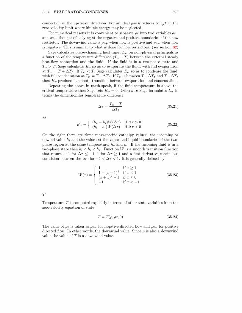
35.4. EVAPORATOR-CONDENSER 393
connection in the upstream direction. For an ideal gas h reduces to cpT in thezero-velocity limit where kinetic energy may be neglected.
For numerical reasons it is convenient to separate ρe into two variables ρe−and ρe+ , thought of as lying at the negative and positive boundaries of the flowrestrictor. The downwind value is ρe+ when flow is positive and ρe− when flowis negative. This is similar to what is done for flow restrictors. (see section 32)
Sage calculates phase-changing heat input Ew on non-physical principals asa function of the temperature difference (Tw − T ) between the external steadyheat-flow connection and the fluid. If the fluid is in a two-phase state andTw > T , Sage calculates Ew so as to evaporate the fluid, with full evaporationat Tw = T + ∆Tf . If Tw < T , Sage calculates Ew so as to condense the fluid,with full condensation at Tw = T −∆Tf . If Tw is between T +∆Tf and T −∆Tf
then Ew produces a smooth transition between evaporation and condensation.
Repeating the above in math-speak, if the fluid temperature is above thecritical temperature then Sage sets Ew = 0. Otherwise Sage formulates Ew interms the dimensionless temperature difference
∆τ =Tw − T
∆Tf(35.21)
as
Ew =
{(hv − hi)W (∆τ ) if ∆τ > 0(hi − hl)W (∆τ ) if ∆τ < 0
(35.22)
On the right there are three mass-specific enthalpy values: the incoming orupwind value hi and the values at the vapor and liquid boundaries of the two-phase region at the same temperature, hv and hl. If the incoming fluid is in atwo-phase state then hl < hi < hv. Function W is a smooth transition functionthat returns −1 for ∆τ ≤ −1, 1 for ∆τ ≥ 1 and a first-derivative continuoustransition between the two for −1 < ∆τ < 1. It is generally defined by
W (x) =
1 if x ≥ 11 − (x− 1)2 if x < 1(x+ 1)2 − 1 if x ≤ 0−1 if x < −1
(35.23)
T
Temperature T is computed explicitly in terms of other state variables from thezero-velocity equation of state
T = T (ρ, ρe, 0) (35.24)
The value of ρe is taken as ρe− for negative directed flow and ρe+ for positivedirected flow. In other words, the downwind value. Since ρ is also a downwindvalue the value of T is a downwind value.

394 CHAPTER 35. LOW T COMPONENTS
P
Pressure P is computed explicitly in terms of other state variables from theequation of state function
P = T (ρ, T ) (35.25)
X
Sage calculates downstream fluid qualityX (vapor fraction) from other solutionvariables exactly like it does for the flow-separator component, as discussed insection 35.3.

Chapter 36
Radiation ExchangeComponents
The components in this chapter model thermal radiation exchange betweenthe walls of radiation enclosures and objects inside. There are two types ofradiation surface components — one for uniform temperature surfaces and onefor distributed temperature surfaces. Then there are several components thatrepresent the various possible view configurations between the surfaces — thefraction of radiation emitted from one surface reaching the other. Radiationbetween two surface components is modeled by connecting them to a commonview configuration component. Each radiation surface is connected this wayto all the other radiation surfaces in the enclosure with which it exchangesradiation — one view configuration component for each surface-to-surface view.
36.1 Sample Radiation Enclosures
Before getting into the details of specific radiation exchange model componentsyou might want to take a look at some representative examples of radiationenclosure submodels that you can cut and paste into your own models and re-vise and expand accordingly. The examples are found in the Apps\LowTCooler\Data\RadEncl sub-directory under the installation directory. Each Sage modelfile has a companion document in pdf format. There are examples for radia-tion between the ends of a cylindrical can, radiation shields (nested-sphericaland stacked-disk) and radiation from a cold finger to a surrounding cylindricalenclosure.
You can use the copy-and-paste function of Sage’s Edit menu (or the toolbuttons) to copy model components from the sample files into your data file.You can only copy single, disconnected, model components this way (althoughany child components are copied too). After you copy a model component youhave to first open the model you wish to paste it into. It is not possible to copyand paste between two separate Sage applications using the Windows clipboard.
395

396 CHAPTER 36. RADIATION EXCHANGE COMPONENTS
36.2 Radiation Surface Components
Radiation surface components define emissivity and surface area without speci-fying anything about the geometrical shape of the surface. Inputs and outputscommon to all radiation surface components are:
A : (real, m2) Surface area emitting or absorbing radiation.
Emiss : (real, dimensionless) Gray-body emissivity ε. A number between 0 and1. ε = 1 for an ideal black body. ε ≈ 0 for a silvered surface. The surfaceis assumed to emit and reflect radiation diffusely with reflectivity equal toemissivity.
Fself : (real, W) Self view factor (Fii, where i is the surface index) implied byall the radiation connections of the model. A diagnostic output. A posi-tive value is normal for concave surfaces (e.g. the outer of two concentricspherical surfaces) where one part of the surface can see another part. Apositive value for a flat or convex surface implies that not all the radiationleaving that surface is arriving at other surfaces of your model. That maybe acceptable if Fself is small or the neglected radiation is going to surfacesat the same temperature where radiation exchange is irrelevant. A nega-tive value implies some of the radiation leaving the surface is accountedfor twice. That may be acceptable if Fself is small.
Br : (real, W/m2) Surface radiosity B. The outgoing radiation intensity forcombined emitted and reflected radiation — reflected from all other con-nected radiation surface components.
Rad : (real, W) Incoming radiation heat load as a result of radiation exchangewith other radiation surface components.
Radiation surface components are designed to solve the surface temperaturefrom an energy balance principle. But there are times when you will want toanchor the temperature of a radiation surface at some value. You can do this byconnecting the radiation surface to another thermal solid in your model with athermal conduction connection. In order to inherit the ability to make thermalconduction connections radiation surface components descend from the heatsource components of chapter 20.
36.2.1 Lumped Radiation Surface
Lumped radiation surfaces assume the entire surface temperature is uniform ata single temperature and define these additional outputs:
Ts : (real, K) Lumped surface temperature T .
QNeg : (real, W) Net conductive heat flow through negative-facing heat-flowconnections.

36.2. RADIATION SURFACE COMPONENTS 397
QPos : (real, W) Net conductive heat flow through positive-facing heat-flowconnections.
These variables are inherited from the point heat source component of chap-ter 20 except that Ts is overridden as a solved variable instead of an input.Temperature is solved so that the net energy flow from combined radiation andconduction is zero.
Thermal Attachments
Lumped radiation surface components include attachments for positive-facingand negative facing thermal radiation flows as well as attachments for conductiveheat flows:
Icon Purpose
steady negative-facing radiation flow
steady positive-facing radiation flow
steady negative-facing conductive heat flow
steady positive-facing conductive heat-flow
Create as many as you need. Then move the connection arrows up one level andconnect them to the view-configuration components or temperature sources inyour model.
Positive and negative facing radiation flows are understood as attached tothe same radiation surface rather than a the opposite sides of a wall. Bothview directions are available to facilitate the multiple connections required in atypical radiation enclosure.
36.2.2 Distributed Radiation Surface
Distributed radiation surfaces assume the surface has a temperature distributionalong its length. The length of the surface comes from the parent componentunder which a distributed temperature radiation surface always resides. Theparent component may be a canister, duct, matrix annular gap, generic cylinderor parallel container. Use of this component is illustrated in the example modelRadColdFinger.ltc.
Distributed temperature radiation surfaces employ a simplified model of ra-diation heat transfer that neglects the variation in view factors along the surface.This is generally only appropriate when the surface length (in the direction ofthe temperature distribution) is small compared to the distance separating thesubdivided surface from other surfaces of the radiation enclosure. (see section

398 CHAPTER 36. RADIATION EXCHANGE COMPONENTS
36.4.3) for more details. Distributed temperature radiation surfaces define theseadditional outputs:
Te : (real, K) Effective surface temperature T .
QyNeg : (real, W) Net conductive heat flow through negative-facing heat-flowconnections.
QyPos : (real, W) Net conductive heat flow through positive-facing heat-flowconnections.
QyNeg and QyPos are inherited from the line heat source component of chapter20. Te is new. It is the effective radiation temperature defined by equation(36.30) below that gives the same radiation heat transfer as the distributedsurface temperature.
Thermal Attachments
Distributed radiation surface components include attachments for positive-facingand negative facing thermal radiation flows as well as attachments for conduc-tive heat flows:
Icon Purpose
steady negative-facing radiation flow
steady positive-facing radiation flow
space-grid negative heat-flow face
space-grid positive heat-flow face
The radiation flow connectors are actually identical to those used for lumped-temperature surfaces. So it is possible to interchangeably connect the same viewconfiguration components to either lumped or distributed-temperature radiationsurfaces.
Meaning of Distributed Temperature
The surface temperature Ts(x) is discretized on a spatial grid and solved ac-cording to an energy balance principal:
qc + qr = 0
where qc is the thermal conduction heat flux (W/m) of all heat-flow face at-tachments and qr is the radiation heat flux of all radiation flow attachments.

36.3. VIEW-CONFIGURATION COMPONENTS 399
The radiation flow attachments do not actually support a distributed radiationflux to other surfaces. Rather they supply only a total heat flux over the entiresurface according to its effective radiation temperature Te. The radiation heatflux is localized internally according to equation (36.31) below.
36.3 View-Configuration Components
View configuration components represent the geometry of the two adjoiningradiation surfaces as well as their relative orientation in space. There are view-configuration components for a selected number of common cases. Inputs andoutputs common to all view configurations are:
FAmult : (real, dimensionless) Empirical multiplier that can be used to scalethe default view area FA to account for radiation blocked by other surfacesor differences between actual surfaces and the perfect geometrical shapesassumed in view configuration theory.
FA : (real, m2) View area FnpAn or FpnAp. The product of an internal calcu-lation and FAmult.
BrNeg : (real, W/m2) Radiosity Bn of negative view.
BrPos : (real, W/m2) Radiosity Bp of positive view.
RadNeg : (real, W) Radiation flow Rnet− negative view
RadNeg : (real, W) Radiation flow Rnet+ positive view
AEQ : (real, W) Available energy loss to radiation heat flow.
Mandatory Surface Component Connections
All view configuration components contain built-in negative-facing and positive-facing radiation connectors for mandatory connection to radiation surface com-ponents.
36.3.1 Generic Configuration
If none of the specific view configurations below are appropriate you can defineyou own view factor with this component. Variable FA is an input rather thanoutput with the intent that you will recast it as an expression involving one orboth of the output variables:
An : (real, m2) Area An of radiation surface connected across negative bound-ary.
Ap : (real, m2) Area Ap of radiation surface connected across positive boundary.

400 CHAPTER 36. RADIATION EXCHANGE COMPONENTS
For example if half of the radiation leavingAn reaches Ap then you would recastFA as the expression 0.5 * An. It is always possible to express the view areaFA as a function of Anand Ap as the view configurations below demonstrate.You may formulate any required parameters besides An and Ap as user-definedinputs. Use of this component is illustrated in the example model RadGeneric.ltc.
36.3.2 Planar Elements
Two planar elements An and Ap separated by distance s with angles θn andθp between surface normals and the view direction. The surface of element An
exchanges radiation with the surface of element Ap :
An
Ap
s
qn
qp
This is the differential basis for all finite area view factors. It is found inSparrow and Cess [59] and example A-1 posted at www.me.utexas.edu/~howell/sectionc/A-1.html. The FA product (either FnpAn or FpnAp is
FA =An cos θnAp cos θp
πs2(36.1)
Strictly speaking this equation applies only to infinitesimal planar elementsAn and Ap but is a reasonable approximation whenever their dimensions aresmall compared to the separation distance s. The shape of the planar elementsis irrelevant. The normal angles and separation distance are inputs for thisconfiguration:
ThetaN : (real, radians) angle θn between An surface normal and view direction.
ThetaP : (real, radians) angle θp between Ap surface normal and view direction.
Sepr : (real, m) separation distance s between planar elements.
Surface areas An and Ap come from the radiation surfaces connected to thenegative-facing and positive-facing views respectively.

36.3. VIEW-CONFIGURATION COMPONENTS 401
36.3.3 Concentric Spheres
Two concentric spheres. The outer surface of an inner sphere A1 exchangesradiation with the inner surface of the outer sphere A2:
A1
A2
As reported in example 31 on p. 790 of [58] view factor F12 = 1 and view factorF21 = A1/A2. In other words all of the radiation leaving surface A1 reachesA2 (obviously) but only the fraction A1/A2 of the radiation leaving surface A2
reaches A1 (from reciprocity condition F12A1 = F21A2). The fact that all theradiation from the inner sphere reaches the outer is true even if the spheres arenot concentric. So these view factors apply to the case of non-concentric spherestoo, so long as one is completely contained in the other.
In the Sage implementation there are two separate components, a NP con-figuration and a PN configuration. In the NP configuration the inner surface ispresumed to be surface An connected to the negative-facing view and the outersurface Ap connected to the positive facing view, as indicated in the componenticon. In the PN configuration the roles are reversed.
There are no input variables for concentric sphere configurations other thanthe inherited FAmult of all configurations. The areas A1 and A2 are importedfrom the radiation surfaces across the connection. View area output FA iscalculated as F12A1 = A1 (which has the same value as F21A2). For the twocases the FA product is
FA =
{An NP configurationAp PN configuration
(36.2)
36.3.4 Separated Spheres
Two spheres separated by distance s. The surface of sphere An exchangesradiation with the surface of sphere Ap :
AnAp
s

402 CHAPTER 36. RADIATION EXCHANGE COMPONENTS
This case corresponds to example C-137 posted at www.me.utexas.edu/~howell/sectionc/C-137.html. An approximate formulation for the FA product (eitherFnpAn or FpnAp is
FA =
(
1 −√
1 − An
Y
)(
1 −√
1 − Ap
Y
)
Y (36.3)
where
Y =(√
4πs+√
An +√
Ap
)2
This approximation derived by J.D. Felske [11] applies to all sphere spacingsand has a worst-case error of 5.8% when the spheres are touching (s = 0). Theseparation distance is an input for this configuration:
Sepr : (real, m) separation distance s between closest points.
Surface areas An and Ap come from the radiation surfaces connected to thenegative-facing and positive-facing views respectively.
36.3.5 Parallel Disks
Two parallel coaxial disks separated by distance s. The surface of disk An
exchanges radiation with the surface of disk Ap :
An
Ap
s
This case corresponds to example C-41 posted at www.me.utexas.edu/~howell/sectionc/C-41.html. The FA product (either FnpAn or FpnAp is
FA =1
2
(
Y −√
Y 2 − 4AnAp
)
(36.4)
whereY = πs2 +An + Ap
The separation distance is an input for this configuration:
Sepr : (real, m) normal separation distance s between disks.
Surface areas An and Ap come from the radiation surfaces connected to thenegative-facing and positive-facing views respectively.

36.3. VIEW-CONFIGURATION COMPONENTS 403
36.3.6 Disk to Inside of Cylinder with Same Radius
A right circular cylinder of radius r and height h separated by distance s froma coaxial disk of the same radius. The inner cylindrical surface A1 exchangesradiation with the disk surface A2:
A1
A2
r
h
s
This case corresponds to example C-81 posted at www.me.utexas.edu/~howell/sectionc/C-81.html. The F12A1 product is
F12A1 =A1
4
[(
1 +H2
H1
)√
4 + (H1 +H2)2 − (H1 + 2H2)
−H2
H1
√
4 +H22
]
(36.5)
where H1 and H2 are defined as
H1 =h
r
H2 =s
r
In the Sage implementation there are two separate components, a NP configu-ration and a PN configuration. In the NP configuration the base is presumed tobe surface An connected to the negative-facing view and the cylindrical surfaceAp connected to the positive facing view, as indicated in the component icon.In the PN configuration the roles are reversed. The separation distance is aninput for this configuration:
Sepr : (real, m) separation distance s between disk and cylinder.
The areas An and Ap imported from the radiation surfaces across the connectiondetermine cylinder radius and height as
r =
{ √
An/π NP configuration√
Ap/π PN configuration
and
h =
{Ap/(2πr) NP configurationAn/(2πr) PN configuration

404 CHAPTER 36. RADIATION EXCHANGE COMPONENTS
36.3.7 Inside of Cylinder to Disk Within Base or Top
A disk of radius r1 within the base or top of a right circular cylinder of radius r2and height h. The disk surface A1 exchanges radiation with the inner cylindricalsurface A2:
A1 A2
h
r2
r1
This case corresponds to example C-80 posted at www.me.utexas.edu/~howell/sectionc/C-80.html. The F12A1 product is
F12A1 =A1
2
[
1 − R2 −H2 +√
(1 +R2 +H2)2 − 4R2]
(36.6)
where R and H are defined as
R =r2r1
H =h
r1
In the Sage implementation there are two separate components, a NP configu-ration and a PN configuration. In the NP configuration the disk is presumed tobe surface An connected to the negative-facing view and the cylindrical surfaceAp connected to the positive facing view, as indicated in the component icon. Inthe PN configuration the roles are reversed. The cylinder diameter is an inputfor this configuration.
Dcyl : (real, m) cylinder diameter 2r2.
The areas An and Ap imported from the radiation surfaces across the connectiondetermine disk radius and cylinder height as
r1 =
{ √
An/π NP configuration√
Ap/π PN configuration
and
h =
{Ap/(2πr2) NP configurationAn/(2πr2) PN configuration

36.3. VIEW-CONFIGURATION COMPONENTS 405
36.3.8 Collinear Cylinders
Two collinear right circular cylinders of inner radius r separated from each otherby a distance s. The inside surface An of one cylinder exchanges radiation withthe inside surface Ap of the other:
An Ap
r
s
This case corresponds to example C-87 posted at www.me.utexas.edu/~howell/sectionc/C-87.html. The FA product (either FnpAn or FpnAp is
FA =2πr2
4
[2AnAp
(2πr2)2+G
(An + 2πrs
2πr2
)
+G
(Ap + 2πrs
2πr2
)
−G(An +Ap + 2πrs
2πr2
)
−G(s
r
)]
(36.7)
where G is the function defined by
G(x) ≡ x√
x2 + 4
The cylinder diameter and separation distance are inputs for this configuration:
Dcyl : (real, m) Cylinder internal diameter (2r).
Sepr : (real, m) Separation gap (s).
Areas An and Ap come from the radiation surfaces connected to the negative-facing and positive-facing views respectively.

406 CHAPTER 36. RADIATION EXCHANGE COMPONENTS
36.3.9 Coaxial Cylinders of Same Height
Two coaxial right circular cylinders of radius r1 and r2 (r1 < r2) with the sameheight h. The inner cylindrical surface A1 exchanges radiation with the outercylindrical surface A2:
A1
A2
h
r2
r1
This case corresponds to example C-92 posted at www.me.utexas.edu/~howell/sectionc/C-92.html. The F12A1 product is
FA = 2h2
[1
2(R2
2 − R21 − 1) arccos
(R1
R2
)
+ πR1 −π
2AB
−2R1 arctan
(√
R22 −R2
1
)
+√
(1 + A2)(1 +B2) arctan
(√
(1 +A2)B
(1 +B2)A
)]
(36.8)
where R1, R2, A and B are defined as
R1 =r1h
R2 =r2h
A = R2 + R1
B = R2 − R1
In the Sage implementation there are two separate components, a NP config-uration and a PN configuration. In the NP configuration the inner cylindricalsurface is presumed to be surface An connected to the negative-facing view andthe outer cylindrical surface Ap connected to the positive facing view, as indi-cated in the component icon. In the PN configuration the roles are reversed.The cylinder height is an input for this configuration.
Hcyl : (real, m) cylinder height h.
The areas An and Ap imported from the radiation surfaces across the connectiondetermine the cylinder radii as
r1 =
{An/(2πh) NP configurationAp/(2πh) PN configuration

36.3. VIEW-CONFIGURATION COMPONENTS 407
and
r2 =
{Ap/(2πh) NP configurationAn/(2πh) PN configuration
36.3.10 Offset Cylinders of Different Diameter
Two coaxial right circular cylinders of radius r1 and r2 (r1 < r2) and heightsh1 and h2 offset by distance s. The outside surface A1 of the smaller cylinderexchanges radiation with the inside surface A2 of the larger cylinder:
A2
h2
r2
A1
r1
h1
s
This case corresponds to example C-98 posted at www.me.utexas.edu/~howell/sectionc/C-98.html. The F12A1 product is
FA =A1
L(fF (L +D) + fF (Y +D) − fF (D) − fF (L +D)) (36.9)
where D, Y , L and R are defined as
D =s
r2
Y =h2
r2
L =h1
r2
R =r1r2
and function fF is defined as
fF (x) =fB(x)
8R+
1
2π
[
x arccos
(fA(x)
fB(x)
)

408 CHAPTER 36. RADIATION EXCHANGE COMPONENTS
−1
2
√√√√
((fA(x) + 2
R
)2
− 4
)
arccos
(fA(x)R
fB(x)
)
−fA(x)
2Rarcsin(R)
]
where
fA(x) = x2 +R2 − 1
fB(x) = x2 −R2 + 1
In the Sage implementation there are two separate components, a NP configu-ration and a PN configuration. In the NP configuration the smaller cylindricalsurface is presumed to be surface An connected to the negative-facing view andthe larger cylindrical surface Ap connected to the positive facing view, as indi-cated in the component icon. In the PN configuration the roles are reversed.The cylinder diameters and separation are inputs for this configuration.
DcylInner : (real, m) smaller cylinder external diameter 2r1.
DcylOuter : (real, m) larger cylinder internal diameter 2r2.
Sepr : (real, m) Separation gap (s).
The areas An and Ap imported from the radiation surfaces across the connectiondetermine the cylinder heights as
h1 =
{An/(2πr1) NP configurationAp/(2πr1) PN configuration
and
h2 =
{Ap/(2πr2) NP configurationAn/(2πr2) PN configuration

36.3. VIEW-CONFIGURATION COMPONENTS 409
36.3.11 Outside of Cylinder to Offset Disk with LargerRadius
A right circular cylinder of radius r1 and height h separated by distance s froma coaxial disk of larger radius r2. The outer cylindrical surface A1 exchangesradiation with the disk surface A2:
A1
A2
r1
h
s
r2
The case for zero separation distance (s = 0) corresponds to example C-77posted at www.me.utexas.edu/~howell/sectionc/C-77.html. For that case theF12A1 product is
F12A1 =πr22B
4+ r1h
{
arccos
(A
B
)
− 1
2H
√(
(A+ 2)2
R2− 4
)
arccos
(AR
B
)
− A
2RHarcsinR
}
(36.10)
where
R =r1r2
H =h
r2
A = H2 + R2 − 1
B = H2 − R2 + 1
For nonzero separation distance (s > 0) Sage calculates F12A1 as the comple-ment to the sum of other view factors (e.g. according to equation (36.19)).Imagine the disk in the drawing above is extended to form the inside surface ofa complete can by adding a disk of the same diameter resting on the top edgeof the cylinder and a cylinder between the outer edges of the two disks. Allthe radiation leaving the inner cylinder reaches the inside surface of this can.

410 CHAPTER 36. RADIATION EXCHANGE COMPONENTS
The view factor for the inner cylinder to the top disk is given above. The viewfactors for the inner cylinder to the outer cylinder (divided into two pieces ofheights h and s are given in sections 36.3.9 and 36.3.10. The view factor to thelower disk in question is the remainder.
In the Sage implementation there are two separate components, a NP con-figuration and a PN configuration. In the NP configuration the cylinder ispresumed to be surface An connected to the negative-facing view and the disksurface Ap connected to the positive facing view, as indicated in the componenticon. In the PN configuration the roles are reversed. The cylinder diameter anddisk-to-cylinder separation are inputs for this configuration.
Dcyl : (real, m) cylinder diameter 2r1.
Sepr : (real, m) separation distance s between cylinder and disk.
The areas An and Ap imported from the radiation surfaces across the connectiondetermine disk radius and cylinder height as
r2 =
{ √
Ap/π NP configuration√
An/π PN configuration
and
h =
{An/(2πr1) NP configurationAp/(2πr1) PN configuration
36.4 Radiation Exchange Theory
Sparrow and Cess [59] discuss the physics of radiation exchange between graysurfaces within enclosures. The formulation in this section is essentially the sameexcept presented in a way consistent with Sage’s implicit solution scheme. Theformulation considers radiation exchange in an enclosure having N surfaces withareas Ai, emissivities εi and temperatures Ti. In a Sage model these variablesare distributed among the radiation surface components of the model and thesolution equations are likewise distributed. Key assumptions are:
absorptivity = emissivity The coefficients of emission ε and absorption αare equal.
diffuse outgoing radiation The emitted and reflected radiation from eachsurface is diffusely distributed.
uniform incident radiation The incident radiation on any surface from an-other is uniformly distributed.
36.4.1 Net Surface Radiation Heat Transfer
The sketch below shows a gray surface with total incoming radiation (per unitarea)Hi. The outgoing radiation is the reflected amount (1−εi)Hi plus the emit-ted radiation εiσT
4i , where σ = 5.66961E–8 W/(m2K4) is the Stefan-Boltzmann

36.4. RADIATION EXCHANGE THEORY 411
constant. The symbol Bi denotes the radiosity, the combined emitted plus re-flected radiation.
Hi e si T4
i
surface i
(1-ei ) Hi
Bi
{
Aiei Hi
The net rate of heat loss QRi from a surface Ai is formulated in general as thedifference between emitted radiation εiσT
4i Ai and the absorbed portion of the
incident radiation εiHiAi
QRi = εi(σT 4
i Ai −HiAi
)(36.11)
The incident radiation is the total amount that arrives from all the surfaces inthe enclosure (including radiation from Ai to itself).
HiAi =
N∑
j=1
BjFjiAj (36.12)
where Bj is the radiosity emitted from surface j and Fji is the fraction ofradiation emitted from surface j reaching surface i — the view factor. Radiositywill be considered more below but for now substituting equation (36.12) forHiAi
in equation (36.11) gives
QRi = εi
σT 4i Ai −
N∑
j=1
BjFjiAj
(36.13)
This constitutes N of the 2N equations required for solving the unknowns Bi
and either Ti or QRi (depending on which is unknown for a given surface).The other N equations come from the definition of radiosity Bi as the emittedradiation per unit area plus the reflected part of the incident radiation per unitarea
Bi = εiσT4i + (1 − εi)Hi (36.14)
Multiplying through by Ai (to convert the left-hand side to total emitted radi-ation) and again substituting equation (36.12) for HiAi the previous equationmay be written
BiAi = εiσT4i Ai + (1 − εi)
N∑
j=1
BjFjiAj (36.15)

412 CHAPTER 36. RADIATION EXCHANGE COMPONENTS
It will be helpful to isolate the Ti and Bj terms into separate equations bymultiplying equation (36.13) by (1 − εi)/εi and adding to equation (36.15) toget
BiAi = σT 4i Ai −
1 − εiεi
QRi (36.16)
then subtracting equation (36.13) from equation (36.15) to get
QRi = BiAi −N∑
j=1
BjFjiAj (36.17)
The previous equation can be put into terms of the radiosity exchange betweensurfaces by writing
∑Nj=1 BjFjiAj as BiFiiAi +
∑
j 6=i BjFjiAj giving
QRi = (1 − Fii)BiAi −∑
j 6=i
BjFjiAj (36.18)
A full accounting of the radiation leaving surface i requires that
N∑
j=1
Fij = 1 (36.19)
In English, all the radiation emitted from surface i goes to other surfaces oritself. So one may replace the term (1− Fii) in equation (36.18) with
∑
j 6=i Fij
to obtainQRi =
∑
j 6=i
BiFijAi −∑
j 6=i
BjFjiAj (36.20)
Equations (36.16) and (36.20) are the basis for the Sage solution scheme de-scribed next.
36.4.2 Sage Solution Scheme
It is convenient to write the individual terms BiFijAi and BjFjiAj appearingin the right-hand side of equations (36.20) using single symbols
Rij ≡ BiFijAi (36.21)
Rji ≡ BjFjiAj (36.22)
Rij is understood as the radiosity emitted from surface Ai that reaches surfaceAj and vice-versa. In terms of Rij and Rji equation (36.20) becomes
QRi =∑
j 6=i
(Rij −Rji) (36.23)
The radiation terms Rij − Rji (for j 6= i) are what flow through radiationconnectors. They are solved implicitly according to the principle that the ra-diosity B is continuous across the connection. The following diagram represents

36.4. RADIATION EXCHANGE THEORY 413
the Sage solution scheme for two area elements An and Ap connected by aview-configuration element. The symbol Rnet denotes the net radiation flowRnp −Rpn.
A
Tn
n
Bn
A
Tp
p
Bp
Rnet
surface n surface pview configuration
BnBp
FABmid
Rnet
Radiation Surface Components
In the surface components An and Ap are inputs and Tn, Tp, Bn, Bp are solved.Tn and Tp are solved implicitly from the component energy balance. For exam-ple, the equation for solving Tn is
QRn +Qcond = 0 (36.24)
In English, the net heat loss from radiation balances the net heat loss throughconductive heat flow connections. Sage calculates QRn explicitly from equa-tion (36.23) where the individual Rnj − Rjn terms come from the radiationconnections (labeled Rnet in the above drawing) and Qcond comes from anyconventional conductive heat transfer connections to the surface. Bn and Bp
are solved explicitly from equation (36.16).
View-Configuration Components
In the view-configuration component either FnpAn or FpnAp (whichever is eas-ier) is calculated explicitly from the areas An and Ap across the connections andother geometrical inputs. A reciprocity principle requires that FnpAn = FpnAp.Either represents the effective view area of an imaginary window through whichsurfaces An and Ap see each other. Calculating only one simplifies things andalso eliminates the possibility that FnpAn might not equal FpnAp due to pro-gramming error.
View configurations also enforce the requirement that the net radiation flowsRnet imported from the radiation connections at each end are equal and relatedto the difference in radiosities across the connections by
(Bn − Bp)FA = Rnet (36.25)
This equation comes from the definitions (36.21) and (36.22) and by substitutingFA for either FnpAn or FpnAp. In this form the electrical circuit analogy forradiation heat transfer is clear. Radiation exchange Rnet is like an electricalcurrent driven by a voltage difference Bn − Bp across a resistance 1/FA. Ormaybe more appropriately a thermal resistance analogy where Rnet is like a heatflow driven by a temperature difference Bn − Bp across a thermal resistance

414 CHAPTER 36. RADIATION EXCHANGE COMPONENTS
1/FA. At any rate view configurations calculate a somewhat ficticious butuseful midpoint radiosity (think temperature) Bmid implicitly according to
Rnet+ − Rnet− = 0 (36.26)
where Rnet+ is the radiation flow imported from the connector to surface Ap
and similarly for Rnet−. Enforcing this equation has the effect of forcing theradiation flows to be the same at both ends. Then to insure that equation(36.25) is satisfied view configurations calculate Bn and Bp explicitly accordingto
Bp = Bmid − 1
2
Rnet+
FA= 0 (36.27)
Bn = Bmid +1
2
Rnet−
FA= 0 (36.28)
Self Radiosity
The radiosity emitted from a surface Ai that reaches itself (BiFiiAi) does notmatter to the overall energy balance of surface i but it is nonetheless importantto consider. The self view factor Fii could be an explicit input for surfacecomponents but it is more convenient to evaluate it indirectly from the radiationaccounting principle (36.19) which implies that it must be
Fii = 1 −∑
j 6=i
Fij (36.29)
In other words, Fii is determined from all the view factors by which Ai seesthe other surfaces of your model. Doing it this way means that if you fail toproperly include all the radiation connections of a radiation enclosure the errorwill show up as more or less than the correct amount of self radiation. Theimplied self view factor Fii is the output Fself for radiation surface components.Keeping an eye on it can help you diagnose problems with your radiation model.It should be zero for a flat or convex surface and greater than zero only for aconcave surface. Never negative.
36.4.3 Distributed Temperature Surface Components
In principle radiation exchange with a surface having a temperature distributionrather than a uniform temperature can be modeled by subdividing that surfaceinto small pieces where the temperature is nearly uniform on each piece. Butmodeling the radiation transfer grows complicated quickly because each piecetypically sees the other surfaces of the enclosure with a different view factor.So if there are N subdivisions there are N view factors required for each ofthe other surfaces of the radiation enclosure. Not to mention the view factorsamong the subdivided pieces themselves.
But when the conditions listed below are satisfied modeling radiation ex-change with a distributed-temperature surface can be greatly simplified.

36.4. RADIATION EXCHANGE THEORY 415
Uniform emissivity The emissivity is uniform over the surface.
Convex surface No two pieces of the subdivided surface see each other.
Uniform view factors The view factors from the subdivided surface elementsto other surfaces of the radiation enclosure are all the same.
These are the assumptions underlying Sage’s distributed radiation surface com-ponent. A necessary condition for the validity of the last assumption is thatthe surface length (in the direction of the temperature distribution) is smallcompared to the distance separating the subdivided surface from other surfacesof the radiation enclosure. For example, the subdivided outer surface of a rela-tively short small diameter cylinder exchanging radiation with the inner surfaceof a larger coaxial cylinder.
To the extent the above assumptions are valid a subdivided surface Ae withequal area elements Ai and temperatures Ti (i = 1..N) has the same radiationheat transfer characteristics as the original surface at the effective temperatureTe provided that
T 4e =
1
N
N∑
i=1
T 4i (36.30)
And the radiation heat transfer QRi to an individual element Ai is related tothe radiation heat transfer QRe to the lumped surface Ae by
QRi =1
N
(Qre − εeσAe(T
4e − T 4
i ))
(36.31)
Two-Surface Case
The above equations are most easily derived for the case where lumped surfaceAe exchanges heat with only one other surface Ax, as illustrated here:
Lumped
Subdivided
A ,Te eAx
A ,T1 1
Ax
A ,TN N
Applying equation (36.13) to the lumped case gives the radiation heat transferto surface Ae as the sum of emitted plus incoming radiation
QRe = εe(σT 4
eAe −BxFxeAx
)(36.32)

416 CHAPTER 36. RADIATION EXCHANGE COMPONENTS
where the assumption that Fee = 0 (no self view) has been used to simplify thelast term on the right side. Applying equation (36.13) to the subdivided casegives the radiation heat transfer to each of the surfaces Ai as
QRi = εi(σT 4
i Ai −BxFxiAx
)(36.33)
where this time the no-self-view assumption Fji = 0, j = 1..N has simplifiedthe last term on the right side. The previous equation can be further simplifiedby requiring that Ae be subdivided into equal area pieces with Ai = Ae/N andusing the assumptions of uniform emissivity and view factors in the form εi = εeand Fxi = Fxe/N (radiation from Ax to Ae distributed uniformly among theAi). Under these assumptions the previous equation becomes
QRi =1
Nεe(σT 4
i Ae −BxFxeAx
)(36.34)
The total radiation heat transfer to all the subdivided surfaces is found bysumming equation (36.34)
N∑
i=1
QRi = εe
(
σ
[
1
N
N∑
i=1
T 4i
]
Ae −BxFxeAx
)
(36.35)
By comparing this equation with equation (36.32) it is clear that the total radi-ation heat transfer to the subdivided surfaces will be the same as the radiationheat transfer for the lumped case provided the lumped temperature Te satisfiesequation (36.30). Eliminating the common term BxFxeAx between equation(36.34) and equation (36.32) gives the above formula (36.31) for the individualradiation heat transfers in terms of the lumped heat transfer.
The radiation leaving the lumped or divided surfaces and reaching surfaceAx is the same in either case. The reflected radiation is the same because ofthe uniform emissivity assumption (εi = εe). The emitted radiation is the same
(e.g. εeσT4e Ae = εe
∑Ni=1 σT
4i Ai), again by choice of Te.
General Case
The general case where surface Ae exchanges radiation with multiple surfacesmay be derived similarly by replacing surface Ax in the above analysis withM surfaces Ak : k = (N + 1)..(N + M) (the k indices start with N + 1 toavoid confusion with the indices for the subdivided surfaces Ai : i = 1..N). Theterm BxFxeAx appearing in equations (36.32) and (36.34) is now replaced with∑
k BkFxeAk which cancels as before and leads to the same conclusions aboutequivalent bulk temperature Te and individual radiation heat transfers.

Bibliography
[1] M. M. Abbott, Cubic Equations of State: An Interpretive Review, in Equa-tions of State in Engineering and Research, Advances in Chemistry Series182, (1978)
[2] B.J. Abu-Ghannam and R. Shaw, Natural Transition of Boundary Layers— The Effects of Turbulence, Pressure Gradient, and Flow History, J.Mech. Engineering Science, V. 22, No. 5, pp. 213–228, (1980)
[3] R. Akhavan, R.D. Kamm and A. H. Shapiro, An Investigation of Transitionto Turbulence in Bounded Oscillatory Stokes Flows, Part 1. Experiments,J. Fluid Mech. vol. 225, pp. 395-422, (1991)
[4] A. Bejan, Entropy Generation Through Heat and Fluid Flow, Wiley-Interscience, (1982)
[5] F. J. Cantelmi, Measurement and Modeling of In-Cylinder Heat Transferwith Inflow-Produced Turbulence, MS Thesis, Virginia Polytechnic Instituteand State University, June (1995)
[6] H.S. Carslaw and J.C. Jaeger, Conduction of Heat in Solids, Oxford at theClarendon Press, (1959)
[7] J.E. Coppage and A.L. London, Heat Transfer and Flow Friction Charac-teristics of Porous Media, Chemical Engineering Progress, Vol. 52, No. 2,pp. 57-63, Feb. (1956)
[8] J.H. Dymond and E.B. Smith, The Virial Coefficients of Gasses, Claren-don, (1969)
[9] E.R.G. Eckert and R.M Drake, Analysis of Heat Mass Transfer, McGraw-Hill, (1972)
[10] D.K. Edwards and I. Catton, Prediction of Heat Transfer by Natural Con-vection in Closed Cylinders Heated from Below, Int. J. Heat and MassTransfer, Vol. 12, pp. 23–30, (1969).
[11] J.D. Felske, Approximate Radiation Shape Factors between Two Spheres,ASME Journal of Heat Transfer, Vol. 100, pp. 547–548, Aug. (1978)
417

418 BIBLIOGRAPHY
[12] D. Gedeon, Mean-Parameter Modeling of Oscillating Flow, ASME Journalof Heat Transfer, Vol. 108, pp. 513–518, Aug. (1986)
[13] D. Gedeon, A Cylinder Heat Transfer Model, personal memorandum,(Tmodel2.pdf), December (1989)
[14] D. Gedeon, An Approximate Cylinder Nusselt Number, personal memoran-dum, (Tmodel3.pdf), December(1989)
[15] D. Gedeon, Advection-Driven vs Compression-Driven Heat Transfer, NASAreport under PO C-23433-R, Task 2, (AdvectionVsCompressionSansFig-ures.pdf), May (1992)
[16] D. Gedeon, Cylinder Heat Transfer Update, personal memorandum,(TModel4.pdf), October (1995)
[17] D. Gedeon and G. Wood, Oscillating-Flow Regenerator Test Rig: Hard-ware and Theory with Correlelations for Screens and Felts, NASA-LewisContractor Report 198422, (1996)
[18] D. Gedeon, Flow Streaming in Compliance Tubes, personal memorandum,(FlowStreamingComplTubes.pdf) (1995)
[19] D. Gedeon, Flow Streaming in Compliance Tubes: High Velocity Correction,personal memorandum, (FlowStreamingHiVelCorrection.pdf) (1999)
[20] D. Gedeon, Sage Tortuosity Reformulation, personal memorandum (Sage-TortuosityFormulation.pdf), February (2006)
[21] D. Gedeon, Random Fiber Data Reduction Results: porosities 85%, 90%96%, personal memorandum (NASARandomFiberDataReduction.pdf),January (2006)
[22] D. Gedeon, Random Fiber Correlations with Porosity Dependent Parame-ters — Updated per New Tests at 90.9%, 93% and 96% Porosity, personalmemorandum (SageRandomFiberMasterCorrelationSept08.pdf), Septem-ber (2008)
[23] D. Gedeon, Random Fiber Correlations with Porosity Dependent Parame-ters — Updated per Revised Fiber Diameter for 90.9% Fecralloy Sample,personal memorandum (SageRandomFiberMasterCorrelationNov08.pdf),November (2008)
[24] D. Gedeon, Radiation Loss Modeling in Sage, personal memorandum (Ra-diationLossModeling.pdf), January (2009)
[25] D. Goldfarb, A. Idnani, A Numerically Stable Dual Method for SolvingStrictly Convex Quadratic Programs, Mathematical Programing, 27, pp.1–33, (1983)

BIBLIOGRAPHY 419
[26] Heames T.J., Uherka D.J., Zabel J.C., Daley J.G., Stirling Engine Ther-modynamic Analysis: A Users Guide to SEAM1, Argonne National Labo-ratory, ANL-82-59, pp. 11–20, Sept. (1982)
[27] K.G.T. Hollands, Natural Convection in Horizontal Thin-Walled Honey-comb Panels, Trans. ASME J. Heat Transfer, Vol. 95, pp. 439–444, (1973).
[28] J.P. Holman, Heat Transfer, Fourth Edition, McGraw-Hill (1976)
[29] E. Fried, I.E. Idelchik, Flow Resistance: A Design Guide for Engineers,Hemisphere, (1989)
[30] D.C. Jiles and D.L. Atherton, Theory of Ferromagnetic Hysteresis, Journalof Magnetism and Magnetic Materials 61, North-Holland, Amsterdam, pp.48–60, (1986)
[31] V.J. Johnson, Properties of Materials at Low Temperature (Phase 1), Perg-amon Press, (1961)
[32] W.M. Kays, A.L. London, Compact Heat Exchangers, 3rd Edition,McGraw-Hill, (1984)
[33] C.J.C. Kruger, Constrained Cubic Spline Interpolation for Chemical Engi-neering Applications, http://www.korf.co.uk/spline.pdf
[34] B.E. Launder and D.B. Spaulding, Mathematical Models of Turbulence,Academic Press, (1972)
[35] K. Lee, A Simplistic model of Cyclic Heat Transfer Penomena in ClosedSpaces, 18th IECEC, pp. 720–723, (1983)
[36] J.M. Lee, P. Kittel, K. D. Timmerhaus and R. Radebaugh, Flow PatternsIntrinsic to the Pulse Tube Refrigerator, International Cryocooler Confer-ence, (1992)
[37] M.A. Lewis and R. Radebaugh, Measurement of Heat Conduction throughMetal Spheres, in Cryocoolers 11, edited by R.G. Ross, Jr., Kluwer Aca-demic/Plenum, pp. 419–425, (2001)
[38] Eric Lemmon, Mark McLinden, Marcia Huber, NIST Standard ReferenceDatabase 23, NIST Reference Fluid Thermodynamic and Transport Prop-erties — REFPROP, U.S. Dept. of Commerce, (2002)
[39] Vitaly Leus and David Elata, Fringing Field Effect in Electrostatic Actua-tors, Technical report ETR-2004-2, Technion – Israel institute of Technol-ogy, (2004)
[40] I.F. Macdonald, M.S. El-Sayed, K. Mow and F.A.L. Dullien, Flow throughPorous Media – the Ergun Equation Revisited, Ind. Eng. Chem. Fundam.,Vol. 18, No. 3, pp. 199–208, (1979)

420 BIBLIOGRAPHY
[41] NIST Standard Reference Database 12, Thermophysical properties of purefluids, avaliable from http:\\www.nist.gov\srd, (1998)
[42] E. Oberg, F. D. Jones, Machinery’s Handbook, Seventeenth Edition, TheIndustrial Press, (1964)
[43] J.R. Olson G.W. Swift, Acoustic streaming in pulse tube refrigerators: Ta-pered pulse tubes, LA-UR-96-3083, (1996)
[44] S. V. Pantakar, W. E. Ibele, W. J Koehler Numerical Predictions of Tur-bulent Oscillating Flow — Initial Studies, NASA-Lewis Progress Report,(1989)
[45] R.P. Peyret and T. D. Taylor, Computational Methods for Fluid flow,Springer-Verlag (1983)
[46] M. J. D. Powell, A Fast Algorithm for Nonlinearly Constrained Optimiza-tion Calculations, in: Lecture Notes in Mathematics, 630, Numerical Anal-ysis (Proc. Biennial Conf. at Dundee, 1977), Springer-Verlag (1978)
[47] W.H. Press, B.P. Flannery, S.A. Teukolsky, W.T. Vetterling, NumericalRecipes, Cambridge, (1986)
[48] O. Redlich, J.N.S. Kwong, On the Thermodynamics of Solutions. V. AnEquation of State. Fugacities of Gaseous Soutions, Chemical Reviews, V44, p. 233, (1949)
[49] R. D. Richtmyer and K. W. Morton, Difference Methods for Initial ValueProblems, Interscience, New York, (1967)
[50] P.A. Rios, An Approximate Solution to the Shuttle Heat-Transfer Losses ina Reciprocating Machine, ASME J. Eng. Power, pp. 177–182, (1971)
[51] H. Schlichting, Boundary-Layer Theory, Seventh Edition, McGraw-Hill,(1979)
[52] E. Schmidt, Thermodynamics, Dover, (1966)
[53] J.R. Seume and T.W. Simon, Oscillating Flow in Stirling Engine HeatExchangers, 21st IECEC, (1986)
[54] J.R. Seume, An Experimental Investigation of Transition in OscillatingPipe Flow, Ph.D. Thesis, University of Minnesota, (1988)
[55] J. Seume, G. Friedman and T.W. Simon Fluid Mechanics Experiments inOscillatory Flow, NASA CR-189127, Lewis Research Center, (1992)
[56] T.W. Simon and J.R. Seume, A Survey of Oscillating Flow in StirlingEngine Heat Exchangers, NASA 182108, (1988)

BIBLIOGRAPHY 421
[57] T.W. Simon, M. Ibrahim, M. Kannapareddy, T. Johnson, G. Friedman,Transition of Oscillatory Flow in Tubes: An Empirical Model for Applica-tion to Stirling Engines, 27th IECEC, (1992)
[58] R. Siegel and J.R. Howell, Thermal Radiation Heat Transfer, McGraw-Hill,(1972)
[59] E.M Sparrow and R.D. Cess, Radiation Heat Transfer, Brooks/Cole, (1970)
[60] G.W. Swift, Thermoacoustic Engines, J. Acoust. Soc. Am., 84 (4), pp.1145–1180, (1988)
[61] G.W. Swift, Thermoacoustics: A Unifying Perspective for some Enginesand Refrigerators, Fourth draft, LA-UR-99-895, 1999
[62] Y.S. Touloukian and C.Y. Ho, Thermophysical Properties of Matter, Pur-due Research Foundation, Plenum Publishing Corp., (1970)
[63] N. B. Vargaftik, Tables on the Thermophysical Properties of Liquids andGases, Second Edition, Wiley, (1975)
[64] A.M. Wahl, Mechanical Springs, McGraw-Hill (1963)

Index
Symbols
ρb(T), 369ρd(T), 369ε(v, T), 366, 368A, 183, 382, 396AEQ, 184, 258, 259, 399AEQw, 189, 194, 202AEQx, 185, 189, 194, 202AEQy, 185, 189, 190AEdiscr, 185, 189, 190, 194, 202AEfric, 202, 349Acoil, 273Aflow, 240, 349Alpha, 273An, 399Ap, 399Apath, 278Aratio, 353Areduc, 351Asec, 240Asolid, 235Avoid, 235Awire, 273BVirialErr, 141Bmult, 337Br, 396BrNeg, 399BrPos, 399C, 268C1, 141C2, 141Ca, Cr, Cs, Cw, Cm, 162Cd, 351Cf, 172Cf0, 172, 287Conductivity, 141, 180, 366Conductor, 273
Cp(v, T), 368D, 85, 88, 163, 173, 185, 188, 194DCRhoUA, 355DPstdy, 355DTfull, 391Dcan, 350Dcentroid, 272Dcyl, 404, 405, 410DcylInner, 408DcylOuter, 408Delta, 190DemagLimit, 281Density, 180Dfiber, 244Dhyd, 248Din, 236–238Dliner, 262Dorf, 351Dout, 237, 238Dshell, 262Dskin, 194Dsphere, 246, 350Dtube, 249, 347Dwire, 243, 272E, 162EOSErrMean, 203Efficiency, 382Emiss, 396Emmis, 259Eratio, 157F, 84FA, 399FAmult, 399FB, 279, 281FBflux, 274, 292FBfluxAir, 289FDP, 202, 349, 386
422

INDEX 423
FDeltaPsi, 274FDeltaV, 266, 268, 274FF, 86, 87FFm, 291FH, 279, 280, 349, 387, 391FHmean, 203FHneg, FHpos, 382FI, 266, 268, 274FIcoil, 172FJ, 282FM, 203FOmega, 154FP, 349, 386, 391FPMean, 202FPNeg, 202FPPos, 202FPsi, 280FPsiNeg, 278FPsiPos, 279FQcombust, 201FQwNet, 194, 201FRestrict, 355FRhoUA, 350, 387, 391FRhoUANeg, 203FRhoUAPos, 203FRhoUAmean, 203FT, 349, 386, 391FTMean, 202FTorque, 153, 154FTsMean, 194FUtilization, 281, 298, 312FV, 202, 266, 268FVneg, 266, 273FVpos, 266, 274FW, 154, 274FWc, 382, 386FWe, 266FWm, 274, 279, 290FWmLinked, 290FX, 86, 87, 169, 387, 391FdC1, 248FdC2, 248FdC3, 248FdM, 248FillFac, 294Fmult, 200, 349
Fneg, 87Fpos, 87Freq, 140FreqNorm, 140FringeMult, 288FsC1, 248FsC2, 248Fscale, 291Fself, 396Gap, 246, 257Gas, 140Gmult, 337HNeg, 202HPos, 202Hchan, 251Hcyl, 406Hmult, 200IMoment, 153Icoil, 172Inorm, 172Jmult, 281K, 84, 88K(v, T), 369K0, 167Ka, 163Kfrac, 169Klocal, 201, 204Kmult, 194, 201KmultBnd, 201, 221Kr, 163KrC1, 248KrC2, 248KrM, 248KrN, 248L, 183, 269Lambda, 194Lcoil, 273Length, 235, 239, 257, 262, 291, 318,
350LinkMult, 273Lnorm, 139Lpath, 278Lpole1, 289Lpole2, 289Lratio, 156, 157, 162Lwire, 273

424 INDEX
M, 163MachMean, 203, 350Mass, 85, 86, 185, 188, 194, 235, 291Material, 279Me, 163MinRestrict, 355Mmag, 278Mscale, 168Mu(v, T), 368Mwire, 273N, 163NCell, 138, 235, 239, 262, 291, 318, 319NTnode, 138, 139, 155Nchan, 251Ntube, 249Nturns, 272NuC1, 248NuC2, 248NuM, 248NuN, 248Offset, 291Omega, 140PV, 201Pcharge, 140, 200Pcrit, 141Phase, 154, 162Pnorm, 140Popen, 353Porosity, 240, 350Pwet, 240, 349QNeg, 181–183, 258, 259, 396QPos, 181, 182, 184, 258, 259, 397QfreeMean, 337Qhtr, 182, 183QmolMean, 337Qnorm, 140QoscMean, 338QstrMean, 338QturbMean, 337QwMean, 391QwNeg, 202QwNet, 181, 183, 189QwPos, 202QxMean, 202QxNeg, 185, 189, 194QxPos, 185, 189, 194
QyNeg, 181, 182, 185, 189, 190, 398QyPos, 181, 182, 185, 189, 190, 398R, 268Rad, 396RadNeg, 399Rcoil, 172, 273Rcrank, 154, 162ReMean, 203, 350Recov, 353Rgas, 140, 366Rho, 162Rn, 167, 172, 287Roughness, 239Rp, 167, 172, 287Sc, 163Sepr, 400, 402, 403, 405, 408, 410Sm, 163Smult, 337Sn, 169Solid, 183, 185, 188, 194, 236Sp, 169Specific heat, 141, 180, 366Sratio, 254Swet, 254T, 162, 181, 182T0, 140, 366, 368TNeg, 202TPos, 202TbInNeg, 201, 224TbInPos, 201, 224TbMean, 203Tcoil, 273Tcrit, 141TdMean, 203Te, 398Tfin, 253ThetaN, 400ThetaP, 400Thk, 246ThkLam, 279Tinit, 232, 236, 240, 262, 318, 319, 349,
386, 391Tm, 279Tmult, 337Tn, 163Tnorm, 138, 140
INDEX 425
Tortuosity, 188, 194Ts, 396TsNeg, 183, 185, 189, 194, 257, 259TsPos, 183, 185, 189, 194, 257, 259TurnRatio, 269TwStdy, 391Twall, 240, 347UpwindFrac, 201, 213VaMean, 203Vcoil, 273Viscosity, 141, 366Vmean, 202Volume, 254Vwire, 273W, 84, 87, 162, 185, 188Wcan, 236, 237Wchan, 251Wcoil, 172Wdissip, 273Win, 237, 238Wnet, 84, 87Wpole, 288Ws, 163X, 86XNeg, 257XPos, 257Xamp, 86Xgap, 289Xlimit, 169Xm, 167, 172, 287XnegRel, 291Xphase, 86XposRel, 291Z(v, T), 141, 366, 368ZMean, 203Zgap, 288ZthkRel, 291
A
accuracy, 138adiabatic compressor
as expander, 381convergence issues, 381, 383energy balance, 384entropy continuity, 384ideal-gas PV power, 385
pulsatile flows, 382PV power, 381theory, 383
air gap, 281moving, 298
annulus shuttle/seal/appendix, 117, 119,120, 257
appendix gap flow, 257available energy, 137, 180, 200
balance principle, 138axial conduction
channels, 253cylinder, 256fins, 254foil, 247generic, 249random fibers, 245screens, 244spheres, 246tubes, 251
axial conductivity enhancement, 337
B
bar conductor, 107, 119, 183Bernoulli’s law, 216bicubic spline, 365Boltzmann constant, 411boundary convection, 340busbar, 112
C
canister, 235annular, 236annular-cone, 238tubular, 106, 110, 236tubular-cone, 237
capacitor, 268charge line, 104charge pressure, 214clearance seal flow, 257coil
fixed, 274moving, 293
coilsmoving, 295
combustion heating, 212
426 INDEX
combustion-space gas domains, 205complex variables, 59compliance tube, 335, 347
tapered, 347composite model components, 261compressibility, 143, 146compressor
pressure regulated, 385adiabatic, 381
computational grids, 90condenser, 390
theory, 392conduction
enhanced, 242conduction continuity, 217conductive surface, 104, 109, 111, 121,
122, 186conductive walls, 123conductivity, 141, 142connection block, 267, 279connections, 55
arrows, 53changing level, 56meaning of, 94structure, 6types, 95
constants, 26constrained piston, 86constrained piston and cylinder, 117, 119,
262, 263constraints
active, 45infeasible, 49overdetermined, 49specifying, 45
container, 317multi-length, 319parallel, 114, 116, 318
continuity equation, 205, 208control volumes, 213
min resolving pressure drop, 214control volumes and accuracy, 343convective triggering, 223coordinates
gas domain, 198thermal solid, 178
criconden point, 369cricondentherm, 369cubic splines, 65current source, 268custom variables, 37
copy and paste, 39cylinder, 254
D
damper, 85relative, 88
damplernegative, 173
data pairs, 64DC flow, 353density, 233, 358, 387, 392density connections, 135, 197diagnostics
optimizer, 48solver, 26
dimensional units, 25discharge coefficient, 351disk files, 4, 21displacer, 118
constrained, 262free, 262, 263kinematic, 263leakage, 120regenerative, 120, 261
displayadd page, 15print, 15remove all, 15remove page, 15show window, 15
display form, 23distributed conductor, 113, 119, 122, 184drivable variables, 79driver, 173duct gas domains, 204
E
eddy currents, 312edit
change bitmap, 17copy model, 16

INDEX 427
cut model, 16delete model, 16down connector, 16paste model, 16print, 17select all, 16show window, 15up connector, 16
edit form, 21, 53levels, 54palette, 55
electrical current connections, 135electromagnetic components, 265electromagnetic connections, 265energy density, 143, 144, 147, 148, 233,
358, 388, 392energy equation, 206, 208energy flow continuity, 216enhanced axial conduction, 212enthalpy flow continuity, 217entropy, 137, 143, 144, 148
gas domain, 199thermal solid, 179
enumerated variables, 66changing, 67Gas, 66Solid, 66
equation of stateerror, 143, 149ideal, 142in gas domain, 213Redlich-Kwong, 143, 144, 322tabular, 149, 365
automatic data entry, 372manual data entry, 324, 367, 372stability issues, 366
evaporator, 390theory, 392
export level, 76expressions, 71
built-in functions, 74case, 73compiling, 73constants, 74identifiers, 73model-specific functions, 75
operators, 73parenthesis, 74parsing, 29, 71qualifiers, 76scope of variables, 76self referencing, 77spaces, 73syntax, 72variables, 76
F
ferromagnetic materialmoving, 301nonmagnetic conductor, 283soft, 282
filelisting preview, 14new, 13open, 13print listing, 14save, 13save embedded property, 14save listing, 14save solution grid, 14, 23save tagged variables, 14save-as, 14
film heat transfer, 210flexure
axial stiffness, 164effective mass, 166radial stiffness, 165springs, 162stack, 162stack couple, 163surge frequency, 166theory, 164torsional stress, 165turning angle, 164
floating isothermal surface, 195flow area, 350, 358flow connections, 135, 197flow inlets, 219flow restrictor, 349
asymmetric sharp-edged, 352check valve, 353DC flow blocking, 355

428 INDEX
mass-flow driver, 357mass-flow pump, 356sharp-edged, 351sintered powder plug, 350time-dependent valve, 354
flow reverser, 232theory, 232
flow separator, 385theory, 387
flow velocity, 359flywheel, 105, 153
attachments, 154force connections, 81, 135, 197Fourier series, 61
accuracy, 62free convection, 338free-piston and cylinder, 105, 262–264friction factor
channels, 252cylinder, 255fins, 254foil, 247generic, 249random fibers, 245screens, 243spheres, 246, 350tubes, 250wall shear stress formulation, 209
G
gas constant, 322gas data file, 322generic cylinder, 103, 254generic matrix, 248gizmo, see resonant systemgrids, 90
full-harmonic differencing, 93saving to file, 14, 23spatial, 91time ring, 81, 93
H
heat conductorbar, 183distributed, 184surface, 186
heat exchangerconductive matrix, 111finned, 109interconnected, 114isothermal duct, 108isothermal matrix, 110
heat flow connections, 135, 177heat sink, see heat sourceheat source, 181, 182
line, 109, 111, 181, 182point, 181, 182surface, 181, 183
heat transformer, 319hydraulic diameter, 204, 350
I
iconspositioning, 54
ideal gas, 142inductor, 269initialization files, 4, 21inputs, 24
user defined, 35installing, 3integer variables, 59interpolation, 92
order, 91, 213isothermal surface, 104, 108, 110, 117,
121, 181, 183
K
kinematic linkage, 105kinematic linkages
rhombic drive, 157Scotch yoke, 156simple crank, 156
kinematic mechanism, 161
L
line temperature drop, 189linear motors, 171listings, 6, 14, 22log files, 41, 46
M
magnet

INDEX 429
moving, 298permanent, 281
magneticcontainers, 290gaps, 288moving, 291
magnetic componentsmoving, 298
magnetic fieldsource, 280
magnetic fluxsource, 280
magnetic flux connections, 135magnetic potential, 277
reference, 280magnetomotive force, 277mapping, 41mass flow rate, 358, 392matrix gas domains, 204mean pressure, 214menu commands, 13mixtures, 374model
class, 5component, 5
active, 13, 22, 23change bitmap, 57creating, 55cut and paste, 56selecting, 54
editing, 53structure, 90tree structure, 54, 56trees, 6views, 22
molecular conduction, 337momentum equation, 206, 208momentum flow continuity, 216motion filters, 175motors
linear, 171moving part
attachments, 82relative, 87variables, 84
N
neg-facing attachment, 106Newton’s method, 96nonlinear programming problem, 43normalization scale factor
specifying, 50numerical diffusion, 343Nusselt number
channels, 253cylinder, 255fins, 254foil, 247generic, 249random fibers, 245screens, 243spheres, 246tubes, 250
O
objective functionspecifying, 45
optimization, 7, 43, 96degrees of freedom, 45ill conditioned , 49line search, 48multiple extrema, 50non convergence, 48pseudo-Lagrangian, 46running, 46
optimization variablesspecifying, 44step limits, 48weakly-determined, 49
optionsmodel class, 20Sage, 20
orifice, see flow restrictor
P
packed sphere matrix, 246palette, 55parasitics, 257Pascal, 97Peclet number, 241phasor variables, 54, 60piston

430 INDEX
constrained, 262free, 262, 263kinematic, 263seal leakage, 116
piston-cylinder composites, 261porosity, 241pos-facing area, 106pos-facing force attachment, 105pos-facing torque attachment, 105power probe, 269Prandtl number, 142, 241pressure connections, 81, 135, 197pressure drop resolving, 214pressure source, 104, 200process
map, 19optimize, 19parse mapping, 19parse optimization, 19parse solution, 19, 29reinitialize, 19solve, 19
propertiesauto-update, 322changing, 321cubic-spline interpolation, 322data files, 321gas, 140, 322saving to file, 14solid, 180, 322two-phase fluids, 370, 378
pulse tube, see compliance tube
Q
quality of vapor, 369quasi-adiabatic surface, 190
R
radiation attachments, 397, 398radiation configuration, 399
coaxial cylinders, 406, 407collinear cylinders, 405concentric spheres, 401disk to cylinder, 403, 404, 409generic, 399parallel disks, 402
planar elements, 400separated spheres, 401
radiation surface, 396distributed temperature, 397lumped temperature, 396
radiation transport path, 119, 259random fiber matrix, 110, 244real variables, 59recast variables, 30
exploring, 37reciprocating mass, 85recovery area ratio, 353rectangular channels, 114, 251rectangular fins, 109, 253Redlich-Kwong, see equation of stateRefpropToSage, 372regenerator, 106resistor, 268resonant system, 9, 43, 53, 81Reynolds number, 204, 350
turbulent, 231rhombic drive mechanism, 157rigorous surface, 107, 195root component, 139rotary mechanisms, 153rotating mechanism, 105
S
Sage architecture, 89sample files, 101, 103, 265, 335, 363,
382, 395scan
comments, 17constraints, 17input values, 17mapped variables, 17optimized variables, 17recast variables, 17user inputs, 17user variables, 17
Scotch yoke mechanism, 156second-law balance, 138shuttle heat transfer, 119, 257simple crank mechanism, 156simple crank piston, 161simple-crank linkage, 105

INDEX 431
simple-crank piston and cylinder, 263snubber, 168
relative, 171solid data file, 322solving, 7, 25, 96
non convergence, 26reinitializing, 26RMS error function, 26
sonic velocity, 142spatial differencing, 91specific heat, 142specify
comment, 18constraints, 18, 45input values, 18mapped variables, 18model order, 19normalization scale factor, 50objective function, 18, 45optimization variables, 44optimized variables, 18recast variables, 18rename, 18user inputs, 18user variables, 18
spring, 84flexure, 162nonlinear, 167nonlinear relative, 168relative, 88
staggered grid, 213Stefan-Boltzmann constant, 411streaming convection, 341submodels, 317
T
temperature drop, 189thermal dispersion, 242thermal penetration depth, 192thermal radiation, 395thermal wavelength, 194thick surface, 104, 194thin surface, 195time differencing, 93time ring, see gridstools
explore custom variables, 20explore optimization, 20
tortuosity, 188, 192, 241foil, 247generic, 249random fibers, 245screens, 244spheres, 246
transducer, 286transformer, 269tube bundle, 108, 114, 249tube bundles, 116turbulence intensity, 223turbulence kinetic energy, 231turbulence models, 222turbulent conduction, 242, 338two-phase fluid properties, 370, 378
U
units, 25user inputs, 35
exploring, 37user variables, 27
exploring, 37export level, 29, 76log files, 29, 41, 46
V
Valensi number, 204variable-volume gas domains, 205variable-volume space, 103variables
complex, 59cubic spline, 65data pairs, 64drivable, 79enumerated, 66Fourier series, 61integer, 59phasor, 60real, 59saving to file, 14smart, 89
virial equation, 145viscosity, 141, 142viscous pressure drop, 350

432 INDEX
viscous pressure gradient, 208voltage
reference, 267source, 268
W
wetted perimeter, 204, 350woven screen matrix, 106, 120, 243wrapped foil matrix, 246