August 2008

NASA/TM-2008-215336NESC-RP-08-09/06-081-E

Ares I-X Upper Stage Simulator StructuralAnalyses Supporting the NESC Critical InitialFlaw Size Assessment

Norman F. Knight, Jr.General Dynamics – Advanced Information Systems, Chantilly, Virginia

Dawn R. PhillipsLockheed Martin Mission Services, Hampton, Virginia

Ivatury S. RajuNASA Langley Research Center, Hampton, Virginia

https://ntrs.nasa.gov/search.jsp?R=20080034821 2019-08-30T05:22:23+00:00Z

The NASA STI Program Office . . . in Profile

Since its founding, NASA has been dedicated to theadvancement of aeronautics and space science. TheNASA Scientific and Technical Information (STI)Program Office plays a key part in helping NASAmaintain this important role.

The NASA STI Program Office is operated byLangley Research Center, the lead center for NASA’sscientific and technical information. The NASA STIProgram Office provides access to the NASA STIDatabase, the largest collection of aeronautical andspace science STI in the world. The Program Office isalso NASA’s institutional mechanism fordisseminating the results of its research anddevelopment activities. These results are published byNASA in the NASA STI Report Series, whichincludes the following report types:

TECHNICAL PUBLICATION. Reports ofcompleted research or a major significant phaseof research that present the results of NASAprograms and include extensive data ortheoretical analysis. Includes compilations ofsignificant scientific and technical data andinformation deemed to be of continuingreference value. NASA counterpart of peer-reviewed formal professional papers, but havingless stringent limitations on manuscript lengthand extent of graphic presentations.

TECHNICAL MEMORANDUM. Scientificand technical findings that are preliminary or ofspecialized interest, e.g., quick release reports,working papers, and bibliographies that containminimal annotation. Does not contain extensiveanalysis.

CONTRACTOR REPORT. Scientific andtechnical findings by NASA-sponsoredcontractors and grantees.

CONFERENCE PUBLICATION. Collectedpapers from scientific and technicalconferences, symposia, seminars, or othermeetings sponsored or co-sponsored by NASA.

SPECIAL PUBLICATION. Scientific,technical, or historical information from NASAprograms, projects, and missions, oftenconcerned with subjects having substantialpublic interest.

TECHNICAL TRANSLATION. English-language translations of foreign scientific andtechnical material pertinent to NASA’s mission.

Specialized services that complement the STIProgram Office’s diverse offerings include creatingcustom thesauri, building customized databases,organizing and publishing research results ... evenproviding videos.

For more information about the NASA STI ProgramOffice, see the following:

Access the NASA STI Program Home Page athttp://www.sti.nasa.gov

E-mail your question via the Internet tohelp@sti.nasa.gov

Fax your question to the NASA STI Help Deskat (301) 621-0134

Phone the NASA STI Help Desk at(301) 621-0390

Write to:NASA STI Help DeskNASA Center for AeroSpace Information7115 Standard DriveHanover, MD 21076-1320

NASA Engineering and Safety CenterLangley Research CenterHampton, Virginia 23681-2199

August 2008

NASA/TM-2008-215336NESC-RP-08-09/06-081-E

Ares I-X Upper Stage Simulator StructuralAnalyses Supporting the NESC Critical InitialFlaw Size Assessment

Norman F. Knight, Jr.General Dynamics – Advanced Information Systems, Chantilly, Virginia

Dawn R. PhillipsLockheed Martin Mission Services, Hampton, Virginia

Ivatury S. RajuNASA Langley Research Center, Hampton, Virginia

Available from:NASA Center for AeroSpace Information (CASI)

7115 Standard DriveHanover, MD 21076-1320

(301) 621-0390

The use of trademarks or names of manufacturers in the report is for accurate reporting and does notconstitute an official endorsement, either expressed or implied, of such products or manufacturers by theNational Aeronautics and Space Administration.

January 23, 2008 1

Ares I-X Upper Stage Simulator Structural Analyses Supporting the NESC Critical Initial Flaw Size

Assessment

Norman F. Knight, Jr. General Dynamics – Advanced Information Systems

Chantilly, VA

Dawn R. Phillips Lockheed Martin Mission Services

Hampton, VA

Ivatury S. Raju NASA Langley Research Center

Hampton, VA

AbstractThe structural analyses described in the present report were performed in support of the NASA Engineering and Safety Center (NESC) Critical Initial Flaw Size (CIFS) assessment for the Ares I-X Upper Stage Simulator (USS) common shell segment. The structural analysis effort for the NESC assessment had three thrusts: shell buckling analyses, detailed stress analyses of the single-bolt joint test; and stress analyses of two-segment 10 -wedge models for the peak axial tensile running load. Elasto-plastic, large-deformation simulations were performed. Stress analysis results indicated that the stress levels were well below the material yield stress for the bounding axial tensile design load.This report also summarizes the analyses and results from parametric studies on modeling the shell-to-gusset weld, flange-surface mismatch, bolt preload, and washer-bearing-surface modeling. These analysis models were used to generate the stress levels specified for the fatigue crack growth assessment using the design load with a factor of safety.

January 23, 2008 2

Table of Contents Abstract ........................................................................................................................... 1 Table of Contents............................................................................................................ 2 Executive Summary ........................................................................................................ 3 Introduction..................................................................................................................... 4 USS Segment Configuration........................................................................................... 5

Configuration and dimensions .................................................................................... 5 Materials ..................................................................................................................... 5Loads........................................................................................................................... 6 Boundary conditions ................................................................................................... 7

Bolt Stress Estimate ........................................................................................................ 7 Buckling Analyses .......................................................................................................... 8

Buckling due to dead weight of vehicle...................................................................... 8 Buckling due to in-plane shear loading ...................................................................... 9

Analysis Tools and Modeling ....................................................................................... 10 Analysis tools............................................................................................................ 10 Modeling assumptions .............................................................................................. 10 Single-bolt joint modeling ........................................................................................ 12 Two-segment 10 -wedge modeling .......................................................................... 12

Single-Bolt Joint Test Analyses.................................................................................... 12 Test configuration ..................................................................................................... 12 Effect of mesh refinement......................................................................................... 13 Baseline analysis case results.................................................................................... 14 Effect of bolt preload ................................................................................................ 15 Effect of washer-bearing-surface modeling.............................................................. 15 Effect of edge boundary conditions .......................................................................... 15 Effect of specimen length ......................................................................................... 16 Test-analysis correlation ........................................................................................... 16

Two-segment 10 -Wedge Analyses.............................................................................. 17 Baseline analysis case results.................................................................................... 17 Relationship between single-bolt and 10 -wedge models ........................................ 18 Stress and strain distributions ................................................................................... 19 Residual plastic strain assessment ............................................................................ 20 Refinement of baseline finite element model ........................................................... 20 Shell-to-gusset weld assessment ............................................................................... 22 Fracture mechanics analysis ..................................................................................... 23 Remote compressive loading .................................................................................... 26 Flange surface mismatch assessment........................................................................ 26

Concluding Remarks..................................................................................................... 31 References..................................................................................................................... 33

January 23, 2008 3

Executive Summary This report describes the structural analyses performed supporting the NESC Critical Initial Flaw Size (CIFS) assessment of the Ares I-X USS common tuna-can segments. First, structural analyses of the single-bolt joint configuration were performed to define the modeling and analysis requirements and to calibrate the analysis models against test data. These analyses were elasto-plastic, large-deformation nonlinear finite element analyses. Different parametric studies were performed, and by far, the most significant parameter affecting the single-bolt joint response was the washer-bearing-surface size. Excellent test-analysis correlation (within 5%) was obtained for displacements, gap opening, and surface strains.

Next, a repeating unit of the US1/US2 segments, a two-segment 10 -wedge model, was identified. Finite element models of this 10 -wedge were developed. Structural analyses were performed to examine the stress state in the vicinity of the shell-to-flange weld. Elasto-plastic, large-deformation simulations were performed. The modeling strategy simulated contact conditions along the flange interface between the two segments. Bolt preload was included, and the washer-bearing-surface effects were also simulated using kinematic coupling constraints. The lower edge of the lower segment and the sliced boundaries of both segments had symmetry conditions imposed. The bounding value of the shell in-plane axial tension running load xN~ of 1,600 lb/in. was applied to the upper edge of the upper segment.

Since these USS segments are unpressurized and only axial loads are applied in the present CIFS assessment, the radial and hoop components are not anticipated to be significant. The axial stress component is examined for an applied running axial load of 1,600 lb/in., which results in a nominal far-field axial stress of 3.2 ksi. The axial stress varies with location and reaches higher values near each bolt hole and reaches maximum values as the gusset is approached. The axial stress distribution for perfectly flat flanges indicated a maximum axial tensile stress of 12.5 ksi at the top of the fillet weld near the gusset.

Both tensile and compressive applied load cases were analyzed to provide stress data at the top of the fillet weld and the centerline of the gusset. These values were used as inputs in the fatigue crack growth analyses. The through-the-thickness axial stress distribution for the tension case decreases from the peak tensile value of 12.5 ksi on the inside surface to essentially zero on the outside surface. The through-the-thickness axial stress distribution for the compression case decreases from the peak compressive value given of 5.2 ksi to approximately 3.3 ksi on the outside surface. For the tension case, bending occurs due to the eccentricity of the load path in the joint. For the compression case, bearing occurs due to closing of the joint by the external loading even more than by the bolt preload.

The manufacturing and assembly of large diameter shells and annular ring segments are difficult tasks in terms of maintaining stringent assembly tolerances on flatness, perpendicularity, and parallelism on the mating surfaces. The influence of flange-surface

January 23, 2008 4

mismatch due to local initial geometric surface imperfections along the flange mating surface contribute to the fit-up stresses. These fit up stresses were evaluated. The peak tensile axial stress at the top of the fillet weld was assessed for the bolt preload step of the structural analysis from a stress free state. The stress distribution for a periodic mismatch distribution with edge gaps indicated with a maximum axial tensile stress of 22.3 ksi. These results indicate that the maximum axial tensile stress at the top of the fillet weld and its circumferential location are dependent on the flange surface mismatch more than the applied external axial loading.

In addition, a preliminary assessment of the buckling margins of the US1 segment to dead-weight loading and to in-plane shear (torsional) flight loads was performed. In both loading cases, the US1 segment had high margins against buckling.

In summary, stress analysis results indicated that the stress levels were well below the material yield stress for the bounding axial tensile design load even with a factor of safety of 1.4. The gussets tend to increase the local stress level near the top of the fillet weld between the gusset and the adjacent bolt hole. Clocking of the gussets during assembly causes only a minor change in the local stress state, and hence, clocking is not an issue. From these structural analyses, for the maximum axial shell running load of 1,600 lb/in. the peak values of the axial stress along the top of the fillet weld at the shell-to-flange interface have been determined to be 12.5 ksi for tensile loading and 5.2 ksi for compressive loading. For a representative flange surface mismatch of 10 mils, the maximum tensile stress was 22.3 ksi. These values are used subsequently in the CIFS analyses.

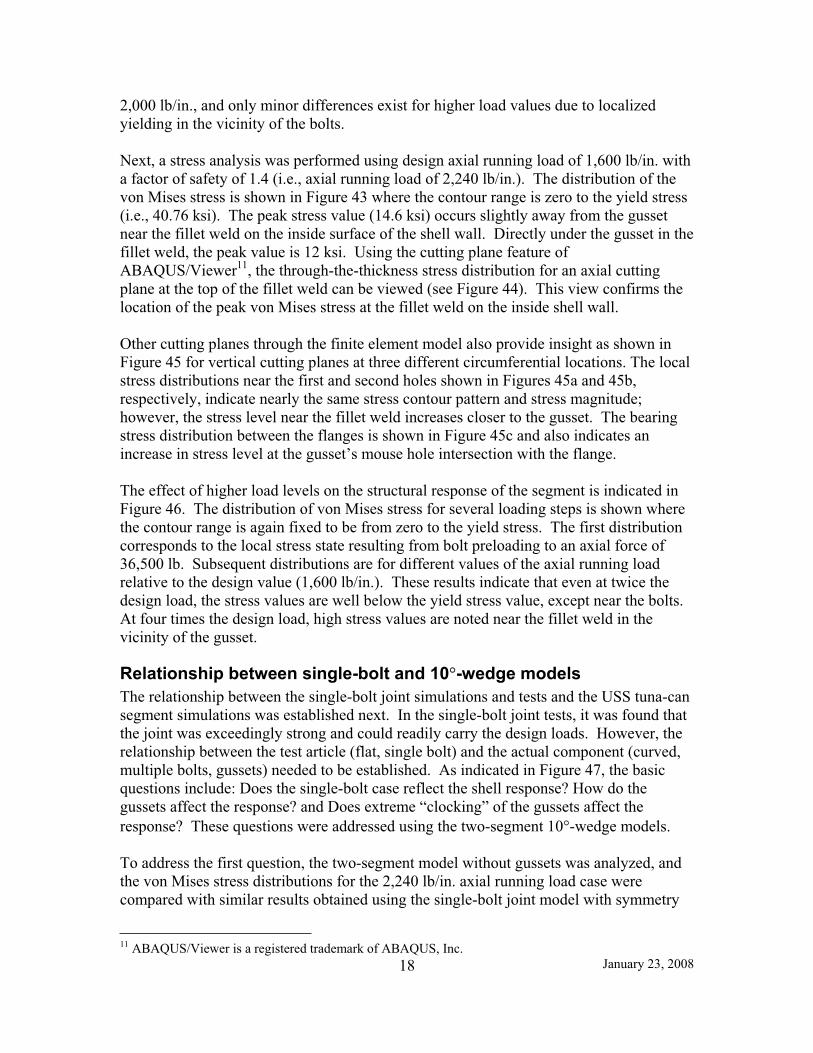
Introduction The Ares I-X Upper Stage Simulator (USS) is a mass simulator element for the Ares I system (see Figure 1). The USS is comprised of seven similar cylindrical shell segments, referred to as “tuna-can segments”, and interface structures as shown in Figure 2. Several tuna-can segments are identical in their design and are referred to as the common segments. Each tuna-can segment, as shown in Figure 3, has a flange welded to each end allowing the different segments to be bolted together. Preloaded bolted-joint connections are commonplace in engineering design of shell segments (e.g., see Ref. 1-5). Preloading the bolts is generally done to reduce cyclic stresses, maintain joint closure, or increase overall stiffness [4].

The structural analyses described in the present report were performed in support of the NESC Critical Initial Flaw Size (CIFS) assessment for the Ares I-X USS common segment. The Ares I-X USS project also independently performed structural analyses reported in Ref. 6. The structural analysis effort for the NESC assessment had three stages. Initially, limited preliminary shell buckling calculations were performed to assess the buckling margins of the US1 segment under dead-weight loading and in-plane shear loading. Next, detailed stress analyses were performed as pre-test predictions for the single-bolt joint test and were followed by test-analysis correlation. The modeling approach and basic analysis assumptions were assessed using the single-bolt joint model. Based on those analyses, finite element models of a 10 -wedge repeating unit were

January 23, 2008 5

developed for two adjacent tuna-can segments. These models are referred to as the two-segment 10 -wedge models. This report summarizes the analyses and results from these parametric studies.

The report is organized as follows. First, a brief overview of the common USS tuna-can segments is presented. Second, an estimate of the bolt stress for the design load is discussed. The preliminary buckling analyses and results are presented next. Then, the analysis tools are described, and the modeling assumptions are presented. Numerical results and discussion follow for the single-bolt joint simulations and the two-segment 10 -wedge simulations.

USS Segment Configuration

Configuration and dimensions A common USS tuna-can segment shown in Figure 3 is 115 inches tall and 216 inches in diameter with a 0.5-inch-thick shell wall. The radius-to-thickness ratio (R/t) is 216 and the shell length to radius ratio ( /R) is approximately unity. On each end of a segment, a one-inch-thick flange is welded to the shell wall using a full penetration butt weld and an interior fillet weld. The flange is 6 inches wide measured from its outer diameter to its inner diameter. To aid in the flange-to-shell assembly, 0.5-inch-thick gussets are installed on the interior of the shell and are spaced 10 apart around the circumference. Each gusset has roughly a 6-inch by 12-inch planform. At the shell-to-flange intersection, each gusset has a 1.5-inch-square cutout to accommodate the fillet weld. This cutout is commonly referred to as a “mouse hole” in the present report and as a “rat hole” in Ref. 6. Adjacent USS segments are assembled together through a series of bolts with a 2 spacing along the flanges as shown in Figure 3. Nominally, these 7/8-inch-diameter bolts have washers on both sides, and the bolts are preloaded. The preload force in the bolt often is not known precisely; however, a preload torque between 300-600 ft-lb was estimated. The dimensions of this bolted joint assembly are presented in Figure 4.

Materials The material for the components of the USS segments (shell wall, flange, and gussets) is A516 Grade 70 steel. Different sources for the material data for this steel were considered. First, the ASTM standard was considered [7]. In addition, the stress-strain data as a function of temperature were obtained from Ref. 8. Since elasto-plastic analyses were anticipated, the data from Battelle were used in the nonlinear finite element analyses. These analyses required the material data in the form of true stress as a function of the plastic strain.1 The room-temperature stress-strain curve for A516 Grade 70 is shown in Figure 5.

1 For the uniaxial case, the nominal stress is the applied load divided by the initial cross sectional area and the nominal strain is the change in length divided by the original length. On the other hand, the true stress is the applied load divided by the current cross-sectional area and the true strain is the change in length divided by the current length. The plastic strain is the difference between the total strain and the elastic strain.

January 23, 2008 6

The material for the bolts is A193 Grade 87 steel with a yield stress of 105 ksi [9]. The material for the washers is A194 steel as described in Ref. 10. In these analyses, the bolts, nuts, and washers were assumed to respond in a linear elastic manner and were not explicitly modeled in any of the analyses.

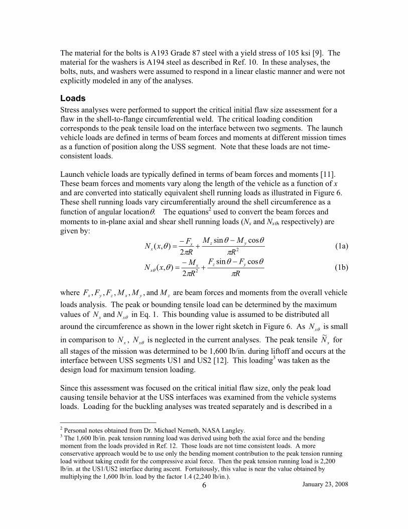
LoadsStress analyses were performed to support the critical initial flaw size assessment for a flaw in the shell-to-flange circumferential weld. The critical loading condition corresponds to the peak tensile load on the interface between two segments. The launch vehicle loads are defined in terms of beam forces and moments at different mission times as a function of position along the USS segment. Note that these loads are not time-consistent loads.

Launch vehicle loads are typically defined in terms of beam forces and moments [11]. These beam forces and moments vary along the length of the vehicle as a function of xand are converted into statically equivalent shell running loads as illustrated in Figure 6.These shell running loads vary circumferentially around the shell circumference as a function of angular location . The equations2 used to convert the beam forces and moments to in-plane axial and shear shell running loads (Nx and Nx , respectively) are given by:

2

cossin2

),(R

MMR

FxN yzxx (1a)

RFF

RMxN yzx

x

cossin2

),( 2 (1b)

where zyxzyx MMMFFF and,,,,, are beam forces and moments from the overall vehicle loads analysis. The peak or bounding tensile load can be determined by the maximum values of xx NN and in Eq. 1. This bounding value is assumed to be distributed all around the circumference as shown in the lower right sketch in Figure 6. As xN is small

in comparison to xN , xN is neglected in the current analyses. The peak tensile xN~ for all stages of the mission was determined to be 1,600 lb/in. during liftoff and occurs at the interface between USS segments US1 and US2 [12]. This loading3 was taken as the design load for maximum tension loading.

Since this assessment was focused on the critical initial flaw size, only the peak load causing tensile behavior at the USS interfaces was examined from the vehicle systems loads. Loading for the buckling analyses was treated separately and is described in a

2 Personal notes obtained from Dr. Michael Nemeth, NASA Langley. 3 The 1,600 lb/in. peak tension running load was derived using both the axial force and the bending moment from the loads provided in Ref. 12. Those loads are not time consistent loads. A more conservative approach would be to use only the bending moment contribution to the peak tension running load without taking credit for the compressive axial force. Then the peak tension running load is 2,200 lb/in. at the US1/US2 interface during ascent. Fortuitously, this value is near the value obtained by multiplying the 1,600 lb/in. load by the factor 1.4 (2,240 lb/in.).

January 23, 2008 7

subsequent section. Loading for the single-bolt test was defined using the test configuration and is also subsequently described.

Boundary conditions Because of the inherent symmetry in a common USS tuna-can segment, computational models that exploit symmetry were examined. A 10 circumferential slice of a half-length tuna-can segment is shown in Figure 7. Symmetry boundary conditions were imposed on the long edges of the boundaries. Along the upper edge, the bounding shell in-plane axial running load xN~ of 1,600 lb/in. was applied and all remaining degrees of freedom were free. To simulate the bolted joint connection and the bearing response, analysis models of two adjacent common segments were analyzed wherein symmetry conditions were imposed along the lower edge of the lower segment. These boundary conditions provided an axial restraint on the finite element model. Additional modeling details for the two-segment finite element models are provided in subsequent sections.

Bolt Stress Estimate The bolt stress estimate is based on a simple strength of materials approach for the bolt and assumes the full utilization of bolt material before failure. The peak tensile load on the interface is taken as 1,600 lb/in., which results in a total axial load of 1.1 million pounds. For the 2 bolt spacing and using a factor of safety of 1.4, the average axial force carried per bolt is 8,450 lb (i.e., 1.4 6,035 lb) for each of the 180 bolts. The stress in a bolt due to this mechanical loading, which includes a 1.4 factor of safety, is the average bolt axial force divided by the bolt cross-sectional area4 (0.6 in.2 for a 7/8-in.-diameter bolt) giving a value of 14 ksi (i.e., 1.4 10 ksi).

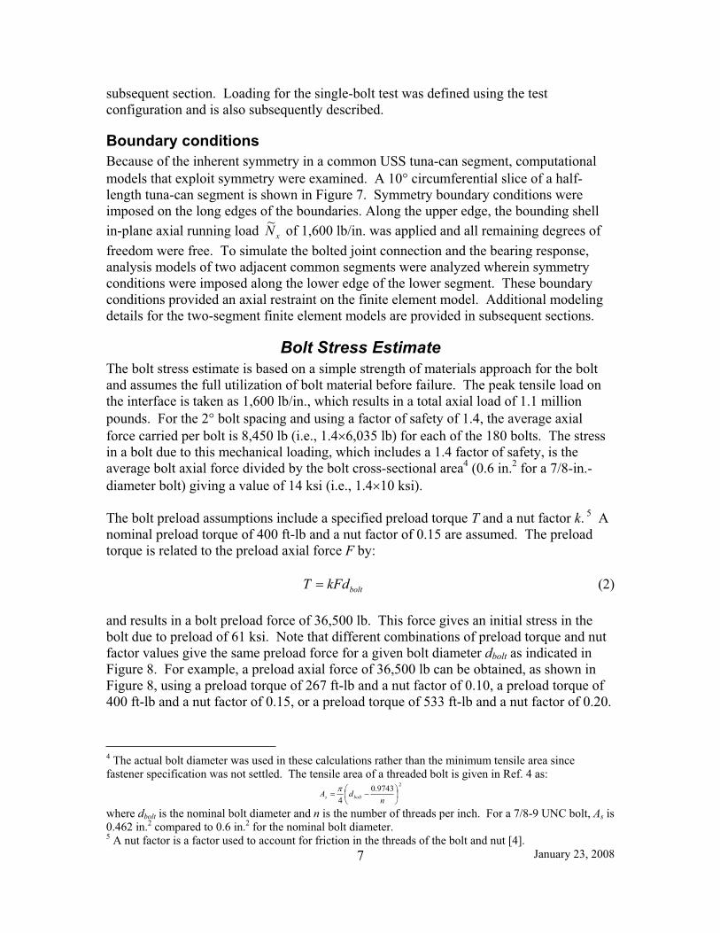
The bolt preload assumptions include a specified preload torque T and a nut factor k. 5 A nominal preload torque of 400 ft-lb and a nut factor of 0.15 are assumed. The preload torque is related to the preload axial force F by:

boltkFdT (2)

and results in a bolt preload force of 36,500 lb. This force gives an initial stress in the bolt due to preload of 61 ksi. Note that different combinations of preload torque and nut factor values give the same preload force for a given bolt diameter dbolt as indicated in Figure 8. For example, a preload axial force of 36,500 lb can be obtained, as shown in Figure 8, using a preload torque of 267 ft-lb and a nut factor of 0.10, a preload torque of 400 ft-lb and a nut factor of 0.15, or a preload torque of 533 ft-lb and a nut factor of 0.20.

4 The actual bolt diameter was used in these calculations rather than the minimum tensile area since fastener specification was not settled. The tensile area of a threaded bolt is given in Ref. 4 as:

29743.04 n

dA bolts

where dbolt is the nominal bolt diameter and n is the number of threads per inch. For a 7/8-9 UNC bolt, As is 0.462 in.2 compared to 0.6 in.2 for the nominal bolt diameter. 5 A nut factor is a factor used to account for friction in the threads of the bolt and nut [4].

January 23, 2008 8

Hence, the total bolt stress is estimated as the sum of the stress due to the mechanical loads and the stress due to the preload force for a total of 75 ksi (i.e., 14 ksi + 61 ksi).This value is below the yield stress of the bolt material, 105 ksi. As an upper bound on bolt load, the incipient bolt yield force is defined as the preload force equivalent to complete bolt cross-sectional yielding (i.e., bolt yield stress multiplied by the nominal bolt cross-sectional area) and is equal to 63,000 lb.6

Buckling Analyses Shell buckling analyses were performed for two loading conditions: a dead-weight uniform in-plane compression case and a uniform in-plane shear case. The shell buckling analyses were performed using the STAGS finite element code [13, 14]. In these cases, the US1 segment was represented as a uniform thickness circular cylindrical shell modeled using two-dimensional shell elements, while the end flanges were modeled using one-dimensional beam elements. Various finite element discretizations were examined to demonstrate convergence of the buckling load and the mode shape.

Buckling calculations based on NASA SP-8007 [15] were also performed. For these shell dimensions, the curvature parameter Z is defined as:

22

1Rt

Z (3)

where is the cylinder length, R is the cylinder radius, t is the cylinder wall thickness, and is Poisson’s ratio for the shell’s material. For the present application, Z takes on a value of 233. The correlation factor accounts for the difference between classical theory and predicted instability loads and is calculated using the following:

e1901.01 (4) where

1500for161

tR

tR (5)

For these dimensions and a linear elastic response, the correlation factor is equal to a value of 0.459. No combined load cases were considered.

Buckling due to dead weight of vehicle For the USS segments, the worst-case dead-weight compression loading occurs for the US1 segment. The total weight of the vehicle at the US1/SR3 interface is 431 kips for the Ares I vehicle and 425 kips for the Ares I-X vehicle. Hence, a total dead weight of 450 kips was assumed. For a circular cylindrical shell with a radius of 108.25 inches, the average bounding compression running load xN~ is 662 lb/in. for the dead-weight case.

6 In cases where the bolt preload force is unknown, a percentage of the incipient bolt yield force is assumed as the bolt preload force, for example, 65% of bolt yield force gives a preload force of 41,000 lb.

January 23, 2008 9

This buckling calculation treated dead weight only and did not account for in-flight compressive loads.

The NASA SP-8007 [15] prediction for the critical axial compressive running load is given by:

2

2DkN xcriticalx (6)

where

Zkx 234 (7)

Here, kx is equal to 75.3 thereby giving a critical axial compressive running load based on SP-8007 of 19,100 lb/in. or 28.9 times the dead weight of the vehicle. That is,

xcriticalx NN ~28.9lbs/in.100,198007 (8)

Finite element buckling analyses of the shell were also performed using a uniform compressive prestress state of 662 lb/in. (i.e., shell running load due to the dead weight of the vehicle). The finite element mesh was successively refined until the buckling eigenvalue and eigenmode remained unchanged. The results of this convergence study are presented in Table 1 and shown in Figure 9. The lowest eigenvalue was 64 times the prestress state. Taking into account the shell correlation factor produces a critical buckling load from the finite element analysis of:

xxFEAcritical

x NNN ~4.29lbs/in.447,19)662)(64)(459(.~1 (9)

Hence, the critical loads predicted by both approaches are in agreement and also indicate a significant margin against buckling due to dead weight of the vehicle. In-flight compressive loads need to be assessed and were not part of the present CIFS assessment.

Buckling due to in-plane shear loading For the in-plane shear loading, the flight load cases provided were examined and the maximum in-plane shear running load xN~ was determined to be 400 lb/in. and occurred during lift-off. It was further assumed that this maximum value represented a uniform bounding in-plane shear loading case for the loads provided.

Using NASA SP-8007 [15], the prediction for the critical in-plane shear shell running load is given by:

2

2DkN xcriticalx (10)

where4/385.0 Zkx (11)

January 23, 2008 10

Here kx is equal to 28.3 thereby giving a critical in-plane shear running load of 7,200 lb/in. That is,

xcriticalx NN ~18.0lbs/in.200,78007 (12)

Finite element buckling analyses of the shell were also performed using a uniform in-plane shear prestress state of 400 lb/in. The finite element mesh was successively refined until the buckling eigenvalue and eigenmode remained unchanged. The results of this convergence study are listed in Table 2 and shown in Figure 10. The lowest eigenvalue was 35 times the prestress state. Taking into account the shell correlation factor produces a critical in-plane shear buckling load from the finite element analysis of:

xxFEAcritical

x NNN ~9.15lbs/in.345,6)400)(6.34)(459(.~1 (13)

Hence, the critical loads predicted by both approaches are in agreement and also indicate a significant margin against buckling due to in-plane shear loading during lift-off.

Analysis Tools and Modeling Engineering analysis of representative USS segments and subcomponents required the use of several different computer-aided engineering analysis tools including those for representing the geometry, those for generating the finite element models, those for performing the structural analyses, and those for post-processing the computed results. In addition, component level analyses were performed to study system response and to identify modeling issues for accurate simulation of the bolted joint structure.

Analysis tools The finite element spatial discretization process (or meshing) of the various components of a USS segment was performed using the ABAQUS [16] software system7. A HEX-meshable solid geometry definition of each component was developed. This solid geometry definition provided a common basis for the finite element modeling tasks performed in the present study.

ABAQUS/Standard Version 6.6-4 was used to perform all analyses. Windows/XP-based desktop computers were used to access Linux-based computing clusters to submit execution runs, to examine results files, and to interrogate the computed solutions using graphical post-processing and data reduction tools.

Modeling assumptions Several different analysis models were used in this report. The development of these analysis models incorporated several fundamental assumptions. Each of these assumptions is described next. These assumptions were common to all of the analysis models used in the stress analyses to support the present CIFS assessment.

7 ABAQUS/Standard is a registered trademark of ABAQUS, Inc.

January 23, 2008 11

First, the bolts, nuts, and washers were not explicitly represented in the finite element models, but rather their influence was simulated. The bolts were represented as one-dimensional linear elastic beams. The washers were represented as sets of kinematic coupling constraints that extend from the bolt centerline to a specified distance on the outer flanges to simulate the bearing load. Kinematic coupling constrained the nodes associated with the washer-bearing surface to the translation and rotation of a node on the bolt. The washer-bearing-surface modeling assumptions are illustrated in Figure 11 where the extent of the kinematic coupling constraints extends a distance radially outward from the edge of the bolt hole. The radius of the bolt hole is 0.5 inches, and the outer radius of the washer is 0.875 inches. The largest value of (i.e., 3/8-inch) corresponds to the size of the washer.

Second, the finite element models were developed to accommodate different material properties in regions of the model as indicated in Figure 12. The shell wall is welded to the flange using a through-the-thickness butt weld followed by a fillet weld along the shell-wall-to-flange intersection on the back side of the L-shaped structure. The weld regions are shown in yellow in Figure 12. Because of the welding process, the material properties in regions near the weld, known as the heat-affected zone (HAZ), could be affected. The regions shown in magenta and light green in Figure 12 are heat-affected zones. In the present analyses, all regions, including the weld and HAZ, used the parent material properties.

Third, the gusset-to-shell and gusset-to-flange fillet welds were not explicitly represented in these models. These welds were initially treated as full-surface, full-length welds and modeled using a tied-nodes approach between the nodes on the shell (or flange) and directly adjacent nodes on the gusset. This assumption was assessed and is described subsequently for the two-segment 10 -wedge analyses.

Fourth, only the bounding load case was analyzed. The bounding load was defined by combining the maximum beam axial force and bending moments rather than just the beam bending moments alone. It was assumed that the in-plane shear loading did not play a significant role in the critical initial flaw size determination. Hence, only the axial loading causing maximum tensile shell running loads was used in these computations. The beam axial force on the vehicle is typically compressive; however, when combined with the beam bending moment, the axial shell running load xN , from Eq. 1a, may change from tension to compression around the shell circumference.

Fifth, the computational effort for these finite element models was bounded somewhat by incorporating two different modeling regions as indicated in Figure 13. Away from the local joint region, a two-dimensional shell finite element model, incorporating the ABAQUS S4 4-node quadrilateral standard shell element, was used to represent the structure. While a shell element has more nodal degrees of freedom than a solid element, no explicit through-the-thickness modeling is required because of the kinematic assumptions employed by shell elements. The use of two-dimensional shell elements for the far-field response readily accommodates the specification of shell running loads or end displacements. Near the joint region, three-dimensional solid finite element

January 23, 2008 12

modeling was employed. The three-dimensional finite element modeling incorporated the ABAQUS C3D8I 8-node solid hexahedral (brick) element, which includes incompatible modes as element shape functions for improved bending response. At the interface of the two-dimensional and three-dimensional regions, multi-point constraints were defined through a shell-to-solid connection constraint for connecting a two-dimensional shell finite element model to a three-dimensional solid finite element model.

Single-bolt joint modeling The single-bolt joint was modeled and analyzed to determine modeling requirements for subsequent finite element models and to support the single-bolt joint tests [17]. These models represented two flat segments with welded flanges and a single bolt (see Figure 13). Two different finite element models were assessed. First, a coarse (less refined) finite element model, as shown in Figure 14, was developed. Then a refined finite element mesh, shown in Figure 15, was developed. Results obtained using the coarse mesh were correlated against those obtained using the refined model. The finite element model shown in Figure 14 was then used to develop the larger two-segment 10 -wedge models, while the more refined model shown in Figure 15 was used in test-analysis correlation.

Two-segment 10 -wedge modeling A single segment 10 -wedge model represents a repeating unit of a single USS tuna-can segment. For the 10 -wedge, the shell wall, flange, one gusset, four complete bolt holes, and two half bolt holes were included as indicated in Figure 16. Details of the shell-to-flange weld modeling are shown in Figure 17. The two-segment 10 -wedge model was developed by combining two single segment models so that it represents a repeating unit (symmetric slice) of two USS tuna-can segments that are bolted together at their flanges. This two-segment model is shown in Figures 18 and 19. The modeling strategy is the same as used in the single-bolt joint analysis coarse mesh in terms of finite element discretization and includes two adjacent common segments. The contact conditions along the flange interface between the two segments were simulated using the ABAQUS/Standard contact algorithm. Bolt preload was included, and the washer-bearing-surface effects were also simulated. The lower edge of the lower segment and the sliced boundaries of both segments had symmetry conditions imposed. The bounding shell in-plane axial tension running load xN~ of 1,600 lb/in. was applied to the upper edge of the upper segment.

Single-Bolt Joint Test Analyses

Test configuration The single-bolt joint test configuration is illustrated in Figure 20. It involves two flat segments with 15 inches of shell wall material and a flange welded to one edge. The 3.77-inch wide specimen is similar to a 2 slice of a single-bolt joint in a USS tuna-can segment. The preload force in the bolt for the test was not known; however, the preload torque was estimated to be between 300-600 ft-lb and a nut factor of 0.15 was assumed as well.

January 23, 2008 13

Two tests were performed at the NASA Glenn Research Center [17]. In each test, the end displacement was applied and the reacted load indicated. While these were displacement-controlled tests, the reacted load was used to make decisions. For each test, the reacted load was increased to a preset value and then unloaded so the specimen could be examined for any evidence of plasticity in the joint, for any local anomalies, and to insure data collection was verified.

A photograph of the specimen in the test setup is shown in Figure 21. Both ends of the specimen were restrained except that the upper end was loaded by uniform end extension and the reacted tensile load determined. The sides of the specimen were free. Photographs of the specimens during the test are shown in Figure 22 and illustrate the joint opening under loading much in excess of the design load. In each test, failure occurred in the bolt and not in the weld region, and failure occurred at load levels far above the design load8.

Effect of mesh refinement Two different finite element models were used in the analysis of the preloaded bolted joint to assess the effect of finite element mesh refinement. First, a coarse finite element mesh, shown in Figure 14, was developed and assessed. The coarse mesh was designed to represent all significant structural behavior up to approximately twice the design load and also to be amenable to multiple bolt structural configurations while keeping the solution times reasonable. Then, a second more refined model, shown in Figure 15, was developed, and the predicted response compared to the results obtained using the coarse model. The refined mesh was designed for use in detailed analysis studies of the bolted joint when loaded to failure.

A ¼-inch washer-bearing-surface assumption and a 400 ft-lb preload torque in the bolt were assumed for both finite element models. The 400 ft-lb bolt preload torque was converted into a 36,500 lb bolt preload axial force using Eq. 2 with an assumed nut factor of 0.15 for steel on steel. An applied uniform extensional end displacement was imposed along the upper edge and reacted through the fixed boundary along the lower edge as illustrated in Figure 13.

The reaction force as a function of end displacement for the coarse and refined meshes is shown in Figure 23. Both results show good correlation up to approximately 20,000 lb – more than twice the design load (8,450 lb). The response predicted using the coarse mesh were somewhat stiffer than the response predicted using the refined mesh for load levels above 20,000 lb. Therefore, the finite element model with the refined mesh shown in Figure 15 is used in all subsequent simulations and is referred to as the baseline analysis model.

8 The design load is estimated to be 8,450 lb using the bounding tensile shell running load of 1,600 lb/in., a factor of safety of 1.4, and the specimen width of 3.77 inches.

January 23, 2008 14

Baseline analysis case results The baseline analysis case is defined as the refined finite element model shown in Figure 15 with a ¼-inch washer-bearing-surface assumption and a 400 ft-lb preload torque in the bolt. The 400 ft-lb bolt preload torque was converted into a 36,500 lb bolt preload axial force using Eq. 2 with an assumed nut factor of 0.15 for steel on steel. An applied uniform end extension was imposed along the upper edge and reacted through the clamped boundary along the lower edge.

The structural response of the single-bolt joint is shown in Figure 24 for the bolt load as a function of the applied end displacement. For the baseline analysis case, the bolt load stays constant at the preload level (36,500 lb) until the joint begins to separate. Following this curve as the end displacement increases will provide the end displacement value when the bolt load reaches incipient yield of the bolt (i.e., 63,000 lb). This value is reached at an end displacement value of 0.046 inches for the baseline analysis case.Using this value of the end displacement at incipient bolt yield and the reaction force as a function of applied end displacement shown in Figure 25, the applied load for bolt failure can be estimated as 30,000 lb for the baseline analysis assumptions.

The flange separation (or gap opening) is shown in Figure 26 in terms of the reaction load. Below the design load of 8,450 lb, minimal flange separation (or gap opening) is observed. As the end displacement increases further, the gap opening also increases in a nonlinear manner and reaches nearly 0.04 inches at an applied load of 30,000 lb., which is the estimated bolt failure load.

The surface strains as a function of the reaction load are shown in Figure 27. The strains are from a location at the center of the specimen width and 1-inch above the flange surface. The design load (8,450 lb) and the bolt incipient-yield load (failure load of 30,000 lb) are indicated on the figure. At the design load, the surface strain level is very low at that location on the specimen.

The lateral displacement response of the joint is shown in Figure 28. The lateral displacement is measured along the front face at the joint interface and is uniform across the joint width. Positive values indicate the joint is displaced in the direction away from the back face, while negative values indicate the joint is displaced in the direction away from the front face. Nonzero values are an indication of the eccentricity in the load path through the bolted joint. These results indicate the bolted joint displaces outward (in the direction of the front face) as the end displacement increases.

The distributions of the axial strain 22 and the von Mises stress vm9 for three different

load levels are shown in Figure 29 wherein the ranges of the contour levels are fixed.Results for 8,450 lb are shown in Figure 29a and indicate low axial strain and von Mises stress levels. Most of the higher stress values are due to the bolt bearing under the

9 The von Mises stress in a local x,y,z coordinate system is expressed as: 222222 6

21

zxyzxyxzzyyxvm

January 23, 2008 15

preload conditions. At 30,000 lb as shown in Figure 29b, the strain levels are still relatively low, while stress levels in the vicinity of the bolt approach the yield value. High stresses are also noted at the top of the fillet weld on the inside surface (bolt side) of the specimen. At 38,300 lb as shown in Figure 29c, high axial strains have developed and widespread yielding of the joint material is predicted.

These results indicate that the basic structural response of a single-bolt joint is simulated using the baseline analysis model and its assumptions. The analysis approach first analyzed the bolt preload step and then incrementally increased the applied uniform end displacement until convergence of the nonlinear solution procedure could not be obtained due to local material failures. Parametric studies were performed next to determine which factors have more influence on the prediction of the joint structural response.

Effect of bolt preload The first factor to consider was the bolt preload torque. In the finite element analysis model, the preload axial force, as determined using Eq. 2, was actually specified rather than the preload torque. However, in the test setup, the preload torque was measured using a torque wrench.

The structural response of the joint is indicated in Figure 30 in terms of the bolt load as a function of applied end displacement for different preload torque values but assuming a nut factor of 0.15 for all cases. The long edges were free, and the washer-bearing-surface size equaled ¼-inch. Increasing the preload torque decreased the end displacement that causes incipient bolt yield. However, the influence on the reaction force was minimal as indicated in Figure 31.

Effect of washer-bearing-surface modeling The second factor to consider was the washer-bearing-surface size as illustrated in Figure 11. The bearing surface is the area under the washer that bears against the flange and holds the joint together. In these studies, the washer-bearing-surface size varied from the nut diameter to somewhat larger than the washer outer diameter (indicated by the “green blocks” in the lower left of diagram in Figure 4). The long edges of the specimen were free, and the bolt preload force was 36,500 lb.

As the value of increased, the bolt load increased as shown in Figure 32 and the reaction load increased as shown in Figure 33 for a given end displacement. The response of the preloaded bolted joint exhibited a significant sensitivity to different washer-bearing-surface size assumptions. The washer-bearing-surface size has a significant effect on the preloaded bolted-joint response.

Effect of edge boundary conditions The third factor to consider was the boundary conditions on the long edges of the specimen. Within the test configuration, these edges were free. However, to assess the relationship between this single-bolt joint test and a full tuna-can segment, symmetry boundary conditions were applied to the long edges. The bolt preload force was 36,500

January 23, 2008 16

lb, and different values of the washer-bearing-surface size were evaluated. These results were then compared to the results obtained when the long edges were free.

The influence of the long edge boundary conditions on the bolt load as a function of end displacement is shown in Figure 34. The influence of the long edge boundary conditions on the reaction load as a function of end displacement is shown in Figure 35. The solid lines with symbols represent the free condition, while the dashed lines with symbols represent the symmetry condition. These results suggest that the use of free or symmetric boundary conditions along the long edges of the specimen has very little influence on the structural response.

Effect of specimen length The fourth factor to consider was the length of the single-bolt joint specimen (i.e., overall specimen length minus twice the grip length). The overall length of the specimen was 30 inches. However, a portion of both ends was covered by mechanical grips to hold the specimen in the test machine. Since this was a tensile test rather than a compression test, the length of the end grips should not have an influence on the local joint response provided the grips were not too close to the region of interest.

Three different grip lengths Lgrip were considered: 0, 3, and 6 inches. The long edges of the specimen were free, a bolt preload force of 36,500 lb was specified, and a ¼-inch washer-bearing-surface was assumed. The influence of specimen length on the reaction force as a function of end displacement is shown in Figure 36. Clearly, a marginal stiffening of the structural response for increased grip length is noted from this figure.The effect on the local von Mises stress distribution is shown in Figure 37 for an applied end displacement of 0.02 inches. As the grip length increased, there is also a marginal change in the stress level near the weld region.

Test-analysis correlation Two tests of a single-bolt joint configuration were compared with finite element analysis results. The analysis models were based on the refined finite element mesh with the long edges free and a bolt preload force of 36,500 lb. Since the washer-bearing-surface size had a significant influence on the analysis predictions, the three values analyzed were compared with the test data as shown in Figure 38. These results indicate that a 1/8-inch washer-bearing-surface size assumption provides the best test-analysis correlation. For this configuration, the analysis continued up to the maximum load observed in the test and then unloading was performed. The correlation between the analysis and test results is very good for both loading and unloading.

Test and analysis results for flange separation (or gap opening) as a function of end displacement were compared in Figure 39. Again, excellent correlation between test and analysis results was evident for the 1/8-inch washer-bearing-surface size assumption.

Surface strain comparisons are given in Figure 40 for Test 1 and in Figure 41 for Test 2. These surface strains were measured at the center of the specimen width and one inch above the flange. The back face is defined as the side of the specimen with the flanges

January 23, 2008 17

and bolt. The front face is defined as the side opposite the bolt side. The average strain value represents the nominal membrane strain. Excellent correlation is evident for both the loading and unloading events prior to bolt failure for the 1/8-inch washer-bearing-surface size assumption.

In summary, the structural response of the single-bolt joint is simulated very well in the current finite element model. Bolt preload and washer-bearing-surface area are important features that need to be modeled to represent the joint behavior accurately. The boundary conditions on the long edges of the specimen and the grip length have marginal effect on the behavior of the joint. The current analysis with a bolt preload force of 36,500 lb (corresponding to a 400 ft-lb preload torque and a nut factor value of 0.15) and a 1/8-inch washer-bearing-surface size yields excellent test-analysis correlation for reaction forces, surface strains, and flange gap opening as a function of end displacement for loading up to the maximum load and unloading to zero load. The single-bolt test provided the validation data for the structural analysis performed for this configuration.

Two-segment 10 -Wedge Analyses The two-segment 10 -wedge models were developed based on the findings from the single-bolt parametric studies. For the stress analysis model, the bolts were simulated as one-dimensional beams, and the effect of the bolts and washers were simulated using kinematic coupling constraints that extended ¼-inch from the bolt hole (i.e., =0.25)10.This nominal washer-bearing-surface size was used in the baseline case. A nominal shell axial running load of 1,600 lb/in. (design load) was applied. Large displacement effects were included in the analyses, and the material behavior was treated as elasto-plastic with strain hardening. Symmetry boundary conditions were imposed on the long, straight edges of the model. Contact conditions were imposed between both flange surfaces. The analyses include preloading the bolts to 36,500 lb as a first step (Step 1) followed by the application of the shell axial running load with different multipliers. The first multiplier (Step 2) was 1.0 for the design load. The second multiplier (Step 3) was 1.25 times the design load and so forth. The mesh refinement was based on the single-bolt joint model with a coarse finite element mesh shown in Figure 14. This finite element model is referred to as the two-segment 10 -wedge baseline model.

Baseline analysis case results The first aspect considered was the importance of nonlinearities (geometrical or material) on the structural response. Using the baseline two-segment 10 -wedge model, analyses were performed assuming small deformations and linear elastic response, assuming small deformations and elasto-plastic response, and assuming large deformations and elasto-plastic response. In each case, a nonlinear analysis had to be performed due to the contact modeling between the flanges. The results from these analyses are shown in Figure 42 for axial running load level as a function of end displacement. The results for different levels of nonlinearities are essentially identical for axial running loads below

10 The two-segment analyses were well underway before the single-bolt joint tests were performed. As a consequence, the baseline 1/4-inch value of the washer-bearing-surface size was used in the two-segment analyses.

January 23, 2008 18

2,000 lb/in., and only minor differences exist for higher load values due to localized yielding in the vicinity of the bolts.

Next, a stress analysis was performed using design axial running load of 1,600 lb/in. with a factor of safety of 1.4 (i.e., axial running load of 2,240 lb/in.). The distribution of the von Mises stress is shown in Figure 43 where the contour range is zero to the yield stress (i.e., 40.76 ksi). The peak stress value (14.6 ksi) occurs slightly away from the gusset near the fillet weld on the inside surface of the shell wall. Directly under the gusset in the fillet weld, the peak value is 12 ksi. Using the cutting plane feature of ABAQUS/Viewer11, the through-the-thickness stress distribution for an axial cutting plane at the top of the fillet weld can be viewed (see Figure 44). This view confirms the location of the peak von Mises stress at the fillet weld on the inside shell wall.

Other cutting planes through the finite element model also provide insight as shown in Figure 45 for vertical cutting planes at three different circumferential locations. The local stress distributions near the first and second holes shown in Figures 45a and 45b, respectively, indicate nearly the same stress contour pattern and stress magnitude; however, the stress level near the fillet weld increases closer to the gusset. The bearing stress distribution between the flanges is shown in Figure 45c and also indicates an increase in stress level at the gusset’s mouse hole intersection with the flange.

The effect of higher load levels on the structural response of the segment is indicated in Figure 46. The distribution of von Mises stress for several loading steps is shown where the contour range is again fixed to be from zero to the yield stress. The first distribution corresponds to the local stress state resulting from bolt preloading to an axial force of 36,500 lb. Subsequent distributions are for different values of the axial running load relative to the design value (1,600 lb/in.). These results indicate that even at twice the design load, the stress values are well below the yield stress value, except near the bolts. At four times the design load, high stress values are noted near the fillet weld in the vicinity of the gusset.

Relationship between single-bolt and 10 -wedge models The relationship between the single-bolt joint simulations and tests and the USS tuna-can segment simulations was established next. In the single-bolt joint tests, it was found that the joint was exceedingly strong and could readily carry the design loads. However, the relationship between the test article (flat, single bolt) and the actual component (curved, multiple bolts, gussets) needed to be established. As indicated in Figure 47, the basic questions include: Does the single-bolt case reflect the shell response? How do the gussets affect the response? and Does extreme “clocking” of the gussets affect the response? These questions were addressed using the two-segment 10 -wedge models.

To address the first question, the two-segment model without gussets was analyzed, and the von Mises stress distributions for the 2,240 lb/in. axial running load case were compared with similar results obtained using the single-bolt joint model with symmetry

11 ABAQUS/Viewer is a registered trademark of ABAQUS, Inc.

January 23, 2008 19

boundary conditions along the long edges of the model and a 2,370 lb/in. axial running load12. The comparison is given in Figure 48. The stress value away from the joint at these load levels from both models is about 5 ksi. At the top of the fillet weld on the inside shell surface, the stress value increased from the 5 ksi level to nearly the same value (11 ksi for the joint model and 10 ksi for the segment model). Both models indicate a local stress gradient in the shell wall opposite the bolt hole, and the segment model indicates a repeating pattern. Thus, the single-bolt joint case does reflect the structural response seen in the shell.

To address the second question, the two-segment model with gussets (baseline case) and the two-segment model without gussets were analyzed, and the von Mises stress distributions for the 2,240 lb/in. axial running load case were compared. The comparison is given in Figure 49. The stress value away from the joint and gussets is the same in both cases. At the top of the fillet weld on the inside shell surface, the stress value increased from 10 ksi without the gussets to 14.6 ksi with the gussets. The presence of the gussets results in a nearby stress gradient in the shell wall near the fillet weld. Peak von Mises stress values still occur opposite the bolt holes at the top of the fillet weld. Thus, the gussets contribute to the stiffening of the 10 -wedge model and hence increase the peak von Mises stress values near the gussets in the fillet weld region.

To address the third question, the two-segment models were again employed. One model included two gussets that were aligned with each other (baseline case), while the second model had a gusset only on the top segment (see Figure 50). This arrangement represents an extreme worse case where there are only gussets on the top segment and no gussets on the bottom segment. This configuration is referred to as extreme “clocking” of the segments. The von Mises stress distributions for the 2,240 lb/in. axial running load case are compared in Figure 50. Peak values of the von Mises stress are reduced slightly to 14 ksi, and the distributions are essentially unchanged. Thus, gusset “clocking” during assembly of adjacent USS segments had minimal effect on either the local von Mises stress distribution or the peak values.

Stress and strain distributions Previously, the von Mises stress distributions have been presented primarily because most plasticity models are defined using uniaxial stress-strain data and effective stress and strain measures, such as the von Mises stress. However, it is useful to examine the distribution of the stresses and strains by component – in particular, the normal components. Since these USS segments are unpressurized and only axial loads are applied in the present CIFS assessment, the radial and hoop components are not anticipated to be significant.

The axial components of the stress and strain are examined first. The applied axial running load is 2,240 lb/in., which results in a nominal far-field axial stress of 4.48 ksi. The distribution of axial stress at the top of the fillet weld on the inside shell surface is shown in Figure 51 as a function of circumferential location. The axial stress varies with

12 A solution at this load level had already been obtained and re-running the simulation was not warranted.

January 23, 2008 20

location and reaches higher values near each bolt hole and maximum values as the gusset is approached. The axial stress distribution is shown in Figure 52 and indicates high compressive stresses near the washer bearing surface. The axial strain distribution is shown in Figure 53 with peak tensile values occurring near the top of the fillet weld close to the gusset.

The radial components of the stress and strain are examined second. The radial stress distribution is shown in Figure 54 and indicates higher values near each bolt hole in the fillet weld at the flange-to-flange interface. The radial stress is approximately 4-5 ksi in the region where the axial stress (see Figure 52) has a maximum value. The radial strain distribution is shown in Figure 55 and exhibits higher values near the bolt holes.

The hoop components of the stress and strain are examined next. The hoop stress distribution is shown in Figure 56 and indicates higher values near the bolt holes. The hoop stress is approximately 5 ksi in the region where the axial stress (see Figure 52) has a maximum value. The hoop strain distribution is shown in Figure 57, and these strains are an order of magnitude smaller than the axial and radial strains.

Residual plastic strain assessment The stress analyses performed thus far for the two-segment 10 -wedge models have not indicated any material yielding of the structure. To assess the residual plastic strains, the loading sequence shown in Figure 58 was simulated. Within ABAQUS/Standard, each solution step is defined in terms of a “pseudo-time” as load factors may be increased or decreased from their value at a previous pseudo-time value (or solution step). In this simulation, the bolt preload was applied first, followed by applying the running axial shell load. The running load was first increased to its design value (1,600 lb/in.), then by factors of 1.25, 1.4, and 4.0. From that load level, the axial running load was removed. Once the axial load was removed, it was re-applied to a level of 1.4 times the design load.

The multiplier for the design running load as a function of end displacement is shown in Figure 59. Incipient yielding in the two-segment 10 -wedge model was noted at a load factor of 2.58 times the design load and occurred in the vicinity of the bolt holes due to bearing. However, the local yielding had little effect on the overall response of the structure.

Contour plots of the equivalent plastic strain are shown in Figure 60 at selected load levels for loading and unloading. These distributions indicate no material yielding up to 1.4 times the design load. Distributions for load factors above 2.58 indicate local material yielding near the bolt holes presumably due to high bearing stresses under the washer. These results indicate that plasticity is not a contributing factor to the present CIFS assessment for the baseline analysis model – even when the axial running load is twice the design value.

Refinement of baseline finite element model Additional parametric studies using the two-segment 10 -wedge baseline finite element model required mesh modifications. The remaining studies were to assess the shell-to-

January 23, 2008 21

gusset weld modeling approach and to perform a preliminary fracture mechanics analysis. The impact of each of these studies on the finite element modeling is described next.

An alternate welding pattern for the shell-to-gusset welds was considered. One approach was to use fillet welds on both sides of the 0.5-inch-thick gussets along their full length.Alternatively, a “stitched” weld pattern was proposed where the fillet welds would start ¼-inch from the ends of the gusset and alternate in a 2-inch-weld/2-inch-free pattern as indicated in Figure 61. Such a welding pattern could not be accommodated using the baseline finite element model, and mesh modifications within the shell and the gusset were required.

Next, it was proposed that since the high stresses occur at the top of the shell-to-flange fillet weld, a fracture mechanics analysis of a through-the-thickness crack in this region would be performed. Again, the baseline finite element model could not be used for two reasons. First, a through-the-thickness crack required a plane of nodes through the thickness of the model at the top of the fillet weld. Since the baseline model was originally developed to accommodate different material properties in the butt weld region, a through-the-thickness plane of nodes at the top of the fillet weld did not exist (see left side of Figure 62). The discretization through the shell thickness was refined, as shown on the right side of Figure 62, to accommodate this need. Second, the element sizes in the vicinity of the proposed crack needed to be sufficiently small and uniform, as shown in Figure 63, in order to compute the fracture mechanics parameters. These mesh modifications required mesh refinement within the shell, the flange, and the gusset.

These three modifications to the baseline finite element model gave rise to the refined finite element model of the two-segment 10 -wedge case. These modifications had consequences of mesh refinement in other regions as a result of the local changes.However, before the refined model was employed in these studies, a verification step was performed using a 2,240 lb/in. axial running load to determine whether any response differences between the baseline model and the refined model were evident.

The axial stress distribution as a function of the circumferential location is shown in Figure 64 for the baseline model and the refined model. In the vicinity of the gusset, the axial stress values increase due to the local mesh refinement with the peak value being ~15 ksi for the refined model and ~14 ksi for the baseline model. Overall distribution patterns are the same for the two models. In addition, a comparison of the axial stress contour plots is given in Figure 65 and indicates the same overall response.

The axial stress distribution as a function of vertical distance z about the flange surface is shown in Figure 66 for the baseline model and the refined model. These values are from a position approximately 1 away from the centerline of the gusset. Again the same overall distribution is obtained for both models. Both models predict an increase in the axial stress at the top of the gusset. Both models also recover the far-field axial stress value of 4.48 ksi (i.e., axial running load divided by the shell wall thickness).

January 23, 2008 22

Prior to the refined model, the axial stress distribution through the shell wall thickness could not be readily obtained. However, the refined model has a plane through the thickness, and the axial stress distribution shown in Figure 67 is easily generated. These results indicate a near linear axial stress distribution through the shell wall. It varies from ~15 ksi tension on the inside (bolt side) surface to ~1 ksi compression on the outside surface. At the middle of the shell wall, the axial stress is equal to the far-field axial stress.

Contour plots of the von Mises stress distribution are shown in Figures 68 and 69. The distributions obtained for the baseline model and the refined model are essentially the same from an overall sense as shown in Figure 68 and in a local sense as shown in Figure 69 for a cutting plane at the top of the fillet weld. The peak value of the von Mises stress obtained from the baseline model is 14.6 ksi, while that for the refined model is 15.5 ksi – within ~6%.

Based on these results, even though the baseline model was not capable of performing these last few studies, the results are consistent and correlated with those obtained using the refined model. Hence, the previously presented results with the baseline model can be considered accurate.

Shell-to-gusset weld assessment All of the analysis models considered so far in the present report model the shell-to-gusset and flange-to-gusset welds as continuous “full-surface” welds. While these welds may be external fillet welds on the structure, the models used in the present report do not explicitly represent these welds as external fillet welds. The only explicitly represented fillet weld is the shell-to-flange weld. A limited assessment of the shell-to-gusset weld modeling is presented in this section.

In the present report, the weld modeling approach is defined using four terms: continuous or stitched and full-surface or edge-only. “Full-surface” weld modeling implies that nodes on the surface of one part have coincident nodes on the opposite surface of the adjacent part. These coincident nodes are tied together and displacement compatibility over these surfaces is enforced. Alternatively, “edge-only” weld modeling implies that only nodes on the bounding surface of the gusset are tied to nodes on the shell; i.e., displacement compatibility is enforced only on the edges of the gusset. “Continuous” implies that the weld modeling approach is imposed along the entire intersection of the two parts, while “stitched” implies an alternating weld/free pattern along the entire intersection. The “continuous” and “stitched” weld patterns are illustrated in Figure 61.

For this assessment, the stress analyses were performed using the refined model of the two-segment 10 -wedge case under a 2,240 lb/in. axial running load. In all cases, the flange-to-gusset weld was modeled as a continuous, full-surface weld. As a reference state, the axial stress distribution for the continuous full-surface weld is shown in Figure 70. The distribution on the left-hand side uses a contour range of zero to 40 ksi, while the distribution shown on the right-hand side uses a narrower contour range of zero to 16 ksi.

January 23, 2008 23

For the reference state, the peak stress value of 16.5 ksi occurred on the gusset in the mouse hole close to the flange-to-gusset intersection and away from the shell-to-gusset weld.

A comparison of the full-surface and edge-only continuous weld modeling assumptions is shown in Figure 71 using the axial stress distributions with the previous narrow contour range. The full-surface region is the area enclosed by the red box on the left side of Figure 71, and the edge-only region is indicated by the red lines on the right side of Figure 71. The axial stress distributions are nearly the same for the full-surface and edge-only continuous weld modeling assumptions.

A comparison of the full-surface and edge-only stitched weld modeling assumptions is shown in Figure 72 using the axial stress distributions with the previous narrow contour range. The full-surface regions are the three areas enclosed by the red boxes on the left side of Figure 72, and the edge-only regions are indicated by the three pairs of red lines on the right side of Figure 72. The axial stress distributions for the full-surface and edge-only stitched weld modeling assumptions are nearly the same. In addition, the overall distributions shown in Figures 71 and 72 are nearly the same indicating that these shell-to-gusset modeling assumptions do not significantly affect the structural response for this loading.

These results indicate that the present approach to modeling the shell-to-gusset weld appears to be insensitive to whether the weld is continuous or stitched and to whether the weld model is a full-surface or edge-only weld model. Again, in these analyses, the gusset welds are only simulated through constraints rather than through explicit modeling of the fillet weld (as was done for the shell-to-flange fillet weld). The stitched edge-only weld modeling assumptions did result in a somewhat different local stress distribution on the gusset; however, the peak axial stress remained in the 16 ksi range for all cases considered. Inclusion of the gusset fillet welds into the finite element model is not expected to affect these results for the present CIFS assessment.

Fracture mechanics analysis Fracture mechanics analysis aims to calculate either stress-intensity factors or strain-energy release rates for a crack in a structure. In the present analysis, the fracture mechanics parameters are calculated using the virtual crack closure technique (or VCCT) [18-25]. Application of VCCT to obtain a through-the-thickness stress intensity factor distribution required mesh refinement in the vicinity of the inserted crack of length 2a.

Using the two-segment 10 -wedge model, the mesh was refined, as described previously, and a through-the-thickness crack was inserted into the finite element model as indicated in Figure 73. This inserted crack essentially involves coincident nodes on either side of the crack face up to the crack tip. The inserted crack is located at the top of the fillet weld in the shell wall and centered in the circumferential direction. In the refined model, the local element edge length along the crack in the circumferential direction is 0.05 inches, and the element edge length in the shell thickness direction is 0.0625 inches.

January 23, 2008 24

Local modeling on the crack plane is shown in Figure 74 when the cracked solid is modeled with 8-node hexahedral (brick) elements. The crack front is represented by rectilinear segments (i-1, i) and (i, i+1). The nodes on the crack front are i-1, i, and i+1.The elements ahead of the crack front and above the crack plane are I and I+1. The elements behind the crack front are J and J+1 above the crack plane and K and K+1below the crack plane. For clarity, the brick elements are not shown in the figure, but rather the element labels point to the corresponding face on the crack plane. As the strain energy release rates G can vary along the crack front, the G values need to be computed at each of the crack front nodes i-1, i, and i+1. Historically, the first attempts of the VCCT scheme evaluated the G values as:

AwZwZ

G kjikjiI 2

1,1'

1,'

(14a)

AuXuX

G kjikjiII 2

1,1'

1,'

(14b)

AvYvY

G kjikjiIII 2

1,1'

1,'

(14c)

where A is an area associated with element I, and wj,k = wj – wk, etc. The forces Z’i,X’

i, and Y’i are the nodal forces at node i evaluated using the elements I and J alone.These G values are attributed at the location of the crack front midway between nodes i-1and i [19].

Raju et al. [20, 21] suggested evaluating the strain energy release rates at the nodes using the nodal forces at the crack front nodes and the relative displacements at the appropriate nodes behind the crack front as:

i

kjiI A

wZG

2, (15a)

i

kjiII A

uXG

2, (15b)

i

kjiIII A

vYG

2, (15c)

where Zi, Xi, and Yi are nodal forces evaluated using the elements I, I+1, J, and J+1. The relative displacements (by component) at the nodes behind the crack front are computed, for example, as wj,k = wj – wk. The Ai is the area attributed to node i and is the shaded area in Figure 74. This area can be computed easily as:

January 23, 2008 25

abbA IIi 2

)( 1 (16)

where bI and bI+1 are the width of elements I and I+1, respectively, as shown in Figure 74.For the nodes at the ends of the crack front, A1 = (b1/2)· a and AN = (bN/2)· a, where b1 and bN are the widths of the first and the last elements on the crack front. This process is repeated at each of the nodes on the crack front to obtain the strain energy release rate distribution along the crack front.

The total strain energy release rate GT can be evaluated using:

GT = GI + GII + GIII. (17)

The stress intensity factors K for each fracture mode can be obtained from the individual strain energy release rates using:

EGK II (18a)

EGK IIII (18b)

)1(III

IIIEGK (18c)

where E’ = E when plane stress assumptions are used, and E’ = E/(1- 2) when plane strain assumptions are used [22-24].

The variation of the strain energy release rates through the shell thickness is shown in Figure 75 for an axial running load of 2,240 lb/in. Based on the finite element results, the strain energy release rate for each fracture mode was calculated using Eq. 15 as a function of position through the shell thickness. For this axial running load case, the dominate fracture mode is the crack opening mode known as Mode I. The sum of the Mode II and Mode III strain energy release rates (GII+GIII) is often referred to as the shearing strain energy release rate. For this application, this sum represents less than 5% of the Mode I strain energy release rate GI.

A close-up view of a slice through the refined finite element model near the crack tip is shown in Figure 76 with exaggerated displacements. The flange separation (or gap opening) is clearly evident in this figure as well as the crack opening. The structural response for tensile axial loading results in local bending near the flanges, which in turn results in a greater crack opening on the inside shell surface than on the outside surface.

To verify these calculations, another finite element model was created with local mesh modifications as indicated in Figure 77. Here, the local element edge length in the crack plane was increased to 0.0833 inches from 0.05 inches. The stress analysis and VCCT

January 23, 2008 26

computations were repeated and gave essentially the same distribution of the Mode I strain energy release rate as the refined model, as shown in Figure 78.

In the present analysis, plane stress assumptions and an elastic modulus of 30 Msi were used. The variation of the VCCT-predicted Mode I stress intensity factor KI through the shell thickness is shown in Figure 79 for a axial running load of 2,240 lb/in. This factor was calculated using the Mode I strain energy release rate GI computed from the finite element results and Eq. 18a. The value of the Mode I stress intensity factor IK at the crack tip on the inside shell surface (back face) was about 10 ksi- in., which decreased in almost a linear fashion to zero on the outside shell surface (front face).

For the fatigue crack growth analyses, stress results are needed for the maximum tensile running axial design load of 1,600 lb/in. The peak stress values for the uncracked body were obtained from the two-segment 10 -wedge refined finite element model and tabulated in Table 3. Values are reported at three locations as indicated in Figure 80: on the element outer face (peak value); at the element centroid (center of the element), and at the element integration points (just inside the element face). The element integration point stress values are considered to be the more accurate and therefore incorporated in the fatigue crack growth analyses.

In addition, the fracture mechanics analysis using VCCT was repeated for the design load case. For the design load case and using the refined finite element model, the value of the VCCT-predicted Mode I stress intensity factor at the crack tip on the inside (bolt side) surface was 6.8 ksi- in.

Remote compressive loading Both tensile and compressive load cases were analyzed to provide stress data for the fatigue crack growth analyses. The through-the-thickness axial stress distribution for the tension case decreases from the peak tensile value of 12.48 ksi to essentially zero on the outside surface. The through-the-thickness axial stress distribution for the compression case decreases from the peak compressive value given of -5.22 ksi to approximately -3.30 ksi on the outside surface. For the tension case, bending occurs due to the eccentricity of the load path in the joint. For the compression case, bearing occurs due to closing of the joint by the external loading even more than by the bolt preload.

Flange surface mismatch assessment The manufacturing and assembly of large diameter shells and annular ring segments are difficult tasks in terms of maintaining stringent assembly tolerances on flatness, perpendicularity, and parallelism on the mating surfaces. The influence of flange surface mismatch due to local initial geometric surface imperfections along the flange mating surface on the peak tensile axial stress at the top of the fillet weld was assessed for the bolt preload step of the structural analysis from a stress free state – residual stresses from the welding process are not included.

January 23, 2008 27

A segment mating test was performed by stacking Pathfinder 1 (PF1) shell segment onto Pathfinder 2 (PF2) shell segment as indicated in Figure 81.13 Gap measurements taken on the front (i.e., outside diameter or OD) and back (i.e., inside diameter or ID) sides of the mating surfaces during a mating test of one flange surface of Pathfinder 1 (PF1) shell with a flange surface of Pathfinder 2 (PF2) shell are indicated in Figure 82.14 These measurements were recorded midway between gussets (i.e., every 10 ), and it was reported that no gaps occurred at the gusset locations. Shimming was proposed as a way to mitigate the magnitude of the gaps measured on the outside diameter and the inside diameter. The installation procedure [26] of the shims (both mechanical and liquid) and its verification are still under development (see Figure 83 for an overview of the shimming procedure). Mechanical shims of varying sizes would be used with liquid shimming material applied to even out the flange surface; however, shim sizes in 10-mil increments are expected to be used in combination with a liquid shimming process. Assuming that the free-state gaps are shimmed, then the remaining gaps around the circumference of the USS segment would be less than 10 mils as indicated in Figure 84. The distribution of these values appears to be somewhat random and not readily characterized.

Limited surface mismatch studies have been performed by the Project (see Ref. 28). Additional surface mismatch studies described in this report were performed using the refined model from the fracture mechanics analyses shown in Figure 63. The modeling procedure was to extract the nodes on the mating surface of the flange on the upper tuna-can segment and to perturb their longitudinal location from the original plane defining a perfect mating surface. Once perturbed, the finite element model was reflected thereby generating a mirror image of the surface mismatch on the opposite flange. When interelement penetration of a perturbed node location was detected, the node location was changed to be exactly on the mating surface (i.e., no mismatch or gap at that node).

The flange surface mismatch was defined using parametric representations in the radial and circumferential directions as given by:

0)()(),( grfr (19)

using the symbols and nomenclature defined on Figures 85 and 86. The size of the gap at a node on the flange outer surface is required to be greater than or equal to zero. When the functional form returns a negative value it is assigned a value of zero, thereby avoiding issues of interelement penetration.

Five radial functions listed in Table 4 and four circumferential functions listed in Table 5 were constructed and provide a capability to generate twenty different flange surface mismatch distributions. Two distributions are illustrated in Figure 87 where blue represents zero gap and red represents peak gaps. Of the twenty possible functions, only 13 In preparation for the fabrication of USS segments, two shells were fabricated to demonstrate the process and to evaluate manufacturing procedures. These shell structures were designated Pathfinder 1 and Pathfinder 2 shells. 14 The gap data were provided by Paul Trimarchi, NASA Glenn. Also refer to Ref. 27.

January 23, 2008 28

the nine different flange surface mismatch distributions shown in Figure 88 were analyzed. These flange surface mismatch distributions are formed by combining the radial and circumferential functions as indicated by Eq. 19 and are divided into three groups: axisymmetric; periodic with edge gaps; and periodic with no edge gaps. The axisymmetric distributions (see Figure 88a) exhibit the same mismatch distribution for every circumferential location (i.e., 0)()( rfr ). The periodic distributions with edge gaps (see Figure 88b) exhibit flange surface mismatch between the gussets and no gap near the gusset. These distributions are generated using the n=-1 circumferential function. The periodic distributions with no edge gaps (see Figure 88c) exhibit peak gaps along the front face and zero gaps along the symmetry planes of the finite element model. These distributions are generated using the linear radial function and the n>0circumferential functions.

Each of these nine flange surface mismatch distributions and the original perfect flange case were analyzed using a bolt preload force only to determine the influence of these assembly mismatches on the local axial stress at the top of the fillet weld. These so-called “fit-up stresses” contribute to the CIFS analyses. These fit-up stresses have been estimated to be approximately 15% of the parent material yield stress (approximately 6 ksi for the data used in this report). Results are shown in Figure 89-91 for the three types of distributions. The free-state flange surface mismatch distributions with 10-mil peak gaps are shown in Figures 89a, 90a, and 91a for a stress-free state. The gap distributions after a bolt preload of 36,500 lb are shown in Figure 89b, 90b, and 91b with the maximum axial tensile stress at the top of the fillet weld noted below each distribution.Maximum axial tensile stress values are reported in Table 6 for these nine mismatch cases and the perfect case. The axial stress values reported are element face values.

First, the influence of the axisymmetric mismatch distributions (n=0 cases) as shown in Figure 89 is discussed. The bolt preload force is 36,500 lb, and the peak gaps are 10 mils. As a basis for comparison, the perfect case (no gapping, perfect mating of the flange surfaces) results in only a 2.2 ksi maximum axial tensile stress at the top of the fillet weld as indicated on the far left of the figure. Next, a linear distribution with no gaps along the back face and peak gaps along the front face was analyzed. This distribution represents a tilting of the flange outer surface, and the bolt preload gradually closes the gap without significantly increasing the axial stress level. The third case (cosine, n=0) exhibits peak gaps at both the back and front faces (including under the gusset) and near zero gaps along the bolt circle. Because of the absence of gaps along the bolt circle, the bolt preload does not increase the axial stress level and is not able to eliminate the free-state gaps. The fourth case (sine, n=0) shown on the far right of Figure 89 exhibits a uniform “bubble” gap that is not easily detected, since the gaps along the front and back faces are zero. This bubble also extends underneath the gusset. Because of the bearing surfaces along the front and back face edges, imposing the bolt preload force causes local bending near the fillet weld and significantly increases the axial stress level to 19.0 ksi – nearly an order of magnitude larger than the perfect case.

Second, the influence of the periodic mismatch distributions with edge gaps (n=-1 cases) as shown in Figure 90 is discussed. The bolt preload force is 36,500 lb, and the peak

January 23, 2008 29

gaps are 10 mils. In the four distributions analyzed, there is no mismatch near the gusset (±1 on either side of the center of the gusset). The two cases on the left side of Figure 90 exhibit linear radial distributions: one with zero gaps on the back face and the other with one half of the peak gap on the back face. Both cases behave in a similar manner with front face gaps remaining after applying the bolt preload and high values for the maximum axial tensile stress at the top of the fillet weld (18.6 ksi and 21.6 ksi). The third case has a peak gap at the front face on the symmetry boundary and half the peak gap on the back face. However, near the bolt circle, the flange mismatch is nearly zero. Again, because of minimal gapping along the bolt circle, the bolt preload neither increases the axial stress level significantly (6.0 ksi) nor eliminates the free-state gaps. The fourth case has a series of interior “bubble” mismatches between the gussets and zero gaps along the front and back faces. The axial stress level is only marginally increased (7.7 ksi) compared to the perfect case.

Third, the influence of the periodic mismatch distributions with no edge gaps (n>0 cases) as shown in Figure 91 is discussed. The bolt preload force is 36,500 lb, and the peak gaps are 10 mils. Both cases assume a linear radial mismatch distribution with zero gaps along the symmetry edges of the analysis model. The first case, left side of Figure 91, is a sinusoidal circumferential distribution (n=1) with the peak gaps occurring underneath the gusset. Here, the bolt preload force was able to close most of the free-state gapping; however, the maximum axial tensile stress was significantly increased (19.9 ksi). The second case, right side of Figure 91, is a sinusoidal circumferential distribution (n=3)with two peak gaps occurring between gussets and no gaps near the gusset. Local bending of the flange-to-skin interface increased the maximum axial stress level to 30.7 ksi without eliminating the initial free-state gaps.

Of the nine distributions analyzed, four mismatch distributions significantly increase the maximum axial tensile stress at the top of the fillet weld. These findings are summarized in Figure 92. The sine, n=0 case is axisymmetric with the peak gaps occurring near the bolt circle including under the gussets but with no gaps on either the front face (segment OD) or the back face (segment ID). The linear, n=1 case is a periodic with no edge gaps but peak gaps occurring directly under the gussets. Limited measurement data has indicated that gaps on the front and back faces are not present, hence this case is deemed not realistic. The linear, n=3 case is also periodic with no edge gaps and also no gaps under the gusset. This distribution exhibits two peak gap regions between each gusset pair. The linear, n=-1 case is periodic with edge gaps and no gaps under the gusset. This distribution has one peak gap region between each gusset pair. While not shown explicitly, it was noted that the location of the maximum axial tensile stress at the top of the fillet weld tended to correspond to the location of the peak gaps in the free-state mismatch distribution. This observation is substantiated later.

Three factors influence the structural response: mismatch distribution, peak gap amplitude and bolt preload force magnitude. The results just described indicate that the flange surface mismatch distribution pattern can have a significant effect. Some distributions have only a minor effect, while others, such as the four indicated in Figure 92, can have a significant effect on the local maximum axial stress at the top of the fillet

January 23, 2008 30

weld. The size of the peak gap and the magnitude of the bolt preload force are examined next using the four cases identified in Figure 92. First, the size of the peak gap was reduced from 10 mils to 5 mils while maintaining the bolt preload force at 36,500 lb. The free-state gap distribution is shown in Figure 93a, the results for the 10-mil peak gap are shown in Figure 93b, and the results for the 5-mil peak gap are shown in Figure 93c. For the 5-mil cases, nearly all the free-state gapping is eliminated and the maximum axial tensile stress levels are reduced by approximately 25% compared to the 10-mil case.

Next, the effect of bolt preload force is analyzed using three values of the preload force:34,000 lb; 36,500 lb (baseline value); and 44,100 lb. Results shown in Figure 94 for the mismatch distribution defined as the linear, n=-1 case indicate only a marginal influence on the maximum axial tensile stress level for one of the worst case mismatch distributions. For a 30% increase in bolt preload force, the maximum axial tensile stress at the top of the fillet weld increased by approximately 5%.

These results are summarized in Figures 95 and 96 in terms of the maximum axial tensile stress at the top of the fillet weld and the maximum front face (outer diameter or OD) gap after applying the bolt preload force of 36,500 lb. The sensitivity of the structural response to different mismatch distributions is clearly evident in these axial stress distributions. Reducing the initial peak gap magnitudes does reduce the maximum axial tensile stress values but not significantly.

Finally, the overall axial stress distributions shown in Figures 97 and 98 using a fixed range for the contour intervals were examined for the case of perfect flanges and three mismatch cases (Sine, n=0; Linear, n=3; and Linear, n=-1; see Figure 92). In Figure 97, the axial stress distributions shown are due to the application of the 36,500-lb bolt preload force only. The stress distribution for the perfect case is shown in Figure 97a with a maximum axial tensile stress of 2.2 ksi at the top of the fillet weld near the gusset. The stress distribution for the axisymmetric mismatch distribution with only an interior gap (sine, n=0 case) is shown in Figure 97b with a maximum axial tensile stress of 19.0 ksi at the top of the fillet weld near the gusset mouse hole. The stress distribution for a periodic mismatch distribution with no edge gaps is shown in Figure 97c with a maximum axial tensile stress of 30.7 ksi at the top of the fillet weld opposite the second bolt hole – essentially at the same circumferential position as the free-state peak gap on the front face. The stress distribution for a periodic mismatch distribution with edge gaps is shown in Figure 97d with a maximum axial tensile stress of 21.6 ksi at the top of the fillet weld at the symmetry plane – again, essentially at the same circumferential position as the free-state peak gap.

The overall axial stress distributions shown in Figures 98 correspond to the stress state after applying the 36,500-lb bolt preload force, a compressive axial running load of 660 lb/in. simulating the deadweight of ten USS tuna cans, and followed by applying the maximum axial tensile running load of 1,600 lb/in. from the ascent conditions. The stress distribution for the perfect case is shown in Figure 98a with a maximum axial tensile stress of 12.5 ksi at the top of the fillet weld near the gusset. This peak value is used in the CIFS analysis for the response to the mechanical loads. The stress distribution for the

January 23, 2008 31

axisymmetric mismatch distribution with only an interior gap (sine, n=0 case) is shown in Figure 98b with a maximum axial tensile stress of 29.0 ksi at the top of the fillet weld near the gusset mouse hole. The stress distribution for a periodic mismatch distribution with no edge gaps is shown in Figure 98c with a maximum axial tensile stress of 28.1 ksi. The stress distribution for a periodic mismatch distribution with edge gaps is shown in Figure 98d with a maximum axial tensile stress of 22.3 ksi. This peak value is used in the CIFS analysis as the peak value of the fit-up stress. These results indicate that the maximum axial tensile stress at the top of the fillet weld and its circumferential location are dependent on the flange surface mismatch more than the applied external axial loading. In addition, the axial stress distribution after applying the maximum axial tensile flight running load has a higher magnitude and is more widespread for the axisymmetric distribution with an interior gap (sine, n=0 case) than the other cases analyzed.

Several implications of the flange surface mismatch assessment reported here can be noted. First, the top of the fillet weld in the flange-to-skin weld is a critical region for the CIFS analyses. Second, mismatch distributions with substantial bearing contact tend to cause only a mild increase of the local axial tensile stress. Third, reducing the peak gaps also reduces the maximum axial tensile stress. Fourth, the axial tensile stress was nearly insensitive to changes in bolt preload force. Fifth, the circumferential location of the maximum axial tensile stress tends to correspond to the circumferential location of the free-state peak gaps on the front face. Fit-up stresses, which develop due to bolting of non-planar flange mating surfaces, near the fillet weld are sensitive to the initial flange gapping distribution and magnitudes.

Concluding Remarks The present report describes the structural analyses performed supporting the NESC critical initial flaw size assessment of the Ares I-X USS common tuna-can segments. These structural analyses included a preliminary assessment of the buckling margins of the US1 segment to dead-weight loading and to in-plane shear (torsional) flight loads. The buckling computations were performed using the STAGS finite element code. In both loading cases, the US1 segment had high margins against buckling.

Structural analyses of the single-bolt joint configuration were performed to define the modeling and analysis requirements and to calibrate the analysis models against test data. These analyses were elasto-plastic, large-deformation nonlinear finite element analyses with contact performed using the ABAQUS/Standard finite element code. Different parametric studies were performed, and by far, the most significant parameter affecting the single-bolt joint response was the washer-bearing-surface size. Excellent test-analysis correlation (within 5%) was obtained for displacements, gap opening, and surface strains.

For the purpose of the analysis, a repeating unit of a 10 -wedge from two adjacent tuna-can segments was identified. The models included five bolt holes, effect of bolt preload, and washer-bearing-surface effects, and each tuna-can segment had a gusset. Different

January 23, 2008 32

parametric studies were performed using the 10 -wedge models, and by far, the most significant influence on the axial tensile stress at the top of the fillet weld was the flange surface mismatch. Elasto-plastic, large-deformation, contact simulations were conducted using the ABAQUS/Standard finite element code.

From the analysis, the following findings were obtained that contribute to the present CIFS assessment:

1. The single-bolt joint response emulates the two-segment response when the gussets are not present.

2. The gussets tend to increase the local stress level near the top of the fillet weld between the gusset and the adjacent bolt hole.

3. Clocking of the gussets during assembly causes only a minor change in the local stress state, and hence, clocking is not an issue.

4. Initial yielding occurs at 2.6 times the design axial running load of 1,600 lb/in. and is confined to the region near the bolt holes.

5. Modeling of the shell-to-gusset weld appears to be insensitive to whether a full-surface or edge-only weld is simulated. A stitched weld causes a local redistribution of stress compared to the continuous weld; however, minimal changes were noted for the overall two-segment response.

6. Maximum axial stress values at the design load were obtained and are used as input for the fatigue crack growth assessment.

7. Flange surface mismatch can have a significant effect on the maximum axial tensile stress at the top of the fillet weld for the CIFS analyses.

8. Reducing the peak gap does reduce the maximum axial stress but does not eliminate it.

9. The bolt preload force does not appear to have any significant effect on the maximum axial stress for the mismatch case considered.

10. Because of the apparent random nature evident in the limited measured gap data and the observation that the maximum axial tensile stress tends to occur near the circumferential locations with peak free-state gaps on the front face, continuous inspection of the mating surfaces and flange-to-flange weld is needed.

January 23, 2008 33

References1. Shigley, J. E. and Mischke, C. R., Mechanical Engineering Design, Fifth Edition,

McGraw-Hill, Inc., New York, 1989.

2. Bickford, J. H., An Introduction to the Design and Behavior of Bolted Joints,Marcel Dekker, Inc., New York, 1990.

3. Krutz, G. W., Schueller, J. K., and Claar, P. W., III, Machine Design for Mobile and Industrial Applications, Society of Automotive Engineers, Inc., Warrendale, PA, 1994.

4. Chambers, J. A., Preloaded Joint Analysis Methodology for Space Flight Systems,NASA TM-106943, December 1995.

5. Anon., Criteria for Preloaded Bolts, NASA Report NSTS-08307 (Rev. A), July 6, 1998.

6. Myers, D., Ramsey, J., Lange, J., and Smith, L., Upper Stage/Spacecraft Adapter/Service Module (USS) Element: USS Flight Hardware Structural Analysis Report, NASA Glenn Research Center, Report GRC-Ares-I-X-RPT-072, April 26, 2007.

7. Anon., Standard Specification for Pressure Vessel Plates, Carbon Steel, for Moderate- and Lower-Temperature Service, Report A516/A 516M-06, American Society for Testing Materials, March 1, 2006.

8. Scott, P., Olson, R., Bockbrader, J., Wilson, M., Gruen, B., Morbitzer, R., Yang, Y., Williams, C., Brust, F. W., Fredette, L., Ghadiali, N., Wilkowski, G., Rudland, D., Feng, Z., and Wolterman, R., The Battelle Integrity of Nuclear Piping (BINP) Program Final Report, NUREG/CR 6837, Volumes I and II, June 2005.

9. Anon., Standard Specification for Alloy-Steel and Stainless Steel Bolting Materials for High Temperature or High Pressure Service and Other Special Purpose Applications, Report A193/A 193M-07, American Society for Testing Materials, March 1, 2007.

10. Anon., Standard Specification for Carbon and Alloy Steel Nuts for Bolts for High Pressure or High Temperature Service or Both, Report A194/A 194M-07a, American Society for Testing Materials, March 1, 2007.

11. Hutchinson, V. L., Jr. and Olds, J. R., “Estimation of Launch Vehicle Propellant Tank Structural Weight using Simplified Beam Approximations,” AIAA Paper No. 2004-3661, presented at the 40th AIAA/ASME/SAE/ASEE Joint Propulsion Conference and Exhibit, Fort Lauderdale, FL, July 11-14, 2004.

12. Larsen, C., Ares I-X USS Fracture Analysis Loads Spectra Development,presentation charts dated March 28, 2007.

13. Rankin, C. C., Brogan, F. A., Loden, W. A., Cabiness, H. D., STAGS User Manual – Version 5.0, Rhombus Consultants Group, Inc., Palo Alto, CA, January 2005.

January 23, 2008 34

14. Knight, N. F., Jr. and Rankin, C. C., STAGS Example Problems Manual, NASA CR-2006-214281, March 2006.

15. Anon., Buckling of Thin-Walled Circular Cylinders, NASA SP-8007 (revised), August 1968.

16. Anon. ABAQUS Analysis User’s Manual: Volumes I – VI, Version 6.6, ABAQUS, Inc., Providence, RI, 2006.

17. Ritzert, F. J. and Thompson, W. K., CLV Project/Ares I-1 Flight Test Upper Stage Simulator (USS) Element Destructive Testing Plan and Procedures, NASA Glenn Research Center, Report GRC-Ares-I-1-PLAN-056, January 30, 2007.

18. Rybicki, E. F. and Kanninen, M. F., “A Finite Element Calculation of Stress Intensity Factors by a Modified Crack Closure Integral,” Engineering Fracture Mechanics, Vol. 9, pp. 931-938, 1977.

19. Shivakumar, K. N., Tan, P. W., and J. C. Newman, J. C., “A Virtual Crack Closure Technique for Calculating Stress Intensity Factors for Cracked Three Dimensional Bodies,” International Journal of Fracture, Vol. 36, R43-R50, 1988.

20. Raju, I. S., Dattaguru, B., and Whitcomb, J. D., “2-D, Quasi 3-D, and 3-D Analysis of Composite Joints,” Paper presented at the 5th ASCE-EMD Specialists Conference, Laramie, Wyoming, August 1-3, 1984.

21. Raju, I. S., Shivakumar, K. N., and Crews, J. H., Jr., “Three-Dimensional Elastic Analysis of a Composite Double Cantilever Beam Specimen,” AIAA Journal, Vol. 26, pp. 1493-1498, 1988.

22. Broek, D., Elementary Engineering Fracture Mechanics, Martinus Nijhoff Publishers, Third revised edition, 1982.

23. Rooke, D. P. and Cartwright, D. J., Compendium of Stress Intensity Factors,Procurement Executive, Ministry of Defense, Her Majesty’s Stationery Office, London, 1976.

24. Murakami, Y. (Editor-in-Chief), Stress Intensity Factors Handbook, Vols. 1 and 2, Pergamon Press, Oxford, 1987.

25. Krueger, R., The Virtual Crack Closure Technique: History, Approach and Applications, NASA CR-2002-211628, April 2002. Also available in Applied Mechanics Review, Vol. 57, Issue 2, pp. 109-143, March 2004.

26. Feikema, D. A, Stroh, J. R., and Davis, L. T., Ares I-X Upper Stage Simulator (USS) IPT: Segment Bonding and Shimming Procedure, NASA Glenn Research Center, Report GRC-Ares-I-X-FAB-142, September 28, 2007.

27. Thompson, W. K. and Stroh, J. R., Ares I-X Upper Stage Simulator (USS) IPT:Segment Stacking, Shimming and Bonding Trials Test Report, NASA Glenn Research Center, Report GRC-Ares-I-X-RPT-130, September 27, 2007.

28. Hunter, J. E. and Myers, D. E., Upper Stage Simulator (USS) Element: USS Flight Hardware Structural Analysis Report- Charge 2, NASA Glenn Research Center, Report GRC-Ares-I-X-RPT-072-CHG2, September 21, 2007.

January 23, 2008 35

Table 1. Finite element mesh convergence study for buckling under axial compression.

FE mesh* Number of axial

half waves

Number of circumferential

full waves

Lowesteigenvalue

1

10 40 6 9 63.775 20 60 9 0 65.998 40 90 9 0 64.855 60 120 9 0 64.736 80 180 9 0 64.700 120 240 4 13 64.106 160 360 5 12 63.949

*FE mesh defined by the number of elements along the shell length by the number of elements around the shell circumference.

Table 2. Finite element mesh convergence study for buckling under in-plane shear.

FE mesh* Number of axial

half waves

Number of circumferential

full waves

Lowesteigenvalue

1

10 40 1 12 44.783 20 60 1 12 38.526 40 90 1 12 36.097 60 120 1 12 35.333 80 180 1 12 34.837 120 240 1 12 34.671 160 360 1 12 34.562

*FE mesh defined by the number of elements along the shell length by the number of elements around the shell circumference.

January 23, 2008 36

Table 3. Peak stress values for input to the fatigue life predictions assuming no flange surface mismatch (perfect mating).

Peak stress values from refined model with 1,600 lb/in. tension Top of fillet weld, inside surface, between gusset and first bolt hole

Element No. Location (see Figure 80)

Axial Stress, ksi

von Mises Stress, ksi

Max. Principal Stress, ksi

8713 Integration Point 12.48 11.17 13.01 8713 Centroid 10.36 8.92 10.92 8713 Element Face 13.88 11.90 14.36

Peak stress values from refined model with 1,600 lb/in. compression Top of fillet weld, inside surface, under mouse hole

Element No. Location AxialStress, ksi

von Mises Stress, ksi

Min. Principal Stress, ksi

8537 Integration Point -5.22 4.75 -5.298537 Centroid -4.56 4.03 -4.658537 Element Face -5.69 4.98 -5.76

Note: the values on the element face are on the inside surface, the integration point values are slightly inside the surface, and the centroid values are at the element centroid (see Figure 80).

January 23, 2008 37

Tabl

e 4.

Rad

ial d

istri

butio

ns o

f the

flan

ge su

rfac

e m

ism

atch

func

tions

.

January 23, 2008 38

Tabl

e 5.

Circ

umfe

rent

ial d

istri

butio

ns o

f the

flan

ge su

rfac

e m

ism

atch

func

tions

.

January 23, 2008 39

Table 6. Axial stress values on the front (OD side) and back (ID side) faces for a peak gap value of 10 mils and after applying a 36,500-lb bolt preload force from a stress-free state.

(1) Peak gaps occur under gussets. (2) Pair of peak gaps between gussets. (3) Stress values are element face values.

Description of Mismatch Distribution

Maximum axial tensile stress at top of fillet weld on back face (on segment

ID), ksi (3)

Axial stress on the front face (on segment OD)

opposite peak tensile stress at top of fillet weld location,

ksi (3)

Perfect case +2.2 -0.5 Axisymmetric distributions (n=0 cases)

Linear, n=0 (1) +3.5 -0.4 Cosine, n=0 (1) +2.4 +0.7 Sine, n=0 (1) +19.0 -11.6

Periodic distributions with edge gaps (n=-1 cases) Linear, n=-1 (zero at ID) +18.6 +2.9 Linear, n=-1 (nonzero at ID) +21.6 +2.7 Piecewise, n=-1 +6.0 +1.4 Sine, n=-1 +7.7 -1.4

Periodic distributions with no edge gaps (n>0 cases) Linear, n=1 (1) +19.9 -0.9 Linear, n=3 (2) +30.7 -0.9

January 23, 2008 40

Figure 1. Schematic of the Ares I-X System.

Interstage with live Separation System

RoCS

CM/LASSimulator

4-Segmentmotor

UpperStage

Simulator

FirstStage

Frustum

Avionicsnot shown

Forward skirts

SM and SA Simulators

CM – Command Module LAS – Launch Abort System SM – Service Module SA – Spacecraft Adapter RoCS – Roll Control System

January 23, 2008 41

Figure 2. Schematic of the Ares I-X Upper Stage Simulator.

Service Module -

Spacecraft Adapter -

US-7

US-6

US-5

US-4

US-3

US-2

US-1

Severance Ring -

IS-2

IS-1

Upper Stage

Interstage

January 23, 2008 42

Figure 3. Representative tuna-can segment from the upper stage simulator.

January 23, 2008 43

Figure 4. Representative joint and bolt dimensions – all dimensions are inches; not drawn to scale.

Figure 5. Room-temperature stress-strain curve for A516 Grade 70 steel.

1

2

1

1.4375

1.75

.5

.375.938

.875

ShellFlange

Bolt head

Washer (15/16” ID; 1.75” OD)

Bolt shank

¼” fillet weld

1

.5

4

.375

.21875

Nut

For centered bolt: .0625-in. radial gap with hole .0315-in. radial gap with washer

Each block represents 1/8” of bearing surface around the bolt in the FE model

Nominalstress

& strain

True stress &

plastic strain

Etrue

nominalplasticln

nominalnominaltrue

1ln

1E=31 Msi;

=0.3yld=40.76 ksi ult=73.66 ksi

January 23, 2008 44

Figu

re 6

. B

eam

load

s to

boun

ding

shel

l run

ning

load

s.

January 23, 2008 45

Figure 7. 10 -wedge repeating unit of a common USS segment.

100

Common USS Segment

10-deg. wedge model of one segment

2D shellmodel

3D solidmodel

33.75

xN~

24 in.

January 23, 2008 46

Figure 8. Effect of bolt preload torque and nut factor on bolt preload force.

Incipient bolt yield

36,500 lb preload force

k=0.10 k=0.15 k=0.20

533 ft-lb 400 ft-lb

267 ft-lb

January 23, 2008 47

Figure 9. Effect of mesh refinement on buckling mode shape for axial compression loading.

Figure 10. Effect of mesh refinement on buckling mode shape for in-plane shear loading.

10 40Mesh

40 90Mesh

20 60Mesh

60 120 Mesh 1=35.333

120 240 Mesh

80 180 Mesh1=34.837

160 360 Mesh1=34.562

Z

X

Y)(~ xNx

10 40Mesh

)(~ xNx

Z

X

Y

40 90Mesh

20 60Mesh

60 120 Mesh

120 240 Mesh

80 180 Mesh

160 360 Mesh

January 23, 2008 48

Figure 11. Washer-bearing-surface modeling assumptions: =0 corresponds to the edge of the bolt hole and =3/8” corresponds to the edge washer.

Figure 12. Illustration of regions within the analysis models potentially having different material properties assigned (gray, dark green, and tan regions are parent material;

magenta and light green regions are heat-affected zones; yellow region is the weld).

1/8”

1/4”

3/8”

Displacement constraints that extend from center of bolt hole to each node within a uniform radial distance from edge of hole outward on exposed surfaces of both flanges

January 23, 2008 49

Figure 13. Single-bolt joint test dimensions and nomenclature.

January 23, 2008 50

Figure 14. Coarse (less refined) finite element model for the single-bolt joint test to identify modeling requirements for the USS tuna-can segment analyses – 286 nodes and 240 4-node shell elements in the shell portion of the model and 9,292 nodes and 7,040 8-

node solid elements in the three-dimensional portion of the model.

Figure 15. Refined finite element model for the single-bolt joint test– 650 nodes and 576 4-node shell elements in the shell portion of the model and 100,088 nodes and 90,176 8-

node solid elements in the three-dimensional portion of the model.

January 23, 2008 51

Figure 16. Single segment 10 -wedge finite element model.

Figure 17. Close-up view of shell-flange weld region in the finite element model.

100

TypicalUSS

10-deg. wedge model

Close-up view

2Dshell

3Dsolid

33.75 in.

Single 10 -Wedge Model29,899 nodes 990 2D shell elements 23,198 3D solid elements

xN~

24 in.

Buttweld

Filletweld

1-in.-thickflange

0.5-in.-thick shell0.5-in.-thick

gusset every 10

1-in.-dia.hole every 2

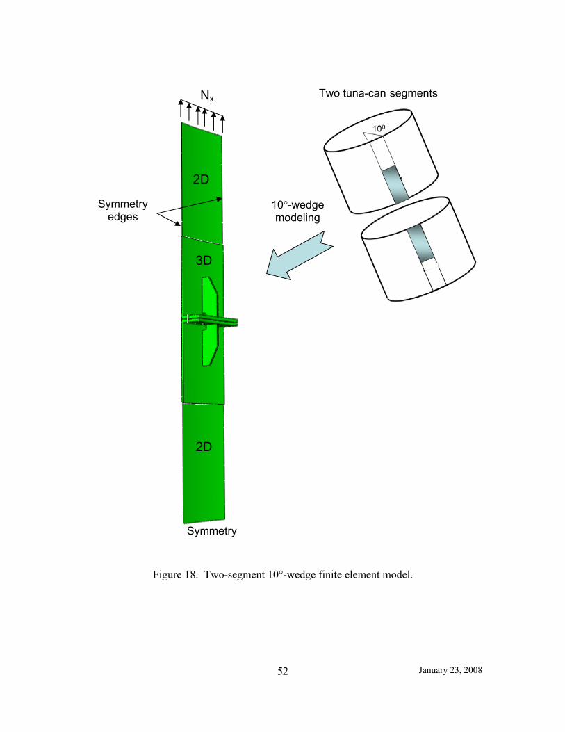
January 23, 2008 52

Figure 18. Two-segment 10 -wedge finite element model.

Two tuna-can segments

10 -wedgemodeling

3D

2D

2D

Nx

Symmetryedges

Symmetry

January 23, 2008 53

Figure 19. Three-dimensional local finite element modeling.

3D local modeling

3D

2D

2D

January 23, 2008 54

6.0

Figure 20. Analysis model and boundary conditions for the single-bolt joint configuration.

Strain Gages

Gap DisplacementGage

PaintedDIC Area

End DisplacementLVDT

Strain Gages

Gap DisplacementGage

PaintedDIC Area

End DisplacementLVDT

Figure 21. Photograph of the single-bolt joint test setup where DIC area is the Digital Image Correlation area and LVDT is a Linear Variable Differential Transducer (from

NASA Glenn).

Back Front

1

2

3

Fixed end

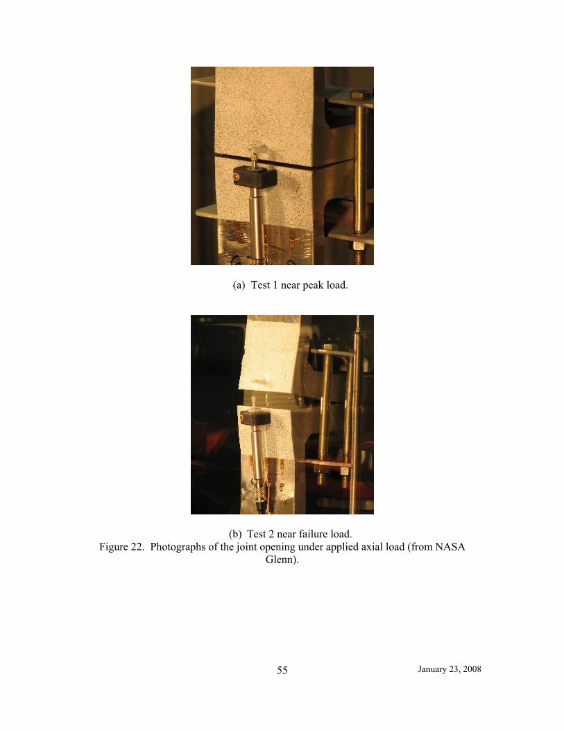
January 23, 2008 55

(a) Test 1 near peak load.

(b) Test 2 near failure load. Figure 22. Photographs of the joint opening under applied axial load (from NASA

Glenn).

January 23, 2008 56

Figure 23. Effect of mesh refinement on single-bolt joint structural response.

Design load 1.4 1600lb/in. 3.77in.=8,450 lb

End displacement , in.

Refined Mesh

Coarse Mesh

January 23, 2008 57

Figure 24. Bolt load as a function of applied end displacement for the baseline analysis case.

Figure 25. Reaction load as a function of applied end displacement for the baseline analysis case.

End displacement , in.

=0.046 in. at bolt yield

Design load 1.4 1600 lb/in. 3.77 in.=8,450 lb

Reaction force at incipient bolt yield, 30,000 lb

Bolt load at incipient bolt yield, 63,000 lb

Bolt load due to preload

=0.046 in.at bolt yield

End displacement , in.

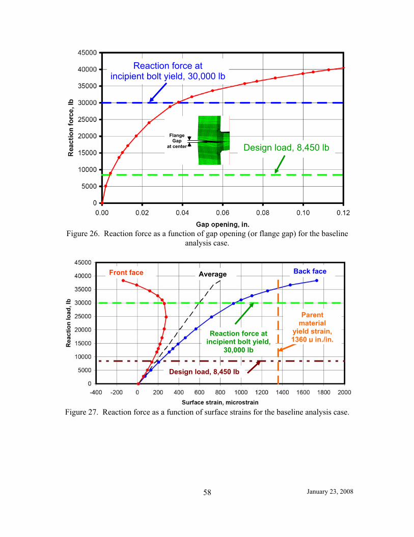
January 23, 2008 58

Figure 26. Reaction force as a function of gap opening (or flange gap) for the baseline analysis case.

Figure 27. Reaction force as a function of surface strains for the baseline analysis case.

Front face Back face Average

Design load, 8,450 lb

Reaction force at incipient bolt yield,

30,000 lb

Parentmaterial

yield strain, 1360 μ in./in.

Design load, 8,450 lb

Reaction force at incipient bolt yield, 30,000 lb

Flange Gap

at center

January 23, 2008 59

Figure 28. Reaction force as a function of front face lateral displacement for the baseline analysis case.

Design load, 8,450 lb

Reaction force at incipient bolt yield,

30,000 lb

Fixed end

–+

Lateraldisplacement

January 23, 2008 60

(a) At 8,450 lb (design load).

(b) At 30,000 lb (incipient bolt failure load).

(c) At 38,300 lb (final load level computed). Figure 29. Axial strain and von Mises stress distributions for different load levels for the

baseline analysis case (deformations scaled by 10).

0

10

20

30

>40

von Mises Stress, ksi

>-.004

-.002

.0

+.002

>+.004

22,in./in.

1

2

3

0

10

20

30

>40

von Mises Stress, ksi

>-.004

-.002

.0

+.002

>+.004

22,in./in.

1

2

3

0

10

20

30

>40

von Mises Stress, ksi

>-.004

-.002

.0

+.002

><+.00

22,in./in.

1

2

3

January 23, 2008 61

Figure 30. Effect of bolt preload torque on bolt load as a function of end displacement.

Figure 31. Effect of bolt preload torque on reaction load as a function of end displacement.

500 ft-lb

300 ft-lb

600 ft-lb

Design load 1.4 1600lb/in. 3.77in.=8,450 lb

End displacement , in.

200 ft-lb

400 ft-lb

500 ft-lb

400 ft-lb

600 ft-lb

Incipient boltyield

End displacement , in.

200 ft-lb

300 ft-lb

January 23, 2008 62

Figure 32. Effect of washer-bearing-surface size on bolt load as a function of end displacement.

Figure 33. Effect of washer-bearing-surface size on reaction load as a function of end displacement.

1/8” ring

1/4” ring

3/8” ring

Design load 1.4 1600lb/in. 3.77in.=8,450 lb

End displacement , in.

Incipientbolt yield

ysAbolt

1/8” ring

1/4” ring 3/8” ring

End displacement , in.

Bolt load due to preload torque

January 23, 2008 63

Figure 34. Effect of edge boundary conditions on bolt load as a function of end displacement (solid lines with symbols denote free long edges; dashed lines with symbols

denote symmetry conditions on long edges).

Figure 35. Effect of edge boundary conditions on reaction load as a function of end displacement (solid lines with symbols denote free long edges; dashed lines with symbols

denote symmetry conditions on long edges).

1/8” ring

1/4” ring

3/8” ring

Design load 1.4 1600lb/in. 3.77in.=8,450 lb

End displacement , in.

Incipientbolt yield

ysAbolt

1/8” ring

1/4” ring

3/8” ring

End displacement , in.

Bolt load due to preload torque

January 23, 2008 64

Figure 36. Effect of specimen length on reaction load as a function of end displacement.

Figure 37. Distribution of von Mises stress at 0.02 inches of end displacement for different grip lengths.

Lgrip=0

Fixed end

30 in.

Lgrip

Lgrip

Lgrip=3 in.

Lgrip=6 in.

Design load 1.4 1600lb/in. 3.77in.=8,450 lb

End displacement , in.

Lgrip=0

Fixed end

30 in.

Lgrip

Lgrip Lgrip=3 in. Lgrip=6 in.

ys

0

½ ys

von Mises Stress

January 23, 2008 65

Figure 38. Reaction force as a function of end displacement test-analysis correlation for the single-bolt joint tests (test data from NASA Glenn).

Test 1

Test 2

Width of bearing surface ring

3/8-inch

1/4-inch1/8-inch

End displacement , in.

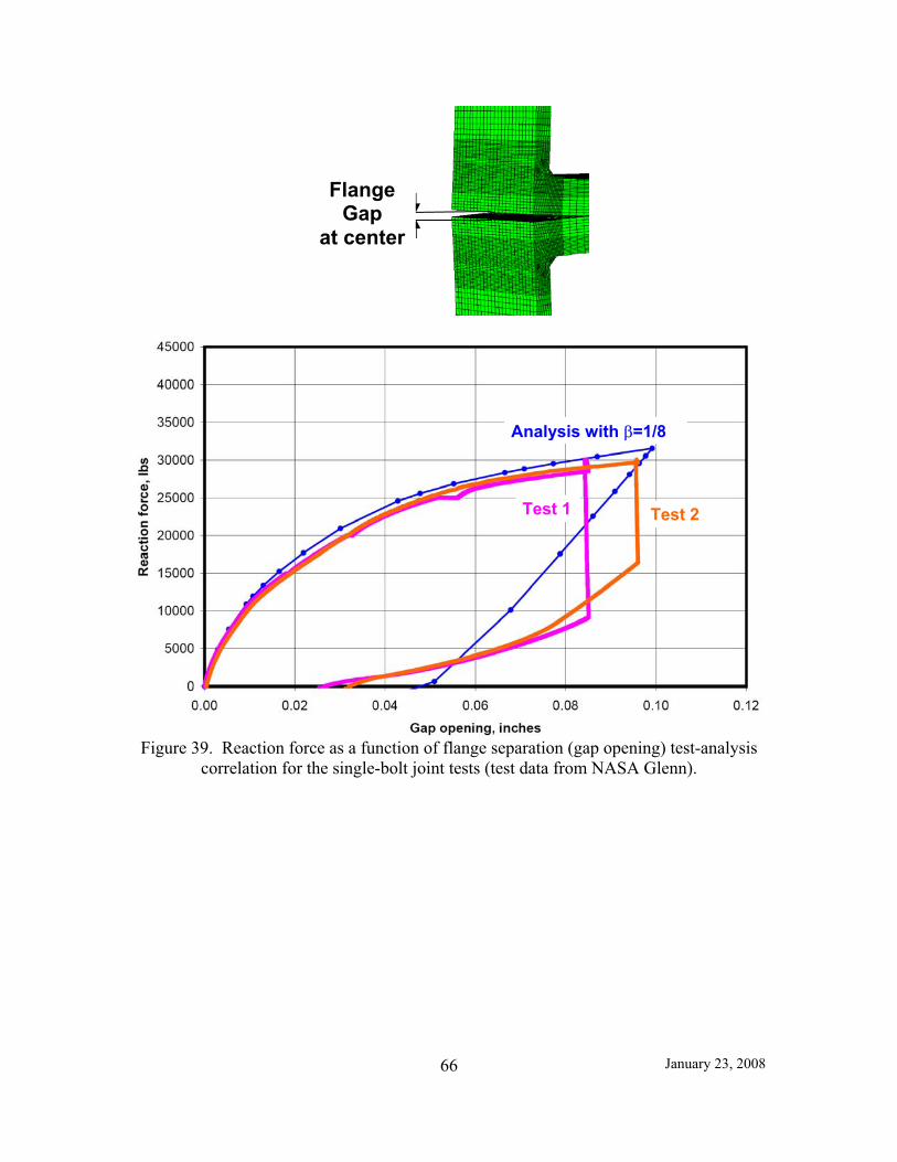
January 23, 2008 66

Figure 39. Reaction force as a function of flange separation (gap opening) test-analysis correlation for the single-bolt joint tests (test data from NASA Glenn).

Test 1 Test 2

Analysis with =1/8

FlangeGap

at center

January 23, 2008 67

Figure 40. Surface strain test-analysis correlation for single-bolt joint Test 1 (test data from NASA Glenn).

Figure 41. Surface strain test-analysis correlation for single-bolt joint Test 2 (test data from NASA Glenn).

Front face Back face Average

Test 2

Analysis

Test 2

Analysis Analysis

Design load, 8,450 lb

Reaction force atIncipient bolt yield,

30,000 lb

Test 2

Front face Back face Average

Test 1

Analysis

Test 1

Analysis Analysis

Design load, 8,450 lb

Reaction force at Incipient bolt yield,

30,000 lb

Test 1

January 23, 2008 68

Figure 42. Effects of geometric and material nonlinearities on the structural response of the two-segment 10 -wedge model – results essentially indistinguishable.

January 23, 2008 69

Figure 43. Distribution of the von Mises stress for 2,240 lb/in. axial running load.

Figure 44. Distribution of the von Mises stress across the top of the fillet weld for 2,240 lb/in. axial running load ( ys=40.76 ksi).

von Mises Stress, ksi

ys=40.76

0

½ ys

vm=12 ksi

vm=14.6 ksi

=10=0

von Mises Stress

ys

0

½ ys

14.6 ksi max. at top of fillet weld

January 23, 2008 70

(a) Plane through center of first hole ( =2 ).

(b) Plane through center of second hole ( =4 ).

(c) Plane through center of gusset ( =5 ).Figure 45. Distribution of the von Mises stress on various vertical cuts through the

analysis model for 2,240 lb/in. axial running load ( ys=40.76 ksi).

ys

0

½ ys

January 23, 2008 71

Figure 46. Effect of load level on the von Mises stress distribution ( ys=40.76 ksi).

Figure 47. Relationship between the single-bolt model and the 10 -wedge models.

lb/in.600,1~ maxxN

max~4.1 xN

max~4.1 xN

ys

0

½ ys

After Preload max~25.1 xN

max~0.2 xN max~0.4 xN

Single Bolt Flat Sample

Two Segments, No Gussets

Two Segments, Two Gussets

Does the single-bolt case reflect the shell response?

How do the gussets affect the response?

Does extreme “clocking” of the gussets affect the response?

Two Segments, One Gusset

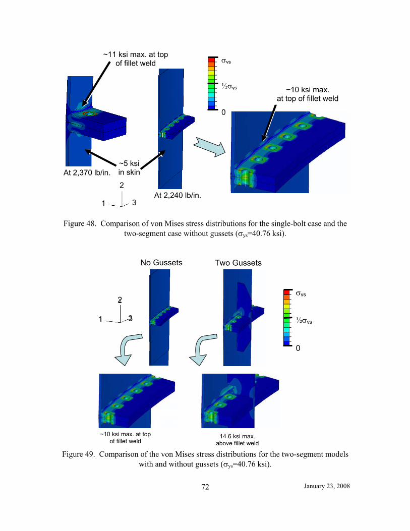
January 23, 2008 72

Figure 48. Comparison of von Mises stress distributions for the single-bolt case and the two-segment case without gussets ( ys=40.76 ksi).

Figure 49. Comparison of the von Mises stress distributions for the two-segment models with and without gussets ( ys=40.76 ksi).

1

2

3

~5 ksiin skin

~11 ksi max. at top of fillet weld

~10 ksi max. at top of fillet weld

ys

0

½ ys

At 2,240 lb/in.

At 2,370 lb/in.

1

2

3

~10 ksi max. at top of fillet weld

14.6 ksi max. above fillet weld

No Gussets Two Gussets

ys

0

½ ys

January 23, 2008 73

Figure 50. Comparison of the von Mises stress distributions for the two-segment models with and without gusset clocking ( ys=40.76 ksi).

Figure 51. Axial stress at the top of the fillet weld as a function of circumferential position for a axial running load of 2,240 lb/in.

1

2

3

14.6 ksi max. above fillet weld

~14 ksi max. above fillet weld

No “Clocking” Extreme “Clocking”

ys

0

½ ys

January 23, 2008 74

Figure 52. Distribution of the axial stress for a axial running load of 2,240 lb/in.

Figure 53. Distribution of the axial strain for a axial running load of 2,240 lb/in.

axial, ksi Axial

+14.6

0

-39.6

axial=11.9

axial=14.3

axial, in./in.

Axial+440

0

-880

January 23, 2008 75

Figure 54. Distribution of the radial stress for a axial running load of 2,240 lb/in.

Figure 55. Distribution of the radial strain for a axial running load of 2,240 lb/in.

radial, ksi

Radial

+15.6

0

-29.8

radial=3.6

radial=4.6

radial, in./in.

Radial

+620

0

-920

January 23, 2008 76

Figure 56. Distribution of the hoop stress for a axial running load of 2,240 lb/in.

Figure 57. Distribution of the hoop strain for a axial running load of 2,240 lb/in.

hoop, ksi

Hoop

+14.6

0

-19.1

hoop=4.8 ksi

hoop=4.8 ksi

hoop, in./in.

Hoop

+500

0

-340

January 23, 2008 77

Figure 58. Loading-unloading sequence for residual plastic strain assessment.

Figure 59. Effect of loading, unloading, and reloading on the structural response.

First yield (2.58)

January 23, 2008 78

Figure 60. Equivalent plastic strain distributions for selected load levels.

Figure 61. Mesh modifications to accommodate the stitched weld pattern.

At bolt preload of 400 ft-lb

Load to Nx=Nx0=1,600 lb/in.

Continue loading to Nx=4Nx0

Unload to Nx=0

Continue loading to Nx=1.4Nx0

Reload to Nx=1.4Nx0

0

0.0025

0.0050

Equivalent PlasticStrain

Baseline Model – Continuous Weld Refined Model – Stitched Weld

Freeregions

Weldedregions

Weldedregions

January 23, 2008 79

Figure 62. Mesh modifications to the butt weld region to accommodate the fracture mechanics analysis.

Figure 63. Circumferential mesh refinement in the vicinity of the gusset mouse hole to accommodate the fracture mechanics analysis.

Baseline Model Refined Model

Uniform mesh over butt weld region

Through-thicknesscrack needs a plane

Original mesh over butt weld

region for different property values

Baseline Model Refined Model

IntendedThrough-thickness

Crack Location

January 23, 2008 80

Figure 64. Axial stress distribution as a function of circumferential location on the inside surface at the top of the fillet weld for a 2,240 lb/in. axial running load.

Figure 65. Comparison of the axial stress distributions for the baseline and refined models using a 2,240 lb/in. axial running load.

Baseline Model Refined Modelaxial, ksi

Axial

+14.6

0

-39.6

January 23, 2008 81

Figure 66. Axial stress distribution along the shell axis on the shell inside surface near the gusset for a 2,240 lb/in. axial running load.

Figure 67. Axial stress distribution through the shell wall thickness at the top of the fillet weld near the gusset for a 2,240 lb/in. axial running load.

January 23, 2008 82

Figure 68. Comparison of the von Mises stress distributions for the baseline and refined models using a 2,240 lb/in. axial running load.

Figure 69. Comparison of the von Mises stress distributions across the top of the fillet weld for the baseline and refined models using a 2,240 lb/in. axial running load.

Baseline Model Refined Model von Mises Stress, ksi

ys=40.76

0

½ ysvm=14.6 ksi vm=15.5 ksi

von Mises Stress, psi

ys

0

½ ys

14.6 ksi max. at top of fillet weld

Baseline Model Refined Model

15.5 ksi max. at top of fillet weld

January 23, 2008 83

Figure 70. Axial stress distributions on the gusset for the continuous “full-surface” shell-to-gusset weld assumption.

Figure 71. Comparison of the axial stress distributions for the continuous “full-surface”and “edge-only” shell-to-gusset weld assumption.

0

4

8

12

<16

Axial Stress, ksi

0

10

20

30

<40

Axial Stress, ksi

Gusset-to-shell interfaceregion

Maximum axial stress = 16.5 ksi

Axial stress contours with narrow stress

0

4

8

12

<16

AxialStress, ksi

Continuous Full-Surface

Continuous Edge-Only

January 23, 2008 84

Figure 72. Comparison of the axial stress distributions for the stitched “full-surface” and “edge-only” shell-to-gusset weld assumption.

Figure 73. Location of the inserted through-the-thickness crack of length 2a along the top of the fillet weld centered about the gusset for the refined model.

0

4

8

12

<16

AxialStress, ksi

StitchedFull-Surface

StitchedEdge-Only

e=0.05

InsertedThrough-thicknessCrack of length 2a

January 23, 2008 85

i

i-1

i+1X, u

Z, w

Y, v

aa

bI

bI+1

Ai

j+1

k+1j

k j-1

k-1

I

I+1

K

J

K+1

J+1

i

i-1

i+1X, u

Z, w

Y, v

aa

bI

bI+1bI+1

Ai

j+1

k+1j

k j-1

k-1

I

I+1

K

J

K+1

J+1

Figure 74. VCCT computational scheme for three-dimensional 8-node brick elements.

Figure 75. Strain energy release rates through the shell thickness for an applied axial running load of 2,240 lb/in. and an initial through crack of length 2a equal to 1 inch.

January 23, 2008 86

Figure 76. Close-up view of crack opening from the refined model simulation with displacements scaled by 150.

Figure 77. Local finite element mesh modification to verify VCCT prediction.

e=0.0833 in.

InsertedThrough-thicknessCrack of length 2a

Bolt Hole

FlangeSeparation

CrackOpening

January 23, 2008 87

Figure 78. Variation of the Mode I strain energy release rate through the shell thickness using two different element edge lengths for an applied axial running load of 2,240 lb/in.

and an initial through crack of length 2a equal to 1 inch.

Figure 79. Variation of the Mode I stress intensity factor through the shell thickness for an applied axial running load of 2,240 lb/in. and an initial through crack of length 2a

equal to 1 inch.

January 23, 2008 88

Figure 80. Sketch showing locations within an element of the stress recovery locations reported in Table 3.

January 23, 2008 89

Figure 81. Segment mating test using pathfinder USS shell segments (NASA Glenn photo).

PF-1

PF-2

GSE

January 23, 2008 90

Figu

re 8

2. F

lang

e m

atin

g su

rfac

e ga

p m

easu

rem

ents

from

PF1

/PF2

mat

ing.

January 23, 2008 91

Figu

re 8

3. B

asic

step

s in

the

shim

min

g pr

oced

ure

(see

Ref

. 26)

.

January 23, 2008 92

Figu

re 8

4. F

lang

e m

atin

g su

rfac

e ga

p re

mai

ning

afte

r shi

mm

ing

in 1

0-m

il in

crem

ents

.

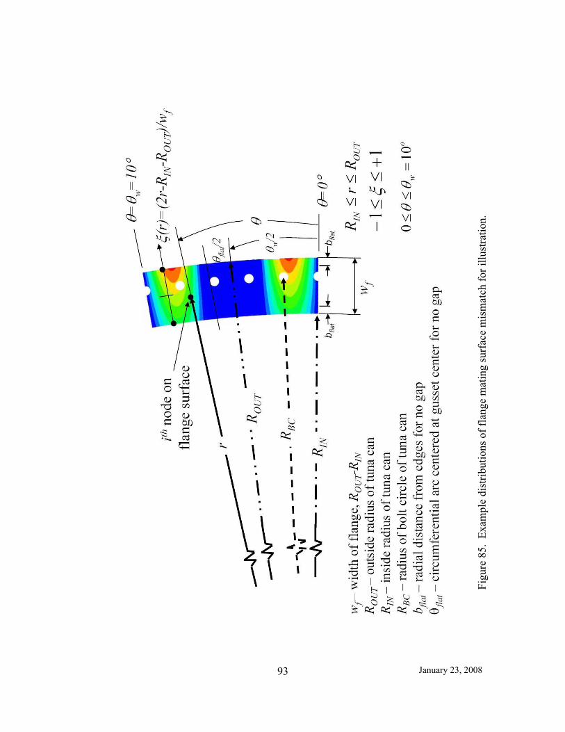
January 23, 2008 93

Figu

re 8

5. E

xam

ple

dist

ribut

ions

of f

lang

e m

atin

g su

rfac

e m

ism

atch

for i

llust

ratio

n.

January 23, 2008 94

Figu

re 8

6. F

lang

e m

atin

g su

rfac

e m

ism

atch

sum

mar

y.

January 23, 2008 95

Figu

re 8

7. E

xam

ple

dist

ribut

ions

of f

lang

e m

atin

g su

rfac

e m

ism

atch

for i

llust

ratio

n w

here

OD

is

the

oute

r dia

met

er.

January 23, 2008 96

Figu

re 8

8. N

ine

flang

e m

atin

g su

rfac

e m

ism

atch

dis

tribu

tions

ana

lyze

d w

here

O

D is

the

oute

r dia

met

er a

nd ID

is th

e in

ner d

iam

eter

.

(a)

Axi

sym

met

ric d

istri

butio

ns.

(b)

Perio

dic

dist

ribut

ions

with

edg

e ga

ps.

(c)

Perio

dic

dist

ribut

ions

with

no

edge

gap

s.

January 23, 2008 97

Figu

re 8

9. A

xial

stre

ss a

nd re

mai

ning

gap

pat

tern

afte

r app

licat

ion

of 3

6,50

0-lb

bo

lt pr

eloa

d fo

rce

for t

he a

xisy

mm

etric

dis

tribu

tions

with

10-

mil

peak

gap

s.

(a)

Free

-sta

te fl

ange

surf

ace

mis

mat

ch d

istri

butio

ns.

(b)

Mis

mat

ch d

istri

butio

ns a

fter a

pply

ing

bolt

prel

oad

forc

e.

January 23, 2008 98

Figu

re 9

0. A

xial

stre

ss a

nd re

mai

ning

gap

pat

tern

afte

r app

licat

ion

of 3

6,50

0-lb

bol

t pre

load

fo

rce

for t

he p

erio

dic

with

edg

e ga

ps d

istri

butio

ns w

ith 1

0-m

il pe

ak g

aps.

(a)

Free

-sta

te fl

ange

surf

ace

mis

mat

ch d

istri

butio

ns.

(b)

Mis

mat

ch d

istri

butio

ns a

fter a

pply

ing

bolt

prel

oad

forc

e.

January 23, 2008 99

Figu

re 9

1. A

xial

stre

ss a

nd re

mai

ning

gap

pat

tern

afte

r app

licat

ion

of 3

6,50

0-lb

bol

t pr

eloa

d fo

rce

for t

he p

erio

dic

dist

ribut

ions

with

no

edge

gap

s and

10-

mil

peak

gap

s.

(a)

Free

-sta

te fl

ange

surf

ace

mis

mat

ch d

istri

butio

ns.

(b)

Mis

mat

ch d

istri

butio

ns a

fter a

pply

ing

bolt

prel

oad

forc

e.

January 23, 2008 100

Figu

re 9

2. F

our

flang

e su

rfac

e m

ism

atch

cas

es re

sulti

ng in

hig

h ax

ial t

ensi

le st

ress

leve

l.

January 23, 2008 101

Figu

re 9

3. E

ffec

t of p

eak

gap

size

on

bolt

prel

oad

resp

onse

for t

he fo

ur w

orst

-cas

e m

ism

atch

dis

tribu

tions

.

(a)

Free

-sta

te fl

ange

surf

ace

mis

mat

ch d

istri

butio

ns.

(b)

Mis

mat

ch d

istri

butio

ns w

ith 1

0-m

il pe

ak g

ap a

fter a

pply

ing

bolt

prel

oad

forc

e.

(c)

Mis

mat

ch d

istri

butio

ns w

ith 5

-mil

peak

gap

afte

r app

lyin

g bo

lt pr

eloa

d fo

rce.

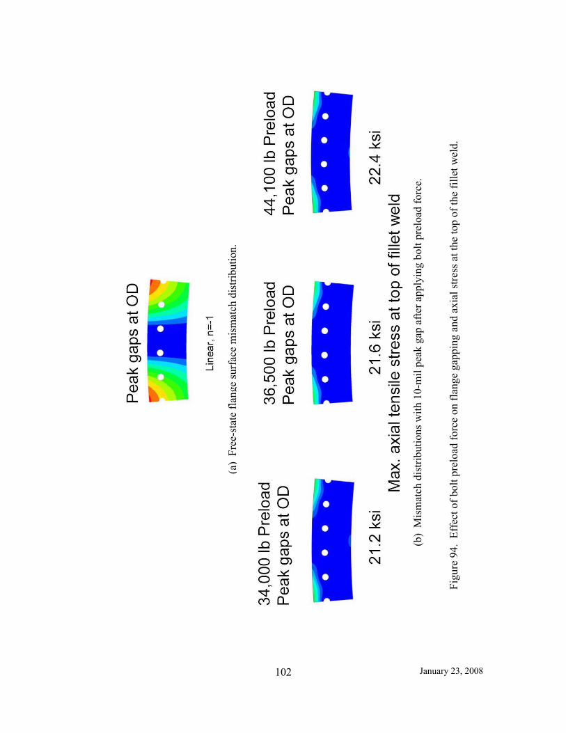
January 23, 2008 102

Figu

re 9

4. E

ffec

t of b

olt p

relo

ad fo

rce

on fl

ange

gap

ping

and

axi

al st

ress

at t

he to

p of

the

fille

t wel

d.

(a)

Free

-sta

te fl

ange

surf

ace

mis

mat

ch d

istri

butio

n.

(b)

Mis

mat

ch d

istri

butio

ns w

ith 1

0-m

il pe

ak g

ap a

fter a

pply

ing

bolt

prel

oad

forc

e.

January 23, 2008 103

Figure 95. Maximum axial tensile stress at the top of the fillet weld after 36,500-lb bolt preload force for different mismatch patterns and magnitudes.

Figure 96. Maximum OD gap after 36,500-lb bolt preload force for different mismatch patterns and magnitudes.

January 23, 2008 104

Figure 97. Axial stress distributions after application of bolt preload force of 36,500 lb.

(d) Linear, n=-1 distribution with peak gap of 10 mils.

(a) Perfect case.

(c) Linear, n=3 distribution with peak gap of 10 mils.

>22

-22

-45

0

Axial stress, ksi

Axial

(b) Sine, n=0 distribution with peak gap of 10 mils.

January 23, 2008 105

Figure 98. Axial stress distributions after application of both bolt preload force of 36,500 lb and design axial running load of 1,600 lb/in.

(d) Linear, n=-1 distribution with peak gap of 10 mils.

(c) Linear, n=3 distribution with peak gap of 10 mils.

(a) Perfect case.

>22

-22

-45

0

Axial stress, ksi

Axial

(b) Sine, n=0 distribution with peak gap of 10 mils.

REPORT DOCUMENTATION PAGE Form Approved

OMB No. 0704-0188 The public reporting burden for this collection of information is estimated to average 1 hour per response, including the time for reviewing instructions, searching existingdata sources, gathering and maintaining the data needed, and completing and reviewing the collection of information. Send comments regarding this burden estimate or any other aspect of this collection of information, including suggestions for reducing this burden, to Department of Defense, Washington Headquarters Services, Directoratefor Information Operations and Reports (0704-0188), 1215 Jefferson Davis Highway, Suite 1204, Arlington, VA 22202-4302. Respondents should be aware thatnotwithstanding any other provision of law, no person shall be subject to any penalty for failing to comply with a collection of information if it does not display a currentlyvalid OMB control number. PLEASE DO NOT RETURN YOUR FORM TO THE ABOVE ADDRESS.

1. REPORT DATE (DD-MM-YYYY) 2. REPORT TYPE 3. DATES COVERED (From - To)

4. TITLE AND SUBTITLE 5a. CONTRACT NUMBER

5b. GRANT NUMBER

5c. PROGRAM ELEMENT NUMBER

6. AUTHOR(S) 5d. PROJECT NUMBER

5e. TASK NUMBER

5f. WORK UNIT NUMBER

7. PERFORMING ORGANIZATION NAME(S) AND ADDRESS(ES) 8. PERFORMING ORGANIZATIONREPORT NUMBER

9. SPONSORING/MONITORING AGENCY NAME(S) AND ADDRESS(ES) 10. SPONSORING/MONITOR'S ACRONYM(S)

11. SPONSORING/MONITORINGREPORT NUMBER

12. DISTRIBUTION/AVAILABILITY STATEMENT

13. SUPPLEMENTARY NOTES

14. ABSTRACT

15. SUBJECT TERMS

16. SECURITY CLASSIFICATION OF: 17. LIMITATION OF

ABSTRACT18. NUMBER

OFPAGES

19a. NAME OF RESPONSIBLE PERSON

a. REPORT b. ABSTRACT c. THIS PAGE19b. TELEPHONE NUMBER (Include area code)

Standard Form 298 (Rev. 8-98)Prescribed by ANSI Std. Z39-18

01-08-2008 Technical Memorandum December 2006 - January 2008

Ares I-X Upper Stage Simulator Structural Analyses Supporting the NESCCritical Initial Flaw Size Assessment

510505.03.07.01.11

Knight Jr., Norman F., Phillips, Dawn R., and Raju, Ivatury S.

NASA Engineering and Safety CenterLangley Research CenterHampton, VA 23681-2199

L-19514 NESC-RP-08-09/06-081-E

National Aeronautics and Space AdministrationWashington, DC 20546-0001

NASA

NASA/TM-2008-215336

Unclassified-Unlimited/Publicly AvailableSubject Category 39 - Structural Mechanics

The structural analyses described in the present report were performed in support of the NASA Engineering and Safety Center(NESC) Critical Initial Flaw Size (CIFS) assessment for the ARES I-X Upper Stage Simulator (USS) common shell segment. Thestructural analysis effort for the NESC assessment had three thrusts: shell buckling analyses, detailed stress analyses of thesingle-bolt joint test; and stress analyses of two-segment 10 degree-wedge models for the peak axial tensile running load.Elasto-plastic, large-deformation simulations were performed. Stress analysis results indicated that the stress levels were wellbelow the material yield stress for the bounding axial tensile design load. This report also summarizes the analyses and resultsfrom parametric studies on modeling the shell-to-gusset weld, flange-surface mismatch, bolt preload, and washer-bearing-surfacemodeling. These analyses models were used to generate the stress levels specified for the fatigue crack growth assessment usingthe design load with a factor of safety.

NESC, CIFS, ARES I-X USS, analyses

UU UU UU UU 110

STI Help Desk (email: help@sti.nasa.gov)

(301) 621-0390