APPLICATIONS OF CLICKSTREAM INFORMATION IN ...
154
APPLICATIONS OF CLICKSTREAM INFORMATION IN ESTIMATING ONLINE USER BEHAVIOR A Dissertation Presented to The Academic Faculty by Susan Lisa Hotle In Partial Fulfillment of the Requirements for the Degree Doctor of Philosophy in the School of Civil and Environmental Engineering Georgia Institute of Technology May, 2015 Copyright © Susan L. Hotle 2015
-
Upload
khangminh22 -
Category
Documents
-
view
2 -
download
0
Transcript of APPLICATIONS OF CLICKSTREAM INFORMATION IN ...
APPLICATIONS OF CLICKSTREAM INFORMATION IN ESTIMATING
ONLINE USER BEHAVIOR
A Dissertation
Presented to
The Academic Faculty
by
Susan Lisa Hotle
In Partial Fulfillment
of the Requirements for the Degree
Doctor of Philosophy in the
School of Civil and Environmental Engineering
Georgia Institute of Technology
May, 2015
Copyright © Susan L. Hotle 2015
APPLICATIONS OF CLICKSTREAM INFORMATION IN ESTIMATING
ONLINE USER BEHAVIOR
Approved by:
Dr. Laurie A. Garrow, Advisor
School of Civil and Environmental Engineering
Georgia Institute of Technology
Dr. Jeffrey P. Newman
Independent Consultant
Chicago, IL
Dr. Matthew J. Higgins
Scheller College of Business
Georgia Institute of Technology
Dr. Ram M. Pendyala
School of Civil and Environmental Engineering
Georgia Institute of Technology
Dr. Patricia L. Mokhtarian
School of Civil and Environmental Engineering
Georgia Institute of Technology
Date Approved: January 5, 2015
iii
ACKNOWLEDGEMENTS
I would like to thank the many people that have supported me during my time at Georgia
Tech. I am especially grateful to my adviser Dr. Laurie Garrow, who not only made research
enjoyable, but also was an invaluable resource during the writing of this dissertation. It was
actually through my undergraduate research experience with her that I realized pursuing a PhD
was even possible. I would also like to thank my committee members, Dr. Matthew Higgins for
his help and expertise with the econometric analyses and Dr. Patricia Mokhtarian, Dr. Jeffrey
Newman, and Dr. Ram Pendyala for their interest in my work.
I am especially grateful to my co-workers in Dr. Garrow’s research group. I would like
to thank Brittany Luken for mentoring me in my initial stages as a researcher and for her
feedback on my research. I would like to thank Stacey Mumbower for giving advice on the
methods and Stata® codes. I would also like to thank the National Science Foundation’s
Graduate Research Fellowship Program and the Airport Cooperative Research Program (ACRP)
for funding part of this research as well as the travel allowance through the Dwight D.
Eisenhower Graduate Transportation Fellowship Program. I really appreciate the feedback given
by the ACRP program officer Larry Goldstein and mentors Eric Amel, Richard Golaszewski,
Eric Ford, Kevin Healy, and Michael Tretheway.
I would like to express appreciation to my family. To my parents, Tim and Nancy Hotle
and my siblings Sarah Johnston, David Hotle, and Anna Hotle for their continuous love, support,
and encouragement as well as providing me with much needed breaks from research.
Lastly, I would like to thank my Lord and Savior, Jesus Christ, for all of the opportunities
He has given me over the past 8 years at Georgia Tech. I could not have done this without Him.
iv
TABLE OF CONTENTS
ACKNOWLEDGEMENTS ........................................................................................................... iii
LIST OF TABLES ......................................................................................................................... vi
LIST OF FIGURES ...................................................................................................................... vii
LIST OF ABBREVIATIONS ...................................................................................................... viii
SUMMARY ................................................................................................................................... ix
CHAPTER 1 Introduction.............................................................................................................. 1 1.1 Background and Motivation ........................................................................................... 1
1.1.1 Airline Industry ......................................................................................................... 2
1.1.2 Educational Studies ................................................................................................... 7 1.2 Major Contributions ........................................................................................................ 8
1.3 Dissertation Structure ..................................................................................................... 9 1.4 References ..................................................................................................................... 10
CHAPTER 2 Competitor Pricing and Multi-Airport Choice ...................................................... 13 2.1 Abstract ......................................................................................................................... 13
2.2 Introduction ................................................................................................................... 13 2.3 Literature on Multi-Airport Choice .............................................................................. 15
2.4 Data ............................................................................................................................... 17 2.4.1 Clickstream Data ..................................................................................................... 17
2.4.2 Pricing Data ............................................................................................................ 23 2.5 Methodology ................................................................................................................. 26
2.5.1 Count Model ........................................................................................................... 26
2.5.2 Fare Variables ......................................................................................................... 26 2.5.3 Other Variables Used in the Analysis ..................................................................... 28
2.6 Results ........................................................................................................................... 28 2.7 Public Policy Implications ............................................................................................ 30 2.8 Limitations and Future Research .................................................................................. 31 2.9 Acknowledgments ........................................................................................................ 32 2.10 References ..................................................................................................................... 33
CHAPTER 3 The Impact of Advanced Purchase Deadlines on Customer Behavior ................. 35 3.1 Abstract ......................................................................................................................... 35 3.2 Introduction ................................................................................................................... 36
3.3 Literature Review ......................................................................................................... 38 3.4 Data ............................................................................................................................... 40
3.4.1 OTA Clickstream Data ........................................................................................... 43
3.4.2 QL2 Software and Southwest Pricing Datasets ...................................................... 45
v
3.4.3 Representiveness of Database ................................................................................. 49
3.5 Methodology ................................................................................................................. 50 3.5.1 Price Endogeneity ................................................................................................... 51 3.5.2 Estimating Parameters for Days from Departure Variables ................................... 55
3.6 Results ........................................................................................................................... 56 3.6.1 Descriptive Statistics for Lowest Fares................................................................... 56 3.6.2 Descriptive Statistics for Number of Searches ....................................................... 61 3.6.3 Descriptive Statistics for Number of Purchases...................................................... 63 3.6.4 Model Results ......................................................................................................... 64
3.7 Validation ...................................................................................................................... 70 3.8 Discussion ..................................................................................................................... 71 3.9 Conclusions and Future Research Directions ............................................................... 73 3.10 Acknowledgments ........................................................................................................ 74
3.11 References ..................................................................................................................... 74
CHAPTER 4 Classroom Attitudes in Traditional, Micro-Flipped, and Flipped Classrooms ...... 80 4.1 Abstract ......................................................................................................................... 80 4.2 Introduction ................................................................................................................... 81
4.3 Study 1: Methodology .................................................................................................. 86 4.3.1 Design ..................................................................................................................... 86
4.3.2 Data Collection ....................................................................................................... 87 4.3.3 Subjects ................................................................................................................... 92 4.3.4 Results ..................................................................................................................... 93
4.3.5 Survey Results ...................................................................................................... 103 4.4 Study 2: Methodology ................................................................................................ 108
4.4.1 Design ................................................................................................................... 108
4.4.2 Data Collection ..................................................................................................... 109
4.4.3 Subjects ................................................................................................................. 112 4.4.4 Results ................................................................................................................... 112
4.4.5 Survey Results ...................................................................................................... 122 4.5 Study Limitations ........................................................................................................ 125 4.6 Summary ..................................................................................................................... 127
4.7 Acknowledgments ...................................................................................................... 129 4.8 References ................................................................................................................... 129
CHAPTER 5 Conclusions and Future Research ........................................................................ 132 5.1 Major Conclusions and Directions for Future Research ............................................. 132
5.1.1 Multi-Airport Choice ............................................................................................ 132
5.1.2 Advance Purchase Deadlines ................................................................................ 133 5.1.3 Flipped Classroom ................................................................................................ 135
5.2 Concluding Thoughts .................................................................................................. 137
APPENDIX ................................................................................................................................. 140
vi
LIST OF TABLES
Table 1.1A: Site-centric behavioral studies in airlines ................................................................... 5 Table 2.1: Defining pseudo-IP, pseudo-visit, and pseudo-page numbers..................................... 19 Table 2.2: Characteristics of markets included in analysis ........................................................... 21 Table 2.3: Example of calculations of fare variables used in analysis ......................................... 27
Table 2.4: List of variables used to predict search ........................................................................ 28 Table 2.5: Truncated negative binomial model results predicting number of searches ................ 30 Table 3.6: Variable definitions and descriptions .......................................................................... 42 Table 3.7: Descriptive statistics for lowest available one-day round-trip fare weighted by number
of searches ...................................................................................................................... 48
Table 3.8: Descriptive statistics for lowest one-day round-trip fare weighted by number of
purchases ........................................................................................................................ 48
Table 3.9: Representativeness of OTA markets ........................................................................... 50 Table 3.10: How often the lowest offered nonstop one-day round trip fare changes ................... 60
Table 3.11: Search model results .................................................................................................. 65 Table 3.12: Leisure search results for DFD coefficients .............................................................. 66 Table 3.13: Purchase model results .............................................................................................. 68
Table 3.14: Leisure purchase results for DFD coefficients .......................................................... 69 Table 4.1: Definition of study 1 variables .................................................................................... 91
Table 4.2: Summary statistics of non-ISyE students in the traditional and flipped sections ........ 93 Table 4.3: Average scores on the two quizzes .............................................................................. 95 Table 4.4: Correlations in traditional section ................................................................................ 99
Table 4.5: Correlations in flipped section ................................................................................... 100
Table 4.6: Percent of study participants per section attending office hours ............................... 101 Table 4.7: Number of student views per video ........................................................................... 102 Table 4.8: Survey results from spring semester .......................................................................... 107
Table 4.9: Definition of summer study variables........................................................................ 111 Table 4.10: Summary statistics of all students in the summer class ........................................... 112 Table 4.11: Average scores on the quizzes ................................................................................. 114
Table 4.12: Correlations in traditional module ........................................................................... 116 Table 4.13: Correlations in micro-flipped module ..................................................................... 117 Table 4.14: Correlations in flipped module ................................................................................ 118 Table 4.15: Number of student views per video ......................................................................... 121 Table 4.16: Length of video viewing .......................................................................................... 122
Table 4.17: Survey results from summer session ....................................................................... 124
Table 4.18: Students’ responses to the pros and cons of each classroom type ........................... 125
Table A1: Variance-covariance matrix for searches ................................................................... 140 Table A2: Variance-covariance matrix for purchases ................................................................ 141 Table A3: List of business and leisure markets included in the study ........................................ 142 Table A4: Airport codes and large hub designation ................................................................... 143
vii
LIST OF FIGURES
Figure 1.1: Yields trends versus internet penetration (Brunger, 2010) ........................................... 3 Figure 1.2: Average fare paid for clearly leisure customers only (Brunger, 2010) ........................ 3 Figure 2.1: Number of visits as a function of days from departure .............................................. 23 Figure 2.2: Representative of RT fares available throughout the booking horizon ...................... 25
Figure 3.1: Length of stay using ARC information ...................................................................... 44 Figure 3.2: How the lowest offered fare evolves in leisure and business markets ....................... 58 Figure 3.3: Average number of searches per market .................................................................... 62 Figure 3.4: Average number of purchases per market .................................................................. 63 Figure 3.5: Validation of search behavior using a major carrier’s clickstream data .................... 71
Figure 4.1: Frequency of the number of videos watched by students ........................................ 102 Figure 4.2: Number of 7 videos viewed by each person in the micro-flipped module ............... 120
Figure 4.3: Number of 4 videos viewed by each person in the flipped module ......................... 120
viii
LIST OF ABBREVIATIONS
2SLS Two-Stage Least Squares
ARC Airlines Reporting Corporation
ATA American Trans Air
BLP Berry, Levinsohn, Pakes
BTS Bureau of Transportation Statistics
CV Coefficient of Variation
DB1B Origin and Destination Data Bank 1B
DFD Days from Departure
FAA Federal Aviation Administration
GMM Generalized Methods of Moments
GPA Grade Point Average
IPR Interactive Price Response
IRR Incidence Rate Ratios
IV Instrumental Variable
LCC Low-Cost Carrier
MOOC Massive Open Online Course
OLS Ordinary Least Squares
OW One-way
OTA Online Travel Agency
RT Round-Trip
Note: Airport codes are listed in Table A4.
ix
SUMMARY
The internet has become a more prominent part of people’s lives. In the past, the internet was
used mainly for basic functions, such as email and news. Today, internet usage is a common
everyday occurrence due to its increased accessibility and its additional roles – for example in
social media, shopping channels, and banking. This shift of activity to the internet has resulted
in many benefits to the user, but at the same time the internet has provided a new opportunity for
researchers. Specifically, researchers can now use clickstream data (i.e., information on each
link clicked on by the user) to analyze the actual decision-making process and behavior of a
significant portion of the population.
This dissertation focuses on using this data in two areas of interest. It contains three
studies, each written in journal format. The first two are based on the airline industry and the last
is on the field of education. Therefore, the rest of this chapter will focus on the usage and
impacts of the internet on the airline industry and the field of education.
The first study investigates if airline passengers departing from or arriving to a multi-
airport city actually consider itineraries at the airports not considered to be their preferred airport.
It was based on search data provided by a single U.S. major carrier for 10 directional markets.
Using a truncated negative binomial model to predict the number of searches based on the
competitors’ lowest-offered fares (from the same and nearby airports), it was found that
customers do consider fares at multiple airports in multi-airport cities. However, other trip
characteristics, typically linked to whether a customer is considered business or leisure, were
found to have a larger impact on customer behavior than offered fares at competing airports.
x
The second study evaluates airline customer search and purchase behavior near the
advance purchase deadlines. These advance purchase deadlines occur in the last 30 days of the
booking horizon and are typically accompanied with fare increases. Search and Purchase
demand models were constructed using instrumented two-stage least squares (2SLS) models
with valid instruments to correct for endogeneity. Results show that search and purchase
behaviors vary by search day of week, days from departure, lowest offered fares, variation in
lowest offered fares across competitors, market distance, and whether the market serves
predominately business or leisure consumers. Although these deadlines are not well-known
among the general public, it is found that there are increased searches and purchases right before
these price increases. It is hypothesized that customers are able to use two methods to
unintentionally book right before these price increases: (1) altering their travel dates by one or
two days using the flexible dates tools offered by an airline’s or online travel agency’s (OTA)
website to receive a lower fare, (2) booking when the coefficient of variation across competitor
fares is high, as the dynamics of one-way and roundtrip pricing differ near these deadlines.
The third study uses clickstream data in the field of education to compare the success of
the traditional, flipped, and micro-flipped classrooms as well as their impacts on classroom
attitudes. There were two parts to this study where the first compared the traditional and flipped
classrooms and the second compared all three types (traditional, flipped, and micro-flipped).
Overall, it was found that students’ quiz grades were not significantly different between the
traditional and flipped classrooms. Also, regardless of classroom type, historically successful
students (as indicated by their transcript Grade Point Average or GPA) continued to be
successful. However, there was a learning curve associated with the flipped classroom where in
the initial weeks of the class, students must get in the habit of watching the videos on their own

xi
and being self-motivated. In the end, it was found that micro-flipped was most preferred by
students as it incorporated several benefits of the flipped classroom without the effects of a
learning curve.
1
CHAPTER 1
INTRODUCTION
1.1 Background and Motivation
Over time, the internet has become a more prominent part of people’s lives, with increased
society dependence. In the past, the internet was used mainly for basic functions, such as email
and news. Today, internet usage is a common everyday occurrence due to its increased
accessibility and its additional roles – for example in social media, shopping channels, and
banking. Individuals’ need for the internet is shown by its growth, as from 2000 to 2013 the
number of worldwide internet users increased from 394 million to 2.71 billion, respectively
(Statista, 2014).
This shift of activity to the internet has resulted in many benefits to the user, including
decreased communication time and increased shopping efficiency. At the same time, the internet
has provided a new opportunity for researchers. Specifically, researchers can now use
clickstream data (i.e., information on each link clicked on by the user) to analyze the actual
decision-making process and behavior of a significant portion of the population.
This dissertation focuses on using this clickstream data in two areas of interest.
Specifically, it contains three studies, each written in journal format. The first two are based on
the airline industry and the last is on the field of education. Therefore, the rest of this chapter
will focus on the usage and impacts of the internet on the airline industry and the field of
education.
2
1.1.1 Airline Industry
Although the internet has impacted several industries, its effects are unmistakable in the airline
industry. The internet has allowed airline customers to compare the price and quality of similar
itineraries across multiple airlines, making search nearly costless to the customer (Moe and
Fader, 2004). Customers can easily now find the best offered product. Due to the increased
accessibility of information, it has been said that “the Internet has had a significant effect on
shifting market power from the seller to the consumer” (Riquelme, 2001).
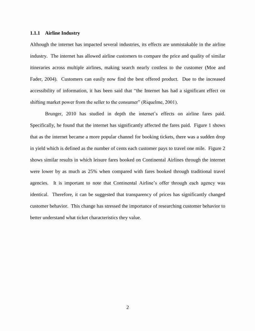
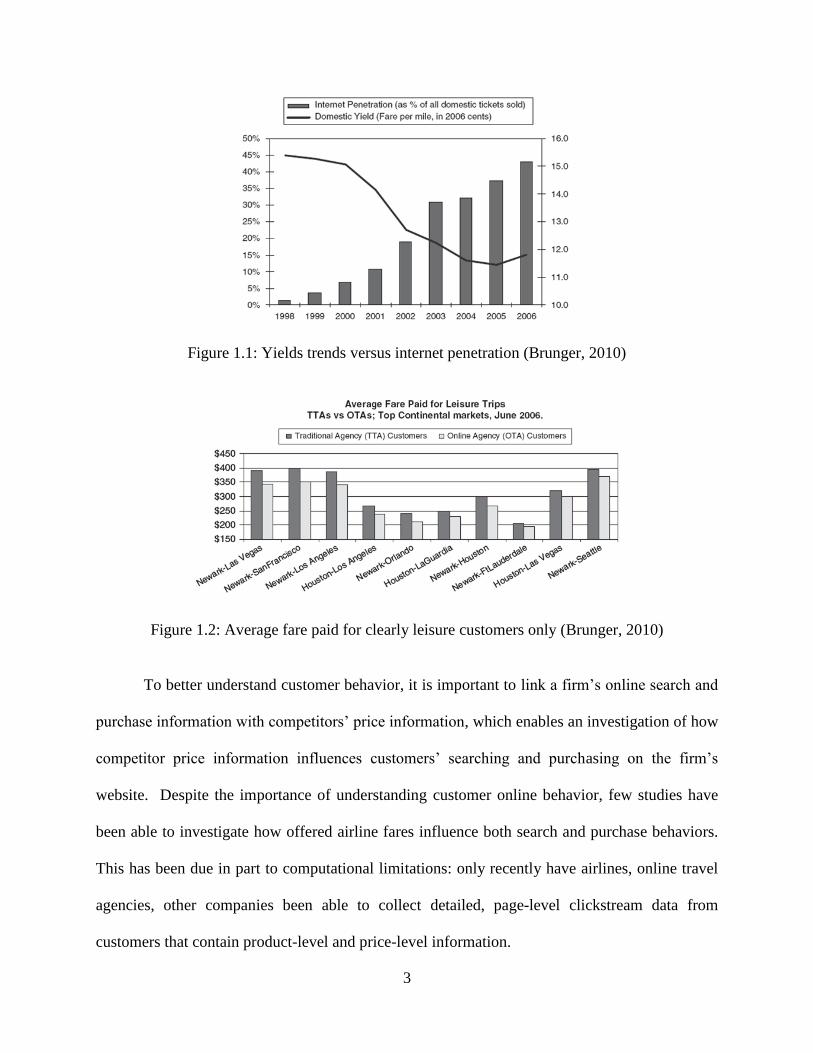
Brunger, 2010 has studied in depth the internet’s effects on airline fares paid.
Specifically, he found that the internet has significantly affected the fares paid. Figure 1 shows
that as the internet became a more popular channel for booking tickets, there was a sudden drop
in yield which is defined as the number of cents each customer pays to travel one mile. Figure 2
shows similar results in which leisure fares booked on Continental Airlines through the internet
were lower by as much as 25% when compared with fares booked through traditional travel
agencies. It is important to note that Continental Airline’s offer through each agency was
identical. Therefore, it can be suggested that transparency of prices has significantly changed
customer behavior. This change has stressed the importance of researching customer behavior to
better understand what ticket characteristics they value.
3
Figure 1.1: Yields trends versus internet penetration (Brunger, 2010)
Figure 1.2: Average fare paid for clearly leisure customers only (Brunger, 2010)
To better understand customer behavior, it is important to link a firm’s online search and
purchase information with competitors’ price information, which enables an investigation of how
competitor price information influences customers’ searching and purchasing on the firm’s
website. Despite the importance of understanding customer online behavior, few studies have
been able to investigate how offered airline fares influence both search and purchase behaviors.
This has been due in part to computational limitations: only recently have airlines, online travel
agencies, other companies been able to collect detailed, page-level clickstream data from
customers that contain product-level and price-level information.
4
Looking at Table 1, it is evident that data limitations have determined the types of
customer behavior studies that could be conducted over the years. It shows the general evolution
of airline studies as more data has become available. In 2006, Sengupta and Wiggins had
transaction information available and were able to look at the distribution of the price of airline
tickets purchased. This study, as well as many studies, accounts for purchase behavior while
failing to observe customer search behavior. Many attempts have been made to overcome this
limitation. Many of the proceeding studies tried to overcome this data limitation with regard to
search behavior. Brunger (2010) interviewed 15 experienced travelers to understand their
thought process during the booking process. However, this means the study was based on stated-
preference information, which can be unreliable. Another study by Collins, Rose, and Hess
(2010), tried to capture the search process by having study participants search through an
artificial OTA environment of ticket offerings to see their search patterns. It was assumed that
customers sorted the ticket offerings based on characteristics that they found to be most
important (i.e., if a customer sorted based on price then finding the lowest price was their main
concern). Lee, Garrow, and Post (2008) used an Interactive Price Response system that was
linked to an airline’s website in order to record customer behavior. All of these attempts still
have limitations in some form. The artificial environment, which was a stated choice survey,
would have induced bias as the “consumers, themselves, may not be able to predict exactly what
they would do, until faced with the decision” (Cross, 2005). Another limitation in the studies
includes failing to observe customer response to non-price attributes. Lee (2009) included
information on both search and purchase behaviors tracked on a single online travel agency’s
(OTA) website. However her study failed to account for price endogeneity when predicting the
number of searches and purchases (a form of demand).
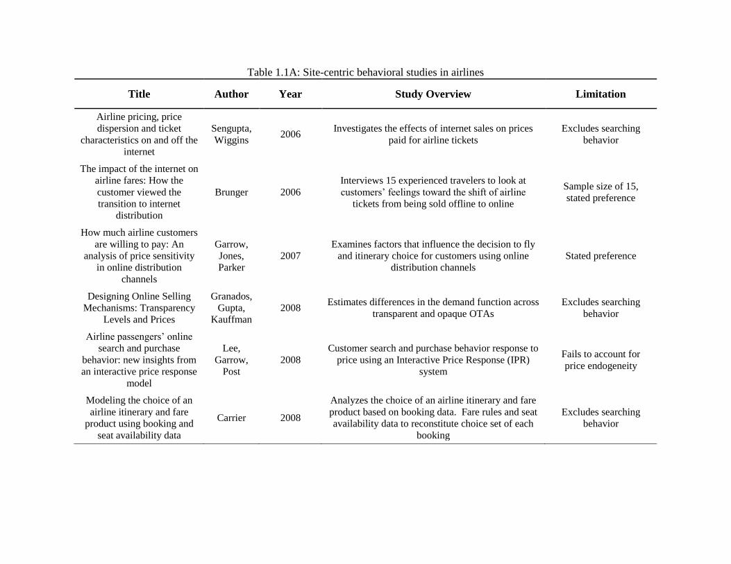
Table 1.1A: Site-centric behavioral studies in airlines
Title Author Year Study Overview Limitation
Airline pricing, price
dispersion and ticket
characteristics on and off the
internet
Sengupta,
Wiggins 2006
Investigates the effects of internet sales on prices
paid for airline tickets Excludes searching
behavior
The impact of the internet on
airline fares: How the
customer viewed the
transition to internet
distribution
Brunger 2006 Interviews 15 experienced travelers to look at
customers’ feelings toward the shift of airline
tickets from being sold offline to online
Sample size of 15,
stated preference
How much airline customers
are willing to pay: An
analysis of price sensitivity
in online distribution
channels
Garrow,
Jones,
Parker 2007
Examines factors that influence the decision to fly
and itinerary choice for customers using online
distribution channels Stated preference
Designing Online Selling
Mechanisms: Transparency
Levels and Prices
Granados,
Gupta,
Kauffman 2008
Estimates differences in the demand function across
transparent and opaque OTAs Excludes searching
behavior
Airline passengers’ online
search and purchase
behavior: new insights from
an interactive price response
model
Lee,
Garrow,
Post 2008
Customer search and purchase behavior response to
price using an Interactive Price Response (IPR)
system
Fails to account for
price endogeneity
Modeling the choice of an
airline itinerary and fare
product using booking and
seat availability data
Carrier 2008
Analyzes the choice of an airline itinerary and fare
product based on booking data. Fare rules and seat
availability data to reconstitute choice set of each
booking
Excludes searching
behavior
6
Table 1.1B: Site-centric behavioral studies in airlines (cont'd)
Title Author Year Study Overview Limitation
Carriers’ pricing behaviors
in the United States airline
industry Chi, Koo 2009
Examines the pricing behaviors of the United States
air carriers in domestic markets
10% sample of airline
tickets purchased from
reporting carriers,
excludes searching
behavior
Airline Passengers’ Online
Search and Purchase
Behaviors Lee 2009
Models search and purchase behavior at a major
OTA website Fails to account for
price endogeneity
The impact of the internet on
airline fares: The ‘Internet
Price Effect’ Brunger 2010
Examines the effects of the internet on customer
behavior, using a database of transactions
maintained by Continental Airlines
Excludes searching
behavior
Interactive stated choice
surveys: a study of air travel
behaviour
Collins,
Rose,
Hess 2010
Participants shop for airline tickets in two
environments: 1) a traditional stated preference grid
2) one that mimics an online travel agency
Based off of artificial
environments and is
stated choice, not
revealed choice
Price Discrimination by
Day-of-Week of Purchase:
Evidence from the U.S.
Airline Industry
Puller,
Taylor 2011
Examines how airfares fluctuate as a function of
day of week using transaction data Excludes searching
behavior
Online and Offline Demand
and Price Elasticities:
Evidence from the Air
Travel Industry
Granados,
Gupta,
Kauffman 2011
Compares the demand functions in the internet and
traditional air travel channels Excludes searching
behavior
7
1.1.2 Educational Studies
Similar to the airline industry, the internet plays a large role in the education system. This role is
expected to increase, especially in higher education to counteract growing education costs. To
make college more affordable, President Obama states, “A rising tide of innovation has the
potential to shake up the higher education landscape. Promising approaches include three-year
accelerated degrees, Massive Open Online Courses (MOOCs), and ‘flipped’ or ‘hybrid’
classrooms where students watch lectures at home and online and faculty challenge them to solve
problems and deepen their knowledge in class. Some of these approaches are still being
developed, and too few students are seeing their benefits” (Fact Sheet on the President’s Plan to
Make College More Affordable, 2013).
The flipped classroom has become a very popular teaching method. This is where students
watch a pre-recorded online lecture before coming to class. This frees up the in-class time to be
used for practice problem sessions, where the instructor walks around answering student
questions one-on-one. Its growth, for example, can be seen through the increasing membership
of the Flipped Learning Network, which more than tripled in one year alone, increasing from
2,500 teachers in 2011 to 9,000 in 2012 (Flipped Learning Network, 2012). It should be noted
that this network is not solely used for higher education (K-12 instructors can also be members).
MOOCs, which are entirely internet-based, will also be more common in the future. Currently in
the United States, “Only 2.6 percent of higher education institutions currently have a MOOC,
another 9.4 percent report MOOCs are in the planning stages” (Allen and Seaman, 2013).
This increased use of the internet can provide opportunities to incorporate clickstream
information into educational studies. Specifically, this type of information can indicate study
and learning habits outside of the classroom, tracking data on when students look at an online
8
resource and for how long. This valuable information is incorporated into the educational study
in this dissertation, which looks at the effects of the flipped classroom.
1.2 Major Contributions
The main contribution of this dissertation is the analysis of airline customer online behavior
while overcoming the limitations of previous studies. Of the three studies in this dissertation, the
first two look at airline customer online behavior in response to competitor fares at the time of
their search and/or purchase. The first contribution of these two studies is that they use revealed-
preference information on both customer behavior and offered fares by competitors. That is,
whereas previous studies were based on stated-preference information, the studies in this
dissertation capture the actual decision the customer faced (i.e., the distribution of competing
fares given consumers’ search date, departure date, origin airport, and destination airport) and
consumers’ actual decision (i.e., whether they searched and/or purchased).
The second contribution was the ability to differentiate between new and returning
customers throughout the last 30 days of the booking period. This was done through the use of
clickstream data with IP address information, which also allowed for the screening out of
samples displaying behavior similar to a travel agency. The findings show that in the last month
of booking, most customers are new and not returning.
The third contribution comes specifically from the second study in that it accounts for the
presence of endogeneity in models predicting airline demand in the form of searches and
purchases. In other words, valid instruments were found for a 2SLS estimation (passing three
tests related to the presence of endogeneity, strength of the instruments, and the validity of the
instruments). This reduced the effects of simultaneity between demand and price.
9
The fourth contribution comes from the third study, an educational study comparing the
traditional, flipped, and micro-flipped classrooms. This study not only presents student opinions
on each classroom type, but also provides information on how elements of each method impacts
success in the course. In addition to examining impact factors on grades commonly used in
previous studies (e.g., GPA, age, etc.), it incorporates clickstream data from the course website
to include additional impact factors not available to previous studies (e.g., how far in advance a
student started the homework assignment or studying for a quiz).
1.3 Dissertation Structure
This dissertation contains three journal articles, each with its own chapter. Each chapter first
starts with a citation of the article and then proceeds in journal format beginning with the study’s
abstract. After the relevant literature and the background of the study are covered in the
introduction, the study’s design is outlined in the methodology and data sections. This is then
followed by key results found in the study and their implications. Also, each chapter concludes
with an overview of the study’s limitations and opportunities for future research in that area.
Acknowledgements and referenced literature can be found at the end of each chapter.
Chapter 2 presents a study on the online search behavior of airline customers flying to or
from a multi-airport region. It examines if customers consider itineraries at the airports other
than their preferred airport during their search process. A truncated negative binomial regression
was used to analyze if fares offered at other airports impact the customer’s search behavior. This
paper was published by the Transportation Research Record as research funded by the Airport
Cooperative Research Program.
10
Chapter 3 investigates airline customer search and purchase behavior in response to the
advance purchase deadlines. These deadlines occur 3, 7, 14, and 21 days from departure and
typically attributed to fare increases. In addition to outlining search behavior, purchase behavior,
and fare trends in the last 30 days of the booking period, this paper presents demand models that
have valid instruments to account for price endogeneity. At the time of submission of this
dissertation, this article was under second round review.
Chapter 4 examines another application of clickstream data research, specifically in the
field of education. This paper compares the effectiveness of three teaching methods in a 3000-
level Civil Engineering course at the Georgia Institute of Technology. Two studies are
incorporated, specifically one during the spring of 2014 which compares the traditional and
flipped classrooms. The second study was conducted during the summer of 2014 and compared
the traditional, flipped, and micro-flipped classrooms. To include several factors that might
impact student success, data was collected from student transcripts, surveys, clickstream data
from the course website, office hour attendance, and course grades. Chapter 5 then gives overall
conclusions of this dissertation and recommendations for future research.
1.4 References
1. Allen, I.E and Seaman, J., “Changing course: ten years of tracking online education in the
United States.” Babson Survey Research Group and Quahog Research Group, LLC.
http://files.eric.ed.gov/fulltext/ED541571.pdf (Accessed December 2, 2014).
2. Brunger, B., “The impact of the Internet on airline fares: the ‘Internet price effect,” Journal
of Revenue and Pricing Management, Vol. 9, No. 1-2, pp. 66-93, 2010.
3. Carrier, E. “Modeling the choice of an airline itinerary and fare product using booking and
seat availability data,” PhD thesis, Massachusetts Institute of Technology, 2008.
11
4. Chi, J., Koo, W.W., “Carriers’ pricing behaviors in the United States airline industry,”
Transportation Research Part E: Logistics and Transportation Review, Vol. 45, No. 5, pp.
710-724, 2009.
5. Clemons, E.K., Hann, I.H., and Hitt, L.M., “Price Dispersion and Differentiation in Online
Travel: An Empirical Investigation,” Management Science, Vol. 48, No. 4, pp. 534-589,
2002.
6. Collins, A.T., Rose, J.M., and Hess, S., “Interactive stated choice surveys: a study of air
travel behavior.” Working Paper ITLS-WP-10-13, Institute of Transport and Logistics
Studies, University of Sydney, Australia, 2010.
7. Cross, R.G. and Dixit, A., “Customer-centric pricing: The surprising secret for
profitability,” Business Horizons, Vol. 48, pp. 483-491, 2005.
8. Garrow, L., Jones, S., Parker, R., “How much airline customers are willing to pay: An
analysis of price sensitivity in online distribution channels,” Journal of Revenue and
Pricing Management, Vol. 5, No. 4, pp 271-290, 2007.
9. Fact sheet on the president’s plan to make college more affordable (2013). The White
House. Retrieved from http://www.whitehouse.gov/the-press-office/2013/08/22/fact-sheet-
president-s-plan-make-college-more-affordable-better-bargain- (Accessed October 15,
2014).
10. Flipped Learning Network (2012). Improve student learning and teacher satisfaction with
one flip of the classroom.
11. Granados, N.F., Gupta, A., and Kauffman, R.J., “Designing online selling mechanisms:
Transparency levels and prices,” Decision Support Systems, Vol. 45, No. 4, pp 729-745,
2008.
12. Granados, N.F., Gupta, A., Kauffman, R.J., “Online and offline demand and price
elasticities: Evidence from the air travel industry,” Information Systems Research, 2011.
13. Lee, M., “Airline Passengers’ Online Search and Purchase Behaviors,” PhD thesis, Georgia
Institute of Technology, 2009.
14. Lee, M., Garrow, L. A., and Post, D., “Airline Passengers’ Online Search and Purchase
Behaviors: New Insights from an Interactive Pricing Response Model,” Working paper at
the Georgia Institute of Technology submitted for publication consideration, 2008.
15. Moe, W. W. and Fadar, P.S. “Dynamic Conversion Behavior at E-Commerce Sites,”
Management Science, Vol. 50, No. 3, pp. 326-335, 2004.
16. Park, Y.H. and Fader, P.S., “Modeling Browsing Behavior at Multiple Websites,”
Marketing Science, Vol. 23, No. 3, pp. 280-303, 2004.
12
17. Puller, S.L., and Taylor, L.M., “Price Discrimination by Day-of-Week of Purchase:
Evidence from the U.S. Airline Industry,” Working Paper,
www.econweb.tamu.edu/puller/AcadDocs/PT_weekend_pricing.pdf, 2011, (Accessed June
28, 2012).
18. Riquelme, Hernan, “An Empirical Review of Price Behaviour on the Internet,” Electronic
Markets, Vol. 11, No. 4, pp. 263-272, 2001.
19. Sengupta, A. and Wiggins, S.N., “Airline pricing, price dispersion and ticket characteristics
on and off the internet,” NET Institute Working Paper No. 06-07, 2006.
20. Statista, “Number of worldwide internet users from 2000 to 2014 (in millions).”
http://www.statista.com/statistics/273018/number-of-internet-users-worldwide/, (Accessed
December 2, 2014).
13
CHAPTER 2
COMPETITOR PRICING AND MULTI-AIRPORT CHOICE
Hotle, S. and Garrow, L.A. (2014). Competitor Pricing and Multiple Airports: Their Role in
Customer Choice. Transportation Research Record. Vol. 2400, pp 21-27.
2.1 Abstract
We investigate how competitors’ low fare offerings in multi-airport regions influence customers’
online search behavior at a major carrier’s website. Clickstream data from a major U.S. airline is
combined with detailed information about competitors’ low fare offerings for 10 directional
markets. Using a truncated negative binomial model, we predict the number of searches on the
carrier’s website as a function of low fare offerings in the same airport pair, as well as competing
airport pairs in the region. We find that the number of searches decreases as the difference
between the carrier’s lowest fare and competitors’ lowest fare increases. However, we find that
trip characteristics have a larger impact on search behavior than the fare variables. Overall
search on the carrier’s website is limited, with less than five percent of customers searching for
fares across multiple airports. Our findings provide insights into the role of competitor pricing
on multi-airport choice, as it relates to customers’ online search behaviors.
2.2 Introduction
To remain economically competitive, many metropolitan areas have built or are considering
building a new airport to expand capacity for the region, attract new airlines, and reduce air
travel delays. Multi-airport choice models are used to forecast how many travelers will use each
airport. The majority of prior multi-airport choice studies have been based on stated-preference
surveys; however, it can be challenging to obtain an accurate estimate of customers’ willingness-
to-pay to travel to less accessible airports from these surveys, as consumers’ actual choices may
14
differ from those they report based on hypothetical survey questions. A smaller number of
studies have been based on revealed-preference data; however, it is also difficult to obtain
accurate willingness-to-pay estimates due to challenges associated with compiling a database of
fares that were available at the time the consumer decided to purchase.
Our study is able to partially overcome these limitations by using two unique databases to
investigate the role of competitor prices in multi-airport choice. These databases enable us to
investigate the multi-airport choice decision process as it relates to individuals’ online searching
behavior at a major carrier’s website. We use online clickstream data from a major carrier’s
website and competitive fare data collected by QL2 Software® to examine if the number of
individuals searching for fares in a specific airport pair is associated with the lowest nonstop fare
offered in the same airport pair and/or the lowest nonstop fare offered in competing airport pairs.
Due to the level of detail available in the clickstream data, we are able to use information about a
customer’s search request for a specific airport pair, search date, departure date, and return date
to construct the choice set of fares the customer would have seen at the time she or he was
searching.
These databases allow us to investigate how round-trip fares in multi-airport areas
influence customers’ online search behavior at a major carrier’s website. Results show that the
number of searches on the carrier’s website increases when the carrier is offering the lowest fare
in the airport pair. The number of searches is also affected by fares in competing airport pairs.
Overall, the influence of fares on searches is small, particularly when compared to the influence
of trip and booking characteristics on fares. Surprisingly, our data shows that the overall amount
of search is relatively low. We hypothesize that this is because many individuals may initially
conduct a broad search of fares in one or more airport pairs using a meta-search engine (such as
15
those provided by online travel agencies Expedia®, Orbitz®, and Travelocity®), and
subsequently visit the carrier’s website if the fare they found on a specific airport pair was
attractive. This would explain why the number of individuals visiting the carrier’s website is
higher when the carrier is offering the lowest fare on that airport pair, and why the majority of
individuals are not extensively searching for fares across multiple departure dates and/or multiple
airports when they visit the carrier’s website.
2.3 Literature on Multi-Airport Choice
The dynamics of customer search and purchase behavior has changed in the past decade as
individuals have moved from purchasing tickets over the phone (or in person) from an airline’s
reservation center or a brick-and-mortar travel agency to purchasing tickets online. The internet
has lowered search costs, and made it much easier for individuals to obtain fare information.
Today, it is easy for customers to compare fares across multiple competitors and multiple
airports using meta-search engines provided by online travel agencies.
Multiple factors influence airport choice, including airport access times, airline schedules
(as reflected in flight frequency, flight times, on-time performance), fares, and airline
preferences, e.g., see (1, 2, 3, 4, 5). A survey of Southwest and America West passengers
traveling from Phoenix to the Boston/Providence or Washington, D.C./Baltimore regions found
that the top three factors customers gave for flying to a less convenient airport were better prices,
fewer flight delays, and better flight schedules (3). The relative importance of specific factors
has been shown to differ by socio-demographic characteristics, such as age and gender (4).
Since fare is regularly cited as one of the most important ticket characteristics to
customers (5), competition among carriers is expected to impact customer behavior. Prior studies
16
have found that lower search costs associated with the internet have led to increased competition
among carriers and lower fares (6, 7). In addition, the presence of a low-cost carrier in the
region has been found to lead to lower fares. Many studies term this the “Southwest Effect,”
where the entrance of a low-cost carrier causes a significant shift in offered fares and customer
choice in a market. In studies not accounting for multi-airport regions, the effect of a low-cost
carrier is easy to identify. For example, Sengupta and Wiggins find that “the presence of a low
cost carrier, other than Southwest, decreases average fares by roughly 10 percent, while
Southwest’s presence decreases average fares by 16 to19 percent” (7). However, multi-airport
studies have to identify both the effect of a low-cost carrier on a specific route and competing
routes. Dresner, Lin, and Windle found that routes experienced a 38 percent fare reduction due
to the presence of a low-cost carrier and a 53 percent reduction if the low-cost carrier was
Southwest. Further, there was an 8 percent reduction of fares on a route if Southwest served an
adjacent route, such as in a multi-airport region (8). Similarly, Morrison found that in 1998
Southwest saved passengers $3.4 billion due to direct competition with an additional $9.5 billion
from actual, adjacent, and potential competition during 1998 (9). However, the distribution of
these savings is dependent on the competition structure. Southwest has been found to increase
its fares in markets that are affected by mergers and acquisitions, specifically ones without
another LCC competitor (10).
Our study contributes to the literature by examining how the lowest nonstop fare in an
airport pair and the lowest nonstop fare in competing airport pairs influence customers’ search
behavior.
17
2.4 Data
Two databases were used in this study. The first is a sample of online clickstream data that
contains information about customers who visited a major U.S. carrier’s website. The second is
a database of nonstop fares collected by QL2 Software®. This section provides an overview of
the two databases and assumptions used to process and merge the data.
2.4.1 Clickstream Data
As its name suggests, “clickstream” data provides information about how customer “clicked” or
navigated through the major U.S. carrier’s website. Customers visit a carrier’s website for many
reasons: to search for fares, purchase tickets, check for flight delays, manage frequent flyer
accounts, etc. In this study, we use data from webpages that correspond to itinerary searches and
restrict our analysis to searches for round-trip nonstop itineraries. The data include information
about the search parameters entered by the customer, namely the origin airport, destination
airport, departure and return dates, and date the search occurred. This information can be used to
calculate trip duration, defined as the number of nights spent away from “home,” and days from
departure, defined as the number of days prior to departure that the customer searched for
information. Frequent flyer numbers are available for a limited number of observations.
Intuitively, this is because many customers do not enter their frequent flyer numbers at the time
they are searching for information, but at the time they make a purchase. Also, the clickstream
data does not record information about the specific itineraries and prices that were shown to
consumers.
Visits, pages, and purchase decision cycles are terms that are commonly used to describe
clickstream data. The carrier that provided the clickstream data defines a visit as a sequence of
18
pages that an individual requests within a specific time period. Typically, a new visit is defined
after an idle period of at least 30 minutes, e.g., see (11, 12). A page refers to a specific set of
itinerary search parameters entered by the customer. Customers can conduct multiple searches
by changing one or more of their search parameters, thus multiple pages can be associated with a
visit. A purchase decision cycle is the period of time during which an individual visits the
retailer's website one or more times prior to making a “final" purchase or no purchase decision
for a specific product. For this study, we define a “product” as any nonstop flights that originate
and terminate in one of the airports associated with a multi-airport region. The airports we
associate with a multi-airport region are generally consistent with the classifications provided by
(13).
We model individuals' searches throughout a purchase decision cycle using IP addresses.
Using IP addresses as a proxy for a customer is not ideal, as an IP address can be dynamically
assigned to a group of computers (and different users). However, cookie information, which has
been shown to pose no significant problems in practice for modeling online search behavior (14,
15) was not available. Thus, we made the assumption that IP addresses could be used as a proxy
for a customer if there were at most three origin airports, three destination airports, and three
frequent flyer numbers associated with the IP address. This assumption provides the ability to
include cases in which multiple individuals, each with their own frequent flyer number, are
traveling together. It also provides the ability to include cases for individuals who were
searching for trip in multiple origin and/or destination airports in the region.
An individual may have made one or more purchases during the data collection period.
This corresponds to different trips, and potentially different preferences for airports that
correspond to a particular trip. We created pseudo-IP, pseudo-visit, and pseudo-page identifiers
19
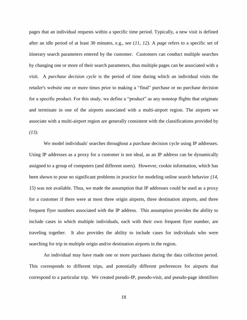
to represent these distinct purchase decision cycles. An example is shown in Table 1. Each row
corresponds to a set of search parameters entered by the individual and provides information as
to what action the individual took upon seeing the results of the search. In this example, the
individual visits the website and enters a set of search parameters (row 1). The individual enters
a different set of search parameters and decides to purchase an itinerary based on this search
(row 2). After making a purchase, the individual searches for more flights in the same market
before leaving the website, or in our terminology, initiates a new purchase decision cycle. Thus,
on row 3, the pseudo-IP address is incremented by one (to represent the initiation of a new
purchase decision cycle) and the pseudo-visit number and pseudo-page number are reinitialized
to one. The customer conducts two more searches (rows 4-5), and then leaves the website (row
5), but returns later to search (rows 6-8) and make another purchase (row 8). The customer
searches one last time before exiting the website and does not return to the carrier’s website
during the data collection period (row 9). Note that when the customer leaves the website, that
upon the next return the pseudo-visit is incremented by one and the pseudo-page is reinitialized
to one (row 6).
Table 2.1: Defining pseudo-IP, pseudo-visit, and pseudo-page numbers
Row IP Visit Page Purchase
Indicator
Interpretation of
Row
Pseudo-IP Pseudo-
Visit
Pseudo-
Page
1 1 1 1 0 Search 1 1 1
2 1 1 2 1 Purchase 1 1 2
3 1 1 3 0 Search 2 1 1
4 1 1 4 0 Search 2 1 2
5 1 1 5 0 Exit, return later 2 1 3
6 1 2 1 0 Search 2 2 1
7 1 2 2 0 Search 2 2 2
8 1 2 3 1 Purchase 2 2 3
9 1 2 4 0 Exit, never return 3 1 1
20
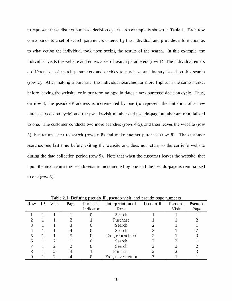
In creating the pseudo numbers, we included information only about searches and
purchases pertaining to a specific market. As an example, consider an individual who wants to
travel from the Chicago region to the Washington, D.C. region. The individual can chose to
depart from one of two airports in Chicago: Midway (MDW) and O’Hare (ORD). The
individual can also chose to arrive at one of three airports in the Washington, D.C. region: Dulles
(IAD), National (DCA), and Baltimore/Washington (BWI). To create pseudo identifiers
corresponding to searches that originated in the Chicago region and terminated in the
Washington D.C. region, we would include any searches for MDW-IAD, MDW-DCA, MDW-
BWI, ORD-IAD, ORD-DCA, and ORD-BWI. If the carrier did not operate nonstop service
between one of the airport pairs, the clickstream data would not contain searches for that airport
pair; however, information about competitors’ nonstop fare offerings at these competing airport
pairs could still be included in the analysis.
The final clickstream dataset includes searches that occurred in ten directional markets,
summarized in Table 2. The directional market “A-B” corresponds to round-trip nonstop
itineraries that originate in region A (with three airports) and terminate in region B (with two
airports). Both the directional market “A-B” and the directional market “B-A” were included in
the analysis. The regions and associated airports are not shown, to protect the identity of the
carrier that provided the clickstream data. The clickstream data include searches that occurred
from October 25, 2007 to December 15, 2007 for outbound departure dates falling between
November 15, 2007 and December 15, 2007. The overlap of search and departure date ranges
ensures we have a minimum of three weeks of search dates for each departure date.
21
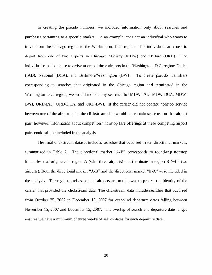
Table 2.2: Characteristics of markets included in analysis
Non-Directional
Market (Number of
Airports)
Competition
Structure
Non-Directional
Routes Served by
Major Carrier
A(3)-B(2) 5 Majors, 3 LCCs 3
A(3)-C(1) 4 Majors, 2 LCCs 3
A(3)-D(1) 3 Majors 1
A(3)-E(1) 4 Majors 1
F(3)-G(1) 4 Majors, 2 LCC 2
The analysis database contains a total of 12,404 customers (or pseudo-IPs) and 65
purchases. Of these customers, 486 (or 3.9%) searched for round-trips in more than one airport
pair. Overall, the number of customers who visit the website more than one time is quite low.
The majority of customers, or 10,826 (87.3%), visit the website just one time, 1,195 (9.6%) visit
the website two times, 262 (2.1%) visit the website three times, and the remaining 121 (1.0%)
visit the website four or more times. The number of pages viewed by customers visiting the
website is also low. A page view corresponds to a unique set of round-trip search parameters
entered by the customer. The majority of visits, or 73.4%, correspond to a single page view. An
additional 16.6% correspond to visits with two page views, 5.1% to visits with three page views,
and the remaining 4.9% to visits with four or more pages. Due to the small number of purchases
in our database, our analysis focuses solely on predicting the number of searches. However, the
conversion rate in our database (defined as the proportion of customers who purchase) is
consistent with typical rates of 1-2% commonly reported in the literature.
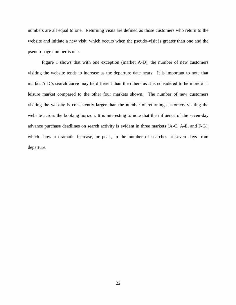
The number of visits for round-trip itineraries as a function of days from departure is
shown in Figure 1. Both directions are included in Figure 1, that is the “A-B” figure contains
round-trip tickets that originate in an airport in region A and round-trip searches that originate at
an airport in region B. New visits are defined as the first set of search parameters that were
entered by the customer, which occurs when the pseudo-IP, pseudo-visit, and pseudo-page
22
numbers are all equal to one. Returning visits are defined as those customers who return to the
website and initiate a new visit, which occurs when the pseudo-visit is greater than one and the
pseudo-page number is one.
Figure 1 shows that with one exception (market A-D), the number of new customers
visiting the website tends to increase as the departure date nears. It is important to note that
market A-D’s search curve may be different than the others as it is considered to be more of a
leisure market compared to the other four markets shown. The number of new customers
visiting the website is consistently larger than the number of returning customers visiting the
website across the booking horizon. It is interesting to note that the influence of the seven-day
advance purchase deadlines on search activity is evident in three markets (A-C, A-E, and F-G),
which show a dramatic increase, or peak, in the number of searches at seven days from
departure.
23
Figure 2.1: Number of visits as a function of days from departure
2.4.2 Pricing Data
QL2 Software® is one of several companies that collects and sells competitive airline pricing
and product information. We used QL2 Software® to compile a representative database of
nonstop fares that were available to consumers at the time they were searching. For each of the
directional markets included in Table 1, we collected one-day roundtrip and seven-day roundtrip
airfares for nonstop flights departing between 11/15/07 and 12/15/07. We have a minimum of
three weeks of pricing information for each departure date. Additional information about this
pricing database is provided in (16, 17).
The data collection periods for the clickstream and pricing databases are similar, but do
not completely overlap. Conceptually, this is because a customer who visits the carrier’s website
24
can enter in any departure and return date combination. This results in a wide range of trip
lengths. However, due to computational considerations, it was not possible for us to collect
round-trip fares for all trip lengths. When merging the clickstream and pricing databases, we
associated the one-day round-trip fare with any itineraries that had a length of stay of three days
or less and the seven-day round-trip fare with any itineraries that had a length of stay of four or
more days. In this context, our fare database is representative of those a consumer would have
seen at the time they searched. That is, the database represents typical – but in some cases, not
the actual – fares a consumer would have seen in an airport pair when searching a specific
number of days prior to departure.
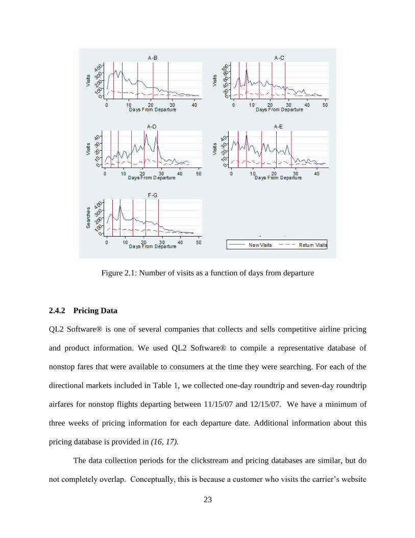
An example of the lowest representative one-day and seven-day round-trip fares for the
non-directional F-G market and the three directional markets originating in region F (denoted as
F1, F2, and F3) are shown in Figure 2. In general, a one-day roundtrip ticket costs more than a
seven-day roundtrip ticket and fares offered by LCCs are lower than those offered by major
legacy carriers. Fares tend to increase on the days that are typically associated with advance
purchase restrictions, i.e., at 3, 7, 14, and 21 days from departure. This is most clearly seen in
the step-like pattern for the F2-G1 airport pair, which is served just by major carriers. The
advance purchase deadlines are represented by vertical lines shown on the charts. We would like
to add that the LCC seven-day fare for the F3-G1 market is not shown on the figure due to an
error in the query script. There are other reasons why the fare data may be incomplete, e.g., the
response time on a server may have been unusually slow. Overall, less than five percent of
search data was excluded from the analysis due to missing fare data.
25
We use the analysis database to examine how the number of searches for round-trip fares
in a specific airport pair on a major carrier’s website relates to the representative lowest nonstop
fare offered in this airport pair as well as the representative lowest nonstop fare offered in
competing airport pairs.
200
300
400
500
600
Ave
rag
e O
ffe
red
Fare
s($
)
0 5 10 15 20 25 30 35Days From Departure
1-Day Fare LCC 1-Day Fare Major
7-Day Fare LCC 7-Day Fare Major
F3-G1
100
200
300
400
500
600
Avg
. O
ffere
d F
are
($)
0 5 10 15 20 25 30 35
F-G
100
200
300
400
500
Avg
. O
ffere
d F
are
($)
0 5 10 15 20 25 30 35
F1-G1
200
300
400
500
600
Avg
. O
ffere
d F
are
($)
0 5 10 15 20 25 30 35
F2-G1
200
300
400
500
600
Avg
. O
ffere
d F
are
($)
0 5 10 15 20 25 30 35Days From Departure
F3-G1
Figure 2.2: Representative of RT fares available throughout the booking horizon
26
2.5 Methodology
This section describes the count model used to predict the number of round-trip searches, as well
as the variables used in the analysis.
2.5.1 Count Model
We use a truncated negative binomial count model to predict the number of round-trip searches
on the carrier’s website. The unit of observation for searches is defined as the total number of
round-trip searches corresponding to a unique directional market, departure date, and search
date. Negative binomial count models are estimated instead of a Poisson count model as the
former can be used when the data are under-dispersed or over-dispersed. Also, the truncated
form of the negative binomial is used as days with zero searches were not included. For more
information on these models, refer to (18).
2.5.2 Fare Variables
We represent information about the lowest representative nonstop fares for airport pairs in the
region using the following definitions and relationships:
Carrier Fare Lowest representative nonstop fare offered by the carrier providing
clickstream data in the airport pair the customer searched in.
Airport Fare Lowest representative nonstop fare offered in the airport pair that the
customer searched in.
Region Fare Lowest representative nonstop fare offered in any airport pair in the multi-
airport region.
27
Airport Diff (Carrier fare – airport fare). Represents whether the carrier is offering the
lowest fare in the airport pair (airport diff=0) or the amount the carrier’s
fare is above the lowest fare in the airport pair (airport diff>0).
Region Diff (Airport fare – region fare). Represents whether the airport pair is offering
the lowest fare in the region (region diff=0) or the amount the lowest fare
in the airport pair is above the lowest fare in the region (region diff>0).
These relationships effectively allow us to relate the lowest fare offered by the carrier to the
lowest fare offered by competitors in the same airport pair and competing airport pairs.
Specifically:
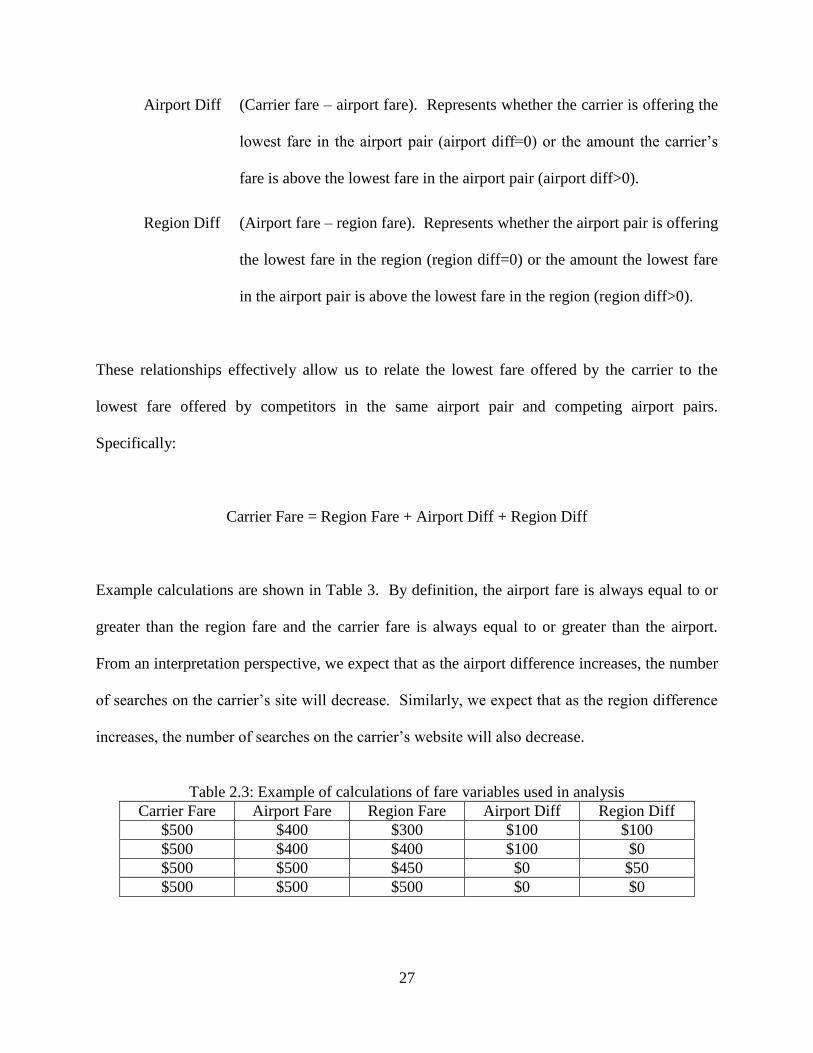
Carrier Fare = Region Fare + Airport Diff + Region Diff
Example calculations are shown in Table 3. By definition, the airport fare is always equal to or
greater than the region fare and the carrier fare is always equal to or greater than the airport.
From an interpretation perspective, we expect that as the airport difference increases, the number
of searches on the carrier’s site will decrease. Similarly, we expect that as the region difference
increases, the number of searches on the carrier’s website will also decrease.
Table 2.3: Example of calculations of fare variables used in analysis
Carrier Fare Airport Fare Region Fare Airport Diff Region Diff
$500 $400 $300 $100 $100
$500 $400 $400 $100 $0
$500 $500 $450 $0 $50
$500 $500 $500 $0 $0
28
2.5.3 Other Variables Used in the Analysis
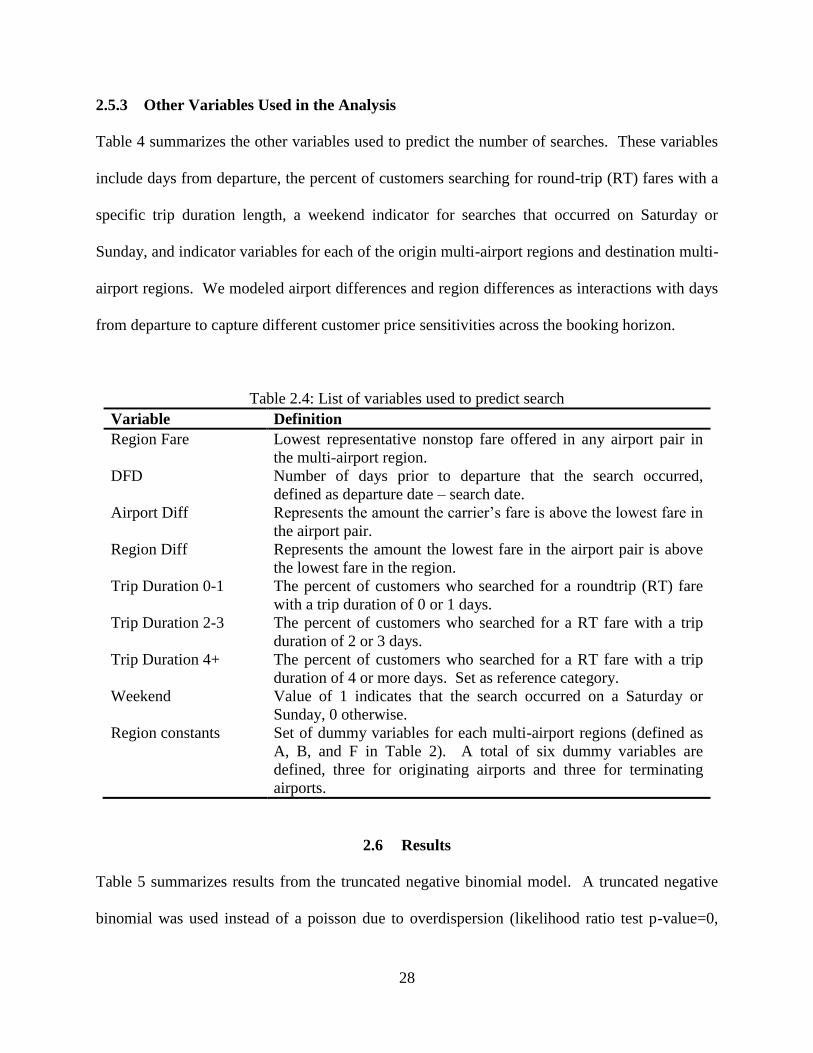
Table 4 summarizes the other variables used to predict the number of searches. These variables
include days from departure, the percent of customers searching for round-trip (RT) fares with a
specific trip duration length, a weekend indicator for searches that occurred on Saturday or
Sunday, and indicator variables for each of the origin multi-airport regions and destination multi-
airport regions. We modeled airport differences and region differences as interactions with days
from departure to capture different customer price sensitivities across the booking horizon.
Table 2.4: List of variables used to predict search
Variable Definition
Region Fare Lowest representative nonstop fare offered in any airport pair in
the multi-airport region.
DFD Number of days prior to departure that the search occurred,
defined as departure date – search date.
Airport Diff Represents the amount the carrier’s fare is above the lowest fare in
the airport pair.
Region Diff Represents the amount the lowest fare in the airport pair is above
the lowest fare in the region.
Trip Duration 0-1 The percent of customers who searched for a roundtrip (RT) fare
with a trip duration of 0 or 1 days.
Trip Duration 2-3 The percent of customers who searched for a RT fare with a trip
duration of 2 or 3 days.
Trip Duration 4+ The percent of customers who searched for a RT fare with a trip
duration of 4 or more days. Set as reference category.
Weekend Value of 1 indicates that the search occurred on a Saturday or
Sunday, 0 otherwise.
Region constants Set of dummy variables for each multi-airport regions (defined as
A, B, and F in Table 2). A total of six dummy variables are
defined, three for originating airports and three for terminating
airports.
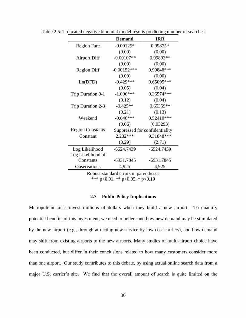
2.6 Results
Table 5 summarizes results from the truncated negative binomial model. A truncated negative
binomial was used instead of a poisson due to overdispersion (likelihood ratio test p-value=0,
29
therefore alpha is significantly different from zero). The model shows that the number of
searches on the carrier’s site increases as the day of departure nears and that less search occurs
on weekends. The model also shows that search intensity increases as the trip duration increases.
This would correspond to leisure travelers searching more intensely for fares. Stated another
way, this would occur if business customers with short trip durations search once based on
schedule, whereas leisure customers with longer trip durations search multiple times to find
lower fares.
The coefficients of a negative binomial model relate a one unit change in an independent
variable to the difference in the logs of the expected counts of the dependent variables, holding
all other independent variables constant. Coefficients may also be interpreted in terms of
incidence rate ratios (IRRs), where an IRR equal to one means no impact of that variable on the
independent variable. For example, customers looking for a same-day or overnight roundtrip are
expected to decrease their rate of searches by a factor of 0.366 compared to customers looking
for a trip of 4 or more days in duration, holding all other variables in the model constant. The
IRRs show that trip characteristics have a larger impact on search behavior than the fare
variables. The IRRs are sensitive to units of measurement, so the IRR for the “region fare”
variable measures how a customer’s rate of searches would decrease if the lowest offered fare in
the region increased by one dollar.
30
Table 2.5: Truncated negative binomial model results predicting number of searches
Demand IRR
Region Fare -0.00125* 0.99875*
(0.00) (0.00)
Airport Diff -0.00107** 0.99893**
(0.00) (0.00)
Region Diff -0.00152*** 0.99848***
(0.00) (0.00)
Ln(DFD) -0.429*** 0.65095***
(0.05) (0.04)
Trip Duration 0-1 -1.006*** 0.36574***
(0.12) (0.04)
Trip Duration 2-3 -0.425** 0.65359**
(0.21) (0.13)
Weekend -0.646*** 0.52410***
(0.06) (0.03293)
Region Constants Suppressed for confidentiality
Constant 2.232*** 9.31848***
(0.29) (2.71)
Log Likelihood -6524.7439 -6524.7439
Log Likelihood of
Constants -6931.7845 -6931.7845
Observations 4,925 4,925
Robust standard errors in parentheses
*** p<0.01, ** p<0.05, * p<0.10
2.7 Public Policy Implications
Metropolitan areas invest millions of dollars when they build a new airport. To quantify
potential benefits of this investment, we need to understand how new demand may be stimulated
by the new airport (e.g., through attracting new service by low cost carriers), and how demand
may shift from existing airports to the new airports. Many studies of multi-airport choice have
been conducted, but differ in their conclusions related to how many customers consider more
than one airport. Our study contributes to this debate, by using actual online search data from a
major U.S. carrier’s site. We find that the overall amount of search is quite limited on the
31
carrier’s website. Across five non-directional multi-airport markets, less than four percent of
customers visiting the website searched for round-trip fares in more than one airport.
From a practical perspective, this suggests that carriers likely face the same challenges as
airports in predicting demand in multi-airport region. That is, it appears as though the major
U.S. carrier captures only part of the customers’ online search, and that customers may be
initially conducting broader searches of fares across multi-airports on meta-search engines
provided by online travel agencies before entering the carrier’s website. Interestingly, this also
suggests that Southwest Airlines is the carrier that is best positioned to understand the role of
multi-airport choice on its customers’ decisions, as Southwest does not distribute its fares
through travel agencies, and is thus able to view the entire set of searches pertaining to
Southwest fares through its own website.
2.8 Limitations and Future Research
By combining clickstream data from a major carrier’s website with representative fare data from
QL2 Pricing®, we were able to investigate how the number of searches at the major carrier’s
website is influenced by representative low fare offerings in the airport pair and competing
airport pairs. We partially overcome limitations in prior studies by incorporating more realistic
information about the fares that customers likely saw at the time they were searching for
information. However, our study does not fully address this limitation, as it was not possible to
collect competitive fare data for every possible round-trip combination.
The use of clickstream data has its own limitations. Clickstream contains little customer
information, limiting our ability to investigate how socio-demographic factors, airport access
time, and trip distances influence multi-airport choice. Consistent with other studies of online
32
search behavior, we find that conversion rates are low. Due to the small number of purchases
represented in our analysis database, we focused our study on understanding the role of
competitive pricing on search behavior; however, the more relevant question to policy makers
and airlines would to understand the role of competitive pricing on purchase decisions.
A second research extension that would be interesting to explore is to compare the results
of our study with data from an online travel agency, as the latter would likely provide a better
estimate of the percentage of customers who consider multi-airports when selecting an itinerary.
This is important, as accurately modeling the percentage of customers who consider multiple
airports is arguably one of the most important inputs to multi-airport choice models.
In summary, we find that using clickstream data to investigate multi-airport choice can
provide some insights into the role of competitors’ prices on customers’ search behavior. One of
the more useful research extensions would be to determine if it is possible for a carrier to use
information about the number of customers visiting its website during the booking process to
identify markets in which the carrier is not be price competitive. That is, if the number of visits
to the carrier’s website is below average or unexpectedly changes, this could be an indication
that more customers are visiting (and purchasing from) competitors’ websites. Early
identification of a large number of customers diverting from the carrier’s website may trigger the
carrier to offer more competitive low fares in the market.
2.9 Acknowledgments
This research was supported by the 2012-2013 Graduate Research Award Program on Public-
Sector Aviation Issues. We would like to thank several individuals for their help and support,
including Lawrence Goldstein (Senior Program Officer of the Airport Cooperative Research
33
Program), Eric Amel (Vice President at Compass Lexecon), Richard Golaszewski (Principal of
GRA Incorporated), Eric Ford (Vice President at Campbell-Hill), Kevin Healy (Senior Vice
President of Campbell-Hill), and Michael Tretheway (President and Chief Economist of
InterVISTAS). This research was funded in part by a National Science Foundation Graduate
Research Fellowship.
2.10 References
1. Başar, G. and Bhat, C. A parameterized consideration set model for airport choice: An
application to the San Francisco Bay Area. Transportation Research Part B, Vol. 38, No.
10, 2004, 889-904.
2. Hess, S. and Polak, J.W. Mixed logit modeling of airport choice in multi-airport regions.
Journal of Air Transport Management, Vol. 11, No. 2, 2005, pp. 59-68.
3. Tierny, S. and Kuby, M. Airline and airport choice by passengers in multi-airport regions:
The effect of Southwest Airlines. The Professional Geographer, Vol. 60, No. 1, 2008, pp.
15-32.
4. Buck, A.J., Blackstone, E.A., and Hakim, S. A multivariate Poisson model of consumer
choice in a multi-airport region. iBusiness, Vol. 1, No. 2, 2009, pp. 85-98.
5. Collins, A.T., Rose, J.M, and Hess, S. Interactive stated choice surveys: A study of air
travel behaviour. Transportation, Vol. 39, No. 1, 2012, pp. 55-79.
6. Brunger, W.G. The impact of the internet on airline fares: The ‘Internet price effect.’
Journal of Revenue & Pricing Management, Vol. 9, No.1-2, 2010, pp. 66-93.
7. Sengupta, A. and Wiggins, S.N. Comparing Price Dispersion on and off the Internet Using
Airline Transaction Data. Review of Network Economics, Vol. 11, No. 1, 2012, pp. 1-38.
8. Dresner, M., Lin, J.S.C., and Windle, R. The impact of low-cost carriers on airport and
route competition. Journal of Transport Economics and Policy, Vol. 30, No. 3, 1996, pp.
309-328.
9. Morrison, S.A. Actual, adjacent, and potential competition: Estimating the full effect of
Southwest Airlines. Journal of Transport Economics and Policy, Vol. 35, No. 2, 2001, pp.
239-256.
34
10. Bin Salam, N.S. Is There Still a Southwest Effect? Thesis submitted to Oregon State
University, 2012.
11. Bucklin, R.E. and Sismeiro, C. A model of web site browsing behavior estimated on
clickstream data. Journal of Marketing Research, Vol. 40, No. 3, 2009, pp. 249-267.
12. Moe, W.W. and Fader, P.S. Dynamic conversion behavior at e-commerce sites.
Management Science, Vol. 50, No. 3, 2004, pp. 326-335.
13. Brueckner, J.K., Lee, D., and Singer, E. City-pairs vs. airport-pairs: A market-definition
methodology for the airline industry. Presented at Kuhmo Nectar Conference of
International Transportation Economics Association, Berlin, Germany, 2012.
14. Bucklin, R.E. and Sismerio, C. Click here for internet insight: Advances in clickstream data
analysis in marketing. Journal of Interactive Marketing, Vol. 23, No. 1, 2009, pp. 35-48.
15. Drèze, X. and Zufryden, F.S. Is internet advertising ready for prime time? Journal of
Advertising Research, Vol. 38, No. 3, 1998, pp. 7-18.
16. Pope, S., Garrow, L.,Guin, A., Leonard, J., Bankston, L. and Campbell, P. A conceptual
framework for collecting online airline pricing data: Challenges, opportunities, and
preliminary results. Transportation Research Record, Vol. 2016, 2009, pp. 30-37.
17. Mumbower, S. and Garrow, L.A. Using online data to explore competitive airline pricing
policies: A case study approach. Transportation Research Record, Vol. 2184, 2010, pp. 1-
12.
18. Greene, W.H. Econometric Analysis. Pearson Education, Inc., New Jersey, 2003.
35
CHAPTER 3
THE IMPACT OF ADVANCED PURCHASE DEADLINES
ON CUSTOMER BEHAVIOR
Hotle, S.L., Castillo, M., Garrow, L.A., and Higgins, M.J. (2014). The Impact of Advanced
Purchase Deadlines on Customer Behavior. Submitted to Transportation Research Part
A: Policy and Practice. Under second round review as of October 30, 2014.
3.1 Abstract
Airlines frequently use advance purchase ticket deadlines to segment consumers. Few empirical
studies have investigated how individuals respond to advance purchase deadlines and price
uncertainties induced by these deadlines. We model the number of searches (and purchases) for
specific search and departure dates using an instrumental variable approach that corrects for
price endogeneity. Results show that search and purchase behaviors vary by search day of week,
days from departure, lowest offered fares, variation in lowest offered fares across competitors,
market distance, and whether the market serves business or leisure consumers. After controlling
for the presence of web bots, we find that the number of consumer searches increases just prior
to an advance purchase deadline, particularly in business markets. This increase can be explained
by consumers switching their desired departure dates by one or two days to avoid higher fares
that occur immediately after an advance purchase deadline has passed. This reallocation of
demand has significant practical implications for the airline industry because the majority of
revenue management and scheduling decision support systems currently do not incorporate these
behaviors.
36
3.2 Introduction
Classic theories of consumer search for perishable goods predict that prices should fall as a
deadline approaches. For example, the value of bakery goods and newspapers decreases over
time, i.e., these products are more valuable at the start of the business day than at the end of the
business day. In contrast, products (or seats) in the airline industry are unique in that their value
increases over time. Consequently, whereas the baker may cut prices as the business day comes
to a close, consumer dynamics in the airline industry lead to the opposite effect. That is, prices
tend to increase as the flight departure date approaches.
Airlines are able to induce this type of pricing behavior through the use of advanced
purchase deadlines. By offering a discount fare that must be purchased by a certain deadline (i.e.,
a minimum number of days in advance of flight departure), airlines can induce price-sensitive
consumers to make their purchases further in advance of flight departure. This leaves less price-
sensitive consumers in the market, which allows airlines to charge higher prices for tickets closer
to departure. In general, airlines typically sell multiple discounted products with different
advance purchase deadlines. A study by Puller and Taylor (2012) found, for example, that
discounted fare products represented 66% of their sample of U.S. bookings. Among these
discounted fare products, 93.3% were associated with just four advance purchase deadlines: 21
days (3%), 14 days (47%), 7 days (32%), and 3 days (12%).
Even though advance purchase deadlines lead to systematic fare increases, their exact
timing is uncertain. For example, the presence of the seven-day deadline does not necessarily
mean that prices will increase on a flight for tickets purchased six (versus seven) days in advance
of departure. This is because revenue management systems determine how many tickets of a
particular product should be offered for sale. For flights in which it is expected that a large
37
number of consumers will arrive in the last week prior to departure, the revenue management
system will recommend selling a limited number of discounted tickets. From the consumer’s
perspective, this means that the discounted product with a seven-day advance purchase deadline
will sell out more than seven days in advance of departure. As this example shows, the presence
of advance purchase deadlines combined with demand fluctuations induces price uncertainty in
markets. Further, variation in prices can be particularly high in markets served by both low cost
and legacy carriers due to misalignment in product offerings. This misalignment is caused by
low cost carriers selling (only) one-way fares and legacy carriers offering a mix of one-way and
round-trip fares.
In this paper, we examine how consumers respond to these advance purchase deadlines
and associated price uncertainties induced by these deadlines using multiple datasets from an
online travel agency (OTA), QL2 Software (a firm that many travel and retail firms use to collect
and analyze competitors’ pricing information), a major U.S. airline, and the Airlines Reporting
Corporation (a clearinghouse that processes all tickets purchased through travel agencies in the
U.S., including OTAs). The OTA data provide information on the number of searches and
purchases that occur in a market for specific search and departure dates. The QL2 Software data
provide information on the fares available to consumers at the time they searched. Online search
data from a major U.S. airline is used to validate results and a sample of tickets from the Airlines
Reporting Corporation (ARC) is used to validate length of stay assumptions. To model the
number of searches (and purchases), we use an instrumental variable (IV) approach to correct for
price endogeneity and predict the number of searches (and purchases) in a market for specific
search and departure dates. Our results provide insights into the impact of advance purchase
deadlines on airline consumers’ search and purchase behaviors.
38
The remaining sections are organized as follows. Section 2 reviews relevant literature to
motivate why airlines offer discounted products with associated advance purchase deadlines.
Section 3 describes the data. Methodology and empirical results are presented in Sections 4 and
5, respectively. Section 6 uses clickstream data from a major U.S. carrier’s website to validate
the key findings of the study, namely that consumer search increases immediately prior to
advance purchase deadlines and new consumers enter the market over time. Section 7 discusses
implications for aviation practice and Section 8 concludes by summarizing the key findings and
providing direction for future research.
3.3 Literature Review
Several studies have developed theories to explain why airline prices increase as the departure
time nears. The interest is motivated, in part, by the fact that the airline industry does not fit with
traditional theories of search theory that predict prices fall in markets with the arrival of
homogeneous consumers. McAfee and te Velde (2006) propose a theory to explain why prices
rise in the airline and other markets that: (1) face uncertain and high demand; (2) have fixed
capacity that can be augmented only at a relatively high marginal cost; (3) sell perishable goods;
and, (4) commit to a price schedule (and capacity) at the beginning of the selling period. The last
point is applicable to the airline industry, as airlines first set their price schedules by determining
what products to sell and at what set of prices. They then use revenue management systems to
determine how many products to sell at each price point (Li, 2001). Airline schedules are also
published at the beginning of the selling period. McAfee and te Velde (2006) show that in
markets that exhibit these four characteristics, prices will rise as the purchase deadline
approaches. The increase in prices over time is due to underlying consumer dynamics, and
specifically the arrival of new, less price-sensitive consumers.
39
Many authors model aggregate demand uncertainty by assuming there are multiple
consumer types with different arrival processes. In the context of the airline industry, this
assumption means that price-sensitive leisure consumers tend to search and purchase fares
further in advance of flight departure than price-insensitive business travelers. Li (2001) and
Dana (1998, 1999a, 1999b) use an aggregate demand uncertainty framework to show that it is
optimal for airlines to offer multiple products distinguished by price and advance purchase
deadlines. In this case, the advance purchase deadlines serve to segment the market and can even
contribute to efficient allocation of demand across flights (Dana 1998, 1999a, 1999b; Gale and
Holmes 1992, 1993).
Airlines and researchers have also explored the use of opaque products to stimulate
leisure travelers that exhibit a high degree of travel flexibility without cannibalizing revenue
from business travelers. Many of these opaque products target “last minute” travelers that can
purchase close to departure date and are likely to be price sensitive, but insensitive with respect
to travel date and/or destination. See Fay 2008, Gallego and Phillips 2004, Lee et al. 2010,
Granados et al. 2008, Jerath et al. 2010, Jiang 2007, and Post 2010 for representative articles in
this area. Examining last minute opaque product sales is outside the scope of this study, as these
last minute purchases are not present in our analysis database.1
Within the economics literature, peak-load pricing models are used to explain the
efficient allocation of demand across different periods. Consistent with peak-load pricing
models, advance purchase deadlines may also result in multiple price levels on flights. This can
1 Economic theories that seek to explain why airline prices increases as a deadline approaches typically assume two
customer segments. These models assume that leisure customers will fall out of the market as we move closer to a
departure date, thereby resulting in less price sensitive customers as the deadline approaches. We acknowledge that
there is likely a last-minute, price sensitive segment that may include non-business travelers. Analyzing the
composition of last-minute travelers, within seven days of departure, would be an interesting research problem.
40
occur when products with advance purchase deadlines sell out on popular, peak-period flights
but are still available for sale on less popular, off-peak flights. This effectively shifts price-
sensitive consumers from peak to off-peak periods (Gale and Holmes, 1992).
In summary, the extant literature has developed several theories to explain why airline
prices increase as the departure dates approach and why it is beneficial for airlines to offer
discount fares with advance purchase deadlines. These theories require the presence of at least
two consumer segments: one that arrives early in the booking process and is price-sensitive and
one that arrives later in the booking process and is less price-sensitive. With the exception of
Hotle and Garrow (2014), few studies have been able to empirically test the validity of these
theories and none have been able to verify that consumers searching online close to flight
departure represent newly arriving (and not returning) consumers. The presence of automated
search tools and different pricing policies used by airlines further complicates the search process,
and we are not aware of any studies that have examined how these factors may influence search
and purchase behaviors. Our study contributes to the literature by examining these questions and
providing empirical evidence that supports existing theory.
3.4 Data
To understand how individuals respond to advance purchase deadlines and price uncertainties
induced by these deadlines, data is needed on individuals’ search and purchase behaviors. Using
clickstream data, researchers have developed ways to identify individual consumers and track
their online search and purchase behaviors across one or more websites (e.g., Bucklin and
Sismerio, 2009).
41
In an ideal world, researchers would be able to use online clickstream data to identify all
of the individual itineraries consumers viewed across multiple travel sites, along with their
ultimate purchase decisions. Unfortunately, most companies do not have the resources required
to extract and store this type of detailed, page-level information. As a consequence, initial studies
of online search and purchase behaviors predominately focused on predicting metrics that did not
require extracting detailed page content. For example, Johnson, et al. (2004) and Zhang, et al.
(2007) developed models to predict the number of online air travel stores consumers visited over
a 30-day time period. A notable exception is Brynjolfsson, Dick and Smith (2010), who extract
page-level content from a major shop bot for books to show that consumers who search multiple
screens are motivated by non-price factors, such as seller reputation.
Our data, which was provided by an OTA, contain information on the number of searches
and purchases for a particular product. Unfortunately, detailed information on the actual set of
products (or itineraries) viewed by consumers and their corresponding prices was not available
from the OTA. To obtain this information a second dataset provided by QL2 Software was used.
Variable definitions and descriptions are presented in Table 1 and correlations are provided in
Appendix Tables A1 and A2.
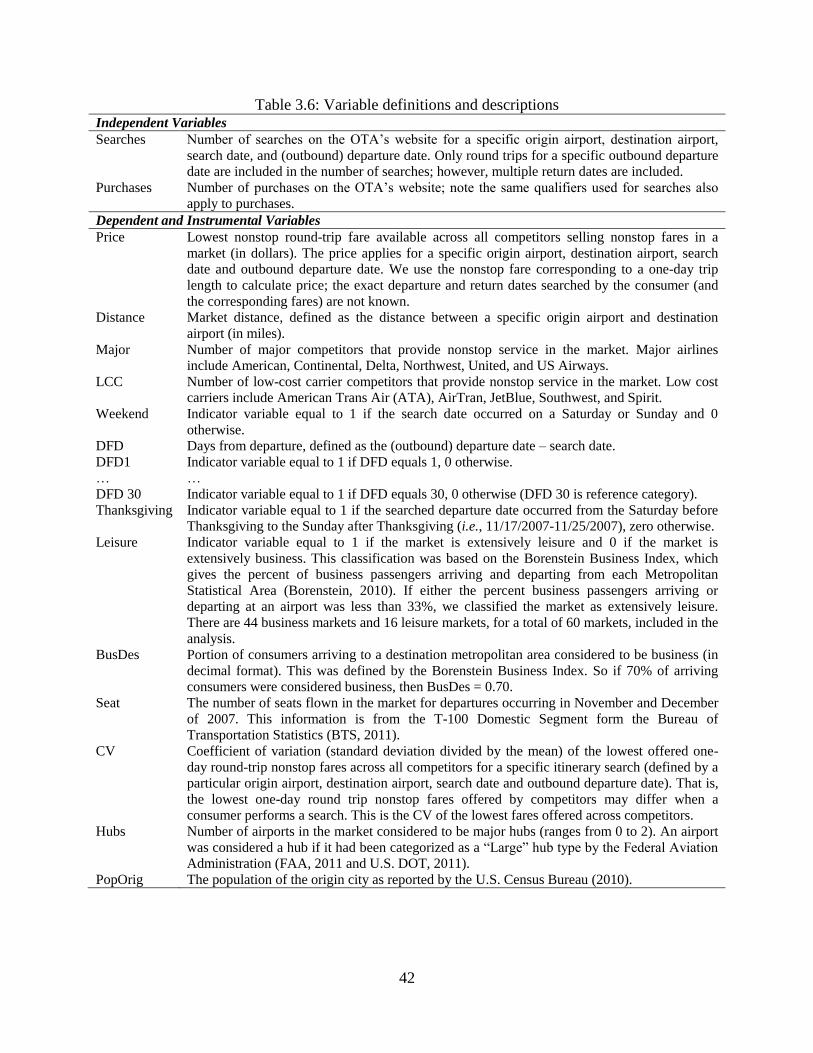
42
Table 3.6: Variable definitions and descriptions Independent Variables
Searches Number of searches on the OTA’s website for a specific origin airport, destination airport,
search date, and (outbound) departure date. Only round trips for a specific outbound departure
date are included in the number of searches; however, multiple return dates are included.
Purchases Number of purchases on the OTA’s website; note the same qualifiers used for searches also
apply to purchases.
Dependent and Instrumental Variables
Price Lowest nonstop round-trip fare available across all competitors selling nonstop fares in a
market (in dollars). The price applies for a specific origin airport, destination airport, search
date and outbound departure date. We use the nonstop fare corresponding to a one-day trip
length to calculate price; the exact departure and return dates searched by the consumer (and
the corresponding fares) are not known.
Distance Market distance, defined as the distance between a specific origin airport and destination
airport (in miles).
Major Number of major competitors that provide nonstop service in the market. Major airlines
include American, Continental, Delta, Northwest, United, and US Airways.
LCC Number of low-cost carrier competitors that provide nonstop service in the market. Low cost
carriers include American Trans Air (ATA), AirTran, JetBlue, Southwest, and Spirit.
Weekend Indicator variable equal to 1 if the search date occurred on a Saturday or Sunday and 0
otherwise.
DFD Days from departure, defined as the (outbound) departure date – search date.
DFD1 Indicator variable equal to 1 if DFD equals 1, 0 otherwise.
… …
DFD 30 Indicator variable equal to 1 if DFD equals 30, 0 otherwise (DFD 30 is reference category).
Thanksgiving Indicator variable equal to 1 if the searched departure date occurred from the Saturday before
Thanksgiving to the Sunday after Thanksgiving (i.e., 11/17/2007-11/25/2007), zero otherwise.
Leisure Indicator variable equal to 1 if the market is extensively leisure and 0 if the market is
extensively business. This classification was based on the Borenstein Business Index, which
gives the percent of business passengers arriving and departing from each Metropolitan
Statistical Area (Borenstein, 2010). If either the percent business passengers arriving or
departing at an airport was less than 33%, we classified the market as extensively leisure.
There are 44 business markets and 16 leisure markets, for a total of 60 markets, included in the
analysis.
BusDes Portion of consumers arriving to a destination metropolitan area considered to be business (in
decimal format). This was defined by the Borenstein Business Index. So if 70% of arriving
consumers were considered business, then BusDes = 0.70.
Seat The number of seats flown in the market for departures occurring in November and December
of 2007. This information is from the T-100 Domestic Segment form the Bureau of
Transportation Statistics (BTS, 2011).
CV Coefficient of variation (standard deviation divided by the mean) of the lowest offered one-
day round-trip nonstop fares across all competitors for a specific itinerary search (defined by a
particular origin airport, destination airport, search date and outbound departure date). That is,
the lowest one-day round trip nonstop fares offered by competitors may differ when a
consumer performs a search. This is the CV of the lowest fares offered across competitors.
Hubs Number of airports in the market considered to be major hubs (ranges from 0 to 2). An airport
was considered a hub if it had been categorized as a “Large” hub type by the Federal Aviation
Administration (FAA, 2011 and U.S. DOT, 2011).
PopOrig The population of the origin city as reported by the U.S. Census Bureau (2010).
43
3.4.1 OTA Clickstream Data
Clickstream data was collected from a single OTA’s website2. The data provide information on
the number of searches and purchases for a particular product. A product is defined by a set of
search parameters entered by the consumer, specifically the market (defined by a specific origin
and destination airport pair), trip type (i.e., one-way or round-trip), and outbound departure date.
A consumer can enter more than one set of search parameters, which is represented in the
database as multiple independent searches. Observations corresponding to round-trip itineraries
that had an outbound departure date between November 15, 2007 and December 15, 2007 are
included in this analysis.3 A booking horizon of 30 days is associated with each departure date.
For example, for round-trip itineraries with an outbound departure date of November 15, a panel
of the number of searches and purchases occurring each day between October 16 (30 days in
advance) and November 14 (1 day in advance) is created.
This unique 30-day booking horizon provides the opportunity to analyze search and
purchase behaviors as a function of advance purchase deadlines. Although we would expect the
distribution of tickets associated with each advance purchase deadline to differ across markets,
we would not expect the advance purchase deadline periods themselves (of 3, 7, 14, and 21 days)
to change.
The distribution for the lengths-of-stay contained in the analysis database could not be
calculated, as the return (or inbound) dates were not available in the OTA database. However,
among those consumers who purchase a round-trip ticket, the percentage of tickets with lengths-
of-stay greater than 14 days is expected to be small. To verify this assumption, we obtained a
2 Although data for this study is from a single OTA, we expect our results to be applicable across OTAs. That is, we
do not expect OTAs to return substantially different choice sets and we expect the number of airlines and number
(and type) of prices associated with nonstop flights to be similar across OTAs. 3 A Thanksgiving indicator variable is included in all models to control for any additional holiday demand.
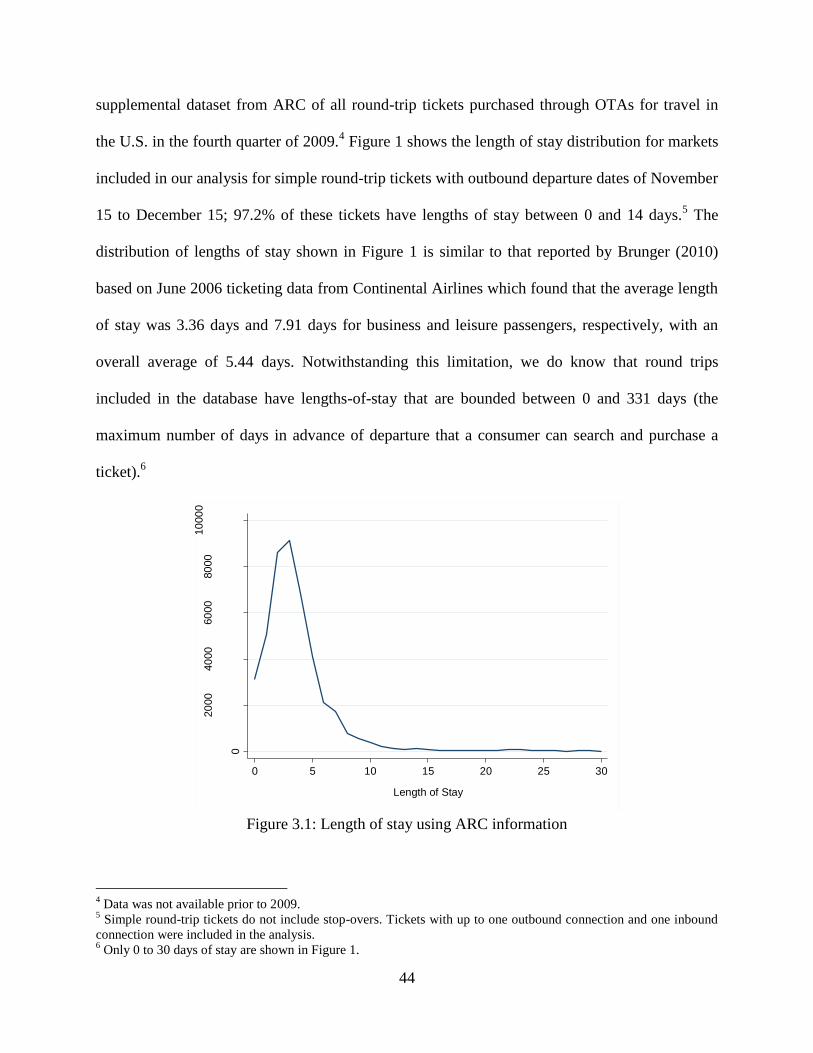
44
supplemental dataset from ARC of all round-trip tickets purchased through OTAs for travel in
the U.S. in the fourth quarter of 2009.4 Figure 1 shows the length of stay distribution for markets
included in our analysis for simple round-trip tickets with outbound departure dates of November
15 to December 15; 97.2% of these tickets have lengths of stay between 0 and 14 days.5 The
distribution of lengths of stay shown in Figure 1 is similar to that reported by Brunger (2010)
based on June 2006 ticketing data from Continental Airlines which found that the average length
of stay was 3.36 days and 7.91 days for business and leisure passengers, respectively, with an
overall average of 5.44 days. Notwithstanding this limitation, we do know that round trips
included in the database have lengths-of-stay that are bounded between 0 and 331 days (the
maximum number of days in advance of departure that a consumer can search and purchase a
ticket).6
Figure 3.1: Length of stay using ARC information
4 Data was not available prior to 2009.
5 Simple round-trip tickets do not include stop-overs. Tickets with up to one outbound connection and one inbound
connection were included in the analysis. 6 Only 0 to 30 days of stay are shown in Figure 1.
0
20
00
40
00
60
00
80
00
10
00
0
Nu
mbe
r o
f B
oo
kin
gs
0 5 10 15 20 25 30
Length of Stay
45
3.4.2 QL2 Software and Southwest Pricing Datasets
The OTA data provide information on the number of searches and purchases for a particular
search date and outbound departure date, but does not provide information on the actual
itineraries and prices viewed by consumers. To gather this missing price information, we used
data compiled by QL2 Software, a company that many travel and retail firms use to collect and
analyze competitors’ pricing information. Within the airline industry, QL2 Software and related
companies can legally collect and sell pricing information for all airlines in the U.S. except for
Southwest Airlines. Information about Southwest Airlines was collected directly by researchers
at the Georgia Institute of Technology; see Pope et al. (2009) for additional details on this data
collection effort.
The QL2 Software and Southwest Airlines pricing databases provide one- and seven-day
stay round-trip prices for all nonstop itineraries in a market. Nonstop fares were obtained from
each of the major airline’s sites (e.g., AA.com) as well as for at least one major online travel
agency (e.g., Orbitz). For our purposes, a pricing observation will be defined as the lowest
nonstop fare that was offered by each airline flying nonstop in a specific market on the date that
the website was queried and for each specific day of flight departure. The lowest fare offered
was used given that “…approximately 60 per cent of online leisure travelers purchase the lowest
fare they can find…” (PhoCusWright, 2004; Weinstein and Keller, 2012).
Although the lengths-of-stay vary in the OTA database, it was not feasible to collect fare
information for every possible length-of-stay combination. In practice, this is a key challenge
that airlines face in integrating competitive pricing data into their revenue management systems.7
7 To put this in context, Delta Air Lines operates more than 5,400 daily flights (Delta Air Lines, 2014). If we were
to collect round-trip price information for each length-of-stay combination for each of these nonstop flights for a
single departure date, we would need to collect more than 1.7 million fares. If we were to do this for all flights
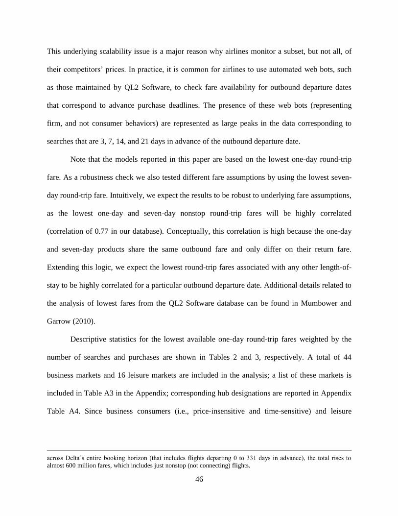
46
This underlying scalability issue is a major reason why airlines monitor a subset, but not all, of
their competitors’ prices. In practice, it is common for airlines to use automated web bots, such
as those maintained by QL2 Software, to check fare availability for outbound departure dates
that correspond to advance purchase deadlines. The presence of these web bots (representing
firm, and not consumer behaviors) are represented as large peaks in the data corresponding to
searches that are 3, 7, 14, and 21 days in advance of the outbound departure date.
Note that the models reported in this paper are based on the lowest one-day round-trip
fare. As a robustness check we also tested different fare assumptions by using the lowest seven-
day round-trip fare. Intuitively, we expect the results to be robust to underlying fare assumptions,
as the lowest one-day and seven-day nonstop round-trip fares will be highly correlated
(correlation of 0.77 in our database). Conceptually, this correlation is high because the one-day
and seven-day products share the same outbound fare and only differ on their return fare.
Extending this logic, we expect the lowest round-trip fares associated with any other length-of-
stay to be highly correlated for a particular outbound departure date. Additional details related to
the analysis of lowest fares from the QL2 Software database can be found in Mumbower and
Garrow (2010).
Descriptive statistics for the lowest available one-day round-trip fares weighted by the
number of searches and purchases are shown in Tables 2 and 3, respectively. A total of 44
business markets and 16 leisure markets are included in the analysis; a list of these markets is
included in Table A3 in the Appendix; corresponding hub designations are reported in Appendix
Table A4. Since business consumers (i.e., price-insensitive and time-sensitive) and leisure
across Delta’s entire booking horizon (that includes flights departing 0 to 331 days in advance), the total rises to
almost 600 million fares, which includes just nonstop (not connecting) flights.
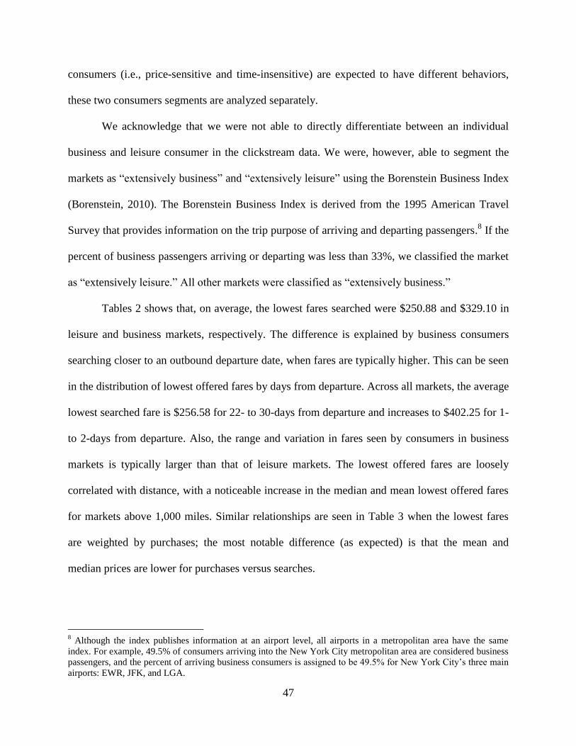
47
consumers (i.e., price-sensitive and time-insensitive) are expected to have different behaviors,
these two consumers segments are analyzed separately.
We acknowledge that we were not able to directly differentiate between an individual
business and leisure consumer in the clickstream data. We were, however, able to segment the
markets as “extensively business” and “extensively leisure” using the Borenstein Business Index
(Borenstein, 2010). The Borenstein Business Index is derived from the 1995 American Travel
Survey that provides information on the trip purpose of arriving and departing passengers.8 If the
percent of business passengers arriving or departing was less than 33%, we classified the market
as “extensively leisure.” All other markets were classified as “extensively business.”
Tables 2 shows that, on average, the lowest fares searched were $250.88 and $329.10 in
leisure and business markets, respectively. The difference is explained by business consumers
searching closer to an outbound departure date, when fares are typically higher. This can be seen
in the distribution of lowest offered fares by days from departure. Across all markets, the average
lowest searched fare is $256.58 for 22- to 30-days from departure and increases to $402.25 for 1-
to 2-days from departure. Also, the range and variation in fares seen by consumers in business
markets is typically larger than that of leisure markets. The lowest offered fares are loosely
correlated with distance, with a noticeable increase in the median and mean lowest offered fares
for markets above 1,000 miles. Similar relationships are seen in Table 3 when the lowest fares
are weighted by purchases; the most notable difference (as expected) is that the mean and
median prices are lower for purchases versus searches.
8 Although the index publishes information at an airport level, all airports in a metropolitan area have the same
index. For example, 49.5% of consumers arriving into the New York City metropolitan area are considered business
passengers, and the percent of arriving business consumers is assigned to be 49.5% for New York City’s three main
airports: EWR, JFK, and LGA.
48
Table 3.7: Descriptive statistics for lowest available one-day round-trip fare weighted by number
of searches
Obs Min Mean Median Max Std. Dev. CV
Market
Leisure 65,909 98.00 250.88 219.20 868.00 88.45 0.3526
Business 117,695 42.00 329.10 268.80 1584.80 203.39 0.6180
Distance (in miles)
0-250 20,131 98.00 277.34 236.00 1488.00 147.74 0.5327
251-500 38,603 42.00 273.29 228.00 1042.80 169.44 0.6200
501-750 25,126 148.00 267.07 248.80 1153.80 89.16 0.3338
751-1000 62,723 98.00 253.10 228.00 868.00 87.80 0.3469
1001-1250 18,090 130.00 361.32 326.80 1009.20 146.05 0.4042
1251-1500 18,931 216.80 528.98 392.80 1584.80 305.24 0.5770
Days From Departure*
1-2 2,316 118.00 402.25 348.80 1584.80 245.86 0.6112
4-6 27,950 98.00 377.57 319.20 1564.80 243.96 0.6461
8-13 44,743 98.00 285.72 248.80 1153.80 149.00 0.5219
15-20 41,352 42.00 263.78 238.80 998.80 115.26 0.4369
22-30 47,755 42.00 256.58 236.00 978.80 109.31 0.4260
*Statistics for 3, 7, 14, and 21 days from departure are excluded as searches are dominated by
automated web bot searches.
Table 3.8: Descriptive statistics for lowest one-day round-trip fare weighted by number of
purchases
Obs Min Mean Median Max Std. Dev. CV
Market
Leisure 2,173 98.00 237.50 218.79 568.80 85.80 0.3613
Business 6,930 42.00 299.54 253.80 1,564.80 186.01 0.6210
Distance (in miles)
0-250 1,492 98.00 267.28 236.00 1,488.00 141.87 0.5308
251-500 1,746 42.00 243.11 198.40 1,042.80 151.30 0.6224
501-750 1,118 158.80 250.95 229.20 861.80 71.53 0.2851
751-1000 2,116 98.00 238.35 218.79 568.80 85.62 0.3592
1001-1250 1,172 130.00 353.14 306.00 950.80 145.86 0.4130
1251-1500 777 232.80 513.18 360.80 1564.80 333.80 0.6504
Days From Departure
1-3 1,564 118.00 374.36 298.80 1,564.80 244.25 0.6524
4-7 1,605 108.00 331.32 263.80 1,564.80 220.30 0.6649
8-14 2,323 98.00 263.01 238.80 986.80 120.57 0.4584
15-21 1,850 42.00 241.65 225.50 976.19 98.57 0.4079
22-30 1,080 42.00 236.60 222.00 692.80 91.35 0.3861
49
3.4.3 Representiveness of Database
Our final dataset contains 381,607 searches (183,604 of which occurred on non-deadline dates)
and 9,103 purchases across 60 markets. This represents an overall conversion rate (i.e., the ratio
of the number of purchases to searches) of 5.0% on the days not affected by web bots. The
conversation rate is consistent with those reported in the literature; Moe and Fader (2004), for
example, note that typical conversion rates for online retailers rarely exceed 5%.
The markets included in our analysis represent U.S. markets that are larger than average.
Using the T-100 database, we ranked 2,622 business markets and 4,726 leisure markets that had
an average demand of at least one passenger per day during November and December 2007
(BTS, 2011). Table 4 provides the rank for the 44 business markets and 16 leisure markets
included in our analysis. Our leisure markets are drawn from the top 10% whereas our business
markets were drawn from the top 69%; leisure markets had higher rankings than our business
markets since the demand of leisure markets tends to be lower than that of business markets. Our
focus on larger markets helped ensure we had a sufficient number of search and purchase
observations in the estimation dataset.
50
Table 3.9: Representativeness of OTA markets
Business Leisure
Ranking
Max
Passengers Markets
Max
Passengers Markets
1-100 222,323 5 229,525 2
101-200 91,033 9 82,063 3
201-300 67,663 5 56,170 5
301-400 54,273 6 38,369 3
401-500 44,576 2 29,509 3
501-600 37,735 2 24,580 0
601-700 31,567 0 20,298 0
701-800 27,915 0 17,387 0
801-900 24,356 3 14,854 0
901-1000 21,044 1 13,271 0
1001-1100 18,322 2 12,118 0
1101-1200 16,580 4 10,874 0
1201-1300 14,770 0 9,726 0
1301-1400 13,005 0 8,635 0
1401-1500 11,426 0 7,771 0
1501-1600 9,934 0 7,032 0
1601-1700 8,609 1 6,476 0
1701-1800 7,418 3 5,954 0
1801-1900 6,620 1 5,539 0
3.5 Methodology
Consistent with the extant literature, we use a linear model to predict air travel demand (e.g.,
Bhadra, 2003; Granados, Gupta and Kauffman, 2012; Mumbower, Garrow and Higgins, 2014).
Specifically, we use linear regression methods to estimate the number of searches (or number of
purchases) for market i with outbound departure date j that are made t days in advance of the
outbound departure date. A key methodological challenge with this framework was finding a set
of valid instruments to correct for price endogeneity.
51
3.5.1 Price Endogeneity
Many prior studies of airline demand have failed to properly address price endogeneity and have
assumed that prices are exogenous. However, in demand models, prices are endogenous because
prices are influenced by demand and demand is, in turn, influenced by prices (this is often
referred to as simultaneity of supply and demand). The presence of endogeneity results in a
correlation between an explanatory variable and the error term (or unobserved factors) and
effectively violates a main assumption required to ensure consistency (Greene, 2003).
Price endogeneity is well documented in the economics and management literatures; see
for example, Guevara-Cue (2010), Train (2009), and Mumbower, Garrow, and Higgins (2014)
for more comprehensive reviews of endogeneity in the air travel setting. Many empirical studies
have shown that price coefficients are underestimated if endogeneity is not corrected. These
include studies that estimate demand for high speed rail travel (Pekgün, Griffin and Keskinocak,
2013), household choice of television reception options (Goolsbee and Petrin, 2004; Petrin and
Train, 2010), household choice of residential location (Guevara and Ben-Akiva, 2006; Guevara-
Cue, 2010), choice of yogurt and ketchup brands (Villas-Boas and Winer, 1999), choice of a new
vehicle (Berry, Levinsohn and Pakes, 1995, 2004; Train and Winston, 2007), and brand-level
demand for hypertension drugs (Branstetter, Chatterjee and Higgins, 2011).
There are multiple methods that can be used to correct for price endogeneity, including
the Generalized Method of Moments (GMM) that accounts for endogeneity using instruments.
An Ordinary Least Squares (OLS) instrumental variable estimate of β (shown in Equation 1) can
be used when errors are homoskedastic. However, the presence of heteroskedasticity in our data
was found using a test proposed by Pagan and Hall (1983). Therefore, this study uses the
52
Generalized Method of Moments (GMM) estimate (Equation 2), which includes weighting
matrices to correct for heteroskedasticity:
�̂�𝐼𝑉 = {𝑋′𝑍(𝑍′𝑍)−1𝑍′𝑋}−1𝑋′𝑍(𝑍′𝑍)−1𝑍′𝑦 (1)
�̂�𝐺𝑀𝑀 = (𝑋′𝑍𝑊𝑍′𝑋)−1𝑋′𝑍𝑊𝑍′𝑦 (2)
where:
W = weighting matrices
X1i = endogenous variable
W1, …, Wr = exogenous explanatory variables
Z1, …, Zm = instruments
Instruments must satisfy two conditions. First, the instruments must be uncorrelated with
the error term. Second, they need to be correlated with the endogenous variable (Judge et al.,
1985). In our context, this means we need to find instruments that are correlated with airfares
(price) but not correlated with a consumer’s purchase or choice of a flight.
Mumbower, Garrow, and Higgins (2014) review instruments that have been or could
potentially be used in airline applications and classify these instruments into four main
categories: (1) cost-shifting instruments; (2) Stern-type measures of competition and market
power; (3) Hausman-type price instruments; and, (4) BLP-type measures of non-price
characteristics of other products. Cost-shifting instruments help explain why costs differ across
geographic areas and/or product characteristics. Stern-type measures of competition and market
power focus on the number of products in the market and also the time since a product (and/or
firm) was introduced into the market (Stern, 1996). Hausman-type price instruments are based on
prices of the same airline in other geographic contexts (Hausman, et al., 1994; Hausman, 1996).

53
BLP instruments, introduced by Berry Levinsohn and Pakes (1995), are based on the average
non-price characteristics of other products.
We use four cost-shifting instruments, two Stern-type instruments, and one Hausman-
type instrument in our search and purchase models. Our cost-shifting instruments include:
distance, the number of hubs in the market, an indicator for whether the destination is
extensively business, and the population of the metropolitan area surrounding the origin airport.
The first two cost-shifting instruments are similar to those used in prior studies (e.g., Hsiao
(2008) uses distance, Berry and Jia (2010) use a hub indicator, and Granados, Gupta and
Kauffman use both distance and a hub indicator). Intuitively, we expect costs to vary as a
function of distance (or length of haul) due to the fact that costs are highly correlated with fuel
and labor. Costs may also vary across airports, as smaller non-hub stations may be served by
connection carriers and/or airlines may contract out services related to servicing customers and
aircraft. Airlines often provide additional services (most notably frequent flyer lounges and
priority check-in lanes) at large airports and/or destinations that serve a large percentage of
business travelers.
Stern-type instruments use measures of market power by multiproduct firms and
measures of competition as instruments. Levels of market power focus on the number of
products in the market and also the time since a product (and/or firm) was introduced into the
market. Our Stern-type instruments include the number of low cost carriers offering nonstop
service in a market during the study time period and the number of nonstop seats offered in the
markets for November and December of 2007 interacted with days from departure. These
instruments are similar to those used in prior studies (e.g., Berry and Jia (2010) use the number
of all carriers offering service on a route and Mumbower, Garrow, and Higgins (2014) use the

54
number of nonstop seats offered in a market). Finally, we use one Hausman-type instrument.
Hausman-type instruments are based on prices of similar brands, usually in different geographic
contexts. In our data, we have prices for all brands (defined as nonstop flights offered across
different competitors) and use the square of the coefficient of variation across the offered fares as
our instrument. Note that because we are predicting the number of searches at a particular OTA
website (that includes products from multiple competitors), we include fare information for all
competitors in the instrument.
The instruments we use in our search and purchase models differ. In our search models,
our instruments include the number of nonstop seats offered in the markets for November and
December of 2007 interacted with days from departure, the number of low cost carriers offering
nonstop service in a market during this time period, and the square of the coefficient of variation
across the offered fares. In our purchase models, we include these three instruments and four
additional ones for distance, the population of the metropolitan area surrounding the origin
airport, the number of hubs in the market, and an indicator for whether the destination is
extensively business.
All of our instruments are valid. We used three tests to test for: (1) endogeneity, (2) the
strength of instruments; and, (3) validity of instruments. First, we checked for the presence of
endogeneity using the Durbin-Wu-Hausman test. Rejecting the null hypothesis indicates that the
focal variable is endogenous.9 Second, we determined the strength of the instruments using a
first-stage estimation F-test. For this test, if the p-value is insignificant and/or the F-statistic is
less than the critical value provided in Stock and Yogo (2005), then the set of instruments are
9 We find that the variable fare was indeed endogenous; the test for endogeneity returned a p-value of 0.0024,
significantly rejecting the null hypothesis of exogeneity.
55
considered to be weak.10
Lastly, we use a Hansen’s J statistic11
to test the validity of our
instruments.12
3.5.2 Estimating Parameters for Days from Departure Variables
To understand the role of deadlines on individuals’ search and purchase behaviors, we included a
full set of dummy variables, each representing a specific day from departure (DFD) in the model.
For example, the variable DFD20 is an indicator variable that equals 1 if the difference between
the search date and outbound departure date is 20 days, and 0 otherwise. We have 29 DFD
variables and including all of them leads to over-fitting the model. Methodologically, there are
several approaches that can be used to address this problem. The most common method is to use
a continuous function (such as the square of DFD) or a spline function that fits separate functions
into groups of DFD variables (e.g., a separate function could be used for each advance purchase
range such as 1-2 DFD, 3-6 DFD, 7-13 DFD, 14-20 DFD, 21-30 DFD). However, neither of
these approaches is applicable to our problem, as we need to isolate how search and purchase
behaviors change immediately before or immediately after an advance purchase deadline, while
simultaneously controlling for other factors that will influence the number of searches and
purchases.
For models that include business markets, we have a sufficient number of observations
(21,557), that we can estimate a single model with 29 DFD coefficients. However, this approach
10
For the strength of instruments test, the p-value was 0.0005 thereby rejecting the null hypothesis of weak
instruments. Also, using a critical value of 12.83 as outlined in Stock and Yogo (2005), we reject the null of weak
instruments given a maximum size distortion of no more than 15% with an F-statistic of 17.673. 11
Although commonly used, it should be noted that the J statistic and other tests of over-identification are
inconsistent (Newey, 1985). 12
The validity of instruments test returned a p-value of 0.0837, which accepts that the instruments are indeed valid.
This last p-value is reported for each of the estimated models on Tables 6-9. In sum, our instruments are valid (and
strong) across all search and purchase models. For more information on the estimation and testing of instrumental
variable regressions, refer to Baum, Schaffer, and Stillman (2003) and Stock and Yogo (2005).
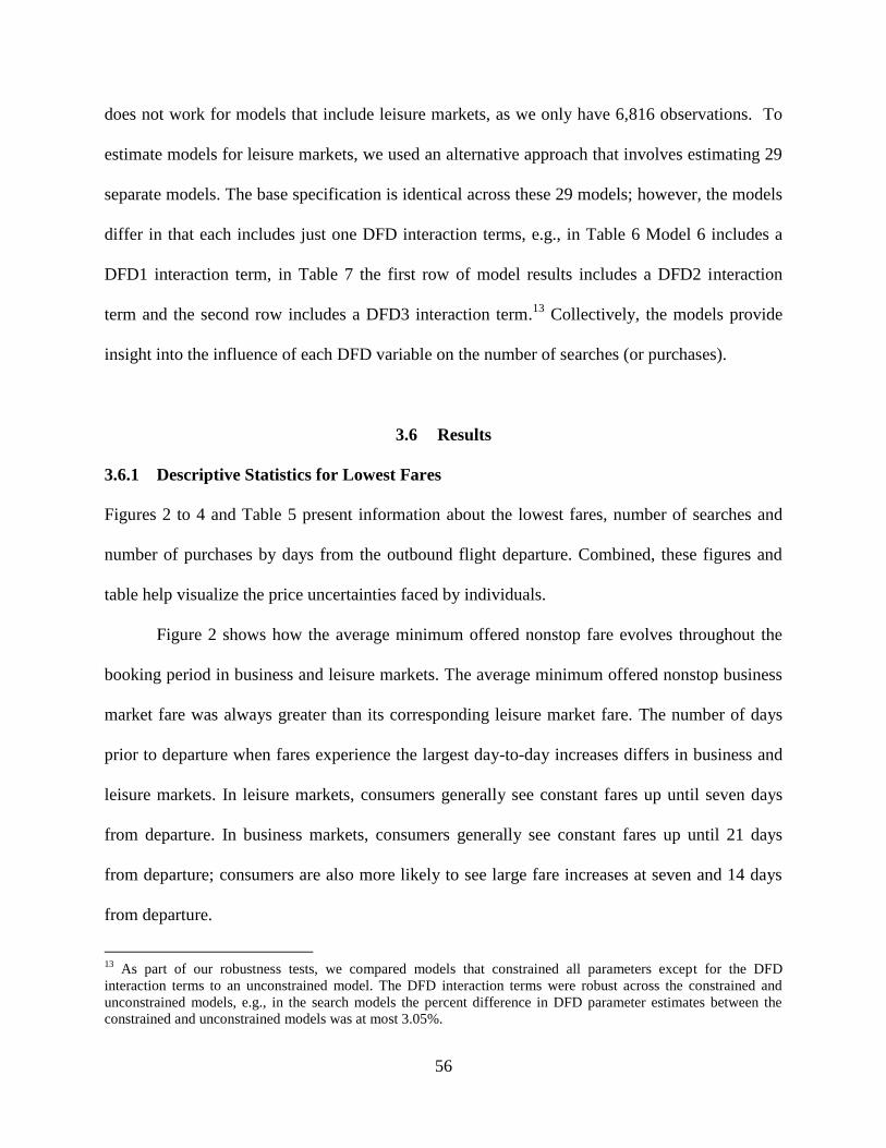
56
does not work for models that include leisure markets, as we only have 6,816 observations. To
estimate models for leisure markets, we used an alternative approach that involves estimating 29
separate models. The base specification is identical across these 29 models; however, the models
differ in that each includes just one DFD interaction terms, e.g., in Table 6 Model 6 includes a
DFD1 interaction term, in Table 7 the first row of model results includes a DFD2 interaction
term and the second row includes a DFD3 interaction term.13
Collectively, the models provide
insight into the influence of each DFD variable on the number of searches (or purchases).
3.6 Results
3.6.1 Descriptive Statistics for Lowest Fares
Figures 2 to 4 and Table 5 present information about the lowest fares, number of searches and
number of purchases by days from the outbound flight departure. Combined, these figures and
table help visualize the price uncertainties faced by individuals.
Figure 2 shows how the average minimum offered nonstop fare evolves throughout the
booking period in business and leisure markets. The average minimum offered nonstop business
market fare was always greater than its corresponding leisure market fare. The number of days
prior to departure when fares experience the largest day-to-day increases differs in business and
leisure markets. In leisure markets, consumers generally see constant fares up until seven days
from departure. In business markets, consumers generally see constant fares up until 21 days
from departure; consumers are also more likely to see large fare increases at seven and 14 days
from departure.
13
As part of our robustness tests, we compared models that constrained all parameters except for the DFD
interaction terms to an unconstrained model. The DFD interaction terms were robust across the constrained and
unconstrained models, e.g., in the search models the percent difference in DFD parameter estimates between the
constrained and unconstrained models was at most 3.05%.
57
Increases in the average minimum nonstop fares are highly correlated with advance
purchase deadlines (shown by the vertical lines on Figure 2). An advance purchase deadline
corresponds to the last day a fare would have been offered in the market. Consequently, given an
advance purchase deadline at time t, we expect fares to increase at time t-1. Given that airlines
use different pricing strategies, we also expect fares to increase at time t-2 for our analysis
database. That is, the increase in fares two periods after a deadline can be attributed to the fact
that the majority of U.S. legacy carriers use round-trip pricing whereas low cost carriers (LCC)
use one-way pricing. Under round-trip pricing, a single price is quoted for the outbound and
inbound itineraries, and the advance purchase deadline is associated with the outbound departure
date. Under one-way pricing, separate prices are quoted for the outbound and inbound itineraries,
and advance purchase deadlines can differ for the outbound and inbound itineraries.
As an example, consider an individual who purchases a one-day round-trip ticket. We
assume for this example that discount product offerings have not been influenced by revenue
management controls and are always available within the allowable selling period. At 14 days
from the outbound departure date, the outbound and inbound fares offered by legacy and LCC
carriers will have identical 14-day advance purchase restrictions. At 13 days from departure,
product misalignment occurs because the legacy carrier jointly prices the outbound and inbound
itineraries (using a 7-day advance purchase restriction) whereas the LCCs separately price the
outbound and inbound itineraries. That is, at 13 days from departure, a consumer is able to
purchase an outbound fare with a 7-day advance purchase fare and an inbound fare with a 14-day
advance purchase fare from a LCC. At 12 days from departure, LCC and legacy carrier products
are realigned as the seven-day advance purchase restriction applies consistently to both outbound
58
and inbound fares. This explains why price increases associated with advance purchase deadlines
occur over a two-day period in our analysis database.
Figure 3.2: How the lowest offered fare evolves in leisure and business markets
Although on average the offered fares increase around the advance purchase deadline,
this increase is uncertain and may be seen only by a small percentage of consumers. This
uncertainty is mainly due to interactions between airlines’ revenue management systems, pricing
systems, and fluctuations in demand forecasts. Table 5 shows fare trends from the consumer
perspective, specifically how often the lowest available nonstop fare available at DFD t changes
on day t-1. For example, in going from three to two days from departure: 27.4% of business
itineraries experienced an increase in fares, 13.6% experienced a decrease, and 59.0%, stayed the
same.14
However, certain periods were more likely to experience fare changes.
14
We tested the sensitivity of results by using different thresholds to define an increase and/or decrease in fares.
Specifically we defined a difference in Table 5 as “any” difference of fare (of one cent or more), but also generated
results defining a difference as one in which the change was at least $10 or at least $15.
59
The DFDs with probabilities greater than 25% of experiencing an increase are
highlighted. The influence of advance purchase deadlines on inducing price uncertainties is
clearly seen by the higher probabilities associated with DFDs occurring at t-1 and t-2 days after
the purchase deadline. For a given deadline at time t, the probability of a fare increase is higher
from (t-1 to t-2) than from (t to t-1) which can also be explained by the different pricing
strategies of legacy carriers and LCCs.
By comparing business and leisure markets, we see that it is more likely the lowest
offered fares will increase for the 21 and 14 advance purchase deadlines in business markets.
This suggests airlines are aggressively using advance purchase deadlines to segment business
and leisure consumers in business markets.
60
Table 3.10: How often the lowest offered nonstop one-day round trip fare changes
How will the lowest fare available today change if I search tomorrow?
Business Markets Leisure Markets
DFD % Decrease % Stay Same % Increase % Decrease % Stay Same % Increase
2 11.7 51.9 36.4 7.3 49.7 43.1
3 13.6 59.0 27.4 9.2 58.3 32.5
4 12.7 71.9 15.4 15.1 73.5 11.4
5 10.1 54.0 35.9 14.2 52.7 33.1
6 8.3 28.5 63.2 6.3 21.4 72.4
7 10.7 50.6 38.8 10.8 32.8 56.4
8 13.9 67.9 18.2 12.1 68.6 19.3
9 11.1 61.6 27.4 11.0 67.9 21.1
10 13.0 67.8 19.2 14.5 68.2 17.4
11 12.0 72.0 16.0 14.0 71.7 14.3
12 14.2 61.6 24.2 13.7 70.6 15.7
13 13.2 37.4 49.4 13.7 58.9 27.4
14 14.1 49.0 36.9 13.0 59.8 27.2
15 14.4 68.1 17.5 13.2 74.2 12.6
16 15.5 68.2 16.3 13.1 73.5 13.4
17 15.2 66.5 18.3 15.6 73.5 10.9
18 12.9 70.0 17.1 12.2 76.2 11.6
19 14.7 68.6 16.8 10.1 77.5 12.4
20 13.8 51.6 34.6 12.8 74.4 12.8
21 14.9 58.1 27.1 12.5 73.4 14.1
22 14.3 66.3 19.5 12.7 75.5 11.9
23 13.3 68.3 18.4 14.5 72.0 13.6
24 15.6 67.7 16.8 13.0 70.8 16.2
25 13.6 71.0 15.5 10.9 75.1 14.0
26 14.9 72.0 13.1 11.4 75.4 13.2
27 14.7 70.2 15.1 15.1 74.0 10.9
28 13.4 73.1 13.6 12.9 75.4 11.7
29 14.5 72.8 12.7 12.6 75.8 11.6
30 12.9 72.7 14.4 13.1 73.5 13.4
*Note: Day-to-day increases in fares that occur more than 25% of the time are shaded.
61
From a modeling perspective, these pricing uncertainties can be incorporated by
including a measure of the coefficient of variation (CV) across the offered fares (See Figure
2).15
.The CV (standard deviation divided by the mean) represents the range of prices a consumer
would likely see on the OTA’s website for a specific day from departure. For example, a
consumer can log into the OTA on a specific search date and request an itinerary for a specific
origin, destination, outbound and inbound departure dates. Typically an OTA website would
return the offered fares by several airlines.
The CV represents the average distribution of these offered (non-stop) fares representing
a one-day length of stay over time. We see that as the day of departure approaches, the CV
increases as the offered fares become more variable across airlines. The CV appears to peak the
day after an advance purchase deadline. This reflects the variation in prices caused by
differences in round-trip and one-way pricing policies across carriers. The large drop in the CV
near the deadline date is attributed to both the increase in the mean offered minimum fare and
fewer competitors offering seats on non-stop itineraries (i.e., flights sell out close to departure).
3.6.2 Descriptive Statistics for Number of Searches
Although the typical airline consumer may not be aware of when the advance purchase deadlines
occur and that they signal fare increases, flexible-date search tools can aid consumers in
identifying these trends. Flexible-date search tools are available through both OTA and airline
websites (although firms differ in how prominently they display their flexible search tools).
These tools typically show fares using either: (1) a matrix format displaying the lowest roundtrip
fares available for outbound and inbound departure dates along with the three days before and
after the preferred dates; or, (2) a calendar displaying the lowest one-way fares available for one
15
The CV is combined for business and leisure markets, as the number of leisure market samples was small.
62
month of possible departures. Legacy carriers and OTAs typically use the matrix format whereas
LCCs typically use the calendar format. This is because the matrix format naturally lends itself to
displaying round-trip fares whereas the calendar format naturally lends itself to displaying one-
way fares.
The question of interest is how consumers’ search and purchase behaviors are influenced
by price uncertainties induced by advance purchase deadlines. Figure 3 shows the average
number of searches in business and leisure markets as a function of days from departure. The
number of searches corresponding to 3, 7, 14, and 21 days from departure are excluded from the
chart as each of these days contains approximately 30,000 or more searches. These unnaturally
large spikes reflect the presence of web bots in the OTA data.
Figure 3.3: Average number of searches per market
50
100
150
200
250
300
Ave
rag
e N
um
be
r o
f S
ea
rche
s
051015202530
Days From Departure
Leisure Markets Business Markets
63
3.6.3 Descriptive Statistics for Number of Purchases
To complete the descriptive analysis, Figure 4 shows the average number of purchases in
business and leisure markets as a function of days from departure. In contrast to Figure 3,
information for all days from departure is included since the number of purchases is not affected
by the presence of web bots. Although the influence of deadline effects is less clear for purchase
(versus search) behavior, we do see some evidence of increased purchase activity on or just
before advance purchase deadlines. This increase is most prevalent (in both leisure and business
markets) for the 7-day advance purchase deadline (which typically sees a very large increase in
fares). The peak at seven days followed immediately by a valley at six days suggests that
consumers may be shifting their preferred departure date by one day in order to qualify for a fare
that has a 7-day advance purchase requirement.
Figure 3.4: Average number of purchases per market
24
68
10
12
Ave
rag
e N
um
be
r o
f P
urc
hase
s
051015202530
Days From Departure
Leisure Markets Business Markets
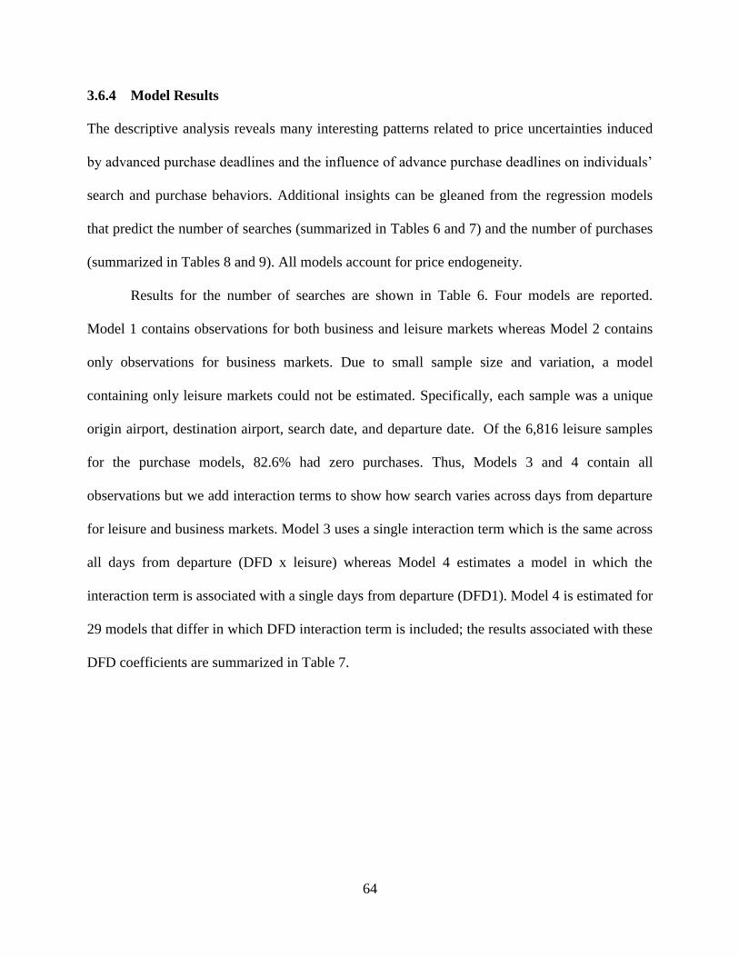
64
3.6.4 Model Results
The descriptive analysis reveals many interesting patterns related to price uncertainties induced
by advanced purchase deadlines and the influence of advance purchase deadlines on individuals’
search and purchase behaviors. Additional insights can be gleaned from the regression models
that predict the number of searches (summarized in Tables 6 and 7) and the number of purchases
(summarized in Tables 8 and 9). All models account for price endogeneity.
Results for the number of searches are shown in Table 6. Four models are reported.
Model 1 contains observations for both business and leisure markets whereas Model 2 contains
only observations for business markets. Due to small sample size and variation, a model
containing only leisure markets could not be estimated. Specifically, each sample was a unique
origin airport, destination airport, search date, and departure date. Of the 6,816 leisure samples
for the purchase models, 82.6% had zero purchases. Thus, Models 3 and 4 contain all
observations but we add interaction terms to show how search varies across days from departure
for leisure and business markets. Model 3 uses a single interaction term which is the same across
all days from departure (DFD x leisure) whereas Model 4 estimates a model in which the
interaction term is associated with a single days from departure (DFD1). Model 4 is estimated for
29 models that differ in which DFD interaction term is included; the results associated with these
DFD coefficients are summarized in Table 7.
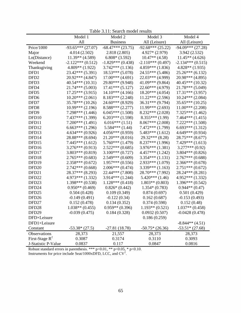
65
Table 3.11: Search model results
Model 1 Model 2 Model 3 Model 4
All Business All (Leisure) All (Leisure)
Price/1000 -93.65*** (27.07) -68.47*** (23.75) -92.68*** (25.22) -94.09*** (27.28) Major 4.014 (2.502) 2.818 (2.805) 4.927* (2.979) 3.942 (2.532) Ln(Distance) 11.39** (4.589) 6.808* (3.592) 10.47** (4.58) 11.45** (4.626) Weekend -2.122*** (0.512) -1.829*** (0.438) -2.110*** (0.497) -2.134*** (0.515) Thanksgiving 4.809** (1.922) 3.742*** (1.136) 4.859*** (1.836) 4.828** (1.935) DFD1 23.42*** (5.391) 18.53*** (5.078) 24.55*** (5.486) 25.26*** (6.132) DFD2 20.92*** (4.847) 17.00*** (4.691) 22.03*** (4.999) 20.98*** (4.895) DFD3 40.54*** (10.31) 29.80*** (9.948) 41.09*** (9.864) 40.45*** (10.32) DFD4 21.74*** (5.003) 17.41*** (5.127) 22.60*** (4.979) 21.78*** (5.049) DFD5 17.25*** (3.915) 14.10*** (4.166) 18.20*** (4.054) 17.31*** (3.957) DFD6 10.20*** (2.061) 8.183*** (2.248) 11.22*** (2.596) 10.24*** (2.084) DFD7 35.78*** (10.26) 24.60*** (8.929) 36.31*** (9.794) 35.65*** (10.25) DFD8 10.99*** (2.196) 8.588*** (2.277) 11.99*** (2.693) 11.00*** (2.208) DFD9 7.298*** (1.446) 6.045*** (1.508) 8.232*** (2.028) 7.325*** (1.462) DFD10 7.437*** (1.399) 6.203*** (1.598) 8.355*** (1.99) 7.464*** (1.415) DFD11 7.200*** (1.491) 6.016*** (1.51) 8.067*** (2.008) 7.222*** (1.508) DFD12 6.663*** (1.296) 5.584*** (1.44) 7.472*** (1.799) 6.693*** (1.312) DFD13 4.634*** (0.926) 4.056*** (0.959) 5.483*** (1.612) 4.649*** (0.934) DFD14 28.88*** (8.694) 21.20*** (8.016) 29.32*** (8.28) 28.75*** (8.677) DFD15 7.445*** (1.612) 5.760*** (1.479) 8.237*** (1.996) 7.429*** (1.613) DFD16 3.276*** (0.913) 2.522*** (0.685) 3.976*** (1.381) 3.277*** (0.92) DFD17 3.803*** (0.819) 3.100*** (0.727) 4.457*** (1.242) 3.804*** (0.826) DFD18 2.765*** (0.683) 2.549*** (0.609) 3.354*** (1.131) 2.767*** (0.688) DFD19 2.358*** (0.672) 1.957*** (0.556) 2.933*** (1.079) 2.366*** (0.678) DFD20 2.742*** (0.668) 2.006*** (0.474) 3.339*** (1.163) 2.751*** (0.672) DFD21 28.37*** (8.293) 22.44*** (7.808) 28.70*** (7.992) 28.24*** (8.281) DFD22 4.973*** (1.332) 3.914*** (1.244) 5.420*** (1.46) 4.952*** (1.332) DFD23 1.398*** (0.538) 1.128*** (0.418) 1.803** (0.803) 1.396*** (0.542) DFD24 0.950** (0.469) 0.826* (0.442) 1.354* (0.783) 0.944** (0.47) DFD25 0.504 (0.428) 0.109 (0.349) 0.874 (0.697) 0.501 (0.429) DFD26 -0.149 (0.491) -0.122 (0.34) 0.162 (0.687) -0.153 (0.493) DFD27 0.152 (0.478) 0.134 (0.352) 0.374 (0.598) 0.152 (0.48) DFD28 1.038** (0.455) 0.959** (0.396) 1.193** (0.521) 1.037** (0.458) DFD29 -0.039 (0.475) 0.184 (0.328) 0.0932 (0.507) -0.0428 (0.478) DFD×Leisure
0.186 (0.259)
DFD1×Leisure
-8.844** (4.51)
Constant -53.38* (27.5) -27.81 (18.78) -50.75* (26.36) -53.51* (27.68)
Observations 28,373 21,557 28,373 28,373 First-Stage R
2 0.3087 0.3174 0.3110 0.3093
J-Statistic P-Value 0.0837 0.117 0.0847 0.0816 Robust standard errors in parenthesis. *** p<0.01, ** p<0.05, * p<0.10.
Instruments for price include Seat/1000xDFD, LCC, and CV2.
66
Table 3.12: Leisure search results for DFD coefficients
X DFDX ×Leisure
Coefficient
Robust
Std Errors
J-Statistic
P-Value
# Searches in
Leisure Markets
# Searches in
Business Markets
2 -10.05* (5.19) 0.0818 3,865 6,907
3 23.36 (25.82) 0.0891 18,593 29,152
4 -8.094 (5.28) 0.0815 4,682 8,576
5 -10.40** (4.90) 0.082 2,602 4,975
6 -7.013 (4.37) 0.0825 2,359 4,756
7 39.06 (30.32) 0.0887 20,774 32,119
8 -0.32 (3.63) 0.0836 4,678 8,032
9 -5.318 (4.19) 0.0831 2,275 4,535
10 -4.447 (4.17) 0.0834 2,397 4,640
11 -5.772 (4.30) 0.0832 2,218 4,021
12 -5.767 (4.19) 0.0833 1,952 3,895
13 -4.835 (3.95) 0.0831 2,101 3,999
14 27.38 (26.21) 0.0841 18,599 30,600
15 2.682 (3.78) 0.0836 4,827 7,879
16 -1.389 (3.74) 0.0837 2,416 4,009
17 -1.662 (3.69) 0.0837 2,171 4,115
18 -2.499 (3.79) 0.0838 1,900 3,483
19 -2.152 (3.71) 0.0838 1,824 3,300
20 -1.321 (3.52) 0.0835 2,113 3,315
21 23.29 (26.37) 0.0828 17,806 30,360
22 2.105 (3.94) 0.0834 4,141 7,058
23 -0.272 (3.42) 0.0837 1,953 3,324
24 -0.683 (3.33) 0.0835 1,938 3,177
25 0.236 (3.37) 0.0837 1,759 2,982
26 -0.811 (3.41) 0.0836 1,647 2,607
27 -0.207 (3.45) 0.0836 1,694 2,622
28 -1.324 (3.28) 0.0837 1,834 2,878
29 -1.814 (3.49) 0.0837 1,550 2,670
30 -0.799 (3.47) 0.0837 1,567 2,354
*** p<0.01, ** p<0.05, * p<0.10. Each model based on 28,373 obs.
Results show that the number of searches tends to increase as the day of departure
approaches. However, this increase is moderated by increases in prices that are associated with
less search – particularly in leisure markets. The positive coefficient for the (DFD x leisure)
interaction in Model 3 suggests that search activity is slightly higher in leisure markets.
67
However, when separate interaction terms for each days from departure are used, we see that
increases in search activity in leisure markets occur at specific time periods – namely on the
advance purchase deadlines of 3, 7, 14, and 21 days from departure. This is likely the result of
web bot activity, and suggests that airlines are more aggressive at monitoring their competitive
prices in leisure markets. After controlling for the presence of web bots and fares, we see that the
number of searches is actually lower in leisure markets. We need to be careful when making
absolute comparisons between the number of searches (and purchases) across markets, as the
potential consumer pool is unknown. That is, this result can be explained if the number of
potential consumers in leisure markets is, on average, smaller than the number of potential
consumers in business markets.
Results from the search models (Models 1-4, Table 6) show that search decreases on
weekends but increases as the number of major competitors offering nonstop service in the
market increases. Search also increases as the distance between the origin and destination
airports increases, particularly in leisure markets. This is likely due to the fact that as distance
increases, driving and other alternative modes of transportation become less attractive compared
to air.
The results from the purchase specifications, summarized in Tables 8 and 9, are similar to
those seen for search models, i.e., the number of purchases is smaller in leisure markets, changes
in prices have a larger impact on the number of purchases in leisure markets, fewer purchases
occur on weekends, and more purchases occur in long-haul markets and markets in which there
are more major competitors.
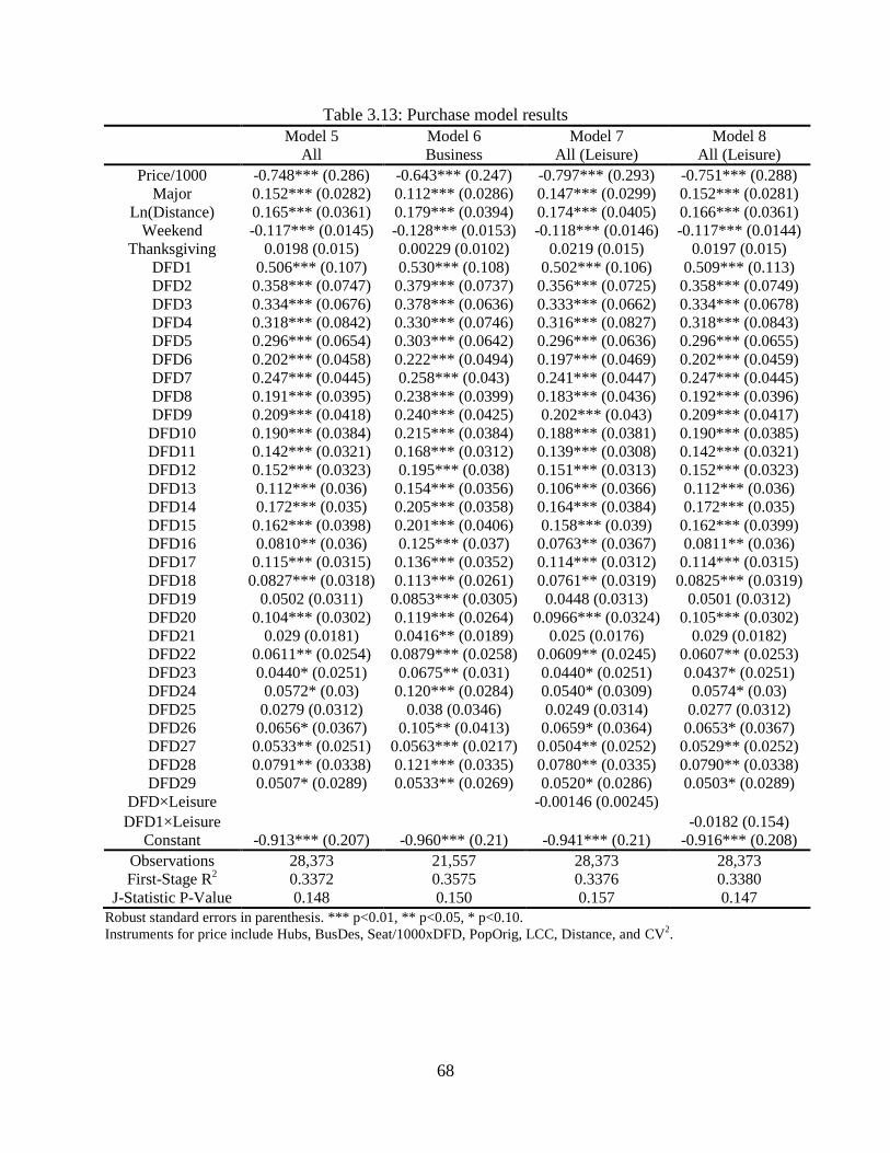
68
Table 3.13: Purchase model results
Model 5 Model 6 Model 7 Model 8
All Business All (Leisure) All (Leisure)
Price/1000 -0.748*** (0.286) -0.643*** (0.247) -0.797*** (0.293) -0.751*** (0.288) Major 0.152*** (0.0282) 0.112*** (0.0286) 0.147*** (0.0299) 0.152*** (0.0281)
Ln(Distance) 0.165*** (0.0361) 0.179*** (0.0394) 0.174*** (0.0405) 0.166*** (0.0361) Weekend -0.117*** (0.0145) -0.128*** (0.0153) -0.118*** (0.0146) -0.117*** (0.0144)
Thanksgiving 0.0198 (0.015) 0.00229 (0.0102) 0.0219 (0.015) 0.0197 (0.015) DFD1 0.506*** (0.107) 0.530*** (0.108) 0.502*** (0.106) 0.509*** (0.113) DFD2 0.358*** (0.0747) 0.379*** (0.0737) 0.356*** (0.0725) 0.358*** (0.0749) DFD3 0.334*** (0.0676) 0.378*** (0.0636) 0.333*** (0.0662) 0.334*** (0.0678) DFD4 0.318*** (0.0842) 0.330*** (0.0746) 0.316*** (0.0827) 0.318*** (0.0843) DFD5 0.296*** (0.0654) 0.303*** (0.0642) 0.296*** (0.0636) 0.296*** (0.0655) DFD6 0.202*** (0.0458) 0.222*** (0.0494) 0.197*** (0.0469) 0.202*** (0.0459) DFD7 0.247*** (0.0445) 0.258*** (0.043) 0.241*** (0.0447) 0.247*** (0.0445) DFD8 0.191*** (0.0395) 0.238*** (0.0399) 0.183*** (0.0436) 0.192*** (0.0396) DFD9 0.209*** (0.0418) 0.240*** (0.0425) 0.202*** (0.043) 0.209*** (0.0417) DFD10 0.190*** (0.0384) 0.215*** (0.0384) 0.188*** (0.0381) 0.190*** (0.0385) DFD11 0.142*** (0.0321) 0.168*** (0.0312) 0.139*** (0.0308) 0.142*** (0.0321) DFD12 0.152*** (0.0323) 0.195*** (0.038) 0.151*** (0.0313) 0.152*** (0.0323) DFD13 0.112*** (0.036) 0.154*** (0.0356) 0.106*** (0.0366) 0.112*** (0.036) DFD14 0.172*** (0.035) 0.205*** (0.0358) 0.164*** (0.0384) 0.172*** (0.035) DFD15 0.162*** (0.0398) 0.201*** (0.0406) 0.158*** (0.039) 0.162*** (0.0399) DFD16 0.0810** (0.036) 0.125*** (0.037) 0.0763** (0.0367) 0.0811** (0.036) DFD17 0.115*** (0.0315) 0.136*** (0.0352) 0.114*** (0.0312) 0.114*** (0.0315) DFD18 0.0827*** (0.0318) 0.113*** (0.0261) 0.0761** (0.0319) 0.0825*** (0.0319) DFD19 0.0502 (0.0311) 0.0853*** (0.0305) 0.0448 (0.0313) 0.0501 (0.0312) DFD20 0.104*** (0.0302) 0.119*** (0.0264) 0.0966*** (0.0324) 0.105*** (0.0302) DFD21 0.029 (0.0181) 0.0416** (0.0189) 0.025 (0.0176) 0.029 (0.0182) DFD22 0.0611** (0.0254) 0.0879*** (0.0258) 0.0609** (0.0245) 0.0607** (0.0253) DFD23 0.0440* (0.0251) 0.0675** (0.031) 0.0440* (0.0251) 0.0437* (0.0251) DFD24 0.0572* (0.03) 0.120*** (0.0284) 0.0540* (0.0309) 0.0574* (0.03) DFD25 0.0279 (0.0312) 0.038 (0.0346) 0.0249 (0.0314) 0.0277 (0.0312) DFD26 0.0656* (0.0367) 0.105** (0.0413) 0.0659* (0.0364) 0.0653* (0.0367) DFD27 0.0533** (0.0251) 0.0563*** (0.0217) 0.0504** (0.0252) 0.0529** (0.0252) DFD28 0.0791** (0.0338) 0.121*** (0.0335) 0.0780** (0.0335) 0.0790** (0.0338) DFD29 0.0507* (0.0289) 0.0533** (0.0269) 0.0520* (0.0286) 0.0503* (0.0289)
DFD×Leisure
-0.00146 (0.00245)
DFD1×Leisure
-0.0182 (0.154)
Constant -0.913*** (0.207) -0.960*** (0.21) -0.941*** (0.21) -0.916*** (0.208)
Observations 28,373 21,557 28,373 28,373 First-Stage R
2 0.3372 0.3575 0.3376 0.3380
J-Statistic P-Value 0.148 0.150 0.157 0.147 Robust standard errors in parenthesis. *** p<0.01, ** p<0.05, * p<0.10.
Instruments for price include Hubs, BusDes, Seat/1000xDFD, PopOrig, LCC, Distance, and CV2.
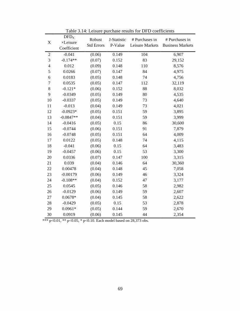
69
Table 3.14: Leisure purchase results for DFD coefficients
X
DFDX
×Leisure
Coefficient
Robust
Std Errors
J-Statistic
P-Value
# Purchases in
Leisure Markets
# Purchases in
Business Markets
2 -0.041 (0.06) 0.149 104 6,907
3 -0.174** (0.07) 0.152 83 29,152
4 0.012 (0.09) 0.148 110 8,576
5 0.0266 (0.07) 0.147 84 4,975
6 0.0183 (0.05) 0.148 74 4,756
7 0.0535 (0.05) 0.147 112 32,119
8 -0.121* (0.06) 0.152 88 8,032
9 -0.0349 (0.05) 0.149 80 4,535
10 -0.0337 (0.05) 0.149 73 4,640
11 -0.013 (0.04) 0.149 73 4,021
12 -0.0923* (0.05) 0.151 59 3,895
13 -0.0847** (0.04) 0.151 59 3,999
14 -0.0416 (0.05) 0.15 86 30,600
15 -0.0744 (0.06) 0.151 91 7,879
16 -0.0748 (0.05) 0.151 64 4,009
17 0.0122 (0.05) 0.148 74 4,115
18 -0.041 (0.06) 0.15 64 3,483
19 -0.0457 (0.06) 0.15 53 3,300
20 0.0336 (0.07) 0.147 100 3,315
21 0.039 (0.04) 0.146 64 30,360
22 0.00478 (0.04) 0.148 45 7,058
23 -0.00179 (0.06) 0.149 46 3,324
24 -0.108** (0.04) 0.152 47 3,177
25 0.0545 (0.05) 0.146 58 2,982
26 -0.0129 (0.06) 0.149 59 2,607
27 0.0678* (0.04) 0.145 58 2,622
28 -0.0429 (0.05) 0.15 53 2,878
29 0.0961* (0.05) 0.144 59 2,670
30 0.0919 (0.06) 0.145 44 2,354
*** p<0.01, ** p<0.05, * p<0.10. Each model based on 28,373 obs.
70
3.7 Validation
For validation of consumer search behavior, we use a sample of clickstream data representing
consumers’ search behaviors for three leisure and seven business markets from a major U.S.
carrier. The departure dates represented this data overlap with those in the OTA data and the
markets are similar.16
In addition to validation, this new data enables us to track individual
consumers across multiple pages and multiple sessions, and identify new and returning
consumers. This means we were able to identify and remove web bots from the clickstream data
and we were also able to define searches as either: (1) the first set of search parameters entered
by a consumer during a visit; or, (2) any set of search parameters entered by a consumer.17
Figure 5 demonstrates the number of searches in the collected markets using the first set
of search parameters entered by a consumer during a visit. Consistent with what we observe in
the OTA data, we see spikes in the number of searches on and/or just prior to the advance
purchase deadlines. The spike is most pronounced at seven days from departure. This is not
surprising since more business markets are contained in the clickstream data.
Interestingly, Figure 5 also provides supportive evidence of extant search theories that
suggest prices should rise in the presence of deadlines due to the arrival of new (and less price-
sensitive) consumers in the market (e.g., see Stokey 1979; McAfee and te Velde, 2006; Mantin
and Koo, 2010). Further, by defining searches using just the first set of parameters versus all
parameters entered by the consumer, we are able to determine that the pattern shown in Figure 5
is not due to increased search intensities (or increases in the number of searches) as the results
were similar for both search definitions.
16
Due to non-disclosure agreements, we cannot reveal the markets represented in the data as they could be used to
identify the carrier that provided the clickstream data. 17
Additional details used to clean and process the carrier’s clickstream data are provided in Hotle and Garrow
(2014).
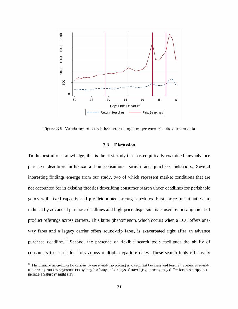
71
Figure 3.5: Validation of search behavior using a major carrier’s clickstream data
3.8 Discussion
To the best of our knowledge, this is the first study that has empirically examined how advance
purchase deadlines influence airline consumers’ search and purchase behaviors. Several
interesting findings emerge from our study, two of which represent market conditions that are
not accounted for in existing theories describing consumer search under deadlines for perishable
goods with fixed capacity and pre-determined pricing schedules. First, price uncertainties are
induced by advanced purchase deadlines and high price dispersion is caused by misalignment of
product offerings across carriers. This latter phenomenon, which occurs when a LCC offers one-
way fares and a legacy carrier offers round-trip fares, is exacerbated right after an advance
purchase deadline.18
Second, the presence of flexible search tools facilitates the ability of
consumers to search for fares across multiple departure dates. These search tools effectively
18
The primary motivation for carriers to use round-trip pricing is to segment business and leisure travelers as round-
trip pricing enables segmentation by length of stay and/or days of travel (e.g., pricing may differ for those trips that
include a Saturday night stay).
0
50
010
00
15
00
20
00
25
00
To
tal N
um
be
r o
f S
ea
rch
es
051015202530
Days From Departure
Return Searches First Searches
72
allow consumers to “avoid” an advance purchase deadline by guiding them on how they need to
switch their desired departure dates.
Differences in pricing policies across carriers combined with search tools make it easier
for consumers to expand their choice sets across multiple departure dates. This results in
increased search activity immediately prior to an advance purchase deadline and demand shifting
to periods immediately prior to an advance purchase deadline. These results have significant
implications on current aviation practice, as revenue management and scheduling models
typically assume demand is independent across different days.
In reality, however, demand appears to be shifting to those days search tools are directing
them to (or to the least full flights across multiple departure days). In this sense, the search tools
can be viewed as an extension of peak load pricing problems, where the peak is determined
across multiple days. This may benefit both leisure and business consumers by shifting price-
sensitive leisure demand to the least time-desirable flights, saving capacity for late-arriving
business travelers with stronger time preferences. However, airlines may not view this as a
profitable strategy.
It is interesting to note that over the past five years, Delta has changed where it displays
its “flexible search day” tools. This tool used to be predominately displayed on its home page,
but can currently only be accessed through clicking on a (more opaque) advanced search tool
option. In contrast, Southwest Airlines prominently displays a link to its low fare calendar when
the first set of itinerary search results is returned. One possible reason for these different website
designs is that the consumer mix for Delta is more heterogeneous than the consumer mix for
Southwest, suggesting Delta benefits more from using advance purchase deadlines to segment
their consumers (as was seen in our data by comparing business and leisure markets). From a
73
practical perspective, many of the decision support tools used by airlines to support revenue,
pricing, and scheduling decisions currently do not model consideration sets that span multiple
days.
3.9 Conclusions and Future Research Directions
In this study, we modeled airline travelers’ online search and purchase behaviors using an
analysis database from an online travel agency and QL2 Software. We model individuals’ search
and purchase behaviors using an instrumental variable approach that corrects for price
endogeneity. Our study contributes to the literature by providing some of the first empirical
insights into how individuals respond to advance purchase deadlines and price uncertainties
induced by advance purchase deadlines.
Results show that the number of searches and purchases that occur in a market for
specific search and departure dates are a function of search day of week, days from departure,
lowest offered fares, variation in lowest fares offered across competitors, market distance, and
whether the market serves business or leisure consumers. Search activity peaks before a deadline
and declines immediately after a deadline. This suggests that automated search tools help
individuals learn about prices across multiple departure and/or return dates. Moreover,
individuals appear to be switching their desired departure dates by one or two days in order to
avoid higher fares that occur immediately after an advance purchase deadline has passed. This is
an important finding, as current revenue management systems do not take this behavior into
account. Determining revenue impacts associated with failing to take this behavior into account
is an important future research direction.
74
Looking ahead, it will be interesting to see how competitive pricing evolves, and whether
LCCs will continue to use one-way pricing strategies. The primary motivation for carriers to use
round-trip pricing is to segment business and leisure travelers as round-trip pricing enables
segmentation by length of stay and/or days of travel (e.g., pricing may differ for those trips that
include a Saturday night stay). Currently, airlines face the same limitation we faced in our study
– it is computationally not feasible for them to monitor all of their competitors’ fares. However,
by restricting the analysis to a smaller subset of lengths of stay and/or by leveraging the fact that
fares with the same departure (or return) date will be highly correlated, carriers may be able to
develop more efficient algorithms for monitoring competitor fares. Determining whether the
ability of carriers to monitor their competitors’ fares is beneficial or harmful to consumers is a
second important future research direction.
3.10 Acknowledgments
This research was partially funded by a National Science Foundation Graduate Research
Fellowship.
3.11 References
1. Baum, C.F., Schaffer, M.E., and Stillman, S. (2003). Instrumental variables and GMM:
Estimation and testing. The Stata Journal, 3(1), 1-31, http://www.stata-
journal.com/sjpdf.html?articlenum=st0030 (accessed Feb. 8, 2014).
2. Berry, S. and Jia, P. (2010). Tracing the woes: An empirical analysis of the airline industry.
American Economic Journal: Microeconomics, 2 (3), 1-43.
3. Berry, S., Levinsohn, J. and Pakes, A. (1995). Automobile prices in market equilibrium.
Econometrica, 63(4), 841-890.
75
4. Berry, S., Levinsohn, J. and Pakes, A. (2004). Differentiated products demand systems
from a combination of micro and macro data: The new car market. Journal of Political
Economy, 112(1), 68-105.
5. Bhadra, D. (2003). Demand for air travel in the United States: Bottom-up econometric
estimation and implications for forecasts by origin and destination pairs. Journal of Air
Transportation, 8(2), 19-56.
6. Borenstein, S. (2010). An index of inter-city business travel for use in domestic airline
competition analysis. UC Berkeley, Index available at http://www.nber.org/data/bti.html
(accessed Feb. 8, 2014).
7. Branstetter, L., Chatterjee, C. and Higgins, M.J. (2011). Regulation and welfare: Evidence
from Paragraph-IV generic entry in the pharmaceutical industry. NBER Working Paper
17188, http://www.nber.org/papers/w17188.
8. Brynjolfsson, E., Dick, A.A. and Smith, M.D. (2010). A nearly perfect market?
Differentiation vs. price in consumer choice. Quantitative Marketing and Economics 8:1-
33.
9. Brunger, W.G. (2010). The impact of the Internet on airline fares: The “Internet price
effect.” Journal of Revenue & Pricing Management, 9(1/2), 66-93.
10. Bucklin, R.E. and Sismerio, C. (2009). Click here for internet insight: Advances in
clickstream data analysis in marketing. Journal of Interactive Marketing 23(1), 35-48.
11. Bureau of Transportation Statistics (2011). Air Carriers: T-100 Domestic Segment (All
Carriers). http://www.transtats.bts.gov/Fields.asp?Table_ID=311 (accessed Feb. 8, 2014).
12. Dana, J. (1998). Advance purchase discounts and price discrimination in competitive
markets. Journal of Political Economy, 106(2), 395-422.
13. Dana, J. (1999a). Using yield management to shift demand when the peak time is
unknown. RAND Journal of Economics, 30(3), 456-474.
14. Dana, J. (1999b). Equilibrium price dispersion under demand uncertainty: The roles of
costly capacity and market structure. RAND Journal of Economics, 30(4), 632-660.
15. Delta Air Lines (2014). Stats & facts: Updated June 2014. http://news.delta.com/Stats-
Facts. (accessed Oct. 16, 2014).
16. Fay, S. (2008). Selling an opaque product through an intermediary: The case of disguising
one’s product. Journal of Retailing 84(1): 59-75.
17. Federal Aviation Administration (2011). Airport categories. http://www.faa.gov/airports/
planning_capacity/passenger_allcargo_stats/categories/ (accessed Feb. 8, 2014).
76
18. Gale, I.L. and Holmes, T.J. (1992). The efficiency of advance-purchase discounts in the
presence of aggregate demand uncertainty. International Journal of Industrial
Organization, 10(3). 413-437.
19. Gale, I. L. and Holmes, T. J. (1993). Advance-purchase discounts and monopoly allocation
of capacity. American Economic Review, 83(1), 135-146.
20. Gallego, G. and Phillips, R. (2004). Revenue management of flexible products.
Manufacturing and Service Operations Management 6(4): 321-37.
21. Goolsbee, A. and Petrin, A. (2004). The consumer gains from direct broadcast satellites
and the competition with cable TV. Econometrica, 72(2), 351-381.
22. Granados, N., Gupta, A. and Kauffman, R.J. (2012). Online and offline demand and price
elasticities: Evidence from the air travel industry. Information Systems Research, 23(1),
164-181.
23. Granados, N., Gupta, A. and Kauffman, R.J. (2008). Designing online selling mechanism:
Transparency levels and prices. Decision Support Systems 45(4): 729-45.
24. Greene, W.H. (2003). Econometric Analysis, 5th Ed., Prentice Hall, Upper Saddle River,
New Jersey.
25. Guevara-Cue, C.A. (2010). Endogeneity and sampling of alternatives in spatial choice
models. Dissertation for Doctor of Philosophy, Department of Civil and Environmental
Engineering, Massachusetts Institute of Technology.
26. Guevara, C.A. and Ben-Akiva, M. (2006). Endogeneity in residential location choice
models. Transportation Research Record, 1977(1), 60-66.
27. Hausman, J.A. (1996). Valuation of new goods under perfect and imperfect competition.
The Economics of New Goods eds Robert J. Gordon and Timothy F. Bresnahan, 207–248.
University of Chicago Press, Chicago.
28. Hausman, J., Leonard, G. and Zona, J.D. (1994). Competitive analysis with differentiated
products. Annals of Economics and Statistics, 34, 159–180.
29. Hotle, S. and Garrow, L.A. (2014). Competitor pricing and multiple airports: Their role in
customer choice.” Forthcoming, Transportation Research Record.
30. Hsiao, C-.Y. (2008). Passenger demand for air transportation in a hub-and-spoke network.
Dissertation for Doctor of Philosophy, Civil and Environmental Engineering, University of
California, Berkeley. http://www.nextor.org/pubs/HsiaoDissertation2008.pdf (accessed
05.18.11).
77
31. Jerath, K., Netessine, S. and Veeraraghavan, S.K. (2010). Revenue management with
strategic customers: Last-minute selling and opaque selling. Management Science, 56(3):
430-448.
32. Jiang, Y. (2007). Price discrimination with opaque products. Journal of Revenue and
Pricing Management 6(2): 118-34.
33. Johnson, E.J., Moe, W.W., Fader, P.S., Bellman, S. and Lohse, G.L. (2004). On the depth
and dynamics of online search behavior. Management Science, 50(3), 299-308.
34. Judge, G.G., Griffiths, W.E., Hill, R.C., Lutkepohl, H, and Lee, S.-C. (1985) The Theory
and Practice of Econometrics, 2nd
Edition. Wiley Series in Probability and Mathematical
Sciences.
35. Lee, M., Khelifa, A., Garrow, L., Bierlaire, M. and Post, D. (2012). An analysis of
destination choice for opaque airline products using multidimensional binary logit models.
Transportation Research Part A 46(10): 1641–1653.
36. Li, M.Z.F. (2001). Pricing non-storable perishable goods by using a purchase restriction
with an application to airline fare pricing. European Journal of Operational Research,
134(3), 631-647.
37. Mantin, B. and Koo, B. (2010). Weekend effect in airline pricing. Journal of Air Transport
Management, 16, 48-50.
38. McAfee, R.P. and te Velde, V. (2006). Dynamic pricing in the airline industry. Handbook
of Economics and Information Systems, Ed. T. Hendershott. Amsterdam, Elsevier, 527-570.
39. Moe, W.W. and Fader, P.S. (2004). Dynamic conversion behavior at e-commerce sites.
Management Science, 50(3), 326-335.
40. Mumbower, S. and Garrow, L.A. (2010). Using online data to explore competitive airline
pricing policies: A case study approach. Transportation Research Record, 2184(1), 1-12.
41. Mumbower, S. and Garrow, L.A. and Higgins, M.J. (2014). Estimating flight-level price
elasticities using online airline data: A first step towards integrating pricing, demand, and
revenue optimization. Transportation Research Part A 66: 196–212.
42. Newey, W. (1985). Generalized method of moments specification testing. Journal of
Econometrics, 29(3): 229-256.
43. Pagan, A. R. and Hall, D. (1983). Diagnostic tests as residual analysis. Econometric
Reviews, 2(2), 159-218.
44. Pekgün, P., Griffin, P.M. and Keskinocak, P. (2013). An empirical study for estimating
price elasticities in the travel industry. Working Paper at University of South Carolina,
http://www2.ie.psu.edu/griffin/price.pdf (accessed Feb. 8, 2014).
78
45. Petrin, A. and Train, K. (2010). A control function approach to endogeneity in consumer
choice models. Journal of Marketing Research, 47(1), 3-13.
46. PhoCusWright (2004). The PhoCusWright consumer travel trends survey. PhoCusWright,
http://store.phocuswright.com/ (accessed Feb. 8, 2014).
47. Pope, S., Garrow, L., Guin, A., Leonard, J., Bankston, L. and Campbell, P. (2009). A
conceptual framework for collecting online airline pricing data: Challenges, opportunities,
and preliminary results. Transportation Research Record, 2016(1), 30-37.
48. Post, D. (2010). Variable opaque products in the airline industry: A tool to fill the gaps and
increase revenues. Journal of Revenue and Pricing Management 9(4). 292-99.
49. Puller, S.L. and Taylor, L.M. (2012). Price discrimination by day-of-week of purchase:
Evidence from the U.S. airline industry. Working paper at Texas A&M University,
http://econweb.tamu.edu/puller/AcadDocs/PT_weekend_pricing.pdf (accessed Feb. 8,
2014).
50. Stern, S. (1996). Market definition and the returns to innovation: Substitution patterns in
pharmaceutical markets. Working paper, Sloan School of Management, Massachusetts
Institute of Technology.
51. Stock, J.H. and Yogo, M. (2005). Testing for weak instruments in linear IV regression.
Identification and Inference for Econometric Models: Essays in Honor of Thomas
Rothenberg. Cambridge University Press, New York, 80-108.
52. Stokey, N.L. (1979). Intertemporal price discrimination. Quarterly Journal of Economics,
93(3), 355-371.
53. Train, K. (2009). Discrete Choice Methods with Simulation, Chapter 13, Cambridge
University Press, New York, NY.
54. Train, K.E. and Winston, C. (2007). Vehicle choice behavior and the declining market
share of U.S. automakers. International Economic Review, 48(4), 1469-1496.
55. U.S. Census Bureau (2010). American Fact Finder.
http://factfinder2.census.gov/faces/nav/jsf/pages/index.xhtml (accessed Feb. 8, 2014).
56. U.S. Department of Transportation (2011). Air Traffic Hubs.
http://www.rita.dot.gov/bts/sites/
rita.dot.gov.bts/files/subject_areas/geographic_information_services/maps/hub_maps/2011/
pdf/2011_Hubs.pdf (accessed Feb. 8, 2014).
57. Villas-Boas, J.M. and Winer, R.S. (1999). Endogeneity in brand choice models.
Management Science, 45(10), 1324-1338.

79
58. Weinstein, D., Keller, J. (2012). Findings from RSG’s bi-annual air passenger study. Proc.,
Choice Based Revenue Management, Georgia Institute of Technology, 15.
59. Zhang, J., Fang, X. and Sheng, O. (2007). Online consumer search depth: Theories and
new findings. Journal of Management Information System, 23(3), 71-95.
80
CHAPTER 4
CLASSROOM ATTITUDES IN TRADITIONAL, MICRO-FLIPPED, AND
FLIPPED CLASSROOMS
Hotle, S. and Garrow, L.A. (2014). The effects of the traditional, micro-flipped, and flipped
classrooms on classroom attitudes and student success. Working paper, Georgia Institute
of Technology.
4.1 Abstract
The flipped classroom is becoming increasingly popular at universities due to its perceived
benefits in promoting active learning and decreasing educational costs. Studies have typically
found positive benefits associated with flipped classrooms; however, many of these studies have
failed to control for confounding factors that may influence results. The objective of this paper
is to compare traditional, flipped, and micro-flipped classrooms while controlling for potential
confounding factors. This paper contains two studies that were conducted in an undergraduate
civil engineering course. The first study was based on two sections, one taught using the
traditional approach and the second using a flipped approach. It represents a quasi-experimental
quantitative study with data reported using descriptive statistics, comparisons among
experimental and control groups using t-tests, and within group comparisons for selected
demographic variables. The second study was based on a single section that used traditional,
flipped, and micro-flipped approaches throughout the semester and uses similar data collection
methods to that of the first study. Both studies incorporate information about students’ online
behaviors, in-class performance, and office hour attendance as well as their responses to
attitudinal and behavioral questions to assess student opinions and learning outcomes associated
with each classroom type. Student performance on quizzes was not significantly different across
the traditional and flipped classrooms. A key shortcoming noted with the flipped classroom was
81
students’ inability to ask questions during lectures. Students in flipped classrooms were more
likely to attend office hours, but this difference was not statistically significant compared to
attendance by students in the traditional classroom. The micro-flipped classroom was preferred
by students. Future research should explore whether students’ inability to ask questions at the
time material is presented in flipped classrooms impacts learning outcomes.
4.2 Introduction
For more than a decade, the educational system in the United States has been evolving and
educators have been calling for the creation of new, innovative classroom techniques. The
arrival of millennials into higher education, a generation unlike any of its predecessors, has left
educators searching for tools on how to reach it. This unique generation, which has been labeled
as “technologically savvy,” will “expect faculty to incorporate technology into their teaching and
to be proficient in using it” (Wilson, 2004). Some argue that millennials’ technological
savviness has led to an inability to focus in the classroom whereas others believe “it is not our
students’ attention capabilities that have changed, but rather their tolerance and needs” (Prensky,
2010). Regardless of the underlying changes in classroom attentiveness, educators need to
rethink their approach on how to capture and keep the attention of their students.
One approach, the flipped classroom, also referred to as the inverted classroom (Strayer,
2012 and Mason et al., 2013), was introduced to promote the use of technology as well as active
and collaborative learning in the classroom. In contrast to the traditional classroom (i.e., a
method that includes an in-class lecture and out-of-class problem solving), the flipped classroom
has students watch pre-recorded lecture videos before coming to class and then “class becomes
the place to work through problems, advance concepts, and engage in collaborative learning”
82
(Tucker, 2012). The flipped classroom also switches the instructor’s availability to students.
Instead of being present during the lecture, the instructor walks around the classroom to answer
questions during the practice problem sessions. It is argued that in the traditional classroom “the
instructor’s availability is at its maximum in class, but this is when the cognitive tasks for
students are at their lowest level and when students need the least help. It would almost seem
that a reversal of the traditional setup would be an improvement: Have students acquire basic
information through lectures, reading, and other sources outside of class, and put them to work
on challenging, high-level cognitive tasks during class” (Talbert, 2012).
The flipped classroom has become increasingly popular as the membership for the
Flipped Learning Network more than tripled in one year alone, increasing from 2,500 teachers in
2011 to 9,000 in 2012 (Flipped Learning Network, 2012). This increase is expected to continue
at the university level. Specifically, higher education has seen a large fluctuation in enrollment,
which is mainly attributed to the recent economic recession (Roach, 2014). This has led to
increased educational costs, prompting President Obama to announce a White House plan to
make college more affordable; the plan includes flipped classrooms as part of the solution. This
plan states, “A rising tide of innovation has the potential to shake up the higher education
landscape. Promising approaches include three-year accelerated degrees, Massive Open Online
Courses (MOOCs), and ‘flipped’ or ‘hybrid’ classrooms where students watch lectures at home
and online and faculty challenge them to solve problems and deepen their knowledge in class.
Some of these approaches are still being developed, and too few students are seeing their
benefits” (Fact Sheet on the President’s Plan to Make College More Affordable, 2013). The
flipped method is assumed to be more cost-effective than the traditional method. In part, this is
because in a flipped environment, instructors who walk through the classroom are able to engage
83
one-on-one with students. Thus, “more students can be added to the classroom without
sacrificing the ‘student to valuable-human-time’ that is traditionally only gained with low student
to teacher ratios” (Roach, 2014).
Although the flipped classroom appears promising in its ability to match the millennials’
learning style and decrease educational costs, it is important to assess whether flipped methods
are indeed better than traditional methods. Do flipped classrooms improve learning outcomes?
Do students in flipped classrooms master course concepts better? Do students like flipped
classrooms? Numerous studies have examined these and related questions at the high school
and university levels. However, the delivery of flipped classrooms at the high school and
university levels differs. It is typically easier to hold students accountable in high school
settings; for example, high school teacher Jonathan Bergmann checks that each student took
notes on the online lecture (Tucker, 2012). This practice would not generally be feasible at the
university level due to time constraints and could be negatively received by students. Similarly,
high school students that finish the practice problems early are expected to start watching the
next night’s assigned video while in class (Fulton, 2012). Most likely college students would
leave class early instead, an option not available to high school students. Due to these
differences, we will focus the remainder of our discussion solely on university-level studies, as
they are most applicable to the research presented in our paper.
Several studies have found that students enjoy and are successful in the flipped
classroom. In a study at Texas Tech University, a single semester of a microeconomics course
was flipped. Not only did 76% of responding students indicate that the “flipped learning helped
them learn,” but also that the “students performed slightly better on average on midterm tests
compared to previous semesters taught by the same instructor even though the tests were more
84
difficult by the standards set forth by the Association to Advance Collegiate Schools of Business
(AACSB)” (Roach, 2014). Flipping a class at Villanova University’s College of Engineering
found that “the bottom third of students’ grades were more than 10 percent higher than in a
traditional classroom (the difference between a D+ and a C) and more than 3 percent higher for
the class as a whole (moving from a C+ to a B-)” (Bidwell, 2014). Similarly, a study at Seattle
University found, “1) the inverted classroom allowed the instructor to cover more material; 2)
students participating in the inverted classroom performed as well or better on comparable quiz
and exam questions and on open-ended design problems; and, 3) while students initially
struggled with the new format, they adapted quickly and found the inverted classroom format to
be satisfactory and effective” (Mason et al., 2013)
Although there are positive studies surrounding the flipped classroom issue, there are
many studies that remain skeptical of this new classroom method. Sam Buemi, an instructor at
Northcentral Technical College, reflects on his flipped classroom experiences stating,
“...technology in the classroom is not a solution to age-old educational problems. Some students
still come to class ill-prepared or unmotivated. Requiring work to be completed outside of class
may not solve that problem” (Buemi, 2014). Similarly, preliminary results in the first year of a
three-year study found that “following the first year of implementation, the inverted classroom
model at Harvey Mudd College showed equivalent results in comparison to the traditional
classroom model in terms of student performance” (Lape et al., 2014). Urbaczewski’s study of a
summer university-level course found that “overall, students were not pleased with [the flipped]
format. Several students complained bitterly about the amount of work in the course, the
frequency and difficulty of the quizzes, and some of the course policies. While many
complained about not ‘learning’ anything in the basic spreadsheet course, they then also
85
complained about having to ‘learn on their own’ or being behind because they did not really
learn anything in the basic class” (Urbaczewski, 2013).
The conflicting results reported in the literature may be due, in part, to confounding
factors that are introduced through the study designs. The presence of two factors that change
between study group A and study group B (e.g., traditional vs. flipped sections) makes it
impossible to statistically attribute the impact of a result to the first (or second) factor. For
example, one of the most common study designs compares traditional and flipped sections of a
course that occur across different semesters. This means that student performance in each
classroom is measured using different exams (Roach, 2014; Mason et al. 2013). The difference
in performance could be attributed to one exam being harder than the other and not necessarily
one classroom method being superior. Sometimes the sections are taught simultaneously, but
with two different professors leading to an instructor bias (Webster and Majerich, 2014). The
difference in performance could be attributed to one instructor being better than the other
instructor. Another common form of bias in the literature is not having a traditional “control”
group, which is very common as “most studies conducted [before June 2012] explored student
perceptions and use single-group study designs” (Bishop and Verleger, 2013). This study design
can lead to incorrect conclusions specifically with student opinion surveys. For example, a
majority of students can indicate that the flipped classroom helps them learn. However, if a
concurrent traditional section had been held, it is possible that the majority of those students
could have responded similarly regarding the traditional method. It can also be hard to recognize
the presence of selection bias in previous studies as the recruitment process is not well described.
For example, there is the possibility of selection bias in flipped classroom studies if students are
given the chance to drop the course after being notified the teaching style of their section.
86
The purpose of this Institutional Review Board (IRB) approved study is to compare student
performance and opinions in the flipped and traditional classrooms while using advanced data
collection techniques and avoiding many sources of bias that have been present in earlier studies.
This study uses information from student records, course grades, surveys, and online tracking
systems to capture a wide range aspects of the classroom that could be impacted by the method
used. This study was conducted over two semesters, where the second semester’s results also
looks at the micro-flipped method. Due to its careful design, this study is expected to
meaningfully contribute to the comparison of the traditional and flipped classrooms at the
university level.
4.3 Study 1: Methodology
4.3.1 Design
Two sections of a required undergraduate course, civil engineering systems, were taught by the
same instructor during the spring 2014 semester. This course is composed of three modules; the
first module is qualitative and covers sustainability concepts whereas the last two modules are
quantitative and cover engineering economy. One section used a traditional classroom approach
to teach the two quantitative modules whereas the second section used a flipped classroom
approach. All other factors between the two sections were identical, i.e., both sections had the
same instructor, teaching assistant, graders, example problems, homework assignments, quizzes,
due dates, and office hours. To control for possible time-of-day bias (e.g., differences in students
who prefer morning versus afternoon courses), the two sections were taught back-to-back in the
afternoon with only a ten minute break in between the sections. The scheduling of the two
sections also helped prevent students in the earlier section from sharing exam information with
students in the later section.
87
Students could register for – and switch between – course sections until the end of the
first week of class. To ensure students did not self-select into the traditional or flipped section,
students were not informed of the study nor told whether they were in the traditional or flipped
section until after the registration period. Students from two majors typically register for the
course: civil and environmental engineering (CEE) and industrial and systems engineering
(ISyE). Students’ prior exposure to engineering economics and the number of years they have
spent in college differ by major. CEE majors typically take the course in their sophomore year
and have had little to no prior exposure to engineering economics. In contrast, due to limited
enrollment space during the during the spring semester, only ISyE majors who are in their last
semester and need the course to fulfill graduation requirements are allowed to register. All ISyE
students who registered in the civil engineering systems course during the spring 2014 semester
had prior exposure to engineering economics as all ISyE students are required to take a course in
engineering economics offered by their department. The amount of overlap between the
engineering economics modules offered in the CEE and ISyE courses is approximately 50
percent. Given these differences, and the fact that more ISyE students registered for the flipped
section, all ISyE students were excluded from the study for the spring 2014 semester.
4.3.2 Data Collection
This study incorporated information from online clickstream data, student records, grades
obtained in the civil engineering systems course, teaching assistant and instructor observations,
and surveys. Table 1 defines the variables used in the study and the source of each variable.
Given the majority of the variables are self-explanatory, this section describes relevant details of
the data collection process.
88
The course used two websites. Clickstream data was collected from both websites.
Students accessed the majority of course materials from the main course site, e.g., the syllabus,
old practice exams, homework assignments, answer keys, and lecture slides. Whenever a link
was clicked on the main course website, the clickstream data would note the student’s name and
computer’s IP address, the link the student clicked on, and when the student clicked on the link.
A second website was used to host the video lectures. On the video website, the clickstream data
would note how many times a student clicked to watch a video. Since each of the websites
required students to sign in using their student identification numbers, each action could be
linked to the individual student.
Information about how far in advance students downloaded course material was also
collected. Due to technological limitations, it was not possible to collect information about the
total duration that a student watched a video and how far in advance it was watched for Study 1.
The average number of days before starting the homework was determined using the course’s
clickstream data. The average number of days before a homework was due was calculated from
the three homework assignments given during the study, each posted about two weeks before its
due date. If the student never opened the homework or viewed it for the first time after the due
date, this variable was set to zero. For example, if a student viewed the Homework 1 assignment
for the first time 6 days before it was due, Homework 2 assignment 1 day after it was due, and
never opened the Homework 3 assignment, then their “Average Number of Days Before
Homework Due” would be 2 (the average of 6, 0, and 0). Days before the Homework 2
assignment would be recoded to zero because it was negative. The same logic was used to
compute how many days before the quiz the student looked at the old practice exams provided
on the course website. These old exams were posted at the beginning of the semester.
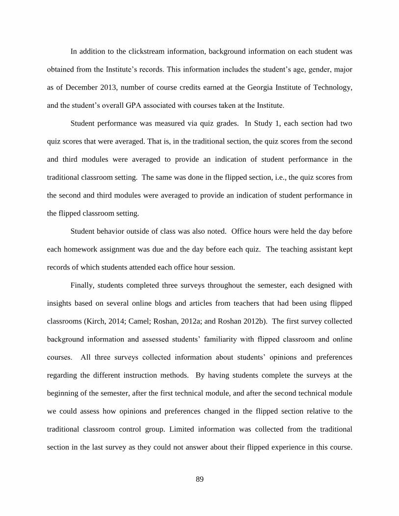
89
In addition to the clickstream information, background information on each student was
obtained from the Institute’s records. This information includes the student’s age, gender, major
as of December 2013, number of course credits earned at the Georgia Institute of Technology,
and the student’s overall GPA associated with courses taken at the Institute.
Student performance was measured via quiz grades. In Study 1, each section had two
quiz scores that were averaged. That is, in the traditional section, the quiz scores from the second
and third modules were averaged to provide an indication of student performance in the
traditional classroom setting. The same was done in the flipped section, i.e., the quiz scores from
the second and third modules were averaged to provide an indication of student performance in
the flipped classroom setting.
Student behavior outside of class was also noted. Office hours were held the day before
each homework assignment was due and the day before each quiz. The teaching assistant kept
records of which students attended each office hour session.
Finally, students completed three surveys throughout the semester, each designed with
insights based on several online blogs and articles from teachers that had been using flipped
classrooms (Kirch, 2014; Camel; Roshan, 2012a; and Roshan 2012b). The first survey collected
background information and assessed students’ familiarity with flipped classroom and online
courses. All three surveys collected information about students’ opinions and preferences
regarding the different instruction methods. By having students complete the surveys at the
beginning of the semester, after the first technical module, and after the second technical module
we could assess how opinions and preferences changed in the flipped section relative to the
traditional classroom control group. Limited information was collected from the traditional
section in the last survey as they could not answer about their flipped experience in this course.

90
That is, their opinion on the traditional method would likely not change throughout the study as
they had not experienced the flipped method. However, the time commitment between the two
modules could change, so they were asked to indicate the time commitment of the class again in
the third survey.
91
Table 4.1: Definition of study 1 variables
Source Variable Description
Main Course
Website
Total Number of
Non-Video Views
Total number of times the student viewed all materials posted on the website (e.g., if a student
viewed the first lecture slides twice and an old exam three times, the total number of views would
be five). Excludes video viewing.
Total Number of
Non-Video Materials
Viewed
Total number of materials viewed at least once on the course website (e.g., if a student viewed the
first lecture slides twice and an old exam three times, the total number of materials viewed would be
two). Excludes video viewing.
Average Number of
Days Before
Homework Due
The number of days between the first viewing of the homework assignment and the day it was due.
Three assignments were given during the study period; the average from these assignments was used
in the study.
Average Number of
Days before Quiz
The number of days between the first viewing of an old exam and the day of the quiz. Two exams
were given during the study period; the average from these quizzes was used in the study.
Video Course
Website
Total Number of
Videos Viewed The number of videos a student viewed at least once.
Student Academic
Records
Male Indicator variable equal to 1 if the student is male, 0 if the student is female.
Age Age of student in years as of December 31, 2013.
Earned Credits Number of hours earned at the Georgia Institute of Technology (excludes advanced placement and
transfer credits).
Transcript GPA Overall grade point average on a 4.0 scale (includes only courses taken at the Georgia Institute of
Technology).
Course Grades Quiz Grade
The average grade the student made on the two quizzes. This variable is used to measure student
performance associated with a particular classroom method.
Course GPA The grade the student received in the civil engineering systems course on a 4.0 scale.
Teaching Assistant
Observations Office Hour Sessions The number of office hour sessions the student attended during the study period.
Surveys
Alone Indicator variable equal to 1 if the student prefers to work alone, 0 otherwise.
Student Background
and Attitude
Information
Used to capture the student’s attitudes about each classroom type and to obtain additional
background information, such as whether the student had access to internet at home.
92
4.3.3 Subjects
Participation in the study was voluntary and had no impact on grades. The instructor and graders
had no knowledge of which students were participating in the study until after course grades
were submitted. Table 2 provides descriptive statistics for students who participated in the
summary and compares these statistics to the total class enrollment. This allows us to determine
if we have selection bias, i.e., if the population of students who participated in the study differs
from the population of students who enrolled in the course. Overall, those students who
participated in the study are similar to the general population of students who registered for the
course. Those who participated are slightly more likely to be female and slightly more likely to
have higher overall GPAs; however, these differences were not statistically significant when
using Welch’s one-sided t-test, which is used to compare samples that possibly have unequal
variances (excluding ISyE students, non-participants – participants <0, p=0.3514).
Students in the traditional and flipped sections are also similar. A comparison of the
students’ overall GPAs on their transcripts shows that the traditional class had a 3.09 average and
the flipped was a 3.24 average. In both classes, the study participants had a higher average GPA
than the total class enrollment. The difference in GPAs between the two study groups was only
0.07. Both study samples were about 60% male, 40% female.
Students were surveyed for additional background information that their transcripts could
not provide. The number of respondents per question is in parentheses. For example, of the 36
study participants in the traditional section, 35 of them answered the question on internet access.
Of the 35 students who responded to this question, 97.1% had internet access at home. It was
found that a very high percent of each study group had internet access at home, which meant
they had a location in addition to the university’s campus where they could access course
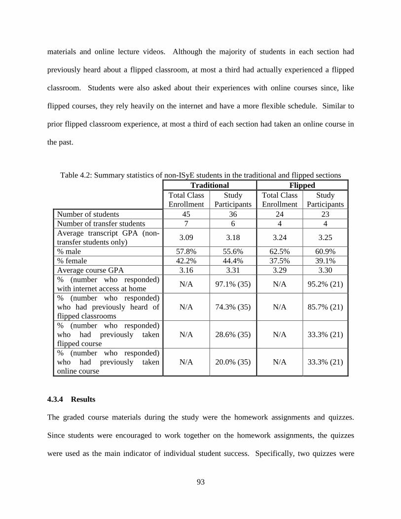
93
materials and online lecture videos. Although the majority of students in each section had
previously heard about a flipped classroom, at most a third had actually experienced a flipped
classroom. Students were also asked about their experiences with online courses since, like
flipped courses, they rely heavily on the internet and have a more flexible schedule. Similar to
prior flipped classroom experience, at most a third of each section had taken an online course in
the past.
Table 4.2: Summary statistics of non-ISyE students in the traditional and flipped sections
Traditional Flipped
Total Class
Enrollment
Study
Participants
Total Class
Enrollment
Study
Participants
Number of students 45 36 24 23
Number of transfer students 7 6 4 4
Average transcript GPA (non-
transfer students only) 3.09 3.18 3.24 3.25
% male 57.8% 55.6% 62.5% 60.9%
% female 42.2% 44.4% 37.5% 39.1%
Average course GPA 3.16 3.31 3.29 3.30
% (number who responded)
with internet access at home N/A 97.1% (35) N/A 95.2% (21)
% (number who responded)
who had previously heard of
flipped classrooms
N/A 74.3% (35) N/A 85.7% (21)
% (number who responded)
who had previously taken
flipped course
N/A 28.6% (35) N/A 33.3% (21)
% (number who responded)
who had previously taken
online course
N/A 20.0% (35) N/A 33.3% (21)
4.3.4 Results
The graded course materials during the study were the homework assignments and quizzes.
Since students were encouraged to work together on the homework assignments, the quizzes
were used as the main indicator of individual student success. Specifically, two quizzes were
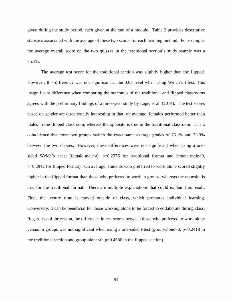
94
given during the study period, each given at the end of a module. Table 3 provides descriptive
statistics associated with the average of these two scores for each learning method. For example,
the average overall score on the two quizzes in the traditional section’s study sample was a
75.1%.
The average test score for the traditional section was slightly higher than the flipped.
However, this difference was not significant at the 0.05 level when using Welch’s t-test. This
insignificant difference when comparing the outcomes of the traditional and flipped classrooms
agrees with the preliminary findings of a three-year study by Lape, et al. (2014). The test scores
based on gender are directionally interesting in that, on average, females performed better than
males in the flipped classroom, whereas the opposite is true in the traditional classroom. It is a
coincidence that these two groups switch the exact same average grades of 76.1% and 73.9%
between the two classes. However, these differences were not significant when using a one-
sided Welch’s t-test (female-male<0, p=0.2376 for traditional format and female-male>0,
p=0.2942 for flipped format). On average, students who preferred to work alone scored slightly
higher in the flipped format than those who preferred to work in groups, whereas the opposite is
true for the traditional format. There are multiple explanations that could explain this result.
First, the lecture time is moved outside of class, which promotes individual learning.
Conversely, it can be beneficial for those working alone to be forced to collaborate during class.
Regardless of the reason, the difference in test scores between those who preferred to work alone
versus in groups was not significant when using a one-sided t-test (group-alone>0, p=0.2418 in
the traditional section and group-alone<0, p=0.4586 in the flipped section).
95
Table 4.3: Average scores on the two quizzes
Traditional Flipped
N Mean Std. Dev. N Mean Std. Dev.
Study Sample 36 75.1 8.9 23 74.8 10.5
Male 20 76.1 7.4 14 73.9 12.3
Female 16 73.9 10.6 9 76.1 7.3
Alone 19 74.5 9.7 12 77.6 8.0
Group 12 76.8 8.6 6 77.1 7.7
Tables 4 and 5 present the correlations and their corresponding p-values among study
variables for the traditional and flipped sections, respectively. Correlations reveal patterns for the
class as a whole. The student’s transcript GPA was a better predictor than earned credit hours of
quiz performance (and positively correlated) in the traditional section. Both of these variables
were also good predictors of quiz performance in the flipped section; in fact the student’s
transcript GPA was more highly correlated in the flipped section than in the traditional section. A
student’s overall GPA may be more indicative of the student’s ability to perform well in a variety
of subjects and situations. To the extent that the flipped classroom represents an unfamiliar
learning environment (and one with an adjustment period), students with higher overall GPAs
would be expected to perform better than students with lower overall GPAs. Therefore, this
means that students’ grades would remain relative to one another (i.e., high GPA means more
likely to get a higher grade in the course and vice versa), not necessarily that the flipped helps
one group more than the other.
We also looked at the impact of the flipped classroom on students with the lower GPAs.
The traditional section had 11 students with a GPA less than 3.0 and the flipped had 12. The
GPAs of these two groups were not significantly different nor were the average test scores. This
is in contrast to the findings of other studies, e.g, in a study on the SCALE-UP model (similar to
96
the flipped), it was found that the classroom model helped students with the lower grades (i.e.,
failure rates reduced) (Beichner, 2008).
Student behavior in the class itself was found to be correlated with success. The average
number of days in advance of a due date that students downloaded a homework assignment was
positively correlated with success on quizzes in the traditional section. The average number of
days in advance of a quiz that students downloaded old exams was also positively correlated
with success on quizzes in the traditional section. Interestingly, these relationships did not
appear in the flipped classroom. That is, it was not as important to prepare in advance to achieve
success in the flipped classroom as compared with the traditional classroom. One explanation is
that access to online lectures and the ability to watch and rewatch videos provides students with
the resources they need to complete homeworks or study for exams; examples of old exams
become less important for success. An alternate explanation is that the assurance of last-minute
resource availability is promoting procrastination, which does not appear to be significantly
impeding success as the grades between the two sections are not significantly different.
Student behavior was also measured via the number of materials students viewed on the
course website (e.g., syllabus, lecture notes, practice quizzes, etc.). The more materials students
viewed, the more likely they were to be successful on the quizzes. Two variables were used to
quantify student presence on the website. As defined in Table 1, the “total number of non-video
views” counts how many times students viewed the materials. However, it was possible for
students to print out the resources, which could make the “total number of non-video materials
viewed” at least once just as important as the number of resource views. For each class, both the
total number of non-video views and total number of non-video materials viewed were positively
correlated with quiz performance. It was more important for flipped classroom students to open
97
each course file at least once than with the traditional classroom. This makes sense as the flipped
classroom is designed to be more dependent on online resources. However, total times “videos
viewed,” i.e., the total number of times the students opened up the videos, was not correlated
with success on the quizzes. This could be due to not being able to track how long students
watched the videos (e.g., we cannot distinguish between view times of two seconds versus 15
minutes). Also, we do not know how focused students were when watching each of the videos.
Some subtle differences in student behavior between the traditional and flipped sections
were related to the number of office hour sessions students attended that merits discussion. The
more office hour sessions that the students attended, the more likely they were to do well on
exams. This is true of both sections. Although the attendance of office hours shown in Table 6
is not significantly different between the two sections using Chi-Square tests, increased
attendance from the flipped section is noticeable. This was somewhat surprising, given that the
flipped classroom allows students, the instructor and/or other teaching assistants to interact
directly with groups of students as they work problems. However, the questions students are
asking the instructor and/or teaching assistants during class are focused more on the problems
they are being asked to work through. Very few students asked questions about general concepts
during the flipped class (nor in office hours). The higher attendance in office hour sessions by
students in the flipped classroom, as shown by Table 6, could potentially be attributed to students
not mastering fundamental concepts when watching the online videos, thereby experiencing
more difficulty in applying concepts to homework problems. There are opportunities in several
classes for students to use “cookbook” problem solving techniques, but miss important overall
concepts. For example, in queueing theory students may be able to calculate the number of cars
in the queue and service time for both determinant and stochastic models, but fail to understand
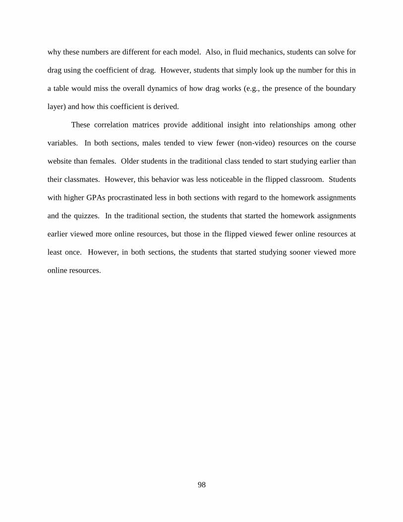
98
why these numbers are different for each model. Also, in fluid mechanics, students can solve for
drag using the coefficient of drag. However, students that simply look up the number for this in
a table would miss the overall dynamics of how drag works (e.g., the presence of the boundary
layer) and how this coefficient is derived.
These correlation matrices provide additional insight into relationships among other
variables. In both sections, males tended to view fewer (non-video) resources on the course
website than females. Older students in the traditional class tended to start studying earlier than
their classmates. However, this behavior was less noticeable in the flipped classroom. Students
with higher GPAs procrastinated less in both sections with regard to the homework assignments
and the quizzes. In the traditional section, the students that started the homework assignments
earlier viewed more online resources, but those in the flipped viewed fewer online resources at
least once. However, in both sections, the students that started studying sooner viewed more
online resources.
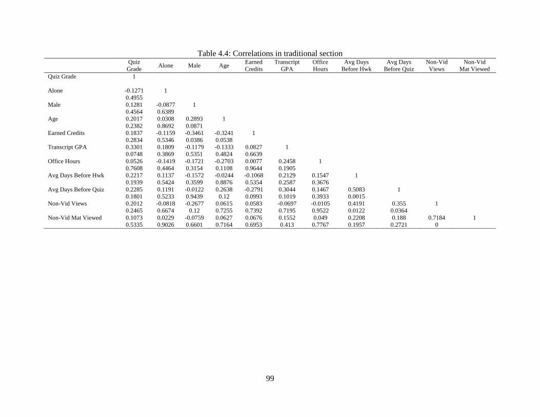
99
Table 4.4: Correlations in traditional section
Quiz
Grade Alone Male Age
Earned
Credits
Transcript
GPA
Office
Hours
Avg Days
Before Hwk
Avg Days
Before Quiz
Non-Vid
Views
Non-Vid
Mat Viewed
Quiz Grade 1
Alone -0.1271 1
0.4955
Male 0.1281 -0.0877 1
0.4564 0.6389
Age 0.2017 0.0308 0.2893 1
0.2382 0.8692 0.0871
Earned Credits 0.1837 -0.1159 -0.3461 -0.3241 1
0.2834 0.5346 0.0386 0.0538
Transcript GPA 0.3301 0.1809 -0.1179 -0.1333 0.0827 1
0.0748 0.3869 0.5351 0.4824 0.6639
Office Hours 0.0526 -0.1419 -0.1721 -0.2703 0.0077 0.2458 1
0.7608 0.4464 0.3154 0.1108 0.9644 0.1905
Avg Days Before Hwk 0.2217 0.1137 -0.1572 -0.0244 -0.1068 0.2129 0.1547 1
0.1939 0.5424 0.3599 0.8876 0.5354 0.2587 0.3676
Avg Days Before Quiz 0.2285 0.1191 -0.0122 0.2638 -0.2791 0.3044 0.1467 0.5083 1
0.1801 0.5233 0.9439 0.12 0.0993 0.1019 0.3933 0.0015
Non-Vid Views 0.2012 -0.0818 -0.2677 0.0615 0.0583 -0.0697 -0.0105 0.4191 0.355 1
0.2465 0.6674 0.12 0.7255 0.7392 0.7195 0.9522 0.0122 0.0364
Non-Vid Mat Viewed 0.1073 0.0229 -0.0759 0.0627 0.0676 0.1552 0.049 0.2208 0.188 0.7184 1
0.5335 0.9026 0.6601 0.7164 0.6953 0.413 0.7767 0.1957 0.2721 0
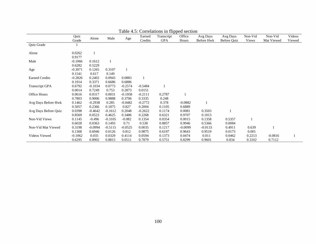
100
Table 4.5: Correlations in flipped section
Quiz
Grade Alone Male Age
Earned
Credits
Transcript
GPA
Office
Hours
Avg Days
Before Hwk
Avg Days
Before Quiz
Non-Vid
Views
Non-Vid
Mat Viewed
Videos
Viewed
Quiz Grade 1
Alone 0.0262 1
0.9177
Male -0.1066 0.1612 1
0.6282 0.5229
Age -0.3071 0.1265 0.3107 1
0.1541 0.617 0.149
Earned Credits -0.2826 0.2402 0.0943 0.0883 1
0.1914 0.3371 0.6686 0.6886
Transcript GPA 0.6792 -0.1034 0.0773 -0.2574 -0.5484 1
0.0014 0.7249 0.753 0.2873 0.0151
Office Hours 0.0616 0.0317 0.0031 -0.1958 -0.2111 0.2787 1
0.7803 0.9006 0.9888 0.3706 0.3335 0.248
Avg Days Before Hwk 0.1462 -0.2938 0.285 -0.0482 -0.2772 0.378 -0.0882 1
0.5057 0.2366 0.1875 0.827 0.2004 0.1105 0.6889
Avg Days Before Quiz 0.0398 -0.4642 -0.1612 0.2048 -0.2622 0.1174 0.0081 0.3503 1
0.8569 0.0523 0.4625 0.3486 0.2268 0.6321 0.9707 0.1013
Non-Vid Views 0.1145 -0.496 -0.3105 -0.082 0.1354 0.0354 0.0015 0.1358 0.5357 1
0.6028 0.0363 0.1493 0.71 0.538 0.8857 0.9946 0.5366 0.0084
Non-Vid Mat Viewed 0.3198 -0.0994 -0.5115 -0.0525 0.0035 0.1217 -0.0099 -0.0133 0.4911 0.639 1
0.1368 0.6946 0.0126 0.812 0.9875 0.6197 0.9643 0.9519 0.0173 0.001
Videos Viewed -0.1062 0.035 0.0329 0.4114 0.0594 0.1373 0.0474 0.011 0.0462 0.2213 -0.0816 1
0.6295 0.8902 0.8815 0.0511 0.7879 0.5751 0.8299 0.9601 0.834 0.3102 0.7112
101
Table 4.6: Percent of study participants per section attending office hours
Traditional Flipped
Homework 1 11.1% 17.4%
Homework 2 16.7% 21.7%
Quiz 1 8.3% 17.4%
Homework 3 27.8% 39.1%
Quiz 2 5.6% 8.7%
Homework 4 13.9% 21.7%
Homework 5 22.2% 21.7%
Quiz 3 5.6% 4.3%
Typically, instructors of flipped classrooms do not know if students are watching the
videos. Based on the in-class problem-solving sessions, instructors cannot differentiate between
students that did not understand the material versus those who did not watch the video.
However, due to the technology used in this study, we were able to analyze students’ video
viewing behavior. On the course website, there were a total of 11 lecture videos for flipped
students to watch. Figure 1 shows how many of the 11 videos each of the study participants
watched. For the flipped section, 8 out of the 23 participants viewed all 11 videos at least once
and 7 watched 10 videos. All of the students watched at least 1 video. It should be pointed out
that Figure 1 simply counts the number of video links that were clicked. That is, the tracking
system could not differentiate between students that watched the entire video versus only two
seconds of the video.
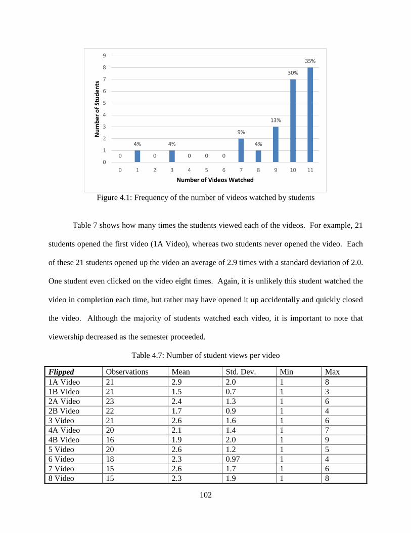
102
Figure 4.1: Frequency of the number of videos watched by students
Table 7 shows how many times the students viewed each of the videos. For example, 21
students opened the first video (1A Video), whereas two students never opened the video. Each
of these 21 students opened up the video an average of 2.9 times with a standard deviation of 2.0.
One student even clicked on the video eight times. Again, it is unlikely this student watched the
video in completion each time, but rather may have opened it up accidentally and quickly closed
the video. Although the majority of students watched each video, it is important to note that
viewership decreased as the semester proceeded.
Table 4.7: Number of student views per video
Flipped Observations Mean Std. Dev. Min Max
1A Video 21 2.9 2.0 1 8
1B Video 21 1.5 0.7 1 3
2A Video 23 2.4 1.3 1 6
2B Video 22 1.7 0.9 1 4
3 Video 21 2.6 1.6 1 6
4A Video 20 2.1 1.4 1 7
4B Video 16 1.9 2.0 1 9
5 Video 20 2.6 1.2 1 5
6 Video 18 2.3 0.97 1 4
7 Video 15 2.6 1.7 1 6
8 Video 15 2.3 1.9 1 8
0
4%
0
4%
0 0 0
9%
4%
13%
30%
35%
0
1
2
3
4
5
6
7
8
9
0 1 2 3 4 5 6 7 8 9 10 11
Nu
mb
er
of
Stu
de
nts
Number of Videos Watched
103
4.3.5 Survey Results
Throughout the semester, both sections were surveyed about their opinions on the classroom
method used. This allowed us to not only compare the opinions between the two sections, but
also assess how students’ opinions evolved as the class progressed. Students in the traditional
classroom were only asked about the traditional method, as the majority of them had never
experienced a flipped classroom and therefore could not answer questions about it. The flipped
students were asked to compare their experiences in the flipped classroom with that in traditional
classrooms. Table 8 shows the survey results. Survey 1 was administered the first day of the
study, before the students had started the traditional and flipped sections. Survey 2 was
administered halfway through the study and Survey 3 was administered at the end of the study.19
The traditional section was treated as the control group and was asked only during the
second survey how they felt about the traditional classroom. On average, the students had a
positive experience in the traditional section, with 33.3% of respondents indicating they loved it
and 63.0% liking it most of the time. Many students noted that they felt most comfortable in this
classroom setting since they had so much experience with it in the past. For example, one
student said, “Traditional is what I am used to, so I like it now just as always.” Another student
believed that the traditional method had a higher educational value by suggesting, “I love
traditional classes. I pay tuition to be taught by a teacher, not teach myself.” A few students
expressed concern that the traditional format did not always agree with their learning speed,
causing them to “feel rushed” or the “need a chance to catch up.” Halfway through the class,
students were asked how much more time they spent per week on this class compared to similar
classes with the same credit hours. The results showed that 0% said much more than average,
19
The percentages are out of all survey respondents. Due to small sample sizes, biases related to attrition over time
may be present.
104
32.2% said somewhat more than average, 35.7% said average, 25.0% said somewhat less than
average, and 7.1% said much less than average. The same question was asked at the end of the
semester and received a very similar response distribution. Therefore when this class was taught
in the traditional style, the time commitment was on par with other the other courses the students
had taken.
Before starting the flipped classroom, the survey administrator, someone who was not
associated with the class, described what a flipped classroom was and then a survey asked them
to give their initial opinion based on the description. This gave us their opinion on the flipped
method before they experienced it. In response, 23.8% would rather have the instructor lecture
during the class (reasons cited included the ability to ask questions to the instructor at the time
the material was presented and the perception that in-class lectures were more interesting and
helped students retain information better). Conversely, 33.3% indicated they would rather watch
the videos (reasons cited included the ability to learn at their own pace, supervised problem-
solving sessions, and shorter in-class lecture times). A total of 38.1% were indifferent (could not
give a good answer without experiencing the flipped method first, liked the videos but also want
to ask questions during lecture), and 4.8% stated they had an opinion other than the options given
(e.g., like the idea of videos but question motivation to watch them without a scheduled lecture
time).
Midway through the semester, the flipped section was surveyed again for their opinions
now that they had experienced the flipped classroom. Overall the students had a positive
experience with the flipped classroom, where 26.3% loved it and 68.4% liked it. Very similar
results were given to the same question at the end of the semester, although the final opinion
distribution was somewhat less favorable than that of the traditional classroom students, with
105
fewer flipped than traditional students loving their format (29.4% versus 33.3%) and more hating
it (5.9% versus 3.7%).
When comparing their flipped learning to that of traditional learning, midway through the
semester 21.1% said flipped helped them learn much better than traditional, 57.9% better than
traditional, 21.0% the same as traditional, 0% less than traditional. By the end of the semester,
their opinions shifted to being more critical of the flipped than when compared to the traditional.
Positive feedback regarding the flipped classroom included the following statements: (1) “I feel
like I am learning in class instead of pretending to listen;” (2) the flipped classroom provided
“great practice and a good opportunity to ask questions;” and, (3) “I like it because it is a more
efficient learning process, but it takes some time to get used to the new method of learning.”
Conversely, negative responses included: (1) a student perceiving inconsistencies in the video
material versus practice problem material; (2) a few students forgetting to watch the videos
before class; and, (3) one student stating “I’d rather be in class so I pay attention.” It is
important to note that the flipped student survey responses did not indicate problems with the
pacing of the class (e.g., too fast or too slow). Students in the flipped section felt the time
commitment was basically the same as their other classes with the same credit hours. Midway
through the semester, the flipped student opinions included 5.3% saying the time commitment
was much more than average, 10.5% somewhat more than average, 52.6% average, 21.1%
somewhat less than average, and 10.5% much less than average. At the end of the semester, this
changed to 0%, 35.3%, 35.3%, 23.5%, and 5.9% respectively. Overall, it could be said that both
the traditional and flipped were on average enjoyable to students, but most students in the flipped
classroom felt that they learned the material better than they would have in the traditional
classroom. Also, the surveys show a learning curve with the flipped classroom, where there was
106
more variation in the time commitment midway through the semester than at the very end. This
learning curve is important as this implies that students are adapting to the new classroom
environment during the first weeks of the course. Although some students catch on quickly,
others can take several weeks to get into the habit of watching the videos on their own. This
segmentation of the classroom could result in a bimodal grade distribution at the beginning of the
semester.
Next, the flipped students were asked about their interactions with the online course
material. Although it was rare for students to do something else while watching the lecture
videos, the majority of students stated that they did not take notes while watching the videos.
Students were more likely to perform actions that lengthened the amount of time they watched
the videos (pause, rewind, and rewatch) than decreased it (fast forward). Also, over time all of
the resources provided to them (video lectures, homework, etc.) became more helpful to their
understanding of the material and success in the class. However, students consistently found the
homework assignments and in-class activities to be the most supportive of their learning.
107
Table 4.8: Survey results from spring semester What are your initial thoughts about the flipped classroom?
Prefer instructor
lecture
Prefer watching
lecture videos Indifferent Other
1st Flipped (21) 23.8% 33.3% 38.1% 4.8%
How are you feeling about the traditional/flipped classroom?
Love it Like it Dislike it Hate it
2nd
Traditional (27) 33.3% 63.0% 3.7% 0%
2nd
Flipped (19) 26.3% 68.4% 5.3% 0%
3rd
Flipped (17) 29.4% 64.7% 5.9% 0%
How much time do you spend on this class compared to others with the same credit hours?
Much more than
average
Somewhat more
than average Average
Somewhat less
than average
Much less than
average
2nd
Traditional (28) 0% 32.2% 35.7% 25.0% 7.1%
3rd
Traditional (21) 0% 33.3% 38.1% 23.8% 4.8%
2nd
Flipped (19) 5.3% 10.5% 52.6% 21.1% 10.5%
3rd
Flipped (17) 0% 35.3% 35.3% 23.5% 5.9%
How does the flipped classroom help you learn the materials compared to the traditional?
Much better Better Same Worse than Much worse
2nd
Flipped (19) 21.1% 57.8% 21.1% 0% 0%
3rd
Flipped (17) 17.7% 58.8% 17.6% 5.9% 0%
What are you doing when you watch the videos?
Listening but doing
something else
Listening and
watching
Listening,
watching and
taking notes
2nd
Flipped (19) 0% 57.9% 42.1%
3rd
Flipped (17) 11.8% 58.8% 29.4%
How often do you do each of the following activities when watching the videos?
Always Sometimes Never
2nd
Flipped Pause (19) 36.8% 63.2% 0%
Rewind (18) 16.7% 61.1% 22.2%
Rewatch (18) 11.1% 61.1% 27.8%
Fast Forward (18) 5.6% 33.35 61.1%
3rd
Flipped Pause (17) 35.3% 52.9% 11.8%
Rewind (17) 17.7% 52.9% 29.4%
Rewatch (17) 17.7% 64.7% 17.6%
Fast Forward (17) 5.9% 35.3% 58.8%
How did the following materials help your understanding?
Helpful Not Sure Waste of Time
2nd
Flipped Video Lectures (19) 84.2% 15.8% 0%
Homework (19) 89.5% 10.5% 0%
In-class discussion (19) 73.7% 21.0% 15.3%
In-class activities (19) 89.5% 10.5% 0%
3rd
Flipped Video Lectures (17) 82.4% 17.6% 0%
Homework (17) 100% 0% 0%
In-class discussion (17) 76.5% 23.5% 0%
In-class activities (17) 94.1% 5.9% 0%
108
4.4 Study 2: Methodology
4.4.1 Design
A second study was conducted during the summer of 2014. Whereas Study 1 had two separate
sections of the same course (holding all variables constant except for the instruction method),
Study 2 had a single section and each module was taught using a different instruction method.
That is, there were three modules, where the first was taught in the traditional style, the second in
the micro-flipped style, and the third in the flipped style. To clarify, the micro-flipped classroom
(also referred to as a partially flipped classroom) is a mixture of the traditional and flipped styles.
In a micro-flipped classroom, “the instructor goes through his or her content for the day’s
lecture. The instructor should not allow more than five minutes of lecture time to pass before
students begin to engage with the material. Tools used might include student responses to
clicker-type questions, mobile-app engagement, and small or large class activities, to name a
few” (Buemi, 2014). This type of classroom is beneficial, as “Unlike the fully flipped approach
where students are expected to come to class prepared, micro-flipping is designed to instruct
both those students who have done the required assignments before class and those who have
not” (Buemi, 2014). It is important to note that our micro-flipped class was organized slightly
differently than the definition presented in the literature. Specifically, the entire lecture was
presented in class, taking half of the class time, not just for 5 minutes. The other half of the class
was a practice problems session. After the class, the lecture video was posted online for students
that were absent or wanted to rewatch the lecture. This type of classroom is possible if the
instructor makes lecture notes available to the class using an electronic format. The time saved
from continuously writing on the board is then used to have an in-class problem solving session.
109
The design of Study 1 was restricted to non-ISyE majors, resulting in a sample with very
little diversity as the vast majority of students studied were second-years majoring in CEE. This
means the results from Study 1 were most applicable to major-specific, sophomore-level courses
as the students will have the same major and experiences due to pre-requisite classes. Since the
study population and sample remained constant in Study 2, all majors were included in the
potential study population. A large number of students taking the course in the summer are
majoring in ISyE; however, unlike the spring semester enrollment, the summer section is not as
restricted and students from this major represent a mix of levels and preparations, i.e., they can
be sophomores, juniors or seniors and may or may not have taken the required ISyE course in
engineering economics. The purpose of Study 2 was to look at a different student population than
that of study 1, namely one with a higher level of diversity across students. Therefore, the study
participants of Study 2 are comparable to core classes that include several majors (e.g., calculus,
physics, and chemistry) and different experience levels.
4.4.2 Data Collection
All data collection methods in Study 1 were used in Study 2, including the exact same surveys
and computer tracking systems. More in-depth information was collected on the study
participants than with those in Study 1. Previously, the only video-viewing information that
could be collected was how many times a student opened each video. Due to better technology,
the date and viewing duration of each video viewing was recorded per participant in Study 2. A
summary of the variables used in Study 2 is shown in Table 9. These variables are similar to
those used in Study 1, but vary slightly in how they were calculated, e.g., in the Study 2 only one

110
quiz (not two) was given per classroom type, eliminating the need to average two scores. Those
variables that were calculated differently from Study 1 are shaded in the table.
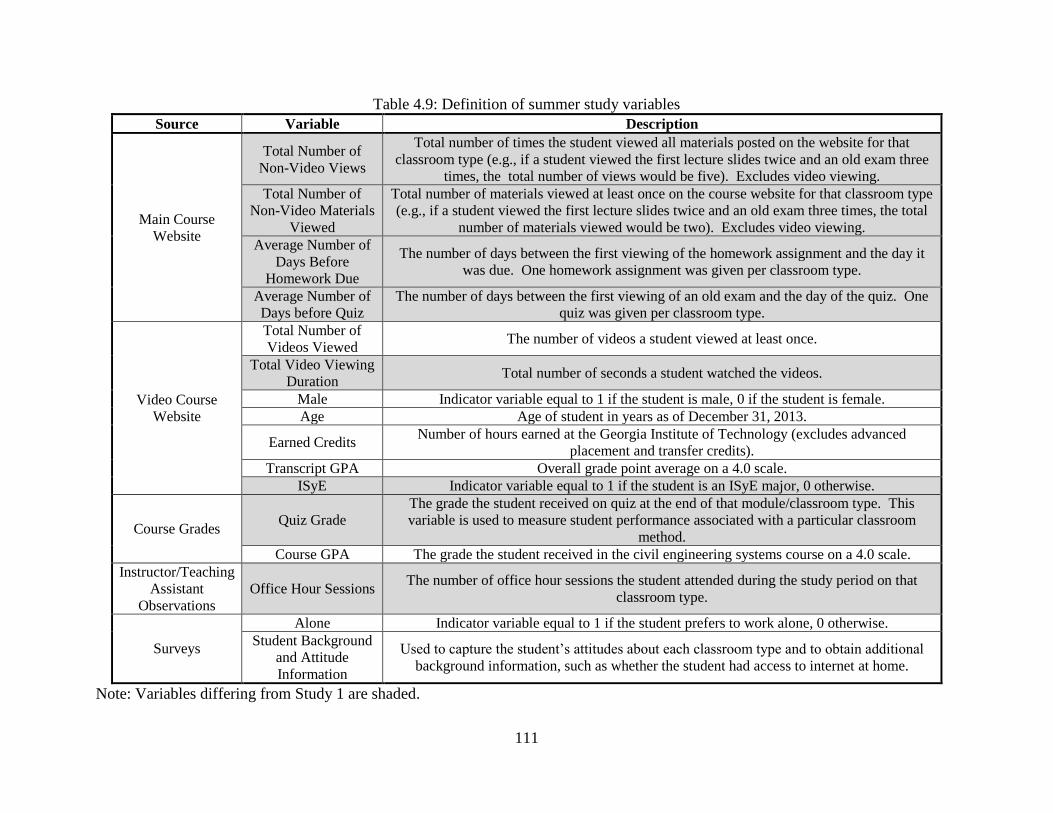
111
Table 4.9: Definition of summer study variables
Source Variable Description
Main Course
Website
Total Number of
Non-Video Views
Total number of times the student viewed all materials posted on the website for that
classroom type (e.g., if a student viewed the first lecture slides twice and an old exam three
times, the total number of views would be five). Excludes video viewing.
Total Number of
Non-Video Materials
Viewed
Total number of materials viewed at least once on the course website for that classroom type
(e.g., if a student viewed the first lecture slides twice and an old exam three times, the total
number of materials viewed would be two). Excludes video viewing.
Average Number of
Days Before
Homework Due
The number of days between the first viewing of the homework assignment and the day it
was due. One homework assignment was given per classroom type.
Average Number of
Days before Quiz
The number of days between the first viewing of an old exam and the day of the quiz. One
quiz was given per classroom type.
Video Course
Website
Total Number of
Videos Viewed The number of videos a student viewed at least once.
Total Video Viewing
Duration Total number of seconds a student watched the videos.
Male Indicator variable equal to 1 if the student is male, 0 if the student is female.
Age Age of student in years as of December 31, 2013.
Earned Credits Number of hours earned at the Georgia Institute of Technology (excludes advanced
placement and transfer credits).
Transcript GPA Overall grade point average on a 4.0 scale.
ISyE Indicator variable equal to 1 if the student is an ISyE major, 0 otherwise.
Course Grades Quiz Grade
The grade the student received on quiz at the end of that module/classroom type. This
variable is used to measure student performance associated with a particular classroom
method.
Course GPA The grade the student received in the civil engineering systems course on a 4.0 scale.
Instructor/Teaching
Assistant
Observations
Office Hour Sessions The number of office hour sessions the student attended during the study period on that
classroom type.
Surveys
Alone Indicator variable equal to 1 if the student prefers to work alone, 0 otherwise.
Student Background
and Attitude
Information
Used to capture the student’s attitudes about each classroom type and to obtain additional
background information, such as whether the student had access to internet at home.
Note: Variables differing from Study 1 are shaded.
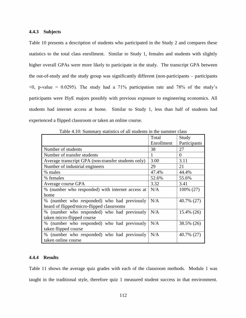
112
4.4.3 Subjects
Table 10 presents a description of students who participated in the Study 2 and compares these
statistics to the total class enrollment. Similar to Study 1, females and students with slightly
higher overall GPAs were more likely to participate in the study. The transcript GPA between
the out-of-study and the study group was significantly different (non-participants – participants
<0, p-value = 0.0295). The study had a 71% participation rate and 78% of the study’s
participants were ISyE majors possibly with previous exposure to engineering economics. All
students had internet access at home. Similar to Study 1, less than half of students had
experienced a flipped classroom or taken an online course.
Table 4.10: Summary statistics of all students in the summer class
Total
Enrollment
Study
Participants
Number of students 38 27
Number of transfer students 1 0
Average transcript GPA (non-transfer students only) 3.00 3.11
Number of industrial engineers 29 21
% males 47.4% 44.4%
% females 52.6% 55.6%
Average course GPA 3.32 3.41
% (number who responded) with internet access at
home
N/A 100% (27)
% (number who responded) who had previously
heard of flipped/micro-flipped classrooms
N/A 40.7% (27)
% (number who responded) who had previously
taken micro-flipped course
N/A 15.4% (26)
% (number who responded) who had previously
taken flipped course
N/A 38.5% (26)
% (number who responded) who had previously
taken online course
N/A 40.7% (27)
4.4.4 Results
Table 11 shows the average quiz grades with each of the classroom methods. Module 1 was
taught in the traditional style, therefore quiz 1 measured student success in that environment.
113
Similarly, the micro-flipped’s outcome was measured by quiz 2 and the flipped’s by quiz 3.
Since the outcomes were measured by a different quiz for each classroom type, it is important
not to compare overall relationships across modules. That is, a decrease in success between two
classroom types could also be the result of one module unintentionally being more difficult than
the other. Instead we compare the success of groups in each classroom type with respect to one
another. With these comparisons there is still the caveat that one group’s success could be
attributed to the material of that module and not the classroom style.
When comparing the traditional and flipped classrooms, our results match up with the
first study. Males tended to do better in the traditional class, whereas females did better in the
flipped class. Again, this finding did not turn out to be statistically significant using the Welch’s
t-test (traditional: female-male>0, p=0.3915 and flipped: female-male>0, p=0.2658). Females
did worse in the micro-flipped classroom (micro-flipped: female-male<0, p=0.1444), although
again not significantly worse. Students that prefer to work alone did better in both the traditional
and flipped classrooms (traditional: group-alone<0, p=0.1147 and flipped: group-alone<0,
p=0.0141); however, this difference was more pronounced in the flipped classroom. Similar to
the results in Study 1, the students who wish to work alone may be more successful in the flipped
classroom because they learn in an isolated environment and also could benefit from
collaborating with peers during the practice problem sessions. Although the students wishing to
work alone seemed to be strong academically, they were less successful in the micro-flipped
classroom with an insignificant difference between the two group’s quiz grades (micro-flipped:
group-alone>0, p=0.4093). This decrease in success compared to the “group” students is
understandable as both the learning and problem-solving practices occur during class, a group
setting, in a micro-flipped classroom.
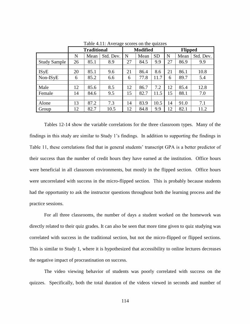
114
Table 4.11: Average scores on the quizzes
Traditional Modified Flipped
N Mean Std. Dev. N Mean SD N Mean Std. Dev.
Study Sample 26 85.1 8.9 27 84.5 9.9 27 86.9 9.9
ISyE 20 85.1 9.6 21 86.4 8.6 21 86.1 10.8
Non-ISyE 6 85.2 6.6 6 77.8 11.7 6 89.7 5.4
Male 12 85.6 8.5 12 86.7 7.2 12 85.4 12.8
Female 14 84.6 9.5 15 82.7 11.5 15 88.1 7.0
Alone 13 87.2 7.3 14 83.9 10.5 14 91.0 7.1
Group 12 82.7 10.5 12 84.8 9.9 12 82.1 11.2
Tables 12-14 show the variable correlations for the three classroom types. Many of the
findings in this study are similar to Study 1’s findings. In addition to supporting the findings in
Table 11, these correlations find that in general students’ transcript GPA is a better predictor of
their success than the number of credit hours they have earned at the institution. Office hours
were beneficial in all classroom environments, but mostly in the flipped section. Office hours
were uncorrelated with success in the micro-flipped section. This is probably because students
had the opportunity to ask the instructor questions throughout both the learning process and the
practice sessions.
For all three classrooms, the number of days a student worked on the homework was
directly related to their quiz grades. It can also be seen that more time given to quiz studying was
correlated with success in the traditional section, but not the micro-flipped or flipped sections.
This is similar to Study 1, where it is hypothesized that accessibility to online lectures decreases
the negative impact of procrastination on success.
The video viewing behavior of students was poorly correlated with success on the
quizzes. Specifically, both the total duration of the videos viewed in seconds and number of

115
videos viewed was not at all correlated with success in the micro-flipped classroom and
insignificantly correlated with the flipped classroom. This could be due to the study not being
able to measure how focused students are when they watch the videos. Also, the videos are not
as important in the micro-flipped classroom because the lecture is covered during the class
session. The number of non-video materials viewed at least once was a better predictor of
success than the total number of non-video material views. Using this, we find that the more
materials students viewed on the course website, the more likely they will be successful on the
quiz. This relationship is strongest in the flipped classroom and is very insignificant in the
micro-flipped classroom.
For correlations between variables not success-related, again we find that males viewed
fewer online course materials than the females. Also, older students tended to view a larger
number of online course materials. Students that have higher GPAs on their transcripts tended to
started assignments and studying for exams earlier. Also, students who started earlier viewed
more online course materials, as they had more time to explore what the course website had to
offer.
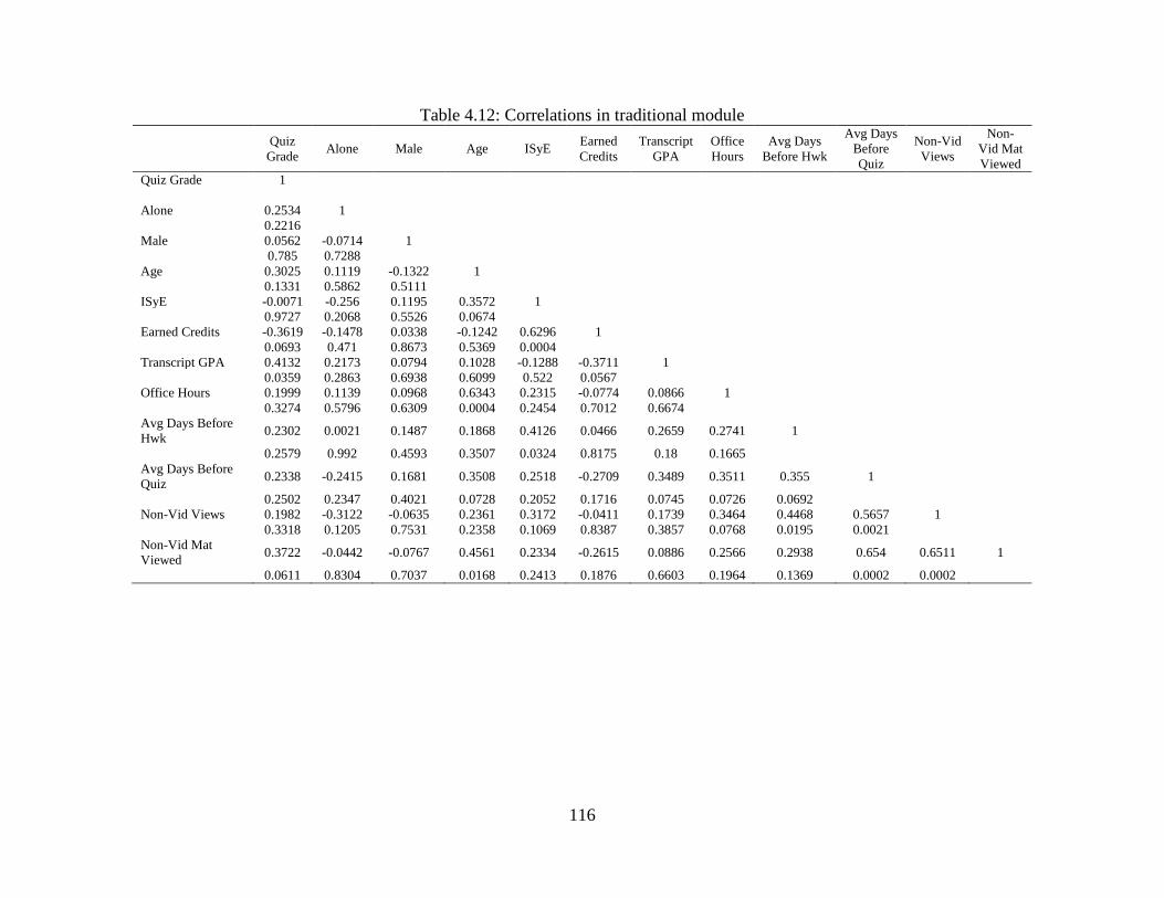
116
Table 4.12: Correlations in traditional module
Quiz
Grade Alone Male Age ISyE
Earned
Credits
Transcript
GPA
Office
Hours
Avg Days
Before Hwk
Avg Days
Before
Quiz
Non-Vid
Views
Non-
Vid Mat
Viewed
Quiz Grade 1
Alone 0.2534 1
0.2216
Male 0.0562 -0.0714 1
0.785 0.7288
Age 0.3025 0.1119 -0.1322 1
0.1331 0.5862 0.5111
ISyE -0.0071 -0.256 0.1195 0.3572 1
0.9727 0.2068 0.5526 0.0674
Earned Credits -0.3619 -0.1478 0.0338 -0.1242 0.6296 1
0.0693 0.471 0.8673 0.5369 0.0004
Transcript GPA 0.4132 0.2173 0.0794 0.1028 -0.1288 -0.3711 1
0.0359 0.2863 0.6938 0.6099 0.522 0.0567
Office Hours 0.1999 0.1139 0.0968 0.6343 0.2315 -0.0774 0.0866 1
0.3274 0.5796 0.6309 0.0004 0.2454 0.7012 0.6674
Avg Days Before
Hwk 0.2302 0.0021 0.1487 0.1868 0.4126 0.0466 0.2659 0.2741 1
0.2579 0.992 0.4593 0.3507 0.0324 0.8175 0.18 0.1665
Avg Days Before
Quiz 0.2338 -0.2415 0.1681 0.3508 0.2518 -0.2709 0.3489 0.3511 0.355 1
0.2502 0.2347 0.4021 0.0728 0.2052 0.1716 0.0745 0.0726 0.0692
Non-Vid Views 0.1982 -0.3122 -0.0635 0.2361 0.3172 -0.0411 0.1739 0.3464 0.4468 0.5657 1
0.3318 0.1205 0.7531 0.2358 0.1069 0.8387 0.3857 0.0768 0.0195 0.0021
Non-Vid Mat
Viewed 0.3722 -0.0442 -0.0767 0.4561 0.2334 -0.2615 0.0886 0.2566 0.2938 0.654 0.6511 1
0.0611 0.8304 0.7037 0.0168 0.2413 0.1876 0.6603 0.1964 0.1369 0.0002 0.0002
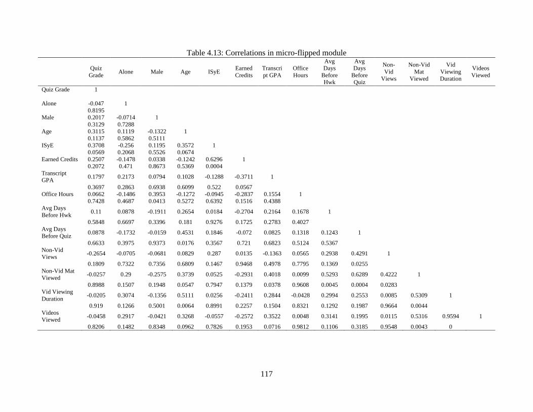
117
Table 4.13: Correlations in micro-flipped module
Quiz
Grade Alone Male Age ISyE
Earned
Credits
Transcri
pt GPA
Office
Hours
Avg
Days
Before
Hwk
Avg
Days
Before
Quiz
Non-
Vid
Views
Non-Vid
Mat
Viewed
Vid
Viewing
Duration
Videos
Viewed
Quiz Grade 1
Alone -0.047 1
0.8195
Male 0.2017 -0.0714 1
0.3129 0.7288
Age 0.3115 0.1119 -0.1322 1
0.1137 0.5862 0.5111
ISyE 0.3708 -0.256 0.1195 0.3572 1
0.0569 0.2068 0.5526 0.0674
Earned Credits 0.2507 -0.1478 0.0338 -0.1242 0.6296 1
0.2072 0.471 0.8673 0.5369 0.0004
Transcript
GPA 0.1797 0.2173 0.0794 0.1028 -0.1288 -0.3711 1
0.3697 0.2863 0.6938 0.6099 0.522 0.0567
Office Hours 0.0662 -0.1486 0.3953 -0.1272 -0.0945 -0.2837 0.1554 1
0.7428 0.4687 0.0413 0.5272 0.6392 0.1516 0.4388
Avg Days
Before Hwk 0.11 0.0878 -0.1911 0.2654 0.0184 -0.2704 0.2164 0.1678 1
0.5848 0.6697 0.3396 0.181 0.9276 0.1725 0.2783 0.4027
Avg Days
Before Quiz 0.0878 -0.1732 -0.0159 0.4531 0.1846 -0.072 0.0825 0.1318 0.1243 1
0.6633 0.3975 0.9373 0.0176 0.3567 0.721 0.6823 0.5124 0.5367
Non-Vid
Views -0.2654 -0.0705 -0.0681 0.0829 0.287 0.0135 -0.1363 0.0565 0.2938 0.4291 1
0.1809 0.7322 0.7356 0.6809 0.1467 0.9468 0.4978 0.7795 0.1369 0.0255
Non-Vid Mat
Viewed -0.0257 0.29 -0.2575 0.3739 0.0525 -0.2931 0.4018 0.0099 0.5293 0.6289 0.4222 1
0.8988 0.1507 0.1948 0.0547 0.7947 0.1379 0.0378 0.9608 0.0045 0.0004 0.0283
Vid Viewing
Duration -0.0205 0.3074 -0.1356 0.5111 0.0256 -0.2411 0.2844 -0.0428 0.2994 0.2553 0.0085 0.5309 1
0.919 0.1266 0.5001 0.0064 0.8991 0.2257 0.1504 0.8321 0.1292 0.1987 0.9664 0.0044
Videos
Viewed -0.0458 0.2917 -0.0421 0.3268 -0.0557 -0.2572 0.3522 0.0048 0.3141 0.1995 0.0115 0.5316 0.9594 1
0.8206 0.1482 0.8348 0.0962 0.7826 0.1953 0.0716 0.9812 0.1106 0.3185 0.9548 0.0043 0
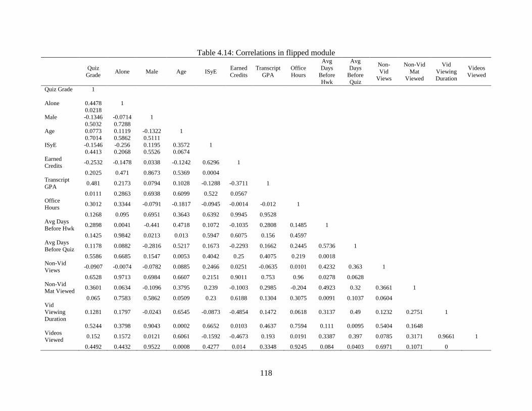
118
Table 4.14: Correlations in flipped module
Quiz
Grade Alone Male Age ISyE
Earned
Credits
Transcript
GPA
Office
Hours
Avg
Days
Before
Hwk
Avg
Days
Before
Quiz
Non-
Vid
Views
Non-Vid
Mat
Viewed
Vid
Viewing
Duration
Videos
Viewed
Quiz Grade 1
Alone 0.4478 1
0.0218
Male -0.1346 -0.0714 1
0.5032 0.7288
Age 0.0773 0.1119 -0.1322 1
0.7014 0.5862 0.5111
ISyE -0.1546 -0.256 0.1195 0.3572 1
0.4413 0.2068 0.5526 0.0674
Earned
Credits -0.2532 -0.1478 0.0338 -0.1242 0.6296 1
0.2025 0.471 0.8673 0.5369 0.0004
Transcript
GPA 0.481 0.2173 0.0794 0.1028 -0.1288 -0.3711 1
0.0111 0.2863 0.6938 0.6099 0.522 0.0567
Office
Hours 0.3012 0.3344 -0.0791 -0.1817 -0.0945 -0.0014 -0.012 1
0.1268 0.095 0.6951 0.3643 0.6392 0.9945 0.9528
Avg Days
Before Hwk 0.2898 0.0041 -0.441 0.4718 0.1072 -0.1035 0.2808 0.1485 1
0.1425 0.9842 0.0213 0.013 0.5947 0.6075 0.156 0.4597
Avg Days
Before Quiz 0.1178 0.0882 -0.2816 0.5217 0.1673 -0.2293 0.1662 0.2445 0.5736 1
0.5586 0.6685 0.1547 0.0053 0.4042 0.25 0.4075 0.219 0.0018
Non-Vid
Views -0.0907 -0.0074 -0.0782 0.0885 0.2466 0.0251 -0.0635 0.0101 0.4232 0.363 1
0.6528 0.9713 0.6984 0.6607 0.2151 0.9011 0.753 0.96 0.0278 0.0628
Non-Vid
Mat Viewed 0.3601 0.0634 -0.1096 0.3795 0.239 -0.1003 0.2985 -0.204 0.4923 0.32 0.3661 1
0.065 0.7583 0.5862 0.0509 0.23 0.6188 0.1304 0.3075 0.0091 0.1037 0.0604
Vid
Viewing
Duration
0.1281 0.1797 -0.0243 0.6545 -0.0873 -0.4854 0.1472 0.0618 0.3137 0.49 0.1232 0.2751 1
0.5244 0.3798 0.9043 0.0002 0.6652 0.0103 0.4637 0.7594 0.111 0.0095 0.5404 0.1648
Videos
Viewed 0.152 0.1572 0.0121 0.6061 -0.1592 -0.4673 0.193 0.0191 0.3387 0.397 0.0785 0.3171 0.9661 1
0.4492 0.4432 0.9522 0.0008 0.4277 0.014 0.3348 0.9245 0.084 0.0403 0.6971 0.1071 0
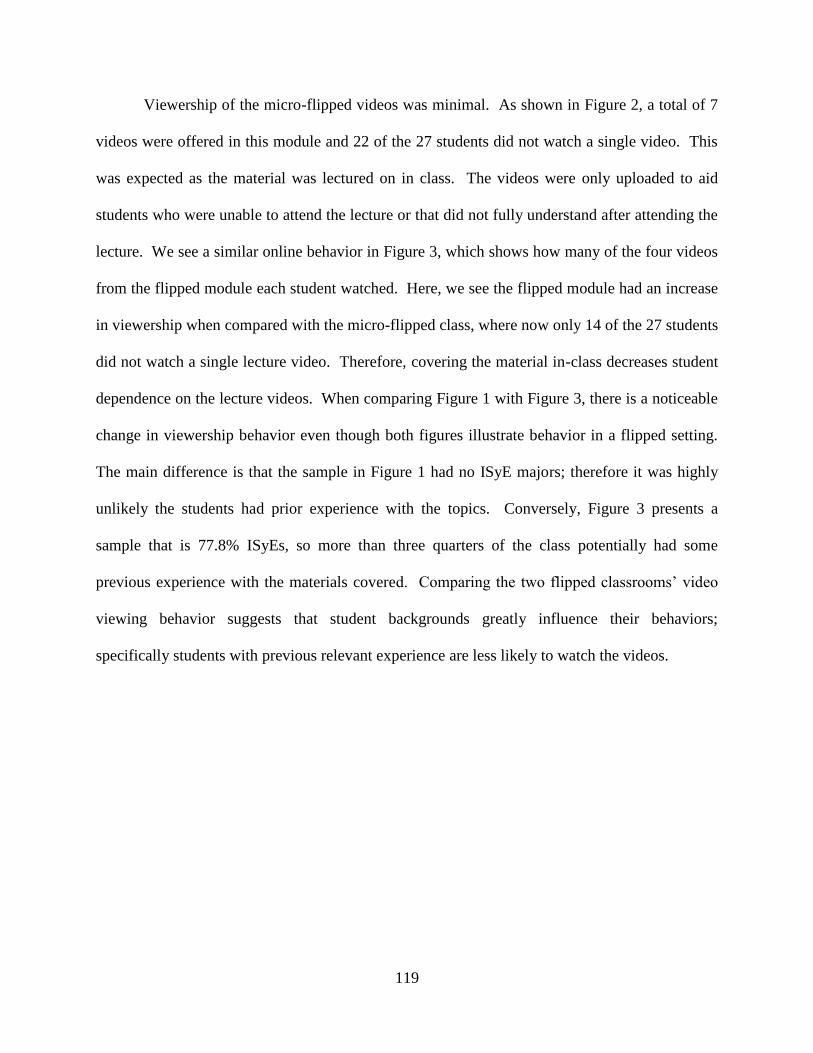
119
Viewership of the micro-flipped videos was minimal. As shown in Figure 2, a total of 7
videos were offered in this module and 22 of the 27 students did not watch a single video. This
was expected as the material was lectured on in class. The videos were only uploaded to aid
students who were unable to attend the lecture or that did not fully understand after attending the
lecture. We see a similar online behavior in Figure 3, which shows how many of the four videos
from the flipped module each student watched. Here, we see the flipped module had an increase
in viewership when compared with the micro-flipped class, where now only 14 of the 27 students
did not watch a single lecture video. Therefore, covering the material in-class decreases student
dependence on the lecture videos. When comparing Figure 1 with Figure 3, there is a noticeable
change in viewership behavior even though both figures illustrate behavior in a flipped setting.
The main difference is that the sample in Figure 1 had no ISyE majors; therefore it was highly
unlikely the students had prior experience with the topics. Conversely, Figure 3 presents a
sample that is 77.8% ISyEs, so more than three quarters of the class potentially had some
previous experience with the materials covered. Comparing the two flipped classrooms’ video
viewing behavior suggests that student backgrounds greatly influence their behaviors;
specifically students with previous relevant experience are less likely to watch the videos.
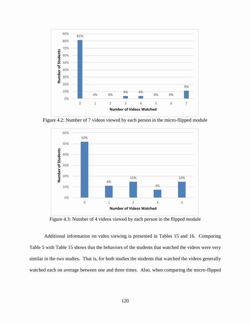
120
Figure 4.2: Number of 7 videos viewed by each person in the micro-flipped module
Figure 4.3: Number of 4 videos viewed by each person in the flipped module
Additional information on video viewing is presented in Tables 15 and 16. Comparing
Table 5 with Table 15 shows that the behaviors of the students that watched the videos were very
similar in the two studies. That is, for both studies the students that watched the videos generally
watched each on average between one and three times. Also, when comparing the micro-flipped
81%
4% 0% 4% 4%
0% 0%
9%
0%
10%
20%
30%
40%
50%
60%
70%
80%
90%
0 1 2 3 4 5 6 7
Nu
mb
er
of
Stu
de
nts
Number of Videos Watched
52%
4% 15%
4%
15%
0%
10%
20%
30%
40%
50%
60%
0 1 2 3 4
Nu
mb
er
of
Stu
de
nts
Number of Videos Watched
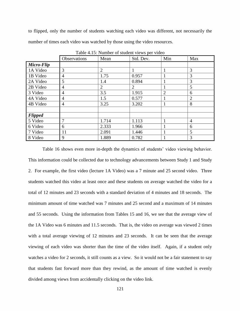
121
to flipped, only the number of students watching each video was different, not necessarily the
number of times each video was watched by those using the video resources.
Table 4.15: Number of student views per video
Observations Mean Std. Dev. Min Max
Micro-Flip
1A Video 3 2 1 1 3
1B Video 4 1.75 0.957 1 3
2A Video 5 1.4 0.894 1 3
2B Video 4 2 2 1 5
3 Video 4 3.5 1.915 2 6
4A Video 4 1.5 0.577 1 2
4B Video 4 3.25 3.202 1 8
Flipped
5 Video 7 1.714 1.113 1 4
6 Video 6 2.333 1.966 1 6
7 Video 11 2.091 1.446 1 5
8 Video 9 1.889 0.782 1 3
Table 16 shows even more in-depth the dynamics of students’ video viewing behavior.
This information could be collected due to technology advancements between Study 1 and Study
2. For example, the first video (lecture 1A Video) was a 7 minute and 25 second video. Three
students watched this video at least once and these students on average watched the video for a
total of 12 minutes and 23 seconds with a standard deviation of 4 minutes and 18 seconds. The
minimum amount of time watched was 7 minutes and 25 second and a maximum of 14 minutes
and 55 seconds. Using the information from Tables 15 and 16, we see that the average view of
the 1A Video was 6 minutes and 11.5 seconds. That is, the video on average was viewed 2 times
with a total average viewing of 12 minutes and 23 seconds. It can be seen that the average
viewing of each video was shorter than the time of the video itself. Again, if a student only
watches a video for 2 seconds, it still counts as a view. So it would not be a fair statement to say
that students fast forward more than they rewind, as the amount of time watched is evenly
divided among views from accidentally clicking on the video link.
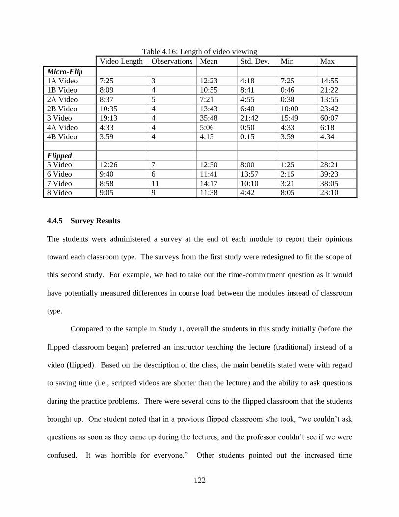
122
Table 4.16: Length of video viewing
Video Length Observations Mean Std. Dev. Min Max
Micro-Flip
1A Video 7:25 3 12:23 4:18 7:25 14:55
1B Video 8:09 4 10:55 8:41 0:46 21:22
2A Video 8:37 5 7:21 4:55 0:38 13:55
2B Video 10:35 4 13:43 6:40 10:00 23:42
3 Video 19:13 4 35:48 21:42 15:49 60:07
4A Video 4:33 4 5:06 0:50 4:33 6:18
4B Video 3:59 4 4:15 0:15 3:59 4:34
Flipped
5 Video 12:26 7 12:50 8:00 1:25 28:21
6 Video 9:40 6 11:41 13:57 2:15 39:23
7 Video 8:58 11 14:17 10:10 3:21 38:05
8 Video 9:05 9 11:38 4:42 8:05 23:10
4.4.5 Survey Results
The students were administered a survey at the end of each module to report their opinions
toward each classroom type. The surveys from the first study were redesigned to fit the scope of
this second study. For example, we had to take out the time-commitment question as it would
have potentially measured differences in course load between the modules instead of classroom
type.
Compared to the sample in Study 1, overall the students in this study initially (before the
flipped classroom began) preferred an instructor teaching the lecture (traditional) instead of a
video (flipped). Based on the description of the class, the main benefits stated were with regard
to saving time (i.e., scripted videos are shorter than the lecture) and the ability to ask questions
during the practice problems. There were several cons to the flipped classroom that the students
brought up. One student noted that in a previous flipped classroom s/he took, “we couldn’t ask
questions as soon as they came up during the lectures, and the professor couldn’t see if we were
confused. It was horrible for everyone.” Other students pointed out the increased time
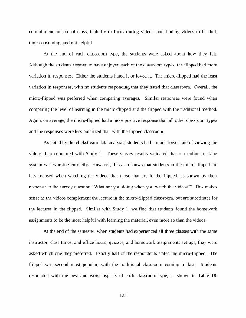
123
commitment outside of class, inability to focus during videos, and finding videos to be dull,
time-consuming, and not helpful.
At the end of each classroom type, the students were asked about how they felt.
Although the students seemed to have enjoyed each of the classroom types, the flipped had more
variation in responses. Either the students hated it or loved it. The micro-flipped had the least
variation in responses, with no students responding that they hated that classroom. Overall, the
micro-flipped was preferred when comparing averages. Similar responses were found when
comparing the level of learning in the micro-flipped and the flipped with the traditional method.
Again, on average, the micro-flipped had a more positive response than all other classroom types
and the responses were less polarized than with the flipped classroom.
As noted by the clickstream data analysis, students had a much lower rate of viewing the
videos than compared with Study 1. These survey results validated that our online tracking
system was working correctly. However, this also shows that students in the micro-flipped are
less focused when watching the videos that those that are in the flipped, as shown by their
response to the survey question “What are you doing when you watch the videos?” This makes
sense as the videos complement the lecture in the micro-flipped classroom, but are substitutes for
the lectures in the flipped. Similar with Study 1, we find that students found the homework
assignments to be the most helpful with learning the material, even more so than the videos.
At the end of the semester, when students had experienced all three classes with the same
instructor, class times, and office hours, quizzes, and homework assignments set ups, they were
asked which one they preferred. Exactly half of the respondents stated the micro-flipped. The
flipped was second most popular, with the traditional classroom coming in last. Students
responded with the best and worst aspects of each classroom type, as shown in Table 18.
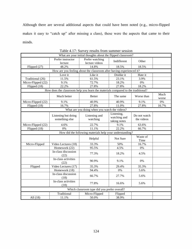
124
Although there are several additional aspects that could have been noted (e.g., micro-flipped
makes it easy to “catch up” after missing a class), these were the aspects that came to their
minds.
Table 4.17: Survey results from summer session What are your initial thoughts about the flipped classroom?
Prefer instructor
lecture
Prefer watching
lecture videos Indifferent Other
Flipped (27) 48.2% 14.8% 18.5% 18.5%
How are you feeling about the classroom after having experienced it?
Love it Like it Dislike it Hate it
Traditional (26) 11.5% 61.5% 23.1% 3.9%
Micro-Flipped (22) 9.1% 72.7% 18.2% 0%
Flipped (18) 22.2% 27.8% 27.8% 18.2%
How does the classroom help you learn the materials compared to the traditional?
Much better Better The same Worse than Much
worse
Micro-Flipped (22) 9.1% 40.9% 40.9% 9.1% 0%
Flipped (18) 16.7% 27.8% 11.0% 27.8% 16.7%
What are you doing when you watch the videos?
Listening but doing
something else
Listening and
watching
Listening,
watching and
taking notes
Do not watch
the videos
Micro-Flipped (22) 4.6% 22.7% 9.1% 63.6%
Flipped (18) 0% 11.1% 22.2% 66.7%
How did the following materials help your understanding?
Helpful Not Sure Waste of
Time
Micro-Flipped Video Lectures (18) 33.3% 50% 16.7%
Homework (22) 95.5% 4.5% 0%
In-class discussion
(22) 77.3% 18.2% 4.5%
In-class activities
(22) 90.9% 9.1% 0%
Flipped Video Lectures (17) 35.3% 29.4% 35.3%
Homework (18) 94.4% 0% 5.6%
In-class discussion
(18) 66.7% 27.7% 5.6%
In-class activities
(18) 77.8% 16.6% 5.6%
Which classroom type did you prefer overall?
Traditional Micro-Flipped Flipped
All (18) 11.1% 50.0% 38.9%
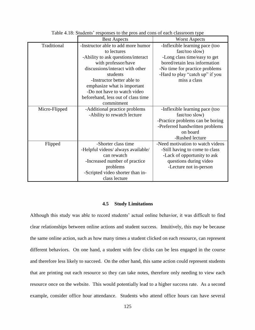
125
Table 4.18: Students’ responses to the pros and cons of each classroom type
Best Aspects Worst Aspects
Traditional -Instructor able to add more humor
to lectures
-Ability to ask questions/interact
with professor/have
discussions/interact with other
students
-Instructor better able to
emphasize what is important
-Do not have to watch video
beforehand, less out of class time
commitment
-Inflexible learning pace (too
fast/too slow)
-Long class time/easy to get
bored/retain less information
-No time for practice problems
-Hard to play “catch up” if you
miss a class
Micro-Flipped -Additional practice problems
-Ability to rewatch lecture
-Inflexible learning pace (too
fast/too slow)
-Practice problems can be boring
-Preferred handwritten problems
on board
-Rushed lecture
Flipped -Shorter class time
-Helpful videos/ always available/
can rewatch
-Increased number of practice
problems
-Scripted video shorter than in-
class lecture
-Need motivation to watch videos
-Still having to come to class
-Lack of opportunity to ask
questions during video
-Lecture not in-person
4.5 Study Limitations
Although this study was able to record students’ actual online behavior, it was difficult to find
clear relationships between online actions and student success. Intuitively, this may be because
the same online action, such as how many times a student clicked on each resource, can represent
different behaviors. On one hand, a student with few clicks can be less engaged in the course
and therefore less likely to succeed. On the other hand, this same action could represent students
that are printing out each resource so they can take notes, therefore only needing to view each
resource once on the website. This would potentially lead to a higher success rate. As a second
example, consider office hour attendance. Students who attend office hours can have several
126
motives for showing up, including to check their approaches after completing the assignment or
to get hints from others before attempting the assignment. There is little that can be done to
overcome this limitation other than to increase the number of survey questions, which might
reduce the number of students willing to participate in the study.
Also, a number of students failed to view some or all of the online lectures and/or never
looked at old practice exams. Either the students never took advantage of these resources or they
could have viewed them during a joint study session where several students use a single
computer with one student’s username. We hypothesize that this limitation can be overcome
simply by changing the classroom setting, specifically to an online course or MOOC where
distance between students would minimize the ability of students to work together in person.
Also, there were design elements of these studies that could be improved. Specifically, it
would be best in the surveys to continue asking the traditional students about their feelings on the
traditional classroom instead of assuming that it stays constant throughout the semester. Also,
due to being limited to a single section in the second study, there were a few confounding factors
with the classroom type that could not be accounted for. There was bias due to the maturation of
the study population and the changing difficulty of each module, which may have impacted
different groups within the study sample differently. It is recommended that future traditional
verses flipped studies contain two simultaneous sections, similar to the first study in this paper.
Lastly, if flipped classrooms continue to become more popular, future flipped classroom studies
will be able to minimize potential reactive effects of experimental arrangements (Campbell and
Stanley, 1963), which may have impacted these studies. That is, once flipped classrooms
become more mainstream, students will be less motivated to act abnormally (e.g., try harder in
the class) due to being heavily scrutinized in an educational study.
127
4.6 Summary
One of the key findings from the study is that regardless of classroom type, good study habits are
essential to student success. The correlations suggest that students who were successful on the
quizzes generally had higher GPAs, started the homework assignments earlier, began studying
for the quizzes earlier, and attended office hours. None of the classrooms promoted or inhibited
good study habits. Simply stated, students that have been successful in the past are likely to
continue being successful whether in a traditional, micro-flipped, or flipped classroom.
Consistent with the findings of Mason and colleagues (2013), we find that students
initially struggled with the flipped classroom format. Survey questions related to time
commitment and enjoyment level received much more polarized answers from the students
during the flipped classroom than compared to either the traditional or micro-flipped classrooms.
This suggests that students must learn to adapt to this new classroom environment in the initial
weeks of the course. This adaptation period varies for each student, where some catch on to the
new idea quickly whereas others need additional time to get in the habit of watching the videos
and being self-motivated. According to Roehl and colleagues (2013), in a flipped classroom the
“... students may require more than a semester to adapt to the new method of instruction and to
recognize its value.” This adaptation period could be problematic, as a typical college course is
only a single semester. This adaptation period can lead to a bimodal distribution in grades. This
research cautions flipped classroom instructors that the method can possibly increase the
frustration of weaker students at the beginning of the course. On the other hand, the adaptation
period can also be viewed positively. Learning a new technology can be seen as an element of
one’s educational experience, where “one’s adaptability to new technologies is crucial for
graduating students to succeed in the workplace” (Roehl et. al, 2013).
128
The inability to ask questions at the time new concepts are introduced appears to be a
critical issue in flipped classrooms. Students want to ask questions during the online video, but
cannot. Importantly, these students appear less likely to ever ask the instructor or teaching
assistant about questions they had about the lecture. Although many students asked questions
during the in-class practice problem sessions, the majority of these questions were focused on the
in-class problems, not lecture material. In turn, this may make it more difficult for student to
apply concepts to homework assignments. This can greatly increase the amount of time these
students need to spend out-of-class to master the material, i.e., out of class time now includes
both watching the lecture videos and going to office hours to ask their questions. This raises
another important question: namely, whether the lack of interaction with the instructor at the
time material is first presented is impacting fundamental understanding of the course concepts.
By viewing lectures ahead of time, students lose the ability to ask questions at the time material
is presented. The lack of this immediate feedback may prevent deeper understanding of the
material, as there is no opportunity for the instructor to dynamically address questions in
different contexts. Further, the problem sessions provide more opportunities for students to
apply the concepts in a problem context, but students may lose the benefit of struggling with the
material and trying different approaches on their own. For future research, it is recommended
that instructors track concept inventories across the sections, through pre- and post- testing
questions included on quizzes, to detect significant differences between the classrooms in
understanding core concepts20
, not just solving problems.
Although the flipped classroom increased the out-of-class workload, the micro-flipped
minimized it. Specifically, the micro-flipped was an effective use of in-class time as both the
20
As part of our study design, we included pre- and post- testing questions but did not include these questions on
exams. Consequently, we found that some students did not take this exercise seriously, limiting our ability to use
these survey results.
129
lecture and practice problems were covered in class; in turn, this minimized the importance of
lecture videos and office hours on student success. Students were able to clarify their
understanding of core concepts during the lecture, which was preferred over watching videos in
advance of class and then having to wait to ask these same questions during the practice problem
sessions (or forgetting to ask these questions at all). Also, the student surveys indicated that
there was little to no adaptation needed for the micro-flipped section. This was evident as the
micro-flipped had the least variation in survey responses.
In summary, our study finds that students preferred the micro-flipped classroom type and
that, in general, students felt they learned material better in flipped and micro-flipped
classrooms. We found that there is an adaptation period associated with the flipped classroom,
which may result in students with poor study habits falling behind; this can result in a bimodal
grade distribution for the course. We recommend that future research explore how learning
outcomes are affected by the inability of students to ask questions at the time lecture material is
first presented.
4.7 Acknowledgments
We thank Gautam Saha for leading the online data collection effort, Stacey Mumbower for
helping with the survey design, and Hunter Stroud for transcribing the handwritten surveys.
4.8 References
1. Beichner, R. (2008) The SCALE-UP Project: a student-centered active learning
environment for undergraduate programs. National Academy of Sciences. Retrieved from
http://www7.nationalacademies.org/bose/Beichner_CommissionedPaper.pdf.
130
2. Bidwesll, A. (2014). Flipped classroom may help weaker STEM students. US News,
Retrieved from http://www.usnews.com/news/stem-solutions/articles/2014/08/05/taking-a-
page-from-humanities-college-engineering-gets-flipped.
3. Bishop, J. L., & Verleger, M. A. (2013). The flipped classroom: A survey of the research.
ASEE National Conference, Atlanta, GA.
4. Buemi, S. (2014). Microflipping: A modest twist on the ‘flipped’ classroom. The Chronicle
of Higher Education, Retrieved from http://chronicle.com/article/Microflipping-a-Modest-
Twist/145951/.
5. Camel, C. BSU EdTech Portfolio. http://camelportfolio.wordpress.com/
6. Campbell, D. T., & Stanley, J. C. (1963). Experimental and quasi-experimental designs for
research. Chicago, IL: Rand McNally.
7. Fact sheet on the president’s plan to make college more affordable (2013). The White
House. Retrieved from http://www.whitehouse.gov/the-press-office/2013/08/22/fact-sheet-
president-s-plan-make-college-more-affordable-better-bargain-.
8. Flipped Learning Network (2012). Improve student learning and teacher satisfaction with
one flip of the classroom.
9. Fulton, K. (2012). Upside down and inside out: Flip your classroom to improve student
learning. Learning & Leading with Technology, 39(8), 12-17.
10. Kirch, C. (2014) Flipping with Kirch. Retrieved from
http://flippingwithkirch.blogspot.com/
11. Lape, N. K. et al. (2014). Probing the inverted classroom: A controlled study of teaching
and learning outcomes in undergraduate engineering and mathematics, American Society of
Engineering Education.
12. Mason, G. S., Shuman, T. R., & Cook, K. E. (2013). Comparing the effectiveness of an
inverted classroom to a traditional classroom in an upper-division engineering
course. Education, IEEE Transactions on, 56(4), 430-435.
13. Noonoo, S. (2012). Flipped learning founders set the record straight, THE Journal,
Retrieved from http://thejournal.com/articles/2012/06/20/flipped-learning-founders-q-and-
a.aspx.
14. Prensky, M. R. (2010). Teaching digital natives: Partnering for real learning. Corwin
Press.
131
15. Roach, T. (2014). Student perceptions toward flipped learning: New methods to increase
interaction and active learning in cconomics. International Review of Economics
Education.
16. Roshan, S. (2012a) Reflecting on the Flipped Classroom Through Student Feedback. The
Daily Riff. <http://www.thedailyriff.com/articles/reflecting-on-the-flipped-class-932.php>
17. Roshan, S. (2012b) The Flipped Class: Students Talk. The Daily Riff.
http://www.thedailyriff.com/articles/students-talk-about-the-flipped-class-survey-results-
933.php
18. Strayer, J. F. (2012). How learning in an inverted classroom influences cooperation,
innovation and task orientation. Learning Environments Research, 15(2), 171-193.
19. Talbert, R. (2012). Inverted classroom. Colleagues, 9(1), 7.
20. Tucker, B. (2012). The flipped classroom. Education Next, 12(1), 82-83.
21. Urbaczewski, A. (2013). Flipping the classroom and problem solving techniques –
Observations and lessons learned. Proceedings from AIS SIG-ED IAIM Conference.
22. Webster, D. R. and Majerich, D. M. (February 2014). Flippin’ Fluid Mechanics-Improved
Student Engagement and Learning via Web-based Applications. Ocean Sciences Meeting,
Honolulu, HI.
23. Wilson, M. E. (2004). Teaching, learning, and millennial students. New directions for
student services, 2004(106), 59-71.
132
CHAPTER 5
CONCLUSIONS AND FUTURE RESEARCH
5.1 Major Conclusions and Directions for Future Research
Three separate studies were presented in this dissertation. The first used clickstream data from a
single major U.S. carrier to analyze airline customer search behavior in markets with an origin
and/or destination in a multi-airport city. The second study used clickstream information from
an OTA to help examine customer online search and purchase behavior near the advance
purchase deadline dates of 3, 7, 14, and 21 days from departure. The third and final study was
related to education and used clickstream data from the course website along with other factors
(e.g., student transcript GPA, age, opinions surveys) to compare the traditional, flipped, and
micro-flipped classroom styles. Each of these studies has its own conclusions and
recommendations for future research, which are outlined in the following sections.
5.1.1 Multi-Airport Choice
By combining clickstream data from a major carrier’s website with representative fare data from
QL2 Pricing®, we were able to investigate how the number of searches at the major carrier’s
website is influenced by representative low fare offerings in the airport pair and competing
airport pairs. We partially overcome limitations in prior studies by incorporating more realistic
information about the fares that customers likely saw at the time they were searching for
information. However, our study does not fully address this limitation, as it was not possible to
collect competitive fare data for every possible round-trip combination.
The use of clickstream data has its own limitations. Clickstream contains little customer
information, limiting our ability to investigate how socio-demographic factors, airport access
133
time, and trip distances influence multi-airport choice. Consistent with other studies of online
search behavior, we find that conversion rates are low. Due to the small number of purchases
represented in our analysis database, we focused our study on understanding the role of
competitive pricing on search behavior; however, the more relevant question to policy makers
and airlines would to understand the role of competitive pricing on purchase decisions.
A second research extension that would be interesting to explore is to compare the results
of our study with data from an online travel agency, as the latter would likely provide a better
estimate of the percentage of customers who consider multi-airports when selecting an itinerary.
This is important, as accurately modeling the percentage of customers who consider multiple
airports is arguably one of the most important inputs to multi-airport choice models.
In summary, we find that using clickstream data to investigate multi-airport choice can
provide some insights into the role of competitors’ prices on customers’ search behavior. One of
the more useful research extensions would be to determine if it is possible for a carrier to use
information about the number of customers visiting its website during the booking process to
identify markets in which the carrier is not be price competitive. That is, if the number of visits
to the carrier’s website is below average or unexpectedly changes, this could be an indication
that more customers are visiting (and purchasing from) competitors’ websites. Early
identification of a large number of customers diverting from the carrier’s website may trigger the
carrier to offer more competitive low fares in the market.
5.1.2 Advance Purchase Deadlines
In this study, we modeled airline travelers’ online search and purchase behaviors using an
analysis database from an online travel agency and QL2 Software. We model individuals’ search
134
and purchase behaviors using an instrumental variable approach that corrects for price
endogeneity. Our study contributes to the literature by providing some of the first empirical
insights into how individuals respond to advance purchase deadlines and price uncertainties
induced by advance purchase deadlines.
Results show that the number of searches and purchases that occur in a market for
specific search and departure dates are a function of search day of week, days from departure,
lowest offered fares, variation in lowest fares offered across competitors, market distance, and
whether the market serves business or leisure consumers. Search activity peaks before a deadline
and declines immediately after a deadline. This suggests that automated search tools help
individuals learn about prices across multiple departure and/or return dates. Moreover,
individuals appear to be switching their desired departure dates by one or two days in order to
avoid higher fares that occur immediately after an advance purchase deadline has passed. This is
an important finding, as current revenue management systems do not take this behavior into
account. Determining revenue impacts associated with failing to take this behavior into account
is an important future research direction.
Looking ahead, it will be interesting to see how competitive pricing evolves, and whether
LCCs will continue to use one-way pricing strategies. The primary motivation for carriers to use
round-trip pricing is to segment business and leisure travelers as round-trip pricing enables
segmentation by length of stay and/or days of travel (e.g., pricing may differ for those trips that
include a Saturday night stay). Currently, airlines face the same limitation we faced in our study
– it is computationally not feasible for them to monitor all of their competitors’ fares. However,
by restricting the analysis to a smaller subset of lengths of stay and/or by leveraging the fact that
fares with the same departure (or return) date will be highly correlated, carriers may be able to
135
develop more efficient algorithms for monitoring competitor fares. Determining whether the
ability of carriers to monitor their competitors’ fares is beneficial or harmful to consumers is a
second important future research direction.
5.1.3 Flipped Classroom
The objective of this paper was to compare traditional, flipped, and micro-flipped classrooms
while controlling for potential confounding factors. Student performance on quizzes was not
significantly different across the traditional and flipped classrooms. A key shortcoming noted
with the flipped classroom was students’ inability to ask questions during lectures. Students in
flipped classrooms were more likely to attend office hours, but this difference was not
statistically significant compared to attendance by students in the traditional classroom. The
micro-flipped classroom was preferred by students. Future research should explore whether
students’ inability to ask questions at the time material is presented in flipped classrooms impacts
learning outcomes.
Although this study was able to record students’ actual online behavior, it was difficult to
find clear relationships between online actions and student success. Intuitively, this may be
because the same online action, such as how many times a student clicked on each resource, can
represent different behaviors. On one hand, a student with few clicks can be less engaged in the
course and therefore less likely to succeed. On the other hand, this same action could represent
students that are printing out each resource so they can take notes, therefore only needing to view
each resource once on the website. This would potentially lead to a higher success rate. As a
second example, consider office hour attendance. Students who attend office hours can have
several motives for showing up, including to check their approaches after completing the
136
assignment or to get hints from others before attempting the assignment. There is little that can
be done to overcome this limitation other than to increase the number of survey questions, which
might reduce the number of students willing to participate in the study.
Also, a number of students failed to view some or all of the online lectures and/or never
looked at old practice exams. Either the students never took advantage of these resources or they
could have viewed them during a joint study session where several students use a single
computer with one student’s username. We hypothesize that this limitation can be overcome
simply by changing the classroom setting, specifically to an online course or MOOC (Massive
Open Online Course) where distance between students would minimize the ability of students to
work together in person.
Also, there were design elements of these studies that could be improved. Specifically, it
would be best in the surveys to continue asking the traditional students about their feelings on the
traditional classroom instead of assuming that it stays constant throughout the semester. Also,
due to being limited to a single section in the second study, there were a few confounding factors
with the classroom type that could not be accounted for. There was bias due to the maturation of
the study population and the changing difficulty of each module, which may have impacted
different groups within the study sample differently. It is recommended that future traditional
verses flipped studies contain two simultaneous sections, similar to the first study in this paper.
Lastly, if flipped classrooms continue to become more popular, future flipped classroom studies
will be able to minimize potential reactive effects of experimental arrangements, which may
have impacted these studies. That is, once flipped classrooms become more mainstream,
students will be less motivated to act abnormally (e.g., try harder in the class) due to being
heavily scrutinized in an educational study.
137
5.2 Concluding Thoughts
The increased use and tracking abilities of the internet has allowed for a more thorough analysis
of user behavior. The three studies in this dissertation take advantage of tracking information,
also known as clickstream data, to draw conclusions surrounding the online behavior of
customers or students. Each study outlines the implications its findings on the area of interest,
whether it is in the airline industry or the field of education.
The first study examines customer search behavior in airline markets containing at least
one multi-airport city. The study’s findings help airlines define the choice set of passengers
flying to and/or from a multi-airport city, specifically that the fares offered at competing airports
significantly affect the search behavior of customer’s at a single major carrier’s website.
However, while the effects of competitor fares at other airports are significant, the weight of
these effects are small compared to other factors that are linked to whether a customer is
considered business or leisure. It is recommended that similar studies based on customer online
behavior of an airline’s website use information from Southwest Airlines as its website captures
all search and purchase activity for its itineraries (i.e., OTAs cannot publish its fares or sell its
tickets).
The second study examines customer online search and purchase behavior near the
advance purchase deadline dates using clickstream information from a single OTA. Models
predicting search and purchase behavior are constructed with valid instrument for price due to
the presence of simultaneity between demand and price. The instruments are based on one-day
stay roundtrip fare information and validated with seven-day stay roundtrip fare information.
The models show that there was an increase in demand right before each deadline and potential
price increase. Since these deadline dates are not well-known, it is hypothesized that customers
138
unintentionally discover the upcoming price hike by noticing an increase in variation of fares
across the different airline competitors and through the use of “flexible dates” tools. These
findings show how customers can easily find the lowest offered fare, making it difficult for
airlines to make a profit. Also, after examining competitor fares near the deadline dates, it was
discovered that the increased variation of fares was due to discrepancies between one-way and
roundtrip pricing. That is, during 2007 (when the data was collected) round-trip fares would
increase both legs of the trip at the same time, while one-way fares would increase the fare of the
first leg and then increase the fare of the second leg days later, based on the length of stay. This
means that near the deadline dates airlines using roundtrip pricing would not be price
competitive with airlines using one-way pricing.
The third and final study analyzes online student behavior on the course website in
attempt to compare the effectiveness of the traditional, flipped, and micro-flipped classrooms.
The benefits of this study include the ability to account for student behavior outside of the
classroom, which can impact their success just as much as the classroom type. Although quiz
grades in the traditional and flipped classrooms were not significantly different, there is a
learning curve and increased office hour attendance associated with the flipped classroom. Also,
the flipped classroom promotes procrastination as student success was not impacted by
procrastination as much as with the traditional classroom. Overall, students prefer the micro-
flipped classroom over both the traditional and flipped classrooms, as it incorporates the best of
both the traditional and flipped classrooms. The micro-flipped classroom allows students to ask
questions during the lecture, have access to helpful online materials (including the lecture
recording), and does not have a learning curve associated with it. Several limitations are
identified in this study including the presence of bias, such as confounding and maturation of the
139
study sample. It is recommended that future studies are carefully designed to prevent the sources
of bias discussed in this study.
These studies overcome the data limitations of previous studies as they are based on
disaggregate, revealed preference information. Also, in the airline studies, actual competitor fare
information is incorporated. Even with these data advances, there is still potential for
improvement. For example, in the two airline studies, clickstream data is only analyzed from
either a single major U.S. carrier or a single OTA. To get a more exhaustive understanding of
customer behavior, it would be beneficial to examine clickstream data from multiple sources
(both carriers and/or OTAs) during the same time period. The clickstream data in the
educational study also had limitations. For example, the data did not indicate if a student printed
out a resource or not, potentially understating the number of times a student referred to that
resource. Also, it was possible that a student could have used another student’s account to view
a resource when collaborating on the homework assignments and studying for quizzes.
Repeating the study in a MOOC setting could potentially reduce the effects of collaboration on
the clickstream data. Therefore, it is recommended that future studies using clickstream data
carefully design the data collection process and the study itself to decrease the impact of bias,
leading to a more accurate behavioral analysis.
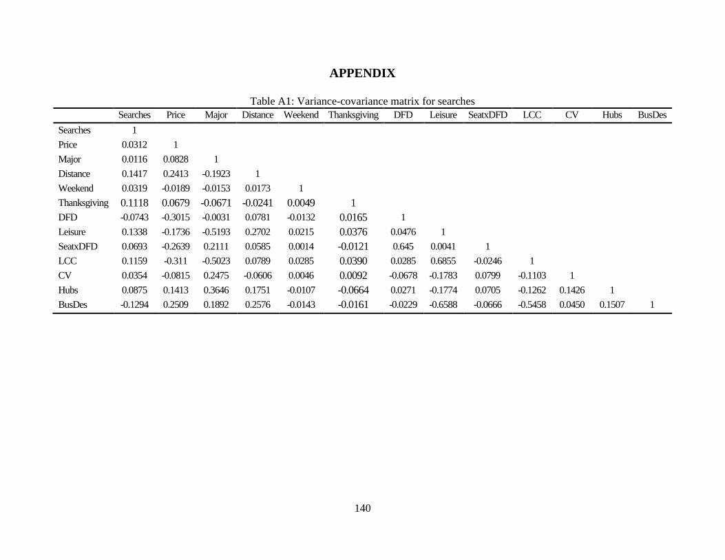
140
APPENDIX
Table A1: Variance-covariance matrix for searches
Searches Price Major Distance Weekend Thanksgiving DFD Leisure SeatxDFD LCC CV Hubs BusDes
Searches 1
Price 0.0312 1
Major 0.0116 0.0828 1
Distance 0.1417 0.2413 -0.1923 1
Weekend 0.0319 -0.0189 -0.0153 0.0173 1
Thanksgiving 0.1118 0.0679 -0.0671 -0.0241 0.0049 1
DFD -0.0743 -0.3015 -0.0031 0.0781 -0.0132 0.0165 1
Leisure 0.1338 -0.1736 -0.5193 0.2702 0.0215 0.0376 0.0476 1
SeatxDFD 0.0693 -0.2639 0.2111 0.0585 0.0014 -0.0121 0.645 0.0041 1
LCC 0.1159 -0.311 -0.5023 0.0789 0.0285 0.0390 0.0285 0.6855 -0.0246 1
CV 0.0354 -0.0815 0.2475 -0.0606 0.0046 0.0092 -0.0678 -0.1783 0.0799 -0.1103 1
Hubs 0.0875 0.1413 0.3646 0.1751 -0.0107 -0.0664 0.0271 -0.1774 0.0705 -0.1262 0.1426 1
BusDes -0.1294 0.2509 0.1892 0.2576 -0.0143 -0.0161 -0.0229 -0.6588 -0.0666 -0.5458 0.0450 0.1507 1
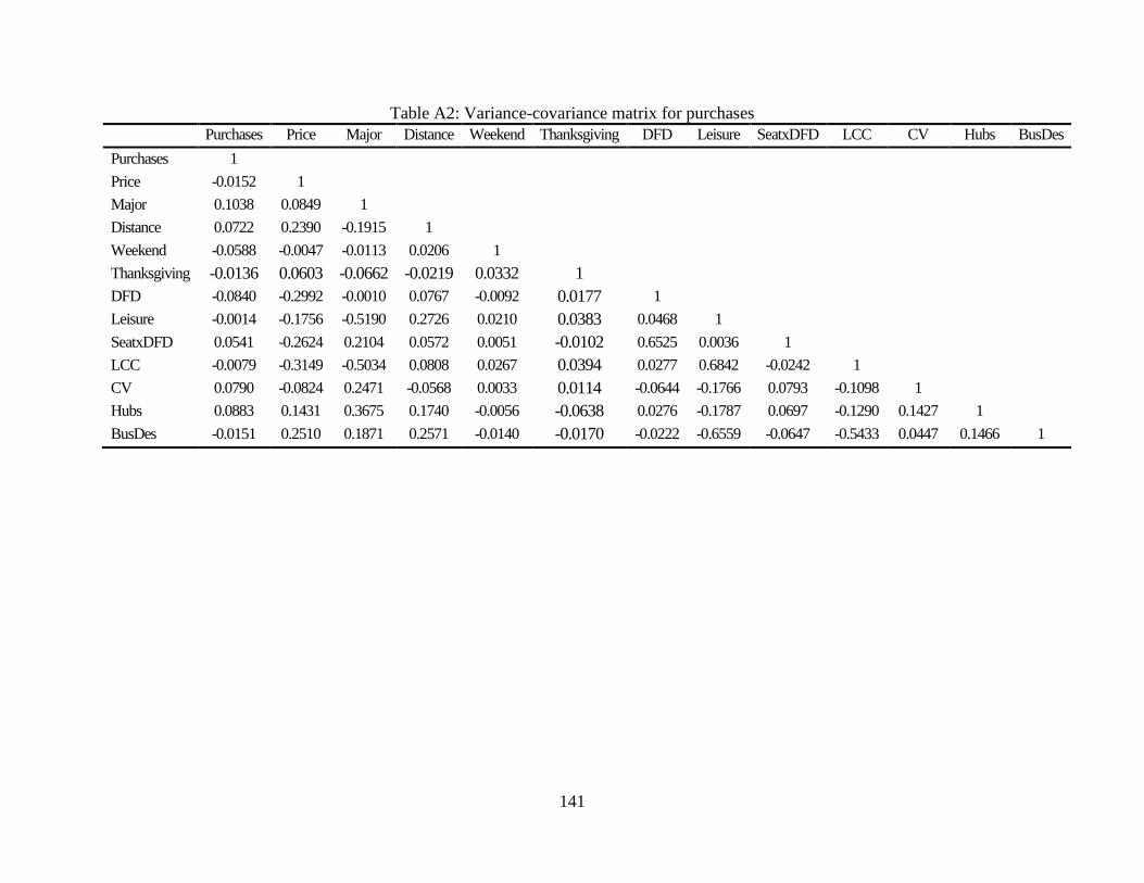
141
Table A2: Variance-covariance matrix for purchases
Purchases Price Major Distance Weekend Thanksgiving DFD Leisure SeatxDFD LCC CV Hubs BusDes
Purchases 1
Price -0.0152 1
Major 0.1038 0.0849 1
Distance 0.0722 0.2390 -0.1915 1
Weekend -0.0588 -0.0047 -0.0113 0.0206 1
Thanksgiving -0.0136 0.0603 -0.0662 -0.0219 0.0332 1
DFD -0.0840 -0.2992 -0.0010 0.0767 -0.0092 0.0177 1
Leisure -0.0014 -0.1756 -0.5190 0.2726 0.0210 0.0383 0.0468 1
SeatxDFD 0.0541 -0.2624 0.2104 0.0572 0.0051 -0.0102 0.6525 0.0036 1
LCC -0.0079 -0.3149 -0.5034 0.0808 0.0267 0.0394 0.0277 0.6842 -0.0242 1
CV 0.0790 -0.0824 0.2471 -0.0568 0.0033 0.0114 -0.0644 -0.1766 0.0793 -0.1098 1
Hubs 0.0883 0.1431 0.3675 0.1740 -0.0056 -0.0638 0.0276 -0.1787 0.0697 -0.1290 0.1427 1
BusDes -0.0151 0.2510 0.1871 0.2571 -0.0140 -0.0170 -0.0222 -0.6559 -0.0647 -0.5433 0.0447 0.1466 1
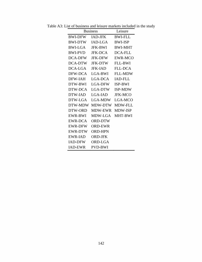
142
Table A3: List of business and leisure markets included in the study
Business Leisure
BWI-DFW IAD-JFK BWI-FLL
BWI-DTW IAD-LGA BWI-ISP
BWI-LGA JFK-BWI BWI-MHT
BWI-PVD JFK-DCA DCA-FLL
DCA-DFW JFK-DFW EWR-MCO
DCA-DTW JFK-DTW FLL-BWI
DCA-LGA JFK-IAD FLL-DCA
DFW-DCA LGA-BWI FLL-MDW
DFW-IAH LGA-DCA IAD-FLL
DTW-BWI LGA-DFW ISP-BWI
DTW-DCA LGA-DTW ISP-MDW
DTW-IAD LGA-IAD JFK-MCO
DTW-LGA LGA-MDW LGA-MCO
DTW-MDW MDW-DTW MDW-FLL
DTW-ORD MDW-EWR MDW-ISP
EWR-BWI MDW-LGA MHT-BWI
EWR-DCA ORD-DTW
EWR-DFW ORD-EWR
EWR-DTW ORD-HPN
EWR-IAD ORD-JFK
IAD-DFW ORD-LGA
IAD-EWR PVD-BWI
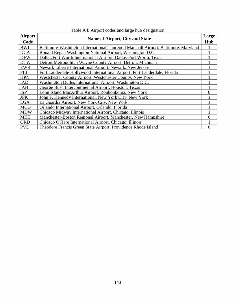
143
Table A4: Airport codes and large hub designation
Airport
Code Name of Airport, City and State
Large
Hub
BWI Baltimore-Washington International Thurgood Marshall Airport, Baltimore, Maryland 1 DCA Ronald Regan Washington National Airport, Washington D.C. 1 DFW Dallas/Fort Worth International Airport, Dallas-Fort Worth, Texas 1 DTW Detroit Metropolitan Wayne County Airport, Detroit, Michigan 1 EWR Newark Liberty International Airport, Newark, New Jersey 1 FLL Fort Lauderdale Hollywood International Airport, Fort Lauderdale, Florida 1 HPN Westchester County Airport, Westchester County, New York 1 IAD Washington Dulles International Airport, Washington D.C. 1 IAH George Bush Intercontinental Airport, Houston, Texas 1 ISP Long Island MacArthur Airport, Ronkonkoma, New York 0 JFK John F. Kennedy International, New York City, New York 1 LGA La Guardia Airport, New York City, New York 1 MCO Orlando International Airport, Orlando, Florida 1 MDW Chicago Midway International Airport, Chicago, Illinois 1 MHT Manchester-Boston Regional Airport, Manchester, New Hampshire 0 ORD Chicago O'Hare International Airport, Chicago, Illinois 1 PVD Theodore Francis Green State Airport, Providence Rhode Island 0