The Sudoku Array and Its Applications in Information Security
210
The Sudoku Array and Its Applications in Information Security A dissertation submitted by Yue Wu In partial fulfillment of the requirements for the degree of Doctor of Philosophy in Electrical Engineering Tufts University August 2012 c 2012, Yue Wu Adviser: Joseph P. Noonan
-
Upload
khangminh22 -
Category
Documents
-
view
0 -
download
0
Transcript of The Sudoku Array and Its Applications in Information Security

The Sudoku Array and ItsApplications in
Information Security
A dissertation submitted by
Yue Wu
In partial fulfillment of the requirements for the degree of
Doctor of Philosophy
in
Electrical Engineering
Tufts University
August 2012
c©2012, Yue Wu
Adviser: Joseph P. Noonan

1. Reviewer: Prof. Joseph P. Noonan
2. Reviewer: Prof. Sos Agaian
3. Reviewer: Prof. Karen Panetta
4. Reviewer: Prof. Brian Tracey
Day of the defense: April 4th, 2012
Signature from head of PhD committee:
ii

Abstract
As one of the most popular pencil-and-paper puzzles with simple con-
straints, Sudoku puzzles are almost everywhere in the world. The popular-
ity of these Sudoku puzzles also encouraged research on their mathematical
properties in recent years, but possible engineering applications of Sudoku
puzzles are rarely considered. In this dissertation, a generalized Sudoku so-
lution, the Sudoku array, is studied for its theoretical properties, practical
generation algorithm and many applications in information security. In par-
ticular, a number of Sudoku based encryption techniques are developed for
digital data by using various properties of a Sudoku array. By using these
techniques as building blocks, Sudoku based cryptosystems are constructed
with respect to different data types: Sudoku-AES cipher for one dimen-
sional data like texts, binary sequences, audio etc; Sudoku-Image cipher for
two dimensional data like images; and Sudoku video encryption for videos
compressed using discrete cosine transforms. Simulation results show that
these Sudoku-based cryptosystems are robust, secure, and comparable to
or outperform existing solutions. Moreover, different Sudoku based mul-
timedia security applications, including pseudorandom number generators,
secret sharing schemes, image watermarking schemes, and visual cryptog-
raphy schemes are also considered and developed. Finally, three different
statistical tests to distinguish an insecure image cipher are derived for the
first time and used for the performance evaluations of image ciphers.

iv

To my family
my grandparents Shaochuan Wu and Guohua Ma
my parents Yongde Wu and Yuefang Gu
my wife Xian Zhang
for their love, encouragement and support

Acknowledgements
First and foremost, I would like to thank my adviser Joseph P. Noonan
for his immense help during the course of my Ph.D. It is my great honor
to have been his last Ph.D student before his retirement. He has taught
me how to think of a problem, how to approach an open question, how to
present a solution in a scientific way and more importantly how to be a
righteous man. I appreciate all his contributions in terms of work, time,
ideas, considerations, patience and funding to make my Ph.D experience
productive and joyful. I am also grateful for the excellent example that he
has given to me as a great teacher.
I would like to thank Professor Sos Agaian in the University of Texas at San
Antonio for his long-term and generous support in research discussions. He
treated me like a father to a son, gave me abundant encouragements and
suggestions. In addition, I want to express my appreciation to Professor Eric
Miller, with whom I worked when I first came to Tufts, for his teachings
in image processing and stochastic process, Professor Karen Panetta who
helped me with my English and revised my papers, Professor Christoph
Borgers and Professor Marjorie Hahn in the Tufts mathematics department
for their excellent courses and generous help when I was confronted with
mathematical problems, Professor Yicong Zhou in the University of Macao
for his support as an elder brother in both my research and daily life, and
Professor Brian Tracey and Professor Norman Ramsey for their instructions
on scientific writing.
The members of Graduate Office 137 in Halligan Hall, especially Jingchen
Pang, Okuary Osechas, Oguz Semerci, Fridrik Larusson, Renato M. Nak-
agomi, George Saveriades, and Dr. Alireza Aghasi, have contributed im-
mensely to my study at Tufts. I thank all of you for taking me out for
coffee, helping me out with various problems, and your continuous support
when I was upset or got stuck. I earned priceless friendship during my life
at Tufts. Besides students in ECE department, I want to acknowledge my
roommates Shuai Nie, Zijing Li, and Rui Li for turning our shared apart-
ment into a joyful living space. I would also like to thank ECE system
manager, George Preble, for his precious and continual help with my study
and living. In regards to spiritual help, I thank all my brothers and sisters
in the Boston Chinese Bible fellowship group and the Emeth Chapel for the
amazing years of growing and walking with Jesus. Through my own expe-
rience in this four-year Ph.D study, I saw HIS great love and faithfulness.
I would like to acknowledge those people working for the LaTeX project for
free and giving beautiful online tutorials for various LaTeX tricks. Without
their help, I cannot write this professional-looking dissertation.

iv

Contents
List of Figures ix
List of Tables xiii
Glossary xv
Acronyms xvii
Symbols xix
1 Introduction 1
1.1 Overview . . . . . . . . . . . . . . . . . . . . . . . . . . . . . . . . . . . 1
1.2 Motivation for Information Security . . . . . . . . . . . . . . . . . . . . 1
1.3 Summary of Contributions in Data Encryption . . . . . . . . . . . . . . 4
1.4 Summary of Contributions in Sudoku Study . . . . . . . . . . . . . . . . 6
1.5 Research Problems in Data Encryption . . . . . . . . . . . . . . . . . . . 7
1.6 Outline of Dissertation . . . . . . . . . . . . . . . . . . . . . . . . . . . . 9
2 The Sudoku Array and Sudoku Generator 13
2.1 Overview . . . . . . . . . . . . . . . . . . . . . . . . . . . . . . . . . . . 13
2.2 Sudoku Introduction . . . . . . . . . . . . . . . . . . . . . . . . . . . . . 13
2.2.1 What is a Sudoku? . . . . . . . . . . . . . . . . . . . . . . . . . . 13
2.2.2 Sudoku’s History . . . . . . . . . . . . . . . . . . . . . . . . . . . 14
2.2.3 Sudoku Variants . . . . . . . . . . . . . . . . . . . . . . . . . . . 15
2.3 Sudoku Array and Properties . . . . . . . . . . . . . . . . . . . . . . . . 18
2.3.1 Mathematical Definition . . . . . . . . . . . . . . . . . . . . . . . 18
2.3.2 Sudoku Notations . . . . . . . . . . . . . . . . . . . . . . . . . . 19
v

CONTENTS
2.3.3 Properties and Facts . . . . . . . . . . . . . . . . . . . . . . . . . 20
2.4 Sudoku Generator . . . . . . . . . . . . . . . . . . . . . . . . . . . . . . 28
2.4.1 Parametric Sudoku Array Generator . . . . . . . . . . . . . . . . 28
2.4.2 A Concrete Example . . . . . . . . . . . . . . . . . . . . . . . . . 32
2.4.3 Key Dependent Sudoku . . . . . . . . . . . . . . . . . . . . . . . 38
2.4.4 Discussion . . . . . . . . . . . . . . . . . . . . . . . . . . . . . . . 40
2.5 3D Extension . . . . . . . . . . . . . . . . . . . . . . . . . . . . . . . . . 41
2.6 Conclusions . . . . . . . . . . . . . . . . . . . . . . . . . . . . . . . . . . 43
3 Sudoku Based Encryption Techniques 49
3.1 Overview . . . . . . . . . . . . . . . . . . . . . . . . . . . . . . . . . . . 49
3.2 Sudoku Whitening . . . . . . . . . . . . . . . . . . . . . . . . . . . . . . 50
3.3 Sudoku Transposition . . . . . . . . . . . . . . . . . . . . . . . . . . . . 54
3.4 Sudoku Permutation . . . . . . . . . . . . . . . . . . . . . . . . . . . . . 56
3.4.1 The method of permutation matrix . . . . . . . . . . . . . . . . . 56
3.4.2 The method of row/colunmn/block shuffling . . . . . . . . . . . . 58
3.4.3 The method of matrix mapping between notations . . . . . . . . 60
3.5 Sudoku Maximum Distance Separable Matrix . . . . . . . . . . . . . . . 62
3.6 Sudoku Substitution . . . . . . . . . . . . . . . . . . . . . . . . . . . . . 66
3.6.1 Methodology . . . . . . . . . . . . . . . . . . . . . . . . . . . . . 67
3.6.2 Differences from the Monte Carlo Simulation . . . . . . . . . . . 68
3.6.3 A Concrete Example . . . . . . . . . . . . . . . . . . . . . . . . . 69
3.7 Conclusions . . . . . . . . . . . . . . . . . . . . . . . . . . . . . . . . . . 71
4 Sudoku-AES Block Cipher 75
4.1 Overview . . . . . . . . . . . . . . . . . . . . . . . . . . . . . . . . . . . 75
4.2 Cipher Structure . . . . . . . . . . . . . . . . . . . . . . . . . . . . . . . 75
4.2.1 A Brief Review of AES . . . . . . . . . . . . . . . . . . . . . . . 75
4.2.2 Sudoku-AES Block Cipher . . . . . . . . . . . . . . . . . . . . . . 77
4.3 Simulation Results . . . . . . . . . . . . . . . . . . . . . . . . . . . . . . 81
4.3.1 CCITT Database . . . . . . . . . . . . . . . . . . . . . . . . . . . 81
4.3.2 Results . . . . . . . . . . . . . . . . . . . . . . . . . . . . . . . . 81
4.4 Security Analysis . . . . . . . . . . . . . . . . . . . . . . . . . . . . . . . 87
4.4.1 Theoretical Analysis . . . . . . . . . . . . . . . . . . . . . . . . . 87
vi

CONTENTS
4.4.2 Experimental Analysis . . . . . . . . . . . . . . . . . . . . . . . . 90
4.5 Conclusions . . . . . . . . . . . . . . . . . . . . . . . . . . . . . . . . . . 91
5 Sudoku Image Cipher 93
5.1 Overview . . . . . . . . . . . . . . . . . . . . . . . . . . . . . . . . . . . 93
5.2 Sudoku-Image Cipher . . . . . . . . . . . . . . . . . . . . . . . . . . . . 93
5.2.1 Cipher Structure . . . . . . . . . . . . . . . . . . . . . . . . . . . 93
5.2.2 Extension to RGB Images . . . . . . . . . . . . . . . . . . . . . 96
5.3 Simulation Results . . . . . . . . . . . . . . . . . . . . . . . . . . . . . . 97
5.3.1 Database . . . . . . . . . . . . . . . . . . . . . . . . . . . . . . . 97
5.3.2 Results . . . . . . . . . . . . . . . . . . . . . . . . . . . . . . . . 101
5.4 Security Analysis . . . . . . . . . . . . . . . . . . . . . . . . . . . . . . . 104
5.4.1 Key Space Analysis . . . . . . . . . . . . . . . . . . . . . . . . . 104
5.4.2 Key Sensitivity Analysis . . . . . . . . . . . . . . . . . . . . . . . 105
5.4.3 Plaintext Sensitivity Analysis . . . . . . . . . . . . . . . . . . . . 107
5.4.4 Ciphertext Randomness Analysis . . . . . . . . . . . . . . . . . . 111
5.4.4.1 Shannon Entropy Measurement . . . . . . . . . . . . . 111
5.4.4.2 Adjacent Pixel Correlation Analysis . . . . . . . . . . . 113
5.5 Conclusions . . . . . . . . . . . . . . . . . . . . . . . . . . . . . . . . . . 118
6 Sudoku Based Multimedia Security Applications 119
6.1 Overview . . . . . . . . . . . . . . . . . . . . . . . . . . . . . . . . . . . 119
6.2 Sudoku Pseudo Random Number Generator . . . . . . . . . . . . . . . . 119
6.3 Sudoku Secret Sharing . . . . . . . . . . . . . . . . . . . . . . . . . . . . 122
6.3.1 Sharing Secret for n out of n people . . . . . . . . . . . . . . . . 124
6.3.2 Sharing Secret for n− 1 out of n people . . . . . . . . . . . . . . 125
6.3.3 Sharing Secret for 2 out of n people . . . . . . . . . . . . . . . . 127
6.4 Sudoku Image Watermarking . . . . . . . . . . . . . . . . . . . . . . . . 129
6.5 Sudoku Visual Cryptography . . . . . . . . . . . . . . . . . . . . . . . . 133
6.6 Sudoku Video Encryption . . . . . . . . . . . . . . . . . . . . . . . . . . 137
6.7 Conclusions . . . . . . . . . . . . . . . . . . . . . . . . . . . . . . . . . . 142
vii

CONTENTS
7 Statistical Tests for Image Randomness 145
7.1 Mathematical Model for True Random Images . . . . . . . . . . . . . . 145
7.2 Shannon Entropy based Statistical Tests . . . . . . . . . . . . . . . . . . 146
7.2.1 Theoretical Statistics about Shannon Entropy under MTRI . . . 146
7.2.2 Shannon Entropy based Statistical Randomness Tests for Image
Encryption . . . . . . . . . . . . . . . . . . . . . . . . . . . . . . 148
7.3 NPCR based Statistical Test . . . . . . . . . . . . . . . . . . . . . . . . 153
7.3.1 Theoretical Statistics about NPCR under MTRI . . . . . . . . . 153
7.3.2 NPCR based Statistical Randomness Test for Image Encryption 154
7.4 UACI based Statistical Test . . . . . . . . . . . . . . . . . . . . . . . . . 155
7.4.1 Theoretical Statistics about UACI under MTRI . . . . . . . . . . 155
7.4.2 UACI based Statistical Randomness Test for Image Encryption . 159
8 Conclusion and Future Work 161
8.1 Concluding Remarks . . . . . . . . . . . . . . . . . . . . . . . . . . . . . 161
8.2 Future works . . . . . . . . . . . . . . . . . . . . . . . . . . . . . . . . . 162
9 Appendix A: NIST SP 800-22 Randomness Test Results for Sudoku-
AES and Sudoku-Image ciphers 165
9.1 Result Report for Sudoku-AES Cipher . . . . . . . . . . . . . . . . . . . 166
9.2 Result Report for Sudoku-Image Cipher . . . . . . . . . . . . . . . . . . 169
10 Appendix B: List of Publications 173
References 175
viii

List of Figures
1.1 The overview of Ph.D works . . . . . . . . . . . . . . . . . . . . . . . . . 2
2.1 Sudoku in newspaper . . . . . . . . . . . . . . . . . . . . . . . . . . . . . 14
2.2 Sudoku variants - part I . . . . . . . . . . . . . . . . . . . . . . . . . . . 16
2.3 Sudoku variants - part II . . . . . . . . . . . . . . . . . . . . . . . . . . . 17
2.4 Sudoku notations . . . . . . . . . . . . . . . . . . . . . . . . . . . . . . . 20
2.5 Sample Sudoku puzzles and solutions . . . . . . . . . . . . . . . . . . . . 35
2.6 Large size Sudoku arrays - part I . . . . . . . . . . . . . . . . . . . . . . 36
2.7 Large size Sudoku arrays - part II . . . . . . . . . . . . . . . . . . . . . 37
2.8 Three-dimensional Sudoku arrays 4× 4× 4 . . . . . . . . . . . . . . . . 44
2.9 Three-dimensional Sudoku arrays - 9× 9× 9 . . . . . . . . . . . . . . . 45
2.10 Constructing three-dimensional Sudoku array using magnet balls . . . . 47
3.1 Sudoku whitening results . . . . . . . . . . . . . . . . . . . . . . . . . . 51
3.2 The cameraman image and its MSB decomposition . . . . . . . . . . . . 52
3.3 Sudoku whitening effects example . . . . . . . . . . . . . . . . . . . . . . 53
3.4 Sudoku transposition results . . . . . . . . . . . . . . . . . . . . . . . . . 55
3.5 4× 4 Sudoku associated unitary permutation matrices . . . . . . . . . . 57
3.6 Sudoku permutation using the associated UPMs . . . . . . . . . . . . . 59
3.7 Sudoku permutation using the row/column/block shuffling . . . . . . . . 60
3.8 4× 4 matrix grid denotation using reference Sudoku (symbols r c and b
denote ‘row’, ‘column’, and ‘block’) . . . . . . . . . . . . . . . . . . . . . 61
3.9 Sudoku permutation results . . . . . . . . . . . . . . . . . . . . . . . . . 63
3.10 4×4 Sudoku MDS matrix. (a)-(h) Sudoku MDS matrices; (i) AES-MDS
matrix . . . . . . . . . . . . . . . . . . . . . . . . . . . . . . . . . . . . . 65
ix

LIST OF FIGURES
3.11 Sudoku matrix and its associated Markov transition matrix. (a) Refer-
ence Sudoku matrix; (b) Normalized Sudoku (doubly stochastic matrix);
(c)The transition matrix within the framework of Monte Carlo chain. . . 68
3.12 A key dependent 256× 256 Sudoku matrix . . . . . . . . . . . . . . . . 70
3.13 An example of Sudoku substitution for eight rounds . . . . . . . . . . . 72
4.1 AES encryption flowchart . . . . . . . . . . . . . . . . . . . . . . . . . . 76
4.2 Sudoku-AES encryption flowchart . . . . . . . . . . . . . . . . . . . . . . 79
4.3 CCITT fax standard image database . . . . . . . . . . . . . . . . . . . . 82
4.4 Plaintext set of CCITT 5 . . . . . . . . . . . . . . . . . . . . . . . . . . 83
4.5 Sample plaintext messages . . . . . . . . . . . . . . . . . . . . . . . . . . 85
4.6 Sample ciphertext messages . . . . . . . . . . . . . . . . . . . . . . . . . 86
5.1 Encryption flowchart of the Sudoku-Image cipher . . . . . . . . . . . . . 94
5.2 USC-SIPI Miscellaneous Image Data Set . . . . . . . . . . . . . . . . . . 100
5.3 Effect of probabilistic encryption stage . . . . . . . . . . . . . . . . . . . 101
5.4 Encryption results by using the Suodku-Image cipher on grayscale images102
5.5 Encryption results by using the Suodku-Image cipher on RGB images . 103
5.6 Sudoku-Image cipher key sensitivity analysis . . . . . . . . . . . . . . . 106
5.7 Sudoku-Image cipher plaintext sensitivity analysis - part I . . . . . . . . 108
5.8 Sudoku-Image cipher plaintext sensitivity analysis - part II . . . . . . . 109
5.9 NPCR and UACI scores vs. cipher rounds in Sudoku-Image cipher . . . 111
5.10 Directional image pixel sequence extraction . . . . . . . . . . . . . . . . 115
5.11 Adjacent pixels correlations before and after encryption . . . . . . . . . 116
6.1 Sudoku matrix and derived puzzle . . . . . . . . . . . . . . . . . . . . . 124
6.2 Share secrets among n− 1 out of n people (n = 3) . . . . . . . . . . . . 125
6.3 Share secrets among n− 1 out of n people (n = 9) . . . . . . . . . . . . 126
6.4 Sharing secret among 2 out of n people (n = 4)-I: share generation . . . 128
6.5 Sharing secret among 2 out of n people (n = 4)-II: secret reconstruction 129
6.6 Flowchart of Sudoku watermarking using LSB embedding . . . . . . . . 130
6.7 Flowchart of extracting Sudoku watermarking using LSB embedding . . 131
6.8 Bit-plane decomposition on image ‘Lenna’ . . . . . . . . . . . . . . . . . 131
6.9 Sudoku watermarking using LSB embedding on image ‘Lenna’ . . . . . 132
x

LIST OF FIGURES
6.10 Fragile Sudoku watermarking using LSB embedding . . . . . . . . . . . 133
6.11 Sudoku visual cryptography - encryption . . . . . . . . . . . . . . . . . . 135
6.12 Sudoku visual cryptography - decryption . . . . . . . . . . . . . . . . . . 136
6.13 A simple model of video coding and decoding using DCT . . . . . . . . 138
6.14 Encryption techniques for a simple video coding model . . . . . . . . . . 140
6.15 Sudoku video encryption . . . . . . . . . . . . . . . . . . . . . . . . . . . 140
6.16 Video encryption results for frame ‘Lenna’ . . . . . . . . . . . . . . . . . 142
6.17 Sudoku video encryption - video frame set I . . . . . . . . . . . . . . . . 143
6.18 Sudoku video encryption - video frame set II . . . . . . . . . . . . . . . 144
xi

LIST OF FIGURES
xii

List of Tables
2.1 LCG parameters used in eight LCGs . . . . . . . . . . . . . . . . . . . . 38
3.1 The Sudoku S-Box When k ∈ Bin#1 . . . . . . . . . . . . . . . . . . . . 70
3.2 The Sudoku S-Box When k ∈ Bin#2 . . . . . . . . . . . . . . . . . . . . 71
4.1 Comparison between classic AES and Sudoku-AES ciphers . . . . . . . . 78
4.2 FIPS 140-2 Statistical test results of ciphertext messages using the Sudoku-
AES cipher . . . . . . . . . . . . . . . . . . . . . . . . . . . . . . . . . . 90
4.3 Lampel-Ziv sequence complexity of ciphertext messages encrypted by
the Sudoku-AES Cipher . . . . . . . . . . . . . . . . . . . . . . . . . . . 91
5.1 USC-SIPI: volume miscellaneous dataset . . . . . . . . . . . . . . . . . . 99
5.2 Encryption/decryption speed comparisons (seconds) . . . . . . . . . . . 105
5.3 Comparisons of NPCR and UACI scores for Image ‘Lenna’ . . . . . . . 111
5.4 NPCR and UACI scores for Encryption using the Sudoku-Image cipher 112
5.5 Comparisons of Shannon entropy score for image ‘Lenna’ . . . . . . . . 113
5.6 Shannon entropy scores for encryption using the Sudoku-Image cipher . 114
5.7 Comparison of APCA Score for Image ‘Lenna’ . . . . . . . . . . . . . . 115
5.8 APCA scores (10−3) for Encryption using the Sudoku-Image cipher . . . 117
6.1 Reference PRNG test results on [1] . . . . . . . . . . . . . . . . . . . . . 121
6.2 NIST test suite results for Sudoku ciphers . . . . . . . . . . . . . . . . . 121
6.3 Truth table of Sudoku visual cryptography . . . . . . . . . . . . . . . . 137
7.1 Theoretical mean and standard deviation under MTRI . . . . . . . . . . 150
7.2 Shannon entropy statistical test reference table for gray and color images 151
xiii

LIST OF TABLES
7.3 Shannon entropy randomness test results for Table 7.3 . . . . . . . . . . 152
7.4 NPCR statistical test reference table for binary and grayscale images . . 155
7.5 NPCR randomness test results for image encryption algorithms . . . . . 156
7.6 NPCR statistical test reference table for binary and grayscale images . . 160
7.7 NPCR randomness test results for image encryption algorithms . . . . . 160
xiv

Glossary
Bit is a basic unit of digital information used
in computing and telecommunications with only
two states ‘0’ and ‘1’.
Bit Stream is a time series of bits, which com-
monly refers to a sequence of bits in computing
and telecommunications.
Byte is a unit of digital information in comput-
ing and telecommunications that most commonly
consists of eight bits.
Cayley Table is a square table defining the
structure of a finite group.
Cipher is a general name for hardware devices
and software algorithms performing encryption
or decryption.
Ciphertext is the encrypted message after per-
forming encryption on a plaintext message.
Confusion Property refers to establishing a
very complicated and involved relationship be-
tween the encryption key and the ciphertext. It is
one of the desired properties suggested by Claude
Shannon in [2] for a secure cipher. A cipher with
this property encrypts plaintext messages with
non-uniform distribution to ciphertext message
with uniform distribution.
Cryptography is the study of techniques allow-
ing secure communications in presence of third
parties. Encryption and decryption are the two
most common procedures in cryptography.
Cryptanalysis is the study of techniques used to
obtain the meaning of encrypted message with-
out knowing the encryption key.
Diffusion Property refers to establishing a
very complicated and involved relationship be-
tween the plaintext and the ciphertext. It is one
of the desired properties suggested by Claude
Shannon in [2] for a secure cipher. A cipher with
this property changes its ciphertext message even
though only one bit of the plaintext message is
changed while the encryption key is unchanged.
DNA (Deoxyribonucleic acid) is a nucleic acid
that contains the genetic instructions used in the
development and operation of all known living
organisms.
Decryption is the process of decrypt-
ing/restoring plaintext messages from ciphertext
messages using a cipher. It normally refers to
the reverse process of Encryption.
Encryption is the process of transforming plain-
text messages into ciphertext messages using a
cipher for making ciphertext messages unintelli-
gent or unrecognizable to unauthorized users.
FIPS 140-2 Test Suite is the statistical test
suite suggested by the U.S. government com-
puter security standard FIPS 140-2 [3], which
is used to accredit cryptographic modules. This
xv

Glossary
test suite contains five main statistical tests for
pseudo-random number generator.
Grayscale Image is a type of images carry-
ing only intensity information. Depending on
the pixel depth, grayscale images can normally
be classified into: 8-bit grayscale images, 16-bit
grayscale image, and 24-bit grayscale image.
Hypothesis testing is a decision-making
method comparing observed data to theoreti-
cal models.
Key is a piece of information, acting like a pa-
rameter, determining the output message in a
cipher. In encryption, the key determines the
ciphertext message when a plaintext message is
given; in decryption, the key determines the de-
crypted message when a ciphertext message is
given.
Latin Square is a class of N × N arrays filled
with N symbols without repeated symbols in any
row or column.
Markov Chain is a mathematical system de-
scribing the relation between one state to another
in a chainlike manner in stochastic process.
Monte Carlo Method is a class of computa-
tional algorithms used for simulating large scale
or very complicated physical and mathematical
problems by employing some degrees of free-
dom controlled by random events. This type of
method is now commonly used in computer sim-
ulations.
NIST SP 800-22 Test Suite is the latest U.S.
governmental standard [1] (last updated in Au-
gust 11, 2010). It includes 15 main statistical
tests for pseudo-random and random number
generators for cryptographic applications.
NP-complete is a class of decision problems in
the computational complexity theory. If a deci-
sion problem is NP-complete, then any solution
to this problem can be verified in polynomial
time, while no fast solution is known.
Plaintext refers to the original message a sender
wishes to transmit to a cipher/encryption algo-
rithm.
P-value is the probability of obtaining a test
statistic at least as extreme as the one that was
actually observed by assuming the null hypothe-
sis is true in statistics.
RGB Image is an additive color image model
in which red, green and blue lights are added
together to represent various colors. A color
channel in a RGB image commonly has a pixel
depth of 8-bits.
Sudoku Puzzle refers to a type of puzzle with
constraints in the filling of every row, column
and puzzle-defined block with regards to the dig-
its/symbols that fill them.
Sudoku Array refers to a class of N ×N arrays
with all Sudoku constraints in rows, columns and
square blocks.
Significance level refers to the amount of evi-
dence required to accept that an event is unlikely
to have arisen by chance.
Test Statistic refers to the interest variable de-
fined in hypotheses tests.
Z-test is a class of statistical tests in classic
statistics. Its test statistic, normally denoted
as z, follows a normal distribution with known
mean and standard deviation.
xvi

xvii
Acronyms
AES: Advanced Encryption Standard [4] is an
encryption standard that was first adopted by
the United States’s government in 2002 and is
now widely accepted in the world.
CDF is the cumulative distribution function de-
scribing the probability that a random variable
X with a given probability distribution will be
found at a value no larger than X.
CLT: Central Limit Theorem is the most impor-
tant theorem in probability theory. It states that
the mean of a sufficiently large number of inde-
pendent random variables, each with finite mean
and variance, follows the normal distribution.
COA: Ciphertext-only Attack is a common type
of attack based on ciphertext messages. This
type of attack necessitates access to a large num-
ber of ciphertext messages using the same key.
CPA: Ciphertext-plaintext Attack is a common
type of attack that explores the relationship be-
tween plaintext messages and ciphertext mes-
sages by choosing arbitrary plaintext messages
and encrypting them to ciphertext messages.
DCT: Discrete Cosine Transform is a discrete
orthogonal transform which expresses a number
of finite data points with a sum of cosine func-
tions of different frequencies.
DES: Data Encryption Standard [5] is a block
cipher and also an encryption standard that was
first adopted by the government of the United
States in 1978.
DFT: Discrete Fourier Transform is a discrete
orthogonal transform commonly used in telecom-
munication and spectrum analysis.
DSS: Digital Signature Standard [6] is a stan-
dard first proposed by the National Institute of
Standards and Technology in 1991.
FIPS: Federal Information Processing Standards
are publicly announced standards developed by
the United States federal government for com-
puter systems.
GF: Galois Field , after Evariste Galois, is a field
containing a finite number of elements.
IDCT: Inverse Discrete Cosine Transform is the
inverse transform of a discrete cosine transform.
IDEA: International Data Encryption Algorithm
is a symmetric block cipher designed by James
Massey and Xuejia Lai in 1991.
i.i.d.: Independent and Identically Distributed
is a term used in statistics to describe the fact
that a number of random variables follow the
exact same probability distribution without de-
pendency.
JPEG: Joint Photographic Experts Group is a
common image format used by digital cameras

Acronyms
and other image capturing devices. It is also
the most common format for transmitting and
storing images on the World Wide Web.
PDF is the probability distribution function de-
scribing the relative likelihood for this random
variable on a given value.
KPA: Known-plaintext Attack is a common type
of attack which analyzes the relationship between
ciphertext messages and the known plaintext
messages.
LCG: Linear Congruential Generator is one of
the oldest and best known pseudo-random num-
ber generator algorithms.
LSB: Least Significant Bit is the bit position in
a binary integer that denotes parity information.
MDS: Maximum Distance Separable MDS code
is used in coding theory for error detection and
correction. The MDS matrix is commonly used
in cryptography.
MSB: Most Significant Bit is the bit position
denoting the greatest value.
MPEG: Moving Picture Experts Group is a
working group of experts that set the standards
for audio and video compression and transmis-
sion.
MTRI: Model of True Random Images is a
mathematical model describing true random im-
ages.
NIST: National Institute of Standards and Tech-
nology is a measurement standards laboratory
which is a non-regulatory agency of the Depart-
ment of Commerce of the United States.
NPCR: Number of Pixel Changing Rate is a
measurement used in image encryption to ana-
lyze the diffusion property.
PRNG: Pseudo Random Number Generator is
an algorithm/physical device used to generate
random-like sequences of numbers in a determin-
istic way.
RNG: Random Number Generator is an algo-
rithm/physical device used to generate sequences
of numbers without recognizable patterns.
RSA: Rivest, Sharmir and Adleman [7] is an
asymmetric key encryption algorithm proposed
in 1977.
SPN: Substitution-Permutation Network is a se-
ries of linked mathematical operations used in
cipher design [8, 9].
UACI: Unified Average Changed Intensity is a
measurement used in image encryption to ana-
lyze the diffusion property.
UPM: Unitary Permutation Matrix is a type of
matrix where there is only one none zero element
in each row or column with value one.
USC-SIPI: University of Southern California
- Signal and Image Processing Institute is the
provider of an open image database with a large
collection of digital images.
WWII: World War II was a global conflict last-
ing from 1939 to 1945 involving most nations in
the world.
xviii

xix
Symbols
A: denotes the symbol set in a Sudoku array.
| · |: denotes the mathematical symbol for the
absolute value function .
B: denotes the Bernoulli distribution in proba-
bility.
BI: denotes the binomial distribution in proba-
bility.
C: denotes a ciphertext message in multimedia
encryption.
Cb: denotes a ciphertext message block in mul-
timedia encryption under the block cipher archi-
tecture (Cb ∈ C).
Cbyte: denotes a byte of ciphertext message in
multimedia encryption (Cbyte ∈ Cb).
f ◦ g: denotes the composition of functions op-
eration in mathematics.
Dtech : (C,K) → P : denotes the decryption
function in cryptography.
∆X: denotes the amount of change on variable
X.
X⊗Y : denotes the difference between two bi-
nary strings X and Y .
eπ: denotes a permutation sequence of the natu-
ral number sequence {1, 2, · · · , N}.
∅: denotes the empty set in set theory.
E[X]: denotes the expectation of random vari-
able X in statistics.
Etech : (P,K)→ C: denotes the encryption func-
tion in cryptography.
fix(x, y): denotes the rounding function to zero
with respect tox
y, i.e. fix(x, y) =
⌊x
y
⌋.
Φ: denotes the cumulative density function of
the standard normal distribution.
M−1: denotes the inverse matrix of M in matrix
theory.
H 0: denotes the null hypothesis in hypothesis
testing.
H(X): denotes the Shannon entropy of a signal
source X.
λ: denotes the eigenvalue of a matrix.
µX : denotes the mean of random variable X in
statistics.
x mod y: denotes the module operation of x over
a ring y in abstract algebra.
#X: denotes the number of possible outcomes

of a discrete random variable X.
N#X (l): denotes the number of pixels with inten-
sity level l in image X.
N: denotes the finite nature number set from 1
to N .
N: denotes the continuous normal distribution
in probability.
N: denotes the NPCR function for two images.
P : denotes a plaintext message in multimedia
encryption.
Pb: denotes a plaintext message block in multi-
media encryption under the block cipher archi-
tecture (Pb ∈ P ).
Pbyte: denotes a byte of plaintext message in
multimedia encryption (Pbyte ∈ Pb).
Pr(X): denotes the probability for the event X
to occur.
Pr(X|Y ): denotes the conditional probability for
the event X to occur when it is known that event
Y happens.
K: denotes the key used in encryption and de-
cryption.
d·e: denotes the rounding function to infinity.
b·c: denotes the rounding function to zero.
rem(x, y): denotes the remainder function with
respect tox
y, i.e. rem(x, y) = x− fix(x, y) · y.
σX : denotes the standard deviation of random
variable X in statistics.
S: denotes a Sudoku array/matrix.
trace(M): denotes the trace of a matrix M in
matrix theory.
MT : denotes the transpose of a matrix M in
matrix theory.
U: denotes the discrete uniform distribution in
probability.
U: denotes the UACI function for two images.
−→v : denotes a vector in linear algebra.
⊕: denotes the exclusive OR operation.
Z: denotes the finite field in number theory.
xx

1
Introduction
1.1 Overview
In this dissertation work, I focused in Sudoku arrays and their applications to in-
formation security. Sudoku puzzles, which have attractive spatial and mathematical
properties, have become popular in recent years. Information security is in high de-
mand to safeguard digital data. Fig. 1.1 shows the tree diagram of my research work
on Sudoku and its applications to information security during the Ph.D period. As
one can see from the diagram, the Sudoku array is applicable to multiple aspects of
information security, including Data Hiding, Data Sharing, Watermarking, and Data
Encryption, all of which rely on one or many of the mathematical properties of Sudoku
arrays. Among these areas, particular focus is given to Data Encryption, the core of this
dissertation; this particular topic of data encryption is further divided into subareas
like Classic Cryptography, Image Encryption,Visual Cryptography, Video Encryption
etc.
1.2 Motivation for Information Security
As the new century begins, our digital world is rapidly changing our daily life with new
digital technologies and new digital devices. Many of these technologies and devices
share one common purpose: helping people send and/or receive information more easily
and efficiently. Email allows people to receive messages from anywhere in the world
within seconds. Cellular phones allow people to chat together wirelessly independent of
location. The Internet gives people a new means to acquire knowledge through search
1

Figure 1.1: The overview of Ph.D works
2

1.2 Motivation for Information Security
engines, which, with the appropriate keywords, forward to relevant content available
online. Online albums enable to share photographs within a specific network of peo-
ple (e.g. colleagues and classmates). Digital papers and books, either scanned from
old scripts or already written in digital format, help contemporary students and re-
searchers to easily access a plethora of knowledge in an easier and efficient way than
their predecessors.
The danger of digital data information theft is a serious issue that has to be resolved.
The breach of personal email accounts is one of many emblematic internet crimes,
which can enable personal information theft and internet frauds. Unauthorized access
to online albums can result in the publication of private photographs, and lead to
uncontrollable situations for the album owners. Unwanted disclosure of business plans
or product designs due to the lost of company laptops, disks, or other digital data
carriers can cause many troubles. All these examples of information leakage are a
reminder of the importance of information security in the digital world.
The US government has been aware of issues related to digital security for a long
time; in 1976, the data encryption standard (DES) [5], a block cipher for binary data
encryption, was selected as an official Federal Information Processing Standard (FIPS)
for the United States by the national bureau of standards. This encryption standard
was quickly widely accepted worldwide. During the 1980s and 1990s, the DES was
updated several times to meet the increasing challenges of digital data security until
the advanced encryption standard (AES) [4] superseded the DES in 2002.
Unfortunately, there is no end to the race between designers of encryption technolo-
gies trying to keep digital information secure and hackers attempting to steal secret
information using cracking techniques. The fast development of the Internet, comput-
ers and other digital devices, gives both designers and hackers more and more powerful
tools. The task of the designers of encryption technologies in this new decade remains
unchanged: How to make digital data secure? However, this question should now be
refined, giving attention to the particular types of information carriers used, i.e. digital
data types.
• How to make bit streams more secure?
• How to make digital audio more secure?
• How to make digital images more secure?
3

• How to make digital videos more secure?
The original question of information security has to be refined because different digital
data types have different properties which should be treated accordingly rather than
in the same manner. For example, digital audio is a type of one-dimensional data
carrying information within its digitalized waveforms. Although it can be treated as a
bit stream, its neighbor bytes are closely correlated rather than loosely correlated in
the case of a bit stream. Therefore, encryption methods with considerations on signal
redundancy might be better for audio data. As a result, although all digital information
are composed of bits or bytes, one good enough method for one data type may not be
necessarily good for other data types.
1.3 Summary of Contributions in Data Encryption
Encryption is the most common technique providing direct protection for digital data.
The original data that inputs to an encryption system/cipher is commonly referred as
plaintext, and the encrypted data that is outputted from an encryption system/cipher
is commonly referred as ciphertext [8, 10]. Therefore, the encryption processing consists
in converting a plaintext message to the corresponding ciphertext message, such that
the information contained in a plaintext message is unrecognizable or unintelligible in
the corresponding ciphertext message.
The beginning of contemporary data encryption can be traced back to World War
II (WWII), when cryptography was extensively used and both theoretical and practical
aspects of cryptanalysis, or codebreaking, were widely researched. Later on, Claude
Shannon’s masterpiece, Communication theory of secrecy systems [2], built the founda-
tions of modern cryptography and cryptanalysis. With the development of computers
and electronics, more complicated ciphers were introduce in the 1970s. One major dif-
ference between the 1970s ciphers and the World War II ones is that the object of the
ciphers, i.e. a plaintext message, turned into stream or block binary bit form in the
1970s rather than the letters and digits used during WWII. IBM personnel designed
an symmetric key 1 encryption algorithm that was later adopted as the data encryp-
tion standard of the United States government in 1976 [5]. Later on, Rivest, Shamir,
and Adleman proposed the RSA algorithm [7]. Since then, both symmetric key en-
cryption and asymmetric key encryption algorithms developed fast. Among symmetric
4

1.3 Summary of Contributions in Data Encryption
key encryption algorithms, the international data encryption algorithm (IDEA) [11]
developed in 1991 and the Rijnael cipher [4], which was selected as the advanced en-
cryption standard in 2001, are the two most well-known ones. Among asymmetric key
encryption algorithms, digital signature standard (DSS) [6, 12, 13] and elliptic curve
cryptography [14, 15] are the two most widely cited ones.
Digital image data carries information within a two-dimensional plane and its nature
commonly includes high information redundancies, high pixel correlations and a much
larger file size compared to 128 bits, which is the processing block size of DES [5] and
AES [4]. Digital image security is addressed with respect to two-levels [16]:
• Bit level encryption: image contents after encryption are completely random-like.
This technique is commonly used for secret data stored for a very long time, for
example, classified images.
• Perceptual level encryption: image contents after encryption are not intelligible or
recognized by human vision system. This technique is commonly used for valuable
data within a certain time period, for example, a first-hand news photograph.
Bit level image encryption algorithms are closely related to classic cryptography because
they share the same goal of reaching random-like ciphertext messages, although in
classic cryptography the information carrier is a bit sequence and in image encryption
it is a two dimensional image.
In the mid-1990s, image encryption started to attract the attention of researchers.
Jiri Fridrich [17] and Josef Scharinger [18] began pioneering work in image encryption,
individually using chaos systems. Since then, hundreds of image encryption algorithms
have been proposed using various chaos systems and properties [19, 20, 21, 22, 23, 24,
25, 26, 26, 27, 28, 29, 30, 31, 32, 33, 34, 35, 36, 37, 38, 39, 40, 41, 42], dominating
the bit level image encryption. However, chaos-based image encryption methods have
shortcomings [43, 44, 45, 46]:
• A chaos system is defined on real numbers, not integers on finite fields, and thus
it is not easily applicable to finite precision systems.
1means that an identical key is used for both encryption and decryption.2means that two distinct keys are used for encryption and decryption, respectively.
5

• Digitalized implementations of a chaos system turn its aperiodic orbits into peri-
odic orbits, and thus may lose its random-like chaotic characteristics.
Besides chaos-based image encryption methods, cellular automata [47], wave transmis-
sion model [48], and magic cube [49, 50] are also used for image encryption.
In many cases, the perceptual level encryption method is referred to as Partial Image
Encryption or Joint Encryption Compression. According to the working mechanism
that a perceptual level encryption method relies on, there are methods based on SCAN-
patterns [51, 52], tree structures [53, 54, 55], discrete cosine transforms [56, 57] and
discrete wavelet transforms [58, 59]. Although it normally performs a faster encryption
than bit level encryption and it is compatible with compression, the perceptual level
encryption is obviously less secure than the bit level encryption due to the possible
information leakage from non-perceptual statistical analysis.
As the transmission capacity of the Internet and the storage capacity of electronic
hardware devices such as hard disks and portable disks increases, digital videos are
becoming more commonly used nowadays. Consequently, video encryption is in demand
in many dimensions of our lives, for example, cable TV. Technologically speaking, video
encryption is a natural extension of image encryption, because a digital video is nothing
but a sequence of frame images. However, due to the size of digital videos and the
existing limits in transmission bandwidth, video encryption is usually performed at
the perceptual level and many methods are direct extensions from image encryption
methods, for example, [52, 54, 56].
1.4 Summary of Contributions in Sudoku Study
Sudoku is a logic-based, combinational number-placement puzzle. It was introduced
in Japan by Nikoli in the paper Monthly Nikolist in April 1984 [60]. Sudoku means
“single number” [61]. The standard Sudoku puzzle consists of a 9× 9 grid divided into
nine 3× 3 blocks. The object of the game is to fill the grid with digits ranging from 1
to 9 without repeating a digit within a row, a column or a block. Sudoku puzzles are
now popular in the whole world and can be seen in many mainstream newspapers, like
The New York Times, USA Today, The Times and The Wall Street Journal.
As the Sudoku craze spread around the world, the mathematical puzzle attracted
attention in various scientific fields. In mathematics and computer science, the general
6

1.5 Research Problems in Data Encryption
problem of solving a Sudoku puzzle has proven to be a NP-complete problem [62, 63].
It has also been shown that the problem of solving a Sudoku puzzle is equivalent to a
graph-coloring problem [64]. The mathematics and the logic behind the Sudoku puzzle
are also widely researched [63, 65, 66, 67, 68, 69, 70, 71, 72, 73]. Recently, the Shannon
entropy of the Sudoku matrix (the solution of a Sudoku puzzle) has been analyzed, and
it was shown that a randomly generated 9×9 Sudoku matrix is even more random than
a random matrix of the same size [74]. Much Sudoku research work has been dedicated
to generate, solve, or rate a Sudoku puzzle efficiently [67, 75, 76].
In chemistry, the Sudoku puzzle is revisited as an educational tool, for example to
teach the chemical elements [77] and organic chemistry [78]. In biology, the Sudoku
puzzle has been transformed into a series of groups with constraints and is used to
efficiently analyze the DNA sequences of multiple specimens [79]. In agriculture, the
Sudoku matrix is used for agricultural experiments [80] and is considered as a good
design for field experiments [81].
As far as information security research is concerned, interest in the Sudoku ma-
trix is recent. In 2008, Shirali-Shahreza et al. suggested a steganography method for
short message service [82], which extracted hidden information by solving a standard
9 × 9 Sudoku puzzle. Hong et al. proposed steganography methods based on 9 × 9
Sudoku matrices using the least significant bit data hiding technique [83, 84]. Wu et al.
showed an image authentication method using 4 × 4 Sudoku matrices [85]. Chang et
al. used 16× 16 Sudoku matrices for data sharing using the (t, n) thresholding method
[86]. However, many of these Sudoku-based methods for information security are still
immature in at least two aspects:
• They have not broken the size bottleneck of the Sudoku matrix, as it is hard to
generate large size Sudoku matrices due to the nature of NP-complete problem.
• They mostly rely on only the naıve properties of the Sudoku matrix, e.g. the
explicit constraints along rows, columns and blocks, rather than more profound
ones.
1.5 Research Problems in Data Encryption
If we adopt the point of view that much digital data needs to be kept secure for periods
spanning over years, perceptual level encryption techniques are not secure enough. This
7
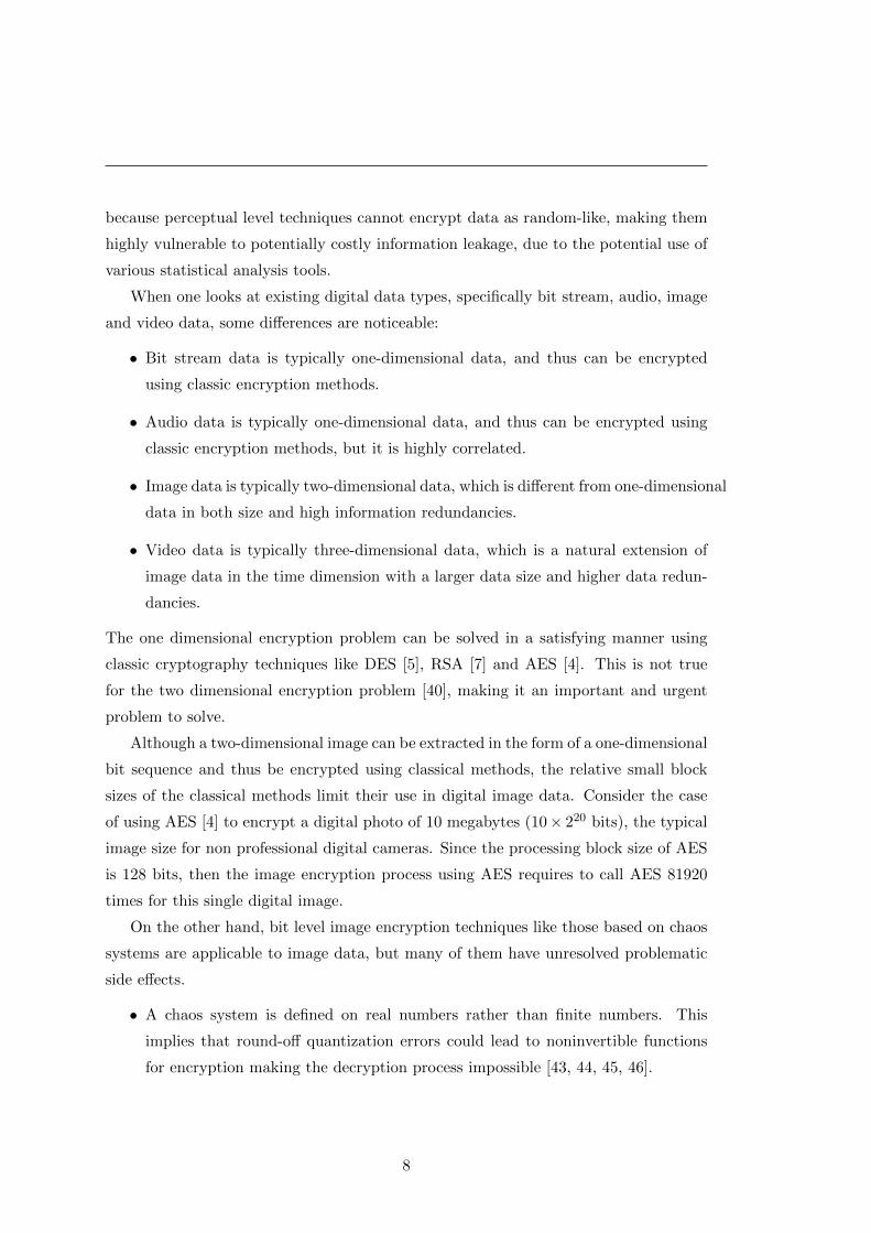
because perceptual level techniques cannot encrypt data as random-like, making them
highly vulnerable to potentially costly information leakage, due to the potential use of
various statistical analysis tools.
When one looks at existing digital data types, specifically bit stream, audio, image
and video data, some differences are noticeable:
• Bit stream data is typically one-dimensional data, and thus can be encrypted
using classic encryption methods.
• Audio data is typically one-dimensional data, and thus can be encrypted using
classic encryption methods, but it is highly correlated.
• Image data is typically two-dimensional data, which is different from one-dimensional
data in both size and high information redundancies.
• Video data is typically three-dimensional data, which is a natural extension of
image data in the time dimension with a larger data size and higher data redun-
dancies.
The one dimensional encryption problem can be solved in a satisfying manner using
classic cryptography techniques like DES [5], RSA [7] and AES [4]. This is not true
for the two dimensional encryption problem [40], making it an important and urgent
problem to solve.
Although a two-dimensional image can be extracted in the form of a one-dimensional
bit sequence and thus be encrypted using classical methods, the relative small block
sizes of the classical methods limit their use in digital image data. Consider the case
of using AES [4] to encrypt a digital photo of 10 megabytes (10× 220 bits), the typical
image size for non professional digital cameras. Since the processing block size of AES
is 128 bits, then the image encryption process using AES requires to call AES 81920
times for this single digital image.
On the other hand, bit level image encryption techniques like those based on chaos
systems are applicable to image data, but many of them have unresolved problematic
side effects.
• A chaos system is defined on real numbers rather than finite numbers. This
implies that round-off quantization errors could lead to noninvertible functions
for encryption making the decryption process impossible [43, 44, 45, 46].
8

1.6 Outline of Dissertation
• A chaos system may contain periodic orbits for some parameters. If a chaotic sys-
tem falls into a periodic orbit, then its behavior is nonchaotic and periodic, which
implies that this system is predictable and thus might be vulnerable to attacks if
the period length is short. For example, chaos-based image encryption methods
[41] and [36] are cryptanalyzed for this reason in [87] and [44], respectively.
• A chaos system may be analyzed and cracked by estimating its initial values
and parameters with existing tools/methods. For example, chaos-based image
encryption methods [37, 42] are cryptanalyzed in [45] and [87], respectively.
Consequently, neither hardware nor software implementations of chaos-based image
encryption methods are good when it comes to the security of encrypted images.
Therefore, the main research challenges in image encryption algorithms are
• Quality: How to design an image encryption algorithm/cipher with good security
considerations, equivalent to those considered in classic ciphers?
• Speed: How to design an image encryption algorithm/cipher with a sufficiently
large processing size, while keeping an affordable computational cost?
• Availability: How to design an image encryption algorithm/cipher with easy hard-
ware and software implementations?
It is also important to emphasize the lack of quality analysis tools for image en-
cryption. Although a number of quantitative tools, like histogram analysis, information
entropy score, pixel correlation coefficient, number of pixel changing rate, and unified
average changed intensity [88] can be used for evaluating the encryption quality of a
ciphertext image, qualitative tools like statistical randomness tests developed for classic
ciphers, such as FIPS 140-1 [89], FIPS 140-2 [3] and NIST SP 800-22 [1], are still rare.
1.6 Outline of Dissertation
In this dissertation, I focus on Sudoku and its applications to information security.
It is worthwile to note that the interest to Sudoku in this work does not pertain to
the “conventional” form (the Sudoku puzzles one can find in newspapers), but to the
generalized form (the Sudoku array) of which the solutions to conventional 9×9 Sudoku
puzzles are a special case.
9
In Chapter 2, I define what Sudoku arrays are and explore their mathematical
properties, many of which can have a direct use in future applications for information
security. I also propose an algorithm to generate an arbitrary size parametric Sudoku
array via a series of transformations and swaps. In addition, Sudoku cubes are also
explored.
In Chapter 3, I propose Sudoku-based data encryption techniques, including Sudoku
Whitening, Sudoku Transposition, Sudoku Permutation, Sudoku Maximum Separable
Distance Matrix and Sudoku Substitution. All these techniques serve as cryptographic
primitives for advanced encryption algorithms/ciphers.
In Chapter 4, I consider the bit stream data and design a data encryption algorithm
named Sudoku-AES cipher. Specifically speaking, the Sudoku-AES cipher mimics the
structure of the AES cipher [4], while using only Sudoku-based encryption techniques.
In the cryptanalysis of the Sudoku-AES cipher, I show it is a Markov cipher [90] and
thus it is immune to differential attacks. Furthermore, I perform a comprehensive
security analysis with respect to known attacks and apply statistical randomness tests to
ciphertext samples. Both theoretical and experimental analyses show that the Sudoku-
AES cipher is safe with respect to the listed known cryptanalysis.
In Chapter 5, I consider digital image data and propose an image encryption algo-
rithm named Sudoku-Image cipher. The Sudoku-Image cipher allows for fast encryption
while respecting some of the characteristics of the particular image including high pixel
correlation, high information redundancy and bulk data. Unlike chaos-based image en-
cryption algorithms, the Sudoku-Image cipher is directly designed on finite fields using
Sudoku cryptographic primitives and thus it can be easily implemented in hardware or
software. In performance analysis, I show that the Sudoku-Image cipher outperforms
many recent commercial or academic image encryption algorithms/ciphers through a
large number of experiments.
In Chapter 6, I consider the use of Sudoku-based techniques to other information
security problems such as Sudoku Pseudo Random Number Generator, Sudoku Secret
Sharing, Sudoku Visual Cryptography and Sudoku Image Watermarking, Sudoku Video
Encryption. All these Sudoku-based techniques demonstrate the wide range of possible
applications of Sudoku arrays in information security.
In Chapter 7, I propose three statistical hypothesis tests for image encryption, which
allows to distinguish a poorly encrypted image from a random-like one.
10

1.6 Outline of Dissertation
I conclude the dissertation and discuss the future works in Chapter 8. For additional
details, I put the comprehensive reports of the NIST SP 800-2 statistical test suite [1]
of the Sudoku-AES cipher and the Sudoku-Image cipher in Appendix A. Finally, my
publications during the Ph.D studies are listed in Appendix B.
11

12

2
The Sudoku Array and Sudoku
Generator
2.1 Overview
In this section, I briefly review the history of Sudoku and its applications in various
scientific areas. I propose a general definition of the square Sudoku array and explore its
mathematical properties as well. Many of these properties are useful and interesting to
related areas e.g. mathematics, logics, education etc.; I show examples of applications
making use of these properties in multimedia security applications in future chapters. I
explain how our parametric Sudoku generator uses the Sudoku structural configuration.
I show that this generator is able to produce an arbitrary size Sudoku and that it can
easily be made key dependent. Such a key dependent Sudoku generator can be directly
used in encryption.
2.2 Sudoku Introduction
2.2.1 What is a Sudoku?
The name Sudoku is the abbreviation of the Japanese ‘Sunji wa dokushin ni kagiru’,
which means ‘single number’ [60]. Conventionally, Sudoku refers to a number-based
puzzle, consisting of 9× 9 grids divided into nine 3× 3 blocks [63] (in some literature,
this 3 × 3 block is referred to as a box, or square). The objective is to complete the
13

grids using digits ranging from 1 to 9, in a manner that there are no repeated digits in
any single row, column and block of the overall puzzle
(a) A Sudoku puzzle (b) The solution to the puzzle
Figure 2.1: Sudoku in newspaper
Fig. 2.1 shows a Sudoku puzzle in a newspaper and its solution. The 9 block indices
are identified in Fig. 2.1-(b) by the large blue colored numerals ranging from 1 to 9.
This is a conventional Sudoku puzzle, with a 9× 9 size, to be filled with digits ranging
from 1 to 9, and divided in square blocks of size 3 × 3. These puzzles are identified
as “conventional Sudoku puzzles” to differentiate them from variants, which will be
introduced in future sections.
2.2.2 Sudoku’s History
Despite having a Japanese name, Sudoku is not originally from Japan [60]. The first Su-
doku puzzle appeared in the May 1979 edition of Dell Pencil Puzzles and Word Games
[63]. This game was later published by Dell as ‘Number Place’. It was popularized
by the puzzle company Nikoli, appearing in its puzzle magazine in 1984 [63], with the
name ‘Sudoku’.
Wayne Gould first discovered Sudoku in 1997 and spent the next several years
designing Sudoku puzzles with varying difficulty levels [60, 63]. He later proposed to
the London Times to publish his Sudoku puzzles, which was done for the first time in
November 2004 [60]. Soon many British newspapers followed suit.
14

2.2 Sudoku Introduction
In 2005, a Sudoku epidemic suddenly spread around the world. Many mainstream
newspapers in Australia, Canada, Israel, India and the United States started publishing
Sudoku puzzles [60, 63].
2.2.3 Sudoku Variants
Although conventional Sudokus are restricted to 9 × 9 grids, with the condition that
there exist no repeat digits in any row, column, or block, many Sudoku variants have
been developed. These variants can be roughly divided in in the following manner:
• Symbol Variant: use alternative symbols to digits.
• Size Variant: use a grid of a different size than the 9× 9 grid.
• Block Shape Variant: use blocks of a different shape than the 3× 3 square.
• Constraint Variant: use additional constraints in a puzzle besides the row, column
and block constraints.
• Multiple Sudoku Variant: use more than one conventional 9 × 9 Sudoku puzzle
to form a bigger size puzzle.
It is worthwhile to note that many Sudoku-like puzzles may contain multiple variant
types. Fig. 2.2 shows examples of Sudoku variants. Fig. 2.3 shows examples of Sudoku
puzzles with multiple variants. The puzzle in Fig. 2.3-(a) it requires to solve the puzzle
is solved using nine different letters such that there are no repeat letters in any row,
column or colored block; the puzzle in Fig. 2.3-(b) consists of ten Sudoku puzzles,
where the tenth Sudoku puzzle is formed by the nine red blocks within the other nine
Sudoku puzzles.
15

(a) Symbol variant: Sudoku in Chinese (b) Size variant: 4× 4 Sudoku
(d) Block variant: Sudoku with extra constraint in blue blocks(c) Block variant: 6× 6 Sudoku with 2× 3 blocks
(e) Constraint variant: Sudoku with extra equation constraints(f) Block variant: twin Sudoku share the same block
Figure 2.2: Sudoku variants - part I
16

2.2 Sudoku Introduction
(a) Multiple variants: symbol and block shape
(b) Multiple variants: size and constraint
Figure 2.3: Sudoku variants - part II
17

2.3 Sudoku Array and Properties
Although the Sudoku name has been used in different configuration puzzles, throughout
this thesis the term Sudoku is only applied to puzzles satisfying Def. 1. We strictly
differentiate three Sudoku related concepts, where N = b2 is a square number:
• Sudoku puzzle: An N ×N Sudoku array with unknown entries
• Sudoku array: The full solution to an N ×N Sudoku puzzle
• Sudoku matrix: An N × N Sudoku array with entries which are digits ranging
from 1 to N
Therefore, a Sudoku matrix is always a Sudoku array, but a Sudoku array is not always
a Sudoku matrix even if in some cases a Sudoku array is formed by digits.
2.3.1 Mathematical Definition
Although Sudoku can be defined alternatively (see [91, 92]), throughout this paper we
only consider a specific family of Sudoku solutions where:
(1) the Sudoku is of size N × N with only N distinctive symbols, where N = b2 is a
square number
(2) rows of the Sudoku do not contain any repeated symbols
(3) columns of the Sudoku do not contain any repeated symbols
(4) b× b blocks of the Sudoku do not contain any repeated symbols
Therefore, the conventional 9× 9 Sudoku is a special case of the Sudoku family we are
studying in this dissertation, where N = 9, b = 3 and the used symbol set is digits
ranging from 1 to 9. In this work, the Sudoku size will not necessarily be 9×9, it could
be of any N ×N size, as long as this N is a square number.
Def. 1 gives a formal mathematical definition of the Sudoku family we are interested
in this article. It is worthwhile to note that in mathematics:
(1) a set contains no repeated elements;
(2) a set is composed of elements without any particular order;
18

2.3 Sudoku Array and Properties
(3) sets X and Y are not equal unless for all x ∈ X and y ∈ Y , there exist x ∈ Y and
y ∈ X.
Definition 1. An N ×N array S is called a Sudoku array, if it satisfies the following
conditions:
(a) for all i ∈ N, there exists a symbol set for the ith row
Ri = {S(i, 1), S(i, 2), · · · , S(i,N)} = A
(b) for all i ∈ N, there exists a symbol set for the ith column
Ci = {S(1, i), S(2, i), · · · , S(N, i)} = A
(c) for all i ∈ N, there exists a symbol set for the ith block
Bi = {S(x(1)i , y
(1)i ), S(x
(2)i , y
(2)i ), · · · , S(x
(N)i , y
(N)i )} = A
where
• N = {1, 2, · · · , N} is a natural number set.
• S(x, y) denotes the symbol located at the intersection of the xth row and the yth
column.
• for all k ∈ N, there exists
x(k)i = rem(i− 1, b) · b+ rem(k − 1, b) + 1
y(k)i = fix(i− 1, b) · b+ fix(k − 1, b) + 1
where b =√N , fix(p, q) is the integer rounding function towards zero with respect
top
q, i.e. fix(p, q) =
⌊p
q
⌋, and rem(p, q) is the remainder function with respect
top
qi.e. rem(p, q) = p− fix(p, q) · q.
When A = N = {1, 2, · · · , N}, a Sudoku array is also a Sudoku matrix. When
N = 9, then it is the solution to some conventional Sudoku puzzle(s). From now on,
when mentioned without any particular specification, the term Sudoku refers to Sudoku
arrays as defined in Def. 1 when A is a number set.
2.3.2 Sudoku Notations
Throughout the paper, we use the following terms associated with an N ×N Sudoku
array S:
19

• Grid: a cell in a Sudoku puzzle, whether it is filled with a digit or not.
• Element: an alternative term to grid, when we consider the Sudoku array S as a
matrix. S(i, j) denotes the Sudoku element located at the intersection of the ith
row and jth column in S.
• Row: a 1×N subset of Sudoku elements in S. S(i, :) denotes the Sudoku elements
of the ith row in S.
• Column: an N × 1 subset of Sudoku elements in S. S(:, j) denotes the Sudoku
elements of the jth column in S.
• Block: a b× b square of Sudoku elements in S, where N = b2.
• Band: a b×N subset of Sudoku elements in S, which covers exactly b blocks.
• Stack: an N × b subset of Sudoku elements in S, which covers exactly b blocks.
Fig. 2.4 illustrates those terms on a Sudoku grid.
Figure 2.4: Sudoku notations
2.3.3 Properties and Facts
The properties of the N × N Sudoku array defined with Def. 1 include, but are not
limited to, the properties listed below.
Property 1. In an N ×N Sudoku array under Def. 1, N has to be a square number.
20

2.3 Sudoku Array and Properties
Proof. Since the shape of a block in a Sudoku S is restricted to a square, suppose this
square has a side of b width. Then each block contains b2 symbols, which implies that
the cardinality of the symbol set used in S is N . Because each row set and and each
column set should also contains b2 symbols, this particular Sudoku is of size b2 × b2,
which implies that N = b2 is a square number.
Property 2. Any row, column or block set in a Sudoku is a permutation of the symbol
set A.
Proof. In Def. 1, any row, column or block set has to be equal to the symbol set A.
This implies that there exists a bijection from A to itself (i.e. a map A→ A for which
every element of A has exactly one image value), which is called a permutation of the
set A in mathematics.
Property 3. An N ×N Sudoku array is an Nth order Latin square [63].
Proof. The difference between a Sudoku array and a Latin square is that a Latin square
does not have the block constraint a Sudoku has. Therefore, any Sudoku array is a
Latin square, while only those Latin squares whose blocks satisfy the block constraint
are Sudoku.
Remark. As a result, the Sudoku array also has the mathematical properties of a general
Latin square. For example, the transpose of a Sudoku array is still a Latin square; a
Sudoku after permutation with respect to all rows or all columns is still a Latin square;
Property 4. For any N × N Sudoku array S, a new Sudoku array can be obtained
simply by replacing the original symbol order with a permutated one [74] and there are
in total N !− 1 distinct Sudoku arrays that can be generated in this manner.
Property 5. A special class of N × N Sudoku arrays can be generated by the fast
algorithm.
Proof. We developed a fast Sudoku generation algorithm based on Latin squares. It is
able to generate an arbitraryN×N random-like Sudoku array, but not all Sudoku arrays
can be generated by this way. More details are to be found in the next section.
Furthermore, an N ×N Sudoku matrix can be treated as a matrix.
Property 6. For any N × N Sudoku matrix S, there exists an eigenvalue λ =N(N + 1)
2, with the corresponding eigenvector −→η = [1, 1, · · · , 1]T [74].
21
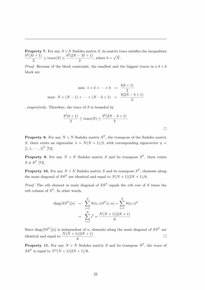
Property 7. For any N×N Sudoku matrix S, its matrix trace satisfies the inequalitiesb2(M + 1)
2≤ trace(S) ≤ b2(2N −M + 1)
2, where b =
√N .
Proof. Because of the block constraint, the smallest and the biggest traces in a b × bblock are
min: 1 + 2 + · · ·+ b =b(b+ 1)
2
max: N + (N − 1) + · · ·+ (N − b+ 1) =b(2N − b+ 1)
2
, respectively. Therefore, the trace of S is bounded by
b2(b+ 1)
2≤ trace(S) ≤ b2(2N − b+ 1)
2.
Property 8. For any N ×N Sudoku matrix ST , the transpose of the Sudoku matrix
S, there exists an eigenvalue λ = N(N + 1)/2, with corresponding eigenvector η =
[1, 1, · · · , 1]T [74].
Property 9. For any N × N Sudoku matrix S and its transpose ST , there exists
S 6= ST [74].
Property 10. For any N ×N Sudoku matrix S and its transpose ST , elements along
the main diagonal of SST are identical and equal to N(N + 1)(2N + 1)/6.
Proof. The nth element in main diagonal of SST equals the nth row of S times the
nth column of ST . In other words,
diag(SST )[n] =N∑i=1
S(n, i)ST (i, n) =N∑i=1
S(n, i)2
=N∑i=1
i2 =N(N + 1)(2N + 1)
6
Since diag(SST )[n] is independent of n, elements along the main diagonal of SST are
identical and equal toN(N + 1)(2N + 1)
6.
Property 11. For any N × N Sudoku matrix S and its transpose ST , the trace of
SST is equal to N2(N + 1)(2N + 1)/6.
22

2.3 Sudoku Array and Properties
Proof. Since diag(SST )[n] =N(N + 1)(2N + 1)
6and SST is of size N ×N , so
trace(SST ) =N∑n=1
diag(SST )[n] =N2(N + 1)(2N + 1)
6
Property 12. For any N × N Sudoku matrix S and its transpose ST , there exists
STS 6= SST and λ = [N(N + 1)/2]2 is an eigenvalue of the covariance matrices of STS
and SST [74].
Property 13. For any digit d ∈ N = {1, 2, · · · , N}, in a random N×N Sudoku matrix
S, there exists
Pr(S(i, j) = d|i) = Pr(S(i, j) = d|j)
= Pr(S(i, j) = d)
= 1/N
where Pr(X|Y ) denotes the conditional probability of the event X to happen when it
is known the event Y happens, S(i, j) denotes the element at the intersection of the
ith row and jth column of the Sudoku matrix.
Proof. Since each row of a Sudoku matrix S is a permutation of the natural number
set 1, 2, · · · , N , then given a digit d, the probability of one element in a row of S is
then 1/N . So,
Pr(S(i, j) = d|i) = 1/N
Similarly, since each column of S is also a permutation of its row, so
Pr(S(i, j) = d|j) = 1/N
Moreover, for a given grid located at (i, j) in a random Sudoku matrix S, its value
S(i, j)
Pr(S(i, j) = d) =∑N
k=1 Pr(S(i, j) = d|i)Pr(i = k) = 1/N
Property 14. For any N ×N Sudoku matrix S, its normalized version DS =2S
N +N2
is a doubly stochastic matrix, which is a special case of the Markov transition matrix
with N states.
23

Proof. Since S is an N ×N Sudoku matrix, the sum of S along any row or any column
is thenN∑k=1
S(i, k) =N +N2
2=
N∑k=1
S(k, j)
, where i, j ∈ N denote the row and the column indexes, respectively. Therefore, the
sum of any row or any column in the normalized version matrix S =2S
N +N2is 1,
which implies DS is a doubly stochastic matrix in a stochastic process [93].
Finally, several relevant additional facts about Sudoku matrices are worth mention-
ing.
Fact 1. An N ×N Sudoku matrix S can be singular [74].
Example. The following Sudoku matrix has one eigenvalue of zero with corresponding
eigenvector−→ξ
8 3 5 9 4 7 6 2 1
7 6 1 2 5 8 3 9 4
2 4 9 6 1 3 5 7 8
5 1 3 7 8 2 9 4 6
6 2 4 3 9 1 8 5 7
9 8 7 4 6 5 1 3 2
3 7 6 1 2 9 4 8 5
4 5 2 8 3 6 7 1 9
1 9 8 5 7 4 2 6 3
and−→ξ =
382
1723
−554
−122
−1148
−1364
1669
355
−941
Fact 2. An N ×N Sudoku matrix S can be indefinite.
Example. For a Sudoku matrix S as follows:4 3 1 2
1 2 4 3
3 4 2 1
2 1 3 4
For X = [ 1 1 1 1 ], XSXT = 40;
For X = [ 1 2 −2 1 ], XSXT = −4
Fact 3. The square/square root of an N ×N Sudoku array S can be still a Sudoku.
Example. We found many Sudoku matrices following this property, here is one of them.
Say Sudoku matrix S with digit set {1, 2, 3, 4, 5, 6, 7, 8, 9} is as follows
24

2.3 Sudoku Array and Properties
S =
9 7 4 8 3 5 1 6 2
6 2 1 7 4 9 3 5 8
5 8 3 2 1 6 4 9 7
7 4 9 3 5 8 6 2 1
2 1 6 4 9 7 5 8 3
8 3 5 1 6 2 9 7 4
4 9 7 5 8 3 2 1 6
1 6 2 9 7 4 8 3 5
3 5 8 6 2 1 7 4 9
Then S2 is also a Sudoku with the symbol set {193, 205, 210, 214, 218, 227, 241, 256, 261}
S2 =
261 214 205 241 210 256 218 227 193
241 210 256 218 227 193 261 214 205
218 227 193 261 214 205 241 210 256
256 241 210 193 218 227 205 261 214
193 218 227 205 261 214 256 241 210
205 261 214 256 241 210 193 218 227
227 193 218 214 205 261 210 256 241
214 204 261 210 256 241 227 193 218
210 256 241 227 193 218 214 205 261
Fact 4. The 9 × 9 Sudoku matrix has been reported to be more random than the
randomly generated 9× 9 matrix [74].
Fact 5. Given a Sudoku matrix, a number of unique solution Sudoku puzzles can be
derived from its solution [76].
Fact 6. An N ×N Sudoku matrix may also be a Cayley table of ZN [66].
Example. The 9 × 9 Sudoku matrix S reported in [66] is also a Cayley table, where
the inter 9 × 9 matrix is a Sudoku and Z9 = {1, 2, · · · , 9} under addition modulo 9 (
a count from 1 to 9 is used instead of the traditional count from 0 to 8 in order to
maintain the Sudoku-like appearance):
25

+ 9 3 6 1 4 7 2 5 8
9 9 3 6 1 4 7 2 5 8
1 1 4 7 2 5 8 3 6 9
2 2 5 8 3 6 9 4 7 1
3 3 6 9 4 7 1 5 8 2
4 4 7 1 5 8 2 6 9 3
5 5 8 2 6 9 3 7 1 4
6 6 9 3 7 1 4 8 2 5
7 7 1 4 8 2 5 9 3 6
8 8 2 5 9 3 6 1 4 7
Fact 7. N ×N Sudoku matrices can be orthogonal [94, 95, 96].
Example. John Lorch [95, 96] provided the following two orthogonal Sudoku matrices:
0 1 3 2
2 3 1 0
3 2 0 1
1 0 2 3
;
0 3 2 1
2 1 0 3
3 0 1 2
1 2 3 0
because it is easy to verify that(0, 0) (1, 3) (3, 2) (2, 1)
(2, 2) (3, 1) (1, 0) (0, 3)
(3, 3) (2, 0) (0, 1) (1, 2)
(1, 1) (0, 2) (2, 3) (3, 0)
contains all possible pairs.
Fact 8. N ×N Sudoku matrices can also be magic-square blocks [97].
26

2.3 Sudoku Array and Properties
Example. A. D. Keedwell gave the following magic-square Sudoku in [97].
16 3 10 5 1 14 4 15 6 9 7 12 11 8 13 2
9 6 15 4 8 11 5 10 3 16 2 13 14 1 12 7
7 12 1 14 13 2 16 3 10 5 11 8 4 15 6 9
2 13 8 11 12 7 9 6 15 4 14 1 5 10 3 16
8 11 5 10 3 16 2 13 14 1 12 7 9 6 15 4
13 2 16 3 10 5 11 8 4 15 6 9 7 12 l 14
12 7 9 6 15 4 14 1 5 10 3 16 2 13 8 11
1 14 4 15 6 9 7 12 11 8 13 2 16 3 10 5
10 5 11 8 4 15 6 9 7 12 1 14 13 2 16 3
15 4 14 1 5 10 3 16 2 13 8 11 12 7 9 6
6 9 7 12 11 8 13 2 16 3 10 5 1 14 4 15
3 16 2 13 14 1 12 7 9 6 15 4 8 11 5 10
5 10 3 16 2 13 8 11 12 7 9 6 15 4 14 1
11 8 13 2 16 3 10 5 I 14 4 15 6 9 7 12
14 1 12 7 9 6 15 4 8 11 5 10 3 16 2 13
4 15 6 9 7 12 1 14 13 2 16 3 10 5 11 8
Some of these particular properties of Sudoku are directly relevant to many cryp-
tography techniques that are discussed in the following sections.
27

2.4 Sudoku Generator
The original article with the fundamental generation idea is still unaware for me. To
my best knowledge, this generation idea is briefly represented and described by A.
Keedwell in [97] to illustrate a magic-square Sudoku. Later he gave another general
form in [98] and this type of Sudoku is called Keedwell Sudoku in [95]. However, early
work [94] also mentioned a similar construction process for a special family of Sudoku
solutions called symmetric Sudoku solution. And the rectangular gerechte designs in a
later work [99] also used a quite similar construction (where Sudoku is a special case
of gerechte design with square regions).
In this section, we used the fundamental generation idea from [97, 98] with ad-
ditional modifications to develop a parametric Sudoku generator using Latin square
expansion and permutation. We also showed a concrete example of how to obtain a
9×9 Sudoku array from a given parameter set. Furthermore, an encryption key depen-
dent Sudoku generator is introduced based on a series of linear congruential generators.
2.4.1 Parametric Sudoku Array Generator
It is well known that the Sudoku matrix is a special type of Latin square with extra
constraints in blocks. Therefore, it is possible to generate a Sudoku matrix from a
Latin square [94, 97, 98]. Algorithm 1 describes a simple Latin square generator based
on permutation sequences.
Algorithm 1 Latin Square Generator
Input :X = a permutated sequence of digits ranging from 1 to nH = a permutated sequence of digits ranging from 1 to n
Output :L = a Latin square with digits ranging from 1 to n
for l = 1 to n doL(l, :) = ringShift(X,H(l)) {Ring Shift sequence X with H(l) units to the left}
end for
Algorithm 2 describes the Sudoku generator we derived for N symbols, where N =
b2 is a square number and the acronym LSG denotes the Latin square generator given
28

2.4 Sudoku Generator
in Algorithm 1. Algorithm 3 describes the proposed pesudo band-swapping algorithm
to break the original symmetries in Sudoku.
29
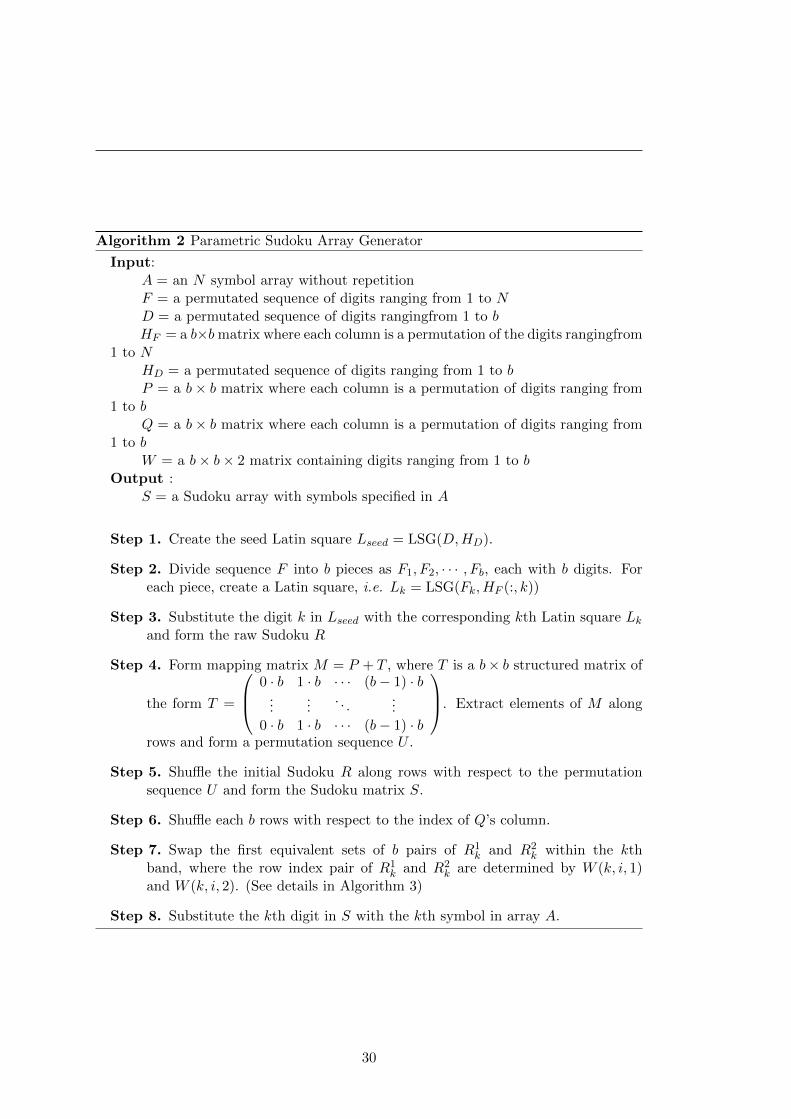
Algorithm 2 Parametric Sudoku Array Generator
Input:A = an N symbol array without repetitionF = a permutated sequence of digits ranging from 1 to ND = a permutated sequence of digits rangingfrom 1 to bHF = a b×bmatrix where each column is a permutation of the digits rangingfrom
1 to NHD = a permutated sequence of digits ranging from 1 to bP = a b× b matrix where each column is a permutation of digits ranging from
1 to bQ = a b× b matrix where each column is a permutation of digits ranging from
1 to bW = a b× b× 2 matrix containing digits ranging from 1 to b
Output :S = a Sudoku array with symbols specified in A
Step 1. Create the seed Latin square Lseed = LSG(D,HD).
Step 2. Divide sequence F into b pieces as F1, F2, · · · , Fb, each with b digits. Foreach piece, create a Latin square, i.e. Lk = LSG(Fk, HF (:, k))
Step 3. Substitute the digit k in Lseed with the corresponding kth Latin square Lkand form the raw Sudoku R
Step 4. Form mapping matrix M = P + T , where T is a b× b structured matrix of
the form T =
0 · b 1 · b · · · (b− 1) · b...
.... . .
...0 · b 1 · b · · · (b− 1) · b
. Extract elements of M along
rows and form a permutation sequence U .
Step 5. Shuffle the initial Sudoku R along rows with respect to the permutationsequence U and form the Sudoku matrix S.
Step 6. Shuffle each b rows with respect to the index of Q’s column.
Step 7. Swap the first equivalent sets of b pairs of R1k and R2
k within the kthband, where the row index pair of R1
k and R2k are determined by W (k, i, 1)
and W (k, i, 2). (See details in Algorithm 3)
Step 8. Substitute the kth digit in S with the kth symbol in array A.
30

2.4 Sudoku Generator
Definition 2. An index set E is called the first equivalent set for the rows R1 and R2
of a N ×N Sudoku matrix, if
• set E contains index 1;
• for any index i ∈ E, there always exists an index j ∈ E, such that R1[i] = R2[j];
• set E is the set satisfying the above two conditions with the least number of
elements.
Algorithm 3 Band Swapping Algorithm
Input :R1k = the 1st selected row in the kth Band of an N ×N Sudoku
R2k = the 2nd selected row in the kth Band of an N ×N Sudoku
Output :R1k and R2
k
r1 = R1k[1]; r2 = R2
k[1];E = [1];if r1 6= r2 then
while setdiff(r1, r2) 6= ∅ & setdiff(r2, r1) 6= ∅ doE[end+1] = find(R1
k == r2[end]);r1[end+1] = R2
k[E[end]];r2[end+1] = R1
k[E[end]];end whileTemp = R1
k[E]; R1k[E] = R2
k[E]; R2k[E] =Temp;
R1k ↔ R2
k {Swap two rows}end if
31

2.4.2 A Concrete Example
Suppose we have the following inputs for generating a 9× 9 Sudoku array:
• A = [♣,z,4,♠,♥,♦,U,�,£]
• F =[9 3 7 2 6 1 8 5 4
]• D =
[1 2 3
]and HD =
[2 3 1
]• HF =
1 2 32 1 23 3 1
and P =
2 2 11 3 23 1 3
• Q =
2 3 23 1 11 2 3
W =
3 1 2 1 2 12 1 2 3 1 13 1 2 3 3 3
Then, in Step 1, we obtain
Lseed = LSG(D,HD) =
3 1 21 2 32 3 1
In Step 2, sequence F is divided into F1 =
[9 3 7
], F2 =
[2 6 1
], and F3 =[
8 5 4]
from which the corresponding Latin squares are derived:
L1 =
3 7 97 9 39 3 7
, L2 =
1 2 66 1 22 6 1
and L3 =
8 5 44 8 55 4 8
They are then substituted for the corresponding digits in Lseed and thus Lseed becomes
of the following form after substitution.
Lseed =
L3 L1 L2
L1 L2 L3
L2 L3 L1
Therefore, the raw Sudoku array R becomes
R =
8 5 4 3 7 9 1 2 64 8 5 7 9 3 6 1 25 4 8 9 3 7 2 6 1
3 7 9 1 2 6 8 5 47 9 3 6 1 2 4 8 59 3 7 2 6 1 5 4 8
1 2 6 8 5 4 3 7 96 1 2 4 8 5 7 9 32 6 1 5 4 8 9 3 7
32

2.4 Sudoku Generator
So far R is still a Latin square but not a Sudoku because it violates the block constraint
for a Sudoku, i.e. symbols in the same block cannot be repeated.
According to Step 4, the mapping matrix M is obtained as
M = P + T =
2 2 11 3 23 1 3
+
0 3 60 3 60 3 6
=
2 5 71 6 83 4 9
and thus the permutation sequence U =
[2 5 7 1 6 8 3 4 9
]The Sudoku matrix S is then generated by shuffling the raw Sudoku R long rows with
respect to U as follows
S =
4 8 5 7 9 3 6 1 27 9 3 6 1 2 4 8 51 2 6 8 5 4 3 7 9
8 5 4 3 7 9 1 2 69 3 7 2 6 1 5 4 86 1 2 4 8 5 7 9 3
5 4 8 9 3 7 2 6 13 7 9 1 2 6 8 5 42 6 1 5 4 8 9 3 7
Then every b rows of S are shuffled using the corresponding column in Q. And we
obtain:
S =
7 9 3 6 1 2 4 8 51 2 6 8 5 4 3 7 94 8 5 7 9 3 6 1 2
6 1 2 4 8 5 7 9 39 3 7 2 6 1 5 4 88 5 4 3 7 9 1 2 6
3 7 9 1 2 6 8 5 45 4 8 9 3 7 2 6 12 6 1 5 4 8 9 3 7
Furthermore, a more random like Sudoku can be obtained by applying Step 7 in Al-
gorithm 2. Here the concept of ‘band’ refers to the region that can be interpreted to
be b consecutive rows in b consecutive blocks. For example, rows 1, 2 and 3 in a 9× 9
Sudoku form a ‘band’. According to Step 7 and W , we need to swap the 1st equivalent
set in row 3 and 1 in the first band using Algorithm 3. We start with the index set
E = [1] and r1 = 7, r2 = 4, then minimum set to make row 3 and row 1 have the same
set of digits is the index set E = [1, 4, 7] and r1 = [7, 6, 4], r2 = [4, 7, 6]. Therefore, we
swap elements in row 3 and row 1 under the same index set E.
33

S =
4 9 3 7 1 2 6 8 51 2 6 8 5 4 3 7 97 8 5 6 9 3 4 1 2
6 1 2 4 8 5 7 9 39 3 7 2 6 1 5 4 88 5 4 3 7 9 1 2 6
3 7 9 1 2 6 8 5 45 4 8 9 3 7 2 6 12 6 1 5 4 8 9 3 7
In this manner, we obtain the following Sudoku S after band swapping:
S =
4 9 3 7 1 2 6 8 57 2 6 8 5 4 3 1 91 8 5 6 9 3 4 7 2
9 3 7 2 6 1 5 4 86 1 2 4 8 5 7 9 38 5 4 3 7 9 1 2 6
3 7 9 1 2 6 8 5 42 4 8 5 3 7 9 6 15 6 1 9 4 8 2 3 7
Finally, substituting the corresponding symbols of A to S, the 9× 9 Sudoku array S is
obtained.
S =
♠ £ 4 z ♣ U ♦ � ♥U z ♦ � ♥ ♠ 4 ♣ £♣ � ♥ ♦ £ 4 ♠ U z£ 4 U z ♦ ♣ ♥ ♠ �♦ ♣ z ♠ � ♥ U £ 4� ♥ ♠ 4 U £ ♣ z ♦4 U £ ♣ z ♦ � ♥ ♠z ♠ � ♥ 4 U £ ♦ ♣♥ ♦ ♣ £ ♠ � z 4 U
In the same fashion, Sudoku arrays of arbitrary size can also be derived. Below are
examples of Sudoku arrays and Sudoku puzzles generated using the provided Sudoku
generator.
To illustrate the fact that large size Sudoku arrays are also easy to obtain, some
examples are provided below.
34

2.4 Sudoku Generator
(a) A 9× 9 Sudoku puzzle (b) A 16× 16 Sudoku puzzle in Chinese
(c) The solution to (a) (d) The solution to (b)
Figure 2.5: Sample Sudoku puzzles and solutions
35

(a) A 25× 25 Sudoku
(b) A 36× 36 Sudoku
Figure 2.6: Large size Sudoku arrays - part I
36

2.4 Sudoku Generator
Figure 2.7: Large size Sudoku arrays - part II
37

2.4.3 Key Dependent Sudoku
In order to use a parametric Sudoku for encryption, the parametric Sudoku has to be
key dependent. In this section, we expand the encryption key K concept to a Sudoku
matrix S.
The core idea of such an expansion is to treat the encryption key K as a seed or
parameter in a pseudo-random number generator (PRNG), and thus a series of key-
dependent sequences can be obtained for generating permutation sequences used in the
Sudoku array generation.
As an example, I used a linear congruential generator (LCG), one of the oldest and
best-known pseudo-random number generator algorithms available [100], as a PRNG
to translate a key K to permutation sequences. Then such an LCG generator can be
iteratively defined as Eq. (2.1), where a, c and m are predetermined parameters.
LCG:Xn+1 = (aXn + c) mod m (2.1)
In the following algorithm 4, we assume the length of the encryption key to be 256
bits, i.e. 64 bytes. This Algorithm transforms a 256-bit key to a set of parameters
required for the Sudoku array generator. The parameters used in the eight LCGs in
Algorithm 4 are listed below:
Table 2.1: LCG parameters used in eight LCGs
LCG # a c m Source
1,5 214013 2531011 232 Microsoft Visual/Quick C/C++2,6 22695477 1 232 Borland C/C++3,7 1103515245 12345 232 IBM VisualAge C/C++4,8 1664525 1013904223 232 Numerical Recipes [101]
The function rand(.) is used to extract the least significant16 ∼ 30 bits in the
subgroup and to form a decimal number. In Step 4, the conversion from an integer
sequence I to a permutation sequence eπ of the same length l can be done by first
sorting an integer sequence I and obtaining the sorted version I ′,where I ′ = sort(I);
and then by finding the permutation sequence eπ, such that I ′[i] = I[eπ[i]] for any
i ∈ {1, 2, · · · , l}.
38

2.4 Sudoku Generator
Algorithm 4 Key to Sudoku Parameter Set
Input:K = an encryption key of 256 bitsN = the size of Sudoku matrix
Output :A = an N symbol array without repetitionF = a permutated sequence of digits ranging from 1 to ND = a permutated sequence of digits ranging from 1 to bHF = a b× b matrix where each column is a permutation of digits ranging from
1 to NHD = a permutated sequence of digits ranging from 1 to bP = a b× b matrix where each column is a permutation of digits ranging from
1 to bQ = a b× b matrix where each column is a permutation of digits ranging from
1 to bW = a b× b× 2 matrix containing digits ranging from 1 to b
Step 1. Set symbol sequence A = {1, 2, 3, · · · , N} and divide 64 byte key into 8subgroups as G1, G2, · · · , G8; each of which contains 8 bytes (32bits).
Step 2. Calculate the required iterations T = d(3N + 2√N)/8e, where d.e is the
rounding function towards infinity.
Step 3. Iteratively generate a sequence Seq of length T , where each part of T iscompatible with the corresponding parameters in the Sudoku array generator.
set i = 1for iter = 1→ T do
for k = 1→ 8 doGk = LCGk(Gk) % generate an 8 byte pseudo random number% extract the random part of this pseudo random numberSeq[i] = rand(Gk)i = i+ 1
end forG1 = G8
for k = 2→ 8 doGk = Gk−1 % shift the random number register to the right
end forend for
Step 4. Sort the element sequence Seq and obtain the permutation sequencesF,D,HF , HD, P ,and Q from the sequence index.
Step 5. Use module√N operation to obtain sequence W
39

Finally, all of the output parameters can be derived. When this set of parameters
is fed in the Sudoku array generator described in Algorithm 2, an N ×N Sudoku array
is generated.
2.4.4 Discussion
Although the provided Sudoku array generator is able to generate a Sudoku of an
arbitrary size, several facts should be paid attention to.
• The Sudoku array generated from Algorithm 2 is a subset of all possible Sudoku
arrays.
• The Sudoku arrays generated by Algorithms 2 are random-like and could be more
random-like if more swaps in Step 7 of 3 are applied.
• The same Sudoku might be generated using different parameter settings, since
the permutation step in the generation might be equivalent to each other (even
though there is a very low probability for that to occur).
• Assume A is fixed and N = b2, then the total number TN of unique Sudoku
arrays that Algorithm 2 can generate has the following lower bound:
TN > (b2)!((b− 1)!)b︸ ︷︷ ︸∑bi=1 #Li
(b− 1)!︸ ︷︷ ︸#Lseed
(b− 1)!(b!)b−1︸ ︷︷ ︸#P
(2.2)
In∑b
i=1 #Li, (b2)! denotes the number of different 1st rows in a Sudoku; and
(b − 1)! denotes the number of different Lk when its first row is determined.
In #Lseed, (b − 1)! denotes the number of different Lseed when its first row is
determined. And in #P , when the first row is fixed, then other rows in the first
band can only be shuffled to the left b− 1 bands, each of which has b blank rows;
then the rows in the second band can be shuffled to b bands, each of which has
b − 1 blank rows; · · · then the rows in the kth band can be shuffled to b bands,
each of which has b − k + 1 blank rows; therefore the total number of Sudoku
arrays this shuffling process is (b−1)!(b!)b−1. Since the possible row swaps are not
counted, this is the lower bound for Algorithm 2. TN > 23072, when N = 256.
40

2.5 3D Extension
• Generating a true random Sudoku matrix is an NP-complete problem and is
time-consuming especially when the Sudoku size is large. However, the provided
Sudoku generator is able to generate large size Sudokus in an instant, because
it utilizes a series of Sudoku structural configurations and a limited numbers of
swaps.
• The LCG in Algorithm 2 can be replaced by any PRNG. As a matter of fact, the
LCG is not considered a cryptographically secure generator ( for secure PRNGs
one can check eSTREAM project3). However, our performance analysis (shown
later) show that even LCG triggered Sudoku ciphers can be used as cryptograph-
ically secure PRNGs because they are designed to resist many kinds of attacks
and their results pass latest statistical test suite (shown in Appendix A). More
details about these Sudoku ciphers and image encryption methods are discussed
in future sections.
2.5 3D Extension
Two nature questions after successfully constructing two-dimensional Sudoku arrays
are that 1) whether there exists higher dimensional Sudoku arrays and 2) whether
we can also construct higher dimensional Sudoku arrays in a parametric way. The
discussions about these two questions are far beyond the scope of this dissertation,
but we conjecture the answers might be both yes. For the first question, we guess the
answer is yes because Sudoku arrays are Latin squares in root whose multidimensional
version, known as Latin hypercubes [102], is widely reported and studied. For the
second question, we guess the answer is also yes because we find a way to construct
three-dimensional Sudoku array in a parametric way and we guess it is also possible
for higher dimensional Sudoku arrays.
The construction idea for 3D Sudoku cube is similar to the idea for 2D Sudoku
arrays introduced before, whereas the major difference is that we construct 3D Sudoku
cubes from 3D Latin cubes rather than 2D Latin squares. To show this construction
3eSTREAM is a project aiming to “identify new stream ciphers suitable for widespread adoption”.
Available at http://www.ecrypt.eu.org/stream/phase3ip.html#rabbit as the date of 03/26/2012.
41

idea, we use construction functions from [98], where operator α and β shift a 2D matrix
with respective to one row and one column, i.e.
X(i+ 1, :) = αX(i, :); X(:, j + 1) = βX(:, j). (2.3)
In addition, we define their iterative construction functions as follows.
αn = α ◦ α · · · ◦ α︸ ︷︷ ︸ntimes
(2.4)
and
βn = β ◦ β · · · ◦ β︸ ︷︷ ︸ntimes
(2.5)
As a result, a 2D Keedwell Sudoku of size b2× b2 can be written in the form of Eq.
(2.6), where R is a construction seed of size b× b containing all b2 symbols.
KS =
R αR α2R · · · αb−1RβR βαR βα2R · · · βαb−1Rβ2R β2αR β2α2R · · · β2αb−1R
......
.... . .
...βb−1R βb−1αR βb−1α2R · · · βb−1αb−1R
(2.6)
Now define two new operators χ and η, where χ shifts one row for a band with
respect to each of b bands and η shifts one column for a stack with respect to each of
b stacks (see Fig. 2.4). Then a 3D Sudoku cube of size b2 × b2 × b2 can be written as
42

2.6 Conclusions
Eq. (2.7).
SudokuCube =
KSηχKSη2χKS
...ηb−1χKS
χKSηχ2KSη2χ2KS
...ηb−1χ2KS
...
χb−1KSηχb−1KSη2χb−1KS
...ηb−1χb−1KS
(2.7)
Consequently, we can build 3D Sudoku arrays for arbitrary size. Other Sudoku
cubes can also be generated by using similar permutation tricks described in the Sudoku
array generator. With the visualization tools in MATLAB, we plot the following 3D
Sudoku arrays of the size N ×N ×N for N = b2 and b ∈ {2, 3, 4, 5}. Note this is not
a 3D Sudoku array because it only has Sudoku on six faces [103].
Thanks helps of magnet balls, we can also physically construct 3D Sudoku arrays
using these colorful magnet balls. Fig. 2.10 shows an example that ensembles the
4× 4× 4 Sudoku cube shown in Fig. 2.8 using magnet balls.
2.6 Conclusions
In this section, we first reviewed the history of the Sudoku puzzle and its variants. We
also extended the Sudoku concept into arrays. Sudoku arrays are then defined and
their mathematical properties are explored in detail. We next designed a parametric
Sudoku array generator via a series of transformation using Latin squares and group
swaps. Finally, we construct 3D Sudoku cubes. As a result, we are able to generate
Sudoku arrays of arbitrary sizes. This enable the use of encryption key-dependent
Sudoku arrays.
43

(a) A 4× 4× 4 Sudoku cube
(b) Slices along x-axis
(c) Slices along y-axis
(d) Slices along z-axis
Figure 2.8: Three-dimensional Sudoku arrays 4× 4× 4
44
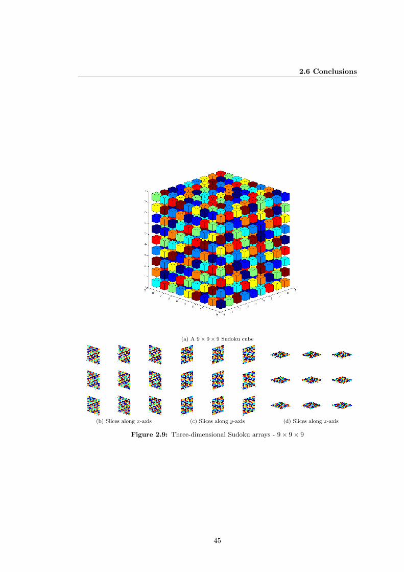
2.6 Conclusions
(a) A 9× 9× 9 Sudoku cube
(b) Slices along x-axis (c) Slices along y-axis (d) Slices along z-axis
Figure 2.9: Three-dimensional Sudoku arrays - 9× 9× 9
45

Multidimensional Sudoku array - 16× 16× 16
Three-dimensional Sudoku array - 25× 25× 25
46

2.6 Conclusions
Figure 2.10: Constructing three-dimensional Sudoku array using magnet balls
47

48

3
Sudoku Based Encryption
Techniques
3.1 Overview
In this section, I assume that an N × N Sudoku array/matrix S has been obtained,
and I introduce encryption techniques based on Sudoku. These techniques are Sudoku
Whitening, Sudoku Transposition, Sudoku Permutation, Sudoku Maximum Separable
Distance Matrix, and Sudoku Substitution. They are designed to not only address clas-
sical cryptography but also multimedia encryption. In order to simplify the discussion
and take advantage of visual assessment, image data is used to represent multime-
dia data throughout this section. It is worthwhile to note that any single encryption
technique introduced below is not sufficiently secure. However, ciphers combining these
techniques provide much higher security levels and will be discussed in the next section.
Throughout the section I use Etech and Dtech to denote the block-wise encryption
and decryption operations using technique tech as shown in Eqs. (3.1) and (3.2), where
Pb and Cb denote the plaintext message and ciphertext message blocks, respectively,
and S is the Sudoku matrix determined by the encryption K. Without any mention to
the contrary, the block size adopted in encryption and decryption is always the same as
the size of the key dependent Sudoku matrix S. In other words, if a plaintext message
P has a size larger than S, then P is encrypted one Pb by another Pb and C is obtained
by forming a number of Cbs. Encryption and decryption functions are written in terms
49

of S rather than K for illustrating these relations in a more direct way.
Etech := (Pb, S)→ Cb (3.1)
Dtech := (Cb, S)→ Pb (3.2)
3.2 Sudoku Whitening
In cryptography, key whitening is usually used as a technique to increase the security
of a cipher [8, 10]. It mixes a plaintext message with an encryption key in order to
make a patterned plaintext message more random-like.
In classical cryptography, the whitening technique is normally referred to as the
XOR (exclusive or) operation between a plaintext message and a key, and is commonly
used in DES [5], AES [4], Blowfish ciphers [104].
In the context of Sudoku, the key used for whitening, either of binary data or
multimedia data, is a key dependent Sudoku matrix. This type of Sudoku matrix
can be easily obtained via the Sudoku generator. Therefore, Sudoku whitening using
XOR technique can be defined as Eq. (3.3) shows, where symbol ⊕ denotes the XOR
operation, and ‘mod’ is the modular operation, and variables Pb, Cb and S refer to the
plaintext block, the ciphertext block and the Sudoku matrix, respectively.
ExorSW : Cb = Pb ⊕ S (3.3)
DxorSW : Pb = Cb ⊕ S (3.4)
Fig. 3.1 shows this Sudoku whitening result for the sample binary image of ‘Tuft-
sLogo’ for different whitening block sizes. It is worthwhile to note that both P and
C have a 256 × 256 size, and the Sudoku matrices chosen for whitening are of size
16× 16, 64× 64 and 256× 256 for C1, C2 and C3, respectively. After applying Sudoku
whitening, the ciphertext message C is almost unrecognizable and very different from
the plaintext message P .
50

3.2 Sudoku Whitening
Alternatively, we can define the Sudoku whitening scheme over a finite field GF (2L)
as follows,
EgfSW : Cb = (Pb + S)2L (3.5)
DgfSW : Pb = (Cb + S)2L (3.6)
where L is the number of intensity scales allowed in the plaintext format.
Fig. 3.2 shows the 8-bit gray 256 × 256 ‘cameraman’ image and its bit-plane de-
compositions with respect to the bit order from the most to the least significant bit.
Fig. 3.3 then shows the Sudoku whitening technique (ESW−II) on this image using
a 256 × 256 Sudoku matrix. It is clear that the histogram of the ‘cameraman’ image
gets flatter and flatter as the whitening process applies to more bit-planes. It can also
be observed that the histogram duplicates itself once for one time whitening, which
implies that the Sudoku whitening is able to randomly change almost half the bits in
each bit-plane.
(a) Plaintext P (b) Ciphertext C1
(c) Ciphertext C2 (d) Ciphertext C3
Figure 3.1: Sudoku whitening results
51

(a) Plaintext P (b) MSB1 (c) MSB2
(d) MSB3 (e) MSB4 (f) MSB5
(g) MSB6 (h) MSB7 (i) MSB8
Figure 3.2: The cameraman image and its MSB decomposition
52

3.2 Sudoku Whitening
(a) Plaintext P
0
100
200
300
400
500
600
700
800
900
1000
0 50 100 150 200 250
(b) Histogram of (a)
(c) Whitened MSB1 (d) Whitened MSB1−2 (d) Whitened MSB1−3 (e) Whitened MSB1−4
0
100
200
300
400
500
600
700
800
0 50 100 150 200 250
(f) Histogram of (c)
0
100
200
300
400
500
600
0 50 100 150 200 250
(g) Histogram of (d)
0
100
200
300
400
500
600
0 50 100 150 200 250
(h) Histogram of (e)
0
100
200
300
400
500
600
0 50 100 150 200 250
(i) Histogram of (f)
(j) Whitened MSB1−5 (k) Whitened MSB1−6 (l) Whitened MSB1−7 (m) Whitened MSB1−8
0
100
200
300
400
500
600
0 50 100 150 200 250
(n) Histogram of (j)
0
100
200
300
400
500
600
0 50 100 150 200 250
(o) Histogram of (k)
0
100
200
300
400
500
600
0 50 100 150 200 250
(p) Histogram of (l)
0
100
200
300
400
500
600
0 50 100 150 200 250
(q) Histogram of (m)
Figure 3.3: Sudoku whitening effects example
53

3.3 Sudoku Transposition
A transposition cipher changes one character from the plaintext to another. Although
multimedia data can be read as bit strings, encrypting multimedia data in this way
is inefficient and cumbersome [16]. As a result, the XOR operation defined on bit
strings becomes inappropriate for the whitening techniques for multimedia data which
usually contains bulk data. Alternatively, this whitening technique is often replaced by
a transposition cipher defined on bytes (a group of bits) rather than bits.
The Sudoku transposition can be defined as Eq. (3.7) shows, where F is a format
related parameter. For example, if P is an 8-bit grayscale image, then F can be defined
as 256, which equals the number of allowed intensity scales compatible with the image
format. As a result, each pixel in plaintext P is shifted by some unit determined by
the Sudoku element in the corresponding grid in the Sudoku matrix S.
EST : Cb = (Pb + S) mod F (3.7)
DST : Pb = (Cb − S) mod F (3.8)
Eq. (3.7) is a very efficient operation for multimedia data, because one distinctive
characteristic of the multimedia data is the high information redundancy [105]. This
implies that a digital image normally has several homogeneous regions, where pixel
intensities are more or less the same. In other words, knowing any pixel in a homo-
geneous region, it is easy to reconstruct its neighbor pixels or even the whole region.
Therefore, it is desirable to make a homogeneous region in P nonhomogeneous during
the encryption process. A Sudoku matrix ensures that no two elements along a row,
column or block are the same, and thus the Sudoku matrix is very suitable to shift
homogeneous regions in P into nonhomogeneous ones. As a result, the worst case of P ,
the blank image where all pixels are all zero elements, is whitened and becomes identi-
cal to the Sudoku matrix S, which is randomly generated with a uniformly distributed
histogram.
Since the data range of an N × N Sudoku matrix is [1, N ], the Sudoku with size
N < F has to be lifted with a factor of F/N , before applying Eq. (3.7) for transposition.
In other words, Eq. (3.7) should be adopted as Eq. (3.9) shows, where d.e is the
54

3.3 Sudoku Transposition
rounding function towards infinity.
EscaledST : Cb = (Pb + dS · F/Ne) mod F (3.9)
DscaledST : Pb = (Cb − dS · F/Ne) mod F (3.10)
Fig. 3.4 shows the Sudoku transposition results for the 256× 256 gray scale ‘cam-
eraman’ image, when the sizes of the used Sudoku matrix for transposition are 16×16,
64 × 64 and 256 × 256, respectively. In spite of the block size, the Sudoku transposi-
tion results give satisfactory results, at least to visual inspection. It is also noticeable
that a small size Sudoku may lead to some pattern-like region in the ciphertext image
(see Fig. 3.4-(b)). However, this issue can be easily solved by using a key dependent
Sudoku for each processing block. This is a common mechanism used in block ciphers
like [4, 5, 11].
(a) Plaintext P (b) Sudoku size 16× 16
(c) Sudoku size 64× 64 (d) Sudoku size 256× 256
Figure 3.4: Sudoku transposition results
55

3.4 Sudoku Permutation
Permutation (also referred as P-Box), which keeps the plaintext statistics unchanged
while reordering the plaintext message, is a common technique used in cryptography
[8, 10], and has been widely applied in DES [5], AES [4], BlowFish [104], TwoFish [106],
IDEA [11], and image ciphers [19, 20, 21, 22, 23, 24, 25, 26, 26, 27, 28, 29, 30, 31, 32, 33,
34, 35, 36, 37, 38, 39, 40, 41, 42, 47, 48, 49, 50] . In general, the bit/pixel permutation
procedure is used to find a bijective mapping, which is one-to-one and onto. Given a
sequence of bits/pixels, the permutation technique shuffles elements in this sequence,
such that the original message content has been disordered and unrecognized. For
example, if ‘Hello world’ is the plaintext, then its ciphertext after permutation might
be ‘lowHerd lol’.
Specifically, the used bijective mapping for permutation is either predetermined or
dynamically generated. For example, the ‘ShiftRows’ step in AES can be considered as
a predetermined permutation, which shuffles the encryption block in a systematic way.
Image ciphers usually use dynamically generated bijective mappings for permutations.
For a given Sudoku matrix, there are at least four methods for permutation pur-
poses, and the first three are:
(1) the method of unitary permutation matrix
(2) the method of row/column/block shuffling
(3) the method of 2D mapping between notations
and will be discussed in the rest of this section.
It also worthwhile to note that the existence of orthogonal Sudoku matrices [95, 98].
Since a pair of orthogonal Sudoku arrays has all possible order pairs, the fourth two-
dimensional bijective mapping can be constructed by mapping these order pairs to the
natural order based on two orthogonal Sudoku matrices.
3.4.1 The method of permutation matrix
It is well known that the unitary permutation matrix (UPM) is a fast way to shuffle
matrix contents. A unitary permutation matrix U can be defined as a square matrix if
56

3.4 Sudoku Permutation
in every column and every row there is exactly one nonzero entry, whose value is one
[107].
For a given N ×N Sudoku matrix S, it is clear that each digit d appears only once
in a row or a column. Equivalently, for each digit d, a unitary permutation matrix can
be extracted from the Sudoku matrix S using the following logical equation.
U(i, j) =
{1 , if S(i, j) = d0 , if S(i, j) 6= d
(3.11)
For example, Fig. 3.5 shows the unitary permutation matrix associated with the 4 ×
4 reference Sudoku. It is well-known that the product of two unitary permutation
matrices is still a unitary permutation matrix (see Fig. 3.5-(f)).
(a) Reference S (b) U1 (c) U2
(d) U3 (c) U4 (d) U1U2
Figure 3.5: 4× 4 Sudoku associated unitary permutation matrices
Consequently, the relationship between the plaintext message Pb and the ciphertext
message Cb after shuffling by unitary permutation matrix U can be denoted as follows:
{Forward Row Shuffling: Cb = PbU
Forward Column Shuffling: Cb = UPb(3.12)
Similarly, the row-and-column shuffling can be obtained by cascading the row shuffling
and the column shuffling. Since a UPM is always invertible, Eq. (3.13) can be directly
57

used in the decryption stage, where UT = U−1 denotes the inverse of U .{Inverse Row Shuffling: Pb = CbU
T
Inverse Column Shuffling: Pb = UTCb(3.13)
Therefore, for encryption techniques using unitary permutation matrix, the encryp-
tion and decryption processes can be denoted as follows:
EupmSP : Cb = UPbU (3.14)
DupmSP : Pb = UTCbU
T (3.15)
Fig. 3.6 shows examples of shuffling images using the Sudoku associated UPMs,
where Ud denotes the digit d associated unitary matrix extracted from the reference
Sudoku S. The benefits of shuffling plaintext using UPM are: 1) it is extremely fast in
the sense that the plaintext needs row/column rearrangements only N times; and 2) its
ciphertext is not recognizable and intelligible. However, the ciphertext always contains
mesh-like patterns (see Fig. 3.6-(d) and (h)), which can be easily differentiated from a
random-like image.
3.4.2 The method of row/colunmn/block shuffling
The second way of doing permutation is to consider each row/column/block in a Sudoku
matrix as one permutation and then shuffle the plaintext row/column/block with re-
spect to the corresponding row/column/block in the reference Sudoku matrix. Denote
the bijective mapping between the ith row in the N ×N Sudoku matrix S and the nat-
ural number sequence {1, 2, · · · , N} as fπi , i.e. fπi = {1, 2, · · · , N} → {1, 2, · · · , N}.
Then the encryption and decryption processes of the jth element in ith row of the
ciphertext Cb(i, j) can be denoted as Eq. (3.16) and (3.17),respectively.
ErcbSP : Cb(i, j) = Pb(i, fπi(j)) (3.16)
DrcbSP : Pb(i, j) = Cb(i, f
−1πi (j)) (3.17)
58

3.4 Sudoku Permutation
(a) Plaintext P (b) Reference Sudoku S
(c) PU100 (d) U100P (c) U100PU100
(c) PU200 (d) U200P (c) U200PU200
Figure 3.6: Sudoku permutation using the associated UPMs
It is worthwhile to note that in the row/column/block shuffling the processed unit is a
row/column/block and thus the scope of the shuffling is limited to the row/column/block.
In order to break such a limitation, I can cascade row shuffling, column shuffling, and
block shuffling as Fig. 3.7 shows. It can be noticed that the cascaded shuffling results
obtained in this way do not lead to the mesh-like pattern obtained in the method of
unitary permutation matrix (see Fig. 3.7-(e) and (f)).
59

(c) Plaintext (d) row shuffling (c) column shuffling
(c) block shuffling (d) row&column shuffling (c) row&column&block shuffling
Figure 3.7: Sudoku permutation using the row/column/block shuffling
3.4.3 The method of matrix mapping between notations
Conventionally, a matrix can be denoted by using the (row,column) notation. In other
words, once the row and column numbers are both specified, the matrix element is
uniquely determined. However, when viewing a Sudoku matrix as a whole, many
different notations can be found to designate unique elements in a matrix.
Fig. 3.8 shows a concrete example for the 4×4 matrix and similar bijective mappings
can be found in all Sudoku matrices because of the three constraints listed in the Sudoku
definition. Conventionally, grids in the 4 × 4 matrix can be denoted using the (row,
column) or (column, row) notations as Fig. 3.8-(b) and (c) show. Besides the row and
column information, matrix grids can be denoted using digit and block information
within a reference 4×4 Sudoku matrix as Fig. 3.8-(e) to (i) show. Each representation
of a symbol pair (s1, s2) in Fig. 3.8 can be interpreted in the way that a grid in a 4× 4
matrix can be denoted when s1 = v1 and s2 = v2 by using the given Sudoku matrix
as the reference. For example, with the reference Sudoku in Fig. 3.8-(a), the grid at
the intersection of the 2nd row and 4th column in a 4 × 4 matrix can be denoted as
the grid with r = 2, c = 4, b = 3, d = 1, and thus this grid is denoted as (r = 2, d = 1),
(c = 4, d = 1), and (b = 3, d = 1) in representations (d), (e), and (f), respectively.
It is obvious that each representation is a permutation of the other representation
60
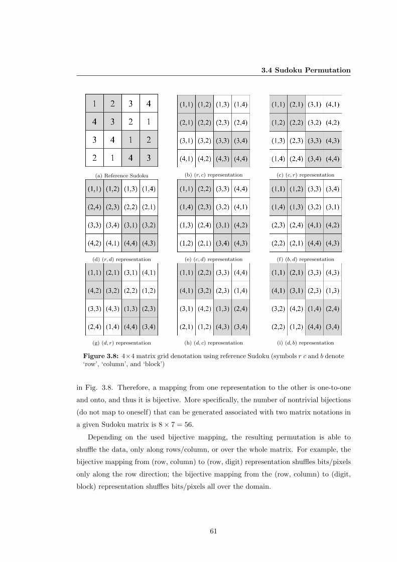
3.4 Sudoku Permutation
(a) Reference Sudoku (b) (r, c) representation (c) (c, r) representation
(d) (r, d) representation (e) (c, d) representation (f) (b, d) representation
(g) (d, r) representation (h) (d, c) representation (i) (d, b) representation
Figure 3.8: 4×4 matrix grid denotation using reference Sudoku (symbols r c and b denote‘row’, ‘column’, and ‘block’)
in Fig. 3.8. Therefore, a mapping from one representation to the other is one-to-one
and onto, and thus it is bijective. More specifically, the number of nontrivial bijections
(do not map to oneself) that can be generated associated with two matrix notations in
a given Sudoku matrix is 8× 7 = 56.
Depending on the used bijective mapping, the resulting permutation is able to
shuffle the data, only along rows/column, or over the whole matrix. For example, the
bijective mapping from (row, column) to (row, digit) representation shuffles bits/pixels
only along the row direction; the bijective mapping from the (row, column) to (digit,
block) representation shuffles bits/pixels all over the domain.
61

It is well known that the composition g ◦ h of two bijections g := X → Y and
h := Y → Z is also a bijection [108]. Therefore, different bijections found within one
Sudoku matrix can be used to compose new bijections. Furthermore, different bijections
between different Sudoku matrices can also be used for new bijections. These facts
imply that the number of bijections based on Sudoku matrices is huge.
Given an N × N Sudoku matrix S and a specific Sudoku bijection g which can
be defined under S, then the ciphertext message C after permutating the plaintext P
can be denoted as Eq. (3.18). Since g is a bijection, g−1 always exists and we have
Eq.(3.19) for decryption.
EmmnSP : Cb = gS(Pb) (3.18)
DmmnSP : Pb = g−1
S (Cb) (3.19)
Fig. 3.9 shows the Sudoku permutation results under various bijective mappings
associated with the same 256× 256 Sudoku matrix. It is noticeable that
• the plaintext information is unrecognized and unintelligent after pixel permuta-
tion,
• permutation qualities of different bijections using the same Sudoku matrix are
not equivalent from the point of view of certain patterns recognized by visual
inspection.
• the composed bijections help improve the permutation quality.
3.5 Sudoku Maximum Distance Separable Matrix
In classical cryptography, the MDS matrix [4, 106] is considered as an important prim-
itive to provide the diffusion property. It is a class of linear transformations used in
the cipher Twofish [106], AES [4] etc. It controls the number of S-boxes involved in
any two rounds of a linear approximation or a differential characteristic equal to the
theoretical maximum [109].
Conventionally, the Reed-Solomon codes [110] are used for MDS matrices. Techni-
cally, an M ×N matrix A over a finite field G is an MDS matrix, if it is the transform
matrix of a linear transformation f(x) = Ax from Gn to Gm such that no two different
62

3.5 Sudoku Maximum Distance Separable Matrix
(a) Plaintext image (b) gb := (r, c)→ (r, d) (c) gc := (r, c)→ (d, c)
(d) gd := (d, b)→ (r, d) (e) ge := (d, b)→ (c, d) (f) gf := (d, b)→ (b, d)
(i) gg := (b, d)→ (d, b) (g) gh := gb ◦ gc (h) gi := gd ◦ gf
(j) gj := gc ◦ gb (k) gk := gb ◦ gg (l) gl := gc ◦ gc ◦ ge
Figure 3.9: Sudoku permutation results
63

(m + n) tuples of the form (x, f(x)) coincide in n or more components. Mathemat-
ically, it can be demonstrated that an M × N matrix A is an MDS matrix if and
only if every square submatrix (formed from any i rows and any i columns), for any
i = 1, 2, · · · ,min(M,N) of A is nonsingular [111].
Using this sufficient and necessary condition of MDS, I found that many 4 × 4
Sudoku matrices can also be MDS matrices. Some of these Sudoku MDS matrices are
listed in Fig. 9. It is worthwhile to note that the Sudoku MDS matrix is not of the
conventional cyclic MDS matrix (see Fig. 9 -(i)) form, because its next row is not a
simple shift of the last row. Meanwhile, the Sudoku MDS matrix of Fig. 9-(h) is of the
same computational complexity as the AES MDS matrix of Fig. 9-(i).
Furthermore, I consider the finite field GF (28) used in AES. In AES, this GF (28)
is represented as GF (2)/m(x), where m(x) = x8 + x4 + x3 + x + 1 is an irreducible
polynomial over GF (2). Then the inverse of all the above Sudoku MDS matrices can
be used for decryption. Finally, I conjecture it is possible to find larger size Sudoku
MDS matrices.
As a result, the encryption and decryption processes using the Sudoku MDS matrix
S can be denoted as Eqs. (3.20) and (3.21), respectively.
ESM : Cb = PbS (3.20)
DSM : Pb = CbS−1 (3.21)
64
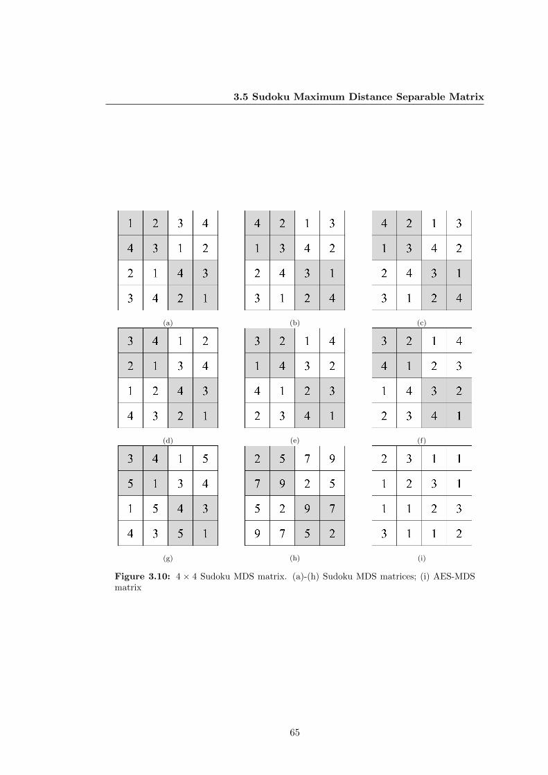
3.5 Sudoku Maximum Distance Separable Matrix
(a) (b) (c)
(d) (e) (f)
(g) (h) (i)
Figure 3.10: 4 × 4 Sudoku MDS matrix. (a)-(h) Sudoku MDS matrices; (i) AES-MDSmatrix
65

3.6 Sudoku Substitution
In cryptography, a substitution box (normally referred to as S-box) is a fundamental
component which performs substitution [8]. The objective of the S-box is to make the
relationship between the key and the ciphertext very complicated and involved such
that the confusion property [2] is achieved. In general, an S-box takes a certain number
of input bits and substitutes these bits with some other number of bits. According to
the origin of the S-box, it can be roughly grouped in two types, i.e. predetermined and
dynamically generated. For example, DES [5] and AES [4] uses predetermined S-boxes,
while Twofish [106] and IDEA [11] use dynamically generated S-boxes.
It is noticeable that in a Sudoku matrix, each row, column or block is a permutation
of digits from 1 to N . Therefore, these rows, columns and blocks can be directly used
for substitution, like those dynamically generated S-boxes [112, 113]. To get more
specific, we can have row, column or block S-boxes with respect to a reference Sudoku
matrix. Assume the plaintext block Pb is of size 256× 256 and each of the elements is
a byte containing 8 bits, then we can define S-boxes using a 256× 256 Sudoku matrix
as follows:
ErcbSS : Cb(i, j) =
S (i, Pb(i, j)) , row S-boxS (Pb(i, j), j) , column S-box
S(x
(Pb(i,j))k , y
(Pb(i,j))k
), block S-box
(3.22)
where S(x
(h)k , y
(h)k
)denotes the hth element located in the kth block with h = Pb(i, j)
a plaintext byte and k the block where Sudoku element S(i, j) is located. Correspond-
ingly, the reverse S-box can be defined as
DrcbSS : Pb(i, j) =
find (S (i, Pb(i, j)) == Cb(i, j)) , row S-boxfind (S (Pb(i, j), j) == Cb(i, j)) , column S-box
find(S(x
(Pb(i,j))k , y
(Pb(i,j))k
)== Cb(i, j)
), block S-box
(3.23)
where ‘find’ is the reverse searching function.
However, we’d like to introduce a new way of obtaining more random-like S-boxes
with nice group properties, which mimic the Markov chain Monte Carlo simulations.
66

3.6 Sudoku Substitution
3.6.1 Methodology
This new method of substitution relies on the fact that any Sudoku matrix can be
normalized into a double stochastic matrix, which is a special type of Markov transition
matrix [93]. The construction details of the Sudoku substitution are as follows:
1. Normalize an N×N Sudoku matrix S to the doubly stochastic matrix DS , where
DS = S/∑N
i=1N and use this matrix as the Markov transition matrix.
2. According to the key distribution, divide the whole probability space intoN exclu-
sive bins such that the probability that a key falls in the nth bin is Pr(BinNo. =
n) = n/∑N
i=1 i, where n ∈ {1, 2, · · · , N}.
3. Consider an input byte Ibyte and its output byte Obyte of the S-box as the input
state and the output state in the Markov chain, respectively.
4. Given a subkey K, find its bin number nK .
5. Look up DS and find Obyte such that Pr(Obyte|Ibyte) = Pr(BinNo. = nK) holds.
Therefore, given an N × N Sudoku matrix S, a key K and the key bin information,
the output ciphertext block Cb is determined by the input block Pb via the Pbyte and
Cbytethe Eq. (3.24)
EMCSS : Find Cbytein DS , such that Pr(Cbyte|Pbyte) = Pr(BinNo. = nK) (3.24)
DMCSS : Find Pbytein DS , such that Pr(Cbyte|Pbyte) = Pr(BinNo. = nK) (3.25)
For example, a 4 × 4 Sudoku matrix S is dynamically generated by the encryption
key as Fig. 3.11-(a) shows. Consequently, its associated doubly stochastic matrix DS
is shown in Fig. 3.11-(b). Furthermore, this DS matrix can be viewed as a Markov
transition matrix and the process of substitution can be viewed as a Markov process
whose transition matrix is DS as shown in Fig. 3.11-(c).
Suppose 10 keys from 1 to 10 are repeatedly used in encryption with the transition
matrix shown in Fig. 3.11-(c). Determine the key bins as binNo.1 = {1}, binNo.2 =
{2, 3}, binNo.3 = {4, 5, 6} and binNo.4 = {7, 8, 9, 10}. Suppose that at one encryption
67

(a) (b) (c)
Figure 3.11: Sudoku matrix and its associated Markov transition matrix. (a) Refer-ence Sudoku matrix; (b) Normalized Sudoku (doubly stochastic matrix); (c)The transitionmatrix within the framework of Monte Carlo chain.
iteration, the given subkey is K = 9. Then I have nK = 4. If the plaintext byte is ‘00’,
then the next state is determined by find ing the next state such that the following
equation holds
Pr(NextState =??|CurrentState = 00) = Pr(BinNo. = nK = 4) = 0.4
Simply looking up the transition matrix, the next state can be seen as ‘11’. Similarly,
if only the next state ‘11’ and K = 9 are given during the decryption stage, then the
current state is determined by finding the current state such that the following equation
holds
Pr(NextState = 11|CurrentState =??) = Pr(BinNo. = nK = 4) = 0.4
Looking up the transition matrix, the current state can be found as ‘00’.
3.6.2 Differences from the Monte Carlo Simulation
It is noticeable that the above substitution process is similar to a one step Monte
Carlo simulation [114]. However, it is different from the Monte Carlo simulation in two
important ways:
1. its transition matrix is of the Sudoku type.
2. its transition matrix is doubly stochastic.
68
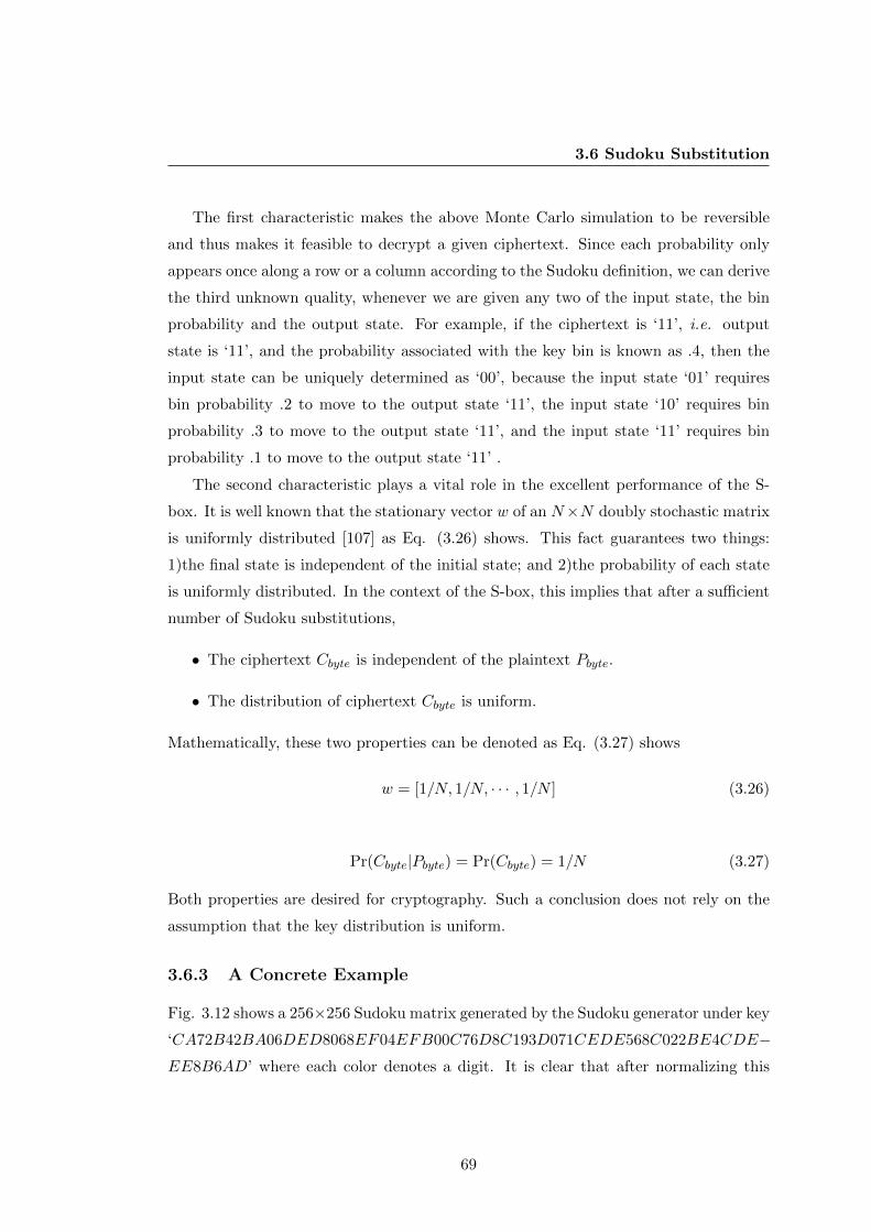
3.6 Sudoku Substitution
The first characteristic makes the above Monte Carlo simulation to be reversible
and thus makes it feasible to decrypt a given ciphertext. Since each probability only
appears once along a row or a column according to the Sudoku definition, we can derive
the third unknown quality, whenever we are given any two of the input state, the bin
probability and the output state. For example, if the ciphertext is ‘11’, i.e. output
state is ‘11’, and the probability associated with the key bin is known as .4, then the
input state can be uniquely determined as ‘00’, because the input state ‘01’ requires
bin probability .2 to move to the output state ‘11’, the input state ‘10’ requires bin
probability .3 to move to the output state ‘11’, and the input state ‘11’ requires bin
probability .1 to move to the output state ‘11’ .
The second characteristic plays a vital role in the excellent performance of the S-
box. It is well known that the stationary vector w of an N×N doubly stochastic matrix
is uniformly distributed [107] as Eq. (3.26) shows. This fact guarantees two things:
1)the final state is independent of the initial state; and 2)the probability of each state
is uniformly distributed. In the context of the S-box, this implies that after a sufficient
number of Sudoku substitutions,
• The ciphertext Cbyte is independent of the plaintext Pbyte.
• The distribution of ciphertext Cbyte is uniform.
Mathematically, these two properties can be denoted as Eq. (3.27) shows
w = [1/N, 1/N, · · · , 1/N ] (3.26)
Pr(Cbyte|Pbyte) = Pr(Cbyte) = 1/N (3.27)
Both properties are desired for cryptography. Such a conclusion does not rely on the
assumption that the key distribution is uniform.
3.6.3 A Concrete Example
Fig. 3.12 shows a 256×256 Sudoku matrix generated by the Sudoku generator under key
‘CA72B42BA06DED8068EF04EFB00C76D8C193D071CEDE568C022BE4CDE−EE8B6AD’ where each color denotes a digit. It is clear that after normalizing this
69

Figure 3.12: A key dependent 256× 256 Sudoku matrix
Sudoku matrix, a 256× 256 doubly stochastic matrix DS is obtained. The S-box used
for encryption is then determined by the key and the divided key bins. Tables 3.1 and
3.1 show the corresponding S-boxes when the used subkeys are in the 1st bin and the
2nd bin, respectively.
Table 3.1: The Sudoku S-Box When k ∈ Bin#1
00 01 02 03 04 05 06 07 08 09 A B C D E F00 1C 8B 25 EF D1 A7 4B CF 5D 95 FF BD 7F 39 02 6D01 70 29 33 11 C4 56 F0 B2 9F AC 0A DD 49 E2 88 6802 6E F9 5B 1A 9E EB C9 35 09 D3 28 79 B6 46 AE 8003 4D A9 16 B8 EA F4 0C 90 2F 61 CB DC 55 82 3D 7804 87 44 D9 32 FB 13 50 05 AA 2D B9 C5 62 ED 72 9205 3E BA 5F 1B 9B C7 DF 6C 8D AF 2E FC 7E 0F 45 EC06 3A A1 5C 85 FA 76 D2 E1 6F 00 BF C2 27 19 48 9D07 C3 D4 64 20 A5 77 E4 91 12 8A 38 BE 01 57 F6 4708 DB 96 A3 81 E5 60 BB FD 71 08 54 18 24 41 C8 3F09 D8 B3 83 4F C0 98 7C E6 0B 26 58 F7 15 69 A2 36A E7 F8 30 1D D7 A6 22 75 52 65 04 9C 8C 40 B1 CEB 17 97 E9 7D 59 F3 D6 B4 4C A0 6A C1 2B 37 0E 84C AD 10 67 3B E3 03 F2 CD 2C B5 4A D0 7B 86 94 5AD 4E 7A CA 9A 89 EE 14 FE 2A 6B BC 0D AB DE 51 34E CC 43 53 31 8F 23 99 07 66 F5 74 D5 E8 1F B0 A8F 1C 8B 25 EF D1 A7 4B CF 5D 95 FF BD 7F 39 02 6D
Fig. 3.13 shows the Sudoku substitution process on an 8 bit plaintext of size 16×16
with all zero entries and its ciphertext for one round encryption. It is noticeable that
such a one round substitution makes the ciphertext completely random-like, although
70

3.7 Conclusions
Table 3.2: The Sudoku S-Box When k ∈ Bin#2
00 01 02 03 04 05 06 07 08 09 A B C D E F00 A7 4B CF 5D 95 FF BD 7F 39 02 6D 1C 8B 25 EF D101 56 F0 B2 9F AC 0A DD 49 E2 88 68 70 29 33 11 C402 EB C9 35 09 D3 28 79 B6 46 AE 80 6E F9 5B 1A 9E03 F4 0C 90 2F 61 CB DC 55 82 3D 78 4D A9 16 B8 EA04 13 50 05 AA 2D B9 C5 62 ED 72 92 87 44 D9 32 FB05 C7 DF 6C 8D AF 2E FC 7E 0F 45 EC 3E BA 5F 1B 9B06 76 D2 E1 6F 00 BF C2 27 19 48 9D 3A A1 5C 85 FA07 77 E4 91 12 8A 38 BE 01 57 F6 47 C3 D4 64 20 A508 60 BB FD 71 08 54 18 24 41 C8 3F DB 96 A3 81 E509 98 7C E6 0B 26 58 F7 15 69 A2 36 D8 B3 83 4F C0A A6 22 75 52 65 04 9C 8C 40 B1 CE E7 F8 30 1D D7B F3 D6 B4 4C A0 6A C1 2B 37 0E 84 17 97 E9 7D 59C 03 F2 CD 2C B5 4A D0 7B 86 94 5A AD 10 67 3B E3D EE 14 FE 2A 6B BC 0D AB DE 51 34 4E 7A CA 9A 89E 23 99 07 66 F5 74 D5 E8 1F B0 A8 CC 43 53 31 8FF 06 B7 8E 63 DA 93 F1 42 3C 21 E0 5E C6 1E 73 A4
the plaintext is very pattern-like. This example shows the powerful group properties of
the Sudoku S-Boxes that on the one hand have key-dependent S-box selection and on
the other hand, all the possible S-boxes put together form a Markov chain transition
matrix with a uniformly distributed stationary vector
It is well known that a Markov chain process converges to the stationary distribution
regardless of where it begins. In other words, the distribution of a ciphertext encrypted
by the Sudoku substitution will eventually become uniform no matter what the distri-
bution of the plaintext is. Heuristically speaking, after 10 rounds of transitions, the
equivalent stationary distribution becomes very uniform-like for 256×256 Sudoku dou-
bly stochastic matrices, where the maximum distance between the possibility of a state
and 1/256 is less than 2−50.
Finally, it is worthwhile to note that there are actually N S-boxes within a given
N ×N Sudoku matrix and that the ciphertext is determined by both the plaintext and
the round key. In [115], I showed that the Sudoku S-box is complete [9] and satisfies
the strict avalanche criterion [116] and the bit independence criterion [116] .
3.7 Conclusions
In this section, I presented the Sudoku-based encryption/decryption techniques and
they are Sudoku Whitening using bit xor (ExorSW ,DxorSW ) and addition over finite field
(EgfSW ,DgfSW ); Sudoku Transposition (EST ,DST ), Sudoku Permutation using unitary
71

(a) Plaintext P (b) Ciphertext Cr=1 (c) Ciphertext Cr=2
(d) Ciphertext Cr=3 (e) Ciphertext Cr=4 (f) Ciphertext Cr=5
(g) Ciphertext Cr=6 (h) Ciphertext Cr=7 (i) Ciphertext Cr=8
Figure 3.13: An example of Sudoku substitution for eight rounds
permutation matrix (EupmSP ,DupmSP ), Sudoku Permutation using row or column or block
shuffling (ErcbSP ,DrcbSP ), Sudoku Permutation using matrix mapping between notations;
(EmmnSP ,DmmnSP ), Sudoku MDS matrix (ESM ,DSM ); and Sudoku Substitution using row
or column or block S-boxes (ErcbSS ,DrcbSS), and Markov chain transition matrix (EMC
SS ,DMCSS ).
Some of these techniques are directly based on similar techniques in classical cryptog-
raphy, for example, key whitening [8], while some are newly developed just for Sudoku,
for example Sudoku Substitution. All of these encryption techniques rely on two things:
72

3.7 Conclusions
• a parametric Sudoku array/matrix
• properties implicitly contained in a Sudoku array/matrix or facts about a Sudoku
array/matrix
The parametric Sudoku array/matrix tells us to use the parameters in Sudoku genera-
tion as the encryption key; the properties implicitly contained in a Sudoky array/matrix
guarantee the performance of a specific encryption technique.
As a result, these fundamental encryption/decryption techniques can be used to-
gether to form more secure product ciphers [2]. Examples of these product ciphers are
discussed in future sections.
73

74

4
Sudoku-AES Block Cipher
4.1 Overview
In the last section, several fundamental encryption techniques based on Sudoku prop-
erties were proposed. It is clear that all of these techniques can be directly used for
encryption/decryption when the N × N Sudoku matrix S is given. In this section,
we focus on implementing the classic Rijndael cipher using only Sudoku associated
techniques.
4.2 Cipher Structure
4.2.1 A Brief Review of AES
The classic Rijndael cipher, also known as the Advanced Encryption Standard (AES)
[4], is a requirement for the encryption of electronic data. It has been adopted by the US
government and is now accepted worldwide. AES is based on the design principle known
as the Substitution-Permutation Network (SPN) which allows fast implementation in
both software and hardware.
AES is a block cipher with a fixed block size of 128 bits, i.e. 16 bytes. Its key size
can be changed to 128, 192 or 256 bits. AES operates on a 4× 4 matrices of bytes and
its calculations are defined on the finite field of GF (28), with the irreducible polynomial
m(x) = x8 + x4 + x3 + x+ 1 for multiplication.
The AES cipher is a multi-round cipher which converts an input plaintext into a
final output of ciphertext. Each round consists of several processing steps, including
75

the Add Round Key step depending on the encryption key. A set of reverse rounds
can be applied to transform ciphertext back into the original plaintext using the same
encryption key.
Fig. 4.1 illustrates the encryption steps of AES. A high-level description of the AES
Figure 4.1: AES encryption flowchart
76
4.2 Cipher Structure
algorithm is as follows:
1. Key Expansion each encryption key is systematically expanded using the Rijn-
dael’s key schedule [4]
2. Initial Round
(1). Add Round Key each byte of the plaintext block is combined with the round
key using bitwise xor operation.
3. Intermediate Rounds
(1). Substitute Bytes A nonlinear step where each input byte is then replaced
by another byte with respect to the Rijndael substitution table.
(2). Shift Rows A transposition step where bytes in a row are shifted cyclically.
(3). Mix Columns A mixing operation which mixes bytes in each column.
(4). Add Round Key
4. Final Round
(1). Substitute Bytes
(2). Shift Rows
(3). Add Round Key
Details about the classic AES cipher can be found in [4].
4.2.2 Sudoku-AES Block Cipher
Besides cipher configurations like the working finite field and the key schedule, it is
noticeable that the conventional AES block cipher has the following core processing
steps for encryption:
Add Round Key is a key whitening step
Substitute Bytes is a substitution step
Shift Rows is a permutation step
Mix Columns is an MDS-based diffusion step
77

As a result, all these AES processing steps can be replaced with the corresponding
Sudoku-based encryption techniques and the resulting cipher is called the Sudoku-AES
cipher in the rest of the section.
Although the Sudoku-AES cipher mimics the structure of the classic AES cipher,
it has a larger block size of 256 bits, i.e. 32 bytes (1 byte = 8 bits). It operates on
two 4 × 4 matrices of bytes. Meanwhile, the Sudoku-AES cipher has both dynamic
substitution and permutation boxes. In short, the following comparison table shows
the similarities and dissimilarities between the Sudoku-AES cipher and the classic AES
cipher.
Table 4.1: Comparison between classic AES and Sudoku-AES ciphers
Items Classic AES Sudoku-AES
General
Block size 128 bits 256 bits (2× 128 bits)Key Size 128, 192, and 256 bits 256 bits
Finite Field GF (28) GF (28)# Rounds 10, 12 and 14 10
Encryption Function
Whitening Add Round Key Sudoku whitening ExorSWSubstitution Substitute Bytes Sudoku Substitution EMC
SSPermutation Shift Rows Sudoku Permutation ESP
Diffusion Mix Columns Sudoku MDS ESM
Operation Type
Whitening Dynamic DynamicSubstitution Fixed Rijndeal S-box Dynamic Sudoku S-boxesPermutation Fixed cyclic row shift Dynamic Sudoku P-boxes
Diffusion Fixed AES MDS Fixed Sudoku MDS
Specifically speaking, three types of Sudoku matrices are used in Sudoku-AES:
Whitening Sudoku Sw of size 16×16 is used to whiten the plaintext message in each
round using the ExorSW function, i.e. the Sudoku Whitening technique described
in Section 3.2.
Substitution Sudoku Ss of size 256×256 is used to substitute each plaintext byte in
each round using the EMCSS function, the Sudoku Substitution technique given
in Section 3.6.
Permutation Sudoku Sp of size 16×16 is used to shuffle plaintext bits in each round
using the EmmnSP function, i.e. the Sudoku Permutation technique provided in
Section 3.4.
Diffusion Sudoku Sms are two Sudokus of size 4× 4 used for mixing plaintext bytes
in each round using the ESM function, i.e. the Sudoku MDS technique discussed
in Section 3.5.
78
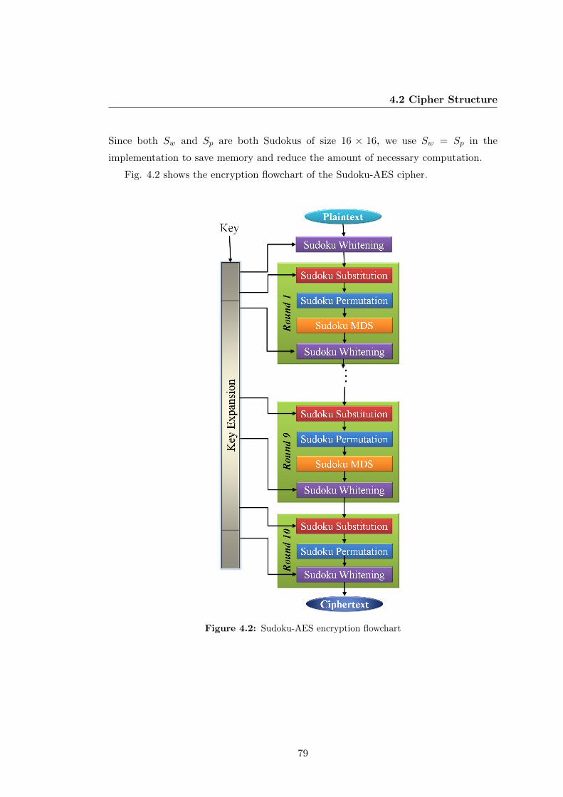
4.2 Cipher Structure
Since both Sw and Sp are both Sudokus of size 16 × 16, we use Sw = Sp in the
implementation to save memory and reduce the amount of necessary computation.
Fig. 4.2 shows the encryption flowchart of the Sudoku-AES cipher.
Figure 4.2: Sudoku-AES encryption flowchart
79
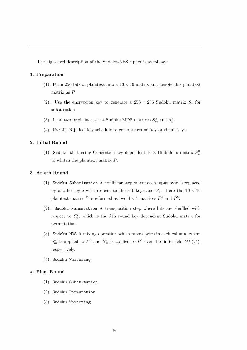
The high-level description of the Sudoku-AES cipher is as follows:
1. Preparation
(1). Form 256 bits of plaintext into a 16× 16 matrix and denote this plaintext
matrix as P
(2). Use the encryption key to generate a 256 × 256 Sudoku matrix Ss for
substitution.
(3). Load two predefined 4× 4 Sudoku MDS matrices Sam and Sbm.
(4). Use the Rijndael key schedule to generate round keys and sub-keys.
2. Initial Round
(1). Sudoku Whitening Generate a key dependent 16 × 16 Sudoku matrix S0w
to whiten the plaintext matrix P .
3. At kth Round
(1). Sudoku Substitution A nonlinear step where each input byte is replaced
by another byte with respect to the sub-keys and Ss. Here the 16 × 16
plaintext matrix P is reformed as two 4× 4 matrices P a and P b.
(2). Sudoku Permutation A transposition step where bits are shuffled with
respect to Skp , which is the kth round key dependent Sudoku matrix for
permutation.
(3). Sudoku MDS A mixing operation which mixes bytes in each column, where
Sam is applied to P a and Sbm is applied to P b over the finite field GF (28),
respectively.
(4). Sudoku Whitening
4. Final Round
(1). Sudoku Substitution
(2). Sudoku Permutation
(3). Sudoku Whitening
80

4.3 Simulation Results
4.3 Simulation Results
4.3.1 CCITT Database
In order to test the performance of the Sudoku-AES cipher, the CCITT fax standard
image database 4 was selected for the simulation. This database was selected because
1) it is an open database that is widely used in the image processing field; and 2) its
images are all binary and thus form a good database to test a block cipher since this
type of data is more correlated than digital audio and bit stream data.
The listed CCITT image database contains 8 binary images of size 1728×2376 with
1 bit depth, namely CCITT 1, CCITT 2, · · · , CCITT 8 as Fig. 4.3 shows. Further,
we divide each CCITT image into blocks of size 80 × 256 without overlapping (the
explanation about this selected size will be discussed in the next section). In other
words, we consider each CCITT image is a plaintext set and use the non-overlapped
image blocks as plaintexts in the simulation. Due to the size constraint, each CCITT
image can produce 189 plaintexts and we name the ith plaintext of the jth CCITT
image as P ij , where 1 ≤ i ≤ 189 and 1 ≤ j ≤ 8. Therefore, our plaintext database has
8 × 189 = 1512 messages. For example, Fig. 4.4 shows the plaintext set of CCITT 5.
Finally, each plaintext P ji is extracted to a binary sequence and then encrypted using
the Sudoku-AES block cipher using random keys and its corresponding ciphertext is
denoted as Cji .
4.3.2 Results
Fig. 4.5 and 4.6 show the random selected plaintext messages and corresponding cipher-
text messages after encryption using the Sudoku-AES cipher, respectively. It is clearly
to see that after encryption, resulting ciphertexts are random-like and unintelligible.
Even though the plaintext messages with strong homogenous regions (see P 1251 and P 26
8
in Fig. 4.5), their corresponding ciphertext messages (see C1251 and C26
8 in Fig. 4.6)
are still random-like. Meanwhile, distinctive plaintext messages become indiscernible
after encryption and this is a visual demonstration of the confusion property [2].
4This database can be found under page: http://cdb.paradice-insight.us as the date of
03/26/2012.
81

(a) CCITT 1 (b) CCITT 2 (c) CCITT 3
(d) CCITT 4 (e) CCITT 5 (f) CCITT 6
(g) CCITT 7 (h) CCITT 8
Figure 4.3: CCITT fax standard image database
82
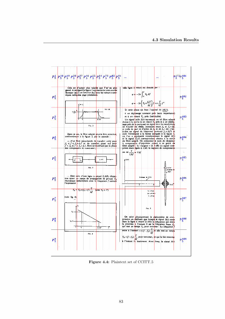
4.3 Simulation Results
Figure 4.4: Plaintext set of CCITT 5
83

With regards to encryption and decryption speed, we test both the Sudoku-AES
cipher and the conventional AES cipher 5 under MATLAB for 10,000 pieces of 256-
bit messages. The average encryption time of Sudoku-AES is 0.4318 seconds with a
standard deviation of 0.00971 seconds. The average encryption/decryption time of the
conventional AES cipher (using 128-bit keys and 10 cipher rounds) is 0.2209 seconds
with a standard deviation of 0.05047 seconds. Roughly speaking, the conventional AES
cipher is one time faster than the Sudoku-AES cipher. The reason why the Sudoku-AES
cipher is slower is because the dynamical P-boxes and S-boxes are all generated with
respect to keys and round keys in encryption or decryption. However, it is worthwhile
to note that dynamic P-boxes and S-boxes help enhance the cipher security (detail
discussion is given in the next section).
5The adopted AES MATLAB code is written by Dr. J. J. Buchholz. This algorithm can be found
http://buchholz.hs-bremen.de/aes/aes.htm as the date of 03/26/2012
84

4.3 Simulation Results
P 1251 P 104
2 P 1343 P 10
4 P 395 P 19
6 P 1407 P 119
8
P 681 P 114
2 P 1413 P 107
4 P 535 P 36
6 P 267 P 26
8
P 661 P 24
2 P 493 P 160
4 P 1625 P 38
6 P 1497 P 92
8
P 761 P 51
2 P 1613 P 87
4 P 955 P 131
6 P 1317 P 98
8
P 1741 P 77
2 P 1733 P 39
4 P 565 P 67
6 P 437 P 57
8
Figure 4.5: Sample plaintext messages
85

C1251 C104
2 C1343 C10
4 C395 C19
6 C1407 C119
8
C681 C114
2 C1413 C107
4 C535 C36
6 C267 C26
8
C661 C24
2 C493 C160
4 C1625 C38
6 C1497 C92
8
C761 C51
2 C1613 C87
4 C955 C131
6 C1317 C98
8
C1741 C77
2 C1733 C39
4 C565 C67
6 C437 C57
8
Figure 4.6: Sample ciphertext messages
86

4.4 Security Analysis
4.4 Security Analysis
4.4.1 Theoretical Analysis
According to the working assumption, the cryptanalysis can be roughly classified into
ciphertext-only, known-plaintext, and chosen-plaintext (chosen-ciphertext). First, we
will briefly discuss the cryptanalysis of Sudoku-AES.
Conventionally, the ciphertext-only attack (COA) is an attack model for crypt-
analysis where the attacker has only access to a set of ciphertext. It is more or less
dependent on the statistics of the set of ciphertext. For example, frequency analysis
[8] is used to analyze the frequency of each ciphertext byte to find patterns related to
prior knowledge, such as the distribution of certain letters or combinations of letters
[8]. It is clear that Sudoku-AES is invulnerable to this type of attacks, because the
special structure generated by the Sudoku-Substitution makes the ciphertext bytes a
uniformly distributed statistics.
The known-plaintext attack (KPA) is an attack model for cryptanalysis where the
attacker has access to both the set of plaintext and its corresponding set of ciphertext.
Its objective is to explore secret information such as encryption keys. The Sudoku-AES
design is also well-protected against this type of attack, as both the SPN structure
and MDS provide strong confusion and diffusion property [2]; making the relationship
between the key and ciphertext very complicated and involved and the non-uniformly
distributed plaintexts uniformly distributed.
The chosen-plaintext attack (CPA) is another attack model where the attacker has
the capacity to choose arbitrary plaintexts and to encrypt them to ciphertexts. Both
linear cryptanalysis [8] and differential cryptanalysis [8] are of this type. The aim of
CPA is to crack the encryption key used in the cipher, or partial key bits. Unlike
the conventional SPN based ciphers [4, 5] operating plaintext/ciphertext directly with
the encryption key, the Sudoku-AES performs this operation in an indirect way by
transforming the encryption key into a series of Sudoku matrices. Moreover, such a
transformation is absolutely nonlinear, which provides additional nonlinearity in the
cipher besides the S-Box. Furthermore, the S-Box in Sudoku-AES also has strong
resistance against the linear cryptanalysis and differential analysis. It is well known
that both cryptanalysis techniques require the knowledge of the used S-Box in the
cipher [112, 113, 117]. However, the S-Box used in the Sudoku-AES is key dependent
87

and thus dynamic, which implies that the knowledge of the used S-Box is inaccessible to
an attacker and thus the knowledge of cryptanalysis on one S-Box is useless to another
one. In other words, the Sudoku-AES cipher is secure with respect to these two attacks.
Even if the S-Boxes in the Sudoku-AES cipher are fixed, the Sudoku-AES cipher is
still able to resist the differential attack, because it is a type of Markov cipher [90]. In
Sudoku-AES, S-Boxes are not used independently but dependently in the way of the
Sudoku transition matrix as Fig. 3.11-(c) shows (the S-Boxes together form a Sudoku
array). Since the Sudoku substitution process has a close relationship to the Markov
chain Monte Carlo simulation, it is natural to guess that Sudoku-Substitution is a
Markov cipher, which it actually is.
In order to prove that the Sudoku-AES cipher is a Markov cipher, first recall the
definition of a Markov cipher in [90]:
Definition 3. An iterated cipher with round function Y = f(X,K) is a Markov cipher
if there is a group operation defining difference ⊗ such that, for all choices of α(α 6= e)
and β(β 6= e), the probability that the difference between two ciphertexts ∆Y = Y ⊗Y ∗
when the difference is known between the two corresponding plaintexts ∆X = X ⊗X∗
and the plaintext X = γ, i.e.
Pr
(∆Y = β
∣∣∣∣∣ ∆X = α
X = γ
)
is independent of γ when the subkey K is uniformly random.
From this definition, it is derived that the Sudoku-Substitution is a Markov cipher.
Proof. Let X = γ and X∗ are two plaintext messages in Sudoku-Substitution, and
Y = f(X,K) and Y ∗ = f(X∗,K) are corresponding ciphertext messages. Since f(.) is
the Sudoku Substitution round function, then the following equation holds
Pr(Y = δ|X = γ) = Pr(Y = δ) = 1/N
Where N is the size of the Sudoku matrix used in Sudoku substitution and N = 256
88

4.4 Security Analysis
in the context of Sudoku-AES cipher. Let α⊗−1 γ = γ∗, then
Pr
(∆Y = β
∣∣∣∣∣ ∆X = α
X = γ
)= Pr
(∆Y = β
∣∣∣∣∣ X∗ = α⊗ γX = γ
)
= Pr
∆Y = β
∣∣∣∣∣∣∣X∗ = γ∗
X = γ
X 6= X∗
=
∑δ Pr
∆Y = β
Y = δ
∣∣∣∣∣∣∣X∗ = γ∗
X = γ
X 6= X∗
=∑
δ Pr
Y = δ
∣∣∣∣∣∣∣X∗ = γ∗
X = γ
X 6= X∗
Pr
∆Y = β
∣∣∣∣∣∣∣∣∣∣X∗ = γ∗
X = γ
X 6= X∗
Y = δ
=∑
δ Pr
Y = δ
∣∣∣∣∣∣∣X∗ = γ∗
X = γ
X 6= X∗
Pr
Y ∗ = β ⊗−1 Y
∣∣∣∣∣∣∣∣∣∣X∗ = γ∗
X = γ
X 6= X∗
Y = δ
=∑
δ Pr
Y = δ
∣∣∣∣∣∣∣X∗ = γ∗
X = γ
X 6= X∗
Pr
Y ∗ = β ⊗−1 δ
∣∣∣∣∣∣∣∣∣∣X∗ = γ∗
X = γ
X 6= X∗
β 6= e
=
∑δ Pr (Y = δ|X = γ) Pr
(Y ∗ = β ⊗−1 δ
∣∣∣∣∣ X∗ = γ∗
β 6= e
)
=∑
δ Pr(Y = δ)Pr(Y ∗ = β ⊗−1 δ|Y 6= Y ∗)
=∑
δ
1
N
1
N − 1
=1
N − 1
Therefore, in Sudoku Substitution we have:
Pr
(∆Y = β
∣∣∣∣∣ ∆X = α
X = γ
)=
1
N
89

which implies the above probability is independent of γ and is uniformly distributed.
Therefore, the Sudoku Substitution, a Markov cipher, is secure against two differential
cryptanalysis attacks after sufficiently many rounds [90].
4.4.2 Experimental Analysis
In the following experimental analysis, the Federal Information Processing Standard
(FIPS)140-2 randomness statistical tests for randomness [3] is selected to give qualita-
tive results of the ciphertext message randomness using the Sudoku-AES cipher. FIPS
140-2 is a U.S government computer security standard used to accredit cryptographic
modules. Its statistical tests for randomness includes four randomness tests, namely
Monobit Test, Poker Test, Run Test and Long Run Test, where the Run Test is further
detailed in six sub tests with respect to different lengths of the run.
Table 4.2: FIPS 140-2 Statistical test results of ciphertext messages using the Sudoku-AES cipher
# of FailsPlantext RunSet Monobit Porker Length of The Run Long Run
1 2 3 4 5 ≥ 6AcceptRange
9725-10725
2.16-46.17
2315-2685
1114-1386
527-723
240-384
103-209
103-209
0
CCITT 1 0 0 0 0 0 0 0 0 0CCITT 2 0 0 0 0 0 0 0 0 0CCITT 3 0 0 0 0 0 0 0 0 0CCITT 4 0 0 0 0 0 0 0 0 0CCITT 5 0 0 0 0 0 1 0 0 0CCITT 6 0 0 0 0 0 0 0 0 0CCITT 7 0 0 0 0 0 0 0 0 0CCITT 8 0 0 0 0 0 0 0 0 0
The FIPS 140-2 specifies the test sequence length to be 20000. In order to analyze
the ciphertext randomness, the first 20000 bits of Cji are used in the test. If it fails
to pass a specific test, the counter of the corresponding test adds 1. Finally, the test
results are listed in Table 4.2, with respect to the plaintext sets. For example, the
row of ‘CCITT 5’ means that in 189 ciphertext messages C15 , C2
5 , · · · , C1895 only one
ciphertext message out of 1512 fails to pass the ‘Run Test’ at the length of 4 in the
FIPS 140-2 statistical tests. This result matches the significant level 0.001 of the test
and shows that the ciphertext messages encrypted by the Sudoku-AES cipher are very
random-like.
90

4.5 Conclusions
Furthermore, the Lampel-Ziv sequence complexity [118] is selected to provide quan-
titative results of the ciphertext message’s randomness. Together they show the per-
formance quality of the Sudoku-AES cipher. The Lampel-Ziv sequence complexity is
usually used to calculate the complexity of a finite sequence and in our case it calcu-
lates the randomness of the ciphertext blocks. Its implementation [119] requires a test
sequence length 10000 or longer. Since the ciphertext string has a length of 20480, it
can be analyzed by the Lampel-Ziv sequence complexity directly. Results are listed in
Table IV 6. It is worthwhile to note that each statistic is calculated from 189 ciphertext
strings. These statistics show that the test ciphertext strings are very random-like and
have a high sequence complexity [119].
Table 4.3: Lampel-Ziv sequence complexity of ciphertext messages encrypted by theSudoku-AES Cipher
Plaintext SetSequence Complexity of Ciphertext Messages
Min Max Mean±StdCCITT 1 1.02 1.03 1.02374± 0.003176CCITT 2 1.01 1.03 1.02396± 0.003490CCITT 3 1.01 1.03 1.02352± 0.003763CCITT 4 1.02 1.03 1.02386± 0.003036CCITT 5 1.01 1.03 1.02404± 0.003299CCITT 6 1.01 1.03 1.02346± 0.003553CCITT 7 1.01 1.03 1.02369± 0.003226CCITT 8 1.02 1.03 1.02405± 0.003506
4.5 Conclusions
In this section, we introduced the Sudoku-AES cipher using Sudoku based encryption
techniques. The Sudoku-AES cipher is a block cipher with cipher structures like the
AES cipher [4], nevertheless it differs from the AES cipher in the following aspects:
• The Sudoku-AES cipher processing block size is twice as big as the AES cipher’s
block size.
• The Sudoku-AES cipher relies on all Sudoku-based encryption techniques defined
in Chapter 3.
• The Sudoku-AES cipher adopts dynamic P-Boxes and S-Boxes for encryption.
6The adopted Lampel-Ziv complexity implementation algorithmto generate this table is written by
Stephen Faul using Matlab. This algorithm can be found http://www.mathworks.com/matlabcentral/
fileexchange/6886-kolmogorov-complexity as the date of 03/26/2012
91

• The Sudoku-AES cipher is a Markov cipher.
I also showed that the Sudoku-AES cipher is secure against various attacks in-
cluding COA, KPA and CPA, and that it is invulnerable to linear cryptanalysis and
differential cryptanalysis. Furthermore, analysis of a large number of ciphertext mes-
sages using FIPS 140-2 statistical tests [3] and the Lampel-Ziv sequence complexity
[119] exhibited excellent performances. We also performed the latest NIST SP 800-22
statistical test suite for ciphertext messages encrypted by the Sudoku-AES cipher and
the comprehensive results can be found in Appendix A.
92

5
Sudoku Image Cipher
5.1 Overview
It is clear that the processing sizes of conventional block/stream ciphers are relatively
small for a digital image, which usually have a size in the 50kb-10mb range and could
be much larger. For example, the block size of AES is 128 bit, and thus it requires
dividing a digital image into more than ten thousand blocks to process it. Such an
encryption process is normally inefficient [16]. Meanwhile, treating a digital image the
same way as a digital bit string neglects the nature of the digital image, whose neighbor
pixels are strongly correlated, and image pixel depths are of different significance levels
[120]. Therefore, new image-ciphers are in high demand.
In this section, we propose a Sudoku-Image cipher using Sudoku-Transposition,
Sudoku-Permutation, Sudoku-Substitution and Sudoku-MDS for 8 bit grayscale images
and 24 bit true color RGB images. It processes 256× 256 images with a pixel depth of
8.
5.2 Sudoku-Image Cipher
5.2.1 Cipher Structure
The Sudoku-Image cipher also uses Sudoku encryption techniques, but in a more effi-
cient way. The overview of the Sudoku-Image cipher is shown in Fig. 5.1.
Besides the Sudoku encryption primitives introduced earlier, we introduce an op-
tional stage of probabilistic encryption [121, 122] with the purpose to achieve semanti-
93

Figure 5.1: Encryption flowchart of the Sudoku-Image cipher
cally secure ciphers [8], thus enhancing cipher security further. Conventionally, proba-
bilistic encryption is achieved by padding random noise within plaintext in encryption
and removing this noise in decryption, which usually requires an encrypting an addi-
tional amount of data. However, due to the psychovisual redundancy of image data,
we can simply introduce random noise without expanding plaintext size: we randomly
94
5.2 Sudoku-Image Cipher
embed binary random noise only in the least significant bit-plane of the plaintext image
by xoring a random number of plaintext least significant bits to the random noise bits.
In this way, for each plaintext image in encryption, this optional stage will randomly
change some bits on the least significant bit-plane of the plaintext image; a slight change
in this stage will lead to significant different ciphertext after encryption. Consequently,
for the same encryption key and the same plaintext image, this optional stage is able
to obtain different ciphertext images. Any slight change in this stage will not influence
image decryption results, because these changes are only made with respect to a num-
ber of bits in the least significant bit-plane, whose changes are unrecognizable to the
human vision system.
There are four types of Sudoku matrices that are used in the Sudoku-Image Cipher:
Ss: A 256× 256 dynamic Sudoku matrix for substitution, controlled by the encryption
key K.
Snt : A 256× 256 dynamic Sudoku matrix for transposition in the nth round controlled
by the round key kn.
Snp : A 256× 256 dynamic Sudoku matrix for permutation in the nth round controlled
by the round key kn.
Sm: A 4× 4 Fixed Sudoku MDS matrix.
Let’s assume the input data is an 8 bit grayscale image, then each pixel in the image
is considered as a byte of 8 bits. All cipher operations are now applied at the byte level
rather than at the bit level.
In Fig. 5.1, the Sudoku Transposition process is defined in Eq. (3.9). The Sudoku
Row/Column Substitution denotes the row-wise or column-wise Sudoku substitution
processing that uses one sub-key k to encrypt a row or a column of pixels. For example,
assume plaintext pixels located in the ith row are denoted as P (i, 1), P (i, 2), · · · ,
P (i, 256), then corresponding ciphertext pixels are calculated in the form of Eq. (3.24)
by using P (i, 1), P (i, 2), · · · , P (i, 256) as input bytes.
EMCSS : Find C(i, j)in DS , such that Pr (C(i, j)|P (i, j)) = Pr(BinNo. = nk)
95

for j ∈ {1, 2, · · · , 256}. In such a way, the substitution process for pixels belonging to
the same row/column requires only one subkey rather than 256 subkeys in the Sudoku-
AES cipher. The cipher applies the Sudoku row substitution when the round number
n is odd and the Sudoku column substitution when n is even.
The ‘Sudoku Permutation’ process is also implemented in two ways with respect to
the parity of the round number n.
• When the round number n is odd, the bijection g := (d, b)→ (r, d) is used.
• when n is even, the bijection g := (d, b)→ (c, d) is used.
Since the permutation process only changes the pixel position, this stage remains the
same as that of the Sudoku-AES cipher, except that the reference Sudoku matrix used
for permutation Sp is now 256× 256 instead of 16× 16.
Finally, the Sudoku MDS process is applied to every 4× 4 block in the permutated
image over the finite field GF (28).
It is worthwhile to note that the Sudoku-Image cipher still uses the Rijndael key
schedule (256 bits) to generate round keys and sub-keys and assume these keys are
uniformly distributed, where a round key is used to generate key dependent Sudoku
matrices in each round and a subkey is used to choose the S-Box during each pixel
substitution processing. The round number is set to 10, because we want the designed
cipher to attain good confusion and diffusion properties. Although the Sudoku MDS is
only of size 4×4, a single pixel change in the plaintext will lead to as many as 16 changes
in its corresponding in a single encryption round. After ten rounds of encryption, there
are as many as 1610 = 240 changes during the encryption process and this number is
much larger than the block size 2562 = 216. In such a way, the Sudoku-Image cipher is
able to resist the CPA on image ciphers [8].
5.2.2 Extension to RGB Images
It is well known that the true color RGB image is composed of three additive primary
colors, i.e. red, green and blue. The intensity of each color is denoted as an 8 bit
integer ranging from 0 to 255. As a result, various colors can be represented using
different combinations of the red, green and blue colors. In other words, a RGB image
can be considered as a 2D image with a pixel depth of 24, where every 8 bits denotes
the intensity of a primary color.
96
5.3 Simulation Results
Since the Sudoku-Image cipher is designed to encrypt an 8 bit grayscale image and
a RGB image can be decomposed to three 8 bit images, the Sudoku-Image cipher can
also be used for RGB images by simply encrypting each primary color channel.
The encryption processing of a RGB image using the Sudoku-Image cipher can be
described as follows:
Step 1: Decompose a RGB image P to three 8 bit images with respect to the three
primary colors and denote these images as PR, PG and PB.
Step 2: Use the encryption key K − 1 to encrypt the red channel 8 bit image PR to
CR.
Step 3: Use the encryption key K to encrypt the red channel 8 bit image PG to CG.
Step 4: Use the encryption key K + 1 to encrypt the red channel 8 bit image PB to
CB.
Step 5: Merge CR, CG and CB into the color ciphertext image C as the output.
This way, the Sudoku-Image cipher can be used to encrypt RGB images. It is also
worthwhile to note that other color image formats are also convertible to the RGB
format. As a result, color images can be encrypted by the Sudoku-Image cipher as
well.
Similar encryption methods can be found to deal with images belonging to other
data types. For example, if the input image is a 16 bit grayscale image, a common
image format for medical images, then this type of image can be properly encrypted
by splitting 16 bits into two groups with 8 bits in each group. Then the encryption
process is the same as processing two 8 bit grayscale plaintext images.
5.3 Simulation Results
5.3.1 Database
We chose the USC-SIPI database9 Volume 3: Miscellaneousfor simulation. As it is
introduced on the database home page, “the USC-SIPI image database is a collection
of digitized images. It is maintained primarily to support research in image processing,
97

image analysis, and machine vision”. This database has been widely accepted and
hundreds of algorithms are analyzed based on their performance on this database.
Since the USC-SIPI has multiple databases reflecting various the various types of
images and their properties which are of interests within the image processing field, we
chose to focus on what we considered to be the most appropriate database Miscella-
neous in simulation. This database is considered to have a good coverage of various
types of digital images including image types, scenes, luminance conditions etc. The
Miscellaneous volume consists of 44 images, 16 color and 28 monochrome. The sizes
are fourteen 256× 256, twenty-six 512× 512 and four 1024× 1024. The full description
of the Miscellaneous image data set is listed in Table 5.1 9.
The complete 44 images in the Miscellaneous data set plus the standard gray ‘Lenna’
image are given in Fig. 5.2. In the future sections, these images will be tested and
analyzed using different methods.
7The USC-SIPI image database can be found on http://sipi.usc.edu/database/ and its origi-
nal miscellaneous dataset description is available at http://sipi.usc.edu/database/database.php?
volume=misc as the date of 03/26/2012.
98

5.3 Simulation Results
Table 5.1: USC-SIPI: volume miscellaneous dataset
Filename Description Size Type4.1.01 Girl 256 Color4.1.02 Couple 256 Color4.1.03 Girl 256 Color4.1.04 Girl 256 Color4.1.05 House 256 Color4.1.06 Tree 256 Color4.1.07 Jelly beans 256 Color4.1.08 Jelly beans 256 Color4.2.01 Splash 512 Color4.2.02 Girl (Tiffany) 512 Color4.2.03 Mandrill (a.k.a. Baboon) 512 Color4.2.04 Girl (Lena, or Lenna) 512 Color4.2.05 Airplane (F-16) 512 Color4.2.06 Sailboat on lake 512 Color4.2.07 Peppers 512 Color5.1.09 Moon surface 256 Gray5.1.10 Aerial 256 Gray5.1.11 Airplane 256 Gray5.1.12 Clock 256 Gray5.1.13 Resolution chart 256 Gray5.1.14 Chemical plant 256 Gray5.2.08 Couple 512 Gray5.2.09 Aerial 512 Gray5.2.10 Stream and bridge 512 Gray5.3.01 Man 1024 Gray5.3.02 Airport 1024 Gray7.1.01 Truck 512 Gray7.1.02 Airplane 512 Gray7.1.03 Tank 512 Gray7.1.04 Car and APCs 512 Gray7.1.05 Truck and APCs 512 Gray7.1.06 Truck and APCs 512 Gray7.1.07 Tank 512 Gray7.1.08 APC 512 Gray7.1.09 Tank 512 Gray7.1.10 Car and APCs 512 Gray7.2.01 Airplane (U-2) 1024 Grayboat.512 Fishing Boat 512 Grayelaine.512 Girl (Elaine) 512 Grayhouse House 512 Colorgray21.512 21 level step wedge 512 Graynumbers.512 256 level test pattern 512 Grayruler.512 Pixel ruler 512 Graytestpat.1k General test pattern 1024 Gray
99

lenna 4.1.01 4.1.02 4.1.03 4.1.04 4.1.05
4.1.06 4.1.07 4.1.08 4.2.01 4.2.02 4.2.03
4.2.04 4.2.05 4.2.06 4.2.07 5.1.09 5.1.10
5.1.11 5.1.12 5.1.13 5.1.14 5.2.08 5.2.09
5.2.10 5.3.01 5.3.02 7.1.01 7.1.02 7.1.03
7.1.04 7.1.05 7.1.06 7.1.07 7.1.08 7.1.09
7.1.10 7.2.01 boat.512 elaine.512 house gray21.512
numbers.512 ruler.512 testpad.1k
Figure 5.2: USC-SIPI Miscellaneous Image Data Set
100
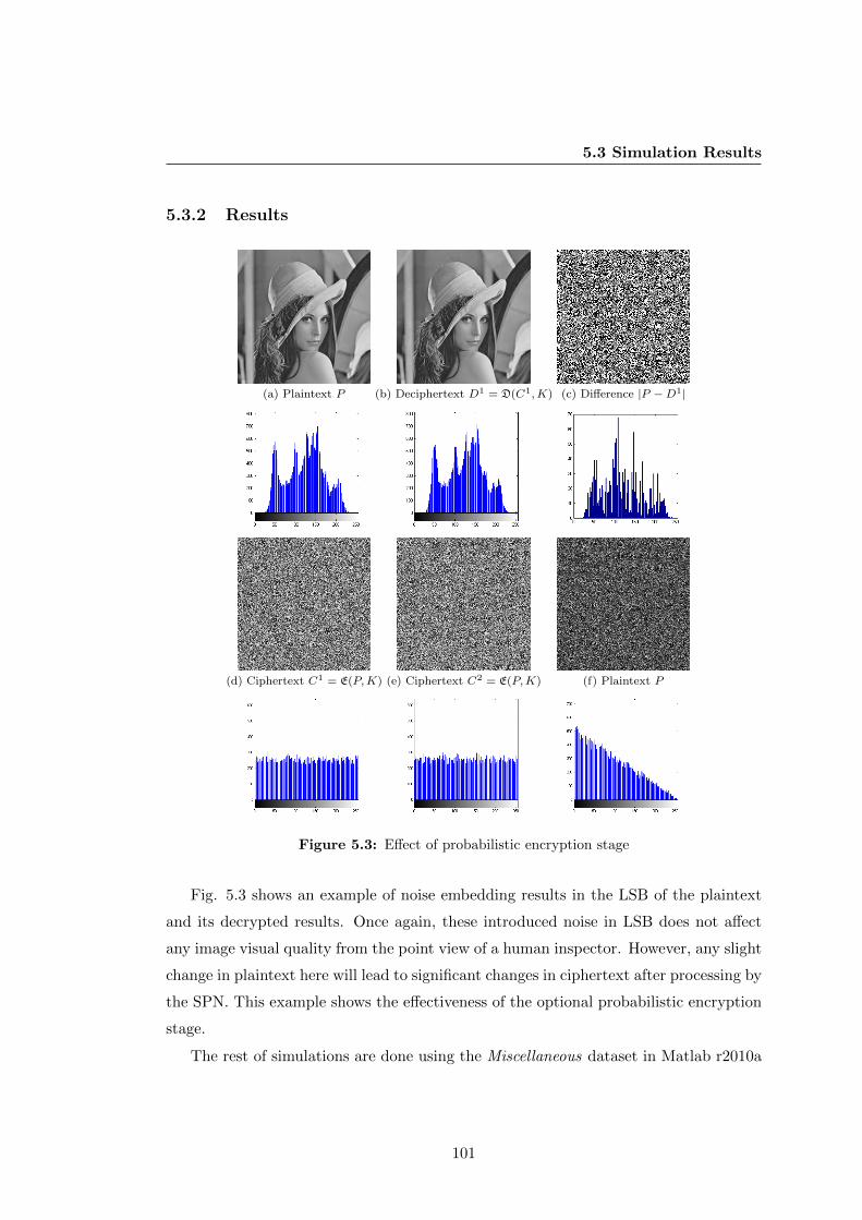
5.3 Simulation Results
5.3.2 Results
(a) Plaintext P (b) Deciphertext D1 = D(C1,K) (c) Difference |P −D1|
(d) Ciphertext C1 = E(P,K) (e) Ciphertext C2 = E(P,K) (f) Plaintext P
Figure 5.3: Effect of probabilistic encryption stage
Fig. 5.3 shows an example of noise embedding results in the LSB of the plaintext
and its decrypted results. Once again, these introduced noise in LSB does not affect
any image visual quality from the point view of a human inspector. However, any slight
change in plaintext here will lead to significant changes in ciphertext after processing by
the SPN. This example shows the effectiveness of the optional probabilistic encryption
stage.
The rest of simulations are done using the Miscellaneous dataset in Matlab r2010a
101

under the Window XP system with 2.6GHz Intel Core2 Quad processor and 3Gb mem-
ory.
Plaintext PlaintextHistogram Ciphertext CiphertextHistogram Decrypted text
Figure 5.4: Encryption results by using the Suodku-Image cipher on grayscale images
102

5.3 Simulation Results
Plaintext Plaintext Histogram Ciphertext Ciphertext Histogram Decrypted text
Figure 5.5: Encryption results by using the Suodku-Image cipher on RGB images
103

With regards to encryption and decryption speed, we test the proposed Sudoku-
Image cipher with a typical chaos-based image cipher10 [123] under the same MATLAB
environment. And their results are listed in Table 5.2. It is clear that the Sudoku-Image
cipher is much faster than chaos-based image cipher, because it does not require any dis-
cretization, iterative computing nonlinear functions, or other expensive computations
in a chaos-based image cipher.
5.4 Security Analysis
In this section, several prevailing security analyses with respect to image encryption are
implemented. Analyses results are compared with recent peer algorithms. Reported
results about [39, 40] are generated by authorized codes; results about bmpPacker9
and I-Cipher 10 are obtained by using corresponding commercial software; and other
results are directly pulled from related papers. It is worthwhile to note that to make
fair comparisons, the optional ‘probabilistic encryption’ stage is not used to generate
simulation results for security analysis.
5.4.1 Key Space Analysis
For a cipher to be secure, its key space has to be large enough to resist a brute force
attack. In the Sudoku-Image cipher, the encryption key is defined as a bit string of
length 256, which is the same length as the key space of the classic AES cipher and is
considered to be sufficiently large. However, this does not mean that the key space of
the Sudoku-Image cipher is limited to 256 bits.
It is clear that all encryption/decryption stages only require parametric Sudoku
matrices, which are dependent on either the encryption key or its derived round keys.
Therefore, the theoretical key space of the Sudoku-Image cipher should be the total
number of the distinctive 256× 256 Sudoku matrices. We’ve already shown that such
8This is an image encryption method based on two-dimensional logistic map. Its MATLAB imple-
mentation is available under the page https://sites.google.com/site/tuftsyuewu/source-code as
the date of 03/26/2012.9bmpPacker is a free encryption software available at http://www.goedeke.net/bmppacker.html
as the date of 03/26/2012, which implements a number of classical cryptographic algorithms including
AES, TwoFish, BlowFish.10I-Cipher is a commercial image encryption software developed by Ambitware under www.
ambitware.com/abw/i-cipher_download.php as the date of 03/26/2012.
104

5.4 Security Analysis
Table 5.2: Encryption/decryption speed comparisons (seconds)
Execution Time Ratio
File Chaos-based [123] Tchaos Sudoku-Image TSudokuTchaosTSudoku
4.1.01 63.02 2.63 24.014.1.02 62.06 2.20 28.234.1.03 61.76 2.18 28.334.1.04 62.72 2.17 28.844.1.05 62.93 2.19 28.714.1.06 62.44 2.21 28.214.1.07 61.89 2.18 28.414.1.08 62.76 2.20 28.494.2.01 256.84 8.73 29.414.2.02 248.28 8.76 28.334.2.03 247.53 8.86 27.944.2.04 243.24 8.80 27.654.2.05 244.63 8.80 27.814.2.06 248.01 8.71 28.484.2.07 248.38 8.72 28.475.1.09 20.84 0.72 29.095.1.10 20.76 0.73 28.575.1.11 21.13 0.72 29.445.1.12 21.34 0.74 28.995.1.13 21.21 0.74 28.855.1.14 21.20 0.73 29.145.2.08 84.09 2.91 28.895.2.09 84.99 2.90 29.295.2.10 84.59 2.96 28.595.3.01 336.06 11.85 28.365.3.02 339.45 11.97 28.367.1.01 83.79 2.93 28.617.1.02 84.05 2.87 29.267.1.03 85.02 2.96 28.727.1.04 84.32 2.97 28.427.1.05 85.12 2.96 28.807.1.06 85.10 2.96 28.747.1.07 85.15 2.95 28.847.1.08 84.92 2.95 28.767.1.09 84.16 2.92 28.817.1.10 85.08 2.96 28.787.2.01 339.54 11.76 28.88
boat.512 84.77 2.92 29.02elaine.512 84.79 2.94 28.81
gray21.512 84.69 2.96 28.61house 246.49 8.93 27.61
numbers.512 84.72 2.88 29.43ruler.512 84.45 2.93 28.87
testpat.1k 338.41 11.72 28.88
a number is at least 23072, which implies the key length could be at least 3072 bits.
Therefore, the Sudoku-Image cipher has sufficiently large key spaces.
5.4.2 Key Sensitivity Analysis
The proposed Sudoku-Image cipher has a strong key sensitivity, because:
105

1. the encryption key is used as the seed in the PRNG and thus different keys lead
to different sets of Sudoku parameters.
2. the encryption key is also expanded to round keys for each iteration and subkeys
for each row-wise and column-wise substitution using the Rijndael key schedule,
which is proven to generate uniformly distributed random-like keys.
3. any change in a round key further influences the reference Sudokus, which Sudoku
encryption techniques relies on.
(a) P (b) CK1 (c) CK2 (d) |CK1 − CK2 |
Figure 5.6: Sudoku-Image cipher key sensitivity analysis
Fig. 5.6 shows two ciphertext images using encryption keyK1 = 05EE38B0781964BF-
DF6F5EE05AD149C5-9A5BB99866603634-D799B04D2E8FAB05 andK2 = 05EE38B07819
64BF-DF6F5EE05AD149C5-9A5BB99866603634-D799B04D2E8FAB06, where the ‘Lenna’
image is used as the plaintext image and K1 and K2 are encryption keys in between
which the only difference is to be found in the last bit. Fig. 5.6-(d) shows the difference
between CK1 = E(P,K1) and CK2 = E(P,K2). It is noticeable that after 10 rounds
of iteration the two ciphertext images are completely different. The reason why the
histogram of the absolute difference image of CK1 and CK2 has a triangle shape is to
be found in the fact that for two pixels x1 and x2 within the range of 0 to 255, there
are 256 possible ways for x1 and x2 to make |x1 − x2| = 0; there are 510 possible ways
for |x1 − x2| = 1; · · · ; there are 2(256 − n) possible ways to make |x1 − x2| = n > 0;
106

5.4 Security Analysis
· · · ; there are two ways for |x1 − x2| = 255, i.e. x1 = 255 and x2 = 0 or x1 = 0 while
x2 = 255.
5.4.3 Plaintext Sensitivity Analysis
It is well known that a good cipher should attain both confusion and diffusion properties
[2]. Further, the diffusion property requires that even if one bit in the plaintext is
changed, the ciphertext should change completely when the encryption key remains
the same.
Due to the Sudoku MDS, one pixel change in the plaintext changes four pixels
after one round of encryption. The Sudoku-Image cipher has 10 rounds and thus at
most 49 pixels change value during the encryption (the first round encryption is pure
transposition and includes no diffusion processing). This way, the Sudoku-Image cipher
attains good diffusion property.
Fig. 5.7 shows the plaintext sensitivity of the Sudoku-Image cipher and Fig. 5.8
gives intermediate results. Here P is the plaintext image ‘Lenna’ and P ′ is its mod-
ified version by changing one bit of the pixel located on the shoulder of the ‘Lenna’
original image. These two plaintext images are then encrypted using the Sudoku-
Image cipher by the same encryption key 05EE38B0781964BF-DF6F5EE05AD149C5-
9A5BB99866603634-D799B04D2E8FAB05 and the difference of the corresponding ci-
phertext images in each iteration is stored and displayed in sequence, where |Cr=n −
Cr=n′ |. denotes the absolute difference of the corresponding ciphertext image at the
nth cipher iteration.
From both the resulting difference images for two ciphertext images and the his-
tograms of the changed pixels, the avalanche effect can be clearly seen: the number of
different pixels between two ciphertext images largely increases as the cipher iteration
number of rounds increases.
Actually, in image encryption, the number of pixels change rate (NPCR) and the
unified average changing intensity (UACI) are two common measurements for testing
the pixel change [21, 25, 40, 48, 124]. The NPCR of two W ×H images A and B can
be mathematically defined in Eq. (5.1), where Diff is a logical image defined in Eq.
(5.2). The UACI score differs from the NPCR score in that it focuses on the average
107

P P ′ |P − P ′|
Cr=10 Cr=10′ |Cr=10 − Cr=10′ |
Figure 5.7: Sudoku-Image cipher plaintext sensitivity analysis - part I
108

5.4 Security Analysis
Cr=1 − Cr=1′ Cr=2 − Cr=2′
Cr=3 − Cr=3′ Cr=4 − Cr=4′
Cr=5 − Cr=5′ Cr=6 − Cr=6′
Cr=7 − Cr=7′ Cr=8 − Cr=8′
Cr=9 − Cr=9′ Cr=10 − Cr=10′
Figure 5.8: Sudoku-Image cipher plaintext sensitivity analysis - part II
109

changed intensity between two images rather than the amount of pixels. This score can
be defined as in Eq. (5.3).
NPCR(A,B) =
H∑j=1
W∑i=1
DiffA,B(i, j))
W ·H× 100% (5.1)
DiffA,B(i, j) =
{0, if A(i, j) = B(i, j)1, if A(i, j) 6= B(i, j)
(5.2)
UACI(A,B) =
H∑j=1
W∑i=1|A(i, j)−B(i, j)|
255 ·W ·H× 100% (5.3)
In the context of testing plaintext sensitivity, the image variables A and B in both
NPCR and UACI should hold the following relationships :
1. A and B are two ciphertext images encrypted by the Sudoku-Image cipher using
the same encryption key.
2. A’s decrypted image and B’s decrypted image should differ from each other only
by one pixel.
With the help of the NPCR and UACI measurements, we plot the NPCR and UACI
curve for Fig. 5.8, where the x axis denotes the cipher round and the y axis denotes
the NPCR and UACI scores for each cipher round. The plot (a) shows the NPCR and
UACI percentage scores directly, where the plot (b) is the logarithm version of (a).
This plot clearly shows the scores exponentially increase as the cipher round number
increases because of the avalanche effect caused by the Sudoku-Image cipher.
Since the ‘Lenna’ image is widely used in testing image cipher performance, we
compared its NPCR and UACI scores from recent published papers with ours. It can
be seen that in Table 5.3, after 10 rounds of encryption, the NPCR and UACI scores
of the ‘Lenna’ image are 99.7241% and 33.6217%, respectively. Both scores satisfy the
randomness tests [125] designed for NPCR and UACI associated with a significance
level of 0.05 (see Chapter 7). These results are better than most prevailing recent peer
algorithms.
110

5.4 Security Analysis
(a)Regular percentage plot (b)Logarithm percentage plot
Figure 5.9: NPCR and UACI scores vs. cipher rounds in Sudoku-Image cipher
Table 5.3: Comparisons of NPCR and UACI scores for Image ‘Lenna’
Encryption Method NPCR% NPCR Test[125] UACI% UACI Test[125]Awad, 2011 [124] 99.62 Pass 30.42 FailZhu et al. , 2011 [25] 99.63 Pass 33.48 PassMao et al. , 2004 [40] 99.25 Fail 33.14 FailKumar et al. , 2011 [21] 99.72 Pass 32.82 FailLiao et al. , 2010 [48] 99.65 Pass 33.48 PassSudoku-Image 99.7341 Pass 33.6217 Pass
5.4.4 Ciphertext Randomness Analysis
In order to be resistant to ciphertext-only attacks, a secure cipher should be able to
encrypt the plaintext of an arbitrary distribution to the corresponding ciphertext of the
uniform-like distribution. The two most common ways to measure the ciphertext ran-
domness for image encryption are Shannon entropy and adjacent pixel auto-correlation.
5.4.4.1 Shannon Entropy Measurement
Shannon entropy, also known as information entropy, is a statistical measure used to
characterize the randomness of an image. It is well known that the entropy of a message
source X containing n symbols can be calculated using Eq. (5.4), where xi is the ith
111

Table 5.4: NPCR and UACI scores for Encryption using the Sudoku-Image cipher
Filename Size TypeNPCR% UACI%
[40] [39] Sudoku [40] [39] Sudoku
4.1.01 256 Color 33.21737 16.40625 99.61294 11.21990 0.25813 33.449584.1.02 256 Color 33.19702 16.40625 99.61294 11.10920 0.06434 33.397554.1.03 256 Color 33.20719 16.40625 99.61480 11.11161 0.06434 33.447774.1.04 256 Color 33.20007 16.40625 99.61632 11.14395 0.12820 33.394644.1.05 256 Color 33.21737 16.40625 99.60938 11.13351 0.06434 33.421984.1.06 256 Color 33.21075 16.40625 99.63378 11.14642 0.06434 33.389114.1.07 256 Color 33.20109 16.40625 99.61141 11.16460 0.06434 33.476214.1.08 256 Color 33.20160 16.40625 99.62209 11.15143 0.06434 33.446924.2.01 512 Color 33.20847 16.40625 99.60124 11.15072 0.06434 33.486694.2.02 512 Color 33.20274 16.40625 99.61522 11.13865 0.06434 33.502834.2.03 512 Color 33.20516 16.40625 99.60442 11.16697 0.25729 33.480384.2.04 512 Color 33.20719 16.40625 99.60759 11.14098 0.12847 33.468864.2.05 512 Color 33.19969 16.40625 99.60976 11.12481 0.06434 33.445454.2.06 512 Color 33.20084 16.40625 99.60556 11.14397 0.06434 33.454504.2.07 512 Color 33.20351 16.40625 99.61777 11.14816 0.06434 33.466695.1.09 256 Gray 99.58801 49.21875 99.63074 33.49620 3.08892 33.534075.1.10 256 Gray 99.59412 49.21875 99.61918 33.51256 0.38681 33.610675.1.11 256 Gray 99.58954 49.21875 99.61191 33.51419 0.19301 33.417555.1.12 256 Gray 99.59412 49.21875 99.61853 33.45498 0.38544 33.370175.1.13 256 Gray 99.57428 49.21875 99.60327 33.40492 0.19301 33.508585.1.14 256 Gray 99.60175 49.21875 99.61038 33.46890 0.38589 33.415945.2.08 512 Gray 99.61090 49.21875 99.61984 33.51440 0.38534 33.378515.2.09 512 Gray 99.60861 49.21875 99.61319 33.41311 0.19301 33.518775.2.10 512 Gray 99.61243 49.21875 99.61815 33.41871 0.19301 33.429125.3.01 1024 Gray 0.00000 49.60938 99.60461 0.00000 0.38878 33.443595.3.02 1024 Gray 0.00000 49.60938 99.60918 0.00000 0.77794 33.490157.1.01 512 Gray 99.61395 49.21875 99.62349 33.42433 0.19301 33.495697.1.02 512 Gray 99.60442 49.21875 99.61395 33.44596 0.19301 33.544487.1.03 512 Gray 99.61853 49.21875 99.61472 33.54306 0.19301 33.507887.1.04 512 Gray 99.60823 49.21875 99.62158 33.53329 0.19301 33.502637.1.05 512 Gray 99.63531 49.21875 99.60060 33.45149 0.19301 33.453507.1.06 512 Gray 99.62234 49.21875 99.60976 33.44455 0.19301 33.447367.1.07 512 Gray 99.61433 49.21875 99.61624 33.42526 0.38670 33.491207.1.08 512 Gray 99.61243 49.21875 99.61662 33.40208 0.19301 33.495057.1.09 512 Gray 99.58038 49.21875 99.62158 33.45122 0.19301 33.390657.1.10 512 Gray 99.59450 49.21875 99.59145 33.45365 0.19301 33.383957.2.01 1024 Gray 0.00000 49.60938 99.60623 0.00000 0.38927 33.47187boat.512 512 Gray 99.58191 49.21875 99.59946 33.52736 0.19301 33.47202elaine.512 512 Gray 99.62120 49.21875 99.60938 33.40028 0.38609 33.41508house 512 Color 99.59564 49.21875 99.63875 33.46655 0.19301 33.52376gray21.512 512 Gray 33.20465 16.40625 99.59869 11.16355 0.12875 33.44459numbers.512 512 Gray 99.60365 49.21875 99.61641 33.45870 0.19301 33.52349ruler.512 512 Gray 99.60899 49.21875 99.61259 33.41801 0.19301 33.48252testpat.1k 1024 Gray 0.00000 49.60938 99.63282 0.00000 24.88352 33.47271
Mean 66.40396 37.32244 99.61360 22.30460 0.83487 33.46283Standard Deviation 37.88777 15.99433 0.00957 12.73019 3.73769 0.05051
112

5.4 Security Analysis
symbol in the source.
H(X) = −n∑i=1
Pr(xi) log2 Pr(xi) (5.4)
In our case, source X is an 8 bit image and n = 256 stands for the 256 intensity scale.
The results of the Shannon entropy test (see Chapter 7) on various image encryption
algorithms [21, 25, 40, 48, 124] for image ‘Lenna’ is shown in Table 5.5. The results
of Shannon entropy measurements on the USC-SIPI Miscellaneous dataset are listed
in Table 7.3. It is clear that the ciphertext image encrypted by the Sudoku-Image
cipher reaches a very high Shannon entropy score (the theoretical upper bound is 8),
which implies that the ciphertext image is very random-like. Compared to other image
ciphers or encryption algorithms, the Sudoku-Image cipher attains the best Shannon
entropy score in most cases. Whether the plaintext image is highly patterned or a
tilted histogram, the Sudoku-Image cipher always encrypts the plaintext to a random-
like distribution (see Fig. 5.4 and 5.5).
Table 5.5: Comparisons of Shannon entropy score for image ‘Lenna’
Encryption Method Shannon Entropy Score Shannon Entropy TestAwad, 2011 [124] 7.9999 FailZhu et al. , 2011 [25] 7.9993 PassMao et al. , 2004 [40] 7.9938 FailKumar et al. , 2011 [21] 7.9996 FailSudoku-Image 7.999425 Pass
5.4.4.2 Adjacent Pixel Correlation Analysis
A typical two dimensional digital image is usually filled with high information re-
dundancy, which implies that neighboring pixels are closely related. To measure the
strength of this relationship, adjacent pixel correlation analysis (APCA) is commonly
used.
The mathematical definition of APCA between two neighboring pixel sequences q1
and q2 is shown in Eq. (11), where ρq1,q2 is the covariance of the pixel sequences q1 and
q2 defined in Eq. (12), and σq1 and σq2 are the standard deviations of sequences q1 and
q2, respectively.
γq1,q2 =ρq1,q2σq1σq2
(5.5)
113

Table 5.6: Shannon entropy scores for encryption using the Sudoku-Image cipher
Filename Size Type Plaintext bmpPacker9 I-Cipher10 [40] [39] Ours4.1.01 256 Color 6.89814 7.98856 7.99899 7.99894 7.99911 7.999134.1.02 256 Color 6.29450 7.97929 7.99907 7.99906 7.99913 7.999214.1.03 256 Color 5.97092 7.99018 7.99903 7.99911 7.99912 7.999094.1.04 256 Color 7.42696 7.99008 7.99901 7.99903 7.99897 7.999194.1.05 256 Color 7.06863 7.98103 7.99905 7.99889 7.99918 7.999004.1.06 256 Color 7.53709 7.98982 7.99904 7.99900 7.99902 7.999054.1.07 256 Color 6.58349 7.99048 7.99900 7.99903 7.99894 7.999164.1.08 256 Color 6.85272 7.99765 7.99975 7.99918 7.99915 7.999084.2.01 512 Color 7.24283 7.99874 7.99976 7.99976 7.99977 7.999774.2.02 512 Color 6.41649 7.99746 7.99975 7.99976 7.99976 7.999784.2.03 512 Color 7.76244 7.99758 7.99976 7.99975 7.99971 7.999794.2.04 512 Color 7.75020 7.99773 7.99975 7.99977 7.99974 7.999784.2.05 512 Color 6.66391 7.99746 7.99977 7.99976 7.99975 7.999774.2.06 512 Color 7.76217 7.99755 7.99977 7.99974 7.99972 7.999754.2.07 512 Color 7.66983 7.90885 7.99691 7.99978 7.99975 7.999745.1.09 256 Gray 6.70931 7.90673 7.99721 7.99701 7.99674 7.997455.1.10 256 Gray 7.31181 7.94187 7.99716 7.99714 7.99745 7.997095.1.11 256 Gray 6.45228 7.92940 7.99718 7.99695 7.99678 7.997445.1.12 256 Gray 6.70567 7.36356 7.99700 7.99673 7.99703 7.996795.1.13 256 Gray 1.54831 7.90355 7.99688 7.99714 7.99662 7.997255.1.14 256 Gray 7.34243 7.99254 7.99925 7.99727 7.99690 7.997245.2.08 512 Gray 7.20101 7.98744 7.99920 7.99925 7.99925 7.999385.2.09 512 Gray 6.99399 7.98463 7.99923 7.99919 7.99928 7.999375.2.10 512 Gray 5.70556 7.99872 7.99982 7.99930 7.99933 7.999305.3.01 1024 Gray 7.52374 7.99859 7.99982 7.99980 7.99982 7.999835.3.02 1024 Gray 6.83033 7.99031 7.99929 7.99983 7.99982 7.999827.1.01 512 Gray 6.02741 7.98954 7.99932 7.99932 7.99914 7.999267.1.02 512 Gray 4.00450 7.98305 7.99926 7.99932 7.99933 7.999257.1.03 512 Gray 5.49574 7.99362 7.99930 7.99919 7.99927 7.999287.1.04 512 Gray 6.10742 7.98357 7.99935 7.99933 7.99920 7.999357.1.05 512 Gray 6.56320 7.98540 7.99929 7.99929 7.99925 7.999327.1.06 512 Gray 6.69528 7.98525 7.99928 7.99926 7.99927 7.999287.1.07 512 Gray 5.99160 7.99030 7.99924 7.99922 7.99931 7.999327.1.08 512 Gray 5.05345 7.98374 7.99932 7.99923 7.99937 7.999277.1.09 512 Gray 6.18981 7.98508 7.99936 7.99927 7.99919 7.999337.1.10 512 Gray 5.90879 7.99847 7.99979 7.99923 7.99926 7.999237.2.01 1024 Gray 5.64145 7.98505 7.99924 7.99982 7.99972 7.99983boat.512 512 Gray 7.19137 7.98956 7.99920 7.99940 7.99931 7.99934elaine.512 512 Gray 7.50598 6.49282 7.99934 7.99934 7.99929 7.99927house 512 Color 4.39230 7.99755 7.99975 7.99978 7.99927 7.99919gray21.512 512 Gray 7.48579 7.97990 7.99922 7.99977 7.99977 7.99978numbers.512 512 Gray 7.72925 6.89324 7.99926 7.99920 7.99929 7.99928ruler.512 512 Gray 0.50003 7.90313 7.99982 7.99929 7.99926 7.99932testpat.1k 1024 Gray 4.40773 7.90313 7.99982 7.99980 7.99982 7.99984
Mean 6.343541 7.905050 7.999082 7.999063 7.999050 7.999112Standard Deviation 1.501774 0.287842 0.000859 0.000860 0.000900 0.000810
# of Best Score 0 6 5 8 25
114

5.4 Security Analysis
ρq1,q2 = E [(q1 − E[q1])(q2 − E[q2])] (5.6)
σ2qi = E
[(qi − E[qi])
2]
, i ∈ 1, 2 (5.7)
It is worthwhile to note that there are multiple ways to extract pixel sequences
from an image. Since only adjacent pixels are of interest in this test, we extract pixel
sequences from an image with respect to the horizontal direction, the vertical direction
and the diagonal direction as Fig. 5.10.
(a) Horizontal Direction (b) Vertical Direction (c) Diagonal Direction
Figure 5.10: Directional image pixel sequence extraction
The APCA results for the image ‘Lenna’ are listed in Table 5.7. It is noticeable
that the Sudoku-Image cipher outperforms other image encryption algorithms [21, 25,
40, 48, 124] listed in the table.
Table 5.7: Comparison of APCA Score for Image ‘Lenna’
Encryption Method Horizontal Vertical DiagonalOriginal Lenna 0.940 0.9709 0.9710Awad, 2011 [124] 0.0127 -0.0093 -0.0059Zhu et al. , 2011 [25] 0.00201613 -0.00916425 0.00165094Mao et al. , 2004 [40] -0.00024 -0.24251 0.23644Kumar et al. , 2011 [21] 0.0004992 -0.0019800 -0.0008371Liao et al. , 2010 [48] 0.0127 -0.0190 -0.0012Sudoku-Image 0.0004628 0.0023497 0.0008308
Furthermore, intensive APCA results for the Sudoku-Image cipher and peer algo-
rithms on the USC-SIPI: miscellaneous dataset are shown in Table 5.8. It should be
noted that:
(1) For each test image, each correlation score listed in the table is the average of the
three directional correlation scores for the encrypted image;
115

(a)Plaintext ‘Lenna’ (b)Ciphertext ‘Lenna’
Horizontal adjacent pixels in (a) Vertical adjacent pixels in (a) Diagonal adjacent pixels in (a)
Horizontal adjacent pixels in (b) Vertical adjacent pixels in (b) Diagonal adjacent pixels in (b)
Figure 5.11: Adjacent pixels correlations before and after encryption
116

5.4 Security Analysis
Table 5.8: APCA scores (10−3) for Encryption using the Sudoku-Image cipher
Filename Plaintext9 bmpPacker10 I-Cipher [40] [39] [35] [126] Sudoku4.1.01 955.730 11.397 2.940 1.780 1.240 3.961 2.887 1.1304.1.02 926.227 13.327 3.147 3.000 1.973 8.119 2.184 0.9304.1.03 922.433 24.657 1.827 1.760 2.170 5.314 0.796 0.7004.1.04 959.193 9.840 1.810 1.443 0.883 11.863 3.210 1.4934.1.05 953.143 11.130 1.967 0.640 1.437 9.243 1.986 0.4604.1.06 932.417 26.303 1.657 1.487 0.910 3.994 3.900 1.1034.1.07 979.317 10.723 2.047 2.050 1.680 1.905 2.231 0.5974.1.08 972.013 11.790 2.687 1.393 2.187 2.922 2.368 1.3434.2.01 988.877 6.757 0.773 0.790 0.427 7.686 1.326 0.9074.2.02 945.423 3.790 1.093 1.137 1.050 8.184 2.239 0.5204.2.03 857.587 6.603 0.890 1.083 0.897 7.076 0.542 0.1704.2.04 978.600 6.940 0.497 1.523 0.743 2.325 0.983 0.9634.2.05 943.307 7.493 0.947 1.067 0.587 2.833 1.005 0.2974.2.06 959.510 7.117 1.070 1.263 0.977 8.145 0.037 0.6604.2.07 974.480 5.347 1.357 1.290 0.990 0.815 1.883 0.2135.1.09 911.973 59.040 5.217 3.053 5.233 0.779 0.728 0.6815.1.10 853.567 61.290 3.633 7.663 7.397 7.672 1.291 3.4875.1.11 890.580 33.700 5.630 2.580 4.567 4.110 2.667 1.8475.1.12 954.440 45.793 5.190 4.097 4.943 11.780 0.216 3.3075.1.13 831.833 162.693 3.920 4.160 3.697 17.896 2.033 1.8875.1.14 892.687 67.513 2.417 4.340 1.407 8.989 1.655 4.0405.2.08 884.630 10.943 2.460 1.600 2.137 6.210 3.028 1.4835.2.09 850.460 18.137 2.703 1.817 1.253 6.024 0.508 1.9805.2.10 917.130 21.857 2.967 1.403 1.070 1.512 2.298 1.0235.3.01 974.543 3.887 1.447 1.400 1.203 0.297 0.530 0.6805.3.02 890.127 3.523 1.433 0.863 0.730 1.944 1.081 0.6037.1.01 926.903 10.853 1.773 1.890 2.217 6.857 1.460 0.5907.1.02 928.663 13.270 3.670 3.263 1.747 6.561 0.002 0.8607.1.03 925.900 22.620 2.687 0.957 1.877 11.244 1.481 0.6077.1.04 958.447 8.640 2.130 1.297 0.780 2.139 1.513 0.6407.1.05 914.000 22.010 2.820 1.857 1.397 6.582 2.319 0.9537.1.06 908.887 22.580 2.497 1.373 1.170 1.338 2.164 1.1037.1.07 866.260 21.397 1.607 0.483 1.577 2.992 1.414 0.9377.1.08 934.933 12.813 1.840 1.257 2.833 6.279 2.334 1.2367.1.09 935.977 24.920 1.863 0.633 1.213 10.011 3.146 0.9577.1.10 946.177 20.797 2.527 2.547 1.707 6.344 0.087 1.7837.2.01 951.530 5.330 1.517 1.180 0.613 4.317 1.650 0.467boat.512 942.427 19.453 2.460 1.207 0.887 9.823 0.524 1.207elaine.512 969.757 14.950 2.010 1.607 2.777 7.839 2.177 1.050house 993.220 116.010 3.477 1.213 2.507 10.950 0.790 1.400gray21.512 941.383 5.990 1.457 1.590 1.280 12.766 0.102 0.520numbers.512 692.123 26.230 3.627 2.257 1.733 11.103 0.221 0.870ruler.512 313.253 51.003 2.593 1.947 0.890 3.126 0.430 1.727testpat.1k 752.093 45.560 1.823 1.557 1.067 0.720 0.247 0.590
Mean 906.8673 25.3640 2.3659 1.8817 1.8195 6.1952 1.4926 1.1364StdEv 108.8469 30.3308 1.1648 1.2747 1.4061 3.9684 1.0049 0.8166
# of Best 0 1 2 4 1 12 24
117

(2) each correlation score is of the order 10−3.
From these comprehensive results, it is easy to see that the Sudoku-Image cipher
changes the highly correlated adjacent pixels in plaintext images into uncorrelated ones
successfully. When compared to the commercial ciphers and recent image encryption
algorithms listed in the table, the Sudoku-Image cipher has the best APCA scores in
most cases.
5.5 Conclusions
In this section, I introduced the Sudoku-Image cipher for image data. All required
cipher encryption/decryption operations referred to still rely on the Sudoku-based en-
cryption techniques developed in Chapter 3. I tested the Sudoku-Image cipher per-
formance via extensive experiments over the USC-SIPI:Miscellaneous image database.
I showed that this simply designed Sudoku-Image cipher with easily implementable
cryptography primitives equals or outperforms the state of the art for both commercial
and academic image ciphers.
118

6
Sudoku Based Multimedia
Security Applications
6.1 Overview
In this section, we discuss Sudoku related applications in multimedia security. These
applications cover various areas in multimedia security and include Sudoku Pseudo Ran-
dom Number Generator, Sudoku Data Hiding, Sudoku Watermarking, Sudoku Visual
Cryptography and Sudoku Video Encryption. Many of these applications are directly
based on a given reference Sudoku array and are very easy to implement. These exam-
ples demonstrate the promise of Sudoku array in multimedia security.
6.2 Sudoku Pseudo Random Number Generator
In multimedia security, Pseudo Random Number Generators (PRNG) play a very
important role in encryption, authentication, and verification. For example, a cryp-
tographically secure PRNG can be directly used as a stream cipher to encrypt bit
streams. A PRNG can be used as the source for providing random encryption keys
for a multimedia cipher. A random number sequence can also be employed as autho-
rized information verifiable in the future. Moreover, PRNGs have an impact beyond
multimedia security. For example, one application of PRNG is for Monte Carlo simula-
tion [100], which is widely used in financial analysis [127, 128], mathematical modeling
[129, 130], computational physics [131, 132] and biology [133].
119

In previous sections, we have already shown the Sudoku-AES cipher and the Sudoku-
Image cipher. In this section, we demonstrate that these two ciphers can be directly
used as good candidates for high quality PRNGs. It is not easy to verify whether a
PRNG is of good quality, but it is well accepted that a good PRNG should be uniformly
distributed and should not be discernable from a true random number generator, i.e.
it should pass all known statistical randomness tests.
The statistical test suite for validation of random number generators and pseudo
random number generators for cryptographic applications [1] proposed by the National
Institute of Standards and Technology (NIST) is used in the following tests. This test
suit is also referred to as the NIST SP 800-22 test suite. As stated in [1],
“These tests may be useful as a first step in determining whether or not a generator is
suitable for a particular cryptographic application.”
The NIST SP 800-22 test suite contains fifteen tests that are useful in studying and
evaluating the binary sequences produced by a PRNG or random number generator
(RNG). All these tests are based on specific hypothesized distributions and use par-
ticular test statistics. The test suite aims to examine the randomness of the test bit
stream on three dimensions:
1. whether the distribution of zeros and ones is not random-like.
2. whether the harmonics of the test bit stream are in fashion.
3. whether detected patterns in the test bit stream satisfy conclusions derived from
probability theory and/or information theory.
The NIST SP 800-22 test suite also provides a reference list of test results for well
known RNGs, including the binary expansion of Π, the binary expansion of e, the
binary expansion of√
2, the binary expansion of√
3 and SHA-1 hash function (see
Table 6.1). These results are calculated under the default parameter settings:
Significance Level: α = 0.01
Non-overlapping Template Test: MAXNUMOFTEMPLATES = 40
Max Number of Tests: NUMOFTESTS = 16
Max number of PRNGs: NUMOFGENERATORS = 12
120

6.2 Sudoku Pseudo Random Number Generator
As a result, if the P-value of some test is less than the significance level, i.e. P-value
< 0.01, then the test bit stream is concluded as non-random; otherwise the test bit
stream is accepted as random.
Table 6.1: Reference PRNG test results on [1]
P-value
Statistical Test Π e√
2√
3 G-Sha-1Frequency 0.578211 0.953749 0.811881 0.610051 0.604458Block Frequency(m = 128) 0.380615 0.211072 0.833222 0.473961 0.091517Cusum-Forward 0.628308 0.669887 0.879009 0.917121 0.451231Cusum-Reverse 0.663369 0.724266 0.957206 0.689519 0.550134Runs 0.419268 0.561917 0.313427 0.261123 0.309757Long Runs of Ones 0.024390 0.718945 0.012117 0.446726 0.657812Rank 0.083553 0.306156 0.823810 0.314498 0.577829Specral DFT 0.010186 0.847187 0.581909 0.776046 0.163062Non-overlapping Templates 0.165757 0.078790 0.569461 0.532235 0.496601Overlapping Templates 0.296897 0.110434 0.791982 0.082716 0.339426Universal 0.669012 0.282568 0.130805 0.165981 0.411079Approximate Entropy(m = 10) 0.361595 0.700073 0.884740 0.180481 0.982885Random Excursions(x = +1) 0.844143 0.786868 0.216235 0.783283 0.000000Random Excursions(x = −1) 0.760966 0.826009 0.566118 0.155066 0.000000Linear Complexity(M = 500) 0.255475 0.826335 0.317127 0.346469 0.309412Serial(m = 16,∇Ψ2
m) 0.143005 0.766182 0.861925 0.157500 0.760793
Table 6.2: NIST test suite results for Sudoku ciphers
Sudoku-AES Sudoku-ImageStatistical Test P-value Result P-value Result
Frequency 0.616305 Success 0.699313 SuccessBlock Frequency(m = 128) 0.181557 Success 0.851383 SuccessCusum-Forward 0.366918 Success 0.145326 SuccessCusum-Reverse 0.987896 Success 0.595549 SuccessRuns 0.455937 Success 0.350485 SuccessLong Runs of Ones 0.554420 Success 0.437274 SuccessRank 0.304126 Success 0.798139 SuccessSpecral DFT 0.534146 Success 0.739918 SuccessNon-overlapping Templates 0.514124 Success 0.935716 SuccessOverlapping Templates 0.867692 Success 0.401199 SuccessUniversal 0.145326 Success 0.946308 SuccessApproximate Entropy(m = 10) 0.085587 Success 0.816537 SuccessRandom Excursions(x = +1) 0.460664 Success 0.509162 SuccessRandom Excursions(x = −1) 0.460664 Success 0.151616 SuccessLinear Complexity(M = 500) 0.637119 Success 0.137282 SuccessSerial(m = 16,∇Ψ2
m) 0.935716 Success 0.181557 Success
Using the default parameter settings in the NIPS SP 800-22 test suite 11, we test
the encrypted bit streams from the Sudoku-AES cipher and the Sudoku-Image cipher.
It is worthwhile to note that the images encrypted using the Sudoku-Image cypher are
bit-decomposed to bit strings to fit the configuration of the test suite. The results
are shown in Table 6.2. For each cipher, a hundred bit streams of length 400,000 are
121

used in the test. The comprehensive test reports for these two ciphers can be found in
Appendix A. From these test results, it is clear that the proposed Sudoku-AES cipher
and Sudoku-Image cipher pass all statistical randomness tests in the NIPS SP 800-22
test suite and thus they are PRNGs with good quality.
6.3 Sudoku Secret Sharing
Secret sharing is an old topic in human history. For example, to open a customer’s
safe, it requires the simultaneous use of two different keys, one from the customer and
one from an authorized bank employee. Secret sharing in multimedia is similar to the
conventional sharing. It often refers to distributing a secret (equivalently a key) among
a group of people. The secret can only be reconstructed when a certain number of
secret recipients are available [134]. The secret sharing scheme is very important to
many multimedia security related affairs in two aspects:
(1) Secret sharing is a good way of applying the two-men rule in multimedia security.
For example, an encryption key that encrypts a large amount of classified data is
safer to split two pieces held by two or more authorized individuals rather than one
[134].
(2) Secret sharing helps lower the risk of important information loss in multimedia
security. For example, if the above encryption key is a single key and is lost,
classified data encrypted by this key then cannot be decrypted. However, if this
encryption key is shared among a group of people, the loss of one of the encryption
key by one person in the group does not influence the perfect reconstruction of the
key at all.
Conventionally, there are one dealer and n players in a secret sharing scheme. Play-
ers receive secret shares from the dealer, but no individual can know the secret based
on any single share. Actually, it is common that the secret cannot be reconstructed
unless the dealer designed conditions are satisfied. If the reconstruction condition is
that any group of t players together can perfectly reconstruct the secret among n total
11The NIPS SP 800-22 test suite also contains a package of software implementing all the discussed
tests under ANSI C. It can be downloaded from http://csrc.nist.gov/groups/ST/toolkit/rng/
documentation_software.html as the date of 03/26/2012.
122

6.3 Sudoku Secret Sharing
number of players, it is commonly called a (t, n) threshold scheme. Such schemes were
introduced in 1979 by Adi Shamir [135] and George Blakley [136] independently from
each other.
In Shamir’s scheme [135], the secret is coded as the first coefficient of a finite
polynomial of form
f(x) = a0 + a1x+ a2x2 + · · ·+ a(t− 1)xt−1 =
t−1∑i=0
aixi (6.1)
where the coefficient a0 denotes the secret. Consequently, the secret share given to each
player is a point on this polynomial. Since such a t−1 order polynomial can be uniquely
determined by t points, any t points out of n points shared among the group can be
used to reconstruct the polynomial and thus the secret. In Blakley’s scheme [136], the
secret is considered as the intersection point of n nonparallel t-dimensional hyperplanes.
As a result, the secret can be uniquely reconstructed when t out of n hyperplanes are
known. There are also secret sharing schemes using the Chinese Remainder Theorem.
In this section, I introduce a secret sharing scheme via the Sudoku matrix. The
general idea is based on the fact that a number of Sudoku puzzles may share the same
solution. If we consider the final Sudoku solution as the secret the dealer wants to
share among n people, then it is clear that the n secret shares s1, s2, · · · sn held by the
n players have to satisfy that:
(1) For all i ∈ {1, 2, · · · , n}, si ⊂ S, namely elements in a Sudoku solution.
(2) For arbitrary t shares with indices j ∈ {r1, r2, · · · , rt} ⊂ {1, 2, · · · , n},t⋃
j=1srj is a
Sudoku puzzle with the unique solution S.
(3) For arbitrary t− 1 shares with indices j ∈ {r1, r2, · · · , rt−1} ⊂ {1, 2, · · · , n},t−1⋃j=1
srj
is a Sudoku puzzle with multiple solutions.
In such a way, the (t, n)-threshold sharing scheme can be performed.
In practice, I found the above method is easy to perform (n, n), (n−1, n), and (2, n)
sharing among n players. For t equal to other numbers, the secret may still be shared
using a Sudoku solution.
123

6.3.1 Sharing Secret for n out of n people
Given a Sudoku matrix S, we construct a Sudoku puzzle on S by randomly removing an
element while satisfying the condition that the new puzzle is uniquely solvable. Since
we start from the solution S, the unique solution of the construct puzzle is also S. We
repeat this removal procedure until all elements in the current puzzle have to be kept to
guarantee the unique solution. the puzzle Z obtained this way is called an irreducible
puzzle. Then the n secret shares are remaining Sudoku hints in the puzzle Z.
For example, Fig. 6.1 shows a Sudoku matrix S and one of the derived irreducible
puzzles Z. Due to the fact that Z is irreducible, the removal of any digit in Z makes the
puzzle underdetermined, i.e. multiple solutions exist. Such an irreducible puzzle can be
directly used to construct n shares for n people, because the problem is underdetermined
unless all shares are used.
(a) Sudoku matrix S (b) A irreducible puzzle Z of S
Figure 6.1: Sudoku matrix and derived puzzle
As a result, if the existing digits in puzzle Z are distributed to n mutually disjoint
shares s1, s2, · · · , sn, i.e.
∀i, j ∈ {1, 2, · · · , n},we have
{si ⊂ Z and sj ⊂ Zsi ∩ sj = ∅
then the n out n sharing scheme is done. An easy example is to divide Z into two
disjoint pieces, while s1 only keeps digits on white blocks and s2 only keeps digits on
gray ones.
124

6.3 Sudoku Secret Sharing
6.3.2 Sharing Secret for n− 1 out of n people
The sharing scheme for n− 1 out n people can be done using an arbitrary size Sudoku
S. The relation between the number n of people in a group and the size of an N ×NSudoku is
N = n2
Therefore, for a group of n people, we first construct a Sudoku matrix S of size N ×N ,
where N = n2. Then we distribute S to the ith person the kth row of the Sudoku S, if
i = mod(k, n) + 1. As a result, in each share, there are exactly n rows of information
about the Sudoku matrix S, while none of the two shares contain one common row in
S.
Share s1 Share s2 Share s1
Share s2 + s3 Share s1 + s3 Share s1 + s2
Figure 6.2: Share secrets among n− 1 out of n people (n = 3)
Fig. 6.2 shows the example of sharing secret for 2 out of 3 people using the 9 × 9
Sudoku matrix shown in Fig. 6.1-(a). It is easy to verify that each single share is
insufficient to determine the solution to the puzzle, while any two shares are sufficient
to determine said solution. It can be shown that the puzzle is underdetermined if
more than two complete rows are missing in a block-row. The reason the problem
is underdetermined is the missing two complete rows can interchange positions while
125

fulfilling the constraints for a Sudoku solution. Therefore, unless n − 1 players are
present and combine their shares, the puzzle cannot be uniquely determined.
Share s1 Share s2 Share s1
Share s4 Share s5 Share s6
Share s7 Share s8 Share s9
Figure 6.3: Share secrets among n− 1 out of n people (n = 9)
Thanks to the Sudoku puzzle structure, a similar sharing scheme can be performed
when n is a square number. In this case, the used Sudoku matrix S should be of the
size n × n. Fig. 6.3 shows an example of sharing secret for n − 1 out n people when
n = 9 and the unique solution to these secret shares is the Sudoku S shown in Fig.
6.1-(a). Then the solution to the puzzle is underdetermined when t < n − 1 shares of
secret.
126

6.3 Sudoku Secret Sharing
6.3.3 Sharing Secret for 2 out of n people
The previously described n−1 out of n sharing scheme is purely based on the structural
properties of the Sudoku matrix. In this section, I focus on sharing secret using the
general secret sharing rules;
(1) Any combination of less than 2 secret shares of a Sudoku puzzle cannot solve the
puzzle, for the puzzle is underdetermined.
(2) Any combination of greater or equal than 2 secret shares of a Sudoku puzzle solves
the puzzle, for the puzzle is overdetermined.
In practice, I implement the sharing scheme for n = 4, because the problem of 2 out
of 3 can be solved by the previous scheme. Similar schemes can be found for n equal
to other values. The general procedure to generate secret shares is as follows:
(1) Derive n distinct irreducible puzzles Z1, Z2, · · · , Zn for a given Sudoku matrix S.
(2) Calculate the initial underdetermined puzzle for each share using si = Zi−n⋃
j=1j 6=iZj .
(3) Calculate the difference set D =n⋃i=1
Zi −n⋃i=1
si.
(4) Add elements in set D to each initial share such that the sharing rules are fulfilled.
(5) Add elements in set S to each initial share to fulfill the sharing rules if Step 4 fails.
Fig. 6.4 shows the procedure of generating four puzzle shares s1, s2, · · · , s4 derived
from four puzzles Z1, Z2, · · · , Zn having the same solution S. As a result, each secret
share is insufficient to solve the puzzle, while any two of them point to the unique
solution S. Fig. 6.5 shows the complete six possible combinations of two shares out of
four. And it can be verified that all these six combined shares have the same unique
solution S.
127

S D =4⋃i=1
Zi −4⋃i=1
si
Z1 s1 s1
Z2 s2 s2
Z3 s3 s3
Z4 s4 s4
Figure 6.4: Sharing secret among 2 out of n people (n = 4)-I: share generation
128

6.4 Sudoku Image Watermarking
s1 + s2 s1 + s3 s1 + s4
s2 + s3 s2 + s4 s3 + s4
Figure 6.5: Sharing secret among 2 out of n people (n = 4)-II: secret reconstruction
6.4 Sudoku Image Watermarking
Digital image watermarking is the process that embeds information into a digital image
for verifying authenticity or ownership information [137, 138, 139, 140]. If a water-
marked image is copied or sent, then the watermarked information is still carried by
the copied/sent version. This technology helps recognize copyright and authenticity
and thus is very popular for digital images.
Depending whether or not the watermarking is visible, digital image watermarking
technology can be roughly classified into two classes [141, 142]:
Visible digital watermarking the information is visible in an image. Typically, the
information is text or a logo, which shows the ownership of the image [143].
One common example of visible watermarking is the floating television logo on
broadcast television programs.
Invisible digital watermarking the information is added into an image in a hid-
den way, which might be detected by some signal analysis methods but not be
recognized by human visual inspection [138]. This type of watermarking can be
129

considered as a form of steganography because it transmits secret information
within a carrier image.
In this section, I propose a Sudoku based invisible image watermarking technology
using the least significant bit (LSB) embedding technique [144, 145]. This technique
can be directly used to recognize the authorized image distribution while leaving the
watermarking information random-like. This method is depicted in the diagram in Fig.
6.6.
Figure 6.6: Flowchart of Sudoku watermarking using LSB embedding
First, it is necessary to decompose the original image, also referred to as a host
image, into bit-planes. The number of bit-planes is completely dependent on the host
image format. For example, if the host image is a gray 8-bit image, then the number
of bit-planes is 8; if it is a 16-bit image, then this number is 16. According to the
significance of bit-planes, we arrange these bit-planes from the least significant one to
the most significant one and replace the LSB of the host image using the watermarked
bit-plane, which is the resulting ”XOR” image on the actual watermarking information
and a reference Sudoku array of the same size. The reason why the ”XOR” version of
the actual watermarking information is used instead of the actual watermarking infor-
mation is because the actual watermarking information normally contains recognizable
patterns, which may remind an attacker that there might be watermarking information.
130

6.4 Sudoku Image Watermarking
The procedure of extracting watermark information is basically the reverse of the
embedding procedure as Fig. 6.7 shows.
Figure 6.7: Flowchart of extracting Sudoku watermarking using LSB embedding
(a) Image ‘Lenna’ (b) Bit-plane #1 (c) Bit-plane #2
(d) Bit-plane #3 (e) Bit-plane #4 (f) Bit-plane #5
(g) Bit-plane #6 (h) Bit-plane #7 (i) Bit-plane #8 (LSB)
Figure 6.8: Bit-plane decomposition on image ‘Lenna’
The following example shows the effectiveness of the proposed watermarking method.
The host image L is the ‘Lenna’ image of size 256×256, which was used in the previous
131

chapter. Its bit-plane decomposition results are shown in Fig. 6.8. The watermarking
information is selected to be the binary ”Tufts” logo T of size 256×256. The Sudoku ar-
ray S is generated under the key FFEB90B0EF735D8DEFC5B2B6EC59FB8746D273-
0145FE3A57DB7DE026EEE138AE of size 256× 256. Since this Sudoku matrix is not
binary, its binary version Sbin can be obtained by ”XOR” the bit-plane decomposition
of S. Finally, this Sbin is ”XOR” with T to generate a random-like watermarked plane
and then this watermarked plane is used to replace the LSB of the host image and
forms the watermarked ‘Lenna’ image W (Fig. 6.9).
(a) Image ‘Lenna’ L (b) Sudoku array S (c) Binary version Sbin
(d) Watermark ‘Tufts’ logo T (f) T⊕Sbin (e) Watermarked ‘Lenna’ image W
Figure 6.9: Sudoku watermarking using LSB embedding on image ‘Lenna’
Fig. 6.10 shows the extracted watermarks from the watermarked image W and its
various modified versions (all modifications are under the standard Adobe PhotoShop
12 functions, version 8.0). It is clear that the proposed watermarking is very fragile
and any slight modification on the watermarked image can completely remove the
watermark and thus the proposed method can be directly used to check whether a
copy is authorized or not.
12Adobe Photoshop is a graphic editing software developed by Adobe Systems Incorporated.
132

6.5 Sudoku Visual Cryptography
(a) Watermarked ‘Lenna’ W (b) AutoContrast(W ) (c) HistogramEqualize(W ) (d) ShadowHighlight(W )
(e) Watermark of (a) (f) Watermark of (b) (g) Watermark of (c) (h) Watermark of (d)
(i) Porterize(W ) (j) Noise(W ) (k) Blur(W ) (l) EdgeShapr(W )
(m) Watermark of (i) (n) Watermark of (j) (o) Watermark of (k) (p) Watermark of (l)
Figure 6.10: Fragile Sudoku watermarking using LSB embedding
6.5 Sudoku Visual Cryptography
Visual cryptography is a relatively new branch of multimedia security [146]. The major
difference between a visual cryptography algorithm and a common encryption algorithm
is that the decryption process of visual cryptography can be directly performed by the
human eye.
The earliest work in visual cryptography is commonly accredited to the pioneers
Mondi Naor and Adi Shamir for their paper [147] in 1994. In this paper, they showed
133

that in a visual secret sharing scheme an image can be reconstructed ”visually” by
overlaying two shares, where each share consists of transparent and black pixels.
Conventionally, each pixel of an image is further divided into smaller blocks with
half of them transparent and the other half black in a visual cryptography scheme
[147, 148, 149]. Then when two pixels are overlaid together, multiple outcomes might
be seen:
1. A complete black pixel, when two pixels are complementary to each other.
2. A half transparent and half black pixel, when two pixels are identical.
3. A pixel with a black area in the range of 50% to 100%, when they are neither
complementary nor identical.
The resulting pixel of the 1st case contains secret information, which can be only
revealed when two image shares are overlaid. The resulting pixel of the 2nd case is a
so called gray pixel, because the human eye automatically averages the intensity of the
pixel and considers its intensity as a mix of black and white, i.e. the color gray. The
resulting pixel described in the 3rd case should be avoided because its appearance might
influence the human eye by introducing a color somewhere between the background
color ‘gray’ and the foreground color ‘black’.
In this section, I introduce a simple visual cryptography based on the Sudoku ar-
ray. The most salient difference between the Sudoku visual cryptography method and
conventional ones is that a Sudoku mask is used to replace a random mask in con-
ventional methods. Following a conventional technique described in [150], the Sudoku
visual cryptography scheme can be described as follows:
Step 1 Load the binary secret image I and generate a Sudoku matrix I with size no
smaller than I.
Step 2 Decompose S to a bit-plane image stack Sbin.
Step 3 Generate a Sudoku mask M =3⊕
bitlv=0
Sbitlv.
Step 4 Take M as the first share R1 = M .
Step 5 Embed I in M and obtain the second share R2 = I ⊕M .
134

6.5 Sudoku Visual Cryptography
where in the above algorithm zeroes and ones denote the transparent and the black,
respectively. Consequently, the generated two image shares are both random-like and
the secret image is recognizable when the two image shares are superimposed together.
Fig. 6.11 shows the encryption stage of the Sudoku visual cryptography, where both
the image size of I and S are 256× 256. The decryption stage can be easily verified by
visual inspection and intermediate results are provided in Fig. 6.12.
(a) Secret image I (b) Sudoku array S (c) Image share R1 =M (d) Image share R2 =I⊕M
Figure 6.11: Sudoku visual cryptography - encryption
If we denote the overlaid image of image shares R1 and R2 as O, then for each pixel
in image O, it should satisfy the following equation:
O(i, j) = R1(i, j) +R2(i, j) = M(i, j) + I(i, j)⊕M(i, j) (6.2)
Since both Sudoku mask image M and secret image I are binary, the output value of
image O can be determined via Table. 6.3, where 0 denotes the background information
and is transparent and 1 denotes the foreground information and is black. Therefore,
we have
(1) 0 + 0 = 0: A transparent pixel is overlaid by another transparent pixel, and thus
the resulting pixel is still transparent.
(2) 0 + 1 = 1 + 0 = 1: A transparent pixel is overlaid by a black pixel, and thus the
resulting pixel is black.
(3) 1 + 1 = 1: A black pixel is overlaid by another black pixel, and thus the resulting
pixel is still black.
From the truth table, it is noticeable that all foreground pixels in I will be 100%
converted to foreground pixels when R1 and R2 are overlaid as image O and that
135

(a) Dist(R1, R2) = 300
(b) Dist(R1, R2) = 200
(c) Dist(R1, R2) = 150 (d) Dist(R1, R2) = 70
(f) Dist(R1, R2) = 8 (e) Dist(R1, R2) = 0 (f) Dist(R1, R2) = −2
Figure 6.12: Sudoku visual cryptography - decryption
136
6.6 Sudoku Video Encryption
a portion of the background pixels in I (approximately 50%) will be converted into
foreground pixels. The digits in a Sudoku matrix are uniformly distributed and thus
its binary version is also uniformly distributed with equal numbers of zeros and ones.
Therefore, roughly speaking the possibility for a background pixel in I turning into a
foreground pixel in O is about 0.5. If we further assume that the ratio of the background
pixel to the total number of pixels in I is p0, then the information loss comparing O
with I is 0.5 × p0. Therefore, if the secret image has less background information as
the ‘Tufts’ logo image used in the above example (p0 = 38.2%), then there is less than
20% information loss in the reconstructed image O. It is clear that the human eye is
able to endure this level of information loss and still recognize a secret image without
difficulty.
Table 6.3: Truth table of Sudoku visual cryptography
O M0 1
I0 0 11 1 1
Because the background and foreground concepts of a given image are relatively
defined, it is always possible to revert the background and foreground to take advantage
of a smaller p0 to reduce the information loss in decryption. It is worthwhile to note
that even in the extreme case where the number of background and foreground pixels
are equal, i.e. p0 = p1 = 50%, information loss in decryption reaches its maximum
(25%), which is still a durable ratio to recognize secret information.
6.6 Sudoku Video Encryption
Digital video is typically three dimensional digital data, which is composed of a sequence
of images, called video frames [120]. It is a common storage format adopted by cable
television, satellite television, video surveillance, and even portable digital camcorder.
Although digital video is a natural extension of two dimensional digital images, it differs
from digital images in the following aspects:
• A digital video requires much more storage space than a digital image [16, 120].
137

• A digital video has a much higher information redundancy than a digital image,
because two consecutive video frames share a large amount of information [120].
• A digital video necessitates compression coding technologies to limit the data size
while maintaining video quality [120].
These differences make additional considerations on data compression and reconstruc-
tion for digital video encryption necessary. In this section, we give an example of digital
video encryption, combining Sudoku arrays with the existing discrete cosine transform
(DCT) based video compression technology.
A simple model of coding a digital video is depicted in Fig. 6.13. First a video frame
is transformed into the DCT space, where the majority of the DCT coefficients (frame
pixels in the DCT space) are close to zero while only a few pixel coefficients are of
large magnitudes. In the next stage, these DCT coefficients are quantized with respect
to the video quality [120]. As a result, most coefficients are quantized to zero. In the
coding stage, these quantized coefficients are coded using lossless coding techniques like
Huffman coding [120]. Finally, the encoded frame is output. The decoding procedure of
(a) Coding procedure
(b) Decoding procedure
Figure 6.13: A simple model of video coding and decoding using DCT
a digital video is almost the reverse of the coding procedure except that the ”quantizer”
is applied after the inverse discrete cosine transform (IDCT).
In order to attain video security in the above model, it is clear that three things
can be done:
(1) Secret Frame: if the input frame is first encrypted using some image encryption
technology, then an encrypted frame cannot be decrypted without using the correct
image decryption techniques.
138

6.6 Sudoku Video Encryption
(2) Secret DCT: if the DCT is used in a secret way, for example a key dependent DCT,
then an encrypted frame cannot be decrypted unless the correct DCT is used.
(3) Secret Codebook: if the code book used for coding is encrypted, then an encrypted
frame cannot be displayed properly unless the correct codebook is used.
The first technique is commonly referred to as video scrambler [151, 152]. The second
technique is a random transform method [153, 154]. The last technique is similar to
conventional codebooks used in secure communication [155, 156, 157]. Fig. 6.14 shows
these techniques applied on the video frame of the ‘Lenna’ image. It is noticeable that
the encrypted frame using the secret frame technique does not change its histogram
and thus should be avoided due to the its vulnerability to chosen-plaintext attack. The
secret transform technique works well within the processing block, but leaks information
about the edges and homogenous regions in a frame. The secret codebook technique
although hides frame information; the appearance of similar blocks indicates that these
are close blocks in the frame. Moreover, the technique of secret codebook suffers from
the fact that the number of codes normally vary from one frame to the other, if a one-
time code book is used for each frame, then it is inefficient; while if a universal codebook
is used for all frames, then the beauty of using varied length code for compression is
lost. As a result, we give an example which combines the first two techniques using
Sudoku arrays.
In this video encryption algorithm, the 64 × 64 Sudoku matrix is used to match
the image block of size 8 × 8 to block-wise DCT in many applications, such as the
Joint Photographic Experts Group (JPEG) and the Moving Picture Experts Group
(MEPG). The Sudoku matrix in this compression compatible encryption algorithm :
(a) Provides a reference matrix to perform image block shuffling and generate secret
frame images similar to Fig. 6.14-(b).
(b) Provides a reference matrix to perform random DCT and generate secret DCT
images similar to Fig. 6.14-(c).
(c) Provides a reference matrix to repeatedly perform the previous two procedures for
a large number of consecutive frame images based on the Sudoku property 4 in
Section 2.3.2.
139
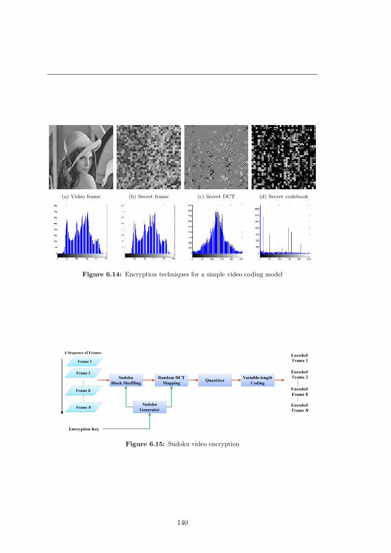
(a) Video frame (b) Secret frame (c) Secret DCT (d) Secret codebook
Figure 6.14: Encryption techniques for a simple video coding model
Figure 6.15: Sudoku video encryption
140

6.6 Sudoku Video Encryption
The encryption procedure is shown in Fig. 6.15. First, a 64 × 64 Sudoku S is
generated for the first frame F1. Then this Sudoku matrix S is used as a reference
matrix to shuffle 64 image blocks of size 8 × 8 in the first frame using the Sudoku
permutation method with respect to image blocks. If the frame size is larger than
64 × 64, then such shuffling is applied repeatedly. In the next step, each 8 × 8 frame
block is transformed into the DCT space using a random DCT matrix MRDCT defined
in Eq. (6.3), where MDCT is the conventional 8 × 8 DCT matrix defined in Eq. (6.4)
and U is a unitary permutation matrix defined with respect to a given digit d in S as
Eq. (6.5).As a result, the random DCT matrix is obtained and used to transform the
shuffled frame image blocks. Finally, the transformed frame is quantized and coded as
in the normal procedure.
MRDCT = U ×MDCT (6.3)
MDCT =
0.3536 0.3536 0.3536 0.3536 0.3536 0.3536 0.3536 0.3536
0.4904 0.4157 0.2778 0.0975 −0.0975 −0.2778 −0.4157 −0.4904
0.4619 0.1913 −0.1913 −0.4619 −0.4619 −0.1913 0.1913 0.4619
0.4157 −0.0975 −0.4904 −0.2778 0.2778 0.4904 0.0975 −0.4157
0.3536 −0.3536 −0.3536 0.3536 0.3536 −0.3536 −0.3536 0.3536
0.2778 −0.4904 0.0975 0.4157 −0.4157 −0.0975 0.4904 −0.2778
0.1913 −0.4619 0.4619 −0.1913 −0.1913 0.4619 −0.4619 0.1913
0.0975 −0.2778 0.4157 −0.4904 0.4904 −0.4157 0.2778 −0.0975
(6.4)
Ud(i, j) =
{1, if the digit d of the jth column is in the ith block0, otherwise
(6.5)
For the kth frame, the 64× 64 key dependent Sudoku matrix S is changed a little
bit and becomes S′ by replacing the symbol order with the order of the kth row. Its
first row is used as a reference to shuffle 64 frame blocks. Then a unitary permutation
matrix Und is generated for randomizing the nth frame block by finding the digit n in
the first block-row of S′. In other words, each 64×64 Sudoku matrix is used to encrypt
a video of 64 frames.
The following Fig. 6.16 shows the encryption results on frame ‘Lenna’, it is clear
that the correct decoded frame is very much alike the original frame except for some
negligible details. Fig. 6.17 and 6.18 show additional results of Sudoku video encryption
on the frame dataset pulled from USC-SIPI: sequence database. It is worthwhile to
note that the wrongly decoded frames are obtained by using the conventional decoder
141

with the DCT matrix defined in Eq. (6.4).
(a) Frame image (b) Permutated frame (c) Restored frame (d) Difference of (a) and (c)
Figure 6.16: Video encryption results for frame ‘Lenna’
6.7 Conclusions
In this section, I showed applications of Sudoku arrays in the multimedia security
areas of pseudo-random number generator, fragile watermarking, secret sharing, visual
cryptography and video encryption. All these examples demonstrate the possible wide
applications of Sudoku arrays for the multimedia security area and beyond.
142

6.7 Conclusions
Figure 6.17: Sudoku video encryption - video frame set I
Column 1 and 4: Original frame; Column 2 and 5: Correct decoded frame; Column 3 and 6: Wrongly decoded frame
143

Figure 6.18: Sudoku video encryption - video frame set II
Column 1 and 4: Original frame; Column 2 and 5: Correct decoded frame; Column 3 and 6: Wrongly decoded frame
144

7
Statistical Tests for Image
Randomness
In this chapter, we provides detailed information about the model of ideally encrypted
images and statistical randomness tests for image encryption performed using this
model.
7.1 Mathematical Model for True Random Images
According to Shannon’s masterpiece [2], an ideally encrypted image should be random-
like. Specifically speaking, that image should be undiscernible from a true random
image under any type of statistical test [1].
Definition 4. True Random Image:
If a random image field R of size M -by-N with L intensity scales satisfies the condition
that ∀i ∈ [1,M ] and ∀j ∈ [1, N ], the image pixel located at the ith row and jth column
R(i, j) is an independently and identically distributed (i.i.d) random variable with the
discrete uniform distribution over 0 to L− 1, namely
∀ pixel x ∈ R,∃x ∼ U[0, L− 1] (7.1)
then this image R is a random image of size M -by-N with L intensity scales.
Since an ideally encrypted image should be like a true random image, the mathe-
matical model of the true random image (MTRI) can be used as a reference to derive
statistical tests for image encryption. Specifically speaking, if a given image fails to
145
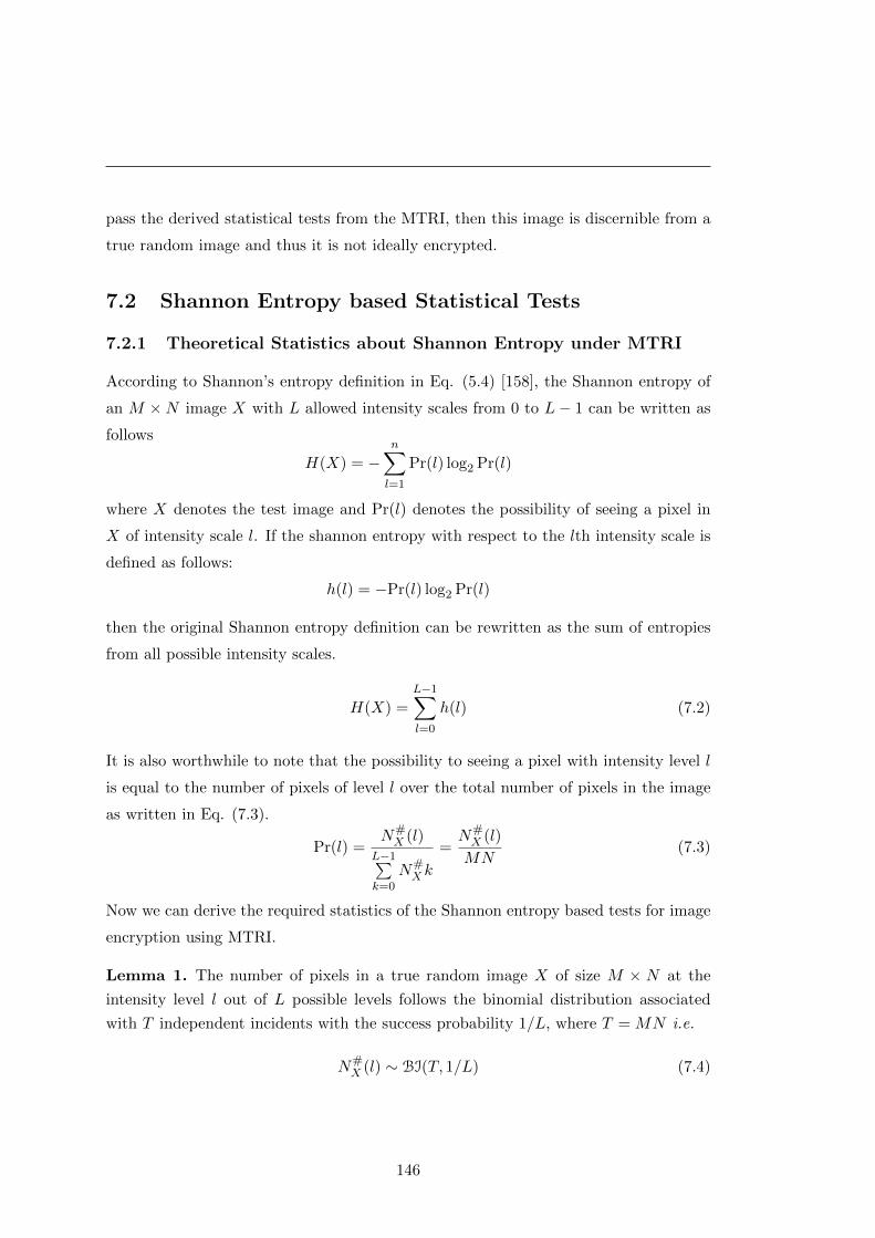
pass the derived statistical tests from the MTRI, then this image is discernible from a
true random image and thus it is not ideally encrypted.
7.2 Shannon Entropy based Statistical Tests
7.2.1 Theoretical Statistics about Shannon Entropy under MTRI
According to Shannon’s entropy definition in Eq. (5.4) [158], the Shannon entropy of
an M ×N image X with L allowed intensity scales from 0 to L− 1 can be written as
follows
H(X) = −n∑l=1
Pr(l) log2 Pr(l)
where X denotes the test image and Pr(l) denotes the possibility of seeing a pixel in
X of intensity scale l. If the shannon entropy with respect to the lth intensity scale is
defined as follows:
h(l) = −Pr(l) log2 Pr(l)
then the original Shannon entropy definition can be rewritten as the sum of entropies
from all possible intensity scales.
H(X) =L−1∑l=0
h(l) (7.2)
It is also worthwhile to note that the possibility to seeing a pixel with intensity level l
is equal to the number of pixels of level l over the total number of pixels in the image
as written in Eq. (7.3).
Pr(l) =N#X (l)
L−1∑k=0
N#X k
=N#X (l)
MN(7.3)
Now we can derive the required statistics of the Shannon entropy based tests for image
encryption using MTRI.
Lemma 1. The number of pixels in a true random image X of size M × N at the
intensity level l out of L possible levels follows the binomial distribution associated
with T independent incidents with the success probability 1/L, where T = MN i.e.
N#X (l) ∼ BI(T, 1/L) (7.4)
146

7.2 Shannon Entropy based Statistical Tests
Proof. According to the MTRI, any pixel x in X follows the discrete uniform distribu-
tion x ∼ U(0, L− 1), i.e.
Pr(x = l) = 1/L
so we have,
Pr(x 6= l) = 1− 1/L = (L− 1)/L
Therefore, any pixel x at intensity level l follows the Bernoulli distribution with success
probability 1/L. As a result, the number of pixels at intensity level l follows the
Binomial distribution as
N#X (l) ∼ BI(T, 1/L)
i.e.
Pr(N#X (l) = n) =
(T
n
)(L− 1)T−n
LT
Corollary 1.
Pr(Pr(l) = n/T ) =
(T
n
)(L− 1)T−n
LT(7.5)
Proof. Since Pr(l) = N#X (l)/T and N#
X (l) ∼ BI(T, 1/L)
N#X (l)
T∼ BI(T, 1/L)
thus
Pr(Pr(l) = n/T ) =
(T
n
)(L− 1)T−n
LT
Theorem 1. In a true random image X with in total T pixels and L possible intensity
levels, if none negative integers n0, n1, · · · , nL−1 satisfying
L−1∑l=0
nl = T (7.6)
then the random variables N#X (0), N#
X (1), · · · , N#X (L− 1) together follow the Multino-
mial distribution below
Pr(N#X (0) = n0, N
#X (1) = n1, · · · , N#
X (L− 1) = nL−1
)=
T !
n0!n1! · · ·nL−1!
1
LT(7.7)
147

Proof. Denote the event N#X (l) = nl as El, then
Pr(N#X (0) = n0, N
#X (1) = n1, · · · , N#
X (L− 1) = nL−1
)= Pr (E0, E1, · · · , EL−1)
= Pr (E0) Pr (E1, · · · , EL−1|E0)
= Pr (E0) Pr (E1|E0) Pr (E2, · · · , EL−1|E0, E1)
=...
= Pr (E0) Pr (E1|E0) · · ·Pr (EL−1|E0, E1, · · · , EL−2)
=
L−1∏l=0
(T −
∑l−1k=0 nk
nl
)(L− l − 1)T−
∑lk=0 nl
(L− l)T−∑l−1k=0 nl
=T !
n0!(T − n0)!
(L− 1)T−n0
LT· (T − n0)!
n1!(T − n0 − n1)!
(L− 2)T−n0−n1
(L− 1)T−n0· · · (nl−2 + nl−1)!
nl−2!nl−1!
(1)nl−1
(2)nl−2+nl−1
=T !
n0!n1! · · ·nL−1!
1
LT
Remark. Although the distribution of H(X) can be derived by directly using the above
theorem, it describes H(X) on an L-dimensional space. Fortunately, Multinomial sums
also follow the central limit theorem (CLT) [159], when L is large enough 13. As
a result, the distribution of H(X) can be approximated by the normal distribution
N(µH(X), σ2H(X)).
7.2.2 Shannon Entropy based Statistical Randomness Tests for Image
Encryption
From the previous section, we know that H(X), the Shannon entropy of a true random
image X with T pixels and L intensity scales under MTRI, has the mean µH(X) and
variance σ2H(X), shown in Eqs. (7.11) and (7.13) respectively; and H(X) approximately
follows the normal distribution N(µH(X), σ2H(X)), when L is large enough. In statistics,
L is considered as sufficiently large when L ≥ 30 and thus when L = 256, the case of
an 8 bit gray image, the theoretical distribution of the Shannon entropy score can be
directly used to test whether a sample image A is under MTRI.
13The approximation condition also specifies that min0≤l≤L−1
{T · Pr(x = l)} is bounded away from
zero. In our case, min0≤l≤L−1 T · Pr(x = l) = T/L > 0 is a constant.
148
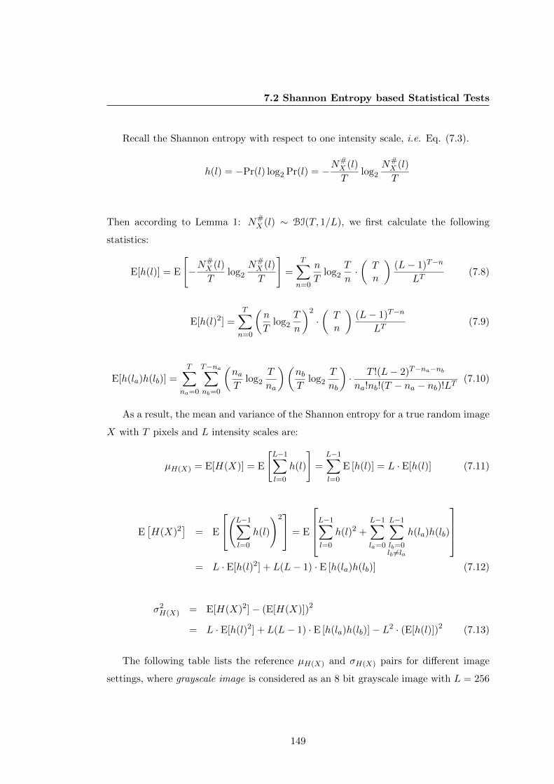
7.2 Shannon Entropy based Statistical Tests
Recall the Shannon entropy with respect to one intensity scale, i.e. Eq. (7.3).
h(l) = −Pr(l) log2 Pr(l) = −N#X (l)
Tlog2
N#X (l)
T
Then according to Lemma 1: N#X (l) ∼ BI(T, 1/L), we first calculate the following
statistics:
E[h(l)] = E
[−N#X (l)
Tlog2
N#X (l)
T
]=
T∑n=0
n
Tlog2
T
n·(Tn
)(L− 1)T−n
LT(7.8)
E[h(l)2] =T∑n=0
(n
Tlog2
T
n
)2
·(Tn
)(L− 1)T−n
LT(7.9)
E[h(la)h(lb)] =T∑
na=0
T−na∑nb=0
(naT
log2
T
na
)(nbT
log2
T
nb
)· T !(L− 2)T−na−nb
na!nb!(T − na − nb)!LT(7.10)
As a result, the mean and variance of the Shannon entropy for a true random image
X with T pixels and L intensity scales are:
µH(X) = E[H(X)] = E
[L−1∑l=0
h(l)
]=
L−1∑l=0
E [h(l)] = L · E[h(l)] (7.11)
E[H(X)2
]= E
(L−1∑l=0
h(l)
)2 = E
L−1∑l=0
h(l)2 +
L−1∑la=0
L−1∑lb=0lb 6=la
h(la)h(lb)
= L · E[h(l)2] + L(L− 1) · E [h(la)h(lb)] (7.12)
σ2H(X) = E[H(X)2]− (E[H(X)])2
= L · E[h(l)2] + L(L− 1) · E [h(la)h(lb)]− L2 · (E[h(l)])2 (7.13)
The following table lists the reference µH(X) and σH(X) pairs for different image
settings, where grayscale image is considered as an 8 bit grayscale image with L = 256
149

and Color Image is considered as a three color channel RGB image with an 8 bit length
in each channel, i.e. L = 256.
Table 7.1: Theoretical mean and standard deviation under MTRI
Tgrayscale image
TColor Image
Mean Std Mean Std2× 2 1.988300234 0.076064119 2× 2× 3 3.542339666 0.0826400204× 4 3.942064617 0.082851351 4× 4× 3 5.407984610 0.0790413058× 8 5.765716929 0.076603439 8× 8× 3 6.938975236 0.059295884
16× 16 7.174966353 0.052437999 16× 16× 3 7.737771412 0.02325355932× 32 7.808756571 0.017246343 32× 32× 3 7.939203149 0.00539314164× 64 7.954588734 0.004024888 64× 64× 3 7.984977322 0.001330526
128× 128 7.988743150 0.000996963 128× 128× 3 7.996254379 0.000331717256× 256 7.997191401 0.000248732 256× 256× 3 7.999064210 0.000082849512× 512 7.999298196 0.000062103 512× 512× 3 7.999766091 0.000020287
Since L is sufficiently large under the assumption of gray and color images, the
known distribution of H(X), N(µH(X), σ
2H(X)
)can be used to construct the random-
ness statistical test via the Z − test directly, where the test statistic z is defined as:
z =H(A)− µH(X)
σH(X)(7.14)
and z ∼ N(0, 1). In other words, given a sample image A, we calculate the test statistic
z in Eq. (7.14). Based on the z value, we perform a two-side hypothesis test, where
Null hypothesis H0: H(A) = H(X) the test image A is random-like as a true random
image.
Alternative hypothesis H1: H(A) 6= H(X) the test image A is NOT random-like
as a true random image.
It is worthwhile to note that statistics µH(X) and σH(X) are derived from Eqs. (7.11)
and (7.13) using T as the number of pixels in the sample image A and L as the intensity
scales allowed in A. As a result,
With respect to different significance levels in the Z-test, we calculate h∗left and
h∗right as the reference values to accept or reject H0 via the formula{h∗left = µH(X) − Φ−1
α/2σH(X)
h∗right = µH(X) + Φ−1α/2σH(X)
(7.15)
150

7.2 Shannon Entropy based Statistical Tests
where Φ−1 is the inverse cumulative density function of the standard normal distri-
bution. As a result, Table 7.2 shows the h∗left and h∗right under test image settings in
Table 7.1.
Table 7.2: Shannon entropy statistical test reference table for gray and color images
Tgrayscale image
TColor Image
h∗left h∗right h∗left h∗right
α=
0.0
5
2× 2 1.839217300 2.137383168 2× 2× 3 3.380368203 3.7043111294× 4 3.779678953 4.104450281 4× 4× 3 5.253066499 5.5629027218× 8 5.615576947 5.915856911 8× 8× 3 6.822757439 7.055193033
16× 16 7.072189764 7.277742942 16× 16× 3 7.692195274 7.78334755032× 32 7.774954360 7.842558782 32× 32× 3 7.928632787 7.94977351164× 64 7.946700098 7.962477370 64× 64× 3 7.982369539 7.987585105
128× 128 7.986789138 7.990697162 128× 128× 3 7.995604226 7.996904532256× 256 7.996703895 7.997678907 256× 256× 3 7.998901829 7.999226591512× 512 7.999176476 7.999419916 512× 512× 3 7.999726329 7.999805853
α=
0.0
1
2× 2 1.792372047 2.184228421 2× 2× 3 3.329473081 3.7552062514× 4 3.728653679 4.155475555 4× 4× 3 5.204387700 5.6115815208× 8 5.568399546 5.963034312 8× 8× 3 6.786239160 7.091711312
16× 16 7.039895019 7.310037687 16× 16× 3 7.677874213 7.79766861132× 32 7.764332935 7.853180207 32× 32× 3 7.925311338 7.95309496064× 64 7.944221310 7.964956158 64× 64× 3 7.981550114 7.988404530
128× 128 7.986175143 7.991311157 128× 128× 3 7.995399933 7.997108825256× 256 7.996550710 7.997832092 256× 256× 3 7.998850805 7.999277615512× 512 7.999138229 7.999458163 512× 512× 3 7.999713835 7.999818347
α=
0.0
01
2× 2 1.738009217 2.238591251 2× 2× 3 3.270410471 3.8142688614× 4 3.669440032 4.214689202 4× 4× 3 5.147897083 5.6680721378× 8 5.513651265 6.017782593 8× 8× 3 6.743860545 7.134089927
16× 16 7.002417716 7.347514990 16× 16× 3 7.661254955 7.81428786932× 32 7.752007018 7.865506124 32× 32× 3 7.921456874 7.95694942464× 64 7.941344732 7.967832736 64× 64× 3 7.980599191 7.989355453
128× 128 7.985462617 7.992023683 128× 128× 3 7.995162855 7.997345903256× 256 7.996372942 7.998009860 256× 256× 3 7.998791593 7.999336827512× 512 7.999093844 7.999502548 512× 512× 3 7.999699336 7.999832846
Recall Table 7.3. Besides evaluating the image encryption quality using Shannon
entropy in the quantitative way, we can apply the α = 0.05 statistical randomness
test for Shannon entropy scores on encrypted images. The following table shows the
results of this statistical test, where the reference scores under various image size s and
type settings are from Table 7.2. The gray shaded cell s designate the cases where the
encrypted image failed to pass the statistical test. Again, the Sudoku-Image cipher
is best among the compared ciphers. More importantly, all other listed image ciphers
have an obviously low pass rate compared to the theoretical rate of 1−α = 0.95, while
the Sudoku-Image cipher is the only exception. These results on one hand show the
effectiveness of the statistical tests and on the other hand show the high quality of
images encrypted using the Sudoku-Image cipher.
151

Table 7.3: Shannon entropy randomness test results for Table 7.3
Filename Size Type bmpPacker9 I-Cipher10 [40] [39] Ours4.1.01 256 Color 7.98856 7.99899 7.99894 7.99911 7.999134.1.02 256 Color 7.97929 7.99907 7.99906 7.99913 7.999214.1.03 256 Color 7.99018 7.99903 7.99911 7.99912 7.999094.1.04 256 Color 7.99008 7.99901 7.99903 7.99897 7.999194.1.05 256 Color 7.98103 7.99905 7.99889 7.99918 7.999004.1.06 256 Color 7.98982 7.99904 7.99900 7.99902 7.999054.1.07 256 Color 7.99048 7.99900 7.99903 7.99894 7.999164.1.08 256 Color 7.99765 7.99975 7.99918 7.99915 7.999084.2.01 512 Color 7.99874 7.99976 7.99976 7.99977 7.999774.2.02 512 Color 7.99746 7.99975 7.99976 7.99976 7.999784.2.03 512 Color 7.99758 7.99976 7.99975 7.99971 7.999794.2.04 512 Color 7.99773 7.99975 7.99977 7.99974 7.999784.2.05 512 Color 7.99746 7.99977 7.99976 7.99975 7.999774.2.06 512 Color 7.99755 7.99977 7.99974 7.99972 7.999754.2.07 512 Color 7.90885 7.99691 7.99978 7.99975 7.999745.1.09 256 Gray 7.90673 7.99721 7.99701 7.99674 7.997455.1.10 256 Gray 7.94187 7.99716 7.99714 7.99745 7.997095.1.11 256 Gray 7.92940 7.99718 7.99695 7.99678 7.997445.1.12 256 Gray 7.36356 7.99700 7.99673 7.99703 7.996795.1.13 256 Gray 7.90355 7.99688 7.99714 7.99662 7.997255.1.14 256 Gray 7.99254 7.99925 7.99727 7.99690 7.997245.2.08 512 Gray 7.98744 7.99920 7.99925 7.99925 7.999385.2.09 512 Gray 7.98463 7.99923 7.99919 7.99928 7.999375.2.10 512 Gray 7.99872 7.99982 7.99930 7.99933 7.999305.3.01 1024 Gray 7.99859 7.99982 7.99980 7.99982 7.999835.3.02 1024 Gray 7.99031 7.99929 7.99983 7.99982 7.999827.1.01 512 Gray 7.98954 7.99932 7.99932 7.99914 7.999267.1.02 512 Gray 7.98305 7.99926 7.99932 7.99933 7.999257.1.03 512 Gray 7.99362 7.99930 7.99919 7.99927 7.999287.1.04 512 Gray 7.98357 7.99935 7.99933 7.99920 7.999357.1.05 512 Gray 7.98540 7.99929 7.99929 7.99925 7.999327.1.06 512 Gray 7.98525 7.99928 7.99926 7.99927 7.999287.1.07 512 Gray 7.99030 7.99924 7.99922 7.99931 7.999327.1.08 512 Gray 7.98374 7.99932 7.99923 7.99937 7.999277.1.09 512 Gray 7.98508 7.99936 7.99927 7.99919 7.999337.1.10 512 Gray 7.99847 7.99979 7.99923 7.99926 7.999237.2.01 1024 Gray 7.98505 7.99924 7.99982 7.99972 7.99983boat.512 512 Gray 7.98956 7.99920 7.99940 7.99931 7.99934elaine.512 512 Gray 6.49282 7.99934 7.99934 7.99929 7.99927house 512 Color 7.99755 7.99975 7.99978 7.99927 7.99919gray21.512 512 Gray 7.97990 7.99922 7.99977 7.99977 7.99978numbers.512 512 Gray 6.89324 7.99926 7.99920 7.99929 7.99928ruler.512 512 Gray 7.90313 7.99982 7.99929 7.99926 7.99932testpat.1k 1024 Gray 7.90313 7.99982 7.99980 7.99982 7.99984
# Success 0 36 40 37 42Success Ratio 0 0.81818 0.90909 0.84091 0.95455
152

7.3 NPCR based Statistical Test
7.3 NPCR based Statistical Test
7.3.1 Theoretical Statistics about NPCR under MTRI
Recall the definition of NPCR given in Eq. (5.1), NPCR of two equal-size images X1
and X2 with L intensity levels can be written as
NPCR N(X1, X2) =
∑Tk dkT
× 100%
where dk is an indicator function with dk = 1 if X1k = X2
k (the kth pixels in X1 and X2
are equal) and dk = 0 otherwise, and T again denotes the number of pixels in image
X1 or X2.
Theorem 2. If X1 and X2 are two random images under MTRI with L intensity levels
and T pixels, then ∀k ∈ {1, 2, · · · , T} dk is a Bernoulli random variable with the success
probability of p = (L− 1)/L.
Proof. Using the assumption of independence and X1k , X
2k ∼ U[0, L− 1], we can show
Pr(dk = 0) = Pr(X1k = X2
k)
=
L−1∑l=0
Pr(X1k = l|X2
k = l)
Pr(X2k = l)
=L−1∑l=0
Pr(X1k = l
)Pr(X2
k = l)
= 1/L
So, Pr(dk = 1) = 1− Pr(dk = 0) = (L− 1)/L. And thus dk ∼ B(L−1L )
Theorem 3. The random variable D defined as the sum of dk for two random images
with L intensity levels and T pixels follows binomial distribution B (T, (L− 1)/L).
D =
T∑k=1
dk (7.16)
Proof. Using the conclusion that ∀k ∈ {1, 2, · · · , T}, dk ∼ B (p) with p = (L − 1)/L
153

and the i.i.d. property between pixels, it is clear that
Pr(D = k) =
(T
k
)pk(1− p)T−k
=
(T
k
)(L− 1
L
)k ( 1
L
)T−kwhich is the binomial distribution B (T, (L− 1)/L).
Therefore, the mean and variance of this binomial random variable D are
µD =L− 1
L(7.17)
σ2D =
L− 1
TL2. (7.18)
It is noticeable that this random variable D is a scaled version of N(X1, X2) because
N(X1, X2) =
∑Tk dkT
× 100% =1
TD.
From now on, we consider N(X1, X2) as a random variable and drop off (X1, X2) for
simplicity. In other words, we consider the random variable N, which is the NPCR
score of two random images X1 and X2, and here are its theoretical distribution, mean
and variance.
Pr
(N =
k
T
)= Pr(D = k) =
(T
k
)pk(1− p)T−k (7.19)
µN =µDT
=L− 1
L(7.20)
σ2N =
σ2D
T 2=L− 1
TL2(7.21)
7.3.2 NPCR based Statistical Randomness Test for Image Encryption
Since we know the exact binomial distribution of a NPCR score for two random images,
we can make the following randomness to test for image encryption whose images are
supposed to be indistinguishable to truly random ones.
Suppose C1 and C2 are two test ciphertext images of L-intensity levels and T pixels,
then the hypotheses test with α-level significance for N(C1, C2), are:
154

7.4 UACI based Statistical Test
Null hypothesis H0: N ≥ µN the test image encryption method generates random-
like ciphertext images.
Alternative hypothesis H1: N < µN the test image encryption method fails to
generate random-like ciphertext images.
where we reject H0, when N(C1, C2) < N∗, the critical value of the NPCR test; other-
wise we accept H0. The critical value N∗ is defined as follows,
N∗α = µN − Φ−1α σN =
L− 1− Φ−1α
√(L− 1)/T
L(7.22)
where Φ−1(.) is the inverse CDF of the standard Normal distribution N(0, 1).
Table 7.4: NPCR statistical test reference table for binary and grayscale images
# of Pixels T µN σN N∗0.05 N∗0.01 N∗0.001
Bin
ary
L=2
64× 64 50.0000% 0.7813% 48.7150% 48.1825% 47.5858%128× 128 50.0000% 0.3906% 49.3575% 49.0913% 48.7929%256× 256 50.0000% 0.1953% 49.6787% 49.5456% 49.3964%512× 512 50.0000% 0.0977% 49.8394% 49.7728% 49.6982%
1024× 1024 50.0000% 0.0488% 49.9197% 49.8864% 49.8491%
Grayscale
L=256
64× 64 99.6094% 0.0975% 99.4491% 99.3826% 99.3082%128× 128 99.6094% 0.0487% 99.5292% 99.4960% 99.4588%256× 256 99.6094% 0.0244% 99.5693% 99.5527% 99.5341%512× 512 99.6094% 0.0122% 99.5893% 99.5810% 99.5717%
1024× 1024 99.6094% 0.0061% 99.5994% 99.5952% 99.5906%
According to these reference values, we test image encryption algorithms based on
their reported NPCR scores and these results are given in Table 7.7.
These results indicate that some image encryption methods fail to pass this ran-
domness test, implying that their ciphertext images are not random-like or equivalently
distinguishable to random images.
7.4 UACI based Statistical Test
7.4.1 Theoretical Statistics about UACI under MTRI
Similar to the derivation for NPCR, we can also derive the theoretical statistics under
MTRI for UACI. Recall UACI is defined as the averaged pixel intensity difference
between two equal size images X1 and X2 with L intensity scales and T pixels.
UACI U(X1, X2) =
∑Tk=1 |X1
k −X2k |
(L− 1)T× 100%
155
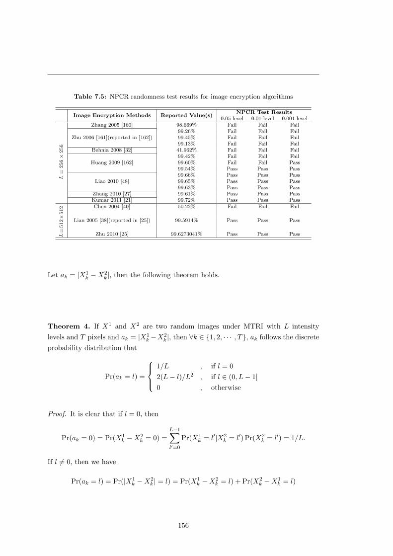
Table 7.5: NPCR randomness test results for image encryption algorithms
Image Encryption Methods Reported Value(s)NPCR Test Results
0.05-level 0.01-level 0.001-level
L=
256×
256
Zhang 2005 [160] 98.669% Fail Fail Fail
Zhu 2006 [161](reported in [162])99.26% Fail Fail Fail99.45% Fail Fail Fail99.13% Fail Fail Fail
Behnia 2008 [32] 41.962% Fail Fail Fail
Huang 2009 [162]99.42% Fail Fail Fail99.60% Fail Fail Pass99.54% Pass Pass Pass
Liao 2010 [48]99.66% Pass Pass Pass99.65% Pass Pass Pass99.63% Pass Pass Pass
Zhang 2010 [27] 99.61% Pass Pass PassKumar 2011 [21] 99.72% Pass Pass Pass
L=
512×
512 Chen 2004 [40] 50.22% Fail Fail Fail
Lian 2005 [38](reported in [25]) 99.5914% Pass Pass Pass
Zhu 2010 [25] 99.6273041% Pass Pass Pass
Let ak = |X1k −X2
k |, then the following theorem holds.
Theorem 4. If X1 and X2 are two random images under MTRI with L intensity
levels and T pixels and ak = |X1k −X2
k |, then ∀k ∈ {1, 2, · · · , T}, ak follows the discrete
probability distribution that
Pr(ak = l) =
1/L , if l = 0
2(L− l)/L2 , if l ∈ (0, L− 1]
0 , otherwise
Proof. It is clear that if l = 0, then
Pr(ak = 0) = Pr(X1k −X2
k = 0) =L−1∑l′=0
Pr(X1k = l′|X2
k = l′) Pr(X2k = l′) = 1/L.
If l 6= 0, then we have
Pr(ak = l) = Pr(|X1k −X2
k | = l) = Pr(X1k −X2
k = l) + Pr(X2k −X1
k = l)
156

7.4 UACI based Statistical Test
The former probability can be rewrote by using the total probability formula as
Pr(X1k −X2
k = l) =L−1∑l′=0
Pr(X1k = l′) Pr(X2
k = l′ − l)
=L−1∑l′=l
Pr(X1k = l′) Pr(X2
k = l′ − l)
=L−1∑l′=l
(1/L)(1/L)
= (L− l)/L2.
Similarly, we can find Pr(X2k − X1
k = l) = Pr(X1k − X2
k = l) = (L − 1)/L2. It is not
difficult to verify that
L−1∑l=0
Pr(ak = l) =1
L+
2∑L−1
l=1 L− lL2
=1
L+
2(1 + L− 1)(L− 1)/2
L2
=L
L2+L(L− 1)
L2
=L+ L2 − L
L2= 1
Therefore, the derived probability is indeed the PDF for ak.
Consequently, the mean of ak can be computed as shown in Eq. (7.23).
µak =L−1∑l=0
lPr(ak = l) =L−1∑l=1
lPr(ak = l)
=
L−1∑l=1
2l(L− l)L2
=2∑L−1
l=1 l
L−
2∑L−1
l=1 l2
L2
=2(L− 1 + 1)(L− 1)/2
L− 2(L− 1)L(2L− 1)/6
L2
= (L− 1) +2L2 − 3L+ 1
3L=L2 − 1
3L(7.23)
157

Meanwhile, the variance of ak can be computed similarly as shown in Eq. (7.24).
σ2ak
=L−1∑l=0
l2 Pr(ak = l)− µ2ak
=L−1∑l=1
l2 Pr(ak = l)− µ2ak
=
L−1∑l=1
2l2(L− l)L2
− µ2ak
=2∑L−1
l=1 l2
L−
2∑L−1
l=1 l3
L2− µ2
ak
=2L(L− 1)L(2L− 1)/6
L2− 2(L− 1)2L2/4
L2−(L2 − 1
3L
)2
=2L2 − 3L+ 1
3− (L− 1)2
2− (L2 − 1)2
9L2=L2 − 1
6− (L2 − 1)2
9L2
=(L2 − 1)(3L2 − 2L2 + 2)
18L2=
(L2 − 1)(L2 + 2)
18L2(7.24)
Let random variable A =∑T
k=1 ak/T , then statistics tells us that the PDF A is
approximately Gaussian.
Theorem 5. If X1 and X2 are two random images under MTRI with L intensity
levels and T pixels, and A =∑T
k=1 ak/T with ak = |X1k −X2
k |, then A is approximately
normally distributed as A ∼ N(µak , σ2ak/T ).
Proof. The Central Limit Theorem(CLT) tells that as long as the sample size n is large
enough, the sample mean of any i.i.d distributed sample with an arbitrary PDF with a
mean µ and a finite variance σ2 is approximately a Gaussian N(µ, σ2/n). In our case,
n = T is the number of pixels and almost surely much larger than 30, which is the
sample size believed the CLT can be applied.
Clearly X1 and X2 are two random images under MTRI, and ak is consequently
i.i.d. distributed ∀k ∈ {1, 2, · · · , T}. Since A =∑T
k=1 ak/T , then A ∼ N(µak , σ2ak/T ),
in other words A has a mean µA and variance σ2A
µA = µak =L2 − 1
3L(7.25)
σ2A =
σ2ak
T=
(L2 − 1)(L2 + 2)
18L2T(7.26)
.
158

7.4 UACI based Statistical Test
Since we have U(X1, X2) =
∑Tk=1 |X1
k −X2k |
(L− 1)T=
A
L− 1, then we have
µU =µAL− 1
=L+ 1
3L(7.27)
σ2U =
σ2A
(L− 1)2=
(L+ 1)(L2 + 2)
18L2(L− 1)T(7.28)
and U ∼ N(µU, σ2U).
7.4.2 UACI based Statistical Randomness Test for Image Encryption
Since we know a NPCR score for two random images follows the normal distribution
U ∼ N(µU, σ2U), we can make the following randomness to test for image encryption
whose images are supposed to be indistinguishable to truly random ones.
Suppose C1 and C2 are two test ciphertext images of L-intensity levels and T pixels,
then the hypotheses test with α-level significance for U(C1, C2), are:
Null hypothesis H0: U ≥ µU the test image encryption method generates random-
like ciphertext images.
Alternative hypothesis H1: U 6= µU the test image encryption method fails to
generate random-like ciphertext images.
where we reject H0, when U(C1, C2) < U∗− or U(C1, C2) > U∗+, the critical values of
the UACI test; otherwise we accept H0. The critical values of α-level of significance
can be determined as, {U∗−α = µU − Φ−1
α/2σU
U∗+α = µU + Φ−1α/2σU
(7.29)
where Φ−1(.) is the inverse CDF of the standard Normal distribution N(0, 1). Numerical
results of these critical values for selected image sizes are given in Table 7.6.
According to these reference values, we test image encryption algorithms based on
their reported UACI scores and these results are given in Table 7.7.
Again, these results indicate that some image encryption methods fail to pass this
randomness test, implying that their ciphertext images are not random-like or equiva-
lently distinguishable to random images.
159

Table 7.6: NPCR statistical test reference table for binary and grayscale images
# of Pixels T µU σUU∗−0.05/
U∗+0.05
U∗−0.01/U∗+0.01
U∗−0.001/U∗+0.001
Bin
ary
Im
age
L=2
64× 64 50.0000% 0.7813% 48.4688%/51.5312%47.9876%/52.0124%
47.4293%/52.5707%
128× 128 50.0000% 0.3906% 49.2344%/50.7656%48.9938%/51.0062%
48.7146%/51.2854%
256× 256 50.0000% 0.1953% 49.6172%/50.3828%49.4969%/50.5031%
49.3573%/50.6427%
512× 512 50.0000% 0.0977% 49.8086%/50.1914%49.7485%/50.2515%
49.6787%/50.3213%
1024× 1024 50.0000% 0.0488% 49.9043%/50.0957%49.8742%/50.1258%
49.8393%/50.1607%
Grayscale
Im
age
L=256
64× 64 33.4635% 0.3697% 32.7389%/34.1882%32.5112%/34.4159%
32.2469%/34.6802%
128× 128 33.4635% 0.1849% 33.1012%/33.8259%32.9874%/33.9397%
32.8552%/34.0718%
256× 256 33.4635% 0.0924% 33.2824%/33.6447%33.2255%/33.7016%
33.1594%/33.7677%
512× 512 33.4635% 0.0462% 33.3730%/33.5541%33.3445%/33.5826%
33.3115%/33.6156%
1024× 1024 33.4635% 0.0231% 33.4183%/33.5088%33.4040%/33.5231%
33.3875%/33.5396%
Table 7.7: NPCR randomness test results for image encryption algorithms
Image Encryption Methods Reported Value(s)UACI Test Results
0.05-level 0.01-level 0.001-level
L=
256×
256
Zhang 2005 [160] 33.362% Pass Pass Pass
Zhu 2006 [161](reported in [162])21.41% Fail Fail Fail23.42% Fail Fail Fail15.08% Fail Fail Fail
Behnia 2008 [32] 33.25% Fail Pass Pass
Huang 2009 [162]27.78% Fail Fail Fail27.66% Fail Fail Fail24.94% Fail Fail Fail
Liao 2010 [48]33.20% Fail Fail Pass33.31% Pass Pass Pass34.61% Fail Fail Fail
Zhang 2010 [27] 38% Fail Fail FailKumar 2011 [21] 32.821% Fail Fail Fail
L=
512×
512 Chen 2004 [40] 25.21% Fail Fail Fail
Lian 2005 [38](reported in [25]) 33.3359% Pass Pass Pass
Zhu 2010 [25] 33.4815979% Pass Pass Pass
160

8
Conclusion and Future Work
8.1 Concluding Remarks
This dissertation investigates the use of Sudoku arrays in data encryption and other
information security applications. It extends the conventional concept of 9× 9 Sudoku
puzzles to a general class of Sudoku arrays with arbitrary sizes and symbols. Extensive
attention is given to the properties and possible applications of Sudoku arrays. A
number of attractive Sudoku array properties are then presented using either proofs
or examples. In order to render possible use of a Sudoku array as an encryption
key for data encryption, a parametric Sudoku generator is developed using a series of
transformations and swaps. Thus, a set of Sudoku arrays can be easily obtained thanks
to this Sudoku parametric generator.
Furthermore, a number of fundamental but useful cryptographic primitives are di-
rectly derived from the intrinsic mathematical properties of Sudoku arrays. Well-known
cryptographic primitives that were originally defined on an encryption key have been
completely rebuilt with respect to a key dependent Sudoku array. This way, these new
Sudoku-based cryptographic primitives connect the ciphertext message C, the plain-
text message P and the encryption K in a more complicated and involved way than in
previous methods and thus enhance the confusion property of these encryption tech-
niques. Meanwhile, a novel way of making S-boxes with a group property is discussed
and analyzed. The new method enhances the strength of S-boxes by making all used S-
boxes a Markov chain Monte Carlo process, which guarantees the substitution process
of a so-called Markov cipher with invulnerability to differential attacks.
161

These Sudoku-based cryptographic primitives are used to form the new Sudoku-AES
cipher for bit sequences. The Sudoku-AES cipher mimics the structure of the classic
AES cipher but uses only Sudoku-based encryption techniques. Compared to the classic
AES cipher, the Sudoku-AES cipher has a larger block size and dynamic P-boxes and
S-boxes. All these properties enhance the security level of the Sudoku-AES cipher.
Indeed, the Sudoku-AES cipher is secure with respect to the plaintext-only attack,
ciphertext-only attack, chosen-ciphertext attack. Extensive simulation results show
that ciphertext messages encrypted by the Sudoku-AES cipher are highly random-like
under the FIPS 140-2 statistical tests for randomness and NIST SP 800-22 statistical
test suite.
We propose a new Sudoku-Image cipher for various image data. Again, all encryp-
tion/decryption modules in this cipher are Sudoku-based. A large number of experi-
ments and simulations using USC SIPI image database shows that the Sudoku-Image
cipher reaches or outperforms the state of the art for image encryption while avoiding
annoying the discrimination problems of chaos-based methods. In order to test the
randomness of ciphertext images from the point view of statistics, we also derive sta-
tistical tests for image randomness. To the best of our knowledge, this is the first effort
in the image encryption community to evaluate the randomness of ciphertext images
qualitatively using tests based on Shannon entropy, NPCR and UACI.
We also show Sudoku applications in many other areas of multimedia security,
including random number generator, watermarking/data hiding, secret sharing, visual
cryptography and video encryption. To the best of our knowledge, the idea of secret
sharing using Sudoku puzzles is proposed for the first time. All these examples of
Sudoku applications illustrate the significance of Sudoku arrays for the digital world.
8.2 Future works
Among various possible multimedia applications of Sudoku arrays, we believe that the
following questions are interesting and may be meaningful for future research:
• How to generate more random-like arbitrary size Sudoku arrays than those gen-
erated by the Sudoku generator introduced in this dissertation?
• How to use Sudoku puzzles to construct a (t, n) secret sharing scheme.
162

8.2 Future works
• How to construct large size Cayley-Sudoku tables for defining a class of key de-
pendent finite fields for possible encryption applications.
• How to use the mathematical properties of Sudoku arrays in new ways?
• What are other useful properties of Sudoku arrays have not been discovered?
• What are other useful multimedia applications of Sudoku arrays?
163

164

165

9
Appendix A: NIST SP 800-22
Randomness Test Results for
Sudoku-AES and Sudoku-Image
ciphers
9.1 Result Report for Sudoku-AES Cipher
RESULTS FOR THE UNIFORMITY OF P-VALUES AND THE PROPORTION OF PASSING SEQUENCES
generator is < ./data/Sudoku− AES.dat >C1 C2 C3 C4 C5 C6 C7 C8 C9 C10 P-VALUE PROPORTION STATISTICAL TEST
8 9 9 11 13 10 8 16 6 10 0.616305 1.0000 Frequency
14 6 10 11 13 17 7 6 7 9 0.181557 0.9700 BlockFrequency
8 6 13 8 12 11 14 12 4 12 0.366918 1.0000 CumulativeSums
9 7 10 11 11 12 9 12 10 9 0.987896 0.9900 CumulativeSums
6 10 11 11 13 6 8 8 16 11 0.455937 0.9900 Runs
7 11 10 9 13 12 9 14 4 11 0.554420 0.9900 LongestRun
6 14 15 9 8 11 9 5 9 14 0.304126 1.0000 Rank
12 7 10 15 13 12 10 6 8 7 0.534146 0.9800 FFT
8 6 12 6 11 16 9 12 10 10 0.514124 1.0000 NonOverlappingTemplate
12 9 9 10 4 11 9 10 12 14 0.699313 0.9900 NonOverlappingTemplate
10 9 14 8 7 15 10 10 12 5 0.494392 0.9800 NonOverlappingTemplate
9 12 5 15 7 11 12 6 13 10 0.334538 0.9700 NonOverlappingTemplate
17 9 9 6 10 10 11 11 8 9 0.595549 1.0000 NonOverlappingTemplate
8 5 13 11 10 12 11 14 8 8 0.657933 1.0000 NonOverlappingTemplate
8 13 10 8 11 9 14 6 11 10 0.816537 0.9800 NonOverlappingTemplate
13 10 10 12 6 14 3 12 8 12 0.304126 1.0000 NonOverlappingTemplate
5 11 12 11 16 10 9 8 4 14 0.191687 1.0000 NonOverlappingTemplate
9 7 16 12 8 11 5 16 6 10 0.153763 0.9900 NonOverlappingTemplate
10 18 7 5 5 9 18 4 12 12 0.005762 0.9900 NonOverlappingTemplate
6 12 14 9 12 13 10 10 4 10 0.474986 1.0000 NonOverlappingTemplate
15 7 8 9 14 7 5 8 15 12 0.202268 0.9700 NonOverlappingTemplate
14 8 7 9 7 11 14 11 11 8 0.719747 0.9900 NonOverlappingTemplate
8 10 13 12 9 12 12 9 6 9 0.883171 0.9700 NonOverlappingTemplate
8 14 6 4 14 10 15 11 11 7 0.191687 0.9800 NonOverlappingTemplate
8 4 11 14 8 11 10 10 11 13 0.616305 0.9800 NonOverlappingTemplate
9 15 11 14 12 6 13 10 7 3 0.162606 0.9900 NonOverlappingTemplate
12 12 12 6 13 13 8 11 6 7 0.574903 1.0000 NonOverlappingTemplate
8 9 8 14 13 13 11 4 13 7 0.366918 0.9800 NonOverlappingTemplate
166

9.1 Result Report for Sudoku-AES Cipher
9 18 14 5 11 11 9 8 8 7 0.181557 0.9900 NonOverlappingTemplate
15 9 11 9 15 11 7 8 6 9 0.494392 0.9800 NonOverlappingTemplate
10 10 6 10 14 14 12 11 8 5 0.514124 0.9900 NonOverlappingTemplate
5 13 9 13 7 11 10 13 13 6 0.455937 1.0000 NonOverlappingTemplate
13 14 7 8 11 11 10 9 7 10 0.834308 0.9900 NonOverlappingTemplate
14 9 8 7 8 10 10 8 14 12 0.759756 1.0000 NonOverlappingTemplate
10 15 6 11 7 6 18 9 12 6 0.085587 0.9800 NonOverlappingTemplate
12 10 9 11 13 8 9 12 6 10 0.911413 1.0000 NonOverlappingTemplate
13 9 10 12 5 9 14 9 7 12 0.514124 0.9700 NonOverlappingTemplate
14 8 9 13 10 8 11 7 11 9 0.867692 0.9700 NonOverlappingTemplate
8 8 12 7 10 12 9 9 14 11 0.883171 0.9900 NonOverlappingTemplate
11 7 6 11 11 8 12 13 9 12 0.834308 0.9900 NonOverlappingTemplate
11 11 14 8 11 9 12 10 8 6 0.851383 0.9900 NonOverlappingTemplate
8 12 13 14 9 10 6 5 11 12 0.534146 1.0000 NonOverlappingTemplate
13 7 13 8 8 9 12 9 8 13 0.798139 0.9800 NonOverlappingTemplate
11 10 12 14 12 9 14 7 7 4 0.383827 0.9800 NonOverlappingTemplate
8 12 9 3 15 10 13 10 8 12 0.350485 1.0000 NonOverlappingTemplate
7 11 10 9 10 9 8 11 11 14 0.946308 0.9800 NonOverlappingTemplate
10 11 13 13 12 7 9 9 9 7 0.883171 0.9800 NonOverlappingTemplate
9 9 6 17 12 9 3 8 18 9 0.025193 0.9900 NonOverlappingTemplate
11 13 4 6 8 16 8 10 10 14 0.202268 0.9800 NonOverlappingTemplate
12 8 10 10 8 8 11 12 7 14 0.867692 0.9900 NonOverlappingTemplate
13 9 6 7 7 6 9 14 15 14 0.224821 0.9900 NonOverlappingTemplate
8 6 6 11 12 8 16 10 11 12 0.474986 0.9900 NonOverlappingTemplate
10 5 12 12 14 10 6 11 8 12 0.595549 1.0000 NonOverlappingTemplate
9 13 12 14 8 11 5 6 9 13 0.474986 0.9800 NonOverlappingTemplate
9 9 13 3 11 11 12 5 15 12 0.213309 1.0000 NonOverlappingTemplate
11 15 5 15 11 7 11 8 7 10 0.350485 0.9900 NonOverlappingTemplate
10 6 12 4 16 7 8 8 13 16 0.080519 1.0000 NonOverlappingTemplate
13 7 7 20 10 9 3 11 11 9 0.035174 0.9800 NonOverlappingTemplate
9 17 10 11 12 7 11 11 9 3 0.236810 0.9900 NonOverlappingTemplate
8 10 11 10 14 6 12 10 11 8 0.867692 0.9900 NonOverlappingTemplate
9 5 6 9 15 8 10 14 12 12 0.383827 1.0000 NonOverlappingTemplate
12 10 6 11 12 11 7 9 10 12 0.911413 0.9900 NonOverlappingTemplate
11 8 12 11 5 14 8 12 8 11 0.699313 0.9900 NonOverlappingTemplate
5 14 11 13 6 15 8 8 8 12 0.289667 0.9900 NonOverlappingTemplate
6 7 13 11 14 8 6 17 10 8 0.191687 0.9900 NonOverlappingTemplate
12 10 12 11 10 12 10 7 7 9 0.955835 1.0000 NonOverlappingTemplate
7 10 10 14 6 15 11 12 10 5 0.383827 0.9900 NonOverlappingTemplate
13 4 8 7 17 16 13 10 9 3 0.016717 0.9900 NonOverlappingTemplate
14 7 10 13 12 4 10 11 10 9 0.574903 0.9900 NonOverlappingTemplate
9 6 13 13 7 16 8 14 10 4 0.137282 0.9900 NonOverlappingTemplate
8 13 14 12 11 9 2 9 13 9 0.275709 1.0000 NonOverlappingTemplate
10 10 8 10 11 6 12 14 15 4 0.334538 0.9900 NonOverlappingTemplate
7 10 10 11 13 13 7 8 7 14 0.678686 1.0000 NonOverlappingTemplate
9 7 11 10 4 5 14 15 8 17 0.055361 1.0000 NonOverlappingTemplate
9 11 12 12 11 8 4 13 9 11 0.719747 0.9900 NonOverlappingTemplate
14 8 6 10 13 10 13 7 7 12 0.574903 1.0000 NonOverlappingTemplate
5 12 9 13 9 7 13 10 8 14 0.554420 1.0000 NonOverlappingTemplate
12 7 6 13 6 15 8 9 7 17 0.115387 1.0000 NonOverlappingTemplate
8 7 9 11 12 10 13 5 14 11 0.637119 0.9900 NonOverlappingTemplate
9 6 12 12 13 8 5 9 13 13 0.514124 0.9900 NonOverlappingTemplate
9 10 9 12 10 10 15 10 6 9 0.851383 0.9900 NonOverlappingTemplate
8 8 11 13 9 13 16 8 7 7 0.474986 1.0000 NonOverlappingTemplate
7 7 11 7 11 16 9 12 10 10 0.637119 1.0000 NonOverlappingTemplate
9 13 5 7 14 15 10 10 11 6 0.334538 0.9900 NonOverlappingTemplate
8 11 10 12 8 8 9 10 12 12 0.978072 1.0000 NonOverlappingTemplate
9 11 12 7 6 11 8 16 9 11 0.595549 0.9800 NonOverlappingTemplate
11 9 6 7 7 11 9 15 12 13 0.574903 0.9700 NonOverlappingTemplate
7 12 11 10 9 10 12 10 11 8 0.983453 0.9800 NonOverlappingTemplate
7 12 11 11 12 9 14 10 6 8 0.779188 0.9900 NonOverlappingTemplate
10 11 9 8 18 4 15 4 9 12 0.045675 1.0000 NonOverlappingTemplate
8 9 5 10 9 14 13 10 12 10 0.739918 0.9900 NonOverlappingTemplate
9 15 10 17 11 2 11 7 6 12 0.048716 0.9900 NonOverlappingTemplate
11 9 10 5 7 11 6 15 17 9 0.171867 0.9900 NonOverlappingTemplate
19 5 8 4 6 9 11 12 15 11 0.021999 0.9900 NonOverlappingTemplate
13 7 11 12 19 8 8 10 6 6 0.108791 1.0000 NonOverlappingTemplate
7 12 12 11 9 5 7 14 15 8 0.366918 0.9900 NonOverlappingTemplate
14 8 8 8 14 9 11 8 11 9 0.816537 0.9900 NonOverlappingTemplate
8 10 13 9 5 12 13 11 10 9 0.798139 0.9900 NonOverlappingTemplate
11 11 7 11 10 7 13 8 12 10 0.924076 0.9800 NonOverlappingTemplate
10 17 4 14 11 10 6 13 12 3 0.035174 1.0000 NonOverlappingTemplate
9 13 9 8 12 12 12 7 12 6 0.779188 0.9800 NonOverlappingTemplate
8 9 8 10 3 9 14 13 13 13 0.334538 1.0000 NonOverlappingTemplate
11 15 20 9 6 8 11 11 5 4 0.012650 1.0000 NonOverlappingTemplate
167

10 9 9 7 11 5 9 15 13 12 0.574903 0.9800 NonOverlappingTemplate
10 5 8 10 10 12 14 8 14 9 0.637119 0.9800 NonOverlappingTemplate
10 11 12 8 8 7 9 11 9 15 0.834308 0.9800 NonOverlappingTemplate
10 15 13 9 8 10 12 7 9 7 0.719747 0.9700 NonOverlappingTemplate
7 8 9 8 11 10 12 12 10 13 0.935716 1.0000 NonOverlappingTemplate
10 7 7 15 13 10 12 6 7 13 0.437274 0.9900 NonOverlappingTemplate
12 8 8 12 7 13 11 16 8 5 0.350485 0.9700 NonOverlappingTemplate
11 7 13 13 10 6 10 10 12 8 0.816537 0.9900 NonOverlappingTemplate
12 12 5 9 8 13 7 11 11 12 0.719747 1.0000 NonOverlappingTemplate
6 10 9 12 14 9 15 9 8 8 0.616305 0.9900 NonOverlappingTemplate
6 7 8 11 12 16 12 8 8 12 0.474986 0.9900 NonOverlappingTemplate
8 10 8 5 10 8 12 14 15 10 0.514124 0.9800 NonOverlappingTemplate
12 12 7 12 8 12 7 10 11 9 0.657933 0.9700 NonOverlappingTemplate
12 11 10 11 10 3 13 12 11 7 0.554420 0.9800 NonOverlappingTemplate
12 9 14 7 10 6 8 8 11 15 0.534146 1.0000 NonOverlappingTemplate
9 15 8 8 12 6 12 9 7 14 0.494392 0.9900 NonOverlappingTemplate
15 6 10 10 10 8 5 11 15 10 0.383827 0.9900 NonOverlappingTemplate
6 10 14 16 9 10 7 13 7 8 0.350485 0.9700 NonOverlappingTemplate
12 13 11 6 10 10 8 10 12 8 0.897763 0.9700 NonOverlappingTemplate
8 9 15 4 17 5 11 6 12 13 0.048716 0.9900 NonOverlappingTemplate
11 13 13 8 10 12 7 12 7 7 0.514124 0.9800 NonOverlappingTemplate
12 6 8 10 11 10 15 11 9 8 0.779188 1.0000 NonOverlappingTemplate
10 8 7 10 15 7 15 7 12 9 0.474986 1.0000 NonOverlappingTemplate
14 5 8 10 8 12 12 11 7 13 0.574903 0.9800 NonOverlappingTemplate
8 11 12 11 6 10 13 10 13 6 0.739918 1.0000 NonOverlappingTemplate
7 8 12 8 13 6 14 8 18 6 0.102526 0.9900 NonOverlappingTemplate
6 9 12 9 13 8 12 10 11 10 0.911413 0.9900 NonOverlappingTemplate
6 6 10 9 17 12 9 8 11 12 0.383827 0.9800 NonOverlappingTemplate
10 9 12 12 7 11 5 6 14 14 0.419021 0.9900 NonOverlappingTemplate
8 9 13 9 7 14 12 8 13 7 0.678686 1.0000 NonOverlappingTemplate
12 11 8 13 10 9 9 14 7 7 0.798139 1.0000 NonOverlappingTemplate
13 9 6 11 12 8 10 12 12 7 0.816537 0.9900 NonOverlappingTemplate
9 12 9 9 3 13 9 14 11 11 0.494392 1.0000 NonOverlappingTemplate
18 11 7 12 4 12 8 5 12 11 0.051942 0.9700 NonOverlappingTemplate
12 9 15 14 9 14 7 6 3 11 0.129620 0.9800 NonOverlappingTemplate
12 11 6 9 8 7 12 18 10 7 0.262249 1.0000 NonOverlappingTemplate
8 7 11 13 7 16 11 9 11 7 0.534146 1.0000 NonOverlappingTemplate
10 10 9 8 8 8 13 8 11 15 0.816537 0.9900 NonOverlappingTemplate
8 9 10 8 15 14 7 13 7 9 0.554420 0.9800 NonOverlappingTemplate
9 11 7 14 7 12 10 16 3 11 0.181557 1.0000 NonOverlappingTemplate
6 11 11 8 11 8 15 10 11 9 0.798139 0.9800 NonOverlappingTemplate
11 8 5 11 11 10 10 12 11 11 0.924076 0.9900 NonOverlappingTemplate
6 5 14 5 16 5 11 8 17 13 0.014550 1.0000 NonOverlappingTemplate
8 13 8 12 11 13 7 7 11 10 0.834308 0.9900 NonOverlappingTemplate
12 12 10 11 9 8 8 12 6 12 0.897763 1.0000 NonOverlappingTemplate
9 10 10 6 10 8 13 13 4 17 0.191687 0.9900 NonOverlappingTemplate
9 6 11 12 6 14 7 13 6 16 0.191687 1.0000 NonOverlappingTemplate
4 10 9 7 11 19 13 11 11 5 0.058984 0.9800 NonOverlappingTemplate
8 9 8 14 12 8 9 11 8 13 0.851383 1.0000 NonOverlappingTemplate
12 8 10 11 10 7 10 12 8 12 0.964295 1.0000 NonOverlappingTemplate
11 6 9 7 9 13 10 10 14 11 0.798139 0.9800 NonOverlappingTemplate
11 4 3 15 12 6 16 10 12 11 0.045675 0.9900 NonOverlappingTemplate
8 8 11 13 9 13 16 8 7 7 0.474986 1.0000 NonOverlappingTemplate
11 7 8 8 10 12 12 14 8 10 0.867692 0.9700 OverlappingTemplate
4 8 10 11 17 11 13 13 6 7 0.145326 1.0000 Universal
14 14 16 6 11 8 7 7 13 4 0.085587 0.9700 ApproximateEntropy
2 7 3 8 1 10 3 6 6 3 0.011585 1.0000 RandomExcursions
5 4 2 5 5 10 5 3 5 5 0.227773 1.0000 RandomExcursions
3 5 3 10 5 7 3 4 3 6 0.131500 1.0000 RandomExcursions
6 4 3 6 4 5 8 6 5 2 0.460664 0.9796 RandomExcursions
4 2 7 7 4 7 4 4 6 4 0.460664 1.0000 RandomExcursions
2 8 4 6 2 8 7 1 4 7 0.038187 0.9796 RandomExcursions
5 3 4 6 4 6 4 5 5 7 0.811993 1.0000 RandomExcursions
3 3 8 7 4 2 4 6 7 5 0.258961 1.0000 RandomExcursions
4 4 5 5 6 6 6 5 7 1 0.509162 1.0000 RandomExcursionsVariant
3 3 11 4 2 6 6 5 6 3 0.044942 1.0000 RandomExcursionsVariant
2 5 3 6 7 9 5 4 4 4 0.258961 1.0000 RandomExcursionsVariant
2 3 4 7 10 4 5 3 9 2 0.016431 1.0000 RandomExcursionsVariant
1 5 7 4 5 4 7 7 6 3 0.293235 1.0000 RandomExcursionsVariant
1 6 8 3 4 8 5 4 3 7 0.113706 1.0000 RandomExcursionsVariant
1 5 7 6 3 6 2 6 6 7 0.199580 1.0000 RandomExcursionsVariant
0 6 7 7 6 3 5 6 3 6 0.151616 1.0000 RandomExcursionsVariant
2 6 5 4 5 9 5 4 5 4 0.414525 1.0000 RandomExcursionsVariant
168

9.2 Result Report for Sudoku-Image Cipher
3 7 3 7 3 3 7 6 7 3 0.258961 1.0000 RandomExcursionsVariant
4 6 3 5 10 5 4 6 2 4 0.174249 1.0000 RandomExcursionsVariant
2 8 4 12 3 7 2 2 2 7 0.000714 1.0000 RandomExcursionsVariant
7 3 5 6 8 9 3 1 4 3 0.052778 1.0000 RandomExcursionsVariant
6 8 3 1 6 11 4 3 4 3 0.011585 0.9796 RandomExcursionsVariant
8 5 3 5 2 9 6 5 1 5 0.072289 0.9796 RandomExcursionsVariant
8 6 5 3 2 4 8 7 1 5 0.084294 0.9796 RandomExcursionsVariant
8 5 5 1 3 8 5 6 4 4 0.199580 0.9796 RandomExcursionsVariant
6 5 5 4 2 10 4 7 2 4 0.098036 1.0000 RandomExcursionsVariant
9 14 10 9 7 10 10 11 12 8 0.935716 1.0000 Serial
9 8 10 13 13 9 5 9 11 13 0.739918 1.0000 Serial
8 8 8 16 8 10 9 10 14 9 0.637119 1.0000 LinearComplexity
The minimum pass rate for each statistical test with the exception of the
random excursion (variant) test is approximately = 0.960150 for a
sample size = 100 binary sequences.
The minimum pass rate for the random excursion (variant) test
is approximately 0.947358 for a sample size = 49 binary sequences.
For further guidelines construct a probability table using the MAPLE program
provided in the addendum section of the documentation.
9.2 Result Report for Sudoku-Image Cipher
RESULTS FOR THE UNIFORMITY OF P-VALUES AND THE PROPORTION OF PASSING SEQUENCES
generator is < ./data/Sudoku− Image.dat >C1 C2 C3 C4 C5 C6 C7 C8 C9 C10 P-VALUE PROPORTION STATISTICAL TEST
10 13 9 7 9 13 7 11 14 7 0.699313 0.9900 Frequency
12 12 14 11 11 9 7 8 8 8 0.851383 0.9900 BlockFrequency
10 19 4 10 11 9 9 7 9 12 0.145326 0.9900 CumulativeSums
10 13 6 12 14 6 11 8 8 12 0.595549 0.9900 CumulativeSums
12 14 10 13 4 9 12 9 12 5 0.350485 1.0000 Runs
14 7 10 9 12 14 5 13 9 7 0.437274 0.9900 LongestRun
11 12 12 8 8 7 13 9 13 7 0.798139 0.9800 Rank
11 8 9 11 6 8 12 13 14 8 0.739918 0.9900 FFT
11 10 10 11 10 6 8 9 12 13 0.935716 0.9900 NonOverlappingTemplate
19 8 7 7 11 10 11 10 7 10 0.249284 0.9900 NonOverlappingTemplate
10 9 11 8 11 13 14 6 9 9 0.834308 0.9800 NonOverlappingTemplate
12 15 10 10 8 11 5 6 7 16 0.213309 0.9900 NonOverlappingTemplate
12 14 13 10 4 12 10 4 8 13 0.224821 0.9800 NonOverlappingTemplate
14 13 14 11 8 7 6 4 11 12 0.262249 1.0000 NonOverlappingTemplate
7 14 11 8 12 7 13 8 12 8 0.699313 1.0000 NonOverlappingTemplate
13 10 8 8 9 9 8 14 9 12 0.883171 0.9900 NonOverlappingTemplate
9 6 7 10 10 9 8 14 10 17 0.383827 1.0000 NonOverlappingTemplate
10 10 9 8 14 6 13 9 9 12 0.816537 0.9900 NonOverlappingTemplate
10 13 9 5 13 8 10 9 12 11 0.798139 0.9900 NonOverlappingTemplate
15 7 13 8 11 9 6 14 7 10 0.437274 0.9900 NonOverlappingTemplate
14 7 16 9 14 10 7 9 4 10 0.191687 1.0000 NonOverlappingTemplate
4 16 8 12 9 13 7 10 9 12 0.319084 1.0000 NonOverlappingTemplate
4 14 6 13 12 11 11 10 11 8 0.455937 0.9800 NonOverlappingTemplate
9 10 11 18 8 8 7 10 9 10 0.494392 0.9900 NonOverlappingTemplate
11 11 9 7 8 9 18 6 12 9 0.334538 1.0000 NonOverlappingTemplate
14 8 4 9 14 12 5 11 7 16 0.096578 0.9900 NonOverlappingTemplate
13 4 12 12 11 11 7 13 6 11 0.437274 0.9800 NonOverlappingTemplate
10 9 9 12 10 11 17 10 5 7 0.437274 1.0000 NonOverlappingTemplate
14 8 15 12 9 9 11 4 8 10 0.419021 0.9700 NonOverlappingTemplate
10 6 12 6 9 11 12 9 13 12 0.779188 1.0000 NonOverlappingTemplate
10 11 8 14 5 10 9 10 9 14 0.699313 0.9900 NonOverlappingTemplate
11 8 14 8 7 11 10 11 8 10 0.739918 0.9700 NonOverlappingTemplate
11 9 13 11 12 8 7 9 10 10 0.964295 0.9900 NonOverlappingTemplate
9 10 8 7 9 18 10 14 8 7 0.289667 0.9900 NonOverlappingTemplate
10 7 16 6 8 11 15 8 7 12 0.289667 0.9900 NonOverlappingTemplate
8 10 12 10 5 10 9 15 7 14 0.494392 1.0000 NonOverlappingTemplate
15 7 12 12 6 11 9 11 10 7 0.637119 1.0000 NonOverlappingTemplate
169

8 16 9 6 9 10 11 6 14 11 0.419021 1.0000 NonOverlappingTemplate
10 9 8 10 10 14 7 10 15 7 0.699313 0.9900 NonOverlappingTemplate
10 10 12 5 6 14 10 16 9 8 0.334538 0.9900 NonOverlappingTemplate
7 6 11 12 7 10 12 12 7 16 0.419021 0.9900 NonOverlappingTemplate
9 6 6 8 18 8 14 13 6 12 0.090936 0.9900 NonOverlappingTemplate
12 7 14 9 5 13 12 11 10 7 0.554420 1.0000 NonOverlappingTemplate
4 11 14 8 10 8 10 9 11 15 0.455937 1.0000 NonOverlappingTemplate
11 9 9 9 12 8 9 13 8 12 0.964295 1.0000 NonOverlappingTemplate
7 14 7 9 12 14 6 7 10 14 0.383827 0.9900 NonOverlappingTemplate
11 8 8 12 11 12 7 9 11 11 0.964295 1.0000 NonOverlappingTemplate
9 10 8 7 10 9 10 10 14 13 0.911413 0.9700 NonOverlappingTemplate
11 4 7 11 7 17 5 17 8 13 0.023545 0.9900 NonOverlappingTemplate
7 8 10 8 9 7 11 17 14 9 0.401199 0.9900 NonOverlappingTemplate
14 9 15 9 8 11 6 10 9 9 0.678686 1.0000 NonOverlappingTemplate
15 10 5 12 11 8 14 6 9 10 0.419021 0.9900 NonOverlappingTemplate
9 7 13 9 8 11 10 11 9 13 0.935716 1.0000 NonOverlappingTemplate
8 9 11 12 7 13 12 5 8 15 0.474986 1.0000 NonOverlappingTemplate
6 15 7 7 12 11 9 14 9 10 0.514124 1.0000 NonOverlappingTemplate
15 11 15 7 5 10 8 11 11 7 0.350485 1.0000 NonOverlappingTemplate
15 4 12 15 11 8 9 11 6 9 0.249284 0.9900 NonOverlappingTemplate
11 5 8 13 12 9 13 8 7 14 0.514124 0.9700 NonOverlappingTemplate
15 11 9 9 13 13 8 8 7 7 0.616305 0.9900 NonOverlappingTemplate
9 4 14 10 12 12 7 9 6 17 0.137282 0.9800 NonOverlappingTemplate
8 5 12 14 9 11 8 9 10 14 0.616305 0.9900 NonOverlappingTemplate
5 16 6 9 8 9 6 11 14 16 0.085587 0.9900 NonOverlappingTemplate
8 9 10 12 10 8 10 6 8 19 0.249284 0.9900 NonOverlappingTemplate
6 12 6 14 12 6 14 13 9 8 0.334538 0.9900 NonOverlappingTemplate
12 8 5 9 11 16 9 11 12 7 0.474986 1.0000 NonOverlappingTemplate
16 6 8 9 9 11 5 14 11 11 0.334538 0.9800 NonOverlappingTemplate
11 8 7 13 9 11 9 9 13 10 0.935716 0.9900 NonOverlappingTemplate
12 8 9 6 11 11 12 10 12 9 0.779188 0.9700 NonOverlappingTemplate
12 5 10 11 9 5 10 15 12 11 0.474986 1.0000 NonOverlappingTemplate
10 8 15 8 6 8 11 13 17 4 0.096578 1.0000 NonOverlappingTemplate
8 9 9 6 12 16 8 11 10 11 0.657933 0.9800 NonOverlappingTemplate
7 10 13 10 7 14 7 12 8 12 0.699313 1.0000 NonOverlappingTemplate
15 8 8 8 7 11 14 9 11 9 0.678686 0.9900 NonOverlappingTemplate
6 7 13 11 14 5 13 13 8 10 0.366918 0.9900 NonOverlappingTemplate
5 11 9 7 13 9 9 9 16 12 0.455937 0.9900 NonOverlappingTemplate
7 7 11 10 10 13 12 12 12 6 0.779188 0.9900 NonOverlappingTemplate
7 6 15 10 14 9 9 14 8 8 0.419021 0.9900 NonOverlappingTemplate
5 6 13 6 13 16 8 9 10 14 0.153763 1.0000 NonOverlappingTemplate
11 5 11 10 13 9 15 9 10 7 0.616305 1.0000 NonOverlappingTemplate
8 7 9 11 11 10 10 7 13 14 0.834308 0.9900 NonOverlappingTemplate
8 8 12 9 13 7 7 12 11 13 0.798139 0.9900 NonOverlappingTemplate
10 7 6 11 11 8 11 9 15 12 0.719747 0.9700 NonOverlappingTemplate
11 10 10 11 10 6 8 9 12 13 0.935716 0.9900 NonOverlappingTemplate
8 7 14 14 9 7 11 13 6 11 0.514124 1.0000 NonOverlappingTemplate
7 12 7 11 17 9 8 9 12 8 0.474986 1.0000 NonOverlappingTemplate
10 7 10 10 16 10 12 8 7 10 0.719747 0.9900 NonOverlappingTemplate
13 12 14 12 6 7 6 10 9 11 0.574903 0.9800 NonOverlappingTemplate
12 11 8 8 7 16 15 6 10 7 0.289667 1.0000 NonOverlappingTemplate
14 10 12 7 8 8 9 11 8 13 0.816537 0.9700 NonOverlappingTemplate
9 13 9 10 9 12 9 11 8 10 0.987896 0.9900 NonOverlappingTemplate
12 10 12 14 8 7 9 9 11 8 0.883171 1.0000 NonOverlappingTemplate
7 6 13 10 5 16 12 13 8 10 0.262249 1.0000 NonOverlappingTemplate
12 10 14 10 10 9 5 7 11 12 0.739918 1.0000 NonOverlappingTemplate
12 8 4 12 5 12 7 14 9 17 0.085587 0.9900 NonOverlappingTemplate
8 10 7 9 13 10 10 11 8 14 0.883171 0.9900 NonOverlappingTemplate
13 13 11 10 7 6 5 12 13 10 0.514124 0.9900 NonOverlappingTemplate
12 12 7 11 7 7 10 8 16 10 0.574903 0.9700 NonOverlappingTemplate
6 9 9 9 6 11 11 15 14 10 0.554420 1.0000 NonOverlappingTemplate
16 10 12 9 9 9 16 6 7 6 0.115387 0.9700 NonOverlappingTemplate
12 8 14 9 7 9 15 9 8 9 0.678686 0.9700 NonOverlappingTemplate
9 10 15 9 6 15 10 8 9 9 0.595549 0.9800 NonOverlappingTemplate
11 9 10 8 10 7 11 8 10 16 0.699313 0.9700 NonOverlappingTemplate
16 8 5 11 7 7 18 8 7 13 0.048716 0.9700 NonOverlappingTemplate
18 13 5 12 6 11 6 8 14 7 0.058984 0.9900 NonOverlappingTemplate
14 13 10 5 15 7 12 8 5 11 0.224821 0.9800 NonOverlappingTemplate
13 11 8 9 6 12 11 12 7 11 0.699313 0.9700 NonOverlappingTemplate
8 13 8 7 10 11 9 10 13 11 0.924076 0.9900 NonOverlappingTemplate
15 4 5 10 8 9 9 14 15 11 0.145326 0.9800 NonOverlappingTemplate
12 13 11 5 10 11 7 13 6 12 0.554420 0.9900 NonOverlappingTemplate
11 10 9 7 12 9 8 8 9 17 0.595549 1.0000 NonOverlappingTemplate
12 14 3 12 15 10 16 7 5 6 0.030806 0.9800 NonOverlappingTemplate
170

9.2 Result Report for Sudoku-Image Cipher
4 9 8 10 8 9 16 11 10 15 0.289667 1.0000 NonOverlappingTemplate
13 6 13 8 10 8 10 10 15 7 0.574903 0.9900 NonOverlappingTemplate
14 7 8 11 7 17 8 16 7 5 0.062821 0.9800 NonOverlappingTemplate
9 13 6 12 15 12 4 6 11 12 0.236810 1.0000 NonOverlappingTemplate
13 5 12 9 13 9 5 11 10 13 0.494392 0.9900 NonOverlappingTemplate
8 13 10 5 10 15 3 16 8 12 0.075719 0.9900 NonOverlappingTemplate
8 9 15 16 7 11 9 11 8 6 0.366918 0.9800 NonOverlappingTemplate
8 10 19 10 10 10 12 5 9 7 0.191687 0.9800 NonOverlappingTemplate
12 9 15 12 8 12 4 9 13 6 0.319084 1.0000 NonOverlappingTemplate
12 8 9 11 12 15 9 7 4 13 0.401199 0.9800 NonOverlappingTemplate
10 8 8 10 12 8 17 11 9 7 0.574903 1.0000 NonOverlappingTemplate
12 9 6 14 10 13 9 14 7 6 0.455937 0.9800 NonOverlappingTemplate
14 11 13 10 9 10 10 8 10 5 0.779188 0.9900 NonOverlappingTemplate
17 13 6 9 9 10 11 7 13 5 0.213309 0.9800 NonOverlappingTemplate
8 11 9 7 8 13 10 11 12 11 0.946308 0.9900 NonOverlappingTemplate
11 13 12 10 14 6 11 11 3 9 0.366918 0.9800 NonOverlappingTemplate
8 11 15 8 8 12 10 16 7 5 0.262249 0.9900 NonOverlappingTemplate
8 8 12 12 10 7 5 6 13 19 0.075719 0.9900 NonOverlappingTemplate
5 12 6 7 13 10 14 13 8 12 0.383827 1.0000 NonOverlappingTemplate
9 18 4 8 12 9 10 7 10 13 0.171867 1.0000 NonOverlappingTemplate
8 9 12 11 7 8 12 11 8 14 0.851383 1.0000 NonOverlappingTemplate
12 11 7 5 11 12 11 9 12 10 0.834308 0.9900 NonOverlappingTemplate
9 10 11 7 17 6 11 9 9 11 0.534146 0.9900 NonOverlappingTemplate
7 8 12 8 18 12 9 10 13 3 0.096578 0.9800 NonOverlappingTemplate
15 7 15 12 9 9 7 10 11 5 0.350485 0.9900 NonOverlappingTemplate
11 8 9 9 18 9 11 8 10 7 0.474986 0.9900 NonOverlappingTemplate
11 10 10 8 11 6 13 6 13 12 0.739918 0.9900 NonOverlappingTemplate
11 14 9 15 8 7 8 11 7 10 0.637119 0.9900 NonOverlappingTemplate
11 11 11 14 17 6 9 4 9 8 0.181557 1.0000 NonOverlappingTemplate
14 9 14 13 7 10 13 9 6 5 0.334538 0.9900 NonOverlappingTemplate
16 12 11 6 9 9 12 7 8 10 0.574903 0.9800 NonOverlappingTemplate
10 10 10 8 10 17 7 4 11 13 0.289667 0.9900 NonOverlappingTemplate
8 10 10 10 13 8 13 6 14 8 0.719747 1.0000 NonOverlappingTemplate
7 9 17 8 10 9 10 16 7 7 0.224821 1.0000 NonOverlappingTemplate
8 10 11 8 8 14 11 9 6 15 0.616305 1.0000 NonOverlappingTemplate
6 10 13 15 9 11 6 10 9 11 0.637119 0.9900 NonOverlappingTemplate
9 6 15 8 11 14 9 7 13 8 0.474986 1.0000 NonOverlappingTemplate
14 13 12 12 5 16 4 6 8 10 0.090936 0.9700 NonOverlappingTemplate
7 6 10 7 14 13 10 7 11 15 0.401199 1.0000 NonOverlappingTemplate
12 9 8 11 12 8 11 14 4 11 0.616305 0.9900 NonOverlappingTemplate
7 12 11 15 11 13 9 4 12 6 0.304126 0.9900 NonOverlappingTemplate
9 13 11 7 12 10 15 9 6 8 0.637119 0.9900 NonOverlappingTemplate
7 13 12 20 9 4 4 12 3 16 0.000818 1.0000 NonOverlappingTemplate
12 6 8 13 11 14 13 3 12 8 0.236810 1.0000 NonOverlappingTemplate
9 8 6 11 11 8 11 9 15 12 0.759756 0.9700 NonOverlappingTemplate
9 5 7 10 16 11 8 9 11 14 0.401199 0.9900 OverlappingTemplate
11 10 7 12 9 13 11 8 11 8 0.946308 0.9800 Universal
9 14 11 11 8 10 6 13 8 10 0.816537 1.0000 ApproximateEntropy
8 2 1 6 8 2 8 3 4 5 0.038187 1.0000 RandomExcursions
4 5 5 3 5 12 4 4 1 4 0.023149 0.9787 RandomExcursions
8 4 5 5 9 2 7 2 1 4 0.044942 0.9787 RandomExcursions
3 7 4 4 6 2 3 6 5 7 0.509162 1.0000 RandomExcursions
0 4 5 5 8 7 5 2 6 5 0.151616 1.0000 RandomExcursions
2 7 6 5 3 4 4 4 8 4 0.460664 1.0000 RandomExcursions
3 4 2 4 7 5 5 7 4 6 0.611108 1.0000 RandomExcursions
3 6 2 6 2 4 3 7 7 7 0.258961 1.0000 RandomExcursions
7 6 2 7 4 2 4 5 4 6 0.460664 0.9787 RandomExcursionsVariant
6 3 7 4 5 4 6 3 4 5 0.811993 0.9787 RandomExcursionsVariant
8 6 3 3 4 8 3 4 4 4 0.371101 1.0000 RandomExcursionsVariant
8 7 4 4 5 4 4 3 6 2 0.460664 0.9787 RandomExcursionsVariant
8 8 2 4 2 8 1 3 7 4 0.027405 0.9787 RandomExcursionsVariant
8 5 5 4 3 4 3 5 5 5 0.764655 0.9574 RandomExcursionsVariant
8 2 3 8 8 4 3 5 4 2 0.098036 0.9787 RandomExcursionsVariant
7 6 5 5 3 5 2 8 4 2 0.330628 0.9787 RandomExcursionsVariant
4 5 7 4 8 2 2 4 7 4 0.293235 0.9787 RandomExcursionsVariant
4 5 4 2 4 5 7 6 6 4 0.764655 1.0000 RandomExcursionsVariant
1 4 7 5 6 3 6 7 4 4 0.414525 1.0000 RandomExcursionsVariant
2 4 6 6 7 2 3 4 5 8 0.293235 1.0000 RandomExcursionsVariant
1 6 5 9 3 3 4 2 6 8 0.061841 0.9787 RandomExcursionsVariant
1 5 7 6 3 5 3 8 5 4 0.293235 1.0000 RandomExcursionsVariant
2 9 4 2 5 5 3 6 3 8 0.113706 1.0000 RandomExcursionsVariant
1 8 6 5 4 5 2 6 9 1 0.032381 1.0000 RandomExcursionsVariant
3 5 9 5 4 6 6 5 3 1 0.227773 1.0000 RandomExcursionsVariant
3 7 8 2 5 8 6 3 2 3 0.113706 1.0000 RandomExcursionsVariant
15 11 16 11 7 9 11 10 4 6 0.181557 0.9800 Serial
15 11 13 13 6 14 6 11 7 4 0.129620 0.9800 Serial
10 6 14 4 8 11 17 9 8 13 0.137282 1.0000 LinearComplexity
171

The minimum pass rate for each statistical test with the exception of the
random excursion (variant) test is approximately = 0.960150 for a
sample size = 100 binary sequences.
The minimum pass rate for the random excursion (variant) test
is approximately 0.947358 for a sample size = 49 binary sequences.
For further guidelines construct a probability table using the MAPLE program
provided in the addendum section of the documentation.
172

10
Appendix B: List of Publications
Journals and Book Chapters
1. Y. Wu, S. Agaian, and J. P. Noonan; A Generalized New Family of 3D Cat
Maps, on IEEE Signal Processing Letters (Submitted).
2. Y. Wu, Y. Zhou, J. P. Noonan, and S. Agaian; A Novel Latin Square Image
Cipher based on Substitution-Permutation Network, on IEEE Transaction of In-
formation Forensics and Security (Submitted).
3. Y. Wu, Y. Zhou, G. Saveriades, S. Agaian, P. Natarajan, and J. P. Noonan;
Local Shannon Entropy Measure with Statistical Tests for Image Randomness, on
Journal of Information Sciences, 2012.
4. Y. Wu, G. Yang, H. Jin and J. P. Noonan; Image Encryption using the Two-
dimensional Logistic Chaotic Map, on SPIE Journal of Electronic Imaging, 2012.
5. Y. Wu, J. P. Noonan, and S. Agaian; NPCR and UACI Randomness Tests for
Image Encryption, on Journal of Selected Areas in Telecommunications, 2011.
6. Y. Wu, J. P. Noonan, and S. Agaian; Book chapter Randomization of Discrete
Orthogonal Transforms and Encryption, in Hadamard Transforms, SPIE, 2011.
Conference Proceedings
1. Y. Wu, J. P. Noonan, and S. Agaian; A Novel Information Entropy based Ran-
domness Test for Image Encryption, in SMC, IEEE International Conference on
173

Systems Man and Cybernetics, Anchorage, Alaska, 2011.
2. Y. Wu, J. P. Noonan, and S. Agaian; Dynamic and Implicit Latin Square Doubly
Stochastic S-Boxes with Reversibility, in SMC, IEEE International Conference on
Systems Man and Cybernetics, Anchorage, Alaska, 2011.
3. Y. Wu, P. Natarjan, J. P. Noonan, R. Prasad and P. Natarjan; Wavelet Band
Pass Filters for Matching Multiple Templates in Real-time, in BMVC, British
Machine Vision Conference, Dundee, U.K., 2011.
4. P. Natarjan, Y. Wu, S. Saleem and R. Prasad; Large-scale, Real-time Logo Recog-
nition in Broadcast Videos, in ICME, IEEE International Conference on Multi-
media & Expo, Barcelona, Spain, 2011.
5. Y. Wu, J. P. Noonan, and S. Agaian; NPCR and UACI Randomness Tests for
Image Encryption, on Journal of Selected Areas in Telecommunications, 2011.
6. Y. Wu, Y. Zhou, J. P. Noonan and S. Agaian; A Wheel-Switch Chaotic System
for Image Encryption, in ICSSE, International Conference on System Science and
Engineering, Macao, China, 2011.
7. Y. Wu, J. P. Noonan and S. Agaian; Image Encryption using the Rectangu-
lar Sudoku Cipher, in ICSSE, International Conference on System Science and
Engineering, Macao, China, 2011.
8. Y. Wu, J. P. Noonan; Image Steganography Scheme using Chaos and Fractals
with the Wavelet Transform, in 2010 ICIMT, International Conference on Infor-
mation and Multimedia Technology, Hongkong, 2010.
9. Y. Wu, J.P. Noonan, and S. Agaian; Binary data encryption using the Sudoku
block cipher, in SMC, IEEE International Conference on Systems Man and Cy-
bernetics, Istanbul, Turkey, 2010.
10. Y. Wu, Y. Zhou, J. P. Noonan, K. Panetta, and S. Agaian, Image encryption
using the Sudoku matrix, in Mobile Multimedia/Image Processing, Security, and
Applications, Orlando, Florida, 2010.
174

References
[1] A. Rukhin, J. Soto, J. Nech-
vatal, M. Smid, E. Barker,
S. Leigh, M. Levenson, M. Vangel,
D. Banks, A. Heckert, J. Dray,
and S. Vo. A Statistical Test Suite
for Random and Pseudorandom
Number Generators for Crypto-
graphic Applications. NIST Special
Publication, pages 800–22, 2010. xiii,
xvi, 9, 11, 120, 121, 145
[2] C. E. Shannon. Communication
Theory of Secrecy Systems. Bell
System Technical Journal, 28(4):656–
715, 1949. xv, 4, 66, 73, 81, 87, 107,
145
[3] Security Requirements for Cryp-
tographic Modules. Federal Infor-
mation Processing Standards Publica-
tion 140-2, pages 800–22, 2001. xv, 9,
90, 92
[4] Advanced Encryption Standard.
Federal Information Processing Stan-
dards Publication 197, 2001. xvii, 3, 5,
8, 10, 50, 55, 56, 62, 66, 75, 77, 87, 91
[5] Data Encryption Standard. Federal
Information Processing Standards Pub-
lication 46, 1977. xvii, 3, 4, 5, 8, 50, 55,
56, 66, 87
[6] Digital Signature Standard. Fed-
eral Information Processing Standards
Publication 186, 1994. xvii, 5
[7] R.L. Rivest, A. Shamir, and
L. Adleman. A Method for Ob-
taining Digital Signatures and
Public-key Cryptosystems. Com-
munications of the ACM, 21(2):120–
126, 1978. xviii, 4, 8
[8] D.R. Stinson. Cryptography: Theory
and Practice. The CRC Press series
on discrete mathematics and its appli-
cations. Chapman & Hall/CRC, 2006.
xviii, 4, 50, 56, 66, 72, 87, 94, 96
[9] J.B. Kam and G.I. Davida. Struc-
tured Design of Substitution-
Permutation Encryption Net-
works. IEEE Transactions on Com-
puters, C-28(10):747–753, October
1979. xviii, 71
[10] A.J. Menezes, P.C. Van Oorschot,
and S.A. Vanstone. Handbook of Ap-
plied Cryptography. CRC, 1997. 4, 50,
56
[11] X. Lai and J. Massey. A Proposal
for A New Block Encryption Stan-
dard. In Advances in Cryptology EU-
ROCRYPT’90 Proceedings, pages 389–
404. Springer, 1990. 5, 55, 56, 66
[12] Digital Signature Standard. Fed-
eral Information Processing Standards
Publication 186-1, 1998. 5
[13] Digital Signature Standard. Fed-
eral Information Processing Standards
Publication 186-3, 2009. 5
175

[14] N. Koblitz. Elliptic curve cryp-
tosystems. Mathematics of computa-
tion, 48(177):203–209, 1987. 5
[15] V. Miller. Use of elliptic curves
in cryptography. In Advances in
Cryptology-CRYPTO ’85 Proceedings,
pages 417–426. Springer, 1986. 5
[16] M. Yang, N. Bourbakis, and Shu-
jun Li. Data-image-video encryp-
tion. IEEE Potentials, 23(3):28–34,
September 2004. 5, 54, 93, 137
[17] J. Fridrich. Image encryption
based on chaotic maps. In Systems,
Man, and Cybernetics, 1997. Compu-
tational Cybernetics and Simulation.,
1997 IEEE International Conference
on, 2, pages 1105–1110, October 1997.
5
[18] Josef Scharinger. Fast encryption
of image data using chaotic Kol-
mogorov flows. 7(2):318–325, 1998.
5
[19] Yong Wang, Kwok-Wo Wong,
Xiaofeng Liao, and Guanrong
Chen. A new chaos-based fast
image encryption algorithm. Ap-
plied Software Computing, 11(1):514–
522, 2011. 5, 56
[20] Guoji Zhang and Qing Liu.
A novel image encryption
method based on total shuffling
scheme. Optics Communications,
284(12):2775–2780, 2011. 5, 56
[21] Anil Kumar and M. K. Ghose.
Extended substitution-diffusion
based image cipher using chaotic
standard map. Communications
in Nonlinear Science and Numerical
Simulation, 16(1):372–382, 2011. 5,
56, 107, 111, 113, 115, 156, 160
[22] Hongjun Liu and Xingyuan
Wang. Color image encryption
using spatial bit-level permuta-
tion and high-dimension chaotic
system. Optics Communications,
284(16-17):3895–3903, 2011. 5, 56
[23] Ruisong and Ye. A novel chaos-
based image encryption scheme
with an efficient permutation-
diffusion mechanism. Optics Com-
munications, 284(22):5290–5298, 2011.
5, 56
[24] Chong Fu, Bin bin Lin, Yu sheng
Miao, Xiao Liu, and Jun jie Chen.
A novel chaos-based bit-level per-
mutation scheme for digital image
encryption. Optics Communications,
284(23):5415–5423, 2011. 5, 56
[25] Zhi liang Zhu, Wei Zhang, Kwok
wo Wong, and Hai Yu. A
chaos-based symmetric image en-
cryption scheme using a bit-level
permutation. Information Sciences,
181(6):1171–1186, 2011. 5, 56, 107,
111, 113, 115, 156, 160
[26] A. Akhshani, S. Behnia, A. Akha-
van, H. Abu Hassan, and Z. Has-
san. A novel scheme for image
encryption based on 2D piecewise
chaotic maps. Optics Communica-
tions, 283(17):3259–3266, 2010. 5, 56
[27] Qiang Zhang, Ling Guo, and Xi-
aopeng Wei. Image encryption us-
ing DNA addition combining with
chaotic maps. Mathematical and
176

REFERENCES
Computer Modelling, 52(11-12):2028–
2035, 2010. 5, 56, 156, 160
[28] Hongjun Liu and Xingyuan Wang.
Color image encryption based on
one-time keys and robust chaotic
maps. Computers and Mathematics
with Applications, 59(10):3320– 3327,
2010. 5, 56
[29] Fuyan Sun, Zongwang L, and
Shutang Liu. A new cryptosys-
tem based on spatial chaotic
system. Optics Communications,
283(10):2066–2073, 2010. 5, 56
[30] Xiaojun Tong and Minggen Cui.
Image encryption scheme based
on 3D baker with dynamical
compound chaotic sequence ci-
pher generator. Signal Processing,
89(4):480–491, 2009. 5, 56
[31] Jun Peng and Du Zhang. Im-
age Encryption and Chaotic Cel-
lular Neural Network. In Machine
Learning in Cyber Trust, pages 183–
213. Springer US, 2009. 5, 56
[32] S. Behnia, A. Akhshani, H. Mah-
modi, and A. Akhavan. A novel
algorithm for image encryption
based on mixture of chaotic
maps. Chaos, Solitons and Fractals,
35(2):408–419, 2008. 5, 56, 156, 160
[33] Xiaojun Tong and Minggen Cui.
Image encryption with compound
chaotic sequence cipher shifting
dynamically. Image and Vision Com-
puting, 26(6):843–850, 2008. 5, 56
[34] H. S. Kwok and Wallace K. S.
Tang. A fast image encryption
system based on chaotic maps
with finite precision representa-
tion. Chaos, Solitons and Fractals,
32(4):1518–1529, 2007. 5, 56
[35] N. K. Pareek, Vinod Patidar, and
K. K. Sud. Image encryption using
chaotic logistic map. Image and Vi-
sion Computing, 24(9):926–934, 2006.
5, 56, 117
[36] Chin Yi Chee and Daolin Xu.
Chaotic encryption using discrete-
time synchronous chaos. Physics
Letters A, 348(3-6):284–292, 2006. 5,
9, 56
[37] AN Pisarchik, NJ Flores-
Carmona, and M. Carpio-
Valadez. Encryption and de-
cryption of images with chaotic
map lattices. Chaos: An Interdisci-
plinary Journal of Nonlinear Science,
16(3):033118, 2006. 5, 9, 56
[38] Shiguo Lian, Jinsheng Sun, and
Zhiquan Wang. A block cipher
based on a suitable use of the
chaotic standard map. Chaos, Soli-
tons and Fractals, 26(1):117–129, 2005.
5, 56, 156, 160
[39] Y Mao, G Chen, and SG Lian.
A novel fast image encryption
scheme based on 3D chaotic Baker
maps. International Journal of Bifur-
cation and Chaos, 2003. 5, 56, 104, 112,
114, 117, 152
[40] Guanrong Chen, Yaobin Mao, and
Charles K. Chui. A symmetric im-
age encryption scheme based on
3D chaotic cat maps. Chaos, Soli-
tons and Fractals, 21(3):749–761, 2004.
177

5, 8, 56, 104, 107, 111, 112, 113, 114,
115, 117, 152, 156, 160
[41] N.K Pareek, Vinod Patidar,
and K.K Sud. Discrete chaotic
cryptography using external key.
Physics Letters A, 309(1-2):75–82,
2003. 5, 9, 56
[42] P. Garcıa and J. Jimenez. Com-
munication through chaotic
map systems. Physics Letters A,
298(1):35–40, 2002. 5, 9, 56
[43] Gonzalo Alvarez, Shujun Li, and
Luis Hernandez. Analysis of secu-
rity problems in a medical image
encryption system. Computers in
Biology and Medicine, 37(3):424–427,
2007. 5, 8
[44] David Arroyo, Gonzalo Alvarez,
Shujun Li, Chengqing Li, and
Juana Nunez. Cryptanalysis of a
discrete-time synchronous chaotic
encryption system. Physics Letters
A, 372(7):1034–1039, 2008. 5, 8, 9
[45] D. Arroyo, G. Alvarez, S. Li,
C. Li, and V. Fernandez. Crypt-
analysis of a New Chaotic Cryp-
tosystem Based on Ergodicity. In-
ternational Journal of Modern Physics
B, 23:651–659, 2009. 5, 8, 9
[46] E. Solak and C. Cokal. Com-
ment on Encryption and decryp-
tion of images with chaotic map
lattices[Chaos 16, 033118 (2006)].
Chaos: An Interdisciplinary Journal
of Nonlinear Science, 18(3):038101–
038101, 2008. 5, 8
[47] Rong-Jian Chen and Jui-Lin
Lai. Image security system us-
ing recursive cellular automata
substitution. Pattern Recognition,
40(5):1621–1631, 2007. 6, 56
[48] Xiaofeng Liao, Shiyue Lai, and
Qing Zhou. A novel image en-
cryption algorithm based on self-
adaptive wave transmission. Signal
Processing, 90(9):2714–2722, 2010. 6,
56, 107, 111, 113, 115, 156, 160
[49] Li Zhang, Shiming Ji, Yi Xie,
Qiaoling Yuan, Yuehua Wan, and
Guanjun Bao. Principle of Im-
age Encrypting Algorithm Based
on Magic Cube Transformation. In
Computational Intelligence and Secu-
rity, 3802 of Lecture Notes in Com-
puter Science, pages 977–982. Springer
Berlin / Heidelberg, 2005. 6, 56
[50] Jianbing Shen, Xiaogang Jin, and
Chuan Zhou. A Color Image
Encryption Algorithm Based on
Magic Cube Transformation and
Modular Arithmetic Operation. In
Advances in Multimedia Information
Processing - PCM 2005, 3768 of Lec-
ture Notes in Computer Science, pages
270–280. Springer Berlin / Heidelberg,
2005. 6, 56
[51] S.S. Maniccam and N.G. Bour-
bakis. Lossless image compres-
sion and encryption using SCAN.
Pattern Recognition, 34(6):1229–1245,
2001. 6
[52] S.S. Maniccam and N.G. Bour-
bakis. Image and video encryp-
178

REFERENCES
tion using SCAN patterns. Pattern
Recognition, 37(4):725–737, 2004. 6
[53] Xiaobo Li, Jason Knipe, and
Howard Cheng. Image compres-
sion and encryption using tree
structures. Pattern Recognition Let-
ters, 18(11-13):1253 – 1259, 1997. 6
[54] H. Cheng and Xiaobo Li. Par-
tial encryption of compressed im-
ages and videos. IEEE Transactions
on Signal Processing, 48(8):2439 –2451,
aug 2000. 6
[55] Henry Ker-Chang Chang and
Jiang-Long Liu. A linear quadtree
compression scheme for image en-
cryption. Signal Processing: Image
Communication, 10(4):279–290, 1997.
6
[56] Ci Wang, Hong-Bin Yu, and Meng
Zheng. A DCT-based MPEG-2
transparent scrambling algorithm.
IEEE Transactions on Consumer Elec-
tronics, 49(4):1208–1213, November
2003. 6
[57] C. Kailasanathan and R.S. Naini.
Compression performance of
JPEG encryption scheme. In Digi-
tal Signal Processing, 2002. DSP 2002.
2002 14th International Conference
on, 2, pages 1329–1332, 2002. 6
[58] P.P. Dang and P.M. Chau. Im-
age encryption for secure Inter-
net multimedia applications. IEEE
Transactions on Consumer Electronics,
46(3):395–403, August 2000. 6
[59] Y. Sadourny and V. Conan. A
proposal for supporting selec-
tive encryption in JPSEC. IEEE
Transactions on Consumer Electronics,
49(4):846–849, November 2003. 6
[60] R. Wilson. The sudoku epidemic.
Focus, 26(1), 2006. 6, 13, 14, 15
[61] B. HAYES. Unwed numbers. Amer-
ican scientist, 94(1):12–15, 2006. 6
[62] T. Yato and T. Seta. Complex-
ity and completeness of finding an-
other solution and its application
to puzzles. IEICE Transactions on
Fundamentals of Electronics Communi-
cations and Computer Sciences E Se-
ries A, 86(5):1052–1060, 2003. 7
[63] L. Aaronson. Sudoku Science.
IEEE Spectrum, 43(2):16–17, feb. 2006.
7, 13, 14, 15, 21
[64] A.M. Herzberg and M.R. Murty.
Sudoku squares and chromatic
polynomials. Notices of the AMS,
54(6):708–717, 2007. 7
[65] J. Rosenhouse and L. Taalman.
Taking Sudoku Seriously: The Math
Behind the World’s Most Popular Pen-
cil Puzzle. Oxford University Press, In-
corporated, 2012. 7
[66] Jennifer Carmichael, Keith
Schloeman, and Michael B.
Ward. Cosets and Cayley-Sudoku
Tables. Mathematics Magazine,
83(2):130–139, April 2010. 7, 25
[67] P. Babu, K. Pelckmans, P. Sto-
ica, and Jian Li. Linear Sys-
tems, Sparse Solutions, and Su-
doku. IEEE Signal Processing Letters,
17(1):40–42, January 2010. 7
179

[68] J. Scott Provan. Sudoku: Strat-
egy versus Structure. The American
Mathematical Monthly, 116(8):702–
707, October 2009. 7
[69] Laura Taalman. Taking Sudoku
Seriously. Math Horizons, 15(1):5–9,
September 2007. 7
[70] D. Berthier. The Hidden Logic of Su-
doku. LULU PR, 2007. 7
[71] B. Felgenhauer and F. Jarvis.
Mathematics of sudoku II. Math-
ematical Spectrum, 39(2):54–58, 2006.
7
[72] B. Felgenhauer and F. Jarvis.
Mathematics of sudoku I. Mathe-
matical Spectrum, 39(1):15–22, 2006. 7
[73] J.P. Delahaye. The science be-
hind Sudoku. Scientific American,
294(6):80–87, 2006. 7
[74] Paul K. Newton and Stephen A.
DeSalvo. The Shannon entropy
of Sudoku matrices. Proceedings
of the Royal Society A: Mathemati-
cal, Physical and Engineering Science,
466(2119):1957–1975, 2010. 7, 21, 22,
23, 24, 25
[75] T.K. Moon, J.H. Gunther, and
J.J. Kupin. Sinkhorn Solves Su-
doku. IEEE Transactions on Infor-
mation Theory, 55(4):1741–1746, April
2009. 7
[76] T. Mantere and J. Koljonen.
Solving, rating and generating Su-
doku puzzles with GA. In IEEE
Congress on Evolutionary Computa-
tion, 2007, pages 1382 –1389, Septem-
ber 2007. 7, 25
[77] Michael J. Welsh. Chemistry
of Art and Color Sudoku Puz-
zles. Journal of Chemical Education,
84(4):610, 2007. 7
[78] Alice L. Perez and G. Lam-
oureux. Sudoku Puzzles for First-
Year Organic Chemistry Stu-
dents. Journal of Chemical Education,
84(4):614, 2007. 7
[79] Yaniv Erlich, Kenneth Chang,
Assaf Gordon, Roy Ronen, Oron
Navon, Michelle Rooks, and Gre-
gory J. Hannon. DNA Sudoku-
harnessing high-throughput se-
quencing for multiplexed speci-
men analysis. Genome Research,
2009. 7
[80] GW Burton and WF Anderson.
Registration of large, erect Pen-
sacola bahiagrass germplasm lines
T18 and T23. Journal of Plant Reg-
istrations, 2(1):51, 2008. 7
[81] H. D. Mo and R. G. Xu. Sudoku
Square-a New Design in Field.
Acta Agronomica Sinica, 34(9):1489–
1493, 2008. 7
[82] M.H. Shirali-Shahreza and
M. Shirali-Shahreza. Steganogra-
phy in SMS by Sudoku puzzle. In
IEEE/ACS International Conference
on Computer Systems and Appli-
cations, pages 844–847, April 2008.
7
[83] Wien Hong, Tung-Shou Chen, and
Chih-Wei Shiu. Steganography Us-
ing Sudoku Revisited. In Intelli-
gent Information Technology Applica-
tion, 2008. IITA ’08. Second Interna-
180

REFERENCES
tional Symposium on, 2, pages 935–
939, December 2008. 7
[84] Wien Hong, Tung-Shou Chen, and
Chih-Wei Shiu. A Minimal Eu-
clidean Distance Searching Tech-
nique for Sudoku Steganography.
In Information Science and Engineer-
ing, 2008. ISISE ’08. International
Symposium on, 1, pages 515 –518, De-
cember 2008. 7
[85] Wen-Chuan Wu and Guang-Ruei
Ren. A New Approach to Im-
age Authentication Using Chaotic
Map and Sudoku Puzzle. In Intelli-
gent Information Hiding and Multime-
dia Signal Processing, 2009. IIH-MSP
’09. Fifth International Conference on,
pages 628–631, September 2009. 7
[86] C.C. Chang, P.Y. Lin, Z.H. Wang,
and M.C. Li. A sudoku-based se-
cret image sharing scheme with
reversibility. Journal of Communica-
tions, 5(1):5–12, 2010. 7
[87] G. Alvarez, F. Montoya,
M. Romera, and G. Pastor.
Cryptanalysis of a discrete chaotic
cryptosystem using external key.
Physics Letters A, 319(3–4):334–339,
2003. 9
[88] E.B. Corrochano. Handbook of geo-
metric computing: applications in pat-
tern recognition, computer vision, neu-
ralcomputing, and robotics. Springer,
2005. 9
[89] Security Requirements for Cryp-
tographic Modules. Federal Infor-
mation Processing Standards Publica-
tion 140-1, 1994. 9
[90] Xuejia Lai, James L. Massey,
and Sean Murphy. Markov Ci-
phers and Differential Cryptanal-
ysis. In Advances in Cryptology –
CRYPTO ’91, pages 17–38. Springer-
Verlag, 1991. 10, 88, 90
[91] G. Dahl. Permutation matrices
related to Sudoku. Linear alge-
bra and its applications, 430(8-9):2457–
2463, 2009. 18
[92] Simona Mancini. Sudoku Game The-
ory, Models and Algorithms. Master’s
thesis, Polytechnic University of Turin,
2006. 18
[93] J. Medhi. Stochastic processes. J. Wi-
ley, 1994. 24, 67
[94] RA Bailey, P.J. Cameron, and
R. Connelly. Sudoku, gerechte
designs, resolutions, affine space,
spreads, reguli, and Hamming
codes. American Mathematical
Monthly, 115(5):383–404, 2008. 26, 28
[95] J. Lorch. Mutually orthogonal
families of linear sudoku solutions.
J. Aust. Math. Soc, 87(3):409–420,
2009. 26, 28, 56
[96] J. Lorch. Orthogonal combings
of linear sudoku solutions. Aus-
tralasian J. Combin, 47:247–264, 2010.
26
[97] AD Keedwell. Two remarks
about Sudoku squares. The
Mathematical Gazette, 90(519):425–
430, 2006. 26, 27, 28
[98] AD Keedwell. On sudoku squares.
Bull. Inst. Combin. Appl, 50:52–60,
2007. 28, 42, 56
181

[99] J. Courtiel and ER Vaughan.
Gerechte designs with rectangular
regions. Journal of Combinatorial De-
signs, 2011. 28
[100] J.E. Gentle. Random number gener-
ation and Monte Carlo methods. Statis-
tics and computing. Springer, 2003. 38,
119
[101] W.H. Press. Numerical recipes: the
art of scientific computing. Cambridge
University Press, 2007. 38
[102] M. Stein. Large sample properties
of simulations using Latin hyper-
cube sampling. Technometrics, pages
143–151, 1987. 41
[103] T.A. Lambert and P.A. Whitlock.
Generalizing Sudoku to three di-
mensions. Monte Carlo Methods and
Applications, 16(3-4):251–263, 2010. 43
[104] Ross Anderson and Bruce
Schneier. Description of a new
variable-length key, 64-bit block cipher
(Blowfish), 809 of Lecture Notes in
Computer Science, pages 191–204.
Springer Berlin / Heidelberg, 1994. 50,
56
[105] Shujun Li, Chengqing Li, Guan-
rong Chen, Nikolaos G. Bour-
bakis, and Kwok-Tung Lo. A gen-
eral quantitative cryptanalysis of
permutation-only multimedia ci-
phers against plaintext attacks.
Signal Processing: Image Communica-
tion, 23(3):212–223, 2008. 54
[106] B Schneier. The twofish encryption
algorithm: a 128-bit block cipher. J.
Wiley, 1999. 56, 62, 66
[107] D.S. Bernstein. Matrix mathematics:
theory, facts, and formulas with appli-
cation to linear systems theory. Prince-
ton University Press, 2005. 57, 69
[108] S.K. Berberian. A first course in real
analysis. Undergraduate texts in math-
ematics. Springer-Verlag, 1994. 62
[109] A. M. Youssef, S. Mister, and
S. E. Tavares. On the Design of
Linear Transformations for Sub-
stitution Permutation Encryption
Networks. In School of Computer Sci-
ence, Carleton University, pages 40–48,
1997. 62
[110] I. S. Reed and G. Solomon. Poly-
nomial Codes Over Certain Fi-
nite Fields. Journal of the Society
for Industrial and Applied Mathemat-
ics, 8(2):300–304, June 1960. 62
[111] J. Lacan and J. Fimes. System-
atic MDS erasure codes based
on Vandermonde matrices. IEEE
Communications Letters, 8(9):570–572,
September 2004. 64
[112] M. Dawson and S. Tavares. An
Expanded Set of S-box De-
sign Criteria Based on Informa-
tion Theory and its Relation to
Differential-Like Attacks. In Don-
ald Davies, editor, Advances in Cryp-
tology EUROCRYPT ’91 Proceedings,
547 of Lecture Notes in Computer Sci-
ence, pages 352–367. Springer Berlin /
Heidelberg, 1991. 66, 87
[113] S. Murphy and M. J. B. Robshaw.
Key-Dependent S-Boxes and Dif-
ferential Cryptanalysis. Designs,
182

REFERENCES
Codes and Cryptography, 27:229–255,
2002. 66, 87
[114] W.R. Gilks, W.R. Gilks,
S. Richardson, and D.J. Spiegel-
halter. Markov chain Monte Carlo
in practice. Interdisciplinary statistics.
Chapman & Hall, 1996. 68
[115] Y. Wu, J.P. Noonan, and S. Aga-
ian. Dynamic and implicit latin
square doubly stochastic S-boxes
with reversibility. In IEEE Inter-
national Conference on Systems, Man,
and Cybernetics (SMC), pages 3358–
3364. IEEE, 2011. 71
[116] Kaisa Nyberg. Perfect nonlin-
ear S-boxes. In Proceedings of the
10th annual international conference
on Theory and application of crypto-
graphic techniques, EUROCRYPT’91,
pages 378–386, Berlin, Heidelberg,
1991. Springer-Verlag. 71
[117] Yong Wang, Kwok-Wo Wong, Xi-
aofeng Liao, and Tao Xiang. A
block cipher with dynamic S-
boxes based on tent map. Commu-
nications in Nonlinear Science and Nu-
merical Simulation, 14(7):3089–3099,
2009. 87
[118] A. Lempel and J. Ziv. On the
Complexity of Finite Sequences.
IEEE Transactions on Information
Theory, 22(1):75–81, jan 1976. 91
[119] F. Kaspar and H. G. Schuster.
Easily calculable measure for the
complexity of spatiotemporal pat-
terns. Phys. Rev. A, 36:842–848, July
1987. 91, 92
[120] R.C. Gonzalez and R.E. Woods.
Digital image processing. Pear-
son/Prentice Hall, 2008. 93, 137, 138
[121] Eiichiro Fujisaki and Tatsuaki
Okamoto. Secure Integration of
Asymmetric and Symmetric En-
cryption Schemes. In Michael
Wiener, editor, Advances in Cryptol-
ogy CRYPTO ’99, 1666 of Lecture
Notes in Computer Science, pages 79–
79. Springer Berlin / Heidelberg, 1999.
93
[122] Zvi Galil, Stuart Haber,
and Moti Yung. Symmetric
Public-Key Encryption. In Hugh
Williams, editor, Advances in Cryp-
tology CRYPTO 85, 218 of Lecture
Notes in Computer Science, pages
128–137. Springer Berlin / Heidelberg,
1986. 93
[123] Yue Wu, Gelan Yang, Huixia
Jin, and Joseph P. Noonan.
Image encryption using the
two-dimensional logistic chaotic
map. Journal of Electronic Imaging,
21(1):013014, 2012. 104, 105
[124] A. Awad. A New Chaos-Based
Cryptosystem for Secure Trans-
mitted Images. IEEE Transactions
on Computers, (99):1, 2011. 107, 111,
113, 115
[125] Y. Wu, J. P. Noonan, and S. Aga-
ian. NPCR and UACI Ran-
domness Tests for Image Encryp-
tion. Journal of Selected Areas in
Telecommunications (JSAT), pages 31–
38, April 2011. 110, 111
183
[126] S. Liu, J. Sun, and Z. Xu. An
improved image encryption algo-
rithm based on chaotic system.
Journal of Computers, 4(11):1091–
1100, 2009. 117
[127] Peter Blum and Michel Da-
corogna. DFA – Dynamic Financial
Analysis. John Wiley& Sons, Ltd, 2006.
119
[128] Po-Chang Ko and Ping-Chen Lin.
An evolution-based approach with
modularized evaluations to fore-
cast financial distress. Knowledge-
Based Systems, 19(1):84–91, 2006. 119
[129] N.A. Gershenfeld. The nature of
mathematical modeling. Cambridge
University Press, 1999. 119
[130] Alain Fournier and Don Fussell.
Stochastic modeling in computer
graphics. SIGGRAPH Comput.
Graph., 14:1–8, July 1980. 119
[131] T. Pang. An introduction to compu-
tational physics. Cambridge University
Press, 2006. 119
[132] Scott Kirkpatrick and Erich P
Stoll. A very fast shift-register
sequence random number genera-
tor. Journal of Computational Physics,
40(2):517–526, 1981. 119
[133] Boris M. Slepchenko, James C.
Schaff, John H. Carson, and
Leslie M. Loew. COMPUTA-
TIONAL CELL BIOLOGY: Spa-
tiotemporal Simulation of Cellu-
lar Events. Annual Review of Bio-
physics and Biomolecular Structure,
31(1):423–441, 2002. 119
[134] Roger M. Needham and
Michael D. Schroeder. Using
encryption for authentication in
large networks of computers. Com-
mun. ACM, 21(12):993–999, December
1978. 122
[135] A. Shamir. How to share a se-
cret. Communications of the ACM,
22(11):612–613, 1979. 123
[136] G. R. Blakley. Safeguarding
cryptographic keys. International
Workshop on Managing Requirements
Knowledge, 0:313, 1979. 123
[137] Zhe-Ming Lu, Dian-Guo Xu, and
Sheng-He Sun. Multipurpose
image watermarking algorithm
based on multistage vector quan-
tization. IEEE Transactions on Image
Processing, 14(6):822–831, june 2005.
129
[138] S. Craver, N. Memon, B.-L. Yeo,
and M.M. Yeung. Resolving right-
ful ownerships with invisible wa-
termarking techniques: limita-
tions, attacks, and implications.
IEEE Journal on Selected Areas in
Communications, 16(4):573–586, May
1998. 129
[139] L. Ghouti, A. Bouridane, M.K.
Ibrahim, and S. Boussakta. Digi-
tal image watermarking using bal-
anced multiwavelets. IEEE Transac-
tions on Signal Processing, 54(4):1519
– 1536, April 2006. 129
[140] F. Frattolillo. Watermarking
Protocol for Web Context. IEEE
Transactions on Information Forensics
184

REFERENCES
and Security, 2(3):350–363, September
2007. 129
[141] Peter Meerwald and Andreas
Uhl. Survey of wavelet-domain
watermarking algorithms. 4314,
pages 505–516. SPIE, 2001. 129
[142] Luis Perez-Freire, Pedro Come-
saa, Juan Troncoso-Pastoriza,
and Fernando Perez-Gonzalez.
Watermarking Security: A Sur-
vey. In Yun Shi, editor, Transactions
on Data Hiding and Multimedia Secu-
rity I, 4300 of Lecture Notes in Com-
puter Science, pages 41–72. Springer
Berlin / Heidelberg, 2006. 129
[143] S.P. Mohanty, K.R. Ramakrish-
nan, and M.S. Kankanhalli. A
DCT domain visible watermark-
ing technique for images. In Mul-
timedia and Expo, 2000. ICME 2000.
2000 IEEE International Conference
on, 2, pages 1029–1032, 2000. 129
[144] Minerva M. Yeung and Fred
Mintzer. An Invisible Water-
marking Technique for Image Ver-
ification. Image Processing, Interna-
tional Conference on, 2:680, 1997. 130
[145] M.U. Celik, G. Sharma, A.M.
Tekalp, and E. Saber. Lossless
generalized-LSB data embedding.
IEEE Transactions on Image Process-
ing, 14(2):253–266, February 2005. 130
[146] M. Dupuy and P. Paradinas.
Trusted Information: The New Decade
Challenge. International Federation for
Information Processing. Springer, 2001.
133
[147] M. Naor and A. Shamir. Vi-
sual cryptography. In Advances in
Cryptology EUROCRYPT ’94, page 1.
Springer, 1995. 133, 134
[148] Zhi Zhou, G.R. Arce, and
G. Di Crescenzo. Halftone visual
cryptography. IEEE Transactions
on Image Processing, 15(8):2441–2453,
August 2006. 134
[149] Meenakshi Gnanaguruparan and
Subhasn Kak. Recursive hiding
of secrets in visual cryptography.
Cryptologia, 26:68–76, January 2002.
134
[150] T.H. Chen and K.H. Tsao. Vi-
sual secret sharing by random
grids revisited. Pattern Recognition,
42(9):2203–2217, 2009. 134
[151] M. Bar-Zohar. Video scrambler
system, March 1986. US Patent
4,575,754. 139
[152] Y. Saeki and H. Uemura. Video
scrambler and descrambler appa-
ratus, December 1977. US Patent
4,064,536. 139
[153] Nuno Roma and Leonel Sousa. A
tutorial overview on the proper-
ties of the discrete cosine trans-
form for encoded image and
video processing. Signal Processing,
91(11):2443 – 2464, 2011. 139
[154] Zhenyong Chen, Zhang Xiong,
and Long Tang. A Novel Scram-
bling Scheme for Digital Video
Encryption. In Long-Wen Chang
and Wen-Nung Lie, editors, Ad-
vances in Image and Video Tech-
nology, 4319 of Lecture Notes in
185

Computer Science, pages 997–1006.
Springer Berlin / Heidelberg, 2006. 139
[155] Ralph C. Merkle. Secure com-
munications over insecure chan-
nels. Commun. ACM, 21:294–299,
April 1978. 139
[156] A.S. Spanias. Speech coding: a
tutorial review. Proceedings of the
IEEE, 82(10):1541 –1582, oct 1994. 139
[157] A.M. Kondoz. Digital speech: coding
for low bit rate communication systems.
Wiley, 2004. 139
[158] C. E. Shannon. A Mathematical
Theory of Communication. Bell
System Technical Journal, 27:379–423
and 623–656, 1948. 146
[159] Carl Morris. Central Limit The-
orems for Multinomial Sums. The
Annals of Statistics, 3(1):165–188, Jan-
uary 1975. 148
[160] L. Zhang, X. Liao, and X. Wang.
An image encryption approach
based on chaotic maps. Chaos, Soli-
tons & Fractals, 24(3):759–765, 2005.
156, 160
[161] C. Zhu. A new image encryption
algorithm based on general Chen’s
chaotic system. Journal of Central
South University (Science and Technol-
ogy), 6, 2006. 156, 160
[162] CK Huang and HH Nien. Multi
chaotic systems based pixel shuffle
for image encryption. Optics Com-
munications, 282(11):2123–2127, 2009.
156, 160
186