Application of hybrid multi-site stochastic model in South

Africa for water resource optimisation

ALBERT JELENI

Report submitted in partial fulfilment of the requirements for the degree

MASTER OF SCIENCE (INDUSTRIAL SYSTEMS)

In the

FACULTY OF ENGINEERING, BUILT ENVIRONMENT, AND INFORMATION

TECHNOLOGY

UNIVERSITY OF PRETORIA

October 2007

i

ACKNOWLEDGEMENTS

To my supervisor Professor Yadavalli, thank you for your guidance and patience to

making this project a success, and much appreciation to Mr Pieter Van Rooyen for

his inputs.

I would also like to express my gratitude to my wife, Faith and my daughter, Tinyiko

and the rest of my family and friends for their unconditional support and

understanding.

ii

Application of hybrid multi-site stochastic model in South Africa for water resource optimisation

Albert Jeleni Supervisor: Prof. V.S.S. Yadavalli

Department of Industrial and Systems Engineering

Master of Science (Industrial Systems)

EXECUTIVE SUMMARY

The long-term water resource management in South Africa is established on the

basis of the so-called Probabilistic Management by accounting for the hydrologic

uncertainty using stochastic simulation. The model currently in use is a Monthly

Multi-Site Stochastic Streamflow referred to as STOMSA (Stochastic Model of South

Africa), and is effectively based on widely used Periodic Parametric Models. In the

context of stochastic modelling of streamflows, a major limitation of the periodic

parametric models is their inability to simultaneously reproduce summary statistics

and dependence structure at different temporal levels. To circumvent this, linear

disaggregation models were developed. However, these models are not

parsimonious, and in addition they require empirical adjustments in order to restore

summability of the disaggregated flows to the aggregate flows, in the event of

normalizing transformations being applied. For this purpose, a multivariate

streamflow generation model called the multivariate contemporaneous PAR(1)NT-

hybrid model was proposed and applied to a multisite monthly streamflow

generation problem for the Vaal, Bloemhof, Delangesdrift, Welbedacht, and Katse

catchments. The proposed model was then compared with a multivariate STOMSA

model. This study showed that the proposed model reproduces the mean, variance,

and standard deviation comparative with the STOMSA and the historical data.

Further, the proposed model reproduces cross-correlations between the last month

of the previous year and the first month of the current year well. The study also

developed a conceptual model for the inclusion of this proposed model into the

South African water industry. The rational for the conceptual model is to ensure that

if a new model is to be introduced or the current models are to be improved on,

current knowledge should not be lost. Keywords: stochastic hydrology, nonparametric models, periodic parametric models, water resource

management, STOMSA.

iii

TABLE OF CONTENTS

ACKNOWLEDGEMENTS............................................................................................. I

EXECUTIVE SUMMARY ............................................................................................. II

TABLE OF CONTENTS.............................................................................................. III

LIST OF ABBREVIATIONS.........................................................................................V

LIST OF TABLES .......................................................................................................VI

LIST OF FIGURES.....................................................................................................VII

CHAPTER 1 .....................................................................................................1

INTRODUCTION..............................................................................................1

1.1 Background...................................................................................1 1.2 Research Statement .....................................................................3 1.3 Literature Review..........................................................................4

1.3.1 Theoretical background .................................................4 1.3.3.1 Stochastic processes and time series ..................4 1.3.3.2 Synthetic streamflow generation...........................6 1.3.3.3 Stochastic simulation ...........................................14

1.3.2 History of stochastic simulation of streamflow.........16 1.3.3 South African situation ................................................21

CHAPTER 2 ...................................................................................................30

METHODOLOGY...........................................................................................30

2.1 Application of Hybrid model.......................................................30 2.2 Conceptual model for implementation......................................32

CHAPTER 3 ...................................................................................................33

APPLICATION OF THE HYBRID MODEL....................................................33

3.1 Analysis.......................................................................................33 3.2 Conceptual model for implementation .....................................36

3.2.1 Development guidelines and framework....................36 3.2.1.1 Pointers from the current modelling environment.

iv

36 3.2.1.2 Conceptual Model .................................................38 3.2.1.3 Stochastic streamflow generation process in

STOMSA.................................................................41 3.2.1.4 Stochastic streamflow generation process in the

Hybrid Model .........................................................42 3.2.1.5 Proposed generation process incorporating both

models....................................................................43

CHAPTER 4 ...................................................................................................44

CONCLUSION ...............................................................................................44

REFERENCES........................................................................................................... 46

APPENDIX A: MODEL INPUT DATA ....................................................................... 49

APPENDIX B: MODEL’S RESULTS COMPARISON............................................... 54

APPENDIX C: MATLAB CODE................................................................................. 76

v

LIST OF ABBREVIATIONS

STOMSA Stochastic model of South Africa

LP Linear parametric

NPD Nonparametric disaggregation

DDM Dynamic disaggregation model

k-NN k-nearest neighbour

NP Nonparametric

ISM Index sequential method

MBB Moving block bootstrap

MABB Matched block bootstrap

vi

LIST OF TABLES

Table 3.1 : Runoff characteristics for the selected sub-catchments.........................33 Table 3.2: Bloemhof Catchment Results comparison ..............................................35

vii

LIST OF FIGURES

Figure 1: Diagrammatic representation of the conceptual model.............................40 Figure 2: Illustration of influence of coefficient of variation on firm yield (Basson et al)

.................................................................................................................................40 Figure B-3: Comparison of the mean for the Bloemhof Catchment .........................54 Figure B-4: Comparison of Coefficient of Variance for the Bloemhof Catchment ....54 Figure B-5: Comparison of the Standard Deviations of the Bloemhof Catchment ...55 Figure B-6: Serial correlation of month 1 and 12 from the Hybrid model for the

Bloemhof Catchment................................................................................................55 Figure B-7: Comparison of the Variances for the Bloemhof Catchment ..................56 Figure B-8: Comparison of the mean flows for the Delangesdrift Catchment ..........57 Figure B-9: Comparison of the standard deviations for the Delangesdrift Catchment

.................................................................................................................................57 Figure B-10: Comparison of the Variances for the Delangesdrift Catchment ..........58 Figure B-11: Comparison of the coefficients of Variations for the Delangesdrift

Catchment ................................................................................................................58 Figure B-12: Box plot of the serial correlation between month 1 current year and 12

previous year for the Delangesdrift Catchment ........................................................59 Figure B-13: Comparison of the Mean flows for the Katse Catchment ....................59 Figure B-14: Comparison of the Standard Deviations for the Katse Catchment ......60 Figure B-15: Comparison of the Coefficients of Variations for the Katse Catchment

.................................................................................................................................60 Figure B-16: Boxplot of the Serial correlation between moth 1 of the current year

and month 12 of the previous year for the Katse Catchment ...................................61 Figure B-17: Comparison of the Mean flows for the Vaal Catchment ......................62 Figure B-18: Comparison of the Standard Deviations for the Vaal Catchment ........62 Figure B-19: Comparison of the Coefficients of Variations for the Vaal Catchment.63 Figure B-20: Boxplot of the Serial Correlation between month 1 of current year and

month 12 of the previous year for the Vaal Catchment ............................................63 Figure B-21: Comparison of the Mean flows for the Welbedacht Catchment ..........64 Figure B-22: Comparison of the Standard Deviations of the Welbedacht Catchment

.................................................................................................................................64 Figure B-23: Comparison of the Coefficients of Variations for the Welbedacht

Catchment ................................................................................................................65

viii

Figure B-24: Boxplot of Serial correlations between month 1 of current year and

month 12 of previous year for the Welbedacht catchment .......................................65 Figure B-25: Bloemhof Catchment's Boxplots of Mean Streamflows.......................66 Figure B-26: Bloemhof Boxplot of Mean streamflows from STOMSA......................66 Figure B-27: Bloemhof Boxplot of Standard Deviations from the Hybrid Model.......67 Figure B-28: Bloemhof Boxplot of Standard Deviations from STOMSA...................67 Figure B-29 : Delangesdrift Catchment's Boxplots of Mean Streamflows................68 Figure B-30: Delangesdrift Catchment Boxplot of Mean streamflows from STOMSA

.................................................................................................................................68 Figure B-31 : Delangesdrift Catchment’s Boxplot of Standard Deviations from the

Hybrid Model ............................................................................................................69 Figure B-32: Delangesdrift Catchment Boxplot of Standard Deviations from

STOMSA ..................................................................................................................69 Figure B-33: Katse Catchment's Boxplots of Mean Streamflows.............................70 Figure B-34: Katse Catchment Boxplot of Mean streamflows from STOMSA .........70 Figure B-35: Katse Catchment’s Boxplot of Standard Deviations from the Hybrid

Model........................................................................................................................71 Figure B-36: Katse Catchment Boxplot of Standard Deviations from STOMSA ......71 Figure B-37: Vaal Catchment's Boxplots of Mean Streamflows...............................72 Figure B-38: Vaal Catchment Boxplot of Mean streamflows from STOMSA ...........72 Figure B-39: Vaal Catchment’s Boxplot of Standard Deviations from the Hybrid

Model........................................................................................................................73 Figure B-40: Vaal Catchment Boxplot of Standard Deviations from STOMSA ........73 Figure B-41: Welbe Catchment's Boxplots of Mean Streamflows............................74 Figure B-42: Welbe Catchment Boxplot of Mean streamflows from STOMSA ........74 Figure B-43: Welbe Catchment’s Boxplot of Standard Deviations from the Hybrid

Model........................................................................................................................75 Figure B-44: Welbe Catchment Boxplot of Standard Deviations from STOMSA .....75

1

CHAPTER 1

INTRODUCTION

1.1 Background

In hydrology, stochastic models are widely used for simulation of streamflows and

other hydro-climatic variables. They have been proven useful for various problems

related to planning and management of water resources systems. Typical examples

include determining the storage capacity of reservoirs, assessment of risk and

reliability of water resources system operation under various potential hydrologic

scenarios and the analysis of critical droughts. In general, the need for stochastic

hydrology originated from the requirement to estimate the assurance of supply, at

say a recurrence interval of a failure of 1:200 years, when the available recorded

streamflow data rarely exceeds 40 years and that, through rainfall-runoff simulation,

a limited period length, in some cases a maximum of only 80 years, can be derived.

Stochastic hydrology provides the capability to synthetically increase the available

data in order to evaluate the behaviour of water resource systems using alternative,

but statistically plausible, streamflow conditions. This gives the opportunity to

assess the probability of occurrence of critical periods that can be as long as nine

years, which is difficult given the relative short historical time series.

In South Africa, Stochastic hydrology is a standard technique that has been applied

to determine the reliability of supply of water resource systems by the Department of

Water Affairs and Forestry since the early nineteen eighties. The model currently in

use is a Monthly Multi-Site Stochastic Streamflow referred to as STOMSA

(Stochastic Model of South Africa), and is effectively based on widely used Periodic

Parametric Models. Since the first version of the stochastic streamflow model was

developed, a number of refinements were introduced to incorporate, amongst

others, the following:

• “warm up” procedures to ensure that generated flows are independent

of the seed values obtained from random number generators;

• Extension of the serial correlation modelling feature to allow for larger

dimensions of the Auto Regressive Moving Average Model. Currently

up to nine possible time-series algorithms are available;

2

• Improved modelling of streamflow sequences that incorporate zero

annual flows;

• Incorporation of basic yield-capacity relationship characteristics to

improve criteria for the selection of appropriate time-series algorithms.

In the context of stochastic modelling of streamflows, a major limitation of the

periodic parametric models is their inability to simultaneously reproduce summary

statistics and dependence structure at different temporal levels. To circumvent this,

linear disaggregation models were developed. However, these models are not

parsimonious, and in addition they require empirical adjustments in order to restore

summability of the disaggregated flows to the aggregate flows, in the event of

normalizing transformations being applied.

The increasing awareness of the need to model nonlinearity and non-stationarity

has spurred the growth of nonparametric methods in several areas of hydrology.

This has gained from the development and use of nonparametric methods in more

general time series analysis and has resulted in a development of a nonparametric

disaggregation (NPD) model. This model is data-driven and relatively automatic,

consequently is able to model the nonlinearity inherent in the dependence structure

of observed flows reasonably well as well as to provide a good amount of smoothing

in synthetic simulations.

While the conventional parametric models require assumptions regarding the

marginal distribution of flows and the order of dependence, the nonparametric

methods are, in general, data-driven and can capture the linear and nonlinear

dependence of observed flows without any prior assumptions. While parametric

models provide considerable smoothing and extrapolation in the simulations,

nonparametric bootstrap methods such as the moving block bootstrap and k-

nearest-neighbor bootstrap cannot. They simply mimic the marginal distribution of

observed flows, because flow values are resampled from the historic data. Such

parsing of the data defeats the purpose of synthetic streamflow simulation.

Considering the relative merits and demerits of both simple low-order linear periodic

parametric models and the nonparametric bootstrap methods, Srinivas and

Srinivasan (2001) introduced simulations from a novel method that blends the merits

of both parametric and nonparametric methods. In Srinivas and Srinivasan (2005),

this technique is further improved by using the matched-block bootstrap in lieu of

moving block bootstrap. In both these hybrid methods, periodic streamflows are

3

partially pre-whitened using a parsimonious linear periodic

autoregressive/autoregressive moving average model and residuals are extracted.

The non-overlapping within-year blocks formed from the residuals are conditionally

resampled using the block/matched-block bootstrap to obtain innovations, which are

then post-blackened to generate synthetic replicates.

They reported that their hybrid model can preserve basic statistics and the

correlation structure of the historical data. The major advantage of the

nonparametric approach in hydrologic time series modeling is that the historical data

do not need to be transformed to satisfy the assumption of normality. Furthermore,

the hybrid time series model can preserve various correlation structures of the

original data by the proper selection of the length of the moving blocks even though

the data have a complex dependence structure.

1.2 Research Statement

The stochastic stream-flow generation techniques contained in STOMSA is

effectively based on parametric models with an annual time step and monthly

disaggregation features, consequently its inability to model the flows in the first

month of a year so as to follow from the flows in the last month of the previous year.

Van Rooyen & Mckenzie (2004), recommended that although the model is

appropriate for a wide variety of hydrological conditions experienced in South Africa,

careful consideration should be given in cases where the critical period of the water

resource system is less than a year, and in such cases it may be found that a

stochastic model based on monthly flows rather than annual flows is required.

Therefore, the objective of this project is to develop and test a Monthly Multi-Site

Stochastic Streamflow model based on the hybrid model of Srinivas & Srinivasan

(2001, 2005) by:

• extending the hybrid model to a multi-site streamflow generation model

• testing the model on one of the South African rivers/ water system,

comparing the results to those of STOMSA where appropriate,

and to develop a conceptual model for the implementation of the methodology in

South Africa, taking cognisance of the current models and the abundant knowledge

available based on the current models.

4

1.3 Literature Review

1.3.1 Theoretical background

1.3.3.1 Stochastic processes and time series

Historical records of rainfall or streamflow at a particular site are a sequence of

observations called a time series. In a time series, the observations are ordered by

time, and it is generally the case that the observed value of the random variable at

one time influences one’s assessment of the distribution of the random variable at

later times. This means that the observations are not independent. Time series are

conceptualised as being a single observation of a stochastic process, which is a

generalisation of the concept of a random variable.

Describing stochastic processes

A random variable whose value changes through time according to probabilistic

laws is called a stochastic process. An observed time series is considered to be one

realisation of a stochastic process, just as a single observation of a random variable

is one possible value the random variable may assume. In the development here, a

stochastic process is a sequence of random variables {X(t)} ordered by a discrete

time variable t = 1, 2, 3, . . . , n. The properties of a stochastic process must

generally be determined from a single time series or realisation. To do this, several

assumptions are usually made. First, one generally assumes that the process is

stationary. This means that the probability distribution of the process is not changing

over time. In addition, if a process is strictly stationary, the joint distribution of the

random variables X(t1), . . . , X(tn) is identical to the joint distribution of X(t1 + t), . . . ,

X(tn + t) for any t; the joint distribution depends only on the differences ti − tj between

the times of occurrence of the events at time ti and tj.

For a stationary stochastic process, one can write the mean and variance as

(1.1) )]([ tXEX =µ

and

(1.2) )]([2 tXVarX =σ

respectively.

Both are independent of time t. The autocorrelations, the correlation of X with itself,

5

are given by

(1.3) )](),([)( 2X

XktXtXCovk

σρ +

=

for any positive integer time lag k. These are the statistics most often used to

describe stationary stochastic processes. When one has available only a single time

series, it is necessary to estimate the values of Xµ , 2Xσ and )(kXρ from values of

the random variable that one has observed. The mean and variance are generally

estimated essentially as follows:

(1.4) )(1ˆ1∑=

==T

tX tX

TXµ

and

(1.5) ])([1ˆ1

22X ∑

=

−=T

tXtX

Tσ

respectively, while the autocorrelations )(kXρ for any time lag k can be estimated

as:

(1.6) . ))((

))()()(()(ˆ

1

2

1

∑

∑

=

−

=

−

−−+== T

t

kT

tkX

XtX

XtXXktXrkρ

The sampling distribution of these estimators depends on the correlation structure of

the stochastic process giving rise to the time series. In particular, when the

observations are positively correlated as is usually the case in natural streamflows

or annual benefits in a river basin simulation, the variances of the estimated x and 2ˆ Xσ are larger than would be the case if the observations were independent. It is

sometimes wise to take this inflation into account. All of this analysis depends on the

assumption of stationarity; only then the quantities defined in Equations (1.1) to (1.3)

have the intended meaning. Stochastic processes are not always stationary. Urban

development, deforestation, agricultural development, climatic variability, and

changes in regional resource management can alter the distribution of rainfall,

streamflows, pollutant concentrations, sediment loads and groundwater levels over

time. If a stochastic process is not essentially stationary over the time span in

question, then statistical techniques that rely on the stationary assumption do not

apply and the problem generally becomes much more difficult.

6

1.3.3.2 Synthetic streamflow generation

This section is concerned primarily with ways of generating sample streamflows

data in water resource systems simulation studies. Generated streamflows have

been called synthetic to distinguish them from historical observations. The activity

has been called stochastic hydrologic modelling. More detailed presentations can be

found in Marco et al. (1989) and Salas (1993).

River basin simulation studies can use many sets of streamflow, rainfall,

evaporation, and/or temperature sequences to evaluate the statistical properties of

the performance of alternative water resources systems. For this purpose, synthetic

flows and other generated quantities should resemble, statistically, those sequences

that are likely to be experienced during the planning period.

Use of only the historical flow or rainfall record in water resource studies does not

allow for the testing of alternative designs and policies against the range of

sequences that are likely to occur in the future. We can be very confident that the

future historical sequence of flows will not be the historical one, yet there is

important information in that historical record. That information is not fully used if

only the historical sequence is simulated. By fitting continuous distributions to the

set of historical flows and then by using those distributions to generate other

sequences of flows, all of which are statistically similar and equally likely, gives one

a broader range of inputs to simulation models. Testing designs and policies against

that broader range of flow sequences that could occur more, clearly identifies the

variability and range of possible future performance indicator values. This in turn

should lead to the selection of more robust system designs and policies.

The use of synthetic streamflows is particularly useful for water resource systems

having large amounts of over-year storage. Use of only the historical hydrologic

record in system simulation yields only one time history of how the system would

operate from year to year. In water resource systems having relatively little storage

so that reservoirs and/or groundwater aquifers refill almost every year, synthetic

hydrologic sequences may not be needed if historical sequences of a reasonable

length are available. In this second case, a 25-year historic record provides 25

descriptions of the possible within-year operation of the system. This may be

sufficient for many studies.

7

Generally, use of stochastic sequences is thought to improve the precision with

which water resource system performance indices can be estimated, and some

studies have shown the evidence this in (Vogel and Shallcross, 1996; Vogel and

Stedinger, 1988). In particular, if system operation performance indices have

thresholds and shape breaks, then the coarse descriptions provided by historical

series are likely to provide relative inaccurate estimates of the expected values of

such statistics.

On the other hand, if one is only interested in the mean flow, or average benefits

that are mostly a linear function of flows, then use of stochastic sequences will

probably add little information to what is obtained simply by simulating the historical

record. After all, the fitted models are ultimately based on the information provided in

the historical record, and their use does not produce new information about the

hydrology of the basin. If in a general sense one has available n years of record, the

statistics of that record can be used to build a stochastic model for generating

thousands of years of flow. These synthetic data can then be used to estimate more

accurately the performance of the system, assuming, of course, that the flow-

generating model accurately represents nature. But the initial uncertainty in the

model parameters resulting from having only n years of record would still remain

(Schaake and Vicens, 1980).

An alternative is to run the historical record (if it is sufficient complete at every site

and contains no gaps of missing data) through the simulation model to generate n

years of output. That output series can be processed to produce estimates of

system performance. So the question is: is it better to generate multiple input series

based on uncertain parameter values and use those to determine average system

performance with great precision, or is it sufficient to just model the n-year output

series that results from simulation of the historical series? The answer seems to

depend upon how well behaved the input and output series are. If the simulation

model is linear, it does not make much difference. If the simulation model were

highly nonlinear, then modelling the input series would appear to be advisable. Or if

one is developing reservoir operating policies, there is a tendency to make a policy

sufficiently complex that it deals very well with the few droughts in the historical

record giving a false sense of security and likely misrepresenting the probability of

system performance failures.

8

Another situation where stochastic data generating models are useful is when one

wants to understand the impact, on system performance estimates, of the parameter

uncertainty stemming from short historical records. In that case, parameter

uncertainty can be incorporated into streamflow generating models, so that the

generated sequences reflect both the variability that one would expect in flows over

time as well as the uncertainty of the parameter values of the models that describe

that variability (Valdes et al., 1977; Stedinger and Taylor, 1982a,b; Stedinger, Pei

and Cohn, 1985; Vogel and Stedinger, 1988).

If one decides to use a stochastic data generator, the challenge is to use a model

that appropriately describes the important relationships, but does not attempt to

reproduce more relationships than are justified or that can be estimated with

available data sets.

Two basic techniques are used for streamflow generation. If the streamflow

population can be described by a stationary stochastic process, a process whose

parameters do not change over time, and if a long historical streamflow record

exists, then a stationary stochastic streamflow model may be fitted to the historical

flows. This statistical model can then generate synthetic sequences that describe

selected characteristics of the historical flows. However, the assumption of

stationarity is not always plausible, particularly in river basins that have experienced

marked changes in runoff characteristics due to changes in land cover, land use,

climate, or the utilization of groundwater during the period of flow record.

Similarly, if the physical characteristics of a basin will change substantially in the

future, the historical streamflow record may not provide reliable estimates of the

distribution of future unregulated flows. In the absence of the stationarity of

streamflows or a representative historical record, an alternative scheme is to

assume that precipitation is a stationary stochastic process and to route either

historical or synthetic precipitation sequences through an appropriate rainfall-runoff

model of the river basin.

Streamflow generation models

The first step in the construction of a statistical streamflow generating model is to

extract from the historical streamflow record the fundamental information about the

joint distribution of flows at different sites and at different times. A streamflow model

should ideally capture what is judged to be the fundamental characteristics of the

9

joint distribution of the flows. The specification of what characteristics are

fundamental is of primary importance. One may want to model as closely as

possible the true marginal distribution of seasonal flows and/or the marginal

distribution of annual flows. These describe both how much water may be available

at different times and also how variable is that water supply. Also, modelling the joint

distribution of flows at a single site in different months, seasons, and years may be

appropriate. The persistence of high flows and of low flows, often described by their

correlation, affects the reliability with which a reservoir of a given size can provide a

given yield (Fiering, 1967; Lettenmaier and Burges, 1977a,b; Thyer and Kuczera,

2000). For multi-component reservoir systems, reproduction of the joint distribution

of flows at different sites and at different times will also be important.

Sometimes, a streamflow model is said to resemble statistically the historical flows if

the streamflow model produces flows with the same mean, variance, skew

coefficient, autocorrelations, and/or cross correlations as were observed in the

historic series. This definition of statistical resemblance is attractive because it is

operational and requires that an analyst need only find a model that can reproduce

the observed statistics. The drawback of this approach is that it shifts the modelling

emphasis away from trying to find a good model of marginal distributions of the

observed flows and their joint distribution over time and over space, given the

available data, to just reproducing arbitrarily selected statistics. Defining statistical

resemblance in terms of moments may also be faulted for specifying that the

parameters of the fitted model should be determined using the observed sample

moments, or their unbiased counterparts.

Other parameter estimation techniques, such as maximum likelihood estimators, are

often more efficient. Definition of resemblance in terms of moments can also lead to

confusion over whether the population parameters should equal the sample

moments, or whether the fitted model should generate flow sequences whose

sample moments equal the historical values. The two concepts are different

because of the biases in many of the estimators of variances and correlations

(Matalas and Wallis, 1976; Stedinger, 1980, 1981; Stedinger and Taylor, 1982a).

For any particular river basin study, one must determine what streamflow

characteristics need to be modelled. The decision should depend on what

characteristics are important to the operation of the system being studied, the

available data, and how much time can be spared to build and test a stochastic

10

model. If time permits, it is good practice to see if the simulation results are in fact

sensitive to the generation model and its parameter values by using an alternative

model and set of parameter values. If the model’s results are sensitive to changes,

then, as always, one must exercise judgment in selecting the appropriate model and

parameter values to use.

Reproducing the marginal distribution

Most models for generating stochastic processes deal directly with normally

distributed random variables. Unfortunately, flows are not always adequately

described by the normal distribution. In fact, streamflows and many other hydrologic

data cannot really be normally distributed because of the impossibility of negative

values. In general, distributions of hydrologic data are positively skewed having a

lower bound near zero and, for practical purposes, an unbounded right-hand tail.

Thus they look like the gamma or lognormal distribution.

The asymmetry of a distribution is often measured by its coefficient of skewness. In

some streamflow models, the skew of the random elements yV is adjusted so that

the models generate flows with the desired mean, variance, and skew coefficient.

Multivariate models

If long concurrent streamflow records can be constructed at the several sites at

which synthetic streamflows are desired, then ideally a general multi-site streamflow

model could be employed. O.Connell (1977), Ledolter (1978), Salas et al. (1980)

and Salas (1993) discuss multivariate models and parameter estimation.

Unfortunately, identification of most appropriate model structure is very difficult for

general multivariate models.

For example, the multi-site generalisation of the annual AR(1) or autoregressive

Markov model following the approach taken by Matalas and Wallis (1976), can be

further extended to generate multi-site/multi-season modelling procedures, by, for

example, employing what have been called disaggregation models or using the

hybrid method.

Multi-season, multi-site models

In most studies of surface water systems it is necessary to consider the variations of

flows within each year. Streamflows in most areas have within-year variations,

11

exhibiting wet and dry periods. Similarly, water demands for irrigation, municipal,

and industrial uses also vary, and the variations in demand are generally out of

phase with the variation in within-year flows; more water is usually desired when

streamflows are low and less is desired when flows are high. This increases the

stress on water delivery systems and makes it all the more important that time

series models of streamflows, precipitation and other hydrological variables correctly

reproduce the seasonality of hydrological processes. This section discusses two

approaches to generating within-year flows. The first approach is based on the

disaggregation of annual flows produced by an annual flow generator to seasonal

flows. Thus the method allows for reproduction of both the annual and seasonal

characteristics of streamflow series. The second approach generates seasonal flows

in a sequential manner using the combination of Parametric and NP method

(Hybrid).

Disaggregation Model

The disaggregation model proposed by Valencia and Schaake (1973) and extended

by Mejia and Rousselle (1976) and Tao and Delleur (1976) allows for the generation

of synthetic flows that reproduce statistics both at the annual level and at the

seasonal level. Subsequent improvements and variations are described by

Stedinger and Vogel (1984), Maheepala and Perera (1996), Koutsoyiannis and

Manetas (1996) and Tarboton et al. (1998).

Disaggregation models can be used for either multi-season single-site or multisite

streamflow generation. They represent a very flexible modelling framework for

dealing with different time or spatial scales. Annual flows for the several sites in

question or the aggregate total annual flow at several sites can be the input to the

model (Grygier and Stedinger, 1988). These must be generated by another model,

such as those discussed in the previous sections. These annual flows or aggregated

annual flows are then disaggregated to seasonal values.

Let TN

yyy ZZ ),...,( 1=Z

be the column vector of N transformed normally distributed annual or aggregate

annual flows for N separate sites or basins. Next, let

TnTy

nyTyyTyyy XXXXXX ),...,,...,,...,,,...,( 1

221

111=X

12

be the column vector of nT transformed normally distributed seasonal flows styX for

season t, year y, and site s = 1, ..., n. Assuming that the annual and seasonal

series, sty

sy XZ and , have zero mean (after the appropriate transformation), the basic

disaggregation model is

(1.7) , yyy BVAZX +=

where Vy is a vector of nT independent standard normal random variables, and A and B are, respectively, nT x N and nT x nT matrices. One selects values of the

elements of A and B to reproduce the observed correlations among the elements of

Xy and between the elements of Xy and Zy. Alternatively, one could attempt to

reproduce the observed correlations of the untransformed flows as opposed to the

transformed flows, although this is not always possible (Hoshi et al., 1978) and often

produces poorer estimates of the actual correlations of the flows (Stedinger, 1981).

When flows at many sites or in many seasons are required, the size of the

disaggregation model can be reduced by disaggregation of the flows in stages. Such

condensed models do not explicitly reproduce every season-to-season correlation

(Lane, 1979; Stedinger and Vogel, 1984; Gryier and Stedinger, 1988; Koutsoyiannis

and Manetas, 1996). Nor do they attempt to reproduce the cross correlations among

all the flow variates at the same site within a year (Lane, 1979; Stedinger et

al.,1985). Contemporaneous models, like the Markov model, are models developed

for individual sites whose innovation vectors Vy have the needed cross-correlations

to reproduce the cross-correlations of the concurrent flows (Camacho et al., 1985).

Grygier and Stedinger (1991) describe how this can be done for a condensed

disaggregation model without generating inconsistencies.

Hybrid Model (HM)

This section presents the algorithm for generating synthetic seasonal streamflows

by the hybrid model proposed by Srinivas and Srinivasan (2001), which uses the

postblackening approach suggested by Davison and Hinkley (1987).

Let the observed (historical) streamflows be represented by the vector τν ,Q , where

ν is the index for year (ν =1,…, N) and τ denotes the index for season (period)

within the year (τ = 1,…, ω ); N refers to the number of years of historical record,

and ω represents the number of periods within the year. The modelling steps

13

involved are as follows:

1. Standardize the elements of the vector τν ,Q as

τ

ττντν s

qqy

−= ,

, , (1.8)

where τq and τs are the mean and standard deviation, respectively, of the

observed streamflows in period τ . Note that the historical streamflows are

not transformed to remove skewness.

2. Pre-whiten the standardized historical streamflows, τν ,Y using a simple

periodic autoregressive model of order one (PAR(1)) and extract the

residuals τνε , . Take 01,0 =y :

(1.9) , 1,,1,, −−= τνττντν φε yy

where τφφ ,11,1 ,..., , are the periodic autoregressive parameters of order one. It

is to be noted that the residuals τνε , may possess some weak dependence

(since the parameters are estimated from a simple PAR(1) model). Srinivas

and Srinivasan (2001) mentioned that bootstrap schemes like the moving

block bootstrap (MBB) (Künsch, 1989) can serve as reliable tools for

modelling the weak linear dependence, if any, in the residuals.

3. Obtain the simulated innovations *,τνε by bootstrapping τνε , using the moving

block bootstrap (MBB) method. The monthly residuals resulting from the

PAR(1) model are divided into (possibly) overlapping blocks Bi with block

size L taken as an integral multiple of the number of periods (ω ) within the

year. It is to be noted that each of the overlapping blocks starts with the first

period in a hydrological water year. This is done with a view to capturing the

within-year correlations for a significant number of lags. For example, the

block sizes of residuals in monthly streamflow modelling context would be

12, 24, 36, and so on (abbreviated as ωωω 3 ,2 , === LLL , and so on).

Note that when the block length L is n years long, the overlap is (n - 1) years,

so that when it is 1 year long there is no overlap. In general, the ith block

with size ωmL = , may be written as

(1.10) , ),...,( ,11, ωεε −+= miiiB

where i = 1,…,q and q = N – m + 1. For example, if 12 and 3 == ωωL , the

fourth block is written as ),...,( 12,61,44 εε=B . The block size L, to be selected

14

for resampling the residuals, would primarily depend on the amount of

unextracted weak dependence present in the residuals. Bootstrapped

innovations *,τνε are generated by resampling the overlapping blocks Bi at

random, with replacement from the set ),...,( 1 qBB and pasting them end-to-

end. It is to be noted that each of the (possibly) overlapping blocks has equal

probability (1/q) of being resampled.

4. The bootstrapped innovation series *,τνε is then postblackened by reversing

Equation (1.9) to obtain the sequence τν ,Z

*,1,,1, τντνττν εφ += −zz . (1.11)

The synthetic generation process is started with 00,1 =z . The “burn-in” or

“warm-up” period is chosen to be large enough to remove any initial bias.

The values of τν ,Z are then inverse standardized (using Equation (1.12)) to

obtain the synthetic streamflow replicate τν ,X :

τττντν qszx +×= )( ,, . (1.12)

It is to be noted that no normalizing transformation is applied in the case of

the hybrid model. In this context it should be noted that when the number of

data points in the historical record is limited (as in case of annual streamflow

modelling), the mean of residuals recovered from the partial pre-whitening

stage need not be necessarily equal to zero. In such a case, the residuals

are to be re-centred to zero before proceeding with resampling them for

generating the innovation series, see Davison and Hinkley (1997). However,

when the data points are relatively plentiful (as in case of periodic streamflow

modelling), it is found that the sum of residuals recovered from the partial

prewhitening stage tends to zero, and hence one need not re-centre the

residuals.

1.3.3.3 Stochastic simulation

This section introduces stochastic simulation. Simulation is the most flexible and

widely used tool for the analysis of complex water resources systems. Simulation is

trial and error. One must define the system being simulated, both its design and

operating policy, and then simulate it to see how it works. If the purpose is to find the

15

best design and policy, many such alternatives must be simulated and their results

must be compared. When the number of alternatives to simulate becomes too large

for the time and money available for such analyses, some kind of preliminary

screening, perhaps using optimization models, may be justified.

As with optimisation models, simulation models may be deterministic or stochastic.

One of the most useful tools in water resource systems planning is stochastic

simulation. While optimisation can be used to help define reasonable design and

operating policy alternatives to be simulated, simulations can better reveal how each

such alternative will perform. Stochastic simulation of complex water resources

systems on digital computers provides planners with a way to define the probability

distributions of multiple performance indices of those systems.

When simulating any system, the modeller designs an experiment. Initial flow,

storage, and water quality conditions must be specified if these are being simulated.

For example, reservoirs can start full, empty, or at random representative conditions.

The modeller also determines what data are to be collected on system performance

and operation and how they are to be summarized. The length of time the simulation

is to be run must be specified and, in the case of stochastic simulations, the number

of runs to be made must also be determined. These considerations are discussed in

more detail by Fishman (2001) and in other books on simulation.

The simulation model

The simulation model is composed primarily of continuity constraints and the

proposed operating policy. The volume of water stored in the reservoir at the

beginning of seasons 1 (winter) and 2 (summer) in year y are denoted by S1y and

S2y. The reservoir’s winter operating policy is to store as much of the winter’s inflow

Q1y as possible. The winter release R1y is determined by the rule

⎪⎩

⎪⎨

⎧

+

≥−+≥

>−+−+

=

, otherwise S(1.13) 0 if

if

11y

min11min

min1111

1

y

yy

yyyy

y

QRQSKR

KRQSKQS

R

where K is the reservoir capacity of 4 x 107 m3 and Rmin is 0.50 x 107 m3, the

minimum release to be made if possible. The volume of water in storage at the

beginning of the year’s summer season is

16

(1.14) 1112 yyyy RQSS −+=

The summer release policy is to meet each year’s projected demand or target

release Dy, if possible, so that

⎪⎩

⎪⎨

⎧

+≤+≤

>−+−+=

otherwise 1.15) (K D-Q0 if

if

22

y2y2

22112

2

yy

yy

yyyyyy

y

QSSD

KDQSRQSR

Therefore, the volume of water in storage at the beginning of the next winter season

is

(1.16) . 22211 yyyy RQSS −+=+

1.3.2 History of stochastic simulation of streamflow

In the past four decades, since the pioneering work of Fiering (1964), a number of

studies have addressed the application of parametric models to stochastic

simulation of multi-season streamflows. Considerable effort has gone into analysis

and development of methods ranging from linear parametric models (Box and

Jenkins, 1976; Salas et al., 1980; Bras and Rodrı ´guez-Iturbe, 1985; Salas, 1993)

to nonlinear parametric models (e.g., Bendat and Piersol, 1986; Tong, 1990), and

from linear disaggregation models (e.g., Valencia and Schaake, 1973; Grygier and

Stedinger, 1988) to nonlinear disaggregation models (e.g., Koutsoyiannis, 1992;

Koutsoyinannis and Manetas, 1996). And in the beginning of the 21st century,

parametric methods that couple stochastic models of different time scales

(Koutsoyiannis, 2001) have also been proposed.

In the linear parametric (LP) modelling framework, it is necessary to identify an

appropriate normalizing transformation to transform the time series to Gaussian (or

near-Gaussian). These normalising transformations may have some ill effects as

identified by Srinivas and Srinivasan (2000). Further, in case of short hydrologic

records often encountered, the errors arising from parameter estimation can easily

overwhelm issues of model choice (Stedinger and Taylor, 1982). Moreover, the

linear form of LP methods restricts their ability to reproduce nonlinearities inherent in

the observed hydrologic sample. Consequently, these methods fail to simulate

historical trend of critical and mean run characteristics effectively (Srinivas &

Srinivasan, 2000). Lall (1995), Tarboton et al. (1998) and Srinivas & Srinivasan

(2000) amongst others have addressed the drawbacks of parametric models. Even

17

though nonlinear parametric models (Bendat and Piersol, 1986; Tong, 1990) can be

used instead of LP models to model time series that exhibit nonlinearity, it is

essential to specify the form of nonlinear dependence, which may not be easy for

the practitioner.

Further, the need to preserve statistical properties at different time and space scales

directed the development of disaggregation models (Valencia and Schaake, 1973;

Mejia and Rousselle, 1976; Grygier and Stedinger, 1988). These models simulate

flow values at higher-level (e.g., annual) by typical LP models such as

autoregressive (AR) or autoregressive moving average (ARMA), which are

subsequently divided into flow values at lower time scale (e.g., monthly, weekly

etc.). The conventional disaggregation models consider the issue of parsimony by

explicitly modelling only a selected set of relationships among the seasonal flows.

In the 1990s, Koutsoyiannis (1992) developed a parsimonious nonlinear multi-

variate dynamic disaggregation model (DDM) that followed a stepwise approach for

simulation of hydrologic time series. This consisted of two parts: (i) a linear step-by-

step moments determination and (ii) an independent nonlinear partitioning. This

model was shown to treat the skewness of the lower level variables explicitly,

without loss of additive property. Koutsoyiannis and Manetas (1996) proposed

another simpler multivariate disaggregation method that retained the parsimony in

model parameters for lower level variables as in DDM and implemented accurate

adjusting procedures to allocate the error in the additive property, followed by

repetitive sampling to improve the approximations of the statistics that are not

explicitly preserved by the adjustment procedures.

In 2000, Koutsoyiannis (2000) proposed a generalised mathematical framework for

stochastic hydrological simulation and forecasting problems, where, a generalised

autocovariance function is introduced and is implemented within a generalised

moving average generating scheme that yields a new time-symmetric (backward–

forward) representation. A notable highlight of this model framework is that unlike in

the traditional stochastic models, the number of model parameters, the type of

generation scheme and the type of autocovariance function can be decided

separately by the modeller. This framework is shown to be appropriate for stochastic

processes with either short-term or long-term memory. Koutsoyiannis (2001) also

proposed a methodology for coupling stochastic models of hydrologic processes

that apply to different time scales. It is noted that DDM and the further developments

(Koutsoyiannis and Manetas, 1996; Koutsoyiannis, 2000, 2001) perform reasonably

18

well at the verification stage. These models were developed to reproduce long-term

dependence and have been validated for practical water resources use through

application to the management of two major multireservoir hydrosystems of Greece

(Koutsoyiannis et al., 2002).

Despite a plethora of studies in the area to date, there is dearth of attempts that

quantify the effect of bias in preservation of the various statistical attributes on the

prediction of the more important validation statistics such as reservoir storage

capacity, critical and mean run characteristics of streamflows. Hence one cannot

justify explicitly selecting a set of statistics and relationships to be modelled by the

disaggregation models.

On this premise, the need to develop data-driven parsimonious models that mimic

various features of the underlying distribution of historical time series, have gained

prominence. In the 1990s, and generally in parallel with developments in

nonparametric (NP) time series analysis in statistics, data-driven NP methods have

gained recognition in hydrology (Lall, 1995; Lall et al., 1996; Lall and Sharma, 1996;

Sharma et al., 1997; Tasker and Dunne, 1997; Tarboton et al., 1998; Rajagopalan

and Lall, 1999; Kumar et al., 2000; Sharma and O’Neill, 2002). Unlike traditional

parametric models, the NP models do not make assumptions regarding the form of

the probability density function of hydrologic data. The NP methods are increasingly

recognised for their ability to model nonlinearity inherent in the underlying dynamics

of the geophysical processes (Helsel and Hirsch, 1992; Lall, 1995). Since these

models are data-driven in nature, they simulate the skewness and other

distributional features (including multi-modality) of the historical flows efficiently.

Bootstrap is a simple NP technique for simulating the distribution of a statistic or a

specific feature of the distribution by resampling data. The use of bootstrap methods

in time series analysis has been receiving considerable attention in recent times

(e.g., Künsch, 1989; Efron and Tibshirani, 1993; Davison and Hinkley, 1997;

Carlstein et al., 1998; Politis et al., 1999; Politis, 2003). Moving block bootstrap

(MBB, Ku¨nsch, 1989) consists of dividing the data into blocks of observations and

resampling the blocks randomly with replacement. The blocks may be non-

overlapping or overlapping. In MBB, although the original dependence structure is

maintained within the blocks, it gets lost at boundaries between the blocks. As a

result, the adjoining blocks appear independent in the synthetic replicates. The

number of blocks available for resampling should be large enough to ensure a good

19

estimate of the distribution of the statistic (Davison and Hinkley, 1997). For a time

series with strong dependence, resampling small size moving blocks leads to poor

preservation of the same in simulations. If the block size is increased in an effort to

capture the dependence structure, the number of blocks that could be formed from a

given time series drop, thus affecting the variety in simulations from MBB. Lahiri

(1993) brought out the drawback of MBB in capturing long-range dependence.

Srinivas and Srinivasan (2000, 2001) addressed the inefficiency of MBB in

simulating streamflows at annual and periodic time scales. Lall and Sharma (1996)

introduced k-nearest neighbour (k-NN) bootstrap in hydrology for resampling

dependent hydrologic data (Sharma et al., 1997). Multivariate nearest neighbour

probability density estimation provides the basis for the resampling scheme. It uses

a discrete kernel to resample from the successors of k-nearest neighbours of the

conditioning vector (Rajagopalan and Lall, 1999; Sharma and Lall, 1999; Kumar et

al., 2000). The nearest neighbour bootstrap and its variations may be preferable if

the data are plentiful, as in case of daily streamflow modeling (Lall and Sharma,

1996). Srinivas and Srinivasan, (2001a) showed that for historical time series with

strong dependence, the k-NN model is ineffective in simulating higher lag serial

correlations, cross-year serial-correlations and autocorrelation at aggregated annual

level. Consequently, the performance of the model in simulating run characteristics

(validation statistics according to Stedinger and Taylor, 1982) at periodic time scale

is not satisfactory.

A limitation of the aforementioned NP methods is that simulations from these

resampling methods can neither fill in the gaps between the data points in the

observed record nor extrapolate beyond the observed extrema.

In the mid 1990s, kernel-based nonparametric methods have been developed for

streamflow simulation (Sharma et al., 1997), streamflow disaggregation (Tarboton et

al., 1998) and for generation of multivariate weather variables (Rajagopalan et al.,

1997) to alleviate the limitation of the bootstrap methods. However, these methods

demand considerable computational effort for the estimation of bandwidth in higher

dimensions. Moreover, the kernel methods suffer from severe boundary problems,

especially in higher dimensions, that can bias the simulations (Prairie, 2002).

Despite the many studies undertaken, none of the methods seem to have gained

universal acceptability among practicing engineers for various water resources

20

applications. This may either be due to lack of confidence in the existing models, or

the inability to adopt models proposed in the literature because of their complexity or

both. Consequently, the practising hydrologists have resorted to simple techniques

that may not model the data adequately. Thus, there is a pressing need for

identification of simulation models that are efficient and at the same time

computationally simple to be readily adopted by practising hydrologists in river basin

simulation and reservoir operation studies.

Davison and Hinkley (1997), introduced post-blackening approach for stochastic

modelling of streamflows that exhibit complex dependence, and further explored by

Srinivas and Srinivasan (2000, 2001a,b). This approach suggests using a

parsimonious linear parametric model for partial pre-whitening of the observed

streamflows. The structure in the residuals extracted from the partial prewhitening

stage is simulated using MBB to generate innovations that are then post-blackened

to synthesize the replicates of the observed flows. This model is referred to as

Hybrid MBB (HMBB) by Srinivas and Srinivasan (2001). They mentioned that HMBB

(like NP models), does not make assumptions regarding the form of the probability

density function of hydrologic data. Izzeldin and Murphy (2000) have suggested the

use of this model for obtaining finite sample critical values of modified rescaled

range, which is used to detect long memory in financial, economic and hydrologic

time series.

Preservation of the complete dependence structure (both linear and nonlinear) of

streamflows is essential for the efficient prediction of reservoir storage capacity and

modelling critical run characteristics. For the effective preservation of these

statistics, the HMBB model needs resampling of long blocks of residuals (Block size

L = 36, 48 months etc.), particularly when the cross-year dependence is strong. This

is owing to the aforementioned limitations of MBB, which is used by HMBB for

synthesizing innovations through resampling of blocks formed from the residuals

extracted at the pre-whitening stage. The variety and the smoothing in the

simulations diminish with increase in the size of blocks being resampled, which

affects the validation performance of the model in the form of poor variability in

simulated critical run characteristics and reservoir storage capacity. The variability in

preservation of a statistic is measured in terms of the interquartile range of the box-

plots depicting the statistic. Adopting a stochastic model with poor validation

performance affects the design decisions.

21

Srinivas and Srinivasan’s (2001) motivation for their work came from a desire to

identify a potential bootstrapping strategy for synthesizing innovation series in a

post-blackening approach. In other words, they believed a viable alternative to MBB

for resampling residuals extracted from the partial pre-whitening stage of a post-

blackening model, would enhance the validation performance of the model.

Therefore, they found the matched block bootstrap (MABB) method presented by

(Hesterberg, 1997; Carlstein et al., 1998) to be useful. The MABB was proposed

with a view to improve the performance of MBB in modeling dependence structure

through matching rules for resampling moving blocks. Out of a few matching rules

recommended by Carlstein et al. (1998), the rank matching rule was found to be the

most accurate and generally satisfactory (Hesterberg, 1997). In a rank matching

procedure, the blocks are matched using a single value at the beginning or the end

of a block. In the proposed model, periodic streamflows are partially pre-whitened

using a parsimonious linear Periodic AR/ARMA model and residuals are extracted.

Non-overlapping within-year blocks formed from the residuals are conditionally

resampled using the rank matching procedure to obtain innovations. The

innovations are then post-blackened to synthesize replicates of the observed flows.

The proposed model was shown to provide efficient simulation of multi-season

streamflows that display strong dependence structure, and as a result, is able to

reproduce the critical drought statistics and predict the storage–performance– yield

relationships effectively.

1.3.3 South African situation

In South Africa, stochastic hydrology is a standard technique that has been applied

to determine the reliability of supply of water resource systems by the Department of

Water Affairs and Forestry since the early nineteen eighties. This section provides a

description of the basic procedures for the generation of stochastic streamflows in

South Africa. Note however that a detailed account of the underlying mathematical

and statistical principles and approaches is not included since extensive information

in this regard can be obtained from existing study reports and papers that have been

published and presented around the world (DWAF, 1986).

Stochastic streamflow generation process

According to Van Rooyen & Mckenzie (2004), the foundation for the generation of

acceptable stochastic streamflow is sound historical naturalised streamflow data that

22

is derived through rigorous hydrological assessments. The first step in the process

of stochastic streamflow generation is to capture the various statistical properties

inherent to the natural historical streamflow sequence of each incremental sub-

catchment under investigation. This, in the case of STOMSA, is achieved by

selecting the appropriate statistical distribution models and parameter sets that best

describe:

• The characteristics of the marginal distribution of the annual flows.

The aim is to find a distribution that can be used most successfully to

transform the annual flows to a normal distribution;

• The time-series distribution that best represents the serial correlation

exhibited by the normalised annual flows. The result is used to

determine the normalised residual annual flows ;

• The cross-correlation between the normalised residual annual flows

from multiple catchments.

Based on the selected statistical distribution models and parameter sets, annual

stochastic flow values are generated for a particular sub-catchment by following

basically the same steps as outlined for parameter estimation above, but undertaken

in reverse order. It starts with random number generation, followed by the

introduction of cross-correlation and then serial correlation characteristics, after

which the marginal distribution model is applied. Monthly stochastic flows, in turn,

are generated based on the annual stochastic flows, disaggregating into 12

corresponding monthly values.

Marginal distribution

The marginal distribution for a historical streamflow sequence refers to the

relationship between the total annual flows when ranked according to magnitude. it

depicts annual flows (in units of volume) plotted against probability of exceedance

(as a percentage). The marginal distribution can also be presented on a transformed

graph, with the probability of exceedance plotted in terms of standard deviations

from the mean.

There are three alternative marginal distribution models used in South Africa. These

are the 3-parameter Log-normal (LN3), 2-parameter Log-normal (LN2), 4-parameter

Bounded (SB4) and 3-parameter Bounded (SB3) distributions respectively.

23

The Log-normal distribution is defined as follows:

Y = γ + δ ln (X - ξ) (1.17)

and the Bounded distribution is defined as follows:

Y = γ + δ ln (X - ξ) / (λ + X - ξ) , (1.18)

where:

• X is an annual streamflow variate;

• Y is the transformed variate;

• ξ < X < λ; and

• γ (Gamma), δ (Delta), ξ (Xi) and λ (Lambda) are parameters.

The aim is to find a marginal distribution that can be used most successfully to

transform the annual historical streamflows to a normal distribution. The selection is

made based on various statistical criteria as described by the so-called Hill

Algorithm which is based on the Johnson Transform Suite (Hill et. al., 1976). More

information in this regard can be found in the publication Stochastic Modelling of

Streamflow (DWAF, 1986).

Serial correlation

Using the normalised annual historical streamflows for the sequence under

consideration, a determination needs to be made of the time-series model and

associated parameter set that best represent the serial correlation exhibited by the

data. The serial correlation characteristics of a particular sequence are illustrated by

means of a graphical representation called a correlogram.

The sequence of normalised annual historical streamflows is analysed by means of

the Auto Regressive Moving Average Model, based on nine possible ARMA(φ,θ)

time-series model types. The most appropriate model type is selected based on a

selection criteria and can be ARMA (0,0), ARMA (0,1), ARMA (0,2), ARMA (1,0),

ARMA (1,1), ARMA (1,2), ARMA (2,0), ARMA (2,1) or ARMA (2,2).

The ARMA(φ,θ) time series model is defined as follows:

24

X(t) - φ1 X(t – 1) - φ2 X(t – 2) = a(t) - θ1 a(t – 1) - θ2 a(t – 2), (1.19)

where:

• X(1), X(2), … X(n) is a stationary sequence of centred (zero mean)

normal variates;

• a(t) is a sequence of independent random variables with a normal

distribution having zero mean and constant variance (white noise);

• φ1 and φ2 (Phi 1 and 2) are auto-regressive model parameters; and

• θ1 and θ2 (Theta 1 and 2) are moving average model parameters.

Once an appropriate time-series model has been selected, the model is applied to

the normalised annual historical streamflow data for the purpose of “removing” its

serial correlation characteristics. This results in a corresponding set of normalised

residual annual historical streamflows.

Cross-correlation

When generating stochastic streamflow data for more than one sub-catchment

simultaneously, the inherent inter-dependence between flows that occur in the

catchments must be preserved. This is required to generate sequences that exhibit

the same correlating properties between adjacent catchment, which is particularly

important for yield analysis of water resource systems with inter-basin transfers.

The cross-correlation that occurs between flows from multiple catchments is

determined based on the normalised residual annual historical streamflows, using a

technique called Singular Value Decomposition. The result of the process is a set of

matrices that are used to re-generate the cross-correlation dependencies among all

the runoff sequences considered for a water resource system. These matrix

parameters together with the results of the marginal distribution and serial

correlation analyses are written to a stochastic parameter file generally referred to

as the PARAM.DAT file. The parameter file is used together with sophisticated

computational routines in the process of generating stochastic streamflows. More

information in this regard can be found in the publication Stochastic Modelling of

Streamflow (DWAF, 1986).

Monthly disaggregation

Over the course of the development of the stochastic model (during the early

25

nineteen eighties), various approaches were considered for the generation of

monthly flow values. Finally, the approach that was adopted is based on a technique

by which each annual stochastic flow is disaggregated into 12 corresponding

monthly values. This method was found to result in realistic monthly flow values

without the necessity of developing a complex monthly stochastic flow generator. A

description of the process of disaggregating annual flows into monthly flows is

provided below.

The disaggregation of the generated annual flow totals to monthly flow values are

undertaken based on a user defined set of so-called key gauges. If a total of say 40

sub-catchments are to be included in the streamflow generation process, 10 of

these might be considered the most important and will therefore be selected as the

key gauges. Using the generated annual flows for each key gauge, the historical

streamflow time series is analysed to identify the year for which the total flow is

closest to the generated annual flow value. If there are 10 key gauges, then 10 such

years will be identified. Some of the years may be the same, for example the year

1956 may be selected for four of the 10 gauges, although it is not unusual for all of

the 10 years to differ. After having identified the 10 key years, a simple

least squares fit-analysis is undertaken to select the single year for which the

difference between the historical and the generated annual flow values is the

smallest for the group of 10 key gauges.

Using the single key historical year identified in this manner, the monthly distribution

for that year is used to distribute the generated annual flows of all catchments. In

other words, if 1956 is selected, the distribution for 1956 in catchment A is used to

disaggregate the annual flows in catchment A, while the distribution for 1956 in

catchment B is used to disaggregate the annual flows in catchment B and so on.

Verification and validation

The primary objective when undertaking stochastic streamflow generation is to

provide realistic alternative sequences of flow data that can be used to determine

the assurance of supply from a water resource system. What is important to note is

that rigorous assessments of the validity of the stochastic streamflow sequences

have to be undertaken to ensure the yield results are reliable realistic and plausible.

Two different classes of tests are used when checking stochastically generated

26

streamflow data:

• Verification tests involve the re-sampling of various statistics from the

generated sequences to ensure that the model can reproduce the

statistics from the historical sequence within reasonable boundaries.

Comparison of the mean and standard deviation are examples of

verification tests;

• Validation tests involve testing certain features of the generated

sequences that were not directly employed as part of the generation

process. All tests in this category relate to the role of reservoir storage

and include the maximum deficit, duration of maximum deficit, duration

of longest depletion and yield-capacity relationship tests. Note that such

tests are always undertaken assuming zero evaporation losses from the

reservoir water surface.

Any one of the above tests is undertaken by generating a number of stochastic

streamflow sequences and calculating, for each sequence, the value of the

characteristic under consideration (e.g. mean, maximum deficit, etc.). The result is a

range of values that are represented as a distribution by means of a so-called

box-and-whisker plot. The box-and-whisker plot is evaluated by comparison with the

corresponding value from the historical data and generally the results are deemed

acceptable if the historical value lies between the 25 and 75 percentiles.

In cases where the historical value lies outside the normally accepted limits, it is the

responsibility of the analyst to decide whether or not there is a problem with either

the historical naturalised data or a shortcoming in the stochastic model. It should be

remembered that no stochastic model is perfect, particularly one in which stochastic

sequences are generated simultaneously for multiple catchments. Errors or

anomalies should be evaluated individually to ensure that they are not large enough

to have a significant influence on the overall results of an analysis. The time and

effort required to address a possible problem should also be compared to the

expected benefit. This model is considered to be one of the most robust available

and has been thoroughly tested over a number of years. It is, however, not

necessarily applicable to every water resources system and modifications may be

required in certain cases.

27

Distribution of normalised annual flows

The first step in generating stochastic flow sequences for a particular catchment is

to select a marginal distribution for the purpose of normalising the annual historical

streamflows. Each distribution has its strengths and weaknesses with the result that,

careful checking needs to be undertaken to ensure that realistic and meaningful

results are produced. For this purpose the annual streamflows are normalised using

the marginal distribution that has been selected and the results plotted on a graph.

Note that in this case a standardised graph is used, which means that both the

normalised annual streamflows and the probability of exceedance are plotted in

terms of standard deviations from the mean. In general the result is considered

acceptable if the trend of the plotted values approximates a straight line.

Correlation of normalised residual annual flows

As discussed in, a time-series model is selected for the purpose of removing the

serial correlation characteristics of the normalised annual streamflows, resulting in a

corresponding set of residual annual flows. In order to evaluate the selected

time-series model, the serial correlation of the normalised residual annual

streamflows is illustrated using a correlogram. This correlogram can then be

compared with that of the normalised annual streamflows before application of the

time-series model.

Monthly and annual means

The first and most basic verification test carried out on stochastically generated

streamflow sequences involves comparing the monthly and annual means of each

generated sequence with that of the historical sequence. The distribution of monthly

and annual means for stochastic sequences is depicted in the form of

box-and-whisker plots.

Monthly and annual standard deviations

The second verification test involves the assessment of the monthly and annual

standard deviations (SDs) of the stochastic and historical streamflow sequences.

Annual SDs are of particular importance in water resource analyses where yield

calculations are involved. The yield from a reservoir will generally be significantly

greater for a low annual SD compared to that obtained when the SD is high.

28

Minimum run-sums

The minimum run-sum is defined for a given streamflow sequence as the lowest

flow to occur during the complete sequence for a specified number of consecutive

months. Minimum run-sums are usually plotted for a variety of time period, such as

12 months, 24 months, 36 months and so on. This is a validation test since the run-

sum characteristics of the historical streamflow sequence are not used in any way to

generate the stochastic flows.

Maximum deficits and deficit durations

The maximum deficit and deficit duration are validation tests undertaken for a

particular generated streamflow sequence by imposing various target water

requirements on an imaginary reservoir, starting full. The maximum deficit is

calculated as the minimum reservoir storage (in units of volume) required to provide

an uninterrupted supply of requirements of 40%, 50%, 60%, 70% and 80% of the

mean annual runoff (MAR) for the sequence in question.

The maximum deficit duration represent the drought event causing the maximum

deficit and is calculated as the period (in months) over which the reservoir level

drops from full supply to the maximum deficit and then recovers again. Note that the

deficit duration can never exceed the total length of the sequence analysed.

Longest depletion durations

This validation test is undertaken in the same way as that for the maximum deficit

duration. In this case the duration of the longest depletion is determined for a

particular streamflow sequence (in months) caused by the supply of requirements of

40%, 50%, 60%, 70% and 80% of the MAR for the sequence in question. Note that

generally the same drought event causes both the maximum deficit and longest

depletion, but that this is not true in all cases.

Yield-capacity relationship

The yield-capacity relationship validation test is undertaken by estimating, for a

particular streamflow sequence, the minimum reservoir storage (in units of volume)

required to provide an uninterrupted supply for a range of target water requirements.

Requirements of 20%, 40%, 60%, 80% and 100% of the MAR of the historical

streamflow sequence are analysed.

29

In this regard it is important to note that the analysis undertaken for the yield-

capacity relationship test is similar to that for the maximum deficit, but differs in that

water requirements are expressed in terms of the MAR of the historical streamflow

sequence, whereas in the case of the maximum deficit, the MAR of the stochastic

sequence being analysed is used.

Cross-correlation test

Finally, an additional test can be undertaken for the purpose of evaluating the

cross-correlation that occurs between monthly and annual flows from selected pairs

of catchment flow time series. Similar to the other tests, the cross correlation is

calculated for each of the generated sequences and the distribution of these values

is compared with the cross-correlations calculated for the pair of historical

sequences.

Correlation tests can be undertaken as described above for various pairs of

sub-catchments, depending on the physical relational characteristics of the

catchments under consideration and the particular requirements of the analyst.

30

CHAPTER 2

METHODOLOGY

The project has two objectives, i.e., to apply the hybrid model to the South African

river basins and to develop a conceptual model for the implementation of the model

in South Africa, of which the approaches to be followed are discussed in the

following sub-sections.

2.1 Application of Hybrid model

The hybrid model proposed in this study uses a simple multivariate

contemporaneous PAR(1) (Salas et al., 1980) as a parametric constituent of the

model and the residual resampling scheme based on the moving block bootstrap as

a nonparametric constituent. The modelling steps are as follows:

(a) Standardize the series τν ,Q to remove the periodicity,

τντττν ,, YsqQ += , (2.1)

where τq and τs are the (n×1) vectors representing periodic mean and

standard deviation of season τ , respectively, τν ,Q is a (n×1) vector of the

original seasonal data and τν ,Y is the standardized data.

(b) Pre-whiten the series at each site with an univariate PAR(1)NT-hybrid

model,

ν,τν,τ,τν,τ εYΑY += −11 , (2.2)

where τ,1A is an (n×n) matrix of lag-1 autoregressive coefficient and τν ,ε is

an (n×1) vector of residuals. Equation (2.2) can be re-written as follows:

31

⎥⎥⎥⎥⎥

⎦

⎤

⎢⎢⎢⎢⎢

⎣

⎡

+

⎥⎥⎥⎥⎥

⎦

⎤

⎢⎢⎢⎢⎢

⎣

⎡

⎥⎥⎥⎥⎥

⎦

⎤

⎢⎢⎢⎢⎢

⎣

⎡

=

⎥⎥⎥⎥⎥

⎦

⎤

⎢⎢⎢⎢⎢

⎣

⎡

−

−

−

)(,

)2(,

)1(,

)(1,

)2(1,

)1(1,

)(,1

)2(,1

)1(,1

)(,

)2(,

)1(,

00

0000

nnnn y

yy

a

aa

y

yy

τν

τν

τν

τν

τν

τν

τ

τ

τ

τν

τν

τν

ε

εε

, (2.3)

where n is the site number and )(,1na τ is a lag-1 autoregressive coefficient for

site n and season τ .

The autoregressive coefficient can be estimated by

( )( )

( )∑

∑−

=

−

=−

−

−−== 1

1

2,

1

11,,

)(,1

)(,1 N

tt

N

ttt

nn

yy

yyyya

ττ

ττττ

ττ γ , (2.4)

where )(,1nτγ is a lag-1 autocorrelation coefficient for site n and season τ , and

N is the length of the time series.

(c) Generate the innovations (or residuals) by moving block bootstrap. To

maintain the cross dependence between sites, the length of moving blocks

should be same at each site.

1,,1,, −−= τνττντν YAYε (2.5)

(d) Generate the series τν ,Y from equation (2.2) using the simulated innovation

τν ,ε and then generate the series τν ,Z by the inverse standardization of

equation (2.1).

The proposed model will be applied to monthly streamflow series of 5 sub-

catchments of the Vaal River basin, using the incremental runoffs files which were

used in the testing of the STOMSA model, i.e the Bloemhof Dam (BLOEM9.INC),

Delangesdrift (DELA9.INC), Katse Dam (KAT9.INC), Vaal Dam (VAAL9.INC) and

Welbedacht Dam (WELB9.INC) sub-catchments. Coding will be done in matlab.

To test performance of the proposed model will be compared as far as possible to

the results of the STOMSA, taking into consideration that STOMSA is based on

Fortran and the application in this study is based on Matlab, as follows:

32

• Verification

Comparison of the mean, standard deviation and skewness will be

performed in the verification tests.

• Validation

Validation tests will involve testing certain features of the generated

sequences that were not directly employed as part of the generation

process. All tests in this category relate to the role of reservoir storage and

include:

o maximum deficit,

o duration of maximum deficit,

o duration of longest depletion,

o cross-correlation test, and

o yield-capacity relationship.

These tests will be undertaken assuming zero evaporation losses from the reservoir

water surface.

2.2 Conceptual model for implementation

The approach will be to develop guidelines to be used in the implementation of the

method, taking cognisance of:

• the current modelling environment,

• the required environment for the operation of the hybrid method,

• envisaged analysis procedure, and

• system layout.

33

CHAPTER 3

APPLICATION OF THE HYBRID MODEL

3.1 Analysis

The proposed model was applied to monthly streamflow series of five selected

incremental sub-catchments, i.e Bloemhof Dam, Delangesdrift, Katse Dam, Vaal

Dam, and Welbedacht Dam sub-catchments. Time-series data files of monthly

natural historical streamflows for each of the sub-catchments are provided in

Appendix A and a summary of the associated characteristics in Table 3.1. The data

exists for at least 68-year period from 1920 to 1994. The data was taken as was

used in the testing of the STOMSA during its development, thus no preliminary data

analysis was undertaken.

Table 3.1 : Runoff characteristics for the selected sub-catchments

Description Data file name Start year (hydrological)

End year (hydrological)

Record period length (years)

Mean annual runoff

(106 m3)

Bloemhof Dam BLOEM9.INC 1920 1994 75 154

Delangesdrift DELA9.INC 1920 1994 75 249

Katse Dam KAT9.INC 1920 1995 76 546

Vaal Dam VAAL9.INC 1920 1994 75 519

Welbedacht Dam WELB9.INC 1920 1987 68 630

To test performance of the proposed model, this study compared two generation

models: STOMSA and the MCPAR(1)-hybrid models. Each model generated 100

sets of 76-year monthly series for each of the selected sub-catchments and the

results were used for undertaking verification tests by comparing the mean,

standard deviation, variance and CV, and further showing the performance of the

MCPAR(1) in producing the correlation between the last month of the previous year

with the first month of the current year, and the very same sequences can be used

for validation, although that was not undertaken in this project. MATLAB was used

for calibrating the MPAR(1)-hybrid while the results from the development tests on

the STOMSA were used for comparison purposes.

34

Table 3.2 shows comparison of the Bloemhof results between STOMSA,

MCPAR(1)NT-hybrid and historical data, and it can be seen that the results are

comparable to the historical data for both models. See appendix B for the rest of

the results.

35

Table 3.2: Bloemhof Catchment Results comparison

mean Variance Coeficient fo Variance Standard deviation month STOMSA Historical MPAR(1) STOMSA Historical MPAR(1) STOMSA Historical MPAR(1) STOMSA Historical MPAR(1)

1.00 6.50 6.32 6.28 156.25 151.56 134.17 1.92 1.95 1.84 12.50 12.31 11.582.00 14.50 14.59 14.77 841.00 861.32 802.93 2.00 2.01 1.92 29.00 29.35 28.343.00 17.00 16.93 16.53 462.25 468.07 424.98 1.26 1.28 1.25 21.50 21.63 20.614.00 26.80 26.84 26.62 2401.00 2449.85 2100.73 1.83 1.84 1.72 49.00 49.50 45.835.00 28.00 28.05 27.71 1936.00 1955.00 1772.80 1.57 1.58 1.52 44.00 44.22 42.106.00 31.80 31.75 29.74 3422.25 3494.57 2951.27 1.84 1.86 1.83 58.50 59.11 54.337.00 13.00 13.24 12.62 400.00 398.55 338.37 1.54 1.51 1.46 20.00 19.96 18.398.00 5.50 5.47 5.35 132.25 115.60 98.93 2.09 1.96 1.86 11.50 10.75 9.959.00 2.50 2.46 2.42 6.25 8.44 7.64 1.00 1.18 1.14 2.50 2.90 2.76

10.00 2.00 1.91 1.93 2.25 3.70 3.24 0.75 1.00 0.93 1.50 1.92 1.8011.00 2.20 2.07 2.21 12.25 14.18 11.33 1.59 1.82 1.52 3.50 3.77 3.3712.00 4.00 4.05 4.03 182.25 190.93 152.46 3.38 3.42 3.06 13.50 13.82 12.35

36

3.2 Conceptual model for implementation

From the literature review chapter, it is clear that there is a need for a parsimonious

model that will be able to reproduce the statistics on temporal level, and it has been

shown that the hybrid model is capable of doing so. However it is also clear that

although there is numeral literature on alternative models, there has not been

implementation or adoption for inclusion to the current modelling environment of

these new modelling methodologies. Therefore this section explores ways in which

this hybrid model can be introduced to the South African water industry and present

a conceptual model that will ensure that current knowledge and experience is

transferred and maintained in the new model.

Therefore, the purpose of this section is to describe conceptually, a Hybrid model for

water resource analysis using the existing network simulation models and analysis

techniques that are applied in South Africa. The section begins by providing

guidelines used to direct the design of the conceptual model and give an

explanation of the framework in which the conceptual model was developed. This is

followed by the description of how the streamflows are stochastically modelled and

validated in the STOMSA and then presents the proposed structure of the Hybrid

model and the connections with STOMSA and finally the proposed analysis

procedure is presented showing how the hybrid model will interact with the

STOMSA.

3.2.1 Development guidelines and framework

This section describes the guidelines that were applied in the design of the

conceptual hybrid model and serve as a means of presenting the thought process

and background that led to the particular model description.

3.2.1.1 Pointers from the current modelling environment.

Introducing a new procedure into the water resource analysis environment, where a

large pool of knowledge is founded on present technologies, requires careful

planning. The aim is to implement the Hybrid model so that high degree of the

current knowledge is maintained and future analysis requirements are recognised.

37

To this end, relevant guidelines are listed below.

• The hybrid model should be developed for the existing water resource

models that are used in practice for the management of most of the countries

water resources. These models are the STOMSA, and the accompanying

Water Resources Yield Model and the Water Resources Planning Model.

The advantage of using the existing models is that the existing pool of

knowledge that reside in water resource analysts, who are currently applying

these models, can be extended further by adding a monthly model.

• Cognisance should be taken of the analysis techniques that are used in

practice in South Africa. Currently the streamflows are modelled to asses the

reliability of the water systems, both regulated and unregulated, therefore,

the hybrid model should be designed for such environment, such that its

performance can be checked against that of the currently used model and/or

the historical record.

• Due to the interconnectedness of the systems, there is a need for the model

to extend to joint modelling of several streamflow sequences simultaneously.

• While there are other benefits to the introduction of the hybrid model in South

Africa, the primary objective should be to overcome the difficulties

encountered in the current models, and in particular, the inability to model

the flows in the first month of a year so as to follow from the flows in the last

month of the previous year and that in the generation. Consequently, the

hybrid model should not be designed to be the replacement of the current

models, but to aid and improve where current models cannot.

• In order to build confidence in the application of the hybrid model it is

deemed essential to introduce (develop and verify) the hybrid model in

phases. The intention is to improve the value of the hybrid model by using

basic stochastic analysis and relatively simple systems as a first step.

• In testing the model, the current model should be used as a benchmark, as

the model have been tested over 20+ years and has been refined where

necessary. Figure 2 shows and example where coefficient of variation

influences the slope of the probabilistic firm yield line. Such things if not

controlled and benchmarked against the existing model, new decision could

have an impact on the water resource system.

• The basic design of the hybrid model should be to maintain the flexibility and

generic structure that is provided by the current models.

38

3.2.1.2 Conceptual Model

It is imperative to have a high-level perspective when designing a conceptual model

for the inclusion of the Hybrid model into the STOMSA for water resource systems

optimisation. It is understood that the Hybrid model is, but one of the many

alternative models that can be incorporated into STOMSA to deal with some of the

short comings, and it is also understood that advances in technology and/or

research will, in the future, necessitate improvement to the whole set of models

packaged in STOMSA/or whatever package it will be called after improvements.

Thus, it is important to have a holistic view of the problem and solution to ensure

that the individual models can merge to provide the maximum benefit.

The conceptual model consists of five main modules, namely: a use interface,

control module, synthetic data generating module, statistical data analysis module

and stochastic model fitting module. The proposed model is shown diagrammatically

in Figure 1.

The user controls the modelling process via the “user interface module”. Allowance

should be made for selecting the type of analysis (i.e. monthly or annual) to be

performed and the type of stochastic model to be used (i.e. disaggregation or

hybrid).

The “control module” handles the analysis process, from statistical data analysis

to generation of synthetic data: it takes input from the user via the user interface,

links with the required analysis and stochastic models to generate synthetic data

and then returns output via the user interface. This control module allows for other

types of the stochastic models and/or other changes to the models to be added as

they are developed, and are linked to allow more than one type of analysis to be

performed simultaneously, which is ideal for comparison purposes.

The “Statistical data analysis module” consists of data plotting, checking the

normality of the data, data transformation, and data statistical characteristics.

Plotting the data helps in detecting trends, shifts, outliers, or errors in the data.

Probability plots are used for verifying the normality of the data. The data can be

transformed to normal by using different transformation techniques. A number of

statistical characteristics of the data can be determined in this module including the

39

basic statistics such as mean, standard deviation, skewness, serial correlations (for

annual data), season-to-season correlations (for seasonal data), annual and

seasonal cross-correlations for multisite data, and drought, surplus, and storage

related statistics. These statistics are important in investigating the stochastic

characteristics of the data.

“Stochastic model fitting module” or parameter estimation allows the user to

perform parameter estimation using different models and choose the best fit, this will

include marginal distribution estimation, selection of a time series distribution from

combinations of ARMA(2,2) and determination of cross correlation. There are

however other processes to be undertaken in parameter estimation depending on

the type of modelling to be performed.

“Synthetic data generation module”, this allows the user to generate stochastic

streamflow sequences based on the results of the parameter estimation. The main

philosophy behind synthetic data generation is that synthetic samples are generated

which preserve certain statistical properties that exist in the natural hydrologic

process. As a result, each generated sample and the historic sample are equally

likely to occur in the future. The historic sample is not more likely to occur than any

of the generated samples. The model should allow the user to generate synthetic

data and eventually compare important statistical characteristics of the historical and

the generated data. Such comparison is important for checking whether the model

used in generation is adequate or not. If important historical and generated statistics

are comparable, then one can argue that the model is adequate.

40

User Interface

Statistical Data

Analysis Module

Data generation module

Control Module

Stochastic

Model fitting Module

Figure 1: Diagrammatic representation of the conceptual model

Exceedance probability of base yield as a percentage of sequences analysed

0 20 40 60 80 100

Dra

ft (%

of m

axim

um d

raft)

0

20

40

60

80

100

0

20

40

60

80

100

Bas

e yi

eld

(% o

f max

imum

yie

ld)

CV = 1.8

CV = 0.43

CV = 0.4

1/20

yea

r

1/50

yea

r

1/10

0 ye

ar

1/20

0 ye

ar

Figure 2: Illustration of influence of coefficient of variation on firm yield (Basson et al)

41

3.2.1.3 Stochastic streamflow generation process in STOMSA

Streamflow

RANK

File name .INC File name| RNK

ANNUAL

File name .COR

File name . ANS

File name .YER

CROSSYR

CROSSYR.ANS Param.DAT

GENTST

GENTST.PIN GENTST.PIN2 GENTST.ANS

STPLOT

42

3.2.1.4 Stochastic streamflow generation process in the Hybrid Model

START

Standardise data, choose the model for pre-whitening

Better performance model obtained

Extract residuals and obtain innovations by bootstrapping

Post-blacken the innovations and inverse standardise to obtain synthetic streamflows

STOP

STOMSA’s Crossys extracts croscorrelation information

43

3.2.1.5 Proposed generation process incorporating both models

STOMSA

ANNUAL

CROSSYR

GENTST

Hybrid model

44

CHAPTER 4

CONCLUSION

A new hybrid stochastic model that effectively blends the merits of the parsimonious

parametric model (PAR(1)NT) and simple moving block bootstrap (nonparametric)

model has been adopted, and applied in simulating multi-season multi-site

streamflows. The models ability was demonstrated through stochastic simulations

performed using monthly streamflows of the Bloemhof Dam, Vaal Dam,

Delangesdrift Dam, Welbedacht Dam and Katse Dam Catchments. The application

focused only on the verification of the model and developing a conceptual model for

validation and incorporation to the South African water industry. Comparison was

drawn between the results from the Hybrid Model, the STOMSA and the historical

data in simulating historical monthly streamflows of the afore mentioned catchments.

This hybrid model is shown to offer alternative and/or even better simulations than

its own constituents, by acquiring certain properties that are characteristic of either

of these models. The preservation of cross-year serial correlations is due to the

hybrid effect. The hybrid model ensures annual-to-monthly consistency, thus

averting the adjustments to monthly or annual flows and the associated problems

that surface in the case of linear parametric disaggregation models.

The mean and the standard deviation of observed stream- flows are well reproduced

by the hybrid model at monthly levels, as presented on figures (B-1) to (B-22) in

Appendix B. Being a data-driven model, the hybrid model reproduces skewness of

flows at monthly levels (see figures B-1 to B-22). It should be noted that in the case

of Hybrid Model, no normalizing transformation is applied to the historical data, and

hence skewness of historical streamflows is apparently retained in the residuals that

are extracted from the partial prewhitening stage. The skewness contained in these

residuals is well reproduced in the bootstrapped innovations. The hybrid model is

found to inherit the characteristic of capturing the salient features of the marginal

distribution (asymmetry, peakedness, and multimodality) of observed flows from its

nonparametric constituent (Bootstrap) and is able to provide some smoothing and

limited extrapolation, owing to its parametric constituent. Modeling monthly serial

correlations across water years is important for the efficient simulation of the critical

water use (validation) statistics (especially when such correlations are significant). It

45

is observed from figures (B-1) to (B-22) that the hybrid model is able to preserve the

serial correlations between adjoining water years, owing to the hybrid effect.

On average, the hybrid model performs better (with reference to the mean, standard

deviations, and coefficient of variations) during the low flow months (i.e May, June,

July and August) as compared to the STOMSA model. Figures (B-23) to (B-42) draw

comparisons of the mean and the standard deviations of the catchments between

the STOMSA and the Hybrid model using box plots. It is observed that the Hybrid

model performs better, as in most cases the mean is on the 50 percentile level.

The conceptual model developed for the incorporation of the Hybrid Model into the

South African Water Industry ensures that current knowledge and experience

acquired through the use of the parametric models is not lost. The Conceptual

model also indicates the importance of using the two models conjunctively, as they

both have areas that they are more suitable for. Further, the conceptual model

indicates that while stochastic simulation is intended to give a wide variety of

possibilities of what might occur, it is imperative that a chosen model provides

realistic alternative sequences of flow data that can be used to determine the

assurance of supply from a water resource system, thus rigorous assessments of

the validity of the stochastic streamflow sequences have to be undertaken to ensure

the yield results are reliable, realistic and plausible, and thus the development of the

conceptual model to be used as a guide.

46

REFERENCES

[1] Basson, M.S., Allen, R.B., Pegram, G.G.S., and Van Rooyen, J.A.,

Probabilistic management of water resource and hydropower systems,

water resource publication, 1994.

[2] Botha, W.M. and Du Toit, P.H., Guidelines for the Preparation of Written

Assignments, 1999.

[3] Box, G. E. P., and Jenkins, G. M., Time Series Analysis Forecasting and

Control, Holden-Day, Boca Raton, Fla., 1970.

[4] Davison, A.C., and Hinkley, D.V., Bootstrap Methods and Their

Application, Cambridge Univ. Press, New York, 1997.

[5] Efron, B., and Tibshirani, R.J., An Introduction to Bootstrap, Chapman

and Hall, New York, 1993.

[6] Efron, B., Bootstrap methods: Another look at the jackknife, Ann. Stat.,

7, 1–26, 1979.

[7] Grygier, J.C., and Stedinger, J.R., Condensed disaggregation

procedures and conservation corrections for stochastic hydrology, Water

Resource. Res., 24(10), 1574–1584, 1988.

[8] Grygier, J.C., and Stedinger, J.R., SPIGOT: A synthetic streamflow

generation package, technical description, version 2.5, School of Civ.

and Environ. Eng., Cornell Univ., Ithaca, N. Y., 1990.

[9] Harms, A.A., and Campbell, T.H., An extension to the Thomas- Fiering

model for the sequential generation of streamflow, Water Resource.

Res., 3(3), 653–661, 1967.

[10] Hjorth, J.S.U., Computer Intensive Statistical Methods—Validation,

Model Selection and Bootstrap, Chapman and Hall, New York, 1994.

[11] Künsch, H.R., The jacknife and the bootstrap for general stationary

observations, Ann. Stat., 17(3), 1217–1241, 1989.

[12] Kumar, D.N., Lall, U., and Peterson, M. R., Multisite disaggregation of

monthly to daily streamflow, Water Resource. Res., 36(7), 1823–1833,

2000.

[13] Lall, U., and Sharma, A., A nearest neighbor bootstrap for resampling

hydrologic time series, Water Resource. Res., 32(3), 679–693, 1996.

[14] Lall, U., Recent advances in nonparametric function estimation:

Hydraulic applications, U.S. Natl. Rep. Int. Union Geod. Geophys.,

1991–1994, Rev. Geophys., 33, 1093–1102, 1995.

47

[15] Lane, W.L., Applied Stochastic Techniques, User’s Manual, Bur. Of

Reclam., Eng. and Res. Cent., Denver, Colo., 1979.

[16] LePage, R., and Billard, L., Exploring the Limits of Bootstrap, John

Wiley, New York, 1992.

[17] Loucks, D.P., Stedinger, J.R., and Haith, D.A., Water Resources

Systems Planning and Analysis, 559 pp., Prentice-Hall, Englewood

Cliffs, N. J., 1981.

[18] Mejia, J.M., and Rousselle, J., Disaggregation models in hydrology

revisited, Water Resource. Res., 12(2), 185–186, 1976.

[19] Postgraduate research guide: Department of Industrial and Systems

Engineering, University of Pretoria.

[20] Postgraduate Study Brochure: Department of Industrial and Systems

Engineering, University of Pretoria.

[21] Rajagopalan, B., and Lall, U., A k-nearest-neighbor simulator for daily

precipitation and other weather variables, Water Resource. Res., 35(10),

3089–3101, 1999.

[22] Salas, J.D., Analysis and modeling of hydrologic time series, in

Handbook of Hydrology, edited by D. R. Maidment, pp. 19.1–19.72

McGraw-Hill, New York, 1993.

[23] Salas, J.D., Tabios, G.Q., and Bartolini, P., Approaches to multivariate

modeling of water resources time series, Water Resource. Bull., 21(4),

683–708, 1985.

[24] Salas, J.D., Delleur, J.W., Yevjevich, V., and Lane, W.L., Applied

Modelling of Hydrologic Time Series, Water Resource. Publ., Littleton,

Colo., 1980.

[25] Santos, E.G., and Salas J.D., Stepwise disaggregation scheme for

synthetic hydrology, J. Hydraul. Eng., 118(5), 765–784, 1992.

[26] Scott, D.W., Multivariate Density Estimation: Theory, Practice and

Visualization, John Wiley, New York, 1992.

[27] Seung, Y.R., Young-Oh, K., Dong, R.L., Streamflow generation using

multivariate hybrid time series model.

[28] Sharma, A., Tarboton, D.G., and Lall, U., Streamflow simulation: A

nonparametric approach, Water Resource. Res., 33(2), 291–308, 1997.

[29] Silverman, B.W., Density Estimation for Statistics and Data Analysis,

Chapman and Hall, New York, 1986.

48

[30] Srinivas, V. V., and Srinivasan, K., Post-blackening approach for

modeling dependent annual streamflows, J. Hydrol., 230(1–2), 86–126,

2000.

[31] Srinivas, V.V., and Srinivasa, K., A hybrid stochastic model for

multiseason streamflow simulation, water resources research, vol. 37,

no. 10, pages 2537–2549, October 2001.

[32] Srinivas, V.V., and Srinivasa, K., Hybrid matched-block bootstap for

stochastic simulation of multiseason streamflows, Journal of Hydrology,

2005.

[33] Stedinger, J. R., and Taylor, M. R., Synthetic streamflow generation, 1,

Model verification and validation, Water Resource. Res., 18(4), 909–

918, 1982.

[34] Tarboton, D. G., Sharma, A., and Lall, U., Disaggregation procedures for

stochastic hydrology based on noparametric density estimation, Water

Resource. Res., 34(1), 107–119, 1998.

[35] Valencia, D. R., and Schaake Jr., J. C., Disaggregation processes in

stochastic hydrology, Water Resource. Res., 9(3), 580–585, 1973.

[36] Van Rooyen, P., and Mckenzie, R., Monthly Multisite Stochastic

streamflow model, STOMSA user guide, WRC report No. 909/04, 2004.

[37] Vogel, R. M., and Shallcross, A. L., The moving blocks bootstrap versus

parametric time series models, Water Resource. Res., 32(6), 1875–

1882, 1996.

49

APPENDIX A: MODEL INPUT DATA

Bloemhof Dam sub-catchment (BLOEM9.INC)

Monthly natural historical streamflows (million m3) 1920 6.29 2.64 1.33 3.46 9.91 234.34 80.28 1.87 1.46 1.24 1.07 0.95 344.84 1921 0.87 24.68 102.70 41.73 4.05 1.20 0.96 0.79 0.82 0.84 0.99 0.89 180.52 1922 1.11 23.26 11.66 21.72 55.11 17.86 1.35 1.20 1.15 1.15 1.06 0.87 137.50 1923 0.73 1.02 0.69 5.96 3.17 34.24 12.44 1.07 0.93 0.88 0.84 1.20 63.17 1924 4.28 25.97 19.67 15.93 9.97 269.12 97.29 5.36 2.62 1.78 1.33 1.12 454.44 1925 0.98 1.53 1.00 3.43 10.66 7.95 2.30 0.87 0.86 0.87 0.82 0.75 32.02 1926 1.33 1.14 4.46 5.78 4.16 23.80 8.66 1.00 0.88 1.11 1.11 0.87 54.30 1927 1.95 1.09 1.38 43.09 20.10 8.56 3.28 1.20 1.05 0.96 0.91 0.98 84.55 1928 1.46 7.10 3.26 24.40 9.58 9.55 4.16 1.33 1.57 1.56 1.26 11.69 76.92 1929 5.03 19.80 26.66 34.08 12.65 6.45 3.23 1.47 1.17 1.06 0.97 0.84 113.41 1930 0.69 0.67 3.68 32.84 13.92 5.27 41.46 14.40 1.11 1.00 0.91 0.75 116.70 1931 1.46 20.73 7.48 0.69 17.03 8.84 1.87 0.97 0.87 0.82 0.78 0.70 62.24 1932 0.62 0.93 12.36 4.55 0.76 1.18 1.00 0.82 0.74 0.71 0.69 0.62 24.98 1933 0.55 75.73 51.98 367.63 123.81 5.63 2.74 12.90 5.46 1.53 1.38 1.06 650.40 1934 4.25 106.46 44.87 3.88 1.51 28.39 10.73 1.32 1.03 0.93 0.84 0.74 204.95 1935 0.66 2.77 6.47 6.72 11.91 73.03 25.13 3.61 2.59 1.59 1.21 0.99 136.68 1936 0.97 199.21 68.31 39.20 21.16 5.40 1.77 1.05 0.91 0.84 0.78 0.69 340.29 1937 0.62 0.55 15.60 23.93 17.62 4.47 4.94 2.52 1.15 1.09 1.11 0.93 74.53 1938 10.70 4.07 15.71 32.36 50.86 26.54 5.61 1.47 1.29 1.79 1.74 1.30 153.44 1939 1.74 11.63 5.30 3.26 2.08 5.58 3.20 1.44 1.24 1.14 1.00 1.15 38.76 1940 0.95 4.66 15.63 28.95 22.36 5.69 2.26 1.52 0.98 0.87 0.79 0.73 85.39 1941 1.66 0.93 1.33 38.69 17.77 11.61 4.65 1.31 1.06 0.96 0.97 0.88 81.82 1942 5.95 5.30 77.66 32.02 3.35 5.34 48.25 57.70 15.45 2.58 2.23 1.54 257.37 1943 21.03 68.89 72.23 24.13 230.19 82.24 2.26 1.33 4.72 3.21 1.63 2.26 514.12 1944 6.54 11.83 4.13 2.29 2.62 75.78 27.11 1.44 1.17 1.06 0.93 0.79 135.69 1945 0.66 0.57 0.69 22.51 14.75 46.75 16.42 1.64 1.33 1.15 1.00 0.84 108.31 1946 4.32 2.49 1.60 8.26 8.33 11.68 8.16 2.77 1.24 1.05 0.91 0.80 51.61 1947 0.73 1.03 21.49 16.99 4.06 190.77 67.00 2.44 1.42 1.15 1.00 0.84 308.92 1948 0.97 4.95 2.06 12.03 4.63 1.71 1.15 0.79 0.80 0.84 0.80 0.73 31.46 1949 1.57 9.10 40.79 17.85 7.18 36.16 34.41 46.86 15.09 2.07 1.56 1.18 213.82 1950 0.96 0.79 43.03 21.81 4.09 3.73 4.12 2.46 1.65 1.44 1.28 1.02 86.38 1951 7.95 3.26 1.26 2.64 8.57 3.41 0.96 0.88 0.82 1.11 1.09 0.83 32.78 1952 0.87 15.42 29.61 9.00 51.14 20.85 3.06 1.66 1.23 1.07 0.96 0.82 135.69 1953 3.12 5.09 3.88 6.30 15.17 17.50 5.36 1.20 1.11 1.05 0.93 0.82 61.53 1954 0.73 3.08 7.02 70.75 92.03 25.49 6.36 3.28 1.62 1.33 1.11 0.91 213.71 1955 1.80 2.75 8.52 3.17 45.98 38.08 8.46 1.69 1.44 1.12 0.95 0.84 114.80 1956 6.93 3.52 61.71 57.52 15.40 5.39 2.54 1.18 1.66 2.22 2.08 103.24 263.39 1957 54.13 9.09 15.03 94.58 31.22 1.68 2.90 2.68 2.02 1.55 1.29 1.28 217.45 1958 1.12 2.93 11.67 7.65 2.59 1.20 4.83 3.35 2.04 1.51 1.06 0.73 40.68 1959 3.15 1.74 20.65 5.01 7.86 11.94 5.36 3.50 1.90 1.51 1.37 1.23 65.22 1960 1.23 1.79 72.86 29.04 2.50 2.21 30.80 14.65 0.70 3.98 1.97 0.80 162.53 1961 0.32 37.55 12.93 0.00 17.76 14.73 12.12 5.09 1.71 0.91 0.37 0.00 103.49 1962 0.00 12.60 7.42 37.91 14.13 0.18 0.00 1.48 2.78 1.98 1.06 0.00 79.54 1963 0.23 19.70 10.74 2.24 1.06 17.70 3.91 1.33 1.56 0.31 0.00 0.00 58.78 1964 52.09 9.77 6.58 14.56 4.61 0.00 2.46 1.79 1.17 1.14 0.42 0.00 94.59 1965 0.00 0.00 0.00 7.20 58.98 25.61 1.15 0.73 0.98 0.58 0.00 0.00 95.23 1966 1.02 1.52 13.59 158.05 120.07 42.58 56.79 20.62 2.59 1.71 1.32 1.09 420.95 1967 0.93 1.54 1.50 0.78 0.56 14.25 7.02 1.93 1.21 0.96 0.84 0.73 32.25 1968 0.40 1.23 4.63 1.72 0.57 2.66 1.54 18.90 6.98 0.78 0.60 0.48 40.49 1969 7.87 3.97 4.23 7.21 2.77 0.84 0.79 0.82 0.84 0.97 0.94 0.84 32.09 1970 0.61 2.35 15.07 16.51 5.12 1.42 5.34 2.72 1.02 0.78 0.66 0.57 52.17 1971 0.00 0.00 11.58 47.00 13.14 19.92 5.16 0.00 0.00 0.67 1.46 0.84 99.77 1972 0.38 0.78 0.60 1.35 14.61 5.29 2.00 1.20 0.63 0.54 0.55 0.99 28.92 1973 2.44 7.01 21.73 51.34 81.03 11.12 38.63 4.10 2.80 2.23 1.17 4.34 227.94 1974 0.45 31.07 19.34 2.37 160.13 80.16 29.56 8.86 5.59 6.58 5.94 5.57 355.62 1975 0.00 0.00 50.41 150.07 165.82 178.83 32.64 53.93 7.98 7.83 7.65 3.28 658.44 1976 60.02 29.45 0.78 0.00 101.98 22.73 6.58 2.24 6.92 6.17 4.16 7.33 248.36 1977 12.63 7.09 10.39 2.02 78.41 60.14 65.66 14.19 10.50 11.24 8.68 8.24 289.19 1978 18.11 5.15 6.69 8.10 10.19 2.50 2.83 4.21 5.17 6.07 30.65 13.89 113.56 1979 0.00 0.09 4.79 0.00 3.54 19.81 4.36 3.13 3.31 3.61 3.37 6.32 52.33 1980 3.97 11.61 41.77 33.61 24.26 71.27 7.71 3.12 4.31 4.91 3.76 4.89 215.19 1981 3.65 6.47 26.93 19.08 4.10 3.47 31.93 11.26 3.65 3.34 3.80 2.78 120.46 1982 16.92 9.28 1.99 2.44 1.84 0.00 1.33 1.02 4.41 2.77 1.31 0.00 43.31 1983 9.42 22.28 9.05 2.06 0.78 3.83 1.75 0.61 0.61 0.65 0.84 0.71 52.59 1984 5.89 5.68 2.13 14.71 12.05 6.21 2.11 0.97 0.91 0.87 0.82 0.73 53.08 1985 5.67 2.35 9.61 6.05 1.57 2.44 3.22 1.59 0.95 0.91 1.00 0.96 36.32 1986 3.78 22.18 9.17 13.05 0.36 0.00 0.00 0.00 0.00 0.00 2.08 62.88 113.50 1987 32.93 10.01 11.70 8.31 0.00 295.93 17.69 7.20 1.88 3.73 3.70 3.89 396.97 1988 42.06 39.82 9.31 77.80 110.32 35.43 10.88 13.07 5.57 5.12 7.35 2.02 358.75 1989 3.25 11.66 13.17 9.13 9.86 18.22 26.79 9.84 4.15 2.21 5.06 8.02 121.36 1990 0.76 0.00 3.53 42.63 37.72 17.17 3.10 0.00 1.65 3.74 3.77 2.81 116.88 1991 10.94 4.58 2.66 2.62 0.00 0.00 0.15 0.00 0.00 0.00 0.00 4.50 25.45 1992 0.00 86.33 7.47 5.21 12.41 2.05 0.60 0.00 0.48 0.00 0.00 0.00 114.55 1993 3.98 0.00 0.00 32.81 38.73 13.25 2.50 2.47 2.54 3.70 4.57 1.84 106.39 1994 0.60 0.91 0.99 9.55 3.73 15.25 5.87 1.02 0.93 0.84 0.78 0.71 41.18

50

Delangesdrift sub-catchment (DELA9.INC)

Monthly natural historical streamflows (million m3) 1920 45.49 35.20 11.23 13.69 11.96 45.01 16.78 4.55 1.93 1.38 0.88 4.22 192.32 1921 2.08 123.68 140.52 40.80 26.85 10.19 3.89 1.99 2.61 1.49 2.73 1.54 358.37 1922 64.87 184.39 102.50 213.19 102.83 22.84 7.24 4.47 3.35 3.54 1.85 1.09 712.16 1923 0.61 5.24 5.43 60.88 38.56 30.93 9.40 4.12 2.13 1.65 1.26 1.81 162.02 1924 6.01 42.29 33.30 22.37 15.63 80.34 73.24 112.44 15.42 8.99 5.52 5.31 420.86 1925 18.94 45.07 6.56 8.88 18.07 12.07 4.97 2.21 3.50 1.73 1.21 13.78 136.99 1926 3.01 6.12 17.48 11.12 47.08 35.79 18.68 3.48 1.96 3.07 4.49 1.31 153.59 1927 15.46 10.03 21.29 35.27 15.04 34.60 9.43 3.88 1.66 1.27 1.40 5.13 154.46 1928 4.13 2.89 7.75 20.53 12.29 51.01 9.26 2.34 3.47 2.38 1.56 22.36 139.97 1929 80.21 111.92 155.74 101.80 29.99 9.13 5.12 2.66 2.04 1.58 1.52 1.05 502.76 1930 1.70 1.90 7.64 33.06 46.99 4.79 6.53 1.27 0.87 1.44 0.63 0.27 107.09 1931 0.33 4.95 2.13 5.27 28.01 29.50 8.68 8.22 3.49 1.58 1.05 0.58 93.79 1932 2.24 2.15 7.91 5.71 13.61 10.36 2.90 0.66 0.58 0.59 0.34 0.26 47.31 1933 1.28 45.69 100.46 130.39 61.44 17.00 7.63 4.22 3.05 4.28 5.95 1.60 382.99 1934 2.57 20.01 66.66 15.70 14.84 19.24 7.76 4.16 2.09 1.55 1.02 0.92 156.52 1935 0.54 1.25 3.69 109.95 23.25 7.66 19.47 29.36 22.51 6.64 2.83 1.67 228.82 1936 1.66 121.84 29.73 132.94 211.01 24.85 7.07 3.34 2.45 2.02 1.51 1.58 540.00 1937 10.97 3.85 120.27 16.55 9.00 7.99 4.16 1.50 1.63 1.56 1.69 0.69 179.86 1938 41.20 7.08 35.98 40.54 308.86 64.99 15.44 8.26 4.85 26.18 10.86 6.37 570.61 1939 7.46 93.32 64.38 31.40 23.66 15.68 8.56 42.33 20.16 10.06 4.74 3.65 325.40 1940 6.51 52.08 66.91 54.39 50.41 22.56 57.17 8.79 4.23 3.73 1.96 1.00 329.74 1941 3.17 0.80 39.33 25.50 20.17 22.89 10.43 3.99 8.86 2.54 2.05 3.30 143.03 1942 23.45 24.35 129.90 53.84 12.07 34.36 42.06 95.38 15.21 105.15 45.65 48.34 629.76 1943 34.53 105.08 78.84 90.72 329.47 60.86 16.75 6.15 15.05 6.01 3.21 21.96 768.63 1944 61.37 25.67 7.22 3.14 9.78 26.42 5.05 2.57 1.84 1.47 1.15 0.71 146.39 1945 0.36 0.57 0.54 14.58 39.90 59.19 13.10 3.51 1.93 1.51 1.07 0.49 136.75 1946 8.73 16.42 12.68 18.16 30.13 10.04 16.71 5.59 5.51 3.31 2.08 0.81 130.17 1947 0.82 7.09 14.15 33.34 10.18 5.75 3.79 1.35 0.85 0.74 0.61 1.16 79.83 1948 2.02 11.69 3.29 10.75 30.43 9.65 2.95 7.74 2.04 1.26 0.82 0.74 83.38 1949 2.35 20.56 58.31 63.99 8.77 28.57 14.05 7.59 2.80 1.67 2.14 1.23 212.03 1950 3.08 1.83 11.07 16.23 24.50 9.07 3.09 2.23 1.07 0.98 0.62 0.97 74.74 1951 16.62 3.78 14.05 23.60 24.97 3.39 9.12 1.37 1.34 5.08 1.73 0.75 105.80 1952 0.42 45.87 15.95 11.89 177.84 58.20 32.95 8.31 3.79 2.57 2.03 1.77 361.59 1953 2.13 5.19 25.12 18.35 23.00 22.01 7.27 0.14 2.62 2.59 1.42 0.92 110.76 1954 4.32 21.81 13.59 12.05 119.67 62.00 10.76 5.52 3.70 2.23 1.69 0.91 258.25 1955 4.29 4.68 19.07 61.27 12.69 21.01 23.42 16.27 5.29 2.97 1.60 2.57 175.13 1956 4.08 49.52 138.54 137.84 21.64 16.77 5.98 2.97 1.87 37.24 12.66 223.36 652.47 1957 297.68 88.54 61.29 183.54 39.33 14.75 26.24 7.26 5.06 3.57 2.29 6.40 735.95 1958 7.55 39.45 51.44 13.68 8.16 4.83 0.12 8.88 5.05 3.17 1.46 1.49 145.28 1959 9.37 131.20 43.24 13.50 11.80 9.32 7.84 8.91 3.12 2.22 2.24 1.26 244.02 1960 8.21 24.91 128.05 46.02 12.32 15.53 45.04 9.91 9.11 4.58 2.40 3.34 309.42 1961 10.42 17.91 41.39 23.94 11.96 6.62 1.41 1.29 0.88 0.92 0.67 0.69 118.10 1962 1.36 13.38 27.68 59.20 16.25 3.87 2.66 1.02 1.32 57.64 7.19 2.36 193.93 1963 3.21 39.66 16.56 54.23 19.86 12.56 5.32 1.93 1.59 1.38 1.58 1.45 159.33 1964 97.30 276.61 50.82 39.48 27.23 4.04 3.66 1.66 1.55 1.60 1.00 1.26 506.21 1965 1.03 10.24 12.38 1.76 12.29 3.27 0.69 0.36 0.35 0.37 0.37 0.55 43.66 1966 1.79 1.79 23.24 39.34 140.38 35.18 27.89 8.49 6.14 6.02 4.56 2.51 297.33 1967 3.95 17.36 26.44 9.25 3.42 5.08 2.64 1.40 1.04 0.94 0.82 1.05 73.39 1968 0.63 4.26 11.39 22.95 6.82 20.83 21.02 11.05 4.70 2.26 1.58 0.77 108.26 1969 23.63 11.75 31.72 13.50 26.28 2.73 0.40 0.75 0.60 0.43 0.86 1.09 113.74 1970 6.05 9.73 0.26 6.89 9.67 3.36 46.72 2.67 0.33 0.35 1.24 2.54 89.81 1971 1.40 22.84 88.58 26.55 10.47 56.25 4.69 0.89 0.76 1.09 1.36 0.77 215.65 1972 0.67 2.11 6.39 2.48 26.71 4.84 21.59 0.42 1.65 0.37 13.27 1.42 81.92 1973 8.53 19.97 21.87 65.07 79.76 20.74 14.48 14.52 9.92 7.09 2.87 3.60 268.42 1974 2.50 41.56 78.79 94.51 409.70 76.13 27.22 11.70 6.51 3.93 3.10 14.32 769.97 1975 22.45 26.82 190.40 117.55 165.54 53.61 33.68 34.76 8.50 5.67 3.31 1.85 664.14 1976 27.31 23.64 25.39 31.72 196.52 25.32 16.75 4.15 2.79 2.25 1.56 2.17 359.57 1977 2.67 8.63 21.89 217.32 61.24 45.36 8.63 4.62 2.83 2.65 1.94 4.13 381.91 1978 13.52 5.33 4.22 3.51 4.33 4.88 1.19 0.48 0.33 0.96 2.28 6.55 47.58 1979 5.34 4.77 14.20 18.88 77.03 34.93 1.10 0.92 1.12 1.02 0.75 0.70 160.76 1980 1.27 2.82 12.54 9.63 31.89 48.91 2.72 2.01 1.48 1.17 1.18 3.66 119.28 1981 1.70 0.75 3.41 9.15 0.76 0.66 0.49 0.36 0.32 0.41 0.40 0.38 18.79 1982 1.82 9.71 1.04 4.07 1.04 0.80 0.97 0.41 0.43 0.50 0.54 1.47 22.80 1983 14.44 56.47 69.24 34.68 13.95 16.84 26.44 2.95 1.84 2.02 1.52 11.58 251.97 1984 12.81 4.70 4.31 2.15 24.30 14.56 1.87 1.07 0.72 0.47 0.35 0.37 67.68 1985 1.30 13.73 16.47 3.91 11.80 3.61 1.71 1.09 0.67 0.79 0.53 0.41 56.02 1986 0.99 4.14 16.94 45.76 6.16 23.77 3.29 1.30 0.84 0.66 1.01 12.30 117.16 1987 106.54 123.92 176.16 111.50 41.05 81.79 9.11 4.04 2.49 5.45 2.37 2.81 667.23 1988 76.98 36.51 58.01 95.04 159.80 85.84 10.89 9.13 11.70 5.08 3.14 1.62 553.74 1989 1.81 53.00 45.78 23.21 17.44 55.27 19.68 18.96 4.01 2.78 1.96 1.14 245.04 1990 0.68 1.42 1.64 37.86 69.08 24.48 6.33 2.67 1.91 1.67 1.06 0.79 149.59 1991 6.06 2.70 7.02 2.90 7.81 3.41 0.89 0.44 0.32 0.28 0.30 0.31 32.44 1992 0.43 1.02 3.46 4.80 10.30 7.76 1.46 1.07 0.66 0.49 0.29 0.36 32.10 1993 59.87 43.98 17.40 60.12 74.45 16.48 10.16 2.63 1.55 1.34 0.90 0.62 289.50 1994 1.41 2.58 0.93 9.21 9.52 3.58 2.93 2.79 1.30 0.65 0.48 0.44 35.82

51

Katse Dam sub-catchment (KAT9.INC)

Monthly natural historical streamflows (million m3) 1920 65.58 27.56 29.18 39.14 81.93 106.63 36.59 5.40 1.95 1.05 0.70 18.29 414.00 1921 18.48 70.18 100.66 108.03 59.14 39.77 10.34 4.51 8.74 4.31 9.34 5.54 439.04 1922 48.43 112.97 71.55 72.88 95.64 45.23 26.32 13.41 34.21 19.61 6.25 4.51 551.01 1923 16.32 35.96 35.43 59.30 50.68 129.15 40.87 1.93 1.55 1.61 1.63 51.58 426.01 1924 70.24 130.18 131.46 63.77 67.06 200.72 106.81 25.21 5.75 2.37 1.46 25.23 830.26 1925 40.88 72.99 34.62 56.00 59.37 83.99 24.30 2.04 2.90 2.00 0.90 41.48 421.47 1926 35.80 39.60 54.80 52.90 71.80 32.40 6.80 2.50 1.10 11.20 17.10 5.30 331.30 1927 45.50 24.60 77.70 98.50 65.50 48.30 14.10 4.00 2.90 1.80 4.20 5.60 392.70 1928 18.50 50.60 47.40 60.50 36.40 94.20 15.60 21.20 59.40 30.30 10.00 79.30 523.40 1929 51.90 49.00 64.70 57.20 55.60 131.20 75.10 13.40 4.10 3.60 9.70 37.70 553.20 1930 28.40 12.10 32.60 112.80 67.90 69.40 163.00 23.00 1.50 20.90 5.30 1.10 538.00 1931 14.30 47.80 21.60 22.70 127.60 96.70 14.50 4.40 2.60 2.00 1.20 3.50 358.90 1932 4.40 60.00 40.80 10.80 35.70 41.80 10.40 3.70 2.70 3.60 2.40 1.70 218.00 1933 2.90 150.90 162.80 244.10 123.30 100.20 79.00 74.70 31.60 54.70 42.20 7.10 1073.50 1934 46.20 205.00 112.70 33.90 35.70 67.30 28.20 12.70 5.00 2.40 5.30 3.70 558.10 1935 10.70 14.90 33.30 30.90 59.80 75.50 12.70 48.40 8.50 2.30 1.40 1.40 299.80 1936 54.00 244.80 69.60 176.20 183.70 83.80 12.00 2.00 1.00 1.80 1.20 0.90 831.00 1937 9.50 10.90 22.50 149.80 147.70 21.90 61.20 12.70 40.00 14.30 51.10 14.10 555.70 1938 54.30 17.00 74.80 86.60 213.60 46.20 5.90 24.20 6.40 17.90 17.40 8.80 573.10 1939 52.70 130.40 51.90 54.50 57.50 54.30 88.00 75.40 13.00 3.20 2.20 45.40 628.50 1940 10.50 75.70 96.00 108.90 97.80 29.60 52.70 9.10 1.20 4.10 2.80 8.30 496.70 1941 83.80 15.30 8.90 77.60 99.70 111.10 60.30 11.70 2.70 6.10 27.40 11.30 515.90 1942 65.10 89.30 111.50 109.70 29.30 74.50 78.40 82.30 15.80 150.00 68.00 10.60 884.50 1943 206.50 157.40 145.90 67.50 123.90 48.00 6.10 5.40 69.20 11.90 1.90 59.50 903.20 1944 65.00 44.70 10.40 11.60 68.40 186.20 44.80 12.20 4.60 1.90 1.30 0.90 452.00 1945 4.80 9.50 10.20 81.00 53.70 95.70 19.60 32.70 6.90 2.70 1.60 1.50 319.90 1946 140.70 95.00 24.50 18.90 68.10 62.10 61.10 10.20 4.90 5.20 2.70 26.20 519.60 1947 57.20 62.80 90.50 73.50 52.40 244.20 78.80 9.80 1.60 1.30 1.50 2.00 675.60 1948 30.20 9.60 6.60 64.30 35.80 97.30 70.60 14.60 3.00 2.40 2.50 4.80 341.70 1949 21.50 40.30 53.30 46.70 93.10 165.80 105.20 55.90 8.60 17.00 90.60 15.70 713.70 1950 11.30 11.70 74.20 64.00 74.50 49.10 43.30 12.40 5.60 2.90 7.80 6.30 363.10 1951 158.60 27.40 14.40 63.90 154.30 68.00 23.70 4.80 2.10 23.50 22.30 7.50 570.50 1952 7.60 40.70 39.20 29.90 158.40 30.80 19.00 6.50 2.60 1.50 5.20 3.50 344.90 1953 63.40 27.50 54.00 56.40 60.70 66.70 14.50 10.50 5.50 2.60 1.50 3.60 366.90 1954 4.40 30.20 26.30 165.60 204.70 37.30 33.00 24.30 5.70 3.30 2.20 1.40 538.40 1955 11.10 65.60 81.40 34.70 144.50 74.80 30.70 26.80 5.50 2.30 1.90 4.30 483.60 1956 74.80 120.00 222.70 118.20 48.30 92.20 26.10 4.40 9.20 21.10 29.70 240.60 1007.30 1957 269.60 72.90 45.50 175.50 37.30 24.50 66.60 32.20 6.60 1.90 1.20 15.40 749.20 1958 17.70 71.00 41.90 18.40 44.70 18.50 96.50 191.50 25.70 44.20 9.20 1.90 581.20 1959 103.70 70.90 96.90 49.50 123.40 101.20 46.50 9.80 3.20 4.00 13.30 8.90 631.30 1960 61.60 78.50 90.40 85.70 24.90 78.20 111.30 53.60 31.90 8.80 4.50 7.20 636.60 1961 2.80 105.60 59.60 61.80 177.40 65.40 44.20 8.20 1.50 1.00 2.30 3.50 533.30 1962 6.20 65.10 30.00 176.90 85.50 92.00 99.40 18.80 18.20 11.50 4.50 2.00 610.10 1963 33.30 65.90 42.50 108.80 38.70 142.70 36.70 4.90 26.40 5.80 4.80 6.80 517.30 1964 176.90 37.60 60.20 72.70 14.40 21.40 60.20 10.60 16.50 8.60 16.40 5.60 501.10 1965 10.10 36.10 12.50 166.30 85.60 21.70 7.40 4.20 3.10 2.00 2.80 2.70 354.50 1966 9.50 32.60 44.10 247.30 150.20 97.40 76.70 29.00 6.30 3.20 4.80 2.60 703.70 1967 1.80 91.60 68.70 16.30 5.90 25.50 25.00 83.00 8.80 6.00 4.00 6.00 342.60 1968 12.20 11.30 58.90 6.10 5.20 27.20 55.00 29.20 24.50 5.00 4.00 3.00 241.60 1969 75.60 29.70 39.60 40.00 46.20 3.60 2.10 1.70 1.00 1.00 1.00 17.80 259.30 1970 89.40 41.30 76.60 103.90 54.60 42.90 69.10 20.20 3.70 3.00 1.50 0.70 506.90 1971 1.60 10.70 25.50 106.10 111.80 152.10 20.80 27.90 7.00 2.80 1.60 1.50 469.40 1972 15.00 50.10 3.80 0.70 103.00 31.80 34.90 5.10 2.20 1.00 51.00 28.60 327.20 1973 30.80 31.00 71.50 107.20 115.20 24.00 41.10 15.20 16.90 6.30 11.00 11.50 481.70 1974 3.60 228.30 46.90 117.50 142.40 148.80 19.10 10.30 3.30 5.10 2.00 50.80 778.10 1975 77.40 252.20 113.30 204.20 190.60 113.50 56.90 32.80 48.20 9.20 4.30 18.20 1120.80 1976 225.20 211.40 13.30 63.30 120.70 190.50 20.90 10.00 3.50 2.00 1.40 6.40 868.60 1977 120.10 39.30 14.70 232.20 51.80 46.30 223.90 14.80 4.20 2.70 2.80 64.10 816.90 1978 60.40 26.30 164.30 33.40 26.90 27.60 3.10 8.70 10.30 31.10 157.00 92.30 641.40 1979 128.70 59.00 121.40 30.80 76.50 18.60 4.70 2.40 1.60 0.80 0.70 18.10 463.30 1980 24.00 73.00 52.10 247.90 64.50 96.00 63.80 24.00 35.70 4.40 33.80 33.90 753.10 1981 7.90 65.20 116.40 11.90 10.40 13.60 104.30 18.80 3.70 4.10 2.20 4.00 362.50 1982 53.60 158.70 14.50 5.10 10.40 18.00 5.80 17.10 8.60 2.60 4.60 3.10 302.10 1983 20.20 30.60 46.20 58.10 5.90 12.60 13.70 20.70 2.10 1.70 1.10 20.60 233.50 1984 14.80 44.30 22.20 11.30 102.90 55.00 11.90 1.90 0.80 0.70 0.20 0.10 266.10 1985 21.00 91.00 198.40 20.10 66.40 13.20 37.60 7.20 21.00 2.60 10.00 32.40 520.90 1986 133.20 240.40 22.60 19.70 20.10 23.90 61.70 4.30 1.30 1.00 44.70 271.70 844.60 1987 178.20 124.00 108.00 72.00 71.20 355.60 59.70 22.30 22.70 22.10 8.90 89.60 1134.30 1988 84.70 104.90 153.30 76.50 236.10 54.00 34.40 46.20 99.40 27.60 8.50 3.80 929.40 1989 15.30 139.10 52.30 16.60 54.90 47.90 124.10 36.80 7.90 14.30 26.90 8.30 544.40 1990 7.00 5.40 14.40 104.30 141.10 78.10 7.20 2.30 1.70 1.30 0.30 2.90 366.00 1991 140.20 50.30 24.60 8.70 2.40 5.20 3.10 0.80 0.10 0.10 0.60 7.60 243.70 1992 16.40 129.10 16.20 11.80 47.70 37.00 82.10 9.10 3.20 2.00 3.70 1.90 360.20 1993 142.50 58.00 93.70 117.50 167.40 45.70 81.70 30.20 4.50 2.80 2.20 1.50 747.70 1994 1.50 9.70 3.80 19.40 43.80 20.40 21.30 25.60 4.40 2.60 2.20 1.90 156.60 1995 11.40 27.90 106.50 108.10 115.90 132.10 10.60 10.80 10.90 20.00 17.40 8.70 580.30

52

Vaal Dam sub-catchment (VAAL9.INC)

Monthly natural historical streamflows (million m3) 1920 680.82 145.28 3.78 2.62 5.72 549.69 147.51 2.26 1.34 0.96 0.71 0.91 1541.60 1921 4.98 422.04 115.31 8.25 5.98 7.00 2.63 1.32 1.39 1.21 3.61 2.54 576.26 1922 217.37 354.78 83.01 476.46 127.60 0.91 1.39 1.22 1.17 1.95 1.50 0.62 1267.98 1923 1.46 5.88 0.35 46.76 76.35 15.44 29.47 10.42 7.00 5.84 4.72 0.44 204.13 1924 12.77 90.11 21.71 84.08 38.28 598.40 118.76 147.94 26.84 24.84 12.70 10.26 1186.69 1925 19.79 26.87 21.78 0.46 32.79 27.56 18.74 7.97 0.16 7.43 6.00 2.51 172.06 1926 12.87 8.23 35.78 42.01 125.24 193.98 64.40 4.92 5.97 3.29 12.07 3.72 512.48 1927 1.71 48.43 29.86 74.25 29.69 55.11 16.90 8.93 5.48 2.94 2.12 0.45 275.87 1928 28.48 20.29 17.65 47.76 72.38 228.68 24.04 13.98 22.45 17.62 7.06 69.31 569.70 1929 67.91 96.40 331.25 58.05 0.37 0.44 0.38 0.35 0.34 0.30 7.50 5.34 568.63 1930 0.81 16.11 2.10 105.20 93.01 20.54 29.97 7.88 1.37 3.70 6.10 1.77 288.56 1931 0.50 22.88 11.34 4.44 45.78 31.96 11.42 8.31 3.93 5.83 3.67 2.26 152.32 1932 7.88 17.38 15.09 21.74 10.65 57.78 6.43 4.44 1.24 1.23 1.49 1.18 146.53 1933 0.06 190.75 130.99 212.96 318.66 5.90 30.82 3.50 21.09 9.57 50.25 16.41 990.96 1934 23.42 202.02 245.70 50.01 19.73 62.34 39.71 23.06 10.57 9.19 7.53 5.82 699.10 1935 5.27 4.79 0.45 135.22 54.40 3.72 88.49 137.67 46.89 15.99 10.87 0.93 504.69 1936 7.94 492.75 72.18 145.56 330.36 32.88 25.24 7.61 7.88 5.85 4.04 1.07 1133.36 1937 20.40 8.71 223.57 80.15 45.15 17.17 7.62 0.58 9.99 8.93 0.91 15.05 438.23 1938 85.28 22.81 66.63 163.16 335.98 67.44 3.61 7.58 10.57 34.32 21.72 7.90 827.00 1939 19.19 184.32 146.20 46.54 0.56 9.56 7.43 6.82 7.81 9.32 9.47 18.69 465.91 1940 2.88 105.32 211.04 129.65 103.27 25.17 58.52 4.62 0.54 14.22 6.02 6.66 667.91 1941 9.75 12.81 11.82 45.94 29.57 20.93 23.48 6.33 10.59 11.54 13.97 2.94 199.67 1942 57.42 21.28 109.53 0.88 0.67 52.52 35.51 135.24 0.50 304.90 66.22 106.60 891.27 1943 89.00 108.86 219.94 150.25 828.86 59.14 0.43 0.22 4.66 19.87 18.06 81.79 1581.08 1944 153.44 46.04 0.24 4.91 83.34 220.89 14.50 1.70 14.21 15.28 6.07 6.40 567.02 1945 0.00 0.00 4.75 78.79 159.64 138.36 9.79 10.18 4.23 10.70 0.99 0.00 417.43 1946 10.16 50.80 53.32 78.01 37.41 1.45 40.64 9.65 7.12 8.34 5.12 2.62 304.64 1947 13.45 30.20 11.32 73.52 9.51 32.33 55.83 8.18 1.84 4.83 4.63 5.98 251.62 1948 1.28 17.16 22.97 28.56 66.75 27.77 1.73 4.80 0.48 0.49 2.51 0.16 174.66 1949 36.45 142.18 213.30 32.79 15.14 95.20 15.55 16.39 0.59 4.75 16.05 14.75 603.14 1950 16.02 2.90 4.56 83.53 57.02 12.71 11.94 4.95 2.82 3.17 6.49 7.02 213.13 1951 150.06 18.40 41.39 47.08 18.52 16.28 12.01 0.83 6.32 0.57 6.68 0.16 318.30 1952 3.85 143.16 25.37 13.33 172.87 120.94 46.55 7.37 0.63 3.39 2.99 0.00 540.45 1953 3.39 14.70 68.14 39.63 39.18 8.30 6.20 0.65 1.08 2.15 2.62 0.38 186.42 1954 0.65 26.91 63.89 1.40 569.63 215.63 9.92 0.60 0.64 10.47 5.43 8.47 913.64 1955 23.03 27.75 119.95 89.33 2.83 75.73 40.27 4.82 9.73 11.53 7.69 1.27 413.93 1956 11.23 175.21 391.30 156.47 29.22 69.77 17.60 0.84 0.53 82.81 17.42 272.71 1225.11 1957 434.71 95.05 21.08 46.83 20.76 23.89 29.38 3.58 3.81 13.33 17.88 33.54 743.84 1958 13.28 45.05 47.88 124.91 66.13 12.11 0.82 24.09 11.95 17.15 12.76 17.78 393.91 1959 18.97 63.57 66.47 10.54 93.45 61.80 2.00 32.13 5.80 9.97 17.89 7.37 389.96 1960 31.10 24.84 169.80 83.32 34.82 17.55 62.14 8.28 23.07 0.69 20.63 5.85 482.09 1961 18.06 8.63 48.08 11.93 39.59 31.91 1.05 1.95 1.98 4.32 5.23 29.62 202.35 1962 17.89 80.94 78.24 32.21 36.21 0.98 11.12 3.98 1.13 50.35 9.06 15.34 337.45 1963 6.21 28.81 71.14 154.07 42.69 36.16 21.22 8.67 0.64 11.65 9.85 9.68 400.79 1964 95.38 231.42 230.36 113.21 67.57 7.65 1.37 3.85 0.61 5.02 0.40 22.52 779.36 1965 0.18 7.74 7.61 30.88 68.12 1.30 0.18 1.13 2.22 0.51 5.28 2.92 128.07 1966 4.67 12.47 114.51 180.94 596.26 49.43 101.66 8.41 4.42 0.57 3.90 4.99 1082.23 1967 3.00 32.91 119.98 17.68 1.16 3.49 1.58 5.56 0.98 0.48 0.68 1.28 188.78 1968 2.26 4.19 3.96 21.62 6.26 33.91 18.70 14.29 6.40 0.81 0.65 2.03 115.08 1969 77.20 48.24 81.17 37.77 23.64 16.27 0.89 0.74 0.85 3.07 1.66 9.90 301.40 1970 15.01 98.92 1.63 46.20 41.99 3.74 140.90 13.68 1.06 0.96 3.93 4.09 372.11 1971 1.31 124.33 118.73 164.12 10.31 21.87 16.15 8.82 1.80 4.56 10.04 8.80 490.84 1972 13.60 22.51 8.33 0.69 61.27 7.09 1.84 1.24 0.80 0.44 14.80 6.29 138.90 1973 3.73 55.24 205.46 346.90 141.94 1.58 11.84 1.62 0.80 0.70 1.96 7.35 779.12 1974 0.69 123.31 211.08 200.87 711.90 123.59 48.66 12.28 8.55 7.13 9.93 10.32 1468.31 1975 28.92 132.75 182.31 168.90 510.02 3.56 11.39 113.82 10.87 12.65 16.75 15.73 1207.67 1976 130.87 51.37 69.16 68.85 400.42 15.63 14.45 0.71 4.83 6.93 9.46 13.75 786.43 1977 15.51 17.76 91.77 468.76 61.59 77.03 25.28 3.97 6.43 6.85 3.20 4.95 783.10 1978 98.89 18.47 43.73 20.11 2.59 12.83 1.40 0.79 0.53 4.61 28.70 21.95 254.60 1979 23.09 66.70 62.16 69.75 178.80 18.78 0.85 0.62 0.58 7.13 7.43 5.62 441.51 1980 10.94 23.37 80.94 83.06 53.32 163.27 1.78 0.82 0.74 2.42 1.11 15.96 437.73 1981 5.67 27.46 22.55 26.43 0.00 3.08 1.28 7.63 0.53 6.68 13.67 21.45 136.43 1982 38.83 25.96 9.74 17.06 6.82 10.16 0.64 0.52 0.70 4.74 16.55 1.84 133.56 1983 10.20 5.58 139.99 63.09 0.77 15.39 8.13 4.27 2.10 5.07 11.69 7.26 273.54 1984 10.60 16.97 11.93 21.86 3.24 17.26 2.58 2.69 4.21 11.51 18.66 13.62 135.13 1985 25.16 57.07 31.29 60.10 25.18 12.98 8.91 2.80 1.00 6.13 10.33 8.92 249.87 1986 13.26 35.78 31.34 76.76 37.92 9.62 7.30 0.87 3.55 3.41 6.33 98.59 324.73 1987 243.00 144.56 235.26 2.82 5.68 49.16 1.34 2.71 0.96 1.01 16.31 15.74 718.55 1988 271.46 80.97 2.19 64.89 551.39 80.98 1.75 12.42 14.77 4.97 18.94 9.38 1114.11 1989 11.02 16.94 16.33 5.75 17.08 16.00 18.85 34.00 3.66 7.49 9.24 12.69 169.05 1990 12.13 5.62 31.16 100.42 93.25 6.65 2.87 5.41 1.72 2.41 15.16 7.13 283.93 1991 5.78 7.47 9.43 16.41 12.89 9.90 5.79 2.12 1.95 4.86 8.90 6.43 91.93 1992 7.88 63.28 16.44 40.80 11.61 20.53 2.86 1.22 3.15 5.69 11.71 11.66 196.83 1993 92.78 15.78 66.98 42.35 23.19 14.71 2.62 1.72 1.03 1.29 5.78 4.76 272.99 1994 5.13 6.58 6.56 4.55 18.57 24.26 23.67 5.86 1.41 1.41 1.75 1.32 101.07

53

Welbedacht Dam sub-catchment (WELB9.INC)

Monthly natural historical streamflows (million m3) 1920 29.90 9.60 1.60 55.00 104.40 88.70 79.50 10.20 2.90 0.60 0.40 1.20 384.00 1921 1.10 56.70 145.10 122.40 14.00 4.30 2.70 0.80 4.60 1.20 0.60 0.40 353.90 1922 10.90 54.60 19.70 64.50 162.30 26.50 19.80 14.40 15.20 11.80 4.60 4.10 408.40 1923 1.60 33.60 14.10 36.00 75.70 214.70 27.10 3.20 1.90 1.10 0.60 16.70 426.30 1924 41.60 279.50 140.90 72.80 96.50 495.90 191.40 91.90 22.40 6.40 3.90 4.40 1447.60 1925 17.80 17.00 10.30 8.90 29.20 82.30 23.10 2.10 1.80 1.30 0.80 3.10 197.70 1926 8.10 52.20 37.60 34.90 35.80 139.00 36.60 2.00 1.10 1.20 2.60 0.80 351.90 1927 29.10 10.20 61.20 171.60 80.90 34.40 17.60 1.90 1.20 0.90 0.60 0.30 409.90 1928 27.80 37.70 58.40 61.20 20.80 88.10 25.10 4.00 11.50 12.60 2.60 64.90 414.70 1929 42.70 32.40 139.10 72.80 35.80 66.50 106.40 14.10 3.00 2.00 1.40 1.30 517.50 1930 10.30 1.90 10.30 75.80 75.60 50.40 199.30 18.90 3.10 5.00 2.20 0.50 453.30 1931 11.40 165.00 17.40 47.10 53.20 53.20 15.40 2.00 1.20 0.80 0.60 1.80 369.10 1932 1.20 14.30 21.30 10.70 15.20 20.70 7.80 0.10 1.20 0.40 0.10 0.00 93.00 1933 0.00 254.10 242.50 854.90 184.40 108.60 83.60 48.20 41.60 14.70 24.30 5.30 1862.20 1934 26.50 187.40 131.50 26.20 20.00 93.10 43.60 31.90 7.40 4.30 2.20 2.50 576.60 1935 5.00 27.00 11.70 66.00 33.70 19.10 40.70 9.80 6.20 0.80 0.40 0.20 220.60 1936 26.40 185.10 81.50 243.00 255.70 76.60 31.00 6.30 2.70 1.40 0.80 0.80 911.30 1937 1.70 8.20 20.50 27.30 143.60 39.20 24.80 15.40 4.00 3.70 4.10 7.20 299.70 1938 23.60 27.50 50.90 115.30 272.30 65.10 5.90 7.10 2.30 2.90 5.90 4.50 583.30 1939 108.80 136.30 22.50 8.30 26.40 41.40 31.40 38.90 3.40 1.70 1.00 37.80 457.90 1940 16.10 93.00 66.70 73.30 233.80 56.50 35.70 11.90 1.30 1.30 0.80 2.20 592.60 1941 49.60 12.70 1.00 78.20 60.70 161.60 33.90 10.80 1.90 1.00 5.20 5.40 422.00 1942 47.40 98.80 216.10 108.30 41.80 32.20 42.00 167.70 29.90 35.00 66.10 113.50 998.80 1943 155.00 503.20 445.00 160.80 137.60 69.70 11.20 4.60 24.60 7.80 2.80 8.60 1530.90 1944 42.90 36.60 14.00 6.90 25.00 110.50 19.90 6.50 3.20 1.40 0.80 0.70 268.40 1945 2.50 4.90 15.10 140.40 83.00 51.30 44.10 14.10 6.00 0.90 0.80 0.70 363.80 1946 64.20 40.30 22.80 36.90 88.90 26.40 35.50 40.20 1.50 0.90 0.80 5.10 363.50 1947 56.60 35.80 126.80 70.50 27.20 316.70 62.20 23.40 5.30 2.60 1.50 0.70 729.30 1948 6.60 6.10 0.60 41.30 49.60 29.00 2.90 2.20 0.70 0.40 0.20 0.40 140.00 1949 2.60 101.50 111.00 73.20 70.60 243.30 364.50 241.20 38.80 15.40 78.40 43.90 1384.40 1950 9.20 5.70 108.00 234.30 75.10 46.70 39.30 13.90 5.20 3.00 1.50 1.70 543.60 1951 209.80 79.80 11.10 32.30 90.50 76.20 11.10 1.70 1.50 6.00 2.60 2.70 525.30 1952 2.10 79.40 67.20 31.40 108.40 33.60 76.00 19.10 2.80 0.60 0.50 0.40 421.50 1953 57.70 57.50 144.50 73.40 68.00 238.90 72.90 16.60 11.90 7.00 0.40 0.40 749.20 1954 0.40 11.80 29.20 259.20 506.50 61.80 23.10 32.90 8.60 6.80 4.50 0.50 945.30 1955 9.90 35.20 189.40 59.70 191.20 169.90 144.80 18.50 7.90 3.20 2.50 1.80 834.00 1956 13.50 97.60 451.90 159.40 168.30 87.30 39.60 5.40 3.50 7.10 9.30 239.60 1282.50 1957 500.50 189.30 147.50 275.20 92.80 32.40 51.40 44.80 11.00 2.70 1.70 3.80 1353.10 1958 2.10 175.10 47.20 42.30 55.40 30.60 18.70 121.30 13.90 12.10 4.50 1.90 525.10 1959 18.90 65.40 133.80 50.20 58.80 62.20 65.50 12.00 3.20 3.00 4.80 3.10 480.90 1960 23.40 34.50 38.80 70.30 29.00 57.80 99.50 31.90 42.30 8.90 5.20 2.40 444.00 1961 1.00 80.50 141.50 25.40 360.10 105.70 17.80 5.90 2.30 1.80 1.30 1.10 744.40 1962 2.10 74.40 17.50 119.00 76.40 94.20 241.00 39.90 5.20 6.90 3.60 1.50 681.70 1963 2.10 89.20 81.60 22.00 16.50 55.80 120.50 4.40 4.30 1.60 1.90 1.00 400.90 1964 105.30 53.50 37.10 40.30 17.10 0.20 17.30 4.60 1.60 0.90 1.00 1.00 279.90 1965 1.00 8.60 5.70 186.00 178.70 5.00 1.10 1.10 1.00 0.60 0.40 0.30 389.50 1966 0.70 18.90 47.20 81.90 338.40 43.10 152.80 44.50 25.50 4.80 2.60 1.60 762.00 1967 6.10 42.70 17.50 7.10 2.20 23.70 31.70 39.10 4.30 2.30 1.30 1.20 179.20 1968 3.10 1.60 39.70 4.30 35.50 74.90 79.70 15.10 6.50 1.50 1.70 0.60 264.20 1969 44.70 17.50 15.70 22.00 28.50 1.10 0.10 0.10 0.20 0.60 0.40 4.90 135.80 1970 33.90 22.90 91.80 91.70 53.40 16.60 46.80 10.70 2.30 1.00 0.80 1.50 373.40 1971 0.90 1.60 14.50 267.30 295.90 240.20 46.50 23.10 3.20 1.30 0.50 2.10 897.10 1972 8.70 20.50 6.60 0.30 97.40 23.80 9.20 0.40 0.30 0.20 13.80 7.80 189.00 1973 4.00 7.50 57.70 325.60 376.20 90.20 31.20 4.70 2.30 1.50 2.10 1.20 904.20 1974 0.60 110.90 64.30 99.70 251.30 283.10 22.10 6.00 2.80 3.40 2.60 3.40 850.20 1975 11.60 107.10 144.10 671.70 780.60 397.10 236.90 43.80 14.10 7.30 4.30 20.20 2438.80 1976 321.50 128.60 23.50 69.40 159.40 326.70 41.80 5.60 3.60 2.30 2.00 33.70 1118.10 1977 83.60 36.40 30.80 310.80 127.00 93.60 473.30 54.10 7.80 5.20 4.00 6.30 1232.90 1978 11.10 4.60 294.70 33.20 43.70 25.00 2.60 2.60 1.40 6.40 57.80 18.50 501.60 1979 58.00 52.50 45.00 19.80 27.00 18.10 3.60 0.40 0.90 1.00 0.90 12.00 239.20 1980 8.60 29.50 53.90 266.60 195.50 140.00 25.80 8.70 8.70 2.60 42.30 16.40 798.60 1981 2.60 50.30 67.20 26.60 27.30 7.90 166.40 26.50 3.60 2.90 1.20 2.00 384.50 1982 40.30 162.90 25.10 3.00 6.10 3.60 3.50 1.90 1.50 5.30 1.70 0.70 255.60 1983 17.30 40.50 61.10 113.00 8.20 17.10 8.50 19.70 1.30 0.70 2.20 4.40 294.00 1984 8.90 45.80 34.10 27.40 58.30 56.20 4.50 0.20 2.60 0.40 0.30 0.50 239.20 1985 9.10 124.70 158.50 33.20 47.20 27.10 9.10 1.80 4.60 0.60 1.90 7.80 425.60 1986 55.20 283.10 25.60 3.90 14.30 16.20 39.60 2.40 0.30 0.40 11.40 161.60 614.00 1987 80.60 81.90 113.40 27.60 392.90 729.10 96.90 28.40 9.70 8.20 4.10 22.90 1595.70

54

APPENDIX B: MODEL’S RESULTS COMPARISON

0.00

5.00

10.00

15.00

20.00

25.00

30.00

35.00

1 2 3 4 5 6 7 8 9 10 11 12

month

Stre

amflo

w (m

illio

n cu

bicm

eter

s/a)

STOMSA meanHybrid MeanHistorical Mean

Figure B-3: Comparison of the mean for the Bloemhof Catchment

0.50

1.00

1.50

2.00

2.50

3.00

3.50

4.00

1 2 3 4 5 6 7 8 9 10 11 12

Month

Coe

ficie

nt o

f Var

ianc

e

Historical Hybrid ModelSTOMSA

Figure B-4: Comparison of Coefficient of Variance for the Bloemhof Catchment

55

0.00

10.00

20.00

30.00

40.00

50.00

60.00

70.00

1 2 3 4 5 6 7 8 9 10 11 12

Month

Stan

dard

dev

iatio

n

STOMSA StdevHybrid StdevHistorical Stdev

Figure B-5: Comparison of the Standard Deviations of the Bloemhof Catchment

-0.2

-0.1

0

0.1

0.2

0.3

0.4

0.5

0.6

0.7

0.8

lag -1 lag 0 lag 1

lag

Seria

l cor

rela

tion

Figure B-6: Serial correlation of month 1 and 12 from the Hybrid model for the Bloemhof Catchment

56

0.00

400.00

800.00

1200.00

1600.00

2000.00

2400.00

2800.00

3200.00

3600.00

1 2 3 4 5 6 7 8 9 10 11 12

Month

Varia

nce STOMSA Variance

Hybrid VarianceHistorical Variance

Figure B-7: Comparison of the Variances for the Bloemhof Catchment

57

0

10

20

30

40

50

60

1 2 3 4 5 6 7 8 9 10 11 12

Month

Stre

amflo

w (m

illio

n cu

bicm

eter

s/a)

STOMSA meanHybrid MeanHistorical Mean

Figure B-8: Comparison of the mean flows for the Delangesdrift Catchment

0

10

20

30

40

50

60

70

80

90

1 2 3 4 5 6 7 8 9 10 11 12

Month

Stan

dard

dev

iatio

n

STOMSA StdevHybrid StdevHistorical Stdev

Figure B-9: Comparison of the standard deviations for the Delangesdrift Catchment

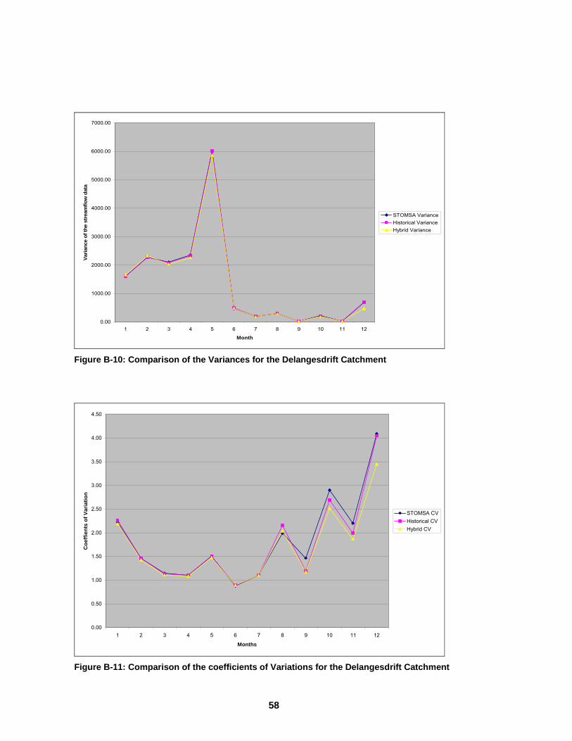
58

0.00

1000.00

2000.00

3000.00

4000.00

5000.00

6000.00

7000.00

1 2 3 4 5 6 7 8 9 10 11 12

Month

Varia

nce

of th

e st

ream

flow

dat

a

STOMSA VarianceHistorical VarianceHybrid Variance

Figure B-10: Comparison of the Variances for the Delangesdrift Catchment

0.00

0.50

1.00

1.50

2.00

2.50

3.00

3.50

4.00

4.50

1 2 3 4 5 6 7 8 9 10 11 12

Months

Coe

ffien

ts o

f Var

iatio

n

STOMSA CVHistorical CVHybrid CV

Figure B-11: Comparison of the coefficients of Variations for the Delangesdrift Catchment

59

-0.4

-0.2

0

0.2

0.4

0.6

0.8

1

Lag -1 Lag 0 Lag 1

Lag

Seria

l Cor

rela

tion

Figure B-12: Box plot of the serial correlation between month 1 current year and 12 previous year for the Delangesdrift Catchment

0

10

20

30

40

50

60

70

80

90

1 2 3 4 5 6 7 8 9 10 11 12

Months

Mea

n of

str

eam

flow

s (M

illio

n cu

bicm

eter

s/a)

STOMSA MeanHybrid MeanHistorical Mean

Figure B-13: Comparison of the Mean flows for the Katse Catchment

60

0

10

20

30

40

50

60

70

1 2 3 4 5 6 7 8 9 10 11 12

Months

Stan

dard

Dev

iatio

ns

STOMSA StdevHybrid StdevHistorical Stdev

Figure B-14: Comparison of the Standard Deviations for the Katse Catchment

0.00

0.50

1.00

1.50

2.00

2.50

1 2 3 4 5 6 7 8 9 10 11 12

Months

Coe

ffici

ents

of V

aria

nce

STOMSA CVHybrid CVHistorical CV

Figure B-15: Comparison of the Coefficients of Variations for the Katse Catchment

61

-0.3

-0.2

-0.1

0

0.1

0.2

0.3

0.4

0.5

0.6

0.7

Lag -1 Lag 0 Lag 1

Lag

Seria

l Cor

rela

tion

Figure B-16: Boxplot of the Serial correlation between moth 1 of the current year and month 12 of the previous year for the Katse Catchment

62

0

20

40

60

80

100

120

1 2 3 4 5 6 7 8 9 10 11 12

Months

Mea

n of

str

eam

flow

s (M

illio

n cu

bicm

eter

s/a)

STOMSA MeanHistorical MeanHybrid Mean

Figure B-17: Comparison of the Mean flows for the Vaal Catchment

0

20

40

60

80

100

120

140

160

180

200

1 2 3 4 5 6 7 8 9 10 11 12

Months

Stan

dard

Dev

iatio

ns o

f str

eam

flow

s

STOMSA StdevHybrid StdevHistorical Stdev

Figure B-18: Comparison of the Standard Deviations for the Vaal Catchment

63

0.00

0.50

1.00

1.50

2.00

2.50

3.00

3.50

1 2 3 4 5 6 7 8 9 10 11 12

Months

Coe

ffici

ents

of V

aria

tions

STOMSA CVHybrid CVHistorical CV

Figure B-19: Comparison of the Coefficients of Variations for the Vaal Catchment

-0.4

-0.2

0

0.2

0.4

0.6

0.8

1

Lag -1 Lag 0 Lag 1

Lag

Seria

l Cor

rela

tion

Figure B-20: Boxplot of the Serial Correlation between month 1 of current year and month 12 of the previous year for the Vaal Catchment

64

0

20

40

60

80

100

120

140

1 2 3 4 5 6 7 8 9 10 11 12

Months

Mea

n flo

ws

(Mill

ion

cubi

cmet

ers/

a)

STOMSA MeanHybrid MeanHistorical Mean

Figure B-21: Comparison of the Mean flows for the Welbedacht Catchment

0

20

40

60

80

100

120

140

160

1 2 3 4 5 6 7 8 9 10 11 12

Months

Stan

dard

Dev

iatio

ns

STOMSA StdevHybrid StdevHistorical Stdev

Figure B-22: Comparison of the Standard Deviations of the Welbedacht Catchment

65

0

0.5

1

1.5

2

2.5

3

1 2 3 4 5 6 7 8 9 10 11 12

Months

Coe

ffici

ents

of V

aria

tions

STOMSA CVHistorical CVHybrid CV

Figure B-23: Comparison of the Coefficients of Variations for the Welbedacht Catchment

-0.2

0

0.2

0.4

0.6

0.8

1

Lag -1 Lag 0 Lag 1

Lag

Seria

l cor

rela

tions

Figure B-24: Boxplot of Serial correlations between month 1 of current year and month 12 of previous year for the Welbedacht catchment

66

0

5

10

15

20

25

30

35

40

45

50

Oct Nov Dec Jan Feb Mar Apr May Jun Jul Aug Sep

Months

Mea

n St

ream

flow

(Mill

ion

cubi

cmet

ers)

Figure B-25: Bloemhof Catchment's Boxplots of Mean Streamflows

Figure B-26: Bloemhof Boxplot of Mean streamflows from STOMSA

67

0

10

20

30

40

50

60

70

80

90

100

Oct Nov Dec Jan Feb Mar Apr May Jun Jul Aug Sep

Months

Stan

dard

Dev

iatio

ns o

f str

eam

flow

s (M

illio

n cu

bicm

eter

s)

Figure B-27: Bloemhof Boxplot of Standard Deviations from the Hybrid Model

Figure B-28: Bloemhof Boxplot of Standard Deviations from STOMSA

68

0

10

20

30

40

50

60

70

80

Oct Nov Dec Jan Feb Mar Apr May Jun Jul Aug Sep

Month

Mea

n st

ream

flow

(Mill

ion

cubi

cmet

ers)

Figure B-29 : Delangesdrift Catchment's Boxplots of Mean Streamflows

Figure B-30: Delangesdrift Catchment Boxplot of Mean streamflows from STOMSA

69

0

20

40

60

80

100

120

Oct Nov Dec Jan Feb Mar Apr May Jun Jul Aug Sep

Months

Stan

dard

Dev

iatio

ns o

f Str

eam

flow

s (M

illio

n cu

bicm

eter

s)

Figure B-31 : Delangesdrift Catchment’s Boxplot of Standard Deviations from the Hybrid Model

Figure B-32: Delangesdrift Catchment Boxplot of Standard Deviations from STOMSA

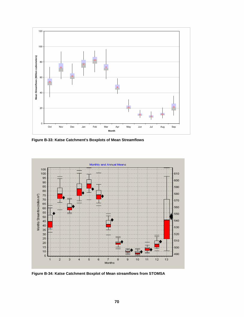
70

0

20

40

60

80

100

120

Oct Nov Dec Jan Feb Mar Apr May Jun Jul Aug Sep

Month

Mea

n St

ream

flow

s (M

illio

n cu

bicm

eter

s)

Figure B-33: Katse Catchment's Boxplots of Mean Streamflows

Figure B-34: Katse Catchment Boxplot of Mean streamflows from STOMSA

71

0

10

20

30

40

50

60

70

80

90

Oct Nov Dec Jan Feb Mar Apr May Jun Jul Aug Sep

Month

Stan

dard

Dev

iatio

ns o

f str

eam

flow

s (M

illio

n cu

bicm

eter

s)

Figure B-35: Katse Catchment’s Boxplot of Standard Deviations from the Hybrid Model

Figure B-36: Katse Catchment Boxplot of Standard Deviations from STOMSA

72

0

20

40

60

80

100

120

140

160

180

Oct Nov Dec Jan Feb Mar Apr May Jun Jul Aug Sep

Month

Mea

n St

ream

flow

(Mill

ion

Cub

icm

eter

s)

Figure B-37: Vaal Catchment's Boxplots of Mean Streamflows

Figure B-38: Vaal Catchment Boxplot of Mean streamflows from STOMSA

73

0

50

100

150

200

250

300

Oct Nov Dec Jan Feb Mar Apr May Jun Jul Aug Sep

Month

Stan

dard

Dev

iatio

ns o

f str

eam

flow

s (M

illio

n cu

bicm

eter

s)

Figure B-39: Vaal Catchment’s Boxplot of Standard Deviations from the Hybrid Model

Figure B-40: Vaal Catchment Boxplot of Standard Deviations from STOMSA

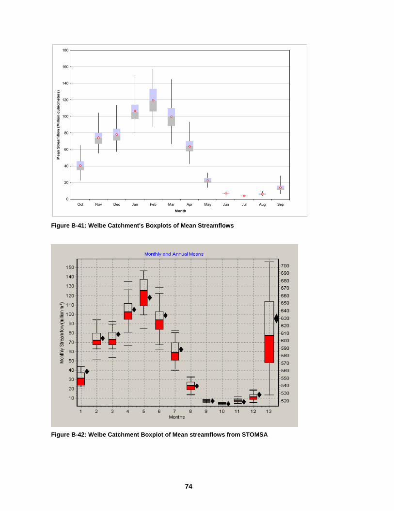
74

0

20

40

60

80

100

120

140

160

180

Oct Nov Dec Jan Feb Mar Apr May Jun Jul Aug Sep

Month

Mea

n St

ream

flow

(Mill

ion

cubi

cmet

ers)

Figure B-41: Welbe Catchment's Boxplots of Mean Streamflows

Figure B-42: Welbe Catchment Boxplot of Mean streamflows from STOMSA

75

0

50

100

150

200

250

Oct Nov Dec Jan Feb Mar Apr May Jun Jul Aug Sep

Month

Stan

dard

Dev

iatio

ns o

f Str

eam

flow

(Mill

ion

cubi

cmet

ers)

Figure B-43: Welbe Catchment’s Boxplot of Standard Deviations from the Hybrid Model

Figure B-44: Welbe Catchment Boxplot of Standard Deviations from STOMSA

76

APPENDIX C: MATLAB CODE

c=0; for i=1:5 c=c+1; if (c>=1 & c<2) load Vaal g=Vaal; elseif (c>=2 & c<3) load Welbe g=Welbe; elseif (c>=3 & c<4) load Dela g=Dela; elseif (c>=4 & c<5) load bloem g=bloem; else load Katse g=Katse; end %load bloem %g=bloem; %obtain the dimention of data and store in vs vs=size(g,1); Y=zeros(vs,12); %standardise original data g, into Y for i=2:13 for j=1:vs Y(j,i-1)=(g(j,i)-mean(g(1:vs,i)))/std(g(1:vs,i)); end end %calculate the coefiecints using autocorrelation coef=zeros(5,12); for i=2:13 coef(1:5,i-1)=autocorr(Y(1:vs,i-1),4); end %transform Y to a vector of (1 X 961), with the first value being zero Yp=zeros(1,vs*12+1); l=0; for j=1:vs for i=1:12 l=l+1; Yp(1,l+1)=Y(j,i); end end %calculate the residual e=zeros(vs*12,1); l=0; for j=1:vs for i=1:12 l=l+1; e(l,1)=Yp(l+1)-coef(2,i)*Yp(l); end end %apply bootstrap vl=76; K=zeros((12*vl*99),1); E=[e;K];

77

a = 1; b = (vl-1); B=zeros((12*vl*100),1); r=(12*vl*100)/24; for i=1:r x = round(a + ((b-a) * rand(1)));%generate random numbers between 1 and 79, uniformly distributed B((i*24-23):(i*24),1)=E((x*12-11):(x*12+12),1); end %postblanketing Z=zeros((12*vl*100),1); Zp=[0;B]; l=0; r=(vl*100); for j=1:r for i=1:12 l=l+1; Z(l)=coef(2,i)*Zp(l)+ Zp(l+1); end end %inverse standardise X=zeros((12*vl*100),1); l=0; r=vl*100; for j=1:r for i=2:13 l=l+1; X(l)=Z(l)*std(g(1:vs,i))+mean(g(1:vs,i)); if (X(l)<0) X(l)=0; end end end %convert the synthetic data to a matrix of a number of years 76 X100 those of the original data M=zeros((vl*100),12); l=1; for i=1:(vl*100) for j=1:12 M(i,j)=X(l,1); l=l+1; end end %Calculate autocorrelation/correlation coeficients to compare with data of origina data coefsyth=zeros(5,12); for i=1:12 coefsyth(1:5,i)=autocorr(M(((vl*100)-vl):(vl*100),i),4); end %calculate the matrices of stsistics (Mean, skew, Stdev, Autocorr) KK=[M,transpose(sum(transpose(M)))];%make totals %MM(1:7600,c)=transpose(sum(transpose(M)); %Mean MeanMatrix=zeros(100,13); l=0; lm=0; for i=1:100 l=l+vl; MeanMatrix(i,1:13)=mean(KK((1+lm):l,1:13)); lm=lm+vl; end %StDev StDevMatrix=zeros(100,13); l=0; lm=0; for i=1:100

78

l=l+vl; StDevMatrix(i,1:13)=std(KK((1+lm):l,1:13)); lm=lm+vl; end %Skewness SkewMatrix=zeros(100,13); l=0; lm=0; for i=1:100 l=l+vl; SkewMatrix(i,1:13)=skewness(KK((1+lm):l,1:13)); lm=lm+vl; end % Maximum deficit which is the lowest storage level for each % sequence for r=1:5 l=0; lm=0; for i =1:100%number of sequences M_Stor =0; l=l+vl; for j=1:vl%number of years in a sequences for rj=1:12 B_Storage(1,rj)=M_Stor-KK(lm+j,rj)+(((9-r)/10)*(mean(g(1:vs,14))))/12; Monthly_Storage(1,rj)=max(0,B_Storage(1,rj)); M_Stor=Monthly_Storage(1,rj); end Storage(j,i)=sum(transpose(Monthly_Storage)); end lm=lm+vl; end Maxd=max(Storage); Maxdef(r,1:100)=Maxd; end %{ % Run Sums 6,12,24,36,48,60,72,84,96,108/ R=[6,12,24,36,48,60,72,84,96,108]; l=0; lm=0; for i=1:100 l=l+912; RunsMatrix=skewness(X((1+lm):l,1)); for j=1:6 r=R(j); t=912-r+1; for k=1:t sumall=sum(RunsMatrix(k:r+k-1)); sums(k)=sumall(k); end minruns=min(sums); Minsums(i,j)=minruns end lm=lm+912; end %} %Serial correlation between month 1 and moth 12 l=0; lm=0;

79

for j=1:100 l=l+vl; AutocorSyth1=KK((1+lm):l,1); AutocorSyth12=KK((1+lm):l,12); SerialS=crosscorr(AutocorSyth1(1:76,1),AutocorSyth12(1:76,1),1); SerialcorrSyth(j,1:3)=transpose(SerialS(1:3,1)); lm=lm+vl; end AutoData1=(g(1:vs,2)); AutoData2=(g(1:vs,13)); SerialData=transpose(crosscorr(AutoData1,AutoData2,1)); SerialSyth=mean(SerialcorrSyth); %storing the results into different matrices if (c>=1 & c<2)% store the results for the Vaal %VautocorrMatrix=AutocorrMatrix; VAutocorr=coefsyth; VMmeanmatrix=MeanMatrix; VStDevMatrix=StDevMatrix; VSkewMatrix=SkewMatrix; VMmean=mean(MeanMatrix); VMeandata=mean(g(1:vs,2:13)); VMeansyth1=mean([M,transpose(sum(transpose(M)))]); VMeansyth=VMeansyth1(1:12); %remove the total from meansyth1 VStddata=std(g(1:vs,2:13)); VStdsyth1=std([M,transpose(sum(transpose(M)))]); VStdsyth=VStdsyth1(1:12); %remove the total from Stdsyth1 VSkdata=skewness(g(1:vs,2:13)); VSksyth1=skewness([M,transpose(sum(transpose(M)))]); VSksyth=VSksyth1(1:12); %remove the total from Sksyth1 VMn=transpose([VMeandata;VMeansyth]); VSt=transpose([VStddata;VStdsyth]); VSk=transpose([VSkdata;VSksyth]); VSythData=KK; VSerialcorr1_12Syth=SerialcorrSyth; VSerialcorr1_12Data=SerialData; VSerialcorSythmean=SerialSyth; %Write data to files csvwrite('Vaalmean.csv',VMn); csvwrite('VaalSTdev.csv',VSt); csvwrite('VaalSkew.csv',VSk); csvwrite('VaalMeanMatrix.csv',VMmeanmatrix); csvwrite('VaalStdevMatrix.csv',VStDevMatrix); csvwrite('VaalSkewMatrix.csv',VSkewMatrix); csvwrite('VaalAutocorr.csv',VAutocorr); csvwrite('Vaal_Sytheticdata.csv',KK); csvwrite('Vaal_Maxdef.csv',transpose(Maxdef)); csvwrite('VSerialcorrSyth.csv',VSerialcorr1_12Syth); csvwrite('VSerialcorrData.csv',VSerialcorr1_12Data); csvwrite('VSerialcorSythmean.csv',VSerialcorSythmean); elseif (c>=2 & c<3)% store the results for the Welbe WAutocorr=coefsyth; WMmeanmatrix=MeanMatrix; WStDevMatrix=StDevMatrix; WSkewMatrix=SkewMatrix; WMmean=mean(MeanMatrix); WMeandata=mean(g(1:vs,2:13)); WMeansyth1=mean([M,transpose(sum(transpose(M)))]); WMeansyth=WMeansyth1(1:12); %remove the total from meansyth1 WStddata=std(g(1:vs,2:13)); WStdsyth1=std([M,transpose(sum(transpose(M)))]); WStdsyth=WStdsyth1(1:12); %remove the total from Stdsyth1

80

WSkdata=skewness(g(1:vs,2:13)); WSksyth1=skewness([M,transpose(sum(transpose(M)))]); WSksyth=WSksyth1(1:12); %remove the total from Sksyth1 WMn=transpose([WMeandata;WMeansyth]); WSt=transpose([WStddata;WStdsyth]); WSk=transpose([WSkdata;WSksyth]); WSythData=KK; WSerialcorr1_12Syth=SerialcorrSyth; WSerialcorr1_12Data=SerialData; WSerialcorSythmean=SerialSyth; %Write data to files csvwrite('Welbemean.csv',WMn); csvwrite('WelbeSTdev.csv',WSt); csvwrite('WelbeSkew.csv',WSk); csvwrite('WelbeMeanMatrix.csv',WMmeanmatrix); csvwrite('WelbeStdevMatrix.csv',WStDevMatrix); csvwrite('WelbeSkewMatrix.csv',WSkewMatrix); csvwrite('WelbeAutocorr.csv',WAutocorr); csvwrite('Welbe_Sytheticdata',KK); csvwrite('Welbe_Maxdef.csv',transpose(Maxdef)); csvwrite('WSerialcorrSyth.csv',WSerialcorr1_12Syth); csvwrite('WSerialcorrData.csv',WSerialcorr1_12Data); csvwrite('WSerialcorSythmean.csv',WSerialcorSythmean); elseif (c>=3 & c<4)% store the results for the Dela DAutocorr=coefsyth; DMmeanmatrix=MeanMatrix; DStDevMatrix=StDevMatrix; DSkewMatrix=SkewMatrix; DMmean=mean(MeanMatrix); DMeandata=mean(g(1:vs,2:13)); DMeansyth1=mean([M,transpose(sum(transpose(M)))]); DMeansyth=DMeansyth1(1:12); %remove the total from meansyth1 DStddata=std(g(1:vs,2:13)); DStdsyth1=std([M,transpose(sum(transpose(M)))]); DStdsyth=DStdsyth1(1:12); %remove the total from Stdsyth1 DSkdata=skewness(g(1:vs,2:13)); DSksyth1=skewness([M,transpose(sum(transpose(M)))]); DSksyth=DSksyth1(1:12); %remove the total from Sksyth1 DMn=transpose([DMeandata;DMeansyth]); DSt=transpose([DStddata;DStdsyth]); DSk=transpose([DSkdata;DSksyth]); DSythData=KK; DSerialcorr1_12Syth=SerialcorrSyth; DSerialcorr1_12Data=SerialData; DSerialcorSythmean=SerialSyth; %Write data to files csvwrite('Delamean.csv',DMn); csvwrite('DelaSTdev.csv',DSt); csvwrite('DelaSkew.csv',DSk); csvwrite('DelaMeanMatrix.csv',DMmeanmatrix); csvwrite('DelaStdevMatrix.csv',DStDevMatrix); csvwrite('DelaSkewMatrix.csv',DSkewMatrix); csvwrite('DelaAutocorr.csv',DAutocorr); csvwrite('Dela_Sytheticdata',KK); csvwrite('Dela_Maxdef.csv',transpose(Maxdef)); csvwrite('DSerialcorrSyth.csv',DSerialcorr1_12Syth); csvwrite('DSerialcorrData.csv',DSerialcorr1_12Data); csvwrite('DSerialcorSythmean.csv',DSerialcorSythmean); elseif (c>=4 & c<5)% store the results for the Bloem BAutocorr=coefsyth; BMmeanmatrix=MeanMatrix; BStDevMatrix=StDevMatrix; BSkewMatrix=SkewMatrix; BMmean=mean(MeanMatrix); BMeandata=mean(g(1:vs,2:13)); BMeansyth1=mean([M,transpose(sum(transpose(M)))]); BMeansyth=BMeansyth1(1:12); %remove the total from meansyth1

81

BStddata=std(g(1:vs,2:13)); BStdsyth1=std([M,transpose(sum(transpose(M)))]); BStdsyth=BStdsyth1(1:12); %remove the total from Stdsyth1 BSkdata=skewness(g(1:vs,2:13)); BSksyth1=skewness([M,transpose(sum(transpose(M)))]); BSksyth=BSksyth1(1:12); %remove the total from Sksyth1 BMn=transpose([BMeandata;BMeansyth]); BSt=transpose([BStddata;BStdsyth]); BSk=transpose([BSkdata;BSksyth]); BSythData=KK; BSerialcorr1_12Syth=SerialcorrSyth; BSerialcorr1_12Data=SerialData; BSerialcorSythmean=SerialSyth; %Write data to files csvwrite('Bloemmean.csv',BMn); csvwrite('BloemSTdev.csv',BSt); csvwrite('BloemSkew.csv',BSk); csvwrite('BloemMeanMatrix.csv',BMmeanmatrix); csvwrite('BloemStdevMatrix.csv',BStDevMatrix); csvwrite('BloemSkewMatrix.csv',BSkewMatrix); csvwrite('BloemAutocorr.csv',BAutocorr); csvwrite('Bloem_Sytheticdata',KK); csvwrite('Bloem_Maxdef.csv',transpose(Maxdef)); csvwrite('BSerialcorrSyth.csv',BSerialcorr1_12Syth); csvwrite('BSerialcorrData.csv',BSerialcorr1_12Data); csvwrite('BSerialcorSythmean.csv',BSerialcorSythmean); else %store the results for Katse KAutocorr=coefsyth; KMmeanmatrix=MeanMatrix; KStDevMatrix=StDevMatrix; KSkewMatrix=SkewMatrix; KMmean=mean(MeanMatrix); KMeandata=mean(g(1:vs,2:13)); KMeansyth1=mean([M,transpose(sum(transpose(M)))]); KMeansyth=KMeansyth1(1:12); %remove the total from meansyth1 KStddata=std(g(1:vs,2:13)); KStdsyth1=std([M,transpose(sum(transpose(M)))]); KStdsyth=KStdsyth1(1:12); %remove the total from Stdsyth1 KSkdata=skewness(g(1:vs,2:13)); KSksyth1=skewness([M,transpose(sum(transpose(M)))]); KSksyth=KSksyth1(1:12); %remove the total from Sksyth1 KMn=transpose([KMeandata;KMeansyth]); KSt=transpose([KStddata;KStdsyth]); KSk=transpose([KSkdata;KSksyth]); KAnnual=transpose(sum(transpose(M))); KSythData=KK; KSerialcorr1_12Syth=SerialcorrSyth; KSerialcorr1_12Data=SerialData; KSerialcorSythmean=SerialSyth; %Write data to files csvwrite('Katsemean.csv',KMn); csvwrite('KatseSTdev.csv',KSt); csvwrite('KatseSkew.csv',KSk); csvwrite('KatseMeanMatrix.csv',KMmeanmatrix); csvwrite('KatseStdevMatrix.csv',KStDevMatrix); csvwrite('KatseSkewMatrix.csv',KSkewMatrix); csvwrite('KatseAutocorr.csv',KAutocorr); csvwrite('Katse_Sytheticdata.csv',KK); csvwrite('Katse_Maxdef.csv',transpose(Maxdef)); csvwrite('KSerialcorrSyth.csv',KSerialcorr1_12Syth); csvwrite('KSerialcorrData.csv',KSerialcorr1_12Data); csvwrite('KSerialcorSythmean.csv',KSerialcorSythmean); end % end storring the results %MM(1:7600,c)=transpose(sum(transpose(M)); %csvwrite('Annual_for_all.csv',MM); end

82

% CROSS CORRELATIONS % 1: Vaal and Welbe l=0; lm=0; for j=1:100 l=l+vl; VSyth=VSythData((1+lm):l,1:13); WSyth=WSythData((1+lm):l,1:13); for i=1:13 XCFS = crosscorr(VSyth(1:76,i),WSyth(1:76,i),4); VWcrosscorSyth(1:9,i)=XCFS(1:9,1); end %sort VWlag14(j,1:13)=VWcrosscorSyth(1,1:13); VWlag13(j,1:13)=VWcrosscorSyth(2,1:13); VWlag12(j,1:13)=VWcrosscorSyth(3,1:13); VWlag11(j,1:13)=VWcrosscorSyth(4,1:13); VWlag0(j,1:13)=VWcrosscorSyth(5,1:13); VWlag1(j,1:13)=VWcrosscorSyth(6,1:13); VWlag2(j,1:13)=VWcrosscorSyth(7,1:13); VWlag3(j,1:13)=VWcrosscorSyth(8,1:13); VWlag4(j,1:13)=VWcrosscorSyth(9,1:13); lm=lm+vl; end for i=1:13 XCFD = crosscorr(Vaal(1:68,i+1),Welbe(1:68,i+1),4); VWcrosscorData(1:9,i)=XCFD(1:9,1); end VWlag14Mean=mean(VWlag14); VWlag13Mean=mean(VWlag13); VWlag12Mean=mean(VWlag12); VWlag11Mean=mean(VWlag11); VWlag0Mean=mean(VWlag0); VWlag1Mean=mean(VWlag1); VWlag2Mean=mean(VWlag2); VWlag3Mean=mean(VWlag3); VWlag4Mean=mean(VWlag4); VWcrosscorSythMean=[VWlag14Mean;VWlag13Mean;VWlag12Mean;VWlag11Mean;VWlag0Mean;VWlag1Mean;VWlag2Mean;VWlag3Mean;VWlag4Mean]; csvwrite('VWcrosscorData.csv',VWcrosscorData); csvwrite('VWcrosscorSyth.csv',VWcrosscorSythMean); Mmeanmatrix=mean(MeanMatrix(1:100,1:12)); %make summary statistics Meandata=mean(g(1:vs,2:13)); Meansyth1=mean([M,transpose(sum(transpose(M)))]); Meansyth=Meansyth1(1:12); %remove the total from meansyth1 Stddata=std(g(1:vs,2:13)); Stdsyth1=std([M,transpose(sum(transpose(M)))]); Stdsyth=Stdsyth1(1:12); %remove the total from Stdsyth1 Skdata=skewness(g(1:vs,2:13)); Sksyth1=skewness([M,transpose(sum(transpose(M)))]); Sksyth=Sksyth1(1:12); %remove the total from Sksyth1 Mn=transpose([Meandata;Meansyth]); St=transpose([Stddata;Stdsyth]); Sk=transpose([Skdata;Sksyth]); Maencomp=[Mmeanmatrix;Meansyth]; figure

83

boxplot(KMmeanmatrix) title('Katse MeanMatrix') figure boxplot (KStDevMatrix) title('Katse Standard deviation matrix') figure boxplot (KSkewMatrix) title('Katse Skewness Matrix') figure plot(St) title('Standard deviation') xlabel({'Raw';'Syth'}) figure plot(Mn) title('Mean') xlabel({'Raw';'Syth'}) figure plot(Sk) title('Skewness') xlabel({'Raw';'Syth'}) gd=g(1:vs,2:13); figure boxplot(gd) title('gd') hold on %boxplot(M) plot(Mn) title('Syth') hold off figure boxplot(transpose(Maxdef)) title('Maxdef') figure plot(transpose(Storage(1:vl,1))) title('Storage trajectory')