La phraséodidactique du francais un siècle de vie: de Charles Bally à aujourdhui
Upload
khangminh22Category
view
0download
0
HAL Id: tel-00909703https://tel.archives-ouvertes.fr/tel-00909703
Submitted on 26 Nov 2013
HAL is a multi-disciplinary open accessarchive for the deposit and dissemination of sci-entific research documents, whether they are pub-lished or not. The documents may come fromteaching and research institutions in France orabroad, or from public or private research centers.
L’archive ouverte pluridisciplinaire HAL, estdestinée au dépôt et à la diffusion de documentsscientifiques de niveau recherche, publiés ou non,émanant des établissements d’enseignement et derecherche français ou étrangers, des laboratoirespublics ou privés.
Mesure de surface 3D pour la caractérisationostéo-musculaire de petits vertébrés : application à la
caractérisation du vieillissement chez la sourisEstelle Duveau
To cite this version:Estelle Duveau. Mesure de surface 3D pour la caractérisation ostéo-musculaire de petits vertébrés :application à la caractérisation du vieillissement chez la souris. Autre [cs.OH]. Université de Grenoble,2012. Français. �NNT : 2012GRENM088�. �tel-00909703�

THÈSEPour obtenir le grade de
DOCTEUR DE L’UNIVERSITÉ DE GRENOBLESpécialité : Informatique
Arrêté ministérial : 7 août 2006
Présentée par
Estelle DUVEAU
Thèse dirigée par Edmond BOYERet codirigée par Lionel REVERET
préparée au sein du Laboratoire Jean Kuntzmann (LJK),UMR CNRS 5224.
et de l’école doctorale EDMSTIIMathématiques, Sciences et Technologies de l’Information, Informatique
Caractérisation squelettique de pe-tits vertébrés par mesure de sur-face 3D
Thèse soutenue publiquement le 03 Décembre 2012,devant le jury composé de :
Saida BouakazProfesseur, Université Claude Bernard Lyon 1, Présidente
Laurent LucasProfesseur, Université de Reims Champagne-Ardenne, Rapporteur
Tamy BoubekeurMaître de conférence, Telecom Paris Tech, Rapporteur
Marie-Paule CaniProfesseur, Grenoble INP, Examinateur
Edmond BoyerDirecteur de recherche, Inria, Directeur de thèse
Lionel ReveretChargé de recherche, Inria, Co-Directeur de thèse

RÉSUMÉ
L’ANALYSE du comportement des petits animaux de laboratoire tels que rats etsouris est fondamentale en recherche biologique. L’objectif de cette thèse estde faire des mesures anatomiques sur le squelette de souris à partir de vidéos
et de démontrer la robustesse de ces mesures par une validation quantitative. Lesprincipales difficultés viennent du sujet d’étude, la souris, qui, vu comme un objetgéométrique, peut subir de grandes déformations très rapidement et des conditions ex-périmentales qui ne permettent pas d’obtenir des flux vidéos de même qualité que pourl’étude de l’humain.
Au vu de ces difficultés, nous nous concentrons tout d’abord dans le Chapitre 2 surla mise en place d’une méthode de recalage de squelette à l’aide de marqueurs colléssur la peau de l’animal. On montre que les effets de couplage non-rigide entre peau etsquelette peuvent être contre-carrés par une pondération de l’influence des différentsmarqueurs dans la cinématique inverse. Cela nous permet de justifier que, malgré cecouplage non rigide, des informations sur la peau de l’animal sont suffisantes pour re-caler de manière précise et robuste les structures squelettiques. Nous développons pourcela une chaîne de traitement de données morphologiques qui nous permet de proposerun modèle générique d’animation du squelette des souris. La méthode de cinématiqueinverse pondérée est validée grâce à des vidéos radiographiques.
Ayant justifié de l’utilisation de points à la surface de la peau (l’enveloppe) pourrecaler le squelette, nous proposons dans le Chapitre 3 un nouveau modèle de dé-formation de l’enveloppe. Ce modèle, appelé OQR (pour Oriented Quads Rigging,gréage de quadrilatères orientés), est une structure géométrique flexible possédant lesbonnes propriétés de déformation de l’animation par cage. A l’instar des squelettesd’animation, elle permet d’avoir une paramétrisation haut-niveau de la morphologie etdu mouvement. Nous montrons également comment, grâce à cette bonne déformationde l’enveloppe, nous pouvons utiliser les sommets du maillage déformé comme mar-queurs pour la méthode de recalage du squelette du Chapitre 2.
Dans les chapitres 2 et 3, nous avons construit un modèle de souris qui permet d’animeren même temps l’enveloppe et le squelette. Ce modèle est paramétré par OQR. Nousproposons donc dans le Chapitre 4 une méthode d’extraction de ces paramètres à partirsoit d’une séquence de maillage sans cohérence temporelle soir directement à partird’images segmentées. Pour contraindre le problème, nous faisons l’apprentissage d’unespace réduit de configurations d’OQR vraisemblables.

ABSTRACT
ANALYSING the behaviour of small laboratory animals such as rats and miceis paramount in clinical research. We aim at recovering reliable anatomicalmeasures of the skeleton of mice from videos and at demonstrating the ro-
bustness of these measures with quantitative validation. The most challenging aspectsof this thesis reside in the study subject, mice, that is highly deformable, very fast andin the experimental conditions that do not allow for video data equivalent to what canbe obtained with human subjects.
In regards to the first challenge, we first focus on a marker-based tracking methodwith markers glued on the skin of the animal in Chapter 2. We show that the effects ofthe non-rigid mapping between skin and bones can be pre-empted by a weighting ofthe influences of the different markers in inverse kinematics. This allows us to demon-strate that, despite the non-rigid mapping, features on the skin of the animal can beused to accurately and robustly track the skeletal structures. We therefore develop apipeline to process morphological data that leads to a generic animation model for theskeleton of mice. The weighted inverse kinematics method is validated with X-rayvideos.
Chapter 2 proves that points on the surface of the animal (on the envelope) can beused to track the skeletal structures. As a result, in Chapter 3, we propose a new defor-mation model of the envelope. This model, called OQR (Oriented Quads Rigging), isa flexible geometrical structure that has the nice deformation properties of cage-basedanimation. Like animation skeletons, OQR gives a high-level representation of themorphology and of the motion. We also show how, thanks to a well-deformed enve-lope, we can use a sub-set of the vertices of the deformed mesh as markers to apply themethod of tracking of skeletal structures developed in Chapter 2.
With Chapters 2 and 3, we have built a model of mice that allows us to animate atthe same time the envelope and the skeleton. This model is parameterised by OQR.In Chapter 4, we therefore propose a method to recover the OQR parameters fromeither a sequence of meshes without temporal coherence or directly from segmentedimages. To regularise the tracking problem, we learn a manifold of plausible OQRconfigurations.


CONTENTS
1 Introduction. 111.1 Context - Ethology . . . . . . . . . . . . . . . . . . . . . . . . . . . 111.2 Objectives . . . . . . . . . . . . . . . . . . . . . . . . . . . . . . . . 12
1.2.1 Vestibular control of skeletal configurations in 0G . . . . . . . 121.2.2 Datasets . . . . . . . . . . . . . . . . . . . . . . . . . . . . . 14
Biplanar X-ray set-up . . . . . . . . . . . . . . . . . . . . . . 15Locomotion set-up . . . . . . . . . . . . . . . . . . . . . . . 15Swimming set-up . . . . . . . . . . . . . . . . . . . . . . . . 17Open field set-up . . . . . . . . . . . . . . . . . . . . . . . . 18Parabolic flight set-up . . . . . . . . . . . . . . . . . . . . . 19
1.3 Overview and Contributions . . . . . . . . . . . . . . . . . . . . . . 221.3.1 Goals . . . . . . . . . . . . . . . . . . . . . . . . . . . . . . 221.3.2 Contributions . . . . . . . . . . . . . . . . . . . . . . . . . . 221.3.3 Overview . . . . . . . . . . . . . . . . . . . . . . . . . . . . 22
2 Shape and motion of the skeletal structures. 252.1 Previous work . . . . . . . . . . . . . . . . . . . . . . . . . . . . . . 26
2.1.1 Internal vs External 3D imaging . . . . . . . . . . . . . . . . 262.1.2 Marker-based vs Markerless tracking . . . . . . . . . . . . . 272.1.3 Inverse Kinematics . . . . . . . . . . . . . . . . . . . . . . . 292.1.4 Overview of our method . . . . . . . . . . . . . . . . . . . . 30
2.2 Geometry and motion data acquisition . . . . . . . . . . . . . . . . . 322.2.1 Acquisition of the geometrical models of the bones . . . . . . 322.2.2 Acquisition of the trajectories of the markers . . . . . . . . . 33
2.3 Animation model of the internal structures . . . . . . . . . . . . . . . 372.3.1 Set of articulated solids . . . . . . . . . . . . . . . . . . . . . 37
7

8
2.3.2 Refined model of the spine and ribcage . . . . . . . . . . . . 412.4 Marker-based tracking of the internal structures . . . . . . . . . . . . 45
2.4.1 Sequence-specific model . . . . . . . . . . . . . . . . . . . . 45Definitions of landmarks on the animation model . . . . . . . 45Morphological adaptation to a specific subject . . . . . . . . . 46
2.4.2 Inverse Kinematics . . . . . . . . . . . . . . . . . . . . . . . 472.4.3 Update of the spine and ribcage . . . . . . . . . . . . . . . . 532.4.4 Automatic refinement of the location of the landmarks . . . . 55
2.5 Validation of the animation model . . . . . . . . . . . . . . . . . . . 572.5.1 Case study : motion of the foreleg of the rat during locomotion 57
Validation of the calibration . . . . . . . . . . . . . . . . . . 57Validation of the 3D trajectories of the markers . . . . . . . . 59Validation of the tracking of the bones . . . . . . . . . . . . . 60Study of the influence of the number and location of the markers 62Application . . . . . . . . . . . . . . . . . . . . . . . . . . . 68
2.5.2 Results for various morphologies and motions . . . . . . . . . 712.6 Conclusion . . . . . . . . . . . . . . . . . . . . . . . . . . . . . . . 75
3 Acquisition and deformation model of the envelope. 773.1 Previous work . . . . . . . . . . . . . . . . . . . . . . . . . . . . . . 79
3.1.1 Multi-view reconstruction . . . . . . . . . . . . . . . . . . . 793.1.2 Deformation model . . . . . . . . . . . . . . . . . . . . . . . 82
3.2 Acquisition of the envelope from videos . . . . . . . . . . . . . . . . 883.2.1 Background subtraction . . . . . . . . . . . . . . . . . . . . 893.2.2 Multi-view reconstruction . . . . . . . . . . . . . . . . . . . 90
3.3 Deformation model of the envelope . . . . . . . . . . . . . . . . . . 943.3.1 Cage-based animation . . . . . . . . . . . . . . . . . . . . . 943.3.2 Oriented Quads Rigging (OQR) . . . . . . . . . . . . . . . . 100
3.4 Link to skeletal structures . . . . . . . . . . . . . . . . . . . . . . . . 1073.5 Conclusion . . . . . . . . . . . . . . . . . . . . . . . . . . . . . . . 110
4 Manifold learning for Oriented Quads Rigging recovery. 1114.1 Previous work . . . . . . . . . . . . . . . . . . . . . . . . . . . . . . 112
4.1.1 Motion recovery from a sequence of meshes . . . . . . . . . . 1124.1.2 Manifold learning for tracking . . . . . . . . . . . . . . . . . 114
4.2 Manifold learning of OQR . . . . . . . . . . . . . . . . . . . . . . . 1154.3 Mesh tracking . . . . . . . . . . . . . . . . . . . . . . . . . . . . . . 118
4.3.1 Objective function . . . . . . . . . . . . . . . . . . . . . . . 1184.3.2 Shape and pose tracking . . . . . . . . . . . . . . . . . . . . 119
Shape tracking . . . . . . . . . . . . . . . . . . . . . . . . . 120Pose tracking . . . . . . . . . . . . . . . . . . . . . . . . . . 121Local adjustment of the OQR . . . . . . . . . . . . . . . . . 122
4.3.3 Validation and results . . . . . . . . . . . . . . . . . . . . . . 122Validation on standard datasets . . . . . . . . . . . . . . . . . 122

9
Results on locomotion tracking . . . . . . . . . . . . . . . . 128Results on open-field tracking . . . . . . . . . . . . . . . . . 135
4.4 Video tracking . . . . . . . . . . . . . . . . . . . . . . . . . . . . . . 1384.4.1 2D objective function . . . . . . . . . . . . . . . . . . . . . . 1384.4.2 Modifications to 3D shape and pose tracking . . . . . . . . . 1384.4.3 Comparison with mesh tracking . . . . . . . . . . . . . . . . 1404.4.4 Results on parabolic flights . . . . . . . . . . . . . . . . . . . 142
4.5 Conclusion . . . . . . . . . . . . . . . . . . . . . . . . . . . . . . . 145
5 Conclusion and perspectives. 147

10

CHAPTER
1
INTRODUCTION.
1.1 CONTEXT - ETHOLOGY
MANY natural and genetically-engineered strains of mice are nowadays usedin medical research. It is therefore required to determine the characteristicbehaviour, the phenotype, of each strain to be able to determine the effect of
the procedures or drugs on the animals during clinical tests. The study of behaviours iscalled ethology. Most often than not, ethology is conducted by human observers thatmonitor the animals. This is a time-consuming task that is lacking in several ways.First of all, this greatly reduces the number of animals that can be observed. Secondly,this is often a qualitative evaluation of the behaviour, with no precise measure to ob-jectively describe the phenotype.
In recent years, automatic monitoring of animals through video systems has been in-creasingly studied. Indeed, such systems make the observation of many animals in anunconstrained environment cheap and non-intrusive. However, automatic extraction ofbehaviours from such systems is for the moment limited to high-level measures suchas the spacial displacement of the animals or a classification of actions such as eating,sleeping, etc [BBDR05]. What is still lacking is a reliable automatic measure of com-plex behaviours to create strain-specific databases of behaviours.
We therefore propose to try to recover reliable measurable parameters of skeletal struc-tures of rodents through video systems. This would give us an unbiased precise way ofstudying behaviours. However, rodents, and in particular mice, are highly deformableand move in an unconstrained erratic way, which makes the task very challenging forstate of the art motion recovery system usually designed for humans.
11

12 CHAPTER 1. INTRODUCTION.
1.2 OBJECTIVES
1.2.1 Vestibular control of skeletal configurations in 0G
Our study of rodents is done in collaboration with the CESEM (Centre d’Etude de laSensoriMotricité) research team at Université Paris Descartes. One of their main axisof research is sensorimotor control in vertebrates, that is to say how the central nervoussystem analyses the different input information it receives from all parts of the body tocontrol the posture and enforce gaze stabilization. This also encompasses the study ofbalance.
This field of research is of interest for different reasons. For instance, falls are oneof the most common causes of accidents in the elderly and better understanding bal-ance impairments may be useful to prevent those falls. Beyond punctual events suchas falls, there exists balance disorders such as Ménière’s disease that can affect peo-ple chronically and become a lifelong disability. On top of clinical applications, thestudy of balance is also paramount to space conquest. Indeed, astronauts need to beprepared to function in a micro-gravity environment as long space journeys can leadthem to experience space adaptation syndrome (also known as space sickness) due toan adaptation of the body to weightlessness.
Balance is a difficult function to study as it is multi-modal. Inputs of different na-tures are integrated to maintain balance : the visual, somatosensory and vestibularsystems all contribute to regulate equilibrium (see Figure 1.1 for a schematic represen-tation). The visual system relies on the scene imprinted on the retina. The somatosen-sory system gives proprioception, the sense of the relative position and movement ofneighbouring parts of the body. The vestibular system detects linear and angular accel-erations of the head as well as its orientation with respect to gravity. It originates in theinner ear. All these informations are combined to create a 3 dimensional representationof the position of the eyes, head and body. From this, the central nervous system willcoordinate the body to enforce posture and gaze stabilization.
Figure 1.1: A schematic representation of the inputs and outputs of the central nervous
system to achieve balance.
1.2. OBJECTIVES 13
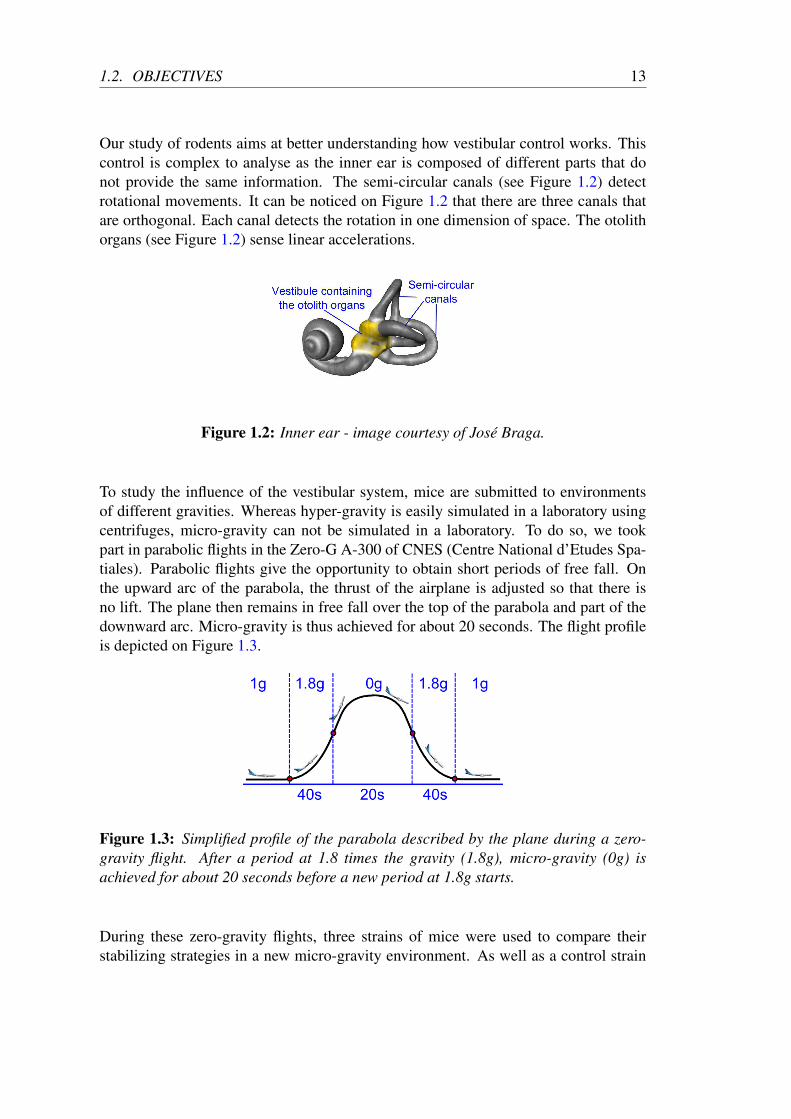
Our study of rodents aims at better understanding how vestibular control works. Thiscontrol is complex to analyse as the inner ear is composed of different parts that donot provide the same information. The semi-circular canals (see Figure 1.2) detectrotational movements. It can be noticed on Figure 1.2 that there are three canals thatare orthogonal. Each canal detects the rotation in one dimension of space. The otolithorgans (see Figure 1.2) sense linear accelerations.
Figure 1.2: Inner ear - image courtesy of José Braga.
To study the influence of the vestibular system, mice are submitted to environmentsof different gravities. Whereas hyper-gravity is easily simulated in a laboratory usingcentrifuges, micro-gravity can not be simulated in a laboratory. To do so, we tookpart in parabolic flights in the Zero-G A-300 of CNES (Centre National d’Etudes Spa-tiales). Parabolic flights give the opportunity to obtain short periods of free fall. Onthe upward arc of the parabola, the thrust of the airplane is adjusted so that there isno lift. The plane then remains in free fall over the top of the parabola and part of thedownward arc. Micro-gravity is thus achieved for about 20 seconds. The flight profileis depicted on Figure 1.3.
Figure 1.3: Simplified profile of the parabola described by the plane during a zero-
gravity flight. After a period at 1.8 times the gravity (1.8g), micro-gravity (0g) is
achieved for about 20 seconds before a new period at 1.8g starts.
During these zero-gravity flights, three strains of mice were used to compare theirstabilizing strategies in a new micro-gravity environment. As well as a control strain

14 CHAPTER 1. INTRODUCTION.
with no vestibular deficiency, ied and IsK mice were used. Ied mice have a deficientotolithic system but functioning semi-circular canals. IsK mice have no functioningvestibular organs at all. As a result, this experiment can help us understand the re-spective influence of semi-circular canals and otholiths on the skeletal configurationby studying the posture of these different strains of mice experiencing weightlessnessfor the first time.
1.2.2 Datasets
name species motionnumber ofcameras
number ofX-ray videos
presence ofmarkers
ratC0X2M1lo ratforelegduring
locomotion0 2
yes - 4 perbone
ratC4X1M1lo rattreadmill
locomotion4 1 yes - sparse
ratC6X1M1lo rattreadmill
locomotion6 1 yes - sparse
ratC5X0M1sw rat swimming 5 0yes - very
sparse
moC8X0M0of mouse open field 8 0 no
moC8X0M0pf mouseparabolic
flights8 0 no
Table 1.1: Different datasets used for validation.
Using mice in zero-gravity flights to develop new techniques of 3D anatomicalmeasurement offers several drawbacks. First of all, experiments in zero-gravity do notallow for a very controlled environment. Indeed, the mice are put in a free-floatingspace where they can reach any position and orientation. As a result, the cameras cannot be located to better capture one given position and orientation but must allow forgood capture of all positions and orientations. The mouse therefore occupies only onesmall portion of the image. The resolution is therefore not optimal. Furthermore, miceare small animals compared to other rodents, for example, rats. Indeed, studying ratsinstead of mice is easier thanks to the size of the animal. Most importantly, equipmentsrequired to validate our techniques can not be incorporated in zero-gravity flights. In-deed, validating measurements of internal structures requires imaging devices such asX-ray videos, which can not be used on-board planes. For all these reasons, we haveacquired other datasets that vary in their ability to offer validation and on the con-trollability of their environment as well as the studied animal. Table 1.1 shows thosedatasets and their specificities, sorted from the one on which validation of our methodsis the easiest to the one where the quality of our measurements can not be quantified

1.2. OBJECTIVES 15
easily. Coincidentally, this also corresponds to the degree of difficulty those datasetsoffer.
Biplanar X-ray set-up
The bi-planar fluoroscopy set-up at the University of Brown was used to acquireratC0X2M1lo, 5 bi-planar X-ray sequences (736 frames) of forward/backward motionof the foreleg of a cadaveric rat mimicking locomotion. Figure 1.4 shows the simulatedmotion. There were 4 markers on the scapula, 4 markers on the humerus, 3 markerson the radius, 1 marker on the ulna and 1 marker on the metacarpal bone of the fourthdigit (see Figure 1.5). Thanks to the two X-ray videos, 3D measures can be done onthe internal structures and used to validate our results.
Figure 1.4: Forward/backward motion of the foreleg of a cadaveric rat.
Locomotion set-up
In order to validate the measurements of internal structures from external videos forwhole morphologies and not just one particular limb, the locomotion acquisition set-upof the Museum National d’Histoire Naturelle of Paris contains one video-radiographyto acquire X-ray images of the motion. The acquisition platform is a room with thematerial required to study the movement of interest. For instance, a treadmill is usedto study the locomotion of rodents, a rod is used when studying landing and take-offsof birds. Those equipments also enable us to control the movements of the animals.For the experiments, the set-up contains 4 to 6 standard cameras capturing at 200Hzgrey-level images of resolution 640x480. It has been observed that capturing at lessthan 200Hz leads to losing some information on the movement of rodents as their lo-comotion cycles are fast. Indeed, in our experiments, a locomotion cycle lasts 250ms

16 CHAPTER 1. INTRODUCTION.
Figure 1.5: Bi-planar X-ray videos for ratC0X2M1lo.
in average, captured in 50 frames at 200Hz. Both the video-radiography and the cam-eras are temporally synchronised through hardware. A validation protocol has beenimplemented using the visual trace of an analog oscilloscope. Figure 1.6 shows anexample of video acquisition for rat locomotion. One can notice that the experimentalconditions are hard to set. In particular, getting the animals to stay within the capturedspace of all cameras without constraining its natural movement is a challenge.
Figure 1.6: Set-up for the study of locomotion of rodents. The animal walks on a
treadmill in front of an image intensifier (X-rays) and 4 to 6 standard cameras. The
lack of constraints of the environment leads to periods of time where the animal is not
completely covered (right).
Once the platform is set up, the goal is to be able to find the 3D coordinates of apoint from its projections on the images. To do so, the cameras must be calibrated inthe same reference frame i.e. their intrinsic parameters must be computed as well as

1.2. OBJECTIVES 17
their position and orientation in a common reference frame. This includes the video-radiography. When using standard cameras, distortion is considered negligible. How-ever, for video-radiography, the distortion produced by the cameras is modeled as aradial and a tangential distortion [Bro71]. This distortion is thus represented by thedistortion coefficients used to map a point from its observed position to its correctedposition. All X-ray images are thereafter treated to correct distortion before being pro-cessed. Figure 1.7 shows an example of correcting distortion.
Figure 1.7: Image with distorsion (left) and same image after calculation of the dis-
torsion coefficients and distortion correction.
Once the distortion is corrected, the intrinsic and extrinsic parameters of the camerasand X-ray video are computed using [Zha00]’s implementation in OpenCV [Bra00].As the video-radiography has to be calibrated in the same reference frame as the cam-eras, the calibration objects, more precisely their features used to calibrate the cameras,must be visible both by camera and X-ray imaging. On top of that, the use of X-raysprohibits the presence of humans within the set-up to manipulate the calibration ob-jects. Such a calibration object of known dimensions can be seen on Figure 1.8 aswell as the support used to be able to set it in different positions without the need forsomeone to hold it. Figure 18 also shows the common reference frame obtained, validfor both cameras and X-ray videos.
As a result, this set-up, used with 6 standard cameras for sequence ratC6X1M1lo and4 standard cameras for sequence ratC4X1M1lo to study rat locomotion, can be usedto measure the 3D positions of points visible on the standard cameras as well as theirprojections on the X-ray video.
Swimming set-up
For a more challenging motion, we have also acquired swimming motions of rat. Fig-ure 1.9 shows one frame of ratC5X0M1sw. However, due to water distortion, it isharder to obtain precise measure on the images.

18 CHAPTER 1. INTRODUCTION.
Figure 1.8: Object of known dimensions used for calibration and result of the cal-
ibration of both the cameras and the X-ray camera in a same 3D reference frame
represented by the X,Y,Z vectors.
Figure 1.9: Set-up for the study of swimming of rodents. Notice how the water creates
distortion.
Open field set-up
Unlike the previous experiments, an open field set-up captures a large space on whichan animal can do as it pleases. For instance, in sequence moC8X0M0of, mice are freeto roam on a flat square, unlike in the locomotion sequences where the animals whereconstrained by the treadmill width and speed (see Figure 1.10). In these sequences,

1.2. OBJECTIVES 19
markers were not used, which makes quantitative validation possible, but not qualita-tive validation.
Figure 1.10: Set-up for open field study of mice : 8 cameras and an example of cali-
bration object.
Parabolic flight set-up
To analyse the behaviour of the different strains of mice during parabolic flights, wedesigned a free-floating set-up as a 50cm3 cube in which the mice can float. The designand building of the set-up was a fastidious and time-consuming task as the set-up hadto adhere to a number of mechanical and electrical rules for safety reasons as well asfor the fact that there could be no trial. A camera was installed in each corner of thiscube, creating a multi-view set-up of 8 high-speed synchronised grey-scale cameras.The cameras were Point Grey Research Grasshopper with a 640x480 pixels resolution,7.4µm CCD captors running at 120Hz with objectives of 5mm focal length. The cam-eras and the acquisition system were provided by 4d View Solutions [4dv]. We thendesigned and built an air-tight rig especially engineered to resist the extreme conditionsof a zero-gravity flight in which to encase the monitored free-floating system. Imagesof the set-up and the free-floating space can be seen on Figure 1.11.
As can be seen on the right of Figure 1.11 (green block), there are 3 cages to hold the

20 CHAPTER 1. INTRODUCTION.
Figure 1.11: Parabolic flight set-up : (left) the whole set-up - (right) the free-floating
space monitored by cameras.
mice out of the free-floating space. During the experiment, each one holds a mouse ofa different strain. During a flight, six series of five parabolas in a row are experiencedwith about five minutes in between two series. As a result, using the manipulatinggloves (seen in pink on the left of Figure 1.11), each mouse can be moved from theholding cage to the free-floating space in-between series so that the different strainscan be tested without breaking the requirement of an air-tight set-up.
The different parabolas are recorded by the cameras. The cameras are placed accord-ing to two criteria : maximising the acquisition space i.e. the space covered by camerasand maximising the viewpoints i.e. not privileging any view direction as mice in 0g canreach any position and rotation within the free-floating space. As illustrated on Fig-ure 1.12 and Table 1.2, by placing the cameras at each corner of the free-floating cubeaiming at the opposite corner, 18.2% of the space is covered by all cameras, 56.2% ofthe space is covered by at least 4 cameras and 96.5% by at least 2 cameras.
Number of cameras Space covered exactly Space covered at least8 18.2% 18.2%7 7.1% 25.3%6 7.5% 32.8%5 6.8% 39.6%4 16.6% 56.2%3 14.0% 70.2%2 26.3% 96.5%1 3.5% 100%
Table 1.2: Percentage of the free-floating space covered by exactly (middle column)
and at least (right column) a given number of cameras (left column).
The cameras are synchronised and calibrated. The synchronisation is done through

1.2. OBJECTIVES 21
Figure 1.12: Representation of points within the free-floating space that are covered
by at least (from left to right) 8, 7, 6, 5, 4, 3, 2 and 1 camera.
the 4d view system [4dv] and calibration is done pre and post-flight using manufac-tured objects of precise dimensions using [Zha00]. Doing the calibration before andafter the flight enables us to check if the plane vibrations and changes in gravity havedisplaced the cameras. If this is the case, the black-and-white targets sticked to thecage that can be seen on the mounts of the free-floating cube on Figure 1.13 are usedto compute at each frame the homography between the current image and the imagesused at calibration. A homography or projective transformation is an invertible lineartransformation from a projective space to itself. It preserves colinearity and incidence.Intuitively, it describes what happens when the point of view of the observer changes.Applying the homography to the 2D points used for computing the extrinsic parametersenables us to compute the correct location of the camera at each frame. The calibra-tion objects can be seen in Figure 1.13. Once the intrinsic and extrinsic parameters ofthe cameras are computed, the imaging parameters and the position and orientation ofthe different cameras are known in the same reference frame and 3D measures can bemade in the free-floating space. All the sequences acquired with this set-up are labeledmoC8X0M0pf.
Figure 1.13: Calibration objects : the checker is used for intrinsic parameters and the
cube for extrinsic parameters.

22 CHAPTER 1. INTRODUCTION.
1.3 OVERVIEW AND CONTRIBUTIONS
1.3.1 Goals
Our objective is to find robust measurements of behaviours of rodents. The require-ment for robustness means that the evaluation must be quantitative and thorough. Aswe saw in the previous section, we have built and used different set-ups that maketracking increasingly difficult. Those different set-ups also allow for various degreesof validation.
Our goal is therefore to develop a model of rodents and a tracking method to regis-ter this model to videos that can be used for all input data. Indeed, we do not want tohave to build a new model for every experiment. We therefore choose to include allskeletal structures in our model to be all-encompassing. However, depending on theinput data, we want to evaluate which measures are robust : are we able to robustlyrecover the position and orientation of each bone or can we only trust our measure ofthe center of mass of the animal?
1.3.2 Contributions
In this perspective, we propose a new animation model : Orientation Quads Rigging(OQR). OQR combines a high-level representation similar to animation skeletons withthe smooth, realistic and more flexible deformations of cage-based animation. It canbe used for both articulated and non-articulated animation. We use it to model and de-form the skin of rodents in a realistic way. The skin is then used to recover the skeletalstructures through weighted Inverse Kinematics (IK). A set of skin features proved tolead to robust and accurate IK is used as markers.
We also develop a new motion recovery method based on manifold learning of OQR.Indeed, to constrain the tracking to plausible postures of the rodent, we search for thedeformation in a low-dimensional subspace of OQR configurations. Using the OQRrepresentation allows for a more flexible model that adapts more robustly to noisy ob-servations compared to animation skeletons. Figure 1.14 illustrates the process.
1.3.3 Overview
Being able to infer the skeletal structures from the deformation of the skin is thegrounds of our studies. Section 2 presents the animation model for the skeletal struc-tures (Section 2.3) and the weighted Inverse Kinematics method used to track theskeleton from features on the skin (Section 2.4). We validate this method by mea-suring errors in 3D on the bi-planar X-ray sequence ratC0X2M0lo and errors in 2D onthe treadmill sequences that have one X-ray video (ratC6X1M1lo, ratC4X1M1lo).
As we can recover the skeletal structures from the skin by tracking features on the

1.3. OVERVIEW AND CONTRIBUTIONS 23
Figure 1.14: Overview of our contributions.
skin, Section 3 develops a deformation model for the envelop of the animal. This newanimation model called Oriented Quads Rigging (OQR) allows for smoother, morerealistic and more flexible deformations of rodent skin compared to skeleton-basedskinning while retaining a high-level parameterisation of motion (Section 3.3). Sec-tion 3.4 shows how this model is used in the framework of Section 2 to recover theskeleton from the OQR configuration.
An animation model of rodents including both the skeleton and the skin is thereforebuilt in Section 2 and Section 3. Section 4 presents the tracking method used to recoverthis model from multi-view inputs. This approach is a flexible model-based approachthat allows for the recovery of OQR from a sequence of 3D meshes without temporalcoherence (Section 4.3) or directly from segmented videos (Section 4.4). To regu-larize the tracking process, the OQR configuration is constrained to plausible posesusing manifold learning (Section 4.2). Results are shown on sequences ratC6X1M1lo(Section 4.3.3 and Section 4.4.3), moC8X0M0of (Section 4.3.3) and moC8X0M0vp(Section 4.4.4) as well as on standard human datasets for comparison with state of theart motion recovery techniques. Depending on the input data, the possibility of quan-titative validation varies as well as the level of details that can be robustly tracked.

24 CHAPTER 1. INTRODUCTION.

CHAPTER
2
SHAPE AND MOTION OF THESKELETAL STRUCTURES.
25

26 CHAPTER 2. SHAPE AND MOTION OF THE SKELETALSTRUCTURES.
THE need to accurately measure internal structures has been studied in many fieldof studies such as biomechanics, computer graphics or biology. However, mosttechniques for 3D acquisition of moving skeletons require expensive cumber-
some experimental set-ups. The experimental process is also often invasive. Whileacceptable for animals, it becomes difficult when dealing with animals. This chapterdevelops a marker-based method to measure the 3D skeletal postures of animals thatloosens the experimental constraints in both the type and cost of equipment requiredand the invasiveness of the process to the subjects of the study, rodents in our case.Our motion analysis method relies on both morphological and motion data acquisition(Section 2.2). The morphological data acquisition results in a set of polygonal meshesrepresenting the anatomical skeleton. The motion data acquisition results in 3D tra-jectories of markers. An animation model based on a set of articulated solids is thenbuilt from the polygonal models of the studied bones (Section 2.3). Then, the ani-mation model and the trajectories of markers are combined to animate the polygonalmodels of the bones through inverse kinematics (Section 2.4). Our inverse kinematicssystem enforces two types of constraints : an anatomical one and a tracking one. Thismethod is automatic and robust enough to be applied on different morphologies andmovements (Section 2.5).
2.1 PREVIOUS WORK
2.1.1 Internal vs External 3D imaging
Understanding the functions of skeletal structures of vertebrates in motor control re-quires accurate 3D measures of posture and movement of the skeleton. [CFM+08]shows the shortcoming of 2D analysis in rat gait analysis. Visualization of animationsof 3D bone models can also be an helpful way of presenting data. In [ZNA03], it isused to diagnose low back pain in humans. However, current techniques for 3D acqui-sition of skeletons such as CT-scan operate in a static way only. Relying on computervision methods, different types of imaging techniques can be used to acquire the neces-sary dynamic data of moving skeletal structures. They can be classified as internal andexternal imaging. Internal imaging such as X-rays provides direct images of the skele-tal structures (see Figure 2.1). At least two of these views have to be used to be able toextract 3D information from the 2D data as in [BZBT06], [BKZ+07] and [DSG+04].More than two views increases the accuracy of the 3D measurement but these equip-ments are usually expensive, of considerable size and not trivial to handle. [WB00]explains all the different parameters that can be tune as well as the danger of extensiveexposition to X-rays. All this sometimes prohibit the use of an X-ray image intensifier,let alone the use of two of these devices simultaneously.
Still, the requirement of two internal imaging equipments can be overcome. Addingconstraints such as collision detection can lead to enough constraints to locate thebones, e.g. for human knees in [PKS+09]. However, it becomes computationally

2.1. PREVIOUS WORK 27
prohibitive for whole morphologies. In the particular case of human study, only oneC-arm can be used if the subject can hold the studied position while the C-arm is beingmoved [AWM+11]. However, such an experimental process is not possible with ani-mals. One way to get around that issue is to apply Dynamic Time Warping (DTW : see[Sak78]) to the data. This technique allows the extraction of 3D information from a2D set-up by temporally aligning data from two different acquisition sequences of thesame movement. Typically, this is done with a lateral view and a dorso-ventral view(see Figure 2.1). Once the two sequences are aligned, we can do as if we were workingon a set-up with multi-view internal imaging. However, the application is limited tomovements that can easily be reproduced within a certain accuracy. It is therefore notapplicable outside regular locomotion on a treadmill.
Figure 2.1: Example of two different acquisition sequences used for Dynamic Time
Warping.
External imaging such as cameras are less invasive and less difficult to set-up. Nowa-days, a multi-camera set-up can easily be installed for a small cost. However, externalimaging gives an indirect access to the skeletal structures because what is being ob-served is the enveloppe of the animal. This enveloppe is not rigidly connected to theskeletal structures as muscles and skins are not rigidly connected to bones (see Fig-ure 2.2). [BC10] and [FPC+06] have measured the bias generated by assuming that amarker on the skin is rigidly connected to an internal structure during rat locomotion.As it is non-negligeable, measures relying on external imaging only are not as preciseand accurate as measures relying on internal imaging.
2.1.2 Marker-based vs Markerless tracking
From this internal or external videos, different features can be extracted and used fortracking. Some techniques use markers, others rely on other cues. Markerless methodscan either be automatic or manual. Automatic image-based registration ([BZBT06],[BKZ+07], [DMKH05]) is a very efficient way to process data but is unfortunatelysensitive to segmentation noise and not yet available for whole-body tracking. All thestudies mentioned above focus on only one articulation (see Figure 2.3). If automaticregistration can not be used, scientific rotoscoping, introduced in [GBJD10], is themost precise method. An articulated model is registered manually to fit the images(Figure 2.4). Not all images have to be specified as the animation curve can be interpo-lated in-between key-frames. However, this is still a very tedious and time consuming

28 CHAPTER 2. SHAPE AND MOTION OF THE SKELETALSTRUCTURES.
Figure 2.2: Skin sliding effect : the markers in red are surgically implanted directly
on the bones (at the ankle and at the knee) whereas the white marker is glued on the
skin of the tibia.
method as the accuracy is as good as the user wants it to be. As a result, markerlesstechniques for internal measures require too much user input and clear imaging to au-tomatically study the motion of an entire morphology.
Figure 2.3: Example from [DMKH05] of automatic registration - left : objective func-
tion values - right : corresponding poses for the two largest minima.
On the other hand, marker-based techniques have been used intensively in biome-chanics, biology and computer animation for automatic measure of the entire skele-ton. While computer animation focuses on fast automatic methods to recover a naturalpose for the body, at the expense of accuracy, biology usually focuses on a precise andaccurate measure for a few bones. Depending on the imaging technique used, one can

2.1. PREVIOUS WORK 29
Figure 2.4: Example from [GBJD10] of scientific rotoscoping. The different bones are
registered manually.
use either internal or external markers. Markers implanted on the skeletal structures,as in [BBG+10] or [TA03], are rigidly connected to its associated bone but requires amore invasive process. Implanting markers on some of the thin long bones of smallanimals can indeed be a difficult surgery. External markers are easier and less invasiveto implant but as the skin is not rigidly connected to the bones, neither are the markers,especially in widely studied animals such as rats and mice where skin-sliding artefactsare important, as demonstrated in [BC10] and [FPC+06]. As a result, the link betweenthe position of the markers and the bones is not trivial.
2.1.3 Inverse Kinematics
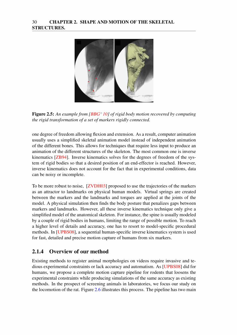
Once the 3D trajectories of the markers are extracted from the videos, different track-ing techniques can be used to extract 3D kinematic information about the skeletalstructures. A common technique consists in computing the transformation of a set ofmarkers considered rigidly connected to the same bone. The transformation of this setfrom one time step to another gives the transformation of the underlying bone. Anexample from [BBG+10] can be seen on Figure 2.5. This method is accurate andprecise. However, it requires at least 3 non-colinear markers to be rigidly connected toeach other and to each of the skeletal structures of interest. It can be difficult to attachthat many markers on small animals, firstly for practical reason, secondly given thelimited resolution of imaging devices.
Decreasing the number of markers required is possible as proven with techniques suchas inverse kinematics. Indeed, most computer animation techniques consider a simpli-fied version of the skeleton as a set of rigid bodies with a reduced number of degrees offreedom. Usually, the skeleton is a hierarchy of rigid bodies linked by ball-and-socketjoints. Some joints are sometimes further constrained to only have one or two degreesof freedom. For instance, the elbow is usually modeled as a hinge joint, having only
30 CHAPTER 2. SHAPE AND MOTION OF THE SKELETALSTRUCTURES.
Figure 2.5: An example from [BBG+10] of rigid body motion recovered by computing
the rigid transformation of a set of markers rigidly connected.
one degree of freedom allowing flexion and extension. As a result, computer animationusually uses a simplified skeletal animation model instead of independent animationof the different bones. This allows for techniques that require less input to produce ananimation of the different structures of the skeleton. The most common one is inversekinematics [ZB94]. Inverse kinematics solves for the degrees of freedom of the sys-tem of rigid bodies so that a desired position of an end-effector is reached. However,inverse kinematics does not account for the fact that in experimental conditions, datacan be noisy or incomplete.
To be more robust to noise, [ZVDH03] proposed to use the trajectories of the markersas an attractor to landmarks on physical human models. Virtual springs are createdbetween the markers and the landmarks and torques are applied at the joints of themodel. A physical simulation then finds the body posture that penalizes gaps betweenmarkers and landmarks. However, all these inverse kinematics technique only give asimplified model of the anatomical skeleton. For instance, the spine is usually modeledby a couple of rigid bodies in humans, limiting the range of possible motion. To reacha higher level of details and accuracy, one has to resort to model-specific proceduralmethods. In [UPBS08], a sequential human-specific inverse kinematics system is usedfor fast, detailed and precise motion capture of humans from six markers.
2.1.4 Overview of our method
Existing methods to register animal morphologies on videos require invasive and te-dious experimental constraints or lack accuracy and automatism. As [UPBS08] did forhumans, we propose a complete motion capture pipeline for rodents that loosens theexperimental constraints while producing simulations of the same accuracy as existingmethods. In the prospect of screening animals in laboratories, we focus our study onthe locomotion of the rat. Figure 2.6 illustrates this process. The pipeline has two main

2.1. PREVIOUS WORK 31
branches, one corresponding to the acquisition of the morphology (Section 2.2.1) andthe animation model built from it (Section 2.3), the other to the acquisition of motiondata (Section 2.2.2). Those two branches join to produce the animation of the internalstructures from the videos (Section 2.4).
Figure 2.6: Pipeline of our method for marker-based tracking of moving morpholo-
gies.

32 CHAPTER 2. SHAPE AND MOTION OF THE SKELETALSTRUCTURES.
2.2 GEOMETRY AND MOTION DATA ACQUISITION
To animate animal morphologies from videos, one must first acquire both the mor-phology of the animal and some motion cues from the videos, as illustrated by the twobranches of Figure 2.6. The animal morphology data is represented by a set of 3Dpolygonal models extracted from CT-scans. The motions cues from the videos are the3D trajectories of markers implanted on the skin of the animal.
2.2.1 Acquisition of the geometrical models of the bones
The geometrical models of the bones of the animal to be studied are extracted fromComputed Tomography scans (CT-scan). The CT-scan of the animal gives us volumet-ric data where each element of the volume, each voxel, contains a density value. Thehigher the density of the material being imaged, the less X-rays make it through to thefilm. As bone is denser than flesh, bones are displayed in white in CT-scans whereasflesh is displayed in grey (see Figure 2.7). If one takes into consideration only thevoxels whose density is the same as the density of bone, one can extract the skeletonfrom the CT-can (see top left of Figure 2.8). From these voxels, an isosurface can bebuilt with a Marching Cube algorithm [LC87]. This results in a 3D mesh (see top rightof Figure 2.8).
Figure 2.7: Slice of a CT-scan of the skull of a rat. The bone’s density is higher than
that of soft tissues, which means the skull is displayed in white whereas the flesh is
displayed in grey.
However, this 3D mesh is one non-articulated piece containing all bones, without anyway of differentiating between the different structures. Using available volumetric vi-sualisation softwares such as Amira Software (Visage Imaging), the different skeletalstructures can be segmented on the volumetric data. Once the segmentation is done,the 3D polygonal models of the different bones can be extracted as separate meshesthough Marching Cubes. Figure 2.8 shows on the bottom row the result of segmenta-tion by colouring each segmented structure differently.

2.2. GEOMETRY AND MOTION DATA ACQUISITION 33
Figure 2.8: CT-scan of a rat - top : unsegmented isosurface of the volumetric data -
bottom : segmentation of the different bones where each bone is represented by its own
colour.
In our case, rodents are rather small animals. To be able to properly segment andextract the different bones, we had the opportunity to acquire high-precision and high-resolution scans at the European Synchrotron Radiation Facility (ESRF) in Grenoble.This acquisition resulted in 4 CT-scans with a 50 micrometers precision of 4 rats. Onthe right of Figure 2.8, we can see the level of details we can obtain on the front pawof the rat. Such precision allows us to individually segment the carpal bones of the rat.However, some other CT-scans we acquired did not have a good enough precision tobe able to segment all the individual bones. Using [GRP10], we were able to adaptthe ESRF CT-scan to automatically segment low-resolution CT-scans of both rats andmice. Figure 2.9 shows an example of automatic segmentations of another rat.
We now have acquired the morphological information we need to register morpholo-gies to videos in the shape of a set of 3D meshes, each mesh representing one individualbone. The motion information used to register those meshes to the videos is the 3Dtrajectories of markers implanted on the animal.
2.2.2 Acquisition of the trajectories of the markers
As explained in Section 2.1, markerless techniques for internal measures require toomuch user input and clear imaging to automatically study the motion of an entire mor-phology. We therefore first focus on marker-based methods. As a result, the informa-tion extracted from the videos are the trajectories of markers.

34 CHAPTER 2. SHAPE AND MOTION OF THE SKELETALSTRUCTURES.
Figure 2.9: From [GRP10], automatic registration of the segmented model of Fig-
ure 2.8 (bottom) to a surface extracted from another CT data (top in white).
As all the cameras of the set-up are synchronised and calibrated in the same refer-ence frame, the set-up can be used to measure the 3D position of points from at least 2of their projections by triangulation. Indeed, knowing the imaging parameters as wellas the position and orientation of a camera, the pixel coordinates of the projection of a3D points gives us a line on which the 3D point lies (see Figure 2.10), the viewing line.Two projections of the same 3D point on two different viewpoints give two viewinglines which intersect at the 3D point.
In our case, the 2D projections of the markers are tracked through the sequence auto-matically (several methods can be used : Lucas-Kanade, correlation factor, see [Hed08]for a short survey). If automatic methods fail on some frames, manual tracking can bemade less difficult by using epipolar geometry. Epipolar geometry gives a number ofgeometric relations between the 3D points and their projections onto the 2D imagesthat lead to constraints between the image points. For example, given the projectionof a 3D point on a camera, the corresponding viewing line can be projected on anotherviewpoint (see Figure 2.11). This projection is a line called the epipolar line of the 2Dpoint and its equation can be directly computed from the camera parameters. The pro-jection of the 3D point on this new viewpoint is therefore known to be on the epipolar

2.2. GEOMETRY AND MOTION DATA ACQUISITION 35
Figure 2.10: Triangulation : if the projection of a 3D point P is known in two view-
points : p0 and p1, then the position of P can be built as the intersection of the 2
viewing lines.
line. Figure 2.12 shows an example on rat locomotion. Figure 2.13 shows an exampleof gait analysis of a rat by showing the 3D trajectories of the eyes and left toe of theanimal during locomotion.
Figure 2.11: Epipolar geometry : if the projection of a 3D point is known to be p0 in a
viewpoint, the projection in another viewpoint lies on the epipolar line of p0 (red line).
We have thus obtained morphological information from CT-scans and motion infor-mation from videos. The morphological information is a set of 3D meshes and themotion information is a set of 3D trajectories of markers. To be able to register themeshes on the markers, one must first define how the 3D meshes are allowed to move.

36 CHAPTER 2. SHAPE AND MOTION OF THE SKELETALSTRUCTURES.
Figure 2.12: Example of marker tracking - top row : a point is marked on one camera
(green point), the epipolar lines can be computed for the other viewpoints (green lines)
- middle row : the same point is marked on another camera (yellow point), it lies on
the green epipolar line. The epipolar lines can be computed for the other viewpoints
(yellow line) - bottom row : from those two projections, the 3D coordinates of the
marker can be computed and projected back to the cameras (red points).
Figure 2.13: Example of 3D trajectories of markers during rat locomotion.

2.3. ANIMATION MODEL OF THE INTERNAL STRUCTURES 37
2.3 ANIMATION MODEL OF THE INTERNAL
STRUCTURES
So far, the models that can be animated are simply geometry : a set of vertices and faceswith no articulation between the different meshes representing the different skeletalstructures. To animate such models, granted that the 3D trajectories of points on themodels are known, one can resort to SVD-based methods [BBG+10] where the rigidmotion of a bone is computed as the rigid transformation of a set of markers implantedon that bone. However, such a method requires at least 3 markers per bone to animate,which is very hard to achieve for motion capture of the complete skeleton of smallanimals. To be able to loosen the experimental constraints by reducing the numberof markers required, one must give an underlying structure to this set of independentmeshes.
2.3.1 Set of articulated solids
To create an underlying structure to the set of meshes, the skeleton is modeled as a setof articulated solids. Each solid represents one bone or a group of bones. The boneor bones represented by a solid will be called the anatomical entity of the solid. Eachsolid has 6 degrees of freedom (3 in translation and 3 in rotation) expressed in theworld reference frame. Given one anatomical entity, the mesh or meshes modeling theentity are rigidly mapped to the solid representing it. As a result, every rigid transfor-mation applied to the solid will be applied to the mesh(es). The solid can be consideredas the animation model of the anatomical entity and the meshes as the visual model ofthe anatomical entity. For example, in Figure 2.14, the forearm is an anatomical entityrepresented by one solid that rigidly drives a visual model made of two meshes : onemodeling the radius and one modeling the ulna. The same way, the humerus is ananatomical entity represented by one solid that rigidly drives a visual model made ofonly one mesh modeling the humerus.
To enforce anatomical constraints on the anatomical entities, we define articulationsbetween pairs of solids. They are illustrated on Figure 2.14. An articulation betweentwo solids is modeled by creating a reference frame at the position of the articula-tion for each solid. Those reference frames are called joint frames. They are definedby their position (3 degrees of freedom) and their orientation (3 degrees of freedom).Those degrees of freedom are rigidly mapped to the solid they belong to. As a result, ateach articulation between two solids, there are two joint frames, each rigidly mappedto one of the two solids. Figure 2.14 shows a 3D representation of those joint framesat the top right and a 2D representation at the bottom (red).

38 CHAPTER 2. SHAPE AND MOTION OF THE SKELETALSTRUCTURES.
Figure 2.14: Animation model - top : Bone models with visualisation of solid bodies
(left), frames defining the solid bodies (middle), joint frames (right) - bottom : Each
solid body (blue) is rigidly connected to a joint frame (red and dark red). On the rest
pose (left), the joint frames are the same. Once the bones move with respect to each
other (right), each joint frame stays rigidly connected to one of the body (see small red
frames), resulting in different transformations for the two joint frames (green).
On the rest pose, the pose in which the solids and articulations are defined, the twojoint frames at an articulation are defined to be the same i.e. they have the same po-sition and orientation. As the two joint frames are rigidly mapped to different solids,when the solids move with respect to one another, the joint frames are subjected to dif-ferent rigid transformations. Therefore, in a deformed pose, the deformation inducesa translation and/or a rotation in-between the two joint frames, see bottom right ofFigure 2.14. For any given deformed pose, there are therefore two types of measuresof motion available. First, the position and orientation of all anatomical entities areknown in the world reference frame. Second, the transformation from the rest pose ofone solid with respect to the other solids it shares an articulation with can be computedin the solid reference fame from the joint frames.
The level of details of the modeling depends on the level of details of the anatomi-cal entities. For instance, each carpal bone can be considered one anatomical entity or,on the other end of the scale, all carpal bones as well as the metacarpal bones and the

2.3. ANIMATION MODEL OF THE INTERNAL STRUCTURES 39
phalanxes can be grouped in one anatomical entity : the front paw. Figure 2.15 showtwo different levels of details that can be considered for the mouse. Treating eachseparate bone individually is a thorough approach but increases the complexity of theproblem, sometimes for irrelevant results, such as each individual carpal bone. On theother hand, if restricting the number of anatomical entities to the few articulations ofinterest seems interesting, experience shows that it is often hard to choose beforehandwhich articulations will turn up to be of interest. For instance, the spine is made upof 20 vertebrae, when excluding the tail. Knowing beforehand which articulations tomodel in-between vertebrae is hard to predict as the movement is usually distributedover all vertebrae. As a result, a trade-off between the complexity of the problem andthe precision of the model must be found depending on the final goal of the tracking.In this thesis, we propose a model that is suited for studies of the global movement ofrodents, not a particular articulation. For instance, our model is suited to measure themovement between the femur and the tibia, but not to measure the movement of thepatella with respect to those two bones.
Figure 2.15: Different level of details possible to model a mouse. The solids are
displayed as red parallelepipeds.
As a result, we model rodent morphology as illustrated on Figure 2.16 and as fol-lows :
1. The head is modeled as one solid.
40 CHAPTER 2. SHAPE AND MOTION OF THE SKELETALSTRUCTURES.
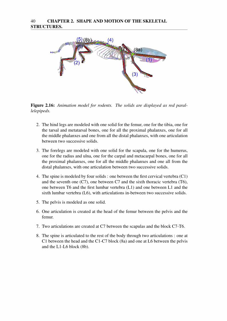
Figure 2.16: Animation model for rodents. The solids are displayed as red paral-
lelepipeds.
2. The hind legs are modeled with one solid for the femur, one for the tibia, one forthe tarsal and metatarsal bones, one for all the proximal phalanxes, one for allthe middle phalanxes and one from all the distal phalanxes, with one articulationbetween two successive solids.
3. The forelegs are modeled with one solid for the scapula, one for the humerus,one for the radius and ulna, one for the carpal and metacarpal bones, one for allthe proximal phalanxes, one for all the middle phalanxes and one all from thedistal phalanxes, with one articulation between two successive solids.
4. The spine is modeled by four solids : one between the first cervical vertebra (C1)and the seventh one (C7), one between C7 and the sixth thoracic vertebra (T6),one between T6 and the first lumbar vertebra (L1) and one between L1 and thesixth lumbar vertebra (L6), with articulations in-between two successive solids.
5. The pelvis is modeled as one solid.
6. One articulation is created at the head of the femur between the pelvis and thefemur.
7. Two articulations are created at C7 between the scapulas and the block C7-T6.
8. The spine is articulated to the rest of the body through two articulations : one atC1 between the head and the C1-C7 block (8a) and one at L6 between the pelvisand the L1-L6 block (8b).

2.3. ANIMATION MODEL OF THE INTERNAL STRUCTURES 41
As a result, we have a set of articulated solids defining anatomical entities. There-fore, each individual bone can be described in the animation model by the anatomicalentity to which it belongs. This entity has an associated solid defined entirely by itsposition and orientation. Given the anatomical entity to which it belongs, the motionof each bone is thus defined by the motion of the associated solid.
2.3.2 Refined model of the spine and ribcage
The model described in Section 2.3.1 only has four solids to describe the motion of thespine and the ribcage attached to it. For large deformations, this can lead to a ‘blocky’aspect as can be seen on Figure 2.17. On top of visual aspects, such a small number ofsolids prevents a precise measure of the position and orientation of each vertebra. Onthe other hand, modeling all vertebrae leads to a complex model that is not necessarilyrequired. We propose a trade-off between accuracy and complexity by modeling thespine and ribcage through a 3D cubic Hermite spline driven by the four solids describ-ing the spine.
Figure 2.17: Top, side and bottom view of the spine and ribcage in the rest pose (left).
When deforming the spine and ribcage using only 4 solids (right), the ribs separate
(bottom), inter-penetrate (middle) and the deformation of the vertebrae is not smooth
(top).

42 CHAPTER 2. SHAPE AND MOTION OF THE SKELETALSTRUCTURES.
Hermite splines are used to smoothly interpolate between key-points. An Hermitespline is a third-degree spline, defined by two control points and two control tangents.It is very easy and fast to calculate. To interpolate a series of points Pk, k = 1..n,interpolation is performed on each interval (Pk, Pk+1). The equation of the Hermitespline between Pk and Pk+1 is :
Ck(u) = h00(u)Pk + h10(u)Dk + h01(u)Pk+1 + h11(u)Dk+1 (2.1)
with u ∈ [0, 1], Dj is the tangent at control point Pj and hij are the basis functions anddefined as :
h00(u) = 1− 3u2 + 2u3
h10(u) = u− 2u2 + u3
h01(u) = 3u2 − 2u3
h11(u) = −u2 + u3
(2.2)
Figure 2.18 shows an example of a 2D Hermite spline.
Figure 2.18: Example of a 2D Hermite spline with 3 control points.
We model the spine and ribcage with an Hermite spline. A rodent has 7 cervicalvertebrae, 13 thoracic vertebrae and 6 lumbar vertebrae. The ribcage is made up of theribs and the sternum (see Figure 2.19). Each thoracic vertebra has a rib attached to it.The first seven ribs are attached to the sternum that is composed of 6 bones.
The Pk of Equation (2.1) are chosen as the mid-points between the two joint framesat each articulation between the four solids defining the spine. Figure 2.20 illustratesthe process on two solids. This gives us five points. Their tangents, i.e. the Dk ofEquation (2.1), are computed by finite difference as :
Dk =Pk+1 − Pk
2+Pk − Pk−1
2(2.3)
We are therefore able to compute the Hermite spline on the rest pose. For each bonei composing the spine and ribcage, the barycenter Bi of the mesh is computed. Thepoint P on the Hermite spline that is closest to Bi is stored as two components : thesegment ki it belongs to and the parametric coordinate ui such that P = Cki(ui). Wealso store P as the initial position on the Hermite curve. Figure 2.21 shows the Her-mite spline reconstructed on the rest pose. Explanations on how the Hermite spline

2.3. ANIMATION MODEL OF THE INTERNAL STRUCTURES 43
Figure 2.19: Segmentation of the different bones constituting the ribcage.
is used during animation and how it improves the animation of the spine and ribcagewith respect to the solids’ animation are shown in Section 2.4.3.
Figure 2.20: Illustration of how the control points and tangents of the Hermite spline
are computed from the set of articulated solids.
Figure 2.21: 3D Hermite spline fit on the rest pose of the animation model.

44 CHAPTER 2. SHAPE AND MOTION OF THE SKELETALSTRUCTURES.
In the end, each individual bone segmented from the CT-scan has its motion defined ineither one of these ways :
• it is defined by the anatomical entity it belongs to and its motion is the same asthe corresponding solid
• it is defined by a segment, a parametric coordinate and an initial position on aHermite spline and its motion will be described in Section 2.4.3.

2.4. MARKER-BASED TRACKING OF THE INTERNAL STRUCTURES 45
2.4 MARKER-BASED TRACKING OF THE INTERNAL
STRUCTURES
We now have an animation model where each piece of geometry defining internalstructures is defined either by their corresponding solid or by a parametric coordinateon a Hermite spline. The Hermite spline itself is computed from the positions of the4 solids of the spine. The problem of tracking can therefore be formulated as : howdo we set the degrees of freedom of the solids so that the visual models fit the videos?The motion cues extracted from the videos are the 3D trajectories of the markers (Sec-tion 2.2.2).
2.4.1 Sequence-specific model
In Section 2.3, we have developed a generic rodent animation model. However, everyanimal that is captured has a different morphology. On top of that, for every sequence,a different set of markers is implanted. This leads us to develop a sequence-specificmodel for each sequence of motion capture from the generic animation model. Thespecificity comes in two forms : the size of the animal and the positions of the markers.
Definitions of landmarks on the animation model
To be able to register the animation model to the markers, one must first know wherethe markers are on the animation model. To do so, we create what we call landmarks
on anatomical entities. These landmarks are the positions of the markers with respectto the anatomical entities in the rest pose. They are rigidly mapped to an anatomicalentity. Figure 2.22 shows how landmarks are submitted to the rigid transformation ofthe solid they are associated with.
In the best case scenario, the animal used in the study has been scanned with the mark-ers implanted as in [BBG+10]. This way, the position of the landmarks can directly bemeasured from the CT-scan. However, as mentioned previously, this is often not thecase. To overcome this issue, several strategies can be used, differing in the amount ofuser intervention involved. First of all, these positions can be specified manually. Thiscan be done with the visual help of the model superimposed on the videos. This way,if the model is manually rotoscoped as in [GBJD10], the 3D position of the marker ascomputed in Section 2.2.2 can be used as landmark. To automate the process, if themarker is implanted on the bone surface, once the animation model is rotoscoped, thepoint on the bone model that is closest to the 3D position of the marker can be selectedas landmark.
Most of the time, however, the makers are glued on the skin that is not rigidly con-nected to the bones. This makes the assumption that a landmark is rigidly mappedto an anatomical entity false (see the white marker on the tibia on Figure 2.2). Theposition of the landmark is therefore an approximation, not a ground truth that can be

46 CHAPTER 2. SHAPE AND MOTION OF THE SKELETALSTRUCTURES.
Figure 2.22: Landmarks (green and red spheres) are rigidly mapped to anatomical
entities. The green landmarks correspond to external markers, the red landmarks cor-
respond to internal markers, not visible on standard cameras. When the anatomical
entity moves (bottom), the landmarks are submitted to the same rigid transformation.
measured by a scan. To better approximate this position, we develop a trial-and-errormethod during tracking that will be explained in Section 2.4.4.
Morphological adaptation to a specific subject
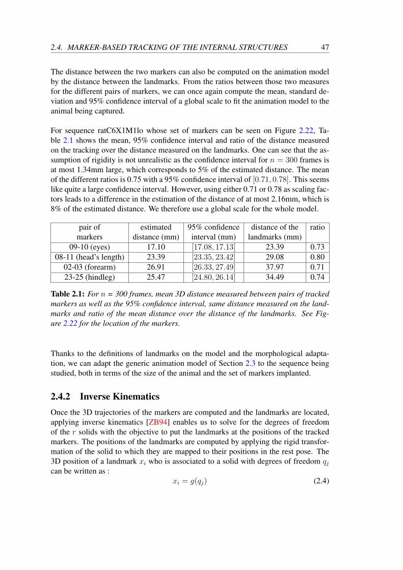
Most of the time, the CT-scan of the animal that is captured through videos is not avail-able. The generic rodent animation model developed in Section 2.3 has to be adaptedto fit the animal being captured. To do this, we align features that can be measured bothon the generic model and the videos. In our case, we align a set of distances betweenlandmarks that are rigidly connected to the same distances between the correspondingmarkers. More precisely, the measured features are the distance between the eyes, thedistance from the front to the back of the head, the length of the forearm and the lengthof the hindleg (see Table 2.1).
Indeed, from the 3D trajectories of a given pair of markers, we can compute the 3Ddistance between those two markers through the n frames of the sequence. From thisseries of distances, one can extract the mean and standard deviation of the distance andcompute the 95% confidence interval of the distance. For a confidence interval smallerthan 1mm, we can approximate the parameters with the mean.
2.4. MARKER-BASED TRACKING OF THE INTERNAL STRUCTURES 47
The distance between the two markers can also be computed on the animation modelby the distance between the landmarks. From the ratios between those two measuresfor the different pairs of markers, we can once again compute the mean, standard de-viation and 95% confidence interval of a global scale to fit the animation model to theanimal being captured.
For sequence ratC6X1M1lo whose set of markers can be seen on Figure 2.22, Ta-ble 2.1 shows the mean, 95% confidence interval and ratio of the distance measuredon the tracking over the distance measured on the landmarks. One can see that the as-sumption of rigidity is not unrealistic as the confidence interval for n = 300 frames isat most 1.34mm large, which corresponds to 5% of the estimated distance. The meanof the different ratios is 0.75 with a 95% confidence interval of [0.71, 0.78]. This seemslike quite a large confidence interval. However, using either 0.71 or 0.78 as scaling fac-tors leads to a difference in the estimation of the distance of at most 2.16mm, which is8% of the estimated distance. We therefore use a global scale for the whole model.
pair of estimated 95% confidence distance of the ratiomarkers distance (mm) interval (mm) landmarks (mm)
09-10 (eyes) 17.10 [17.08, 17.13] 23.39 0.7308-11 (head’s length) 23.39 [23.35, 23.42] 29.08 0.80
02-03 (forearm) 26.91 [26.33, 27.49] 37.97 0.7123-25 (hindleg) 25.47 [24.80, 26.14] 34.49 0.74
Table 2.1: For n = 300 frames, mean 3D distance measured between pairs of tracked
markers as well as the 95% confidence interval, same distance measured on the land-
marks and ratio of the mean distance over the distance of the landmarks. See Fig-
ure 2.22 for the location of the markers.
Thanks to the definitions of landmarks on the model and the morphological adapta-tion, we can adapt the generic animation model of Section 2.3 to the sequence beingstudied, both in terms of the size of the animal and the set of markers implanted.
2.4.2 Inverse Kinematics
Once the 3D trajectories of the markers are computed and the landmarks are located,applying inverse kinematics [ZB94] enables us to solve for the degrees of freedomof the r solids with the objective to put the landmarks at the positions of the trackedmarkers. The positions of the landmarks are computed by applying the rigid transfor-mation of the solid to which they are mapped to their positions in the rest pose. The3D position of a landmark xi who is associated to a solid with degrees of freedom qjcan be written as :
xi = g(qj) (2.4)

48 CHAPTER 2. SHAPE AND MOTION OF THE SKELETALSTRUCTURES.
where g is the result of applying the rigid transformation described by qj to the land-mark’s initial position. This is forward kinematics. Inverse kinematics (IK) consistsin setting the position xi of the landmark and search for qj such that Equation (2.4) istrue. Equation (2.4) can be written for all m landmarks and lead to equation :
x = f(q) (2.5)
where x = (xi)i=1..m, q = (qi)i=1..r and f(q) = (g(qji))i=1..m where ji is the solid thatdrives the landmark i.
As f is not linear, the problem can have zero, one or many solutions though a closed-form solution can be derived in particular cases. To solve the IK problem, it is standardto linearize Equation 2.5 around the current configuration :
f(q + δq) = f(q) + J(q)δq (2.6)
which leads toδx = f(q + δq)− f(q) = J(q)δq (2.7)
where J is the jacobian matrix of f i.e.
Jij =∂fi
∂qj(2.8)
For a small displacement, solving Equation (2.5) comes down to computing the inverseof J to compute the variations of the degrees of freedom δq.
In general, J is non-square, non-inversible. In those cases, the pseudo-inverse of Jcan be used :
δq = J+(q)δx (2.9)
If m < n, the system is under-determined, there are many solutions. The pseudo-inverse is
J+ = JT (JJT )−1 (2.10)
and leads to the solution that minimizes the euclidean norm of δq i.e. chooses thesolution that creates the less variation in the degrees of freedom. If m > n, the systemis over-determined and there may be no solution. In that case, the pseudo-inverse of Jis
J+ = (JTJ)−1JT (2.11)
and leads to the solution in the least-square sense, the one that minimises∑
i
‖xi − x∗i ‖2 (2.12)
where xi is the achieved position of landmark i and x∗i is the tracked position of markeri.

2.4. MARKER-BASED TRACKING OF THE INTERNAL STRUCTURES 49
As we use a linearisation of the IK equation, this solution is valid for small displace-ments. To have the solution ∆q such that
x∗ = f−1(q0 +∆q) (2.13)
where q0 is the initial value of q and x∗ = (x∗i )i=1..m we iterate on small displacementsuntil we reach x∗.
However, IK has a few drawbacks. It involves inverting a matrix, which can be nu-merically unstable. On top of that, all the markers have the same influence. However,as the external markers are not rigidly coupled to the skeletal structures, some markersare more or less representative of the position of the anatomical entity they are asso-ciated with. For example, the assumption of rigidity between the marker and the boneis much more accurate for a point at the ankle where there is not a lot of flesh than fora point on the tibia (see white point in Figure 2.2). As a result, to find the degrees offreedom, we have much more confidence on the marker at the ankle than on the markerat the tibia. Thus, if the landmark at the tibia does not reach the position of the marker,it is less likely that this means the tibia is badly registered than if the landmark at theankle does not reach the marker. It may simply be because the rigidity constraint isnot valid. Finally, to integrate anatomical constraints at the articulations through thejoint frames, one must either solve the IK system with constraints on q or has to re-parameterise the animation model with reduced degrees of freedom to have a hierarchyof joints whose degrees of freedom are the degrees of freedom at the articulations. Wewill see later on how such a parameterisation is not suitable for rodents.
For these reasons, we formulate the tracking as a weighted Inverse Kinematics problemmodeled as a forward dynamics system. Indeed, another way of modeling the IK prob-lem is to consider that markers attract landmarks the way a spring would [ZVDH03].Such a spring creates a force fx applied on the landmarks. As the landmark is rigidlymapped to a certain solid, this force is mapped on the solids as a force fq. Accordingto the principle of virtual work :
qTfq = xTfx (2.14)
where b is the derivative of b with respect to time. We have seen that for a smalldisplacement, linearising gives us Equation (2.7). Substituting Equation (2.7) in Equa-tion (2.14) gives :
fq = J(q)Tfx (2.15)
Applying Newton’s second law, we can compute q, the second derivative of q, from
Mq = fq (2.16)
using the conjugate gradient method for instance. We can then integrate q to computeq, then q. This moves the landmarks towards the positions of the markers x. The
50 CHAPTER 2. SHAPE AND MOTION OF THE SKELETALSTRUCTURES.
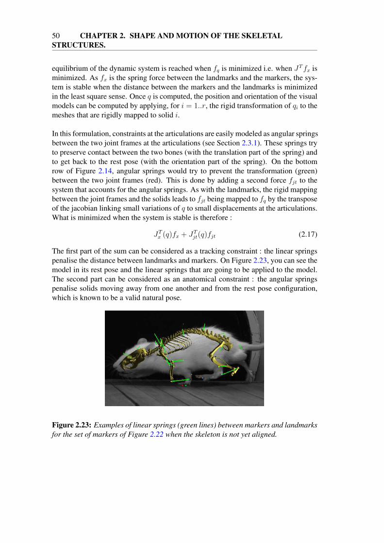
equilibrium of the dynamic system is reached when fq is minimized i.e. when JTfx isminimized. As fx is the spring force between the landmarks and the markers, the sys-tem is stable when the distance between the markers and the landmarks is minimizedin the least square sense. Once q is computed, the position and orientation of the visualmodels can be computed by applying, for i = 1..r, the rigid transformation of qi to themeshes that are rigidly mapped to solid i.
In this formulation, constraints at the articulations are easily modeled as angular springsbetween the two joint frames at the articulations (see Section 2.3.1). These springs tryto preserve contact between the two bones (with the translation part of the spring) andto get back to the rest pose (with the orientation part of the spring). On the bottomrow of Figure 2.14, angular springs would try to prevent the transformation (green)between the two joint frames (red). This is done by adding a second force fjt to thesystem that accounts for the angular springs. As with the landmarks, the rigid mappingbetween the joint frames and the solids leads to fjt being mapped to fq by the transposeof the jacobian linking small variations of q to small displacements at the articulations.What is minimized when the system is stable is therefore :
JTx (q)fx + JT
jt(q)fjt (2.17)
The first part of the sum can be considered as a tracking constraint : the linear springspenalise the distance between landmarks and markers. On Figure 2.23, you can see themodel in its rest pose and the linear springs that are going to be applied to the model.The second part can be considered as an anatomical constraint : the angular springspenalise solids moving away from one another and from the rest pose configuration,which is known to be a valid natural pose.
Figure 2.23: Examples of linear springs (green lines) between markers and landmarks
for the set of markers of Figure 2.22 when the skeleton is not yet aligned.

2.4. MARKER-BASED TRACKING OF THE INTERNAL STRUCTURES 51
The influence of those different penalties can be set through the stiffnesses of the lin-ear and angular springs. Indeed, the higher the stiffness, the higher the penalty. Themore likely the assumption of rigidity between a marker and a solid is to be valid, thehigher the stiffness of the associated linear spring. As for the angular springs, there aretwo stiffnesses : one in translation and one in rotation. The stiffness in translation isusually set high with respect to the stiffness of the linear springs and to the stiffness inrotation because except between the scapula and the the spine, it it unlikely that twoarticulated solids separate. Figure 2.24 illustrates the sliding movement the scapulahas with respect to C7. This also validates the choice not to use reduced degrees offreedom by modeling the animal as a hierarchy of joints. In this type of model, thedegrees of freedom are the rotations at the articulation and do not allow for leniency intranslation, which makes modeling the movements of the scapula harder.
Figure 2.24: The movement of the scapula (delimited by red dots) with respect to the
spine (C7 is enclosed in the red square) can not be considered to be a pure rotation, a
translation has to be modeled as well.
To better understand the influence of adding angular springs, we compare three meth-ods to register the bones to the markers :
1. [BBG+10], an SVD-based method where the rigid transformation of at least 3markers is computed at each instant and applied to the geometry,
2. our method without the angular springs,
3. our method with the angular springs.
Figure 2.25 shows the results on the tracking of the humerus and the forearm (radiusand ulna) of a rat with 4 markers on each anatomical entity. The radius-ulna complexis a long thin entity. Placing 3 non-collinear markers on such structures is difficult. Asa result,computing rigid transformations between those ‘barely’ non-colinear markers

52 CHAPTER 2. SHAPE AND MOTION OF THE SKELETALSTRUCTURES.
is close to ill-conditioned. This can lead to an unnatural roll of the radius with respectto the humerus when using SVD-based methods. Not using the angular springs in ourmethod produces the same artefacts than with an SVD-based methods. Adding angularsprings regularises the solution and prevents the roll of the forearm.
Figure 2.25: From top to bottom : tracking of the forelimb of the rat using an SVD-
based method (grey), using our method with active joint springs (yellow), using our
method with inactive joint springs i.e. with a null stiffness both in rotation and in
translation (pink). Notice how the joint springs correct an invalid roll of the radius.
The influence of the stiffness in rotation can also be seen in Figure 2.40 where wecan see that lowering this stiffness leads to a better reconstruction. Indeed, if a markeris directly implanted on the bone (hence there is a perfect rigid connection between thelandmark and the bone) then we can trust this marker to be a good clue to locate thebone and lower the influence of the rest pose by lowering the stiffness in rotation. Thiscan also be seen on Figure 2.26.
Figure 2.27 shows how using different stiffnesses for the different markers can alsoimprove tracking. Indeed, if the assumption of rigidity is ill-suited (as for marker 3 onFigure 2.22) then lowering the stiffness of that marker leads to a better registration asthe angular springs kick in to help find a correct pose.
In practice, the stiffnesses of the angular springs are set to be the same for all angularsprings with the stiffness in translation three times larger than the stiffness in rotation.The stiffnesses of the linear springs are set individually for each marker depending onthe confidence in the rigidity hypothesis.
Thanks to weighted Inverse Kinematics, we have recovered the positions and orien-tations of the solids. Through rigid transformation, this gives us the position and ori-entation of the different bones. However, as explained in Section 2.3.2, due to coarse-

2.4. MARKER-BASED TRACKING OF THE INTERNAL STRUCTURES 53
Figure 2.26: Choosing a high stiffness in rotation for the angular springs in com-
parison to the stiffnesses of the linear springs (left) leads to a solution closer to the
rest pose but further away from the markers. Decreasing this stiffness leads to results
closer to the markers (right).
ness of the model for the spine, the vertebrae and ribcage deform in an unnatural way(Figure 2.17).
2.4.3 Update of the spine and ribcage
To prevent the ‘blocky’ deformation of the spine and ribcage due to the approximationof the spine by only four solids, we modeled the individual bones of the vertebrae, ribsand sternum through a Hermite spline. This Hermite spline is built from the articula-tions in-between the solids of the spine in the articulated model. Once the IK systemis solved as in Section 2.4.2, we can compute the new joint frames at each articulationthrough rigid transformation as each joint frame is rigidly driven by one solid. Oncethe mid-points of the articulations are computed, the Hermite spline can be updatedfollowing Equation (2.1).
A bone of the spine and ribcage is defined by a segment k, a parametric coordinateu and an initial position P . The translation that is applied to the bone is thereforecomputed as :
T = Ck(u)− P (2.18)
The rotation to apply to the bone is computed by spherical linear interpolation (slerp)between the rotation of the neighbouring solids. Indeed each segment k of the Hermitespline corresponds to a solid. The rotation of each bone belonging to the solid k iscomputed as an interpolation of the the rotation of the solid k − 1 and the rotation ofthe solid k + 1 with the interpolating coefficient u. Figure 2.28 shows an example onhow the use of the Hermite spline improves the tracking of the spine and ribcage.

54 CHAPTER 2. SHAPE AND MOTION OF THE SKELETALSTRUCTURES.
Figure 2.27: From top to bottom : frame of an experience with the set of markers of
Figure 2.22 - tracking with a stiffness on marker 3 on the forearm lower than other
stiffnesses - tracking with a stiffness on marker 3 twice the stiffness on other markers.
Thanks to Inverse Kinematics and Hermite spline interpolation, we can compute theposition and orientation of each bone of the skeleton. However, this tracking reliesheavily on the location of the landmarks with respect to the bones. As explained inSection 2.4.1, this process is usually manual and sometimes difficult. We have how-ever developed a strategy to improve this estimation.

2.4. MARKER-BASED TRACKING OF THE INTERNAL STRUCTURES 55
Figure 2.28: To correct the artefacts created by having only 4 solids to model the spine
(left), we use Hermite spline interpolation and spherical linear interpolation to set the
position and orientation of the ribcage (left).
2.4.4 Automatic refinement of the location of the landmarks
Manual placement of landmarks is highly unreliable depending on the number of cam-eras and on the actual placement of the marker. Indeed, a marker implanted on ananatomical point such as the wrist or ankle is easier to locate than a marker implantedat a place where there is a lot of soft tissues, on the thigh for instance. Unfortunately,an error in the location of the landmarks can completely spoil tracking results. Tocompensate for this limitation, we have developed a trial-and-error strategy. Once atracking solution is computed, improving the location of the markers can be done bymeasuring the elongation of the linear springs.
Indeed, after a first estimation of the animation, if a linear spring produces a consistentelongation vector between the landmark and the tracked 3D position in the correspond-ing solid’s reference frame throughout the sequence, one can assume that the landmarkplacement is slightly off. This can be corrected by shifting the landmark by this elon-gation vector.
On all the sequences from the University of Brown described in Section 2.5.1 wherethe animal and set of markers are the same, after a manual estimation of the positionof the landmarks, we track the foreleg of the rat through 736 frames. We applied theautomatic refinement method from this tracking for the 4 markers on the scapula, the 4on the humerus and the 4 on the radius-ulna. We then tracked again the foreleg with thenew positions of the landmarks. Table 2.2 shows that applying this correction signifi-cantly lowers the elongations of the linear springs as the mean elongation is 0.6597mmwithout correction and 0.2688mm after applying the correction.
We have therefore developed a tracking method that registers a generic rodent anima-tion model to a set of 3D trajectories of markers. To do so, landmarks are first defined

56 CHAPTER 2. SHAPE AND MOTION OF THE SKELETALSTRUCTURES.
Scapula Humerus Radius-Ulna
Without correctionmean 0.3618 0.6088 1.0086s.d. 0.1321 0.1696 0.1480max 0.9146 1.4286 2.7222
With correctionmean 0.1232 0.2615 0.2961s.d. 0.0896 0.1035 0.1232max 0.2488 1.0200 1.1161
Table 2.2: Distances in mm between landmarks and tracked 3D positions before and
after automatic refinement of the location of the landmarks for n = 736 frames.
on the model and the animation model is then scaled down to fit the captured animal.Once the sequence-specific animation model is created, the positions and orientationsof the different skeletal structures are tracked through weighted Inverse Kinematicsand refined through Hermite spline interpolation.
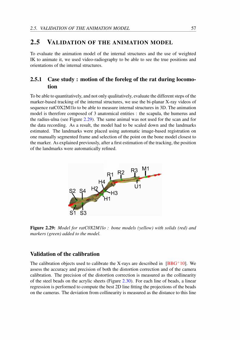
2.5. VALIDATION OF THE ANIMATION MODEL 57
2.5 VALIDATION OF THE ANIMATION MODEL
To evaluate the animation model of the internal structures and the use of weightedIK to animate it, we used video-radiography to be able to see the true positions andorientations of the internal structures.
2.5.1 Case study : motion of the foreleg of the rat during locomo-tion
To be able to quantitatively, and not only qualitatively, evaluate the different steps of themarker-based tracking of the internal structures, we use the bi-planar X-ray videos ofsequence ratC0X2M1lo to be able to measure internal structures in 3D. The animationmodel is therefore composed of 3 anatomical entities : the scapula, the humerus andthe radius-ulna (see Figure 2.29). The same animal was not used for the scan and forthe data recording. As a result, the model had to be scaled down and the landmarksestimated. The landmarks were placed using automatic image-based registration onone manually segmented frame and selection of the point on the bone model closest tothe marker. As explained previously, after a first estimation of the tracking, the positionof the landmarks were automatically refined.
Figure 2.29: Model for ratC0X2M1lo : bone models (yellow) with solids (red) and
markers (green) added to the model.
Validation of the calibration
The calibration objects used to calibrate the X-rays are described in [BBG+10]. Weassess the accuracy and precision of both the distortion correction and of the cameracalibration. The precision of the distortion correction is measured as the collinearityof the steel beads on the acrylic sheets (Figure 2.30). For each line of beads, a linearregression is performed to compute the best 2D line fitting the projections of the beadson the cameras. The deviation from collinearity is measured as the distance to this line

58 CHAPTER 2. SHAPE AND MOTION OF THE SKELETALSTRUCTURES.
of the projected beads. The beads project as discs of about 10 pixels of radius. Beforedistortion correction, the mean of those distances is 3.9±5.1 pixels (see Figure 2.31for their distribution). As Figure 2.31 illustrates, once the distortion of the images iscorrected, most of those distances are below 2 pixels. This results in a mean of 2.0±2.6pixels. Distortion has a greater impact the farther away from the image center (see Fig-ure 1.7). As a result, correcting the distortion mostly corrects the position of the beadsprojecting on the border of the images. This is why we see that the distribution is farless spread and the maximum distance is smaller when distortion correction is applied.Distortion correction brings back the beads that were creating the greatest distances(up to 24 pixels) to a more correct position.
Figure 2.30: Calibration object used for bi-planar X-ray sequences.
Figure 2.31: Distribution of the collinearity error before (left) and after (right) distor-
tion correction.
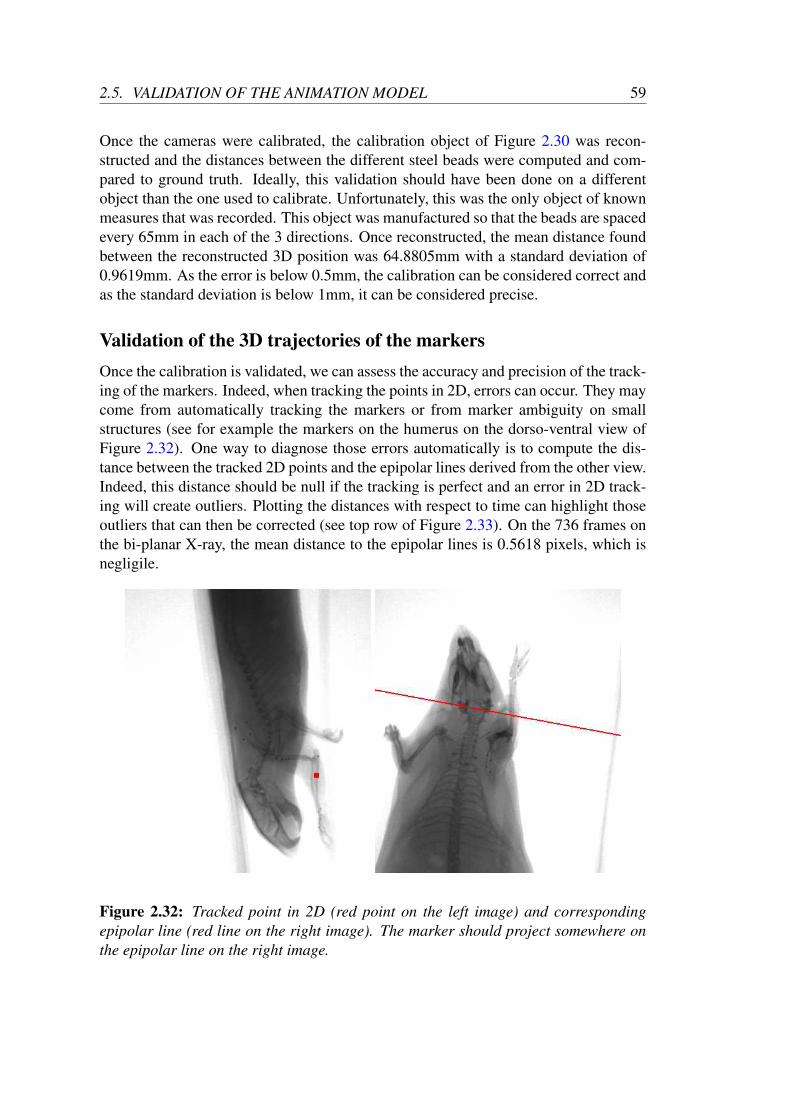
2.5. VALIDATION OF THE ANIMATION MODEL 59
Once the cameras were calibrated, the calibration object of Figure 2.30 was recon-structed and the distances between the different steel beads were computed and com-pared to ground truth. Ideally, this validation should have been done on a differentobject than the one used to calibrate. Unfortunately, this was the only object of knownmeasures that was recorded. This object was manufactured so that the beads are spacedevery 65mm in each of the 3 directions. Once reconstructed, the mean distance foundbetween the reconstructed 3D position was 64.8805mm with a standard deviation of0.9619mm. As the error is below 0.5mm, the calibration can be considered correct andas the standard deviation is below 1mm, it can be considered precise.
Validation of the 3D trajectories of the markers
Once the calibration is validated, we can assess the accuracy and precision of the track-ing of the markers. Indeed, when tracking the points in 2D, errors can occur. They maycome from automatically tracking the markers or from marker ambiguity on smallstructures (see for example the markers on the humerus on the dorso-ventral view ofFigure 2.32). One way to diagnose those errors automatically is to compute the dis-tance between the tracked 2D points and the epipolar lines derived from the other view.Indeed, this distance should be null if the tracking is perfect and an error in 2D track-ing will create outliers. Plotting the distances with respect to time can highlight thoseoutliers that can then be corrected (see top row of Figure 2.33). On the 736 frames onthe bi-planar X-ray, the mean distance to the epipolar lines is 0.5618 pixels, which isnegligile.
Figure 2.32: Tracked point in 2D (red point on the left image) and corresponding
epipolar line (red line on the right image). The marker should project somewhere on
the epipolar line on the right image.

60 CHAPTER 2. SHAPE AND MOTION OF THE SKELETALSTRUCTURES.
Figure 2.33: Diagnosis of errors in the tracking of markers - top row : sum of the dis-
tances between the tracked 2D points and the epipolar lines for the markers attached
to the radius, bottom row : elongation created by the markers on the radius.
As the markers are implanted directly on the bones, one can measure the accuracyof the 3D tracking by measuring the distance between markers implanted on the samebone and checking that this distance stays constant through the tracking. Mathemati-cally, this means that the standard deviation of the distance between markers implantedon the same bone measured over the 736 frames should be null. We computed the dis-tance between the 18 pairs of rigidly-connected markers of our experiment on the 736frames available. The mean standard deviation is 0.2006mm, which is negligible foranatomical study of rat bones.
Validation of the tracking of the bones
To validate the marker-based tracking of the bones, we compare our method to theSVD-based tracking of [BBG+10]. Indeed, as there are 4 markers on the scapula, 4markers on the humerus and 4 markers on the radius-ulna, we can use the rigid trans-formation of each set of markers to reconstruct the motion of the different bones. Wecan as a result test our method against a method proven to be accurate.
In our method, as the markers are implanted on the bones and therefore all rigidlyconnected to the bone, the stiffness of the linear springs is the same for all markers.For the same reason, the stiffness in rotation of the angular springs is chosen low. Asthe joints involved are assumed to be ball-and-socket joints, the stiffness in translationof the angular springs is chosen high.

2.5. VALIDATION OF THE ANIMATION MODEL 61
One measure of the correctness of the tracking is the elongation of the linear springs.The elongations for the 5 sequences are reported on Table 2.2. Observing these dis-tances over time, spikes in the elongations can be seen (bottom of Figure 2.33). Oneway to diagnose these errors is by looking at those side by side with the 2D trackingerror computed to validate the 2D tracking of the markers. We can see on Figure 2.33that the spikes in the elongations match errors in the 2D tracking. These spikes arethus more likely to come from tracking errors than from a fault in our tracking method.
To validate our method, we also compare our results by tracking the bones using theUniversity of Brown Xromm tools presented in [BBG+10]. Quantitatively, we cancompare directly the transformations computed by the two methods. Figure 2.34 (re-spectively Figure 2.35, Figure 2.36) shows the position and orientation of the scapula(respectively humerus, radius-ulna) obtained with both methods for one of the 5 se-quences. If the results seem similar, our solution appears to give smoother results (seethe rotation about Y of the radius-ulna for example). The only major difference is thepeaks for the humerus that have a smaller amplitude with our method. This can be seenfor instance around frame 660 on Figure 2.35. Figure 2.37 shows the reconstructionfor both methods on frame 660. One can notice that, unlike the SVD-based method,our method does not lead to penetration between the scapula and the humerus. Fol-lowing [WAK+10], we assess the similarity between both results by computing thecorrelation coefficient between the trajectories of the degrees of freedom of the model.Table 2.3 shows those correlation coefficients for the different anatomical entities. Thetrajectories can be considered equivalent.
Tx Ty Tz Rx Ry Rzscapula 0.9958 0.9943 0.9976 0.9958 0.9993 0.9897humerus 0.9917 0.9495 0.9719 0.8753 0.9810 0.9761
radius-ulna 0.9829 0.9742 0.9781 0.8570 0.9789 0.7302
Table 2.3: Correlation coefficients of the degrees of freedom of the solids recovered
with rigid transformations between sets of markers and recovered with our method for
n = 736 frames.
Qualitatively, we can however point out a few differences between both methods. Asexplained in Section 2.4.2, for long thin bones, placing 3 non-collinear markers canbe difficult and leads to ill-conditioned problem with an SVD-based model. As shownin Figure 2.25, this creates noise on the roll of the radius-ulna whereas the angularsprings in our method regularises the solution and prevents that noise. Overall, ourmethod gives less jittery results by preserving natural articulation constraints. It is lesssensitive to noise coming from the tracking of the markers or from the fact that the po-sitions of the landmarks are estimated and not extracted from the CT-scan. Qualitativecomparisons of SVD-based methods and our method can be seen on Figure 2.38 and2.39.

62 CHAPTER 2. SHAPE AND MOTION OF THE SKELETALSTRUCTURES.
(a) Translation X (red), Y (green), Z (blue)
(b) Rotation X (red), Y (green), Z (blue)
Figure 2.34: Comparison of the tracking of the scapula with rigid transformations
between sets of markers (dots) and our method (line).
Study of the influence of the number and location of the markers
This experiment also allows us to study the influence of the number of markers as wellas the influence of where the markers are implanted on the quality of our tracking.Unlike methods that rely on at least 3 markers per bone to compute the rigid transfor-

2.5. VALIDATION OF THE ANIMATION MODEL 63
(a) Translation X (red), Y (green), Z (blue)
(b) Rotation X (red), Y (green), Z (blue)
Figure 2.35: Comparison of the tracking of the humerus with rigid transformations
between sets of markers (dots) and our method (line).
mation of a bone, our method does not require a certain amount of markers. However,the number of markers will influence the precision of the tracking. We study this in-fluence using the animation with all markers (4 per anatomical entity) presented aboveas ground truth.

64 CHAPTER 2. SHAPE AND MOTION OF THE SKELETALSTRUCTURES.
(a) Translation X (red), Y (green), Z (blue)
(b) Rotation X (red), Y (green), Z (blue)
Figure 2.36: Comparison of the tracking of the radius-ulna with rigid transformations
between sets of markers (dots) and our method (line).
To do so, we decrease the number of markers used to reconstruct the movement ofthe animal and study the difference between this tracking and the ground truth. Wealso measure the distance between the landmarks and the tracked 3D markers for themarkers that are not used in the weighted IK. Table 2.4 sums up the results. We cansee, logically, that using 3 or 4 markers does not make a significant difference. Even

2.5. VALIDATION OF THE ANIMATION MODEL 65
Figure 2.37: Comparison of the scapula-humerus articulation tracked with rigid
transformations between sets of markers (left) and our method (right) on frame 660.
(a) (b) (c) (d)
(e) Lateral view (f) Ventrodorsal view
Figure 2.38: Comparison of tracking using rigid transformations between sets of
markers (grey) and our method (yellow) on 4 consecutive frames (a-d). One can notice
the sudden shift of the radius that occurs between (a) and (b) as well as its sudden
twist that occurs between (b) and (c) with the SVD-based method. On the other hand,
our method produces a smooth natural tracking. Bottom row shows the frames used
for tracking.
with 1 marker per bone, we can obtain a reconstruction valid within 5◦.
This experiment also highlights which markers lead to a more accurate tracking. Wecan notice on Table 2.4 that choosing marker R1 (on the elbow) or marker R3 (on the

66 CHAPTER 2. SHAPE AND MOTION OF THE SKELETALSTRUCTURES.
Figure 2.39: Overlay of SVD-based tracking (middle) and our tracking (right). Notice
how the radius comes out of the body at the radius/carpal articulation in the SVD-
based tracking.
radius-metacarpal articulation) greatly modifies the reconstruction (see Figure 2.29 forthe name and location of the markers). The first two images in Figure 2.40 illustratethe issue raised by choosing marker R3. In the first image, the elbow is not constrainedby a marker. This leads the angular springs to have a greater influence on the anglemade between the humerus and the radius. Indeed, as R1 and Hii=1..4 are not enoughto remove the ambiguity of the location of the elbow, the preferred position is onesimilar to the one in the rest pose. This results in a badly located elbow. This can beavoided by lowering the stiffness in rotation of the angular springs, hence lowering theinfluence of the rest pose (right of Figure 2.40).
This process gives us an experimental protocol on how to loosen experimental con-straints by lowering the number of markers. Indeed, we have shown that we do notrequire as many markers as SVD-based methods to track the bones. However, not alllocations for markers lead to the same accuracy. One could first do an experimentwith many markers on a cadaveric animal, test which ones are important and then leadother experiments on live animals with a less invasive experimental protocol by onlyimplanting the markers required to fall within a certain accuracy.
The robustness of our method can be used to reconstruct bones on which 3 non-collinear markers are hard to implant. On the data from the cadaver rat, there is onlyone marker on the metacarpal bone of the fourth digit. With our technique, we can

2.5. VALIDATION OF THE ANIMATION MODEL 67
Markers used Bones ‖TXromm − TSbromm‖ (mm), difference in Rx,Ry,Rz (◦) Max d(landmark,marker) (mm)S1 S2 S4 scapula 0.1511, 0.4541 0.3271 0.6269
1.8969H1 H2 H4 humerus 0.1369, 0.3932 0.3768 0.3573R1 R2 R3 M1 radius 0.3012, 0.6228 1.0359 0.9641S1 S3 scapula 0.8965, 2.1927 2.3722 3.8907
2.1768H1 H4 humerus 0.4446, 1.1578 1.1019 1.5233R1 R3 M1 radius 0.2877, 0.5563 0.9345 0.9878S1 S4 scapula 0.7716, 1.7582 1.4798 3.3740
1.8198H1 H4 humerus 0.2549, 0.6268 0.8091 0.9363R1 R3 M1 radius 0.3230, 0.6488 1.1306 1.0537S1 scapula 1.2050, 2.8222 3.1287 5.1481
2.4442H1 humerus 0.4934, 1.2698 1.1907 1.9536R1 R3 M1 radius 0.3048, 0.6230 1.0353 1.0366S1 scapula 2.7641, 4.3179 5.6471 12.8113
8.2003H1 humerus 1.7550, 5.5889 4.8697 9.9182R3 M1 radius 1.6557, 5.3109 5.4406 5.6671S1 scapula 1.1779, 2.9475 2.9435 4.9965
3.9305H1 humerus 0.5898, 1.6811 1.6512 1.8233R1 M1 radius 1.0598, 1.9516 3.3752 3.6056
Table 2.4: Study of the influences of the markers used for tracking for n = 736 frames.
See Figure 2.29 for markers’ location.
Figure 2.40: Study of the influences of the markers used for tracking. From left to
right : using marker R1, using marker R3, using marker R3 with stiffness in rotation
lowered. See Figure 2.29 for markers’ location.
reconstruct the movement of this bone (Figure 2.41).

68 CHAPTER 2. SHAPE AND MOTION OF THE SKELETALSTRUCTURES.
Figure 2.41: Tracking of the metacarpal bone of the rat with only one marker on it.
Application
Bi-planar X-ray videos has allowed us to evaluate the different steps of our marker-based tracking (Figure 2.6) : calibration, tracking of markers, influence of the numberand location of landmarks, weighted IK. However, this is an ideal set-up with severalX-ray videos and markers implanted on the bones, which is not always available. Wetherefore try to reproduce the same experiment but on our locomotion platform, pre-sented in Section 1.2.2 by tracking the foreleg of a rat running on a treadmill.
The set-up consists of 4 cameras and 1 lateral cineradiography. As studied before[BC10][FPC+06], reconstructing motion from markers on the skin suffers from thefact that those markers are not rigidly connected to the bones. As such, SVD-basedmethods result in largely incorrect results. However, with our weighted Inverse Kine-matics method that relies on two types of constraints (anatomical and tracking), wecan obtain valid results (Figure 2.42). Figure 2.43 shows the flexion-extension at thearticulations as well as the height of the wrist for 2 cycles of locomotion for both thebi-planar set-up (left) and the treadmill set-up (right). The movement is not expectedto be the same in both cases as a manual simulation of locomotion is not the same as anatural cycle of locomotion. However, we can see that the movements are consistent.

2.5. VALIDATION OF THE ANIMATION MODEL 69
Figure 2.42: Tracking of rat locomotion. The green spheres in the top left image are
the landmarks of the bones.
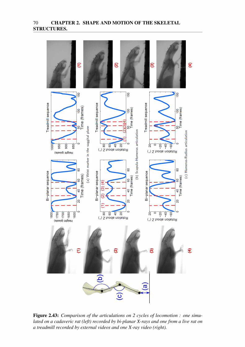
70 CHAPTER 2. SHAPE AND MOTION OF THE SKELETALSTRUCTURES.
Figure 2.43: Comparison of the articulations on 2 cycles of locomotion : one simu-
lated on a cadaveric rat (left) recorded by bi-planar X-rays and one from a live rat on
a treadmill recorded by external videos and one X-ray video (right).

2.5. VALIDATION OF THE ANIMATION MODEL 71
2.5.2 Results for various morphologies and motions
The process having been validated on the foreleg, we use the whole model as describedin Section 2.3 on two types of motion : locomotion and swimming. Results on the lo-comotion sequences (ratC6X1M1lo and ratC4X1M1lo) can be seen on Figure 2.44 andFigure 2.46. For those sequences, an X-ray video is available as well as makers surgi-cally implanted directly on the bones. Those markers can not be tracked in 3D, thusthey can not be used in our tracking, but their 2D positions can be tracked on the X-rayvideo. There are not enough markers to be able to conduct a comparison to SVD-basedmethods but our tracking can be evaluated by comparing the 2D reprojections on theX-ray of landmarks on the bone and the true positions of the markers as tracked onthe X-ray video. For ratC6X1M1lo, the mean error of these reprojections over 300frames (6 cycles of locomotion) for the 9 internal markers is 15 pixels. At the depthof the rat, this is equivalent to 2.4mm. Figure 2.45 shows a comparison of the positionof the simulated landmarks and the ground truth (tracked markers) for one cycle oflocomotion. One can see that the markers on the humerus (left) and the tibia (right) arevery close to ground truth whereas they were not used for tracking. In the middle, onecan see that one of the markers of the spine is pretty far from ground truth. However,the trajectory is the same. This bias is explained by the fact that the landmark was notproperly located on the animation model. As this marker is not used for tracking, ithas no impact on our results. For the sequence ratC4X1M1lo, the mean error for the17 internal markers over 375 frames (4 cycles of locomotion) is 10 pixels, which isequivalent to 1.6mm.
On the swimming sequence ratC5X0M1sw, no X-ray video is available. Figure 2.47shows our tracking from the 15 markers. The distribution of the markers is : 4 mark-ers on the head, 3 on the spine, 1 on each shoulder, thigh, wrist and fifth metatarsal.This leads to only 8 anatomical entities with makers on them. For comparison, in thelocomotion sequences, about 15 anatomical entities had external markers attached. Itcan qualitatively be seen that this leads the tracking to be less precise. Therefore, eventhough our method is more robust to a low number of markers than previous methodsto precisely and accurately track internal structures of animals, the precision of ourmethod is still dependent on the number of markers.
In the context of this thesis, the method has been extensively used and validated onrodents. However, nothing in our method is specific to rodents. For any species, ananimation model can be derived as in Section 2.3 and our tracking method used to re-cover the state of the animation model from videos. Figure 2.48 shows an example oftracking zebra finches during take-off and landing.
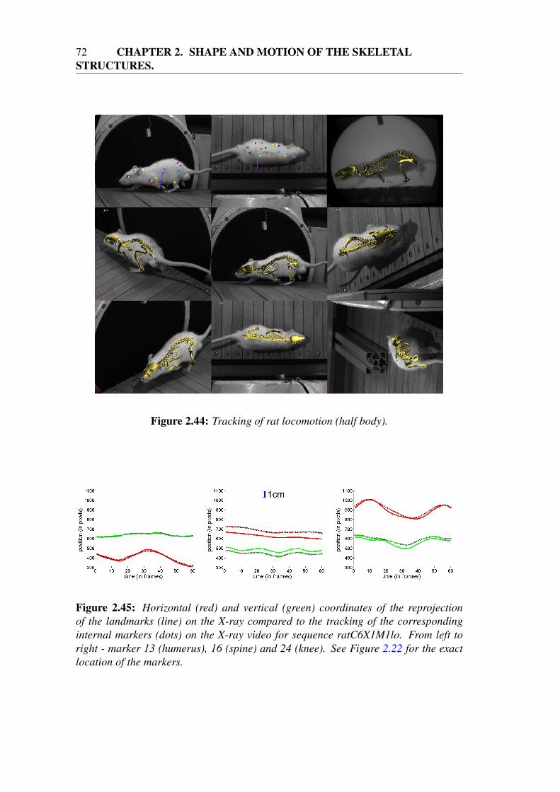
72 CHAPTER 2. SHAPE AND MOTION OF THE SKELETALSTRUCTURES.
Figure 2.44: Tracking of rat locomotion (half body).
Figure 2.45: Horizontal (red) and vertical (green) coordinates of the reprojection
of the landmarks (line) on the X-ray compared to the tracking of the corresponding
internal markers (dots) on the X-ray video for sequence ratC6X1M1lo. From left to
right - marker 13 (humerus), 16 (spine) and 24 (knee). See Figure 2.22 for the exact
location of the markers.

2.5. VALIDATION OF THE ANIMATION MODEL 73
Figure 2.46: Tracking of rat locomotion (half body).
Figure 2.47: Tracking of rat swimming.

74 CHAPTER 2. SHAPE AND MOTION OF THE SKELETALSTRUCTURES.
Figure 2.48: Tracking of zebra finch landing.
2.6. CONCLUSION 75
2.6 CONCLUSION
We have presented a model for the skeletal structures of rodents that can be animatedwith weighted Inverse Kinematics using markers on the skin. Thanks to the weightingsystem and the use of anatomical constraints, we have been able to overcome the arte-facts usually seen when using markers on the envelope of the animal. This has beenvalidated with the use of X-ray videos. However, a perfect validation would have beento use a set-up with both standard cameras and external markers (as in ratC6X1M1lo)and bi-planar X-ray videos and internal markers (as in ratC0X2M1lo). Unfortunately,such a set-up was not available to us.
Still, we have demonstrated that our method is reliable and robust to skin sliding.Nevertheless, markers are not always available or desirable. Most often than not, theonly cue available is images of the envelope. But given what we have demonstratedin this chapter, if we are able to track the skin from those images with a temporallycoherent mesh, we can track the internal structures by using points of this mesh tosimulate markers. To do so, we therefore need a temporally consistent envelope thatdeforms over time.

76 CHAPTER 2. SHAPE AND MOTION OF THE SKELETALSTRUCTURES.
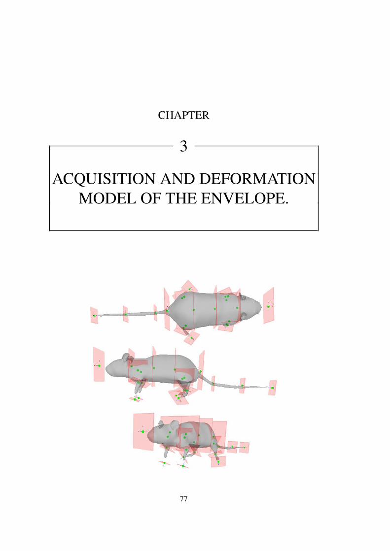
CHAPTER
3
ACQUISITION AND DEFORMATIONMODEL OF THE ENVELOPE.
77
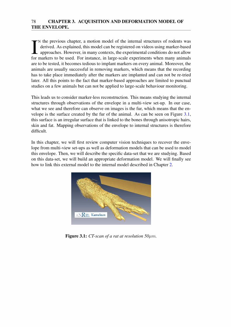
78 CHAPTER 3. ACQUISITION AND DEFORMATION MODEL OFTHE ENVELOPE.
IN the previous chapter, a motion model of the internal structures of rodents wasderived. As explained, this model can be registered on videos using marker-basedapproaches. However, in many contexts, the experimental conditions do not allow
for markers to be used. For instance, in large-scale experiments when many animalsare to be tested, it becomes tedious to implant markers on every animal. Moreover, theanimals are usually successful in removing markers, which means that the recordinghas to take place immediately after the markers are implanted and can not be re-triedlater. All this points to the fact that marker-based approaches are limited to punctualstudies on a few animals but can not be applied to large-scale behaviour monitoring.
This leads us to consider marker-less reconstruction. This means studying the internalstructures through observations of the envelope in a multi-view set-up. In our case,what we see and therefore can observe on images is the fur, which means that the en-velope is the surface created by the fur of the animal. As can be seen on Figure 3.1,this surface is an irregular surface that is linked to the bones through anisotropic hairs,skin and fat. Mapping observations of the envelope to internal structures is thereforedifficult.
In this chapter, we will first review computer vision techniques to recover the enve-lope from multi-view set-ups as well as deformation models that can be used to modelthis envelope. Then, we will describe the specific data-set that we are studying. Basedon this data-set, we will build an appropriate deformation model. We will finally seehow to link this external model to the internal model described in Chapter 2.
Figure 3.1: CT-scan of a rat at resolution 50µm.

3.1. PREVIOUS WORK 79
3.1 PREVIOUS WORK
3.1.1 Multi-view reconstruction
In order to recover the geometry of the envelope, we use a marker-less multi-viewset-up as a capture device. Extracting dense information from several cameras is be-ing studied extensively in computer vision. The different techniques can be classifieddepending on the kind of information they extract from the images : depth maps orgeometry.
Historically, monocular vision systems have evolved to several cameras with the de-velopment of stereo-vision techniques. Indeed, from two calibrated stereo-cameras, adisparity map can be computed. Each pixel of the disparity map stores the differencein location of corresponding features in the two images. As illustrated on Figure 3.2,the closer the point is to the camera, the larger the disparity is. From this disparitymap, a depth information can thus be extracted and stored in a depth map. An in-depthsurvey of stereo-vision techniques can be found in [SS02].
Figure 3.2: Disparity map - left : original image - right : disparity map from [SS02].
This however requires to find corresponding features in both images. To overcomethe difficulty that stereo-vision has to tackle scenes that lack textures, structured lightcan be used. In structured light set-ups, patterns are projected onto the scene to createartificial textures that make the matching process easier and more robust. An examplefrom [ZSCS04] can be seen on Figure 3.3. However, such set-ups are cumbersome andunpleasant for live subjects, even frightening for animals because the projectors tendto dazzle the subjects.
In recent years, time-of-flight cameras have been developed. These cameras directly

80 CHAPTER 3. ACQUISITION AND DEFORMATION MODEL OFTHE ENVELOPE.
Figure 3.3: An example of structured light reconstruction from [ZSCS04].
record the depth map of the observed scene. An evaluation of the use of those camerascan be found in [KBKL09].
However, stereo-vision provides us with limited knowledge of the 3D scene as thethickness of the observed object is unknown and the surfaces occluded by the objecton the foreground can not be reconstructed. For instance, the back of the head can notreconstructed in Figure 3.3.
The second kind of information that can be extracted from multi-view systems is ge-ometry. The techniques that extract such information fall into different categories de-pending on the information they use : matched features or silhouettes.
In the first category, the techniques are the same as the ones used in stereo-vision.Features are matched in-between different cameras. If one camera gives us a 3D lineon which the 3D point lies, the line that goes from the center of camera through thepixel on the image plane (as seen on Figure 3.4), two cameras provide two lines thatcan be intersected at the position of the 3D point. This process is called triangulation.In [SCD+06], a review and an evaluation of those techniques are conducted. As instereo-vision techniques, this approach suffers from lack of textures in the scene andstructured light can be used.
Another clue that can be used to extract 3D geometry from multi-view systems is thesilhouette of the studied object on the images. As explained in [Lau94], the silhouettesdefine a 3D space in-which the object can lie. Laurentini defines the visual hull as themaximal 3D envelope of the studied object that projects back inside the silhouettes ofall cameras. As a result, the studied object is completely inside the visual hull. Anexample of a visual hull can be seen on Figure 3.4. The visual hull is not the objectitself but an approximation of it. For instance, concavities can not be recovered fromsilhouettes. The quality of the visual hull depends on the quality of the silhouettes andon the number of viewpoints.
One of the most common methods to compute the visual hull is to voxelise the scene

3.1. PREVIOUS WORK 81
Figure 3.4: An example of a visual hull (slice representation).
and decide for each voxel if they belong to the object or not. A voxel belongs to theobject if and only if it projects into a silhouette in all images. A review of voxel-basedtechniques can be found in [SMCS]. The result is a set of voxels labeled as being partof the object (Figure 3.5). The precision of the reconstruction thus depends on theresolution of the voxel grid. Most of the time, Marching Cube [LC87] is then used tobuild a mesh from the voxel grid in order to apply many computer graphics techniquessuch as texturing or smoothing to the result.
Figure 3.5: An example of a voxel model inside the scene volume as reconstructed in
[CKBH00].

82 CHAPTER 3. ACQUISITION AND DEFORMATION MODEL OFTHE ENVELOPE.
Another method relies not on the inside of the silhouettes but on its contours to di-rectly build a surface. Indeed, as can be seen in Figure 3.4, each pixel on the contourof the silhouettes generates a viewing line going through the center of the camera andthe pixel. The set of viewing lines generated from one image generates a viewing conewhose peak is the center of the camera. The intersection of the viewing cones gener-ated from the different viewpoints is the visual hull. Unlike in voxel techniques, thisvisual hull is a polyhedron.
All these methods generate temporally independent reconstructions of the studied ob-ject that can be used as a template on which a deformation model can be built. Thechoice of this deformation model is paramount to realistic and smooth deformations.
3.1.2 Deformation model
Traditionally, in computer animation, characters (humans, animals or creatures) are an-imated with skeleton animation. Skeleton animation requires a mesh and a hierarchyof joints called skeleton (see Figure 3.6). Each joint (except the root of the hierarchy)is traditionally modeled as an ideal revolute or ball-and-socket mechanical joint de-fined by its rotation relative to its parent. As a result, it has either 1, 2 or 3 degrees offreedom and its distance to its parent is constant. The root has 6 degrees of freedomwhich determines the global position and orientation of the skeleton.
The mesh, called skin, is first binded to the skeleton. This operation is called skin-ning. To do that, the skeleton is fitted to the mesh in a rest pose. For each vertex ofthe mesh, a weight is set to each joint. We therefore have a weight wi,j for each pair ofvertex and joint. This weight represents the influence of the bone j on vertex pi : thelarger the weight, the more influenced the vertex is. It can be computed automaticallyas a function of the distance between the vertex and the joint or attributed manually.In the end, in linear blend skinning, each vertex pi can be expressed as the weightedlinear interpolation of the transformation of the joints :
pi =∑
j
wi,jMjM−10,j p0,i (3.1)
where Mj is the current global transformation at joint j, M0,j is the global transforma-tion of joint j in the rest pose and p0,i is the position of vertex i in the rest pose. It canbe noticed that skinning does not deform the mesh when the skeleton is in its rest poseif and only if for each vertex i, the sum of all the weights wi,j is equal to 1.
Then, to animate the mesh, the animation skeleton is animated i.e. the transforma-tions of the joints are modified, leading to a deformation of the initial mesh as a resultof equation (3.1) (see bottom of Figure 3.6). Linear blend skinning is thus a simpleand intuitive way to animate a mesh as a simplification of the real skin-bones complex.

3.1. PREVIOUS WORK 83
Figure 3.6: Mesh skinned on an animation skeleton : (top) rest pose - (bottom) ani-
mation of the left elbow joint and right knee joint.
However, linear blend skinning leads to many artefacts such as collapsing joints ortwisting elbows (left of Figure 3.7). This is due to the fact Equation (3.1) can berewritten as pi = Qp0,i where Q =
∑
j wi,jMjM−10,j , which is not necessarily a rigid
transformation.
Several techniques have been proposed over the years to correct these artefacts. In2000, [LCF00] used examples to improve the deformed mesh obtained after linearblend skinning. The modifications made on the skinned mesh are stored as displace-ments : δpexi = pi − pLBS
i where pLBSi is the position obtained by linear blend skin-
ning and pi is the position as set in the example. Then, for any pose of the skeleton,instead of simply computing the vertex as the result of skinning, it is computed aspi = pLBS
i + δpi where δpi is interpolated from all the δpexi with respect to the poseof the skeleton. In 2003, [MG03] built on this idea but instead of storing the dis-placements, they learn from the examples in order to add joints to have more precise
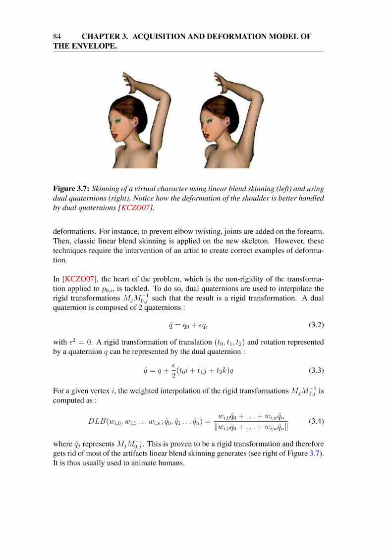
84 CHAPTER 3. ACQUISITION AND DEFORMATION MODEL OFTHE ENVELOPE.
Figure 3.7: Skinning of a virtual character using linear blend skinning (left) and using
dual quaternions (right). Notice how the deformation of the shoulder is better handled
by dual quaternions [KCZO07].
deformations. For instance, to prevent elbow twisting, joints are added on the forearm.Then, classic linear blend skinning is applied on the new skeleton. However, thesetechniques require the intervention of an artist to create correct examples of deforma-tion.
In [KCZO07], the heart of the problem, which is the non-rigidity of the transforma-tion applied to p0,i, is tackled. To do so, dual quaternions are used to interpolate therigid transformations MjM
−10,j such that the result is a rigid transformation. A dual
quaternion is composed of 2 quaternions :
q = q0 + ǫqǫ (3.2)
with ǫ2 = 0. A rigid transformation of translation (t0, t1, t2) and rotation representedby a quaternion q can be represented by the dual quaternion :
q = q +ǫ
2(t0i+ t1j + t2k)q (3.3)
For a given vertex i, the weighted interpolation of the rigid transformations MjM−10,j is
computed as :
DLB(wi,0, wi,1 . . . wi,n; q0, q1 . . . qn) =wi,0q0 + . . .+ wi,nqn
‖wi,0q0 + . . .+ wi,nqn‖(3.4)
where qj represents MjM−10,j . This is proven to be a rigid transformation and therefore
gets rid of most of the artifacts linear blend skinning generates (see right of Figure 3.7).It is thus usually used to animate humans.

3.1. PREVIOUS WORK 85
Still, in the case of rodents, skinning gives unsatisfactory results, particularly on thehind legs. This is due to the fact that mice have a lot more fat that humans do. Thiscreates an important skin sliding effect (Figure 3.8). It is therefore difficult to bindthe skin to the skeleton since a vertex of the hind leg may for instance slide from in-between the knee and ankle to in-between the head of the femur and the knee. Definingthe influence of a joint on a vertex by a simple weighting system as is done in skinningis not appropriate anymore.
Figure 3.8: Skin sliding effect : the markers in red are surgically implanted directly
on the bones (at the ankle and at the knee) whereas the white marker is glued on the
skin of the tibia.
In recent years, cage-based animation has emerged as an extension of lattices andas an alternative to skinning. In cage-based animation, the mesh to deform, called themodel, is embedded in a low-resolution mesh, called the cage. This cage controls thedeformation of the model. The degrees of freedom of the deformation are the positionsof the vertices of the cage vj, j ∈ [0..m]. The vertices of the model pi, i ∈ [0..n],n >> m are computed as the weighted linear combination of the vertices of the cage :
pi =m∑
j=0
wi,jvj (3.5)
The weights wi,j are called coordinates as a reference to barycentric coordinates. Thecore of this method is to compute theses coordinates such that the deformation of thecage leads to an intuitive and realistic deformation of the model. In [FKR05] and[JSW05], a larger study on how to create a function over a mesh that interpolatesknown values at vertices, mean-value coordinates are derived and an analytical solu-tion for piece-wise linear forms is expressed.

86 CHAPTER 3. ACQUISITION AND DEFORMATION MODEL OFTHE ENVELOPE.
However, the mean-value coordinates are based on euclidean distance and do not re-spect such properties as interior locality and non-negativity. Interior locality meansthat the coordinates should decrease as a function of the distance between cage ver-tices and model vertices, the distance being measured within the cage (see top of Fig-ure 3.9). Non-negativity ensures that no coordinate is negative. If a coordinate isnegative then the model vertex and the cage vertex would move in opposite directions,which is counter-intuitive (see bottom left of Figure 3.9). To ensure those two prop-erties, [JMD+07] uses the Laplace equation to derive harmonic coordinates that arenon-negative and have interior locality. However, Harmonic coordinates do not havean analytical solution. A comparison between mean-value coordinates and harmoniccoordinates can be seen on Figure 3.9.
Figure 3.9: Comparison between mean-value coordinates (left) and harmonic coordi-
nates (right) from [JMD+07] - top row : coordinate value for vertex C, yellow indi-
cates positive values, green indicates negative values, grey indicates null values and
red indicates undefined values - bottom row : example on a 3D model, note how mov-
ing the left leg moves the right leg in the opposite direction when using mean-value
coordinates.
In [LLCO08a], Green coordinates are derived from the third integral identity of Green,which is derived from harmonic functions. Green coordinates are proven to be confor-mal in 2D, as well as quasi-conformal in 3D. This ensures that angles are preservedand therefore leads to nice properties in terms of shape preservation and smoothness(Figure 3.10).
Cage-based animation is thus more adequate to deform the envelope of rodents. This
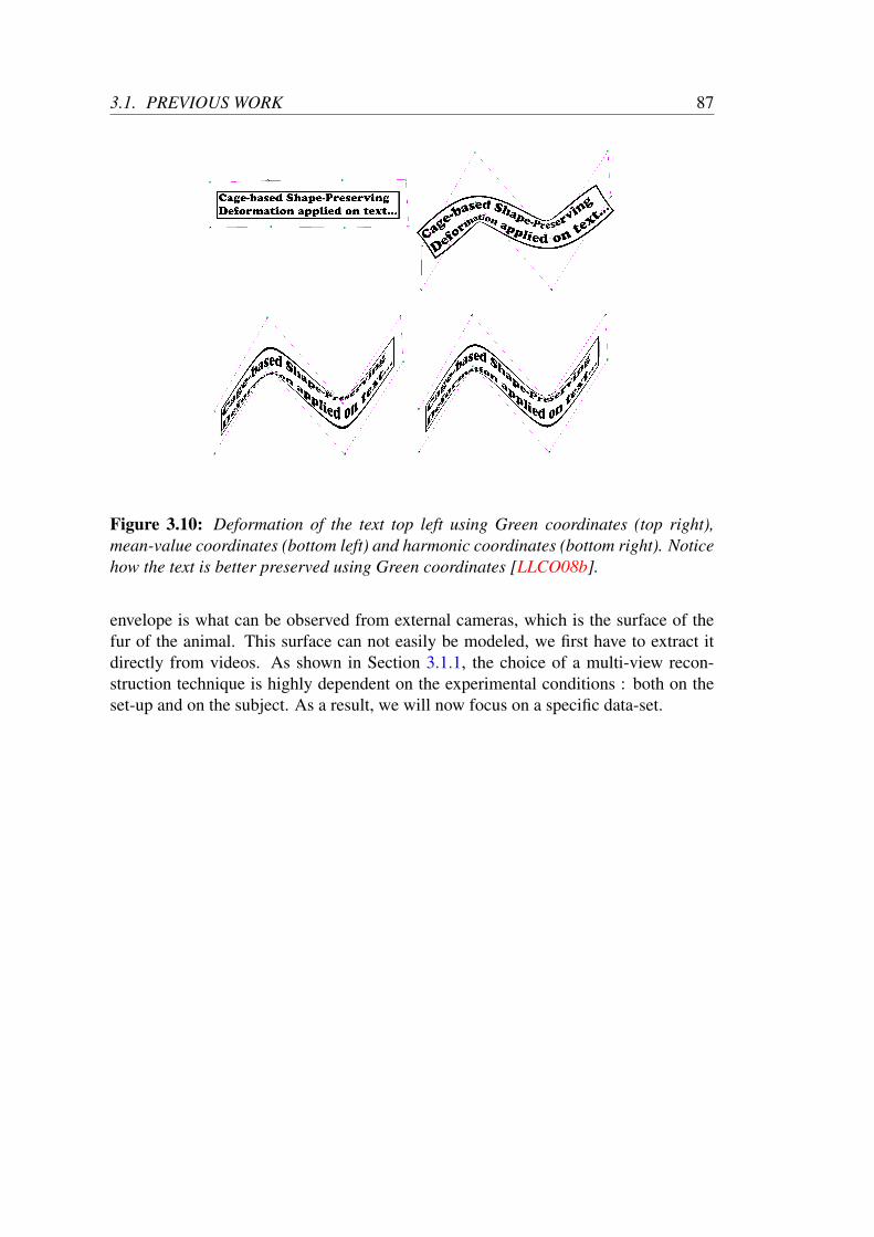
3.1. PREVIOUS WORK 87
Figure 3.10: Deformation of the text top left using Green coordinates (top right),
mean-value coordinates (bottom left) and harmonic coordinates (bottom right). Notice
how the text is better preserved using Green coordinates [LLCO08b].
envelope is what can be observed from external cameras, which is the surface of thefur of the animal. This surface can not easily be modeled, we first have to extract itdirectly from videos. As shown in Section 3.1.1, the choice of a multi-view recon-struction technique is highly dependent on the experimental conditions : both on theset-up and on the subject. As a result, we will now focus on a specific data-set.

88 CHAPTER 3. ACQUISITION AND DEFORMATION MODEL OFTHE ENVELOPE.
3.2 ACQUISITION OF THE ENVELOPE FROM VIDEOS
Multi-view reconstruction is a vast field of research and many methods have been de-veloped over the years to extract shapes from videos. Most methods rely heavily on thescene to reconstruct and on the multi-view set-up as explained in Section 3.1.1. Con-sequently, we will now focus on a specific dataset from which we aim at extractingthe deformation of the envelope of rodents. We focus on the set-up designed to studyvestibular control of mice in micro-gravity, sequences moC8X0M0pf, to explore howstate of the art techniques in multi-view reconstruction perform on our dataset.
Figure 3.11: Video processing pipeline.
From the specific dataset obtained during the parabolic flights, we wish to extract 3Dgeometrical information about the envelope of the mice. As explained in Section 3.1.1,we can either match features or use silhouette informations. As the fur of mice lackstexture and structured light can not be used in our set-up, we wish to use silhouette in-formation. Figure 3.11 illustrates the data processing pipeline to extract and use thesesilhouettes. After having synchronised and calibrated all the cameras so that they are

3.2. ACQUISITION OF THE ENVELOPE FROM VIDEOS 89
defined in a common space and time, the images are segmented to obtain the silhouetteof the mouse, which is then used for multi-view reconstruction.
3.2.1 Background subtraction
The parabolic flight set-up was designed to facilitate background subtraction. Indeed,lighting and materials were selected to avoid shadows and reflections as well as mov-ing background due to activity around the set-up. Figure 3.12 shows the evolution ofthe set-up to improve background subtraction leading to DEL panels covered by anti-reflexive material on the faces of the free-floating cube.
Figure 3.12: Evolution of the set-up to improve background subtraction : from a set-up
with reflections and view of the outside (left) to a better controlled environment (right).
Several options have been tested to define the background in our dataset. Once thisbackground is defined, for each pixel of the image, we want to define if it belongsto the background or to the foreground i.e. the mouse. This leads to computing abinary image where pixels with value 1 are foreground and pixels with value 0 arebackground. The user can define one or several frames as background. If several aredefined, single background subtraction is done with all frames and a criterion to re-duce false positives is chosen : a pixel is in the foreground if it is foreground againstall backgrounds. Indeed, false positives are more likely to be corrected than false neg-atives as false negatives usually happen when the mouse is in front of dark parts of thebackground such as the objectives of the cameras and using several backgrounds willnot solve the problem. Avoiding false positives on the other hand reduces noise thatoccurs especially on the top panel of the free-floating space where the trapdoor is andwhere the outside environment can be seen (see top left of the images in Figure 3.12).When images are chosen by the user for background subtraction, a pixel belongs to theforeground if its grey-level in the current image differs more than a certain thresholdfrom its value in the background image. The threshold is constant for the whole im-age. One can also learn a mean background and its variance throughout a sequence offrames. In this case, a pixel belongs to the foreground if its grey-level in the current
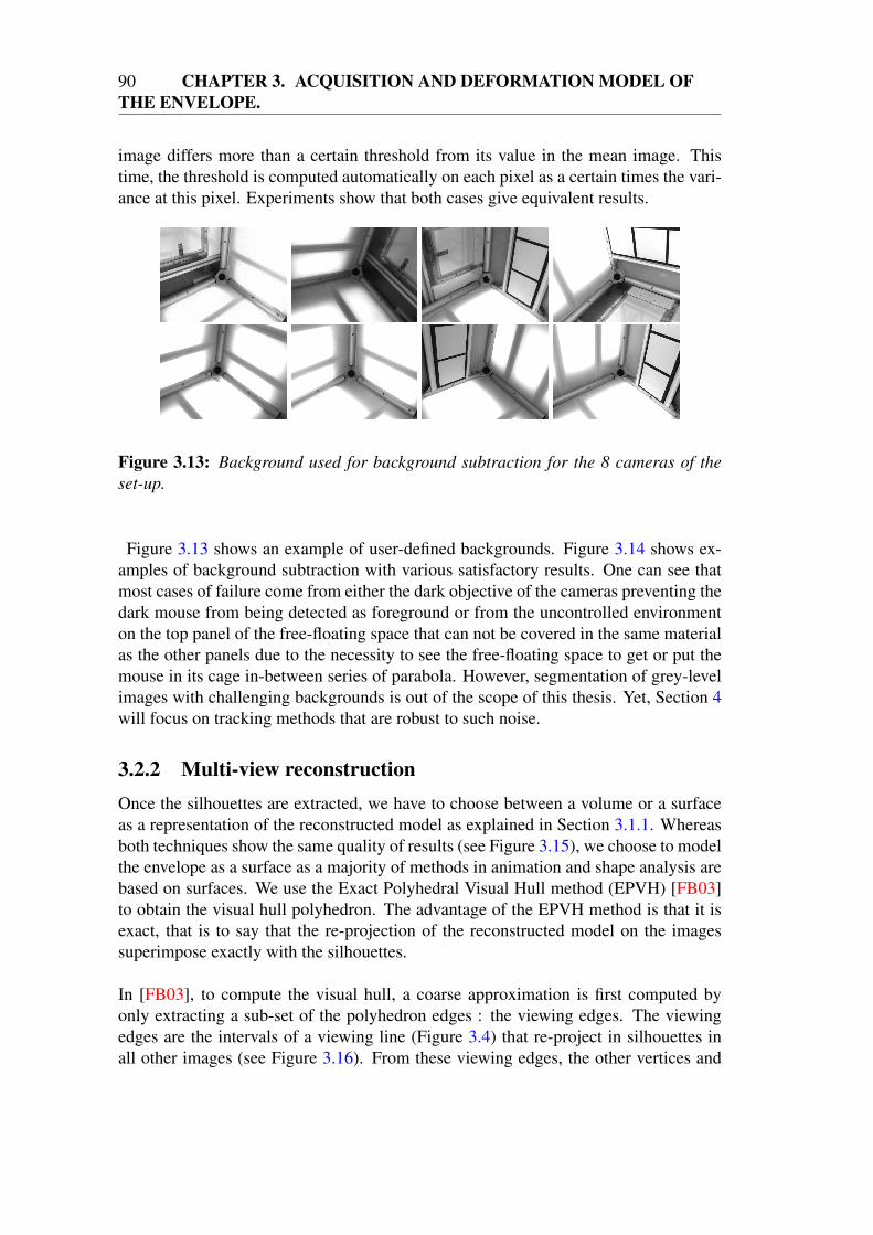
90 CHAPTER 3. ACQUISITION AND DEFORMATION MODEL OFTHE ENVELOPE.
image differs more than a certain threshold from its value in the mean image. Thistime, the threshold is computed automatically on each pixel as a certain times the vari-ance at this pixel. Experiments show that both cases give equivalent results.
Figure 3.13: Background used for background subtraction for the 8 cameras of the
set-up.
Figure 3.13 shows an example of user-defined backgrounds. Figure 3.14 shows ex-amples of background subtraction with various satisfactory results. One can see thatmost cases of failure come from either the dark objective of the cameras preventing thedark mouse from being detected as foreground or from the uncontrolled environmenton the top panel of the free-floating space that can not be covered in the same materialas the other panels due to the necessity to see the free-floating space to get or put themouse in its cage in-between series of parabola. However, segmentation of grey-levelimages with challenging backgrounds is out of the scope of this thesis. Yet, Section 4will focus on tracking methods that are robust to such noise.
3.2.2 Multi-view reconstruction
Once the silhouettes are extracted, we have to choose between a volume or a surfaceas a representation of the reconstructed model as explained in Section 3.1.1. Whereasboth techniques show the same quality of results (see Figure 3.15), we choose to modelthe envelope as a surface as a majority of methods in animation and shape analysis arebased on surfaces. We use the Exact Polyhedral Visual Hull method (EPVH) [FB03]to obtain the visual hull polyhedron. The advantage of the EPVH method is that it isexact, that is to say that the re-projection of the reconstructed model on the imagessuperimpose exactly with the silhouettes.
In [FB03], to compute the visual hull, a coarse approximation is first computed byonly extracting a sub-set of the polyhedron edges : the viewing edges. The viewingedges are the intervals of a viewing line (Figure 3.4) that re-project in silhouettes inall other images (see Figure 3.16). From these viewing edges, the other vertices and

3.2. ACQUISITION OF THE ENVELOPE FROM VIDEOS 91
Figure 3.14: Examples of background subtraction with the original image on the top
right corner : top row shows a case where the results are satisfactory - middle row
shows a case where the dark objective of the camera leads to false negative (see the
head on camera 3 and 6) - bottom row shows a case where the absence of anti-reflexive
material on the top panel leads to false positives (top left on camera 1). The back-
grounds are those shown on Figure 3.13.
edges of the polyhedron are computed by recursively using the geometry and orienta-tion properties of the image contours. Finally, the edges are walked through to identifythe faces.
Figure 3.17 shows the different reconstructions from the silhouettes displayed on Fig-

92 CHAPTER 3. ACQUISITION AND DEFORMATION MODEL OFTHE ENVELOPE.
Figure 3.15: Comparison of space carving and Exact Polyhedron Visual Hull using
the silhouettes of the top row of Figure 3.14.
Figure 3.16: From [FB03] - Viewing edges (red) along a given viewing line.
ure 3.14. Obviously, the quality of reconstruction is highly dependent on the quality ofthe silhouettes as well as on the number of cameras. False negatives in the silhouetteslead to holes in the reconstruction (middle row of Figure 3.17). False positives can leadto small separated connexe components if there is no other view where it reprojects inthe background. This is why the number of cameras that cover the mouse is important.If it is too low, there will not be enough information to discriminate along certain viewdirections which leads to a very coarse approximation of the visual hull (bottom rowof Figure 3.17). When the quality of the reconstruction is good enough as in top rowof Figure 3.17, we can expect to be able to measure differences in pose and motionbetween strains of mice. For instance, Figure 3.18 shows the EPVH of the fall posturethe different strains tend to assume.
However, a comparison other than visual can not be done on these meshes as theyare completely independent, we do not have correspondences between their verticesand the meshes do not even have the same topology. To quantify the differences be-tween the different postures, we have to be able to match information in-between those

3.2. ACQUISITION OF THE ENVELOPE FROM VIDEOS 93
Figure 3.17: Profile, top and front view of the Exact Polyhedron Visual Hulls (EPVH)
reconstructed from the silhouettes on Figure 3.14. The quality of the visual hulls de-
teriorates with the quality of the silhouettes and the number of cameras that cover the
mouse.
Figure 3.18: From left to right : fall postures for control mice, ied mice and IsK mice
(Section 1.2.1) - Control mice tend to adopt an adapted posture and maintain their
spacial orientation, ied mice tend to adopt the same posture but do not seem able
to maintain an appropriate spacial orientation, IsK mice do not seem to adopt any
particular posture or orientation.
meshes. For this, we need a model that we can deform to fit to the reconstructedmeshes.

94 CHAPTER 3. ACQUISITION AND DEFORMATION MODEL OFTHE ENVELOPE.
3.3 DEFORMATION MODEL OF THE ENVELOPE
Multi-view reconstruction applied to a sequence gives us a set of meshes with differ-ent topologies. As a result, extracting anatomical or motion measurements from thissequence of meshes requires to first identify on each and every one of these mesheswhere the features are located. Given the quality of the meshes (see Figure 3.17), thisis a very difficult task as some of the features may not even be reconstructed (see leftfoot on bottom row of Figure 3.17). Another approach is to use an a-priori model ofthe observed object and deform this model to fit the observations. By doing so, anymeasurement defined on the model can be tracked through the sequence. The modelcan for instance be a result of multi-view reconstruction that comprehend all requiredfeatures (for example, the reconstruction on the top row of Figure 3.17). It can alsobe manually modeled or be the result of a 3-D scan. In all those cases, we have thegeometry and topology of the model but no way to deform it to fit the observations. Tobe able to do so, we need a deformation model. As the multi-view reconstruction tech-nique used results in a mesh, we only consider meshes as models. First, Section 3.3.1describes the deformation technique used. Then a parameterisation of this deformationin introduced in section 3.3.2.
3.3.1 Cage-based animation
As explained in section 3.1.2, rodents are not easy to animate because, unlike humanswhose limbs are clearly defined, the limbs of rodents are sometimes not easily discern-able from the body. For example, on Figure 3.19, whereas the thigh and the forearmare easy to identify on the left image, they can not be told apart from the trunk on theright image.
Figure 3.19: Rat during a locomotion cycle.
Due to this skin sliding effect, skinning does not seem an appropriate way to deformthe model. Indeed, thanks to the tube-like shape of humans, an animation skeleton isquite straightforward to design for humans. However, to model deformations such asthe ones on Figure 3.19, designing an animation skeleton and setting good skinning

3.3. DEFORMATION MODEL OF THE ENVELOPE 95
weights is highly difficult. On top of that, an animation skeleton is a very constraineddeformation model as it is usually designed to have at most 3 degrees of freedom perarticulation in rotation and 0 in translation. Once again, this is very well suited for hu-man beings but breaking these constraints becomes necessary to deform other modelsin a natural way. On the other hand, cage-based animation doesn’t lead to such con-straints as the cage that controls the deformations is a mesh. As a result, the degrees offreedom of the model are the positions of the vertices of the cage and those positionsare unconstrained. We opt for a cage-based animation to deform the envelope as it hasbetter properties in terms of shape preservation and smoothness than skinning for bigdeformations such as those that can be witnessed on rodents. From now on, the meshto deform is called the model and the low-resolution mesh controlling the deformationis called the cage. As explained in Section 3.1.2, unlike other barycentric coordinates,Green coordinates are empirically proven to be quasi-conformal (i.e. the angles arepreserved) in 3D and have a closed-form solution. We therefore choose these barycen-tric coordinates to generate the model from the cage.
To ensure that the Green Coordinates are quasi-conformal, the new positions of thevertices of the model are not only dependent on the positions of the vertices of thecage as expressed in Equation (3.5) but also on the orientation of the faces. Keepingthe same notations as in Equation (3.5),
pi =m∑
j=0
φj(p0i )vj +
r∑
j=0
ψj(p0i )sjn(tj) (3.6)
where p0i is the position of the vertex i of the model prior to any deformation, (t0 . . . tr)are the faces of the cage, n(tj) is the unitary normal of face tj , sj is the scaling factorassociated with the face tj and φ, ψ are the Green coordinates functions.
The Green coordinates functions φ and ψ are defined so that the deformation preservesthe shape. Green’s third identity states that for any harmonic function u in a domainD ⊂ R
d, for any p in interior(D) :
u(p) =
∫
∂D
(u(ξ)∂G(ξ, p)
∂n(ξ)−G(ξ, p)
∂u(ξ)
∂n(ξ))dσξ (3.7)
where G is the fundamental solution of the Laplace equation, n is the oriented outwardnormal to ∂D and dσξ is the area element on ∂D. Taking the domain enclosed by thecage to be D and defining u(p) = p, we can derive Equation (3.6) from Equation (3.7)with :
φj(p) =
∫
ξ∈N(vj)
Γj(ξ)∂G(ξ, p)
∂n(ξ)dσξ (3.8)
and
ψj(p) = −∫
ξ∈tj
G(ξ, p)dσξ (3.9)

96 CHAPTER 3. ACQUISITION AND DEFORMATION MODEL OFTHE ENVELOPE.
where N(vj) is the union of all faces in the 1-ring neighbourhood of vj , Γj is thepiecewise-linear hat function defined on N(vj), which is 1 at vj and 0 at all other ver-tices in the 1-ring and linear on each face. We refer to [LLCo08c] for these derivationsas well as for the derivation of closed-form solutions in a 3-dimensional space.
The scaling factors sj in Equation (3.6) are picked to ensure the following proper-ties : linear reproduction, translation, rotation and scale invariance, shape preservationand smoothness. Linear reproduction ensures that applying Equation (3.6) without anydeformation of the cage does not deform the model and is enforced by construction ifsj = 1 when the normal of face tj does not change. Translation, rotation and scale in-variance ensures that any affine transformation applied to the cage deforms the modelas if the same affine transformation was directly applied to the model. Shape preser-vation ensures that the deformations are quasi-conformal in dimension 3. Smoothnessensures that φj and ψj are C∞ inside the cage. In [LLCO08b], those conditions areused to define sj such that, when the normal of tj changes, the deformation is the leastdeforming. ‘The least deforming’ is defined as introducing the less stretch on tj . Thisis measured in 3D as some average chosen empirically between the singular values ofthe linear map deforming the face. This leads to :
sj =
√
‖u′‖2 ‖v‖2 − 2(u′.v′)(u.v) + ‖v′‖2 ‖u‖2√8area(tj)
(3.10)
where (u, v) are vectors defining the edges in tj prior to deformation and (u′, v′) arethe vectors defining the same edges after deformation. This is the optimal coefficientto enforce shape preservation. However, sj can be set to 1 for every face tj if shapepreservation is not required as in the example on Figure 3.28.
As a result, we have a closed-form solution for the Green coordinates and the scal-ing factors. To have fast interactive deformations, the coordinate functions are pre-calculated at the desired positions so that only the scaling factors (if required) and thesums in Equation (3.6) have to be computed to update the model when deforming thecage. There are no requirements on the model : the only information used is the posi-tion of its vertices. This is a very important as the models we aim at deforming are builtfrom multi-view reconstruction and are far from being 2-manifold (see Figure 3.17).
The shape preserving property ensures that artifacts observed in linear blend skinningsuch as elbow collapse do not occur. Figure 3.20 shows both linear blend skinningand cage-based animation applied to same model. The animation skeleton used forskinning consists of two bones. The cage is built as a cube subdivided at the articu-lation between the two bones. It can be seen that the surface is better-preserved withcage-based animation as there is no elbow collapse effect at the articulation betweenthe bones.

3.3. DEFORMATION MODEL OF THE ENVELOPE 97
Figure 3.20: Comparison between skinning and cage-based animation on a cylinder
- left : initial model - middle : skinning - right : cage-based animation with Green
Coordinates.
Figure 3.21: Comparison between skinning and cage-based animation on a more com-
plex model - top, from left to right : initial model, skinning, cage-based animation -
bottom row, from left to right : zoom on skinning result, zoom on cage-based animation
result.
This, of course, can be observed on more complex models such as a rat on Fig-ure 3.21.
Figure 3.22 shows an example of trying to use both skinning and cage-based defor-mation to fit a model made by an artist to an EPVH reconstruction from the parabolicflight dataset. As can be seen on the top row, the animation skeleton and the cage havethe same rest pose on which both the Green coordinates and the skinning weights arecomputed. The skinning is a dual quaternion skinning with skinning weights com-puted automatically with Autodesk Maya [may]. Some manual tuning of the skinning
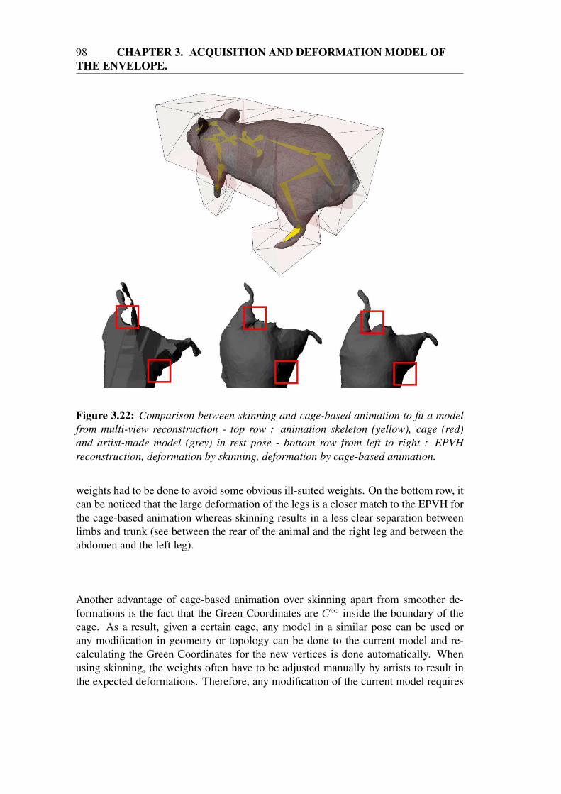
98 CHAPTER 3. ACQUISITION AND DEFORMATION MODEL OFTHE ENVELOPE.
Figure 3.22: Comparison between skinning and cage-based animation to fit a model
from multi-view reconstruction - top row : animation skeleton (yellow), cage (red)
and artist-made model (grey) in rest pose - bottom row from left to right : EPVH
reconstruction, deformation by skinning, deformation by cage-based animation.
weights had to be done to avoid some obvious ill-suited weights. On the bottom row, itcan be noticed that the large deformation of the legs is a closer match to the EPVH forthe cage-based animation whereas skinning results in a less clear separation betweenlimbs and trunk (see between the rear of the animal and the right leg and between theabdomen and the left leg).
Another advantage of cage-based animation over skinning apart from smoother de-formations is the fact that the Green Coordinates are C∞ inside the boundary of thecage. As a result, given a certain cage, any model in a similar pose can be used orany modification in geometry or topology can be done to the current model and re-calculating the Green Coordinates for the new vertices is done automatically. Whenusing skinning, the weights often have to be adjusted manually by artists to result inthe expected deformations. Therefore, any modification of the current model requires

3.3. DEFORMATION MODEL OF THE ENVELOPE 99
tweaking once again the weights manually and using a different model either requiresre-tuning the weights or using complex tools such as transfer functions. Figure 3.23shows an example of using the same motion of the same cage to animate two verydifferent humanoid models of the same size. No manual adjustment had to be made totransfer the animation from one model to the other.
Figure 3.23: Example of the same cage used to animate two different models.
Cage-based animation is thus a flexible fully-automatic way of deforming meshes withensured shape-preservation and smoothness properties. However, the degrees of free-dom of a cage-based deformation model are the positions of the vertices of the cage.This has several drawbacks. First of all, this leads the cage to be counter-intuitiveto create or deform. Indeed, whereas it is intuitive to create and animate a skeleton aseach joint corresponds to an anatomical articulation, vertices of a cage do not representa real-life object and can be moved unconstrained and independently from one-anotherin the 3D space. This lack of link to real-life features such as morphological structuresalso has the inconvenience of making the task of measuring or analysing motion froma cage-based animation hard. Indeed, when studying different gaits of animals fromdigitised animations, one can easily study the movement of the legs by studying thetrajectories of the degrees of freedom of an animation skeleton [GBJD10]. However,there is no direct measure of those trajectories on a cage-based animation. This leadsus to believe that, even though cage-based animation provides a better tool than skin-ning as a deformation model for rodents, it lacks a higher-level representation to makethese deformations intuitive to design, manipulate and analyse. We develop such arepresentation in the next section.
100 CHAPTER 3. ACQUISITION AND DEFORMATION MODEL OFTHE ENVELOPE.
3.3.2 Oriented Quads Rigging (OQR)
Being a coarse approximation of the model, the cage is easier to deform than the ac-tual model but lacks the high-level representation that a skeleton conveys. Converselyto manipulating vertices, a higher-level representation leads to benefits in all steps ofdeformation modeling and analysing. Generating and deforming a cage becomes moreintuitive and analysing these deformations becomes direct. For this, we introduce Ori-ented Quads Rigging (OQR).
Oriented Quads Rigging (OQR) provides an underlying structure to intuitively gen-erate and deform the cage. Oriented quads have 8 degrees of freedom : 2 in scale, 3in translation and 3 in rotation, defined globally. Their geometric representation is arectangle. This quad is defined from a canonical quad transformed according to thedegrees of freedom. The canonical quad is defined as a square of size 1 centered on(0, 0, 0) whose normal is (0, 0, 1) and whose rotation around its normal, the Z axis ,isnull. That means that the four vertices defining the canonical quad have coordinates :
c0 = (−0.5,+0.5, 0)c1 = (+0.5,+0.5, 0)c2 = (+0.5,−0.5, 0)c3 = (−0.5,−0.5, 0)
(3.11)
The degrees of freedom of the oriented quads are :
• two degrees of freedom in scale S = (sx, sy) ;
• three degrees of freedom in rotation θ that define a rotation in 3D. We call Rθ
the rotation representation of this rotation ;
• three degrees of freedom in translation T that define a translation in 3D.
With those notations, the vertices of a quad are computed as :
c0(S, θ, T ) = Rθ
sx 0 00 sy 00 0 1
c0 + T
c1(S, θ, T ) = Rθ
sx 0 00 sy 00 0 1
c1 + T
c2(S, θ, T ) = Rθ
sx 0 00 sy 00 0 1
c2 + T
c3(S, θ, T ) = Rθ
sx 0 00 sy 00 0 1
c3 + T
(3.12)

3.3. DEFORMATION MODEL OF THE ENVELOPE 101
which can be written using the Rodrigues rotation formula :
ci(S, θ, T ) = cos(α)ci(S) + (e× ci(S))sin(α) + e(e.ci(S))(1− cos(α)) + T (3.13)
where e is the unit vector of the axis of the rotation Rθ and α its angle of rotation and :
ci(S) =
sx 0 00 sy 00 0 1
ci (3.14)
Figure 3.24 shows the effect of each degree of freedom on the canonical quad. We
Figure 3.24: Different degrees of freedom of an oriented quad - Top row : canonical
quad and canonical quad translated - Middle row : rotation about the two directions
defined by the quad and rotation about the normal - Bottom row : scale along the two
directions defined by the quad.
can therefore animate those oriented quads by modifying their 8 degrees of freedom.

102 CHAPTER 3. ACQUISITION AND DEFORMATION MODEL OFTHE ENVELOPE.
We can modify in the world space their translation and orientation as well as the scalein both directions X and Y . For their orientation, a very intuitive way to interactivelymodify the orientation is to use as degrees of freedom the rotation about the two di-rections defined by the perpendicular edges of the quad to set the normal of the planeand the rotation about that normal to set the 2D orientation in the plane supporting thequad.
A set of r oriented quads is then used as the underlying structure of a cage. We call thisstructure an Oriented Quads Rigging (OQR). In the following, we call clk, k = 0..3,l = 0..r− 1 the kth vertex (as defined in Equation (3.11)) defining the geometry of theoriented quad l. The topology of the cage is defined from the set of oriented quads by
Figure 3.25: Three types of relation that can exist between oriented quads - from left
to right : bridge, extrusion, fork. The oriented quads are displayed in red and the
resulting cage is displayed in black wireframe.
a set of relations in-between those oriented quads. We identify three types of relation(all represented in Figure 3.25) :
• bridge : Two oriented quads l0 and l1 can be linked (see left of Figure 3.25). Todo so, we create four faces that link the vertices cl0k to the vertices cl1k to build aparallelepiped with the geometry of the oriented quads as opposite faces.
• extrusion : We create a branch from a quad contained inside the oriented quadl0 to the oriented quad l1 (see middle of Figure 3.25). To do so we create four
new vertices cl0k inside quad l0. Then, we mesh l0 to create a hole defined by the
vertices cl0k , thus creating 8 triangles. We then use a bridge between the verticesof the hole and l1. Figure 3.27 illustrates the process.
• fork : We create a branch from one of the faces of a parallelepiped built by abridge to an oriented quad l1 (see right of Figure 3.25). The process is the sameas with an extrusion.
In the end, the faces tj of the cage (see Equation (3.6)) are the faces created by apply-ing bridges, extrusions and forks plus the oriented quads themselves if they have notbeen meshed by an extrusion and if they are used in at most one bridge. If they are

3.3. DEFORMATION MODEL OF THE ENVELOPE 103
Figure 3.26: When a quad is used in only one bridge (left), its geometry becomes a
face of the cage. When it is used in two bridges as is the middle quad on the right, its
face does not contribute as a face of the cage but its vertices are used to build other
faces.
used in two bridges then they are inside the cage and a face must not be created, asillustrated in Figure 3.26.
These relations give us the topology of the cage, which remains the same during cage-based animation. However, the positions of the vertices of the cage vj (see Equa-tion (3.6)) have to be updated procedurally from the vertices clk when the degrees offreedom of the oriented quads are changed. We differentiate two cases :
• the vertex vj is one of the clk. It is a vertex of an oriented quad (for example, thevertices v0, v1, v2 and v3 in Figure 3.27). It is therefore built from the translation,rotation and scale of the oriented quad l using Equation (3.12). We call the setof vertices built this way Vc.
• the vertex vj is one of the clk. It is not a vertex of an oriented quad : it was createdby applying an extrusion or a fork (for example,the vertex v in Figure 3.27). Wecall the set of vertices built this way Vb. These vertices are defined by barycentriccoordinates i.e. for each vertex v in Vb :
v = v0 + α(v1 − v0) + β(v3 − v0), v0, v1, v3 ∈ Vc (3.15)
Therefore, once all the vertices of Vb have been updated, the vertices of Vc canbe updated. Figure 3.27 illustrates α and β.
As a result, each vertex of the cage either belongs to Vc and therefore is defined by theglobal position and orientation of one quad or it belongs to Vb and therefore is definedby linear interpolation of 3 vertices that belong to Vc. The cage can thus be built auto-matically from the oriented quads in a procedural manner. Deforming the model thenconsists in setting the translation, orientation and scale of each quad, which procedu-rally defines the vertices of the cage through Equations (3.12) or (3.15). Finally, thiscage defines the vertices of the model by linear combination of the vertices of the cageand its normals through Equation (3.6).

104 CHAPTER 3. ACQUISITION AND DEFORMATION MODEL OFTHE ENVELOPE.
Figure 3.27: To create a branch, in case of an extrusion or a fork, first vertices are
defined on the quad where the branch is created (left) in order to create a hole (center)
then the face is re-meshed around the hole (right).
We have thus described an intuitive way of generating and manipulating cages for cage-based animation. It makes deformations that are most of the time undesirable such asfold-overs highly unlikely to happen whereas they can easily happen when manipulat-ing vertices independently. To sum it up, OQR combines the high-level representationof skeletons with the smooth and shape-preserving deformations of cage-based anima-tion.
The main advantage of OQR over animation skeletons is that the degrees of freedomof the oriented quads are unconstrained. The oriented quads are defined globally andcan move in translation, orientation and even scale whereas animation skeletons are of-ten represented as a hierarchy of ball-and-socket joints. Indeed, animation by orientedquads goes beyond articulated motion and can model a wide variety of movements.For example, Figure 3.28 shows how 2 oriented quads can be used to animate the tra-ditional squash and stretch effect, which is one of the 12 basic principles of animationas defined by Walt Disney. By keyframing the 2 quads on the five frames highlightedon the top left image of Figure 3.28 and interpolating in-between those frames (topright of Figure 3.28), we apply the procedural construction of the cages as describedbefore (middle left of Figure 3.28) and compute the cage-based deformation resultingon the ball (middle right of Figure 3.28). It should be noted that this is a real-timeprocess as the update of the vertices of the cage corresponds to either an affine trans-formation if the vertex belongs to Vc (Equation (3.12)) or a linear combination if itbelongs to Vb (Equation (3.15)). As for updating the model, it is also a linear combi-nation (Equation (3.6)) and is therefore O(nm) where n is the number of vertices ofthe model and m is is the number of vertices of the cage. As the number of verticesof the cage m is by construction far lower than the number of vertices of the model n,updating the model is O(n).
Of course, one other advantage of oriented quads is that it provides a standard mor-phological representation for articulated objects that would usually be animated with

3.3. DEFORMATION MODEL OF THE ENVELOPE 105
Figure 3.28: Example of how oriented quads can be used to create a squash and
stretch effect with a few keyframes.
skeletons. Indeed, by positioning the oriented quads at the interface between rigidzones of the model, typically where joints would be located in joint-based animation,we can define a cage that has the same morphological meaningfulness as joints. Forexample, an OQR of 20 oriented quads is used to model rodents (see section 3.4 formore details). This cage can then be used to animate either a rat (Figure 3.29) or amouse (Figure 3.30). Notice on the bottom row of Figure 3.30 how we can model bothfull extension and full folding of the mouse with only 4 quads on the spine. If we wereusing animation skeletons, creating such a large bend with a smooth deformation of theskin would require much more than 4 joints on the spine. Indeed, the constant lengthof bones in animation skeletons leads to the use of many joints to be able to modelhighly deformable objects such as the spine of rodents.

106 CHAPTER 3. ACQUISITION AND DEFORMATION MODEL OFTHE ENVELOPE.
Figure 3.29: Example of how oriented quads can be used to create an animation of an
articulated objet, here the locomotion of a rat.
Figure 3.30: Example of how oriented quads can be used to create an animation of an
articulated objet, here different postures of a mouse.

3.4. LINK TO SKELETAL STRUCTURES 107
3.4 LINK TO SKELETAL STRUCTURES
We have thus introduced Oriented Quads Rigging (OQR), a flexible high-level riggingthat allows for smooth shape-preserving deformations. In the case of rodents, the OQRis built from 20 quads. Figure 3.31 shows the OQR used for rats and mice. It can beseen super-imposed with the skeletal structures on Figure 3.33. The head is borderedby 2 quads. The spine is rigged with 4 quads : one at the first cervical vertebra, one atthe last thoracic vertebra, one at the last lumbar vertebra and one at the fourth caudalvertebra. The tail is rigged with 4 quads. Due to the amount of soft tissue on ro-dents, the quads rigging the legs do not correspond to skeletal structures but to placeswhere the skin folds. Both forelegs and hindlegs are rigged with 3 quads each. Fromthese models, we also build a tail-less model made of 17 quads both for the rat and themouse (right of Figure 3.31). Such models allow us to animate the envelope of rodentsthrough a high-level representation in a temporally coherent manner.
Figure 3.31: Oriented Quads Rigging (OQR) for rodents - top : mouse, bottom : rat
without the tail.
However, measures on the envelope are not what we aim at extracting. As explained inChapter 2, accurate measure of internal structures is paramount. In the same chapter,we developed a model that allows us to track the bones through weighted Inverse Kine-matics thanks to markers. This model was validated for tracking with external markerson X-ray videos. The results show that, even though the precision of the tracking isdependent on the number of markers, precise reconstruction of the motion of the bonescan be achieved with a reduced number of markers in comparison to SVD-based meth-ods. There are two main reasons for that : the use of anatomical constraints throughangular springs that attract the solids towards their rest pose and the use of differentweights for the different markers, which conveys a confidence in the relevance of thedifferent markers.
Consequently, we can expect to track the bones with accuracy by simulating exter-

108 CHAPTER 3. ACQUISITION AND DEFORMATION MODEL OFTHE ENVELOPE.
nal markers with the OQR. The markers can be any point within the cage defined bythe OQR. Indeed, any point within the cage is animated when the degrees of freedomof the OQR are changed. As a result, the animation trajectory of this point as recon-structed through linear interpolation thanks to its Green Coordinates can be used asa trajectory of a marker as in Section 2.4. A first idea is to directly use the degreesof freedom of the cage. This leads to using the positions of the quads of the OQR asmarkers. However, due to the low resolution of the rigging, this leads to an under-constrained tracking as can be seen on left of Figure 3.32.
Figure 3.32: Tracking of the bones using the position of the quads of the OQR (left)
and vertices of the skin (right) as markers. Note how the problem is under-constrained
when using quads, which leads to the scapula being improperly tracked.
As the OQR has enough quads to model the deformations we study, instead of increas-ing the number of quads to have a more constrained system, we decide to use pointswithin the cage as markers. There are several options to select those points. For eachsolid or articulation, the point on the skin model that is closest to it can be automati-cally selected. However, the solution that yields the best results is to use marker-basedstudies such as ratC6X1M1lo or, even better if available, ratC0X2M1lo to define a setof markers that are necessary and sufficient to achieve a given precision and accuracy.Once such a study is done and a set of points is selected, they can be used for all fol-lowing studies. As can be seen on Figure 3.32, this approach gives better results thanusing the centers of the quads.
In our case, inspired by our experience on sequence ratC6X1M1lo, we define a setof 27 markers that can be seen on Figure 3.33 for the left side of the animal. We se-lect 3 markers on anatomical points of the head (tip of the nose and ears) so that theposition of the skull is completely defined by those three points. We select 4 markerson the spine, 6 markers on each foreleg and 4 markers on each hindleg. Figure 3.34shows results of Inverse Kinematics for the sequence created on Figure 3.29. Thanksto the 3 markers on the head, the skull is always properly tracked. On the bottom rightimage, one can see that the radius is outside the skin of the forearm. This is due tothe fact that the position of the forearm set manually is not reachable by the internalstructures, except by violating anatomical constraints. It can be seen on other imagesas well that sometimes the elbow is slightly out of the skin. This is due to the fact thatwe have chosen the resolution of the cage to be quite low. Indeed, out goal is to havea compact representation that conveys information about the shape, not a perfect skin

3.4. LINK TO SKELETAL STRUCTURES 109
model. And, as can be seen on Figure 3.34, even though the shape of the forearm is notalways detailed enough to model the elbow correctly, it does not impede the correctreconstruction of the radius.
Figure 3.33: Set of skin points (green spheres) selected to be used as markers for the
tracking of internal structures from OQR configurations.
Figure 3.34: Examples of tracking of the bones during locomotion using the OQR of
Figure 3.31 and the markers of Figure 3.33.

110 CHAPTER 3. ACQUISITION AND DEFORMATION MODEL OFTHE ENVELOPE.
3.5 CONCLUSION
We have proposed a new animation primitive, the Oriented Quads Rigging (OQR)as an alternative to skeleton-based animation. OQR has a high-level representationthat enables the extraction of meaningful motion parameters directly from its low-dimensional representation. It also allows for smoother and more flexible deformationscompared to skinning as it is a layer on top of cage-based animation. Even though weuse it to animate articulated creatures, it is a very general primitive that can be used inmany contexts. In the context of our studies, it allows for realistic and coherent trajec-tories of the vertices of the deformed mesh when animating the model. As a result, asub-set of those vertices can be used for the weighted Inverse Kinematics frameworkderived in Chapter 2 to recover the skeletal structures from the OQR configuration.
With both Chapter 2 and Chapter 3, we have built a complete rodent model that in-tegrates both the skeleton and the skin of the animal and is animated by a high-levelstructure, the OQR. Consequently, if we are able to track the OQR configuration fromthe videos, we can extract the trajectories of the skeletal structures.

CHAPTER
4
MANIFOLD LEARNING FORORIENTED QUADS RIGGING
RECOVERY.
111
112 CHAPTER 4. MANIFOLD LEARNING FOR ORIENTED QUADSRIGGING RECOVERY.
SO far, we have proposed and validated an animation model for both the enve-lope and the skeleton of rodents. Given a set of oriented quads organised asan Oriented Quads Rigging (OQR), we can deform the mesh representing the
envelope of the animal. Vertices of this mesh can then be used as markers in weigthedInverse Kinematics to animate the internal structures. To be able to track the bonesfrom markerless videos, we propose a model-based approach for the recovery of theparameters of the OQR from multi-view set-ups. To regularise the tracking, the OQRspace is constrained to plausible configurations using manifold learning (Section 4.2).The motion recovery can be done from a sequence of 3D meshes without temporal co-herence extracted from the multi-view set-up as in Section 3.2 (Section 4.3) or directlyfrom the images (Section 4.4).
4.1 PREVIOUS WORK
4.1.1 Motion recovery from a sequence of meshes
Motion recovery using multiple view environments has known important develop-ments in both computer vision and computer graphics. Applications to biomechanicsand character animation require a reliable and interpretable measurement of motion. Inthat respect, a recovery of parameterised motion appears as a relevant goal. As a pre-process, it is now common to calibrate multiple views to obtain a streams of 3D meshesfrom visual inputs such as silhouettes as explained in Section 3.1.1. The resulting in-formation from these methods is not temporally structured nor related to interpretableparameters in terms of motion.
Skeleton-based methods impose a strong prior on how the surface deforms. Theseapproaches have shown successful results such as in [VBMP08] [UFF06] [GSdA+09].In those cases, a skeleton of a human or animal character has to be aligned on a ref-erence template mesh of high quality. A skinning algorithm deforms the mesh, whichis matched against 2D silhouettes. However, as explained in Section 3, the skinningalgorithm is known to be sensitive to a careful tuning of vertices weights, which areoften manually adjusted after an automatic computation, and can not model correctlythe type of deformations one can observe on the envelopes of rodents. On top of that,a skeleton prior can sometimes be too constraining. For instance, if the knee is notproperly registered, the fixed length of the leg makes it impossible to properly fit thefoot, leading to a completely erroneous result.
On the opposite direction, feature-level methods such as the patch-based approachof [CBI10] offer a maximum flexibility. This approach, where vertices are grouped inrigid patches, is robust to large changes in the topology of the analysed scene as noassumption is made on the internal structure. However, it does not fulfill the objectiveof motion recovery as no interpretable parametrisation can be directly derived fromthis formulation. Furthermore, in case of very noisy input meshes, an approach that

4.1. PREVIOUS WORK 113
works at this level of locality risks providing unreliable results with non recoverabledrift.
In contrast to existing methods for mesh tracking, we propose to relax the strongparametric constraint of the skeleton and deliver a more structure output than patchesby making use of the Oriented Quads Rigging (Section 3.3.2). Contrary to skinningweights, the weights provided automatically by Green Coordinates show superior sta-bility and do not require further tuning. The output is thus a sequence of values forthe degrees of freedom of the OQR that can directly be used to interpret motion or forgenerating a sequence of temporally coherent coordinates of the vertices of the model,which can then be used for weighted Inverse Kinematics. Tracking mesh data usinga cage for barycentric coordinates has first been proposed by [SF10] and recently im-proved by [TTB12]. However, those works assume temporal coherence of the input3D data, which is not the case in our inputs.
However, for most methods, the accuracy of tracking may still be challenged by light-ing conditions, poor camera positioning and occlusions, especially when studying an-imals and not actors in a capture studio. For instance, [VBMP08] allows the user tointervene when ambiguity leads to an incorrect fit of the skeleton (Figure 4.1). One ofthe key factor is therefore the ability to bring an efficient regularisation to the trackingproblem. In [SF10], the cage deformation is constrained by a Laplacian smoothing. Ithas been reported that it did not prevent the cage from collapsing when tracking longsequences. For a better regularisation, we constrain the OQR to plausible configura-tions using manifold learning.
Figure 4.1: User intervention when the skeleton is incorrectly fitted to the silhouettes
in [VBMP08].

114 CHAPTER 4. MANIFOLD LEARNING FOR ORIENTED QUADSRIGGING RECOVERY.
4.1.2 Manifold learning for tracking
The success of manifold learning for robust tracking of human motion from monocularvideos has been typically proven with works such as [UFF06]. For animation, an ap-plication of manifold learning has also been shown for 3D pose editing by [GMHP04].We use it in the context of motion recovery as a postprocess of 3D reconstructionof meshes from multiple view silhouettes. We build on the formalism introducedin [PR11a] and [PR11b] for a rigorous derivation of the gradients of the object mea-surement with respect to the learned space.
While [PR11a] uses manifold learning of 2D contours to segment 2D images, we usea non-linear manifold as a deformation prior to track OQR configurations. We useGP-LVM to learn a space of plausible OQR configurations (Section 4.2). This allowsus to constrain the search space for motion recovery from a sequence of meshes. (Sec-tion 4.3). In the prospects of using other cues such as appearance, we also derive atracking algorithm directly from the images (Section 4.4).

4.2. MANIFOLD LEARNING OF OQR 115
4.2 MANIFOLD LEARNING OF OQR
Even though the Oriented Quads Rigging somewhat regularises the tracking problemby preventing unrealistic deformations such as the shrinking of the circumference ofa limb if the scales of the quads are fixed, nothing preserves properties such as thelength of a limb or prevents non physiological configurations. The learning of a non-linear manifold of the possible positions and orientations of the quads enforces suchconstraints. We learn three different manifolds as Gaussian Process Latent VariableModels : one for locomotion, one for open field exploration and one for parabolicflights.
As in [PR11a], where GP-LVM are used to segment 2D images, we use GP-LVMto learn a manifold of OQR configuration. A Gaussian Process Latent Variable Model
(GP-LVM) is a low dimensional representation of the original data called the latentspace. Each data point yi of dimension d can be represented by a latent point xi ofdimension q, where q is smaller than d. Conversely, every point x in the latent spaceprojects to a data point through a Gaussian distribution defined by its mean µ and itsvariance σ2.
As derived in [Law05], given n learning samples Y = [y1 . . . yn], those learning sam-ples are mapped to n latent points X = [x1 . . . xn] such that :
P (Y |X, θ) =n∏
i=1
N (yi|0, K(θ)) (4.1)
whereKi,j = k(xi, xj), k being the covariance function defined by the hyper-parametersθ. For instance, if k is a radial basis function, as in our case, it is computed as :
k(xi, xj) = αexp(−γ2(xi − xj)
T (xi − xj)) (4.2)
and the hyper-parameters are α ∈ R and γ ∈ R.
To learn the GP-LVM, Equation (4.1) is maximised with respect to both X and θ. Thatmeans that, given n learning samples Y and a latent space dimension q, we search forX of size n × q and θ that maximise the likelihood of Y given X and θ. Once X andθ are learned, we know that every point x ∈ R
q in the latent space projects back to adata point through a Gaussian distribution defined by its mean µ ∈ R
d:
µ = Y TK−1Kx (4.3)
where Kx is the covariance between x and all the learned latent points and its varianceσ2 ∈ R :
σ2 = k(x, x)−KTxK
−1Kx (4.4)

116 CHAPTER 4. MANIFOLD LEARNING FOR ORIENTED QUADSRIGGING RECOVERY.
However, there is no way to map a point y ∈ Rd in the data space to a point x ∈ R
q inlatent space. GP-LVM gives a smooth mapping from latent to data space. That meansthat points close in the latent space will be close in data space. However, the converseis not true : GP-LVM does not guarantee that points close in the data space are closein the latent space. To constrain points close in the data space to be close in the la-tent space, back-constraints have to be imposed [LQnC06]. To do so, the latent points(xi)i=1..n are made a smooth function of the data :
xi,j = fj(yi, w) (4.5)
where w are then the parameters we optimise for instead of xi. By constraining thelatent points to be a smooth mapping from data space, we enforce that small distancesin data space are small in latent space. Usually, fj is a kernel based function such as aradial basis function :
fj(yi, w) =∑
m=1..n
wj,mexp(−γ
2(yi, ym)
T (yi, ym)) (4.6)
where γ controls the smoothness of the mapping i.e. the closeness in latent space.
In our case, each data point yi describes one deformation by the positions and ori-entations of the r quads in the OQR. Following the notations of Equation (3.12), wehave :
yi = [θ0T0 . . . θrTr] (4.7)
where θj (respectively Tj) is the rotation (respectively the translation) of the quad j ofthe OQR. The scales of the quads are considered fixed, which is a safe assumption forarticulated creatures such as human and animals.
In the case of rodents, the learning samples yi are built manually by having the userlocate the quads on EPVH extracted as in 3.2. We will show in Section 4.3.3 howthe learning samples can be built automatically when motion capture databases areavailable, as is the case for humans. Prior to building Y from the learning samples, wealign all the samples with respect to the position and orientation of the abdomen (Q2 inFigure 3.31). We then learn the latent variables and hyper-parameters by maximisingEquation (4.1) using back-constraints.
Figure 4.2 and Figure 4.3 show two examples of latent space. Figure 4.2 shows alatent space of OQR for rat locomotion built from 6 learning samples (blue points).Figure 4.3 shows a latent space of OQR for the parabolic flights of mice built from 8learning samples (blue points). The grey level value of a point in the latent space cor-responds to the variance at that given point in the latent space. The whiter the pixel, the

4.2. MANIFOLD LEARNING OF OQR 117
higher the variance, the more likely the point is to correspond to a plausible configura-tion of the OQR. Red points and their corresponding reconstructions as computed byEquation (4.3) show that the latent space is suitable for interpolation between learnedconfigurations. All those shapes are new shapes that are physiologically reachable.
Figure 4.2: Example of a 2D latent space of OQR and corresponding deformations
for rat locomotion.
Figure 4.3: Example of a 2D latent space of OQR and corresponding deformations
for parabolic flights.

118 CHAPTER 4. MANIFOLD LEARNING FOR ORIENTED QUADSRIGGING RECOVERY.
4.3 MESH TRACKING
To recover the motion of the OQR from videos, we must fit the model, i.e. the shapebeing deformed by the OQR, to the current representation of the shape, namely thetarget. In our case, the target is a 3D mesh, the visual hull reconstructed from multipleviews. To do so, we derive a differentiable energy that measures how well the modelfits the target (Section 4.3.1). Instead of searching in the space of all OQR configura-tions, we differentiate this energy in the latent space to recover the deformation of themodel (Section 4.3.2). By doing so, we stay in the learned manifold i.e. in the spaceof plausible shapes.
4.3.1 Objective function
In deriving an energy that measures how well the model fits the target, we can notmake assumptions on the temporal coherence of the target meshes. As the input is astream of independent 3D meshes with each their own geometry and topology, whichis different from the geometry and topology of the model, the energy can not relyon correspondences between vertices as in [FB03]. To measure how well the modelmesh fits the target mesh, we thus need to measure the distance between two differentmeshes having potentially two different topologies. As we will minimize this distance,we need a function which is differentiable with respect to the model mesh.
To that end, one can first estimate vertex-to-vertex sparse correspondences, then usethose pairs of vertices to compute the distance between the two meshes. However,computing correspondences is costly and can fail, especially with data as noisy asours. Another approach is to directly use a mesh to mesh distance, such as the Haus-dorff distance. Even though the Hausdorff distance gives a better representation of thecloseness of two meshes than most of other distances, it is often hard to compute andcan not be differentiated because it implies finding maxima of minima.
To avoid these issues, we use a distance field built such that the target mesh is itszero level-set [JBS06]. Distance fields have the advantages of being easy and fast tocompute. They are differentiable everywhere and can be used to measure the distancebetween meshes of different topologies. As we compute the distance field correspond-ing to the target mesh, it can be pre-computed before tracking as, contrary to the modelmesh, the target mesh does not evolve. Figure 4.4 shows an example of slices of a dis-tance field for a visual hull from sequence ratC6X1M1lo.
Once the distance field is computed, we can define the distance function that has tobe minimized. For a given mesh M, the distance to the target T is computed as thesum of the distances of each vertex of M to T . The distance of a vertex to T is thevalue of the distance field at the voxel to which the vertex belongs. Thus the distance
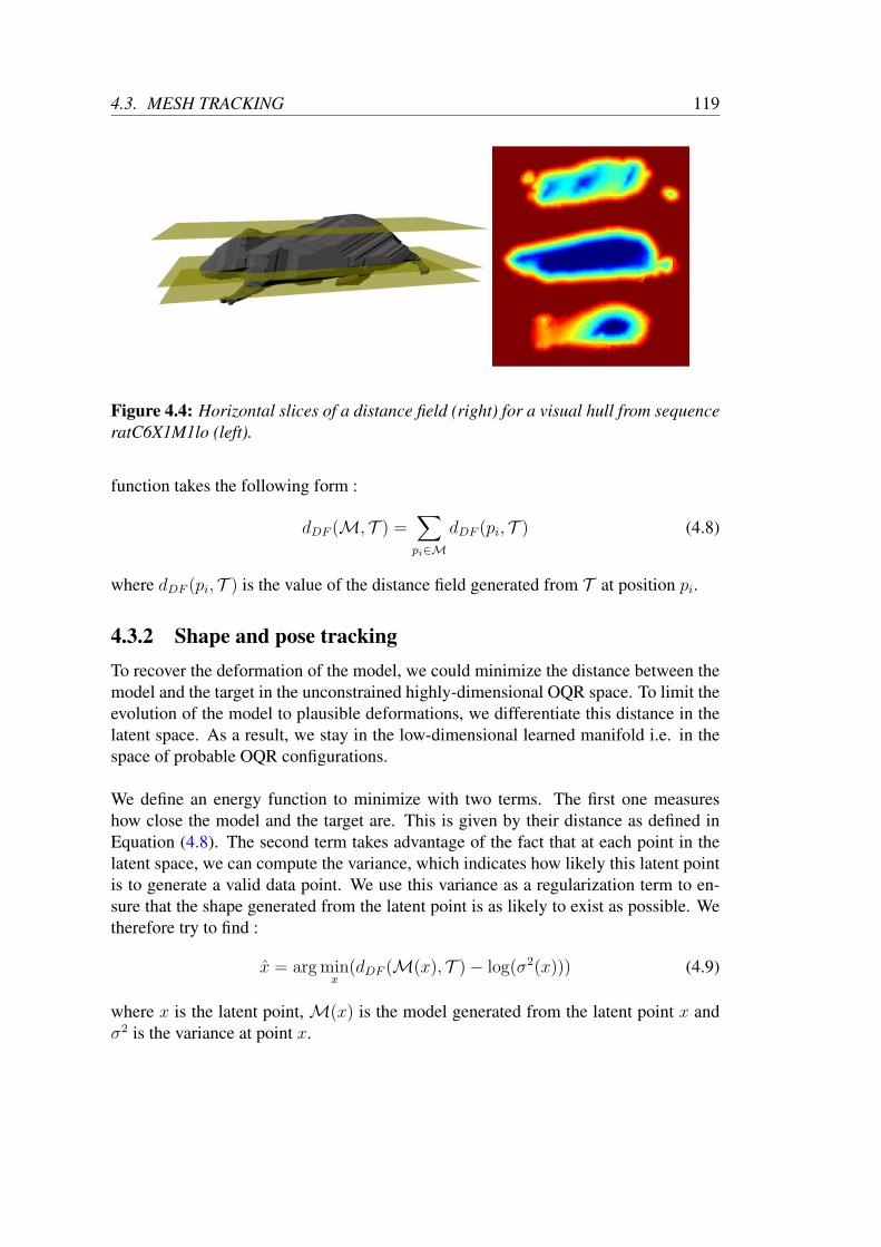
4.3. MESH TRACKING 119
Figure 4.4: Horizontal slices of a distance field (right) for a visual hull from sequence
ratC6X1M1lo (left).
function takes the following form :
dDF (M, T ) =∑
pi∈M
dDF (pi, T ) (4.8)
where dDF (pi, T ) is the value of the distance field generated from T at position pi.
4.3.2 Shape and pose tracking
To recover the deformation of the model, we could minimize the distance between themodel and the target in the unconstrained highly-dimensional OQR space. To limit theevolution of the model to plausible deformations, we differentiate this distance in thelatent space. As a result, we stay in the low-dimensional learned manifold i.e. in thespace of probable OQR configurations.
We define an energy function to minimize with two terms. The first one measureshow close the model and the target are. This is given by their distance as defined inEquation (4.8). The second term takes advantage of the fact that at each point in thelatent space, we can compute the variance, which indicates how likely this latent pointis to generate a valid data point. We use this variance as a regularization term to en-sure that the shape generated from the latent point is as likely to exist as possible. Wetherefore try to find :
x = argminx
(dDF (M(x), T )− log(σ2(x))) (4.9)
where x is the latent point, M(x) is the model generated from the latent point x andσ2 is the variance at point x.
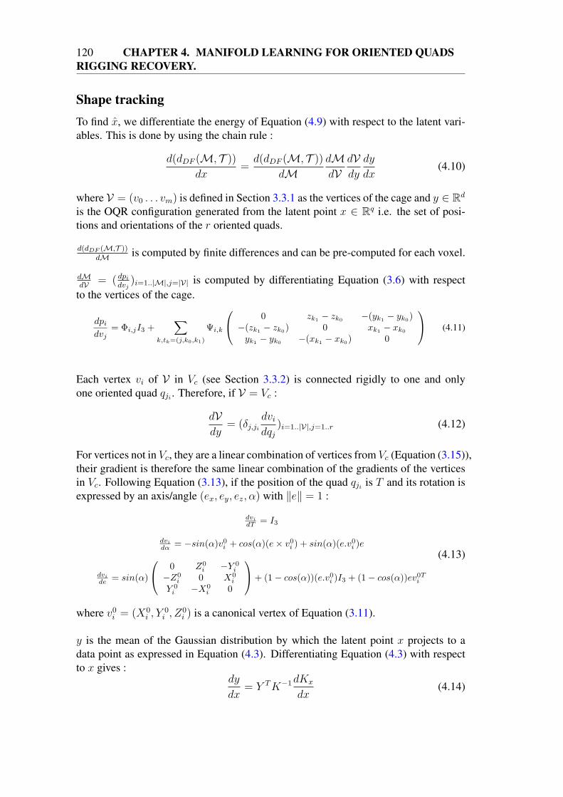
120 CHAPTER 4. MANIFOLD LEARNING FOR ORIENTED QUADSRIGGING RECOVERY.
Shape tracking
To find x, we differentiate the energy of Equation (4.9) with respect to the latent vari-ables. This is done by using the chain rule :
d(dDF (M, T ))
dx=d(dDF (M, T ))
dMdMdV
dVdy
dy
dx(4.10)
where V = (v0 . . . vm) is defined in Section 3.3.1 as the vertices of the cage and y ∈ Rd
is the OQR configuration generated from the latent point x ∈ Rq i.e. the set of posi-
tions and orientations of the r oriented quads.
d(dDF (M,T ))dM
is computed by finite differences and can be pre-computed for each voxel.
dMdV
= ( dpidvj
)i=1..|M|,j=|V| is computed by differentiating Equation (3.6) with respectto the vertices of the cage.
dpi
dvj= Φi,jI3 +
∑
k,tk=(j,k0,k1)
Ψi,k
0 zk1− zk0
−(yk1− yk0
)−(zk1
− zk0) 0 xk1
− xk0
yk1− yk0
−(xk1− xk0
) 0
(4.11)
Each vertex vi of V in Vc (see Section 3.3.2) is connected rigidly to one and onlyone oriented quad qji . Therefore, if V = Vc :
dVdy
= (δj,jidvi
dqj)i=1..|V|,j=1..r (4.12)
For vertices not in Vc, they are a linear combination of vertices from Vc (Equation (3.15)),their gradient is therefore the same linear combination of the gradients of the verticesin Vc. Following Equation (3.13), if the position of the quad qji is T and its rotation isexpressed by an axis/angle (ex, ey, ez, α) with ‖e‖ = 1 :
dvidT
= I3
dvidα
= −sin(α)v0i + cos(α)(e× v0i ) + sin(α)(e.v0i )e
dvi
de= sin(α)
0 Z0i −Y 0
i
−Z0i 0 X0
i
Y 0i −X0
i 0
+ (1− cos(α))(e.v0i )I3 + (1− cos(α))ev0Ti
(4.13)
where v0i = (X0i , Y
0i , Z
0i ) is a canonical vertex of Equation (3.11).
y is the mean of the Gaussian distribution by which the latent point x projects to adata point as expressed in Equation (4.3). Differentiating Equation (4.3) with respectto x gives :
dy
dx= Y TK−1dKx
dx(4.14)

4.3. MESH TRACKING 121
Each element of Kx is the covariance function k applied on x and one learned latentpoint. As a result, dKx
dx= (dk(x,xi)
dx)i=1..n follows from Equation (4.2) :
dk(x, xi)
dx= −γ(x− xi)k(x, xi) (4.15)
As for the regularization term, x projects to a data point with a mean as expressedin Equation (4.3) and a variance σ2 as expressed in Equation (4.4). As a result :
dσ2
dx= −2KT
xK−1dKx
dx(4.16)
Thanks to Equations (4.10) and (4.16), a simple first order method such as gradientdescent can be used to minimize Equation (4.9) and recover the OQR configurationcorresponding to the target.
Pose tracking
So far, we have captured the deformation of the shape as encoded in the latent space.As explained in Section 4.2, this shape is defined up to the global transformation Γ ofa reference quad (Q2 in Figure 3.31 for the latent spaces of Figure 4.2 and Figure 4.3).As a result, we also need to recover the global translation and orientation of the model.
To do so, we minimize the energy without the regularization term by differentiatingEquation (4.8) with respect to the pose parameters :
d(dDF (M, T ))
dΓ=d(dDF (M, T ))
dMdMdΓ
(4.17)
where
dMdΓ
=
dp1
dTx
dp1
dTy
dp1
dTy
dp1
dex
dp1
dey
dp1
dez
dp1
dα
......
......
......
...dp|M|
dTx
dp|M|
dTy
dp|M|
dTy
dp|M|
dex
dp|M|
dey
dp|M|
dez
dp|M|
dα
(4.18)
if Γ is parameterised by a translation T and an axis/angle rotation (ex, ey, ez, α) where‖e‖ = 1 with :
dpi
dT= I3
dpi
dα= −sin(α)p0i + cos(α)(e× p0i ) + sin(α)(e.p0i )e
dpi
de= sin(α)
0 Z0i −Y 0
i
−Z0i 0 X0
i
Y 0i −X0
i 0
+ (1− cos(α))(e.p0i )I3 + (1− cos(α))ep0Ti
(4.19)

122 CHAPTER 4. MANIFOLD LEARNING FOR ORIENTED QUADSRIGGING RECOVERY.
with p0i = (X0i Y
0i Z
0i ) is the position of pi in the rest pose.
Pose and shape optimization can be done either jointly or iteratively until convergence.Joint optimization is more correct but it converges more slowly as the search space islarger. Furthermore, experimentally, iterating between pose and shape optimizationworks faster and better, especially when tracking a sequence. In this case, the globaltransformation and the deformation between two frames are small enough that optimiz-ing first for the pose does not lead to a pose from which finding the good deformationis impossible, and vice-versa.
Local adjustment of the OQR
One limitation of our method is its dependence on the learning data. As with everymanifold-based method, we are limited to what the manifold can reconstruct. To ac-count for this limitation, we can first optimize with respect to latent variables to get asclose as possible to the target mesh. Once this has converged, a few more iterations canbe done with respect to the oriented quads to locally adjust the cage by differentiatingthe energy function with respect to the oriented quads :
d(dDF (M, T ))
dy=d(dDF (M, T ))
dMdMdV
dVdy
(4.20)
All these derivatives have been expressed previously as Equation (4.20) is part of Equa-tion (4.10). Section 4.3.3 shows examples where local adjustment improve the track-ing.
4.3.3 Validation and results
To validate our method, we show results on our datasets as well as on standard com-puter vision datasets. Unfortunately, standard computer vision datasets for whichground truth is known only exist for humans.
Validation on standard datasets
As standard datasets only exist for humans, we built an OQR for humans made of 21oriented quads (Figure 4.5). We tested our method on two test sets. We first tested ourapproach on a temporally coherent mesh of high quality from [VBMP08]. We thentackled more challenging data by tracking a sequence of noisy visual hulls extractedfrom the HumanEva II dataset [SBB10], without temporal coherence, learning the mo-tion manifold automatically from the CMU Motion Capture Database.

4.3. MESH TRACKING 123
Figure 4.5: Oriented Quads Rigging for humans.
(a) (b) (c)
Figure 4.6: (a) Target model - (b) Initial pose - (c) Samples on the convergence tra-
jectory.
We first tested our deformation optimization without the pose recovery. To do so,we use the bouncing sequence from [VBMP08]. The sequence of target meshes ismade of a temporally coherent animated mesh of 10000 vertices and 20000 faces. Wedefine the template mesh as one of these meshes simplified to 4000 vertices and 8000faces. The training was done by manually locating the oriented quads on 16 framesof the sequence. We learn a 10-D manifold from these samples. Figure 4.6 shows theprogression of the gradient descent towards an optimal deformation. We can noticethat, since we are optimizing in the latent space, each of the sample deformations is avalid deformation.
Figure 4.7 shows the advantage of tracking in the manifold. As there is no struc-ture on the cage, optimizing with respect to the oriented quads creates a shrinking ofthe cage as the quads are attracted to the closest patch of surface without any influencefrom the position and orientation of the other oriented quads. We can see on Figure 4.7the influence of the regularization term of the energy. Without it, the model mesh isattracted to the shape that is the closest to the target mesh and can be generated fromthe latent space without any regard for the likelihood of this shape. Using the varianceas a regularization term forces the optimal latent point to be more likely to generate avalid deformation.

124 CHAPTER 4. MANIFOLD LEARNING FOR ORIENTED QUADSRIGGING RECOVERY.
(a) (b) (c)
Figure 4.7: With the same target model and initial pose as in Figure 4.6 - (a) Result of
the optimisation in the oriented quad space. Notice how the head collapses - (b) Result
of the optimisation in the 10-D latent space without any regularisation term. Notice
how the arms shorten - (c) Result with the regularisation term.
Figure 4.8: Optimisation of both pose and deformation. The tracking (grey) is overlaid
over the target (yellow).
As explained in Section 4.3.2, we can also recover the global pose of the mesh. In prac-tice, we noticed that pose recovery and deformation recovery done iteratively worksbetter than joint optimization. Figure 4.8 shows results on the bouncing sequence.
We use the walk sequence of subject S4 in the HumanEva II dataset [SBB10] for aquantitative evaluation of our tracking as it contains the positions of joints acquiredwith markers and a Vicon system. This data consists of 4 synchronized color cameras.Using the background subtraction software and the mixture of Gaussian distributionmodel provided with the dataset, we extracted the silhouettes from the videos. Fromthese silhouettes, we generated the visual hulls using the Exact Polyhedral Visual Hullmethod [FB03]. As the the camera locations are not optimal for a preprocess step us-ing visual hull reconstruction, the visual hulls are a very coarse approximation of theobserved shape as can be seen on the left of Figure 4.9. The model used for cage-baseddeformation is the mesh model for subject S4 generated by Stefano Corazza and the

4.3. MESH TRACKING 125
(a) (b)
Figure 4.9: Examples of tracking on the HumanEva II dataset : (from left to right)
visual hull, result and overlay of the model on the visual hull. (a) The location of the
cameras can lead the visual hull to be a very coarse approximation of the observed
shape. (b) When the visual hull quality increases, the tracking becomes more precise.
Stanford BioMotion Group using [CGMA10].
Instead of manually creating the learning data by manually fitting the OQR to meshes,we also propose a method to use an existing database of movements. From walkingsequences in the CMU Motion Capture Database (http://mocap.cs.cmu.edu/), we au-tomatically generate 120 training samples by rigidly mapping the quads of the OQRto the animation skeleton. It has to be done only once for a given frame of one ofthe subject’s performance. After that, more samples can be automatically added tothe training set using any available motion capture data samples for this subject. Thistraining data is then used to build a 2D-manifold.
Figure 4.10 shows reprojections of the model tracked on the sequence. An exampleof local adjustment is shown in Figure 4.11, where a 2D latent space does not captureenough variance to track the mesh properly. Local adjustment allows for more preci-sion once the mesh is already well fitted from the latent space.
Table 4.1 shows the 3D error as specified in the HumanEva II dataset with and withoutthe local adjustment for the first 150 frames. This error is computed from the positionsof the joints as computed from the markers. As our approach is not skeleton-based, thepositions of the joints are computed by cage-based animation. On the first frame wheremotion capture data is available i.e. where the positions of the joints are known, theGreen Coordinates are computed on these positions and then used to compute the newpositions of the joints when the cage is deformed. With local adjustment, the meanerror drops from 90mm to 38.6mm.
For the whole walking sequence, the error is 85.2mm (see Table 4.1). However, whenconsidering only the first 150 frames, where the visual hulls are of better quality (right

126 CHAPTER 4. MANIFOLD LEARNING FOR ORIENTED QUADSRIGGING RECOVERY.
Figure 4.10: Reprojection on camera 3 and 4 of the tracked model for frames 5, 45,
102 and 148 of the sequence for subject S4 in the HumanEva II dataset.
of Figure 4.9), the error drops to 38.6mm. The error for the whole sequence is aboutthe same as the error for the first 150 frames without local adjustment. This can be
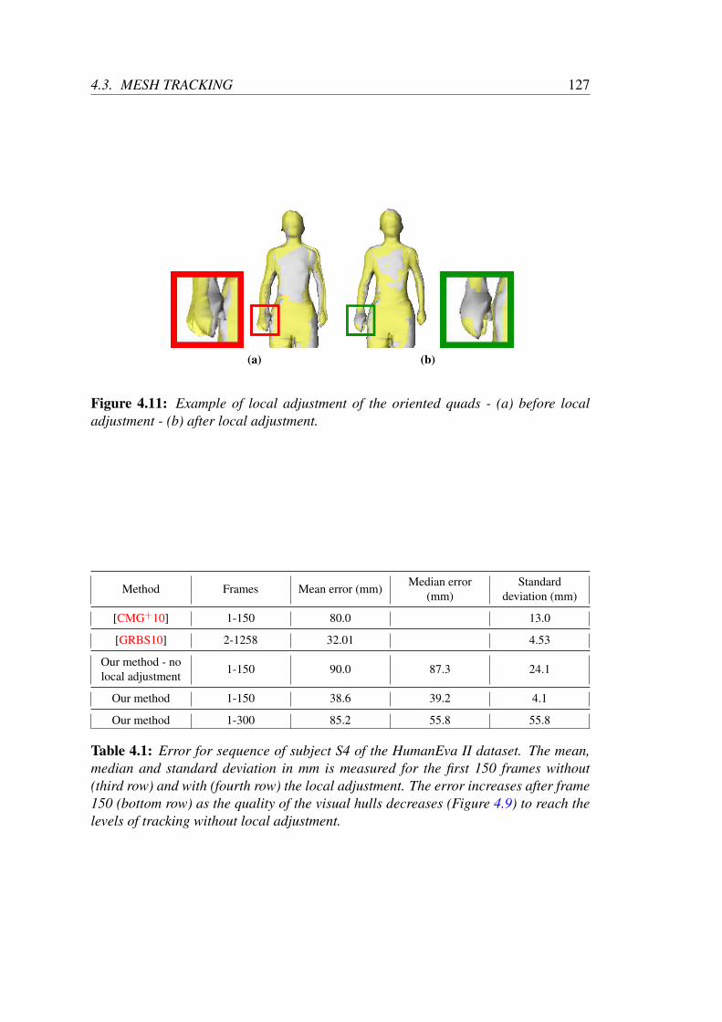
4.3. MESH TRACKING 127
(a) (b)
Figure 4.11: Example of local adjustment of the oriented quads - (a) before local
adjustment - (b) after local adjustment.
Method Frames Mean error (mm)Median error
(mm)Standard
deviation (mm)
[CMG+10] 1-150 80.0 13.0
[GRBS10] 2-1258 32.01 4.53
Our method - nolocal adjustment
1-150 90.0 87.3 24.1
Our method 1-150 38.6 39.2 4.1
Our method 1-300 85.2 55.8 55.8
Table 4.1: Error for sequence of subject S4 of the HumanEva II dataset. The mean,
median and standard deviation in mm is measured for the first 150 frames without
(third row) and with (fourth row) the local adjustment. The error increases after frame
150 (bottom row) as the quality of the visual hulls decreases (Figure 4.9) to reach the
levels of tracking without local adjustment.

128 CHAPTER 4. MANIFOLD LEARNING FOR ORIENTED QUADSRIGGING RECOVERY.
explained by the non-discriminative quality of the target mesh. Indeed, the coarsenessof the visual hull (left of Figure 4.9) prevents any fine adaptation of the shape by localadjustment. Table 4.1 also reports the results found in [CMG+10] and [GRBS10]. Themethod of Corazza et al. [CMG+10] also takes as input a series of visual hulls. Theresults are limited to the first 150 frames as re-initialisation is necessary after that dueto the poor quality of the visual hulls. Thanks to the use of a manifold of deformations,even though the error increases after frame 150, we are still able to attain good resultswithout re-initialisation. To our knowledge, Gall et al. [GRBS10] report the best re-sults. However, they also use information not taken into consideration by our methodsuch as the appearance of the model.
Results on locomotion tracking
We now focus on our rodent datasets, starting with sequence ratC6X1M1lo, which islocomotion of a rat. We therefore use the 2D latent space represented on Figure 4.2. Asthis sequence has 6 cameras in a good configuration for geometry reconstruction, theEPVH are of a better quality than the ones from the HumanEva II dataset. Figure 4.12shows the result of tracking. The tracking is mostly correct, with the biggest impre-cisions occurring for the foreleg. On the middle left image, the tracking is stuck in alocal minimum as putting the leg further back would increase the error at the shouldereven though it would be a better fit for the paw. On the bottom left image, the EPVHis ambiguous on whether the foreleg is facing forward (as reconstructed) or backwards(as it should be). As both positions are possible and reachable in the latent space, therest of the target does not help to disambiguate. On the bottom right image, we can seethat the foreleg is not forward enough. This illustrates a flaw inherent to our method.Indeed, our energy function measures how close the model is to the target but does nottake into consideration how close the target is to the model. As a result, this position ofthe foreleg gives an energy equivalent to what the correct position of the foreleg wouldgive. We talk more about this issue in Section 4.5.
Figure 4.13 shows the results of Figure 4.12 reprojected on the top and side camerasof the set-up. We can see that due to the level of details of the OQR, the shape is notprecisely matched (for instance the back of the animal). However, the motion is welltracked.
In the same way as we did for the HumanEva II dataset, we measure the quality of thetracking by comparing the positions of markers as tracked on the videos and as recon-structed from markerless tracking. In this case, Table 4.2 shows the mean and standarddeviation of the distance between both for the external markers of Figure 2.22. Toreconstruct the position of the markers from the OQR tracking, we compute the GreenCoordinates of the landmarks in the rest pose and then proceed to update their positionsby cage-based animation when the OQR configuration changes. To better understandthis error, we also compute the same errors for body parts, only considering the mark-ers mapped to a given body part. We can see that the error is quite high, slightly lower

4.3. MESH TRACKING 129
Figure 4.12: Examples of tracking for sequence ratC6X1M1lo. The tracking (grey) is
overlaid over the target (yellow).
than 1cm. However, except for the foreleg, the standard deviation is very low, whichleads to think that the error is mostly due to a bias. This bias probably comes fromthe fact that the model does not correspond perfectly to the studied animal or from aplacement of the landmarks that is not perfect.
Markers : All Head (4 markers) Foreleg (4 markers) Hindleg (4 markers)Mean error (mm) : 9.8 6.4 7.3 10.2
Standard deviation (mm) : 3.6 0.7 2.8 0.8
Table 4.2: Mean and standard deviation of the 3D distance between the external mark-
ers of Figure 2.22 as tracked on the videos and as reconstructed from the tracked OQR
for n = 45 frames.
As explained in Section 3.4, once we have an animation of OQR, one can use the ani-mation model of Chapter 2 to animate the bones from the skin. As simulated markersfor weighted Inverse Kinematics, we use the manually chosen markers of Figure 3.33.Figure 4.14 shows the results for the frames seen on Figure 4.12 and Figure 4.13. In-terestingly enough, we had labeled the third and fifth examples as incorrectly trackedfor the foreleg. However, on Figure 4.14, we can see that, even though on the fifth

130 CHAPTER 4. MANIFOLD LEARNING FOR ORIENTED QUADSRIGGING RECOVERY.
Figure 4.13: Examples of Figure 4.12 reprojected on the side and top cameras.
example, the foreleg remains incorrectly tracked, on the third example, the radius ispositioned outside the skin but closer to the truth. This is due to the angular springsthat impose anatomical constraints. As the shape of the envelope on the third exampleis only achievable by the animation model of the bones by large elongations of theangular springs, a solution closer to the rest pose but farther away from the markersis chosen. As explained previously, the error of the fifth example is due to an ambi-guity of the visual hull but leads to a plausible result, which is why the anatomicalconstraints in the weighted Inverse Kinematics can not correct this error.
As in Section 2.5.2, the internal markers tracked in 2D on the X-ray video can be usedto evaluate our tracking. As Figure 2.45 compared the projection of the landmarks to

4.3. MESH TRACKING 131
Figure 4.14: Examples of Figure 4.12 reprojected on the side and top cameras with
the result of weighted Inverse Kinematics from the skin as explained in Section 3.4.
the tracking of the internal markers for marker-based tracking, Figure 4.15 comparesthe projection of the landmarks on the X-ray video to the 2D tracking of the internalmarkers for markerless tracking. Comparing both, we can see that, even though thebias is still here, the results are less precise with markerless tracking. Quantitatively,whereas we had a mean error of about 15 pixels, which is equivalent to 2.4mm, withmarker-based tracking, we have an error of 49 pixels, which is equivalent to 7mm, withmarkerless tracking. However, given the fact that the error of the tracking of the skinwas measured to be 9mm, it seems as if using the vertices of the skin for weightedInverse Kinematics does not lead to further errors than the ones due to skin tracking.On the contrary, as shown in Figure 4.14, our Inverse Kinematics method sometimes

132 CHAPTER 4. MANIFOLD LEARNING FOR ORIENTED QUADSRIGGING RECOVERY.
correct some of these errors because of anatomical constraints.
Figure 4.15: Horizontal (red) and vertical (green) coordinates of the reprojection on
the X-ray of the landmarks as tracked with our markerless technique (line) compared
to the tracking of the corresponding internal markers (dots) on the X-ray video for
sequence ratC6X1M1lo. From left to right - marker 13 (humerus), 16 (spine) and 24
(knee). See Figure 2.22 for the exact location of the markers.
Figure 4.16: Comparison between marker-based (left) and markerless (right) tracking
of the internal structures.
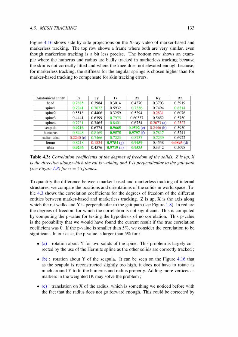
4.3. MESH TRACKING 133
Figure 4.16 shows side by side projections on the X-ray video of marker-based andmarkerless tracking. The top row shows a frame where both are very similar, eventhough markerless tracking is a bit less precise. The bottom row shows an exam-ple where the humerus and radius are badly tracked in markerless tracking becausethe skin is not correctly fitted and where the knee does not elevated enough because,for markerless tracking, the stiffness for the angular springs is chosen higher than formarker-based tracking to compensate for skin tracking errors.
Anatomical entity Tx Ty Tz Rx Ry Rzhead 0.7885 0.3984 0.3014 0.4370 0.3703 0.3919
spine1 0.7241 0.7672 0.5932 0.7356 0.7494 0.8314spine2 0.5518 0.4406 0.3259 0.5394 0.2831 0.6076spine3 0.4441 0.6399 0.7975 0.60337 0.5652 0.5750spine4 0.7731 0.3465 0.8401 0.6754 0.2073 (a) 0.2527scapula 0.9216 0.6774 0.9665 0.9592 (e) 0.2446 (b) 0.5950humerus 0.8448 0.8169 0.9575 0.9797 (f) 0.7817 0.5241
radius-ulna 0.2240 (c) 0.7466 0.7223 0.8737 0.7239 0.6922femur 0.8218 0.1834 0.9754 (g) 0.9459 0.4538 0.0893 (d)tibia 0.9246 0.4576 0.9719 (h) 0.9535 0.3342 0.5098
Table 4.3: Correlation coefficients of the degrees of freedom of the solids. Z is up, X
is the direction along which the rat is walking and Y is perpendicular to the gait path
(see Figure 1.8) for n = 45 frames.
To quantify the difference between marker-based and markerless tracking of internalstructures, we compare the positions and orientations of the solids in world space. Ta-ble 4.3 shows the correlation coefficients for the degrees of freedom of the differententities between marker-based and markerless tracking. Z is up, X is the axis alongwhich the rat walks and Y is perpendicular to the gait path (see Figure 1.8). In red arethe degrees of freedom for which the correlation is not significant. This is computedby computing the p-value for testing the hypothesis of no correlation. This p-valueis the probability that we would have found the current result if the true correlationcoefficient was 0. If the p-value is smaller than 5%, we consider the correlation to besignificant. In our case, the p-value is larger than 5% for :
• (a) : rotation about Y for two solids of the spine. This problem is largely cor-rected by the use of the Hermite spline as the other solids are correctly tracked ;
• (b) : rotation about Y of the scapula. It can be seen on the Figure 4.16 thatas the scapula is reconstructed slightly too high, it does not have to rotate asmuch around Y to fit the humerus and radius properly. Adding more vertices asmarkers in the weighted IK may solve the problem ;
• (c) : translation on X of the radius, which is something we noticed before withthe fact that the radius does not go forward enough. This could be corrected by
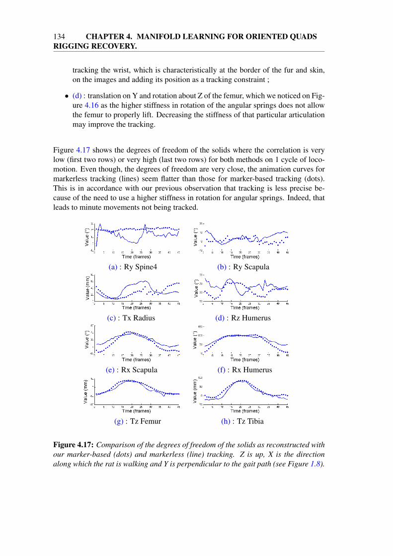
134 CHAPTER 4. MANIFOLD LEARNING FOR ORIENTED QUADSRIGGING RECOVERY.
tracking the wrist, which is characteristically at the border of the fur and skin,on the images and adding its position as a tracking constraint ;
• (d) : translation on Y and rotation about Z of the femur, which we noticed on Fig-ure 4.16 as the higher stiffness in rotation of the angular springs does not allowthe femur to properly lift. Decreasing the stiffness of that particular articulationmay improve the tracking.
Figure 4.17 shows the degrees of freedom of the solids where the correlation is verylow (first two rows) or very high (last two rows) for both methods on 1 cycle of loco-motion. Even though, the degrees of freedom are very close, the animation curves formarkerless tracking (lines) seem flatter than those for marker-based tracking (dots).This is in accordance with our previous observation that tracking is less precise be-cause of the need to use a higher stiffness in rotation for angular springs. Indeed, thatleads to minute movements not being tracked.
(a) : Ry Spine4 (b) : Ry Scapula
(c) : Tx Radius (d) : Rz Humerus
(e) : Rx Scapula (f) : Rx Humerus
(g) : Tz Femur (h) : Tz Tibia
Figure 4.17: Comparison of the degrees of freedom of the solids as reconstructed with
our marker-based (dots) and markerless (line) tracking. Z is up, X is the direction
along which the rat is walking and Y is perpendicular to the gait path (see Figure 1.8).

4.3. MESH TRACKING 135
Results on open-field tracking
A challenging and interesting dataset is moC8X0M0of as the mouse can roam freelyon a flat square. A 12-D latent space is built from 12 samples. Figure 4.18 showssome examples of results of mesh tracking on this sequence and Figure 4.19 showsthe corresponding reprojection on 2 of the 8 cameras. As the mouse only occupies asmall percentage of the 640 × 480 images (see Figure 1.10), the visual hulls are notvery precise. As a result, even though the body and the head are correctly registered,the legs are often not properly fit unless they really stand out of the body.
Figure 4.18: Examples of tracking for sequence moC8X0M0of. The tracking (grey) is
overlaid over the target (yellow).
Figure 4.20 shows the result of weighted Inverse Kinematics reprojected on a thirdcamera. A set of vertices equivalent to that of Figure 3.33 is used as markers.

136 CHAPTER 4. MANIFOLD LEARNING FOR ORIENTED QUADSRIGGING RECOVERY.
Figure 4.19: Examples of Figure 4.18 reprojected on two cameras.
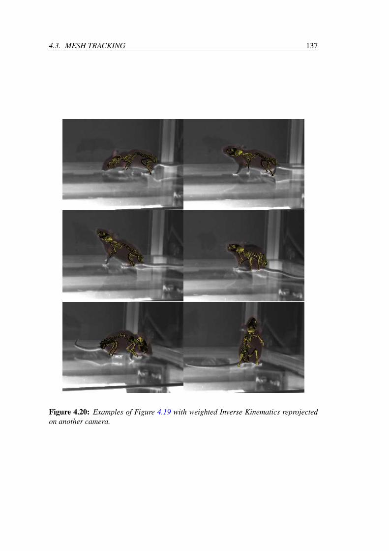
4.3. MESH TRACKING 137
Figure 4.20: Examples of Figure 4.19 with weighted Inverse Kinematics reprojected
on another camera.

138 CHAPTER 4. MANIFOLD LEARNING FOR ORIENTED QUADSRIGGING RECOVERY.
4.4 VIDEO TRACKING
As has been shown in Section 3.2, if there is a false-negative in one silhouette or ifthe reconstructed object is partially out of one image then the corresponding geometryis not reconstructed. As a result, when dealing directly with meshes, we lose someinformation that was in the images. For instance, if for one camera, the head of theanimal is out of the viewing volume whereas it is visible in all other cameras, it will notbe reconstructed in the EPVH and the mesh will have no information on the head. Eventhough manifold learning helps tackling these issues as seen with the HumanEva IIdataset (Section 4.3.3), it motivates the idea of directly working on images so as to notlose any information. This is further motivated by the fact that adding other cues suchas appearance has been demonstrated to improve tracking by works such as [GRBS10].Working directly on images makes the use of appearance cues easier. Therefore, weadapt our markerless tracking of Section 4.3 to an energy function computed on theimages, not the resulting visual hull.
4.4.1 2D objective function
To directly compute an energy function on the images, we need to have a measure ofhow well the 3D mesh of the model fits what is observed on the images. For this, givena camera c, the error of the model M is measured on this cameras as :
dDF,c(M) =∑
pi∈M
dDF,c(projc(pi)) (4.21)
where projc(pi) is the projection of 3D point pi on camera c and dDF,c((u v)) is thedistance at pixel (u, v) to the silhouette on camera c. As for the 3D distance field, the2D distance field can be pre-processed. Figure 4.21 shows examples of this distance.
For one set-up with nc cameras, the overall error is computed as :
dDF (M) =∑
c=1..nc
δvdDF,c(M) (4.22)
where δv is a visibility flag. This visibility flag is set to 1 if more than 75% of thevertices of M projects back within the image, 0 otherwise. In the following, we noteZ = (projj(pi))pi∈M,j=1..nc
.
4.4.2 Modifications to 3D shape and pose tracking
As in Section 4.3.2, to recover the deformation of the model, we minimise Equa-tion (4.22) by differentiating it with respect to the latent space. Applying chain rulesgives us :
d(dDF (M))
dx=d(dDF (M))
dZdZdM
dMdV
dVdy
dy
dx(4.23)

4.4. VIDEO TRACKING 139
Figure 4.21: Examples for two images (left) of the distance to the silhouette : the
darker the pixel, the closest to the silhouette the pixel is (right).
for shape tracking,
d(dDF (M))
dΓ=d(dDF (M))
dZdZdM
dMdΓ
(4.24)
for pose tracking and :
d(dDF (M))
dy=d(dDF (M))
dZdZdM
dMdV
dVdy
(4.25)
for local adjustment. We see that the only difference with Equations (4.10), (4.17)and (4.20) is that d(dDF (M,T ))
dMis replaced by d(dDF (M))
dZdZdM
in all three equations.
d(dDF (M))dZ
, just like d(dDF (M,T ))dM
, is computed by finite differences that can be be pre-processed.
dZdM
is the gradient of the projections onto the different cameras of the points of M. Assuch it can be written as :
dZdM = (δi,j
d(projc(pj))
dpi)i=1..|M|,j=1..|Z|,c=1..nc
(4.26)

140 CHAPTER 4. MANIFOLD LEARNING FOR ORIENTED QUADSRIGGING RECOVERY.
Every point (Xc, Yc, Zc) in the camera canonical reference frame projects to a 2Dpoint :
(
u
v
)
=
(
f Xc
Zc+ u0
f Yc
Zc+ v0
)
(4.27)
where f is the focal length of the camera and (u0, v0) is the principle point on theimage plane. For a point (X, Y, Z) in the world reference frame, its coordinates in thecamera reference frames are computed as :
Xc
YcZc
= R
X
Y
Z
+ T (4.28)
where (R, T ) are the rotation and translation of the camera. This gives us :
d(projc(pi))
dpi=
(
fR0,0Zc−R2,0Xc
Z2c
fR0,1Zc−R2,1Xc
Z2c
fR0,2Zc−R2,2Xc
Z2c
fR1,0Zc−R2,0Yc
Z2c
fR1,1Zc−R2,1Yc
Z2c
fR1,2Zc−R2,2Yc
Z2c
)
(4.29)
4.4.3 Comparison with mesh tracking
We first compare the mesh tracking of Section 4.3 with our video tracking. In case ofperfect silhouettes, the results are equivalent. Figure 4.22 shows the result on a frameof sequence ratC6X1M1lo for both methods initialised with the same pose and latentpoint. The results are equivalent. Indeed, in the 2D latent space where the training sam-ples are within [−3.17, 0.69] × [−1.65, 1.75], from the initial latent point (−1.93, 0),mesh tracking converges to the latent point (−2.77,−0.15) and video tracking con-verges to (−2.66,−0.26).
Figure 4.22: From left to right : initialisation - result of mesh tracking - result of video
tracking.
However, if one of the silhouettes is noisy, video tracking is more robust than meshtracking. For instance, on the same frame as Figure 4.22, we deteriorate the silhouetteof one of the six cameras by removing the legs. The right column of Figure 4.23 shows

4.4. VIDEO TRACKING 141
those silhouettes and the resulting visual hull reconstruction. As the visual hull repro-jects exactly in the silhouettes of all cameras, the target mesh does not have any geom-etry for the missing legs. For video tracking, even though the legs have disappearedin that particular camera, the silhouettes of the other cameras still contain informationabout the missing limb. Figure 4.23 shows the results for both mesh and video trackingwhen removing 1 to 3 limbs on one camera. Table 4.4 shows the latent point to whichthe tracking converges to for the same data. Thanks to the fact that tracking is done inthe learned manifold, both mesh and video tracking locate the missing limb correctlywhen only one leg is missing. However, when the two limbs of the left side of therat are missing, mesh tracking begins to deteriorate. Indeed, the visual hull enablesthe tracking to correctly locate the right side of the animal but does not disambiguatebetween several shapes that can be created by the latent space. As for video tracking,as the information about the missing limbs is still present in the silhouettes from theother cameras, the tracking does not deteriorate. Video tracking is thus more robustthan mesh tracking when dealing with false negatives in background subtraction.
Figure 4.23: From left to right : deteriorated silhouette and resulting EPVH - result
of mesh tracking - result of video tracking.
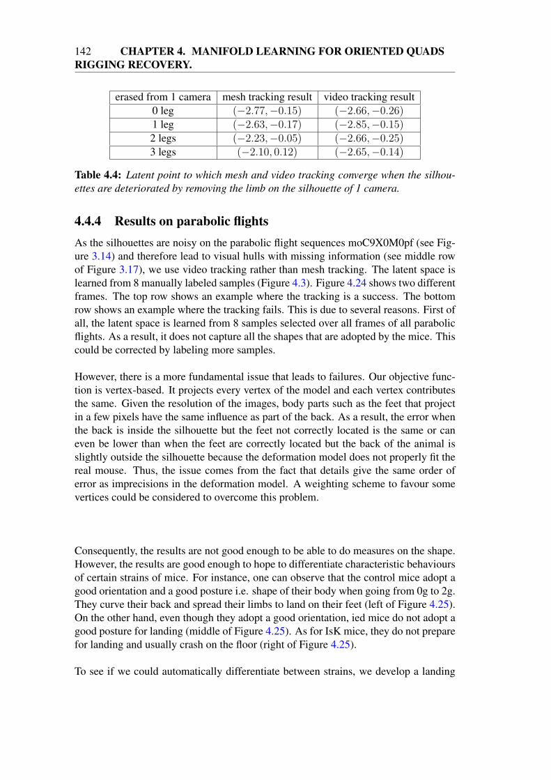
142 CHAPTER 4. MANIFOLD LEARNING FOR ORIENTED QUADSRIGGING RECOVERY.
erased from 1 camera mesh tracking result video tracking result0 leg (−2.77,−0.15) (−2.66,−0.26)1 leg (−2.63,−0.17) (−2.85,−0.15)2 legs (−2.23,−0.05) (−2.66,−0.25)3 legs (−2.10, 0.12) (−2.65,−0.14)
Table 4.4: Latent point to which mesh and video tracking converge when the silhou-
ettes are deteriorated by removing the limb on the silhouette of 1 camera.
4.4.4 Results on parabolic flights
As the silhouettes are noisy on the parabolic flight sequences moC9X0M0pf (see Fig-ure 3.14) and therefore lead to visual hulls with missing information (see middle rowof Figure 3.17), we use video tracking rather than mesh tracking. The latent space islearned from 8 manually labeled samples (Figure 4.3). Figure 4.24 shows two differentframes. The top row shows an example where the tracking is a success. The bottomrow shows an example where the tracking fails. This is due to several reasons. First ofall, the latent space is learned from 8 samples selected over all frames of all parabolicflights. As a result, it does not capture all the shapes that are adopted by the mice. Thiscould be corrected by labeling more samples.
However, there is a more fundamental issue that leads to failures. Our objective func-tion is vertex-based. It projects every vertex of the model and each vertex contributesthe same. Given the resolution of the images, body parts such as the feet that projectin a few pixels have the same influence as part of the back. As a result, the error whenthe back is inside the silhouette but the feet not correctly located is the same or caneven be lower than when the feet are correctly located but the back of the animal isslightly outside the silhouette because the deformation model does not properly fit thereal mouse. Thus, the issue comes from the fact that details give the same order oferror as imprecisions in the deformation model. A weighting scheme to favour somevertices could be considered to overcome this problem.
Consequently, the results are not good enough to be able to do measures on the shape.However, the results are good enough to hope to differentiate characteristic behavioursof certain strains of mice. For instance, one can observe that the control mice adopt agood orientation and a good posture i.e. shape of their body when going from 0g to 2g.They curve their back and spread their limbs to land on their feet (left of Figure 4.25).On the other hand, even though they adopt a good orientation, ied mice do not adopt agood posture for landing (middle of Figure 4.25). As for IsK mice, they do not preparefor landing and usually crash on the floor (right of Figure 4.25).
To see if we could automatically differentiate between strains, we develop a landing
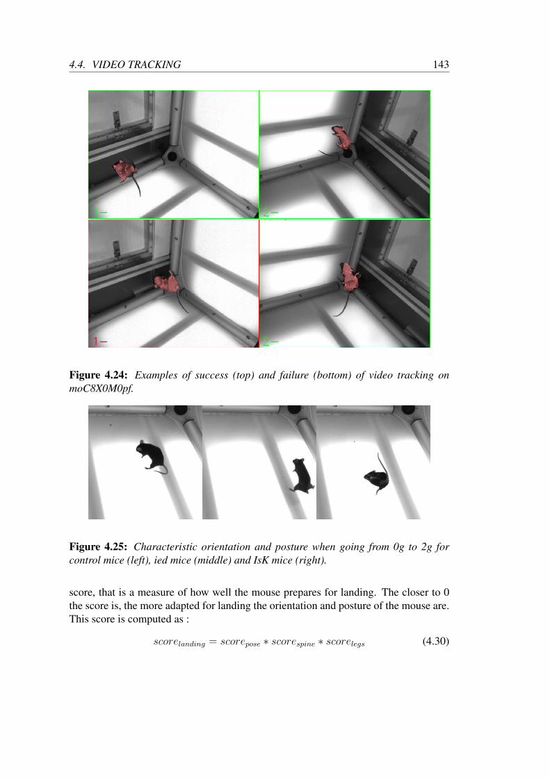
4.4. VIDEO TRACKING 143
Figure 4.24: Examples of success (top) and failure (bottom) of video tracking on
moC8X0M0pf.
Figure 4.25: Characteristic orientation and posture when going from 0g to 2g for
control mice (left), ied mice (middle) and IsK mice (right).
score, that is a measure of how well the mouse prepares for landing. The closer to 0the score is, the more adapted for landing the orientation and posture of the mouse are.This score is computed as :
scorelanding = scorepose ∗ scorespine ∗ scorelegs (4.30)

144 CHAPTER 4. MANIFOLD LEARNING FOR ORIENTED QUADSRIGGING RECOVERY.
scorepose measures how fitted the orientation is for landing by checking how paral-lel to the floor the mouse is. This is measured by the angle between the normal tothe floor and the normal of the plane defined by the quads Q0 (nose), Q13 and Q16(hindlegs). See Figure 3.31 for their location.
scorespine measures the curvature of the spine. It is measured as the inverse of theangle between the axis (Q0,Q2), the thorax, and the axis (Q2,Q4), the abdomen.
scorelegs measures how well the legs are located for the impact. This is measuredby projecting Q2 (the center of mass) on the axis (Q13,Q16), the axis between the twohind legs. Let’s call P2 that projection. The measure is then computed as
scorelegs = d(Q13, Q16)−1
∣
∣
∣
∣
1− d(P2, Q13)
d(P2, Q16)
∣
∣
∣
∣
(4.31)
It checks that the hindlegs are extended and symmetrical.
Figure 4.26 shows the landing score for 3 mice of the each strain. One can see that onlycontrol mice are able to reach and, above all, maintain a good orientation and postureprior to landing.
Figure 4.26: Landing score for 3 mice of each strain. The points represent the moment
of impact with the floor.

4.5. CONCLUSION 145
4.5 CONCLUSION
From the deformation model proposed in Chapter 3, we have derived a mesh trackingalgorithm that can work with both a sequence of meshes or segmented images as in-puts. This tracking algorithm is regularised by a learned manifold of plausible OQRconfigurations, leading to a more robust solution. Experimental results on standard hu-man datasets demonstrate the validity of our approach. The quality of rodent trackinghighly depends on the resolution of the input data. However, given the same quality ofinput data, rodent tracking performs as well as human tracking.
One major advantage of using an OQR representation over using a skeleton repre-sentation is that the different morphologies of the animals can be encoded in the samemanifold. Indeed, unlike joints in a skeleton that are defined locally in the hierarchy,oriented quads are defined globally. As a result, whereas morphology is encoded bydifferent parameters in skeletons, morphology is encoded implicitly in the OQR pa-rameters and as a result can be directly integrated in the latent space.
However, our current method has not considered the fact that classic GP-LVM strug-gles with learning a good model for complex datasets and becomes intractable forlarge datasets as one containing both motion and morphology information would be.Exploring other dimensional-reduction techniques or using a stochastic approach asin [YGvGU11] may overcome these issues and lead to a better tracking on complexsequences.
In terms of performance, the main reason for failure seems to be the fact that weare using a ‘one-way’ distance. Indeed, we measure how far the model is from thetarget but not how far the target is from the model. As a result, our tracking algorithmsometimes gets stuck in a local minimum where the surface of the model is close tothe surface of the target but some parts of the target gets unaccounted for. This canhappen both with the 3D or 2D objective function. For example, on the bottom rightimage of Figure 4.24, the right hindleg of the animal is within the silhouette. However,no part of the mouse projects back into the observed right hindleg. Using a ‘two-way’distance would be better but would increase the computation time and make the gra-dient derivation harder. Some more research has therefore yet to be done on a betterobjective function, either in 3D or 2D.
Our method would also greatly benefit from using appearance cues. So far, the de-cision is based purely on geometrical considerations. Using appearance to improverobustness can be incorporated in our framework as we use an image-based 2D objec-tive function.

146 CHAPTER 4. MANIFOLD LEARNING FOR ORIENTED QUADSRIGGING RECOVERY.

CHAPTER
5
CONCLUSION AND PERSPECTIVES.
WE have presented a complete pipeline on how to measure behaviours of ro-dents from videos. From the acquisition of morphologies and motion totracking, we have broached various fields such as image processing, com-
puter vision and computer graphics. In particular, we have proposed a single animationmodel of rodents combining both the skeleton and the skin and a tracking algorithmassociated to this model.
Our animation model is based on a new structure : the Oriented Quads Rigging (OQR).OQR is a high-level representation of a shape that produces smooth realistic deforma-tions and is more flexible than skeletons as it is not a hierarchical representation withreduced degrees of freedoms. As such, it allows us to model both full extension andfull bending of the spine of rodents with very few primitives, unlike skeletons, whichwould require many joints to produce a smooth bend of the skin.
Thanks to this model, our tracking algorithm is more robust to noise. Robustness isalso increased by the use of manifold learning that gives us a low-dimensional space ofplausible OQR configurations in which to search for the solution. For humans, wherevalidation datasets are available, this approach has shown to perform well compared tostate-of-the-art techniques.
Of course, there is room for improvement and future work. The first thing that onecan notice is that the quality of our results is highly dependent on the quality of theinput data. Indeed, in a controlled environment such as treadmill locomotion wherethe cameras can be set up to have the animal take most of the field of view, markerlesstracking performs correctly. However, in unconstrained environments such as explo-
147
148 CHAPTER 5. CONCLUSION AND PERSPECTIVES.
ration sequences or parabolic flights, the animal is a small part of the field of view andthe precision decreases. As a result, we are unable to properly track the legs but can ro-bustly track the body and the head. Consequently, one can think that a multi-resolutionscheme can improve the performance both in terms of results and computation time. Ahierarchy of latent spaces as presented in [PR11b] is something worth exploring. Onecould also create a multi-resolution OQR where, given a resolution, only a subset oforiented quads would be active, whereas the others would be inferred from the activeones.
In my opinion, the most promising path to improve precision would be to add featuretracking to help and improve the results of latent space tracking. Techniques developedfor object recognition could be used to track features of interest such as the nose, theears and the feet. These features could then be used to derive tracking constraints asthe centers of colour patches are in [WP09].
One might say that using learning is a limitation of our method. Indeed, in the contextof animal studies where databases of movements are not available, manual labeling isrequired. Because of the tediousness of the process, a minimal subset of examples isoften used as learning samples. Unfortunately, the smaller the learning samples, theless all-encompassing the latent space is. To make the labeling process less tedious andmore effective, one could imagine that the tracking results and its quality as measuredby the objective function could be used to determine which frames are not tracked cor-rectly. The user could then determine if the tracking fails because of the input data(e.g. the head is not reconstructed on the visual hull) or because the posture can not bereached with the current manifold. In the latest case, the user could label this frame andre-try the tracking. However, this points to a drawback of using GP-LVM for manifoldlearning. When using GP-LVM, adding a learning sample means re-learning the entirelatent space from scratch. As it is a computationally expensive process, manually la-beling and re-learning could not be done interactively.
Finally, building a set-up with both 8 standard cameras and 2 X-ray devices is nec-essary to fully measure the accuracy and precision of our method. In such a set-up,we could surgically implant markers on the bones, perform markerless tracking and beable to compare in 3D the tracked positions of the skeletal structures to the real ones.
In retrospect, this work has allowed us to explore if and when existing techniquesfail when dealing with the difficulty of real-life inputs, may it be the shape and defor-mation rodents can assume or the capturing set-ups with few low-resolution grey-levelcameras and to propose new solutions to overcome some of these issues as well asleads for a thorough validation procedure. A powerful incentive for this research hasbeen the interdisciplinarity collaboration that has allowed me to participate in projectswith fallouts outside of computer science.

BIBLIOGRAPHY
[4dv] 4d view solutions.
[AWM+11] S. Amiri, D.R. Wilson, B.A. Masri, G. Sharma, and C. Anglin, A novel
multi-planar radiography method for three dimensional pose reconstruc-
tion of the patellofemoral and tibiofemoral joints after arthroplasty., JBiomech (2011).
[BBDR05] Serge Belongie, Kristin Branson, Piotr Dollár, and Vincent Rabaud,Monitoring animal behavior in the smart vivarium, Measuring Behav-ior (Wageningen, NL), 2005, pp. 70–72.
[BBG+10] E.L. Brainerd, D.B. Baier, S.M. Gatesy, T.L. Hedrick, K.A. Metzger,S.L. Gilbert, and J.J. Crisco, X-ray reconstruction of moving morphology
(xromm): precision, accuracy and applications in comparative biome-
chanics research., J Exp Zool A Ecol Genet Physiol (2010).
[BC10] Jay M. Bauman and Young-Hui Chang, High-speed x-ray video demon-
strates significant skin movement errors with standard optical kinemat-
ics during rat locomotion, Journal of Neuroscience Methods 186 (2010),no. 1, 18 – 24.
[BKZ+07] M.J. Bey, S.K. Kline, R. Zauel, T.R. Lock, and P.A. Kolowich, Mea-
suring dynamic in-vivo glenohumeral joint kinematics: Technique and
preliminary results., J Biomech (2007).
[Bra00] G. Bradski, The OpenCV Library, Dr. Dobb’s Journal of Software Tools(2000).
[Bro71] Duane C. Brown, Close-range camera calibration, PHOTOGRAM-METRIC ENGINEERING 37 (1971), no. 8, 855–866.
149

150 BIBLIOGRAPHY
[BZBT06] M.J. Bey, R. Zauel, S.K. Brock, and S. Tashman, Validation of a new
model-based tracking technique for measuring three-dimensional, in
vivo glenohumeral joint kinematics., J Biomech Eng 128 (2006), no. 4,604–9.
[CBI10] Cedric Cagniart, Edmond Boyer, and Slobodan Ilic, Probabilistic de-
formable surface tracking from multiple videos, ECCV, 2010.
[CFM+08] P.A. Couto, V.M. Filipe, L.G. Magalhães, J.E. Pereira, L.M. Costa,P. Melo-Pinto, J. Bulas-Cruz, A.C. Maurício, S. Geuna, and A.S.P. Vare-jão, A comparison of two-dimensional and three-dimensional techniques
for the determination of hindlimb kinematics during treadmill locomo-
tion in rats following spinal cord injury., J Neurosci Methods (2008).
[CGMA10] S. Corazza, E. Gambaretto, L. Mundermann, and T.P. Andriacchi, Au-
tomatic generation of a subject-specific model for accurate markerless
motion capture and biomechanical applications, Biomedical Engineer-ing, IEEE Transactions on 57 (2010), no. 4, 806 –812.
[CKBH00] Kong Man Cheung, Takeo Kanade, J.-Y. Bouguet, and M. Holler, A real
time system for robust 3d voxel reconstruction of human motions, Pro-ceedings of the 2000 IEEE Conference on Computer Vision and PatternRecognition (CVPR ’00), vol. 2, June 2000, pp. 714 – 720.
[CMG+10] Stefano Corazza, Lars Mündermann, Emiliano Gambaretto, Gian-carlo Ferrigno, and Thomas Andriacchi, Markerless motion capture
through visual hull, articulated icp and subject specific model gener-
ation, International Journal of Computer Vision 87 (2010), 156–169,10.1007/s11263-009-0284-3.
[DMKH05] Douglas A. Dennis, Mohamed R. Mahfouz, Richard D. Komistek, andWilliam Hoff, In vivo determination of normal and anterior cruciate
ligament-deficient knee kinematics, Journal of Biomechanics 38 (2005),no. 2, 241 – 253, <ce:title>Knee Mechanics: An Update of Theoreticaland Experimental Analyses</ce:title>.
[DSG+04] L.E. DeFrate, H. Sun, T.J. Gill, H.E. Rubash, and G. Li, In vivo
tibiofemoral contact analysis using 3d mri-based knee models., JBiomech 37 (2004), no. 10, 1499–504.
[FB03] Jean-Sébastien Franco and Edmond Boyer, Exact polyhedral visual
hulls, British Machine Vision Conference (BMVC’03) (Norwich,Royaume-Uni), vol. 1, 2003, pp. 329–338 (Anglais).
[FKR05] Michael S. Floater, Géza Kós, and Martin Reimers, Mean value coordi-
nates in 3D, Computer Aided Geometric Design 22 (2005), no. 7, 623–631.

BIBLIOGRAPHY 151
[FPC+06] Vitor M. Filipe, José E. Pereira, Luís M. Costa, Ana C. Maurício, Pe-dro A. Couto, Pedro Melo-Pinto, and Artur S.P. Varejão, Effect of skin
movement on the analysis of hindlimb kinematics during treadmill loco-
motion in rats, Journal of Neuroscience Methods 153 (2006), no. 1, 55 –61.
[GBJD10] S.M. Gatesy, D.B. Baier, F.A. Jenkins, and K.P. Dial, Scientific rotoscop-
ing: a morphology-based method of 3-d motion analysis and visualiza-
tion., J Exp Zool A Ecol Genet Physiol (2010).
[GMHP04] Keith Grochow, Steven L. Martin, Aaron Hertzmann, and ZoranPopovic, Style-based inverse kinematics, ACM Trans. Graph. 23 (2004),522–531.
[GRBS10] Juergen Gall, Bodo Rosenhahn, Thomas Brox, and Hans-Peter Seidel,Optimization and filtering for human motion capture, International Jour-nal of Computer Vision 87 (2010), 75–92, 10.1007/s11263-008-0173-1.
[GRP10] Benjamin Gilles, Lionel Revéret, and Dinesh Pai, Creating and ani-
mating subject-specific anatomical models, Comput. Graph. Forum 29(2010), no. 8, 2340–2351.
[GSdA+09] J. Gall, C. Stoll, E. de Aguiar, C. Theobalt, B. Rosenhahn, and H.-P.Seidel, Motion capture using joint skeleton tracking and surface esti-
mation, Computer Vision and Pattern Recognition, 2009. CVPR 2009.IEEE Conference on, june 2009, pp. 1746 –1753.
[Hed08] Tyson L Hedrick, Software techniques for two- and three-dimensional
kinematic measurements of biological and biomimetic systems.
[JBS06] M.W. Jones, J.A. Baerentzen, and M. Sramek, 3d distance fields: a sur-
vey of techniques and applications, Visualization and Computer Graph-ics, IEEE Transactions on 12 (2006), no. 4, 581 –599.
[JMD+07] Pushkar Joshi, Mark Meyer, Tony DeRose, Brian Green, and TomSanocki, Harmonic coordinates for character articulation, ACM Trans-actions on Graphics (TOG). Proccedings of ACM SIGGRAPH 26(2007), no. 3.
[JSW05] Tao Ju, Scott Schaefer, and Joe Warren, Mean Value Coordinates for
Closed Triangular Meshes, ACM Transaction on Graphics (TOG), Pro-ceedings of ACM SIGGRAPH 24 (2005), no. 3.
[KBKL09] A. Kolb, E. Barth, R. Koch, and R. Larsen, Time-of-Flight Sensors in
Computer Graphics, Eurographics 2009 - State of the Art Reports (CH-1288 Aire-la-Ville) (M. Pauly and G. Greiner, eds.), Eurographics Asso-ciation, Eurographics, March 2009, pp. 119–134.

152 BIBLIOGRAPHY
[KCZO07] Ladislav Kavan, Steven Collins, Jiri Zara, and Carol O’Sullivan, Skin-
ning with dual quaternions, Symposium on Interactive 3D Graphics andGames (i3D) (2007).
[Lau94] A. Laurentini, The visual hull concept for silhouette-based image un-
derstanding, IEEE Trans. Pattern Anal. Mach. Intell. 16 (1994), no. 2,150–162.
[Law05] N. D. Lawrence, Probabilistic non-linear principal component analy-
sis with gaussian process latent variable models, Machine Learning Re-search 6 (2005), 1783 – 1816.
[LC87] William E. Lorensen and Harvey E. Cline, Marching cubes: A high reso-
lution 3d surface construction algorithm, COMPUTER GRAPHICS 21(1987), no. 4, 163–169.
[LCF00] J. P. Lewis, Matt Cordner, and Nickson Fong, Pose space deformation: a
unified approach to shape interpolation and skeleton-driven deforma-
tion, Proceedings of the 27th annual conference on Computer graph-ics and interactive techniques (New York, NY, USA), SIGGRAPH ’00,ACM Press/Addison-Wesley Publishing Co., 2000, pp. 165–172.
[LLCO08a] Yaron Lipman, David Levin, and Daniel Cohen-Or, Green coordinates,ACM Transactions on Graphics (TOG). Proceedings of ACM SIG-GRAPH 27 (2008), no. 3.
[LLCO08b] Yaron Lipman, David Levin, and Daniel Cohen-Or, Green coordinates,ACM Trans. Graph. 27 (2008), 78:1–78:10.
[LLCo08c] Yaron Lipman, David Levin, and Daniel Cohen-or, On the derivation of
green coordinates, Tech. report, 2008.
[LQnC06] Neil D. Lawrence and Joaquin Quiñonero Candela, Local distance
preservation in the gp-lvm through back constraints, Proceedings ofthe 23rd international conference on Machine learning (New York, NY,USA), ICML ’06, ACM, 2006, pp. 513–520.
[may] Autodesk maya.
[MG03] Alex Mohr and Michael Gleicher, Building efficient, accurate character
skins from examples, ACM SIGGRAPH 2003 Papers (New York, NY,USA), SIGGRAPH ’03, ACM, 2003, pp. 562–568.
[PKS+09] A.H. Prins, B.L. Kaptein, B.C. Stoel, J.H.C. Reiber, and E.R. Valstar,Detecting femur-insert collisions to improve precision of fluoroscopic
knee arthroplasty analysis., J Biomech (2009).
BIBLIOGRAPHY 153
[PR11a] V.A. Prisacariu and I. Reid, Nonlinear shape manifolds as shape pri-
ors in level set segmentation and tracking, Computer Vision and PatternRecognition (CVPR), 2011 IEEE Conference on, june 2011, pp. 2185–2192.
[PR11b] Victor Adrian Prisacariu and Ian Reid, Shared shape spaces, ComputerVision (ICCV), 2011 IEEE International Conference on, nov. 2011,pp. 2587 –2594.
[Sak78] Hiroaki Sakoe, Dynamic programming algorithm optimization for spo-
ken word recognition, IEEE Transactions on Acoustics, Speech, and Sig-nal Processing 26 (1978), 43–49.
[SBB10] Leonid Sigal, Alexandru O. Balan, and Michael J. Black, Humaneva:
Synchronized video and motion capture dataset and baseline algorithm
for evaluation of articulated human motion, Int. J. Comput. Vision 87(2010), no. 1-2, 4–27.
[SCD+06] Steven M. Seitz, Brian Curless, James Diebel, Daniel Scharstein, andRichard Szeliski, A comparison and evaluation of multi-view stereo re-
construction algorithms.
[SF10] Yann Savoye and Jean-Sébastien Franco, Cage-based Tracking for Per-
formance Animation, ACCV’10 :the Tenth Asian Conference on Com-puter Vision (Queenstown, New Zealand), 2010.
[SMCS] Greg Slabaugh, Tom Malzbender, Bruce Culbertson, and Ron Schafer, A
survey of methods for volumetric scene reconstruction from photographs.
[SS02] Daniel Scharstein and Richard Szeliski, A taxonomy and evaluation of
dense two-frame stereo correspondence algorithms, Int. J. Comput. Vi-sion 47 (2002), no. 1-3, 7–42.
[TA03] S. Tashman and W. Anderst, In-vivo measurement of dynamic joint mo-
tion using high speed biplane radiography and ct: application to canine
acl deficiency., J Biomech Eng 125 (2003), no. 2, 238–45.
[TTB12] Jean-Marc Thiery, Julien Tierny, and Tamy Boubekeur, Cager: Cage-
based reverse engineering of animated 3d shapes, Computer GraphicsForum 31 (2012), no. 8, 2303–2316.
[UFF06] Raquel Urtasun, David J. Fleet, and Pascal Fua, 3d people tracking
with gaussian process dynamical models, Proceedings of the 2006 IEEEComputer Society Conference on Computer Vision and Pattern Recogni-tion - Volume 1 (Washington, DC, USA), IEEE Computer Society, 2006,pp. 238–245.

154 BIBLIOGRAPHY
[UPBS08] Luis Unzueta, Manuel Peinado, Ronan Boulic, and Ángel Suescun, Full-
body performance animation with sequential inverse kinematics, Graph.Models 70 (2008), no. 5, 87–104.
[VBMP08] Daniel Vlasic, Ilya Baran, Wojciech Matusik, and Jovan Popovic, Artic-
ulated mesh animation from multi-view silhouettes, ACM Transactionson Graphics 27 (2008), no. 3, 97.
[WAK+10] J.T. Weinhandl, B.S.R. Armstrong, T.P. Kusik, R.T. Barrows, and K.M.O’Connor, Validation of a single camera three-dimensional motion
tracking system., J Biomech (2010).
[WB00] Jihong Wang and Timothy J. Blackburn, X-ray image intensifiers for flu-
oroscopy.
[WP09] Robert Y. Wang and Jovan Popovic, Real-time hand-tracking with a
color glove, ACM Transactions on Graphics 28 (2009), no. 3.
[YGvGU11] A. Yao, J. Gall, L. van Gool, and R. Urtasun, Learning probabilistic
non-linear latent variable models for tracking complex activities, Pro-ceedings of Neural Information Processing Systems (NIPS) (Granada,Spain), December 2011.
[ZB94] Jianmin Zhao and Norman I. Badler, Inverse kinematics positioning us-
ing nonlinear programming for highly articulated figures, ACM Trans.Graph. 13 (1994), 313–336.
[Zha00] Z. Zhang, A flexible new technique for camera calibration, Pattern Anal-ysis and Machine Intelligence, IEEE Transactions on 22 (2000), no. 11,1330 – 1334.
[ZNA03] Y. Zheng, M.S. Nixon, and R. Allen, Lumbar spine visualisation based
on kinematic analysis from videofluoroscopic imaging., Med Eng Phys25 (2003), no. 3, 171–9.
[ZSCS04] Li Zhang, Noah Snavely, Brian Curless, and Steven M. Seitz, Space-
time faces: High-resolution capture for modeling and animation, SIG-GRAPH (2004).
[ZVDH03] Victor Brian Zordan and Nicholas C. Van Der Horst, Mapping optical
motion capture data to skeletal motion using a physical model, Proceed-ings of the 2003 ACM SIGGRAPH/Eurographics symposium on Com-puter animation (Aire-la-Ville, Switzerland, Switzerland), SCA ’03, Eu-rographics Association, 2003, pp. 245–250.
CONTENTS
1 Introduction. 111.1 Context - Ethology . . . . . . . . . . . . . . . . . . . . . . . . . . . 111.2 Objectives . . . . . . . . . . . . . . . . . . . . . . . . . . . . . . . . 12
1.2.1 Vestibular control of skeletal configurations in 0G . . . . . . . 121.2.2 Datasets . . . . . . . . . . . . . . . . . . . . . . . . . . . . . 14
1.3 Overview and Contributions . . . . . . . . . . . . . . . . . . . . . . 221.3.1 Goals . . . . . . . . . . . . . . . . . . . . . . . . . . . . . . 221.3.2 Contributions . . . . . . . . . . . . . . . . . . . . . . . . . . 221.3.3 Overview . . . . . . . . . . . . . . . . . . . . . . . . . . . . 22
2 Shape and motion of the skeletal structures. 252.1 Previous work . . . . . . . . . . . . . . . . . . . . . . . . . . . . . . 26
2.1.1 Internal vs External 3D imaging . . . . . . . . . . . . . . . . 262.1.2 Marker-based vs Markerless tracking . . . . . . . . . . . . . 272.1.3 Inverse Kinematics . . . . . . . . . . . . . . . . . . . . . . . 292.1.4 Overview of our method . . . . . . . . . . . . . . . . . . . . 30
2.2 Geometry and motion data acquisition . . . . . . . . . . . . . . . . . 322.2.1 Acquisition of the geometrical models of the bones . . . . . . 322.2.2 Acquisition of the trajectories of the markers . . . . . . . . . 33
2.3 Animation model of the internal structures . . . . . . . . . . . . . . . 372.3.1 Set of articulated solids . . . . . . . . . . . . . . . . . . . . . 372.3.2 Refined model of the spine and ribcage . . . . . . . . . . . . 41
2.4 Marker-based tracking of the internal structures . . . . . . . . . . . . 452.4.1 Sequence-specific model . . . . . . . . . . . . . . . . . . . . 452.4.2 Inverse Kinematics . . . . . . . . . . . . . . . . . . . . . . . 472.4.3 Update of the spine and ribcage . . . . . . . . . . . . . . . . 53
155

156 BIBLIOGRAPHY
2.4.4 Automatic refinement of the location of the landmarks . . . . 552.5 Validation of the animation model . . . . . . . . . . . . . . . . . . . 57
2.5.1 Case study : motion of the foreleg of the rat during locomotion 572.5.2 Results for various morphologies and motions . . . . . . . . . 71
2.6 Conclusion . . . . . . . . . . . . . . . . . . . . . . . . . . . . . . . 75
3 Acquisition and deformation model of the envelope. 773.1 Previous work . . . . . . . . . . . . . . . . . . . . . . . . . . . . . . 79
3.1.1 Multi-view reconstruction . . . . . . . . . . . . . . . . . . . 793.1.2 Deformation model . . . . . . . . . . . . . . . . . . . . . . . 82
3.2 Acquisition of the envelope from videos . . . . . . . . . . . . . . . . 883.2.1 Background subtraction . . . . . . . . . . . . . . . . . . . . 893.2.2 Multi-view reconstruction . . . . . . . . . . . . . . . . . . . 90
3.3 Deformation model of the envelope . . . . . . . . . . . . . . . . . . 943.3.1 Cage-based animation . . . . . . . . . . . . . . . . . . . . . 943.3.2 Oriented Quads Rigging (OQR) . . . . . . . . . . . . . . . . 100
3.4 Link to skeletal structures . . . . . . . . . . . . . . . . . . . . . . . . 1073.5 Conclusion . . . . . . . . . . . . . . . . . . . . . . . . . . . . . . . 110
4 Manifold learning for Oriented Quads Rigging recovery. 1114.1 Previous work . . . . . . . . . . . . . . . . . . . . . . . . . . . . . . 112
4.1.1 Motion recovery from a sequence of meshes . . . . . . . . . . 1124.1.2 Manifold learning for tracking . . . . . . . . . . . . . . . . . 114
4.2 Manifold learning of OQR . . . . . . . . . . . . . . . . . . . . . . . 1154.3 Mesh tracking . . . . . . . . . . . . . . . . . . . . . . . . . . . . . . 118
4.3.1 Objective function . . . . . . . . . . . . . . . . . . . . . . . 1184.3.2 Shape and pose tracking . . . . . . . . . . . . . . . . . . . . 1194.3.3 Validation and results . . . . . . . . . . . . . . . . . . . . . . 122
4.4 Video tracking . . . . . . . . . . . . . . . . . . . . . . . . . . . . . . 1384.4.1 2D objective function . . . . . . . . . . . . . . . . . . . . . . 1384.4.2 Modifications to 3D shape and pose tracking . . . . . . . . . 1384.4.3 Comparison with mesh tracking . . . . . . . . . . . . . . . . 1404.4.4 Results on parabolic flights . . . . . . . . . . . . . . . . . . . 142
4.5 Conclusion . . . . . . . . . . . . . . . . . . . . . . . . . . . . . . . 145
5 Conclusion and perspectives. 147

LIST OF FIGURES
1.1 A schematic representation of the inputs and outputs of the centralnervous system to achieve balance. . . . . . . . . . . . . . . . . . . . 12
1.2 Inner ear - image courtesy of José Braga. . . . . . . . . . . . . . . . . 131.3 Simplified profile of the parabola described by the plane during a zero-
gravity flight. After a period at 1.8 times the gravity (1.8g), micro-gravity (0g) is achieved for about 20 seconds before a new period at1.8g starts. . . . . . . . . . . . . . . . . . . . . . . . . . . . . . . . . 13
1.4 Forward/backward motion of the foreleg of a cadaveric rat. . . . . . . 151.5 Bi-planar X-ray videos for ratC0X2M1lo. . . . . . . . . . . . . . . . 161.6 Set-up for the study of locomotion of rodents. The animal walks on a
treadmill in front of an image intensifier (X-rays) and 4 to 6 standardcameras. The lack of constraints of the environment leads to periodsof time where the animal is not completely covered (right). . . . . . . 16
1.7 Image with distorsion (left) and same image after calculation of thedistorsion coefficients and distortion correction. . . . . . . . . . . . . 17
1.8 Object of known dimensions used for calibration and result of the cal-ibration of both the cameras and the X-ray camera in a same 3D refer-ence frame represented by the X,Y,Z vectors. . . . . . . . . . . . . . 18
1.9 Set-up for the study of swimming of rodents. Notice how the watercreates distortion. . . . . . . . . . . . . . . . . . . . . . . . . . . . . 18
1.10 Set-up for open field study of mice : 8 cameras and an example ofcalibration object. . . . . . . . . . . . . . . . . . . . . . . . . . . . . 19
1.11 Parabolic flight set-up : (left) the whole set-up - (right) the free-floatingspace monitored by cameras. . . . . . . . . . . . . . . . . . . . . . . 20
1.12 Representation of points within the free-floating space that are coveredby at least (from left to right) 8, 7, 6, 5, 4, 3, 2 and 1 camera. . . . . . 21
157
158 LIST OF FIGURES
1.13 Calibration objects : the checker is used for intrinsic parameters andthe cube for extrinsic parameters. . . . . . . . . . . . . . . . . . . . . 21
1.14 Overview of our contributions. . . . . . . . . . . . . . . . . . . . . . 23
2.1 Example of two different acquisition sequences used for Dynamic TimeWarping. . . . . . . . . . . . . . . . . . . . . . . . . . . . . . . . . . 27
2.2 Skin sliding effect : the markers in red are surgically implanted directlyon the bones (at the ankle and at the knee) whereas the white markeris glued on the skin of the tibia. . . . . . . . . . . . . . . . . . . . . . 28
2.3 Example from [DMKH05] of automatic registration - left : objectivefunction values - right : corresponding poses for the two largest minima. 28
2.4 Example from [GBJD10] of scientific rotoscoping. The different bonesare registered manually. . . . . . . . . . . . . . . . . . . . . . . . . . 29
2.5 An example from [BBG+10] of rigid body motion recovered by com-puting the rigid transformation of a set of markers rigidly connected. . 30
2.6 Pipeline of our method for marker-based tracking of moving mor-phologies. . . . . . . . . . . . . . . . . . . . . . . . . . . . . . . . . 31
2.7 Slice of a CT-scan of the skull of a rat. The bone’s density is higherthan that of soft tissues, which means the skull is displayed in whitewhereas the flesh is displayed in grey. . . . . . . . . . . . . . . . . . 32
2.8 CT-scan of a rat - top : unsegmented isosurface of the volumetric data- bottom : segmentation of the different bones where each bone isrepresented by its own colour. . . . . . . . . . . . . . . . . . . . . . 33
2.9 From [GRP10], automatic registration of the segmented model of Fig-ure 2.8 (bottom) to a surface extracted from another CT data (top inwhite). . . . . . . . . . . . . . . . . . . . . . . . . . . . . . . . . . . 34
2.10 Triangulation : if the projection of a 3D point P is known in two view-points : p0 and p1, then the position of P can be built as the intersectionof the 2 viewing lines. . . . . . . . . . . . . . . . . . . . . . . . . . . 35
2.11 Epipolar geometry : if the projection of a 3D point is known to be p0in a viewpoint, the projection in another viewpoint lies on the epipolarline of p0 (red line). . . . . . . . . . . . . . . . . . . . . . . . . . . . 35
2.12 Example of marker tracking - top row : a point is marked on onecamera (green point), the epipolar lines can be computed for the otherviewpoints (green lines) - middle row : the same point is marked onanother camera (yellow point), it lies on the green epipolar line. Theepipolar lines can be computed for the other viewpoints (yellow line)- bottom row : from those two projections, the 3D coordinates of themarker can be computed and projected back to the cameras (red points). 36
2.13 Example of 3D trajectories of markers during rat locomotion. . . . . . 36

LIST OF FIGURES 159
2.14 Animation model - top : Bone models with visualisation of solid bod-ies (left), frames defining the solid bodies (middle), joint frames (right)- bottom : Each solid body (blue) is rigidly connected to a joint frame(red and dark red). On the rest pose (left), the joint frames are thesame. Once the bones move with respect to each other (right), eachjoint frame stays rigidly connected to one of the body (see small redframes), resulting in different transformations for the two joint frames(green). . . . . . . . . . . . . . . . . . . . . . . . . . . . . . . . . . 38
2.15 Different level of details possible to model a mouse. The solids aredisplayed as red parallelepipeds. . . . . . . . . . . . . . . . . . . . . 39
2.16 Animation model for rodents. The solids are displayed as red paral-lelepipeds. . . . . . . . . . . . . . . . . . . . . . . . . . . . . . . . . 40
2.17 Top, side and bottom view of the spine and ribcage in the rest pose(left). When deforming the spine and ribcage using only 4 solids(right), the ribs separate (bottom), inter-penetrate (middle) and the de-formation of the vertebrae is not smooth (top). . . . . . . . . . . . . . 41
2.18 Example of a 2D Hermite spline with 3 control points. . . . . . . . . 422.19 Segmentation of the different bones constituting the ribcage. . . . . . 432.20 Illustration of how the control points and tangents of the Hermite spline
are computed from the set of articulated solids. . . . . . . . . . . . . 432.21 3D Hermite spline fit on the rest pose of the animation model. . . . . 432.22 Landmarks (green and red spheres) are rigidly mapped to anatomical
entities. The green landmarks correspond to external markers, the redlandmarks correspond to internal markers, not visible on standard cam-eras. When the anatomical entity moves (bottom), the landmarks aresubmitted to the same rigid transformation. . . . . . . . . . . . . . . 46
2.23 Examples of linear springs (green lines) between markers and land-marks for the set of markers of Figure 2.22 when the skeleton is notyet aligned. . . . . . . . . . . . . . . . . . . . . . . . . . . . . . . . 50
2.24 The movement of the scapula (delimited by red dots) with respect tothe spine (C7 is enclosed in the red square) can not be considered to bea pure rotation, a translation has to be modeled as well. . . . . . . . . 51
2.25 From top to bottom : tracking of the forelimb of the rat using an SVD-based method (grey), using our method with active joint springs (yel-low), using our method with inactive joint springs i.e. with a null stiff-ness both in rotation and in translation (pink). Notice how the jointsprings correct an invalid roll of the radius. . . . . . . . . . . . . . . 52
2.26 Choosing a high stiffness in rotation for the angular springs in com-parison to the stiffnesses of the linear springs (left) leads to a solutioncloser to the rest pose but further away from the markers. Decreasingthis stiffness leads to results closer to the markers (right). . . . . . . . 53

160 LIST OF FIGURES
2.27 From top to bottom : frame of an experience with the set of markers ofFigure 2.22 - tracking with a stiffness on marker 3 on the forearm lowerthan other stiffnesses - tracking with a stiffness on marker 3 twice thestiffness on other markers. . . . . . . . . . . . . . . . . . . . . . . . 54
2.28 To correct the artefacts created by having only 4 solids to model thespine (left), we use Hermite spline interpolation and spherical linearinterpolation to set the position and orientation of the ribcage (left). . 55
2.29 Model for ratC0X2M1lo : bone models (yellow) with solids (red) andmarkers (green) added to the model. . . . . . . . . . . . . . . . . . . 57
2.30 Calibration object used for bi-planar X-ray sequences. . . . . . . . . . 582.31 Distribution of the collinearity error before (left) and after (right) dis-
tortion correction. . . . . . . . . . . . . . . . . . . . . . . . . . . . . 582.32 Tracked point in 2D (red point on the left image) and corresponding
epipolar line (red line on the right image). The marker should projectsomewhere on the epipolar line on the right image. . . . . . . . . . . 59
2.33 Diagnosis of errors in the tracking of markers - top row : sum of thedistances between the tracked 2D points and the epipolar lines for themarkers attached to the radius, bottom row : elongation created by themarkers on the radius. . . . . . . . . . . . . . . . . . . . . . . . . . . 60
2.34 Comparison of the tracking of the scapula with rigid transformationsbetween sets of markers (dots) and our method (line). . . . . . . . . . 62
2.35 Comparison of the tracking of the humerus with rigid transformationsbetween sets of markers (dots) and our method (line). . . . . . . . . . 63
2.36 Comparison of the tracking of the radius-ulna with rigid transforma-tions between sets of markers (dots) and our method (line). . . . . . . 64
2.37 Comparison of the scapula-humerus articulation tracked with rigid trans-formations between sets of markers (left) and our method (right) onframe 660. . . . . . . . . . . . . . . . . . . . . . . . . . . . . . . . . 65
2.38 Comparison of tracking using rigid transformations between sets ofmarkers (grey) and our method (yellow) on 4 consecutive frames (a-d).One can notice the sudden shift of the radius that occurs between (a)and (b) as well as its sudden twist that occurs between (b) and (c) withthe SVD-based method. On the other hand, our method produces asmooth natural tracking. Bottom row shows the frames used for tracking. 65
2.39 Overlay of SVD-based tracking (middle) and our tracking (right). No-tice how the radius comes out of the body at the radius/carpal articula-tion in the SVD-based tracking. . . . . . . . . . . . . . . . . . . . . . 66
2.40 Study of the influences of the markers used for tracking. From leftto right : using marker R1, using marker R3, using marker R3 withstiffness in rotation lowered. See Figure 2.29 for markers’ location. . . 67
2.41 Tracking of the metacarpal bone of the rat with only one marker on it. 682.42 Tracking of rat locomotion. The green spheres in the top left image are
the landmarks of the bones. . . . . . . . . . . . . . . . . . . . . . . . 69

LIST OF FIGURES 161
2.43 Comparison of the articulations on 2 cycles of locomotion : one sim-ulated on a cadaveric rat (left) recorded by bi-planar X-rays and onefrom a live rat on a treadmill recorded by external videos and one X-rayvideo (right). . . . . . . . . . . . . . . . . . . . . . . . . . . . . . . 70
2.44 Tracking of rat locomotion (half body). . . . . . . . . . . . . . . . . 722.45 Horizontal (red) and vertical (green) coordinates of the reprojection
of the landmarks (line) on the X-ray compared to the tracking of thecorresponding internal markers (dots) on the X-ray video for sequenceratC6X1M1lo. From left to right - marker 13 (humerus), 16 (spine)and 24 (knee). See Figure 2.22 for the exact location of the markers. . 72
2.46 Tracking of rat locomotion (half body). . . . . . . . . . . . . . . . . 732.47 Tracking of rat swimming. . . . . . . . . . . . . . . . . . . . . . . . 732.48 Tracking of zebra finch landing. . . . . . . . . . . . . . . . . . . . . 74
3.1 CT-scan of a rat at resolution 50µm. . . . . . . . . . . . . . . . . . . 783.2 Disparity map - left : original image - right : disparity map from [SS02]. 793.3 An example of structured light reconstruction from [ZSCS04]. . . . . 803.4 An example of a visual hull (slice representation). . . . . . . . . . . . 813.5 An example of a voxel model inside the scene volume as reconstructed
in [CKBH00]. . . . . . . . . . . . . . . . . . . . . . . . . . . . . . . 813.6 Mesh skinned on an animation skeleton : (top) rest pose - (bottom)
animation of the left elbow joint and right knee joint. . . . . . . . . . 833.7 Skinning of a virtual character using linear blend skinning (left) and us-
ing dual quaternions (right). Notice how the deformation of the shoul-der is better handled by dual quaternions [KCZO07]. . . . . . . . . . 84
3.8 Skin sliding effect : the markers in red are surgically implanted directlyon the bones (at the ankle and at the knee) whereas the white markeris glued on the skin of the tibia. . . . . . . . . . . . . . . . . . . . . . 85
3.9 Comparison between mean-value coordinates (left) and harmonic co-ordinates (right) from [JMD+07] - top row : coordinate value for ver-tex C, yellow indicates positive values, green indicates negative values,grey indicates null values and red indicates undefined values - bottomrow : example on a 3D model, note how moving the left leg moves theright leg in the opposite direction when using mean-value coordinates. 86
3.10 Deformation of the text top left using Green coordinates (top right),mean-value coordinates (bottom left) and harmonic coordinates (bot-tom right). Notice how the text is better preserved using Green coordi-nates [LLCO08b]. . . . . . . . . . . . . . . . . . . . . . . . . . . . . 87
3.11 Video processing pipeline. . . . . . . . . . . . . . . . . . . . . . . . 883.12 Evolution of the set-up to improve background subtraction : from a set-
up with reflections and view of the outside (left) to a better controlledenvironment (right). . . . . . . . . . . . . . . . . . . . . . . . . . . . 89
3.13 Background used for background subtraction for the 8 cameras of theset-up. . . . . . . . . . . . . . . . . . . . . . . . . . . . . . . . . . . 90
162 LIST OF FIGURES
3.14 Examples of background subtraction with the original image on the topright corner : top row shows a case where the results are satisfactory -middle row shows a case where the dark objective of the camera leadsto false negative (see the head on camera 3 and 6) - bottom row showsa case where the absence of anti-reflexive material on the top panelleads to false positives (top left on camera 1). The backgrounds arethose shown on Figure 3.13. . . . . . . . . . . . . . . . . . . . . . . 91
3.15 Comparison of space carving and Exact Polyhedron Visual Hull usingthe silhouettes of the top row of Figure 3.14. . . . . . . . . . . . . . . 92
3.16 From [FB03] - Viewing edges (red) along a given viewing line. . . . . 923.17 Profile, top and front view of the Exact Polyhedron Visual Hulls (EPVH)
reconstructed from the silhouettes on Figure 3.14. The quality of thevisual hulls deteriorates with the quality of the silhouettes and the num-ber of cameras that cover the mouse. . . . . . . . . . . . . . . . . . . 93
3.18 From left to right : fall postures for control mice, ied mice and IsKmice (Section 1.2.1) - Control mice tend to adopt an adapted postureand maintain their spacial orientation, ied mice tend to adopt the sameposture but do not seem able to maintain an appropriate spacial orienta-tion, IsK mice do not seem to adopt any particular posture or orientation. 93
3.19 Rat during a locomotion cycle. . . . . . . . . . . . . . . . . . . . . . 943.20 Comparison between skinning and cage-based animation on a cylinder
- left : initial model - middle : skinning - right : cage-based animationwith Green Coordinates. . . . . . . . . . . . . . . . . . . . . . . . . 97
3.21 Comparison between skinning and cage-based animation on a morecomplex model - top, from left to right : initial model, skinning, cage-based animation - bottom row, from left to right : zoom on skinningresult, zoom on cage-based animation result. . . . . . . . . . . . . . . 97
3.22 Comparison between skinning and cage-based animation to fit a modelfrom multi-view reconstruction - top row : animation skeleton (yel-low), cage (red) and artist-made model (grey) in rest pose - bottomrow from left to right : EPVH reconstruction, deformation by skin-ning, deformation by cage-based animation. . . . . . . . . . . . . . . 98
3.23 Example of the same cage used to animate two different models. . . . 993.24 Different degrees of freedom of an oriented quad - Top row : canonical
quad and canonical quad translated - Middle row : rotation about thetwo directions defined by the quad and rotation about the normal -Bottom row : scale along the two directions defined by the quad. . . . 101
3.25 Three types of relation that can exist between oriented quads - fromleft to right : bridge, extrusion, fork. The oriented quads are displayedin red and the resulting cage is displayed in black wireframe. . . . . . 102
3.26 When a quad is used in only one bridge (left), its geometry becomes aface of the cage. When it is used in two bridges as is the middle quadon the right, its face does not contribute as a face of the cage but itsvertices are used to build other faces. . . . . . . . . . . . . . . . . . . 103

LIST OF FIGURES 163
3.27 To create a branch, in case of an extrusion or a fork, first vertices aredefined on the quad where the branch is created (left) in order to createa hole (center) then the face is re-meshed around the hole (right). . . . 104
3.28 Example of how oriented quads can be used to create a squash andstretch effect with a few keyframes. . . . . . . . . . . . . . . . . . . 105
3.29 Example of how oriented quads can be used to create an animation ofan articulated objet, here the locomotion of a rat. . . . . . . . . . . . 106
3.30 Example of how oriented quads can be used to create an animation ofan articulated objet, here different postures of a mouse. . . . . . . . . 106
3.31 Oriented Quads Rigging (OQR) for rodents - top : mouse, bottom : ratwithout the tail. . . . . . . . . . . . . . . . . . . . . . . . . . . . . . 107
3.32 Tracking of the bones using the position of the quads of the OQR (left)and vertices of the skin (right) as markers. Note how the problem isunder-constrained when using quads, which leads to the scapula beingimproperly tracked. . . . . . . . . . . . . . . . . . . . . . . . . . . . 108
3.33 Set of skin points (green spheres) selected to be used as markers forthe tracking of internal structures from OQR configurations. . . . . . 109
3.34 Examples of tracking of the bones during locomotion using the OQRof Figure 3.31 and the markers of Figure 3.33. . . . . . . . . . . . . . 109
4.1 User intervention when the skeleton is incorrectly fitted to the silhou-ettes in [VBMP08]. . . . . . . . . . . . . . . . . . . . . . . . . . . . 113
4.2 Example of a 2D latent space of OQR and corresponding deformationsfor rat locomotion. . . . . . . . . . . . . . . . . . . . . . . . . . . . 117
4.3 Example of a 2D latent space of OQR and corresponding deformationsfor parabolic flights. . . . . . . . . . . . . . . . . . . . . . . . . . . . 117
4.4 Horizontal slices of a distance field (right) for a visual hull from se-quence ratC6X1M1lo (left). . . . . . . . . . . . . . . . . . . . . . . . 119
4.5 Oriented Quads Rigging for humans. . . . . . . . . . . . . . . . . . . 1234.6 (a) Target model - (b) Initial pose - (c) Samples on the convergence
trajectory. . . . . . . . . . . . . . . . . . . . . . . . . . . . . . . . . 1234.7 With the same target model and initial pose as in Figure 4.6 - (a) Re-
sult of the optimisation in the oriented quad space. Notice how thehead collapses - (b) Result of the optimisation in the 10-D latent spacewithout any regularisation term. Notice how the arms shorten - (c)Result with the regularisation term. . . . . . . . . . . . . . . . . . . . 124
4.8 Optimisation of both pose and deformation. The tracking (grey) isoverlaid over the target (yellow). . . . . . . . . . . . . . . . . . . . . 124
4.9 Examples of tracking on the HumanEva II dataset : (from left to right)visual hull, result and overlay of the model on the visual hull. (a) Thelocation of the cameras can lead the visual hull to be a very coarseapproximation of the observed shape. (b) When the visual hull qualityincreases, the tracking becomes more precise. . . . . . . . . . . . . . 125

164 LIST OF FIGURES
4.10 Reprojection on camera 3 and 4 of the tracked model for frames 5, 45,102 and 148 of the sequence for subject S4 in the HumanEva II dataset. 126
4.11 Example of local adjustment of the oriented quads - (a) before localadjustment - (b) after local adjustment. . . . . . . . . . . . . . . . . . 127
4.12 Examples of tracking for sequence ratC6X1M1lo. The tracking (grey)is overlaid over the target (yellow). . . . . . . . . . . . . . . . . . . . 129
4.13 Examples of Figure 4.12 reprojected on the side and top cameras. . . 1304.14 Examples of Figure 4.12 reprojected on the side and top cameras with
the result of weighted Inverse Kinematics from the skin as explainedin Section 3.4. . . . . . . . . . . . . . . . . . . . . . . . . . . . . . . 131
4.15 Horizontal (red) and vertical (green) coordinates of the reprojection onthe X-ray of the landmarks as tracked with our markerless technique(line) compared to the tracking of the corresponding internal markers(dots) on the X-ray video for sequence ratC6X1M1lo. From left toright - marker 13 (humerus), 16 (spine) and 24 (knee). See Figure 2.22for the exact location of the markers. . . . . . . . . . . . . . . . . . . 132
4.16 Comparison between marker-based (left) and markerless (right) track-ing of the internal structures. . . . . . . . . . . . . . . . . . . . . . . 132
4.17 Comparison of the degrees of freedom of the solids as reconstructedwith our marker-based (dots) and markerless (line) tracking. Z is up,X is the direction along which the rat is walking and Y is perpendicularto the gait path (see Figure 1.8). . . . . . . . . . . . . . . . . . . . . 134
4.18 Examples of tracking for sequence moC8X0M0of. The tracking (grey)is overlaid over the target (yellow). . . . . . . . . . . . . . . . . . . . 135
4.19 Examples of Figure 4.18 reprojected on two cameras. . . . . . . . . . 1364.20 Examples of Figure 4.19 with weighted Inverse Kinematics reprojected
on another camera. . . . . . . . . . . . . . . . . . . . . . . . . . . . 1374.21 Examples for two images (left) of the distance to the silhouette : the
darker the pixel, the closest to the silhouette the pixel is (right). . . . . 1394.22 From left to right : initialisation - result of mesh tracking - result of
video tracking. . . . . . . . . . . . . . . . . . . . . . . . . . . . . . 1404.23 From left to right : deteriorated silhouette and resulting EPVH - result
of mesh tracking - result of video tracking. . . . . . . . . . . . . . . . 1414.24 Examples of success (top) and failure (bottom) of video tracking on
moC8X0M0pf. . . . . . . . . . . . . . . . . . . . . . . . . . . . . . 1434.25 Characteristic orientation and posture when going from 0g to 2g for
control mice (left), ied mice (middle) and IsK mice (right). . . . . . . 1434.26 Landing score for 3 mice of each strain. The points represent the mo-
ment of impact with the floor. . . . . . . . . . . . . . . . . . . . . . . 144

LIST OF TABLES
1.1 Different datasets used for validation. . . . . . . . . . . . . . . . . . 141.2 Percentage of the free-floating space covered by exactly (middle col-
umn) and at least (right column) a given number of cameras (left column). 20
2.1 For n = 300 frames, mean 3D distance measured between pairs oftracked markers as well as the 95% confidence interval, same distancemeasured on the landmarks and ratio of the mean distance over the dis-tance of the landmarks. See Figure 2.22 for the location of the markers. 47
2.2 Distances in mm between landmarks and tracked 3D positions beforeand after automatic refinement of the location of the landmarks forn = 736 frames. . . . . . . . . . . . . . . . . . . . . . . . . . . . . . 56
2.3 Correlation coefficients of the degrees of freedom of the solids recov-ered with rigid transformations between sets of markers and recoveredwith our method for n = 736 frames. . . . . . . . . . . . . . . . . . . 61
2.4 Study of the influences of the markers used for tracking for n = 736frames. See Figure 2.29 for markers’ location. . . . . . . . . . . . . . 67
4.1 Error for sequence of subject S4 of the HumanEva II dataset. Themean, median and standard deviation in mm is measured for the first150 frames without (third row) and with (fourth row) the local adjust-ment. The error increases after frame 150 (bottom row) as the qualityof the visual hulls decreases (Figure 4.9) to reach the levels of trackingwithout local adjustment. . . . . . . . . . . . . . . . . . . . . . . . . 127
4.2 Mean and standard deviation of the 3D distance between the externalmarkers of Figure 2.22 as tracked on the videos and as reconstructedfrom the tracked OQR for n = 45 frames. . . . . . . . . . . . . . . . 129
165

166 LIST OF TABLES
4.3 Correlation coefficients of the degrees of freedom of the solids. Z is up,X is the direction along which the rat is walking and Y is perpendicularto the gait path (see Figure 1.8) for n = 45 frames. . . . . . . . . . . 133
4.4 Latent point to which mesh and video tracking converge when the sil-houettes are deteriorated by removing the limb on the silhouette of 1camera. . . . . . . . . . . . . . . . . . . . . . . . . . . . . . . . . . 142
Copyright © 2022 FDOKUMEN