HAL Id: tel-03384748https://hal.univ-lorraine.fr/tel-03384748

Submitted on 19 Oct 2021

HAL is a multi-disciplinary open accessarchive for the deposit and dissemination of sci-entific research documents, whether they are pub-lished or not. The documents may come fromteaching and research institutions in France orabroad, or from public or private research centers.

L’archive ouverte pluridisciplinaire HAL, estdestinée au dépôt et à la diffusion de documentsscientifiques de niveau recherche, publiés ou non,émanant des établissements d’enseignement et derecherche français ou étrangers, des laboratoirespublics ou privés.

Caractérisation des formes d’agriculture et évaluation deleur résilience aux perturbations

Manon Dardonville

To cite this version:Manon Dardonville. Caractérisation des formes d’agriculture et évaluation de leur résilience auxperturbations. Sciences agricoles. Université de Lorraine, 2021. Français. �NNT : 2021LORR0123�.�tel-03384748�

AVERTISSEMENT

Ce document est le fruit d'un long travail approuvé par le jury de soutenance et mis à disposition de l'ensemble de la communauté universitaire élargie. Il est soumis à la propriété intellectuelle de l'auteur. Ceci implique une obligation de citation et de référencement lors de l’utilisation de ce document. D'autre part, toute contrefaçon, plagiat, reproduction illicite encourt une poursuite pénale. Contact : ddoc-theses-contact@univ-lorraine.fr

LIENS Code de la Propriété Intellectuelle. articles L 122. 4 Code de la Propriété Intellectuelle. articles L 335.2- L 335.10 http://www.cfcopies.com/V2/leg/leg_droi.php http://www.culture.gouv.fr/culture/infos-pratiques/droits/protection.htm

THÈSE

Présentée et soutenue publiquement pour l’obtention du titre de

Docteur de l’Université de Lorraine

Mention : Sciences Agronomiques

par Manon DARDONVILLE

Sous la direction de Olivier THEROND et Christian BOCKSTALLER

Caractérisation des formes d’agriculture et évaluation de

leur résilience aux perturbations

8 juin 2021

Membres du jury:

Directeurs de thèse: Olivier THEROND HDR, Ingénieur de recherche, UMR LAE, Colmar

(membre invité) Christian

BOCKSTALLER HDR, Ingénieur de recherche, UMR LAE, Colmar

Rapporteures: Amélie GAUDIN Associate Professor, Department of Plant Sciences, Davis

Pytrik REIDSMA Associate Professor, Plant Production System, Wageningen

Examinateur·rice·s: Marc DECONCHAT Directeur de recherche, Dynafor, Toulouse

Guillaume MARTIN Directeur de recherche, UMR AGIR, Toulouse

Muriel VALANTIN-

MORISON Directrice de recherche, Unité Agronomie, Grignon

Invité: Rodolphe SABATIER Chargé de recherche, UR Ecodev, Avignon

MANON DARDONVILLE : Caractérisation des formes d’agriculture et évaluation de leur

résilience aux perturbations © 2021

ENCADREMENT :

Olivier THEROND (directeur)

Christian BOCKSTALLER (co-directeur)

ÉTABLISSEMENT :

Université de Lorraine

LABORATOIRE DE RATTACHEMENT :

UMR LAE 1132, Université de Lorraine, INRAE

FINANCEMENTS :

Cette thèse a fait l’objet d’un financement Cifre par l’entreprise Agrosolutions.

PUBLICATIONS

REVUES À COMITÉ DE LECTURE

Dardonville, M., Urruty, N., Bockstaller, C., Therond, O., 2020. Influence of diversity and

intensification level on vulnerability, resilience and robustness of agricultural systems.

Agricultural Systems 184, 102913. https://doi.org/10.1016/j.agsy.2020.102913

Dardonville, M., Bockstaller, C., Therond, O., 2021. Review of quantitative evaluations of the

resilience, vulnerability, robustness and adaptive capacity of temperate agricultural systems.

Journal of Cleaner Production 125456. https://doi.org/10.1016/j.jclepro.2020.125456

Dardonville, M., Legrand, B., Clivot, H., Bernardin, C., Bockstaller, C., Therond, O., under

revisions at Ecosystem Services. A low-data approach for assessing ecosystem services provided

to and used by farmers and dynamics of natural capital.

Dardonville, M., Bockstaller, C., Villerd, J., Therond, O., submitted to Ecosystem Services.

Resilience of agriculture models: biodiversity-based models are stable, while intensified models

perform well.

Catarino, R., Dardonville, M., Gourdon, B., Misslin, R., Villerd, J., Therond, O., in writing.

Resilience for sustainable crop-livestock systems: A conceptual framework with MAELIA.

CONFÉRENCES À COMITÉ DE LECTURE

Dardonville, M., Urruty, N., Bockstaller, C., Thérond, O., 2019. Does diversity affect dynamics

of agricultural system facing perturbations? Presented at the European Conference on Crop

Diversification, Budapest.

Dardonville, M., Bockstaller, C., Legrand, B., Therond, O., 2019. Quantifying ecosystem

capacity, modulation by agricultural practices and actual use of ecosystem services by farmers.

Presented at the Ecosystem Services Partnership, Hannover.

Dardonville, M., Bockstaller, C., Legrand, B., Therond, O., 2019. Quantifying ecosystem

capacity, modulation by agricultural practices and actual use of ecosystem services by farmers.

Présenté au congrès EASY, Nice.

Dardonville, M., Urruty, N., Bockstaller, C., Therond, O., 2019. Dynamique des systèmes

agricoles face aux perturbations : review des méthodes d’évaluation et facteurs explicatifs.

Présenté au séminaire annuel de l’école doctorale SIReNA, Nancy.

Dardonville, M., Bockstaller, C., Therond, O., 2019. Evaluer la résilience, vulnérabilité et

robustesse des systèmes agricoles. Présenté au congrès Vulnérabilité et résilience dans le

renouvellement des approches du développement et de l’environnement, Versailles.

Dardonville, M., Bockstaller, C., Therond, O., 2020. Evaluation de la résilience de différentes

formes d’agriculture face aux changements climatiques et crises économiques. Présenté au

congrès Phloeme, Paris. Prix de la thèse la plus prometteuse.

Dardonville, M., Bockstaller, C., Therond, O., 2022. Dynamics of agricultural systems facing

hazards: is intensification level explaining resilience ? Présentation prévue au congrès IFSA,

Evora.

RAPPORTS DE STAGE ENCADRES DURANT LA THESE

Baudelet, S., Bockstaller, C., Therond, O., Dardonville, M., 2019. État de l’art de l’évaluation de

la résilience, vulnérabilité et robustesse des systèmes agricoles en zone tropicales et arides

(Rapport de stage de Master 2).

Legrand, B., Bockstaller, C., Dardonville, M., Therond, O., 2019. Caractérisation des formes

d’agriculture au sein d’un réseau d’exploitations agricoles (Mémoire de Master 2).

Dubois, L., Therond, O., Dardonville, M., 2020. Enquêtes au sein d’un réseau d’exploitations

agricoles pour caractériser leur fourniture et utilisation de services écosystémiques (Mémoire de

fin de stage d’alternance).

Osei-Tutu, K., Therond, O., Dardonville, M., 2021. Assessment of the resilience of arable

farming in the Grand Est region (Mémoire de Master 2).

ARTICLE DE PRESSE NATIONALE

Dardonville, M., Cabeza-Orcel, P., 2020. Evaluer la résilience des différentes formes

d’agriculture. Perspectives agricoles.

REMERCIEMENTS

Je voudrais pour commencer remercier Amélie Gaudin et Pytrik Reidsma pour leurs rôles de

rapporteures du jury ainsi que pour leurs travaux de recherche inspirants qui ont constitué un socle

scientifique important pour cette thèse. Je voudrais ensuite remercier Marc Deconchat, Guillaume

Martin, Rodolphe Sabatier et Muriel Valantin-Morison, pour leur participation au jury de cette

thèse.

Cette thèse est l’aboutissement de trois ans de recherche que j’ai réalisé entourée d’un soutien

important de la part de plusieurs personnes que je voudrais remercier ici.

Tout d’abord, un grand merci à Olivier Therond d’avoir imaginé ce sujet de thèse passionant,

de me l’avoir confié et surtout d’avoir été un formidable partenaire de travail. Je te suis

extrêmement reconnaissante pour ta disponibilité, pour tes enseignements scientifiques ainsi que

pour ton encadrement qui ont su me motiver au quotidien. Je re-signe d’ailleurs sans hésitations

pour une collaboration, cette fois à durée illimitée.

Ensuite, merci à Christian Bockstaller de m’avoir procuré tes conseils et ton expertise

agronomique tout au long de ma thèse. Je remercie tous mes collègues du Laboratoire Agronomie

et Environnement pour leur aide à forger mon projet de thèse lors de la formation pour les

doctorants et des différentes présentations de mon travail. A Colmar, j’ai été très bien accueillie et

très facilement intégrée dans notre petit comité, je vous en suis très reconnaissante.

Je remercie toutes les personnes d’Agrosolutions, partenaire Cifre de cette thèse, et en

particulier Nicolas Urruty et Céline Denieul qui ont activement contribué à la mise en place et au

bon déroulement de ce partenariat. Mes échanges formels et informels avec l’équipe

d’Agrosolutions ont permis d’ancrer mon travail aux problématiques du conseil et du monde

agricole.

Parmi les personnes qui ont contribué à la réalisation du travail de thèse, je voudrais féliciter

les stagiaires que j’ai encadrés et les remercier pour leurs apports précieux pour la thèse: Sophie

Baudelet, Baptiste Legrand, Léa Dubois et Kwabena Osei-Tutu. Merci à Frédéric Pierlot d’avoir

convaincu les Chambres d’Agriculture de collaborer avec nous sur ce projet. Merci à David

Justeau, Grégory Lemercier, Claude Rettel et Jean-François Strehler d’avoir sélectionné les

exploitations agricoles et de m’avoir mise en contact avec les agriculteur·rices. Merci aux 28

agriculteur·rices qui ont fourni leurs données, leur expertise du terrain et leur temps pour les

entretiens. Leurs avis sur les résultats du cas d’étude constitueront une évaluation de ce travail de

thèse importante pour moi. Merci à Baptiste, Léa et Claire Bernardin pour avoir rodé, avec ou sans

moi, sur les routes du Grand Est, micro à la main, pour réaliser les entretiens. Merci à Jean Villerd

pour nos échanges et ton soutien méthodologique. Enfin, merci à Hugues Clivot et à Paul van Dijk

pour m’avoir aidée à utiliser vos super modèles.

J’ai été suivie durant ces trois années par deux comités scientifiques qui ont questionné mes

travaux et m’ont apporté de nombreux conseils. Je souhaite remercier chaleureusement Michel

Duru, Jean Roger-Estrade et Guy Richard pour nos rencontres (presque) trimestrielles desquelles

je ressortais toujours plus motivée par vos encouragements. Merci aussi aux membres du comité

de suivi de la thèse : François Bousquet, Alain Carpentier, David Makowski, Guillaume Martin et

Marc Tchamitchian. En plus de nos rencontres annuelles, nos échanges au détour de conférences,

de séminaires, ou encore lorsque j’avais besoin de votre expertise, ont été crutiaux pour l’avancée

de la thèse.

I would like to thank Wim Paas, Pytrik Reidsma and all the people at the Plant Production

System lab in Wageningen for their warm welcome. I hope that our scientific collaboration will

continue and that we will soon have the opportunity to meet for lunch walk again.

Ce manuscrit de thèse ne serait pas ce que vous allez lire sans le travail de relecture rigoureux

effectué par Olivier, Marine Belorgey, Renaud Misslin et Henri Nicod. Les articles scientifiques

publiés au cours de cette thèse ont été fortement améliorés grâce aux retours de mes co-auteurs et

autrices, ainsi qu’à la relecture de l’anglais de Michelle et Michael Corson, que je remercie.

Au-delà du soutien professionnel, j’ai été entourée de personnes géniales qui ont fortement

contribué au maintien de mon moral quotidien et donc à la bonne réalisation de cette thèse. Au

LAE, je souhaite faire un grand merci à Alix, Bruno, Emma, Eric, Floriane, Laurène, Marine,

Nirina, Renaud et Rui pour votre bienveillance, nos franches parties de rigolades, le jardin partagé,

les critiques culinaires, les sorties d’escalade et d’observations ornithologiques. Cela dit, Bruno et

Renaud, sachez que je me souviens toujours que vous m’aviez fait manger un piment-oiseau du

jardin, très piquant, à mon insu. Merci à mes colocs, ami·es de Colmar et d’ailleurs, à ma famille

et surtout à Henri de m’avoir soutenue tout au long de la thèse et de m’entourer, tout simplement.

TABLE DES MATIERES

INTRODUCTION GÉNÉRALE 1

1. Impact environnemental des activités humaines 1

1.1 Anthropocène et limites biophysiques planétaires 1

1.2 Services écosystémiques 3

2. De nouvelles formes d’agriculture 7

2.1 Répondre aux enjeux socio-environnementaux 8

2.2 Redéfinir les formes d’agriculture 9

2.3 Évaluer les services écosystémiques à la production 10

3. Menaces sur les systèmes agricoles 12

3.1 Changements climatiques 12

3.2 Épuisement des ressources 13

3.3 Volatilité des prix 14

4. Faire face : résilience ou vulnérabilité ? 15

4.1 Définitions usuelles 15

4.2 Un débat conceptuel clivant 16

4.3 Identité du système agricole, fonctions et performances 17

4.4 Évaluer la résilience 18

5. Résilience des formes d’agriculture 21

6. Problématiques, questions de recherche et stratégie de la thèse 25

CAS D’ÉTUDE 29

1. Détermination du territoire et des agroécosystèmes étudiés 30

2. Dispositif de collecte de données 33

2.1 Itinéraires techniques synthétisés 33

2.2 Itinéraires techniques réalisés 33

3. Perturbations biophysiques et économiques dans la région Grand Est 34

CHAPITRE I : ÉTAT DE L’ART SUR L’ÉVALUATION DE LA RÉSILIENCE,

VULNÉRABILITÉ ET ROBUSTESSE : OBJETS, MÉTHODES ET CONNAISSANCES 37

1. Influence de la diversité et de l’intensification sur la vulnérabilité, résilience et

robustesse des systèmes agricoles 41

1.1 Introduction 43

1.2 Generic analytical framework 44

1.3 Method and study selection 45

1.4 Results 47

1.5 Discussion and conclusion 57

1.6 Concluding remarks 60

2. Revue des évaluations quantitatives de la résilience, vulnérabilité, robustesse et

capacités d’adaptation des systèmes agricoles de zones tempérées 62

2.1 Introduction 64

2.2 Methodology 66

2.3 Results 69

2.4 Discussion 77

2.5 Conclusion 83

CHAPITRE II : CARACTÉRISATION DE FORMES D’AGRICULTURE PAR LES

SERVICES ÉCOSYSTÉMIQUES 86

1. Introduction 91

2. Conceptual framework 92

3. Assessment approach 94

3.1 Literature review of determinants of potential and real capacity and components

of natural capital 95

3.2 Indicators and multicriteria assessment of the four dimensions of ESF 99

4. Example of application 101

4.1 Materials and methods 101

4.2 Results 102

5. Discussion 107

5.1 Strengths of the assessment approach 108

5.2 Shortcomings and expected improvements of the approach 108

5.3 Lack of knowledge and agenda for research 109

5.4 Insights into agriculture models 110

6. Conclusion 111

CHAPITRE III : RÉSILIENCE DES FORMES D’AGRICULTURE 118

1. Introduction 124

2. Methods 126

2.1 Agroecosystems and farm characteristics 126

2.2 Performances and explanatory variables 128

2.3 Explanatory factor test 134

3. Results 135

3.1 Energy yield 135

3.2 Gross margin 138

3.3 Workload 140

3.4 Positive deviants 142

4. Discussion 142

4.1 Biodiversity at the hub of resilience 142

4.2 Multifaceted dynamics 143

4.3 Use of high ESF levels: a way to reach resilience? 144

4.4 Specific characteristics of irrigated systems 145

4.5 Workload, an original attribute of performance 145

4.6 Methodological advances and issues 146

5. Conclusion and perspectives 146

DISCUSSION GÉNÉRALE 149

1. Aspects conceptuels et méthodologiques 153

1.1 Dynamique de la littérature des cadres conceptuels 153

1.2 Evaluation de la résilience et identification de ses facteurs explicatifs 157

1.3 Évaluation des services écosystémiques et de la dynamique du capital naturel

166

2. Facteurs de resilience 174

2.1 Analyse de la relation complexe entre l'influence du rendement et sa stabilité sur

la résilience le long du gradient d'intensification 174

2.2 Diversification 184

2.3 Services écosystémiques et résilience 188

CONCLUSION 195

BIBLIOGRAPHIE 200

ANNEXES 245

1. Matériel supplémentaire du cas d’étude 246

2. Matériel supplémentaire de l’article « Influence of diversity and intensification level

on vulnerability, resilience and robustness of agricultural systems » 251

3. Matériel supplémentaire de l’article « Review of quantitative evaluations of the

resilience, vulnerability, robustness and adaptive capacity of temperate agricultural systems »

262

4. Matériel supplémentaire de l’article « A low-data approach for assessing ecosystem

services provided to and used by farmers and dynamics of natural capital » 271

5. Matériel supplémentaire de l’article « Resilience of agriculture models: biodiversity-

based models are stable, while intensified models perform well » 302

LISTE DES TABLEAUX

Table 1. Services écosystémiques selon leur type de bénéficiaire proposés et étudiés dans l’étude EFESE-EA

(Therond et al., 2017b). .......................................................................................................................................... 6 Table 2. Résumé des 34 agroécosystèmes (par numéro d’identification ID) appartenant aux 28 exploitations agricoles

sélectionnées dans la région Grand Est, en France. ............................................................................................. 32 Table 3. Analytical framework used for the systematic review, regardless of the conceptual framework used in the

study (vulnerability, resilience and robustness (VRR)), inspired by Allen et al. (2016), Carpenter et al. (2001),

Meuwissen et al. (2019) and Müller et al. (2016). ............................................................................................... 45 Table 4. Definitions of the four concepts investigated................................................................................................... 64 Table 5. Summary of the criteria used to describe dynamics in the articles reviewed .................................................. 73 Table 6. Distribution of the 53 articles reviewed as a function of the number of performance attributes and criteria of

dynamics of performance considered................................................................................................................... 74 Table 7. Resilience properties described by Cabell and Oelofse (2012) and potential explanatory factors encountered

in the articles reviewed. ........................................................................................................................................ 82 Table 8. Summary of the main determinants of ecosystem services provided to farmers (ESF). The spatial and

temporal configuration and composition of the cover and soil composition determine an ecosystem’s potential

capacity. The crop management of soil and biomass determined an ecosystem’s real capacity. The 9 ESF

studied include pollination (POL); pest (PEST), weed (WEED) and disease (DIS) control; soil structuration

(STR); nitrogen supply to crops (NS); phosphorus supply to crops (PS); water retention and return to crops

(WATER) and stabilization and control of erosion (ERO). The effects of crop management on ESF provision

can be positive (+) or negative (-). References are mainly meta-analyses, reviews or multisite studies.

*Depends on the type of habitat. **Several combinations of soil characteristics are suitable for ESF, see Table

2. ......................................................................................................................................................................... 113 Table 9. Indicators used to assess effects of each determinant on the potential capacity of an agroecosystem to

provide ecosystem services to farmers (ESF) (I_potential, [0:1]) and the modulation (I_modulation, [-1:1]) of

this potential capacity, thus determining the real capacity to provide ESF. References: * from Craheix et al.

(2012), ¹ from Rega et al. (2018), ² from Saxton and Rawls (2006) ³ from Johannes et al. (2017), ⁴ from Olsen

et al. (1954) ⁵ from Chabert (2017)⁶. For a, b, c, d, e, f, g, h, i, j references, see Supplementary Material 3.

Abbreviations: semi-natural habitats (SNH), treatment frequency index (TFI), soil organic matter (SOM) .... 114 Table 10. Method used to assess the actual use of ecosystem services provided to farmers (ESF), based on the

precision of the action performed by farmers to use ecosystem services, considering the ability of the

agroecosystem to provide services instead of using anthropogenic inputs to replace them. ............................. 115 Table 11. Indicators used to evaluate biodiversity dynamics through the effect of determinants on each community.

References are shown in Table 1. * From Craheix et al. (2012), ¹ from Rega et al. (2018), ⁵ from Chabert

(2017). For e, f, h, i, j, k, l indicator calculation details, see Supplementary Material 3. Abbreviations: treatment

frequency index (TFI), soil organic matter (SOM) ............................................................................................ 116 Table 12. Performance attributes (response variables) whose dynamics were analysed, proxies of disturbances

(exogenous) and explanatory variables tested as determinants of resilience. ESF: ecosystem services to

farmers, SNH: semi-natural habitats, TFI: treatment frequency index, SD: standard deviation, SCA: soil

conservation agriculture ..................................................................................................................................... 131 Table 13. Performance attributes whose dynamics were analysed, associated criteria of dynamics and metrics. ...... 133 Table 14. Summary of results for two categories of systems: those based on ecosystem services provided to farmers

(ESF), biodiversity, and natural capital or intensified systems (irrigation and tillage, and to a lesser extent,

pesticide or fertiliser). A “+” indicates a resilient system), “-“ indicates a non-resilient system, “+/-” indicates a

variable system and “(+)” indicates a specific relationship to criteria of dynamics. ......................................... 143

LISTE DES FIGURES

Figure 1. État des neuf limites biophysiques planétaires et rôle estimé des activités agricoles dans leur statut. Figure

issue de Campbell et al. (2017). ............................................................................................................................. 2 Figure 2. Représentation schématique des effets des deux grands types de facteurs de production, intrants

anthropiques et services écosystémiques fournis à la production (SEP), qui permettent de limiter l’effet des

facteurs réducteurs (tels que les ravageurs par exemple). Ces derniers déterminent le niveau de production réel,

limité et potentiel. Adaptée de van Ittersum and Rabbinge (1997) dans EFESE-EA (Therond et al., 2017b). .... 4 Figure 3. Conceptualisation de la contribution des intrants anthropiques et des services écosystémiques à la

production agricole (SEP) pour deux formes d’agriculture (basée sur l’efficience des intrants anthropiques ou

la biodiversité, et donc les SEP) ayant un même niveau de production. Les intrants anthropiques et les SEP

peuvent contrôler ou réduire l’impact des facteurs limitants (eau, nutriments) ou réduisants (pression biotique)

la production. La légende indique la nature des intrants dans les deux formes qui assurent la fertilité du sol et la

protection des cultures. Figure extraite de Duru et al. (2015). ............................................................................... 5 Figure 4. Schéma de l’agroécosystème désignant l’écosystème en interaction avec le système socioéconomique et le

climat. Les gestionnaires définissent la composition et la configuration spatiale et temporelle des couverts

végétaux et des animaux d’élevage. Adapté de Gaba et al. (2015) dans Therond et al. (2017b).......................... 7 Figure 5. Caractérisation biophysique des formes d’agriculture selon un gradient bidirectionnel de services

écosystémiques à la production (SEP) et d’intrants anthropiques (« externes ») mobilisés pour la production

agricole. Trois formes d’agriculture types sont détaillées : « basée sur les intrants chimiques », « basée sur les

intrants biologiques », « basée sur la biodiversité ». Figure extraite de Therond et al. (2017a).......................... 10 Figure 6. (Gauche) Projection de l'évolution du rendement des cultures en fonction du temps pour toutes les cultures

et toutes les régions (n = 1,090 d'après 42 études) sous différents scénarios. (Droite) Projection de l’évolution

du coefficient de variation (%) du rendement des cultures en fonction du temps pour quelques études. Figures

issues de Challinor et al. (2014). .......................................................................................................................... 12 Figure 7. Évolution des prix de vente mondiaux des cultures d’orge, maïs, riz, seigle et blé (1850-2015) sous forme

d’indices de prix par rapport aux prix réels de 1900 d’après les données de Jacks (2013). ................................ 14 Figure 8. Deux types de démarche d’évaluation de la dynamique d’un système. ......................................................... 19 Figure 9. Rôle des services écosystémiques à la production agricole (SEP dans le texte) - supportés par la

composition et la configuration spatiotemporelle des couverts végétaux, de la matrice paysagère et des

pratiques agricoles de la gestion des couverts végétaux et de la biomasse - dans la résilience de

l’agroécosystème. Adapté d’après la revue de littérature et la Figure 9 présentée dans Altieri et al. (2015). ..... 23 Figure 10. Deux types de facteurs de production (services écosystémiques à la production (SEP) et intrants

anthropiques) et de résilience de la production agricole (résilience par régulation interne par les SEP, résilience

contrainte par les intrants anthropiques) pour un agroécosystème donné. Adapté de Peterson et al. (2018) et sur

les principes de Rist et al. (2014). ........................................................................................................................ 24 Figure 11. Stratégie de recherche et organisation de la thèse. ....................................................................................... 27 Figure 12. Région Grand Est (en rose) et ses départements délimités, France métropolitaine. .................................... 30 Figure 13. Localisations des 34 agroécosystèmes appartenant aux 28 exploitations agricoles sélectionnées dans la

région Grand Est, en France ................................................................................................................................. 31 Figure 14. Évolution de la température moyenne annuelle en Champagne (10), région Grand Est, à l’image des

évolutions observées sur toute la région. Figure issue du rapport ORACLE (CRAGE, 2019). .......................... 34 Figure 15. Rendement du blé tendre dans l’ancienne région Champagne-Ardenne. Figure issue du rapport ORACLE

(CRAGE, 2019).................................................................................................................................................... 35 Figure 16. Overview of the main characteristics of the 37 articles selected that address the vulnerability, resilience

and robustness of agricultural systems. ................................................................................................................ 47 Figure 17. Number of results (and associated number of articles) indicating a direction and degree of effect of climate

variability and change on desired (resilient) dynamics of yield, by (a) level of production (i.e. yield) at the

plot/field level for grassland systems and (b) organisation level for crop systems. For grassland studies, we

distinguish grasslands by annual productivity level (high (> 20 t/ha), medium (5-20 t/ha) or low (< 5 t/ha)). The

desired direction of criteria of dynamics is described in the text. Significant effects are those that could be

tested statistically and were found significantly different (p<0.05). .................................................................... 49 Figure 18. Number of results (and associated number of articles) indicating a direction and degree of effect of

diversity on the effect of climate variability and change on desired (resilient) dynamics of yield, by (a) level of

production (i.e. yield) at the plot/field level for grassland systems and (b) organisation level for crop systems.

For grassland studies, we distinguish grasslands by annual productivity level (high (> 20 t/ha), medium (5-20

t/ha) or low (< 5 t/ha)). The desired direction of criteria of dynamics is described in the text. Significant effects

are those that could be tested statistically and were found significantly different (p<0.05). ............................... 51 Figure 19. Number of results (and associated number of studies) indicating a direction and degree of effect of species

composition on the effect of climate variability and change on desired (resilient) dynamics of yield by type of

production for (a) grassland and (b) crops. The desired direction of criteria of dynamics is described in the text.

Significant effects are those that could be tested statistically and were found significantly different (p<0.05). . 54 Figure 20. Number of results (and associated number of studies) indicating a direction and degree of effect of crop

intensification (fertilisation, soil improvement, tillage, irrigation, pesticide use, farm size) on the effect of

climate variability and change on desired (resilient) dynamics of yield, by organisation level (plot/field or

region). The desired direction of criteria of dynamics is described in the text. Significant effects are those that

could be tested statistically and were found significantly different (p<0.05). ..................................................... 55 Figure 21. Number of results (and associated number of studies) indicating a direction and degree of effect on the

effect of climate variability and change on desired (resilient) dynamics of yield, by type of explanatory factor

(endogenous or exogenous) for all systems. The desired direction of criteria of dynamics is described in the

text. Significant effects are those that could be tested statistically and were found significantly different

(p<0.05). ............................................................................................................................................................... 56 Figure 22. Number of results (and associated number of studies) indicating a direction and degree of effect on the

effect of climate variability and change on desired (resilient) dynamics of economic net return, by type of

explanatory factor (endogenous or exogenous) for all systems. The desired direction of criteria of dynamics is

described in the text. Significant effects are those that could be tested statistically and were found significantly

different (p<0.05). ................................................................................................................................................ 57 Figure 23. Description of the method used to select and sort articles according to the PRISMA protocol for a

systematic review (Moher et al., 2015). ............................................................................................................... 68 Figure 24. Temporal extent (duration) of analysis in each study reviewed (years). ...................................................... 71 Figure 25. Number of results (in black) and articles (in red) by performance attribute whose dynamics are studied

when disturbance occurs. ..................................................................................................................................... 72 Figure 26. Number of articles reviewed as a function of concept(s) and criterion of dynamics of performance

attribute. A given article can mention several concepts and/or criteria. .............................................................. 75 Figure 27. Number of results (in black) and articles (in red) by explanatory factor and its category. .......................... 76 Figure 28. Framework for assessing the four dimensions of the levels of ecosystem services provided to farmers

(ESF) and used by them. AI: anthropogenic inputs ............................................................................................. 94 Figure 29. Approach used to assess ecosystem services provided to farmers (ESF) and the dynamics of natural capital

of an agroecosystem. Brackets indicate ranges of indicator scores. .................................................................... 95 Figure 30. Scores (symbols) for agroecosystem #26 of a) the potential capacity (tan) and real capacity (magenta) to

provide nine ecosystem services to farmers (ESF), b) actual use of ESF by the farmer (blue) and c) natural

capital dynamics (green). Shading and lines indicate the ranges of possible and observed values, respectively,

of the 34 agroecosystems studied. Violet shading indicates the range added by the conservation agriculture

bonus. ................................................................................................................................................................. 103 Figure 31. Levels of the potential capacity and real capacity to provide ecosystem services to farmers (ESF) as a

function of the actual use of ESF by farmers for 34 agroecosystems on 28 farms in the Grand-Est region

(NUTS2) of France. Arrows indicate the direction in which agricultural practices modulated potential capacity

to real capacity. ................................................................................................................................................... 104 Figure 32. Five clusters of agriculture models identified by k-means clustering according to (i) the ecosystem’s real

capacity to provide ecosystem services to farmers (ESF), (ii) actual use of ESF by farmers and (iii) direction

and intensity of natural capital dynamics for 34 agroecosystems on 28 farms in the Grand Est region of France.

............................................................................................................................................................................ 107

Figure 33. (A) Energy yields (kcal/ha), (B) workload (h/ha) and (C) gross margin (€/ha) for each agroecosystem

(each colour). ...................................................................................................................................................... 129 Figure 34. (A) Clustered Image Map and (B) network representation of the partial least squares regression of metrics.

for energy yield on explanatory variables, showing positive (blue) and negative (red) correlations to resilient

dynamics). (C) Multivariate regression tree of normalised metrics for energy yield on explanatory variables,

which shows patterns of levels of criteria of dynamics for two types of resilience situations. See Table 1 for

definitions of variable abbreviations. Error = residual error, CV Error = mean residual error of 10-fold cross-

validation procedure, SE = standard error of the 10 CV errors. ........................................................................ 137 Figure 35. (A) Clustered Image Map and (B) network representation of the partial least squares regression of metrics

for gross margin on explanatory variables, showing positive (blue) and negative (red) correlations to resilient

dynamics). (C) Multivariate regression tree of normalised metrics for gross margin on explanatory variables,

which shows patterns of levels of criteria of dynamics for two types of resilience situations. See Table 1 for

definitions of variable abbreviations. Error = residual error, CV Error = mean residual error of 10-fold cross-

validation procedure, SE = standard error of the 10 CV errors. ........................................................................ 139 Figure 36. (A) Clustered Image Map and (B) network representation of the partial least squares regression of metrics

for workload on explanatory, showing positive (blue) and negative (red) correlations to resilient dynamics). (C)

Multivariate regression tree of normalised metrics for workload on explanatory variables, which shows

patterns of levels of criteria of dynamics for two types of resilience situations. See Table 1 for definitions of

variable abbreviations. Error = residual error, CV Error = mean residual error of 10-fold cross-validation

procedure, SE = standard error of the 10 CV errors. ......................................................................................... 141 Figure 37. Démarche de la thèse amendée par l’affinage des innovations conceptuels et méthodologiques ainsi que

par la production de connaissances réalisées dans cette thèse. .......................................................................... 152 Figure 38. Nombre de publications liées à la résilience (gris clair) dont celles liées à l'agriculture (gris foncé) par an

dans les bases de données CAB et Agricola, de 1970 à 2015. Figure issue de Peterson et al. (2018). ............. 153 Figure 39. Démarche d’évaluation de la résilience développée et réalisée (Chapitre III) pour tester différents facteurs

explicatifs sur la dynamique de trois attributs de performance. Figure adaptée de Peterson et al. (2018). ....... 158 Figure 40. Recommandations le long de la chaîne de production alimentaire (simplifiée) pour atteindre la résilience.

............................................................................................................................................................................ 165 Figure 41. Réalisation du flux de services écosystémiques aux bénéficiaires pour un système socio-écologique, sous-

tendu notamment par le capital naturel (comme un stock). Figure issue de Jones et al. (2016). ...................... 167 Figure 42. Représentation schématique des déterminants biophysiques et facteurs exogènes majeurs affectant la

production agricole à travers la détermination ou l’impact sur les services écosystémiques supports de la

production agricole. Figure issue du rapport de l’étude EFESE-EA (Therond et al., 2017b). .......................... 168 Figure 43. Cercle de corrélation de l'ACP des quatre dimensions du cadre conceptuel : la capacité potentielle

(Potential), réelle (Real capacity), l'utilisation effective (Actual use) et la dynamique du capital naturel (Natural

capital). Les descripteurs traditionnels des systèmes agricoles ont été ajoutés pour montrer que les variables

constituent une combinaison complexe qui ne peut être réduite à l'une d'entre elles : le niveau d'intensité des

intrants (Iintensity), le rendement relatif régional (Ryield), l'intensité de l’irrigation (Irrigation), de la

fertilisation minérale (Fertilization), l’usage de pesticides (Pesticide), du travail du sol (Tillage), la présence de

couverts intermédiaires longs (> 6 mois, Lcover) ou courts (< 6 mois, Scover), le taux de matière organique

(SOM), le respect du cahier des charges de l'agriculture biologique (OA), ou de l'agriculture de conservation

(CA) et la complexité de la rotation (indicateur combiné du nombre d’années et du nombre de cultures, RCI).

............................................................................................................................................................................ 170 Figure 44. Diagram of effects of production level and input intensification on production variability in a

crop/grassland system at the field level due to resource availability (water, nutrients) for a given climate and

soil. Without fertilization or irrigation (bottom), the associated low yield (low biomass) results in low plant

water demand that is usually met by soil water availability, and thus climate variability has little influence on

yield dynamics. With fertilization alone (middle), the higher yield and biomass increases plant water demand,

which makes yield dynamics more sensitive to climate variability. With fertilization and irrigation (top), the

highest yield and biomass increase plant water demand, which is met by irrigation, which makes yield nearly

insensitive to climate variability (when irrigation water is not limited). ........................................................... 180

Figure 45. Schéma d’une exploitation agricole diversifiée d’après la synthèse de littérature sur les bénéfices

écologiques et économiques de ces éléments agroécologiques. Issu de Rosa-Schleich et al. (2019). .............. 185 Figure 46. Représentation schématique des relations supposées entre les caractéristiques des agroécosystèmes, les

propriétés émergentes et les mécanismes associés, les services écosystémiques supports de la production

agricole et la résilience de l’agroécosystème. L’ampleur et le poids relatifs des relations reste à explorer. ..... 191

LISTE DES ABBRÉVIATIONS PRINCIPALES

- MEA : Millenium Ecosystem Assessment

- SE : services écosystémiques

- EFESE-EA : Evaluation Française des Ecosystèmes et Services Ecosystémiques – volet

Ecosystèmes Agricoles

- INRAE : Institut national de recherche pour l’agriculture, l’alimentation et

l’environnement

- SEP : Services Ecosystémiques fournis pour la Production agricole

- ESF (équivalent anglophone de SEP) : Ecosystem Services provided to Farmers to

produce

- AB : Agriculture Biologique

- AC : Agriculture Conventionnelle

- ACS : Agriculture de Conservation des Sols

- CRAGE : Chambre Régionale d’Agriculture du Grand Est

INTRODUCTION GÉNÉRALE

1

1. Impact environnemental des activités humaines

1.1 Anthropocène et limites biophysiques planétaires

Le concept d’Anthropocène, popularisé au XXème siècle, décrit une nouvelle ère géologique,

amorcée depuis la Révolution industrielle, durant laquelle l'influence des activités humaines sur la

biosphère est devenue une force majeure capable de marquer la lithosphère (Lewis and Maslin,

2015). Si son utilisation et sa pertinence scientifique font débat (Chernilo, 2017), ce concept a la

vertu de mettre en lumière l’importance et l’incidence globale des activités humaines sur

l’environnement et de les positionner sur la scène des débats scientifiques, politiques et

médiatiques (Hickmann et al., 2018).

La révolution industrielle, liée à l’essor de la combustion d’énergie fossile et les déforestations

massives dans certaines régions du monde sont désormais reconnues comme les principaux

déterminants de l’accélération des changements climatiques observés (Diffenbaugh and Field,

2013; Edenhofer, 2015). Considérant les hypothèses sur l’accroissement de la concentration

atmosphérique en dioxyde de carbone (CO2), les mécanismes de rétroaction et les dynamiques

exponentielles, les projections climatiques pour le siècle à venir prévoient l’augmentation des

instabilités climatiques et un réchauffement global (Pachauri et al., 2014; Xu et al., 2020). Les

ressources naturelles minières, comme le pétrole, le phosphore et le potassium, mais aussi d’autres

ressources limitées à l’échelle locale, comme l’eau douce, subissent une surexploitation (Ellis,

2015) par rapport à leurs cycles de régénération. En outre, les écosystèmes sont affectés par

l’industrialisation, la mondialisation, le changement d’usage des terres, l’urbanisation, et

l’augmentation de la population mondiale (Foley et al., 2005). Leurs communautés biologiques

sont modifiées (Van Kleunen et al., 2015) et leurs caractéristiques pédologiques et conditions

biophysiques sont altérées. Ces modifications induisent des dynamiques inédites de changements

de régimes de fonctionnement des écosystèmes (Scheffer et al., 2001) et de diminution de la

richesse fonctionnelle et spécifique des habitats (Newbold et al., 2015).

Neuf limites biophysiques planétaires sont décrites par Rockström et al. (2009) pour

lesquelles un « safe operating space » (c.-à-d. le seuil limite à ne pas franchir) permet de rendre

compte des impacts des activités humaines durant l’Anthropocène. Parmi les activités humaines,

le modèle d’agriculture industriel développé cette dernière décennie (Bullock et al., 2017) est

considéré comme une des forces majeures du franchissement critique de deux des neuf limites

biophysiques planétaires. Ces deux limites sont la perte de biodiversité génétique et fonctionnelle

et la perturbation des cycles biogéochimiques du phosphore et de l’azote (Campbell et al., 2017 ;

Figure 1). L’agriculture est aussi impliquée dans le changement des habitats, dans l’usage excessif

de l’eau et dans les changements climatiques (Campbell et al., 2017).

2

Figure 1. État des neuf limites biophysiques planétaires et rôle estimé des activités agricoles dans leur statut.

Figure issue de Campbell et al. (2017).

L’agriculture « industrielle », c.-à-d. l’usage intensif d’intrants issus de la pétrochimie pour

la production agricole (Frison and IPES-Food, 2016), a connu un essor fulgurant, permettant de

tripler les rendements agricoles durant le dernier siècle (Foley et al., 2011; Tilman et al., 2011).

L’uniformisation (taxonomique et génétique) des cultures, la simplification des paysages agricoles

(Bianchi et al., 2006) et la mobilisation de facteurs de production d’origine anthropique (c.-à-d.

sélection génétique, irrigation, fertilisants synthétisés ou extraits, pesticides et énergie fossile ; (van

Ittersum and Rabbinge, 1997)) (Tilman et al., 2002) ont permis de déplafonner les rendements

(Bowler, 2002) mais ont fortement modifié les sols, le cycle de l’eau (Shiklomanov and Rodda,

2004), les cycles biogéochimiques (Cordell and White, 2014), le climat (Vermeulen et al., 2012)

et la biodiversité (Newbold et al., 2015). Plus précisément, ces pratiques agricoles ont eu pour

conséquences des phénomènes d’eutrophisation (Cordell et al., 2009), de pollution des eaux

souterraines (Bodirsky et al., 2014), d’émission de gaz à effet de serre (Smith et al., 2008),

d’érosion physique des sols (Gomiero et al., 2011), de déclin du taux de matière organique, de

dépendance à des ressources non renouvelables (Tilman et al., 2002), de pénurie d’eau disponible

pour les écosystèmes (Falkenmark and Rockström, 2006), de salinisation des sols (Foley et al.,

2011; Gomiero et al., 2011), d’érosion de la biodiversité aérienne et tellurique (Geiger et al., 2010;

Tscharntke et al., 2005) et par conséquence, et plus généralement, la dégradation des services

écosystémiques (Bianchi et al., 2006; Bommarco et al., 2013a; Tscharntke et al., 2005).

3

1.2 Services écosystémiques

Le concept de « service rendu par la nature » a été introduit pour la première fois en 1970

dans le rapport de l’étude SCEP (Study of Critical Environmental Problems) qui présentait les

impacts environnementaux des activités humaines (Baveye et al., 2016). Dans la sphère

scientifique, le concept a été principalement diffusé par deux publications majeures traitant, d’un

côté, de la conservation de la biodiversité (Daily, 1997) et, de l’autre, de l’évaluation monétaire

des écosystèmes à l’échelle mondiale (Costanza et al., 1997). Suite au sommet international de

l’Evaluation pour le millénaire (Millennium Ecosystem Assessment - MEA, 2005), le concept de

services écosystémiques (SE) a été plus largement adopté dans les sphères publiques (Fisher et al.,

2009) et a été défini par : « the benefits people obtain from ecosystems ». Dans le MEA, l’objectif

était d’évaluer, sur des fondements scientifiques, l’ampleur et les conséquences des changements

des écosystèmes fournissant des services écosystémiques indispensables aux humains. Ce concept

permet ainsi d’identifier les processus écologiques valorisés activement ou passivement par les

humains pour leur bien-être (Fisher et al., 2009). Il s’inscrit dans une vision anthropocentrée du

monde et, de ce fait, il fait l’objet d’un débat épistémologique (Maris, 2014). Depuis, la notion de

services écosystémiques a constitué le point de départ ou s’est diffusée au sein de nombreuses

arènes internationales telles que la Convention sur la biodiversité biologique (CDB), l’Agenda

2030 de l’ONU ou encore la mise en place de l’Intergovernmental Science-Policy Platform on

Biodiversity and Ecosystem Services (IPBES). En 2009, une proposition de classification

internationale des services écosystémiques (Common International Classification for Ecosystem

Services - CICES) a été développée (Haines-Young and Potschin, 2012) et est régulièrement mise

à jour (Haines-Young and Potschin, 2018). En écho à ces dynamiques, l’Union Européenne a

défini sa « Stratégie de la biodiversité pour 2020 » et a lancé le programme et groupe de travail

« Mapping and Assessment of Ecosystems and their Services » (MAES). Ce dernier incite les Etats

membres à réaliser une évaluation fine des SE sur leur territoire national et leur apporte un appui

méthodologique (European commission, 2006; Maes et al., 2013). En France, depuis 2012, la

déclinaison de ce programme est réalisée via le programme « Evaluation Française des

Ecosystèmes et Services Ecosystémiques » (EFESE) Dans le cadre de cette évaluation, déclinée

en six écosystèmes types, l’Institut national de recherche pour l’agriculture, l’alimentation et

l’environnement (INRAE) a été mandaté pour conduire le volet « écosystèmes agricoles »

(EFESE-EA). Celui-ci est spécifiquement dédié à la production de connaissances sur le

fonctionnement des espaces agricoles afin d’éclairer les politiques publiques sur la diversité et le

niveau des services écosystémiques fournis par ces milieux (Therond et al., 2017b).

Les définitions du concept de SE ont évolué au fil du temps et sont toujours nombreuses

actuellement, entre autres du fait de divers points de vue disciplinaires (écologie, économie… ;

Braat and de Groot, 2012). On peut néanmoins dissocier deux grands types de définitions : soit les

SE correspondent à des éléments de structure ou à des processus écologiques dont sont dérivés des

avantages pour le(s) bénéficiaire(s) (Fisher et al., 2009; Therond et al., 2017b), soit les SE

correspondent aux avantages eux-mêmes, comme défini dans le MEA (2005). La classification

par le CICES, le travail de conceptualisation du MAES ainsi que le cadre conceptuel de (Nelson

and Daily, 2010) convergent avec le premier type de définition et ont été le point de départ du

cadre conceptuel proposé dans EFESE-EA (Therond et al., 2017b).

4

Considérant que la définition des SE dépend des bénéficiaires considérés (Fisher et al., 2009),

deux grands types de bénéficiaires sont maintenant classiquement distingués dans le domaine de

l’agriculture : les agriculteur·rices (i.e. les gestionnaires de l’écosystème) et la société (Therond et

al., 2017b; Zhang et al., 2007). Cette distinction de deux types de bénéficiaires conduit à distinguer

deux grands types de SE : (i) les SE fournis à la société tels que les services culturels (comme

définis dans le MEA 2005), de régulation des condition de vie des humain·es et de préservation

d’options envisageables pour leur survie (Nelson and Daily 2010) et (ii) les SE fournis au

gestionnaire de l’écosystème c.-à-d. qui supportent la production de biens consommables issus des

activités agricoles (par exemple les régulations biologiques (Bommarco et al., 2013a; Duru et al.,

2015b; Swinton et al., 2007; Zhang et al., 2007)). Cette distinction permet d’expliciter le fait que

les écosystèmes agricoles (i.e. agroécosystèmes) sont à la fois dépendants de la fourniture de SE

pour la production agricole et déterminent la fourniture des SE à la société (Therond et al., 2017b).

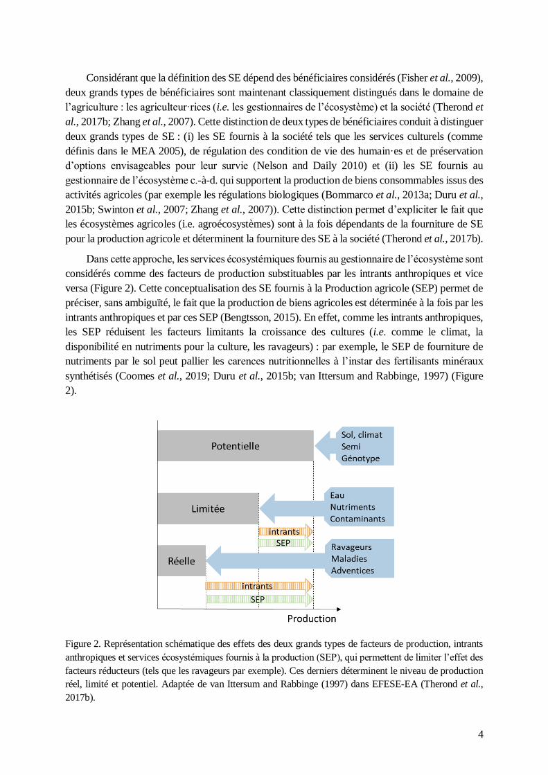
Dans cette approche, les services écosystémiques fournis au gestionnaire de l’écosystème sont

considérés comme des facteurs de production substituables par les intrants anthropiques et vice

versa (Figure 2). Cette conceptualisation des SE fournis à la Production agricole (SEP) permet de

préciser, sans ambiguïté, le fait que la production de biens agricoles est déterminée à la fois par les

intrants anthropiques et par ces SEP (Bengtsson, 2015). En effet, comme les intrants anthropiques,

les SEP réduisent les facteurs limitants la croissance des cultures (i.e. comme le climat, la

disponibilité en nutriments pour la culture, les ravageurs) : par exemple, le SEP de fourniture de

nutriments par le sol peut pallier les carences nutritionnelles à l’instar des fertilisants minéraux

synthétisés (Coomes et al., 2019; Duru et al., 2015b; van Ittersum and Rabbinge, 1997) (Figure

2).

Figure 2. Représentation schématique des effets des deux grands types de facteurs de production, intrants

anthropiques et services écosystémiques fournis à la production (SEP), qui permettent de limiter l’effet des

facteurs réducteurs (tels que les ravageurs par exemple). Ces derniers déterminent le niveau de production

réel, limité et potentiel. Adaptée de van Ittersum and Rabbinge (1997) dans EFESE-EA (Therond et al.,

2017b).

5

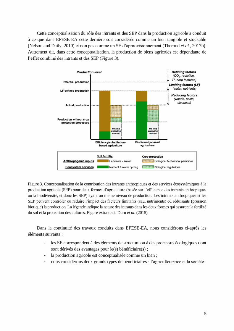
Cette conceptualisation du rôle des intrants et des SEP dans la production agricole a conduit

à ce que dans EFESE-EA cette dernière soit considérée comme un bien tangible et stockable

(Nelson and Daily, 2010) et non pas comme un SE d’approvisionnement (Therond et al., 2017b).

Autrement dit, dans cette conceptualisation, la production de biens agricoles est dépendante de

l’effet combiné des intrants et des SEP (Figure 3).

Figure 3. Conceptualisation de la contribution des intrants anthropiques et des services écosystémiques à la

production agricole (SEP) pour deux formes d’agriculture (basée sur l’efficience des intrants anthropiques

ou la biodiversité, et donc les SEP) ayant un même niveau de production. Les intrants anthropiques et les

SEP peuvent contrôler ou réduire l’impact des facteurs limitants (eau, nutriments) ou réduisants (pression

biotique) la production. La légende indique la nature des intrants dans les deux formes qui assurent la fertilité

du sol et la protection des cultures. Figure extraite de Duru et al. (2015).

Dans la continuité des travaux conduits dans EFESE-EA, nous considérons ci-après les

éléments suivants :

- les SE correspondent à des éléments de structure ou à des processus écologiques dont

sont dérivés des avantages pour le(s) bénéficiaire(s) ;

- la production agricole est conceptualisée comme un bien ;

- nous considérons deux grands types de bénéficiaires : l’agriculteur·rice et la société.

6

Parmi les SE traités dans l’étude EFESE-EA (Therond et al., 2017b)(Table 1), nous avons

retenu les SEP suivants : pollinisation des espèces cultivées, régulations des graines d’adventices,

des insectes ravageurs, des maladies (ajouté), stabilisation des sols et contrôle de l’érosion,

structuration du sol, rétention et restitution de l’eau aux plantes cultivées par le sol, fourniture

d’azote et de phosphore minéral aux plantes cultivées.

Services écosystémiques

fournis aux agriculteur·ices

Services écosystémiques

fournis à la société

Structuration du sol Régulation du climat global

Fourniture de N minéral Atténuation naturelle des pesticides Fourniture d’autres minéraux Régulation de la qualité de l’eau

Rétention et restitution de l’eau bleue

aux plantes cultivées

Stockage et restitution de l’eau

bleue Régulation des insectes ravageurs Potentiel récréatif sans prélèvement

Régulation des graines d’adventices Potentiel récréatif avec prélèvement

Pollinisation des espèces cultivées

Stabilisation des sols

Table 1. Services écosystémiques selon leur type de bénéficiaire proposés et étudiés dans l’étude EFESE-

EA (Therond et al., 2017b).

Il est important de noter que contrairement aux écosystèmes « naturels », les agroécosystèmes

sont gérés par les humains pour une finalité principale de production agricole au travers des

pratiques agricoles. Ils présentent ainsi des interactions fortes entre processus écologiques et

sociotechniques (Conway, 1987; Gliessman, 2004; Robinson et al., 2012; Swift et al., 2004 ;

Figure 4). Dans l’agroécosystème, deux types de biodiversité en interaction sont distingués : la

biodiversité planifiée par les gestionnaires (i.e. plantes semées et animaux introduits) et la

biodiversité associée, composée des organismes non-introduits et dépendants de la configuration

et de la composition spatiotemporelle de l’agroécosystème et des écosystèmes adjacents (Duru et

al., 2015b; Kremen and Miles, 2012a; Tscharntke et al., 2005). Le niveau de fourniture des SE par

les agroécosystèmes dépend de l’état de leur structure (par exemple de la biodiversité) et de

l’interaction entre le climat, les processus écologiques et des pratiques agricoles (Therond et al.,

2017b). Aussi, les dégradations de l’environnement mentionnées ci-avant impactent la fourniture

des SE. Par exemple, l’impact de l’usage des insecticides systémiques sur le SE de pollinisation

des plantes cultivées (Brittain and Potts, 2011) a conduit à une suspension de l’utilisation de trois

néonicotinoïdes par la Commission européenne en 2013 (EFSA, 2013).

7

Figure 4. Schéma de l’agroécosystème désignant l’écosystème en interaction avec le système

socioéconomique et le climat. Les gestionnaires définissent la composition et la configuration spatiale et

temporelle des couverts végétaux et des animaux d’élevage. Adapté de Gaba et al. (2015) dans Therond et

al. (2017b).

2. De nouvelles formes d’agriculture

L’impact des activités agricoles sur leur environnement à l’échelle globale mais aussi locale

questionne la durabilité du modèle de production industriel encouragé depuis les dernières

décennies dans certaines régions (Chaudhary et al., 2018). La capacité de ce modèle d’agriculture

à alimenter 9 milliards de personnes d’ici 2050 (Godfray et al., 2010) est vivement mise en doute.

Frison and IPES-Food, 2016 mentionnent ainsi que: « modern agriculture is failing to sustain the

people and resources on which it relies, and has come to represent an existential threat to itself ».

Du point de vue de l’alimentation, la modification des régimes alimentaires vers des régimes moins

carnés et plutôt basés sur des protéines végétales semble prometteuse (Tilman and Clark, 2014).

Mais du point de vue agronomique, les pratiques agricoles sont à redéfinir pour atteindre les

objectifs de durabilité tels qu’ils sont formulés par les Etats membres des Nations unies dans

l’Agenda 2030 (SDG, 2015). Pour répondre aux enjeux de dépendance aux ressources non

renouvelables et d’impact de l’agriculture sur l’environnement et sous l’impulsion de crises

agricoles, environnementales et sociétales, les dernières décennie ont vu émerger de nouvelles

« formes d’agriculture » (Therond et al., 2017a). Par forme d’agriculture, on désigne un ensemble

de systèmes de production agricole aux fonctionnements biotechniques similaires (par exemple les

pratiques agricoles, principes de gestion ect.) (ibid.).

8

2.1 Répondre aux enjeux socio-environnementaux

Plusieurs formes emblématiques d’agriculture se sont développées en France et en Europe.

Ainsi, depuis les années 2000, en France, en même temps que la médiatisation des effets des

pesticides sur la santé humaine et sur la santé des écosystèmes, les produits issus de l’agriculture

biologique (AB) sont de plus en plus consommés par les ménages français (France Agrimer,

2106b). L’agriculture biologique est soutenue depuis 1998 par des politiques publiques qui visent

à augmenter les surfaces cultivées en AB pour atteindre 15% de la surface agricole utile en 2022

(Le Foll, 2017; Leroux, 2015; Ministère de l’agriculture et de l’alimentation, 2018). Pour les

cultures, le cahier des charges français de l’AB impose de produire sans produits chimiques de

synthèse et sans organismes génétiquement modifiés. Bien que cela dépende des organismes et

des territoires/paysages, l’AB est globalement associée à une plus grande diversité et une plus

grande abondance d’espèces (oiseaux, insectes prédateurs, organismes du sol, plantes) (Bengtsson

et al., 2005). Cependant, les systèmes certifiés « Agriculture biologique », souvent opposés aux

systèmes conventionnels (« Agriculture conventionnelle » AC) , englobent un large éventail de

systèmes agricoles avec différents degrés de diversification et différentes pratiques agricoles, et

donc, de performances associées (Freyer and Bingen, 2015; Reeve et al., 2016; Seufert et al.,

2012). La dénomination « AB » n’est donc suffisante pour caractériser la diversité des

fonctionnements biotechniques des systèmes agricoles correspondants, ce qui pose des problèmes

méthodologiques de comparaison des performances des systèmes (Kirchmann et al., 2016).

L’agriculture de conservation des sols (ACS) s’est initialement développée pour pallier des

problématiques de fortes érosions (voir la description du « Dust Bowl » par J. Steinbeck dans « Les

raisins de la colère ») en favorisant la couverture permanente des sols avec des cultures

intermédiaires et des techniques de semis direct sous couvert (Mitchell et al., 2019). Par la suite,

l’agriculture de conservation a été officiellement définie en 2008 par la FAO comme « un système

cultural qui favorise une perturbation mécanique des sols minimale (pas de travail du sol), le

maintien d'une couverture permanente du sol, et la diversification des espèces végétales »

(Pittelkow et al., 2015a; FAO, 2021). La mise en place de ces trois principes vise à stimuler la

biodiversité et les processus écologiques édaphiques dont sont dérivés des services

écosystémiques liés aux cycles de l’eau, des nutriments et du carbone (Chabert and Sarthou, 2020).

L’ACS présente des intérêts (i) socio-économiques, par la réduction des interventions culturales,

surtout de travail du sol, (ii) agronomiques, par la stimulation de la fourniture en services

écosystémiques, et (iii) environnementaux, par la réduction de la consommation d’énergies

fossiles et d’impact environnementaux tels que l’érosion ou la perte de biodiversité du sol. Pour

autant, l’ACS présente des inconvénients quant à la mise en œuvre technique de ces 3 principes,

qui ne sont parfois pas réalisés de concert (Pittelkow et al., 2015a) et qui requièrent parfois des

herbicides systémiques à haut impact environnemental pour la destruction des couverts végétaux

et la gestion des adventices sans travail du sol (Chauhan et al., 2012).

9

De nombreuses autres formes d’agriculture ont émergé durant cette période. On parle ainsi

d’agriculture « biodynamique », « extensive », « de précision », « intégrée », « régénérative ». Il

est question aussi de systèmes « agroécologiques », « d’intensification écologique »

et « d’intensification durable » (Garbach et al., 2017a; Therond et al., 2017a). Comme pour l’AB,

ces formes d’agriculture sont définies de manière ambigüe et peu spécifique recouvrant ainsi une

diversité de fonctionnements biotechniques et de performances (Therond et al., 2017a). Elles sont

aussi difficilement comparables les unes aux autres car certaines se définissent relativement à la

nature des technologies mises en œuvre (par exemple l’agriculture de précision) tandis que d’autres

le sont relativement à la nature des intrants (par exemple l’AB) ou encore à la nature des processus

promus (par exemple l’agriculture intégrée). L’évaluation et la comparaison des performances de

ces types de systèmes agricoles ou de ces formes d’agriculture ne peuvent donc pas être réalisées

sur la seule base des dénomination utilisées (ibid.). Dans un objectif d’identification de formes

d’agriculture plus durables et résilientes, il y a donc besoin d’une approche renouvelée de la

caractérisation de la diversité observée des systèmes agricoles (Therond et al., 2017a; Wezel et al.,

2015).

2.2 Redéfinir les formes d’agriculture

Toutes ces nouvelles formes d’agriculture convergent sur la diminution de l’utilisation des

intrants industriels (c.-à-d. issus de la pétrochimie ou de l’extraction minière). Trois grandes voies

de progrès peuvent être identifiées (Duru et al., 2015b; Therond et al., 2017a). La première vise à

augmenter l’efficience des intrants chimiques via l’utilisation de technologies de précision et de

robotisation permettant d’optimiser les apports spatiotemporels de ces intrants (Rains et al., 2011).

La deuxième se base sur le remplacement de tout ou une partie des intrants chimiques par des

intrants biologiques (par exemple les stimulateurs de croissance, de la vie du sol ou de santé des

plantes, l’introduction d’organismes, les biopesticides) pour diminuer l’impact néfaste de certaines

pratiques agricoles sur la biodiversité et la santé humaine. Ces deux premières voies, parfois

qualifiées d’ « intensification écologique » (Hochman et al., 2013), ne remettent pas en cause la

simplification ni la standardisation des systèmes agricoles industriels.

La troisième, en rupture avec le modèle de production industriel, parfois qualifiée

d’ « écologiquement intensive » (Bonny, 2011), est basée sur le développement et la gestion de la

biodiversité pour assurer le développement des services écosystémiques (Kremen and Miles,

2012a) supports de la production agricole et ainsi, réduire fortement l’utilisation des intrants

externes. L’enjeu pour ces nouvelles formes d’agriculture basées sur l’usage des SEP est de

régénérer la structure et les fonctionnements biologiques des agroécosystèmes qui ont été

fortement dégradés par des décennies d’agriculture industrielle (Bommarco et al., 2013a; Nyström

et al., 2019). Pour cela, la connaissance du fonctionnement des écosystèmes est déterminante afin

d’évaluer les niveaux de SEP potentiels (Bastian et al., 2012), mais aussi réellement utilisés

(Schröter et al., 2014), et d’encourager les processus à l’origine de la fourniture de SEP désignés

comme le capital naturel (Dominati et al., 2010; Kleijn et al., 2019a).

10

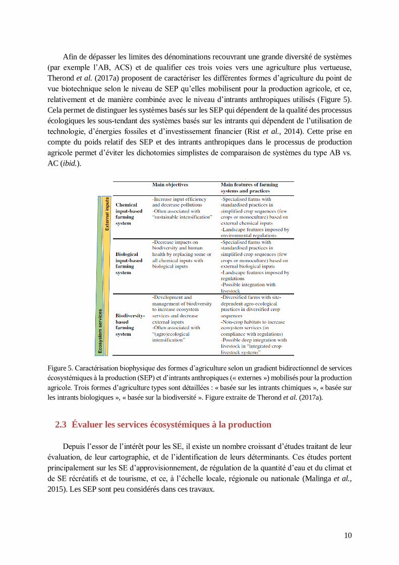
Afin de dépasser les limites des dénominations recouvrant une grande diversité de systèmes

(par exemple l’AB, ACS) et de qualifier ces trois voies vers une agriculture plus vertueuse,

Therond et al. (2017a) proposent de caractériser les différentes formes d’agriculture du point de

vue biotechnique selon le niveau de SEP qu’elles mobilisent pour la production agricole, et ce,

relativement et de manière combinée avec le niveau d’intrants anthropiques utilisés (Figure 5).

Cela permet de distinguer les systèmes basés sur les SEP qui dépendent de la qualité des processus

écologiques les sous-tendant des systèmes basés sur les intrants qui dépendent de l’utilisation de

technologie, d’énergies fossiles et d’investissement financier (Rist et al., 2014). Cette prise en

compte du poids relatif des SEP et des intrants anthropiques dans le processus de production

agricole permet d’éviter les dichotomies simplistes de comparaison de systèmes du type AB vs.

AC (ibid.).

Figure 5. Caractérisation biophysique des formes d’agriculture selon un gradient bidirectionnel de services

écosystémiques à la production (SEP) et d’intrants anthropiques (« externes ») mobilisés pour la production

agricole. Trois formes d’agriculture types sont détaillées : « basée sur les intrants chimiques », « basée sur

les intrants biologiques », « basée sur la biodiversité ». Figure extraite de Therond et al. (2017a).

2.3 Évaluer les services écosystémiques à la production

Depuis l’essor de l’intérêt pour les SE, il existe un nombre croissant d’études traitant de leur

évaluation, de leur cartographie, et de l’identification de leurs déterminants. Ces études portent

principalement sur les SE d’approvisionnement, de régulation de la quantité d’eau et du climat et

de SE récréatifs et de tourisme, et ce, à l’échelle locale, régionale ou nationale (Malinga et al.,

2015). Les SEP sont peu considérés dans ces travaux.

11

Parmi les méthodes d’évaluation des SEP à l’échelle de l’agroécosystème, trois grands types

d’approches peuvent être distingués :

- l’utilisation de modèles précis (par exemple de croissance des cultures comme STICS

(Therond et al., 2017b), d’érosion du sol comme RUSLE (Panagos et al., 2015)) ;

- les expérimentations et relevés en plein champ pour directement évaluer le niveau de

SEP (par exemple avec des cartes de prédation, Boeraeve et al., 2020; Petit et al.,

2017) ;

- l’évaluation indirecte de SEP via l’utilisation d’indicateurs de l’état des déterminants

biophysiques de ceux-ci tels que l’abondance ou la diversité taxonomique ou

fonctionnelle des organismes support des SEP comme des pollinisateurs (par exemple

Potts et al. (2009) ou des auxiliaires des cultures (par exemple Dainese et al. (2019),

les caractéristiques du paysage (par exemple Burkhard et al., 2012; Martin et al.,

2019a) ou encore la teneur en matière organique (par exemple Vogel et al. (2019)).

Deux grands types déterminants peuvent être distingués ici : ceux modifiables via les

activités humaines telles que les pratiques agricoles, c.-à-d. « gérables », et ceux

relevant de propriétés « inhérentes », c.-à-d. non modifiables, comme par exemple la

texture des sols (Vogel et al., 2019).

Sans chercher à évaluer les SEP spécifiquement, d’autres études évaluent la qualité du sol ou

encore le niveau de biodiversité, ce qui fournit une indication sur la capacité de l’agroécosystème

à fonctionner et à fournir des SEP. Par exemple, van Leeuwen et al. (2019a) proposent une

évaluation des fonctions remplies par la biodiversité du sol par 34 attributs-proxy (caractéristiques

pédoclimatiques, de pratiques agricoles, de configuration et composition et de traits biologiques)

de l’agroécosystème dans des prairies et des grandes cultures. Ils proposent une agrégation basée

sur l’expertise de ces attributs (modèle DEXi). Sur le même principe, à l’échelle de l’exploitation

agricole, Birrer et al. (2014) démontrent la capacité prédictive, en Suisse, de 32 indicateurs de

pratiques agricoles et de caractéristiques du paysage vis-à-vis de 19 mesures de la biodiversité.

Toujours en Suisse, Lüscher et al. (2017a) montrent aussi l’intérêt de l’évaluation par analyse de

cycle de vie (Life Cycle Assessment) de la biodiversité en comparaison avec des relevés d’espèces.

Ces études, ainsi que celles qui évaluent les SEP, ne portent généralement que sur un ou

quelques SEP (Malinga et al., 2015). En d’autres termes, la majorité des d’études n’appréhendent

pas le bouquet des SEP (Wam, 2010). De plus, l’application de certaines méthodes proposées

précédemment peut être difficile à mettre en œuvre du fait des besoins en connaissances

scientifiques (par exemple sur l’effet des SEP sur la production), de la complexité des méthodes

(par exemple un modèle de culture dynamique) ou des données et moyens nécessaires (par

exemple des expérimentations, modélisation).

12

3. Menaces sur les systèmes agricoles

Si les SEP permettent d’envisager la réduction ou le remplacement des intrants anthropiques

néfastes à l’environnement en favorisant les formes d’agriculture basées sur les SEP, les menaces

qui pèsent et pèseront sur les systèmes agricoles viennent ajouter des contraintes à considérer dans

l’analyse de la durabilité des systèmes agricoles, et ce, quelles que soient les formes d’agriculture

impliquées.

3.1 Changements climatiques

Si les systèmes agricoles ont une responsabilité dans les changements climatiques observés

et à venir (Introduction 1.1), ils sont aussi particulièrement impactés par ces changements du fait

de la dépendance forte de la production primaire, voire secondaire, aux conditions climatiques et

biotiques.

Globalement, les analyses des effets potentiels des projections climatiques sur les rendements

des cultures, toutes choses égales par ailleurs, prévoient des réductions importantes dans la plupart

des régions du monde et une augmentation de leur variabilité dans la plupart des scénarios, même

parmi les plus optimistes (Challinor et al., 2014; Gaupp et al., 2019) (Figure 6). L’augmentation

des températures et des sécheresses durant la floraison, des épisodes de gel printanier tardif, de la

propagation de ravageurs et pathogènes (Deutsch et al., 2018), de précipitations intenses entraînant

des inondations sont autant de phénomènes biophysiques liés aux changements climatiques qui

peuvent et pourront impliquer des pertes de production (Zampieri et al., 2020b). Par ailleurs,

l’augmentation projetée de la fréquence de ces stress, dont les effets peuvent se combiner et

s’alimenter, conduira à une diminution de la prédictibilité des conditions biophysiques de

production et donc à une prise de risque plus importante pour les agriculteur·rices (Cohen et al.,

2021).

Figure 6. (Gauche) Projection de l'évolution du rendement des cultures en fonction du temps pour toutes les

cultures et toutes les régions (n = 1,090 d'après 42 études) sous différents scénarios. (Droite) Projection de

l’évolution du coefficient de variation (%) du rendement des cultures en fonction du temps pour quelques

études. Figures issues de Challinor et al. (2014).

13

3.2 Épuisement des ressources

Le modèle agricole industriel base le processus de production sur l’utilisation intensive de

ressources fossiles et minières dont la disponibilité future est incertaine, voire menacée. Il est

estimé que 3 kcal d’énergies fossiles sont consommées pour la production d’1 kcal d’énergie

alimentaire (y compris la transformation alimentaire) dans les systèmes agricoles industriels

(Verma, 2015) et ce, grâce à la disponibilité de combustibles fossiles bon marché (Tilman et al.,

2002). Un tiers de l’énergie consommée sur chaque exploitation agricole est utilisée pour la

mécanisation, le séchage ou encore l’irrigation. Les 2/3 restants correspondent à une

consommation indirecte par la production de fertilisants (dont 1/3 pour l’azote synthétisé), de

matériels et de transport (Fluck, 2012). Déjà en 1973, Pimentel et al. alertaient sur la dépendance

des systèmes agricoles des U.S.A. aux combustibles fossiles (à 80% du pétrole ou gaz naturel)

pour assurer les travaux agricoles. Depuis 2008, l’International Energy Agency reporte une

stagnation de l’extraction du pétrole conventionnel et prévoit une contraction de la fourniture (IEA,

2018). La production d’engrais azotés via le procédé d’Haber-Bosch consomme 3 à 5% de la

production annuelle mondiale de gaz naturel (Wang et al., 2018) alors que les ressources en gaz

naturel deviennent de moins en moins accessibles (Word Energy Council, 2013).

Ces potentielles limitations futures concernent aussi les ressources minières utilisées comme

fertilisants des cultures ou correcteurs des caractéristiques du sol, comme le phosphore, le

potassium ou la chaux, dont l’extraction requiert en plus du pétrole (Chowdhury et al., 2017), ou

encore les sous-produits de l’exploitation pétrolière comme le soufre (Zheljazkov et al., 2008).

Le développement du modèle agricole industriel a aussi été soutenu par le développement de

l’irrigation pour assurer le besoin en eau des cultures (James, 1988). En France, par exemple,

l’irrigation agricole représente la moitié de l’eau douce prélevée annuellement, et les prélèvements

sont concentrés durant l’été, période coïncidant avec celles des étiages naturels des cours d’eau

(Observatoire des territoires, 2009). Dans beaucoup de régions du monde, les volumes des nappes

phréatiques sollicitées par l’irrigation sont en déclin (Schwartz and Ibaraki, 2011). La diminution

tendancielle des ressources en eau de surface et souterraine, liées aux changements climatiques et

à leur surutilisation, exposent les systèmes basés sur l’irrigation à une augmentation des

impossibilités physiques, surcoûts ou restrictions de pompage durant les périodes critiques de

croissance des cultures (Rad et al., 2020).

Le saviez-vous ?

Il existe une possibilité pour les plantes d’acquérir une résistance transgénérationnelle

aux stress biophysiques (Holeski et al., 2012) par épigénétique, par exemple par méthylation

de l’ADN (Chang et al., 2020). Malheureusement, dans le modèle agricole industriel, la

plupart des plantes cultivées ne sont pas reproduites sur les exploitations agricoles et donc

sont dénuées de mémoire transgénérationnelle et d’adaptation au pédoclimat local

(Thorogood et al., 2020).

14

3.3 Volatilité des prix

La dépendance du modèle agricole industriel aux intrants industriels l’expose et le rend

sensible aux fluctuations de leurs prix qui dépendent de l’état des gisements, des spéculations

économiques et des évènements géopolitiques (Kaltalioglu et al., 2011; Lécuyer et al., 2014). Les

activités de production agricole sont également impactées par la variabilité des prix des produits

eux-mêmes. Ces différents prix sont volatiles car ils sont négociés sur le marché économique

mondial et dépendent ainsi des productions et spéculations mondiales (Gilbert and Morgan, 2010;

Headey and Fan, 2008; Figure 7). La concurrence entre les régions productrices du monde

complexifie et induit des variations de prix imprévisibles et potentiellement importantes. Ainsi, les

marchés qui ont été protégés par le passé, comme par exemple celui du lait via les quotas laitiers

supprimés le 1er avril 2015 en Europe, subissent depuis leur libéralisation une plus grande volatilité

des prix (Baldursson and Nils-Henrik, 2012). Des études commencent à démontrer l’impact des

politiques agricoles, comme la Politique Agricole Commune des membres de l’Union Européenne,

ou la mise en place d’outils de stabilisation du revenu, sur la robustesse et l’adaptabilité des

systèmes agricoles et de leur revenu (Buitenhuis et al., 2020; Castañeda-Vera and Garrido, 2017).

Figure 7. Évolution des prix de vente mondiaux des cultures d’orge, maïs, riz, seigle et blé (1850-2015)

sous forme d’indices de prix par rapport aux prix réels de 1900 d’après les données de Jacks (2013).

15

4. Faire face : résilience ou vulnérabilité ?

L’exposition présente et future des différentes formes d’agriculture aux perturbations

climatiques et économiques questionne leur capacité à y faire face et à persister dans le temps

(Therond et al., 2017a). La prise en compte de ces changements à venir dans l’élaboration des

stratégies d’évolution des systèmes agricoles est au cœur des débats de la communauté scientifique

agronomique et agroécologique (Peterson et al., 2018). Il en résulte une multiplicité de points de

vue concernant l’enjeu des systèmes agricoles à « faire face » aux perturbations, illustrée par la

multiplicité des concepts, des définitions et cadres conceptuels associés : résilience, vulnérabilité,

robustesse, flexibilité, intégrité, résistance, capacité d’adaptation, stabilité (Urruty et al., 2016).

Ces concepts convergent dans le sens où ils traitent tous de la dynamique des systèmes face à des

perturbations identifiées ou non (latentes) (Urruty et al., 2016).

4.1 Définitions usuelles

Il ne s’agit pas ici de reprendre l’historique de l’émergence de ces concepts, ni de leur

utilisation dans les différents domaines scientifiques, et encore moins de présenter l’exhaustivité

des définitions et cadres conceptuels existants. Il existe plusieurs articles très bien documentés à

ce sujet (par exemple Gallopín, 2006; Miller et al., 2010; Mumby et al., 2014; Turner et al., 2003;

Urruty et al., 2016). Aussi, cette section vise à présenter les définitions usuelles des principaux

concepts qui seront ensuite mentionnés dans la thèse : résilience, vulnérabilité, robustesse (Mumby

et al., 2014), stabilité et résistance (Urruty et al., 2016).

Le concept de résilience, popularisé en 1973 par Crawford Stanley Holling (Holling, 1973),

est désormais solidement ancré dans le vocabulaire scientifique (pour l’agriculture, voir (Peterson

et al., 2018), politique (par exemple le nom de mission des forces armées françaises) et public (par

exemple l’adjectif décrivant les populations face à la crise sanitaire COVID-19). En 2014, ce

concept a été défini par le groupe d’experts intergouvernemental sur l’évolution du climat (IPCC)

par « the capacity of social, economic, and environmental systems to cope with a hazardous event

or trend or disturbance, responding or reorganizing in ways that maintain their essential function,

identity, and structure, while also maintaining the capacity for adaptation, learning, and

transformation ». Le Stockholm Resilience Center définit la resilience comme « the capacity of a

system […] to deal with change and continue to develop ». Récemment, le projet de recherche

européen Towards SUstainable and REsilient EU FARMing systems (SURE-Farm) a proposé une

définition de la résilience pour les systèmes agricoles et déploie un cadre méthodologique associé :

« ability to ensure the provision of the system functions in the face of increasingly complex and

accumulating economic, social, environmental and institutional shocks and stresses, through

capacities of robustness, adaptability and transformability » (Meuwissen et al., 2019). Ces trois

définitions intègrent toutes l’idée de « faire avec » les perturbations et de « continuer à » assurer

les fonctions du système (Delettre, 2021).

La vulnérabilité est définie plus consensuellement comme « the degree to which a system is

harmed due to disturbances or stress » (Turner et al., 2003). Elle peut être déclinée en trois

composantes : exposition [à la perturbation], sensibilité [à la perturbation] et capacité d’adaptation

16

[du système] (Adger, 2006). Alors que certains auteurs analysent les différences et recoupements

entre les concepts de vulnérabilité et de résilience (Gallopín, 2006), d’autres considèrent la

vulnérabilité comme l’antagonisme de la résilience (Bahadur et al., 2010; Cutter et al., 2008). La

capacité d’adaptation, décrite explicitement dans le cadre conceptuel de la vulnérabilité, est parfois

reprise pour d’autres concepts, notamment dans certains cadres conceptuels de la résilience (Engle,

2011). Elle est définie généralement comme la capacité des humains à se préparer à répondre aux

perturbations (Engle, 2011). En revanche, ses déterminants et son lien à la résilience et à la

vulnérabilité ne font pas l’objet d’un consensus (Eakin and Luers, 2006; Gallopín, 2006) et cette

notion diffère et/ou recouvre celles de l’adaptabilité et la transformabilité (Engle, 2011; Walker et

al., 2004).

Le concept de robustesse est défini par Urruty et al. (2016) pour les systèmes agricoles

comme « the ability to maintain desired levels of agricultural outputs despite the occurrence of

perturbations ». Il est plutôt utilisé pour analyser l’impact de perturbations précises sur les

performances agronomiques ou économiques (Urruty et al., 2016) et semble moins intégrateur (un

seul aspect de la dynamique, un seul évènement perturbateur) que la résilience. La robustesse est

l’une des trois composantes du cadre conceptuel de la résilience proposé par Meuwissen et al.

(2019), avec l’adaptation et la transformation.

La résistance est plutôt considérée comme un sous-concept de celui de résilience, portant sur

l’impact d’une perturbation précise, ou de tolérance aux perturbations (Lake, 2013; Urruty et al.,

2016). Il est souvent considéré comme complémentaire de recovery, correspondant au taux ou

temps de récupération du niveau pré-perturbation (Holling, 1996).

La stabilité est définie comme (i) le fait de rester dans le même état d’équilibre stable (au sens

de l’analyse des systèmes dynamiques) (Holling, 1973) ou comme (ii) « the constancy of

agricultural outputs over long periods » (Urruty et al., 2016), c.-à-d. l’inverse de la variabilité.

Il existe ainsi une diversité des concepts relatifs à l’analyse de la dynamique d’un système

face aux perturbations (Martin et al., 2011; Urruty et al., 2016), qui est accompagnée d’une

diversité de cadres conceptuels associés à chaque concept (Quinlan et al., 2016). Au sein même

parfois d’une communauté scientifique, ces concepts sont polysémiques et leurs différents cadres

conceptuels associés peuvent recouvrir plusieurs concepts ou s’imbriquer (par exemple la

résilience comme composante de la vulnérabilité) (Miller et al., 2010; Mumby et al., 2014; Turner

et al., 2003). Ce foisonnement conceptuel rend difficile l’accès, la comparaison et la capitalisation

des travaux d’analyse de la dynamique des performances des systèmes (Urruty et al., 2016).

4.2 Un débat conceptuel clivant

Deux grandes « écoles de pensée » coexistent concernant la résilience. Holling et son équipe

conçoivent la résilience comme la capacité à ne pas basculer dans un nouveau bassin d’attraction

correspondant à un nouveau régime de fonctionnement. Il est question ici de « résilience

écologique » (Holling, 1996). Les concepts de seuils de basculement (tipping points) et de régimes

de fonctionnement sont des concepts structurants du cadre conceptuel proposé par Holling. Inscrite

dans cette école de pensée, la théorie des limites planétaires de Rockström et al. (2009) considère

17

qu’il existe des seuils écologiques et biophysiques franchissables déterminant l’état et le

fonctionnement de la planète. Leur franchissement induirait des changements drastiques et

irrévocables qui pourraient faire basculer la planète dans un autre état (Steffen et al., 2018). L’autre

école de pensée, positionnée derrière Stuart Pimm, considère que cette théorie n’est pas

généralisable : « Certainly, there may be systems that show the tipping points that underpin this

world. Importantly, there is nothing to suggest they are ubiquitous and so demand their having

logical primary. Nature might work this way sometimes, but there is no compelling argument that

it must » (citation issue de Donohue et al. (2016). Ses défenseurs considèrent que les changements

d’un système se font de manière graduelle et progressive plutôt que par basculement. Cette école

se focalise sur la capacité d’un système à revenir à l’équilibre après une perturbation (Oliver et al.,

2016). C’est ce qu’on appelle la résilience « ingénierique » (Holling, 1996). Grafton et al. (2019)

ont essayé de réconcilier ces deux approches fondamentalement clivantes (Editorial board of

Nature Sustainability, 2019), sans pour autant satisfaire les protagonistes des deux écoles (Allen

et al., 2019; Pimm et al., 2019).

Dans la continuité de la résilience écologique, Holling et ses collègues ont formulé la notion

de cycle adaptatif (Holling and Gunderson, 2002). Ils distinguent quatre étapes dans le

développement d’un système : l’exploitation (et organisation), la consolidation (et conservation),

la destruction par collapse et enfin la réorganisation ou échec. Cette vision de la dynamique des

systèmes est intimement liée à l’existence de seuils et d’un collapse ponctuel. Les applications

théoriques du cycle adaptatif sont nombreuses mais peu observées dans la réalité (Hillebrand et

al., 2020). Plus généralement, l’identification des seuils de basculement représente un véritable

enjeux méthodologique : des méthodes existent mais semblent peu satisfaisantes, surtout pour des

systèmes dont le basculement n’a pas été encore observé et serait donc à venir (Scheffer et al.,

2015). Par exemple, l’approche d’un seuil de basculement serait caractérisée par une augmentation

de l’asymétrie de la distribution des valeurs des variables considérées (Scheffer et al., 2015) mais,

récemment, Xie et al. (2019) ont montré que cet indicateur n’est pas toujours fiable. L’approche

de résilience écologique est critiquée pour les conséquences alarmistes ou, au contraire, optimistes

qu’elle implique concernant l’immédiateté du basculement et l’opportunité que représente l’état

suivant. Ainsi, concernant les limites planétaires, Donohue et al. (2016) reprochent à Steffen et al.

(2018) de ne pas s’exprimer sur l’étendue spatiale et temporelle que représentent ces basculements

pour les territoires, laissant les institutions décisionnelles confrontées à un discours théorique alors

que très médiatisé.

4.3 Identité du système agricole, fonctions et performances

Analyser la dynamique d’un système nécessite d’en définir la ou les caractéristique(s) que

l’on cherche à suivre dans le temps. Dans un contexte d’analyse de la résilience, l’identité à

maintenir dans le temps face aux perturbations doit être définie clairement (Bousquet et al., 2021).

Elle peut correspondre à une ou des caractéristiques de la structure (par exemple la diversité des

activités), des propriétés (par exemple d’une trajectoire) et/ou des fonctions (par exemple fournir

un revenu suffisant) du système (Folke, 2016). Meuwissen et al. (2019) incitent à se poser la

question « resilience for what purpose ? » afin d’identifier les fonctions du système agricole à

maintenir (par exemple la production alimentaire) et ainsi les performances qui seront étudiées

18

(par exemple le rendement des cultures). Ensuite, Meuwissen et al. (2019) suggèrent de traiter

« what resilience capacities ? ». Les fonctions à maintenir étant identifiées au préalable, des

adaptations et transformations peuvent être envisagées pour les maintenir. Dans un contexte

agricole, l’adaptation se réfère à des changements de pratiques agricoles, de cultures ou de marchés

de commercialisation sans pour autant changer la structure du système (par exemple en continuant

à cultiver des grandes cultures) alors que la transformation suggère un changement interne radical

de structure et des mécanismes de rétroaction qui en découlent (par exemple l’introduction d’un

atelier d’élevage), pouvant aller jusqu’à entraîner un changement de fonctions (ibid.).

4.4 Évaluer la résilience

Parmi les nombreux cadres conceptuels proposés pour analyser la dynamique des systèmes,

peu d’entre eux vont jusqu’à l’opérationnalisation de leur proposition, c.-à-d. jusqu’à la définition

d’un cadre méthodologique ou d’une démarche à suivre voire à la proposition de méthodes

d’analyse (Martin et al., 2019b; Oliver et al., 2015; Weise et al., 2019). On peut cependant

distinguer deux grands types d’approche d’évaluation de la résilience (et des concepts parents

présentés ci-avant) : (i) via l’analyse quantitative de la dynamique de caractéristique(s) du système

ou (ii) via l’évaluation qualitative ou quantitative de caractéristiques ou de propriétés du système

associées a priori à la résilience (Figure 8) (Douxchamps et al., 2017; Weise et al., 2019; Zhang,

2020). Dans le premier type, l’analyse de la dynamique de l’identité du système dans le temps, et

ainsi l’identification des propriétés ou caractéristiques des systèmes résilients (c.-à-d. des facteurs

explicatifs de résilience, « resilience enhancing attributes » dans Meuwissen et al. (2019)), relève

d’une démarche empirico-inductive. Dans le second type, les propriétés de résilience à évaluer

peuvent être définies à dire d’expert ou à partir de connaissances issues de travaux scientifiques

antérieurs tels que ceux conduits dans le premier type d’approche ou issus de domaines d’études

connexes (par exemple de l’écologie) (Douxchamps et al., 2017). En d’autres termes, les

connaissances sur les facteurs explicatifs de la résilience issues du premier type d’évaluation

peuvent être utilisées comme point de départ du second type d’évaluation. Aussi, les hypothèses

émises dans le deuxième type d’évaluation peuvent être utilisées dans le premier type d’évaluation

dans le cadre d’un raisonnement hypothético-déductif. Par exemple, la diversité (comme celle des

cultures dans une rotation culturale) est utilisée comme un critère pour évaluer la résilience des

systèmes agricoles (démarche déductive) suite aux nombreux travaux en écologie qui ont montré

que la diversité est souvent un facteur explicatif de résilience (par exemple Isbell et al., 2015;

Pfisterer and Schmid, 2002). Cependant, l’application de ces connaissances sur des systèmes pour

la caractérisation de la dynamique des agroécosystèmes, du fait de leur caractère très anthropisé

(Introduction 1.2 p3), requiert des précautions (Gaba et al., 2018).

19

Figure 8. Deux types de démarche d’évaluation de la dynamique d’un système.

A partir de la définition séminale de Holling de la résilience écologique, basée sur le concept

de bassin d’attraction, Scheffer et al. (2015) identifient une diversité d’études (approche (i)) sur

les écosystèmes qui ont développé et appliqué des indicateurs de résilience ou des méthodes

d’évaluation en utilisant des modèles ou des données observées. Ces indicateurs ou méthodes

décrivent soit un ralentissement critique, un vacillement d’état ou une fluctuation autonome (un

pattern) qui décrirait la résilience de l’écosystème. Le site internet www.early-warning-

signals.org/ recense une plus grande gamme de démarches pour évaluer le risque de changement

d’état (Early Warning Signals, 2016).

Concernant les agroécosystèmes, Cabell and Oelofse (2012) proposent, sur la base d’une

revue de littérature, une liste de 13 indicateurs des propriétés qui déterminent la résilience

(approche (ii)). Toutefois, ils ne vont pas jusqu’à appliquer leur proposition sur un cas d’étude.

Diserens et al. (2018) l’appliquent dans le Canton de Vaud à travers une évaluation qualitative

formalisée dans l’outil SHARP (Self-evaluation and Holistic Assessment of climate Resilience of

farmers and Pastoralists). Depuis la proposition des 13 indicateurs par Cabell and Oelofse (2012),

d’autres l’ont adapté à certains niveaux d’organisation (par exemple à l’échelle du système

alimentaire (Himanen et al., 2016)), ont proposé d’autres listes (Douxchamps et al., 2017) ou ont

porté leur travail sur d’autres types de systèmes socio-écologiques (Quinlan et al., 2016).

Concernant les agroécosystèmes, peu d’études semblent aller jusqu’à des évaluations de la

résilience (et autres concepts) par des approches d’analyse quantitative de la dynamique (approche

(i)) (Douxchamps et al., 2017; Gillespie‐Marthaler et al., 2019; Martin et al., 2017; Oliver et al.,

2015). Par exemple, Martin et al. (2017) développent une méthode innovante d’évaluation de la

vulnérabilité via l’analyse couplée du niveau, de la variabilité et de la tendance d’une performance

20

grâce à une régression linéaire mixte. Leur proposition a initié une série de travaux qui déploient

et adaptent la méthode (Bouttes et al., 2018b; Perrin et al., 2020). Autre exemple, Dong (2015)

évalue la vulnérabilité à l’échelle de la parcelle et de la région comme le changement de rendement

agricole causé par le changement climatique avant et après une période de mutation (identifiée par

la méthode de Mann-Kendall). Le peu d’études sur ce sujet (au commencement de cette thèse)

peut être expliqué par la diversité et la faible opérabilité des cadres conceptuels proposés (Weise

et al., 2019) mais aussi par le besoin d’accéder à des séries de données observées ou simulées,

temporelles ou spatiales (Allen et al., 2016), sur une période durant laquelle des perturbations se

seront exprimées (Thorogood et al., 2020). Sur des expérimentations contrôlées, des équipements

technologiques permettent de simuler des perturbations sur des parcelles (par exemple un stress

hydrique avec un pare-pluie (Hoover et al., 2014)). Sur des observations moins contrôlées ou non

anticipées, il faut en revanche être au bon endroit au bon moment pour avoir des informations

pertinentes (Alkan-Olsson et al., 2009; Duru and Therond, 2015; Thorogood et al., 2020).

Boîte 1. Évaluer la durabilité vs. évaluer la résilience.

De nombreuses méthodes permettent d’évaluer la durabilité des systèmes agricoles (Soulé

et al., soumis). La grande majorité d’entre elles l’évaluent via une estimation des performances

du système à un instant donné ou en moyenne sur une période (états/performances jugé(s)

durable(s) relativement aux objectifs écologiques, économiques et sociaux atteints). Elles

proposent ainsi une évaluation « statique » du niveau (moyen) des performances (Duru and

Therond, 2015). Les évaluations de la « dynamique » des performances du système visent à

l’identification de propriété(s) de ces dynamiques au regard d’un enjeu de maintien dans le

temps du niveau de cette performance (Oliver et al., 2015). Le premier type d’évaluation,

souvent qualifié d’évaluation de la durabilité, s’intéresse donc plutôt à qualifier un niveau vis-

à-vis d’un « but » à atteindre, souvent défini de manière normative (Elmqvist et al., 2019). Elle

peut être qualifiée d’objectif-orienté (goal-oriented, Olsson et al., 2009). Le second type

d’évaluation s’intéresse donc plutôt aux « propriétés » de la dynamique des performances et

peut être qualifié de propriété-orienté (ibid.). Ce deuxième type d’approche s’exprimerait de

manière moins normative (Elmqvist et al., 2003). Ainsi, la résilience n’est pas toujours

souhaitable si l’état dans lequel se maintient le système n’est pas souhaitable, c.-à-d. ne

correspond pas aux buts à atteindre (Gallopín, 2006; Walker and Meyers, 2004). Depuis, ce

positionnement a néanmoins été critiqué (Voir Discussion, Cote and Nightingale, 2012).

21

5. Résilience des formes d’agriculture

Si les nouvelles formes d’agriculture permettent de répondre aux enjeux socio-

environnementaux (Duru et al., 2015b), les systèmes agricoles sont déjà ou seront exposés aux

perturbations climatiques et/ou économiques, quelle que soit la forme d’agriculture dans laquelle

ils s’inscrivent. Leur capacité à présenter un niveau de performances acceptables et à faire face

aux perturbations est déterminante pour leur adoption et leur déploiement dans les territoires

agricoles (Therond et al., 2017a). Alors que de nombreuses études visent à évaluer la durabilité

des systèmes de production agricole (Soulé et al., soumis, Boîte 1), l’évaluation et la comparaison

de la résilience des différentes formes d’agriculture reste un front de recherche (Therond et al.,

2017a). Cependant, quelques travaux récents ont initié ce type d’analyse.

Knapp and van der Heijden (2018) et Smith et al. (2019) ont produit récemment deux

méta-analyses sur la variabilité du rendement des systèmes en AB et ACS vs. AC. Knapp and van

der Heijden (2018) montrent que les systèmes en AB présentent, par unité de rendement, une

stabilité temporelle significativement moindre (- 15 %) comparée aux systèmes conventionnels.

Ces résultats convergent avec ceux de (Smith et al., 2019) mais certaines études expérimentales

concluent le contraire (par exemple Schrama et al., 2018). En revanche, d’après Knapp and van

der Heijden (2018), la stabilité du rendement des systèmes en ACS ne diffère pas significativement

de celle des systèmes conventionnels. Pour les systèmes horticoles (production de fruits et de

légumes) en particulier, Lesur-Dumoulin et al. (2017) n’observent pas de différence de variabilité

du rendement mais une plus grande probabilité d’obtenir de plus hauts (+ 10 %) et de plus faibles

rendements (+ 20 %) en système AB par rapport à des systèmes conventionnels. Comme

mentionné précédemment, les résultats peinent à converger probablement dû au fait que les

systèmes en AB et AC recouvrent une très grande diversité de systèmes (Kirchmann et al. (2016),

voir Discussion 2.1). Afin de proposer une comparaison plus fine, certaines études analysent plutôt

les effets de pratiques agricoles précises comme le non travail du sol et la diminution de l’usage

d’intrants chimiques pour une même culture (Smith et al., 2007) ou différentes rotations culturales

incluant des légumineuses à grains (Reckling et al., 2018).

Gil et al. (2017) proposent une revue de littérature plus large qui traite de la résilience

aux changements climatiques des systèmes agricoles « intégrés » en relatif des systèmes

conventionnels, définis comme des systèmes présentant des relations synergétiques entre les

entités du système, une diversité d’espèces cultivées et une répartition équilibrée de la production

parmi les différentes cultures. S’ils indiquent que, parmi les 24 études analysées, les systèmes

diversifiés présentent une meilleure résilience, il faut toutefois noter que certaines d’entre elles

comparent uniquement des niveaux moyens de rendement, sans prise en compte de sa dynamique

temporelle.

Du point de vue théorique, la diversité est considérée comme un déterminant important de la

résilience des systèmes agricoles (Altieri et al., 2015; Biggs et al., 2012; Cabell and Oelofse, 2012).

En effet, d’après l’hypothèse de l’« assurance écologique » (Yachi and Loreau, 1999), la diversité

offre une plus grande probabilité que certains types d’individus (espèces, génotypes, types de

22

production) maintiennent leur fonctionnement ou leur niveau de production dans un contexte

changeant. La diversité peut également être source d’interactions synergétiques entre ses

composantes dans l’espace et le temps, favoriser les complémentarités de niche et la redondance

des fonctions biologiques (Duru et al., 2015b). En outre, la diversité des réponses au sein d’un

mélange d’espèces permettrait de compenser la perte pour une espèce (Altieri et al., 2015). Par

exemple, le mélange de variétés au sein d’une même parcelle d’orge d’hiver permettrait d’obtenir

des rendements comparables aux meilleures monocultures tout en améliorant la stabilité spatiale

du rendement face aux perturbations (Creissen et al., 2016). Plusieurs études expérimentales

testent l’effet de la diversification sur la dynamique de la production de biomasse (voir synthèse

Chapitre I) mais leurs résultats ne convergent pas unanimement (voir par exemple Prieto et al.,

2015; Wang et al., 2019a).

Si la diversité est un déterminant clé de la fourniture des SEP (Kleijn et al., 2019a; Palomo-

Campesino et al., 2018a), les SEP pourraient contribuer à la résilience des systèmes agricoles

(Altieri et al., 2015; Peterson et al., 2018) (Figure 9). Leur effet « théorique » est d’ailleurs souvent

énoncé dans la littérature, avec ou sans relation avec la diversité (Altieri et al., 2015). Les SEP

auraient un effet « tampon » face aux perturbations, surtout biotiques et abiotiques, via une

régulation interne au système (Peterson et al., 2018), c.-à-d. l’autoadaptation du système (Müller

et al., 2000), ce qui augmenterait la tolérance des cultures aux stress associés (Altieri et al., 2015).

Les services de contrôle de l’érosion du sol, de stockage et restitution de l’eau aux plantes cultivées,

et de contrôles biologiques permettraient de faire face à la dégradation de l’agroécosystème et de

ses fonctions respectivement par les précipitations et le vent, par les sécheresses et les fortes

températures ainsi que par les attaques de ravageurs, la propagation des maladies et la compétition

des adventices (Altieri et al., 2015) (Figure 9). Par exemple, Zhu et al. (2000) montrent l’intérêt

du contrôle des maladies par la diversification des variétés de riz pour éviter 44 % de l’incidence

de la pyriculariose sur le riz. Autre exemple, Khan et al. (1997) montrent l’efficacité par un facteur

40 du contrôle du parasite du maïs Striga en semant à l’interculture du maïs la légumineuse

Desmodium (qui a aussi la vertu de repousser les tiques) en comparaison à une monoculture. Les

études qui testent l’effet des SEP sur la résilience le font généralement à travers la mise en place

de structures agroécologiques favorisant la fourniture de SEP (dans les exemples précédents, par

la diversification variétale et spécifique) mais ne quantifient généralement ni le niveau de SEP, ni

n’appréhendent l’ensemble des SEP ou l’intérêt de stratégies globales comme celle des formes

d’agriculture basées sur les SEP.

23

Figure 9. Rôle des services écosystémiques à la production agricole (SEP dans le texte) - supportés par la

composition et la configuration spatiotemporelle des couverts végétaux, de la matrice paysagère et des

pratiques agricoles de la gestion des couverts végétaux et de la biomasse - dans la résilience de

l’agroécosystème. Adapté d’après la revue de littérature et la Figure 9 présentée dans Altieri et al. (2015).

Plusieurs études ont cherché à analyser l’effet du niveau d’intensification de l’utilisation des

intrants sur la résilience (Renard and Tilman, 2019; Stampfli et al., 2018; Wang et al., 2019a)

(Figure 10). En effet, le travail du sol, l’irrigation, les fertilisants et les pesticides sont de puissants

leviers pour éviter le stress hydrique, la baisse de fertilité des sols, les dégâts des ravageurs, des

maladies et la concurrence des adventices (Peterson et al., 2018; Rist et al., 2014). Ainsi, dans une

vision à court-terme, sans prise en compte de la finitude des ressources non renouvelables

nécessaires à la production et l’utilisation de ces intrants, les systèmes intensifs peuvent s’avérer

résilients aux perturbations via l’artificialisation des conditions de développement des cultures et

animaux et la minimisation de leur hétérogénéité dans l’espace et le temps (ibid.). Rist et al. (2014)

qualifient cette situation de coercition de la résilience, c.-à-d. d’une situation où la résilience serait

contrainte par les intrants anthropiques qui sont plutôt des moyens de « réaction » aux

perturbations, i.e. une régulation externe par le·a gestionnaire (Peterson et al., 2018).

En conclusion, les études existantes semblent se concentrer sur la comparaison de la résilience

de quelques formes d’agriculture (AB, ACS) cachant une grande hétérogénéité de systèmes

agricoles, de l’effet de pratiques agricoles particulières, et se limitent le plus souvent à une analyse

de la dynamique du rendement. De plus, les études ne vont pas jusqu'à tester les SEP en tant que

facteur de résilience et ce, au regard de l’intérêt de l’intensification du système par les intrants

anthropiques (Figure 10). Cependant, cette première analyse de la littérature reste partielle du fait

du manque d’une synthèse des travaux conduisant une évaluation quantitative de la résilience des

systèmes agricoles.

24

Figure 10. Deux types de facteurs de production (services écosystémiques à la production (SEP) et intrants

anthropiques) et de résilience de la production agricole (résilience par régulation interne par les SEP,

résilience contrainte par les intrants anthropiques) pour un agroécosystème donné. Adapté de Peterson et

al. (2018) et sur les principes de Rist et al. (2014).

Boîte 2. Intérêt pour le conseil agricole

Les institutions qui cherchent à orienter le développement d’une agriculture durable et

résiliente et les entreprises qui conseillent les agriculteur·rices ont besoin de connaissances sur les

facteurs qui déterminent le niveau et la stabilité des performances et l’efficacité d’outils de

stabilisation de celles-ci (par exemple les assurances personnalisées par forme d’agriculture et

informées sur leur résilience). De manière générale ces institutions rencontrent un besoin d’outillage

pour évaluer les nouvelles formes d’agriculture, mieux définir celles basées sur les SE et connaitre

lesquelles sont vulnérables afin de mieux dimensionner les programmes de support ou encore les

programmes assurantiels. La Chambre Régionale d’Agriculture du Grand Est ainsi que le cabinet

de conseil agricole Agrosolutions ont été partenaires respectivement pour la récolte des données et

pour le financement de la thèse afin d’encourager la recherche sur ce sujet.

25

6. Problématiques, questions de recherche et stratégie de la thèse

L’exposition des systèmes agricoles aux perturbations biophysiques ou économiques liées

aux changements climatiques et à la volatilité des prix des marchés économiques questionne leur

capacité à continuer à maintenir leur identité et à assurer certaines fonctions. Précédemment, j’ai

fait le constat qu’il semble exister peu d’études réalisant une évaluation quantitative de la résilience

de ces systèmes par l’analyse de la dynamique du système. De manière plus générale, au

démarrage de cette thèse, il n’existait pas de synthèse de la littérature des méthodes disponibles

pour conduire ce type d’évaluation, ni des connaissances disponibles sur les déterminants de la

résilience des systèmes agricoles. Seules des hypothèses issues principalement des travaux

d’écologie, basés le plus souvent sur l’analyse de systèmes peu anthropisés, étaient mobilisées.

L’identification des facteurs explicatifs de la résilience des systèmes agricoles restait donc un enjeu

important et, a priori, aucune étude ne testait le rôle des SEP relativement à celui des intrants

anthropiques ou de la diversification. La synthèse de littérature préliminaire faisait pourtant

émerger l’hypothèse est que si les intrants anthropiques pourraient maintenir une résilience par

coercition, les SEP, mais aussi la diversification présentaient un intérêt pour la résilience des

agroécosystèmes. En outre, peu de travaux traitaient de la résilience des différentes formes

d’agriculture visant au développement d’une agriculture plus durable. Les seuls travaux existants

analysaient la stabilité du rendement pour des catégorie de systèmes de type AB vs. AC, recouvrant

une grande diversité de fonctionnements biotechniques. Le manque de méthodes opérationnelles

pour caractériser finement le fonctionnement biotechnique des systèmes, notamment au regard du

rôle des SEP (vs. des intrants agricoles), était un verrou méthodologique pour dépasser les

approches basées sur ce type de dichotomie. En conclusion, il existait donc peu de connaissances

sur la résilience des formes d’agriculture et sur le rôle des SEP dans cette résilience alors même

qu’il y a une volonté de développement et d’adoption de formes d’agriculture permettant de

s’extraire du modèle d’agriculture industriel pour répondre aux enjeux mondiaux actuels et futurs.

Ainsi, le front de recherche sur le sujet nécessite des développement théoriques et

opérationnels et plus précisément :

- Des développements d’analyses conceptuelles transversales aux différents concepts

existants pour l’évaluation de la dynamique des performances et détaillées pour les

différentes dimensions des SEP ;

- Des développements d’outils opérationnels pour caractériser les différentes formes

d’agriculture ;

- Des connaissances sur les leviers à actionner pour développer l’usage des SEP par

les agroécosystèmes et sur les facteurs explicatifs de la résilience des systèmes

agricoles.

Mon projet de thèse vise à participer à combler ces trous de connaissances. Aussi dans cette

thèse, l’objectif a été d’évaluer la résilience des formes d’agriculture aux perturbations

biophysiques et économiques. Viser cet objectif général a nécessité de répondre à la question et

aux sous-questions de recherches suivantes :

26

- Quelles formes d’agriculture sont résilientes aux perturbations biophysiques et

économiques ?

- De quelles connaissances et méthodes dispose-t-on concernant la

résilience des systèmes agricoles ?

- Quel rôle jouent le niveau de SEP, le degré de diversification et le degré

d’intensification dans la résilience des différentes formes d’agriculture ?

Cependant, répondre à ces questions relatives aux relations entre formes d’agriculture, SEP

et résilience a nécessité de répondre à une question méthodologique intermédiaire : Comment

caractériser les différentes formes d’agriculture selon les SEP ? L’objectif ici était de

développer une approche de caractérisation des formes d’agriculture déployable facilement

permettant de dépasser les limites des classifications actuellement mobilisées (par exemple l’AB

vs. AC).

Pour répondre à ces questions, j’ai développé une stratégie de recherche organisée suivant 3

grandes étapes :

1- Réalisation d’une synthèse (review) des méthodes mobilisées et des connaissances

produites par les travaux scientifiques visant à évaluer quantitativement la dynamique des

performances des systèmes agricoles ;

2- Développement et application à un cas d’étude d’une méthode de caractérisation

des formes d’agriculture considérant explicitement le niveau de SEP mobilisés dans le

processus de production agricole ;

3- Développement et application à ce même cas d’étude d’une méthode pour évaluer

la résilience des formes d’agriculture caractérisées au préalable et pour identifier les

facteurs / caractéristiques des agroécosystèmes étudiés explicatifs de la résilience.

L’étape 1 a permis de développer un cadre analytique et d’identifier des méthodes

d’évaluation de la résilience qui viennent alimenter le développement méthodologique de l’étape

3 (Figure 11). L’étape 2 a permis d’identifier plusieurs formes d’agriculture dont la résilience est

évaluée dans l’étape 3.

Dans cette thèse, nous avons pris le parti d’évaluer la résilience des systèmes agricoles via le

déploiement de méthodes d’évaluation quantitative de la dynamique temporelle (vs. spatiale) de

leurs performances afin de participer à l’identification des déterminants propres à ces systèmes très

anthropisés. Nous nous sommes focalisés sur les systèmes agricoles des zones climatiques

tempérées afin de comparer des fonctionnements biotechniques du même ordre. Dans la phase de

synthèse de la littérature, première étape de la thèse, afin de dresser un panorama complet, nous

avons considéré l’ensemble des travaux conduisant une analyse quantitative de la dynamique des

systèmes agricoles de l’échelle de la parcelle au système alimentaire (territoire) quel que soit le

type de système agricole (grande culture, élevage…). En revanche, pour les deux étapes suivantes

de la thèse, considérant les verrous méthodologiques à lever et les compétences de mes encadrants,

nous avons focalisé notre approche sur l’échelle de la parcelle et les systèmes de grandes cultures,

c.-à-d. de cultures annuelles de céréales, d’oléagineux et de protéagineux, sans considérer les

27

prairies permanentes et temporaires. Nous avons également choisi de focaliser notre analyse sur

des systèmes établis depuis plusieurs années et donc considérés comme stabilisés. Nous ne traitons

donc pas dans cette thèse des dimensions de la résilience en relation avec des processus de

transformation. Dans la troisième étape de la thèse notre analyse de la résilience considère les

dynamiques de court-moyen terme c.-à-d. sur quelques années (quatre à huit ans). Dans cette thèse

nous présentons une démarche inscrite volontairement dans la notion de résilience ingénierique,

qui considère que la dynamique de la résilience des systèmes est graduelle et ne chercherons pas

à identifier de point de basculement. En effet, d’après les éléments du débat sur les limites des

approches de résilience écologiques vs. ingénieriques mentionnés ci-avant (Introduction 4.2), nous

avons considéré que la théorie de la résilience ingénierique est plus adaptée à l’analyse de la

résilience des systèmes agricoles sur le court-terme. Les situations de basculement de seuil

semblent s’effectuer sur un temps plus long.

Après l’introduction, le Chapitre I de la thèse est un état de l’art sous forme de de deux revues

systématiques de la littérature des objets étudiés, des méthodes utilisées et des connaissances

produites par les études scientifiques traitant de l’évaluation quantitative de la dynamique des

systèmes agricoles face à des perturbations. Le Chapitre II de la thèse présente le développement

d’une méthode quantitative de caractérisation des formes d’agriculture à l’échelle de

l’agroécosystème selon leur fonctionnement biotechnique et son application sur un cas d’étude

afin de démontrer l’intérêt de cette méthode. Le Chapitre III de la thèse présente le développement

d’une méthode quantitative d’évaluation de la résilience des formes d’agriculture par le

développement d’une méthode générique d’évaluation et l’application sur le jeu

d’agroécosystèmes du cas d’étude préalablement caractérisés en formes d’agriculture. La

discussion de la thèse critique les résultats présentés dans le chapitres précédents et identifie les

perspectives de recherche associées.

Figure 11. Stratégie de recherche et organisation de la thèse.

28

29

CAS D’ETUDE

30

Dans la deuxième et troisième étapes décrites ci-avant, nous appliquons les méthodes

développées sur un cas d’étude afin de démontrer leur opérationnalité et de répondre aux questions

de recherches de la thèse. L’objectif de ce cas d’étude était de présenter un ensemble de systèmes

agricoles très contrastés représentant a priori des formes d’agriculture les plus distinctes possibles.

Ainsi, nous recherchions un ensemble de systèmes de grandes cultures représentant une large

gamme de fonctionnements biotechniques, notamment en termes de rotations et pratiques

culturales. De plus, afin d’analyser la dynamique temporelle des performances des systèmes, nous

devions disposer de l’historique sur plusieurs années des interventions journalières et des

rendements annuels. Du fait de la localisation de l’UMR LAE et de son partenariat actif avec la

Chambre Régionale d’Agriculture de la Région Grand-Est (CRAGE), nous nous sommes focalisés

sur des exploitations agricoles de la Région Grand-Est pré-identifiées par des conseillers de cette

Chambre.

1. Détermination du territoire et des agroécosystèmes étudiés

La région Grand Est (Figure 12, NUTS 2) est la première région productrice de grains en

France (Chambre Régionale d’Agriculture Grand Est, 2018).

Figure 12. Région Grand Est (en rose) et ses départements délimités, France métropolitaine.

La CRAGE coordonne un réseau de suivi d’exploitations de références dans les départements

de la région depuis de nombreuses années. Aussi, sur sollicitation de la CRAGE, quatre conseillers

de quatre chambres départementales d’agriculture ont été chargés d’identifier des exploitations

agricoles contrastées dans leur département. Ces dernières devaient être suivies depuis plusieurs

années et avoir renseigné les interventions culturales sur ces années de suivi au pas de temps

journalier dans une outil de gestion (par exemple l’outil MesParcelles® distribué par les Chambres

d’Agriculture en France). In fine, 28 exploitations agricoles ont été ainsi sélectionnées. Elles

couvrent une large gamme allant de systèmes très simplifiés (monoculture) et intensifs jusqu’à des

systèmes diversifiés (par exemple 9 cultures dans la rotation) avec un gradient de travail du sol

(Table 2). Ce jeu d’exploitations agricoles intègre des systèmes déclarés en agriculture biologique,

de conservation des sols et de polyculture-élevage, mais pour ces derniers seuls les systèmes de

cultures ont été considérés.

Afin de s’extraire des situations en transition, qui ne relèvent pas du champ d’analyse de la

thèse (Introduction 6) et qui se déroulent sur un temps long, les conseillers ont choisi des

exploitations agricoles dont les systèmes de culture étaient a priori relativement stabilisés. En

31

d’autres termes, les systèmes de cultures des exploitations agricoles choisies ne présentaient pas

de changement de fonctionnement ou de structure, c.-à-d. d’adaptations majeures ou de

transformations (par exemple la conversion à l’AB) dans les dernières années.

Comme la méthode d’évaluation SEP s’attachent à identifier et qualifier les déterminants de

ces services à l’échelle de la parcelle agricole (Chapitre II), chaque exploitation a été caractérisée

au travers d’un ou deux agroécosystèmes dominant(s). L’agroécosystème, unité fonctionnelle

d’analyse choisie pour les étapes 2 et 3 de la thèse, correspond à un ensemble de parcelles agricoles

conduites de manière homogène. Il est caractérisé par l’espace cultivé et les espaces non cultivés

(ou semi-naturels) présents dans ces parcelles. Les agroécosystèmes du cas d’étude ont été

caractérisés en deux étapes. Dans un premier temps, pour chacune des 28 exploitations agricoles

identifiées, le(s) système(s) de culture principaux ont été identifié(s) et décrit(s) lors d’entretiens

individuels avec les agriculteur·rices. L’objectif était d’identifier et décrire le(s) système(s)

stabilisé(s) dans le temps c.-à-d. une rotation régulière et des pratiques moyennes associées à

travers un itinéraire technique synthétisé. Pour la majorité des exploitations agricoles, un seul

système de culture a été décrit. Pour 6 exploitations agricoles, présentant des systèmes de cultures

très contrastés, deux systèmes de culture ont été décrits. Aucun système de culture n’incluait de

prairies temporaires dans la rotation. Les parcelles avec des prairies permanentes n’ont pas été

considérées. Dans un deuxième temps, pour passer à l’échelle de l’agroécosystème, chaque

système de culture a été associé à un ensemble de parcelles considérées homogènes en termes de

type de sol, de climat et de traitement par l’agriculteur·rice. Ensuite, les habitats semi-naturels

présents aux alentours des parcelles considérées (prairies permanentes, haies, forêts, bandes

enherbées, fossés) ont été positionnés par les agriculteur·rices sur la carte des parcelles issues du

registre parcellaire graphique. Au final, 34 agroécosystèmes ont été décrits (Figure 13, Table 2)

Figure 13. Localisations des 34 agroécosystèmes appartenant aux 28 exploitations agricoles sélectionnées

dans la région Grand Est, en France

32

Table 2. Résumé des 34 agroécosystèmes (par numéro d’identification ID) appartenant aux 28 exploitations agricoles

sélectionnées dans la région Grand Est, en France.

ID

Dép

art

emen

t

Nom

bre

d’a

nn

ées

dan

s la

rota

tion

Nom

bre

de

cult

ure

s d

an

s la

rota

tion

Nom

bre

de

lon

gs

cou

ver

ts i

nte

rméd

iair

es

Nom

bre

de

cou

ver

ts i

nte

rméd

iair

es c

ou

rts

% d

e m

ati

ère

org

an

iqu

e d

an

s le

sol

Typ

e d

e tr

avail

du

sol

Usa

ge

de

pes

tici

de?

Fer

tili

sati

on

min

érale

?

Irri

gati

on

?

Agri

cult

ure

de

con

serv

ati

on

des

sols

?

Cer

tifi

é agri

cult

ure

bio

logiq

ue?

1 57 5 5 1 0 2 Labour Oui Oui Non Non Non

2 68 4 4 2 0 4.5 Non labour Non Non Non Non Oui

3 10 6 4 0 2 2.9 Labour Oui Oui Non Non Non

4 10 4 5 0 2 3.2 Labour Oui Oui Non Non Non

5_1 68 4 2 1 0 2.1 Labour Oui Oui Oui Non Non

5_2 68 4 2 1 0 2.1 Labour Oui Oui Oui Non Non

6 68 6 3 0 1 2.5 Labour Pas d’insecticide Oui Oui Non Non

7 67 5 3 0 1 2.6 Labour / Travail du sol réduit Oui Oui Oui Non Non

8_1 68 1 1 0 0 2.5 Labour Oui Oui Oui Non Non

8_2 68 4 3 0 0 2.5 Travail du sol réduit Oui Oui Oui Non Non

9_1 68 6 2 0 0 2.8 Labour / Travail du sol réduit Pas de fongicide Oui Oui Non Non

9_2 68 4 3 0 1 2.8 Labour Pas d’insecticide Oui Oui Non Non

10_1 68 6 2 1 0 3.6 Labour / Travail du sol réduit Oui Oui Oui Non Non

10_2 68 1 1 0 0 3.6 Labour Pas d’insecticide Oui Oui Non Non

11 57 6 5 0 1 2.6 Labour / Travail du sol réduit Oui Oui Oui Non Non

12 57 5 5 0 1 3 Labour / Travail du sol réduit Oui Oui Non Non Non

13 57 6 5 0 1 3.1 Labour / Travail du sol réduit Oui Oui Non Non Non

14 57 6 4 2 2 2.4 Non labour Oui Oui Non Non Non

15 57 6 6 0 2 2.7 Travail du sol réduit Non No Non Non Oui

16 57 6 6 0 2 3.1 Labour / Travail du sol réduit / Non labour Oui Oui Non Non Non

17 57 3 3 0 0 2.9 Labour / Travail du sol réduit Oui Oui Non Non Non

18_1 68 3 3 1 0 3.5 Labour Oui Oui Non Non Non

18_2 68 4 3 2 0 3.5 Labour Oui Oui Non Non Non

19_1 67 5 4 4 0 2.9 Travail du sol réduit Oui Oui Oui Non Non

19_2 67 1 1 1 0 3.2 Labour Oui Oui Non Non Non

20 67 5 3 1 0 2.2 Labour Pas de fongicide Oui Non Non Non

21 10 8 6 0 4 3.6 Travail du sol réduit / Non labour Oui Oui Non Non Non

22 10 5 6 0 2 2.9 Labour / Travail du sol réduit Oui Oui Non Non Non

23 10 7 9 0 4 4.2 Travail du sol réduit Oui Oui Non Non Non

24 10 8 6 0 2 3 Labour / Travail du sol réduit Oui Oui Non Non Non

25 10 9 8 0 2 2.6 Travail du sol réduit Oui Oui Non Oui Non

26 67 4 6 0 2 2.7 Labour / Travail du sol réduit Oui Oui Oui Non Non

27 67 5 4 0 2 2.4 Labour / Travail du sol réduit Pas d’insecticide Oui Non Non Non

28 67 3 3 1 0 2.1 Labour / Travail du sol réduit Non No Non Non Oui

33

2. Dispositif de collecte de données

2.1 Itinéraires techniques synthétisés

Pour chaque agroécosystème, l’itinéraire technique synthétisé a été décrit durant les entretiens

individuels réalisés durant l’année 2019 avec les agriculteur·rices concerné·es afin d’identifier la

stratégie moyenne de gestion (travail du sol, fertilisation, produits phytosanitaires, irrigation) en

prenant comme année de référence la campagne 2018. La méthode d’évaluation des SEP (Chapitre

II) a été appliquée sur cet itinéraire synthétisé. Les entretiens ont été réalisés par 4 personnes

différentes, moi et trois personnes que j’ai encadrées et formées au préalable (Baptiste Legrand

(stagiaire), Léa Dubois (stagiaire) et Claire Bernardin (en prestation). Lors de chaque entretien

(d’une durée d’1h à 2h), après la présentation du projet, un questionnaire (Annexe 1) a été utilisé

pour structurer l’entretien. Il abordait successivement :

- les informations générales sur l’exploitation agricole : la cartographie des parcelles,

la structure socio-économique, son historique de gestion, les grands types de sols. Les

habitats semi-naturels adjacents aux parcelles (bandes enherbées, prairies

permanentes, bandes fleuries, les haies et les forêts) étaient positionnés sur une carte ;

- l’identification du ou des système(s) de culture dominant(s) et des parcelles

homogènes sur lesquelles se déroulaient la rotation. Les parcelles n’ayant pas reçu

toutes les cultures de la rotation ou présentant des spécificités (par exemple

inondables) ont été exclues. La présence d’agroforesterie était notée. Les cultures et

inter-cultures, les variétés et espèces, des dates de semi et de récolte, ainsi que les

modes de gestion des résidus de cultures et des biomasses par couvert ont été

renseignées.

- les interventions de travail du sol (outil, fréquence de passage, profondeur), des

apports de fertilisants minéraux et organiques par culture, des doses et fréquences des

produits phytosanitaires, du système d’irrigation et du chaulage ;

- les analyses de sols comprenant le taux de matière organique, la texture du sol, le pH

et l’évaluation du niveau de phosphore disponible dans le sol ;

- pour les parcelles de blé, le niveau moyen de diversité (richesse spécifique et

abondance) de la flore non cultivée (nuisible et non nuisible) avant la première

intervention pour cette culture et à la récolte ;

- la perception de l’agriculteur·rice du niveau de SEP fournis et utilisés ;

- la précision des techniques d’observation des SEP mises en œuvre.

Lors de l’évaluation des SEP, les indicateurs liés aux caractéristiques de sol et aux habitats

semi-naturels ont été calculés à l’échelle de la parcelle puis moyennés pour l’agroécosystème.

2.2 Itinéraires techniques réalisés

L’itinéraire réalisé sur les précédentes années a été récupéré sur l’outil de gestion parcellaire

MesParcelles® avec l’accord des agriculteur·rices. Dans cette base de données renseignée par les

agriculteur·rices, les interventions culturales (travail du sol, fertilisation, produits phytosanitaires,

34

irrigation, récolte), les produits et les quantités appliqués ou récoltés sont renseignés au pas de

temps journalier, à l’échelle de la parcelle. Lors de cette extraction de données, les parcelles

correspondant à chaque agroécosystème étudié ont été préalablement sélectionnées. Lors de

l’évaluation de la résilience, les performances ont été calculées à la parcelle, puis moyennées par

culture et enfin moyennées par agroécosystème en pondérant par la fréquence des cultures dans la

rotation. Le nombre d’année renseigné allait de 2 ans à 8 ans et n’était pas forcément continu. Pour

4 agroécosystèmes (#2, #26, #9_1, #19_2), l’historique de l’itinéraire réalisé était inférieur à 4

années. Ceux-ci ont été écartés de l’analyse de la résilience réalisée en Chapitre III car nous avons

considéré que c’était trop peu pour analyser la dynamique du système (mais ils ont été analysés

dans le Chapitre II).

3. Perturbations biophysiques et économiques dans la région

Grand Est

Les exploitations agricoles de la région Grand Est sont exposées à des perturbations

biophysiques liées aux changements climatiques et aux pressions biotiques, et à des perturbations

économiques liées à l’ancrage des activités agricoles dans les marchés économiques globaux.

En France métropolitaine, les changements climatiques se font ressentir par l’augmentation

des températures (Calvet et al., 2008), des sécheresses inédites comme celle de 2003, et une

diminution des ressources en eau en période d’étiage, des évènements pluvieux intenses et des

inondations importantes, notamment en 2016 (Zhao et al., 2015). De 1959 à 2015, l’Observatoire

Régional sur l’agriculture et le changement climatique de la région Grand Est (ORACLE),

développé par la CRAGE, reporte une augmentation de la température annuelle de 0,3°C par

décennie, avec une accélération sur les trois dernières années, une augmentation des jours

échaudant (Tmax > 25°C) et très chauds (Tmax > 30°C) et de l’évapotranspiration et une

diminution du bilan hydrique précipitation – évapotranspiration (Figure 14, CRAGE, 2019).

Figure 14. Évolution de la température moyenne annuelle en Champagne (10), région Grand Est, à l’image

des évolutions observées sur toute la région. Figure issue du rapport ORACLE (CRAGE, 2019).

35

En outre, les évènements climatiques extrêmes vont très probablement s’intensifier,

s’allonger et advenir plus fréquemment à l’avenir (Grillakis, 2019; Shukla et al., 2019). Dans la

région Grand Est, les projections climatiques d’un réchauffement d’environ 3°C d’ici 2100 (RCP

6.0) prévoient un niveau moyen d’humidité des sols en 2055 équivalent à celui observé lors de

sécheresse de 2003 (Les Greniers d’Abondance, 2020).

Dans cette région, la stagnation du rendement du blé depuis le milieu des années 90 résulterait

pour moitié de stress hydriques et thermiques en fin de cycle cultural et durant la phase de

remplissage des grains (Figure 15) (Brisson et al., 2010). En Champagne-Ardenne, le climat serait

responsable de 40 à 60% des perte de rendement enregistrés depuis 2000, soit par échaudage, soit

par d’autres évènements climatiques (CRAGE, 2019).

Figure 15. Rendement du blé tendre dans l’ancienne région Champagne-Ardenne. Figure issue du rapport

ORACLE (CRAGE, 2019).

Les changements climatiques dans cette région céréalière sont aussi susceptibles d’augmenter

la pression des ravageurs de culture pour lesquelles la dynamique climatique est favorable, comme

par exemple la pression du puceron russe du blé (Deutsch et al., 2018). Enfin, la production de

cette Région, comme celle de la France, exportatrice nette en blé, est soumise à la fluctuation du

cours du blé annuel, pouvant aller du simple au double.

Pour résumer, les systèmes agricoles dans la région Grand Est, sont déjà, et seront exposés à

des perturbations climatiques et économiques liées aux changements climatiques et de

mondialisation des marchés agricoles.

36

37

CHAPITRE I : ÉTAT DE L’ART

SUR L’ÉVALUATION DE LA

RÉSILIENCE, VULNÉRABILITÉ

ET ROBUSTESSE : OBJETS,

MÉTHODES ET

CONNAISSANCES

38

RÉSUMÉ DU CHAPITRE

Rappel. Dans un contexte global d’accélération des changements climatiques et de fluctuation

des marchés économiques, l’identification des facteurs de résilience, vulnérabilité ou robustesse

(VRR) des systèmes agricoles de grandes cultures est devenu un enjeu majeur afin d’assurer la

durabilité des filières de production. L’étude de la VRR, qui consiste à analyser la dynamique des

performances d’un système sujet à des perturbations biophysiques ou socioéconomiques, a connu un

essor important ces dernières années aboutissant à la production de nombreux cadres conceptuels et,

dans une moindre mesure, de travaux d’évaluation quantitative. La dispersion de ces derniers parmi

les concepts de VRR rend difficile la capitalisation de connaissances génériques et actionnables sur

les facteurs explicatifs (i.e. drivers) de VRR des systèmes agricoles alors même que les enjeux de

résilience des systèmes agricoles, et plus largement des systèmes alimentaires, sont de plus en plus

prégnants. Ainsi, au début de ma thèse, je faisais le constat qu’il ne semblait pas exister de synthèse

de la littérature des études réalisant une évaluation quantitative de la résilience des systèmes agricoles.

Contenu du chapitre. Avec mes co-auteurs Olivier Therond, Christian Bockstaller et Nicolas

Urruty, nous avons donc réalisé une synthèse systématique de littérature sur le sujet qui a pris la forme

de deux articles de reviews publiées. Elles sont présentées ci-dessous telles qu’elles ont été publiées

dans les journaux Agricultural System (Dardonville et al., 2020) et Journal of Cleaner Production

(Dardonville et al., 2021). La première revue propose une synthèse des connaissances concernant les

facteurs explicatifs de la résilience tandis que la seconde revue présente les différents objets d’étude,

les méthodes d’analyses et les concepts mobilisés.

Démarche mise en œuvre. L’identification du corpus d’étude a été initiée via l’application d’une

requête dans la base de données Web of Science. Ensuite, le tri des études pertinentes a été réalisée

via l’utilisation du logiciel de visualisation VOSviewer et la sélection a été restreinte aux zones

climatiques tempérées afin de comparer des fonctionnements biotechniques proches. Ensuite, j’ai

finalisé le tri par la lecture des articles et Nicolas a validé ma sélection. Sans limitation sur les niveaux

d’organisation, la sélection concernait a priori toutes les échelles d’organisation allant de la parcelle,

l’atelier de production et l’exploitation agricole à celle du territoire et de la filière. Les études ont été

analysées grâce à un cadre analytique générique et une base de données a été renseignée afin de

recenser (et de compter) systématiquement et de manière homogène les différents résultats obtenus

dans les études.

Grands résultats. Dans la première revue de littérature intitulée « Influence of diversity and

intensification level on vulnerability, resilience and robustness of agricultural systems » (Dardonville

et al., 2020), nous montrons que la diversification, largement considérée comme un facteur de

résilience, est associée à une résilience du rendement des cultures, mais ne contribue pas

systématiquement à la résilience de la productivité des prairies (par exemple associée à une faible

résistance aux sécheresses). Nous montrons également que l’intensification (i.e. artificialisation des

milieux) n’est pas non plus toujours gage de résilience puisque les effets sont variables et dépendants

39

des pratiques agricoles, des pédoclimats et de la disponibilité des ressources locales, par exemple en

eau pour l’irrigation.

Dans la seconde revue intitulée « Review of quantitative evaluations of the resilience,

vulnerability, robustness and adaptive capacity of temperate agricultural systems » (Dardonville et al.,

2021), nous présentons la diversité des méthodes et critères d’analyse de la dynamique utilisés. Nous

démontrons que les études peuvent conduire des analyses de la dynamique des performances

similaires (même critère de dynamique) alors qu’elles mobilisent des concepts de référence différents

(vulnérabilité, résilience ou robustesse). Cette deuxième revue basée sur la même requête que la

première mais publiée plus tard a été réalisée sur une sélection d’articles étendue par ceux publiés

entre juillet 2018 et juillet 2020, sur demande des reviewers. En outre, toujours sur sollicitation des

reviewers, la capacité d’adaptation a été plus explicitement considérée et discutée que dans la première

publication.

Portée des résultats pour la thèse. Cette synthèse de la littérature a alimenté la suite du travail de

thèse de plusieurs manières. Le cadre d’analyse développé pour cette synthèse identifie clairement les

éléments à spécifier avant de conduire une évaluation de la VRR. Sa terminologie et ses composantes

ont donc été reprises pour la réalisation du Chapitre III. La mise en lumière de l’importance des travaux

sur de l’effet de l’intensification et de la diversification sur la VRR des systèmes agricoles m’a conduit

à placer au cœur de l’analyse du Chapitre III ces deux caractéristiques des systèmes agricoles. Par

ailleurs les différentes méthodes identifiées dans cette synthèse m’ont servi de base pour la

construction de la méthode d’évaluation de la résilience du Chapitre III. Enfin, cette synthèse montre

qu’il n’existe pas d’évaluation quantitative des effets des services écosystémiques sur la dynamique

des performances des systèmes et a donc confirmé l’intérêt de mes travaux présentés dans les deux

Chapitres suivants.

40

Publications dans des journaux internationaux :

Dardonville, M., Urruty, N., Bockstaller, C., Therond, O., 2020. Influence of diversity and

intensification level on vulnerability, resilience and robustness of agricultural systems. Agricultural

Systems 184, 102913. https://doi.org/10.1016/j.agsy.2020.102913

Dardonville, M., Bockstaller, C., Therond, O., 2021. Review of quantitative evaluations of the

resilience, vulnerability, robustness and adaptive capacity of temperate agricultural systems. Journal

of Cleaner Production 125456. https://doi.org/10.1016/j.jclepro.2020.125456

Communications lors de congrès internationaux :

Dardonville, M., Urruty, N., Bockstaller, C., Thérond, O., 2019. Does diversity affect dynamics

of agricultural system facing perturbations? Presented at the European Conference on Crop

Diversification, Budapest.

Dardonville, M., Bockstaller, C., Therond, O., 2019. Evaluer la résilience, vulnérabilité et

robustesse des systèmes agricoles. Presented at the congress Vulnérabilité et résilience dans le

renouvellement des approches du développement et de l’environnement, Versailles.

Communication lors de congrès français :

Dardonville, M., Urruty, N., Bockstaller, C., Therond, O., 2019. Dynamique des systèmes

agricoles face aux perturbations : review des méthodes d’évaluation et facteurs explicatifs. Présenté

au Séminaire annuel de l’école doctorale SIReNA, Nancy.

Activité d’encadrement : stage de Master 2 de Sophie Baudelet (6 mois)

41

1. Influence de la diversité et de l’intensification sur la vulnérabilité,

résilience et robustesse des systèmes agricoles

Cite as: Dardonville, M., Urruty, N., Bockstaller, C., Therond, O., 2020. Influence of diversity

and intensification level on vulnerability, resilience and robustness of agricultural systems.

Agricultural Systems 184, 102913. https://doi.org/10.1016/j.agsy.2020.102913

Influence of diversity and intensification level on vulnerability, resilience and

robustness of agricultural systems

Manon DARDONVILLE1, 2*

, Nicolas URRUTY2, Christian BOCKSTALLER

1, Olivier

THEROND1*

1 Université de Lorraine, INRAE, LAE, F-68000 Colmar, France

2Agrosolutions, F-75782 Paris, France

42

ABSTRACT

In a changing world, identifying the drivers of vulnerability, resilience and robustness (VRR) of

agricultural systems has become a major issue. We developed and applied a generic analytical

framework to perform a systematic review of studies that quantitatively assess VRR of agricultural

systems in temperate climate zones. After a thorough selection process based on visualizing

bibliometric networks in the Web of Science database of peer-reviewed articles in English, we show

that the core set of the 37 selected studies addressed mainly the effect of climate change on the yield

of grassland and crop systems. Synthesis of the studies’ results yields some main conclusions, but also

reveals differences in the influence of diversity and intensification level. First, the synthesis shows

that diversity enhances (i) resilient crop yield dynamics and (ii) levels of grassland biomass, but (iii)

its effect on grassland biomass dynamics is unclear. In addition, the effect of crop intensification on

yield dynamics depends on (iv) the intensification practice considered (e.g. irrigation, fertilisation),

(v) its combination with other practices and (vi) the soil and climate. Transversally, the synthesis

reveals that (vii) the nature of species in grasslands or crop rotations (e.g. presence of a legume) and

(viii) the nature of farms in a region (e.g. economic size distribution) are strong drivers of VRR, i.e.

composition has a strong effect. Furthermore, (ix) the frequency of climate events, (x) short- vs. long-

term analysis, (xi) nonlinear effects and (xii) the relative impact of disturbances in comparison with

the impact of agricultural practices are all elements that make it difficult to draw clear conclusions

about the influence of diversity and intensification. Finally, our results highlight that a functional

approach should be used to decipher diversity-productivity relationships, and that agricultural

practices and their appropriateness to the pedoclimatic context and local resources must be

characterised finely when analysing drivers of VRR.

KEYWORDS

dynamics; farming system; climate change; yield; composition effect; diversification

43

1.1 Introduction

Agricultural systems increasingly experience climatic and economic disturbances, and at the

same time must address issues such as food security, economic viability and the quality of the

environment (Coumou and Rahmstorf, 2012; Dessai and van der Sluijs, 2007). Identifying drivers that

determine the ability of agricultural systems to continue to achieve these goals despite the occurrence

of disturbances remains an operational and research issue (Tendall et al., 2015).

According to Mumby et al. (2014), three key conceptual frameworks are relevant and commonly

used to analyse the ability of a managed ecosystem, such as an agricultural system, to maintain

performances when disturbances occur:

- Resilience, which has received wide research interest in agriculture (Peterson et al., 2018)

and is based mainly on Holling’s ecological definition: the ability to withstand a shock

and recover from adverse disturbances (Gunderson, 2000; Holling, 1973). Most recently,

it has been defined as the ability to absorb disturbances and to benefit from the resulting

changes to generate opportunities that increase adaptive capacity (Engle, 2011; Resilience

Alliance, 2010; Walker and Salt, 2012).

- Vulnerability, which is inversely related, is interdependent or intersects with resilience

(Engle, 2011; Gallopín, 2006; Turner, 2010). It is defined as the degree to which a system

is harmed due to disturbances or stress (Turner et al., 2003). Most studies present

vulnerability as a function of the system’s exposure to disturbances, its sensitivity and its

adaptive capacity (Adger, 2006).

- Robustness, which is the ability to maintain desired levels of system outputs, especially

agricultural, despite the occurrence of disturbances (Urruty et al., 2016).

These three conceptual frameworks are used to analyse dynamics (i.e. changes over time) of the

structure or functions of a system to describe its behaviour when it experiences disturbances (Martin

et al., 2011; Perrings, 1998; Urruty et al., 2016). The research community attempts to standardise

definitions to provide common vocabulary and generic tools (from theoretical uses to quantification).

However, debate continues about the differences and overlap among these three concepts (Miller et

al., 2010; Mumby et al., 2014; Turner, 2010; Urruty et al., 2016; Wu, 2013). They are non-normative,

as they do not specify, per se, structural characteristics or functions that should be maintained

(Elmqvist et al., 2019). Because maintaining certain performances can be undesirable, “resilience is

not always a good thing” (Gallopín, 2006; Walker and Meyers, 2004). Accordingly, vulnerability,

resilience and robustness (VRR) frameworks may be considered as system properties, or the “tools”

to achieve a “goal”, which may be sustainability (a normative concept) (Elmqvist et al., 2019; Turner,

2010). Applying VRR frameworks to a system, such as an agricultural system, can identify the key

functions to maintain. For example, Meuwissen et al. (2018) established a list of functions (“resilience

for what purpose?”) that farming systems provide that ensure sustainable development. For each

function, they developed specific associated performance attributes (e.g. yield as an attribute of the

function “agronomic performance”).

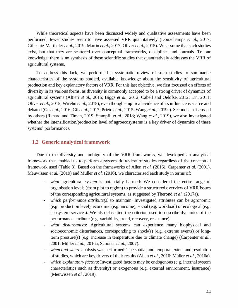
44

While theoretical aspects have been discussed widely and qualitative assessments have been

performed, fewer studies seem to have assessed VRR quantitatively (Douxchamps et al., 2017;

Gillespie-Marthaler et al., 2019; Martin et al., 2017; Oliver et al., 2015). We assume that such studies

exist, but that they are scattered over conceptual frameworks, disciplines and journals. To our

knowledge, there is no synthesis of these scientific studies that quantitatively addresses the VRR of

agricultural systems.

To address this lack, we performed a systematic review of such studies to summarise

characteristics of the systems studied, available knowledge about the sensitivity of agricultural

production and key explanatory factors of VRR. For this last objective, we first focussed on effects of

diversity in its various forms, as diversity is commonly accepted to be a strong driver of dynamics of

agricultural systems (Altieri et al., 2015; Biggs et al., 2012; Cabell and Oelofse, 2012; Lin, 2011;

Oliver et al., 2015; Wiréhn et al., 2015), even though empirical evidence of its influence is scarce and

debated (Ge et al., 2016; Gil et al., 2017; Prieto et al., 2015; Wang et al., 2019a). Second, as discussed

by others (Renard and Timan, 2019; Stampfli et al., 2018; Wang et al., 2019), we also investigated

whether the intensification/production level of agroecosystems is a key driver of dynamics of these

systems’ performances.

1.2 Generic analytical framework

Due to the diversity and ambiguity of the VRR frameworks, we developed an analytical

framework that enabled us to perform a systematic review of studies regardless of the conceptual

framework used (Table 3). Based on the frameworks of Allen et al. (2016), Carpenter et al. (2001),

Meuwissen et al. (2019) and Müller et al. (2016), we characterised each study in terms of:

- what agricultural system is potentially harmed: We considered the entire range of

organisation levels (from plot to region) to provide a structured overview of VRR issues

of the corresponding agricultural systems, as suggested by Therond et al. (2017a).

- which performance attribute(s) to maintain: Investigated attributes can be agronomic

(e.g. production level), economic (e.g. income), social (e.g. workload) or ecological (e.g.

ecosystem services). We also classified the criterion used to describe dynamics of the

performance attribute (e.g. variability, trend, recovery, resistance).

- what disturbances: Agricultural systems can experience many biophysical and

socioeconomic disturbances, corresponding to shock(s) (e.g. extreme events) or long-

term pressure(s) (e.g. increase in temperature due to climate change) (Carpenter et al.,

2001; Müller et al., 2016a; Scoones et al., 2007).

- when and where analysis was performed: The spatial and temporal extent and resolution

of studies, which are key drivers of their results (Allen et al., 2016; Müller et al., 2016a).

- which explanatory factors: Investigated factors may be endogenous (e.g. internal system

characteristics such as diversity) or exogenous (e.g. external environment, insurance)

(Meuwissen et al., 2019).

45

VRR study

characteristics

Description Caution

about

Categories Examples Reference

what

agricultural

system

Agricultural

system studied and harmed by the

disturbance

Nature and

level of the system

investigated

Plot/field,

farming system,

region, food

system

Plot/field level:

grassland Farm level: mixed

production

Carpenter et

al., 2001

which

performance

attribute(s)

Performance

attribute of the

system whose

dynamics are disturbed, and

associated criteria

used to describe the dynamics

Temporal

extent of

dynamics of

the attribute and threshold

of desired

dynamics

Agronomic,

economic,

ecological

Yield, economic

net return,

ecosystem services

provided to the population

Meuwissen

et al., 2019;

Müller et

al., 2016

what

disturbance

Disturbance that

occurred

How

disturbance is

measured and threshold

values

Shocks or

long-term

pressure

Shock: drought

Long-term

Pressure: climate change

Carpenter et

al., 2001;

Müller et al., 2016;

Scoones et

al., 2007

when and

where

Spatial and temporal resolution

and extent of the

study

- - Monthly over 3 years

Country level over

Europe

Allen et al., 2016;

Müller et

al., 2016

which

explanatory

factors

Potential

explanatory factor

of the VRR tested

- Endogenous

or exogenous

Diversity,

agricultural

practices, subsidies

Meuwissen

et al., 2019

Table 3. Analytical framework used for the systematic review, regardless of the conceptual framework used in

the study (vulnerability, resilience and robustness (VRR)), inspired by Allen et al. (2016), Carpenter et al.

(2001), Meuwissen et al. (2019) and Müller et al. (2016).

1.3 Method and study selection

To identify studies that quantitatively assessed VRR of agricultural systems, we performed an

advanced search on the ISI Web of Science Core Collection (WoS, http://www.isiknowledge.com) for peer-

reviewed articles in English for all available years (1956-July 2018). Our review focussed on studies

that analysed dynamics of agricultural systems from the plot/field to regional levels. Studies that

addressed dynamics of organism communities and the biology and genetics of organisms (animals

and crops) were excluded from the study.

46

As VRR are related to other key concepts used in agricultural research, in order not to miss an

important article, we considered three key related concepts in the WOS query: (i) adaptive capacity,

because it is a key sub-concept of vulnerability (Adger, 2006) but also can be considered an

independent concept (Engle, 2011; Gallopín, 2006); (ii) viability theory and (iii) ecological integrity,

of which the latter two are traditionally used to analyse dynamics of agricultural systems (Aubin, 2009;

Müller et al., 2000). Accordingly, our WOS query was the following:

TS = ((vulnerabilit* OR resilien* OR robustness* OR "adaptive capacity" OR "ecological

integrit*" OR (viabilit* AND theory)) AND (agri* OR agro* OR crop* OR farm* OR grass* OR

pastor*) AND (indicator* OR evaluat* OR quantitativ* OR quantif* OR model* OR simulat* OR

decrease OR increase OR assess*))

This query identified 9,807 articles. We first identified the relevant journals and WOS categories

(6,451 articles remained) and then restricted the list to temperate climate zones (Kottek et al., 2006)

to focus on similar agricultural systems, disturbances and ecological functioning, based on

recommendations of Gil et al. (2017), who highlighted the inconsistency in generalising results from

around the world, as their ecological and socio-economic functioning differ (3,399 articles remained).

We used VOSviewer software to perform co-occurrence analysis (n=10 terms) of titles and abstracts

to identify fields of study that lay outside our scope (e.g. genetics, glyphosate). We then used EndNote

x9 software to search articles with a combination of terms to identify studies related to previously

identified fields (with titles manually verified before exclusion) (1,409 articles remained). Then, titles

and abstracts were read manually to select 231 potential articles. In this step, a second reader manually

sorted a 10% random sample to test the influence of reader selection. This double-checking yielded

100% agreement between the two readers. Finally, full reading of the 231 articles identified 37 that

fell within the scope of the study (Supplementary material 2).

Our selection process showed that including adaptive capacity, viability theory and ecological

integrity in the query did not add articles to the final selection of 37 articles (Supplementary material

3). Indeed, articles that mention these three concepts always mentioned VRR in their abstract.

Accordingly, these additional concepts were not considered in our subsequent analysis.

Results of these 37 articles were extracted according to our analytical framework. Each result

(combination of a system – disturbance – performance attribute – dynamics criterion – explanatory

factor) was saved on one line of a database. Terminology was standardised, and each result was

associated with its corresponding study, and results of statistical tests, if performed, were noted. This

step enabled identification of similar systems and thus comparison of results.

47

1.4 Results

1.4.1 General studies’ characteristics

We draw two main conclusions from analysis of these articles. First, the few quantitative studies

identified (Supplementary material 2) confirms that quantitative assessment of agricultural system

VRR remains rare. Second, most studies focus on certain systems, disturbances and performance

attributes (Figure 16). Overall, 65% of the articles address climate change, while the main systems

studied are grassland (35%) and crop (40%) systems, at the plot/field (38%), farm (35%) and regional

(27%) levels. Studies focus mainly on the impact of disturbances on yield (72% of articles) and

economic net return (16% of articles). Overall, 13% of the studies only analyse the sensitivity of

dynamics of system attribute(s), while 86% of them seek to determine the main factors that explain

the behaviour studied. Diversity and intensification levels are the explanatory factors tested most,

confirming their interest to the scientific community.

Figure 16. Overview of the main characteristics of the 37 articles selected that address the vulnerability,

resilience and robustness of agricultural systems.

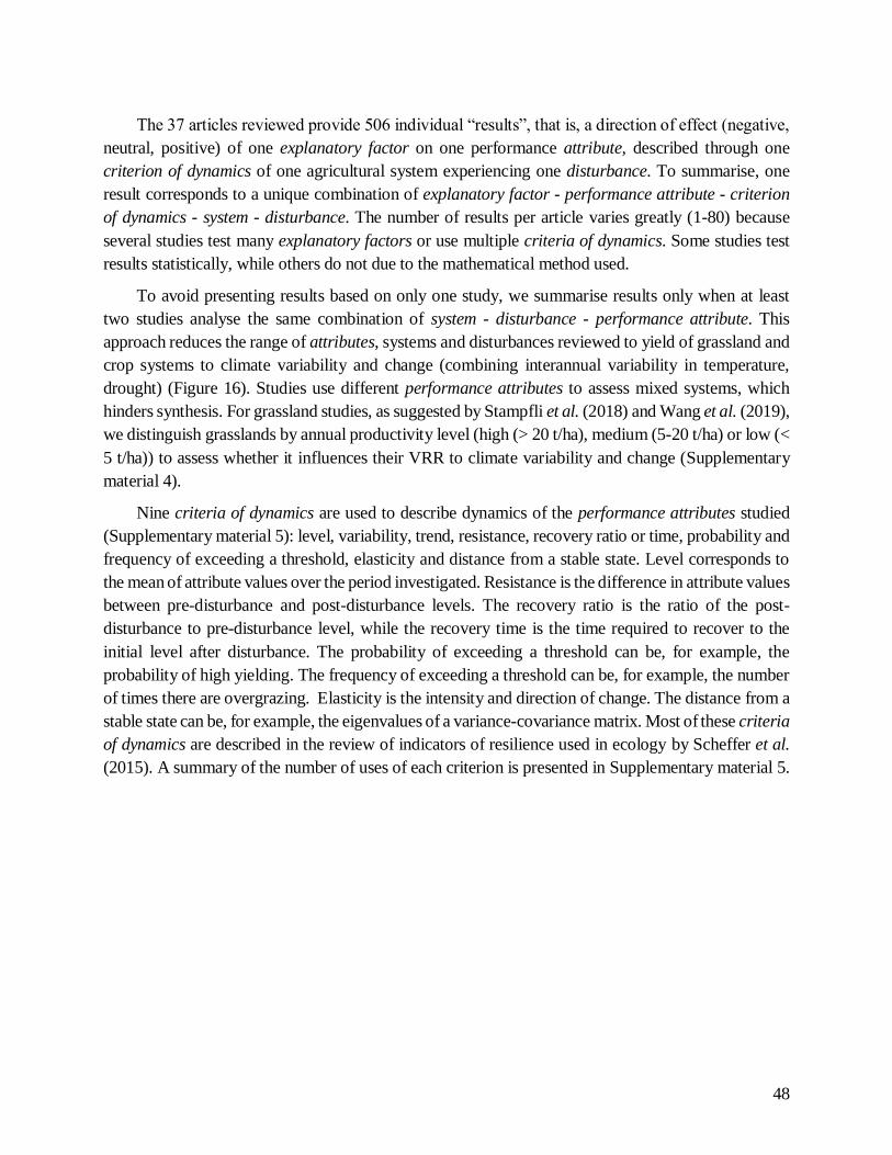
48

The 37 articles reviewed provide 506 individual “results”, that is, a direction of effect (negative,

neutral, positive) of one explanatory factor on one performance attribute, described through one

criterion of dynamics of one agricultural system experiencing one disturbance. To summarise, one

result corresponds to a unique combination of explanatory factor - performance attribute - criterion

of dynamics - system - disturbance. The number of results per article varies greatly (1-80) because

several studies test many explanatory factors or use multiple criteria of dynamics. Some studies test

results statistically, while others do not due to the mathematical method used.

To avoid presenting results based on only one study, we summarise results only when at least

two studies analyse the same combination of system - disturbance - performance attribute. This

approach reduces the range of attributes, systems and disturbances reviewed to yield of grassland and

crop systems to climate variability and change (combining interannual variability in temperature,

drought) (Figure 16). Studies use different performance attributes to assess mixed systems, which

hinders synthesis. For grassland studies, as suggested by Stampfli et al. (2018) and Wang et al. (2019),

we distinguish grasslands by annual productivity level (high (> 20 t/ha), medium (5-20 t/ha) or low (<

5 t/ha)) to assess whether it influences their VRR to climate variability and change (Supplementary

material 4).

Nine criteria of dynamics are used to describe dynamics of the performance attributes studied

(Supplementary material 5): level, variability, trend, resistance, recovery ratio or time, probability and

frequency of exceeding a threshold, elasticity and distance from a stable state. Level corresponds to

the mean of attribute values over the period investigated. Resistance is the difference in attribute values

between pre-disturbance and post-disturbance levels. The recovery ratio is the ratio of the post-

disturbance to pre-disturbance level, while the recovery time is the time required to recover to the

initial level after disturbance. The probability of exceeding a threshold can be, for example, the

probability of high yielding. The frequency of exceeding a threshold can be, for example, the number

of times there are overgrazing. Elasticity is the intensity and direction of change. The distance from a

stable state can be, for example, the eigenvalues of a variance-covariance matrix. Most of these criteria

of dynamics are described in the review of indicators of resilience used in ecology by Scheffer et al.

(2015). A summary of the number of uses of each criterion is presented in Supplementary material 5.

49

1.4.2 Sensitivity of agricultural systems experiencing climatic disturbances

Before analysing effects of diversity and intensification level on the VRR of agricultural systems,

we first summarise results of studies that analyse the sensitivity (Adger, 2006) of the yield of grassland

and crop systems to climate change. Nine articles explicitly provide 76 results of such analysis (Di

Falco and Chavas, 2008; Ferreyra et al., 2001; Hoover et al., 2014; Mäkinen et al., 2015; Prieto et al.,

2015; Reidsma et al., 2009a; Reidsma and Ewert, 2008; Stampfli et al., 2018; Zavalloni et al., 2008).

The criteria of dynamics they used to analyse sensitivity of yield to climate change are level,

variability, trend, resistance and probability of exceeding a threshold. Results by study are detailed in

Supplementary material 6.

Figure 17. Number of results (and associated number of articles) indicating a direction and degree of effect of

climate variability and change on desired (resilient) dynamics of yield, by (a) level of production (i.e. yield) at

the plot/field level for grassland systems and (b) organisation level for crop systems. For grassland studies, we

distinguish grasslands by annual productivity level (high (> 20 t/ha), medium (5-20 t/ha) or low (< 5 t/ha)). The

desired direction of criteria of dynamics is described in the text. Significant effects are those that could be tested

statistically and were found significantly different (p<0.05).

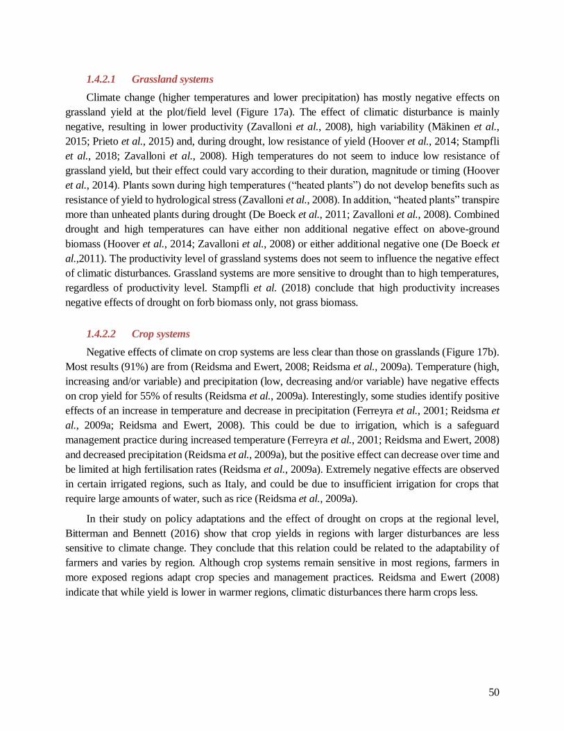
50

1.4.2.1 Grassland systems

Climate change (higher temperatures and lower precipitation) has mostly negative effects on

grassland yield at the plot/field level (Figure 17a). The effect of climatic disturbance is mainly

negative, resulting in lower productivity (Zavalloni et al., 2008), high variability (Mäkinen et al.,

2015; Prieto et al., 2015) and, during drought, low resistance of yield (Hoover et al., 2014; Stampfli

et al., 2018; Zavalloni et al., 2008). High temperatures do not seem to induce low resistance of

grassland yield, but their effect could vary according to their duration, magnitude or timing (Hoover

et al., 2014). Plants sown during high temperatures (“heated plants”) do not develop benefits such as

resistance of yield to hydrological stress (Zavalloni et al., 2008). In addition, “heated plants” transpire

more than unheated plants during drought (De Boeck et al., 2011; Zavalloni et al., 2008). Combined

drought and high temperatures can have either non additional negative effect on above-ground

biomass (Hoover et al., 2014; Zavalloni et al., 2008) or either additional negative one (De Boeck et

al.,2011). The productivity level of grassland systems does not seem to influence the negative effect

of climatic disturbances. Grassland systems are more sensitive to drought than to high temperatures,

regardless of productivity level. Stampfli et al. (2018) conclude that high productivity increases

negative effects of drought on forb biomass only, not grass biomass.

1.4.2.2 Crop systems

Negative effects of climate on crop systems are less clear than those on grasslands (Figure 17b).

Most results (91%) are from (Reidsma and Ewert, 2008; Reidsma et al., 2009a). Temperature (high,

increasing and/or variable) and precipitation (low, decreasing and/or variable) have negative effects

on crop yield for 55% of results (Reidsma et al., 2009a). Interestingly, some studies identify positive

effects of an increase in temperature and decrease in precipitation (Ferreyra et al., 2001; Reidsma et

al., 2009a; Reidsma and Ewert, 2008). This could be due to irrigation, which is a safeguard

management practice during increased temperature (Ferreyra et al., 2001; Reidsma and Ewert, 2008)

and decreased precipitation (Reidsma et al., 2009a), but the positive effect can decrease over time and

be limited at high fertilisation rates (Reidsma et al., 2009a). Extremely negative effects are observed

in certain irrigated regions, such as Italy, and could be due to insufficient irrigation for crops that

require large amounts of water, such as rice (Reidsma et al., 2009a).

In their study on policy adaptations and the effect of drought on crops at the regional level,

Bitterman and Bennett (2016) show that crop yields in regions with larger disturbances are less

sensitive to climate change. They conclude that this relation could be related to the adaptability of

farmers and varies by region. Although crop systems remain sensitive in most regions, farmers in

more exposed regions adapt crop species and management practices. Reidsma and Ewert (2008)

indicate that while yield is lower in warmer regions, climatic disturbances there harm crops less.

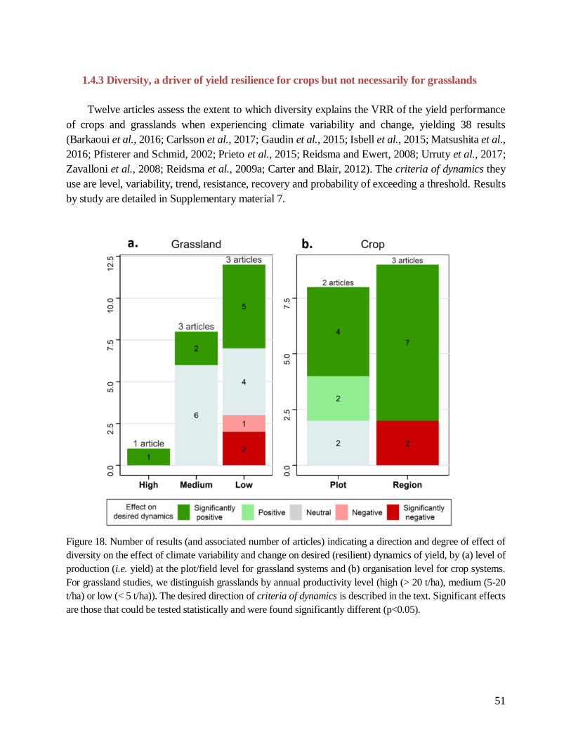
51

1.4.3 Diversity, a driver of yield resilience for crops but not necessarily for grasslands

Twelve articles assess the extent to which diversity explains the VRR of the yield performance

of crops and grasslands when experiencing climate variability and change, yielding 38 results

(Barkaoui et al., 2016; Carlsson et al., 2017; Gaudin et al., 2015; Isbell et al., 2015; Matsushita et al.,

2016; Pfisterer and Schmid, 2002; Prieto et al., 2015; Reidsma and Ewert, 2008; Urruty et al., 2017;

Zavalloni et al., 2008; Reidsma et al., 2009a; Carter and Blair, 2012). The criteria of dynamics they

use are level, variability, trend, resistance, recovery and probability of exceeding a threshold. Results

by study are detailed in Supplementary material 7.

Figure 18. Number of results (and associated number of articles) indicating a direction and degree of effect of

diversity on the effect of climate variability and change on desired (resilient) dynamics of yield, by (a) level of

production (i.e. yield) at the plot/field level for grassland systems and (b) organisation level for crop systems.

For grassland studies, we distinguish grasslands by annual productivity level (high (> 20 t/ha), medium (5-20

t/ha) or low (< 5 t/ha)). The desired direction of criteria of dynamics is described in the text. Significant effects

are those that could be tested statistically and were found significantly different (p<0.05).

52

1.4.3.1 Grassland diversity

To quantify plant diversity in grasslands at the plot level, 86% of results use species richness, 9%

genetic richness and 5% (one result) functional description of plant diversity. Generally, diversity is

not always related to the desired dynamics of yield (i.e. high level, low variability, increasing trend,

high resistance and rapid recovery). The 48% of grassland results that are neutral (Figure 18a)

corroborate the assumption that the relation between diversity and grassland’s yield resilience is not

well established and requires additional study. However, results differ according to the criteria of

dynamics used.

For the production level, species richness definitely increases the level of above-ground biomass

produced during drought and climate variability (Isbell et al., 2015; Pfisterer and Schmid, 2002; Prieto

et al., 2015; Zavalloni et al., 2008). In total, 80% of results indicate a positive effect of diversity on

yield level, with no clear difference among annual production levels (high, medium or low). However,

the effect of species richness on resistance (vs. level) of yield due to climate events depends on the

study. Isbell et al. (2015) show higher resistance of yield of species-rich grasslands regardless of the

direction and intensity of events, whereas Pfisterer and Schmid (2002) describe lower resistance of

yield of species-rich grasslands under climatic disturbance. The frequency of climate events (Isbell et

al., 2015) and the “composition effect” due to the presence of certain species (Pfisterer and Schmid,

2002) are considered explanatory factors. These results show that (i) biodiversity increases resistance

to climate events that are preceded by other climate events and (ii) legumes decrease, but Poa pratensis

increases, the resistance of yield of grasslands. Zavalloni et al. (2008) test whether complementarity

and the selection effects (i.e. the probability of highly productive species) can explain low resistance

of yield of species-rich grasslands. They determined that resistance to hydrological stress decreased

due to the niche complementarity effect, since it increased plant water uptake and, in turn, subsequent

soil water availability.

Species richness and root functional diversity have no impact (6 results, Barkaoui et al., 2016;

Carter and Blair, 2012; Isbell et al., 2015) or negative impact on the recovery ratio of yield (1 result,

Pfisterer and Schmid, 2002), which is surprising, because diversity is often associated with resilience,

commonly assessed as a recovery time or ratio (Pimm, 1984). In tests of potential composition effects,

Pfisterer and Schmid (2002) show that the presence of species particularly resistant to drought that are

also highly productive (P. pratensis, Dactylis glomerata and Arrhenatherum elatius) may determine

the direction of observed results. Important results are that recovery of biomass production can be

temporary, and so the temporal extent of observations influences the results (Pfisterer and Schmid,

2002). When considering the production trend, Prieto et al. (2015) show that during drought,

multispecies grasslands grow an average of 10% faster than monocultures do. Furthermore, diversity

in grassland species influences variability in yield both positively and negatively, depending on the

frequency and direction of climatic disturbances (Isbell et al., 2015; Prieto et al., 2015). Finally,

regardless of the level of intensification, effects of diversity on yield dynamics of grasslands

experiencing climate change are not obvious and seem to depend on grassland composition, which

indicators are used to assess yield dynamics and the temporal extent of observation.

53

1.4.3.2 Crop diversity

For crop systems at the plot/field level, studies quantify biodiversity as species diversity in

rotations. At the regional level, studies investigate diversity in farm types (size, land-cover richness

and equity), taxonomic diversity of cultivars and diversity of responses (e.g. variability in yield by

region). Again, results for crop systems are clearer than those for grasslands. For most results (76%),

diversity has a positive effect on desired dynamics (high level, low variability, increasing trend, rapid

recovery and a high probability of exceeding a threshold) when disturbance occurs (Figure 18b).

At the plot/field level, diversity in crop rotations always has a positive effect on the level of

production and negative effect on its variability when soya bean is present (Gaudin et al., 2015; Urruty

et al., 2017). Furthermore, diversity does influence the trend for yield. At plot and regional levels,

within-farm diversity (crop species, varieties and rotations) has a positive effect on the desired

dynamics of yield: high level, low variability, positive trend, resistance of yield, rapid recovery time

and probability of exceeding a threshold (Di Falco and Chavas, 2008; Gaudin et al., 2015; Matsushita

et al., 2016; Urruty et al., 2017). A single negative effect (Matsushita et al., 2016) is explained as

being due to specific characteristics of rice production (a composition effect).

At the regional level, Reidsma and Ewert (2008) show that diversity in farm type, size and

intensity of production have a positive effect on decreasing yield variability under high temperatures.

They also show that diversity in land use can increase negative effects of high temperatures on the

variability in regional yield. Reidsma and Ewert (2008) show that the negative effect of high

temperatures increased for the largest farms, which they assume could be due to farmers on large

farms having less aversion to risk.

1.4.4 Major composition effects

Previous results tend to highlight the importance of considering the composition effect on the

dynamics of system performances. Accordingly, we summarise results of the reviewed studies for the

effect of a particular species or species group (Figure 19). Cereals, summer crops, temporary

meadows, the proportion of grass/forbs, native cultivars and P. pratensis are tested for their effect on

levels, variability, trend, resistance, recovery and probability of exceeding a threshold of yield of

grassland and crop systems (Barkaoui et al., 2016; Carlsson et al., 2017; Gaudin et al., 2015; Pfisterer

and Schmid, 2002; Urruty et al., 2017).

Barkaoui et al. (2016) show that the composition of Mediterranean grassland species has more

effect than species diversity during drought. They emphasise root functional identity rather than root

functional diversity as a key factor of resilience of the plant community, since root-depth distribution

and root morphology determine the volume of soil water extracted and the ability to use it (additional

reference in Nippert and Knapp, 2007). For example, deep-rooted plant communities resist more

during summer drought and thus recover faster (Lopez-Iglesias et al., 2014; Padilla and Pugnaire,

2007).

54

Similarly, Carlsson et al. (2017) show that a single dominant functional group can resist drought

more than several functional groups. Their study also shows that grassland systems with a high

proportion of grass have higher resistance of yield than those with high proportion of forbs or legumes.

Pfisterer and Schmid (2002) observed a positive correlation between P. pratensis abundance and the

resistance of grassland yield. They also specify that resistant species can be selected and in turn induce

rapid recovery following disturbances. Carlsson et al. (2017) suggest that the composition effect must

be considered as a function of fertilisation rate because the latter can increase the abundance of certain

species, such as grasses.

Specific effects of legumes have also been identified (Supplementary material 8). Carlsson et al.

(2017) and Pfisterer and Schmid (2002) show that the abundance of legumes in grasslands can

decrease resistance of yield during drought (p<0.05). In contrast, crop rotations that include legumes

as a catch or cover crop improve the yield level and stability (Gaudin et al., 2015; Urruty et al., 2017),

but the probability of exceeding the threshold of a high yield level depends on the legume species

(Gaudin et al., 2015). For example, relay cropping with red clover more than doubled the likelihood

of yield exceeding the 90th percentile (p<0.05), while alfalfa decreased the probability of exceeding a

threshold of high yield (Gaudin et al., 2015).

Figure 19. Number of results (and associated number of studies) indicating a direction and degree of effect of

species composition on the effect of climate variability and change on desired (resilient) dynamics of yield by

type of production for (a) grassland and (b) crops. The desired direction of criteria of dynamics is described in

the text. Significant effects are those that could be tested statistically and were found significantly different

(p<0.05).

55

1.4.5 Intensifying inputs is not necessarily related to better yield dynamics

We summarised results of the reviewed studies for the effect of the level of input use

intensification on the VRR of crop systems to climate change (temperature and drought) at the

plot/field (2 articles) and regional (2 articles) levels (Figure 20). These studies focussed on the effect

of intensification level on the dynamics of yield of crop systems. Intensification levels are described

by fertilisation, soil improvement, tillage, irrigation, pesticide use and farm size. Results by study are

detailed in Supplementary material 9.

Figure 20. Number of results (and associated number of studies)

indicating a direction and degree of effect of crop intensification

(fertilisation, soil improvement, tillage, irrigation, pesticide use, farm

size) on the effect of climate variability and change on desired

(resilient) dynamics of yield, by organisation level (plot/field or

region). The desired direction of criteria of dynamics is described in

the text. Significant effects are those that could be tested statistically

and were found significantly different (p<0.05).

Nitrogen fertilisation, fungicide use, tillage and pesticide

use are related to higher levels and the probability of exceeding a high yield, but their effect on

variability and trends of yield is unclear (Gaudin et al., 2015; Urruty et al., 2017). Gaudin et al. (2015)

show that reducing tillage can decrease yield variability in favourable years but does not influence

yield when extreme events occur. Urruty et al. (2017) show that intensive management (fertiliser use,

soil improvement, pesticide use, tillage) in France has no significant effect on the trend for wheat

yield, whereas at the regional level, the study of Matsushita et al. (2016) in Japan indicates that

chemical fertiliser use significantly improves the short-term trend for yield.

Results of Reidsma et al. (2009b) at the farm level (the only study at this level) show that the

effect of fertilisation on the trend for yield (positive or negative) depends on the country and when

low precipitation or high temperatures occur. They explain this effect by the ability of fertilisation and

water availability to meet crop nitrogen and water demand, respectively. Their study also shows that

irrigation can increase the negative effect of high temperatures in certain countries due to the higher

water demand of irrigated crops and can improve yield when water is available, such as in non-water-

limited irrigated systems. They observe a combined non-linear effect of temperature and irrigation,

with a threshold above which effects of fertilisation and irrigation change from positive to negative.

56

1.4.6 General drivers of agricultural system dynamics

The scarcity of articles that address similar combinations of system - disturbance (Figure 16)

preclude further transversal analysis of drivers of agricultural systems. However, to provide a general

overview of effects of the explanatory factors tested, we consider all systems and all disturbances for

the two performance attributes used most: yield (Figure 21) and economic net return (Figure 22).

These summary results must be used with caution since they are based on a wide diversity of studies,

but they may provide insights into effects of explanatory factors on these two key attributes of

agricultural systems. Results are detailed by study in Supplementary material 10 and Supplementary

material 11.

For both attributes, exogenous factors (policies, a positive economic market or insurance)

mitigate the effect of disturbance, indicating that these factors have real potential to improve the

resilience of farming systems (Castañeda-Vera and Garrido, 2017; Ferreyra et al., 2001; Matsushita

et al., 2016; Reidsma et al., 2009b).

Results are scattered for other potential explanatory factors, and no consistent effect emerges.

For example, while some studies observed that high levels of labour and capital can have a negative

impact on yield dynamics at the farm level (Bardaji and Iraizoz, 2015), others observed they can have

a positive effect at the regional level (Matsushita et al., 2016; Salvati, 2010). Bardaji and Iraizoz (2015)

explain that both labour (annual work units) and capital (fixed assets) can be considered as proxies of

intensification level.

Figure 21. Number of results (and associated number of studies) indicating a direction and degree of effect on

the effect of climate variability and change on desired (resilient) dynamics of yield, by type of explanatory

factor (endogenous or exogenous) for all systems. The desired direction of criteria of dynamics is described in

the text. Significant effects are those that could be tested statistically and were found significantly different

(p<0.05).

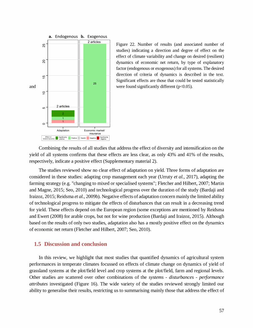
57

Figure 22. Number of results (and associated number of

studies) indicating a direction and degree of effect on the

effect of climate variability and change on desired (resilient)

dynamics of economic net return, by type of explanatory

factor (endogenous or exogenous) for all systems. The desired

direction of criteria of dynamics is described in the text.

Significant effects are those that could be tested statistically

and were found significantly different (p<0.05).

Combining the results of all studies that address the effect of diversity and intensification on the

yield of all systems confirms that these effects are less clear, as only 43% and 41% of the results,

respectively, indicate a positive effect (Supplementary material 2).

The studies reviewed show no clear effect of adaptation on yield. Three forms of adaptation are

considered in these studies: adapting crop management each year (Urruty et al., 2017), adapting the

farming strategy (e.g. "changing to mixed or specialised systems"; Fletcher and Hilbert, 2007; Martin

and Magne, 2015; Seo, 2010) and technological progress over the duration of the study (Bardaji and

Iraizoz, 2015; Reidsma et al., 2009b). Negative effects of adaptation concern mainly the limited ability

of technological progress to mitigate the effects of disturbances that can result in a decreasing trend

for yield. These effects depend on the European region (some exceptions are mentioned by Reidsma

and Ewert (2008) for arable crops, but not for wine production (Bardaji and Iraizoz, 2015). Although

based on the results of only two studies, adaptation also has a mostly positive effect on the dynamics

of economic net return (Fletcher and Hilbert, 2007; Seo, 2010).

1.5 Discussion and conclusion

In this review, we highlight that most studies that quantified dynamics of agricultural system

performances in temperate climates focussed on effects of climate change on dynamics of yield of

grassland systems at the plot/field level and crop systems at the plot/field, farm and regional levels.

Other studies are scattered over other combinations of the systems - disturbances - performance

attributes investigated (Figure 16). The wide variety of the studies reviewed strongly limited our

ability to generalise their results, restricting us to summarising mainly those that address the effect of

58

climate change on yield dynamics. Another key methodological challenge of our review was to

summarise the results of studies that address the same combination of system - disturbance -

performance attribute but that use different criteria of dynamics and associated indicators to analyse

performance dynamics (Supplementary material 5). While the diversity of indicators enables

researchers to analyse different characteristics of dynamics, it makes studies much more difficult to

compare and summarise. Thus, we aggregate results regardless of the criterion/indicator used in order

to determine general trends among studies but highlight differences in the results according to the

criterion used for analysis.

1.5.1 Diversity effects

The studies reviewed indicate that biodiversity has a positive influence on the (mean) level of

yield of grasslands and crop systems. For grasslands, this influence is observed regardless of

production level. These results do not converge fully with those of Wang et al. (2019) that confirm

the stress-gradient hypothesis: “facilitative interactions amongst plant species dominate under harsh

environments, whereas competitive interactions dominate under more favourable conditions”. In their

study on the effect of diversity on natural grassland yields over space, these authors highlight the

strong effect of the stress gradient in biodiversity-productivity (i.e. production) relationships, with a

shift from a strongly positive effect in low-productivity communities to a strongly negative effect in

high-productivity communities. We do not observe this difference in effect as a function of

productivity level in our results. To explain their results relative to plot-level experiments, Wang et al.

(2019) claim that they explore a large gradient of productivity (30-1382 g/m2 at peak biomass).

However, the studies we reviewed explored an even larger gradient, as Zavalloni et al. (2008) show a

positive effect of high functional diversity on a more productive grassland (500-2500 g/m2 at peak

biomass) with a mixture of species from three functional groups (grasses, N-fixing dicots and non-N-

fixing dicots). Differences between results of our study and those of Wang et al. (2019) may be

explained by the fact that diversity can be characterised using different indicators/approaches (e.g.

functional or taxonomic) and that a functional approach may be necessary to disentangle diversity-

productivity relationships (see below).

Like for grasslands, but in only two studies, diversity in crop rotations is positively related to

yield level (Gaudin et al. 2015; Urruty et al., 2017). To our knowledge, the positive effect of

diversified rotations, which provide nutrients and biological regulation services, is debated less, as

recent studies confirm that they are strong positive effects of rotation diversity on crop yield level

(Bowles et al., 2020; Duru et al., 2015b; Kleijn et al., 2019a; Kremen and Miles, 2012a; Lin, 2011;

Palomo-Campesino et al., 2018a).

These results for grassland and crop systems based on yield level as an indicator of yield

dynamics seem debatable, as a level is more a static indicator of state. When using an indicator more

adapted for analysing yield dynamics, our review shows that diversity is not always a strong positive

driver of yield resilience, low vulnerability or high robustness. For grasslands, the effect of

59

biodiversity varies among studies when using criteria such as resistance or the recovery ratio. Isbell

et al. (2015) identify that diversity increases yield resistance in grasslands mainly when they

experience frequent disturbances, while Pfisterer and Schmid (2002) show the importance of

composition effects (facilitative/competitive interaction). In contrast to grasslands, our review shows

that diversity has a clearer positive effect on crop yield dynamics, from plot/field to regional levels.

Within-farm diversity over space and time (rotation) usually has a positive effect on yield dynamics

(76% of results are positive) regardless of the indicator used. Only a few results show negative effects,

due to specific composition effects (e.g. rice, in Matsushita et al. 2016). Our results are similar to those

of Renard and Tilman (2019), who show that crop diversity has a strong effect on the temporal stability

of countries’ total yield (in kcal), and of Bowles et al. (2020), who show that trend of yield increases

and risk of crop failure decreases over time as the diversity of maize rotations in North America

increases.

Diversity in farm economic size and production intensity also has a positive effect on yield

variability Reidsma and Ewert (2008). Although based on few studies, our results seem to confirm the

strategy of not putting all eggs in one basket: diversification of farm production may provide economic

security at farm and regional levels (Abson et al., 2013).

Our review highlights that composition effects, rather than a species-diversity effect per se, can

have a strong effect on yield dynamics in agricultural systems. Functional diversity, as discussed by

Barkaoui et al. (2016) and Zavalloni et al. (2008), seems to be key in explaining the relationships

between diversity and the dynamics observed. However, although ecology and agroecology now

usually use the functional approach, few of the articles reviewed (n= 6/37) use a functional description

of plant diversity to address effects of species characteristics (traits) on ecosystem functioning. Thus,

the community that studies agricultural system dynamics seems to be poorly connected to the one that

uses functional approaches, although functional characterisation of species is a recognised way to

support the design of planned biodiversity to develop sustainable agricultural systems (Duru et al.,

2015b; Wood et al., 2015).

1.5.2 Effects of agricultural system intensification

Our results show that yield of grassland systems seems more sensitive to climate variability and

change than that of crop systems. This difference may be due mainly to the management adaptations

available to the crop systems studied, especially irrigation, in the face of higher temperatures and

drought. From a methodological viewpoint, crop/grassland management needs to be described

accurately when comparing the sensitivity of different agricultural systems.

While intensification has a major effect on yield levels, we find no clear trend in its effect on

yield dynamics (55 % of results are neutral). Rather than intensification level, the appropriateness of

the combination of crop, management and pedoclimatic context (i.e. production situation, Aubertot

and Robin (2013)) plays an important role. For example, Reidsma and Ewert (2008) highlight that the

positive effect of irrigation depends on water availability and fertilisation level, which later drives crop

60

water demand. They also suggest that lower yields (and thus, less intensive crop systems) in warm

climates are less sensitive to climate change because crop management there already seems adapted

to the climate. More generally, Reidsma and Ewert (2008) show that farm characteristics (e.g. size,

diversity of land use) can have a stronger influence on yield variability than climate change, whose

impacts are perceived more at larger levels (e.g. regional).

Our results for the effect of intensification are consistent with those of Renard and Tilman (2019),

who show that irrigation, and thus adaptation to water scarcity, is an important mechanism to improve

national yield stability, whereas nitrogen-use intensity (intensification level) has no significant impact.

They also show that effects of diversity and irrigation on total yield stability are approximately equal

to those of precipitation and temperature instability.

As discussed in the studies reviewed (Bitterman and Bennett, 2016; Hoover et al., 2014; Pfisterer

and Schmid, 2002; Isbell et al., 2015) and shown by Müller et al. (2016), results from analysing system

performance dynamics can depend strongly on the temporal extent of the studies. Study duration is

crucial when analysing (i) climatic and economic trends or rupture scenarios and (ii) effects of

resource availability (e.g. water, phosphorus). For example, the frequency of climate events can

explain the effect of diversity on yield resistance (Isbell et al., 2015). More generally, showing that

increasing irrigation or fertilisation improves resilience in the short term can mask the more long-term

scarcity effects of local water resources, finite resources (e.g. phosphorus, petroleum) and negative

feedback loops (e.g. pollution). Accordingly, studies that investigate the VRR of agricultural systems

while considering effects of intensification should assess middle- and long-term effects on natural and

fossil resources and the environment.

Finally, our transversal analysis of studies (regardless of the system - disturbance combination)

highlights potential negative effects of intensification of labour, capital and machinery on yield

dynamics at the farm level (Bardaji and Iraizoz, 2015), while positive effects are observed at the

regional level (Matsushita et al., 2016; Salvati, 2010). These results are similar to those of Reidsma et

al. (2009b) at the farm level, suggesting that the largest farms (economically) are less resilient.

1.6 Concluding remarks

In addition to increasing functional diversity, ensuring that the level of intensification is

appropriate for the production situation seems the best way to ensure the resilience/robustness of yields

to climate change. Farm diversity in economic size and intensity (of economic outputs) at the regional

level also seems a way to improve the VRR of agricultural production at the local/regional level. In

addition, our transversal analysis suggests that policies (e.g. income-stabilisation tools, direct

payments, subsidies, government investment in agricultural infrastructure) and insurance are effective

external factors, complementary to internal ones, for improving the resilience of economic net return

of farming systems.

61

Contributions

M.D and O.T. developed the conceptual framework with guidance and contributions from all

other co-authors; M.D. performed the literature review with the help of N.U. for reviewing; M.D. and

O.T. wrote the manuscript; and C.B. and N.U. proofread the manuscript.

Acknowledgements

We thank the three reviewers who helped improve the manuscript greatly. We thank

Agrosolutions, the agricultural consulting firm that supported and funded the PhD work of M.D. but

had no role in the decision to publish. We thank Michelle and Michael Corson for proofreading. We

thank Guy Richard, Michel Duru and Jean-Roger Estrade for providing general guidance and

discussion.

62

2. Revue des évaluations quantitatives de la résilience, vulnérabilité,

robustesse et capacités d’adaptation des systèmes agricoles de

zones tempérées

Cite as: Dardonville, M., Bockstaller, C., Therond, O., 2021. Review of quantitative evaluations

of the resilience, vulnerability, robustness and adaptive capacity of temperate agricultural systems.

Journal of Cleaner Production 125456. https://doi.org/10.1016/j.jclepro.2020.125456

Review of quantitative evaluations of the resilience, vulnerability, robustness and

adaptive capacity of temperate agricultural systems

Manon DARDONVILLE1, 2*

, Christian BOCKSTALLER1, Olivier THEROND

1

1 Université de Lorraine, INRAE, LAE, F-68000 Colmar, France

2Agrosolutions, 75782, Paris, France

63

ABSTRACT

Vulnerability, resilience, robustness and adaptive capacity are four key concepts that characterize

dynamics of systems when disturbance occurs. However, rendering them operational for agricultural

systems using an approach to quantify dynamics remains a challenge. To provide a synthesis of studies

that attempt to do so, we systematically reviewed scientific articles that quantified the vulnerability,

resilience, robustness or adaptive capacity of agricultural systems in temperate zones. Our semi-

automatic selection based on the Web of Science and textual visualization with VOSviewer enabled

us to identify only 53 articles. They focus mainly on the effect of climate change on yield dynamics

but are diverse in terms of agricultural systems (organizational levels, type of production), methods,

criteria of dynamics (e.g. trend, variability, recovery, resistance) and explanatory factors tested (e.g.

diversity, intensification, management). Studies that refer to one of these four investigated concepts

use criteria of dynamics interchangeably to analyze dynamics, confirming the fuzzy definition of these

concepts. While a wide range of methods are used, most studies focus on only one performance

attribute, mainly yield, which hides the multifunctionality of agriculture. However, half of the studies

use multiple criteria of dynamics to describe them in a multifaceted manner. We highlight that

combining short-term and long-term studies is rare, and social and ecological explanatory factors are

rarely tested. Identifying key generic explanatory factors (properties) that determine vulnerability,

resilience, robustness or adaptive capacity requires identifying a shared core set of factors to

investigate systematically. We show that this set of properties could be identified through cross-

sectional analysis of results of expert-based and quantitative assessments.

64

2.1 Introduction

Agricultural systems are facing increasing climatic and economic disturbances (IPCC, 2013;

Wright, 2011). Characterizing agricultural systems able to manage shocks (e.g. economic crisis) or

disturbance trends (e.g. increasing temperature) while ensuring their essential functions remains an

issue (Tendall et al., 2015). Vulnerability, resilience, robustness and adaptive capacity (VRRAC,

Table 4) are key concepts used to characterize dynamics when disturbance occurs (Gallopín, 2006;

Mumby et al., 2014). These concepts are related, and their definitions and overlaps remain an open

debate (Miller et al., 2010; Mumby et al., 2014; Turner, 2010; Urruty et al., 2016; Wu, 2013).

Although developed and discussed in multiple disciplinary communities, they remain challenging to

operationalize (i.e. to translate into an operational evaluation approach) (Callo-Concha and Ewert,

2014; Ge et al., 2016, 2016; M. Li et al., 2019; Martin et al., 2017; Quinlan et al., 2016; Urruty et al.,

2016). For example, how to evaluate resilience is currently being debated (Allen et al., 2019; Grafton

et al., 2019; Pimm et al., 2019).

Concepts Definitions Reference

Resilience “the ability to ensure the provision of the system

functions in the face of increasingly complex and

accumulating economic, social, environmental and institutional shocks and stresses”

Meuwissen et al. (2019)

Vulnerability “the degree to which a system is harmed due to

disturbances or stress”

Turner et al. (2003)

Robustness “the ability to maintain desired levels of system outputs, […] despite the occurrence of disturbances”

Urruty et al. (2016)

Adaptive

capacity

“the ability of a system to prepare for stresses and

changes in advance or adjust and respond to the effects caused by the stresses”

Smit and Pilifosova (2003)

Table 4. Definitions of the four concepts investigated.

In the literature, two approaches for addressing quantitatively the operationalization of VRRAC

frameworks can be identified (AminShokravi and Heravi, 2020; Prosperi et al., 2016; Tendall et al.,

2015; Zhang et al., 2019). First, based on expert opinion or a literature review, a set of system

properties (characteristics) is considered a set of key factors that determine VRRAC (Biggs et al.,

2012; Bonisoli et al., 2018; Cabell and Oelofse, 2012; Gillespie‐Marthaler et al., 2019; Prosperi et al.,

2016; Quinlan et al., 2016; Wiréhn et al., 2015). Here, VRRAC is considered the “sum of a range of

characteristics” (Douxchamps et al. 2017). For example, Cabell and Oelofse (2012), in a qualitative

review, identified 13 properties (called “behavior-based indicators”) of agroecosystem resilience. In

another example, based on thorough expert knowledge and a qualitative literature review, Biggs et al.

(2012) defined three system properties (diversity and redundancy, connectivity, and slow variables

and feedbacks) and four management principles (consider the complex adaptivity of socio-ecological

systems; and enhance learning, participation, and polycentric governance) that promote the resilience

65

of ecosystem services in social-ecological systems. These two key studies are the foundation for recent

studies that define conceptual frameworks (Meuwissen et al., 2019; Stockholm Resilience Center,

2015) or identify pre-defined properties of VRRAC (Diserens et al., 2018; Gillespie‐Marthaler et al.,

2019; Martin et al., 2019b; Nyström et al., 2019). Douxchamps et al. (2017)mentioned that the study

of Cabell and Oelofse (2012) remains innovative due to the indicators they developed to integrate

aspects of social, ecological and system connectivity and diversity. In this approach, VRRAC is

operationalized by estimating levels of predefined properties (e.g. diversity, connectivity) (e.g. in

Allen et al., (2018); Altieri et al., (2015); Brooks et al., (2005); Corobov et al., (2013); Dalsgaard et

al., (1995); Schmitt et al., (2017); Žurovec et al., (2017)). In agronomy, however, this predefined-

properties approach can suffer from little experimental evidence for the properties used (Dardonville

et al., 2020; Gil et al., 2017). The properties rely mostly on experts’ viewpoints (Urruty et al. 2016)

or transposition of proven properties of VRRAC from one scientific field to another (e.g. from ecology

to agronomy (Peterson et al., 2018)). This is usually the case when considering that diversity is a

property of resilience of agricultural systems, while the experimental evidence remains unclear (Gil

et al., 2017). The second approach is based on analysis of (i) observed or simulated dynamics of one

or more functions of a studied system that is experiencing disturbances and (ii) relationships between

system dynamics and multiple system characteristics to identify key explanatory factors of its

dynamics (Brzezina et al., 2016; Nelson et al., 2019). In this dynamics-analysis approach,

performance attributes characterize the functions of systems to maintain (Meuwissen et al., 2019). For

example, yield performance characterizes the food production function of agricultural systems.

Evaluation criteria, such as recovery or variability, are used to summarize the dynamics of the

performance attribute quantitatively (Barkaoui et al., 2016; Grafton et al., 2019; Martin et al., 2017

(i.e. “characterize systems’ behavior” in Müller (2005)). Analysis of relationships between these

VRRAC criteria of dynamics and system characteristics allows endogenous (eg. crop diversity,

Piedra-Bonilla et al. (2020)) or exogenous (eg. policies, Singh and Dhadse (2021)) explanatory factors

of VRRAC to be identified. These factors provide insights into pathways for improving resilience

(Coomes et al., 2019; Meuwissen et al., 2019). Based on observed or simulated data, this approach

can provide “objective” information about properties of VRRAC. Once properties of VRAAC are

identified (i.e. explanatory factors supported by evidence), they can be used as proxies of resilience in

the predefined-properties approach (Tendall et al., 2015). For example, if dynamics analysis shows

that crop diversity enhances resilience in agricultural systems, then resilience can be evaluated as a

function of crop diversity. In short, the properties that determine VRRAC are pre-determined in the

predefined-properties approach, while they are outcomes of assessments in the dynamics-analysis

approach.

While the first approach is widely known and disseminated, the second approach is applied much

less due to the complexity of the mathematical methods involved and the data or models required

(Brzezina et al., 2016; Callo-Concha and Ewert, 2014a; Coomes et al., 2019; Gillespie-Marthaler et

al., 2019; Prosperi et al., 2016). However, the dynamics-analysis approach is necessary to identify

objectively the level and properties of VRRAC systems, based on quantitative analysis of observed or

predicted dynamics of stressed systems. Once identified well, these properties can be used in the

66

predefined-properties approach. In other words, the second approach can provide the first one with

well-identified properties.

To our knowledge, no exhaustive review of studies with this second approach exists in

agricultural research (but see the review of Donohue et al. (2016) in ecology). The few reviews

available focus on only one concept and one explanatory factor (resilience and diversity in Gil et al.,

2017), a qualitative and non-exhaustive analysis of the literature (Urruty et al., 2016) or only a small

set of both qualitative and quantitative studies (n=10 in Callo-Concha and Ewert, 2014). An exhaustive

synthesis of the quantitative dynamics-analysis approach that considers the four parent concepts (V,

R, R and AC) is needed. It would help disseminate and thus facilitate the use of available methods and

to identify key explanatory factors of VRRAC (and feed the predefined-properties approach).

Ultimately, it would provide future researchers with the main characteristics of past studies and

warnings and tips for future studies.

To this end, we conducted a systematic review of studies that had used a dynamics-analysis

approach of VRRAC of agricultural systems (crop and livestock systems). It was based on a generic

query and semi-automated sorting and focused on agricultural systems of temperate climatic zones.

We focused on studies of temperate zones to address ecological and socio-economic systems that

function in a similar manner (Gil et al., 2017; Dardonville et al., 2020). Through this review we sought

to address the following research questions. What are the natures of the agricultural systems and

disturbances studied most by this research community? Which VRRAC concepts are used most in

these studies? Which methods are used to evaluate VRRAC quantitatively? Which performances have

had their dynamics studied in the face of disturbance? What criteria of dynamics are used to describe

the dynamics of the performances? Are the criteria associated with specific concepts? What

explanatory factors are tested to determine whether they are properties of VRRAC? We conclude our

review by discussing shortfalls in the reviewed studies and research needs, providing

recommendations for future studies and illustrating how key properties of VRRAC could be identified

by comparing and coupling the two VRRAC analysis approaches (i.e. predefined-properties- and

dynamics-analysis).

Hereafter, we present the methodology used to select the studies reviewed, the results that answer

the research questions and the discussion, which provides recommendations to other researchers.

2.2 Methodology

To select scientific articles that quantitatively analyzed dynamics of the VRAAC of agricultural

systems, we followed the PRISMA protocol for systematic review (Moher et al., 2015). We ran the

query in the ISI Web of Science Core Collection database (WoS, http://www.isiknowledge.com) to

identify peer-reviewed English articles and reviews published from 1956 (the beginning of the

collection) to September 2020. We focused on temperate studies that analyzed agricultural system

dynamics from field to regional levels without considering dynamics of communities of organisms.

The query was organized in three sections to select articles that addressed at least one of the VRRAC

67

concepts, agricultural crop and livestock systems and quantitative assessment. Accordingly, the query

was:

Topic = ((vulnerabilit* OR resilien* OR robustness OR "adaptive capacity") AND (agri* OR

agro* OR crop* OR farm* OR grass* OR pastor*) AND (indicator* OR evaluat* OR assess* OR

quantitativ* OR quantif* OR model* OR simulat* OR decrease OR increase))

The WoS Core Collection database was chosen because it encompasses a variety of research

fields, such as those in the natural sciences, but also in the social sciences, which could have performed

the studies we sought.

The query identified 12,125 articles (Figure 23). Then, using the advanced search function of the

WoS, we excluded off-topic journals, WoS categories and articles that involved non-temperate zones,

based on mapping by Kottek et al. (2006). Since the remaining corpus was still large (7940 articles),

we performed bibliometric analysis to detect off-topic articles semi-automatically based on their

lexical fields. To do this, like Wang et al. (2020) and Obiang Ndong et al. (2020), we first used the

bibliometric analysis and mapping software VOSviewer to visualize the co-occurrence of terms (at

least n = 10 times) in the title and abstract of all the articles (Supplementary material 12). From the

resulting bibliometric network, we identified potential off-topic lexical fields, such as soil community

dynamics, soil health, plant or animal genetics, fisheries and obvious non-agricultural production (i.e.

forests) (Figure 23). Keywords in these off-topic lexical fields were then used in the bibliographical

management software EndNote X9 to select potential off-topic articles. Next, the title and abstract of

these articles were read to identify which ones were truly off-topic and to ensure that relevant articles

were not excluded. After this screening process, 1761 articles remained. One reviewer read all titles

and abstracts of the articles and identified 281 articles within our study’s scope. Finally, one reviewer

read the 281 articles deeply and identified the final subset of 53 articles within the scope of the review.

A second reviewer read a random sample of 10% of the 281 articles, and the result was 100%

agreement between the two reviewers. Articles that did not assess temporal dynamics of an agricultural

system quantitatively were excluded (e.g. those that assessed only one year of production).

68

Figure 23. Description of the method used to select and sort articles according to the PRISMA protocol for a

systematic review (Moher et al., 2015).

We described each of the 53 studies using the analytical framework defined by Dardonville et al.

(2020), which combined recommendations of Allen et al. (2016), Carpenter et al. (2001), Meuwissen

et al. (2019), Müller et al. (2016) and Peterson et al. (2018). Thus, for each study, we specified:

1. The nature of the agricultural system studied (VRRAC "of what"): the type of production (e.g.

annual crops, perennial crops) and the level of organization (e.g. field, farm, region)

2. The exogenous disturbance that affects the system (VRRAC "to what disturbance"), which

corresponds to a shock or long-term pressure

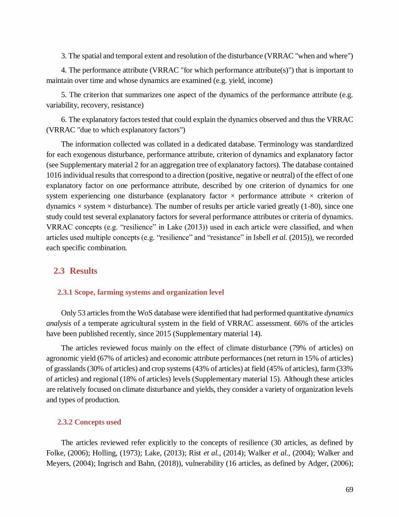
69

3. The spatial and temporal extent and resolution of the disturbance (VRRAC "when and where")

4. The performance attribute (VRRAC "for which performance attribute(s)") that is important to

maintain over time and whose dynamics are examined (e.g. yield, income)

5. The criterion that summarizes one aspect of the dynamics of the performance attribute (e.g.

variability, recovery, resistance)

6. The explanatory factors tested that could explain the dynamics observed and thus the VRRAC

(VRRAC "due to which explanatory factors")

The information collected was collated in a dedicated database. Terminology was standardized

for each exogenous disturbance, performance attribute, criterion of dynamics and explanatory factor

(see Supplementary material 2 for an aggregation tree of explanatory factors). The database contained

1016 individual results that correspond to a direction (positive, negative or neutral) of the effect of one

explanatory factor on one performance attribute, described by one criterion of dynamics for one

system experiencing one disturbance (explanatory factor × performance attribute × criterion of

dynamics × system × disturbance). The number of results per article varied greatly (1-80), since one

study could test several explanatory factors for several performance attributes or criteria of dynamics.

VRRAC concepts (e.g. “resilience” in Lake (2013)) used in each article were classified, and when

articles used multiple concepts (e.g. “resilience” and “resistance” in Isbell et al. (2015)), we recorded

each specific combination.

2.3 Results

2.3.1 Scope, farming systems and organization level

Only 53 articles from the WoS database were identified that had performed quantitative dynamics

analysis of a temperate agricultural system in the field of VRRAC assessment. 66% of the articles

have been published recently, since 2015 (Supplementary material 14).

The articles reviewed focus mainly on the effect of climate disturbance (79% of articles) on

agronomic yield (67% of articles) and economic attribute performances (net return in 15% of articles)

of grasslands (30% of articles) and crop systems (43% of articles) at field (45% of articles), farm (33%

of articles) and regional (18% of articles) levels (Supplementary material 15). Although these articles

are relatively focused on climate disturbance and yields, they consider a variety of organization levels

and types of production.

2.3.2 Concepts used

The articles reviewed refer explicitly to the concepts of resilience (30 articles, as defined by

Folke, (2006); Holling, (1973); Lake, (2013); Rist et al., (2014); Walker et al., (2004); Walker and

Meyers, (2004); Ingrisch and Bahn, (2018)), vulnerability (16 articles, as defined by Adger, (2006);

70

McCarthy et al., (2001); Smit and Wandel, (2006)), adaptive capacity (12 articles, as defined by

McCarthy et al. (2001); Parry et al. (2007)) and/or robustness (3 articles, as defined by Stelling et al.

(2004); Urruty et al. (2016)), but also, additionally, to stability (7 articles, May, (1975)), sustainability

(3 article) and resistance (7 articles, as defined by Pimm (1984)) (Figure 26). Here, “resistance” refers

to a concept and not to a criterion that describes the dynamics of the attribute. The concepts of

vulnerability, resilience and robustness are rarely combined; for example, only one article combines

vulnerability and resilience (Figure 26), confirming that they are used by different scientific

communities. However, resilience is often combined with the other concepts (16 out of 30 articles),

mainly with resistance or stability. In contrast, vulnerability is often combined with adaptive capacity

(9 out of 16 articles). Robustness is mentioned only alone (Figure 26).

2.3.3 Methods to measure and assess dynamics and test explanatory factors

Many methods are used to address the dynamics of agricultural systems and test potential

explanatory factors. Methods can be distinguished by how they (i) measure dynamics (e.g. source of

data, protocols), (ii) assess dynamics (criteria and mathematical indicators) and (iii) identify

explanatory factors for these dynamics.

Dynamics are measured from experimental studies, existing observed data or simulations.

Twenty articles are based on long-term field experiments (e.g. Barkaoui et al., 2016; Hoover et al.,

2014; Macholdt et al., 2020; Mäkinen et al., 2015)), while 22 articles use an existing or constituted

database (e.g. FADN in Bardaji and Iraizoz, (2015); Reidsma and Ewert, (2008); Zampieri et al.,

(2020a)). Eleven articles use observed data on disturbances (e.g. climate, prices) as input data for

simulation models, such as a grassland model (Sabatier et al., 2015a), a farming system model (Martin

and Magne, 2015) and an agent-based model (Bitterman and Bennett, 2016; Brunner and Grêt-

Regamey, 2016; Grêt-Regamey et al., 2019; van Strien et al., 2019). The temporal extent and

resolution of the studies range from 1-80 years (Figure 24) with a 1 day to 1-year time step. The spatial

extents of the studies cannot be compared because they range from 1 m² plots at several sites in the

world to a few dozen farms within a European Union NUTS2 region. Only one article studies the

impact of the spatial extent of a disturbance (Mechler et al., 2010).

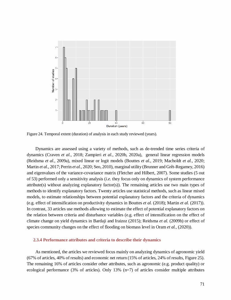
71

Figure 24. Temporal extent (duration) of analysis in each study reviewed (years).

Dynamics are assessed using a variety of methods, such as de-trended time series criteria of

dynamics (Craven et al., 2018; Zampieri et al., 2020b, 2020a), general linear regression models

(Reidsma et al., 2009a), mixed linear or logit models (Bouttes et al., 2019; Macholdt et al., 2020;

Martin et al., 2017; Perrin et al., 2020; Seo, 2010), marginal utility (Brunner and Grêt-Regamey, 2016)

and eigenvalues of the variance-covariance matrix (Fletcher and Hilbert, 2007). Some studies (5 out

of 53) performed only a sensitivity analysis (i.e. they focus only on dynamics of system performance

attribute(s) without analyzing explanatory factor(s)). The remaining articles use two main types of

methods to identify explanatory factors. Twenty articles use statistical methods, such as linear mixed

models, to estimate relationships between potential explanatory factors and the criteria of dynamics

(e.g. effect of intensification on productivity dynamics in Bouttes et al. (2018); Martin et al. (2017)).

In contrast, 33 articles use methods allowing to estimate the effect of potential explanatory factors on

the relation between criteria and disturbance variables (e.g. effect of intensification on the effect of

climate change on yield dynamics in Bardaji and Iraizoz (2015); Reidsma et al. (2009b) or effect of

species community changes on the effect of flooding on biomass level in Oram et al., (2020)).

2.3.4 Performance attributes and criteria to describe their dynamics

As mentioned, the articles we reviewed focus mainly on analyzing dynamics of agronomic yield

(67% of articles, 40% of results) and economic net return (15% of articles, 24% of results, Figure 25).

The remaining 16% of articles consider other attributes, such as agronomic (e.g. product quality) or

ecological performance (3% of articles). Only 13% (n=7) of articles consider multiple attributes

72

(usually agronomic and economic performance) in a multi-performance approach (Table 6). Two

articles study social performance attribute as farmers’ satisfaction or continuity of farming business

(Bitterman and Bennett, 2016; Perrin et al., 2020). In an original approach, Brunner and Grêt-

Regamey (2016) use an attribute that aggregates four ecosystem services, but they do not discuss them

separately.

Figure 25. Number of results (in black) and articles (in red) by performance attribute whose dynamics are

studied when disturbance occurs.

We identify ten criteria of dynamics of performance attributes used in the articles reviewed: trend

(15 articles, 35% of results), level (19 articles, 27% of results), variability (as defined by Pimm (1984),

17 articles, 16% of results), trend (14 articles, 35% of results),resistance (difference between pre-

disturbance and post-disturbance level, as defined by Pimm (1984), 15 articles, 5% of results),

elasticity (intensity and direction of change, 2 articles, 3% of results), frequency that a threshold was

exceeded (as defined by Walker et al. (2004), 4 articles, 3% of results), probability of exceeding a

given threshold (as defined by Walker et al. (2004), 6 articles, 2% of results, e.g. high yield), time

required to recover to the pre-disturbance level (‘resilience’ of Pimm (1984), 5 articles, 2% of results,

and distance to a stable state (as defined by Ludwig et al. (1997), 4 articles, 1% of results, e.g.

eigenvalues of the variance-covariance matrix), distance to a threshold (1 article, 2% of results), (Table

5). Most of these criteria are described by Meyer et al. (2018) and Scheffer et al. (2015).

73

Table 5. Summary of the criteria used to describe dynamics in the articles reviewed

Criterion Example of

indicator

Reference Articles that use the criterion Number of

articles

(and

results)

Level Mean - Bouttes et al., 2018, 2019; Castañeda-Vera and Garrido, 2017;

Ferreyra et al., 2001; Gaudin et al., 2015; Isbell et al., 2015;

Leonhardt et al., 2013; J. Li et al., 2019; M. Li et al., 2019; Martin

et al., 2017; Perrin et al., 2020; Pfisterer and Schmid, 2002; Prieto

et al., 2015; Redhead et al., 2020; Reidsma and Ewert, 2008; Seo,

2010; Urruty et al., 2017; Yang et al., 2019; Zavalloni et al., 2008

19 (284)

Variability Residuals of

linear

regression

Pimm (1984) Bouttes et al., 2018; Castañeda-Vera and Garrido, 2017; Cociu

and Cizma, 2015; Craven et al., 2018; Gaudin et al., 2015; Isbell

et al., 2015; Khumairoh et al., 2018; Leonhardt et al., 2013; M. Li et al., 2019; Macholdt et al., 2020; Mäkinen et al., 2015; Martin et

al., 2017; Prieto et al., 2015; Redhead et al., 2020; Reidsma et al.,

2009a; Reidsma and Ewert, 2008; Sneessens et al., 2019; Yang et

al., 2019

17 (163)

Trend Slope of linear

regression

- Bardaji and Iraizoz, 2015; Bouttes et al., 2018, 2019; Cociu and

Cizma, 2015; Di Falco and Chavas, 2008; Kahiluoto et al., 2014;

Leonhardt et al., 2013; J. Li et al., 2019; Martin et al., 2017;

Matsushita et al., 2016; Perrin et al., 2020; Prieto et al., 2015;

Reidsma et al., 2009b, 2009a, 2010; Salvati, 2010; Urruty et al.,

2017

15 (365)

Resistance Difference

between pre-

disturbance

and post-disturbance

Pimm (1984) Brunner and Grêt-Regamey, 2016; Carlsson et al., 2017; de la

Rosa et al., 2000; Di Falco and Chavas, 2008; Hoover et al., 2014;

Isbell et al., 2015; Martin and Magne, 2015; Mechler et al., 2010;

Oram et al., 2020; Pfisterer and Schmid, 2002; Redhead et al., 2020; Seo, 2010; Stampfli et al., 2018; Vetter et al., 2020;

Zavalloni et al., 2008

15 (51)

Recovery Time or ratio

(pre/post) to

return to the

pre-

disturbance

level

‘resilience’ of

Pimm (1984)

Barkaoui et al., 2016; Carter and Blair, 2012; Di Falco and

Chavas, 2008; Isbell et al., 2015; J. Li et al., 2019; Matsushita et

al., 2016; Oram et al., 2020; Pfisterer and Schmid, 2002;

Sneessens et al., 2019

9 (33)

Distance to a

stable state

Eigenvalue of

the variance-

covariance

matrix

Ludwig et al.

(1997)

Chavas and Di Falco, 2017; Fletcher and Hilbert, 2007; Grêt-

Regamey et al., 2019; van Strien et al., 2019

4 (5)

Distance to a

threshold

Difference

between a desired level

and actual

level

- Sneessens et al., 2019 1 (19)

Probability of

exceeding a

threshold

- Walker et al.

(2004)

Ferreyra et al., 2001; Gaudin et al., 2015; M. Li et al., 2019;

Macholdt et al., 2020; Zampieri et al., 2020b, 2020a

6 (26)

Frequency

that threshold

was exceeded

- Walker et al.

(2004)

Bitterman and Bennett, 2016; Lien et al., 2007; Sabatier et al.,

2015; Sneessens et al., 2019

4 (33)

Elasticity Intensity and

direction of

change

- Bardaji and Iraizoz, 2015; Reidsma et al., 2009b 2 (36)

74

Among the criteria of dynamics used together (Supplementary material 5), level is used most

often in combination with others (i.e. variability, trend, probability of exceeding a threshold, resistance

and/or recovery). Level, distance to a threshold and elasticity are never used alone, likely because they

describe dynamics only partially. Distance to a stable state and the frequency that a threshold was

exceeded are always used alone, likely due to methodological limitations (Bitterman and Bennett,

2016; Chavas and Di Falco, 2017; Fletcher and Hilbert, 2007; Lien et al., 2007; Sabatier et al., 2015a).

Resistance is usually used alone (8 out of 21 articles) or with recovery time (4 out of 21). The

combination of level-trend-variability is the trio used most often (4 articles, Bouttes et al. (2018);

Leonhardt et al. (2013); Martin et al. (2017); Prieto et al. (2015)). Multiple criteria are analyzed in

53% of studies, most of which use 2-3 criteria of dynamics for each attribute (Table 6). Seven multi-

performance studies use 2-5 criteria of dynamics for each attribute investigated.

Criteria Attributes

One Two Four Five

One 25 0 0 0

Two 11 3 1 0

Three 7 2 0 0

Four 2 0 0 1

Eight 1 0 0 0

Table 6. Distribution of the 53 articles reviewed as a function of the number of performance attributes and

criteria of dynamics of performance considered.

2.3.5 Combinations of concepts and criteria of dynamics

Most criteria of dynamics are associated with more than one of the four concepts investigated

(VRRAC) (Figure 26). Criteria of level, trend and variability are associated with all four concepts,

while resistance, probability of exceeding a threshold and frequency that a threshold was exceeded are

associated only with resilience, vulnerability and adaptive capacity. However, since only six of the

articles reviewed refer to robustness, this concept is less common than the other two. The criteria

“recovery time/ratio” and “distance to a stable state” are associated in majority with resilience.

Elasticity is associated only with vulnerability and adaptive capacity (Bardaji and Iraizoz, 2015;

Reidsma et al., 2009b).

75

Figure 26. Number of articles reviewed as a function of concept(s) and criterion of dynamics of performance

attribute. A given article can mention several concepts and/or criteria.

2.3.6 Explanatory factors tested

Most of the articles reviewed seek to determine explanatory factors of VRRAC (48 articles, 84%

of results). They tested 121 explanatory factors, which we categorized into 31 categories (Figure 27,

Supplementary material 13) that correspond to descriptors of system structure (64% of articles, 20%

of results), agricultural practices (23% of articles, 34% of results), institutional context (16% of

articles, 8% of results), adaptation (11% of articles, 3% of results), economic characteristics (11% of

articles, 4% of results), biophysical context (13% of articles, 7% of results), ecological processes (2%

of articles, 0.5% of results) and disturbance scale (2% of articles, 0.03% of results). Most factors

studied (71%) are endogenous to the agricultural system (i.e. controllable by the farmer).

Although many explanatory factors are studied, articles address mainly effects of system

structure, agricultural practices and institutional context, while economic characteristics are studied

less, and ecological and biophysical factors are minors. The effect of system structure is studied by

analyzing the effect of diversity, crop species surface areas, herd and farm labor structure, farm

76

typologies (e.g. size, specialization), farm self-sufficiency and diversity. The effect of diversity is

studied the most widely (27 articles) by analyzing effects of the spatial and/or temporal diversity of

crops in rotations and mixtures or plants in grasslands, and the diversity of farm characteristics and

response (see Dardonville et al., (2020) for more details). Agricultural practices are assessed mainly

by considering input/practice intensification levels (e.g. pesticide, fertilization, irrigation, tillage) or

ways to perform certain practices (e.g. sowing, grassland use). The institutional context is assessed to

identify effects of policy or income stabilization measures. Adaptation is assessed by analyzing

adaptations in crop management (Urruty et al., 2017), farm strategy (Fletcher and Hilbert, 2007;

Martin and Magne, 2015; Seo, 2010) or technological progress over time (Bardaji and Iraizoz, 2015;

Reidsma et al., 2009b). The effect of ecological functioning is assessed only through the pollination

service (Leonhardt et al., 2013) and the interaction effect (i.e. synergy or competition effects

(Zavalloni et al., 2008)). The biophysical context category represents assessment of effects of a

combination of disturbances (e.g. heat and drought in Zavalloni et al., 2008), regional climate

(Leonhardt et al., 2013), initial soil water availability (Ferreyra et al. 2001) or invasion by other species

(Vetter et al., 2020).

Figure 27. Number of results (in black) and articles (in red) by explanatory factor and its category.

77

2.4 Discussion

Our systematic review summarizes the system studied, methods, performance attributes used,

criteria of dynamics used and explanatory factors tested in the studies that quantitatively assess the

VRRAC of temperate agricultural systems. As shown, these studies use a variety of concepts, methods

and criteria. Based on results of our analysis and observations of other key researchers, we discuss

conceptual and methodological aspects of quantitative VRRAC assessments. Consequently, we

identify several points of vigilance and advice for future researchers.

2.4.1 Relationships between VRRAC concepts and criteria of dynamics

The analysis of combinations of concepts and criteria in this review confirm that definitions of

VRRAC concepts are fuzzy and highlight interchangeable use of criteria of dynamics. Many

researchers have highlighted the redundancy, ambiguity and polysemy of VRRAC concepts (Callo-

Concha and Ewert, 2014; Gallopín, 2006; Miller et al., 2010; Turner, 2010; Urruty et al., 2016), and

Allen et al. (2019) does so recently for resilience. In the studies we reviewed, the concepts of

vulnerability and resilience are used in combination with the one of adaptive capacity (25 out of 53

articles). In contrast, these concepts are less frequently combined in the review of Callo-Concha and

Ewert (2014) covering qualitative and quantitative studies from 2004 to 2013. Nonetheless, the

dispersion of studies among VRAAC concepts that we observed confirms the conclusion of Callo-

Concha and Ewert (2014) that operationalization of quantitative analysis of dynamics of agricultural

systems is spread over the concepts. By focusing our query on the four VRRAC concepts, we may

have missed articles that analyzed dynamics of agricultural systems in the face of disturbances but that

did not mention one of these four concepts in their title, abstract or keywords. Our review of these

four concepts could be widened by including studies of more distant concepts, such as stability or

flexibility.

Because most studies defining VRRAC concepts do not explicitly develop operational criteria of

dynamics (Grafton et al., 2019; Pimm et al., 2019), we show that most of these latter are developed

by operational studies and are used interchangeably, regardless of the concept used. The only

exceptions are some resilience studies that focus on one criterion (e.g. “recovery time/ratio”, “distance

to a stable state”) that translates the conceptual foundation of the resilience concept in the seminal

article of Holling (1973). We can assume that researchers who assess dynamics of agricultural systems

quantitatively would have less interest in using only one concept, because doing so would not help

them choose criteria of dynamics.

This dispersion hides the fact that studies use same criteria and/or method to analyze dynamics,

whatever the concept, which makes it more difficult to capitalize on knowledge. Our review, based

on a generic analytical framework to analyze all studies that consider four key concepts, is one way to

overcome this difficulty.

78

2.4.2 Adaptive capacity

Although adaptive capacity is mentioned in 26% of the studies that we reviewed, and adaptation-

related concepts are mentioned in 61% of the studies reviewed by Callo-Concha and Ewert (2014),

only 6 articles reviewed in the present study test an explanatory factor related to adaptation, for

example by analyzing the effect of management variability or scenarios on VRRAC. Thus, it seems

that the bridge between theoretical/qualitative use of this concept and its use in quantitative assessment

still remains to be built, perhaps due to difficulty in identifying tractable variables that represent

adaptation. Following the same logic, no article reviewed analyzes the entire adaptive cycle introduced

by Holling et al. (1995), probably due to the difficulty in developing quantitative criteria of dynamics

in the four phases of the cycle (exploitation, conservation, release, reorganization). Only Fletcher and

Hilbert (2007) study the reorganization phase of the adaptive cycle by simulating the farmer’s choice

of strategy each year as a function of previous years.

2.4.3 Temporal-scale effects

Our results show that many methods have been used to track dynamics when a shock (e.g.

drought) or trend change (e.g. higher temperature, lower precipitation) occurs. The studies reviewed

analyze short-term (58% of studies less than 11 years) and medium- to long-terms (more than 11

years) in relatively equal measure (Figure 24). The short-term studies correspond mainly to one- or

two-year experimental plot studies of grassland dynamics with artificial disturbances (n=6, e.g.

Barkaoui et al., 2016; Carter and Blair, 2012; Oram et al., 2020). We found only one study (Isbell et

al., 2015) that addressed effects of recurring disturbance, unlike most of the experimental and

observational studies in ecology reviewed by Donohue et al. (2016). This is surprising, since changes

in climate (Meyer et al., 2018) and in the economic context can be considered as a succession of

events. Furthermore, short and long temporal extents are not studied at the same time, which ignores

recommendations of Bitterman and Bennett (2016), Hoover et al. (2014) and Pfisterer and Schmid

(2002). Indeed, they argue that the temporal extent studied (VRRAC “when”) can influence the results

strongly: a system could be resilient in the short term but vulnerable in the longer term, and vice-versa

(Donohue et al., 2016; Müller et al., 2016b; Peterson et al., 2018). Considering long-term dynamics

also allows long-term response variables to be assessed, such as resource depletion or the dynamics

of natural capital (Dardonville et al., 2020; Peterson et al., 2018). However, addressing long-term

dynamics is often resource-consuming since it requires long-term experimental studies and data sets

or development of model-based approaches (Douxchamps et al., 2017).

2.4.4 Multi-performance of agricultural systems

Most articles reviewed (86%) address only one performance attribute, mostly yield (67% of

articles). Few articles reviewed address other attributes, such as ecological performance (3% of

articles). This agrees with conclusions of the review by Donohue et al. (2016) of ecological studies,

79

which focus mainly on the stability of biomass production. Studies that focus on only one performance

attribute (or two, in 5 articles), particularly yield, overlook the multifunctionality of agricultural

systems. Assessing the dynamics of agronomic (yield), ecological (e.g. ecosystem functions and

services), social (e.g. work time) and economic attributes together is necessary to understand dynamics

that underpin the behavior of agricultural systems in the framework of sustainability (Darnhofer et al.,

2010). However, analyzing dynamics of several types of performance attributes (e.g. yield and quality

of production by Bardaji and Iraizoz (2015), yield and economic net return by Ferreyra et al. (2001))

requires developing methods to aggregate and analyze dynamics of trade-offs and synergies between

them (Hodbod et al., 2016).

2.4.5 Multiplicity, complementarity and selection of criteria of dynamics

Unlike studies that focus on only one performance attribute, half of the articles (53%) reviewed

use multiple criteria to analyze the dynamics of system attributes. In contrast, Donohue et al. (2016)

indicated that 85-93% of studies in ecology used only one criterion, mainly variability (61% of

experimental and 72% of observational studies). The multicriteria approach enables studies to provide

complementarity points of view about the dynamics studied. Although level is the criterion combined

most often with other criteria, it should obviously not be considered alone as a criterion of dynamics

due to its static nature. When combined with other criteria, it can provide key information that helps

to put other criteria values into perspective. Indeed, it may be easier to show a positive trend when a

performance level, such as yield, is low than when it is already high. For example, among the studies

we reviewed, Martin et al. (2017) combine level, trend and variability to analyze how a given

performance level is associated with a direction of trend and degree of variability. More recently,

Sneessens et al. (2019) assess the economic vulnerability of farming systems using the relative

standard deviation (i.e. variability), mean relative distance (i.e. distance to a threshold), number of

disturbances (i.e. frequency of exceeding a threshold) and recovery time. Some studies take the

multicriteria approach a step further by developing several indicators per criterion to cover different

aspects of the criterion. For example, Li et al. (2019), while using an innovative combination of level,

stability, resistance and maximum potential to analyze yield dynamics, use four and two indicators to

estimate stability and resistance, respectively. In ecology research field, Ingrisch and Bahn (2018)

compare several indicators of recovery: absolute recovery time, as well as baseline-normalized and

impact-normalized indicators. Resistance is rarely combined with recovery time (4 articles), even

though these dynamics are interdependent: comparing two recovery times requires knowing each fall

in performance and thus the extent of the recovery required (like the “half-life” of radioactive decay,

Pimm et al. (2019)).

Overall, there is a lack of justification for the criteria chosen. Donohue et al. (2016) claim that

criteria should be chosen based on the nature of the disturbance observed. Recovery and resistance are

suitable for a shock disturbance, while level, variability, elasticity and trend are suitable for a trend or

for “noisy” disturbance. The decision to combine criteria also depends on the conceptualization of the

nature of system dynamics. Variability, trend, resistance, recovery and elasticity refer to the

80

“engineering” vision of dynamics in the resilience framework (Donohue et al., 2016), while distance

to a stable state and the probability and frequency of exceeding a threshold assume the existence of

tipping points and different stability regimes, in reference to the “ecological” resilience framework

(Holling, 1973). Accordingly, only one of the articles reviewed (Gaudin et al., 2015) combines an

“engineering” criterion (variability) with an “ecological” criterion (probability of exceeding a

threshold). This kind of study tries to reconcile the “engineering” and “ecological” dimensions of

resilience (Allen et al., 2019). However, recent debate on the ability to reconcile them suggests that

their differing conceptual positions on the existence of other states of stability remain far apart and

may be unresolvable (Pimm et al., 2019).

2.4.6 Multiplicity, complementarity and selection of explanatory factors

Many explanatory factors of VRRAC are explored in the articles reviewed. This dispersion can

make it difficult to provide generic information about the main system properties that influence the

VRRAC of agricultural systems. Developing a shared core set of explanatory factors that should

always be investigated in VRAAC studies could help build generic knowledge. As Callo-Concha and

Ewert (2014) recommend, doing so would allow for development of a more standardized analysis

protocol. One strategy could be to test in dynamics-analysis studies the main properties used in

predefined-properties studies. In this perspective, despite the greatly different terminologies used, we

estimated the extent to which explanatory factors of VRRAC in the studies we reviewed corresponded

to the resilience properties of agricultural systems identified by Cabell and Oelofse (2012) (Table 7).

As expected, diversity (i.e. redundancy, functional complementarity and heterogeneity) is investigated

in the two approaches (predefined-properties and dynamics-analysis). As Dardonville et al. (2020)

show, however, the effect of diversity depends on the nature of the agricultural system (crop vs.

grassland) and is modulated by the system’s composition (e.g. species, type of farm). Human capital

and profitability are also well explored, showing appropriation and convergence of these objectives

within research communities. Since articles reviewed ignore social explanatory factors, they do not

consider the four social properties of resilience (i.e. socially self-organized, appropriately connected

socially, reflective and shared learning, honors legacy) identified by Cabell and Oelofse (2012). Like

them, Biggs et al. (2012), in their thorough review of principles of ecosystem service resilience in

social-ecological systems, highlight the need to consider both ecological (biophysical) and social

properties in such systems (see also Cinner and Barnes (2019)). The most surprising aspect of our

analysis is that the two approaches yield opposite points of view of the effect of certain factors. For

example, while exogenous supports of agricultural systems (e.g. policy and insurance) are identified

as favorable explanatory factors of VRRAC in the articles reviewed, two resilience properties

(“globally autonomous and locally interdependent” and “reasonably profitable” without “distortionary

subsidies”) highlight the importance for agricultural systems of remaining independent of such

financial supports for their resilience. We assume that these two points of view could be related to the

different temporal scales considered: exogenous supports can have a favorable effect in the short term

but may make agricultural systems dependent on them, and thus sensitive to them, in the long term.

81

To a lesser extent, the same holds true for the intensification of agricultural systems: some of the

articles reviewed perceive it as a positive driver of VRRAC, while Cabell and Oelofse (2012) consider

it a negative property (“globally autonomous and locally interdependent”). In their review of effects

of intensification on the VRRAC of agricultural systems, Dardonville et al. (2020) show, as discussed

by Ge et al. (2016) and Peterson et al. (2018), that intensification can have positive or negative effects

depending on the initial level of production, temporal scale of the study and availability of local

resources (e.g. water for irrigation). As discussed, both points of view highlight the influence of the

temporal and spatial scales chosen on study results. Finally, for the other resilience properties, the

ambiguous definitions and terminologies used make it difficult to relate the factors encountered to

resilience properties. This highlights that both research communities need to develop sound and clear

assumptions and definitions (including spatiotemporal scales) that underpin the selected or studied

explanatory factors (properties) of VRRAC in agricultural systems (Peterson et al., 2018).

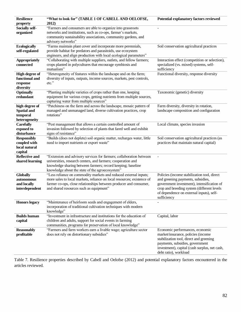
82

Table 7. Resilience properties described by Cabell and Oelofse (2012) and potential explanatory factors encountered in the

articles reviewed.

Resilience

property

“What to look for” (TABLE 1 OF CABELL AND OELOFSE,

2012)

Potential explanatory factors reviewed

Socially self-

organized

“Farmers and consumers are able to organize into grassroots networks and institutions, such as co-ops, farmer’s markets,

community sustainability associations, community gardens, and

advisory networks”

-

Ecologically

self-regulated

“Farms maintain plant cover and incorporate more perennials,

provide habitat for predators and parasitoids, use ecosystem

engineers, and align production with local ecological parameters”

Soil conservation agricultural practices

Appropriately

connected

“Collaborating with multiple suppliers, outlets, and fellow farmers;

crops planted in polycultures that encourage symbiosis and

mutualism”

Interaction effect (competition or selection),

specialized (vs. mixed) systems, self-

sufficiency

High degree of

functional and

response

diversity

“Heterogeneity of features within the landscape and on the farm;

diversity of inputs, outputs, income sources, markets, pest controls,

etc.”

Functional diversity, response diversity

Optimally

redundant

“Planting multiple varieties of crops rather than one, keeping

equipment for various crops, getting nutrients from multiple sources, capturing water from multiple sources”

Taxonomic (genetic) diversity

high degree of

Spatial and

temporal

heterogeneity

“Patchiness on the farm and across the landscape, mosaic pattern of

managed and unmanaged land, diverse cultivation practices, crop

rotations”

Farm diversity, diversity in rotation,

landscape composition and configuration

Carefully

exposed to

disturbance

“Pest management that allows a certain controlled amount of

invasion followed by selection of plants that fared well and exhibit

signs of resistance”

Local climate, species invasion

Responsibly

coupled with

local natural

capital

“Builds (does not deplete) soil organic matter, recharges water, little

need to import nutrients or export waste”

Soil conservation agricultural practices (as

practices that maintain natural capital)

Reflective and

shared learning

“Extension and advisory services for farmers; collaboration between

universities, research centers, and farmers; cooperation and

knowledge sharing between farmers; record keeping; baseline

knowledge about the state of the agroecosystem”

-

Globally

autonomous

and locally

interdependent

“Less reliance on commodity markets and reduced external inputs; more sales to local markets, reliance on local resources; existence of

farmer co-ops, close relationships between producer and consumer,

and shared resources such as equipment”

Policies (income stabilization tool, direct and greening payments, subsidies,

government investment), intensification of

crop and breeding system (different levels

of dependence on external inputs), self-

sufficiency

Honors legacy “Maintenance of heirloom seeds and engagement of elders,

incorporation of traditional cultivation techniques with modern

knowledge”

-

Builds human

capital

“Investment in infrastructure and institutions for the education of

children and adults, support for social events in farming

communities, programs for preservation of local knowledge”

Capital, labor

Reasonably

profitable

“Farmers and farm workers earn a livable wage; agriculture sector

does not rely on distortionary subsidies”

Economic performances, economic

market/insurance, policies (income

stabilization tool, direct and greening payments, subsidies, government

investment), capital (cash surplus, net cash,

debt ratio), workload

83

2.4.7 Normative vs. participatory approaches

Although the dynamics-analysis approach can be considered more objective than the

predefined-properties approach, we agree with Córdoba Vargas et al. (2019), who highlight the a

priori and subjective points of view, and especially the normativity of VRRAC, in studies that

follow the former approach. Following these researchers, we highlight the importance of

considering “who defines”, “for what purpose” and “according to what interests” the

characteristics of VRRAC studies and analyzing the results in light of this key information. For

example, researchers may argue and discuss the spatial and/or temporal extent of the study (e.g.

local resource limitation or depletion), the performance attribute(s) to maintain (e.g. whether

maintaining a high yield is relevant given potential environmental impacts) and the nature of the

desired dynamics of the performance attribute (e.g. increasing the trend in yield or a high level of

income is desired). To define these key characteristics in their studies, researchers could interact

with the intended stakeholders, such as farmers, food-chain actors, policy-makers or researchers

from another field (Callo-Concha and Ewert, 2014; Ge et al., 2016). This could result in

considering multiple system characteristics, such as its structure (richness), performances

(ecological, agronomic, economic and/or social) or key properties, such as the conservation of

open spaces for potential futures (Enfors-Kautsky et al. 2018).

2.5 Conclusion

Our systematic review provides an original synthesis of the concepts, methods, performance

attributes, criteria of dynamics and explanatory factors tested in studies that assess dynamics of

agricultural systems quantitatively using the four key reference concepts of vulnerability,

resilience, robustness or adaptive capacity. The weak conditionality between concepts and criteria

of dynamics confirm both the fuzzy definitions of the former and the utility of our transversal

review, based on a generic analytical framework, to collect knowledge spread over different

conceptual fields of study. While operationalizing the assessment of VRRAC in agricultural

systems remains a research challenge, this review describes potential methods and criteria of

dynamics with which to analyze these dynamics.

Based on the results of this review, we recommend that future studies and users of these

studies, such as policy-makers, pay attention to (i) the spatial and temporal scales of studies

(VRRAC “when and where”) that determine their results (short vs. long term, field or farm vs.

local (resource) level), (ii) the need to analyze more than yield dynamics alone to embrace the

multifunctionality of agriculture (VRRAC “for which performance attributes”), (iii) the need to

choose relevant and complementarity criteria of dynamics depending on the performance attributes

analyzed and (iv) clarification and transparency of who defines, for what purpose and according

to what interests the characteristics of VRRAC studies.

This review also shows that a wide range of agronomic and, to a lesser extent, economic and

institutional explanatory factors are studied, but ecological and social aspects are rarely addressed.

We claim that identifying the key system properties that determine the VRRAC of agricultural

systems requires identifying a shared core set of potential explanatory factors, including social and

84

ecological factors, to consider systematically. Based on this review, this set could be identified

through cross-sectional analysis of results of expert-based and quantitative analysis and updated

in future studies based on new results. Identifying methods for assessing VRRAC should not stop

there, and we expect a significant increase in the number of studies with a dynamics-analysis

approach in the future.

Contributions

M.D and O.T developed the analytical framework with guidance and contributions from all

co-authors; M.D performed the literature review; M.D and O.T wrote the manuscript; and C.B

proofread the manuscript.

Acknowledgements

We thank Agrosolutions, the agricultural consulting firm that supported and funded the

project. The funder played no role in the decision to publish. We thank Michelle and Michael

Corson for proofreading. We also thank Guy Richard, Michel Duru and Jean-Roger Estrade for

providing general guidance and discussion.

85

86

CHAPITRE II :

CARACTÉRISATION DE

FORMES D’AGRICULTURE PAR

LES SERVICES

ÉCOSYSTEMIQUES

87

RÉSUMÉ DU CHAPITRE

Rappel. Les travaux réalisant une analyse de la résilience de différentes formes d’agriculture

traitent majoritairement de dichotomies classiques telles que AB ou ACS vs. AC alors même que ces

catégories recouvrent une diversité de fonctionnements biotechniques. Caractériser plus finement la

résilience des formes d’agriculture nécessite donc le développement d’une méthode permettant de

mieux appréhender leur diversité. Therond et al. (2017b) ont proposé de distinguer des formes

d’agriculture au regard du poids relatif des services écosystémiques supports de la production agricole

(SEP) relativement à celui des intrants anthropiques. L’opérationnalisation du cadre d’analyse proposé

par ces auteurs se heurte au manque de méthodes d’évaluation considérant le bouquet de SEP et ne

nécessitant pas de lourdes campagnes de relevés de terrain. En outre, au-delà des enjeux scientifiques,

le conseil agricole est également intéressé par la mise à disposition d’une approche facilement

applicable pour réaliser des diagnostics des SEP sur les exploitations agricoles suivies et ainsi

accompagner le développement de systèmes basés sur ces SEP.

Contenu du chapitre. Afin de répondre à l’enjeu de caractérisation fine du fonctionnement

biotechnique des formes d’agriculture, nous avons développé une approche d’évaluation des SEP.

Dans ce chapitre, je présente cette méthode opérationnelle et diffusable à travers le conseil agricole,

et en démontre le potentiel par son application sur un cas d’étude. Ce travail a été soumis au journal

Ecosystem Services et est actuellement en révision (majeure) à la suite de l’avis favorable et très positif

des reviewers. Cet article remplit le double objectif méthodologique d’évaluation des SEP et

d’identification de différentes formes d’agriculture dont la résilience sera analysée en Chapitre III.

Démarche mise en œuvre. Notre méthodologie est basée sur une évaluation indirecte du niveau

de SEP au travers de l’analyse de l’état de leurs déterminants identifiés lors une large revue de la

littérature. De manière originale, nous distinguons explicitement quatre composantes des SEP : (i) le

niveau potentiel de SEP et (ii) le niveau réellement fourni de SEP, (iii) le niveau de SEP utilisé pour

la production et (iv) la dynamique du capital naturel qui sous-tend la fourniture des SEP. Nous les

avons évaluées, à l’échelle des agroécosystèmes (voir Cas d’étude p30), à l'aide d'une méthode

multicritère basée sur des indicateurs calculés à partir de données recueillies durant des enquêtes d’1

à 2 heures avec l'agriculteur·rice. Nous déterminons un score pour (i) la qualité de la configuration

spatio-temporelle de l'agroécosystème, (ii) les modulations positives ou négatives de l'expression des

SEP causées par les pratiques agricoles en cours de campagne, (iii) la stratégie d'utilisation des SEP

par l'agriculteur·rice et (iv) les quatre composantes de la dynamique du capital naturel (la stabilité du

sol, le carbone dans le sol, le cycle du phosphore et la biodiversité qui sous-tend les SEP). Ce chapitre

présente donc des avancées conceptuelles sur les différentes dimensions des SEP, une revue de

littérature sur les déterminants des SEP et une proposition d’évaluation multicritère. Nous démontrons

l’intérêt de l'approche en l'appliquant à 34 agroécosystèmes contrastés de la région Grand Est en

France. En utilisant un algorithme de partitionnement selon le niveau de SEP fournis, le niveau de

SEP utilisé et la dynamique du capital naturel pour chaque agroécosystème, cinq formes d’agriculture

distinctes sont identifiées. Parallèlement à l’évaluation des SEP, le niveau d’intensification, de

88

rendement et de diversification de ces cinq formes sont analysés car ils sont intimement liés à la

fourniture de SEP et déterminent la dynamique des performances de ces agroécosystèmes.

Grands résultats. Nous montrons que la combinaison des pratiques agroécologiques, telles que

l’agriculture de conservation des sols, l’agriculture biologique et la diversification des cultures, permet

la fourniture de hauts niveaux de SEP. Nous n’observons pas de différence significative de rendement

entre les différentes formes d’agriculture bien que celles qui disposent du plus haut niveau de SEP

soient aussi les moins intensives en intrants anthropiques. L'analyse de cette étude de cas a permis

d'identifier plusieurs façons d'obtenir des agroécosystèmes à haut rendement qui soient basés sur les

intrants anthropiques, sur les SEP ou sur les deux.

Portée des résultats pour la thèse. Dans le chapitre III, consacré à l’évaluation de la résilience

des agroécosystèmes, nous analysons les effets sur la résilience des formes d’agriculture et les niveaux

de SEP, d’intensification et diversification, déterminées dans ce chapitre.

Dans l’article en anglais, les services écosystémiques fournis à la production agricole (SEP) sont

dénommés par « ecosystem services provided to farmers (ESF) ».

89

Publication dans des journaux internationaux :

Dardonville, M., Legrand, B., Clivot, H., Bernardin, C., Bockstaller, C., Therond, O., under

revisions at Ecosystem Services. A low-data approach for assessing ecosystem services provided to

and used by farmers and dynamics of natural capital.

Communication lors de congrès internationaux :

Dardonville, M., Bockstaller, C., Legrand, B., Therond, O., 2019. Quantifying ecosystem

capacity, modulation by agricultural practices and actual use of ecosystem services by farmers.

Presented at the Ecosystem Services Partnership, Hannover.

Communication lors de congrès français :

Dardonville, M., Bockstaller, C., Legrand, B., Therond, O., 2019. Quantifying ecosystem

capacity, modulation by agricultural practices and actual use of ecosystem services by farmers.

Présenté au congrès EASY, Nice.

Activités d’encadrement :

- stage d’ingénieur de Baptiste Legrand (6 mois) : Legrand, B., Bockstaller, C.,

Dardonville, M., Therond, O., 2019. Caractérisation des formes d’agriculture au sein d’un

réseau d’exploitations agricoles (Mémoire de fin d’études)

- stage d’alternance de Léa Dubois (3 mois) : Dubois, L., Therond, Olivier, Dardonville,

M., 2020. Enquêtes au sein d’un réseau d’exploitations agricoles pour caractériser leur

fourniture et utilisation de services écosystémiques (Mémoire de fin d’études)

90

ABSTRACT

Increasing the levels of ecosystem services provided to farmers (ESF) is a challenge for the

sustainability of agricultural systems. Agricultural advisors lack low-data operational approaches for

assessing ESF and knowledge to support development of ESF-based systems. To fill this gap, we

developed an approach that assesses relations between characteristics of agroecosystems and the ESF

they offer. We distinguished four dimensions of ESF: potential capacities, real capacities, levels

actually used by farmers and dynamics of the natural capital that supports ESF provision. We assessed

them with a low-data indicator-based method at the agroecosystem level. It provided a score for (i)

the quality of the agroecosystem’s spatiotemporal configuration, (ii) positive or negative modulations

in ESF expression caused by agricultural practices, (iii) the farmer’s strategy for using ESF and (iv)

four components of natural capital dynamics (soil quantity, soil organic matter, phosphorus cycling

and the biodiversity that supports ESF). We demonstrate the interest of the approach by applying it to

34 contrasting agroecosystems in France and subsequently identifying five agriculture models.

Analysis of this case study identified several ways to attain high-yield agroecosystems based on

anthropogenic inputs, ESF or both. We discuss strengths and possible improvements of our approach

and highlight key knowledge gaps to examine in future studies.

KEYWORDS

cropping system, agroecosystem, multicriteria evaluation, indicator, biodiversity, farmer strategy

Assessing ecosystem services provided to and used by farmers and dynamics of natural

capital

Manon DARDONVILLE1, 2*

, Baptiste LEGRAND1, Hugues CLIVOT1, Claire

BERNARDIN1, Christian BOCKSTALLER1, Olivier THEROND

1

1 LAE, Univ Lorraine, INRAE, 68000, Colmar, France

2Agrosolutions, 75782, Paris, France

Under revisions at Ecosystem Services

91

1. Introduction

Modern industrial agriculture depends strongly on synthetic inputs, mechanization and fossil

resources (Cumming et al., 2014; Foley et al., 2005). It is now well-known that this production model

is the source of high negative environmental impacts (Therond et al., 2017a). Duru et al. (2015b)

identified two main pathways to address these environmental issues. The first involves increasing the

efficiency of anthropogenic inputs (e.g. pesticides, fertilizers, tillage energy) or replacing

anthropogenic inputs with organic inputs. The second involves increasing planned and associated

biodiversity and, in turn, ecosystem services to reduce the use of anthropogenic inputs. In the latter

pathway, ecosystem services are considered to be production factors to the same extent as

anthropogenic inputs because they can ensure the same functions (i.e. counteracting limiting and

reducing factors) (Bommarco et al., 2013a; Coomes et al., 2019; van der Linden et al., 2015). The two

pathways described correspond to the two extremes of a gradient of combinable strategies: from

anthropogenic input-based systems to biodiversity-based systems (Therond et al., 2017a).

While the first pathway remains actively under development in private and public research, the

second pathway often relies on deep redesign of agroecosystem structure and functioning, is less

supported and still lacks operational knowledge (Duru et al., 2015a, 2015b). However, supporting

biodiversity-based systems requires clarifying which biological structures and processes to manage,

and how (Garbach et al., 2017; Kremen and Miles, 2012). In other words, there is a need for

operational knowledge on current levels of ecosystem services and how to enhance them (Kleijn et

al., 2019).

Research on ecosystem accounting and mapping is increasing, addresses few ecosystem services

and focuses mostly on ecosystem services provided to society (Malinga et al., 2015). When dealing

with agricultural issues, however, two beneficiaries of ecosystem services are now commonly

distinguished: farmers and society (Therond et al., 2017a; Zhang et al., 2007). Ecosystem services to

farmers (ESF) are related mainly to soil fertility, biological control and regulation (Bommarco et al.,

2013b; Duru et al., 2015b). Three main types of approaches are applied to assess ESF:

- accurate models (e.g. of crop growth, such as STICS (Therond et al., 2017b); of soil

erosion, such as RUSLE (Panagos et al., 2015))

- field experiments and surveys, to assess levels of ESF directly (e.g. predation maps

(Boeraeve et al., 2020; Petit et al., 2017))

- indicators of the status of biophysical determinants of ESF (which assess levels of ESF

indirectly), such as the abundance or taxonomic or functional diversity of organisms that

support ESF, such as pollinators (Potts et al., 2009) and natural enemies (Dainese et al.,

2019); landscape characteristics (Burkhard et al., 2012; Martin et al., 2019) and soil

organic matter (SOM) content (Vogel et al., 2019)

Most ESF studies focus on few ESF and thus do not capture the associated bundles (Wam, 2010).

In addition, these methods may be difficult to apply due to the need for scientific knowledge (e.g. on

92

effects of ESF on production), their complexity (e.g. dynamic crop models) or the data and resources

required (e.g. experiments, models). These methods describe ESF levels in detail but are resource-

consuming and difficult to scale up to a large set of farms. To our knowledge, no operational method

for assessing ESF based on easily accessible and commonly-acquired data exists. However, such a

method is required to allow agricultural support institutions to support the development of agriculture

based on ESF rather than on anthropogenic inputs (Duru et al., 2015b).

To help address this knowledge gap, we developed a low-data assessment approach to assess

levels of ESF and identify mechanisms to increase them. After presenting the conceptual framework

that underlies our approach and the approach itself, we demonstrate its power of expression by

applying it to a case study. We show the ability of our assessment approach to characterize

agroecosystems through an ESF lens, and thus to identify different agriculture models, and how it

overcomes limits, highlighted by Therond et al. (2017a), of simplistic and dichotomous classifications

of agroecosystems (e.g. organic vs. conventional).

2. Conceptual framework

Like Haines-Young and Potschin (2018), we defined ecosystem services as the ecosystem

structure (e.g. landscape matrix) or processes (e.g. in the Common International Classification of

Ecosystem Services (CICES)): filtration, sequestration, storage, accumulation) from which humans

benefit. As Fisher et al. (2009) state, this definition clearly distinguishes ecosystem services, which

are functionally connected to ecosystems (e.g. biological regulation), from benefits, which are derived

from these services (e.g. crop protection) and part of socio-economic systems. As suggested by Zhang

et al. (2007), we distinguished two types of ecosystem services according to the main beneficiaries:

society or farmers (see also Duru et al. (2015a); Jones et al. (2016); Therond et al. (2017b)). We then

focused on farmer beneficiaries (i.e. ESF). Following Nelson and Daily (2010), we considered

agricultural production as a good and ESF as the processes or functions that support the provision of

these goods. A conceptualization that clearly distinguishes goods from services specifies explicitly

that anthropogenic inputs and/or ecosystem services can support production of agricultural goods

(Figure 28, bottom right).

Following Bommarco et al. (2013); Duru et al. (2015b); Garbach et al. (2014); Therond et al.

(2017b), we focused on nine ESF: pollination (POL); pest (PEST), weed (WEED) and disease (DIS)

control; soil structuration (STR); nitrogen (N) supply to crops (NS); phosphorus (P) supply to crops

(PS); water retention and return to crops (WATER) and stabilization and control of erosion (ERO).

The functional scale studied was an agroecosystem (Swift et al., 1996) (i.e. agricultural ecosystem),

which is defined as the field area (spatial) that contains an entire crop rotation (temporal) and the same

crop management strategy, plus the surrounding semi-natural habitats, which are useful to consider

for ESF (Holland et al., 2017). Potschin and Haines-Young (2011) formalize a cascade that represents

relationships between ecosystem structure or processes, ecosystem function, ecosystem services,

benefits and human values. For levels of ecosystem services, as suggested by several authors

93

(Burkhard et al., 2012, 2014; Guerra et al., 2014; Haines-Young and Potschin, 2010; Therond et al.,

2017b; Villamagna et al., 2013), we distinguished four key dimensions (Figure 28):

- Potential capacity, which corresponds to the capability of an ecosystem to deliver

ecosystem services in a given year (Bastian et al., 2012). It is determined by the current

manageable spatiotemporal configuration (e.g. crop rotations, cover crops, semi-natural

habitats) and the state of key “slow variables” (i.e. characteristics that change slowly over

a year that farmers can manage (e.g. SOM, soil P content) or that are inherent (e.g. soil

texture)). It results from interactions among soil, climate and agricultural practices, which

determine an “inherent” history (Robinson et al., 2012).

- Real capacity, which corresponds to effective levels of ESF over the cropping season

(Villamagna et al., 2013). It results from modulation of the potential capacity by annual

crop management, which directly increases or decreases (i.e. pressure) the expression of

ESF (Garbach et al., 2014; Gliessman, 2004; Kandziora et al., 2013), or through

biodiversity-ESF relations (Duru et al., 2015b).

- Actual use, which is the proportion of the real capacity that farmers actually use as a

production factor (Schröter et al., 2014). It depends on the technology available to take

advantage of an ecosystem service (Boyd and Banzhaf, 2007).

- Natural capital, which corresponds to the state of slow variables that determine the

potential capacity (Dominati et al., 2010). Over several years, crop management

influences natural capital through a positive or negative feedback loop (Dominati et al.,

2010; Weyers and Gramig, 2017). Dynamics of natural capital (i.e. of the state of slow

variables) determine the future potential capacity of ecosystems to deliver ESF and thus

dynamics of ESF in the middle term (several years to decades)

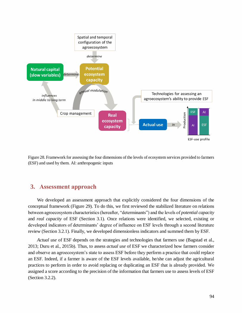
94

Figure 28. Framework for assessing the four dimensions of the levels of ecosystem services provided to farmers

(ESF) and used by them. AI: anthropogenic inputs

3. Assessment approach

We developed an assessment approach that explicitly considered the four dimensions of the

conceptual framework (Figure 29). To do this, we first reviewed the stabilized literature on relations

between agroecosystem characteristics (hereafter, “determinants”) and the levels of potential capacity

and real capacity of ESF (Section 3.1). Once relations were identified, we selected, existing or

developed indicators of determinants’ degree of influence on ESF levels through a second literature

review (Section 3.2.1). Finally, we developed dimensionless indicators and summed them by ESF.

Actual use of ESF depends on the strategies and technologies that farmers use (Bagstad et al.,

2013; Duru et al., 2015b). Thus, to assess actual use of ESF we characterized how farmers consider

and observe an agroecosystem’s state to assess ESF before they perform a practice that could replace

an ESF. Indeed, if a farmer is aware of the ESF levels available, he/she can adjust the agricultural

practices to perform in order to avoid replacing or duplicating an ESF that is already provided. We

assigned a score according to the precision of the information that farmers use to assess levels of ESF

(Section 3.2.2).

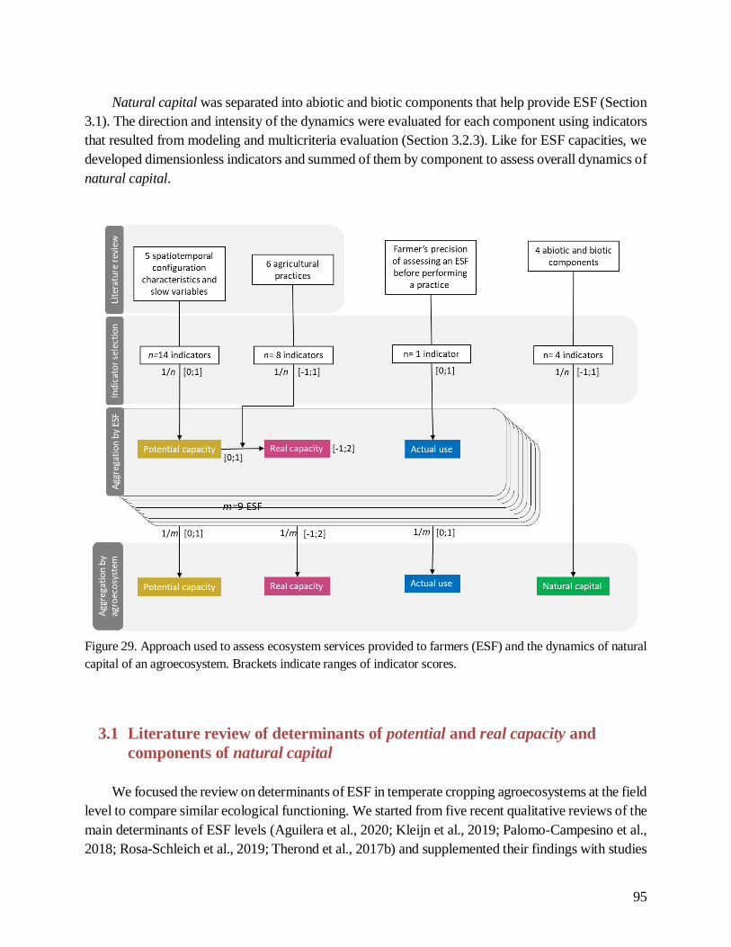
95

Natural capital was separated into abiotic and biotic components that help provide ESF (Section

3.1). The direction and intensity of the dynamics were evaluated for each component using indicators

that resulted from modeling and multicriteria evaluation (Section 3.2.3). Like for ESF capacities, we

developed dimensionless indicators and summed of them by component to assess overall dynamics of

natural capital.

Figure 29. Approach used to assess ecosystem services provided to farmers (ESF) and the dynamics of natural

capital of an agroecosystem. Brackets indicate ranges of indicator scores.

3.1 Literature review of determinants of potential and real capacity and

components of natural capital

We focused the review on determinants of ESF in temperate cropping agroecosystems at the field

level to compare similar ecological functioning. We started from five recent qualitative reviews of the

main determinants of ESF levels (Aguilera et al., 2020; Kleijn et al., 2019; Palomo-Campesino et al.,

2018; Rosa-Schleich et al., 2019; Therond et al., 2017b) and supplemented their findings with studies

96

identified by “snowball” searches when details were required. We selected information only from

reviews, meta-analyses and multi-site studies to ensure that the assessment approach was robust when

applied to a variety of temperate agroecosystems and production situations.

The literature review identified that (i) the crop rotation, (ii) soil coverage, (iii) use of species

mixtures, (iv) local semi-natural habitats and (v) abiotic soil composition (e.g. SOM content, texture,

P content) are elements of the spatiotemporal configuration and composition of agroecosystems that

influence the potential capacity to provide ESF (Figure 28; Table 8; Box 3; Supplementary material

17). These determinants can influence ESF directly or indirectly by influencing the biodiversity that

supports ESF (González-Chang et al., 2020).

Box 3. Determinants of potential ecosystem capacity.

The 9 ESF studied include pollination (POL); pest (PEST), weed (WEED) and disease (DIS)

control; soil structuration (STR); nitrogen supply to crops (NS); phosphorus supply to crops (PS);

water retention and return to crops (WATER) and stabilization and control of erosion (ERO).

The diversity of crops in the rotation is known to (i) break the cycle of weed development due

to a variety of sowing periods (WEED, Kleijn et al., 2019; Palomo-Campesino et al., 2018;

Scholberg et al., 2010; Weisberger et al., 2019), (ii) reduce the cycle of disease development and

reduce disease levels (DIS, Scholberg et al., 2010) and (iii) develop habitats for natural enemies

(PEST,Dassou and Tixier, 2016; Kleijn et al., 2019; Letourneau et al., 2011; Palomo-Campesino

et al., 2018). More specifically, the presence of legumes in a rotation increases soil nitrogen by

symbiotic fixation (NS, Duchene et al., 2017; Kleijn et al., 2019; Palomo-Campesino et al., 2018)

and available phosphorus by excreting catalyzers in the rhizosphere (PS, Bender et al., 2016; El

Mujtar et al., 2019; Ghosh et al., 2007; Hinsinger et al., 2011). The presence of a permanent soil

cover decreases weed germination (WEED, Aguilera et al., 2020; Kleijn et al., 2019; Palomo-

Campesino et al., 2018; Scholberg et al., 2010; Shackelford et al., 2019). Cover crops also structure

the soil via root penetration and maintain the soil moisture necessary for development of glomalin-

producing fungi, which are beneficial for aggregation of soil particles, stimulate soil life by

excreting root exudates and decrease erosion during periods of risk (STR, ERO, Aguilera et al.,

2020; Bertrand et al., 2019; Kleijn et al., 2019; Palomo-Campesino et al., 2018; Scholberg et al.,

2010; Shackelford et al., 2019). By avoiding nitrogen leaching during periods of risk, soil cover of

grass, crucifers or, to a lesser extent, legumes, between crops helps maintain nitrogen in the soil

(NS, Justes et al., 2012; Shackelford et al., 2019).

97

The literature review also identified that (i) insecticide use, (ii) tillage and herbicide use, (iii)

organic-matter application, (iv) tillage, (v) harvest conditions and (vi) conservation agriculture (a

combination of diversified rotations, permanent cover crops and reduced tillage) are agricultural

practices that can modulate an ecosystem’s potential capacity, thus determining its real capacity

(Figure 28; Box 4; Supplementary material 17).

Box 3. Determinants of potential ecosystem capacity (continued).

By avoiding nitrogen leaching during periods of risk, soil cover of grass, crucifers or,

to a lesser extent, legumes, between crops helps maintain nitrogen in the soil (NS, Justes et

al., 2012; Shackelford et al., 2019). Species mixtures compete for resources with weeds

better than individual species do (WEED, Bedoussac et al., 2015; Duchene et al., 2017;

Kleijn et al., 2019; Malézieux et al., 2009; Palomo-Campesino et al., 2018; Verret et al.,

2017). By dilution, confusion and barrier effects and the presence of habitats for natural

enemies, species mixtures reduce the pressure of diseases and pests and thus decrease major

health risks (DIS, PEST, Bedoussac et al., 2015; Dassou and Tixier, 2016; Duchene et al.,

2017; Iverson et al., 2014; Letourneau et al., 2011; Malézieux et al., 2009; Scholberg et al.,

2010; Vandermeer et al., 1998). Local (less than 200 m) herbaceous semi-natural habitats

provide habitats for pollinators, which enhances pollination (POL, Albrecht et al., 2020;

Bartual et al., 2019; Holland et al., 2017; Palomo-Campesino et al., 2018; Tscharntke et al.,

2007; Tschumi et al., 2016; Zulian et al., 2013). Local (less than 500 m) and in-field

herbaceous areas and woody edges enhance the presence of natural enemies and increase

the biological control of pests (PEST, Bartual et al., 2019; Bianchi et al., 2006; Blaauw and

Isaacs, 2014; Letourneau et al., 2011; Rega et al., 2018; Tscharntke et al., 2007; Tschumi et

al., 2016). While organic matter in the soil is only marginally responsible for an increase in

water holding capacity (Bauer and Black, 1992; Minasny and McBratney, 2018), it increases

infiltrability and thus increases water flow into the soil (WATER, Boyle et al., 1989; Chen

and Tessier, 1998; Green et al., 2003; Lado et al., 2004; Saxton and Rawls, 2006). Organic

matter and clay contribute to aggregate formation (physically and through microbial activity,

Diacono and Montemurro (2010)) in the soil and thus to the soil structure and the ability to

control erosion (STR, ERO, Johannes et al., 2017). Other things being equal, organic matter

determines the amount of nitrogen that will be mineralized in the soil and available to plants

(NS, Bender et al., 2016; Clivot et al., 2017; El Mujtar et al., 2019). The amount of

phosphorus available in the soil determines the soil's ability to provide phosphorus to crops

(PS, Bender et al., 2016; El Mujtar et al., 2019; Olsen et al., 1954).

98

To our knowledge, there is no systematic inventory of the components of natural capital that

underlie ESF (i.e. slow variables that determine ESF levels). Thus, based on the literature review and

expert knowledge, we selected four key components: soil quantity (which depends mainly on erosion),

SOM, soil P balance and the biodiversity that supports ESF. Considering this last component as

Box 4. Determinants of real capacity

Insecticides can have negative impacts on pollinators (POL, Brittain and Potts, 2011;

Colin et al., 2004; Potts et al., 2009), but also on organisms that control weeds (WEED,

Emmerson et al., 2016; Labruyere et al., 2016) and pests (PEST, Desneux et al., 2007;

Emmerson et al., 2016; Geiger et al., 2010) and that are involved in soil structuration (STR,

Wang et al., 2012). Adding organic matter from straw or organic-matter application increases

the stock of humified carbon in the soil and enhancing microbial activity, promotes the

formation and stabilization of macro-aggregates that contribute to porosity and water

infiltration, and thus water storage capacity (WATER, Aguilera et al., 2020; Boyle et al., 1989;

Khaleel et al., 1981; Lado et al., 2004), soil structuration (STR, Abiven et al., 2009; Diacono

and Montemurro, 2010; Khaleel et al., 1981; Liu et al., 2014) and erosion control (ERO,

Aguilera i, 2020; Khaleel et al., 1981; Liu et al., 2014; Paradelo et al., 2019). Once they

mineralize, straw returned to the soil and applied organic matter increase the soil's nitrogen and

phosphorus reserves (NS, PS, Diacono and Montemurro, 2010; Khaleel et al., 1981; Liu et al.,

2014). Harvesting in adverse conditions can deform the soil structure (e.g. compact it), which

restricts soil life and its effect on structuration (STR, Hamza and Anderson, 2005). Tillage can

harm the suppressive capacity of soils by disrupting of food webs and impeding weed and pest

control (WEED, PEST, Blubaugh and Kaplan, 2015; Kuntz et al., 2013; Menalled et al., 2007;

Trichard et al., 2014). Plow tillage disrupts the natural channels that allow water to circulate

and prevents optimal storage due to the sole created (WATER, Aguilera et al., 2020; Blanco-

Canqui and Ruis, 2018; Soane et al., 2012). This sole compacts soil and exposes it to

compaction, which disturbs soil structuration and reduces erosion control (STR, ERO, Aguilera

et al., 2020; Blanco-Canqui and Ruis, 2018; Blevins et al., 2018; Hamza and Anderson, 2005;

Soane et al., 2012). In the field, the abundance and diversity of non-crop plants result from the

tillage and herbicide strategy and these plants provide diversified habitats for pollinators (POL,

Bretagnolle and Gaba, 2015; Petit et al., 2016) and natural enemies (PEST, Dassou and Tixier,

2016; Petit et al., 2015). Conservation agriculture, which is a combination of diversified

rotations, permanent soil cover and reduced tillage, creates synergistic positive effects for weed

control, water retention capacity, soil structuration and the supply of nitrogen and phosphorus

(WEED, WATER, STR, NS, PS, Blanco-Canqui and Ruis, 2018; Kleijn et al., 2019; Lee et

al., 2019; Pittelkow et al., 2015).

99

“ecosystem service providers” (Luck et al., 2009), we considered the dynamics of abundance and

diversity of the key above-ground and soil organisms that support ESF in a disaggregated manner (i.e.

natural enemies of pests, pollinators, granivores, soil animals, soil bacteria and soil fungi) by assessing

practices that influence them (Supplementary material 17, González-Chang et al. (2020); Weyers and

Gramig (2017)). Supplementary material 18 describes relations between the four components of

natural capital and ESF and provides details about mechanisms.

3.2 Indicators and multicriteria assessment of the four dimensions of ESF

The indicators used for multicriteria assessment of the four dimensions of ESF were either

discrete or continuous. In both cases, values were scaled when necessary (into five classes, if discrete)

relative to the corresponding value of the case study region (NUTS 2); thus, the values were

dimensionless so they could be aggregated by averaging them. The limits of each indicator were

defined according to the range of potential absolute values of each indicator or according to local

experts. For example, the maximum percentage of legumes in a rotation was 100%, while the

maximum SOM mineralization rate was defined by experts according to that observed in the case

study region.

3.2.1 Indicators of an agroecosystem’s potential and real capacities

Due to the literature review, we identified or developed a set of consistent indicators to quantify

the positive or negative effect of each determinant on the potential and real capacity levels of each of

the nine ESF (Table 9). Depending on the number of determinants considered for each ESF (n), its

indicator was based on one variable or a mean of n variables. Indicators of potential capacity

(hereafter, I_potential) ranged from 0 (no contribution) to 1 (maximum positive contribution).

Quantifying the I_potential required using information about crop rotations, cover crops, the number

of cultivars, the location of semi-natural habitats around the fields and/or soil analyses (i.e. texture and

SOM content). For each ESF, potential capacity was the average of n I_potential scores. Indicators of

the modulation of potential capacity (hereafter, I_modulation) provided information about how

agricultural practices influence ESF during the year. For each ESF, the modulation was the average

of n I_modulation scores. Adding I_potential ([0; 1]) to I_modulation([-1; 1]) yielded indicators of

real capacity ([-1; 2]) for each ESF (Figure 29). Quantifying the I_modulation indicators required

information about agricultural practices (i.e. fertilization, pesticide application, organic-matter

application, crop-residue management), local climate and the number of non-crop plants at harvest

and before the first tillage or herbicide application, depending on the farm. We assumed that

conservation agriculture that combines diversified rotations, permanent soil cover and minimal tillage

provides a synergistic effect (Pittelkow et al., 2015). To reflect this, a bonus score of 1 was added to

I_modulation if all three of these conditions were met. Indicators related to semi-natural habitats were

calculated at the field level and averaged for the agroecosystem. Potential and real capacity scores by

agroecosystem were aggregated by averaging all ESF potential and real capacity scores, respectively.

100

3.2.2 Indicators of actual use of ESF

Farmers can use a variety of actions (e.g. counting natural enemies) or tools (e.g. tensiometers to

estimate soil water content) to assess an agroecosystem’s ability to provide ESF. Thus, for each of the

seven ESF that can be replaced with an anthropogenic input, we identified the main actions that

farmers can perform to estimate the capacity of an agroecosystem to provide a given ESF (Table 10).

We then ranked them according to the precision of the information provided and assigned them a score

from 0-1 (i.e. least to most precise). Two experts in agriculture practices defined each action’s degree

of precision. For example, they considered that the most precise technology available to farmers to

assess soil structure is the spade test (even though it is low technology). They also considered that

using an unmanned aerial vehicle or remote-sensing robot would allow farmers to estimate the spatial

distribution of ESF levels precisely and to adjust product doses accordingly. We determined that

farmers in the case study had no technology at the field level (i.e. no action) that could replace the

pollination or erosion-control ESF, so no indicator was calculated for them. Actual use scores by

agroecosystem were aggregated by averaging all ESF actual use scores.

3.2.3 Natural capital dynamics

Among the variety of methods to assess dynamics of the n = 4 components of natural capital

selected, we chose four that could be applied easily to data usually available on farms. Natural capital

was assessed using dimensionless indicators that expressed the dynamics of its components and

ranged from -1 (depletion) to 1 (capitalization).

Soil quantity dynamics were assessed using an index of the potential sensitivity to erosion, which

equals the product of erodibility and exposure indexes for all crops in a rotation (van Dijk et al. (2016);

Supplementary material 20). It is based on monthly rainfall, soil bulk density, SOM content, the

proportion of area covered by vegetation and the spatial structure of vegetation. According to

Rosenfelder and van Dijk (2014), index values of 0.015 and 0.022 are considered acceptable and very

high, respectively. From this index, we developed an indicator of potential sensitivity to erosion ([-1;

1]) with five classes that ranged from high to unlikely.

The trend in SOM was estimated from the trend in soil carbon content predicted by the AMG

model (Clivot et al., 2019), considering the climate from 1997-2017. AMG explicitly simulates a

rotation of crops and intercrops, the type and amount of organic matter applied and crop-residue

management (Andriulo et al., 1999). The slope of a linear regression of AMG’s predictions of annual

SOM were transformed into an indicator of the trend in SOM. A positive or negative trend (i.e. score)

indicated capitalization or depletion of soil carbon, respectively (Supplementary material 21). We

centered the data and defined five classes from the data’s quintiles.

Due to the difficulty in estimating dynamics of the soil P stock, we considered the annual balance

between the amount of P exported in harvested straw and grain and that imported by mineral

101

fertilization, organic-matter application and straw left in fields (Supplementary material 22). The

indicator expressed the extent to which the cropping system increases or decreases the soil P stock. A

positive or negative balance indicated soil P capitalization or depletion, respectively. We centered the

data and defined five classes from the data’s quintiles.

The dynamics of biodiversity were estimated using a composite index of indicators that, based

on a literature review (Table 8), provided information about average effects of the determinants and

agricultural practices considered on six key communities of service providers: natural enemies of

pests, pollinators, granivores, soil animals, soil bacteria and soil fungi (Table 11, Supplementary

material 17; González-Chang et al., 2020). These service-provider communities are influenced by the

spatial and temporal configurations and compositions of the ecosystem, SOM content and crop

management. Indicators of effects of each determinant on each community ([-1; 0] or [0; 1], Table 11)

were summed to estimate a score for each community. To assess the dynamics of all biodiversity that

supports ESF, these indexes were summed and then divided by the sum of maximum possible scores

of the six communities. Because the number of determinants that influence each community can differ,

this method aggregated information into a single score. A negative score indicates an expected middle-

to-long-term reduction in biodiversity due to crop management.

Natural capital dynamics scores by agroecosystem were aggregated by averaging the scores of

the four components.

4. Example of application

4.1 Materials and methods

4.1.1 Case study and data collection

Twenty-eight farms in the Grand Est region (NUTS2) of France were chosen by advisors from

the Regional Chamber of Agriculture to represent a wide range of rotation complexity and input

intensity in agroecosystems (Supplementary Material 23). The systems selected ranged from an

irrigated monoculture of maize to a complex rotation in organic and conservation agriculture

(Supplementary Material 24). Data required to apply the approach (Supplementary Material 25) came

from a farmer survey conducted in 2019 and the farmers’ computer-based management tool (2018

data). In the latter, farmers enter the crop rotation, cover crops and practices (i.e. sowing, tillage;

pesticide and fertilizer applications) each year. Along with the survey, each farmer was interviewed

for ca. 1.5 h. The survey was used to identify one or two main types of agroecosystems on each farm

and the associated fields, the characteristics of semi-natural habitats in these fields (using orthophotos)

and the farmers’ strategies for their actual use of ESF. On the 28 farms surveyed, we identified 34

types of agroecosystems (450 fields), each of which corresponded to fields with the same soil and

cropping systems (i.e. rotation, cover crops, crop management).

102

4.1.2 Methods

We analyzed yields and input intensity of the 34 agroecosystems. We defined the “relative yield”

of each as the ratio of its mean yield of wheat (or, if not available, maize) from 2017-2019 to that of

the French department in which it was located. Input intensity was estimated by aggregating scores of

(i) mineral fertilization intensity relative to the regional mean, (ii) pesticide treatment frequency index

relative to the regional mean and (iii) the frequency of plowing and irrigation (Supplementary Material

26). We performed principal component analysis (PCA) with R to help interpret relations among real

capacity, actual use, natural capital, relative yield and input intensity. Potential capacity was not

included because it was highly correlated (r=0.780) with real capacity, which exceeded the

collinearity threshold (r=0.700) recommended by Dormann et al., (2013). To identify different

agriculture models according to the four dimensions of ESF, we performed clustering analysis with a

partitioning (k-means) algorithm in the three-dimensional data space of real capacity, actual use, and

natural capital. The optimal number of clusters (k) was defined according to the elbow method, which,

for k ranging from 1 to n clusters, calculates the within-cluster sum of squares and the location of a

“elbow” can be considered an indicator of the suitable number of clusters (Supplementary material

11). We compared cluster-specific means of input intensity and relative yield to each other with Tukey

honestly significant difference (HSD) post-hoc tests to test all pairwise comparisons with 95%

confidence. Analyses were performed using the open-source FactoMineR package of R software

(Husson et al., 2010; MacQueen, 1967; R Core, 2013).

4.2 Results

4.2.1 Application of the assessment approach

For each agroecosystem, the scores of potential capacity, real capacity, actual use and natural

capital of each ESF was assessed and represented in absolute value and relative value compared to

those of the entire group (Figure 30, Supplementary material 27). A group’s ranges may not cover the

ranges of all possible values. For example, for agroecosystem #26, pesticide use rendered WEED’s

real capacity only slightly lower than its potential capacity (Figure 30a). Relative to the group, the

agroecosystem’s configuration and crop management practices favored POL, WEED, DIS and PEST,

since its potential and real capacities were among the highest in the group (Figure 30a). Moreover,

since the farmer of #26 always used counting and field observations to assess biological regulation of

pests, weeds and diseases, the actual use of these ESF was also relatively high (Figure 30b). The

potential capacity of the NS service was high but could be increased by improving agroecosystem

configuration and crop management. The agroecosystem’s natural capital components had

contrasting dynamics (Figure 30c). Biodiversity and SOM capitals were relatively high, indicating

that biological regulation services would continue for the farmer, while N provision should increase.

Potential sensitivity to soil erosion (with a medium value) could be improved, while the P balance

indicator had a low value, which indicated the risk of depleting the soil P stock.

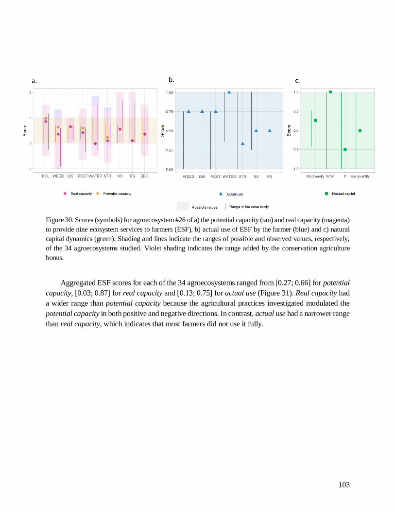
103

Figure 30. Scores (symbols) for agroecosystem #26 of a) the potential capacity (tan) and real capacity (magenta)

to provide nine ecosystem services to farmers (ESF), b) actual use of ESF by the farmer (blue) and c) natural

capital dynamics (green). Shading and lines indicate the ranges of possible and observed values, respectively,

of the 34 agroecosystems studied. Violet shading indicates the range added by the conservation agriculture

bonus.

Aggregated ESF scores for each of the 34 agroecosystems ranged from [0.27; 0.66] for potential

capacity, [0.03; 0.87] for real capacity and [0.13; 0.75] for actual use (Figure 31). Real capacity had

a wider range than potential capacity because the agricultural practices investigated modulated the

potential capacity in both positive and negative directions. In contrast, actual use had a narrower range

than real capacity, which indicates that most farmers did not use it fully.

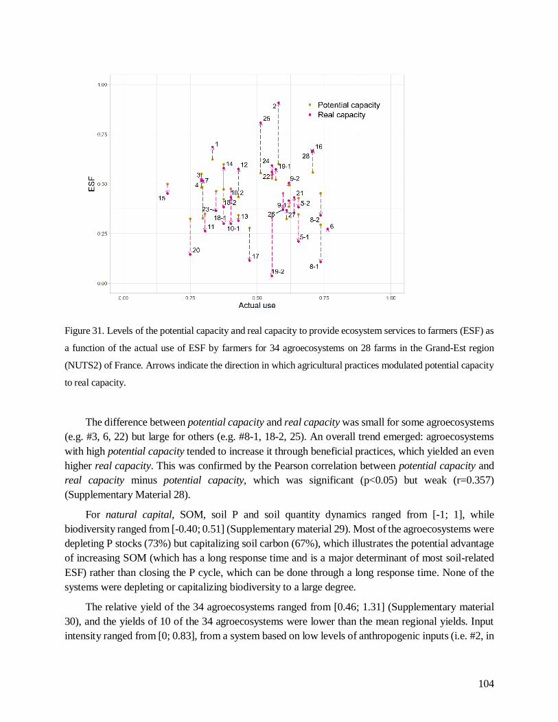
104

Figure 31. Levels of the potential capacity and real capacity to provide ecosystem services to farmers (ESF) as

a function of the actual use of ESF by farmers for 34 agroecosystems on 28 farms in the Grand-Est region

(NUTS2) of France. Arrows indicate the direction in which agricultural practices modulated potential capacity

to real capacity.

The difference between potential capacity and real capacity was small for some agroecosystems

(e.g. #3, 6, 22) but large for others (e.g. #8-1, 18-2, 25). An overall trend emerged: agroecosystems

with high potential capacity tended to increase it through beneficial practices, which yielded an even

higher real capacity. This was confirmed by the Pearson correlation between potential capacity and

real capacity minus potential capacity, which was significant (p<0.05) but weak (r=0.357)

(Supplementary Material 28).

For natural capital, SOM, soil P and soil quantity dynamics ranged from [-1; 1], while

biodiversity ranged from [-0.40; 0.51] (Supplementary material 29). Most of the agroecosystems were

depleting P stocks (73%) but capitalizing soil carbon (67%), which illustrates the potential advantage

of increasing SOM (which has a long response time and is a major determinant of most soil-related

ESF) rather than closing the P cycle, which can be done through a long response time. None of the

systems were depleting or capitalizing biodiversity to a large degree.

The relative yield of the 34 agroecosystems ranged from [0.46; 1.31] (Supplementary material

30), and the yields of 10 of the 34 agroecosystems were lower than the mean regional yields. Input

intensity ranged from [0; 0.83], from a system based on low levels of anthropogenic inputs (i.e. #2, in

105

organic and conservation agriculture; Supplementary material 24) to one based on high levels of

anthropogenic inputs (i.e. #8-1).

The most intensive systems exceeded mean regional yields and were generally those with the

lowest real capacity. The first axis of the PCA, influenced by input intensity and the relative yield on

one side and real capacity on the other, explained 41.8% of the variance (Supplementary material 31).

This negative relation between input intensity (and thus relative yield, since they were strongly

correlated) and real capacity was significant and moderately strong (Supplementary material 32,

p<0.05 and r=-0.564). However, there were a few notable exceptions, such as agroecosystems #25

and #23, which had, respectively, a real capacity of 0.80 and 0.27 and a relative yield of 1.27 and

0.61. In contrast, there was no relation between input intensity and the dynamics of natural capital or

actual use of ESF (e.g. agroecosystem #15).

4.2.2 Description of the agriculture models

The clustering analysis identified five clusters (Figure 32) that referred to five combinations of

scores of real capacity and actual use of ESF and dynamics of natural capital. The first cluster of (5

agroecosystems) had some of the highest real capacity ([0.57; 0.87]), above-average actual use ([0.51;

0.70]) and no specific natural capital dynamics (but no large depletion) (Figure 32, MH-H). This

cluster had varied rotations (rapeseed-wheat-barley-legume-other or soybean-wheat-other) but which

always included legumes and often uncommon crops (e.g. spelt, spring peas, mustard, alfalfa, sainfoin,

flax). Rotation duration ranged from 3-9 years (mean: 5.4 years). These five systems performed

reduced tillage or no tillage. One was an irrigated conventional farm, two were organic, and one

performed conservation agriculture. They corresponded to models with “Medium-High use of High

ESF capacity” (“MH-H”).

The second cluster (8 agroecosystems) had a wide range of real capacity ([0.26; 0.68]), low

actual use [0.16; 0.43]) and neutral or positive natural capital dynamics (Figure 32, I-M). This cluster

had rotations based mainly on rapeseed-wheat-barley-other, with a mean rotation duration of 5.6 years,

5.5 crops in the rotation and varied types of tillage (plowing, reduced tillage, no-till). Only one farm

in this model, a maize-based rotation (#1), was depleting its natural capital. Agroecosystem #23 was

unique in this group since it had low real capacity despite having 9 crops and practicing reduced

tillage. These systems corresponded to models with “Inefficient use of Medium ESF capacity” (“I-

M”).

The third cluster (7 agroecosystems) had a wide range of real capacity ([0.03; 0.59]), medium

actual use ([0.43; 0.63]) and positive natural capital dynamics (Figure 32, M-LM-C). This cluster

mainly (8 out of 9) had rotations such as rapeseed-wheat-barley-other, included less common crops

(e.g. sainfoin, faba bean, and hemp) and had a mean rotation duration of 5.6 years. All but one of the

farms occasionally practiced simplified tillage, and only one irrigated. Agroecosystem #19-2 was

unique in this cluster because it was a plowed maize monoculture. All of these farms applied pesticides

106

and mineral fertilizers. These systems corresponded to models with “Medium use of Low-to-Medium

ESF capacity, with Capitalization” (“M-LM-C”).

The fourth cluster (6 agroecosystems) had low real capacity ([0.14; 0.59]), medium-low actual

use ([0.25; 0.4]) and negative natural capital dynamics (Figure 32, I-LM-D). This cluster contained

had only maize-wheat-other crop rotations (mean of 2.5 crops in the rotation, often with 2 years of

maize). Its agricultural practices varied (plowing, reduced tillage, pesticides or not, irrigation or not).

These systems corresponded to models with “Inefficient use of Low-to-Medium ESF capacity, with

Depletion” (“I-LM-D”).

The fifth cluster (8 agroecosystems) had low real capacity ([0.10; 0.50]), high actual use ([0.61;

0.76]) and negative natural capital dynamics (Figure 32, E-LM-D). This cluster contained only maize-

wheat-other crop rotations (a mean of 2.5 crops in the rotation), with at least 2 years of maize and a

mean rotation of 4 years. Three of the 8 agroecosystems sometimes practiced reduced tillage, and all

but one irrigated. All farms in this cluster applied pesticides and mineral fertilizers, and four did not

use insecticides or fungicides. These systems corresponded to models with “Efficient use of Low-to-

Medium ESF capacity, with Depletion” (“E-LM-D”).

Relative yield and input intensity did not differ significantly among the five clusters, although

the MH-H cluster had high variability in relative yield (p>0.05, pairwise Tukey HSD test, [0.66; 1.27],

Supplementary material 33).

107

Figure 32. Five clusters of agriculture models identified by k-means clustering according to (i) the ecosystem’s

real capacity to provide ecosystem services to farmers (ESF), (ii) actual use of ESF by farmers and (iii) direction

and intensity of natural capital dynamics for 34 agroecosystems on 28 farms in the Grand Est region of France.

5. Discussion

We developed an original assessment approach to ESF based on assessing relations between

characteristics of agroecosystems and the main ESF they provide. In agreement with the objective of

developing operational tools for agricultural support institutions, the approach provides a detailed

description for farmers of the potential capacity of each ESF, effects that agricultural practices have

on it, the actual use of ESF capacity and the dynamics of natural capital under current agricultural

practices (Figure 30). The approach is part of a large field of research that assesses ecosystem services

in agroecosystems (Malinga et al., 2015). It focuses on ESF involved in agricultural production (and

not on those provided to the larger society) and characterizes relations between agroecosystems and

ESF at two temporal scales: the classic short term, which corresponds to the cropping season, and the

medium-/long-term dynamics of natural capital (Robinson et al., 2012).

108

5.1 Strengths of the assessment approach

Our approach is an original development of the conceptual framework and its operationalization

by integrating scientific knowledge and low-data indicators. One of the innovations is that it

conceptually clarifies and renders operational the assessment of four components of ESF, which

separates components of the cascade that underlie the provision of ESF in the short and medium/long

terms. Accordingly, as claimed by Kleijn et al. (2019), this provides agricultural stakeholders with

useful information about (i) “limiting services” (Bommarco et al., 2013; Garibaldi et al., 2018;

Sperfeld et al., 2012) and (ii) potential mechanisms to enhance the potential and real capacities of

ESF. In other words, it provides a sound conceptual framework with which to analyze the functioning

of agroecosystems and define a strategy to manage it in the quest for ESF-based agriculture models.

As also noted by Therond et al. (2017a), our assessment approach can classify agroecosystems

more finely than broad typologies (e.g. organic vs. conventional agriculture, diversified vs. simplified

farming systems) (Garibaldi et al., 2017). As Duru et al. (2015b) theorized, our fine-grained approach

can identify multiple strategies that can be used to obtain given levels of ESF and dynamics of natural

capital. For example, three organic agroecosystems (#28, 2 and 15) that covered a range of rotation

diversification (from 3-6 crops) differed strongly in real capacity and actual use of ESF (Figure 32).

This confirms that organic systems, which vary from complex biodiversity-based systems to

simplified monocultures, can result in agroecosystems with greatly different functioning (Reeve et al.,

2016; Seufert et al., 2012).

Our approach may also help assess payments for environmental services provided by agricultural

support institutions, in which beneficiaries (society) pay ecosystem-service providers (here, farmers)

for the services provided (Donohue et al., 2016). For the ESF assessed in the present study, these

payments would reward farmers for using ESF instead of anthropogenic inputs and thus intentionally

encourage biodiversity-based solutions and reduce negative environmental impacts related to input-

based systems (Bommarco et al., 2013). This method provides the strong scientific foundations needed

to assess such payments, as required by Naeem et al. (2015), by developing a scientifically robust

method that is operational and requires relatively little data.

5.2 Shortcomings and expected improvements of the approach

Since the approach developed is the first version, it will be improved. Applying it to the case

study of the Grand Est required parameterizing it for this region; applying it to other regions will

require expert knowledge of the regions and associated reference data. In particular, the range of

technologies that could be used to assess the provision of ESF and thus determine the actual use of

ESF needs to be adapted to the technologies available locally. It is currently defined from expert

opinion, but other ways to estimate as closely as possible farmers’ actual use of ESF, both active and

inactive, can be considered. Results of future studies of determinants of ESF are also expected to

improve the selection of low-data indicators and the method used to aggregate them for individual

109

ESF and entire sets of ESF (as in Vogel et al. (2019) and Zhang (2020); see Section 5.3 for details).

To date, without available knowledge about the relative weights of determinants of ESF, the

aggregation remains simplistic (the same weight for all).

The application domain of the approach is currently limited to cropping systems and needs to be

extended to other agroecosystems (e.g. livestock, orchards, vineyards agroforestry). Using the same

logic, the method could be extended to other ES provided to farmers (e.g. local climate regulation) or

to society (e.g. global climate regulation) (Aguilera et al., 2013; Techen et al., 2020). This could

identify synergies and trade-offs between ESF provided to different beneficiaries (Obiang Ndong et

al., 2020). Finally, for the natural capital components, only the biodiversity that supports ESF was

considered, but the approach could be extended to consider all biodiversity from a larger conservation

perspective (Lüscher et al., 2017; Moller et al., 2008).

Another key improvement would be to quantify the part of production that comes from using

ESF vs. the part that comes from anthropogenic inputs (Jones et al., 2016). For now, the approach

developed does not exactly follow the recommendations of Therond et al. (2017a) for classifying

agricultural models. However, partitioning production between these two types of production factors

is complex due to intertwined ecological processes (Barot et al., 2017; Jones et al., 2016). Few studies

have attempted to do this. Pérez-Soba et al. (2019) performed emergy analysis, which coarsely

distinguished effects of natural (e.g. solar radiation) vs. anthropogenic flows. Therond et al. (2017b)

and Tibi and Therond (2018) developed an approach based on a crop model to estimate the part of

production related to groundwater-, rainwater- and nitrogen-related ESF vs. N fertilization and

irrigation.

Finally, this approach does not address environmental impacts of agriculture (e.g. N leaching)

(Uusitalo et al., 2019) or multifunctional aspects of agricultural performance (de Olde et al., 2016;

Rasmussen et al., 2017; Zahm et al., 2018). Performing such classic impact assessments along with

our assessment approach would provide a more complete environmental assessment.

5.3 Lack of knowledge and agenda for research

The literature review highlighted a substantial lack of knowledge. First, we were not able to

consider effects of semi-natural habitats in the landscape beyond the farm scale. Karp et al. (2018)

show that the influence of non-crop habitats on biological control depends on the context. Multiple

communities may be involved in providing an ESF, and little information about their interactions (e.g.

inter-guild predation) is available. For example, results for the effects of carabids on weed regulation

(Frei et al., 2019) are ambiguous, showing a positive effect (Chapman, 2014; Knapp and Řezáč, 2015)

or negative effect (Jonason et al., 2013) of landscape heterogeneity. Dispersal distances of carabids

depend on their guild, which causes variability among observations. Moreover, the relative

contribution of carabids vs. birds and small mammals to weed regulation is still under research (Petit

et al., 2011). In other words, landscape effects on biological regulation services may depend strongly

on the functional characteristics of ESF providers (Martin et al., 2019).

110

We felt that certain relations between determinants and ESF already mentioned in the literature

were not yet sufficiently documented to include them. For example, non-crop plants in and around

fields might have a key influence on dynamics of natural enemies by providing a diverse habitat and

food resource for biodiversity (Marshall et al., 2003; Petit et al., 2015; Pocock et al., 2012). However,

we could not find key reviews or meta-analyses that provided usable information. Cover crops appear

to influence disease control, but this seems specific to each combination of host/disease/cover crop

(Justes et al., 2012). Soil cover influences the soil structuration service via the canopy and root

exudates (Bardgett et al., 2014; Scavo et al., 2019). Although the influence is well established, we did

not find a suitable database of root exudates from crops to be able to consider this effect. More

generally, Techen et al. (2020) present key soil research challenges for a few management practices

such as nutrient efficiency in agroforestry, the influence of rotations and crops on microbiome

composition, ecotoxicity of plastics, stoichiometry management, biotic inoculations and

pharmaceuticals.

Finally, there is a serious lack of information about the relative influence of determinants on the

provision of each ESF. For example, weed control is promoted by spatial (species mixtures) and

temporal (rotations) plant diversity and permanent soil cover, but their relative influence is unknown.

Therefore, we assigned the same influence to all n determinants for a given ESF and to the

contributions of potential and modulation effects to the ESF level. Until studies provide information

about these relative effects, improving our approach could mean bringing a group of experts together

to refine the aggregation method, as van Leeuwen et al. (2019) and Zahm et al. (2018) recommended.

Ultimately, this information is also needed to integrate potential trade-offs that may exist among the

determinants of ESF (Garibaldi et al., 2018; Obiang Ndong et al., 2020).

5.4 Insights into agriculture models

In general, agroecological practices, such as organic, biodiversity-based practices (e.g. rotations,

species mixtures) and conservation agriculture, are expected to provide higher ESF capacity (Palomo-

Campesino et al., 2018). We show that this is true when several agroecological practices are

implemented together, as in the MH-H agriculture model in which organic farming, reduced or no-

tillage, soil cover and diversified rotations were combined, as suggested by Duru et al. (2015b). To a

lesser extent, and because agroecological practices are usually combined less often, the I-M agriculture

model also followed this pattern. However, our results suggest that implementing these practices does

not necessarily mean that farmers use the potential capacity of ESF well.

In the present study, real capacity was significantly negatively correlated with input intensity and

relative yield. In other words, agriculture models with higher real capacity of ESF are often those with

lower input use and relative yield. However, this trend hides high variability. First, excluding organic

agroecosystems weakens this correlation because they have the lower relative yields and input

intensity due to organic specifications (Supplementary material 34) (Knapp and van der Heijden,

2018). Second, no significant difference in input intensity or relative yield was observed among

111

clusters. Indeed, variability in relative yield among agroecosystems was high within each cluster,

particularly in the agroecological agriculture models with high/medium real capacity. Thus, there are

many ways to obtain high yields, based mainly on anthropogenic inputs, ESF or both (Therond et al.,

2017a). For example, within these agroecological models, the yield of agroecosystems #25, 16, 12,

and 3 was higher than the regional mean. Agroecosystem #25 was unique in the present study since it

obtained high yields with a high input intensity but also used ESF capacity efficiently (Supplementary

material 35). It was also the only agroecosystem that met our requirements to be classified as

conservation agriculture and thus to benefit from the bonus. The farmer of this agroecosystem

increased the yield greatly by using ESF as much as possible and supplementing them with inputs,

and the ESF levels could have been increased even further.

In the M-LM-C agriculture model, system #19-2, a maize monoculture, which had the lowest

ESF real capacity of the group, was managed by the same farmer as system #19-1, which had higher

ESF capacities. This large difference between two agroecosystems of the same farmer reflects a

separation of the land that results from two different rationales and European Union Common

Agricultural Policy (CAP) regulations. System #19-2 is based on maize, which is the most

economically profitable crop locally and usually managed intensively in monoculture with irrigation

and plowing on the best soils. However, due to CAP regulations on the proportion of farm area that

can be planted in monocultures, farmers cannot plant monocultures over the entire farm.

Consequently, system #19-1 was based on a multicrop rotation that was managed less intensively.

CAP regulations allowed the farmer to open up space for testing solutions based on planned

biodiversity. This pattern was repeated on other maize farms (#8, 10, and 19).

Finally, we highlight that all maize-based rotations depleted natural capital, regardless of the

agricultural model to which they belonged. Soil erosion due to the absence of cover crops drove this

negative trend, which could be addressed by adding cover crops to maize-based systems (Laloy and

Bielders, 2010). However, weather conditions after the late maize harvest period make it difficult to

plant cover crops (Marcillo et al., 2019).

6. Conclusion

We developed a new conceptual framework to clearly distinguish multiple aspects of ESF and

an operational low-data indicator-based approach to assess them. It highlights the important distinction

between short-term ESF capacities and medium/long term dynamics of natural capital that underlie

these services and the actual use of them. The literature review performed to develop this approach

enabled us to build upon well-known relations between characteristics of agroecosystems and ESF,

identify consistent indicators of these relations, and identify areas in which knowledge is lacking. This

indirect evaluation of ESF allows for (i) the use of easily available data on characteristics of

agroecosystems and their management instead of resource-consuming field measurements, (ii)

detailed description of ESF associated with an agroecosystem and (iii) identification of agronomic

mechanisms to use to increase the provision or use of ESF. Through better understanding of the ability

112

of agroecosystems to generate ESF, and how to enhance them, our approach may help farmers build

agroecosystems based on natural production factors instead of importing petrochemicals.

We demonstrated the utility of our approach by applying it to a set of 34 French agroecosystems.

This application provided key insights into the biotechnical functioning of arable agroecosystems: (i)

combining agroecological practices maximizes the real capacity of ESF and (ii) there are many ways

to reach high-yielding agroecosystems based on anthropogenic inputs, ESF or both.

Contributions

M.D., B.L. and O.T. developed the conceptual framework; M.D. and B.L. performed the

literature review and indicator selection with the guidance of O.T. and C.Bo.; H.C. developed the

AMG model used; M.D., B.L. and C.Be. performed the farm surveys and calculations; M.D. and O.T.

wrote the manuscript; and C.Bo., B.L. and C.Be. proofread the manuscript.

Acknowledgments

We thank Agrosolutions, the agricultural consulting firm that supported and funded the Ph.D.

research of M.D. but had no role in the decision to publish. We thank Michel Duru, Jean Roger-Estrade

and Guy Richard for providing general guidance and discussion; Frédéric Pierlot for assistance in

building the case study network; Léa Dubois for conducting the surveys and calculating the indicators;

Paul Van Dijk for guiding us in the application of his method; David Justeau, Grégory Lemercier,

Claude Rettel, and Jean-François Strehler, the advisors of the Chambers of Agriculture who selected

the farms and the 28 farmers who provided their time and data. We thank Michelle and Michael

Corson for proofreading. The conceptual framework and several key ideas in this article were

developed during the INRAE study EFESE-EA (2014-2017), which identified and assessed

ecosystem services provided by agricultural ecosystems across France, as part of the French National

Ecosystem Assessment.

113

TABLES OF THE SECTION

Table 8. Summary of the main determinants of ecosystem services provided to farmers (ESF). The spatial and

temporal configuration and composition of the cover and soil composition determine an ecosystem’s potential

capacity. The crop management of soil and biomass determined an ecosystem’s real capacity. The 9 ESF studied

include pollination (POL); pest (PEST), weed (WEED) and disease (DIS) control; soil structuration (STR);

nitrogen supply to crops (NS); phosphorus supply to crops (PS); water retention and return to crops (WATER)

and stabilization and control of erosion (ERO). The effects of crop management on ESF provision can be

positive (+) or negative (-). References are mainly meta-analyses, reviews or multisite studies. *Depends on the

type of habitat. **Several combinations of soil characteristics are suitable for ESF, see Table 9.

Capacity Determinant ESF and direction of

the effect

References

Pote

nti

al

Crop rotation

WEED, DIS, PEST

(diversified: +)

NS, PS (legume

presence: +)

Bender et al., 2016; Dassou and Tixier, 2016; Duchene et al., 2017; El Mujtar

et al., 2019; Ghosh et al., 2007; Hinsinger et al., 2011; Kleijn et al., 2019;

Letourneau et al., 2011; Palomo-Campesino et al., 2018; Rosa-Schleich et al.,

2019; Scholberg et al., 2010

Soil coverage WEED, STR, NS, ERO

(permanent: +)

Aguilera et al., 2020; Bertrand et al., 2019; Justes et al., 2012; Kleijn et al.,

2019; Palomo-Campesino et al., 2018; Rosa-Schleich et al., 2019; Scholberg

et al., 2010; Shackelford et al., 2019

Use of species

mixtures

WEED, DIS, PEST (+) Bedoussac et al., 2015; Dassou and Tixier, 2016; Duchene et al., 2017;

Iverson et al., 2014; Kleijn et al., 2019; Letourneau et al., 2011; Malézieux et

al., 2009; Palomo-Campesino et al., 2018; Rosa-Schleich et al., 2019, p.;

Scholberg et al., 2010; Vandermeer et al., 1998; Verret et al., 2017

Local semi-natural

habitats

POL, PEST

(close to fields*, +)

Bartual et al., 2019; Bianchi et al., 2006; Blaauw and Isaacs, 2014; Holland et

al., 2017; Palomo-Campesino et al., 2018; Rega et al., 2018; Tscharntke et

al., 2007; Tschumi et al., 2016; Zulian et al., 2013

Abiotic soil

composition

STR, NS, PS, WATER, ERO **

Bender et al., 2016; Boyle et al., 1989; Chen and Tessier, 1998; Clivot et al., 2019; El Mujtar et al., 2019; Green et al., 2003; Johannes et al., 2017; Lado

et al., 2004; Olsen et al., 1954; Saxton and Rawls, 2006

Rea

l

Insecticide use POL, WEED, PEST,

STR (-)

Brittain and Potts, 2011; Colin et al., 2004; Desneux et al., 2007; Emmerson

et al., 2016; Geiger et al., 2010; Labruyere et al., 2016; Potts et al., 2009;

Wang et al., 2012

Organic-matter

application STR, NS, PS, WATER,

ERO (+)

Abiven et al., 2009; Aguilera et al., 2020; Boyle et al., 1989; Khaleel et al.,

1981; Lado et al., 2004; Liu et al., 2014

Tillage WEED, PEST, STR,

WATER, ERO (-)

Aguilera et al., 2020; Blanco-Canqui and Ruis, 2018; Blevins et al., 2018;

Blubaugh and Kaplan, 2015; Hamza and Anderson, 2005; Kuntz et al., 2013;

Menalled et al., 2007; Soane et al., 2012; Trichard et al., 2014

Harvest conditions STR (wet: -) Hamza and Anderson, 2005

Non-crop plants POL, WEED (-) Bretagnolle and Gaba, 2015; Dassou and Tixier, 2016; Petit et al., 2016, 2015

Conservation

agriculture WEED, STR, NS, PS,

WATER, ERO (+)

Blanco et al., 2016; Kleijn et al., 2019; Lee et al., 2019; Pittelkow et al.,

2015a; Rosa-Schleich et al., 2019

114

Table 9. Indicators used to assess effects of each determinant on the potential capacity of an agroecosystem to provide ecosystem services to farmers (ESF) (I_potential,

[0:1]) and the modulation (I_modulation, [-1:1]) of this potential capacity, thus determining the real capacity to provide ESF. References: * from Craheix et al. (2012), ¹

from Rega et al. (2018), ² from Saxton and Rawls (2006) ³ from Johannes et al. (2017), ⁴ from Olsen et al. (1954) ⁵ from Chabert (2017)⁶. For a, b, c, d, e, f, g, h, i, j

references, see Supplementary material 19. Abbreviations: semi-natural habitats (SNH), treatment frequency index (TFI), soil organic matter (SOM)

Determinant Pollination Disease control Pest control Weed control Water retention Soil structuration Nitrogen supply Phosphorus

supply

Erosion control I_

po

ten

tia

l

Crop rotation - Number of crop

families in the

rotation*

Number of crop

families in the

rotation*

Number of sowing

periods in the

rotation*

- - Proportion of

legumes in the

rotation a

Proportion of

legumes in the

rotation a

-

Soil coverage - - - Quality of coverage

of each crop and

intercrop*

- 95% root density

depth and proportion

of cover crops in the

rotationb

Proportion of

crops and

intercrops in the

fall to avoid

leachingc

- Lack of coverage

during the rainy

period*

Use of species

mixture

Proportion of

crops and

intercrops with a

species mixture d

Proportion of crops

and intercrops with a

species mixture d

Proportion of crops

and intercrops with

a species mixture d

- - - - -

Local semi-

natural habitats

Proportion of field

areas close to an

herbaceous habitate

- Quality and distance

of SNH to field

barycenter¹

- - - - - -

Abiotic soil

composition

- - - - Saturated

conductivity²

SOM/clay³ SOM P Olsen⁴ SOM/clay³

I_m

od

ula

tio

n

Insecticide use TFI relative to mean

regional TFIf

- TFI relative to mean

regional TFIf

TFI relative to

mean regional TFIf

- TFI relative to mean

regional TFIf

- - -

Organic-matter

application

- - - - Annual humified

carbon inputs g

Annual humified

carbon inputs g

Annual organic

nitrogen inputs g

Annual organic

phosphorus

inputs g

Annual humified

carbon inputs g

Tillage - - - - - Proportion of crops

harvested in often

wet conditions*

- - -

Harvest

conditions

- - Cumulative depth of

tillage ⁵, h

Cumulative depth

of tillage ⁵, h

Cumulative depth

of tillage ⁵, h

Cumulative depth of

tillage ⁵, h

- - Cumulative depth

of tillage ⁵, h

Non-crop plants Abundance and

diversity of non-crop

plants at harvest and

before first hoeing or

herbicide applicationi

- Abundance and

diversity of non-

crop plants at harvest

and before first

hoeing or herbicide

applicationi

- - - - - -

Conservation

agr.

Synergistic effect of conservation agriculture: crop diversity, permanent soil coverage and no-tillj

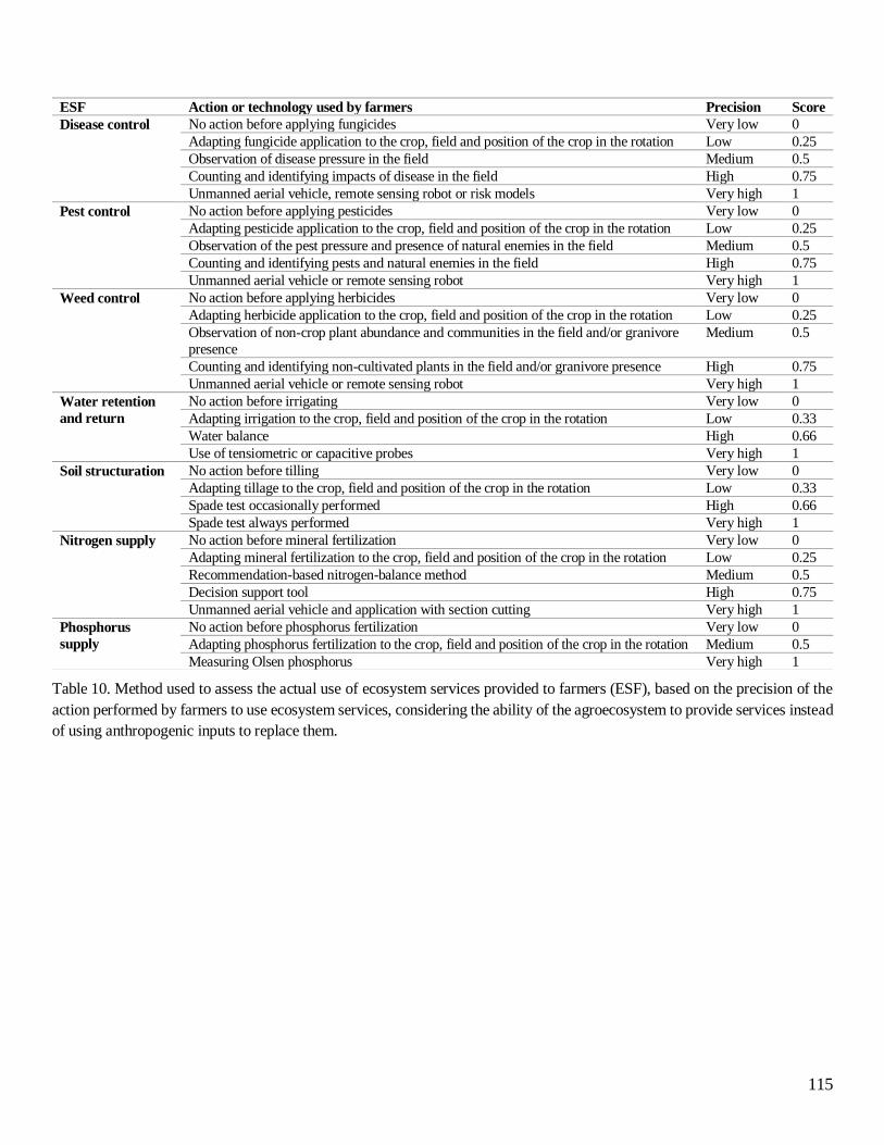
115

Table 10. Method used to assess the actual use of ecosystem services provided to farmers (ESF), based on the precision of the

action performed by farmers to use ecosystem services, considering the ability of the agroecosystem to provide services instead

of using anthropogenic inputs to replace them.

ESF Action or technology used by farmers Precision Score

Disease control No action before applying fungicides Very low 0

Adapting fungicide application to the crop, field and position of the crop in the rotation Low 0.25

Observation of disease pressure in the field Medium 0.5

Counting and identifying impacts of disease in the field High 0.75

Unmanned aerial vehicle, remote sensing robot or risk models Very high 1

Pest control No action before applying pesticides Very low 0

Adapting pesticide application to the crop, field and position of the crop in the rotation Low 0.25

Observation of the pest pressure and presence of natural enemies in the field Medium 0.5

Counting and identifying pests and natural enemies in the field High 0.75

Unmanned aerial vehicle or remote sensing robot Very high 1

Weed control No action before applying herbicides Very low 0

Adapting herbicide application to the crop, field and position of the crop in the rotation Low 0.25

Observation of non-crop plant abundance and communities in the field and/or granivore

presence

Medium 0.5

Counting and identifying non-cultivated plants in the field and/or granivore presence High 0.75

Unmanned aerial vehicle or remote sensing robot Very high 1

Water retention

and return

No action before irrigating Very low 0

Adapting irrigation to the crop, field and position of the crop in the rotation Low 0.33

Water balance High 0.66

Use of tensiometric or capacitive probes Very high 1

Soil structuration No action before tilling Very low 0

Adapting tillage to the crop, field and position of the crop in the rotation Low 0.33

Spade test occasionally performed High 0.66

Spade test always performed Very high 1

Nitrogen supply No action before mineral fertilization Very low 0

Adapting mineral fertilization to the crop, field and position of the crop in the rotation Low 0.25

Recommendation-based nitrogen-balance method Medium 0.5

Decision support tool High 0.75

Unmanned aerial vehicle and application with section cutting Very high 1

Phosphorus

supply

No action before phosphorus fertilization Very low 0

Adapting phosphorus fertilization to the crop, field and position of the crop in the rotation Medium 0.5

Measuring Olsen phosphorus Very high 1

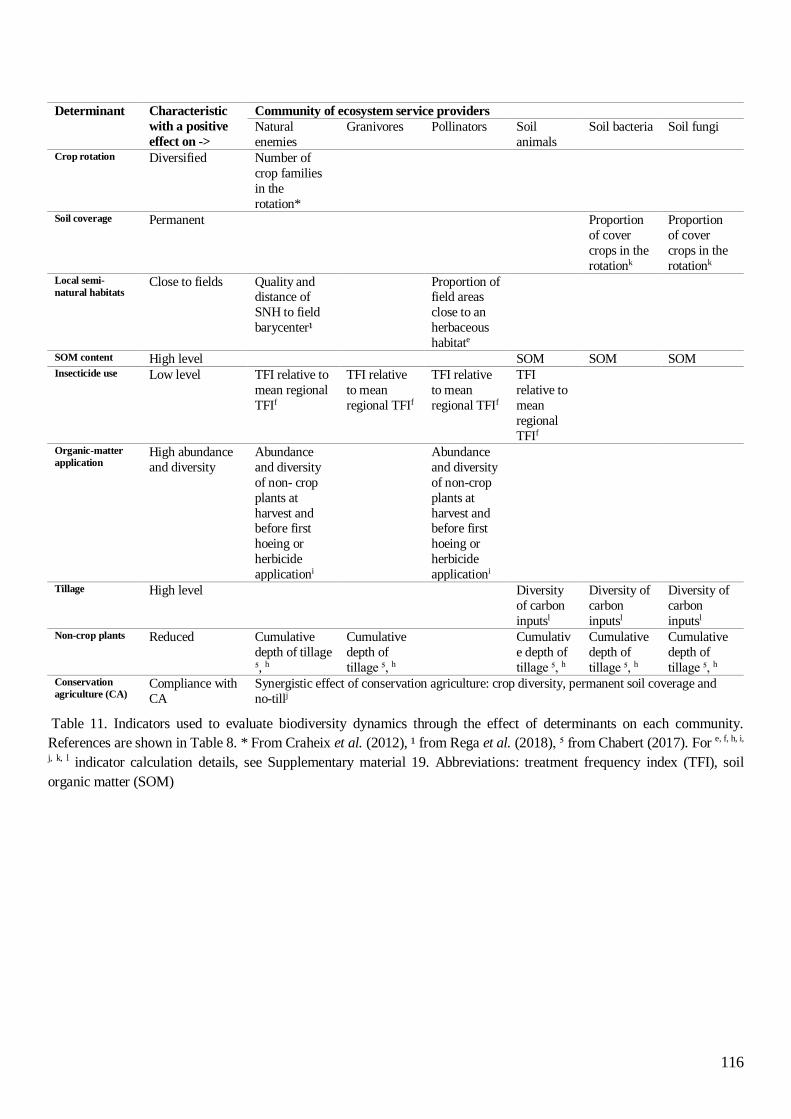
116

Table 11. Indicators used to evaluate biodiversity dynamics through the effect of determinants on each community.

References are shown in Table 8. * From Craheix et al. (2012), ¹ from Rega et al. (2018), ⁵ from Chabert (2017). For e, f, h, i,

j, k, l indicator calculation details, see Supplementary material 19. Abbreviations: treatment frequency index (TFI), soil

organic matter (SOM)

Determinant Characteristic

with a positive

effect on ->

Community of ecosystem service providers

Natural

enemies

Granivores Pollinators Soil

animals

Soil bacteria Soil fungi

Crop rotation Diversified Number of

crop families

in the

rotation*

Soil coverage Permanent Proportion

of cover

crops in the

rotationk

Proportion

of cover

crops in the

rotationk Local semi-

natural habitats Close to fields Quality and

distance of

SNH to field

barycenter¹

Proportion of field areas

close to an

herbaceous

habitate

SOM content High level SOM SOM SOM Insecticide use Low level TFI relative to

mean regional

TFIf

TFI relative

to mean

regional TFIf

TFI relative

to mean

regional TFIf

TFI

relative to

mean

regional

TFIf

Organic-matter

application High abundance

and diversity

Abundance

and diversity

of non- crop

plants at

harvest and before first

hoeing or

herbicide

applicationi

Abundance

and diversity

of non-crop

plants at

harvest and before first

hoeing or

herbicide

applicationi

Tillage High level Diversity

of carbon

inputsl

Diversity of

carbon

inputsl

Diversity of

carbon

inputsl Non-crop plants Reduced Cumulative

depth of tillage

⁵, h

Cumulative

depth of

tillage ⁵, h

Cumulativ

e depth of

tillage ⁵, h

Cumulative

depth of

tillage ⁵, h

Cumulative

depth of

tillage ⁵, h Conservation

agriculture (CA) Compliance with

CA

Synergistic effect of conservation agriculture: crop diversity, permanent soil coverage and

no-tillj

117

118

CHAPITRE III : RÉSILIENCE

DES FORMES D’AGRICULTURE

119

RÉSUMÉ DU CHAPITRE

Rappel. Alors que de nouvelles formes d’agriculture émergent dans l’objectif de répondre aux

problématiques socio-environnementales en basant leur production sur les services

écosystémiques (SEP), nous ne disposons pas de connaissance sur leur résilience face aux

perturbations biophysiques et socio-économiques. La synthèse de littérature présentée en Chapitre

I ne recensait pas d’études portant sur le rôle des SEP dans la dynamique des agroécosystèmes

face aux perturbations. Pourtant, certains auteurs considèrent que les SEP peuvent être des facteurs

de résilience dans le sens où ils permettent une régulation interne de l’agroécosystème, c.-à-d. un

effet tampon lors de perturbations (Introduction 5, p21). Parallèlement, l’intensification de la

production ainsi que la diversification, tous deux déterminants de la fourniture de SEP, peuvent

jouer un rôle dans la résilience des agroécosystèmes (Introduction 5, p21).

Contenu du chapitre. Afin de participer à la production de connaissances sur les facteurs

explicatifs de résilience, nous évaluons la résilience des agroécosystèmes considérant les formes

d’agriculture auxquelles ils appartiennent et leurs niveaux de SEP, d’intensification et de

diversification. Ce chapitre prend la forme d’un article scientifique qui a été soumis au journal

Ecosystem Services en avril 2021. Répondant directement à la question de recherche de la thèse,

ce travail a pour objectif de conclure sur le rôle des SEP, de l’intensification et de la diversification

dans la résilience face aux perturbations auxquelles font face les agroécosystèmes du Grand-Est.

Démarche mise en œuvre. Dans ce chapitre, contrairement au Chapitre I qui analysait de

concert les différents concepts relatifs à la dynamique des systèmes face aux perturbations, nous

faisons référence au concept de la résilience tel qu’il est défini par Meuwissen et al. (2019). A

l’instar de Peterson et al., (2018), nous considérons la résilience comme une propriété de la

dynamique des systèmes agricoles, comme l’inverse de la vulnérabilité et comme un concept

englobant les aspects de stabilité et de résistance. Nous avons développé une évaluation de la

résilience par l’analyse quantitative de la dynamique des performances des agroécosystèmes du

cas d’étude sur 4 à 8 ans entre 2012 et 2020. Sur les recommandations qui émergeaient de la

synthèse du Chapitre I, nous avons analysé conjointement la dynamique d’une performance

agronomique (le rendement), économique (la marge brute) et sociale (le temps de travail) grâce à

différents critères de dynamique adaptés à chacune : le niveau, la stabilité, la résistance et la

tendance. Nous avons utilisé trois méthodes complémentaires (la régression des moindres carrés

partiels, l’arbre de régression multivarié et la frontière de Pareto) afin d’identifier les relations entre

les caractéristiques des agroécosystèmes, les perturbations climatiques et économiques survenues

sur la période de l’étude et la résilience des performances.

Grands résultats. Les résultats montrent que les agroécosystèmes basés sur la biodiversité

(i.e. diversifiés, à haut niveau de SEP fournis et/ou avec un capital naturel qui augmente) présentent

des performances stables. Ils présentent aussi les temps de travail les plus faibles. A l’inverse, les

agroécosystèmes intensifiés par les intrants anthropiques, en particulier par l’irrigation et le travail

du sol, présentent des rendements et des marges brutes plus élevés, plus résistants aux perturbations

majeures comme celle de l’année 2016, mais moins stables. Ces dynamiques sont aussi observées

pour les agroécosystèmes qui utilisent fortement les SEP. Si nos résultats montrent les avantages

120

de s’appuyer sur la biodiversité pour stabiliser les performances des agroécosystèmes, nous

mettons aussi en évidence un antagonisme potentiel entre le niveau de rendement et sa stabilité.

Pour dépasser cet antagonisme, nous identifions deux stratégies potentielles : (i) amplifier le

potentiel de production lié aux SEP via l’utilisation d’intrants anthropiques tout en veillant à éviter

les pratiques néfastes au capital naturel et à la fourniture des SEP (et plus généralement dans une

visée de durabilité globale des écosystèmes), et/ou (ii) d’augmenter le niveau de SEP fournis et

utilisés pour la production agricole.

Dans l’article en anglais, les services écosystémiques fournis à la production agricole (SEP)

sont dénommés par « ecosystem services provided to farmers (ESF) ».

121

Publications dans des journaux internationaux :

Dardonville, M., Bockstaller, C., Villerd, J., Therond, O., submitted to Ecosystem Services in

April 2021. Resilience of agriculture models: biodiversity-based models are stable, while

intensified models perform well.

Communication lors de congrès français :

Dardonville, M., Bockstaller, C., Therond, O., 2020. Evaluation de la résilience de différentes

formes d’agriculture face aux changements climatiques et crises économiques. Présenté au congrès

Phloeme, Paris.

Interview :

Dardonville, M., Cabeza-Orcel, P., 2020. Evaluer la résilience des différentes formes

d’agriculture. Perspectives agricoles.

Activité d’encadrement : stage de Master 2 de Kwabena Osei-Tutu (6 mois)

122

Resilience of agriculture models: biodiversity-based models are stable, while intensified

models perform well

Manon DARDONVILLE 1, 2*, Christian BOCKSTALLER1, Jean VILLERD1, Olivier

THEROND1

1Université de Lorraine, INRAE, LAE, F-68000 Colmar, France

2Agrosolutions, 75782, Paris, France

Submitted to Ecosystem Services in April 2021

123

ABSTRACT

New agriculture models have emerged in response to societal demands to reduce

environmental impacts and dependence on non-renewable resources. They can be classified

according to their relative use of anthropic inputs or biodiversity and associated ecosystem services

as agricultural production factors. All these models are exposed to climate change, price volatility

and other disturbances. However, little is known about their resilience levels and the factors that

drive them. We assessed the resilience of 30 highly contrasted cropping agroecosystems in north-

eastern France which covered a broad gradient from simplified and intensified to complex and

biodiversity-based agroecosystems. We applied a quantitative analysis of the dynamics of three

key performances over eight years: yield, gross margin and workload. An original combined set

of adapted criteria - level, variability, trend and resistance - was used to assess their dynamics. We

use partial least squares regression, multiple regression trees and Pareto ranking to identify

relationships among the characteristics and resilience performance of these systems. The results

showed that biodiversity-based agroecosystems, which provide a high level of ecosystem services

to farmers or an increase in natural capital, tended to have stable performances. These systems also

had a lower workload than intensified systems. Conversely, anthropic intensive systems, especially

irrigated and tillage-intensive systems, had higher yields and gross margins, were resistant to major

disturbances but were less stable. While our results show benefits of relying on biodiversity to

stabilise system performances, we highlight a potential trade-off between performance level and

stability, as well as possible solutions to overcome it. We also discuss the short-term strategy of

anthropic input-based systems, which perform well, but consume large amounts of human and

natural resources. We show potential advantages of systems that balance both ecosystem services

and anthropic inputs to provide a strategy to fill the yield gap and attain resilience.

KEYWORDS

ecosystem services, natural capital, stability, resistance, cropping system

124

1. Introduction

Many new agriculture models have emerged in response to societal demands to increase food

quality and reduce environmental impacts and dependence on non-renewable resources (Therond et

al., 2017b). They invest in two ways: they optimise the use of anthropic inputs (i.e. fertilisers,

pesticides, energy for irrigation and labour) or replace them with ecosystem services provided by the

biodiversity (Duru et al., 2015c). For example, precision agriculture seeks to optimise the use of

anthropic inputs to reduce their harmful effects (Pierce and Nowak, 1999), while biodiversity-based

agriculture seeks to base agricultural production on ecosystem services provided to farmers (ESF). In

the latter, ESF are considered production factors (Duru et al., 2015c) as they counteract limiting factors

(e.g. water, nutrients) and reducing factors (e.g. weeds, pests, diseases) (van Ittersum and Rabbinge,

1997). For example, increasing the service of nitrogen provision to crops by the soil can meet crop

needs and replace mineral fertilisation. Existing agriculture models can be classified along a gradient

representing the relative use of anthropic inputs and ESF for agricultural production: from anthropic

input-based to biodiversity-based systems (Therond et al., 2017b).

Most of agricultural systems are exposed to climate changes, price volatility, pest outbreaks

and/or other disturbances. Anthropic input-based systems can address biophysical risks by managing

input levels when a disturbance occurs. For example, irrigation is considered a suitable strategy to

avoid hydric stress (Zou et al., 2012) exacerbated by climate change (Grillakis, 2019; Konapala et al.,

2020). Similarly, chemical insecticides are effective at limiting losses caused by pest outbreaks

(Deutsch et al., 2018). However, these systems depend greatly on non-renewable resources (e.g.

natural gas, petroleum, phosphorus and potassium) whose reserves are dwindling and becoming more

energy-intensive to extract (Pelletier et al., 2011; Wachtmeister et al., 2018). Biodiversity-based

systems tend to be freed from scarcity in non-renewable resources through developing and using ESF.

They must address the inadequate state of natural capital in most agricultural areas that has resulted

from decades of ecosystem simplification and intensive management (Nyström et al., 2019), which

drastically reduces ecosystem functioning and the ability to provide ESF (Bommarco et al., 2013a;

Saha et al., 2017). In addition, these systems are exposed to climate change, price volatility, pest

outbreaks and other disturbances. However, increasing the ecosystem service of soil water retention

and restitution can avoid or delay hydric stress when drought occurs. Similarly, improving

conservation biological control could limit crop failure due to pest outbreaks. Consequently,

increasing the level and use of ESF and developing the natural capital that supports their supply in the

middle term could be a suitable strategy to prevent vulnerability. This could reduce their dependence

on non-renewable resources while protecting against the harmful effects of climate change (Munang

et al., 2013) and other biophysical risks. Both anthropic input-based and biodiversity-based systems

are exposed to volatility in crop prices (Gaetano et al., 2018).

125

Biophysical and economic disturbances challenge a system’s “ability to ensure provision of

system functions” (Meuwissen et al., 2019) (i.e. their resilience). A review of the influence of input

intensification on the resilience of crop yield (Dardonville et al., 2020) highlighted that the level and

type of fertilisation (Macholdt et al., 2020; Reidsma et al., 2009b), irrigation (Reidsma et al., 2009b),

type of tillage (Gaudin et al., 2015) and the overall intensity of management (Urruty et al., 2017) can

be related to the resilience or vulnerability of yield, depending on the production situation. To date

and to our knowledge, no study has addressed relationships between the level of ESF and resilience

(Dardonville et al., 2021, 2020). Studies have focused instead on the influence of diversification, a

major determinant of ESF levels (Kleijn et al., 2019a). A review of the influence of crop diversity on

the resilience of yield showed generally positive relationships (Dardonville et al., 2020), in agreement

with the “ecological insurance” hypothesis, i.e. diversity provides a greater probability that certain

types of individuals (species, genotypes, production types, etc.) will maintain their functioning or level

of production in a changing context (Yachi and Loreau, 1999). Farm diversity has a positive influence

on yield and dynamics (i.e. resilience), except for specific crops such as rice or soya bean, as observed

in several studies (Chavas and Di Falco, 2017; Gaudin et al., 2015; J. Li et al., 2019; Matsushita et

al., 2016; Urruty et al., 2017). Recently, Zampieri et al. (2020) highlighted a potential nonlinear

influence of crop diversity, with a threshold of six crops grown on the same farm. Dardonville et al.

(2020) highlighted that available information on the influence of crop diversity or intensification is

limited to an analysis of yield, which ignores the multifunctionality of agriculture (Hodbod et al.,

2016). While biodiversity-based systems are promising from agronomic and environmental

viewpoints (Weyers and Gramig, 2017), their absolute resilience to disruption, and relative resilience

compared to that of input-based systems, has yet to be evaluated (Therond et al., 2017a).

To address this knowledge gap, we assessed the resilience of 30 contrasting cropping

agroecosystems in the Grand Est region (north-eastern France) and the determinants of resilience. The

30 agroecosystems represented a wide range of production situations (i.e. crop rotations, management

practices and field configurations). Dardonville et al. (under revision) showed that they cover a large

gradient of anthropic inputs, ESF use and diversification (from highly simplified to highly diversified).

The production level and economic and social performances were analysed based on dynamics of

gross margin and workload, as performed by Catarino et al. (2021), over eight years, which provided

relevant analysis of the dynamics of several key performances. The performance dynamics were

described by one or more criteria of dynamics (e.g. variability, trend) chosen for their ability to

describe the performance dynamics and expressive power of the related metrics. We analysed a large

set of explanatory factors (determinants) of the performance of resilience, such as (i) the type of

agriculture model, as defined by Dardonville et al. (under revision); (ii) the anthropic intensity of

cropping practices (total and by practice) and (iii) the biodiversity level of the agroecosystem (i.e. crop

rotation, species mixture, surrounding semi-natural habitats (SNH)).

126

2. Methods

2.1 Agroecosystems and farm characteristics

The 30 cropping agroecosystems investigated belonged to 26 farms in the Grand Est region

(Supplementary material 36). This region is one of the main crop-oriented regions in France and

contains mainly input-intensive systems (Chambre Régionale d’Agriculture Grand Est, 2018). Like

all regions, it is exposed to climate change (Caubel et al., 2018; Poumadere et al., 2005; van der Velde

et al., 2012). While this region currently produces more grain than any other region in France, its

ability to sustain this production in the long term in the face of climatic and economic crises is less

certain.

These agroecosystems, described in detail by Dardonville et al., (under revision), were chosen

by advisors from the Regional Chamber of Agriculture and represented a wide range of rotations (from

1-9 crops in the rotation, with intermediate crops) and input intensities (from irrigated and fertilised

to organic with soil-conservation practices). Based on a review of the relationships between system

properties and ESF and associated indicators, these authors assessed, for each agroecosystem: (i) real

capacity of ESF (i.e. potential ESF influenced by crop management practices during the cropping

season), (ii) actual use of ESF by the farmer and (iii) dynamics of natural capital that underpins ESF

(Table 12). Based on their results, the agroecosystems were classified into five types of agriculture

models using a clustering approach (Table 12, Box 5).

127

Box 5. Five clusters of agriculture models identified by Dardonville et al. (under review) according to (i)

the ecosystem’s real capacity to provide ecosystem services to farmers (ESF), (ii) actual use of ESF by

farmers and (iii) dynamics of natural capital for 30 agroecosystems on 26 farms in the Grand Est region

(north-eastern France). Figure adapted from Dardonville et al. (under review).

The MH-H model has high ESF capacity and medium-high ESF use but no specific natural capital

dynamics. It includes relatively long rotations of legumes and uncommon crops and reduced or no tillage.

The I-M model uses its medium ESF capacity inefficiently and has neutral or positive natural capital

dynamics. It includes longer and complex rotations and varied types of tillage. The M-LM-C model has

medium use of its low-to-medium ESF capacity with capitalisation of natural capital. It includes long

rotations of uncommon crops, is ploughed and uses pesticides and mineral fertilisers. The E-LM-D model

uses its low-to-medium ESF capacity efficiently but depletes natural capital. It includes short maize-based

rotations that are usually irrigated and ploughed. The I-LM-D model uses its low-to-medium ESF

capacity inefficiently and all depletes natural capital. It includes only maize-based rotations and varied

agricultural practices.

128

Historical data on performances from 2012-2020 were obtained from the farmers’ computer-

based management tool “Mes Parcelles®”, which included data for at least four years of observations.

This tool records daily crop management data for each field, including the amounts of inputs applied

and products harvested. Fields receiving special interventions were excluded (e.g. floodable). The

prices of mineral fertilisers, crops sold, pesticides, fuel and irrigation were obtained from the INRAE

Agrosyst database (Ancelet et al., 2014). Prices of organic fertiliser and pesticides were assumed to

have remained constant over the 8-year period. Fuel consumption of the equipment and the duration

they were used per ha were extracted from the French national reference source (CUMA, 2019).

The semi-continental climate of the Grand Est region has a large amount and high frequency of

rainfall each year (except for central Alsace). Since 1959, the region has experienced an increase in

mean annual temperature of +1.3°C, an increase in the number of days when the temperature exceeds

25°C, a decrease in the number of frost days and an increase in total annual evapotranspiration

(CRAGE, 2018). This has caused wheat yield to stagnate since 1990, advanced phenological stages,

stunted development, induced water stress and fostered the expansion and colonisation of certain pests

(e.g. bivoltine corn borer on maize).

2.2 Performances and explanatory variables

2.2.1 Attributes of performances

To address the question “resilience for what purpose?” (Meuwissen et al., 2019), we considered

the following agronomic, social and economic performances as important to maintain in the face of

disturbances: crop energy yield (kcal per ha), workload (hours of work per ha) and agroecosystem

gross margin (input – output in € per ha). Thus, we believe it is important to guarantee a certain level

of food production, maintain sustainable work hours for each farmer and maintain economic viability.

Energy yield was calculated by converting each harvested product into an energy equivalent, as

reported by Sauvant et al. (2004) and recommended by Zampieri et al. (2020) (Figure 33). Wheat

yield was analysed to avoid uncertainty related to crop diversity and energy-conversion coefficients.

Workload equalled the total hours per year spent on arable field activities for all crops in the

agroecosystem per ha. Gross margin equalled crop revenue (from harvested crops) minus costs (i.e.

fertilisation, irrigation, pesticides and fuel consumption) per ha (Supplementary material 37).

129

Figure 33. (A) Energy yields (kcal/ha), (B) workload (h/ha) and (C) gross margin (€/ha) for each agroecosystem

(each colour).

2.2.2 Exogenous disturbances

Meteorological data (i.e. daily rainfall; minimum, maximum and mean temperatures; and

evapotranspiration), interpolated to grid of 8 × 8 km, came from Météo France. We selected variables

(proxies) to characterise exposure and sensitivity of agroecosystems to climatic and economic

disturbances. To characterise climate, the main agro-climatic indicators developed by Caubel et al.

(2015) (see also www.agrometinfo.fr) were calculated for each year from 2012-2019 (Table 12,

Supplementary material 38) for the location of each agroecosystem. After analysing the correlation

between these indicators, we selected the least correlated indicators: cumulative daily minimum and

maximum temperature (°C) respectively for quarters 1 and 4 and quarters 2 and 3, the number of hot

days (> 27°C) and the largest number of consecutive days of drought in a year (rainfall –

evapotranspiration < -5 mm). The hottest years in France since 1900 were 2015, 2018 and 2019, which

also had the longest droughts, highest heat stress (i.e. hot days), and longest drought (Supplementary

material 38). In addition, as the agroecosystems were spread over 50,000 km² and could have had

different local climates (Supplementary material 36), we analysed differences in climatic situations.

Differences were generally not significant, except for one agroecosystem (#14) near the northern

border (Supplementary material 39). Price volatility, described by wheat price (€/t) and fuel price (€/L)

(Ancelet et al., 2014), decreased significantly until 2016, when it increased (Supplementary material

40).

2.2.3 Endogenous explanatory variables

Endogenous explanatory variables correspond to variables that characterise the agroecosystems

(Table 12). In addition to the five agriculture models and their determinants (i.e. levels of real capacity

130

and actual use of ESF, and natural capital dynamics), we tested characteristics that are often considered

as resilience factors: (i) input (i.e. pesticides, irrigation and fertilisers) intensity, (ii) crop diversity (i.e.

rotation duration and number of crops), proportion of species mixtures in the rotation and an indicator

that aggregated the quantity and quality of SNH; and (iii) soil organic matter content. We also tested

agroecosystems’ membership in common classifications of agricultural systems, such as organic and

soil-conservation practice.

131

Table 12. Performance attributes (response variables) whose dynamics were analysed, proxies of disturbances (exogenous) and explanatory variables tested as determinants

of resilience. ESF: ecosystem services to farmers, SNH: semi-natural habitats, TFI: treatment frequency index, SD: standard deviation, SCA: soil conservation agriculture

Type of

variable

Indicator Unit Calculation Reference Name Mean

± SD

Per

form

an

ces Gross margin €/ha revenue – costs - gm 965± 521

Workload h/ha cumulative hours spent on arable field activities - wrkldha 2.5 ± 2

Energy yield kcal/ha energy equivalent of crops in kcal × production (t) - eyld 3.107± 1.107

Exogen

ou

s

dis

turb

an

ces

Cumulative daily

temperature

°C cumulative daily minimum and maximum temperatures respectively for quarters 1 and 4 and

quarters 2 and 3

www.agrometinfo.fr cum_temp_min/max_quarter (max) 5444

± 348

Number of hot days - www.agrometinfo.fr hot_days 26 ± 9

Maximum drought

sequence

Days largest number of consecutive days of drought (rainfall – evapotranspiration < -5mm) www.agrometinfo.fr seq_PETP5 5 ± 2.5

Wheat price €/t - Ancelet et al., 2014 wheat_price 20 ± 2

Fuel price €/L - Ancelet et al., 2014 fuel_price 0.7 ± 0.1

En

do

gen

ou

s ex

pla

na

tory

varia

ble

s

Real capacity of ESF - aggregated score of the quality with which the spatial and temporal compositions of the

agroecosystems provide ESF, as influenced by crop practices

Dardonville et al., under review ESF_r 0.4 ±0.2

Actual use of ESF - precision of the action performed by farmers to use ESF, given the ability of the agroecosystem to

provide ESF instead of using anthropic inputs to replace them

Dardonville et al., under review ESF_u 0.5 ±0.2

Natural capital dynamics - aggregated score of erosion sensitivity, soil carbon and phosphorus dynamics, and biodiversity

dynamics

Dardonville et al., under review nat_cap 0 ±0.4

Input intensity - aggregated scores of (i) intensity of mineral fertilisation relative to the regional mean, (ii)

pesticide TFI relative to the regional mean TFI and (iii) the frequency of ploughing and irrigation

Dardonville et al., under review intensity 0.5±0.2

Rotational complexity

index

- square root of the number of cash and cover-crop species (richness) in a rotation × the rotation

duration

Bowles et al., 2020 RCI 4.5±1.7

Proportion of species

mixtures in the rotation

- proportion of crops and intercrops with a species mixture Dardonville et al., under review mix 0.4±0.2

SNH - mean scores for the proportion of nearby field areas and herbaceous habitat and the quality and

distance of SNH to the field barycenter

Dardonville et al., under review,

Rega et al., 2018

SNH 0.5±0.2

Organic matter % - - SOM 2.8±0.5

Tillage type - mean score for ploughing frequency (1 = always, 0.5 = occasionally, 0 = never) of crops - tillage 0.6±0.3

Pesticide intensity - TFI ([0;1]) (1 = intensive) relative to the regional mean (0.5) Dardonville et al., under review pesticide 0.5±0.2

Fertilisation intensity - amount of mineral nitrogen and phosphorus supplied ([0;1]) (1 = intensive) relative to the regional

mean (0.5)

Dardonville et al., under review fertilization 0.6±0.3

Irrigation intensity - ([0;1]) (1 = intensive), with two levels: 0 = no irrigation, 1 = irrigated Dardonville et al., under review irrigation 0.3±0.5

SCA 0/1 synergistic effect of conservation agriculture: crop diversity, permanent soil coverage and no-till

(Supplementary material 41)

Dardonville et al., under review SCA -

organic 0/1 two levels: 0 = no organic label, 1 = organic label - organic -

Agriculture model I_M - Inefficient use of Medium ESF capacity Dardonville et al., under review I_M -

Agriculture model

I_LM_D

- Inefficient use of Low-to-Medium ESF capacity, with Depletion of natural capital Dardonville et al., under review I_LM_D -

Agriculture model

M_LM_C

- Medium use of Low-to-Medium ESF capacity, with Capitalization of natural capital Dardonville et al., under review M_LM_C -

Agriculture model

MH_H

- Medium-high use of High ESF capacity Dardonville et al., under review MH_H -

Agriculture model

E_LM_D

- Efficient use of Low-to-Medium ESF capacity, with Depletion of natural capital Dardonville et al., under review E_LM_D -

132

2.2.4 Criteria of dynamics

The following criteria were used to describe the dynamics of agricultural performances

(Dardonville et al., 2021):

- level of performance (e.g. mean level);

- stability or, conversely, variability;

- trend (i.e. maintenance, increase or decrease in the level over time);

- resistance (i.e. the ability to resist a specific or unspecified event).

Not all criteria were relevant for all performance attributes. Thus, for each performance

attribute, we selected criteria of dynamics based on their suitability. For energy yield, high level,

resistance and stability are usually desirable targets, as guaranteeing a certain level of production

to ensure the food supply, avoiding frequent crop failures and decreasing variability in production

over time are crucial to ensure resilience. This is also true for gross margin, but an increasing trend

is often expected to keep up with inflation. For these two attributes, we also considered resistance

to the historic decrease in wheat yield in France in 2016 due to excess rainfall in spring and

abnormally high temperatures in autumn that caused lodging (Ben-Ari et al., 2018). For workload,

we assumed that a lower level, higher stability and high resistance to peak work are desirable

objectives for resilience, as labour-intensive systems are sensitive to the lack of available workers

(as Mitaritonna et al. (2020) observed during the COVID-19 health crisis), and if the workload is

likely to peak or is highly variable, a lack of labour may not be bearable or even feasible for the

farmer due to the adjustment in labour required.

For each criterion of dynamics, several metrics were explored due to the wide variety of ways

in which these criteria can be measured. For example, to estimate ecosystem stability, Wang et al.

(2019) used the standard deviation and coefficient of variation. We summarised the main metrics

(Supplementary material 42) and selected a metric for the criterion of each performance attribute

(Table 13). The selection was based on (i) minimising the correlation between the metrics of the

criteria, (ii) the predictability (percentage of variance explained by random forest) of each metric

for each attribute, considering all explanatory variables, and (iii) the interpretability (i.e. easily

understandable and makes sense to experts) of each metric. Level was the mean level, as developed

by Perrin et al. (2020). For workload, we used the inverse of level, as low workload is considered

better for farmers. For gross margin, as recommended by Sneessens et al. (2019), we used the

mean relative distance (RD) to the regional gross margin (Supplementary material 43) to consider

the social acceptance of the income level. A strongly negative RD indicated that the gross margin

was significantly below the regional mean, while a strongly positive RD indicated the ability to

generate above-average profit. Stability (Mean Stability Variable, MSV) was calculated as the

difference between each year and the mean of the preceding year and following year, averaged

over the time series (Redhead et al., 2020). Low or high resistance to unspecified events was the

probability of respectively falling under 75% (probalow) or exceeding 125% (probahigh) of the

mean over the eight years (adapted from Gaudin et al. (2015) and Li et al. (2019)). Resistance to

2016’s decrease in wheat yield (RESe) was calculated as the proportional decrease in 2016 from

the 2013-2015 mean (Redhead et al., 2020). Trend (TRENDr) was calculated as the random slope

133

coefficient of mixed linear regression of individuals, which excluded the group trend due to

technological and genetic improvements (see Martin et al. (2017)).

Table 13. Performance attributes whose dynamics were analysed, associated criteria of dynamics and

metrics.

Performance

attribute

Criterion

of

dynamics

Metric Name Description Reference Direction

for

resilience

En

ergy y

ield

Level Mean

level

level mean level Perrin et

al., 2020

Higher

Stability Stability

around a

moving

average

MSV inverse of the absolute

difference between the yield

of each year and the mean of

the preceding year and

following year, averaged

over the time series

Redhead

et al.,

2020

Higher

Resistance

to an event

Resistance

to 2016

RESe 2016 level – averaged 2015,

2014, 2013 level

Redhead

et al.,

2020

Higher

Gro

ss m

arg

in

Level Mean

relative distance to

regional

margin

RD mean relative distance to the

regional gross margin (Supplementary material 43)

Redhead

et al., 2020;

Sneessens

et al.,

2019

Positive

and high

Stability Stability

around a

moving

average

MSV inverse of the absolute

difference between the gross

margin of each year and the

mean of the preceding year

and following year, averaged

across the time series

Redhead

et al.,

2020

Higher

Resistance

to

unspecified

events

Probability

of failure

probalow probability of gross margin >

75% of the mean level over

the time series using the

normal distribution

Adapted

from Li et

al., 2019

Higher

Resistance to an event

Resistance to 2016

RESe 2016 level – averaged 2015, 2014 and 2013 level

Redhead et al.,

2020

Higher

Trend Trend of

mixed

regression

TRENDr random slope coefficient of

mixed linear regression

Martin et

al., 2017

Increasing

Work

load

Level Inverse of

averaged

level

level inverse of mean level Adapted

from

Martin et

al., 2017)

Higher

Stability Stability

around a

moving

average

MSV inverse of the absolute

difference between the

workload of each year and

the mean of the preceding

year and following year, averaged over the time series

Redhead

et al.,

2020

Higher

Resistance

to

unspecified

events

Probability

of peak

work

intensity

probahigh probability of workload >

125% of the mean level over

the time series using the

normal distribution

Adapted

from Li et

al., 2019)

Higher

134

2.3 Explanatory factor test

Three additional approaches were used to analyse relationships deeply between the metrics

of dynamics for each performance and the explanatory factor: partial least squares regression (PLS,

statistical method), multivariate regression trees (MRT, a machine-learning method) and Pareto

ranking. They are complementary as they can perform several levels of analysis. Using PLS to

evaluate resilience was recommended by Martin et al. (2017) and applied by Bouttes et al. (2018)

and Perrin et al. (2020). To our knowledge, however, MRT have never been used to identify

predictors of dynamics. To verify this, we queried the Web of Science Core Collection from 2000

to November 2020 using the query of Dardonville et al. (2020) (three sections including (i) the

concepts of vulnerability, resilience, robustness and adaptive capacity, (ii) agricultural systems and

(iii) quantitative assessment) plus “regression tree*”. Of the 39 references identified, 3 mentioned

the topic. Hou et al. (2020) used regression tree analysis to evaluate explanatory factors of fruit

yields. Lokonon (2019) used regression tree analysis to identify the utility of combining exposure,

sensitivity and adaptive capacity into a vulnerability index. Diack et al. (2017) used the CART

model to quantify the level of vulnerability of a zone, but not to identify explanatory factors. In

short, they did not use regression to analyse dynamics or multiple response variables.

2.3.1 Exploratory univariate approach using PLS

We applied the method developed by Martin et al. (2017) and applied by Bouttes et al. (2018)

and Perrin et al. (2020) which uses PLS to identify explanatory factors of performance dynamics

(i.e. to explain determinants of resilience). At the crossroads of principal component analysis and

linear regression, it performs multiple linear regression by maximising the square covariance

between response and explanatory variables (through a linear combination of each) for each

component, and handles correlated and incomplete data well (Wold et al., 2001). We performed

PLS using the mixOmics package of R software (Lê Cao et al., 2018; R Core Team, 2013). To

define the explicative and predictive ability of the model, R², the mean squared error of prediction

and Q² values were analysed (maximised, minimised and maximised, respectively). The NIPALS

algorithm was used to fill in missing climate data (since 2018). The common ad hoc threshold of

total Q² > 0.0975 was used.

2.3.2 Predictive multivariate approach using MRT

In addition to the PLS, we used MRT (De’Ath, 2002), which is an extension of univariate

regression trees (Breiman et al., 1984). The approach considers multiple response variable patterns

and then identifies trade-offs between (normalised) metrics of dynamics of each performance

attribute and predictors among explanatory variables by considering potential thresholds due to

non-linear effects (Borcard et al., 2018). We performed MRT using the archived mvpart 1.6-2

package of R software (Therneau et al., 2014). A 10-fold cross-validation procedure was

conducted to calculate the cross-validated error. As suggested by Breiman et al. (1984), we

selected the optimal size of the tree (i.e. number of leaves) following the “1-SE” rule, which

consists in of using as the smallest tree within 1 standard error of the minimum cross-validated

135

error. Like Obiang-Ndong et al. (2020) and Smith et al. (2019), we replaced bar plot leaves with

boxplot leaves to show the distribution of each metric. We included explanatory variables of

disturbance that described the climate to test whether the agroecosystems experienced different

meteorological situations which resulted in different dynamic patterns.

2.3.3 Identifying positive deviants with Pareto ranking

Pareto ranking was used to identify positive deviant agroecosystems with the best

combination of multiple performances without subjective weights (i.e. agroecosystems that were

exemplary in achieving all dynamic objectives) (Modernel et al., 2018; Steinke et al., 2019;

Toorop et al., 2020). We analysed the combination of all criteria for agronomic, social and

economic attributes. We used the emoa package of R software (Mersmann et al., 2015) following

the procedure of Steinke et al. (2019).

3. Results

3.1 Energy yield

Level, stability (MSV) and resistance to 2016’s decrease in wheat production (RESe) were

used to describe energy yield (kcal/ha) dynamics. Three PLS components were acceptable: the

first component represents mainly the level (mainly), the second the resistance and the third

stability (Supplementary material 45 and Supplementary material 46). Level was positively related

to the intensity of cropping practices, particularly irrigated and tillage-intensive systems (Figure

34A and B). Level was also positively related to the “Efficient use of Low-to-Medium ESF

capacity, with Depletion of natural capital” (E_LM_D) model, which referred mainly to intensive

and irrigated maize monocropping systems. Farms with more hot days had slightly higher levels.

In comparison, level was negatively related to natural capital dynamics, crop diversification, real

ESF capacity and the “Inefficient use of Medium ESF capacity” (I_M) model, whose

agroecosystems had significantly lower yields than the others (pairwise Tukey HSD test,

Supplementary material 47). Natural capital dynamics was negatively related to resistance, which

was positively related to the “Inefficient use of Low-to-Medium ESF capacity, with Depletion of

natural capital” (I_LM_D) model and irrigation. Conversely, stability was negatively related to

irrigation, E_LM_D (and to a lesser extent, intensification) and the level of ESF used. Stability

was positively related to crop diversification, the I_M model and, to a lesser extent, natural capital

dynamics, SNH and use of species mixtures.

The MRT was organised into two levels and two leaves with acceptable predictive quality

(cross-validated error of 0.76; i.e. the tree explained 24% of the variance) (Figure 34C). Natural

capital dynamics, with a threshold of -0.23, was selected to split the two leaves, which represented

two main types of resilience situations. The 12 agroecosystems with natural capital < -0.23 had

relatively high yield and resistance, but low stability (Leaf 2), while the 18 others had more

homogenous pattern of dynamics, with higher stability and lower level and resistance (Leaf 1).

136

Comparing the criteria for this split revealed significant differences between the two groups

(Supplementary material 48).

137

Fig

ure

34. (A

) C

lust

ered

Im

age

Map

and (

B)

net

work

rep

rese

nta

tion o

f th

e par

tial

lea

st s

quar

es r

egre

ssio

n o

f m

etri

cs. f

or

ener

gy y

ield

on e

xpla

nat

ory

var

iable

s,

show

ing p

osi

tiv

e (b

lue)

an

d n

egat

ive

(red

) co

rrel

atio

ns

to r

esil

ient dynam

ics)

. (C

) M

ult

ivar

iate

reg

ress

ion tre

e o

f no

rmal

ised

met

rics

fo

r en

erg

y y

ield

on e

xpla

nat

ory

var

iable

s, w

hic

h s

how

s p

atte

rns

of

lev

els

of

crit

eria

of

dynam

ics

for

two t

ypes

of

resi

lien

ce s

ituat

ions.

See

Tab

le 1

for

def

init

ions

of

var

iable

abb

revia

tions.

Err

or

= r

esid

ual

err

or,

CV

Err

or

= m

ean r

esid

ual

err

or

of

10-f

old

cro

ss-v

alid

atio

n p

roce

dure

, S

E =

sta

ndar

d e

rro

r o

f th

e 1

0 C

V e

rrors

.

138

When analysing wheat yield (for the 27 agroecosystems with wheat in their rotations (all but

#10_2, 5_2, 8_1)), dynamics followed the same pattern with less confidence (Supplementary

material 49). Intensive systems had higher levels of wheat yield, while diversified (organic, crop

diversity in the rotation and SNH) systems had lower levels.

3.2 Gross margin

The relative distance to the regional gross margin (RD), stability (MSV), resistance to 2016’s

conditions (RESe), resistance to unspecified events (probalow) and trend (TRENDr) were used to

describe gross margin (€/ha) dynamics. Three PLS components were acceptable: the first

component represents level (mainly), the second is a combination of all metrics and the third one

is the resistance to unspecified events (Supplementary material 50 and Supplementary material

51). Like for energy yield, level was positively related to intensity of cropping practices,

particularly irrigated and tillage- intensive systems (Figure 35A and B). It was also positively

related to the “Efficient use of Low-to-Medium ESF capacity, with Depletion of natural capital”

(E_LM_D) model, which referred mainly to irrigated and intensive maize monocropping systems.

However, level was negatively related to natural capital dynamics, crop diversification, real ESF

capacity and the “Medium use of Low-to-Medium ESF capacity, with Capitalization” model

(M_LM_C). Natural capital dynamics was negatively related to resistance to unspecified events

and 2016’s conditions. The irrigated system resisted 2016’s conditions better, even though it was

not a strong drought year (Supplementary material 38). Tillage intensity and species mixture

management was positively related to resistance, in general (probalow). Stability, crop

diversification and real ESF capacity (and to a lesser extent, the “Medium-high use of High ESF

capacity” (MH_H) model and natural capital dynamics) were positively related, unlike E_LM_D

(and to a lesser extent, irrigated systems), which were negatively related. Trend was also positively

related to the MH_H model and real ESF capacity but negatively related to intensity.

The MRT was organised into two levels and two leaves with acceptable predictive quality

(cross-validated error of 0.88; i.e. the tree explained 12% of the variance) (Figure 35C). Natural

capital dynamics, with a threshold of -0.28, was selected to split the two leaves to consider two

situations. The 11 agroecosystems with natural capital < -0.28 had a gross margin much higher

than the regional mean (RD > 0, Supplementary material 52) and greater resistance to 2016’s

conditions and to unspecified events, but less stability, while the 19 others had a more homogenous

pattern of dynamics, with higher stability and lower level and resistance. Comparing criteria for

this split revealed significant differences between the two groups (Supplementary material 52).

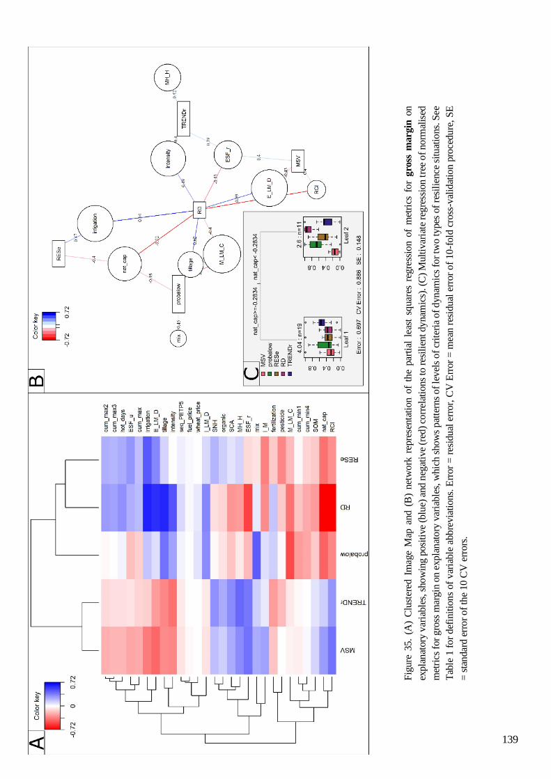
139

Fig

ure

35.

(A)

Clu

ster

ed I

mag

e M

ap a

nd (

B)

net

work

rep

rese

nta

tion o

f th

e par

tial

lea

st s

quar

es r

egre

ssio

n o

f m

etri

cs f

or

gro

ss m

arg

in o

n

expla

nat

ory

var

iable

s, s

ho

win

g p

osi

tive

(blu

e) a

nd n

egat

ive

(red

) co

rrel

atio

ns

to r

esil

ient dynam

ics)

. (C

) M

ult

ivar

iate

reg

ress

ion t

ree

of

no

rmal

ised

met

rics

for

gro

ss m

argin

on

expla

nat

ory

var

iable

s, w

hic

h s

how

s pat

tern

s of

level

s of

crit

eria

of

dyn

amic

s fo

r tw

o ty

pes

of

resi

lien

ce s

itu

atio

ns.

See

Tab

le 1

fo

r d

efin

itio

ns

of

var

iable

abbre

via

tions.

Err

or

= r

esid

ual

err

or,

CV

Err

or

= m

ean r

esid

ual

err

or

of

10

-fold

cro

ss-v

alid

atio

n p

roce

du

re, S

E

= s

tan

dar

d e

rro

r o

f th

e 10 C

V e

rrors

.

140

3.3 Workload

Level, stability (MSV), resistance to workload peak intensity (probahigh) described workload

(h/ha) dynamics. Three PLS components were acceptable: the first component represents the level

(mainly) and stability, the third one is the resistance to unspecified events (Supplementary material

53 and Supplementary material 54). Unlike for gross margin and energy yield, level (specifically,

the inverse) was positively related to natural capital dynamics, crop diversification, real ESF

capacity and the “Inefficient use of Medium ESF capacity” (I_M) model (Figure 36A and B). It

was negatively related to intensity of cropping practices, especially irrigated and tillage-intensive

systems. It was also negatively related to the “Efficient use of Low-to-Medium ESF capacity, with

Depletion of natural capital” (E_LM_D) model, which referred mainly to irrigated and intensive

maize monocropping systems. Natural capital dynamics and crop diversification were also

positively related to workload stability, unlike irrigated systems, which had more variable

workload. Pesticide use and mineral fertilisation were positively related to resistance to a high peak

in workload intensity, while organic systems were negatively related.

The MRT was organised into two levels and two leaves with acceptable predictive quality

(cross-validated error of 0.88; i.e. the tree explained 12% of the variance) (Figure 36C). Crop

diversification, with a threshold of 4.357, was selected to split the two leaves to consider two

situations. The 16 agroecosystems with RCI > 4.357 had lower workload levels, high resistance to

a high peak in workload intensity and workload stability over the eight years (Leaf 2). Comparing

criteria for this split revealed significant differences between the two groups (Supplementary

material 55).

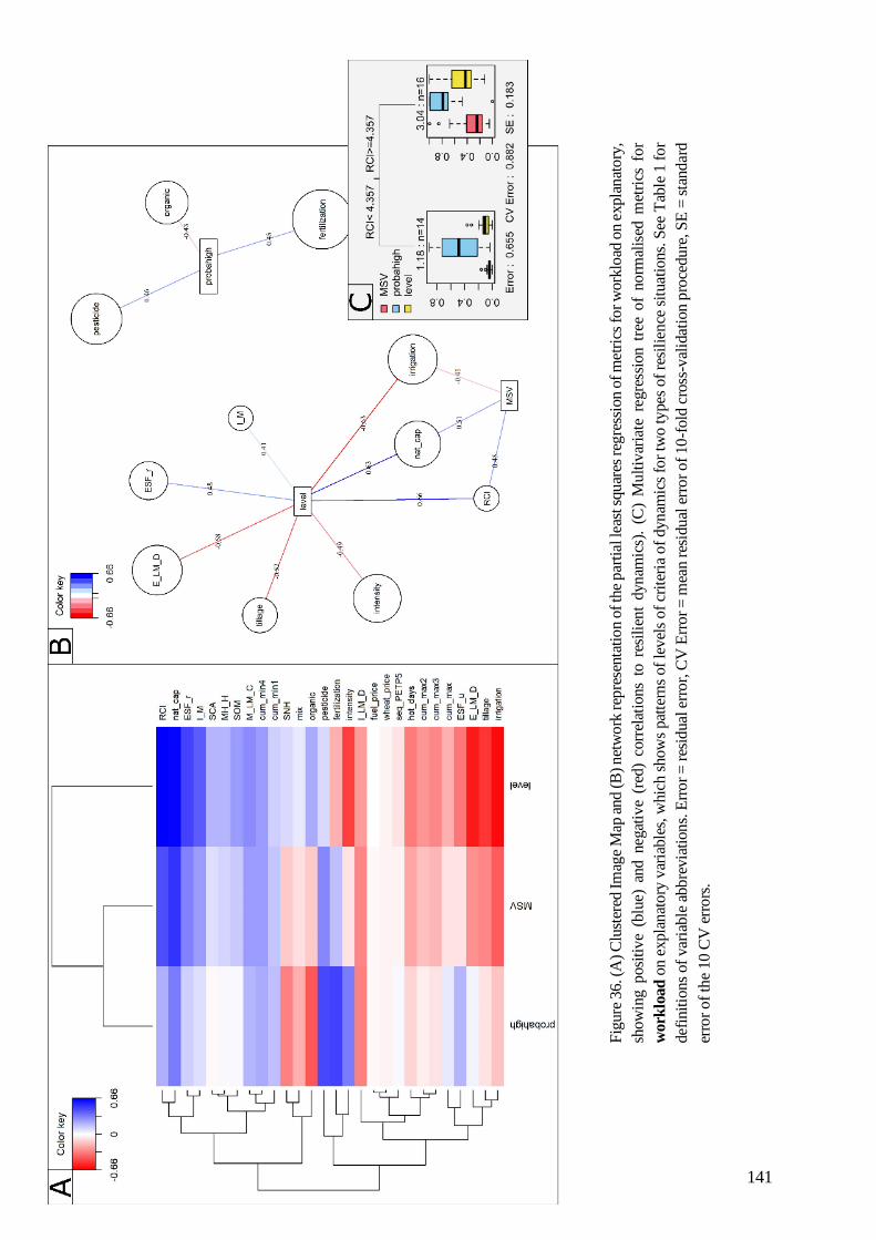
141

Fig

ure

36. (

A) C

lust

ered

Im

age

Map

and (

B)

net

work

rep

rese

nta

tion o

f th

e par

tial

lea

st s

quar

es r

egre

ssio

n o

f m

etri

cs f

or

work

load

on e

xpla

nat

ory

,

show

ing p

osi

tiv

e (b

lue)

and n

egat

ive

(red

) co

rrel

atio

ns

to r

esil

ient

dynam

ics)

. (C

) M

ult

ivar

iate

reg

ress

ion t

ree

of

no

rmal

ised

met

rics

fo

r

work

load

on e

xpla

nat

ory

var

iable

s, w

hic

h s

how

s pat

tern

s of

level

s of

crit

eria

of

dynam

ics

for

two ty

pes

of

resi

lien

ce s

ituat

ions.

See

Tab

le 1

fo

r

def

init

ions

of

var

iable

abb

revia

tions.

Err

or

= r

esid

ual

err

or,

CV

Err

or

= m

ean r

esid

ual

err

or

of

10

-fold

cro

ss-v

alid

atio

n p

roce

du

re, S

E =

sta

nd

ard

erro

r o

f th

e 10 C

V e

rro

rs.

142

3.4 Positive deviants

Pareto ranking identified two positive deviant agroecosystems in the group that had the best

performance dynamics without compromising the other performances (Supplementary material

56). Agroecosystem #1 had an average performance for all attributes, but high stability in working

time and little probability of peaks in intensity. Agroecosystem #5_2 had high yields and gross

margins, without much working time, despite variability in performances.

4. Discussion

We assessed the resilience of 30 agroecosystems that represented agriculture models along a

gradient of level and use of ESF and natural capital dynamics. The multicriteria analysis of

dynamics (level, stability, resistance and trend) of the multi-performances (energy yield, gross

margin and workload) of these contrasting systems helped to identify system characteristics that

explain resilience.

Analysis of the relationship between performance dynamics and exogenous explanatory

factors (with PLS) showed that the observed dynamics were related primarily to endogenous

characteristics, as observed by Martin et al. (2017). The variability in wheat and fuel prices seemed

to have little influence on the dynamics of gross margin (Figure 35A), perhaps because there was

not sufficient variation or due to compensation between crop and input prices. Spatial differences

in annual weather patterns can influence performances, but less so than farm characteristics. The

MRTs did not identify climatic variables as main predictors. Consequently, farmers are able to

manage the mechanisms that improve system resilience.

4.1 Biodiversity at the hub of resilience

Our results show two main types of resilience situations (Table 14). Systems based on

biodiversity (crop diversification, SNH and species mixtures), ESF and increasing natural capital

tend to be more stable for the three performances investigated. These systems also require less

work than intensified systems and have lower gross margin. Conversely, intensive systems,

especially irrigated and tillage-intensive ones, have higher yield and gross margin performances

and are relatively more resistant to major (2016) impacting disturbances. Using a species mixture,

although a strategy to promote biodiversity, is also related to economic resistance to unspecified

disturbances. Organic farming has a greater likelihood of workload peaks, which can be due to

mechanical weeding emergencies (Chikowo et al., 2009), while diversified crop systems have

fewer workload peaks.

143

Table 14. Summary of results for two categories of systems: those based on ecosystem services provided to

farmers (ESF), biodiversity, and natural capital or intensified systems (irrigation and tillage, and to a lesser

extent, pesticide or fertiliser). A “+” indicates a resilient system), “-“ indicates a non-resilient system, “+/-”

indicates a variable system and “(+)” indicates a specific relationship to criteria of dynamics.

Our results suggest that systems with a high ESF capacity and a constant or increasing natural

capital have more stable performances than simplified systems. Biodiversity (in a broad sense,

such as crop diversity, SNH, use of cover crops, species mixtures, non-crop plants) is a major

determinant of ESF (Kleijn et al., 2019a) and underpins natural capital dynamics (Dardonville et

al., under revision; González-Chang et al., 2020). Therefore, the stability of these systems seems

to be related to their biodiversity. In the literature, when ESF-based systems are suggested as more

resilient (Elmqvist et al., 2003), the justifications often focus on their biodiversity aspects and

clearly identified processes, such as complementary functions redundancy and synergistic

interactions (Tscharntke et al., 2005). Conversely, our results also show that systems that use ESF

effectively have relatively high performances but are less stable, as intensified systems. However,

with a few exceptions (#25, 28, 16, Box 5), the agroecosystems that used the most ESF were not

those that had the highest ESF capacity overall.

More generally, our case study results agree with the extensive literature on biodiversity-

stability relationships for production (Craven et al., 2018; McCann, 2000; Tilman et al., 1994) due

to the buffering effect predicted by the insurance hypothesis (Yachi and Loreau, 1999). This

relationship depends on the intensity and type of climate events and the random or non-random

assembly of species (De Boeck et al., 2017). Its relevance for grasslands is strongly debated due

to the diversity of results observed (Wang et al., 2019a), which can be explained by composition

effects (Dardonville et al., 2020) or species asynchrony (Craven et al., 2018). For crops, results

are more consistent (Bowles et al., 2020; Gaudin et al., 2015; Renard and Tilman, 2019), likely

due to farmers selecting complementary species (unlike for non-seeded grasslands).

4.2 Multifaceted dynamics

While stability is an interesting characteristic of dynamics, it is not sufficient alone and must

be combined with a sufficient level of production to ensure agricultural system sustainability. Our

results suggest a possible trade-off between these two facets of resilience (i.e. criteria of dynamics)

which are “unlikely to be independent” (Donohue et al. 2016). In our case study, crop-

intensification strategies effectively decreased yield and economic gaps (Van Dijk et al., 2017). In

Energy yield Gross margin Workload

Systems Level Stability Resistance

2016

Level Stability Resistance

2016

Trend Resistance

unspecified

Leve

l

Stability Resistance

unspecified

ESF,

biodiversity,

organic, and

natural

capital based

systems

- + - - + - + +/- + + +/-

Anthropic

input based

systems + - + + - + - - - (+)

144

addition, using inputs to control production factors (e.g. water, nutrients, crop health) can be

effective during episodes of intense disturbance, as in 2016. Conversely, systems based on

biodiversity, and more in line with environmental and ESF conservation, reach stable

performances more effectively but have lower productivity and economic return. The issue is thus

whether this level is sufficient for farmers. This highlights the potential trade-off between the

aspects of dynamics that are important to farmers (e.g. economic return) and to society (e.g. food

security (Godfray et al., 2010), biodiversity conservation (Brussaard et al., 2010)). Farmers

themselves must define their objectives in terms of dynamics in order to become resilient (Córdoba

Vargas et al., 2019). Their interests may diverge depending on their risk aversion, financial

commitments, work values or family situation (e.g. the entire family works on the farm,

complementary activities) (Darnhofer, 2014; De Roest et al., 2018a).

Nevertheless, the choice between performance level and stability is not dichotomous: Pareto

ranking helped to identify positive deviant agroecosystem #1, which had high performance levels,

stability, resistance and an increasing trend of all attributes. This agroecosystem is diversified, with

a high ESF level, but intensive use of pesticides and mineral fertilisers, and achieves adequate

agronomic and economic performances. By combining a high real ESF capacity due to having

many crops in rotation, organic fertilisation, SNH around fields and adjusted inputs,

agroecosystem #1 has an interesting combination of characteristics (Box 5). Interestingly, it uses

irrigation and combines livestock and cropping systems at the farm level. However, its natural

capital dynamics are decreasing, which could influence its performance dynamics over the long

term.

Natural capital was twice the determining factor that distinguished dynamic patterns (for

energy yield and gross margin (MRT)). Consequently, whether dynamics are observed in the short

term - as in this study - or in the long term influences the results strongly. Natural capital is

degraded by agricultural practices which are currently harmful and which will continue to have

effects in the future. While we assessed natural capital dynamics through four components (i.e.

biodiversity, phosphorus balance, carbon storage and sensitivity to erosion), further analysis could

explore which dimension influences the performance dynamics the most.

4.3 Use of high ESF levels: a way to reach resilience?

Our results suggest that hosting biodiversity is a successful strategy to ensure stable

performances, while the actual use of the ESF provided by this biodiversity is an alternative

strategy to intensification to ensure an acceptable performance level and resistance. Because

intensification in our case study was not related to the level of actual ESF use (Supplementary

material 57), maximising real ESF capacity and actual ESF use could be a way to address the

apparent trade-off between performance level and stability. In our case study, however,

agroecosystems with the highest combination of real capacity and actual use of ESF (#25, 28, 16)

were not the positive deviants identified earlier (#1). They had fairly low energy yields and gross

margins or required more working time (Supplementary material 56). These systems belong to the

MH_H agriculture model, which has lower mean yields than at least two other agriculture models

(Supplementary material 47), probably because these systems are not intensive (similar to organic

145

agriculture and no-till practices) and do not have sufficient real ESF capacity (i.e. ca. 0.50-0.75) to

achieve high yields.

Thus, to ensure a sufficient yield and gross margin while controlling workload and achieving

resilience of these performances through stable, increasing and resistant performances, the most

effective strategy is to have both high levels of ESF and actual use of them, and to complement

them with a parsimonious supply of anthropic inputs to decrease the yield gap. The challenge is

thus to use anthropic inputs while minimising negative impacts on associated biodiversity that

supports short- and long-term ESF supply (Duru et al., 2015c), such as integrated pest management

(Holland et al., 1994). If the objective is to cease anthropic inputs due to their impacts on the

environment, human health and the climate, another strategy is to develop policies that provide

economic support to diversified farming systems that use no anthropic inputs (Bennett et al., 2015;

Larsen and Noack, 2020). Payments for environmental services is a well-known option to support

such systems (Bowman and Zilberman, 2013) by going further than agri-environmental schemes

for including agroecological practices on crop farms (Burton and Paragahawewa, 2011).

4.4 Specific characteristics of irrigated systems

Irrigation played an important role in the dynamics observed. Irrigation can counteract spring

and summer droughts and increases yields. Unlike Renard and Tilman (2019), we observed that

irrigation was not always accompanied by greater production stability. Conversely, the two studies

agree that diversifying the system is the best strategy to stabilise yield. Importantly, beyond its

potential positive influence on dynamics, intensive irrigation can result in water shortage issues

for agriculture and society (Mazzega et al., 2014; Murgue et al., 2015), as well as for downstream

ecosystems, especially during low-water periods (Gordon et al., 2010). In Alsace, a sub-region of

the Grand Est which contains most of the region’s irrigated maize systems, public water-resource

managers must increasingly set pumping limits in summer on the edges of the plain (www.haut-

rhin.gouv.fr). More generally, the decrease in availability of water resources in agricultural regions

and of fossil resources (e.g. petroleum, phosphorus; Ellis, 2015) could compromise agriculture

models based on anthropic inputs in the long term. Rist et al. (2014) warn against the resilience by

coercision due to input-based systems that maintain the systems in an artificial state that “mimic

the response of resilient natural ecosystems”.

4.5 Workload, an original attribute of performance

In agreement with the incentives of Dardonville et al. (2021), we considered social

performance in addition to the traditionally investigated agronomic and economic performances.

We chose work hours, as variability in workload is a key issue for farmers (Hostiou and Dedieu,

2012). Our analysis determined that diversification, increase in natural capital, high real ESF

capacity and organic agriculture are mechanisms to achieve a homogenous interannual distribution

and low level of workload. Two hypotheses can emerge. The first hypothesis was that systems

based on biodiversity and associated ESF reduce the need for farmers to manage their systems

intensively (i.e. alter the agroecosystem) (Dardonville et al., under revision). Thus, for a given

146

production level, some of the work required in intensified systems is "ensured" by the ESF. The

second hypothesis was that in biodiversity-based systems, farmers manage each crop less

intensively due to the diversity of crops or less risk of a crop failing at farm level due to ecological

insurance. In our study, the correlation between level of workload (not reversed) and level of actual

ESF use was significantly positive (Pearson correlation, r = 0.43, p < 0.05), i.e. the more the

systems are observed/analysed by the farmers to maximise ESF use, the higher the workload. Thus,

in this study, we cannot demonstrate that using and observing the ESF level before implementing

crop management allow to reduce workload.

4.6 Methodological advances and issues

As Dardonville et al. (2021) recommended, we combined a multi-performance approach

using the multiple and complementary dynamics criteria selected to be adapted to the

performances analysed. By considering more than agronomic, economic and social performances,

our study goes beyond those conducted to date. However, it would be interesting to study the

environmental function to meet the three pillars of sustainability (Purvis et al., 2019), such as the

system not harming the environment over time. Donohue et al. (2016) recommended choosing

criteria of dynamics that make sense from a performance viewpoint and considering the multi-

dimensional aspect of system dynamics. Thus, we identified determinants of resilience

individually (PLS; Martin et al., 2017) and in bundles, considering compensation among responses

(MRT; Obiang-Ndong et al., 2020). We also used Pareto ranking to identify positive deviants

(Steinke et al., 2019). These three steps of analysing the relationship between agroecosystem

characteristics and performance dynamics allow one to deeply analyse and highlight the

complexities of intricate explanatory factors of resilience in agricultural systems.

Throughout our analysis, we were aware that analysing the yield requires taking major

precautions, especially when comparing systems along an intensification gradient. A large amount

of literature focuses on the level and stability of agricultural yields, especially when comparing

organic vs. conventional systems (Knapp and van der Heijden, 2018). Döring et al. (2015) showed

that there are many stochastic and/or agronomic relationships between the level and standard

deviation of crop yield due to Taylor’s Power Law, which can bias comparisons. Assessing this

relationship in our data following their method indicated that our results for yield stability are

robust (Supplementary material 58).

5. Conclusion and perspectives

In this study, we presented an original quantitative multi-performance, multi-criteria and

multi-method approach to identify relationships between characteristics of agricultural systems

and multiple facets of resilience. Agronomic, social and economic performances were analysed in

the context of climatic and economic disruptions for agroecosystems with a wide variety of crops

and management practices. We show that cropping practices and the spatiotemporal structure of

plant cover in agroecosystems can influence resilience strongly. While our results agree with

studies that show the benefits of relying on biodiversity to stabilise system performances, we

147

highlight a potential trade-off between performance level and stability and a potential way to

overcome it and make it bearable for the farmer. Our results criticise an anthropic input-based

strategy in the short-term, which performs well but consumes large amounts of time and resources.

Systems based on biodiversity seem promising for resilience, for their lower environmental

impacts and as an alternative to intensified agriculture. Avoiding anthropic inputs and resilience

by coercision, developing systems with high ESF levels and actual use seems a promising way to

increase resilience. In these systems, natural capital will have still to be restored and improved to

increase and maintain ESF levels. This emphasises the relevance of understanding relationships

between agricultural practices and ecological processes and the natural capital that underpins ESF

and agroecosystems. Optimising the actual use of ESF requires advances in detection technologies

and especially in training farmers to assess field ESF levels and apply adapted agroecosystem

management strategies. These are the conditions required to fill the yield gap while strongly

decreasing the use of anthropic inputs and achieving food security and sustainability.

Contributions

M.D. and O.T. developed the project; M.D. developed the methodology with the guidance of

O.T. and J.V.; M.D. extracted and formatted data and performed the analysis; M.D. and O.T. wrote

the manuscript; and C.B. and J.V. proofread the manuscript.

Acknowledgments

We thank Agrosolutions, the agricultural consulting firm that supported and funded the Ph.D.

research of M.D. but had no role in the decision to publish. We thank Michelle and Michael Corson

for proofreading. We thank Frédéric Pierlot for assistance in building the case study network;

David Justeau, Grégory Lemercier, Claude Rettel and Jean-François Strehler, the advisors of the

Chambers of Agriculture who selected the farms; and the 28 farmers who provided their time and

data. We thank Agrosyst team for providing price references.

148

149

DISCUSSION GÉNÉRALE

150

L’objectif de cette thèse est de caractériser les formes d’agriculture puis d’en évaluer la résilience

aux perturbations climatiques et économiques. Une hypothèse centrale de cette analyse est que si les

intrants anthropiques assurent une résilience par coercition des agroécosystèmes, les SEP et la

diversification (Figure 10), présentent un intérêt pour la résilience, leur rôle étant à renforcer. Les

résultats de ce travail mettent en lumière les principaux facteurs explicatifs de la résilience des

systèmes agricoles. Ces facteurs ont été identifiés à plusieurs niveaux d’organisation (du local au

global) par le biais dd’une synthèse de littérature et, de façon plus spécifique, sur une gamme

contrastée d’agroécosystèmes par le biais d’une analyse de données de suivi.

La synthèse (Chapitre I) démontre que la diversification et l’intensification n’ont pas un effet

systématiquement positif sur la dynamique des performances des systèmes agricoles et révèle un

manque de connaissances concernant l’effet des SEP sur la résilience des systèmes agricoles. Sur la

base de cette synthèse, nous suggérons de considérer les effets de la diversité fonctionnelle, plus que

taxonomique, et d’adapter les pratiques agricoles au pédoclimat ainsi qu’à la disponibilité des

ressources locales pour assurer la VRRA à court et long terme. Dans ce Chapitre, nous décrivons

également la diversité des méthodes et des critères d’analyse de la dynamique utilisés et nous pointons

la nécessité de développer des approches multicritère / multi-performances dépassant la seule analyse

du rendement.

Le Chapitre II constitue une étape méthodologique intermédiaire visant à caractériser finement

les agroécosystèmes au regard des niveaux potentiels, réels et utilisés de SEP ainsi que de la

dynamique de capital naturel dans le but d’identifier des formes d’agriculture. Nous avons montré que

l’approche développée pour conduire cette caractérisation peut être aisément déployée dans le

domaine des grandes cultures. Son application permet de produire un diagnostic original du

fonctionnement biotechnique des agroécosystèmes et d’identifier les leviers de développement des

différentes composantes des SEP. Cette approche fait l’objet d’actions de transfert vers des Chambres

d’Agriculture (par exemple la formation de conseillers agricoles). Son application pour caractériser

34 agroécosystèmes contrastés de la région Grand-Est nous a permis d’identifier cinq formes

d’agriculture aux profils contrastés en termes de niveaux de SEP réels et utilisés ainsi que de

dynamique du capital naturel. Parmi ces formes, l’une des formes est constituée d’agroécosystèmes

aux hauts niveaux de SEP fournis et utilisés alors qu’une autre présente des niveaux de SEP faibles,

mais un capital naturel voué à s’accroitre, ce qui pourrait améliorer la fourniture de SEP à long-terme

pour ces agroécosystèmes.

Sur la base des recommandations issues de la synthèse (Chapitre I) et considérant les formes

d’agriculture identifiées en Chapitre II, nos travaux présentés dans le Chapitre III explorent les effets

des SEP et des formes d’agriculture sur la dynamique des rendements, des marges brutes et des temps

de travail sur la base de critères de dynamique complémentaires : niveau, stabilité, résistance et

tendance. Nous montrons ainsi que les agroécosystèmes disposant d’un haut niveau de SEP, basés sur

la biodiversité et qui augmentent leur capital naturel, présentent des caractéristiques spécifiques : une

meilleure stabilité des performances, peu de temps de travail, une faible probabilité de pics d’intensité

de travail, une marge brute à la hausse mais un niveau généralement plus bas de production. En

151

revanche, les systèmes intensifs présentent de plus hauts niveaux et une meilleure résistance des

rendements ainsi que des marges brutes mais une quantité de travail plus importante. Nous observons

aussi que les systèmes utilisant le plus les SEP présentent de bonnes performances agronomiques et

économiques qui résistent aux perturbations. Ainsi, cela nous permet d’émettre l’hypothèse selon

laquelle la combinaison d’un haut niveau de SEP fournis et l’optimisation de leur usage conduirait à

réduire ou supprimer les intrants tout en offrant la possibilité d’atteindre des rendements à la fois

élevés et résistants. Néanmoins, cela nécessiterait d’augmenter les niveaux de SEP potentiels et utilisés

en restaurant le capital naturel.

152

Figure 37. Démarche de la thèse amendée par l’affinage des innovations conceptuels et méthodologiques ainsi

que par la production de connaissances réalisées dans cette thèse.

La première partie de cette discussion porte sur les apports, les limites et les perspectives à la fois

conceptuels et méthodologiques de cette thèse. La seconde partie de cette discussion traite des

hypothèses qui émergent des résultats de la thèse concernant les facteurs déterminants de la résilience

qui ont été étudiés tout au long de la thèse : intensification, diversification et services écosystémiques

à la production agricole.

153

1. Aspects conceptuels et méthodologiques

1.1 Dynamique de la littérature des cadres conceptuels

1.1.1 Diversité des concepts et cadres conceptuels

Plonger dans la littérature scientifique portant sur la Résilience et les concepts apparentés comme

la Vulnérabilité, la Robustesse ou encore la Capacité d’Adaptation (VRRA) s’est avérée un exercice

ambitieux et difficile car celle-ci est foisonnante. Peterson et al. (2018) et Wang et al. (2020) montrent

que le rythme annuel de publications traitant du concept de résilience, et plus particulièrement les

études portant sur des systèmes agricoles, suit une dynamique exponentielle (Figure 40). La diversité

de concepts, de cadres conceptuels, de démarche d’opérationnalisation associés contribue à la richesse

du débat scientifique ainsi qu’à la difficulté de son accès et de sa compréhension globale.

Figure 38. Nombre de publications liées à la résilience (gris clair) dont celles liées à l'agriculture (gris foncé)

par an dans les bases de données CAB et Agricola, de 1970 à 2015. Figure issue de Peterson et al. (2018).

Dans cette thèse, nous avons pris le parti de ne pas nous positionner explicitement dès le

démarrage dans un cadre conceptuel donné en réalisant une analyse de la littérature transversale aux

différents concepts : résilience, vulnérabilité, robustesse, capacité d’adaptation, mais aussi intégrité

écologique et viabilité. La synthèse de la littérature du Chapitre I décrit non seulement les

connaissances générées par les études traitant de l’évaluation quantitative de la dynamique des

systèmes agricoles tempérés mais aussi les méthodes utilisées et les objets étudiés. Le pari et le parti

pris des deux revues de littératures sur le sujet ont été de considérer, comme d’autres auteurs (Miller

et al., 2010; Mumby et al., 2014; Turner et al., 2003), que les nombreux cadres conceptuels relatifs à

l’analyse de la dynamique des systèmes sont polysémiques, souvent assez ambigus et recouvrant. Pour

154

conduire cette analyse conceptuelle de façon transversale à ces différents concepts, nous avons

développé et appliqué un cadre d’analyse générique : VRR of what system, to what disturbance(s), of

which performance attribute(s), when and where and due to which explanatory factor(s). Ce cadre

d’analyse correspond à une hybridation des cadres existants au lancement de ce travail de synthèse

(Allen et al., 2016; Carpenter et al., 2001; Meuwissen et al., 2019; Müller et al., 2016a).

La faible relation existant dans les études entre le concept de référence (VRRA), les méthodes

d’analyse et les critères d’évaluation de la dynamique utilisés (Chapitre I.2.3) conforte a posteriori

l’intérêt, voire le besoin, d’embrasser la gamme de ces concepts. En revanche, le choix d’inclure ni le

terme de « stabilité », ni celui de « résistance » dans la requête a réduit le corpus sélectionné, induisant

peut-être un biais dans cette analyse. Ce choix a été motivé par deux éléments. Premièrement, les

concepts de stabilité et de résistance introduisaient un bruit important dans la sélection. Cela rendait

le traitement du corpus incompatible avec le temps et les moyens alloués au travail de synthèse. Nous

avons constaté qu’introduire ces concepts dans la requête conduisait à la sélection de plusieurs dizaines

de milliers d’articles supplémentaires, dont un très grand nombre se situait en dehors de notre champ

d’analyse. Ces articles traitaient par exemple de la résistance variétale, la stabilité des génotypes ou

de la stabilité de la structure des écosystèmes (voir Donohue et al. (2016) pour une synthèse ciblée sur

des travaux en écologie). Deuxièmement, ces deux concepts sont parents des concepts VRRA.

D’abord, selon le sens entendu par la résilience écologique dans la définition séminale de Holling

(1973), la stabilité est très différente de la résilience. Ensuite, la stabilité — au sens de l’inverse de la

variabilité — et la résistance peuvent être considérés comme des composantes de concepts plus

englobants comme celui de résilience (Oliver et al., 2015). De plus, ces concepts sont considérés

comme des composantes de la résilience dans notre analyse plutôt que comme des concepts cadres ou

chapeaux tels que VRRA. Cependant, pour compléter nos revues de littérature, il serait intéressant de

conduire une analyse ciblée sur ces deux concepts, tout particulièrement sur celui de « stabilité » qui

est associé à une riche littérature, incluant notamment des études quantitatives.

Par ailleurs, une autre limite de notre travail de synthèse a été de se concentrer sur les systèmes

agricoles des zones tempérées afin de considérer des systèmes présentant des fonctionnements

écologiques et socio-techniques de même ordre. Afin d’appréhender l’effet de cette sélection et la

nature de la littérature traitant des systèmes agricoles des autres zones climatiques, j’ai lancé et encadré

un stage de six mois en 2019. Dans ce cadre, Sophie Baudelet, en stage optionnel de Master 2, a réalisé

une première analyse de la littérature des études des zones arides et tropicales qui l’a conduit à

identifier 47 articles complémentaires dont les objets d’analyse sont assez différents des zones

tempérées. Les études identifiées traitent surtout de sécurité alimentaire, de systèmes agricoles

vivriers, de problématiques d’adaptation aux changements climatiques et aux inondations ainsi que de

la gestion de la ressource en eau. De plus, ces études mobilisent principalement le concept de

vulnérabilité. Une analyse préliminaire de ce corpus a permis d’observer que si du point de vue

conceptuel et méthodologiques il ne semble pas y avoir de spécificités, les objets d’études sont

associés à certains concepts. Par exemple, la vulnérabilité est mobilisée en majorité dans les travaux

sur le changement climatique, la sécurité alimentaire et les systèmes agricoles vivriers alors que la

155

résilience concerne plutôt des analyses de relations entre le rendement et des perturbations précises

telles que les sécheresses.

Depuis le début de cette thèse, des cadres d’analyse et des cadres conceptuels ont été développés.

Cela témoigne de la richesse et du dynamisme de la communauté de recherche qui s’est structurée

autour de ces thèmes. Gillespie-Marthaler et al. (2019) couplent les concepts de durabilité et de

résilience au sein d’un cadre conceptuel intégrateur de différents concepts (résilience, vulnérabilité,

capacité d’adaptation) pour les systèmes complexes adaptatifs. Leur proposition pour conceptualiser

la « résilience durable » intègre et formalise les relations entre (i) la notion de durabilité c.-à-d.

atteindre des performances sociales, économiques et environnementale, (ii) la notion de vulnérabilité

qui inclue l’exposition et la sensibilité (i.e. le risque), ainsi que (iii) la capacité d’adaptation, qui est à

l’interface entre la vulnérabilité et (iv) la notion résilience constituée de la capacité à résister à des

perturbations systémiques, à récupérer, à s’adapter et à se transformer. Dans une démarche

spécifiquement orientée vers les systèmes agricoles, Meuwissen et al. (2019) proposent un cadre

d’analyse proche de celui que nous avons développé et présenté en Chapitre I, basé sur cinq questions :

- Resilience of what (le système) ? ;

- Resilience to what (les perturbations) ? ;

- Resilience for what purpose (les fonctions à maintenir) ? ;

- For what resilience capacities (les dimensions de la résilience : robustesse, adaptabilité,

transformabilité) ? ;

- For what enhances resilience (les facteurs explicatifs de résilience ou mécanismes

améliorant la résilience) ?

Leur proposition présente l’intérêt de prendre en compte le fait que les systèmes agricoles sont

susceptibles de présenter des adaptations majeures ou transformations profondes (par exemple la

conversion en AB (Bouttes et al., 2018a)). De plus, développé dans le cadre du projet SURE Farm

Project (Towards SUstainable and REsilience EU), ce cadre conceptuel présente aussi l’avantage

d’avoir été opérationnalisé et appliqué dans une diversité de cas d’étude en Europe, et ainsi de faciliter

et de diffuser son adoption dans la recherche en agriculture (Naylor et al., 2020; Termeer et al., 2019).

En rupture avec les cadres conceptuels classiques et à partir de la proposition de Leach et al., (2013)

et Rockström et al. (2009), le projet Wayfinder (www.wayfinder.earth) propose de manière originale

de considérer la diversité des trajectoires possibles dans un « safe operating space » comme une

source de résilience (Enfors-Kautsky et al., 2018b). Ainsi, depuis le début de cette thèse, de nouveaux

cadres conceptuels ont continué à être proposés, témoignant de l’effort de recherche important alloué

à cette conceptualisation via son incrémentation et son hybridation à d’autres concepts/notions.

Dans cette thèse, nous avons choisi de nous inscrire dans le cadre conceptuel large de la résilience

ingéniérique (en opposition à la résilience écologique), considérant qu’il était plus adapté à la nature

et dynamique des systèmes agricoles que nous avons étudiés (Introduction 4.2). Plusieurs auteurs ont

tenté récemment de combiner l’approche ingéniérique et écologique au sein de cadres conceptuels

communs (Grafton et al., 2019; Lam et al., 2020). Cependant, leur approche est critiquée par les

protagonistes des deux écoles (Allen et al., 2019; Pimm et al., 2019). Dans cette thèse, l’évaluation de

156

la résilience a été réalisée sur un temps relativement court (4 à 8 ans) et pour des agroécosystèmes

stabilisés du point de vue de leur fonctionnement biotechnique (pas de transitions ni d’adaptations

majeures ; par exemple les AB sont sortis de la période de transition). Ainsi, le concept de changement

de régime ou d’état de stabilité, et donc de résilience écologique, n’ont pas été mobilisés dans nos

travaux. La mobilisation de ce cadre conceptuel et des métriques associés relève d’autres travaux plus

ciblés sur des systèmes en cours de transition ou transformation (Bouttes et al., 2018a; Naylor et al.,

2020; Scheffer et al., 2015; Termeer et al., 2019).

1.1.2 Résilience et durabilité

Plusieurs cadres conceptuels cherchent à expliciter la relation existant entre la durabilité et la

résilience des systèmes et désignent l’objectif à atteindre par « résilient et durable » (Elmqvist et al.,

2019; Gillespie-Marthaler et al., 2019; Nelson et al., 2019) ou encore considèrent que la résilience est

un « chemin » conduisant à la durabilité (Darnhofer et al., 2010). Ainsi, la résilience peut être vue

comme une « propriété » qui détermine la dynamique du système alors que la durabilité correspondrait

au « but » à atteindre (Boîte 1) (Alkan-Olsson et al., 2009; Dardonville et al., 2020). Dans le Chapitre

III, et comme le proposent Peterson et al. (2018), un des critères de dynamique considérés est le niveau

de performance (Figure 39). Néanmoins, celui-ci n’est pas un critère de la dynamique à proprement

parler mais plutôt un indicateur d’état à confronter à un objectif à atteindre. Atteindre un niveau

suffisant de performances correspond plus à l’accomplissement d’un objectif désirable tel qu’il est

présent dans la notion de durabilité selon les trois piliers (Purvis et al., 2019). Ainsi, il semblerait que

la durabilité et la résilience soient des caractérisations complémentaires des systèmes (Chopin et al.,

2021). De plus, les fonctions mobilisées pour analyser la résilience pourraient s’inscrire dans les trois

piliers de la durabilité (Purvis et al., 2019). En d’autres termes, il s’agirait de répondre à la question

suivante : les objectifs souhaités (de durabilité) sont-ils atteints et dans quelle mesure sont-ils

maintenus face aux perturbations (résilience) ?

En tant que propriété, la résilience pourrait être considérée comme non normative contrairement

à la durabilité définie selon des critères normatifs de « souhaitabilité » des objectifs définis (Elmqvist

et al., 2019). Cependant, Córdoba Vargas et al. (2019) et Cote and Nightingale (2012) s’élèvent contre

cette hypothèse et alertent sur l’aspect normatif de la résilience. En effet, Córdoba Vargas et al. (2019)

argumentent contre la neutralité présumée de la résilience, qui, pour les systèmes socio-écologiques,

sous-tend et est déterminée par des jeux de pouvoir et d’inégalité liés à la situation économique et

politique. Ainsi, ils rappellent les contraintes socio-économiques qui peuvent s’appliquer sur les

systèmes et gestionnaires agricoles, de l’exploitation agricole au système alimentaire global, et

limitent leur capacité d’adaptation, de transformation et plus généralement leur résilience (ibid.). De

plus, ces contraintes diffèrent pour chaque niveau d’organisation (par exemple les contraintes

familiales, l’ancrage territorial). Leurs effets peuvent transcender les différents niveaux, se répercutant

sur la résilience observée dans chacun des niveaux, mais aussi sur d’autres secteurs (Barreteau et al.,

2020; Mathevet et al., 2017). Cote and Nightingale (2012), quant à elles, alertent sur l’aspect situé des

approches d’analyse de la résilience et recommandent aux chercheurs de conduire une analyse critique

157

de leurs postures en se posant les deux questions suivantes : qui définit les états/directions

désirables de la résilience ? Pour quels acteurs la résilience est-elle souhaitable ? Cote and Nightingale

(2012) amènent les chercheurs et leurs financeurs à questionner leurs approches et l’impact de celles-

ci sur les résultats de leur recherche (« the technique is never neutral » (Saltelli et al., 2020)). Weise

et al. (2019) argumentent d’ailleurs qu’il n’existe pas « une » résilience mais plusieurs résiliences

(resilience trinity), dépendant du contexte de l’étude, du niveau d’organisation et des objectifs. Notre

cadre d’analyse, formalisé en Chapitre I (Dardonville et al., 2021, 2020), en forçant à expliciter le

système étudié (et son niveau d’organisation), les perturbations, l’étendue spatiale et temporelle de

l’analyse et des perturbations, les fonctions du systèmes étudiés et leur direction de désirabilité,

souligne la diversité des approches possibles pour un même système. Ces différentes approches

peuvent conclure sur différents niveaux de résilience en fonction de l’attribut de performance ou de la

perturbation étudiée. Dans une visée de trajectoire globale d’adaptation vers des systèmes agricoles

plus durables et résilients, Hodbod et al. (2016) pointent que les différentes fonctions d’un système et

leur résilience aux perturbations ne peuvent être traitées de manière indépendante. Ils incitent ainsi à

considérer explicitement la multifonctionnalité des systèmes agricoles. Les systèmes résilients sont

donc ceux dont l’ensemble des fonctions présentent des dynamiques désirables. Cette approche permet

de prendre en compte les aspects de compromis et d’interaction qui peuvent exister entre différentes

fonctions des systèmes agricoles (German et al., 2017; Kanter et al., 2018).

1.2 Evaluation de la résilience et identification de ses facteurs explicatifs

1.2.1 Opérationnalisation de la résilience

Nous faisions l’hypothèse sur la base d’observation d’autres auteurs (par exemple Oliver et al.,

2015; Urruty et al., 2016; Weise et al., 2019) que la diversité des cadres conceptuels et leur faible

opérationnalité aboutissaient finalement à peu d’évaluations quantitatives. En introduction (4.4, p18),

j’ai distingué deux approches d’évaluation de la dynamique des systèmes : via l’évaluation de

propriétés prédéfinies ou via l’analyse quantitative de la dynamique de performances (Figure 8). Alors

que les approches par « propriétés prédéfinies » sont toujours très utilisées (Assarkhaniki et al., 2020;

Zhang, 2020) et font face à des problématiques d’agrégation semblables aux évaluations multicritère

de la durabilité (Zhang, 2020), on observe l’accélération des travaux concernant les approches par

analyse quantitative de la dynamique. Ainsi, lors de la mise à jour du corpus étudié dans le cadre de

la synthèse (Chapitre I, 2, p62), entre juillet 2018 et juillet 2020, seize nouveaux articles ont été

identifiés sur les zones tempérées, représentant une augmentation des travaux de (+ 43 %) et

confirmant l’essor des analyses quantitatives concernant les systèmes agricoles.

Du point de vue de leur opérationnalisation, certains cadres conceptuels ou définitions

déterminent fortement la démarche d’évaluation. C’est le cas par exemple de la définition de la

résilience comme « the amount of disturbance that a system can absorb without changing state »

(Gunderson, 2000) qui conduit implicitement à l’identification de la bifurcation ou à la quantification

de la taille du bassin d’attraction (Ludwig et al., 1997). Cependant, comme cela a été montré en

158

Chapitre I, dans la plupart des cadres conceptuels, la démarche d’opérationnalisation n’est pas

formalisée, laissant le champ à l’innovation méthodologique. Ainsi, les travaux les plus récents (M.

Li et al., 2019; Macholdt et al., 2020; Redhead et al., 2020; Sneessens et al., 2019) confirment la

tendance identifiée dans notre synthèse de la littérature (Dardonville et al., 2021) : ils mobilisent pour

la plupart d’entre eux des critères de la dynamique conjugués sans forcément faire le lien avec un

concept en particulier (Figure 26). Dans cette même lignée, sur la base des critères de dynamique

identifiés dans la synthèse de littérature (Chapitre I) et selon la proposition de Peterson et al. (2018),

nous avons développé (Chapitre III) une évaluation de la résilience s’appuyant sur plusieurs critères

de dynamique (Figure 39).

Figure 39. Démarche d’évaluation de la résilience développée et réalisée (Chapitre III) pour tester différents

facteurs explicatifs sur la dynamique de trois attributs de performance. Figure adaptée de Peterson et al. (2018).

1.2.2 Choix des fonctions et attributs de performances

La synthèse de littérature présentée en Chapitre I, ainsi que le travail exploratoire de stage de

Sophie Baudelet sur les zones climatiques tropicales et aride, nous amènent à conclure qu’il existe très

peu de travaux qui considèrent simultanément différents attributs de performances, pourtant

indispensables pour appréhender la multifonctionnalité de l’agriculture (Hodbod et al., 2016). Pour

159

répondre à cet enjeu, nous avons combiné l’étude de la dynamique des fonctions de production

(rendement), de rentabilité économique (marge brute) et de conditions de travail acceptables (temps

de travail ; Figure 39). Du fait des effets de système et de précédent cultural (Duru et al., 2015a), il

existe un véritable enjeu à comparer les rendements émergeant de rotations incluant différents

enchaînement de cultures. Pour permettre cette comparaison, nous avons choisi de transformer les

rendements massiques de chaque culture en énergie (kilocalories). Cependant, les équivalences ne

sont pas disponibles pour toutes les cultures qui peuvent être implantées dans des agroécosystèmes

innovants, induisant des conversions imprécises. Par ailleurs, le fait d’utiliser une unité unique ne doit

faire oublier le fait que les espèces ont des niveaux de production potentiellement très différents (par

exemple maïs vs. tournesol) et restent donc difficilement comparable via cette transformation. C’est

pour cela que nous avons combiné cette approche avec une approche plus classique ciblée sur une

culture pivot des rotations (par exemple blé) dont on peut plus facilement comparer le rendement

d’une rotation à une autre (Chapitre III, Supplementary material 49). Concernant l’aspect économique,

nous avons pris en compte la marge brute mais aussi la marge semi-nette (incluant des coûts matériels

et amortissements standardisés, avec ou sans subventions agricoles fixes). Cependant, ces valeurs étant

très corrélées (r = 0.96 > 70 %) et les résultats d’évaluation étant très similaires, nous n’avons retenu

que la première pour l’analyse. Il serait cependant intéressant d’analyser une performance économique

qui permette de prendre en compte les économies d’échelles liées par exemple au dimensionnement

du parc matériel (coût réel ou via des profil types de parcs matériels) au regard des surfaces exploitées

avec celui-ci. Cette analyse permettrait de prendre en compte les effets de la stratégie de gestion du

système de production. Elle nécessiterait cependant de changer de niveau d’organisation considéré,

par exemple en passant du niveau de l’agroécosystème au niveau du système de production. Ce

changement de niveau d’organisation induirait alors de nouveaux questionnements méthodologiques

liés à l’agrégation des performances des agroécosystèmes inclus dans les systèmes de production.

Concernant le temps de travail, il serait intéressant de regarder la variabilité intra-annuelle afin

d’identifier les pressions plus ponctuelles sur la main d’œuvre (pic de travail) pour effectuer les

travaux agricoles. Enfin, nous n’avons pas considéré de performance environnementale, comme il est

suggéré dans les analyses de durabilité (Alkan-Olsson et al., 2009). Pourtant, l’analyse de la

dynamique des impacts environnementaux permettrait d’envisager si le système n’était pas en train

de dégrader l’écosystème local et global. Du fait du manque de données, nous n’avons pas non plus

analysé directement la dynamique (résilience) des services écosystémiques. Cependant, via l’analyse

de la dynamique du capital naturel, nous avons cherché à capturer ces dynamiques plus

particulièrement celle des SEP (voir Discussion 2.3.3, p192 ci-après).

De manière générale, et ce quel que soit les attributs de performances considérés, leur analyse

requière des données temporelles sur une période suffisamment longue pour caractériser et quantifier

les dynamiques en œuvre. Cela constitue souvent le facteur limitant de ces approches par analyse de

la dynamique (Bowles et al., 2020). Les observatoires et les expérimentations de long terme sont une

solution clef pour fournir de tels jeux de données (Müller et al., 2016a). La modélisation dynamique

des systèmes est également une solution intéressante (Duru et al., 2015b). Elle présente l’avantage de

permettre la simulation des dynamiques sur le temps long et selon différents scénarios prospectifs (par

160

exemple techniques, climatiques ou socio-économiques). A titre d’exemple, Catarino et al. (2021) ont

utilisé la plateforme MAELIA (Therond et al., 2014) pour évaluer l’autonomie, la durabilité et la

vulnérabilité d’alternatives d’organisation de systèmes culture-élevage territorialisés. Dans la

continuité de ces travaux, en collaboration avec ces auteurs et sur le même cas d’étude en Vendée

(France), nous sommes en train de développer une analyse multi-performances et multicritère de la

résilience de ces systèmes aux changements climatiques et économiques. Nous montrons ainsi l’intérêt

de l’utilisation de MAELIA pour conduire l’évaluation de la résilience sous une large gamme de

scénarios climatiques et socio-économiques (publication en cours de finalisation).

1.2.3 Relations entre critères de la dynamique

En Chapitre III, j’ai présenté une méthode d’évaluation de la dynamique des performances

prenant en compte différents critères de dynamique : le niveau, la stabilité (inverse de variabilité

sensu), la résistance (spécifique à un évènement marquant ou générale) et la tendance (Figure 39).

Nous n’avons pas mobilisé le critère de temps de récupération (recovery) comme le suggèrent Peterson

et al. (2018) car les données ne couvraient pas une période suffisamment longue pour étudier ce critère.

Donohue et al. (2016) insistent sur l’aspect multidimensionnel de la dynamique des systèmes

écologiques et soulignent les compromis pouvant exister entre les différents critères de dynamique.

Dans la Discussion 2.1 p174, je discute plus particulièrement du possible antagonisme, entre le niveau

et la stabilité des rendements des cultures, central en agriculture (Ben-Ari and Makowski, 2016). Des

antagonismes peuvent exister pour d’autres couples de critères de dynamiques comme la variabilité et

la résistance, comme observé en Chapitre III. La gestion de ces antagonismes peut conduire au besoin

d’établir des compromis ou des hiérarchies entre critères, l’établissement d’un seuil minimal ou

maximal acceptable et des conditions de compensation entre critères (accepte-t-on qu’une

caractéristique puisse être compensée par une autre ? ; Bockstaller et al., 2017). Si les critères

disposent du même niveau hiérarchique, il est possible de qualifier globalement la qualité de la

dynamique d’une performance à travers l’optimisation par une frontière de Pareto comme présenté en

Chapitre III. Si certains critères sont plus importants que d’autres, les pondérations entre critères

devraient être décidées par les acteurs concernés (par exemple les gestionnaires du système étudié),

relativement à leur situation afin de prendre en compte leur diversité de valeurs, d’aversion au risque

et d’intérêts. De plus, il est important de justifier les critères de dynamiques choisis en fonction de ce

qui fait sens du point de vue de la performance. Dans cette logique, en Chapitre III, nous n’avons pas

attribué les mêmes critères à tous les attributs de performances.

1.2.4 Analyse de la dynamique sans décomposition par critères

Dans les propositions d’analyse de la dynamique des performances des systèmes par

décomposition en critères de dynamique, un certain nombre de contraintes et de problématiques se

posent : le choix des critères et des métriques associées (parmi une diversité importante, notamment

pour la stabilité (Dehghani et al., 2008)) ou la prise en compte des antagonismes par exemple. Décrire

161

la dynamique d’une performance sous la forme de différentes facettes c’est aussi prendre le risque de

négliger un aspect important de celle-ci qui ne serait pas identifié a priori. Pour tenter de dépasser ces

contraintes, je développe actuellement avec le doctorant Wim Paas et sous l’encadrement de Pytrik

Reidsma, membres du Laboratoire Plant Production System de la Wageningen University and

Research Center, une méthode d’analyse de la dynamique d’une performance sans décomposition de

celle-ci. Nous progressons actuellement sur une piste de recherche qui tente d’identifier des individus

(par exemple agroécosystèmes) particuliers, dont la dynamique se distingue des autres par la

désirabilité de leur singularité (i.e. déviants positifs). Pour cela, nous explorons la décomposition de

l’erreur quadratique moyenne (mean squared error) entre différentes séries temporelles d’une

performance en trois composantes : un biais systématique, une erreur systématique de la variance et

une erreur non-systématique de la variance (variable d’intérêt pour distinguer la singularité d’une série

temporelle) (Ahlburg, 1984). Par ailleurs j’ai récemment identifié d’autres méthodes de ce type qui

reste à explorer :

- Le Klm (K-means for Longitudinal data), un algorithme de clustering de données

longitudinales qui identifie des trajectoires-types. Cette méthode vise à regrouper les

séries temporelles présentant le même type de variations de manière simultanée (Genolini

and Falissard, 2010).

- Le KmlShape, qui regroupe les séries temporelles en trajectoires selon leur forme et

l’intensité des variations, en tenant compte des délais de variations entre différentes séries

(www.rdocumentation.org/packages/kmlShape).

1.2.5 Exposition et sensibilité

Le plus souvent la vulnérabilité est déclinée en trois composantes (Introduction 4.1 p15) :

exposition, sensibilité et capacité d’adaptation. Les deux premiers éléments positionnent le système

étudié face aux perturbations qu’il subit. D’après Gallopín (2006), il s’agit d’une différence majeure

entre les concept de vulnérabilité et de résilience. Zhang (2020) différencie les approches micro

(analyser l’effet d’une perturbation donnée) et macro (analyser la résilience de manière générale selon

les caractéristiques du système) de la résilience. Dans le Chapitre III, nous proposons une combinaison

de ces approches en analysant non seulement la résistance aux perturbations climatiques de l’année

2016, mais aussi l’effet de facteurs explicatifs de la résilience du système. L’approche proposée

explore précisément l’effet de l’année 2016 (RESe) et examine les perturbations de manière non

spécifiées (probalow) en évaluant la probabilité de passer sous un niveau donné de performance. La

dynamique des performances du système est liée à un ensemble de facteurs perturbateurs (biotique ou

abiotiques par exemple) qu’il n’est pas toujours possible d’identifier et de tester tant ils peuvent être

nombreux et intriqués. Dans l’article de Martin et al., (2017) et les résultats du Chapitre III, les

dynamiques sont mieux expliquées par les pratiques culturales que par les perturbations climatiques

et économiques (prix du blé et prix du carburant). Cependant, ce résultat peut être lié à la sélection des

indicateurs agro-climatiques ou économiques qui ne sont pas pertinents vis-à-vis de la dynamique

observée. De façon générale, plusieurs éléments entrent en jeu et peuvent biaiser les résultats de

162

l’analyse de l’exposition et de la sensibilité. L’effet de la ou des perturbation(s) peuvent être différents

et aboutir à différentes conclusions en fonction de (Allen et al., 2016; Donohue et al., 2016; Martin et

al., 2019b; Müller et al., 2016a; Peterson et al., 2018) :

- l’étendue spatiale et temporelle de la perturbation considérée ;

- la fréquence d’évènements perturbateurs ;

- la magnitude de la perturbation ;

- les différentes localisations dans le temps et dans l’espace ;

- la variabilité des perturbations ;

- le type d’impact (resource limitation ou resource flooding).

1.2.6 Identification des facteurs explicatifs

Concernant l’identification des facteurs explicatifs de résilience, nous avons opté dans le Chapitre

III pour trois approches qui fournissent différents niveaux d’information. La partial least square a

l’avantage de pouvoir s’appliquer sur un jeu de données réduit malgré un grand nombre de variables

explicatives testées et colinéaires (Martin et al., 2017; Wold et al., 2001). Le multivariate regression

tree (MRT) permet de prédire différents schémas de dynamique selon des variables prédictives

(Borcard et al., 2018; Breiman et al., 1984; De’Ath, 2002). Cette méthode a permis d’apporter une

vision par « pattern » de dynamique mais le pouvoir de prédiction des facteurs explicatifs identifiés

est relativement faible sur les facteurs testés dans ce cas d’étude. En revanche, cette méthode présente

l’intérêt d’identifier des effets non linéaires, ce qui n’est pas possible avec la PLS linéaire que nous

avons utilisée. Elle permet ainsi d’identifier des seuils clefs sur les variables distinguant des

comportements différents (par exemple comme montré en Chapitre III, un niveau de variation du

capital naturel). La détection de déviants positifs par détermination des frontières de Pareto (d’après

la démarche de Steinke et al., 2019) nous a permis d’identifier les systèmes présentant la meilleure

combinaison de critères × attributs. Du fait de l’analyse multicritère conduite et de la volonté de ne

pas prioriser un critère ou un attribut, cette méthode nous a permis d’identifier dans le jeu de donnée,

les agroécosystèmes les plus résilients sur toutes les dimensions. Cela a pu être réalisé malgré un

nombre élevé de critères réduisant le nombre de déviants positifs (seulement deux déviants positifs

identifiés). La comparaison des distributions et/ou des régressions logistiques présente deux intérêts

majeurs pour identifier des facteurs explicatifs de déviance positive. Premièrement, cette méthode

comparative rend compte de la distribution des valeurs et fournie une évaluation de l’intervalle des

valeurs d’intérêt. Deuxièmement, la comparaison des distributions et/ou des régressions logistiques

permet de pointer de potentielles relations non linéaires pouvant être liées à des seuils écologiques

(Martin et al., 2019b).

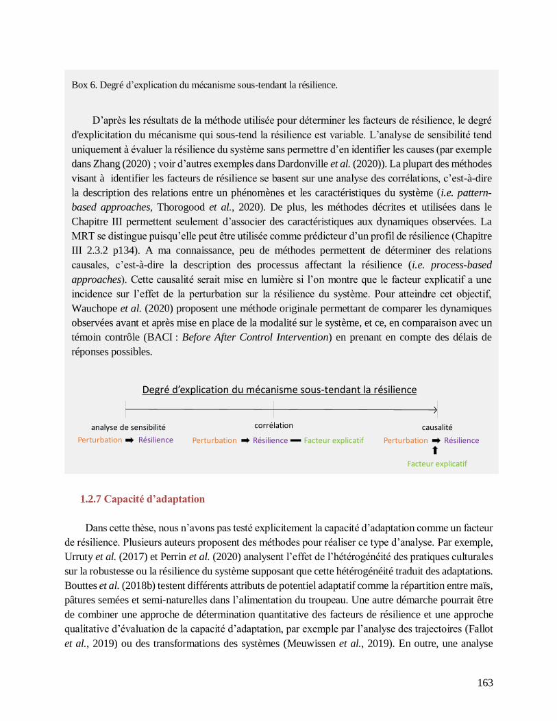
163

1.2.7 Capacité d’adaptation

Dans cette thèse, nous n’avons pas testé explicitement la capacité d’adaptation comme un facteur

de résilience. Plusieurs auteurs proposent des méthodes pour réaliser ce type d’analyse. Par exemple,

Urruty et al. (2017) et Perrin et al. (2020) analysent l’effet de l’hétérogénéité des pratiques culturales

sur la robustesse ou la résilience du système supposant que cette hétérogénéité traduit des adaptations.

Bouttes et al. (2018b) testent différents attributs de potentiel adaptatif comme la répartition entre maïs,

pâtures semées et semi-naturelles dans l’alimentation du troupeau. Une autre démarche pourrait être

de combiner une approche de détermination quantitative des facteurs de résilience et une approche

qualitative d’évaluation de la capacité d’adaptation, par exemple par l’analyse des trajectoires (Fallot

et al., 2019) ou des transformations des systèmes (Meuwissen et al., 2019). En outre, une analyse

Box 6. Degré d’explication du mécanisme sous-tendant la résilience.

D’après les résultats de la méthode utilisée pour déterminer les facteurs de résilience, le degré

d'explicitation du mécanisme qui sous-tend la résilience est variable. L’analyse de sensibilité tend

uniquement à évaluer la résilience du système sans permettre d’en identifier les causes (par exemple

dans Zhang (2020) ; voir d’autres exemples dans Dardonville et al. (2020)). La plupart des méthodes

visant à identifier les facteurs de résilience se basent sur une analyse des corrélations, c’est-à-dire

la description des relations entre un phénomènes et les caractéristiques du système (i.e. pattern-

based approaches, Thorogood et al., 2020). De plus, les méthodes décrites et utilisées dans le

Chapitre III permettent seulement d’associer des caractéristiques aux dynamiques observées. La

MRT se distingue puisqu’elle peut être utilisée comme prédicteur d’un profil de résilience (Chapitre

III 2.3.2 p134). A ma connaissance, peu de méthodes permettent de déterminer des relations

causales, c’est-à-dire la description des processus affectant la résilience (i.e. process-based

approaches). Cette causalité serait mise en lumière si l’on montre que le facteur explicatif a une

incidence sur l’effet de la perturbation sur la résilience du système. Pour atteindre cet objectif,

Wauchope et al. (2020) proposent une méthode originale permettant de comparer les dynamiques

observées avant et après mise en place de la modalité sur le système, et ce, en comparaison avec un

témoin contrôle (BACI : Before After Control Intervention) en prenant en compte des délais de

réponses possibles.

Perturbation Résilience Facteur explicatif

corrélationanalyse de sensibilité

Perturbation Résilience

causalité

Facteur explicatif

Perturbation Résilience

Degré d’explication du mécanisme sous-tendant la résilience

164

temporelle de la dynamique de la capacité d’adaptation couplée à l’analyse de l’exposition et de

sensibilité est une méthode permettant d’identifier des périodes critiques pour la résilience des

systèmes (voir Naylor et al., 2020).

1.2.8 Dynamique de la résilience

Au-delà de la dynamique de la capacité d’adaptation, il serait intéressant d’analyser la dynamique

de la résilience (Stone and Rahimifard, 2018). On peut ainsi se demander dans quelle mesure l’impact

des perturbations modifie la capacité du système à persister dans le temps (Martin et al., 2019b). Cette

modification peut être engendrée par une transformation de la structure de l’agroécosystème ou du

système de production ou par une altération de leurs dynamiques internes (par l’intermédiaire de

« poverty traps » par exemple) (Tittonell et Giller, 2013). En effet, les perturbations peuvent dégrader

le capital naturel qui sous-tend le fonctionnement de l’agroécosystème. En fin de compte, ces

perturbations détérioreraient la réalisation des fonctions de l’agroécosystème à travers l’altération

graduelle des variables à temps de réponse long ou des boucles de rétroaction négatives, mais aussi à

travers des changements de régimes suite au franchissement d’un seuil écologique (Biggs et al., 2012).

A ce sujet, nous montrons en Chapitre III que la dynamique du capital naturel est fortement liée à la

résilience des agroécosystèmes, et ce, malgré une période d’analyse relativement restreinte (moins

d’une dizaine d’année).

La dynamique spatiale de la résilience doit aussi être analysée car elle peut se transférer entre

différents niveaux organisationnels (Barreteau et al., 2020; Mathevet et al., 2017). Tittonell (2014)

mentionnent ainsi un effet Matryoshka (dit des « poupées russes » pour décrire un effet associé à un

emboitement hiérarchique d’échelles d’organisation), similaire au concept de panarchie utilisé par

Holling et Gunderson (2002) pour traiter des cycles adaptatifs. Comme discutés dans le Chapitre I,

ces effets d’emboitement peuvent conduire à des conclusions sur la résilience qui diffèrent suivant le

ou les niveaux, ou la ou les échelles spatiales considérées. Par exemple, Reidsma et al. (2009)

n’observent pas les mêmes effets du climat et des pratiques agricoles sur la tendance et la variabilité

du rendement des cultures et du revenu agricole si elles sont analysées à l’échelle de l’exploitation

agricole ou à l’échelle régionale. Ainsi, la résilience à l’échelle de l’agroécosystème ne suffit pas à

assurer la résilience aux échelles locales ou régionales ou à l’échelle du système alimentaire (Bullock

et al., 2017). Par ailleurs, des facteurs de résilience peuvent jouer un rôle important à un niveau

d’organisation différent de celui où ils s’expriment, sont gérés et/ou étudiés (ibid.). Par exemple, les

formes d’agriculture ancrées territorialement qui ne s’inscrivent pas dans le marché économique

mondial (par exemple par vente directe ou locale) ne sont pas exposées à la volatilité du prix mondial

des cultures (Therond et al., 2017a). Leurs agroécosystèmes (à un niveau inférieur d’organisation) ne

sont donc pas exposés à ces perturbations. A l’inverse, l’homogénéisation génétique des semences

proposées par les firmes semencières et contraintes par la certification de celles-ci via un « catalogue

des espèces et variétés de plantes cultivées » en France (décision à l’échelle du territoire national) est

susceptible d’induire une plus grande vulnérabilité des cultures à l’échelle des agroécosystèmes

(Kahiluoto et al., 2019). Ainsi, une analyse multiniveau de la résilience semble indispensable. Cette

165

démarche nous paraît encore trop peu mise en œuvre dans cette thèse notamment – du fait des verrous

à l’évaluation de la résilience mentionnés en introduction (données, modèles disponibles) mais aussi

du fait de problématiques propres à l’évaluation des systèmes agricoles lors de changements d’échelle

organisationnelle (Dalgaard et al., 2003). D’ailleurs, aucune étude évaluant quantitativement la VRRA

à l’échelle du système alimentaire (food system) n’a été identifiée durant notre synthèse de littérature

(Chapitre I, Figure 16) (Dardonville et al., 2020). Ce résultat contraste avec le fait que plusieurs

travaux clefs traitent de cette question de manière conceptuelle de manière qualitative ou en produisant

une synthèse sur le sujet (Brzezina et al., 2016; Challinor et al., 2007; Himanen et al., 2016; Hodbod

and Eakin, 2015; Macfadyen et al., 2015; Prosperi et al., 2016; Stone and Rahimifard, 2018; Tendall

et al., 2015; Valencia et al., 2019). Par exemple, Macfadyen et al. (2015) proposent dix

recommandations pour améliorer la résilience du système alimentaire le long de la chaîne d’acteurs

des agriculteur·rices aux consommateur·rices (Figure 40).

Figure 40. Recommandations le long de la chaîne de production alimentaire (simplifiée) pour atteindre la

résilience.

166

1.3 Évaluation des services écosystémiques et de la dynamique du capital

naturel

Partant du cadre d’analyse des formes d’agriculture proposé par Therond et al. (2017a) et dans la

continuité des avancées conceptuelles et méthodologiques réalisées dans l’étude EFESE-EA (Therond

et al., 2017b), nous avons proposé une méthode de détermination opérationnelle des formes

d’agriculture en grandes cultures (Chapitre II). La proposition de Therond et al. (2017a) consistait à

caractériser ces formes, du point de vue biotechnique, selon la part de la production permise par les

services écosystémiques relativement à celle permise par les intrants d’origine anthropique (voir aussi

Tibi and Therond (2018)). Dans un objectif d’opérationnalisation de leur proposition via une

caractérisation semi-quantitative, nous avons défini un cadre conceptuel et construit une méthode

d’évaluation des SEP (Chapitre II). L’application de cette méthode pour caractériser 34

agroécosystèmes du Grand-Est, nous a permis d’identifier plusieurs groupes représentant différentes

formes d’agriculture relativement à leurs relations avec les SEP.

Pour évaluer le poids relatif des SEP dans la production agricole, nous avons été confrontés à des

problématiques d’applicabilité des méthodes existantes (voir Introduction 2.3 p10) et de disponibilité

de données (relevés de terrain par exemple). Durant le stage de fin d’études d’ingénieur agronome de

l’ENSAIA de Baptiste Legrand en 2019, nous avons exploré différentes pistes méthodologiques. La

première a été de passer par des méthodes de « mise à unités communes » telles que : l’évaluation de

l’émergie (Solar Emergy Joule ; Wilfart, 2012), l’évaluation de l’éxergie (Hau and Bakshi, 2004),

l’évaluation de l’énergie (production primaire nette ; Costanza et al., 2007; Prince et al., 2001) et

l’analyse des cycles de vie (Othoniel et al., 2016; Zhang et al., 2010). Ces méthodes n’ont finalement

pas été retenues car elles présentaient des limites considérées rédhibitoires ou non surmontable dans

le temps imparti au stage et à la thèse (voir détail dans Legrand et al., 2019). D’abord, ces méthodes

traitent de manière « boite noire » les processus écologiques à des échelles différentes de celles de

l’agroécosystème. Par exemple, les processus biophysiques à l’origine des SEP considérés dans les

approches basées sur l’émergie ou l’exergie sont l’énergie solaire, la chaleur interne de la Terre ou/et

l’énergie marémotrice. Ensuite, les valeurs de transformité (coefficient de transformation de quantité

de matière ou d’énergie en énergie solaire) pour les sorties (i.e. la production agricole) ou les intrants

anthropiques sont peu stabilisées et dépendantes d’hypothèses émises sur les marchés économiques

(car utilisant une transformation d’unité monétaire) (Hau and Bakshi, 2004; Othoniel et al., 2016;

Zhang et al., 2010). Aucune de ces méthodes ne permet de décrire finement les interactions entre

l’environnement, les pratiques agricoles et les SEP à l’échelle de l’agroécosystème. En explorant

d’autres pistes méthodologiques, comme l’utilisation de modèles de cultures fins (type STICS) comme

réalisé dans l’étude EFESE-EA, nous nous sommes rendu compte qu’ils ne nous permettraient pas

d’évaluer l’ensemble des SEP considérés dans cette étude et nécessiteraient des compétences difficiles

à acquérir et peu transférables pour en assurer une utilisation fondée et robuste. Nous avons donc opté

pour le développement d’une méthode basée sur l’évaluation de la qualité des déterminants connus

des SEP présentée en Chapitre II.

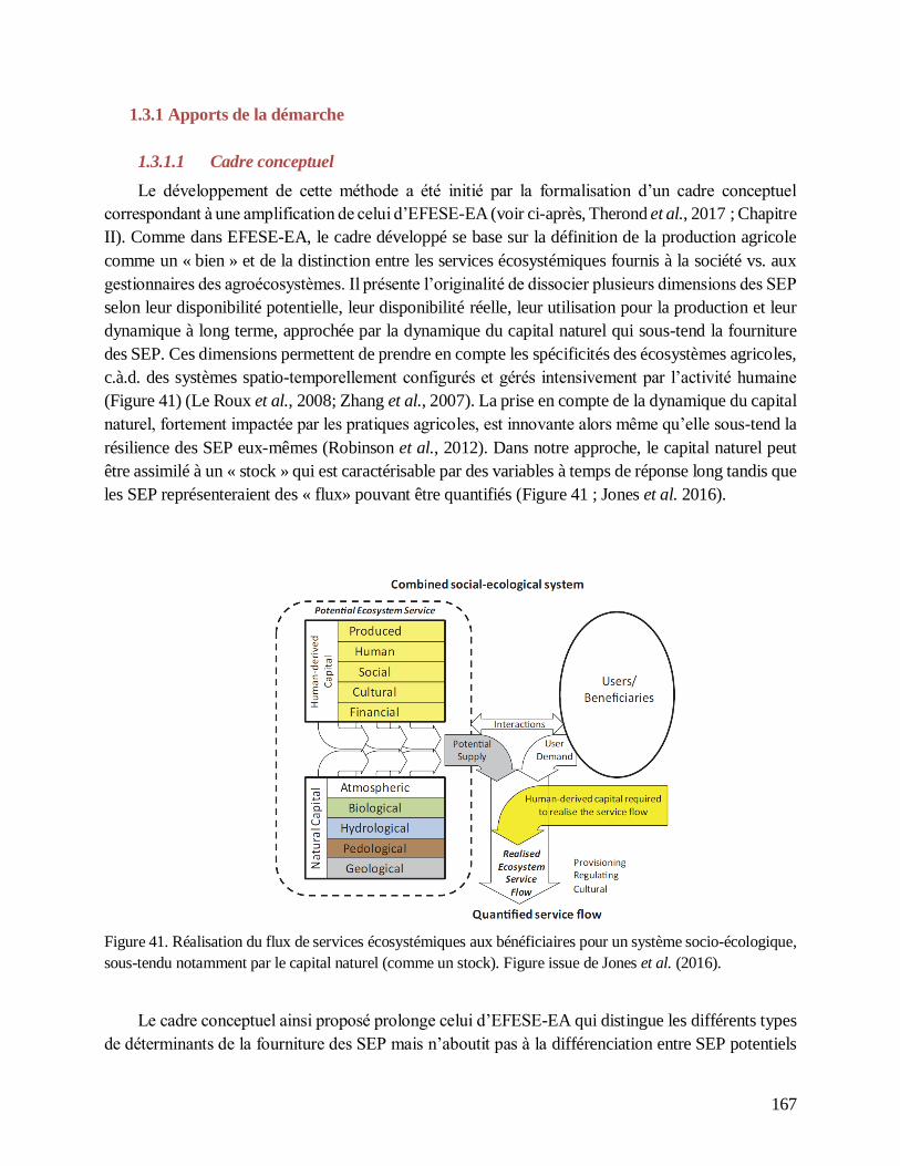
167

1.3.1 Apports de la démarche

1.3.1.1 Cadre conceptuel

Le développement de cette méthode a été initié par la formalisation d’un cadre conceptuel

correspondant à une amplification de celui d’EFESE-EA (voir ci-après, Therond et al., 2017 ; Chapitre

II). Comme dans EFESE-EA, le cadre développé se base sur la définition de la production agricole

comme un « bien » et de la distinction entre les services écosystémiques fournis à la société vs. aux

gestionnaires des agroécosystèmes. Il présente l’originalité de dissocier plusieurs dimensions des SEP

selon leur disponibilité potentielle, leur disponibilité réelle, leur utilisation pour la production et leur

dynamique à long terme, approchée par la dynamique du capital naturel qui sous-tend la fourniture

des SEP. Ces dimensions permettent de prendre en compte les spécificités des écosystèmes agricoles,

c.à.d. des systèmes spatio-temporellement configurés et gérés intensivement par l’activité humaine

(Figure 41) (Le Roux et al., 2008; Zhang et al., 2007). La prise en compte de la dynamique du capital

naturel, fortement impactée par les pratiques agricoles, est innovante alors même qu’elle sous-tend la

résilience des SEP eux-mêmes (Robinson et al., 2012). Dans notre approche, le capital naturel peut

être assimilé à un « stock » qui est caractérisable par des variables à temps de réponse long tandis que

les SEP représenteraient des « flux» pouvant être quantifiés (Figure 41 ; Jones et al. 2016).

Figure 41. Réalisation du flux de services écosystémiques aux bénéficiaires pour un système socio-écologique,

sous-tendu notamment par le capital naturel (comme un stock). Figure issue de Jones et al. (2016).

Le cadre conceptuel ainsi proposé prolonge celui d’EFESE-EA qui distingue les différents types

de déterminants de la fourniture des SEP mais n’aboutit pas à la différenciation entre SEP potentiels

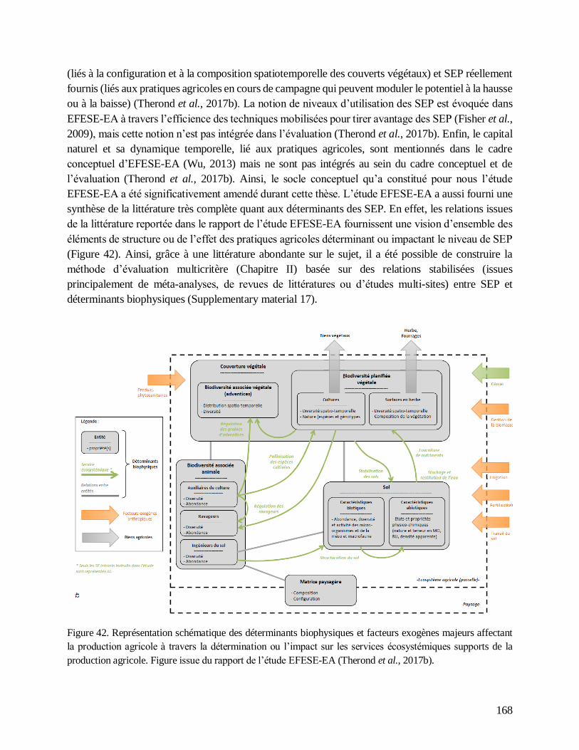
168

(liés à la configuration et à la composition spatiotemporelle des couverts végétaux) et SEP réellement

fournis (liés aux pratiques agricoles en cours de campagne qui peuvent moduler le potentiel à la hausse

ou à la baisse) (Therond et al., 2017b). La notion de niveaux d’utilisation des SEP est évoquée dans

EFESE-EA à travers l’efficience des techniques mobilisées pour tirer avantage des SEP (Fisher et al.,

2009), mais cette notion n’est pas intégrée dans l’évaluation (Therond et al., 2017b). Enfin, le capital

naturel et sa dynamique temporelle, lié aux pratiques agricoles, sont mentionnés dans le cadre

conceptuel d’EFESE-EA (Wu, 2013) mais ne sont pas intégrés au sein du cadre conceptuel et de

l’évaluation (Therond et al., 2017b). Ainsi, le socle conceptuel qu’a constitué pour nous l’étude

EFESE-EA a été significativement amendé durant cette thèse. L’étude EFESE-EA a aussi fourni une

synthèse de la littérature très complète quant aux déterminants des SEP. En effet, les relations issues

de la littérature reportée dans le rapport de l’étude EFESE-EA fournissent une vision d’ensemble des

éléments de structure ou de l’effet des pratiques agricoles déterminant ou impactant le niveau de SEP

(Figure 42). Ainsi, grâce à une littérature abondante sur le sujet, il a été possible de construire la

méthode d’évaluation multicritère (Chapitre II) basée sur des relations stabilisées (issues

principalement de méta-analyses, de revues de littératures ou d’études multi-sites) entre SEP et

déterminants biophysiques (Supplementary material 17).

Figure 42. Représentation schématique des déterminants biophysiques et facteurs exogènes majeurs affectant

la production agricole à travers la détermination ou l’impact sur les services écosystémiques supports de la

production agricole. Figure issue du rapport de l’étude EFESE-EA (Therond et al., 2017b).

169

1.3.1.2 Evaluation multicritère

Afin de proposer une approche générique et reproductible de l’évaluation des SEP, les indicateurs

sont calculés en notation absolue (mis à part pour le capital naturel) et les notes sont normalisées par

rapport aux moyennes des anciennes régions (Lorraine, Champagne-Ardenne, Alsace) pour tenir

compte de la dispersion des exploitations agricoles sur les différents pédoclimats (van Leeuwen et al.,

2019a). De plus, dans le but de ne pas conclure sur des différences de niveau de SEP liées aux

différents pédoclimats de la région Grand Est (ce qui ne relève pas de notre objectif), tous les

déterminants des SEP retenus dans l’évaluation multicritère sont contrôlés par le gestionnaire (Guerra

et al., 2014). Ainsi, les critères retenus pour l’évaluation sont : le choix des cultures et intercultures,

de la rotation, des stratégies de gestion des résidus de culture, des habitats semi-naturels adjacents aux

parcelles étudiées et des pratiques agricoles (fertilisation, irrigation, application de produits

phytosanitaires et travail du sol). Ces critères dépendent des décisions des gestionnaires (Conway,

1987; Gliessman, 2004; Swift et al., 2004; Therond et al., 2017b). Le taux de matière organique est

aussi considéré comme déterminé par le gestionnaire car il dépend, entre autres, de sa stratégie de

fertilisation organique et de sa gestion des résidus de culture (Aguilera et al., 2020b).

L’évaluation multicritère développée permet de décrire de manière fine et multidimensionnelle

les SEP des agroécosystèmes. Bien que la plupart des SEP soient fortement déterminés par la

biodiversité et/ou le taux de matière organique du sol (Box 3 et Box 4, Aguilera et al., 2020b; Therond

et al., 2017b), les résultats de l’évaluation des SEP ne peuvent pas être inférés simplement sur la base

de ces seules caractéristiques. Les multiples propriétés considérées pour estimer les quatre

composantes du cadre conceptuel des SEP sont nécessaires pour leur évaluation. L’Analyse en

Composantes Principales (ACP) sur les quatre dimensions évaluées du cadre conceptuel et sur les

variables utilisées pour décrire les propriétés des agroécosystèmes ou sur des variables classiquement

utilisées (par exemple le classement en AB, en agriculture de conservation ; Figure 43) montre que les

quatre dimensions sont peu corrélées (> 60 %) entre-elles.

170

Figure 43. Cercle de corrélation de l'ACP des quatre dimensions du cadre conceptuel : la capacité potentielle

(Potential), réelle (Real capacity), l'utilisation effective (Actual use) et la dynamique du capital naturel (Natural

capital). Les descripteurs traditionnels des systèmes agricoles ont été ajoutés pour montrer que les variables

constituent une combinaison complexe qui ne peut être réduite à l'une d'entre elles : le niveau d'intensité des

intrants (Iintensity), le rendement relatif régional (Ryield), l'intensité de l’irrigation (Irrigation), de la

fertilisation minérale (Fertilization), l’usage de pesticides (Pesticide), du travail du sol (Tillage), la présence de

couverts intermédiaires longs (> 6 mois, Lcover) ou courts (< 6 mois, Scover), le taux de matière organique

(SOM), le respect du cahier des charges de l'agriculture biologique (OA), ou de l'agriculture de conservation

(CA) et la complexité de la rotation (indicateur combiné du nombre d’années et du nombre de cultures, RCI).

1.3.1.3 Formes d’agriculture

La classification des formes d’agriculture a été réalisée en considérant le niveau de SEP

fournis/utilisés et la dynamique du capital naturel. Cette caractérisation des formes d’agriculture

apporte des informations nouvelles sur la capacité de l’agroécosystème à fournir les SEP et à les

maintenir sans les dégrader. Les conclusions tirées de l’ACP viennent étayer le fait que les formes

d’agriculture décrites en Chapitre III recouvrent une diversité de caractéristiques agro-écologiques.

Les différentes formes d’agriculture ne peuvent pas être réduites à des pratiques types (par exemple

par type de rotation, de gestion du sol ou de la stratégie d’application de produits phytosanitaires).

Cette caractérisation originale permet de dépasser les limites des classifications usuelles (par exemple

AB vs. AC) via la description de la diversité des relations qu’entretiennent les agroécosystèmes avec

les SEP. Cependant, les formes identifiées sont dépendantes de l’échantillon d’agroécosystèmes

considérés. Un nombre et une gamme d’agroécosystèmes plus importants auraient pu faire émerger

des clusters différents. En dernier lieu, la caractérisation des formes d’agriculture proposée apporte

une description de l’agroécosystème qui diffère des visions par « impact » sur les écosystèmes

(pollution et dégradation par exemple) (German et al., 2017). Alors que les approches d’évaluation

d’impact adoptent une vision plutôt négative (voire culpabilisante) de la gestion de l’agroécosystème,

l’évaluation des SEP valorise la gestion de l’agroécosystème à travers l’identification de la plus-value

pouvant bénéficier à la production agricole en remplacement des intrants anthropiques. Ces visions

171

sont complémentaires et gagneraient à être articulées l’une par rapport à l’autre (Kanter et al., 2018;

Therond et al., 2017a).

1.3.2 Limites de la démarche

De nombreux travaux récents pointent l’importance de l’évaluation de la part de la production

permise par les SEP (vs. les intrants anthropiques) afin de quantifier leur poids relatif et de faire

reconnaître l’importance de ces derniers dans le processus de production de biens agricoles (Jones et

al., 2016; Therond et al., 2017b). C’est également l’objectif du cadre d’analyse des formes

d’agriculture de Therond et al. (2017a). L’évaluation de l’utilisation effective de SEP (actual use)

(Chapitre II) renseigne sur ce partitionnement mais ne permet pas de l’évaluer. Elle donne une

information sur l’efficience potentielle d’utilisation des SEP par le biais de la qualité de la prise en

compte du niveau de SEP dans la stratégie de gestion de l’agroécosystème. A ma connaissance, il

existe à ce jour un nombre très limité d’études ayant opérées ce partitionnement et cela constitue

toujours un front de recherche actif (Bengtsson, 2015). Dans l’étude EFESE-EA, la part de la

production agricole permise par les services de fourniture d’azote et de restitution d’eau aux plantes

cultivées a été évaluée par le biais de l’utilisation d’un modèle de culture (STICS) à l’échelle de la

France ainsi que par la comparaison des niveaux de production avec et sans apport de fertilisants et

d’eau d’irrigation (Therond et al., 2017b). Pérez-Soba et al. (2019) ont réalisé un partitionnement des

flux d'émergie (énergie solaire, cf. Introduction 2.3 p10) engagés dans la production agricole selon

leur origine anthropique ou écosystémique à l’échelle européenne. Selon nous, la méthode développée

dans cette thèse reste ainsi la plus pertinente à l’échelle de l’agroécosystème. Cette méthode constitue

un point de départ pour des améliorations et développements futurs.

1.3.3 Perspectives pour l’évaluation des services écosystémiques

Si l’approche de caractérisation des formes d’agriculture et d’évaluation des SEP semble

atteindre ses objectifs principaux tout en présentant certaines limites, plusieurs perspectives

d’améliorations ou de prolongement de mes travaux peuvent être envisagées.

Premièrement, certains éléments qui déterminent un ensemble de SEP mais qui n'étaient pas

pertinents dans notre étude de cas pourraient être ajoutés, comme par exemple l'agroforesterie et le

chaulage (Aguilera et al., 2020b; Haynes and Naidu, 1998; Pumariño et al., 2015; Torralba et al.,

2016). En outre, certains indicateurs pourraient être améliorés afin de refléter plus précisément l'effet

du déterminant mesuré. La qualité des indicateurs en tant que proxy du déterminant pour supporter ou

moduler l'expression du SEP dépend de la proximité conceptuelle et opérationnelle entre les

informations fournies par l'indicateur et les informations cibles (Augstburger et al., 2018). Par

exemple, le tassement du sol causé par certaines pratiques agricoles lors de conditions pédoclimatiques

défavorables peut dégrader un certain nombre de SEP (comme la structuration du sol par exemple).

Actuellement, l'indicateur prend en compte uniquement les conditions d'humidité du sol au moment

de la récolte et en fonction des cultures de la rotation. Il existe des modèles de compactage du sol plus

172

fins (Arvidsson and Haakansson, 1991) mais qui nécessitent des informations au niveau parcellaire,

une dynamique au pas de temps journalier et une description très précise du matériel agricole employé.

Comme la structure du sol est un déterminant central des SEP (Therond et al., 2017b), un travail

complémentaire pourrait viser à développer un indicateur simplifié basé sur ces modèles. De plus, la

taille des parcelles est de plus en plus considérée comme un déterminant important des SEP, en

particulier pour les régulations biologiques (Martin et al., 2019a; Sirami et al., 2019). Cette

information est actuellement inclue dans les deux indicateurs de l'effet des habitats semi-naturels sur

les régulations biologiques, mais ne constitue pas un déterminant en soi. Pour considérer uniquement

des déterminants contrôlables, nous n’avons pas inclus de déterminants paysagers mis à part les

éléments jouxtant les parcelles, gérés par le gestionnaire de l’agroécosystème. Pourtant, de plus en

plus d’études montrent l’effet de la complexité du paysage sur la biodiversité qui supporte la fourniture

de SEP (Kleijn et al., 2019a) sa stabilité (Larsen and Noack, 2020). L’effet du paysage sur la

biodiversité semble être particulièrement marqué pour certain taxons (Martin et al., 2019a) ou traits

d’espèces ravageuses (Tamburini et al., 2020) et peut dépendre du niveau d’utilisation de pesticides

localement (Ricci et al., 2019). De même, il semblerait que la proportion d’agriculture biologique dans

le paysage impacterait également la fourniture de SEP (Muneret et al., 2019) en fonction de la

complexité du paysage (Winqvist et al., 2011). Ainsi, des indicateurs de la capacité du paysage à

fournir des SEP pourraient être développés et intégrés à l’évaluation multicritère proposée dans ce

travail. Enfin, l’échelle d’évaluation de l’efficience de l’utilisation des SEP est principalement basée

sur l’avis d’experts (Table 10) et devra être adaptée en fonction de sa pertinence vis-à-vis de la gestion

de l’agroécosystème et des disponibilités en connaissances et en technologies dans les différentes

régions d’application.

Une des grandes perspectives de la recherche portant sur l’évaluation des SEP est de développer

une méthode d’agrégation des déterminants par composante de SEP (par exemple entre l’effet rotation

et l’effet mélange de cultures sur le SEP de régulation des adventices) permettant de gérer les

interactions entre ceux-ci (Bockstaller et al., 2017). Actuellement, dans notre méthode, du fait du

manque d'information dans la littérature, toutes ces étapes d’agrégation sont réalisées avec les mêmes

poids relatifs. De plus, les synergies et antagonismes entre les SEP ne sont ni analysés, ni considérés.

Il serait donc nécessaire de s’appuyer sur les travaux récents d’analyse quantitative des relations entre

SEP (ceux de Garibaldi et al., 2018 ou Obiang-Ndong et al., 2020 par exemple) pour tenir compte de

ces effets. En attendant que des études identifient le poids des déterminants sur la base de

connaissances biophysiques des processus sous-tendant la fourniture des SEP, une démarche

envisageable serait de réunir un groupe d'experts afin de définir collectivement des poids relatifs

semblant pertinents au vu des connaissances expertes disponibles (voir par exemple les démarches de

van Leeuwen et al., 2019 et Zahm et al., 2018). Afin de valider l’agrégation ainsi que les indicateurs

proposés, il est aussi envisageable de comparer les résultats obtenus avec ceux qui seraient obtenus

par des mesures directes de SEP comme cela est proposé dans Boeraeve et al. (2020) par exemple.

Il serait également intéressant d'étendre notre méthode à d'autres SEP qui n'ont pas été considérés,

comme la régulation du climat local (Aguilera et al., 2013; Techen et al., 2020). Le cadre conceptuel

et la méthode peuvent aussi être adaptés pour couvrir les services fournis à la société. Cela permettrait

173

notamment d’analyser les synergies et les antagonismes potentiels entre ces deux type de services et

entre les deux types de gestionnaires associés (Aguilera et al., 2020b; Therond et al., 2017b). Dans

notre approche, seule l’effet de la biodiversité support de la fourniture des SEP (biodiversité associée)

sur la dynamique du capital naturel est évalué. Pourtant, l’ensemble de la biodiversité, même celle qui

ne présente pas d’intérêt connus dans la fourniture de SEP, pourrait être évaluée afin de la protéger

pour elle-même et pour les fonctions encore inconnues qu’elle assure (Duelli et al., 1999; Lüscher et

al., 2017a; Moller et al., 2008). Enfin, cette approche a été développée pour les systèmes de grandes

cultures sous un climat tempéré et sous des conditions technico-économiques caractéristiques de

l’agriculture française de plaine. Il serait donc nécessaire de poursuivre les développements de manière

à considérer une plus large gamme de systèmes agricoles et d’autres conditions climatiques.

174

2. Facteurs de resilience

2.1 Analyse de la relation complexe entre l'influence du rendement et sa

stabilité sur la résilience le long du gradient d'intensification

Les résultats du Chapitre III montrent l’existence d’un antagonisme entre le niveau et la stabilité

du rendement des cultures pour différents niveaux d’intensification de la production : les systèmes

intensifiés par les intrants anthropiques sont les systèmes les plus performants et leur productivité est

la moins stable dans le temps. Ces résultats convergent avec ceux de certains travaux, mais une analyse

de la littérature a montré que d’autres travaux ne partagent pas les mêmes conclusions. Nous explorons

dans un article de perspectives l’hypothèse selon laquelle il existe une relation (stochastiques et/ou

agronomique) non-linéaire entre le niveau et la stabilité du rendement le long d’un gradient

d’intensification. Cet article de perspectives a été soumis au journal Environmental Research Letter

en Avril 2021.

175

ABSTRACT

The type of agricultural system that promotes the most stable yield is under debate, especially

when comparing conventional and organic agriculture. Whether statistical or agroecological, a

relationship often exists between the level and stability of agricultural production. In comparative

studies of agricultural system yields, Taylor’s Power Law often applies, and thus the issue is to identify

the proportion of stability that is determined by the agricultural model tested rather than by the

production level. From an agroecological viewpoint, analyzing potential effects of limiting factors at

different levels of fertilization and irrigation can explain tradeoffs between yield level and stability.

However, the level of intensification of cropping practices is not the only factor to consider; it is also

necessary to consider soil and climate differences, the economic context, and ecosystem services. In

the short and medium terms, the appropriateness of the production situation (i.e. the combination of

crops, management, soil and climate) and resource availability and dynamics is also crucial to consider

when designing resilient agricultural systems. In the long term, natural capital must be conserved to

ensure the level and stability of agricultural production. We highlight that identifying how production

situations influence yield level and stability requires detailed multiscale and multifactor approaches to

avoid biased design, inappropriate interpretations and flawed conclusions.

Analyzing the complex relationship between the influence of yield and its stability

on resilience along the intensification gradient

Dardonville M. a,b, Villerd J. a, Therond O. a

a LAE, Université de Lorraine, INRAE, Colmar, France

b Agrosolutions, France

Submitted to Environmental Research Letters in April 2021

176

2.1.1 Intensification of crop production

To control factors that limit or decrease crop yields (van Ittersum and Rabbinge, 1997),

modern agriculture has taken advantage of inexpensive energy from anthropic inputs such as

fertilizers, irrigation, mechanical tillage and pesticides (Duru et al., 2015b). As Grumbach and

Hamant (2020) state, “As a machine, Earth’s problems could be fixed”. By reducing the yield gap

in some regions of the world (Van Ittersum et al., 2013), intensification of agricultural systems has

freed these systems from several biophysical constraints in agroecosystems but has harmed the

environment (Emmerson et al., 2016; Therond et al., 2017b). For example, irrigation decreases

hydric deficit in the soil and thus increases yields (Zaveri and Lobell, 2019), but the subsequent

depletion of water resources can cause substantial local-to-regional water scarcity (Rad et al.,

2020). In addition, yields have stagnated in some regions for several years (Brisson et al., 2010),

which raises doubts about the ability of technological and varietal progress to ensure food security

for the world's growing population (Godfray et al., 2010), especially under climate change and

resource scarcity (Lobell and Tebaldi, 2014).

2.1.2 Stability of production

The stability of production, whether spatial or temporal, is an important criterion for meeting

the increasing global demand for food production (Schrama et al., 2018). The increasingly frequent

biophysical and socio-economic disruptions of the food system challenge production stability and

will continue to challenge it (Reidsma et al., 2010). Stability is a parent concept of resilience since

it focuses on the dynamics of the system and the ability to maintain its identity in the face of

disturbances (Holling, 1973). After decades of examining effects of agricultural practices on crop

yield levels, yield stability has become a key area of study (Knapp and van der Heijden, 2018).

Exploration of the stability of genotype-based yields in a variety of environments has been

extended to a variety of management practices (Urruty et al., 2016). Several studies have

investigated whether different management practices or agriculture models (e.g. organic vs.

conventional) are related to yield stability (e.g. Brown et al., 2019; Cociu and Cizma, 2015; Gaudin

et al., 2015; Khumairoh et al., 2018; Macholdt et al., 2020). The studies usually investigate a

gradient of production intensification (i.e. use of anthropic inputs) (Therond et al., 2017b).

2.1.3 Yield stability among agricultural systems

Organic agriculture often has lower yields (Ponisio et al., 2015; Seufert et al., 2012) but has

more environmental benefits than conventional (also called “industrial” or “intensive”) agriculture

(Smith et al., 2019; Tuomisto et al., 2012). In this context, the production stability of organic

systems is another strong argument for agriculture to adopt them. However, results of studies of

the relative stability of organic vs. conventional yields vary greatly. The thorough meta-analysis

of Knapp and van der Heijden (2018) confirms that organic systems have lower yield levels (-

16%) and suggests, like (Smith et al., 2019), that they also have lower yield stability when

considering coefficients of variation. Since the standard deviations of yields do not differ

177

significantly, however, they conclude that the difference in yield level between the two agricultural

models explains mainly why organic systems have lower yield stability. Other studies show the

opposite trend (Schrama et al., 2018; Smolik et al., 1995) or no differences (Lesur-Dumoulin et

al., 2017; Stanhill, 1990), especially when individual crops are analyzed. For example, Smith and

Gross (2006) observe that maize yield is more stable (using the coefficient of variation) in organic

systems than in conventional least-diverse systems. (M. Li et al., 2019) observe that organic

management of tomato increases yield stability (using the coefficient of variation).

The same difficulty is observed when comparing conservation agriculture and conventional

agriculture. Knapp and van der Heijden (2018) observe no significant differences in yield stability

regardless of how stability is measured. Rusinamhodzi et al. (2011) draw the same conclusions for

maize, but conversely Williams et al. (2018) observe that soybean yield stabilizes under cover

cropping in conservation agriculture.

As Therond et al. (2017b) highlight, these results may diverge because conventional

agriculture, like organic and conservation agriculture, covers a wide variety of cropping systems

with different performances, mean levels and dynamics. Kirchmann et al. (2016) mention many

pitfalls of comparing agricultural systems of different agricultural models: comparisons require

sound “conditions for equitable evaluations…to avoid biased design, inappropriate interpretations

and flawed conclusions” (see also Gattinger et al. 2012). For example, conservation agriculture is

often considered without necessarily applying its three principles at the same time, which induces

even more variability in the results observed (Pittelkow et al., 2015a; Williams et al., 2018).

Williams et al. (2018) show the ability of cover crops to stabilize soybean yields, and Smith et al.

(2007) show that no-till effectively increases soybean yield stability. Cociu and Cizma (2015) draw

the same conclusions about the ability of no-till and crop-residue retention to stabilize maize yield

(using the coefficient of variation). Gaudin et al. (2015) explain that the effect may be related to

climate conditions: reducing tillage deceases yield variability at the field level in favorable years

but not in abnormal years (i.e. heat, dry, cold or wet stress). Even when data in meta-analyses are

processed in the same way (by size effect), and thus the two agricultural models have the same

agricultural practices, soil and climate, the experiments were conducted in different situations (i.e.

soil, climate, landscape complexity) and experienced different agricultural practices (e.g. rotation

complexity, irrigation). These differences can lead to contrasting results (Lori et al., 2017;

Pittelkow et al., 2015b).

Besides studies that focus on the influence of agriculture models on yield stability, some

studies assess effects of agricultural practices, such as low-input (Smith et al., 2007), no-till (Smith

et al., 2007), reduced tillage (Gaudin et al., 2015) or different types of fertilization (Berzsenyi et

al., 2000). Studies also focus on the composition of the rotation (Nielsen and Vigil, 2018), crop-

variety mixtures (Creissen et al., 2016), perennial vs. annual crops (Vico and Brunsell, 2018) and

the introduction of grain legumes (Reckling et al., 2018). An extended meta-analysis would be

needed to identify agricultural practices that increase yield stability. It would have to address

multiple practices, crops and production situations.

178

2.1.4 Intensification and yield resilience

In their review of effects of diversification and intensification on the resilience of agriculture

systems, Dardonville et al. (2020) find that input intensification did not always mitigate negative

effects of climate change on the dynamics of crop yield at field or farm levels. Of 145 comparisons,

67 % of intensification effects on resilience are negative or neutral, suggesting that intensification

is less often a relevant strategy to stabilize yield, increase the trend in yield or have a high

probability of a high yield. Reidsma and Ewert (2008) show that farm economic size has a negative

effect on the variability (i.e. stabilization) in yield at the regional level.

2.1.5 Statistical issues

Each study that investigates the origin of crop yield stability measures stability in one or more

ways, such as the standard deviation, coefficient of variation and slope of the Finlay-Wilkinson

regression (e.g. in Knapp and van der Heijden, 2018; M. Li et al., 2019; Macholdt et al., 2020).

They can provide different results depending on whether they assess absolute (e.g. standard

deviation) or relative variability (e.g. coefficient of variation) in the production level (e.g. Wang

et al., 2019b). Döring et al. (2015) highlight that Taylor's Power Law (TPL) indicates a potential

relationship between the logarithm of the standard deviation and the mean of crop production. As

these authors highlight, TPL holds true in many studies of ecological systems and is applicable to

many agricultural systems at several levels of organization. When TPL applies, the variance

depends on the yield level, and differences in yield between agricultural models (e.g. organic vs.

conventional) bias the analysis of variance (Döring and Reckling, 2018). Dehghani et al. (2008)

analyze a few stability metrics using principal component analysis and show that the coefficient

of variation of yield is half correlated with yield level. Because of TPL, the coefficient of variation

is biased, and thus using it to estimate differences in stability is incorrect (Döring et al., 2015;

Döring and Reckling, 2018). For most of the many agricultural datasets that Döring et al. (2015)

test, TPL applies and the variance in yield is positively correlated with the yield level. Conversely,

a meta-analysis of organic vs. conventional systems (Knapp and van der Heijden, 2018), observes

that (i) TPL does not apply to size effects but does apply to observations, (ii) the standard deviation

of yield is constant regardless of the yield level, (iii) organic systems have lower yields than

conventional systems and (iv) relative stability (i.e. coefficient of variation) in yield differs

between agricultural models due to differences in yield levels. The statistical challenge that

emerges is thus to identify the part of the variability that is due to the systems/models compared

and not to the difference in yield level.

Unfortunately, studies that focus on yield stability rarely verify whether TPL applies (Döring

et al., 2015). To address this problem, several authors have developed methods to resolve

analytical bias when TPL applies by using the residuals of the TPL regression (Döring et al., 2015)

to correct the coefficient of variation (Döring and Reckling, 2018) or to consider the coefficient of

the fixed effect of the agricultural model in a linear regression that includes a mean (Eq. 18 in

(Nakagawa et al., 2015). When TPL is observed, it is not yet known whether it is due to purely

stochastic or behavioral aspects (Bittencourt-Oliveira et al., 2012; Kendal and Jørgensen, 2011).

179

However, the most recent hypothesis suggests that the stochastic effects observed could emerge at

the population level due to interactions or behaviors of individuals (Cohen, 2013).

2.1.6 Agronomic principles of yield stability

In most of the datasets that Döring et al. (2015) test, the relationship between the logarithm

of the standard deviation of yield and the mean yield is positive and linear, which indicates that

yield variability increases with yield level. When analyzing biophysical processes that underlie

this relationship, we assume that variability in yield due to climate variability (e.g. drought, heat)

is intrinsically related to the yield level (Figure 44). This can be explained by the influence of

biomass quantity on the demand for resources required for growth. Biomass quantity determines

a plant’s water and nutrient demands: the more biomass, the more water and nutrients it demands.

The availability of soil water and nutrients determines whether these demands are met or not. In

agricultural systems, the influence of fertilization and irrigation are related: increasing one

increases crop demand for the other. Consequently, the demand for and availability of water and

nutrients influence each other. However, by reasoning at the level of fertilization and irrigation,

two practices that increase yield, we can attempt to assess relationships between the level of yield

and its variability (Figure 44).

First, without fertilization or irrigation, the nutrient-limited yield (low biomass) results in low

plant water demand, which can be met by the soil water available, and thus climate variability may

have little influence on yield. With fertilization, the higher yield and biomass increase plant water

demand, which makes yield more sensitive to water stress during drought. With fertilization and

irrigation, irrigation meets the higher nutrient and water demands, which makes yield nearly

insensitive to climate variability (when irrigation water is not limited). Consequently, rainfed

systems with high production due to high fertilization, and thus high water demand, are expected

to be more sensitive to climate variability than those with lower production or those that are

irrigated. When intensification and production level are not considered, the yields of non-intensive

situations and the most intensive situations have similar standard deviations (i.e. low sensitivity to

climate variability), different coefficients of variation and different explanatory factors. Limiting

factors are nutrients in the non-intensive system (lowest yield), water in the fertilized system

(medium yield) due to heat and drought, and genetics in the fertilized and irrigated system (highest

yield) (van Ittersum and Rabbinge, 1997). Rist et al. (2014) call this maintenance of desired

dynamics through intensive use of anthropic inputs a resilience by coercision.

180

Figure 44. Diagram of effects of production level and input intensification on production variability in a

crop/grassland system at the field level due to resource availability (water, nutrients) for a given climate and

soil. Without fertilization or irrigation (bottom), the associated low yield (low biomass) results in low plant

water demand that is usually met by soil water availability, and thus climate variability has little influence

on yield dynamics. With fertilization alone (middle), the higher yield and biomass increases plant water

demand, which makes yield dynamics more sensitive to climate variability. With fertilization and irrigation

(top), the highest yield and biomass increase plant water demand, which is met by irrigation, which makes

yield nearly insensitive to climate variability (when irrigation water is not limited).

Supporting this conceptualization, Reidsma et al. (2008b) show that farms with lower yields

(and less intensification) are less sensitive to climate disturbance in regions that have already

adapted to recurring drought and increasing temperatures (e.g. Mediterranean regions). Berzsenyi

et al. (2000) show that wheat and maize yield stabilizes when the crops are not fertilized. Smith et

al. (2007) draw the same conclusion for low-input systems. For grasslands, Wang et al. (2019)

show that variability in production increases significantly as production increases. Consequently,

we assume that the differing results of studies that compare conventional to organic or

conservation agriculture is due to differences in the limiting factors and levels of intensification

considered.

2.1.7 Other factors that explain yield stability

In addition to the influence of intensification level on yield stability, the literature makes

several other assumptions about the influence of factors such as genetics, type of fertilization,

biological regulation, state of the soil, and the market and institutional context. The review of

Calderini and Slafer (1998) shows that crop varieties developed by genetic selection to increase

yield respond more to environmental variability but that the relative stability of yield remains the

same or increases for most of the 21 countries analyzed. However, Kahiluoto et al. (2019) show a

decrease in wheat response diversity, which confirms that yield dynamics have become more

homogeneous since the beginning of the 21st century, probably due to genetic selection. Murphy

et al. (2007) highlight that wheat varieties are particularly suited to provide high and stable yields,

181

but only with intensive inputs. Knapp and van der Heijden (2018) observe that intensifying organic

systems using nitrogen and phosphorus fertilizers or green manure would help fill the stability gap

between organic and conventional yields, mainly by filling the yield gap. They also suggest that

organic fertilization is more difficult to manage than mineral fertilization, which can cause the

fertilization effect to vary (depending on mineralization dynamics), and that ecosystem pest

control, encouraged in organic farming systems, follows predator-prey dynamics that are subject

to lag times. For the delivery of ecosystem services, Garibaldi et al. (2011) show that crops that

depend on pollinators have lower yield stability (using the coefficient of variation), and Deguines

et al. (2014) show this relationship for intensively managed fields. (Williams et al., 2018) show

that improving soil properties, especially soil organic matter content, increases yield stability.

Hazell (1985) suggests that, in addition to new intensification technologies (e.g. improved

seeds and fertilizers), the dependence on the economic market of inputs and crop prices, and their

volatility, increases yield variability.

2.1.8 Short-, medium- and long-term effects

While some agricultural practices can provide desired yield dynamics in the short term, they

can fail to do so in the medium or long terms ( Coomes et al., 2019). Consequently, short-term

studies may not be able to identify or highlight middle- or long-term effects (Müller et al., 2016a).

From a middle-term perspective, the dynamics of soil natural capital and local/regional resources

(e.g. water) can influence dynamics strongly, especially those of the level and stability of

agricultural production (Dardonville et al., 2021; Weyers and Gramig, 2017). Agricultural systems

can exhibit dynamics in the short term (e.g. season, year(s)) while experiencing degradation in soil

natural capital and local resources due to intensive management and a high production level

(Dardonville et al., 2021). For example, intensive use of groundwater for irrigation can result in a

water shortage that renders irrigation more difficult (costlier) or even impossible (de Graaf et al.,

2019). This problem also occurs in agricultural systems that use soil natural capital without

recycling it, such as those that deplete soil organic matter (Drinkwater and Snapp, 2007) or organic

systems that use soil phosphorus reserves without supplying organic matter to replace the

phosphorus exported (Kirchmann et al., 2009; Oelofse et al., 2010).

Although less intuitive, the dynamics of soil resource use can influence yield dynamics in the

short term. Efficient resource acquisition during a given period (e.g. by exploring soil horizons

(Barkaoui et al., 2016; Vico and Brunsell, 2018)) can initially result in higher biomass production

or stability (e.g. at the beginning of a season) but also greater depletion of soil resources. If a

disturbance (e.g. drought) lasts or repeats, empty resource reserves (e.g. soil water, nutrients) and

the large amount of biomass with high water and nutrient demands will influence vulnerability in

the short term (e.g. at the end of a season) (Zavalloni et al., 2008).

2.1.9 Considering production situations

The influence of intensification on yield dynamics depends strongly on the production

situation, defined as “the physical, chemical and biological components, except for the crop, of a

given field (or agroecosystem) and its environment, as well as socio-economic drivers that affect

182

farmer’s decisions" (Aubertot and Robin 2013). Reidsma et al. (2008b) show that the influence of

irrigation on yield depends mainly on water availability, fertilization level and crop type. Recently,

Renard and Tilman (2019) reveal that yield stability increases with irrigation, but more so due to

species diversity and even more so due to diversity in crop functional groups (e.g. legumes,

cereals). They claim that diversification could be a better strategy for adapting to climate change

than irrigation in countries where water is unaffordable or insufficient, as is the case for 30-47%

of rainfed wheat and maize croplands in the world (Wang et al., 2021). At the global scale, Ben-

Ari and Makowski (2014) identify regions that drive worldwide stability in maize and rice yields

and suggest that developing croplands in some regions could increase or decrease this stability in

global production. Ben-Ari and Makowski (2016) identify a relatively constant tradeoff over time

between yield level and stability for all crops aggregated and for maize. They identify regions in

which to develop crops to achieve an optimal relationship between yield level and stability and

mention that “expected yield differences can be explained by contrasts in production systems and

intensification levels” and by climates. This indicates that the type and management of crops must

be adapted to the soil, climate and (water) resources of local production situations.

2.1.10 Conclusion and perspectives

Variability in results of studies of yield stability of different agricultural systems show that it

is not easy to draw conclusions. Many of these studies do not consider TPL or key differences

between production situations. Given these limits, we propose several research paths to increase

the replicability of results and to be able to generalize factors that explain yield stability. First, we

emphasize the importance of considering the production level when comparing systems and its

statistical and agroecological relationships with its dynamics. TPL should always be tested and its

bias excluded. Thus, we strongly recommend considering and describing in detail the cropping

practices (e.g. irrigation, rainfed systems), soil and climate conditions and the overall production

situation. These factors determine the dynamics of crop-soil-climate interactions and thus yield

dynamics. We also recommend analyzing the appropriateness of crop choice and intensification

level for the production situation. Relationships between the yield level and dynamics of limiting

and reducing factors can be also analyzed. Finally, even for a short-term study, we recommend

investigating and, if possible, evaluating middle- or long-term effects of intensification on

endogenous (e.g. natural capital) or exogenous (e.g. local) resources and, in turn, on the stability

of agricultural production. We emphasize the importance of considering both short- and long-term

issues to highlight that degrading natural capital in the present will create negative feedback loops

in the future. This is especially important because promising agriculture models are based on

ecosystem services and depend on the quality of natural capital (Smith et al., 2020). Grumbach

and Hamant (2020) present crop intensification that uses anthropic inputs as an irrational i.e. “a

strategy that has self-defeating consequences when universally adopted”, and it can no longer

remain the dominant agricultural model.

More than ever, the intensification level and the level and stability of production need to be

reintegrated into the design of agricultural systems. We hope that this analysis contributes to the

general debate on the strengths and weaknesses of intensification and how to meet local-to-global

objectives for agricultural system production and associated food security. Agricultural

183

stakeholders and society must take a stance on the compromise between short- and long-term

objectives for production, especially in the most productive regions of the world. In the quest for

agricultural sustainability, in the context of climate change and associated increasingly extreme

climatic events, it may be necessary to redefine objectives: less focus on the production level and

more focus on desired dynamics, such as conservation or development of natural capital and

associated ecosystem services (Tittonell et al., 2016).

184

2.2 Diversification

L’intensification par les intrants anthropiques a permis d’augmenter la productivité (Bowler,

2002) mais a encouragé la simplification de la structure des agroécosystèmes pour augmenter les

effets d’économie d’échelle (De Roest et al., 2018b). Cette simplification a conduit vers la

diminution de la diversité spécifique et génétique sur les parcelles et l’uniformisation des paysages

agricoles (Altieri and Nicholls, 2020).

2.2.1 Diversification et dynamique de la production

L’intérêt de la diversification pour la production de biomasse est pourtant largement démontré

dans les études récentes. Certaines études montrent que la diversification peut favoriser la

productivité de l’agroécosystème (Bowles et al., 2020; Zhao et al., 2020). D’autres démontrent

son rôle dans la stabilisation des rendements (Creissen et al., 2016; Gaudin et al., 2015; Renard

and Tilman, 2019). Nous avons montré dans la synthèse de littérature (Chapitre I) que 76 % des

résultats se prononcent en faveur d’une meilleure dynamique (hauts rendements, faible variabilité,

tendance à la hausse, résistance, récupération rapide, plus forte probabilité d’atteindre de hauts

rendements) dans les systèmes diversifiés (Dardonville et al., 2020). Dans notre cas d’étude, nous

avons montré que les systèmes basés sur une rotation longue et diversifiée présentent un rendement

plus faible en moyenne mais aussi plus stable (Chapitre III). Les hypothèses issues de l’écologie

et transposées aux agroécosystèmes (Hufnagel et al., 2020) qui expliqueraient ces phénomènes

sont de plusieurs natures. La diversification favoriserait :

- une complémentarité entre niches écologiques (par exemple par l’exploitation de

différents volumes racinaire) qui augmenterait l’efficience d’acquisition des

ressources (Tilman, 1997) ;

- une redondance fonctionnelle qui diminue le risque de voir une fonction importante

de l’écosystème disparaître suite à une perturbation (Steudel et al., 2012) ;

- l’existence de phénomènes de facilitation entre espèces (par exemple, la solubilisation

de nutriments (Beillouin et al., 2019)) ;

- une diversité de réponses (liées à l’asynchronie et variabilité des fonctionnements)

aux perturbations (i.e. hypothèse de l’ « assurance écologique » (Yachi and Loreau,

1999)) ;

- un effet portfolio de diminution du risque : la production de toutes les espèces s’ajoute,

tandis que les risques d’effet négatif de perturbations se distribuent parmi les espèces,

réduisant le ratio risque-production (Figge, 2004).

Au-delà de ces mécanismes, la diversification peut engendrer l’amélioration du capital naturel

(par exemple, par l’augmentation de la biodiversité associée) et d’améliorer le niveau ainsi que la

dynamique de fourniture de SEP (Chapitre II, 3.1 p95) qui contribuent à réguler l’impact des

perturbations extérieures sur l’agroécosystème (Figure 9). Comme observé dans la synthèse de

littérature (Chapitre I), la diversité est principalement caractérisée d’un point de vue taxonomique

185

(Dardonville et al., 2020), alors que certains effets sont plutôt liés à la diversité fonctionnelle

(Komainda et al., 2020; Mori, 2016) et à la diversité associées des réponses (Elsalahy et al., 2020;

Kahiluoto et al., 2014). Leur réalisation repose sur différents éléments de la configuration et de la

composition spatiale et temporelle de l’agroécosystème : (i) les espèces cultivées dans la séquence

temporelle de couverts (par exemple la rotation) et dans l’espace (assolement, associations

spécifiques ou génétiques intra-parcellaires, agroforesterie), ainsi que (ii) les espèces - présentes

dans les habitats semi-naturels aux alentours des parcelles (bandes enherbées, fleuries, haies par

exemple (Beillouin et al., 2019; Hufnagel et al., 2020; Rosa-Schleich et al., 2019)) (Figure 45).

En outre, les effets de ces leviers de diversification sont dépendants du contexte pédoclimatique et

des pratiques agricoles (Duru et al., 2015b). De plus, certains auteurs peuvent analyser l’effet de

la diversité de la rotation (Bowles et al., 2020) ou des mélanges variétaux (Creissen et al., 2016)

et aboutir à résultats différents du fait des multiples mécanismes sous-tendant la résilience engagés

dans l’effet observé.

Figure 45. Schéma d’une exploitation agricole diversifiée d’après la synthèse de littérature sur les bénéfices

écologiques et économiques de ces éléments agroécologiques. Issu de Rosa-Schleich et al. (2019).

Pour dépasser ce problème, Hufnagel et al. (2020) proposent un cadre conceptuel permettant

une meilleure comparaison des résultats de différentes études. Ils encouragent les auteurs à intégrer

explicitement le champ d’étude de « crop diversification » (plutôt que celui de « diversity » qui

désigne l’état plutôt que le processus) et à suivre des étapes précises de description des

expérimentations (Hufnagel et al., 2020) :

1. Définir le problème posé par la situation et le besoin de diversification ;

2. Caractériser une situation de référence ;

3. Définir précisément l’étendue spatiotemporelle ;

4. Décrire précisément le design expérimental et choisir des variables d’intérêt ;

5. Expliciter les hypothèses initiales.

186

Suivre ce protocole faciliterait l’identification d’éléments modulant l’effet de la

diversification sur les performances de l’agroécosystème. Par exemple, comme identifié dans

certaines études (Chapitre I), il peut y avoir des effets de composition liés à la présence d’espèces

aux traits dominants (comme des plantes résistantes à la sécheresse ou des espèces produisant

beaucoup de biomasse) (Dardonville et al., 2020). De plus, la description fine des situations

pédoclimatiques et des pratiques agricoles mises en œuvre sur les expérimentations, ainsi que

l’analyse des évènements biophysiques ayant eu lieu au cours des périodes d’étude, peuvent

aboutir à l’identification de facteurs modulant les relations comme : le type de sol (Francaviglia et

al., 2020), le degré d’intensification par des intrants (Chimonyo et al., 2019) ou encore les

pressions biotiques (Vetter et al., 2020). Ainsi, alors que les études sur la diversification testent

souvent conjointement d’autres facteurs explicatifs de la résilience (Hufnagel et al., 2020), l’usage

de ce cadre conceptuel permettrait aux méta-analyses présentant l’intérêt de la diversification pour

la production agricole de produire des connaissances plus génériques (par exemple Beillouin et

al., 2019).

2.2.2 Intérêts multiples de la diversification

Certains chercheurs travaillant sur les effets de la diversification sur les performances des

systèmes agricoles encouragent à dépasser le prisme de la productivité et à analyser son intérêt

socio-économique (Beillouin et al., 2019). En effet, comme observé dans les résultats du Chapitre

III, mais aussi dans d’autres études (Abson et al., 2013; Boeraeve et al., 2020), la diversification

peut se montrer intéressante du point de vue de la stabilisation des performances économiques afin

de répartir les risques (Van Noordwijk et al., 1994). De Roest et al. (2018) indiquent que si

l’intensification permet des économies d’échelles, la diversification permet des économies « de

but » en utilisant le même intrant pour plusieurs cultures, en produisant des cultures en synergie

(par exemple les légumineuses et céréales) ou interdépendantes (par exemple le lait et la viande)

et en réduisant les risques de « crop failure ». Dans notre cas d’étude, le temps de travail moins

important requis pour la gestion d’un agroécosystème diversifié (comme montré dans le Chapitre

III, Table 14) peut permettre d’allouer du temps à d’autres activités complétant le revenu agricole,

et pourrait même offrir aux agriculteur·rices la possibilité de s’extraire des marchés économiques

volatiles en changeant de mode de commercialisation (par exemple la vente locale), en

transformant la production ou en organisant des activités pédagogiques (Boeraeve et al., 2020).

Les avantages économiques de la diversification à court-terme sont plutôt liés à la réduction

du cout des semences, des intrants chimiques, des machines et dans une certaine mesure de la main

d’œuvre (Rosa-Schleich et al., 2019). Dans notre cas d’étude, les agroécosystèmes aux rotations

les plus diversifiées ne sont pourtant pas forcément les moins intensifs : la corrélation entre niveau

d’intensification et de diversification des cultures est négative, mais faible (r = -0.45). Ainsi,

l’économie liée à la réduction des intrants anthropiques par la diversification (de la rotation) n’est

pas observée dans notre étude et, quand elle existe, est souvent altérée par d’autres facteurs

(comme une réduction des rendements par exemple).

Au-delà de l’aspect socio-économique, la diversification est souvent considéré comme l’un

des changements fondateurs des démarches de transition agroécologique (Palomo-Campesino et

al., 2018a). La diversification de la rotation est l’une des méthodes des plus appréciées et acceptées

187

par les gestionnaires des agroécosystèmes, avec la mise en place de haies, fossés et arbres (Kleijn

et al., 2019a). Elle sous-tend un ensemble de processus qui permettent de fournir de multiples

SEP, notamment de régulation des adventices, des maladies et des ravageurs de cultures (Chapitre

II,3.1 p95, Table 8 ; Dassou and Tixier, 2016; Kleijn et al., 2019; Letourneau et al., 2011; Palomo-

Campesino et al., 2018; Scholberg et al., 2010; Weisberger et al., 2019). A l’inverse, la mise en

place de bandes fleuries, de couverts intermédiaires et de mélanges d’espèces sont les moins

appréciés alors que leur intérêt pour l’amélioration de la fourniture de SEP est solidement prouvée

(Kleijn et al., 2019a). La mise en place de bandes fleuries, particulièrement efficace pour

promouvoir la fourniture de SEP, peut compenser la diminution de production liée à la diminution

de la surface cultivée (Tschumi et al., 2016), voire même être accompagnée d’augmentation de

production dans certaines études (Blaauw and Isaacs, 2014). D’après la revue de littérature de

Rosa-Schleich et al. (2019), les avantages économiques et écologiques liés aux SEP, peuvent

dépasser sur le long terme les inconvénients des réductions de rendements observés dans les

systèmes diversifiés (par exemple par la réduction des coûts). Enfin, au-delà des bénéfices pour

les exploitations agricoles, la diversification peut permettre de réduire l’impact environnemental

des activités agricoles (notamment les émission de gaz à effet de serre) et l’érosion de la

biodiversité (Beillouin et al., 2019; Kleijn et al., 2019a; Kremen and Miles, 2012a; Rosa-Schleich

et al., 2019), ce qui peut faire l’objet de rétributions économiques dans le cadre des paiements pour

services environnementaux.

188

2.3 Services écosystémiques et résilience

2.3.1 Services écosystémiques et yield gap

Les services écosystémiques à la production agricole sont beaucoup étudiés sous l’angle de

la qualité des processus dont ils sont dérivés (par exemple le taux de prédation pour le service de

contrôle biologique), mais très peu sous celui de leur impact sur le niveau et la qualité de la

production (Kleijn et al., 2019a), en témoigne le peu d’études évaluant la part de la production

permise par les SEP. En revanche, leur intérêt économique est particulièrement bien documenté.

Certains chercheurs étudient par exemple par exemple le coût de remplacement d’un SEP par des

techniques artificielles (Aisbett and Kragt, 2010; Hanley et al., 2009). A notre connaissance, il

n’existe pas d’étude analysant l’effet du niveau des SEP sur les conditions de travail de

l’agriculteur.rice. En analysant les niveaux de SEP et leur relation avec la résilience des

performances agronomiques, économiques et sociales, nous travaillons à combler ce double

manque de connaissances.

Dans notre cas d’étude (Chapitre III), les agroécosystèmes présentant les niveaux de SEP

fournis les plus élevés sont ceux présentant les rendements les plus faibles (r = -0.56 et p-value du

test de Pearson < 0.05), même si la corrélation n’est pas très forte (< 0.7), et que des exceptions

existent (par exemple l’agroécosystème #25). Comme d’autres auteurs, nous observons un

antagonisme entre la fourniture de SEP et la productivité ( Coomes et al., 2019; Garbach et al.,

2017a; Kremen and Miles, 2012a). Il y aurait donc des niveaux de productivité différents selon les

types de facteurs de production, ce qui constitue un frein important à l’adoption des formes

d’agriculture basées sur les SEP (Duru et al., 2015b; Therond et al., 2017a). En effet,

l’intensification des cultures par l’usage d’intrants anthropiques est très intéressante pour réduire

l’écart au rendement potentiel (yield gap) (Beza et al., 2017). Cependant, l’effort d’intensification

tend à devoir être augmenté du fait de la diminution de la fourniture des SEP, affectés par ces

pratiques agricoles néfastes pour les processus et entités sous-tendant les SEP (Bommarco et al.,

2013a). De plus, certains SEP dont la fourniture est menacée, comme le service de pollinisation,

ne peuvent pas toujours être remplacés par des intrants anthropiques (Potts et al., 2010). Aussi, la

réduction du yield gap, qui équivaut à une augmentation de la production, devrait se faire non plus

par l’augmentation ou le maintien d’un haut niveau d’utilisation des intrants anthropiques, mais

plutôt en favorisant les SEP (Aguilera et al., 2020b; Altieri et al., 2015; Rosa-Schleich et al., 2019;

Zhang, 2020). Pour ce faire, comme montré dans le Chapitre III, il est nécessaire non seulement

d’adopter les caractéristiques de structure et les pratiques agricoles favorisant les processus et les

mécanismes à l’origine de la fourniture des SEP afin d’augmenter la capacité de l’agroécosystème

à fournir ces SEP, mais aussi de mettre œuvre une stratégie de gestion permettant d’obtenir une

valorisation optimale des SEP. Par ailleurs, pour atteindre des objectifs de production qui dépasse

le niveau permis par les seuls SEP, il est possible de mobiliser les intrants anthropiques. Ainsi,

dans notre cas d’étude, l’agroécosystème #25 présente un haut niveau de SEP et de production,

bien qu’il soit assez intensifié. Plus généralement, comme cela a été évoqué dans le Chapitre II,

les formes d’agricultures basées sur les SEP ne sont pas forcément celles présentant des niveaux

189

d’intensification faibles. Pour promouvoir ces types de formes d’agriculture, l’enjeu pour la

recherche est de :

(i) Poursuivre l’identification des mécanismes sous-tendant la fourniture de SEP ;

(ii) Identifier les choix de la composition et de configuration spatiotemporelle des couverts et

des pratiques agricoles favorisant ces mécanismes ;

(iii) Construire des stratégies de gestion agricoles adaptées aux différentes situations de

production limitant l’utilisation d’intrants afin de ne pas remettre en cause à court terme ou moyen-

long terme le SEP et le capital naturel (Duru et al., 2015b).

Comme l’ont montré (Garbach et al., 2017a) ainsi que le travail réalisé dans le cadre de thèse

(Chapitre III), il est également nécessaire d’identifier les formes d’agriculture gagnantes-

gagnantes présentant des niveaux de SEP et de rendements agricoles hauts.

Pour le monde agricole, l’enjeu est à la diffusion des connaissances acquises par la recherche

sur les leviers d’amélioration et de mobilisation des SEP (Zhang, 2020). Dans cet objectif, je

participerai fin de semestre 2021 à cet effort de diffusion en animant plusieurs formations

présentant les connaissances et la méthode d’évaluation des SEP à destination (i)

d’agriculteur·rices (formation organisée par la DREAL et La Communauté Européenne

d’Agglomération de Strasbourg), (ii) de conseillers d’Agrosolutions (partenaires du projet de

thèse) et (iii) des conseillers des Chambre d’Agriculture du Grand Est (2 jours de formation

VIVEA). Il me semble qu’un des enjeux majeurs sera de sensibiliser ces publics au temps

nécessaire au rétablissement des fonctionnements écologiques dans les agroécosystèmes dégradés

pour permettre un développement conséquent des SEP. Par exemple, il faut compter une dizaine

d’années d’application des pratiques de l’agriculture de conservation des sols avant de pouvoir

bénéficier de ses effets positifs sur la fertilité physique, chimique et biologique des sols (Mondal

et al., 2019; Pittelkow et al., 2015a). En effet, les agroécosystèmes qui ne sont pas « matures » et

stabilisés du point de vue du fonctionnement écologique mais aussi dont les pratiques agricoles ne

sont pas adaptées à leur situation de production, ne présentent pas les niveaux de production qui

peuvent s’exprimer dans de bonnes conditions de mise en œuvre (Boeraeve et al., 2020; Hodbod

et al., 2016).

2.3.2 De l’analyse des caractéristiques des agroécosystèmes à celle des mécanismes de

résilience

En Introduction 4.4 p18, nous avons distingué deux approches d’évaluation de la résilience :

par propriétés prédéfinies ou par analyse quantitative de la dynamique et identification des facteurs

explicatifs (Figure 8). Dans la synthèse de littérature (Chapitre I), les facteurs explicatifs testés

concernaient en grande majorité les caractéristiques propres à la structure du système agricole ou

au degré d’intensification des pratiques agricoles de gestion de la biomasse et des sols (Figure 27;

(Dardonville et al., 2021). Dans le Chapitre I, 2.4.6 p80, nous avons montré que la comparaison

des facteurs explicatifs testés dans les études synthétisées avec les propriétés prédéfinies de la

190

résilience identifiées par Cabell and Oelofse (2012), montre qu’il y a peu de convergence entre les

deux types d’approches. Depuis la publication de cet article, de nouvelles listes de propriétés de la

résilience ont été proposées (Assarkhaniki et al., 2020; Martin et al., 2019b; Mori, 2016; Oliver et

al., 2015; Weise et al., 2019). Ces travaux permettent d’identifier les principaux facteurs qui sous-

tendraient la résilience des agroécosystèmes (adaptés de la classification de Weise et al., 2019):

- L’effet portfolio ainsi que la diversité spécifique et génétique (décrits dans la section

précédente) conduisant à des phénomènes de complémentarité, de redondance,

d’asynchronie pouvant être observés dans pour les niches, les fonctionnements

écologiques, et les réponses aux perturbations ;

- Les mécanismes fonctionnels liés à des traits clés ou dominants, d’interactions (par

exemple de facilitation), et l’état de variables à temps de réponse long, pouvant

induire des effets de rétroaction positives ou négatives ;

- L’adaptation phénotypique ainsi que les capacités d’adaptation et d’apprentissage des

agriculteur·rices ;

- Les propriétés de la structure : la connectivité, la modularité, la capacité d’auto-

organisation.

Ces facteurs sont convergents avec ceux de Cabell and Oelofse (2012) mais aussi avec ceux

identifiés par Biggs et al. (2012). Mis à part les aspects de diversité sont souvent étudiés, mais sans

entrer dans les détails des mécanismes induits, peu de ces mécanismes sont retrouvés dans les

facteurs explicatifs testés par les études synthétisées en Chapitre I (Dardonville et al., 2021). Il

semblerait ainsi que les approches d’analyse de la dynamique testent plutôt des caractéristiques

des systèmes expliquant la résilience plutôt que les propriétés/mécanismes théoriques qui

confèreraient la résilience (ibid.). Pour les agroécosystèmes, on observe ainsi peu d’études

abordant les aspects fonctionnels ou traitant explicitement de la redondance, de l’effet

composition. Ces études concernent principalement les systèmes prairiaux et héritent des habitudes

d’analyse des systèmes écologiques peu anthropisés (par exemple (Barkaoui et al., 2016; Carlsson

et al., 2017; Hoover et al., 2014). L’analyse des mécanismes sous-tendant la résilience reste à

déployer dans les systèmes de production agricole plus anthropisés comme ceux en grandes

cultures (Weise et al., 2019).

Développer les SEP en tant que facteurs de production peut permettre de réduire l’utilisation

des intrants anthropiques, réduisant ainsi la dépendance aux ressources limitées, les effets néfastes

sur l’environnement (notamment sur la biodiversité) et les émissions de gaz à effets de serre émis

par les activités agricoles (Aguilera et al., 2020b). Du point de vue de l’effet des SEP dans la

résilience des agroécosystèmes, nous montrons que le niveau de SEP et la capitalisation du capital

naturel qui les sous-tendent, présentent un intérêt pour la stabilisation de la production et des

marges brutes (Chapitre III), mais que les systèmes basés sur les SEP présentent des performances

moindres. Nous montrons aussi qu’un haut niveau d’utilisation des SEP est associé à des

performances importantes et résistantes aux aléas (Chapitre III). Aussi, ces observations

m’amènent à formuler l’hypothèse suivante : combiner un haut niveau de SEP (réellement) fourni

et utilisé permettrait d’obtenir l’ensemble des dynamiques désirables (un haut niveau de

performance, la stabilité et la résistance des performances) pour les performances agronomiques

191

et économiques de l’agroécosystème. Cependant, les SEP ne sont ni des caractéristiques, ni des

propriétés de l’agroécosystème telles qu’identifiées précédemment : ce sont des processus

émergeant de l’agroécosystème (voir la définition en Introduction 1.2 p3). En revanche, leur

fourniture dépend des caractéristiques de structure ainsi que des propriétés de l’agroécosystème.

Par exemple, l’état des variables à temps de réponse long (comme le taux de matière organique du

sol), qui constituent le capital naturel sous-tendant la fourniture de nombreux SEP (Berrouet et al.,

2018), contraignent et contrôlent des variables à temps de réponse court (comme l’azote minéralisé

par le sol) et donc les services de fourniture de nutriments tels que l’azote. De la même façon, la

richesse spécifique de pollinisateurs et de leurs ennemis naturels détermine fortement le niveau de

pollinisation et de contrôle biologique (Dainese et al., 2019). Les SEP auraient un statut différent

des caractéristiques de structure de l’agroécosystème et des propriétés/mécanismes de résilience

(Figure 46). Détricoter les multiples relations et les boucles de rétroaction entre ces différents

éléments au sein de l’agroécosystème pour mieux en saisir le rôle vis-à-vis de sa résilience reste

un front de recherche. Ainsi, on peut se demander si la résilience est liée uniquement aux

mécanismes et propriétés identifiées jusqu’ici par les auteurs cités ci-avant ou si les SEP jouent un

rôle propre.

Figure 46. Représentation schématique des relations supposées entre les caractéristiques des

agroécosystèmes, les propriétés émergentes et les mécanismes associés, les services écosystémiques

supports de la production agricole et la résilience de l’agroécosystème. L’ampleur et le poids relatifs des

relations reste à explorer.

D’après Bowles et al. (2020) et Sanford et al. (2021), les SEP, particulièrement ceux liés au

sol et à la rétention de l’eau, permettent de réduire les effets des aléas climatiques à l’origine des

stress hydriques. Plus généralement, les SEP permettraient d’augmenter la capacité de réponse du

système face à une perturbation (Folke et al., 2010), de diminuer la sensibilité de l’agroécosystème

aux changements environnementaux (Oliver et al., 2015) et d’augmenter la tolérance aux

perturbations (Altieri et al., 2015) par le biais d’un effet tampon en interne (Peterson et al., 2018).

Dans notre étude, nous ne sommes pas allés jusqu’à l’identification des mécanismes

expliquant la relation entre les SEP et la résilience de l’agroécosystème : nous avons évalué d’une

192

part le niveau de SEP (Chapitre II) et d’autre part la dynamique de trois performances : le

rendement, la marge brute et le temps de travail (Chapitre III). Ce travail serait à prolonger afin de

théoriser et d’identifier les propriétés et mécanismes déterminants de la résilience directement ou

indirectement à travers les SEP (Figure 46). Au-delà de l’effet sur la résilience de la diversité

(Dardonville et al., 2020) qui est déjà fortement étudiée sans forcément détailler les mécanismes

sous-jacents (mis à part dans quelques études sur les prairies), l’étude des autres mécanismes

supposés déterminants de la résilience est amorcée et gagnera probablement en importance dans

les prochaines années (Oliver et al., 2016; Weise et al., 2019). Les connaissances sur les propriétés

et mécanismes déterminant la résilience permettraient de gérer les agroécosystèmes avec l’objectif

de créer et maintenir ces mécanismes, quelque soi les pratiques agricoles ou les caractéristiques

structurelles de l’agroécosystème à mettre en œuvre pour y arriver (Martin et al., 2019b; Weise et

al., 2019). Si ces propriétés et mécanismes sont également des déterminants des SEP et de leur

résilience (diversité, variables à temps de réponse long par exemple) (Bennett et al., 2021; Biggs

et al., 2012), les encourager aboutirait à l’augmentation du niveau de SEP et permettrait de tendre

vers une résilience moins contrainte par les intrants anthropiques (Therond et al., 2017a) (Figure

46).

2.3.3 Résilience des services écosystémiques

Nous avons montré que les SEP pouvaient présenter un intérêt pour la résilience des

agroécosystèmes (Chapitre III). Cependant, la résilience offerte par les SEP est conditionnée par

la résilience des SEP eux-mêmes (Biggs et al., 2012). Comme cela a été évoqué précédemment,

nous n’évaluons pas la résilience des SEP, mais nous estimons la dynamique du capital naturel qui

sous-tend la fourniture des SEP (Chapitre II, Robinson et al., 2012). En effet, la prise en compte

de la dynamique du capital naturel dans l’évaluation des SEP permet d’intégrer les phénomènes

de dégradation ou d’amélioration des processus qui sous-tendent la fourniture des SEP par des

facteurs extérieurs anthropiques ou biophysiques. Ainsi, de la décapitalisation des composantes du

capital naturel résulterait une possibilité qu’à long-terme les SEP ne puissent plus être fournis car

les processus seraient fortement amoindris à leur origine. Dans notre cas d’étude, l’agroécosystème

#1 présente la meilleure résilience d’après l’analyse des déviants positifs (Chapitre III). Pourtant,

les sols de cet agroécosystème présentent un potentiel érosif important du fait de leurs

caractéristiques (texture et taux de matière organique) et des cultures à fort espacement qui y sont

implantées (principalement du maïs et du tournesol). Aussi, notre indicateur de dynamique du

capital naturel traduit qu’à long-terme la fourniture de SEP par le sol est incertaine.

Si nous émettons l’hypothèse qu’augmenter le niveau de fourniture de SEP et leur utilisation

permettrait d’augmenter la résilience des systèmes à court-terme (d’après les résultats du Chapitre

III ; (Altieri et al., 2015), la résilience à long-terme de l’agroécosystème serait aussi conditionnée

à la résilience des SEP (Rosa-Schleich et al., 2019). Dans la synthèse de la littérature (Chapitre I),

j’ai identifié une seule étude évaluant la résilience de SE culturels liés à l’agriculture de montagne

(Brunner and Grêt-Regamey, 2016). Martin et al. (2019b) font une synthèse des études sur les

facteurs impactant la dynamique des SEP de pollinisation et contrôle biologique des ravageurs et

des maladies mais concluent que peu d’études réalisent une évaluation de la résilience en analysant

la dynamique spatiale ou temporelle du niveau de SEP. Analyser la dynamique des SE(P) et son

193

effet sur les performances des systèmes agricoles est un front de recherche majeur, encore peu

traité actuellement (ibid.). Une piste méthodologique, à la croisée des méthodes développées dans

cette thèse, serait d’évaluer la résilience des SEP (leur capacité à persister) face aux aléas de types

biophysiques ou anthropiques. Cette évaluation pourrait être conduite par l’intermédiaire de

l’analyse de la dynamique du niveau de SEP dans le temps selon la démarche proposée dans le

Chapitre III. Pour cela, des séries temporelles sur le niveau de SEP seraient nécessaires.

2.3.4 Formes d’agriculture basées sur les services écosystémiques

Dans notre cas d’étude, identifier les formes d’agriculture selon leur niveau de SEP a permis

d’éviter d’aborder leur résilience selon leurs caractéristiques (rotations, pratiques culturales etc.).

Cette démarche aurait rendu la tâche compliquée du fait de la diversité de stratégies de gestion de

l’agroécosystème que recouvrent les formes d’agriculture. Par exemple, dans la forme

d’agriculture « MH-H » qui présente des hauts niveaux de SEP fournis et utilisés, on retrouve des

systèmes intensifs, en AB et/ou en ACS (Figure 32). Cependant, l’analyse des facteurs de

résilience des agroécosystèmes étudiés (Chapitre III) a conduit à identifier des relations plus fortes

avec les niveaux de SEP, de diversification et la dynamique du capital naturel plutôt qu’avec les

formes d’agriculture identifiées au préalable par partitionnement. Il est possible que la faible taille

de l’échantillon du cas d’étude, et donc le faible nombre d’agroécosystèmes dans chaque forme

d’agriculture, ait limité l’identification des dynamiques communes aux groupes. Par ailleurs, dans

la proposition de Therond et al. (2017a), les formes d’agriculture sont décrites selon deux axes :

(i) leur fonctionnement biotechnique (poids relatifs des SEP et intrants dans la production agricole)

et (ii) leur contexte socio-économique (poids relatif des marchés basés sur les prix mondiaux et

des ancrages territoriaux). Dans cette thèse, nous n’avons caractérisé les formes d’agriculture que

sous l’angle de leur fonctionnement biotechnique, relativement au niveau de SEP. Un travail de

caractérisation reste à mener pour distinguer ces différentes formes selon le type de relation

qu’elles entretiennent avec leur contexte socio-économique. Cette perspective permettrait de

prendre en compte les formes d’inclusion des systèmes de production au sein des systèmes

alimentaires (Capone et al., 2014) et d’offrir une analyse des déterminants de la résilience à travers

les différents niveaux d’organisation (exploitation agricole, territoire, système alimentaire

mondial).

194

195

CONCLUSION

196

Au fil des chapitres, cette thèse explore la résilience des systèmes agricoles face aux

perturbations auxquelles ils sont soumis.

La synthèse de la littérature sur l’évaluation de la résilience, et de concepts proches comme

la vulnérabilité et la robustesse, pour les systèmes agricoles, à tous niveaux d’organisation

confondus, a permis d’identifier les objets étudiés, les méthodes utilisées et les connaissances

disponibles sur les facteurs déterminants de la dynamique des performances de ces systèmes

(Chapitre I). L’analyse de ce large corpus a nécessité l’utilisation d’un cadre d’analyse générique.

Elle a permis d’identifier les fronts de recherche clefs comme le développement d’approches multi-

performances et multicritère de dynamique et l’importance de l’effet composition (fonctionnelle).

En outre, cette synthèse a permis de conforter notre hypothèse initiale sur le besoin de travaux sur

le rôle des SEP et des formes d’agriculture, plus finement définies que l’AB ou l’ACS, dans la

résilience des systèmes agricoles.

Pour répondre à ce dernier enjeu, du fait du manque de méthode d’évaluation des SEP et de

ces formes d’agriculture, dans la deuxième étape de la thèse, j’ai développé un cadre conceptuel

d’analyse des SEP et une méthode d’évaluation de ceux-ci et des formes d’agriculture. Leur

application au cas d’étude d’agroécosystèmes contrastés de la région Grand Est en France et

l’identification de cinq formes d’agriculture associées a montré le potentiel et l’intérêt de cette

démarche (Chapitre II). À la suite de plusieurs sollicitations, je suis activement impliquée dans le

transfert de la démarche auprès d’institutions de conseil agricole pour leur permettre de réaliser

des analyses d’exploitations agricoles sous le prisme des SEP et de diffuser les connaissances

disponibles sur leurs déterminants.

Dans la dernière étape de la thèse, j’ai testé l’effet de ces formes d’agriculture et celui du

niveau des SEP, d’intensification et de diversification des agroécosystèmes sur la résilience dans

le cas d’étude précédent (Chapitre III). Les résultats obtenus visaient à répondre à la principale

question de recherche de ma thèse : Quelles formes d’agriculture sont résilientes aux perturbations

biophysiques et économiques ?

Pour les agroécosystèmes étudiés, nous observons un antagonisme entre le niveau de la

production et sa stabilité. Ce résultat fait écho à d’autres travaux concernant la comparaison des

rendements en AB ou ACS vs. AC. Nous émettons l’hypothèse que cette relation, souvent vérifiée

de manière statistique, peut trouver une explication agronomique via l’analyse de l’effet des

facteurs limitants la production selon le niveau de production (Discussion générale, 2.1 p174).

Nous ne distinguons pas une forme d’agriculture plus résiliente que les autres mais plutôt

plusieurs voies potentielles pour atteindre non seulement des hauts niveaux de production et de

marges économiques associées mais aussi des dynamiques désirables (stabilité, résistance,

tendance à la hausse). La comparaison des rendements des différentes formes d’agriculture montre

qu’il n’y a pas, en moyenne, de forme d’agriculture plus productive que les autres, qu’elles soient

plus basées sur les intrants ou les SEP (Chapitre III). En effet, quelques agroécosystèmes

présentent à la fois des niveaux de SEP parmi les plus importants au sein de la population étudiée

et utilisent des intrants anthropiques afin de déplafonner et atteindre une production agricole

comparable à celle observée par les systèmes basés surtout sur les intrants. Un de ces

agroécosystèmes, combinant SEP et intrants, identifié comme déviant positif, présente le meilleur

197

compromis de dynamiques désirables pour les trois performances (Supplementary material 56).

Aussi, nous émettons l’hypothèse qu’une première voie pour assurer la résilience de

l’agroécosystème pourrait être de combiner un haut niveau de SEP afin de bénéficier des avantages

qu’ils procurent pour la dynamique des performances (la stabilité par exemple) avec des intrants

anthropiques de manière parcimonieuse pour déplafonner les rendements. Concernant cet

agroécosystème déviant positif, nous observons qu’il est caractérisé par une faible utilisation des

SEP malgré leur haut niveau de fourniture. Or, nous avons montré par ailleurs que l’augmentation

du niveau de SEP utilisé est associé à l’augmentation du niveau de rendement, de la marge brute

et à la résistance de ces performances (Figure 34, Figure 35). Nous émettons alors l’hypothèse

qu’un autre levier de résilience serait de coupler de hauts niveaux de SEP et d’optimiser leur

utilisation. Cependant, dans notre cas d’étude, les agroécosystèmes appartenant à la forme

d’agriculture caractérisée par de hauts niveaux de SEP, moyennement à très utilisés, n’est pas

déterminante de dynamiques complètement souhaitables (Supplementary material 56). Les

niveaux de SEP fournis et utilisés sont-ils trop faibles dans les agroécosystèmes de notre cas

d’étude pour permettre d’observer des niveaux de production comparables à ceux des systèmes

intensifs en intrants ainsi que les avantages pour la résilience liés à l’utilisation importante des

SEP ? Ces différentes hypothèses et interrogations m’amènent à pointer l’importance de ne pas

seulement chercher à identifier les caractéristiques des systèmes qui sont des facteurs de résilience

mais aussi à identifier les mécanismes (i.e. propriétés) qui sont déterminants de leur résilience

(Discussion générale, 2.3.2 p189).

Plus généralement, cette thèse a permis d’identifier plusieurs grandes perspectives

d’approfondissement et d’améliorations de mon travail que ce soit sur l’évaluation des SEP et

formes d’agriculture ou sur l’évaluation de la résilience.

Tout au long de la thèse, la littérature sur les cadres conceptuels de la résilience et des concepts

parents étudiés a continué à s’étoffer. Ils tendent à se spécialiser pour les systèmes agricoles et à

développer des démarches plus génériques et intégratives mais aussi plus opérationnelles afin de,

respectivement, faciliter la comparaison des résultats d’évaluation et d’en favoriser leur adoption.

Considérant les systèmes agricoles, le concept de résilience (dynamique des performances) est de

plus en plus utilisé conjointement à celui de durabilité (niveau de performances à atteindre) de par

leur complémentarité de visions qu’ils apportent. Ils restent cependant à explicitement articuler

l’un par rapport à l’autre. D’un point de vue méthodologique, une piste d’évolution de l’évaluation

de la résilience qui nous semble prometteuse est celle de l’analyse des séries temporelles sans

distinction critère par critère. En dernier lieu, les travaux sur la dynamique de la résilience elle-

même et les transferts de vulnérabilités au sein du système alimentaire nous semblent importants

à développer car peu de connaissances sont encore disponibles.

Au cours de la deuxième étape de cette thèse, nous avons fortement souhaité développer une

méthode d’évaluation des SEP applicable dans la thèse et adoptable par le conseil agricole. Le

cadre conceptuel et la méthode d’évaluation que nous avons développé pour cela n’est pas triviale

à expliquer ainsi qu’à mettre en œuvre (plusieurs dimensions de SEP, enquête en exploitation,

indicateurs nécessitant l’utilisation de modèles). Cependant, elle a été appréciée par les conseillers

auprès desquels elle a été présentée jusqu’alors pour la vision complémentaire qu’elle apporte par

rapport aux évaluations d’impacts et surtout pour l’identification des leviers à mettre en œuvre

pour augmenter les niveaux de SEP. Cette méthode est donc vouée à être amendée, selon l’usage

198

des utilisateurs, mais aussi en fonction des nouvelles connaissances issues de la recherche très

active sur le sujet. Deux éléments majeurs me semblent à ce jour importants pour asseoir la

pertinence scientifique et opérationnelle de cette méthode : la confrontation des résultats de

l’évaluation à des relevés de terrain et le développement d’une méthode plus aboutie pour

l’agrégation des déterminants de chaque SEP.

Pour finir, je souhaite revenir sur le champ d’application de la méthode d’évaluation de la

résilience des formes d’agriculture mise en œuvre dans cette thèse. Deux grands types d’extension

seraient à envisager. Il serait nécessaire de la rendre applicable à d’autres niveaux d’organisation

que l’agroécosystème : celui de l’exploitation agricole afin de prendre en compte les opportunités

et contraintes socio-économiques qui s’expriment à ce niveau, celui du territoire afin de prendre

en compte les interactions et synergies possibles entre les différentes entités et leur ancrage socio-

économique. En fin, il serait également nécessaire d’intégrer plus explicitement les effets

d’adaptations et de transformations profondes sur la résilience des systèmes agricoles, pour tous

les niveaux d’organisation, jusqu’à l’échelle du système alimentaire.

199

200

BIBLIOGRAPHIE

201

Abiven, S., Menasseri, S., Chenu, C., 2009. The effects of organic inputs over time on soil

aggregate stability – A literature analysis. Soil Biology and Biochemistry 41, 1–12.

https://doi.org/10.1016/j.soilbio.2008.09.015

Abson, D.J., Fraser, E.D., Benton, T.G., 2013. Landscape diversity and the resilience of

agricultural returns: a portfolio analysis of land-use patterns and economic returns from

lowland agriculture. Agric & Food Secur 2, 2. https://doi.org/10.1186/2048-7010-2-2

Adger, W.N., 2006. Vulnerability. Global Environmental Change 16, 268–281.

https://doi.org/10.1016/j.gloenvcha.2006.02.006

Aguilera, E., Díaz-Gaona, C., García-Laureano, R., Reyes-Palomo, C., Guzmán, G.I., Ortolani, L.,

Sánchez-Rodríguez, M., Rodríguez-Estévez, V., 2020a. Agroecology for adaptation to

climate change and resource depletion in the Mediterranean region. A review. Agricultural

Systems 181, 102809. https://doi.org/10.1016/j.agsy.2020.102809

Aguilera, E., Lassaletta, L., Gattinger, A., Gimeno, B.S., 2013. Managing soil carbon for climate

change mitigation and adaptation in Mediterranean cropping systems: A meta-analysis.

Agriculture, Ecosystems & Environment 168, 25–36.

https://doi.org/10.1016/j.agee.2013.02.003

Ahlburg, D.A., 1984. Forecast evaluation and improvement using theil’s decomposition. J.

Forecast. 3, 345–351. https://doi.org/10.1002/for.3980030313

Aisbett, E., Kragt, M., 2010. Valuing Ecosystem Services to Agricultural Production to Inform

Policy Design: An Introduction. Environmental Economics Research Hub Research

Reports 25.

Albrecht, M., Williams, N.M., Tschumi, M., 2020. The effectiveness of flower strips and

hedgerows on pest control, pollination services and crop yield: a quantitative synthesis 11.

Alkan-Olsson, J., Bockstaller, C., Stapleton, L.M., Ewert, F., Knapen, R., Therond, O., Geniaux,

G., Bellon, S., Correira, T.P., Turpin, N., others, 2009. A goal oriented indicator

framework to support integrated assessment of new policies for agri-environmental

systems. Environmental Science & Policy 12, 562–572.

Allen, C., Birge, H., Angeler, D., Arnold, C., Chaffin, B., DeCaro, D., Garmestani, A., Gunderson,

L., 2018. Quantifying uncertainty and trade-offs in resilience assessments. Ecology and

Society 23. https://doi.org/10.5751/ES-09920-230103

Allen, C.R., Angeler, D.G., Chaffin, B.C., Twidwell, D., Garmestani, A., 2019. Resilience

reconciled. Nat Sustain 2, 898–900. https://doi.org/10.1038/s41893-019-0401-4

Allen, C.R., Angeler, D.G., Cumming, G.S., Folke, C., Twidwell, D., Uden, D.R., 2016.

Quantifying spatial resilience. Journal of Applied Ecology 53, 625–635.

https://doi.org/10.1111/1365-2664.12634

Altieri, M.A., Nicholls, C.I., 2020. Agroecology and the reconstruction of a post-COVID-19

agriculture. The Journal of Peasant Studies 47, 881–898.

Altieri, M.A., Nicholls, C.I., Henao, A., Lana, M.A., 2015. Agroecology and the design of climate

change-resilient farming systems. Agronomy for Sustainable Development 35, 869–890.

https://doi.org/10.1007/s13593-015-0285-2

AminShokravi, A., Heravi, G., 2020. Developing the framework for evaluation of the inherent

static resilience of the access to care network. Journal of Cleaner Production 267, 122123.

https://doi.org/10.1016/j.jclepro.2020.122123

202

Ancelet, E., Schellenberger, A., Jolys, O., Munier-Jolain, N., Cadoux, S., 2014. Système

d’Information Agrosyst.

Arvidsson, J., H\aakansson, I., 1991. A model for estimating crop yield losses caused by soil

compaction. Soil and Tillage Research 20, 319–332.

Assarkhaniki, Z., Rajabifard, A., Sabri, S., 2020. The conceptualisation of resilience dimensions

and comprehensive quantification of the associated indicators: A systematic approach.

International Journal of Disaster Risk Reduction 51, 101840.

https://doi.org/10.1016/j.ijdrr.2020.101840

Aubertot, J.-N., Robin, M.-H., 2013. Injury Profile SIMulator, a Qualitative Aggregative

Modelling Framework to Predict Crop Injury Profile as a Function of Cropping Practices,

and the Abiotic and Biotic Environment. I. Conceptual Bases. PLoS ONE 8, e73202.

https://doi.org/10.1371/journal.pone.0073202

Aubin, J.-P., 2009. Viability theory. Springer Science & Business Media.

Augstburger, H., Jacobi, J., Schwilch, G., Rist, S., 2018. Agroecosystem Service Capacity Index

– A methodological approach. LO 64, 1–48. https://doi.org/10.3097/LO.201864

Bahadur, A.V., Ibrahim, M., Tanner, T., 2010. The resilience renaissance? Unpacking of resilience

for tackling climate change and disasters.

Baldursson, F.M., Nils-Henrik, M., 2012. Price volatility and risk exposure: on the interaction of

quota and product markets. Environmental and Resource Economics 52, 213–233.

Bardaji, I., Iraizoz, B., 2015. Uneven responses to climate and market influencing the geography

of high-quality wine production in Europe. Regional Environmental Change 15, 79–92.

https://doi.org/10.1007/s10113-014-0623-y

Bardgett, R.D., Mommer, L., De Vries, F.T., 2014. Going underground: root traits as drivers of

ecosystem processes. Trends in Ecology & Evolution 29, 692–699.

https://doi.org/10.1016/j.tree.2014.10.006

Barkaoui, K., Roumet, C., Volaire, F., 2016. Mean root trait more than root trait diversity

determines drought resilience in native and cultivated Mediterranean grass mixtures.

Agriculture, Ecosystems & Environment 231, 122–132.

https://doi.org/10.1016/j.agee.2016.06.035

Barreteau, O., Anderies, J.M., Guerbois, C., Quinn, T., Therville, C., Mathevet, R., Bousquet, F.,

2020. Transfers of vulnerability through adaptation plan implementation: an analysis based

on networks of feedback control loops.

Bartual, A.M., Sutter, L., Bocci, G., Moonen, A.-C., Cresswell, J., Entling, M., Giffard, B., Jacot,

K., Jeanneret, P., Holland, J., Pfister, S., Pintér, O., Veromann, E., Winkler, K., Albrecht,

M., 2019. The potential of different semi-natural habitats to sustain pollinators and natural

enemies in European agricultural landscapes. Agriculture, Ecosystems & Environment

279, 43–52. https://doi.org/10.1016/j.agee.2019.04.009

Bastian, O., Haase, D., Grunewald, K., 2012. Ecosystem properties, potentials and services–The

EPPS conceptual framework and an urban application example. Ecological indicators 21,

7–16.

Bauer, A., Black, A.L., 1992. Organic Carbon Effects on Available Water Capacity of Three Soil

Textural Groups. Soil Science Society of America Journal 56, 248.

https://doi.org/10.2136/sssaj1992.03615995005600010038x

203

Baveye, P.C., Baveye, J., Gowdy, J., 2016. Soil “ecosystem” services and natural capital: critical

appraisal of research on uncertain ground. Frontiers in Environmental Science 4, 41.

Bedoussac, L., Journet, E.-P., Hauggaard-Nielsen, H., Naudin, C., Corre-Hellou, G., Jensen, E.S.,

Prieur, L., Justes, E., 2015. Ecological principles underlying the increase of productivity

achieved by cereal-grain legume intercrops in organic farming. A review. Agronomy for

Sustainable Development 35, 911–935. https://doi.org/10.1007/s13593-014-0277-7

Beillouin, D., Ben-ari, T., Makowski, D., 2019. Evidence map of crop diversification strategies at

the global scale. Environ. Res. Lett. https://doi.org/10.1088/1748-9326/ab4449

Ben-Ari, T., Boé, J., Ciais, P., Lecerf, R., Van der Velde, M., Makowski, D., 2018. Causes and

implications of the unforeseen 2016 extreme yield loss in the breadbasket of France.

Nature communications 9, 1–10.

Ben-Ari, T., Makowski, D., 2016. Analysis of the trade-off between high crop yield and low yield

instability at the global scale. Environmental Research Letters 11, 104005.

https://doi.org/10.1088/1748-9326/11/10/104005

Ben-Ari, T., Makowski, D., 2014. Decomposing global crop yield variability. Environmental

Research Letters 9, 114011.

Bender, S.F., Wagg, C., van der Heijden, M.G.A., 2016. An Underground Revolution:

Biodiversity and Soil Ecological Engineering for Agricultural Sustainability. Trends in

Ecology & Evolution 31, 440–452. https://doi.org/10.1016/j.tree.2016.02.016

Bengtsson, J., 2015. Biological control as an ecosystem service: partitioning contributions of

nature and human inputs to yield: Ecosystem services and human inputs. Ecological

Entomology 40, 45–55. https://doi.org/10.1111/een.12247

Bengtsson, J., Ahnström, J., WEIBULL, A.-C., 2005. The effects of organic agriculture on

biodiversity and abundance: a meta-analysis. Journal of applied ecology 42, 261–269.

Bennett, E.M., Baird, J., Baulch, H., Chaplin-Kramer, R., Fraser, E., Loring, P., Morrison, P.,

Parrott, L., Sherren, K., Winkler, K.J., others, 2021. Ecosystem services and the resilience

of agricultural landscapes. in press.

Bennett, E.M., Cramer, W., Begossi, A., Cundill, G., Díaz, S., Egoh, B.N., Geijzendorffer, I.R.,

Krug, C.B., Lavorel, S., Lazos, E., others, 2015. Linking biodiversity, ecosystem services,

and human well-being: three challenges for designing research for sustainability. Current

opinion in environmental sustainability 14, 76–85.

Berrouet, L.M., Machado, J., Villegas-Palacio, C., 2018. Vulnerability of socio—ecological

systems: A conceptual Framework. Ecological Indicators 84, 632–647.

https://doi.org/10.1016/j.ecolind.2017.07.051

Bertrand, I., Sauvadet, M., Guillot, E., D’hervilly, C., Plassard, C., Taschen, E., Marsden, C.,

Hedde, M., 2019. Relations entre modes de gestion des agroécosystèmes et biodiversité

fonctionnelle des sols. Innovations Agronomiques 107–124.

Berzsenyi, Z., Gy\Horffy, B., Lap, D., 2000. Effect of crop rotation and fertilisation on maize and

wheat yields and yield stability in a long-term experiment. European Journal of Agronomy

13, 225–244.

Beza, E., Silva, J.V., Kooistra, L., Reidsma, P., 2017. Review of yield gap explaining factors and

opportunities for alternative data collection approaches. European Journal of Agronomy

82, 206–222.

204

Bianchi, F.J.J.., Booij, C.J.., Tscharntke, T., 2006. Sustainable pest regulation in agricultural

landscapes: a review on landscape composition, biodiversity and natural pest control.

Proceedings of the Royal Society B: Biological Sciences 273, 1715–1727.

https://doi.org/10.1098/rspb.2006.3530

Biggs, R., Schlüter, M., Biggs, D., Bohensky, E.L., Burnsilver, S., Cundill, G., Dakos, V., Daw,

T.M., Evans, L.S., Kotschy, K., Leitch, A.M., Meek, C., Quinlan, A., Raudsepp-Hearne,

C., Robards, M.D., Schoon, M.L., Schultz, L., West, P.C., 2012. Toward principles for

enhancing the resilience of ecosystem services. Annual Review of Environment and

Resources 37, 421–448. https://doi.org/10.1146/annurev-environ-051211-123836

Birrer, S., Zellweger-Fischer, J., Stoeckli, S., Korner-Nievergelt, F., Balmer, O., Jenny, M.,

Pfiffner, L., 2014. Biodiversity at the farm scale: A novel credit point system. Agriculture,

Ecosystems & Environment 197, 195–203. https://doi.org/10.1016/j.agee.2014.08.008

Bittencourt-Oliveira, M.C., Castro, A.C., Rodrigues, T.E., Harari, J., Mesa, J., Genofre, G.C.,

others, 2012. Global Warming and the Power-Laws of Ecology.

Bitterman, P., Bennett, D.A., 2016. Constructing stability landscapes to identify alternative states

in coupled social-ecological agent-based models. Ecology and Society 21, 21.

https://doi.org/10.5751/ES-08677-210321

Blaauw, B.R., Isaacs, R., 2014. Flower plantings increase wild bee abundance and the pollination

services provided to a pollination-dependent crop. J Appl Ecol 51, 890–898.

https://doi.org/10.1111/1365-2664.12257

Blanco, J., Vandenbroucke, H., Carriere, S.M., 2016. A novel index to quantify agrobiodiversity

in a biocultural perspective: the case of shifting cultivation gardens in Vanuatu (Pacific).

Agroecology and Sustainable Food Systems 40, 190–214.

https://doi.org/10.1080/21683565.2015.1127307

Blanco-Canqui, H., Ruis, S.J., 2018. No-tillage and soil physical environment. Geoderma 326,

164–200. https://doi.org/10.1016/j.geoderma.2018.03.011

Blevins, R., Lal, R., Doran, J., Langdale, G., Frye, W., 2018. Conservation tillage for erosion

control and soil quality, in: Advances in Soil and Water Conservation. Routledge, pp. 51–

68.

Blubaugh, C.K., Kaplan, I., 2015. Tillage compromises weed seed predator activity across

developmental stages. Biological Control 81, 76–82.

https://doi.org/10.1016/j.biocontrol.2014.11.007

Bockstaller, C., Beauchet, S., Manneville, V., Amiaud, B., Botreau, R., 2017. A tool to design

fuzzy decision trees for sustainability assessment. Environmental modelling & software

97, 130–144.

Bodirsky, B.L., Popp, A., Lotze-Campen, H., Dietrich, J.P., Rolinski, S., Weindl, I., Schmitz, C.,

Müller, C., Bonsch, M., Humpenöder, F., others, 2014. Reactive nitrogen requirements to

feed the world in 2050 and potential to mitigate nitrogen pollution. Nature communications

5, 1–7.

Boeraeve, F., Dendoncker, N., Cornélis, J.-T., Degrune, F., Dufrêne, M., 2020. Contribution of

agroecological farming systems to the delivery of ecosystem services. Journal of

Environmental Management 260, 109576.

https://doi.org/10.1016/j.jenvman.2019.109576

205

Bommarco, R., Kleijn, D., Potts, S.G., 2013a. Ecological intensification: harnessing ecosystem

services for food security. Trends in Ecology & Evolution 28, 230–238.

https://doi.org/10.1016/j.tree.2012.10.012

Bonisoli, L., Galdeano-Gómez, E., Piedra-Muñoz, L., 2018. Deconstructing criteria and

assessment tools to build agri-sustainability indicators and support farmers’ decision-

making process. Journal of Cleaner Production 182, 1080–1094.

https://doi.org/10.1016/j.jclepro.2018.02.055

Bonny, S., 2011. L’agriculture écologiquement intensive: nature et défis. Cahiers agricultures 20,

451–462.

Borcard, D., Gillet, F., Legendre, P., 2018. Numerical ecology with R. Springer.

Bousquet, F., Quinn, T., Therville, C., Mathevet, R., Barreteau, O., Bonté, B., Guerbois, C., 2021.

Social and Ecological Systems Resilience and Identity. Michael Ungar, Oxford University

Press.

Bouttes, M., Bize, N., Maréchal, G., Michel, G., Cristobal, M.S., Martin, G., 2019. Conversion to

organic farming decreases the vulnerability of dairy farms. Agron. Sustain. Dev. 39, 19.

https://doi.org/10.1007/s13593-019-0565-3

Bouttes, M., Darnhofer, I., Martin, G., 2018a. Converting to organic farming as a way to enhance

adaptive capacity. Organic Agriculture. https://doi.org/10.1007/s13165-018-0225-y

Bouttes, M., San Cristobal, M., Martin, G., 2018b. Vulnerability to climatic and economic

variability is mainly driven by farmers’ practices on French organic dairy farms. European

Journal of Agronomy 94, 89–97. https://doi.org/10.1016/j.eja.2018.01.013

Bowler, I., 2002. Developing sustainable agriculture. Geography 205–212.

Bowles, T.M., Mooshammer, M., Socolar, Y., Calderón, F., Cavigelli, M.A., Culman, S.W., Deen,

W., Drury, C.F., Garcia y Garcia, A., Gaudin, A.C.M., Harkcom, W.S., Lehman, R.M.,

Osborne, S.L., Robertson, G.P., Salerno, J., Schmer, M.R., Strock, J., Grandy, A.S., 2020.

Long-Term Evidence Shows that Crop-Rotation Diversification Increases Agricultural

Resilience to Adverse Growing Conditions in North America. One Earth 2, 284–293.

https://doi.org/10.1016/j.oneear.2020.02.007

Bowman, M.S., Zilberman, D., 2013. Economic factors affecting diversified farming systems.

Ecology and society 18.

Boyd, J., Banzhaf, S., 2007. What are ecosystem services? The need for standardized

environmental accounting units. Ecological Economics 63, 616–626.

https://doi.org/10.1016/j.ecolecon.2007.01.002

Boyle, M., Frankenberger, W.T., Stolzy, L.H., 1989. The Influence of Organic Matter on Soil

Aggregation and Water Infiltration. jpa 2, 290. https://doi.org/10.2134/jpa1989.0290

Braat, L.C., de Groot, R., 2012. The ecosystem services agenda:bridging the worlds of natural

science and economics, conservation and development, and public and private policy.

Ecosystem Services 1, 4–15. https://doi.org/10.1016/j.ecoser.2012.07.011

Breiman, L., Friedman, J., Stone, C.J., Olshen, R.A., 1984. Classification and regression trees.

CRC press.

Bretagnolle, V., Gaba, S., 2015. Weeds for bees? A review. Agron. Sustain. Dev. 35, 891–909.

https://doi.org/10.1007/s13593-015-0302-5

206

Brisson, N., Gate, P., Gouache, D., Charmet, G., Oury, F.-X., Huard, F., 2010. Why are wheat

yields stagnating in Europe? A comprehensive data analysis for France. Field Crops

Research 119, 201–212.

Brittain, C., Potts, S.G., 2011. The potential impacts of insecticides on the life-history traits of bees

and the consequences for pollination. Basic and Applied Ecology 12, 321–331.

https://doi.org/10.1016/j.baae.2010.12.004

Brooks, N., Neil Adger, W., Mick Kelly, P., 2005. The determinants of vulnerability and adaptive

capacity at the national level and the implications for adaptation. Global Environmental

Change 15, 151–163. https://doi.org/10.1016/j.gloenvcha.2004.12.006

Brown, J.K.M., Beeby, R., Penfield, S., 2019. Yield instability of winter oilseed rape modulated

by early winter temperature. Sci Rep 9, 6953. https://doi.org/10.1038/s41598-019-43461-

7

Brunner, S.H., Grêt-Regamey, A., 2016. Policy strategies to foster the resilience of mountain

social-ecological systems under uncertain global change. Environmental Science & Policy

66, 129–139. https://doi.org/10.1016/j.envsci.2016.09.003

Brussaard, L., Caron, P., Campbell, B., Lipper, L., Mainka, S., Rabbinge, R., Babin, D., Pulleman,

M., 2010. Reconciling biodiversity conservation and food security: scientific challenges

for a new agriculture. Current Opinion in Environmental Sustainability 2, 34–42.

https://doi.org/10.1016/j.cosust.2010.03.007

Brzezina, N., Kopainsky, B., Mathijs, E., 2016. Can Organic Farming Reduce Vulnerabilities and

Enhance the Resilience of the European Food System? A Critical Assessment Using

System Dynamics Structural Thinking Tools. Sustainability 8, 971.

https://doi.org/10.3390/su8100971

Büchi, L., Georges, F., Walder, F., Banerjee, S., Keller, T., Six, J., van der Heijden, M., Charles,

R., 2019. Potential of indicators to unveil the hidden side of cropping system classification:

Differences and similarities in cropping practices between conventional, no-till and

organic systems. European Journal of Agronomy 109, 125920.

https://doi.org/10.1016/j.eja.2019.125920

Buitenhuis, Y., Candel, J.J., Termeer, K.J., Feindt, P.H., 2020. Does the Common Agricultural

Policy enhance farming systems’ resilience? Applying the Resilience Assessment Tool

(ResAT) to a farming system case study in the Netherlands. Journal of Rural Studies 80,

314–327.

Bullock, J.M., Dhanjal‐Adams, K.L., Milne, A., Oliver, T.H., Todman, L.C., Whitmore, A.P.,

Pywell, R.F., 2017. Resilience and food security: rethinking an ecological concept. Journal

of Ecology 105, 880–884. https://doi.org/10.1111/1365-2745.12791

Burkhard, B., Kandziora, M., Hou, Y., Müller, F., 2014. Ecosystem service potentials, flows and

demands-concepts for spatial localisation, indication and quantification. Landscape online

34, 1–32.

Burkhard, B., Kroll, F., Nedkov, S., Müller, F., 2012. Mapping ecosystem service supply, demand

and budgets. Ecological indicators 21, 17–29.

Burton, R.J., Paragahawewa, U.H., 2011. Creating culturally sustainable agri-environmental

schemes. Journal of Rural Studies 27, 95–104.

Cabell, J.F., Oelofse, M., 2012. An Indicator Framework for Assessing Agroecosystem Resilience.

Ecology and Society 17. https://doi.org/10.5751/ES-04666-170118

207

Calderini, D.F., Slafer, G.A., 1998. Changes in yield and yield stability in wheat during the 20th

century. Field Crops Research 57, 335–347.

Callo-Concha, D., Ewert, F., 2014. Using the Concepts of Resilience, Vulnerability and

Adaptability for the Assessment and Analysis of Agricultural Systems. Change and

Adaptation in Socio-Ecological Systems 1. https://doi.org/10.2478/cass-2014-0001

Calvet, J.-C., Gibelin, A.-L., Roujean, J.-L., Martin, E., Le Moigne, P., Douville, H., Noilhan, J.,

2008. Past and future scenarios of the effect of carbon dioxide on plant growth and

transpiration for three vegetation types of southwestern France.

Campbell, B., Beare, D., Bennett, E., Hall-Spencer, J., Ingram, J., Jaramillo, F., Ortiz, R.,

Ramankutty, N., Sayer, J., Shindell, D., 2017. Agriculture production as a major driver of

the Earth system exceeding planetary boundaries. Ecology and Society 22.

https://doi.org/10.5751/ES-09595-220408

Capone, R., Bilali, H.E., Debs, P., Cardone, G., Driouech, N., 2014. Food system sustainability

and food security: connecting the dots. Journal of Food Security 2, 13–22.

Carlsson, M., Merten, M., Kayser, M., Isselstein, J., Wrage-Mönnig, N., 2017. Drought stress

resistance and resilience of permanent grasslands are shaped by functional group

composition and N fertilization. Agriculture, Ecosystems & Environment 236, 52–60.

https://doi.org/10.1016/j.agee.2016.11.009

Carpenter, S., Walker, B., Anderies, J.M., Abel, N., 2001. From Metaphor to Measurement:

Resilience of What to What? Ecosystems 4, 765–781. https://doi.org/10.1007/s10021-001-

0045-9

Carter, D.L., Blair, J.M., 2012. High richness and dense seeding enhance grassland restoration

establishment but have little effect on drought response. Ecological Applications 22, 1308–

1319. https://doi.org/10.1890/11-1970.1

Casagrande, M., Alletto, L., Naudin, C., Lenoir, A., Siah, A., Celette, F., 2017. Enhancing planned

and associated biodiversity in French farming systems. Agronomy for Sustainable

Development 37. https://doi.org/10.1007/s13593-017-0463-5

Castañeda-Vera, A., Garrido, A., 2017. Evaluation of risk management tools for stabilising farm

income under CAP 2014-2020. Economía Agraria y Recursos Naturales 17, 3.

https://doi.org/10.7201/earn.2017.01.01

Catarino, R., Therond, O., Berthomier, J., Miara, M., Mérot, E., Misslin, R., Vanhove, P., Villerd,

J., Angevin, F., 2021. Fostering local crop-livestock integration via legume exchanges

using an innovative integrated assessment and modelling approach based on the MAELIA

platform. Agricultural Systems 189, 103066.

Caubel, J., García de Cortázar-Atauri, I., Launay, M., de Noblet-Ducoudré, N., Huard, F., Bertuzzi,

P., Graux, A.-I., 2015. Broadening the scope for ecoclimatic indicators to assess crop

climate suitability according to ecophysiological, technical and quality criteria.

Agricultural and Forest Meteorology 207, 94–106.

https://doi.org/10.1016/j.agrformet.2015.02.005

Caubel, J., Garcia de Cortazar-Atauri, I., Vivant, A.C., Launay, M., de Noblet-Ducoudré, N., 2018.

Assessing future meteorological stresses for grain maize in France. Agricultural Systems

159, 237–247. https://doi.org/10.1016/j.agsy.2017.02.010

Chabert, A., 2017. Expression combinée des services écosystémiques en systèmes de production

agricole conventionnels et innovants : étude des déterminants agroécologiques de gestion

du sol, des intrants et du paysage. Université de toulouse, Toulouse.

208

Chabert, A., Sarthou, J.-P., 2020. Conservation agriculture as a promising trade-off between

conventional and organic agriculture in bundling ecosystem services. Agriculture,

Ecosystems & Environment 292, 106815. https://doi.org/10.1016/j.agee.2019.106815

Challinor, A., Wheeler, T., Garforth, C., Craufurd, P., Kassam, A., 2007. Assessing the

vulnerability of food crop systems in Africa to climate change. Climatic Change 83, 381–

399. https://doi.org/10.1007/s10584-007-9249-0

Challinor, A.J., Watson, J., Lobell, D.B., Howden, S.M., Smith, D.R., Chhetri, N., 2014. A meta-

analysis of crop yield under climate change and adaptation. Nature Climate Change 4,

287–291. https://doi.org/10.1038/nclimate2153

Chambre Régionale d’Agriculture Grand Est, 2018. Agriculture et agro alimentaire dans le Grand

Est : Etat des lieux et perspectives, Assises de la recherche, du développement et de

l’innovation en agriculture.

Chapman, M.A.N., 2014. The influence of landscape heterogeneity-ground beetles (Coleoptera:

Carabidae) in Fthiotida, central Greece. Biodiversity data journal.

Chaudhary, A., Gustafson, D., Mathys, A., 2018. Multi-indicator sustainability assessment of

global food systems. Nature Communications 9. https://doi.org/10.1038/s41467-018-

03308-7

Chauhan, B.S., Singh, R.G., Mahajan, G., 2012. Ecology and management of weeds under

conservation agriculture: a review. Crop Protection 38, 57–65.

Chavas, J.-P., Di Falco, S., 2017. Resilience, Weather and Dynamic Adjustments in

Agroecosystems: The Case of Wheat Yield in England. Environ Resource Econ 67, 297–

320. https://doi.org/10.1007/s10640-015-9987-9

Chen, Y., Tessier, S., 1998. Estimates of tillage effects on saturated hydraulic conductivity 40, 9.

Chernilo, D., 2017. The question of the human in the Anthropocene debate. European Journal of

Social Theory 20, 44–60.

Chikowo, R., Faloya, V., Petit, S., Munier-Jolain, N., 2009. Integrated Weed Management systems

allow reduced reliance on herbicides and long-term weed control. Agriculture, ecosystems

& environment 132, 237–242.

Chimonyo, V.G.P., Snapp, S.S., Chikowo, R., 2019. Grain legumes increase yield stability in

maize based cropping systems. Crop Science 59, 1222–1235.

Chopin, P., Mubaya, C.P., Descheemaeker, K., Öborn, I., Bergkvist, G., 2021. Avenues for

improving farming sustainability assessment with upgraded tools, sustainability framing

and indicators. A review. Agronomy for Sustainable Development 41, 1–20.

Chowdhury, R.B., Moore, G.A., Weatherley, A.J., Arora, M., 2017. Key sustainability challenges

for the global phosphorus resource, their implications for global food security, and options

for mitigation. Journal of Cleaner Production 140, 945–963.

Cinner, J.E., Barnes, M.L., 2019. Social Dimensions of Resilience in Social-Ecological Systems.

One Earth 1, 51–56. https://doi.org/10.1016/j.oneear.2019.08.003

Clivot, H., Mary, B., Valé, M., Cohan, J.-P., Champolivier, L., Piraux, F., Laurent, F., Justes, E.,

2017. Quantifying in situ and modeling net nitrogen mineralization from soil organic

matter in arable cropping systems. Soil Biology and Biochemistry 111, 44–59.

https://doi.org/10.1016/j.soilbio.2017.03.010

209

Clivot, H., Mouny, J.-C., Duparque, A., Dinh, J.-L., Denoroy, P., Houot, S., Vertès, F., Trochard,

R., Bouthier, A., Sagot, S., Mary, B., 2019. Modeling soil organic carbon evolution in

long-term arable experiments with AMG model. Environmental Modelling & Software

118, 99–113. https://doi.org/10.1016/j.envsoft.2019.04.004

Cociu, A., Cizma, G.D., 2015. Maize yield and its stability as affected by tillage and crop residue

management. AgroLife Scientific Journal 4, 46–51.

Cohen, I., Zandalinas, S.I., Huck, C., Fritschi, F.B., Mittler, R., 2021. Meta-analysis of drought

and heat stress combination impact on crop yield and yield components. Physiologia

Plantarum 171, 66–76.

Cohen, J.E., 2013. Taylor’s power law of fluctuation scaling and the growth-rate theorem.

Theoretical Population Biology 88, 94–100.

Colin, M.E., Bonmatin, J.M., Moineau, I., Gaimon, C., Brun, S., Vermandere, J.P., 2004. A

Method to Quantify and Analyze the Foraging Activity of Honey Bees: Relevance to the

Sublethal Effects Induced by Systemic Insecticides. Arch Environ Contam Toxicol 47.

https://doi.org/10.1007/s00244-004-3052-y

Conway, G.R., 1987. The properties of agroecosystems. Agricultural Systems 24, 95–117.

https://doi.org/10.1016/0308-521X(87)90056-4

Coomes, O. T., Barham, B.L., MacDonald, G.K., Ramankutty, N., Chavas, J.P., 2019. Leveraging

total factor productivity growth for sustainable and resilient farming. Nature Sustainability

2, 22–28. https://doi.org/10.1038/s41893-018-0200-3

Cordell, D., Drangert, J.-O., White, S., 2009. The story of phosphorus: global food security and

food for thought. Global environmental change 19, 292–305.

Cordell, D., White, S., 2014. Life’s bottleneck: sustaining the world’s phosphorus for a food secure

future. Annual Review of Environment and Resources 39, 161–188.

Córdoba Vargas, C.A., Hortúa Romero, S., León Sicard, T., 2019. Key points of resilience to

climate change: a necessary debate from agroecological systems. Climate and

Development 1–11. https://doi.org/10.1080/17565529.2019.1664376

Corobov, R., Sîrodoev, I., Koeppel, S., Denisov, N., Sîrodoev, G., 2013. Assessment of Climate

Change Vulnerability at the Local Level: A Case Study on the Dniester River Basin

(Moldova). The Scientific World Journal 2013, 1–13.

https://doi.org/10.1155/2013/173794

Costanza, R., d’Arge, R., De Groot, R., Farber, S., Grasso, M., Hannon, B., Limburg, K., Naeem,

S., O’neill, R.V., Paruelo, J., others, 1997. The value of the world’s ecosystem services

and natural capital. nature 387, 253–260.

Costanza, R., Fisher, B., Mulder, K., Liu, S., Christopher, T., 2007. Biodiversity and ecosystem

services: A multi-scale empirical study of the relationship between species richness and

net primary production. Ecological Economics 61, 478–491.

https://doi.org/10.1016/j.ecolecon.2006.03.021

Cote, M., Nightingale, A.J., 2012. Resilience thinking meets social theory: Situating social change

in socio-ecological systems (SES) research. Progress in Human Geography 36, 475–489.

https://doi.org/10.1177/0309132511425708

Coumou, D., Rahmstorf, S., 2012. A decade of weather extremes. Nature Climate Change 2, 491–

496. https://doi.org/10.1038/nclimate1452

210

CRAGE, 2019. Oracle Grand Est 2019 : état des lieux sur le changement climatique et ses

incidences agricoles en Grand Est.

CRAGE, 2018. Le changement climatique pour l’agriculture du Grand Est : quelles conséquences

et opportunités à la clé ?

Craheix, D., Angevin, F., Bergez, J.-E., Bockstaller, C., Colomb, B., Guichard, L., Omon, B.,

Reau, R., Doré, T., others, 2012. Multicriteria assessment of the sustainability of cropping

systems: A case study of farmer involvement using the MASC model, in: Producing and

Reproducing Farming Systems. New Modes of Organisation for Sustainable Food Systems

of Tomorrow. 10th European IFSA Symposium, Aarhus, Denmark, 1-4 July 2012.

International Farming Systems Association.

Craven, D., Eisenhauer, N., Pearse, W.D., Hautier, Y., Isbell, F., Roscher, C., Bahn, M.,

Beierkuhnlein, C., Bönisch, G., Buchmann, N., Byun, C., Catford, J.A., Cerabolini, B.E.L.,

Cornelissen, J.H.C., Craine, J.M., De Luca, E., Ebeling, A., Griffin, J.N., Hector, A., Hines,

J., Jentsch, A., Kattge, J., Kreyling, J., Lanta, V., Lemoine, N., Meyer, S.T., Minden, V.,

Onipchenko, V., Polley, H.W., Reich, P.B., van Ruijven, J., Schamp, B., Smith, M.D.,

Soudzilovskaia, N.A., Tilman, D., Weigelt, A., Wilsey, B., Manning, P., 2018. Multiple

facets of biodiversity drive the diversity–stability relationship. Nat Ecol Evol 2, 1579–

1587. https://doi.org/10.1038/s41559-018-0647-7

Creissen, H.E., Jorgensen, T.H., Brown, J.K.M., 2016. Increased yield stability of field-grown

winter barley (Hordeum vulgare L.) varietal mixtures through ecological processes. Crop

Protection 85, 1–8. https://doi.org/10.1016/j.cropro.2016.03.001

CUMA, 2019. Barème d’entraide 2018-2019.

Cumming, G.S., Buerkert, A., Hoffmann, E.M., Schlecht, E., von Cramon-Taubadel, S.,

Tscharntke, T., 2014. Implications of agricultural transitions and urbanization for

ecosystem services. Nature 515, 50–57. https://doi.org/10.1038/nature13945

Cutter, S.L., Barnes, L., Berry, M., Burton, C., Evans, E., Tate, E., Webb, J., 2008. A place-based

model for understanding community resilience to natural disasters. Global Environmental

Change 18, 598–606. https://doi.org/10.1016/j.gloenvcha.2008.07.013

Daily, G.C., 1997. Nature’s services: societal dependence on natural ecosystems. Washington,

DC: Island Press.

Dainese, M., Martin, E.A., Aizen, M.A., Albrecht, M., Bartomeus, I., Bommarco, R., Carvalheiro,

L.G., Chaplin-Kramer, R., Gagic, V., Garibaldi, L.A., Ghazoul, J., Grab, H., Jonsson, M.,

Karp, D.S., Kennedy, C.M., Kleijn, D., Kremen, C., Landis, D.A., Letourneau, D.K.,

Marini, L., Poveda, K., Rader, R., Smith, H.G., Tscharntke, T., Andersson, G.K.S.,

Badenhausser, I., Baensch, S., Bezerra, A.D.M., Caballero-Lopez, B., Cavigliasso, P.,

Classen, A., Cusser, S., Dudenhöffer, J.H., Ekroos, J., Fijen, T., Franck, P., Freitas, B.M.,

Garratt, M.P.D., Gratton, C., Hipólito, J., Holzschuh, A., Hunt, L., Iverson, A.L., Jha, S.,

Keasar, T., Kim, T.N., Kishinevsky, M., Klatt, B.K., Klein, A.-M., Krewenka, K.M.,

Krishnan, S., Larsen, A.E., Lavigne, C., Liere, H., Maas, B., Mallinger, R.E., Pachon,

E.M., Martínez-Salinas, A., Meehan, T.D., Mitchell, M.G.E., Molina, G.A.R., Nesper, M.,

Nilsson, L., O’Rourke, M.E., Peters, M.K., Ple, M., Ramos, D. de L., Rosenheim, J.A.,

Rundlöf, M., Rusch, A., Sáez, A., Scheper, J., Schleuning, M., Schmack, J.M., Sciligo,

A.R., Seymour, C., Stanley, D.A., Stewart, R., Stout, J.C., Sutter, L., Takada, M.B., Taki,

H., Tamburini, G., Tschumi, M., Viana, B.F., Westphal, C., Willcox, B.K., Wratten, S.D.,

Yoshioka, A., Zaragoza-Trello, C., Zhang, W., Zou, Y., Steffan-Dewenter, I., 2019. A

211

global synthesis reveals biodiversity-mediated benefits for crop production. SCIENCE

ADVANCES 14.

Dalgaard, T., Hutchings, N.J., Porter, J.R., 2003. Agroecology, scaling and interdisciplinarity.

Agriculture, Ecosystems & Environment 100, 39–51. https://doi.org/10.1016/S0167-

8809(03)00152-X

Dalsgaard, J.P.T., Lightfoot, C., Christensen, V., 1995. Towards quantification of ecological

sustainability in farming systems analysis. Ecological Engineering 4, 181–189.

https://doi.org/10.1016/0925-8574(94)00057-C

Dardonville, M., Bockstaller, C., Therond, O., 2021. Review of quantitative evaluations of the

resilience, vulnerability, robustness and adaptive capacity of temperate agricultural

systems. Journal of Cleaner Production 125456.

https://doi.org/10.1016/j.jclepro.2020.125456

Dardonville, M., Legrand, B., Clivot, H., Bernardin, C., Bockstaller, C., Therond, O., under

revisions at Ecosystem Services. Assessing ecosystem services provided to and used by

farmers and dynamics of natural capital.

Dardonville, M., Urruty, N., Bockstaller, C., Therond, O., 2020. Influence of diversity and

intensification level on vulnerability, resilience and robustness of agricultural systems.

Agricultural Systems 184, 102913. https://doi.org/10.1016/j.agsy.2020.102913

Darnhofer, I., 2014. Resilience and why it matters for farm management. European Review of

Agricultural Economics 41, 461–484. https://doi.org/10.1093/erae/jbu012

Darnhofer, I., Fairweather, J., Moller, H., 2010. Assessing a farm’s sustainability: insights from

resilience thinking. International Journal of Agricultural Sustainability 8, 186–198.

https://doi.org/10.3763/ijas.2010.0480

Dassou, A.G., Tixier, P., 2016. Response of pest control by generalist predators to local-scale plant

diversity: a meta-analysis. Ecology and Evolution 6, 1143–1153.

https://doi.org/10.1002/ece3.1917

De Boeck, H.J., Bloor, J.M.G., Kreyling, J., Ransijn, J.C.G., Nijs, I., Jentsch, A., Zeiter, M., 2017.

Patterns and drivers of biodiversity-stability relationships under climate extremes. Journal

of Ecology. https://doi.org/10.1111/1365-2745.12897

De Boeck, H.J., Dreesen, F.E., Janssens, I.A., Nijs, I., 2011. Whole-system responses of

experimental plant communities to climate extremes imposed in different seasons. New

Phytologist 189, 806–817. https://doi.org/10.1111/j.1469-8137.2010.03515.x

de Graaf, I.E.M., Gleeson, T., (Rens) van Beek, L.P.H., Sutanudjaja, E.H., Bierkens, M.F.P., 2019.

Environmental flow limits to global groundwater pumping. Nature 574, 90–94.

https://doi.org/10.1038/s41586-019-1594-4

de la Rosa, D., Moreno, J.A., Mayol, F., Bonsón, T., 2000. Assessment of soil erosion vulnerability

in western Europe and potential impact on crop productivity due to loss of soil depth using

the ImpelERO model. Agriculture, Ecosystems & Environment 81, 179–190.

https://doi.org/10.1016/S0167-8809(00)00161-4

de Olde, E.M., Oudshoorn, F.W., Sørensen, C.A.G., Bokkers, E.A.M., de Boer, I.J.M., 2016.

Assessing sustainability at farm-level: Lessons learned from a comparison of tools in

practice. Ecological Indicators 66, 391–404. https://doi.org/10.1016/j.ecolind.2016.01.047

212

De Roest, K., Ferrari, P., Knickel, K., 2018a. Specialisation and economies of scale or

diversification and economies of scope? Assessing different agricultural development

pathways. Journal of Rural Studies 59, 222–231.

De’Ath, G., 2002. Multivariate regression trees: a new technique for modeling species–

environment relationships. Ecology 83, 1105–1117.

Deguines, N., Jono, C., Baude, M., Henry, M., Julliard, R., Fontaine, C., 2014. Large-scale trade-

off between agricultural intensification and crop pollination services. Frontiers in Ecology

and the Environment 12, 212–217.

Dehghani, H., Sabaghpour, S., Sabaghnia, N., 2008. Genotype x environment interaction for grain

yield of some lentil genotypes and relationship among univariate stability statistics.

Spanish Journal of Agricultural Research 385–394.

Delettre, O., 2021. Identity of Ecological Systems and the Meaning of Resilience. Journal of

Ecology.

Desneux, N., Decourtye, A., Delpuech, J.-M., 2007. The Sublethal Effects of Pesticides on

Beneficial Arthropods. Annu. Rev. Entomol. 52, 81–106.

https://doi.org/10.1146/annurev.ento.52.110405.091440

Dessai, S., van der Sluijs, J.P., 2007. Uncertainty and climate change adaptation: a scoping study.

Copernicus Institute for Sustainable Development and Innovation.

Deutsch, C.A., Tewksbury, J.J., Tigchelaar, M., Battisti, D.S., Merrill, S.C., Huey, R.B., Naylor,

R.L., 2018. Increase in crop losses to insect pests in a warming climate. Science 361, 916–

919.

Di Falco, S., Chavas, J.-P., 2008. Rainfall Shocks, Resilience, and the Effects of Crop Biodiversity

on Agroecosystem Productivity. Land Economics 84, 83–96.

https://doi.org/10.3368/le.84.1.83

Diack, M., Loum, M., Diop, C.T., Holloway, A., 2017. Quantitative risk analysis using

vulnerability indicators to assess food insecurity in the Niayes agricultural region of West

Senegal. Jàmbá: Journal of Disaster Risk Studies 9, 1–8.

Diacono, M., Montemurro, F., 2010. Long-term effects of organic amendments on soil fertility. A

review. Agron. Sustain. Dev. 30, 401–422. https://doi.org/10.1051/agro/2009040

Diffenbaugh, N.S., Field, C.B., 2013. Changes in ecologically critical terrestrial climate

conditions. Science 341, 486–492.

Diserens, F., Choptiany, J., Barjolle, D., Graeub, B., Durand, C., Six, J., 2018. Resilience

Assessment of Swiss Farming Systems: Piloting the SHARP-Tool in Vaud. Sustainability

10, 4435. https://doi.org/10.3390/su10124435

Dominati, E., Patterson, M., Mackay, A., 2010. A framework for classifying and quantifying the

natural capital and ecosystem services of soils. Ecological economics 69, 1858–1868.

Dong, Z., 2015. A novel method for quantitatively evaluating agricultural vulnerability to climate

change. Ecological Indicators 49–54.

Donohue, I., Hillebrand, H., Montoya, J.M., Petchey, O.L., Pimm, S.L., Fowler, M.S., Healy, K.,

Jackson, A.L., Lurgi, M., McClean, D., O’Connor, N.E., O’Gorman, E.J., Yang, Q., 2016.

Navigating the complexity of ecological stability. Ecol Lett 19, 1172–1185.

https://doi.org/10.1111/ele.12648

213

Döring, T.F., Knapp, S., Cohen, J.E., 2015. Taylor’s power law and the stability of crop yields.

Field Crops Research 183, 294–302.

Döring, T.F., Reckling, M., 2018. Detecting global trends of cereal yield stability by adjusting the

coefficient of variation. European Journal of Agronomy 99, 30–36.

https://doi.org/10.1016/j.eja.2018.06.007

Dormann, C.F., Elith, J., Bacher, S., Buchmann, C., Carl, G., Carré, G., Marquéz, J.R.G., Gruber,

B., Lafourcade, B., Leitao, P.J., others, 2013. Collinearity: a review of methods to deal

with it and a simulation study evaluating their performance. Ecography 36, 27–46.

Douxchamps, S., Debevec, L., Giordano, M., Barron, J., 2017. Monitoring and evaluation of

climate resilience for agricultural development – A review of currently available tools.

World Development Perspectives 5, 10–23. https://doi.org/10.1016/j.wdp.2017.02.001

Drinkwater, L.E., Snapp, S.S., 2007. Nutrients in agroecosystems : rethinking the management

paradigm. Advances in Agronomy 92, 0065–2113. https://doi.org/10.1016/S0065-

2113(04)92003-2

Duchene, O., Vian, J.-F., Celette, F., 2017. Intercropping with legume for agroecological cropping

systems: Complementarity and facilitation processes and the importance of soil

microorganisms. A review. Agriculture, Ecosystems & Environment 240, 148–161.

https://doi.org/10.1016/j.agee.2017.02.019

Duelli, P., Obrist, M.K., Schmatz, D.R., 1999. Biodiversity evaluation in agricultural landscapes:

above-ground insects 32.

Duru, M., Therond, O., 2015. Livestock system sustainability and resilience in intensive

production zones: which form of ecological modernization? Regional environmental

change 15, 1651–1665.

Duru, M., Therond, O., Fares, M., 2015. Designing agroecological transitions; A review.

Agronomy for Sustainable Development 35, 1237–1257. https://doi.org/10.1007/s13593-

015-0318-x

Duru, M., Therond, O., Martin, G., Martin-Clouaire, R., Magne, M.-A., Justes, E., Journet, E.-P.,

Aubertot, J.-N., Savary, S., Bergez, J.-E., Sarthou, J.P., 2015b. How to implement

biodiversity-based agriculture to enhance ecosystem services: a review. Agronomy for

Sustainable Development 35, 1259–1281. https://doi.org/10.1007/s13593-015-0306-1

Eakin, H., Luers, A.L., 2006. Assessing the Vulnerability of Social-Environmental Systems.

Annual Review of Environment and Resources 31, 365–394.

https://doi.org/10.1146/annurev.energy.30.050504.144352

Early Warning Signals Toolbox | A User’s Guide for Detecting Critical Transitions in Time series

and Spatial data, 2016.

Edenhofer, O., 2015. Climate change 2014: mitigation of climate change. Cambridge University

Press.

Editorial board of Nature Sustainability, 2019. The resilience of the resilience debate. Nat Sustain

2, 887–887. https://doi.org/10.1038/s41893-019-0411-2

EFSA, P. on P.P.P. and R., 2013. Scientific Opinion on the developmental neurotoxicity potential

of acetamiprid and imidacloprid. EFSA Journal 11, 3471.

El Mujtar, V., Muñoz, N., Prack Mc Cormick, B., Pulleman, M., Tittonell, P., 2019. Role and

management of soil biodiversity for food security and nutrition; where do we stand? Global

Food Security 20, 132–144. https://doi.org/10.1016/j.gfs.2019.01.007

214

Ellis, E.C., 2015. Ecology in an anthropogenic biosphere. Ecological Monographs 85, 287–331.

Elmqvist, T., Andersson, E., Frantzeskaki, N., McPhearson, T., Olsson, P., Gaffney, O., Takeuchi,

K., Folke, C., 2019. Sustainability and resilience for transformation in the urban century.

Nat Sustain 2, 267–273. https://doi.org/10.1038/s41893-019-0250-1

Elmqvist, T., Folke, C., Nyström, M., Peterson, G., Bengtsson, J., Walker, B., Norberg, J., 2003.

Response diversity, ecosystem change, and resilience. Frontiers in Ecology and the

Environment 1, 488–494. https://doi.org/10.1890/1540-

9295(2003)001[0488:RDECAR]2.0.CO;2

Elsalahy, H.H., Bellingrath-Kimura, S.D., Roß, C.-L., Kautz, T., Döring, T.F., 2020. Crop

Resilience to Drought With and Without Response Diversity. Front. Plant Sci. 11, 721.

https://doi.org/10.3389/fpls.2020.00721

Emmerson, M., Morales, M.B., Oñate, J.J., Batáry, P., Berendse, F., Liira, J., Aavik, T., Guerrero,

I., Bommarco, R., Eggers, S., Pärt, T., Tscharntke, T., Weisser, W., Clement, L.,

Bengtsson, J., 2016. How Agricultural Intensification Affects Biodiversity and Ecosystem

Services, in: Advances in Ecological Research. Elsevier, pp. 43–97.

https://doi.org/10.1016/bs.aecr.2016.08.005

Enfors-Kautsky, E., Järnberg, L., Quinlan, A., Ryan, P., 2018a. Wayfinder: a resilience guide for

navigating towards sustainable futures. GRAID Program. Stock. Resil. Cent.

https://wayfinder. earth/. Accessed 31.

Engle, N.L., 2011. Adaptive capacity and its assessment. Global Environmental Change 21, 647–

656. https://doi.org/10.1016/j.gloenvcha.2011.01.019

European commission, 2006. EU Biodiversity strategy 2020.

Falkenmark, M., Rockström, J., 2006. The new blue and green water paradigm: Breaking new

ground for water resources planning and management. American Society of Civil

Engineers.

Fallot, A., Sanon, A., Tionyélé, F., Dury, S., Ouédraogo, S., Bousquet, F., 2019. “ Le penser

résilience” pour un cadre d’analyse renouvelé des trajectoires de développement:

Elaboration de profils historiques sur l’évolution de la diversité alimentaire de ménages

agricoles au Burkina Faso. CEMOTEV.

Fan, J., McConkey, B., Wang, H., Janzen, H., 2016. Root distribution by depth for temperate

agricultural crops. Field Crops Research 189, 68–74.

https://doi.org/10.1016/j.fcr.2016.02.013

Ferreyra, R.A., Podesta, G.P., Messina, C.D., Letson, D., Dardanelli, J., Guevara, E., Meira, S.,

2001. A linked-modeling framework to estimate maize production risk associated with

ENSO-related climate variability in Argentina. Agricultural and Forest Meteorology 107,

177–192.

Figge, F., 2004. Bio-folio: applying portfolio theory to biodiversity. Biodiversity and Conservation

13, 827–849. https://doi.org/10.1023/B:BIOC.0000011729.93889.34

Fisher, B., Turner, R.K., Morling, P., 2009. Defining and classifying ecosystem services for

decision making. Ecological Economics 68, 643–653.

https://doi.org/10.1016/j.ecolecon.2008.09.014

Fletcher, C.S., Hilbert, D.W., 2007. Resilience in landscape exploitation systems. Ecological

Modelling 201, 440–452. https://doi.org/10.1016/j.ecolmodel.2006.10.011

Fluck, R.C., 2012. Energy in farm production. Elsevier.

215

Foley, J.A., DeFries, R., Asner, G.P., Barford, C., Bonan, G., Carpenter, S.R., Chapin, F.S., Coe,

M.T., Daily, G.C., Gibbs, H.K., Helkowski, J.H., Holloway, T., Howard, E.A., Kucharik,

C.J., Monfreda, C., Patz, J.A., Prentice, I.C., Ramankutty, N., Snyder, P.K., 2005. Global

Consequences of Land Use. Science 309, 570–574.

https://doi.org/10.1126/science.1111772

Foley, J.A., Ramankutty, N., Brauman, K.A., Cassidy, E.S., Gerber, J.S., Johnston, M., Mueller,

N.D., O’Connell, C., Ray, D.K., West, P.C., others, 2011. Solutions for a cultivated planet.

Nature 478, 337–342.

Folke, C., 2016. Resilience (republished). Ecology and Society 21.

Folke, C., 2006. Resilience: The emergence of a perspective for social–ecological systems

analyses. Global Environmental Change 16, 253–267.

https://doi.org/10.1016/j.gloenvcha.2006.04.002

Folke, C., Carpenter, S.R., Walker, B., Scheffer, M., Chapin, T., Rockström, J., 2010. Resilience

thinking: integrating resilience, adaptability and transformability. Ecology and society 15.

Food, Agriculture Organization of the United Nations, F., 2021. Three principles of Conservation

Agriculture.

Francaviglia, R., Álvaro-Fuentes, J., Di Bene, C., Gai, L., Regina, K., Turtola, E., 2020.

Diversification and Management Practices in Selected European Regions. A Data Analysis

of Arable Crops Production. Agronomy 10, 297.

https://doi.org/10.3390/agronomy10020297

Frei, B., Guenay, Y., Bohan, D.A., Traugott, M., Wallinger, C., 2019. Molecular analysis indicates

high levels of carabid weed seed consumption in cereal fields across Central Europe. J Pest

Sci 92, 935–942. https://doi.org/10.1007/s10340-019-01109-5

Freyer, B., Bingen, J., 2015. Re-thinking organic food and farming in a changing world. Springer.

Frison, E.A., IPES-Food, 2016. From uniformity to diversity: a paradigm shift from industrial

agriculture to diversified agroecological systems.

Gaba, S., Alignier, A., Aviron, S., Barot, S., Blouin, M., Hedde, M., Jabot, F., Vergnes, A., Bonis,

A., Bonthoux, S., Bourgeois, B., Bretagnolle, V., Catarino, R., Coux, C., Gardarin, A.,

Giffard, B., Le Gal, A., Lecomte, J., Miguet, P., Piutti, S., Rusch, A., Zwicke, M., Couvet,

D., 2018. Ecology for Sustainable and Multifunctional Agriculture, in: Gaba, S., Smith,

B., Lichtfouse, E. (Eds.), Sustainable Agriculture Reviews 28. Springer International

Publishing, Cham, pp. 1–46. https://doi.org/10.1007/978-3-319-90309-5_1

Gaba, S., Lescourret, F., Boudsocq, S., Enjalbert, J., Hinsinger, P., Journet, E.-P., Navas, M.-L.,

Wery, J., Louarn, G., Malézieux, E., Pelzer, E., Prudent, M., Ozier-Lafontaine, H., 2015.

Multiple cropping systems as drivers for providing multiple ecosystem services: from

concepts to design. Agron. Sustain. Dev. 35, 607–623. https://doi.org/10.1007/s13593-

014-0272-z

Gaetano, S.F., Emilia, L., Francesco, C., Gianluca, N., Antonio, S., 2018. Drivers of grain price

volatility: a cursory critical review. Agricultural Economics 64, 347–356.

Gallopín, G.C., 2006. Linkages between vulnerability, resilience, and adaptive capacity. Global

Environmental Change 16, 293–303. https://doi.org/10.1016/j.gloenvcha.2006.02.004

Garbach, K., Milder, J.C., DeClerck, F.A.J., Montenegro de Wit, M., Driscoll, L., Gemmill-

Herren, B., 2017. Examining multi-functionality for crop yield and ecosystem services in

216

five systems of agroecological intensification. International Journal of Agricultural

Sustainability 15, 11–28. https://doi.org/10.1080/14735903.2016.1174810

Garbach, K., Milder, J.C., Montenegro, M., Karp, D.S., DeClerck, F.A.J., 2014. Biodiversity and

Ecosystem Services in Agroecosystems, in: Encyclopedia of Agriculture and Food

Systems. Elsevier, pp. 21–40. https://doi.org/10.1016/B978-0-444-52512-3.00013-9

Garibaldi, L.A., Aizen, M.A., Klein, A.M., Cunningham, S.A., Harder, L.D., 2011. Global growth

and stability of agricultural yield decrease with pollinator dependence. Proceedings of the

National Academy of Sciences 108, 5909–5914.

Garibaldi, L.A., Andersson, G.K.S., Requier, F., Fijen, T.P.M., Hipólito, J., Kleijn, D., Pérez-

Méndez, N., Rollin, O., 2018. Complementarity and synergisms among ecosystem

services supporting crop yield. Global Food Security 17, 38–47.

https://doi.org/10.1016/j.gfs.2018.03.006

Garibaldi, L.A., Gemmill-Herren, B., D’Annolfo, R., Graeub, B.E., Cunningham, S.A., Breeze,

T.D., 2017. Farming Approaches for Greater Biodiversity, Livelihoods, and Food Security.

Trends in Ecology & Evolution 32, 68–80. https://doi.org/10.1016/j.tree.2016.10.001

Gattinger, A., Muller, A., Haeni, M., Skinner, C., Fliessbach, A., Buchmann, N., Mader, P., Stolze,

M., Smith, P., Scialabba, N.E.-H., Niggli, U., 2012. Enhanced top soil carbon stocks under

organic farming. Proceedings of the National Academy of Sciences 109, 18226–18231.

https://doi.org/10.1073/pnas.1209429109

Gaudin, A.C.M., Tolhurst, T.N., Ker, A.P., Janovicek, K., Tortora, C., Martin, R.C., Deen, W.,

2015. Increasing Crop Diversity Mitigates Weather Variations and Improves Yield

Stability. PLOS ONE 10, e0113261. https://doi.org/10.1371/journal.pone.0113261

Gaupp, F., Hall, J., Mitchell, D., Dadson, S., 2019. Increasing risks of multiple breadbasket failure

under 1.5 and 2 C global warming. Agricultural Systems 175, 34–45.

Ge, L., Anten, N.P., van Dixhoorn, I.D., Feindt, P.H., Kramer, K., Leemans, R., Meuwissen, M.P.,

Spoolder, H., Sukkel, W., 2016. Why we need resilience thinking to meet societal

challenges in bio-based production systems. Current Opinion in Environmental

Sustainability, Open Issue, part I 23, 17–27. https://doi.org/10.1016/j.cosust.2016.11.009

Geiger, F., Bengtsson, J., Berendse, F., Weisser, W.W., Emmerson, M., Morales, M.B., Ceryngier,

P., Liira, J., Tscharntke, T., Winqvist, C., Eggers, S., Bommarco, R., Pärt, T., Bretagnolle,

V., Plantegenest, M., Clement, L.W., Dennis, C., Palmer, C., Oñate, J.J., Guerrero, I.,

Hawro, V., Aavik, T., Thies, C., Flohre, A., Hänke, S., Fischer, C., Goedhart, P.W.,

Inchausti, P., 2010. Persistent negative effects of pesticides on biodiversity and biological

control potential on European farmland. Basic and Applied Ecology 11, 97–105.

https://doi.org/10.1016/j.baae.2009.12.001

Genolini, C., Falissard, B., 2010. KmL: k-means for longitudinal data. Computational Statistics

25, 317–328.

German, R.N., Thompson, C.E., Benton, T.G., 2017. Relationships among multiple aspects of

agriculture’s environmental impact and productivity: a meta-analysis to guide sustainable

agriculture: Multiple measures of agricultural sustainability. Biol Rev 92, 716–738.

https://doi.org/10.1111/brv.12251

Ghosh, P.K., Bandyopadhyay, K.K., Wanjari, R.H., Manna, M.C., Misra, A.K., Mohanty, M.,

Rao, A.S., 2007. Legume Effect for Enhancing Productivity and Nutrient Use-Efficiency

in Major Cropping Systems–An Indian Perspective: A Review. Journal of Sustainable

Agriculture 30, 59–86. https://doi.org/10.1300/J064v30n01_07

217

Gil, J., Cohn, A.S., Duncan, J., Newton, P., Vermeulen, S., 2017. The resilience of integrated

agricultural systems to climate change. WIREs Climate Change 8, e461.

https://doi.org/10.1002/wcc.461

Gilbert, C.L., Morgan, C.W., 2010. Food price volatility. Philosophical Transactions of the Royal

Society B: Biological Sciences 365, 3023–3034.

Gillespie‐Marthaler, L., Nelson, K., Baroud, H., Abkowitz, M., 2019. Selecting Indicators for

Assessing Community Sustainable Resilience. Risk Analysis risa.13344.

https://doi.org/10.1111/risa.13344

Gillespie-Marthaler, L., Nelson, K.S., Baroud, H., Kosson, D.S., Abkowitz, M., 2019. An

integrative approach to conceptualizing sustainable resilience. Sustainable and Resilient

Infrastructure 4, 66–81. https://doi.org/10.1080/23789689.2018.1497880

Gliessman, S.R., 2004. Agroecology and agroecosystems. Agroecosystems analysis 43, 19–29.

Godfray, H.C.J., Beddington, J.R., Crute, I.R., Haddad, L., Lawrence, D., Muir, J.F., Pretty, J.,

Robinson, S., Thomas, S.M., Toulmin, C., 2010. Food security: the challenge of feeding 9

billion people. science 327, 812–818.

Gomiero, T., Pimentel, D., Paoletti, M.G., 2011. Is there a need for a more sustainable agriculture?

Critical reviews in plant sciences 30, 6–23.

González-Chang, M., Wratten, S.D., Shields, M.W., Costanza, R., Dainese, M., Gurr, G.M.,

Johnson, J., Karp, D.S., Ketelaar, J.W., Nboyine, J., Pretty, J., Rayl, R., Sandhu, H.,

Walker, M., Zhou, W., 2020. Understanding the pathways from biodiversity to agro-

ecological outcomes: A new, interactive approach. Agriculture, Ecosystems &

Environment 301, 107053. https://doi.org/10.1016/j.agee.2020.107053

Gordon, L.J., Finlayson, C.M., Falkenmark, M., 2010. Managing water in agriculture for food

production and other ecosystem services. Agricultural Water Management 97, 512–519.

Grafton, R.Q., Doyen, L., Béné, C., Borgomeo, E., Brooks, K., Chu, L., Cumming, G.S., Dixon,

J., Dovers, S., Garrick, D., Helfgott, A., Jiang, Q., Katic, P., Kompas, T., Little, L.R.,

Matthews, N., Ringler, C., Squires, D., Steinshamn, S.I., Villasante, S., Wheeler, S.,

Williams, J., Wyrwoll, P.R., 2019. Realizing resilience for decision-making. Nat Sustain

2, 907–913. https://doi.org/10.1038/s41893-019-0376-1

Green, T.R., Ahuja, L.R., Benjamin, J.G., 2003. Advances and challenges in predicting

agricultural management effects on soil hydraulic properties. Geoderma 116, 3–27.

https://doi.org/10.1016/S0016-7061(03)00091-0

Grêt-Regamey, A., Huber, S.H., Huber, R., 2019. Actors’ diversity and the resilience of social-

ecological systems to global change. Nature Sustainability.

https://doi.org/10.1038/s41893-019-0236-z

Grillakis, M.G., 2019. Increase in severe and extreme soil moisture droughts for Europe under

climate change. Science of The Total Environment 660, 1245–1255.

Grumbach, S., Hamant, O., 2020. How humans may co-exist with Earth? The case for suboptimal

systems. Anthropocene 100245.

Guerra, C.A., Pinto-Correia, T., Metzger, M.J., 2014. Mapping soil erosion prevention using an

ecosystem service modeling framework for integrated land management and policy.

Ecosystems 17, 878–889.

Gunderson, L.H., 2000. Ecological Resilience—In Theory and Application. Annual Review of

Ecology and Systematics 31, 425–439. https://doi.org/10.1146/annurev.ecolsys.31.1.425

218

Haines-Young, R., Potschin, M., 2012. Common international classification of ecosystem services

(CICES, Version 4.1). European Environment Agency 33, 107.

Haines-Young, R., Potschin, M., 2010. The links between biodiversity, ecosystem services and

human well-being, in: Raffaelli, D.G., Frid, C.L.J. (Eds.), Ecosystem Ecology. Cambridge

University Press, Cambridge, pp. 110–139.

https://doi.org/10.1017/CBO9780511750458.007

Haines-Young, R., Potschin, M.B., 2018. Common International Classification of Ecosystem

Services (CICES) V5.1 and Guidance on the Application of the Revised Structure.

Hamza, M.A., Anderson, W.K., 2005. Soil compaction in cropping systems. Soil and Tillage

Research 82, 121–145. https://doi.org/10.1016/j.still.2004.08.009

Hanley, N., Barbier, E.B., Barbier, E., 2009. Pricing nature: cost-benefit analysis and

environmental policy. Edward Elgar Publishing.

Hau, Jorge L., Bakshi, B.R., 2004. Expanding Exergy Analysis to Account for Ecosystem Products

and Services. Environmental Science & Technology 38, 3768–3777.

https://doi.org/10.1021/es034513s

Haynes, R.J., Naidu, R., 1998. Influence of lime, fertilizer and manure applications on soil organic

matter content and soil physical conditions: a review. Nutrient Cycling in Agroecosystems

51, 123–137.

Hazell, P.B., 1985. Sources of increased variability in world cereal production since the 1960s.

Journal of Agricultural Economics 36, 145–159.

Headey, D., Fan, S., 2008. Anatomy of a crisis: the causes and consequences of surging food

prices. Agricultural economics 39, 375–391.

Hickmann, T., Partzsch, L., Pattberg, P., Weiland, S., 2018. The anthropocene debate and political

science. Routledge.

Hillebrand, H., Donohue, I., Harpole, W.S., Hodapp, D., Kucera, M., Lewandowska, A.M.,

Merder, J., Montoya, J.M., Freund, J.A., 2020. Thresholds for ecological responses to

global change do not emerge from empirical data. Nat Ecol Evol.

https://doi.org/10.1038/s41559-020-1256-9

Himanen, S.J., Rikkonen, P., Kahiluoto, H., 2016. Codesigning a resilient food system. Ecology

and Society 21. https://doi.org/10.5751/ES-08878-210441

Hinsinger, P., Betencourt, E., Bernard, L., Brauman, A., Plassard, C., Shen, J., Tang, X., Zhang,

F., 2011. P for Two, Sharing a Scarce Resource: Soil Phosphorus Acquisition in the

Rhizosphere of Intercropped Species. PLANT PHYSIOLOGY 156, 1078–1086.

https://doi.org/10.1104/pp.111.175331

Hochman, Z., Carberry, P., Robertson, M., Gaydon, D., Bell, L., McIntosh, P., 2013. Prospects for

ecological intensification of Australian agriculture. European Journal of Agronomy 44,

109–123.

Hodbod, J., Barreteau, O., Allen, C., Magda, D., 2016. Managing adaptively for multifunctionality

in agricultural systems. Journal of Environmental Management 183, 379–388.

https://doi.org/10.1016/j.jenvman.2016.05.064

Hodbod, J., Eakin, H., 2015. Adapting a social-ecological resilience framework for food systems.

Journal of Environmental Studies and Sciences 5, 474–484.

https://doi.org/10.1007/s13412-015-0280-6

219

Holland, J., Frampton, G., Cilgi, T., Wratten, S., 1994. Arable acronyms analysed–a review of

integrated arable farming systems research in Western Europe. Annals of applied biology

125, 399–438.

Holland, J.M., Douma, J.C., Crowley, L., James, L., Kor, L., Stevenson, D.R.W., Smith, B.M.,

2017. Semi-natural habitats support biological control, pollination and soil conservation in

Europe. A review. Agron. Sustain. Dev. 37, 31. https://doi.org/10.1007/s13593-017-0434-

x

Holling, C.S., 1996. Engineering resilience versus ecological resilience. Engineering within

ecological constraints 31, 32.

Holling, C.S., 1973. Resilience and Stability of Ecological Systems. Annual Review of Ecology

and Systematics 4, 1–23. https://doi.org/10.1146/annurev.es.04.110173.000245

Holling, C.S., Gunderson, L., Light, S., 1995. Barriers and Bridges to the Renewal of Ecosystems.

New york: columbia university Press.

Holling, C.S., Gunderson, L.H., 2002. Resilience and adaptive cycles. In: Panarchy:

Understanding Transformations in Human and Natural Systems, 25-62.

Hoover, D.L., Knapp, A.K., Smith, M.D., 2014. Resistance and resilience of a grassland ecosystem

to climate extremes. Ecology 95, 2646–2656. https://doi.org/10.1890/13-2186.1

Hostiou, N., Dedieu, B., 2012. A method for assessing work productivity and flexibility in

livestock farms. Animal 6, 852–862.

Hou, P.-F., Chang, Y.-T., Lai, J.-M., Chou, K.-L., Tai, S.-F., Tseng, K.-C., Chow, C.-N., Jeng, S.-

L., Huang, H.-J., Chang, W.-C., 2020. Long-Term Effects of Fertilizers with Regional

Climate Variability on Yield Trends of Sweet Corn 17.

Hufnagel, J., Reckling, M., Ewert, F., 2020. Diverse approaches to crop diversification in

agricultural research. A review. Agron. Sustain. Dev. 40, 14.

https://doi.org/10.1007/s13593-020-00617-4

Husson, F., Lê, S., Pages, J., 2010. Exploratory multivariate analysis by example using R, volume

20105550 of Chapman & Hall/CRC Computer Science & Data Analysis. CRC Press 30,

101–102.

IEA, I.E.A., 2018. World Energy Outlook. Paris.

Ingrisch, J., Bahn, M., 2018. Towards a Comparable Quantification of Resilience. Trends in

Ecology & Evolution 33, 251–259. https://doi.org/10.1016/j.tree.2018.01.013

Isbell, F., Craven, D., Connolly, J., Loreau, M., Schmid, B., Beierkuhnlein, C., Bezemer, T.M.,

Bonin, C., Bruelheide, H., de Luca, E., Ebeling, A., Griffin, J.N., Guo, Q., Hautier, Y.,

Hector, A., Jentsch, A., Kreyling, J., Lanta, V., Manning, P., Meyer, S.T., Mori, A.S.,

Naeem, S., Niklaus, P.A., Polley, H.W., Reich, P.B., Roscher, C., Seabloom, E.W., Smith,

M.D., Thakur, M.P., Tilman, D., Tracy, B.F., van der Putten, W.H., van Ruijven, J.,

Weigelt, A., Weisser, W.W., Wilsey, B., Eisenhauer, N., 2015. Biodiversity increases the

resistance of ecosystem productivity to climate extremes. Nature 526, 574–577.

https://doi.org/10.1038/nature15374

Iverson, A.L., Marín, L.E., Ennis, K.K., Gonthier, D.J., Connor-Barrie, B.T., Remfert, J.L.,

Cardinale, B.J., Perfecto, I., 2014. REVIEW: Do polycultures promote win-wins or trade-

offs in agricultural ecosystem services? A meta-analysis. Journal of Applied Ecology 51,

1593–1602. https://doi.org/10.1111/1365-2664.12334

220

Jacks, D.S., 2013. From boom to bust: A typology of real commodity prices in the long run.

National Bureau of Economic Research.

James, L.G., 1988. Principles of farm irrigation systems design. John Wiley and Sons Limited.

Johannes, A., Matter, A., Schulin, R., Weisskopf, P., Baveye, P.C., Boivin, P., 2017. Optimal

organic carbon values for soil structure quality of arable soils. Does clay content matter?

Geoderma 302, 14–21. https://doi.org/10.1016/j.geoderma.2017.04.021

Jonason, D., Smith, H.G., Bengtsson, J., Birkhofer, K., 2013. Landscape simplification promotes

weed seed predation by carabid beetles (Coleoptera: Carabidae). Landscape Ecology 28,

487–494.

Jones, L., Norton, L., Austin, Z., Browne, A.L., Donovan, D., Emmett, B.A., Grabowski, Z..,

Howard, D.C., Jones, J.P.G., Kenter, J.., Manley, W., Morris, C., Robinson, D.A., Short,

C., Siriwardena, G.M., Stevens, C.J., Storkey, J., Waters, R.D., Willis, G.F., 2016a. Stocks

and flows of natural and human-derived capital in ecosystem services. Land Use Policy

52, 151–162. https://doi.org/10.1016/j.landusepol.2015.12.014

Jones, L., Norton, L., Austin, Z., Browne, A.L., Donovan, D., Emmett, B.A., Grabowski, Z..,

Howard, D.C., Jones, J.P.G., Kenter, J.., Manley, W., Morris, C., Robinson, D.A., Short,

C., Siriwardena, G.M., Stevens, C.J., Storkey, J., Waters, R.D., Willis, G.F., 2016b. Stocks

and flows of natural and human-derived capital in ecosystem services. Land Use Policy

52, 151–162. https://doi.org/10.1016/j.landusepol.2015.12.014

Justes, E., al., 2012. Réduire les fuites de nitrate au moyen de cultures intermédiaires

Conséquences sur les bilans d’eau et d’azote, autres services écosystémiques (Rapport

d’étude), Inrae (France).

Justes, E., Beaudoin, N., Bertuzzi, P., Charles, R., Constantin, J., Dürr, C., Hermon, C., Joannon,

A., Le Bas, C., Mary, B., Mignolet, C., Montfort, F., Ruiz, L., Sarthou, Jean-Pierre,

Souchère, V., Tournebize, J., Savini, I., Réchauchère, O., 2012. The use of cover crops to

reduce nitrate leaching : Effect on the water and nitrogen balance and other ecosystem

services.

Kahiluoto, H., Kaseva, J., Balek, J., Olesen, J.E., Ruiz-Ramos, M., Gobin, A., Kersebaum, K.C.,

Takáč, J., Ruget, F., Ferrise, R., Bezak, P., Capellades, G., Dibari, C., Mäkinen, H., Nendel,

C., Ventrella, D., Rodríguez, A., Bindi, M., Trnka, M., 2019. Decline in climate resilience

of European wheat. Proceedings of the National Academy of Sciences 116, 123–128.

https://doi.org/10.1073/pnas.1804387115

Kahiluoto, H., Kaseva, J., Hakala, K., Himanen, S.J., Jauhiainen, L., Rötter, R.P., Salo, T., Trnka,

M., 2014. Cultivating resilience by empirically revealing response diversity. Global

Environmental Change 25, 186–193. https://doi.org/10.1016/j.gloenvcha.2014.02.002

Kaltalioglu, M., Soytas, U., others, 2011. Volatility spillover from oil to food and agricultural raw

material markets. Modern Economy 2, 71.

Kandziora, M., Burkhard, B., Müller, F., 2013. Interactions of ecosystem properties, ecosystem

integrity and ecosystem service indicators—A theoretical matrix exercise. Ecological

indicators 28, 54–78.

Kanter, D.R., Musumba, M., Wood, S.L.R., Palm, C., Antle, J., Balvanera, P., Dale, V.H., Havlik,

P., Kline, K.L., Scholes, R.J., Thornton, P., Tittonell, P., Andelman, S., 2018. Evaluating

agricultural trade-offs in the age of sustainable development. Agricultural Systems 163,

73–88. https://doi.org/10.1016/j.agsy.2016.09.010

221

Karp, D.S., Chaplin-Kramer, R., Meehan, T.D., Martin, E.A., DeClerck, F., Grab, H., Gratton, C.,

Hunt, L., Larsen, A.E., Martínez-Salinas, A., O’Rourke, M.E., Rusch, A., Poveda, K.,

Jonsson, M., Rosenheim, J.A., Schellhorn, N.A., Tscharntke, T., Wratten, S.D., Zhang, W.,

Iverson, A.L., Adler, L.S., Albrecht, M., Alignier, A., Angelella, G.M., Zubair Anjum, M.,

Avelino, J., Batáry, P., Baveco, J.M., Bianchi, F.J.J.A., Birkhofer, K., Bohnenblust, E.W.,

Bommarco, R., Brewer, M.J., Caballero-López, B., Carrière, Y., Carvalheiro, L.G.,

Cayuela, L., Centrella, M., Ćetković, A., Henri, D.C., Chabert, A., Costamagna, A.C., De

la Mora, A., de Kraker, J., Desneux, N., Diehl, E., Diekötter, T., Dormann, C.F., Eckberg,

J.O., Entling, M.H., Fiedler, D., Franck, P., Frank van Veen, F.J., Frank, T., Gagic, V.,

Garratt, M.P.D., Getachew, A., Gonthier, D.J., Goodell, P.B., Graziosi, I., Groves, R.L.,

Gurr, G.M., Hajian-Forooshani, Z., Heimpel, G.E., Herrmann, J.D., Huseth, A.S., Inclán,

D.J., Ingrao, A.J., Iv, P., Jacot, K., Johnson, G.A., Jones, L., Kaiser, M., Kaser, J.M.,

Keasar, T., Kim, T.N., Kishinevsky, M., Landis, D.A., Lavandero, B., Lavigne, C., Le

Ralec, A., Lemessa, D., Letourneau, D.K., Liere, H., Lu, Y., Lubin, Y., Luttermoser, T.,

Maas, B., Mace, K., Madeira, F., Mader, V., Cortesero, A.M., Marini, L., Martinez, E.,

Martinson, H.M., Menozzi, P., Mitchell, M.G.E., Miyashita, T., Molina, G.A.R., Molina-

Montenegro, M.A., O’Neal, M.E., Opatovsky, I., Ortiz-Martinez, S., Nash, M., Östman,

Ö., Ouin, A., Pak, D., Paredes, D., Parsa, S., Parry, H., Perez-Alvarez, R., Perović, D.J.,

Peterson, J.A., Petit, S., Philpott, S.M., Plantegenest, M., Plećaš, M., Pluess, T., Pons, X.,

Potts, S.G., Pywell, R.F., Ragsdale, D.W., Rand, T.A., Raymond, L., Ricci, B., Sargent,

C., Sarthou, J.-P., Saulais, J., Schäckermann, J., Schmidt, N.P., Schneider, G., Schüepp,

C., Sivakoff, F.S., Smith, H.G., Stack Whitney, K., Stutz, S., Szendrei, Z., Takada, M.B.,

Taki, H., Tamburini, G., Thomson, L.J., Tricault, Y., Tsafack, N., Tschumi, M., Valantin-

Morison, M., Van Trinh, M., van der Werf, W., Vierling, K.T., Werling, B.P., Wickens,

J.B., Wickens, V.J., Woodcock, B.A., Wyckhuys, K., Xiao, H., Yasuda, M., Yoshioka, A.,

Zou, Y., 2018. Crop pests and predators exhibit inconsistent responses to surrounding

landscape composition. Proc Natl Acad Sci USA 115, E7863–E7870.

https://doi.org/10.1073/pnas.1800042115

Kendal, W.S., Jørgensen, B., 2011. Tweedie convergence: A mathematical basis for Taylor’s

power law, 1/f noise, and multifractality. Physical review E 84, 066120.

Khaleel, R., Reddy, K.R., Overcash, M.R., 1981. Changes in Soil Physical Properties Due to

Organic Waste Applications: A Review1. Journal of Environment Quality 10, 133.

https://doi.org/10.2134/jeq1981.00472425001000020002x

Khan, Z., Ampong-Nyarko, K., Chiliswa, P., Hassanali, A., Kimani, S., Lwande, W., Overholt,

W., Picketta, J., Smart, L., Woodcock, C., 1997. Intercropping increases parasitism of

pests. Nature 388, 631–632.

Khumairoh, U., Lantinga, E.A., Schulte, R.P.O., Suprayogo, D., Groot, J.C.J., 2018. Complex rice

systems to improve rice yield and yield stability in the face of variable weather conditions.

Sci Rep 8, 14746. https://doi.org/10.1038/s41598-018-32915-z

Kirchmann, H., Kätterer, T., Bergström, L., 2009. Nutrient supply in organic agriculture–plant

availability, sources and recycling, in: Organic Crop Production–Ambitions and

Limitations. Springer, pp. 89–116.

Kirchmann, H., Kätterer, T., Bergström, L., Börjesson, G., Bolinder, M.A., 2016. Flaws and

criteria for design and evaluation of comparative organic and conventional cropping

systems. Field Crops Research 186, 99–106. https://doi.org/10.1016/j.fcr.2015.11.006

222

Kleijn, D., Bommarco, R., Fijen, T.P.M., Garibaldi, L.A., Potts, S.G., van der Putten, W.H., 2019.

Ecological Intensification: Bridging the Gap between Science and Practice. Trends in

Ecology & Evolution 34, 154–166. https://doi.org/10.1016/j.tree.2018.11.002

Knapp, M., Řezáč, M., 2015. Even the smallest non-crop habitat islands could be beneficial:

distribution of carabid beetles and spiders in agricultural landscape. PLoS one 10.

Knapp, S., van der Heijden, M.G.A., 2018. A global meta-analysis of yield stability in organic and

conservation agriculture. Nature Communications 9. https://doi.org/10.1038/s41467-018-

05956-1

Komainda, M., Küchenmeister, F., Küchenmeister, K., Kayser, M., Wrage-Mönnig, N., Isselstein,

J., 2020. Drought tolerance is determined by species identity and functional group diversity

rather than by species diversity within multi-species swards. European Journal of

Agronomy 119, 126116. https://doi.org/10.1016/j.eja.2020.126116

Konapala, G., Mishra, A.K., Wada, Y., Mann, M.E., 2020. Climate change will affect global water

availability through compounding changes in seasonal precipitation and evaporation.

Nature communications 11, 1–10.

Kottek, M., Grieser, J., Beck, C., Rudolf, B., Rubel, F., 2006. World Map of the Köppen-Geiger

climate classification updated. Meteorologische Zeitschrift 15, 259–263.

https://doi.org/10.1127/0941-2948/2006/0130

Kremen, C., Miles, A., 2012. Ecosystem Services in Biologically Diversified versus Conventional

Farming Systems: Benefits, Externalities, and Trade-Offs. Ecology and Society 17.

https://doi.org/10.5751/ES-05035-170440

Kuntz, M., Berner, A., Gattinger, A., Scholberg, J.M., Mäder, P., Pfiffner, L., 2013. Influence of

reduced tillage on earthworm and microbial communities under organic arable farming.

Pedobiologia 56, 251–260. https://doi.org/10.1016/j.pedobi.2013.08.005

Labruyere, S., Ricci, B., Lubac, A., Petit, S., 2016. Crop type, crop management and grass margins

affect the abundance and the nutritional state of seed-eating carabid species in arable

landscapes. Agriculture, Ecosystems & Environment 231, 183–192.

https://doi.org/10.1016/j.agee.2016.06.037

Lado, M., Paz, A., Ben-Hur, M., 2004. Organic Matter and Aggregate Size Interactions in

Infiltration, Seal Formation, and Soil Loss. SOIL SCI. SOC. AM. J. 68, 8.

Laflen, J., Colvin, T., 1981. Effect of crop residue on soil loss from continuous row cropping.

Transactions of the ASAE 24, 605–0609.

Lake, P.S., 2013. Resistance, Resilience and Restoration. Ecological Management & Restoration

14, 20–24. https://doi.org/10.1111/emr.12016

Laloy, E., Bielders, C., 2010. Effect of intercropping period management on runoff and erosion in

a maize cropping system. Journal of environmental quality 39, 1001–1008.

Lam, V.Y.Y., Doropoulos, C., Bozec, Y.-M., Mumby, P.J., 2020. Resilience Concepts and Their

Application to Coral Reefs. Front. Ecol. Evol. 8, 49.

https://doi.org/10.3389/fevo.2020.00049

Langdale, G., Blevins, R., Karlen, D., McCool, D., Nearing, M., Skidmore, E., Thomas, A., Tyler,

D., Williams, J., 1991. Cover crop effects on soil erosion by wind and water. Cover crops

for clean water 15–22.

Larsen, A.E., Noack, F., 2020. Impact of local and landscape complexity on the stability of field-

level pest control. Nature Sustainability 1–9.

223

Lê Cao, K.-A., Rohart, F., Gonzalez, I., Le Cao, M.K.-A., 2018. Package ‘mixOmics.’

Le Foll, S., 2017. Programme Ambition Bio 2017.

Le Roux, X., Barbault, R., Baudry, J., Burel, F., Doussan, I., Garnier, E., Herzog, F., Lavorel, S.,

Lifran, R., Roger-Estrade, J., others, 2008. Agriculture et biodiversité. Valoriser les

synergies.

Leach, M., Raworth, K., Rockström, J., 2013. Between social and planetary boundaries:

Navigating pathways in the safe and just space for humanity.

Lécuyer, B., Chatellier, V., Daniel, K., 2014. Analysis of price volatility of mineral fertilisers:

possible issues for European farmers. International Journal of Agricultural Resources,

Governance and Ecology 10, 344–361.

Lee, H., Lautenbach, S., Nieto, A.P.G., Bondeau, A., Cramer, W., Geijzendorffer, I.R., 2019. The

impact of conservation farming practices on Mediterranean agro-ecosystem services

provisioning—a meta-analysis. Regional Environmental Change 1–16.

Legrand, B., Bockstaller, C., Dardonville, M., Therond, O., 2019. Caractérisation des formes

d’agriculture au sein d’un réseau d’exploitations agricoles (Mémoire de fin d’études).

Leonhardt, S.D., Gallai, N., Garibaldi, L.A., Kuhlmann, M., Klein, A.-M., 2013. Economic gain,

stability of pollination and bee diversity decrease from southern to northern Europe. Basic

and Applied Ecology 14, 461–471. https://doi.org/10.1016/j.baae.2013.06.003

Leroux, B., 2015. L’émergence de l’agriculture biologique en France: 1950-1990. Pour 59–66.

Les Greniers d’Abondance, 2020. Vers la résilience alimentaire. Faire face aux menaces globales

à l’échelle des territoires., Première édition.

Lesur-Dumoulin, C., Malézieux, E., Ben-Ari, T., Langlais, C., Makowski, D., 2017. Lower

average yields but similar yield variability in organic versus conventional horticulture. A

meta-analysis. Agronomy for Sustainable Development 37, 1–12.

Letourneau, Deborah K., Armbrecht, I., Rivera, B.S., Lerma, J.M., Carmona, E.J., Daza, M.C.,

Escobar, S., Galindo, V., Gutiérrez, C., López, S.D., Mejía, J.L., Rangel, A.M.A., Rangel,

J.H., Rivera, L., Saavedra, C.A., Torres, A.M., Trujillo, A.R., 2011. Does plant diversity

benefit agroecosystems? A synthetic review. Ecological Applications 21, 9–21.

https://doi.org/10.1890/09-2026.1

Letourneau, Deborah K, Armbrecht, I., Rivera, B.S., Lerma, J.M., Rrez, C.G., Rangel, J.H., Rivera,

L., Saavedra, C.A., Torres, A.M., Trujillo, A.R., 2011. Does plant diversity benefit

agroecosystems? A synthetic review. Ecological Applications 21, 13.

Lewis, S.L., Maslin, M.A., 2015. Defining the anthropocene. Nature 519, 171–180.

Li, J., Huang, L., Zhang, J., Coulter, J.A., Li, L., Gan, Y., 2019. Diversifying crop rotation

improves system robustness. Agron. Sustain. Dev. 39, 38. https://doi.org/10.1007/s13593-

019-0584-0

Li, M., Peterson, C.A., Tautges, N.E., Scow, K.M., Gaudin, A.C.M., 2019. Yields and resilience

outcomes of organic, cover crop, and conventional practices in a Mediterranean climate.

Sci Rep 9, 12283. https://doi.org/10.1038/s41598-019-48747-4

Lien, G., Hardaker, J.B., Flaten, O., 2007. Risk and economic sustainability of crop farming

systems. Agricultural Systems 94, 541–552. https://doi.org/10.1016/j.agsy.2007.01.006

224

Lin, B.B., 2011. Resilience in Agriculture through Crop Diversification: Adaptive Management

for Environmental Change. BioScience 61, 183–193.

https://doi.org/10.1525/bio.2011.61.3.4

Liu, C., Lu, M., Cui, J., Li, B., Fang, C., 2014. Effects of straw carbon input on carbon dynamics

in agricultural soils: a meta-analysis. Glob Change Biol 20, 1366–1381.

https://doi.org/10.1111/gcb.12517

Lobell, D.B., Tebaldi, C., 2014. Getting caught with our plants down: the risks of a global crop

yield slowdown from climate trends in the next two decades. Environmental Research

Letters 9, 074003.

Lokonon, B.O.K., 2019. Farmers’ vulnerability to climate shocks: insights from the Niger basin

of Benin. Climate and Development 11, 585–596.

Lopez-Iglesias, B., Villar, R., Poorter, L., 2014. Functional traits predict drought performance and

distribution of Mediterranean woody species. Acta Oecologica 56, 10–18.

https://doi.org/10.1016/j.actao.2014.01.003

Lori, M., Symnaczik, S., Mäder, P., De Deyn, G., Gattinger, A., 2017. Organic farming enhances

soil microbial abundance and activity—A meta-analysis and meta-regression. PloS one 12,

e0180442.

Luck, G.W., Harrington, R., Harrison, P.A., Kremen, C., Berry, P.M., Bugter, R., Dawson, T.P.,

De Bello, F., Díaz, S., Feld, C.K., others, 2009. Quantifying the contribution of organisms

to the provision of ecosystem services. Bioscience 59, 223–235.

Ludwig, D., Walker, B., Holling, C.S., 1997. Sustainability, Stability, and Resilience.

Conservation Ecology 1.

Lüscher, G., Nemecek, T., Arndorfer, M., Balázs, K., Dennis, P., Fjellstad, W., Friedel, J.K.,

Gaillard, G., Herzog, F., Sarthou, J.-P., Stoyanova, S., Wolfrum, S., Jeanneret, P., 2017.

Biodiversity assessment in LCA: a validation at field and farm scale in eight European

regions. The International Journal of Life Cycle Assessment 22, 1483–1492.

https://doi.org/10.1007/s11367-017-1278-y

Macfadyen, S., Tylianakis, J.M., Letourneau, D.K., Benton, T.G., Tittonell, P., Perring, M.P.,

Gómez-Creutzberg, C., Báldi, A., Holland, J.M., Broadhurst, L., Okabe, K., Renwick,

A.R., Gemmill-Herren, B., Smith, H.G., 2015. The role of food retailers in improving

resilience in global food supply. Global Food Security 7, 1–8.

https://doi.org/10.1016/j.gfs.2016.01.001

Macholdt, J., Styczen, M.E., Macdonald, A., Piepho, H.-P., Honermeier, B., 2020. Long-term

analysis from a cropping system perspective: Yield stability, environmental adaptability,

and production risk of winter barley. European Journal of Agronomy 117, 126056.

https://doi.org/10.1016/j.eja.2020.126056

MacQueen, J., 1967. Some methods for classification and analysis of multivariate observations,

in: Proceedings of the Fifth Berkeley Symposium on Mathematical Statistics and

Probability. Oakland, CA, USA, pp. 281–297.

Maes, J., Teller, A., Erhard, M., Liquete, C., Braat, L., Berry, P., Egoh, B., Puydarrieux, P., Fiorina,

C., Santos, F., others, 2013. Mapping and Assessment of Ecosystems and their Services.

An analytical framework for ecosystem assessments under action 5, 1–58.

Mäkinen, H., Kaseva, J., Virkajärvi, P., Kahiluoto, H., 2015. Managing resilience of forage crops

to climate change through response diversity. Field Crops Research 183, 23–30.

https://doi.org/10.1016/j.fcr.2015.07.006

225

Malézieux, E., Crozat, Y., Dupraz, C., Laurans, M., Makowski, D., Ozier-Lafontaine, H., Rapidel,

B., de Tourdonnet, S., Valantin-Morison, M., 2009. Mixing Plant Species in Cropping

Systems: Concepts, Tools and Models: A Review 25.

Malinga, R., Gordon, L.J., Jewitt, G., Lindborg, R., 2015. Mapping ecosystem services across

scales and continents–A review. Ecosystem Services 13, 57–63.

Marcillo, G.S., Carlson, S., Filbert, M., Kaspar, T., Plastina, A., Miguez, F.E., 2019. Maize system

impacts of cover crop management decisions: A simulation analysis of rye biomass

response to planting populations in Iowa, USA. Agricultural Systems 176, 102651.

Maris, V., 2014. Nature à vendre: Les limites des services écosystémiques. Éditions Quae.

Marshall, E.J.P., Brown, V.K., Boatman, N.D., Lutman, P.J.W., Squire, G.R., Ward, L.K., 2003.

The role of weeds in supporting biological diversity within crop fields*. Weed Res 43, 77–

89. https://doi.org/10.1046/j.1365-3180.2003.00326.x

Martin, E.A., Dainese, M., Clough, Y., Báldi, A., Bommarco, R., Gagic, V., Garratt, M.P.D.,

Holzschuh, A., Kleijn, D., Kovács‐Hostyánszki, A., Marini, L., Potts, S.G., Smith, H.G.,

Al Hassan, D., Albrecht, M., Andersson, G.K.S., Asís, J.D., Aviron, S., Balzan, M.V.,

Baños‐Picón, L., Bartomeus, I., Batáry, P., Burel, F., Caballero‐López, B., Concepción,

E.D., Coudrain, V., Dänhardt, J., Diaz, M., Diekötter, T., Dormann, C.F., Duflot, R.,

Entling, M.H., Farwig, N., Fischer, C., Frank, T., Garibaldi, L.A., Hermann, J., Herzog, F.,

Inclán, D., Jacot, K., Jauker, F., Jeanneret, P., Kaiser, M., Krauss, J., Le Féon, V., Marshall,

J., Moonen, A., Moreno, G., Riedinger, V., Rundlöf, M., Rusch, A., Scheper, J., Schneider,

G., Schüepp, C., Stutz, S., Sutter, L., Tamburini, G., Thies, C., Tormos, J., Tscharntke, T.,

Tschumi, M., Uzman, D., Wagner, C., Zubair‐Anjum, M., Steffan‐Dewenter, I., 2019a.

The interplay of landscape composition and configuration: new pathways to manage

functional biodiversity and agroecosystem services across Europe. Ecology Letters

ele.13265. https://doi.org/10.1111/ele.13265

Martin, E.A., Feit, B., Requier, F., Friberg, H., Jonsson, M., 2019b. Assessing the resilience of

biodiversity-driven functions in agroecosystems under environmental change, in:

Advances in Ecological Research. Elsevier, pp. 59–123.

https://doi.org/10.1016/bs.aecr.2019.02.003

Martin, G., Magne, M.A., 2015. Agricultural diversity to increase adaptive capacity and reduce

vulnerability of livestock systems against weather variability – A farm-scale simulation

study. Agriculture, Ecosystems & Environment 199, 301–311.

https://doi.org/10.1016/j.agee.2014.10.006

Martin, G., Magne, M.-A., Cristobal, M.S., 2017. An Integrated Method to Analyze Farm

Vulnerability to Climatic and Economic Variability According to Farm Configurations and

Farmers’ Adaptations. Frontiers in Plant Science 8, 1483.

https://doi.org/10.3389/fpls.2017.01483

Martin, S., Deffuant, G., Calabrese, J.M., 2011. Defining Resilience Mathematically: From

Attractors To Viability, in: Deffuant, G., Gilbert, N. (Eds.), Viability and Resilience of

Complex Systems. Springer Berlin Heidelberg, Berlin, Heidelberg, pp. 15–36.

https://doi.org/10.1007/978-3-642-20423-4_2

Mathevet, R., Barreteau, O., Bonte, B., Bousquet, F., Brémond, P., Dhenain, S., Grelot, F.,

Therville, C., 2017. In role in a rolling landscape: Re-thinking multi-scale vulnerability

transfers in the Anthropocene.

226

Matsushita, K., Yamane, F., Asano, K., 2016. Linkage between crop diversity and agro-ecosystem

resilience: Nonmonotonic agricultural response under alternate regimes. Ecological

Economics 126, 23–31. https://doi.org/10.1016/j.ecolecon.2016.03.006

May, R.M., 1975. Stability in ecosystems: some comments, in: Unifying Concepts in Ecology.

Springer, pp. 161–168.

Mazzega, P., Therond, O., Debril, T., March, H., Sibertin-Blanc, C., Lardy, R., Sant’Ana, D., 2014.

Critical multi-level governance issues of integrated modelling: An example of low-water

management in the Adour-Garonne basin (France). Journal of hydrology 519, 2515–2526.

McCann, K.S., 2000. The diversity–stability debate. Nature 405, 228–233.

https://doi.org/10.1038/35012234

McCarthy, J.J., Canziani, O.F., Leary, N.A., Dokken, D.J., White, K.S., 2001. Climate change

2001: impacts, adaptation, and vulnerability: contribution of Working Group II to the third

assessment report of the Intergovernmental Panel on Climate Change. Cambridge

University Press.

Mechler, R., Hochrainer, S., Aaheim, A., Salen, H., Wreford, A., 2010. Modelling economic

impacts and adaptation to extreme events: Insights from European case studies. Mitig

Adapt Strateg Glob Change 15, 737–762. https://doi.org/10.1007/s11027-010-9249-7

Menalled, F.D., Smith, R.G., Dauer, J.T., Fox, T.B., 2007. Impact of agricultural management on

carabid communities and weed seed predation. Agriculture, Ecosystems & Environment

118, 49–54. https://doi.org/10.1016/j.agee.2006.04.011

Mersmann, O., Mersmann, M.O., RUnit, S., 2015. Package ‘emoa.’ Citeseer.

Meuwissen, M., Paas, W., Slijper, T., COOPMANS, I., CIECHOMSKA, A., 2018. Report on

resilience framework for EU agriculture Work Performed by P1 (WU) in cooperation with

all partners 29.

Meuwissen, M.P.M., Feindt, P.H., Spiegel, A., Termeer, C.J.A.M., Mathijs, E., Mey, Y. de, Finger,

R., Balmann, A., Wauters, E., Urquhart, J., Vigani, M., Zawalińska, K., Herrera, H.,

Nicholas-Davies, P., Hansson, H., Paas, W., Slijper, T., Coopmans, I., Vroege, W.,

Ciechomska, A., Accatino, F., Kopainsky, B., Poortvliet, P.M., Candel, J.J.L., Maye, D.,

Severini, S., Senni, S., Soriano, B., Lagerkvist, C.-J., Peneva, M., Gavrilescu, C., Reidsma,

P., 2019. A framework to assess the resilience of farming systems. Agricultural Systems

176, 102656. https://doi.org/10.1016/j.agsy.2019.102656

Meyer, K., Hoyer-Leitzel, A., Iams, S., Klasky, I., Lee, V., Ligtenberg, S., Bussmann, E., Zeeman,

M.L., 2018. Quantifying resilience to recurrent ecosystem disturbances using flow–kick

dynamics. Nature Sustainability 1, 671–678. https://doi.org/10.1038/s41893-018-0168-z

Millennium Ecosystem Assessment, 2005. Ecosystems and human well-being. Island press United

States of America.

Miller, F., Osbahr, H., Boyd, E., Thomalla, F., Bharwani, S., Ziervogel, G., Walker, B., Birkmann,

J., van der Leeuw, S., Rockström, J., Hinkel, J., Downing, T., Folke, C., Nelson, D., 2010.

Resilience and Vulnerability: Complementary or Conflicting Concepts? Ecology and

Society 15, 11. https://doi.org/10.5751/ES-03378-150311

Minasny, B., McBratney, A.B., 2018. Limited effect of organic matter on soil available water

capacity: Limited effect of organic matter on soil water retention. Eur J Soil Sci 69, 39–

47. https://doi.org/10.1111/ejss.12475

Ministère de l’agriculture et de l’alimentation, 2018. Programme Ambition Bio 2022.

227

Mitaritonna, C., Ragot, L., others, 2020. After Covid-19, will seasonal migrant agricultural

workers in Europe be replaced by robots. Policy brief 33.

Mitchell, J., Reicosky, D., Kueneman, E., Fisher, J., Beck, D., others, 2019. Conservation

agriculture systems. CAB Reviews 14, 1–25.

Modernel, P., Dogliotti, S., Alvarez, S., Corbeels, M., Picasso, V., Tittonell, P., Rossing, W.A.,

2018. Identification of beef production farms in the Pampas and Campos area that stand

out in economic and environmental performance. Ecological Indicators 89, 755–770.

Moller, H., MacLeod, C.J., Haggerty, J., Rosin, C., Blackwell, G., Perley, C., Meadows, S., Weller,

F., Gradwohl, M., 2008. Intensification of New Zealand agriculture: Implications for

biodiversity. New Zealand Journal of Agricultural Research 51, 253–263.

https://doi.org/10.1080/00288230809510453

Mondal, S., Chakraborty, D., Das, T., Shrivastava, M., Mishra, A., Bandyopadhyay, K., Aggarwal,

P., Chaudhari, S., 2019. Conservation agriculture had a strong impact on the sub-surface

soil strength and root growth in wheat after a 7-year transition period. Soil and Tillage

Research 195, 104385.

Mori, A.S., 2016. Resilience in the studies of biodiversity–ecosystem functioning. Trends in

ecology & evolution 31, 87–89.

Müller, F., 2005. Indicating ecosystem and landscape organisation. Ecological Indicators 5, 280–

294. https://doi.org/10.1016/j.ecolind.2005.03.017

Müller, F., Bergmann, M., Dannowski, R., Dippner, J.W., Gnauck, A., Haase, P., Jochimsen,

M.C., Kasprzak, P., Kröncke, I., Kümmerlin, R., Küster, M., Lischeid, G., Meesenburg,

H., Merz, C., Millat, G., Müller, J., Padisák, J., Schimming, C.G., Schubert, H., Schult, M.,

Selmeczy, G., Shatwell, T., Stoll, S., Schwabe, M., Soltwedel, T., Straile, D., Theuerkauf,

M., 2016. Assessing resilience in long-term ecological data sets. Ecological Indicators 65,

10–43. https://doi.org/10.1016/j.ecolind.2015.10.066

Müller, F., Hoffmann-Kroll, R., Wiggering, H., 2000. Indicating ecosystem integrity — theoretical

concepts and environmental requirements. Ecological Modelling 130, 13–23.

https://doi.org/10.1016/S0304-3800(00)00210-6

Mumby, P.J., Chollett, I., Bozec, Y.-M., Wolff, N.H., 2014. Ecological resilience, robustness and

vulnerability: how do these concepts benefit ecosystem management? Current Opinion in

Environmental Sustainability 7, 22–27. https://doi.org/10.1016/j.cosust.2013.11.021

Munang, R., Thiaw, I., Alverson, K., Liu, J., Han, Z., 2013. The role of ecosystem services in

climate change adaptation and disaster risk reduction. Current Opinion in Environmental

Sustainability 5, 47–52.

Muneret, L., Auriol, A., Bonnard, O., Richart-Cervera, S., Thiéry, D., Rusch, A., 2019. Organic

farming expansion drives natural enemy abundance but not diversity in vineyard-

dominated landscapes. Ecology and evolution 9, 13532–13542.

Murgue, C., Therond, O., Leenhardt, D., 2015. Toward integrated water and agricultural land

management: Participatory design of agricultural landscapes. Land use policy 45, 52–63.

Murphy, K.M., Campbell, K.G., Lyon, S.R., Jones, S.S., 2007. Evidence of varietal adaptation to

organic farming systems. Field Crops Research 102, 172–177.

Naeem, S., Ingram, J., Varga, A., Agardy, T., Barten, P., Bennett, G., Bloomgarden, E., Bremer,

L., Burkill, P., Cattau, M., others, 2015. Get the science right when paying for nature’s

services. Science 347, 1206–1207.

228

Nakagawa, S., Poulin, R., Mengersen, K., Reinhold, K., Engqvist, L., Lagisz, M., Senior, A.M.,

2015. Meta-analysis of variation: ecological and evolutionary applications and beyond.

Methods in Ecology and Evolution 6, 143–152.

Naylor, A., Ford, J., Pearce, T., Van Alstine, J., 2020. Conceptualizing Climate Vulnerability in

Complex Adaptive Systems. One Earth 2, 444–454.

https://doi.org/10.1016/j.oneear.2020.04.011

Nelson, E.J., Daily, G.C., 2010. Modelling ecosystem services in terrestrial systems. F1000

biology reports 2.

Nelson, K., Gillespie-Marthaler, L., Baroud, H., Abkowitz, M., Kosson, D., 2019. An integrated

and dynamic framework for assessing sustainable resilience in complex adaptive systems.

Sustainable and Resilient Infrastructure 1–19.

https://doi.org/10.1080/23789689.2019.1578165

Newbold, T., Hudson, L.N., Hill, S.L., Contu, S., Lysenko, I., Senior, R.A., Börger, L., Bennett,

D.J., Choimes, A., Collen, B., others, 2015. Global effects of land use on local terrestrial

biodiversity. Nature 520, 45–50.

Nielsen, D.C., Vigil, M.F., 2018. Wheat yield and yield stability of eight dryland crop rotations.

Agronomy Journal 110, 594–601.

Nippert, J.B., Knapp, A.K., 2007. Linking water uptake with rooting patterns in grassland species.

Oecologia 153, 261–272. https://doi.org/10.1007/s00442-007-0745-8

Nyström, M., Jouffray, J.-B., Norström, A.V., Crona, B., Søgaard Jørgensen, P., Carpenter, S.R.,

Bodin, ö., Galaz, V., Folke, C., 2019. Anatomy and resilience of the global production

ecosystem. Nature 575, 98–108. https://doi.org/10.1038/s41586-019-1712-3

Obiang-Ndong, G., Therond, O., Cousin, I., 2020. Analysis of relationships between ecosystem

services: A generic classification and review of the literature. Ecosystem Services 43,

101120.

Obiang-Ndong, G., Villerd, J., Cousin, I., Therond, O., 2020. Using a multivariate regression tree

to analyze trade-offs between ecosystem services: Application to the main cropping area

in France. Science of The Total Environment 142815.

Observatoire des territoires, 2009. Les prélèvements en eau par usage.

Oelofse, M., Høgh-Jensen, H., Abreu, L.S., Almeida, G.F., El-Araby, A., Hui, Q.Y., de Neergaard,

A., 2010. A comparative study of farm nutrient budgets and nutrient flows of certified

organic and non-organic farms in China, Brazil and Egypt. Nutr Cycl Agroecosyst 87,

455–470. https://doi.org/10.1007/s10705-010-9351-y

Oliver, T.H., Heard, M.S., Isaac, N.J., Roy, D.B., Procter, D., Eigenbrod, F., Freckleton, R.,

Hector, A., Orme, C.D.L., Petchey, O.L., others, 2016. A synthesis is emerging between

biodiversity–ecosystem function and ecological resilience research: reply to Mori. Trends

in ecology & evolution 31, 89–92.

Oliver, T.H., Heard, M.S., Isaac, N.J.B., Roy, D.B., Procter, D., Eigenbrod, F., Freckleton, R.,

Hector, A., Orme, C.D.L., Petchey, O.L., Proença, V., Raffaelli, D., Suttle, K.B., Mace,

G.M., Martín-López, B., Woodcock, B.A., Bullock, J.M., 2015. Biodiversity and

Resilience of Ecosystem Functions. Trends in Ecology & Evolution 30, 673–684.

https://doi.org/10.1016/j.tree.2015.08.009

229

Olsen, S.R., Cole, C.V., Watanabe, F.S., Dean, L.A., 1954. Estimation of available phosphorus in

soils by extraction with sodium bicarbonate., Washington, D. C. : U. S. Dept. of

Agriculture. ed, USDA Circular.

Oram, N.J., De Deyn, G.B., Bodelier, P.L.E., Cornelissen, J.H.C., Groenigen, J.W., Abalos, D.,

2020. Plant community flood resilience in intensively managed grasslands and the role of

the plant economic spectrum. J Appl Ecol 57, 1524–1534. https://doi.org/10.1111/1365-

2664.13667

Othoniel, B., Rugani, B., Heijungs, R., Benetto, E., Withagen, C., 2016. Assessment of Life Cycle

Impacts on Ecosystem Services: Promise, Problems, and Prospects. Environmental

Science & Technology 50, 1077–1092. https://doi.org/10.1021/acs.est.5b03706

Pachauri, R.K., Allen, M.R., Barros, V.R., Broome, J., Cramer, W., Christ, R., Church, J.A.,

Clarke, L., Dahe, Q., Dasgupta, P., others, 2014. Climate change 2014: synthesis report.

Contribution of Working Groups I, II and III to the fifth assessment report of the

Intergovernmental Panel on Climate Change. Ipcc.

Padilla, F.M., Pugnaire, F.I., 2007. Rooting depth and soil moisture control Mediterranean woody

seedling survival during drought. Functional Ecology 21, 489–495.

https://doi.org/10.1111/j.1365-2435.2007.01267.x

Palomo-Campesino, S., González, J., García-Llorente, M., 2018. Exploring the Connections

between Agroecological Practices and Ecosystem Services: A Systematic Literature

Review. Sustainability 10, 4339. https://doi.org/10.3390/su10124339

Panagos, P., Borrelli, P., Poesen, J., Ballabio, C., Lugato, E., Meusburger, K., Montanarella, L.,

Alewell, C., 2015. The new assessment of soil loss by water erosion in Europe.

Environmental Science & Policy 54, 438–447.

https://doi.org/10.1016/j.envsci.2015.08.012

Paradelo, R., Eden, M., Martínez, I., Keller, T., Houot, S., 2019. Soil physical properties of a

Luvisol developed on loess after 15 years of amendment with compost. Soil and Tillage

Research 191, 207–215. https://doi.org/10.1016/j.still.2019.04.003

Parry, M., Parry, M.L., Canziani, O., Palutikof, J., Van der Linden, P., Hanson, C., others, 2007.

Climate change 2007-impacts, adaptation and vulnerability: Working group II contribution

to the fourth assessment report of the IPCC. Cambridge University Press.

Péguy, C.-P., 1970. Précis de climatologie. Masson.

Pelletier, N., Audsley, E., Brodt, S., Garnett, T., Henriksson, P., Kendall, A., Kramer, K.J.,

Murphy, D., Nemecek, T., Troell, M., 2011. Energy intensity of agriculture and food

systems. Annual review of environment and resources 36.

Pérez-Soba, M., Elbersen, B., Braat, L., Kempen, M., Wijngaart, R. van der, Staritsky, I., Rega,

C., Paracchini, M.L., European Commission, Joint Research Centre, 2019. The emergy

perspective: natural and anthropic energy flows in agricultural biomass production.

Perrin, A., Cristobal, M.S., Milestad, R., Martin, G., 2020. Identification of resilience factors of

organic dairy cattle farms. Agricultural Systems 183, 102875.

https://doi.org/10.1016/j.agsy.2020.102875

Perrings, C., 1998. Resilience in the Dynamics of Economy-Environment Systems. Environmental

and Resource Economics 3, 503–520.

230

Peterson, C. A., Eviner, V.T., Gaudin, A.C.M., 2018. Ways forward for resilience research in

agroecosystems. Agricultural Systems 162, 19–27.

https://doi.org/10.1016/j.agsy.2018.01.011

Petit, S., Boursault, A., Guilloux, M., Munier-Jolain, N., Reboud, X., 2011. Weeds in agricultural

landscapes. A review. Agronomy Sust. Developm. 31, 309–317.

https://doi.org/10.1051/agro/2010020

Petit, S., Gaba, S., Grison, A.-L., Meiss, H., Simmoneau, B., Munier-Jolain, N., Bretagnolle, V.,

2016. Landscape scale management affects weed richness but not weed abundance in

winter wheat fields. Agriculture, Ecosystems & Environment 223, 41–47.

https://doi.org/10.1016/j.agee.2016.02.031

Petit, S., Munier-Jolain, N., Bretagnolle, V., Bockstaller, C., Gaba, S., Cordeau, S., Lechenet, M.,

Mézière, D., Colbach, N., 2015. Ecological Intensification Through Pesticide Reduction:

Weed Control, Weed Biodiversity and Sustainability in Arable Farming. Environmental

Management 56, 1078–1090. https://doi.org/10.1007/s00267-015-0554-5

Petit, S., Trichard, A., Biju-Duval, L., McLaughlin, ó. B., Bohan, D.A., 2017. Interactions

between conservation agricultural practice and landscape composition promote weed seed

predation by invertebrates. Agriculture, Ecosystems & Environment 240, 45–53.

https://doi.org/10.1016/j.agee.2017.02.014

Pfisterer, A.B., Schmid, B., 2002. Diversity-dependent production can decrease the stability of

ecosystem functioning. Nature 416, 84–86. https://doi.org/10.1038/416084a

Piedra-Bonilla, E.B., da Cunha, D.A., Braga, M.J., 2020. Climate variability and crop

diversification in Brazil: An ordered probit analysis. Journal of Cleaner Production 256,

120252. https://doi.org/10.1016/j.jclepro.2020.120252

Pierce, F.J., Nowak, P., 1999. Aspects of precision agriculture. Advances in agronomy 67, 1–85.

Pimentel, D., Hurd, L., Bellotti, A., Forster, M., Oka, I., Sholes, O., Whitman, R., 1973. Food

production and the energy crisis. Science 182, 443–449.

Pimm, S.L., 1984. The complexity and stability of ecosystems. Nature 307, 321–326.

Pimm, S.L., Donohue, I., Montoya, J.M., Loreau, M., 2019. Measuring resilience is essential to

understand it. Nat Sustain 2, 895–897. https://doi.org/10.1038/s41893-019-0399-7

Pittelkow, Cameron M., Liang, X., Linquist, B.A., van Groenigen, K.J., Lee, J., Lundy, M.E., van

Gestel, N., Six, J., Venterea, R.T., van Kessel, C., 2015. Productivity limits and potentials

of the principles of conservation agriculture. Nature 517, 365–368.

https://doi.org/10.1038/nature13809

Pittelkow, Cameron M., Linquist, B.A., Lundy, M.E., Liang, X., van Groenigen, K.J., Lee, J., van

Gestel, N., Six, J., Venterea, R.T., van Kessel, C., 2015b. When does no-till yield more?

A global meta-analysis. Field Crops Research 183, 156–168.

https://doi.org/10.1016/j.fcr.2015.07.020

Pocock, M.J.O., Evans, D.M., Memmott, J., 2012. The Robustness and Restoration of a Network

of Ecological Networks. Science 335, 973–977. https://doi.org/10.1126/science.1214915

Ponisio, L.C., M’Gonigle, L.K., Mace, K.C., Palomino, J., De Valpine, P., Kremen, C., 2015.

Diversification practices reduce organic to conventional yield gap. Proceedings of the

Royal Society B: Biological Sciences 282, 20141396.

231

Potts, S.G., Biesmeijer, J.C., Kremen, C., Neumann, P., Schweiger, O., Kunin, W.E., 2010. Global

pollinator declines: trends, impacts and drivers. Trends in Ecology & Evolution 25, 345–

353. https://doi.org/10.1016/j.tree.2010.01.007

Potts, S.G., Woodcock, B.A., Roberts, S.P.M., Tscheulin, T., Pilgrim, E.S., Brown, V.K.,

Tallowin, J.R., 2009. Enhancing pollinator biodiversity in intensive grasslands. Journal of

Applied Ecology 46, 369–379. https://doi.org/10.1111/j.1365-2664.2009.01609.x

Poumadere, M., Mays, C., Le Mer, S., Blong, R., 2005. The 2003 heat wave in France: dangerous

climate change here and now. Risk Analysis: an International Journal 25, 1483–1494.

Prieto, I., Violle, C., Barre, P., Durand, J.-L., Ghesquiere, M., Litrico, I., 2015. Complementary

effects of species and genetic diversity on productivity and stability of sown grasslands.

Nature Plants 1, 15033. https://doi.org/10.1038/nplants.2015.33

Prince, S.D., Haskett, J., Steininger, M., Strand, H., Wright, R., 2001. NET PRIMARY

PRODUCTION OF U.S. MIDWEST CROPLANDS FROM AGRICULTURAL

HARVEST YIELD DATA. Ecological Applications 11, 1194–1205.

https://doi.org/10.1890/1051-0761(2001)011[1194:NPPOUS]2.0.CO;2

Prosperi, P., Allen, T., Cogill, B., Padilla, M., Peri, I., 2016. Towards metrics of sustainable food

systems: a review of the resilience and vulnerability literature. Environment Systems and

Decisions 36, 3–19. https://doi.org/10.1007/s10669-016-9584-7

Pumariño, L., Sileshi, G.W., Gripenberg, S., Kaartinen, R., Barrios, E., Muchane, M.N., Midega,

C., Jonsson, M., 2015. Effects of agroforestry on pest, disease and weed control: a meta-

analysis. Basic and Applied Ecology 16, 573–582.

Purvis, B., Mao, Y., Robinson, D., 2019. Three pillars of sustainability: in search of conceptual

origins. Sustainability science 14, 681–695.

Qin, D., Plattner, G.-K., Tignor, M.M.B., Allen, S.K., Boschung, J., Nauels, A., Xia, Y., Bex, V.,

Midgley, P.M., 2013. Working Group I Contribution to the Fifth Assessment Report of the

Intergovernmental Panel on Climate Change 14.

Quinlan, A.E., Berbés-Blázquez, M., Haider, L.J., Peterson, G.D., 2016. Measuring and assessing

resilience: broadening understanding through multiple disciplinary perspectives. Journal

of Applied Ecology 53, 677–687. https://doi.org/10.1111/1365-2664.12550

R Core, 2013. R: A language and environment for statistical computing.

Rad, M.R., Araya, A., Zambreski, Z.T., 2020. Downside risk of aquifer depletion. Irrigation

Science 38, 577–591.

Rains, G.C., Olson, D., Lewis, W., 2011. Redirecting technology to support sustainable farm

management practices. Agricultural Systems 104, 365–370.

Rasmussen, L.V., Bierbaum, R., Oldekop, J.A., Agrawal, A., 2017. Bridging the practitioner-

researcher divide: Indicators to track environmental, economic, and sociocultural

sustainability of agricultural commodity production. Global Environmental Change 42,

33–46. https://doi.org/10.1016/j.gloenvcha.2016.12.001

Reckling, M., Döring, T.F., Bergkvist, G., Stoddard, F.L., Watson, C.A., Seddig, S., Chmielewski,

F.-M., Bachinger, J., 2018. Grain legume yields are as stable as other spring crops in long-

term experiments across northern Europe. Agronomy for sustainable development 38, 1–

10.

232

Redhead, J. W., Oliver, T.H., Woodcock, B., Pywell, R.F., 2020. The influence of landscape

composition and configuration on crop yield resilience. Journal of Applied Ecology.

https://doi.org/10.1111/1365-2664.13722

Reeve, J., Hoagland, L.A., Villalba, J.J., Carr, P.M., Atucha, A., Cambardella, C., Davis, D.R.,

Delate, K., 2016. Organic farming, soil health, and food quality: considering possible links,

in: Advances in Agronomy. Elsevier, pp. 319–367.

Rega, C., Bartual, A.M., Bocci, G., Sutter, L., Albrecht, M., Moonen, A.-C., Jeanneret, P., van der

Werf, W., Pfister, S.C., Holland, J.M., Paracchini, M.L., 2018. A pan-European model of

landscape potential to support natural pest control services. Ecological Indicators 90, 653–

664. https://doi.org/10.1016/j.ecolind.2018.03.075

Reidsma, P., Ewert, F., 2008. Regional Farm Diversity Can Reduce Vulnerability of Food

Production to Climate Change. Ecology and Society 13. https://doi.org/10.5751/ES-

02476-130138

Reidsma, P., Ewert, F., Lansink, A.O., Leemans, R., 2010. Adaptation to climate change and

climate variability in European agriculture: The importance of farm level responses.

European Journal of Agronomy 32, 91–102. https://doi.org/10.1016/j.eja.2009.06.003

Reidsma, P., Ewert, F., Lansink, A.O., Leemans, R., 2009a. Vulnerability and adaptation of

European farmers: a multi-level analysis of yield and income responses to climate

variability. Reg Environ Change 9, 25. https://doi.org/10.1007/s10113-008-0059-3

Reidsma, P., Oude Lansink, A., Ewert, F., 2009b. Economic impacts of climatic variability and

subsidies on European agriculture and observed adaptation strategies. Mitigation and

Adaptation Strategies for Global Change 14, 35–59. https://doi.org/10.1007/s11027-008-

9149-2

Renard, D., Tilman, D., 2019. National food production stabilized by crop diversity. Nature 571,

257–260. https://doi.org/10.1038/s41586-019-1316-y

Resilience Alliance, 2010. Assessing resilience in social-ecological systems: workbook for

practitioners.

Ricci, B., Lavigne, C., Alignier, A., Aviron, S., Biju-Duval, L., Bouvier, J.C., Mezerette, F.,

Plantegenest, M., Savary, G., Thomas, C., Vialatte, A., Petit, S., 2019. Local pesticide use

intensity conditions landscape effects on biological pest control. Proceedings of the Royal

Society B: Biological Sciences 286, 10. https://doi.org/10.1098/rspb.2018.2898

Rist, L., Felton, A., Nyström, M., Troell, M., Sponseller, R.A., Bengtsson, J., Österblom, H.,

Lindborg, R., Tidåker, P., Angeler, D.G., Milestad, R., Moen, J., 2014. Applying resilience

thinking to production ecosystems. Ecosphere 5, art73. https://doi.org/10.1890/ES13-

00330.1

Robinson, D.A., Hockley, N., Dominati, E., Lebron, I., Scow, K.M., Reynolds, B., Emmett, B.A.,

Keith, A.M., de Jonge, L.W., Schjønning, P., Moldrup, P., Jones, S.B., Tuller, M., 2012.

Natural Capital, Ecosystem Services, and Soil Change: Why Soil Science Must Embrace

an Ecosystems Approach. Vadose Zone Journal 11. https://doi.org/10.2136/vzj2011.0051

Rockström, J., Steffen, W., Noone, K., Persson, Å., Chapin, F.S., Lambin, E.F., Lenton, T.M.,

Scheffer, M., Folke, C., Schellnhuber, H.J., Nykvist, B., de Wit, C.A., Hughes, T., van der

Leeuw, S., Rodhe, H., Sörlin, S., Snyder, P.K., Costanza, R., Svedin, U., Falkenmark, M.,

Karlberg, L., Corell, R.W., Fabry, V.J., Hansen, J., Walker, B., Liverman, D., Richardson,

K., Crutzen, P., Foley, J.A., 2009. A safe operating space for humanity. Nature 461, 472–

475. https://doi.org/10.1038/461472a

233

Rosa-Schleich, J., Loos, J., Mußhoff, O., Tscharntke, T., 2019. Ecological-economic trade-offs of

Diversified Farming Systems – A review. Ecological Economics 160, 251–263.

https://doi.org/10.1016/j.ecolecon.2019.03.002

Rosenfelder, C., van Dijk, P., 2014. Evaluation et adaptation des systèmes de culture pour réduire

la sensibilité potentielle des sols à lérosion en alsace. Le Cahier des Techniques de lINRA.

Rusinamhodzi, L., Corbeels, M., Van Wijk, M.T., Rufino, M.C., Nyamangara, J., Giller, K.E.,

2011. A meta-analysis of long-term effects of conservation agriculture on maize grain yield

under rain-fed conditions. Agronomy for sustainable development 31, 657.

Sabatier, R., Oates, L.G., Brink, G.E., Bleier, J., Jackson, R.D., 2015a. Grazing in an Uncertain

Environment: Modeling the Trade-Off between Production and Robustness. Agronomy

Journal 107, 257. https://doi.org/10.2134/agronj14.0357

Sabatier, R., Oates, L.G., Jackson, R.D., 2015b. Management flexibility of a grassland

agroecosystem: A modeling approach based on viability theory. Agricultural Systems 139,

76–81. https://doi.org/10.1016/j.agsy.2015.06.008

Saha, J.K., Selladurai, R., Coumar, M.V., Dotaniya, M., Kundu, S., Patra, A.K., 2017. Soil

pollution-an emerging threat to agriculture. Springer.

Saltelli, A., Benini, L., Funtowicz, S., Giampietro, M., Kaiser, M., Reinert, E., van der Sluijs, J.P.,

2020. The technique is never neutral. How methodological choices condition the

generation of narratives for sustainability. Environmental Science & Policy 106, 87–98.

https://doi.org/10.1016/j.envsci.2020.01.008

Salvati, L., 2010. Exploring the Relationship between Agricultural Productivity and Land

Degradation in a Dry Region of Southern Europe. New Medit 35.

Sanford, G.R., Jackson, R.D., Booth, E.G., Hedtcke, J.L., Picasso, V., 2021. Perenniality and

diversity drive output stability and resilience in a 26-year cropping systems experiment.

Field Crops Research 263, 108071.

Sauvant, D., Perez, J.-M., Tran, G., 2004. Tables of composition and nutritional value of feed

materials: pigs, poultry, cattle, sheep, goats, rabbits, horses and fish. Wageningen

Academic Publishers.

Saxton, K.E., Rawls, W.J., 2006. Soil Water Characteristic Estimates by Texture and Organic

Matter for Hydrologic Solutions. Soil Science Society of America Journal 70, 1569.

https://doi.org/10.2136/sssaj2005.0117

Scavo, A., Abbate, C., Mauromicale, G., 2019. Plant allelochemicals: agronomic, nutritional and

ecological relevance in the soil system. Plant Soil 442, 23–48.

https://doi.org/10.1007/s11104-019-04190-y

Scheffer, M., Carpenter, S., Foley, J.A., Folke, C., Walker, B., 2001. Catastrophic shifts in

ecosystems. Nature 413, 591–596.

Scheffer, M., Carpenter, S.R., Dakos, V., van Nes, E.H., 2015. Generic Indicators of Ecological

Resilience: Inferring the Chance of a Critical Transition. Annu. Rev. Ecol. Evol. Syst. 46,

145–167. https://doi.org/10.1146/annurev-ecolsys-112414-054242

Schmitt, E., Galli, F., Menozzi, D., Maye, D., Touzard, J.-M., Marescotti, A., Six, J., Brunori, G.,

2017. Comparing the sustainability of local and global food products in Europe. Journal of

Cleaner Production 165, 346–359. https://doi.org/10.1016/j.jclepro.2017.07.039

Scholberg, J.M.S., Dogliotti, S., Leoni, C., Cherr, C.M., Zotarelli, L., Rossing, W.A.H., 2010.

Cover Crops for Sustainable Agrosystems in the Americas, in: Lichtfouse, E. (Ed.),

234

Genetic Engineering, Biofertilisation, Soil Quality and Organic Farming. Springer

Netherlands, Dordrecht, pp. 23–58. https://doi.org/10.1007/978-90-481-8741-6_2

Schrama, M., De Haan, J., Kroonen, M., Verstegen, H., Van der Putten, W., 2018. Crop yield gap

and stability in organic and conventional farming systems. Agriculture, ecosystems &

environment 256, 123–130.

Schröter, M., Barton, D.N., Remme, R.P., Hein, L., 2014. Accounting for capacity and flow of

ecosystem services: A conceptual model and a case study for Telemark, Norway.

Ecological Indicators 36, 539–551.

Schwartz, F.W., Ibaraki, M., 2011. Groundwater: A resource in decline. Elements 7, 175–179.

Schwertmann, U., Vogl, W., Kainz, M., 1987. Soil erosion by water: Prediction of soil loss and

valuation of counter-measures. German.) Ulmer Verlag, Stuttgart, Germany.

Scoones, I., Leach, M., Smith, A., Stagl, S., Stirling, A., Thompson, J., 2007. Dynamic Systems

and the Challenge of Sustainability (No. STEPS Working Paper 1, Brighton: STEPS

Centre).

SDG, U., 2015. Transforming our world: the 2030 Agenda for Sustainable Development.

Seo, S.N., 2010. A Microeconometric Analysis of Adapting Portfolios to Climate Change:

Adoption of Agricultural Systems in Latin America. Applied Economic Perspectives and

Policy 32, 489–514. https://doi.org/10.1093/aepp/ppq013

Seufert, V., Ramankutty, N., Foley, J.A., 2012. Comparing the yields of organic and conventional

agriculture. Nature 485, 229–232.

Shackelford, G.E., Kelsey, R., Dicks, L.V., 2019. Effects of cover crops on multiple ecosystem

services: Ten meta-analyses of data from arable farmland in California and the

Mediterranean. Land Use Policy 88, 104204.

https://doi.org/10.1016/j.landusepol.2019.104204

Shiklomanov, I.A., Rodda, J.C., 2004. World water resources at the beginning of the twenty-first

century. Cambridge University Press.

Shukla, P., Skea, J., Calvo Buendia, E., Masson-Delmotte, V., Pörtner, H., Roberts, D., Zhai, P.,

Slade, R., Connors, S., Van Diemen, R., others, 2019. IPCC, 2019: Climate Change and

Land: an IPCC special report on climate change, desertification, land degradation,

sustainable land management, food security, and greenhouse gas fluxes in terrestrial

ecosystems.

Singh, A.P., Dhadse, K., 2021. Economic evaluation of crop production in the Ganges region under

climate change: A sustainable policy framework. Journal of Cleaner Production 278,

123413. https://doi.org/10.1016/j.jclepro.2020.123413

Sirami, C., Gross, N., Baillod, A.B., Bertrand, C., Carrié, R., Hass, A., Henckel, L., Miguet, P.,

Vuillot, C., Alignier, A., Girard, J., Batáry, P., Clough, Y., Violle, C., Giralt, D., Bota, G.,

Badenhausser, I., Lefebvre, G., Gauffre, B., Vialatte, A., Calatayud, F., Gil-Tena, A.,

Tischendorf, L., Mitchell, S., Lindsay, K., Georges, R., Hilaire, S., Recasens, J., Solé-

Senan, X.O., Robleño, I., Bosch, J., Barrientos, J.A., Ricarte, A., Marcos-Garcia, M.Á.,

Miñano, J., Mathevet, R., Gibon, A., Baudry, J., Balent, G., Poulin, B., Burel, F.,

Tscharntke, T., Bretagnolle, V., Siriwardena, G., Ouin, A., Brotons, L., Martin, J.-L.,

Fahrig, L., 2019. Increasing crop heterogeneity enhances multitrophic diversity across

agricultural regions. Proc Natl Acad Sci USA 116, 16442–16447.

https://doi.org/10.1073/pnas.1906419116

235

Smit, B., Pilifosova, O., 2003. Adaptation to climate change in the context of sustainable

development and equity. Sustainable Development 8, 9.

Smit, B., Wandel, J., 2006. Adaptation, adaptive capacity and vulnerability. Global Environmental

Change 16, 282–292. https://doi.org/10.1016/j.gloenvcha.2006.03.008

Smith, O.M., Cohen, A.L., Reganold, J.P., Jones, M.S., Orpet, R.J., Taylor, J.M., Thurman, J.H.,

Cornell, K.A., Olsson, R.L., Ge, Y., others, 2020. Landscape context affects the

sustainability of organic farming systems. Proceedings of the National Academy of

Sciences 117, 2870–2878.

Smith, O.M., Cohen, A.L., Rieser, C.J., Davis, A.G., Taylor, J.M., Adesanya, A.W., Jones, M.S.,

Meier, A.R., Reganold, J.P., Orpet, R.J., 2019. Organic farming provides reliable

environmental benefits but increases variability in crop yields: a global meta-analysis.

Frontiers in Sustainable Food Systems 3, 82.

Smith, P., Martino, D., Cai, Z., Gwary, D., Janzen, H., Kumar, P., McCarl, B., Ogle, S., O’Mara,

F., Rice, C., others, 2008. Greenhouse gas mitigation in agriculture. Philosophical

transactions of the royal Society B: Biological Sciences 363, 789–813.

Smith, R., Kasprzyk, J., Rajagopalan, B., 2019. Using multivariate regression trees and

multiobjective tradeoff sets to reveal fundamental insights about water resources systems.

Environmental Modelling & Software 120, 104498.

Smith, R.G., Gross, K.L., 2006. Weed community and corn yield variability in diverse

management systems. Weed science 54, 106–113.

Smith, R.G., Menalled, F.D., Robertson, G.P., 2007. Temporal yield variability under conventional

and alternative management systems. Agronomy Journal 99, 1629–1634.

Smolik, J.D., Dobbs, T.L., Rickerl, D.H., 1995. The relative sustainability of alternative,

conventional, and reduced-till farming systems. American Journal of Alternative

Agriculture 25–35.

Sneessens, I., Sauvée, L., Randrianasolo-Rakotobe, H., Ingrand, S., 2019. A framework to assess

the economic vulnerability of farming systems: Application to mixed crop-livestock

systems. Agricultural Systems 176, 102658. https://doi.org/10.1016/j.agsy.2019.102658

Soane, B.D., Ball, B.C., Arvidsson, J., Basch, G., Moreno, F., Roger-Estrade, J., 2012. No-till in

northern, western and south-western Europe: A review of problems and opportunities for

crop production and the environment. Soil and Tillage Research 118, 66–87.

https://doi.org/10.1016/j.still.2011.10.015

Sperfeld, E., Martin-Creuzburg, D., Wacker, A., 2012. Multiple resource limitation theory applied

to herbivorous consumers: Liebig’s minimum rule vs. interactive co-limitation. Ecology

Letters 15, 142–150.

Stampfli, A., Bloor, J.M.G., Fischer, M., Zeiter, M., 2018. High land-use intensity exacerbates

shifts in grassland vegetation composition after severe experimental drought. Global

Change Biology 24, 2021–2034. https://doi.org/10.1111/gcb.14046

Stanhill, G., 1990. The comparative productivity of organic agriculture. Agriculture, ecosystems

& environment 30, 1–26.

Steffen, W., Rockström, J., Richardson, K., Lenton, T.M., Folke, C., Liverman, D., Summerhayes,

C.P., Barnosky, A.D., Cornell, S.E., Crucifix, M., Donges, J.F., Fetzer, I., Lade, S.J.,

Scheffer, M., Winkelmann, R., Schellnhuber, H.J., 2018. Trajectories of the Earth System

236

in the Anthropocene. Proceedings of the National Academy of Sciences 115, 8252–8259.

https://doi.org/10.1073/pnas.1810141115

Steinke, J., Mgimiloko, M.G., Graef, F., Hammond, J., van Wijk, M.T., van Etten, J., 2019.

Prioritizing options for multi-objective agricultural development through the Positive

Deviance approach. PLoS ONE 14, e0212926.

https://doi.org/10.1371/journal.pone.0212926

Stelling, J., Sauer, U., Szallasi, Z., Doyle, F.J., Doyle, J., 2004. Robustness of Cellular Functions.

Cell 118, 675–685. https://doi.org/10.1016/j.cell.2004.09.008

Steudel, B., Hector, A., Friedl, T., Löfke, C., Lorenz, M., Wesche, M., Kessler, M., 2012.

Biodiversity effects on ecosystem functioning change along environmental stress

gradients. Ecology letters 15, 1397–1405.

Stockholm Resilience Center, 2015. What Is Resilience? An Introduction to a Popular yet Often

Misunderstood Concept.

Stone, J., Rahimifard, S., 2018. Resilience in agri-food supply chains: a critical analysis of the

literature and synthesis of a novel framework. Supply Chain Management: An

International Journal 23, 207–238. https://doi.org/10.1108/SCM-06-2017-0201

Swift, M., Vandermeer, J., Ramakrishnan, P., Anderson, J., Ong, C., Hawkins, B., 1996.

Biodiversity and agroecosystem function. Scope-Scientific Committee on Problems of the

Environment International Council of Scientific Unions 55, 261–298.

Swift, M.J., Izac, A.-M., Van Noordwijk, M., 2004. Biodiversity and ecosystem services in

agricultural landscapes—are we asking the right questions? Agriculture, ecosystems &

environment 104, 113–134.

Swinton, S.M., Lupi, F., Robertson, G.P., Hamilton, S.K., 2007. Ecosystem services and

agriculture: cultivating agricultural ecosystems for diverse benefits. Elsevier.

Tamburini, G., Santoiemma, G., E. O’Rourke, M., Bommarco, R., Chaplin-Kramer, R., Dainese,

M., Karp, D.S., Kim, T.N., Martin, E.A., Petersen, M., others, 2020. Species traits elucidate

crop pest response to landscape composition: a global analysis. Proceedings of the Royal

Society B 287, 20202116.

Techen, A.-K., Helming, K., Brüggemann, N., Veldkamp, E., Reinhold-Hurek, B., Lorenz, M.,

Bartke, S., Heinrich, U., Amelung, W., Augustin, K., Boy, J., Corre, M., Duttman, R.,

Gebbers, R., Gentsch, N., Grosch, R., Guggenberger, G., Kern, J., Kiese, R., Kuhwald, M.,

Leinweber, P., Schloter, M., Wiesmeier, M., Winkelmann, T., Vogel, H.-J., 2020. Soil

research challenges in response to emerging agricultural soil management practices, in:

Advances in Agronomy. Elsevier, pp. 179–240.

https://doi.org/10.1016/bs.agron.2020.01.002

Tendall, D.M., Joerin, J., Kopainsky, B., Edwards, P., Shreck, A., Le, Q.B., Kruetli, P., Grant, M.,

Six, J., 2015. Food system resilience: Defining the concept. Global Food Security 6, 17–

23. https://doi.org/10.1016/j.gfs.2015.08.001

Termeer, C.J., Feindt, P.H., Karpouzoglou, T., Poppe, K.J., Hofstede, G.J., Kramer, K., Ge, L.,

Mathijs, E., Meuwissen, M.P., 2019. Institutions and the resilience of biobased production

systems: the historical case of livestock intensification in the Netherlands. Ecology and

Society 24.

Therneau, T.., Atkinson B., Ripley B., Oksanen J., 2014. mvpart : multivariate partitioning. P

package version 1.6-2. (Retrieved from).

237

Therond, O., Duru, M., Roger-Estrade, J., Richard, G., 2017a. A new analytical framework of

farming system and agriculture model diversities. A review. Agronomy for Sustainable

Development 37. https://doi.org/10.1007/s13593-017-0429-7

Therond, O., Sibertin-Blanc, C., Lardy, R., Gaudou, B., Balestrat, M., Hong, Y., Louail, T.,

Nguyen, V.B., Panzoli, D., Sanchez-Perez, J.-M., others, 2014. Integrated modelling of

social-ecological systems: The MAELIA high-resolution multi-agent platform to deal with

water scarcity problems.

Therond, O., Tichit, M., Tibi, A., Accatino, F., Bockstaller, C., Bohan, D.A., Bonaudo, T., Boval,

M., Cahuzac, E., Casellas, E., Chauvel, B., Choler, P., Constantin, J., Cousin, I., Daroussin,

J., David, M., Delacote, P., Derocles, S., De Sousa, L., Dominges Santos, J.., Dross, C.,

Duru, M., Eugène, M., Fontaine, C., Garcia, B., Geijzendorffer, I., Girardin, A., Graux, A.-

I., Jouven, M., Langlois, B., Le Bas, C., Le Bissonnais, Y., Lelièvre, V., Lifran, R., Maigné,

E., Martin, G., Martin, R., Martin-Laurent, F., Martinet, V., McLaughlin, O., Meillet, A.,

Mignolet, C., Mouchet, M., Nozières-Petit, M.-O., Ostermann, O.., Paracchini, M..,

Pellerin, S., Peyraud, J.-L., Petit-Michaut, S., Picaud, C., Poméon, T., Porcher, E., Puech,

T., Puillet, L., Rambonilaza, T., Raynal, H., Resmond, R., Ripoche, D., Ruget, F., Rulleau,

B., Rusch, A., Salles, J.-M., Sauvant, D., Schott, C., Tardieu, L., 2017b. Volet

“écosystèmes agricoles” de l’Evaluation Française des Ecosystèmes et des Services

Ecosystémiques. (Rapport d’étude), Inrae (France).

Thorogood, R., Mustonen, V., Aleixo, A., Aphalo, P.J., Asiegbu, F.O., Cabeza, M., Cairns, J.,

Candolin, U., Cardoso, P., Eronen, J.T., others, 2020. Understanding biological resilience,

from genes to ecosystems.

Tibi, A., Therond, O., 2018. Services écosystémiques fournis par les espaces agricoles. éditions

Quae.

Tilman, D., 1997. The Influence of Functional Diversity and Composition on Ecosystem

Processes. Science 277, 1300–1302. https://doi.org/10.1126/science.277.5330.1300

Tilman, D., Balzer, C., Hill, J., Befort, B.L., 2011. Global food demand and the sustainable

intensification of agriculture. Proceedings of the national academy of sciences 108, 20260–

20264.

Tilman, D., Cassman, K.G., Matson, P.A., Naylor, R., Polasky, S., 2002. Agricultural

sustainability and intensive production practices. Nature 418, 671–677.

Tilman, D., Clark, M., 2014. Global diets link environmental sustainability and human health.

Nature 515, 518–522.

Tilman, D., Downing, J.A., Wedin, D.A., 1994. Does diversity beget stability? Nature 371, 114–

114.

Tittonell, P., 2014. Livelihood strategies, resilience and transformability in African

agroecosystems. Agricultural Systems 126, 3–14.

https://doi.org/10.1016/j.agsy.2013.10.010

Tittonell, P., Giller, K.E., 2013. When yield gaps are poverty traps: The paradigm of ecological

intensification in African smallholder agriculture. Field Crops Research 143, 76–90.

Tittonell, P., Klerkx, L., Baudron, F., Félix, G.F., Ruggia, A., van Apeldoorn, D., Dogliotti, S.,

Mapfumo, P., Rossing, W.A., 2016. Ecological intensification: local innovation to address

global challenges, in: Sustainable Agriculture Reviews. Springer, pp. 1–34.

238

Toorop, R.A., Ceccarelli, V., Bijarniya, D., Jat, M.L., Jat, R.K., Lopez-Ridaura, S., Groot, J.C.,

2020. Using a positive deviance approach to inform farming systems redesign: A case

study from Bihar, India. Agricultural Systems 185, 102942.

Torralba, M., Fagerholm, N., Burgess, P.J., Moreno, G., Plieninger, T., 2016. Do European

agroforestry systems enhance biodiversity and ecosystem services? A meta-analysis.

Agriculture, Ecosystems & Environment 230, 150–161.

https://doi.org/10.1016/j.agee.2016.06.002

Torri, D., Poesen, J., Borselli, L., 1997. Predictability and uncertainty of the soil erodibility factor

using a global dataset. Catena 31, 1–22.

Trichard, A., Ricci, B., Ducourtieux, C., Petit, S., 2014. The spatio-temporal distribution of weed

seed predation differs between conservation agriculture and conventional tillage.

Agriculture, Ecosystems & Environment 188, 40–47.

https://doi.org/10.1016/j.agee.2014.01.031

Tscharntke, T., Bommarco, R., Clough, Y., Crist, T.O., Kleijn, D., Rand, T.A., Tylianakis, J.M.,

Nouhuys, S. van, Vidal, S., 2007. Conservation biological control and enemy diversity on

a landscape scale. Biological Control 43, 294–309.

https://doi.org/10.1016/j.biocontrol.2007.08.006

Tscharntke, T., Klein, A.M., Kruess, A., Steffan-Dewenter, I., Thies, C., 2005. Landscape

perspectives on agricultural intensification and biodiversity – ecosystem service

management. Ecology Letters 8, 857–874. https://doi.org/10.1111/j.1461-

0248.2005.00782.x

Tschumi, M., Albrecht, M., Bärtschi, C., Collatz, J., Entling, M.H., Jacot, K., 2016. Perennial,

species-rich wildflower strips enhance pest control and crop yield. Agriculture,

Ecosystems & Environment 220, 97–103. https://doi.org/10.1016/j.agee.2016.01.001

Tuomisto, H.L., Hodge, I., Riordan, P., Macdonald, D.W., 2012. Does organic farming reduce

environmental impacts?–A meta-analysis of European research. Journal of environmental

management 112, 309–320.

Turner, B.L., 2010. Vulnerability and resilience: Coalescing or paralleling approaches for

sustainability science? Global Environmental Change 20, 570–576.

https://doi.org/10.1016/j.gloenvcha.2010.07.003

Turner, B.L., Kasperson, R.E., Matson, P.A., McCarthy, J.J., Corell, R.W., Christensen, L.,

Eckley, N., Kasperson, J.X., Luers, A., Martello, M.L., Polsky, C., Pulsipher, A., Schiller,

A., 2003. A framework for vulnerability analysis in sustainability science. Proceedings of

the National Academy of Sciences 100, 8074–8079.

https://doi.org/10.1073/pnas.1231335100

Urruty, N., Guyomard, H., Tailliez-Lefebvre, D., Huyghe, C., 2017. Factors of winter wheat yield

robustness in France under unfavourable weather conditions. European Journal of

Agronomy 90, 174–183. https://doi.org/10.1016/j.eja.2017.08.002

Urruty, N., Tailliez-Lefebvre, D., Huyghe, C., 2016. Stability, robustness, vulnerability and

resilience of agricultural systems. A review. Agronomy for Sustainable Development 36,

15. https://doi.org/10.1007/s13593-015-0347-5

Uusitalo, V., Kuokkanen, A., Grönman, K., Ko, N., Mäkinen, H., Koistinen, K., 2019.

Environmental sustainability assessment from planetary boundaries perspective – A case

study of an organic sheep farm in Finland. Science of The Total Environment 687, 168–

176. https://doi.org/10.1016/j.scitotenv.2019.06.120

239

Valencia, V., Wittman, H., Blesh, J., 2019. Structuring Markets for Resilient Farming Systems.

Agron. Sustain. Dev. 39, 25. https://doi.org/10.1007/s13593-019-0572-4

van der Linden, A., Oosting, S.J., van de Ven, G.W.J., de Boer, I.J.M., van Ittersum, M.K., 2015.

A framework for quantitative analysis of livestock systems using theoretical concepts of

production ecology. Agricultural Systems 139, 100–109.

https://doi.org/10.1016/j.agsy.2015.06.007

van der Velde, M., Tubiello, F.N., Vrieling, A., Bouraoui, F., 2012. Impacts of extreme weather

on wheat and maize in France: evaluating regional crop simulations against observed data.

Climatic change 113, 751–765.

Van Dijk, M., Morley, T., Jongeneel, R., van Ittersum, M., Reidsma, P., Ruben, R., 2017.

Disentangling agronomic and economic yield gaps: An integrated framework and

application. Agricultural Systems 154, 90–99.

van Dijk, P., Rosenfelder, C., Scheurer, O., Duparque, A., Martin, P., Sauter, J., 2016. Une

approche agronomique territoriale pour lutter contre le ruissellement et l’érosion des sols

en Alsace. Agronomie, Environnement & Sociétés 6, 35–47.

Van Ittersum, M.K., Cassman, K.G., Grassini, P., Wolf, J., Tittonell, P., Hochman, Z., 2013. Yield

gap analysis with local to global relevance—a review. Field Crops Research 143, 4–17.

van Ittersum, M.K., Rabbinge, R., 1997. Concepts in production ecology for analysis and

quantification of agricultural input-output combinations. Field Crops Research 52, 197–

208. https://doi.org/10.1016/S0378-4290(97)00037-3

Van Kleunen, M., Dawson, W., Essl, F., Pergl, J., Winter, M., Weber, E., Kreft, H., Weigelt, P.,

Kartesz, J., Nishino, M., others, 2015. Global exchange and accumulation of non-native

plants. Nature 525, 100–103.

van Leeuwen, J.P., Creamer, R.E., Cluzeau, D., Debeljak, M., Gatti, F., Henriksen, C.B.,

Kuzmanovski, V., Menta, C., Pérès, G., Picaud, C., Saby, N.P.A., Trajanov, A.,

Trinsoutrot-Gattin, I., Visioli, G., Rutgers, M., 2019. Modeling of Soil Functions for

Assessing Soil Quality: Soil Biodiversity and Habitat Provisioning. Front. Environ. Sci. 7,

113. https://doi.org/10.3389/fenvs.2019.00113

Van Noordwijk, M., Dijksterhuis, G., Van Keulen, H., 1994. Risk management in crop production

and fertilizer use with uncertain rainfall; how many eggs in which baskets? NJAS

wageningen journal of life sciences 42, 249–269.

van Strien, M.J., Huber, S.H., Anderies, J.M., Grêt-Regamey, A., 2019. Resilience in social-

ecological systems: identifying stable and unstable equilibria with agent-based models.

E&S 24, art8. https://doi.org/10.5751/ES-10899-240208

Vandermeer, J., van Noordwijk, M., Anderson, J., Ong, C., Perfecto, I., 1998. Global change and

multi-species agroecosystems: Concepts and issues. Agriculture, Ecosystems &

Environment 67, 1–22. https://doi.org/10.1016/S0167-8809(97)00150-3

Verma, M., 2015. Energy use in global food production: considerations for sustainable food

security in the 21st century. Springer.

Vermeulen, S.J., Campbell, B.M., Ingram, J.S., 2012. Climate change and food systems. Annual

review of environment and resources 37, 195–222.

Verret, V., Gardarin, A., Pelzer, E., Médiène, S., Makowski, D., Valantin-Morison, M., 2017. Can

legume companion plants control weeds without decreasing crop yield? A meta-analysis.

Field Crops Research 204, 158–168. https://doi.org/10.1016/j.fcr.2017.01.010

240

Vetter, V.M.S., Kreyling, J., Dengler, J., Apostolova, I., Arfin‐Khan, M.A.S., Berauer, B.J.,

Berwaers, S., De Boeck, H.J., Nijs, I., Schuchardt, M.A., Sopotlieva, D., Gillhausen, P.,

Wilfahrt, P.A., Zimmermann, M., Jentsch, A., 2020. Invader presence disrupts the

stabilizing effect of species richness in plant community recovery after drought. Glob

Change Biol 26, 3539–3551. https://doi.org/10.1111/gcb.15025

Vico, G., Brunsell, N.A., 2018. Tradeoffs between water requirements and yield stability in annual

vs. perennial crops. Advances in water resources 112, 189–202.

Villamagna, A.M., Angermeier, P.L., Bennett, E.M., 2013. Capacity, pressure, demand, and flow:

A conceptual framework for analyzing ecosystem service provision and delivery.

Ecological Complexity 15, 114–121. https://doi.org/10.1016/j.ecocom.2013.07.004

Vogel, H.-J., Eberhardt, E., Franko, U., Lang, B., Ließ, M., Weller, U., Wiesmeier, M.,

Wollschläger, U., 2019. Quantitative Evaluation of Soil Functions: Potential and State.

Front. Environ. Sci. 7, 164. https://doi.org/10.3389/fenvs.2019.00164

Vopravil, J., Janeček, M., Tippl, M., others, 2007. Revised soil erodibility K-factor for soils in the

Czech Republic. Soil and Water Research 2, 1–9.

Wachtmeister, H., Henke, P., Höök, M., 2018. Oil projections in retrospect: Revisions, accuracy

and current uncertainty. Applied Energy 220, 138–153.

Walker, B., Holling, C.S., Carpenter, S.R., Kinzig, A.P., 2004. Resilience, Adaptability and

Transformability in Social-ecological Systems. E&S 9, art5. https://doi.org/10.5751/ES-

00650-090205

Walker, B., Meyers, J.A., 2004. Thresholds in Ecological and Social Ecological Systems: a

Developing Database. Ecology and Society 9, 3. https://doi.org/10.5751/ES-00664-

090203

Walker, B., Salt, D., 2012. Resilience practice: building capacity to absorb disturbance and

maintain function. Island Press.

Wam, H.K., 2010. Economists, time to team up with the ecologists! Ecological Economics 69,

675–679.

Wang, L., Xia, M., Wang, H., Huang, K., Qian, C., Maravelias, C.T., Ozin, G.A., 2018. Greening

ammonia toward the solar ammonia refinery. Joule 2, 1055–1074.

Wang, X., Müller, C., Elliot, J., Mueller, N.D., Ciais, P., Jägermeyr, J., Gerber, J., Dumas, P.,

Wang, C., Yang, H., others, 2021. Global irrigation contribution to wheat and maize yield.

Nature Communications 12, 1–8.

Wang, Y., Cadotte, M.W., Chen, Y., Fraser, L.H., Zhang, Y., Huang, F., Luo, S., Shi, N., Loreau,

M., 2019. Global evidence of positive biodiversity effects on spatial ecosystem stability in

natural grasslands. Nat Commun 10, 3207. https://doi.org/10.1038/s41467-019-11191-z

Wang, Y., Cang, T., Zhao, X., Yu, R., Chen, L., Wu, C., Wang, Q., 2012. Comparative acute

toxicity of twenty-four insecticides to earthworm, Eisenia fetida. Ecotoxicology and

Environmental Safety 79, 122–128. https://doi.org/10.1016/j.ecoenv.2011.12.016

Wang, Y., Hulse, D., Von Meding, J., Brown, M., Dedenbach, L., 2020. Conceiving resilience:

Lexical shifts and proximal meanings in the human-centered natural and built environment

literature from 1990 to 2018. Developments in the Built Environment 1, 100003.

https://doi.org/10.1016/j.dibe.2019.100003

Weisberger, D., Nichols, V., Liebman, M., 2019. Does diversifying crop rotations suppress weeds?

A meta-analysis. PloS one 14, e0219847.

241

Weise, H., Auge, H., Baessler, C., Baerlund, I., Bennett, E.M., Berger, U., Bohn, F., Bonn, A.,

Borchardt, D., Brand, F., Chatzinotas, A., Corstanje, R., De Laender, F., Dietrich, P.,

Dunker, S., Durka, W., Fazey, I., Groeneveld, J., Guilbaud, C.S.E., Harms, H., Harpole,

S., Harris, J.A., Jax, K., Jeltsch, F., Johst, K., Joshi, J., Klotz, S., Kuehn, I., Kuhlicke, C.,

Mueller, B., Radchuk, V., Reuter, H., Rinke, K., Schmitt-Jansen, M., Seppelt, R., Singer,

A.S., Standish, R.J., Thulke, H.-H., Tietjen, B., Weitere, M., Wirth, C., Wolf, C., Grimm,

V., 2019. Resilience trinity: safeguarding ecosystem services across three different time

horizons and decision contexts. bioRxiv. https://doi.org/10.1101/549873

Weyers, S.L., Gramig, G., 2017. Low-Input and Intensified Crop Production Systems Effects on

Soil Health and Environment. Soil Health and Intensification of Agroecosytems 277–303.

https://doi.org/10.1016/B978-0-12-805317-1.00013-0

Wezel, A., Soboksa, G., McClelland, S., Delespesse, F., Boissau, A., 2015. The blurred boundaries

of ecological, sustainable, and agroecological intensification: a review. Agron. Sustain.

Dev. 35, 1283–1295. https://doi.org/10.1007/s13593-015-0333-y

Wilfart, A., 2012. La méthode EMERGY : principes et application en analyse environnementale

des systèmes agricoles et de production animale 9.

Williams, A., Jordan, N.R., Smith, R.G., Hunter, M.C., Kammerer, M., Kane, D.A., Koide, R.T.,

Davis, A.S., 2018. A regionally-adapted implementation of conservation agriculture

delivers rapid improvements to soil properties associated with crop yield stability.

Scientific reports 8, 1–8.

Winqvist, C., Bengtsson, J., Aavik, T., Berendse, F., Clement, L.W., Eggers, S., Fischer, C.,

Flohre, A., Geiger, F., Liira, J., Pärt, T., Thies, C., Tscharntke, T., Weisser, W.W.,

Bommarco, R., 2011. Mixed effects of organic farming and landscape complexity on

farmland biodiversity and biological control potential across Europe: Organic farming and

landscape affect bio control. Journal of Applied Ecology 48, 570–579.

https://doi.org/10.1111/j.1365-2664.2010.01950.x

Wiréhn, L., Danielsson, Å., Neset, T.-S.S., 2015. Assessment of composite index methods for

agricultural vulnerability to climate change. Journal of Environmental Management 156,

70–80. https://doi.org/10.1016/j.jenvman.2015.03.020

Wold, S., Sjöström, M., Eriksson, L., 2001. PLS-regression: a basic tool of chemometrics.

Chemometrics and intelligent laboratory systems 58, 109–130.

Wood, S.A., Karp, D.S., DeClerck, F., Kremen, C., Naeem, S., Palm, C.A., 2015. Functional traits

in agriculture: agrobiodiversity and ecosystem services. Trends in Ecology & Evolution

30, 531–539. https://doi.org/10.1016/j.tree.2015.06.013

Word Energy Council, 2013. World energy resources. London: World Energy Council.

Wright, B.D., 2011. The Economics of Grain Price Volatility. Applied Economic Perspectives and

Policy 33, 32–58. https://doi.org/10.1093/aepp/ppq033

Wu, J., 2013. Landscape sustainability science: ecosystem services and human well-being in

changing landscapes. Landscape Ecology 28, 999–1023. https://doi.org/10.1007/s10980-

013-9894-9

Xie, X.-Q., He, W.-P., Gu, B., Mei, Y., Wang, J., 2019. The robustness of the skewness as an early

warning signal for abrupt climate change. International Journal of Climatology 39, 5672–

5687.

242

Xu, C., Kohler, T.A., Lenton, T.M., Svenning, J.-C., Scheffer, M., 2020. Future of the human

climate niche. Proc Natl Acad Sci USA 117, 11350–11355.

https://doi.org/10.1073/pnas.1910114117

Yachi, S., Loreau, M., 1999. Biodiversity and ecosystem productivity in a fluctuating

environment: The insurance hypothesis. Proceedings of the National Academy of Sciences

96, 1463–1468. https://doi.org/10.1073/pnas.96.4.1463

Yang, L.-N., Pan, Z.-C., Zhu, W., Wu, E.-J., He, D.-C., Yuan, X., Qin, Y.-Y., Wang, Y., Chen,

R.-S., Thrall, P.H., Burdon, J.J., Shang, L.-P., Sui, Q.-J., Zhan, J., 2019. Enhanced

agricultural sustainability through within-species diversification. Nat Sustain 2, 46–52.

https://doi.org/10.1038/s41893-018-0201-2

Zahm, F., Ugaglia, A.A., Barbier, J.-M., Boureau, H., 2018. Evaluating sustainability of farms:

introducing a new conceptual framework based on three dimensions and five key

properties relating to the sustainability of agriculture. The IDEA method version 4 21.

Zampieri, Matteo, Toreti, A., Ceglar, A., Naumann, G., Turco, M., Tebaldi, C., 2020a. Climate

resilience of the top ten wheat producers in the Mediterranean and the Middle East. Reg

Environ Change 20, 41. https://doi.org/10.1007/s10113-020-01622-9

Zampieri, Matteo, Weissteiner, C.J., Grizzetti, B., Toreti, A., van den Berg, M., Dentener, F.,

2020b. Estimating resilience of crop production systems: From theory to practice. Science

of The Total Environment 735, 139378. https://doi.org/10.1016/j.scitotenv.2020.139378

Zavalloni, C., Gielen, B., Lemmens, C.M.H.M., Boeck, H.J.D., Blasi, S., Bergh, S.V. den, Nijs, I.,

Ceulemans, R., 2008. Does a warmer climate with frequent mild water shortages protect

grassland communities against a prolonged drought? Plant Soil 308, 119–130.

https://doi.org/10.1007/s11104-008-9612-6

Zaveri, E., Lobell, D., 2019. The role of irrigation in changing wheat yields and heat sensitivity in

India. Nat Commun 10, 4144. https://doi.org/10.1038/s41467-019-12183-9

Zhang, F., Chen, Y., Zhang, J., Guo, E., Wang, R., Li, D., 2019. Dynamic drought risk assessment

for maize based on crop simulation model and multi-source drought indices. Journal of

Cleaner Production 233, 100–114. https://doi.org/10.1016/j.jclepro.2019.06.051

Zhang, W., Ricketts, T.H., Kremen, C., Carney, K., Swinton, S.M., 2007. Ecosystem services and

dis-services to agriculture. Ecological economics 64, 253–260.

Zhang, Y., 2020. Multi-criteria assessment of the resilience of ecological function areas in China

with a focus on ecological restoration. Ecological Indicators 10.

Zhang, Y., Singh, S., Bakshi, B.R., 2010. Accounting for Ecosystem Services in Life Cycle

Assessment, Part I: A Critical Review. Environmental Science & Technology 44, 2232–

2242. https://doi.org/10.1021/es9021156

Zhao, G., Webber, H., Hoffmann, H., Wolf, J., Siebert, S., Ewert, F., 2015. The implication of

irrigation in climate change impact assessment: a European-wide study. Global change

biology 21, 4031–4048.

Zhao, J., Yang, Y., Zhang, K., Jeong, J., Zeng, Z., Zang, H., 2020. Does crop rotation yield more

in China? A meta-analysis. Field Crops Research 245, 107659.

Zheljazkov, V.D., Cantrell, C.L., Ebelhar, M.W., Rowe, D.E., Coker, C., 2008. Productivity, oil

content, and oil composition of sweet basil as a function of nitrogen and sulfur fertilization.

HortScience 43, 1415–1422.

243

Zhu, Y., Chen, H., Fan, Jinghua, Wang, Y., Li, Y., Chen, J., Fan, JinXiang, Yang, S., Hu, L.,

Leung, H., others, 2000. Genetic diversity and disease control in rice. Nature 406, 718–

722.

Zou, X.X., Li, Y.E., Gao, Q.Z., Wan, Y.F., 2012. How water saving irrigation contributes to

climate change resilience-a case study of practices in China. Mitigation and Adaptation

Strategies for Global Change 17, 111–132. https://doi.org/10.1007/s11027-011-9316-8

Zulian, G., Maes, J., Paracchini, M., 2013. Linking Land Cover Data and Crop Yields for Mapping

and Assessment of Pollination Services in Europe. Land 2, 472–492.

https://doi.org/10.3390/land2030472

Žurovec, O., Čadro, S., Sitaula, B., 2017. Quantitative Assessment of Vulnerability to Climate

Change in Rural Municipalities of Bosnia and Herzegovina. Sustainability 9, 1208.

https://doi.org/10.3390/su9071208

244

245

ANNEXES

246

1. Matériel supplémentaire du cas d’étude

Matériel supplémentaire 1. Questionnaire d’enquête.

Date d’entretien Heure début-fin

NOM Enquêteur n°1

Prénom Enquêteur n°2 Portable Email

Enregistrement Oui/non Enquête n°

i. Généralités sur l’exploitation agricole

1) Pouvez-vous présenter votre exploitation et grands objectifs en 5 minutes (utiliser le

support carte)

Surfaces, employés, circuit de vente, historique de la ferme

2) Sur la carte, pouvez-vous distinguer les grands types de sol et placer les bandes enherbées

et prairies adjacentes au champ, fleuries type semées ou gérées comme telles (= 1 fauche),

les haies, et enlever les prairies (X) ?

3) Etes-vous en zone vulnérable ?

4) Est-ce que l’on peut utiliser les informations de votre logiciel de gestion ?

ii. Choix des système(s) de cultures dominant(s) et des parcelles homogènes

1) Quel est selon vous le ou les systèmes de culture dominant(s) sur l’exploitation ? Càd

quelle est la ou les rotation(s) qui sont les plus importantes ? Quel % par culture (= la

surface par culture) ?

2) Plus importantes en termes de … surface, économique… ? Si c’est rentabilité quel est

le système de culture dominant en termes de surface ?

3) Pouvez-vous exclure les parcelles qui ont reçu autre chose que les cultures de cette

rotation et celle qui n’ont pas eu toutes les cultures de la rotation (X) ? (À placer sur la

carte)

4) Avez-vous des analyses de sol sur les parcelles indiquées précédemment ? et pourquoi

? (Renseigner le tableau « Description parcelles » ou prendre en photo toutes les

analyses de sol disponibles, pour chaque parcelle même si d’années différentes)

5) Présence d’agroforesterie (Renseigner tableau « Description parcelles ») ?

6) Parmi ces parcelles, est-ce qu’il y en a qu’on devrait exclure de l’étude à cause de

certaines particularités (inondables etc., description parcelles) (X) ? (À placer sur la

carte)

Séquences de cultures et couverts dans la rotation

(Renseigner tableau « description SdC »)

7) Quelles cultures dans la rotation et quelles intercultures après quelles cultures ?

8) Quelles variétés utilisez-vous pour les cultures et intercultures ?

9) Si pas de couverts, mulchs ? Sur quelle interculture ?

10) Quelles dates de semis des couverts et cultures en moyenne par culture sur toutes les

parcelles concernées ?

247

11) Quelles dates de récole des cultures et de destruction des couverts en moyenne par

culture sur toutes les parcelles concernées ?

12) Faites-vous du relais cropping ?

13) Faites-vous des cultures inter-rang ?

14) Mélanges de variétés (cultures de rentes et couverts intermédiaires) ?

15) Mélanges d’espèces (cultures de rentes et couverts intermédiaires) ?

16) Comment gérez-vous les résidus pour les cultures et les couverts ? A définir en termes

de fréquence pour les parcelles concernées par la culture : exportés (%), restitués (%)

17) Quelles quantités moyenne de biomasse en moyenne sur toutes les parcelles et sur les

dernières années par couvert ?

iii. Interventions

Travail du sol

(Renseigner tableau « Description des interventions » « travail du sol »)

1) Labour/TCS/semi direct ?

2) Nombre passage sans compter le semi

3) Itinéraire classique (semi, labour, reprise, récolte)

4) Outils

5) Profondeurs

6) % de labour jugés en mauvaises conditions (humide) par culture sur une année

Autres interventions

(Renseigner tableau « Description des interventions » « autres interventions »)

1) Si pas MesParcelles (ou pas renseigné) : IFT (dose et fréquence) insecticide, herbicide,

et fongicide par an en moyenne sur les parcelles recevant la culture

2) Si pas MesParcelles (ou pas renseigné) : N, P, K apporté sous forme minérale par an

en moyenne sur les parcelles recevant la culture

3) Si pas MesParcelles (ou pas renseigné) : Apports organiques ?

4) Quel(s) système(s) d’irrigation utilisez-vous ?

5) Quelles quantités d’irrigation par an en moyenne sur les parcelles recevant la culture

appliquez-vous ?

6) Raisonnez-vous le chaulage par culture ou par parcelle ?

7) Chaulage ? Pourquoi ? Où ? Quel pH avant chaulage ?

8) Faites-vous d'autres interventions que celles décrites précédemment ?

iv. Description du sol par parcelle du SdC

(Renseigner tableau « Description parcelles »)

1) Quel type de sol ?

2) pH ?

3) Taux d’argile, limon, sable ?

4) Taux de MO ?

5) Bilan des reliquats azotés ?

6) Précédent cultural de l’analyse

7) C/N

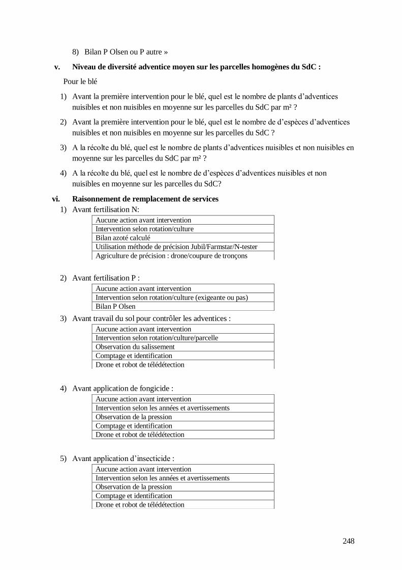
248

8) Bilan P Olsen ou P autre »

v. Niveau de diversité adventice moyen sur les parcelles homogènes du SdC :

Pour le blé

1) Avant la première intervention pour le blé, quel est le nombre de plants d’adventices

nuisibles et non nuisibles en moyenne sur les parcelles du SdC par m² ?

2) Avant la première intervention pour le blé, quel est le nombre de d’espèces d’adventices

nuisibles et non nuisibles en moyenne sur les parcelles du SdC ?

3) A la récolte du blé, quel est le nombre de plants d’adventices nuisibles et non nuisibles en

moyenne sur les parcelles du SdC par m² ?

4) A la récolte du blé, quel est le nombre de d’espèces d’adventices nuisibles et non

nuisibles en moyenne sur les parcelles du SdC?

vi. Raisonnement de remplacement de services

1) Avant fertilisation N:

2) Avant fertilisation P :

3) Avant travail du sol pour contrôler les adventices :

4) Avant application de fongicide :

5) Avant application d’insecticide :

Aucune action avant intervention

Intervention selon rotation/culture

Bilan azoté calculé

Utilisation méthode de précision Jubil/Farmstar/N-tester

Agriculture de précision : drone/coupure de tronçons

Aucune action avant intervention

Intervention selon rotation/culture (exigeante ou pas)

Bilan P Olsen

Aucune action avant intervention

Intervention selon rotation/culture/parcelle

Observation du salissement

Comptage et identification

Drone et robot de télédétection

Aucune action avant intervention

Intervention selon les années et avertissements

Observation de la pression

Comptage et identification

Drone et robot de télédétection

Aucune action avant intervention

Intervention selon les années et avertissements

Observation de la pression

Comptage et identification

Drone et robot de télédétection

249

6) Avant travail du sol pour structurer le sol :

7) Avant irrigation :

Aucune action avant intervention

Intervention selon les cultures/rotation et parcelles

Test bêche sur quelques parcelles

Test bêche systématiquement

Aucune action avant intervention

Intervention selon pluviométrie

Bilan hydrique

Utilisation de sonde tensiométriques ou capacitives

250

Description Système de Culture n°

Description parcelles du sdc n° : Analyses de sol Parcelles Type de sol Agrofor

esterie

Raison analyse pH Texture Teneur MO C/N P Olsen

P1

L :

A :

S :

P2

L :

A :

S :

P3

L :

A :

S :

P4

L :

A :

S :

Description des interventions du SdC n° : Travail du sol Culture et

intercultures

Labour/TCS/semi-direct Nombre de

passage

Itinéraire classique Outils Profondeur Fréquence labour en

mauvaise condition

pour cette culture (%)

C1

I1

Description des interventions du SdC n° : Autres interventions Culture

et

intercult

ures

Dose I Part de la

parcelle

traitée I

Produit I Dose F Part de la

parcelle

traitée F

Produit F Dose H Part de la

parcelle

traitée H

Produit

H

N

minéral

P

minéral

K

minéral

Autres

apports

organiqu

es

Qté

d’irrigati

on

C1

I1

Culture et intercultures

(couverts ? ou mulch ?)

Date

semi,RC

Date

récolte ou

destruction

couverts

Relais

cropping

ou inter-

rang

Variétés Mélanges

de variétés

Mélanges

d’espèces

Gestion des résidus

exporté/restitué (%)

Quantité de

biomasse

(en

moyenne

sur les

dernières

années)

C1

I1

251

2. Matériel supplémentaire de l’article « Influence of diversity and

intensification level on vulnerability, resilience and robustness of

agricultural systems »

Supplementary material 2. The 37 articles selected with description of the type of production, organisation

level, disturbance (categorised), attribute of performance (categorised) and explanatory factors tested.

Reference Prod.

Type

Org.

level

Disturbance Attribute Explanatory factors

Bardaji and Iraizoz

(2015)

Wine Farm

system

Climate variability

and change

Yield, quality of

production

Capital, labour, intensification of wine

production, adaptation

Barkaoui et al. (2016) Grassland Plot Drought Yield Composition effect, taxonomic diversity, functional diversity

Bitterman and Bennett

(2016)

Crop Region Policy adaptation

and drought

Number of

farmers in

business at the

end of

simulation

Economic market/insurance

Bouttes et al. (2018) Mixed Farm

system

Climate variability

and change

Yield, economic

efficiency of

production

Economic performance, intensification of

breeding system, composition effect, farm

diversity, livestock structure

Brunner and Grêt-

Regamey (2016)

Grassland Region Climatic and

economic

variability

Indicators of

ecosystem

services

provided

Open markets and migration policies

Carlsson et al. (2017) Grassland Plot Drought Yield Composition effect, taxonomic diversity

Carter and Blair (2012) Grassland Plot Drought Yield Taxonomic diversity

Castañeda-Vera and

Garrido (2017)

Crop Farm

system

Price volatility Economic net

return

Economic market/insurance, policies,

diversity of rotations

Chavas and Di Falco

(2017)

Crop Farm system

Pest and weather Yield

Cociu and Cizma (2015) Crop Plot Drought Yield Typology of agricultural systems

de la Rosa et al. (2000) Crop Farm

system

Climate variability

and change

Yield Soil characteristics

Di Falco and Chavas

(2008)

Crop Farm

system

Drought Yield Taxonomic diversity

Ferreyra et al. (2001) Crop Farm

system

Climate variability

and change

Yield, economic

net return

Initial soil water availability

Fletcher and Hilbert

(2007)

Grassland Farm

system

Not well defined Economic net

return

Adaptation

Gaudin et al. (2015) Crop Plot Climate variability

and change

Yield Diversity in rotation, intensification of crop

system, composition effect

Hoover et al. (2014) Grassland Plot Climate variability

and change

Yield

Isbell et al. (2015) Grassland Plot Climate variability

and change

Yield Taxonomic diversity

Kahiluoto et al. (2014) Crop Region Climatic and

economic

variability

Yield Taxonomic diversity

Leonhardt et al. (2013) Region Pollinator decrease Economic value

of crop production

Climate, pollination

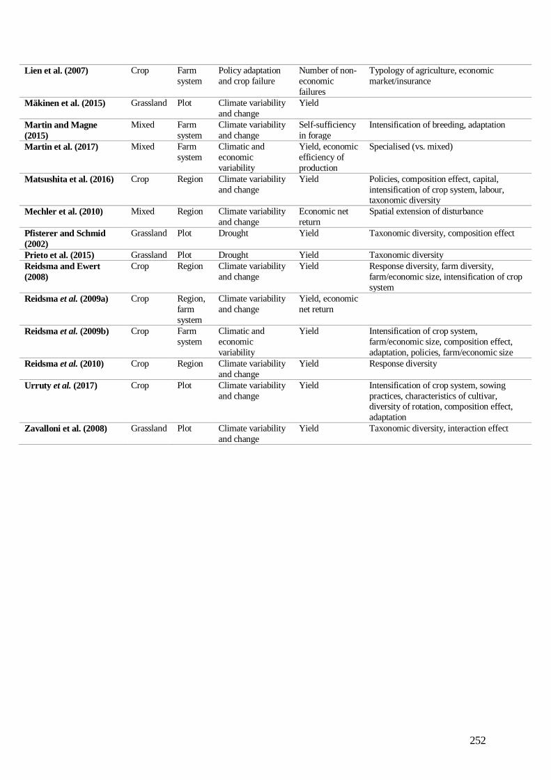
252

Lien et al. (2007) Crop Farm

system

Policy adaptation

and crop failure

Number of non-

economic

failures

Typology of agriculture, economic

market/insurance

Mäkinen et al. (2015) Grassland Plot Climate variability

and change

Yield

Martin and Magne

(2015)

Mixed Farm

system

Climate variability

and change

Self-sufficiency

in forage

Intensification of breeding, adaptation

Martin et al. (2017) Mixed Farm

system

Climatic and

economic

variability

Yield, economic

efficiency of

production

Specialised (vs. mixed)

Matsushita et al. (2016) Crop Region Climate variability

and change

Yield Policies, composition effect, capital,

intensification of crop system, labour, taxonomic diversity

Mechler et al. (2010) Mixed Region Climate variability

and change

Economic net

return

Spatial extension of disturbance

Pfisterer and Schmid

(2002)

Grassland Plot Drought Yield Taxonomic diversity, composition effect

Prieto et al. (2015) Grassland Plot Drought Yield Taxonomic diversity

Reidsma and Ewert

(2008)

Crop Region Climate variability

and change

Yield Response diversity, farm diversity,

farm/economic size, intensification of crop

system

Reidsma et al. (2009a) Crop Region,

farm

system

Climate variability

and change

Yield, economic

net return

Reidsma et al. (2009b) Crop Farm

system

Climatic and

economic

variability

Yield Intensification of crop system,

farm/economic size, composition effect,

adaptation, policies, farm/economic size

Reidsma et al. (2010) Crop Region Climate variability

and change

Yield Response diversity

Urruty et al. (2017) Crop Plot Climate variability

and change

Yield Intensification of crop system, sowing

practices, characteristics of cultivar, diversity of rotation, composition effect,

adaptation

Zavalloni et al. (2008) Grassland Plot Climate variability

and change

Yield Taxonomic diversity, interaction effect

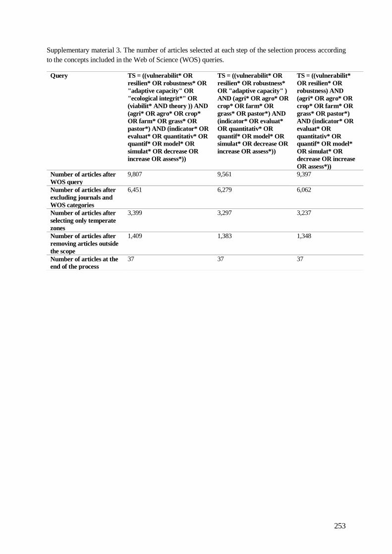
253

Supplementary material 3. The number of articles selected at each step of the selection process according

to the concepts included in the Web of Science (WOS) queries.

Query TS = ((vulnerabilit* OR

resilien* OR robustness* OR

"adaptive capacity" OR

"ecological integrit*" OR

(viabilit* AND theory )) AND

(agri* OR agro* OR crop*

OR farm* OR grass* OR

pastor*) AND (indicator* OR

evaluat* OR quantitativ* OR

quantif* OR model* OR

simulat* OR decrease OR

increase OR assess*))

TS = ((vulnerabilit* OR

resilien* OR robustness*

OR "adaptive capacity" )

AND (agri* OR agro* OR

crop* OR farm* OR

grass* OR pastor*) AND

(indicator* OR evaluat*

OR quantitativ* OR

quantif* OR model* OR

simulat* OR decrease OR

increase OR assess*))

TS = ((vulnerabilit*

OR resilien* OR

robustness) AND

(agri* OR agro* OR

crop* OR farm* OR

grass* OR pastor*)

AND (indicator* OR

evaluat* OR

quantitativ* OR

quantif* OR model*

OR simulat* OR

decrease OR increase

OR assess*))

Number of articles after

WOS query

9,807 9,561 9,397

Number of articles after

excluding journals and

WOS categories

6,451 6,279 6,062

Number of articles after

selecting only temperate

zones

3,399 3,297 3,237

Number of articles after

removing articles outside

the scope

1,409 1,383 1,348

Number of articles at the

end of the process

37 37 37

254

Supplementary material 4. Categories of production levels (low (< 5 t/ha), medium (5-20 t/ha), high (> 20

t/ha)) for grassland studies. Values were extracted from the articles’ graphs when data were not available.

Reference Description of harvest Biomass (g/m²) Category

Isbell et al. (2015) Peak biomass 256 low

Prieto et al. (2015) Peak biomass 900 medium

Barkaoui et al. (2016) Peak biomass 500 medium

Zavalloni et al. (2008) Peak biomass 2,000 high

Carlsson et al. (2017) Peak biomass after spring drought 300 low

Stampfli et al. (2018) During the summer after drought 200 low

Hoover et al. (2014) Peak biomass 600 medium

Mäkinen et al. (2015) Annual 800.7 medium

Pfisterer and Schmid (2002) Peak biomass after drought 461 low

Sabatier et al. (2015) Grazing season 200 low

Carter and Blair (2012) During the summer after drought 600 medium

255

Supplementary material 5. Number of criteria of performance attribute dynamics observed in the results

(black) and articles (red). See the article for a description of the criteria.

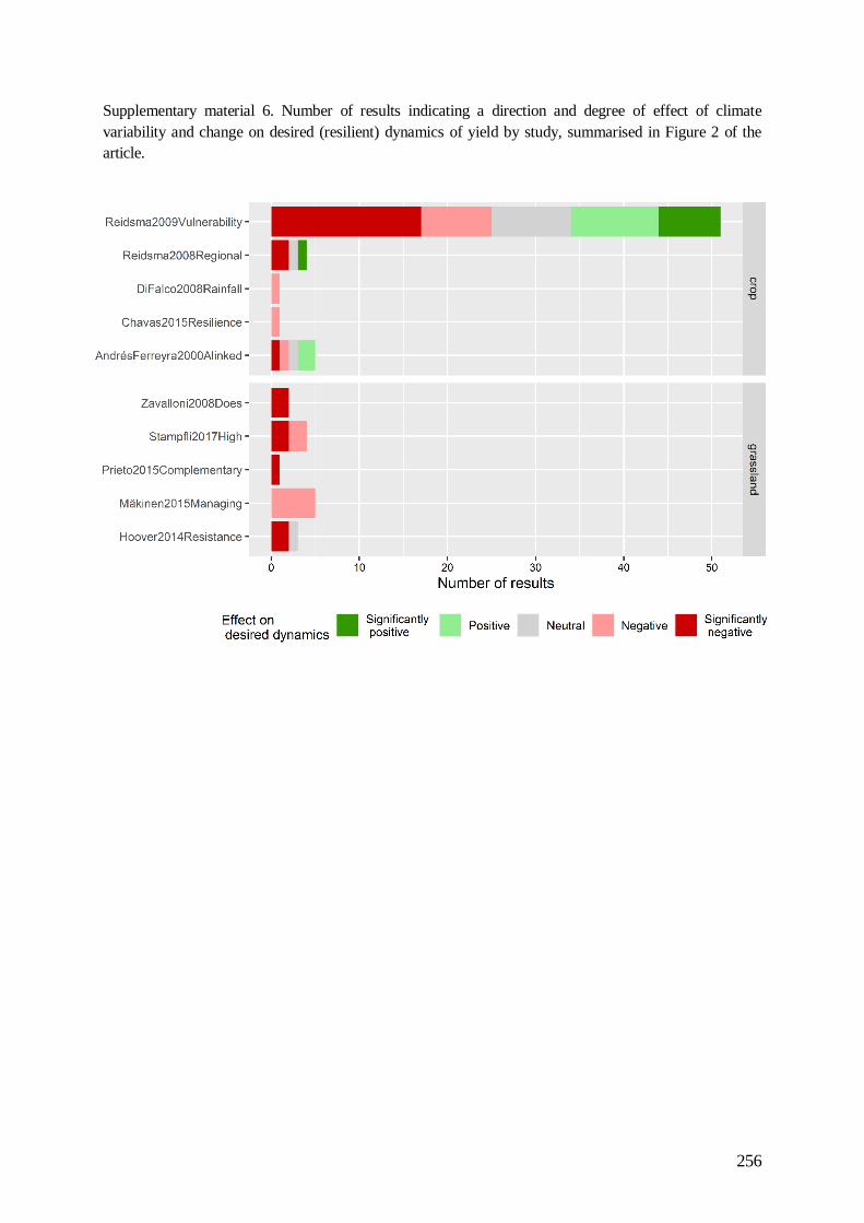
256

Supplementary material 6. Number of results indicating a direction and degree of effect of climate

variability and change on desired (resilient) dynamics of yield by study, summarised in Figure 2 of the

article.

257

Supplementary material 7. Number of results indicating a direction and degree of effect of effect of diversity

on the effect of climate variability and change on desired (resilient) dynamics of yield by study, summarised

in Figure 3 of the article.

258

Supplementary material 8. Number of results indicating a direction and degree of effect of the presence of

legumes on the effect of climate variability and change on desired (resilient) dynamics of yield for the

legume species for all systems. Each criterion was found in one article only. Significant effects are those

that could be tested statistically and were found significantly different (p<0.05).

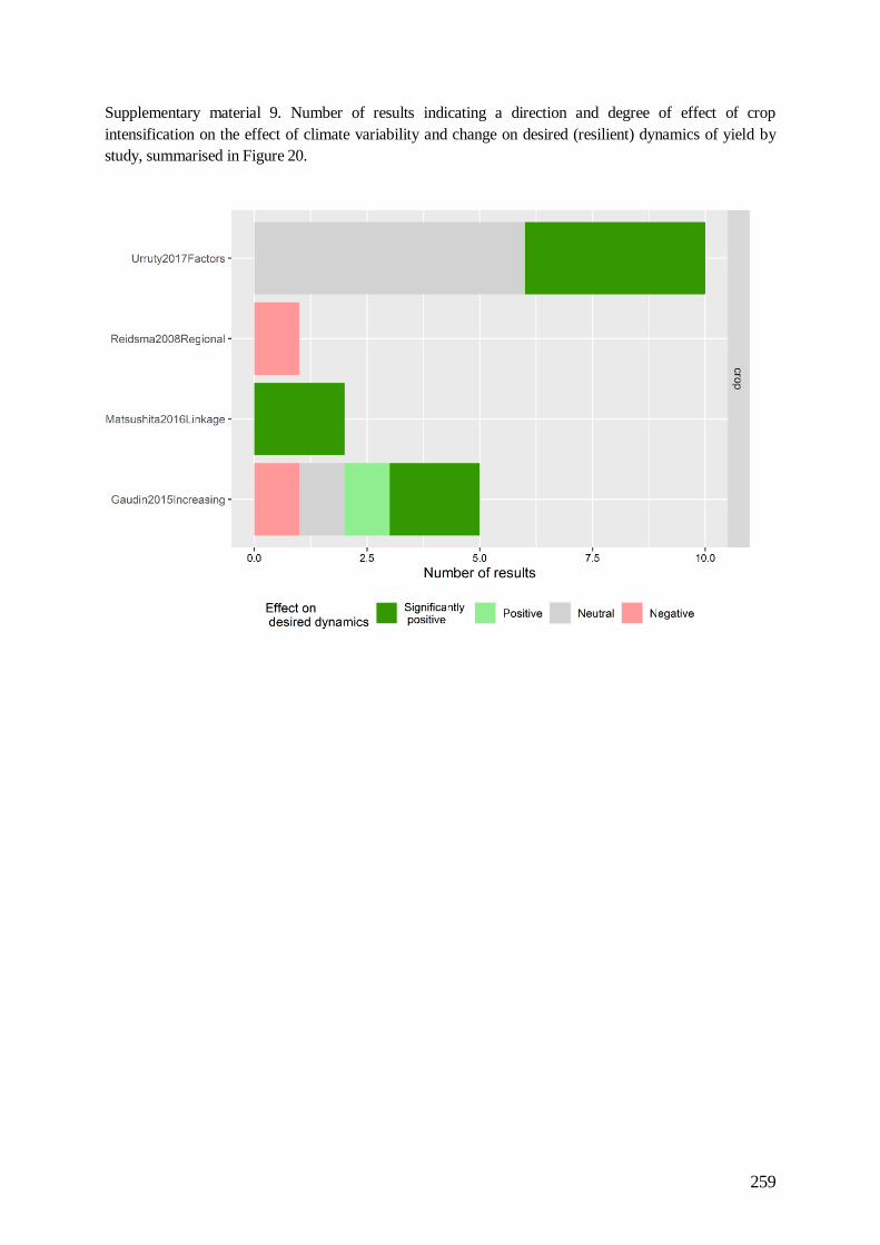
259

Supplementary material 9. Number of results indicating a direction and degree of effect of crop

intensification on the effect of climate variability and change on desired (resilient) dynamics of yield by

study, summarised in Figure 20.

260

Supplementary material 10. Number of results indicating a direction and degree of effect on the effect of

climate variability and change and economic variability on desired (resilient) dynamics of yield for crops,

wine and grasslands by type of explanatory factor and by study, summarised in Figure 21.

261

Supplementary material 11. Number of results indicating a direction and degree of effect on the effect of

climate variability and change on desired (resilient) dynamics of economic net return by type of explanatory

factor and by study, summarised in Figure 22.

262

3. Matériel supplémentaire de l’article « Review of quantitative

evaluations of the resilience, vulnerability, robustness and

adaptive capacity of temperate agricultural systems »

Supplementary material 12. Co-occurrence network of terms in the title and abstract of 3.938 articles

identified for screening.

263

Supplementary material 13. Explanatory factors encountered in the review.

Main category Subcategory Sub sub-category Sub sub-sub-category

Typology of

agricultural system

Organic system

Conservation practices

Specialized vs.

mixed

Specialized vs. mixed breeding system

Specialized vs. mixed crop-

livestock

Self-sufficiency For pasture-based grazing

systems

In fodder

In concentrates

Area available for grazing

Area used to feed livestock

Composition effect Legume

Poaceae

Cultivated paddy field area

Area of other agricultural

activities

Area of other arable crops

Cereal area

Maize or non-maize area

Cultivar (vs. wild)

Grass (vs. forbs)

Share of agriculture in the gross

national product of the country

Landscape composition and

configuration

Permanent and temporary

pasture area

Utilized agricultural area

Interaction effect Complementary effect

Selection effect

Livestock structure Percentage of heifers in the

herd

Calving period

Number of dairy cows

Characteristics of

cultivar

Variety earliness

Variety disease resistance

Adaptation Adaptation of agricultural

practices

Pesticide-use intensity

Nitrogen rate

Sowing density

Sowing date

Variety earliness at a different

stage (heading and joint)

Variety disease resistance

Technological evolution

Diversity Rotation

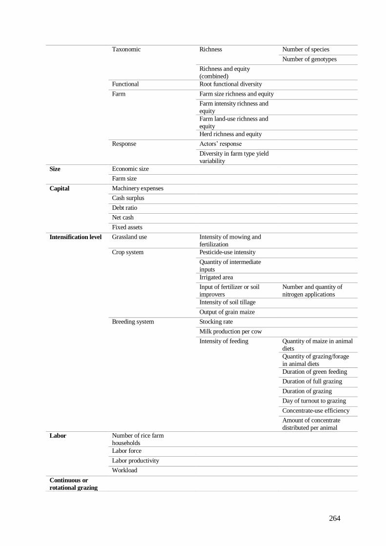
264

Taxonomic Richness Number of species

Number of genotypes

Richness and equity

(combined)

Functional Root functional diversity

Farm Farm size richness and equity

Farm intensity richness and

equity

Farm land-use richness and

equity

Herd richness and equity

Response Actors’ response

Diversity in farm type yield

variability

Size Economic size

Farm size

Capital Machinery expenses

Cash surplus

Debt ratio

Net cash

Fixed assets

Intensification level Grassland use Intensity of mowing and

fertilization

Crop system Pesticide-use intensity

Quantity of intermediate

inputs

Irrigated area

Input of fertilizer or soil

improvers

Number and quantity of

nitrogen applications

Intensity of soil tillage

Output of grain maize

Breeding system Stocking rate

Milk production per cow

Intensity of feeding Quantity of maize in animal

diets

Quantity of grazing/forage

in animal diets

Duration of green feeding

Duration of full grazing

Duration of grazing

Day of turnout to grazing

Concentrate-use efficiency

Amount of concentrate

distributed per animal

Labor Number of rice farm

households

Labor force

Labor productivity

Workload

Continuous or

rotational grazing

265

Policies Income stabilization tool

Direct payments “Green” direct payments

Governmental investment

Subsidies

Sowing practices Sowing date

Sowing density

Economic

performance

Economic efficiency of

production

Climate Warmer or colder country

Economic market/

insurance

Price of production (high)

Variable costs

Yield and production price

(both high)

Alternative market (Panicum virgatum)

Insurance

Initial water

availability

Invasion

Pollination Number of wild bees

Number of honey bees

Disturbed climate Low precipitation (drought)

Spatial extent of

disturbance

country level

region level

in an adjacent region

Soil characteristics

266

Supplementary material 14. Years of publication of the 53 reviewed articles.

267

Supplementary material 15. Type of production, organization level, disturbance (by category), performance

attribute (by category) and explanatory factors assessed in the 53 articles reviewed.

Reference Prod.

Type

Org.

level

Disturbance Attribute Explanatory factors

Bardaji and Iraizoz,

(2015)

Wine Farm

system

Climate variability

and change

Yield, quality of

production

Capital, labor, intensification of wine

production, adaptation

Barkaoui et al. (2016) Grassland Field Drought Yield Composition effect, taxonomic diversity,

functional diversity

Bitterman and

Bennett, (2016)

Crop Region Policy adaptation

and drought

Number of

farmers in

business at the

end of

simulation

Economic market/insurance

Bouttes et al. (2018) Mixed Farm

system

Climate variability

and change

Yield, economic

efficiency of

production

Economic performance, intensification of

breeding system, composition effect, farm

diversity, livestock structure

Bouttes et al. (2019) Mixed Farm

system

Climatic and

economic disturbances

Self-sufficiency

for forage, economic

efficiency of

production,

independence

from CAP,

economic net

return

Intensification of livestock system,

livestock structure, composition effect, farm diversity, perturbed climate,

economic market/ insurance,

Brunner and Grêt-

Regamey, (2016)

Grassland Region Climatic and

economic variability

Indicators of

ecosystem

services

provided

Open markets and migration policies

Carlsson et al. (2017) Grassland Field Drought Yield Composition effect, taxonomic diversity

Carter and Blair,

(2012)

Grassland Field Drought Yield Taxonomic diversity

Castañeda-Vera and

Garrido, (2017)

Crop Farm system

Price volatility Economic net return

Economic market/insurance, policies, diversity of rotations

Chavas and Di Falco,

(2017)

Crop Farm

system

Pest and weather Yield

Cociu and Cizma,

(2015)

Crop Field Drought Yield Typology of agricultural systems

Craven et al. (2018) Grassland Field Climate change and

biodiversity loss

Yield Taxonomic diversity

de la Rosa et al. (2000) Crop Farm

system

Climate variability

and change

Yield Soil characteristics

Di Falco and Chavas,

(2008)

Crop Farm

system

Drought Yield Taxonomic diversity

Ferreyra et al. (2001) Crop Farm

system

Climate variability

and change

Yield, economic

net return

Initial soil water availability

Fletcher and Hilbert,

(2007)

Grassland Farm

system

Not well defined Economic net

return

Adaptation

Gaudin et al. (2015) Crop Field Climate variability

and change

Yield Diversity in rotation, intensification of

crop system, composition effect

Grêt-Regamey et al.

(2019)

Mixed Farm

system

Socio-economic and

climate disturbances

Indicators of

ecosystem

services

Response diversity

Hoover et al. (2014) Grassland Field Climate variability and change

Yield

Isbell et al. (2015) Grassland Field Climate variability

and change

Yield Taxonomic diversity

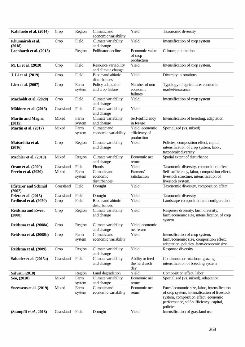
268

Kahiluoto et al. (2014) Crop Region Climatic and

economic variability

Yield Taxonomic diversity

Khumairoh et al.

(2018)

Crop Field Climate variability

and change

Yield Intensification of crop system

Leonhardt et al. (2013) Region Pollinator decline Economic value

of crop

production

Climate, pollination

M. Li et al. (2019) Crop Field Resource variability

and climate change

Yield Intensification of crop system,

J. Li et al. (2019) Crop Field Biotic and abiotic

disturbances

Yield Diversity in rotations

Lien et al. (2007) Crop Farm

system

Policy adaptation

and crop failure

Number of non-

economic failures

Typology of agriculture, economic

market/insurance

Macholdt et al. (2020) Crop Field Climate variability

and change

Yield Intensification of crop system

Mäkinen et al. (2015) Grassland Field Climate variability

and change

Yield

Martin and Magne,

(2015)

Mixed Farm

system

Climate variability

and change

Self-sufficiency

in forage

Intensification of breeding, adaptation

Martin et al. (2017) Mixed Farm

system

Climatic and

economic variability

Yield, economic

efficiency of

production

Specialized (vs. mixed)

Matsushita et al.

(2016)

Crop Region Climate variability

and change

Yield Policies, composition effect, capital,

intensification of crop system, labor,

taxonomic diversity

Mechler et al. (2010) Mixed Region Climate variability

and change

Economic net

return

Spatial extent of disturbance

Oram et al. (2020) Grassland Field Floods Yield Taxonomic diversity, composition effect

Perrin et al. (2020) Mixed Farm

system

Climatic and

economic

disturbances

Farmers’

satisfaction

Self-sufficiency, labor, composition effect,

livestock structure, intensification of

livestock system,

Pfisterer and Schmid

(2002)

Grassland Field Drought Yield Taxonomic diversity, composition effect

Prieto et al. (2015) Grassland Field Drought Yield Taxonomic diversity

Redhead et al. (2020) Crop Field Biotic and abiotic

disturbances

Yield Landscape composition and configuration

Reidsma and Ewert

(2008)

Crop Region Climate variability

and change

Yield Response diversity, farm diversity,

farm/economic size, intensification of crop

system

Reidsma et al. (2008a) Crop Region Climate variability

and change

Yield, economic

net return

Reidsma et al. (2008b) Crop Farm

system

Climatic and

economic variability

Yield Intensification of crop system,

farm/economic size, composition effect,

adaptation, policies, farm/economic size

Reidsma et al. (2009) Crop Region Climate variability

and change

Yield Response diversity

Sabatier et al. (2015a) Grassland Field Climate variability

and change

Ability to feed

the herd each

day

Continuous or rotational grazing,

intensification of breeding system

Salvati, (2010) Region Land degradation Yield Composition effect, labor

Seo, (2010) Mixed Farm

system

Climate variability

and change

Economic net

return

Specialized (vs. mixed), adaptation

Sneessens et al. (2019) Mixed Farm system

Climatic and economic variability

Economic net return

Farm/ economic size, labor, intensification of crop system, intensification of livestock

system, composition effect, economic

performance, self-sufficiency, capital,

policies

(Stampfli et al., 2018) Grassland Field Drought Yield Intensification of grassland use

269

Urruty et al. (2017) Crop Field Climate variability

and change

Yield Intensification of crop system, sowing

practices, characteristics of cultivar,

diversity of rotation, composition effect,

adaptation

van Strien et al. (2019) Mixed Farm

system

Climate variability

and change

Area of

extensive

agriculture

Policies

Vetter et al. (2020) Grassland Field Drought Yield Invasion, taxonomic diversity

Yang et al. (2019) Crop Field Disease impact Yield Taxonomic diversity

Zampieri et al. (2020b) Crop Field Climatic and socio-

economic events

Yield Taxonomic diversity

Zampieri et al. (2020a) Crop Region Heat and water

stress

Yield Intensification of crop system

Zavalloni et al. (2008) Grassland Field Climate variability and change

Yield Taxonomic diversity, interaction effect

270

Supplementary material 16. Number of articles that use each pair of criteria. The pairing of a criterion with

itself corresponds to articles that use only this criterion in the analysis. Pb = probability, Fq = frequency.

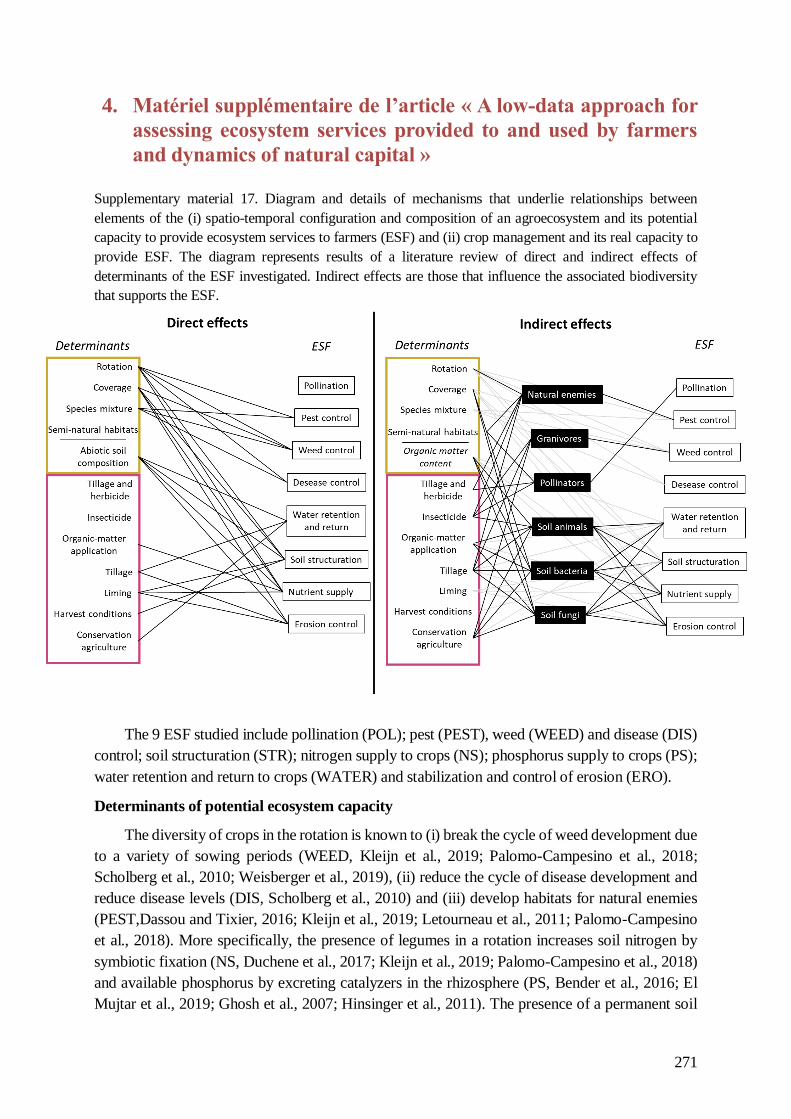
271

4. Matériel supplémentaire de l’article « A low-data approach for

assessing ecosystem services provided to and used by farmers

and dynamics of natural capital »

Supplementary material 17. Diagram and details of mechanisms that underlie relationships between

elements of the (i) spatio-temporal configuration and composition of an agroecosystem and its potential

capacity to provide ecosystem services to farmers (ESF) and (ii) crop management and its real capacity to

provide ESF. The diagram represents results of a literature review of direct and indirect effects of

determinants of the ESF investigated. Indirect effects are those that influence the associated biodiversity

that supports the ESF.

The 9 ESF studied include pollination (POL); pest (PEST), weed (WEED) and disease (DIS)

control; soil structuration (STR); nitrogen supply to crops (NS); phosphorus supply to crops (PS);

water retention and return to crops (WATER) and stabilization and control of erosion (ERO).

Determinants of potential ecosystem capacity

The diversity of crops in the rotation is known to (i) break the cycle of weed development due

to a variety of sowing periods (WEED, Kleijn et al., 2019; Palomo-Campesino et al., 2018;

Scholberg et al., 2010; Weisberger et al., 2019), (ii) reduce the cycle of disease development and

reduce disease levels (DIS, Scholberg et al., 2010) and (iii) develop habitats for natural enemies

(PEST,Dassou and Tixier, 2016; Kleijn et al., 2019; Letourneau et al., 2011; Palomo-Campesino

et al., 2018). More specifically, the presence of legumes in a rotation increases soil nitrogen by

symbiotic fixation (NS, Duchene et al., 2017; Kleijn et al., 2019; Palomo-Campesino et al., 2018)

and available phosphorus by excreting catalyzers in the rhizosphere (PS, Bender et al., 2016; El

Mujtar et al., 2019; Ghosh et al., 2007; Hinsinger et al., 2011). The presence of a permanent soil

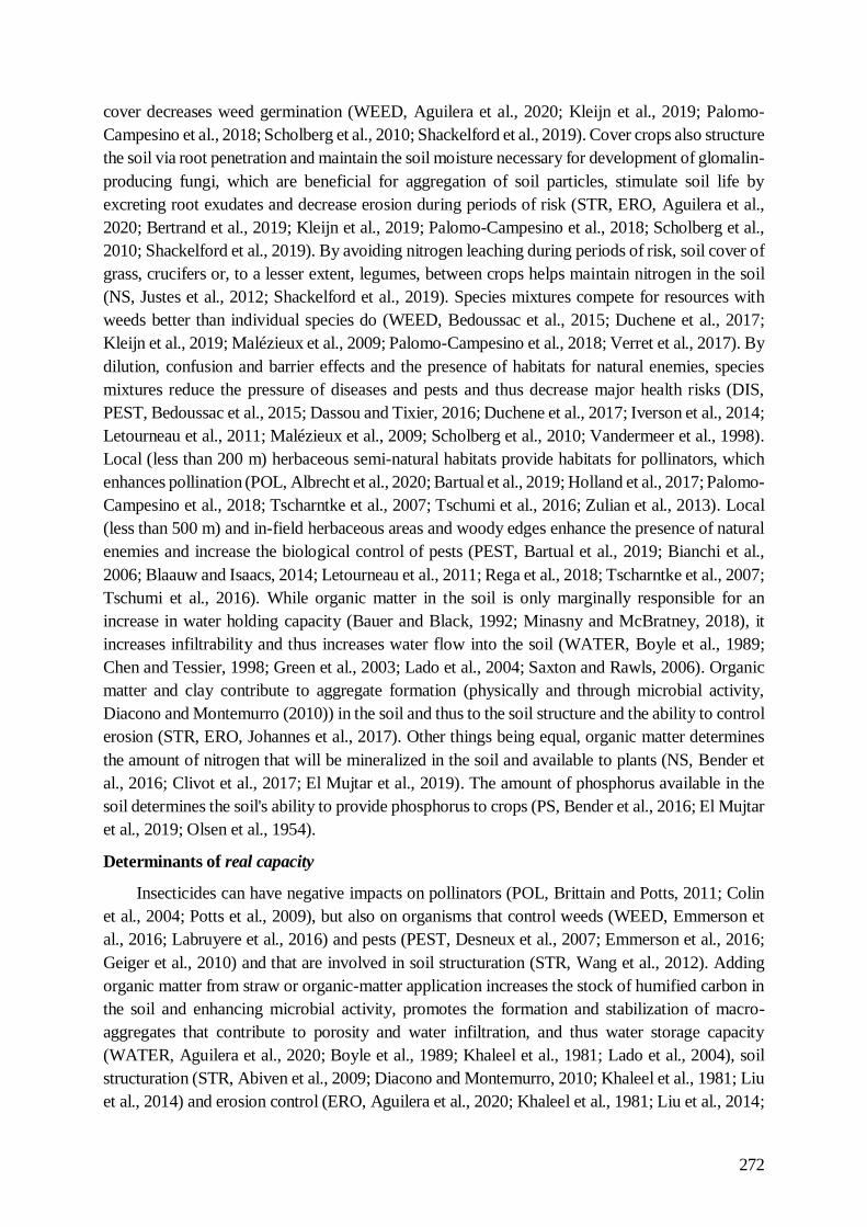
272

cover decreases weed germination (WEED, Aguilera et al., 2020; Kleijn et al., 2019; Palomo-

Campesino et al., 2018; Scholberg et al., 2010; Shackelford et al., 2019). Cover crops also structure

the soil via root penetration and maintain the soil moisture necessary for development of glomalin-

producing fungi, which are beneficial for aggregation of soil particles, stimulate soil life by

excreting root exudates and decrease erosion during periods of risk (STR, ERO, Aguilera et al.,

2020; Bertrand et al., 2019; Kleijn et al., 2019; Palomo-Campesino et al., 2018; Scholberg et al.,

2010; Shackelford et al., 2019). By avoiding nitrogen leaching during periods of risk, soil cover of

grass, crucifers or, to a lesser extent, legumes, between crops helps maintain nitrogen in the soil

(NS, Justes et al., 2012; Shackelford et al., 2019). Species mixtures compete for resources with

weeds better than individual species do (WEED, Bedoussac et al., 2015; Duchene et al., 2017;

Kleijn et al., 2019; Malézieux et al., 2009; Palomo-Campesino et al., 2018; Verret et al., 2017). By

dilution, confusion and barrier effects and the presence of habitats for natural enemies, species

mixtures reduce the pressure of diseases and pests and thus decrease major health risks (DIS,

PEST, Bedoussac et al., 2015; Dassou and Tixier, 2016; Duchene et al., 2017; Iverson et al., 2014;

Letourneau et al., 2011; Malézieux et al., 2009; Scholberg et al., 2010; Vandermeer et al., 1998).

Local (less than 200 m) herbaceous semi-natural habitats provide habitats for pollinators, which

enhances pollination (POL, Albrecht et al., 2020; Bartual et al., 2019; Holland et al., 2017; Palomo-

Campesino et al., 2018; Tscharntke et al., 2007; Tschumi et al., 2016; Zulian et al., 2013). Local

(less than 500 m) and in-field herbaceous areas and woody edges enhance the presence of natural

enemies and increase the biological control of pests (PEST, Bartual et al., 2019; Bianchi et al.,

2006; Blaauw and Isaacs, 2014; Letourneau et al., 2011; Rega et al., 2018; Tscharntke et al., 2007;

Tschumi et al., 2016). While organic matter in the soil is only marginally responsible for an

increase in water holding capacity (Bauer and Black, 1992; Minasny and McBratney, 2018), it

increases infiltrability and thus increases water flow into the soil (WATER, Boyle et al., 1989;

Chen and Tessier, 1998; Green et al., 2003; Lado et al., 2004; Saxton and Rawls, 2006). Organic

matter and clay contribute to aggregate formation (physically and through microbial activity,

Diacono and Montemurro (2010)) in the soil and thus to the soil structure and the ability to control

erosion (STR, ERO, Johannes et al., 2017). Other things being equal, organic matter determines

the amount of nitrogen that will be mineralized in the soil and available to plants (NS, Bender et

al., 2016; Clivot et al., 2017; El Mujtar et al., 2019). The amount of phosphorus available in the

soil determines the soil's ability to provide phosphorus to crops (PS, Bender et al., 2016; El Mujtar

et al., 2019; Olsen et al., 1954).

Determinants of real capacity

Insecticides can have negative impacts on pollinators (POL, Brittain and Potts, 2011; Colin

et al., 2004; Potts et al., 2009), but also on organisms that control weeds (WEED, Emmerson et

al., 2016; Labruyere et al., 2016) and pests (PEST, Desneux et al., 2007; Emmerson et al., 2016;

Geiger et al., 2010) and that are involved in soil structuration (STR, Wang et al., 2012). Adding

organic matter from straw or organic-matter application increases the stock of humified carbon in

the soil and enhancing microbial activity, promotes the formation and stabilization of macro-

aggregates that contribute to porosity and water infiltration, and thus water storage capacity

(WATER, Aguilera et al., 2020; Boyle et al., 1989; Khaleel et al., 1981; Lado et al., 2004), soil

structuration (STR, Abiven et al., 2009; Diacono and Montemurro, 2010; Khaleel et al., 1981; Liu

et al., 2014) and erosion control (ERO, Aguilera et al., 2020; Khaleel et al., 1981; Liu et al., 2014;

273

Paradelo et al., 2019). Once they mineralize, straw returned to the soil and applied organic matter

increase the soil's nitrogen and phosphorus reserves (NS, PS, Diacono and Montemurro, 2010;

Khaleel et al., 1981; Liu et al., 2014). Harvesting in adverse conditions can deform the soil

structure (e.g. compact it), which restricts soil life and its effect on structuration (STR, Hamza and

Anderson, 2005). Tillage can harm the suppressive capacity of soils by disrupting of food webs

and impeding weed and pest control (WEED, PEST, Blubaugh and Kaplan, 2015; Kuntz et al.,

2013; Menalled et al., 2007; Trichard et al., 2014). Plow tillage disrupts the natural channels that

allow water to circulate and prevents optimal storage due to the sole created (WATER, Aguilera

et al., 2020; Blanco-Canqui and Ruis, 2018; Soane et al., 2012). This sole compacts soil and

exposes it to compaction, which disturbs soil structuration and reduces erosion control (STR, ERO,

Aguilera et al., 2020; Blanco-Canqui and Ruis, 2018; Blevins et al., 2018; Hamza and Anderson,

2005; Soane et al., 2012). In the field, the abundance and diversity of non-crop plants result from

the tillage and herbicide strategy and these plants provide diversified habitats for pollinators (POL,

Bretagnolle and Gaba, 2015; Petit et al., 2016) and natural enemies (PEST, Dassou and Tixier,

2016; Petit et al., 2015). Conservation agriculture, which is a combination of diversified rotations,

permanent soil cover and reduced tillage, creates synergistic positive effects for weed control,

water retention capacity, soil structuration and the supply of nitrogen and phosphorus (WEED,

WATER, STR, NS, PS, Blanco-Canqui and Ruis, 2018; Kleijn et al., 2019; Lee et al., 2019;

Pittelkow et al., 2015a).

274

Supplementary material 18. Results of a literature review of effects of components of natural capital on the

ecosystem services provided to farmers (ESF) investigated.

The 9 ESF studied include pollination (POL); pest (PEST), weed (WEED) and disease (DIS)

control; soil structuration (STR); nitrogen supply to crops (NS); phosphorus supply to crops (PS);

water retention and return to crops (WATER) and stabilization and control of erosion (ERO).

Soil erosion results in a loss of soil due to runoff, which depends on precipitation, soil

composition (mostly soil organic matter (SOM) content and texture), slope, management and the

plant cover (Therond et al., 2017b). Soil quantity influences all ESF provided by the soil (WATER,

STR, ERO, NS, PS). SOM is a well-known determinant of soil structure, stability and functioning

(e.g. N mineralization regime, water infiltrability) and in turn many ESF (STR, NS, ERO,

WATER, Supplementary material 1) (Abiven et al., 2009; Aguilera et al., 2020a; Bender et al.,

2016; Diacono and Montemurro, 2010; El Mujtar et al., 2019; Weyers and Gramig, 2017).

Phosphorus is a non-renewable variable (Biggs et al., 2012) with a long response time that can

limit crop growth. The dynamics of this essential nutrient for crops rely on a complex balance

between annual imports (soluble P from mineral fertilization but not soluble from major organic-

matter application) and exports and a long mean residence time in the soil before used by plants

due to substantial P fixation in mineral P reservoirs and slow solubilization (Drinkwater and Snapp,

2007).

275

Supplementary material 19. Details of calculations of the indicators.

a. Proportion of legumes in the rotation

𝑙𝑒𝑔𝑢𝑚𝑒_𝑝𝑟𝑜𝑝𝑜𝑟𝑡𝑖𝑜𝑛_𝑟𝑜𝑡𝑎𝑡𝑖𝑜𝑛 = (%𝑙𝑐𝑟𝑜𝑝𝑠 . 𝑝𝑙 + %𝑙𝑙𝑜𝑛𝑔. 𝑝𝑙 + (1

2) %𝑙𝑠ℎ𝑜𝑟𝑡 . 𝑝𝑙)/maximum

%𝑙𝑐𝑟𝑜𝑝𝑠,𝑙𝑜𝑛𝑔,𝑠ℎ𝑜𝑟𝑡: percentage of legume crops in the rotation, including long-term (>6

months) crops and short-term cover crops.

maximum: 250% (= 100% + 100% + 50%)

𝑝l: proportion of legumes if the field has a species mixture

b. 95% root density depth and proportion of cover crops in the rotation

𝑐𝑜𝑣𝑒𝑟𝑎𝑔𝑒𝑆𝑇𝑅 =1

2∑ 𝑆𝑐𝑜𝑟𝑒_𝑑95𝑖

𝑖+

1

2∑

𝑛𝑗

𝑁𝑦𝑒𝑎𝑟𝑠𝑗

With: 𝑖 each crop in the rotation

𝑑95: the soil depth that contains 95% of the total roots of crop 𝑖, according to Fan et al. (2016)

𝑗: each intercrop in the rotation

𝑛𝑗: number of cover crops in the rotation

𝑁𝑦𝑒𝑎𝑟𝑠: duration of the rotation in years

𝑺𝒄𝒐𝒓𝒆_𝒅𝟗𝟓𝒊 𝒎𝒆𝒂𝒏(𝒅𝟗𝟓𝒊

)

0 𝒎𝒆𝒂𝒏(𝒅𝟗𝟓𝒊) < 80

0.25 80 ≤ 𝒎𝒆𝒂𝒏(𝒅𝟗𝟓𝒊)< 97

0.5 97 ≤ 𝒎𝒆𝒂𝒏(𝒅𝟗𝟓𝒊)< 115

0.75 115 ≤ 𝒎𝒆𝒂𝒏(𝒅𝟗𝟓𝒊)< 132

1 132 ≤ 𝒎𝒆𝒂𝒏(𝒅𝟗𝟓𝒊)

The maximum depth is determined by sugar beets, whose 95% root density depth is 150 cm.

c. Proportion of crops and intercrops in the fall to avoid leaching

𝑐𝑜𝑣𝑒𝑟𝑎𝑔𝑒𝑁 = ∑𝑠𝑐𝑜𝑟𝑒_𝑐𝑜𝑣𝑒𝑟𝑎𝑔𝑒𝑖

𝑁𝑦𝑒𝑎𝑟𝑠𝑖

With: 𝑖 each crop or intercrop during the fall

276

𝒔𝒄𝒐𝒓𝒆_𝒄𝒐𝒗𝒆𝒓𝒂𝒈𝒆𝒊 𝒊 family

0 Others

0.5 Fabaceae

0.75 Fabaceae, Poaceae, Brassicaceae mixture

1 Poaceae or Brassicaceae

𝑁𝑦𝑒𝑎𝑟𝑠: duration of the rotation in years

d. Proportion of crops and intercrops with a species mixture

𝑚𝑖𝑥𝑡𝑢𝑟𝑒𝑊𝐸𝐸𝐷 =1

2∑

𝑛𝑚𝑖𝑥𝑡𝑖

𝑁𝑖+ 1/2 ∑

𝑛𝑚𝑖𝑥𝑡𝑗

𝑀𝑗

With: 𝑖 each crop in the rotation

𝑛𝑚𝑖𝑥𝑡𝑖: number of crops with a species mixture in the rotation

𝑗: each intercrop in the rotation

𝑁: number of crops in the rotation

𝑛𝑚𝑖𝑥𝑡𝑗: number of intercrops with a species mixture in the rotation

𝑀: number of intercrops in the rotation

e. Proportion of field area close to herbaceous habitat

𝑆𝑁𝐻𝑃𝑂𝐿 =1

𝑆𝑡𝑜𝑡∑ 𝑠200_𝑘

𝑘

With: 𝑘 each field in the agroecosystem

𝑆𝑡𝑜𝑡: total area of the agroecosystem

𝑠200_𝑘: area of field 𝑘 at least 200 m from a herbaceous semi-natural habitat

f. TFI relative to average regional TFI

𝑖𝑛𝑠𝑒𝑐𝑡𝑖𝑐𝑖𝑑𝑒𝑃𝑂𝐿,𝑊𝐸𝐸𝐷,𝑃𝐸𝑆𝑇,𝑆𝑇𝑅 =1

𝑁∑ 𝑠𝑐𝑜𝑟𝑒_𝑇𝐹𝐼𝑖

𝑖

With: 𝑖 each crop in the rotation

𝑇𝐹𝐼𝑖: treatment frequency index, i.e. the number of pesticide treatments per ha for crop 𝑖,

based on standard dose rates of active ingredients and the amount of pesticides sold yearly

𝑇𝐹𝐼𝑟𝑒𝑔𝑖𝑜𝑛𝑎𝑙 : mean regional reference TFI for crop 𝑖

𝑁: number of crops in the rotation

𝒔𝒄𝒐𝒓𝒆_𝑻𝑭𝑰𝒊

- 1 𝑻𝑭𝑰𝒊 ≥ 𝑻𝑭𝑰𝒓𝒆𝒈𝒊𝒐𝒏𝒂𝒍𝒊

277

- 0.75 𝑻𝑭𝑰𝒓𝒆𝒈𝒊𝒐𝒏𝒂𝒍𝒊> 𝑻𝑭𝑰𝒊 > ½ 𝑻𝑭𝑰𝒓𝒆𝒈𝒊𝒐𝒏𝒂𝒍𝒊

- 0.5 𝑻𝑭𝑰𝒊= ½ 𝑻𝑭𝑰𝒓𝒆𝒈𝒊𝒐𝒏𝒂𝒍𝒊

- 0.25 ½ 𝑻𝑭𝑰𝒓𝒆𝒈𝒊𝒐𝒏𝒂𝒍𝒊> 𝑻𝑭𝑰𝒊> 0

0 𝑻𝑭𝑰𝒊 = 0

g. Annual humified carbon inputs

- Carbon input

The score is assigned according to the following table. The upper boundary is set for the

maximum possible carbon input set by experts: 100% rapeseed whose straw is returned, with a

mean yield of 3.3 t/ha and a harvest index of 0.25, and 1 t/ha of dried poultry manure with 23.8%

C.

Score X =

𝑪𝒐𝒓𝒈𝒂𝒏𝒊𝒄_𝒂𝒑𝒑𝒍𝒊𝒄𝒂𝒕𝒊𝒐𝒏𝑾𝑨𝑻𝑬𝑹,𝑺𝑻𝑹,𝑬𝑹𝑶

0 X ≤ 227

0.25 227 < X ≤ 454

0.5 454 < X ≤ 681

0.75 681 < X ≤ 908

1 908 < X

𝐶𝑜𝑟𝑔𝑎𝑛𝑖𝑐_𝑎𝑝𝑝𝑙𝑖𝑐𝑎𝑡𝑖𝑜𝑛𝑊𝐴𝑇𝐸𝑅,𝑆𝑇𝑅,𝐸𝑅𝑂 =1

𝑆𝑡𝑜𝑡∑ 𝑘1𝑖 ∗ 𝑚𝐶𝑖

𝐶𝑜𝑟𝑔_𝑎𝑝𝑝𝑙𝑖𝑐𝑎𝑡𝑖𝑜𝑛𝑊𝐴𝑇𝐸𝑅,𝑆𝑇𝑅,𝑁,𝑃,𝐸𝑅𝑂 is the annual humified organic carbon (Corg) inputs

across the agroecosystem (kg C/ha/yr) from crops, intercrops and organic waste products (OWP).

𝑆𝑡𝑜𝑡: total area of the agroecosystem

𝑘1𝑖: isohumic coefficient of carbon source 𝑖

𝑚𝐶𝑖: mass of carbon (kg) in carbon source 𝑖

𝑚𝐶𝑖 𝑟𝑒𝑠𝑖𝑑𝑢𝑎𝑙𝑠 = 1000 ∗ (𝑠𝑡𝑟𝑎𝑤/100 ∗ (𝑦𝑙𝑑 ∗ (1 −

ℎ𝑢𝑚100 ) − 𝑖𝑟 ∗ 𝑦𝑙𝑑 ∗ (1 −

ℎ𝑢𝑚100 )

𝑖𝑟

)

∗ 𝑎 ∗ 𝐶

278

+𝑓𝑒𝑥𝑝𝑜𝑟𝑡 ∗ (1 −𝑠𝑡𝑟𝑎𝑤

100) ∗ (

𝑦𝑙𝑑 ∗ (1 −ℎ𝑢𝑚100 ) − 𝑖𝑟 ∗ 𝑦𝑙𝑑 ∗ (1 −

ℎ𝑢𝑚100 )

𝑖𝑟

) ∗ 𝑎 ∗ 𝐶)

With 𝑠𝑡𝑟𝑎𝑤: percentage of 𝑖 straw returned to the ground at harvest

𝑓𝑒𝑥𝑝𝑜𝑟𝑡: proportion of stubble of 𝑖 remaining on the ground

𝐶: carbon concentration in straw of 𝑖, set at 0.44 (g/g) according to Clivot et al. (2019)

𝑦𝑙𝑑: mean 𝑖 grain yield (t/ha)

ℎ𝑢𝑚: percentage grain moisture of 𝑖 at harvest

𝑖𝑟: harvest index (grain yield/total biomass)

𝑎: area of 𝑖 (ha)

𝑚𝐶𝑖𝑂𝑊𝑃= 𝑡 ∗ 𝑎 ∗ 𝐶 ∗ 10

𝑡: amount of 𝑖 supplied in t (fresh matter) per ha

𝑎: area of 𝑖 (ha)

𝐶: carbon concentration in 𝑖

- Nitrogen input

The score is assigned according to the following table. The upper boundary is set for the

maximum possible nitrogen input set by experts: 100% rapeseed whose straw is returned, with a

mean yield of 3.3 t/ha and a harvest index of 0.25, and 1 t/ha of dried poultry manure with 23.8%

C.

Score X =

𝑵𝒐𝒓𝒈𝒂𝒏𝒊𝒄_𝒂𝒑𝒑𝒍𝒊𝒄𝒂𝒕𝒊𝒐𝒏𝑵

0 X ≤ 8.5

0.25 8.5 < X ≤ 17

0.5 17 < X ≤ 25.5

0.75 25.5 < X ≤ 34

1 34 < X

𝑁𝑜𝑟𝑔𝑎𝑛𝑖𝑐_𝑎𝑝𝑝𝑙𝑖𝑐𝑎𝑡𝑖𝑜𝑛𝑁 = 1

𝑆𝑡𝑜𝑡∑

𝑚𝐶𝑖

𝐶: 𝑁𝑖

𝑁𝑜𝑟𝑔𝑎𝑛𝑖𝑐_𝑎𝑝𝑝𝑙𝑖𝑐𝑎𝑡𝑖𝑜𝑛𝑁 is the annual nitrogen inputs across the agroecosystem (kg

N/ha/yr) from crops, intercrops and organic waste products (OWP).

𝑚𝐶𝑖: mass of carbon (kg) in carbon source 𝑖

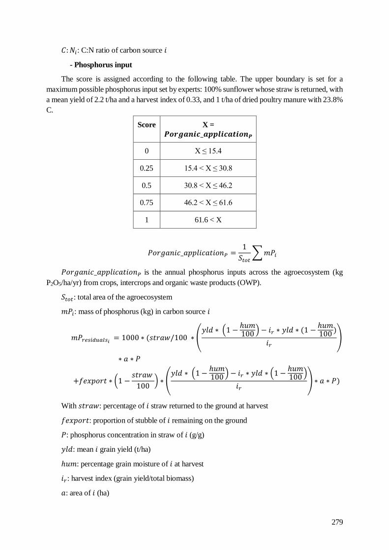
279

𝐶: 𝑁𝑖: C:N ratio of carbon source 𝑖

- Phosphorus input

The score is assigned according to the following table. The upper boundary is set for a

maximum possible phosphorus input set by experts: 100% sunflower whose straw is returned, with

a mean yield of 2.2 t/ha and a harvest index of 0.33, and 1 t/ha of dried poultry manure with 23.8%

C.

Score X =

𝑷𝒐𝒓𝒈𝒂𝒏𝒊𝒄_𝒂𝒑𝒑𝒍𝒊𝒄𝒂𝒕𝒊𝒐𝒏𝑷

0 X ≤ 15.4

0.25 15.4 < X ≤ 30.8

0.5 30.8 < X ≤ 46.2

0.75 46.2 < X ≤ 61.6

1 61.6 < X

𝑃𝑜𝑟𝑔𝑎𝑛𝑖𝑐_𝑎𝑝𝑝𝑙𝑖𝑐𝑎𝑡𝑖𝑜𝑛𝑃 =1

𝑆𝑡𝑜𝑡∑ 𝑚𝑃𝑖

𝑃𝑜𝑟𝑔𝑎𝑛𝑖𝑐_𝑎𝑝𝑝𝑙𝑖𝑐𝑎𝑡𝑖𝑜𝑛𝑃 is the annual phosphorus inputs across the agroecosystem (kg

P2O5/ha/yr) from crops, intercrops and organic waste products (OWP).

𝑆𝑡𝑜𝑡: total area of the agroecosystem

𝑚𝑃𝑖: mass of phosphorus (kg) in carbon source 𝑖

𝑚𝑃𝑟𝑒𝑠𝑖𝑑𝑢𝑎𝑙𝑠𝑖 = 1000 ∗ (𝑠𝑡𝑟𝑎𝑤/100 ∗ (𝑦𝑙𝑑 ∗ (1 −

ℎ𝑢𝑚100

) − 𝑖𝑟 ∗ 𝑦𝑙𝑑 ∗ (1 −ℎ𝑢𝑚100

)

𝑖𝑟

)

∗ 𝑎 ∗ 𝑃

+𝑓𝑒𝑥𝑝𝑜𝑟𝑡 ∗ (1 −𝑠𝑡𝑟𝑎𝑤

100) ∗ (

𝑦𝑙𝑑 ∗ (1 −ℎ𝑢𝑚100 ) − 𝑖𝑟 ∗ 𝑦𝑙𝑑 ∗ (1 −

ℎ𝑢𝑚100 )

𝑖𝑟

) ∗ 𝑎 ∗ 𝑃)

With 𝑠𝑡𝑟𝑎𝑤: percentage of 𝑖 straw returned to the ground at harvest

𝑓𝑒𝑥𝑝𝑜𝑟𝑡: proportion of stubble of 𝑖 remaining on the ground

𝑃: phosphorus concentration in straw of 𝑖 (g/g)

𝑦𝑙𝑑: mean 𝑖 grain yield (t/ha)

ℎ𝑢𝑚: percentage grain moisture of 𝑖 at harvest

𝑖𝑟: harvest index (grain yield/total biomass)

𝑎: area of 𝑖 (ha)

280

𝑚𝑃𝑂𝑊𝑃 𝑖= 𝑡 ∗ 𝑎 ∗ 𝑃 ∗ 10

𝑡: quantity of 𝑖 supplied in t (fresh matter) per ha

𝑎: area of 𝑖 (ha)

𝑃: phosphorus concentration in 𝑖

h. Cumulative depth of tillage operations

𝑡𝑖𝑙𝑙𝑎𝑔𝑒𝑃𝐸𝑆𝑇,𝑊𝐴𝑇𝐸𝑅,𝑆𝑇𝑅,𝐸𝑅𝑂 = −(1

𝑁∑ 𝑑𝑖

𝑖)/𝐷

With: 𝑖 each crop in the rotation

𝑁: number of crops in the rotation

𝑑𝑖: depths of all mechanical operations that disturb the soil deeper than 1 cm for 𝑖

𝐷: = 88 is the estimated maximum disturbance according to experts, which is a highly soil-

disturbing tillage: stubble plowing (10 cm) / plowing (20 cm) / rotary harrow (10 cm) / sowing (3

cm) / hoeing (5 cm).

i. Abundance and diversity of non-crop plants at harvest and before first tillage or

herbicide application

𝑛𝑜𝑛𝑐𝑟𝑜𝑝𝑝𝑙𝑎𝑛𝑡𝑠𝑃𝑂𝐿,𝑃𝐸𝑆𝑇 =1

4𝑎1 +

1

4𝑑1 +

1

4𝑎2 +

1

4𝑑2

𝒂𝟏 Number of non-crop plants per m² before first tillage or herbicide

application for wheat estimated by the farmer (N)

0 0

0.25 0 < N ≤ 50

0.5 50 < N ≤ 100

0.75 100 < N ≤ 150

1 150 < N

𝒅𝟏 Number of species of non-crop plants before first tillage or herbicide

application for wheat estimated by the farmer (N)

0 0

0.25 0 < N ≤ 4

0.5 4 < N ≤ 8

281

j. Synergistic effect of conservation agriculture

When the score of cropfamily * > 0.75, when the land cover is continuous

(continuouslandcover = 1) and cumulative depth of tillage operations (𝑡𝑖𝑙𝑙𝑎𝑔𝑒) < -0.25, a

bonus score of 1 is given for WEED, WATER, STR, N and P.

1. cropfamily =1

∑ (𝑛𝑖𝑁

)2

𝑖

𝑛𝑖: number of crops belonging to family 𝑖

𝑁: number of crops in the rotation

* from (Craheix et al., 2012)

2. continuouslandcover =

1, if the rotation has fewer than 3 months without crops or intercrops; otherwise, 0

3. 𝑡𝑖𝑙𝑙𝑎𝑔𝑒 = −(1

𝑁∑ 𝑑𝑖𝑖 )/𝐷

With: 𝑖 each crop in the rotation

0.75 8 < N ≤ 12

1 12 < N

𝒂𝟐 Number of non-crop plants per m² before wheat harvest estimated by the

farmer (N)

0 0

0.25 0 < N ≤ 12.5

0.5 12.5 < N ≤ 25

0.75 25 < N ≤ 37.5

1 37.5 < N

𝒅𝟐 Number of species of non-crop plants before wheat harvest estimated

by the farmer (N)

0 0

0.25 0 < N ≤ 4

0.5 4 < N ≤ 8

0.75 8 < N ≤ 12

1 12 < N

282

𝑁: number of crops in the rotation

𝑑𝑖: depths for all mechanical operations that disturb the soil deeper than 1 cm for 𝑖

𝐷: = 88 is the estimated maximum disturbance according to experts, which is a highly soil-

disturbing tillage: Stubble plowing (10 cm) / plowing (20 cm) / rotary harrow (10 cm) / sowing (3

cm) / hoeing (5 cm).

k. Proportion of cover crops in the rotation

𝑐𝑜𝑣𝑒𝑟𝑐𝑟𝑜𝑝𝑝𝑟𝑜𝑝𝑜𝑟𝑡𝑖𝑜𝑛 = ∑𝑛𝑗

𝑁𝑦𝑒𝑎𝑟𝑠𝑗

With: 𝑗 each crop in the rotation

𝑗: each intercrop in the rotation

𝑛𝑗: number of cover crops in the rotation

𝑁𝑦𝑒𝑎𝑟𝑠: duration of the rotation in years

l. Diversity in carbon inputs

𝑑𝑖𝑣𝐶𝑖𝑛𝑝𝑢𝑡𝑠=

ncropfamily

10+

𝑛𝑂𝑊𝑃

3+

𝑛𝑐𝑜𝑣𝑒𝑟𝑐𝑟𝑜𝑝

12

With ncropfamily: number of crop families in the rotation

𝑛𝑂𝑊𝑃 : number of each type of organic waste product applied in the agroecosystem

𝑛𝑐𝑜𝑣𝑒𝑟𝑐𝑟𝑜𝑝: number of plant species in cover crops in the rotation

283

Supplementary material 20. Method used to assess soil quantity dynamics as the potential sensitivity to

erosion, developed by Rosenfelder and van Dijk (2014) and van Dijk et al. (2016)

The index for the potential sensitivity to erosion (PSE) (1) of the agroecosystem was

calculated using the mean of the product of an erodibility index (K_ER) and an exposure

(EX(crop)) index for all crops in the rotation (𝑛_𝑐𝑟𝑜𝑝 is the number of crops) as described by

Rosenfelder and van Dijk (2014) and van Dijk et al. (2016). The K-factor of PSE is calculated as

recommended by Torri et al. (1997) (1) and is divided into five classes according to Schwertmann

et al. (1987) and Vopravil et al. (2007).

𝑃𝑆𝐸 =∑ 𝐾𝐸𝑅 ∗ 𝐸𝑋(𝑐𝑟𝑜𝑝)𝑐𝑟𝑜𝑝

𝑛_𝑐𝑟𝑜𝑝

𝐾𝐸𝑅 = 0.0293(0.65 − 𝐵𝐷 + 0.24𝐵𝐷2) ∗ exp (−0.0021𝑂𝑀

𝐶/10− 0.00037

𝑂𝑀

𝐶/10

2

− 4.02𝐶

+ 1.72(𝐶

10)2)

With bulk density 𝐵𝐷 = −0.35𝐶−2𝐿−0.5𝑆

100; C, L, S, and OM are the percentage of clay, loam,

sand, and organic matter, respectively.

Exposure under the crop 𝐸𝑋(𝑐𝑟𝑜𝑝) is calculated as the precipitation erosivity index

(𝐸𝑅𝑝𝑟𝑒𝑐(𝑚)) multiplied by the land cover effect on the erosion index 𝑓(𝑐𝑟𝑜𝑝) for each month

from April to July (the most erosive period in the region). The precipitation erosivity index is the

Angot index, which equals the ratio of monthly rainfall to annual rainfall per month (Péguy, 1970).

The influence of land cover on the erosion index is defined according to Langdale et al. (1991) (1

= land cover has no influence on erosion, 0 = land cover results in zero erosion).

𝐸𝑋(𝑐𝑟𝑜𝑝) = ∑ 𝐸𝑅𝑝𝑟𝑒𝑐(𝑚) ∗

𝐽𝑢𝑙𝑦

𝐴𝑝𝑟𝑖𝑙

𝑓(𝑐𝑟𝑜𝑝)

With 𝐸𝑅𝑝𝑟𝑒𝑐(𝑚) = 𝑝𝑟𝑒𝑐(𝑚) ∗ 365 ∗ (1

𝑝𝑟𝑒𝑐𝑎𝑛𝑛) ∗ (

1

𝑛𝑚); 𝑝𝑟𝑒𝑐(𝑚) is total precipitation for

month 𝑚, 𝑝𝑟𝑒𝑐𝑎𝑛𝑛 is total precipitation for the year, and 𝑛𝑚 is the number of days in month 𝑚.

With 𝑓(𝑐𝑟𝑜𝑝) = exp (−𝑏𝑐𝑟𝑜𝑝 ∗ 𝑐𝑐𝑟𝑜𝑝) ; 𝑐𝑐𝑟𝑜𝑝 is the proportion of the area covered with

vegetation, and 𝑏𝑐𝑟𝑜𝑝 is a coefficient related to the spatial structure of vegetation (weeded or

unweeded, density and spacing of plants, and plant architecture (height and foliage structure));

values range from ca. 2.5 to 7, with higher values for straw cereals with high plant density and

lower values for weeded crops with low plant density (Laflen and Colvin, 1981).

According to Rosenfelder and van Dijk (2014), PSE = 0.022 is considered high, and PSE =

0.015 is acceptable. We developed an indicator of sensitivity to erosion [-1:1] with five classes

that range from highly to unlikely.

284

potential sensitivity to erosion (PSE) Class Score

PSE <0.0105 Non-erodible soil 1

0.0105 ≤ PSE <0.015 Slightly erodible soil 0.5

0.0015 ≤ PSE <0.0195 Moderately erodible soil 0

0.0195 ≤ PSE <0.022 Highly erodible soil -0.5

0.022 ≤ PSE Very highly erodible soil -1

285

Supplementary material 21. Distribution of the trend of the linear regression of soil carbon stock dynamics

for 34 agroecosystems.

The trend of the linear

regression of soil carbon stock

dynamics

Score

0.22 ≤ Trend 1

0.025 ≤ Trend < 0.22 0.5

-0.035 < Trend <0.025 0

-0.22 < Trend ≤ -0.035 -0.5

Trend ≤ -0.22 -1

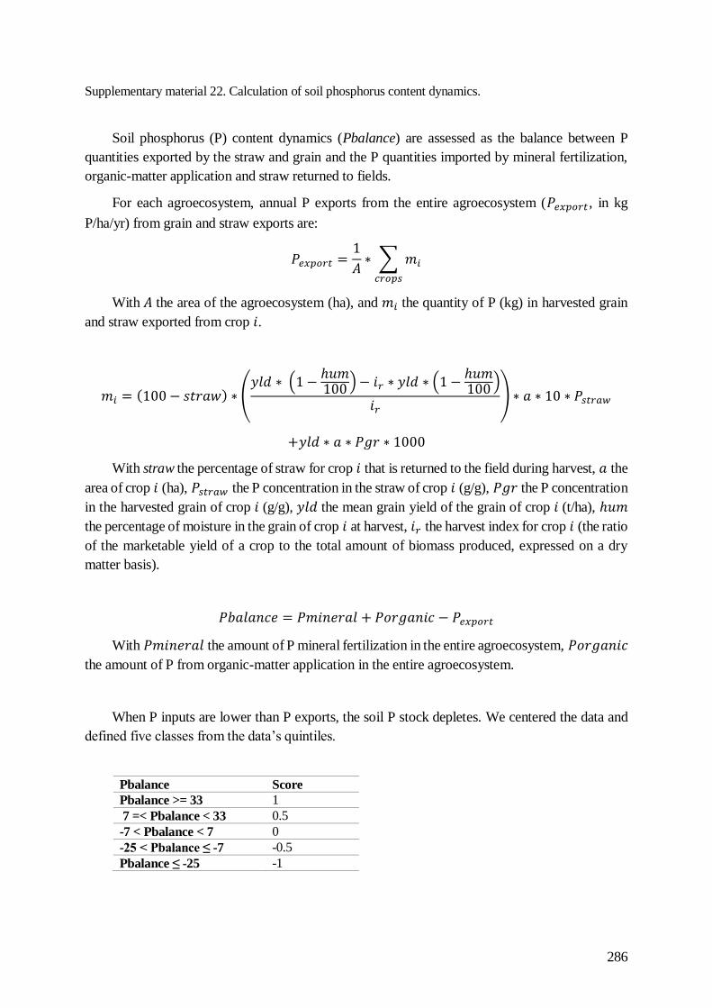
286

Supplementary material 22. Calculation of soil phosphorus content dynamics.

Soil phosphorus (P) content dynamics (Pbalance) are assessed as the balance between P

quantities exported by the straw and grain and the P quantities imported by mineral fertilization,

organic-matter application and straw returned to fields.

For each agroecosystem, annual P exports from the entire agroecosystem (𝑃𝑒𝑥𝑝𝑜𝑟𝑡 , in kg

P/ha/yr) from grain and straw exports are:

𝑃𝑒𝑥𝑝𝑜𝑟𝑡 =1

𝐴∗ ∑ 𝑚𝑖

𝑐𝑟𝑜𝑝𝑠

With 𝐴 the area of the agroecosystem (ha), and 𝑚𝑖 the quantity of P (kg) in harvested grain

and straw exported from crop 𝑖.

𝑚𝑖 = (100 − 𝑠𝑡𝑟𝑎𝑤) ∗ (𝑦𝑙𝑑 ∗ (1 −

ℎ𝑢𝑚100 ) − 𝑖𝑟 ∗ 𝑦𝑙𝑑 ∗ (1 −

ℎ𝑢𝑚100 )

𝑖𝑟

) ∗ 𝑎 ∗ 10 ∗ 𝑃𝑠𝑡𝑟𝑎𝑤

+𝑦𝑙𝑑 ∗ 𝑎 ∗ 𝑃𝑔𝑟 ∗ 1000

With straw the percentage of straw for crop 𝑖 that is returned to the field during harvest, 𝑎 the

area of crop 𝑖 (ha), 𝑃𝑠𝑡𝑟𝑎𝑤 the P concentration in the straw of crop 𝑖 (g/g), 𝑃𝑔𝑟 the P concentration

in the harvested grain of crop 𝑖 (g/g), 𝑦𝑙𝑑 the mean grain yield of the grain of crop 𝑖 (t/ha), ℎ𝑢𝑚

the percentage of moisture in the grain of crop 𝑖 at harvest, 𝑖𝑟 the harvest index for crop 𝑖 (the ratio

of the marketable yield of a crop to the total amount of biomass produced, expressed on a dry

matter basis).

𝑃𝑏𝑎𝑙𝑎𝑛𝑐𝑒 = 𝑃𝑚𝑖𝑛𝑒𝑟𝑎𝑙 + 𝑃𝑜𝑟𝑔𝑎𝑛𝑖𝑐 − 𝑃𝑒𝑥𝑝𝑜𝑟𝑡

With 𝑃𝑚𝑖𝑛𝑒𝑟𝑎𝑙 the amount of P mineral fertilization in the entire agroecosystem, 𝑃𝑜𝑟𝑔𝑎𝑛𝑖𝑐

the amount of P from organic-matter application in the entire agroecosystem.

When P inputs are lower than P exports, the soil P stock depletes. We centered the data and

defined five classes from the data’s quintiles.

Pbalance Score

Pbalance >= 33 1

7 =< Pbalance < 33 0.5

-7 < Pbalance < 7 0

-25 < Pbalance ≤ -7 -0.5

Pbalance ≤ -25 -1

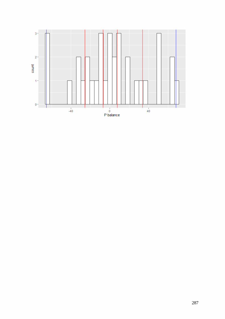
287

288

Supplementary material 23. Locations of the 34 agroecosystems belonging to 28 farms in the Grand Est

region of France.

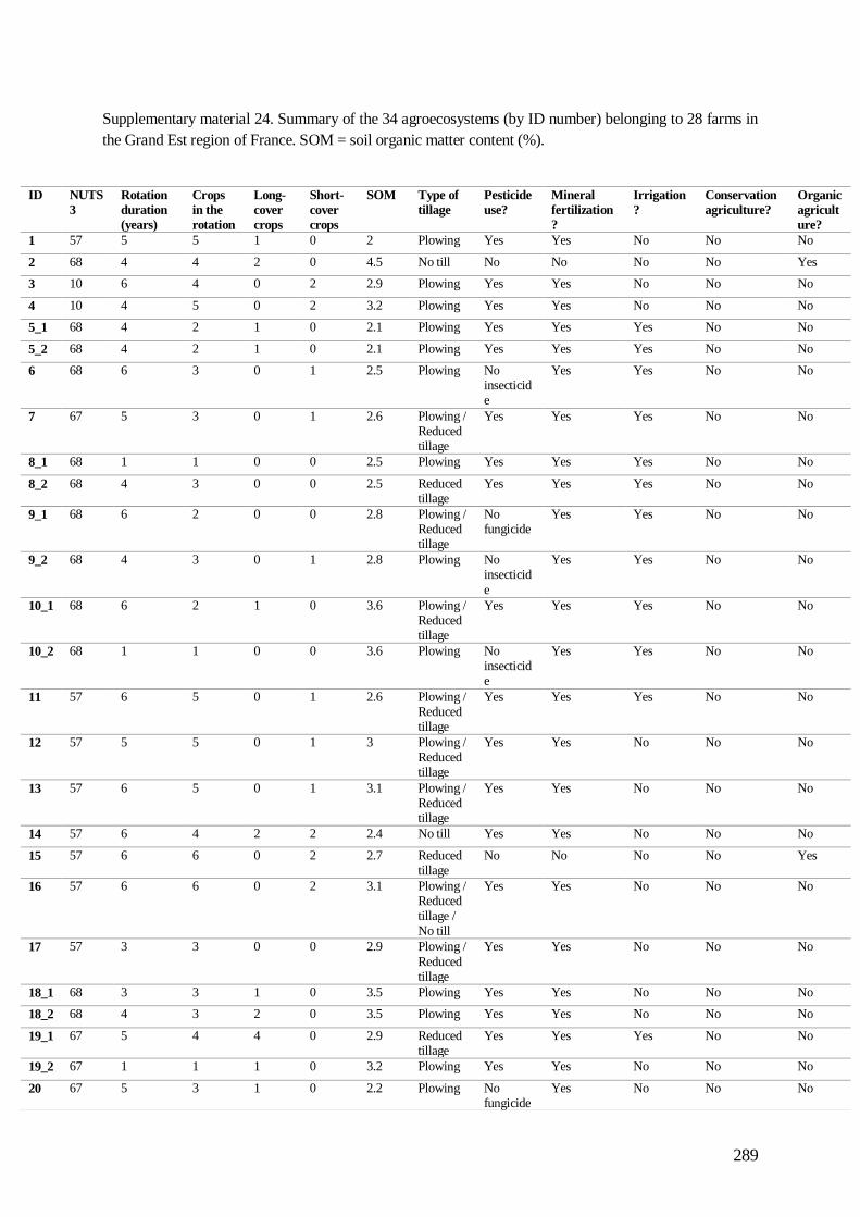
289

Supplementary material 24. Summary of the 34 agroecosystems (by ID number) belonging to 28 farms in

the Grand Est region of France. SOM = soil organic matter content (%).

ID NUTS

3

Rotation

duration

(years)

Crops

in the

rotation

Long-

cover

crops

Short-

cover

crops

SOM Type of

tillage

Pesticide

use?

Mineral

fertilization

?

Irrigation

?

Conservation

agriculture?

Organic

agricult

ure?

1 57 5 5 1 0 2 Plowing Yes Yes No No No

2 68 4 4 2 0 4.5 No till No No No No Yes

3 10 6 4 0 2 2.9 Plowing Yes Yes No No No

4 10 4 5 0 2 3.2 Plowing Yes Yes No No No

5_1 68 4 2 1 0 2.1 Plowing Yes Yes Yes No No

5_2 68 4 2 1 0 2.1 Plowing Yes Yes Yes No No

6 68 6 3 0 1 2.5 Plowing No insecticide

Yes Yes No No

7 67 5 3 0 1 2.6 Plowing / Reduced tillage

Yes Yes Yes No No

8_1 68 1 1 0 0 2.5 Plowing Yes Yes Yes No No

8_2 68 4 3 0 0 2.5 Reduced tillage

Yes Yes Yes No No

9_1 68 6 2 0 0 2.8 Plowing / Reduced tillage

No fungicide

Yes Yes No No

9_2 68 4 3 0 1 2.8 Plowing No insecticid

e

Yes Yes No No

10_1 68 6 2 1 0 3.6 Plowing / Reduced tillage

Yes Yes Yes No No

10_2 68 1 1 0 0 3.6 Plowing No insecticide

Yes Yes No No

11 57 6 5 0 1 2.6 Plowing / Reduced tillage

Yes Yes Yes No No

12 57 5 5 0 1 3 Plowing / Reduced tillage

Yes Yes No No No

13 57 6 5 0 1 3.1 Plowing / Reduced tillage

Yes Yes No No No

14 57 6 4 2 2 2.4 No till Yes Yes No No No

15 57 6 6 0 2 2.7 Reduced tillage

No No No No Yes

16 57 6 6 0 2 3.1 Plowing / Reduced tillage / No till

Yes Yes No No No

17 57 3 3 0 0 2.9 Plowing /

Reduced tillage

Yes Yes No No No

18_1 68 3 3 1 0 3.5 Plowing Yes Yes No No No

18_2 68 4 3 2 0 3.5 Plowing Yes Yes No No No

19_1 67 5 4 4 0 2.9 Reduced tillage

Yes Yes Yes No No

19_2 67 1 1 1 0 3.2 Plowing Yes Yes No No No

20 67 5 3 1 0 2.2 Plowing No fungicide

Yes No No No

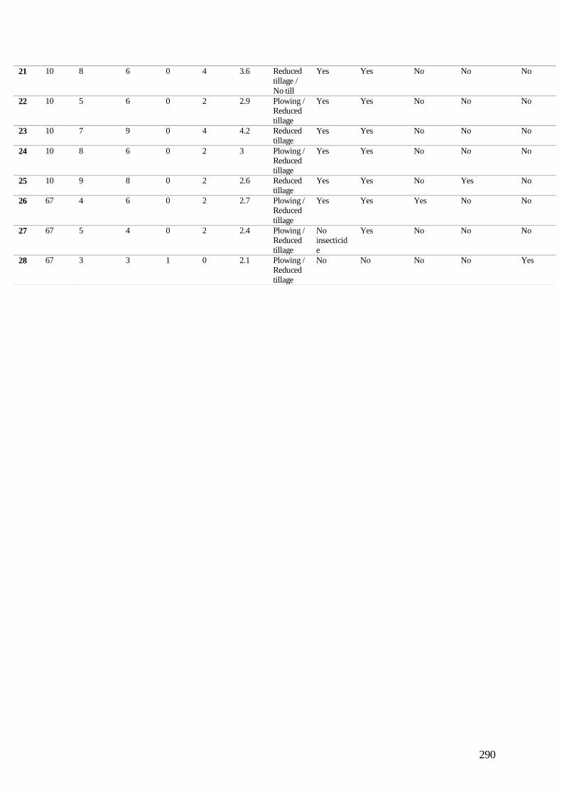
290

21 10 8 6 0 4 3.6 Reduced tillage /

No till

Yes Yes No No No

22 10 5 6 0 2 2.9 Plowing / Reduced tillage

Yes Yes No No No

23 10 7 9 0 4 4.2 Reduced tillage

Yes Yes No No No

24 10 8 6 0 2 3 Plowing / Reduced tillage

Yes Yes No No No

25 10 9 8 0 2 2.6 Reduced tillage

Yes Yes No Yes No

26 67 4 6 0 2 2.7 Plowing / Reduced

tillage

Yes Yes Yes No No

27 67 5 4 0 2 2.4 Plowing / Reduced tillage

No insecticide

Yes No No No

28 67 3 3 1 0 2.1 Plowing / Reduced tillage

No No No No Yes

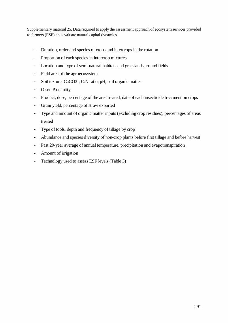
291

Supplementary material 25. Data required to apply the assessment approach of ecosystem services provided

to farmers (ESF) and evaluate natural capital dynamics

- Duration, order and species of crops and intercrops in the rotation

- Proportion of each species in intercrop mixtures

- Location and type of semi-natural habitats and grasslands around fields

- Field area of the agroecosystem

- Soil texture, CaCO3-, C:N ratio, pH, soil organic matter

- Olsen P quantity

- Product, dose, percentage of the area treated, date of each insecticide treatment on crops

- Grain yield, percentage of straw exported

- Type and amount of organic matter inputs (excluding crop residues), percentages of areas

treated

- Type of tools, depth and frequency of tillage by crop

- Abundance and species diversity of non-crop plants before first tillage and before harvest

- Past 20-year average of annual temperature, precipitation and evapotranspiration

- Amount of irrigation

- Technology used to assess ESF levels (Table 3)

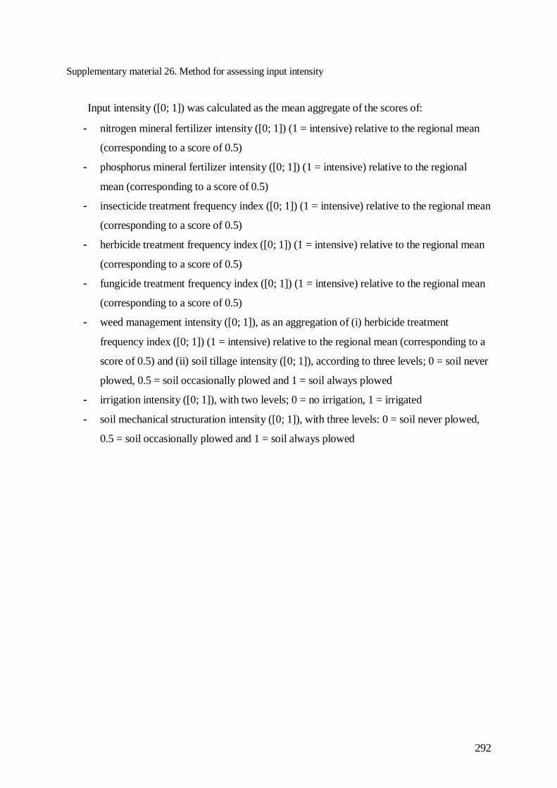
292

Supplementary material 26. Method for assessing input intensity

Input intensity ([0; 1]) was calculated as the mean aggregate of the scores of:

- nitrogen mineral fertilizer intensity ([0; 1]) (1 = intensive) relative to the regional mean

(corresponding to a score of 0.5)

- phosphorus mineral fertilizer intensity ([0; 1]) (1 = intensive) relative to the regional

mean (corresponding to a score of 0.5)

- insecticide treatment frequency index ([0; 1]) (1 = intensive) relative to the regional mean

(corresponding to a score of 0.5)

- herbicide treatment frequency index ([0; 1]) (1 = intensive) relative to the regional mean

(corresponding to a score of 0.5)

- fungicide treatment frequency index ([0; 1]) (1 = intensive) relative to the regional mean

(corresponding to a score of 0.5)

- weed management intensity ([0; 1]), as an aggregation of (i) herbicide treatment

frequency index ([0; 1]) (1 = intensive) relative to the regional mean (corresponding to a

score of 0.5) and (ii) soil tillage intensity ([0; 1]), according to three levels; 0 = soil never

plowed, 0.5 = soil occasionally plowed and 1 = soil always plowed

- irrigation intensity ([0; 1]), with two levels; 0 = no irrigation, 1 = irrigated

- soil mechanical structuration intensity ([0; 1]), with three levels: 0 = soil never plowed,

0.5 = soil occasionally plowed and 1 = soil always plowed

293

Supplementary material 27. Scores assigned to each cropping system for 1. potential capacity of the

agroecosystem ([0; 1]) (tan) , 2. real capacity of the agroecosystem ([-1; 2]) (magenta for positive values

and red for negative values) resulting from adding the score of the potential capacity and the score of the

modulation by agricultural practices , and 3. actual use of ecosystem services by the farmer (blue) ([0; 1]).

294

Supplementary material 28. Linear regression of real capacity minus potential capacity as a function of

potential capacity. Pearson correlation between them was significant (p<0.05) but weak (r=0.357).

295

Supplementary material 29. Dynamics of the four components of natural capital: biodiversity that supports

ecosystem services supplied to farmers, soil quantity (i.e. potential sensitivity to soil erosion) soil

phosphorus (P) balance and soil organic matter for 34 agroecosystems on 28 farms in the Grand Est region

of France. Positive values indicate capitalization (i.e. an increase in biodiversity, carbon storage, soil P

content, and no erosion), while negative values indicate depletion.

296

Supplementary material 30. Level of real capacity of the ecosystem to provide ecosystem services to farmers

(ESF), and actual use of ESF by farmers. Green lines indicate the direction and intensity of natural capital

dynamics, circle size indicates the input intensity (fertilization, pesticide, tillage, and irrigation), and circle

color indicates the wheat or maize yield relative to that of its mean regional yields for 34 agroecosystems

on 28 farms in the Grand Est region of France.

297

Supplementary material 31. Correlation circle of principal component analysis of the five variables shown

in Figure 28: real capacity, actual use, natural capital, relative yield and intensity of practices.

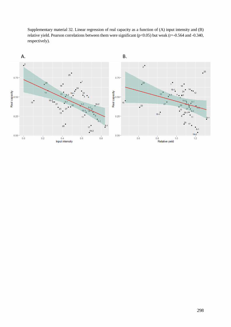
298

Supplementary material 32. Linear regression of real capacity as a function of (A) input intensity and (B)

relative yield. Pearson correlations between them were significant (p<0.05) but weak (r=-0.564 and -0.340,

respectively).

299

Supplementary material 33. For each agriculture model cluster, (A) wheat or maize yield relative to that of

its mean regional yields and (B) input intensity level. Whiskers represent 1.5 times the interquartile range.

Cluster means did not differ significantly (p>0.05, pairwise Tukey HSD test). I-M : “inefficient use of

medium ESF capacity”, I-LM-D : “inefficient use of low to medium ESF capacity, with depletion”, M-LM-

C: “medium use of low-to-medium ESF capacity, with capitalization”, MH-H : “medium-high use of high

ESF capacity”, E-LM-D: “efficient use of low-to-medium ESF capacity, with depletion” clusters.

Supplementary material 34. Linear regression of real capacity as a function of (A) input intensity and (B)

relative yield without organic agroecosystems. Pearson correlations were significant (p <0.05) but weak

(r=0.400) for input intensity and non-significant relative yield (p>0.05).

300

Supplementary material 35. Scores (symbols) for agroecosystem #25 of a) the potential capacity (tan) and

real capacity (magenta) to provide nine ecosystem services to farmers (ESF), b) actual use of ESF by the

farmer (blue) and c) natural capital dynamics (green). Shading and lines indicate the ranges of possible and

observed values, respectively, of the 34 agroecosystems studied. Violet shading indicates the range added

by the conservation agriculture bonus. The 9 ESF studied include pollination (POL); pest (PEST), weed

(WEED) and disease (DIS) control; soil structuration (STR); nitrogen supply to crops (NS); phosphorus

supply to crops (PS); water retention and return to crops (WATER) and stabilization and control of erosion

(ERO).

301

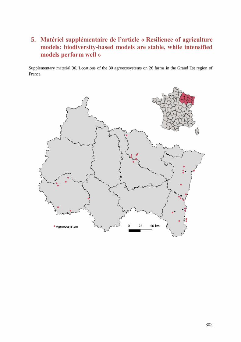
302

5. Matériel supplémentaire de l’article « Resilience of agriculture

models: biodiversity-based models are stable, while intensified

models perform well »

Supplementary material 36. Locations of the 30 agroecosystems on 26 farms in the Grand Est region of

France.

303

Supplementary material 37. Equation used to calculate the gross margin and references of data source.

𝑔𝑟𝑜𝑠𝑠𝑚𝑎𝑟𝑔𝑖𝑛 (€

ℎ𝑎)

= 𝑐𝑟𝑜𝑝𝑠𝑒𝑙𝑙𝑖𝑛𝑔𝑝𝑟𝑖𝑐𝑒 (€

𝑡 𝑜𝑟 𝑞) × 𝑦𝑖𝑒𝑙𝑑 (

𝑡 𝑜𝑟 𝑞

ℎ𝑎) − (𝑓𝑒𝑟𝑡𝑖𝑚𝑖𝑛 (

𝑙

ℎ𝑎)

× 𝑓𝑒𝑟𝑡𝑚𝑖𝑛𝑝𝑟𝑖𝑐𝑒 (€

𝑙) + 𝑓𝑒𝑟𝑡𝑖𝑜𝑟𝑔 (

𝑡

ℎ𝑎) × 𝑓𝑒𝑟𝑡𝑖𝑜𝑟𝑔𝑝𝑟𝑖𝑐𝑒 (

€

𝑡) + 𝑝ℎ𝑦𝑡𝑜 (

𝑙

ℎ𝑎)

× 𝑝ℎ𝑦𝑡𝑜𝑝𝑟𝑖𝑐𝑒(€

𝑙) + 𝑒𝑛𝑒𝑟𝑔𝑦𝑐𝑜𝑛𝑠𝑜 (

𝑙

ℎ𝑎) × 𝑒𝑛𝑒𝑟𝑔𝑦𝑝𝑟𝑖𝑐𝑒 (

€

𝑙))

With:

- 𝑐𝑟𝑜𝑝𝑠𝑒𝑙𝑙𝑖𝑛𝑔𝑝𝑟𝑖𝑐𝑒, the price of the crop, from statistics of the French Ministry of

Agriculture, indexed yearly by the producer prices for agricultural product index (IPPAP)

- 𝑦𝑖𝑒𝑙𝑑, crop yield

- 𝑓𝑒𝑟𝑡𝑖𝑚𝑖𝑛, amount of mineral fertiliser applied

- 𝑓𝑒𝑟𝑡𝑚𝑖𝑛𝑝𝑟𝑖𝑐𝑒, price of mineral fertiliser, estimated for 2012 when purchased by

Agrosyst, indexed annually by the IPPAP index

- 𝑓𝑒𝑟𝑡𝑖𝑜𝑟𝑔, the amount of organic fertiliser applied

- 𝑓𝑒𝑟𝑡𝑖𝑜𝑟𝑔𝑝𝑟𝑖𝑐𝑒, price of organic fertiliser, estimated for 2012 when purchased by

Agrosyst, indexed annually by the IPPAP index but assumed to remain constant over

time due to low variability

- 𝑝ℎ𝑦𝑡𝑜, the amount of pesticide applied

- 𝑝ℎ𝑦𝑡𝑜𝑝𝑟𝑖𝑐𝑒, price of pesticides, estimated from those purchased by Agrosyst or

collected by their users, indexed annually by the IPPAP index but assumed to remain

constant over time due to low variability

- 𝑒𝑛𝑒𝑟𝑔𝑦𝑐𝑜𝑛𝑠𝑜, consumption of energy by machinery

- 𝑒𝑛𝑒𝑟𝑔𝑦𝑝𝑟𝑖𝑐𝑒, price of energy (fuel or electricity), estimated for 2015 from the APCA

(Office of Agricultural French Chambers), indexed annually by the IPPAP index

304

Supplementary material 38. Agro-climatic indicators of the 30 agroecosystems: cumulative daily maximum

temperature (°C), number of hot days (> 27°C), and maximum drought sequence (days). Whiskers represent

1.5 times the interquartile range.

305

Supplementary material 39. Analysis of variance of agro-climatic indicators paired with Tukey multiple

pairwise-comparisons test.

Agro-climatic indicator Differed significantly

among agroecosystems?

Agroecosystem

outliers

Cumulative daily maximum

temperature

Yes #14

Number of hot days (> 27°C) Yes #14

Maximum drought duration No -

306

Supplementary material 40. Price volatility indicators: fuel and wheat prices.

307

Supplementary material 41. Method used to calculate the synergistic effect of conservation agriculture

(SCA).

When cropfamily* > 0.75, land cover (continuouslandcover) is continuous (i.e. 1) and

cumulative depth of tillage operations (tillage) < -0.25, SCA is set to 1.

2. cropfamily =1

∑ (𝑛𝑖𝑁

)2

𝑖

With:

𝑛𝑖: number of crops in family 𝑖

𝑁: number of crops in the rotation

* from Craheix et al. (2012)

continuouslandcover

= 1, if the rotation has fewer than 3 months without crops or intercrops; otherwise, 0

𝑡𝑖𝑙𝑙𝑎𝑔𝑒 = −(1

𝑁∑ 𝑑𝑖

𝑖)/𝐷

With:

𝑖: each crop in the rotation

𝑑𝑖: depth of all mechanical operations that disturb the soil deeper than 1 cm for 𝑖

𝐷: 88 cm, the estimated maximum disturbance according to experts, for tillage that disturbs

the soil greatly: Stubble ploughing (10 cm) / ploughing (20 cm) / rotary harrow (10 cm) / sowing

(3 cm) / hoeing (5 cm). The depth of disturbance ploughing is multiplied by 2 and the rotary tools

by 3 according to (Dardonville et al., under revisions at Ecosystem Services) method.

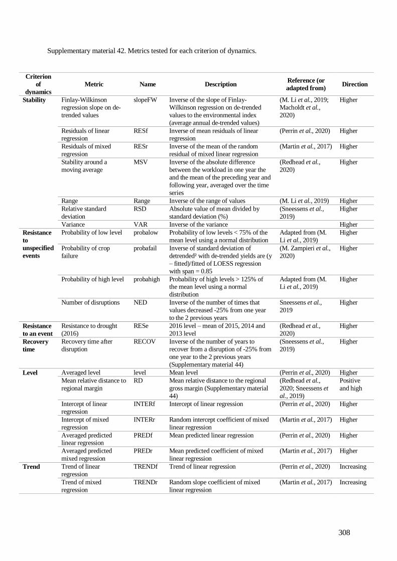
308

Supplementary material 42. Metrics tested for each criterion of dynamics.

Criterion

of

dynamics

Metric Name Description Reference (or

adapted from) Direction

Stability Finlay-Wilkinson

regression slope on de-

trended values

slopeFW Inverse of the slope of Finlay-

Wilkinson regression on de-trended

values to the environmental index

(average annual de-trended values)

(M. Li et al., 2019;

Macholdt et al.,

2020)

Higher

Residuals of linear regression

RESf Inverse of mean residuals of linear regression

(Perrin et al., 2020) Higher

Residuals of mixed

regression

RESr Inverse of the mean of the random

residual of mixed linear regression

(Martin et al., 2017) Higher

Stability around a

moving average

MSV Inverse of the absolute difference

between the workload in one year the

and the mean of the preceding year and

following year, averaged over the time

series

(Redhead et al.,

2020)

Higher

Range Range Inverse of the range of values (M. Li et al., 2019) Higher

Relative standard

deviation

RSD Absolute value of mean divided by

standard deviation (%)

(Sneessens et al.,

2019)

Higher

Variance VAR Inverse of the variance Higher

Resistance

to

unspecified

events

Probability of low level probalow Probability of low levels < 75% of the

mean level using a normal distribution

Adapted from (M.

Li et al., 2019)

Higher

Probability of crop

failure

probafail Inverse of standard deviation of

detrended² with de-trended yields are (y

– fitted)/fitted of LOESS regression

with span = 0.85

(M. Zampieri et al.,

2020)

Higher

Probability of high level probahigh Probability of high levels > 125% of the mean level using a normal

distribution

Adapted from (M. Li et al., 2019)

Higher

Number of disruptions NED Inverse of the number of times that

values decreased -25% from one year

to the 2 previous years

Sneessens et al.,

2019

Higher

Resistance

to an event

Resistance to drought

(2016)

RESe 2016 level – mean of 2015, 2014 and

2013 level

(Redhead et al.,

2020)

Higher

Recovery

time

Recovery time after

disruption

RECOV Inverse of the number of years to

recover from a disruption of -25% from

one year to the 2 previous years

(Supplementary material 44)

(Sneessens et al.,

2019)

Higher

Level Averaged level level Mean level (Perrin et al., 2020) Higher

Mean relative distance to

regional margin

RD Mean relative distance to the regional

gross margin (Supplementary material

44)

(Redhead et al.,

2020; Sneessens et

al., 2019)

Positive

and high

Intercept of linear

regression

INTERf Intercept of linear regression (Perrin et al., 2020) Higher

Intercept of mixed

regression

INTERr Random intercept coefficient of mixed

linear regression

(Martin et al., 2017) Higher

Averaged predicted linear regression

PREDf Mean predicted linear regression (Perrin et al., 2020) Higher

Averaged predicted

mixed regression

PREDr Mean predicted coefficient of mixed

linear regression

(Martin et al., 2017) Higher

Trend Trend of linear

regression

TRENDf Trend of linear regression (Perrin et al., 2020) Increasing

Trend of mixed

regression

TRENDr Random slope coefficient of mixed

linear regression

(Martin et al., 2017) Increasing

309

Supplementary material 43. Equation used to calculate annual regional gross margin based on FADN data

for OTEX OTEFDD 15 “cereals, oilseeds, protein crops” for the mean CDEX and large farms in the Grand

Est region of France (Agreste).

𝑟𝑒𝑔𝑖𝑜𝑛𝑎𝑙. 𝑔𝑟𝑜𝑠𝑠𝑚𝑎𝑟𝑔𝑖𝑛 (€

ℎ𝑎)

=1

𝑆𝐴𝑈× (𝑟𝑒𝑣𝑒𝑛𝑢𝑒 − 𝑓𝑒𝑟𝑡𝑖𝑐𝑜𝑠𝑡𝑠 − 𝑝𝑒𝑠𝑡𝑖𝑐𝑜𝑠𝑡𝑠 − 𝑒𝑛𝑒𝑟𝑔𝑦𝑐𝑜𝑠𝑡𝑠)

310

Supplementary material 44. Calculation of the recovery time indicator.

The recovery time is determined by the number of years that the performance does not reach

the pre-disruption level. A disrupted year corresponds to a year with a – 25 % decrease in

performance compared to the average of the previous two years. If an agroecosystem experienced

several disruptive events during the 8-year time-series, the recovery time was averaged. If not

enough years were available in the time-series to reach the recovery time, the disruption was not

counted. Future studies could consider that the system has recovered if it returns to approximately

the same level to that before the disruption (e.g. the standard deviation of the two years before the

disruption).

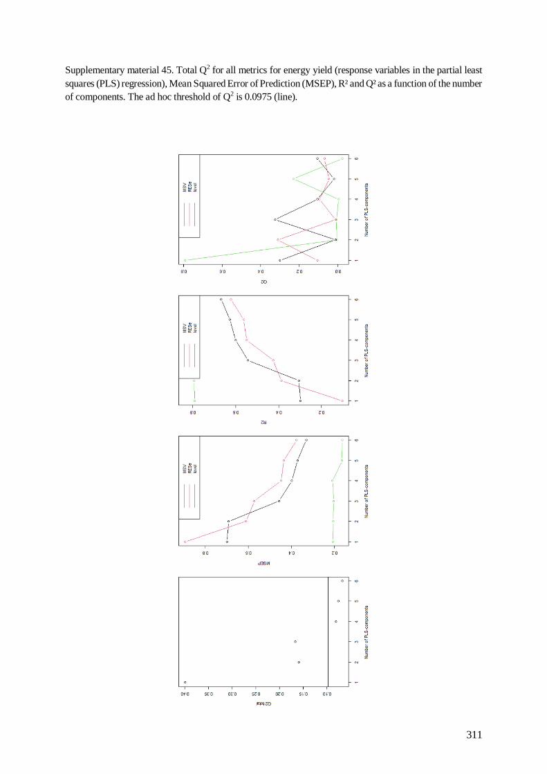
311

Supplementary material 45. Total Q2 for all metrics for energy yield (response variables in the partial least

squares (PLS) regression), Mean Squared Error of Prediction (MSEP), R² and Q² as a function of the number

of components. The ad hoc threshold of Q2 is 0.0975 (line).

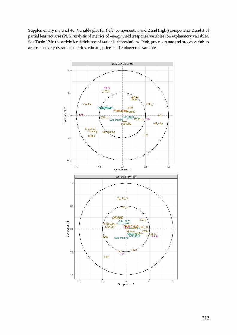
312

Supplementary material 46. Variable plot for (left) components 1 and 2 and (right) components 2 and 3 of

partial least squares (PLS) analysis of metrics of energy yield (response variables) on explanatory variables.

See Table 12 in the article for definitions of variable abbreviations. Pink, green, orange and brown variables

are respectively dynamics metrics, climate, prices and endogenous variables.

313

Supplementary material 47. Energy yield for each agriculture model. Whiskers represent 1.5 times the

interquartile range. Cluster means differ significantly (p < 0.05) between two groups (a and b, pairwise

Tukey HSD test). I_M: “Inefficient use of Medium ESF capacity”, I_LM_D: “Inefficient use of Low-to-

Medium ESF capacity, with Depletion”, M_LM_C: “Medium use of Low-to-Medium ESF capacity, with

Capitalization”, MH_H: “Medium-High use of High ESF capacity”, E_LM_D: “Efficient use of Low-to-

Medium ESF capacity, with Depletion” clusters.

314

Supplementary material 48. Level, MSV and RESe distribution below and above the natural capital

dynamics (nat_cap) threshold of -0.2306. All means differed significantly (p < 0.001 (***)) according to

Welch two-sample t-tests. Whiskers represent 1.5 times the interquartile range.

315

Supplementary material 49. Total Q2 for all metrics for wheat yield (t/ha, excluding agroecosystems #10_2,

5_2, 8_1) (response variables in the partial least squares (PLS) regression), Mean Squared Error of

Prediction (MSEP), R² and Q² as a function of the number of components. The ad hoc threshold of Q2 is

0.0975 (line).

316

Variable plot for components 1 and 2 of partial least squares (PLS) analysis of wheat yield metrics (response

variables) on explanatory variables. See Table 12 in the article for definitions of variable abbreviations.

Pink, green, orange and brown variables are respectively dynamics metrics, climate, prices and endogenous

variables.

317

Clustered Image Map and network representation of the partial least squares regression of metrics for energy

yield on explanatory variables (blue: positive, red: negative correlation to a resilient dynamic). See Table

12 in the article for definitions of variable abbreviations.

318

Supplementary material 50. Total Q2 for all metrics for gross margin (response variables in the partial least

squares (PLS) regression), Mean Squared Error of Prediction (MSEP), R² and Q² as a function of the number

of components. The ad hoc threshold of Q2 is 0.0975 (line).

319

Supplementary material 51. Variable plot for (left) components 1 and 2 and (right) components 2 and 3 of

partial least squares (PLS) analysis of metrics for gross margin (response variables) on explanatory

variables. See Table 12 in the article for definitions of variable abbreviations. Pink, green, orange and brown

variables are respectively dynamics metrics, climate, prices and endogenous variables.

320

Supplementary material 52. RD, MSV, probalow, RESe and TRENDr distribution below and above the

natural capital dynamics (nat_cap) threshold of -0.2834. All means differed significantly (p < 0.001 (***))

according to Welch two-sample t-tests. Whiskers represent 1.5 times the interquartile range.

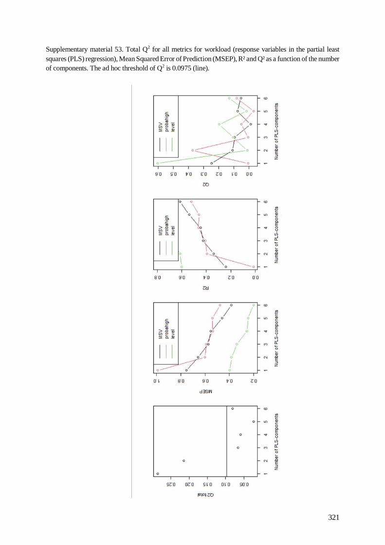
321

Supplementary material 53. Total Q2 for all metrics for workload (response variables in the partial least

squares (PLS) regression), Mean Squared Error of Prediction (MSEP), R² and Q² as a function of the number

of components. The ad hoc threshold of Q2 is 0.0975 (line).

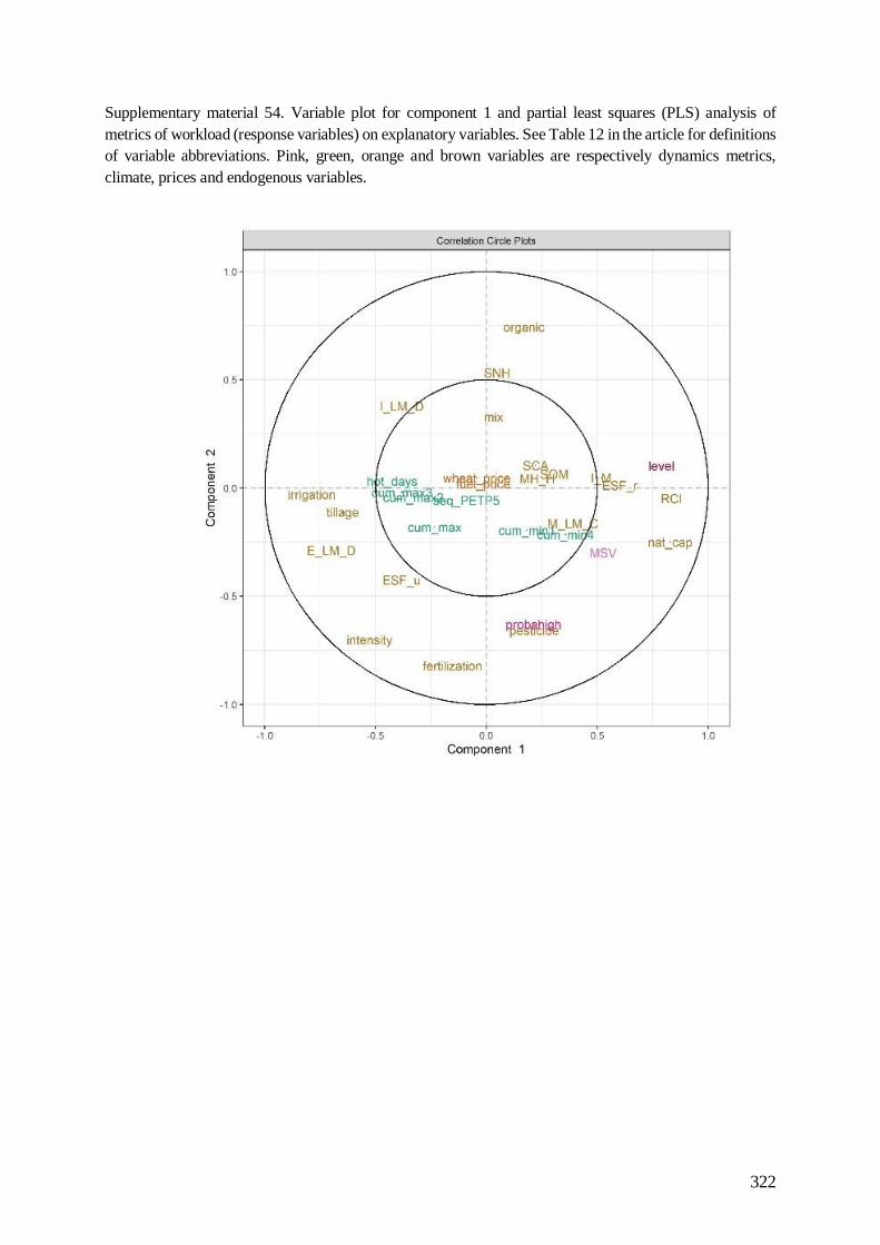
322

Supplementary material 54. Variable plot for component 1 and partial least squares (PLS) analysis of

metrics of workload (response variables) on explanatory variables. See Table 12 in the article for definitions

of variable abbreviations. Pink, green, orange and brown variables are respectively dynamics metrics,

climate, prices and endogenous variables.

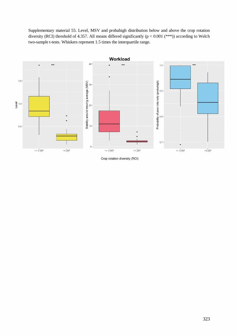
323

Supplementary material 55. Level, MSV and probahigh distribution below and above the crop rotation

diversity (RCI) threshold of 4.357. All means differed significantly (p < 0.001 (***)) according to Welch

two-sample t-tests. Whiskers represent 1.5 times the interquartile range.

324

Supplementary material 56. Pareto ranking (from best (green) to worst (red)) of all metrics of all attributes

of the 30 agroecosystems.

Agroecosystem Rank

level MSV RESe RD MSV probalow RESe TRENDr level MSV probahigh

1 2,4E+07 6,8E-07 -3,5E+06 -5,4E+01 8,5E-03 8,0E-01 -2,5E+02 -1,4E+00 1,4E+00 2,7E+01 9,98E-01 1

5_2 4,9E+07 3,3E-07 -1,3E+06 8,6E+02 5,8E-03 9,5E-01 2,0E+01 -1,1E+01 5,5E+00 2,5E+00 9,02E-01 1

10_1 4,6E+07 4,1E-07 3,4E+06 8,5E+02 9,6E-03 9,4E-01 1,7E+02 -1,2E+01 4,0E+00 1,6E+00 8,14E-01 2

10_2 4,0E+07 1,4E-07 1,1E+07 6,4E+02 3,6E-03 8,0E-01 4,5E+02 4,8E+00 6,0E+00 1,0E+00 8,75E-01 2

11 1,9E+07 9,3E-07 -7,4E+05 -1,2E+02 1,1E-02 8,2E-01 -1,1E+02 4,8E+00 7,7E-01 1,6E+01 9,45E-01 2

12 2,3E+07 7,2E-07 -6,9E+06 -6,9E+01 1,4E-02 8,4E-01 -4,5E+02 2,8E+00 1,2E+00 7,0E+00 9,71E-01 2

13 2,3E+07 9,5E-07 -4,4E+06 -2,9E+01 1,1E-02 8,6E-01 -3,2E+02 2,6E+00 1,5E+00 3,6E+00 8,39E-01 2

14 2,5E+07 5,1E-07 -2,5E+06 1,6E+02 7,6E-03 8,7E-01 -2,4E+02 4,6E+00 2,3E+00 2,8E+00 9,24E-01 2

15 1,2E+07 1,3E-06 -5,7E+06 -3,1E+02 1,1E-02 7,3E-01 -5,0E+01 1,6E+01 5,4E-01 7,1E+00 6,91E-01 2

16 2,4E+07 9,7E-07 -5,3E+06 4,8E+01 1,7E-02 9,2E-01 -2,9E+02 5,0E+00 8,9E-01 3,4E+01 9,98E-01 2

17 2,7E+07 3,7E-07 -7,0E+06 4,6E+01 7,2E-03 8,1E-01 -4,4E+02 1,1E+01 1,6E+00 4,9E+00 9,16E-01 2

18_2 3,3E+07 3,5E-07 3,5E+06 3,0E+02 8,2E-03 8,6E-01 -5,2E+01 1,6E+00 1,4E+00 7,1E+00 7,57E-01 2

19_1 2,6E+07 5,7E-07 -2,9E+06 1,0E+02 1,4E-02 8,4E-01 -3,8E+02 1,5E+01 2,2E+00 8,0E+00 9,13E-01 2

20 3,7E+07 2,2E-07 -1,7E+06 5,5E+02 5,7E-03 8,5E-01 -1,8E+02 -1,3E+01 3,0E+00 2,9E+00 8,11E-01 2

22 1,9E+07 2,4E-07 -1,2E+07 -5,9E+00 5,5E-03 7,2E-01 -5,6E+02 -6,3E+00 1,3E+00 1,1E+01 9,19E-01 2

23 1,1E+07 2,1E-06 -2,1E+06 -5,0E+02 2,6E-02 7,0E-01 -1,1E+02 1,8E+01 7,2E-01 9,7E+00 9,08E-01 2

24 1,2E+07 6,9E-07 -3,5E+06 -5,5E+02 1,1E-02 6,4E-01 -2,4E+02 1,2E+01 6,3E-01 3,9E+01 1,00E+00 2

25 1,8E+07 5,2E-07 3,9E+06 -3,0E+02 1,2E-02 6,4E-01 -1,8E+02 3,8E+01 1,2E+00 8,8E+00 8,84E-01 2

27 4,6E+07 1,4E-07 -1,1E+07 8,4E+02 3,1E-03 8,6E-01 -6,0E+02 -1,2E+01 3,2E+00 1,3E+01 1,00E+00 2

28 1,5E+07 4,7E-07 -5,5E+06 -3,1E+02 9,2E-03 7,0E-01 -2,2E+02 1,4E+01 3,9E+00 2,4E+00 7,49E-01 2

3 2,3E+07 1,8E-07 -8,3E+06 8,2E+01 3,9E-03 7,2E-01 -5,0E+02 -2,5E+01 8,6E-01 1,7E+01 9,76E-01 2

4 1,7E+07 7,6E-07 -6,5E+06 1,3E+02 4,6E-03 7,2E-01 -7,1E+02 7,6E+00 9,5E-01 1,4E+01 9,99E-01 2

5_1 5,3E+07 3,8E-07 -5,5E+06 7,8E+02 8,3E-03 9,4E-01 -3,2E+02 -1,2E+01 5,1E+00 2,3E+00 9,72E-01 2

6 4,3E+07 1,0E-07 -4,1E+06 7,8E+02 2,2E-03 7,0E-01 -2,7E+02 -2,2E+01 3,5E+00 2,6E+00 8,27E-01 2

7 4,4E+07 3,3E-07 -3,0E+06 5,5E+02 7,2E-03 8,3E-01 -2,8E+02 -2,0E+01 3,5E+00 3,8E+00 9,47E-01 2

8_1 6,0E+07 5,2E-07 6,7E+05 6,9E+02 6,5E-03 8,0E-01 -4,7E+01 -2,6E+01 9,9E+00 9,8E-01 9,50E-01 2

8_2 3,6E+07 2,5E-07 3,8E+06 -2,7E+01 2,7E-03 6,6E-01 5,5E+02 1,7E+01 3,2E+00 2,8E+00 8,55E-01 2

9_2 2,8E+07 9,3E-08 9,1E+06 6,5E+02 2,6E-03 6,3E-01 2,9E+02 2,1E+01 2,3E+00 2,2E+00 7,01E-01 2

21 1,8E+07 3,2E-07 -4,2E+06 -6,5E+01 5,7E-03 6,4E-01 -2,8E+02 -1,1E+01 1,2E+00 7,3E+00 9,08E-01 2

18_1 4,4E+07 2,7E-07 -2,6E+06 3,0E+02 5,4E-03 7,8E-01 -2,8E+02 -2,3E+01 3,4E+00 2,1E+00 7,38E-01 2

Energy yield Gross margin Workload

325

Supplementary material 57. Correlation plot of all explanatory factors. See Table 12 in the article for

definitions of abbreviations.

326

Supplementary material 58. Variance, standard coefficient of variation (CV = SD/Mean) and adjusted CV

(Döring and Reckling, 2018) based on mean performance.

A significant positive relation exists between paired log(variance) and log(mean) of crop

yields of the investigated agroecosystems. In other words, higher energy yields indicate higher

stability, as most datasets in (Döring et al., 2015). This relation also occurs when comparing

intensive (intensity score >= 0.4) to low intensive systems. As b<2, the coefficient of variation

(CV) decreased when the means increased, which is an artefact. As TPL holds, the CV decreased

non-linearly with increasing mean. When the CV was corrected, as suggested by these authors, the

relation was reversed: adjusted CV increased with increasing mean. In other words, removing

dependence from the mean by setting the TPL slope to 2 revealed unbiased CV-mean relations.

Adjusted CV was significantly positively correlated with MSV (our stability measure).

327

RÉSUMÉ

Pour répondre aux enjeux d’impacts environnementaux et de dépendance aux ressources fossiles de

l’agriculture moderne, de nouvelles formes d’agriculture ont émergé : l’agriculture régénérative ou

l’agroforesterie par exemple. Elles visent à utiliser les services écosystémiques comme support de la

production agricole (SEP) en remplacement des intrants anthropiques. Leur résilience aux changements

climatiques et aux fluctuations des marchés économiques, c.-à-d. leur capacité à faire face à ces

perturbations, fait l’objet d’intenses débats. Aussi, ma thèse visait à produire des connaissances sur la

résilience des formes d’agriculture de grandes cultures et des méthodes opérationnelles pour les institutions

de conseil agricole.

J’ai ainsi d’abord réalisé une synthèse de la littérature traitant de l’évaluation quantitative de la

résilience, et de concepts proches tels que la vulnérabilité et la robustesse (V, R, R). Une première

publication montre que l’intensification et la diversification de la production ne sont pas systématiquement

des facteurs de VRR et qu’il est nécessaire de considérer la diversité fonctionnelle, plus que taxonomique,

et d’adapter les pratiques agricoles, au pédoclimat et à la disponibilité des ressources locales, pour assurer

une VRR à court et long terme. Une deuxième publication décrit la diversité de méthodes et critères

d’analyse de la dynamique utilisés et pointe la nécessité de développer des approches multicritère et multi-

performances dépassant la seule analyse du rendement.

J’ai ensuite développé et appliqué une méthode d’évaluation du niveau de SEP pour caractériser les

agroécosystèmes et identifier des formes d’agriculture associées. L’évaluation distingue le niveau potentiel

de SEP, le niveau réellement fourni, le niveau utilisé pour la production et la dynamique à long-terme du

capital naturel, qui sous-tend les SEP. Les niveaux potentiel et réel de SEP sont évalués indirectement par

des indicateurs de la qualité de la configuration spatiotemporelle de l’agroécosystème et de l’impact des

pratiques culturales. Le niveau de SEP utilisé est estimé par la technologie mise en œuvre par

l’agriculteur·rice pour évaluer la fourniture réelle de SEP. La dynamique du capital naturel est estimée par

des indicateurs de sensibilité à l’érosion, dynamique du carbone et du phosphore du sol et de la biodiversité.

En appliquant cette méthode à un cas d’étude de 34 agroécosystèmes de la région Grand Est en France

représentant une diversité de rotations de culture et de pratiques agricoles, j’ai identifié finalement cinq

grandes formes d’agriculture.

Enfin, j’ai développé une méthode d’évaluation de la résilience de ces agroécosystèmes et des formes

d’agriculture associées face aux perturbations. J’ai analysé la dynamique du rendement, de la marge brute

et du temps de travail considérant leur niveau moyen, variabilité, tendance et/ou résistance sur huit ans. Je

montre que les formes d’agriculture disposant d’un haut niveau de SEP, basées sur la biodiversité et qui

augmentent leur capital naturel, présentent une meilleure stabilité du rendement et de la marge brute. En

revanche, les systèmes intensifs, mais aussi ceux utilisant le plus les SEP, présentent de plus hauts niveaux

et une meilleure résistance des rendements et marges brutes mais nécessitent plus de temps de travail. Aussi,

j’émets l’hypothèse que la combinaison d’un haut niveau de SEP et l’optimisation de leur usage permettrait

d’éviter l’usage d’intrants tout en permettant d’atteindre de hauts rendements, résistants. Cependant, pour

atteindre cet objectif, il faudrait augmenter les niveaux de SEP potentiels et utilisés, encore insuffisants dans

les agroécosystèmes étudiés.

En résumé, ce travail de thèse a produit des connaissances sur la nature des formes d’agriculture et des

facteurs de résilience et des méthodes originales pour évaluer les niveaux de SEP et leur résilience. Ses

résultats montrent l’intérêt, dans un objectif de résilience, de développer et mobiliser les SEP et alertent sur

l’importance de restaurer le capital naturel, souvent dégradés par des décennies d’agriculture intensive.

329

ABSTRACT

In response to the issues of environmental impact and dependence on fossil resources of modern

agriculture, new agriculture models have emerged: regenerative, integrated agriculture, agroforestry, for

example. They aim to use ecosystem services provided to farmer (ESF) as a support for agricultural

production to replace anthropogenic inputs. Their resilience to climate change and economic market

fluctuations, i.e. their capacity to cope with these disturbances, is the subject of intense debate. Yet,

knowledge of their resilience would be key to accelerating their adoption by the agricultural community

and achieving sustainability goals. In response to this challenge, my PhD thesis aimed to produce knowledge

on the resilience of different agriculture cropping models.

To achieve this objective, first, I synthesized the literature on the quantitative assessment of resilience,

and related concepts such as vulnerability and robustness (V, R, R). A first publication shows that

intensification and diversification of production are not systematic factors of VRR and that it is necessary

to consider functional, rather than taxonomic, diversity and to adapt agricultural practices, to the

pedoclimate and to the availability of local resources, to ensure VRR in the short and long term. A second

publication describes the diversity of methods and criteria for analyzing the dynamics used so far and points

out the need to develop multi-criteria and multi-performance approaches that go beyond yield analysis

alone.

Then, I developed and applied a method for assessing the level of ESF to characterize agroecosystems

and identify agriculture models. ESF levels were differentiated according to the potential capacity of ESF,

the real capacity of ESF, the actual use of ESF for production, and the long-term dynamics of natural capital,

which underlies ESF. The potential and real levels of ESF are assessed indirectly with indicators of the

quality of the spatial and temporal configuration of the agroecosystem and the impact of cropping practices.

The level of ESF used is estimated by the technology implemented to assess ESF real capacity. The

dynamics of natural capital is estimated by the aggregation of indicators of erosion sensitivity, soil carbon

and phosphorus dynamics and biodiversity. Applied to a case study in Grand Est region in France of 34

agroecosystems contrasted in terms of crop rotation and cropping practices, I identified with a clustering

method five agriculture models.

Finally, I developed a method to assess the resilience of these agroecosystems and associated

agriculture models in the face of disturbances. I analyzed the dynamics of the yield, gross margin and

workload considering their average level, variability, trend and/or resistance over the last eight years. I thus

showed that models with a high level of ESF and biodiversity, and which increase their natural capital,

present a better stability of yield and gross margin but a generally lower level of production. In contrast,

intensive systems have higher levels and greater resistance of yields and gross margins but require a greater

amount of labor. I have also observed that the systems that use ESF the most have good agronomic and

economic performances, resistant to disturbances. Thus, I hypothesize that the combination of a high level

of ESF and the optimization of their use would avoid the use of inputs while achieving high, resistant yields.

However, to achieve this goal, it would be necessary to increase the levels of potential and used ESF, which

are still insufficient in the agroecosystems studied.

In summary, this work has produced knowledge on the nature of agriculture models and resilience

factors and original methods to assess the levels of ESF and their resilience. Its results show the interest,

with a view to resilience, of developing and mobilizing ESF and alert on the importance of restoring natural

capital, often degraded by decades of intensive agriculture.