Animation rendering with Population Monte Carlo image-plane sampler

Vis Comput (2010) 26: 543–553DOI 10.1007/s00371-010-0503-5

O R I G I NA L A RT I C L E

Animation rendering with Population Monte Carlo image-planesampler

Yu-Chi Lai · Stephen Chenney · Feng Liu · Yuzhen Niu ·Shaohua Fan

Published online: 17 April 2010© Springer-Verlag 2010

Abstract Except for the first frame, a population MonteCarlo image plane (PMC-IP) sampler renders with a start-up kernel function learned from previous results by usingmotion analysis techniques in the vision community to ex-plore the temporal coherence existing among kernel func-tions. The predicted kernel function can shift part of theuniformly distributed samples from regions with low visualvariance to regions with high visual variance at the start-up iteration and reduce the temporal noise by consideringthe temporal relation of sample distributions among frames.In the following iterations, the PMC-IP sampler adapts thekernel function to select pixels for refinement according to

Y.-C. Lai funded by: NSC 99-2218-E-011-005-, Taiwan.

Y.-C. LaiNational Taiwan University of Science and Technology, Taipei,ROCe-mail: [email protected]

S. ChenneyEmergent Game Technology, Chapel Hill, USAe-mail: [email protected]

F. LiuUniversity of Wisconsin-Madison, Madison, USAe-mail: [email protected]

Y. NiuShandong University, Jinan, Chinae-mail: [email protected]

S. Fan (�)Suzhou University Financial Engineering Research Center,Suzhou, Chinae-mail: [email protected]

S. FanNYU Courant Institute of Mathematical Sciences, New York,USA

a perceptually-weighted variance criterion. Our results im-prove the rendering efficiency by a factor between 2 to 5over existing techniques in single frame rendering. The ren-dered animations are perceptually more pleasant.

Keywords Ray-tracing · PMC · Monte Carlo · Globalillumination

1 Introduction

Global illumination based on Monte Carlo integration pro-vides the most general solution for photorealistic render-ing problems. To reduce image noise (variance) at practi-cal computation times is the core of research in the globalillumination community. To render an animation the tempo-ral variance at each pixel among consecutive frames mustalso be considered because our eyes are good at noticingtemporal inconsistency among consecutive frames for sur-vival purposes; our algorithm is derived from the PopulationMonte Carlo (PMC) sampling framework, which is a tech-nique that adapts sampling distributions over iterations, allwith theoretical guarantees on error and little computationaloverhead. Our algorithm generates a start-up kernel functionfrom previous rendered frames by considering the temporalcorrelation among the kernel functions. In addition, our al-gorithm evenly distributes the variance over the image planein each frame to remove noisy spikes on the image and inturn, reduce the temporal inconsistency generally existingin a frame-by-frame ray-tracing-based algorithm.

PMC algorithms iterate on a population of samples. Forour sampler, image-plane sampling (PMC-IP), the popula-tion is a set of image-plane locations. To render each frame,the population is initialized with a sample distribution whosepredictions are based on the previous rendering results, and

mailto:[email protected]





544 Y.-C. Lai et al.

then PMC-IP generates an intermediate image to start the it-eration. Any information available at this stage can then beused to adapt a kernel function that produces a new popu-lation. The initial prediction of the kernel function is basedon the result of the current frame rendered with a few sam-ples in each pixel, the result of previous frames, and thesample distribution of previous frames. We can explore thetemporal coherence of sample distributions among consec-utive frames by using computer vision techniques to gener-ate a good start-up kernel function. This prediction preventsthe redundant probed samples on smooth regions of the im-age. In addition, the prediction takes the temporal varianceinto account: perceptually high variance regions in previ-ous frames have higher probability to be perceptually highvariance regions in current frame, and as a result, the algo-rithm puts more samples at these regions to reduce the noisyspikes. In image-plane sampling, the perceptually-weightedvariance in the intermediate images is used to construct thekernel function, resulting in more image-plane samples inregions of high variance. The procedure is then iterated:sample, adapt, sample, . . . . The result is an unbiased adap-tive algorithm. This can achieve an evenly-distributed vari-ance over the image plane.

Photon mapping and path tracing have been the indus-trial rendering algorithms for global illumination. Our sam-pler can be easily incorporated into ray-tracing-based globalillumination with minimal modifications to improve the ef-ficiency of these algorithms. We demonstrate the ease of in-corporation into the current rendering framework by modi-fying the ray-starting pixel positions.

Our contribution is a specific tool for rendering that usesthe Population Monte Carlo framework: An image-planesampler, PMC-IP, that adapts to guide samples to percep-tually high variance image regions, is cheap to compute,maintains stratification, and is unbiased. In addition, we in-corporate motion analysis techniques from the vision com-munity into global illumination algorithms to explore thetemporal coherence of sample distributions among consec-utive frames to improve the sample usage and enhance thetemporal consistency among consecutive frames.

We include results comparing each algorithm to existingapproaches. We find that PMC-based algorithms improvethe efficiency in a factor of 2 to 5 over existing methodswhen rendering a single frame. In addition, our algorithmcan generate a more perceptually pleasant animation thanothers.

2 Related work

Here we focus on the adaptive image-plane sampling andalgorithms using sequential Monte Carlo algorithm. For anoverview of Monte Carlo rendering in general, see Pharr andHumphreys [22].

Typically, adaptive image-plane algorithms perform afirst pass with a small number of samples per pixel and usethe resulting values to label pixels as adequately sampled orin need of further refinement. The algorithm then iterates onthe pixels requiring more samples [3, 11, 20, 21, 23, 24].

A common property of these existing algorithms is thatthey stop sampling a given pixel when some image-derivedmetric is satisfied. As Kirk and Arvo [13] point out, theevaluation of the image metric relies on random samples,so there is some non-zero probability that the threshold isincorrectly detected and that sampling stops too soon. Thisintroduces bias in the final image, which is a problem whenphysically accurate renderings are required. Our algorithmnever uses a threshold to stop sampling a pixel and is statis-tically unbiased.

Many metrics have been proposed for the test to triggeradditional sampling. Lee et al. [16] used a sample variance-based metric. Dippé and Wold [5] estimated the changein error as sample counts increase. Painter and Sloan [21]and Purgathofer [23] used a confidence interval test, whichTamstorf and Jensen [30] extended to account for the toneoperator. Mitchell [20] proposed a contrast-based criterionbecause humans are more sensitive to contrast than to ab-solute brightness, and Schlick [27] included stratificationinto an algorithm that used contrast as its metric. Bolin andMeyer [3], Ramasubramanian et al. [24] and Farrugia andPéroche [7] used models for human visual perception, ofwhich we use a variant. Rigau et al. [25, 26] introducedentropy-based metrics. References [1, 19] introduced met-rics utilizing a model of the human visual system from thevisible distortion based on the detection and classification ofvisible changes in the image structures.

Our algorithm views the image plane as a single sam-ple space for the purposes of sampling. Dayal et al. [4]used a variance-based metric to control a kD-tree subdivi-sion where samples are drawn uniformly within each adap-tively sized cell of the subdivision. Stokes et al. [28] alsotook a global approach with their perceptual metric.

A Sequential Monte Carlo algorithm, similar in spiritto Population Monte Carlo, has recently been applied byGhosh, Doucet and Heidrich [10] to the problem of sam-pling environment maps in animated sequences. Their workexploits another property of iterated importance samplingalgorithms—the ability to re-use samples from one iterationto the next—and is complementary to our approach.

Lai et al. [14, 15] adapted the Population Monte Carloalgorithm into the energy redistribution framework to adaptthe extent of energy redistribution. Their method focuses onthe global rendering algorithm but our algorithm focuses onthe first step of sample distributions. Our algorithm can beeasily adapted to incorporate the algorithm by adjusting theenergy of each path according to the kernel function of thepixel-position distribution.

Animation rendering with Population Monte Carlo image-plane sampler 545

3 PMC-IP: image-plane sampling

To render a frame in a sequence of animation is to computethe intensity, I (i, j, t), of each pixel (i, j) for each frame t ,by estimating the integrals:

Ii,j,t =∫

IWi,j,t (u)L(x,ω, t) du, (1)

where I is the image plane, Wi,j,t (u) is the measurementfunction for pixel (i, j) of t th frame—non-zero if u iswithin the support of the reconstruction filter at (i, j) of t thframe—and L(x,ω, t) is the radiance leaving the point, x,seen through u in the direction −ω at t th frame, determinedby the projection function of the camera. We are ignoring,for discussion purposes, depth of field effects, which wouldnecessitate integration over directions out of the pixel, andmotion blur, which would require integration over time. Inthe following discussion, we will neglect the denotation of t

for the simplification of description. And all the adaptationof the sample distribution happens in the process of render-ing a single frame.

An image-plane sampler selects the image-plane loca-tions, x in (1) for a specific frame. For simplicity, assume weare working with a ray-tracing-style algorithm that shootsfrom the eye out into the scene. Adaptive sampling aimsto send more rays through image locations that have highnoise, while avoiding bias in the final result.

Taking an importance sampling view, given a set of sam-ples, {X1, . . . ,XN } from an importance function p(x) for asingle frame, each pixel is estimated using

Ii,j = 1

n

N∑k=1

Wi,j (Xk)L(Xk,ω)

p(Xk). (2)

The source of bias in most existing adaptive image-planesamplers is revealed here. Adaptive sampling without biasmust avoid decisions to terminate sampling at an individualpixel, and instead look at the entire image plane to decidewhere a certain number of new samples will be cast. Everypixel with non-zero brightness must have non-zero probabil-ity of being chosen for a sample, regardless of its estimatederror. This guarantee that all pixels will have chance to re-ceive samples to achieve unbiasedness.

We also note the (2) can be broken into many integrals,one for the support of each pixel. Provided p(x) is known ineach sub-domain, the global nature of p(x) is not important.

Figure 1 summarizes the final PMC-IP algorithm for asingle frame:

3.1 Integrating the sampler into a global rendering system

The PMC-IP is easily incorporated into a single renderingpipeline and allows us to improve the rendering efficiency

1 Estimate the start-up kernel function α(0)k from previous frames

2 for s = 0, . . . , S

4 Use DMS to allocate samples according to α(s)k

5 Generate samples from K(s)IP (x) and accumulate to image

6 Compute the perceptually-weighted variance image7 Compute α

(s+1)k for each pixel k

Fig. 1 The PMC-IP Algorithm for rendering a single frame

for ray-tracing-based algorithms such as path tracing, pho-ton mapping. Figure 2 shows a modern plug-in style MonteCarlo rendering framework. The only core framework modi-fication required to support adaptive sampling is the additionof a feedback path from the output image generator back tothe samplers, required to pass information from one sam-pling iteration back to the samplers for the next iteration.The PMC-IP sampler also contains a tracking algorithm, de-scribed in Sect. 3.2, to guess the sample distribution fromthe previous rendering frames and sample distributions.

The kernel function is the starting point in creating aPMC algorithm for adaptive image-plane sampling. Weneed a function that has adaptable parameters, is cheapto sample from, and supports stratification. This can beachieved with a mixture model of component distributions,hIP(i,j)(x), one for each pixel:

K(s)IP (x) =

∑(i,j)∈P

α(s)(i,j)

hIP(i,j)(x),∑

(i,j)∈Pα

(s)(i,j)

= 1,

where (i, j) is the pixel coordinate and P is the set of allpixels in this image. Each component is uniform over thedomain of a single pixel integral. The parameters to the dis-tribution are all the α

(s)(i,j)

values, and these change for each

iteration, s. We achieve an unbiased result if every α(s)(i,j) ≥ ε,

where ε is a small positive constant (we use 0.01). We en-force this through the adaptive process, and the use of ε,rather than 0, provides some assurance that we will not over-look important contributions (referred to as defensive sam-pling [12]).

The use of a mixture as the kernel results in a D-kernelPMC [6] algorithm. Sampling from such a distribution isachieved by choosing a pixel, (i, j) according to the α

(s)(i,j)

,and then sampling from hIP(i,j)(x). The latter can be donewith a low-discrepancy sampler within each pixel, givingsub-pixel stratification. Stratification across the entire imageplane can be achieved through deterministic mixture sam-pling, which we describe shortly. The importance functionp(x) in estimating contribution of a path for a given pixelmust be modified as psample(x) = ppath(x)puniform/α

(s)(i,j)

where ppath is the probability to generate the path start-ing from that pixel position and puniform is the probabil-ity to choose that pixel uniformly for guaranteeing un-biasedness. Notice that this kernel function is not condi-tional, in other words, KIP(x(s)|x(s−1)) = KIP(x(s)). Hence,


Fig. 2 A block diagram of aplug-in style Monte Carlorendering system, followingPharr and Humphreys [22]. ThePMC-IP sampler replaces auniform sample generator withthe addition of a feedback pathfrom the sample accumulator inorder to calculate the perceptualvariance. The PMC-IP sampleralso contains a predictor toestimate the start-up sampledistribution for rendering asingle frame

for image-plane sampling we do not include a resamplingstep in the PMC algorithm because no samples are re-used.The knowledge gained from prior samples is instead used toadapt the kernel function.

3.2 Predict a good initial start-up kernel

When observing the kernel function for each frame by us-ing PMC-IP algorithm, we realize that the high-probabilityregions should be temporally correlated among consecutiveframes. Thus, if we can use motion analysis techniques topredict the movement of these regions, we can save the ex-tra cost of probing the entire image plane to estimate theα(i,j). In addition, since the high-probability regions shouldalso be regions with high variance in general Monte Carlomethods, to use the prediction can also reduce the tempo-ral inconsistency between noise by putting more samples inthese regions.

For the current frame t , we first obtain a coarse renderingresult I t using a small amount of initial samples per pixelsuch as 4 in our implementation. Then we predict the kernelfunction of the current frame αt

(i,j) from that of the previ-

ous frame αt−1(i,j) by exploring the correspondence between

I t and I t−1 as follows:

αt(i,j) = αt−1

Mtt−1(i,j)

, (3)

where Mtt−1 describes the correspondence between αt and

αt−1.We approximate Mt

t−1 by estimating the correspondence

between images I t and I t−1. Optical flow [2, 18] algo-rithms in computer vision community provide natural so-lutions to estimate this correspondence. However, since the

coarse rendering result I t is noisy, optical flow estimationis not reliable. We regularize the optical flow using a ho-mography between I t and I t−1. A homography is a 2D per-spective matrix described by 8 parameters. It describes thecorrespondence between I t and I t−1 as follows:

⎡⎣ sit

sj t

s

⎤⎦ =

⎡⎣h11 h12 h13

h21 h22 h23

h31 h32 1

⎤⎦

⎡⎣ it−1

j t−1

1

⎤⎦ (4)

Vision research has provided rich literatures for estimatingthe homography [29]. We adopt a feature-based method.SIFT features [17] are used due to their robustness to noise.Ideally, 4 pairs of correctly matched feature points areenough to estimate the homography. In practice, to get arobust estimation, we extract from each image a dense setof SIFT features. (I t is pre-processed using a median filterto reduce the noise before estimating the homography.) Weuse a RANSAC [9] algorithm to obtain a robust estimationof the homography.

When the scene is a plane, or the camera only rotatesalong its optical center, the homography perfectly describesthe correspondence between two images. In practice, whenthe difference between two consecutive frames are small, thehomography can be a good approximation. However, whenthe camera motion or object motion is significant, the ho-mography is not accurate enough. To relieve this problem,we first detect the high-density regions of the kernel αt−1;then we estimate the homography within these regions be-tween two images, and use this new homography to describethe correspondence between the high-density regions. Theinsight of this strategy is two-fold: first, a homography islikely to be successful when modeling the correspondencebetween small regions; second, the high-density region is


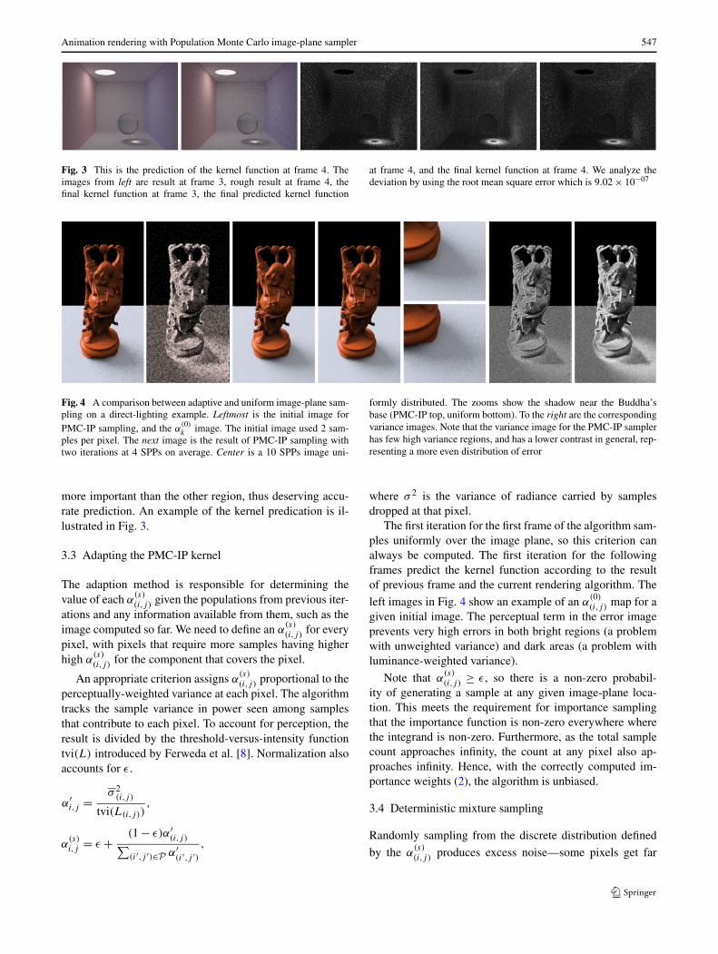
Fig. 3 This is the prediction of the kernel function at frame 4. Theimages from left are result at frame 3, rough result at frame 4, thefinal kernel function at frame 3, the final predicted kernel function

at frame 4, and the final kernel function at frame 4. We analyze thedeviation by using the root mean square error which is 9.02 × 10−07

Fig. 4 A comparison between adaptive and uniform image-plane sam-pling on a direct-lighting example. Leftmost is the initial image forPMC-IP sampling, and the α

(0)k image. The initial image used 2 sam-

ples per pixel. The next image is the result of PMC-IP sampling withtwo iterations at 4 SPPs on average. Center is a 10 SPPs image uni-

formly distributed. The zooms show the shadow near the Buddha’sbase (PMC-IP top, uniform bottom). To the right are the correspondingvariance images. Note that the variance image for the PMC-IP samplerhas few high variance regions, and has a lower contrast in general, rep-resenting a more even distribution of error

more important than the other region, thus deserving accu-rate prediction. An example of the kernel predication is il-lustrated in Fig. 3.

3.3 Adapting the PMC-IP kernel

The adaption method is responsible for determining thevalue of each α

(s)(i,j)

given the populations from previous iter-ations and any information available from them, such as theimage computed so far. We need to define an α

(s)(i,j) for every

pixel, with pixels that require more samples having higherhigh α

(s)(i,j) for the component that covers the pixel.

An appropriate criterion assigns α(s)(i,j) proportional to the

perceptually-weighted variance at each pixel. The algorithmtracks the sample variance in power seen among samplesthat contribute to each pixel. To account for perception, theresult is divided by the threshold-versus-intensity functiontvi(L) introduced by Ferweda et al. [8]. Normalization alsoaccounts for ε.

α′i,j = σ 2

(i,j)

tvi(L(i,j)),

α(s)i,j = ε + (1 − ε)α′

(i,j)∑(i′,j ′)∈P α′

(i′,j ′),

where σ 2 is the variance of radiance carried by samplesdropped at that pixel.

The first iteration for the first frame of the algorithm sam-ples uniformly over the image plane, so this criterion canalways be computed. The first iteration for the followingframes predict the kernel function according to the resultof previous frame and the current rendering algorithm. The

left images in Fig. 4 show an example of an α(0)(i,j) map for a

given initial image. The perceptual term in the error imageprevents very high errors in both bright regions (a problemwith unweighted variance) and dark areas (a problem withluminance-weighted variance).

Note that α(s)(i,j)

≥ ε, so there is a non-zero probabil-ity of generating a sample at any given image-plane loca-tion. This meets the requirement for importance samplingthat the importance function is non-zero everywhere wherethe integrand is non-zero. Furthermore, as the total samplecount approaches infinity, the count at any pixel also ap-proaches infinity. Hence, with the correctly computed im-portance weights (2), the algorithm is unbiased.

3.4 Deterministic mixture sampling

Randomly sampling from the discrete distribution defined

by the α(s)(i,j) produces excess noise—some pixels get far


more or fewer samples than their expected value. This prob-lem is solved with deterministic mixture sampling, DMS,which is designed to give each component (pixel) a num-

ber of samples roughly proportional to its α(s)(i,j). Determin-

istic mixture sampling is unbiased and always gives lowervariance when compared to random mixture sampling, asproven by Hesterberg [12].

The number of samples per iteration, N (the populationsize) is fixed at a small multiple of the number of pixels. Wetypically use 4 samples per pixel, which balances betweenspending too much effort on any one iteration and the over-head of computing a new set of kernel parameters. For eachpixel, the deterministic sampler computes n′

(i,j) = Nα(i,j),the target number of samples for that pixel. It takes �n′

(i,j)�samples from each pixel (i, j)’s component. The remainingun-allocated samples are sampled from the residual distrib-ution with probability n′

(i,j)−�n′

(i,j)� at each pixel (suitably

normalized).

4 Results

This section presents the rendering results when we applyour PMC-IP algorithm to render a single frame of scenesand animation scenes by plugging in our sampler into themodern global illumination framework to demonstrate theusefulness of our algorithm

4.1 Static image rendering

Adaptive image-plane sampling can be used in many situa-tions where pixel samples are required and an iterative algo-rithm can be employed. We have implemented it in the con-texts of direct lighting using a Multiple Importance Sampler(MIS) and global illumination with path tracing, and as partof a complete photon mapping system.

Figure 4 shows the Buddha direct-lighting example. Thesurface is diffuse with an area light source. Each pixel sam-ple used 8 illumination samples, and the images were ren-dered at 256×512, with statistics presented in Table 1.Weintroduce the perceptually-based mean squared efficiency(P-Eff) metric for comparing algorithms, computed as:

Err =∑

pixels e2

tvi(L), P-Eff = 1

T × Err

where e is the difference in intensity between a pixel andthe ground truth value and T is the running time of the algo-rithm on that image. P-Eff is a measure of how much longer(or less) you would need to run one algorithm to reach theperceptual quality of another [22].

The final adaptive image shown is the unweighted aver-age of three sub-images (initial and two iterations). While

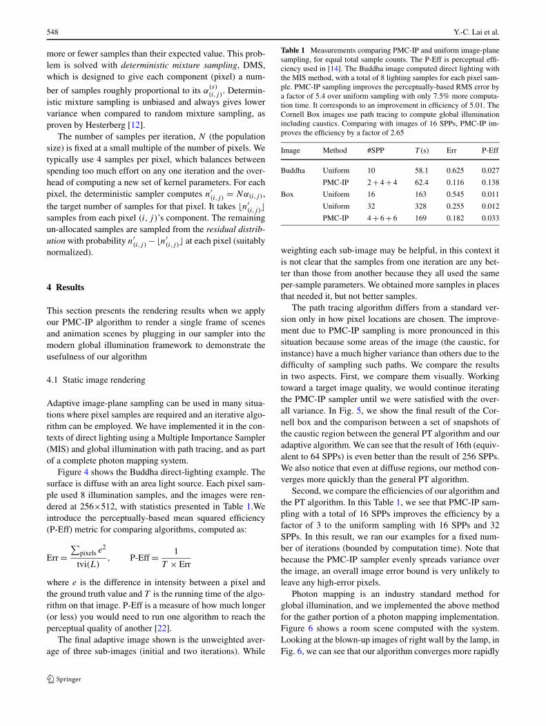
Table 1 Measurements comparing PMC-IP and uniform image-planesampling, for equal total sample counts. The P-Eff is perceptual effi-ciency used in [14]. The Buddha image computed direct lighting withthe MIS method, with a total of 8 lighting samples for each pixel sam-ple. PMC-IP sampling improves the perceptually-based RMS error bya factor of 5.4 over uniform sampling with only 7.5% more computa-tion time. It corresponds to an improvement in efficiency of 5.01. TheCornell Box images use path tracing to compute global illuminationincluding caustics. Comparing with images of 16 SPPs, PMC-IP im-proves the efficiency by a factor of 2.65

Image Method #SPP T (s) Err P-Eff

Buddha Uniform 10 58.1 0.625 0.027

PMC-IP 2 + 4 + 4 62.4 0.116 0.138

Box Uniform 16 163 0.545 0.011

Uniform 32 328 0.255 0.012

PMC-IP 4 + 6 + 6 169 0.182 0.033

weighting each sub-image may be helpful, in this context itis not clear that the samples from one iteration are any bet-ter than those from another because they all used the sameper-sample parameters. We obtained more samples in placesthat needed it, but not better samples.

The path tracing algorithm differs from a standard ver-sion only in how pixel locations are chosen. The improve-ment due to PMC-IP sampling is more pronounced in thissituation because some areas of the image (the caustic, forinstance) have a much higher variance than others due to thedifficulty of sampling such paths. We compare the resultsin two aspects. First, we compare them visually. Workingtoward a target image quality, we would continue iteratingthe PMC-IP sampler until we were satisfied with the over-all variance. In Fig. 5, we show the final result of the Cor-nell box and the comparison between a set of snapshots ofthe caustic region between the general PT algorithm and ouradaptive algorithm. We can see that the result of 16th (equiv-alent to 64 SPPs) is even better than the result of 256 SPPs.We also notice that even at diffuse regions, our method con-verges more quickly than the general PT algorithm.

Second, we compare the efficiencies of our algorithm andthe PT algorithm. In this Table 1, we see that PMC-IP sam-pling with a total of 16 SPPs improves the efficiency by afactor of 3 to the uniform sampling with 16 SPPs and 32SPPs. In this result, we ran our examples for a fixed num-ber of iterations (bounded by computation time). Note thatbecause the PMC-IP sampler evenly spreads variance overthe image, an overall image error bound is very unlikely toleave any high-error pixels.

Photon mapping is an industry standard method forglobal illumination, and we implemented the above methodfor the gather portion of a photon mapping implementation.Figure 6 shows a room scene computed with the system.Looking at the blown-up images of right wall by the lamp, inFig. 6, we can see that our algorithm converges more rapidly


Fig. 5 A Cornell Box image computed using the PMC-IP algorithm.The left image is the final result using PMC-IP algorithm with 64 it-erations, with each iteration averaging 4 SPPs. It is easier to find con-verged values in diffuse regions than in the caustic region. Thus, wecompare the results by focusing on this region. The images in the sec-ond row on the top, from top to down, are the cropped images of thecaustic region computed using non-adaptive path tracing with 16, 32,

64 and 128 SPPs. The images in the third row on the top, from topto down, are intermediate results from the adaptive algorithm at 4, 8,16 and 32 iterations when computing the top image. The right bottomdemonstrates that our adaptive sampler produces better visual resultsat lower sample counts: on the top is the result from 256 SPPs, un-adapted, and on the bottom image is the result of 16 adapting iterationsat an average of 4 SPPs per iteration

Fig. 6 The top is a room scene with complex models computed usingphoton mapping and the adaptive image plane sampler. The bottomrow are blown up images of the upper right portion of the room scene.The image was generated with a standard photon shooting phase. Onthe left is the result of a final gather with 4 PMC-IP iterations, with

each iteration averaging 4 samples per pixel. Right is the result of astandard photon mapping gather using 16 SPPs and using 16 shadowrays per light to estimate direct lighting. Note the significant reductionin noise with our methods


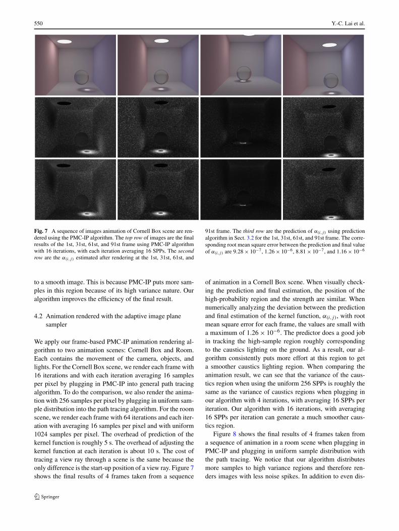
Fig. 7 A sequence of images animation of Cornell Box scene are ren-dered using the PMC-IP algorithm. The top row of images are the finalresults of the 1st, 31st, 61st, and 91st frame using PMC-IP algorithmwith 16 iterations, with each iteration averaging 16 SPPs. The secondrow are the α(i,j) estimated after rendering at the 1st, 31st, 61st, and

91st frame. The third row are the prediction of α(i,j) using predictionalgorithm in Sect. 3.2 for the 1st, 31st, 61st, and 91st frame. The corre-sponding root mean square error between the prediction and final valueof α(i,j) are 9.28 × 10−7, 1.26 × 10−6, 8.81 × 10−7, and 1.16 × 10−6

to a smooth image. This is because PMC-IP puts more sam-ples in this region because of its high variance nature. Ouralgorithm improves the efficiency of the final result.

4.2 Animation rendered with the adaptive image planesampler

We apply our frame-based PMC-IP animation rendering al-gorithm to two animation scenes: Cornell Box and Room.Each contains the movement of the camera, objects, andlights. For the Cornell Box scene, we render each frame with16 iterations and with each iteration averaging 16 samplesper pixel by plugging in PMC-IP into general path tracingalgorithm. To do the comparison, we also render the anima-tion with 256 samples per pixel by plugging in uniform sam-ple distribution into the path tracing algorithm. For the roomscene, we render each frame with 64 iterations and each iter-ation with averaging 16 samples per pixel and with uniform1024 samples per pixel. The overhead of prediction of thekernel function is roughly 5 s. The overhead of adjusting thekernel function at each iteration is about 10 s. The cost oftracing a view ray through a scene is the same because theonly difference is the start-up position of a view ray. Figure 7shows the final results of 4 frames taken from a sequence

of animation in a Cornell Box scene. When visually check-ing the prediction and final estimation, the position of thehigh-probability region and the strength are similar. Whennumerically analyzing the deviation between the predictionand final estimation of the kernel function, α(i,j), with rootmean square error for each frame, the values are small witha maximum of 1.26 × 10−6. The predictor does a good jobin tracking the high-sample region roughly correspondingto the caustics lighting on the ground. As a result, our al-gorithm consistently puts more effort at this region to geta smoother caustics lighting region. When comparing theanimation result, we can see that the variance of the caus-tics region when using the uniform 256 SPPs is roughly thesame as the variance of caustics regions when plugging inour algorithm with 4 iterations, with averaging 16 SPPs periteration. Our algorithm with 16 iterations, with averaging16 SPPs per iteration can generate a much smoother caus-tics region.

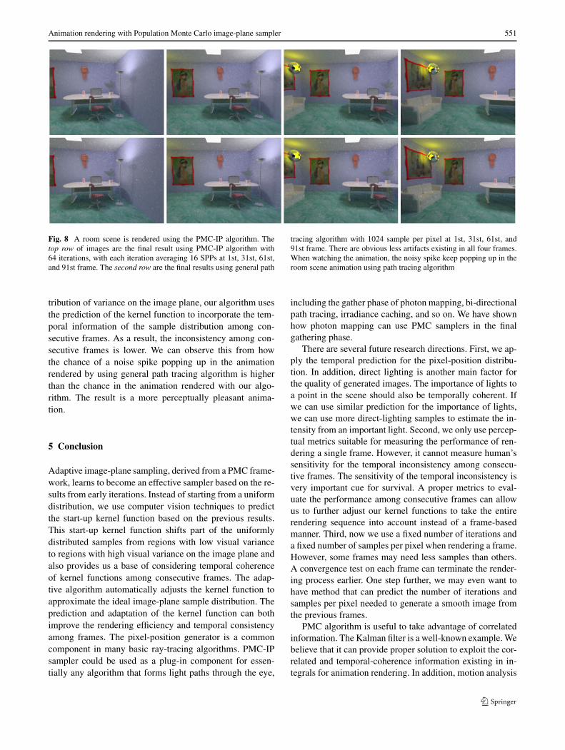
Figure 8 shows the final results of 4 frames taken froma sequence of animation in a room scene when plugging inPMC-IP and plugging in uniform sample distribution withthe path tracing. We notice that our algorithm distributesmore samples to high variance regions and therefore ren-ders images with less noise spikes. In addition to even dis-


Fig. 8 A room scene is rendered using the PMC-IP algorithm. Thetop row of images are the final result using PMC-IP algorithm with64 iterations, with each iteration averaging 16 SPPs at 1st, 31st, 61st,and 91st frame. The second row are the final results using general path

tracing algorithm with 1024 sample per pixel at 1st, 31st, 61st, and91st frame. There are obvious less artifacts existing in all four frames.When watching the animation, the noisy spike keep popping up in theroom scene animation using path tracing algorithm

tribution of variance on the image plane, our algorithm usesthe prediction of the kernel function to incorporate the tem-poral information of the sample distribution among con-secutive frames. As a result, the inconsistency among con-secutive frames is lower. We can observe this from howthe chance of a noise spike popping up in the animationrendered by using general path tracing algorithm is higherthan the chance in the animation rendered with our algo-rithm. The result is a more perceptually pleasant anima-tion.

5 Conclusion

Adaptive image-plane sampling, derived from a PMC frame-work, learns to become an effective sampler based on the re-sults from early iterations. Instead of starting from a uniformdistribution, we use computer vision techniques to predictthe start-up kernel function based on the previous results.This start-up kernel function shifts part of the uniformlydistributed samples from regions with low visual varianceto regions with high visual variance on the image plane andalso provides us a base of considering temporal coherenceof kernel functions among consecutive frames. The adap-tive algorithm automatically adjusts the kernel function toapproximate the ideal image-plane sample distribution. Theprediction and adaptation of the kernel function can bothimprove the rendering efficiency and temporal consistencyamong frames. The pixel-position generator is a commoncomponent in many basic ray-tracing algorithms. PMC-IPsampler could be used as a plug-in component for essen-tially any algorithm that forms light paths through the eye,

including the gather phase of photon mapping, bi-directionalpath tracing, irradiance caching, and so on. We have shownhow photon mapping can use PMC samplers in the finalgathering phase.

There are several future research directions. First, we ap-ply the temporal prediction for the pixel-position distribu-tion. In addition, direct lighting is another main factor forthe quality of generated images. The importance of lights toa point in the scene should also be temporally coherent. Ifwe can use similar prediction for the importance of lights,we can use more direct-lighting samples to estimate the in-tensity from an important light. Second, we only use percep-tual metrics suitable for measuring the performance of ren-dering a single frame. However, it cannot measure human’ssensitivity for the temporal inconsistency among consecu-tive frames. The sensitivity of the temporal inconsistency isvery important cue for survival. A proper metrics to eval-uate the performance among consecutive frames can allowus to further adjust our kernel functions to take the entirerendering sequence into account instead of a frame-basedmanner. Third, now we use a fixed number of iterations anda fixed number of samples per pixel when rendering a frame.However, some frames may need less samples than others.A convergence test on each frame can terminate the render-ing process earlier. One step further, we may even want tohave method that can predict the number of iterations andsamples per pixel needed to generate a smooth image fromthe previous frames.

PMC algorithm is useful to take advantage of correlatedinformation. The Kalman filter is a well-known example. Webelieve that it can provide proper solution to exploit the cor-related and temporal-coherence information existing in in-tegrals for animation rendering. In addition, motion analysis


of a film in the vision community provides us with tech-niques to explore the temporal coherence which may be thekey to render a consistent animation in an efficient way.

References

1. Aydin, T., Mantiuk, R., Myszkowski, K., Seidel, H.: (2008)2. Baker, S., Black, M.J., Lewis, J., Roth, S., Scharstein, D., Szeliski,

R.: A database and evaluation methodology for optical flow. In:IEEE ICCV (2007)

3. Bolin, M.R., Meyer, G.W.: A perceptually based adaptive sam-pling algorithm. In: SIGGRAPH ’98, pp. 299–309 (1998)

4. Dayal, A., Woolley, C., Watson, B., Luebke, D.: Adaptive frame-less rendering. In: Proc. of the 16th Eurographics Symposium onRendering, pp. 265–275 (2005)

5. Dippé, M.A.Z., Wold, E.H.: Antialiasing through stochastic sam-pling. In: SIGGRAPH ’85, pp. 69–78 (1985)

6. Douc, R., Guillin, A., Marin, J.M., Robert, C.P.: Convergence ofadaptive sampling schemes. Technical Report 2005–2006, Uni-versity Paris Dauphine (2005). http://www.cmap.polytechnique.fr/~douc/Page/Research/dgmr.pdf

7. Farrugia, J.P., Péroche, B.: A progressive rendering algorithm us-ing an adaptive pereptually based image metric. Comput. Graph.Forum (Proc. Eurograph. 2004) 23(3), 605–614 (2004)

8. Ferwerda, J.A., Pattanaik, S.N., Shirley, P., Greenberg, D.P.:A model of visual adaptation for realistic image synthesis. In:SIGGRAPH ’96, pp. 249–258 (1996)

9. Fischler, M.A., Bolles, R.C.: Random sample consensus: a par-adigm for model fitting with applications to image analysis andautomated cartography. Commun. ACM 24(6), 381–395 (1981).doi:10.1145/358669.358692

10. Ghosh, A., Doucet, A., Heidrich, W.: Sequential sampling fordynamic environment map illumination. In: Proc. EurographicsSymposium on Rendering, pp. 115–126 (2006)

11. Glassner, A.: Principles of Digital Image Synthesis. Morgan Kauf-mann, San Mateo (1995)

12. Hesterberg, T.: Weighted average importance sampling and defen-sive mixture distributions. Technometrics 37, 185–194 (1995)

13. Kirk, D., Arvo, J.: Unbiased sampling techniques for image syn-thesis. In: SIGGRAPH ’91, pp. 153–156 (1991)

14. Lai, Y., Fan, S., Chenney, S., Dyer, C.: Photorealistic image ren-dering with population Monte Carlo energy redistribution. In: Eu-rographics Symposium on Rendering, pp. 287–296 (2007)

15. Lai, Y.C., Liu, F., Zhang, L., Dyer, C.: Efficient schemes for MonteCarlo Markov chain algorithms in global illumination. In: ISVC’08: Proceedings of the 4th International Symposium on Advancesin Visual Computing, pp. 614–623 (2008)

16. Lee, M.E., Redner, R.A., Uselton, S.P.: Statistically optimizedsampling for distributed ray tracing. In: SIGGRAPH ’85, pp. 61–68 (1985)

17. Lowe, D.G.: Distinctive image features from scale-invariant key-points. Int. J. Comput. Vis. 60(2), 91–110 (2004)

18. Lucas, B., Kanade, T.: An iterative image registration techniquewith an application to stereo vision. In: Proc. of International JointConference on Artificial Intelligence, pp. 674–679 (1981)

19. Mantiuk, R., Myszkowski, K., Seidel, H.P.: Visible differencepredicator for high dynamic range images. In: Proceedings ofIEEE International Conference on Systems, Man and Cybernet-ics, pp. 2763–2769 (2004)

20. Mitchell, D.P.: Generating antialiased images at low samplingdensities. In: SIGGRAPH ’87, pp. 65–72 (1987)

21. Painter, J., Sloan, K.: Antialiased ray tracing by adaptive progres-sive refinement. In: SIGGRAPH ’89, pp. 281–288 (1989)

22. Pharr, M., Humphreys, G.: Physically Based Rendering from The-ory to Implementation. Morgan Kaufmann, San Mateo (2004)

23. Purgathofer, W.: A statistical method for adaptive stochastic sam-pling. In: Proc. EUROGRAPHICS 86, pp. 145–152 (1986)

24. Ramasubramanian, M., Pattanaik, S.N., Greenberg, D.P.: A per-ceptually based physical error metric for realistic image synthesis.In: SIGGRAPH ’99, pp. 73–82 (1999)

25. Rigau, J., Feixas, M., Sbert, M.: New contrast measures for pixelsupersampling. In: Proc. of CGI’02, pp. 439–451. Springer, Berlin(2002)

26. Rigau, J., Feixas, M., Sbert, M.: Entropy-based adaptive sampling.In: Proc. of Graphics Interface 2003, pp. 149–157 (2003)

27. Schlick, C.: An adaptive sampling technique for multidimensionalintegration by ray-tracing. In: Proc. of the 2nd Eurographics Work-shop on Rendering, pp. 21–29 (1991)

28. Stokes, W.A., Ferwerda, J.A., Walter, B., Greenberg, D.P.: Per-ceptual illumination components: a new approach to efficient,high quality global illumination rendering. In: SIGGRAPH ’04,pp. 742–749 (2004)

29. Szeliski, R.: Image alignment and stitching: A tutorial. Tech. Rep.MSR-TR-2004-92, Microsoft Research (2006)

30. Tamstorf, R., Jensen, H.W.: Adaptive sampling and bias estima-tion in path tracing. In: Proc. of the 8th Eurographics Workshopon Rendering, pp. 285–296 (1997)

Yu-Chi Lai received the B.S. fromNational Taiwan University, Taipei,ROC, in 1996 in Electrical Engi-neering Department. He receivedhis M.S. and Ph.D. degrees fromUniversity of Wisconsin—Madisonin 2003 and 2009 respectively inElectrical and Computer Engineer-ing and his M.S. and Ph.D. degreesin 2004 and 2010 respectively inComputer Science.He is currently an assistant profes-sor in NTUST and his Research in-terests are in the area of graphics,vision, and multimedia.

Stephen Chenney received his aPh.D. in 2000 from the ComputerScience division at the University ofCalifornia at Berkeley. He is currenta programmer in Emergent GameTechnology.

http://www.cmap.polytechnique.fr/~douc/Page/Research/dgmr.pdf

http://www.cmap.polytechnique.fr/~douc/Page/Research/dgmr.pdf

http://dx.doi.org/10.1145/358669.358692


Feng Liu received the B.S. andM.S. degrees from Zhejiang Univer-sity, Hangzhou, China, in 2001 and2004, respectively, both in computerscience. He is currently a Ph.D. can-didate in the Department of Com-puter Sciences at the University ofWisconsin-Madison, USA.His research interests are in the ar-eas of graphics, vision and multime-dia.

Yuzhen Niu received the B.S. de-gree from Shandong University,Jinan, China, in 2005 in computerscience. She is currently a Ph.D.candidate in the School of Com-puter Science and Technology at theShandong University, China.Her research interests are in the ar-eas of graphics, vision and human-computer interaction.

Shaohua Fan received his B.S de-gree in Mathematics from BeijingNormal University, M.S. degree inMathematical Finance from CourantInstitute at NYU, and Ph.D. in com-puter science from University ofWisconsin-Madison. He is currentlya professor at financial engineeringresearch center at Suzhou Univer-sity, China and a quantitative re-searcher at Ernst & Young in NewYork.His research interests are statisti-cal arbitrage, high-frequency trad-ing, and Monte Carlo methods forfinancial derivatives pricing.

Animation rendering with Population Monte Carlo image-plane sampler

Documents

Transcript of Animation rendering with Population Monte Carlo image-plane sampler