
Analysis of Thin Concrete Shells Revisited - TU Delft
435
Analysis of Thin Concrete Shells Revisited: Opportunities due to Innovations in Materials and Analysis Methods Delft University of Technology Faculty of Civil Engineering and Geosciences Structural and Building Engineering Concrete Structures Stevinweg 1, Delft, the Netherlands Master’s thesis committee Prof.dr.ir. J.C. Walraven Concrete Structures Ir. W.J.M. Peperkamp Concrete Structures Prof.dr.ir. J.G.Rots Structural Mechanics Dr.ir. P.C.J. Hoogenboom Structural Mechanics Ir. L.J.M. Houben Graduation coordinator
-
Upload
khangminh22 -
Category
Documents
-
view
0 -
download
0
Transcript of Analysis of Thin Concrete Shells Revisited - TU Delft

Analysis of Thin Concrete Shells Revisited:
Opportunities due to Innovations in Materials and Analysis Methods Delft University of Technology Faculty of Civil Engineering and Geosciences Structural and Building Engineering Concrete Structures Stevinweg 1, Delft, the Netherlands Master’s thesis committee Prof.dr.ir. J.C. Walraven Concrete Structures Ir. W.J.M. Peperkamp Concrete Structures Prof.dr.ir. J.G.Rots Structural Mechanics Dr.ir. P.C.J. Hoogenboom Structural Mechanics Ir. L.J.M. Houben Graduation coordinator


I
Preface
This is the final report of my Master’s thesis performed at the department of Structural and Building
Engineering, part of the faculty of Civil Engineering and Geosciences of Delft University of Technology. The
subject of this thesis is “Analysis of Thin Concrete Shells Revisited: Opportunities due to Innovations in
Materials and Analysis Methods”.
The subject of the thesis associates with today’s renewed interest in free-form shells by the society. The
construction of thin concrete shells ended abruptly at the end of the 1970s, mainly caused by the high costs
in compare to other structural systems. However, uncertainties in the structural behaviour of shells did not
help either. Contemporary progress in finite element software discards these uncertainties as it allows the
engineer to closely approach the actual behaviour of thin concrete shells by performing geometrically and
physically nonlinear finite element analy ses. In addition, recent developments in concrete technology have
led to ultra high performance fibre reinforced concrete with revolutionary performance in tension and
compression. In fact, ultra high performance fibre reinforced concrete can be seen as a completely new
construction material and its possibilities are still to be revealed. The combination of advanced finite
element analyses and ultra high performance fibre reinforced concrete may lead to shells with even greater
spans and thinner thicknesses than achieved so far. In the following, this hypothesis is tested on a case
study. The thesis’ report describes the activities undertaken and the results found, supplemented with
historical, practical and theoretical background.
I would like to thank my graduation committee, Prof.dr.ir. J.C. Walraven, Ir. W.J.M. Peperkamp, Prof.dr.ir.
J.G.Rots, Dr.ir. P.C.J. Hoogenboom and Ir. L.J.M. Houben for their guidance and ideas during the project.
Special thanks to Dr.ir. M.A.N. Hendriks and Ir. R.A. Burgers, for their support and advice on finite element
analyses. Furthermore, I would like to thank the other graduates in room 0.72 for their inspirational
conversations during coffee breaks. Last but not least, I would like to thank my parents for giving me the
opportunity to develop my self both professionally and socially during my years in Delft.
Bart Peerdeman
Delft, June 2008

II

III
Summary
Shell structures have been constructed since ancient times. The Pantheon in Rome and the Hagia Sophia in
Istanbul are well-known examples. After the Roman times the traditions of domes continued up to the 17 th
century. Since then they seemed forgotten. Stimulated by the newly developed reinforced concrete and the
demand to cov er long-spans economically and column free the shell made a comeback in the early 20th
century. Franz Dischinger and Ulrich Finsterwalder designed in 1925 the first thin concrete shell of the
modern era, the Zeiss planetarium in Germany. The modern era of shell construction is recognised by the
trend towards greater spans and thinner shells. Guided by well-known engineers as Pier Luigi Nervi,
Eduardo Torroja, Anton Tedesko, Nicolas Esquillan, Felix Candela and Heinz Isler a blooming period of
widespread shell construction took place between 1950 and 1970. Shell construction suddenly vanished at
the end of the 1970s, mainly caused by the high costs in compare to other structural systems. Moreover,
inflexible usability and uncertainties in the structural behaviour of shells and difficulty of proper analy sis
methods did not help neither did the stylistic identification with the 1950s and 1960s. Today the great era of
thin shells is over, however, nowadays natural free-form shapes and blobs attract more and more attention.
In addition, recent developments in concrete technology have led to ultra high performance fibre reinforced
concrete with rev olutionary performance in tension and compression. Eventually this may lead to a revival of
the thin concrete shell.
Shells are constructed from concrete, profoundable due to the combination of filling and load carrying
capacities. They are being built as ‘thin shells’, with a radius-to-thickness ratio starting at 200 reaching up to
800 and higher. The low consumption of material follows from the profound that shells are very efficient in
carrying loads acting perpendicular to their surface by in-plane membrane stresses. In fact, the preference
for membrane action arises as a consequence of being thin. Bending moments eventually arise only to satisfy
specific equilibrium or deformation requirements. They do not carry loads and have a local character.
Concrete shells include single and double curved surfaces which are either synclastic, monoclastic or
anticlastic. The surface can be generated by mathematical functions or by form-finding methods such as
hanging membranes or pneumatic models. Contemporary computational advancement launched (real-time)
computer based shell generation techniques such as the particle-spring sy stems. To calculate the membrane
stresses of a given geometry quantitative information can be obtained by constructing a polygon of forces
(for simple geometries), by using the Kirchhoffean based classical thin shell theory or by computer software
such as finite element programs. For qualitative information over the force flow the rainflow analysis or
model tests can be performed. The geometry forms a structural effective shell if the shell is able to develop a
prevalent membrane stress field up to the highest degree. Optimisation techniques, such as shape
optimisation by minimising strain energy, may lead to a design which is much more efficient from a

IV
structural point of view. Optimisation may be enhanced by computation optimisation algorithms such as
ESO or ACO. In general the design will lead to a shell with a rise to span ratio between 1/10 and 1/6 with an
opening angle between 60 and 90 degrees. The shell thickness is practically bounded by 60 to 80 mm for
one- or two-layers of traditional steel reinforcing bars, respectively. Fibre reinforced structures may be even
thinner. The reinforcement percentages are rather low, approximately 0.15 to 0.4%. Possible prestressing
may be applied in the edge (ring) beam or even in the shell surface itself. Finally, for a sound shell structure
extra attention must be paid to the shell edge design in case of free edges. In general, forces flowing away
from the edge prevent large edge beams which may cause problems such as shear off.
Most shells are constructed in a conventional manner: pouring concrete on a formwork. Other possibilities
are the use of airform moulds or stressed membranes combined with sprayed concrete. Although the
number of repetition is often not very high, prefabricated elements may be used. After hydratation, the
concrete is predominantly left blank, allowing the climate freely attack the concrete skin.
In case of a failure, the shell may fail due to large deformations (buckling) or due to material nonlinearity
(cracking and crushing) or by a combination of both (so-called inelastic or plastic buckling). The buckling
behaviour of shells is a complicated phenomenon. Opposite to columns and plates, shells experience a
sudden decrease in load carrying capacity after the bifurcation point (which can be obtained by a simple
linear buckling analysis). The fall-back is caused by the phenomenon of compound buckling which refers to
sev eral buckling modes associated with the same critical load. In the postbuckling range the modes, which
were orthogonal in the linear prebuckling range, start to interact resulting in a significantly reduced load
carrying capacity. As discovered by Koiter, the major problem of the shell buckling behaviour is the
accompanied imperfection sensitivity. Initial geometrical imperfections in the shell cause the bifurcation
point never to be reached and lead to limit point buckling at a considerably lower load. The size of the
imperfections determines the limit load at which the shell fails. In case of plastic buckling, the fall-back is
further intensified by material nonlinearity.
From the foregoing two primary research questions can be formulated:
What is for a shell of hemispherical geometry, with given material properties, given support conditions,
and subjected to a given load, the knock-down factor which indicates the difference between the linear
critical buckling load and the actual critical buckling load taking into account imperfections and
geometrical and physical nonlinearities?
And
Can high strength fibre reinforced concrete add to the trend towards greater spans and thinner shells with
possibilities for even more slender structures?
To obtain an answer to the research questions a series of analyses (linear elastic, stability, geometrically
nonlinear and geometrically and phy sically nonlinear) is performed on a given hemispherical shell: the Zeiss
planetarium shell. The shell has a radius of curvature of 12500 mm and a thickness of 60 mm. Thereby, the

V
R/t ratio is equal to 200. The shell is reinforced with one layer of low quality reinforcement FeB220 and
assumed to be made from a C20/25 low quality concrete mixture to ally with the early 20th century concrete
technology. For this research the shell is modelled with an axisymmetric curved line model and a three-
dimensional model subjected to uniform spherical or vertical load. During analyses, the R/t ratio is ranged
from 200 up to 1000 (stepsize 200). Additionally, the possibilities of even more slender structures by using
high strength fibre reinforced concrete are investigated by comparing the original C20/25 shell to a
C180/210 ultra high performance fibre reinforced concrete mixture. To investigate the influence of initial
geometrical imperfections a local top imperfection is modelled with an imperfection amplitude ranging from
w0/t = 0.0 to 1.0 (stepsize 0.2). Moreover, the influence of four boundary conditions is investigated, i.e.
roller, inclined-roller, hinged and clamped support.
The linear elastic analysis proved to be in fair agreement with the (benchmark) analytical results for the
three-dimensional model. The axisymmetric model is found to be less accurate and reliable, in particular
with respect to the bending moments caused by restrained deformation at the supports. In both models
disturbances in the stress and bending moment distribution were caused by the numerical imperfections.
They appeared to be negligible on the linear solution. The disturbances are more apparent in the stability
analysis, as they cause premature buckling modes preceding the actual shell buckling shape. Membrane
supported shells with spherical load show a global buckling pattern of small local waves. The critical
buckling load is significantly lower for membrane incompatible support conditions and/or vertical load.
Shells subjected to v ertical load, by definition, buckle in the boundary layer. The three-dimensional buckling
results reveal the occurrence of compound buckling as adjacent critical loads are very close to each other. In
general, thinner shells experience compound buckling up to a higher degree than thicker shells. The results
of the axisymmetric shell model are poor, as compound buckling is not predicted correctly. Moreover, the
axisymmetry causes the tendency to buckle at the top and the buckling loads are disturbed by the incorrect
bending moments in case of a hinged and clamped support.
The geometrically nonlinear results demonstrate the imperfection sensitivity of shells as even small
imperfection amplitudes already cause a significant decrease in load carrying capacity. The results appear to
be in reasonable correlation to the Koiter half-power law and the relation as proposed by the IASS
Recommendations, Kollar and Dulacska [54]. The inclined-roller supported shell subjected to spherical load
provides an upper bound solution. The shell, by definition, fails at the imperfection. Variations in boundary
and load conditions may lead to a shell failure insensitive to the top imperfection until the imperfection
progresses to a certain size. The introduction of material nonlinearity leads to a further decrease in load-
carrying capacity and the transformation to a strength failure rather than a buckling failure in case of shells
subjected to uniform vertical load. Buckling eventually takes place after significant cracking, responsible for
the major part of the knock-down factor, has occurred. In the considered hemispherical shells cracking,
crushing and buckling strongly interact before and during failure. This is influenced by loading, shell
thickness, material properties and geometrical imperfections. For the considered C20/25 hemispherical
shell the knock-down factor is much smaller than the knock-down factor as derived using the IASS
recommendations, which apparently are very conservative. The use of high strength fibre reinforced concrete
appeared to be advantageous, in particular the higher axial and flexural tensile strength give the engineer
opportunities to design thinner shells. Furthermore, high strength concrete is advantageous in compression

VI
as it excludes premature compressive crushing failure before the critical buckling load is reached. Opposed
to fibre reinforced beams in bending, the significant ductility (postcracking plateau) of high strength fibre
reinforced concrete does not influence the ultimate load carrying capacity of hemispherical shells. This
might be caused by the buckling which occurs simultaneously with significant cracking.
From the results it can be concluded that it is impossible to derive a general expression for the knock-down
factor, unless high factors of uncertainty are taken into consideration. However, contemporary finite element
software makes possible to determine the structural behaviour of an imperfect shell and to compute its fall-
back in load carrying capacity conveniently within a small amount of time by performing a geometrically and
physically nonlinear analysis. In fact, it is this conclusion that is the most salient.

Table of Contents
VII
Contents at a Glance
Preface I
Summary III
Contents at a Glance VII
Contents IX
Chapter 1: Introduction and Aim of Thesis 1
PART I. Background
Chapter 2: History of Thin Concrete Shell 6
Chapter 3 : Shell Design 36
Chapter 4: Shell Construction 70
PART II. Theory
Chapter 5: Theory of Shells 86
Chapter 6: Structural Failure 116
PART III. Case Study
Chapter 7: Zeiss Planetarium 167
Chapter 8: Material 169
Chapter 9: Loading 189
Chapter 10: Hemispherical Example 197
PART IV. Finite Element Analysis
Chapter 11: Finite Element Method 220
Chapter 12: Linear Elastic Finite Element Analysis 274
Chapter 13: Stability Finite Element Analysis 306
Chapter 14: Geometrically Nonlinear Finite Element Analysis 330
Chapter 15: Geometrically and Physically Nonlinear Finite Element Analy sis 348
Chapter 16: Conclusions 381
Chapter 17: Recommendations 391
References XVIII

Table of Contents
VIII

Table of Contents
IX
Contents
Preface I
Summary III
Contents at a Glance VII
Contents IX
Chapter 1. Introduction and Aim of Thesis 1
1.1 Context of Thesis 2
1.2 Aim of Thesis 3
1.2.1 Problem Description 3
1.2.2 Objective 3
1.2.3 Process 4
1.3 Approach of Thesis Aim 4
PART I. Background
Chapter 2. History of Thin Concrete Shells 6
2.1 Precursors 7
2.2 Start of Modern Era 8
2.3 World War II 15
2.4 Blooming Period, Sudden Death 16
2.5 Contemporary Shells 30
2.6 Future History 33
2.7 National Schools 34
2.8 Shell Dimensions 35
Chapter 3. Shell Design 36
3.1 Preliminaries of Shell Design and Analysis 38
3.1.1 Membrane Behaviour 38
3.1.2 Bending Behaviour 38
3.1.3 Material Effects on Shell Behaviour 39
3.1.4 In-extensional Deformation 39
3.1.5 Structural Failure 40
3.2 Classification of Shell Surfaces 40
3.2.1 Synclastic 41

Table of Contents
X
3.2.2 Monoclastic 41
3.2.3 Anticlastic 41
3.3 Geometrical Surface Generation 42
3.3.1 Surfaces of Rev olution 42
3.3.2 Translational Surfaces 42
3.3.3 Ruled Surfaces 42
3.3.4 Free-Form Surfaces 43
3.4 Non-Geometrical Surface Generation 43
3.4.1 Physical Modelling 44
3.4.2 Computational Modelling 45
3.5 Mechanical Behaviour 46
3.5.1 Balance Calculation 47
3.5.2 Polygon of Forces 47
3.5.3 Classical Shell Theory 48
3.5.4 Model Tests 49
3.5.5 Computational Numerical Analysis 50
3.5.6 Rainflow Analy sis 51
3.6 Structural Optimisation 52
3.6.1 Size Optimisation 53
3.6.2 Material Optimisation 53
3.6.3 Topology Optimisation 54
3.6.4 Shape Optimisation 54
3.6.5 Computational Optimisation Algorithms 55
3.7 Design Codes 57
3.8 Design Considerations 58
3.8.1 Span/Rise/Radius of Curvature 58
3.8.2 Thickness 58
3.8.3 Ribbed Shells 59
3.8.4 Reinforcement 61
3.8.5 Prestressing 64
3.8.6 Material 65
3.8.7 Supports 65
3.8.8 Edge Design/Free Edges 66
3.8.9 Loading 68
3.8.10 Economics 69
3.9 Conclusions 69
Chapter 4. Shell Construction 70
4.1 Formwork 71
4.1.1 Conventional Formwork 72
4.1.2 Prefabricated Moulds 73
4.1.3 Airform Shells 74

Table of Contents
XI
4.1.4 Stresses Membranes 76
4.2 Reinforcement 77
4.3 Placement of Concrete 79
4.3.1 Conventional Placement 80
4.3.2 Sprayed Concrete 81
4.4 Finishing 82
4.4.1 Prestressing 82
4.4.2 Surface Treatment 82
4.5 Prefabrication 83
4.6 Conclusions 85
PART II. Theory
Chapter 5. Theory of Shells 86
5.1 General 87
5.1.1 History 87
5.1.2 Basic Relations 88
5.1.3 Assumptions 89
5.2 Theory of Bars 90
5.2.1 Extension 90
5.2.2 Bending 91
5.2.3 Combined Extension and Bending 94
5.3 Theory of Plates 94
5.3.1 Extension 95
5.3.2 Bending 98
5.3.3 Combined Extension and Bending 101
5.4 Theory of Shells 101
5.4.1 Extension 102
5.4.2 Bending 107
5.4.3 Combined Extension and Bending 110
5.5 Solve Methods 111
5.5.1 Direct Methods 111
5.5.2 Indirect Methods 112
Chapter 6. Structural Failure 116
6.1 Strength Failure 117
6.2 Buckling Failure 117
6.2.1 Stability and Instability 119
6.2.2 Form of Buckling 119
6.2.3 Koiter Initial Postbuckling Theory 122
6.2.4 Path of Equilibrium 123
6.3 Elastic Column Buckling 125
6.3.1 Ideal Linear Elastic Column 125

Table of Contents
XII
6.3.2 Ideal Nonlinear Elastic Column 127
6.3.3 Imperfect Elastic Column 128
6.3.4 Imperfections (I) 129
6.4 Elastic Place Buckling 130
6.4.1 Ideal Linear Elastic Plate 130
6.4.2 Ideal Nonlinear Elastic Plate 133
6.4.3 Imperfect Elastic Plate 135
6.4.4 Imperfections (II) 135
6.5 Elastic Shell Buckling 135
6.5.1 General Buckling Equation 136
6.5.2 Axially Compressed Circular Cylindrical Shells 139
6.5.3 Spherical Shells under External Pressure 148
6.5.4 Imperfections (III) 156
6.6 Inelastic Shell Buckling 157
6.7 Initial Geometrical Imperfections 158
6.8 Knock-Down Factor Approach 160
6.9 Buckling Recommendations 161
6.9.1 Linear Buckling Load 161
6.9.2 Postbuckling Category 161
6.9.3 Large Deflections and Geometric Imperfections 162
6.9.4 Modification for Material Properties 163
6.9.5 Total Reduction Factor and Safety Factor 165
6.9.6 Conclusion IASS Recommendations 165
6.10 Conclusions 166
PART III. Case Study
Chapter 7. Zeiss Planetarium 167
7.1 Geometry 168
7.2 Material 168
7.3 Support 168
7.4 Loading 168
Chapter 8. Material 169
8.1 Conventional Concrete 170
8.1.1 Compressive Behaviour 170
8.1.2 Tensile Behaviour 172
8.1.3 C20/25 Mixture Design 173
8.2 High Strength Fibre Reinforced Concrete 175
8.2.1 High Compression Strength 175
8.2.2 Fibre Reinforcement 176
8.2.3 UHPFRC in Practice 182
8.2.4 Compressive Behaviour 182
Table of Contents
XIII
8.2.5 Tensile Behaviour 183
8.2.6 C180/210 Mixture Design 184
8.3 Conclusions 187
Chapter 9. Loading 189
9.1 Permanent Loads 190
9.2 Variable Loads 190
9.2.1 Wind Load 190
9.2.2 Snow Load 193
9.3 Accidental Loads 196
9.4 Load Cases 196
9.5 Conclusions 196
Chapter 10. Hemispherical Example 197
10.1 Shell Parameters 198
10.1.1 Geometry 198
10.1.2 Material 198
10.1.3 Support 198
10.1.4 Loading 198
10.2 Analysis Scheme 198
10.3 Linear Analy sis 199
10.3.1 Membrane Behaviour 199
10.3.2 Membrane Stress Resultants 202
10.3.3 Membrane Strains 204
10.3.4 Membrane Displacements 204
10.3.5 Bending Behaviour 206
10.3.6 Bending Solution 208
10.3.7 Total Solution 212
10.4 Geometrical and Material Influences 214
10.4.1 Geometrical Influences 214
10.4.2 Material Influences 215
10.5 Linear (Euler) Buckling Analysis 215
10.6 Postbuckling Analysis 216
10.7 Inelastic Buckling Analysis on Imperfect Shells 217
10.8 Conclusions 218
PART IV. Finite Element Analysis
Chapter 11. Finite Element Method 220
11.1 Mathematical Fundamentals 221
11.11.1 Matrices and Vectors 221
11.11.2 Tensors 223
11.2 Generalised Finite Element Procedure 223

Table of Contents
XIV
11.2.1 Global Formulation 223
11.2.2 Displacements 224
11.2.3 Strains and Stresses 226
11.2.4 Equilibrium Relations 227
11.2.5 Strong Form – Weak Form 227
11.2.6 Numerical Integration 231
11.2.7 System Stiffness Matrix 232
11.2.8 Right Hand Side Vector 233
11.3 Linear Finite Element Procedure 233
11.3.1 Virtual Work Formulation 233
11.3.2 Stiffness Matrix Formulation 235
11.3.3 Assembling RHS Vector 235
11.3.4 Equilibrium 236
11.4 Nonlinear Finite Element Procedure 236
11.4.1 Physical Nonlinearity 237
11.4.2 Geometrical Nonlinearity 238
11.5 Solution Procedures for Static Linear Analysis 239
11.5.1 Direct Procedures 239
11.5.2 Iterative Procedures 240
11.5.3 General Remarks 241
11.6 Solution Procedures for Static Nonlinear Analysis 241
11.6.1 Iterative Procedures 241
11.6.2 Incremental Procedures 243
11.6.3 General Remarks 246
11.7 Stability Analysis 246
11.7.1 Euler Stability (Linear Buckling) 247
11.7.2 Generalised Eigenproblem 248
11.7.3 Shifting 249
11.7.4 Postbuckling Analysis 249
11.8 Solution Methods for Eigenproblems 250
11.9 Finite Element Software 252
11.10 Geometrical Modelling 253
11.10.1 Geometry 253
11.10.2 Mesh Generation 253
11.10.3 Element Types 256
11.10.4 Integration Schemes 260
11.11 Material Modelling 262
11.11.1 Tensile Cracking 263
11.11.2 Compressive Behaviour 268
11.11.3 Modelling Conclusions 273
11.12 Conclusions and Comments 273

Table of Contents
XV
Chapter 12. Linear Elastic Finite Element Analysis 274
12.1 Shell Parameters 275
12.1.1 Geometry 275
12.1.2 Material Properties 275
12.1.3 Boundary Conditions 275
12.1.4 Loading 275
12.1.5 Analysis Scheme 275
12.2 Axisymmetric Shell Model 276
12.2.1 FE Model 276
12.2.2 Support Reactions 276
12.2.3 Stresses 277
12.2.4 Strains 285
12.2.5 Displacements 286
12.3 Three-Dimensional Model 288
12.3.1 FE Model 288
12.3.2 Support Reactions 289
12.3.3 Stresses 290
12.3.4 Strains 296
12.3.5 Displacements 296
12.4 Geometrical Influences 299
12.5 Material Influences 300
12.6 Load Influences 301
12.7 Conclusions 303
Chapter 13. Stability Finite Element Analysis 306
13.1 Shell Parameters 307
13.1.1 Geometry 307
13.1.2 Material 307
13.1.3 Boundary Conditions 307
13.1.4 Loading 307
13.1.5 Analysis Scheme 307
13.2 Linear Buckling Analy sis 307
13.2.1 Axisymmetric Shell Model 307
13.2.2 Three-Dimensional Shell Model 315
13.3 Geometrical Influences 323
13.4 Material Influences 323
13.5 Perturbation and Continuation Analysis 324
13.6 Conclusions 326
Chapter 14. Geometrically Nonlinear Finite Element Analy sis 330
14.1 Shell Parameters 331
14.1.1 Geometry 331

Table of Contents
XVI
14.1.2 Initial Geometrical Imperfections 331
14.1.3 Material 332
14.1.4 Boundary Conditions 332
14.1.5 Loading 332
14.1.6 Analysis Scheme 332
14.1.7 FEA Settings 332
14.2 Perfect Shell 333
14.2.1 Results and Findings 333
14.2.2 Axisymmetric Comparison 334
14.3 Imperfect Shell 335
14.3.1 Results and Findings 335
14.4 Effect of Imperfections 339
14.4.1 Theoretical Comparison 340
14.4.2 Axisymmetric Comparison 341
14.5 Support and Load Influences 341
14.6 Geometrical Influences 344
14.7 Material Influences 344
14.8 Knock-Down Factor Approach 344
14.9 Conclusions 345
Chapter 15. Geometrically and Physically Nonlinear Finite Element Analysis 348
15.1 Shell Parameters 349
15.1.1 Geometry 349
15.1.2 Initial Geometrical Imperfections 349
15.1.3 Material Modelling 349
15.1.4 Boundary Conditions 352
15.1.5 Loading 352
15.1.6 Analy sis Scheme 352
15.1.7 FEA Settings 352
15.2 Results UHPFRC Shell under Spherical Load 352
15.2.1 Zeiss 2 353
15.2.2 Zeiss 1, 3 and 4 359
15.3 Results UHPFRC Shell under Vertical Load 360
15.3.1 Zeiss 1, 2, 3 and 4 360
15.4 Results C20/25 Shell under Spherical Load 364
15.4.1 Zeiss 2 364
15.4.2 Zeiss 1, 3 and 4 369
15.5 Results C20/25 Shell under Vertical Load 370
15.5.1 Zeiss 1, 2, 3 and 4 370
15.6 Practical Considerations 374
15.7 Material Influences 375
15.8 Knock-Down Factor Approach 376

Table of Contents
XVII
15.9 Conclusions 377
Chapter 16. Conclusions 381
16.1 Part I Conclusions 381
16.2 Part II Conclusions 382
16.3 Part III Conclusions 383
16.4 Part IV Conclusions 384
16.4.1 Linear Elastic Analysis 384
16.4.2 Stability Analy sis 384
16.4.3 Geometrically Nonlinear Analysis 385
16.4.4 Geometrically and Physically Nonlinear Analysis 387
16.5 Principal Conclusions 389
Chapter 17. Recommendations 391
17.1 Part I Recommendations 391
17.2 Part II Recommendations 391
17.3 Part III Recommendations 391
17.4 Part IV Recommendations 392
References XVIII


Chapter 1. Introduction and Aim of Thesis
1
1 Introduction and Aim of Thesis
Appearing first in the early 20th century, thin concrete shell structures were frequently used for long-span
roof structures throughout Europe and beyond during the period between 1920 and 1970. The development
stemmed from the need to cover medium to large spans economically and from a fascination with a new
material: reinforced concrete. Concrete shells include single curved shapes such as cylinders and cones and
double curved geometries such as domes which are either synclastic (curves running in the same direction)
or anticlastic (curves running in opposite directions). Most shells are constructed in a conventional matter:
pouring concrete on a formwork. Concrete shells are built as ‘thin shells’. There is referred to a thin shell as
the radius-to-thickness ratio of 200 puts the shell in the range of being ‘thin’. Thin shells provide in an
advantageous low consumption of material.
The low consumption of material in shell structures follows from the unique character of the shell: the
curvature in spatial form. This unique character is responsible for the profound that shell structures are very
efficient in carrying loads acting perpendicular to their surface by so-called membrane action, a general state
of stress which consists of in-plane normal and shear stress resultants only, whereas other structural forms
carry the applied load mostly by bending action, the least efficient load carrying method. This membrane
action results in (low) in-plane membrane stresses which can be absorbed by only a small thickness of the
shell. As a consequence shell structures can be very thin and still span great distances. Radius-to-thickness
ratios of 400 or 500 are not uncommon. Bending moments eventually arise to satisfy specific equilibrium or
deformation requirements. Because bending moments are confined to a small region the rest of the shell is
virtually free from bending actions and still behaves as a true membrane. It is this salient feature of shells
that is responsible for the most profound and efficient structural performance!
Historically, shell structures have been developed since ancient times. The Pantheon in Rome and the Hagia
Sophia in Istanbul are two well-known examples, respectively constructed in the 2nd and 6 th century A.C.
After the Roman times the tradition of domes continued up to the 17 th century, however, in the 18th/19th
century, the art of designing concrete shell structures seemed forgotten. Guided by German designers Franz
Dischinger and Ulrich Finsterwalder, the concrete shell made a come-back in the early 20th century. The first
shell of the modern era is the Zeiss planetarium in Germany built in 1925.
The Zeiss planetarium was the start of a new tradition of thin concrete shell structures. Besides Dischinger
and Finsterwalder, Eduardo Torroja in Spain, Pier Luigi Nervi in Italy and Anton Tedesko in the United
States were among the pioneer shell builders. The inception of the Second World War caused an interruption

Chapter 1. Introduction and Aim of Thesis
2
in shell development. The post-war period, however, created exactly those conditions needed for flourishing
shell construction: low labour costs and construction material (in particular steel) being in short supply.
That launched the blooming period of shell construction which spans approximately 20 years between the
1950s and 1970s and can be characterised by wide spread shell construction throughout the entire world.
The post-war thin shell tradition was carried forward by engineers such as Felix Candela, Mircea Mihailescu
and Nicolas Esquillan. In particular the shells of Candela are spectacular and attracted the attention of
architects like Saarinen which became inv olved in shell design.
The blooming period ended abruptly in the 1970s. Already since the 1960s the emphasis of concrete shell
building has moved to developing countries as shells in Europe became too expensive in compare to other
structural systems, mainly due to labour and formwork costs. However, from the 1970s almost no shells were
built, except for those of Swiss Heinz Isler who used inventive reusable formwork and standardised shell
sizes. Isler is, however, most famous for his elegant free-form shells derived from form-finding methods
which are the basis of much contemporary research.
Today the great era of thin concrete shells is ov er. However, stimulated by the search towards new
architectural boundaries and stemming from the fascination of contemporary computational design as well
as the availability of high tech construction materials such as carbons and ultra high performance concrete,
nowaday s more natural free-form shapes and blobs attract attention of architects (and engineers) and are
accepted and liked by the society. So far these structures do not behave like shells but with more
architectural and engineering interaction these structures may be turned into form active structural
surfaces in time.
1.1 Context of Thesis
The modern era of shell construction is recognised by the trend towards greater spans and thinner shells.
Modern shell structures span larger column-free areas (up to 200 m and more) and, more important, with
thinner thicknesses than the traditional domes. The desire to reduce the thickness is understandable as the
dead weight of the shell represents the major portion of the total load. Moreover, the preference for
membrane action arises as a consequence of being thin. For engineers, the significance of the ever growing
span in combination with a larger radius-to-thickness ratio lies in the realisation that the shell contains less
strength reserve and, more important, buckling becomes dominant for failure.
Similar to the stability theory of centrally compressed bars (Euler), the critical load for shells can be found
by looking for the load at which, besides the original, unbuckled state, another neighbouring shape, infinitely
close to the first one, also becomes possible. This was successfully done for the first time by Zoëlly as he
derived the equation for the linear critical buckling load of a sphere under radial pressure in 1915. However,
opposite to bars (and plates) significant discrepancies were found between theory and experiment. The
answer to the great discrepancy between theory and experiment laid in the geometrically nonlinear theories
and the influence of initial geometric imperfections. The introduction of geometrical nonlinearities (large
deformations) enabled investigation to the postbuckling behaviour of shells. It was found that after the

Chapter 1. Introduction and Aim of Thesis
3
bifurcation point the shell experiences a significant decrease in load carrying capacity caused by the
phenomenon of compound buckling. Compound buckling refers to the situation in which several buckling
modes are associated with the same critical load. Within the linear range the modes are orthogonal;
however, they start to interact in the postbuckling regime causing the load to fall down. Moreov er, it was
discovered that shells are very sensitive to initial geometric imperfections which cause the bifurcation point
never to be reached and premature limit point failure is detected. Furthermore, the differences are not only
the result of the nonlinear behaviour due to large deflections and imperfections in geometry, but also the
result of material nonlinearities such as cracking and crushing.
Extensive research to the shell buckling behaviour has resulted in a qualitative explanation of the
phenomenon. It is clear that shells by no means can be designed on the basis of the linear critical buckling
load. Engineers solved this by using (very) high safety factors for their shells. However, this is not very
accurate and reliable. Hence, there is a need for usable design aids to determine the (quantitative) buckling
response of thin concrete shell structures.
1.2 Aim of Thesis
1.2.1 Problem Description
Modern era shell design is recognised by the trend toward greater spans and thinner shells. Recent
development of high strength fibre reinforced concrete can add to this trend with possibilities for even more
slender shell structures. However, in correlation with high slenderness, shells become very sensitive for
initial geometrical imperfections which may lead to a buckling failure at substantially lower load than follows
from the linear theory. The need at this time is to extend the understanding in concrete shell buckling and to
provide shell designers and analysts with reliable design aids to determine the fall-back in load carrying
capacity, easily understood and used.
1.2.2 Objective
The objective of this master thesis is to verify the expectation of constructing shells with an even higher
slenderness than is reached today using high strength fibre reinforced concrete. Furthermore, the research
must contribute to a better understanding of the buckling phenomenon, in particular, a better
understanding of the decrease in load carrying capacity caused by initial geometrical imperfections and
geometrical and material nonlinearities. As the structural engineer prefers general methods of calculation
with a limited amount of computational work, a procedure is proposed for which the actual buckling load is
determined by multiplying the linear critical buckling load (which can easily be obtained from a linear
stability analysis) with a so-called knock-down factor. Perhaps, a reliable design aid can be obtained to
determine the knock-down factor using simple design formulae.

Chapter 1. Introduction and Aim of Thesis
4
The objective leads to two research questions which can be formulated as;
1. What is for a shell of hemispherical geometry, with given material properties, given support
conditions, and subjected to a given load, the knock-down factor which indicates the difference
between the linear critical buckling load and the actual critical buckling load taking into account
imperfections and geometrical and physical nonlinearities?
2. Can high strength fibre reinforced concrete add to the trend towards greater spans and thinner
shells with possibilities for even more slender structures?
1.2.3 Process
To obtain an answer to the research questions, a shell with given geometry is introduced: the 1925 Zeiss
planetarium in Jena, Germany. The Zeiss planetarium shell is analy sed with the finite element program
DIANA. For the research the base shell is modelled by conventional and high strength fibre reinforced
concrete. In order to gain insight in the structural behaviour first a linear elastic analysis is performed and
compared to a benchmark hand calculation determined using the classical shell theory. Afterwards the
linear critical buckling load and the actual critical buckling load taking into account for imperfections and
geometrical and phy sical nonlinearities are computed in a stepwise approach. First the effect of initial
geometrical imperfections and geometrical nonlinearities is considered while additional material
nonlinearities are introduced in succession. By varying the load conditions, support conditions and the
radius-to-thickness ratio the general response may be found. The results are compared to buckling theories.
1.3 Approach of Thesis Aim
The aim of the thesis is reached through four parts with, in total, 14 chapters;
Part I – Background
Chapter 2 History of Thin Concrete Shells
Chapter 3 Shell Design
Chapter 4 Shell Construction
Part II – Theory
Chapter 5 Theory of Shells
Chapter 6 Structural Failure
Part III – Case Study
Chapter 7 Zeiss Planetarium

Chapter 1. Introduction and Aim of Thesis
5
Chapter 8 Material
Chapter 9 Loading
Chapter 10 Hemispherical Example
Part IV – Finite Element Analysis
Chapter 11 Finite Element Method
Chapter 12 Linear Elastic Finite Element Analy sis
Chapter 13 Stability Finite Element Analy sis
Chapter 14 Geometrically Nonlinear Finite Element Analysis
Chapter 15 Fully Nonlinear Finite Element Analysis
Part I discusses general background information. Chapter 2 covers the historical development in modern era
shell construction from the Zeiss planetarium in Jena up to contemporary free-form designs. In Chapter 3
the design process is studied by means of structural behaviour, surface generation and classification,
optimisation techniques and important design considerations. Chapter 4 discusses the shell construction
process.
Part II represents the theoretical part. In Chapter 5, the classical shell theory as formulated by Love is
derived using a stepwise approach starting with the theory of bars and plates. In Chapter 6 the structural
failure, mainly gov erned by the phenomenon of buckling, is extensively reported. Similar to Chapter 5, the
bar and plate are discussed first.
Part III includes the elaboration of a case study of a hemispherical shell; the Zeiss planetarium in Germany.
The case study is prepared by setting the geometry in Chapter 7, the material properties in Chapter 8 and the
load conditions using the Eurocode 2 in Chapter 9. In Chapter 10, the linear elastic behaviour of the
hemispherical shell is determined and a buckling calculation is performed.
Part IV discusses the finite element analy sis. Some theoretical background is provided in Chapter 11. In
Chapter 12, 13, 14 and 15, the finite element analy sis is performed in the case study shell described in Part
III. The results of the linear elastic finite element analy ses are presented in Chapter 12 while the buckling
response is reported in Chapter 13. Chapter 14 covers limit point buckling caused by large deformations and
initial geometrical imperfections and Chapter 15 approaches the actual behaviour with the inclusion of
material nonlinearity such as cracking and crushing.
The thesis concludes in Chapter 16 and 17 with the Conclusion and Recommendations.


part I Background


Chapter 2. History of Thin Concrete Shells
6
2 History of Thin Concrete Shells
The Roman Pantheon, as it stands today in the centre of the city of Rome, really is a remarkable and
imposing structure. The Pantheon is a masterpiece of ancient shell construction and has withstood for
almost two-thousand years. Today, the span of 43 m still impresses the engineering profession. The
Pantheon, built in the early 2nd century A.C., approximately 125, is the largest unreinforced dome in the
history, Croci [26]. It can be seen in Figure 2.1.
The Hagia Sophia is a second example of the structural capacity of the classical builders. It is built in the 6 th
century, however, damages from earthquakes and fires have drastically altered the structure giving the
building the appearance that it has today. The Hagia Sophia features some important differences with the
Pantheon because of the fact that the dome is supported by four huge columns on the corners of a 32 by 32
m square. The problems how to resists the circumferential tensile stresses of the lower part of the dome and
how to transfer the vertical meridian forces to the pillars are solved by the introduction of hemidomes and
abutments (to balance the thrust) and pendentives associated with arches (to transfer the vertical load). The
dome, which rises up to 54 m, has a diameter of 32 m, Croci [26]. Cronogically it is the second biggest dome
in the ancient times, after the Pantheon. It is also seen in Figure 2.1.
Long before the Pantheon and the Hagia Sophia, classical builders constructed pseudo vaults in early aged
beehive houses (2500 B.C.) and Egyptian and Assyrian cultures used barrel vaults for tombs and cov ered
canals, Hanselaar [44]. The widespread arch construction for aqueducts and amphitheatres in the Roman
Empire leaded to the domes of the Pantheon and Hagia Sophia. After the Roman times the tradition of vaults
and domes continued in Byzantium, the Romanesque, the Gothic, the Renaissance and the Baroque.
However, in the 18th and 19th century, the art of designing shell structures seemed forgotten, Popov and
Medwadowski [62].
Guided by German designers Franz Dischinger and Ulrich Finsterwalder and the newly developed reinforced
concrete, the shell made a come-back in the 1920s. The modern era of shell design, which started with the
completion of the Zeiss planetarium in Germany, is recognised by the trend toward greater spans and
thinner shells. Furthermore, theoretical progression and state-of-the-art computational features enabled
more and more architectural freedom, leading to the contemporary free-form and blob structures.

Chapter 2. History of Thin Concrete Shells
7
The modern era of shell history is discussed in this chapter. Therefore, the era is divided into four periods. A
period of precursors before the Second World War (1925-1940), the War years (1940-1945), the blooming
period with widespread shell construction which ended suddenly in the 70s (1945-1970) and the
contemporary period with pioneering construction techniques, modern architecture and computational
advancement. The historical perception is guided by the important shell structures and designers of the 20th
century.
Figure 2.1. Aerial view of the Pantheon (125) in Rome, http.nl .wikipedia.org, and the interior of the Hagia Sophia (537) in Istanbul ,
http://folk.uio.no
While reading, one must keep in mind that, however in reality different historical events coincide, it is not
possible to write like that. Therefore, and because of the relationship between certain events, occasionally
there are made small steps (forward and backward) in time.
2.1 Precursors (1900-1925)
The modern era of shell structures started in 1925 with the completion of the first thin reinforced concrete
shell covering the Zeiss planetarium in Jena, Germany. It was, however, a few years earlier, in the beginning
of the 20th century that throughout Europe several reinforced concrete shell structures arise, inspired by the
new material reinforced concrete, patented and promoted by Joseph Monier, a French gardener, Billington
[7]. These early ‘thick’ shells are mostly documented in national literature only, and, therefore, less
accessible for historical research. An example is the dome of the 1914 Cenakel church by J.G. Wiebenga,
constructed in Nijmegen in the east of the Netherlands. The church, presented in Figure 2 .2, was most
probably the largest reinforced concrete dome in Europe at that time with a diameter of 14.5 m and a

Chapter 2. History of Thin Concrete Shells
8
thickness of 100 mm, Haas [42]. The thickness to span ratio is 1/73 (hence, the shell is referred to a thick
shell as a thickness to span ratio of 1/200 puts the shell in the range of being ‘thin’).
Figure 2.2. Cenakel church (1914) Nijmegen by J.G. Wiebenga, h ttp.nl.wikipedia.org
Nine years later French engineer Eugene Frey ssinet (1870-1947) did pioneering work and constructed two
celebrated cylindrical vaults at the military airfield in Orly, presented in Figure 2.3. The corrugated airship
hangars are a fine example of an early folded slab, where Freyssinet used the folding to stiffen the hangar
avoiding heavy material use. They span 86 m with a height of 50 m, Billington [7]. The structures were
demolished at the end of the Second World War. In 1924 Freyssinet applied the same principle for the
construction of two airplane hangars spanning 55 m at Velizy -Villacoublay airport. Unfortunately, also these
hangers did not survive; however, there still is an international subsidiary of the modern civil engineering
Freyssinet Company in the village near Paris.
Figure 2.3. Freysinnet’s Airship hangar (1923) Orly , www.essential-architecture.com
2.2 Start of Modern Era (1925-1940)
The pioneering work of early 20th century engineers like Freyssinet raised the fascination of the new
reinforced concrete of Germans Franz Dischinger (1887-1953) and Ulrich Finsterwalder (1897-1988),
engineers at Dyckerhoff & Widmann AG. They recognised that the combination of concrete and steel would
enable them to overcome the tension problems of ancient domes which forced large cross-sections and
limited spans. Dischinger and Finsterwalder became inv olved in designing a reinforced concrete shell
structure for the Carl Zeiss Optical Industries in Jena in the east of Germany. Walter Bauersfeld (1879-1959),

Chapter 2. History of Thin Concrete Shells
9
an engineer of the Carl Zeiss Company, wanted to build a planetarium and needed a large hemisphere for the
projection of the starry sky. He had developed a triangular steel grid as stay -in-place framework and
reinforcement (and with that he became the inventor of the so-called geodesic dome, later developed to its
full potential by Buckminster Fuller). Before designing the planetarium Dischinger and Finsterwalder
experienced with the steel framework and constructed several small-scale models which eventually leaded to
a small, but very thin, canopy with a span of 16 m and a thickness of only 30 mm on top of the Zeiss factory
seen in Figure 2.4, Günschel [40].
Figure 2.4. The experimental canopy on the Zeiss factory, http://ke.arch.rwth-aachen.de
The success of the canopy resulted in the construction of the shell for the planetarium in 1925, the first thin
reinforced concrete shell structure in the world. The planetarium shell has a span of 25 m and a thickness of
just 60 mm. The Zeiss planetarium shell has a height of 12.5 m and spans a circular room with 500 seats.
The shell and the triangular steel framework can be seen on Figure 2.5. The reinforcement grid is encased
with concrete using the so-called Torkret method in which concrete is sprayed with air pressure on a wooden
formwork. Eventually the concrete was covered by sheet metal. The planetarium is supported by a
continuous tension ring capable of absorbing the circumferential tensile stresses rising in the lower part of
the shell, Günschel [40]. The planetarium is still in use today and scheduled to become a historic monument.
Figure 2.5. Zeiss Planetarium (1925) by Dischinger, Finsterwalder and Bauersfeld, www.structurae.co.uk
The realisation of the Zeiss planetarium shell became a huge success for Dyckerhoff & Widmann AG in shell
construction. Dyckerhoff & Widmann AG and in particular Dischinger and Finsterwalder earned world wide
recognition. Following their success of the planetarium construction and the successful cooperation with
Walter Bauersfeld, the construction system with the stay -in-place steel network system encased by concrete
was patented the Zeiss-Dywidag system, Billington [7].

Chapter 2. History of Thin Concrete Shells
10
From 1925 to 1931, the year in which Dischinger became lecturer for reinforced concrete construction at the
Berlin University of Technology, Dischinger and Finsterwalder engineered several impressive Zeiss-Dywidag
shell structures, such as market halls in Hanover, Frankfurt, Leipzig and Basel. In particular, the structures
in Frankfurt and Leipzig where milestones in early reinforced concrete shell construction, as both structures
showed the enormous potential of shell structures cov ering large areas with less material, Billington [7].
Martin Elsässer’s design for the market hall in Frankfurt, Figure 2 .6, consists of 15 cylindrical shells of 14 m
wide and 37 m long which lay side-by-side forming a column-free area of 11000 m2. The thickness of a shell
is just 70 mm and it is reinforced by a double layer of the Zeiss-Dywidag triangular steel network.
Figure 2.6. Frankfurter market hall (1927) with the Zeiss-Dywidag steel reinforcement, Joedicke 1962
The Leipzig hall, Figure 2.7, is designed by H. Ritter and is cov ered by two elliptical segmental shells with a
thickness of 90 mm. The shell segments are stiffened at the corners by 8 arch-shaped beams and span 74 m.
At the base of the shell structure, the tensile stresses are absorbed by a tension ring which is practically
continuous supported by a system of columns and arches. The upper part of the shell is replaced by a glass
façade through which natural light enters the building, Joedicke [52].
Figure 2.7. Leipzig market hall (1929) by Dischinger and Finsterwalder, www.structurae.co.uk
The German construction firm Dyckerhoff & Widmann AG played a major role in early shell construction
and distribution with their patented Zeiss-Dywidag sy stem. First in Germany and neighbouring countries as
The Netherlands, Switzerland and Hungary and later further throughout Europe and in the United States of
America, Billington [7]. The company had a remarkable group of structural engineers developing their new
reinforced thin concrete shells in the early 1930s. Besides head engineer Franz Dischinger and his assistant
(and later successor) Ulrich Finsterwalder, there were young promising engineers as Hubert Rüsch (1904-
1979), Wilhelm Flügge (1904-1990) and Anton Tedesko (1903-1994).

Chapter 2. History of Thin Concrete Shells
11
The name of Anton Tedesko is directly related to the history of shells in the USA. In 1932 Dyckerhoff and
Widmann AG decided to send young engineer Anton Tedesko and their patent to Roberts & Schaefer in
Chicago to promote their Zeiss-Dywidag shell systems in the United States. Hence, not without success, the
rise of thin concrete shell structures in the USA can completely be attributed to Tedesko. At the age of 33 he
constructed the first shell of America in 1936, the Hersheypark Arena in Hershey, Pennsylvania. The
Hersheypark shell is a cylindrical barrel vault shell, see Figure 2.8. As he did with most of his shell
structures, Tedesko designed the Arena as a shell with stiffening ribs. The Hersheypark shell has a square
plan of 70 by 110 m and a height of 30 m. The thickness of the shell is just 90 mm which slightly increases
near the supports. The shell, which covers an ice-hockey rink and 7228 seats, was financed by the Hershey
Chocolate Company, Weingardt [84].
Figure 2.8. Hersheypark Arena (1936) with inside stiffening ribs by Anton Tedesko, www.hersheyarchives.org
Although Tedesko had made many designs before 1936, none of them where built. However, the publicity
relating to the Hersheypark Arena opened doors and more shell structures followed. Also other engineers
came involved in shell construction. Besides Anton Tedesko, the names of Richard Bradshaw, Norwegian
Frederick Severud (also of the St. Louis Gateway Arch) and the Ammann & Whitney Company must be
mentioned. Their contribution to the American shell history is, however, post-war and thus discussed later.
Where the construction of the Zeiss planetarium first only served as cataly st for thin reinforced concrete
shells in Germany and neighbouring countries, it did not last for long until the shell experiences distributed
throughout entire Europe. Besides Franz Dischinger and Ulrich Finsterwalder in Germany, Eugene
Freyssinet and Bernard Laffaille (1900-1955) in France, Pier Luigi Nervi (1891 -1979) and Giorgio Baroni in
Italy and Eduardo Torroja (1899-1961) in Spain where among the first shell builders.
Pier Luigi Nervi completed Italy’s first shell structure in 1932. The shell cov ered the grandstand of the new
municipal stadium in Florence, a single curved shell structure which cantilevers 17 m and is supported every
4.7 m by cantilever frames. The design was the winner of a competition, largely because of the relatively low
costs inv olved in realisation (!). The shell for the municipal stadium turned out to be a presage of Nervi’s
imposing career involving shells. Immediately after Nervi finished the Florence project he won another
competition written by the Italian Air Force. They needed housing for their air fleet at the military airports of
Orvieto, Orbetello and Torre del Lago. Inspired by nature, Nervi constructed large ribbed cylindrical hangars
of intense beautiness as can be seen in Figure 2.9. The structures are designed as a geodetic framework and

Chapter 2. History of Thin Concrete Shells
12
span 100 by 40 m. They were built in 1935 using wooden formwork and reinforced concrete. The application
of ribs to stiffen the shell would return in later shell designs, becoming his trademark. To Nervi, the
problems that arise during construction provided an illustration of the disadvantages of wooden formwork
wherever the concrete work goes beyond the simple shape. When Nervi got commission to build another
series of airplane hangars in 1940, he made a second design to overcome the disadvantages, Desideri [28].
He came with the pioneering idea of replacing the poured-in-place concrete beams with beams constructed
of prefabricated parts. Nervi designed the ribs of the new hangar as lattice ribs making the construction
lighter and suitable for prefabrication. Only at the points of greatest stress Nervi used poured-in-place
concrete beams. The connections between the prefabricated parts where done by welding the steel and using
high strength concrete in the space left at the junction. The difference between the first and second hangar
designs can be seen on Figure 2 .9. The left imagine shows the original design and both righter imagines the
new shell with the prefabricated lattice ribs. The precasting and erection was simple and fast and when the
Germans dynamited his airplane hangars at the end of the war, the majority of the joints stayed intact. Nervi
had proved that the monolithic qualities of the construction were not disturbed by dividing the structure into
precast elements, Desideri [28].
Figure 2.9. The two Airplane Hangar designs at Orvieto, Orbetello and Torre del Lago (1935, 1940), www.structurae.co.uk
In Spain the first engineer to construct thin reinforced concrete shells was Eduardo Torroja, one of the
greatest engineers of the 20th century and the founder of the International Association of Shell Structures
(IASS) in 1959, a platform organisation for scientists, architects and engineers, IASS [93]. Torroja followed
Antonio Gaudi in his search for expressing the structural idea of thinness. Torroja showed how the identity
of form and architecture achieved by Gaudi in masonry (e.g. a saddle-shaped roof for a school alongside the
church of the Sagrada Familia) could be realised in concrete, Billington [7]. The shell structures of Torroja
are a combination of structural efficiency and aesthetical assessment. The first shell he constructed was a
market hall in Algeciras in the southern region Andalusia in 1933, by the time of completion the largest shell
in the world. The shell, seen in Figure 2.10, is a lowered semi-spherical dome with an octagonal plan and a
diameter span of 47.6 m. The radius of curvature is 44 m and the shell has a predominant thickness of 90
mm. At the supports the thickness is increased to 500 mm. At each corner point the shell is supported by a
column which only transfers vertical load. The horizontal tension stress is absorbed by a hoop tension cord.
When the shell was finished, the tension cord was used to bring compression into the shell causing an
upward mov ement. This enabled a fast and easy removal of the formwork. Torroja was a smart engineer; he
confined the shell to the compression zone and used curvature from cylindrical cantilevering vaults to obtain
sufficient rigidity between the supporting columns. An inventive solution, which later would be used by
sev eral other shell engineers like Nervi and Isler. Because the low rising shell is in complete compression,

Chapter 2. History of Thin Concrete Shells
13
there is no cladding needed to obtain water tightness. At the top of the shell there is an oculus of 9 m
diameter that consists of a triangulated area to provide for daylight in the shell, Fernandez Ordonez and
Navarro Vera [35]
Figure 2.10. Algeciras market hall (1933) by Eduardo Torroja, www.structurae.co.uk
Three years after finishing the market hall, Torroja constructed the Fronton Recoletos in Madrid in 1936.
The Fronton Recoletos, seen Figure 2.11, consists of two large intersecting cylindrical vaults, only supported
at the two end facades. The structure was built as a basketball stadium (in contrast to the often impute
function of concert hall). The cylindrical shells have a radius of 6.4 and 12.2 m and together span an area of
55 by 32.6 m. The thickness of the shell is only 85 mm, except in the region in which both cylindrical shells
meet each other. For placement of extra reinforcement to absorb the large tension forces, the shell is
thickened there. Daylight enters through large triangular sections in both cylinders. Unfortunately, the
Fronton Recoletos was destroyed in 1936 in the Spanish Civil War (1936-1939), Fernandez Ordonez and
Navarro Vera [35].
Figure 2.11. Fronton Recoletos (1936) by Eduardo Torroja, Fernandez Ordonez and Navarro Vera 1999
In the same year as Torroja completed the Fronton Recoletos he also completed the much celebrated
grandstand of the hippodrome La Zarzuela in Madrid. The structure consists of neighbouring 12.8 m
cantilevering hyperboloid umbrella shells. The shells are only 50 mm thick and. The shells are supported by

Chapter 2. History of Thin Concrete Shells
14
a mechanism of compression studs and tension rods to compensate the cantilever. Torroja used an
ov erhanging base structure to raise tension forces needed for balancing the cantilevering shell, resulting in a
cunning ensemble of compensating forces. Also the Zarzuela shell was under attack during the Spanish Civil
War, but withstood several impacts, Fernandez Ordonez and Navarro Vera [35]. The structure is illustrated
in Figure 2.12.
Figure 2.12. Hippodrome La Zarzuela (1936) by Eduardo Torroja, Fernandez Ordonez and Navarro Vera 1999
Near the end of the 1930s the shell structures of Freyssinet, Dischinger, Finsterwalder, Tedesko, Torroja and
Nervi attracted the attention of other great engineers of that time, like Robert Maillart (1872-1940). They
where beginning to see that thin concrete shell structures can cover the roofs of various buildings efficiently
and aesthetically. Swiss innovating engineer Robert Maillart, famous for his reinforced concrete arch bridges
of high slenderness, designed his first shell structure in 1939. Maillart constructed an exposition hall in
Zurich, a hyperbolic curved shell of 16 m height, 12 m span and a thickness of 60 mm, seen in Figure 2.13.
Remarkable, the main vertical load is carried only by four tapered columns, Billington [7]. His positive
experiences would probably have leaded to more shell structures if he had not suddenly died shortly after
completion in 1940 at the age of 68.
Figure 2.13. Zurich Exposition Hall (1939) by Robert Maillart, Giovannardi 2007

Chapter 2. History of Thin Concrete Shells
15
The history of concrete shells in the UK, closely related to influential engineer Ove Arup (1895-1988), shows
a slower initial progress than the rest of Europe, with the first reinforced concrete shells appearing in the late
1930s, just before the inception of the Second World War. Also the shell construction in The Netherlands
and Belgium is largely a post-war event.
2.3 World War II (1939-1945)
The inception of the Second World War caused an interruption in shell development. Throughout entire
Europe the construction of new shell structures vanished as proposals for new shells were rejected. For
example in Germany where two designs of Finsterwalder, a large dome of 280 m span for a stadium in
Munich in 1939 and a 250 m span shell for a congress hall in Berlin, were not realised as the German leader
Hitler rejected concrete shell architecture, Dicleli [30]. Furthermore, during the war several existing shell
structures, such as the airplane hangars of Nervi, were demolished.
Although shell construction in Europe was disturbed during the war, the construction of shell structures in
the USA continued and started in South America. Brazilian Architect Oscar Niemeyer (1907 -) may be seen as
the founder of the Brazilian thin shell structures, Underwood [75]. Oscar Niemeyer is considered to be one of
the most important architects in international modern architecture and was a pioneer in constructing with
reinforced concrete. Making use of the favourable reinforced concrete characteristics he constructed several
thin shell structures. The 1943 Pampulha Church of Sao Francisco de Assis near the village of Belo Horizonte
was the first shell of Niemeyer as it was of Brazil and South America. The Church is seen in Figure 2.14. It
immediately caused controversy as the conservative church authorities refused to inaugurate the building
due to the unorthodox shape and external paintings of Candido Portinari, Underwood [75].
Figure 2.14. Pampulha Church of Sao Francisco de Assis (1943) by Oscar Niemeyer, h ttp://pt.trekearth.com
Following the Pampulha project Niemeyer would design several shells receiving orders from Juscelino
Kubitschek, first major of the city of Belo Horizonte and later president of Brazil. Niemeyer is most famous
for his architectural contribution to the new capital Brasilia, founded by Kubitschek in 1960, in which he
constructed all buildings of importance as the Nation Congress and the Cathedral of Brasilia, Figure 2 .15,

Chapter 2. History of Thin Concrete Shells
16
Underwood [75]. Although, Oscar Niemeyer introduced thin shells in Brazil, he did not have much following.
It would last until 1951 before Felix Candela promoted shell construction throughout the entire continent
and bey ond.
Figure 2.15. The 1960 shell structures of Oscar Niemeyer in Brasilia, the national congress (left) and the national museum (right),
http://en.wikipedia.org
2.4 Blooming Period, Sudden Death (1945-1970)
However, the Second World War had a catastrophic and destructive effect throughout entire Europe; the
consequences of the war for shells were two sided. Besides disturbed shell construction and shell
demolishing, the post-war reconstruction period created exactly those conditions that are needed for
flourishing shell construction. Low labour costs and the need for many new buildings and (as a consequence)
the construction material, and in particular steel, being in short supply. Hence, the need for structures which
offer economical material use: shells. The post-war reconstruction consequently served as main catalyst for
the start of a blooming period of shell construction. The labour intensive construction of the complex shape
could be economically justified through the significant savings in materials. Thus, the economy in
construction was the key to the popularity of thin concrete shells at that time.
Figure 2.16. Cruise Terminal (1949) Rotterdam, www.locaties.nl
Throughout entire Europe, shell construction gained high interest. Many industrial shells were built in Italy.
In France, new engineers as Rene Sarger and Nicolas Esquillan contributed to the revival by building market
halls, while in Germany Dyckerhoff & Widmann AG constructed many shells with their Zeiss-Dywidag

Chapter 2. History of Thin Concrete Shells
17
sy stem. The Zeiss-Dywidag sy stem was also used a number of times in the Netherlands for cylindrical shells,
such as storehouses in Hilversum and Amsterdam and the 1949 Cruise Terminal in Rotterdam, seen in
Figure 2.16, Garcia [37]. Although it is often assumed that shell structures are quite unknown in the
Netherlands, a report carried out by the Dutch magazine Cement [43] in the year 1961, recorded 131 shell
structures by then, mainly domes (14), cylindrical shells (35) and shed frames (41). Most of them are for
industrial purposes, which might be the reason of unknowingness. A major contribution to the Dutch shell
history was delivered by Prof. A.M. Haas, the successor of Eduardo Torroja as the second President of the
IASS. Haas contributed as researcher (buckling research on cylindrical shells together with Van Koten
during the 1960s), designer (e.g. ANWB Building, The Hague) and Professor (Delft University of
Technology). Furthermore, he wrote a series of books on shells (e.g. Design of Thin Concrete Shells [42]).
Also in Belgium, shell construction commenced in the early post-war years. The key Figure in design,
construction and popularisation was English born André Paduart (1914-1985), Espion et al. [32]. In
particular the 1948 shells at the Antwerp harbour attained international attention, as specialist designers
noticed the originality of the construction as the cylindrical shells were constructed one after another by
reusing the same formwork and balancing the outward thrust with temporary ties. A total of 50000 m2 was
cov ered by large cylindrical shells with spans of 15 m and a thickness of 80 to 120 mm. Paduart worked as
engineer for the SETRA Company and did pioneering work for the Comité Européen du Béton (CEB) and in
1971 he was elected as the third president of the IASS, after Torroja and Haas. Paduart remained president
until 1980.
Besides continental Europe, the post-war scarcity gave an enormous boost to the use of shell roofing in
Britain. The shells were designed by known UK specialist designers like Ove Arup and Felix Samuely.
Moreov er the construction of thin reinforced shells extended to the Eastern part of Europe and Russia. The
names of Czech Konrad Hruben, Romanian Mircea Mihailescu and later Bulgarian Ilia Doganoff must be
mentioned as important shell builders.
The sudden surge of popularity of shells was further stimulated in the mid 1950s by the work of Felix
Candela (1910-1997) in Mexico. Felix Candela, a Spanish-Mexican engineer, is most famous for his hypar
shaped shell structures. He can claim on constructing an impressive series of exciting and beautiful hypar
shells, inspiring many new (shell) engineers and architects.
Candela decided to practice shell engineer as he was inspired by Eduardo Torroja’s Fronton Recoletos, but
an attempt to go to Germany and benefit from German engineers Dischinger and Finsterwalder failed
because of the sudden inception of the Spanish civil war in 1936. Candela stayed in Spain and fight, sided
with the republic, against Franco. After imprisoned in France, liberation came by a ship to Mexico chartered
by fellow republicans and there Candela would design his renowned hypar shells, Colin [23]. The first
attempts on hypar shells were done by French engineers Bernard Laffaille and Fernand Aimond who
committed theoretical investigations in 1933-36. Moreover, Italian engineer Giorgio Baroni constructed a
few hypar shells at the end of the 1940s in Milan and Ferrara, Popov and Medwadowski [62]. The hypar
shape remained unknown until Candela started experimenting with hypar shells in Mexico in 1951 and,
however Felix Candela did not invent the hypar shell shape, he is solely responsible for the wide

Chapter 2. History of Thin Concrete Shells
18
popularisation of the form in the early 1950s. The success of the form rests for the architect in its appealing
aspect, for the structural engineer in its simple structural analysis (under the oversimplifying assumptions of
membrane behaviour) and for the contractor in its economical formwork consisting in a sy stem of straight
planks supported by another system of straight lines, Bradshaw et al. [18].
Candela constructed his first hypar shell for a laboratory building for the University of Mexico. The
University needed a laboratory for measuring neutrons and the roof had to be thin enough to admit cosmic
rays. Candela designed and constructed a double curvature shell, his first hyperbolic paraboloid, seen in
Figure 2.17. The very thin hypar shell, local as thin as 15 mm, spans an almost square area of 132 m2. Despite
the double curvature of the shell Candela did not fully trusted the stability, given the fact that he assumed a
safety factor of 9 against buckling, Colin [23].
Figure 2.17. Cosmic Rays Pavilion (1951), http://bloggers.ja.bz, and umbrella shell experiment by Candela, Colin 1963
In 1952 Candela started experimenting with hypar umbrella prototypes, a shell geometry which Candela
would widely used for factories, warehouses and statues. During experimenting he found the proper rise of
the slab to decrease the deflections at the edges and learned about the tendency of flutter in the wind.
Candela developed an appropriate and economical footing solution, to ov ercome the problem of the low
bearing capacity of the Mexican subsoil. The footing has the same, but inverted, shape as the umbrella shell.
The umbrella shell was as a Candela trademark for low-cost industrial construction, building about 30
umbrellas per week at that time. Mostly designed in groups, the formwork could be used several times and
the final structure could be built in a very short period, Colin [23].
Figure 2.18. Church of San Jose Obrero (1959) near Monterrey and the church of San Felipe de Jesus y la Ascencion del Senor
(1959) in Morelos, Mexico, Colin 1963

Chapter 2. History of Thin Concrete Shells
19
Candela constructed all (over 300) his shells in just two decades. He constructed his most celebrated shells
at the end of the 1950s. From 1956 the edge beams disappeared out of the shells designs and the curvy free
edges of the structures showed great slenderness and elegance. Candela realised his best known structures
which include the 1959 Church San Jose Obrero near Monterrey, seen in Figure 2.18, and the famous 1957
Los Manantiales restaurant in Xochimilco in this period.
If one shell has to be chosen as being the inspiration for a complete generation of new shell engineers, it
must be the Los Manantiales Restaurant in Xochimilco, Mexico. Felix Candela completed the shell in 1957
and the design was that much of a success that, at the present day, it has been copied several times. Jorg
Schlaich designed a Xochimilco-like shell in 1977 in Stuttgart, Ulrich Muther constructed the Seerose in 1983
in Potsdam and in just recently in 2002 in Valencia another look-a-like has been constructed by Santiago
Calatrava: the new l’Oceanografic. Furthermore, famous shell builder Heinz Isler was inspired by the
slenderness of the Manantiales restaurant. The original Xochimilco shell, seen on Figure 2.19, is an
octagonal groined vault composed of four intersecting hypars.
Figure 2.19. Los Manantiales Restaurant (1957) in Xochimilco, Mexico by Felix Candela, www.structurae.co.uk
The efficient structural system and the upward direction of the edges results in a very slender shell structure
with a thickness of just 40 mm and an internal span of 30 m. In the middle part the shell has a height of 5.8
m and the edges rise up to 9.9 m. The supports are connected to each other by a tension rod beneath the
floor construction of the shell, capable of compensating the horizontal stress resultants at the supports. The
Xochimilco shell is a light, simple and graceful shell and Candela himself considers the shell to be his most
significant work, Colin [23].
The shells of Felix Candela are spectacular both for engineering as for appearance. It was an article in
Progressive Architecture in 1955 on the shells of Candela that launched the modern shell era by attracting
the attention of architects, Bradshaw et al. [18]. Until then, the shell industry mainly had build vaults and
domes for industrial or military services of little architectural value. Candela showed architects the
possibilities of extravagant and fancy shell geometries which they started to use for concert halls, sport
buildings, auditoria and even houses. The architectural profession got interested in the apparent ‘free forms’
of shell constructions and famous architects like Eero Saarinen, Jørn Utzon and Bernard Zehrfuss started to
design spatial structures with more luxury shapes and less emphasis on the force flow. The involvement of
architects in shell construction was, however, not only beneficial as architects tended to forget that not all

Chapter 2. History of Thin Concrete Shells
20
curved surfaces are appropriate for thin-shell construction, resulting in shell-like structures in which the
curvature is not of any structural use. Therefore, many of the most prominent thin shell constructions
designed during the 1950s by architects were not thin, far overran cost estimates and often performed badly,
Billington [7]. Famous examples are the Berlin Congress Hall, the Sydney Opera House, the Kresge
Auditorium and the TWA Terminal, seen in Figure 2.20.
Figure 2.20. Interior of the TWA Terminal (1962) at JFK International Airport by Eero Saarinen, www.mfa.fi
Probably the best example of a bad conditioned shell structure is the Kresge Auditorium on the campus of
the Massachusetts Institute of Technology, Figure 2.21. The shell covering the Kresge Auditorium is designed
by Finnish architect Eero Saarinen and completed in 1955. The shape of the Auditorium is diverted from the
top one-eight part of a hemisphere sliced to a triangular base shape. The shell spans 49 m at each side and
rises up to 15 m. The thickness of the shell is 650 mm and the radius of curvature of the hemisphere is 34 m.
The total weight is only 1200 ton. The Auditorium houses a concert hall with 1226 seats, a theatre with 204
seats and several rehearsal rooms and offices.
The reason for the bad condition of the shell is found in the misunderstanding of the importance of edge
effects in shell structures. The shape of the shell implied the use of (large) edge beams to transfer the forces
which reach the edge of the shell to the supports. After removal of the scaffolding the edge beam had
considerable larger settlement in compare to the thin, flexible shell. Hence, the shell surface was pulled
down and the large deformation caused bending and cracking, Ramm and Wall [65]. Due to the cracks the

Chapter 2. History of Thin Concrete Shells
21
shell lost it water tightness and the problem was not solved until a copper cladding was put on top of the
concrete surface. The problems did not end with the structural problems, it was difficult and unusual to
construct and significant difficulties were encountered in concrete placement and protection of the
reinforcing steel. The repair of the problems was annoying, costly and forced the closure for a few months.
Figure 2.21. Kresge Auditorium (1955) by Eero Saarinen, www.structurae.co.uk
A second example of a bad conditioned shell is the hyper shell of the Berlin Congress Hall constructed in
1957 and designed by American architect Hugh Stubbins, Figure 2.22. The shell was the American
contribution to the International Building Exhibition in Berlin. In 1980 the shell partly collapsed after a
portion of the prestressing ties failed by corrosion, Ramm and Wall [65]. However, actually, the poor design
was responsible for the collapse. Although it looked like a real surface oriented shell, the structure did not
allow the shell to exhibit its two dimensional membrane behaviour as the main reinforcement by the already
mentioned ties was only unidirectional. After the collapse the shell was rebuilt by a membrane design.
Figure 2.22. Berlin Congress Hall (1957) by Hugh Stubbins, www.archrecord.construction.com
Besides architectural attention, the post-war shell period can be characterised by the search toward greater
spans and thinner thicknesses. The short supply of construction materials urged to material economic
construction which forced shell engineers to utilise larger spans with the same or even less amount of
material. Furthermore, during the cold war, military purposes required long-span shell structures. Where
the largest span before the war was 74 m, in the late 1940s the spans of shells where already slightly
exceeding 100 m. The search for greater spans led to radically different solutions in the USA and Europe,

Chapter 2. History of Thin Concrete Shells
22
Espion et al. [32]. The record span at that time in the USA, 103 m, was achieved by two hangars of the
Roberts & Schaefer Company of Anton Tedesko and completed in 1949, see Figure 2.23. The hangars were
based at a major military base in Limestone, Maine, and Rapid City, South Dakota. The span was reached by
a 130 mm thick cylindrical shell stiffened with external ribs. The thickness is only slightly increased to 180
mm at the base. In Europe the record span of 101.5 m was held by the Marignane hangar which consists of 6
neighbouring double curved 60 mm thick shells, see Figure 2.23 (the Figure is rather misleading, in reality
the span is larger than the supporting wall). The shell is equilibrated by prestressing ties resulting in a much
more delicate and appealing structure. It was designed by French engineer Nicolas Esquillan in 1942 but not
built before 1952, Espion et al. [32].
Figure 2.23. Airplane hangar (1949) Limestone, Weingardt 2007, and the Marignane hangar (1952), www.structurae.co.uk
Besides the ever growing spans the radii of curvature to thickness ratio increased rapidly. Though, before the
war already amazing large ratios where up to 500 obtained, the post-war development advanced to ratios of
800 and even more. The record ratio is hold by the abov e Marignane hall with a ratio of 1470, however,
achieved by placing a series of stiffening ribs in each individual shell lane. The record ratio for single surface
shells is kept by the 1957 shopping centre in Kaneohe, Hawaii, with a ratio of 1000, Popov and
Medwadowski [62]. The shell is designed by Richard Bradshaw and illustrated in Figure 2.24.
Figure 2.24. Kaneohe Shopping Centre (1957), Joedicke 1962
French engineer Nicolas Esquillan can be seen as the record span builder. Besides the aforementioned
Marignane hangar he constructed many long-span shells in the 1950s and 1960s, along them the CNIT shell
in Paris (1958), the Exposition Palace in Turin (1961) and the Olympic Ice Stadium in Grenoble (1967). At
the present day, the Centre des Nouvelles Industries et Technologies (CNIT) in Paris holds the record span

Chapter 2. History of Thin Concrete Shells
23
for shell structures with a span of 219 m. The largest shell structure of the world, seen in Figure 2.25, is
designed by Bernard Zehrfuss. Zehrfuss designed a triangular ground plan, covered by a large curved
surface. The first designs for the cover came from renowned engineers as Nervi and Freyssinet. Their ideas,
however, appear to be impracticable due to various reasons. Finally, Esquillan, head engineer of the
constructor Entreprises Boussiron, came with the design as it is built today, Caquot [21].
Figure 2.25. CNIT shell (1958) Paris by Nicolas Esquillan, www.insecula.com
The shell of the CNIT is a groined vault, formed from the intersection of three parabolic cylinder segments
rising up to 50 m. The shell has a radius of curvature changing from 90 m to 420 m and covers an area of
900000 m2. Buckling considerations forced Esquillan to construct the skin of the shell out of two thin
surface layers, connected by cellular shear transferring diaphragms, see Figure 2.26. The thickness of both
surface layers is only 170 to 240 mm and the total thickness of the cross-section develops from 1910 mm at
the top to 2740 mm at the support, Caquot [21]. Therefore, the thickness to radii ratio of the shell is rather
large, 1:47 to 1:153, but misleading. During construction a movable framework was used and many parts
were prefabricated to save costs.
Figure 2.26. The double skin of the CNIT shell in Paris with prefabricated shear transferring diaphragms, Joedicke 1962
A remarkable part of the shell structure forms the tensile cord which is applied beneath the ground surface
to counteract the pointing outward thrust forces at each support. Due to underground entrance and service
shafts, the cord needed to be lowered in the middle part forming a trapezoidal shape with two bending
points. To ensure the cable stays in place, the bending points are fixed in place with 8 vertical and 8
horizontal tensile cords each, anchored in the ground, Caquot [21].

Chapter 2. History of Thin Concrete Shells
24
Esquillan’s other long span shells, the Turin Exposition Palace and the Grenoble Stadium, may not be the
largest in the world, they still are special as they served as Olympic Stadium. However shells are par
excellence suitable for covering sport halls, shells have played only a minor role for the most important sport
ev ent in the world; the Olympic Games. The only two shell engineers having a special connection with the
Olympic Games are Nicolas Esquillan and Pier Luigi Nervi. In fact, Nervi is probably most famous for his
contribution to the 1960 Olympic Games sport facilities in Rome, the Olympic Games which gave Rome the
possibility to show the world its re-birth from the ruins of the Second World War, Desideri [28].
Figure 2.27. Palazzetto dello Sport (1960) Rome, www.structurae.co.uk
For the 1960 Olympic Games, Nervi designed the Olympic Stadium, which is nowadays in use as a football
stadium (Lazio and AS Roma), and two domed sport arenas, the Palazzetto dello Sport (small sport palace),
Figure 2.27, and the larger Palazzo dello Sport. Both arenas have a double curved shell roof construction
which is built using prefabricated aced shaped ferrocement elements filled with poured-in-place concrete.
Ferrocement, a material composed of several layers of steel mesh sprayed with cement mortar requiring no
formwork, was developed by Nervi a view years earlier for moulds of clean surface to save time and costs in
the construction of the Turin exhibition hall, Desideri [28]. The dome with webbed ceiling of the Palazzetto
dello Sport covers a basketball field and a stand of 5000 seats, which Nervi also designed in reinforced
concrete. At the top, daylight enters via a compression ring and a cupola. The base of the shell is supported
by exterior Y-shaped buttresses which rest on a pre-stressed reinforced concrete ring. The Palazzo dello
Sport seats 16000 people under the webbed ceiling which is stabilised by a tension ring, Desideri [28].
Unfortunately, the impressive construction is not seen on the outside, due to the peripheral gallery
surrounding the structure.
Figure 2.28. Turin Exhibition hall (1949) after construction and during the 2006 Olympic Games, www.structurae.co.uk
The 1960 Olympics where not the only Olympic Games at which Nervi contributed. However, the second
time was without his consciousness. When to Olympic committee needed housing for the Ice-hockey

Chapter 2. History of Thin Concrete Shells
25
tournament of the 2006 Olympic Games in Turin they found the Turin exhibition hall which Nervi
constructed in 1949. The shell is illustrated in Figure 2.28. The 2006 Olympic Games did not only reuse
Nervi’s Exhibition hall in Turin. The committee also decided to give the Turin Exposition Palace of Nicolas
Esquillan an Olympic rebirth as being the home of the Ice-dancing event. The Turin Exposition Palace, one
of the long-span shells that French engineer Nicolas Esquillan constructed, is a large groined vault shell with
a span of 130 m between the supports and has a rise of 29 m. The shell has a hexagonal plan which is created
by the ov erhang of the free edges of three intersecting cylinders. As with the CNIT shell, buckling
considerations forced Esquillan to design a double skin cellular shell surface, Scordelis [69]. The shell cross-
section consists of two layers of 60 mm which are coupled by a 1300 mm diaphragm. Esquillan finished the
structure in 1961, and just before the Games in 2006, a complete Ice-hall was built under the shell,
indicating its immense proportions. The shell is seen in Figure 2.29.
Figure 2.29. The new Olympic facility beneath the Turin Exposition Palace (1961) of Nicolas Esquillan, Salardi 2006
It was not the first time a shell of Esquillan was used as sport facility for the Olympic Games. For the
Olympic Games in 1968 in Grenoble, Esquillan designed a long-span groined vault which was based on the
same principles as the double-skinned CNIT and Turin shells. The Grenoble shell consists of two intersecting
cylindrical vaults with approximate spans of 91 and 61 m. The shell has a double skin with two layers of 60
mm and a diaphragm of 1300 mm and raises up to 18.9 and 13.7 m.
The emphasis of shell construction lay in the years between 1950 and 1970. Under the leading of the great
engineers, many shells were built throughout Europe and the United States. Along them Dyckerhoff &
Widmann and Fred Severud in Germany, Freyssinet, Sarger, Hereng and Esquillan in France, Ammann &

Chapter 2. History of Thin Concrete Shells
26
Whitney, Anton Tedesko, Richard Bradshaw in the USA, Felix Candela in Mexico, Giorgio Baroni and Pier
Luigi Nervi in Italy and later the USA, Torroja in Spain, Arup and Samuely in the UK, and Mircea
Mihailescu, Konrad Hruben and Ilja Doganoff in East Europe.
Figure 2.30. St. Louis Airport by Tedesko, www.ketchum.org, and the Auditorium in Hamburg by Dyckerhoff & Widmann,
http://en.wikipedia.org
During this period many famous shell structures were constructed, such as the aforementioned Kresge
Auditorium, the Palazzetto dello Sport, the shells of Candela including the Xochimilco restaurant, the
Hamburg University Auditorium, the Kaneohe Shopping centre, the TWA Terminal, the St. Louis airport
shell, the long span shells of Esquillan, etc. Some shells of this period are seen in Figure 2.30 and 2.31.
Figure 2.31. The Royan Market hall (1956) by Sarger, www.structurae.co.uk, and the Smithfield Poultry Market (1963) in London
by Arup, www.viewimages.com
In the blooming period also a few shells have been constructed in Africa, for example Torroja’s Fedala
reservoir in Mohamedia near the west coast of Morocco in 1957, the 1968 University of Constantine in
Algeria by Niemeyer, both seen in Figure 2.32, and a sports hall in Pretoria, South Africa. However, bad
economical, constructural and climatological circumstances have prevented shell success.
By the late 1960s, a curious paradox became evident. Although more and more articles appeared on thin
shell analy sis and construction, fewer and fewer shells were being built, Billington [7]. The costs of labour
increased and shell engineers were forced to start their search for, simpler, faster and more economical,
construction techniques. The conventional construction method of spatial curved wooden formwork
supported on steel framework became too expensive and time consuming for shells to compete with other

Chapter 2. History of Thin Concrete Shells
27
structural sy stems. The first attempts to new construction techniques were already done by Pier Luigi Nervi,
first with prefabricated lattice beams and later with the ferrocement moulds (as well stay behind as re-
usable) in combination with poured-in-place concrete. These small prefabricated parts eventually evolved to
the large prefabricated shell elements seen today, e.g. the 1977 Stuttgart Federal Garden Fair shell of Jörg
Schlaich, fabricated from 8 parts, and the 2003 Shawnessy LRT Station in Calgary. Aforementioned,
alongside with Nervi, Nicolas Esquillan used prefabricated elements for the construction of his long-span
shells in which he also saved costs by using a movable framework; the skin was poured in place on a
moveable frame which each time moved outwards for realisation of neighbouring segments.
Figure 2.32. Universi ty of Constantine (1968) by Niemeyer, www.arcspace.com, and the Fedala Reservoir (1957) of Torroja,
www.structurae.co.uk
An engineer that contributed major to new construction techniques is Heinz Isler (1926-). The innovation in
construction of Heinz Isler provide in large scale re-use of formwork. Isler reused special formwork for
standard sized bubble shells, developed in collaboration with the Bösiger Construction Company. The
economical, fast and simple construction method enabled Isler to build several shells until the 1990s, despite
the ever increasing labour costs. Isler showed that shells where still wanted and still economically viable.
Heinz Isler can be considered as the most important shell engineer at the present day and the founder of
modern free-form design and shape optimisation. However, Isler started designing shell structures at the
end of the 1950s, at a time in which increasing labour costs in Europe became a growing threat for shells, he
was still able to make career by developing an economical construction method based on standardised
bubble shells, Chilton [22]. He developed in the early 1950s the bubble shell from his observations of a
pumped-up pillow. The bubble shell appeared to be the answer to the growing labour costs as it was suitable
for a standardised construction method. Because of the rigid strong curved corner ribs bubble shells transfer
about 90% of their total load directly to the corner supports. This enabled Isler to make a standard type of
bubble shell on four supports mainly used for small industrial units, garages and warehouses. By
prestressing the edge beams the supporting columns only had to transfer vertical load. Heinz Isler developed
in combination with the Bösiger Construction Company standard sizes and re-usable formwork and
falsework to economise the construction. Most of them were 80 to 100 mm with spans of ranging in size
from 14 × 20 m to 25 × 25 m. For daylight and ventilation, they are executed with domed roof lights. The
standard shell can be seen in Figure 2.33.

Chapter 2. History of Thin Concrete Shells
28
The bubble shell is the most commonly constructed shell of Heinz Isler. Between 1956 and 1985 a total of
749 shells of this type, generally arranged in groups, were constructed. The largest bubble shell of Heinz Isler
was constructed in 1960 as a distribution facility for railway wagons. The shell spans 54.6 × 58.8 m with a
centre rise of 9 m and contained 17 circular roof lights. The edge of the shell is supported by six intermediate
supports resulting in a column free area of ov er 3200 m2. Isler was concerned about the buckling behaviour
due to the fact that parts of the shell were close to cylindrical in form, a shape with a much lower buckling
resistance. He thickened the shell to 150 mm in critical areas. Concreting took three consecutive days and
night, using around 1000 m3 of concrete, Chilton [22].
Figure 2.33. The 1950 standard Bubble shell from the Bösiger Construction Company, www.boesiger-ag.ch
While the bubble shell is Isler’s most commonly constructed shell, Isler obtained world-wide fame with his
pioneering experimental free-form shells. When Isler recognised a plumped-up pillow on his bed as the
continuously curved shape he searched for a roof of a concert hall at the hotel Kreuz in Langental, he realised
that a phy sical model was the solution for designing free-formed shells, Chilton [22]. Isler started to
construct numerous shells by finding the most efficient form and then perform small-scale model tests to
verify their performance. The shells can be classified on the way their efficient form is determined, the
aforementioned ‘Bubble’ shells, free form expansion shells and free-form shells from hanging membranes.
Figure 2.34. The Wyss Garden Centre (1962) and the Bellinzona Supermarket (1964) by Heinz Isler, Chilton 2000

Chapter 2. History of Thin Concrete Shells
29
Isler’s first free-expansion form shell was realised in 1962, the Wyss Garden Centre in Solothurn, and ended
in 1973 with the Bürgi Garden Centre in Camorino. However these shells are free form in the sense that they
are not consisting of a regular geometry, they are based on combinations of circular curves, Chilton [22].
This was the reason for the lack of efficiency in shape, which resulted in problems like tensile stresses in the
shell surface (Wyss Garden Centre) or the need for vertical prestressing to pull-down the free edge near the
supported corners (Bellinzona shell). In Figure 2.34 the painted Wyss Garden Centre and the rather forced
shape of the Bellinzona shell can be seen.
Figure 2.35. Deitingen Service Station (1968) and the Sicli shell (1969) in Geneva by Heinz Isler, Chilton 2000
Free-form shells from hanging membranes solved the problems encountered by the expansion formed shells.
Furthermore, the inverted hanging membranes helped Isler to fulfil his wish to show the slender character of
the thin concrete shell as he had seen by Felix Candela’s Manantiales restaurant in Xochimilco. According to
Isler, the shell shapes derived with hanging models give the best performance, due to the fact that they are
almost pure compression structures, Chilton [22]. Form follows force. The first shell of Isler being built
following the hanging membrane technique is the shell over a service station near Deitingen, built in 1968.
Two shells are symmetrically situated on each side of an amenity building, which houses the facilities of the
service station, see Figure 2.35. The 31.6 m long and 26.0 m wide shells rise up to 11.5 m abov e the ground
and have a thickness of 90 mm. Prestressed ties in the subsoil connect the outer supports with the base of
the amenity building, so that the outward thrust is balanced. The slab of the amenity building transmits the
inward horizontal thrust. During construction the shells where balanced with temporary ties. This made it
possible to construct both shells separately and, more important, to make use of the formwork twice. To
introduce compressive stresses into the shell surface, the two outer supports were moved 12 mm towards the
central building, Chilton [22]. The concrete of both shells has a white external protection and is still, after 39
years, in perfect condition. However, Isler’s most impressive job is that he realised the shell without the need
for edge beams.
Isler’s most complex prestressed concrete shell distracted from a hanging membrane is probably the shell
being built for a factory of Sicli in Geneva in 1969, also seen in Figure 2.35. The seven-point supported
irregular surface has spans of 35 m and a general thickness of 100 mm. There are no edge beams required as
the forces flow away of the slightly curved up edges. Due to its complexity, Isler has measured the behaviour
of the shell over almost 20 years.

Chapter 2. History of Thin Concrete Shells
30
Isler presented his innovative method of form-finding of shells for the first time to the engineering and
architectural establishment in 1959 in Madrid at the First Congress of the International Association for Shell
Structures, founded and at that time also presided by Eduardo Torroja. He discussed three methods of form-
finding, ‘the freely shaped hill, the membrane under pressure and the hanging cloth reversed’. The
presentation had an enormous impact and eminent engineers, like Ove Arup, Eduardo Torroja and Nicolas
Esquillan, where somewhat sceptical of the ideas proposed by Isler. Today Heinz Isler has designed nearly
1000 thin concrete shell structures, most of them in Switzerland. He returned to the 20th Anniversary
Congress of IASS in 1979 as a keynote speaker and is now member of the IASS Executive Council, Chilton
[22]. As Felix Candela was the undisputed shell master builder, is difficult to believe that his shells could be
surpassed in elegance. But Isler’s shells are even better. His wish to intervene gently in nature leaves us some
exceptional light and extreme thin shell structures, see Figure 2.36.
Figure 2.36. Aichtal Outdoor Theatre (1977) by Heinz Isler, Flury 2002
After the immense success of shell construction in the 1950s and 1960s there was a sudden death in shell
construction in the early 1970s. The sudden death can be clarified by the changes in the society.
Aforementioned, where, at first, the labour intensive construction of the complex shape was economically
justified through significant savings in materials, the high rise of European and American labour costs made
that shells became very expensive in compare to other structural systems. This was already the reason that
during the 1960s the emphasis of shell construction moved to dev eloping countries in South America, where
labour is often cheap and material still costly. Moreover, inflexible usability and uncertainties in the
behaviour of shells and difficulty of proper analysis methods did not help and neither did the stylistic
identification with the 50s and 60s. All these circumstances urged the end of large-scale shell construction in
Europe and the USA. The only shells constructed were possible through inventive solutions to reduce costs,
as the bubble-shell of Isler, or shells for industrial purposes, as cooling towers.
2.5 Contemporary Shells (1970-2008)
During the golden years the first shell builders where succeed by a new generation of spatial engineers. It
was Isler in Switzerland, Ulrich Müther (1934-), Jörg Schlaich (1934-) and Frei Otto (1925-) in Germany,
sev eral engineers such as Jack Christiansen in the USA and Eladio Dieste (1917 -2000) in Uruguay. The new
generation of spatial designers continued the concrete shell v oyage as it was developed by the first shell

Chapter 2. History of Thin Concrete Shells
31
engineers, however, obliged by increasing labour costs (among other things), they also searched for new
types of spatial structures. Engineers like Müther remained active in conventional concrete shell structures.
Müther constructed many shell structures in Germany from 1965. He can be considered the most important
shell builder in Germany after Dischinger and Finsterwalder, Dechau [27]. Several Americans engineers
constructed concrete shells for churches and large sport arenas, a typical American tradition. Jack
Christiansen is one of them and known from his contribution to the Seattle Kingdome, a large sport arena
which was built in 1975. The Seattle Kingdome was the world’s largest thin shell concrete dome with a span
of 202 m until demolished in March 2000.
Figure 2.37. Teepott restaurant (1968) by Ulrich Müther, www.structurae.co.uk and the Seattle Kingdome (1976) by Jack
Christiansen, http://www.arche.psu.edu
The search for new spatial structures resulted in widespread pioneering with new types of shells. Jörg
Schlaich constructed a few concrete shells before he started experimenting with glass reinforced concrete
shells and later with grid shells, a shell where the continuous surface is replaced by linear or curvilinear
interconnected members. By constructing the grid shells from triangular elements or quadrilaterals with
internal tie rods the spatial grid acts like a real shell structure, if the curvature allows for membrane stresses
to dev elop. The grid shell was originally developed by Frei Otto in the late 60s and is mostly built with steel
or timber (but sometimes even concrete, see Figure 2.38). In that period Otto also developed the tensioned
membranes as spatial structure, e.g. the 1957 Dance Pavilion at the Federal Garden Exhibition. From the
same period is the geodesic dome for the Montreal Expo in 1967 by Richard Buckminster Fuller, Holgate
[46]. Besides the new grid shells, Eladio Dieste in Uruguay became famous with his reinforced brick shells
which show large similarities with reinforced concrete shells, see Figure 2.38.
Figure 2.38. Unknown concrete honeycomb grid shell and a reinforced brick shell of Eladio Dieste, h ttp.nl.wikipedia.org

Chapter 2. History of Thin Concrete Shells
32
An important development for fast and more economical shell construction was the concept of the air
inflated membranes as formwork for concrete shells. The concept, that came from the search of new, more
economical, construction techniques, was already developed by Wallace Neff in the 1940s (he received a
patent in the system in 1942). However, it did not find much application until the late 1970s. Wallace Neff’s
patent inv olved an inflated membrane to the shape of a shell structure and subsequently placing
reinforcement and shotcrete on the exterior to form the final shell. Later, Dante Bini developed and patented
(BINI 1986) the BINI Shell, which is also based on an inflated airform, however, the reinforcement and
concrete are placed in the exterior before inflation. Dante Bini constructed the first shell houses in 1954 in
Florida. Alternatively, Lloyd Turner inverted the principle and applied a foam structural layer on the internal
airform. He achieved a patent in 1972. A breakthrough to long-span airform shell was the development of the
Monolithic Dome by the South brothers, Figure 2.39. The monolithic dome concept inv olves, besides a
polyurethane foam layer, reinforcement and shotcrete to construct a thin concrete shell. The practicality and
workability of the process was first proven in 1975 for the construction of a potato storage facility of a height
of 9 m and a diameter of 26 m. For that project the patent was earned in 1979, Monolithic Dome [94].
Figure 2.39. The Monolithic Dome concept, www.monolithic.com
Since 1976 the Monolithic Dome concept is used for the construction of houses, schools, churches, sport and
commercial facilities in 45 states and many countries ov er the world. At the present day, the innovative
construction method is still gaining popularity for as well long-span shells up to 300 m as for small houses in
developing countries (Solid House Foundation). However their aesthetical appearance is questioned, the
domes are wanted due to the advantages of low costs, energy efficiency, low maintenance requirements, their
strength and stiffness and their relative simple construction, Monolithic Dome [94].
Despite the new construction techniques, today, reinforced concrete shells find only minor application and
are mostly built using conventional formwork. The shells which are constructed, however, can be of high
architectural and structural value. Due to the computational advancement, architects are more and more
able to construct highly esthetical free-form shapes and so-called blobs. Blobs refer to organic, amoeba,
multi curved shaped buildings which first appeared in the mid 1990s and completely redefined the look of
buildings, Bechthold [5]. A designer much involved in contemporary concrete shell designs is Santiago
Calatrava. Two of his latest shells, the l’Oceanografic in Valencia and the Tenerife Opera House are
illustrated in Figure 2.43. The aforementioned similarity of the l’Oceanografic with the Xochimilco

Chapter 2. History of Thin Concrete Shells
33
restaurant of Felix Candela is clearly seen. The l’Oceanografic shell and the shell for the Tenerife Opera
House are fine examples of the sculpterous capabilities of modern concrete structures.
Figure 2.40. l ’Oceanografic (2002) Valencia, www.fundacioncac.es, and the Tenerife Opera House (2003) by Calatrava,
http://www.arch .mcgill .ca
In this historical reflection, shells in Asia (in particular Japan and China), Australia and the Middle East are
not mentioned. Almost no information on their shell history was found, although several shells are known to
be constructed in these continents. Nowadays, thin concrete shells encounter increasing interest in Asia and
the Middle East. Examples of recent shell structures are seen in Figure 2.41.
Figure 2.41. The Baha’l House of Worship (1986) in Delhi by architect Fariburz Sahba, www.melburns.com, and Abu Dhabi
Conference Centre, www.academie-des-beaux-arts.fr
2.6 Future History (2008-)
Future architecture seems to continue the recent revival of double curved shapes with undefined free-form
shapes (Deconstructivism), as mentioned, in particular in the Middle East and Asia. Besides their ambition
to built sky high, they have increasing interest to curvy shaped landmark buildings. However, also in Europe
there seem to be interest to develop special shapes counteracting the rectangular environments which have
realised over the last few decades. Two contemporary designs using concrete as base material are illustrated
in Figure 2.42. The design of Tadao Ando foresees in a large concrete shell covering a boat housing basin

Chapter 2. History of Thin Concrete Shells
34
under and above which the museum is situated. The architects of SANAA designed a very shallow thin
concrete shell-like landscape for the EPFL Learning Centre in Lausanne, currently in engineering stage.
Figure 2.42. Design for the Abu Dhabi Maritime Museum by Tadao Ando, www.tdic.ae, and the design for the EPFL Learning
Centre in Lausanne by SANAA, www.normale .net
The curiosity to free-form curved shapes is also seen in the popularity of the designs of architect Zaha Hadid,
who won the Pritzker-Price in 2004. In Figure 2.43 her designs for the Sardinia museum in Cagliari and the
Opera House in Dubai are seen. Although her designs are not based on concrete as primary construction
material, it is not unthinkable they end up (in slightly adapted shapes) as thin concrete shells.
Figure 2.43. Zaha Hadid’s designs for the Sardinia Museum in Cagliari and the Dubai Opera House, www.zaha-hadid.com
2.7 National Schools
With the great shell engineers coming from Germany, Italy and Spain, Billington [7] describes three
prominent ‘national schools ’ of thin shell construction. According to Billington distinction can be made in
the German school, the I talian school and the Spanish school. Each school has their own traditions
encompassing sev eral decades and, more important, their own skilled designers. The German school is
pioneered by Dischinger and Finsterwalder and carried forward by Anton Tedesko in the USA. The school,
mathematical and scientific, characterise itself by the reliance on basic geometrical forms amenable for
mathematical treatment, e.g. cylindrical shells or shells of revolution. The Italian school, historic and artistic,

Chapter 2. History of Thin Concrete Shells
35
is propagated by Nervi and characterised by a more intuitive than mathematical structural design. The shell
shapes are derived from ancient arches, vaults and domes and re-designed in reinforced concrete and
ferrocement, i.e. the ribbed Nervi shells are in fact based on the Italian tradition of coffering domes like the
Pantheon. These shell structures are much less constrained than those of the German school. The Spanish
school, rooted in an artisan building traditions such as the designs of Gaudi, stands for shell shapes
primarily motivated by aesthetics. Carried forward by Torroja and Candela, the Spanish school tends to use
double curved shapes, as hyperbolic paraboloids, instead of stiffening ribs. Since the late 1950s, it may be
fair to add a fourth school, the Swiss school of free-form shells, founded by Heinz Isler.
2.8 Shell Dimensions
Shell dimensions and thickness to span ratios have increased significantly since the 1925 Zeiss planetarium,
first shell of the modern era. Some of the shells constructed since then are shown in the table below, together
with the ancient Pantheon and Hagia Sophia. Moreov er, the enormous structural capacity of human
engineers can be seen by comparing thickness-to-span ratios of modern concrete shells with a hen’s egg.
Year Shell Geometry Dimensions Radius R Thickness t/R
- Hen’s Egg Surface of revolution 20 mm 0.2 to
0.4 mm
1:100 to 1:50
100 Pantheon Hemisphere 43.3 m (dia) 21.6 m 1.2 m at top 1:24
537 Hagia Sophia Hemisphere 31 m 15.5 m 0.6 m at top
1:26
1926 Jena
Planetarium
Hemisphere 25 m (dia) 12.5 m 60 mm 1:200
1928 Leipzig
Market Hall
Segmented shell of
revolution
74 m 46 m 90 mm 1:500
1934 Algeciras
Market Hall
Spherical cap 47.6 m (dia) 44.1 m 90 mm 1:490
1936 Fronton
Recoletos
Cylindrical
combination
32.5 m 12.2 m (largest) 85 mm 1: 150
1936 Hershey Arena Cylindrical vault 70 m span 35 m 90 mm 1:390
1955 Auditorium MIT Segment of a sphere 48.0 m between
supports
34.0 m 65 mm 1:520
1955 Royan
Market Hall
Axisymmetric hypars 52,4 m (dia) 6 m, single hypar
65 m span
80 mm 1:75
1:812
1957 Kaneohe
Shopping
Groined
Vault
39 x 39 between
supports
78 m 76 mm 1:1000
1957 Palazzetto
dello Sport
Spherical cap 58.5 m (dia) 30.9 m 335 m (rib) 1:92
1959 Hamburg
Auditorium
Segment of a sphere 50 m between
supports
65 m 130 mm 1:500

Chapter 3. Shell Design
36
3 Shell Design
Structural design refers to the iterative process of designing an efficient structural system which transfers
loads on a structure to the supports. For most building structures the structural design differs from the
geometrical design, hence, the distinction between architect and engineer. For shell structures, however, the
structural design and the geometrical form converge in the three-dimensional curved shell surface. The shell
needs the spatial curvature to develop the profound membrane behaviour and the geometrical shape has
major influence on how the shell behaves and how the shell fails. Obviously, the expression ‘form active
structural surface’ finds its origin here. To design an efficient shell structure, it is thus important to provide
in an extensive study of the geometrical and structural interaction. There is often referred to the term
‘structural morphology’. An optimal shell design provides in an advantageous geometrical and structural
interaction which results in a prevalent membrane stress field.
A prevalent membrane stress field forms an efficient load-carrying system without the need for bending
moments. Bending moments normally arise when the line of thrust, determined by the loading and
supporting conditions, does not coincide with the sy stem line of the structure. In shells, however,
circumferential stresses are able to ‘correct’ the deviating line of thrust back into the sy stem line. By this
principle, the surface of a properly designed shell can give rise to quite large shape deviations form the line
of thrust while staying in a membrane stress state. Provided that there is sufficient curvature in the other
direction, even back curvature is possible. Hence, the geometry and structural behaviour can benefit from
each other, giving the designer more architectural freedom.
The important geometrical and structural interaction was already concerning classical master builders.
Ancient engineers were well aware of the force flow in shell structures as can be seen in the construction of
old domes and churches, for example the famous Pantheon in Rome. The Pantheon in Rome can practically
be seen as a combination between an arch and a shell. The upper part of the Pantheon is in compression and
acts like a real shell structure. In the lower part, however, tensile stresses arise in circumferential direction.
Because their low quality concrete was unable to absorb these tension forces, the lower part of the pantheon
acts like an arch. The ancient engineers must have been aware of the tension forces and even must have
known the location where the circumferential stresses transform from compression into tension, providing
the increase in cross-sectional thickness at the turning point. The larger cross-section makes sure the line of
thrust stays inside the sy stem line. In other ancient structures tension is absorbed by the wooded ties placed
along the parallel circles of the dome or prevented by constructing domes confined to the compression zone,
Farshad [34].

Chapter 3. Shell Design
37
It is presumed that the classical engineers used graphical methods and physical models, like the hanging
chain, to construct their arch and shell structures. Although these principles made them conscious about the
relation between force and form, they were restricted by their limited constructional possibilities. Therefore,
modern shells achieve longer spans with a thickness which is much smaller than the thickness of traditional
domes. Not only the higher quality contemporary construction materials capable of resisting tension forces
contributed to this development, but also the theoretical knowledge gained from the late 19th century up to
the present day. The first basic shell equations which describe the behaviour of thin elastic shell structures
were derived in 1888 by Love. The elastic theory he proposed was based on the Kirchhoffean thin plate
assumptions. The theory can be described as an extension of the plate theory to structures with surface-like
geometries. In 1912 Reissner discovered that the membrane and bending solution can be obtained separately
and that superposition of both yields the total solution. This relative simple but effective calculation method
handed the early shell builders of the modern era quantitative information about the stresses in shells.
The early shell builders employed only simple geometrical shapes for their shells as stresses in an irregular
shape where impossible to determine by hand calculation. Intrigued by the hanging models of the early shell
builders, it was Swiss engineer Heinz Isler who developed a new concept for designing shells in the 1950s.
He derived the shell shape from experiments with phy sical models such as inflatable rubber membranes or
hanging fabric. These Isler shells are equilibrium shapes, their shape balances loads through membrane
stresses. At the same time, researches at the Frei Otto’s Institute of Lightweight Construction at Stuttgart
University experimented with form-finding methods for tensile sy stems by studying minimal surfaces using
soap bubbles and other methods.
Up to the present day the theory of shells and the physical models of Isler and Otto are extended by
computational design and analysis methods. Numerical analyses facilitate engineers in determining stresses
and techniques as form-finding and shape optimisation are automised. These new techniques offer
innovative design possibilities to determine membrane supporting shapes, for example for the contemporary
free-form blob architecture. Hereby, it must be mentioned that, however often assumed, not all curved
surfaces are useful as primary structural elements. Referring back to the first lines of this introduction,
surface curvature forms a structural effective shell only if the shell is able to develop membrane stresses. The
curvature present in the flowing shapes of the blob architecture seldom allows membrane stresses to
develop. The shape algorithms are optimised for visualisation purposes and not for structural membrane
behaviour. In practice the free-form of the blob structure is therefore often achieved by conventional
structural systems which carry a non-structural building skin or they rely on a hybride structural system in
which there is a supporting frame and a supporting skin (like a car). These sy stems, however, often rely
heavily on bending, the least efficient basic load carrying system, while in a sound shell the shell surface
itself is the primary structural element and carries the load with the more efficient in-plane membrane
stresses. Thus, although, the blob architecture reminds us of thin concrete shells, the structural elegance of
the shell often contrasts with the relative clumsiness of the supporting systems of the irregular shapes.
Hence, the transformation of the form-active designed blobs to surface-active structures is an area of
ongoing research.

Chapter 3. Shell Design
38
3.1 Preliminaries of Shell Design and Analysis
Before determining the structural design of a shell one has to know about the structural behaviour that is
observed in shell structures. Especially with shell structures, the structural design is of great importance in
developing the advantageous membrane stress field and to prevent uninvited deformations and failure. The
most important aspects of the structural behaviour are discussed below.
3.1.1 Membrane Behaviour
The membrane behaviour of shell structures refers to the general state of stress in a shell element that
consists of in-plane normal and shear stress resultants which transfer loads to the supports, illustrated in
Figure 3.1. In thin shells, the component of stress normal to the shell surface is negligible in comparison to
the other internal stress components and therefore neglected in the classical thin shell theories. The initial
curvature of the shell surface enables the shell to carry even load perpendicular to the surface by in-plane
stresses only.
The carrying of load only by in-plane extensional stresses is closely related to the way in which membranes
carry their load. Because the flexural rigidity is much smaller than the extensional rigidity, a membrane
under external load mainly produces in-plane stresses. In case of shells, the external load also causes
stretching or contraction of the shell as a membrane, without producing significant bending or local
curvature changes. Hence, there is referred to the membrane behaviour of shells, described by the
membrane theory.
Figure 3.1. Membrane stress field of a shell element, Hoefakker and Blaauwendraad 2003
Carrying the load by in-plane membranes stresses is far more efficient than the mechanism of bending which
is often seen by other structural elements such as beams. Consequently, it is possible to construct very thin
shell structures. Thin shell structures are unable to resist significant bending moments and, therefore, their
design must allow and aim for a predominant membrane state. Bending stresses eventually arise when the
membrane stress field is insufficient to satisfy specific equilibrium or deformation requirements.
3.1.2 Bending Behaviour
In regions where the membrane solution is not sufficient for describing the equilibrium and/or deformations
requirements, bending moments arise to compensate for the shortcoming of the membrane behaviour. For

Chapter 3. Shell Design
39
example at the supports, by local concentrated load (thin shell structures are exceptionally suited to carrying
distributed loads, however, they are unsuited to carrying concentrated loads) or a sudden change in
geometry the membrane state is disturbed causing bending action, see Figure 3.2. Bending moments only
compensate the membrane solution and do not carry loads. Hence, there is often referred to compatibility
moments. Due to their compensating character, bending moments are confined to a small region; the major
part of the shell still behaves as a true membrane. It is this salient feature of shells that is responsible for the
most profound and efficient structural performance!
Figure 3.2. Bending moments to compensate the shortcomings of the membrane behaviour, Hoefakker and Blaauwendraad 2003
The preference for membrane action arises as a consequence of being thin. In thicker shells the preference is
not so notorious and eventually it may reverse. According to Farshad [34], shells can be categorisation into
membrane-dominated, bending dominated and mixed shell problems. The category can be made more
specific by considering the asymptotic behaviour of shells.
3.1.3 Material Effects on Shell Behaviour
Reinforced concrete shells have complicated nonlinear material behaviour with strong influence on the
structural behaviour. Significant tensile stresses in the shell will cause cracking and with that weakening of
the shell cross-section. Micro-cracking at the surface is caused by the evaporation of water. Due to the high
amount of surface exposed the micro-cracking in the shell surface may exceed the allowable value.
Furthermore, creep of concrete will cause flattening of the shell surface, resulting in less curvature and
possible bending stresses to occur. Additionally, shrinkage may lead to unwanted residual stresses. The
material behaviour is discussed in detail in Chapter 8.
3.1.4 In-extensional Deformation
An in-extensional deformation is a deformation of a shell surface in which only bending moments arise,
without producing membrane extension and contraction. Thus, the strains of the middle surface are equal to
zero. This special deformation mode is highly undesirable as the shell is unable to produce significant
resistance against such deformations. A thin shell has very high in-plane stiffness but the perpendicular
direction has very low flexural stiffness. Hence, a shell will have a strong preference for such deformations.
Figure 3.3 shows an in-extensional deformation of a circular cylindrical shell due to settlement of the
foundation. Consequently, the ovalisation of the upper part of the shell produces no strains. A remarkable
property of an in-extensional deformation is that the product of the minimal and maximal curvature
(Gaussian curvature) is equal to the undeformed state.

Chapter 3. Shell Design
40
Figure 3.3. In-extensional deformation of a circular cylindrical shell , Hoefakker and Blaauwendraad 2003
A shell is only a shell when it remains it shape when it is loaded. Otherwise in-extensional deformation
occurs. Shells sometimes are referred to as form resistant structures.
3.1.5 Structural Failure
Shell structures are remarkable thin structures with the radius to thickness ratio varying between 200 up to
800 and more. Such high slenderness immediately concerns the engineer of the possible occurrence of the
premature failure of the structure due to buckling instability. In case of thin concrete shells, the shell may
also fail because of material degradation such as cracking and crushing. Furthermore, professor E. Ramm
[66] of the University of Stuttgart argues that the highly nonlinear behaviour of reinforced concrete, e.g.
cracking, creep, shrinkage, yielding of reinforcement, may have a severe influence on the structural failure of
shells, referring to so-called inelastic or plastic buckling. According to professor Ramm a failure can be
addressed as a buckling failure when finite deformations cause the collapse of the shell and a strength failure
when the nonlinear material behaviour is responsible. The classification can be seen in Figure 3.4.
Figure 3.4. Structural failure due to buckling or strength, Ramm 1987
Unfortunately the type of failure cannot be determined in advance. In Chapter 6 the structural failure of
shells will be discussed in more detail.
3.2 Classification of Shell Surfaces
The spatially curved surfaces of shell structures can be classified in several ways. For shell structures it is
convenient to make a classification according the Gaussian curvature. The Gaussian curvature of a three-
dimensional surface is the product of the principal curvatures, which are defined as the maximum and
minimum curvature of a certain surface. The principal curvatures can be found by intersecting a shell by an

Chapter 3. Shell Design
41
infinite number of planes normal to the shell surface at an arbitrary point and determining the two planes
for which the secant with the surface has a maximum curvature and a minimum curvature. The principal
curvatures are, by definition, orthogonal to each other. The product of the principal curvatures is either
positive, zero or negative. Classification in Gaussian curvature therefore means a classification in surfaces
with positive Gaussian curvature (synclastic), zero Gaussian curvature (monoclastic) or negative Gaussian
curvature (anticlastic), visualised in Figure 3.5.
Figure 3.5 a. positive Gaussian curvature, b. zero Gaussian curvature and c. negative Gaussian curvature, Hoefakker and
Blaauwendraad 2003
3.2.1 Synclastic
The Gaussian curvature of synclastic shells is positive; both principal curvatures have the same sign. A
synclastic surface is non-developable. A shell surface is either developable or non-developable. If it is
possible to develop a surface it can, in contrast with non-developable surfaces, be changed into a plane form
without cutting and/or stretching the middle surface. Therefore, surfaces which are non-developable are
stronger. An example of a synclastic structure is the dome. Synclastic surfaces carry their load by meridional
and circumferential in-plane stresses. Except for the elpar (hemisphere sliced to a square base shape) which
carries forces with in-plane shear
3.2.2 Monoclastic
An example of a developable surface is a monoclastic surface. The Gaussian curvature of monoclastic
surfaces equals zero. Zero Gaussian curvature refers also to structures with zero curvature in both directions,
as plates; however, these structures are named zeroclastic. Monoclastic shells do have curvature in one
direction but zero in the orthogonal direction. An example of monoclastic surfaces are cylindrical shells such
as barrel vaults. Cylindrical shells, probably the most used form of concrete shells, are widely used to cover
e.g. airplane hangars or train stations. The membrane behaviour of cylindrical shells loaded perpendicular to
their surface consists of an interaction of two behavioural components: beam action and arch action.
Whether the cylindrical shell has mostly the beam action or the arch action depends on the shell geometry
and the edge conditions. Long cylindrical shells resting on end supports act like simply supported beams.
3.2.3 Anticlastic
A surface with negative Gaussian curvature is called anticlastic and is, like synclastic surfaces, non-
developable. The two principal curvatures have opposite signs, which make the product negative. The
characteristic feature of having a positive curvature in one direction and a negative curvature in the
perpendicular direction makes the shell act as a combination of a compression and tension arch when loaded

Chapter 3. Shell Design
42
perpendicular to its surface. Examples of anticlastic shell are the hyperbolic paraboloid (hypar) shells of
Felix Candela. The hypar carries forces with in-plane shear like elpar shells.
3.3 Geometrical Surface Generation
The generation of three-dimensional surfaces like shells, with either positive, zero or negative Gaussian
curvature, can be done by geometrical or non-geometrical methods. Geometrical generation is based on
defining surfaces by mathematical functions. It can be recognised that most of the early twentieth century
shells consist of analytically defined regular shapes. Typical design practice was to experiment with standard
geometries, like sphere, cones and cylinders, and adjust the final shape to the prescribed plan by cutting out
segments or different shell types are put together. In this way the shape stayed in range of the classical shell
theory. Generated surfaces can be divided into surfaces of revolution, translational surfaces, ruled surfaces
and free-form surfaces which are defined by a series of NURBS. Non-geometrical generation refers to
methods which define shapes by a more natural process as form-finding, discussed in the next section.
3.3.1 Surfaces of Revolution
Surfaces of revolution (Figure 3.6.a) are created by rotating a plane, two-dimensional, curve (meridional
curve) around an axis (axis of revolution). The surface that is created using the rev olution method is a
synclastic surface.
Figure 3.6 a. Surface of revolu tion, b. translational surface and c. ruled surface, Hoefakker and Blaauwendraad 2003
3.3.2 Translational Surfaces
Translational surfaces (Figure 3.6.b) are formed by sliding a plane curve (generator) along another plane
curve (directrix). During this process the orientation of the sliding curve remains constant. Surfaces
generated can be either synclastic, anticlastic or monoclastic, depending on the curvatures of the generator
and the directrix.
3.3.3 Ruled Surfaces
Ruled surfaces (Figure 3.6.c) are generated by sliding the two ends of a straight line on their own curve,
while remaining parallel to a prescribed direction or plane. Ruled surfaces are generated by straight lines

Chapter 3. Shell Design
43
only. Hence, from a practical point of view, ruled surfaces can be more easily and economically made for
concrete shells. A ruled surface is anticlastic.
3.3.4 Free-Form Surfaces
The shape used, however, need not be restricted to those easily described in mathematical terms. Free-form
shapes may provide a viable solution to many structural problems. A special group of geometrical generated
surfaces are free-form surfaces generated by NURBS. NURBS stands for Non-Uniform Rational B-Spline
and makes possible to present almost all imaginable shapes or free-forms by a combination of mathematical
objects, formulas and procedures. The NURBS technique forms a curve of a certain degree between control
points. Usually, the first and last control points coincide with the start and end of the curve. The points in
between have certain weights which determines how the curve is influenced by that particular point,
Vambersky et al. [76]. Thus, unlike other geometrical generated surfaces, the free-forms are not described by
fixed equations. Generating free-form surfaces with NURBS-techniques is particularly suitable for computer
implementation (CAD software). Architects make use of the free-form NURBS surfaces when designing the
blob structures mentioned in the introduction. A famous example of a free-form shell is the TWA Terminal
at the New York JFK Airport designed by Eero Saarinen, Figure 2.20.
3.4 Non-Geometrical Surface Generation
It can be stated that, ideally, the type of load determines the shape of a shell. A technique that is based on
this hypothesis is form-finding, a non-geometrical surface generation technique. Form-finding refers to a
technique that determines the shape of a structure by equilibrium with the applied load, form follows force.
Figure 3.7. The inverted hanging model phrase from Robert Hooke and the principle applied by Poleni for finding the thrust-line
of the St. Peter in Rome, Ramm and Wall 2002
In the year 1675 the basis of the form finding principle was established by Robert Hooke (1635-1703),
famous for his elastic law which relates strains to stresses. Robert Hooke asked his contemporaries about the
optimum shape of a masonry arch. Their explanation poses that how the flexible chain hangs, the inverted
arch stays, Ramm and Wall [65]. Later, in 1691, Johann Bernoulli generated the exact equation for the
catenary. The hanging model concept of Robert Hooke has been of great importance as it has been the basic
ingredient for designing spatial structures up to the present time. A famous example of application is the
hanging model of the Sagrada Familia Church of Antonio Gaudi, under construction since 1882.

Chapter 3. Shell Design
44
Form-finding techniques in structural design were re-introduced by Heinz Isler and Frei Otto. The shapes
derived from standard geometries did not lead to optimal membrane oriented designs (as less bending as
possible). In fact, the cutting out of segments or put together of regular shapes often leads to high bending
regions and large displacements which were usually av oided by additional stiffening elements. For shells, the
principle of inverting hanging models reduced the form-finding of a shell to a natural process, leading to
bending free shapes in pure compression.
Form-finding surfaces can be achieved by physical modelling and/or computation modelling.
3.4.1 Physical Modelling
Form-finding for shells by physical modelling became famous due to the pioneering work of Antonio Gaudi
and, for shells, Heinz Isler. Isler’s experimental work with hanging membranes resulted in the advantageous
stress flow for shells, no tensile stresses and bending free. The hanging models can for example be made
from a chain net or a textile fabric. The materials cannot absorb bending moments and therefore are in
complete tension due to the gravity load. The structure that is achieved by inverting the hanging model, thus,
contains only compression. The hanging membrane is an example of an equilibrium shape; the basis of the
hanging model experiment is that one characteristic load case is used to generate the final shape by large
deflections of a given membrane.
Figure 3.8. A hanging model from Heinz Isler and a pneumatic model of a shell structure, Chil ton 2000
The procedure has the drawback that when different load cases are dominant, it is not possible to find a
compromise. Furthermore, it is not possible to consider criteria for the genesis of shapes not based on elastic
deformations. Before Isler used hanging models, he derived the shape of his shells from pneumatic models
where a membrane is deformed under influence of air pressure.
Form-finding with a pneumatic model is based on the homogeneous stress state; everywhere in the surface
yields the same stress. The pneumatic shapes therefore fit extremely well with ‘pressure like’ loading (water),
but develop a less favourable stress field when applied in other circumstances with different load (dead
weight or wind). Therefore, their application is less desirable for concrete shell structures.
For the determination of minimal surfaces between predefined boundaries, use can be made of soap film
modelling. A minimal surface can be described as the smallest possible surface area between given
boundaries. The minimal surface has zero mean curvature and a constant surface stress. Soap bubbles

Chapter 3. Shell Design
45
automatically find the minimal surface for membrane structures and shells and by applying internal
pressure the minimal surface is found for pneumatic structures. The minimal surface can be captured by
photographing.
Figure 3.9. A minimal surface (left) and a pneumatic soap film model (right), Vambersky, Wagemans and Coenders 2006
The form-finding methods described before refer to human models. However, structural shapes can also be
obtained by close investigation of nature. The theory of Charles Darwin, survival of the fittest, and gravity
forces nature to develop and optimise its own structures like trees, spider webs, leafs and honey combs.
Considering a simple example of a tree, it can be observed that its trunk is optimised to resist wind load. The
thickness of the trunk increases with the magnitude of internal bending moment. Furthermore, everything in
nature, whatever y ou find is organic shape, is double curvature, nothing plane. Shell engineers and architects
may take profit by using the structural intelligence of nature to construct their own spatial curved surfaces as
sev eral shapes appearing in nature show similarities with thin concrete shells, e.g. the shell of an egg, shells
of fruits, etc. A variety of information on this subject can be found in the books of Gibson and Ashby (1997)
and D’Arcy Thompson (1942) in which several of nature’s structures are described and analysed.
Figure 3.10. Structure inspired by nature designed by Gaudi for the Sagrada Familia (left) and leafs on water (right),
The form-finding methods give designers a powerful tool in designing structures. However, it must be
mentioned that it is impossible to design efficient structures by simple scaling of the form-finding shapes to
real dimensions.
3.4.2 Computational Modelling
Modern computer software enables designers to define an efficient structural shape by means of
mathematical form-finding without using physical models. Computational modelling can be seen as the
numerical equivalent of physical modelling. They provide in an additional form-finding method, thus not

Chapter 3. Shell Design
46
replacing the physical one. The underlying mathematical theory in computational modelling defines shapes
on the basis of minimal surface by solving the weak form of the equation of virtual work for a prescribed
stress. In other words, they aim for finding the equilibrium position of a structural network with a desired
level of internal force. Two conventional computational methods are the Dynamic Relaxation Method and
the Force Density Method. Dynamic relaxation is based on a step-by -step small time increment traced
motion of the nodes in the structure. The nodes are set for motion by an imposed stress or force and their
behaviour is determined by equating the geometrical nonlinear problem to a dynamic problem. To ensure
convergence the structures damping properties must be specified. The Force Density Method differs from
the Dynamic Relaxation Method as it is specially developed for tension structures. The Force Density
Method finds the minimal surface by levelling the force densities for each node. Force densities ratios, the
force in a cable divided by the cable length, defined for each element in the net, linearise the form-finding
equation. The method is independent of the material properties of the structure and, thus, can be used for
membrane structures if they are discretised in cable-net elements.
Figure 3.11. Square shell formed by a particle-spring network supported near the corners, Kilian and Ochsendorf 2005, and the
Wyss Garden Centre that Isler constructed using a hanging model , Chilton 2000
A novel approach for the exploration of funicular involves Particle-spring systems. Particle-spring sy stems
are based on lumped masses, particles, which are connected by linear elastic springs used for finding
structural forms composing only axial forces. Each spring is assigned a constant axial stiffness, an initial
length, and a damping coefficient. External forces such as gravitational acceleration can be applied to the
particles and subsequently equilibrium is found using an implicit iterative Runge-Kutta solver, Kilian and
Ochsendorf [53]. Allowing large deformations and real-time discovery of structural form they provide in a
powerful tool for form finding. In Figure 3.11 an example of a square shell formed by a three-dimensional
particle-spring network supported near the corners is illustrated, together with a shell designed by Isler
using phy sical (hanging) models.
3.5 Mechanical Behaviour
To determine the mechanical behaviour of the shell surfaces, generated with techniques as described in the
previous section, there are several methods, each of them having their own favours and restrictions. The
mechanical behaviour of shell structures refers to the stresses, strains and displacements which arise in the
shell due to the applied load. This section discusses several techniques which are often used in shell analy sis.
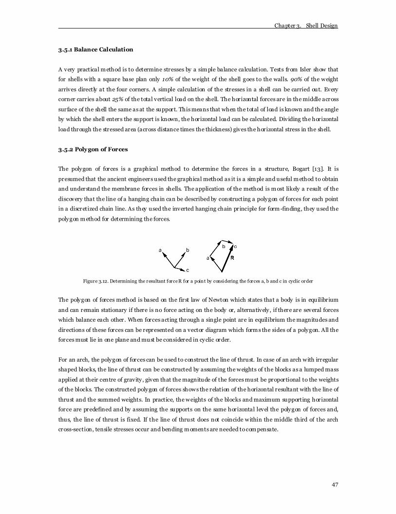
Chapter 3. Shell Design
47
3.5.1 Balance Calculation
A very practical method is to determine stresses by a simple balance calculation. Tests from Isler show that
for shells with a square base plan only 10% of the weight of the shell goes to the walls. 90% of the weight
arrives directly at the four corners. A simple calculation of the stresses in a shell can be carried out. Every
corner carries about 25% of the total vertical load on the shell. The horizontal forces are in the middle across
surface of the shell the same as at the support. This means that when the total of load is known and the angle
by which the shell enters the support is known, the horizontal load can be calculated. Dividing the horizontal
load through the stressed area (across distance times the thickness) gives the horizontal stress in the shell.
3.5.2 Polygon of Forces
The polygon of forces is a graphical method to determine the forces in a structure, Bogart [13]. It is
presumed that the ancient engineers used the graphical method as it is a simple and useful method to obtain
and understand the membrane forces in shells. The application of the method is most likely a result of the
discovery that the line of a hanging chain can be described by constructing a polygon of forces for each point
in a discretized chain line. As they used the inverted hanging chain principle for form-finding, they used the
polygon method for determining the forces.
Figure 3.12. Determining the resultant force R for a point by considering the forces a, b and c in cyclic order
The polygon of forces method is based on the first law of Newton which states that a body is in equilibrium
and can remain stationary if there is no force acting on the body or, alternatively, if there are several forces
which balance each other. When forces acting through a single point are in equilibrium the magnitudes and
directions of these forces can be represented on a vector diagram which forms the sides of a polygon. All the
forces must lie in one plane and must be considered in cyclic order.
For an arch, the polygon of forces can be used to construct the line of thrust. In case of an arch with irregular
shaped blocks, the line of thrust can be constructed by assuming the weights of the blocks as a lumped mass
applied at their centre of gravity, given that the magnitude of the forces must be proportional to the weights
of the blocks. The constructed polygon of forces shows the relation of the horizontal resultant with the line of
thrust and the summed weights. In practice, the weights of the blocks and maximum supporting horizontal
force are predefined and by assuming the supports on the same horizontal level the polygon of forces and,
thus, the line of thrust is fixed. If the line of thrust does not coincide within the middle third of the arch
cross-section, tensile stresses occur and bending moments are needed to compensate.

Chapter 3. Shell Design
48
For shells, as mentioned in the introduction, bending is prevented by the circumferential stresses which
correct the line of thrust back into the system line of the shell. These circumferential stresses can be found
using the polygon of forces. This is shown in Figure 3.13 below.
Figure 3.13. Graphical solution of a shell of revolution, Haas 1962
The graphical method is a useful method to understand the behaviour of shell geometries. It is however
restricted to simple shell geometries and linear behaviour.
3.5.3 Classical Shell Theory
Founded by Augustus Edward Hough Love in 1888, the classical shell theory was the first shell theory and is
often referred to as Lov e’s first approximation. The theory was an extension of the plate theory to structures
with surface-like geometries using the same assumptions as the Kirchhoffean theory of plates. Hence, the
approximation of Lov e essentially is a thin shell theory. The most important part of the approximation of
Love is the reduction of the three-dimensional problem to a two-dimensional surface problem, i.e. stresses
or strains in normal direction are of no significance to the solution. Furthermore, Love identified that the
shell behaviour can be approached by a membrane field in combination with plate bending that compensates
for the shortcomings of the membrane solution. The classical shell theory is further discussed in Chapter 5.
Although the approximation of Lov e is restricted to thin shells, it must be mentioned that the approximation
still appeared to be sufficient for conceptualising the behaviour of older three-dimensional shapes as
masonry domes, which are considerably thicker relative to their span and cannot be exactly characterised as
carrying loads by in-plane axial or shear stresses (more bending exits and final stresses are not uniform).
The emphasis of pre-war shell investigations laid on theoretical description of the linear elastic behaviour.
By exception Zoëlly, Von Karman and Tsien did investigations to the buckling phenomenon of shells. After
the war the research on buckling failure predominated. The trend towards greater spans and thinner shells
leaded to buckling sensitive structures with less strength reserve. However, modern designers where aware

Chapter 3. Shell Design
49
of these disadvantages and fully realised the need to protect shells for buckling failure, they could not predict
the buckling load due to their limited understanding of the phenomenon. At first, mathematicians tried to
capture the buckling problem in the same linear manner as Euler did with the buckling of a column. The
shell buckling problem is, however, far more complicated and those attempts failed as they resulted in large
deviations with the experimental obtained critical loads.
Figure 3.14. The collapse of the Ferrybridge cooling towers on the 1st November 1965
From the year 1965 the research on shell buckling was further stimulated by a collapse of three large cooling
towers of 115 m height at Ferrybridge, UK. The collapse is subscribed to insufficient study on wind loading as
mistakes in assumptions of wind speeds as well as the non-investigated effect of turbulence due to grouping
of the towers caused unforeseen dynamic wind loads. The single layered reinforced concrete towers could
not resist these loads and failed. Luckily, no one got injured. The collapse is seen in Figure 3.14.
It was found that the lack of correlation between theory and practice finds its origin in the initial geometrical
imperfections of the small-scale models which caused deviation from the linear path of equilibrium to the
nonlinear post-buckling path. It appeared that the linear bifurcation point is never reached as the shell fails
due to the reduced post-buckling load carrying capacity. A significant step in the direction of providing this
answer was made by Dutch professor Koiter who investigated the post-buckling behaviour of shells in the
vicinity of the bifurcation point: the Koiter initial post-buckling theory. Koiter permits in a study of the slope
and curvature of the secondary path of equilibrium in the immediate vicinity of the bifurcation point on the
basis of linearised formulation. The conclusions of Koiter are discussed in Chapter 6.
3.5.4 Model Tests
Until recent progress of computational numerical analysis, experimental tests on small-scale models did
provide in a very practical and convenient method to determine stresses in a shell which goes beyond the
simple shape. The shells of Heinz Isler are a famous example of shells designed using small-scale models.
Besides his form-finding models Heinz Isler used small-scale models to determine stresses and to observe
the possible full-scale performance. He used the experimental results to optimise his shell designs.

Chapter 3. Shell Design
50
Before performing experimental tests the intention must be discussed, whether it is to confirm a
mathematical theory, to verify a specific design or for observation of full-scale performance. For using small-
scale model tests in determining the full-scale mechanical behaviour it is important to approach the reality
as close as possible. For example, small-scale models made of metals or plastics are not representative for
concrete shells in the situation where pre-buckling cracking is known to be present. The high tensile strength
of metals and plastics in relation to concrete will give misleading results. Because of the importance of
cracking in structural behaviour of shells, time effects as creep and shrinkage and local effects such as bond
slip and aggregate interlock, small-scale models should in be made from micro-concrete or other
cementitious model material. The loading which can be expected in reality can be modelled by hanging
weights, hydrostatic pressure, air pressure or partial vacuum.
Figure 3.15. Experiments on buckling of spherical caps under uniform pressure
Because of the long-time absent of mathematical answers, much research on different types of shell
phenomena has been done by experimental tests on small-scale models. Scientists as Csonka, Klöppel and
Jungbluth, Von Karman and Tsien and Vandenpitte have done numerous small-scale experiments on as well
concrete as metal or plastic shells. At the TU Delft during the 1960s experiments on several concrete
cylindrical shells have been performed by Van Koten and Haas.
A lot of these experiments where done to obtain information about the buckling behaviour of thin shells, the
field of the aforementioned Koiter initial post-buckling theory. In particular the tests performed at the
University of Ghent of Vandenpitte provide in an extensive experimental studies on concrete dome buckling.
The research on the buckling phenomenon resulted in an enormous scatter in experimental results as can be
seen in Figure 3.15. This scatter is ascribed to the effects of initial imperfections in the shell surface.
3.5.5 Computational Numerical Analysis
Late shell designs are largely influenced by the advent of the computer. The importance of nonlinear features
(large deformations) in shell design raised a huge barrier for designers to find an analytical solution. The
advent of the computer made it possible to solve the nonlinear shell equations by numerical approximation
methods. A classical method is the numerical integration of the shell equations with methods such as Runge-
Kutta or predictor-corrector techniques. The method is only applicable to shell problems which can be
reduced to a system of ordinary differential equations, primarily the problems of shells of rev olution.

Chapter 3. Shell Design
51
A powerful method for numerical computer analysis is the finite element method, essentially an
approximation method for calculating the real behaviour of a structure by performing a solution of a set of
equations describing an idealised situation. The finite element method discretises the structural domain into
elements bounded by nodes. The methods work like a spider web. The movement of a point forces other
surrounding points also to make a movement. The movement of the nodal points is connected to the rise of
strains and stresses in the elements. By energy formulation and boundary conditions the response of the
structure to certain loads is determined.
The finite element method (FEM) has rev olutionised the analysis of structures and is widely available in
computer software programs as ADINA, DIANA and ANSYS. It is difficult to quote a date of invention, but
the roots of the finite element method is both mathematicians, phy sicists and engineers. The name ‘finite
element’ first appeared in the paper of R.W. Clough (1960). Important early contributions are linked to the
names of Argyris, Zienkiewicz and Cheung. Since the 1960s a large amount of research and publications was
dev oted to the technique, Bathe [3]. Commercial software producers embraced the method and have
developed it into very advanced analysis programs. The finite element method is discussed in Chapter 11.
It must be mentioned that the computer software based on numerical analy sis must not be confused with the
frame analysis programs as MATRIX FRAME and ESA PT. Frame analysis programs are based on the exact
solution of a linear elastic formulation. Finite element programs are able to give a far better approximation
of the nonlinear reality. However, the producers of frame analysis programs are trying to close the gap (ESA
PT includes the possibility of a plate analysis with finite elements) they are by no means applicable for the
more advance structural problems with large influences of nonlinear behaviour.
3.5.6 Rainflow Analysis
A relative new method is the rainflow analysis which is based on the way how rainwater runs off the surface.
Like the rain flow loads will flow. The problem of modern computational numerical analysis, as the finite
element method, is that only quantitative information is obtained. The designer does not know how the
applied load is transferred from the loading point to the supports. In particular for designing irregular
surfaces and/or supporting conditions, the undefined force flow gives raise to questions whether the shell
has a sufficient structural surface. In order to obtain qualitative information about the force flow the
rainflow analysis is developed, Bogart [14].
The rainflow analysis is derived from the study to the way in which plates carry their load. A plate carries
load perpendicular to their surface by bending and out-of-plane shear. From the equations for plates
engineers know that, when there is no torsional load, the second equilibrium equation yields that the shear
force is equal to the derivative of the sum of the bending moments (see Chapter 5). The maximum shear
force in a plate is a vector equal to the value of the applied load and points in the direction of the shear flow
to the support. Hence, the maximum shear vector can be found by making a gradient plot of the deflection
curvature. The deflection curved surface also represents an air inflated membrane and, analogous to this
hypothesis, the flow of shear forces represents the way in which the rainwater flows from the inflated
membrane, with the largest run-off at the curves with the steepest ascent and thus the largest shear.

Chapter 3. Shell Design
52
In the case of shell structures, the deflection curvature is replaced by the initial curvature of the shell surface.
In this case the rainflow represents the force flow and qualitative information can be obtained. Drain curves
indicate the membrane force flow. Slow flow means little slope causing a distortion of the membrane
behaviour by out-of-plane shear and bending. Fast flow, thus, represent a sound structural surface. Bending
can also be expected at regions with water accumulation or when loads are acting perpendicular to the drain
curves (for example at the edges). Furthermore, a rapid change in the slope of a drain curve is sign of large
circumferential stresses (and even can lead to bending as well), Bogart [14].
3.6 Structural Optimisation
Structural optimisation can be regarded as the search for a better solution to a structural problem by
generating additional sensitivities with respect to non-considered parameters. The optimised structure is
thus better and more efficient than the initial structure. However this seems to be a very simple principle,
the question how to define the optimisation problem and to which extend it is executed is not.
Figure 3.16. The most efficient Michell structure for carrying a point load
The preliminary stage of structural optimisation were the structures of A.G.M. Michell which he developed at
the beginning of the 20th century, see Figure 3.16. Michell structures carry the load with the least possible
weight. The structural system follows the force trajectories and each member is either in compression or
tension. Despite their efficiency, Michell structures are of little practical use due to their specific structural
scheme.
Structural optimisation is a synthesis of various individual disciplines, design modelling, structural analysis,
behaviour-sensitivity analysis and mathematical programming with special emphasis on the modelling
stage. It is one of the most significant processes obtained from nature. An example is the aforementioned
tapered trunk of a tree and the constant stress distribution in the stem and branches of a tree. This principle
of constant surface stress, also seen in the minimal surface of a soap-film, may be applied to the optimisation
of engineering components.
Structural optimisation deals with maximising the performance of a structure for certain objectives and
constraints. The choice of the objectives and constraints can lead to a large diversion of solutions to the
optimisation question. Think of the differences in optimisation results when optimised with respect to
construction costs, weight, or natural frequencies. In a so-called multi criterion optimisation these

Chapter 3. Shell Design
53
(conflicting) objectives can be considered simultaneously to obtain an optimal compromise of structural
design. Moreover, limitations of the optimisation process give rise to questions whether a local or global
optimum is obtained.
The basic idea of the optimisation process is much related to the engineer approach. At first a shape is
chosen for which the structural behaviour according to the given load cases and support conditions is
evaluated. After the stresses, displacements, buckling loads and other safety requirements are checked a new
and better design can be proposed by means of a sensitivity analysis. The process is repeated until the
desired optimum is obtained.
Shape-sensitive structures like shells require high quality design to obtain an optimal membrane design.
Since in many situations this optimal shape is not obvious, the need for optimisation techniques is evident.
To fulfil the basic membrane oriented design rules, a modification of the original design could substantially
improve the structural behaviour reaching the ideal of a pure membrane stress in compression for all loading
conditions. Optimisation for shells results in a highly nonlinear optimisation problem. This means that, in
order to generate a reliable design by structural optimisation, the nonlinear structural response, e.g.
buckling or plasticity must be considered.
With respect to optimisation shells are known to be extremely parameter sensitive because they are already
optimised structures. This means that the danger of over-optimisation is very close. In fact, shells often show
typical characteristics of ‘over-optimised’ specialisations with high sensitivity with respect to small changes
of certain parameters such as the reduction of the buckling load due to only small initial imperfections. On
the other hand an optimisation may contribute to a better design with more safety.
The difference between optimisation objectives has resulted in various classifications over the years, none of
them having reached global usage. In this thesis the categorisation which can be made according to Ramm
and Wall [65] is used. Ramm and Wall argue that distinction can be made between size optimisation,
material optimisation, topology optimisation and shape optimisation, even though these optimisation
techniques may have a lot of overlapping.
3.6.1 Size Optimisation
Size optimisation refers to the optimisation of the size of structural elements in a structure. The initial
geometry is not changed. Size optimisation leads to an optimal structure with respect to the weight and
ov erall stiffness or strength satisfying the equilibrium condition and the boundary constraints. It results in
structures with modified cross-sections of structural elements.
3.6.2 Material Optimisation
Material optimisation is everyday practice for engineers. Material optimisation is namely related to the
optimal use of material in the structure, e.g. reinforcement dimensions. The goal is to achieve an optimum in
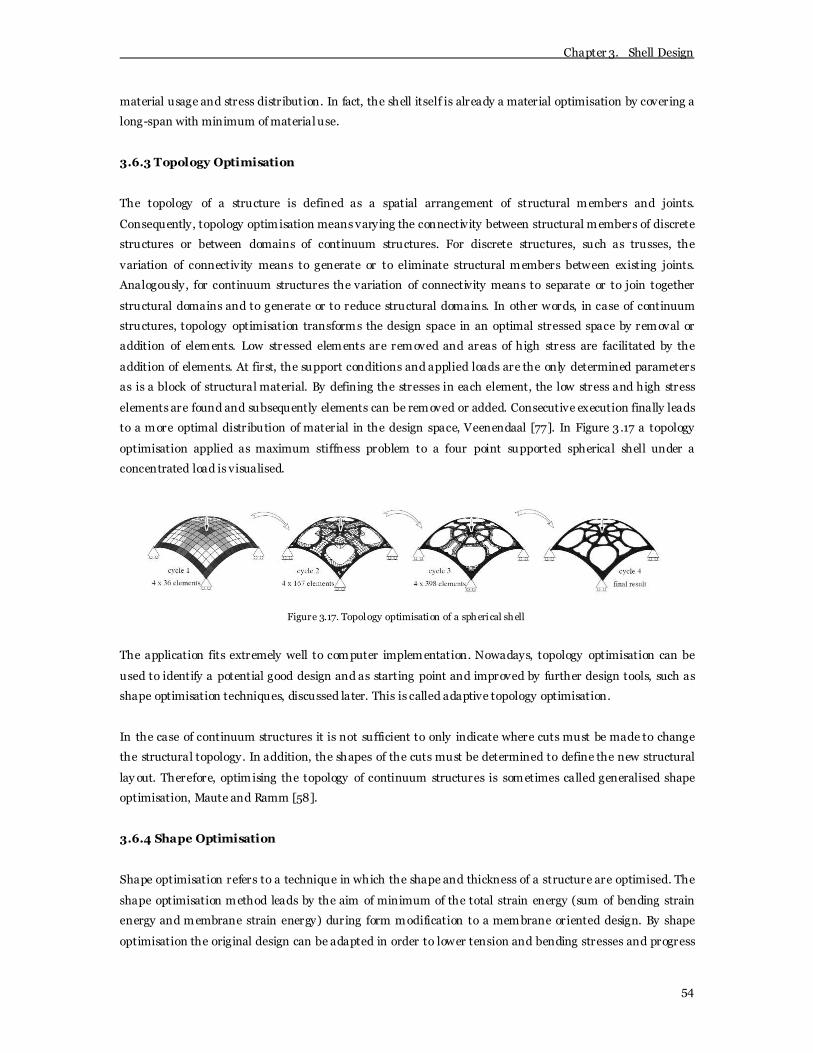
Chapter 3. Shell Design
54
material usage and stress distribution. In fact, the shell itself is already a material optimisation by covering a
long-span with minimum of material use.
3.6.3 Topology Optimisation
The topology of a structure is defined as a spatial arrangement of structural members and joints.
Consequently, topology optimisation means varying the connectivity between structural members of discrete
structures or between domains of continuum structures. For discrete structures, such as trusses, the
variation of connectivity means to generate or to eliminate structural members between existing joints.
Analogously, for continuum structures the variation of connectivity means to separate or to join together
structural domains and to generate or to reduce structural domains. In other words, in case of continuum
structures, topology optimisation transforms the design space in an optimal stressed space by removal or
addition of elements. Low stressed elements are removed and areas of high stress are facilitated by the
addition of elements. At first, the support conditions and applied loads are the only determined parameters
as is a block of structural material. By defining the stresses in each element, the low stress and high stress
elements are found and subsequently elements can be removed or added. Consecutive execution finally leads
to a more optimal distribution of material in the design space, Veenendaal [77]. In Figure 3 .17 a topology
optimisation applied as maximum stiffness problem to a four point supported spherical shell under a
concentrated load is visualised.
Figure 3.17. Topology optimisation of a spherical shell
The application fits extremely well to computer implementation. Nowadays, topology optimisation can be
used to identify a potential good design and as starting point and improved by further design tools, such as
shape optimisation techniques, discussed later. This is called adaptive topology optimisation.
In the case of continuum structures it is not sufficient to only indicate where cuts must be made to change
the structural topology. In addition, the shapes of the cuts must be determined to define the new structural
lay out. Therefore, optimising the topology of continuum structures is sometimes called generalised shape
optimisation, Maute and Ramm [58].
3.6.4 Shape Optimisation
Shape optimisation refers to a technique in which the shape and thickness of a structure are optimised. The
shape optimisation method leads by the aim of minimum of the total strain energy (sum of bending strain
energy and membrane strain energy) during form modification to a membrane oriented design. By shape
optimisation the original design can be adapted in order to lower tension and bending stresses and progress
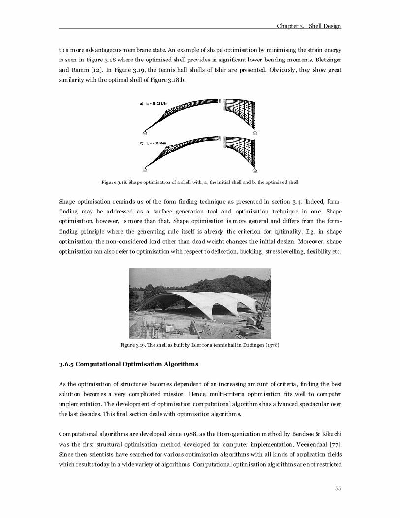
Chapter 3. Shell Design
55
to a more advantageous membrane state. An example of shape optimisation by minimising the strain energy
is seen in Figure 3.18 where the optimised shell provides in significant lower bending moments, Bletzinger
and Ramm [12]. In Figure 3.19, the tennis hall shells of Isler are presented. Obviously, they show great
similarity with the optimal shell of Figure 3.18.b.
Figure 3.18. Shape optimisation of a shell with , a, the initial shell and b. the optimised shell
Shape optimisation reminds us of the form-finding technique as presented in section 3.4. Indeed, form-
finding may be addressed as a surface generation tool and optimisation technique in one. Shape
optimisation, however, is more than that. Shape optimisation is more general and differs from the form-
finding principle where the generating rule itself is already the criterion for optimality. E.g. in shape
optimisation, the non-considered load other than dead weight changes the initial design. Moreover, shape
optimisation can also refer to optimisation with respect to deflection, buckling, stress levelling, flexibility etc.
Figure 3.19. The shell as built by Isler for a tennis hall in Düdingen (1978)
3.6.5 Computational Optimisation Algorithms
As the optimisation of structures becomes dependent of an increasing amount of criteria, finding the best
solution becomes a very complicated mission. Hence, multi-criteria optimisation fits well to computer
implementation. The development of optimisation computational algorithms has advanced spectacular over
the last decades. This final section deals with optimisation algorithms.
Computational algorithms are developed since 1988, as the Homogenization method by Bendsøe & Kikuchi
was the first structural optimisation method developed for computer implementation, Veenendaal [77].
Since then scientists have searched for various optimisation algorithms with all kinds of application fields
which results today in a wide variety of algorithms. Computational optimisation algorithms are not restricted

Chapter 3. Shell Design
56
to the classification as presented abov e, but often use a combination between different types of optimisation,
for example an integrated shape and topology optimisation. Roughly, they can be categorised in specific or
tailored algorithms and general algorithms, Veenendaal [77].
The most popular specific algorithm for structural optimisation is, by far, Evolutionary Structural
Optimisation (ESO). ESO is a topology optimisation method and thus involves consecutive removal of low
stresses material until the maximum stress in the remaining material part is reached. Computational
software based on ESO is, for example, OPTFRAME or EVOLVE97. The software makes use of finite element
techniques to determine stresses. The algorithm of ESO is further refined to Additive ESO (AESO), Bi-
directional ESO (BESO) and Extended ESO (XESO) which are equipped with more extensive and efficient
optimisation techniques, for example the possibility of as well removal as adding of material and faster
removal methods.
Other specific algorithms are the aforementioned Homogenization method and the Metamorphic
Dev elopment (MD) method.
Genetic algorithms are the most used general algorithms. The Darwinian based method (survival of the
fittest) generates every iteration new solutions by selection and crossover of previous obtained solutions in
order to end up with a higher fitness generation. Random mutation of the new generation increases the
change of reaching a global optimum. The process is repeated several times, keeping the size of the
population constant. One can imagine that the large amount of work that has to be done results in a long
optimisation time.
Other general algorithms are the Differential Ev olution (DE) method, the Simulated Annealing (SA) method
and the rather eccentric named Ant Colony Optimisation (ACO) method. The latter optimisation is based on
the fact that ants, by leaving behind the chemical pheromone on their followed path, find the most optimum
(the shortest) way from their nest to a food source. Think of two paths, short and long, from their nest to a
food source. Ants at the short path reach the food earlier and go back in the way with the most pheromone.
Ev entually all ants use the way with the most pheromone which is the shortest way. ACO uses this to find an
optimum solution for a given problem. A disadvantage of ACO is its sensitivity to local optima. Therefore,
the optimalisation algorithm must be programmed not to converge to one solution immediately, but to allow
for more solutions for a longer period of time.
Optimisation software, however, must still be further developed as the bulk of investigations are devoted
towards cross-sectional optimisation, 2D shape optimisation and the, for shell important, nonlinear
behaviour is usually not taken into account as it greatly increases the complexity of the problem. Hence, the
application of computation optimisation algorithms seems to be far away from designing a sound shell
structure. Ongoing progression may foresee in sufficient optimising shell software in the future.

Chapter 3. Shell Design
57
3.7 Design Codes
Two design codes that contain recommendations for the analysis of concrete shells are the codes of the
American Concrete Institute (ACI) and the International Association for Shell and Spatial Structures
(IASS). According to Farshad [34] the German Norm (DIN), the British Standards (BS) and the Indian
Standards (IS) also offer general design guidelines for shells. The guidelines mainly focus on buckling.
The ACI Committee 334 on concrete shells was formed in 1959 under the chairmanship of Anton Tedesko.
The committee published two reports on shell design in 1964. The first report ‘Criteria’ cov ered general
design considerations and the second report ‘Commentary’ discussed data of general interest to shell
designers. The discussion of stability is mainly gov erned by the second report. In the ‘Commentary’ the
relative importance of post-buckling behaviour and the significant reduction in the buckling load when both
principal in-plane stresses are compressive is mentioned. The report states that for anticlastic shells it is
possible to use the linear buckling theory. For synclastic shells the ACI report assumes that information on
buckling of ideal shells for cylinders and spheres may be used as starting point of the analysis for the
considered shell. The report recommends that the combined apparent safety factor F based on the apparent
safety factors calculated for an ideal shell in the direction of the principal radii of curvature, using an
analogous sphere of cylinder in each direction, however, not less than 5. The rather large value was intended
to allow for uncertainties of the various effects not included in the calculation. The effect of creep was
allowed for by assuming a reduced value of E or a tangent value divided by a value not less than 2. Finally, it
is mentioned that a shell with two layers of reinforcement has greater buckling load than a shell with only
one layer.
In general, the report reflects the concern and imperfect state of knowledge on buckling at its time of
publication. When the report was implemented in the ACI Standard, the problem of stability of concrete
shells was confined to the point where almost no information of the use to a shell designer survived.
The IASS recommendations on shell design where developed by a working group in 1969. The text intended
to serve as recommended practice in the design, analy sis and construction of concrete shells. However, shells
such as cooling towers where excluded. The recommendation was published in 1979. The discussion on
stability of shells was largely based on Kollar and Dulacska [54]. After the qualitative discussion on buckling,
including the mentioning of the importance of post-buckling behaviour, the report offers a five step
approach to calculate the safety factor to be used. The IASS recommendations provides in a rational
approach by covering all the effects which might influence the buckling in a shell. Throughout a conservative
approach is taken. According to Popov and Medwadowski [62] the critical load may be as little as 1 or 2% of
the linear buckling load, if all of the cumulative effects are taken into account. Since the safety factor is yet to
be applied, the allowable load is even less.
A more detailed discussion concerning the application of the IASS recommendations is found in Chapter 6.

Chapter 3. Shell Design
58
3.8 Design Considerations
The numerous of shell structures built up to the present day give an enormous amount of information for
new shell designs. The information which has been achieved may provide the new shell engineer a guideline
and a series of do’s and don’ts when designing a sound shell structure. This section tries to formulate the
things learned in design considerations.
3.8.1 Span/Rise/Radius of Curvature
The span of the shell is determined by its final usage. Shells can span up to 200 m and more. The main
concern of long span shells is the question of stability of the shell structure. Today, the largest span of a shell
is the 218 m span of the CNIT in Paris, Figure 2.25
When the span is known, the rise and radii of curvature must be set. According to ACI Committee 344 domes
usually give rise to span ratios of 1/10 to 1/6 while Scordelis [69] reports on shells with rise to span ratios of
1/7.46 to 1/4.82 and radius of curvature to span ratios of 1 to 0.707. The ideal rise-to-span ratio for arches,
1/7, is considered to be reasonable for shells as well. Shells with lower ratios than 1/7 are considered to be
flat shells. It is generally suggested that the rise should be larger than 1/10. The rise to span ratio also fixes
the radius of curvature. The central angle of shells is usually selected between 60 to 90 degrees, Scordelis
[69]. Higher central angles would result in shell geometries with steeper slopes. Placing of concrete on these
slopes would then require double forming.
Candela believes that every shell has an optimum span, keeping in mind structural, practical and economical
parameters. Spans which exceed 30 m makes the shell rise greater giving it tremendous cubage, which
requires costly formwork. Large span improper shells, like folded slabs or barrel vaults, need extra thickness
which causes high dead weight and increasing reinforcement. At this point transverse bending ceases to be
secondary and becomes critical. In short cylinders stiffening arches get so big with large spans that the
advantages natural to the shell are nullified.
3.8.2 Thickness
The thickness of the shell is an important parameter in shell design. Because the dead weight of the shell
often represents the major portion of the total load, there is a desire to reduce the thickness. Secondly,
thinner shells approach more closely to the profoundable membrane state. However a reduced shell
thickness is less fav ourable of resisting bending moments. Fortunately, the edge disturbances have only local
character and can be compensated by local increase of thickness.
The thickness of the shell surface is prescribed by either practical or structural purposes, depending on the
span and the construction material of the shell. For long-span shells structural considerations as failure due
to buckling or surpassing material strength demand a certain shell thickness. Usually dimensioning the shell
thickness is based on buckling considerations rather than material strength criteria. However, for short span
shells the thickness is determined by practical considerations as the concrete cover for preventing corrosion

Chapter 3. Shell Design
59
of the reinforcement or concrete placement. The turning point whether the shell thickness is determined by
practical or structural factors is not a fixed parameter.
Determining the thickness with respect to practical considerations means providing enough space for the
reinforcement (in combination with the concrete cover) and the maximum grain size. As a general rule it can
be said that the thickness should at least equal three to four times the maximum aggregate dimensions, Haas
[42]. By this it is possible to ov ercome imperfections as gravel pockets or separation of the concrete mixture.
For the concrete cover climatological considerations play a large role. Because the surface of the shell often
remains untreated the concrete cover must avoid water reaching the reinforcement to prevent corrosion. In
general a concrete cover of 30 mm will be sufficient for maritime regions. The thickness is further influenced
by the application of one or two layers of reinforcement. The practical thickness of a shell is also influenced
by the placing method of the concrete and placing difficulties. Using common placing methods the thickness
of slabs can be controlled up to about 19 mm. With extreme care 6 mm can be obtained. The curvature of the
shell will have a negative effect and the designer must take account for larger deviations. Special fabrication
methods as prefabrication may reduce surface deviations. As a rule, the thinner the shell is as compared to
its radius of curvature, the less accurately it can be built. A common practical thickness of conventional
concrete shells varies between 60 to 80 mm.
The practical thickness is the minimum thickness of the conventional concrete shell. Structural
considerations may, however, force the designer to increase the thickness. Most shells have an increased
thickness near the supports to prevent stress concentrations and to facilitate the force flow to the supports.
Long-span shell structures may take this increase thickness to be necessary over the complete shell surface.
Although, the shell thickness has no influence on the membrane stresses (the thickness parameter falls out
of the equations) and only minor influence on the bending stress (double thickness increase the bending
moment just 26%!) the thickness is important for buckling considerations. Aforementioned, as increasing
spans become more and more vulnerable for buckling, long-span shells may need a thickness which is larger
than the practical thickness.
3.8.3 Ribbed Shells
Instead of increasing the thickness of a shell, several shell designers such as Nervi and Tedesko used ribs to
stiffen their shells in order to obtain a larger resistance against buckling. Ribs came in order to find a
modification in the way the material is distributed throughout the surface of the shell. They are applied to
increase the effective depth of the shell greater than if the material were evenly distributed. Though ribbed
shells are not thoroughly discussed in this thesis, their principle and influence on the buckling behaviour is
outlined here.
The functioning of ribs can be simply explained. Due to the rib-stiffening the buckling is represented by the
local buckling of the skin between the ribs, conditionally that the ribs distances are chosen inferior to the
buckling lengths of the unstiffened shell (if the distance between neighbouring ribs is larger than the
buckling length of the unstiffened shell, they have, off course, no influence). When the rib design is known,
the rib shell can be replaced by a continuous surface for the analy sis. The continuous surface must include

Chapter 3. Shell Design
60
the effective width of the skin with respect to the bending of the ribs, possible eccentricity of the ribs and the
role of Poisson’s ratio. After that, the rigidity characteristics of the equivalent orthotropic shell can be
established and an overall buckling analysis can be performed.
The latter explanation leads to some questions. First of all, the dimensions of the buckle must be known in
order to determine the rib distances. A safe choice is the linear buckling lengths of the unstiffened shell as
the imperfect buckling lengths are larger, see Chapter 6. For example, when assuming rectangular buckles,
the half buckling wavelengths of a spherical shell subjected to radial pressure cannot be shorter than 1.72
√(Rt). This means that if the rib distances are shorter than 1.72 √(Rt) they lead to an increased critical load.
According to Kollar and Dulacska [54], in general, ribs can certainly be considered as practically effective if
the distance of the ribs is not greater than 0.7 times the buckling length of the unstiffened shell. In that case
the critical load of the shell panel between the ribs is approximately twice the value of the unstiffened shell.
The second problem that may arise is the question to what is the necessary stiffness of the ribs to allow us to
consider the ribs as rigid supports of the skin during buckling. As this question is not generally been
answered yet, Kollar and Dulacska introduced the following analogy. If we want to stiffen a weak simple
frame, we can add a sufficient rigid structure according to Figure 3.20.
Figure 3.20. The basic principle of the necessary rib rigidity , Kollar and Dulacska 1984
The rigidity of the added part can be taken as sufficient if its critical load, computed assuming infinitely
elastic material, is not less than the sum of all loads on the stiffened frame. When this is projected to our
shell, we have to demand that the ribs be capable of carrying all the load acting on the shell surface and on
the ribs, assuming infinitely elastic behaviour. In this computation an effective width of the skin, as valid
before skin buckling can be assumed as part of the rib.
The shell surface can be stiffened in two ways: the ribs can be arranged on both sides of the skin,
symmetrically to its middle surface, or eccentric stiffening on one side only. For symmetrical positioned ribs,
the rigidity can be smeared out and the orthotropic shell equations can be applied. This is, however, much
more difficult to construct and is less economical to eccentric ribs which foresee in a considerable higher
bending rigidity with the same amount cross-sectional area. However, eccentric ribs can be described by the
orthotropic shell equations much more difficult. Like symmetrical rib-stiffeners, eccentrically ribbed shells
cause increase in rigidity. However, as discov ered by Van der Neut in 1947, it does make a difference
whether the ribs are positioned on the outer (e.g. the St. Louis airport shell, Figure 2.30) or on the inner
(Palazzetto dello Sport, Figure 2.27) side of the shell surface. This is caused by so-called primary

Chapter 3. Shell Design
61
(phenomenon of twist due to varying amplitude of outward and inward buckles which cause shearing
deformation in the shell surface) and secondary (outward buckling waves in longitudinal direction cause
tension in ring direction due to Poisson’s ratio) effects which act in opposite sense. Unfortunately, it cannot
be decided without a detailed analy sis which effect, and thus which eccentric arrangement, prevails.
To draw a conclusion, the following comments must be made. The difference in primary behaviour of outer
and inner stiffeners only appears if the buckling deformation contains some twist. The secondary effect is
present, however, ceases when the Poisson’s ratio is chosen equal to zero which also benefits the safety.
Furthermore, as concluded by Hutchinson and Amazigo (1967), the fav ourable effect of outside stiffeners is
greatly reduced as it is partially counterbalanced by its sensitivity to initial imperfections. Therefore, Kollar
and Dulacska propose to neglect the ‘warping rigidity’ and the primary and secondary effects caused by the
eccentricity of the stiffening ribs. Hence, the analysis of ribbed stiffened shells can be reduced to that of
simple orthotropic shells with a higher stiffness.
3.8.4 Reinforcement
Modern shell structures are reinforced concrete structural surfaces. Reinforcement in shells is applied for
four requirements. At first, reinforcement is the reason that modern shell structures are capable of
transferring tensile stresses resulting from the membrane and bending action as well as the tensile stresses
due to transverse and membrane shear. Secondly, reinforcement provides in a distribution net for local
concentrated loads and, thirdly, the application of a reinforcement grid enables the shell to control shrinkage
and temperature effects. The final reason for applying reinforcement is the reduction of deformations due to
local bending and thereby decreasing the likelihood of instability due to buckling of the shell. Thus, the
reinforcement has an important role in preventing buckling.
Figure 3.21. Welded wire mesh reinforcement for the Jena Planetarium, Joedicke 1962
Ordinary reinforcement in a concrete shell consists of conventional steel rebars or a welded wire mesh,
Figure 3 .21. Wire mesh is recommended where possible. It is v ery suitable for developable surfaces as it can
be obtained in flat sheets and easily bended in the right shape. For doubly curved shells wire mesh is less
useful as it is difficult to obtain the double curved shape. Mild steel reinforcement is commonly applied for
such surfaces. A small amount of shells has been built using high-tech reinforcement. An example is the shell

Chapter 3. Shell Design
62
of Jorg Schlaich which was built for the Federal Garden Fair in Stuttgart in 1977 using glass reinforced
concrete. However, this is not common practice due to the higher costs. The research within this thesis on
the applicability of fibre reinforcement may open new ways.
Using conventional rebars or welded mesh reinforcement, usually a percentage between 0.15 and 0.4% is
applied for single layer reinforced shells, although, due to their extreme thinness, the shells of Candela may
reach higher percentages. The reinforcement of a series of concrete shells is illustrated in Table 3.1. To
compare, beam reinforcement is approximately between 0.8 and 1.2 %. The shell can be executed with one or
two layers of reinforcement. Generally, engineers as Heinz Isler prefer two layers of reinforcement, mostly to
give more resistant against buckling. However, two layers also provide more resistant to the previously
described negative effects as shrinkage, temperature gradients and local concentrated loads. The application
of single layer reinforcement is therefore restricted to shells with small dimensions or sometimes when
prestressing is applied.
Shell Thickness (mm) Ø (mm) Spacing (mm) %
Shopping Centre Hawaii , Bradshaw 76 9.5 300 (max)* 0.37 (min)
Market hall Algeciras, Torroja 85 12 300 (max)* 0.40 (min)
Church Monterrey, Candela 40 9.5 150 1.24
Restaurant Xochimilco, Candela 40 8 100 1.25
Factory Tacuba, Candela 40 9.5 200 0.89
Swimming pool Norwich, Isler 80 6 100 0.57**
* Reinforcement is placed in circumferential direction; ** Two layers of reinforcement
Table 3.1. Reinforcement in concrete shell structures
Shells with combined reinforcement, one layer in the compression zone and two layers near its base, are
often seen in practice. Candela makes his shell surface such thin (40 mm) that there is only space for one
layer. While in the majority of the shell surface only one layer is applied, the reinforcement ratio is increased
by supports. The table below shows the reinforcement ratios of different shells. The values are surface values
which hold for the majority of the shell surface without taken into account extra reinforcement near the edge
or at supports.
Figure 3.22. Rebars aligned with the stress trajectories, Joedicke 1962
The reinforcement can be placed in different patterns. Initially, shells where reinforced with the bars parallel
to the stress trajectories, Figure 3.22. However technical and academic, this consumes much labour and is
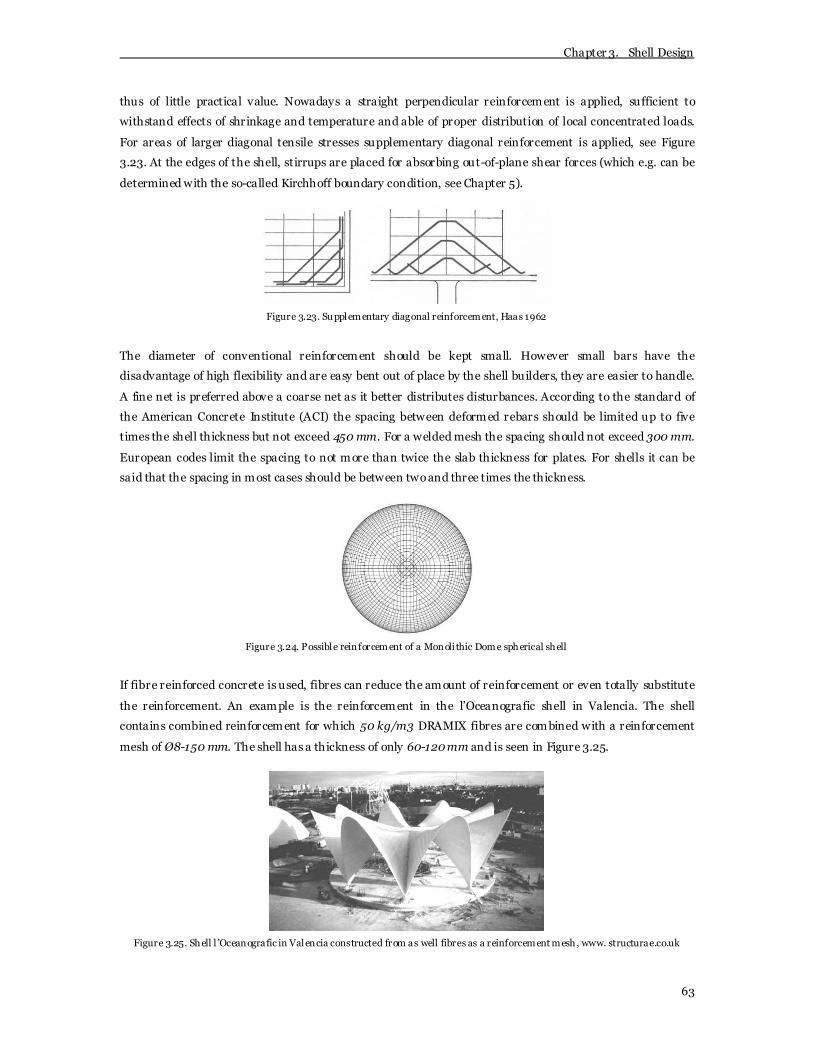
Chapter 3. Shell Design
63
thus of little practical value. Nowadays a straight perpendicular reinforcement is applied, sufficient to
withstand effects of shrinkage and temperature and able of proper distribution of local concentrated loads.
For areas of larger diagonal tensile stresses supplementary diagonal reinforcement is applied, see Figure
3.23. At the edges of the shell, stirrups are placed for absorbing out-of-plane shear forces (which e.g. can be
determined with the so-called Kirchhoff boundary condition, see Chapter 5).
Figure 3.23. Supplementary diagonal reinforcement, Haas 1962
The diameter of conventional reinforcement should be kept small. However small bars have the
disadvantage of high flexibility and are easy bent out of place by the shell builders, they are easier to handle.
A fine net is preferred above a coarse net as it better distributes disturbances. According to the standard of
the American Concrete Institute (ACI) the spacing between deformed rebars should be limited up to five
times the shell thickness but not exceed 450 mm. For a welded mesh the spacing should not exceed 300 mm.
European codes limit the spacing to not more than twice the slab thickness for plates. For shells it can be
said that the spacing in most cases should be between two and three times the thickness.
Figure 3.24. Possible reinforcement of a Monoli thic Dome spherical shell
If fibre reinforced concrete is used, fibres can reduce the amount of reinforcement or even totally substitute
the reinforcement. An example is the reinforcement in the l’Oceanografic shell in Valencia. The shell
contains combined reinforcement for which 50 kg/m3 DRAMIX fibres are combined with a reinforcement
mesh of Ø8-150 mm. The shell has a thickness of only 60-120 mm and is seen in Figure 3.25.
Figure 3.25. Shell l ’Oceanografic in Valencia constructed from as well fibres as a reinforcement mesh, www. structurae.co.uk

Chapter 3. Shell Design
64
3.8.5 Prestressing
Prestressing in concrete shells is, as with other structures, applied for the aim of reduction or even
prevention of tensile stresses by introduction of compressive stresses. For example to ensure that long-span
shells are in compression prestressing may be applied. A practical rule states that shells up to 30 m can be
made of non-prestressed reinforced concrete. For longer spans prestressing must be applied. However,
prestressing can also be included in short-span shells as it may cause the edge beams to be superfluous.
Figure 3.26. Prestressing canals in the edge beams of an Isler shell , Chilton 2000
Prestressing was first applied in shells to balance the outward thrust of a dome by bringing into compression
a tension ring, or to contain the compression state in the shell surface under all possible loading conditions.
Initially, the prestressing ties where accommodated into the edge beams of shells as is seen in Figure 3.26.
Isler used prestressing to control the size of the edge beams. He applies prestressing if the span exceeds 30
m. Later, shell designers also placed the prestressing ties inside the shell surface or outside the basic
structure, as tension cord within the foundation or across the diagonals (hypars). An example of a
prestressed shell with prestressing in the shell surface is the 1982 Olympic Swimming Pool in Kirchberg,
Luxembourg City, designed by French architect Roger Taillibert, seen in Figure 3.27.
Figure 3.27. The 1982 Kirchberg Olympic Pool in Luxembourg City by architect Roger Taillibert, www.academie-des-beaux-arts.fr

Chapter 3. Shell Design
65
The shell of Isler at the Deitingen Service Station is an example of prestressing outside the basic structure as
the prestressing cords are placed beneath the ground surface and connects the outer support of the shell with
an embankment structure which supports the two inner supports. By pulling the support points slightly
inwards using the pre-tensioning cables the shell is brought into compression.
The use of prestressing in shells also has the advantage of improving crack control. Furthermore, with
prestressing the influences of shrinkage and temperature is kept in check and the bending moments can be
better controlled. The prestressing ties are also used for simple removal of the formwork. The tensioning of
the ties after hardening not only brings the shell in compression, but also causes an up-lift of the shell
surface. The shell moves free from the formwork which easily can be removed.
3.8.6 Material
The shells discussed here are constructed from (fibre) reinforced concrete. Stresses in concrete shells are
often a small proportion of those permitted by the strength of the material. From experience, in a shell of 20
or 30 m span the stresses vary from 1.5 to 3.0 N/mm2, including the effect of pre-stressing, Chilton [22]. The
foot of the shell is the only point where the stresses go abov e 50% of the allowable concrete strength.
Therefore, durability of the concrete is probably more important than strength.
After placement, attention must be paid to the surface treatment of the concrete, as the majority of shells do
not have cladding or painting. A smooth surface improves the appearance and reflection of light.
Furthermore, a smooth surface shows higher resistance against degeneration due to climate attacks.
Measurements of Heinz Isler at some of his shell structures have shown that the shells lose 1 or 2 mm of
their surface in the first ten years. Over 35 years the erosion does usually not exceed 2 to 4 mm. During a
similar period of about 35 years the concrete will suffer carbonation to a depth of less than 10 mm, Chilton
[22]. However, the durability largely depends on the climatological circumstances. For example, in South
Africa, which is largely sub-tropical, the temperature differential can vary 30 degrees and thin concrete
shells suffer large expansion variations. For increased durability, or visual reasons, the concrete cover may
be coated, painted or cladded.
3.8.7 Supports
With respect to the supports, it is most important that they are fixed in place. Possible movement of the
supports may lead to a disturbed membrane stress field, significantly increased deflections and/or in-
extensional deformations such as seen in Figure 3 .3. For self balancing shells (e.g. hemispherical shells) the
supports only have to carry the dead weight of the shell. However, in case of more shallow shells, the
supports sometimes also must absorb the outward thrust of the shell. In these situations the supports may
be connected to each other by tensile cords or they are balanced by piles and/or (grouted) anchors.
The shell support design is closely related to the shell design as the membrane stress field is locally disturbed
by suppressed deformations. A choice for a particular support condition, thus, influences the shell edge

Chapter 3. Shell Design
66
design, discussed hereafter. Commonly, shells are clamped supported, e.g. encased in concrete beams, or
membrane compatible supported, e.g. ball-and-socket hinges. An example of a (rare) hinged support is seen
in Figure 3.28 in which the hinge is approximated by a series of pendulums, with the horizontal thrust
absorbed by a prestressed edge ring, Haas [42].
Figure 3.28. Support detail of a hinged support for a dome in Zürich , Haas 1962
3.8.8 Edge Design/Free Edges
The first shells of the early twentieth century were fully supported along their boundaries. However, when
the architectural profession got interested, they wanted to show the spectacular thin cross-sections of shells
by building shells with unsupported boundaries. If shells are unsupported at their edges, there is referred to
shells with free edges. Obviously, shells with free edges are more appealing as they appear to be more
graceful.
Discontinuously supported shells, e.g. Nervi’s Palazzetto dello Sport in Rome, experience a significant
change in the principal stress directions, simply as a consequence of transferring the weight of the shell to a
small portion of the edge, illustrated in Figure 3.29. Moreover, in case of structures such as the Palazzetto
dello Sport with columns tangential to the meridian, also the outward thrust contributes to the change of the
stress trajectories.
Figure 3.29. Stress distribution in a hemispherical dome on six supports, Haas 1962
In Figure 3 .29 it can be seen that the meridional and circumferential stresses must vanish at the
unsupported edge part while at the supports the stresses show high peaks. Furthermore, it can be seen that
the edge disturbance caused by the discontinuous support stretches up to about halfway the shell surface. To
counteract the change of stress trajectories a possible solution is to introduce a stiff ring girder. The ring
girder is also beneficial as it simplifies the calculation, i.e. the shell abov e the ring girder can be analysed as a
uniformly supported shell. A more aesthetical solution is the aforementioned feathered shell in which the
unbalanced forces are fluently transferred to the (tangential) columns by arch action, Haas [42]. Basically,
the feathered shell is an example of a shell with a free edge.

Chapter 3. Shell Design
67
Although the possible thrust from the dome is usually taken by an edge ring beam or tension cord which is
commonly prestressed, in some cases the edge ring beam is replaced by a thickening of the shell near its
supports or by a feathered upturned shell, in case of a discontinuous support, Scordelis [69].
The membrane stress state of shells, however, seldom allows for totally free edges. In general, longitudinal
edge beams must be applied to carry the applied loads, which have been transferred to them by the
mechanism of internal shear force, and transfer them in turn to the supports of the shell structure.
Furthermore, due to their free edges, these shells generally do not buckle locally, but the combined shell-
edge system buckles as a whole. In other words, the shell-like buckling merges to arch-like buckling of the
complete structure. This phenomenon is seen in Figure 3.30. The Figure shows a buckling analysis of an
elpar shaped shell in DIANA with increasing edge beam stiffness. The most left picture (no edge beam)
shows typical arch-like buckling while the most right picture (fully supported) has shell buckling with 5%
accuracy with respect to the theoretical value of a radially pressed sphere (see Chapter 6). The problem is
that the arch-like buckling load is considerably lower than the load necessary to cause shell buckling. Thus,
besides carrying load, the edge beams must also provide additional stiffness for buckling instability.
Figure 3.30. A series of shell buckling analyses with increasing edge stiffness
Edge members are found in various sizes and shapes. Distinction is made between edge beams and curved
edges. Curved edges are essentially curved edge beams with open cross sections, while edge beams have
rectangular closed cross-sections. The size of the edge members is determined by the magnitude of the load
which they must transfer or buckling considerations. A possible height of an edge beam to shell length is
somewhere between 1/25 and 1/20, Farshad [34].
Figure 3.31. A shell of Heinz Isler in Switzerland and the shell at the Deitingen Service Station by Isler
The main problem of shell designers is the fact that the cross section of an edge beam, under influence of
load transfer or buckling, becomes so large that they cause deformation problems. Large edge beams tend to
shear-off easily from the shell or prescribe the shell deformation due to their own deformation.

Chapter 3. Shell Design
68
Aforementioned in Chapter 2, the Kresge Auditorium on the MIT campus had major problems with
watertighness due to the shear-off of the edge beam from the shell.
The problem can be solved by designing a more sound shell structure in which the membrane stress
resultants do not run out of the edge. Think of the rainflow analysis mentioned before. If the rainwater flows
ov er the edge, the shell often needs (large) edge beams. To prevent large edge beams the shell can be
provided with curved-up edges, which obviously leads to forces running away from the edge. An example is
shown in Figure 3.31. The graceful curved edge solution is used many times by great designers such as
Candela and Isler. In particular, Isler was the master of edge design, as he was able to construct the famous
shell at the Deitingen service station without edge members, Figure 3.31.
Concluding, a good shell design has a proper designed edge. Most important is that forces flow away from
the edge in order not to have large discrepancies at the edge. Curved edges work like edge beams, but better,
and may lead to the elegant and stylish shells as desired by architects.
3.8.9 Loading
Loads on the shell can be classified by their variation in time into permanent variable accidental and time
dependent loads. For shell roofs, as dealt with here, the predominant loading is often the dead weight of the
shell structure. Hence, in case of shell walls, cooling towers, the primary wall loading is wind and the
distribution of the load is of major significance. The climatological conditions determine the variable loads
such as wind and snow. Wind and snow load may cause the meridional curves and parallel circles do no
longer present the principal directions of the internal stresses as there is a nonzero membrane shear force
field, as well as normal membrane forces. Thus, the so-called stress trajectories transform under the
influence of wind or snow load.
Time depended loading refers to effects such as creep, shrinkage and temperature gradients. Creep and
shrinkage cause flattening of the shell, which in turn has major influence on the load carrying capacity,
especially in case of a shallow shell. An example of a shell for which creep and shrinkage are dominant is the
new EPFL Learning Centre shell in Lausanne, illustrated in Figure 2 .42. Furthermore, due to the large
exposed area with respect to the concrete volume, high temperature gradients can be critical.
Aforementioned, in South Africa, temperature differences of 30 degrees cause large expansion variations. A
parabolic shell structure for a sports hall in Pretoria was constructed in the 1960s using a 250 mm higher
thickness than structurally needed to provide sufficient mass to resists the climate attacks. Still it was
plagued with maintenance problems. Furthermore, a recent example of cracks due to temperature gradients,
are the cracks in the dome houses of the solid house foundation in El Alto, Bolivia, constructed in 2004.
In Chapter 9 the loading will be further discussed.

Chapter 3. Shell Design
69
3.8.10 Economics
The economics of shells is not of interest for this thesis. However, in general it can be said that if the ultimate
ov erall object is economics, do not build a shell structure. As shell construction techniques traditionally rely
heavily on labour, their construction is hampered by today’s high labour costs. According to Martin
Bechthold [5], Professor at Harvard University Graduate School of Design, labour costs increased with the
factor eight to eleven (unskilled labour and manufacturing labour) between the golden years of shell
construction around 1960 and 2002 whereas the costs of construction materials increased only 4.8 in the
same period. Less labour-intensive construction techniques need to be found as the formwork and falsework
accounts for the major part of the costs, about 50%. Cheaper alternatives may lead to a shell revival. Until
then, the construction of new shells is dependent on the feeling for fine engineering art and structural
honesty of the client.
3.9 Conclusions
From this Chapter it can be concluded that to design a sound shell structure, the designer must ensure firm
support, allow for membrane stresses to develop, add sufficient curvature everywhere, and take care of edge
effects by designing proper curved edges. Subsequently, the designer should optimise the shape and
thickness of the shell for buckling and membrane dominant behaviour (minimising strain energy).
Furthermore, a shell is only a shell when it remains it shape when it is loaded (shells sometimes are referred
to as form resistant structures). Thus, in-extensional deformation must be prevented.

Chapter 4. Shell Construction
70
4 Shell Construction
After the historical reflection of the modern shell era in Chapter 2 and the discussion concerning the
structural design of shell structures in Chapter 3, one may wonder how the three-dimensional curved surface
of the thin concrete shell can be realised in practice. In this chapter the theoretical and practical
considerations affecting the construction of shells are discussed.
Historically, shells are constructed using conventional timber formwork and supporting framework.
However, as mentioned in Chapter 3, the conventional formwork had traditionally relied heavily on labour
as forming the spatial curvature of the shell by timber formwork consisting of curved boards and beams is
labour intensive. With increasing labour costs came the search to new construction techniques. A few of
those new construction methods and applications were already mentioned in Chapter 2, such as the
prefabricated elements of Nervi and the airform shells.
Besides developments in less labour intensive and inexpensive formwork there is the search for high quality
materials and improved placement methods. At first, progress was searched in the position and quantity of
rebar or mesh reinforcement, depending on the size and shape of the shell and the application of
prestressing. Today, research extends towards the application of high strength mixtures and the possible
addition of fibres which may reduce or even totally replace the conventional reinforcement. Furthermore,
common concrete placement evolves to faster and better controlled processes and, in addition, new
techniques as the vacuum method are introduced.
After the concrete is hardened and the possible prestressing activated, the formwork can be removed. What
results is the free standing, bare shell, Figure 4.1.
Figure 4.1. Bürgi Garden Centre (1973), Camorino, Switzerland by Heinz Isler, Flury 2002

Chapter 4. Shell Construction
71
4.1 Formwork
The formwork of the shell, in combination with the framework, is a dominant factor in shell construction.
The formwork gives the shell its final shape, is of main importance for the costs of the shell and the choice
for a certain type of formwork may influence the design. Hence, the relevance of careful selecting and
manufacturing of formwork.
The main purpose of the formwork is to support the reinforcement and to provide in a mould for the wet
concrete until it has reached sufficient strength. As mentioned, the formwork gives the shell its final shape
and because of the structural importance of correctness in shape, possible shape deviations such as dents or
local loss of curvature may lead to a significant decrease in load bearing capacity (Chapter 3), the formwork,
and the workman, must meet high standards. I.e. forming the three-dimensional curved shell requires
craftsmanship as the spatial curvature must be applied over a large amount of surface with a minimum of
shape deviations. Moreover, it is pointed out by Haas [42], that a shell usually attracts attention and every
blemish of unevenness, for example a displaced board or mould, will immediately become apparent.
A well-proportioned formwork is, however, of no use if the supporting framework fails at its job. A
framework must provide in a continuous supporting frame in which by no means (local) settlements may
occur. This irrevocably will lead to the much unwanted imperfections in the shell surface. In order to prevent
possible settlements, conventional shell construction may start with the realisation of a concrete slab,
providing in a sound foundation for the framework and the shell structure in a later stage.
Besides the technological requirements, the formwork must meet economical demands. The cost of
formwork and framework is perhaps the major constraint on widespread shell construction. Already for
simple geometries, intensive labour is needed to obtain a well lined formwork with a smooth surface. The
restriction in costs becomes even more pertinent where free-form shells are inv olved. Because there is
neither a considerable element of repetition or symmetry nor a simple geometrical shape, forming the spatial
curvature is time consuming and, thus, expensive. Furthermore, costs are negatively influenced by the
possible need for double formwork. The need for double forms is primarily governed by the aperture of the
shell. At maximum, the inclination of the shell surface cannot exceed 30 to 45 degrees, depending on the
consistency of the concrete mixture. Besides the economical drawback, a double formwork also has a
negative influence on the quality of the concrete due to the higher water content required for the placement
within the double form. Hence, when designing a shell, double forms should be av oided, Haas [42].
To reduce formwork costs several shell engineers have tried (and still do) to overcome the disadvantages of
the conventional construction method in roughly three ways. At first, there is the search for improvement of
the conventional timber formwork, secondly, the introduction of standardised shell dimensions for re-use of
moulds. Thirdly, up to the present day, widespread pioneering with new construction techniques is done. In
this paragraph three techniques most used for shell construction are discussed in combination with a rather
new technique showing large potential. The sequence of discussion may in short be named as conventional
formwork, prefabricated moulds, airform techniques and stressed membranes. In practice, when
constructing a shell structure, there are also combinations possible.

Chapter 4. Shell Construction
72
4.1.1 Conventional Formwork
Conventional formwork can be divided into the mould itself and a supporting framework. The supporting
framework builds up the skeleton of the shell. In general, the relative thin layer of concrete of a shell does
not need scaffolding designed to carry heavy load. The major question forming the double curvature of the
shell formwork is to fill or to shape. The double-curved shape predominantly is achieved using lines of
curved glued-laminated timber beams (shape) supported by adjustable height metal trestles or metal frames,
like the Brügg shell (1981) seen in Figure 4.2. If necessary, the number of supporting metal frames can be
reduced using curved trusses of timber, e.g. for the Wyss Garden Centre (1962). Another option to construct
a double curved shape is to add a form layer (fill) between straight beams and the timber board mould.
Figure 4.2. Framework of the Swimming Pool shell in Brügg (1981) by Isler, Flury 2002
The centres between the beams are such that thin timber boards placed across them take up the appropriate
spatial curvature. Regular timber boards of sizes of 2.4 × 1.2 m with a thickness of 18 mm may be used. Steel
boards are rarely used. Possibly, the timber boards are used to support a layer of insulation used as
permanent shuttering, such as wood-wool slabs with a final topping of sprayed polyurethane. On top of the
insulation layer (or the timber boards) the steel reinforcement is placed. To guarantee detachment of the
insulation to the concrete, plastic fixings connect the insulation to the reinforcement with the least amount
of cold bridging. For seamless clean concrete surfaces a hybrid plastic coating may be used, Haas [42].
Figure 4.3. Formwork of the Fronton Recoletos (1936) in Madrid by Torroja, Fernandez Ordonez and Navarro Vera 1999
Regardless of the fact that there may be some symmetry in the shell design, each beam in the framework
slightly differs from its neighbour. For doubly curved shells, the timber boards and insulation must be cut
exactly to measure and placed well lined. Additionally, shells may have daylight openings or points of
intersecting curvatures which are extremely labour intensive, see Figure 4.3. The shape of the shell may be

Chapter 4. Shell Construction
73
that complex that prefabrication of the timber formwork in a factory using more advanced construction
techniques is required. Hence, forming (and designing) the conventional formwork is extremely time
consuming and, thus, expensive (an exception form the hypar shaped shells, because the formwork can be
made mainly from straight beams and boards). Despite the disadvantages, the great advantage of the
conventional formwork is that every possible shape of a shell can be constructed. This is the reason that
Swiss engineer Heinz Isler used conventional formwork for his shells. Isler solved the economical problem
by cooperation with the Bösiger Construction Company. He designed his shells using standard sizes and
shapes. This made possible the development of re-usable formwork and framework. Because of that, Heinz
Isler was able to construct shells even after the sudden death in the early 1970s, Chilton [22].
The first shells of the modern era are constructed using plates and boards. However, at highly double curved
areas seams are visible indicating small deviations from the pure shape and highly curved sections were
impossible to achieve with sufficient accuracy. Therefore, new techniques were developed and used to
construct the contemporary, highly curved, free-form shells and blobs with amorphous shapes. Foamed
plastic (poly styrene) formwork fabricated with a computer numerical controlled (CNC) milling cutter is a
popular but expensive type of formwork. It can be combined with conventional timber boards for less curved
areas. To prevent seams both surfaces are treated afterwards with a hybrid plastic coating, Dingsté [31].
4.1.2 Prefabricated Moulds
The first attempts to save costs and time in shell construction were made by Italian Pier Luigi Nervi. He was
the first to use prefabricated elements in shell construction (discussed later in Section 4.5) and the first to
use prefabricated Ferrocement moulds of clean surface. Prefabricated moulds are used in shell construction
as permanent formwork. Commonly, the units are small, while combined they form a structural element or
complete shell. Placed on conventional scaffolding (or self supporting) and topped with a layer of
reinforcement they can be filled with concrete. The final shell consists of a composite structure of in-situ
placed concrete and permanent (Ferrocement) formwork.
Figure 4.4. Prefabricated floor elements in Nervi ’s Palazzo dello Sport (1960) in Rome, www.uniroma1.it
Using prefabricated moulds, it is important that the permanent mould interacts with the poured-in-place
concrete. Therefore, it is desirable that the material chosen for mould fabrication matches the concrete
and/or additional facilities (e.g. reinforcement) fixed to the mould make connection. Nervi used the material
Ferrocement, a material which consists of several layers of steel mesh sprayed with a cement mortar easily
fabricated in several shapes, for the fabrication of the moulds. He first used Ferrocement for the construction

Chapter 4. Shell Construction
74
of the Turin exposition hall (1949), saving time and costs successfully, see Figure 2.28. This leaded to several
other applications in shells and floors, for example the floor elements used for the Palazzo dello Sport (1960)
in Rome, Figure 4.4. A modern type of a prefabricated mould is the Comshell roof sy stem for monoclastic
shells, a steel-concrete composite shell roof formed by pouring concrete on a thin stiffened steel base shell
which serves as both the permanent formwork and the tensile steel reinforcement. The steel base shell is
constructed by bolting together modular steel units in the form of an open-topped box consisting of a flat or
slightly curved base plate surrounded by edge plates. The edge plates serves as barriers to prevent concrete
from flowing, shear connectors, stiffeners and spacers for positioning additional reinforcing bars. They may
have lip stiffeners for enhanced local buckling resistance.
The prefabricated moulds are beneficial mainly due to the reduced construction time as is the easiness with
which complex geometry can be made and the small units can be handled. The elimination of much of the
labour intensive temporary formwork, and sometimes framework, results in a further reduction of costs.
Prefabricated moulds allow for long-span structures of great sophistication to be built relatively
economically.
4.1.3 Airform Shells
From the pioneering work of Wallace Neff in 1942 to widespread inflated dome construction today, airform
shells have made their mark in shell construction. Aforementioned in Chapter 2, the airform immediately
became popular in the USA and several successive developments have resulted in a wide offer of commercial
sy stems at the present day. Well-known are the BINI shell and the Monolithic Dome techniques.
The airform construction technique uses air inflated membranes as formwork. The fabric for airforms must
be selected to meet requirements of strength, elongation, ruggedness, durability and desired surface
characteristics. Strength requirements are dictated by inflation pressures and the shape and size of the
structure. In general, the limitation of the shell diameter is the pressure withstanding of the allowable
stresses in the fabric and the welds. Durability for withstanding degradation from ultraviolet and weather
exposure is only important when the fabric serves as permanent cladding, like the Monolithic Dome concept.
A common choice for the fabric is PVC coated nylon or polyester fabrics with thicknesses of 0.7 to 0.8 mm.
The shape of the shell is created by welding pieces of fabric together at high temperature (>500°C). By using
cable net patterns it is possible to form ribs. In this way a ribbed shell can be realised, Monolithic Dome [94].
Before the airform can be inflated, the foundation of the shell must be realised. Subsequently, the membrane
is connected to the foundation by requirement of airtightness. Inflating the membrane using blower fans
usually takes 1 to 1.3 hour for a hemispherical dome with a diameter of 50 m (approximately 200 m3 per
minute). Since the airform is most vulnerable when partially inflated, inflation must stop at strong winds (no
more than 16-24 km/h). When inflated, it is recommended to let the membrane stand for at least 12 hours,
providing time to stretch (at normal air pressures the fabrics may stretch 10%). After sufficient air pressure
is present, the structural surface can be formed against the inflated membrane. During this process the
pressure must be accurately controlled; a change in air pressure will affect the stress and the geometry of the

Chapter 4. Shell Construction
75
final shell. For the placement of an internal structural surface the airform is provided with an airlock
entrance whereas a small opening in the fabric allows for healthy airflow, Monolithic Dome [94].
For the placement of the reinforcement and concrete, distinction can be made in three different techniques:
(1) the reinforcement and concrete are placed on the exterior of the membrane, (2) the reinforcement and
concrete are put in between two layers of membrane or (3) the reinforcement and concrete are placed on the
interior of an inflated membrane. With respect to alternative 1 and 2, distinction can be made between
techniques in which the reinforcement and concrete are placed before inflation of the membrane and
techniques in which this is done after inflation. They will be denoted (a) and (b), respectively.
Figure 4.5. The MINI Shell concept, www.binisystems.com
The different types of sy stems each have their own benefits and restrictions. System 1.a is commercially
available as the MINI shell concept, developed as addition to the BINI shell. Reinforcement and wet concrete
are placed on top of the membrane which subsequently is inflated to form the shell. The shell can be erected
in just 30 to 40 minutes but is restricted to small dimensions. When the shell dimensions become too large
(diameter exceeds 10 m), correct placement of reinforcement and appropriate thickness of concrete cannot
be guaranteed, BINI Shell [90]. The MINI sy stem can be seen in Figure 4.5.
Figure 4.6. The BINI Shell system inflating and making a gap, www.binisystems.com
Sy stem 1.b is closely related to the patent of Wallace Neff and the Solid House Foundation which constructs
small houses in developing countries. After inflation of the membrane the reinforcement and concrete are
placed. Prefabrication of the reinforcement may shorten construction time. An appropriate dry concrete
mixture must be applied to prevent it from sliding down. For larger dimensioned shells, system 2.a is
available as the BINI shell, see Figure 4.6. The construction process is very much similar to the MINI shell
concept. However, before inflation the concrete is covered by a second layer of fabric. By this, the correctness

Chapter 4. Shell Construction
76
of the concrete thickness and placement of the reinforcement is secured, even for diameters up to 40 m. The
BINI shell can be erected in just 60 to 120 minutes, BINI Shell [90].
Sy stem 2.b is relative new as the concrete is by vacuum leaded into an inflated, double layered membrane. It
is rarely used as it is difficult to assure proper concrete distribution and not discussed further. The largest
shells are constructed with technique 3, e.g. the Monolithic Dome system. The Monolithic Dome starts as a
concrete ring foundation reinforced with steel rebar. Vertical steel bars are embedded in the ring to attach
the steel reinforcing of the dome itself later. For small domes an integrated floor/ring foundation is often
applied whereas the floor is poured after completion of the dome in case of larger sizes. Then, an airform is
placed on the ring base which is inflated. After the membrane is inflated, the shape is fixed by a layer of 80
mm of polyurethane foam on the interior. The foaming takes place at roughly 500 Pa air pressure,
significant lower than needed for a direct placement of concrete. Hence, because of the limitation of shell
diameter by the strength of the fabric, this concept enables much larger shell dimensions. The polyurethane
foam serves as permanent insulation as well as formwork and temporary base for the reinforcement. After
placement of reinforcement the structural concrete is sprayed onto the foam in layers of 20 mm. Depending
on the type of commercial sy stem, the membrane is removed or serves as permanent outer surface.
Therefore, the fabric is available in several styles, colours, and finishes, Monolithic Dome [94].
Figure 4.7. Combination of inflated membranes, Pronk et al. 2003
The airform technique offers fast, simple and efficient shell construction. The fabric saves the need for
expensive and labour intensive formwork. It forms a proper mould of high correctness and, when damaged,
the fabric can usually be repaired on the construction site. The biggest disadvantage of the airform shell is
the lack of variety in shape. Because the flexible membrane buckles when the skin stress is equal or less than
zero, the use of air pressure only allows for construction of synclastic spherical shapes. The only variation
possible is to slice down part of the sphere, or to construct a membrane which consists out of a combination
of sev eral spherical shapes (of different sizes). However, the architectural freedom for free-form shell
structures remains limited.
4.1.4 Stressed Membranes
A new technique showing large potential is the use of stressed membranes for shell construction. Similar to
the airform shells, a fabric is used as formwork for the reinforced concrete. However, instead of air pressure,
prestressing is used to stress the membrane into a desired shape. The most advantageous property lies in the
fact that stressed membranes enable anticlastic shapes, Figure 4.8, and, combined with airform shapes, even
free-forms, Figure 4.9, Pronk et al. [63]. The construction technique is recently tested at the University of
Eindhov en in The Netherlands. A fabric was stressed between three points into an anticlastic shape.
Subsequently, the shape was transformed into a structural surface by spraying it with 20 mm layers of fibre

Chapter 4. Shell Construction
77
reinforced concrete. Because of the large self-weight of the concrete, the fibre mixture was enhanced with
plasticizers and accelerators to speed up the hardening of the concrete, preventing hydrostatical pressure to
develop, Pronk [64]. The test model is seen in Figure 4.8.
Figure 4.8. Stressed membrane with concrete, Cement 2006
From the tests, it can be concluded that it is possible to construct structural surfaces by the use of stressed
membranes. The deformations of the membrane sprayed with concrete are within reasonable limits.
However, during construction, one must take into account the larger deformations of the middle surface in
compare to the corner points in order to arrive at the correct shape. Furthermore, the tests also included a
successful application of conventional reinforcement. The method allows for prefabrication, as parts of the
shell can be constructed independently before combined at the construction site, Pronk [64].
Figure 4.9. Free form shells out of several inflatable membranes, Pronk et al. 2003
The application may provide in a good alternative for conventional formwork in the construction of all types
of shell shapes. However, there are no applications of this method on large dimensioned shells yet, so their
use and effectiveness needs further research.
4.2 Reinforcement
In Chapter 3 the dimensioning of reinforcement in the design stage is discussed. This paragraph gives a
reflection of the placement of reinforcement in practice. Due to the fact that shells are mainly constructed
using conventional formwork or by airform technique, the placement of reinforcement at both will be
considered.
Typical shell reinforcement consists of one or two layers of steel rebar or wire mesh. Usually, the
reinforcement consists of relatively small diameters, which is beneficial for placement. A small bar is easy to
carry and bent in the correct curvature. For conventional formwork the reinforcement is put in place by
crane and workman. A single layer of reinforcement consists of bars in perpendicular directions wired

Chapter 4. Shell Construction
78
attached or by welding. To ensure the concrete cover, distance controllers are used between the mould and
the reinforcement. If a second layer is applied, supporting frames are placed on top of the first layer. Finally,
distance controllers are placed for the outer concrete cov er. When placed correctly, they provide in a helpful
visual tool for ‘measuring’ the thickness of the shell during concreting. Using wire mesh reinforcement for a
double-curved shell may require bending before placement to prevent residual stresses. As pointed out in
Chapter 3, the reinforcement is placed in the most straight perpendicular manner possible. The points of
greatest interest (and care) are the corner points of the shell near the supports. These points of high stress
need large amounts of reinforcement and may include anchorages of prestressing cables. The curvature of
the shell is not necessarily a problem for placement of reinforcement. Practically disadvantageous roll-off of
rebars or easily bended out of place bars by workman are only of minor importance, Haas [42]. It may
happen that the shape of a shell is that steep and complex that difficulties for the placement of reinforcement
between double formwork are introduced. A possible solution is to prefabricate a steel or concrete frame to
which the reinforcement can be attached before the formwork is placed. In case of a steel frame the frame
itself already serves as part of the reinforcement. A steel frame technique is, for example, used for the
construction of the University Music Theatre in Graz, Austria, Dingsté [31].
Figure 4.10. Steel spring reinforcement for a BINI Shell structure just before inflation, www.binisystems.com
The placement of reinforcement in airform shells varies for different types of construction method. Using the
MINI shell or BINI shell system, great care is needed to ensure the reinforcement is at the right position
after inflation. As can be seen in Figure 4.10, the before inflation arrangement is chaotic. The reinforcement
may consist of a square mesh or steel springs capable of stretching so as to become automatically positioned
on the curved surface when the membrane is inflated. Analogously, a wire mesh, which lays bunched on the
membrane, is autopositioned because of the articulations at the joints of the mesh. The wire mesh reaches a
particular shape while the spring mesh adapts itself to a variety of shapes, BINI Shell [90].
Figure 4.11. The placement of reinforcement on the foam of a Monolithic Dome, www.monolithic.com

Chapter 4. Shell Construction
79
Different placement techniques are inv olved when the reinforcement is added after the inflation of the
membrane. An exterior concreted shell makes possible to just lay over a (prefabricated) wire mesh or rebar
network. For internal shell construction, such as the Monolithic Dome, the rebars are fixed to the foam by
hangers. Rebar hangers are 50 mm square thin steel base plates with a wire welded perpendicular in the
center and barbs protruding the opposite side. The barbs are pressed into the initial 40 mm of foam, before
the additional layers of foam are applied. After that, steel reinforcing rebars can be attached to the hangers
using a specially engineered lay out of hoop (horizontal) and vertical steel rebar. Small domes need small
diameter bars with wide spacing. Large domes require larger bars with closer spacing. Placing the
reinforcement into the hangers takes effort, see Figure 4.11. A continual tugging of workman pulling hoop
reinforcement inside when attaching vertical reinforcement uninvitingly move the bars outward of the foam.
Hence, careful treatment is needed. Furthermore, one must think of possibilities to transport the
reinforcement and scaffolding, or other supporting material, through the airlock into the internal airform,
Monolithic Dome [94].
4.3 Placement of Concrete
The placement of concrete of shells is a rigorous job. The large surface has to be of the correct thickness and
needs to be properly compacted with an accurately smooth finish. Added to that, the placement introduces
difficulties as the shell often has double curvature and quite steeply inclined locations. Therefore, it takes
time and care to form the correct concrete profile, Haas [42].
Concreting starts when formwork is finished and reinforcement put into position. In general, shells are
constructed using sprayed concrete or placed from a skip using a tower crane with a jib. The latter will be
referred to as conventional placement, even though the first modern shell was constructed using the spray
technique. Other techniques, as the vacuum method, only find minor application and are not considered.
The placement technique to choose is mainly governed by the type of formwork. In general, the choice
between sprayed and skipped concrete may said to be as follows: inflated airform moulds and stressed
membranes require sprayed concrete whereas economical considerations imply for the use of skipped
concrete in all other situations.
The choice for the type of concrete mixture is gov erned by strength and durability demands. As mentioned,
the durability of the concrete is probably more important than strength, except for the possible high stressed
regions near the supports. It is, thus, of great importance that the hardened concrete reaches sufficient
quality. To reach high quality concrete, the mixture composition differs for each placement method. Sprayed
concrete needs self-compacting properties and fast hardening. Conversely, concrete placed by skip needs
heavy retardation to remain the concrete workable for periods longer than normal as forming of the shell by
skipped concrete is a time-consuming process. Sometimes the mixture composition even varies for different
locations in the shell, Chilton [22]. For example, a drier mix needed to prevent flow down from steep slopes.
In this paragraph, the placement, compacting and finishing techniques are discussed as well as the required
accompanying concrete mixture characteristics.

Chapter 4. Shell Construction
80
4.3.1 Conventional Placement
The conventional placement technique refers (in this thesis) to placement from a skip using a tower crane
with a jib long enough to cover the whole plan area of the shell. For placement a special designed skip for
easy placing of concrete with low water content is used. Usually, concrete takes place starting at one corner,
filling the thickest part of the shell containing heavy reinforcement (and prestressing anchorages). Once the
anchor block is full, concrete is placed on the sloping shuttering. When reaching about one third of the way
to the top, first the other three corners are filled. The remainder of the shell is finished later, which is the
reason for the heavy retardation of the concrete setting time at the joint, Chilton [22]. Besides heavy
retardation, the concrete mixture composition must contain enough plasticizers to permit a drier mix which
does not flow down steep slopes. Furthermore, plasticizers must assist in compaction around the network of
reinforcement and prestressing ducts. A tricky part of the operation occurs at the end as the concreting
progresses towards the middle of the shell. All workers and equipment ends up at the top and have to be
removed by crane. The final area of concrete has to be placed and finished from a platform suspended from
the jib of the crane.
Figure 4.12. The placement of concrete at the Kresge Auditorium (1955), www.arche.psu .edu
During placement and spreading, see Figure 4.12, the thickness of the concrete is assessed by gauging
whether the correct cover is being provided to the top reinforcement. Careful concrete compaction of the
thickest part is done by poker (or needle) vibrators. The steeply corner slopes of the shell are compacted
using a flat vibrating plate and a rotating vibrating plate which looks like an electric floor polishing machine.
For the remainder of the surface, fast compaction by flat vibrating plates only, is sufficient to obtain an
acceptable surface finish. For the largest part of the shell surface, the common used poker vibrators are not
suitable because of the small thickness of the shell. Besides the vibrating plate, compaction may be reached
by vibration of the reinforcement or supporting framework. Vibrating the reinforcement is only satisfactory
with rigid reinforcement grids. When vibrating the framework, the vibrators are attached directly to the
supporting steel beams as to set the entire formwork in vibration. Usually the damping of the formwork will
be sufficient to provide only a low energy level for compaction. No matter which compaction method is
chosen, for satisfactory results the equipment used should be designed to operate on the principle of small
energy dissipation with normal vibration amplitude; the danger of segregation is ever present, Haas [42].
Aforementioned, the final surface may be finished by vibrating plate or, for small shells, by screeding of the
surface using suitable curved guides. If the finishing leaves a smooth surface, little surface-treatment is
required and maintenance can be limited to occasional whitewashing or treatment with cement paint.

Chapter 4. Shell Construction
81
Sometimes even plasterers are used, e.g. to mould a rim along the edges. Because of the form of the shell is
such that the rainwater run-off converges on the corners and water cascade off the edge looks careless, a rim
is needed to channel the rainwater into the drainage system. Over the years it has been found that forming
these channels is more easily carried out by hand by skilled craftsmen, Chilton [22].
4.3.2 Sprayed Concrete
Sprayed concrete or pneumatic concrete, also known as the Torkret method in Germany or the Gunite
method (only for dry -mix process) in the UK, consists of spraying a mortar or concrete mixture with air
pressure on a mall or an existing structure. The process is seen in Figure 4.13. The method finds its origin in
the USA and is invented by American Carl Akeley. Akeley developed a system to strengthen plaster models.
He used a dry plaster which he transported through a tube by air pressure before mixing it with water and
spraying it onto the models. The technique for spraying concrete used today is actually quite similar to the
one from Akeley; however, sometimes the water is added before transportation by tube, Speelman [71].
Figure 4.13. Spraying the concrete inside the airform of a Monolithic Dome, www.monolithic.com
In 1919 the method was first introduced in Europe by Carl Weber and the Torkret Company in Germany to
repair damaged concrete. Obviously, the term Torkretieren finds its origin here. The success leaded to
widespread usage in repairing operations for damaged concrete structures during and after the war. For the
Zeiss planetarium in Jena in 1925, designers Dischinger and Finsterwalder came up with the idea to use the
Torkret method for the construction, spraying the concrete against timber formwork. Spraying concrete
means transporting a dry mixture of structural concrete by tube to the desired place where it is mixed with
water, deposited and compacted. The dry mixture, consisting of sand, gravel and cement, is mixed at a
special designed nozzle with water, just before it is sprayed. Advantageous of the dry mixture is the possible
transportation ov er large distances and heights with relatively little energy. Spraying is done by workman or
robot arms (less scaffolding, higher capacity). The chemical reaction starts when the mix is deposited. Using
pneumatic sprayed concrete limits the grain size and modification by plasticizers and accelerators to achieve
a low water-cement ratio and fast hardening. Today, to control shrinkage and thermical cracking and enlarge
the tension capacity, fibre reinforcement is often applied. The mixture is sprayed in layers of 20 mm
thickness, and as the layers builds up, the coarser pieces can embed themselves and are firmly compacted
therein. During initial application the coarser particles bounce back until the surface is covered with a thin
coating of cement paste in which at first only the finer aggregate is retained. The amount of bounced back
particles can be influenced by adapting the air pressure while keeping in mind the decrease of compaction.
Sprayed concrete with dry mixture has a capacity of 4 to 10 m3 per hour, Speelman [71].

Chapter 4. Shell Construction
82
From the middle 1940s, also wet mixtures were transported through tubes before spraying. The technique is
based on premature water mixing with only little air addition at the nozzle. Wet mixtures had been rarely
used, as the large water amount needed badly influenced the concrete quality. However, after World War II,
new developments made it possible to reduce the water cement ratio while increasing the quality of the
concrete. Today, the method is used ever more for its higher capacity of 7 to 12 m3 each hour, Speelman [71].
Using sprayed concrete, the final reached mixture has good density and bonding character with relatively
high standard compression strength of 30 to 50 N/mm2. The concrete shows high water tightness and little
shrinkage, as a result of the low water cement ratio. The disadvantage is the higher costs inv olved in
compare to conventional placement and the dust formation when using the dry method, Speelman [71].
4.4 Finishing
After hydration of the concrete, the shell construction can be finished. The formwork and framework can be
removed and possible surface treatment applied. The finishing may also include bringing into compression
of the shell by pulling inward its supports (so-called precompressing) or activating the prestressing ties.
4.4.1 Prestressing
The procedure of bringing the shell into compression differs for each shell design. Therefore, as an example,
the stressing procedure of the Aquapark shell of Heinz Isler in Norwich (1991), as described by Chilton [22],
is listed here. The Aquapark shell has a thickness of 100 mm and a square ground plan with sides of 35 m.
The reinforcement consists of two layers of 6 mm diameter steel bars at 100 mm centres on a square grid. In
the foundation beams prestressing ties are positioned. The first stage of prestressing initiated once the pour
was completed and the concrete had developed strength for approximately three days. The initial prestress
applied was more or less 25% of the final force. This was achieved by stressing the foundation beams along
each side, which had the effect of pulling the corners slightly towards each other and the precompressed
shell lifted up from the formwork. The supporting trestles curved beams and light boards were then
dismantled and stored for future reuse. After 21 days the remaining part of the prestress was applied using
the same method.
4.4.2 Surface Treatment
Uncracked, well compacted concrete with appropriate cement content often is durable and impermeable
enough to apply no surface protection, allowing the climate freely attack the concrete skin. This is generally
the case, as the majority of the shell surfaces remain untreated. Maintenance can be limited to occasional
whitewashing if, however, the skin is smooth enough, Chilton [22]. If not, for visual reasons or in case of
tensile cracking, a surface treatment is applied. Several surface treatments are available, from simple cement
paint to complete copper claddings similar to the skin of the Kresge Auditorium. In case of the Monolithic
Dome concept shells, the fabric serves as surface protection. Surface protection or periodical surface
treatment is a straight ahead operation which can be carried out on the hardened concrete surface.

Chapter 4. Shell Construction
83
4.5 Prefabrication
An increasing number of shell structures are constructed using prefabricated elements. Prefabricated
elements in conventional structures have the advantage of faster erection time and save costs on formwork.
For shells, the relative cost of formwork and staging are even greater than for more conventional concrete
structures. Besides that, the use of prefabricated elements also offers advantages as reduced independency of
the weather conditions, greater flexibility in construction methods and schedules and the possibility to
standardisation and automation.
The use of prefabricated elements in shell construction goes back to 1940, when Pier Luigi Nervi used
prefabricated lattice ribs for his airplane hangars in Italy. Later, in 1958, Nicolas Esquillan used
prefabricated internal shear walls for his long span shells in Paris, Grenoble and Turin. Just before, in 1957,
Ilia Doganoff constructed a fully prefab shell in Bulgaria. The shell of Doganoff consisted of a series of conoid
shells, each of them formed out of four prefab elements which rest on prefabricated beams. The elements
had a thickness varying from 30 to 60 mm. A second example is the shell of Heinz Hossdorft in Switzerland,
a storage hall built in 1961. The shell consisted of small (1.39 m) neighbouring curved panels which were
prestressed afterwards, Joedicke [52]. Recently prefabricated shells appeared in Duxford and Millau.
Figure 4.14. A concept of a prefabricated shell out of many small elements by the BINI shell company, www.binisystems.com
With respect to shell construction, the question is how to apply prefabrication and which are the problems
that arise. A shell can be prefabricated as a whole, in large parts, or in very small parts. In general, the choice
is determined by the aim of prefabrication, namely, to obtain a maximum of repetition with a minimum of
joints and work on site. Furthermore, prefabrication introduces three basic problems: transportation and
erection, question of tolerances and the joints to be used. Obviously, they have a close relationship with each
other. To obtain a proper prefabricated shell, the geometrical (subdivision) and practical (joints, placement)
based problem must be solved to an optimum with a minimum of costs.
The transportation and erection of prefab elements limits the weight and dimensions of the shell elements.
Ev en though they can be very thin (thicknesses of only 30 mm) due to the low compressive stresses in shells
and the accurate construction possible, the hoisting of complete shells is only possible for small shells and
therefore finds minor application. The assembly of a large number of small shell elements is also possible,
similar to the Duxford Imperial War Museum (1997) by Ove Arup and Partners and the prefabricated shell
concept seen in Figure 4.14. This offers the possibility of standardisation and re-useable formwork,

Chapter 4. Shell Construction
84
simplification of concreting and transportation and handling as desired in prefabrication. The advantages of
small components are, however, offset by the problem of supporting the many individual parts during
erection and the problem of joining the pieces into a monolithic shell. This can be solv ed by using smart
framework, e.g. an inflatable membrane, see Figure 4.14. This is, however, only applicable for small spans.
Figure 4.15. A prefabricated segment of the Stuttgart Federal Garden Fair shell (1977) by Jorg Schlaich , Holgate 1997
Besides the problem of framework, there are many joints. Joints are labour consuming and therefore
expensive to apply. The more there are, the less the advantage is of prefabrication. Furthermore, the guiding
principle should be that the joints are in areas where compression and/or shear will prevail, which forms a
limitation to the structural design. There is a difference in wet and dry joints, referring to the use of filler
material at the site. For example, cast in place concrete. Other possibilities are for bolded welded or glued
connections. Joints may be unreinforced, simply reinforced or prestressed. The joints in Figure 4.14 are to be
filled with poured-in-place concrete.
Figure 4.16. Placement of the prefabricated elements on temporary scaffolding of the Millau shell (2005), Servant 2006
A compromise solution is to construct the shell out of middle large prefab elements. They still can be
transported and they have fewer joints to be constructed. An example of very thin large precast shell
elements are the elements used for the Stuttgart Federal Garden Fair shell (1977) by German engineer Jörg
Schlaich. The sections consisted out of Glass Reinforced Concrete with a thickness of only 12 mm and
combined they spanned a circular area with a diameter of 26 m. The segments are seen in Figure 4.15.
The Millau shell, seen in Figure 4.16, is a special example of a prefabricated shell. The shell near Millau
consists of several prefabricated curved elements of self-compacting high strength fibre reinforced concrete
with a length of 28 m and a maximum height of 850 mm, however with a hollow core. The skin is only 100
mm thick. The elements are put side-by-side on temporary framework and, subsequently, the elements are

Chapter 4. Shell Construction
85
pressed together by longitudinal prestressing ties. The positioning of the elements is executed using
temporary scaffolding. The special part is the fact that the elements are prefabricated on site, avoiding
maximum transportation sizes (except for the crane capacity).
4.6 Conclusions
Shells are predominantly constructed using conventional timber formwork as mould. In conventional timber
formwork the spatial curvature is achieved by curved glued-laminated beams supported by trestles or metal
frames and timber boards. The timber formwork allows for almost every possible shell shape to be
constructed. For highly double curved sections, the timber formwork can be replaced by foamed plastic
(polystyrene) formwork fit into shape with a CNC milling cutter. The main disadvantages of conventional
formwork are the high costs involved, in particular, labour costs. Therefore, prefabricated moulds, airform
techniques and by spraying concrete on stressed membranes have been developed. Furthermore, shells
assembled from prefabricated elements are developed to save on costs. However, for sev eral reasons (e.g.
lack of repetition for prefabrication or lack of architectural freedom when airforms are inv olved), only minor
success has been reached on replacing the timber moulds.
The choice for a particular formwork may not only influence the design of the shell, but also puts restrictions
on the placement and design of the reinforcement and the concrete mixture. The placement of reinforcement
on double curved surfaces follows ordinary principles, however, for airform construction methods the
reinforcement may be asked to autoposition itself. The placement of concrete is either by skip of sprayed.
Conventional timber moulds are mainly filled using a skip and compacted by flat vibrating plates and poker
vibrators for the thicker parts. Unusual techniques involve the vibration of the reinforcement mesh or the
framework. Concrete placed by skip needs heavy retardation and plasticizers to permit a drier mix which
does not flow down the slope. When the concrete is sprayed onto the formwork, accelerators are
indispensable for fast hardening when the mix is deposited. Spraying bounds the grain size and fibres may
be required to control shrinkage and thermal cracking. During placement the bounce back of particles must
be closely examined and modified by adapting the air pressure.
After hydratation of the concrete possible prestressing ties can be activated and the concrete surface may be
finished by, e.g. cement paint or complete claddings. However, generally, the concrete can be left untreated
and maintenance can be limited to occasionally whitewashing.

part II Theory


Chapter 5. Theory of Elasticity
86
5 Theory of Shells
The introduction to the ‘classical shell theory’ in Chapter 3 remained restricted to a short historical
perception. Following Chapter 3, this Chapter will give a concise description of the theory of elasticity, an
explanation of the linear equations concerning the relation between loads, stresses, strains and deformations
of (shell) structures. The sequence of explanation may in short be named as bar, plate, shell. Hence, it is
logical and comprehensive to develop the theoretical considerations in stages, each time stepping up one
dimension.
The theory of elasticity is an idealisation of the nonlinear reality and uses linear elastic laws to describe the
structural behaviour. Similar to any other theory in continuum mechanics, the classical shell theory is based
on three sets of basic equations; the kinematic equations, the constitutive equations and the equilibrium
equations. The three basic equations are based on observed intensities of infinitesimal elements. They
connect the deformations to the external applied load (external work) by relating them to the stresses and
strains of the deformed structure (internal work). Boundary conditions conclude the mathematical
description of the problem.
To be able to use the theory in hand calculation, the relations are simplified by restricting them to small
deformations and slender cross-sections. It is, thus, impossible to analy se large deformation (nonlinear)
problems. Regarding slender cross-sections, it is assumed that stress or strain in normal direction is of no
significance to the solution. Aforementioned in Chapter 3, this so-called thin shell assumption is the most
important hypothesis of the classical shell theory of Lov e and reduced the original three-dimensional
problem to a surface deformation problem.
To perform a solution, use can be made of direct and indirect methods. Directs methods are closely related
to the formulation of the basic relations. They solve the problem in a so-called direct manner, by the use of
relationships based on observed intensities. Indirect methods are energy based methods and solve the
problem by stating that the energy has to be stationary. The application of energy principles are the basis of
computational numerical software such as the finite element method as they offer the possibility to generate
approximated solutions and are also valid in the plastic range. This is discussed in Chapter 11.
In this Chapter, the application of the theory of elasticity on the bar, plate and shell is limited to types of
loads that lead to both membrane straining and flexural deformation.

Chapter 5. Theory of Elasticity
87
5.1 General
5.1.1 History
Most of the twentieth century shell structures rely on the progress made in the theory of elasticity from the
late 19th century by mathematicians as Cauchy, Kirchhoff and Lov e. Elasticity always attracted the attention
of the greatest minds in mathematical science. From the study of Galileo, the physical investigations of
Hooke and Young, the theories by Euler and Bernoulli, the research of Navier and Saint Venant and the
researches of Poisson, Cauchy, Kirchhoff, Lamé, the generalisations of Green, the papers of Stokes and Lord
Rayleigh. The great merit of the theory of elasticity is that via an analytical approach ‘exact’ solutions could
be obtained for problems of mechanics, long before numerical methods were developed, Milne [61].
Founded by Augustus Edward Hough Love in 1888, the classical shell theory was the first theory which
enabled engineers to calculate the stresses in shells assuming linear elastic behaviour. The theory was an
extension of the plate theory to structures with surface-like geometries using the same assumptions as the
Kirchhoffean theory of plates. Thus, the theory is a low order theory and does not include shear deformation.
The classical shell theory from Lov e is often referred to as Lov e’s first approximation, Milne [61].
Love identified that the load carrying behaviour of shells consisted of a membrane effect in combination with
bending action. The most important of his theory was, however, the reduction of the three-dimensional
problem to two dimensions, the description of a surface deformation. His classical shell theory, therefore, is
a ‘thin shell’ theory. The assumption that the thickness of the shell is much smaller than the radius of
curvature yields that the flexural rigidity is much smaller than the extensional rigidity. Hence, the shell
produces mainly in-plane membrane forces, resultants of the in-plane normal and shear stresses. The
bending solution will arise in regions were the membrane solution is insufficient, for example at the supports
where the membrane displacements are suppressed. The bending moments are often referred to as
compatibility moments as they do not carry any load but only compensate the shortcomings of the
membrane behaviour. The bending moments can be calculated separately and superimposed on the
membrane solution as discovered in 1912 by H. Reissner, Hoogenboom [49].
The years following Lov e’s formulation of linear elastic shell behaviour, scientist as Geckeler, Flügge and
Byrne questioned Lov e’s theory and formulated their own expressions. In particular the equations that
Flügge derived in 1934 often serve as theoretical background in literature. The main reason it that the theory
as presented by Flügge is based on the exact formulation and, thus, is valid for non-shallow shells as well.
Independently from each other, Sanders and Koiter removed the inconsistencies of the different theories and
concluded that there was only little difference between their accuracies. Therefore, sometimes is referred to
the Sanders-Koiter equations, Hoogenboom [49].

Chapter 5. Theory of Elasticity
88
5.1.2 Basic Relations
The behaviour of structures can be determined by three sets of basic relations; the kinematic relation, the
constitutive relation and the equilibrium relation. The connection between the relations is seen in Figure
5.1. To complete the mathematical description, the boundary conditions of the particular problem must be
introduced.
Figure 5.1. Relations of continuum mechanics, Hoefakker and Blaauwendraad 2003
The three basic relations between the degrees of freedom, deformations, stress resultants and external loads
for an arbitrary structure can, in short, be described as
e = Bu kinematic relation
s = De constitutive relation (5.1)
p = BTs equilibrium relation
In the relations, u and p represent respectively the deformation and load vector, and e and s the strain and
stress resultant tensor, see Chapter 11.1. A three-dimensional body can be completely described by:
u T
x y z= u u u
e ε ε ε γ γ γ κ κ κ ρ ρ ρ T
xx yy zz xy yz zx xx yy zz xy yz zx=
s T
n n nxx yy zz xy yz zx xx yy zz xy yz zx= n n n m m m m m m (5.2)
p T
x y z= p p p
Furthermore, in the three basic relations, B is the kinematic matrix, D the stiffness matrix and BT the
equilibrium matrix. One presumably will notice the remarkable similarity in notation between the
equilibrium matrix and the kinematic matrix. The equilibrium matrix BT is the adjoint matrix of the
kinematic matrix B, in which the adjoint matrix is, in this context, defined as the transpose of a matrix where
the uneven derivatives do change sign and the even or zero-order derivatives do not, Hoefakker and
Blaauwendraad [45]. The similarity between the kinematic and equilibrium matrices can be simply
explained with the virtual work equation as is done later in Paragraph 5.5.

Chapter 5. Theory of Elasticity
89
5.1.3 Assumptions
By determining the matrices relating the displacements to the strains, the strains to the stress resultants and
the stress resultants to the external loads a few assumptions are done to obtain simplified equations usable
for hand calculation. They are valid for as well the bar and plate as the shell equations, being all slender
structures with small deformations.
a. All points lying on a normal of the middle surface before deformation remain on that normal, which
remains a normal of the deformed middle surface.
b. For all kinematic relations it is assumed that the distance z of a point from the middle surface remains
unaltered by the deformation.
c. The stress component σzz normal to the middle surface is considered to be very small in comparison to
the other stress components and is therefore neglected.
d. All displacements are so small that they are negligible in comparison to the radii of curvature of the
middle surface. Consequently, their higher powers can be neglected and the first derivatives of the lateral
displacement uz, the slopes, are negligible compared to unity.
Assumption a is in the beam theory known as the Bernoulli hypothesis, deformations due to transverse
shearing stresses are neglected. Assumptions b and c are the so-called thin shell assumptions. Stresses or
strains in normal direction are of no significance to the solution, reducing the three-dimensional problem to
a two dimensional surface deformation problem. The last assumption d is done to keep the equations linear,
discarding possible nonlinear behaviour, Hoefakker and Blaauwendraad [45].
Applying the assumptions to the general vectors of (5.2) yields a reduced vector scheme:
u T
x y z= u u u
e ε ε γ κ κ ρ T
xx yy xy xx yy xy=
s T
n nxx yy xy xx yy xy= n m m m (5.3)
p T
x y z= p p p
Or, represented in a relation scheme it reads:
Figure 5.2. The vector scheme used for thin shells, Hoefakker and Blaauwendraad 2003

Chapter 5. Theory of Elasticity
90
Note that the longitudinal shear terms are represented by only one parameter (nxy) as the moment
equilibrium with respect to the z-axis implies that the in-plane terms must be equal.
5.2 Theory of Bars
Because of its relative simplicity, the straight slender bar will serve as starting point for a simple application
of formulating the basic relations. The three basic relations are derived for a one-dimensional bar in
extension and, separately, a bar in bending. This means that the vectors of (5.3) further reduce, leaving only
terms in x- and z-direction.
u [ ]Tx z= u u s [ ]T= N M
e [ ]ε κ T= p [ ]Tx z= p p (5.4)
Because of the fact that the quantities of n and m have the dimension of force and moment, respectively, they
are indicated by a capital.
5.2.1. Extension
Equilibrium Relations
For the one-dimensional problem of a bar loaded in extension, for example a column, the quantities that
play a role are the displacement ux(x), the strain ε(x), the stress resultant N(x) and the external applied force
px(x), see Figure 5.3.
Figure 5.3. The bar subjected to extension with relevant quantities, Blaauwendraad 2004
The relations between the quantities can be determined by examining an infinitesimal element of the bar
with length dx. For the equilibrium relations, the sum of the applied external force px(x) and the normal
force N(x) must hold equilibrium. On an infinitesimal element the applied external force is px(x)dx and the
change in normal force is − dN dNN dx dx
dx dx + N + = , as can be seen in Figure 5.3. This yields the equilibrium
relation between the stress resultant gradient and the applied external force:
dN + p = 0
dx BTs + p = 0 (5.5)

Chapter 5. Theory of Elasticity
91
Constitutive Relations
The internal normal force N(x) causes straining of the bar. The strain ε(x) is calculated using Hooke’s law for
the stress-strain relation of linear elastic structures. By dividing the normal force through a stiffness term
EA, the axial stiffness of the bar, the strain is found. The stiffness term is the product of Young’s modulus E,
representing the linear stress-strain relation of Hooke, and the cross-sectional area A over which the force
acts. Thus, the constitutive relation is:
ε N
EA = (flexibility formulation) e = Cs
or εN = EA (stiffness formulation) s = De (5.6)
Kinematic Relations
The strain ε(x) of the bar gives rise to extensional deformation. The strain can be determined by dividing an
infinitesimal extension dux through the original length dx, see Figure 5.3. Therefore, the kinematic relation
can be described as:
ε xdu
dx = e = Bu (5.7)
The kinematic, constitutive and equilibrium relations (respectively 5.5, 5.6 and 5.7), in combination with the
particular boundary conditions of a certain problem, can be solved with direct or indirect methods,
discussed in Paragraph 5.5.
The one-dimensional bar in extension is a very simple, statically determined problem. However, the same
analogy holds for less trivial, statically indetermined problems, where there are more quantities that play a
role. Various examples can be found in literature.
5.2.2 Bending
When the one-dimensional bar of section 5.2.1 is loaded eccentrically, or perpendicular to the bar axis, for
example by a distributed load in z-direction, bending occurs. Bending in a bar causes curvature. Thus, when
considering a bar loaded by a distributed load in z-direction, the quantities that play a role are the
displacement uz(x) (or w(x)) in z-direction, the curvature κ(x), a moment M(x) and the distributed load
pz(x).
It must be said that, because of the slender beam assumption, the quantities concerning shear rotation,
shear deformation, shear force and torsion are not included in the vector scheme of (5.4). However, in the
following they will be mentioned to obtain an understandable derivation of the equations.

Chapter 5. Theory of Elasticity
92
Equilibrium Relations
The distributed load p(x) perpendicular to the bar axis generates a shear force V(x) in the same direction. To
ensure equilibrium of an infinitesimal element of the bar, bending moments arise. The equilibrium
behaviour, thus, can be divided into two parts, seen in Figure 5.4.
Figure 5.4. Equilibrium of a bar loaded in z-direction, Blaauwendraad 2004
In Figure 5.4 the equilibrium of the external load with the internal shear force V and the internal moment M
can be seen. Aforementioned in the introduction of the chapter, the torsion load q is set equal to zero.
The equilibrium relations become:
dV + p = 0
dx in z-direction
−dM V = 0
dx in x-direction (5.8)
By substitution of the second equilibrium relation into the first relation the shear force V is eliminated and
the basic equation for equilibrium is obtained:
2
2
d M + p = 0
dx BTs + p = 0 (5.9)
Note that, by setting the torsion load equal to zero, the shear force is the derivative of the bending moment,
which is well-known to engineers.
Constitutive Relations
The constitutive relation between the curvature κ and the bending moment M can be determined by dividing
the bending moment through the bending stiffness of the bar EI, the product of the Young’s modulus and the
moment of inertia I. The equation shows similarities with equation (5.6).
κ M
EI = (flexibility formulation) s = De

Chapter 5. Theory of Elasticity
93
or
κM = EI (stiffness formulation) e = Cs (5.10)
Kinematic Relations
The kinematic relation couples the curvature κ to a displacement uz (or w(x)). If an infinitesimal element of
length dx deforms duz, then the rotation φ of the element can be described as:
ϕ = − zdu
dx (5.11)
The minus sign enters the equation due to the fact that a positive displacement uz is related to a negative
rotation of the cross-section, see Figure 5.5. This can be explained by examining a shear deformation γ.
Figure 5.5 also shows the definition of shear deformation. The deformation can be calculated with the
equation γ ϕ zdu = +
dx.
Figure 5.5. The definition of shear deformation (left) and curvature (right), Blaauwendraad 2004
Due to the fact that the shear deformation is set equal to zero, the rotation φ can be determined with
equation (5.11).
It can also be seen in the Figure 5.5, that the curvature of the same element is the described by the increase
of the rotation φ over the element length dx.
The situation in Figure 5.5 can be formulated as:
ϕκ = −2
z2
d ud =
dx dx e = Bu (5.12)
The latter is the kinematic relation of a bar in bending and completes the description of a bar in bending.
Looking at equation (5.9) and (5.12) it can be concluded that the quantities concerning shear are eliminated
and neglected. However, it must be pointed out that, this is only possible because the calculation remains
restricted to slender bars. This assumption is applicable when the slenderness ratio of the depth of the bar to

Chapter 5. Theory of Elasticity
94
the span is smaller than 1/5. Then, the shear contribution is smaller than 10%. There is referred to the Euler-
Bernoulli or Navier beam solution. When the beam cannot be regarded as slender, shear deformation must
be included in the calculation. Engineers will recognise this as the Timoshenko beam solution.
5.2.3 Combined Extension and Bending
Finally, the extensional and bending relations can be combined in the slender beam equations:
Kinematic Relations
εκ
−
dud
ud
d
2
x
z
2
0x
=
0x
Constitutive Relations
εκ
N EA
M EI
0= 0
(5.13)
Equilibrium Relations
− −
dpNdpMd
d
2
x
z
2
0x
=
0x
From the relations it can be seen that, in case of a linear beam, extension and bending are not coupled and,
thus, can take place independently from each other (theoretically). Furthermore, it can be seen that the
kinematic matrix B indeed is the adjoint of the equilibrium matrix BT.
The beam equations, complemented with the boundary conditions, can be solved with direct- or indirect
methods as discussed in Paragraph 5.5.
5.3 Theory of Plates
Following the preceding discussion of the theory of bars, this paragraph contains the derivation of the plate
theory. Plates are two-dimensional structures which can be loaded in-plane (plates) or perpendicular of their
plane (slabs). They can be divided into thick and thin plates. For flat plates loaded in their plane, there is a
plane stress situation. A plate can be seen as a generalisation of bars and therefore, equations derived in
Paragraph 5.2 are valuable for the derivation of the theory of plates as well. Stepping up one dimension from

Chapter 5. Theory of Elasticity
95
the bar to the plate, the vector scheme of (5.4) expands with terms of the y-direction. By that, the general
vector scheme of (5.3) is reached. Recapitulate from Paragraph 5.1.2:
u T
x y z= u u u
e ε ε γ κ κ ρ T
xx yy xy xx yy xy=
s T
n nxx yy xy xx yy xy= n m m m (5.3)
p T
x y z= p p p
Because the forces and moments are now expressed per unit of length, the quantities are written down
without a capital.
5.3.1 Extension
Kinematic Relations
Like the derivation of the arch bending equations, for plates (and later also for shells) at first the kinematic
equations are deduced. For the kinematic relations of a two-dimensional plate loaded in-plane an
infinitesimal small part of a plate is considered of dimensions dx dy. The plate part can deform in x-direction
and y-direction, therefore equation (5.7) must be extended to a two-dimensional situation. The strains in
both directions become:
ε ∂∂
xxx
u
x = and ε
∂∂
y
yy
u
y = (5.14)
Note that d is substituted a curved ∂ , indicating the equation is a partial differential equation.
Moreov er, the plate can also experience a shear deformation γxy, which changes the shape of the plate. This
possible shear deformation γxy, is graphically shown in Figure 5.6.
Figure 5.6. Deformations of a plate part, Blaauwendraad 2004

Chapter 5. Theory of Elasticity
96
The shear deformation can be determined by adding the rotations α ∂ ∂
xu = y and β
∂ ∂
yu = x:
γ∂∂
∂ ∂yx
xy
uu
y x = + (5.15)
The kinematic relations are, thus, described as:
εεγ
∂ ∂
∂ ∂ ∂ ∂
∂ ∂
xy
u
uy
y
xxx
yyy
0x
= 0
x
e = Bu (5.16)
Constitutive Relations
The constitutive relations provide the relation between the stresses and the strains according Hooke’s law.
For a two-dimensional stress state the three strains need to be related to the three internal forces; nxx, nyy
and nxy for the shear stress belonging to the shear deformation γxy. The three internal forces are also called
extensional forces or membrane forces and are determined by multiplying the three strains εxx, εyy en γxy by
the stiffness parameter. For thin plates the stiffness parameter is determined by multiplication of the
Young’s modulus E with the thickness of the plate t (yields the stiffness per square unit plate).
Figure 5.7. Plate without (left) and with (right) lateral contraction, Blaauwendraad 2004
In addition to the relations found for a one-dimensional bar (equation 5.6) a two-dimensional plate part
under extension in one direction experiences lateral contraction in the perpendicular direction, see Figure
5.7. Lateral contraction is the phenomenon of decreasing width in one direction while pulling in another
direction, e.g. seen when stressing an elastic band. In the relation the lateral contraction coefficient or
Poisson’s ratio ν appears.
The constitutive relation of a plate part in flexibility formulation then becomes:
( )
ε νε ν
νγ
− −
xx xx
yy yy
xy xy
1 0 n1
= 1 0 nE t
0 0 2 1 + n
e = C s

Chapter 5. Theory of Elasticity
97
By inverting the stiffness formulation is found:
( )
ν εν ε
νν γ
− −
xx xx
yy yy
xy xy
n 1 0E t
n = 1 01
1 n0 0
2
2 s = D e (5.17)
For a more general formulation the terms in the rigidity matrix may be replaced by stiffness terms such as
Dxx, Dνy and Dxy.
Equilibrium Relations
The final relation completing the basic equations for a plate in extension is the equilibrium relation between
the membrane forces and the external applied loads. In the figure below a plate part dx dy is projected with
the equilibrium quantities.
Figure 5.8. Equilibrium of a 2D plate part, Blaauwendraad 2004
As is seen in Figure 5.8, both the x-directional and y-directional part of load p must be in equilibrium with
the membrane forces. The total equation in x-direction becomes:
∂ ∂∂ ∂∂ ∂ ∂ ∂
d d d d d d d d d dy yyx yxxx xx
xx xx yx yx x x
n nn n-n y + n y + x y - n x + n x + y x + p x y = + + p = 0
x x
and in y-direction:
∂ ∂ ∂ ∂∂ ∂ ∂ ∂
d d d d d d d d d dx y x
yy xy yy xy
yy yy x y xy y y
n n n n-n x + n x + y x - n y + n y + x y + p x y = + + p = 0
y (5.18)
Due to the moment equilibrium with respect to the out-of-plane z-axis, the two longitudinal shearing stress
resultants must be equal: nxy = nyx. The equilibrium relation in matrix notation is then

Chapter 5. Theory of Elasticity
98
∂ ∂ − − ∂ ∂ ∂ ∂ − − ∂ ∂ xy
npy
np
ny
xxx
yyy
0x
=
0x
BTs = p (5.19)
The basic equations for a plate in extension are now determined.
5.3.2 Bending
Plates loaded perpendicular to their plane (slabs) experience bending behaviour. Again, the plate or slab can
be seen as a generalisation of bars which span in two directions. By loading the slab, bending moments and
shear deformation can be expected. As with the bar, the slenderness of the slab is decisive for possible
neglecting the shear deformation. For thin plates it also holds that if the thickness to span ratio is smaller
than 1/5, Blaauwendraad [8].
Kinematic Relations
The kinematic relation between the displacement uz perpendicular to the plate surface and the curvature κ of
a plate part dx dy shows equalities with the bar in bending. From Chapter 5.2.2 it can be read that the
curvature (in x-direction) is equal to minus the second derivative of the displacement uz:
ϕκ = −2
z2
d ud =
dx dx (5.12)
For thin plates, the same expression holds for curvature in x-direction. Additional, in a 2D plate part, there is
also a curvature in y-direction. Both curvatures are:
ϕκ ∂ ∂= −
∂ ∂
2x z
xx 2
u =
x x
κ ∂= −
∂
2z
yy 2
u
y (5.20)
The third curvature in a 2D plate part is the curvature due to possible torsional moments mxy and myx:
ϕϕρ∂∂ ∂
= + = −∂ ∂ ∂ ∂
2yx z
xy
u2
y x x y (5.21)
The three curvatures can be seen in Figure 5.9.

Chapter 5. Theory of Elasticity
99
Figure 5.9. Stress resultants and curvatures of a plate in bending with lateral contraction, Blaauwendraad 2004
Subsequently, the kinematic relations for a plate in bending can be described as:
[ ]
∂−
∂ ∂− ∂
∂ −∂ ∂
2
xx
yy z2
xy
xκ
κ = uy
ρ
2x y
2
2
2
e = Bu (5.22)
Constitutive Relations
The quantities that play a role in the constitutive relations can also be seen in Figure 5.9. Again, the bending
moment can be determined by multiplying the curvature with the bending stiffness. For the plate relation
the general bending stiffness Db is used. Like the plate in extension, the lateral contraction ν enters the
constitutive relation.
ν κν κ
ν ρ
−
xx b b xx
yy b b yy
xy xyb
m D D 0
m = D D 0
1 m0 0 D
2
s = D e (5.23)
For a thin plate, the expression for the bending stiffness can be described as ν
3
b 2
EtD =
12(1 - ).
Equilibrium Relations
The equilibrium relation for a thin plate can easily be obtained by extending the equilibrium relations for a
bar in bending with the y-direction. Hence, the equilibrium in z-direction becomes:
∂∂∂ ∂
yxz
vv + + p = 0
x y (5.24)

Chapter 5. Theory of Elasticity
100
Analogous to the bar equations, the out-of-plane shear is eliminated by setting-up the equilibrium of
moments with respect to the x-direction and y-direction and therefore, the first two terms of the equilibrium
relation can be replaced by terms which contain bending moments:
∂∂∂ ∂
yxxxx
mm + - v = 0
x y
∂ ∂∂ ∂
yy xyy
m m + - v = 0
y x (5.25)
The equilibrium relation, thus, becomes:
[ ] ∂ ∂ ∂− − − ∂ ∂ ∂ ∂
xx
yy2 2
xy
m
2 m = px y x y
m
2 2 2
BTs = p (5.26)
Note that, when the kinematic relation is substituted into the constitutive relation and the equilibrium
relation, a partial differential equation in uz is derived:
∂ ∂ ∂+ + ∂ ∂ ∂ ∂
b z4 2 2 4D 2 u = p
x x y y
4 4 4
(5.27)
By replacing the term ∂ ∂
+∂ ∂
2 2
2 2 x y
by the Laplace operator ∇2 (or ∆) the well known biharmonic plate
equation is found, derived for the first time by Lagrange in 1811:
∇ ∇2 2bD w = p (5.28)
To perform a solution to the biharmonic equation at the free edge, the Kirchhoff or ‘modified shear’
boundary condition is introduced along with the prescribed (zero) stress resultants and moments. Kirchhoff
stated that the transverse shearing stress summed up with the derivative of the torsional moment is equal to
zero (this also leads to the well-known corner forces of plates). There is referred to the Kirchhoff thin plate
theory. As denoted by Zienkiewicz and Taylor [87], Kirchhoff formulated his thin plate theory in 1850,
though, an early version was presented by Sophie Germain in 1811. A modification of the thin plate theory
was made by Reissner in 1945 and, slightly different, by Mindlin in 1951 (they are similar for a Poisson’s ratio
equal to zero). These modified theories, including shear deformation like the Timoshenko beam, extend the
field of application of the theory to thick plates.

Chapter 5. Theory of Elasticity
101
5.3.3 Combined Extension and Bending
Finally, the extensional and bending relations can be combined in the thin plate equations:
Kinematic Relations Constitutive Relations
∂ ∂
∂ ∂
∂ ∂ ∂ ∂ ∂ − ∂
∂− ∂
∂−
∂ ∂
xx
yy
xxy
yxx
2 zyy
xy 2
0 0x
0 0ε yε
0 uy xγ
= uκ
0 0 uxκ
ρ 0 0y
0 0 2x y
2
2
2
νν
ν
νν
ν
m m
xx xxm m
yy yy
mxy xy
xx b b xx
yy b b yy
xy xyb
D D 0 0 0 0n εD D 0 0 0 0n ε1 -
0 0 D 0 0 0n γ2
= m 0 0 0 D D 0 κ
m 0 0 0 D D 0 κ
1 - m ρ0 0 0 0 0 D
2
Equilibrium Relations
∂ ∂ − − ∂ ∂ ∂ ∂ − − ∂ ∂ ∂ ∂ ∂ − − − ∂ ∂ ∂ ∂
xx
yy
xxy
yxx
zyy
2 2
xy
n0 0 0 0 nx y
pn
0 0 0 0 = py x m
pm
0 0 0 2x y x y m
2 2 2
(5.29)
From the relations it can be seen that, similar to the straight bar, for the plate extension and bending are not
coupled.
All basic relations, for a plate in extension as well for a plate in bending are known. To solv e the relations the
use of direct- or indirect methods is necessary together with the boundary conditions of the particular
problem.
5.4 Theory of Shells
Last, but not least, formulas for extensional shells and shells with bending are provided in this paragraph. A
shell is a three-dimensional curved surface. They are essentially curved plates, a combination of a plate in
extension and a plate in bending. The theory that deals with the extension of shells is called the membrane
theory. The membrane theory describes the shell in an idealised pure membrane action: there are only
normal and longitudinal shearing stresses produced, uniformly distributed through the thickness. Thus, in
the case of extension the middle surface of the thin shell remains free of bending and twisting moments as
well as transverse shear forces. This is possible due to correcting circumferential stresses, as described in
Chapter 3. The membrane force field, therefore, causes the stretching or contraction of the shell, as a
membrane, without producing any bending and/or local curvature changes. However, in many shell
Chapter 5. Theory of Elasticity
102
problems the presence of moments and shear forces is necessary to accept the type of loading and to satisfy
the shell boundary conditions. For example, bending eventually occurs due to (restricted) deformations of
the shell causing curvature and thus bending. Aforementioned bending moments do not carry load and,
therefore, they are referred to as compatibility moments. The need for a shell theory which combines
membrane behaviour with bending has led to, a more comprehensive shell theory including bending. The
describing relations will be derived here.
The vector scheme of (5.3) is used. Recapitulate from Paragraph 5.1.2:
u T
x y z= u u u
e ε ε γ κ κ ρ T
xx yy xy xx yy xy=
s T
n nxx yy xy xx yy xy= n m m m (5.3)
p T
x y z= p p p
5.4.1 Extension
Aforementioned, the structural behaviour of a thin shell in extension is described by the membrane theory
dealing with membrane forces. Membrane forces are actually resultants of the normal stresses and the in-
plane shear stresses that are uniformly distributed ov er the thickness. A shell is in pure membrane action
when bending stress actions are not developed. Thus, the membrane theory is based on the assumption that
bending stress resultants can be neglected and that the transverse shearing stress resultants are
correspondingly equal to zero. Therefore, all bending actions and transverse shearing stress resultants are
not of interest in this Chapter. They will be deal with in Paragraph 5.4.2.
Kinematic relations
Due to the assumptions made in Paragraph 5.1.2 the deformation is the shell surface is only dependent of
translations of the middle surface. Because there is no bending, rotations of the surface are of no interest.
For a shell, the kinematic relation between the strain ε and the displacement u can be found by describing
the displacement of the middle surface. For simplicity, a polar coordinate system is used in which the
curvature and length of a ring segment are expressed in terms of radius r and angle dθ. Hence, the terms can
be converted back to a global coordinate system with the relation θ dx = rd .
Considering an infinitesimal ring segment of length dsθ = rdθ as is shown in the left of Figure 5.10, the strain
corresponding to the elongation of the ring segment by ∆dsθ is defined by εθθ = ∆dd
θ
θ
s
s

Chapter 5. Theory of Elasticity
103
Figure 5.10. Ring segment before and after deformation, Hoefakker and Blaauwendraad 2003
Further in Figure 5.10, the elongation of the segment without a radial displacement ur is equal to θdu dθdθ
.
The radial displacement ur results in additional elongation. The radius r increases to r + ur and therefore the
length of the segment increases proportionally to
θ rθ
du r + u ds + dθ
dθ r. The elongation of a segment is
defined by −
θ θr rθ θ θ θ
du dur + u u ∆ds = ds + dθ ds = dθ + ds
dθ r dθ r. Hereby, the strain for all fibres in the ring
segment becomes:
θ
θr
du1ε = + u
r dθ (5.30)
Herein the initial curvature k of the arch is represented by the term 1/r.
However, for a shell of arbitrary curvature it is convenient to stay within the general coordinate sy stem.
When the relation is converted back to the global coordinate sy stem, the kinematic equation reads:
∂∂
xxx z
x
u 1ε = + u
x r (5.31)
And in the y-direction:
∂∂
yyy z
y
u 1ε = + u
y r (5.32)
The curvatures are x xk = 1/r and y yk = 1/r . Hence, the curvature for shells is positive when the centre of
curvature lies on the positive part of the normal of the middle surface.
Similar to the bar-to-plate transformation, additional shear rotation is necessary for a correct description of
the surface deformation.

Chapter 5. Theory of Elasticity
104
When placing the general coordinate system parallel to the principal curvatures, the formula describing the
shell shear deformation is equal to the plate shear deformation. Recapitulate from Paragraph 5.3.1:
γ∂∂
∂ ∂yx
xy
uu
y x = + (5.15)
Substitution of the three kinematic equations yields the kinematic relation for a coordinate sy stem placed in
principal direction:
εεγ
∂−
∂ ∂
− ∂ ∂ ∂
∂ ∂
x
xx x
yy y y
xy z
0 kx u
= 0 k uy
u0
y x
e = Bu
For an arbitrary placed coordinate system the relation changes into:
εεγ
∂−
∂ ∂
− ∂ ∂ ∂
− ∂ ∂
x
xx x
yy y y
xy z
xy
0 kx u
= 0 k uy
u2k
y x
e = Bu (5.33)
The similarity with the kinematic relation for the plate part is evident; it is the curvature that makes the
difference.
Constitutive relations
For the constitutive relations the shell is assumed to behave according to Hooke’s law. The stresses and
strains are uniformly distributed over the thickness due to the assumption that the shell is in pure
membrane behaviour with no bending actions. As mentioned, the moment equilibrium around the z-axis
implies equal longitudinal shearing stresses and, therefore, the deformation of the middle surface is
described by the normal strains εxx, εyy, and shear strain γxy.
Hooke’s law for the stress-strain relation for the linear elastic shell is described by
σ ν εσ ν ε
ννσ γ
xx
yy
xy xy
xx
yy2
1 0E
= 1 0 1 -
1 - 0 0
2

Chapter 5. Theory of Elasticity
105
The stress resultants can be determined from the strains by multiplication with the thickness t.
ε
εν ν γ
nxx
nyy
nxy xy
1 ν 0 xxEt
= ν 1 0 yy21 - 1 -
0 02
s = D e (5.34)
Hence, the constitutive relation of the shell is equal to the constitutive relation of the plate part derived in
section 5.3.1.
Equilibrium relations
The stress resultants on a shell element, with thickness t, are shown in Figure 5.11. The coordinate sy stem is
placed in the direction of the principal curvatures.
Figure 5.11. Stress resultants and load components on a shell element, Hoefakker and Blaauwendraad 2003
Considering an infinitesimal element of the shell with length dx and dy, the equilibrium in x- and y-direction
can be described as:
∂ ∂∂ ∂∂ ∂ ∂ ∂
d d d d d d d d d dy yyx yxxx xx
xx xx yx yx x x
n nn n-n y + n y + x y - n x + n x + y x + p x y = + + p = 0
x x
And
∂ ∂ ∂ ∂∂ ∂ ∂ ∂
d d d d d d d d d dx y x
yy xy yy xy
yy yy xy xy y y
n n n n-n x + n x + y x - n y + n y + x y + p x y = + + p = 0
y (5.35)
Hereby, as mentioned, the two longitudinal shearing stress resultants must nxy and nyx are equal.
Equation (5.35) is equal to the equilibrium relations found for the 2D plate part in extension in Section 5.3.1.
Because of the curvature of the shell element, there is also equilibrium in z-direction. For the equilibrium in
z-direction the principal curvatures x xk = 1/r and y yk = 1/r must be determined.

Chapter 5. Theory of Elasticity
106
Figure 5.12 shows a ring segment of the shell surface in the x-direction with the normal load component pz in
the z-direction and the stress resultant nxx. The segment has a (negative) curvature kx.
Figure 5.12. Normal load pz and stress resultant nxx, , Hoefakker and Blaauwendraad 2003
A simple equilibrium for the x-direction segment can be described as
− ⋅xx z x x xx zn dθ + p r dθ = k n + p = 0 (5.36)
(Note that the equation is independent of the sign of the curvature)
When the y-direction is also included in the equation, the final equation for the equilibrium of pz can be
described as
x xx y yy zk n + k n + p = 0 (5.37)
Substitution of equations (5.35) and (5.37) yields the equilibrium relation for a coordinate system placed in
principal direction:
∂ ∂ − − ∂ ∂ ∂ ∂− − ∂ ∂ − −
xx x
yy y
xy zx y
0x y
n p
0 n = py x
n pk k 0
BTs = p
For an arbitrary placed coordinate sy stem the shear stress resultants also takes part in the equilibrium in z-
direction and the relation changes into:
∂ ∂ − − ∂ ∂ ∂ ∂− − ∂ ∂ − − −
xx x
yy y
xy zx y xy
0x y
n p
0 n = py x
n pk k 2k
BTs = p (5.38)

Chapter 5. Theory of Elasticity
107
It can be seen that the equilibrium relation is equal to the equilibrium relation of a 2D plate part with the
addition of the initial shell curvatures.
5.4.2 Bending
Aforementioned in the introduction of the paragraph, the classical shell theory consists of a membrane field
and a moment field. Because of the high extensional rigidity in compare to the flexural rigidity, the shell
mainly produces membrane stresses, described by the membrane theory. The membrane theory is, however,
only sufficient if the membrane stress field is not disturbed. If not, for example in the case of deformation
constrains, compatibility moments are required to compensate the shortcomings of the membrane theory
(and, thus, not for carrying load). The compatibility or bending force field consists of bending moments,
twisting couples and transverse shear forces. The theory for calculating the shell bending moments is derived
in this paragraph. For that, the hypothesis which states that the shell in bending can be described with the
shell membrane theory in combination with the plate bending theory is used.
Recapitulate from Chapter 3, it can be stated that bending moments arise at:
1. Deformation constrains and some boundary conditions which are incompatible with the requirements of
a pure membrane field
2. Application of concentrated forces, and change in the shell geometry and/or sudden change of curvature
Kinematic relations
The kinematic relation for the bending of shells can be derived using the thin shell assumptions as for a shell
the cross-sectional thickness is small in compare to the radius of curvature. For the derivation of kinematic
relations of a shell, first a ring segment is considered. For the kinematic relation for the ring segment in
bending, the extension of the middle surface is extended with a description for the strain at an arbitrary
point in the cross-section, seen in the right picture of Figure 5.10. By using the relation r = a + z for a certain
point A at distance z from the middle surface and an additional rotation of the gradient rdu
adθ that produces a
displacement -z rdu
adθ, the displacement of point A is described by:
ϕ − −
r rθ,A θ θ θ θ θ
du dua + z z zu = u = u + u = u + z
a a dθ a dθ where ϕ = −
r
θ θ
du1 u a dθ
.
The strain distribution at an arbitrary point related to the displacement and the rotation of the middle
surface is hereby:
ϕ
θ θθ r
du d1ε (z) = + u + z
a + z dθ dθ
Or, after substitution of the rotation:

Chapter 5. Theory of Elasticity
108
( )−2
θ r rθ 2
du u d u1 zε (z) = +
a dθ a + z a a+z dθ (5.39)
Equation (5.39) represents the exact strain distribution across the thickness expressed by the displacement
of the middle surface. Setting the distance z is equal to zero (middle surface), an identical expression as
equation (5.30) in Paragraph 5.4.1 is obtained.
An important step is the introduction of the assumptions b and c of Paragraph 5.1.2, the thin shell
assumptions. For a thin shell, it holds that z « a, and therefore the approximation a + z ≈ a is used.
Consequently, equation (5.39) changes into:
θκ−2
θ r rθ θ2 2
du u d u1 zε (z) = + = ε + z
a dθ a a dθ (5.40)
Hence, the thin shell assumption leads to the approximated expression for the deformation curvature:
θκ −2
r2 2
d u1 =
a dθ (5.41)
The latter is the kinematic relation for a ring segment in bending and shows similarity with the kinematic
relation for the bar in bending. Actually, when the result is converted to a global coordinate sy stem using the
relation dx = rdθ , the exact same relation is found:
κ = −2
zx 2
d u
dx e = Bu (5.42)
It can be concluded that the strain distribution at an arbitrary point in the cross-section of a ring segment in
extension and bending can be described by the strain of the middle surface added with the curvature due to
bending of a straight bar.
By simply combining the ring segment equations with additional y-direction and twisting curvature ρxy
(similar to the bar-to-plate extension of section 5.5.2) the kinematic relation for a shell in bending is found:
[ ]
∂−
∂ ∂− ∂
∂ −∂ ∂
2
xx
yy z2
xy
xκ
κ = uy
ρ2
x y
2
2
2
e = Bu (5.43)
This is exact the same relation as (5.22).

Chapter 5. Theory of Elasticity
109
Constitutive relations
Similar to the plate in bending, the constitutive relation between the curvatures and bending moments is
described by the bending stiffness and a term for the lateral contraction. As the shell is a two-dimensional
surface structure the constitutive law is equal to the plate bending constitutive law, even though the shell is
in a three-dimensional space. The constitutive relations are:
νν
ν
xx b b xx
yy b b yy
xy xyb
m D D 0 κ
m = D D 0 κ
1 - m ρ0 0 D
2
s = D e (5.44)
with ν
3
b 2
EtD =
12(1 - ) as the bending stiffness.
Equilibrium relations
The equilibrium relations involve the equilibrium between the moments, out-of-plane shear stresses and the
external applied load. The out-of-plane shear, neglected for the extensional behaviour, is generated by the
applied load, analogous to the beam and plate in bending. Therefore, the equilibrium is satisfied if:
∂∂∂ ∂
yxz
vv + + p = 0
x y (5.45)
As with the plate equations, the out-of-plane shear is eliminated by setting-up the equilibrium of moments
with respect to the x-direction and y-direction:
∂∂∂ ∂
yxxxx
mm + - v = 0
x y
∂ ∂∂ ∂
yy xyy
m m + - v = 0
y x (5.46)
The first to terms of the equilibrium relation (5.45), the out-of-plane shears, can be replaced by the moment
equilibrium relations (5.46). The total equilibrium relation of a shell in membrane and bending action can
thus be described as:
[ ]xx
yy z2 2
xy
m
2 m = px y x y
m
∂ ∂ ∂− − − ∂ ∂ ∂ ∂
2 2 2
BTs = p (5.47)
Thus, it can be concluded that the bending equations of a shell are similar to the plate in bending.

Chapter 5. Theory of Elasticity
110
5.4.3 Combined Extension and Bending
Finally, the extensional and bending relations can be combined in the thin shell equations:
Equilibrium Relations
∂ ∂ − − ∂ ∂ ∂ ∂ − − ∂ ∂ ∂ ∂ ∂ − − − − − − ∂ ∂ ∂ ∂
xx
yy
xxy
yxx
zyy
x y xy 2 2
xy
n0 0 0 0 nx y
pn
0 0 0 0 = py x m
pm
k k k 2x y x y m
2 2 2
2
Constitutive Relations
νν
ν
νν
ν
m m
xx xxm m
yy yy
mxy xy
xx b b xx
yy b b yy
xy xyb
D D 0 0 0 0n εD D 0 0 0 0n ε1 -
0 0 D 0 0 0n γ2
= m 0 0 0 D D 0 κ
m 0 0 0 D D 0 κ
1 - m ρ0 0 0 0 0 D
2
(5.48)
with νm 2
EtD =
(1 - ) and
ν
3
b 2
EtD =
12(1 - )
Kinematic Relations
∂ − ∂
∂ − ∂
∂ ∂ − ∂ ∂ ∂ − ∂ ∂
− ∂ ∂
− ∂ ∂
x
yxx
yy
xy xxy
yxx
2 zyy
xy 2
0 kx
0 kε yε
2k uy xγ
= uκ
0 0 uxκ
ρ 0 0y
0 0 2x y
2
2
2
The classical shell theory is now derived. In the deduced basic relations, the similarity with the plate
equations (5.29) is clear. Only the kinematic and equilibrium membrane relations have additional
parameters due to the initial geometric curvatures of the shell. Two important conclusions that can be drawn
following the equalities and differences between the basic relations of a plate and a shell is that (1) the initial

Chapter 5. Theory of Elasticity
111
curvature of the shell indicates that, unlike plates, the in-plane and the flexural problem are coupled, even
for the linear case, and (2) the combined stretching and bending behaviour of a shell can be described by the
extension behaviour of the shell (including the initial curvature) in combination with the bending behaviour
of a plate. Thus, the shell behaviour can be approximated by superposition of shell membrane stresses and
the plate bending moments. This hypothesis, first discov ered by H. Reissner in 1912, enabled simple hand
calculation of stresses in shells.
To solve the classical shell relations the use of direct- or indirect methods is necessary together with the
boundary conditions of the particular problem. This will be discussed in the next paragraph.
5.5 Solve Methods
5.5.1 Direct Methods
The three relations including additional boundary conditions can be solved by direct methods or by indirect
methods. Direct Methods solve the problem by the use of relationships based on observed intensities. They
can be divided into the force method and the displacement or stiffness method. The indirect methods are
discussed in the next paragraph.
Force Method
The force method evaluates the three basic equations in opposite order. First, the equilibrium relations, than
the constitutive relations (flexibility formulation) and finally the kinematic relations. When the equations
contain only one unknown, direct solution by integration and substitution of the boundary conditions is
allowed. If not, the equilibrium equations are used to express the stresses in one or more redundants which
guarantees an equilibrium system of stresses. Subsequently, the deformations are expressed in the
redundants after substitution of the equilibrium sy stem into the constitutive equations. Finally, the
kinematic relations are evaluated by eliminating the degrees of freedom which results in one or more
relations between the deformations and the compatibility conditions. Combining the steps leads to a
differential equation with respect to the redundants. While following the force method, attention must be
paid to the construction of a stress field, with redundants, which satisfies the equilibrium equations and the
derivation of suitable compatibility equations by elimination of the displacements. The equations of the force
method have similarities with classical graphical methods. The associated equilibrium equation is actually
the mathematical description of the graphical method involving the drawing of the Cremona diagrams and
the kinematic relation corresponds with the mathematical formulation of the graphical displacement
diagram or Williot diagram (1877), Blaauwendraad [10]. The force method is extensively used in historical
mathematics.

Chapter 5. Theory of Elasticity
112
Displacement Method
In the displacement method the kinematic and constitutive relations are substituted into the equilibrium
relations without any modifications. The constitutive relations are used in stiffness formulation. The result of
the displacement method is a set of one or more differential equations with respect to the degrees of
freedom. Increasing use of the displacement method came with the invention of the computer. The method
appeared to be the more suitable for computer analysis as the computer is unable to choose proper
redundants.
5.5.2 Indirect Methods
The principle of minimum potential energy and the principle of minimum complementary energy are
indirect methods. Indirect or variational methods are energy based methods. They solve the problem by the
use of a differential equation which is determined by minimising the potential or complementary energy
with respect to variations in displacements or stresses respectively. For both methods the equation of virtual
work serves as base. The main reason for discussing variational methods is that the computer has only minor
application of classical calculation procedures but more and more on energy based principles, such as the
solution procedures of the finite element method, Blaauwendraad [11].
Principle of Minimum Potential Energy
Potential energy can be described as the energy which is accumulated in a material; it represents the area
under the σ-ε diagram. The potential energy can be determined by adding the amount of energy which is
needed for a small deformation of a certain v olume, the deformation (or strain) energy, and the energy from
the position of the external loads. When implemented in the virtual work equation it results in a differential
equation for unknown displacements; the equation of virtual work for potential energy. By minimising the
potential energy a stationary value with respect to variations of displacements is determined, which provides
the equilibrium relation between the external and internal forces. Therefore, the principle of minimum
potential energy is related to the direct displacement method.
Principle of Minimum Complementary Energy
The principle of minimum complementary energy is related to the direct force method, it provides in a
differential equation for unknown stresses; the equation of virtual work for complementary energy.
Complementary energy represents the area above the σ-ε diagram and relates, for elastic materials, to
potential energy by the equation σε ε−c s E' = E' ( ) . It is hard to give a physical interpretation. By minimising
the complementary energy a stationary value with respect to variations of stresses is found. The equation
which follows describes the relation between the strains and displacements.
Chapter 5. Theory of Elasticity
113
Virtual Work Equation
The equation of virtual work relates the internal energy to the external energy. The internal energy is formed
by the stresses and strains. They are related according to the constitutive relations. The external energy deals
with as well the v olume loads and displacements as the ones on the edge. The equation can be obtained by
setting-up the energy equilibrium for any admissible displacement field. Such a field is admissible if it
corresponds with prescribed displacements and satisfies the kinematic relations in the v olume of the body.
Without any further derivation (done in Chapter 11), the equation of virtual work is given below:
σδε δ δ− − =∫∫∫ ∫∫ ∫∫ 0V V S
dV P udV p udS (5.49)
As mentioned in Paragraph 5.1.2 the equation of virtual work can be used to explain the similarity between
the two matrices of the kinematic and equilibrium relation. As reported by Hoefakker and Blaauwendraad
[45], the equation of virtual work (5.49) can be rewritten, leaving out possible load applied in the v olume.
σδε δ∫∫∫ ∫∫V S
dV = p udS (5.50)
By integration ov er the thickness t the stresses are transformed to the stress resultant and the v olume
integral changes to a surface integral. This is, however, only valid for slender cross-sections. Furthermore,
rewriting the equation by using the vector notation of Paragraph 5.1, the virtual work equation changes to:
δ δ∫∫ ∫∫T T
S S
dS dSe s = u p (5.51)
To obtain equilibrium between the stress resultant vector and the load vector, the variations of the strains
are expressed in variations of the displacements using the kinematic relation (5.1):
( )δ δ∫∫ ∫∫T T
S
dS dSS
Bu s = u p (5.52)
According the rules of matrix calculation ( ) =T TT Bu u B equation (5.50) can be rewritten:
δ δ=∫∫ ∫∫T T T
S
dS dSS
u B s u p (5.53)
Which means that =TB s p .
Hence, the differential operator matrix BT of the equilibrium relation must be the transpose matrix B of the
kinematic relation. Furthermore, by the fact that the matrix transformation ( ) =T TT Bu u B is performed
within the area integrals dS = dx dy , the integration by parts rule must be used. The rule reads:

Chapter 5. Theory of Elasticity
114
[ ] = ⋅ − ∫ ∫
2
1
x
x
df dgg dx f g f dx
dx dx
As the constant term [ ]⋅ 2
1
x
x f g is used for the boundary conditions, it is not of interest for the equilibrium
equation. Leaving out the constant term, yields:
= − ∫ ∫df dg
g dx f dxdx dx
(5.54)
Or by integration twice:
=
∫∫ ∫∫
2 2
2 2
d f d gg dxdx f dxdx
dx dx (5.65)
Equations (5.52) and (5.53) give answer to the question why the even terms do not change sign and the
uneven do. Therefore, in Section 5.1.1 the similarity between the matrices is not regarded as being the
transpose of each other, but is referred to as being their adjoint matrices.

Chapter 5. Theory of Elasticity
115

Chapter 6. Structural Failure
116
6 Structural Failure
In Chapter 5 the classical shell theory of elasticity is discussed. Equally important is to know how the shell
fails. In this Chapter the structural failure of shells is discussed. Aforementioned in Chapter 3, shells may fail
either due to large deformations or because of material degradation or by a combination of both. The first
failure mechanism is referred to as buckling instability and the second is a so-called strength failure, Ramm
[66]. The distinction between both failure mechanisms can be seen in Figure 6.1.
For thin shells, the stresses are normally so low that the strength criteria are satisfied and the safety against
buckling is dominant, although intensified by inelastic material behaviour (inelastic buckling). For sure in
case of shells made of high strength materials, the stability behaviour often dictates the structural
dimensions. As a buckling failure can be sudden and catastrophic, sufficient factors of safety must ensure
that it will not occur. The buckling phenomenon is extensively discussed in Section 6.2 to 6.9.
Figure 6.1. Structural failure due to buckling or strength, Ramm 1987
When significant compressive stresses or tensile stresses arise (e.g. in the lower part of hemispherical caps)
the material degradation may become critical. In particular, the highly nonlinear behaviour of concrete in
tension causing cracking and rebar yielding considerably lowers the load carrying capacity. Strength failure
is discussed first in Section 6.1.

Chapter 6. Structural Failure
117
6.1 Strength Failure
A strength failure is a failure for which the load causing plastic flow of the material is lower than the critical
(buckling) load causing large deformations. Thus, a strength failure is caused by tensile cracking or
compressive crushing of concrete while the deformations of the shell are small. In case of reinforced
concrete, a third failure mechanism is yielding of rebars or continuous frictional pull-out of fibres.
A strength failure is purely material orientated. Therefore the behaviour of material surpassing the elastic
branch up to plastic failure is captured in Chapter 8. Subsequently, a simple example is outlined in Chapter
10 and the modelling of the material properties in a so-called material model which enables finite element
programs to determine whether a material failure or buckling failure will occur, follows in Chapter 15.
6.2 Buckling Failure
Under certain conditions structures may fail not on account of high stresses surpassing the strength of
material, but due to insufficient stability. A special mode of instability of equilibrium is buckling. All
structures that are subjected to loads which cause in-plane compressive forces are subject to buckling.
Buckling instability can be characterised as a premature failure mechanism caused by eccentricity of
compression forces, initiated by deformations or initial geometric imperfections. Consequently, the critical
buckling load causing the structure to be in an unstable state of equilibrium can be found by introducing an
eccentricity of normal forces in the equation of equilibrium that produces a moment. The form of the
equation for buckling of structural elements is linear and homogeneous. The study of the solutions of such
equations is in the branch of mathematics known as the eigenvalue theory.
The phenomenon of buckling is closely related to the name of 18 th century mathematician Leonhard Euler.
Euler derived a formula which gives the maximum axial load that a long, slender ideal column can carry
without buckling in 1744 (even before Navier formulated the general theory of elasticity in 1821). He
presented his solution in the first paper on structural stability in which he described the behaviour of a bar
under axial load before and after the buckling load was exceeded. This so-called postbuckling behaviour was
captured in a nonlinear formulation and solved by Lagrange in 1867. It took about one century and a half
before an extension into the domain of plates was formulated by Bryan in 1891, and only in the 20th century
the investigation of the stability of shells took place. Earliest solutions for buckling of axially compressed
cylinders were obtained by Lorenz in 1908, Timoshenko in 1910 and Southwell in 1914, Popov and
Medwadowski [62]. On the basis of the linear theory Zoëlly developed in 1915 his buckling formula for a
spherical dome under radial pressure.
For some 200 y ears after the basic paper of Euler, the underlying theory of buckling was thought to be
completed. The critical load of a structure was found by assuming an infinitesimal deviation from the
prebuckling position and subsequently determine the load at which the structure remained in equilibrium in
the perturbed position. For as far as columns and plates are considered the analytical results are in fair

Chapter 6. Structural Failure
118
agreement with experiments. In 1928, however, Robertson indicated a significant discrepancy between
theory and experiment while axial compressed thin cylindrical shells, Seide [70].
The question to which caused the great discrepancy was not answered until Von Karman and Tsien
discovered the answer to lie within the nonlinear behaviour in 1941. Von Karman and Tsien discovered that
for shells, contrary to columns and plates, the equilibrium path after the bifurcation point falls-down,
showing decreasing load carrying capacity. Strangely enough, they did not recognise the role of the initial
imperfections causing the bifurcation point never to be reached as demonstrated in experiments, Kollar and
Dulacska [54]. The paper that can be said to have the most influence on the understanding of the buckling
process and indicating that the postbuckling behaviour determines the sensitivity to initial imperfections is
the basic paper of Koiter published in 1945. Since the first version was in Dutch, it did not gain international
attention before the English translation in 1963, Seide [70]. The Koiter initial postbuckling theory, later
improved by the so-called special theory of Koiter which was more accurate (Kollar and Dulacska [54]),
handed a simple linearised formulation for finding the postbuckling path in the vicinity of the bifurcation
point and prov ed that even small imperfections lead to significant decrease in buckling capacity. According
to Popov and Medwadowski [62] it seems fair to say that the Koiter initial post-buckling theory represents
one of the most important contributions in the field of stability of elastic systems since the initial
investigations of Euler and Lagrange.
Throughout the twentieth century, the buckling was expanded to inelastic behaviour where loss of stability
and material failure are intertwined due to plastic behaviour and creep. Furthermore, the negative effects of
fracture propagation and finite strain effects on stability gained attention. Contemporary advancement is
mostly by nonlinear finite element analysis, allowing the calculation of bifurcation loads of perfect shells and
collapse loads of imperfect shells.
In the following, the previously mentioned buckling phenomena are explained. As the curvature, which is an
obv ious distinguishing feature of the shell, introduces mathematical complexities, the relative simple bar is
considered first. Similar to Chapter 5 the sequence can in short be named as bar-plate-shell. For each
structural element the linear critical load is determined. These values are important to ally with the first
research question as to find the so-called knock-down factor which indicates the difference between the
linear and actual critical load taking into account geometrical and physical nonlinearity. Furthermore, the
nonlinear behaviour (caused by large deformations) is described and subsequently the influence of initial
geometric imperfections. In the end, the influence of inelastic material behaviour on buckling is discussed.
But first the basic terms are explained.
In the subsequent buckling survey the literature is not completely processed, nor is the theory discussed in
ev ery detail. But the most important phenomena are to make known and clearly described serving the reader
with sufficient knowledge for the analyses in the following Chapters.

Chapter 6. Structural Failure
119
6.2.1 Stability and Instability
An effective starting point in the buckling investigation is to explain the terms of stability and instability.
Therefore, there is referred to the state of a system, which is the collection of values of the sy stem parameters
at any instant of time. The state of a sy stem is stable if relatively small changes in sy stem parameter (for
shells e.g. geometrical and material properties) and/or environmental conditions (e.g. applied forces and
thermal conditions) would bring relatively small changes in the existing state of the system, at any instant
time. Analogously, the state of a system in unstable if relatively small changes in system parameter and/or
environmental conditions cause major changes in the existing state, at any instant time.
In case of buckling there is referred to the stability and instability of the equilibrium state of a sy stem.
Buckling is a mode of instability of equilibrium. The equilibrium state of a system is stable if small
perturbations, caused by effects such as load changes, would confine to vicinity of the existing equilibrium
state whereas slight changes in an unstable equilibrium state of a system force the system away from that
equilibrium configuration. The unstable sy stem finds other equilibrium states which may be close to the
initial state or far away, Farshad [34]. In terms of energy, the state of equilibrium can said to be stable if the
potential energy is a minimum. For any small displacement from the equilibrium position the potential
energy increases. Hence, for unstable equilibrium the potential energy is a maximum.
Buckling occurs in deformable bodies subjected to compressive loadings. Hereby, the loading causing
instability of equilibrium can be classified as conservative or non-conservative loading. Conservative loads,
such as the dead weight of a shell, are time independent loads whereas non-conservative loads are generally
time dependent or depend on the state of the sy stem. Bodies subjected to conservative loading may suffer
buckling type loss of equilibrium stability and find other equilibrated configurations. Bodies subjected to
non-conservative loading may become dynamically unstable which cause oscillations with increasing
amplitude, Farshad [34]. This instability mode is known as flutter. Buckling in structural problems, as
considered, alters the initial state of equilibrium due to loss of stability and finds a new equilibrium state
(which also may be a total collapse) under the influence of conservative load. Hence, buckling is also referred
to as static instability.
6.2.2 Forms of Buckling
According to Popov and Medwadowski [62], it can be said that there are five types of loss of stability due to
buckling; (1) bifurcation buckling and (2) limitation buckling in the elastic branch expanded with (3)
inelastic buckling, (4) creep buckling and (5) dynamic buckling. They will be discussed in the following.
Bifurcation Buckling
The process of buckling can be divided into a prebuckling, buckling and postbuckling stage. The path up to
the critical buckling load is often named the primary path, while the secondary path represents the
postbuckling portion. Bifurcation of equilibrium refers to a situation in which a body subjected to increased
loading will have, at the point of buckling, two possible paths of equilibrium: the primary path which

Chapter 6. Structural Failure
120
becomes unstable after buckling (a small perturbation leads to large deflection) and the (adjacent) stable
secondary path, represented in Figure 6.2. In reality the structure chooses the path that yields the minimum
energy of the system. Both paths intersect at the buckling point, or so-called bifurcation point as in that
point two states of equilibrium can exists for the same load, Farshad [34].
Figure 6.2. Bifurcation buckling of an axially compressed column, Farshad 1992
The existence of two equilibrium paths and the fact that the structure chooses its own buckled shape beyond
the bifurcation point is characteristic for the bifurcation of equilibrium. Bifurcation buckling is often referred
to as classical buckling: in a classical linear (Euler) stability analy sis the existence of a bifurcation point and
an adjacent equilibrium state are assumed, Farshad [34].
Limitation Buckling
Structures that carry transverse load mainly by axial compressive forces, such as shallow shells, typically
may suffer loss of stability by limitation of equilibrium. Instability due to limitation of equilibrium is
characterised by a continuous load-deformation curve without a bifurcation point. The curve has stationary
maximum and minimum points in which one of them represents the critical load or limit point. The limit
point is the intersection of the prebuckling and postbuckling path. In limitation buckling the structure may
show a smooth transition from prebuckling to postbuckling or may show a sudden snap-through towards a
non-adjacent equilibrium point caused by an unstable region after the limit point. Snap-through buckling is
visualised in Figure 6.3.
Figure 6.3. Snap-through buckling, Farshad 1992

Chapter 6. Structural Failure
121
Unfortunately, whether a structure experiences bifurcation buckling or limitation buckling cannot be
determined in advance. The buckling mode of spherical shells under external pressure may be as well
bifurcation as snap-through buckling, depending on the geometry of the shell.
Inelastic Buckling
Previous modes of buckling failure may also be addressed as elastic instability failures. However, shells are
mostly built of materials for which the assumption of elastic behaviour does not apply. Thus, in addition to
the elastic buckling, inelasticity must be considered, Popov and Medwadowski [62], Reinforced concrete
shells experience nonlinear material behaviour almost from the beginning of the loading process. If the
material behaviour becomes plastic the critical load will be less than given by the elastic theory. The amount
of decrease due to inelasticity it is not known and has to be determined by computational analy sis or
experimental tests. Inelastic buckling is discussed later in Section 6.6.
Creep Buckling
So far, in the discussion, no time effect is assumed. However, most materials develop deformations that not
only depend on stresses but also on time. In other words, the initial elastic deformation increases in time,
ev en with constant stress. This so-called creep effect may become important for buckling as creep causes
flattening and therefore loss of curvature. In case of a sound reinforced concrete structure, the process tends
to an asymptote as the compressive reinforcement enables the composite to reach equilibrium. However,
ev en sound designed structure can show load-carrying capacities depending on the length of time a load is
sustained. Thus, the longer the structure is subjected to load, the lower the collapse load.
For an analytical calculation it appears that a sufficiently accurate approach consists of the introduction of a
creep modulus of elasticity into the critical load formulae, together with a somewhat larger factor of safety to
ov ercome its uncertainties. The creep modulus is approximately one-third the value of the Young’s modulus.
For reasons of simplicity, the effect is often taken into consideration with a critical time, although not correct
(critical load is normative). More accurate is to idealise creep based on the concepts of linear visco-elasticity
using a (chain spring-dashpot) Maxwell model, a (parallel spring-dashpot) Kelvin model or a Burger model
(combination of both). The solutions based on linear visco-elasticity appear to be satisfactory for reinforced
concrete, Popov and Medwadowski [62].
Although creep may lead to a significant lower critical load, approximately one third of the short time test as
found in experiments, Billington and Harris [6], it is not treated in this thesis.
Dynamic Buckling
Dynamic buckling refers to a situation in which buckling is caused by rapidly varying or transient loads. In
rare circumstances that such loading occurs, the mechanical properties of materials are significantly
increased and, due to the inertia effect, the same holds for the critical buckling load. The dynamic critical

Chapter 6. Structural Failure
122
load may be up to 3 times as high as the normal critical load, as shown by Volmir (1967). Hence, it appears
that dynamic buckling is only of minor importance and therefore not taken into account here.
6.2.3 Koiter Initial Postbuckling Theory
The main question of the buckling phenomena is the shape of the postbuckling path of equilibrium. The
axially compressed column, seen in Figure 6.2, shows increasing load carrying capacity after the bifurcation
point, independent on the chosen path of equilibrium. The question is, however, if this is true for all
columns, or even in general, for all structures. As mentioned, the importance of postbuckling research was
stressed when it was examined that shells may experience a significant reduction in load carrying capacity.
To determine the shape of the secondary path it is not possible to use the linear theory, which was sufficient
to calculate the critical buckling load. As the postbuckling stage inv olves large deformations, in general, it
demands a nonlinear formulation and solution. Such solutions are very complex and have been obtained for
just a few simple shell geometries, Popov and Medwadowski [62].
A significant step to determine the postbuckling behaviour of a structure in the vicinity of its bifurcation
point is taken by Koiter; the Koiter initial postbuckling theory. In his dissertation Koiter provides in a study
to the slope and curvature of the secondary path in the immediate vicinity of the bifurcation point. Instead of
using a nonlinear formulation he approached the secondary path on the basis of linearised formulation in
such a way that the buckling shape(s) are expanded into power series of displacements measured from the
prebuckling state. Consequently, it is only exact at the point of bifurcation, Popov and Medwadowski [62].
By adding as many terms as the computing possibilities allow, the actual postbuckling behaviour is
approached, Kollar and Dulacska [54].
Koiter concluded that the shape of the secondary path can be divided into three possible types of bifurcation
of equilibrium: (I) stable symmetrical bifurcation, (II) labile symmetrical bifurcation and (III) labile
unsymmetrical bifurcation, represented in Figure 6.4. Labile unsymmetrical bifurcation is characteristic for
structures in which the postbuckling behaviour can only occur in a preferred direction. In case of an
imperfect structure, also seen in Figure 6.4, the primary and secondary paths of equilibrium often show a
fluent transition. More important, imperfect structures do not show a clear bifurcation point and they may
fail before the linear critical buckling load is reached (limit point buckling). Such imperfection buckling is
discussed later.
Figure 6.4. Possible paths of equilibrium according to the Koiter theory, Hoogenboom 2006

Chapter 6. Structural Failure
123
Using the theory of Koiter, for different type of buckling behaviour the paths of equilibrium can be defined.
As the equilibrium of a perfect sy stem can be described by:
( )λ λ − − 2
1 2 = 1 cr c w c w
Herein, the load factor λ depends on the imperfection amplitude w and the characteristic constants c
dependent on the structural shape.
For type II and type III behaviour, Koiter developed the so-called power laws:
Two-third Power Law: ( )λ λ ρ −
0
231
max cr 22 = 1 3 w c (6.1)
Half Power Law: ( )( )λ λ ρ− 0
12
max cr 1 = 1 2 w c (6.2)
Using the power laws and a correct description of the constants which depends on the type of structure (c)
and the imperfection shape (ρ) and magnitude (w0) the structural behaviour of an imperfect structure can be
computed.
6.2.4 Paths of Equilibrium
The buckling behaviour of various structures is extensively investigated. According to Kollar and Dulacska
[54], these investigations show that way in which most structures find a new equilibrium state is according
to one of the diagrams presented below in Figure 6.5. Figure 6.5 shows the load P plotted against the
buckling deformation w for different types of buckling behaviour. Kollar and Dulacska [54], describe the
following situations:
When the equilibrium of a certain structure becomes indifferent after buckling, the path of equilibrium is
similar to the one presented in Figure 6.5.a. The load bearing capacity of this type of structures remains
constant and initial imperfections increase the deformations, but finally approach the linear critical load.
Structures which behave according to this diagram are, thus, insensitive to imperfections. For shells, the
behaviour seldom occurs, however, the graph reasonably accurately describes the behaviour of bar
structures.
The diagram of Figure 6.5.b shows increasing load carrying capacity in the postbuckling range.
Consequently, structures that fit into this type of behaviour are insensitive to imperfections. Without initial
imperfections these structures demonstrate bifurcation buckling, but with eccentricity of compression
forces, the buckling behaviour shows a smooth transition between prebuckling and postbuckling
equilibrium. Furthermore, the diagram is symmetrical, in other words, it makes no difference whether the
imperfection is in positive of negative direction. Examples of such structures are plates and shells with
negative Gaussian curvature. Hence, the latter are not of interest for the investigation to shell buckling.

Chapter 6. Structural Failure
124
Figure 6.5.c also shows symmetrical buckling behaviour as imperfections in both direction cause decrease in
load carrying capacity. If disturbances are present, either geometrical imperfections or initial bending
moments (e.g. at boundary conditions or point loads), the maximum load is a limit point after which the
structure transforms to a new (non-adjacent) equilibrium shape. Obviously, these structures cannot be
designed on the basis of the linear critical buckling load as they are very sensitive to imperfections.
Figure 6.5. Characteristic cases of postbuckling load bearing behaviour plotted against the buckling deformation, Kollar and
Dulacska 1984
Figure 6.5.d represents structures which have asymmetrical buckling behaviour with respect to the direction
of the initial imperfection. The physical explanation of this asymmetric behaviour is that the structure
stiffens during buckling deformation in one direction, while in the other it unstiffens. An example is an
axially compressed circular cylindrical shell, in which outward buckles increase the curvature and thus
stiffen the shell while inward buckles unstiffen, see Figure 6.6. In practice only the declining branch is of
interest as it shows decreasing load behaviour similar to diagram c. However, this time, the decrease in load
is more sudden.
Figure 6.6. Asymmetric post-cri tical behaviour (left) and different types of arch buckling, Kollar and Dulacska 1984

Chapter 6. Structural Failure
125
Figure 6.5.e is a special type of buckling behaviour. The structure deforms according to the shape of a certain
imperfection, however, before snap-through, a bifurcation occurs as the structure finds a new adjacent
equilibrium shape. This kind of behaviour is referred to as a composite behaviour. A simple example of such
composite behaviour is the flat arch of Figure 6.6. After the arch is brought into compression the arch may
snap-through downwards or can buckle by bifurcation into an antisymmetric shape with in-extensional
deformation, depending on the geometrical proportions.
Finally, multimode (or compound) buckling must be mentioned, a mode in which several buckling modes
are associated with the same critical buckling load. Within the frame of the linear theory, these buckling
modes are orthogonal to each other. However, in the nonlinear frame, the modes interact resulting in a
dramatic fall-back in postbuckling load carrying capacity. Hence, this kind of buckling is highly uninvited.
Unfortunately, as will become clear in the following, the spherical shell under external pressure experiences
this kind of behaviour. Furthermore, compound buckling may also be associated with initial imperfections
causing further decrease in load bearing behaviour.
Hence, aforementioned in the introduction of this chapter, it can be concluded that the postbuckling
behaviour of a shell determines the sensitivity to initial imperfections.
6.3 Elastic Column Buckling
Analogous to the previous Chapter, the buckling phenomenon is discussed considering a sequence which in
short may be named bar, plate and shell. The bar serves as starting point while the plate and shell are
discussed in the following paragraphs.
6.3.1 Ideal Linear Elastic Column
The buckling phenomenon can be introduced by an example of a simple column subjected to a concentric
compressive load. By gradually increase of the compressive load, at first, the column remains straight and
experiences only a small shortening. However, at a certain load, the column may also experience a lateral
displacement, which increases significant without a corresponding change in the compression load. By then,
the column is said to be buckled and the value of the load at which the buckling occurred is the so-called the
critical buckling load, Popov and Medwadowski [62].
To determine the critical buckling load of a column, an ideal elastic column under increasing axial
compression force P is considered. The column is assumed to be simply supported (pinned) at both ends.
Recapitulate from Chapter 5.2 the kinematic and constitutive relations for a bar in compression:
ε xdu =
dx (5.7)
εN = EA (5.6)

Chapter 6. Structural Failure
126
κ −2
2
d w
dx = (5.12)
κIM = E (5.10)
By assuming small deflections and negligible shear force in z-direction, the equilibrium relations of the
deformed column can be described as:
dN = 0
dx in-plane equilibrium
And
− =
4 2
4 2
d w d wEI N 0
dx dx out-of-plane equilibrium (6.3)
Here, w is the lateral displacement as seen in Figure 6.7.
The sy stem of differential equations (6.3) is nonlinear as there are two unknowns which appear as a product
in the second equation. Fortunately, equation one can be solved and the solution can be substituted into the
second equation. For the second equation, it holds that the internal axial compression N equals minus the
external compression force P. This is based on reasoning that at the bifurcation point the pre-buckling load
and internal forces are in equilibrium. The second equation evolves to a general solution:
+ =4 2
4 2
d w d wEI P 0
dx dx (6.4)
The equilibrium relation is valid for any value of P in case of zero lateral displacement. From a physical point
of view, the trivial solution corresponds to the pre-buckled configuration. However, at a certain point, the
bifurcation point, there is another equilibrium state in which w is nontrivial. Thus, the force P must be
determined in such a way that it allows the solution for w to be nontrivial.
Figure 6.7. Buckling of an ideal elastic column, Popov and Medwadowski 1981
This stability problem, described by this general equation, is mathematically an eigenvalue problem. An
eigenvalue problem is a problem which has only trivial solution unless the existing free parameter acquires
certain values. With those values, the homogeneous problem has a nontrivial solution. The special parameter
values are called the eigenvalues or synonymously the characteristic values; the corresponding nonzero

Chapter 6. Structural Failure
127
solutions are called the eigenfunctions or characteristic functions. The eigenvalues are the values of critical
buckling loads and the buckling modes are the eigenfunctions of the problem.
As can be seen in Figure 6.7, the bending moment M can be described as the compression force times the
lateral displacement. By using the relations (5.12) and (5.10), the general equation of (6.4) can be
transformed to the well-known differential equation for a column with static boundary conditions:
∂ =∂
22 2
2
w P + k w 0 where k =
x EI (6.5)
The general solution to this differential equation is:
w = A sin kx + B cos kx (6.6)
To satisfy the boundary conditions at the bottom support of Figure 1 (x = 0) the value of B in relation (6.6) is
equal to zero, which means that the shape of the lateral displacement over the length of the column equals a
sinus-wave. Obviously, the lowest critical load is obtained with the least amount of sinus-waves; for the
column in Figure 6.7 a one-sinus-wave is normative. The boundary conditions at the lower support (x = 0)
are satisfied for any value of k. The top support (x = l) boundary conditions are fulfilled ifπ= k l.
Hence, equation (6.5) is satisfied and the critical load is equal to:
π 2
2cr
EIP =
l (6.7)
Engineers will recognise expression (6.7) as the Euler buckling equation of a column in axial compression.
The solution to equation (6.4) can be plotted in load-displacement graphs as is done in Figure 6.7. Clearly,
the column is an example of bifurcation buckling as at the buckling point the path of equilibrium splits into
two. Note that the magnitude of the lateral displacement remains indefinite.
6.3.2 Ideal Nonlinear Elastic Column
The weakness of equation (6.4) lies in the fact that it is linearly derived and, therefore, unable to predict the
magnitude of the lateral displacement ∆ or provide in information about the slope and shape of the
secondary path after the bifurcation point. Evidently, the solution to this problem lies in a nonlinear
formulation of the column equations.
The nonlinear formulation and solution was first obtained by Lagrange in 1867, based on the exact
expressions of the strain and curvature, Popov and Medwadowski [62]. The solution predicted a critical load
equally to the one as found with the linear Euler theory. In contrast with the linear solution, the nonlinear

Chapter 6. Structural Failure
128
postbuckling path of the column, Figure 6.8 showed an increase in load carrying capacity, while being in a
bent position. This is visualised in Figure 6.8. Referring back to Section 6.2.3, the column is, thus, an
example of stable symmetrical bifurcation. However, so far as the structural problem is concerned, it must
be mentioned that the lateral deflection may become so large that the column is unacceptable to serve as
proper structural element.
Figure 6.8. Buckling behaviour of ideal elastic column according to the nonlinear theory, Popov and Medwadowski 1981
The observation that the nonlinear critical load is equal to the linear critical load raised the thought that the
nonlinearity has only minor influence on the postbuckling behaviour in the vicinity of the bifurcation point,
Popov and Medwadowski [62]. This turns out to be true and the simplest nonlinear strain formulation
including fairly large rotations leads to:
ε = +
2du 1 dw
dx 2 dx
(6.8)
For columns, this relation may be of little practical use as the exact solution is already offered by Lagrange.
However, relation (6.8) will proof worthy later in the equivalent discussion of plates and shells.
When equation (6.8) is implemented into the equilibrium relation, this leads to a factor between the linear
critical buckling load and a nonlinear critical buckling load equal to:
λ π = +
2
2 A 1 0.125
l
From the above relation, the increase in load carrying capacity becomes clear. The increase is, however,
rather small. For a substantial deflection of w = 0.2· l the carrying capacity is only 3% higher, Vrouwenvelder
[81].
6.3.3 Imperfect Elastic Column
Since ideal straight columns are almost unachievable in practice, it is important to investigate the effect of an
initial lateral displacement w0, a so-called initial geometrical imperfection, on the path of equilibrium. The
effect is illustrated in Figure 6.9. The influence of the initial imperfection according to the linear theory as
described in equation (6.4) is plotted in the left graph. In the graph it is seen that initial lateral

Chapter 6. Structural Failure
129
displacements cause a departure from the linear path of equilibrium to a nonlinear equilibrium path. As the
initial imperfection increases the deviation of the ideal line becomes larger and larger.
Figure 6.9. Linear and nonlinear buckling behaviour of ini tial imperfect elastic column, Popov and Medwadowski 1981
However, regardless the magnitude of the imperfection, the critical load as obtained by Euler serves as an
asymptote. When the initial lateral deflection becomes so large that the linear theory is not suitable
anymore, the nonlinear solution provides in a more accurate approximation. The nonlinear result is plotted
in the right graph of Figure 6.9.
Aforementioned in the previous paragraph, it must be emphasised that the solutions as illustrated in Figure
6.9 are bounded by practical considerations. The nonlinear path of equilibrium suggests the possibility of
very large lateral displacements to a value of 0.4 times the original length of the column. For a pin-ended
column this means that the column is almost a complete circle, which obviously is unacceptable for a
structural element.
Finally, it must be mentioned that the buckling of a column is by no means restricted to the phenomenon
described above. Dependent of the character of the applied load, buckling also appears in other ways such as
torsional buckling or lateral buckling.
6.3.4 Imperfections (I)
The previous example of an imperfect column shows that initial imperfections cause the buckling path of
equilibrium to be nonlinear from the beginning. This nonlinearity implies large lateral displacements to
reach up for the asymptotic linear critical load. Concerning structural elements, this may result in a lower
allowable load than follows from the linear theory as the lateral displacement is often bounded by practical
considerations. Hence, the magnitude of the imperfection that must be taken into account is often prescribed
in national building codes.
The column is an example of a structural element that shows stable symmetrical bifurcation of equilibrium
according to Koiter, seen in the outer left graph of Figure 6.5.b. I.e. the influence of imperfections does not
result in a decrease in load carrying capacity.

Chapter 6. Structural Failure
130
6.4 Elastic Plate Buckling
6.4.1 Ideal Linear Elastic Plate
The elastic theory of a thin plate is outlined in Chapter 5.3. It was found that the thin plate can be idealised
as a two-dimensional structure which can be described by three in-plane forces, three bending moments and
two transverse shear terms which vanish in case of zero torsional moment. Recapitulate from Chapter 5, the
kinematic relations (replacing ux, uy and uz by u, v and w):
ε ∂∂xx
u
x = and ε ∂
∂yy
v
y = (5.14)
γ ∂ ∂∂ ∂xy
u v
y x = + (5.15)
κ ∂= −∂
2
xx 2
w
x and κ ∂= −
∂
2
yy 2
w
y (5.20)
ρ ∂= −∂ ∂
2
xy
w2
x y (5.21)
And the constitutive relations:
ν εν ε
ν γ
xx m m xx
yy m m yy
xy xym
n D D 0
n = D D 0
1 - n0 0 D
2
(5.17)
ν κν κ
ν ρ
xx b b xx
yy b b yy
xy xyb
m D D 0
m = D D 0
1 - m0 0 D
2
(5.23)
Where νm 2
EtD =
1 - and
ν
3
b 2
Et D =
12(1 - ).
Analogous to the ideal elastic column, the equilibrium equations for a slightly deformed plate are:
∂ ∂+ = ∂ ∂
∂ ∂ + = ∂ ∂
y
y x
yxxx
yy xy
nn 0
x
n n 0
in-plane equilibrium
∂ ∂ ∂ ∇ ∇ − + + = ∂ ∂ ∂ ∂ b xx xy yy2 2
w w wD w n 2n n 0
x x y y
2 2 22 2 out-of-plane equilibrium (6.9)

Chapter 6. Structural Failure
131
In which the biharmonic plate equation as derived by Lagrange (5.28) is rewritten, replacing the load pz by
the in-plane stresses that arise due to the initial displacement w perpendicular to the plate surface. Note that
the third equation becomes equal to the column equation (6.4) if the plate becomes a column and the terms
in y-direction vanish.
Figure 6.10. Rectangular edge loaded plate, Popov and Medwadowski 1981
When an edge loaded plate as seen in Figure 6.10 is assumed, for small deformations the in-plane forces are
constant throughout the plate. Assuming compression forces in only one-direction, the third relation of (6.9)
changes to a differential equation in w of the fourth order which can be solved easily using simply (pinned)
supported plate edges similar to those of the column. For one-directional compression, equation (6.9)
changes to:
∂∇ ∇ =∂
xx
2b
n ww
D x
22 2 (6.10)
For a rectangular plate of length a and width b the trail solution to this equation is:
π π
n x m yw = W sin sin
a b (6.11)
Where n and m are the number of half-waves in the x- and y-direction respectively
Equation (6.11) satisfies the boundary conditions if:
∂= = =
∂ 2
2ww 0 for x 0
x
∂= = =
∂ 2
2ww 0 for x a
x
∂= = =
∂ 2
2ww 0 for y 0
y
∂= = =
∂ 2
2ww 0 for y b
y
Substituting the general solution (6.11) in equation (6.10) gives the expression:

Chapter 6. Structural Failure
132
π = +
2 2
bxx 2
a D n mn
n a b
22 2
2 2 (6.12)
The smallest value of nxx, and therefore the critical load, is found when m is taken equal to one. The plate
buckles in such a way that there can be several half-waves in the direction of compression but only one half-
wave in the perpendicular direction. By introducing parameter k and the expression for Db equation (6.12)
simplifies to:
( )π
ν=
−
2
xx,cr 2
Etn k
12 1 b
3
2 (6.13)
Where = +
2a nb
k nb a
and n the number of half-waves buckles in the compression direction
Finally, the general expression for the buckling stress of an ideal elastic rectangular plate of length a and
width b can be obtained;
( )πσ
ν = −
2
cr 2
E t k
b12 1
2
(6.14)
This solution was first obtained by Bryan in 1891. Therefore, there is sometimes referred to the Bryan critical
buckling load, Popov and Medwadowski [62]. Note that when k is equal to one and the stress is equal to the
critical load divided by the area, equation (6.14) is similar to the Euler critical buckling load.
If the number of half-waves in the compression direction is equal to one, k in equation (6.14) reaches its
minimum for a square plate (k = 4). Similarly, if the plate buckles in two half-waves, k acquires its minimum
when the plate length is twice the plate width. The relationship between k and the plate dimensions is
represented in Figure 6.11.
Figure 6.11. Buckling coefficient k for axially compressed simply supported plates, Popov and Medwadowski 1981

Chapter 6. Structural Failure
133
As an example, the half-wave buckling pattern of a plate in which the length is three times the width which is
only simply supported along the loaded boundaries is seen in Figure 6.12.
Figure 6.12. Buckling shape of a simply supported plate panel, Popov and Medwadowski 1981
The plate as seen in Figure 6.12 can also buckle in several other shapes. In fact plates exhibit many buckling
modes, similar to shells as will be seen later. However, unlike shells, the corresponding critical loads are far
apart, so that compound buckling (see Section 6.2.4) will not occur.
Finally, it must be said that, in general, the critical buckling load is very sensitive to the way in which the
plate is supported.
6.4.2 Ideal Nonlinear Elastic Plate
As with the column, the linear theory is insufficient to predict the slope and shape of the postbuckling path.
To find the postbuckling behaviour in the immediate vicinity of the bifurcation point, again, the simplest
nonlinear formulation is assumed to be sufficient. I.e. considering the squares of the greatest displacement
component w, perpendicular to the surface, is good enough to describe the behaviour of the buckled shape
up to displacements several times the thickness of the plate. Equivalent to equation (6.8), the strains
become:
ε ∂ ∂ = + ∂ ∂
2
xx
u 1 w
x 2 x
ε ∂ ∂= + ∂ ∂
2
yy
v 1 w
y 2 y
γ ∂ ∂ ∂ ∂= +∂ ∂ ∂ ∂xy
u v w w
y x x y (6.15)
Hence, the effect of transverse deflections on in-plane strains is approximated.
From these expressions and the linear elastic constitutive relations found earlier, the resulting gov erning
sy stem of differential equations can be derived. For reasons of simplicity, the stress function of Airy Φ is
introduced defined by:

Chapter 6. Structural Failure
134
∂ Φ∂
2
2 xx = ny
∂ Φ∂
2
2 yy = nx
(6.16)
∂ Φ −∂ ∂
2
xy = nx y
With simple equating the system of differential equation describing equilibrium (6.9) changes to:
∂ ∂ ∂ ∇ ∇ Φ − − = ∂ ∂ ∂ ∂
22 2 22 2
2 2
w w w E h 0
x y x y in-plane equilibrium
∂ Φ ∂ ∂ Φ ∂ ∂ Φ ∂ ∇ ∇ − + + = ∂ ∂ ∂ ∂ ∂ ∂ ∂ ∂ b 2 2 2 2
w w wD w 2 0
y x x y x y x y
2 2 2 2 2 22 2 out-of-plane equilibrium (6.17)
The nonlinear theory as described above was first proposed by Von Karman in 1910. It is by no means simple
to find a solution which satisfies the equilibrium. Therefore, the solution is only examined with respect to the
distribution of in-plane forces and the corresponding path of equilibrium, as described in the paper of Popov
and Medwadowski [62].
The nonlinear postbuckling stress distribution of a simply supported buckled plate is illustrated in Figure
6.13. Obviously, the difference with the linear stress distribution is the fact that the unloaded y-directional
sides are not free of stress anymore. The buckling pattern develops lateral compressive stresses at both of the
loaded edges and pulling stresses in the midheight part. Furthermore, the buckled plate has lower vertical
stresses in the middle of the plate, which might be expected by engineers intuitively. The corresponding path
of equilibrium that belongs to the nonlinear stress distribution is shown in the Figure 6.14.a.
Figure 6.13. Postbuckling in-plane stresses in a pinned plate with uniform end shortening, Popov and Medwadowski 1981
In Figure 6.14.a point A is the bifurcation point as derived by the linear theory in the previous paragraph. It
can be seen that after the bifurcation point the load carrying capacity continuous to increase along the stable
path of equilibrium.

Chapter 6. Structural Failure
135
Figure 6.14. Postbuckling behaviour of perfect and imperfect elastic plates, Popov and Medwadowski 1981
6.4.3 Imperfect Elastic Plate
Similar to the column buckling, it seldom occurs that an ideal straight plate is formed. Therefore, the
influence of initial geometrical imperfections to the buckling behaviour is investigated. They are plotted in
Figure 6.14. It is seen that for each initial imperfection, a separate path of equilibrium is found similar to the
column example. With increasing imperfection, the deviation from the linear path and ideal nonlinear path
also increases. The plate is, like the column, an example of stable symmetrical bifurcation of equilibrium. In
general, the buckling behaviour of unrestrained (only supported along the loaded edges) plates, tends toward
columns. Restrained plates however show significant increase in load carrying capacity after the bifurcation
point, which in turn means that the factor of safety can be lower. The same holds for biaxial loaded plates
with one load tension and the perpendicular load compression. Logically, the tension load stiffens the plate.
6.4.4 Imperfections (II)
As the plate shows stable symmetrical bifurcation of equilibrium, the imperfections show no decrease in
critical load after a certain amount of deflection. Hereby it is important to mention that the horizontal scale
of Figure 6.14.b is smaller by a factor of approximately ten than the scale of Figure 6.9. In other words, the
influence of initial imperfections on the plate buckling behaviour is confined to the vicinity of the bifurcation
point. Plates are a good example of structures insensitive to imperfections as the postbuckling load intensity
increases. Also note the symmetrical behaviour as the direction of the imperfection makes no difference.
6.5 Elastic Shell Buckling
Shell buckling shows some major differences with the cases described before. As it is probably accurate to
say that the origin of the current understanding of the problem lies in the widespread studies towards as well
spheres as circular cylindrical shells, in this section two basic cases are discussed: an axially compressed
circular cylindrical shell and a spherical shell under external pressure. In this way the main characteristics of
shell buckling behaviour will come out.

Chapter 6. Structural Failure
136
The text below is based on Popov and Medwadowski [62], Kollar and Dulacska [54] and Hoefakker and
Blaauwendraad [45].
6.5.1 General Buckling Equation
In Chapter 5.4 the linear theory of shells with arbitrary curvature is discussed. It was illustrated the
structural behaviour of shells is described by three in-plane forces, three bending moments and two
transverse shear terms that, analogous to the plate example, vanish in case of zero torsional moment.
Recapitulate from Chapter 5.4 the kinematic, constitutive and equilibrium relations (replacing ux, uy and uz
by u, v and w):
Kinematic relations:
∂= +∂xx x
uε k w
x and
∂= +∂yy y
vε k w
y
γ ∂ ∂= + −∂ ∂xy xy
u v 2k w
y x (5.33)
κ ∂= −∂
2
xx 2
w
x and κ ∂= −
∂
2
yy 2
w
y
ρ ∂= −∂ ∂
2
xy
w2
x y (5.43)
Constitutive relations:
ν εν ε
ν γ
= −
xx
yy
xy xy
n
n
n
m m xx
m m yy
m
D D 0
D D 0
1 0 0 D
2
(5.34)
νν
ν
=
xx b b xx
yy b b yy
xy xyb
m D D 0 κ
m D D 0 κ
1 - m ρ0 0 D
2
(5.44)
Where νm 2
EtD =
1 - and
ν
3
b 2
Et D =
12(1 - ).
The equilibrium relations derived in Chapter 5.4 are:
Chapter 6. Structural Failure
137
∂ ∂ + + = ∂ ∂ ∂ ∂ + + = ∂ ∂
yxxxx
yy xy
y
nn p 0
x y
n n p 0
y x
in-plane equilibrium
∂ ∂∂ ∂ ∂ ∂ ∂
2 22xy yyxx
x xx y yy xy xy z2 2
m mm + 2 + + k n + k n + 2k n + p = 0
x x y y out-of-plane equilibrium (5.48)
From these equations the differential equation for a lateral displacement w perpendicular to the shell surface
can be derived. Therefore, the stress functions of Airy Φ (with additional load terms) are introduced,
replacing the membrane stress resultants:
∂ Φ∂ ∫
2
2 xx x = n + p dxy
∂ Φ∂ ∫
2
2 yy y = n + p dyx
(6.18)
∂ Φ −∂ ∂
2
xy = nx y
The Airy stress function satisfies the in-plane equilibrium (first two equilibrium relations) and the out-of-
plane equilibrium can be described with:
∂ ∂∂∂ Φ ∂ Φ ∂ Φ− − − − − ∂ ∂ ∂ ∂ ∂ ∂ ∂ ∂ ∫ ∫
2 222 2 2xy yyxx
x xy y z x x y y2 2 2 2
m mmk + 2k k + 2 + = p k p dx k p dy
y x y x x x y y (6.19)
By substituting the kinematic relations for a shell in bending in the constitutive relations and subsequently
in the out-of-plane equilibrium relation (6.19) the relation changes into:
∂ Φ ∂ Φ ∂ Φ ∂ ∂ ∂− − + − − ∂ ∂ ∂ ∂ ∂ ∂ ∂ ∂ ∫ ∫
2 2 2 4 4 4
2x xy y b z x x y y2 2 4 2 4
w w wk + 2k k D + 2 + = p k p dx k p dy
y x y x x x y y (6.20)
The notation is simplified by introducing the shell differential operator Γ (or Pucher operator) and the
Laplace operator ∇2 defined as:
∂ ∂ ∂Γ − +∂ ∂ ∂ ∂x xy y
( ) ( ) ( )( ) = k 2k k
y x y x
2 2 2
2 2
∂ ∂∇∂ ∂
2 22
2 2
( ) ( )( ) = +
x y (6.21)
The out-of-plane equilibrium equation is then:
−ΓΦ ∇ ∇ − −∫ ∫2 2
b z x x y y + D w = p k p dx k p dy (6.22)

Chapter 6. Structural Failure
138
Note that the latter equation shows similarity with the biharmonic plate equation (5.28), however extended
with a term covering the membrane stress field, the reason why shells have such a preferable stress
distribution in compare to plates.
To solv e equation (6.22) for the unknown w another differential equation for the displacement w is derived
from the kinematic relations of a shell in bending. Therefore, first, the in-plane displacements u and v are
eliminated by differentiate the normal strains and shear strain of the middle surface.
Differentiated normal strain equilibrium:
εε ∂∂ ∂ ∂ ∂ ∂− −
∂ ∂ ∂ ∂ ∂ ∂ ∂ ∂
22 3 3 2 2
2 2 2 2
yyxxx y2 2
u v w w + = + k k
y x x y x y y x (6.23)
Differentiated shear strain equilibrium:
γ∂ ∂ ∂ ∂−∂ ∂ ∂ ∂ ∂ ∂ ∂ ∂
xyxy2 2
u v w = + 2k
x y x y x y x y
2 3 3 2
(6.24)
The difference of the two equations results in the compatibility requirement for thin shells. The compatibility
requirement thus relates the change of curvature to the deformation of the middle surface by:
γ εε ∂ ∂∂ ∂ ∂ ∂− − + −∂ ∂ ∂ ∂ ∂ ∂ ∂ ∂
xy yyxxx xy y2 2
w w w + = k 2k k
y x y x y x y x
2 22 2 2 2
2 2 (6.25)
By introducing the constitutive relations into the latter equation and replacing the membrane stress
resultants by the stress function of Airy, the differential equation reads:
ν ν ν∂ ∂∂ Φ ∂ Φ ∂ Φ ∂ ∂ ∂ ∂ ∂+ − − − ∂ ∂ ∂ ∂ ∂ ∂ ∂ ∂ ∂ ∂ ∂ ∂
∫ ∫2 2
y2 xm x xy y x y4 2 4 2 2 2 2
ppw w w + 2 + D ( 1 ) k + 2k + k = p dx + p dy
x x y y y x y x y x x y
4 4 4 2 2 2
2 (6.26)
Which can be simplified to the equation for the in-plane equilibrium of a shell:
ν ν ν∂∂∂ ∂∇ ∇ Φ − Γ − −
∂ ∂ ∂ ∂∫ ∫2 2
y2 2 2 xm x y2 2
pp + D (1 ) w = p dx + p dy
y x x y (6.27)
If the shell differential operator has constant coefficients, the relation between the shell differential operator
and the Laplace operator becomes:
∇ Γ Γ∇2 2( ) = ( ) (6.28)
The differential equation for a lateral displacement w is achieved by multiplying equation (6.22) by ∇ ∇2 2
and equation (6.27) by Γ and subsequently eliminating the stress function of Airy:

Chapter 6. Structural Failure
139
( )ν
ν
∇ ∇ ∇ ∇ − Γ ∇ ∇ − ∇ ∇
∂ ∂∂ ∂Γ − ∂ ∂ ∂ ∂
∫ ∫
∫ ∫
2 2 2 2 2 2 2 2 2b m z x x y y
2 2yx
x y2 2
D w + D (1 ) w = p k p dx + k p dy
pp+ p dx + p dy +
y x x y
2
(6.29)
The latter equation is an eight order differential equation for one displacement. The equation is sometimes
referred to as the Sanders-Koiter equation and is of general validity, Hoogenboom [49].
For the case in which only the load component perpendicular to the shell surface is present, equation (6.29)
simplifies to:
ν∇ ∇ ∇ ∇ − Γ ∇ ∇2 2 2 2 2 2 2b m zD w + D (1 ) w = p2 (6.30)
As buckling instability is caused by eccentricity of compressive forces, the general buckling equation for the
linear critical buckling load of a shell is derived by introducing an incremental radial load zp whereas the
pre-buckling load and the internal forces (being in equilibrium) are omitted. The increment radial load is the
product of the eccentric compressive forces nxx, nyy, and nxy and the change of curvature due to the buckling
deformation w perpendicular to the shell surface. Indeed, this was previously done without mentioning in
the bar and plate examples. The general buckling equation becomes:
ν∇ ∇ ∇ ∇ − Γ ∇ ∇2 2 2 2 2 2 2b m zD w + D (1 ) w = p2 (6.31)
Where ∂ ∂ ∂ ∂ ∂ ∂ ∂
2 2 2
z xx xy yy2 2
w w wp = n + n + n
x x y y
Similar to the bar and plate examples, the attained equation (6.31) actually represents an eigenvalue
problem: the stresses nxx, nyy and nxy must be determined in such a way that they allow the solution for w to
be nontrivial.
Note that the general buckling equation is only valid if the buckle takes place in the shell surface, as is
assumed. In other cases the stability of the combined shell-edge member sy stem must be considered.
6.5.2 Axially Compressed Circular Cylindrical Shells
Perfect Linear Shell
The general buckling equation can be transformed to an expression for circular cylindrical shells in axial
compression. Then, the smallest characteristic value represents the critical buckling load for an axially
compressed cylindrical shell. Previously, the critical buckling load of a plate was found using the following
general solution:

Chapter 6. Structural Failure
140
π π
n x m yw = W sin sin
a b (6.11)
Here, n and m represented the number of half-waves and a and b the plate dimensions. In case of shells,
however, the type of buckling expected is different: according to experiments local buckling occurs rather
than global buckling. For developing the critical buckling load, the fact that one buckle extends ov er a small
area only, as observed in the experiments, in which the shell can be regarded as shallow, is used. This means
that the dimension terms a and b for shells represent the area of a single buckle. When assuming a buckled
area of πa, πb and initial deformation W, which logically has a one half-wave in each direction, equation
(6.11) changes to:
x yw = W sin sin
a b (6.32)
Subsequently the shell differential operator Γ and the Laplace operator ∇2 change to:
Γ +
2 2
y x
1 1( ) =
R a R b and
∇
2 2
1 1( ) = +
a b2 (6.33)
When the coordinate system is placed in the direction of the principal stresses, the shear terms vanish:
∂ ∂ ∂ ∂
2 2
z xx yy2 2
w wp = n + n
x y (6.34)
Equation (6.31) furnishes the general expression for the calculation of the linear critical buckling load:
( )ν −
yy2 xxb m2 2 2 2 2 2 2 2
y x
nn1 1 1 1 1 1D + + D 1 + = + +
a b a R b R a b a b
24 2
(6.35)
Note that equation (6.35) for the linear critical buckling load is of general validity and, thus, can be used for
sev eral structural elements. For example, by putting both radii and the variable b to infinity, the well-known
expression of the Euler buckling load for a bar in compression is reached if the buckle dimension is chosen
equal to the length of the beam divided by π, which obviously makes sense. Furthermore, the equation for
plate buckling can be determined by putting both radii to infinity and then finding the minimum value for
the first buckling load.
To find the buckling load of the cylindrical shell due to axial compression, the stress nyy and the terms
containing Rx vanish. By that, the load increment is given by the prebuckling internal force nxx multiplied by
the change in curvature during buckling which is equal to 1/a2 as was prov en in equation (6.33).
Subsequently, relation (6.35) changes to:

Chapter 6. Structural Failure
141
( )ν −
2 xxb m2 2 2 2 2 2
y
n1 1 1 1 1D + + D 1 = +
a b a R a a b
24 2
(6.36)
This can simply be rewritten to:
( )ν− =
2m2
xx b 2 2 2y
2 2
D 1 1 1 1n a D + +
a b a R 1 1 +
a b
2
22 (6.37)
By introduction of =
2
2 by 2 2
m
D 1 1K a R +
D a b the latter equation becomes:
( )ν− = +
2b m
xxy
D D 1 1n K
R K (6.38)
It can be shown that the expression
1K +
K has a minimum of 2 and because of the fact that buckling
occurs at the lowest possible value the equation changes into:
( ) ( ) ( )( )
νν ν ν
−
− − − = = =
222 2
b mlincr,xx
y y y
Et Et E t2 1 212 1 1 12 1 2 D D
n R R R
3 2 4
(6.39)
Simplified:
( )ν=
−
2lin
cr,xx 2
y
Etn
R 3 1 (6.40)
The latter equation is the linear critical buckling load which is similar to the one that Donnell, Mushtari and
Vlasov found for the critical load that belongs to their simple shell theory: the so-called DMV theory.
Remarkable: the buckled shape does not take part in the buckling equation (6.40). This means that, despite
the fact that it is known the buckle is local; the shape of the buckling mode is not defined. As indicated by
Popov and Medwadowski [62], subsequent investigations show that the equation holds for as well
axisymmetric as asymmetric buckling modes.
Figure 6.15. A ring and square buckling pattern and a Y oshimura pattern of an axially compressed cylindrical shell, Bažant and
Cedolin 1991

Chapter 6. Structural Failure
142
As denoted by Farshad [34], from experiments follows that the buckled shape that belongs to equation
(6.40) is either a local ring buckling mode or a local square (chess-board) buckling mode, illustrated by the
two left pictures in Figure 6.15 (the right Yoshimura pattern is discussed later). Whether the cylindrical shell
buckles in the ring mode or square mode depends on the shell proportions.
Despite the fact that equation (6.40) is derived from the general buckling equation, there are some
restrictions to its usage. First shown by Batdorf (1947), the assumed shallowness of the shell surface cause
the expression to be valid only for cylindrical shells larger than L > 1.72 Rt (this is actually quite obvious as
it is the length of the longitudinal buckle). Shorter shells need a modification due to the influence of edge
effects (membrane disturbance by bending moments). They buckle as wide flat plates. Furthermore, when
the length becomes v ery large, the total shell may experience global buckling, like a column with circular
tube-like cross-Section, instead of local buckling as assumed in the above derivation, Farshad [34]. Clearly,
global buckling behaviour is not predicted correctly as equation (6.40) is derived for small deformations.
Buckling equations based on the non-shallow shell theory of Flügge (1932) do predict column-like buckling
correct. Kollar and Dulacska [54], denote that the three buckling phenomena as mentioned above can be
found in the diagram of Flügge (1962), seen in Figure 6.16.
Figure 6.16. Exact diagram for the axial linear critical stress of the cylinder for short shells (a) and long shells (b), Kollar and
Dulacska 1984
Herein, the geometric parameters ω1 and ω2 are:
( )νω
π−
=4
1
212 1 L
Rt (6.41)
And
( )ω
π ν=
− 2
1 L t
R R12 1 2
4
(6.42)
In the left diagram of Figure 6.16 the ascending part represents plate-like buckling while the descending
branch of the right Figure is column-like buckling. The more or less horizontal branch is the actual shell
buckling with local buckling pattern described in equation (6.40), Kollar and Dulacska [54].

Chapter 6. Structural Failure
143
Unfortunately, test results of axially compressed circular cylindrical shells yielded only about 15 to 60% of
the linear critical stress derived before, seen in Figure 6.17. Note that the fall-back in load bearing capacity
increases with increasing R/t ratio, a phenomenon prescribed to the decreasing bending stiffness of the
relatively thinner shells as they are more vulnerable to imperfections during construction. Furthermore, one
may notice the Figure represents R/t ratios much larger than possible for concrete shell structures (which
are currently limited to R/t ratios of about 1000).
Figure 6.17. Experimental results on axially compressed cylindrical shells, Kollar and Dulacska 1984
The explanation of the great discrepancy between the theoretical and experimental results led to extensive
studies to the effects of boundary conditions and prebuckling rotations and the effects of nonlinearity and
initial imperfections, Kollar and Dulacska [54]. Hoff and Soong (1965) solved the buckling equations for
axially compressed cylinders for several boundary conditions. Their results, later confirmed by Thielemann
and Esslinger (1964), showed that the boundary conditions indeed may lead to lower critical stresses. For
example, for a cylinder with the edges free to move circumferentially, the critical load is half the value of
equation (6.38) and for simply supported edges (not constrained in circumferential direction) the value is
ev en lower. Furthermore, for shells, as a rule, pre-buckling rotations will occur due to restraint supports and
are relative big. The inclusion of the prebuckling deformations, caused by radial expansion (nonzero
Poisson’s ratio) which cannot be followed by the supports, is actually an inclusion of initial deformations.
This so-called consistent theory (it applies similar boundary conditions to both the buckled and unbuckled
shell) also yielded a value 8 to 15% lower than equation (6.38), Kollar and Dulacska [54].
However, the most important step towards the experimental obtained buckling values is the introduction of
large deformations (the nonlinear theory discussed below) and initial geometrical imperfections (discussed
thereafter).
Perfect Nonlinear Shell
As the linear solution gives no information about the postbuckling behaviour, a nonlinear solution is
required. Analogous to the column and plate a simple approximation is done by adding the first nonlinear
terms. Equation (5.43) changes to:

Chapter 6. Structural Failure
144
∂ ∂ = + ∂ ∂ xx
u 1 wε
x 2 x
2
and ∂ ∂= + + ∂ ∂
yy y
v 1 wε k w
y 2 y
2
γ ∂ ∂ ∂ ∂= + + ∂ ∂ ∂ ∂ xy
u v w w
y x x y (6.43)
Note the fact that the curvature is left out of the strain in x-direction as the cylinder only has curvature in y-
direction. The nonlinear formulation of (6.43) was first set-up by Donnell (1934).
As the curvature terms and constitutive law remains, the in-plane and out-of-plane equilibrium equations,
respectively (6.29) and (6.24), transform to:
ν ν ν∂ ∂∂ ∂ ∂ ∂ ∂∇ ∇ Φ − Γ − − = − − ∂ ∂ ∂ ∂ ∂ ∂ ∂ ∂
∫ ∫2 2 2 2 2
y2 2 2 xm x y2 2
ppw w w + D ( 1 ) w Et p dx + p dy
x y x y y x x y2 2 (6.44)
∂ Φ ∂ ∂ Φ ∂ ∂ Φ ∂−ΓΦ ∇ ∇ − − + = − − ∂ ∂ ∂ ∂ ∂ ∂ ∂ ∂
∫ ∫2 2 2 2 2 2
b z x x y y
w w w + D w 2 p k p dx k p dy
y x x y x y x y
2 2
2 2 2 2 (6.45)
Solving the latter sy stem of differential equations truly is a formidable task. A suitable method to solv e the
equations is the energy method. By writing down the total potential energy of the system and subsequently
minimise it, it can replace the equilibrium relation. The more terms of buckling deformation w taken into
account, the more exact the obtained solution, Popov and Medwadowski [62]. Von Karman and Tsien (1941)
were the first to obtain a confident solution, taken into account two coefficients. The results of Von Karman
and Tsien are shown in Figure 6.18.a. Von Karman and Tsien found that, contrary to plates, there are several
buckling modes associated with the same critical load. Therefore, the shell experiences the phenomenon of
multimode or compound buckling. Within the linear range, the buckling modes are orthogonal to each other,
but in the case of nonlinear post-buckling deformations, they interact resulting in a significant decrease in
post-buckling load-bearing capacity.
Figure 6.18.a. Postbuckling path of equilibrium for an Ideal Axially Compressed Cylinder, Popov and Medwadowski 1981 and b.
Increasingly accurate postbuckling curves for axially compressed cylinders, Seide 1981

Chapter 6. Structural Failure
145
Later, the solution of Von Karman and Tsien was improved by mathematicians such as Kempner (1954) and
Almroth (1963) taken into account more and more free parameters, Figure 6.18.b. However, it did not
change the shape of the postbuckling branch, its lowest point further dropped. The buckling pattern that
belongs to the lowest point is the so-called Yoshimura pattern, shown previously in Figure 6.15.c. The
Yoshimura pattern is the limit buckling pattern and clearly shows the tendency of axially compressed shells
to ‘snapping’. The Yoshimura pattern is an in-extensional mapping of the cylindrical surface. However, for
practical geometrical reasons, the shell first has to deform extensional. This explains the ‘snapping’
phenomenon: the Yoshimura pattern represents a smaller resistance than the preceding stage leading to it,
Kollar and Dulacska [54]. The diamond shape of the Yoshimura pattern may be described as a combination
of the axisymmetric and reticulated (chess-board) shape and yields the same linear critical buckling load.
Remarkable, Hoff, Madsen and Mayers (1965) found that, when increasing the number of terms considered,
the lowest point in the end tends to zero, see Figure 6.18.b. The explanation for this can be found in the fact
that several simplifications in the formulation lead to demands which are practically nonsense. An example
is the fact that the method also requires the minimisation of the potential energy with respect to the number
of waves in circumferential direction, resulting in less than two waves, which is obviously impossible for
geometric reasons, Kollar and Dulacska [54]. Eventually, these observations leaded to the energy criterion as
proposed by Tsien (1941) to be put aside, in fav our of the Koiter initial postbuckling theory.
Imperfect Shell
The solution of the nonlinear buckling equations for axially compressed cylindrical shells by Von Karman
and Tsien (1941), served as basis for further research to the discrepancies between the critical buckling loads
as obtained by experimental tests and the theoretical ones. The answer was found in the extreme sensitivity
of buckling behaviour to geometrical imperfections. As described in the paper of Popov and Medwadowski
[62], Donnell and Wan (1950) investigated the influence of geometrical imperfections by assuming a shape
similar to the deflected surface with an increasing unevenness factor U, taking into account five free
parameters. Although this buckling configuration assumption is theoretically wrong (the buckle varies in
during the buckling process) it was assumed to be the worst one, Popov and Medwadowski [62]. The
influence of the non-dimensional factor UR/h, which is the unevenness factor times the radius divided by
the shell thickness, is shown in Figure 6.19.
Figure 6.19. The effect of imperfections according to Donnell and Wan, Popov and Medwadowski 1981

Chapter 6. Structural Failure
146
In Figure 6.19 the pre-buckling path and the postbuckling path of equilibrium as determined by Von Karman
and Tsien are seen. Furthermore, the results as obtained by Donnell and Wan show the effect of initial
geometrical imperfections. It can be seen that the imperfections drastically decrease the load carrying
capacity introducing limitation of equilibrium buckling. Even small imperfections already have a significant
influence on the critical buckling load, up to less than 50% of the ideal shell. Moreov er, imperfections cause
the stability problem to be nonlinear from the beginning as the primary path smoothly approaches the
secondary path of the perfect shell. The investigations of Donnell and Wan also introduce the phenomenon
of snap-through. In Figure 6.19 it is seen that for the case of UR/h = 0.05, the shell experiences a snap-
through, a sudden jump from the prebuckled shape to a non-adjacent equilibrium configuration (not seen in
the figure). Clearly, whether the structure experiences snap-through or a smooth transition to the secondary
path depends on geometrical parameters, such as the size of the imperfection. Unfortunately, it cannot be
determined in advance which structural behaviour will appear.
Due the complexity of the approach of Donnell and Wan, only solutions of an approximate nature were
obtained. The initial postbuckling theory of Koiter (1945) provided in a simpler and faster approach and,
with this method, Budiansky (1969), Hutchinson (1968) and others performed many studies on the critical
load degradation due to imperfections for a variety of shell structures. As denoted by Kollar and Dulacska
[54], using the general theory of Koiter (1945) makes possible a qualitative investigation to the influence of
sev eral imperfections (axisymmetric, asymmetric, reticulated or combined) and buckling modes on the
critical load. Koiter selects the linear modes which in the nonlinear frame interact and thereby yield the
minimum value of the critical load. Kollar and Dulacska [54] argue that the investigations of Koiter show
that, as far as shells are considered, it is not necessarily true that the imperfections shaped similar to the
buckling modes prove to be the most onerous ones. They referred to Figure 6.5.e where the shell begins to
deform according to an initial imperfection but bifurcates before the limit point. According to Kollar and
Dulacska [54] the latter approach yields that axisymmetric imperfections provide in the lowest critical load
as the structure jumps over into another buckling mode similar to the diagram presented in Figure 6.5.e. It
must be noted, however, that others find the reasoning of the hypothesis of Kollar and Dulacska far-fetched
and doubt whether this is true. They presume the imperfection shaped similar to the buckling mode to be the
most onerous.
Figure 6.20. Approximate dependence of the buckling load of an axially compressed cylinder to ini tial imperfections (left) and the
path of equilibrium of an imperfect and ideal cylindrical shell , Popov and Medwadowski 1981
The analytical results described above show great similarity with the experimental obtained values. The fall-
back in load carrying capacity can be, in case of buckling, almost totally ascribed to the sensitivity to

Chapter 6. Structural Failure
147
geometrical imperfections of axially compressed cylinders. The amount of sensitivity is illustrated in Figure
6.20, which can be constructed from a graph such as illustrated in Figure 6.19. It can be seen that the largest
fall-back in load carrying capacity occurs for small imperfections. Besides the dependence to imperfections
Figure 6.20 also shows the path of equilibrium of an imperfect and perfect cylindrical shell.
An attempt to bring into account the initial imperfections and nonlinear behaviour in a so-called knock-
down factor C which bridges the cap between the linear critical load and the experiments (Figure 6.17) can be
found in the paper of Seide [70]. The experimentally obtained relation is a lower bound solution:
− = = − −
1 R
cr 16 tlin
cr
PC 1 0.9 1 e
P (6.46)
Valid for cylinder dimensions equal to:
< <L
0.5 5R
< <R
100 3000t
(6.47)
Finally, the predominant effect of initial imperfections can be clarified by observing experimental test on
nearly -perfect circular cylindrical shells in axial compression. The models are constructed using highly
accurate fabrication methods (such as electroforming) and testing equipment. The results are seen in Figure
6.21 and clearly show that the critical values approach the linear critical buckling load. With that, the circle is
completed.
Figure 6.21. Near-perfect models of axially compressed cylindrical shells, Kollar and Dulacska 1984
A final remark on cylindrical shells may be that, besides axial compression, the circular cylindrical shell
under circumferential compression and torsion are also extensively investigated. As illustrated by Popov and
Medwadowski [62] and Seide [70], these investigations show much less decrease in the load carrying
capacity in the postbuckling range than for axially compressed cylinders. According to Kollar and Dulacska
[54], it can be concluded that a cylinder is most sensitive to initial imperfections if subjected to axial

Chapter 6. Structural Failure
148
compression. Less sensitive in case of circumferential compression and, in case of torsion, the influence of
initial imperfections is very small.
6.5.3 Spherical Shells under External Pressure
Perfect Linear Shell
The general buckling equation can also be transformed to an expression for spherical shells under external
pressure. Similar to the cylindrical shell, the spherical dome is simply to treat mathematically due to the fact
that the geometry can be described by a single curvature. Again, the derivation is facilitated by assuming the
shell shallow in the buckled region, known from the exact derivation using Legendre functions, Kollar and
Dulacska [54], and from experiments that have demonstrated that the buckled shape for a spherical dome
under uniform pressure is a circular area extending over only a comparatively small portion of the area of
the shell, Billington and Harris [6].
Similar to the circular cylindrical shell a buckling pattern with a buckled area of πa, πb and initial
deformation W is assumed, described by equation (6.32):
x yw = W sin sin
a b (6.32)
And, with the coordinate system parallel to the meridian and circumferential stresses (the principal stresses
of the spherical dome), once more equation (6.35) appears:
( )ν −
yy2 xxb m2 2 2 2 2 2 2 2
y x
nn1 1 1 1 1 1D + + D 1 + = + +
a b a R b R a b a b
24 2
(6.35)
Now, the geometric expressions corresponding to the sphere can be substituted into equation (6.35). For a
sphere it holds that the curvature in both directions can be described by:
∂ ∂∂ ∂
2 2
2 2
z z 1 = =
x y R (6.48)
By neglecting the in-plane shear stress and the load component in x- and y-direction, the internal forces
from equation (5.38) of the pre-buckling state can be described as:
−xx yy
pRn = n =
2 (6.49)
Substituting the internal forces and the geometric expressions into equation (6.35) the differential equation
for a spherical shell is derived:

Chapter 6. Structural Failure
149
( )ν −
2b m2 2 2 2 2 2 2 2
1 1 1 1 1 pR 1 1 1 1D + + D 1 + = + +
a b R a b 2 a b a b
4 2 2
2 (6.50)
By introduction of =
b
2 2m
D 1 1K R +
D a b the latter equation becomes:
( )ν = −
2
b m
2 1p D D 1 K +
R K2 (6.51)
Using the previously statement that 1
K + K has a minimum of 2, equation (6.51) changes into:
( )ν= − 2
b m
4p D D 1
R2 (6.52)
Filling in the terms for the bending stiffness and membrane stiffness, the latter yields the classical linear
critical buckling load for a perfect elastic sphere under uniform radial pressure load:
ν = −
2lin
cr 2
2E tP
R3(1 ) (6.53)
Note that, similar to equation (6.40), the buckling pattern has disappeared, the critical load being
independent of the buckling shape. Therefore, again, several buckling modes are associated with the same
critical load and the shell experiences the phenomenon of multimode or compound buckling.
The equation for the classical linear critical buckling load for a perfect elastic sphere under uniform radial
pressure was derived first by Zoëlly (1915). However, Zoëlly derived the critical pressure assuming an
axisymmetric buckling pattern (disregarding experimental results) and using exact equations (non-shallow
equations), solving them with Legendre polynomials. Later it was proved by Van der Neut (1932) that the
same critical pressure also yields for an asymmetric buckling pattern, Popov and Medwadowski [62].
According to Simitses and Cole (1968), the type of uniform loading (spherical, uniform load over the
horizontal projection or uniform load over the shell) does not appear to change the linear critical buckling
load drastically. As contrasted with the cylindrical shell under external pressure. The reason for this may be
due to the fact that spherical shells always buckle in small, local, shallow waves, Kollar and Dulacska [54].
However, this is only valid if buckling occurs in the upper part of the shell. Furthermore, as denoted by
Scordelis [69], Klöppel and Roos (1956) have shown that the critical pressure load for a partially loaded
sphere is close to that for a load over the total shell surface.
Unfortunately, similar to the cylindrical shell (Figure 6.17), the experimental buckling values are significant
lower than the linear critical buckling load. Again, the most important step towards the explanation of the

Chapter 6. Structural Failure
150
lack of correlation between theoretical and experimental obtained results was the introduction of large
deformations.
Perfect Nonlinear Shell
Von Karman and Tsien (1939) were the first to formulate a nonlinear theory, based on similar additions as
proposed for cylindrical shells (equation (6.43)), that is, taken into account for the second powers of the first
derivatives. Although the derivation contained some errors of principle, as denoted by Friedrichs (1941) and
Mushtari and Surkin (1955): in Kollar and Dulacska [54], their result was convincing and it was found that in
as well the nonlinear behaviour as the sensitivity to initial imperfections the spherical shell acts qualitatively
identical to axially compressed cylindrical shells. Their result is shown in Figure 6.22. In Figure 6.22 the load
ratio is plotted against the ratio of the average postbuckling displacement f ov er the linear buckling
displacement fcrlin which is similar to the ratio of the change in postbuckling volume to the change in linear
buckling volume.
Figure 6.22. Postcritical behaviour of the perfect spherical shell, Kollar and Dulacska 1984
Similar to the previous shell examples, the decrease in load carrying capacity indicates that the shell
experiences multimode or compound buckling and the interacting linear buckling modes in the postbuckling
can said to be responsible.
As seen in Figure 6.22, Von Karman and Tsien determined the lowest point of the postbuckling path of
equilibrium being equal to (zero Poisson’s ratio):
2
cr
tP E
R = 0.365 (6.54)
The latter being optimised (improving the accuracy of the calculation) by Tsien in 1942:
2
cr
tP E
R = 0.312 (6.55)

Chapter 6. Structural Failure
151
The expressions of Von Karman and Tsien and Tsien were later improved by other investigators such as
Mushtari (1950) and Feodosjew (1954), arriving at respectively:
2
cr
tP E
R = 0.34 and
2
cr
tP E
R = 0.32 (6.56)
The results obtained by Thompson (1962) must be mentioned. Thompson was able to show that the shape
and size of the buckle vary during snapping-through, as he assumed four free parameters, see Figure 6.23.
Figure 6.23. Variation of the buckling shape during the buckling process as found by Thompson, Kollar and Dulacska 1984
According to Thompson, the lowest point of Figure 6.23 is determined by:
2
cr
tP E
R = 0.268 (6.57)
Supplementary investigations on a similar basis show an even further decrease of the lowest nonlinear
buckling point. Dostanowa and Raiser (1973) found:
2
cr
tP E
R = 0.126 (6.58)
And Del Pozo and Del Pozo (1979) arrived at:
2
cr
tP E
R = 0.228 (6.59)
Further research on spherical buckling was based on Koiter’s method. Using the Koiter initial postbuckling
theory and Koiter’s special theory Hutchinson (1967) found an even steeper postbuckling branch than
Thompson, although he did not determine the corresponding lower point.

Chapter 6. Structural Failure
152
Imperfect Shell
Similar to axially compressed circular cylindrical shells, spherical shells are extremely sensitive to initial
geometrical imperfections. A rapid reduction in the maximum critical load and a transition from bifurcation
buckling to limit point buckling is observed with increasing imperfection amplitude. The phenomenon is
sketched in Figure 6.24.
Figure 6.24. Influence of increasing imperfection amplitude on the load carrying capacity, Scordelis 1981
In his research on imperfect shells, Hutchinson discovered that the sphere behaves according to Figure 6.5.e,
if initial imperfections are present. Hutchinson plotted the lower bifurcation load against the amplitude of
the initial imperfection, as seen in Figure 6.25.
Figure 6.25. Influence of the initial imperfection ampli tude on the upper critical load of spherical shells, Kollar and Dulacska 1984
In Figure 6.25 it can be seen that Hutchinson investigation integrated the most onerous combination of
axisymmetric and asymmetric buckling modes caused by both axisymmetric and asymmetric initial
imperfections, with the latter producing the lowest curve. Furthermore, Hutchinson used the special theory
of Koiter to produce a more accurate solution for larger imperfection amplitudes, yielding the upper bound
curve, Kollar and Dulacska [54].

Chapter 6. Structural Failure
153
From the results of Hutchinson as illustrated in Figure 6.25, it can be concluded that the critical load of a
spherical shell loaded in external pressure, in contrast to the cylindrical shell, is practically the same whether
symmetric imperfection and buckling deformation or asymmetric imperfection and deformation are taken
into account. Subsequent research on axisymmetric imperfections and buckling shapes by Bushnell (1967)
and Koga and Hoff (1969), based on an exact formulation, underlines this hypothesis, Kollar and Dulacska
[54]. The results of Koga and Hoff are also plotted in Figure 6.25, and consist of two graphs, referring to two
types of imperfection shapes. Both shapes (a) and (b) are seen in Figure 6.26 below.
Figure 6.26. Assumed initial imperfections by Koga and Hoff (1969), Kollar and Dulacska 1984
As both graphs of Koga and Hoff lie close to each other, it can be concluded that, for practical purposes, the
initial imperfections can be characterised by their amplitude only.
Similar to the axially compressed cylindrical shell, extensive research has been done to the influence of
boundary conditions and prebuckling rotations. To investigation to the effects of boundary conditions,
different types of supports are introduced, see Figure 6.27.
Figure 6.27. Roller supported, clamped supported, and hinged supported spherical caps, Kollar and Dulacska 1984
The roller supported spherical cap undergoes compression without bending when subjected to external
pressure. Hence, there is referred to a ‘membrane’ support. In as well the clamped as hinged supported
situation bending moments arise, even in the perfect shell, causing prebuckling rotations. This means that
the shell behaves according to the imperfect equilibrium path illustrated in Figure 6.5.d. It was found that
the bending deformation caused by the bending moments can be either of the same character as the buckling
deformations or of opposite character, depending on a geometrical parameter. This geometrical parameter is
a characteristic of a spherical cap, and is defined as:

Chapter 6. Structural Failure
154
( )λ = − 24H
2 3 1 νt (6.60)
Using the latter geometrical parameter, the change of slope of the bending and buckling deformation can be
plotted side by side as is done in Figure 6.28.
Figure 6.28. Change in slope of the bending (left) and buckling deformations (right) , Kollar and Dulacska 1984
Clearly, depending on the geometrical parameter, the prebuckling rotations caused by restrained
deformation at the supports amplify or reduce the buckling deformations. By varying the geometrical
parameter, a graph can be found which indicates the influence of the geometrical parameter on the buckling
load, see Figure 6.29.
Figure 6.29. Snapping load of the perfect spherical cap assuming axisymmetric buckling shape, Kollar and Dulacska 1984
In Figure 6.29 it can be seen that the upper critical load of the clamped shell oscillates about the line of the
upper critical load being similar to the linear critical load. This can be explained by comparing the values of λ
in Figure 6.29 to Figure 6.28. For example, when the bending deformation counteracts the buckling
deformation, the buckling load is greater than the linear critical load. That this phenomenon does not occur
in reality, as demonstrated by many experiments, can be contributed to initial imperfections in the shell
surface. Hence, Figure 6.29 is only valid for a perfect shell. When, next to the bending deformations,
axisymmetric initial imperfections are introduced in the shell surface, Figure 6.29 changes to the graphs as
illustrated in Figure 6.30 (with n the number of circumferential full-waves of the asymmetric mode).

Chapter 6. Structural Failure
155
Figure 6.30. Critical load pertaining to the asymmetric buckling which bifurcates from the axisymmetric deformation of the (left)
clamped perfect spherical cap and (right) hinged spherical cap, Kollar and Dulacska 1984
The graphs in Figure 6.30 are proposed by Weinitschke (1965). Weinitschke, and independently Huang
(1964), solved the performance of the spherical cap with initial imperfections and different types of supports
according to the behaviour which corresponds to Figure 6.5.e. Assuming an initial axisymmetric initial
imperfection, Huang and Weinitschke determined the point in Figure 6.5.e at which the axisymmetric
deformation (described by the nonlinear theory) bifurcates into an asymmetric mode, a phenomenon
discovered by careful observation of high-speed motion-picture recordings of the buckling process. They
solv ed the lower bifurcation problem by the linear theory, combining a linear eigenvalue problem with a
nonlinear axisymmetric deformation. Based on the graphs of Figure 6.30 it can be concluded that deep caps
(λ >> 10) bifurcate before limitation of equilibrium.
As reported by Kollar and Dulacska [54], a further improvement of Weinitschke and Huang is the
incorporation of asymmetric initial imperfections as is done by Kao and Perrone (1971) and Kao (1972). They
found that, taking into account an asymmetrical initial imperfection extending over a quarter of the shell
(see Figure 6.31) the critical load further decreases, as shown in Figure 6.32. Furthermore, Kao and Perrone
found that, when the asymmetric initial imperfection is extended over one-eight of the shell, this does not
change the snapping load significantly.
Figure 6.31. Ground plan of the assumed asymmetric initial imperfection, Kollar and Dulacska 1984
With the imperfection of Figure 6.31, Kao obtained the greatest reduction so far. However, the extremely
onerous imperfection is rather unlikely to occur in practice. Therefore, the results of Kao are often only
partly taken into account, for example in the IASS Recommendations, discussed later in Section 6.9.

Chapter 6. Structural Failure
156
Figure 6.32. Influence of the asymmetric imperfection on the snapping load of the clamped spherical cap, Kollar and Dulacska
1984
A final remark on the influence of boundary conditions on the buckling behaviour of spherical shells may be
that if, contrary to what is assumed here, the boundary conditions are not stiff enough (or weaker than that
provided by an imaginary adjacent part of the shell as being a complete sphere), the shell buckles prior to the
critical load of a complete sphere. Shells with a ground plan sliced to a rectangle and supported by
diaphragms belong to this group, Kollar and Dulacska [54]. Here, the investigations of Van Koten and Haas
[41] must be mentioned as they formulated to problem on the basis of a comparison between the rigidities of
the boundary with the missing part of the shell. Although, according to Scordelis [69], the relations as
proposed by Van Koten and Haas give rather low buckling load as compared to the experimental results.
Later, Bushnell (1967) improved the relations of Van Koten and Haas by incorporating the extensional
rigidity (which was neglected by Van Koten and Haas). The results of Bushnell showed more resemblance
with the experiments and consequently showed that the edge rotational rigidity is, with respect to buckling,
highly inferior to its extensional rigidity, effective against displacement.
6.5.4 Imperfections (III)
Contrary to the previously discussed columns and plates, it is found that shells are extremely sensitive to
initial imperfections. Only small initial imperfections may already cause the load carrying capacity of the
shell to decrease drastically. Furthermore, in the foregoing it was found that, not only geometric
imperfections lower the critical load, but also the restrained boundary conditions introduced uninvited
bending moments, acting like imperfections. Most sensitive to initial imperfections is the spherical shell
subjected to radial pressure load as it contains areas of compression in both principal directions. Hence, it is
logic to investigate the spherical buckling behaviour more closely as done in Chapter 13, 14 and 15. For a
further discussion on imperfections, there is referred to Chapter 6.7.
Chapter 6. Structural Failure
157
6.6 Inelastic Shell Buckling
In the previous paragraph, the buckling description is restricted to elastic structures. However, as far as
reinforced concrete shells are considered, material inelasticity (plasticity) must be taken into account as the
shell contains inelastic properties. Unfortunately, the inclusion of inelasticity gives a further reduction of the
buckling load found for an elastic homogeneous shell.
The most trivial solution is to introduce inelasticity in the calculation by the tangent (Engesser (1899)) or
reduced modulus theories (Jasiński (1894) and Considère (1899)), Popov and Medwadowski [62].The
tangent modulus is defined as the slope of a line tangent to the stress-strain curve at a point of interest. The
tangent modulus is alway s equal (in the elastic path) or less (in the plastic path) than the Young’s modulus.
The reduced modulus theory is based on the observation that in a buckling mode a purely elastic strain
reversal will occur, while in the remaining part, plastic loading will continue. The reduced modulus theory
recognises this elastic unloading branch and it defines a reduced Young’s modulus to compensate for the
underestimation given by the tangent modulus. Hence, the reduced modulus theory is sometimes referred to
as the double modulus theory, Popov and Medwadowski [62].
By simply replacing the original Young’s modulus by the tangent modulus, the critical buckling load of ideal
inelastic columns can be found with reasonable correlation to experimental results. The reduced modulus
theory approximately yields the same result. For imperfect columns, as proposed by Von Karman (1910), the
entire path of equilibrium belonging to an initial imperfection can be found by carrying out a series of
equilibrium solutions for different bend configurations which corresponds to a given force, hereby, taking
into account for (idealised) elasto-plastic behaviour, Popov and Medwadowski [62].
Also for plates and shells it appears that good correlation with experimental values is achieved by assuming
isotropic behaviour based on the tangent modulus in both directions. However, for plates and shells with
initial imperfections the problem is vastly more complicated. Kollar and Dulacska [54] developed, on the
basis ideal elasto-plastic behaviour, a method for determining the inelastic buckling load while assuming
that during buckling plastic flow develops simultaneously in both directions. Their resulting graph is seen in
Figure 6.33. Without any further introduction, the value of the abbreviations γ is given by:
γ = yield
0lincr
n < H
n (6.61)
In which nyield is the central compressive stress causing yield stress in an entire cross-Section and ncrlin the
linear elastic buckling stress resultant. The value of H0 is approximately equal to 4 in case of axially
compressed isotropic cylinders and 2 for radially compressed spheres.
The graph of Figure 6.33 shows decreasing influence of inelasticity as the buckling approaches to elastic
buckling (γ > H0). Obviously, this makes sense. Furthermore, it can be seen that initial imperfections reduce
the difference between the elastic and inelastic critical stress.

Chapter 6. Structural Failure
158
Figure 6.33. The plastic critical loads of axially compressed cylindrical and of radially compressed spherical shells, Kollar and
Dulacska 1984
Since the finite element era, much progress in the analysis of inelastic imperfect shells has been obtained.
The actual structural behaviour can be approached more accurately by replacing the idealised elasto-plastic
behaviour by more exact material models. In Chapter 15, the influence of inelastic material effects is further
investigated using a finite element approach.
6.7 Initial Geometrical Imperfections
To investigate the effect of initial geometrical imperfections on a spherical shell, the question is what
reasonable dimensions of imperfections are. As imperfection dimensions do not appear in the critical
buckling load equations, this question has not been answered yet. In general, it can be said that
imperfections in concrete shells arise due to imperfections of the formwork, due to removal of the formwork
after concrete hardening or by external effects such as concentrated loads. The size of the imperfections
depends on practical considerations such as the shape and proportions of the shell, the type of construction
material, the construction technique, etc.
Figure 6.34. Space distribution of imperfections, Godoy 1996
According to Godoy [38], initial imperfections can be classified by several criteria. Godoy gives three
possible classifications, based on (1) the relation between an imperfection and the loading process, (2) the
space distribution of imperfections and (3) whether the source of the imperfections is found in intrinsic
(constitutive) or geometric parameters. As far as initial geometric imperfections are considered, the second

Chapter 6. Structural Failure
159
category is most useful as in Section 6.5.3 it is shown by Kao and Perrone (1971) and Kao (1972) that the
position of the imperfection does influence the decrease in load carrying capacity. Godoy suggests a
subdivision in axisymmetric imperfections, imperfections with a repeated pattern, a localised imperfection
and a global imperfection, see Figure 6.34. For a logic and comprehensive investigation, the influences of
each imperfection pattern must be determined.
As yet the shape, size and amplitude of the local imperfection are left to be determined. For the shape of the
imperfection, Godoy suggests cosine or polynomial curves. Aforementioned, as concluded by Koga and Hoff
(1969), initial imperfections can be characterised by their amplitude only.
The shape of the imperfection depends on practical considerations and, hence, cannot be given a geometric
description in advance. Therefore, several investigators searched for a shape which produces the most
uninvited situation. A proper choice may be to shape the imperfection according to the linear buckling
shape, although, aforementioned in Section 6.5.3, others argue that it is not alway s an initial imperfection
similar to the buckling shape that is most detrimental. According to Scordelis [69] many experiments
demonstrated that the buckled shape for a spherical dome under uniform external pressure usually consists
of a circular area over a portion of the dome snapping through. The theoretical diameter of the buckled area
can be defined as:
φ =imp 2.5 Rt (6.62)
According to Scordelis, the buckled area for other double curvature shells is found to be much similar: a
roughly circular portion. Though, as denoted by Godoy [38], Ballesteros (1978) found an elliptical shape
when investigating the collapse of a concrete elliptical paraboloidal shell (elpar). Nevertheless the choice for
a circular area can be considered appropriate as in the extensive experimental tests of Vandepitte in 1967
and 1976 all ninety spherical shells failed due to snapping of a nearly circular disc with a diameter
corresponding to equation (6.62), Billington and Harris [6].
The magnitude of the amplitude of the imperfection, as found in literature (Farshad [34], Popov and
Medwadowski [62], Scordelis [69], Seide [79]), varies from 0 to 1.0 times the shell thickness for average
thicknesses (concrete shells) and up to 1.5 and higher for very thin thicknesses (steel, plastics). Godoy [38]
reports that Ballesteros (1978) found the amplitude of deviation from the mid-surface between 1 and 1.5
times the thickness, however, these values may be considered as extremely high as concrete shells normally
are as thick as 60 to 80 mm (Chapter 3).
The influence of initial geometrical imperfections is investigated in Chapter 14 and 15. Here, the
imperfection is limited to a local imperfection, as it is most likely to occur, located at the top of the shell. The
size is chosen equal to the theoretical buckled area of Scordelis and the imperfection amplitude ranges from
0.0 to 1.0 times the shell thickness.
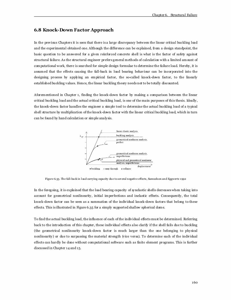
Chapter 6. Structural Failure
160
6.8 Knock-Down Factor Approach
In the previous Chapters it is seen that there is a large discrepancy between the linear critical buckling load
and the experimental obtained one. Although the difference can be explained, from a design standpoint, the
basic question to be answered for a given reinforced concrete shell is what is the factor of safety against
structural failure. As the structural engineer prefers general methods of calculation with a limited amount of
computational work, there is searched for simple design formulae to determine the failure load. Hereby, it is
assumed that the effects causing the fall-back in load bearing behaviour can be incorporated into the
designing process by applying an empirical factor, the so-called knock-down factor, to the linearly
established buckling values. Hence, the linear buckling theory needs not to be totally discounted.
Aforementioned in Chapter 1, finding the knock-down factor by making a comparison between the linear
critical buckling load and the actual critical buckling load, is one of the main purposes of this thesis. Ideally,
the knock-down factor handles the engineer a simple tool to determine the actual buckling load of a typical
shell structure by multiplication of the knock-down factor with the linear critical buckling load, which in turn
can be found by hand calculation or simple analysis.
Figure 6.35. The fall-back in load carrying capacity due to several negative effects, Samuelson and Eggwertz 1992
In the foregoing, it is explained that the load bearing capacity of synclastic shells decreases when taking into
account for geometrical nonlinearity, initial imperfections and inelastic effects. Consequently, the total
knock-down factor can be seen as a summation of the individual knock-down factors that belong to these
effects. This is illustrated in Figure 6.35 for a simply supported shallow spherical dome.
To find the actual buckling load, the influence of each of the individual effects must be determined. Referring
back to the introduction of this chapter, these individual effects also clarify if the shell fails due to buckling
(the geometrical nonlinearity knock-down factor is much larger than the one belonging to physical
nonlinearity) or due to surpassing the material strength (vice versa). To determine each of the individual
effects can hardly be done without computational software such as finite element programs. This is further
discussed in Chapter 14 and 15.

Chapter 6. Structural Failure
161
6.9 Buckling Recommendations
Aforementioned in Chapter 3, there are two design codes that contain recommendations for the analysis of
buckling of concrete shells. However, the ACI Standard is known to be of little practical use as it gives almost
no information of use to a shell designer, Popov and Medwadowski [62]. Therefore, only the IASS
recommendation is discussed here. The IASS recommendation includes a buckling paragraph largely based
on Kollar and Dulacska [54] (and in particular on Chapter 9) which gives a practical application of the
stability theory with respect to shells fabricated from reinforced concrete, timber, synthetics and metal. The
method as proposed by Kollar and Dulacska is a practical semi-empirical (analytical formulas adapted to test
results), but rational, approach. The method tries to ov ercome the differences in linear critical buckling load
and the actual buckling load by considering influences of initial imperfections and nonlinear geometrical and
physical behaviour. The procedure followed in the IASS recommendations is discussed below in five steps
(Paragraph 6.9.1 to 6.9.5). In paragraph 6.9.6 the total reduction factor and safety factor are derived. In the
final paragraph some conclusions are drawn.
6.9.1 Linear Buckling Load
The first step is to determine the linear critical buckling load for an ideal shell. For simple shell geometries
with external normal pressure, the formulas derived by Zoëlly, van der Neut and Flügge may be applied to
calculate the linear buckling load. This is already extensively described in the previous chapter. The linear
buckling load of more advanced shell geometries may be determined using computational software, for
example DIANA. An example and some critical comments are given in Chapter 13.
6.9.2 Postbuckling Category
As explained in the previous chapter, different types of shells experience different types of post-buckling
behaviour. For shells which experience increasing capacity in the post-buckling range, such as some
anticlastic shells (hypars), no reduction is necessary and simply applying the safety factor ov er the linear
critical buckling load is sufficient for a safe shell structure. For shells with decreasing capacity in the post-
buckling regime, however, the load bearing capacity decreases significantly. An important step is therefore to
ascertain in which category the shell problem falls with respect to its post-buckling behaviour.
Depending on the shell geometry this may be more or less apparent. In case of uncertainty, the
categorisation can be done on the basis of established analytical or experimental results which conclusively
show whether the shell experiences a reduction in the buckling load or not. If the shell problem does not fall
in the category of increasing load bearing capacity in the post-buckling range, the initial linear buckling load
is presumed to decrease after the buckling point. To determine the allowable load the IASS
recommendations lower the linear critical buckling load with several reduction parameters. The reduction
parameters are related to effects which have significant influence on the buckling behaviour.
Aforementioned in this Chapter, there is referred to large deflections, geometrical imperfections, and
material parameters as creep, cracking and inelastic behaviour. They will be dealt with in the following
paragraphs.

Chapter 6. Structural Failure
162
6.9.3 Modification for Large Deflections and Geometric Imperfections
The first modification is for large deflections. The reduction factor can be obtained from the graph of Figure
6.36 after computing the linear deflection w0’ and the deflection to thickness ratio w0’/h. The curves shown
are calculated analytically using a large deformation theory. For other geometries similar graphs can be
found in literature. In case that there is no solution available, the lowest possible value of Figure 6.36 must
be used.
Figure 6.36. Reduction in critical load due to postbuckling behaviour and initial imperfections, Popov and Medwadowski 1981
A second modification concerns geometric imperfections. As explained in the previous Chapter, geometric
imperfections cause a significant decrease in load bearing capacity even before the linear buckling load is
reached. The IASS recommendations suggest to calculate or assume an additional deflection w0” as shape
imperfection. The calculation of the additional deflection is based on Chapter 9.2.2 of Kollar and Dulacska
[54]. The proposed equations are listed below.
The additional deflection w0” is in Kollar and Dulacska [54] denoted as the accidental imperfection due to
inaccuracies of erection. By analytical equating the following expression is found:
=0 ,accid
Rw
3500 (6.63)
The latter expression showed acceptable results in compare to measurements on carefully fabricated
cylinders. However, a shortcoming is that it disregards the fact that the imperfection also depends on the
thickness as denoted in Chapter 3 and that it cannot become infinitely large. Furthermore, when the erection
method results in greater imperfections such as reinforced concrete shells erected with a sliding formwork, it
may be reasonable to assume larger imperfections. Therefore, by evaluating measurements on cooling tower
shells, Kollar and Dulacska propose the empirical formula:

Chapter 6. Structural Failure
163
= ++
,accid
R aw 0.05h
R/h 10002000 R/h
0
1000
(6.64)
Where a stands for the influence of the accuracy of the erection method. For reinforced concrete shells with
conventional (rigid) formwork the value of a can be set equal to 1, while for sliding formwork the value can
be taken equal to 6.
Independent of the chosen equation, the total deflection according to the IASS recommendations becomes:
= +0 0 0' "w w w (6.65)
Again, the (total) deflection to thickness ratio must be determined in order to obtain the reduction factor
from the graph of Figure 6.36 as previously explained in Section 6.9.3.
Kollar and Dulacska [54] state that it is rather improbable that the maximum values of both imperfections
coincide. Therefore, by the rules of probability theory, they take the largest value of:
+≥
0 00
0
' "
"
w 0.8 ww
w (6.66)
However, this hypothesis is not borrowed by the IASS recommendations.
6.9.4 Modification for Material Properties
The final step is to include material modification factors for creep, reinforcement and cracking and the effect
of inelastic behaviour of reinforced concrete.
Effect of Creep
To allow for creep influences a reduced value of the modulus of elasticity is introduced according to the
equation:
= −+
ccr u c
u
EE = where C 4 2log f
1 C (6.67)
In which Ec is the modulus of elasticity of concrete and fc is the strength of concrete in MPa. Furthermore Cu
represents the ultimate creep coefficient for the concrete.
The previously found critical load pucr must be reduced in the same proportion as the reduction of the value
of Ec.

Chapter 6. Structural Failure
164
Effect of Reinforcement and Cracking
In accordance with an empirical approach as proposed by Kollar and Dulacska [54], the effect of
reinforcement and concrete cracking on the modulus of elasticity is related to the product of the modular
ratio and the steel ratio:
⋅s s
cr c
E A
E A (6.68)
The quantity of equation (6.78) is used to determine the value of coefficient ψ in Figure 6.37.a.
Figure 6.37.(a) Modification of critical load due to reinforcement and cracking and (b) Reduction of buckling capacity , Popov and
Medwadowski 1981
Consequently, the coefficient ψ and the deflection to thickness ratio w0/h are used in Figure 6.37.b. to
determine the ratio between the upper critical buckling load and the value of pucr,reinf.
Effect of Inelasticity of Concrete
Due to the nonlinear behaviour of concrete the critical buckling load further reduces. The critical load due to
inelasticity of concrete can be determined according to the semi-quadratic interaction formula:
+ =
2plast plastcr cr
uplast cr ,re inf
p p 1
p p (6.69)
Where pp la st is the load bearing capacity of a shell as governed by the ultimate strength of the reinforced
concrete shell cross-Section, independent of any buckling consideration.
The IASS recommendations suggest reducing the thickness of shells thinner than 80 mm with 10 mm to
allow for possible inaccuracies of construction resulting in a thinner shell than designed. This is based on

Chapter 6. Structural Failure
165
extensive measurements on a series of erected reinforced concrete slabs, conducted by the Institute of
Quality Control of the Building Industry in Budapest.
6.9.5 Total Reduction Factor and Safety Factor
Summarising the steps taken in the paragraphs 6.9.3 and 6.9.4 a reduced buckling load can be found in
terms of the linear critical buckling load with the following equation:
α α α α α= =reduced lin lincr 1 2 3 4 cr crp p p (6.70)
In which α1 to α4 are the reduction factors from paragraph 6.9.3 to 6.9.5 and α is the single product of the
individual reduction factors.
α1 = Large deformation and imperfection factor
α2 = Creep factor
α3 = Crack factor
α4 = Material nonlinearity factor
Finally, the allowable load on the shell is determined by dividing the reduced critical load through a factor of
safety γ:
γ=
redcr
allow
pp (6.71)
The IASS recommends value of 1.75 for shells which experience an increase in load bearing capacity of the
point of linear buckling and a value of 3.5 for shells with decreasing capacities in the post-buckling range.
6.9.6 Conclusion IASS Recommendations
Basically, the IASS recommendations provide in a reduced factor approach which shows similarities with the
searched knock-down factor which determines the fallback in load bearing capacity between the linear
critical buckling load and the actual buckling load. Hence, the thesis research can be extended with the
question whether the reducing factor as proposed by the IASS fits with the observations made in this thesis
or not. Furthermore, it must be mentioned that the design approach as proposed in the recommendations
assumes that the boundaries of the shell are well supported so that the buckling instability occurs within the
shell surface. In a different situation additional analytical and/or experimental studies are necessary.

Chapter 6. Structural Failure
166
6.10 Conclusions
The aforementioned survey on the buckling of circular cylindrical shells and spherical shells have revealed
that close agreement between theoretical and experimental results may exist when the effect of
imperfections, geometrical and physical nonlinearity and the boundary conditions are taken into
consideration. The strengths are in particular sensitive to the amplitude of the initial imperfections in the
shell surface. To bring into account for these negative effects on the critical load, a design procedure is
proposed using a knock-down factor which represents the discrepancy between the idealised linear elastic
theory and the actual nonlinear inelastic reality. However, it is difficult to give a general expression for the
knock-down factor since it is very dependent on the shell geometry and boundary conditions, the shape of
imperfection, the shell theory used, and the approximations made. In Chapter 15 it is tried to give a complete
description of the knock-down factor for spherical shells.
The buckling discussion is by far not complete. For a more comprehensive review on shell buckling one
could read the following books and papers. A general review of the buckling phenomenon is found in the
books of Bažant and Cedolin (1991), Brush and Almroth (1975), Timoshenko and Gere (1961) [72], Kollar
and Dulacska (1984) [54] and Hutchinson and Koiter (1970). Additionally, for thin concrete shells, one may
read the review of existing knowledge paper of Bradshaw (1963) and the books of Ramaswamy (1968),
Budiansky and Hutchinson (1979) and Popov and Medwadowski (1981) [62] and the paper of Haas and Van
Koten (1970) [41].


part III Case Study


Chapter 7. Zeiss Planetarium
167
7 Zeiss Planetarium
The lack of theoretical knowledge on postbuckling behaviour and decreasing load carrying capacity caused
by imperfection sensitivity and concrete cracking, as discussed in the previous chapter, is one of the main
objectives of this thesis. In order to obtain qualitative and quantitative information about the structural
response up to structural failure a base shell is introduced. The shell used is the first thin concrete shell of
the modern era, the Zeiss planetarium in the city of Jena. The shell is seen in Figure 7.1.
Figure 7.1. The 1925 Zeiss planetarium in Jena, Germany, www.structurae.co.uk
The choice for the Zeiss planetarium can be explained by the fact that the shell has a simple geometrical
hemispherical shape, easily described by a radius of curvature and an angle. Due to its relative simplicity the
linear elastic behaviour is widely discussed in literature. Furthermore, the buckling and postbuckling
behaviour of a (hemi) sphere is extensively investigated, which results in several theoretical formulae and
benchmark tests to validate the thesis’ results.

Chapter 7. Zeiss Planetarium
168
7.1 Geometry
The Zeiss planetarium is a hemispherical cap situated on a circular base. Part of the shell is concealed behind
an entrance building. On top of the hemisphere, an extension is built. Later, both the entrance building and
the top extension are disregarded in the shell modelling phase. The hemispherical geometry dimensions of
the Zeiss planetarium are tabulated below in table 7.1.
Geometry Dimension
Total height of building 17000 mm
Span 25000 mm
Radius of Curvature 12500 mm
Thickness 60 mm
Shell surface area 981.75 m2
R/t 200
Table 7.1. Geometrical dimensions of the Zeiss planetarium
7.2 Material
The Zeiss planetarium is a thin reinforced concrete shell. There is no information about the concrete quality
or the reinforcement in the shell. Therefore, the material proportions of the shell must be guessed. As the
shell is completed in the early 20th century, a relative low quality of concrete is chosen for the analysis.
Chosen is for a C20/25 mixture. Furthermore, the quality of the reinforcement is chosen rather low selecting
FeB220. The reinforcement of the shell is a single layer geodesic Zeiss-Dywidag triangular mesh, seen in
Figure 2 .5. The reinforcement is located in the middle of the shell cross-section. In general, shells are low
reinforced structures, thus, the percentage of reinforcement is chosen to be between 0.15 and 0.40 volume %
(Chapter 3). The material properties and characteristics are further discussed in Chapter 8.
7.3 Support
However not seen in Figure 7.1, the base of the Zeiss planetarium is stiffened by a tension ring with a depth
of 800 mm, which rest on the circular base building, Fernandez Ordonez and Navarro Vera [35]. The ring
ensures a continuous clamped support at the base of the shell.
7.4 Loading
The loading on the shell consists out of the dead weight and variable loads such as wind and snow. As is seen
in Figure 7.1, today the shell surface is cladded by sheet metal. However, the cladding is assumed to be
negligible when determining the dead weight of the structure. For the variable loading it is important to
know the environmental conditions. The Zeiss planetarium is built in the city of Jena, in the east of Germany
on the river Saale. Jena lies at a height of 155 m above sea level in a slightly hilly country. The surrounding
area of the shell shows regular cover of v egetation and buildings. The loading is determined in Chapter 9.

Chapter 8. Material Properties
169
8 Material Properties
To obtain an answer to the question whether high strength concrete can contribute to more slender shells or
not, the thesis’ shells are analysed using two different types of concrete mixtures. A reference conventional
concrete mixture and a high strength fibre reinforced concrete mixture are selected for analyses. Both
mixtures and their characteristics are discussed in this chapter.
The shell analysed in Chapter 10 and 12 to 15 is the Zeiss planetarium in Jena in the east of Germany,
discussed in the previous chapter. The shell is completed in 1925. Therefore, the conventional concrete
employed is a low quality mixture to ally with the early 20th century concrete technology. Chosen is for a
C20/25 mixture according to the Eurocode 2. The high strength mixture originates from late developments
in concrete technology. They find extensional application by the engineering profession at the present day.
Recently, the first high strength concrete shell structures are realised in Canada and France. The shell in
Calgary is a station cap for a light rail concept constructed in 2003. The double curved individual cast shell
elements are only 20 mm thick and span an area of 5.5 × 6.1 m. The shell is constructed using a Ductal
mixture with compression strength of 151 MPa and a flexural strength of 25 MPa. Typically, there is no
conventional reinforcement in the shell. This also holds for the 2005 tollgates in front of the Millau viaduct
in France. Architect Michel Herbert designed a 98 × 28 m twisted shell with spans of 28-26-28 m.
Longitudinal prestressing ties bring the shell into compression. The shell is 850 mm thick; however, it
includes a hollow core as can be seen in Figure 4.16. The skin is only 100 mm thick. It is constructed using a
BSI-Céracem self-compacting mixture with average compression strength of 200 MPa. The mixture contains
3.5 volume % synthetic fibres, Walraven [83]. Both structures are seen in Figure 8.1.
Figure 8.1. Shawnessy LRT Station in Calgary and the Tollgates near Millau , structurae.co.uk

Chapter 8. Material Properties
170
It must be mentioned that all material properties used in this thesis are mean values. Hence, the real
structural response can be approximated as closely as possible. In practice, design values must be used.
8.1 Conventional Concrete
Conventional (reinforced) concrete does not need much of introduction. The compressive and tensile
behaviour of conventional reinforced concrete according to the Eurocode 2 is outlined in the following. The
constitutive behaviour of concrete is characterised by compressive crushing and tensile cracking. For
reinforced concrete, a third failure mechanism is the yielding of rebars. Time-dependent material behaviour
such as creep, shrinkage and ambient influences like temperature are not considered, although they might
be of significant influence on the shell structural behaviour (Chapter 3).
8.1.1 Compressive Behaviour
The nonlinear compressive behaviour of conventional concrete is characterised by a linear branch followed
by nonlinear branch with strain hardening and strain softening up to compressive crushing. The presence
and propagation of micro cracks in the cement matrix cause the stress-strain curve to be ‘rounded’ near the
point of maximum compression strength. The height of the diagram depends on the concrete quality, the
loading time and the amount of confinement. Confinement results in a modification of the stress-strain law,
higher strength and higher critical strains are achieved. The uniaxial stress-strain relation can be modelled
in several ways. For relatively low compression strengths (< 40 MPa) a parabola is applicable and the
approximation of Thorenfeldt et al. Furthermore, the Eurocode provides in a relation for short term uniaxial
loading for nonlinear structural analysis.
The mean value of the cylinder compression strength fcm, used in the analyses, can be determined from the
5% characteristic value of the cylinder compression strength fck obtained according to EN 206-1 by:
( )= +cm ckf f 8 MPa (8.1)
Furthermore, according to Table 3.1 of Eurocode EN 1992-1 -1 [33], the strain at the peak stress is:
( )ε = ⋅ <.c cm 0.7 f 2.80 311 ‰ (8.2)
Subsequently, the stress-strain diagram can be defined using the mean value of the compression strength
and the expression for the strain at peak stress.
The parabola is described by:
ε εσε ε
= −
c cc cm
c c
f 2
2
1 1
(8.3)

Chapter 8. Material Properties
171
The Thorenfeldt curve, a modification to the Popovics compression curve as the slope of the descending
curve is increased by a factor k, is described by:
εσε ε
ε
= − − +
cc cm nk
c c
c
nf
n 11
1
(8.4)
where = + cmfn 0.8017
ε ε
ε ε
≤=
+ < <
c c
cmc c
1 if
k f0.67 if 0
62
1
1
The Eurocode 2 (art. 3.1.5) relation for short term uniaxial loading is described by:
( )σ η η
η−−
2c
cm
k =
f 1 + k 2 (8.5)
where εηεc
c
= 1
with εc1 the strain at peak stress and ε c1
cmcm
k = 1.05 Ef which is only valid for ε εc1 cu10 < < with
εcu1 the nominal ultimate strain
Relation (8.5) is schematically presented in Figure 8.2 below:
Figure 8.2. Schematic representation of stress-strain curve for structural analyses, Eurocode 2 EN 1992-1-1 2001
(The value of 0,4 fcm for the definition of the secant modulus of elasticity Ecm in Figure 8.2 is approximate,
depending on the moduli of elasticity of the mixture components.)
The compressive behaviour of concrete is often simplified to a parabolic or a bi-linear diagram, both with
yield plateau.

Chapter 8. Material Properties
172
8.1.2 Tensile Behaviour
Typically, conventional concrete shows relatively high compressive strength while it cannot resist much of
tensile stress. Therefore, the shells that are commonly built are reinforced by one or two layers of steel
reinforcement to absorb tension forces in the post-cracking stage. Hence, the tensile behaviour of
conventional concrete is largely influenced by the amount of reinforcement in the structure. The tensile
behaviour is characterised by concrete cracking and rebar yielding. Prior to cracking the tensile behaviour is
assumed to be linear up to the tensile strength of the concrete mixture. Characteristically, the tensile
behaviour can be divided into axial tensile behaviour and flexural tensile behaviour.
The axial tensile strength of the plain concrete, thus, without reinforcement, can be found in Table 3.1 of the
Eurocode 2 EN 1992-1 -1. The axial tensile strength is, for strength classes below C50/60, determined
according to the relation:
( )= ⋅ 2 /3ctm ckf 0.3 f (8.6)
Where, fck is the characteristic (5%) value of the cylinder compression strength according to EN 206-1.
The mean value of the flexural tensile strength can be determined from the axial tensile strength by the
relation (3.23) in Eurocode EN 1992-1 -1 [33], which is defined as:
( ){ }= −ctm, fl ctm ctmf max 1.6 h / 1000 f ; f (8.7)
With h the height of the cross-section in mm and fctm is the mean value of the axial tensile strength in MPa.
For the steel reinforcement the strength is chosen equal to the characteristic yield strength or 0.2% strain
value. The steel will deform according to the typical stress-strain diagrams for steel as seen in Figure 8.3. In
practice they are often approximated by a simplified bi-linear law in which the horizontal branch is
maximised by the yield strength.
Figure 8.3. Typical stress-strain diagrams for hot rolled steel (left) and cold worked steel (right), Eurocode 2 EN 1992-1-1 2001
When the tensile strength of the plain concrete is surpassed, cracks initiate and the reinforcement is
activated. The tensile behaviour after cracking is a complex phenomenon. Two post-cracking phenomena
can be distinguished. First, the tensile stresses in the concrete are zero at a crack; however, they are

Chapter 8. Material Properties
173
introduced into the concrete between cracks by bonded reinforcement. Secondly, the stresses in the
reinforcement fully absorb the tensile stresses at the crack but decrease in the concrete in between which
causes the total strain being smaller when compared to single steel rebars in tension, Walraven [82]. Crack
development and redistribution of tensile stresses from concrete to reinforcement due to bond between the
rebars and the concrete is called tension stiffening. The largest problem of the post-cracking behaviour is the
occurrence of a few wide cracks. This non-isotropic behaviour makes it impossible to capture the structural
behaviour of reinforced concrete into a constitutive law. The exact post-cracking behaviour of the combined
phenomena depends on the concrete and reinforcement proportions in a cross-section. Assuming that the
reinforcement satisfies the minimum and maximum percentages to prevent sudden failure and has good
bonding strength, the composite structure in tension will, in the end, fail due to y ielding of rebars; however,
at that stage the serviceability of the shell is often far in violation.
8.1.3 C20/25 Mixture Design
Aforementioned in the introduction, there is chosen for a relative low quality C20/25 concrete mixture
according to the Eurocode to associate with the early 20th century Zeiss planetarium shell. Using the
equations (8.1), (8.2), (8.6) and (8.7), the properties of the C20/25 mixture are tabulated in Table 8.1.
C20/25
Mean value of cylinder compressive strength fcm -28 MPa
Yield compressive strain εc1 -2.0 ‰
Ultimate compressive strain εcu -3.5 ‰
Mean value of axial tensile strength fctm +2,2 MPa
Mean value of flexural tensile strength (h=60 mm) fctm,fl +3,4 MPa
Y oung’s modulus Ec 30 GPa
Specific weight ρc 2500 kg/m 3
Table 8.1. Material properties of a C20/25 concrete mixture
The quantities of Table 8.1 can be combined with the expressions for the compression stress-strain law of
Section 8.1.1. The two approximation methods are presented in the graph of Figure 8.4 for C20/25 concrete.
0
5
10
15
20
25
30
0 0,0005 0,001 0,0015 0,002 0,0025 0,003 0,0035Compressive strain
Co
mp
res
siv
e s
tre
ss
(MP
a)
Thorenfeldt
Parabola
Eurocode
Figure 8.4. Uniaxial compressive stress-strain curves for C20/25 concrete

Chapter 8. Material Properties
174
In addition to the C20/25 mixture, the choice is made to apply a relative low quality of steel reinforcement
FeB220. For the chosen reinforcement there is referred to FeB220 HWL in which the latter stands for
weldable hot rolled steel (cold worked steel is addressed by the addition of HK). The constitutive law is
depicted in the left of Figure 8.3. For FeB220 HWL the following values are prescribed in the Dutch codes:
FeB220 HWL Steel Reinforcement
Yield strength fyk 220 MPa
Strain at maximum load εuk 5 %
Y oung’s modulus Es 200 GPa
Specific weight ρs 7850 kg/m 3
Table 8.2. Properties of FeB220 steel reinforcement according to the Dutch code
The data of Table 8.1, 8.2 and 7.1 can be used to determine the behaviour in axial tension and flexural
bending of a flat plate with similar cross-sectional dimensions as the Zeiss shell. The characteristic stress-
strain relations for the flat plate (or shell) in axial tension and flexural bending can be seen in Figure 8.5.
0
Conc rete crac king
Rebar yielding
Rein forcement on ly
0
0,5
1
1,5
2
2,5
3
0 0,02 0,04 0,06 0,08 0,1 0,12 0,14
Strains (%)
Str
ess
(MP
a)
Rebar yielding
Fracture momentSimplif ied M-k
diagram
Concrete cracking
0
0,5
1
1,5
2
2,5
3
0 20 40 60 80 100 120 140 160 180 200
Curvatu re (1/mm x 10E-6)
Mo
men
t (k
Nm
)
Figure 8.5. Typical stress-strain relationship in axial tension (left) and flexural bending (right) for a low reinforced beam with one
layer of reinforcement located in the middle of the cross-section
Both relationships seen in Figure 8.5 are typical stress-strain diagrams for low reinforced concrete structures
as shells with a low quality of steel located in the middle of the cross-section. In the left Figure, this can be
seen by the relative long horizontal stage, which represents crack propagation. The low peak stress of rebar
yielding is caused by the low quality of steel. In the right Figure as well as the low quality, as the low
percentage of reinforcement, is responsible for a minimal increase of bending moment by increasing
curvature. Furthermore, in the right Figure the reinforcement is assumed to be located in the middle of the
concrete cross-section, which results in a relative long path of increasing moment during the cracking
process (curvature causes the cross-section to open). This can be explained simply as the cross-section needs
to develop large curvature before the reinforcement in the middle is activated. Hence, shells with a double
layer of reinforcement will experience less cracking and reduced crack opening. Both graphs in Figure 8.5
end rather abruptly, which is caused by the brittle failure of the steel reinforcement. However, not at this
stage already as both graphs are cut-off for clarity.

Chapter 8. Material Properties
175
8.2 High Strength Fibre Reinforced Concrete
8.2.1 High Compression Strength
Recent developments in concrete technology have lead to concrete mixtures with high compressive strength.
During the 1980s research was done to concrete mixtures with a higher early strength, requested by
contractors to speed up the building process. When the new developed concrete mixture hardened, it showed
higher compression strength than usual. The newly achieved knowledge in concrete technology, fillers and
additives contributed to a substantial advancement in the concrete industry and the development of high
strength concrete. The new material was captured in regulations for the first time in France in 2002. Today,
these codes are still the main codes of practice.
According to Den Hollander [47] high strength concrete can be classified as concrete with a characteristic
cube compressive strength above 95 MPa. Within the high strength range further classification is made in
normal high strength concrete ranging from 95 to 155 MPa, ultra high strength concrete from 155 to 250
MPa and super high strength concrete with compression strengths ov er 250 MPa. However, various other
classifications may be found in literature.
The higher compressive strength of concrete is reached by optimising the mixture composition. The mixture
composition can be subdivided into aggregate, cement and the interface between the aggregate and cement.
Optimisation of the three components to a more homogeneous mixture with higher internal bond lowers
tensile stresses perpendicular to the compression direction, see Figure 8.6.a. By reducing the largest particle
size to a prescribed maximum value the homogeneity of the concrete becomes more favourable and the
stress variation decreases. Additionally, an optimal (or higher) packing density yields higher compression
strength as more particles contribute to the bearing capacity and weak v oids are reduced, see Figure 8.7.b.
Figure 8.6.a. The force transmission in the concrete and b. an increased packing density, Den Hollander 2006
To optimise the interface between the aggregate and the cement silica fume is added to the mixture. Silica
fume, which is highly reactive, contributes to a better bond between the aggregate and cement particles by
the forming of secondary calcium-silicate cry stals which grow through the primary crystals formed at the
surface of the cement particles, see Figure 8.7. Furthermore, silica fume reduces the voids filled with water
and air, Den Hollander [47].
Contrasting with the conventional concrete reflection that there must be enough water to react all cement
particles, for high strength concrete the amount of water is not sufficient. Cement particles that do not react
are assumed to strengthen the cement matrix as fillers. Superplasticizers enable the lowering of the

Chapter 8. Material Properties
176
water/cement ratio without reducing the workability. Possible hardening at higher temperature and/or at
higher atmospheric pressure improves the microstructure, however, is of less practical use.
Figure 8.7. The hydration of concrete with and without silica fume, Den Hollander 2006
An optimal mixture can give compression strength of 200 MPa and higher, theoretically up to about 800
MPa. Not only the compression strength enhances, the mixture can also be classified as more durable with
low permeability and favourable creep and shrinkage characteristics, Den Hollander [47]. Also the fatigue
behaviour, however experiments show high scatter, is profoundable in compare to conventional concrete,
Lappa [56]. Additionally, designing with high strength concrete has ecological advantages such as low
material consumption.
For some differences between normal C45 concrete and C200 ultra high performance concrete the mixture
components are shown in Table 8.3 from Den Hollander [47].
Component [kg/m 3] C45 C200
Cement 360 1075
Silica fume - 165
Sand 790 1030
Gravel 1110 -
Steel fibres - 235
Superplasticizers 0.5 39
Water 145 200
Specific mass 2405 2810
Water/cement ratio 0.40 0.19
Table 8.3. Mixture components plain concrete and UHPFRC, Den Hollander 2006
8.2.2 Fibre Reinforcement
The properties of high strength concrete before cracking are similar to the properties of plain concrete.
However, experiments show that when the cracking process initiates, the high strength concrete fails almost
instantly, being a highly brittle material. In general: the higher the concrete strength the more brittle the
concrete behaviour, Den Hollander [47]. To counteract the brittleness, fibres are added during the mixing
process, which can be seen in Table 8.3.
The addition of fibres can be explained by examining the cracking behaviour of (high strength) concrete.
Cracking appears on micro level and macro level, see Figure 8.8. Micro cracks appear in the interface layer
due to the imposed deformation of the cement matrix by stiff aggregates during hydratation. In a loading

Chapter 8. Material Properties
177
situation micro cracks grow until they become visual as macro cracks. Fibres added to the mixture act as well
on micro level, as reinforcement of the cement matrix, as on macro level, as reinforcement of the structure.
The reduction of micro cracking by fibres is achieved by the takeover of the tension stresses around a crack
and thereby reducing the tension stresses in the cement matrix. On macro level the fibre tends to span the
crack and prevent enlarging. By local pull-out behaviour the post-cracking ductility is significantly improved
as fibres provide in the most advantageous low-level post cracking plateau, Markovic [57].
Figure 8.8 Micro-cracking and macro-cracking, Markovic 2006
Fibres do not necessarily lead to an increase in tensile strength; however, it is possible to increase the tensile
strength through the addition of fibres with different dimensions (fibre mixture). The micro cracking can be
decreased with the smaller fibres and with that the elastic behaviour extended while in case of macro
cracking the longer fibres become active, Markovic [57]. Though, fibres are added to improve ductility, they
can reduce the amount of reinforcement or even totally substitute the reinforcement.
Different shape for steel fibers
Different transverse sectionGlued steel fibers
Figure 8.9. Different types of (a) shapes, (b) transverse sections and (c) glued steel fibres, Burgers 2006
Fibres are needle shaped elements manufactured from different materials such as steel or plastics. Fibres are
available in all shorts of shapes and lengths, see Figure 8.9. Fibre lengths vary from 7 to 75 mm with a
diameter ranging from 0.15 to 2 mm. In general they are in between 25 to 60 mm with a diameter of 0.4 to
0.8 mm. Fibre geometry is classified according their aspect ratio, which is qualified as the fibre length
divided by the fibre diameter (Lf/df). Hence, the general aspect ratio is in between 40 to 80. In structures,
the amount of fibres starts at 35 kg/m3, or 0.45 volume %. Hereby the fibres are additional to conventional

Chapter 8. Material Properties
178
steel bar reinforcement. In traditional fibre reinforced concrete the v olume amount is smaller than 2 %,
though, fibre v olumes ov er 2 % are becoming more and more accepted. Hereby the fibres totally substitute
the original reinforcement which is referred to as high performance material, recognised by an increasing
plastic strain (strain hardening) and multiple cracking. They may be applied up to an amount of 15 volume
%, e.g. the SIFCON (slurry infiltrated fibre concrete) mixtures, Kooiman [55]. Fibres have a ductile plastic
stress strain relation and show only minor shrinkage. The strength of steel fibres ranges from 900 to 3000
MPa. Plastic fibres have even higher strengths up to 4000 MPa and more. Plastic fibres are more expensive
and therefore find less application, Bouquet and Braam [17].
Fibres added to the concrete mixture can be considered as coarse aggregates. Fibres cannot just be added,
they must be able to take position without disturbing the mixture composition, Figure 8.10. For an optimal
mixture the addition thus leads to adjustment of the original components. An increase of the cement weight
of approximately 10 % compensates the larger amount of internal surface. Hence, to ensure workability, the
amount of water must be increased or replaced by superplasticizers. The aggregates must be properly chosen
for a sufficient fibre distribution in the mixture, Grünewald [39].
Figure 8.10. Effect of maximum grain size on fibre distribution and orientation, Kooiman 2000
Limiting the maximum grain size to half the fibre length is recommended for satisfying fibre distribution and
favourable for workability and preventing so-called fibre balling. As fibres are needle shaped elements in a
mixture of spherical elements, they tend to decrease the workability considerable. Furthermore, refining the
ratio of fine particles to total volume of the aggregate contributes to a higher packing density which is
negatively influenced by the addition of fibres, as is illustrated in Figure 8.11. According the American
Concrete Institute (ACI) Committee 544, 1993, depending on the fibre v olume, an optimal packing density is
reached by a ratio of fine particles to total volume between 40 and 60 %, Den Hollander [47].
Figure 8.11. Effect fibres on packing density , Kooiman 2000

Chapter 8. Material Properties
179
The influence of the type of fibres in the mixture is often presented referring to the aforementioned fibre
aspect ratio. For example, in Table 8.4, the limitations to the fibre v olume in relation to the maximum grain
size are shown with respect to the fibre aspect ratio. The values are obtained by Kooiman [55] for hooked-
end fibres in dry mixtures.
dmax (mm) Lf/df = 60 Lf/df = 75 Lf/df = 100
4 2.0 % 1.6 % 1.2 %
8 1.5 % 1.3 % 0.9 %
16 1.0 % 0.9 % 0.7 %
32 0.6 % 0.5 % 0.4 %
Table 8.4. Maximum fibre volume for di fferent maximum grain size and di fferent aspect ratio, Kooiman [55]
Some restrictions to the mixture components due to application of fibres are determined by the ACI
Committee 544, 1993. Table 8.5 provides ranges for mixture components for different fibre aspect ratios.
Though, effects of additives as superplasticizers are not mentioned.
Component Lf/df = 60 Lf/df = 75 Lf/df = 100
Water/cement ratio 0.35 – 0.45 0.35 – 0.50 0.35 – 0.55 -
Cement 360 – 600 300 – 540 280 – 420 kg/m 3
Fine/total aggregates 45 – 60 45 – 55 40 – 55 %
Air volume 4- 8 4 – 6 4 – 5 %
V f straight fibres 0.8 – 2.0 0.6 – 1.6 0.4 – 1.4 %
V f deformed fibres 0.4 – 1.0 0.3 – 0.8 0.2 – 0.7 %
Table 8.5. ACI guideline for SFRC mixtures, Den Hollander [47]
When the fibres are added to the mixture, the tensile behaviour, and in particular the post-cracking tensile
behaviour, of the composite mixture must be determined. To provide information about the expected post-
cracking behaviour, pullout test on a simple fibre out of a block of matrix material is widely accepted as one
of the basic tests. The pullout behaviour is dependent of the fibre characteristics, the quality of the cement
matrix and the fibre orientation. Figure 8.12 shows a close-up of the pullout behaviour of a straight fibre as
determined by Naaman 1999, as reported by Kooiman [55].
Figure 8.12. Close-up of a typical pullout versus end-slip relationship for a straight fibre, Kooiman 2000

Chapter 8. Material Properties
180
The fully bonded stage OA is of significance influence to stabilise micro cracks in the early stage of loading.
The graph path AB indicates the debonding stage until full debonding occurs in BC. The frictional stage is
decaying out due to the increasing slip of the progressing pulled out fibre. The debonding stage and frictional
pullout stage are of importance for the total amount of cracking energy consummated by the fibre, the so-
called fracture energy. The area under the curve denotes a value for the ductility, Kooiman [55]. The
complete pullout versus end-slip relationship is seen in Figure 8.13 for straight and hooked-end fibres. The
influence of a higher bonding of the fibre on the pullout load can be seen.
Figure 8.13. Typical pullout versus end-slip relationship for a straight and hooked-ended fibre, Kooiman 2000
Due to the random distribution of the fibres in the cross-section, the results of the pullout test of a single
fibre can not be directly translated to the behaviour of a fibre reinforced concrete structure. Because of the
efficiency of a single fibre is related to the orientation of the fibre with respect to the pullout load, the so-
called inclination angle, there is a difference in efficiency between a single fibre and a group of fibres, which
must be taken into account. The orientation of the fibres is included in the structural design method by the
orientation factor 1/K that deals with randomly distributed fibres and the so-called wall-effect (fibres align
with the wall). Furthermore, the orientation factor depends on the dimensions of the structural element and
on the placement technique, Den Hollander [47]. For plates and shells the orientation of fibres is not
negatively influenced by the wall effect and, thus, the factor can be set equal to the minimum value of one.
Variations in fibre material, shape, size and quantity cause differences in the mechanical behaviour as found
for single fibre pullout tests. The stiffness of the fibre is a measure for the resistance to micro cracking, with
the higher stiffnesses causing lesser micro cracks. On the other hand the fibre contributes to enlargement of
the tension stiffness of the cement matrix as soon as the fibre goes through the micro crack. Hereby the
bonding and aspect ratio of the fibre are essential. This can be explained by the observation that fibres,
although they stiffen the cement matrix, still need a certain amount of cracking before they are activated,
Bouquet and Braam [17].
In case of macro cracking, the fibre must ensure a ductile post-cracking behaviour. When the cracking stage
initiates, there are three mechanisms which can occur. At first, the composite can have brittle failure when
the fibres are unable to resist the tensile force in the composite after cracking. Secondly, the composite can
fail due to consecutively pulled out fibres and, at last, the composite can have increasing tension strength

Chapter 8. Material Properties
181
due to a large amount of fibres in combination with high bonding capacity before it fails due to fibre pullout.
In such cases, attention must be paid to prevent the possibility of brittle failure of the compression zone.
Hence, when appropriately applied, the use of fibres to reinforce the concrete changes the third mechanism
of plain concrete, being the yielding of rebars, to pull-out failure of fibres. As the first mechanism is highly
uninvited, the pull-out failure mechanisms are to be obtained. Therefore the fibre must contain enough
tensile and bonding strength. By increasing the fibre tensile and bonding strength, the fracture energy, and
thus the toughness of the concrete can be enlarged. Furthermore, a larger amount of fibres, increased aspect
ratio and a better orientation of the fibres (higher effectiveness of the fibre) also increase the ductility.
However, attention must be paid to the possible occurrence of brittle failure. To high bonding strength leads
to brittle failure of fibres or the compression zone, Bouquet and Braam [17].
The problem is, however, the contrary fibre demands in case of micro or macro cracking. At micro level a
high bonding is profound while at macro level a to large bonding strength results in uninvited brittle
behaviour of the fibres or the compression zone. It can be concluded, that there is an optimal relation
between the fibre tension strength and the bonding capacity, the critical fibre length, Burgers [20].
Avoiding fibre rupture, the fibre bridging stress must be smaller than the fibre tensile stress which, in turn,
is a function of the embedded fibre length, the maximum bond stress at the fibre to the matrix interface and
the fibre diameter. If the length is smaller, the fibre is not loaded to its full capacity. The fibre will be pulled
out of the matrix. When larger, there is brittle failure. If the length of the fibre is critical, theoretically, the
fibre and cement matrix fail at the same time. In practice the fibre must be pulled out, but as close to the
critical value as possible for higher toughness. Therefore, the fibre length is sub critical, Kooiman [55].
Hence, the basic idea of fibre reinforcement is fundamentally different to the application of conventional
steel bar reinforcement that must fit tight in the concrete and start yielding before brittle cracking of the
compression zone occurs.
Figure 8.14. Typical stress-strain opening displacement relations for FRC and plain concrete, Kooiman 2000
In the final UHPFRC mixture design, the total amount of cracking energy consummated by the fibres by
continuous frictional pullout is the cause for the most advantageous property of fibre reinforced concrete in
contrast to plain concrete, namely the low level post-cracking plateau, seen in Figure 8.14. Figure 8.14 shows
a typical stress-crack opening displacement relation for plain concrete and fibre reinforced concrete in case
of uni-axial tensile stress. The low level post-cracking plateau due to the addition of fibres leads to a higher

Chapter 8. Material Properties
182
toughness and more ductile failure behaviour. Besides the advantageous low level post-cracking plateau, also
a slightly higher tensile peak stress is seen.
8.2.3 UHPFRC in Practice
Different types of mixtures of high strength concrete are available on the market. However, basically there
are only three which are commonly used. The Ductal mixture, patented by French cooperation Lafarge,
Bouygues and Rhodia, the BSI / Céracem product by French company Eiffage and the CRC (Compact
Reinforced Composite) mixture developed by Aalborg Portland A/S and marketed by CRC Technology. Both
the Ductal and BSI mixture contain only (steel) fibres, the CRC mixture combines fibres with closely spaced
reinforcement bars. A shell constructed with such a mixture is the l’Oceanografic shell in Valencia, seen in
Figure 3 .25. The material properties of the three mixtures are captured in Table 8.6. More information
concerning the latter mixtures is available on the internet, e.g. BSI Eiffage [92].
Property Ductal BSI CRC
Specific weight 2500 2800 3200 Kg/m3
Characteristic compressive strength 200 (HT)* 180 140 MPa
Tensile strength 8.0 10.0 7.0 MPa
Flexural bending strength 42.0 45.0 25.0 MPa
Y oung’s modulus 58000 65000 46000 MPa
Poisson’s ratio 0.2 0.2 ? -
* HT = Heat treatment
Table 8.6. Material properties of Ductal , BSI and CRC
8.2.4 Compressive Behaviour
Like conventional concrete, the compressive behaviour of UHPFRC is characterised by a nonlinear stress-
strain curve. After the linear branch the aforementioned micro cracks that occur in the cement matrix at
relatively low stress levels cause a ‘rounded’ compression curve with strain hardening and strain softening
up to compressive crushing. Though, fibres act as reinforcement of the cement matrix and reduce the micro
cracking, several researchers such as Maidl, König & Kützing, Sato found that the contribution of fibres to
the compression strength is negligible, Den Hollander [47]. Furthermore, the contribution of the steel fibres
to the modulus of elasticity is rather small and therefore neglected. Hence, the compression curve is only
determined by the concrete properties.
To describe the uniaxial stress-strain relation of high strength concrete in compression, the approximation
of Thorenfeldt et al. is used, described by relation (8.4). For higher compressive strength the Thorenfeldt
curve gives a better approximation than the parabola expressed in relation (8.3), Burgers [20]. The relation
as presented by the Eurocode 2 (equation (8.5)) is not applicable for such high strengths.
According to the French codes, the compressive behaviour of high strength concrete can be approximated
with a bi-linear constitutive law defined by the concrete strength and the Young’s modulus. The strain

Chapter 8. Material Properties
183
hardening/softening is neglected as there is a yield plateau up to failure due to crushing, illustrated in Figure
8.15. In general, the higher the concrete compression strength, the more linear the stress-strain relation is
up to the peak load. Hence, for UHPFRC the bi-linear law makes sense.
Figure 8.15. The compressive behaviour of high strength concrete according to the French codes, Den Hollander 2006
The characteristic points of the bi-linear law are defined in the French codes. The yield plateau initiates at
60% of the characteristic compression strength fck at a strain of -1.75 ‰. Crushing is assumed to occur at a
strain of -3.0 ‰.
8.2.5 Tensile Behaviour
The tensile behaviour of UHPFRC depends on the proportions of conventional reinforcement, fibres and
concrete and on the concrete quality. Here, the tensile behaviour of a UHPFRC mixture in which fibres
totally substitute the conventional reinforcement is examined. The tensile behaviour is characterised by a
linear stage, limited by the tensile strength of the cement matrix, and a nonlinear post-cracking stage with
low-level post-cracking plateau.
A big advantage of fibre reinforced concrete in tension is the occurrence of a large amount of small cracks
instead of a few wide cracks which were seen in conventional reinforced structures. Due to the addition of
fibres, the composite mixture loaded in tension will behave more like an isotropic material, which means
that the structural behaviour can be observed with a constitutive law instead of a stress-crack relation. Thus,
especially the mathematical part simplifies.
Figure 8.16. The tensile behaviour of UHPFRC, Den Hollander 2006
According to the French codes, the tensile stress-strain relation of UHPFRC may be modelled with a multi-
linear stress-strain diagram with either strain softening (reduction in load bearing capacity accompanied by
increasing deformation) or strain hardening (increasing deformation and increasing load bearing capacity)
in the plastic stage. Strain hardening is visualised in Figure 8.16 as, in general, UHPFRC mixtures allow for

Chapter 8. Material Properties
184
further load increase after the first cracking load. The characteristic point of the tensile strengths of Figure
8.16 must be determined by experimental tests. The French codes provide in the following relations for the
multi-linear strain hardening/softening tension curve:
εγ
= ctct
c c
f
E1
1 (8.8)
Where the material factor γc is set equal to 1.
ε ε= +ct ctc
w
l2
2 1 (8.9)
Where w2 is the crackwidth at t2
ε ε= +ct ctc
w
l3
3 1 (8.10)
With w3 the crackwidth at point t3
ε = ≤fctu
c
l 1 %
4l (8.11)
Where lc is the characteristic length and lf the fibre length.
The characteristic length is a quantity to change the stress-crackwidth relation resulting from the pull-out
tests to a constitutive stress-strain law needed in the analyses. For a rectangular shaped cross-section the
value equals 2/3 times the height, Den Hollander [47].
8.2.6 C180/210 Mixture Design
For the thesis’ shell analyses a high strength concrete mixture BSI C180/210 according to Redaelli and
Muttoni [67] is chosen with 2.4 volume % steel fibres and no conventional reinforcement. The fibres are 20
mm long and have a diameter of 0.16 mm. The mixture has a characteristic value of the cylinder compressive
strength of 180 MPa and a Young’s modulus of 60 GPa. The compressive behaviour is captured in Table 8.7.
BSI C180/210
Mean value of cylinder compressive strength fcm -190 MPa
Yield compressive strain εc1 -1.75 ‰
Ultimate compressive strain εc1 -3 ‰
Y oung’s modulus Ec 60 GPa
Specific weight ρc 2800 kg/m 3
Table 8.7. Material properties of the applied high strength concrete mixture from Redaelli and Muttoni [67]

Chapter 8. Material Properties
185
The compressive stress-strain curve of C180/210 UHPFRC is approximated by the Thorenfeldt rule (relation
(8.4)) and the parabola (relation (8.3)). In addition the compression curve according to Popovics is
determined. The approximation methods are presented in the graph of Figure 8.17. In particular the
Thorenfeldt curve shows high brittleness after the point of peak stress/strain.
0
20
40
60
80
100
120
140
160
180
200
0 0,00 05 0 ,001 0,0015 0,00 2 0,0025 0,003 0,003 5Compressive strain
Co
mpr
essi
ve
stre
ss
(MP
a)
Thorenfeldt
ParabolaPopovics
Figure 8.17. Compressive stress-strain curves for C180/210 UHPFRC
The tensile behaviour is based on the values as found by Redaelli and Muttoni [67]. They are represented in
the Figure 8.20. In the figure it can be seen that the strain hardening branch is introduced by adding a linear
branch bey ond the elastic branch in the stress-strain relation. After hardening phase, the strain softening
initiates and the relation changes to a stress-crackwidth relation.
Figure 8.18. Axial tensile behaviour of a BSI C180/210 mixture, Redaelli and Muttoni 2007
The material behaviour as seen in Figures 8.17 and 8.18 is simplified in accordance with the French codes to
a multi-linear stress-strain relation, a combination of Figure 8.15 and 8.16. The characteristic points of the
compressive branch are tabulated in Table 8.7. For the tensile regime the values as seen in Figure 8.20 are
used. The strain softening branch seen in Figure 8.18, caused by continuous pullout of fibres, is
approximated with a bi-linear law. The value of the tensile strength at the point of 2 mm crackwidth is
determined using the fracture energy as denoted in Figure 8.18.

Chapter 8. Material Properties
186
The values obtained from Figure 8.18 are captured in Table 8.8.
Component
Characteristic tensile strength at point t1 fct1 +8.9 MPa
Characteristic tensile strength at point t2 fct2 +9.7 MPa
Characteristic tensile strength at point t3 fct3 +2.0 MPa
Tensile strain at point t1 εct1 0.148 ‰
Tensile strain at point t2 εct2 2.5 ‰
Crack opening at point t3 w0 2 mm
Ultimate crack opening wmax 10 mm
Table 8.8. Characteristic axial tensile strengths from Redaelli and Muttoni [67]
For the flexural tensile strength of UHPFRC, the values of Table 8.8 may also be converted using relation
(8.7). However, doing so, the obtained values are significant lower than the values found at the material
properties of Ductal and BSI on the internet. The main reason is that the flexural strengths obtained by both
French companies are misleading. They assumed that the advantageous low-level post-cracking plateau,
which allows for much larger cross-sectional rotations, can be introduced in the calculation by increasing the
pre-cracking material flexural tensile strength. In other words, they propose to add cracked properties to
uncracked properties. The graphical explanation of their method is seen in Figure 8.19.
Figure 8.19. Section modulus in cracked and uncracked state, Kooiman 2000
In Figure 8.19 it is seen that the translation from plastic to elastic deformation is based on the assumption
that the depth of the compression zone is approximately 1/10 of the beam depth or structural thickness.
Thus, the equivalent linear-elastic flexural tensile stress can be determined by multiplying the plastic
flexural tensile stress with 1/0.37 = 2.7 .
Though, they reached reasonable agreement with their experimental tests as they have chosen their
specimen dimensions such that the factor which results from equation (8.7) is almost at maximum.
Obviously, such low cross-sectional heights are not representative for structures that appear in practice.
Hence, the extremely high flexural tensile strengths can be questioned and are of little practical value.

Chapter 8. Material Properties
187
8.3 Conclusions
To obtain an answer to the question whether high strength fibre reinforced concrete can contribute to more
slender shells in this chapter two mixtures are designed. A reference conventional concrete mixture with a
relatively low quality is selected to ally with concrete technology available at the time the Zeiss planetarium
was constructed and an ultra high performance fibre reinforced mixture. The conventional concrete mixture
selected is a C20/25 mixture (cylindrical compression strength/cube compression strength) which is
characterised by a rounded compression curve with, after a linear branch, strain hardening, strain softening
and finally compressive crushing, respectively. The behaviour in compression can, for example, be described
by a Thorenfeldt, parabola or Eurocode 2 curve. The tensile behaviour is characterised by concrete cracking
and rebar yielding and determined by the axial concrete tensile strength and the amount of reinforcement in
the cross-section. The interaction between the cracked concrete and bonded reinforcement is complicated
and non-isotropic and impossible to capture within a single constitutive law. The material properties of the
C20/25 mixture and FeB220 HWL steel reinforcement can be found in table 8.1 and 8.2.
High strength fibre reinforced concrete is a relative new development in concrete technology and still subject
to many researches. An optimised mixture composition allows for much higher strengths than conventional
concrete compositions. The selected high strength mixture is a C180/210 mixture for which the compression
curve can, for example, be described by a Thorenfeldt curve or a bi-linear law according to the French codes.
Opposite to the profoundable high compression strength, the material is highly brittle in tension. To
counteract the brittleness, fibres are added, needle shaped elements manufactured from materials such as
steel or plastics. Fibres work both on micro-level, as reinforcement of the cement matrix, as on macro-level
as reinforcement of the structure providing in an advantageous low-level post-cracking plateau. Therefore,
fibres can reduce the amount of reinforcement or even totally substitute the reinforcement as in the selected
C180/210 mixture. Opposite to conventional steel rebars, fibre addition allows for the modelling of the
tensile behaviour within one constitutive law, e.g. the multi-linear law as defined in the French codes, as a
fibre reinforced concrete behaves more like an isotropic material with a large amount of small cracks. The
fibres have only minor influence on the compressive behaviour and, hence, the compression curve is only
determined by the concrete properties. The material properties of the C180/210 mixture can be found in
table 8.7 and 8.8.

Chapter 8. Material Properties
188

Chapter 9. Loading
189
9 Loading
Before going into analysis, the loads on the shell must be determined. As it is not known on forehand which
load, or combination of loads, will challenge the shell to the limit, several loads are defined here. Loads can
be classified by their variation in time into permanent, variable, accidental and time dependent loads.
Aforementioned in Chapter 3, time dependent effects such as creep, shrinkage and temperature gradients
are not considered, although they might have severe influence on the structural failure of a shell. The loads
that are discussed are referred to as static loads as they do not change in time.
Figure 9.1. The Zeiss planetarium in Jena, Germany
When determining (static) loads on a structure, the basic parameters include the magnitude of the load, the
direction of the load and the location of the load. These parameters are determined according to the
Eurocode 2. To provide in a proper explanation the loads are determined for the Zeiss planetarium in Jena,
described in Chapter 7. Similar to Chapter 8, no safety factors are applied in order to approach the real
behaviour of the structure as closely as possible.

Chapter 9. Loading
190
9.1 Permanent Loads
The permanent load is assumed to act vertically over the shell surface. In general, the load consists out of the
dead weight of the shell and possible finishing such as insulation or cladding. However, it is assumed that
the shell does not contain any finishing, thus, the permanent load only consists out of the dead weight. The
dead weight is determined by multiplying the shell area times the thickness times the specific weight. The
values for the specific weight are obtained from the previous chapter. The conventional concrete has a
specific weight of 2500 kg/m3 and the UHPC has a specific weight of 2800 kg/m3. The values include the
additional weight of reinforcement.
Zeiss Planetarium Specific weight (kN/m 2)
C20/25 1.50
UHPC 1.68
Table 9.1. Speci fic weight of concrete
The shell cov ering the Zeiss planetarium has a thickness of 60 mm, as can be seen in Table 7.1. Depending on
the type of concrete, the dead weight of the shell can be seen in Table 9.1.
9.2 Variable Loads
The variable loading on the shell is covered by wind load and snow load. They are discussed in the following.
9.2.1 Wind Load
Wind action is represented by a simplified set of pressures whose effects are equivalent to the extreme effects
of the turbulent wind. Wind load is an example of a non-axisymmetric load. In shell structures subjected to
loading which is not axisymmetric, the meridional curves and parallel circles do no longer present the
principal directions of the internal stresses as there is a nonzero membrane shear force field, as well as
normal membrane forces. Thus, the so-called stress trajectories transform under the influence of wind load.
Other examples of non-axisymmetric loadings are earthquake effects and temperature gradients.
The wind load is determined according to the Eurocode 2 EN 1991-1.4. Wind loads act, by definition,
perpendicular to the shell surface. Depending on the wind direction, some areas of the shell structure are
subjected to wind pressure or wind suction. The basis for calculation is a basic wind velocity depending on
the wind climate. The basic values are characteristic values having annual probabilities of exceedence of
0.02, which is equivalent to a mean return period of 50 years. To determine the effect of wind on a structure,
the basic wind velocity is transformed to a wind pressure acting on the external surfaces while taking into
account for size, shape and dynamic properties as well as landscape effects like terrain roughness and
orography.

Chapter 9. Loading
191
Peak Velocity Pressure
As is recommended by the Eurocode 2 EN 1991 -1.4, Chapter 4.2, the basic wind velocity vb depends on the
fundamental value of the basic wind velocity vb,0. The fundamental value is, however, unknown for the city of
Jena in the east of Germany. There is chosen for a wind speed of 27 m/s which corresponds to a wind speed
of a 10 Beaufort storm. This value is similar to the value as proposed by the Dutch codes for wind region 2
(e.g. coastal areas near Delft) with a return period of 50 years. Hence, the wind speed is considered to be a
save choice. According to the Eurocode basic wind velocity is:
= ⋅ ⋅b dir season b,0v c c v (9.1)
To determine the peak velocity pressure, Eurocode 2 EN 1991-4.5 suggests the relation:
= ⋅ ⋅ ⋅ 21p e b2q (z) c ρ v (9.2)
In which ρ represents the air density, recommended equal to 1.25 kg/m3, and ce is the exposure factor
depending on the height and terrain roughness, determined according to Figure 9.2.
Figure 9.2. The exposure factor ce according to figure 4.2 of Eurocode 2 EN 1991-1.4
For the city of Jena, in the east of Germany, there is chosen for terrain category III, which refers to areas
with regular cover of vegetation or building. With a height of 17 m the exposure factor is approximately equal
to 2.2. When implemented in equation (9.2) the peak velocity pressure becomes:
= ⋅ ⋅ ⋅ = =2 2 21p 2q (z) 2.2 1.25 27 1002 kg/ms 1 kN/m

Chapter 9. Loading
192
Wind Pressure on Surfaces
The final step is to determine the wind pressures on the structure. Wind actions are determined taking into
account of both external and internal actions. However, as the inside of the Zeiss planetarium shell is not
accessible to wind, the internal part is neglected. Chapter 5 of the Eurocode 2 EN 1991-1.4 suggest the
following relation for the external wind pressure:
= ⋅e p e pew q (z ) c (9.3)
Here, qp(ze) is the peak velocity pressure at reference height ze and cpe is the pressure coefficient for the
external pressure. The reference height is set equal to the maximum height of the shell.
For the external pressure coefficient, the Eurocode provides in various values depending on the geometrical
shape of the structure. For domes with circular base the values of cpe can be determined using Figure 9.3. In
the figure the coefficient is denoted as cpe,10 which refers to the fact that the pressure coefficient depends on
the size of the loaded area A, which is the area of the structure, that produces the wind action in the section
to be calculated. The external pressure coefficient is given for loaded areas A of 1 m2 (local, denoted by cpe,1)
and 10 m2 (global, denoted by cpe,10).
Figure 9.3. The external pressure coefficient cpe,10 according to figure 7.12 of Eurocode 2 EN 1991-1.4
For the shell over the Zeiss planetarium, the value of f/d is equal to 0.5. Depending on the location on the
shell surface, the external pressure coefficient becomes:
Region Cpe,10 we (kN/m 2)
A +0.8 +0.8
B -1.2 -1.2
C 0.0 0.0
Table 9.2. External pressure coefficient

Chapter 9. Loading
193
The regions A, B and C on the shell surface are still to be located. As the Eurocode does not give any
recommendations for domes, the distribution as suggested for vaulted roofs is used, see Figure 9.4.a,
however, projected on a hemispherical cap. This means that turning point of wind pressure to wind suction
is located at one fourth of the dome at 45 degrees, Figure 9.4.b. Note that the wind load of Figure 9.4.b.
shows a stepwise transition between region A and B.
Figure 9.4.a. The distribution suggested for vaulted roofs and b. the distribution on the Zeiss planetarium
For the circumferential distribution of the wind load, there is chosen for an opening angle of 30 degrees on
each side, thus, a total angle of 60 degrees, see Figure 9.5. The transition between wind pressure and wind
suction is smooth, however, a stepwise transition is assumed for simplicity.
Figure 9.5. Wind distribution in circumferential direction
The wind load on the Zeiss planetarium shell is defined.
9.2.2 Snow load
Snow load is assumed to act vertically and refers to a horizontal projection of the roof area. Whether the
snow is distributed over the total surface of the shell or not, depends on the curvature of the shell and
possible drift of the snow. The load situation after the snow has been moved from one location to another
(drift), e.g. by the action of the wind, can be highly onerous. The magnitude of the snow load largely depends
on the location of the shell. The Eurocode recognises 8 climatic regions throughout entire Europe. The
largest snow loads are found in the Alpine region. Furthermore, the magnitude of the load depends on the
bulk weight density of the snow as it varies with the duration of the snow cov er and possible rainfalls with
consecutive melting and freezing. The snow load is determined according to the Eurocode 2 EN 1991 -1.3.
Characteristic Value
To determine the snow load on a structure, first the characteristic snow load on the ground must be
determined. The characteristic value of snow on the ground at the relevant site follows from Annex C in the

Chapter 9. Loading
194
Eurocode EN 1991-1.3. The value is the result of scientific work carried out by a specially formed research
group. The characteristic values of ground snow loads given are referred to mean recurrence interval (MRI)
equal to 50 years (also based on annual probability of exceedence of 0.02).
In Annex C a relation for the characteristic value of snow on the ground is recommended for each of the 8
climatic regions. The city of Jena falls under the climate region ‘Central East’ and subsequently, the
characteristic value is described by:
( )
= − +
k
As 0.264 Z 0.002 1
256
2
(9.4)
Here, Z is a zone number from Figure C.3 of Annex C and A stands for the attitude above sea level. The city
of Jena lies in zone number 2 on 155 m above sea level. The characteristic value becomes:
( )
= ⋅ − + =
2k
155s 0.264 2 0.002 1 0.72 kN/m
256
2
According to the table in Annex E of the Eurocode EN 1991 -1.3, the bulk weight density increases with the
duration of the snow cov er, represented in Table 9.3. When the characteristic value is compared to the bulk
weight density, there may be a snow layer of 720 mm fresh snow on top of the shell.
Type of snow Bulk weight density [kN/m3]
Fresh 1,0
Settled (several hours or days after its fall) 2,0
Old (several weeks or months after its fall ) 2,5 – 3,5
Wet 4,0
Table 9.3. Mean bulk weight density of snow according to Annex E of the Eurocode EN 1991-1.3
Snow Loads on Surfaces
The snow load on the shell depends, besides the characteristic value, on the arrangement of the snow over
the surface. Snow load can be deposited on a roof in many different patterns. Hereby, there is referred to
undrifted snow load (Case I) and drifted snow load (Case II), both represented in Figure 9.6. In particular
situations this can lead to a combination of exceptional snow falls and drifts which consequently lead to
areas with exceptional snow load. For the hemispherical cap the latter is, however, not of interest.
The snow load on a surface can be determined by:
µ= ⋅ ⋅ ⋅k i e t ks C C s (9.5)

Chapter 9. Loading
195
Where, µi is the roof shape coefficient, Ce the exposure coefficient, Ct the thermal coefficient and sk the
previously defined characteristic value of the snow load on the ground.
Figure 9.6. Snow load shape coefficients for cylindrical roof, figure 5.6 of Eurocode 2 EN 1991-1.3.
As a reference, according to the Dutch codes, the snow must be applied at regions up to 30 degrees.
From 30 to 60 degrees, the snow load may decrease linearly to zero.
The recommended value for the exposure coefficient Ce following from table 5.1 EN 1991-1.3 for normal
topography equals 1.0. Moreover, the value of the thermal coefficient Ct also equals to 1.0 as the thermal
transmittance of concrete is lower than 1 W/m2K. Thus, relation (9.5) simplifies to:
µ= ⋅k i ks s (9.6)
The roof shape coefficient is defined for different shapes. For cylindrical shaped roofs, the value of µ is equal
to 0.8 for the undrifted case (Case I), while for the drifted case the value is equal to:
For β > 60°, µ3 = 0
For β ≤ 60°, µ3 = 0.2 + 20 h/b
An upper value of µ3 = 2 is recommended for rise to span ratios larger than 0.18 (see Figure 9.7).
Figure 9.7. Snow load shape coefficient for cylindrical roofs (for β ≤ 60°) of figure 5.5 of Eurocode 2 EN 1991-1.3

Chapter 9. Loading
196
For the Zeiss hemisphere, with a rise to span ratio of 0.5, µ3 is equal to 2. In Table 9.4 the resulting snow
loads on the shell are tabulated.
Load case Magnitude [kN/m2]
Case I (Undri fted) 0.58
Case II (Drifted) 1.44 (max)
0.72 (min)
Table 9.4. Snow loads on the Zeiss planetarium shell
9.3 Accidental Loads
Accidental loads may cause highly uninvited stresses and bending moments in the shell. Though, they are
not considered here. The effect of accidental loading, in particular accidental loading that appears like a
point load on the shell surface, is, however, included in the analysis by the introduction of initial geometrical
imperfections. They are discussed in Chapter 10 and 12.
9.4 Load Cases
The loading scheme of the shell covering the Zeiss planetarium is illustrated in Table 9.5 in which the loads
as defined in this chapter are combined in several load combinations. The load combinations follow from
reasonable thinking, e.g. because there is little chance that wind and snow load have their maximum at the
same time, they are divided into different load cases. The loads are not multiplied with a safety factor to
approximate the structural behaviour as close as possible.
LC Dead weight Wind Undri fted Snow Drifted Snow
1 x
2 x x
3 x x
4 x x
Table 9.5. Load cases for the analysis of the Zeiss planetarium shell
9.5 Conclusions
In the foregoing the permanent dead weight load and variable wind and snow load are determined for the
Zeiss planetarium in Jena constructed out of conventional and UHPFRC (see Chapter 8). Furthermore, the
loads are combined into four basic load combinations. Comparing the load intensities, it can already be
concluded that the dead weight of the shell is the main load, pointing in vertical direction.

Chapter 10. Hemispherical Example
197
10 Hemispherical Example
The Zeiss planetarium shell as discussed in Chapter 7 is used to apply the linear elastic theory as described in
Chapter 5 and the buckling theory as discussed in Chapter 6 in this chapter in a numeric example. Therefore,
in this chapter several computations are performed on the Zeiss’ hemispherical shell shape. The results serve
as benchmark for the finite element results discussed in Chapter 12.
Aforementioned, the Zeiss planetarium is a hemispherical shell and the hemispherical shape is extensively
discussed in literature. The fact that the hemisphere is widely discussed can simply be explained. Usually 10
stress resultants are considered to act on the shell element. Membrane stress resultants remain as shown in
Figure 5.11, while non-membrane stress resultants are the out-of-plane shear stresses and bending
moments, similar to the plate bending problem. Because there are only 6 equilibrium equations, the shell in
bending is statically indeterminate. However, if the loads are axisymmetric, the twisting moments, in-plane
shear forces, and the transverse shear forces on the meridional planes are zero. The shell turns into a
statically determined problem.
For the numeric example the original design of the Zeiss planetarium is modelled in different ways. The
linear elastic theory is applied on a shell subjected to a uniformly distributed vertical load with varying
support conditions to investigate the effect of the so-called edge disturbances. The sequence of supports may
in short be named as roller supports, inclined-roller supports and a hinged and clamped supports. The
different models are numbered Zeiss 1 to 4, respectively, and the same numbering will return in Chapter 12
to 1 5. Opposite to the v ertical ‘civil engineering’ load, e.g. the dead weight of the shell, a uniformly
distributed spherical load is used for the calculation of the linear critical buckling load. The spherical load is
applied in combination with an inclined-roller support, as if the shell is a complete sphere, as almost all of
the buckling investigations are directed towards spheres and radial pressure loads (originating from the
aeroplane industry)
Thus, in this chapter the linear stresses, strains and displacements are determined for a vertically loaded
shell with varying support conditions and the linear critical buckling is determined for a shell under radial
pressure load, restricted to an inclined-roller support condition. Moreover, the spherically loaded inclined-
roller supported shell also serves as basis for a nonlinear buckling discussion.

Chapter 10. Hemispherical Example
198
10.1 Shell Parameters
10.1.1 Geometry
Recapitulate from Chapter 7; the shell covering the Zeiss planetarium in Jena has a radius of 12500 mm, a
thickness of 60 mm.
10.1.2 Material
The numeric example is elastic based. Hence, the material is modelled as infinite elastic and the only
material parameters that have to be defined are the Young’s modulus of elasticity, the Poisson’s ratio and the
specific weight. Recapitulate from Chapter 8, for the conventional C20/25 mixture the Young’s modulus is
30 GPa whereas the C180/210 mixture has a Young’s modulus of 60 GPa. The specific weights are 2500
kg/m3 and 2800 kg/m3, respectively. For simplicity, the Poisson’s ratio is equal to zero.
10.1.3 Support
The shell of the Zeiss planetarium is, aforementioned in Chapter 7, assumed to be based on a continuous
clamped support. To illustrate characteristic shell behaviour, or in case of the buckling analysis, to ally with
the experiments, the shell behaviour will be determined with different types of supports also, namely, a
roller support, inclined-roller support, a pinned support and a clamped support.
10.1.4 Loading
The loading is previously derived in Chapter 9. For the hand calculation, the load on the structure is
simplified to an equally distributed vertical load over the total shell surface with the magnitude of the dead
weight of the shell and the undrifted snow load. Except for the buckling analysis, where the load is an equally
distributed spherical load with a dummy magnitude equal to 1.0 MPa.
Load Magnitude (kN/m2)
Specific weight C20/25 1.5
Undri fted snow load 0.58
Total 2.08
Table 10.1. Load on the shell as used in hand calculation
10.2 Analysis Scheme
The various linear analyses done are described in Table 10.2. The Zeiss 2 shells appears twice as it is first
considered subjected to vertical load for the stresses, strains and displacements, while later is loaded by a
spherical compression load to determine the linear critical buckling load.

Chapter 10. Hemispherical Example
199
Name Loading Conditions Supporting Conditions Type of Analysis
Zeiss 1 Vertical load Roller Linear Elastic
Zeiss 2 Vertical load Inclined-roller Linear Elastic
Zeiss 3 Vertical load Hinged Linear Elastic
Zeiss 4 Vertical load Clamped Linear Elastic
Zeiss 2 Spherical load Inclined-roller Linear Buckling
Table 10.2. Analysis scheme
10.3 Linear Analysis
The theoretical solution is based on the relations found in Chapter 5. The relations are for shells with
arbitrary curvature which are described using a global coordinate sy stem. A spherical shell can be described
as non-shallow and is a thin shell of rev olution; it is generated by rotating a curve (meridian) over a vertical
axis of revolution. For simplification the general coordinate sy stem is changed to a local polar coordinate
sy stem when the membrane stress field is to be determined. In the local polar coordinate system the z-axis
points outward of the shell surface, the x-axis is the meridian direction and the y-axis the circumferential
direction. In the description the x and y terms are replaced by φ and θ respectively, see Figure 10.1. As mentioned in Chapter 5, the total solution to the behaviour of the shell consists out of the membrane
solution and the bending solution. For performing a solution to the shell in bending the global coordinate
sy stem is more convenient. As only in the bending solution the influence of different support conditions will
be seen, the membrane solution is valid for all Zeiss shell types.
Figure 10.1. Geometry and coordinate system of a spherical shell of revolution, Hoefakker and Blaauwendraad 2003
10.3.1 Membrane Behaviour
For the membrane behaviour, first the general relations for a thin shell of arbitrary curvature are
recapitulated from Chapter 5. As explained, the general relations with global coordinate sy stem are rewritten
for a shell of rev olution with local polar coordinate system. Comparing the new coordinate system with the
conventional system, it is observed that 1dx = rdφ and dy = rdθ . Since the edges of the shell of rev olution are
often in the θr-plane, an extra displacement ur is introduced, perpendicular to the axis of revolution (Figure
10.2). Because of axisymmetry, displacement and rotational terms in the θ-direction become zero and,

Chapter 10. Hemispherical Example
200
therefore, are left out of the relation. For the same reason, the load component pθ, the derivative θ∂ ∂/ and
the longitudinal shearing stress resultant nφθ are set equal to zero.
Figure 10.2. Geometry of the meridian and positive directions of the displacements, Hoefakker and Blaauwendraad 2003
The meridional strain of a small part of a shell of revolution is dependent on the elongation of an element
due to the tangential displacement uφ and the normal displacement uz. The elongation of the element due to
the difference in the normal displacement uz at each end of the element is of second order and, therefore,
negligible. The meridional strain becomes:
z
u1= + ur
φφφε
φ∂
∂ 1
(10.1)
Which is equal to the strain relation (5.30) found in Chapter 5 for a shell in extension.
The strain in θ-direction is, due to the axisymmetry, also determined by the tangential and normal
displacement only. The tangential displacement causes an elongation of the horizontal radius r in
circumferential direction. The strain contribution can thus be calculated by dividing the elongation
dr = u cosφ φ by the original radiusr = a sinφ . The circumferential strain becomes:
( )θθ φε φ z1
= u cot + ur2
(10.2)
Combining equation (10.1) and (10.2) and setting r3 = r2 tanφ yields the kinematic relation for a shell of revolution in polar coordinates:
φφ φ
θθ
φεε
∂ ∂
z
1 1
r r u=
u1 1
r r
1 1
3 2
(10.3)
The constitutive relations are equal to the relations derived in Chapter 5 omitting the shear terms, thus:

Chapter 10. Hemispherical Example
201
φφ φφ
θθ θθ
ενεν ν
2
n 1Et=
n 1 - 1 (10.4)
And
φφ φφ
θθ θ θ
ε νε ν
− −
n11=
nEt 1 (10.5)
Finally, the equilibrium relations can be obtained from Figure 10.3. The load component pz and pφ must be
in equilibrium with the constant circumferential stress resultants nθθ and the meridional stress resultants
nφφ. Additional, the meridional load component pφ must be in equilibrium with the increase of the meridional
stress resultant φφ φφ
dnd
d. Because the load component in circumferential direction is equal to zero and the
equilibrium of forces in the circumferential direction needs not to be investigated due to the constant stress
resultant nθθ, the equilibrium relations simplify to a statically determinate sy stem with two unknown stress
resultants and two load components.
Figure 10.3 Load components and stress resultants on an infinitesimal element, Hoefakker and Blaauwendraad 2003
The equations of equilibrium for an infinitesimal shell element become:
( )φφθθ φφ
φ− 1 1
d n r n r cos + p rr = 0
d and
z
n n + p r = 0r r
φφ θθ− −1 2
(10.6)
The equations can also be written in matrix notation:
φφ φ
θθ
φ −
1 3
z
1 2
1 d 1
r d r n r p r=
n r p r1 1
r r
(10.7)

Chapter 10. Hemispherical Example
202
Relation (10.7) could also have been obtained directly by determining the adjoint matrix from the kinematic
relation (10.3).
10.3.2 Membrane Stress Resultants
Because of the statically determinate system, the stress resultants can be derived directly from the
equilibrium equations. By eliminating the circumferential stress resultant in the equation (10.6) after
multiplying the first equation by sinφ and the second with cosφ , the vertical equilibrium for a shell part
limited by two adjacent parallel circles with radius r at distance dφ from each other is found.
( ) ( ) ( )φφ φφφφ φ
φφ φ φ φ
φ φ− 1z
d n r d n r sinsin + n r cos = = p cos p sin rr
d d (10.8)
The meridional stress resultant is found by integration of equation (10.8).
( )φφ φφ φ φφ
−∫ 1z
1n = p cos p sin rr d
r sin (10.9)
Consequently, the circumferential stress resultant can be obtained by substitution of expression for nφφ in
equation (10.6).
( )θθ φφ φ φφ
− −∫2 1z z21
1n = p r p cos p sin rr d
r sin (10.10)
The membrane solution is hereby obtained.
For a spherical shell of revolution under uniform vertical load over the shell surface the exact values of the
stress resultants can be obtained. The geometry of a spherical shell can be described with only one radius:
r1 = r2 = a
r = a sinφ
Furthermore, the load components of the vertical load read:
φ−zp = pcos
φ φp = psin
Hence, the expressions for the internal forces, (10.9) and (10.10) can be rewritten and integrated to:
φφφ
φ φ −
2 2
cos 1 Cn = pa +
sin asin

Chapter 10. Hemispherical Example
203
θθφφ
φ φ −− − −
2 2
cos 1 Cn = pa cos pa
sin asin
Using the relation φ φ−2 2sin = 1 cos this can be rewritten to:
φφ φ φ− 2
1 Cn = pa +
1 + cos asin
θθ φφ φ
− −
2
1 Cn = pa cos
1 + cos asin
The constant term C must be equal to zero, considering that the term becomes infinite for φ = 0. Thus, the equations simplify to:
φφ φ−
1n = pa
1 + cos (10.11)
θθ φφ
−
1n = pa cos
1 + cos (10.12)
The stress resultants for a spherical shell subjected to uniform vertical load are now derived. The meridional
stress resultants are always compression stresses. The circumferential stresses, however, change from
compression to tension, as is visualised in Figure 10.4.
Figure 10.4. Distribution of the stress resultants for a spherical shell under vertical load, Hoefakker and Blaauwendraad 2003
Figure 10.4 shows the meridional stress resultants and the circumferential stress resultants for a spherical
shell under vertical load that can move freely at its base, i.e. roller supported (Zeiss 1 ). At the top and base of
the shell, both stress resultants give the same value, however, at the base the circumferential stress
resultants are of opposite sign. It can be calculated, using equation (10.12) that the stresses change sign at
52° from the top of the shell. Thus, when the shell is constructed, reinforcement must be placed in the lower
part of the shell structure. It can be concluded, that when the shell stops at 52° the shell is completely in
compression. Then, theoretically, no reinforcement is necessary.
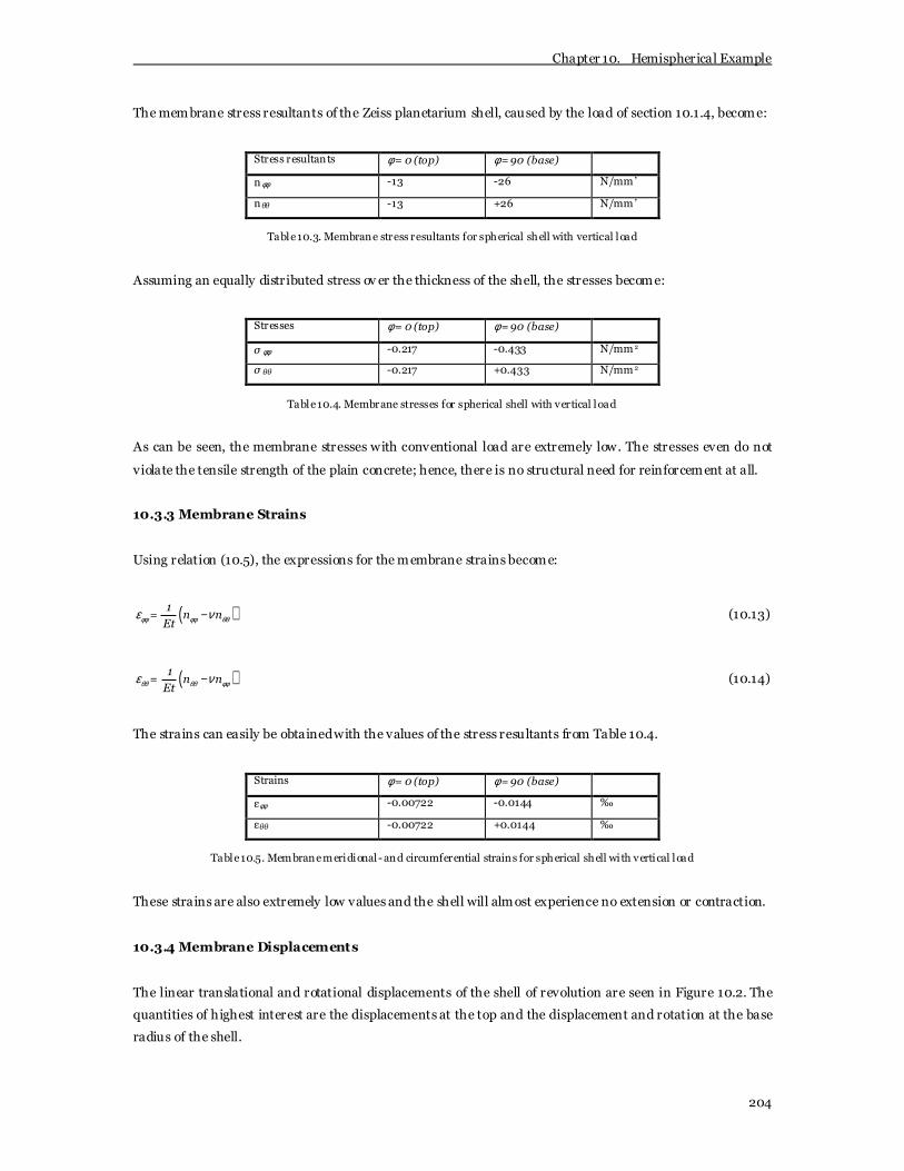
Chapter 10. Hemispherical Example
204
The membrane stress resultants of the Zeiss planetarium shell, caused by the load of section 10.1.4, become:
Stress resultants φ = 0 (top) φ = 90 (base)
n φφ -13 -26 N/mm’
nθθ -13 +26 N/mm’
Table 10.3. Membrane stress resultants for spherical shell with vertical load
Assuming an equally distributed stress ov er the thickness of the shell, the stresses become:
Stresses φ = 0 (top) φ = 90 (base)
σ φφ -0.217 -0.433 N/mm 2
σ θθ -0.217 +0.433 N/mm 2
Table 10.4. Membrane stresses for spherical shell with vertical load
As can be seen, the membrane stresses with conventional load are extremely low. The stresses even do not
violate the tensile strength of the plain concrete; hence, there is no structural need for reinforcement at all.
10.3.3 Membrane Strains
Using relation (10.5), the expressions for the membrane strains become:
( )φφ φφ θθε ν−1
= n nEt
(10.13)
( )θθ θθ φφε ν−1
= n nEt
(10.14)
The strains can easily be obtained with the values of the stress resultants from Table 10.4.
Strains φ = 0 (top) φ = 90 (base)
εφφ -0.00722 -0.0144 ‰
εθθ -0.00722 +0.0144 ‰
Table 10.5. Membrane meridional- and circumferential strains for spherical shell with vertical load
These strains are also extremely low values and the shell will almost experience no extension or contraction.
10.3.4 Membrane Displacements
The linear translational and rotational displacements of the shell of revolution are seen in Figure 10.2. The
quantities of highest interest are the displacements at the top and the displacement and rotation at the base
radius of the shell.

Chapter 10. Hemispherical Example
205
From equation (10.1) and (10.2) can be derived that the equation for the displacement u z at the top of the
shell reads:
z,topu = r rφφ θθε ε+1 2 (10.15)
It can be shown that after filling in the expressions for the radii of curvature and the integrated strain energy
in both directions, and subsequently setting Poisson’s ratio equal to zero, the equation becomes:
z,top
pau = 2
Et
2
(10.16)
The translation ur can be calculated multiplying the strain in circumferential direction with the radius r.
Because r = r3 cosφ = r2 sinφ the translation ur can be described by:
θθ φε φ φr zu = r = u cos + u sin (10.17)
For axisymmetric loading only the rotation φφ in the φr-plane needs to be derived. The rotation is dependent
of the meridional displacement uφ and the normal displacement uz. The rotation due to the meridional
displacement is a positive rotation of the tangent, being uφ/r1. The uniform normal displacement does not
contribute to the rotation, however, the additional normal displacement does. The additional displacement
φφzdud
d divided by the length of a surface element r1dφ yields a negative rotation. Thus rotation φφ, becomes:
φ φϕφ
−
z
1
du1 = u
r d (10.18)
Equation (10.18) describes the displacement of the spherical shell. However, it provides in a relation where
the meridional and normal displacement must be known. A more useful expression for the rotation can be
obtained by direct derivation from the strains. Therefore, the displacement uz is eliminated from the
equations (10.1) and (10.2) and, subsequently, the relations are multiplied by cotφ which results in the expression:
( )φφ φφ θθφ φ φ ε ε
φ− −1 2
2ducot u cot = cot r r
d (10.19)
Differentiating (10.19) for ( )φ φ zu cot + u , eliminating the term φ φφ
ducot
d by adding the differentiated result to
(10.19) and subsequently dividing by the radius of curvature r1 yields:
( )φ φφ θ θ θθφε φ ε ε
φ φ φ φ
− −
2z
1 1
du1 1 d r cosu = cot + r
r d r d sin sin

Chapter 10. Hemispherical Example
206
The rotation φφ, (10.18) can easily be recognised in this expression, thus
( )θθφ φφ
εϕ ε φ
φ φ−
1
d r1 = cot
r sin d (10.20)
To calculate the membrane rotation at the base the strain equations (10.13), (10.14) are introduced and the
Poisson’s ratio is equal to zero. Equation (10.20) changes into
( ) ( )φφ φϕ φ
φ φ φ
− +
2
pa cot pa sin = sin
Et 1 + cos Etsin 1 + cos (10.21)
The membrane displacements of the Zeiss planetarium shell under vertical load can now be calculated using
equation (10.16), (10.17) and (10.21) and the values of Table 10.6. The rotations are tabulated in Table 10.7.
Displacements φ = 0 (top) φ = 90 (base)
u z -0.181 0 mm
u r 0 0.181 mm
φφ 0 -0.0000288 mm/mm
Table 10.7 Membrane displacements for a spherical shell with vertical load
10.3.5 Bending Behaviour
The total solution for the shell behaviour is obtained by adding the bending solution to the membrane
solution which is thus taken as the inhomogeneous solution. With the bending solution the influence of the
different support conditions will be defined; the bending solution makes sure the final solution satisfies the
boundary conditions. For the description of the bending behaviour of shell of revolution, use is made of a
local coordinate sy stem, in which the x and y terms remain and the z-axis is always perpendicular to the
shell surface. Identical to the membrane behaviour it is observed that 1dx = rdφ and dy = rdθ and due to
axisymmetry, displacement and rotational terms in the θ-direction, the load component py and the
derivative θ
∂ ∂∂ ∂( ) ( )
= r y
are zero. Also the longitudinal shearing stress resultants are equal to zero.
Recapitulating from Chapter 5.4 the general relations for a shell of arbitrary curvature are rewritten to the
new local coordinate system, leaving out the zero parts. The kinematic relation thus becomes
− −
−
xxx
yy xy
zxx
yy 2
d 1
dx rε
1ε 0 u
r = uκ
dκ 0
dx
0 0
2
(10.20)

Chapter 10. Hemispherical Example
207
Hence, due to the zero derivate θ
∂ ∂∂ ∂( ) ( )
= r y
the change of curvature in circumferential κyy is zero.
The constitutive relation remains unchanged, apart from the zero terms, thus
ενεν
ν κν κ
=
xx xxm m
yy yym m
b bxx xx
b byy yy
n D D 0 0
n D D 0 0
0 0 D Dm
0 0 D Dm
(10.21)
Where, the extensional and bending rigidity are already defined in Chapter 5.4.
νm 2
EtD =
(1 - )
ν
3
b 2
EtD =
12(1 - )
To complete the description for the bending behaviour of a shell of rev olution, the equilibrium relations
must be derived. Rewriting the equilibrium equations for a shell of rev olution yields:
xxx
dn + p = 0
dx
yyx xxz
x y
ndv n + + + p = 0
dx r r
From the bending action of a flat plate, described in Chapter 5.3, is known that the derivative of the moment
stress resultant is equal to the transverse shearing stress resultant. Thus, eliminating vx out of the latter
equation, yields
xxx
dn + p = 0
dx (10.22)
2
2yyxx xx
zx y
nd m n + + + p = 0
dx r r (10.23)
And, written down in matrix notation, reads
− − − −
xx
yy x
zxx2
x y yy
nd0 0 0
ndx p =
1 1 d pm0
r r dx m
2 (10.24)
Conform the earlier examples; the equation that is derived is equal to the adjoint matrix of equation (10.20).

Chapter 10. Hemispherical Example
208
10.3.6 Bending Solution
From the bending relations, the single differential equation for the displacement uz can be obtained, similar
to the procedure followed in Chapter 5.3. However, because the stress resultant nxx can directly derived from
the first equilibrium condition, the differential equation can be found in a simpler way.
The stress resultant can be determined by integrating equation (10.22)
− ∫xx xn = p dx (10.25)
Substituting the stress resultant in equation (10.23) yields
− − − ∫2
yy xxz x
y x
n d m 1 = p p dx
r dx r2 (10.26)
Using the constitutive relations (10.21) and kinematic relations (10.20) in combination with equation (10.26)
the normal stress resultant nyy can be completely expressed by the displacement uz
( )ν ν− − − ∫2
yy m y z xn = D 1 k u p dx (10.27)
Again, using the constitutive relations (10.21) and kinematic relations (10.20), the bending stress resultants
can be expressed in the displacement uz.
− 2
2z
xx b
d um = D
dx
ν ν− 2
2z
yy b xx
d um = D = m
dx (10.28)
Substituting the equations (10.25), (10.27) and (10.28) in (10.24) yields the differential equation for the
displacement uz
( ) ( )ν ν− − ∫2z
b m y z z x y x
d uD + D 1 k u = p k + k p dx
dx
42
4 (10.29)
By setting the curvature ky equal to zero, the radius ry is constant and the bending behaviour of the shell of
revolution is equal to the bending behaviour of a circular cylinder under axisymmetric loading.
The inhomogeneous solution to the differential equation corresponds with the membrane solution.
Therefore, to obtain the bending solution, the homogeneous solution to the differential equation (10.29)
must be determined:

Chapter 10. Hemispherical Example
209
( )ν− 2zb m y z
d uD + D 1 k u = 0
dx
42
4
To simplify the equation, a parameter µ is introduced: ( ) ( )
( )ν ν
µ− −2 2
m y
b y
D 1 k 3 1 = =
4D r t
2
42
The differential equation then simplifies to
µ4
44z
z
d u + 4 u = 0
dx (10.30)
Obviously, the similarity with a differential equation for a beam on an elastic foundation is clear. The general
solution to the fourth order differential equation with constant coefficients consist of four terms of the form
rxzu (x) = Ce
When the solution is substituted into the equation (10.30) the differential equation reads
µ4 4r + 4 = 0
The four solutions to the differential equation are:
( ) µ± ±r = 1 i
The solution describes two pairs of conjugate complex functions. Because the sum and the difference of the
functions of each pair are purely real or purely imaginary and constitute another set of four independent
homogeneous solutions, the solution can be written as
[ ] [ ]µ µµ µ µ µ1 2 3 4- x x
zu (x) = e C cos x + C sin x + e C cos x + C sin x (10.31)
The terms which are multiplied with e±µx have an influence length of:
ππµ υ−4
y
i 2
r tl = =
3(1 ) (10.32)
Neglecting the effect of Poisson’s ratio, the influence length of the bending behaviour on the shell of
revolution can be determined:
i yl = 2.4 r t (10.33)

Chapter 10. Hemispherical Example
210
The influence length is illustrated in Figure 10.5.
Figure 10.5. Influence length of a spherical shell under external pressure, Hoogenboom 2006
From equation (10.33) it can be concluded that the influence of an edge disturbance becomes smaller with
decreasing thickness. Thus, thinner shells have increasing preference for membrane-dominant behaviour.
For determining the constants the equation (10.31) must be transformed. The term of equation (10.31)
multiplied with the constants C3 and C4, damped oscillations which decrease exponentially for decreasing x,
is rewritten using an ordinate x’ which is positive in the negative x-direction.
[ ] [ ]µ µµ µ µ µ− −1 2 1 2
x x'zu (x) = e A cos x + A sin x + e B cos x' + B sin x'
By introduction of free constants C1 and C2 and phase angles ψ 1 and ψ 2 the equation transforms to:
( ) ( )µ µµ ψ µ ψ− −x x'z 1 1 2 2u (x,x') = C e sin x + + C e sin x' + (10.33)
Where:
2 2 21 1 2C = A + A ; ψ 1
12
Atan =
A
2 2 22 1 2C = B + B ; ψ 1
22
Btan =
B
By substitution of equation (10.33) in the relations (10.20), (10.25), (10.26), (10.27) and (10.28), the
quantities of interest become:
( ) ( )µ µµ ψ µ ψ− −x x'z 1 1 2 2u = C e sin x + + C e sin x' +
( ) µ µν π πµ ψ µ ψµ
− − − −
x y x x'x 1 1 2 2
k + ku = C e sin x + + C e sin x' + +
4 42
µ µπ πϕ µ µ ψ µ ψ− − − − −
x x'x 1 1 2 2 = 2 C e sin x + C e sin x' +
4 4
( ) ( ) ( )( )µ µν µ ψ µ ψ− −− − 2 x x'yy m y 1 1 2 2n = D 1 k C e sin x + + C e sin x' +

Chapter 10. Hemispherical Example
211
µ µπ πµ µ ψ µ ψ− − − − −
x x'xx b 1 1 2 2m = 2D C e sin x + + C e sin x' +
2 2
2
µ µπ πµ µ ψ µ ψ− − − − −
x x'x b 1 1 2 2
3 3v = 2 2D C e sin x + C e sin x' +
4 4
3 (10.34)
From equation (10.32) it can be seen that the influence length of an edge disturbance, as a result of the
exponential damping of the wave, for a thin shell is small (t « r) in comparison to the distance between two
edges. In that case, the term which determines the bending behaviour at one edge, is negligible at the other
edge. Therefore, the constants in the equations (10.33) can be derived independently from each other with
the aid of the boundary conditions at x = 0 and x’ = 0.
To determine the free constants C1 and C2 and phase angles ψ 1 and ψ 2 the boundary conditions of the shell
are divided into two elementary cases: a first case in which the shell undergoes a displacement ur due to an
edge load fr and a second case in which the shell undergoes an rotation φx due to an edge torque tx.
φ φϕ ϕ
0 0r z z r
x x x x
u = u sin f = f sin
= t = t
The homogeneous boundary condition for the edge load is
=0x ( x' ) zv = f ; =0xx (x ' ) xm = t = 0
From these boundary conditions and the equations (10.34), the phase angle ψ 2 and the constant C2 can be
derived directly
πψ 2 = 2 ;
µ2 3r
b
fC =
2D
For the second case, the edge torque, the same procedure can be followed, however, this time the shear
component is equal to zero and the moment is equal to the torque. The phase angle and constant can be
described as
πψ 3 =
42 ; µ
−2 2
x
b
tC =
2D
Combining the two elementary cases yields the relation
ϕ
− −
z z
x xb
f uµ µ =
tD
µ µ
3 2
2
1 1
2 21
1 1
2

Chapter 10. Hemispherical Example
212
Or written in r-direction
ϕr r
x xb
sin φ sinφf uµ µ
= tD
sinφµ µ
−
−
2
0 03 2
02
1 1
2 21
1 1
2
(10.35)
The inverse relation is
µ µφ φ
ϕµ µφ
r rb
x x
4
sin sinf u = D
t2
sin
3 2
2
0 0
2
0
2
2 (10.36)
Obviously, for the spherical shell of revolution, at the base, the z-direction equals the r-direction.
The solutions to the bending behaviour of the shell can now be determined in combination with the results of
the membrane behaviour and the boundary conditions of each of the shells as denoted in Table 10.3.
10.3.7 Total Solution
The total solution is the bending solution added to the membrane solution. As mentioned the membrane
solution will yield ov er the majority of the shell. The bending solution occurs only locally near the supports.
Therefore, for the total solution, only the displacement, rotation and moment distribution of the lower part
of the shell (near the supports) are determined. Recapitulating the membrane results at the base radius of
each Zeiss shell, obtained with the equations (10.11), (10.12), (10.13), (10.14), (10.17), (10.21) yields:
Displacements φ = 0 (top) φ = 90 (base)
u r 0 0.181 mm
φφ 0 -0.0000288 mm/mm
Table 10.8 Membrane displacements for a spherical shell with vertical load
Zeiss 1
The Zeiss 1 shell is roller supported and, thus, neither displacements nor rotations are restrained.
Consequently no edge disturbance occurs. Therefore, the membrane solution is the total solution.
Zeiss 2
The shell has inclined-roller supports which mean that the shell is not allowed to rotate near the supports
but is free to move outward. The boundary conditions thus yields a zero rotation φx,tota l and zero edge force
fr, thus:
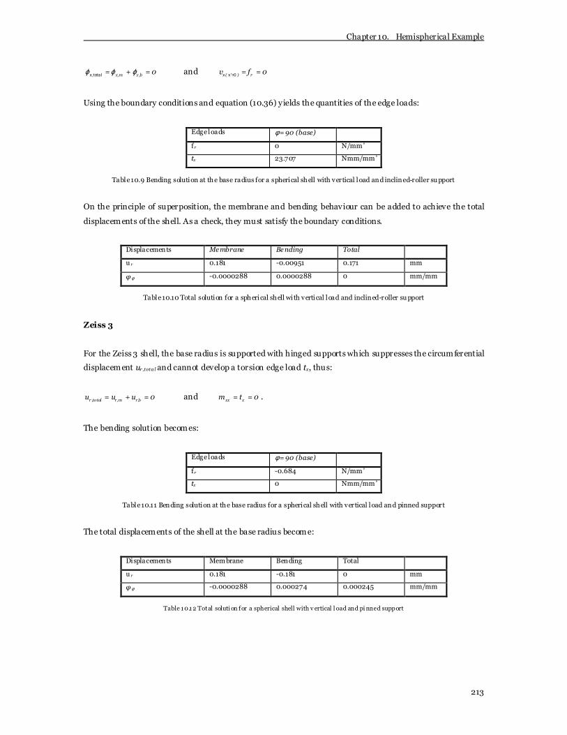
Chapter 10. Hemispherical Example
213
ϕ ϕ ϕx,total x,m x ,b = + = 0 and =x x 0( ' ) rv = f = 0
Using the boundary conditions and equation (10.36) yields the quantities of the edge loads:
Edge loads φ = 90 (base)
fr 0 N/mm’
tx 23.707 Nmm/mm’
Table 10.9 Bending solution at the base radius for a spherical shell with vertical load and inclined-roller support
On the principle of superposition, the membrane and bending behaviour can be added to achieve the total
displacements of the shell. As a check, they must satisfy the boundary conditions.
Displacements Membrane Bending Total
u r 0.181 -0.00951 0.171 mm
φφ -0.0000288 0.0000288 0 mm/mm
Table 10.10 Total solution for a spherical shell with vertical load and inclined-roller support
Zeiss 3
For the Zeiss 3 shell, the base radius is supported with hinged supports which suppresses the circumferential
displacement ur ,tota l and cannot develop a torsion edge load tx, thus:
r ,total r,m r,bu = u + u = 0 and xx xm = t = 0 .
The bending solution becomes:
Edge loads φ = 90 (base)
fr -0.684 N/mm’
tx 0 Nmm/mm’
Table 10.11 Bending solution at the base radius for a spherical shell with vertical load and pinned support
The total displacements of the shell at the base radius become:
Displacements Membrane Bending Total
u r 0.181 -0.181 0 mm
φφ -0.0000288 0.000274 0.000245 mm/mm
Table 10.12 Total soluti on for a spherical shell with v ertical l oad and pi nned support

Chapter 10. Hemispherical Example
214
Zeiss 4
Finally, the bending solution for the clamped Zeiss 4 shell, the most realistic model of the actual shell, must
be determined. The boundary conditions at the base circle of the shell are:
r ,total r,m r,bu = u + u = 0 and ϕ ϕ ϕx ,total x,m x,b = + = 0
Using equation (10.36) this results in the following expressions for the edge loads:
Edge loads φ = 90 (base)
fr -1.297 N/mm’
tx 402,92 Nmm/mm’
Table 10.13 Bending solution at the base radius for a spherical shell with vertical load and clamped support
The total displacement solution must satisfy the boundary conditions:
Displacements Membrane Bending Total
u r 0.181 -0.181 0 mm
φφ -0.0000288 0.0000288 0 mm/mm
Table 10.14 Total solu tion for a spherical shell with vertical load and clamped support
From the above results it can be observed that the calculated values of maximal stresses and displacements
are remarkably low for such a structure. In particular, the maximum tensile hoop stress is very small and can
be carried by weak materials such as various masonry products. This is generally true for most shell
structures and the many historical masonry shells which still remain after many centuries demonstrates this
unique feature of shells.
10.4 Geometrical and Material Influences
10.4.1 Geometrical Influences
As the hemispherical shell is the basic shape of this thesis, the shell thickness is the only parameter to vary.
In the membrane situation, if additional snow load is left out of scope, a smaller thickness lowers the shell
dead weight and the stress resultants while it increases the stresses, strains and displacements with the same
amount. The gov erning effect is, thus, zero. For the bending solution, a twice as thin shell reduces the
bending moments 26%. Aforementioned, the influence of an edge disturbance becomes smaller with
decreasing thickness. Thus, thinner shells have increasing preference for membrane-dominant behaviour.

Chapter 10. Hemispherical Example
215
10.4.2 Material Influences
In linear elastic analysis, the material is characterised by the Young’s modulus and Poisson’s ratio only.
Moreov er, fibre additions and higher packing density increases the specific weight of the UHPFRC concrete
and the dead weight of the shell increases. Therefore, when the UHPFRC mixture is applied, the stress
resultants increase and the strains decrease according to the equations described above. A non-zero
Poisson’s ratio means that the membrane displacements slightly increase at the supports
(compression/tension) while the top displacement decreases (biaxial compression). Still, the resulting effect
may be that of an increasing top displacement (see Chapter 12).
10.5 Linear (Euler) Buckling Analysis
The next step is to calculate the linear critical buckling load for the Zeiss planetarium shell. Buckling causes
premature instability failure caused by eccentricity of compressive forces. The phenomenon is discussed in
Chapter 6. Here, the general equation of Zoëlly for shells as obtained in Chapter 6 is used to determine the
critical load of the Zeiss planetarium.
In Chapter 6 the expression for the linear critical buckling load of a sphere under external pressure load
(equation (6.53)) is derived. When Poisson’s ratio is set equal to zero the equation changes to:
lincr
tP = 1.16E
R
2
(10.46)
For the given parameters the critical load for the Zeiss shell under radial pressure load becomes:
lincrP 1.16 30000 0.802 MPa 802 kN/m
= ⋅ = =
2
260
12500
This is an extremely large load in compare to the load as determined in Chapter 9. Moreover, the linear
critical buckling load is so high that the shell fails on surpassing the concrete compression strength
( plast cmcr
f t 28 60P 2 2 0.268 MPa
R 12500
⋅ ⋅= = = ) rather than failure due to buckling instability (crushing load is 33.4%
of buckling load). The critical crushing load can simply be calculated from the uniaxial compression stresses
(the shell is in complete compression). For the C180/210 UHPFRC mixture with mean cylinder compression
strength of 190 MPa, however, it can be computed that buckling occurs before concrete crushing is reached.
The above paragraph is interesting as the question arises if, for a shell constructed with conventional
C20/25, the buckling load will prevail ov er the crushing load when the shell thickness decreases. Therefore,
in Figure 10.6 the maximum spherical load corresponding to the linear critical buckling load and the
concrete crushing load is plotted against an increasing radius to thickness ratio. In Figure 10.6 it can be seen
that with increasing R/t ratio, the critical buckling load eventually will be lower than the crushing load. In

Chapter 10. Hemispherical Example
216
other words, when the R/t ratio becomes larger than approximately 600, buckling will occur before
crushing. For UHPFRC the linear critical buckling load is lower for all R/t ratios.
0
0,1
0,2
0,3
0,4
0,5
0,6
0,7
0,8
0,9
1
100 300 500 700 900
R/t
P (M
Pa)
Concrete CrushingLinear cri tical buckling load
Figure 10.6. Decisive failure mechanism at increasing thickness to radius ratio for C20/25
The fact that the shell fabricated from conventional C20/25 concrete does not fail by buckling for all R/t
ratios means that in the search to the knock-down factor the shell behaves different for various thicknesses.
For lower R/t ratios the shell fails by surpassing the material strength whereas for higher R/t ratios the shell
fails by buckling instability. Later, in Chapter 14 and 15, imperfections and material nonlinearities move the
buckling curve downwards and the turning point moves towards the left, i.e. buckling may also prevail for
lower R/t ratios than 600.
10.6 Postbuckling Analysis
The next step in this numeric example is to determine the lowest postbuckling load. As explained in Chapter
6 the shell experiences a significant decrease in load-carrying capacity after the bifurcation point. The
maximum decrease in load carrying capacity in the postbuckling range, as illustrated in Figure 6.22, can be
computed using the analytical relations as obtained by Von Karman and Tsien, Tsien, Thompson and Del
Pozo and Del Pozo. Their research has resulted in various analytical relations for obtained the lowest point
for a spherical shell subjected to radial pressure load (from Chapter 6):
Classical theory by Zoëlly: =
lincr
tP = . E 0.802 MPa
R
2
1 16
Von Karman and Tsien: =
cr
tP = 0. E 0.252 MPa
R
2
365
Thompson: =
cr
tP = 0. E 0.196 MPa
R
2
283
Chapter 10. Hemispherical Example
217
Del Pozo and Del Pozo: =
cr
tP = 0. E 0.158 MPa
R
2
228
Dostanowa and Raiser: =
cr
tP = 0. E 0.087 MPa
R
2
126
The values of the lowest postbuckling load range from 0.252 to 0.087 MPa. The lowest value as proposed by
Del Pozo and Del Pozo shows a decrease in load carrying capacity of almost 90%. Although, the lowest
postbuckling load is far greater than the external applied load as determined according to the Eurocode in
Chapter 9 (= 0.0021 MPa), the load is lower than the load needed for compressive crushing of the concrete.
This means that the original Zeiss shell (with R/t ratio 200 and conventional concrete) with imperfections
may fail due to buckling rather than to compressive crushing after all, if, however, the imperfection is large
enough.
10.7 Inelastic Buckling Analysis on Imperfect Shells
To determine the load-carrying capacity of an inelastic imperfect shell, the relations as proposed by the IASS
recommendations have been introduced in Chapter 6. Basically, the IASS recommendations determine a
reduced load by multiplying the linear critical buckling load by a factor which takes into account for
imperfections and material nonlinearities. The relation proposed in Chapter 6 is:
α α α α α= =reduced lin lincr 1 2 3 4 cr crp p p (6.70)
Herein:
α1 = Large deformation and imperfection factor
α2 = Creep factor
α3 = Crack factor
α4 = Material nonlinearity factor
If the maximum imperfection is taken equal to the shell thickness, α1 is equal to 0.2 (see Figure 6.36).
For the creep factor the mean value of cylinder compression strength and the Young’s modulus of Table 8.1
are used into equation (6.67):
α= −
+
u
2cr
C 4 2 log 28 = 1.1114247
= = 0.4753000030000E = = 14247
1 1.11
For the crack factor a reinforcement percentage of 0.4% is assumed (see Chapter 3) and the properties of
reinforcement are taken from Table 8.2. Using equation (6.68) and Figure 6.37 the crack factor becomes:

Chapter 10. Hemispherical Example
218
ρα
ψ
= ⋅ = ⋅ =
s s
cr c 3
E A 200 GPan 0.004 = 0.06
E A 14247 MPa = 0.2
0.21
Finally, the material nonlinearity factor is determined using equation (6.69):
αα α α
= ≈ ≈⋅ ⋅ ⋅
plastcr
4 lincr
p 0.015 1.0
p 0.0151 2 3
The reduced critical load, thus, becomes:
α α α α= = ⋅ ⋅ ⋅ ⋅ =reduced lincr 1 2 3 4 crp p 0.2 0.475 0.2 1 0.7981 0.015
Applying the safety factor of 3.5, described in Section 6.9.5, the allowable load is equal to:
= =reduced
2crallow
p 0.015p = 0.00433 MPa = 4.33 kN/m
3.5 3.5
Hereby, the total reducing factor is approximately 184.3. However, aforementioned, creep is not taken into
account in the finite element analysis. Hence, the allowable load is assumed to be equal to:
⋅ ⋅ ⋅= = 2
allow
0.2 0.2 1 0.7981p 0.00912 MPa = 9.12 kN/m
3.5 (Total reducing factor is equal to 87.5)
The allowable loads are close to the external applied loads as determined in Chapter 9 and used in the
numeric example described above. However, it must be mentioned that the IASS procedure followed is
rather unclear and the author’s confidence in the correctness of this procedure is not very high.
10.8 Conclusions
In this chapter a linear solution to the Zeiss planetarium is performed for different types of support
conditions. The stresses, strains and deformations of a shell in membrane action are determined in
combination with the influence of edge disturbances caused by restrained deformation at the supports. For
the chosen dimensions and material and loading parameters the stresses, strains, and displacements appear
to be v ery low, i.e. in reality they may not be noticed at all. When the thickness of the shell is decreased, the
dead weight and membrane stress resultants lower, however, the stresses, strains and displacements
increase with the same amount. The governing effect is, thus, zero. For the bending solution, a twice as thin
shell reduces the bending moments 26%. Moreover, the influence of an edge disturbance becomes smaller
with decreasing thickness. Thus, thinner shells have increasing preference for membrane-dominant
behaviour. The linear solution changes linearly with changes in material parameters, if variations in specific
weight are not taken into account.

Chapter 10. Hemispherical Example
219
Besides the linear solution, the linear (Euler) buckling load, the (lowest) postbuckling load and the inelastic
imperfect buckling load are determined. The linear buckling load yields extreme high values in compare to
the expected external loads and concrete crushing may prevail over buckling instability for low qualities of
concrete. This may change when the radius to thickness ratio or the quality of the concrete is increased. After
the bifurcation point the maximum decrease in load carrying capacity in the postbuckling branch is
determined with the various equations as proposed by mathematicians such as Von Karman and Tsien, Del
Pozo and Del Pozo and Dostanowa and Raiser. The maximum load carrying capacity decreases up to more
than 80%. Finally, inelastic buckling of imperfect shells is considered using an approach suggested by the
IASS Recommendations. The procedure, however, is rather unclear and the author’s confidence in the
correctness of the procedure is not very high.


part IV Finite Element Analysis


Chapter 11. Finite Element Method
220
11 Finite Element Method
From the preceding discussion on shells and their sensitivity to initial imperfections it is clear that the
behaviour of a shell structure must be closely investigated. However, analytic solutions to the structural
behaviour of many shell structures are almost unattainable due to the importance of nonlinear features such
as large deformations and material nonlinearities.
As denoted by Schnobrich [68], the arrival of the computer made possible a rational approach to the analy sis
of structures by the use of numerical methods. In particular the finite element method, basically a numerical
approximation method, has revolutionised numerical computer analysis and is widely available in advanced
software. The finite element method that is the most convenient for the majority of the problems is the
displacement approach which uses displacements as basic variables. The general procedure inv olves the
construction and solution of a matrix sy stem from partial differential equations describing the equilibrium of
an idealised structure by transferring it to an equivalent weak form, a reduced order problem, which has a
relaxing effect. Instead of finding an exact solution everywhere, there is searched for a solution that satisfies
the equilibrium ‘on average’ over the domain allowing an approximated displacement field for which the
structure is discretised into finite elements. In the elements a displacement field is described by nodal
parameters, and stretched over the element by shape functions. The discrete set of unknown displacement
coefficients are related by a stiffness matrix to the external applied load. The problem is solved by evaluating
the stiffness matrix by numerical integration over the elements and subsequently performing a solution to
the unknown displacements. The strains and stresses can successively be computed from there.
To analy se a structure using the finite element method, the analyst must make a model which correctly
describes the structural behaviour. Basically, the finite element model consists out of the discretized
geometry of the structure by a mesh, the phy sical properties and the loading and boundary conditions such
as supports. The implementation of the model in computational software is often aided by pre-processors
offered in combination with the finite element program which e.g. offer design tools and mesh generation
algorithms. A postprocessor can be used to present the analysis result by graphical methods such as a
contour plots. For analysis the program DIANA is used equipped with iDIANA as pre- and postprocessor.
The aim of this chapter is to introduce the reader into finite element procedures and to familiar the reader
with the most important aspects so that more advanced literature such as Bathe [3], Crisfield [25], Hughes
[51] or Zienkiewicz and Taylor [87], [88] can be understood.

Chapter 11. Finite Element Method
221
11.1 Mathematical Fundamentals
Throughout Chapter 5 reference was made to matrices and vectors, e.g. in the notation of the basic
quantities, related to each other by the kinematic, constitutive and equilibrium matrices. In this chapter
vectors, matrices and tensors are used to express the finite element procedure in a compact manner, similar
to the relations in Chapter 5. For the benefit of the reader the fundamentals of v ectors, tensors and matrices
will be presented. Obviously, the discussed is rather limited considering only those aspects which are
important in finite element analysis. Straight formulations of the definitions can e.g. be found in Bathe [3].
11.1.1 Matrices and Vectors
Basically, a matrix is a two-dimensional array of scalars (physical quantities that have the same value,
irrespective of the choice of reference frame, Wells [85]. A matrix is said to have m rows and n columns,
which do not have to be equal, and denoted by capital bold characters. In general, a matrix represents the
relation between a set of variables and often it has a phy sical meaning, such as a system stiffness matrix. An
example from Zienkiewicz and Taylor [88] shows the definition of a matrix:
A linear relationship between a set of variables x and b, e.g.:
+ + + =
+ + + =+ + + =
1
2
3
a x a x a x a x b
a x a x a x a x b
a x a x a x a x b
11 1 12 2 13 3 14 4
21 1 22 2 23 3 24 4
31 1 32 2 33 3 34 4
Can be written shortly as [ ][ ] [ ]=A x b or =Ax b . Where the matrix A is defined as:
[ ] ≡ =
A
a a a a
A a a a a
a a a a
11 12 13 14
21 22 23 24
31 32 33 34
and the variables are presented by [ ] ≡ =
x
x
xx
x
x
1
2
3
4
and [ ] ≡ =
b
b
b b
b
1
2
3
The particular column matrix presentation of the variables is often referred to as a vector. A vector is a one-
dimensional array of scalars which is said to have m entities (in an m-dimensional space) and denoted by
normal bold characters. As seen in Chapter 5, in structural mechanics quantities such as forces and
displacements can be listed as a vector.
Besides the definition of a matrix and a vector, the example shows the multiplication process of two
matrices. In general, multiplication is not commutative like ordinary algebra, i.e. ≠AX XA . Addition and
subtraction of matrices is based on the addition and subtraction of individual terms of the array and follows
the ordinary rules. Addition and subtraction is only possible if the matrices are of identical size.
Two important matrix operations are the calculation of the transpose and inverse of a matrix. The transpose
of a matrix is a definition for simple reordering of the terms in an array in the following manner:

Chapter 11. Finite Element Method
222
=
Ta aa a a
a aa a a
a a
11 21
11 12 13
12 22
21 22 23
13 23
The transpose vector is indicated by the addition of a capital T. In case of a vector, the transpose vector
simply means that the scalars are written down as a row. An operation that often occurs is to take the
transpose of a matrix product, which follows by the rule ( ) =T T TAB B A . Furthermore, the transpose becomes
useful as, by the rule of matrix multiplication, the product of two vectors is written as =f a a fT T .
Previously, these multiplications were done in Chapter 5, e.g. the virtual work equation.
Taking the inverse of a matrix may be required to solve a system of equations. The inverse of a matrix is a
matrix A-1 such that = =A A I AA- -1 1 , where I represents the identity matrix with only unity terms on the
diagonal and zero terms in off-diagonal positions. The inverse of a matrix is only possible for square matrices
with the additional requirement of a non-zero determinant. A matrix possessing an inverse is called
nonsingular or invertible. Nonsingular matrices are sometimes also called regular matrices. If the matrix in
the example of Zienkiewicz and Taylor is square, it is possible to solve for the unknowns in terms of the
known coefficients b. The solution can be written as =x A b-1 which can be obtained by multiplying each
side with the inverse matrix A-1 . Taking the inverse of a matrix is previously executed in Chapter 5, e.g.
rewriting the flexibility formulation of the constitutive relation to the stiffness formulation.
Special properties of matrices appearing in structural problems are symmetry and sparseness. Symmetry
simply means that for all terms in the array it holds = ij jia a or =A AT . A symmetric matrix, thus, always is a
square matrix. Furthermore, in case of symmetry, it can be shown that ( )= ≡A A AT- - -T1 1 . Matrices with a
high percentage of zero entries are called sparse.
Finally, a very important matrix operation inv olves the determination of the eigenvalues of a matrix.
Eigenvalues are a special set of scalars which arises in common applications such as stability analysis. An
eigenvalue of a symmetric matrix A is a scalar λ i which allows the solution of ( )λ− =A I φ i i 0 and
λ− =A I idet 0 , Zienkiewicz and Taylor [88]. Herein, φi is called the eigenvector which is paired with a
corresponding eigenvalue. For a symmetric matrix A of size n x n there are n such eigenpairs. The
eigenvectors can be shown to be orthogonal; ( )δ= = = ≠T
i j ij for i j and for i jφ φ 1 0 where δ ij is known as
the Kronecker delta. For symmetric matrices all eigenvalues are real. The matrix is said to be positive-
definite if all eigenvalues are not only real, but also positive and, as a consequence, the inverse of the matrix
exists and has a unique solution. Furthermore, the condition of a matrix is defined as the largest eigenvalue
divided ov er the smallest eigenvalue. If this operation results in a large value, the matrix is said to be ill-
conditioned. For a singular matrix the smallest eigenvalue is zero, and thus, it is ill-conditioned.
Unfortunately, ill-conditioning is often the case for beam, plate and shell elements, Bathe [3]. Ill-
conditioning of the stiffness matrix may also be caused by improper or few boundary conditions.

Chapter 11. Finite Element Method
223
11.1.2 Tensors
A more general way to express scalars, vectors and matrices is the tensor. In fact, all calculations described
above are based on tensor calculus. A tensor is said to have an n-th rank in an m-dimensional space. Tensors
are generalisations of scalars (ero-order tensor), v ectors (first-order tensor) and matrices (second-order
tensor) to an arbitrary number of indices. A tensor is a multi-dimensional array relative to a choice of basis
of the particular space on which it is defined. A tensor is independent of any chosen frame of reference, and
hence, provides in a natural and concise mathematical framework. In structural problems stresses and
strains are referred to as tensors, although they are actually tensor fields, a tensor valued function defined on
a geometric or topological space. In this context the tensor field is a generalisation of the idea of a vector
field which can be thought of as a 'vector that varies from point to point', Bathe [3].
11.2 Generalised Finite Element Procedure
Aforementioned in Chapter 5, any problem in continuum mechanics is based on three basic relations; the
kinematic relation, the constitutive relation and the equilibrium relation. The three basic relations serve as
starting point for the derivation of the finite element formulation. Recapitulate from Chapter 5, the three
basic relations between the displacements u, the strains e, the stresses s and the external loads p:
=e Bu
=s De (5.1)
= Tp B s
By stating that the system stiffness matrix is defined as = T K B DB , the basic relations can be combined to:
=Ku p (11.1)
Equation (11.1) is the governing equilibrium relation that has to be solved. In general, the problem is
identified by known external applied forces and unknown displacements. Basically, the finite element
method involves performing a solution to the sy stem of equations by the composition of the sy stem stiffness
matrix and successive solution of the unknown displacement vector.
11.2.1 Global Formulation
An arbitrary three-dimensional body is subjected to external applied loads and experiences unknown
displacements u. The arbitrary three-dimensional body is denoted V and seen in Figure 11.1. The body is
subjected to known body forces per unit v olume g. Furthermore, external forces such as concentrated forces
and known tractions t are applied on the boundary part St and the displacements are specified as known
values u on the boundary part Su. The known tractions t on St are called the natural or Neumann boundary
conditions whereas the prescribed displacements u on Su are referred to as essential or Dirichlet boundary

Chapter 11. Finite Element Method
224
conditions, Wells [85]. In Figure 11.1 a vector n is visualised as being a component of the unit outward
pointing normal to the surface. To find the unknown displacements u, a finite element procedure is used.
Figure 11.1. Continuous body with forces and boundary conditions, Wells 2004
Aforementioned in the introduction, using the finite element method means looking for an approximate
solution of the displacement field u that satisfies the partial differential equations describing the equilibrium
of the body V and the boundary conditions. In that process, the discretisation procedure in which the body V
is divided into a finite number of elements connected at a finite number of nodes plays a major part.
11.2.2 Displacements
Spatial Discretisation by Finite Elements
The discretisation procedure leads to an approximation of the body V as an assemblage of finite elements
connected by nodes. The geometric arrangement of elements and nodes is called a mesh and the elements
and nodes of the mesh are used in describing the unknown displacement field.
Shape Functions
The finite element method describes the displacement field in the nodes, as the nodes represent points at
which displacements and rotations occur. For that, each node has 6 degrees of freedom, 3 translational and 3
rotational (and each degree of freedom is associated with a corresponding load vector).To generate a
solution for the approximated displacement field of a structure it is assumed that the nodal displacements
are somehow known. To determine the value of a displacement at an arbitrary point so-called trail or shape
functions are introduced which describe a reasonable displacement path between the nodes.
Figure 11.2. Linear (left) and quadratic shape functions, Wells 2004

Chapter 11. Finite Element Method
225
Generally, shape functions are associated with a single node and they are presented by typical piecewise
continuous polynomial functions with compact support, i.e. they equal unity at their node and they are only
non-zero close to their node and zero at all others. Typically, the finite element method uses linear or
quadratic polynomial shape functions for C0 continuity between elements, Wells [85]. Shape functions must
ensure continuity up to a certain degree in order to let the solution converge to the exact solution if the mesh
is refined. Continuity is, as a consequence, a common topic in finite element analysis and refers to whether
or not the derivatives of a function are continuous. Most common are C0 functions, Wells [85], which means
that the functions are continuous but their first derivatives are not and second (and higher) derivatives do
not exists. Two types of shape functions for a two and three noded line element are illustrated in Figure 11.2.
Compatibility and Isoparametric Mapping
The shape functions between neighbouring elements must satisfy the compatibility demands, see Figure 11.3.
Compatibility demands refer to the continuity of corresponding element boundaries without openings of
ov erlap, both in the undistorted as the deformed state, Wells [85]. By adaptation of the finite element
method, the shape of the element is fixed in the original coordinates of the nodes of the elements in the
undistorted state. If the nodal displacements are known, the deformed shape of the element is known. Like
the undistorted element boundaries, the deformed boundaries also must meet the compatibility requirement
that they have coinciding boundary lines. The shape of the undistorted and deformed element boundaries,
therefore, must be determined by the original coordinates to be sure that they are compatible.
Figure 11.3. Non-compatible (left) and compatible elements, Wells 2004
To simplify the compatibility problems between neighbouring elements with interpolation functions of
higher order, isoparametric mapping is introduced. Elements with higher order interpolation functions can
have deformed boundaries with unknown curvature and, hence, it becomes impossible to achieve
compatibility. The problem is solved by the introduction of a base element of unit length, convenient origin
and sides aligned with the coordinate system. Both, the undistorted and the deformed element, are seen as a
transformed base element and the transformation is called isoparametric mapping, see Figure 11.3.
Figure 11.3. The basic element (left) and the real (undistorted or distorted) element, Wells 2004

Chapter 11. Finite Element Method
226
When isoparametric mapping is used, the independent parameters are the base element ξ- and η-
coordinates instead of the x- and y-coordinates. The mapping of the isoparametric element to the real
element is done by a matrix with transfer functions. For both mapping operations the same transfer
functions can be used. Hence, there is referred to ‘isoparametric’. An important finding is that the shape
functions used earlier, can be used for the mapping as well, significantly reduce coding, Wells [85]. In
addition, isoparametric mapping is numerical advantageous. Because the shape functions are formed for
simple elements it requires the programming of only one shape function to evaluate the shape functions of a
type of element, irrespective of the exact shape of the element. It also allows for simple application of
numerical integration (discussed later).
Discretised Displacement Equations
In order to solv e the problem of equation (11.1) the displacements u are, thus, approximated by nodal point
variables (such as components of displacements and rotations) and shape functions, clustered in an
interpolation matrix N. The displacements of a particular point (x,y,z) are assumed to be continuous
functions expressed in terms of discretised variables at the nodal points and are approximated as:
( ) ( ) ( )≈ =ɶx y z x y z x y z, , , , , ,cu u N u (11.2)
Obviously, the approximated displacement field must satisfy the essential boundary conditions:
= uon Su u (11.3)
Within each element the displacement of an arbitrary point (x,y,z) can be defined in a convenient local
Cartesian coordinate sy stem and approximated by the shape functions and the element nodal displacement
(degrees of freedom ) vector ue. The displacements of an arbitrary point are then described as:
( ) =c ex y z, ,u Nu (11.4)
Using the element transformation matrix Te the element displacement vector can be composed from the
nodal variables of the sy stem degrees of freedom vector by:
=e eu T u (11.5)
11.2.3 Strains and Stresses
The strains at any point in the discretised structure can be determined from the element displacements ue.
In combination with the approximated displacement field, the strain field can be written as the derivative of
the vector ue by:
= =ε LNu Bue e (11.6)

Chapter 11. Finite Element Method
227
In which L is a differential operator matrix and B the kinematic relation for a particular point and is called
the differential matrix. Hence, the displacements ue has to satisfy differentiability to a necessary degree.
The relationship between the strains and stresses is either linear or nonlinear. For now, there is no
constitutive relation ascribed and the relation is simply formulated using the stress-strain constitutive
relation matrix D. In this way, the procedure will be valid for as well linear as nonlinear material behaviour.
=σ Dε (11.7)
11.2.4 Equilibrium Relations
The third basic relation of (5.1) can be rewritten to the equilibrium between the stress vector σ and the
vector of the known body forces g which hold for every point in the structural domain:
+ =TL σ g 0 in V (11.8)
(Note that, in the case of a dynamical problem, the right hand side vector of equation (11.8) is not equal to
zero but contains a term which describes the acceleration.)
Furthermore, the stress vector needs to satisfy the natural boundary conditions on St:
=Tn ton SL σ t (11.9)
Equation (11.8) and (11.9) represent the gov erning equilibrium equations of the structural body V in which
equation (11.8) is identified as the strong form of the equilibrium. The strong form serves, in combination
with the finite element discretisation of the previous paragraph, as basis for the derivation of a column of
nodal displacements of a 3D continuum. However, to find a displacement field u that satisfies the partial
differential equilibrium condition and the boundary conditions is (almost) impossible. This certainly is true
for shells, as the equilibrium relation results in an 8 th order partial differential equation. An important step
in finite element analy sis is, therefore, to transform the strong form to its equivalent weak form.
11.2.5 Strong form – Weak form
Constructing the governing equilibrium equation or strong form and transferring it to the corresponding
weak form is an essential step in the finite element method, Wells [85]. The strong form represents the
original partial differential equation with the particular boundary conditions of the problem which appeared
to be (almost) impossible to solv e. Fortunately, the original governing equation is proven to be equivalent to
an integral weak form statement of the problem, an equation of reduced order, suitable for numerical
solution. The weak form has a relaxing effect on the problem, as it allows for solutions which hold ‘in
average’. Though, it may be surprising that the weak form often is more realistic physically than the original
differential equation which implied an excessive ‘smoothness’ of the true solution, Zienkiewicz and Taylor

Chapter 11. Finite Element Method
228
[87]. In general, the transformation of the strong form to the weak form is either based on the method of
weighted residuals, on global physical statements such as virtual work or on variational principles.
Weighted Residual Method (Galerkin Procedure)
The transformation of the strong form to the weak form by the method of weighted residuals is done by
multiplication with continuous weight functions and consecutive integration by parts. A weight function
can be defined as an arbitrary chosen function which comes from a predefined space ν and must satisfy the
essential boundary conditions. If the structural domain is assumed to be divided into finite elements, the
strong form (equation (11.8)) can be transferred to the weak form by multiplication with a column of
arbitrary weight functions w:
( ) ν+ = ∀ ∈∫w L σ g w
e
T T
V
dV 0 (11.10)
It can be noted that the term between the brackets represents the residual or error obtained by the
substitution of the approximated displacement field Nu into the differential equation. Thus, equation (11.10)
is a weighted integral of such residuals. Applying Gauss’ theorem to transfer the v olume integral to a surface
integral by partial integration in more dimensions, the weighted equilibrium can be rewritten to a part that
holds inside the volume which needs to be equal to a part that holds on the surface. Equation (11.10)
transforms to:
( ) ( )( ) ( )+ =∫ ∫Tw L σ Lw σ w L σ
e t
TT T T
n
V S
dV dS (11.11)
When applied into equation (11.10) the weak form of the gov erning equilibrium relations is found:
( ) ν= + ∀ ∈∫ ∫ ∫Lw σ w g w L σ we e t
T T T T
n
V V S
dV dV dS (11.12)
Note that, equation (11.12) is equivalent to equation (11.8) as the weight function is any arbitrary function.
Subsequently, after introduction of the Neumann boundary condition ( )=L σ t T
n ton S this changes to:
( ) ν= + ∀ ∈∫ ∫ ∫Lw σ w g w t we e t
T T T
V V S
dV dV dS (11.13)
The latter equation is the weak form of the governing equilibrium relation.
Aforementioned, miscellaneous weight functions are to be chosen to complete the weak form formulation.
However, one weight function may give better results than another. Hence, to find the best possible solution
to the weak form inv olves the selection of proper weight functions. Common choices are called point
collocation (impulse functions selected as weight functions, Burden and Faires [19]), subdomain collocation

Chapter 11. Finite Element Method
229
(each weight function equal unity over a specific region, Burden and Faires [19]) and, in particular, the
Galerkin method. Basically, the (Bubnov-)Galerkin method chooses the shape functions as weight
functions: = w Nj j . The Galerkin method is beneficial as it provides some numerical advantages. I.e. the
weight functions are already there, the stiffness matrix often ends up symmetric and the method gives good
approximations (Galerkin orthogonality). It can be prov en that the Galerkin method is optimal in strain
energy terms, Bathe [3].
Virtual Work
When applied for structures in the continuum mechanics, the finite element procedure is closely related to
the concepts of energy and virtual work. In fact, the principle of v irtual work is a simpler way of introducing
the equilibrium relations (11.8) and (11.9). The exact solution of the equations (11.8) and (11.9) is found if for
ev ery variation δ of the virtual displacement u the following relation is satisfied:
( ) ( )δ δ+ + − =∫ ∫TL σ g u u L σ t
t
T T T
n
V S
dV dS 0 (11.14)
Applying Gauss’ theorem for partial integration in more dimensions to transform the internal equilibrium of
equation (11.14) to a v olume integral and a surface integral, yields after some equating:
( )δ δ δ= +∫ ∫ ∫ε σ u g u tt
T T T
V V S
dV dV dS (11.15)
The latter equation is the well-known equation of virtual work. Note that, when the weight functions of the
weighted residual method are considered to be a variation of the virtual displacement (w = δu) and the
virtual strains are described by δ δ=ε L u equation (11.13) is equivalent to the virtual work equation. Thus,
the virtual work equation represents the weak form of the governing equilibrium relations (11.8) and (11.9).
In general, it can be stated that, there is a close relation between weak forms and virtual work for a wide
range of problems.
Variational Principles
The variational approach of establishing the governing equilibrium equations is based on the calculation of
the total potential ∏ of the system and to inv oke stationarity, i.e. δ ∏ = 0 . The total potential can be defined
by an integral form (which e.g. represents the equilibrium of a continuum problem):
∂ ∂ ∏ = + ∂ ∂ ∫ ∫
u uF u E u
e tV S
, , ... dV , ,... dSx x
(11.16)
Herein, u is the unknown displacement function and F and E are specified differential operators.

Chapter 11. Finite Element Method
230
The solution to equation (11.16) is a function u which makes ∏ stationary with respect to small changes δu.
Substituting the approximate displacement field defined by equation (11.4) into equation (11.16) yields:
1 21 2
δ δ δ δ∂ ∏ ∂ ∏ ∂ ∏∏ = + + + =
∂ ∂ ∂ u u u u u u
n
n
..... 0 (11.17)
This being true for any variations δu yields a set of equations:
1
∂ ∏ ∂ ∂ ∏ = =
∂ ∂ ∏ ∂
u
u
un
.... 0 (11.18)
From equation (11.18) the parameters ui are found. The process of finding stationarity with respect to the
trial functions u is called the Rayleigh-Ritz method, Burden and Faires [19].
The equations listed above need to be of an integral form necessary for the finite element approximation as
∏ is given in terms of v olume and boundary integrals. Hence, if ∏ is a quadratic form (a scalar, quadratic
function of a vector), equation (11.18) reduces to a linear form similar to equation (11.1), thus:
∂ ∏≡ + =
∂ Ku p
u0 (11.19)
Generally, two types of variational principles can be distinguished; natural and contrived variational
principles. Natural variational principles refer to situations in which the physical aspects of the problem,
such as minimisation of total potential energy to achieve equilibrium, can be stated directly in a variational
principle form. In the latter case natural variational principles are closely related to the Galerkin method and
the method of virtual work. Hence, the weak form can also be addressed as a variational form.
Unfortunately, natural variations do not exist for all continuum problems. Contrived variational principles
refer to situations in which natural variations do not exist. A variational principle can, however, still be
constructed for any differentially specified problem either by extending the number of unknown functions u
by additional variables known as Lagrange multipliers or, alternatively, by procedures such as using Penalty
functions (force a function to stay inside a region determined by a constrained equation, while minimising
the total potential, Bathe [3]) or the Least Square method (minimises a new error term defined as the
volume integral of the squared residual, Burden and Faires [19]) which, opposite to Lagrange multipliers, do
not posses the drawback of increasing the total number of unknowns, Zienkiewicz and Taylor [88]. Least
Square approximations can also be used to minimise an error term based on the residual of the weighted
residual approach.

Chapter 11. Finite Element Method
231
The finite element procedure, discussed so far, is summarised in Figure 11.4, by Zienkiewicz and Taylor [87].
Figure 11.4. Finite element approximation, Zienkiewicz and Taylor 2000
In the Figure the dotted lines indicate a close relationship between the methods. The result at the end of each
procedure is the weak form of equilibrium ready to solv e.
11.2.6 Numerical Integration
To solv e the weak form of equilibrium still inv olves the construction of the right hand side vector (discussed
later) and the stiffness matrix by applying numerical integration ov er the elements. Basically, numerical
integration is the approximate computation of a definite integral, e.g. an area under a graph or a v olume
under a surface. In the case of structural finite element analy sis, the graph or volume represents the material
properties of an element and integration leads to the element stiffness matrix.
Within the elements the stiffness integrand is determined with respect to a number of specific integration
points, part of an integration scheme, and then weighted and summed to obtain the v olume total value. The
weight function is dependent on the chosen integration scheme as each integration point represents a certain
ascribed, weighted, v olume part of the total element volume. Depending on the number of integration
points, the position of the integration points and the appropriate corresponding v olumes, the integration is
more or less accurate. Obviously, it is a trivial demand that the integration points are equally scattered over
the element. Two schemes which frequently arise in finite element analysis are Newton-Cotes and Gauss
integration. The system stiffness matrix is computed by looping over each element and within each element
looping over the individual integration points.

Chapter 11. Finite Element Method
232
With respect to the chosen integration scheme, the concept of reduced integration is introduced. Until now,
there was referred to full integration as the stiffness matrix was assumed to be integrated exactly. However,
the displacement formulation of finite element analy sis produces a strain energy lower than the exact strain
energy of the model considered, which means that the system stiffness is overestimated. Countering the
ov erly stiff behaviour (caused by the finite element discretisation) the idea is to not evaluate the stiffness
matrix exactly in the numerical integration but to use less integration points than needed to soften the
element, Zienkiewicz and Taylor [88]. This so-called reduced integration causes higher order polynomial
terms to vanish at the low-order Gaussian points so that they do not make any contribution to the strain
energy. The application of reduced integration also has the advantageous property of lowering
computational time and is effective in overcoming numerical difficulties such as locking (discussed later).
Figure 11.5. Deformation modes of an element
Disadvantageous of reduced integration is the danger that spurious modes or hourglass modes may arise,
Bathe [3]. A spurious mode is an instability mode of an element, referring to a nodal displacement vector
that is not a rigid-body motion but nevertheless produces zero strain energy. Hence, there is also referred to
zero-energy modes. Using reduced 1-point Gauss integration, mode 1, 2 and 3 of Figure 11.5 are rigid body
motions, 4, 5 and 6 are non-zero energy modes, but 7 and 8 are zero-energy modes as the single Gaussian
point does not notice the deformation modes (normal strains and the shear strain are zero in the centre of
the element). Using full 4-point Gauss integration, the zero-energy modes disappear. Spurious modes
indicate that the solution of the problem is not unique, and the global stiffness is singular or nearly singular.
A test for the spurious modes is to calculate the eigenvalues of the stiffness matrix. The number of zero
eigenvalues indicates the number of rigid body modes, modes which do not contribute to the energy. If there
are more zero eigenvalues than there should be on the basis of the number of translations and rotations,
there are spurious modes. A more practical test is to observe the mesh of the deformed structure.
11.2.7 System Stiffness Matrix
The stiffness matrix which results from the finite element approximation has a rank equal to the total
number of unknown nodal degrees of freedom. The matrix is in general a sparse banded matrix with, caused
by the spatial connectivity of the elements and the compact support of the shape functions, an irregular
cluster of non-zero elements near the diagonal. A graphical representation is illustrated in Figure 11.6. As
rigid body motions of the structural domain are assumed to be suppressed, the matrix is stated to be regular.

Chapter 11. Finite Element Method
233
Figure 11.6. Graphical representation of a sti ffness matrix, Wells 2004
The special properties of the stiffness matrix of a linear elastic problem offer a number of advantages in the
solution process. Because the matrix is a sparse banded matrix, computational time (and storage
requirements) can be saved by storing only the diagonal non-zero elements. Furthermore, as the matrix is
symmetric, storing only the terms at the diagonal and above the diagonal is sufficient.
11.2.8 Right Hand Side Vector
Besides the stiffness matrix, the external force column, or right hand side (RHS) vector, consisting of
element loads and external nodal forces, must be determined. Element loads refer to the contribution of the
element body forces, the element surface tractions, and element initial stress and strain contributions,
DIANA User’s Manual [29]. In general, all the element loads are transferred to equivalent nodal forces and
subsequently assembled and added to the nodal force column. Therefore, the body forces are determined by
numerical integration ov er the elements. The surface tractions result from external boundary loading, known
at the places where the natural boundary conditions are prescribed. The surface tractions received from
neighbouring elements are eliminated because of the third law of Newton.
11.3 Linear Finite Element Procedure
Linear analysis is the most elementary finite element procedure. In linear analysis the relation between a
force vector and a displacement vector is linear, an idealisation of the nonlinear reality. Using the finite
element method, the displacement vector is discretised and represented by nodal variables and shape
functions. The linear analysis inv olves the calculation of the discretised displacement vector that equilibrates
the internal and external forces.
11.3.1 Virtual Work Formulation
The linear finite element procedure can be formulated using the principle of virtual work, which represents
the weak form of the equilibrium relations. Aforementioned, the principle of virtual work states that an

Chapter 11. Finite Element Method
234
elastic structure is in equilibrium if for any virtual displacement δu the virtual work is equal to the virtual
strain energy:
( )δ δ δ= +∫ ∫ ∫ε σ u g u tt
T T T
V V S
dV dV dS (11.20)
Or, written as a summation over ne elements:
1 1 1
δ= = =
= +∑ ∑ ∑∫ ∫ ∫ε σ u g u te e e
e e t
n n nT T T
e ee e eV V S
dV dV dS (11.21)
Opposite to equation (11.20), the discretised equation (11.21) imposes some restrictions on the displacement
functions. This can be explained by examining element equilibrium of the equations (11.8) and (11.9) for
ev ery variation δ of the virtual displacement u:
( ) ( )δ + − − =∫ ∫u L σ g L σ t e e
T T T
e n e
V S
dV dS 0 (11.22)
Equation (11.22) is only valid if all derivatives of u and σ are finite through V. In general, the stresses do not
achieve continuity across element interfaces, however, if the shape functions are such that they provide in
matching nodal displacements at the interface of neighbouring elements, then continuity of stresses in the
mean is met, DIANA User’s Manual [29]:
( )δ+
− − =∫ u L σ L σ t ei j
T T Ten i n j
S
dS 0 (11.23)
Herein, te is the contribution of the external applied loads. Equation (11.23) is another approximate
expression of satisfying equilibrium, and therefore, equation (11.21) is valid only within a single element up
to its boundaries. If the displacements satisfy equation (11.21) the integrations can be performed over the
element v olumes and surfaces safely. Introducing relation (11.4) and (11.6) into (11.22) yields for an
individual element:
δ δ δ= +∫ ∫ ∫u B σ u N g u N t e e e
T T T T T T
e e e e e
V V S
dV dV dS (11.24)
If the integral of the element boundary tractions is replaced by a kinematically equivalent nodal force vector
re which corresponds to ue, reordering of (11.24) leads to:
δ δ − = ∫ ∫u B σ N g u re e
T T T T
e e e e
V V
dV dV (11.25)
As equation (11.25) must be valid for all virtual displacements, the equilibrium can be rewritten to:

Chapter 11. Finite Element Method
235
− =∫ ∫B σ N g re e
T T
e e
V V
dV dV (11.26)
Note that, equation (11.26) is valid for any stress-strain relation (linear and nonlinear).
11.3.2 Stiffness Matrix Formulation
If the stress-strain relation is linear, i.e. ( )= − +σ D ε ε σ0 0 equation (11.26) is equal to:
+ =K u p re e e e (11.27)
Herein, the element stiffness is defined as = ∫ K B DB e
T
e
V
dV and the element contribution to the force vector
is equal to = − +∫ ∫ ∫ p N g B Dε B σ e e e
T T T
e e 0 0
V V V
dV dV dV .
If the displacement approximate relation (11.4) and the discrete strain-displacement relation (11.6) are
substituted into equation (11.21) a similar expression can be found as summation over the elements, thus:
1 1 1 1
δ δ δ δ= = = =
= + + −
∑ ∑ ∑ ∑∫ ∫ ∫ ∫ ∫u B DB u u N g u N t u B Dε B σ e e e e
e e t e e
n n n nT T T T T T T T T
e e e e e e e 0 0e e e eV V S V V
dV dV dS dV dV (11.28)
Then, the sy stem stiffness matrix can be defined as:
1=
= ∑K T K Ten
T
e e ee
(11.29)
Herein, the element stiffness matrix is defined as = ∫ K B DB e
T
e
V
dV and the matrix T transforms the element
stiffness from local (element) to global coordinates.
11.3.3 Assembling RHS Vector
The right hand side vector is composed out of element loads and the contribution of the external nodal
forces pc . The element loads are added to the external nodal force vector after integration over the elements.
In the DIANA User’s Manual [29], they are defined as:
1=
= ∑ ∫p T N g e
e
nT T
g e ee V
dV Contribution of the element body forces
1=
= ∑ ∫p T N t e
e
nT T
t e ee S
dS Contribution of the element surface tractions

Chapter 11. Finite Element Method
236
1ε
=
= ∑ ∫p T B Dε e
0
e
nT T
e ee V
dV Contribution of the element initial strains
1σ
=
= ∑ ∫p T B σ e
0
e
nT T
e ee V
dV Contribution of the element initial stresses
The right hand side vector can, thus, be expressed as:
ε σ= + + − +0 0g t cp p p p p p (11.30)
11.3.4 Equilibrium
After applying the theorem of v irtual displacement the weak equilibrium equations of the element
assemblage are:
=Ku p (11.31)
Herein, p is described by equation (11.30) and the stiffness matrix K by equation (11.29). Finite element
programs approximate the displacements u either direct of iteratively. This is discussed in section 11.4.
11.4 Nonlinear Finite Element Procedure
In practice, the range of linear structural response is rather limited and the physical (e.g. plasticity, creep,
viscoelasticity) and geometrical (large deformations, large strains) behaviour may become nonlinear.
Moreov er, boundary nonlinearity (contact, nonlinear supports or opening/closing of gaps) may occur
(however, not further discussed here). For a realistic assessment of the structural behaviour these nonlinear
effects must be incorporated. In particular in situations such as research, the assessing of existing structures
or to establish the cause of a structural failure. Hence, there is a need for finite element procedures which are
able to bring into account for nonlinearities.
In nonlinear finite element analy sis the relation become nonlinear and the displacements often depend on
the displacement at earlier stages. Similar to the linear analysis, in nonlinear analysis a displacement vector
is to be found that equilibrates the internal and external forces. However, in nonlinear analysis the solution
vector cannot be calculated right away. To determine the state of equilibrium the problem is not only made
discrete in place (with finite elements) but also in time (with increments). Hence, the nonlinear problem can
be formulated as to find a displacement increment (step) such that there is equilibrium of external and
internal forces in the increment.
Thus, the objective is to calculate a displacement vector which satisfies equilibrium between the internal and
external force vectors, satisfying the essential boundary conditions:
Chapter 11. Finite Element Method
237
=p pint ext (11.32)
( )0=u u i i i prescribed (11.33)
In nonlinear analysis the internal force vector depends nonlinearly on the displacements (nonlinear
elasticity) or on the displacements in the history (plasticity). The external force vector can also be dependent
of the displacements, e.g. in case of the magnitude or direction of loading being depending on the
displacements, DIANA User’s Manual [29]. Therefore, relation (11.32) must be rewritten to:
( ) ( )=p u p uint ext,history (11.34)
To solv e the above relation, the system must be discretised in space (the finite elements) and in time.
Starting at time t with a corresponding approximated solution tu, a solution t+∆tu is searched that complies
with equation (11.34). For each time increment, only the displacements at the beginning and at the end are
known. The internal force vector of equation (11.34) is calculated from the situation at time t, the time
increment ∆t and the displacement increment ∆u. The external forces are determined by the current
geometry. For one time step, equilibrium only depends on the displacement increment ∆u. Thus, the
nonlinear problem involves the search for ∆u such that:
+∆ = + ∆tu u ut t (11.35)
Thus, equation (11.32) transforms to:
( ) ( ) ( )∆ = ∆ − ∆ =g u p u p u 0ext int (11.36)
Herein g(∆u) stand for the residual force vector or out-of-balance force vector which has to be zero for the
exact solution. Starting at time t we can increment the time with a number of increment until the desired end
value t is reached.
To achieve equilibrium at the end of the increment, we can use an iterative solution algorithm; the
combination is called an incremental-iterative solution procedure. This is discussed in Section 11.5.
11.4.1 Physical Nonlinearity
Physical nonlinearity refers to nonlinear material behaviour, i.e. the constitutive relationship between the
stresses and strains is nonlinear. Physical nonlinear behaviour can be categorised by its variation in time.
Time independent physical behaviour refers to effects such as cracking, plasticity and nonlinear elasticity
whereas time dependent behaviour deals with creep, shrinkage, viscoelasticity and viscoplasticity. In finite
element programs the physical nonlinear behaviour is modelled in so-called material models. They are
discussed later in Section 11.11.

Chapter 11. Finite Element Method
238
11.4.2 Geometrical Nonlinearity
In a geometrical nonlinear analy sis large deformations and rotations are accounted for. Two convenient
types of geometrical nonlinear descriptions are a Total Lagrange and an Updated Lagrange description.
Basically, both descriptions are conceptually identical but they use different type of reference geometry for
their stress and strain measures. In a Total Lagrange description the stress and strain measures are defined
with reference to the undeformed geometry. According to Crisfield [25], a Total Lagrange description is
useful if rotations and displacements are large and strains are small, and is even obligatory for large strain
hyper-elastic (rubber) material behaviour. Opposed to the Total Lagrange description, an Updated Lagrange
description uses an updated reference geometry (e.g. last known equilibrium state). An Updated Lagrange
description can be used advantageously in case of large plastic deformations, Crisfield [25].
It must be pointed out that, the choice of geometrical nonlinear description determines the stress and strain
measures that will be used. In order to correctly describe large deformations and rotations in a Total
Lagrange description, the small strain formulation used in Chapter 5 is insufficient and the strains must be
determined according to the Green-Lagrange formulation. The Green-Lagrange strain tensor (or short,
Green strain tensor) gives deformations exact for any size deformation independent of rigid body motions.
The Green strain tensor E is defined as:
( )= ⋅ −t t T tE F F I10 0 02
(11.37)
Herein F represents the deformation-gradient matrix and I the identity matrix.
Just as new strains are needed, new stress measures are needed; the small-stress definition ‘force over area’
is not unique in geometrical nonlinear analy sis as the area may change in magnitude and/or direction. The
stress measure that is energy conjugate to the Green strain tensor is the second Piola-Kirchhoff stress tensor.
In very simple terms it can be said that the second Piola-Kirchhoff stress is force of original area and is
related to the original configuration. Hence, a Total Lagrange description requires second Piola-Kirchhoff
stress representation. Contrary, Updated Lagrangian formulations strictly require Cauchy stress
formulation, which can be defined as force ov er final area and is related to the deformed configuration. The
energy conjugate of the Cauchy stress is the linearised strain. With respect to the Updated Lagrange
description, it must be mentioned that, although large displacements, rotations and strain are described
correctly, still a constitutive relation appropriate for large strain behaviour has to be used, DIANA User’s
Manual [29].
As denoted by Bathe [3], second Piola-Kirchhoff stresses have little phy sical meaning and, in practice,
Cauchy stresses must be calculated. The second Piola-Kirchhoff stress tensor S is related to the Cauchy
stresses σ by:
= ⋅ ⋅ ⋅t t t - t t -tdetS F F σ F1 1
0 0 0 0 (11.38)

Chapter 11. Finite Element Method
239
Generally, the finite element program will execute the transformation and the user may ask for Cauchy
stresses independent from the chosen formulation.
11.5 Solution Procedures for Static Linear Analysis
To obtain the approximated displacements, stresses and strains a solution to the linear system of equations
needs to be performed. The solution of this sy stem of equations is usually the most computation intensive
part in the finite element analysis and the overall effectiveness largely depends on the numerical procedures
used. Basically, there are two different classes of methods for the solution. In a direct solution method the
equations are solved using a number of steps and operations that are predetermined in an exact manner,
whereas iteration is used when an iterative solution method is employed. At present, direct techniques are
employed in most cases, but for very large systems iterative methods can be more effective, Bathe [3].
11.5.1 Direct Procedures
Direct solvers obtain the exact solution of the displacement vector in a known number of steps (floating
point operations), subject only to roundoff error. The most effective direct solution methods currently used
are essentially applications of Gauss elimination, Bathe [3]. The basic procedure of Gauss elimination is to
reduce the equations to an upper triangular coefficient matrix from which the unknowns can be calculated
by back-substitution. A commonly used Gaussian’ method, however, under the guise of a matrix
factorisation, is LDU-decomposition. The LDU-decomposition divides the stiffness matrix into three
matrices, the lower triangular matrix L, the upper triangular matrix U and the diagonal matrix D, from
which the product is equal to the original matrix. The advantage of LDU-decomposition (or LDLT in case of
a positive-definite symmetric matrix) is that the triangular matrices can be solved apart from each other by
simple and fast successive forward and backward-substitution. For specific (e.g. sparse, symmetric and
positive-definite such as for linear elastic problems) systems the direct solver algorithm can be modified.
Examples are the Generalised Element method, based on a combined wavefront (active rows during the
elimination of the i-th equation)-super-element technique, and the (Sparse) Cholesky decomposition
method. The Cholesky method (DIANA default) is optimised for cache based memory access and is superior
to all other methods; however, it needs more primary memory, DIANA User’s Manual [29].
The efficiency of solving large systems of equations with direct methods is governed by the pattern of
nonzero elements in the matrix. Therefore, ordering techniques have been developed to reorder the
equations so as to increase the effectiveness of the numerical solution process. Ordering techniques refer to
row-column interchanging in the matrix (pivoting) in order to limit the bandwidth and minimise fill-in
elements (elements that originally are zero but become nonzero, Bathe [3]). Especially when a sparse solver
(not operating on elements that remain zero throughout the solution) is involved, ordering algorithms play a
major role to decrease the number of fill-ins. Ordering is also used to minimise effects of roundoff error
between large and small terms on the diagonal. When dealing with symmetric positive-definite matrices,
Gauss elimination can be done without row interchanges. Moreover, the computations are stable with
respect to the growth of roundoff errors.
Chapter 11. Finite Element Method
240
11.5.2 Iterative Procedures
Disadvantageous of the ‘robust’ direct solvers are the long computational time needed for solving very large
problems and the amount of storage required. Therefore, alternatively, iterative solvers can be used which
require less storage as only the nonzero matrix elements are stored and operated on, Bathe [3]. The basic
idea behind iterative solvers is to create a sequence of initial approximations to the displacement vector and,
from there, approach to the exact solution by successive iteration:
( )1 γ+ = + −u u p Kui i i i (11.39)
Herein, − =p Ku ri i represents the residual which must converge to zero (or the desired accuracy).
Historically, iterative solvers have been employ ed during initial developments of the finite element method,
though abandoned in the 60s and 70s as the number of steps to achieve convergence is impossible to
calculate in advance, Bathe [3]. Besides that, ill-conditioned matrices, which often occur in structural
mechanics, show slow convergence.
Examples of iterative solvers are the Gauss-Seidel method (not offered by DIANA), the Conjugate Gradient
method and Generalised Minimal Residual algorithm. The iterative methods differ in the way the iteration
parameters γ i are computed, DIANA User’s Manual [29].
The Conjugate Gradient (CG) method is the most popular method used today. It is the best method involving
sy stems with a symmetric positive-definite matrix, significantly reducing the number of iterations in
compare to the other methods, DIANA User’s Manual [29]. The CG method is based on the variational
principle idea that the solution of Ku = p minimises the total potential. Recapitulate, the linear total
potential is a quadratic form defined as ∏ = −12
u Ku u pT T . If K is symmetric and positive-definite, ∏ is
described by a paraboloid bowl and is minimal at the solution of Ku = p. Hence, when the gradient of ∏ is
zero, the solution is found. The CG algorithm iterates to the zero gradient by selecting a set of K-conjugate
(or K-orthogonal) search directions di ( =d Kd T
i j 0 ) for which each search direction is orthogonal to all
previous ones (in the n x n dimensional space of the matrix). If each step is orthogonal to all previous ones,
the next step represents the orthogonal residual of all previous ( 1+ =d r Ti i 0 ). In fact, if the residual is
orthogonal to all previous search directions, it is also orthogonal to all previous residuals ( =r r T
i j 0 ). Storing
all previous residuals is, however, costly. By making clever use of the symmetry of K the CG algorithm uses
only the residuals of the two previous iterations obtaining the same result. The new displacement can be
defined as 1+ = + u u α d i i i i wherein = α r r d KdT Ti i i i i/ . For optimal use, preconditioners must be used to
improve the condition number of the stiffness matrix. If the stiffness matrix is not positive-definite (e.g. non-
symmetry) the Conjugate Gradient method need not converge, DIANA User’s Manual [29].
For non-symmetric systems other iterative schemes like the more generally applicable Generalised Minimal
Residual (GMRES) method have been developed. In the GMRES method the iteration parameters are

Chapter 11. Finite Element Method
241
computer by orthogonalising the residual explicitly against all previous residuals. Disadvantageous is the fact
that all previous residuals must be stored and that the number of iterations increases per iteration, similar to
the CG method. GMRES differs from the CG method in the way that the iteration is restarted after a fixed
number of iterations is added to the basis instead of only the two previous ones, DIANA User’s Manual [29].
The key to effective iterative solvers is to reach convergence within a reasonable number of iterations. Of
major importance in the iterative scheme are precondition procedures to speed up the rate of convergence
when slow convergence is observed. Basically, the rate of convergence depends on the matrix condition and
preconditioners provide in a more favourable eigenvalue distribution. Various preconditioners have been
proposed, but particularly effective is the use of some incomplete Cholesky factors of K (or the more general
Incomplete LU-decomposition or ILU preconditioning) or Jacobi preconditioning. Incomplete LDU-
decomposition only factorises non-zero elements larger than a given threshold parameter and, thus,
approximates K by the product of incomplete upper and lower diagonal matrices. Jacobi preconditioning
refers to a scale process of the stiffness matrix with its own diagonal matrix for problems with a diagonally
dominant stiffness matrix. Hence, the resulting matrix is equal to the inverse of the diagonal of the original
matrix and good-conditioned. In the preconditioning process it is not necessary to reorder the stiffness
matrix as preconditioning does not depend on the ordering of the equations.
11.5.3 General Remarks
It is observed that ill-conditioned matrices show slow convergence in case of iterative solution procedures.
Aforementioned, this is often the case for beam, plate and shell elements. An ill-conditioned linear sy stem is
also susceptible to rounding errors which may ruin the solution. This is the case for as well iterative as direct
solv ers, but more hidden for direct and therefore even more dangerous.
11.6 Solution Procedures for Static Nonlinear Analysis
Nonlinear problems are successfully solved using an incremental-iterative solution procedure as a purely
incremental procedure (explicit process) only leads to accurate solutions with very small step sizes. The
combination with an iterative procedure, which is implicit, allows for larger steps sizes as it effectively
reduces errors. Basically, the incremental-iterative solution procedure for a nonlinear problem involves the
solution of a linear set of equations at every iteration with a ‘reasonable’ stiffness matrix. Both the
incremental and the iterative procedures can be discussed separately.
11.6.1 Iterative Procedures
Essentially, the general procedure for all iteration processes is the same as it involves the adaptation of the
total displacement ∆u iteratively by iterative increments δu until convergence is reached up to the desired degree. Thus, the incremental displacement at iteration i + 1 is defined as:
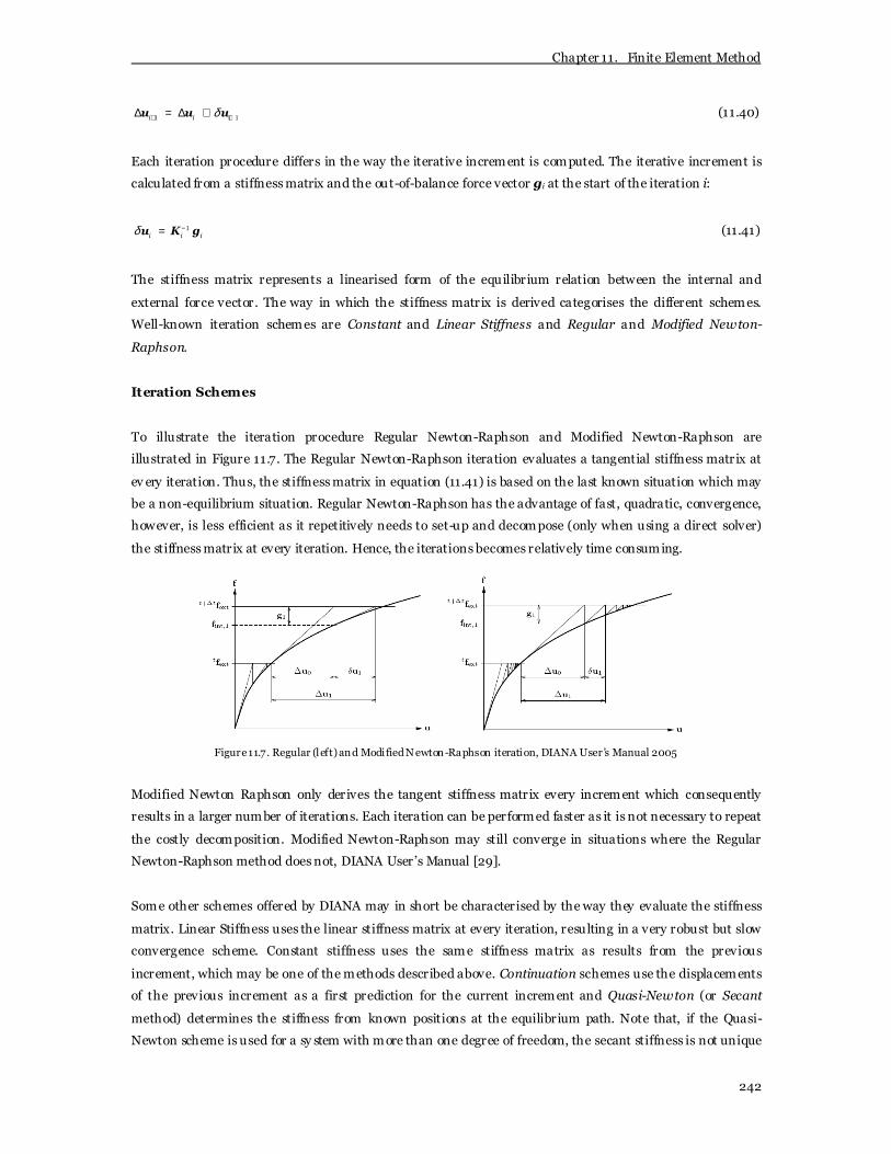
Chapter 11. Finite Element Method
242
1 1δ+ +∆ = ∆ +u u ui i i (11.40)
Each iteration procedure differs in the way the iterative increment is computed. The iterative increment is
calculated from a stiffness matrix and the out-of-balance force vector gi at the start of the iteration i:
1δ −=u K gi i i (11.41)
The stiffness matrix represents a linearised form of the equilibrium relation between the internal and
external force vector. The way in which the stiffness matrix is derived categorises the different schemes.
Well-known iteration schemes are Constant and Linear Stiffness and Regular and Modified Newton-
Raphson.
Iteration Schemes
To illustrate the iteration procedure Regular Newton-Raphson and Modified Newton-Raphson are
illustrated in Figure 11.7. The Regular Newton-Raphson iteration evaluates a tangential stiffness matrix at
ev ery iteration. Thus, the stiffness matrix in equation (11.41) is based on the last known situation which may
be a non-equilibrium situation. Regular Newton-Raphson has the advantage of fast, quadratic, convergence,
however, is less efficient as it repetitively needs to set-up and decompose (only when using a direct solver)
the stiffness matrix at every iteration. Hence, the iterations becomes relatively time consuming.
Figure 11.7. Regular (left) and Modified Newton-Raphson iteration, DIANA User’s Manual 2005
Modified Newton Raphson only derives the tangent stiffness matrix every increment which consequently
results in a larger number of iterations. Each iteration can be performed faster as it is not necessary to repeat
the costly decomposition. Modified Newton-Raphson may still converge in situations where the Regular
Newton-Raphson method does not, DIANA User’s Manual [29].
Some other schemes offered by DIANA may in short be characterised by the way they evaluate the stiffness
matrix. Linear Stiffness uses the linear stiffness matrix at every iteration, resulting in a very robust but slow
convergence scheme. Constant stiffness uses the same stiffness matrix as results from the previous
increment, which may be one of the methods described above. Continuation schemes use the displacements
of the previous increment as a first prediction for the current increment and Quasi-Newton (or Secant
method) determines the stiffness from known positions at the equilibrium path. Note that, if the Quasi-
Newton scheme is used for a sy stem with more than one degree of freedom, the secant stiffness is not unique

Chapter 11. Finite Element Method
243
and the stiffness matrix must be computed using methods such as Broyden, BFGS (Broy den, Fletcher,
Goldfarb and Shanno) and Crisfield. These methods use the previous secant stiffness and so-called update
vectors to determine the inverse of the new (unique) stiffness matrix (via the Sherman-Morrison formula
which computes the sum of a regular matrix and a dyadic product of a column and row vector). In
combination with the global selected iteration method, Line Search algorithms may be applied to stabilise
the convergence (Line Search ensures a ‘reasonable’ prediction close to the equilibrium path) or increase the
speed. Basically, the Line Search algorithm reads the out-of-balance force and checks whether a better
solution can be found by a try solution of small interpolated displacement steps.
Convergence Criteria
Similar to linear iteration procedures, the number of iterations depends on the desired accuracy of the final
solution. To stop the iteration there are several convergence criteria. The iteration is also stopped at a
specified number of maximum iterations or when divergence occurs. The convergence criteria are force,
displacement or energy based and illustrated in Figure 11.8. The force norm checks the out-of-balance force
norm of the current iteration against the out-of-balance force norm of the previous iteration. The
displacement norm compares the norm of the current displacement with the norm of the displacement
increments in the first prediction of the increment. The energy norm checks the ratio between the current
and previous energy norm, composed out of the internal forces and relative displacements. The force norm
immediately knows whether divergence or convergence occurs, all other require one additional iteration.
Figure 11.8. Norm items, DIANA User’s Manual 2005
The question of which convergence criteria is the best option for a particular problem cannot be answered
directly. In general, it is the best option to select a norm in which the reference value (ratio denominator) is
not close to zero, DIANA User’s Manual [29]. It is important to put the convergence criteria strict enough,
i.e. the discrepancy between the iterated and actual equilibrium point is passed on to the next increment.
11.6.2 Incremental Procedures
The iterative part is combined with an incremental procedure. Most typical incremental procedures are the
Load and Displacement controlled methods, discussed first. A more powerful method is the Arc-length
method, capable of handling heavy nonlinear material behaviour.

Chapter 11. Finite Element Method
244
Load and Displacement Control
The Load and Displacement Control are the most basic incremental procedures. The iteration processes
discussed in Section 11.6.1 are an example of load controlled methods as at the start of an increment, the
external load vector is directly increased. Besides load controlled incremental methods there are
displacement controlled methods which were introduced to ov ercome difficulties with limit points. At the
start of an increment, the displacement is prescribed. Both methods are illustrated in Figure 11.9.
Figure 11.9. Load control (left) and displacement control , DIANA User’s Manual 2005
In load control the load is kept constant during a load step and in the displacement control the displacement
is kept constant during increment.
Arc-length Control
For structural sy stems which experience limit point snap-through or snap-back behaviour, see Figure 11.10,
both the load control and the displacement control lead to error. E.g. the tangent stiffness becomes singular
in limit points. To ov ercome these problems the arc-length method, originally developed by Riks (1972;
1979) and Wempner (1971) and later modified by others, can be used. The arc-length method modifies the
load-factor at each iteration so that the solution follows some specified path until convergence is achieved.
All iteration schemes described above may be combined with the arc-length control method.
Figure 11.10. Arc-length control on snap-through (left) and snap-back, DIANA User’s Manual 2005
In the arc-length method a variable load-factor is introduced in the equilibrium equation of a nonlinear
sy stem. Then the method is aimed to find the intersection of the new equilibrium equation with constant ∆ l
termed as the arc-length. Arc-length methods that have been developed differ in the way the iterations are
banded and the way the tangential stiffness matrix is used, i.e. the way in which the tangent stiffness matrix
is derived and whether or not the tangential stiffness matrix is updated each iteration.

Chapter 11. Finite Element Method
245
DIANA offers updated normal plane and spherical path arc-length control. Originally, the work of Riks and
Wempner include an iterative change orthogonal to the predictor solution. Each iteration is banded by this
so-called normal plane which is updated every new step, Crisfield [25]. Hence, the method is referred to as
the Updated Normal Plane arc-length method. The method is seen in Figure 11.11. Crisfield (1981, 1983;
1984) developed a method in which a constraint equation is introduced which forms a circular constraint.
The proposed technique is termed as cylindrical path arc-length method for one-dimensional problems and
was later modified to the spherical path arc-length method for higher-dimensional problems. Hence, the
spherical path arc-length is sometimes referred to as the Arc-length Crisfield method, Memon et al. [60].
The spherical constrained arc-length method is also seen in Figure 11.11.
Figure 11.11. Updated normal plane (left) and spherical path (right) arc-length method
The either spherical (quadratic terms included) or updated normal plane (only linear terms) constraint
approximately yield the same result. More important is the choice for the value of the arc-length. Generally,
for the first increment the trail load-factor is assumed to be 1/5 or 1/10 of the total load. Further increments
determine the load-factor according to the rate of convergence of the solution process, Memon et al. [60].
The arc-length method shows faster convergence when combined with Line Searches as proven by Foster
(1992), Memon et al. [60]. Moreover, the arc-length method is particularly useful if combined with adaptive
load incrementation (discussed later). The arc-length method fails if convergence is not obtained within the
maximum number of iterations or by numerical instabilities.
In case of a local collapse mechanism, De Borst and Rots (1987) introduced an indirect displacement control
option. In the iterations of the standard arc-length method the load increment (or decrement) is scaled as a
function of all nodal displacements. When localisation of deformation occurs, the standard method may fail
and a selection of a limited number of displacements near the localisation in a reduced displacement
increment vector to scale the load increment or decrement can yield better results. This is indirect
displacement control. It differs from the standard method in that it involves a constraint equation based on a
few dominant displacement parameters. Another option is CMOD (Crack Mouth Opening Displacement)
control which uses a vector formed with new degrees of freedom that can e.g. simulate the difference in
nodal displacements at a crack, DIANA User’s Manual [29].

Chapter 11. Finite Element Method
246
Adaptive Loading
Besides the choice for an incremental step control method, the incremental process also involves the choice
for the initial step size. An optimal choice for the increment sizes is not known and cannot be fixed in
advance. Therefore, adaptive loading is introduced which uses increment sizes dependent of previous
results. In DIANA, adaptive loading can either be iteration based (all types of loading) or energy based (only
for arc-length methods). Iteration based refers to a method which adapts the increment by a desired number
of iterations, using the results of the previous increment for the increment prediction. The energy based
method determines a load increment such that the vector product of the load increment and the
displacement increment (the work increment) in the first prediction equals the final work increment of the
previous step. Furthermore, adaptive loading also refers to the choice between load increments or
decrements (loading-unloading). A simple way is to choose based on the appearance of negative pivots in
the global sy stem of equations as negative pivots often indicate unstable structural behaviour related with
some type of snap-through, DIANA User’s Manual [29].
11.6.3 General Remarks
In nonlinear analysis it is observed that, generally, over stiff stiffness matrices lead to a slow convergence but
are stable. Matrices which are too soft, however, will lead to divergence. Furthermore, exact tangent
stiffnesses will lead to a fast (quadratic) convergence but might become unstable.
For nonlinear analysis additional substructuring can be used. Substructuring is a standard technique in
finite element analysis and refers to group treatment of elements as they are a single substructure. For
example when in non-linear analysis many elements behave linearly, these elements can be put in a
substructure. The internal degrees of freedom are then removed and the calculation goes faster.
11.7 Stability Analysis
Aforementioned, a property of matrices is the existence of a set of scalars which, when multiplied with the
identity matrix, allow for the solution of ( )λ− =A I φ i i 0 and λ− = A I idet 0 . Here, φi is a corresponding
mode shape vector. The set of scalars are called eigenvalues and the corresponding mode shape vectors are
called the eigenvectors. The determination of eigenvalues and eigenvectors of a matrix is mathematically
known as an eigenvalue problem.
Eigenvalue problems arise in common applications such as stability analysis. In case of a stability analy sis
the eigenvalues represent critical buckling loads and the buckling shapes are defined by the eigenvectors. In
a stability analysis a critical displacement (or stability point) ucrit is searched such that the internal force
vector r(u) equilibrates the external force vector p(u) and that incremental variations δu to the solution
exist such that the equilibrium remains satisfied, DIANA User’s Manual [29]. Thus:
Chapter 11. Finite Element Method
247
( ) ( )=crit cri t
r u p u (11.42)
( ) ( )δ δ+ = +crit crit
r u u p u u (11.43)
Assuming δu close to ucrit equation (11.43) can be linearised as:
( ) ( )δ δ∂ ∂ + ≈ + ∂ ∂ crit crit
crit crit
r pr u u p u u
u u (11.44)
Subtracting equation (11.42) from equation (11.44), introducing a tangent stiffness matrix∂ = ∂ crit
r K
u and
assuming conservative loading (load not dependent of displacement) the equation can be simplified to:
δ ≈K u 0 (11.45)
The latter equation is the instability condition.
11.7.1 Euler Stability (Linear Buckling)
The Euler stability analysis verifies whether the solutions from linear elastic analysis are stable or whether
small disturbances exist, requiring no extra external energy. An Euler stability analysis partly takes into
account for geometrical nonlinear effects. Therefore, the tangent stiffness matrix is presented by a linear and
a nonlinear part = +K K KL NLwhich can be described as:
= ∫K B DBTL L L
V
dV with 0 1= +B B BL L L
= ∫K B τBTNL NL NL
V
dV (11.46)
The kinematic differential matrix B is subdivided into a zero displacement effect (BL0) and an initial
displacement effect (BL1). Both the linear and the nonlinear matrix have up to second-order displacement
contributions. The Euler stability analysis is, however, a linear buckling analy sis and, thus, only first order
displacement terms are of interest. Suppose that ulin is known from the linearised equilibrium between the
internal force vector r(u) and the external force vector p(u):
0 0 0
= =
∫K B DB u pT
L L L lin
V
dV (11.47)
The question is then if there is a critical displacement satisfying equation (11.42) and (11.45) such that:
λ=u ucrit crit lin (11.48)

Chapter 11. Finite Element Method
248
Which results from a loading λ=p pcrit crit , as can be shown by multiplying equation (11.47) with λcrit :
0λ λ=K u pcrit L lin crit (11.49)
Taking into account only first-order displacement terms, stored in ( )1 0 0 1= +∫V
K B DB B DBT TLL L L L L dV and
linearising the second Piola-Kirchhoff stresses by λ≈τ σcrit lin leads to the approximation solution:
( ) ( )( )( )0 λ δ+ + =K K u K u u L crit LL lin G lin 0 (11.50)
Where ( ) = ∫V
K u B σ BTG lin NL lin NLdV and 0 0 0= ∫
V
K B DBTL L L dV .
Hence, equation (11.50) is satisfied for any incremental variation δu if:
( ) ( )( )( )0 λ+ + =K K u K u L crit LL lin G lindet 0 (11.51)
In linear stability analysis, the general stability conditions of equation (11.42) and (11.43) are replaced by
equation (11.49) and (11.51). Equation (11.51) can be written as:
( ) ( )( )0 λ= − +
K φ K u K u φL i i crit LL lin G lin i (11.52)
Where i
φ is the i-th buckling mode and λ i is the corresponding buckling value. Note that the Euler stability
analysis is a linearised stability analysis and, thus, is an upper bound solution as it neglects displacement
terms of a higher order than one.
11.7.2 Generalised Eigenproblem
Equation (11.52) is solv ed as a generalised eigenproblem. The generalised eigenproblem is defined by the
equation:
2ω=Kφ Mφ (11.53)
Where, M is the mass matrix and ω is the circular natural frequency in radians per second. In stability
analysis the generalised equation changes to the linearised problem described by:
λ=Kφ K φG (11.54)
Where, KG is the geometric stress-stiffness matrix. Obviously, equation (11.54) is closely related to equation
(11.52). Solution procedures to the generalised eigenproblem are discussed in section 11.8.

Chapter 11. Finite Element Method
249
11.7.3 Shifting
An important operation involving the solution of a generalised eigenproblem is shifting. Shifting refers to a
shift factor µ applied on the stiffness matrix which provides the eigenvalues and eigenmodes close to -µ first:
� �2
ω=Kφ Mφ (11.55)
Where � µ= +K K M and �2
2ω ω µ= + . Then, the actual eigenvalues are corrected by �( )2λ ω µ= + . Note
that a negative shift factor is equivalent to a positive shift.
Shifting may be applied to ov ercome difficulties with zero or negative eigenvalues, in case of softening
material behaviour (when the tangent stiffness is obtained by a phy sical nonlinear analysis) where only the
first negative eigenvalue is of interest. Furthermore, shifting may be effective in a perturbation analy sis
where the nonlinear interaction of eigenmodes is considered (discussed hereafter) to improve the accuracy
of the interacting eigenvalues and modes, DIANA User’s Manual [29].
11.7.4 Postbuckling Analysis
If the postbuckling behaviour needs to be investigated, the Euler stability analysis must be followed by a
perturbation analysis and a continuation analysis, the finite element presentation of the Koiter initial
postbuckling theory (see Chapter 6). The analyses describe the static initial postbuckling path in the vicinity
of the bifurcation point by an asymptotic expansion of the displacement field around the bifurcation point.
In fact, the analyses represent a nonlinear analysis; however, instead of a large set of nonlinear equations in
full nonlinear analy sis, the calculation is done with a reduced number of equations.
Perturbation Analysis
In the perturbation, or reduced, analysis the nonlinear interaction of a (small) selection of buckling modes is
considered which were orthogonal within the linear scheme. Basically, the perturbation analysis inv olves the
calculation of a postbuckling displacement upb satisfying r(upb) = p(upb) but different from the primary path
described by u = λ ulin with λ the load parameter. Assuming M coinciding or nearly interacting buckling
modes, denoted by φk with k = 1, …, M, the (mode interacted) initial postbuckling displacement field is
defined as:
λ φ= + +i
u u upb lin i i i j ja a a (11.56)
Where uij is the second-order displacement vector and ai the amplitude of the respective mode. It is shown
by Koiter that uij must be calculated by solving the sy stem:
( )( )0 1λ λ+ =K K u u pL p G lin ij ij (11.57)
Chapter 11. Finite Element Method
250
Herein, λp ≠ 1 is a user specified factor. Applying the orthogonality conditions
0 =φ K u T
k L ij 0 with k = 1, …, M (11.58)
Where, pij is defined as the mode interaction load vector:
( ) ( )( )= + +∫V
p B σ B φ σ B φ σT T Tij L0 ij NL i j NL j i dV (11.59)
Where σij is the stress related to interaction of modes i and j and σi is the stress related to mode i. Further,
the potential can be written as a function of the load parameter λ and the mode amplitudes ai:
( ) 12
1
λλλ=
= − + +
∑ M
i I I ijk i j k ijk l i j k lI I
P a 1 a a A aa a A aa a a (11.60)
Wherein 12= ∫ σ εijk ij k
V
A dV and 1 18 2= −∫ σ ε u pijkl ij kl ij k l
V
A dV are the third- and fourth-order potential terms.
Hence, the perturbation analysis yields a potential energy function expressed in terms of amplitudes of
modes determined by a linear stability analy sis, DIANA User’s Manual [29].
Continuation Analysis
The potential function (11.60) is the basis for the calculation of the initial postbuckling nonlinear equilibrium
equations in a stepwise approach, the continuation analy sis. The equilibrium points of the initial
postbuckling path are indicated by terms of ai and λ. The postbuckling displacement field upb can be derived
using equation (11.56) using a stepwise generalised Newton-Raphson scheme.
11.8 Solution Methods for Eigenproblems
The solution of an eigenproblem inv olves the calculation of the eigenpairs (eigenvalues and eigenvectors) for
a given matrix. For a symmetric matrix K of size n x n there are n eigenpairs. The solution for p eigenpairs
(used specified number) can be written as = KΦ ΦΛ where × Φn p is the matrix with eigenvectors and × Λp p is
a diagonal matrix with the corresponding eigenvalues.
In general, all solution methods for eigenproblems are iterative. Basically, solving the eigenproblem
λ=Kφ Mφ is equivalent to calculating the roots of the polynomial ( )λp , which has order equal to the order
of K and M. Since there are for the general case no explicit formulas available for the calculation of the roots
of ( )λp when the order of p is larger than 4, an iterative solution method has to be used, Bathe [3]. Once one
member of the eigenpair is known the other member can be obtained without further iteration. Hence, a
Chapter 11. Finite Element Method
251
basic question is whether first to solve the eigenvalue or the eigenvector. Another option is to solve them
simultaneously. The best choice depends on the solution requirements and the properties of the matrices
involved, i.e. number of eigenpairs requested, order of the matrices, bandwidth and bandedness. The
effectiveness of a chosen solution procedure depends largely on the reliability of the procedure and the
computational effort determined by the number of high-speed storage operations and an efficient use of
backup storage devices. With respect to reliability one must be aware of the fact that numerical stability is by
no means mechanical instability.
The iterative solution methods can be divided into four basic procedures; Vector I teration Methods,
Transformation Methods, Polynomial I terations and Sturm Sequence Techniques. In finite element
programs, however, the solution procedures offered are often a combination these techniques.
The basic relation of Vector Iteration algorithm can be described as λ= Kφ Mφi i i . The aim of the method is
to satisfy the basic relation by directly operating on it, Bathe [3]. Thus, introducing an arbitrary vector x1 for
φi and setting λ = 1 the basic relation changes to = R Mx1 1 and = Kx R2 1 . Assuming x2 an approximation
more closely to the eigenvector than x1 it is possible to iterate to a better approximation. Some vector
iteration methods are the Inverse I teration, Forward I teration and the Rayleigh Quotient I teration.
Transformation Methods have basic properties described by =Φ KΦ ΛT and = Φ MΦ IT . Where,
[ ]=Φ φ φ1 n, ..., and ( )λ= =Λ idiag , i 1, ...,n . Basically, the unique matrix Φ diagonalises K and M and is
computed by multiplication of K and M by a matrix Pk which diagonals K and M more closely each
iteration. Thus, + →
K Λk 1 and 1+ →
M Ik as → ∞ k . At the last iteration l the eigenvector matrix is then
[ ]=Φ P P P1 2 l... . In practice K and M only need to converge to the diagonal form, thus, ( )+ →
K Kk 1 rdiag
and ( )1+ →
M Mk rdiag . The most effective Transformation Methods are the Jacobi Method, Generalised
Jacobi Method and the Householder QR Inverse I teration Method (HQRI), Bathe [3].
Polynomial and Sturm Sequence Iteration methods have a close relationship as they both use the
characteristic polynomials and can be employed in one solution scheme. The important property of the
eigenvalues of the generalised eigenproblem, i.e. that they are the roots of the characteristic polynomial, is
the basic property of polynomial iteration. Thus, polynomial iteration methods operate on ( )λ = ip 0 (either
explicit or implicit) where ( ) ( )λ λ= − K Mp det . In combination with a polynomial iteration, it is natural
and can be effective to use Sturm Sequence Techniques. Sturm Sequence (or chain) is a symbolic procedure
to determine the number of unique roots of a polynomial. It finds all the eigenpairs in a given range. The
basic property is described as ( ) ( )λ λ= − K Mp det and ( ) ( )( ) ( ) ( ) ( )( )λ λ= − = − K M r r r r r
p det ; r 1, ....,n 1
where ( ) ( )( )λr rp is the characteristic polynomial of the r-th associated constraint problem corresponding
to φ λ φ=K M , Bathe [3].
Aforementioned, finite element programs offer methods which are a combination of the basic properties.
Well-known algorithms are the Lanczos Method, the Arnoldi Method and the Subspace I teration Method.

Chapter 11. Finite Element Method
252
The Lanczos method transforms the generalised eigenproblem into a standard form with a tridiagonal
(almost a diagonal) coefficient matrix which is real and symmetric. It is particular effective if only a few
eigenpairs need to be calculated. The Arnoldi Method is analogous to the Lanczos Method, however, also
applies to non-Hermitian matrices. Subspace Iteration is the most widely used due to its robustness and
simplicity. It is particular effective for calculating a few eigenpairs of very large systems, Bathe [3].
11.9 Finite Element Software
The finite element procedure is widely available in computer software programs such as ABAQUS, ANSYS,
ADINA and DIANA. Typically, finite element software architecture is based on the general finite element
procedure, i.e. pre-process, analysis and post-process. Therefore, finite element software consists of a pre-
processor, an analysis frame and a post-processor which is often combined with the pre-processor. The pre-
process inv olves the description of the physical problem, which, in general, depends on the response to be
predicted. It can be divided into three major parts; modelling the structure, i.e. the geometrical modelling,
material modelling, boundary conditions, defining the nature of the problem to be solved, i.e. linear analysis,
nonlinear analysis, stability analysis, and the modelling of external actions such as imposed displacements,
environmental conditions and loading. The analysis part solves the physical problem and in the post-process
the response of the structure can be viewed.
Considerable concern may arise on the reliability of the finite element programs. Therefore, important for
finite element programs are the so-called Benchmark tests. Benchmark tests are developed to validate the
solution and solution accuracy of finite element programs by comparing results to references, Hoogenboom
[48]. Since 1983 the finite element benchmark tests are set and maintained by the National Agency for Finite
Element Methods and Standards (NAFEMS), an independent non-profit organisation ‘to promote the safe
and reliable use of finite element and related technology’, NAFEMS [95].
The finite element program DIANA is used for the thesis’ analyses. DIANA is a software package for finite
element analysis of structures and fluids, developed by TNO in Delft, the Netherlands since 1972. DIANA is
FORTRAN coded, a code especially developed for technological programs, Burden and Faires [19]. The finite
element code is based on the displacement approach using displacements as basic variables. Most appealing
capabilities of DIANA are soil and concrete calculations. For the pre- and post-processing the iDIANA user’s
interface is used which works with two databases called FemGV (Fem generation and Fem view) which both
comprise an index file and a data file in binary format. FemG is the design environment and FemV the
results environment. The geometrical and physical modelling and the mesh generator are included in the
iDIANA design environment. DIANA offers a wide variety of almost 200 elements. Using FemG the structure
can be modelled and stored in a Neutral file format in ASCII text format (the so-called dat-file). The
contents of the results database can also represented in a Neutral file. If the results are viewed with iDIANA,
the structural response can be visualised (contour plots, stress graphs, etc) by selecting a load case, attribute
and component of analysis results for assessment. Results may be viewed as values at the nodes for averaged
nodal results, element wise at the nodes of each element if discontinuities at the element boundaries are to
be examined, or as values at integration points within the elements or as a single value per element.

Chapter 11. Finite Element Method
253
11.10 Geometrical Modelling
The implementation of a structural domain into a finite element program starts with the definition and
discretization of the geometry in the design environment. The primary objective of a model is to realistically
replicate the important parameters and features of the real model, thus, the geometrical modelling must
approach the geometry of a designed (or realised) shape in the most optimal way. Mesh generation is part of
geometrical modelling and the discretisation of the geometry must result in a correctly described structural
response to external loads.
To define the geometry the user must be familiar with computer aided design. For the discretization the user
needs knowledge of applied mechanics and finite elements in particular. This section contains some of the
knowledge needed to create an appropriate geometrical model. However, as geometrical modelling (or
modelling in general) gives access to an extremely large amount of background information, there will only
be referred to the modelling as needed for thin shell structures.
11.10.1 Geometry
The geometry of a structure can be drawn in a pre-processor or imported out of computer aided design
programs such as AutoCAD or MAYA. Commonly, the computer aided design programs foresee in more
advanced design aids than the pre-processors of finite element programs. However, problems may arise
when converting the imported model as in general the programs are based on different codes. This may lead
to a situation in which (a part of) the original drawn geometry becomes useless. Finite element programs
may include repair and merge options, which repairs geometry and deletes duplicated points, lines, surfaces
and bodies, respectively. However, the final result is different for each particular problem.
The geometrical model is parametric as lines, surfaces and bodies can be defined from points and transforms
(transformation of an original part to a new part). The nodal points of the geometry are stored in a data file
in terms of a global coordinate sy stem. To create, basic shapes can be combined by complement (appends
the complement of two sets to another set) and intersect (only the intersecting part of two sets remains)
operations. It must be mentioned, however, that there is no such thin as a perfect numerical model. The
model alway s contains numerical irregularities and, thus, is imperfect.
11.10.2 Mesh Generation
The geometrical shape of the structure is discretised by a finite element mesh. To generate a mesh that
correctly describes the structural behaviour is as complicated as it is important. The mesh contains all the
properties that are needed in order to let the finite element analyses determine how the structure will
respond. Hence, errors in the mesh formulation or too coarse meshes will lead to an insufficient solution.
Basically, the efficiency of the finite element solution depends on the mesh fineness, the elements (type and
integration scheme, discussed later) and the mesh quality. The mesh fineness determines the exactness of
the solution and must be fine enough the reach the desired solution accuracy. The mesh can be refined until

Chapter 11. Finite Element Method
254
it reaches the limit imposed by the amount of RAM available plus the size of the virtual memory swap file.
Unfortunately, the rank of the stiffness matrix is equal to the total number of unknown nodal degrees of
freedom and the matrix (and computational time) can become extremely large when applying many
elements. Hence, it is important to find a compromise between the exactness of the approximation and the
calculation time needed.
The mesh quality is important for the reliability of the solution as finite element programs tend to develop
mesh sensitivity with respect to distortions. The elements of the mesh must be smooth as abrupt shape
deviations between neighbouring elements are uninvited as they, for example, lead to irregular stress and
strain representations. A major requirement is that the elements are not folded or degenerate any points or
lines. Furthermore, the aspect ratio (the ratio of the length of the smallest side of the element to the length
of the longest) of the elements must not be too large. A large aspect ratio leads to convergence problems and
has a bad accuracy. To correctly and efficiently describe the boundary, a sufficient number of nodes must be
present at the edges. To evaluate the mesh quality, finite element programs often contain a mesh quality
test. In general, the mesh quality test evaluates the shape of the element with respect to a theoretical ideal.
The criteria involved, such as element angles, warping, aspect ratio, and midnode position, depends on the
selected element type. Sometimes an ov erall quality value is offered which averages the contribution from all
other tests, with an option to add a weight factor to a quality test of personal preference.
The mesh can be generated by hand (for simple problems) or by a mesh generator. The mesh generator is
often part of the pre-processor, although it is also possible to import. During the import operation, however,
the same problems may occur as previously mentioned for the geometry. Once more, merging may be the
key. A computer mesh generator is based on an advanced discretisation formula, which are often very
complicated to meet the high standards needed for an accurate finite element solution. As denoted by
Vermeij [78], in general, a mesh can be divided into three classes, a structured mesh and an unstructured
mesh or a combination of both. The difference between the classes lies in the way the connectivity is stored.
A structured mesh is implicitly taken into account as the nodes have a fixed relationship to each other. A
structured mesh is often based on mapping as a regular flat grid is mapped to the irregular geometrical
shape. The mesh is usually generated by a differential method which defines interior coordinate lines by
performing a solution to partial differential equations which are constructed by describing the original
geometry in terms of computational space coordinates. Another technique is the algebraic method which
interpolates internal coordinates from their values on the boundaries. The differential method is more
popular as it results in a smooth mesh without irregularities from discontinuous boundaries, Vermeij [78].
However, as a structured mesh has difficulties to handle complex geometries, often an unstructured (or free)
mesh is applied as they provide in a flexible aid for the discretization. In an unstructured mesh, the
connectivity must be explicitly described by a data structure. The unstructured grid is often generated by an
Octree approach, a Delaunay approach or an Advancing Front approach, Vermeij [78]. The Octree
approach is a fast meshing technique as it simply overlays a triangular of quadrilateral mesh over the
structural domain and crops off the protruding elements, replacing them by triangular boundary elements.
However, the mesh quality at the boundary is poor. The Delaunay approach divides a surface into triangular
elements by stating that, when a circle is drawn through the vertices of the triangular element, the circle does

Chapter 11. Finite Element Method
255
not contain any other nodal points. The Advancing Front method generates the mesh by successive cell
building, one at a time, and progress from the boundary into the volume. Independent of the chosen mesh
algorithm, effective nodal point numbering is needed to cluster all nonzero terms around the diagonal of the
stiffness matrix.
DIANA offers both meshing generation techniques. A structured mesh can be generated by the IJK-complex
algorithm, which is based on the differential method or the mapped option, based on the conventional
simple algebraic equations. To ov ercome the disadvantages of a non-smooth mesh, DIANA offers a
smoothing algorithm which can be applied after the mapped mesh generation. For unstructured mesh
generation, see Figure 11.12, DIANA offers the (default) Paving algorithm which generates a quadrilateral
free mesh on any type of surface and the Delaunay approach for a triangular free mesh, both based on the
Advancing Front method (like a pavior). Furthermore, a specific algorithm can be specified for a closed
polygon surface which does not alter the algorithm assigned to any existing surface by the Default Region
option. A combination of different meshing techniques is possible by simply ascribe a technique to a surface.
Figure 11.12. Delaunay (left) and a Paving mesh, DIANA User’s Manual 2005
Before the mesh can be generated a generic element type must be chosen. A generic element only describes
the shape of the element and the number of nodes. To achieve an actual finite element, the generic element
types must be mapped onto elements for applied analysis program containing the mathematical description
of the shape functions and integration points. Using generic elements, the density of the mesh is controlled
by division of lines, surfaces and bodies or by a specified length of an element.
Figure 11.13. The mesh of a hemisphere by DIANA (left) or the hand regulated mesh (right)
Despite the fact that mesh generators have matured, meshing spatial curved structures may still lead to
unwanted or irregular element arrangements. This can be seen below in Figure 11.13 for the case of a
hemispherical shell used in the thesis’ next chapters. The left picture represents the mesh as generated by

Chapter 11. Finite Element Method
256
DIANA and the right picture shows the mesh as is programmed partly by hand (meridional and
circumferential ribs) and partly by the mesh generator (the surface in between the ribs).
11.10.3 Element Types
For structural analysis, the element types can be divided into line elements, surface elements, volume
elements and the interface elements which are used for contact boundary problems. The choice for a
particular element type largely depends on the nature of the structural problem. Theoretically, for the most
optimal description of a shell structure (a v olume), volume elements are to be chosen. However, v olume
elements are of little practical use for shells as they do not only have the tendency to produce very large
sy stems of equations, leading to exceptional long computational time. In addition it may lead to serious
numerical ill-conditioning problems, Zienkiewicz [87]. Their usage is, thus, restricted to relatively small
structural elements or parts of a larger structure. Fortunately, as seen in Chapter 5, the three-dimensional
thin shell problem can be reduced to a two-dimensional surface problem by applying the thin shell
assumptions. Hence, the shell can be modelled by using two-dimensional surface elements. Moreov er, for
thin shells of revolution, the model can be even further simplified by using axisymmetric curved line
elements. In linear analysis the circumferential displacement of shells of revolution is equal to zero and the
belonging strains and stresses are constant. Hence, a line model is sufficient to describe the meridional and
out-of-plane response. For buckling or nonlinear analysis, however, the axisymmetric elements may become
useless as the circumferential behaviour is not by definition constant. When a finite element program does
not offer special shell elements, a simple approximation is to design a (segmented) shell by a combination of
flat plate elements. However, uninvited bending will undoubtedly arise at every segment connection.
The two-dimensional surface elements offered by DIANA are based on isoparametric degenerated-solid
approach which means that the stress component normal to the shell surface is equal to zero (plain stress
assumption) and that a normal remains straight after deformation but not necessarily normals. The
transverse shear deformation is included according to the Mindlin-Reissner hypothesis, discussed below.
The elements are named after their usage. For example, the surface element QU8-CQ40S, where QU8 stands
for an 8 noded Quadrilateral shaped element and CQ40 specifies the belonging to a Curved Quadrilateral
with 40 degrees of freedom. The S at the end stands for a regular Shell element. The boundaries of the
element are pointed out by nodes. The vertex nodes indicate the corners of the element and, depending on
the type of element that is chosen, there are zero, one or more interior points at the element edge or even
midnodes inside the element. Aforementioned, every node has 6 degrees of freedom, 3 translational and 3
rotational, and just as many corresponding load vectors. However, in the case of surface elements, the out-
of-plane rotation is not included. Hence, there are (5 x 8 =) 40 degrees of freedom in a QU8 element. This is
seen in Figure 11.14.
Figure 11.14. QU8-CQ40S Curved shell element and i ts degrees of freedom, DIANA User’s Manual 2005

Chapter 11. Finite Element Method
257
The number of nodes determines the order of the shape functions. Normally, 6 noded triangular or 8 noded
quadrilateral elements with quadratic shape functions are appropriate for shell analysis. The polynomial
terms of the shape functions of higher-order elements can be taken from a Pascal triangle. The quadratic
shape functions of triangular elements are complete, they contain all polynomial terms in the triangle.
Triangular elements of higher order are complete if they have one or more midnote(s). Higher-order
quadrilateral elements belong to the serendipity or Lagrange family, Wells [85]. Serendipity elements have
only nodes on the element boundaries. When the Pascal triangle is drawn, Figure 11.15, it can be seen that
serendipity elements of second order already miss polynomials terms. For higher-order than three they are
therefore not recommended. The problem can be solved by using Lagrange elements which have nodes on
the element interior as well and therefore remain complete. As a consequence, serendipity elements are
suboptimal on quadrilateral elements. The 9-node Lagrange element is shown to be superior to the more
commonly used 8-noded serendipity element. The main advantage of serendipity elements is that since the
internal nodes of the higher-order Lagrange elements do not contribute to the inter-element connectivity,
the elimination of internal nodes results in reductions in the size of the element matrices, still providing the
same order of convergence. Therefore, Lagrange elements are not implemented since the 1970s, Arnold [1].
Figure 11.15. The Pascal triangle for serendipity (left) and Lagrange elements, Wells 2004
The order of the shape functions, combined with the number of integration points, appear in the exactness of
the derived variables (strains, stresses and the generalised moments and forces). In general, it can be said
that linear interpolation and area integration yields a constant stress and strain distribution in the main
direction and a linearly varying stress and strain in the perpendicular direction. Elements with quadratic
interpolation and area integration, Figure 11.16, yields a linearly varying stress and strain in the main
direction and a quadratically in the perpendicular direction. The same logic holds for higher-order elements.
In the elements, the in-plane strains vary linearly in thickness direction. Furthermore, the transverse strain
is forced to be constant, equivalent to the shear strain energy of the actual, parabolically varying, transverse
shearing strain. Therefore a shear correction factor is applied. For shells, it is convenient to use elements
with quadratic interpolation and area integration.
Figure 11.16. Two-dimensional shape functions of a six-noded triangular element, Wells 2004

Chapter 11. Finite Element Method
258
Aforementioned in paragraph 11.2.2, typically, the finite element method uses C0 continuous shape
functions, made possible by the fact that shell elements (and plate elements) include the transverse shear
deformation according to the Mindlin-Reissner theory. However, essentially a thick shell theory, it can be
used for thin shells as well. It is used as in the formulation of shell elements according to the classic bending
theory, a problem stems from the need of C1 continuity in the shape functions. This can be explained by
examining the classical thin shell equations, derived in Chapter 5. The shell equations are simplified for
hand calculation by introducing the thin shell assumptions and the hypothesis that the in-plane shear
deformations are negligible. Neglecting the in-plane shear deformation means that the rotation of the shell
element can be calculated from the curvature (equation (5.12)), similar to the bending theory of thin plates
(Kirchhoff thin plate theory). Consequently, the governing equilibrium equation of a shell in bending is
similar to the biharmonic plate equation, a partial differential equation of the fourth order. The transfer of
the fourth order strong form to the weak form yields a differential equation of the second order which needs
C1 continuous shape functions (a second derivative unequal to zero). Unfortunately, in general unstructured
meshes, it is not possible to ensure C1 continuity as it leads to inabilities to account for stress and strain
discontinuities in case of properties varying discontinuously across element boundaries, and, the presence of
spurious oscillations in the solution, Hughes [51]. Referring to the problems that arise, the few Kirchhoff
elements that are available (DIANA offers plate bending Kirchhoff elements with prescribed moments) are
non-conforming, which means that they do not meet C1 continuity and thus not meet the compatibility
demands, either within or across the element boundaries. The elements, often based on a sort of mixed
formulation (they are not tricked Mindlin neither C1 continuous), are tested by a patch test in order to check
whether it correctly describes rigid body motions and constant strain (constant curvature). In general they
are not very reliable, e.g. common rectangular elements with four nodes are not able to pass the patch test as
a quadrilateral. Despite the disadvantages they might give proper solutions in some situations.
The problem of C1 continuity is, thus, solved by using the Mindlin-Reissner theory. The difference of the
Mindlin-Reissner theory to the Kirchhoff theory lies in the kinematic and constitutive model as it includes
shear deformation, analogous to the Timoshenko beam theory. In other words, the rotation of the plate
cannot be calculated from the curvature and, as a result, the equilibrium cannot be described in a single
equation. In contrast to the Kirchhoff theory, the Mindlin-Reissner theory is modelled by a sy stem of
differential equations of second order and their corresponding weak forms contain derivatives no higher
than order one. Thus, ironically, the simplest shell bending theory presents the most problems when using
finite elements.
The major concern of Mindlin-Reissner elements is shear-locking. When the thickness of the shell
approaches to zero, the elements show an excessively stiff behaviour in compare to the exact thin shell
solution which leads to inaccurate results. The reason is that the contribution of the transverse shear
deformation to the energy does not vanish. The simplest solution to prevent shear locking is to use a reduced
integration scheme as it excludes the contribution of the transverse shear deformation to the bending
energy. However, one must be aware of spurious modes. For linear elements DIANA prevent shear locking
by automatically modifying the transverse shear strain fields, the so-called assumed strain concept. For
quadratic and higher order elements DIANA uses a reduced integration scheme.

Chapter 11. Finite Element Method
259
Note that, constant strains and stresses, which are calculated in the integration points, are discontinuing
ov er the element boundaries. Graphical presentation in postprocessors may lead to misleading smoothened
results, especially in areas with large gradients.
For shell analysis DIANA offers the following elements:
Triangular Curved Shell Elements
The Triangular curved shell elements have 3, 6 or 9 nodes, see Figure 11.17. The 3-node element is based on
linear interpolation and area integration. For more accurate results, the 6-node element is available, based
on quadratic interpolation and area integration, and the 9-node element in combination with third-order
interpolation and area integration. The shape of the element may be of flat, cylindrical, spherical, conical,
hyperbolic or parabolic.
Figure 11.17. Triangular curved shell elements, DIANA User’s Manual 2005
Each of the elements represented in Figure 11.17 is combined with an integration scheme. The integration
schemes of triangular elements are outlined in paragraph 11.10.4. It can be stated that, triangular elements
with more than 6 nodes rarely find practical application, DIANA User’s Manual [29].
Quadrilateral Curved Shell Elements
The quadrilateral curved shell elements have 4, 8 or 12 nodes, distributed as in Figure 11.18. Analogously to
the triangular elements, the quadrilaterals are based on linear, quadratic or third-order interpolation and
area integration, respectively. The shape of the element may be of flat, cylindrical, spherical, conical,
hyperbolic or parabolic.
Figure 11.18. Quadrilateral curved shell elements, DIANA User’s Manual 2005
Each of the elements represented in Figure 11.8 is combined with an integration scheme. The integration
schemes of quadrilateral elements are outlined in paragraph 11.10.4. It can be stated that, quadrilateral
elements with more than 8 nodes rarely find practical application, DIANA User’s Manual [29].

Chapter 11. Finite Element Method
260
Axisymmetric Curved Line Elements
The CL9AX element is an axisymmetric curved line element with similar properties as the surface elements.
The element has three nodes and is based on quadratic interpolation and line integration and, thus, yields a
strain and stress that varies linearly in length direction. The shape of the element may be of flat, spherical or
parabolic. The element, seen in Figure 11.19, is combined with an integration scheme of in section 11.10.4.
Figure 11.19. The CL9AX element and i ts degrees of freedom, DIANA User’s Manual 2005
Note that, when ascribing a certain element to a mesh, one must be aware of the fact that the element has a
default shape which may not be the same as the desired shape of the geometry. For example, the
axisymmetric element has a default parabolic shape and, thus, is not compatible with a spherical line. In
these situations, the shape of the elements must be mapped onto the geometrical shape manually.
Furthermore, it must be mentioned that problems may be encountered with the tolerances of adjacent
elements at the element assembly operation. If these problems cannot be solved by either mesh refinement
or increasing the allowed tolerance, redefinition of the geometry is needed.
11.10.4 Integration schemes
The finite element is combined with an integration scheme which specifies the number and position of the
integration points and the corresponding integration method. DIANA offers the Gauss, Simpson, Newton-
Cotes and Lobatto integration schemes. Usually, over the surface of a curved shell element a Gauss
integration scheme is used as requires the least number of integration points, DIANA User’s Manual [29].
For elements with linear interpolation and area integration it is even the only possible integration method.
In the thickness direction the Simpson method may be preferred over Gauss integration as it gives
information about the surface strains and stresses. Standard is Simpson 3, with integration points at both
outer surfaces and one in the middle. Higher order Simpson is recommended for phy sical nonlinear analy sis
where the number of integration points depends on the expected nonlinearity, Hughes [51].
The integration scheme chosen is either a full integration scheme or a reduced integration scheme. Full
integration schemes integrate the stiffness matrix exactly. For higher order elements than one, a reduced
scheme is recommended to prevent membrane and shear locking. Aforementioned, when reduced
integration is applied, the strain and stress solution is better while the accuracy of the displacement is not
affected. Off course, this is only true when spurious modes do not arise.
Questions may arise on the position of the integration points inside or at the boundary of the element. The
integration points must give the most optimal approximation for the whole element. However, it is known
that at certain places, the strains and stresses are obtained with a higher accuracy than at other places.
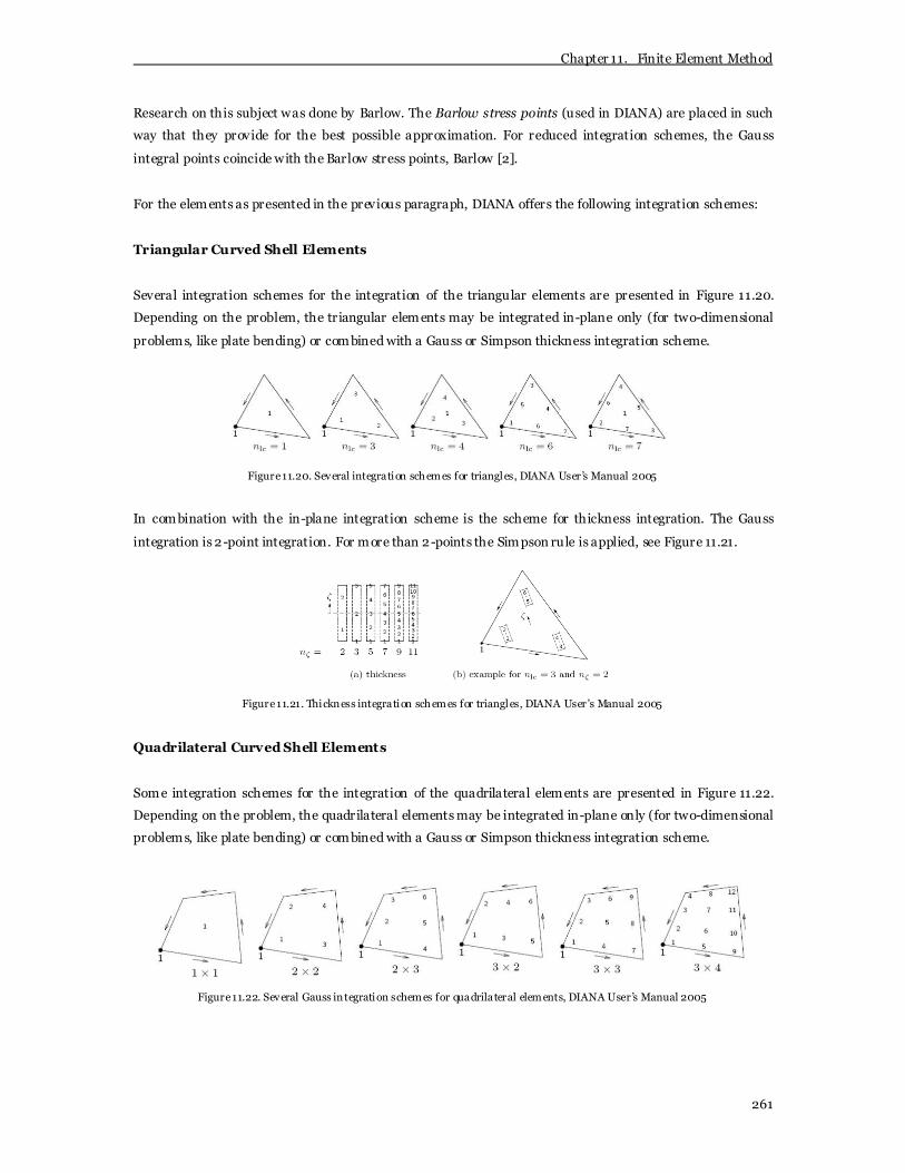
Chapter 11. Finite Element Method
261
Research on this subject was done by Barlow. The Barlow stress points (used in DIANA) are placed in such
way that they provide for the best possible approximation. For reduced integration schemes, the Gauss
integral points coincide with the Barlow stress points, Barlow [2].
For the elements as presented in the previous paragraph, DIANA offers the following integration schemes:
Triangular Curved Shell Elements
Several integration schemes for the integration of the triangular elements are presented in Figure 11.20.
Depending on the problem, the triangular elements may be integrated in-plane only (for two-dimensional
problems, like plate bending) or combined with a Gauss or Simpson thickness integration scheme.
Figure 11.20. Several integration schemes for triangles, DIANA User’s Manual 2005
In combination with the in-plane integration scheme is the scheme for thickness integration. The Gauss
integration is 2-point integration. For more than 2-points the Simpson rule is applied, see Figure 11.21.
Figure 11.21. Thickness integration schemes for triangles, DIANA User’s Manual 2005
Quadrilateral Curved Shell Elements
Some integration schemes for the integration of the quadrilateral elements are presented in Figure 11.22.
Depending on the problem, the quadrilateral elements may be integrated in-plane only (for two-dimensional
problems, like plate bending) or combined with a Gauss or Simpson thickness integration scheme.
Figure 11.22. Several Gauss integration schemes for quadrilateral elements, DIANA User’s Manual 2005

Chapter 11. Finite Element Method
262
In combination with the in-plane integration scheme is the scheme for thickness integration. The Gauss
integration is 2-point integration. For more than 2-points the Simpson rule is applied, Figure 11.23.
Figure 11.23. Thickness integration schemes for quadrilaterals, DIANA User’s Manual 2005
Axisymmetric Curved Line Elements
For axisymmetric shell elements, DIANA offers Gauss and Simpson integration schemes, Figure 11.24. The
default integration scheme is Gauss integration in the length and thickness direction. Higher order schemes
in the direction of the length of the element are not recommended as the element will become extremely
sensitive the shear locking, DIANA User’s Manual. Possible higher order integration in thickness, Simpson
integration, is only useful for surface stress-strain evaluation and nonlinear analysis.
Figure 11.24. Some integration schemes for axisymmetric curved line elements, DIANA User’s Manual 2005
Aforementioned, the structural behaviour is determined in the integration points and the values as
determined there are the best approximated values. This means that the nodal strains and stresses are
interpolated (and averaged) values. One must take into account that the interpolation operation sometimes
yields largely deviating results. This is certainly true in case of irregular meshes.
11.11 Material Modelling
The response of a structure under load is evaluated within the elements using the material properties.
Therefore, the actual elastic and plastic (permanent or irreversible deformations) material behaviour as
determined in Chapter 8 must be implemented into a numerical material model. The aim of the material
model is to approach the actual material behaviour in the most optimal way.
The material model for this thesis must correctly describe the properties and characteristics of the (fibre)
reinforced concrete mixtures. The elastic behaviour is easily described by a constant Young’s modulus and
Poisson’s ratio. However, when the yield condition, which specifies the state of stress at which the material

Chapter 11. Finite Element Method
263
starts to deform permanent, is violated, reinforced concrete experiences highly nonlinear plastic behaviour
up to failure. For the modelling process, the user needs knowledge about the failure mechanisms which can
occur in (fibre) reinforced concrete. Recapitulate from Chapter 8; the nonlinear behaviour of reinforced
concrete is characterised by direct failure due to compressive crushing, tensile cracking and yielding of
reinforcement and indirect failure due to long-term effects as shrinkage, creep and ambient influences like
temperature and maturity. Fibre additions further contribute to the nonlinear behaviour through the
continuous frictional pullout of fibres in the post-cracking stage.
To model brittle or quasi-brittle materials such as reinforced concrete with their physical nonlinear
behaviour, DIANA offers several material models. Commonly, in multi-axial stress states, a crack model for
tension is combined with a plasticity model which describes the crushing of the material. Regular yield
models as Tresca, Von Mises, Drucker-Prager and Mohr-Coulomb are available combined with a (isotropic)
plasticity formulation. Furthermore, DIANA offers the concept of Total Strain, that describes compression
and tension within one constitutive relation, and the Modified Maekawa Concrete model which combines a
multi-axial damage plasticity model for compression with a crack model based on Total Strain for tension.
Damage plasticity models are similar to plasticity models with the difference that unloading does not take
place elastically but that the degradation of the elastic stiffness is taken into account. The Maekawa model is
in particular suitable to describe hysteresis in tensile and compression unloading/reloading loops (e.g.
earthquake loading). For two-dimensional plane stress, plane strain or axisymmetric situations, the Rankine
model, possibly combined with Von Mises or Drucker-Prager, foresees in a plasticity-based formulation for
cracking. However, for three-dimensional analysis Rankine cannot be used. Finally, the modelling of so
called long-term effects as relaxation and creep (not treated in this thesis) is done with viscoelastic models as
the Power law, a Maxwell Chain and a Kelvin Chain.
11.11.1 Tensile Cracking
The tensile behaviour of reinforced concrete is characterised by a linear elastic branch up to crack initiation,
followed by a nonlinear post-cracking path with tension stiffening (redistribution of tensile stresses from
concrete to reinforcement due to bond between the rebars) or tension softening (reduction in tensile load
capacity accompanied by increasing deformation), see Chapter 8. The crack propagation in the post-cracking
stage is numerically decomposed in crack opening (mode-I behaviour) and crack sliding (mode-II
behaviour). The crack process can be modelled with a discrete or smeared cracking approach.
Discrete Cracking Concept
Discrete cracking models consist of predefined cracks modelled by interface elements. Interface elements
have equal located dual nodes which move away from each other after the tensile strength is violated. Before
crack initiation, they have an extremely high dummy stiffness as if they are not there. The discrete cracking
approach is limited to trivial situations in which the location of one dominant crack is known on forehand,
such as a notched beam. Discrete cracking models are, thus, not appropriate for distributed failure and large
scale analy sis in which a wide variety of cracks can be expected at unknown locations such as shell analyses.

Chapter 11. Finite Element Method
264
Smeared Cracking Concept
In the smeared cracking concept cracks may appear at arbitrary locations with arbitrary orientation.
Opposite to the discrete cracking approach, the smeared cracking concept describes cracking within the
elements. For each element in the mesh holds that, when the maximum tensile stress is violated, a crack will
appear. The tension cut-off criterion specifies the initiation of cracks. In DIANA it is possible to use a
constant or a linear tension cut-off, represented in Figure 11.25. The constant stress cut-off criterion neglects
the positive influence of a compression stress in the other direction whereas a linear tension cut-off does not.
The actual behaviour of concrete is neither constant nor linear, but somewhere in between.
Figure 11.25. Tension cut-off in a two-dimensional stress state, DIANA User’s Manual 2005
The crack propagation in an element is described by a crack model. A crack model determines the stiffness
around a crack in the constitutive law. To be able to correctly express different stiffnesses in different
directions, the crack model must be orthogonal and the original isotropic constitutive law is changed to an
orthogonal stress-strain law. The crack relation is described within a crack orientated coordinate sy stem n-t.
A simplification is made by ignoring the coupling between mode-I and mode-II behaviour according to:
σ εσ γ
=
cr I cr
nn sec ant nn
cr II cr
nt sec ant nt
D 0
0 D (11.61)
The secant stiffness terms can be determined by use of the constitutive relations of Chapter 5. When, for
example, assuming a plane stress situation the linear elastic stiffness matrix reads:
( )
σ ν εσ ν ε
ννσ γ
− −
xx xx
yy yy
xy xy
1 0E
= 1 01
1 0 0
2
2 (5.34)
Supposed, that, relation (5.34) is transformed to the crack coordinate system and both the normal crack
stiffness as the shear crack stiffness are assumed to be zero, the relation can be rewritten to:
σ εσ εσ γ
nn nn
tt tt
nt nt
0 0 0
= 0 E 0
0 0 0
(11.62)
To achieve a closer estimation of the reality, the normal and shear crack stiffnesses are reintroduced,
equipped with tension softening behaviour and shear reduction respectively. Therefore, the parameters µ

Chapter 11. Finite Element Method
265
and β are introduced. Furthermore, the reimplementation of the Poisson coupling contributes to a better
approximation. Substitution of the approximations in equation (11.62) yields the orthogonal relation:
( )
µ µνµν µνσ ε
µνσ εµν µν
σ γβ
ν
− − = − −
+
nn nn
tt tt
nt nt
E E0
1 1
E E 0
1 1
E0 0
2 1
2 2
2 2 (11.63)
In the latter, the parameters µ and β represent the coupling between the traditional and secant crack
parameters. They are related to the secant stiffness by:
µµ
=−
I
sec antD E1
and β
β=
−II
sec antD G1
(11.64)
The parameter µ determines the stiffness of the material normal to the crack depending on the crack strain.
Hence, the crack stress implicitly depends on the crack strain and can be written as a multiplicative relation:
( ) εσ εε =
crcr cr nnnn nn t cr
nn.ult
f y (11.65)
Here y(….) represents a user specified softening function. The crack propagation in concrete is characterised
by tension softening, i.e. the concrete increasingly eases up to open a crack after initiation. The type of
softening behaviour can be implemented after the typical material characteristics. In equation (11.65) the
softening is represented by the (linear) function y(.…),. DIANA offers various softening models such as linear
tension softening, multi-linear tension softening, nonlinear tension softening according to Hordijk et al., etc.
They are seen in Figure 11.26. The softening models determine whether the construction is in elastic stage
(positive tangent modulus), cracking stage (negative tangent modulus) or fully cracked (beyond diagram).
Figure 11.26. Tension softening relations, DIANA User’s Manual 2005
As can be seen in the Figure, Brittle cracking is a special form of tension softening as it is distinguished by
full reduction immediately after cracking and, thus, does not contain a tension softening branch. The
softening relation to be chosen depends on the mode-I fracture energy of the material, e.g. measurable by
means of material tests.

Chapter 11. Finite Element Method
266
With respect to the fracture energy, the so-called crack bandwidth is introduced. Figure 11.26 shows tension
softening behaviour on the constitutive level, a relation between cracking stress and strain. Hence, for the
smeared crack concept, the relation between stress and crack (used in the discrete crack model) must be
transformed to a relation between stress and strain. However, releasing the mode-I fracture energy in an
element after the tensile strength is violated, results in a crack-width dependent of the size of the element.
More practical, a larger element consumes more energy to reach the ultimate crack strain than a smaller
element and, thus, the fracture energy dissipation differs with respect to the size of the element.
The simplest and general accepted solution to the problem is so-called fracture energy regularisation.
Fracture energy regularisation is based on the assumption that each element can have only one crack (in
reality cracks occur at every integration point) related to an equivalent length or crack bandwidth. In this
way the crack is ‘smeared’ over the element. Doing so, the result is that, upon mesh refinement, the thickness
of the crack region decreases while the dissipated energy remains constant. The relation between the crack
width w and the crack bandwidth h can be written as:
ε =crnn
c
w
h (11.66)
A crucial point is the definition of the bandwidth. Irregularity in element shapes force the use of a so-called
characteristic length hc that approximates the crack bandwidth with respect to the average element area A.
For higher-order plane stress elements DIANA uses the relation = ch A . Hence, the ideal element is a
square. In the postprocessor the above relation can be reversed to calculate the crack width.
Following the fracture energy regularisation, the mode-I fracture energy becomes related to the softening
behaviour by crack bandwidth multiplication and, thus, related to the size of an element:
0
ε
ε
ε εε
=∞
=
=
∫cr
I crnnf t nncr
nn.ult
G h f y dcrnn
crnn
(11.67)
Aforementioned, y(….) represents the softening diagram.
Unfortunately, the introduction of the crack bandwidth also has a disadvantage as it may lead to a snap-back
in the constitutive model. One can probably imagine that overly large elements lead to a characteristic length
so large that the integral of equation (11.67) leads to a decreasing crack strain while the crack further opens
(decreasing crack stress). This so-called snap-back behaviour is highly uninvited and therefore must be
solv ed. The simplest solution is to refine the mesh such that the crack bandwidth is smaller. Alternatively,
the tensile strength can be reduced, although this implies that the material becomes more ductile.
Besides the parameter µ, the parameter β, which determines the shear behaviour, must be defined. The
reducing shear stiffness during cracking is modelled with so-called shear retention. Shear retention deals
with selecting a value for the parameter β between 0 and 1. DIANA offers full shear retention (β = 1) and
constant shear retention (0 < β < 1).

Chapter 11. Finite Element Method
267
Finally, as unloading and reloading situations may lead to closing and reopening of cracks, the behaviour
during these conditions must be prescribed. The closing and reopening of cracks is done by the linear secant
modulus in DIANA. This means that in the constitutive model the unloading and reloading branch goes
linearly back to zero, although we might expect residual strain upon closing the crack in reality.
Strain Decomposition Concept
The principle of smeared cracking to model the tensile behaviour is offered by DIANA in two different
concepts, Strain Decomposition and the later discussed Total Strain concept. Strain decomposition is based
on decomposition of the total strain into an elastic and irreversible plastic (or crack) part, like a series
connection of strains. The crack stresses are solely determined by the corresponding crack strain. Strain
decomposition is related to the decomposed Multi-direction fixed crack model, seen in Figure 11.27.
Figure 11.27. Multi -directional fixed crack model , DIANA User’s Manual 2005
The Multi-direction fixed crack model determines crack stresses from the corresponding crack strains in the
local n-t coordinate system. A fundamental feature is that the crack-strains are sub-decomposed in order to
allow for several cracks occur simultaneously in one element. Therefore, in addition to the aforementioned
tension cut-off, a threshold angle between two cracks is defined for consecutive crack initiation. The user
must be aware of the possibility that the tensile stress temporarily becomes greater than three times the
tensile strength while cracking does not start as the threshold is not violated yet, DIANA User’s Manual [29].
The decomposition of strains also allows for the combination of a crack model in tension with a plasticity
model in compression. In DIANA, the Multi-directional fixed crack model may be combined with a Tresca,
Von Mises, Drucker-Prager or Mohr-Coulomb plasticity model discussed later.
Total Strain Concept
The total strain concept also describes the stress as a function of the strain; however, opposite to strain
decomposition, total strain models describe the elastic and plastic strain in one constitutive relation. This is
also known as hypo-elasticity, however, the DIANA formulation includes secant unloading and reloading. In
the total strain concept the principal directions are uncoupled (the linear elastic stress space is a cube),
cracks occur whenever the tensile strength in one direction is violated, indicated by a negative tangent
modulus. Consequently, the crack stress is evaluated in a direction given by the crack direction.

Chapter 11. Finite Element Method
268
The total strain concept is related to the Total Strain Rotating Crack model and the Total Strain Fixed
Crack model. Basically, the total strain rotating crack model is a coaxial stress-strain concept which ensures
that the crack orientated coordinate system is orthogonal to the principal stresses by rotating the crack. The
model is only realistic if the crack rotation angle is small. Hence, the model is useless in case of consecutive
loadcases with significant loads in different directions. The most advantageous property is its numerical
uncomplicatedness as there is no shear stress which implicitly means that the shear retention factor, which
often causes numerical stability problems, is not needed.
The fixed crack model does not rotate the crack with the principal stresses. When the principal stresses
change in direction, the aforementioned shear retention factor will enfold for the shear stresses which
appear along the crack surface. The fixed crack concept is off course closer to the nature of concrete cracking.
The advantage lies in the fact that it is numerical simpler than the multi-directional fixed crack model.
11.11.2 Compressive Behaviour
The compressive behaviour of concrete is discussed in Chapter 8. It was found that the nonlinear
compressive behaviour of concrete can be characterised by compression hardening and softening up to
compressive crushing. This resulted in the ‘rounded’ stress strain curve. Hereby, the influence of (fibre)
reinforcement was neglected. The compressive behaviour as observed can be modelled with a plasticity
model or a constitutive curve, depending on the chosen model in tension. Therefore, the compression
models are treated separately under their corresponding tension concept.
Strain Decomposition Concept
The strain decomposition concept allows for the combination of a crack model in tension with a yield model
and a plasticity formulation in the compressive regime. Similar to the decomposed crack model, the
compressive behaviour is decomposed in an elastic and irreversible plastic part. The yield condition specifies
the state of stress at which the plastic part is initiated. The usual approach to describe the so-called
elastoplastic behaviour is the flow theory of plasticity. The total stress σ at time t is then modelled as a
function of the total strain ε at time t, but also as a function of the stress and strain history, Vrouwenvelder
[80].
Typically, the stress and strain history is taken into account implicitly by an internal state parameter κ which
is governed by a specific evolution law. The elastoplastic material behaviour can then by described by
assuming and elastic stress-strain relation, a yield condition (specifying the state of stress at which the
plastic flow is initiated), a flow rule (specifying the plastic strain rate vector as a function of the state of
stress) and a hardening hypothesis (specifying the ev olution of the internal state parameter κ). DIANA
User’s Manual [29].
The yield function f is a function of the stress vector σ and the internal state parameter κ:
( )κ =σf , 0 (11.68)

Chapter 11. Finite Element Method
269
Note that, if the value of the yield function is smaller than zero, the material is in elastic state and if the state
of stress forces the yield function equal to zero, plastic deformation can occur. A value larger than zero is not
allowed for rate-independent plasticity, DIANA User’s Manual [29].
The yield function describes the yield contour of a yield model, a hypersurface in the n-dimensional stress
space. In DIANA, the Multi-directional fixed crack model can be combined with yield models such as Tresca,
Von Mises, Drucker-Prager or Mohr-Coulomb. They are illustrated in Figure 11.28 and 11.29.
Figure 11.28. Tresca and Von Mises yield condition, DIANA User’s Manual 2005
A yield model determines whether the concrete is in elastic (inside the yield surface) or plastic range (on the
yield surface) in a uniaxial stress state. The yield model to be chosen alongside the Multi-directional fixed
crack model depends on the type of structure, material, analysis, etc. In general, it can be said that Tresca
and Von Mises are typical yield models for steel. They are based on the notion that when a material fails it
does so in shear. The model of Von Mises provides in a better approximation as it does not underestimates
the yield shear stress like Tresca, which is more conservative (Tresca lies inside the Von Mises yield
criterion). Although in particular suited to steel, they may give proper solutions in some concrete situations.
Figure 11.29. Mohr-Coulomb and Drucker-Prager yield condition, DIANA User’s Manual 2005
The Mohr-Coulomb and Drucker-Prager yield conditions are especially applicable for quasi-brittle materials
such as concrete. Both models better suits to the characteristic property of concrete as that there is an
enormous difference in compression and tension. It is assumed that failure occurs if in an arbitrary plane the
shear stress equals the maximum allowable shear stress. Hereby, the allowable shear stress depends linearly
on the normal stress on the same plane. The Drucker-Prager yield model is a less conservative smooth
approximation of the Mohr-Coulomb condition, as can be seen in Figure 11.29.
The yield function determines whether plastic deformation can occur. However, plastic deformations only
occur when the stress point remains on the yield contour for a ‘short’ period, De Borst and Sluys [15]. Thus,
plastic straining will occur if and only if ( )κ =σf , 0 and ( )κ =ɺ σf , 0 (Prager’s consistency equation).

Chapter 11. Finite Element Method
270
The plastic behaviour on the yield surface is described by the flow rule and the hardening hypothesis.
Aforementioned, the flow rule defines the plastic strain rate vector as a function of the stress state vector.
For elastoplastic materials undergoing an infinitesimal deformation, the total strain increment is therefore
decomposed in an elastic and plastic part ε ε ε= + . ..e p . By definition, the elastic deformations occur in a
zero network dissipation, i.e. ( ) ε− =∫ σ σ .T e
0 dt 0 while in case of plastic deformations ( ) ε− ≥∫ σ σ .T p
0 dt 0 .
The plastic part, or so-called plastic strain rate vector, is described with the flow rule. The flow rule derives
the plastic strain rate vector from the so-called plastic potential function gj. The plastic potential function
describes the variation in equilibrium of the energy dissipation equation. By definition the gradient of the
plastic potential function is perpendicular to the yield contour (normality rule). The problem is however that
the plastic potential is not uniquely defined and thus only the direction of the strain rate vector can be
obtained. Therefore the flow rule involves a multiplication with a scale factor or plastic multiplier:
( )1
κε λ
=
∂=
∂∑. n .
jpj
j
g ,σ
σ (11.69)
In which λ.
j is the plastic multiplier.
The plastic multipliers are restricted depending on the yield function value. Considering that the plastic
multiplier is nonzero only when plastic deformations occur, the loading-unloading criterion can be
established via the Kuhn-Tucker conditions λ λ≤ ≥ = . .
j jf 0 ; 0 ; f 0 .
The final step is to use the yield function and the flow rule to define the plastic constitutive law, including the
hardening hypothesis which specifies the evolution of the internal state parameter according to:
κ ε =
..ph , σ (11.70)
Herein, h is the hardening function which in DIANA is either based on strain hardening or on work
hardening for Tresca and Von Mises or, in case of Mohr-Coulomb or Drucker-Prager, only strain hardening.
To determine the (tangent) material stiffness matrix, first the initial tangent stiffness matrix following from
the elastic branch is calculated. The initial stress rate vector can be determined from the elastic part of the
strain rate vector and the material stiffness matrix D by:
ε ε ε λ ∂ = − = − ∂
.. . . .p g
σ D D σ (11.71)
Subsequently, the necessary expression for the scale factor can be determined from Prager’s consistency
condition, i.e. 0κ λ
κ λ∂ ∂ ∂= + =∂ ∂ ∂
T. .f ff
.
σ σ
, which leads to the formulation:

Chapter 11. Finite Element Method
271
1λ ∂=∂
T.
p
f
E
.
σσ
with κ
κ λ∂ ∂= −∂ ∂p
fE the plastic hardening modulus (11.72)
Substitution of equation (11.72) in equation (11.71) after applying the Sherman-Morrison formula (described
earlier) yields the continuum tangent material stiffness matrix:
ε
∂ ∂ ∂ ∂= − ∂ ∂ + ∂ ∂
T
. .
T
p
g f
f gE
D Dσ σσ D
Dσ σ
(11.73)
Note that the matrix is symmetric for f = g, thus, as the plastic potential is equal to the yield function.
To update the constitutive equations of elastoplastic materials in a consistent manner the Euler Backward
algorithm (accurate and stable independent of the step size) can be used within an elastic predictor-plastic
corrector algorithm. The updated stress at the end of iteration i+1 is used to derive the consistent tangent
stiffness matrix. For increasing the performance and robustness of the iteration method used, the tangent
stiffness matrix may be obtained by consistent linearisation of the stress resulting from the return-mapping
algorithm. Using the return-mapping algorithm leads to a modification of equation (11.73) by substituting
the elastic stiffness matrix D by H, in which H is defined as:
12
2λ ∂= + ∆ ∂
-g
H I D Dσ
(11.74)
Total Strain Concept
Aforementioned, the total strain concept describes the elastic and plastic strain in one constitutive relation.
As the principal directions are uncoupled it is not possible to combine the total strain crack models with a
yield model. Instead, the compression behaviour is modelled with predefined stress-strain curves. Some of
the compression curves are presented in Figure 11.30, such as Thorenfeldt, parabolic curves and the multi-
linear stress-strain curve which may be used to approximate the Eurocode 2 behaviour.
Figure 11.30. Predefined compression behaviour for Total Strain crack models, DIANA User’s Manual 2005
The behaviour of compression is evaluated in a rotating coordinate sy stem when the material is not cracked,
where in case of a fixed concept the compressive behaviour is evaluated in the fixed coordinate sy stem
determined by the crack directions.

Chapter 11. Finite Element Method
272
However, the cracking behaviour is based on a single stress-strain relation it may be refined to include
influences of lateral confinement and lateral cracking to approach the pressure-dependent behaviour of
concrete in compression more closely. Therefore, the parameters of the compressive stress-strain function,
fcf and εp are determined with a failure function which gives the failure compressive stress as a function of
the confining stresses in the lateral direction, DIANA User’s Manual [29]. The confinement relation used in
DIANA is graphically presented in Figure 11.31. Clearly, the beneficial effect of increasing lateral
confinement is at maximum for full triaxial loading in which failure cannot be reached and the graph is
linear.
Figure 11.31. Influence of lateral confinement on compressive stress-strain curve, DIANA User’s Manual 2005
For compressive behaviour with lateral cracking, the parameters of the compressive stress-strain function, fcf
and εp are determined with a failure function given by:
σβ= ⋅ crp cff f
εα β ε= ⋅ crp p
In which α p represents the reduced strain at the reduced ultimate stress pf . The reduction factors ( )σ εβ βcr cr,
are functions of the average lateral damage variable formulated as α α α= + 2 2lat l,1 l,2 in which α 2
l,i represents
the strain in perpendicular direction to the compression direction. DIANA models the reduction due to
lateral cracking according to Vecchio and Collins. Vecchio and Collins suggested εβ = cr
1 and σβ = ≤+
cr
c
11
1 K
with αε
= − −
latc
0
K 0.27 0.37 . The relation is illustrated in Figure 11.32.
Figure 11.32. Reduction factor due to lateral cracking, DIANA User’s Manual 2005
In the total strain formulation, the possible nonzero Poisson’s ratio is included by a numerical trick.

Chapter 11. Finite Element Method
273
11.11.3 Modelling Conclusions
From the foregoing it can be concluded that a concrete shell is best modelled using the smeared crack
approach using either strain decomposition or total strain. The question of which material model is the best
option for a particular problem cannot be answered in directly. Basically, the main differences refer to the
way they evaluate crushing and cracking criteria for multi-axial stress states, the way in which stress
rotations are treated and in the way loading and unloading is managed. Strain decomposition results in a
multi-directional fixed crack model with secant unloading in tension combined with an elastoplastic yield
model in compression. Total strain describes the elastic and plastic strain in tension and compression in one
constitutive relation using secant unloading for both. Opposite to the strain decomposition concept the total
strain cannot include creep, shrinkage, temperature and maturity effects. From a physical point of v iew, the
strain decomposition concept is more attractive whereas total strain based models are, in general, numerical
advantageous as they are much more stable.
The multi directional fixed crack model (in combination with a Drucker-Prager yield model) and total strain
based crack models are compared in the report of Burgers [20]. Burgers made a compare between the results
of an actual test and the results of the DIANA crack models (and a damaged plasticity model of ABAQUS) for
a four point bending test on a notched beam fabricated from fibre reinforced concrete. Burgers reports on
satisfying results for the total strain rotating crack model while the accurateness of the approximations of the
total strain fixed crack model and the multi directional fixed crack model depends on the magnitude of the
shear retention factor. Satisfying results of these models is accompanied by numerical difficulties.
11.12 Conclusions and Comments
In the foregoing the general finite element procedure is discussed. The spatial discretisation into finite
elements and the formulation of the approximated displacement field using shape functions. The
construction of the weak form of equilibrium which allows for approximated solutions and the stiffness
matrix which is computed using numerical integration in and ov er the elements. Successively, the sy stem of
equations can be solved either linear, nonlinear or by performing a stability analysis using direct, iterative or
incremental-iterative solution algorithms. More specific the geometrical and material modelling in DIANA is
discussed, with extra attention for cracking and crushing of concrete.
Despite of the great power of the finite element method, the disadvantages must be kept in mind. The
method does not necessarily reveal how the stresses are influenced by important problem variables such as
material properties and geometrical features and errors in input data may produce large incorrect results
that can be ov erlooked by the analyst. Furthermore, it should be mentioned that, for the displacement
approach, the approximate solution alway s overestimates the total potential energy, which is the strain
energy minus the work performed by the external loads. However, complied with the fact that the potential
energy is negative near its minimum, the displacement based finite element method underestimates the
strain or deformation energy and, therefore, the solution is often referred to as the lower bound solution.
This means that the structural behaviour appears to be stiffer than the exact solution.

Chapter 12. Linear Elastic Analysis
274
12 Linear Elastic FEA
In this chapter, a linear elastic finite element analysis is discussed. The theory as described before in Chapter
5 and the hemispherical example of Chapter 10, serve as background. Subsequently, in Chapter 13, the linear
buckling and linearised postbuckling behaviour is discussed. Linear elastic analyses, however, may not be
representative for the actual shell behaviour. Therefore, in Chapter 14 and 15, the actual shell behaviour is
approached more accurately by implementation of nonlinear behaviour, i.e. a geometrically nonlinear
analysis with initial imperfections in Chapter 14, and finally a geometrically and phy sically nonlinear
analysis in Chapter 15, also taking into account for material nonlinearities.
For the linear analysis the Zeiss planetarium case study shell is used as geometry. The analyses are
performed on an axisymmetric curved line model and a three-dimensional shell model consisting of two-
dimensional quadrilateral and triangular curved shell elements. The axisymmetric model is the most simple
shell model possible in finite element analysis. The model is, however, unable to deal with variations in
circumferential direction. If these variations may occur, a three-dimensional model is required. The
calculations are based on an ideal shell without any imperfections assuming infinite linear elastic material
behaviour. The material properties are previously described in Chapter 8.
The results of the linear analyses are compared with the ‘benchmark’ results of Chapter 10. The stresses,
strains and displacements are compared with the results of the classical shell theory. In addition to Chapter
10, the influence of different load conditions on the shell structural response is investigated. Therefore, wind
load as derived in Chapter 9, is projected on the three-dimensional shell model.

Chapter 12. Linear Elastic Analysis
275
12.1 Shell Parameters
12.1.1 Geometry
For the shell geometry, the dimensions of the Zeiss planetarium as discussed in Chapter 7 are used, i.e. a
hemispherical shell with a radius of 12500 mm and a thickness of 60 mm.
12.1.2 Material Properties
The finite element analysis of Chapter 12 is linear elastic based. Hence, the material is modelled as infinite
elastic and the only material parameters that have to be defined are the Young’s modulus of elasticity and
Poisson’s ratio. Recapitulating from Chapter 8, for the conventional C20/25 mixture the Young’s modulus is
30 GPa whereas the C180/210 mixture is assumed to be twice as stiff with a Young’s modulus of 60 GPa. For
as well the conventional C20/25 mixture as the C180/210 mixture the Poisson’s ratio is set equal to zero.
12.1.3 Boundary Conditions
The shell is analysed using four types of support; a roller, inclined-roller, hinged and a clamped support. In
this way the influences of boundary conditions on the structural behaviour can be investigated. The actual
support of the Zeiss planetarium is a clamped support as the shell is rigidly connected (by steel
reinforcement) to a tension ring which, in turn, rests on a circular base building, see Chapter 7.
12.1.4 Loading
The external applied load is equal to the (trivial) uniform vertical load consisting of the dead weight of the
shell and snow load, described in Table 10.2. That is, a load P = 0.0021 N/mm2 (2.1 kN/m2). Furthermore, a
spherical load with the same magnitude is considered and in Section 12.6 the structural response to wind
load as defined in Chapter 9 is investigated.
12.1.5 Analysis Scheme
The different types of analyses are presented in the scheme below. As wind load varies in circumferential
direction, it is not possible to combine the wind load with an axisymmetrical model.
Name Loading Conditions Supporting Conditions Type of Analysis Model
Zeiss 1 Spherical and Vertical Roller Linear Elastic Axisymmetric + 3D
Zeiss 2 Spherical and Vertical Inclined-roller Linear Elastic Axisymmetric + 3D
Zeiss 3 Spherical and Vertical Pinned Linear Elastic Axisymmetric + 3D
Zeiss 4 Spherical and Vertical Clamped Linear Elastic Axisymmetric + 3D
Zeiss 5 Wind load Clamped Linear Elastic 3D
Table 12.1. Analysis scheme

Chapter 12. Linear Elastic Analysis
276
12.2 Axisymmetric Shell Model
The axisymmetric shell model is analysed first. The model is far less complicated and allows for much faster
analyses than a three-dimensional model. The axisymmetric model is checked on support reactions, stresses,
strains and displacements, respectively.
12.2.1 FE Model
The axisymmetric shell model consists of a curved line, a quarter of a circle, which presents a complete
hemisphere as DIANA considers the vertical axis as axis of rotational symmetry. The line model is composed
out of 92 axisymmetric curved line elements CL9AX (see Chapter 11) with in total 185 nodes. Consequently,
each element has a circumferential length of approximately 213 mm, which means that the requirement of at
least 6 elements within the region of influence of a local bending moment (2078 mm, equation (10.32)) to
ensure results of sufficient accuracy is satisfied, Hoogenboom [50]. Each element has 2 point Gauss
integration over the length of the element and 3 point Simpson integration in thickness direction, which is
appropriate for linear elastic analysis, DIANA User’s Manual [29]. The three-point Simpson integration
allows for inner, outer and middle surface stress and strain presentation. The integration polynomial of the
axisymmetric elements, typically, produces stresses and strains which vary linearly over the length of the
element (see Chapter 11). The shell top node is inclined-roller supported, as if it represents a complete
sphere. The varying base supports are modelled by each time allowing or disallowing translation and/or
rotation at the base node. The model is vertically or spherically loaded. Due to a modelling drawback of
DIANA, i.e. for axisymmetrical elements it is not possible to construct a purely spherical load, the spherical
load is modelled by modification of the direction of a line load; a line load is formed perpendicular to the
element only at the middle node.
12.2.2 Support Reactions
The most elementary test is probably to check whether the support reactions correlate with the external
applied load. For the axisymmetrical model, the support reactions resulting from the finite element analy sis
are illustrated by simple vectors which represent a summation of all reaction forces ov er the base radius. The
support reactions for a vertical loaded hemisphere are presented in Table 12.2.
Vertical support reaction (kN) Horizontal support reaction (kN) Name
FEA Theory FEA Theory
Zeiss 1 2060 2062 0 0
Zeiss 2 2060 2062 0 0
Zeiss 3 2060 2062 38.4 38.3
Zeiss 4 2060 2062 73.8 73.8
Table 12.2. FEA Support reactions of a shell under vertical load for different types of supports
For each shell model the total v ertical support reaction (summation over the base radius) as obtained by the
finite element analysis is equal to 2060 kN. To validate the finite element result, the external applied load

Chapter 12. Linear Elastic Analysis
277
must be multiplied with the total shell surface area (2.1 kN/m2 · 981.75 m2 ≈ 2062 kN). The horizontal
reaction differs for each type of support. Again, the value represents a summation over the base radius of all
horizontal supporting reactions. In Chapter 10, the horizontal support reactions are determined with the
classical shell theory. Hence, to compare the results with the theoretical results, the values as found in
Chapter 10 must be multiplied with the circumferential length.
Vertical support reaction (kN) Horizontal support reaction (kN) Name
FEA Theory FEA Theory
Zeiss 1 1030 1031 0 0
Zeiss 2 1030 1031 0 0
Zeiss 3 1030 1031 -19.2 -19.2
Zeiss 4 1030 1031 -36.9 -36.9
Table 12.3. FEA Support reactions of a shell under spherical load for different types of supports
The supporting reactions of the spherical loaded shell are shown in Table 12.3. They are quite simple to
validate, i.e. by definition, the vertical support reactions are equal to half the values as shown in Table 12.2
(which is, off course, also valid for the theoretical values). The same holds for the horizontal support
reactions, however, they are of opposite sign. From Table 12.2 and Table 12.3 it can be concluded that the
results of the finite element analy sis show good correlation with the theoretical obtained results, i.e. the
maximum difference is within 0.3%.
12.2.3 Stresses
Zeiss 1
First, the axisymmetric shell model is analy sed while being subjected to a uniform vertical load. The Zeiss 1
under vertical load is in a state of pure membrane action. In other words, the shell is supported in such a way
that it will not disturb the membrane stress field and, consequently, there will be no bending moments in the
shell. The principal meridional and circumferential stresses are presented in Figure 12.1.
-0,5
-0,45
-0,4
-0,35
-0,3
-0,25
-0,2
-0,15
-0,1
-0,05
00 2 4 6 8 10 12 14 16 18
Distance (m)
Str
esse
s (
MP
a)
-0,3
-0,2
-0,1
0
0,1
0,2
0,3
0,4
0,5
0 2 4 6 8 10 12 14 16 18
Dis tance (m)
Stre
sses
(M
Pa)
Figure 12.1. FEA membrane meridional and circumferential stresses for a shell under vertical load

Chapter 12. Linear Elastic Analysis
278
On the horizontal axis of Figure 12.1 the meridional direction of the shell surface is shown from the base
radius to the top node at 19635 mm (quarter of a circle with radius 12500 mm). The vertical axis shows the
stresses from the finite element analysis. Clearly, the membrane stresses show no surprises as they have a
similar distribution as Figure 10.4. Qualitatively, the stresses coincide with the values of Chapter 10.
-0,25
-0,2
-0,15
-0,1
-0,05
00 2 4 6 8 10 12 14 16 18
Distance (m)
Str
esse
s (
MP
a)
-0,25
-0,2
-0,15
-0,1
-0,05
00 2 4 6 8 10 12 14 16 18
Distance (m)
Str
esse
s (
MP
a)
Figure 12.2. FEA meridional and circumferential stresses for a roller shell under spherical load
The roller supported Zeiss 1 shell subjected to a spherical load is a second example of a shell in a pure
membrane state. The roller supports do not suppress any rotation which means that, theoretically, the shell
is free from bending. Moreov er, the spherical load only cause uniformly distributed radial pressing of the
shell and no rotation. As can be seen in the rather trivial graphs of Figure 12.2, the principal meridional and
circumferential stresses are equal to -0.219 MPa. Again, on the horizontal axis of the figures the meridional
direction of the shell surface is shown. The vertical axis shows the stresses from the FEA.
-0,219
-0,219
-0,219
-0,219
-0,219
-0,219
-0,219
-0,219
-0,219
-0,219
-0,2190 2 4 6 8 10 12 14 16 18
Distance (m)
Str
esse
s (
MP
a)
-0,5
-0,4
-0,4
-0,3
-0,3
-0,2
-0,2
-0,1
-0,1
0,00 2 4 6 8 10 12 14 16 18
Distance (m)
Mo
men
ts (
Nm
m/m
m)
Figure 12.3. FEA uninvited meridional stress discrepancies and bending moments of a roller shell under spherical load
A closer look at the membrane stresses, however, uncovers inaccuracies in the solution. Within a very small
bandwidth, between -0.218 and -0.219 MPa, adjacent nodal stresses show uninvited discrepancies which
lead to uninvited bending moments, both illustrated in Figure 12.3. The three different lines in the stress
graph of Figure 12.3 represent the stresses in the outer, middle and inner Simpson integration points,
respectively. The inaccuracies are caused by the modelling drawback of DIANA, i.e. for the axisymmetrical

Chapter 12. Linear Elastic Analysis
279
elements it is not possible to construct a purely spherical load. As a consequence of the aforementioned
solution, small disturbances arise between adjacent nodes. These disturbances cause the stress discrepancies
and bending moments. The disturbances are relatively small.
In Figure 12.3 it is also seen that the bending moments do not completely vanish at the support.
Theoretically, the shell is free to rotate and thus no bending moments can be absorbed at the support. The
reason for the nonzero bending moments is found in the element formulation; they do not return to zero at
the support due to the fact that the mapping operation from the ‘exact’ integration points (which are not
situated at the end of an element) to the end nodes is linear. As the actual moments experience higher order
degradation, the linear mapping operation is of insufficient degree.
Zeiss 2
The Zeiss 2 shell has inclined-roller support, which means that the base radius of the shell is restrained from
rotating. When the inclined-roller shell is subjected to vertical load, the supports are not membrane
compatible anymore. Hence, bending moments inevitable arise and there is referred to a so-called edge
disturbance. The meridional stresses and bending moments are seen in Figure 12.4. The bending moments
rising from the edge disturbance do not influence the circumferential stresses, which is evident as they are in
perpendicular direction. Consequently, the circumferential stresses of the inclined-roller supported shell are
similar to the pure membrane situation in Figure 12.1. Due to the fact that the bending moments have a local
character and decay out, reaching up to approximately 2078 mm (equation (10.33)), both graphs of the
figure are zoomed in upon the boundary layer of the shell, which is bending-dominated.
-25
-20
-15
-10
-5
0
5
0 0,5 1 1,5 2 2,5 3 3,5 4
Dis tanc e (m)
Mom
ents
(Nm
m/m
m)
-0,48
-0,46
-0,44
-0,42
-0,4
-0,38
-0,36
-0,34
-0,32
-0,30 0,2 0,4 0,6 0,8 1 1,2 1,4 1,6 1,8 2
Dis tance (m)
Str
ess
es
(MP
a)
Figure 12.4. FEA bending moments and meridional stresses for a shell under vertical load with inclined-roller support
The bending moments plotted in Figure 12.4 correspond to the back curving of the shell surface for
compatibility requirements. In other words, the shell flattens under the vertical load and needs to be rotated
reversely at the base radius to end up straight. This is also seen in the stress graph where the meridional
stresses split into three paths near the support (-0.412, -0.434 and -0.456 MPa). As previously observed in
the spherically loaded Zeiss 1 shell, these splitted lines represent the discrepancy between the both outer
Simpson integration points. One line (the upper) represents the outer shell surface and experiences a release
in compressive stress due to the bending moments. The other line (the lower) represents the inner shell
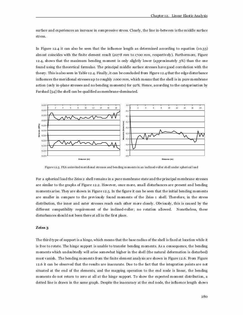
Chapter 12. Linear Elastic Analysis
280
surface and experiences an increase in compressive stress. Clearly, the line in-between is the middle surface
stress.
In Figure 12.4 it can also be seen that the influence length as determined according to equation (10.33)
almost coincides with the finite element result (2078 mm to 1700 mm, respectively). Furthermore, Figure
12.4, shows that the maximum bending moment is only slightly lower (approximately 3%) than the one
found using the theoretical formulae. The principal middle surface stresses have good correlation with the
theory. This is also seen in Table 12.4. Finally, it can be concluded from Figure 12.4 that the edge disturbance
influences the meridional stresses up to roughly 1000 mm, which means that the shell is in pure membrane
action (only in-plane stresses and no bending moments) for 92%. Hence, according to the categorisation by
Farshad [34] the shell can be qualified as membrane-dominated.
-0,219
-0,219
-0,219
-0,219
-0,219
-0,219
-0,219
-0,219
-0,219
-0,219
-0,2190 2 4 6 8 10 12 14 16 18
Distance (m)
Str
esse
s (
MP
a)
-0,5
-0,4
-0,4
-0,3
-0,3
-0,2
-0,2
-0,1
-0,1
0,00 2 4 6 8 10 12 14 16 18
Distance (m)
Mo
men
ts (
Nm
m/m
m)
Figure 12.5. FEA uninvited meridional stresses and bending moments in an inclined-roller shell under spherical load
For a spherical load the Zeiss 2 shell remains in a pure membrane state and the principal membrane stresses
are similar to the graphs of Figure 12.2. However, once more, small disturbances are present and bending
moments arise. They are shown in Figure 12.5. In the figure it can be seen that the initial bending moments
are smaller in compare to the previously found moments of the Zeiss 1 shell. Therefore, in the stress
distribution, the inner and outer stresses reach each other more closely. Obviously, this is caused by the
different compatibility requirement of the inclined-roller; no rotation allowed. Nonetheless, these
disturbances should not been there at all in the first place.
Zeiss 3
The third type of support is a hinge, which means that the base radius of the shell is fixed at location while it
is free to rotate. The hinge support is unable to transfer bending moments. As a consequence, the bending
moments which undoubtedly will arise somewhat higher in the shell (the natural deformation is disturbed)
must vanish. The bending moments from the finite element analysis are shown in Figure 12.6. From Figure
12.6 it can be observed that the results are inaccurate. Due to the fact that the integration points are not
situated at the end of the elements, and the mapping operation to the end node is linear, the bending
moments do not return to zero at all at the hinge support. To show the expected moment distribution, a
dotted line is drawn in the same graph. Despite the inaccuracy at the end node, the influence length shows

Chapter 12. Linear Elastic Analysis
281
good correlation with the theoretical value. The maximum bending moment is much higher than for the
inclined-roller supported Zeiss 2 shell (145 Nmm/mm to 23.2 Nmm/mm). Obviously, this may be expected;
for compatibility requirements the shell must deform completely against its urge.
-160
-140
-120
-100
-80
-60
-40
-20
0
20
0 0,5 1 1,5 2 2,5 3 3,5 4
Distance (m)
Mo
men
ts (
Nm
m/m
m)
Figure 12.6. FEA and expected (dotted line) bending moments for a shell under vertical load with hinged supports
The principal meridional and circumferential stresses are plotted in Figure 12.7. Due to the nonzero bending
moments at the support, the resulting graphs show a discrepancy between correct and found results,
indicated by the difference in continuous and dotted lines. The dotted lines represet the correct solution.
The stresses end with values of -0.491 and -0.377 MPa. Also the circumferential stresses do not vanish at the
support. From the figure it can be concluded that the hinged supported shell is in pure membrane action for
more approximately 90%.
-0,6
-0,55
-0,5
-0,45
-0,4
-0,35
-0,3
-0,25
-0,20 0,5 1 1,5 2 2,5 3 3,5 4
Dis tance (m)
Str
ess
es
(MP
a)
-0,3
-0,2
-0,1
0
0,1
0,2
0,3
0,4
0,5
0 2 4 6 8 10 12 14 16 18
Distance (m)
Str
ess
es (
MP
a)
Figure 12.7. FEA meridional and circumferential stresses for a shell under vertical load with hinged supports
Also for a spherical load, a hinge supported shell is not in a pure membrane state. In fact, the stresses and
bending moments of a hinged shell subjected to spherical load show great similarity with the shell under
vertical load. The finite element result is plotted in Figure 12.8. Both graphs of Figure 12.8 are zoomed in
upon the bending-dominated boundary layer of the shell. The bending moments are in contradiction to the
theory as they do not vanish. As can be expacted based on the deformation of the shell under spherical load,

Chapter 12. Linear Elastic Analysis
282
the bending moments are of opposite signin compare to the bending moments of Figure 12.7. Hence, the
non-vanishing meridional stresses are also of opposite sign.
-10
0
10
20
30
40
50
60
70
80
0 0,5 1 1,5 2 2,5 3 3,5 4
Distance (m)
Mo
men
ts (
Nm
m/m
m)
-0,31
-0,29
-0,27
-0,25
-0,23
-0,21
-0,19
-0,17
-0,15
-0,130 0,5 1 1,5 2 2,5 3 3,5 4
Dis tance (m)
Str
ess
es
(MP
a)
Figure 12.8. FEA meridional stresses and bending moments in a hinged supported shell under spherical load
With respect to the uninvited stresses and bending moments seen in Figure 12.3 and 12.5, it can be
concluded that they become irrelevant as they are negligible in compare to the much larger stress variations
caused by the edge disturbance.
Zeiss 4
The final shell support is a clamped support, no rotation and displacement allowed. For a vertically loaded
clamped shell, the bending moments determined in the finite element analy sis are plotted in Figure 12.9.
-150
-50
50
150
250
350
450
0 0,5 1 1,5 2 2,5 3 3,5 4
Dis tanc e (m)
Mom
ents
(Nm
m/m
m)
Figure 12.9. FEA and theoretical bending moments for a shell under vertical load with clamped supports
The value is significantly lower than the one found in Chapter 10 using the classical shell theory, indicated by
the dotted line. The considerable disagreement is an extreme example of the factual error of the linear stress
mapping within the axisymmetric elements. Counteracting the size disagreement, the influence length of the
bending moment is correct and the shell behaves like a membrane for approximately 80%, regardless of the
‘severe’ compatibility requirement.

Chapter 12. Linear Elastic Analysis
283
-0,8
-0,7
-0,6
-0,5
-0,4
-0,3
-0,2
-0,1
0
0 0,5 1 1,5 2 2,5 3 3,5 4
Distance (m)
Str
ess
es
(MP
a)
-0,3
-0,2
-0,1
0
0,1
0,2
0,3
0,4
0 2 4 6 8 10 12 14 16 18
Distance (m)
Str
ess
es (
MP
a)
Figure 12.10. FEA meridional and circumferential stresses for a shell under vertical load with clamped supports
The resulting stresses of the vertically loaded clamped shell are illustrated in the graphs of Figure 12.10. It
can be seen that, contrary to the Zeiss 3 shell, the circumferential stresses approach the actual zero stress at
the base radius more closely. The meridional outer and inner surface stresses show a remarkable pattern
which can be explained by curving and back curving of the shell surface near its support corresponding to
the expected deformations, i.e. flattening at the top and bulging and back curving near the base. The large
bending moments cause the outer surface stresses (-0.705 and -0.163 MPa) to be far away from each other.
Hence, as a larger moment can be expected, Figure 12.9, the actual stress dissimilarity will be even greater.
-0,40
-0,35
-0,30
-0,25
-0,20
-0,15
-0,10
-0,05
0,00
0 0,5 1 1,5 2 2,5 3 3,5 4
Dis tance (m)
Str
ess
es
(MP
a)
-200
-150
-100
-50
0
50
100
0 0,5 1 1,5 2 2,5 3 3,5 4
Distance (m)
Mom
ent
s (N
mm
/mm
)
Figure 12.11. FEA meridional stresses and bending moments in a clamped supported shell under spherical load
When the clamped shell is subjected to a spherical pressure load, the bending moments and stress variation
in the shell may expected to be even higher than previously found for the Zeiss 3 shell. That is, the shell does
not only must preserve its initial position at the base, but also is not allowed to rotate. The results of the
finite element analysis are seen in Figure 12.11. The trend of the graphs is quite similar to the graphs of
Figure 12.9 and 12.10. Like the vertically loaded clamped shell, the bending moment may be underrated.
Similar to the Zeiss 3 shell, the uninvited stresses and moments caused by the modelling drawback are
negligible.

Chapter 12. Linear Elastic Analysis
284
Meridional stresses (MPa) Circumferential stresses (MPa)
Top Base Top Base
Name
FEA Theory FEA Theory FEA Theory FEA Theory
Zeiss 1 -0.219 -0.219 -0.434 -0.438 -0.219 -0.219 0.429 0.438
Zeiss 2 -0.219 -0.219 -0.434 -0.438 -0.219 -0.219 0.429 0.438
Zeiss 3 -0.219 -0.219 -0.434 -0.438 -0.219 -0.219 0.09 0
Zeiss 4 -0.219 -0.219 -0.434 -0.438 -0.219 -0.219 0.03 0
Table 12.4. Meridional and circumferential stresses for vertical loaded shells
To give a quantitative comparison between the theoretical results of Chapter 10 and the finite element
results, the stresses found for vertical and spherical loaded shells are summarised in Table 12.4 and Table
12.5. In case of varying stresses ov er the thickness of the shell, the middle surface stresses are tabulated.
Meridional stresses (MPa) Circumferential stresses (MPa)
Top Base Top Base
Name
FEA Theory FEA Theory FEA Theory FEA Theory
Zeiss 1 -0.219 -0.219 -0.219 -0.219 -0.219 -0.219 -0.219 -0.219
Zeiss 2 -0.219 -0.219 -0.219 -0.219 -0.219 -0.219 -0.219 -0.219
Zeiss 3 -0.219 -0.219 -0.219 -0.219 -0.219 -0.219 -0.049 0
Zeiss 4 -0.219 -0.219 -0.219 -0.219 -0.219 -0.219 -0.012 0
Table 12.5. Meridional and circumferential stresses for spherical loaded shells
If the supports are not membrane compatible, bending moments arise. They are quantitatively represented
in Table 12.6. In the spherical (right) table, the disturbances of the load-modelling can be seen.
Bending moments (Nmm/mm) Bending moments (Nmm/mm) Name
Base Base
AXI FEA Theory AXI FEA Theory
Zeiss 1 0 0 -0.079 0
Zeiss 2 -23.2 -23.93 -0.049 0
Zeiss 3 -59.0 0 29.5 0
Zeiss 4 281.0 406.79
-161 -
Table 12.6. Bending moments of the vertical (left) and spherical (right) loaded shell
From Table 12.4, 12.5 and 12.6 it can be concluded that, generally, the finite element results are in
reasonable agreement with the classical shell theory (within 1%). The circumferential stresses at the base and
the bending moments due to edge constraint, however, uncovers the factual error of linear stress mapping.
In particular for the hinged Zeiss 3 and clamped Zeiss 4 shells the linear mapping has a significant influence
on the stress distribution and bending moments. The overcome the (large) discrepancy between expected
and computed results one may opt for choosing a higher order scheme in length direction with integration
points at the element ends. However, aforementioned in Chapter 11, this is not recommended as the element
becomes highly sensitive to shear locking. Hence, the engineer must keep in mind that these elements may

Chapter 12. Linear Elastic Analysis
285
yield results of insufficient accuracy. Note that, by selecting a finer mesh, the engineer is able to obtain an
impression of the size of the discrepancy which he can use in the design process.
12.2.4 Strains
In linear elastic analysis the strains can directly be derived from the stresses conform the constitutive law,
which is even further simplified as the Poisson’s ratio is set equal to zero. Therefore, the strain graphs show a
same trend as the previously plotted stresses. E.g. this is seen in Figure 12.12 for the Zeiss 1 shell.
-0,016
-0,014
-0,012
-0,01
-0,008
-0,006
-0,004
-0,002
0
0 2 4 6 8 10 12 14 16 18
Distance (m)
Str
ains
(‰
)
-0,01
-0,005
0
0,005
0,01
0,015
0 2 4 6 8 10 12 14 16 18
Dis tance (m)
Str
ain
s (
‰)
Figure 12.12. FEA meridional and circumferential strains for a shell under vertical load with roller supports
The graphs of Figure 12.12 represent the principal membrane strains for a hemispherical shell subjected to a
uniform vertical load. If the boundary condition is not membrane compatible, the membrane strains will be
disturbed locally (only in the boundary layer of the shell) such as the stress disturbances seen before. In
those regions, the inner and outer surface strains will deviate from each other presenting the cross-sectional
rotation of the shell surface. Clearly, as the strains are mapped linear ov er the element length, the strains
violate the theory in the same manner as the stresses did. The strain results as obtained by the finite element
analysis are summarised in Table 12.7.
Meridional strains (‰) Circumferential strains (‰)
Top Base Top Base
Name
FEA Theory FEA Theory FEA Theory FEA Theory
Zeiss 1 -0.0073 -0.0073 -0.0145 -0.0146 -0.0073 -0.0073 0.0143 0.0146
Zeiss 2 -0.0073 -0.0073 -0.0145 -0.0146 -0.0073 -0.0073 0.0143 0.0146
Zeiss 3 -0.0073 -0.0073 -0.0145 -0.0146 -0.0073 -0.0073 0.003 0
Zeiss 4 -0.0073 -0.0073 -0.0145 -0.0146 -0.0073 -0.0073 0.0009 0
Table 12.7. Meridional and circumferential middle surface strains for a shell under vertical load
For the strains in the shells subjected to spherical pressure load, the same observations can be made. That is,
their distribution is similar to the graphs seen in Figure 12.2. When the supports suppress the membrane
deformation, the strains are disturbed locally and the inner and outer surface strains move away from each
other. Like the stresses, the strains are not perfect and they show the same irregular pattern as seen in

Chapter 12. Linear Elastic Analysis
286
Figure 12.3 and 12.5. Finally, also for the spherical strains, the linear mapping is the reason for the
disagreement with the classical shell theory. The strains resulting from the finite element analysis are seen in
Table 12.8.
Meridional strains (‰) Circumferential strains (‰)
Top Base Top Base
Name
FEA Theory FEA Theory FEA Theory FEA Theory
Zeiss 1 -0.0073 -0.0073 -0.0073 -0.0073 -0.0073 -0.0073 -0.0073 -0.0073
Zeiss 2 -0.0073 -0.0073 -0.0073 -0.0073 -0.0073 -0.0073 -0.0073 -0.0073
Zeiss 3 -0.0073 -0.0073 -0.0073 -0.0073 -0.0073 -0.0073 0 0
Zeiss 4 -0.0073 -0.0073 -0.0073 -0.0073 -0.0073 -0.0073 0.0004 0
Table 12.8. Meridional and circumferential middle surface strains for a shell under spherical load
Analogous to the previous section, the conclusion can be drawn that the finite element results show
reasonable agreement with the classical shell theory, except for the disturbed boundary regions where large
bending moments are present.
12.2.5 Displacements
The shell subjected to v ertical or spherical load undergoes a displacement from its initial shape. Clearly, the
deformation depends on the type and magnitude of the load, the shell proportions and the boundary
conditions. The deformed and undeformed vertically loaded Zeiss shells are visualised in Figure 12.13.
Quantitative information concerning the deformed shells can be found in Table 12.9.
-0,4
-0,3
-0,2
-0,1
0,0
0,1
0,2
0,3
0 2 4 6 8 10 12 14 16 18
Distance (m)
Def
orm
atio
n (m
m)
0,00
0,02
0,04
0,06
0,08
0,10
0,12
0,14
0,16
0,18
0,20
0 0,5 1 1,5 2 2,5 3
Distance (m)
De
form
atio
n (
mm
)
Figure 12.13. Displacements of a shell under vertical load with several support conditions
In Figure 12.13, the initial (zero line) and deformed Zeiss 1 to 4 shells are shown. The ‘membrane’ supported
Zeiss 1 shell (dot line) can move freely, restricted by its circumferential stresses only. The largest
displacement is seen at the top of the shell. At the base radius the shell moves outward and rotates slightly.
Contrary to the Zeiss 1 shell, the Zeiss 2 shell (ace line) cannot rotate at the base. Hence, bending moments
must bend back the shell against its membrane deformation. The support has no influence on the top
displacement as it is similar to the membrane supported shell. The initial and deformed shapes of the Zeiss 3

Chapter 12. Linear Elastic Analysis
287
and Zeiss 4 shell are also illustrated in Figure 12.13. The hinged support of the Zeiss 3 shell (triangular line)
does not allow for any displacement at the base. Additionally, in case of the clamped supported Zeiss 4 shell
(cross line), the rotation is also suppressed, causing adjacent curvatures in different directions. Both
supports do not only influence the base displacement, but the top displacement as well. Due to the restraints,
the top displacement is slightly less than the ones found for the Zeiss 1 and 2 shells.
Displacements (mm) Rotations (mm/mm)
Top Base Top Base
Name
FEA Theory FEA Theory FEA Theory FEA Theory
Zeiss 1 -0.308 -0.365 0.182 0.182 0 0 -2.92 E-5 -2.92 E-5
Zeiss 2 -0.308 -0.365 0.170 0.173 0 0 0 0
Zeiss 3 -0.304 -0.365 0 0 0 0 0.00025 0.00025
Zeiss 4 -0.299 -0.365 0 0 0 0 0 0
Table 12.9. Displacements and rotations of the FEA and the classical shell theory
Comparing the results from the finite element analysis with the theoretical values in Table 10.8, 10.10, 10.12
and 10.14, it can be concluded that the base displacements and rotations are (nearly) similar. The top
displacements, however, show considerable dissimilarities as the shell seems to act stiffer (up to 15% and
more). This discrepancy is discussed further in Section 12.3.
-220
-170
-120
-70
-200 2 4 6 8 10 12 14 16 18
Distance (m)
De
form
atio
n (
mm
)
-220
-170
-120
-70
-200 0,5 1 1,5 2 2,5 3
Distance (m)
Def
orm
atio
n (m
m)
Figure 12.14. Displacements of a shell under spherical load with several supporting conditions
The deformations of the spherical loaded shell with respect to the initial (zero line) position are seen in
Figure 12.14. The Zeiss 1 and Zeiss 2 shell deform very much similar and their deformation lines coincide
(ace line). The corresponding deformation is presented quantitatively in Table 12.10. In Table 12.10 it is
observed that the aforementioned stress and strain disturbances cause the top displacement of Zeiss 1 and 2
being different from the base displacement. Moreover, the disturbances cause both shells experience top
rotation and, additionally, the Zeiss 1 shell undergoes a rotation at the base. In Figure 12.14 the deformed
shapes of Zeiss 3 (triangular line) and 4 (cross line) caused by a spherical load are shown as well. It can be
observed that the hinged supported shell experiences one directional curving to meet the compatibility
requirement. For the clamped shell the additional requirement of zero rotation means that the shell needs
two consecutive curves of opposite direction. In Figure 12.14 it can be seen that this more severe boundary

Chapter 12. Linear Elastic Analysis
288
condition leads to a larger disturbed region. From Figure 12.14 and Table 12.10 it can be concluded that the
more severe support conditions lead to slightly higher top deformations, in contrast with the observation
made for the vertical load. Aforementioned, the base displacement of Zeiss 1 and 2 and the base rotation of
Zeiss 1 are misleading results caused by the stress and strain disturbances.
Displacements (mm) Rotations (mm/mm) Name
Top Base Top Base
Zeiss 1 -0.0909 -0.0913 -0.478 E-7 -0.934 E-7
Zeiss 2 -0.0909 -0.0913 -0.478 E-7 0
Zeiss 3 -0.0933 0 -0.478 E-7 0.139 E-3
Zeiss 4 -0.0957 0 -0.478 E-7 0
Table 12.10. Displacements and rotations of the FEA for shell under spherical load
With respect to the differences between a shell subjected to a spherical load and a v ertical load, it can be
concluded that, in general, the vertical load causes higher stresses and bending moments. Consequently, the
deformations caused by a spherical pressure load are far less than the deformations caused by a uniformly
distributed vertical load with the same magnitude. This, however, may be expected from a simple
equilibrium consideration; in the lower part of the hemisphere the vertical load does not contain a
‘supporting’ transverse component and, thus, the shell behaves less stiff in that region.
12.3 Three-Dimensional Model
Aforementioned in the introduction, the axisymmetric shell model is unable to produce variations in
circumferential direction. However, in case of non-axisymmetric loading (wind, drifted snow), buckling, or
imperfect shells the hypothesis of constant circumferential behaviour is not applicable anymore. Therefore, a
three-dimensional shell model is necessary. The three-dimensional shell model is checked on support
reactions, stresses, strains and displacements for each of the given supports and load conditions given in
Table 12.1. However, first the 3D finite element model is discussed in detail.
12.3.1 FE Model
The three-dimensional shell model is seen in Figure 12.15. The model consists of two-dimensional curved
shell elements. The model is generated by constructing several meridional and circumferential ribs which
enclose rectangular and triangular surface areas. These individual areas are meshed with two-dimensional
quadrilateral QU8-CQ40S curved shell and triangular TR6-CT30S curved shell elements (both discussed in
Chapter 11). To ensure a pure spherical shape, the base shape of the elements is mapped onto spherical
shape. Typically, the elements produce x- and y-directional stresses and strains which vary linearly in their
own direction and quadratically in their perpendicular direction. For both elements a reduced integration
scheme is applied to av oid membrane and shear locking. In thickness direction a 3 point Simpson
integration is sufficient for linear elastic analyses, DIANA User’s Manual [29]. The final model consists of
7168 elements bounded by 20609 nodes, see Figure 12.15. The requirement of at least 6 elements within the

Chapter 12. Linear Elastic Analysis
289
influence region of possible edge disturbance is satisfied. Similar to the axisymmetric model, the type of
support is modelled by allowing or disallowing translation and/or rotation of the nodes on the base radius.
The load is purely vertical or spherical.
Figure 12.15. Three-dimensional shell model
Within the scheme of shell mesh generation procedures, it is also possible to let DIANA construct a mesh or
to import one. The DIANA mesh, containing only quadrilateral elements, was already shown in Figure 11.13.
From the figure it can be concluded that the DIANA mesh is non-smooth, showing large size deviations
between neighbouring elements. This is, in fact, inherent to the generation method. To model a
hemispherical cap, DIANA constructs a complete sphere which can be sliced in at least four parts (and not
two). Thus, to construct a hemisphere two quarter parts of a sphere must be combined, resulting in two
adjacent surfaces separated by a line of symmetry. Due to this line of symmetry two different meshes are
required. Moreover, DIANA meshes the spherical shape using a paving algorithm (see Chapter 11). For a
double curved shape this inevitable means that, starting at one point, at certain moment the mesh
generation operation becomes entangled causing several elements of various sizes appearing next to each
other. Unfortunately, the non-smoothness produces highly irregular stress and strain graphs (although they
are not wrong in general). Therefore, the DIANA mesh is disregarded in fav our of the manual generated
mesh. Furthermore, some attempts were made to import a mesh from MAYA and RHINO. However, the
import operation failed as several elements did not survive.
12.3.2 Support Reactions
The elementary support reaction test of the three-dimensional model provide in a simple and fast first check
to validate the model. The finite element results for each individual support condition are summarised in
Table 12.11 and 12.12. In order to be able to compare the results of the three-dimensional model with the
ones previously found, the values of Table 12.2 and 12.3 are present. Similar to Table 12.2 and 12.3, the
support reactions are the sum of all support reactions of the base radius.

Chapter 12. Linear Elastic Analysis
290
Vertical support reaction (kN) Horizontal support reaction (kN) Name
3D AXI Theory 3D AXI Theory
Zeiss 1 2062.0 2060 2061 0 0 0
Zeiss 2 2062.4 2060 2061 0 0 0
Zeiss 3 2060.8 2060 2061 39.9 38.4 38.3
Zeiss 4 2056.8 2060 2061 74.8 73.8 73.8
Table 12.11. Support reactions for a shell under vertical load
In Table 12.11 it can be observed that there are several small differences in displacements which can be
contributed to the numerical process. The differences in displacements of the three-dimensional model and
the axisymmetric model are within a few percent (4%).
Vertical support reaction (kN) Horizontal support reaction (kN) Name
3D AXI Theory 3D AXI Theory
Zeiss 1 1030,8 1030 1031 0 0 0
Zeiss 2 1030,7 1030 1031 0 0 0
Zeiss 3 1030,9 1030 1031 -18,4 -19.2 -19.2
Zeiss 4 1031,0 1030 1031 -37,8 -36.9 -36.9
Table 12.12. Support reactions for a shell under spherical load
The support reactions corresponding to the spherical loaded shell are seen in Table 12.12. It can be
concluded that the results are sufficient as the discrepancies stay within a negligible 4.2%.
12.3.3 Stresses
Zeiss 1
The roller supported Zeiss 1 shell under vertical load is in a pure membrane state. A graphical presentation
of the principal stress distribution of the three-dimensional shell analy sis is plotted in Figure 12.16. In the
figure, the horizontal axis represents the shell meridional direction from the base radius to the top node. The
vertical axis gives the meridional (thick line) and circumferential (thin line) stresses. It can be seen that there
are disturbances in the finite element solution indicated a difference in stress between the inner, middle and
outer Simpson integration points near the top of the shell. As observed in the stress output, the dissimilarity
between the inner, middle and outer stress varies in meridional direction, with a pattern repeating each
2000 mm. Remarkable (or not) this is exactly the distance between to adjacent model-ribs. The explanation
is found in the mapping operation of the element onto a spherical base shape. The mapping operation failed
and the meshed areas between the ribs slightly deviate from an ideal sphere. In other words, the mesh lies
ov er the ribs of the model like an unstressed fabric. The imperfectness undoubtedly leads to bending
moments as there are curvature variations ov er the shell surface. The right graph of Figure 12.16 shows the
meridional (thick) and circumferential (thin) bending moments which, in theory, would not occur.

Chapter 12. Linear Elastic Analysis
291
-0,5
-0,4
-0,3
-0,2
-0,1
0
0,1
0,2
0,3
0,4
0,5
0 2 4 6 8 10 12 14 16 18
Distance (m )
Str
ess
es (
MP
a)
-20
-15
-10
-5
0
5
10
0 2 4 6 8 10 12 14 16 18
Distance (m)
Mo
men
ts (N
mm
/mm
)
Figure 12.16. Meridional (thick) and hoop stresses and uninvited bending moments of a roller supported shell under vertical load
In Figure 12.16 it is observed that, especially in the triangular elements and in the transition zone between
the quadrilateral and triangular elements, the curvature variation has large influence and the moments show
‘high’ peaks (up to -18.8 Nmm/mm). The peaks can be explained by the fact that the main shape deviations
are located within the triangular zone and close to the transition zone. The average shape deviation equals
0.43 mm with a largest value of 2.9 mm. This is extremely high in compare to the expected discrepancy
based on the number of significant digits (7) stored in the data file (there is no such thing as a perfect
numerical model). As the disturbances have minor influence on the stress distribution the model is assumed
to be sufficient.
A final remark on Figure 12.16 is that the bending moments do not vanish at the support. Similar to the
axisymmetric shell model, this can be contributed to the stress mapping between the ‘exact’ integration point
and the element nodes.
For the Zeiss 1 shell subjected to spherical load, the meridional (thick) and circumferential (thin) stresses are
visualised in Figure 12.17. The deviating inner and outer surface stresses indicate the presence of the same
disturbances as described above. The corresponding bending moments are also shown in Figure 12.17.
-0,27
-0,26
-0,25
-0,24
-0,23
-0,22
-0,21
-0,2
-0,19
-0,18
-0,17
0 2 4 6 8 10 12 14 16 18
Distance (m)
Str
ess
es (
MP
a)
-25
-20
-15
-10
-5
0
5
0 2 4 6 8 10 12 14 16 18
Dis tanc e (m)
Mo
men
ts (N
mm
/mm
)
Figure 12.17. Meridional (thick) and hoop (thin) stresses and uninvited bending moments of a roller supported shell under
spherical load

Chapter 12. Linear Elastic Analysis
292
It can be seen that the stresses and bending moments show a repetitive pattern between the ribs. The
bending moments are approximately of the same magnitude, though slightly higher, as the moments
appearing in the Zeiss 1 shell under vertical load (-20.9 Nmm/mm to -18.8 Nmm/mm).
Zeiss 2
As seen before in the axisymmetric analysis, the Zeiss 2 shell is not membrane compatible when subjected to
vertical load and bending moments arise. The stress distribution and bending moments along the meridian
are illustrated in Figure 12.18.
-0,6
-0,4
-0,2
0
0,2
0,4
0,6
0 2 4 6 8 10 12 14 16 18
Dis tance (m)
Str
ess
es (
MP
a)
-35
-30
-25
-20
-15
-10
-5
0
5
10
0 2 4 6 8 10 12 14 16 18
Dis tance (m)
Mom
ent
s (N
mm
/mm
)
Figure 12.18. Meridional (thick) and hoop (thin) stresses and (uninvited) bending moments of an inclined-roller supported shell
under vertical load
Most interesting in Figure 12.18 is the right graph presenting the moment distribution. It is observed that the
uninvited moments are somewhat lower than the bending moments caused by the edge restraint.
When subjected to spherical load, the inclined-roller supported Zeiss 2 shell is still membrane compatible.
Therefore, both graphs of Figure 12.19 are very much similar to the graphs of Figure 12.17. Only small
differences arise in the inner and outer surface stresses and the bending moments due to the restrained
deformation of the nodes at the base radius.
-0,28
-0,26
-0,24
-0,22
-0,2
-0,18
-0,16
0 2 4 6 8 10 12 14 16 18
Distance (m)
Str
ess
es (
MP
a)
-25
-20
-15
-10
-5
0
5
0 2 4 6 8 10 12 14 16 18
Dis tance (m)
Mo
men
ts (N
mm
/mm
)
Figure 12.19. Meridional (thick) and hoop (thin) stresses and (uninvited) bending moments of an inclined-roller supported shell
under spherical load

Chapter 12. Linear Elastic Analysis
293
Zeiss 3
The stresses and bending moments in the hinged supported Zeiss 3 shell subjected to uniform vertical load
are illustrated in Figure 12.20. It can be seen that, the influence of the bending moments caused by the
numerical imperfectness is less in compare to the edge disturbance. If Figure 12.20 is compared to Figure
12.6, it can be concluded that the bending moments are almost similar. Besides, the stresses are determined
more accurately by the three-dimensional model as they are in better agreement with the theory.
-0,8
-0,6
-0,4
-0,2
0
0,2
0,4
0,6
0 2 4 6 8 10 12 14 16 18
Distance (m )
Str
ess
es (
MP
a)
-160
-140
-120
-100
-80
-60
-40
-20
0
20
0 2 4 6 8 10 12 14 16 18
Distance (m )
Mom
ents
(N
mm
/mm
)
Figure 12.20. Meridional (thick) and hoop (thin) stresses and (uninvited) bending moments of a hinged supported shell under
vertical load
The results of the hinged supported shell subjected to spherical load are plotted in Figure 12.21. Similar to
the vertical loaded shell, it can be concluded that the three-dimensional model leads to more accurately
stress and bending moment distribution at the support. The magnitude of the bending moments of both
models is approximately the same.
-0,4
-0,35
-0,3
-0,25
-0,2
-0,15
-0,1
-0,05
0
0 2 4 6 8 10 12 14 16 18
Dis tance (m)
Str
ess
es (
MP
a)
-40
-20
0
20
40
60
80
100
0 2 4 6 8 10 12 14 16 18
Distance (m)
Mo
men
ts (N
mm
/mm
)
Figure 12.21. Meridional (thick) and hoop (thin) stresses and (uninvited) bending moments of a hinged supported shell under
spherical load
Zeiss 4
The stress and bending moment distribution along the meridian of the clamped Zeiss 4 shell are seen in
Figure 12.22. The severe edge restraint, nor any translation or rotation is allowed, leads to large bending
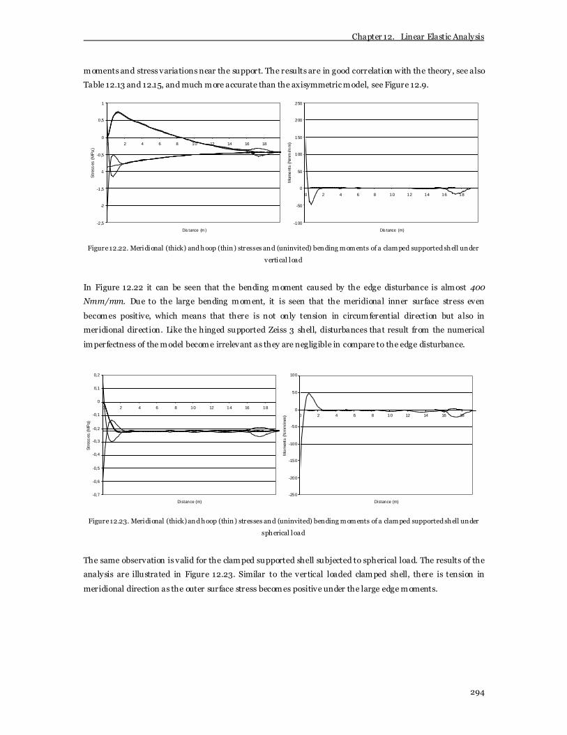
Chapter 12. Linear Elastic Analysis
294
moments and stress variations near the support. The results are in good correlation with the theory, see also
Table 12.13 and 12.15, and much more accurate than the axisymmetric model, see Figure 12.9.
-2,5
-2
-1,5
-1
-0,5
0
0,5
1
0 2 4 6 8 10 12 14 16 18
Dis tance (m )
Str
ess
es (
MP
a)
-100
-50
0
50
100
150
200
250
0 2 4 6 8 10 12 14 16 18
Dis tance (m)
Mom
ent
s (N
mm
/mm
)
Figure 12.22. Meridional (thick) and hoop (thin) stresses and (uninvited) bending moments of a clamped supported shell under
vertical load
In Figure 12.22 it can be seen that the bending moment caused by the edge disturbance is almost 400
Nmm/mm. Due to the large bending moment, it is seen that the meridional inner surface stress even
becomes positive, which means that there is not only tension in circumferential direction but also in
meridional direction. Like the hinged supported Zeiss 3 shell, disturbances that result from the numerical
imperfectness of the model become irrelevant as they are negligible in compare to the edge disturbance.
-0,7
-0,6
-0,5
-0,4
-0,3
-0,2
-0,1
0
0,1
0,2
0 2 4 6 8 10 12 14 16 18
Distance (m)
Str
ess
es (
MP
a)
-250
-200
-150
-100
-50
0
50
100
0 2 4 6 8 10 12 14 16 18
Distance (m)
Mo
men
ts (N
mm
/mm
)
Figure 12.23. Meridional (thick) and hoop (thin) stresses and (uninvited) bending moments of a clamped supported shell under
spherical load
The same observation is valid for the clamped supported shell subjected to spherical load. The results of the
analysis are illustrated in Figure 12.23. Similar to the vertical loaded clamped shell, there is tension in
meridional direction as the outer surface stress becomes positive under the large edge moments.

Chapter 12. Linear Elastic Analysis
295
The stresses found in the three-dimensional finite element analysis are summarised in Table 12.13 and 12.14.
The table shows the middle surface stresses.
Meridional stresses (MPa) Circumferential stresses (MPa)
Top Base Top Base
Name
3D FEA Theory 3D FEA Theory 3D FEA Theory 3D FEA Theory
Zeiss 1 -0.215 -0.219 -0.441 -0.438 -0.215 -0.219 0.447 0.438
Zeiss 2 -0.215 -0.219 -0.440 -0.438 -0.215 -0.219 0.424 0.438
Zeiss 3 -0.215 -0.219 -0.436 -0.438 -0.215 -0.219 0.004 0
Zeiss 4 -0.215 -0.219 -0.437 -0.438 -0.215 -0.219 -0.011 0
Table 12.13. Meridional and circumferential stress distribution for vertical loaded shells
Table 12.13 shows the stresses from the shells loaded vertically. The maximum difference is approximately
3% whereas the average difference is about 1%. Hence, the conclusion can be drawn that the ‘average’ middle
surface stresses from the three-dimensional analysis are in good correlation with the classical shell theory.
In Table 12.14 the results in case of a spherical load are plotted. It can be seen that the stresses show less
correlation in compare to the ones from Table 12.13. The average difference is somewhat higher and equal to
1.5%. However, the greatest discrepancy, again found for the circumferential base stress of the roller
supported shell, is less than for the vertical load.
Meridional stresses (MPa) Circumferential stresses (MPa)
Top Base Top Base
Name
3D FEA Theory 3D FEA Theory 3D FEA Theory 3D FEA Theory
Zeiss 1 -0.215 -0.219 -0.218 -0.219 -0.215 -0.219 -0.214 -0.219
Zeiss 2 -0.215 -0.219 -0.218 -0.219 -0.215 -0.219 -0.217 -0.219
Zeiss 3 -0.215 -0.219 -0.219 -0.219 -0.215 -0.219 0 0
Zeiss 4 -0.215 -0.219 -0.218 -0.219 -0.215 -0.219 0 0
Table 12.14. Meridional and circumferential stress distribution for spherical loaded shells
In Table 12.15 the bending moments are tabulated. Obviously, the bending moments arising at the roller
support of the Zeiss 1 shell is the main reason for the discrepancies described abov e. In Table 12.15 it can be
seen that the three-dimensional analysis approaches the classical shell theory bending moments more
closely than the axisymmetric analysis.
Bending moments (Nmm/mm) Bending moments (Nmm/mm) Name
Base Base
3D FEA AXI FEA Theory 3D FEA AXI FEA Theory
Zeiss 1 -0.851 0 0 0.23 -0.079 0
Zeiss 2 -31.0 -23.2 -23.93 1.23 -0.049 0
Zeiss 3 -9.54 -59.0 0 -4.11 29.5 0
Zeiss 4 390.0 281.0 406.79
-222 -161.0 -
Table 12.15. Bending moments of the vertical (left) and spherical (right) loaded shell

Chapter 12. Linear Elastic Analysis
296
In fact, it can be concluded from Table 12.13, 12.14 and 12.15 that, in general, the three-dimensional shell
model approaches the classical shell theory more closely than the axisymmetric shell model. However, in
case of the given three-dimensional shell model, the stress distribution over the meridian is less smooth than
the axisymmetric stress distribution.
12.3.4 Strains
For the linear elastic analy sis, three-dimensional strain graphs show the same trend as the stress graphs.
Therefore, the strains as obtained by the finite element analysis are not shown. They are tabulated in Table
12.16 and Table 12.17 for the vertical load and spherical load, respectively. The table shows the middle
surface strains.
Meridional strains (‰) Circumferential strains (‰)
Top Base Top Base
Name
3D FEA Theory 3D FEA Theory 3D FEA Theory 3D FEA Theory
Zeiss 1 -0.0072 -0.0073 -0.0147 -0.0146 -0.0072 -0.0073 0.0149 0.0146
Zeiss 2 -0.0072 -0.0073 -0.0147 -0.0146 -0.0072 -0.0073 0.0141 0.0146
Zeiss 3 -0.0072 -0.0073 -0.0146 -0.0146 -0.0072 -0.0073 0 0
Zeiss 4 -0.0072 -0.0073 -0.0146 -0.0146 -0.0072 -0.0073 0 0
Table 12.16. Meridional and circumferential strain distribution for vertical loaded shells
Meridional strains (‰) Circumferential strains (‰)
Top Base Top Base
Name
3D FEA Theory 3D FEA Theory 3D FEA Theory 3D FEA Theory
Zeiss 1 -0.0072 -0.0073 -0.0073 -0.0073 -0.0072 -0.0073 -0.0072 -0.0073
Zeiss 2 -0.0072 -0.0073 -0.0073 -0.0073 -0.0072 -0.0073 -0.0073 -0.0073
Zeiss 3 -0.0072 -0.0073 -0.0073 -0.0073 -0.0072 -0.0073 0 0
Zeiss 4 -0.0072 -0.0073 -0.0073 -0.0073 -0.0072 -0.0073 0 0
Table 12.17. Meridional and circumferential strain distribution for spherical loaded shells
12.3.5 Displacements
The deformations of the three-dimensional shells subjected to vertical load are plotted in Figure 12.24 and
Figure 12.25. In Figure 12.24, the initial undeformed and deformed shapes of the membrane supported Zeiss
1 shell are plotted against each other. Clearly, the shell can move and rotate freely at the base. Qualitatively,
the deformed shape is similar to the one found before with the axisymmetric model.
In Figure 12.25 the initial and deformed shapes of the inclined-roller, hinged and clamped supported shell
are plotted, respectively. The Figures are zoomed in upon the boundary layer of the shell to visualise the
differences in deformation due to allowed or disallowed translations and rotations at the support.
Qualitatively the shapes are similar to the axisymmetric deformed shells.

Chapter 12. Linear Elastic Analysis
297
Figure 12.24. Displacement of a roller supported shell subjected to vertical load
Figure 12.25. Displacement of a inclined-roller, hinged and clamped supported shell subjected to vertical load
A quantitative representation of the deformations and rotations of the top and base radius of the shell under
vertical load is seen in Table 12.13. The displacements presented are the polar displacements while the
rotations are examined in perpendicular direction of a node. The finite element results are compared with
the values of as obtained in Chapter 10 using the classical shell theory. From Table 12.13 and Table 12.9 it
can be concluded that the displacements (and the rotations) of the three-dimensional shell and the
axisymmetrical shell are very much similar to each other. The top deformations of the three-dimensional
model are somewhat lower whereas the base ring displacements are a little bit larger. These variations are
not strange as small variations previously raised in the stresses and strains.
Displacements (mm) Rotations (mm/mm)
Top Base Top Base
Name
3D FEA Theory 3D FEA Theory 3D FEA Theory 3D FEA Theory
Zeiss 1 -0.305 -0.365 0.184 0.183 0 0 -0.352E-4 -2.92 E-5
Zeiss 2 -0.305 -0.365 0.172 0.176 0 0 0 0
Zeiss 3 -0.3 -0.365 0 0 0 0 0.00024 0.00025
Zeiss 4 -0.296 -0.365 0 0 0 0 0 0
Table 12.13. Displacements and rotations for vertical loaded shells
With respect to the top deformations, once more the conclusion can be drawn that the shell acts stiffer than
predicted by the theoretical relation. Therefore, based on the finite element results, it is suggested to replace
the factor of 2 in the energy based equation (10.16) by a factor of 1.7. This factor also finds reasonable
accordance with other programs; using ESA PT a value of 1.73 was found. Thus, equation (10.16) changes to:

Chapter 12. Linear Elastic Analysis
298
( )φz 0
pau = 1.7
Et
2
(12.1)
The factor also gives proper (safe-side) approximations in case of a varying R/t ratio.
In Figure 12.26 and 12.27 a qualitative representation of the deformations of the hemispherical shell under
external spherical pressure load is shown. In Figure 12.26 the complete deformed shell is seen inside the
original geometry. It is observed that the shell experiences local variations within the global radial
compaction, i.e. the maximum displacement is 0.094 mm and the minimum displacement is equal to 0.088
mm. Therefore, the top and base displacements are quite different from the axisymmetric model, see Table
12.10 and 12.14. The average displacement is 0.091 mm which is equal to the one previously found in the
axisymmetric analysis. The variations in the nodal displacements are caused by the non-sphericalness of the
three-dimensional shell surface. Hence, although not seen in Figure 12.24, the variations are present there as
well. Furthermore, the numerical imperfectness causes rotations at the base radius of the shell which are in
disagreement with the theory.
Figure 12.26. Displacement of a roller supported shell subjected to spherical load
In Figure 12.27, the inclined-roller, hinged and clamped supported shells are seen, zoomed in upon the
boundary layer of the shell. The different boundary restraints are evident.
Figure 12.27. Displacement of a inclined-roller, hinged and clamped supported shell subjected to spherical load
A quantitative presentation of the deformed shell under spherical load is seen in Table 12.14. The
displacements presented are the polar displacements while the rotations are the resulting values of the
rotations in x-, y- and z-direction. It can be concluded from Table 12.14 and Table 12.10 that, due to the

Chapter 12. Linear Elastic Analysis
299
numerical imperfectness, the displacements of the three-dimensional shell model subjected to spherical load
leads to different results than for the axisymmetric model.
Displacements (mm) Rotations (mm/mm) Name
Top Base Top Base
Zeiss 1 -0.0879 -0.0895 0 -0.262 E-5
Zeiss 2 -0.0879 -0.0906 0 0
Zeiss 3 -0.0903 0 0 -0.138 E-3
Zeiss 4 -0.0927 0 0 0
Table 12.14. Displacements and rotations of the FEA for shell under spherical load
12.4 Geometrical Influences
The influence of geometrical parameters on the structural behaviour as described abov e must be
investigated. As the hemisphere is the basic shape of this chapter, the thickness of the shell is the only
parameter to investigate. The possibility of a varying shell thickness over the surface is not considered,
although an increased thickness near the support is beneficial counteracting edge disturbances (Chapter 3).
In particular in case of thin shells, the linear static behaviour might be very sensitive to changes in the shell
thickness. There is referred to this so-called ‘highly sensitive’ behaviour if a change in shell thickness causes
a significant change in spatial distribution of displacement and stress response. The problem of highly
sensitive behaviour is described in the paper of Bathe, Chapelle and Lee [4] which is based on the analytical
studies on the asymptotic behaviour of sensitive shells with small thickness as presented by Pitkäranta and
Sanchez-Palencia (1997). In general, shells can be identified into one of the categories of membrane-
dominated, bending-dominated and mixed shells (Chapter 3) and their asymptotic behaviour (the R/t ratio
reaching infinity) distinctly shows in which category the shell falls. The high sensitivity for changes in
thickness, however, is characterised by the fact that the ratio of the bending energy to the total strain energy
does not converge to a specific behaviour as the shell thickness decreases, but show an irregular pattern of
oscillating energies. In other words, within the scheme of linear static analysis several structural responses
appear for different shell thicknesses with no indication to which structural behaviour prevails.
Figure 12.28. Deformed shapes as the shell thickness decreases from R/t = 100 to R/t = 1000

Chapter 12. Linear Elastic Analysis
300
As an example, Bathe, Chapelle and Lee investigated the behaviour of a clamped hemispherical cap with a
sliced off top under a distributed pressure load ov er a small part of the shell surface. For their research they
used the finite element program ADINA; however, the same results are obtained in this thesis with a DIANA
linear analysis. The results are seen in Figure 12.28. In the Figure the deformed shapes of two shells are
illustrated for R/t ratios equal to 100 and 1000. The local distributed load on both shells is placed
approximately halfway the shell surface (clearly seen in the left Figure, though also present in the right).
Regardless of the asymptotic behaviour; the phenomenon of high sensitivity is already observed for
thicknesses reachable for thin concrete shells. Phy sically, the shell considered is an overly sensitive structure
in the sense that the spatial distribution of displacement and stress response changes significantly with
changes in the shell thickness. For higher R/t ratios the tendency seen in Figure 12.28 continuous, with the
number of circumferential displacement waves increased each time the ratio R/t is multiplied with a factor
of 1 0. However, such high ratios loose their practicability for thin concrete shells.
The question is whether the same sensitivity is seen in the Zeiss hemisphere. Therefore the analy sis is done
with several shell thicknesses with the R/t ratios varying from 200 up to 1000. From the analy sis it can be
concluded that, qualitatively, the shells behaves similar. I.e. there is no change in spatial distribution of
displacement and the stress distribution is equal. However, it is observed that for thinner shells, the
meridional stress distribution changes slightly as it shows an increasing local peak in the region meshed by
triangular elements. The peaks are the result of the failed element mapping caused by the modelling
drawback of DIANA. Obviously, the thinner shell is more vulnerable to stiffness variations as the
deformation is larger in compare to a thicker shell. From a quantitative examination of the results, the
conclusion can be drawn that in thinner shells, the bending moments are smaller (as expected) whereas the
stress variation between the integration points in thickness direction becomes larger. The stress variation
becomes larger as the disturbances caused by the modelling drawback have less influence on thicker shells.
The influence length of the bending moment is also smaller for thinner shells, which is in agreement with
equation (10.32) and (10.33), and the statement that the preference for membrane behaviour arises by being
thin (Chapter 3). In general, it can be concluded from the finite element results that the complete
hemisphere is relatively insensitive to thickness variations.
12.5 Material Influences
The investigation to material influences on the stresses, strains and displacements is limited in linear elastic
analysis. As the material in linear elastic analy ses is modelled by the Young’s modulus and the Poisson’s
ratio only, these are the only parameters to vary. E.g. when the shell is fabricated using the high strength
mixture as proposed in Chapter 8.6.2, with a Young’s modulus of 60 GPa (twice as stiff), the stresses do not
change, but the strains and displacements lower by a factor of two. Thus, in a linear elastic analysis a stiffer
material is beneficial to control the displacement of the shell. This advantageous effect is slightly distressed
by the increase in specific weight. The influence of a non-trivial Poisson’s ratio (ν) can easily be explained
with the constitutive law as determined in Chapter 5. The stresses do not change whereas the strains and
displacements change by a factor related to the Poisson’s ratio. For all concrete mixtures it is assumed that

Chapter 12. Linear Elastic Analysis
301
the actual Poisson’s ratio is equal to 0.2 (Chapter 8). Thus, the new spherical displacements can be found by
multiplication with a factor of 0.8 (= 1 – ν). For a vertical loaded shell it is observed that both the top
displacement as the base displacement increase (in the initial direction).
12.6 Load Influences
In the analysis as presented above, the shell is loaded with a trivial uniform vertical or spherical load.
Basically, the load represents the snow load summed up with the dead weight of the shell. Here, the
influence of a non-axisymmetrical wind loading on the shell structural behaviour is considered.
Aforementioned in Chapter 9, due to non-axisymmetrical loading the meridional curves and parallel circles
do no longer present the principal directions of the internal stresses as there is a nonzero membrane shear
force field, as well as normal membrane forces. Thus, the so-called stress trajectories transform under the
influence of wind load. The load intensities as determined in Chapter 9 will serve as input for the analysis.
The shell is loaded by (non-axisymmetric) wind suction (1.2 kN/m2) and wind pressure (0.8 kN/m2) load,
distributed according to Figure 9.4 and 9.5. Additionally, the dead weight of the shell is presented by a
uniformly distributed vertical load (1.5 kN/m2). For reasons of simplicity, the wind load is modelled with an
abrupt transition between wind suction and wind pressure. Moreover, the circumferential reduction in wind
suction at the leeward side (Figure 9.5) is neglected.
The deformations of a shell subjected to dead weight only and a shell subjected to dead weight and
additional wind load are illustrated in Figure 12.29. Obviously, in reality the wind load is more fluently
distributed and the deformed shape is smoother. Although the shells deform significantly different, the
maximum deformations are almost similar, i.e. the shell loaded by dead weight deforms 0.212 mm at the top
while the wind loaded shell deforms 0.202 mm in the boundary layer. Hence, the effect of wind load on the
maximum displacement is negligible.
Figure 12.29. Deformation of shell loaded by dead weight (left) and a shell loaded by wind and dead weight
The stress distribution of wind load only and a combination of wind load and dead weight is shown in Figure
12.30. In Figure 12.30 the meridional stresses are indicated by the thick lines and the circumferential
stresses by the thin lines. Both graphs show the stress distribution over the middle shell cross-section,
parallel with the main wind direction. In the left figure it is clearly seen that the abrupt transition between
wind pressure and wind suction causes large stress ‘jumps’, located nearby point 30 m in the graph. The
same discontinuities can be seen in the moment distribution graphs, Figure 12.31. Hence, the moments
nearby 30 m do not appear in reality.

Chapter 12. Linear Elastic Analysis
302
-0,40
-0,30
-0,20
-0,10
0,00
0,10
0,20
0,30
0,40
0,50
0,60
0 5 10 15 20 25 30 35 40
Distanc e (m)
Str
esse
s (
MP
a)
-1 ,20
-1,00
-0,80
-0,60
-0,40
-0,20
0,00
0,20
0,40
0,60
0,80
0 5 10 15 20 25 30 35 40
Distance (m)
Str
esse
s (
MP
a)
Figure 12.30. ‘Wind parallel ’ stress distribution of a shell loaded by wind load only (left) and a shell loaded by dead weight and
wind load (right)
-300
-250
-200
-150
-100
-50
0
50
100
150
200
250
0 5 10 15 20 25 30 35 40
Distanc e (m)
Mom
ent
s (N
mm
/mm
)
-200
-100
0
100
200
300
400
500
0 5 10 15 20 25 30 35 40
Distanc e (m)
Mom
ent
s (N
mm
/mm
)
Figure 12.31. ‘Wind parallel ’ moment distribution of a shell loaded by wind load only (left) and a shell loaded by dead weight and
wind load
The stress distribution in the other direction, perpendicular to the wind direction, differs at each location in
the shell. In Figure 12.32 the meridional and circumferential stresses are plotted together with the shear
stresses that appear halfway of the shell. It can be seen that, at the middle section of the hemisphere, the
wind load is transferred to the supports partly by meridional stresses and partly by shear.
-1,00
-0,80
-0,60
-0,40
-0,20
0,00
0,20
0,40
0,60
0 5 10 15 20 25 30 35 40
Dis tanc e (m)
Stre
sse
s (M
Pa)
-0,15
-0,10
-0,05
0,00
0,05
0,10
0,15
0 5 10 15 20 25 30 35 40
Distance (m)
Stre
sse
s (M
Pa)
Figure 12.32. ‘Wind perpendicular’ stress distribution of a shell loaded by dead weight and wind load

Chapter 12. Linear Elastic Analysis
303
From Figure 12.30, 12.31 and 12.32 it can be concluded that wind load significantly changes the stress and
bending moment distribution over the shell. The circumferential tensile stresses, which e.g. appear in the
vertical loaded shell of Figure 12.22, are compensated for at the leeward side. At the windward side, the
meridional bending moment caused by the clamped support is completely compensated by the bending
moments caused by the wind. Moreov er, shear stresses appear which change the direction of the stress
trajectories.
When the shell subjected to wind load and dead weight is compared to the shell previously examined in
Section 12.3.3 (dead weight and snow load) it can be concluded that the stresses and bending moments
caused by wind load do not prevail. At the leeward boundary the bending moments may be significantly
higher; however, the modelling of the wind suction in that particular location is highly unrealistic, i.e. in
reality the wind suction vanishes at the support, see Figure 9.3 and 9.5.
12.7 Conclusions
The linear elastic finite element analysis is performed using an axisymmetric and a three-dimensional shell
model. Both models suffer numerical imperfections. In the axisymmetric line model, the spherical load could
not be modelled directly, and, therefore, consists of segmented line load which introduces uninvited stress
discrepancies and bending moments. The numerical imperfections in the three-dimensional model are
caused by a failed mapping operation of the element base shape onto a sphere, i.e. the elements lay over a
ribbed skeleton like an unstressed fabric introducing curvature variations. These curvature variations cause
stress discrepancies and bending moments. However, although both models are not perfect, the general
results show reasonable stress and strain distributions, bending moment localisations and displacements.
The membrane supported hemisphere subjected to spherical load is in evenly distributed compression while
the membrane supported hemisphere loaded by a uniform vertical load demonstrates compression at the top
and compression-tension at the bottom, analogue to the classical shell theory. When the shell support is not
membrane compatible anymore, edge disturbances arise and local bending moments are introduced in the
boundary layer. A clamped support is most onerous, because it introduces the largest bending moments into
the shell. The shell structural behaviour is not sensitive to variations in thickness or material, i.e. the
response is no other than expected. However, this is only inspected for R/t ratios of 200 up to 1000. In case
of a non-symmetrical wind load the axisymmetric shell model is not applicable anymore as it is unable to
deal with variations in circumferential direction. From the three-dimensional finite element analysis it is
observed that wind load changes the stress and bending moment distribution significantly and the
meridional and circumferential directions do no longer present the principal directions of the internal
stresses. Although the deformed shape is completely different, the maximum deformation caused by wind
and dead weight is approximately similar to the deformation caused by dead weight only. Moreover, for the
selected shell parameters, the combination of wind load and dead weight does not prevail ov er the
combination of snow load and dead weight.

Chapter 12. Linear Elastic Analysis
304
With respect to the solution accuracy, it can be concluded that the displacements, stress and strain results
are almost similar to the results of Chapter 10 determined with the classical shell theory, i.e. within 3%. For
the bending moments the results are less convincing as they are significantly lower caused by the low order
stress mapping between the ‘exact’ integration points and the element nodes. In particular the axisymmetric
model is insufficient with discrepancies reaching 30%. Hence, it can be concluded that, although the
axisymmetric shell model provides in a (more) effective analysis, it is less accurate and reliable than the
three-dimensional model.

Chapter 12. Linear Elastic Analysis
305

Chapter 13. Stability Analysis
306
13 Stability FEA
The topic of this chapter is the investigation to the linear elastic stability behaviour of a hemispherical shell.
The theory of the stability behaviour of shells is discussed in Chapter 6. Here, the research is restricted to
small deformations (linear) and elastic material behaviour. For these circumstances the validity of the
stability relations and hypotheses of Chapter 6 are investigated.
Aforementioned in Chapter 6, in the stability behaviour of shells distinction can be made between
prebuckling and postbuckling behaviour. The path up to the critical buckling point is named the prebuckling
path. This path and corresponding buckling point can be determined by a linear (Euler) buckling analy sis. In
this type of analysis a bifurcation point is assumed and, as pointed out in Chapter 11, the finite element
program solves the problem by a so-called eigenvalue analysis using an iterative solution scheme. The
eigenvalues represent the critical buckling loads and the corresponding eigenfunctions determine the
buckling modes.
After the bifurcation point the nonlinear postbuckling path of equilibrium initiates. For synclastic shells
loaded perpendicular to their plane, the postbuckling path shows a dramatic fall in load bearing capacity.
The fall-back is caused by postbuckling interaction of buckling modes, which where orthogonal within the
linear scheme. Koiter found that the slope and curvature of the postbuckling path in the vicinity of the
bifurcation point can be approximated closely by a linearised interaction of these buckling modes. In
DIANA, the linear interaction of buckling modes is simulated by carrying out a so-called perturbation
analysis. The corresponding postbuckling path of equilibrium can be found performing a continuation
analysis. Hence, the successive execution of a perturbation and continuation analysis is the finite element
presentation of the Koiter initial postbuckling theory.
In the following a full linear elastic stability analysis, i.e. a linear buckling analysis and a perturbation and
continuation analy sis, is reported. Similar to the previous chapter, the analyses concern as well the
axisymmetric model as the three-dimensional model. In addition to Chapter 10, not only uniform pressure
load is considered, but also the behaviour under uniform vertical load is investigated, as it shows much more
resemblance with the type of load to which thin concrete shells are subjected in practice.

Chapter 13. Stability Analysis
307
13.1 Shell Parameters
13.1.1 Geometry
See Chapter 12.1.1.
13.1.2 Material
See Chapter 12.1.2.
13.1.3 Boundary Conditions
See Chapter 12.1.3
13.1.4 Loading
The shell is loaded by uniform pressure or vertical load. Snow and wind load are not considered.
13.1.5 Analysis Scheme
The linear buckling calculations are presented in the analy sis scheme of Table 13.1.
Name Loading Conditions Supporting Conditions Type of Analysis Model
Zeiss 1 Spherical and Vertical Roller Linear Stability Axisymmetric + 3D
Zeiss 2 Spherical and Vertical Inclined-roller Linear Stability Axisymmetric + 3D
Zeiss 3 Spherical and Vertical Hinged Linear Stability Axisymmetric + 3D
Zeiss 4 Spherical and Vertical Clamped Linear Stability Axisymmetric + 3D
Zeiss 5 Partially loaded Clamped Linear Stability 3D
Table 13.1 . Analy sis scheme
13.2 Linear Buckling Analysis
The shell is modelled by axisymmetric shell elements (discussed first) and two-dimensional curved shell
elements similar to the finite element models described in Chapter 12.
13.2.1 Axisymmetric Shell Model
The axisymmetrical shell model provides in a simple and fast model for buckling analysis. The spherical
pressure load is analysed first. Then, the influence of a uniform vertical load is investigated. For each load
the influence of several supporting conditions is considered.

Chapter 13. Stability Analysis
308
Zeiss 1
The shell roller supported Zeiss 1 shell subjected to spherical load is in pure membrane action, i.e. the shell is
free to move without any boundary restraint (Chapter 12). For spherical load, the buckling modes from the
finite element analysis are seen in Figure 13.1. The corresponding critical loads are presented in Table 13.2.
Figure 13.1. Buckling modes 1, 2 and 3 for a roller supported axisymmetrical shell subjected to spherical load
In Figure 13.1 it can be seen that mode 1, 2 and 3 are quite different. First the shell buckles at the base radius
with a corresponding buckling load which is extremely low, for sure when compared to adjacent modes (50%
less than mode 2) or to the theoretical buckling load as derived by Zoëlly, see Table 13.2.The buckling mode
seems to stands alone, which gives rise to the thought that the mode may be a premature buckling mode
caused by numerical disturbances. On the other hand, the shell is considerably ‘weaker’ near the support as
it is free to rotate. Confirmation for these thoughts will be searched later in the three-dimensional buckling
analysis. From mode 2, the consecutive modes alternately show top buckling (even modes) or a global wave
pattern extending over the complete shell surface (odd modes). The top buckling modes must be addressed
as premature buckling modes as, according to Kollar and Dulacska [54], the shell will alway s buckle in small
local waves distributed evenly over the shell surface. The tendency to buckle at the top stems from the basic
characteristic of the model, namely, axisymmetry. The axis of axisymmetry is vertical, which means that
buckling at the top corresponds to a local buckle whereas buckling in the shell surface is represented by a
global buckling pattern extending in circumferential direction. The appearance of the global buckling modes
can, therefore, be ascribed to the interaction of the top buckling mode with the edge mode 1.
Buckling mode Critical buckling load (MPa)
1 0.3969
2 0.7938
3 0.8001
4 0.8106
5 0.8274
10 0.9702
Zoëlly 0.7981
Table 13.2. Linear critical buckling load for a roller axisymmetrical shell subjected to spherical load

Chapter 13. Stability Analysis
309
In Table 13.2, the critical buckling loads are presented. With the exception of mode 1, it can be seen that the
critical buckling loads of the axisymmetrical shell model are very close to each other (each mode differs less
than 2% and all modes between 2 and 10 are within 20%). Aforementioned in Chapter 6, this indicates the
sensitivity of the shell to multimode or compound buckling, a characteristic feature of shells where several
buckling modes are associated with the same critical load. Despite the premature top buckling modes, the
critical loads find good correlation (within 1%) with the theoretical linear buckling load for a complete
sphere as derived by Zoëlly (equation 6.53).
Figure 13.2. Buckling modes 1, 4 and 7 for a roller supported axisymmetrical shell subjected to vertical load
The next step is to investigate the influence of a uniformly distributed vertical load on the shell stability
behaviour. The results of the finite element analysis are seen in Figure 13.2. From Figure 13.2 it immediately
can be concluded that, except for mode 1, the buckling pattern is significantly different in compared to
buckling caused by spherical load. Under the influence of v ertical load, the buckling first stays within the
boundary layer. Later, the buckling pattern extends towards the total shell. Similar to the spherical case, the
critical load of mode 1 is less than 50% of its successors. The lower based buckling is contributed to the fact
that the vertical load, opposite to a spherical load, does not contain a ‘supporting’ transverse component in
that boundary layer.
A quantitative description of the buckling behaviour is represented in Table 13.3. It can be seen that the
vertical critical buckling loads approach to the spherical critical load for higher buckling modes (from 60% at
mode 2 to 20% at mode 10). Furthermore, it can be seen that adjacent critical loads lie further away from
each other (up to more than 10%). With respect to the compound buckling, differences up to 2% are to be
expected, Hoogenboom [50], which means that the phenomenon is disqualified here.
Buckling mode Critical buckling load (MPa)
1 0.2035
2 0.5061
3 0.5418
4 0.6048
7 0.7098
10 0.7875
Zoëlly 0.7981
Table 13.3. Linear critical buckling load for a roller axisymmetrical shell subjected to vertical load

Chapter 13. Stability Analysis
310
The observation that the critical loads approach the spherical critical load when the buckling modes
approach towards a global wave pattern stresses that the statement of Simitses and Cole (1968), i.e. that the
type of load, radial pressure or gravity, does not appear to change the critical load drastically, is valid if and
only if global buckling takes place (thus, also in the compression zone).
Zeiss 2
The ‘membrane’ supported inclined-roller Zeiss 2 shell model subjected to spherical load experiences only
radial displacements up to buckling instability and no bending moments. Therefore, the hemispherical Zeiss
2 shell behaves as if it is a complete sphere. The results of the buckling analysis are presented in Figure 13.3
and Table 13.4.
Figure 13.3. Buckling modes 1, 5 and 10 of an inclined-roller supported axisymmetrical shell subjected to spherical load
In Figure 13.3 the buckling modes 1, 5 and 10 are shown. The first mode of the roller supported Zeiss 1 shell
has disappeared as the inclined-roller support gives sufficient resistance against rotation. Moreover, the
rotational disallowing releases the shell from successive appearance of local top and global modes. The
buckling modes of Figure 13.3 have a global character as the wave pattern extends over the total shell,
however with maximum buckling amplitude at the top due to the axisymmetry of the model. The given
modes appear to be more or less similar, with only small differences in the number of half-waves (14, 12 and
20, respectively). The other computed (unplotted) buckling modes show the same tendency, i.e. the
maximum buckling amplitude is unconditionally found at the top node.
Buckling mode Critical buckling load (MPa)
1 0.7917
2 0.7959
3 0.8043
4 0.8169
5 0.8421
10 1.0017
Zoëlly 0.7981
Table 13.4. Linear cri tical buckling load for an inclined-roller axisymmetrical shell subjected to spherical load

Chapter 13. Stability Analysis
311
It can be concluded from Table 13.4 that the critical buckling loads of the inclined-roller shell are very close
to each other (compound buckling) and find good correlation (within 1%) with the theoretical linear buckling
load as derived by Zoëlly. Hence, this is encouraging as Zoëlly derived his buckling equation for a complete
sphere and he already predicted the occurrence of compound buckling.
The influence of a uniform vertical load on the stability behaviour of an inclined-roller supported shell is
visualised in Figure 13.4 and Table 13.5. Similar to the Zeiss 1 shell, the buckling starts at the base while it
extends more and more towards the complete shell in following modes. The mode 1 which caused an
extremely low buckling load is vanished, however, this time lower based buckling is intensified by the so-
called edge disturbance; i.e. for a vertical load the supporting conditions are not membrane compatible
anymore and bending moments undoubtedly will arise.
Figure 13.4. Buckling modes 1, 3, 6 for an inclined-roller supported axisymmetrical shell subjected to vertical load
The critical buckling loads are represented in Table 13.5. When the values of Table 13.5 are compared with
the surface bucking values in Table 13.3 (neglecting mode 1), it can be concluded that the bending moments
caused by the boundary conditions intensify the buckling as the critical loads are somewhat lower.
Buckling mode Critical buckling load (MPa)
1 0.4515
2 0.5229
3 0.5754
6 0.6972
10 0.8043
Zoëlly 0.7981
Table 13.5. Linear critical buckling load for an inclined-roller supported axisymmetrical shell under vertical load
Iit can be concluded from Table 13.5 that the phenomenon of compound buckling is disqualified as adjacent
critical loads vary up to 13%. Furthermore, similar to Zeiss 1, the statement of Simitses and Cole is valid if
and only if global buckling occurs.
Zeiss 3
The Zeiss 3 shell is hinged supported. The results of the finite element analy sis for a hinged supported shell
subjected to spherical load are illustrated in Figure 13.5. It can be observed that a hinged supported shell

Chapter 13. Stability Analysis
312
buckles similar to the roller Zeiss 1 shell. The lowest critical buckling load produces a local buckle in the
boundary layer (though, in opposite direction to Zeiss 1 due to the ‘hinged’ edge disturbance) whereas
adjacent buckling modes buckle locally at the top or show a global wave pattern.
Figure 13.5. Buckling modes 1, 2 and 3 for a hinged supported axisymmetrical shell subjected to spherical load
The repetitive sequence of local top buckling and global buckling in mode 2 to 10 is caused by a similar
interaction or not of adjacent buckling modes as seen in Figure 13.1. Thus, the bending moments caused by
the restrained support interact or not with the top buckling mode.
Buckling mode Critical buckling load (MPa)
1 0.6405
2 0.7938
3 0.8001
10 0.9576
Zoëlly 0.7981
Table 13.6. Linear cri tical buckling load for a hinged supported axisymmetrical shell under spherical load
The critical loads corresponding to the buckling modes are seen in Table 13.6. Due to the hinge support the
shell buckles already at a value which is approximately 80% of the theoretical critical load for radially
pressed spheres. Furthermore, a remarkable difference of approximately 20% between the first and second
critical load is seen, whereas the critical loads from mode 2 to 10 are within 12%. This may be caused by the
fact that the buckling solution is disturbed by the non-vanishing bending moments in the linear solution (see
Chapter 12.2.3).
Figure 13.6. Buckling modes 1, 3 and 6 for a hinged supported axisymmetrical shell subjected to vertical load

Chapter 13. Stability Analysis
313
The Zeiss 3 shell with vertical load behaves similar to the v ertical loaded Zeiss 2 shell. The first buckling
mode is locally, confined to the boundary layer of the shell, whereas following modes increasingly stretch
towards the total shell, illustrated in Figure 13.6. The buckling modes are quantitative represented in Table
13.7. It can be concluded that the buckling load decreases to 44% of the theoretical buckling load for radially
pressed spheres (the hinge supports cause a fall back in critical load of 13% in compare to the inclined-roller
support). Moreover, there is a great discrepancy between the first and second critical load (almost 32%),
whereas the other values differ more or less 7%. Again, this can be attributed to the nonzero bending
moments that appeared in the linear solution (Chapter 12.2.3).
Buckling mode Critical buckling load (MPa)
1 0.3507
2 0.5103
3 0.5481
6 0.6825
10 0.7896
Zoëlly 0.7981
Table 13.7. Linear critical buckling load for a hinged supported axisymmetrical shell under vertical load
From the hinged supported shell it can, once more, be concluded that prebuckling rotations caused by edge
disturbance bending moments amplify the buckling deformations or even may become dominant in buckling
failure (e.g. Zeiss 3 spherical mode 1 in compare to Zeiss 2 spherical mode 1).
Zeiss 4
The Zeiss 4 axisymmetric shell model is clamped supported. The finite element results are plotted in Figure
13.7. In Figure 13.7 it can be seen that the restrained rotation stimulates top node buckling. Hence, the
corresponding critical load, seen in Table 13.8, is almost equal to the critical load for a radially pressed
sphere.
Figure 13.7. Buckling modes 1, 2 and 3 for a clamped supported axisymmetrical shell subjected to spherical load
The repetitive sequence of global and local top buckling indicates whether the critical load is spherical or
based on the interaction of the spherical load with the bending moments that arise from the restraint
deformation at the support. Table 13.8 shows adjacent critical loads within 2% demonstrating the sensitivity
to compound buckling.

Chapter 13. Stability Analysis
314
Buckling mode Critical buckling load (MPa)
1 0.7938
2 0.7980
3 0.8106
4 0.8211
5 0.8421
10 0.9870
Zoëlly 0.7981
Table 13.8. Linear cri tical buckling load for a clamped supported axisymmetrical shell under spherical load
The buckling modes of the vertically loaded clamped shell, shown in Figure 13.8, show the same tendency as
seen in all previous (vertical) cases. That is, a local first buckling mode confined to the boundary layer of the
shell which ‘mode by mode’ extends towards the complete shell. The corresponding critical buckling loads
are tabulated in Table 13.9.
Figure 13.8. Buckling modes 1, 5 and 10 for a clamped supported axisymmetrical shell subjected to vertical load
When the values of Table 13.9 are compared to the previous cases in which vertical load is prescribed, it is
observed that the clamped supported shell shows the highest critical loads. The lowest critical load at which
buckling occurs is approximately 60% of the value found by Zoëlly, and is 8% and 28% higher than the
inclined-roller and hinged supported shell, respectively.
Buckling mode Critical buckling load (MPa)
1 0.4977
2 0.5229
3 0.5964
4 0.6174
7 0.7371
10 0.7938
Zoëlly 0.7981
Table 13.9. Linear cri tical buckling load for a clamped supported axisymmetrical shell under vertical load
In particular, the fact that the clamped supported shell shows higher resistance against buckling than the
inclined-supported shell is noticeable as one may expect that a more severe restraint, which introduces the
highest bending moments, would be most onerous. Evidently, the resulting bending moment as obtained in

Chapter 13. Stability Analysis
315
the linear solution has a positive stiffening effect on the boundary layer of the shell causing the shell to be
less vulnerable to buckling. This effect is, however, restricted to the first critical buckling load as the mode 2
yields a similar buckling load as the Zeiss 2 shell under vertical load.
With respect to the effect of various supporting conditions, none of them produced a positive effect on the
critical buckling load as suggested in Figure 6.28 and 6.29. Thus, it can be concluded that those observations
are only valid for relative low values of λ which represents shallow shells showing local snap-through
behaviour.
13.2.2 Three-Dimensional Shell Model
The major deficiency of the axisymmetric model is the fact that it is unable to produce terms, and buckling
modes, which vary in circumferential direction. Therefore, the stability research is extended with a three-
dimensional shell model. The analysis procedure for the three-dimensional shell is similar to the
axisymmetric model. The shell is first subjected to spherical load and, subsequently, the behaviour of a shell
under uniform vertical load is investigated. For each load condition, the influence of the four boundary
conditions is discussed.
It is observed that all three-dimensional shell models experience compound buckling up to a high level.
Therefore, it is needed to compare a large number of modes and to select the ones which give good insight in
the buckling behaviour. There are in total 150 modes examined for each shell. With such a high number of
modes it is necessary to check whether the relative error approximately stays the same in order to ensure the
correctness of the found modes. From the results in can be concluded that the relative error stays more or
less equal, which means that all modes are of comparable exactness.
Zeiss 1
The first 3D buckling analysis is the roller supported shell under spherical load. The results of the analy sis
are seen in Figure 13.9 and Table 13.10. It is observed that the shell first buckles in the boundary layer with
an axisymmetric buckling pattern, similar to the axisymmetric shell. Contrary to the axisymmetric finite
element model, a lot of associative (boundary layer) modes arise which demonstrate asymmetric buckling or
buckles in a large number of local circumferential waves. From mode 50 the buckling is found at the top of
the shell or the buckling modes extend over a large part of the shell middle surface. The first global mode, i.e.
ev enly distributed buckling over the total shell surface, is mode 110.
Figure 13.9. Buckling modes 1, 50 and 110 for a roller supported 3D shell subjected to spherical load

Chapter 13. Stability Analysis
316
The associative critical buckling loads are presented in Table 13.10. Similar to the axisymmetric shell, mode 1
is approximately 50% of the top buckling mode 50. Aforementioned, the shell experiences compound
buckling as several buckling modes are associated with the same critical load. Furthermore, it can be seen
that the global buckling mode 110 yields the same critical load as the equation found by Zoëlly for a radially
pressed sphere. Combining Figure 13.9 and Table 13.10, the buckling process can be explained by the fact
that the roller support is considerable ‘weaker’ than the shell itself. The shell is, thus, likely to buckle first in
that particular area. At mode 50 the shell suddenly steps-over towards top buckling. However, the top
buckling can be addressed as a premature buckling mode, similar to the top buckling that appeared in the
axisymmetric model. Opposite to the axisymmetric model, not axisymmetry causes the top buckling, but the
uninvited circumferential bending moments which were previously found in the linear solution of Chapter 12
(due to the numerical imperfectness of the model). The first global mode, mode 110, yields the same critical
load as derived for the radially pressed sphere. In mode 110 the expected chessboard pattern is clearly seen
(see Chapter 6). Hence, the shell can indeed be regarded as shallow in the region of a buckle, as previously
assumed in the derivation of equation (6.53).
Buckling mode Critical buckling load (MPa)
1 0.3969
50 0.7812
110 0.7980
Zoëlly 0.7981
Table 13.10. Linear critical buckling load for a roller 3D shell subjected to spherical load
When the three-dimensional buckling analy sis results are compared to the axisymmetric buckling results it
can be concluded that the three-dimensional modes gives lower values for similar buckling patterns. In fact,
this phenomenon is also seen in all other analy ses.
For the vertical load, the shell is membrane supported and no bending moments arise. From the buckling
output file it is observed that, within the first 150 modes, the critical load does not exceed 0.6654 MPa. This
means that no global buckling patterns can be expected. The characteristic buckling modes of the analy sis
are seen in Figure 13.10.
Figure 13.10. Buckling modes 1, 38 and 146 for a roller supported 3D shell subjected to vertical load
Similar to the spherical loaded Zeiss 1 shell, the first modes are restricted to the boundary layer. The
buckling pattern of the vertical loaded shell stretches step-by -step towards the complete shell surface. It is
observed that the buckling process evaluates each time with the same procedure, i.e. first an axisymmetrical

Chapter 13. Stability Analysis
317
mode occurs, followed by several asymmetrical modes with an increasing number of circumferential waves
and slightly higher critical loads. The modes visualised in Figure 13.10 are mode 1, 38 and 146. Up to mode
37 the buckling is in the boundary layer. Mode 38 is the first mode in which the buckling is more stretched
towards global shell buckling. Mode 146 is a mode in which the buckling pattern is maximal stretched within
the 150 modes scheme. I.e. sometimes lower based modes with an extremely high number of circumferential
waves interchange with modes which are stretched higher upon the shell surface.
The critical loads of Figure 13.10 are tabulated in Table 13.11. In the table it is seen that the critical loads
approach the load of a radially pressed sphere more closely with higher modes. Hence, eventually, global
buckling will occur similar to the spherical load confirming that the statement of Simitses and Cole (1968) is
valid if and only if global buckling takes place. Furthermore, it is observed that asymmetrical modes are
associated with almost the same critical load as the adjacent axisymmetrical modes (e.g. differences of
0.4%). Thus, the statement of Van der Neut (1932), i.e. that the critical pressure corresponding to an
asymmetric buckling pattern is similar to an axisymmetrical buckling pattern may assumed to be valid,
however, ‘within a few percent’.
Buckling mode Critical buckling load (MPa)
1 0.2022
38 0.5028
146 0.6543
Zoëlly 0.7981
Table 13.11. Linear critical buckling load for a roller 3D shell subjected to vertical load
A remarkable observation made during the examination of the finite element results refers to the existence
of negative eigenmodes which seem to arise only in case of vertical load. Negative buckling modes are
numerically correct; however, phy sically they have no meaning for concrete shells. It simply means that the
load is of opposite sign with respect to the input. These modes are, thus, numerical modes and as they are of
no practical meaning they are neglected.
Comparing the results with the axisymmetric results it is seen that the first critical loads are nearly similar,
however, successive critical loads are significantly lower in case of the three-dimensional shell. Encouraging
is the fact that the buckling process of a step-by -step stretching towards global buckling is similar.
Zeiss 2
The inclined-roller supported shell under spherical load behaves as a complete sphere. The results of the
analysis are seen in Figure 13.11. Similar to the Zeiss 1 shell (and the axisymmetric shell) premature buckling
modes are observed before the expected global modes appear. Again, these modes are ascribed to the
uninvited bending moments from the linear solution. It is observed that successive buckling patterns ev olve
rapidly towards global buckling. Within the first 12 modes, top buckling, middle shell surface buckling and
global buckling takes place. Furthermore, all the global buckling modes show sign of a chessboard pattern of
local buckling waves.

Chapter 13. Stability Analysis
318
Figure 13.11. Buckling modes 1, 5 and 12 for an inclined-roller supported 3D shell subjected to spherical load
The corresponding critical loads in Table 13.12 show that all buckling values are very close (approximately
2%) to the linear critical buckling load of a radially pressed sphere. This observation strengthens the
conclusion that the finite element program delivers correct results. Furthermore, it can be concluded that the
Zeiss 2 shell behaves much stiffer than the roller supported Zeiss 1 shell under spherical load, i.e. the first
buckling mode is twice as high and correlates with mode 50 of the roller shell.
Buckling mode Critical buckling load (MPa)
1 0.7811
5 0.7861
12 0.7884
Zoëlly 0.7981
Table 13.12. Linear cri tical buckling load for an inclined-roller 3D shell subjected to spherical load
The three-dimensional shell model shows faster global buckling with lower critical loads in compare to the
axisymmetric model which seems entangled in its axisymmetry.
The vertical loaded inclined-roller shell is not membrane supported anymore and, thus, significant bending
moments are present in the boundary layer. The results of the analysis are illustrated in Figure 13.12. The
influence of bending moments is seen in the first buckling mode as the buckling amplitude is in opposite
direction in compare to the Zeiss 1 shell. Furthermore, the bending moments cause the buckling pattern to
be more stretched and it reaches global buckling faster. The procedure of reaching global buckling is
analogue to the previous roller case, i.e. the buckling pattern slowly extends towards the total shell surface,
hereby showing an increasing number of circumferential waves with nearly the same critical load before
stepping through to a more global mode. Again, lower based modes with an extremely high number of
circumferential waves interchange with modes which are stretched higher up on the shell surface.
Figure 13.12. Buckling modes 1, 20 and 150 for an inclined-roller supported shell subjected to vertical load

Chapter 13. Stability Analysis
319
The corresponding critical buckling loads are seen in Table 13.13. Again, it can be concluded that the shell is
much stiffer that the roller supported shell as the critical load of mode 1 is approximately equal to the critical
load of mode 35 of the roller shell. Clearly, from the critical load output it could already be seen that there
would be no global mode as the previous analyses have shown that the critical load must be within 2% of the
buckling load for a radially pressed sphere to demonstrate global buckling. The result is practically equal to
the axisymmetric case.
Buckling mode Critical buckling load (MPa)
1 0.4460
20 0.5204
150 0.7057
Zoëlly 0.7981
Table 13.13. Linear cri tical buckling load for an inclined-roller shell subjected to vertical load
Zeiss 3
The hinged supported Zeiss 3 shell subjected to spherical load experiences high bending moments in the
boundary layer. The analysis results are shown in Figure 13.13. Parallel to the axisymmetric model, the initial
three-dimensional buckling process is restricted to the boundary layer (up to mode 67). At mode 68 the
buckling process suddenly moves to the top of the shell (the premature mode) followed by a series of
asymmetric middle surface buckling modes. Before global buckling at mode 117, a irregular series of shell
buckling patterns extending over large parts of the shell surface. The expected chessboard pattern of local
buckling waves is clearly seen in the global mode.
Figure 13.13. Buckling modes 1, 68 and 117 for a hinged supported shell subjected to spherical load
The critical loads are presented in Table 13.14. It can be seen that the hinged support condition provides in a
stiffer support than the roller support, as one would expect from an engineering point of view. It can be seen
that the shell experiences top buckling at approximately the same critical loads as previously found at Zeiss 1
and 2. Moreov er, the critical load that corresponds to the global mode 117 is within 1% of the theoretical
solution for a radially pressed sphere.

Chapter 13. Stability Analysis
320
Buckling mode Critical buckling load (MPa)
1 0.5732
68 0.7812
117 0.7949
Zoëlly 0.7981
Table 13.14. Linear cri tical buckling load for a hinged shell subjected to spherical load
The hinged shell subjected to v ertical load behaves similar to all previous vertically loaded shells. I.e. the
buckling pattern initiates in the boundary layer and slowly extends towards a global buckling pattern. The
results of the analysis are seen in Figure 13.14. Up to mode 31 the buckling remains in the boundary layer
before its stretches further over the shell surface in mode 32. The closest mode to global buckling (within the
research range) is mode 150 which is represented by four circumferential waves. The buckling modes are
quite similar to the modes of the axisymmetric model.
Figure 13.14. Buckling modes 1, 32 and 150 for a hinged supported shell subjected to vertical load
The corresponding buckling modes are tabulated in Table 13.15. Despite the fact that the modes look very
much similar to the axisymmetric ones, the critical loads are significantly lower. In compare to the roller
support, the hinged support is more severe and leads to higher critical loads.
Buckling mode Critical buckling load (MPa)
1 0.3285
32 0.5031
150 0.6419
Zoëlly 0.7981
Table 13.15. Linear critical buckling load for a hinged shell subjected to vertical load
Zeiss 4
The result of the buckling analysis of a clamped supported Zeiss 4 shell subjected to spherical load is seen in
Figure 13.15. It is observed that, opposite to the axisymmetric model, at first the bending moments caused by
the clamped support cause the shell to buckle in the boundary layer. Most probably, this is caused by the
much larger (but more correct) bending moments in the linear solution (Chapter 12). From mode 1, the
successive modes, however, extend more and more towards the total shell surface. At mode 39, the shell
jumps over towards premature top buckling. Adjacent modes of mode 39 buckle in the top region as well,

Chapter 13. Stability Analysis
321
however, after mode 46, the buckling moves away from the top. The first global modes appear at mode 41;
although large areas remain unaltered and no mode shows an equally distributed buckling pattern until
mode 70.
Figure 13.15. Buckling modes 1, 39 and 70 for a clamped supported shell subjected to spherical load
The corresponding critical buckling loads are seen in Table 13.16. It is seen that the clamped support yields a
mode 1 critical load as close as 11% to the critical load of a radially pressed sphere. Therefore, the clamped
support is less fav ourable with respect to buckling than the inclined-roller support in which the shell
immediately buckles inside the shell surface.
Buckling mode Critical buckling load (MPa)
1 0.7067
39 0.7812
70 0.7926
Zoëlly 0.7981
Table 13.16. Linear cri tical buckling load for a clamped shell subjected to spherical load
The buckling process of a clamped shell under vertical load is visualised in Figure 13.16. Similar to all
previous vertical loaded shells, the buckling initiates in the boundary layer and stretches more and more
towards the total shell surface. The closest mode to global buckling is mode 148. The chessboard pattern of
local buckling waves is already visual.
Figure 13.16. Buckling modes 1, 10 and 148 for a clamped supported shell subjected to vertical load
The critical buckling loads of the clamped shell under vertical load are seen in Table 13.17. It is seen that the
critical load of mode 1 is the highest critical load in compare to all previous support conditions. The load is

Chapter 13. Stability Analysis
322
approximately 40% of the critical load for radially pressed spheres. Thus, in case of a uniform vertical
distributed load, the clamped support is most fav ourable with respect to buckling.
Buckling mode Critical buckling load (MPa)
1 0.4874
10 0.5159
148 0.7224
Zoëlly 0.7981
Table 13.17. Linear critical buckling load for a clamped shell subjected to vertical load
Nota that, the buckling process shows large similarity with the axisymmetric buckling process.
Zeiss 5
The Zeiss 5 shell stand on its own and is introduced to validate the findings of Klöppel and Roos (1956) i.e.
that the critical pressure load for a partially loaded sphere is close to that for a load over the total shell
surface (Chapter 6). To investigate the validity with DIANA, an inclined-roller supported hemispherical cap
is subjected to a uniform pressure load, restricted to the upper part of the shell and with a smooth transition
between the loaded and unloaded part. The result of the analysis is seen in Figure 13.17.
Figure 13.17. Buckling modes 1, 19 and 39 of a partially loaded sphere with inclined-roller supports
Form Figure 13.17 it can be concluded that the higher buckling modes (>19) show reasonable buckling
patterns in which the shell buckles globally in the loaded area, with small buckling waves organised in a
chessboard pattern. The critical loads of the buckling modes are presented in Table 13.18.
Buckling mode Critical buckling load (MPa)
1 0.7126
19 0.7494
39 0.7782
Zoëlly 0.7981
Table 13.18. Cri tical buckling load for a partially loaded inclined-roller supported shell
In Table 13.18 it is seen that the first mode differs approximately 10% with the buckling load for a radially
pressed sphere. Higher modes show critical loads with increasing correspondence with the critical load for a

Chapter 13. Stability Analysis
323
radially pressed sphere, i.e. mode 19 differs 6%, mode 39 differs 2.4% and the difference of mode 48 is
within 0.5%. However, the corresponding modes are less convincing as the shell buckles away from the
loaded region. Hence, from the observations done on the partially loaded Zeiss 5 shell, no conclusions on the
validity of the theory of Klöppel and Roos can be drawn.
13.3 Geometrical Influences
Similar to Chapter 12, the influence of the thickness parameter is investigated. Previously, it was found that
the linear behaviour was not sensitive to variations in shell thickness. With respect to buckling a series of
shells is investigated with varying R/t ratios. The analy ses are equally shifted to a percentage of the first
buckling mode, counteracting the possible misleading influence of an accuracy interval.
Based on equation (6.53) it can be expected that a thinner shell will lead to a critical load which is lower by
the difference in thickness squared. However, besides the logical difference in critical load, it is observed that
thinner shells experience compound buckling up to a higher degree. In other words, there are more buckling
modes found for thinner shells than for thicker shells when the load is equally increased. It can, for example,
be seen when comparing the modes in which top buckling occurs for the first time for a shell with R/t = 200
and a shell with R/t = 400. For a roller, hinged and clamped support, the modes are 50-66, 68-90, 39-47, for
a R/t = 200 and a R/t = 400 shell respectively. For an inclined-roller supported shell top buckling occurs
already at mode 1, however, for successive modes the same phenomenon is seen. Besides the difference in
critical loads, the buckling modes of thicker shells are more distributed than the same modes for thinner
shells and the number of hoop waves may be different as well.
The phenomenon described abov e is caused by the fact that thinner shells behave more like membranes than
thicker shells. As a consequence of being thicker, bending effects have a larger influence length which means
that the buckling pattern will be more stretched. Thus, more membrane dominant behaviour causes the shell
to experience compound buckling up to a higher degree.
13.4 Material Influences
As is seen in Chapter 6, the modulus of elasticity appears as a constant in the buckling equation. Therefore,
by changing the material, the critical buckling load changes linear with the change in Young’s modulus. The
critical load increases in correspondence with equation (6.53) while the relative discrepancy between the
finite element result and the theory is similar. The influence of a non-trivial Poisson’s ratio in the analy sis is
negligible.

Chapter 13. Stability Analysis
324
13.5 Perturbation and Continuation Analysis
Aforementioned in the introduction, after the bifurcation point the nonlinear postbuckling path of
equilibrium initiates and may demonstrate a dramatic fall-back in load carrying capacity. If the postbuckling
behaviour needs to be investigated, the Euler stability analysis can be followed by a perturbation (or
reduced) and continuation analysis, the finite element presentation of the Koiter initial postbuckling theory.
In the perturbation and continuation analysis the postbuckling path of equilibrium is approximated by a
linearised interaction of the Euler buckling modes from which the nonlinear postbuckling path is
constructed. The postbuckling analysis is performed on the three-dimensional shell model only as DIANA
does not offer perturbation and continuation analyses for axisymmetric elements.
For the perturbation analysis a series of buckling modes must be selected. In the foregoing, it is observed
that, in particular, the inclined-roller supported shell under spherical load yielded critical loads which closely
approached the theory. In order to control the computational effort, a small number of modes are used.
Therefore, the first 5 modes of the inclined-roller shell subjected to radial pressure load are selected. To
improve the accuracy of the interaction process, shifting is applied towards the first mode (see Chapter 11).
Perturbation Result
The result of the perturbation analy sis is illustrated in Figure 13.18. In Figure 13.18 the first three interacted
modes are presented. It can be seen that the modes are a combination of the first buckling modes which
demonstrated top buckling, seen in Figure 13.11.
Figure 13.18. The first three perturbation modes combined from the linear buckling modes
The selection of mode 1 to 4 may seem strange as the modes were falsified as they did not show the typical
shell buckling, i.e. a global buckling pattern of small local waves, organised in a chessboard pattern. This,
however, is caused by the highly numerical instability of the continuation analysis which appeared to be
successful only for these modes. Hence, the validity of the postbuckling analysis can be questioned.
Continuation Result
The continuation analysis appeared to be a highly numerical unstable and time consuming process. Several
shell settings (different R/t ratios, different modes, etc) and finite element settings were implemented, but

Chapter 13. Stability Analysis
325
none of them proved to be successful. The results as presented below (for the 5 selected modes from the
spherical loaded inclined-roller shell) took 2 day s (43 hours and 5 minutes) to complete on a 3.0 GHz
Pentium 4 with 2.0 GB of RAM. Hence, this is far too long for an analy sis which is assumed to provide in a
fast linearised approach to the nonlinear postbuckling path.
The continuation analysis that provided the best result is shown in Figure 13.19, 13.20 and 13.21. In Figure
13.19 the top node load-displacement curve is illustrated. It can be seen that the top node experiences a
decrease in load carrying capacity and deformation after the bifurcation point. The trend is similar to the
trend seen in Figure 6.22. The load-displacement curves of other selected nodes are seen in Figure 13.20.
Figure 13.20 represents the pre- and postbuckling behaviour of node 5163, 9551 and 10307. These nodes are
selected as they are located on strategic locations in the shell. Node 10307 is found at a maximum
perturbation buckling amplitude, node 5163 is located in between to maximum buckling amplitudes and
node 9551 is located at the transition between triangular and quadrilateral elements, which is close the
boundary of the buckles seen in Figure 13.18. It can be observed that the modes show completely different
load-displacement curves.
Figure 13.19. Top node load-displacement curve from FE continuation analysis for an inclined-roller supported shell under
spherical load
Figure 13.20. Node 5163, 9551 and 10307 load-displacement curves from FE continuation analysis for an inclined-roller supported
shell under spherical load
To validate the obtained result, the load-displacement behaviour of all nodes must be determined. This is
done similar to the graph of Figure 6.22, i.e. the ratio of the postbuckling load ov er the linear critical load is

Chapter 13. Stability Analysis
326
plotted against the ratio of the change of postbuckling volume ov er the change in linear buckling volume.
The solution is presented in Figure 13.21.
0
0,1
0,2
0,3
0,4
0,5
0,6
0,7
0,8
0,9
1
0 0,2 0,4 0,6 0,8 1
∆∆∆∆V/∆∆∆∆Vcrl in
P/P
crli
n
0,75
0,8
0,85
0,9
0,95
1
0,75 0,8 0,85 0,9 0,95 1
∆∆∆∆V/∆∆∆∆ Vcrlin
P/P
crli
n
Figure 13.21. FEA initial postcri tical behaviour of a perfect shell under spherical load
In Figure 13.21 the continuous line represents the prebuckling path of equilibrium and the dotted line
represents the postbuckling path of equilibrium. The right graph is zoomed in upon the initial path in the
vicinity of the bifurcation point. It can be seen that the results are poor. Perhaps, the best conclusion is that,
at least, the results are not in contradiction with the theory.
13.6 Conclusions
In this chapter the linear elastic stability behaviour of a hemispherical shell is investigated. The prebuckling
path and corresponding bifurcation point of a hemispherical shell are determined by a linear finite element
(Euler) buckling analysis. The bifurcation point is computed for sev eral support conditions and two types of
external applied load, i.e. a radial pressure load and a uniformly distributed vertical load. The analy ses are
performed on an axisymmetric shell model and a three-dimensional shell model. Attempts were made to
investigate the postbuckling behaviour by a perturbation and continuation analy sis, the finite element
formulation of the Koiter initial postbuckling theory. However, although the results are not in contradiction
with the theory, they are poor and therefre not discussed further.
The results of the linear elastic stability analyses are summarised in Table 13.19 and 13.20.
Axisymmetric shell model Three-dimensional shell model
Spherical load (MPa) Vertical load (MPa) Spherical load (MPa) Vertical load (MPa)
Roller 0.3969 0.2035 0.3969 0.2022
Inclined-roller 0.7917 0.4515 0.7811 0.4460
Hinged 0.6405 0.3507 0.5732 0.3285
Clamped 0.7938 0.4977 0.7067 0.4874
Table 13.19. Linear cri tical buckling loads corresponding to mode 1

Chapter 13. Stability Analysis
327
The linear critical buckling loads of Table 13.19 can be compared to the theoretical linear critical buckling
load as found by Zoëlly for radially pressed spheres (note that, the inclined-roller shell subjected to spherical
load must approach closely this theoretical buckling load). In Table 13.20, the buckling loads from the finite
element analysis are expressed in percents of the theoretical load of a radially pressed sphere.
Axisymmetric shell model Three-dimensional shell model
Spherical load (%) Vertical load (%) Spherical load (%) Vertical load (%)
Roller 49.7 25.5 49.7 25.3
Inclined-roller 99.2 56.6 97.9 55.9
Hinged 80.3 43.9 71.8 41.2
Clamped 99.5 62.4 88.5 61.1
Table 13.20. Linear cri tical buckling loads in compare to the theoretical linear critical buckling load for a radially pressed sphere
From Table 13.19 and 13.20 it can be seen that, when compared to the linear critical buckling load of a
radially pressed sphere, the buckling loads obtained by DIANA are lower. Furthermore, it can be concluded
that a uniform vertical load, which by definition buckles in the boundary layer, drastically decreases the
linear critical buckling loads in compare to the spherical loaded hemispheres. The roller support, which is
weaker than the shell itself, is the most onerous support condition with a maximum decrease of 74.7% of the
linear critical buckling load for a radially pressed sphere. When the roller support is not considered, the
hinged support is most onerous. With respect to the theory as presented in Chapter 6, the hypotheses of Van
der Neut and Simitses and Cole are validated for shells confined to their compression zone or if a global
buckling pattern appears.
With respect to the differences between the axisymmetric shell model and the three-dimensional shell
model, it can be concluded that all buckling loads determined using the three-dimensional shell model are
lower than the critical loads found using the axisymmetric model. In general the results are very much
similar, however, not for the hinged and clamped supported shells subjected to spherical load. The
discrepancies are 8.5% and 11%, respectively and is governed by the fact that for the axisymmetric shell
model the bending moments in the linear solution of the hinged support do not vanish at the supports and,
in case of a clamped support, the bending moments are much too low (Chapter 12). Evidently, this has a
positive effect on the stability behaviour. Besides the difference in the first critical buckling load, it can be
concluded that the axisymmetrical shell, as it is unable to deal with variations in circumferential direction,
does not predict the effect of compound buckling correctly. Using the three-dimensional shell model it is
found that compound buckling, by definition, occurs. Hence, the three-dimensional model is superior to the
axisymmetric model.
Qualitatively, the conclusion can be drawn that several false buckling modes appeared in the finite element
solution. The axisymmetric shell model yields false modes caused by the basic property of the model,
namely, axisymmetry. The axisymmetry causes the tendency to buckle at the top of the shell as top buckling
corresponds to a local buckle whereas buckling in the shell surface is accompanied by a global buckling
pattern extending in circumferential direction. For the three-dimensional shell model, the uninvited bending
moments which occurred in the linear solution due to the numerical imperfectness of the model (Chapter 12)

Chapter 13. Stability Analysis
328
appeared to be the reason for several falsified top modes as a global buckling pattern of small local waves in
a chessboard pattern is expected (Chapter 6).
The buckling analyses appeared to be very sensitive to small (numerical) imperfections with several false
modes arising between correct buckling modes. Therefore, the author strictly advices not only to examine
the buckling loads, but also to examine the corresponding buckling shape. Only by viewing them together a
good understanding of the buckling behaviour of the shell can be obtained.

Chapter 13. Stability Analysis
329

Chapter 14. Geometrically Nonlinear Analy sis
330
14 Geometrically Nonlinear FEA
In Chapter 13 the linear critical buckling loads of a hemispherical shell with various types of loading and
boundary conditions were computed. Furthermore, several attempts were made to construct the initial
postbuckling path of equilibrium, but the obtained results from the perturbation and continuation analy sis
proved to be insufficient to confirm the theory of Chapter 6 (and in particular Figure 6.22). In experiments,
however, initial geometrical imperfections in models cause the bifurcation point never to be reached.
Imperfect shells suffer premature failure with a limit point dependent on the size of the imperfection (Figure
6.24). After the limit point the path of equilibrium bends downwards to the original postbuckling path of
equilibrium. To bring into account for this nonlinear behaviour, geometrically nonlinear analyses need to be
performed on imperfect shells.
In this chapter, the influence of geometrical nonlinearities and the influence of an initial geometrical
imperfection on the shell load carrying capacity is investigated. Therefore, the shell is analysed with a
geometrically nonlinear finite element analy sis, thus, taking into account for large deformations, and
modelled with an imperfection with increasing amplitude. The shape and implementation of the initial
geometrical imperfection into the finite element model is described. Moreover, the chosen incremental-
iterative solution procedure of the geometrically nonlinear analy sis is explained.
To v erify the finite element results, a shell with imperfection amplitude equal to zero (perfect shell) is
compared to the linear critical buckling load obtained in Chapter 13. The results must be (approximately)
similar. Furthermore, the results are verified by comparing the finite element output of the three-
dimensional shell model with the theory of Chapter 6 and with results from the same analysis with an
axisymmetric shell model.

Chapter 14. Geometrically Nonlinear Analy sis
331
14.1 Shell Parameters
14.1.1 Geometry
See Chapter 12.1.1.
14.1.2 Initial Geometrical Imperfections
To determine the influence of initial geometrical imperfections, the imperfections must be modelled in the
original geometry of the shell. The main modelling questions refer to the amplitude of the imperfection, the
size and shape of the imperfection and the location of the imperfection. Furthermore, the spatial distribution
of possible several imperfections must be defined.
In this thesis the investigation to the influence of initial geometrical imperfections is restricted to a local
imperfection of varying amplitudes between 0.0 and 1.0 times the shell thickness, with a step size of 0.2. The
maximum imperfection amplitude is located at the top (node) of the shell, which is assumed to be most
onerous in case of buckling in the shell surface as it is in biaxial compression. At other locations, e.g. the
middle of the shell meridian or near the supports, a vertical load produces one-directional compression
stresses only or compression-tension stresses, respectively. Hereby, the possible interaction with an edge
disturbance caused by restrained deformation at the supports is not taken into account. Thus, imperfections
located near the supports may lead to a more onerous situation if they interact with the edge disturbance.
For a spherical loaded shell, the location of the imperfection is not important if the shell buckles inside its
surface. However, similar to the vertical loaded shell, interaction of geometrical imperfections with edge
disturbances may lead to a lower load carrying capacity of the shell. The imperfections included in the finite
element model are tabulated in Table 14.1.
Location in Shell Space distribution Amplitude (w0/t) FE Model
1 Top Local 0 (Axisymmetric +) 3D
2 Top Local 0.2 (Axisymmetric +) 3D
3 Top Local 0.4 (Axisymmetric +) 3D
4 Top Local 0.6 (Axisymmetric +) 3D
5 Top Local 0.8 (Axisymmetric +) 3D
6 Top Local 1.0 (Axisymmetric +) 3D
Table 14.1. Imperfections in the shell
According to Koga and Hoff (1969) the imperfections can be characterised by their amplitude only. The local
imperfection is modelled by a geometrically nonlinear analysis of a shell subjected to a point load at the top
node. By each time increasing the point load, different imperfection amplitudes are obtained. Scordelis [69]
denotes, however, that the shape of the imperfection is also important and that experiments show that the
buckled shape for a spherical dome consists of a circular area of the shell snapping through (equation
(6.62)), which is confirmed by the experiments of Vandepitte, as denoted by Billington and Harris [6]
(Chapter 6). Although, there is discussion if the imperfection shaped according to the buckling shape is the

Chapter 14. Geometrically Nonlinear Analy sis
332
most onerous (see Chapter 6), it is assumed here. Thus, the dimensions of the imperfection are checked
upon Scordelis’ theoretical buckling diameter equation (6.62). If the area is significantly different, the area is
enlarged. For the investigation of the influence of an initial geometrical imperfection, the final deformed
shell geometries are implemented as original imperfect geometry in the geometrically nonlinear analy sis.
14.1.3 Material
See Chapter 12.1.2.
14.1.4 Boundary Conditions
See Chapter 12.1.3.
14.1.5 Loading
The shell is loaded by uniform pressure or vertical load. Hence, snow load and wind load are not considered,
although asymmetrical loading in combination with asymmetrical initial geometrical imperfections may lead
to situations more onerous than the one investigated here.
14.1.6 Analysis Scheme
The different types of analysis are presented in Table 14.2. Each analy sis is combined with the imperfections
tabulated in Table 14.1.
Name Loading Conditions Supporting Conditions Type of Analysis Model
Zeiss 1 Spherical and Vertical Roller Geometrically Nonlinear (Axisymmetric +) 3D
Zeiss 2 Spherical and Vertical Inclined-roller Geometrically Nonlinear (Axisymmetric +) 3D
Zeiss 3 Spherical and Vertical Hinged Geometrically Nonlinear (Axisymmetric +) 3D
Zeiss 4 Spherical and Vertical Clamped Geometrically Nonlinear (Axisymmetric +) 3D
Table 14.2. Analy sis scheme
14.1.7 FEA Settings
The geometrically nonlinear analysis is based on a Total Lagrange formulation, Green strains and Second
Piola-Kirchhoff stresses (although transformed to ordinary Cauchy stresses by DIANA), see also Chapter 11.
The selected incremental-iterative procedure is a Regular Newton-Raphson scheme combined with a
spherical path arc-length control. The arc-length control is modified with an indirect displacement control
on the top node in the negative vertical direction. The indirect displacement control ensures an increasing
displacement of the top node in the vicinity and beyond the limit point. For convergence both the
displacement and the force norm must be satisfied. During analy ses the user specified arc-length controlled
step sizes are varied in order to pass the limit point and to find as many points of the adjacent postbuckling
equilibrium path as possible.

Chapter 14. Geometrically Nonlinear Analy sis
333
14.2 Perfect Shell
Using the geometrical nonlinear analysis only limit points can be detected; bifurcations are not taken into
account. However, if the initial imperfection amplitude is equal to zero (perfect shell), the bifurcation points
as determined in Chapter 13 can be approximated closely and, hence, may serve as benchmark test for the
geometrical nonlinear procedure. Therefore, the geometrically nonlinear analysis is compared to the results
of Chapter 13, summarised in Table 13.19 and Table 13.20.
14.2.1 Results and Findings
The geometrically nonlinear analysis on perfect three-dimensional shell models is accompanied by
numerical difficulties. Convergence on postbuckling equilibrium is reached in only a v ery few situations and
often yields non-smooth load-displacement curves. In spherical load situations, DIANA was able to construct
only the linear path losing convergence just before the bifurcation point (which by definition is not found).
Typical load-displacements curves of spherical shells subjected to spherical or vertical load are seen in the
left graph of Figure 14.1.
Figure 14.1. Typical load-displacement curves of a perfect membrane supported shell subjected to spherical (left) and vertical load
In Figure 14.1 it can be seen that, for a membrane supported shell subjected to spherical load (inclined-roller
support), a nonlinear branch initiates just before the bifurcation point is reached. It is expected that, if
convergence would have been achieved, the nonlinear branch would be the starting point of the fall-back in
load carrying capacity as indicated by Figure 6.22. For a membrane supported vertical loaded shell (roller
support), the finite element analysis finds convergence for an (almost) horizontal postbuckling path of
equilibrium. Thus, the shell does not experience a sudden decrease in load bearing capacity. This can be
explained by examining the buckling modes of Chapter 13 for vertically loaded shells. A shell subjected to
vertical load, by definition, buckles in the boundary layer. I.e. the buckling does not take place inside the
shell surface and, therefore, does not show the typical shell-like behaviour of Figure 6.22. The question
arises if an initial geometrical imperfection at the top of the shell transforms this type of buckling behaviour

Chapter 14. Geometrically Nonlinear Analy sis
334
to the shell-like buckling behaviour. In other words, will the imperfection become the dominant failure
mechanism or not? The answer is discussed later in Section 14.3.
Quantitative results of the geometrically nonlinear analy ses on perfect shells are presented in Table 14.3. The
results are compared to the theoretical linear critical buckling load (equation (6.53)).
Three-dimensional shell model
Spherical load Vertical load
Max. Load (MPa) Max. Load (MPa)
Zeiss 1 0.3965 49.7 % 0.2009 25.3 %
Zeiss 2 0.7860 98.5 % 0.4447 55.7 %
Zeiss 3 0.5680 71.2 % 0.3269 41.0 %
Zeiss 4 0.6989 87.6 % 0.4840 60.6 %
Table 14.3. Comparison between geometrically nonlinear analysis on perfect shells and the theoretical buckling load
In Table 14.3 it can be seen that, however the bifurcation point by definition is not reached, the result of the
inclined-roller shell subjected to spherical load is close to the theoretical load as found for a radially pressed
sphere. The results from the geometrically nonlinear analysis can also be compared to the linear critical
buckling loads for each support and load type, as obtained in Chapter 13. The results are expected to be
approximately similar and may even be higher as the finite element linear stability analysis is solved for a
discretised structure by iteration and, thus, do not yield the exact bifurcation point.
Three-dimensional shell model
Spherical load Vertical load
Zeiss 1 99.9 % 99.4 %
Zeiss 2 100.6 % 99,7 &
Zeiss 3 99.1% 99,5 %
Zeiss 4 98.9% 99.3 %
Table 14.4. Comparison between geometrically nonlinear analysis on perfect shell and buckling loads of Chapter 13
In Table 14.4 it can be seen that the expected results are obtained. The geometrically nonlinear analyses, in
general, yield slightly lower results than the linear critical buckling loads as obtained in Chapter 13. Hence, it
can be concluded that the graph of Figure 6.35, is misleading: the introduction of geometrical nonlinearities
in the analysis only has minor influence on the maximum load that is found. With the obtained results the
geometrically nonlinear analy sis has passed the (author’s) benchmark test.
14.2.2 Axisymmetric Comparison
The maximum loads of the axisymmetric shell model approximately yield the same result as the three-
dimensional shell model. The results of the geometrical nonlnear axisymmetric model are compared to the
buckling loads of the axisymmetric model as obtained in Chapter 13 in Table 14.5.

Chapter 14. Geometrically Nonlinear Analy sis
335
Axisymmetric shell model
Spherical load Vertical load
Zeiss 1 99.8 % 99.9 %
Zeiss 2 99.6 % 99.9 %
Zeiss 3 99.8 % 99.6 %
Zeiss 4 99.7 % 99.8 %
Table 14.5. Compare between geometrically nonlinear analysis on perfect axisymmetric shell and buckling loads of Chapter 13
14.3 Imperfect Shell
Aforementioned, experiments on (e.g.) synclastic shells loaded by a load (almost) perpendicular to their
surface do not reach the bifurcation point but show premature buckling failure caused by initial geometrical
imperfections in the test models. This so-called imperfection sensitivity is extremely dangerous and, hence,
extensive investigations are needed to determine to load-carrying capacity of such imperfect shells.
For the investigation the initial geometrical imperfections are modelled according to Section 14.1.2, i.e. a
local imperfection located at the top node with imperfection amplitude ranging from 0 to 1.0 times the shell
thickness with a step size of 0.2. First a basic shell type, the Zeiss 2 shell under radial pressure, is treated as
it is widely discussed in literature. The analyses are computer with an each time increasing imperfection
amplitude. Afterwards the influence on the base solution caused by different types of support and load
conditions, as described in Section 14.1.4 and 14.1.5, is treated.
14.3.1 Results and Findings
The Zeiss 2 shell under radial pressure load behaves similar to a complete shell. When the shell is subjected
to a geometrical nonlinear finite element analysis with increasing imperfection amplitude, the shell shows
limit point buckling. At the limit point, the buckling process may show a smooth transition between the
nonlinear prebuckling and postbuckling path of equilibrium, or may experience a sudden snap-through to a
non-adjacent equilibrium configuration. The simplest way to examine the nonlinear buckling response is to
plot the deformations of an individual load-step and compare them to adjacent load-steps. In Figure 14.2
typical adjacent deformations of the hemisphere under radial pressure with initial imperfection at the top
are presented. It is observed that the shell experiences an initial smooth buckling process with adjacent
modes showing ever growing buckling amplitudes at the location of the initial geometrical imperfection.

Chapter 14. Geometrically Nonlinear Analy sis
336
Figure 14.2. Typical smooth buckling deformation of a hemisphere under radial pressure with initial geometrical imperfection
After the smoot initial buckling process, the finite element procedure fails at finding equilibrium in the
vicinity of the current position while increasing the top node deformation (indirect displacement controlled
analysis). DIANA steps back a few times (the load and deformation decreases) but then snaps-through as it
jumps to a non-adjacent equilibrium state. The process is illustrated in Figure 14.3.
Figure 14.3. Typical snap-through buckling of a hemisphere under radial pressure with initial geometrical imperfection
The geometrically nonlinear analy sis with infinite elastic material properties may also snap towards an
equilibrium state with positive displacement and, thus, a spherical tensile load. These equilibrium states are
not considered as they have no practical value.
A convenient way to plot the hemisphere buckling behaviour is to plot a load-displacement curve. Figure
14.4 represents a typical load-displacement curve of a hemisphere under radial pressure with an initial
geometrical top imperfection (equal to w0/t = 0.2 in the figure). The left curve of Figure 14.4 is the actual
finite element results whereas the right curve is a ‘cleaned’ curve, leaving out the sudden jumps between
equilibrium states. In the left curve the smooth limit point is seen, corresponding to the buckling
propagation of Figure 14.2. The snap-through behaviour illustrated in Figure 14.3 is indicated by the straight
lines after the limit point. The shell jumps to an equilibrium point far away from the limit point
(deformations ov er 120 mm). Thus, the buckling response seen in Figure 14.2 and 14.3 can occur in
succession within the same shell. It is observed that, after the snap-through (arrow number 1), the finite
element method finds a smoothly curved postbuckling path of equilibrium leading back to the limit point
(indicated arrows number 2). Therefore, the question may arise whether the snap-through is only a
numerical phenomenon related to the finite element process or actually takes place in reality. This question
cannot be answered without further tests, e.g. different finite element solvers (programs) or model tests. If
the left graph of Figure 14.4 is cleared from the sudden jumps (the linear lines) the right graph is obtained.
The shape of the right graph is in close relationship with the graphs plotted in Chapter 6 for imperfect shells

Chapter 14. Geometrically Nonlinear Analy sis
337
(Figure 6.24) and only shows the prebuckling and postbuckling equilibrium paths (the linear lines in the left
figure cannot be addressed as an equilibrium path).
0,0
0,1
0,2
0,3
0,4
0,5
0,6
0,7
0 20 40 60 80 100 120 140
Top node displacement
Pg
nl /P
crlin
0,0
0,1
0,2
0,3
0,4
0,5
0,6
0,7
0 20 40 60 80 100 120 140
Top node displacementP
gn
l /Pc
rlin
Figure 14.4. Finite element (left) and cleared load-displacement curves of limit point buckling of a hemisphere under radial
pressure with an initial geometrical imperfection w0/t = 0.2
The typical load-displacement curve seen in Figure 14.4, obtained by a geometrically nonlinear finite
element analysis on an imperfect shell, yields a maximum load carrying capacity of approximately 64% of the
linear critical buckling load. Thus, an imperfection of 12 mm amplitude (in case of a 60 mm shell) already
causes a fall-back in load carrying capacity of 36%.
If the imperfection amplitude is stepwise increased up to w0/t = 1.0, the load carrying capacity further
decreases and the load-displacement curve has increased prebuckling nonlinearity resulting in an even
smoother approach to the secondary path. Hereby it must be mentioned that numerical difficulties
frequently disturbed the analy sis preventing convergence on postbuckling points further away from the limit
point. It is observed in the finite element results that the snapping phenomenon (physical and/or
numerical?) does not disappears for larger imperfection amplitudes, although the discrepancy between the
snapping branch and the equilibrium path becomes smaller. Hence, smooth buckling may be expected for a
shell which includes large imperfections. If the (cleaned) load-displacement curves of a series of
imperfections are plotted into one graph, the abov e described effects become visual. It can be seen in Figure
14.5. In Figure 14.5 all imperfection amplitudes (w0/t = 0.2, 0.4, 0.6, 0.8 and 1.0) are plotted together with
the reference linear buckling solution. Obviously, the highest imperfection amplitude causes the maximum
decrease in load carrying capacity. The lines which end abruptly indicate shell settings for which the finite
element analysis did not find convergence.
1
2

Chapter 14. Geometrically Nonlinear Analy sis
338
0,0
0,1
0,2
0,3
0,4
0,5
0,6
0,7
0,8
0,9
1,0
0 50 100 150 200 250 300 350 400
Top node displacements
Pgn
l /Pcr
lin
Figure 14.5. Load-displacement curves of a shell with various initial geometrical imperfection sizes
In Figure 14.5 the decrease in load-carrying capacity with increasing imperfection amplitude is clearly seen.
Furthermore, it is seen that the absolute minimum of the postbuckling path as predicted by mathematicians
(Chapter 6). If the minimum postbuckling load is compared to the equations of Von Karman and Tsien, Del
Pozo and Del Pozo and Dostanowa and Raiser (see Chapter 6 and Chapter 10.6) it can be concluded that the
load-displacement curves already violate the values of Von Karman and Tsien and Del Pozo and Del Pozo but
asymptotically still may converge to the minimum load as proposed by Dostanowa and Raiser (equation
(6..58)) plotted with the straight lower line. However, no real conclusions can be drawn as the finite element
results are of insufficient range.
In Chapter 12 it is seen that an inclined-roller shell subjected to radial pressure load is in uniform
compression, i.e. the meridional and circumferential stresses are compression stresses with the same
magnitude at each location in the shell. Moreover, there are no bending moments. The geometrically
imperfect shell, however, will experience stress variations and bending moments caused by the disturbed
membrane field in the vicinity of the imperfection. Typical stress and bending moment distribution is
plotted against the shell meridian in Figure 14.6. In the left graph the middle surface stresses and both outer
surface stresses are plotted (obtained by the 3-point Simpson integration scheme). From the finite element
results it is observed that the initial geometrical imperfections cause a local disturbance decaying out, e.g.
similar to a point load. Furthermore, it can be seen that tensile stresses arise (which eventually may lead to
concrete cracking, discussed in Chapter 15). The bending moments that appear show high peaks at the
imperfection. The highest peak occurs at the eye of the imperfection which, off course, experiences the
highest curvature. As the material is infinite elastic in compression and tension, the stresses and bending
moments are inferior to the load-displacement curves, i.e. the maximum load is by definition determined by
large deformations.

Chapter 14. Geometrically Nonlinear Analy sis
339
-4,0
-3,5
-3,0
-2,5
-2,0
-1,5
-1,0
-0,5
0,0
0,5
1,0
1,5
0 5 10 15 20 25 30 35 40
Dis tance (m)
Str
ess
es (
MP
a)
-400
-350
-300
-250
-200
-150
-100
-50
0
50
100
150
200
0 5 10 15 20 25 30 35 40
Distance (m)
Mom
ents
(N
mm
/mm
)
Figure 14.6. Typical stress and bending moment distribution plotted against the shell meridian
14.4 Effect of Imperfections
The inclusion of large deformations and initial geometrical imperfections indicated the shell sensitivity for
imperfections; the shell experiences a fall-back in load carrying capacity. In Figure 14.5 it can be seen that
this decrease in load capacity is higher for larger imperfection amplitudes. Furthermore, it can be seen in
Figure 14.5 that the decrease in load carrying capacity between to imperfect shells is not linear, but seems to
become less for larger imperfection amplitudes. This is also seen in Figure 14.7, where the load carrying
capacity is plotted against increasing imperfection amplitude for a hemisphere under radial pressure.
0,0
0,1
0,2
0,3
0,4
0,5
0,6
0,7
0,8
0,9
1,0
0 0,2 0,4 0,6 0,8 1
w 0/t
Pcr
gnl
/Pcr
lin
Figure 14.7. Effect of initial geometrical imperfections on load carrying capacity for a hemisphere under radial pressure

Chapter 14. Geometrically Nonlinear Analy sis
340
In Figure 14.7, which is valid for all R/t ratios investigated in this thesis, it is observed that even the smallest
imperfections already have a considerable effect on the load bearing capacity. When the imperfection is
equal to the shell thickness the load is as low as 32% of the linear critical buckling load (a fall-back of 68%).
Although the graph seems to develop asymptotic behaviour, it is not likely to occur. An ever growing
imperfection will lead to an ever decreasing load.
The range of application of Figure 14.7 is restricted. The graph is constructed by putting a spherical load on a
shell with a local imperfection at the top. However, an imperfection at another location in the shell surface
would yield the same result, provided that the buckling does not interact with edge disturbances. Therefore,
the graph is valid for all situations in which a spherical load causes buckling and the buckling takes place
within the shell surface. The effect of other support conditions, loads or material properties is discussed in
Section 14.5 to 14.7.
14.4.1 Theoretical Comparison
The validity of the graph presented in Figure 14.7 can be checked in two ways; by comparing the results with
the theory of Chapter 6 and by comparing the results with an axisymmetric shell model similar to previous
chapters (Section 14.4.2).
The theory in Chapter 6 describes two methods for determined the effect of initial geometrical imperfections,
i.e. the Koiter half-power law and the special theory of Koiter. The Koiter half-power law is described in
equation (6.2) and corresponds to type III buckling behaviour illustrated in Figure 6.4. Type III buckling
behaviour is widely accepted as the structural response of imperfect spherical shells subjected to radial
pressure, Kollar and Dulacska [54]. Recapitulate from Chapter 6:
( )λ ρ= −uppercr
olincr
p = 1 2 w c
p
12
1 (6.2)
Herein, c1 represents type III behaviour and ρ is a coefficient depending on the imperfection shape.
The parameter ρc1 is determined such that the Koiter half-power curve is optimal aligned with the finite
element curve of Figure 14.7. Hence, the validity of the points with the largest discrepancy between the
Koiter half-power curve and the curve of Figure 14.7 must be questioned. It is found that the curves coincide
most optimal if the parameter ρc1 is equal to 0.16. The Koiter half-power curve is plotted against the finite
element curve in Figure 14.8.
Using the special theory of Koiter, Hutchinson found an upper bound curve for an imperfect shell (see Figure
6.25). Kollar and Dulacska [54] used the results of Hutchinson for their graph in the IASS
Recommendations, partially taking into account for the results of Kao (Figure 6.32). The IASS graph is
previously presented in Figure 6.36. The graph defined by Kollar and Dulacska is also illustrated in Figure
14.8.

Chapter 14. Geometrically Nonlinear Analy sis
341
0,0
0,1
0,2
0,3
0,4
0,5
0,6
0,7
0,8
0,9
1,0
0 0,2 0,4 0,6 0,8 1
w0/t
P crg
nl/P
crlin Finite Element Results
Half-Power Law
Kollar and Dulacska
Figure 14.8. Comparison between FEA, Koiter half-power law (red) and the curve of Hutchinson/Kollar and Dulacska (blue)
From Figure 14.8 it can be concluded that the results of the finite element analysis, initially, shows good
correlation with the curve of the Koiter half-power law. However, for imperfection amplitudes of w0/t > 0.6
the similarity is less convincing. Hereby, it must be mentioned that the Koiter half-power law is the less exact
the greater the buckling deformations are (which, in turn, are related to the size of the imperfection). For
imperfections of 0.6 > w0/t = 1.0 the curve has approximately the same inclination as the curve of
Hutchinson and Kollar and Dulacska (for which no mathematical formulation was found). Therefore, it can
be concluded that reasonable correspondence is found.
14.4.2 Axisymmetric Comparison
A second check is related to the axisymmetric shell model. Due to the axisymmetry, the shell appeared to
have a strong preference for local top buckling (see Chapter 13). However, in case of an inclined-roller shell
with spherical load and a top imperfection, the drawback is not important anymore as the shell already fails
at the top. Therefore, the axisymmetric finite element results can be used to validate the three-dimensional
results. It is observed from the axisymmetric finite element results that the curve almost completely
coincides with the three-dimensional curve with a maximum difference of 3%.
14.5 Support and Load Influences
In Chapter 13 it is seen that different types of support conditions lead to lower linear critical buckling loads
than a spherical shell subjected to radial pressure (or an inclined-roller hemisphere subjected to radial
pressure). Moreover, if the shell was subjected to a uniform vertical load the shell, by definition, buckled first
in the boundary layer. Or, as described before in Section 14.1, a vertical loaded shell does not show the shell-

Chapter 14. Geometrically Nonlinear Analy sis
342
like buckling as defined in Figure 6.22. An imperfection in the shell may transform this type of buckling
behaviour back to shell buckling if the imperfection causes the shell to buckle within the shell surface.
Similar to Chapter 12 and 13, the shell support is either roller, inclined roller, hinged or clamped. Their
introduction into the shell analy sis changes the stress and bending moment distribution of Figure 14.6, due
to an edge disturbance (disturbed membrane stresses accompanied by bending moments). This can be seen
in the stress and bending moment distribution graphs of Chapter 12. An example of an adapted stress and
bending moment distribution is illustrated in Figure 14.9 for a clamped supported shell subjected to
spherical load. Hence, the question is if whether the edge disturbance will be decisive for buckling or the
disturbance caused by the initial geometrical imperfection.
-10
-8
-6
-4
-2
0
2
4
0 5 10 15 20 25 30 35 40
Distance (m)
Str
ess
es (
MP
a)
-800
-600
-400
-200
0
200
400
600
800
1000
0 5 10 15 20 25 30 35 40
Distance (m)
Mom
ents
(N
mm
/mm
)
Figure 14.9. Typical stress and bending moment distribution of a clamped shell plotted against the shell meridian
From the finite element analysis it is observed that in case of a clamped shell subjected to radial pressure
load the imperfection is dominant ov er the edge disturbance for imperfection amplitudes w0/t ≥ 0.2. It can
be seen when the deformed shells of increasing load steps are plotted, see Figure 14.10.
Figure 14.10. Typical deformation of a clamped shell subjected to radial pressure load with initial top imperfection dominant over
edge disturbance

Chapter 14. Geometrically Nonlinear Analy sis
343
In case of a roller support there is no edge disturbance which means that the stress and bending moment
distribution do not change. However, as the support is weaker than the shell itself, the shell is very sensitive
to buckling in the boundary layer.
To investigate the influence of each of the four support conditions in combination with as well spherical load
as vertical load for an imperfect shell with an each time increasing top imperfection amplitude a extensive
series of analy ses are performed within the range of R/t ratios between 200 and 1000. From the finite
element analyses it is observed that the graph of Figure 14.7 can be modified to include the aforementioned
effects. The result is the graph of Figure 14.11.
0,0
0,1
0,2
0,3
0,4
0,5
0,6
0,7
0,8
0,9
1,0
0 0,2 0,4 0,6 0,8 1
w0/t
Pcr
gn
l /Pc
rlin
Inclined-rolle r, spherical load
Clamped, spherical l oad
Hinged, spherical l oad
Clamped, vertical load
Inclined-rolle r, verti cal l oad
Roller, spherical l oad
Hinged, vertical load
Roller, vertical load
Figure 14.11. Decrease in load-carrying capacity due to boundary conditions, loads and initial geometrical imperfections at the top
of the shell for R/t ratios between 200 and 1000
In the graph of Figure 14.11 the Zeiss 1 to 4 shells are plotted subjected to spherical or vertical load. At
imperfection amplitude w0 = 0.0, the values are equal to the linear buckling loads obtained in Chapter 13.
Hence, starting from the top, the lines correspond to the inclined-roller shell subjected to spherical load, the
clamped shell subjected to spherical load, the hinged shell subjected to spherical load, the clamped shell
subjected to v ertical load, the inclined-roller shell subjected to vertical load, the roller shell subjected to
spherical load, the hinged shell subjected to v ertical load and the roller shell subjected to vertical load,
respectively.
From Figure 14.11 it can be concluded that, except for the roller shell subjected to vertical load, imperfection
buckling becomes dominant ov er boundary layer buckling at a certain size of imperfection amplitude. Thus,
provided that the edge supports are not weaker than the shell itself, it can be seen that, for imperfection
amplitudes w0/t ≥ 0.6 the critical load depends solely on the initial geometrical imperfections. For
imperfection amplitudes w0/t < 0.6 the type of buckling failure depends on the support condition and type
of load. Hereby, it must be mentioned that the graph is only valid for an imperfection at the top of the shell

Chapter 14. Geometrically Nonlinear Analy sis
344
in case of vertical load. For spherical load the graph is valid for all possible imperfection locations, provided
that the buckling does not interact with possible edge disturbances. The roller shell subjected to v ertical load
is a special case. The shell critical load is not dependent a top imperfection, but by definition buckles in the
boundary layer. However, hereby it must be mentioned that if the actual behaviour is like the graphs of
Figure 14.8, eventually imperfection buckling becomes dominant, even for the roller shell under vertical
load.
14.6 Geometrical Influences
The graphs as presented abov e are, at least, valid for all investigated R/t ratios between 200 up to 1000.
14.7 Material Influences
The influence of material properties can be named ‘as expected’ as the Young’s modulus is linearly present in
the relations and analyses. The influence of a non-zero Poisson’s ratio is negligible.
14.8 Knock-Down Factor Approach
Aforementioned, a structural engineer prefers general methods of calculation with a limited amount of
computational work. Therefore, a procedure is proposed for which the linear critical buckling load is
multiplied (which can easily be obtained from a theoretical formula or a simple linear buckling finite
element analysis) with a so-called knock-down factor which incorporates the effects causing a fall-back in
load carrying capacity. The knock-down factor that incorporates effects of large deformations and initial
geometrical imperfections can be determined from the results presented above.
When determining the knock-down factor, the question is which imperfection amplitude must be taken into
account. In Figure 14.10 it can be seen that for higher imperfection amplitudes there is little difference in
maximum load carrying capacity. In the absence of imperfection measurements it seems a safe estimation to
use an imperfection amplitude equal to the shell thickness. For concrete shells this leads to imperfections
with a magnitude of approximately 60 to 80 mm. Moreover, for such imperfection amplitudes the critical
load is independent of boundary conditions and type of loading if the roller support is neglected (which
sounds reasonable as a roller support is unlikely to occur in practice (Chapter 3)).
According to the finite element results, the knock-down factor is approximately equal to 68% (multiplication
of linear critical buckling load with 0.32). If the knock-down factor is based on the Koiter half-power law or
on the graph of Hutchinson and Kollar and Dulacska, the knock-down factor is equal to 0.2 (Figure 14.8).
Obviously, the author opts for choosing 0.32.

Chapter 14. Geometrically Nonlinear Analy sis
345
14.9 Conclusions
Before reading the following conclusions, one must keep in mind that they are based on shell analy sis
involving shells with R/t ratios between 200 and 1000 and a local imperfection located at the top.
Furthermore, the shell is loaded by uniform pressure or vertical load. Hence, snow load and wind load are
not considered, although asymmetrical loading in combination with asymmetrical initial geometrical
imperfections may lead to situations more onerous than the one investigated here.
From the geometrically nonlinear analysis on imperfect shells it can be concluded that, for an imperfection
equal to zero (perfect shell) the geometrically nonlinear analysis approaches the linear critical buckling load
as obtained in Chapter 13 closely. In the geometrically nonlinear analysis it was found that shells experience
either shell-like buckling (with decrease of load-carrying capacity in postbuckling range) or buckling with a
almost horizontal postbuckling path, determined by the type of external applied load on the shell, uniform
spherical or vertical load, respectively.
When imperfections are introduced the load carrying capacity falls down considerably. With increasing
imperfection amplitude, the critical load becomes less and less, however, the larger the imperfection, the less
difference in critical load in compare to adjacent critical loads. This can be seen in the graph of Figure 14.7.
With respect to Figure 14.7 one must keep in mind that, although the graph implies asymptotic behaviour,
this is not to be expected, i.e. an increasing imperfection will always lead to a lower critical load. For an
inclined-roller shell subjected to spherical load, the largest decrease in load carrying capacity within the
range of research (maximum imperfections equal to the shell thickness) is approximately equal to 70% (for
as well the three-dimensional shell model as the axisymmetric shell model). When the maximum decrease in
load carrying capacity is compared to the Koiter half-power law or to the graph of Hutchinson and Kollar
and Dulacska [54] it is observed that there is a discrepancy of approximately 10% as they results lead to a
maximum decrease of 80%. Hence, reasonable correspondence is found.
When the influence of support conditions and load conditions are considered, it can be concluded that for
imperfection amplitudes w0/t ≥ 0.6 the critical load depends solely on the initial geometrical imperfections,
if the support is not weaker than the shell itself. I.e. a roller supported shell subjected to v ertical load yields
critical loads independent of any top imperfection within the range of the R/t ratios investigated. Hereby, it
must be mentioned that with increasing R/t ratio ev entually imperfection buckling becomes dominant, even
for the roller shell under vertical load. For imperfection amplitudes w0/t < 0.6 the type of buckling failure
depends on the support condition and type of load.
Qualitatively the geometrically nonlinear analysis on imperfect shells shows a smooth transition from the
prebuckling path of equilibrium to the postbuckling path of equilibrium, as e.g. is illustrated in Figure 14.5.
However, also snap-through behaviour is observed. The question if the snap-through behaviour actually
occurs in practice or only in the numerical approximation cannot be answered. Additional research may
provide in the answer, e.g. using alternative finite element solution procedures or by testing small-scale
models. Furthermore, with respect to the obtained postbuckling path it can be concluded that the graph
seems to approach to a horizontal asymptote, the absolute minimum postbuckling point of equilibrium. If

Chapter 14. Geometrically Nonlinear Analy sis
346
the minimum postbuckling load is compared to the equations in Section 6.5.3, proposed by mathematicians
such as Von Karman and Tsien, Del Pozo and Del Pozo and Dostanowa and Raiser (see Chapter 6 and
Chapter 10.6) it can be concluded that the postbuckling load-displacement curve already violates all values
between Von Karman and Tsien and Del Pozo and Del Pozo, but asymptotically still may converge to the
minimum load as proposed by Dostanowa and Raiser (equation (6.58)). However, no real conclusions can be
drawn on the validity of the latter relation as the reach of the finite element results is insufficient.

Chapter 14. Geometrically Nonlinear Analy sis
347

Chapter 15. Geometrically and Physically Nonlinear Analysis
348
15 Geometrically and Physically
Nonlinear FEA
In Chapter 14, the influence of initial geometrical imperfections on the load-carrying capacity of a
hemispherical shell subjected to uniform spherical or vertical load is investigated by performing a
geometrically nonlinear analy sis. However, in reality, the matter is further complicated by the highly
nonlinear material characteristics of (fibre) reinforced concrete, i.e. compressive crushing, tensile cracking
and yielding of reinforcement/continuous fibre pull-out. In this chapter material nonlinearity is also taken
into consideration and, hence, there is referred to a geometrically and physically nonlinear finite element
analysis.
Similar to Chapter 10, 12, 13 and 14, the Zeiss planetarium shell is the given hemispherical shape. To
investigate the additional effect of material nonlinearity on the structural behaviour as found in Chapter 14,
the previously described finite element model is modified with a so-called material model, which contains
the properties and characteristics of the mixture designs defined in Chapter 8. Material models were
previously discussed in Chapter 11. Based on the observations done by Burgers [20] the material is modelled
using the total strain concept with a rotating crack approach. The nonlinearity of concrete is confined to
crushing and cracking and (fibre) reinforcement characteristics. Long term effects as shrinkage and creep
and ambient influences as temperature, concentration or maturity are not taken into consideration. In fact,
these effects cannot be included into the total strain modelling concept.
The finite element analyses are restricted to the three-dimensional shell model as asymmetric behaviour
may occur. To verify the finite element results, the results are compared to the theory and IASS
Recommendations as described in Chapter 6.

Chapter 15. Geometrically and Physically Nonlinear Analysis
349
15.1 Shell Parameters
15.1.1 Geometry
See Chapter 12.1.1.
15.1.2 Initial Geometrical Imperfections
See Chapter 14.1.2.
15.1.3 Material Modelling
Aforementioned, based on the observations done by Burgers [20] the material is modelled using the total
strain concept with a rotating crack approach. Thus, the material properties and characteristics are
described within one constitutive law. The modelling of the conventional mix and the UHPFRC mix is
discussed separately.
UHPFRC C180/210
The properties of C180/210 are discussed in Chapter 8.2 and summarised in Table 8.7 and 8.8. Due to the
addition of fibres, the composite mixture loaded in tension will behave like an isotropic material, which
means that the structural behaviour can be captured in a single constitutive law. The axial tensile behaviour
is presented in Figure 8.18. According to the French codes, this behaviour can be approximated by a multi-
linear stress-strain law. To obtain a constitutive relation (stress-strain) from a stress-crack relation of Figure
8.18, so-called fracture energy regularisation must be used to prevent crackwidths related to the element
size, previously discussed in Chapter 11. Recapitulate from Chapter 11, equation (11.66):
ε =crnn
c
w
h (11.66)
For higher-order plane stress elements (as used) DIANA suggests the relation = ch A , with A the average
element area which can simply be calculated by dividing the total shell surface area ( 12 π⋅ = 2 2 4 R 981.7 m )
through the number of elements (7168). Doing so:
⋅= ≈6
c
981.7 10h 370
7168
Thus, to obtain the crack strains from the crack width, the crack width must be divided through 370.

Chapter 15. Geometrically and Physically Nonlinear Analysis
350
In the graph of Figure 8.18, the stress at crackwidth 2 mm is not defined, however, the fracture energy of the
postcracking stage is equal to 20 N/mm. Hence, using a bilinear postcracking graph with strains determined
according to fracture energy regularisation, the point can be calculated and yields 2 MPa.
0
0,2
0,4
0,6
0,8
1
1,2
1,4
1,6
1,8
2
100 300 500 700 900
R/t
P (M
Pa)
Concrete CrushingLinear cri tical buckling load
Figure 15.1. Comparison between compressive crushing of UHPFRC with a mean value cylinder strength of 190 MPa and the linear
critical buckling load as obtained by Zoëlly
The compressive behaviour is illustrated in Figure 8.17. It can be seen that the Thorenfeldt curve behaves
almost linear up to compressive crushing. Moreover, if the maximum applicable load is plotted against the
linear critical buckling load, Figure 15.1, it can be seen that buckling prevails over crushing, at least within
the range of 200 ≤ R/t ≥ 1000. Hence, the crushing strength is not reached and the concrete can be
modelled as infinite elastic in compression, obtaining a much simpler constitutive law.
In Figure 15.2, the complete stress-strain relationship for the UHPFRC mixture that is modelled in a total
strain rotating crack model for the nonlinear finite element analysis is seen.
Figure 15.2. Stress-strain relationship for UHPFRC as used in the nonlinear fini te element analysis

Chapter 15. Geometrically and Physically Nonlinear Analysis
351
Conventional C20/25
The conventional mix properties are discussed in Chapter 8.1 and summarised in Table 8.1 and 8.2. It was
argued that the non-isotropic behaviour of plain reinforced concrete in tension, caused by crack
development in a few wide cracks and redistribution of tensile stresses from concrete to bonded
reinforcement, makes it impossible to capture the structural behaviour in a single constitutive law. However,
as shells are low reinforced structures and the quality of the rebars is assumed to be low (Table 8.2), a
serviceability approach is suggested by the author.
In Figure 8.5 it can be seen that, for axial tension, the low quality and percentage of reinforcement results in
only a small increase of axial tensile forces after crack initiation. Therefore, it is proposed to neglect the
effect of reinforcement and to model the axial tensile behaviour with a bilinear law. The bilinear law is
defined by a linear branch up to the axial tensile strength with an inclination determined by the Young’s
modulus, followed by a horizontal postcracking branch. The horizontal branch is implemented into the
material model with a slightly negative inclination as DIANA evaluates crack initiation when the E-modulus
becomes negative (see Chapter 11). The (almost) horizontal branch extends to strains of 30‰, which is
extremely large (according to the aforementioned fracture energy regularisation approach, 30‰ corresponds
to cracks equal to 11 mm). In the finite element results the serviceability limit state bounds the solution as at
a certain moment the crack size violates the maximum crack size as dictated by the codes, discussed later.
In Chapter 7 it is defined that the reinforcement is located in the middle of the shell cross-section. In case of
a flexural tensile stress situation, the reinforcement is not activated until a significant amount of cracking
has occurred. Therefore, it is proposed to neglect the effect of reinforcement and to model the flexural tensile
behaviour as brittle. Thus, the flexural tensile behaviour is modelled by a linear branch up to the axial tensile
strength (with inclination equal to the Young’s modulus) and after the axial tensile strength is reached the
graph instantly returns to zero. Again, in the finite element results the serviceability limit state bounds the
solution as at a certain moment the crack size violates the maximum crack size as dictated by the codes. The
axial and flexural tensile models are seen in Figure 15.3.
Figure 15.3. Axial and flexural tensile behaviour as implemented into the material model
Obviously, it is not possible to perform an analysis with two tensile relations implemented in the finite
element model. Therefore, the decisive failure mechanism needs to be determined in advance.

Chapter 15. Geometrically and Physically Nonlinear Analysis
352
The compression branch is modelled by a Thorenfeldt curve. To include effects of biaxial compression,
lateral confinement is incorporated according to the relation of Selby and Vecchio (see Figure 11.31).
15.1.4 Boundary Conditions
See Chapter 12.1.3.
15.1.5 Loading
See Chapter 14.1.5.
15.1.6 Analysis Scheme
The different types of analy sis are presented in Table 15.1. Each analysis is combined with the imperfections
tabulated in Table 14.1.
Name Loading Conditions Supporting Conditions Type of Analysis Model
Zeiss 1 Spherical and Vertical Roller Geometrical and physical nonlinear 3D
Zeiss 2 Spherical and Vertical Inclined-roller Geometrical and physical nonlinear 3D
Zeiss 3 Spherical and Vertical Hinged Geometrical and physical nonlinear 3D
Zeiss 4 Spherical and Vertical Clamped Geometrical and physical nonlinear 3D
Table 15.1. Analysis scheme
15.1.7 FEA Settings
Similar to Chapter 14, the geometrically nonlinear analysis is based on a Total Lagrange formulation, Green
strains and Second Piola-Kirchhoff stresses. Physical nonlinearities are incorporated by the restrictions and
constitutive formulation described in the material model. To obtain a more accurate stress distribution in
thickness direction, the number of integration points in thickness direction is changed to a 7-point Simpson
integration scheme. Similar to Chapter 14, the selected incremental-iterative procedure is a Regular Newton-
Raphson scheme combined with a spherical path arc-Length control which is, in turn, modified with an
indirect displacement control on the top node in the negative vertical direction. For convergence both the
displacement and the force norm must be satisfied. During analy ses the user specified arc-length controlled
step sizes are varied in order to pass the limit point and to find as many points of the adjacent postbuckling
equilibrium path as possible.
15.2 Results UHPFRC Shell under Spherical Load
Similar to Chapter 14, first the basic (sphere under radial pressure) shell type is investigated, the Zeiss 2
(inclined-roller) shell subjected to a spherical pressure load in combination with an each time increasing top
imperfection amplitude. Afterwards the influence of different boundary conditions is discussed. In Section
15.3, the UHPFRC shell under uniform vertical load is discussed.

Chapter 15. Geometrically and Physically Nonlinear Analysis
353
15.2.1 Zeiss 2
The C180/210 Zeiss 2 shell, subjected to spherical load with increasing top imperfection amplitude and
increasing R/t ratio is considered first. The deformations of the shells are similar to the deformations seen in
Chapter 14 (Figure 14.2 and 14.3). Hence, due to the introduction of material nonlinearities, the shell
ev entually will fail by surpassing the flexural tensile strength. The fully nonlinear response of the Zeiss 2
shell is illustrated by load-displacement curves, stresses and bending moments and, off course, crack plots.
Load-displacement relation
The top node load-displacement (MPa)-(mm) relation for a (cracked) inclined-roller supported C180/210
shell with R/t ratio equal to 400 and increasing top imperfection amplitude is presented in Figure 15.4. In
the graphs, the point of crack initiation is marked with a black spot. The final step of each of the load-
displacement curves is questionable as the analyses failed in finding convergence in the next step.
0,00
0,05
0,10
0,15
0,20
0,25
0,30
0 5 10 15 20 25 30
Displacement (w0/t =0.2)
Loa
d
0,00
0,02
0,04
0,06
0,08
0,10
0,12
0,14
0,16
0,18
0,20
0 50 100 150 200
Displacement (w0/t=0.4)
Loa
d
0,00
0,02
0,04
0,06
0,08
0,10
0,12
0,14
0,16
0 20 40 60 80 100 120 140 160
Displacement (w0/t=0.6)
Loa
d
0,00
0,02
0,04
0,06
0,08
0,10
0,12
0,14
0 50 100 150 200 250
Displacement (w0/t=0.8)
Loa
d

Chapter 15. Geometrically and Physically Nonlinear Analysis
354
0,00
0,02
0,04
0,06
0,08
0,10
0,12
0 20 40 60 80 100
Displacement (w0/t=1.0)
Loa
d
Figure 15.4. Typical top node load-displacement curves for a (cracked) inclined-roller supported C180/210 shell with an R/t ratio
of 400 and increasing top imperfection amplitude ranging from 0.2 to 1.0 subjected to spherical load
From Figure 15.4 several observations can be made. First of all, it can be seen that, similar to Chapter 14,
increasing imperfection amplitudes cause a further decreasing critical load, which occurs approximately at a
deformation of 20 to 30 mm. It can be seen that cracking is not present for a small imperfection amplitude of
w0/t = 0.2. This can be explained by the fact that the compression stresses in the shell do not allow for
tensile stresses to develop (yet) and the buckling is dominant, similar to Chapter 14. Hence, the same critical
load is found. When the imperfection amplitude is equal to w0/t = 0.4 cracking initiates after the limit point.
However, the maximum critical load is lower than obtained for the same shell in Chapter 14, caused by the
fact that the C180/210 losses linearity and experiences strain hardening after the linear branch, seen in
Figure 8.18. Although the material is able to stay uncracked (at least for macro cracking, see Chapter 8), the
stiffness reduces significantly causing a reduced load-displacement curve. The strange forward-and-
backward-step behaviour of the graph just after the limit point may be explained as a numerical self-
correcting procedure caused by lack of convergence in successive steps of the first selected equilibrium
direction. For imperfection amplitudes of w0/t = 0.6 and 0.8, the point of crack initiation is close to the
critical load and, thus, the additional decrease in compare to Chapter 14 is caused by the loss of linearity in
tension. At an imperfection equal to w0/t = 1.0, the cracking coincides with the maximum critical load and a
combination of buckling, softening by loss of linearity and cracking may said to be decisive; plastic buckling.
With respect to the postbuckling path, it can be seen that there are ‘bumps’ indicating stiffness variations.
The bumps are related to the crack propagation process, i.e. weakening (and redistribution) due to local loss
of linearity, initiation of new cracks, closing and re-opening of old cracks, change in principal crack direction
and the transition towards the low level postcracking plateau, characteristic for fibre reinforced concrete.
Effect of increasing imperfection amplitude
The influence of loss of linearity and cracking in the tensile regime on the load carrying capacity can be
plotted against an increasing imperfection amplitude as is done in Figure 15.5. As a reference the curve
previously obtained in Chapter 14 (Figure 14.7) is plotted in the same graph. From Figure 15.5 it can be

Chapter 15. Geometrically and Physically Nonlinear Analysis
355
concluded that with increasing imperfection amplitude the influence of material nonlinearity becomes
larger. Obviously, this makes sense, as it was observed in Figure 15.4 that the effects of loss of linearity and
cracking became more and more important with increasing top imperfection amplitude. It can also be seen
that the ‘cracked’ shell experiences a maximum decrease in load carrying capacity up to 23% of the linear
critical buckling load. Hence, cracking leads to an additional decrease of approximately 9% which means a
cracking factor equal to 0.72 and a total knock-down factor of 0.23.For imperfection amplitudes w0/t = 0.4,
0.6 and 0.8 the differences are 2.2, 3.4 and 5.4%, respectively.
0,0
0,1
0,2
0,3
0,4
0,5
0,6
0,7
0,8
0,9
1,0
0 0,2 0,4 0,6 0,8 1
w0/t
Pcr
gp
nl /P
crlin
Inclined-roller,uncracked
Inclined-roller, cracked
Figure 15.5. Effect of initial geometrical imperfections and cracking on the cri tical load for hemispherical C180/210 shell with top
imperfection subjected to spherical load for an R/t ratio equal to 400
Stresses and bending moments
The stresses and bending moments of an imperfect shell subjected to radial pressure load are seen in Figure
14.6. Opposite to the results of Chapter 14, this time the tensile and compressive stresses are bounded by
crushing and cracking.
Figure 15.6. Typical nodal stress and bending moment distributions in a hemispherical shell subjected to radial pressure at the
point of crack initiation for a shell with R/t = 400 and w0/t =0.8

Chapter 15. Geometrically and Physically Nonlinear Analysis
356
In Figure 15.6 typical stress and bending moment distributions at the point of crack initiation are shown for
a C180/210 hemispherical shell with inclined-roller support subjected to radial pressure load. They are
much similar to the distribution graphs of Chapter 14, although the tensile stress peak is cut-off and the
compressive stresses are approximately 8 times higher than the tensile stresses. Hence, a nonlinear stress
distribution appears over the shell cross-section, similar to Figure 8.19. It can be seen that the compressive
crushing strength of the C180/210 mixture for the given shell is not violated, as assumed before when
modelling the structural behaviour of the UHPFRC mixture. Furthermore, it can be seen that crack initiation
is accompanied by maximum nodal tensile stresses equal to 23.4 MPa. The averaged stress is 11.7 MPa and
the maximum stress in the integration points is 9.7 MPa, which indicates the difference that is introduced by
stress mapping from the integration points to the nodes. Based on the tensile stresses, it can be concluded
that the high flexural strengths claimed by the companies of Ductal and BSI are not reached (see Chapter 8).
Cracking
Typical crack initiation and crack propagation for a hemispherical shell under radial pressure load with a
local top imperfection is seen in Figure 15.7 and 15.8. In Figure 15.7 the cracking development for the inner
surface is illustrated by an arbitrary series of crack patterns. In Figure 15.8 the cracks that appear in the
outer surface of the shell are shown.
Figure 15.7. Typical crack propagation in the inner surface at the imperfection

Chapter 15. Geometrically and Physically Nonlinear Analysis
357
In Figure 15.7 the crack pattern at steps 21, 28, 49 and 59 of a particular analysis are presented. More
important are the corresponding sizes of the cracks that appear. The crackwidth can be determined by
examination of the crack strain and transform them to crackwidths by reversing relation (11.66), thus using
the average element size. The maximum crack strains (red discs) that correspond to the steps presented in
Figure 15.7 are 0.00284, 0.0135, 0.0928 and 0.404, respectively. The corresponding maximum crackwidths
are 1.1 mm, 5.0 mm, 34.3 mm and 149.5 mm. Obviously, these cracks far exceed the stress-strain diagram
and serviceability limits.
During buckling the shell does not only crack at the inner surface, but also on the outer surface. The outer
surface cracks at step 28, 34 and 51 are presented in Figure 15.8. Thus, the left crack pattern of Figure 15.8
corresponds to the upper right crack pattern of Figure 15.7. The correlating crackwidths are 0.97 mm, 1.57
mm and 39.22 mm. The latter cracks are so large that the structure is disqualified on serviceability demands.
Figure 15.8. Typical crack propagation in the outer surface in the region of the imperfection
After a close inspection of the crack patterns, one may notice that some cracks (discs) change direction in
successive crack steps. Apparently, this is originated in the selected total strain rotating crack concept.
Different R/t ratios
The load-displacement curves as presented in Figure 15.4 and the effect of initial imperfections and cracking
as illustrated in Figure 15.5 are valid for spherical loaded inclined-roller supported hemispherical shells with
an R/t ratio equal to 400. For other R/t ratios the effect of cracking may be different as the point of crack
initiation varies depending on the ratio of membrane over bending behaviour (i.e. is the shell closer to
membrane dominant behaviour or bending dominant behaviour). Aforementioned in Chapter 3, the
preference for membrane or bending behaviour is governed by the radius to thickness ratio of the shell.
Thinner shells behave more like membranes than thicker shells. Consequently, for thicker shells than the
one of Figure 15.4 (R/t = 400) the point of crack initiation moves to the prebuckling stage while for thinner
shells the effect of cracking becomes less important for the maximum critical load as the point of cracking
moves further away from the limit point. This phenomenon is illustrated in Figure 15.9, the load-
displacement curves of the top node. Due to the point of cracking (and the point of loss of linearity in the
tension relation) the critical load varies. For an R/t ratio of 400, 600, 800 and 1000, the maximum critical
load at maximum imperfection amplitude is as low as 23%, 24%, 25% and 33% of the linear critical buckling
load, respectively. For the R/t ratio equal to 1000, the maximum critical load is similar to the one found in
Chapter 14. Hence, the possible occurrence of cracking does not influence the maximum load carrying

Chapter 15. Geometrically and Physically Nonlinear Analysis
358
capacity which is solely determined by buckling instability. This may also lead to the conclusion that the
critical load of even thinner shells (R/t ratios > 1000) is not influenced by possible cracking.
Figure 15.9. The effect of the R/t ratio on the maximum critical load and cracking behaviour in a typical top node load-
displacement curve of a hemispherel loaded by radial pressure with a local top imperfection equal to 0.4 the shell thickness (for
R/t = 200) or equal to the thickness of the shell
For the shell with an R/t ratio of 200, no analyses could be made for imperfection amplitudes w0/t > 0.4 as
modelling errors were encountered (out-of-tolerance radius errors between adjacent nodes). Therefore, in
Figure 15.9, imperfection amplitude w0/t = 0.4 is plotted for the shell with an R/t ratio equal to 200.
However, the phenomenon still can be seen if the graph is compared to the graph of Figure 15.4 for the same
imperfection amplitude. In can be seen that, opposite to the R/t = 400 shell, in which the point of crack
initiation was far from the limit point, the point of cracking in the R/t = 200 shell is before the limit point
and, thus, has major influence on the maximum critical load. The cracking causes the graph of Figure 15.5 to
lower approximately 2% at the imperfection amplitude w0/t = 0.4. When the graphs of R/t = 400 and R/t =
800 (shell thickness is twice as thin) are compared an increase of 2% is observed. If the same difference
occurs between the R/t = 400 and R/t = 200 shell, the maximum critical load may approach 19-21% of the
linear critical buckling load.In Figure 15.10 the influence of a local initial geometrical imperfection at the top
of the shell on the load carrying capacity is illustrated for several R/t ratios. The order of the curves follows
the order of the list right of the figure. Hereby, the curve for R/t = 1000 coincides with the uncracked curve
as the shell does not experience an additional decrease due to material nonlinearity. It can be seen that the
curves are very close to each other, indicating the small effect of cracking in compare to the effect of buckling
in combination with an initial imperfection. The curve for R/t = 200 stops at w0/t = 0.4. Aforementioned,
further results could not be obtained due to out-of-tolerance errors of the finite element model.

Chapter 15. Geometrically and Physically Nonlinear Analysis
359
0,0
0,1
0,2
0,3
0,4
0,5
0,6
0,7
0,8
0,9
1,0
0 0,2 0,4 0,6 0,8 1
w0/t
Pc
rgp
nl/P
crli
nUncracked
R/t = 1000
R/t = 800
R/t = 600
R/t = 400
R/t = 200
Figure 15.10. Influence of increasing imperfection amplitude on a cracked C180/210 hemispherical shell with inclined-roller
support and top imperfection subjected to spherical load for several R/t ratios
15.2.2 Zeiss 1, 3 and 4
Similar to Chapter 14, the influence of different types of support is investigated. Besides the inclined-roller
support (Section 15.2.1) the shell is also modelled with a roller, hinged and clamped support. Because there
is only referred to a spherical load on a hemispherical shell, the expected result can simply be obtained from
Figure 14.11. In Figure 15.11 the influence of various support conditions for a hemisphere subjected to radial
pressure load with increasing top imperfection amplitude is visualised.
0,0
0,1
0,2
0,3
0,4
0,5
0,6
0,7
0,8
0,9
1,0
0 0,2 0,4 0,6 0,8 1
w0/t
Pcr
gp
nl /P
crli
n
UncrackedR/t = 1000R/t = 800R/t = 600R/t = 400R/t = 200ClampedHingedRoller
Figure 15.11. Effect of ini tial geometrical imperfections and cracking on the critical load for hemispherical C180/210 shell with top
imperfection subjected to spherical load for several R/t ratios and support conditions
From Figure 15.11 it can be concluded that the boundary conditions only have influence on the critical load
for imperfection amplitudes w0/t < 0.4. In that region the edge disturbances caused by restrain deformation
at the support are dominant ov er the effects of a local top imperfection. For imperfection amplitudes w0/t ≥
0.4 buckling takes place inside the shell surface independent of the boundary conditions.

Chapter 15. Geometrically and Physically Nonlinear Analysis
360
15.3 Results UHPFRC Shell under Vertical Load
In Chapter 14 it was discov ered that the UHPFRC shell under vertical load may experience shell-like
postbuckling behaviour or a buckling behaviour without a sudden decrease in load carrying capacity after the
bifurcation point, depending on the imperfection amplitude. It can be seen in Figure 14.11 that for w0/t ≥ 0.6
the shell experiences shell-like buckling, except for the vertical loaded shell with roller support which
appeared to be insensitive to any local top imperfection (at least within the range of the research). If cracking
is introduced, the vertical loaded shell may fail due to surpassing the axial tensile strength or, in case of
shell-like buckling in the shell surface, due to surpassing the flexural tensile strength.
15.3.1 Zeiss 1, 2, 3 and 4
Similar to Section 15.2, the fully nonlinear response of the vertical loaded shells is illustrated by load-
displacement curves, stresses and bending moments and crack plots.
Load-displacement relation
To determine whether the shell experiences shell-like buckling, the analyses involving vertical loaded shells
are performed for all support conditions with maximum imperfection amplitude. From the analyses it can be
concluded that the shell, by definition, fails due to surpassing the axial tensile stress of the C180/210 in the
boundary layer (major part) after which buckling occurs, as can be seen in Figure 15.12.
Figure 15.12. Typical deformed shapes of cracked hemispherical shells with varying support condition subjected to vertical load
The resulting load-displacement (MPa)-(mm) relations of the top node for a cracked C180/210 shell with
R/t ratio equal to 400 and varying supports are presented in Figure 15.13. Crack initiation is marked with a
black spot. From the load-displacement curves in Figure 15.13 it can be seen that the finite element analy sis
encounters difficulties in finding convergence when the shell starts to crack. By definition, the final step of
each load-displacement curve is questionable as the analyses fails in finding convergence in the next step.
The results of an analy sis on a roller supported shell show a load-displacement curve which experiences a
fall-back after which cracks appear. The process is reversed for the inclined-roller shell. For the hinged and

Chapter 15. Geometrically and Physically Nonlinear Analysis
361
clamped supported shell, the finite element procedure was unable to find any convergence after crack
initiation. Obviously, the step size is rather large and better results may be obtained with smaller steps.
Based on Figure 15.12 and 15.13, it can be concluded that the shell experiences the same type of buckling as
illustrated in the right graph of Figure 14.1. Hence, the results of the roller graph are misleading.
Figure 15.13. Typical top node load-displacement curves for several support conditions for a hemisphere subjected to uniform
vertical load with an R/t ratio equal to 400 and a local top imperfection ampli tude equal to the shell thickness
In Figure 15.13 it can be seen that the shells with different types of supports approximately fail at the same
magnitude of external applied vertical load. The deformations at the point of maximum critical load are
significantly different. The roller supported shell fails already at a deformation of 5.5 mm, the inclined-roller
and hinged shell fail approximately at 8 mm and the clamped shell fails at 12 mm.
The critical loads are tabulated in Table 15.2. As expected, based on the linear stress distribution of the
circumferential stresses as seen in the figures of Chapter 12, the clamped support yields the maximum
allowable load equal to 0.0309 MPa (= 30.9 kN/m2).

Chapter 15. Geometrically and Physically Nonlinear Analysis
362
Name P crgpnl (MPa)
Zeiss 1 0.0216
Zeiss 2 0.0245
Zeiss 3 0.0269
Zeiss 4 0.0309
Table 15.2. Cri tical load for hemispherical C180/210 shell with R/t = 400 subjected to uniform vertical load
The load-carrying capacity is compared to the linear critical buckling load of a spherical shell under radial
pressure as defined in Chapter 6 in Table 15.3. Moreov er, in Table 15.3, the results are compared to the
buckling loads found in Chapter 13 for the same shells (for which buckling did occur due to the assumption
of linear elastic material behaviour). When compared to the results of Chapter 6 and Chapter 13, it can be
said that the introduction of cracking lowers the critical load drastically.
Name P crgpnl/P crlin, equa tion (6.63) P crgpnl/P crlin, chapter 13
Zeiss 1 5.4% 21.4%
Zeiss 2 6.2% 11.0%
Zeiss 3 6.8% 16.4%
Zeiss 4 7.7% 12.7%
Table 15.3. Cri tical load for hemispherical C180/210 shell with R/t = 400 subjected to uniform vertical load
From Table 15.3 it can be observed that for hemispherical shells subjected to uniform vertical load, the
introduction of material nonlinearities, which cause strength failure rather than buckling failure, lead to
critical loads which are as low as 11% of their linear critical buckling load and 5.4% of the linear critical
buckling load for spherical shell under radial pressure load.
Stresses and bending moments
In the stress distribution, the effect of reaching the axial tensile stress can be seen. When the stresses reach
the axial tensile strength, the stresses are bounded and a horizontal plateau develops due to redistribution.
The phenomenon is seen in Figure 15.14.

Chapter 15. Geometrically and Physically Nonlinear Analysis
363
Figure 15.14. Stress distribution at crack initiation of a hemisphere with R/t = 400 under vertical load for several supports
Figure 15.14 presents the stress distribution at the point of crack initiation of a hemisphere with R/t = 400
subjected to uniform vertical load for all types of support conditions. In the figure it is observed that the axial
tensile stresses slightly violate the axial tensile strength of 9.7 MPa (Chapter 8). This is caused by the stress
mapping. Furthermore, in Figure 15.14, the effect of the initial geometrical imperfection, which is equal to
w0/t = 1.0, is clearly seen given by the disturbances at the top of the shell. As the stress distribution over the
cross-section at the imperfection is practically linear (tensile and compressive stresses show peaks of the
equal size), there is no plastic deformation (cracking).
With respect to the bending moments, although not shown, it can be said that the distribution is (almost)
similar to Figure 15.6. This is caused by the fact that the bending moments at the imperfection are far higher
than the bending moments resulting from the so-called edge disturbance.
Cracking
For the vertical loaded shells, two types of crack patterns are observed, illustrated in Figure 15.15 and 15.16.
In figure 15.15 two successive symmetrical crack scatters are shown, typical for the isotropic type of
behaviour one would expect from fibre reinforced concrete. However, in the analysis of the Zeiss 2 shell
another crack pattern appeared which demonstrates a few wide cracks (more like the behaviour of
conventional reinforced structures), shown in Figure 15.16.
Figure 15.15. Typical crack scatter propagation in hemispherical shells subjected to vertical load

Chapter 15. Geometrically and Physically Nonlinear Analysis
364
Figure 15.16. Inexplicable cracking with few wide cracks and corresponding deformed shell in hemispherical shell subjected to
vertical load
In Figure 15.16 the occurrence of a few wide cracks is clear. Also the corresponding deformation of the shell
is illustrated. The occurrence of a few wide cracks cannot be explained via the material model and, hence,
must be originated in numerical disturbances.
Different R/t ratios
The observed structural behaviour appeared to be independent of R/t ratios between 200 and 1000.
However, it is seen that for a shell with R/t = 1000, the shell also cracks at the location of maximum
imperfection amplitude, although, the largest crack strains and deformations are still located near the
supports. The expectation is that for a certain (higher) R/t ratio the shell may fail by buckling inside the shell
surface instead of failure by surpassing the axial tensile strength near the base radius. Based on the
observation that the thickness appears linearly in the axial tensile strength equation but quadratically in the
linear buckling equation the turning point may be more or less R/t = 2333 (for the chosen material
properties and the expectation that the critical load is approximately 32% of the linear critical buckling load
for R/t ratios > 1000, thus ( )2
2lincr ctR / t 0.32 p R / t / f= ⋅ ⋅ )
15.4 Results C20/25 Shell under Spherical Load
Similar to Section 15.2, first the basic shell type is investigated, the Zeiss 2 shell subjected to a spherical
pressure load in combination with an each time increasing imperfection amplitude. Afterwards the influence
of different boundary conditions is discussed. In Section 15.5, the C20/25 shell under uniform vertical load is
discussed. In Section 15.2 it is found that the shell under spherical load fails due to surpassing the flexural
tensile strength in the region of the local top imperfection. Therefore, the conventional reinforced concrete is
modelled according to the right brittle relation of Figure 15.3.
15.4.1 Zeiss 2
The C20/25 Zeiss 2 shell, subjected to spherical load with increasing local top imperfection amplitude and
increasing R/t ratio is considered first. The deformations of the shells are similar to the deformations seen in

Chapter 15. Geometrically and Physically Nonlinear Analysis
365
Chapter 14 (Figure 14.2 and 14.3). The fully nonlinear response of the Zeiss 2 shell is illustrated by load-
displacement curves, stresses and bending moments and crack plots.
Load-displacement relations
In Figure 15.17 the typical load-displacement curves for an inclined-roller C20/25 hemispherical shell with
R/t = 400 subjected to spherical load are plotted for imperfection amplitudes ranging from w0/t = 0.2 to
w0/t = 1.0. Crack initiation is marked with a black spot and, additionally, the point of compressive crushing
is marked with a black square. Due to the low quality of concrete, concrete compressive crushing may be
dominant for the maximum applicable load. The final step of the load-displacement curves is questionable as
the analy ses failed in finding convergence in the next step.
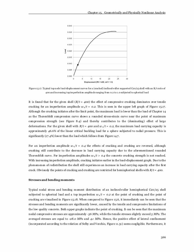
Chapter 15. Geometrically and Physically Nonlinear Analysis
366
Figure 15.17. Typical top node load-displacement curves for a (cracked) inclined-roller supported C20/25 shell with an R/t ratio of
400 and increasing top imperfection amplitude ranging from 0.2 to 1.0 subjected to spherical load
It is found that for the given shell (R/t = 400) the effect of compressive crushing dominates over tensile
cracking for an imperfection amplitude w0/t = 0.2. This is seen in the upper left graph of Figure 15.17.
Although the crushing initiates after the limit point, the maximum load is lower than the load of Chapter 14
as the Thorenfeldt compression curve shows a rounded stress-strain curve near the point of maximum
compression strength (see Figure 8.4) and thereby contributes to the (dominating) effect of large
deformations. For the given shell with R/t = 400 and w0/t = 0.2, the maximum load carrying capacity is
approximately 46.6% of the linear critical buckling load for a sphere subjected to radial pressure. This is
significantly (17.4%) lower than the load which follows from Figure 14.7.
For an imperfection amplitude w0/t = 0.4 the effects of cracking and crushing are reversed, although
crushing still contribute to the decrease in load carrying capacity due to the aforementioned rounded
Thorenfeldt curve. For imperfection amplitudes w0/t > 0.4 the concrete crushing strength is not reached.
With increasing imperfection amplitude, cracking initiates earlier in the load-displacement graph. Due to the
phenomenon of redistribution the shell still experiences an increase in load carrying capacity after the first
crack. Obviously the points of cracking and crushing are restricted for hemispherical shells with R/t = 400.
Stresses and bending moments
Typical nodal stress and bending moment distribution of an inclined-roller hemispherical C20/25 shell
subjected to spherical load and a top imperfection w0/t = 0.2 at the point of crushing and the point of
cracking are visualised in Figure 15.18. When compared to Figure 15.6, it immediately can be seen that the
stresses and bending moments are significantly lower, caused by the tensile and compressive limitations of
the low quality concrete. Both upper graphs indicate the point of crushing. It can be seen that the maximum
nodal compressive stresses are approximately -36 MPa, while the tensile stresses slightly exceed 5 MPa. The
averaged stresses are equal to -28.0 MPa and 4.1 MPa. Hence, the positive effect of lateral confinement
(incorporated according to the relation of Selby and Vecchio, Figure 11.31) seems negligible. Furthermore, it

Chapter 15. Geometrically and Physically Nonlinear Analysis
367
is observed that the axial tensile stress is violated but no cracking occurs. This can be contributed to the
stress mapping operation from the integration points towards the nodes. Obviously, the stresses in the
integration points do not violate the axial tensile strength.
Figure 15.18. Typical nodal stress and bending moment distributions in a hemispherical shell subjected to radial pressure at the
point of crushing (upper) and crack initiation (lower) for a shell with R/t = 400 and w0/t =0.2
The lower graphs of Figure 15.18 illustrate the point of crack initiation. It can be seen that the maximum
nodal tensile stresses further increase to approximately 8.5 MPa whereas the nodal compressive stresses
increase up to almost 40 MPa. The averaged stresses are, however, approximately 5.19 MPa and 28.5 MPa.
Effect of increasing imperfection amplitude
Similar to Section 15.2 the decrease in load carrying capacity can be plotted against the effect of increasing
top imperfection amplitude. The result is seen in Figure 15.19. It can be seen that the effect of cracking leads
to a significantly lower critical load which, additionally, is bounded by the crushing strength for imperfection
amplitudes w0/t < 0.2. The initial crushing path is a dotted line, as lateral confinement may lead to a higher
crushing strength and, thus, a higher allowable critical load. Quantitatively, the decrease in load carrying
capacity for w0/t > 0.2 can in short be written as 46.6%, 35.5%, 27.1%, 21.6% and 17.8%. Hence, the

Chapter 15. Geometrically and Physically Nonlinear Analysis
368
difference at the maximum imperfection amplitude is equal to 14.2% which means that the linear critical
buckling load needs to be multiplied with a factor 0.556 to include the effects of tensile cracking. The total
knock-down factor (large deformations, imperfections and cracking) for this particular shell with maximum
imperfection amplitude, thus, becomes 0.556 × 0.32 = 0.178.
0,0
0,1
0,2
0,3
0,4
0,5
0,6
0,7
0,8
0,9
1,0
0 0,2 0,4 0,6 0,8 1
w0/t
Pcr
gpn
l /Pcr
lin
Inclined-roller,uncrackedand uncrus hed
Inclined-roller, crackedand crus hed
Figure 15.19. Effect of initial geometrical imperfections, cracking and crushing on the critical load for hemispherical C20/25 shell
with top imperfection subjected to spherical load for an R/t ratio equal to 400
For the graph of Figure 15.19, it is assumed that the crushing strength limits the graph to a load which is
equal to 66% of the linear critical buckling load. For the given shell (R/t = 400, E = 30 GPa and v = 0.2) this
equals the compressive strength of the shell (-28 MPa). Strangely enough the effect of cracking for higher
imperfection amplitudes, which occurs more earlier in the load-displacement graph every time the
imperfection is increased, does not has significant influence on the decrease in load-carrying capacity (stays
approximately 13-14%). Apparently, the effect of cracking, partly compensated for by the increase of internal
lever arm, takes ov er the combined effect of loss of linearity and crushing in compression, leading to a
maximum critical load caused by a combination of cracking and buckling.
Cracking
The cracks that appear in the C20/25 hemisphere show similar scatter as the cracks presented in Figure 15.7
and 15.8. Obviously, the crack strains are different. The crack strains are discussed later in Section 15.6.
Different R/t ratios
For thicker shells the point of cracking as well the point of crushing moves towards the prebuckling path and
will become dominant for the load carrying capacity at a certain point. Thinner shells (R/t > 600) do not
experience crushing at all, as can be seen in Figure 10.6, and the effect of cracking is much smaller. However,
all shells fail due to buckling and crushing or due to buckling and cracking, opposite to Section 15.2 for which
the thinnest shell (R/t = 1000) did not experienced a further decrease in critical load due to cracking. The
load carrying capacity of different R/t ratios is visualised in Figure 15.20.

Chapter 15. Geometrically and Physically Nonlinear Analysis
369
0,0
0,1
0,2
0,3
0,4
0,5
0,6
0,7
0,8
0,9
1,0
0 0,2 0,4 0,6 0,8 1
w0/t
Pcr
gp
nl /P
crlin
Uncracked
R/t = 1000
R/t = 600
R/t = 400
Figure 15.20. Influence of increasing imperfection ampli tude on a cracked or crushed (for R/t = 400, w0/t = 0.0) C20/25
hemispherical shell with inclined-roller support and top imperfection subjected to spherical load for several R/t ratios
In Figure 15.20 it can be seen that the critical loads at maximum imperfection amplitude are equal to 17.8%
(R/t = 400), 24.8% (600), 27.0% (800) and 29.3% (1000). Aforementioned, the shell with R/t ratio equal to
400 experiences crushing for small imperfection amplitudes (w0/t < 0.2) and, thus, does not reach the linear
critical buckling load.
15.4.2 Zeiss 1, 3 and 4
The results above correspond to the inclined-roller supported Zeiss 2 shell. The influence of a roller, hinged
or clamped support is illustrated in Figure 15.21.
0,0
0,1
0,2
0,3
0,4
0,5
0,6
0,7
0,8
0,9
1,0
0 0,2 0,4 0,6 0,8 1
w0/t
Pc
rgp
nl /P
crli
n
UncrackedR/t = 1000R/t = 600R/t = 400ClampedHingedRoller
Figure 15.21. Effect of initial geometrical imperfections and cracking on the critical load for hemispherical C20/25 shell with top
imperfection subjected to spherical load for several R/t ratios and support conditions

Chapter 15. Geometrically and Physically Nonlinear Analysis
370
In Figure 15.21 it can be seen that only the roller supported shell influences the curves as obtained for the
Zeiss 2 shell without confinement. As the linear critical buckling load is lower, the roller shell under
spherical pressure load fails due to buckling with axial tension in the boundary layer if the imperfection
amplitude w0/t < 0.2. The lines of the clamped and hinged supported shells are not important for a shell
with R/t < 400. Their linear critical buckling loads are so high that they show premature failure on
compressive crushing. Hence, they follow the line of the inclined-roller shell. It can be concluded that for
imperfection amplitudes w0/t ≥ 0.2 the shell fails independent of the type of support.
With respect to other R/t ratios it is observed that, for an R/t ratio equal to 200, the roller support linear
critical load coincides with the crushing load and boundary conditions do not influence the load carrying
capacity at all. Aforementioned, for R/t ratios equal to 600 (turning point, see Figure 10.6), 800 and 1000,
the crushing load is not important anymore as the shell fails by a combination of large deformations and
cracking. Hence, the curve of an inclined-roller shell starts, by definition, at 1.0 for w0/t = 0.0 and the
influence of the supports can be plotted similar to Figure 15.10. Obviously, the curves are bounded by a
different line for the cracked inclined-roller shell as there is referred to the C20/25 shell here.
15.5 Results C20/25 Shell under Vertical Load
In Section 15.3 it is discovered that the UHPFRC shell under vertical load, by definition, fails mainly due to
surpassing the axial tensile stress of the C180/210 in the boundary layer after which buckling occurs, as can
be seen in Figure 15.11. Hence, the shell constructed from the low quality concrete C20/25, with an even
lower axial tensile strength, experiences a similar failure mode. As a consequence, an initial geometrical
imperfection at the top of the shell can be neglected and, moreover, the conventional reinforced concrete
must be modelled according to the left bilinear relation of Figure 15.3.
15.5.1 Zeiss 1, 2, 3 and 4
Similar to Section 15.3, the fully nonlinear response of the vertical loaded C20/25 shells is illustrated by
load-displacement curves, stresses and bending moments and crack plots.
Load-displacement relations
The deformation of a vertical loaded C20/25 shell is similar the deformation of a C180/210 shell subjected to
vertical load, seen in Figure 15.11. The load-displacement curves for a cracked C20/25 shell with R/t ratio
equal to 400 and varying supports are presented in Figure 15.22. Crack initiation is marked with a black
spot. The final step of each load-displacement curve is questionable as the analysis failed in finding
convergence in the next step.
From the load-displacement curves it can be seen that the shell fails by cracking as the tensile strength of the
material is violated and buckling as the curves show similar trend as seen in the right graph of Figure 14.1. As
the stress-strain relation is modelled as a bilinear diagram, the cracking suddenly appears in the linear load-

Chapter 15. Geometrically and Physically Nonlinear Analysis
371
displacement curve. In reality a more rounded curve may be expected. Furthermore, it is observed in the
load-displacement curves that, after crack initiation, the point of maximum critical load is not significantly
higher as ‘meridional based’ buckling immediately initiates after the circumferential crack process. Hence,
safety with respect to the ultimate limit state may be dominant over the maximum allowable crackwidth,
although it is argued in Section 15.1 that the finite element solution must be bounded by the maximum
crackwidth as dictated by the serviceability limit state. This is discussed further in Section 15.6.
0,000
0,001
0,002
0,003
0,004
0,005
0,006
0 0,5 1 1,5 2 2,5 3 3,5 4
Displacement (R/t = 400, Roller)
Loa
d
0,000
0,001
0,002
0,003
0,004
0,005
0,006
0,007
0 10 20 30 40 50
Displacement (R/t = 400, Inclined-roller)
Loa
d
0,000
0,001
0,002
0,003
0,004
0,005
0,006
0,007
0,008
0 1 2 3 4 5 6 7 8
Displacement (R/t = 400, Hinged)
Loa
d
0,000
0,001
0,002
0,003
0,004
0,005
0,006
0,007
0,008
0,009
0 2 4 6 8 10 12
Displacement (R/t = 400, Clamped)
Loa
d
Figure 15.22. Typical top node load-displacement curves for several support conditions for a C20/25 hemispherical shell subjected
to uniform vertical load with an R/t ratio equal to 400
The maximum load as obtained from the finite element analysis are summarised in Table 15.4. It can be seen
that, similar to the results of Section 15.3, the shell fails approximately at the same magnitude of external
applied load for each type of support. As one would expect, based on the linear stress distribution of the
circumferential stresses as seen in the figures of Chapter 12, the clamped support yields the maximum
allowable load, although it is only 0.00804 MPa (8.0 kN/m2).

Chapter 15. Geometrically and Physically Nonlinear Analysis
372
Name P crgpnl (MPa)
Zeiss 1 0.00554
Zeiss 2 0.00612
Zeiss 3 0.00708
Zeiss 4 0.00804
Table 15.4. Critical load for hemispherical C20/25 shell with R/t = 400 subjected to uniform vertical load
When the results of Table 15.4 are compared to the critical load of Table 15.2, it can be concluded that the
critical loads are approximately 4 times lower. Remarkable (or not) this is more or less the difference in axial
tensile strength between the UHPFRC and conventional concrete mixture. Hence, the given shell under
vertical load can be approximately 4 times thinner if the shell is fabricated using C180/210. For the given
hemispherical shell geometry (R = 12500 mm, t = 60 mm), this means that the thickness (theoretically) can
be reduced to just 15 mm.
The results of the cracking and buckling failure can be compared to the linear critical buckling load of a
spherical shell under radial pressure as defined in Chapter 6. Moreover, the results can be compared to the
buckling loads found in Chapter 13 assuming linear elastic material behaviour. When compared to the
results of Chapter 6 and Chapter 13, it can be said that the introduction of cracking lowers the critical load
drastically. The decrease in load carrying capacity is seen in Table 15.5.
Name P crgpnl/P crlin, equa tion (6.63) P crgpnl/P crlin, chapter 13
Zeiss 1 2.8 % 10.8 %
Zeiss 2 3.1 % 5.5 %
Zeiss 3 3.5 % 8.6 %
Zeiss 4 3.9 % 6.3 %
Table 15.5. Cri tical load for hemispherical C20/25 shell with R/t = 400 subjected to uniform vertical load
It can be observed that for hemispherical shells subjected to uniform vertical load, the introduction of
material nonlinearities, which cause strength failure rather than buckling failure, lead to critical loads which
are as low as 5.5% of their linear critical buckling load and 2.8% of the linear critical buckling load for
spherical shell under radial pressure load.
Stresses and bending moments
In Figure 15.20 the stress distribution at the point of crack initiation of a C20/25 hemisphere with R/t = 400
subjected to uniform vertical load is presented, for all considered support conditions. In the stress
distribution, the effect of reaching the axial tensile stress of 2.2 MPa can be seen. Similar to Section 15.3, in
case of an increasing external load, stress redistribution cause a horizontal plateau to develop, with a
magnitude equal to the tensile strength. Clearly the effect of the initial geometrical imperfection, which is
equal to w0/t = 1.0, causes the disturbances at the top of the shell, however does not influence the maximum
critical load. When the graphs of Figure 15.20 are compared to the graphs of Figure 15.13, it can be seen that
the tensile stresses are approximately 4 times lower.

Chapter 15. Geometrically and Physically Nonlinear Analysis
373
-4
-3
-2
-1
0
1
2
3
0 5 10 15 20 25 30 35 40
Distance (m) (Roller)
Stre
sse
s (M
Pa)
-5
-4
-3
-2
-1
0
1
2
3
0 5 10 15 20 25 30 35 40
Distance (m) (Inc lined-roller)
Stre
sse
s (M
Pa)
-5
-4
-3
-2
-1
0
1
2
3
0 5 10 15 20 25 30 35 40
Distance (m) (Hinged)
Stre
sse
s (M
Pa)
-6
-5
-4
-3
-2
-1
0
1
2
3
0 5 10 15 20 25 30 35 40
Distance (m) (Clamped)
Stre
sse
s (M
Pa)
Figure 15.23. Stress distribution at crack initiation of a C20/25 hemisphere with R/t = 400 under vertical load for several supports
The bending moment distribution is not shown as it has a similar to Figure 15.6. This is caused by the fact
that the bending moments at the imperfection are far higher than the bending moments resulting from the
so-called edge disturbance.
Cracking
The cracks that appear in the C20/25 hemisphere subjected to vertical load show similar scatter as the
cracks presented in Figure 15.15. A crack scatter is shown in Figure 15.24.
Figure 15.24. Typical finite element crack scatter propagation in hemispherical shells subjected to vertical load

Chapter 15. Geometrically and Physically Nonlinear Analysis
374
Typically, cracked reinforced concrete demonstrates a few wide cracks rather than a large amount of small
cracks. However, as the reinforced concrete is modelled with a bilinear law this does not occur (the cracks in
the left shell are very small and immediately transform to a distributed crack pattern in the next load step).
Different R/t ratios
For the C20/25 low quality of concrete (with low quality and percentage of reinforcement), the structural
failure due to surpassing the axial tensile strength is independent of R/t ratios between 200 and 1000.
15.6 Practical Considerations
In the previous sections the load-displacement curves are evaluated by their maximum load-carrying
capacity. However, as cracking initiates before the maximum load is reached, the shell may be disqualified
by the maximum crackwidth as dictated by the serviceability limit state. Especially for the conventional
concrete mixture the serviceability may be dominant, e.g. the axial tensile behaviour is modelled with a long
horizontal branch in the bilinear stress-strain relation allowing cracks up to 11 mm.
To obtain a quantitative boundary for the crackwidth, in Table 15.6 a series of crackwidths are summarised
together with their corresponding crack strains (determined by reversing equation (11.66)). For an
environmental class 5 (aggressive conditions), the maximum allowable crackwidth is equal to 0.2.
Crack width (mm) Crack strain (‰)
0.1 0.27
0.2 0. 54
0.3 0.81
0.4 1.08
Table 15.6. Crack width – crack strain relationship based on fracture energy regularisation
For a maximum allowable crackwidth equal to 0.2 mm and no safety factors applied, the following
observations can be made. For C180/210 shells, the maximum load carrying capacity is determined by the
ultimate limit state. Thus the maximum critical load can be derived from the load-displacement curves. The
maxima are bounded by (a combination of) buckling and nonlinearity of concrete in tension (loss of linearity
when the hardening branch initiates and cracking). Also for C20/25 shells subjected to vertical load the
ultimate limit state is dominant. The maximum critical load, determined by significant cracking after which
buckling occurs, is bounded by the ultimate limit state as the critical load does not significantly increases
after crack initiation. The serviceability limit state only determines the maximum allowable displacement
(when the crackwidth violates the norm). For C20/25 shells subjected to spherical load, the serviceability is
decisive if cracking occurs far before the limit point. In all other situations the ultimate limit state prevails
and the maximum critical load is bounded by (a combination of) buckling, nonlinearity of concrete in
compression (loss of linearity and crushing) and nonlinearity of concrete in tension (cracking). E.g. applying

Chapter 15. Geometrically and Physically Nonlinear Analysis
375
a maximum allowable crackwidth 0.2, the critical load of the last three graphs of Figure 15.16 decreases
significantly to 0.0513 MPa, 0.0323 MPa and 0.0244 MPa, respectively.
15.7 Material Comparison
From the foregoing it can be seen that UHPFRC shells are able to carry much higher loads than their
conventional concrete equivalents. In case of vertical load, for a given shell (R/t = 400) the maximum critical
load of the C20/25 shell is approximately 25% of the C180/210 shell. Remarkable (or not) the factor of 4 is
approximately the difference between the axial tensile strength of both mixtures. Consequently, the
C180/210 shell can be 4 times thinner than a shell constructed from C20/25 concrete. This happens to be
true for all R/t ratios (200 – 1000) included in this research. Hence, for vertical loaded shells, the axial
tensile strength of the UHPFRC in compare to conventional concrete governs the difference in maximum
critical load.
In case of a shell R/t = 400 subjected to spherical load, with inclined-r0ller support and initial geometrical
top imperfection, the difference in maximum critical load between C180/210 and C20/25 is summarised in
Table 15.6. The values denoted with * are values bounded by the maximum crackwidth of 0.2 mm (see
Section 15.6).
w0/t UHPFRC Load (MPa) C20/25 Load (MPa) Difference C/UHPFRC (%)
0.2 0.262 0.0888 0.173 33.9
0.4 0.189 0.0708 0.118 37.5
0.6 0.144 0.0513* 0.093 35.6
0.8 0.118 0.0323* 0.086 27.4
1.0 0.100 0.0244* 0.076 24.4
Table 15.6. Difference in maximum allowable cri tical load based on a maximum crackwidth of 0.2 mm for an inclined-roller
supported hemisphere with R/t = 400 and an initial geometrical imperfection at the top subjected to spherical load
In Table 15.6 it can be seen that the maximum difference is 24.4% (7.6 kN/m2), in case of an imperfection
w0/t = 1.0. This means that the shell made from the C20/25 is able to carry only one quarter of the load of
the shell made from the C180/210 mixture. For larger imperfections, it may be expected that the difference
will be even larger; however, this is counteracted by the fact that cracking of the C180/210 starts to influence
the maximum point in the load-displacement curve (see Figure 15.4).
The given shell with maximum imperfection, however, cannot be four times thinner when using the chosen
C180/210 over C20/25. This is caused by the fact that the thickness of the shell appears quadratically in the
buckling relation. Moreov er, the effect of loss on linearity and cracking is different for different R/t ratios.
As an example, the given shell R/t = 400 with given material properties can be reduced to R/t = 700, based
on the maximum critical load as found in by DIANA, while the shell can be reduced to R/t = 800 when the
maximum allowable crackwidth (Table 15.6) is taken into account.

Chapter 15. Geometrically and Physically Nonlinear Analysis
376
For small imperfections (w0/t < 0.2) in combination with a low quality of concrete and a relative thick shell
(R/t ratio between 200 and 400), it is found that compressive crushing is decisive above buckling failure
(strength failure). E.g., for a shell R/t = 400 crushing leads to a load which is 34% lower than the elastic
theory while for a shell R/t = 200 the load is just 50% of the elastic theory. Using the given C180/210 the R/t
ratios can be increased to 700 and 400, respectively. Hence, the use of UHPFRC is advantageous to prevent
the negative effect of compressive crushing on the load carrying capacity
15.8 Knock-Down Factor Approach
In Chapter 14, the knock-down factor that incorporated effects of large deformations and initial geometrical
imperfections was defined at a value of 68%, thus the decrease in load carrying capacity is determined by
multiplication with 0.32. It is observed in the results described abov e that cracking and crushing lead to a
further decrease in load carrying capacity, except for the thinnest C180/210 shell. In fact, for vertical loaded
shells, cracking appeared to be dominant after which buckling occurs. Hence, for vertical loaded shells, the
knock-down factor is superfluous as the failure load can be determined simply by computing the
circumferential stresses. This is not the case for shells subjected to spherical load. However, opposite to the
general influence of large deformations and initial geometrical imperfections, the general effects of crushing
and cracking (both accompanied by loss of linearity) on spherical loaded shells cannot be reduced to a
simple graph or equation. A different shell thickness, imperfection, boundary condition and material
property leads to an enormous scatter of results. Therefore, it is not possible to formulate a general
expression for the knock-down factor which determines the decrease in load-carrying capacity for a
hemispherical shell under spherical load. However, as can be seen in the results reported abov e, it is possible
to determine the fall-back in load carrying capacity for a specific case by introducing initial geometrical
imperfections and material nonlinearities in a geometrically and physically nonlinear finite element analysis.
Based on the observation that it is possible to find the knock-down factor of a specific case, valuable
conclusions can be drawn by determining the knock-down factor for the most onerous situation. In Figure
15.19 it can be seen that for a R/t 400 shell subjected to spherical load with an imperfection amplitude equal
to the shell thickness leads to a knock-down factor of 82.2% (multiplication by 0.178), independent of the
boundary conditions. Hence, for thinner shells, a higher quality of concrete or a higher percentage of
reinforcement, the decrease in load carrying capacity will be less. If the additional cracking multiplication
factor (0.556) is compared to the one found in Chapter 10, using the IASS Recommendations (0.2), it is
observed that the latter leads to a load capacity which is significantly lower. Most likely, the large
discrepancy may be explained by the conservative approach of the IASS Recommendations. The
recommendations provide in a crack parameter based on reinforcement percentages and (reduced) material
stiffness and does not take into account for geometrical influences such as the point of crack initiation in
case of a varying R/t ratio. Furthermore, the crack parameter of the IASS Recommendations is based on the
hypothesis of a so-called second state of reinforced concrete structures, i.e. assuming a cracked tensile zone
but still linearly elastic behaviour over the cross-section of the shell. The DIANA results yield a nonlinear
stress distribution over the cross-section which, as can be seen in Figure 8.19, may lead to a large
discrepancy between elastic and plastic behaviour.

Chapter 15. Geometrically and Physically Nonlinear Analysis
377
15.9 Conclusions
Before reading the following conclusions, one must keep in mind that they are based on shell analy sis
involving shells with R/t ratios between 200 and 1000 and a local imperfection at the top of the shell.
Furthermore, the shell is loaded by uniform pressure or v ertical load. The results are based on a
geometrically and physically nonlinear finite element analysis. The material behaviour is implemented in a
so-called total strain rotating crack model according to Section 15.1.3. I.e. a multi-linear tensile relation and
an infinite linear elastic compressive relation for the UHPFRC and a compressive behaviour according to the
Thorenfeldt curve for the conventional concrete combined with either a bilinear or brittle tensile relation,
depending on the type of failure (axial tensile or flexural tensile failure, respectively).
Hemispherical shells subjected to uniform spherical load (or shells confined to their compression zone such
that the vertical load can be approximated by a spherical load):
From the results obtained by a geometrically and physically nonlinear analysis on hemispherical shells
subjected to uniform spherical load, it can be concluded that spherical load leads to flexural tensile failure or
compressive crushing in the region of the initial geometrical imperfection. For a spherical load the results
are independent of the location of the imperfection if and only if the imperfection does not interact with
(possible) edge disturbances. Depending on the R/t ratio, the imperfection size and the properties of the
concrete, the maximum critical load is determined by cracking, crushing, buckling or a combination. The
effects of cracking and crushing are accompanied by reduced material stiffness due to loss of linearity; at the
initiation of the hardening branch in the C180/210 tensile relation and due to the ‘rounded’ Thorenfeldt
curve used to model the compressive behaviour of the C20/25 mixture (Chapter 8). Thus, besides the
cracking and crushing, an additional decrease in load carrying capacity is caused by this loss of linearity.
In general, for thicker shells cracking and loss of linearity in tension are more prevalent than for thinner
shells, governed by the fact that thicker shells experience bending up to a higher degree. Very thin shells of
high quality concrete may not experience any negative influence of cracking at all. Then, the critical load is
exclusively determined by buckling, as observed for the thinnest C180/210 shell (R/t = 1000). The
increasing influence of cracking is clearly seen in the load-displacement curves as the point of crack
initiation moves further and further towards the origin of the graph as the shell becomes thicker (Figure
15.9). The same phenomenon occurs in case of an increasing imperfection amplitude (Figure 15.4). As an
increasing imperfection causes substantial higher bending moments and stresses, the point of crack initiates
moves towards the origin of the load-displacement curve which, consequently, leads to an increased
discrepancy between the theoretical critical load and the critical load as obtained by DIANA. An increasing
imperfection also leads to a critical load independent of the boundary conditions if w0/t > 0.4. For smaller
imperfections, w0/t < 0.4, boundary conditions cannot be neglected and lead to considerable lower loads
than found for the ‘membrane’ inclined-roller supported shell which provides in an upper bound solution.
I.e. a roller support leads to a maximum critical load of approximately 50% of the critical load for an
inclined-roller supported shell. Moreover, small imperfections in combination with a low quality of concrete
may lead to a failure by compressive crushing, as observed for the C20/25 shell with a load 34% lower than
the elastic shell.

Chapter 15. Geometrically and Physically Nonlinear Analysis
378
In case of a spherical loaded hemispherical shell, the expectation that UHPFRC can contribute to more
slender shells may said to be confirmed. In case of a failure due to surpassing the flexural tensile strength,
the UHPFRC shell can carry significant higher loads than the same shell fabricated from a low quality of
concrete, mainly due to the higher axial tensile strength and Young’s modulus. Therefore, UHPFRC may lead
to a thinner shell; however, the possibilities are counteracted by the importance of the thickness parameter
in the buckling process. Furthermore, the effect is less then expected due to the fact that the advantageous
postcracking plateau of UHPFRC has no influence on the maximum critical load and is only related to the
inclination of the postbuckling path. I.e. the inclination of the decreasing postbuckling path is much less in
compare to conventional concrete without fibre addition and only one layer of reinforcement. This might be
caused by the buckling which occurs simultaneously with significant cracking. Quantitatively, for the given
concrete mixtures and a maximum imperfection amplitude w0/t = 1.0, cracking leads to a critical load as low
as 23% (R/t = 400), 24% (600), 25% (800) and 33% (1000) in case of a C180/210 shell and 18% (400), 25%
(600) and 29% (1000) in case of a C20/25 shell of the theoretical linear critical buckling load of a sphere
under spherical load. Based on the critical load and cracking influence as found by DIANA, the C20/25 shell
R/t = 400 can be reduced to R/t = 700 when using C180/210.
Besides the high flexural tensile strength and Young’s modulus, the use of UHPFRC can be advantageous
with respect to compressive crushing. Aforementioned, for small imperfections and a low quality of concrete,
crushing may be decisive for failure. In case of a sufficient UHPFRC mixture crushing does not occur (and,
hence, the material can be modelled as infinite elastic in compression). As an example: for a C20/25 shell
R/t = 400 crushing leads to a load which is 34% lower than the elastic theory while for a C20/25 shell R/t =
200 the load is just 50% of the elastic theory. Using C180/210 the R/t ratios can be increased to 700 and
400, respectively.
From the obtained results it is impossible to formulate a general expression which defines the knock-down
factor for an arbitrary shell structure. However, it is observed that it is possible to determine (within the
scheme of a master thesis) the fall-back in load carrying capacity for a specific case by introduction of initial
geometrical imperfections and material nonlinearities in a geometrically and physically nonlinear analysis.
Thus, although the analysis involving shells may not be reduced to a simple expression (and may never be),
contemporary finite element procedures allows the engineer to find answers to questions within days (based
on current status of the author) were it took historical mathematicians years, decades or even centuries.
Based on the observation that it is possible to find the knock-down factor of a specific case, valuable
conclusions can be drawn by determining the knock-down factor for the most onerous situation. In this
thesis, the most onerous situation (R/t 400, C20/25, w0/t = 1.0) a knock-down factor of 82.2%
(multiplication by 0.178) is found, independent of the boundary conditions. Herein, the additional effect of
cracking yields a multiplication factor of 0.556. Previously, in Chapter 10, a cracking factor equal to 0.2 was
found using the IASS Recommendations. The large discrepancy may be explained by the conservative
approach of the IASS Recommendations, i.e. neglecting the influence of the R/t ratio on the point of crack
initiation and assuming a cracked tensile zone but still linearly elastic behaviour.

Chapter 15. Geometrically and Physically Nonlinear Analysis
379
With respect to the numerical process it must be mentioned that the analyses were numerically more stable
in case of a multi-linear tensile diagram as used to model fibre reinforced C180/210, than when using the
brittle behaviour describing the tension relation of C20/25 with one layer of reinforcement.
Hemispherical shells subjected to uniform vertical load:
From the results obtained by a geometrically and physically nonlinear analysis on hemispherical shells
subjected to uniform vertical load, it can be concluded that the shell, by definition, fails due to surpassing the
axial tensile strength in circumferential direction after which buckling occurs in meridional direction. As the
material degradation is responsible for the major part of the fall-back in load carrying capacity, the failure
load can approximated by determining the membrane stresses and calculate the failure load by simple
equating using the axial tensile strength of the material. Thus, the knock-down factor is superfluous,
however, based on the observation that the thickness appears quadratically in the buckling equation, it can
be expected that for a given R/t ratio buckling becomes dominant. Due to the failure in the boundary layer,
the maximum critical load is not influenced by a local top imperfection. Consequently, the cross-sectional
stress distribution at the imperfection stays linear. With respect to the support conditions, it can be
concluded that the type of support does not change the maximum critical load significantly. Within a small
range the roller support provides in the lowest critical load, followed by the inclined-roller, hinged and
clamped support. This observation is in fair agreement with the magnitude of circumferential tensile stresses
found in Chapter 12.
With respect to the concrete quality, also for vertical loaded shells the expectation that UHPFRC can
contribute to more slender shells may said to be confirmed. The difference in maximum allowable load is
mainly governed by the difference in axial tensile strength of the given materials. Consequently, the
UHPFRC shell can be thinner by the ratio of UHPFRC axial tensile strength over conventional concrete axial
tensile strength. For the given concrete mixtures, this results in a shell which can be approximately 4 times
thinner. Qualitatively, due to the multi-linear tensile relation of UHPFRC with strain hardening branch
(Figure 15.2), the corresponding load-displacement curve show sudden appearing cracks and lead to
solutions with bad convergence. The bilinear approach of the conventional mixture is much more
numerically stable and cracking ends the linear branch of the load-displacement curve (which obviously
makes sense).


Chapter 16. Conclusions
381
16 Conclusions
The conclusions reported in the following, summarise the most important conclusions of the individual
chapters. A more extensive conclusion can be found at the end of each chapter. The conclusions are ordered
corresponding to their occurrence in the thesis, i.e. conclusions with respect to Part I: Background, Part II:
Theory, Part III: Case Study and Part IV: Finite Element Analysis. In the end, the general conclusions are
discussed point wise. The figures in this chapter correspond to figures of previous chapters and are indicated
by the same subscription.
16.1 Part I Conclusions
Shell structures have been constructed since ancient times. Early examples are the Roman Pantheon and the
Hagia Sophia. In the 18th and 19th century, however, the art of designing shells seemed to be forgotten.
Guided by German designers Franz Dischinger and Ulrich Finsterwalder, the shell made a comeback in the
early 20th century. The modern era of shell started in 1925 with the completion of the Zeiss planetarium shell
in Jena. The modern era is recognised by the trend towards greater spans and thinner shells. Besides
Dischinger and Finsterwalder, Pier Luigi Nervi, Eduardo Torroja and Anton Tedesko were among the first
shell builders. In fact, their specific design approach has lead to three prominent design schools; the German
school, the Italian school and the Spanish school. Up to the Second World War shells gained more and more
interest to cover medium to large spans economically and aesthetically. After the Second World War, the low
labour costs and steel being in short supply created exactly those conditions needed for flourishing shell
construction, leading to a blooming period of widespread shell construction between 1950 and 1970. The
blooming period was further stimulated by the work of Felix Candela which attracted the attention of
architects. The inv olvement of architects leaded to more luxury shapes with less emphasis on the force flow.
The blooming period ended abruptly, mainly caused by the high costs in compare to other structural
sy stems. Still, Swiss engineer Heinz Isler was able to continue designing shells by innovative reusable
formwork. Isler may also said to be the founder of free-form shells, designed by using form-finding
techniques such as hanging membranes. Hence, it seems fair to add the Swiss school as the fourth prominent
design school. Late 20th century shell development leaded to pioneering formwork techniques and several
new shell-like structures such as grid shells. Today, there seemed to be a renewed interest in shells,
stimulated by the desire to built landmark structures and by the fascination to new construction materials
such as ultra high performance concrete.

Chapter 16. Conclusions
382
Shells typically show membrane behaviour with bending effects to satisfy specific equilibrium or
deformation requirements. The stresses in shells can be determined by hand, e.g. using the classical shell
theory or by computer, e.g. using finite element software. Furthermore, model tests provide in a very
practical and convenient method to determine the structural response. They are classified according to their
Gaussian curvature and generated by mathematical functions or form-finding techniques. To design a sound
shell structure, the designer must prevent in-extensional deformation, allow for membrane stresses to
develop, add sufficient curvature everywhere, and take care of edge effects. Subsequently, the designer
should optimise the shape and thickness of the shell for buckling and membrane dominant behaviour
(minimising strain energy). Shells are low reinforced structures and prestressing may be applied to balance
the outward thrust or to ensure compression in the shell surface. Effects of crushing, cracking, creep and
shrinkage of concrete and the effect of temperature gradients significantly influence the structural response
and must be included in the design process.
Shells are predominantly constructed by pouring concrete on a conventional timber formwork. The timber
formwork allows for almost every possible shell shape to be constructed. For highly double curved sections,
the timber formwork can be replaced by foamed plastic (polystyrene) formwork fit into shape with a CNC
milling cutter. The main disadvantages of conventional formwork are the high costs inv olved. Therefore,
prefabricated moulds, airform techniques and stressed membranes have been developed to serve as
formwork. Furthermore, shells may be assembled from prefabricated elements to save on costs. However,
for several reasons, none of them gained widespread use. The choice for a particular formwork may not only
influence the design of the shell, but also puts restrictions on the placement and design of the reinforcement
and the concrete mixture. The placement of reinforcement on double curved surfaces follows ordinary
principles, however, for airform construction methods the reinforcement may be asked to autoposition itself.
The placement of concrete is either by skip of sprayed. Generally, after hydratation, the concrete is left
untreated and maintenance is limited to occasionally whitewashing.
16.2 Part II Conclusions
The classical shell theory can be used to determine the stresses, strains and deformations in an idealised
linear elastic shell. The theory is a thin shell theory, an extension of the Kirchhoffean plate theory. The
assumption that the thickness of the shell is much smaller than the radius of curvature yields that the
flexural rigidity is much smaller than the extensional rigidity which is the reason that shells mainly carry
their load by in-plane normal and shear stresses. Stresses or strains in normal direction are of no
significance to the solution, reducing the three-dimensional problem to a surface deformation problem.
Bending moments only compensate for the shortcomings of the membrane field and do not carry loads. As
shells are essentially curved plates, the extensional and flexural problem are coupled, even for the linear
case. The combined stretching and bending can be described by the membrane theory in combination with
plate bending behaviour which can be calculated separately and superimposed.
Shells fail by a buckling or by strength. Strength failure refers to cracking or crushing being the dominant
failure mechanism and is governed by the material properties. If the shell mainly fails by large deformations,

Chapter 16. Conclusions
383
the shell is said to be buckled. Buckling can be characterised as a premature failure mechanism caused by
eccentricity of compression forces, initiated by deformations or initial geometrical imperfections. The
buckling behaviour of shells is a complicated phenomenon. Opposite to columns and plates, shells
experience a sudden decrease in load carrying capacity after the bifurcation point. The fall-back is caused by
the phenomenon of compound buckling which refers to sev eral buckling modes associated with the same
critical load. In the postbuckling range the modes, which were orthogonal in the linear prebuckling range,
start to interact resulting in a significantly reduced load carrying capacity. The major problem of the shell
buckling behaviour is the accompanied imperfection sensitivity. Initial geometrical imperfections in the shell
cause the bifurcation point never to be reached and lead to limit point buckling at a considerably lower load.
The size of the imperfections determines the limit load at which the shell fails.
16.3 Part III Conclusions
To obtain an answer to the research questions, the Zeiss planetarium shell is subject of a case study. The
stresses, strains and displacements in the shell are determined using the aforementioned classical shell
theory for two types of concrete and two types of external applied load. The first concrete mixture is a low
quality C20/25 concrete mixture with a single layer of low quality reinforcement to ally with the early 20th
century concrete technology. Typically, the compressive behaviour can be modelled by a Thorenfeldt curve.
Due to the low quality of reinforcement, the axial tensile relation is mainly determined by the axial tensile
strength of the concrete. Also in case of bending, the flexural tensile strength mainly depends on the concrete
flexural tensile strength as the single layer of reinforcement is activated not before significant cracking has
occurred. The second concrete mixture is a high strength fibre reinforced concrete mixture. The selected
mixture is a so-called ultra high performance concrete which refers to compressive strengths between 155
and 250 MPa. The higher compressive strength originates from an optimised mixture composition. The
major deficiency is the highly brittle behaviour which is counteracted by the addition of fibres. The fibres
work as well on micro-level, as reinforcement of the cement matrix, as on macro-level, as reinforcement of
the structure. They do not necessarily lead to a higher tensile strength, although it is possible to increase the
tensile strength through the addition of fibres with different dimensions. Most advantageous is the low-level
postcracking plateau that leads to a higher toughness and more ductile failure behaviour. The Zeiss
planetarium shell is loaded by dead weight in combination with either wind load or snow, determined
according to the Eurocode 2. The results of the classical shell theory show the profound structural behaviour
of shells as they experience very small stresses, strains and deformations. I.e. the stresses are -0.217 MPa at
the top and ±0.433 MPa at the base, the corresponding strains are -0.00722 ‰ and ±0.0144 ‰ and the
maximum deformation is equal to 0.181 mm. Furthermore, it can be seen that the restrained deformation at
the supports leads to local edge disturbances reaching up to approximately 2 m, with a maximum bending
moment of 403 Nmm/mm’ in case of a clamped support. This means that 90% of the shell is free from
bending. When the shell thickness is reduced, the shell behaves more like a membrane and the influence of
the edge disturbances is even less. The buckling load of the Zeiss planetarium is 802 kN/m2. In case of the
C20/25 concrete this means that crushing occurs before buckling. To determine the load carrying capacity in
case of an imperfect concrete shell, the procedure as proposed by the IASS is followed. According to the IASS
Recommendations, the maximum allowable load, including safety factors, equals 4.33 kN/m2.

Chapter 16. Conclusions
384
16.4 Part IV Conclusions
All following findings and conclusions are restricted to hemispherical shells with R/t 200 – 1000 subjected
to uniform vertical or spherical load. The shell is modelled with an axisymmetric curved line model and a
three-dimensional model consisting of two-dimensional quadrilateral and triangular curved shell elements.
For the geometrically nonlinear analy sis a local top imperfection with an amplitude varying between 0 – 1.0
times the shell thickness is introduced. For the geometrically and physically nonlinear analysis the material
behaviour is implemented in a so-called total strain rotating crack model. The C180/210 UHPFRC is
modelled with a multi-linear tensile relation and an infinite linear elastic compressive relation. The C20/25
is modelled by a compressive behaviour according to the Thorenfeldt curve combined with either a bilinear
or brittle tensile relation, depending on the type of failure expected (axial tensile or flexural tensile failure,
respectively).
16.4.1 Linear Elastic Analysis
The linear elastic analy sis proved to be in fair agreement with the (benchmark) analytical results, except for
the bending moments that appear in the boundary layer due to restrained deformation at the supports. In
particular the axisymmetric shell model yielded bending moments with high discrepancy in compare to the
theory (up to 30%). This is caused by insufficient stress mapping between the ‘exact’ integration points and
the end nodes. Therefore, the axisymmetric shell model is less accurate and reliable in compare to the three-
dimensional model. In addition to the case study of Part III, a non-symmetrical wind load is considered in
combination with dead weight. It is observed that wind load changes the direction of the principal stresses
and is transferred to the supports partly by meridional stresses and partly by shear. The deformed shape,
although different, yields approximately similar deformations as caused by dead weight only as they partly
compensate for each other. In the linear elastic results of the three-dimensional shell model disturbances in
the stress and bending moment distribution were observed, due to the numerical imperfectness of the
model. In particular in the top region of the shell relative large inconsistencies were found. The
imperfectness of the model does not disturb the linear results considerably.
16.4.2 Stability Analysis
The disturbances are more apparent in the linear elastic stability analysis, as the analysis prov ed to be very
sensitive to small numerical disturbances. The numerical disturbances cause premature buckling modes
preceding the actual shell buckling shape; a global scatter of small local waves in a chessboard pattern.
Remarkable, the corresponding critical buckling loads of these premature modes may be nearly similar to
the theoretical critical buckling load. Additionally, several false modes were observed between the correct
buckling modes. Hence, to obtain a good understanding of the buckling behaviour of a shell, it is necessary
to examine both the critical buckling loads as well as their corresponding buckling modes. It is observed that
adjacent buckling loads are very close to each other, revealing the occurrence of compound buckling. In
general, thinner shells experience compound buckling up to a higher degree than thicker shells.

Chapter 16. Conclusions
385
The critical buckling load is significantly lower for membrane incompatible support conditions. This is
caused by the edge disturbances or, in case of a roller support, due to the fact that the support is weaker than
the shell itself. Shells subjected to v ertical load, by definition, buckle in the boundary layer, accompanied by
a much lower bifurcation load. Higher modes advance to global buckling modes similar to the global
buckling behaviour of a radial pressed spherical shell. Simultaneously, the corresponding critical buckling
load approaches the theoretical load of the sphere subjected to radial pressure. The results of the
axisymmetric shell model are poor, as compound buckling is not predicted correctly. Moreover, the
axisymmetry causes the tendency to buckle at the top and the buckling loads are disturbed by the incorrect
bending moments in case of a hinged and clamped support.
Attempts were made to investigate the postbuckling behaviour by a Koiter theory based perturbation and
continuation analysis; however, although the results are not in contradiction with the theory, the results are
poor and no conclusions can be drawn.
16.4.3 Geometrically Nonlinear Analysis
A geometrically nonlinear analy sis on a perfect shell, finds the buckling bifurcation load. It is observed that
perfect shells experience either shell-like buckling with decrease of load-carrying capacity in postbuckling
range or buckling with an almost horizontal postbuckling path. The type of external applied load on the
shell, i.e. uniform spherical or uniform vertical load, determines the type of buckling. For inclined-roller
supported shells subjected to spherical load, the introduction of initial geometrical imperfections leads to
premature limit point failure, as the bifurcation point is never reached. The corresponding load-
displacement relation shows a smooth transition between the nonlinear prebuckling and postbuckling path
of equilibrium, or may experience a sudden snap-through to a non-adjacent equilibrium configuration. Most
likely, the snap-through is a numerical related process and does not occur in reality. The amount of decrease
in load-carrying capacity is governed by the size of the initial geometrical imperfection. This can be seen in
Figure 14.5, which is valid for an inclined-roller supported hemispherical shell subjected to spherical load.
The graph is valid for all R/t ratios.
0,0
0,1
0,2
0,3
0,4
0,5
0,6
0,7
0,8
0,9
1,0
0 50 100 150 200 250 300 350 400
Top node displacements
Pgn
l /Pcr
lin
Figure 14.5. Load-displacement curves of a shell with various initial geometrical imperfection sizes (0, 0.2, 0.4, 0.6, 0.8 and 1.0)
and the minimum postbuckling load as proposed by Dostanowa and Raiser

Chapter 16. Conclusions
386
In Figure 14.8 it can be seen that an initial imperfection equal to the shell thickness causes a fall-back of
approximately 70%. It is observed that the influence of an initial geometrical imperfection on the load-
carrying capacity depends on the size of the imperfection, as can be seen in Figure 14.8. To validate, the
finite element results are be compared to the Koiter half-power law and the graph as proposed by the IASS
Recommendations. It can be concluded that there is reasonable correlation.
0,0
0,1
0,2
0,3
0,4
0,5
0,6
0,7
0,8
0,9
1,0
0 0,2 0,4 0,6 0,8 1
w 0/t
Pc
rgn
l /Pcr
lin Finite Element Results
Half-Power Law
Kollar and Dulacska
Figure 14.8. Comparison between FEA, Koiter half-power law (red) and the curve of Hutchinson/Kollar and Dulacska (blue)
The influence of a different type of load, e.g. uniform vertical load replacing the uniform spherical load, and
different types of support can be incorporated in the graph of Figure 14.8 as illustrated in Figure 14.11.
0,0
0,1
0,2
0,3
0,4
0,5
0,6
0,7
0,8
0,9
1,0
0 0,2 0,4 0, 6 0,8 1
w0/t
P crg
nl /P
crli
n
Incl ined-roller, spherical load
Clamped, spherical load
Hinged, spherical load
Clamped, vertical load
Inclined-roller, vertical load
Roller, spherical load
Hinged, vertical load
Roller, vertical load
Figure 14.11. Decrease in load-carrying capacity due to boundary conditions, loads and initial geometrical imperfections at the top
of the shell for R/t ratios between 200 and 1000
From Figure 14.11 it can be concluded that the inclined-roller supported shell subjected to spherical, which
buckles by definition in the shell surface, is an upper bound solution. Furthermore, it can be seen that a
roller supported shell subjected to v ertical load yields a critical load independent of any top imperfection
(within the range of the R/t ratios investigated). If the roller support it neglected, the shell buckles in the
shell surface when w0/t > 0.6. For imperfection amplitudes w0/t < 0.6 the type of buckling failure depends
on the support condition and type of load.

Chapter 16. Conclusions
387
16.4.4 Geometrically and Physically Nonlinear Analysis
The introduction of material nonlinearity leads to two major effects: (1) the further reduction of the load-
carrying capacity due to cracking and/or crushing (accompanied by loss of linearity) and (2) the
transformation to a strength failure rather than a buckling failure in case of shells subjected to uniform
vertical load. Shells subjected to vertical load mainly fail by violation of the axial tensile strength due to
circumferential tensile stresses at (or near) the base radius of the shell (depending on the type of support).
After significant cracking has occurred, responsible for the major part of the knock-down factor, buckling
ev entually occurs. As the strength failure is governed by the axial tensile strength of the (fibre) reinforced
concrete, the shell can be thinner as much as the difference in axial tensile strength. For the given concrete
mixtures this means that the C180/210 can be 4 times thinner than the C20/25 shell.
Spherical loaded shells, or shells confined to their compression zone such that the vertical load can be
approximated by a spherical load, fail in the region of the imperfection by surpassing the flexural tensile
strength, by compressive crushing, by buckling or a combination. Whether cracking, crushing or buckling
occurs first and to which amount depends on the size of the imperfection, the material properties and on the
thickness of the shell. The C20/25 shell failed due to compressive crushing for small imperfections (w0/t ≤
0.2) combined with a relative thick shell (200 < R/t ≤ 400). The occurrence of crushing lowered the load
carrying capacity up to 50%, for R/t = 200 and w0/t ≥ 0.0). For C180/210 crushing did not occur and, hence,
UHPFRC is advantageous. For thinner shells (R/t ≥ 600), crushing does not occur as buckling prevails.
In case of imperfection amplitudes w0/t > 0.2, crushing is not decisive or does not occur at all and the shell
fails by cracking and buckling. The influence of cracking increases for larger imperfection amplitudes and
thicker shells (gov erned by the fact that thicker shells experience bending up to a higher degree). Thus, the
point of crack initiation moves further and further towards to origin of the load-displacement curve if the
imperfection amplifies or the shell thickness increases. Consequently, for a given imperfection amplitude
and R/t ratio, cracking initiates before, at or after the maximum load carrying capacity. In the latter case, the
maximum load carrying capacity may be influenced by the loss of linearity preceding crack initiation or is
exclusively determined by initial geometrical imperfections and buckling (no influence of cracking at all).
0,0
0,1
0,2
0,3
0,4
0,5
0,6
0,7
0,8
0,9
1,0
0 0, 2 0,4 0,6 0,8 1
w0/ t
Pcr
gp
nl /P
crli
n
UncrackedR/t = 1000R/t = 800R/t = 600R/t = 400R/t = 200ClampedHingedRoller
Figure 15.11. Effect of ini tial geometrical imperfections and cracking on the critical load for hemispherical C180/210 shell with top
imperfection subjected to spherical load for several R/t ratios and support conditions

Chapter 16. Conclusions
388
The influence of buckling, cracking and crushing on the load carrying capacity of the hemispherical shell can
be plotted in a graph for various R/t ratios and support conditions. In Figure 15.11 the influence of cracking
and imperfection buckling can be seen for various R/t ratios for a shell constructed from C180/210 fibre
reinforced ultra high performance concrete. Each line represents an R/t ratio ordered similar as the legend.
It can be concluded that the shell with R/t = 1000 does not experience cracking as it coincides with the
uncracked line. The results of the shell with R/t = 200 are limited, as modelling errors were encountered.
The inclined-roller shell provides an upper bound solution. Edge disturbances or the support being weaker
than the shell itself (roller) cause premature failure in the boundary layer for imperfection sizes w0/t < 0.4.
In case of imperfection amplitudes w0/t ≥ 0.4 the shell fails by surpassing the flexural tensile strength
and/or by buckling in the region of the imperfection, independent of the support conditions. It can be seen
that the influence of cracking leads to a maximum knock-down factor equal to 77% in case of a hemispherical
shell with R/t = 400. Thus, the additional effect of cracking on the load capacity equals 9%.
0,0
0,1
0,2
0,3
0,4
0,5
0,6
0,7
0,8
0,9
1,0
0 0,2 0,4 0,6 0, 8 1
w0/t
Pcr
gp
nl /P
crli
n
UncrackedR/t = 1000R/t = 600R/t = 400ClampedHingedRoller
Figure 15.21. Effect of initial geometrical imperfections and cracking on the critical load for hemispherical C20/25 shell with top
imperfection subjected to spherical load for several R/t ratios and support conditions
In Figure 15.21 the influence of cracking, crushing and imperfection buckling can be seen for various R/t
ratios for a shell constructed from C20/25 reinforced concrete. Each line represents an R/t ratio ordered
similar as the legend. Note that not all R/t ratios are included due to missing results. It can be seen that the
influence of cracking is restricted to the shell with R/t = 400. Crushing lowers the load carrying capacity by
34%. Therefore, the influence of boundary conditions is limited to small imperfection sizes. However, if
crushing not occurs (for thinner shells), the roller support influences the failure up to w0/t = 0.4. Similar to
the C180/210 shell, for imperfection amplitudes w0/t ≥ 0.4 the shell fails by surpassing the flexural tensile
strength and/or by buckling in the region of the imperfection, independent of the support conditions. It can
be concluded from Figure 15.21 that the difference between the lines of R/t = 400 and R/t = 600 is
significantly larger than for a shell constructed from C180/210. This is caused by the much greater influence
of cracking in case of a shell constructed from a low quality concrete with a single layer of reinforcement. For
a shell R/t = 400, it can be concluded that the influence of initial geometrical imperfections, buckling and
material nonlinearity leads to a maximum knock-down factor equal to 82%. Herein the cracking parameter
lowers the linear critical buckling load by 14%.

Chapter 16. Conclusions
389
From the results it can be concluded that the thickness reduction possible due to the use of C180/210 is not
governed by a single parameter but depends on the shell geometry (R/t ratio), the material properties and
the size of the initial geometrical imperfection. For spherical loaded shells, which fail by surpassing the
flexural tensile strength, by compressive crushing, by buckling or by a combination, the advantageous higher
axial tensile strength and Young’s modulus are counteract by the importance of the thickness parameter in
the buckling process. As an example: from the obtained results it can be concluded that a C20/25 shell with
R/t = 400 and one layer of reinforcement can be reduced to R/t = 700 in case of a C180/210 concrete, based
on the maximum load carrying capacity. Besides, the shell can be reduced to R/t = 800 when the maximum
allowable crackwidth of 0.2 mm is taken into consideration.
The finite element results clearly show that cracking, crushing and buckling strongly interact, depending on
the R/t ratio, material properties and initial geometrical imperfections. Hence, it can be concluded that it is
impossible to find a general expression for the knock-down factor, unless high factors of uncertainty are
taken into consideration. In this thesis, the most onerous situation (R/t 400, C20/25, w0/t = 1.0) yields a
knock-down factor of 82.2%, leading to a maximum load carrying capacity of 0.178 times the linear critical
buckling load of a radially pressed sphere. Herein, the additional effect of cracking is a factor of 0.556. Using
the IASS Recommendations, a cracking factor equal to 0.2 is found. The large discrepancy can indeed be
explained by the very conservative approach of the IASS Recommendations, i.e. neglecting the influence of
the R/t ratio on the point of crack initiation and assuming a cracked tensile zone but still linearly elastic
behaviour.
16.5 Principal Conclusions
1) Contemporary finite element software makes possible to determine the structural behaviour of an
imperfect shell and to compute its fall-back in load carrying capacity conveniently within a small amount of
time by performing a geometrically and physically nonlinear analysis. The reliability and accuracy is proved
by the performed checks. In fact, it is this conclusion that is the most salient.
2) For the considered hemispherical shell the knock-down factor is much smaller than the knock-down
factor as derived using the IASS Recommendations, which apparently are very conservative.
3) Concrete shells with traditional steel reinforcing bars are practically limited to thicknesses not thinner
than 60 mm or 80 mm, for one or two layers of reinforcement, respectively. Using high strength fibre
reinforced concrete the shell thickness can be much less.
4) High strength fibre reinforced concrete can contribute to the trend towards greater spans and thinner
shells. In particular the higher axial tensile strength and modulus of elasticity give the engineer
opportunities to design thinner shells. Furthermore, high strength concrete is advantageous in compression
as it excludes premature compressive crushing failure before the critical buckling load is reached. Opposite
to fibre reinforced beams in bending, the significant ductility (postcracking plateau) of high strength fibre
reinforced concrete does not influence the ultimate load carrying capacity of hemispherical shells. This
might be caused by the buckling which occurs simultaneously with significant cracking.

Chapter 16. Conclusions
390
5) In the considered hemispherical shells cracking, crushing and buckling interact strongly before and
during failure. This is influenced by loading, shell thickness, material properties and geometrical
imperfections. Therefore, it is impossible to formulate a general expression for the knock-down factor
without significant concession on the accuracy.
6) High strength fibre reinforced concrete can be modelled straightforward in a finite element program as
the isotropic-like behaviour with a large amount of small cracks allow for the modelling within one
constitutive law. The modelling of traditional reinforcing bars is far more complicated due to the interaction
between the cracked concrete and bonded reinforcement. The thesis’ approximation by a simple bilinear and
brittle law, neglecting the (small) influence of the reinforcement, makes the results difficult to interpret.

Chapter 17. Recommendations
391
17 Recommendations
The recommendations reported in the following are ordered corresponding to their occurrence in the thesis,
i.e. recommendations with respect to Part I: Background, Part II: Theory, Part III: Case Study and Part IV:
Finite Element Analysis. The recommendations are discussed point wise.
17.1 Part I Recommendations
1) More research is needed on shell history in Asia, in particular Japan, and Russia
2) More research is needed on computational shell modelling and (computational) shell optimisation. There
is a wide field of possibilities still to discov er in designing shells and optimise shells using the computer.
3) Further research is needed on shell construction with stressed membrane formwork.
4) Further research is needed on shell construction by the use of prefabrication.
17.2 Part II Recommendations
1) Research is needed into the shape deficiency, sizes and amplitudes of imperfections that occur in practice,
e.g. by making measurements on all kinds of realised shells.
2) Research is needed on the parameters used in the Koiter power laws for other types of shell structures.
17.3 Part III Recommendations
1) Research is needed towards possibilities to further increase the axial and flexural tensile strength of high
strength fibre reinforced concrete as specifically these properties lead to opportunities for thinner shells.
2) Extension of shell loading towards accidental load, foundation settlement and seismic load.

Chapter 17. Recommendations
392
17.4 Part IV Recommendations
1) Research is needed to include more effective meshing algorithms for double curved surfaces.
2) Research is needed on the influence of variations in size, location, number and distribution of initial
geometrical imperfections on the fall-back in load carrying capacity.
3) Research is needed towards the inclusion of time-dependent material behaviour such as creep, shrinkage
and ambient influences like temperature into the analysis. To incorporate the effects of creep, shrinkage and
temperature a different material model is required as it is not possible to include these effects in the total
strain concept.
4) Research is needed to a more optimal concrete mixture for a given shell structure, i.e. hemispherical shells
need a concrete mixture with high axial and flexural tensile strength, whereas shallow shells need concrete
which is able to give high resistance against creep.
5) Extension of the research field to a variety of shell shapes.
6) Research is needed to the effectiveness of other finite element solution procedures on finding convergence
in the postbuckling regime.

Chapter 17. Recommendations
393

Chapter 17. Recommendations
394

References
XVIII
References
Literature
[1] Arnold, D.N. (2002). Approximation by quadrilateral finite elements. Minneapolis: Institute of
Mathematics and its Applications, University of Minnesota.
[2] Barlow, J. (1974). Optimal stress locations in finite element models. International Journal for
Numerical Methods in Engineering, Vol. 10, Issue 2, 243-251.
[3] Bathe, K.J. (1996). Finite Element Procedures. New York: Prentice Hall.
[4] Bathe, K.J., Chappelle, D. and Lee, P.S. (2003) A Shell Problem ‘Highly Sensitive’ to Thickness
Changes. International Journal for Numerical Methods in Engineering, No 57 , 1039-1052.
[5] Bechthold, M. (2002). On Shells and Blobs. ARQ Lecturas Readings, No 7, 30-35.
[6] Billington, D.P. and Harris, H.G. (1981). Test Methods for Concrete Shell Buckling. In: Popov, E.P.
and Medwadowski, S.J. (Eds) Concrete Shell Buckling (pp. 187 -231). Detroit: Publication American
Concrete Institute.
[7] Billington, D.P. (1983). The Tower and the Bridge: The New Art of Structural Engineering.
Princeton: Princeton University Press.
[8] Blaauwendraad, J. (2003). Plates and Slabs: Volume 1, Theory. Delft: Delft University of
Technology.
[9] Blaauwendraad, J. (2004). Plates and Slabs: Volume 2, Numerical Methods. Delft: Delft University
of Technology.
[10] Blaauwendraad, J. (2002). Theory of Elasticity: Direct Methods. Delft: Delft University of
Technology.
[11] Blaauwendraad, J. (2002). Theory of Elasticity: Energy Principles and Variational Methods.
Delft: Delft University of Technology.

References
XIX
[12] Bletzinger, K.U. and Ramm, E. (1993). Form Finding of Shells by Structural Optimisation.
Engineering with Computers, No 9, 27 -35.
[13] Bogart, A. (2007). The relationship between form and force of curved surfaces: A graphical
solution. Delft: Delft University of Technology.
[14] Bogart, A. (2007). The relationship between form and force of curved surfaces: The Rain Flow
analysis. Delft: Delft University of Technology.
[15] Borst, R. de. Sluys, L.J. (2007). Computational Methods in Non-linear Solid Mechanics. Delft:
Delft University of Technology.
[16] Bosch, I. (2006). Siebenfussler und andere Naturformen. Tec21, No 22, 14-20.
[17] Bouquet, G.Chr. and Braam, C.R. (2006). Vezels in beton. Cement, No 5, 31 -35.
[18] Bradshaw, R., Campbell, D., Gargari, M., Mirmiran, A. and Tripeny, P. (2002). Special Structures:
Past, Present, and Future. Journal of Structural Engineering, June, 691 -709.
[19] Burden, R.L. and Faires, J.D. (2001). Numerical Analysis. Pacific Grove: Brooks/Cole.
[20] Burgers, R.A. (2006). Non-linear FEM modelling of steel fibre reinforced concrete for the analysis
of tunnel segments in the thrust jack phase. Delft: Delft University of Technology.
[21] Caquot, A. (1974). Nicolas Esquillan: Cinquante ans a l'avant-garde de genie civil. Paris: Syndicat
National de Beton Arme et des Techniques industrialisees.
[22] Chilton, J. (2000). Heinz Isler: The Engineer’s Contribution to Contemporary Architecture.
London: Thomas Telford Publishing.
[23] Colin, F. (1963). Candela: The Shell Builder. New York: Reinhold.
[24] Corts, K. (2006). Muthers Freilichtmuseum. Tec21, No 22, 5-11.
[25] Crisfield, M.A. (2001). Non-linear Finite Element Analysis of Solids and Structures, Volume 1:
Essentials. New York: John Wiley and Sons.
[26] Croci, G. (2006). Seismic Behaviour of Masonry Domes and Vaults Hagia Sophia in Istanbul and St.
Francis in Assisi. Proceedings of the First European Conference on Earthquake Engineering and
Seismology (paper number: K8). Geneva.
References
XX
[27] Dechau, W. (2000). Kuhne Solitare: Ulrich Muther, Schalenbaumeister der DDR. Stuttgart:
Deutsche Verlags-Anstalt.
[28] Desideri, P. (1982). Pier Luigi Nervi. Zurich: Artemis.
[29] DIANA (2005). User’s manual: Release 9. Delft: TNO DIANA BV.
[30] Dicleli, C. (2006). Ulrich Finsterwalder, Ingenieur aus Leidenschaft. Design Report, No 10, 76-80.
[31] Dingsté, A. and Boer, M, de. (2008). Landschap als organisatiestructuur. Cement, No 1, 24-33.
[32] Espion, B., Halleux, P. and Schiffmann, J.I. (2003). Contribution of Andre Paduart to the art of thin
concrete shell vaulting. In: Huerta, S. (Ed). Proceedings of the First International Congress on
Construction History (pp. 829-838). Madrid: Instituto Juan de Herrera, Escuela Técnica Superior
de Arquitectura.
[33] European Committee for Standardization (2002), Eurocode 2, European Standard.
[34] Farshad, M. (1992). Design and Analysis of Shell Structures. Dordrecht: Kluwer Academic
Publishers.
[35] Fernandez Ordonez, J.A. and Navarro Vera, J.R. (1999). Eduardo Torroja: Engineer. Madrid:
Pronaos Publishers.
[36] Flury, P. (2002). Die Such nach der perfekte Schale. Tec21, No 49-50, 13-17.
[37] Garcia, R. (2006). Concrete folded plates in The Netherlands. Cambridge: Cambridge University.
[38] Godoy , L.A. (1996). Thin-Walled Structures with Structural Imperfections: Analysis and
Behavior. Oxford: Elsevier Science Ltd.
[39] Grünewald, S. (2004). Performance-based design of self-compacting fibre reinforced concrete.
Delft: Delft University Press.
[40] Günschel, G. (1996). Groβe Konstrukteure 1: Freyssinet, Maillart, Dischinger, Finsterwalder.
Berlin: Verlag Ullstein.
[41] Haas, A.M. and Koten, H. van. (1970). The Stability of doubly curved shells having a positive
curvature index. HERON Vol. 17, No 4, 9-48.
[42] Haas, A.M. (1962). Design of Thin Concrete Shells: Vol. 1 Positive Curvature Index. London: John
Wiley and Sons.

References
XXI
[43] Haas, A.M. (1961). Overzicht Nederlandse Schaalconstructies. Cement, No 8, 423-504.
[44] Hanselaar, H. (2003). Indoor Sneeuwskibaan. Delft: Delft University of Technology.
[45] Hoefakker, J.H. and Blaauwendraad, J. (2003). Theory of Shells. Delft: Delft University of
Technology.
[46] Holgate, A. (1997). The Work of Jorg Schlaich and his Team. London: Axel Menges.
[47] Hollander, J. den. (2006). Technical Feasibility Study of a UHPC Tied Arch Bridge. Delft: Delft
University of Technology.
[48] Hoogenboom, P.C.J. (2006). Finite Element Benchmarks. Delft: Delft University of Technology.
[49] Hoogenboom, P.C.J. (2006). Shell Equations. Delft: Delft University of Technology.
[50] Hoogenboom, P.C.J. (2006). Stability of Shells. Delft: Delft University of Technology.
[51] Hughes, T.J.R. (2000). The Finite Element Method: Linear Static and Dynamic Finite Element
Analysis. New York: Dover Publishers.
[52] Joedicke, J. (1962). Schalenbau. Hilversum: Uitgeverij G van Saane.
[53] Kilian, A. and Ochsendorf, J. (2005). Particle-Spring Systems for Structural Form Finding. IASS
Journal, No 6, 139-147.
[54] Kollar, L. and Dulacska, E. (1984). Buckling of Shells for Engineers. New York: John Wiley and
Sons.
[55] Kooiman, A.G. (2000). Modelling Steel Fibre Reinforced Concrete for Structural Design. Delft:
Delft University Press.
[56] Lappa, E.S. (2007). High Strength Fibre Reinforced Concrete Static and fatigue behaviour in
bending. Delft: Delft University Press.
[57] Markovic, I. (2006). High-Performance Hybrid-Fibre Concrete: Development and Utilisation.
Delft: Delft University Press.
[58] Maute, K. and Ramm, E. (1995). Adaptive topology optimisation. Structural Optimisation, No 10,
100-112.

References
XXII
[59] Maute, K. Schwarz, S. and Ramm, E. (1998). Adaptive topology optimisation for elastoplastic
structures. Structural Optimisation, No 15, 81-91.
[60] Memon, B.A. and Su. X. (2004). Arc-length technique for nonlinear finite element analysis. Journal
of Zhejiang University SCIENCE, No 5, 618-628.
[61] Milne, E.A. (1941). Augustus Edward Hough Love: 1863-1940. Oxford: Oxford University Press.
[62] Popov, E.P. and Medwadowski, S.J. (1981). Stability of Reinforced Concrete Shells: State-of-the-Art
Ov erview. In: Popov, E.P. and Medwadowski, S.J. (Eds). Concrete Shell Buckling (pp. 1 -41).
Detroit: Publication American Concrete Institute.
[63] Pronk, A.D.C., Houtman, R., Hanselaar, H. and Bogart, A. (2003). A Fluid Pavillion by Rigidizing a
Membrane. Delft: Delft University of Technology.
[64] Pronk, A.D.C. (2006). Spuitbeton op v oorgespannen membranen. Cement, No 5, 40-42.
[65] Ramm, E. and Wall, W.A. (2002). Shell Structures: A Sensitive Interrelation between Physics and
Numerics. Stuttgart: University of Stuttgart.
[66] Ramm, E. (1987). Ultimate Load and Stability Analy sis of Reinforced Concrete Shells. In: IABSE
CCMCS. (Eds). Colloquium on Computational Mechanics of Concrete Structures - Advances and
Applications (pp. 145-159). Delft: Delft University Press.
[67] Redaelli, D. and Muttoni, A. (2007). Tensile Behaviour of Reinforced Ultra-High Performance Fiber
Reinforced Concrete Elements. In: Radic, J. (Ed). Proceedings Concrete Structures - Stimulators of
Development (pp. 267 -274). Zagreb: FIB Croatian Member Group & Croatian Society of Structural
Engineers.
[68] Schnobrich, W.C. (1981). Analytical and Numerical Evaluation of the Buckling Strength of
Reinforced Concrete Shells. In: Popov, E.P. and Medwadowski, S.J. (Eds). Concrete Shell Buckling
(pp. 161 -186). Detroit: Publication American Concrete Institute.
[69] Scordelis, A. (1981). Stability of Reinforced Concrete Domes and Hyperbolic Paraboloid Shells. In:
Popov, E.P. and Medwadowski, S.J. (Eds). Concrete Shell Buckling (pp. 63-110). Detroit:
Publication American Concrete Institute.
[70] Seide, P. (1981). Stability of Cylindrical Reinforced Concrete Shells. In: Popov, E.P. and
Medwadowski, S.J. (Eds). Concrete Shell Buckling (pp. 42-62). Detroit: Publication American
Concrete Institute.
[71] Speelman, N. (2006). Hoge capaciteit spuitbeton. Cement, No 5, 36-39.

References
XXIII
[72] Timoshenko, S. and Gere, J.M. (1961). Theory of Elastic Stability. London: McGraw-Hill Book
Company.
[73] Timoshenko, S. and Woinowsky -Krieger, S. (1959). Theory of Plates and Shells. London: McGraw-
Hill Book Company.
[74] Timoshenko, S. and Young, D.H. (1945). Theory of Structures. London: McGraw-Hill Book
Company.
[75] Underwood, David. (1994). Oscar Niemeyer and Brazilian free-form modernism. New York:
Braziller.
[76] Vambersky, J.N.J.A. Wagemans, L.A.G. and Coenders, J.L. (2006). Structural Design: Special
Structures. Delft: Delft University of Technology.
[77] Veenendaal, D. (2008). Evolutionary Optimisation of Fabric Formed Structural Elements. Delft:
Delft University of Technology.
[78] Vermeij, P.Th. (2006). Parametric Associative Design for Free Form Architecture. Delft: Delft
University of Technology.
[79] Vree, J.H.P. de. (2002). Eindige Elementen Methode. Eindhoven: Eindhoven University of
Technology.
[80] Vrouwenvelder, A.C.W.M. (2003). Plasticity: The Plastic Behaviour and the Calculation of Beams
and Frames Subjected to Bending. Delft: Delft University of Technology.
[81] Vrouwenvelder, A.C.W.M. (2003). Structural Stability. Delft: Delft University of Technology.
[82] Walraven, J.C. (2002). Gewapend beton. Delft: Delft University of Technology.
[83] Walraven, J.C. (2006). Ultra-hogesterktebeton: een materiaal in ontwikkeling. Cement, No 5, 57-
61.
[84] Weingardt, R.G. (2007). Anton Tedesko: Father of Thin-Shell Concrete Construction in America.
Structure Magazine, No 4, 69-71.
[85] Wells, G.N. (2004). The Finite Element Method: An Introduction. Delft: Delft University of
Technology.
[86] Wilde, R.E. (2003). American Concrete Institute: A Century of Progress. Detroit: Publication
American Concrete Institute.

References
XXIV
[87] Zienkiewicz, O.C. and Taylor, R.L. (2000). Finite Element Method: The Basis, volume 1. Boston:
Butterworth Heinemann.
[88] Zienkiewicz, O.C. and Taylor, R.L. (2000). Finite Element Method: Solid Mechanics, volume 2.
Boston: Butterworth Heinemann.
[89] Zutven, R. van. and Vogels, F. (2003). Bekisting v oor complexe betonv ormen. Cement, No 2, 34-37 .
Internet
[90] BINI Shell, www.bini.com
[91] Bösiger, www.boesiger-ag.ch
[92] BSI, www.bsi-eiffage.com
[93] IASS, www.iass-structures.org
[94] Monolithic Dome, www.monolithicdome.com
[95] NAFEMS, www.nafems.org
[96] Structurae, www.structurae.uk