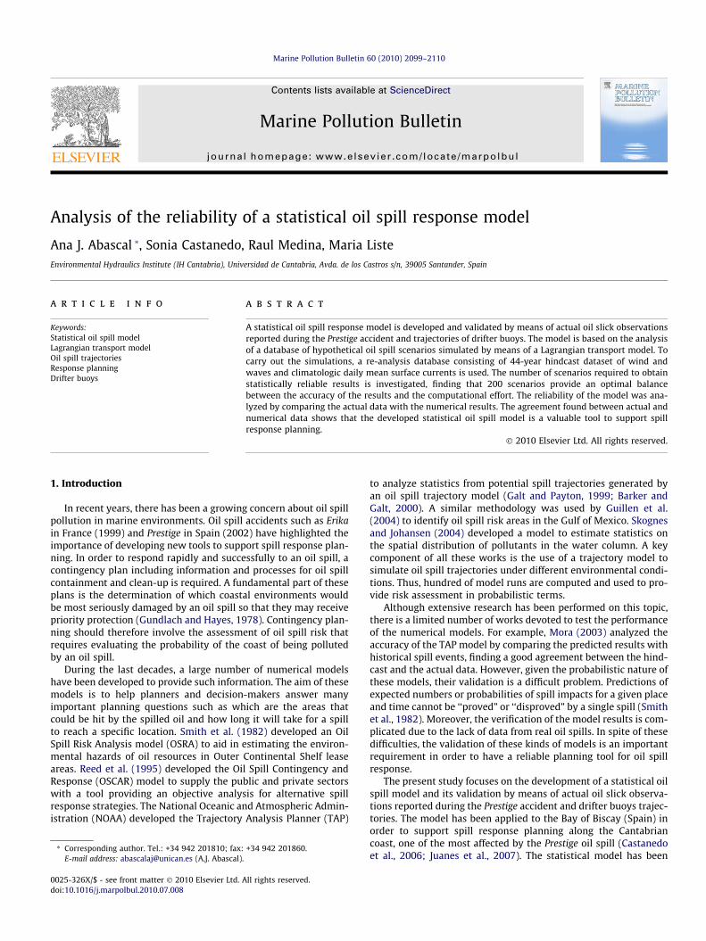
Marine Pollution Bulletin 60 (2010) 2099–2110

Contents lists available at ScienceDirect

Marine Pollution Bulletin

journal homepage: www.elsevier .com/locate /marpolbul

Analysis of the reliability of a statistical oil spill response model

Ana J. Abascal *, Sonia Castanedo, Raul Medina, Maria ListeEnvironmental Hydraulics Institute (IH Cantabria), Universidad de Cantabria, Avda. de los Castros s/n, 39005 Santander, Spain

a r t i c l e i n f o

Keywords:Statistical oil spill modelLagrangian transport modelOil spill trajectoriesResponse planningDrifter buoys

0025-326X/$ - see front matter � 2010 Elsevier Ltd. Adoi:10.1016/j.marpolbul.2010.07.008

* Corresponding author. Tel.: +34 942 201810; fax:E-mail address: abascalaj@unican.es (A.J. Abascal).

a b s t r a c t

A statistical oil spill response model is developed and validated by means of actual oil slick observationsreported during the Prestige accident and trajectories of drifter buoys. The model is based on the analysisof a database of hypothetical oil spill scenarios simulated by means of a Lagrangian transport model. Tocarry out the simulations, a re-analysis database consisting of 44-year hindcast dataset of wind andwaves and climatologic daily mean surface currents is used. The number of scenarios required to obtainstatistically reliable results is investigated, finding that 200 scenarios provide an optimal balancebetween the accuracy of the results and the computational effort. The reliability of the model was ana-lyzed by comparing the actual data with the numerical results. The agreement found between actual andnumerical data shows that the developed statistical oil spill model is a valuable tool to support spillresponse planning.

� 2010 Elsevier Ltd. All rights reserved.

1. Introduction

In recent years, there has been a growing concern about oil spillpollution in marine environments. Oil spill accidents such as Erikain France (1999) and Prestige in Spain (2002) have highlighted theimportance of developing new tools to support spill response plan-ning. In order to respond rapidly and successfully to an oil spill, acontingency plan including information and processes for oil spillcontainment and clean-up is required. A fundamental part of theseplans is the determination of which coastal environments wouldbe most seriously damaged by an oil spill so that they may receivepriority protection (Gundlach and Hayes, 1978). Contingency plan-ning should therefore involve the assessment of oil spill risk thatrequires evaluating the probability of the coast of being pollutedby an oil spill.

During the last decades, a large number of numerical modelshave been developed to provide such information. The aim of thesemodels is to help planners and decision-makers answer manyimportant planning questions such as which are the areas thatcould be hit by the spilled oil and how long it will take for a spillto reach a specific location. Smith et al. (1982) developed an OilSpill Risk Analysis model (OSRA) to aid in estimating the environ-mental hazards of oil resources in Outer Continental Shelf leaseareas. Reed et al. (1995) developed the Oil Spill Contingency andResponse (OSCAR) model to supply the public and private sectorswith a tool providing an objective analysis for alternative spillresponse strategies. The National Oceanic and Atmospheric Admin-istration (NOAA) developed the Trajectory Analysis Planner (TAP)

ll rights reserved.

+34 942 201860.

to analyze statistics from potential spill trajectories generated byan oil spill trajectory model (Galt and Payton, 1999; Barker andGalt, 2000). A similar methodology was used by Guillen et al.(2004) to identify oil spill risk areas in the Gulf of Mexico. Skognesand Johansen (2004) developed a model to estimate statistics onthe spatial distribution of pollutants in the water column. A keycomponent of all these works is the use of a trajectory model tosimulate oil spill trajectories under different environmental condi-tions. Thus, hundred of model runs are computed and used to pro-vide risk assessment in probabilistic terms.

Although extensive research has been performed on this topic,there is a limited number of works devoted to test the performanceof the numerical models. For example, Mora (2003) analyzed theaccuracy of the TAP model by comparing the predicted results withhistorical spill events, finding a good agreement between the hind-cast and the actual data. However, given the probabilistic nature ofthese models, their validation is a difficult problem. Predictions ofexpected numbers or probabilities of spill impacts for a given placeand time cannot be ‘‘proved” or ‘‘disproved” by a single spill (Smithet al., 1982). Moreover, the verification of the model results is com-plicated due to the lack of data from real oil spills. In spite of thesedifficulties, the validation of these kinds of models is an importantrequirement in order to have a reliable planning tool for oil spillresponse.

The present study focuses on the development of a statistical oilspill model and its validation by means of actual oil slick observa-tions reported during the Prestige accident and drifter buoys trajec-tories. The model has been applied to the Bay of Biscay (Spain) inorder to support spill response planning along the Cantabriancoast, one of the most affected by the Prestige oil spill (Castanedoet al., 2006; Juanes et al., 2007). The statistical model has been

2100 A.J. Abascal et al. / Marine Pollution Bulletin 60 (2010) 2099–2110

developed following the methodology presented by Barker andGalt (2000). However, a new approach based on numerically gen-erated data has been applied in this work. Thus, an extensive mete-orological and oceanographic data from re-analysis has been usedto generate a modelled track database of hypothetic oil spills usinga 2D Lagrangian transport model. By analyzing this database, themodel estimates the probability of a region to be polluted by anoil spill, the time taken for the oil to reach a specific site, and theareas that could be a threat for a given shoreline.

The performance of the model has been tested by means of oilslick observations from the Prestige accident and the track of drifterbuoys deployed in the Prestige sinking area. As mentioned, valida-tion of this kind of models is difficult because real data are scarceand insufficient for estimating the statistical behaviour of oil spills.In this work, the most extensive database available in the studyarea, obtained during the Prestige accident and in a later exerciseconducted in the same area, has been used to evaluate the reliabil-ity of the model. The Prestige oil tanker, carrying approximately77,000 tons of heavy oil, split in half and sunk on November 19at about 130 miles from the Galicia coast (Spain) (see Fig. 1). Thelatest estimation of the amount of oil spilled until August 2003was of 63,000 tons (Castanedo et al., 2006) affecting more than2000 km of shoreline (Ministerio de Medio Ambiente, 2005). Dur-ing the oil spill response, intense efforts were made on the moni-toring of the oil spill. With this purpose, daily overflights wereconducted to evaluate its evolution and satellite tracked Lagrang-ian floats were deployed in order to track the largest oil slicks (Gar-cía-Ladona et al., 2005). In addition, four years after the Prestigeaccident (November 2006), a set of buoys were released in theoil spill area as part of the operational exercise ‘Finisterre 2006’(Álvarez Fanjul et al., 2007).

The main contribution of this paper is the use of this broaddatabase, both oil slick observations and drifter data, to test theperformance of a statistical oil spill model. In this work, this isdone by means of two performance tests. First, the probability ofan oil spill reaching the coast was compared against the path fol-lowed by real data (oil slicks and drifter data). Secondly, the accu-

Fig. 1. Model domain (indicated by the dashed-line). The location of Cantabriancoast and the Prestige sinking point are presented.

racy of the model to estimate the arrival time of the oil spilled tothe receptor sites was evaluated by comparison to the evolutionof the oil spilled during the Prestige accident. The validation per-formed in this study is an important process to demonstrate thatthese models provide reliable results for decision-makers, becom-ing useful tools during oil spill response planning.

2. Methods

2.1. Methodology overview

The statistical model presented in this paper extends the workdeveloped by Galt and Payton (1999) and Barker and Galt (2000).In this study, a re-analysis database provided by state-of-the artnumerical models have been used to apply the model over a moreextensive domain with variable spatial resolution. The presentedmodel analyzes statistics from potential spill trajectories generatedby an oil spill trajectory model. The main goal of the model is tohelp answer many important planning questions such as: whereare spills likely to go? How long will it take for a spill to reach alocation? Or where could the oil, possibly threatening a givenshoreline, come from?

The first step of the presented methodology is the selection ofthe model domain, which will depend on the time and spatialmodelling scale. The aim of the model is to provide statistical infor-mation for evaluating oil spill hazards at a regional scale. There-fore, the model domain must be large enough to simulate theevolution of contaminating spills at this spatial scale. Once thestudy area is defined, the launch points (potential oil spills) andreceptor sites are selected. Due to the fact that the oil spilled onthe sea surface is moved by the combined effect of waves, windsand currents, the next step is to gather meteorological and ocean-ographic data on the study area. In order to simulate oil spill trajec-tories providing probabilistic information, a long period ofenvironmental data are required to obtain reliable statistical re-sults. In this study, an extensive meteorological and oceanographicdatabase provided by state-of-the-art ocean and atmospheric mod-els has been used. Specifically, a 44-year high resolution hindcastdataset of wind and wave for North Atlantic and climatologic dailymean ocean currents has been used as input of a 2D Lagrangiantransport model.

Taking into account the ocean and meteorological conditions ofthe study area, the forcing data are classified into statistically rep-resentative seasons. Therefore, the trajectory model is used to sim-ulate a set of oil spill scenarios for each climatic season. Here, ascenario is defined as an oil spill trajectory computed by the trans-port model and forced by specific meteorological and oceano-graphic conditions corresponding to a randomly selected date. Inorder to obtain statistically reliable results, an analysis is per-formed to determine the appropriate number of scenarios (N).Once it is established, a set of N oil spill trajectories is generatedfrom each launch point and the number of contacts is computedin the receptor sites. This modelled track database of hypotheticoil spills is used by the statistical model to answer the aforemen-tioned planning questions. Finally, actual data in the study areaare collected to test the reliability of the developed statisticalmodel.

2.2. Model domain

The selection of the model domain depends on the coastal areato be protected, and the spatial and temporal scale of the modelapplication. As mentioned, the statistical model developed in thiswork is a regional model, focusing on the Cantabrian coast. Toselect the area and the temporal scale of the model application,

A.J. Abascal et al. / Marine Pollution Bulletin 60 (2010) 2099–2110 2101

the experience acquired during the Prestige accident was taken intoaccount. This accident demonstrated the vulnerability of the Can-tabrian coast to an oil spill occurring in the Bay of Biscay. The oilspilt in front of the Galician coast (see Fig. 1) reached Cantabria,which is located about 450 nautical miles east from the sinkingpoint, 17 days later.

Therefore, given the regional scale of the model and based on theevidence that the Cantabrian coast was affected by the Prestige oilspill, the selected model domain extends over the Bay of Biscay(see Fig. 1) from the Northern coast of Portugal to the Northern coastof France. Regarding the temporal scale, each oil spill trajectory wassimulated for a 30 day period in order to allow for an oil spill locatedon the boundary of the domain to reach the Cantabrian coast.

The entire domain of the model was divided into 519 potentialspill points and 878 target points (in water and on the shoreline).The location of these points is indicated by circles (spill points)and points (target points) in Fig. 2. Both launch and contact pointswere distributed over three grids with different resolution thatincreases on the proximity to the coast. It is important to note thatthe launch points are located regularly, which means that they aregiven the same probability of occurrence. The resolution of thepoints located on the sea ranges from 55 to 27 km in most partsof the model domain, and increases to 6 km in the proximity ofthe Cantabrian coast. The resolution of the target points becomesfiner close to the coast and, specifically, it was around 2 km alongthe studied shoreline (Cantabria shoreline).

2.3. Lagrangian transport model

The hypothetical oil spills were simulated using a two-dimen-sional Lagrangian transport model, PICHI, developed by the Univer-sity of Cantabria as part of the operational forecasting systemcreated in response to the Prestige oil spill (Castanedo et al.,2006). In this model, the drift process of the spilled oil is describedby tracking numerical particles equivalent to the oil slicks. At eachtime step, the new position of the particles is computed by thesuperposition of the transports induced by the currents, wind,waves and turbulent dispersion.

The numerical model solves the following vector equation:

d~xdt¼~uað~xi; tÞ þ~udð~xi; tÞ ð1Þ

Fig. 2. Potential spill (circles) and target points (points). The resolution of the point

where xi! is the particle position, and ua

�! and ud�! are the advective

and diffusive velocities respectively in xi!.

The advective velocity, ua�!, is calculated as the linear combina-

tion of currents and wind velocity and the wave induced Stokesdrift. The turbulent diffusive velocity is obtained using a MonteCarlo sampling in the range of velocities ½� ud

�!; ud�!� (Hunter

et al., 1993; Maier-Reimer, 1982). A more detailed description ofthe model is provided by Castanedo et al. (2006) and Abascalet al. (2009a).

In the present model, the oil evaporation is calculated as a pos-teriori process by reducing the amount of oil that reaches the targetpoints. The rate of evaporation is evaluated using the Stiver andMacKay (1984) formulation. Because the evaporation depends onthe oil properties, the model includes a simplified oil database withthe main properties of light and heavy products.

The oil spill model has been calibrated and validated using datafrom drifting buoys (Abascal et al., 2007, 2009a,b). Specifically,buoys deployed in the Bay of Biscay during the Prestige accidentwere used to calibrate the model and to obtain the optimal coeffi-cients for the study area (Abascal et al., 2009a).

2.4. Data

2.4.1. Meteorological and oceanographic dataData used in the analysis were provided by atmospheric and

oceanographic models. Regarding winds and sea state, a re-analy-sis database, SIMAR-44 (Puertos del Estado, 2008), was used. Thesedata consist of a 44-year (1958–2001) hindcast dataset of wind,wave and sea-level for North Atlantic waters and coastal seas.The wind fields were the output of the REMO model (Jacob andPodzun, 1997) forced by the NCEP Global Forecasting Systematmospheric prediction fields. The results of the REMO model havebeen validated with in situ measurements obtained from buoy sta-tions, suggesting that the simulation reproduces with great reli-ability the 10-m wind field (Sotillo et al., 2005). The 44-year(1958–2001) hindcast was performed with a horizontal resolutionof 0.5 � 0.5. The data consist of 10-m wind speed and direction,provided with a 6-h time interval.

Sea state conditions were the output of the numerical modelWAM, a third generation spectral wave generation model (Komenet al., 1994; WAMDIG, 1988). The WAM model solves the energy

s increases in the proximity to the coast, especially along the Cantabrian coast.

2102 A.J. Abascal et al. / Marine Pollution Bulletin 60 (2010) 2099–2110

transfer equation for the wave spectrum. The results were thesignificant wave height, mean direction and mean period for seaand swell components with a 3-h time interval. These data havebeen calibrated with buoy data from the Spanish network (Puertosdel Estado, www.puertos.es) and validated with satellite data fromTOPEX/POSEIDON (Tomas et al., 2008).

The mean daily climatologic surface currents were carried outapplying the MEDiNA ocean model (Dietrich et al., 2008; Liste,2009) to the Bay of Biscay. The MEDiNA model, which comesfrom the DieCAST model (Dietrich et al., 1987), is a 4th-order-accurate ocean model employing six grids that are all two-way-coupled to their adjacent grids. Longitudinal resolution variesfrom 1/24� in the Strait of Gibraltar regional grid to 1/4� in thecentral North Atlantic Ocean grid. Specifically, the spatial resolu-tion in the Gulf of Biscay is 1/16�. This allows the MEDiNA modelto efficiently solve small features in a multi-basin model. TheMEDiNA wind-forcing is obtained from the interpolated monthlyHellerman winds (Hellerman and Rosenstein, 1983), and WorldOcean Atlas climatology database and MEDAR-MEDATLAS areused to initialize the model. The MEDiNA model has been vali-dated by comparison with the flux transport in the main Straitsof the Western Mediterranean Basin and the Gulf of Mexico andusing data from satellite-tracked surface drifting buoys of theGDP database (Global Drifter Program, www.aoml.noaa.gov/phod/dac/gdp.html) (Liste, 2009).

2.4.2. Oil slick observations from the Prestige accidentOil slick observations were collected during the Prestige oil spill

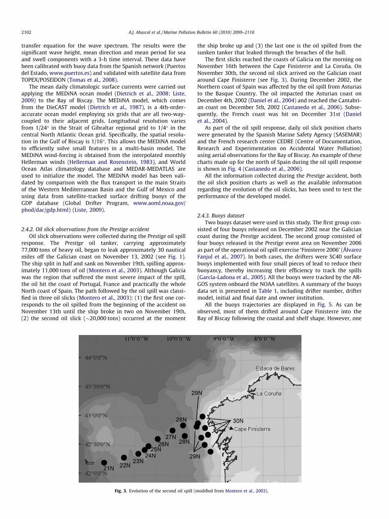
response. The Prestige oil tanker, carrying approximately77,000 tons of heavy oil, began to leak approximately 30 nauticalmiles off the Galician coast on November 13, 2002 (see Fig. 1).The ship split in half and sank on November 19th, spilling approx-imately 11,000 tons of oil (Montero et al., 2003). Although Galiciawas the region that suffered the most severe impact of the spill,the oil hit the coast of Portugal, France and practically the wholeNorth coast of Spain. The path followed by the oil spill was classi-fied in three oil slicks (Montero et al., 2003): (1) the first one cor-responds to the oil spilled from the beginning of the accident onNovember 13th until the ship broke in two on November 19th,(2) the second oil slick (�20,000 tons) occurred at the moment

Fig. 3. Evolution of the second oil spill (m

the ship broke up and (3) the last one is the oil spilled from thesunken tanker that leaked through the breaches of the hull.

The first slicks reached the coasts of Galicia on the morning onNovember 16th between the Cape Finisterre and La Coruña. OnNovember 30th, the second oil slick arrived on the Galician coastaround Cape Finisterre (see Fig. 3). During December 2002, theNorthern coast of Spain was affected by the oil spill from Asturiasto the Basque Country. The oil impacted the Asturian coast onDecember 4th, 2002 (Daniel et al., 2004) and reached the Cantabri-an coast on December 5th, 2002 (Castanedo et al., 2006). Subse-quently, the French coast was hit on December 31st (Danielet al., 2004).

As part of the oil spill response, daily oil slick position chartswere generated by the Spanish Marine Safety Agency (SASEMAR)and the French research center CEDRE (Centre of Documentation,Research and Experimentation on Accidental Water Pollution)using aerial observations for the Bay of Biscay. An example of thesecharts made up for the north of Spain during the oil spill responseis shown in Fig. 4 (Castanedo et al., 2006).

All the information collected during the Prestige accident, boththe oil slick position charts as well as the available informationregarding the evolution of the oil slicks, has been used to test theperformance of the developed model.

2.4.3. Buoys datasetTwo buoys dataset were used in this study. The first group con-

sisted of four buoys released on December 2002 near the Galiciancoast during the Prestige accident. The second group consisted offour buoys released in the Prestige event area on November 2006as part of the operational oil spill exercise ‘Finisterre 2006’ (ÁlvarezFanjul et al., 2007). In both cases, the drifters were SC40 surfacebuoys implemented with four small pieces of lead to reduce theirbuoyancy, thereby increasing their efficiency to track the spills(García-Ladona et al., 2005). All the buoys were tracked by the AR-GOS system onboard the NOAA satellites. A summary of the buoysdata set is presented in Table 1, including drifter number, driftermodel, initial and final date and owner institution.

All the buoys trajectories are displayed in Fig. 5. As can beobserved, most of them drifted around Cape Finisterre into theBay of Biscay following the coastal and shelf shape. However, one

odified from Montero et al., 2003).

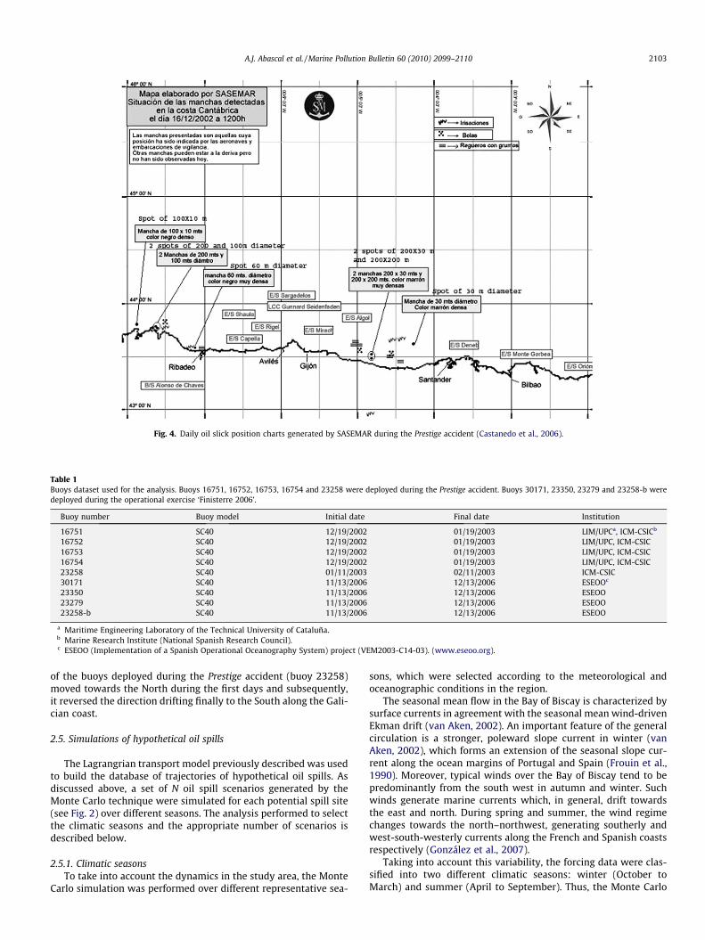
Fig. 4. Daily oil slick position charts generated by SASEMAR during the Prestige accident (Castanedo et al., 2006).

Table 1Buoys dataset used for the analysis. Buoys 16751, 16752, 16753, 16754 and 23258 were deployed during the Prestige accident. Buoys 30171, 23350, 23279 and 23258-b weredeployed during the operational exercise ‘Finisterre 2006’.

Buoy number Buoy model Initial date Final date Institution

16751 SC40 12/19/2002 01/19/2003 LIM/UPCa, ICM-CSICb

16752 SC40 12/19/2002 01/19/2003 LIM/UPC, ICM-CSIC16753 SC40 12/19/2002 01/19/2003 LIM/UPC, ICM-CSIC16754 SC40 12/19/2002 01/19/2003 LIM/UPC, ICM-CSIC23258 SC40 01/11/2003 02/11/2003 ICM-CSIC30171 SC40 11/13/2006 12/13/2006 ESEOOc

23350 SC40 11/13/2006 12/13/2006 ESEOO23279 SC40 11/13/2006 12/13/2006 ESEOO23258-b SC40 11/13/2006 12/13/2006 ESEOO

a Maritime Engineering Laboratory of the Technical University of Cataluña.b Marine Research Institute (National Spanish Research Council).c ESEOO (Implementation of a Spanish Operational Oceanography System) project (VEM2003-C14-03). (www.eseoo.org).

A.J. Abascal et al. / Marine Pollution Bulletin 60 (2010) 2099–2110 2103

of the buoys deployed during the Prestige accident (buoy 23258)moved towards the North during the first days and subsequently,it reversed the direction drifting finally to the South along the Gali-cian coast.

2.5. Simulations of hypothetical oil spills

The Lagrangrian transport model previously described was usedto build the database of trajectories of hypothetical oil spills. Asdiscussed above, a set of N oil spill scenarios generated by theMonte Carlo technique were simulated for each potential spill site(see Fig. 2) over different seasons. The analysis performed to selectthe climatic seasons and the appropriate number of scenarios isdescribed below.

2.5.1. Climatic seasonsTo take into account the dynamics in the study area, the Monte

Carlo simulation was performed over different representative sea-

sons, which were selected according to the meteorological andoceanographic conditions in the region.

The seasonal mean flow in the Bay of Biscay is characterized bysurface currents in agreement with the seasonal mean wind-drivenEkman drift (van Aken, 2002). An important feature of the generalcirculation is a stronger, poleward slope current in winter (vanAken, 2002), which forms an extension of the seasonal slope cur-rent along the ocean margins of Portugal and Spain (Frouin et al.,1990). Moreover, typical winds over the Bay of Biscay tend to bepredominantly from the south west in autumn and winter. Suchwinds generate marine currents which, in general, drift towardsthe east and north. During spring and summer, the wind regimechanges towards the north–northwest, generating southerly andwest-south-westerly currents along the French and Spanish coastsrespectively (González et al., 2007).

Taking into account this variability, the forcing data were clas-sified into two different climatic seasons: winter (October toMarch) and summer (April to September). Thus, the Monte Carlo

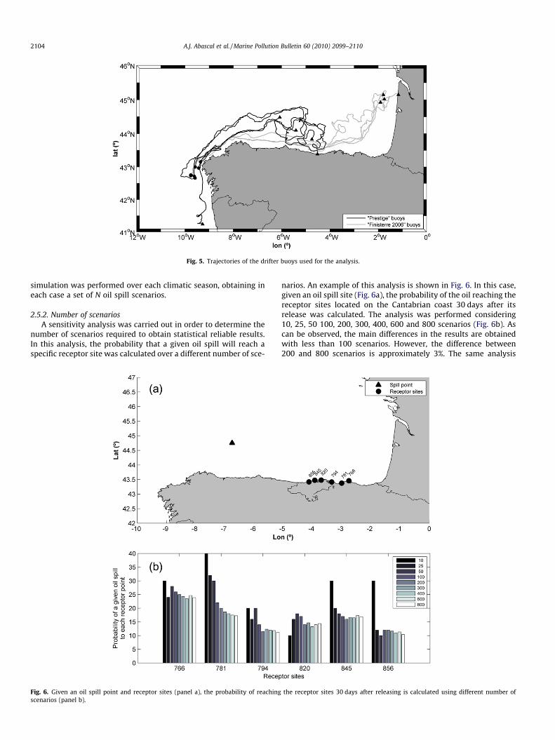
Fig. 5. Trajectories of the drifter buoys used for the analysis.

2104 A.J. Abascal et al. / Marine Pollution Bulletin 60 (2010) 2099–2110

simulation was performed over each climatic season, obtaining ineach case a set of N oil spill scenarios.

2.5.2. Number of scenariosA sensitivity analysis was carried out in order to determine the

number of scenarios required to obtain statistical reliable results.In this analysis, the probability that a given oil spill will reach aspecific receptor site was calculated over a different number of sce-

Fig. 6. Given an oil spill point and receptor sites (panel a), the probability of reachingscenarios (panel b).

narios. An example of this analysis is shown in Fig. 6. In this case,given an oil spill site (Fig. 6a), the probability of the oil reaching thereceptor sites located on the Cantabrian coast 30 days after itsrelease was calculated. The analysis was performed considering10, 25, 50 100, 200, 300, 400, 600 and 800 scenarios (Fig. 6b). Ascan be observed, the main differences in the results are obtainedwith less than 100 scenarios. However, the difference between200 and 800 scenarios is approximately 3%. The same analysis

the receptor sites 30 days after releasing is calculated using different number of

A.J. Abascal et al. / Marine Pollution Bulletin 60 (2010) 2099–2110 2105

was performed for different oil spill points and receptor sites, withsimilar results. Taking into account the accuracy of the results andthat the computational time increases with the number of simu-lated trajectories, a total of 200 scenarios were simulated for eachseason.

2.5.3. Model applicationThe oil spill trajectories were computed by means of the trans-

port equation (Eq. (1)). As mentioned, the spilled oil was describedby tracking a cloud of numerical particles equivalent to the oilslicks. The minimum number of particles was determined follow-ing Barker and Galt (2000). The authors studied the uncertaintythat arises from using a finite number of particles in a Lagrangiantransport model. They computed the confidence intervals for thenumber of particles that might impact a particular site at a partic-ular time for a particular run. The analysis was performed using100, 500, 1000, 1500 and 2000 particles. In all cases, the accuracyof the results was compared with the computational effort. Theauthors found the optimal balance between the accuracy of the re-sults and the computational effort using 1000 particles in theLagrangian transport model. Based on these results, each oil spillscenario simulated in this study was represented by 1000 indepen-dent numerical particles. Simulations were performed using a timestep of 1800 s. If the integration time step is too long, the simulatedspill traverses over two or more velocity grid points, and the re-solved spatial variability of the velocity field is not fully utilized.If, on the other hand, the selected intervals are too small, the re-quired computer run may be impractical (Price et al., 2004). Forthe grid size and velocities of forcing data used in this study, theselected time step ensures that particles will not displace morethan one grid in one time step.

As mentioned, each trajectory was allowed to continue for aslong as 30 days. At every time step, the model compared the loca-tions of the hypothetical oil spills against the target points. Con-

Fig. 7. Probability of oil contamination after 15 days of the initial release. The white circlA detailed over the Cantabrian coast is shown.

tacts to the target points were recorded for 6 h, 12 h, 1 day,3 days, 15 days and 30 days after the initial time of the hypotheti-cal spill.

In summary, a total of 200 scenarios were simulated for each ofthe over 519 spill points and each of two distinct seasons. This rep-resents approximately 200,000 individual runs and extensive com-putational and storage resources. The results were arranged in a 3Dmatrix for each scenario, the dimensions being launch points (519),receptor site points (878) and record times (6 h, 12 h, 1 day, 3 days,15 days, 30 days). Each 3D matrix provides the amount of oil thathits each receptor site, from each spill point at the recorded timeintervals. The statistical analysis was based on the post-processingof this 3D database.

The numerical results and the analysis carried out to assess thereliability of the model will be shown in the next section.

3. Model reliability analysis

In order to test the model reliability, two exercises were pro-posed: (1) in the first one, the probability of the oil reaching thereceptor sites was compared against the path followed by real data(oil slicks and drifter data), (2) in the second exercise, the time ta-ken from the second oil spill to reach the Galician coast was com-pared with the time calculated by the numerical model.

3.1. Exercise 1: what target points are likely to be impacted by the oilspill?

The skill of the numerical model to estimate the regions withthe highest probability to be impacted by an oil spill was assessedby comparing the numerical results with oil slick observationsfrom the Prestige accident and trajectories of drifter buoys. Theanalysis performed is described below.

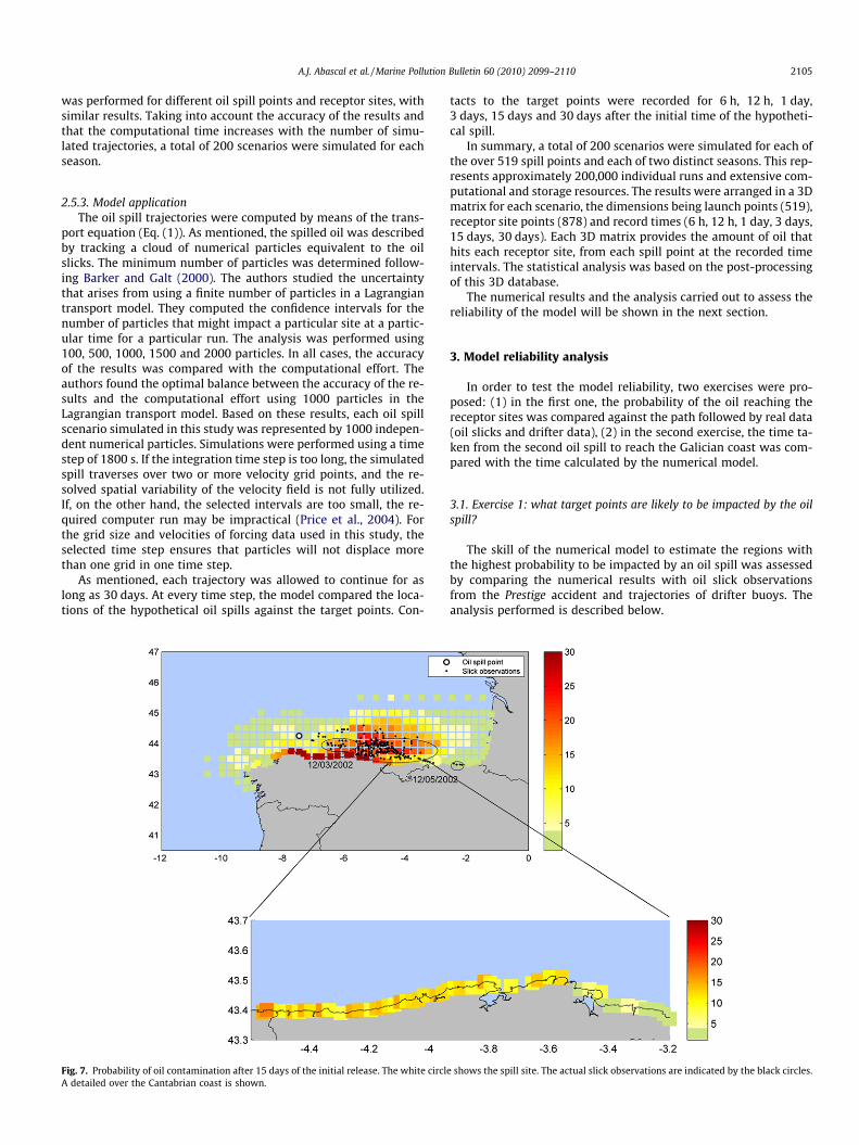
e shows the spill site. The actual slick observations are indicated by the black circles.

2106 A.J. Abascal et al. / Marine Pollution Bulletin 60 (2010) 2099–2110

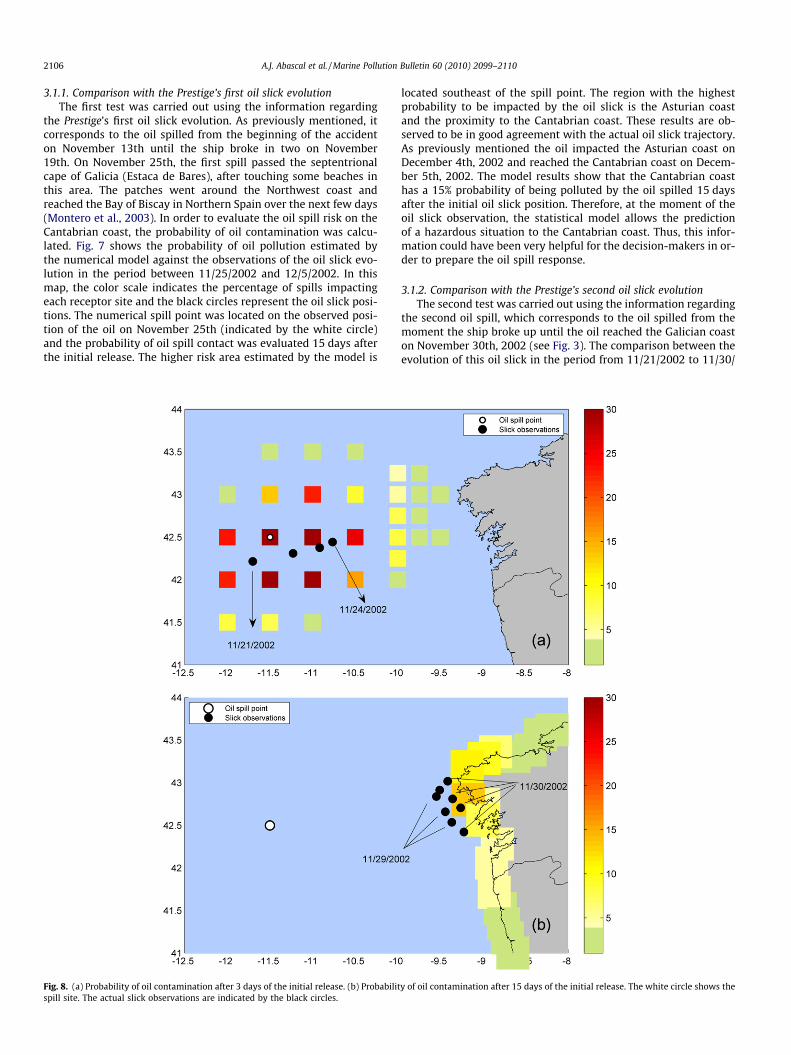
3.1.1. Comparison with the Prestige’s first oil slick evolutionThe first test was carried out using the information regarding

the Prestige’s first oil slick evolution. As previously mentioned, itcorresponds to the oil spilled from the beginning of the accidenton November 13th until the ship broke in two on November19th. On November 25th, the first spill passed the septentrionalcape of Galicia (Estaca de Bares), after touching some beaches inthis area. The patches went around the Northwest coast andreached the Bay of Biscay in Northern Spain over the next few days(Montero et al., 2003). In order to evaluate the oil spill risk on theCantabrian coast, the probability of oil contamination was calcu-lated. Fig. 7 shows the probability of oil pollution estimated bythe numerical model against the observations of the oil slick evo-lution in the period between 11/25/2002 and 12/5/2002. In thismap, the color scale indicates the percentage of spills impactingeach receptor site and the black circles represent the oil slick posi-tions. The numerical spill point was located on the observed posi-tion of the oil on November 25th (indicated by the white circle)and the probability of oil spill contact was evaluated 15 days afterthe initial release. The higher risk area estimated by the model is

Fig. 8. (a) Probability of oil contamination after 3 days of the initial release. (b) Probabilitspill site. The actual slick observations are indicated by the black circles.

located southeast of the spill point. The region with the highestprobability to be impacted by the oil slick is the Asturian coastand the proximity to the Cantabrian coast. These results are ob-served to be in good agreement with the actual oil slick trajectory.As previously mentioned the oil impacted the Asturian coast onDecember 4th, 2002 and reached the Cantabrian coast on Decem-ber 5th, 2002. The model results show that the Cantabrian coasthas a 15% probability of being polluted by the oil spilled 15 daysafter the initial oil slick position. Therefore, at the moment of theoil slick observation, the statistical model allows the predictionof a hazardous situation to the Cantabrian coast. Thus, this infor-mation could have been very helpful for the decision-makers in or-der to prepare the oil spill response.

3.1.2. Comparison with the Prestige’s second oil slick evolutionThe second test was carried out using the information regarding

the second oil spill, which corresponds to the oil spilled from themoment the ship broke up until the oil reached the Galician coaston November 30th, 2002 (see Fig. 3). The comparison between theevolution of this oil slick in the period from 11/21/2002 to 11/30/

y of oil contamination after 15 days of the initial release. The white circle shows the

A.J. Abascal et al. / Marine Pollution Bulletin 60 (2010) 2099–2110 2107

2002 and the probability of oil contamination given by the model isdisplayed in Fig. 8. Fig. 8a and b show the probability that spilledoil (indicated by the white circle) reaches the receptor sites 3and 15 days after the initial release. Fig. 8a shows that after 3 daysthe oil is likely to travel to the coast of Galicia, according to the oilevolution from 11/21/2002 to 11/24/2002. Fifteen days after theinitial release (Fig. 8b), the North coast of Galicia is the coastal areawith the highest probability of being impacted by the Prestige oilspill. This is in agreement with the trajectory followed by the sec-ond oil slick that arrived to this region on November 30, 2002. As inthe previous exercise, this information could have been very help-ful while planning the oil spill response.

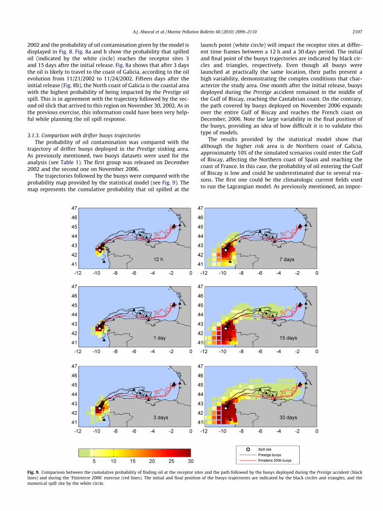
3.1.3. Comparison with drifter buoys trajectoriesThe probability of oil contamination was compared with the

trajectory of drifter buoys deployed in the Prestige sinking area.As previously mentioned, two buoys datasets were used for theanalysis (see Table 1). The first group was released on December2002 and the second one on November 2006.

The trajectories followed by the buoys were compared with theprobability map provided by the statistical model (see Fig. 9). Themap represents the cumulative probability that oil spilled at the

Fig. 9. Comparison between the cumulative probability of finding oil at the receptor sitlines) and during the ‘Finisterre 2006’ exercise (red lines). The initial and final positionnumerical spill site by the white circle.

launch point (white circle) will impact the receptor sites at differ-ent time frames between a 12 h and a 30 days period. The initialand final point of the buoys trajectories are indicated by black cir-cles and triangles, respectively. Even though all buoys werelaunched at practically the same location, their paths present ahigh variability, demonstrating the complex conditions that char-acterize the study area. One month after the initial release, buoysdeployed during the Prestige accident remained in the middle ofthe Gulf of Biscay, reaching the Cantabrian coast. On the contrary,the path covered by buoys deployed on November 2006 expandsover the entire Gulf of Biscay and reaches the French coast onDecember, 2006. Note the large variability in the final position ofthe buoys, providing an idea of how difficult it is to validate thistype of models.

The results provided by the statistical model show thatalthough the higher risk area is de Northern coast of Galicia,approximately 10% of the simulated scenarios could enter the Gulfof Biscay, affecting the Northern coast of Spain and reaching thecoast of France. In this case, the probability of oil entering the Gulfof Biscay is low and could be underestimated due to several rea-sons. The first one could be the climatologic current fields usedto run the Lagrangian model. As previously mentioned, an impor-

es and the path followed by the buoys deployed during the Prestige accident (blackof the buoys trajectories are indicated by the black circles and triangles, and the

2108 A.J. Abascal et al. / Marine Pollution Bulletin 60 (2010) 2099–2110

tant feature of the general circulation in winter is a poleward slopecurrent along the Iberian coast. This flow, know as the PortugalCounter Current (PCC), arrives at Cape Finisterre and turns to theright, entering the Bay of Biscay following the northern part ofthe Spanish coast (Martins et al., 2002; Coelho et al., 2002). Dueto climatologic currents representing mean patterns of the oceandynamics, the PCC could be underestimated decreasing the num-ber of spill trajectories that enters the Gulf of Biscay. These resultscould be improved using a hindcast of high-temporal resolutionocean currents, which would provide a more realistic simulationof the circulation in the study area. The second reason could bethe resolution of the receptor sites. As mentioned above, the spatialresolution around the Galician coast is 27 km. Because of this spa-tial resolution, there are few receptor points between the spillpoint (see Fig. 9) and the coast. As a result, the oil spill tends togo travel towards the coast and, consequently, does not enter theBay of Biscay. These results could be improved by increasing thespatial resolution of the receptor sites near the coast in all thestudy area.

3.2. Exercise 2: how long it will take for a spill to reach a location?

In order to test the performance of the model in evaluating thearrival time of the oil spilled at the receptor sites, a comparison ofthe temporal evolution of the second oil slick (see Fig. 3) and thenumerical results was carried out. Fig. 10 shows the comparisonbetween the minimum time required for the oil spill to reach thereceptor sites given by the model and actual dates of the oil slickobservations. In this map, the oil spill point is indicated by theblack circle and the actual oil slick observations by the blackpoints. As can be observed, the oil spill trajectory spans from

Fig. 10. Minimum time required to the oil spill to reach the receptor si

November 21st, 2002 (oil initial position) to November 30th,2002 (oil landing time). The selected spill point was closest atthe oil location on November 21st.

During the first days, the time for the spill point to reach thereceptor sites provided by the model is lower than that observedin real life. This overestimation of the arrival time could be dueto the low spatial resolution of the receptor sites in this area. Notethat the daily oil slick displacement is smaller than the spatial res-olution of the launch points. Therefore, these results could be im-proved increasing the spatial resolution of the launch points inthis area.

However, according to the calculations, the minimum time re-quired for the spilled oil to reach the north coast of Galicia is 7–9 days (see ellipse in Fig. 10). These results are observed to be ingood agreement with the actual oil slick trajectory, accurately pro-viding the landing time. Note that the oil slick was near the Gali-cian coast on November 29th and arrived at the Galician coast onthe northern part of Cape Finisterre on November 30th. These re-sults show the capability of the numerical model to estimate thearrival time of an oil spill to a coastal area.

4. Summary and conclusions

This paper focuses on the development of a statistical oil spillmodel and its validation by means of real oil slick observationsand drifter buoy trajectories. The model has been applied to theBay of Biscay (Spain) in order to support spill response planningalong the Cantabrian coast. The developed model was based onthe methodology presented by Barker and Galt (2000). This meth-odology has been extended using numerically generated data andby applying the model to a more extensive domain with variable

tes. The actual slick observations are indicated by the black circles.

A.J. Abascal et al. / Marine Pollution Bulletin 60 (2010) 2099–2110 2109

spatial resolution. A re-analysis database consisting of 44-yearhindcast dataset of wind and waves for North Atlantic watersand coastal seas was used. Moreover, climatologic daily mean sur-face currents were carried out applying the ocean model MEDiNAto the Bay of Biscay. A 2D Lagrangian model, forced by these exten-sive meteorological and oceanographic data, was used to simulateoil spill trajectories and to build a modelled track database of hyp-othetic oil spills by means of the Monte Carlo technique. A sensitiv-ity analysis was performed in order to determine the number ofscenarios required to obtain reliable statistical results. In this anal-ysis, the probability that a given oil spill will reach a specific recep-tor site was calculated over a different number of scenarios, findingthat 200 scenarios provided an optimal balance between the accu-racy of the results and the computational effort. Therefore, a totalof 200 scenarios were simulated under different oceanographicand atmospheric conditions for each of over 519 spill points andeach of two distinct seasons (winter and summer). The modelledtrack database of hypothetic oil spills were used for evaluatingoil spill hazard for planning purposes.

The performance of the developed model has been tested bymeans of oil slick observations from the Prestige accident and thetrack of drifter buoys deployed in the Prestige sinking area. It isimportant to emphasize that the interpretation of the results mustbe done carefully because of the different nature of the data used.Real data are scarce and insufficient to estimate the statisticalbehaviour of oil spills, so the comparison involves statistical data,provided by the numerical model, and discrete data. However,the aim of this paper is to test the reliability of the developed mod-el using the available data, identifying strengths and weaknesses.

The reliability of the model was assessed by comparing thenumerical results with the actual data evolution. Specifically, twokinds of exercises were carried out: (1) the probability of oil reach-ing the receptor sites given by the model was compared against thepath followed by real data (oil slicks and drifter data), (2) the timeneeded for the Prestige oil spill to reach the Galician coast wascompared with the time calculated by the numerical model. Thefirst exercise showed that the Northern coast of Galicia, the regionimpacted by the Prestige oil spill, was the coastal area with thehighest probability of becoming polluted by the oil spill. Moreover,the minimum time required for the spilled oil to reach this regiongiven by the model was 7–9 days, in agreement with the actual oilslick trajectory. These results show the capability of the model todetermine the areas with the highest probability of being affectedby a particular oil spill and the arrival time of the oil spilled at aparticular coastal area.

As discussed above, the comparison of the numerical resultswith actual data has allowed identifying the weaknesses andstrengths of the developed model. Despite the performance ofthe model, the results could be improved considering the followingadvances in the presented methodology: (1) using a hindcast ofocean currents for the study area, (2) increasing the spatial resolu-tion in the numerical domain close to the coast and (3) assigning adifferent probability of occurrence for the launch points taking intoaccount the most common transportation routes. Because oil spillsoften occur due to activities associated with shipping traffic, thespill probability is higher in the transportation routes. To take thisinto account, a higher probability of occurrence could be assignedfor the launch points located in the navigation routes. Therefore,further study is required to include these improvements in themodel.

Among the strengths the authors note that, on the one hand, themethodology presented is easily relocatable, in that it could easilybe applied to evaluate the risk of contamination in any given coast-al area. On the other hand, the good agreement found between thenumerical results and the actual data show that the developed sta-tistical oil spill model is a valuable tool to support spill response

planning. Finally, it is worth noting that this study highlights theimportance of the validation of oil spill statistical models in orderto provide decision-makers with reliable planning tools for oil spillresponse.

Acknowledgments

This work has been partly funded by the Spanish Ministry ofEducation and Science under the research project TRA2007-65133/TMAR (PREVER project). S.C. would like to thank the Span-ish Ministry of Science and Innovation for its support within theRamon y Cajal Program. The authors would like to thank Puertosdel Estado for the SIMAR-44 database provided for this study.Buoys data and oil slick position charts were kindly provided byICM-CSIC, LIM/UPC, SASEMAR and CEDRE in the framework ofthe ESEOO project.

References

Abascal, A.J., Castanedo, S., Gutierrez, A.D., Comerma, E., Medina R., Losada, I.J., 2007.TESEO, An Operational System for Simulating Oil Spills Trajectories and FateProcesses. In: Proceedings, ISOPE-2007: The 17th International Offshore Oceanand Polar Engineering Conference, vol. 3. The International Society of OffshoreOcean and Polar Engineers (ISOPE), Lisboa (Portugal), pp. 1751–1758.

Abascal, A.J., Castanedo, S., Mendez, F.J., Medina, R., Losada, I.J., 2009a. Calibration ofa Lagrangian transport model using drifting buoys deployed during the Prestigeoil spill. J. Coast. Res. 25 (1), 80–90.

Abascal, A.J., Castanedo, S., Medina, R., Losada, I.J., Alvarez-Fanjul, E., 2009b.Application of HF radar currents to oil spill modelling. Mar. Pollut. Bull. 58, 238–248.

Álvarez Fanjul, E., Losada, I., Tintoré, J., Menéndez, J., Espino, M., Parrilla, G.,Martinez, I., Muñuzuri, V.P., 2007. The ESEOO Project: Developments andPerspectives for Operational Oceanography at Spain. In: Proc. ISOPE-2007: The17th International Offshore Ocean and Polar Engineering Conference, vol. 3. TheInternational Society of Offshore Ocean and Polar Engineers (ISOPE), Lisbon,Portugal, pp. 1708–1715.

Barker, C.H., Galt, J.A., 2000. Analysis of methods used in spill response planning:trajectory analysis planner TAP II. Spill Sci. Technol. Bull. 6 (2), 145–152.

Castanedo, S., Medina, R., Losada, I.J., Vidal, C., Méndez, F.J., Osorio, A., Juanes, J.A.,Puente, A., 2006. The Prestige oil spill in Cantabria (Bay of Biscay). Part I:operational forecasting system for quick response, risk assessment andprotection of natural resources. J. Coast. Res. 22 (6), 1474–1489.

Coelho, H.S., Neves, R.J.J., White, M., Leitão, P.C., Santos, A.J., 2002. A model for oceancirculation on the Iberian coast. J. Mar. Syst. 32 (1–3), 153–179.

Daniel, P., Josse, P., Dandin, P., Lefevre, J.-M., Lery, G., Cabioch, F., Gouriou, V., 2004.Forecasting the Prestige Oil Spills. In: Proceedings of the Interspill 2004Conference. Trondheim, Norway.

Dietrich, D.E., Marietta, M.G., Roache, P.J., 1987. A ocean modelling system withturbulent boundary layers and topography: numerical description. Int. J.Numerical Methods Fluids 7, 833–855.

Dietrich, D.E., Tseng, Y-H., Medina, R., Piacsek, S.A., Liste, M., Olabarrieta, M.,Bowman, M.J., Mehra, A., 2008. Mediterranean Overflow Water (MOW)simulation using a coupled multiple-grid Mediterrranean Sea/North Atlanticocean model. J. Geophys. Res. 113, C07027, doi:10.1029/2006JC003914.

Frouin, R., Fiúza, A.F.C., Ambar, I., Boyd, T.J., 1990. Observations of a polewardsurface current off the coasts of Portugal and Spain during winter. J. Geophys.Res. 95 (C1), 679–691.

Galt, J.A., Payton, D.L., 1999. Development of quantitative methods for spill responseplanning: a trajectory analysis planner. Spill Sci. Technol. Bull. 5 (1), 17–28.

García-Ladona, E., Font, J., del Río, E., Julià, A., Salat, J., Chic, O., Orfila, A., Alvarez, A.,Basterretxea, G., Vizoso, G., Piro, O., Tintoré, J., Gil, M., Herrera, J.L., Castanedo, S.,2005. The use of surface drifting floats in the monitoring of oil spills. ThePrestige case. In: Proc. of the 19 Biennial International Oil Spill Conference(IOSC), CD-ROM: 14718A.

González, M., Ferrer, L., Uriarte, A., Urtizberea, A., Caballero, A., 2007. Operationaloceanography system applied to the Prestige oil-spillage event. J. Mar. Syst. 72(1–4), 178–188.

Guillen, G., Rainey, G., Morin, M., 2004. A simple rapid approach using coupledmultivariate statistical methods, GIS and trajectory models to delineate areas ofcommon oil spill risk. J. Mar. Syst. 45 (3–4), 221–235.

Gundlach, E.R., Hayes, M.O., 1978. Vulnerability of coastal environments to oil spillimpacts. Mar. Technol. Soc. J. 12, 18–27.

Hellerman, S., Rosenstein, M., 1983. Normal monthly wind stress over the worldocean with error estimates. J. Phys. Oceanogr. 13 (7), 1093–1104.

Hunter, J.R., Craig, P.D., Phillips, H.E., 1993. On the use of random walk models withspatially variable diffusivity. J. Comput. Phys. 106, 366–376.

Jacob, D., Podzun, R., 1997. Sensitivity studies with the regional climate modelREMO. Meteorol. Atmos. Phys. 63, 119–129.

Juanes, J.A., Puente, A., Revilla, J.A., Alvarez, C., Garcia, A., Medina, R., Castanedo, S.,Morante, L., Gonzalez, S., Garcia-Castrillo, G., 2007. The Prestige oil spill in

2110 A.J. Abascal et al. / Marine Pollution Bulletin 60 (2010) 2099–2110

Cantabria (Bay of Biscay). Part II: environmental assessment and monitoring ofcoastal ecosystems. J. Coast. Res. 23 (4), 978–992.

Komen, G.J., Cavaleri, L., Donelan, M., Hasselmann, K., Janssen, P.A.E.M., 1994.Dynamics and Modeling of Ocean Waves. Cambridge University Press, UK.

Liste, M., 2009. Patrones de circulación oceánica en el litoral español. Ph.D. Thesis,University of Cantabria.

Maier-Reimer, E., 1982. On tracer methods in computational hydrodynamics. In:Abbott, M.B., Cunge, J.A. (Eds.), Engineering Application of ComputationalHydraulics, vol. 1. Pitman, London (Chapter 9).

Martins, C.S., Hamann, M., Fiúza, A.F.G., 2002. Surface circulation in theeastern North Atlantic, from drifters and altimetry. J. Geophys. Res. 107(C12), 3217.

Ministerio de Medio Ambiente, Dirección General de Costas, 2005. La catástrofe delPrestige. Limpieza y restauración del litoral norte peninsular. 288 páginas.

Montero, P., Blanco, J., Cabanas, J.M., Maneiro, J., Pazos, Y., Moroño, A., Balseiro,C.F., Carracedo, P., Gomez, B., Penabad, E., Pérez-Muñuzuri, V., Braunschweig,F., Fernandes, R., Leitao, P.C., Neves, R., 2003. Oil spill monitoring andforecasting on the Prestige-Nassau accident. In: Proc. Environment Canada’s26th Artic and Marine Oil spill (AMOP) Technical Seminar. Otawa, Canada. pp.1013–1029.

Mora, D., 2003. Puget Sound Trajectory Analysis Planner (TAP). Spill Prevention,Preparedness, and Response Program. Publication 03-08-007.

Puertos del Estado, 2008. Conjunto de datos SIMAR-44 (Proyecto HIPOCAS). http://www.puertos.es/export/download/oceanografia_informes/INT_SIMAR.pdf.

Price, J.M., Johnson, W.R., Ji, Z.-G., Marshall, C.F., Rainey, G.B., 2004. Sensitivitytesting for improved efficiency of a statistical oil-spill risk analysis model.Environ. Model. Software 19, 671–679.

Reed, M., Aamo, O.M., Daling, P.S., 1995. Quantitative analysis of alternate oil spillresponse strategies using OSCAR. Spill Sci. Technol. Bull. 2 (1), 67–74.

Skognes, K., Johansen, O., 2004. Statmap – a 3-dimensional model for oil spill riskassessment. Environ. Model. Software 19, 727–737.

Smith, R.A., Slack, J.R., Wyant, T., Lanfear, K.J., 1982. The Oil Spill Risk AnalysisModel of the US Geological Survey. US Geological Survey Professional Paper, p.1227.

Sotillo, M.G., Ratsimandresy, A.W., Carretero, J.C., Bentamy, A., Valero, F., Gonzalez-Rouco, F., 2005. A high-resolution 44-year atmospheric hindcast for theMediterranean Basin: contribution to the regional improvement of globalreanalysis. Climate Dynamics 25, 219–236.

Stiver, W., Mackay, D., 1984. Evaporation rate of spills of hydrocarbons andpetroleum mixtures. Environ. Sci. Technol. 18, 834–840.

Tomas, A., Mendez, F.J., Losada, I.J., 2008. A method for spatial calibration of wavereanalysis data bases. Continental Shelf Res. 28, 391–398.

Van Aken, H.M., 2002. Surface currents in the Bay of Biscay as observed with driftersbetween 1995 and 1999. Deep-Sea Res. I 49 (6), 1071–1086.

WAMDI Group: Hasselman, S.K., Janssen, P.A.E.M., Komen, G.J., Bertotti, L., Lionello,P., Guillaume, A., Cardone, V.C., Greenwood, J.A., Reistad, M., Zambresky, L.,Ewing, J.A., 1988. The WAM model – A third generation ocean wave predictionmodel. J. Phys. Oceanogr. 18, 1775–1810.