IOP PUBLISHING PLASMA PHYSICS AND CONTROLLED FUSION

Plasma Phys. Control. Fusion 53 (2011) 035001 (20pp) doi:10.1088/0741-3335/53/3/035001

Analysis of Faraday rotation in JET polarimetricmeasurements

F P Orsitto1, A Boboc2, P Gaudio3, M Gelfusa3, E Giovannozzi1,C Mazzotta1, A Murari4 and JET EFDA Contributors5

JET-EFDA, Culham Science Centre, OX14 3DB, Abingdon, UK1 Associazione EURATOM-ENEA C R Frascati 00044 Frascati, Italy2 Association EURATOM-CCFE Culham Science Centre Abingdon OX14 3DB, UK3 Associazione EURATOM-ENEA Universita Roma II Tor Vergata, Italy4 Associazione EURATOM-ENEA Consorzio RFX Padova, Italy

E-mail: orsitto@frascati.enea.it

Received 29 April 2010, in final form 8 November 2010Published 27 January 2011Online at stacks.iop.org/PPCF/53/035001

AbstractThe paper deals with JET polarimeter measurements and in particular it presentsa study of the Faraday rotation angle, which is used as a constraint in equilib-rium codes. This angle can be calculated by means of the rigorous numericalsolution of Stokes equations. A detailed comparison of calculations is carriedout with the time traces of measurements, inside a limited dataset representativeof JET discharges: in general, it is found that the Faraday rotation angle andCotton–Mouton phase shift measurements can be represented by the numericalsolution to Stokes equations. To obtain this agreement in particular for Faradayrotation, a shift of the magnetic surfaces must be included. This results in animprovement of the position of the magnetic surfaces as calculated by the EFITequilibrium code. The approximated linear models normally used can be app-lied only at low density and current. The Cotton–Mouton is calculated at highplasma density including the contribution by the Faraday rotation angle. Forhigh plasma current the non-linear terms in the propagation equations can be im-portant. These conclusions have some impact on the mathematical form of thepolarimetric constraints (Faraday and Cotton–Mouton) in equilibrium codes.

(Some figures in this article are in colour only in the electronic version)

1. Introduction

The measurements of polarimetry in tokamak plasmas can give important information onplasma current and density [1]. In a plasma, in the presence of a magnetic field, the polarization

5 See the appendix of Romanelli F et al 2008 Proc. 22nd IAEA Int. Conf. on Fusion Energy Conference 2008(Geneva, Switzerland).

0741-3335/11/035001+20$33.00 © 2011 IOP Publishing Ltd Printed in the UK & the USA 1

Plasma Phys. Control. Fusion 53 (2011) 035001 F P Orsitto et al

plane of a laser beam propagating along the magnetic field rotates (the Faraday effect).Whereas, if the laser beam is propagating perpendicular to the magnetic field there is a change inthe ellipticity of the polarization (the Cotton–Mouton effect). In a beam propagating verticallyalong a line of sight in a poloidal plane of a tokamak, both effects are present: due to thetopology of the magnetic field in a tokamak there is a component of the magnetic field alongthe toroidal axis (which is perpendicular to the beam) and a component of the poloidal magneticfield (generated by the plasma current) along the propagation line. The polarization of the beambecomes elliptical because the plasma is birefringent, i.e. the optical properties of the plasma aredescribed by a dielectric tensor instead of a simple dielectric scalar. As a first approximation,it is possible to consider the two effects as being independent: specifically, the Faraday effectdepending only on the magnetic field parallel to the beam direction times the plasma density,while the Cotton–Mouton depends only on the plasma density and the perpendicular (to theline of sight) magnetic field squared. For example, in low density plasmas this scheme is valid(see section 2).

Since the structure of the propagation equations of polarization inside the plasma in themagnetic field of a tokamak couples the Faraday and Cotton–Mouton (see section 2 and 5),the two effects must be taken into account at the same time, in a rigorous approach to calculatethe change in polarization of a laser beam.

In a previous paper [2], the analysis of Cotton–Mouton measurements was carried out andthe consistency of measurements with the Stokes equation models was assessed. It was shownthat the Cotton–Mouton phase shift angle can be calculated by means of the rigorous solutionof Stokes equations, which define the spatial evolution of the polarization of the laser beaminside the plasma. The coupling between Faraday and Cotton–Mouton was demonstrated asbeing important for large Faraday effects. In fact, to analyse the coupling between Faradayand Cotton–Mouton a new approximate analytic solution (type II) [2] was introduced. Usingthe topology of tokamak magnetic fields, an ordering was found between the components ofthe vector �� appearing in the Stokes equations (see section 2), leading to a simplified analyticsolution, which exhibits (i) a sensible dependence of the Cotton–Mouton phase shift upon theFaraday rotation angle, while (ii) the Faraday rotation is not dependent on Cotton–Mouton(see comments to (2.12)).

In this paper the analysis of Faraday rotation measurements is carried out, following thesame method developed in [2], using the Stokes equations and their numerical and approximatesolutions. The coupling between Faraday and Cotton–Mouton is further analysed, from thegeneral point of view, using a new set of non-linear equations derived from the Stokes ones.

The main questions, which are addressed in this paper, are: (i) which is the mostsuitable model for the Faraday rotation measurements on JET and the possible improvementto the equilibrium calculation which can be obtained through the comparison between themeasurements and the numerical solution of Stokes equations (see sections 3 and 4); (ii) howthe coupling acts on Faraday and Cotton–Mouton, i.e. whether the dependence found using thetype II solution is general (see section 5). Both points are relevant to the modelling of Faradayrotation and Cotton–Mouton effects to be used as constraints in equilibrium codes.

To answer the previous questions, the data from a JET polarimetric system are used: fewdischarges are studied which are representative of regimes where the polarimetric effects arereasonably strong (see tables 1 and 3).

The JET interfero-polarimeter is a Mach–Zehnder interferometer [1] where the analysisof the polarimetry has been added; it has a DCN laser working at a wavelength of 195 µm,and eight channels, four vertical channels crossing the poloidal plane at radial coordinatesR(m) = 1.889, 2.701, 3.039, 3.738; and four horizontal channels crossing the poloidal planeat different angles. In the following, the data from channels 3 (R = 3.039 m, crossing the

2

Plasma Phys. Control. Fusion 53 (2011) 035001 F P Orsitto et al

Table 1. Plasma parameters.

ne min (a) ne max (a)∫

ne dl Ch3(b) Te min Te max IP

Shot # (1019 m−3) (1019 m−3) (1019 m−2) (keV) (keV) BT (MA) W1 W3

60980 2 3.9 4–9 1.5 3.1 1.6/2.4 2/1.6 0.016 0.2567777 2.7 12 6–28 2.5 3.5 2.7 2.5 0.11 1.475238 3 10 18–20 5 6 2.75 3.4 0.08 1.4

a Measured values of electron density by LIDAR Thomson scattering.b Line integrated density interval as measured by the FIR interferometer, on channel 3.

2

1

0

-1

-2

2 3 4 51

Hei

ght (

m)

Major radius (m)

JG10

.380

-1c

SURF Lx201.1

Pulse No: 67777 t @ 20.02180575238 t @ 13.014599Kg1h (Mk2A-)Kg1v (Mk2A-)

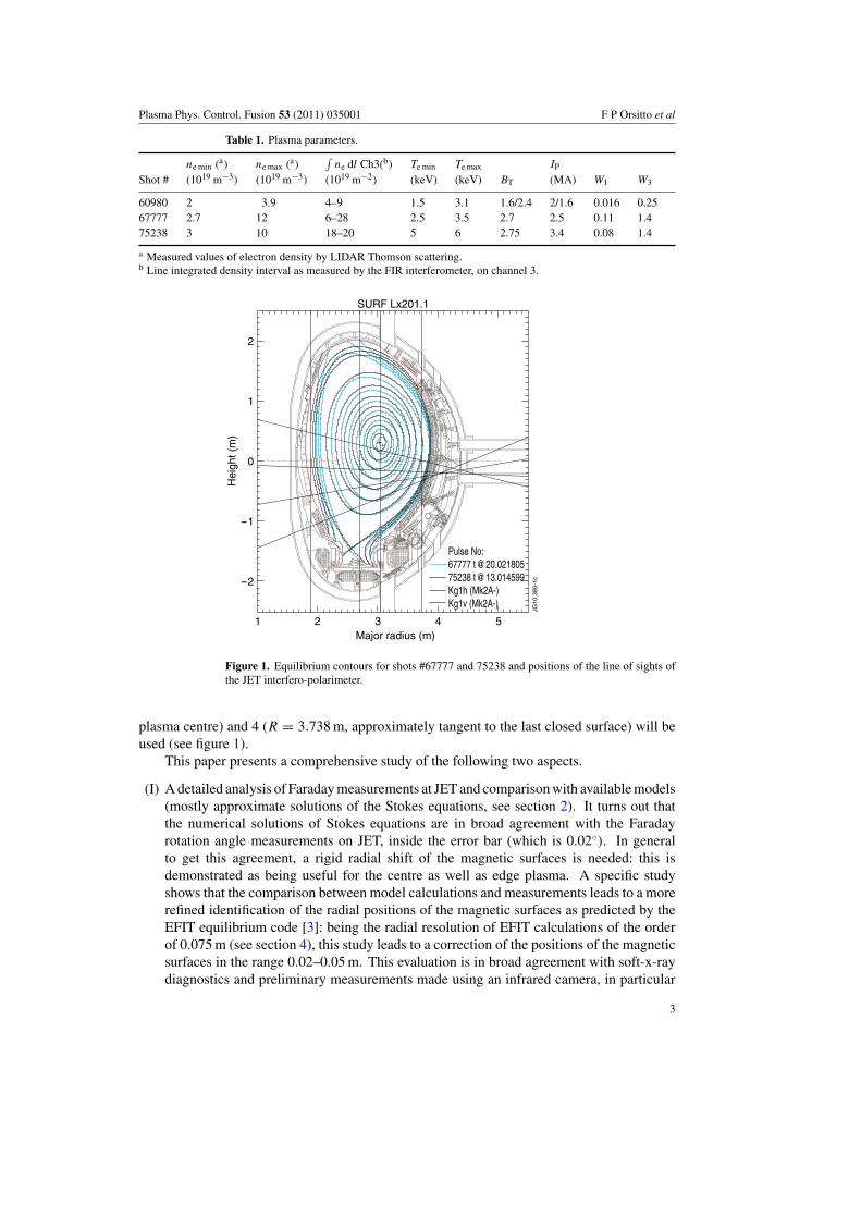
Figure 1. Equilibrium contours for shots #67777 and 75238 and positions of the line of sights ofthe JET interfero-polarimeter.

plasma centre) and 4 (R = 3.738 m, approximately tangent to the last closed surface) will beused (see figure 1).

This paper presents a comprehensive study of the following two aspects.

(I) A detailed analysis of Faraday measurements at JET and comparison with available models(mostly approximate solutions of the Stokes equations, see section 2). It turns out thatthe numerical solutions of Stokes equations are in broad agreement with the Faradayrotation angle measurements on JET, inside the error bar (which is 0.02◦). In generalto get this agreement, a rigid radial shift of the magnetic surfaces is needed: this isdemonstrated as being useful for the centre as well as edge plasma. A specific studyshows that the comparison between model calculations and measurements leads to a morerefined identification of the radial positions of the magnetic surfaces as predicted by theEFIT equilibrium code [3]: being the radial resolution of EFIT calculations of the orderof 0.075 m (see section 4), this study leads to a correction of the positions of the magneticsurfaces in the range 0.02–0.05 m. This evaluation is in broad agreement with soft-x-raydiagnostics and preliminary measurements made using an infrared camera, in particular

3

Plasma Phys. Control. Fusion 53 (2011) 035001 F P Orsitto et al

the difference, with respect to EFIT evaluation, of the plasma centre position measured bysoft-X and IR camera measurements of the strike points on the external divertor targets,is close to the shift of the magnetic surfaces obtained using polarimetry.

(II) A rigorous approach to the interaction between Faraday and Cotton–Mouton (studied inrecent papers, see [2] for details): it is demonstrated that at high density and current, theCotton–Mouton must be calculated including the dependence by Faraday rotation.

Since the solutions to the Stokes equations were discussed in [2], the names andclassification of the solutions are retained in this paper, and only a short introduction to Stokesequations and solutions will be presented, the details are given in [2].

The paper is organized as follows: in section 2, a short summary of the measurements ofthe JET polarimetry system is given, together with the Stokes equations and their approximatesolutions: an example of a comparison between Faraday rotation measurements and modelcalculations is presented; in section 3, the analysis of Faraday rotation measurements and acomparison with a rigorous solution of polarimetry propagation equations is used to determinean improvement of the position of the magnetic surfaces as calculated by EFIT (magneticequilibrium code); in section 4, a statistical analysis on large databases of the determination ofthe position is presented; in section 5, a theoretical analysis of the coupling between Faradayand Cotton–Mouton effects and its application to study shots with high density and high plasmacurrent is presented. The coupling between Faraday and Cotton–Mouton is analysed using anew set of equations (derived from and equivalent to the Stokes equations) which are useful tounderstand how the coupling acts; in section 6, comments are presented on the mathematicalmodels of Faraday and Cotton–Mouton to be used as constraints in equilibrium codes; insection 7, the conclusions are presented.

Hereafter a plasma discharge is also named as ‘shot’; and ‘numerical solution’ alwaysrefers to the numerical solution of the Stokes equations (see equation (2.2)), using as inputto the equations, the density profile measured by Thomson scattering and the magnetic fieldscalculated by the EFIT equilibrium code [3] (see section 2); the terms ‘Faraday’ (‘Cotton–Mouton’) will be used often, meaning ‘Faraday rotation angle’ (‘Cotton–Mouton phase shiftangle’) measurements. In the paper the symbols: (i) ϕT and ψT are used for the Cotton–Mouton phase shift (CM) and Faraday rotation angle (FR), respectively, obtained by numericalsolutions of Stokes equations; (ii) ϕex and ψex are used for the corresponding CM and FRpolarimetric measurements; (iii) ϕTyII and ψTyII are used for the quantities calculated usingformulae (2.12); (iv) Wi (i = 1, 2, 3) are defined in equation (2.7)–(2.9) defining the type Iapproximation; (v) W3G is the Gunther Model A approximation, whose explicit expression isgiven in [2].

2. Stokes equations and their approximate solutions

The considered geometry includes the propagation of a laser beam along a vertical chord (takenas the z-axis) in a poloidal plane of a tokamak. The toroidal magnetic field ( �Bt) is taken alongthe y-axis, while the component of the poloidal magnetic field perpendicular to the propagationz-axis is taken along the x-axis (identical to the radial axis). The angle of the electric fieldvector of the input wave with �Bt is 45◦, to maximize the Cotton–Mouton phase shift angle orthe ellipticity of the wave.

The polarization of a beam can be described using the Stokes vector �s, whose componentsare expressed in terms of the ellipticity angle (χ) and Faraday angle (ψ), or in terms of theratio of the hortogonal components of the laser beam electric field (the ratio Ey/Ex = tan α)

and their phase shift angle (ϕ).

4

Plasma Phys. Control. Fusion 53 (2011) 035001 F P Orsitto et al

The equations defining the Stokes vector �s = (s1, s2, s3) [2, 4, 5], in terms of (χ, ψ) and(α, ϕ) are

s1 = cos(2χ) cos(2ψ) = cos(2α),

s2 = cos(2χ) sin(2ψ) = sin(2α) cos(ϕ),

s3 = sin(2χ) = sin(2α) sin(ϕ),

s21 + s2

2 + s23 = 1.

(2.1)

In terms of the polarization ellipse, ψ (the Faraday rotation angle) is the azimuth of thepolarization ellipse (0 � ψ � π), χ is the ellipticity angle given by tan χ = ±b/a

(−π/4 � χ � π/4), where the major semiaxis of the polarization ellipse is a and theminor semiaxis is b, and the plus sign is taken for clockwise rotation of the wave electric field,looking towards the radiation source.

The previous equations are valid when the absorption of the wave is negligible (see [8])so that the Stokes vector is described by only three components (two of them are independent,see (2.1)).

The JET polarimeter system measures primarily (i) two components of the electric field(Ex and Ey , in a plane orthogonal to the propagation direction) of the laser beam emergingfrom the plasma as well as (ii) the phase shift (ϕ) between these components. So the primarymeasurements are

tan α = Ey

Ex

and ϕ.

In principle, the JET polarimetric system gives the possibility of determining directly the valuesof the components of the Stokes vector, using the measurements of α and ϕ and definitions (2.1).

The Faraday rotation angle and ellipticity (defined as ε = tan χ) are obtained fromequation (2.1):

tan 2ψ = tan 2α cos ϕ,

tan 2χ = s3√1 − s2

3

.

The spatial evolution along the z-axis of the polarization of a beam is given by the Stokesequation:

d�sdZ

= �� × �s (2.2)

where�� = ka(�1, �2, �3) and �1 = C1n(B2

t − B2x ), �2 = 2C1nBxBt, �3 − C3nBz

(2.3)

where Bt is the toroidal magnetic field (Tesla), Bz is the component of the poloidal magneticfield along the propagation axis, Bx is the component of poloidal magnetic field orthogonal tothe propagation axis (the ratio Bx/Bt � 10−1, so neglecting Bx implies an error �1% in theevaluation of �1), n is the electron density (m−3), C1 = 1.8 × 10−22 and C3 = 2 × 10−20,calculated for the laser wavelength of λ = 195 µm, and Z = z/ka is the normalized coordinatealong a vertical chord, where k is the elongation anda is the minor radius. The relations betweenthe Faraday rotation ψ and the Cotton–Mouton phase shift ϕ angles and the correspondingcomponents of Stokes vector follow from (2.1):

s2

s1= tan 2ψ (2.4)

s3

s2= tan ϕ. (2.5)

5

Plasma Phys. Control. Fusion 53 (2011) 035001 F P Orsitto et al

Table 2. Error bars of measurements used in the calculations.

Diagnostic system Measured quantity Symbol Error bar

Polarimeter Faraday rotation ψ 0.2◦

Polarimeter Cotton–Mouton phase shift ϕ 2◦

LIDAR Thomson scattering Line-integral plasma density∫

ne dL 10%LIDAR TS Plasma density profile ne 5%LIDAR TS Plasma temperature profile Te 10%

Equation (2.2) is solved, with the initial condition (i.e. the Stokes vector of the inputwave):

�sinput = (0, 1, 0) (2.6)

corresponding to a 45◦ angle between the electric field vector of the input wave and �Bt . Thisarrangement is optimized for Cotton–Mouton measurements.

In this work data related to the channels 3 and 4 are presented: the data exhibit a reasonablygood signal to noise ratio and the geometry to be analysed is relatively simple. Figure 1 showsfor shots #67777 and #75238 the equilibrium contours and the positions of the line of sightsof the vertical and horizontal channels of the polarimeter, channel 3 is the vertical line atR = 3.039 m, while (vertical) channel 4 has the radial coordinate at R = 3.738 m.

The values of the vector �� = ka(�1, �2, �3) are obtained [2] using the values of �Bas calculated by the EFIT equilibrium reconstruction and the LIDAR Thomson scatteringmeasurements of plasma density (n) projected along the line of sight of the vertical channelson the basis of the reconstructed equilibrium.

The values of �B in the following sections are determined by EFIT using mainly external(to the plasma) magnetic measurements. The question is about the accuracy of the evaluationof the magnetic field given by EFIT, and its effect on the accuracy of the calculations of Faradayrotation by solving the Stokes equations. This question is linked to the accuracy of the EFITdetermination of the current profile and the related safety factor spatial profile. The accuracy ofthe safety factor evaluations made by EFIT could be estimatedq(0)/q(0) � 20–30% [12, 13],where q(0) is the safety factor at the plasma centre. The effect of the accuracy of the currentprofile on the interpretation of polarimetric measurements can be evaluated noting that channel3 has a line of sight passing through the magnetic centre where the poloidal magnetic field(Bp) is inverting the sign (being Bp = 0 at the magnetic centre) so the determination ofthe Faraday is mostly influenced by the values of Bp at mid-radius where the accuracy isrelatively improved and the error bar could be estimated in Bp/Bp(mid-radius) � 10%,leading to an estimation of the accuracy of �i(i = 1, 2, 3)/�i � 15% (if the accuracy onthe measurements of the plasma density profile, see table 2, is included). To link this evaluationto the accuracy on the calculation of Stokes vector we note that the Stokes equations (2.2) can bewritten as

d�sdZ

= M · �s,where M is a matrix containing �i . The formal solution can be expressed as si =exp(

∫Mij dZ) · s0j which implies that the error bar on the values of the Stokes vector can be

evaluated as s/s � max(M/M) � �i(i = 1, 2, 3)/�i ∼ 15%. The accuracy on theequilibrium calculation has the effect on the calculation of the Faraday rotation angle leading tothe rough evaluation of ψ/ψ ∼ s/s � 15% (using equation (2.4), and the approximationof tan 2ψ ∼ 2ψ).

6

Plasma Phys. Control. Fusion 53 (2011) 035001 F P Orsitto et al

The type I solution [2, 5] is obtained as the first term of a series expansion in Wi =∫�i dz,W 2

i � 1 (i = 1, 2, 3), to the solution of the system of ordinary differential equations(2.2), together with the initial condition (2.6). In this approximation the relations between theStokes vector, the Faraday rotation ψ and Cotton–Mouton phase shift angle ϕ are given by

s1 = −W3 = C3

∫neBz dz = 1/ tan 2ψ, (2.7)

s2 = 1 − (W 21 + W 2

3 )/2 ≈ 1, (2.8)

s3 = W1 = C1

∫B2

t ne dz = tan ϕ. (2.9)

Relations (2.7) and (2.9) are the key equations used for evaluating the polarimetricmeasurements linking the Faraday rotation to the component of the poloidal magnetic fieldalong the direction of propagation of the laser beam (and then to the plasma current profile), andthe Cotton–Mouton phase shift angle to the line integral of the electron density. The expressionsin (2.7) and (2.9) are valid only for W 2

i � 1: for large Faraday and Cotton–Mouton angles(see also in the following the discussion on type II approximation) other methods must be usedto find solutions to the Stokes equations. The term ‘linear approximation’ will be used in thispaper with reference to formulae (2.7)–(2.9).

The physical meaning of the type I approximation can be appreciated, if we considerthe situation where the transverse components of the magnetic field are not present (i.e.Bt = Bx = 0 in (2.3), and �1 = �2 = 0), and there is a magnetic field Bz in the directionof beam propagation. This is the case of a ‘pure’ Faraday rotation. Solving the Stokesequations (2.2) with the initial conditions (2.6) leads to the solutions:

s1 = cos 2ψ = cos(2ψ0 + W3),

s2 = sin 2ψ = sin(2ψ0 + W3),

s3 = sin 2χ0 = 0,

the Faraday rotation is then obtained from the previous equations:

2ψ = 2ψ0 + W3. (2.10)

It can be verified that the previous formula leads to (2.7) (type I) at the same level of theapproximation (i.e. W3 � 1, in practice W3 � π/6 = 0.5). The ‘pure’ Faraday rotation isrepresented by W3/2.

The ‘pure Cotton–Mouton’ can be derived from the solutions of Stokes equationsconsidering the case of Bz = Bx = 0, i.e. �3 = 0 = �2:

s1 = s10 = 0,

s2 = sin 2α0 cos ϕ = sin 2α0 cos(ϕ0 + W1) = cos(ϕ0 + W1),

s3 = sin 2α0 sin ϕ = sin 2α0 sin(ϕ0 + W1) = sin(ϕ0 + W1).

The ‘pure Cotton–Mouton’ is then represented by W1; in fact from the previous equations weobtain

ϕ = ϕ0 + W1.

Under the ideal conditions ϕ0 = 0, so ϕ = W1.The physical meaning of W1 and W3 is related to ‘pure’ Cotton–Mouton and Faraday

rotation, respectively, in a context where the two effects can be considered separately,independent and small.

7

Plasma Phys. Control. Fusion 53 (2011) 035001 F P Orsitto et al

More general approximate solutions [2] to equation (2.2) can be found, observing that thefollowing inequalities between the components of the vector �� hold for tokamak plasmas:

|�3| � �1 > |�2|. (2.11)

As a consequence of condition (2.10), the terms with component �2 can be neglectedin the Stokes equations (2.2) and terms in �1s3 neglected with respect to �3s1, in theseapproximations the Stokes equations can be integrated analytically, and the expressions (type IIsolutions) for the Faraday angle and Cotton–Mouton phase shift can be obtained [2]:

s2

s1(z) = tan 2ψ = − 1

tan(W3)= tan(W3 + 2∗π/4),

s3

s2(z) = tan ϕ =

∫ +z

−zdy�1(y) cos(W3(y))

cos(W3(z)). (2.12)

A clear trend present in formulae (2.12) is that the Cotton–Mouton phase shift increaseswith W3 (for values corresponding to JET data) (see section 3 and figure 6). In practicefor Faraday rotation angles ψ − ψ0 � 12◦ (the initial angle is ψ0 = π/4, see (2.6)),1 � cos(W3) � 0.9 and tan ϕ ≈ W1, within an approximation of 10%, whereas for Faradayangles ψ − ψ0 � 12◦ the Cotton–Mouton increases due to the enhancement linked withFaraday rotation (W3 � 2π/15 = 0.4).

In the following discussion concerning the comparison between measurements and modelcalculations, the Guenther Model A [4] will be cited as well: a discussion of the details of thismodel is given in [2, 5]. This model is the analytic solution of Stokes equations in the limit of�3/�1 ∼ Bz/B

2x = K = constant.

Examples of the calculations of the Faraday effect can be produced, starting from data ofshots representative of JET typical operational space. Table 1 gives a choice of three shots withparameters from low density/low current, to high density/high current. Table 2 summarizesthe values of the experimental errors in the measurements used in the Stokes equations.

We start with a low density shot (#60980): the case of ‘pure’ Faraday effect. In particular,type I is expected to fit well the data and this is due to the low value of the Faradayangle and corresponding W3. Figure 2(a) shows the numerical solution of Stokes equations(1/ tan 2ψT), together with the Faraday measurements (1/ tan 2ψex) for shot #60980: thenumerical solution agrees with measurements within the error bar, which for Faraday rotationangle is ψ = 0.004 rad(0.22◦). The data shown on the plot are taken every 840 ms. Aχ2/n = 0.9 (n is the number of data) is calculated: the model fits well the data. Figure 2(b)shows the plasma parameters of shot #60980: time evolution of the line integrated electrondensity on channel 3 measured by the interferometer, maximum temperature as measured byLIDAR Thomson scattering, toroidal magnetic field and plasma current. The strong dynamicsof the polarimeter at time = 15 s is reflected by the variation of the interferometer.

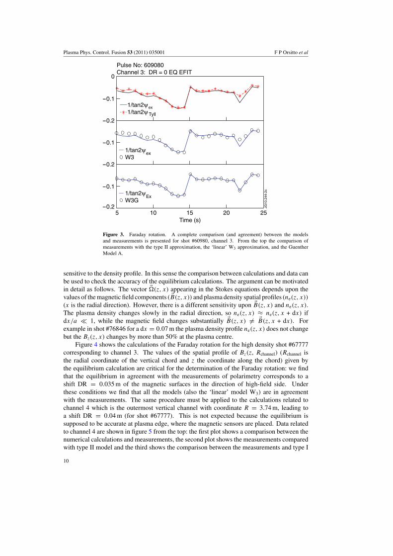
Figure 3 shows the comparison between Faraday measurements and the approximatesolutions (type I (2.7-9), type II (2.12) and Guenther Model A (W3G)) for the low densityshot #60980. All the models are in agreement with the measurements, with different levelsof accuracy: the values of the χ2/n = 1.33 (type II), 1.46 (type I) and 0.0025 (GuentherModel A). The Guenther Model A fits well the data.

Effects on polarization state due to dichroism (differential absorption of the characteristicwaves propagating inside plasma) were analysed (see [8]): for JET plasma parameters theabsorption of the injected wave is negligible and calculations show that the order of magnitudeof the matrix elements corresponding to dichroism are a factor of 10−9 with respect to valuesof �1,3, appearing in the Stokes equations.

8

Plasma Phys. Control. Fusion 53 (2011) 035001 F P Orsitto et al

Figure 2. (a) Faraday rotation measurement (continuous line, shot #60980, channel 3) is plottedtogether with the calculated values (‘∗’ symbol) using the numerical solution of Stokes equations.Plasma parameters are given in table 1. Agreement within the error bars. (b) Plasma parametersof shot #60980, from top: measurements of line integrated density by the interferometer channel3 shot #60980; Electron temperature measured by LIDAR Thomson scattering; plasma current(MA); toroidal magnetic field (T).

3. Faraday rotation measurements and EFIT equilibrium evaluation

The calculation of the Faraday rotation angle using the Stokes model is very sensitive to thecomponents of the magnetic field used in the numerical solution of equation (2.1): it is less

9

Plasma Phys. Control. Fusion 53 (2011) 035001 F P Orsitto et al

Figure 3. Faraday rotation. A complete comparison (and agreement) between the modelsand measurements is presented for shot #60980, channel 3. From the top the comparison ofmeasurements with the type II approximation, the ‘linear’ W3 approximation, and the GuentherModel A.

sensitive to the density profile. In this sense the comparison between calculations and data canbe used to check the accuracy of the equilibrium calculations. The argument can be motivatedin detail as follows. The vector ��(z, x) appearing in the Stokes equations depends upon thevalues of the magnetic field components ( �B(z, x)) and plasma density spatial profiles (ne(z, x))

(x is the radial direction). However, there is a different sensitivity upon �B(z, x) and ne(z, x).The plasma density changes slowly in the radial direction, so ne(z, x) ≈ ne(z, x + dx) ifdx/a � 1, while the magnetic field changes substantially �B(z, x) �= �B(z, x + dx). Forexample in shot #76846 for a dx = 0.07 m the plasma density profile ne(z, x) does not changebut the Bz(z, x) changes by more than 50% at the plasma centre.

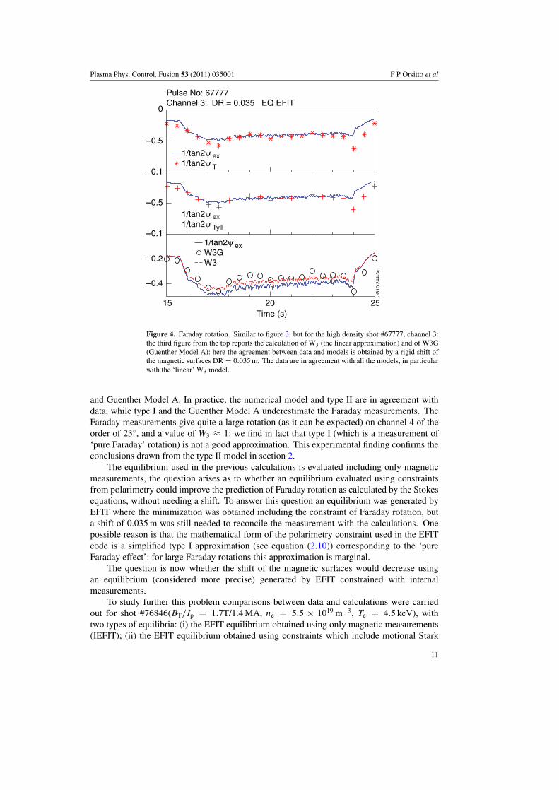
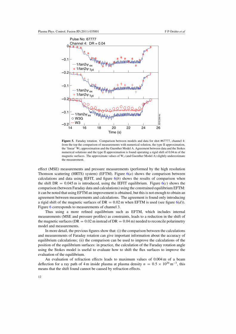
Figure 4 shows the calculations of the Faraday rotation for the high density shot #67777corresponding to channel 3. The values of the spatial profile of Bz(z, Rchannel) (Rchannel isthe radial coordinate of the vertical chord and z the coordinate along the chord) given bythe equilibrium calculation are critical for the determination of the Faraday rotation: we findthat the equilibrium in agreement with the measurements of polarimetry corresponds to ashift DR = 0.035 m of the magnetic surfaces in the direction of high-field side. Underthese conditions we find that all the models (also the ‘linear’ model W3) are in agreementwith the measurements. The same procedure must be applied to the calculations related tochannel 4 which is the outermost vertical channel with coordinate R = 3.74 m, leading toa shift DR = 0.04 m (for shot #67777). This is not expected because the equilibrium issupposed to be accurate at plasma edge, where the magnetic sensors are placed. Data relatedto channel 4 are shown in figure 5 from the top: the first plot shows a comparison between thenumerical calculations and measurements, the second plot shows the measurements comparedwith type II model and the third shows the comparison between the measurements and type I

10

Plasma Phys. Control. Fusion 53 (2011) 035001 F P Orsitto et al

Figure 4. Faraday rotation. Similar to figure 3, but for the high density shot #67777, channel 3:the third figure from the top reports the calculation of W3 (the linear approximation) and of W3G(Guenther Model A): here the agreement between data and models is obtained by a rigid shift ofthe magnetic surfaces DR = 0.035 m. The data are in agreement with all the models, in particularwith the ‘linear’ W3 model.

and Guenther Model A. In practice, the numerical model and type II are in agreement withdata, while type I and the Guenther Model A underestimate the Faraday measurements. TheFaraday measurements give quite a large rotation (as it can be expected) on channel 4 of theorder of 23◦, and a value of W3 ≈ 1: we find in fact that type I (which is a measurement of‘pure Faraday’ rotation) is not a good approximation. This experimental finding confirms theconclusions drawn from the type II model in section 2.

The equilibrium used in the previous calculations is evaluated including only magneticmeasurements, the question arises as to whether an equilibrium evaluated using constraintsfrom polarimetry could improve the prediction of Faraday rotation as calculated by the Stokesequations, without needing a shift. To answer this question an equilibrium was generated byEFIT where the minimization was obtained including the constraint of Faraday rotation, buta shift of 0.035 m was still needed to reconcile the measurement with the calculations. Onepossible reason is that the mathematical form of the polarimetry constraint used in the EFITcode is a simplified type I approximation (see equation (2.10)) corresponding to the ‘pureFaraday effect’: for large Faraday rotations this approximation is marginal.

The question is now whether the shift of the magnetic surfaces would decrease usingan equilibrium (considered more precise) generated by EFIT constrained with internalmeasurements.

To study further this problem comparisons between data and calculations were carriedout for shot #76846(BT/Ip = 1.7T/1.4 MA, ne = 5.5 × 1019 m−3, Te = 4.5 keV), withtwo types of equilibria: (i) the EFIT equilibrium obtained using only magnetic measurements(IEFIT); (ii) the EFIT equilibrium obtained using constraints which include motional Stark

11

Plasma Phys. Control. Fusion 53 (2011) 035001 F P Orsitto et al

Figure 5. Faraday rotation. Comparison between models and data for shot #67777, channel 4:from the top the comparison of measurements with numerical solution, the type II approximation,the ‘linear’ W3 approximation and the Guenther Model A. Agreement between data and the Stokesnumerical solutions and the type II approximation is found operating a rigid shift of 0.04 m of themagnetic surfaces. The approximate values of W3 (and Guenther Model A) slightly underestimatethe measurement.

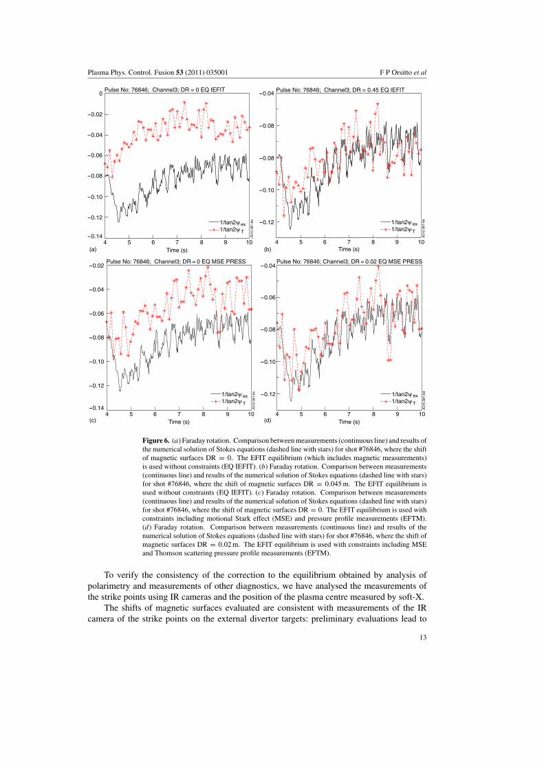
effect (MSE) measurements and pressure measurements (performed by the high resolutionThomson scattering (HRTS) system) (EFTM). Figure 6(a) shows the comparison betweencalculations and data using IEFIT, and figure 6(b) shows the results of comparison whenthe shift DR = 0.045 m is introduced, using the IEFIT equilibrium. Figure 6(c) shows thecomparison (between Faraday data and calculations) using the constrained equilibrium EFTM:it can be noted that using EFTM an improvement is obtained, but this is not enough to obtain anagreement between measurements and calculations. The agreement is found only introducinga rigid shift of the magnetic surfaces of DR = 0.02 m when EFTM is used (see figure 6(d)).Figure 6 corresponds to measurements of channel 3.

Thus using a more refined equilibrium such as EFTM, which includes internalmeasurements (MSE and pressure profiles) as constraints, leads to a reduction in the shift ofthe magnetic surfaces (DR = 0.02 m instead of DR = 0.04 m) needed to reconcile polarimetrymodel and measurements.

In more detail, the previous figures show that: (i) the comparison between the calculationsand measurements of Faraday rotation can give important information about the accuracy ofequilibrium calculations; (ii) the comparison can be used to improve the calculations of theposition of the equilibrium surfaces: in practice, the calculation of the Faraday rotation angleusing the Stokes model is useful to evaluate how to shift the flux surfaces to improve theevaluation of the equilibrium.

An evaluation of refraction effects leads to maximum values of 0.004 m of a beamdeflection for a ray path of 4 m inside plasma at plasma density n = 0.5 × 1020 m−3, thismeans that the shift found cannot be caused by refraction effects.

12

Plasma Phys. Control. Fusion 53 (2011) 035001 F P Orsitto et al

Figure 6. (a) Faraday rotation. Comparison between measurements (continuous line) and results ofthe numerical solution of Stokes equations (dashed line with stars) for shot #76846, where the shiftof magnetic surfaces DR = 0. The EFIT equilibrium (which includes magnetic measurements)is used without constraints (EQ IEFIT). (b) Faraday rotation. Comparison between measurements(continuous line) and results of the numerical solution of Stokes equations (dashed line with stars)for shot #76846, where the shift of magnetic surfaces DR = 0.045 m. The EFIT equilibrium isused without constraints (EQ IEFIT). (c) Faraday rotation. Comparison between measurements(continuous line) and results of the numerical solution of Stokes equations (dashed line with stars)for shot #76846, where the shift of magnetic surfaces DR = 0. The EFIT equilibrium is used withconstraints including motional Stark effect (MSE) and pressure profile measurements (EFTM).(d) Faraday rotation. Comparison between measurements (continuous line) and results of thenumerical solution of Stokes equations (dashed line with stars) for shot #76846, where the shift ofmagnetic surfaces DR = 0.02 m. The EFIT equilibrium is used with constraints including MSEand Thomson scattering pressure profile measurements (EFTM).

To verify the consistency of the correction to the equilibrium obtained by analysis ofpolarimetry and measurements of other diagnostics, we have analysed the measurements ofthe strike points using IR cameras and the position of the plasma centre measured by soft-X.

The shifts of magnetic surfaces evaluated are consistent with measurements of the IRcamera of the strike points on the external divertor targets: preliminary evaluations lead to

13

Plasma Phys. Control. Fusion 53 (2011) 035001 F P Orsitto et al

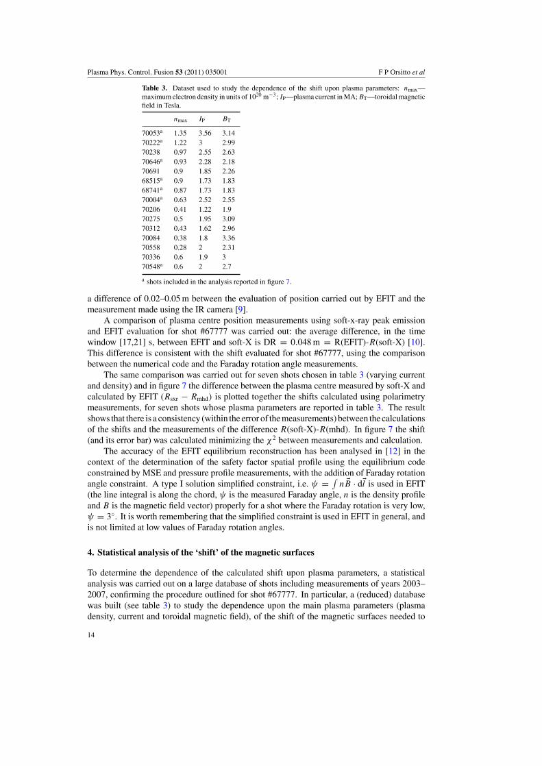
Table 3. Dataset used to study the dependence of the shift upon plasma parameters: nmax—maximum electron density in units of 1020 m−3; IP—plasma current in MA; BT—toroidal magneticfield in Tesla.

nmax IP BT

70053a 1.35 3.56 3.1470222a 1.22 3 2.9970238 0.97 2.55 2.6370646a 0.93 2.28 2.1870691 0.9 1.85 2.2668515a 0.9 1.73 1.8368741a 0.87 1.73 1.8370004a 0.63 2.52 2.5570206 0.41 1.22 1.970275 0.5 1.95 3.0970312 0.43 1.62 2.9670084 0.38 1.8 3.3670558 0.28 2 2.3170336 0.6 1.9 370548a 0.6 2 2.7

a shots included in the analysis reported in figure 7.

a difference of 0.02–0.05 m between the evaluation of position carried out by EFIT and themeasurement made using the IR camera [9].

A comparison of plasma centre position measurements using soft-x-ray peak emissionand EFIT evaluation for shot #67777 was carried out: the average difference, in the timewindow [17,21] s, between EFIT and soft-X is DR = 0.048 m = R(EFIT)-R(soft-X) [10].This difference is consistent with the shift evaluated for shot #67777, using the comparisonbetween the numerical code and the Faraday rotation angle measurements.

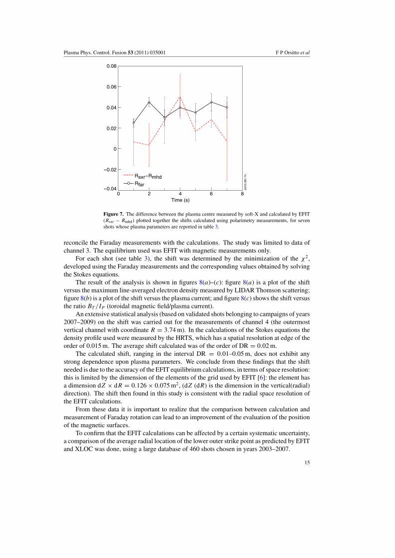
The same comparison was carried out for seven shots chosen in table 3 (varying currentand density) and in figure 7 the difference between the plasma centre measured by soft-X andcalculated by EFIT (Rsxr − Rmhd) is plotted together the shifts calculated using polarimetrymeasurements, for seven shots whose plasma parameters are reported in table 3. The resultshows that there is a consistency (within the error of the measurements) between the calculationsof the shifts and the measurements of the difference R(soft-X)-R(mhd). In figure 7 the shift(and its error bar) was calculated minimizing the χ2 between measurements and calculation.

The accuracy of the EFIT equilibrium reconstruction has been analysed in [12] in thecontext of the determination of the safety factor spatial profile using the equilibrium codeconstrained by MSE and pressure profile measurements, with the addition of Faraday rotationangle constraint. A type I solution simplified constraint, i.e. ψ = ∫

n �B · d�l is used in EFIT(the line integral is along the chord, ψ is the measured Faraday angle, n is the density profileand B is the magnetic field vector) properly for a shot where the Faraday rotation is very low,ψ = 3◦. It is worth remembering that the simplified constraint is used in EFIT in general, andis not limited at low values of Faraday rotation angles.

4. Statistical analysis of the ‘shift’ of the magnetic surfaces

To determine the dependence of the calculated shift upon plasma parameters, a statisticalanalysis was carried out on a large database of shots including measurements of years 2003–2007, confirming the procedure outlined for shot #67777. In particular, a (reduced) databasewas built (see table 3) to study the dependence upon the main plasma parameters (plasmadensity, current and toroidal magnetic field), of the shift of the magnetic surfaces needed to

14

Plasma Phys. Control. Fusion 53 (2011) 035001 F P Orsitto et al

0.06

0.04

0.02

0

-0.02

-0.04

0.08

2 4 60 8Time (s)

JG10

.381

-7cRsxr-Rmhd

Rfar

Figure 7. The difference between the plasma centre measured by soft-X and calculated by EFIT(Rsxr − Rmhd) plotted together the shifts calculated using polarimetry measurements, for sevenshots whose plasma parameters are reported in table 3.

reconcile the Faraday measurements with the calculations. The study was limited to data ofchannel 3. The equilibrium used was EFIT with magnetic measurements only.

For each shot (see table 3), the shift was determined by the minimization of the χ2,developed using the Faraday measurements and the corresponding values obtained by solvingthe Stokes equations.

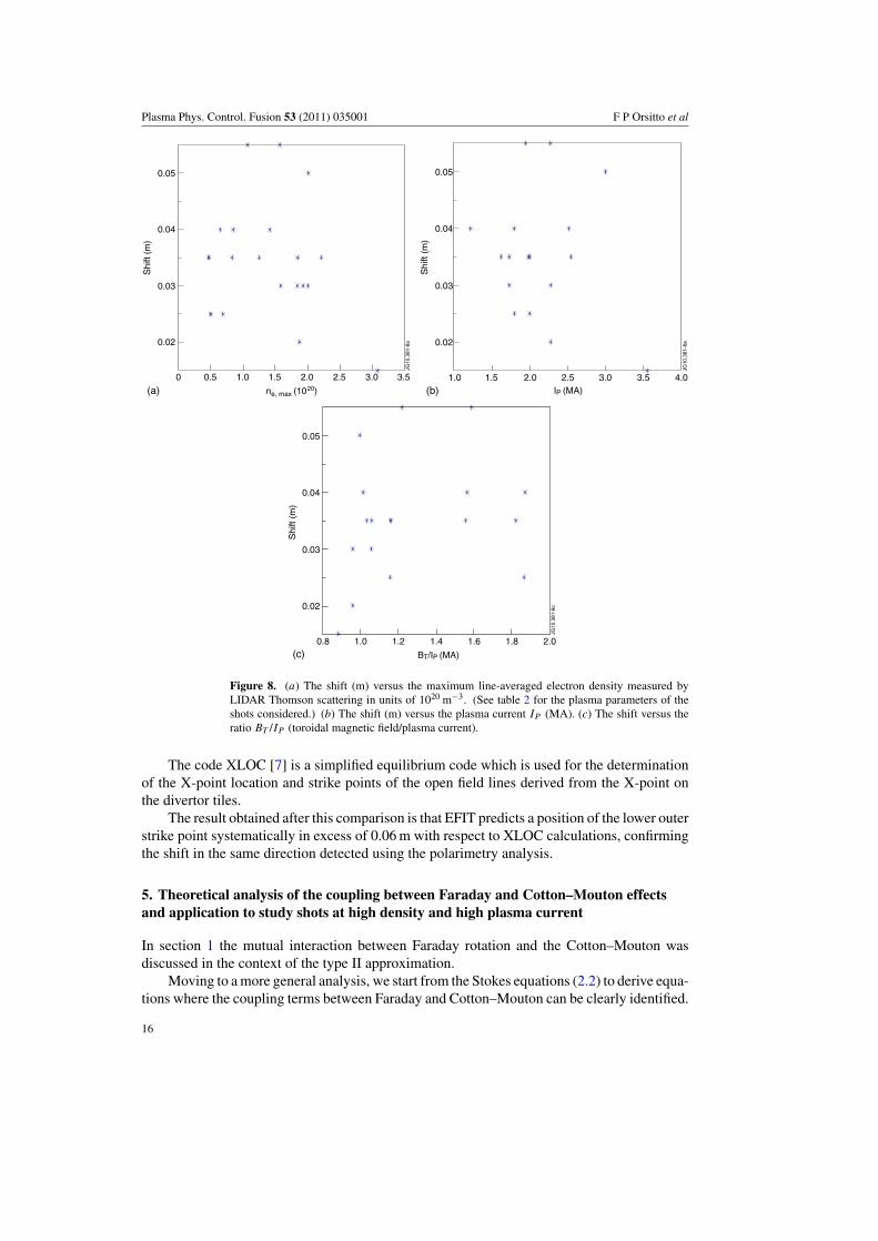
The result of the analysis is shown in figures 8(a)–(c): figure 8(a) is a plot of the shiftversus the maximum line-averaged electron density measured by LIDAR Thomson scattering;figure 8(b) is a plot of the shift versus the plasma current; and figure 8(c) shows the shift versusthe ratio BT /IP (toroidal magnetic field/plasma current).

An extensive statistical analysis (based on validated shots belonging to campaigns of years2007–2009) on the shift was carried out for the measurements of channel 4 (the outermostvertical channel with coordinate R = 3.74 m). In the calculations of the Stokes equations thedensity profile used were measured by the HRTS, which has a spatial resolution at edge of theorder of 0.015 m. The average shift calculated was of the order of DR = 0.02 m.

The calculated shift, ranging in the interval DR = 0.01–0.05 m, does not exhibit anystrong dependence upon plasma parameters. We conclude from these findings that the shiftneeded is due to the accuracy of the EFIT equilibrium calculations, in terms of space resolution:this is limited by the dimension of the elements of the grid used by EFIT [6]: the element hasa dimension dZ × dR = 0.126 × 0.075 m2, (dZ (dR) is the dimension in the vertical(radial)direction). The shift then found in this study is consistent with the radial space resolution ofthe EFIT calculations.

From these data it is important to realize that the comparison between calculation andmeasurement of Faraday rotation can lead to an improvement of the evaluation of the positionof the magnetic surfaces.

To confirm that the EFIT calculations can be affected by a certain systematic uncertainty,a comparison of the average radial location of the lower outer strike point as predicted by EFITand XLOC was done, using a large database of 460 shots chosen in years 2003–2007.

15

Plasma Phys. Control. Fusion 53 (2011) 035001 F P Orsitto et al

0.05

0.04

0.03

0.02

0.5 1.0 1.5 2.0 2.5 3.00 3.5

Shi

ft (m

)

ne, max (10(a) (b)

(c)

20)

JG10

.381

-8a

0.05

0.04

0.03

0.02

1.0 1.5 2.0 3.53.02.5 4.0

Shi

ft (m

)

IP (MA)

JG10

.381

-8a

0.05

0.04

0.03

0.02

1.0 1.2 1.4 1.6 1.80.8 2.0

Shi

ft (m

)

BT/IP (MA)

JG10

.381

-8c

Figure 8. (a) The shift (m) versus the maximum line-averaged electron density measured byLIDAR Thomson scattering in units of 1020 m−3. (See table 2 for the plasma parameters of theshots considered.) (b) The shift (m) versus the plasma current IP (MA). (c) The shift versus theratio BT /IP (toroidal magnetic field/plasma current).

The code XLOC [7] is a simplified equilibrium code which is used for the determinationof the X-point location and strike points of the open field lines derived from the X-point onthe divertor tiles.

The result obtained after this comparison is that EFIT predicts a position of the lower outerstrike point systematically in excess of 0.06 m with respect to XLOC calculations, confirmingthe shift in the same direction detected using the polarimetry analysis.

5. Theoretical analysis of the coupling between Faraday and Cotton–Mouton effectsand application to study shots at high density and high plasma current

In section 1 the mutual interaction between Faraday rotation and the Cotton–Mouton wasdiscussed in the context of the type II approximation.

Moving to a more general analysis, we start from the Stokes equations (2.2) to derive equa-tions where the coupling terms between Faraday and Cotton–Mouton can be clearly identified.

16

Plasma Phys. Control. Fusion 53 (2011) 035001 F P Orsitto et al

Defining

F = s1

s2= 1

tan 2ψand C = s3

s2= tan ϕ

from the Stokes equations (2.2) the following system can be derived:

dF

dZ= −�3 − �3F

2 + �1FC + �2C, (5.1)

dC

dZ= �1 + �1C

2 − �3FC − �2F. (5.2)

System (5.1)–(5.2), which is exactly equivalent to the Stokes model, can be consideredas a generalized Volterra-like problem, with non-constant coefficients. The propagationof polarization in a plasma (without absorption) can be described using a first order non-linear differential system in two variables: plasma polarimetry is intrinsically described by abidimensional dynamical system, so chaotic behaviour cannot be realized [11].

The type II approximation (equation (2.12)) is obtained neglecting the terms �1FC +�2C

in equation (5.1) and the terms �1C2 − �2F in equation (5.2).

It appears from the inspection of system (5.1)–(5.2) that two types of non-linearities appearin the propagation of polarization: (i) quadratic terms in F and C; (ii) coupling terms F ∗C.Since usually �3 � �1 it could be expected that the main non-linearity in Faraday is due tothe quadratic term F 2, while for Cotton–Mouton the main non-linearity would be the couplingterm F ∗C.

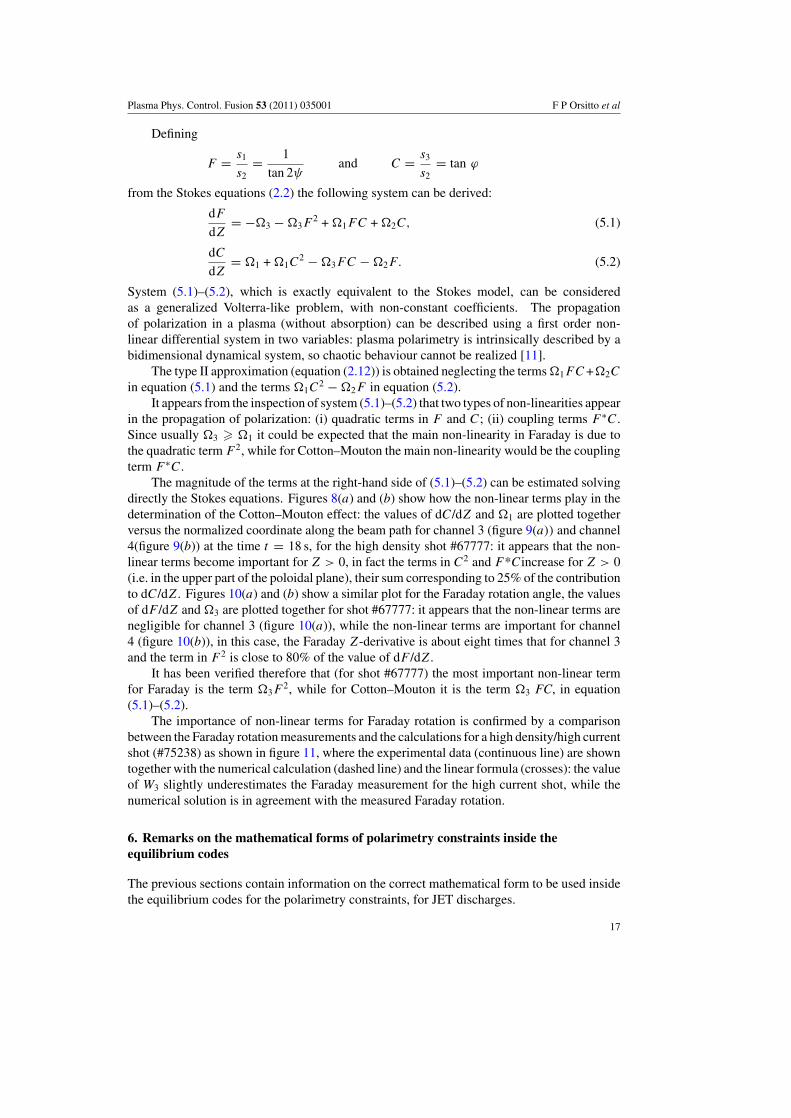
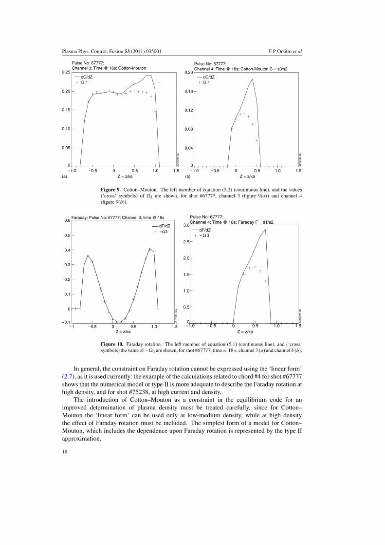
The magnitude of the terms at the right-hand side of (5.1)–(5.2) can be estimated solvingdirectly the Stokes equations. Figures 8(a) and (b) show how the non-linear terms play in thedetermination of the Cotton–Mouton effect: the values of dC/dZ and �1 are plotted togetherversus the normalized coordinate along the beam path for channel 3 (figure 9(a)) and channel4(figure 9(b)) at the time t = 18 s, for the high density shot #67777: it appears that the non-linear terms become important for Z > 0, in fact the terms in C2 and F*Cincrease for Z > 0(i.e. in the upper part of the poloidal plane), their sum corresponding to 25% of the contributionto dC/dZ. Figures 10(a) and (b) show a similar plot for the Faraday rotation angle, the valuesof dF /dZ and �3 are plotted together for shot #67777: it appears that the non-linear terms arenegligible for channel 3 (figure 10(a)), while the non-linear terms are important for channel4 (figure 10(b)), in this case, the Faraday Z-derivative is about eight times that for channel 3and the term in F 2 is close to 80% of the value of dF /dZ.

It has been verified therefore that (for shot #67777) the most important non-linear termfor Faraday is the term �3F

2, while for Cotton–Mouton it is the term �3 FC, in equation(5.1)–(5.2).

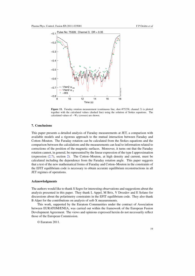
The importance of non-linear terms for Faraday rotation is confirmed by a comparisonbetween the Faraday rotation measurements and the calculations for a high density/high currentshot (#75238) as shown in figure 11, where the experimental data (continuous line) are showntogether with the numerical calculation (dashed line) and the linear formula (crosses): the valueof W3 slightly underestimates the Faraday measurement for the high current shot, while thenumerical solution is in agreement with the measured Faraday rotation.

6. Remarks on the mathematical forms of polarimetry constraints inside theequilibrium codes

The previous sections contain information on the correct mathematical form to be used insidethe equilibrium codes for the polarimetry constraints, for JET discharges.

17

Plasma Phys. Control. Fusion 53 (2011) 035001 F P Orsitto et al

Figure 9. Cotton–Mouton. The left member of equation (5.2) (continuous line), and the values(‘cross’ symbols) of �1 are shown, for shot #67777, channel 3 (figure 9(a)) and channel 4(figure 9(b)).

Figure 10. Faraday rotation. The left member of equation (5.1) (continuous line), and (‘cross’symbols) the value of −�3 are shown, for shot #67777, time = 18 s, channel 3 (a) and channel 4 (b).

In general, the constraint on Faraday rotation cannot be expressed using the ‘linear form’(2.7), as it is used currently: the example of the calculations related to chord #4 for shot #67777shows that the numerical model or type II is more adequate to describe the Faraday rotation athigh density, and for shot #75238, at high current and density.

The introduction of Cotton–Mouton as a constraint in the equilibrium code for animproved determination of plasma density must be treated carefully, since for Cotton–Mouton the ‘linear form’ can be used only at low-medium density, while at high densitythe effect of Faraday rotation must be included. The simplest form of a model for Cotton–Mouton, which includes the dependence upon Faraday rotation is represented by the type IIapproximation.

18

Plasma Phys. Control. Fusion 53 (2011) 035001 F P Orsitto et al

Figure 11. Faraday rotation measurement (continuous line, shot #75238, channel 3) is plottedtogether with the calculated values (dashed line) using the solution of Stokes equations. Thecalculated values of −W3 (crosses) are shown.

7. Conclusions

This paper presents a detailed analysis of Faraday measurements at JET, a comparison withavailable models and a rigorous approach to the mutual interaction between Faraday andCotton–Mouton. The Faraday rotation can be calculated from the Stokes equations and thecomparison between the calculations and the measurements can lead to information related tocorrections of the position of the magnetic surfaces. Moreover, it turns out that the Faradayrotation cannot, in general, be represented by the linear expression of the type I approximation(expression (2.7), section 2). The Cotton–Mouton, at high density and current, must becalculated including the dependence from the Faraday rotation angle. This paper suggeststhat a test of the new mathematical forms of Faraday and Cotton–Mouton in the constraints ofthe EFIT equilibrium code is necessary to obtain accurate equilibrium reconstructions in allJET regimes of operations.

Acknowledgments

The authors would like to thank S Segre for interesting observations and suggestions about theanalysis presented in this paper. They thank L Appel, M Brix, V Drozdov and E Solano fordiscussions about the polarimetry constraints in the EFIT equilibrium code. They also thankB Alper for the contributions on analysis of soft-X measurements.

This work, supported by the Euratom Communities under the contract of Associationbetween EURATOM/ENEA, was carried out within the framework of the European FusionDevelopment Agreement. The views and opinions expressed herein do not necessarily reflectthose of the European Commission.

© Euratom 2011.

19

Plasma Phys. Control. Fusion 53 (2011) 035001 F P Orsitto et al

References

[1] Braithwaite G, Gottardi N, Magyar G, O’Rourke J, Ryan J and Veron D 1989 Rev. Sci. Instrum. 60 2825Veron D 1974 Opt. Commun. 10 95

[2] Orsitto F P, Boboc A, Mazzotta C, Giovannozzi E, Zabeo L and JET EFDA Contributors 2008 Plasma Phys.Control. Fusion 50 115009

[3] O’Brien D et al 1992 Nucl. Fusion 32 1351[4] Guenther K et al 2004 Plasma Phys. Control. Fusion 46 1423[5] Segre S E and Zanza V 2006 Plasma Phys. Control. Fusion 48 339[6] Solano E, private communication[7] Sartori F, Cenedese A and Milani F 2003 Fusion Eng. Des. 66–68 735–9[8] Segre S E 2003 J. Phys. D: Appl. Phys. 36 2806 (equations (48) and (49))[9] Devaux S 2010 Talk given at JET Data Validation Coordination Meeting (27 July 2010, Culham Science Centre,

Abingdon, UK)[10] Alper Bprivate communication[11] Glendinning P 2001 By the Peixoto theorem the dynamics of autonomous differential equations in a plane are

relatively simple, there is no possibility for chaotic behaviour Stability, Instability and Chaos (Cambridge:Cambridge University Press) chapter 5

[12] Brix M, Hawkes N C, Boboc A, Drozdov V, Sharapov S and JET-EFDA Contributors 2008 Rev. Sci. Instrum.79 10F325

[13] De Angelis R et al IAEA FEC 2010—Determination of q profiles in JET by Consistency of Motional StarkEffect and MHD Mode location EXS/P2-03

20