Atmospheric Research 109–110 (2012) 95–113

Contents lists available at SciVerse ScienceDirect

Atmospheric Research

j ourna l homepage: www.e lsev ie r .com/ locate /atmos

Artificial intelligence techniques for clutter identification with polarimetricradar signatures

Tanvir Islam⁎, Miguel A. Rico-Ramirez, Dawei Han, Prashant K. SrivastavaDepartment of Civil Engineering, University of Bristol, Bristol, UK

a r t i c l e i n f o

⁎ Corresponding author at: Department of Civil EngBristol, Bristol, BS8 1TR, UK. Tel.: +44 1173315724; f

E-mail address: tanvir.islam@bristol.ac.uk (T. Islam

0169-8095/$ – see front matter © 2012 Elsevier B.V. Adoi:10.1016/j.atmosres.2012.02.007

a b s t r a c t

Article history:Received 12 July 2011Received in revised form 30 November 2011Accepted 7 February 2012

The use of different artificial intelligence (AI) techniques for clutter signals identification in thecontext of radar based precipitation estimation is presented. The clutter signals considered arebecause of ground clutter, sea clutter and anomalous propagation whereas the explored AItechniques include the support vector machine (SVM), the artificial neural network (ANN),the decision tree (DT), and the nearest neighbour (NN) systems. Eight different radar measure-ment combinations comprising of various polarimetric spectral signatures — the reflectivity(ZH), differential reflectivity (ZDR), differential propagation phase (ΦDP), cross-correlation coef-ficient (ρHV), velocity (V) and spectral width (W) from a C-band polarimetric radar are takeninto account as input vectors to the AI systems. The results reveal that all four AI classifierscan identify the clutter echoes with around 98–99% accuracy when all radar input signaturesare used. As standalone input vectors, the polarimetric textures of the ΦDP and the ZDR havealso demonstrated excellent skills distinguishing clutter echoes with an accuracy of 97–98%approximately. If no polarimetric signature is available, a combination of the texture of ZH, Vand W representing typical measurements from a single-polarization Doppler radar may beused for clutter identification, but with a lower accuracy when compared to the use ofpolarimetric radar measurements. In contrast, the use of ZH or W alone is found less reliablefor clutter classification. Among the AI techniques, the SVM has a slightly better score interms of various clutter identification indicators as compared to the others. Conversely, theNN algorithm has shown a lower performance in identifying the clutter echoes correctly con-sidering the standalone radar signatures as inputs. Despite this, the performance among thedifferent AI techniques is comparable indicating the suitability of the developed systems,and this is further supported when results are compared with the fuzzy logic and Bayesclassifiers.

© 2012 Elsevier B.V. All rights reserved.

Keywords:Dual polarization radarNon-meteorological echoNon-precipitation echoSupport vector machine (SVM)Artificial neural network (ANN)Decision tree (DT)Nearest neighbour algorithm (NN)Target classificationPattern recognitionRainfall estimation uncertaintyAnomalous propagation

1. Introduction

Clutter signals are one of the most common sources of errorin radar remote sensing for quantitative precipitation estimation(QPE). In addition to the drop size distributions' variation (Beardet al., 2010; Bringi et al., 2003), radar miscalibration(Anagnostou et al., 2001; Lee and Zawadzki, 2006), beam block-age (Germann et al., 2006; Krajewski et al., 2006), variation of

ineering, University ofax: +44 1173315719.).

ll rights reserved.

the vertical reflectivity profile (Rico-Ramirez and Cluckie,2007; Rico-Ramirez et al., 2005), and attenuation at higher fre-quency (Bringi et al., 2001; Kramer et al., 2005); the difficultiesin precipitation estimation due to such clutter signals haveremained a challenge (Rico-Ramirez et al., 2007). For accurateand improved QPE from radar measurements, identificationand removal of the clutter signals are essential. However, anyclutter removal algorithm needs to make sure that precipitationechoes are not eliminated since such inaccurate eliminationwould result into underestimation of precipitation. Moreover,misclassification of radar clutter caused by the non-meteorological targets may also lead to ambiguity on

96 T. Islam et al. / Atmospheric Research 109–110 (2012) 95–113

quantitative precipitation forecasting (QPF) (Liguori et al., 2012;Sokol, 2011).

In general, radar clutter refers to the unwanted signalsthat return to the radar from radar emitted energy scatteringoff of mountains and buildings near the earth's surface. Theseunwanted signals are known as ground clutter, which mostlyoccur when the antenna rotates at low elevation angles. Inaddition and depending on the elevation angle, ground clut-ter is found mostly at close range to the radar location. Fortu-nately, the ground clutter is predictable and easy todetermine. However, changes in atmospheric conditions in-troduce another type of unwanted signals, which are difficultto predict. These unwanted signals are the cause of anoma-lous propagation (AP) of the radar beam which forces thebeam to trap towards the earth's surface. The AP has beenrecognized as a severe problem in radar rainfall estimation.From an investigation using eight years of Swiss radar data,Joss and Lee (1995) showed that such AP signals contributedsignificant error in radar rainfall estimation. They estimatedthat the error brought by the AP echoes was 13% of thetotal rainfall accumulations using a 60 month dataset.Moszkowicz et al. (1994) also found that the influence ofnon-eliminated AP echoes on precipitation retrievals was be-tween 59% and 97% of the monthly accumulations. The situa-tion becomes worse when AP signals are embedded inprecipitation as stated in an overview article by Steiner andSmith (2002). Clear air echoes are another form of clutter re-ceived by radars in cloud and precipitation free atmosphere.The sources of clear air echoes are mainly from refractiveindex gradient resulting in Bragg scatter, and biological tar-gets such as birds and insects (Martin and Shapiro, 2007).Sea clutter, chaff, vehicles, and airplane may also introducesignal inconsistency in the radar domain respective to the lo-cation of the radar.

Conventionally, clutter maps have been used for decadesto characterize the clutter signals and predefined cluttermaps obtained during a dry day typically help to removethem. However, false alarm rate of this technique is veryhigh and it cannot detect AP with an adequate accuracy dur-ing precipitation events. The reason is because AP echoesoriginate due to changes in atmospheric conditions whilstground clutter maps are used to identify stationary groundclutter. Particularly, clutter maps are unsatisfactory whenclutter signals are embedded with precipitation echoes (daSilveira and Holt, 2001).

In recent years, as an alternative method to the conven-tional clutter map approach, there has been an increasing in-terest in the use of Artificial Intelligence (AI) techniques forclutter signals' identification. One of the most common andsuccessful techniques from the AI community in identifyingclutter echoes is the fuzzy logic approach. For example,Berenguer et al. (2006) showed satisfactory performance oftheir fuzzy system to classify meteorological echoes fromnon-meteorological echoes. Cho et al. (2006) also describeda fuzzy logic algorithm for non-precipitation echoes' identifi-cation. Another AI technique used from the machine learningcommunity for radar clutter recognitions is the neural net-works. A feed forward neural network with a fuzzy strategyfor AP detection was described in Grecu and Krajewski(1999). This work was followed by the study of Krajewskiand Vignal (2001), where they evaluated the proposed

methodology on a pixel-by-pixel basis and applied it to alarge volume of scans. Statistical learning based Bayesian ap-proach for clutter identification is also reported in the litera-ture. For instance, Pamment and Conway (1998) developedan automatic scheme by taking the information from severalsources such as Meteosat infrared images, a climatology of APechoes, and detected lightning. Moszkowicz et al. (1994)inspected three Bayesian functions for AP detection and ap-plied statistical pattern technique to discard contaminatedsignals considering various feature vectors such as maximumreflectivity, echo top, and horizontal gradients. The recogni-tion error of their approach was around 6% for the best per-forming function. A decision tree based algorithm forautomated recognition and exclusion of undesired signalswas proposed by Steiner and Smith (2002). In fact, past stud-ies conclude that Doppler processing methods in conjunctionwith AI techniques can be considered as a reliable way to de-tect clutter using single polarization Doppler radars since theradial velocity product is a good indicator of the location ofground clutter (i.e. ground targets have a radial velocity ofzero). Nevertheless, the use of Doppler radar alone can beless successful in clutter identification if precipitation regionstravel tangentially relative to the radar (da Silveira and Holt,2001).

In contrast, polarimetric radar is capable of transmittinghorizontal and vertical electromagnetic spectrum. Thus, addi-tional polarimetric signatures such as differential reflectivity(Zdr), differential propagation phase (Φdp), cross-correlationcoefficient (ρHV) and linear depolarization ratio (LDR) areavailable (Husson et al., 1989; Meischner, 1989). The advan-tage of polarimetric radar over single polarization Dopplerradars is that additional information regarding clutter scattercharacteristics can be gained. There are several studies fo-cused on the identification of clutter and anomalous propa-gation using polarimetric radar. One of the first studies wasconducted by Giuli et al. (1991). They showed the potentialof dual-linear polarization measurements for rainfall andclutter classification. Following this work, Ryzhkov andZrnic (1998) demonstrated the usefulness of the correlationcoefficient and the changes of differential phase as robust pa-rameters to classify clutter signals by applying a thresholdbased technique on an S-band radar. In addition to this, afew AI techniques have also been reported for clutter identi-fication in recent times, such as, a fuzzy logic led approachpresented by Gourley et al. (2007), and a neural network ap-proach presented by da Silveira and Holt (2001).

More recently, Rico-Ramirez and Cluckie (2008) havedemonstrated the classification of clutter signals by usingtwo AI techniques — the fuzzy logic and Bayes classifiersfrom polarimetric radar measurements. They have intro-duced a new texture function T(.) calculation methodologyto take into account the edge effects at the boundaries of pre-cipitation regions. Our paper is the extension of this prior ex-periment for clutter identification with new AI techniques.Note that the clutter echoes to be classified in this paper arecaused by ground clutter, sea clutter and AP echoes. Clearair echoes and other form of moving targets (e.g. chaff, vehi-cles, birds, insects and airplanes) are not considered in thisstudy. Indeed, this work is the first attempt in using supportvector machine (SVM), decision tree (DT), and nearest neigh-bour (NN) methods on clutter classification using

97T. Islam et al. / Atmospheric Research 109–110 (2012) 95–113

polarimetric radar signatures to improve QPE. In addition, theperformance of artificial neural network (ANN) based AItechnique in terms of clutter pattern recognitions is also eval-uated. A comprehensive comparison of different AI tech-niques is also provided in this paper.

This paper is structured as follows. Section 2 describes thepolarimetric radar system and radar measurements used inthis study. Different AI techniques, such as, SVM, ANN, DT,and NN, are described in Section 3. Section 4 presents theclassification results obtained from the AI systems with thesummary of different clutter identification indicators whichhave been used in this work for the evaluation of clutter rec-ognition performance. We also compare the performance ofdifferent AI techniques with the fuzzy logic system andBayes classifiers in this section. Finally, the summary andconclusions of this work are included in Section 5.

2. Polarimetric radar system and signatures

This section briefly summarizes the polarimetric radarsystem and signatures used for this study. For detailed dataprocessing, readers are suggested to see the former article(Rico-Ramirez and Cluckie, 2008).

2.1. Radar system

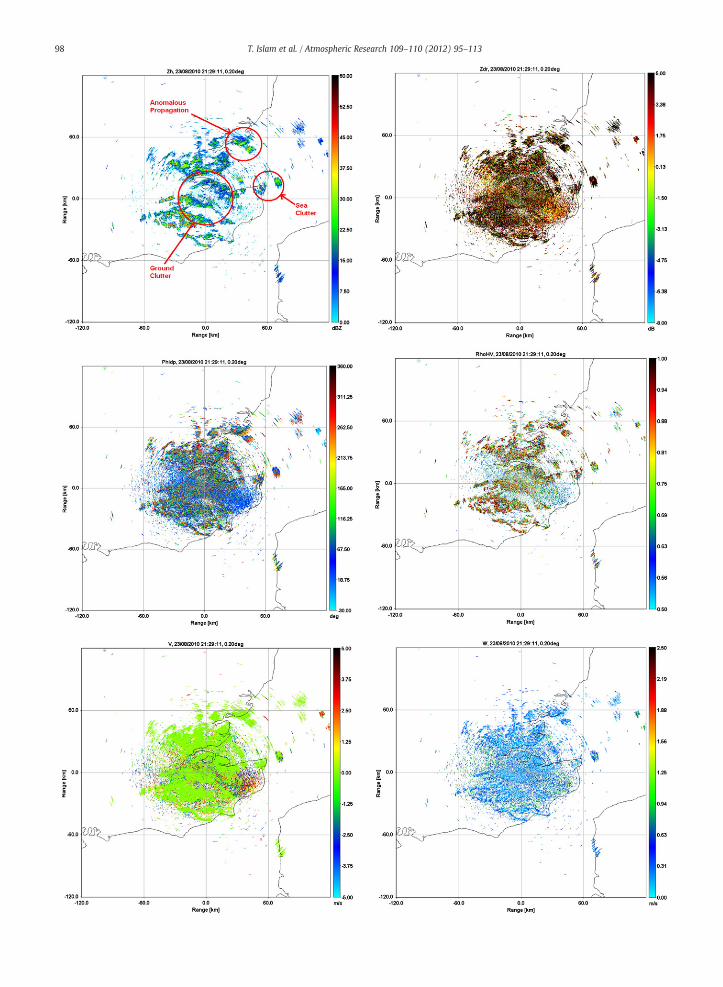
The radar system used in this work is from the Thurnhampolarimetric radar, located in the South-Eastern region of theUK. A detailed technical specification of the radar is given inRico-Ramirez et al. (2009). Operationally, the radar transmitsand receives horizontally and vertically polarized waves withthe default radar settings of 250 m gate size, 2 μs pulselength, 2.16 RPM (revolutions per minute) and 300 Hz PRF(pulse repetition frequency). This radar is particularlyinstalled to improve QPE accuracy fulfilling UK's transitiontowards dual polarization technology. Preliminary QPE as-sessment of the Thurnham radar can be found in Bringi etal. (2011). Fig. 1 gives an example of the various clutter ech-oes scanned by the Thurnham radar for the different radarsignatures viz reflectivity (ZH), differential reflectivity (ZDR),differential propagation phase (ΦDP), cross-correlation coeffi-cient (ρHV), velocity (V) and spectral width (W) during a dryday. In this particular scan, the radar returns signals indicat-ing corresponding values where the nearby rain gauges andUK Met Office Nimrod composite product at 5 km resolution(see Fig. 2) confirm “no precipitation”. In fact, in this case,the Thurnham radar has received signals that are generatedfrom various clutter echoes such as ground clutter, sea clutterand AP.

2.2. Textures and input vectors

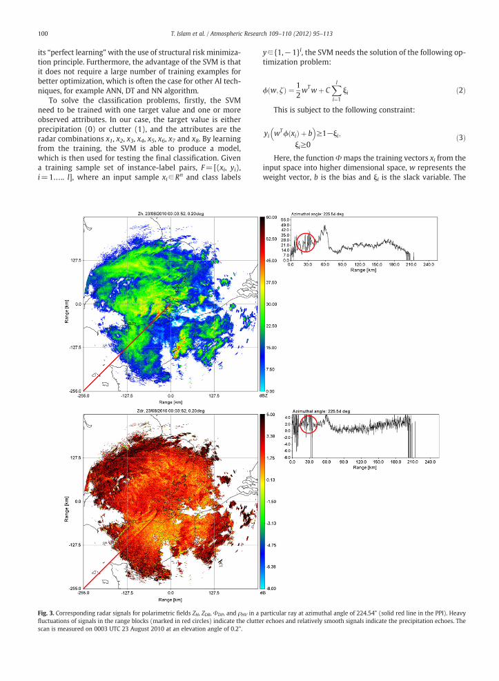
The texture is considered as a very good measure of char-acterizing meteorological targets from non-meteorologicaltargets. The texture of a particular cell of a radar scan canbe calculated by observing the fluctuations of the radar signalwithin a small window covering the observed cell. An exam-ple of such erratic fluctuations for a particular radar beam forZH, ZDR, ΦDP, and ρHV signatures are expressed in Fig. 3. Theradar scan is obtained from the Thurnham system on UTC23 August 2010 00:03:52. The erratic fluctuations of the

radar signals indicate the existence of clutter whereas rela-tively smooth fluctuations represent precipitation. By usingsuch knowledge, one can discriminate between precipitationand clutter echoes. The texture function given by σ(.) can becomputed using the standard deviation of the radar echoeswithin a small window. In this study, we have consideredsix radar vectors as input elements for clutter identification,i.e. σ(ZH,), σ(ZDR), σ(ΦDP), σ(ρHV), V andW. The texture is cal-culated using a window of the size 5×5 (1250 m×5°) inpolar coordinates, but excluding ‘clear air’ echoes. To defineclear air echoes, it is necessary to use the signal-to-noiseratio (SNR), which can be defined as:

SNR ¼ Z−20 log rð Þ þ C ð1Þ

where, Z is the radar reflectivity in dBZ, r is the radar range ofa given radar pixel in km and C is the radar constant. The SNRis computed for every single pixel in a radar scan. If the SNRfor a given pixel is above the minimum SNR, then that pixelis due to precipitation, otherwise is regarded as noise (i.e.clear air echo). Textures are calculated at different rangeswithin a range ring of 255 km and in order to reduce the in-formation loss, the transformation from polar to Cartesiangrids is circumvented. It is to be noted that in the previousstudy (Rico-Ramirez and Cluckie, 2008), both 3×3(750 m×3°) and 5×5 (1250 m×5°) windows were investi-gated. However, larger windows usually can provide betteraccuracy in the computation of the texture function. Thus,in this study, 5×5 (1250 m×5°) windows are used in the cal-culations. Moreover, in the former work, eight input mea-surements have been considered to train the classifier (seeTable 1 from Rico-Ramirez and Cluckie (2008)), includingLDR, clutter frequency map Pc and ρHV. Nevertheless, in thiswork, we have not considered the latter three measurements.The reason for not using LDR here is that if the radar is used insimultaneous transmission mode (i.e. transmitting H and Vspectrum), it is not possible to achieve LDR. Moreover, at C-band wavelength, propagation effects affect LDR measure-ments (Bringi and Chandrasekar, 2001). The clutter frequen-cy map Pc is also not used in order to use only radarmeasurements. Since, the texture of the correlation coeffi-cient σ(ρHV) is used in this work, thus ρHV is also not includedin the input vectors. However, the spectral width (W) hasbeen used in this article, which was not used in the formerwork. In summary, the input vector combinations used inthe classification are given in Table 1. Indeed, eight inputcombinations are selected to feed the AI classifiers. The firstsix combinations of inputs represent the six individual radarvectors as discussed above and denoted as x1, x2, x3, x4, x5and x6 representing σ(ZH), σ(ZDR), σ(ΦDP), σ(ρHV), V, and Wrespectively. The input combination x7 uses typical radarmeasurements from a single polarized Doppler radar withσ(ZH), V, and W. Finally, the input combination x8 uses allradar fields σ(ZH), σ(ZDR), σ(ΦDP), σ(ρHV), V, and W, whichare available from typical polarimetric radar observations.

2.3. Training and testing distribution

The radar datasets used in this work come from a widerange of meteorological scenarios and contain differentkinds of clutter signals viz ground clutter, sea clutter, and

98 T. Islam et al. / Atmospheric Research 109–110 (2012) 95–113

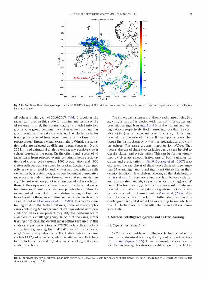
Fig. 2. UKMet Office Nimrod composite product on 2130 UTC 23 August 2010 at 5 km resolution. The composite product displays “no precipitation” in the Thurn-ham radar range.

99T. Islam et al. / Atmospheric Research 109–110 (2012) 95–113

AP echoes in the year of 2006/2007. Table 2 tabulates theradar scans used in this study for training and testing of theAI systems. In brief, the training dataset is divided into twogroups. One group contains the clutter echoes and anothergroup contains precipitation echoes. The clutter cells fortraining are selected from several events at the time of “noprecipitation” through visual examination. Whilst, precipita-tion cells are selected at different ranges (between 0 and255 km) and azimuthal angles avoiding any possible clutterechoes present in the scans. On the other hand, a total of 44radar scans from selected events containing both precipita-tion and clutter cells (around 1000 precipitation and 1000clutter cells per scan) are used for testing. Specially designedsoftware was utilised for such clutter and precipitation cellsextraction by a meteorological expert looking at consecutiveradar scans and identifying those echoes that remain station-ary. The software outputs the animation of echo evolutionthrough the sequence of consecutive scans in time and eleva-tion domains. Therefore, it has been possible to visualize themovement of precipitation cells distinguishing clutter pat-terns based on the echo evolution and vertical echo structureas illustrated in Moszkowicz et al. (1994). It is worth men-tioning that in the testing datasets, some of the complexcases containing AP and ground clutter embedded with pre-cipitation signals are present to justify the performance ofclassifiers in a challenging way. In both of the cases, eithertraining or testing, the default radar settings are used in thisanalysis. In particular, a total of 870,285 radar cells are select-ed for training. Among them, 417,418 are clutter cells and452,867 are precipitation cells. The testing dataset containsa total of 112,274 radar cells, where 49,440 radar cells belongto the clutter echoes and 62,834 radar cells belong to the pre-cipitation echoes.

Fig. 1. Thurnham radar PPI of different polarimetric fields ZH, ZDR,ΦDP, ρHV, V, andWat an elevation angle of 0.2°.

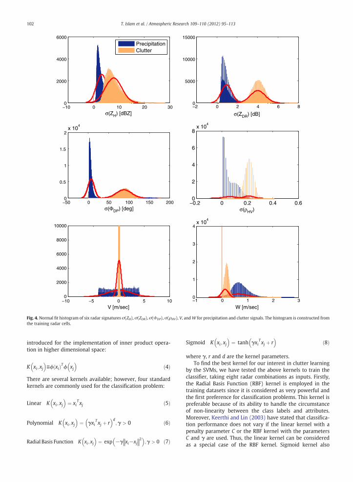
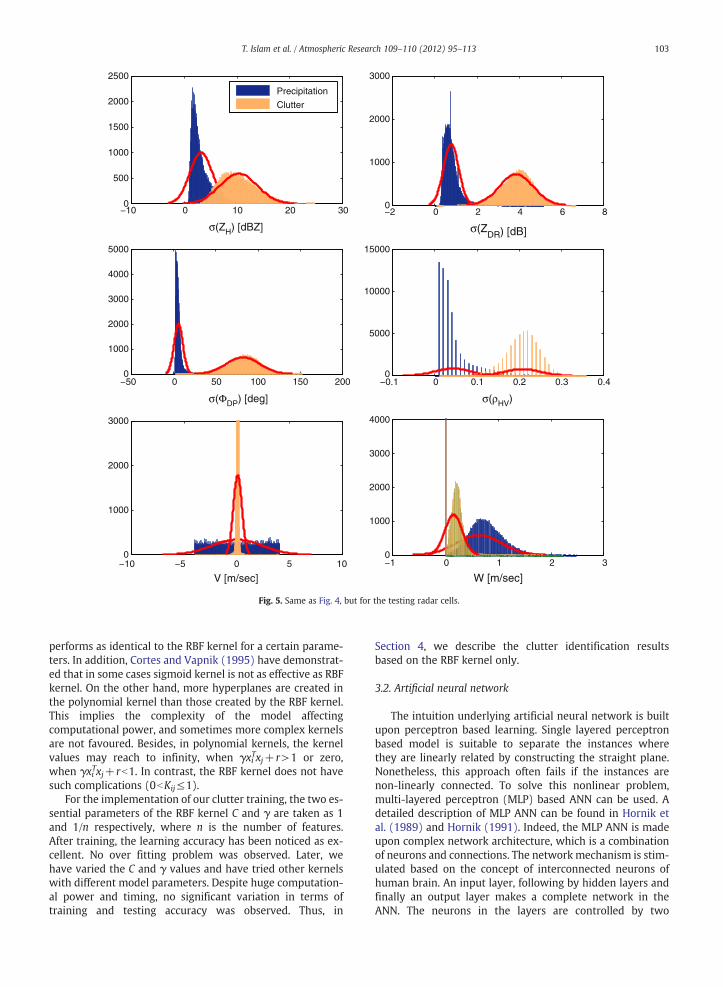
The individual histograms of the six radar input fields (x1,x2, x3, x4, x5 and x6) is plotted with normal fit for clutter andprecipitation signals in Figs. 4 and 5 for the training and test-ing datasets respectively. Both figures indicate that the vari-able σ(ΦDP) is an excellent way to classify clutter andprecipitation because of the small overlapping region be-tween the distributions of σ(ΦDP) for precipitation and clut-ter echoes. The same argument applies for σ(ZDR). Thatmeans, the use of these two variables can be very helpful toclassify clutter and precipitation. This can be further visual-ized by bivariate smooth histograms of both variables forclutter and precipitation in Fig. 6. Gourley et al. (2007) alsoexpressed the usefulness of these two polarimetric parame-ters (ΦDP and ZDR) and found significant distinction in theirdensity function. Nevertheless, looking at the distributionsin Figs. 4 and 5, there are some overlaps between clutterand precipitation signals, in particular for the σ(ZH) and Wfields. The texture σ(ρHV) has also shown overlap betweenprecipitation and non-precipitation signals in our C-band ob-servations, similar to those found by Zrnic et al. (2006) at S-band frequency. Such overlap in clutter identification is achallenging task and it would be interesting to see which ofthe AI techniques can handle the classification moreaccurately.

3. Artificial intelligence systems and clutter learning

3.1. Support vector machine

SVM is a novel artificial intelligence technique, which isbased on a statistical learning theory and support vectors(Cortes and Vapnik, 1995). It can be considered as an excel-lent tool in solving classification problems due to the fact of

displaying clutter signals. The scan is measured on 2129 UTC 23 August 2010

100 T. Islam et al. / Atmospheric Research 109–110 (2012) 95–113

its “perfect learning”with the use of structural risk minimiza-tion principle. Furthermore, the advantage of the SVM is thatit does not require a large number of training examples forbetter optimization, which is often the case for other AI tech-niques, for example ANN, DT and NN algorithm.

To solve the classification problems, firstly, the SVMneed to be trained with one target value and one or moreobserved attributes. In our case, the target value is eitherprecipitation (0) or clutter (1), and the attributes are theradar combinations x1, x2, x3, x4, x5, x6, x7 and x8. By learningfrom the training, the SVM is able to produce a model,which is then used for testing the final classification. Givena training sample set of instance-label pairs, F=[(xi, yi),i=1….. l], where an input sample xi∈Rn and class labels

Fig. 3. Corresponding radar signals for polarimetric fields ZH, ZDR, ΦDP, and ρHV in afluctuations of signals in the range blocks (marked in red circles) indicate the cluttescan is measured on 0003 UTC 23 August 2010 at an elevation angle of 0.2°.

y∈ {1,−1}l, the SVM needs the solution of the following op-timization problem:

ϕ w; ζð Þ ¼ 12wTwþ C

Xli¼1

ξi ð2Þ

This is subject to the following constraint:

yi wTϕ xið Þ þ b� �

≥1−ξi;ξi≥0

ð3Þ

Here, the function Φ maps the training vectors xi from theinput space into higher dimensional space, w represents theweight vector, b is the bias and ξi is the slack variable. The

particular ray at azimuthal angle of 224.54° (solid red line in the PPI). Heavyr echoes and relatively smooth signals indicate the precipitation echoes. The

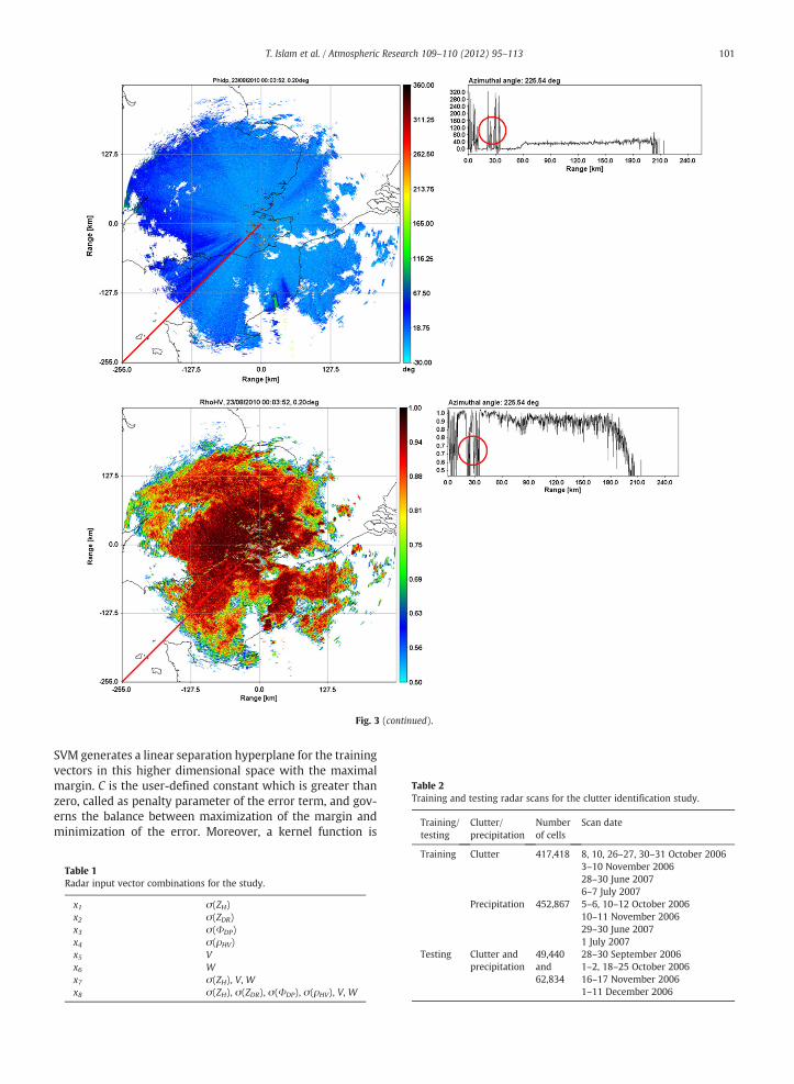
Fig. 3 (continued).

Table 2Training and testing radar scans for the clutter identification study.

Training/testing

Clutter/precipitation

Numberof cells

Scan date

101T. Islam et al. / Atmospheric Research 109–110 (2012) 95–113

SVM generates a linear separation hyperplane for the trainingvectors in this higher dimensional space with the maximalmargin. C is the user-defined constant which is greater thanzero, called as penalty parameter of the error term, and gov-erns the balance between maximization of the margin andminimization of the error. Moreover, a kernel function is

Table 1Radar input vector combinations for the study.

x1 σ(ZH)x2 σ(ZDR)x3 σ(ΦDP)x4 σ(ρHV)x5 Vx6 Wx7 σ(ZH), V, Wx8 σ(ZH), σ(ZDR), σ(ΦDP), σ(ρHV), V, W

Training Clutter 417,418 8, 10, 26–27, 30–31 October 20063–10 November 200628–30 June 20076–7 July 2007

Precipitation 452,867 5–6, 10–12 October 200610–11 November 200629–30 June 20071 July 2007

Testing Clutter andprecipitation

49,440and62,834

28–30 September 20061–2, 18–25 October 200616–17 November 20061–11 December 2006

−50 0 50 100 150 2000

0.5

1

1.5

2x 10

4

σ(ΦDP) [deg]

−10 0 10 20 300

2000

4000

6000

σ(ZH) [dBZ]−2 0 2 4 6 80

5000

10000

15000

σ(ZDR) [dB]

−0.2 0 0.2 0.4 0.60

2

4

6

8x 10

4

σ(ρHV)

−10 −5 0 5 100

2000

4000

6000

8000

10000

V [m/sec]−1 0 1 2 30

1

2

3

4x 10

4

W [m/sec]

PrecipitationClutter

Fig. 4. Normal fit histogram of six radar signatures σ(ZH), σ(ZDR), σ(ΦDP), σ(ρHV), V, andW for precipitation and clutter signals. The histogram is constructed fromthe training radar cells.

102 T. Islam et al. / Atmospheric Research 109–110 (2012) 95–113

introduced for the implementation of inner product opera-tion in higher dimensional space:

K xi; xj� �

≡ϕ xið ÞTϕ xj� �

ð4Þ

There are several kernels available; however, four standardkernels are commonly used for the classification problem:

Linear K xi; xj� �

¼ xiTxj ð5Þ

Polynomial K xi; xj� �

¼ γxiTxj þ r

� �d;γ > 0 ð6Þ

Radial Basis Function K xi; xj� �

¼ exp −γ‖xi−xj‖2

� �;γ > 0 ð7Þ

Sigmoid K xi; xj� �

¼ tanh γxiT xj þ r

� �ð8Þ

where γ, r and d are the kernel parameters.To find the best kernel for our interest in clutter learning

by the SVMs, we have tested the above kernels to train theclassifier, taking eight radar combinations as inputs. Firstly,the Radial Basis Function (RBF) kernel is employed in thetraining datasets since it is considered as very powerful andthe first preference for classification problems. This kernel ispreferable because of its ability to handle the circumstanceof non-linearity between the class labels and attributes.Moreover, Keerthi and Lin (2003) have stated that classifica-tion performance does not vary if the linear kernel with apenalty parameter C or the RBF kernel with the parametersC and γ are used. Thus, the linear kernel can be consideredas a special case of the RBF kernel. Sigmoid kernel also

−10 0 10 20 300

500

1000

1500

2000

2500

σ(ZH) [dBZ]

−2 0 2 4 6 80

1000

2000

3000

σ(ZDR) [dB]

−50 0 50 100 150 2000

1000

2000

3000

4000

5000

σ(ΦDP) [deg]

−0.1 0 0.1 0.2 0.3 0.40

5000

10000

15000

σ(ρHV)

−10 −5 0 5 100

1000

2000

3000

V [m/sec]

−1 0 1 2 30

1000

2000

3000

4000

W [m/sec]

Precipitation

Clutter

Fig. 5. Same as Fig. 4, but for the testing radar cells.

103T. Islam et al. / Atmospheric Research 109–110 (2012) 95–113

performs as identical to the RBF kernel for a certain parame-ters. In addition, Cortes and Vapnik (1995) have demonstrat-ed that in some cases sigmoid kernel is not as effective as RBFkernel. On the other hand, more hyperplanes are created inthe polynomial kernel than those created by the RBF kernel.This implies the complexity of the model affectingcomputational power, and sometimes more complex kernelsare not favoured. Besides, in polynomial kernels, the kernelvalues may reach to infinity, when γxiTxj+r>1 or zero,when γxiTxj+rb1. In contrast, the RBF kernel does not havesuch complications (0bKij≤1).

For the implementation of our clutter training, the two es-sential parameters of the RBF kernel C and γ are taken as 1and 1/n respectively, where n is the number of features.After training, the learning accuracy has been noticed as ex-cellent. No over fitting problem was observed. Later, wehave varied the C and γ values and have tried other kernelswith different model parameters. Despite huge computation-al power and timing, no significant variation in terms oftraining and testing accuracy was observed. Thus, in

Section 4, we describe the clutter identification resultsbased on the RBF kernel only.

3.2. Artificial neural network

The intuition underlying artificial neural network is builtupon perceptron based learning. Single layered perceptronbased model is suitable to separate the instances wherethey are linearly related by constructing the straight plane.Nonetheless, this approach often fails if the instances arenon-linearly connected. To solve this nonlinear problem,multi-layered perceptron (MLP) based ANN can be used. Adetailed description of MLP ANN can be found in Hornik etal. (1989) and Hornik (1991). Indeed, the MLP ANN is madeupon complex network architecture, which is a combinationof neurons and connections. The network mechanism is stim-ulated based on the concept of interconnected neurons ofhuman brain. An input layer, following by hidden layers andfinally an output layer makes a complete network in theANN. The neurons in the layers are controlled by two

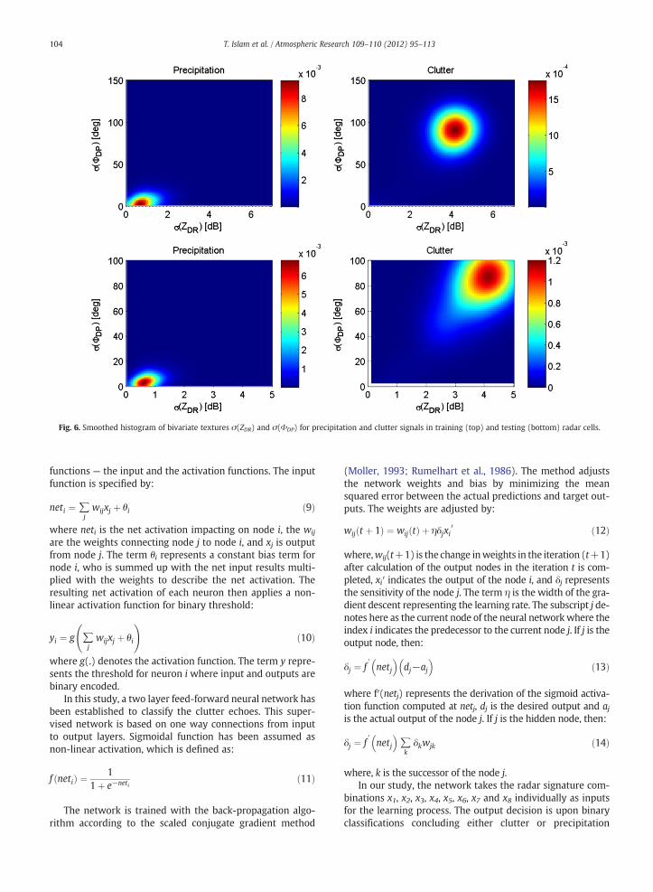
Fig. 6. Smoothed histogram of bivariate textures σ(ZDR) and σ(ΦDP) for precipitation and clutter signals in training (top) and testing (bottom) radar cells.

104 T. Islam et al. / Atmospheric Research 109–110 (2012) 95–113

functions — the input and the activation functions. The inputfunction is specified by:

neti ¼ ∑jwijxj þ θi ð9Þ

where neti is the net activation impacting on node i, the wij

are the weights connecting node j to node i, and xj is outputfrom node j. The term θi represents a constant bias term fornode i, who is summed up with the net input results multi-plied with the weights to describe the net activation. Theresulting net activation of each neuron then applies a non-linear activation function for binary threshold:

yi ¼ g ∑jwijxj þ θi

!ð10Þ

where g(.) denotes the activation function. The term y repre-sents the threshold for neuron i where input and outputs arebinary encoded.

In this study, a two layer feed-forward neural network hasbeen established to classify the clutter echoes. This super-vised network is based on one way connections from inputto output layers. Sigmoidal function has been assumed asnon-linear activation, which is defined as:

f netið Þ ¼ 11þ e−neti

ð11Þ

The network is trained with the back-propagation algo-rithm according to the scaled conjugate gradient method

(Moller, 1993; Rumelhart et al., 1986). The method adjuststhe network weights and bias by minimizing the meansquared error between the actual predictions and target out-puts. The weights are adjusted by:

wij t þ 1ð Þ ¼ wij tð Þ þ ηδjxi0 ð12Þ

where,wij(t+1) is the change inweights in the iteration (t+1)after calculation of the output nodes in the iteration t is com-pleted, xi′ indicates the output of the node i, and δj representsthe sensitivity of the node j. The term η is the width of the gra-dient descent representing the learning rate. The subscript j de-notes here as the current node of the neural networkwhere theindex i indicates the predecessor to the current node j. If j is theoutput node, then:

δj ¼ f0netj� �

dj−aj� �

ð13Þ

where f′(netj) represents the derivation of the sigmoid activa-tion function computed at netj, dj is the desired output and ajis the actual output of the node j. If j is the hidden node, then:

δj ¼ f0netj� �

∑kδkwjk ð14Þ

where, k is the successor of the node j.In our study, the network takes the radar signature com-

binations x1, x2, x3, x4, x5, x6, x7 and x8 individually as inputsfor the learning process. The output decision is upon binaryclassifications concluding either clutter or precipitation

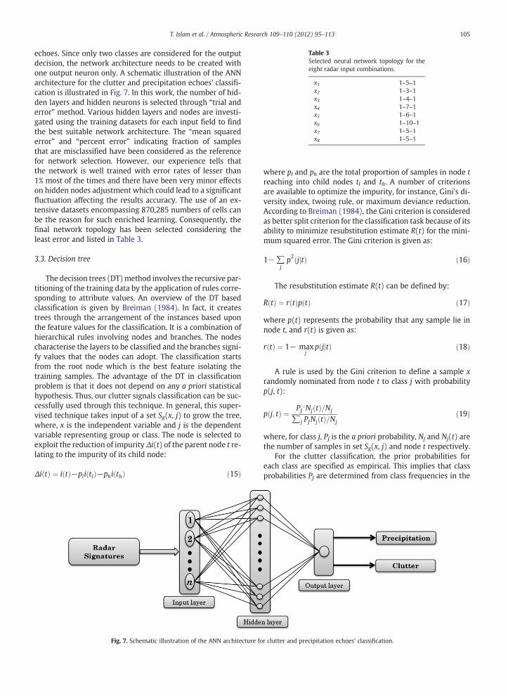
Table 3Selected neural network topology for theeight radar input combinations.

x1 1–5–1x2 1–3–1x3 1–4–1x4 1–7–1x5 1–6–1x6 1–10–1x7 1–5–1x8 1–5–1

105T. Islam et al. / Atmospheric Research 109–110 (2012) 95–113

echoes. Since only two classes are considered for the outputdecision, the network architecture needs to be created withone output neuron only. A schematic illustration of the ANNarchitecture for the clutter and precipitation echoes' classifi-cation is illustrated in Fig. 7. In this work, the number of hid-den layers and hidden neurons is selected through “trial anderror” method. Various hidden layers and nodes are investi-gated using the training datasets for each input field to findthe best suitable network architecture. The “mean squarederror” and “percent error” indicating fraction of samplesthat are misclassified have been considered as the referencefor network selection. However, our experience tells thatthe network is well trained with error rates of lesser than1% most of the times and there have been very minor effectson hidden nodes adjustment which could lead to a significantfluctuation affecting the results accuracy. The use of an ex-tensive datasets encompassing 870,285 numbers of cells canbe the reason for such enriched learning. Consequently, thefinal network topology has been selected considering theleast error and listed in Table 3.

3.3. Decision tree

The decision trees (DT)method involves the recursive par-titioning of the training data by the application of rules corre-sponding to attribute values. An overview of the DT basedclassification is given by Breiman (1984). In fact, it createstrees through the arrangement of the instances based uponthe feature values for the classification. It is a combination ofhierarchical rules involving nodes and branches. The nodescharacterise the layers to be classified and the branches signi-fy values that the nodes can adopt. The classification startsfrom the root node which is the best feature isolating thetraining samples. The advantage of the DT in classificationproblem is that it does not depend on any a priori statisticalhypothesis. Thus, our clutter signals classification can be suc-cessfully used through this technique. In general, this super-vised technique takes input of a set Sg(x, j) to grow the tree,where, x is the independent variable and j is the dependentvariable representing group or class. The node is selected toexploit the reduction of impurityΔi(t) of the parent node t re-lating to the impurity of its child node:

Δi tð Þ ¼ i tð Þ−pli tlð Þ−phi thð Þ ð15Þ

Fig. 7. Schematic illustration of the ANN architecture fo

where pl and ph are the total proportion of samples in node treaching into child nodes tl and th. A number of criterionsare available to optimize the impurity, for instance, Gini's di-versity index, twoing rule, or maximum deviance reduction.According to Breiman (1984), the Gini criterion is consideredas better split criterion for the classification task because of itsability to minimize resubstitution estimate R(t) for the mini-mum squared error. The Gini criterion is given as:

1−∑jp2 j tj Þð ð16Þ

The resubstitution estimate R(t) can be defined by:

R tð Þ ¼ r tð Þp tð Þ ð17Þ

where p(t) represents the probability that any sample lie innode t, and r(t) is given as:

r tð Þ ¼ 1− maxj

p j tj Þð ð18Þ

A rule is used by the Gini criterion to define a sample xrandomly nominated from node t to class j with probabilityp(j, t):

p j; tð Þ ¼ PJ⋅Nj tð Þ=Nj

∑j PJNj tð Þ=Njð19Þ

where, for class j, PJ is the a priori probability, Nj and Nj(t) arethe number of samples in set Sg(x, j) and node t respectively.

For the clutter classification, the prior probabilities foreach class are specified as empirical. This implies that classprobabilities PJ are determined from class frequencies in the

r clutter and precipitation echoes' classification.

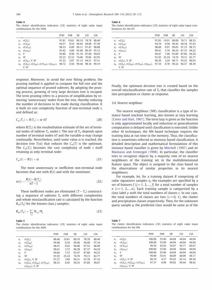
Table 4The clutter identification indicators (CII) statistics of eight radar inputcombinations for the SVM.

POD FAR SR CSI CIA

x1 σ(ZH) 97.81 19.81 80.19 78.78 88.40x2 σ(ZDR) 94.57 0.55 99.45 94.08 97.38x3 σ(ΦDP) 98.33 0.89 99.11 97.47 98.88x4 σ(ρHV) 93.42 4.60 95.40 89.39 95.12x5 V 95.80 8.90 91.10 87.60 94.03x6 W 93.23 25.52 74.48 70.66 82.95x7 σ(ZH), V, W 97.22 2.87 97.13 94.51 97.51x8 σ(ZH), σ(ZDR), σ(ΦDP), σ(ρHV),

V, W98.72 0.56 99.44 98.18 99.19

Table 6The clutter identification indicators (CII) statistics of eight radar input com-binations for the DT.

POD FAR SR CSI CIA

x1 σ(ZH) 97.85 19.91 80.09 78.71 88.35x2 σ(ZDR) 94.70 0.58 99.42 94.18 97.43x3 σ(ΦDP) 98.08 0.97 99.03 97.15 98.73x4 σ(ρHV) 90.41 3.76 96.24 87.33 94.22x5 V 94.47 7.40 92.60 87.84 94.24x6 W 91.92 25.24 74.76 70.15 82.77x7 σ(ZH), V, W 96.30 3.29 96.71 93.25 96.93x8 σ(ZH), σ(ZDR), σ(ΦDP), σ(ρHV),

V, W97.10 0.78 99.22 96.37 98.39

106 T. Islam et al. / Atmospheric Research 109–110 (2012) 95–113

response. Moreover, to avoid the over fitting problem, thepruning method is applied to compute the full tree and theoptimal sequence of pruned subtrees. By adopting the prun-ing process, growing of very large decision tree is escaped.The term pruning refers to a process of simplification by re-moving ‘unnecessary’ nodes from the tree, thereby reducingthe number of decisions to be made during classification. Itis built on cost complexity function of non-terminal node t,and defined as:

Cα Ttð Þ ¼ R Ttð Þ þ α⋅nT ð20Þ

where R(Tt) is the resubstitution estimate of the set of termi-nal nodes of subtree Tts under t. The size of Tts depends uponnumber of terminal nodes nT and the variable α may changecontinually. Nevertheless, until some value α is reached, thedecision tree T(α) that reduces the Cα(T) is the optimum.The Cα(Tt) becomes the cost complexity of node t itselfretaining as only terminal node:

Cα tð Þ ¼ R tð Þ þ α ð21Þ

The most unnecessary or inefficient non-terminal nodebecomes that one with R(t) and with the minimum:

α tð Þ ¼ R tð Þ−R Ttð ÞnT−1

ð22Þ

These inefficient nodes are eliminated (T−Ts) construct-ing a sequence of subtrees Tk with different complexitiesand whole misclassification rate is calculated by the functionRm(Tk) for the known class j samples:

Rm Tkð Þ ¼ ∑i;j

Ni;j=Nj ð23Þ

Table 5The clutter identification indicators (CII) statistics of eight radar inpucombinations for the ANN.

POD FAR SR CSI CIA

x1 σ(ZH) 88.40 19.81 80.19 78.78 88.40x2 σ(ZDR) 94.48 0.54 99.46 94.00 97.34x3 σ(ΦDP) 98.41 0.92 99.08 97.52 98.90x4 σ(ρHV) 90.41 3.72 96.28 87.37 94.24x5 V 94.66 7.53 92.47 87.88 94.25x6 W 91.92 25.24 74.76 70.15 82.77x7 σ(ZH), V, W 97.27 3.69 96.31 93.78 97.16x8 σ(ZH), σ(ZDR), σ(ΦDP),

σ(ρHV), V, W98.33 0.45 99.55 97.89 99.07

Table 7The clutter identification indicators (CII) statistics of eight radar inputcombinations for the NN.

POD FAR SR CSI CIA

x1 σ(ZH) 100.00 55.96 44.04 44.04 44.04x2 σ(ZDR) 100.00 55.96 44.04 44.04 44.04x3 σ(ΦDP) 99.39 43.03 56.97 56.77 66.67x4 σ(ρHV) 100.00 55.96 44.04 44.04 44.04x5 V 100.00 55.96 44.04 44.04 44.04x6 W 99.99 55.91 44.09 44.09 44.17x7 σ(ZH), V, W 96.19 4.37 95.63 92.14 96.39x8 σ(ZH), σ(ZDR), σ(ΦDP),

σ(ρHV), V, W97.37 0.98 99.02 96.44 98.42

t

Finally, the optimum decision tree is created based on theoverall misclassification rate of Tk that classifies the samplesinto precipitation or clutter as response.

3.4. Nearest neighbour

The nearest neighbour (NN) classification is a type of in-stance based machine learning, also known as lazy learning(Cover and Hart, 1967). The term lazy is given as the functionis only approximated locally and induction or generalizationcomputation is delayed until classification is executed. Unlikeother AI techniques, the NN based technique requires thetraining data at run time in the memory. Thus, the classifica-tion is sometimes referred as memory-based classification. Adetailed description and mathematical formulations of thisinstance based classifier is given by Mitchell (1997) and deMantaras and Armengol (1998). In particular, the classifiertries to recognize objects by a majority vote of its nearestneighbours of the training set in the multidimensionalfeature space. The object is assigned to the class based onthe observations of similar properties in its nearestneighbours.

For example, let, for a training dataset R comprising ofradar signatures samples xi, the examples are specified by aset of features f (j=1, 2,…, f) for a total number of samplesn (i=1, 2,…,n). Each training sample is categorized by aclass label y with the total numbers of classes c. In our case,the total numbers of classes are two (c=0, 1), the clutterand precipitation classes respectively. Then, for the unknownquery sample q, the predicted class would be same as of the

107T. Islam et al. / Atmospheric Research 109–110 (2012) 95–113

class label y of its nearest neighbour based on the smallestdistance:

D q;mið Þ ¼ min D q;m1ð Þ;D q;m2ð Þ; ::::::;D q;mj

� �h ið24Þ

where, mi is a nearest neighbour to the query q. To solve theclassification problem, the distance can be defined throughthe use of distance metric. There are several metrics availableto perform the task whilst common choices are the Euclidian,Minkowsky, Manhattan, and Chebychev. In our classification,we have considered the most widely used Euclidian distanceas distance metric, which is expressed as:

D q; xið Þ ¼Xf

qf−xif��� ���2

0@

1A1=2

ð25Þ

The “majority rule” has been implied for the task, whichimplies that samples are assigned to that group where theformed nearest neighbours are in major quantities. Once allthe samples are processed for classification, the classificationaccuracy A can be calculated by:

A ¼ ∑cyCyy

nð26Þ

where, Cyy represents a diagonal element of a confusionmatrix C and n denotes the total number of samples thatare classified.

4. Clutter identification results

4.1. The clutter identification indicators

In this work, five clutter identification indicators (CII) areemployed to judge the performance of clutter suppression bythe various AI techniques. The indicators are — the probabil-ity of detection (POD), false alarm rate (FAR), success ratio(SR), critical success index (CSI), and clutter identificationaccuracy (CIA). For detailed explanations on them, let usconsider a set of clutter classification results (clutter orprecipitation cells) given by the AI technique, where thenumber of positive identifications corresponding to theclutter samples is denoted by P, the number of negativeidentifications corresponding to the clutter samples isdenoted by Q, the number of positive identifications corre-sponding to the precipitation samples is denoted by S andthe number of negative identifications corresponding to theprecipitation samples is denoted by R. Then, the POD(Panofsky and Brier, 1958) can be defined as the ratio of thepositive clutter identifications (P) to the total number of clut-ter samples (P+Q):

POD ¼ PP þ Q

ð27Þ

The FAR can be used to show the failure of the AI systemthat is not related to the clutter cells. It is defined as the

ratio of the negative clutter identifications to the total num-ber of clutter identifications by the AI classifier:

FAR ¼ RP þ R

ð28Þ

The SR is the ratio of number of positive clutter identifica-tions to the total number of clutter identifications by the AIclassifier:

SR ¼ PP þ R

ð29Þ

The CSI (Schaefer, 1990), also known as threat score orverification ratio, is the ratio of positive clutter identifications(P) to the summation of P, Q, and R:

CSI ¼ PP þ Q þ R

ð30Þ

The CIA is simply the overall accuracy defining the ratio ofpositive clutter and precipitation identifications by the AI tothe total number of samples:

CIA ¼ P þ SP þ Q þ Rþ S

ð31Þ

It is to be noted that all of the CII statistics are given aspercentage in this work unless otherwise stated.

4.2. The CII statistics

The CII statistics obtained from the testing datasets for dif-ferent radar combinations x1, x2, x3, x4, x5, x6, x7 and x8 arepresented in this section and summarized in Tables 4 to 7for the SVM, ANN, DT, and NN systems respectively.

From Tables 4 and 5, it is revealed that the two black boxtechniques SVM and ANN have successfully identified theclutter signals with very satisfactory and similar perfor-mance. The result suggests that all polarimetric signaturesused in this study are capable of clutter identification withquite reliable accuracy. According to the statistics, exceptfor the inputs x1 and x6, the CIA is found over 90%. The polar-imetric input σ(ΦDP) alone has shown excellent skill withCIA=98.88% for the SVM and CIA=98.90% for the ANN. Italso expresses the highest POD for the ANN. Another polari-metric input σ(ZDR) also exhibits a good success in clutteridentification specifying CIA=97.38% using the SVM andCIA=97.34% using the ANN. This supports the findingsfrom earlier studies of Giuli et al. (1991) and Ryzhkov andZrnic (1998), where they suggested the use of these two po-larimetric parameters ZDR and ΦDP for clutter classification.Furthermore, these two parameters are good identifiers ofsea clutter. Nevertheless, the top most accuracy in our studyis attained when all the radar signatures are used, that isthe x8 combination. In this scenario, the CIA produced bythe SVM is 99.19% and by the ANN is 99.07%. The highestPOD (98.72%) is also noticed in this combination for theSVM. In case of single polarized radar signatures, that is,input combination x7, the identification accuracy is also verypromising, representing CIA of 97.51% for the SVM and of97.16% for the ANN. The velocity input vector (x5) has

108 T. Islam et al. / Atmospheric Research 109–110 (2012) 95–113

demonstrated a good performance with CIA=94.03% (SVM)and CIA=94.25% (ANN), but with a large FAR (8.9% and 7.5%for SVM and ANN respectively). Mostly, Doppler velocity of0 m/s in the Doppler spectrum offers a good indicator inidentifying clutter echoes. This can be brought in consider-ation from the normal fit histograms in Figs. 4 and 5, whichillustrate massive modes at V=0m/s. However, this is not al-ways the case that clutter echo is present at 0 m/s and some-times clutter echo can be detected in the nearby Doppler cells(Unal, 2009). Over the sea, the waves may also have non-zerovelocities in the clutter cells (Berenguer et al., 2006). Hence,inclusion of other parameter with the Doppler velocitycould produce better classification, which is witnessed inour results, for instance for the x7 combination. Previous re-search shows that ρHV is a good option for the detection ofclutter presence (Gourley et al., 2007; Ryzhkov and Zrnic,1998). This is also reflected in our study, seeing as, theσ(ρHV) input vector has achieved very good accuracy (SVMCIA=95.12% and ANN CIA=94.24%). On the other hand,the σ(ZH) and W signatures have failed to identify clutter re-liably. The CIA acquired for σ(ZH) and W are given as, respec-tively, 88.40% and 82.95% for the SVM, and 88.40% and 82.77%for the ANN. The CSI also shows similar patterns as of the CIAfor different radar combinations ranging from 70% (x6) to 98%(x8) approximately. If we look at the FAR, which representsthe classification failures, the lowest FAR is obtained withinput x2 for the SVM, that is 00.55% (SR=99.45%), andinput combination x8 for the ANN, that is 00.45%(SR=99.55%). In contrast, W shows the highest false alarmrate of 25.52% and 25.24%, and lowest SR of 74.48% and74.76%, next to the σ(ZH), for the SVM and the ANN respec-tively. Berenguer et al. (2006) have stated that the parame-ters ZH and W are less used for clutter identifications. Yet,these two parameters are used in several studies (Grecuand Krajewski, 2000; Moszkowicz et al., 1994) and consid-ered as useful to characterize echoes that come from movingvehicles and scattered clutter as conferred in Liu et al. (2008).According to Grecu and Krajewski (2000), these parametersmight be suitable when they are applied in combinationwith other inputs.

On the other hand, the results using the decision treebased classification are given in Table 6. The best CIA(98.73%) and CSI (97.15%) are seen for the standalone polar-imetric input σ(ΦDP) instead of the combination of all radarsignatures (x8). It has also corroborated the highest POD of98.08%. Yet, the x8 combination shows very high identifica-tion rates following σ(ΦDP) indicating CIA=98.39% andCSI=96.37%. Once again, the worst performances are illus-trated by the spectral width W input measurement. It hasthe lowest CIA (82.77%), lowest CSI (70.15%), lowest SR(74.76%) and highest FAR (25.24%) among the eight radarcombinations. Slightly better than the W, yet, poor CII statis-tics are revealed for the reflectivity texture σ(ZH) showingCSI=78.71% and CIA=88.35%. The clutter identificationskill is considerably improved to around 87% CSI and around94% CIA if either the polarimetric radar texture σ(ρHV) orDoppler velocity V is used. The CII statistics is further im-proved when a combination of the single polarization radarsignatures σ(ZH), V and W is used. In this case, the CIA andCSI percentage are enhanced to 96.93% and 93.25% respec-tively. It is, indeed, ranked 4 among the eight input

measurements if all five CII statistics are accounted for. Fur-ther accuracy is achieved with the σ(ZDR) vector, whichshows CIA of 97.43% (CSI=94.18%) and lowest FAR of 0.58%(SR=99.42%).

The CII statistics from Table 7 indicate that the NN tech-nique has failed to identify clutter where the classificationencompasses only one input signature. More specifically, forthe input measurements x1, x2, x3, x4, x5, and x6, both calculat-ed CIA and CSI are very unsatisfactory and with very largeFAR. With the exception of the specific propagation phasetexture, the CIA, CSI and SR are calculated as about 44% onlyfor the “one signature” input vectors. FAR is computed asslightly over 56% in this case. For the σ(ΦDP), the CSI and SRstatistics are found slightly better showing around 56%,whereas the percentage of CIA is given as around 66%. Thecomputed FAR is also better (43% as opposed to 56%), yet,the clutter identification measure is not acceptable. On theother hand, if input measurements are more than one, theperformance significantly improves. For instance, consideringthe x7 input, the single polarized radar parameters, the CIImeasures are ominously enriched. In the x7 combination,the CIA and CSI statistics are noted as 96.39% and 92.14% ac-cordingly. SR (95.63%) and FAR (4.37%) are also encouraging.Use of all the radar signatures making x8 input combinationhas produced the best CII statistics for clutter segregation inthe NN. The calculated CIA and CSI are 98.42% and 96.44% inthis case respectively, plus FAR is low representing 0.98%only with SR=99.02%. To conclude, NN can be successfullyemployed with the use of multiparameter radar observations,and should not be used with a single input variable as shownin Table 7.

It is also to be remembered, the advantage of multipara-meter over single parameter is that if any of the signaturesis not available because of radar malfunction or poor dataquality, the rest of the parameters can perform the task andthe classification would not be affected to a larger extent.Furthermore, the polarimetric parameters are exaggeratedto inherent noise which is associated with radar hardwareand its operating characteristics (Gourley et al., 2007).Hence, the sources of errors in radar rainfall estimation be-cause of such unexpected ambiguity can be minimized.

4.3. Comparison with fuzzy logic and Bayes classifiers

Here, we compare the results acquired from the four AItechniques — the SVM, ANN, DT, and NN with the fuzzylogic and Bayes classifiers from the previous study of Rico-Ramirez and Cluckie (2008). The textures of the most com-mon parameters for polarimetric based radar rainfall estima-tion viz reflectivity (ZH), differential reflectivity (ZDR), anddifferential propagation phase (ΦDP) (Bringi andChandrasekar, 2001; Ryzhkov and Zrnic, 1998) are of partic-ular interest. For comparison, the critical success index (CSI)is used as the performance indicator. To be noted, fuzzylogic and Bayes classifiers' results are taken from Tables 3and 1 from Rico-Ramirez and Cluckie (2008).

We report the CSI statistics for our four AI techniquescomparing with the fuzzy logic using the product operators(denoted by FL(Π)), sum operators (denoted by FL(Σ)), con-ditional probability density functions (denoted by FL(Σ*)), aswell as the Bayes classifier (denoted by BY(Π)) in Table 8.

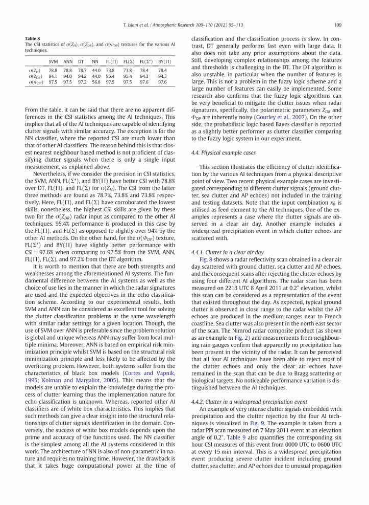
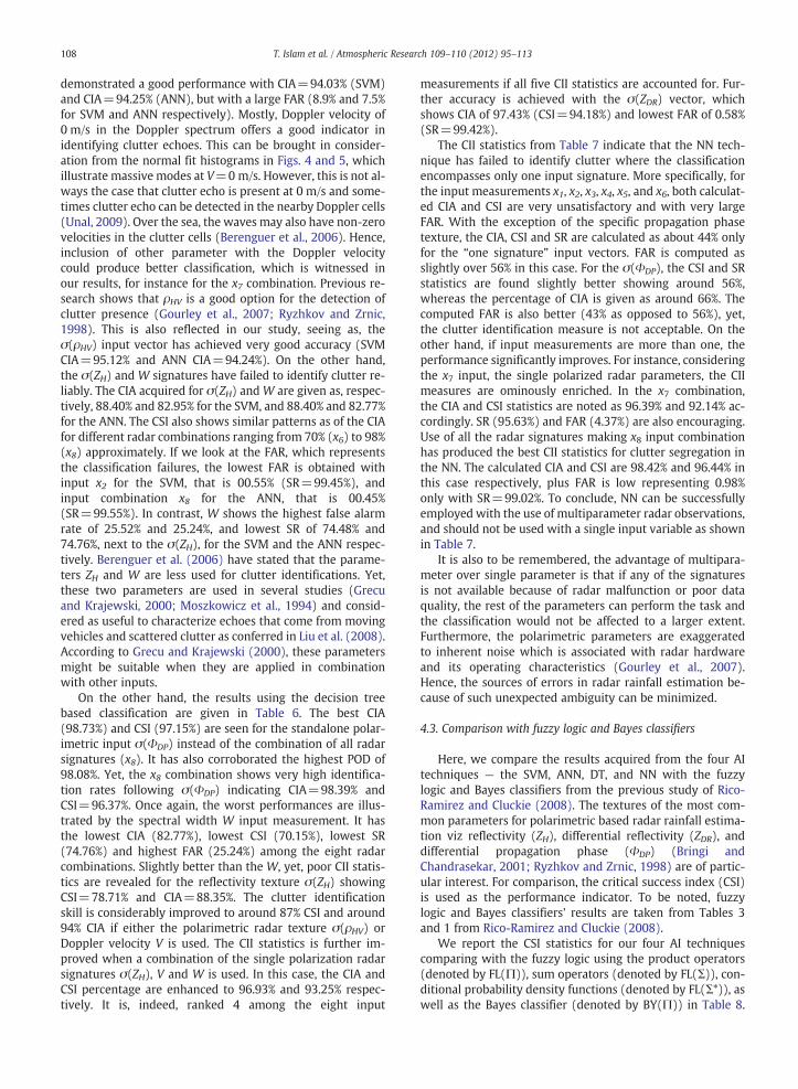
Table 8The CSI statistics of σ(ZH), σ(ZDR), and σ(ΦDP) textures for the various AItechniques.

SVM ANN DT NN FL(Π) FL(Σ) FL(Σ*) BY(Π)

σ(ZH) 78.8 78.8 78.7 44.0 73.8 73.8 78.4 78.4σ(ZDR) 94.1 94.0 94.2 44.0 95.4 95.4 94.3 94.3σ(ΦDP) 97.5 97.5 97.2 56.8 97.5 97.5 97.6 97.6

109T. Islam et al. / Atmospheric Research 109–110 (2012) 95–113

From the table, it can be said that there are no apparent dif-ferences in the CSI statistics among the AI techniques. Thisimplies that all of the AI techniques are capable of identifyingclutter signals with similar accuracy. The exception is for theNN classifier, where the reported CSI are much lower thanthat of other AI classifiers. The reason behind this is that clos-est nearest neighbour based method is not proficient of clas-sifying clutter signals when there is only a single inputmeasurement, as explained above.

Nevertheless, if we consider the precision in CSI statistics,the SVM, ANN, FL(Σ*), and BY(Π) have better CSI with 78.8%over DT, FL(Π), and FL(Σ) for σ(ZH). The CSI from the latterthree methods are found as 78.7%, 73.8% and 73.8% respec-tively. Here, FL(Π), and FL(Σ) have corroborated the lowestskills, nonetheless, the highest CSI skills are given by thesetwo for the σ(ZDR) radar input as compared to the other AItechniques. 95.4% performance is produced in this case bythe FL(Π), and FL(Σ) as opposed to slightly over 94% by theother AI methods. On the other hand, for the σ(ΦDP) texture,FL(Σ*) and BY(Π) have slightly better performance withCSI=97.6% when comparing to 97.5% from the SVM, ANN,FL(Π), FL(Σ), and 97.2% from the DT algorithm.

It is worth to mention that there are both strengths andweaknesses among the aforementioned AI systems. The fun-damental difference between the AI systems as well as thechoice of use lies in the manner in which the radar signaturesare used and the expected objectives in the echo classifica-tion scheme. According to our experimental results, bothSVM and ANN can be considered as excellent tool for solvingthe clutter classification problems at the same wavelengthwith similar radar settings for a given location. Though, theuse of SVM over ANN is preferable since the problem solutionis global and unique whereas ANNmay suffer from local mul-tiple minima. Moreover, ANN is based on empirical risk min-imization principle whilst SVM is based on the structural riskminimization principle and less likely to be affected by theoverfitting problem. However, both systems suffer from thecharacteristics of black box models (Cortes and Vapnik,1995; Kolman and Margaliot, 2005). This means that themodels are unable to explain the knowledge during the pro-cess of clutter learning thus the implementation nature forecho classification is unknown. Whereas, reported other AIclassifiers are of white box characteristics. This implies thatsuch methods can give a clear insight into the structural rela-tionships of clutter signals identification in the domain. Con-versely, the success of white box models depends upon theprime and accuracy of the functions used. The NN classifieris the simplest among all the AI systems considered in thiswork. The architecture of NN is also of non-parametric in na-ture and requires no training time. However, the drawback isthat it takes huge computational power at the time of

classification and the classification process is slow. In con-trast, DT generally performs fast even with large data. Italso does not take any prior assumptions about the data.Still, developing complex relationships among the featuresand thresholds is challenging in the DT. The DT algorithm isalso unstable, in particular when the number of features islarge. This is not a problem in the fuzzy logic scheme and alarge number of features can easily be implemented. Someresearch also confirms that the fuzzy logic algorithms canbe very beneficial to mitigate the clutter issues when radarsignatures, specifically, the polarimetric parameters ZDR andΦDP are inherently noisy (Gourley et al., 2007). On the otherside, the probabilistic logic based Bayes classifier is reportedas a slightly better performer as clutter classifier comparingto the fuzzy logic system in our experiment.

4.4. Physical example cases

This section illustrates the efficiency of clutter identifica-tion by the various AI techniques from a physical descriptivepoint of view. Two recent physical example cases are investi-gated corresponding to different clutter signals (ground clut-ter, sea clutter and AP echoes) not included in the trainingand testing datasets. Note that the input combination x8 isutilised as feed element to the AI techniques. One of the ex-amples represents a case where the clutter signals are ob-served in a clear air day. Another example includes awidespread precipitation event in which clutter echoes arescattered with.

4.4.1. Clutter in a clear air dayFig. 8 shows a radar reflectivity scan obtained in a clear air

day scattered with ground clutter, sea clutter and AP echoes,and the consequent scans after rejecting the clutter echoes byusing four different AI algorithms. The radar scan has beenmeasured on 2213 UTC 8 April 2011 at 0.2° elevation, whilstthis scan can be considered as a representation of the eventthat existed throughout the day. As expected, typical groundclutter is observed in close range to the radar whilst the APechoes are produced in the medium ranges near to Frenchcoastline. Sea clutter was also present in the north east sectorof the scan. The Nimrod radar composite product (as shownas an example in Fig. 2) and measurements from neighbour-ing rain gauges confirm that apparently no precipitation hasbeen present in the vicinity of the radar. It can be perceivedthat all four AI techniques have been able to reject most ofthe clutter echoes and only the clear air echoes haveremained in the scan that can be due to Bragg scattering orbiological targets. No noticeable performance variation is dis-tinguished between the AI techniques.

4.4.2. Clutter in a widespread precipitation eventAn example of very intense clutter signals embedded with

precipitation and the clutter rejection by the four AI tech-niques is visualized in Fig. 9. The example is taken from aradar PPI scan measured on 7 May 2011 event at an elevationangle of 0.2°. Table 9 also quantifies the corresponding sixhour CSI measures of this event from 0000 UTC to 0600 UTCat every 15 min interval. This is a widespread precipitationevent producing severe clutter incident including groundclutter, sea clutter, and AP echoes due to unusual propagation

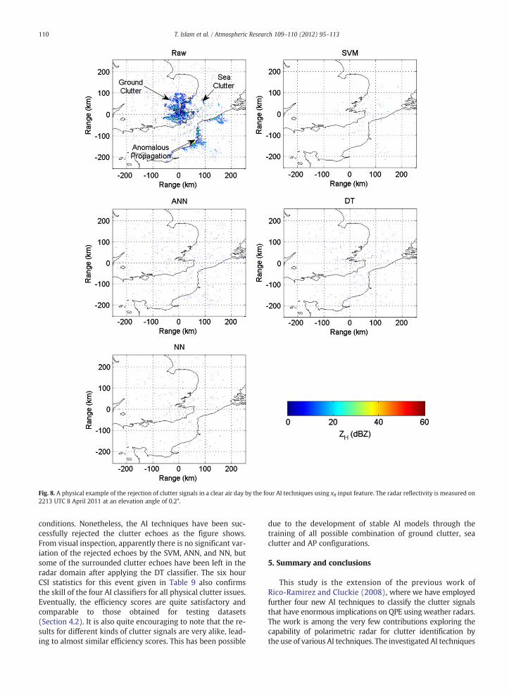
Fig. 8. A physical example of the rejection of clutter signals in a clear air day by the four AI techniques using x8 input feature. The radar reflectivity is measured on2213 UTC 8 April 2011 at an elevation angle of 0.2°.

110 T. Islam et al. / Atmospheric Research 109–110 (2012) 95–113

conditions. Nonetheless, the AI techniques have been suc-cessfully rejected the clutter echoes as the figure shows.From visual inspection, apparently there is no significant var-iation of the rejected echoes by the SVM, ANN, and NN, butsome of the surrounded clutter echoes have been left in theradar domain after applying the DT classifier. The six hourCSI statistics for this event given in Table 9 also confirmsthe skill of the four AI classifiers for all physical clutter issues.Eventually, the efficiency scores are quite satisfactory andcomparable to those obtained for testing datasets(Section 4.2). It is also quite encouraging to note that the re-sults for different kinds of clutter signals are very alike, lead-ing to almost similar efficiency scores. This has been possible

due to the development of stable AI models through thetraining of all possible combination of ground clutter, seaclutter and AP configurations.

5. Summary and conclusions

This study is the extension of the previous work ofRico-Ramirez and Cluckie (2008), where we have employedfurther four new AI techniques to classify the clutter signalsthat have enormous implications on QPE using weather radars.The work is among the very few contributions exploring thecapability of polarimetric radar for clutter identification bythe use of various AI techniques. The investigated AI techniques

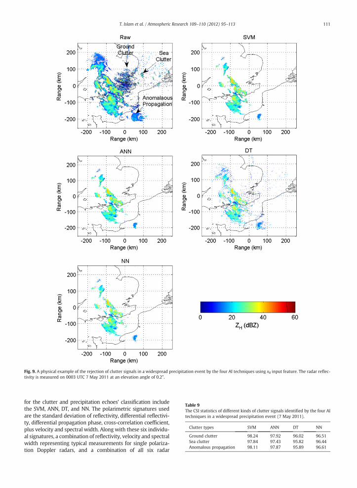
Fig. 9. A physical example of the rejection of clutter signals in a widespread precipitation event by the four AI techniques using x8 input feature. The radar reflec-tivity is measured on 0003 UTC 7 May 2011 at an elevation angle of 0.2°.

Table 9The CSI statistics of different kinds of clutter signals identified by the four AItechniques in a widespread precipitation event (7 May 2011).

Clutter types SVM ANN DT NN

Ground clutter 98.24 97.92 96.02 96.51Sea clutter 97.84 97.43 95.82 96.44Anomalous propagation 98.11 97.87 95.89 96.61

111T. Islam et al. / Atmospheric Research 109–110 (2012) 95–113

for the clutter and precipitation echoes' classification includethe SVM, ANN, DT, and NN. The polarimetric signatures usedare the standard deviation of reflectivity, differential reflectivi-ty, differential propagation phase, cross-correlation coefficient,plus velocity and spectral width. Along with these six individu-al signatures, a combination of reflectivity, velocity and spectralwidth representing typical measurements for single polariza-tion Doppler radars, and a combination of all six radar

112 T. Islam et al. / Atmospheric Research 109–110 (2012) 95–113

signatures representing polarimetric radar measurements areselected to feed the AI techniques developing classificationmodel with the use of training radar cells. Various AI modelsand network configurations have been tried in order to findthe optimum model for the corresponding AI system in termsof better learning process. Five different indicators — probabil-ity of detection, false alarm rate, success ratio, critical successindex, and clutter identification accuracy have been employedto evaluate the performance of the clutter classificationsystems.

Based on the indicators' statistics, it can be concluded thatany of the AI techniques can be used confidently for clutteridentification when all six radar fields are available. By utilis-ing all radar signatures, the accuracy has been gained as highas over 99% but not less than 98% for all the four AI methods.This signifies the excellent learning and later on classificationby the AI systems with this combination. Standalone inputvector with polarimetric capability has also produced goodresults. More specifically, the performance with the use thetextures of differential reflectivity and differential propaga-tion phase are found very close to that of the collective polar-imetric radar input combination revealing 97–98% accuracy.Another polarimetric texture cross-correlation coefficienthas also demonstrated a good skill with around 94–95% accu-racy. It is expected that future weather radar networksaround the world will have polarimetric capabilities, thusthe polarimetric signatures can easily be integrated into theAI systems for the improvement of data quality. Yet, if polar-imetric radar signatures are not available, single polarizationradar parameters can still be used, although with a loss inclassification accuracy. It is to be noted that in this case theclassification performance significantly rely on the radial ve-locity thus accessibility of the Doppler capability is a must.This can be confidently explained by referring the resultsfrom the individual input measurement of the reflectivity, ra-dial velocity and spectral width performance. The use of re-flectivity or spectral width has generated the poorestclassification score; however, the velocity signature hasexhibited satisfactory performance (94–95% accuracy), butat the expense of a large false alarm rate (7–9%).

We have not found any significant variation between theAI techniques in view of clutter classification indicators.Still, SVM has shown slightly better statistics if we considerthe overall results. On the other hand, NN has not been ableto identify the clutter signals taking single parameters asinput vectors. Despite, the performance for the NN is foundquite similar to the other AI techniques considering morethan one radar field as inputs. It is worth mentioning that,our results are consistent to those established in the previousstudy using fuzzy logic and Bayes classifiers. This has alsobeen validated in this work by comparing the four AI tech-niques viz. the SVM, ANN, DT, and NN with the formerfuzzy logic and Bayes systems for the imperative polarimetricradar rainfall parameters reflectivity, differential reflectivity,and differential propagation phase.

Acknowledgements

The authors would like to thank the UKMet Office and theBritish Atmospheric Data Centre for providing the radar data.

References

Anagnostou, E.N., Morales, C.A., Dinku, T., 2001. The use of TRMM precipitationradar observations in determining ground radar calibration biases. J.Atmos. Oceanic Technol. 18, 616–628.

Beard, K.V., Bringi, V.N., Thurai, M., 2010. A new understanding of raindropshape. Atmos. Res. 97, 396–415.

Berenguer, M., Sempere-Torres, D., Corral, C., Sanchez-Diezma, R., 2006. Afuzzy logic technique for identifying nonprecipitating echoes in radarscans. J. Atmos. Oceanic Technol. 23, 1157–1180.

Breiman, L., 1984. Classification and Regression Trees. Chapman & Hall/CRC.Bringi, V., Chandrasekar, V., 2001. Polarimetric Doppler Weather Radar:

Principles and Applications. Cambridge Univ Pr.Bringi, V.N., Chandrasekar, V., Hubbert, J., Gorgucci, E., Randeu, W.L.,

Schoenhuber, M., 2003. Raindrop size distribution in different climaticregimes from disdrometer and dual-polarized radar analysis. J. Atmos.Sci. 60, 354–365.

Bringi, V.N., Keenan, T.D., Chandrasekar, V., 2001. Correcting C-band radarreflectivity and differential reflectivity data for rain attenuation: a self-consistent method with constraints. IEEE Trans. Geosci. Remote Sens.39, 1906–1915.

Bringi, V.N., Rico-Ramirez, M.A., Thurai, M., 2011. Rainfall estimation with anoperational polarimetric C-band radar in the United Kingdom: comparisonwith a gauge network and error analysis. J. Hydrometeorol. 12, 935–954.

Cho, Y.H., Lee, G., Kim, K.E., Zawadzki, I., 2006. Identification and removal ofground echoes and anomalous propagation using the characteristics ofradar echoes. J. Atmos. Oceanic Technol. 23, 1206–1222.

Cortes, C., Vapnik, V., 1995. Support–vector networks. Mach. Learn. 20,273–297.

Cover, T.M., Hart, P.E., 1967. Nearest neighbor pattern classification. IEEETrans. Inf. Theory 13, 21-+.

da Silveira, R.B., Holt, A.R., 2001. An automatic identification of clutter andanomalous propagation in polarization–diversity weather radar datausing neural networks. IEEE Trans. Geosci. Remote Sens. 39, 1777–1788.

de Mantaras, R.L., Armengol, E., 1998. Machine learning from examples: in-ductive and lazy methods. Data Knowl. Eng. 25, 99–123.

Germann, U., Galli, G., Boscacci, M., Bolliger, M., 2006. Radar precipitationmeasurement in a mountainous region. Q. J. R. Meteorol. Soc. 132,1669–1692.

Giuli, D., Gherardelli, M., Freni, A., Seliga, T.A., Aydin, K., 1991. Rainfall andclutter discrimination by means of dual-linear polarization radarmeasurements. J. Atmos. Oceanic Technol. 8, 777–789.

Gourley, J.J., Tabary, P., Du Chatelet, J.P., 2007. A fuzzy logic algorithm for theseparation of precipitating from nonprecipitating echoes usingpolarimetric radar observations. J. Atmos. Oceanic Technol. 24,1439–1451.

Grecu, M., Krajewski, W.E., 2000. An efficient methodology for detection ofanomalous propagation echoes in radar reflectivity data using neuralnetworks. J. Atmos. Oceanic Technol. 17, 121–129.

Grecu, M., Krajewski, W.F., 1999. Detection of anomalous propagationechoes in weather radar data using neural networks. IEEE Trans. Geosci.Remote Sens. 37, 287–296.

Hornik, K., 1991. Approximation capabilities of multilayer feedforwardnetworks. Neural Netw. 4, 251–257.

Hornik, K., Stinchcombe, M., White, H., 1989. Multilayer feedforwardnetworks are universal approximators. Neural Netw. 2, 359–366.

Husson, D., Pointin, Y., Ramond, D., 1989. Discrimination between hail andrain precipitation types from dual polarization radar, raingage and hailpaddata. Theor. Appl. Climatol. 40, 201–207.

Joss, J., Lee, R., 1995. The application of radar–gauge comparisons tooperational precipitation profile corrections. J. Appl. Meteorol. 34,2612–2630.

Keerthi, S.S., Lin, C.J., 2003. Asymptotic behaviors of support vector machineswith Gaussian kernel. Neural Comput. 15, 1667–1689.

Kolman, E., Margaliot, M., 2005. Are artificial neural networks white boxes?IEEE Trans. Neural Netw. 16, 844–852.

Krajewski, W.F., Ntelekos, A.A., Goska, R., 2006. A GIS-based methodology forthe assessment of weather radar beam blockage in mountainousregions: two examples from the USNEXRAD network. Comput. Geosci.32, 283–302.

Krajewski, W.F., Vignal, B., 2001. Evaluation of anomalous propagation echodetection in WSR-88D data: a large sample case study. J. Atmos. OceanicTechnol. 18, 807–814.

Kramer, S., Verworn, H.R., Redder, A., 2005. Improvement of X-band radarrainfall estimates using a microwave link. Atmos. Res. 77, 278–299.

Lee, G., Zawadzki, L., 2006. Radar calibration by gage, disdrometer, andpolarimetry: theoretical limit caused by the variability of drop sizedistribution and application to fast scanning operational radar data. J.Hydrol. 328, 83–97.

113T. Islam et al. / Atmospheric Research 109–110 (2012) 95–113

Liguori, S., Rico-Ramirez, M.A., Schellart, A.N.A., Saul, A.J., 2012. Using proba-bilistic radar rainfall nowcasts and NWP forecasts for flow prediction inurban catchments. Atmos. Res. 103, 80–95.

Liu, L.P., Xu, Q., Zhang, P.F., Liu, S., 2008. Automated Detection of contaminatedradar image pixels in mountain areas. Adv. Atmos. Sci. 25, 778–790.

Martin, W.J., Shapiro, A., 2007. Discrimination of bird and insect radar echoesin clear air using high-resolution radars. J. Atmos. Oceanic Technol. 24,1215–1230.

Meischner, P., 1989. Observations of dynamical and microphysical aspectsrelated to hail formation with the polarimetric Doppler radarOberpfaffenhofen. Theor. Appl. Climatol. 40, 209–226.

Mitchell, T.M., 1997. Machine Learning. McGraw Hill, Burr Ridge, IL.Moller, M.F., 1993. A scaled conjugate gradient algorithm for fast supervised

learning. Neural Netw. 6, 525–533.Moszkowicz, S., Ciach, G.J., Krajewski, W.F., 1994. Statistical detection of

anomalous propagation in radar reflectivity patterns. J. Atmos. Ocean.Technol. 11, 1026–1034.

Pamment, J.A., Conway, B.J., 1998. Objective identification of echoes due toanomalous propagation in weather radar data. J. Atmos. Ocean. Technol.15, 98–113.

Panofsky, H.A., Brier, G.W., 1958. Some Applications of Statistics toMeteorology.College of Mineral Industries, Pennsylvania State University, MineralIndustries Extension Services.

Rico-Ramirez, M.A., Cluckie, I.D., 2007. Bright-band detection from radarvertical reflectivity profiles. Int. J. Remote. Sens. 28, 4013–4025.

Rico-Ramirez, M.A., Cluckie, I.D., 2008. Classification of ground clutter andanomalous propagation using dual-polarization weather radar. IEEETrans. Geosci. Remote Sens. 46, 1892–1904.

Rico-Ramirez, M.A., Cluckie, I.D., Han, D., 2005. Correction of the bright bandusing dual-polarisation radar. Atmos. Sci. Lett. 6, 40–46.

Rico-Ramirez, M.A., Cluckie, I.D., Shepherd, G., Pallot, A., 2007. A high-resolution radar experiment on the island of Jersey. Meteorol. Appl. 14,117–129.

Rico-Ramirez, M.A., Gonzalez-Ramirez, E., Cluckie, I., Han, D.W., 2009. Real-time monitoring of weather radar antenna pointing using digital terrainelevation and a Bayes clutter classifier. Meteorol. Appl. 16, 227–236.

Rumelhart, D.E., Hinton, G.E., Williams, R.J., 1986. Learning representationsby back-propagating errors. Nature 323, 533–536.

Ryzhkov, A.V., Zrnic, D.S., 1998. Polarimetric rainfall estimation in thepresence of anomalous propagation. J. Atmos. Oceanic Technol. 15,1320–1330.

Schaefer, J.T., 1990. The critical success index as an indicator of warning skill.Weather. Forecast. 5, 570–575.

Sokol, Z., 2011. Assimilation of extrapolated radar reflectivity into a NWPmodel and its impact on a precipitation forecast at high resolution.Atmos. Res. 100, 201–212.

Steiner, M., Smith, J.A., 2002. Use of three-dimensional reflectivity structurefor automated detection and removal of nonprecipitating echoes inradar data. J. Atmos. Oceanic Technol. 19, 673–686.

Unal, C., 2009. Spectral polarimetric radar clutter suppression to enhanceatmospheric echoes. J. Atmos. Oceanic Technol. 26, 1781–1797.

Zrnic, D.S., Melnikov, V.M., Ryzhkov, A.V., 2006. Correlation coefficientsbetween horizontally and vertically polarized returns from groundclutter. J. Atmos. Oceanic Technol. 23, 381–394.