To appear in the Proceedings of ECCV'00, June, 2000

Monocular perception of biological motion {

clutter and partial occlusion

Yang Song1, Luis Goncalves1, and Pietro Perona1;2

1 California Institute of Technology, 136-93,

Pasadena, CA 91125, USA2 Universit�a di Padova, Italy

fyangs, luis, peronag@vision.caltech.edu

Abstract. The problem of detecting and labeling a moving human body

viewed monocularly in a cluttered scene is considered. The task is to

decide whether or not one or more people are in the scene (detection),

to count them, and to label their visible body parts (labeling).

It is assumed that a motion-tracking front end is supplied: a number of

moving features, some belonging to the body and some to the background

are tracked for two frames and their position and velocity is supplied

(Johansson display). It is not guaranteed that all the body parts are

visible, nor that the only motion present is the one of the body.

The algorithm is based on our previous work [12]; we learn a proba-

bilistic model of the position and motion of body features, and calcu-

late maximum-likelihood labels e�ciently using dynamic programming

on a triangulated approximation of the probabilistic model. We extend

those results by allowing an arbitrary number of body parts to be unde-

tected (e.g. because of occlusion) and by allowing an arbitrary number

of noise features to be present. We train and test on walking and danc-

ing sequences for a total of approximately 104 frames. The algorithm is

demonstrated to be accurate and e�cient.

1 Introduction

Humans have developed a remarkable ability in perceiving the posture and mo-

tion of the human body (`biological motion' in the human vision literature).

Johansson [7] �lmed people acting in total darkness with small light bulbs �xed

to the main joints of their body. A single frame of a Johansson movie is nothing

but a cloud of bright dots on a dark �eld; however, as soon as the movie is ani-

mated one can readily detect, count, segment a number of people in a scene, and

even assess their activity, age and sex. Although such perception is completely

e�ortless, our visual system is ostensibly solving a hard combinatorial problem

(which dot should be assigned to which body part of which person?).

Perceiving the motion of the human body is di�cult. First of all, the human

body is richly articulated { even a simple stick model describing the pose of arms,

legs, torso and head requires more than 20 degrees of freedom. The body moves

in 3D which makes the estimation of these degrees of freedom a challenge in a

monocular setting [4, 6]. Image processing is also a challenge: humans typically

wear clothing which may be loose and textured. This makes it di�cult to identify

limb boundaries, and even more so to segment the main parts of the body. In a

general setting all that can be extracted reliably from the images is patches of

texture in motion. It is not so surprising after all that the human visual system

has evolved to be so good at perceiving Johansson's stimuli.

Perception of biological motion may be divided into two phases: �rst detec-

tion and, possibly, segmentation; then tracking. Of the two, tracking has recently

been object of much attention and considerable progress has been made [10, 9,

4, 5, 2, 14, 3]. Detection (given two frames: is there a human, where?), on the

contrary, remains an open problem. In [12], we have focused on the Johannson

problem proposing a method based on probabilistic modeling of human motion

and on modeling the dependency of the motion of body parts with a triangulated

graph, which makes it possible to solve the combinatorial problem of labeling

in polynomial time. Excellent and e�cient performance of the method has been

demonstrated on a number of motion sequences. However, that work is limited

to the case where there is no clutter (the only moving parts belong to the body,

as in Johansson's displays). This is not a realistic situation: in typical scenes one

would expect the environment to be rich of motion patterns (cars driving by,

trees swinging in the wind, water rippling... as in Figure 1). Another limitation

is that only limited amounts of occlusion is allowed. This is again not realistic:

in the typical situations little more than half of the body is visible, the other

half being self-occluded.

Fig. 1. Perception of biological motion in real scenes: one has to contend with a large

amount of clutter (more than one person in the scene, other objects in the scene are also

moving), and a large amount of self-occlusion (typically only half of the body is seen).

Observe that segmentation (arm vs. body, left and right leg) is at best problematic.

We propose here a modi�cation of our previous scheme [12] which addresses

both the problem of clutter and of large occlusion. We conduct experiments

to explore its performance vis a vis di�erent types and levels of noise, variable

amounts of occlusion, and variable numbers of human bodies in the scene. Both

the detection performance and the labeling performance are assessed, as well as

the performance in counting the number of people in the scene.

In section 2 we �rst introduce the problem and some notation, then propose

our approach. In section 3 we explain how to perform detection. In section 4 a

simple method for aggregating information over a number of frames is discussed.

In section 5 we explain how to count how many people there may be in the

picture. Section 6 contains the experiments.

2 Labeling

In the Johansson scenario, each body part appears as a single dot in the image

plane. Our problem can then be formulated as follows: given the positions and

velocities of a number of point-features in the image plane (Figure 2(a)), we

want to �nd the con�guration that is most likely to correspond to a human

body. Detection is done based on how human-like the best con�guration is.

N

SL

EL ER

WR

KL KR

AR

H

N

SL SR

EL ER

WLWR

HL HR

KL KR

AL AR

(a) (b) (c)

Fig. 2. Illustration of the problem. Given the position and velocity of point-features

in the image plane (a), we want to �nd the best possible human con�guration: �lled

dots in (b) are body parts and circles are background points. Arrows in (a) and (b)

show the velocities. (c) is the full con�guration of the body. Filled (blackened) dots

represent the 'observed' points which appear in (b), and the '*'s are unobserved body

parts. 'L' and 'R' in label names indicate left and right. H:head, N:neck, S:shoulder,

E:elbow, W:wrist, H:hip, K:knee and A:ankle.

2.1 Notation

Suppose that we observe N points (as in Figure 2(a), where N = 38). We assign

an arbitrary index to each point. Let Sbody

= fLW;LE;LS;H : : : RAg be the

set of M body parts, for example, LW is the left wrist, RA is the right ankle,

etc. Then:

i 2 1; : : : ; N Point index (1)

X = [X1; : : : ; XN] Vector of measurements (position and velocity) (2)

L = [L1; : : : ; LN ] Vector of labels (3)

Li2 S

body[ fBGg Set of possible values for each label (4)

Notice that since there exist clutter points that do not belong to the body, the

background label BG is added to the label set. Due to clutter and occlusion N is

not necessarily equal to M (which is the size of Sbody

). We want to �nd L�

, over

all possible label vectors L, such that the posterior probability of the labeling

given the observed data is maximized, that is,

L�

= argmaxL2L

P (LjX) (5)

where P (LjX) is the conditional probability of a labeling L given the data X.

Using Bayes' law:

P (LjX) = P (X jL)P (L)

P (X)(6)

If we assume that the priors P (L) are equal for di�erent labelings, then,

L�

= argmaxL2L

P (X jL) (7)

Given a labeling L, each point feature i has a corresponding label Li. There-

fore each measurement Xicorresponding to body labels may also be written

as XLi, i.e. the measurements corresponding to a speci�c body part associated

with label Li. For example if L

i= LW , i.e. the label corresponding to the left

wrist is assigned to the ith point, then Xi= X

LWis the position and velocity

of the left wrist.

Let Lbody

denote the set of body parts appearing in L, Xbody

be the vector

of measurements labeled as body parts, and Xbg

be the vector of measurements

labeled as background (BG). More formally,

Lbody

= fLi; i = 1; : : : ; Ng \ S

body

Xbody

= [Xi1; : : : ; X

iK] such that fL

i1; : : : ; L

iKg = L

body

Xbg

= [Xj1; : : : ; X

jN�K] such that L

j1= � � � = L

jN�K= BG (8)

where K is the number of body parts present in L.

If we assume that the position and velocity of the visible body parts is inde-

pendent of the position and velocity of the clutter points, then,

P (XjL) = PLbody

(Xbody

) � Pbg(X

bg) (9)

where PLbody

(Xbody

) is the marginalized probability density function of PSbody

according to Lbody

. If independent uniform background noise is assumed, then

Pbg(X

bg) = (1=S)N�K , where N�K is the number of background points, and S

is the volume of the space Xilies in, which can be obtained from the training set.

In the following sections, we will address the issues of estimating PLbody

(Xbody

)

and �nding the L�with the highest likelihood.

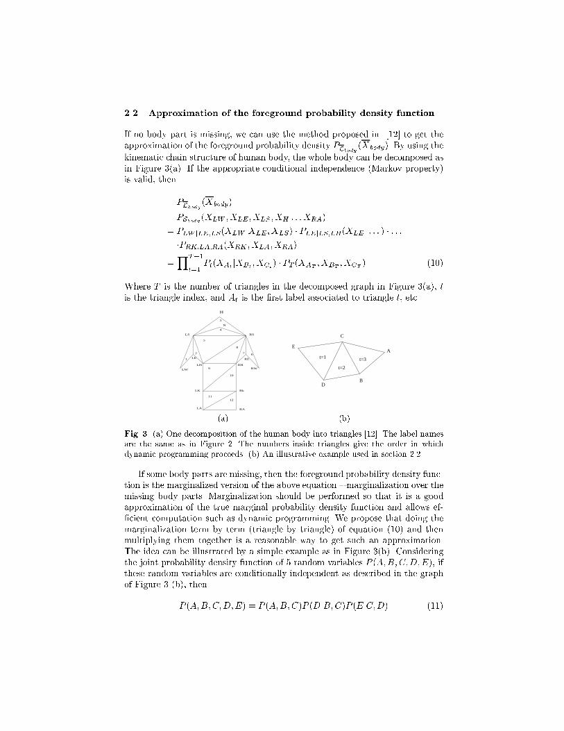
2.2 Approximation of the foreground probability density function

If no body part is missing, we can use the method proposed in [12] to get the

approximation of the foreground probability density PLbody

(Xbody

). By using the

kinematic chain structure of human body, the whole body can be decomposed as

in Figure 3(a). If the appropriate conditional independence (Markov property)

is valid, then

PLbody

(Xbody

)

= PSbody (XLW; X

LE; X

LS; X

H: : : X

RA)

= PLW jLE;LS(XLW

jXLE; X

LS) � P

LEjLS;LH(XLEj : : : ) � : : :

�PRK;LA;RA

(XRK

; XLA; X

RA)

=Y

T�1

t=1Pt(X

AtjX

Bt; X

Ct) � P

T(X

AT; X

BT; X

CT) (10)

Where T is the number of triangles in the decomposed graph in Figure 3(a), t

is the triangle index, and Atis the �rst label associated to triangle t, etc.

H

N

LS RS

LE

LH

LK

RE

RH

Rk

LA RA

LW RW

2 67

1

3

4

5

8

9

10

1112

E

C

DB

At=1

t=2

t=3

(a) (b)

Fig. 3. (a) One decomposition of the human body into triangles [12]. The label names

are the same as in Figure 2. The numbers inside triangles give the order in which

dynamic programming proceeds. (b) An illustrative example used in section 2.2.

If some body parts are missing, then the foreground probability density func-

tion is the marginalized version of the above equation { marginalization over the

missing body parts. Marginalization should be performed so that it is a good

approximation of the true marginal probability density function and allows ef-

�cient computation such as dynamic programming. We propose that doing the

marginalization term by term (triangle by triangle) of equation (10) and then

multiplying them together is a reasonable way to get such an approximation.

The idea can be illustrated by a simple example as in Figure 3(b). Considering

the joint probability density function of 5 random variables P (A;B;C;D;E), if

these random variables are conditionally independent as described in the graph

of Figure 3 (b), then

P (A;B;C;D;E) = P (A;B;C)P (DjB;C)P (EjC;D) (11)

If A is missing, then the marginalized PDF is P (B;C;D;E). If the conditional

independence as in equation (11) can hold, then,

P (B;C;D;E) = P (B;C) � P (DjB;C) � P (EjC;D) (12)

In the case of D missing, the marginalized PDF is P (A;B;C;E). If we assume

that E is conditionally independent of A and B given C, which is a more de-

manding conditional independence requirement with the absence of D compared

to that of equation (11), then,

P (A;B;C;E) = P (A;B;C) � 1 � P (EjC) (13)

Each term on the right hand sides of equations (12) and (13) is the marginalized

version of its corresponding term in equation (11). Similarly, if some stronger con-

ditional independence can hold, we can obtain an approximation of PLbody

(Xbody

)

by performing the marginalization term by term of equation (10). For example,

considering triangle (At; B

t; C

t), 1 � t � T � 1, if all of A

t, B

tand C

tare

present, then the tth term of equation (10) is PAtjBt;Ct

(XAtjX

Bt; X

Ct); if A

t

is missing, the marginalized version of it is 1; if Atand C

tare observed, but

Btis missing, it becomes P

AtjCt(X

AtjX

Ct)); if At exists but both Btand C

t

missing, it is PAt(X

At). For the T th triangle, if some body part(s) are miss-

ing, then the corresponding marginalized version of PTis used. The foreground

probability PLbody

(Xbody

) can be approximated by the product of the above

(conditional) probability densities. Note that if too many body parts are miss-

ing, the conditional independence assumptions of the graphical model will no

longer hold; it is reasonable to assume that the wrist is conditionally indepen-

dent of the rest of the body given the shoulder and elbow, but if both shoulder

and elbow are missing, this is no longer true. Nevertheless, we will use inde-

pendence as an approximation. All the above (conditional) probability densities

(e.g. PLW jLE;LS(XLW

jXLE; X

LS)) can be estimated from the training data.

2.3 Cost functions and comparison of two labelings

The best labeling (L�

) can be found by comparing the likelihood of all the

possible labelings. To compare two labelings L1and L

2, if we can assume that

the priors P (L1) and P (L

2) are equal, then by equation (9),

P (L1jX)

P (L2jX)

=P (X jL

1)

P (X jL2)=PL1

body

(X1

body) � P

bg(X

1

bg)

PL2

body

(X2

body) � P

bg(X

2

bg)

=PL1

body

(X1

body) � (1=S)N�K1

PL2

body

(X2

body) � (1=S)N�K2

=PL1

body

(X1

body) � (1=S)M�K1

PL2

body

(X2

body) � (1=S)M�K2

(14)

where L1

bodyand L

2

bodyare the sets of observed body parts for L

1and L

2respec-

tively, K1 and K2 are the sizes of L1

bodyand L

2

body, and M is the total number

of body parts (M = 14 here). PLi

body

(Xi

body), i = 1; 2, can be approximated as in

section 2.2. From equation (14), the best labeling L�

is the L which can maxi-

mize PLbody

(Xbody

) �(1=S)M�K . This formulation makes both search by dynamic

programming and detection in di�erent frames (possibly with di�erent numbers

of candidate features N) easy, as will be explained below.

The dynamic programming algorithm [1, 12] requires that the local cost func-

tion associated with each triangle (as in Figure 3(a)) should be comparable for

di�erent labelings: whether there are missing part(s) or not. Therefore we cannot

only use the terms of PLbody

(Xbody

), because, for example, as we discussed in

the previous subsection, the tth term of PLbody

(Xbody

) is PAtjBtCt

(XAtjX

Bt; X

Ct)

when all the three parts are present and it is 1 when Atis missing. It is unfair

to compare PAtjBtCt

(XAtjX

Bt; X

Ct) with 1 directly. At this point, it is useful

to notice that in PLbody

(Xbody

) � (1=S)M�K , for each unobserved (missing) body

part (M �K in total), there is a 1=S term. 1=S (S is the volume of the space

XAt

lies in) can be a reasonable local cost for the triangle with vertex At(the

vertex to be deleted) missing because then for the same stage, the dimension of

the domain of the local cost function is the same. Also, 1=S can be thought of

as a threshold of PAtjBtCt

(XAtjX

Bt; X

Ct), namely, if P

AtjBtCt(X

AtjX

Bt; X

Ct) is

smaller than 1=S, then the hypothesis that Atis missing will win. Therefore, the

local cost function for the tth (1 � t � T � 1) triangle can be approximated as

follows:

- if all the three body parts are observed, it is PAtjBtCt

(XAtjX

Bt; X

Ct);

- if Atis missing or two or three of A

t; B

t; C

tare missing, it is 1=S;

- if either Btor C

tis missing and the other two body parts are observed, then

it is PAtjCt

(XAtjX

Ct) or P

AtjBt(X

AtjX

Bt).

The same idea can be applied to the last triangle T . These approximations are to

be validated in experiments. Notice that when two body parts in a triangle are

missing, only velocity information for the third body part is available since we use

relative positions. The velocity of a point alone doesn't have much information,

so for two parts missing, we use the same cost function as the case of three body

parts missing.

With the local cost functions de�ned above, dynamic programming can be

used to �nd the labeling with the highest PLbody

(Xbody

) � (1=S)M�K . The com-

putational complexity is on the order of M �N3.

3 Detection

Given a hypothetical labeling L, the higher P (XjL) is, the more likely it is that

the associated con�guration of features represents a person. The labeling L�

with the highest PLbody

(Xbody

)�(1=S)M�K provides us with the most human-like

con�guration out of all the candidate labelings. Note that since the dimension

of the domain of PLbody

(Xbody

) � (1=S)M�K is �xed regardless of the number

of candidate features and the number of missing body parts in the labeling L,

we can directly compare the likelihoods of di�erent hypotheses, even hypotheses

from di�erent images.

In order to perform detection we �rst get the most likely labeling, then com-

pare the likelihood of this labeling to a threshold. If the likelihood is higher

than the threshold, then we will declare that a person is present. This threshold

needs to be set based on experiments, to ensure the best trade-o� between false

acceptance and false rejection errors.

4 Integrating temporal information [11]

So far, we have only assumed that we may use information from two consecutive

frames, from which we obtain position and velocity of a number of features.

In this section we would like to extend our previous results to the case where

multiple frames are available. However, in order to maintain generality we will

assume that tracking across more than 2 frames is impossible. This is a simpli�ed

model of the situation where, due to extreme body motion or to loose and

textured clothing, tracking is extremely unreliable and each individual feature's

lifetime is short.

Let P (OjX) denote the probability of the existence of a person givenX. From

equation (14) and the previous section, we use the approximation: P (OjX) is pro-

portional to � (X jL�

) de�ned as � (X jL�

)def= max

L2LPLbody

(Xbody

) �(1=S)M�K ,

where L�is the best labeling found from X. Now if we have n observations

X1; X2; : : : ; Xn, then the decision depends on:

P (OjX1; X2; : : : ; Xn)

= P (X1; X2; : : : ; XnjO) � P (O)=P (X1; X2; : : : ; Xn

)

= P (X1jO)P (X2jO) : : : P (XnjO) � P (O)=P (X1; X2; : : : ; Xn

) (15)

The last line of equation (15) holds if we assume that X1; X2; : : : ; Xnare in-

dependent. Assuming that the priors are equal, P (OjX1; X2; : : : ; Xn) can be

represented by P (X1jO) : : : P (XnjO), which is proportional to

Qn

i=1� (XijL�

i).

If we set up a threshold forQn

i=1� (XijL�

i), then we can do detection given

X1; X2; : : : ; Xn.

5 Counting

Counting how many people are in the scene is also an important task since

images often have multiple people in them. By the method described above,

we can �rst get the best con�guration to see if it could be a person. If so, all

the points belonging to the person are removed and the next best labeling can

then be found from the rest of points. We repeat until the likelihood of the best

con�guration is smaller than a threshold. Then the number of con�gurations

with likelihood greater than the threshold is the number of people in the scene.

6 Experiments

In this section we explore experimentally the performance of our system. The

data were obtained from a 60 Hz motion capture system. The motion capture

system can provide us with labeling for each frame which can be used as ground

truth. In our experiments, we assumed that both position and velocity were

available for each candidate point. The velocity was obtained by subtracting the

positions in two consecutive frames.

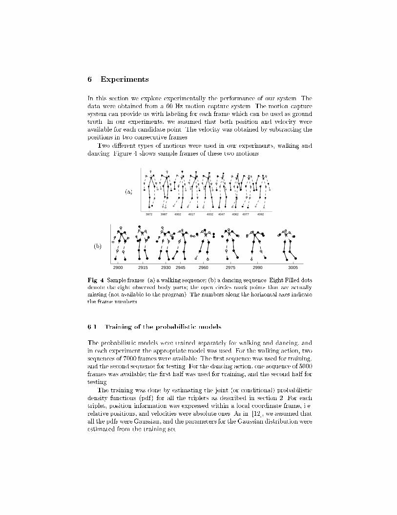
Two di�erent types of motions were used in our experiments, walking and

dancing. Figure 4 shows sample frames of these two motions.

(a)

3972 3987 4002 4017 4032 4047 4062 4077 4092

(b)

2900 2915 2930 2945 2960 2975 2990 3005

Fig. 4. Sample frames. (a) a walking sequence; (b) a dancing sequence. Eight Filled dots

denote the eight observed body parts; the open circles mark points that are actually

missing (not available to the program). The numbers along the horizontal axes indicate

the frame numbers.

6.1 Training of the probabilistic models

The probabilistic models were trained separately for walking and dancing, and

in each experiment the appropriate model was used. For the walking action, two

sequences of 7000 frames were available. The �rst sequence was used for training,

and the second sequence for testing. For the dancing action, one sequence of 5000

frames was available; the �rst half was used for training, and the second half for

testing.

The training was done by estimating the joint (or conditional) probabilistic

density functions (pdf) for all the triplets as described in section 2. For each

triplet, position information was expressed within a local coordinate frame, i.e.

relative positions, and velocities were absolute ones. As in [12], we assumed that

all the pdfs were Gaussian, and the parameters for the Gaussian distribution were

estimated from the training set.

6.2 Detection

In this experiment, we test how well our method can distinguish whether or not

a person is present in the scene (Figure 2). We present the algorithm with two

types of inputs (presented randomly in equal proportions); in one case only clut-

ter (background) points are present, in the other body parts from the walking

sequence are superimposed on the clutter points. We call 'detection rate' the

fraction of frames containing a body that is recognized correctly. We call 'false

alarm rate' the fraction of frames containing only clutter where our system de-

tects a body.

We want to test the detection performance when only part of the whole body

(with 14 body parts in total) can be seen. We generated the signal points (body

parts) in the following way: for a �xed number of signal points, we randomly

selected which body parts would be used in each frame (actually pair of frames,

since consecutive frames were used to estimate the velocity of each body part).

So in principle, each body part has an equal chance to be represented, and as far

as the decomposed body graph is concerned, all kinds of graph structures (with

di�erent body parts missing) can be tested.

The positions and velocities of clutter (background) points were indepen-

dently generated from uniform probability densities. For positions, we used the

leftmost and rightmost positions of the whole training sequence as the horizon-

tal range, and highest and lowest body part positions as the vertical range. For

velocities, the possible range was inside a circle in velocity space (horizontal and

vertical velocities) with radius equal to the maximum magnitude of body part

velocities in the training sequences. Figure 2 (a) shows a frame with 8 body parts

and 30 added background points with arrows representing velocities.

The six solid curves of Figure 5 (a) are the receiver operating characteristics

(ROCs) obtained from our algorithm when the 'positive' test images contained

3 to 8 signal points with 30 added background points and the 'negative' test

images contained 30 background points. The more signal points, the better the

ROC. With 30 background points, when the number of signal points is more

than 8, the ROCs are almost perfect.

When using the detector in a practical situation, some detection threshold

needs to be set; if the likelihood of the best labeling exceeds the threshold, a

person is deemed to be present. Since the number of body parts is unknown

beforehand, we need to �x a threshold that is independent of (and robust with

respect to) the number of body parts present in the scene. The dashed line in

Figure 5 (a) shows the overall ROC of all the frames used for the six ROC curves

in solid lines. We took the threshold when Pdetect

= 1�Pfalse�alarm on it as our

threshold. The star ('*') point on each solid curve shows the point corresponding

to that threshold. Figure 5 (b) shows the relation between detection rate and

number of body parts displayed with regard to the �xed threshold. The false

alarm rate is 12.97%.

When the algorithm can correctly detect whether there is a person, it doesn't

necessarily mean that all the body parts are correctly labeled. Therefore we also

studied the correct label rate when a person is correctly detected. Figure 5 (c)

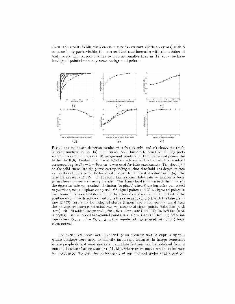
shows the result. While the detection rate is constant (with no errors) with 8

or more body parts visible, the correct label rate increases with the number of

body parts. The correct label rates here are smaller than in [12] since we have

less signal points but many more background points.

0 0.2 0.4 0.6 0.8 10

0.1

0.2

0.3

0.4

0.5

0.6

0.7

0.8

0.9

1

false alarm rate

dete

ctio

n ra

te

3 4 5 6 7 80

0.2

0.4

0.6

0.8

1

number of signal points (body parts)de

tect

ion

rate

2 4 6 8 10 120

0.2

0.4

0.6

0.8

1

number of signal points (body parts)

corr

ect l

abel

rat

e

(a) (b) (c)

0 1 2 3 40

0.2

0.4

0.6

0.8

1

std of added Gaussian noise (in pixels)

dete

ctio

n ra

te

3 4 5 6 7 8 9 100

0.2

0.4

0.6

0.8

1

number of signal points (body parts)

dete

ctio

n ra

te

1 2 3 4 5 6 7 80

0.2

0.4

0.6

0.8

1

numer of frames integrated

dete

ctio

n ra

te

(d) (e) (f)

Fig. 5. (a) to (e) are detection results on 2 frames only, and (f) shows the result

of using multiple frames. (a) ROC curves. Solid lines: 3 to 8 out of 14 body parts

with 30 background points vs. 30 background points only. The more signal points, the

better the ROC. Dashed line: overall ROC considering all the frames. The threshold

corresponding to PD = 1 � PFA on it was used for later experiments. The stars ('*')

on the solid curves are the points corresponding to that threshold. (b) detection rate

vs. number of body parts displayed with regard to the �xed threshold as in (a). The

false alarm rate is 12.97%. (c) The solid line is correct label rate vs. number of body

parts when a person is correctly detected. The chance level is shown in dashed line. (d)

the detection rate vs. standard deviation (in pixels) when Gaussian noise was added

to positions, using displays composed of 8 signal points and 30 background points in

each frame. The standard deviation of the velocity error was one tenth of that of the

position error. The detection threshold is the same as (b) and (c), with the false alarm

rate 12.97%. (e) results for biological clutter (background points were obtained from

the walking sequences): detection rate vs. number of signal points. Solid line (with

stars): with 30 added background points, false alarm rate is 24.19%; Dashed line (with

triangles): with 20 added background points, false alarm rate is 19.45%. (f) detection

rate (when Pdetect = 1 � Pfalse�alarm) vs. number of frames used with only 5 body

parts present.

The data used above were acquired by an accurate motion capture system

where markers were used to identify important features. In image sequences

where people do not wear markers, candidate features can be obtained from a

motion detector/feature tracker ( [11, 13]), where extra measurement noise may

be introduced. To test the performance of our method under that situation,

independent Gaussian noise was added to the position and velocity of the signal

points (body parts). We experimented with displays composed of 8 signal points

and 30 background points in each frame. Figure 5 (d) shows the detection rate

(with regard to the same threshold as Figure 5(b) and (c)) vs. standard deviation

(in pixels) of added Gaussian noise to positions. The standard deviation of noise

added to velocities is one tenth of that of positions, which re ects the fact that

the position error, due to the inaccurate localization of a feature by a tracking

algorithm ( [11, 13]), is usually much larger than the velocity error which is due

to the tracking error from one frame to the next.

We also tested our method by using biological clutter, that is, the background

points were generated by independently drawing points (with position and ve-

locity) of randomly chosen frames and body parts from the walking sequence.

Figure 5(e) shows the results.

6.3 Using temporal information

The detection rate improves by integrating information over time as discussed

in section 4. We tested this using displays composed of 5 signal points and 30

background points (the 5 body parts present in each frame were chosen randomly

and independently). The results are shown in Figure 5(f).

6.4 Counting

We call 'counting' the task of �nding how many people are present in a scene. Our

stimuli with multiple persons were obtained in the following way. A person was

generated by randomly choosing a frame from the sequence, and several frames

(persons) can be superimposed together in one image with the position of each

person selected randomly but not overlapped with each other. The statistics of

background features was similar to that in section 6.2 (Figure 5(a)), but with

the positions distributed on a window three times as wide as that in Figure 2

(a). Figure 6(a) gives an example of images used in this experiment, with three

persons (six body parts each) and sixty background points.

Our stimuli contained from zero to three persons. The threshold from Figure

5(a) was used for detection. If the probability of the con�guration found was

above the threshold, then it was counted as a person. The curves in Figure 6(b)

show the correct count rate vs. the number of signal points. To compare the

results conveniently, we used the same number of body parts for di�erent persons

in one image (but the body parts present were randomly chosen). The solid line

represents counting performance when one person was present in each image,

the dashed line with circles is for stimuli containing two persons, and the dash-

dot line with triangles is for three persons. If there was no person in the image,

the correct rate was 95%. From Figure 6(b), we see that the result for displays

containing fewer people is better than that with more people, especially when

the number of observed body parts is small. We can explain it as follows. If the

probability of counting one person correctly is P , then the probability of counting

n people correctly is Pn if the detection of di�erent people is independent. For

N

ER

WR

KL KR

AL

H

N SL SR

WL

AL

SR

WLHR

KR

ALAR 4 5 6 7 8 90

0.2

0.4

0.6

0.8

1

number of signal points (body parts)

corr

ect r

ate

(a) (b)

Fig. 6. (a) One sample image of counting experiments. '*'s denote body parts and

'o's are background points. There are three persons (six body parts for each person)

with sixty superimposed background points. Arrows are the velocities. (b) Results of

counting experiments: correct rate vs. number of body parts. Solid line (with solid

dots): one person; dashed line (with open circles): two persons; dash-dot line (with

triangles): three persons. Detection of a person is with regard to the threshold chosen

from Figure 5(a). For that threshold the correct rate for recognizing that there is no

person in the scene is 95%.

example, in the case of four body parts, for one person the correct rate is 0:6,

then the correct rate for counting three person is 0:63 = 0:216. This is just an

approximation since body parts from di�erent persons may be very close and the

body part of one person may be perceived as belonging to another. Furthermore,

the assumption of independence is also violated since once a person is detected

the corresponding body parts are removed from the scene in order to detect

subsequent people.

6.5 Experiments on dancing sequence

In the previous experiments, walking sequences were used as our data. In this

section, we tested our model on a dancing sequence. Results are shown in Figure

7. The signal points (body parts) were from the dancing sequence and the clutter

points were generated the same way as in section 6.2 (Figure 5(a)).

7 Conclusions

We have presented a method for detecting, labeling and counting biological mo-

tion in a Johansson-like sequence. We generalize our previous work [12] by

extending the technique to work on arbitrary amounts of clutter and occlusion.

We have tested our implementation on two kinds of moving sequences (walk-

ing and dancing) and demonstrated that it performs well under conditions of

clutter and occlusion that are possibly more challenging than one would expect

in a typical real-life scenario. The motion clutter we injected in our displays was

designed to resemble the motion of individual body parts, the number of noise

points in our experiments far exceeded the number of signal points, the num-

ber of undetected/occluded signal features in some experiments exceeded the

number of detected features. Just to quote one signi�cant performance �gure:

2-frame detection rate is better than 90% when 6 out of 14 body parts are seen

0 0.2 0.4 0.6 0.8 10

0.1

0.2

0.3

0.4

0.5

0.6

0.7

0.8

0.9

1

false alarm rate

dete

ctio

n ra

te

4 5 6 7 8 9 100.5

0.6

0.7

0.8

0.9

1

number of signal points (body parts)

dete

ctio

n ra

te

(a) (b)

Fig. 7. Results of dancing sequences. (a) Solid lines: ROC curves for 4 to 10 body parts

with 30 background points vs. 30 background points only. The more signal points, the

better the ROC. Dashed line: overall ROC considering all the frames used in seven

solid ROCs. The threshold corresponding to PD = 1� PFA on this curve was used for

(b). The stars ('*') on the solid curves are the points corresponding to that threshold.

(b) detection rate vs. the number of body parts displayed with regard to the �xed

threshold. The false alarm rate is 14.67%. Comparing with the results in Figure 5 (a,

b), we can see that more body parts must be observed during the dancing sequence to

achieve the same detection rate as with the walking sequences, which is expected since

the motion of dancing sequences is more active and harder to model. Nevertheless, the

ROC curve with 10 out of 14 body parts present is nearly perfect.

within 30 clutter points (see Figure 5(b)). When the number of frames consid-

ered exceeds 5 then performance quickly reaches 100% correct (see Figure 5(f)).

This means that even in high-noise conditions detection is awless in 100ms or

so (considering a 60 Hz imaging system), a �gure comparable to the alleged

performance of the human visual system [8]. Moreover, our algorithm is com-

putationally e�cient, taking order of 1 second in our Matlab implementation

on a regular Pentium computer, which gives signi�cant hope for a real-time C

implementation on the same computer.

The next step in our work is clearly the application of our system to real

image sequences, rather than Johansson displays. We anticipate using a simple

feature/patch detector and tracker in order to provide the position-velocity mea-

surements that are input in our system. Since our system can work with features

that have a short life-span (in the limit 2-frame) this should be feasible without

modifying the overall approach. A �rst set of experiments is described in [11].

Comparing in detail the performance of our algorithm with the human visual

system is another avenue that we intend to pursue.

Acknowledgments

Funded by the NSF Engineering Research Center for Neuromorphic Systems

Engineering (CNSE) at Caltech (NSF9402726), and by an NSF National Young

Investigator Award to PP (NSF9457618).

References

1. Y. Amit and A. Kong, \Graphical templates for model registration", IEEE Trans-

actions on Pattern Analysis and Machine Intelligence, 18:225{236, 1996.

2. C. Bregler and J. Malik, \Tracking people with twists and exponential maps", In

Proc. IEEE CVPR, pages 8{15, 1998.

3. D. Gavrila, \The visual analysis of human movement: A survey", Computer Vision

and Image Understanding, 73:82{98, 1999.

4. L. Goncalves, E. Di Bernardo, E. Ursella, and P. Perona, \Monocular tracking of

the human arm in 3d", In Proc. 5th Int. Conf. Computer Vision, pages 764{770,

Cambridge, Mass, June 1995.

5. I. Haritaoglu, D.Harwood, and L.Davis, \Who, when, where, what: A real time

system for detecting and tracking people", In Proceedings of the Third Face and

Gesture Recognition Conference, pages 222{227, 1998.

6. N. Howe, M. Leventon, and W. Freeman, \Bayesian reconstruction of 3d human

motion from single-camera video", Tech. Rep. TR-99-37, a Mitsubishi Electric

Research Lab, 1999.

7. G. Johansson, \Visual perception of biological motion and a model for its analysis",

Perception and Psychophysics, 14:201{211, 1973.

8. P. Neri, M.C.Morrone, and D.C.Burr, \Seeing biological motion", Nature, 395:894{

896, 1998.

9. J.M. Rehg and T. Kanade, \Digiteyes: Vision-based hand tracking for human-

computer interaction", In Proceedings of the workshop on Motion of Non-Rigid

and Articulated Bodies, pages 16{24, November 1994.

10. K. Rohr, \Incremental recognition of pedestrians from image sequences", In Proc.

IEEE Conf. Computer Vision and Pattern Recognition, pages 8{13, New York City,

June, 1993.

11. Y. Song, X. Feng, and P. Perona, \Towards detection of human motion", To

appear in IEEE Conference on Computer Vision and Pattern Recognition, 2000.

12. Y. Song, L. Goncalves, E. Di Bernardo, and P. Perona, \Monocular perception

of biological motion - detection and labeling", In Proceedings of International

Conference on Computer Vision, pages 805{812, Sept 1999.

13. C. Tomasi and T. Kanade, \Detection and tracking of point features", Tech. Rep.

CMU-CS-91-132,Carnegie Mellon University, 1991.

14. S. Wachter and H.-H. Nagel, \Tracking persons in monocular image sequences",

Computer Vision and Image Understanding, 74:174{192, 1999.