Clutter Removal in Single

Radar Sensor Reflection

Data via Digital Signal

Processing

Master Thesis Project

Author: Mohammadreza Kazemisaber

Supervisor: J. Peter Hessling

Examiner: Sven-Erik Sandström

Term: Spring 2020

Subject: Electrical Engineering

Level: Master 30 hp

Course Code: 5ED36E Department of Physics and Electrical

Engineering

Dedication

This dissertation is dedicated to my beloved grandfather for his manner,

patience, and love. He has always been an inspiration to me and was the best

grandfather one could have. May his memory forever be a comfort and a

blessing.

Abstract

Due to recent improvements, robots are more applicable in factories and various

production lines where smoke, fog, dust, and steam are inevitable. Despite their

advantages, robots introduce new safety requirements when combined with humans.

Radars can play a crucial role in this context by providing safe zones where robots

are operating in the absence of humans.

The goal of this Master’s thesis is to investigate different clutter suppression methods

for single radar sensor reflection data via digital signal processing. This was done in

collaboration with ABB Jokab AB, Sweden. The calculations and implementation of

the digital signal processing algorithms are made with Octave. A critical problem is

false detection that could possibly cause irreparable damage. Therefore, a safety

system with an extremely low false alarm rate is desired to reduce costs and damages.

In this project, we have studied four different digital low pass filters: moving average,

multiple-pass moving average, Butterworth, and window-based filters. The results are

compared, and it is ascertained that all the results are logically compatible, broadly

comparable, and usable in this context.

Keywords: Surveillance Radar, Ultra-Wideband Radar, Clutter Reduction, FMCW

radar, Digital signal processing, Moving target detection, Doppler Processing.

Acknowledgments

I would like to thank ABB Jokab AB for providing the opportunity for me to learn

and gain knowledge, which is the most valuable favor and benefit that can be gained

at this point in my life.

Then, special thanks to my supervisor Peter Hessling because he patiently provided

me with his knowledge and experience so that I could accomplish this project.

Finally, I would like to express my appreciation to my examiner and course

coordinator, Sven-Erik Sandström, for his precious guidance and support not only

throughout the thesis period but for the past two years.

Table of contents

1 Introduction 1

1.1 Overview and Background 2

1.2 Description of The Radar System 3

1.3 Objectives and Goals 4

1.4 Research Method 5

1.5 Thesis Outline 5

2 Theory 6

2.1 Ultra-Wideband Radar Systems 6

2.2 UWB systems with FMCW 7

2.3 Doppler shift 8

2.4 Radar data cube 11

2.4.1 Range estimation 12

2.4.2 Angle of arrival estimation 12

2.4.3 Velocity estimation 13

2.5 Digital filters 14

2.5.1 Filter characteristics in the frequency domain 15

2.5.2 Time delay and phase shift in digital filters 16

3 Methods 18

3.1 Filter design 18

3.2 Introduction of the scenario for the clutter removal 19

3.3 Moving average filters 19

3.3.1 Frequency response, poles, and zeros of the moving average filters 21

3.3.2 Sidelobe suppression in moving average filters 23

3.3.3 Clutter removal by moving average filters 23

4.3 rettuB hBtowrettuB Error! Bookmark not defined.

3.4.1 Clutter removal by an LP Butterworth filter 25

3.5 Window-based FIR filter 28

3.5.1 Clutter removal by Window-based FIR filter 29

4 Results 32

4.1 Moving average results 35

4.2 Butterworths results 36

4.3 Window-based FIR filter (Hamming) 37

4.4 Comparable results 39

5 Discussion and conclusion 41

5.1 Moving average filters 41

5.2 Butterworth filters 42

5.3 Window-based FIR filter (Hamming) 42

6 References 44

List of Figures

1.11 Safety and availability profile for the safety system 1

1.21 Functional block diagram of IWR6843 3

1.311 Marine radar reflectors used in the project 4

2.11 Comparison of the Power spectrum of a conventional and an UWB radar 5

2.21 Simplified block diagram of an FMCW radar system 7

2.31 Transmitted and received signal in an FMCW radar system 8

2.41 Motion and Doppler frequency shift 8

2.51 FMCW signals with nonzero Doppler shift 9

2.61 Radar processing block diagram 11

2.71 A Radar data cube 11

2.81 Angular estimation 13

2.9 The first and the second FFT for Doppler calculation 13

2.10 Frequency response of the 4 basic filters 15

2.11 The phase response of a linear and nonlinear filter 16

3.1 The defined clutter range in the frequency domain 18

3.2 The RA heat map of the scenario 19

3.3 The scenario seen from the radar 19

3.4 Moving average filter block diagram 20

3.5 Frequency response of some moving average filters 21

3.6 Poles and zeros of a moving average filter with 21 taps 22

3.7 Frequency and phase response of a moving average filter with 21 taps 22

3.8 Multiple-pass filtering with moving average filters 23

3.9 Frequency response of a moving average filter and a multiple-pass

moving average filter 24

3.10 RA heat map of the clutter removed signal in which (a) clutter is removed

by moving average filter, and (b) clutter is removed with the multiple-pass

moving average filter. 25

3.11 Pols and zeros of Butterworth filter where (a) is second-order, (b) is forth

order and (c) is sixth-order Butterworth filter 26

3.12 Phase response of Butterworth filter for second, fourth, and sixth order

26

3.13 Group delay of Butterworth filter for second, fourth, and sixth order 26

3.14 Frequency response of Butterworth filter for the second, fourth, and sixth-order

in a linear scale 27

3.15 The RA heat map of clutter removed signals by the Butterworth filter in which

(a) is the second-order filter,(b) is the fourth-order filter, and (c) is

the sixth-order filter. 27

3.16 Impulse and frequency response of an ideal filter 28

3.17 Poles and zeros of the window-based FIR filter (Hamming Window ) 29

3.18 Frequency and phase response of the 44-tap window-based FIR filter

(Hamming Window) 30

3.19 Frequency response of the 44-tap window-based FIR filter(Hamming Window)

in a linear scale 30

3.20 RA heat map of the 44-tap window-based FIR filter(Hamming Window) 31

4.1 FFT for a chosen pixel of the received signal (before removing clutter) 32

4.2 The weight function compared to the frequency responses of the filters 33

4.3 Captured clutter from the received signal for a chosen pixel 34

4.4 Histogram of captured clutter from the received signal 34

4.5 Frequency response of two types of moving average filters in dB 35

4.6 Histogram of captured clutter by moving average methods

(presented for 20 bins) 35

4.7 Histogram of captured clutter by moving average filters

(presented for 20 bins) 36

4.8 Frequency response of three Butterworth filters in dB 36

4.9 Histogram of captured clutter by Butterworth filters

(presented for 20 bins) 37

4.10 Histogram of captured clutter by Butterworth filters

(presented for 10 bins) 37

4.11 Frequency responses of the window-based filter with different lengths 38

4.12 Histogram of captured clutter by the window-based filters

and different lengths (presented for 20 bins) 38

4.13 Histogram of captured clutter by the window-based filters

with different lengths (presented for 20 bins) 39

4.14 Frequency responses of three applied filters 39

4.15 Histogram of clutter captured of the filters (presented for 20 bins) 40

4.16 Histogram of clutter captured of the filters (presented for 10 bins) 40

Notations

µ Signal relative wideband index

c Speed of light

R Range of the target from the radar

𝑓𝑑 Doppler frequency

𝑡𝑟 Time delay

𝑅0 The distance of the moving object from the radar

𝑣𝑟 The velocity of the moving object

t Time of transmission the signal

𝑡′ The time when the signal reflected from the target

𝜆 Wavelength

𝑓𝑅𝑋 Frequency of the received signal

𝑓𝑇𝑋 Frequency of the transmitted signal

𝑓𝐼𝐹 Frequency of the intermediate frequency

𝑇𝑐 The time duration of the chirp

𝛥𝑑 Distance between two adjacent targets

𝛥𝑓 Difference in IF signals of two adjacent targets

𝛥𝑟 Range resolution

𝜃 Angle of arrival with respect to the normal line

𝜑𝑚 Measured phase difference between two successive chirps

𝑇𝑓 Frame time

𝑡φ Phase delay

𝑡𝑔 Group delay

𝛿𝑠 Stopband ripple

𝛿𝑐 Passband ripple

𝑥𝐶𝑙𝑢𝑡𝑡𝑒𝑟(𝑡) Clutter signal which is captured by an LP filter

𝑦𝐶𝑙𝑢𝑡𝑡𝑒𝑟 𝑟𝑒𝑚𝑜𝑣𝑒𝑑(𝑡) A signal which the clutter has been removed from it

𝑥𝑆𝑖𝑔𝑛𝑎𝑙(𝑡) The received signal by the receiving antenna of the radar sensor

𝑥(𝑡)𝑤𝑒𝑖𝑔ℎ𝑡 Weight signal

𝜎 Target reflection coefficient

Acronyms

CFAR Constant false alarm rate

MTI Moving target indication

SVD Singular value decomposition

HPF High pass filter

UWB Ultra-wideband

FMCW Frequency-modulated continuous wave

RF Radio Frequency

ADC Analog to Digital Converter

Msps Mega samples per second

FFT Fast Fourier transform

DSP Digital signal processing

RCS Radar cross-section

LPF Low-Pass filter

CW Continuous Wave

IF Intermediate Frequency

SFTF Short-time Fourier transform

RA Range-Angle

FIR Finite Impulse Response

FPS Frame per second

DTFT Discrete-Time Fourier Transform

AoA Angle of arrival

CA- CFAR Cell-averaging constant false alarm rate

PFD Probability of Failure on Demand

FM Frequency modulation

Eqn Equation

1(46)

Chapter 1

1 Introduction Since collaboration between humans and robots has been increasing in recent years,

both human safety and machinery performance/availability are of interest in heavy

industry. Safety and availability interact with each other. So, to provide a safe

industrial area observed by a radar system, the availability of machines or robots

should be considered.

As shown in Figure 1.1, reinforcing safety increases cost. The cost comes from

stopping machines without evidence or justification due to false detection, which may

be due to a low detection threshold of the Constant False Alarm Rate (CFAR). As the

detection threshold increases, the availability of the system increases. This means that

the radar may ignore some targets that need to be detected. As a result, the safety

system does not stop the production line. Therefore, increasing the detection

threshold, and hence the availability, is risky and not desirable. In industrial situations

stopping the whole production line can be highly expensive and should be based on

reliable detection of human presence. Accordingly, the current system is based on a

compromise between the two essential factors, availability, and reliable detection

(Figure 1.1).

Figure 1.1: Safety and availability profile for the safety system.

2(46)

Radar imaging systems could be designed with mm-wave radar sensors, which can

provide large bandwidth, and hence high image resolution. Removing clutter, which

has time-varying statistical properties, from the received radar signal, is the focus of

this study. It is intended to improve the availability and raise the reliability of

detection.

Consequently, a new safety system profile can be designed with a higher Safety

Integrity Level (SIL). As stated in [34], SIL measures the reduction in risk in a safety

system. The higher the SIL, the lower the Probability of Failure on Demand (PFD),

ranging from 10−1 to 10−5. In other words, the risk of failure in the safety system

decreases when requiring a higher level of SIL. The desired safety system profile is

presented in Figure 1.1.

The current chapter gives a description of the radar system, a problem formulation,

and a summary of how the objectives are achieved.

1.1 Overview and Background

In order to provide safe area supervision, radar technology is often better than lasers

or cameras. The reason is that radar can provide 3D area supervision even in harsh

environments where smoke, fog, fluids, and debris are inevitable. Hence, the

performance is not affected by dust, dirt, rain, intense light, sparks, or shock. By

overcoming these limitations, we can provide a safe area in a dynamic industrial

environment without physical barriers, while machines and robots are operating

freely.

Various kinds of signals can overwhelm safety radar systems. There could be clutter,

random disturbances, intentional interference, or accidental interference from other

radars or masking effects (due to the imperfection of CFAR methods). Among these,

clutter is the main topic of this study. The definition applicable to radar is that clutter

can be anything, except the target, that scatters the signal back to the receiver. Clutter

refers to those undesirable reflected signals which can interfere with the primary

signal in the data analysis and affect overall performance.

The definition of clutter in this study includes motionless/ slow-moving objects. In

the safe area supervised by the radar, which is usually highly cluttered, stationary

objects should be considered as clutter, and only nonstationary objects are of interest.

As stated, the removal of clutter improves the availability of the system since the main

signal stands out. So, we can improve availability with safety maintained.

There are many studies of radar clutter removal in various environments with the help

of DSP techniques [27]-[31]. Sonia Sethi et al. [2] investigated digital signal

processing techniques for surveillance radar. The objective of her research was to

reduce the rain clutter in the reflected echoes. She used Moving Target Indication

(MTI) filters, Notch filters, and Matched filters. Arun Rane et al. [3] proposed

3(46)

Singular Value Decomposition (SVD) and Wavelet transform techniques besides

bandpass filters to remove the clutter for better detection of a human behind a wall.

Also, V. Goncharenko et al. [4] suggested an adaptive MTI method with a High-Pass

Filter (HPF) in a windblown clutter environment. Since the environment varies, the

characteristics of clutters are consequently different and not entirely comparable.

Therefore, none of the mentioned clutter removal techniques in the quoted work is

used in this study due to the particular characteristics of clutter in the industrial

environment. It is also noteworthy that all clutter removal methods (customized

digital filers) in this study are applied in the Doppler/time-domain (over a sequence

of frames). To the best of our knowledge, few other studies have utilized similar

methods regardless of the characteristics of the clutter.

Previous research shows that clutter removal can be effective, and this study suggests

some approaches to achieve this.

1.2 Description of The Radar System

In this project, an Ultra Wide Band (UWB) radar system is used in various

arrangements to provide a safety zone. The advantage of the UWB radar system is the

high-resolution ranging provided by this radar. The radar system consists of a number

of mm-wave Frequency-Modulated Continuous Wave (FMCW) radar sensors. This

kind of radar sensor is applicable for gesture recognition radar, wall-penetrating radar

for detection, anti-intrusion security radars, and imaging radar. The main idea with

several radar sensors is to expand the viewing angle, minimize the random errors, and

improve resolution. The radar system sends and receives millimeter waves and

produces radar reflection images over the range, angle, and velocity in terms of point

objects.

Figure 1.3: Marine radar reflectors used in the project.

4(46)

Figure 1.2: Functional block diagram of IWR6843.

The single-chip modules that were used in this work are developed by Texas

Instruments. IWR6843 is a mmWave sensor with a Radio Frequency (RF) operating

range between 60 and 64 GHz with an Analog to Digital Converter (ADC) sampling

rate of 25 Msps. This module has 4 receiver antennas and 3 transmission antennas,

with a total of 12 virtual channels. This radar sensor is applicable in industrial

environments and can also do Fast Fourier Transform (FFT) and detection with the

help of its embedded DSP. Its range for large targets like a van is up to 160 m, and

1m for small targets like a coin. The block diagram of this module is shown in Figure

1.2 [12].

A traditional CA-CFAR detection method could be used for this radar system to find

a proper threshold of detection for distributed objects. In the process of data

collection, marine radar reflectors were used as reference targets (Figure 1.3). The

reflectors are typically used in situations where clutter dominates. These reflectors

have a high Radar Cross Section (RCS) in relation to the size [1].

1.3 Objectives and Goals

The main goal of this study is to remove clutter and improve single radar data

reflection by using DSP filtering techniques. Clutter suppression methods can vary

according to speed, application, accuracy, and memory [5].

5(46)

The overall objective can be specified in a number of points:

1. To investigate the possible filtering methods to remove clutter that are

matched to the current clutter.

2. Define and simulate the combined clutter and signal as a platform for filter

design.

3. To evaluate the performance and efficiency of different digital filtering

methods.

4. Compare the results obtained with the various methods.

5. Find constraints that motivate the modification of the current filter design.

1.4 Research Method

Due to the complexity and sensitivity of radar clutter removal methods in safety

applications, this project started with a literature review of methods for clutter

removal, advantages, and disadvantages. Thanks to ABB AB Jokab Safety, some real-

world difficulties regarding data collection in an industrial environment could be

identified. The reviewed theories have been tested and compared and then validated

with experimental results. All calculations and simulations have been made with

GNU Octave.

This study is accomplished in collaboration with ABB AB Jokab Safety and involves

no personal or critical information. No animals were involved in the data collection

and no destructive environmental actions were taken.

1.5 Thesis Outline

This study is divided into chapters as follows.

Chapter 2: Theory

In this chapter, some general radar theory is discussed, involving methods of

clutter removal, filters, algorithms, and their implementation.

Chapter 3: Methods

This part presents the methods used to remove clutter.

Chapter 4: Results

This section demonstrates results obtained when the methods were applied to

the collected data.

Chapter 5: Discussion and Conclusion

This part discusses and compares the results and points to the strengths and

weaknesses of each method.

6(46)

Chapter 2

2 Theory

2.1 Ultra-Wideband Radar Systems

A UWB is a radar system that uses a large part of the radio spectrum but at a lower

power level compared to conventional radar systems (Figure 2.1). UWB has

applications in data transmission, accurate distance measurement, positioning, radar,

and imaging. The cost of implementing this system is lower than for conventional

narrow-band systems. The pulse length of the UWB signals is much shorter than the

coherence time of the channel. Therefore, UWB is inherently resistant to multipath

fading. In addition, UWB is also resistant to intentional and unintentional interference

because its bandwidth is much broader than the bandwidth of the interfering signal.

Figure 2.1: Comparison of the Power spectrum of a conventional and an Ultra Wideband

radar system [33].

Since UWB uses a high bandwidth and low energy, it is applicable for short distances.

Based on the Fourier transform, a pulse with a length of T has a bandwidth of T/2

Hz. The pulse length used in UWB is often in the range of nanoseconds, so the pulse

bandwidth is in the range of several hundred MHz to several GHz. As presented in

Eq 2.1, µ is the relative wideband index, 𝑓max and 𝑓min are the maximum and

minimum frequency of the channel [6][7].

µ = 2 𝑓max −𝑓min

𝑓max +𝑓min (2.1)

7(46)

2.2 UWB systems with FMCW

As stated in [9], FMCW is a radar technique that uses low power and is suitable for

measuring distance. With the help of this technique, low frequencies can penetrate

media like forests. One of the most popular applications is traffic radars that use a

wide band and can measure range with good resolution [10].

Due to the advantages of UWB radar technology, different types of this system have

been developed. There are three categories based on their wave form: pulse UWB

radar, M-sequence UWB radar, and (FMCW) UWB radar [5]. FMCW is used in this

project to provide a safety zone due to its accuracy in short-range applications.

Figure 2.2: Simplified block diagram of an FMCW radar system.

The information in the received signal, including phase and range, can be extracted

after mixing, low pass filtering, and FFT processing, as shown in Figure 2.2.

Continuous Wave (CW) radars can merely measure Doppler frequency since

modulation is necessary for range measurement. FMCW radar, however, is based on

frequency modulation. This radar changes the frequency of the transmitted signals

linearly as a function of time. Consequently, they can measure both range and velocity

of the target simultaneously. By mixing the TX signal and RX signal with a mixer,

there is an output Intermediate Frequency (IF) signal. After ADC and 2D FFT

processing, the IF signal provides range and velocity (Doppler) data [32].

FMCW radar is used here since the updating of data is fast, allowing clutter removal

in the Doppler/time-domain (over a sequence of frames).

8(46)

Figure 2.3 shows transmitted and received signals in time with the frequency

modulation (FM) indicated. The time delay Δ𝑡, and the frequency difference Δ𝑓 are

marked [8].

Figure 2.3: Transmitted and received signal in an FMCW radar system.

2.3 Doppler shift

In this project, every stationary object is seen as clutter. So the velocity of all moving

objects, even low-speed moving objects, is of interest. In our safety test zone, there

are two equidistant targets, one of them is stationary, and the other one is coming

toward the radar sensor (Figure 2.4).

Figure 2.4: Motion and Doppler frequency shift.

When the radar transmits signals toward these two objects, the moving object will

reflect the signal with a shift in the frequency because of the movement, which is

the Doppler shift.

9(46)

Figure 2.5: FMCW signals with nonzero Doppler shift.

Fig. 2.5 shows a different type of FMCW with a modulation needed for the Doppler

measurement. Due to the time delay, there is a frequency shift between the transmitted

and the received signal, which is marked in the above figure as the downbeat

frequency 𝑓𝑏(𝑑𝑜𝑤𝑛) and the upbeat frequency 𝑓𝑏(𝑢𝑝). During the upward ramp, the

Doppler effect (𝑓𝑑) raises the frequency of the reflected signal and the frequency

difference 𝑓𝑏(𝑢𝑝) is reduced. During the downward ramp, the opposite effect increases

the beat frequency 𝑓𝑏(𝑑𝑜𝑤𝑛). The range frequency 𝑓𝑟 and Doppler frequency 𝑓𝑑 can

be calculated from the following formulas [8].

𝑓𝑟 =1

2[𝑓𝑏(𝑑𝑜𝑤𝑛) + 𝑓𝑏(𝑢𝑝)] (2.2)

𝑓𝑑 =1

2[𝑓𝑏(𝑑𝑜𝑤𝑛) − 𝑓𝑏(𝑢𝑝)] (2.3)

The distance to the target is given by the following expression, where r is the range,

T is the time duration of the chirp, and c is the speed of light [8].

𝑟 =𝑐 𝑇 𝑓𝑟

2 𝐵 (2.4)

For better understanding, we can assume that the reflected signal would first be

received at 𝑡𝑟 which is the time delay of the backscattered signal with respect to the

transmitted signal 𝑝(𝑡) (Eqn. 2.6). 𝑢(𝑡) is the signal amplitude and 𝜎 is the target

reflection coefficient. So, the backscattered signal 𝑠(𝑡) from the static target can be

approximated as in Eqn. 2.6.

𝑝(𝑡) = 𝑢(𝑡) 𝑒𝑗𝜔0𝑡 (2.5)

𝑠(𝑡) ≃ 𝜎𝑝(𝑡 − 𝑡𝑟) = 𝜎𝑢(𝑡 − 𝑡𝑟) 𝑒𝑗𝜔0𝑡 𝑒−𝑗𝜔0𝑡𝑟 (2.6)

10(46)

From the time delay for a static target, we can also calculate the Doppler

characteristics when the target is moving. If a signal is backscattered from a moving

target and is received at 𝑡, then it was transmitted time 𝑡 − 𝑡𝑟. By symmetry, this

signal was then reflected from the target at 𝑡 − 𝑡𝑟/2. Consequently, the distance to

the target from the radar at the time of reception is then given by Eq. 2.7

r = 𝑟0 − 𝑣𝑟𝑡 (2.7)

We assume that the radar is at rest at r= 0, and the target is at 𝑟 = 𝑟0 when 𝑡=0.

Moreover, the distance traveled by the signal is 2𝑟0. Subsequently, the time delay

from emission to reception of the signal by radar can be estimated by Eqn. 2.8 [11]:

𝑡𝑟 ≃2𝑟0

𝑐 (2.8)

There is also the phase relating to the distance. The phase corresponding to the round

trip is [36]:

𝜑 = 2𝜋 2𝑟

𝜆=

2𝜋 2(𝑟0−𝑣𝑟𝑡)

𝜆 (2.9)

The angular frequency then relates to the velocity of the moving object as follows

[35] [36]:

𝜔= 𝑑𝜑

𝑑𝑡= 2𝜋

−2𝑣𝑟

𝜆 (2.10)

And finally, the Doppler frequency is presented in Eqn. 2.11, where 𝑓0 is the start

frequency of the signal or the transmitter frequency. The factor of two indicates the

Doppler frequency corresponds to reflection from a moving target and not from a

moving source [36].

𝑓𝑑 = |𝜔

2𝜋| =

2𝑣𝑟

𝜆 =

2𝑣𝑟𝑓0

𝑐 (2.11)

The Doppler frequency depends on the direction of movement of the moving object

(radial velocity) relative to the radar sensor. As we can see in Eqn. 2.11, only the

radial component of velocity contributes to the Doppler shift. When the object is

moving toward the radar sensor, this frequency is higher than the transmitted signal,

and when the target is moving away from the radar sensor, the frequency of the return

signal is lower than the frequency for 𝑣𝑟 = 0 [11].

11(46)

Figure 2.6: Radar processing block diagram.

2.4 Radar data cube

In radar data processing, the data cube (Fig. 2.7) represents the complete data set. As

shown in Figure 2.6, raw radar data is processed by FFT to calculate the range. A

second FFT should then be done to the data across chirps in one frame. Thus the

second FFT operates on the velocity data in the radar cube. However, by applying the

Short-time Fourier Transform (SFTF) to the range-FFT data, an SFTF heat map can

be obtained but this is out of scope here. To obtain a Range-Angle (RA) heat map for

a spatial representation of the data, a third FFT should be applied to the data after the

2D-FFT. This refers to a radar data cube with three indices corresponding to angle,

range, and velocity [13].

Figure 2.7: A radar data cube.

12(46)

2.4.1 Range estimation

As shown in Figure 2.2, TX transmits a signal toward the target, and the reflected

signal is received by the RX. The IF signal is obtained by mixing the TX signal and

the RX signal. The IF frequency is the difference in the frequency of the TX signal

and the RX signal.

𝑓𝑇𝑋−𝑓𝑅𝑋 = 𝑓𝐼𝐹 =𝐵𝑡𝑟

𝑇 (2.12)

To extract the information in the IF signal in the frequency domain, the first FFT

should be done to the IF signal. The result shows the range of each target in the form

of spectral peaks in the resulting FFT which is called the range FFT. Since the IF

signal contains several tones or frequencies, each tone corresponds to the range of an

object. When two targets are located close to each other with a radial distance

difference of 𝛥𝑑, they will have a difference in their IF signals 𝛥𝑓 =1

𝑇. The range

resolution of the radar determines the ability of the radar to distinguish two adjacent

targets in the range FFT. Eqn. 2.13 gives the range resolution which depends only on

the bandwidth of the chirps [14] [15].

𝛥𝑟 =𝑐

2𝐵 (2.13)

2.4.2 Angle of arrival estimation

The range can be calculated by one transmitter and one receiver. However, to estimate

the target angle to the radar, at least two receiver antennas are required. The angle of

a target corresponds to one of the necessary indices in the radar data cube. Fig. 2.8

shows a reflected echo arriving at an angle 𝜃 at the receiving antennas. However, to

arrive at the second antenna, the reflected signal propagates the additional distance d.

So, the Angle of Arrival (AoA) between the two received signals is different. The

FFT of the received signal by each receiving antenna would yield the same range-

FFT, with the same peaks, but with different phases. This phase difference 𝜑 can be

expressed by Eqn. 2.14, where β is the wave number 𝛽 = 2𝜋/𝜆 [14] [15].

𝜑 = 𝛽 𝛥𝑑 = 𝛽 𝑑 𝑠𝑖𝑛 𝜃 =2𝜋𝑑 sin 𝜃

𝜆 (2.14)

Moreover, the angle of arrival can be estimated from this phase difference by simply

inverting Eq. 2.14 [15].

𝜃 = sin−1(𝜆 𝜑

2𝜋𝑑) (2.15)

13(46)

Figure 2.8: Angular Estimation.

2.4.3 Velocity estimation

The different velocity of two objects produces different phases in two successivew

chirps. Then, there is a phase difference between two successive chirps (𝜑𝑚) with

respect to the movement of the moving objects. This phase differencewis expressed as

follows:

𝜑𝑚 =4𝜋 𝑣𝑟 𝑇

𝜆 (2.16)

Figure 2.9: The first and the second FFT for Doppler calculation.

Then, a number n of transmitted chirps with the constant time difference in a specified

time interval can be called a frame (Fig. 2.9). By doing FFT over the sequence of

chirps in a frame, will have a range-FFT for each chirp, so that a matrix is formed.

This matrix has n columns, the number of chirps in each frame, and N rows that refer

to the number of bins in the range-FFT. By doing 2D-FFT on the sequence of phasors

(each row), we have n values of 𝜑𝑚 which shows different velocities and can then

resolve different velocities in the range-FFT. This is called a Doppler-FFT. The data

cube has three indices; angle, velocity, and range [14] [15].

14(46)

Since the main goal of this study is to improve the reliability of detection, the radar

should provide accurate measurements. To distinguish low-speed moving objects and

stationary objects, a high velocity resolution is required. The velocity resolution for

fast data updates depends on the frame rate. The higher the frame rate, the more chirps

and phase samples, and the higher the resulting velocity resolution. Figure 2.9 shows

that the shorter the duration of the frame time (𝑇𝑓), the higher the frame rate, and the

higher the velocity resolution [14] [16].

𝑉𝑟𝑒𝑠 =𝜆

2𝑇𝑓 (2.17)

2.5 Digital filters

In signal processing, there are two major types of filters, digital and analog filters.

The goal of using these types of filters is the same, but the performance of the digital

filters is higher. Another name for analog filters is electronic filters since they are

built with electronics.

A signal can be combined with signals with different frequencies, like noise. To

separate frequency bands, one uses filters. In the radar context, for example, the

received signal would be combined with thermal noise, clutter, and various

interferences. An FFT of the signal shows this spectrum of frequencies. So, with the

help of digital filters, we can select and separate frequency bands. Moreover, digital

filters are applicable to the restoration of damaged signals due to systematic errors

like faulty equipment [17]. However, what makes digital filers a true game-changer

is their flexibility. It is easier to change a coefficient in a register (digital filters) than

to modify an electronic circuit (analog filters).

To characterize a filter, it is common to focus on three response functions: impulse,

step, and frequency response. They all represent essential but different information

about the filter. An impulse response is the output of a dynamic system. As the

impulse response covers all frequencies, it is a general description of a linear system.

A digital filter is based on a discrete convolution of the impulse response and the input

signal in the time domain:

𝑦(𝑡) = ∑ ℎ(𝑘)𝑥(𝑡 − 𝑘)∞𝑘=1 (2.18)

The step response also describes the filter characteristics in the time domain and

would typically be used when a signal has most of the critical information in the time

domain than the frequency domain. On the other hand, the frequency response relates

to the frequency domain. These responses are all needed to design the desired filter.

Filters that have good performance in the time domain have weak efficiency in the

frequency domain. Conversely, filters with good efficiency in the frequency domain

may be poor in the time domain. The frequency response of a filter is the FFT of its

15(46)

impulse response which is shown by substituting frequency variable 𝑧 = 𝑒𝑗𝜔𝑡 as

follows:

𝐻(𝑧) = 𝑌(𝑒𝑗𝜔𝑡)

𝑋(𝑒𝑗𝜔𝑡) (2.19)

Consequently, the phase response of the filter is:

𝜑(𝐻(𝑧)) = ∠ 𝐻(𝑒𝑗𝜔𝑡) (2.20)

2.5.1 Filter characteristics in the frequency domain

Filters are divided into four groups based on their frequency responses. Low-pass

filters allow only low frequencies to pass while high-pass filters allow high

frequencies. Bandpass filters have a passband between two stop bands. Band reject

filters, or notch filters, have a stop band between two pass bands.

The cutoff frequency refers to the frequency where the power is down to half the

maximum value, and the amplitude is reduced by 0.70, or down 3 dB (Eqn. 2.22). The

filter types are shown in Figure 2.10 [18].

10 log10 (1

2) = −3.01𝑑𝐵 (2.21)

Figure 2.10: Frequency response of the 4 basic filters.

A good property of a filter is a linear phase response. When the phase response is

linear, every frequency component of the signal is shifted in time linearly. Since all

frequencies have the same time shift the phase is not distorted in linear phase filters.

If the phase response is linear and the impulse response is symmetric, then the filter

has no phase distortion. A linear and a nonlinear response is shown in Fig 2.11 [17].

16(46)

Figure 2.11: The phase response of a linear and a nonlinear filter.

2.5.2 Time delay and phase shift in digital filters

Any system has a time delay, and in a digital filter there is a phase shift corresponding

to this delay. For the Laplace transform a time delay 𝑡𝑑 can be described by:

𝐻(𝑠) = ∫ 𝑒−𝑠𝑡∞

0ℎ(𝑡)𝑑𝑡

= ∫ 𝑒−𝑠𝑡∞

𝑡𝑑𝑓(𝑡 − 𝑡𝑑)𝑑𝑡 = ∫ 𝑒−𝑠(𝑡𝑑+τ)∞

0 𝑓(τ)𝑑τ

𝐻(𝑠) = 𝑒−𝑠𝑡𝑑𝐹(𝑠) (2.22)

By letting s=j𝜔, we can examine the time delay in the frequency domain. The

amplitude is not affected since:

|𝑒−𝑗𝜔𝑡𝑑| = 1 (2.23)

But the phase shift and the corresponding delay are important and simply related:

𝑡𝑑 = −∠𝑒−𝑗𝜔𝑡𝑑

𝜔 (2.24)

As shown in Eqn. 2.25, the group delay 𝑡𝑔 in a linear phase filter is the negative

derivative of phase with respect to angular frequency. This relation can be interpreted

as the slope of the phase response of the linear phase filter, which can give us the

number of delayed samples resulting from applying the digital filter.

Consequently, in a linear phase filter, the group delay is not dependent on the

frequency since it constant for all frequencies.

17(46)

𝑡𝑔 = −𝑑∠H(𝜔)

𝑑𝜔 (2.25)

When the phase response of a filter is linear, the group delay is equal to the phase

delay (Eqn. 2.25). Since ∠H(𝜔) = − 𝜔𝑡𝑑, we have the following relation:

𝑡𝑔 = −𝑑(−𝜔𝑡𝑑)

𝑑𝜔= 𝑡𝑑 (2.26)

18(46)

Chapter 3

3 Methods

3.1 Filter design

As stated before, the goal of this work is to remove clutter in order to improve the

availability and raise the reliability of detection. This is dealt with by designing filters

that can capture and remove clutter from the received signal. We relate clutter to any

object that is stationary for more than 11 consecutive frames in the data captured by

the radar module. Assume captured data with a frame rate of 248 Frequency Per

Second (FPS). We then have the exact information in the time domain that is needed

to design the filters. Thus, clutter appears below 9% (11 Hz) of the Nyquist frequency

(Fs/2=124 Hz) in the filter frequency response. Subsequently, we have the exact

characteristics of the clutter in the frequency domain.

Figure 3.1: The defined clutter range in the frequency domain.

The term “ Prohibited Area ” used in Figure 3.1, indicates that the LP filters in

question must not miss capturing any frequency components inside this area. In

designing the filters, the Prohibited Area should lie inside the filter passband so that

the filters can capture all the clutter components. In this way, the maximum amount

of clutter is removed from the received signal in the following subtraction.

In other words, if the LP filter misses any frequency components corresponding to

the prohibited area, there is some remaining clutter in the “clutter removed signal”.

19(46)

Figure 3.2: The RA heat map of the scenario.

3.2 Introduction of the scenario for the clutter removal

To have a well-defined clutter in the data collection, we put a radar reflector at a

distance of 1.6 m from the radar sensor. In addition, there will be some metal tools in

a wider area within 2.5 m to simulate an industrial environment. The data were

captured in 4 seconds, and the duration of each frame is 4 ms. There was no moving

object until frame number 100. Then a person with another radar reflector entered

from behind the industrial tools and moved straight toward the stationary radar

reflector. Thereafter, he passed from the radar reflector and out of the area of

observation. In this way, we have data for both stationary and moving objects from

frame number 100. An RA heat map and a picture of the scenario appear in figures

3.2 and 3.3.

3.3 Moving average filters

In statistics, the moving average is a way of smoothing a time series by using an

average of past data points with the purpose of eliminating short fluctuations.

In DSP, a properly designed moving average filter can be used to reduce fluctuations.

For example, in a signal affected by random white noise, it can suppress the noise and

keep the step response as sharp as possible.

20(46)

Figure 3.3: The scenario seen from the radar.

A moving average filter with constant input coefficients is categorized as a low pass

Finite Impulse Response (FIR) filter. It sums some past samples of the input signal

and then divides the sum by the number of samples. The average is then shifted step

by step to form the filtered signal. This is excellent for random noise, but the moving

average filter is as poor in the frequency domain as it is good in the time domain

because of its inability to separate different frequency components. This filter can be

expressed by Eqn. 3.1, where M is the number of samples, and consequently the

length of the filter, 𝑦 is the output signal, and 𝑥 is the input signal. This filter can be

implemented by convolving an M-point rectangular pulse, with the unit area, with the

input signal (Eqn. 3.1) [20].

Figure 3.4: Moving average filter block diagram [19].

21(46)

𝑦(𝑛) =1

𝑀∑ 𝑥(𝑛 − 𝑗)𝑀−1

𝑗=0 (3.1)

For example, point 40 in the output signal of a 3-point moving average filter becomes:

𝑦(40) =𝑥(40)+𝑥(39)+𝑥(38)

3 (3.2)

3.3.1 Frequency response, poles, and zeros of the moving average filters

The frequency response of the moving average filters can be calculated as the Fourier

transform of a rectangular pulse:

𝑀[𝑓] =sin(𝜋𝑓𝑀)

𝑀 sin(𝜋𝑓) (3.3)

Figure 3.5: Frequency response of some moving average filters.

The cutoff frequency in moving average filters is defined by the number of samples

M. The more samples, the narrower the passband (Figure 3.5). The transition band

characteristics, however, are also related to the length of the filter so that longer

window lengths result in a sharper roll-off and a shorter transition band. This is

described by the following formula where 𝛿𝑠 is the stopband ripple, 𝛿𝑐 is the passband

ripple, 𝜔𝑠𝑇 is the passband edge, and 𝜔𝑐𝑇 is the stopband edge [26]:

𝑀 ≈ −2

3 log(10𝛿𝑐𝛿𝑠)

2𝜋

𝜔𝑠𝑇−𝜔𝑐𝑇+ 1 (3.4)

Poles and zeros determine the filter in the z-plane (z-transform). These two

parameters determine the frequencies where the system is unstable. Poles are the

frequencies where the transfer function 𝐻(𝑧) diverges. The zeroes or nulls result in a

zero output (𝐻(𝑧) → 0) where 𝐻(𝑧) is the transfer function of the moving average

filter (Eqn. 3.5). In moving average filters, the number of zeros is equal to the number

of filter coefficients [21].

22(46)

𝑦(𝑛) =1

𝑀(𝑥(𝑗) + 𝑥(𝑗 − 1) + ⋯ . 𝑥(𝑗 − 𝑀 − 1) (3.5)

𝑌(𝑧) =1

𝑀(𝑧𝑗 + 𝑧𝑗−1 + ⋯ 𝑧𝑗−𝑀−1)𝑋(𝑧) (3.6)

𝐻(𝑧) =𝑌(𝑧)

𝑋(𝑧)=

1

𝑀∑ 𝑧−𝑗𝑀−1

𝑗=0 (3.7)

Figure 3.6: Poles and zeros of a moving average filter with 21 taps.

Figure 3.7: Frequency and phase response of a moving average filter with 21 taps.

As highlighted in Figure 3.7, every zero in the denominator of the filter transfer

function can lead to a -180 degree shift in the phase response of the filter (the red

arrow). Also, at the cutoff frequency, which is marked with the dotted line, the phase

of the system is precisely -90 degrees (the gray arrow).

23(46)

3.3.2 Sidelobe suppression in moving average filters

As shown in Fig. 3.7, there are some significant sidelobes in the moving average filter

stopband. The more samples, the larger the sidelobes that can impair the filter

performance. The reason is that they capture some of the stopband frequency

components that are not defined as clutter and are needed in the clutter removed signal

as the main part of the received data.

One method to suppress these sidelobes is to use another moving average filter to

filter the output. This is repeated until the sidelobes in the stopband are suppressed

enough, as is evident in Figure 3.8. After each pass, the passband becomes narrower,

but the cutoff frequency also varies. Accordingly, the phase of the system changes,

which leads to different time delays.

Figure 3.8: Multiple-pass filtering with moving average filters.

3.3.3 Clutter removal by moving average filters

In the first part of this chapter, we defined the exact characteristics of the clutter in

this study. A moving average filter is good at removing clutter because it averages

previous samples and makes them smoother. Here, the samples are frames, and the

filter is supposed to take the average over previous frames. By choosing M=11, we

set the cutoff frequency to 9% of the Nyquist frequency. So, the first step of the clutter

removal process is to maximize the clutter that is captured by our LP filer. The clutter

signal can be written as:

𝑥𝐶𝑙𝑢𝑡𝑡𝑒𝑟(𝑡) =1

𝑀∑ 𝑥𝑆𝑖𝑔𝑛𝑎𝑙(𝑡 − 𝑗)𝑀−1

𝑗=0 (3.8)

In this study, we have compared two moving average filters with respect to clutter

removal. The first one is a moving average filter with length M and the second filter

is the first one after 4 passes with the same cutoff frequency.

24(46)

Figure 3.9: Frequency response of a moving average filter and a multiple-pass

moving average filter.

As shown in Figure 3.9, we could first design our LP filters with respect to the desired

cutoff frequency. The second step is to subtract this clutter signal from the received

signal. In this way, we have a received signal in which clutter is subtracted. This

means that by defining 10 samples as the background of static objects, we could

subtract the background and only see moving objects (Eqn. 3.9).

𝑦𝐶𝑙𝑢𝑡𝑡𝑒𝑟 𝑟𝑒𝑚𝑜𝑣𝑒𝑑(𝑡) = 𝑥𝑆𝑖𝑔𝑛𝑎𝑙(𝑡) − 𝑥𝐶𝑙𝑢𝑡𝑡𝑒𝑟(𝑡) (3.9)

In order to do the subtraction, the clutter signal and the received signal should be

synchronized, which can be done by compensating for the time delay of the filter

output. As we mentioned before, every linear system causes a time delay, and moving

average filters are no exception. As we proved before, the time delay in the output is

easily calculated by calculating the slope of the phase shift in the filter phase response.

Here the slope is 5 samples (frames).

With a known time delay, we should first shift the output by 5 samples and then

subtract it from the received signal to remove the clutter. Although the RA heat map

is not a good format for comparing outputs, the results are still presented so in Fig.

3.10. This figure shows that there is no significant difference between the two ways

of using the moving average filter, even if there are almost no sidelobes in the

passband of the multiple-pass filter. The radar reflector at 1.5 m has much less

reflectivity compared to the unfiltered results, and the same is true for the industrial

tools at 2.5 m. In contrast, the moving object, which had almost no reflectivity in

Figure 3.2 (before clutter removal), now has the highest reflectivity in the RA heat

maps.

25(46)

Figure 3.10: RA heat map of the clutter removed signal in which (a) clutter isw

removed by moving average filter, and (b) clutter is removed with the multiple-pass

moving average filter.

3.4 Butterworth filter

As stated in [22], the Butterworth is labeled as an optimal maximally flat Infinite

Impulse Response (IIR) filter due to the flat amplitude response in the passband,

which decreases smoothly to the cutoff frequency (-3dB) without a ripple. The

magnitude of the gain is [23]: wwwwwwww

wwwwwwwwwwwwwww|𝐺(𝜔)| =1

√1+(𝜔/𝜔𝑐) 2𝑁 (3.10)

Where N is the order, and the number of poles that are situated on a circle with a

radius equal to the filter cutoff frequency 𝜔𝑐. The magnitude at 𝜔= 𝜔

𝑐 is:

wwwwwwwwwwwwwwwwwwwwwwwwwwwwwwwwwwww|𝐺(𝜔)| =1

√1+(𝜔/𝜔𝑐) 2𝑁=

1

√1+1

= 0.707wwwwwwwwwwwwwwwwwwwww(3.11)

The pole locations, in terms of the number m of the pole pairs, is [23]:

P = -sin(2𝑚−1)𝜋

2𝑁+ 𝑗 cos

(2𝑚−1)𝜋

2𝑁 𝑚 = 1,2, … … , 𝑁 (3.12)

3.4.1 Clutter removal by an LP Butterworth filter

In this project, three LP Butterworth filters with different orders have been used to

remove clutter. The cutoff frequency is based on the characteristic of the clutter in

this project and is set to 9% of the Nyquist frequency. The selected orders range from

2 to 6. The method for removing clutter was explained in Eqn. 3.9. By increasing the

orders, we have more poles in the systemw)Figure 3.11), and this makes the filter more

sensitive to noise. The higher the order, the lower the linearity in the phase response.

This result in more phase distortion, but a sharper roll-off at the cutoff frequency (Fig.

3.14).

26(46)

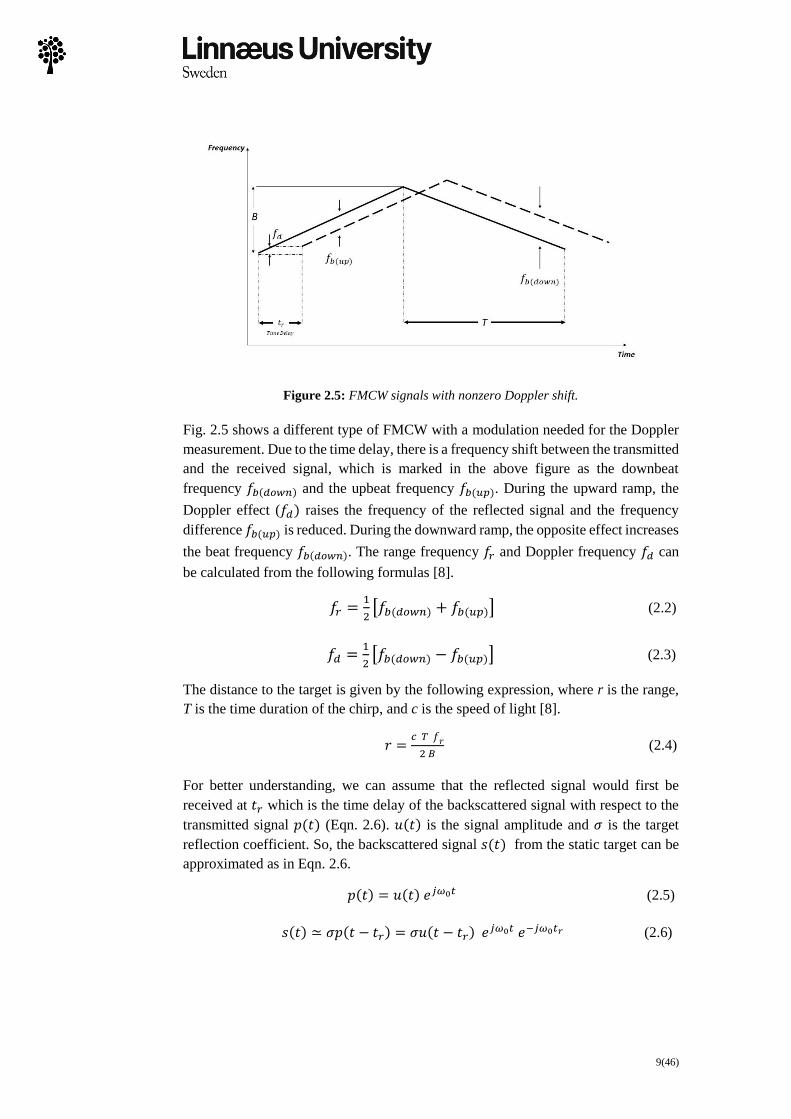
Figure 3.11: Poles and zeros of the Butterworth filter in which (a) is second-

order,(b) is forth order, and (c) is sixth-order Butterworth filter.

The phase responses for each filter are shown in Fig. 3.12. It is clear that the phase is

almost linear up to the filter cutoff frequency 𝜔𝑐 after which the linearity disappears.

This means that above 𝜔𝑐 the frequency components of the received signal are not

shifted by the same amount. Thus, phase distortion is inevitable in Butterworth filters.

Figure 3.12: Phase response of the Butterworth filter for second, fourth, and sixth order.

Figure 3.13: Group delay of the Butterworth filter for second, fourth, and sixth

order.

27(46)

Figure 3.13 presents the group delay, which is the negative derivative of the phase

with respect to frequency (Eqn. 2.27). From this figure, we can tell by how many

samples (frames) the received signal is delayed. This allows a synchronized

subtraction of clutter from the received signal.

The frequency responses of the Butterworth filter is presented in Figure 3.14 on a

linear scale for different orders. The responses show that the filter order does not

affect cutoff frequency since all the filters have the same cutoff frequency at -3dB

(0.707). Also, by increasing the filter order, the slope at the cutoff frequency rolls off

gradually (about -6dB) for each order (Figure 4.9). First-order has 6dB, second-order

12dB, and so on. Also, the higher the order, the flatter the passband.

Figure 3.14: Frequency response of the Butterworth filter for the second, fourth,

and sixth-order in a linear scale.

Figure 3.15: The RA heat map of clutter removed signals by the Butterworth filter

in which (a) is the second-order filter,(b) is the fourth-order filter, and (c) is the

sixth-order filter.

The RA heat map of the cluttered removed signal is plotted in Figure 3.15. It is

obvious that the radar reflector at 1.5 m has less reflection than in the past, while the

industrial tools are almost gone in all three cases. The negative effect of phase

distortion is clear in the third map, where the filter order is 6. The reason is the

increase in the order of the phase distortion.

28(46)

3.5 Window-based FIR filter

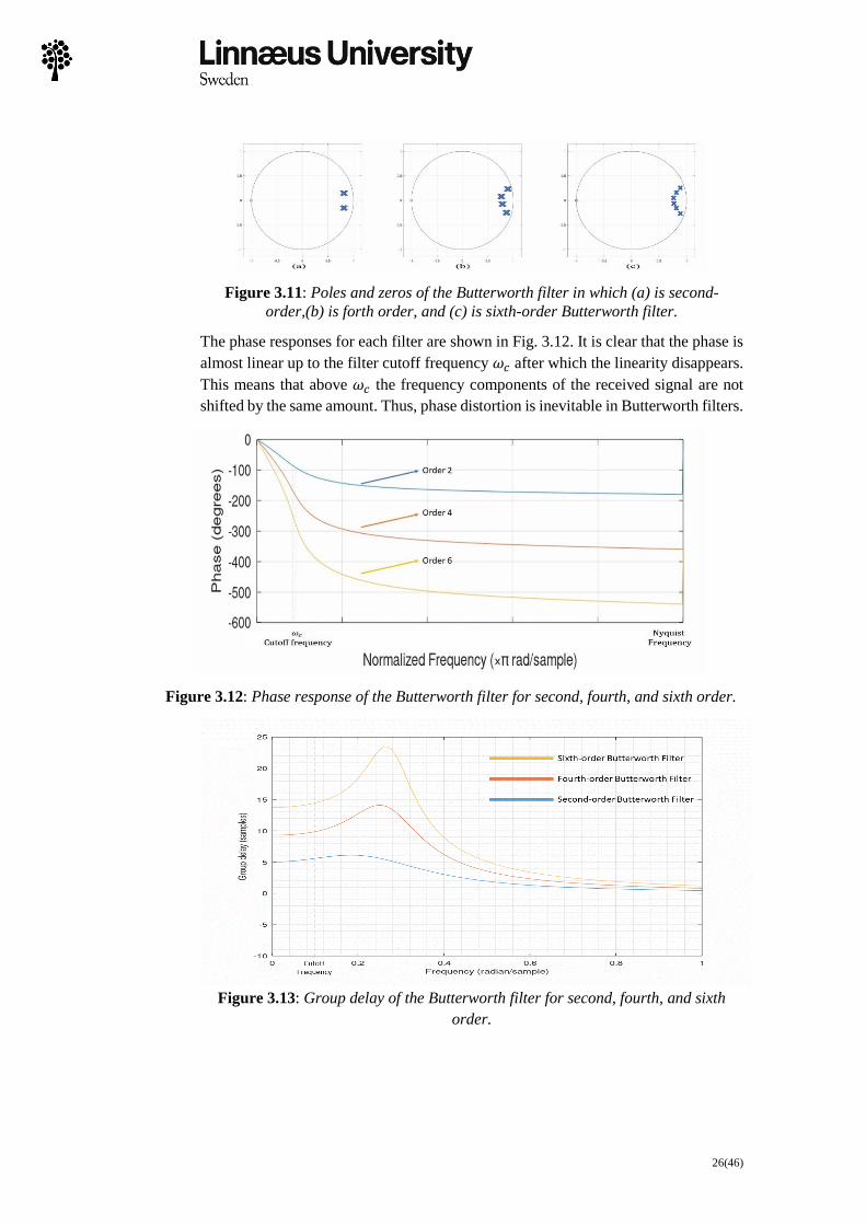
The Fourier transform of the frequency response of the desired LP filter

has the impulse response in Fig 3.16.wThe desired LP filter has zero output for all

frequencies above cutoff. This means that no frequency components from the none-

clutter part of the received signal should be captured by the LP filter. The passband

should be perfectly flat with an abrupt transition to the stopband and capture all clutter

frequencies from the received signal. These properties prevent clutter leakages into

the clutter removed signal after the subtraction (Eqn. 3.9). However, the inverse

Fourier transform gives an impulse response in the form of a sinc function that decays

slowly [24]:

ℎ[𝑗] =sin (2𝜋𝑓𝑐 𝑗)

𝜋𝑗 (3.13)

Figure 3.16: Impulse and frequency response of an ideal filter.

Figure 3.16 shows the slow decay of the impulse response [24]. This can be handled

with windows so as to obtain an impulse response filter with zero output outside the

window. So, the modified impulse response can be expressed as:

ℎ𝑤[𝑗] = 𝑤[𝑗] ℎ[𝑗] (3.14)

Window functions have a length given by a finite integer, so they are time-limited.

Thus, linear FIR filters can be designed by convolving the Discrete-Time Fourier

Transform (DTFT) of the window with the DTFT of the desired frequency response

in the frequency domain. The frequency response of the windowed sinc function is

shown in Eqn. (3.15) [25].

𝐻𝑤 = 𝑊(𝑓) ∗ 𝐻(𝑓) (3.15)

Different windows can be used but we have chosen the common Hamming window.

The transfer function is a raised cosine that is strictly positive [25].

29(46)

The Hamming window uses M+1 samples where M is an even number. The larger

the M, the sharper the roll-off, but this may result in undesired ripples in the passband.

So, choosing the filter order is a trade-off. The Hamming window is described by

[24]:

𝑊[𝑗] = 0.54 + 0.46cos (2𝜋𝑗/𝑀) (3.16)

Contrary to other filters, the cutoff frequency of the window-based FIR filter is at the

half amplitude point, or 6 dB down from the passband value. The reason is that the

Hamming window has a symmetrical passband and stopband in the frequency

response. This means that the ripple in the passband is equal to the ripple in stopband

attenuation (figures 3.18 and 3.19) [24].

Figure 3.17: Poles and zeros of the window-based FIR filter (Hamming Window).

3.5.1 Clutter removal by Window-based FIR filter

Among different windows, the Hamming window was used for the LP filter. The

clutter signal in Eqn. 3.17 has ℎ𝑤(𝑗) as the filter coefficients or the impulse response,

M as the filter order, and M+1 as the window length.

The clutter removed signal can be calculated by subtracting the clutter signal from the

received signal, as explained by Eqn. 3.7.

𝑥𝐶𝑙𝑢𝑡𝑡𝑒𝑟(𝑡) = ∑ ℎ𝑤(𝑗) 𝑥𝑆𝑖𝑔𝑛𝑎𝑙(𝑡 − 𝑗)𝑀𝑗=0 (3.17)

In FIR filters like moving average or window-based filters, the number of poles and

zeros are equal. All the poles are located at zero in the z-plane. The number of zeros,

however, is equal to filter length or the length of the window. For this application, we

used two Hamming windows with length M+1 equal to 44 and 20 taps, respectively.

Consequently, there are 44 zeros for the 44-tap filter (Fig. 3.17).

The phase response of this filter is linear, not only up to the cutoff frequency (the

Butterworth filter) but also up to the Nyquist frequency, like all FIR filters. The time

delay here, like all linear phase response filters, is equal to the group delay in Eqn.

2.28, which for these window-based filters is 22 or 10. Also, the number of zeros in

the frequency response corresponds to the change in phase around 180°.

30(46)

Figure 3.18: Frequency and phase response of the 44-tap window-based FIR filter

(Hamming Window).

The filter requirements and the frequency response of the 44-tap Hamming window

filter are plotted in Fig. 3.19. The defined clutter must be included in the filter

passband. Therefore, we called it a prohibited area. It means that all frequency

components in the prohibited area need to be captured by the LP filter in order to have

a clutter signal. The RA heat map after clutter removal is plotted in Figure (3.20). The

industrial tools are almost removed in the range of 2.5 m, and the radar reflector in

the range of 1.5 m has a reduced reflection.

Figure 3.19: Frequency response of the 44-tap window-based FIR filter (Hamming

Window) in a linear scale.

31(46)

Figure 3.20: The RA heat map of the 44-tap window-based FIR filter (Hamming

Window).

32(46)

Chapter 4

4 Results The main goal of this study is to remove clutter. This is most easily done in the

frequency domain and by focusing on the clutter part of the received signal. In order

to obtain measurable results, the comparison of the filters must be made in a suitable

way. As we have said earlier, each pixel in an RA heat map refers to information from

three dimensions, range, angle, and time (sequence of frames). If one employs FFT

to the third dimension (sequence of frames) to each pixel, the received signal can be

presented in the frequency domain for each pixel (Figure 4.1).

Figure 4.1: FFT for a chosen pixel of the received signal (before removing clutter).

Stationary and slow-moving objects would then appear at low frequencies, and

moving objects would appear at high frequencies. So, by applying this FFT over a

sequence of frames of the clutter removed signal, we should not see strong LF signals

because they are supposed to be captured by the LP filter and subtracted from the

received signal. This low-frequency part is the exact information needed to measure

the performance of each filter. It can be compared with the FFT of the same pixel

before removing clutter, and this would show how much clutter has been removed.

Consequently, if we apply FFT to all pixels of both the received and the clutter

removed signals (Eq. 4.1), we can see all frequency components of the signal before

and after the filter (clutter removal) in each pixel over the sequence of frames.

𝑌(𝜔)𝐶𝑙𝑢𝑡𝑡𝑒𝑟 𝑟𝑒𝑚𝑜𝑣𝑒𝑑 = 𝑋(𝜔)𝑆𝑖𝑔𝑛𝑎𝑙 − 𝑋(𝜔)𝐶𝑙𝑢𝑡𝑡𝑒𝑟 (4.1)

33(46)

As stated before, only low frequency components are of interest as a clutter signal.

To compare clutter with clutter, we should precisely determinewthe frequency range

of the clutter in the reflected signal.

Figure 4.2: The weight function compared to the frequency responses of the filters.

Since the ability to extract clutter varies with the filter type, the output differs

accordingly. Hence, we need to weight both clutter signals and the received signal

with a weight function. In other words, to focus on clutter removal rather than random

fluctuations, we apply low-frequency weighting to the recorded signal (received

signal) to construct a relevant calibration signal. We use a modified hyperbolic

tangent (Eq. 4.1) as a weight function (Fig. 4.2) where 𝑎 and 𝑏 define the slope and

scale.

𝑥(𝑡)𝑤𝑒𝑖𝑔ℎ𝑡 = 𝑡𝑎𝑛ℎ((𝑡+𝑎)/𝑏)+1

2 (4.1)

By applying the weight function to both the received and the clutter signals, they

would be weighted for each pixel as follows:

𝑋(𝜔)𝑤𝑒𝑖𝑔ℎ𝑡𝑒𝑑−𝑟𝑒𝑐𝑖𝑒𝑣𝑒𝑑 𝑠𝑖𝑔𝑛𝑎𝑙 = 𝑥(𝜔)𝑤𝑒𝑖𝑔ℎ𝑡 𝑋(𝜔)𝑆𝑖𝑔𝑛𝑎𝑙 (4.2)

And:

𝑋(𝜔)𝑤𝑒𝑖𝑔ℎ𝑡𝑒𝑑−𝑐𝑙𝑢𝑡𝑡𝑒𝑟 𝑠𝑖𝑔𝑛𝑎𝑙 = 𝑥(𝜔)𝑤𝑒𝑖𝑔ℎ𝑡 𝑋(𝜔)𝑐𝑙𝑢𝑡𝑡𝑒𝑟 (4.3)

According to the convolution theorem, this product then corresponds to a convolution

in the time domain. By this procedure, the clutter part of the signal can be extracted.

Moreover, by applying the weight function to the clutter removed signal, we can

capture the residual clutter for each method in question. In this way, the clutter

removal methods can be checked by comparing the captured signals and the reference.

34(46)

Figure 4.3: Captured clutter from the received signal for a chosen pixel.

Figure 4.4: Histogram of captured clutter from the received signal.

The captured clutter from the received signal, which shows only the clutter part in the

frequency domain for a given pixel, is plotted in Fig. 4.3.

Now that both clutter signals and the received signal are weighted, we can measure

the reduction of clutter in each pixel and show the clutter in a histogram. This

presentation of continuous numerical data gives an estimate of the probability density.

Accordingly, each pixel shows how much clutter there is, which can be compared to

the captured clutter from the received signal. Fig 4.4 is a histogram of the captured

clutter from the received signal and shows the distribution of clutter with respect to

the magnitude.

35(46)

Figure 4.5: Frequency response of two types of moving average filters in dB.

4.1 Moving average results

As discussed before, we have applied two kinds of moving average filters to see which

one is better. The frequency responses of these two are presented in Figure 4.5 in a

dB scale.

Figure 4.6 shows which removal method is better and compares the amount of clutter

after filtering with the captured clutter from the received signal.

Figure 4.6: Histogram of captured clutter by moving average methods

(presented for 20 bins).

In Fig 4.6, clutter removal is presented for 3 methods. For transparency, Fig. 4.7

shows the bars for 3 methods next to each other and with respect to the magnitude

and the number of pixels involved.

36(46)

Figure 4.7: Histogram of captured clutter by moving average filters (presented for

20 bins).

4.2 Butterworths results

As stated in the previous chapter, we have compared three Butterworth filters with

orders ranging from 2 to 6 as shown in Fig. 4.8.

Figure 4.8: Frequency response of three Butterworth filters in dB.

All three filters have the same cutoff frequency, but the different transient bands and

phase responses resulted in different outputs. The behavior for each order is presented

in the following histograms.

In Fig. 4.9, clutter reduction is not easily compared since it is small, but it is strong

enough to be compared to the captured clutter from the received signal.

37(46)

For comparison, we can show each bar of this plot with respect to the magnitude and

number of pixels (Figure 4.10).

Figure 4.9: Histogram of captured clutter by Butterworth filters (presented for 20

bins).

Figure 4.10: Histogram of captured clutter by Butterworth filters (presented for 10

bins).

4.3 Window-based FIR filter (Hamming)

To see the effect of window length on the efficiency of the window-based FIR filters,

we used a Hamming window with two different lengths, 44 taps, and 20 taps, but with

the same cutoff frequency. The two responses are shown in Fig. 4.11.

38(46)

In Figure 4.12, the histogram of the clutter captured by the Hamming windows is

presented. This is a comparison of captured clutter before and after clutter removal

that shows thewreduction in clutter magnitude.

Figure 4.11: Frequency responses of the window-based filters with different

lengths.

Figure 4.12: Histogram of captured clutter by the window-based filter and different

lengths (presented for 20 bins).

Figure 4.12 shows that the amount of clutter reduction is not easily compared.

Because the difference in magnitude is small but large enough for comparing with the

captured clutter from the received signal. Again, the bars can be shown next to each

other with respect to the magnitude and number of involved pixels (Figure 4.13).

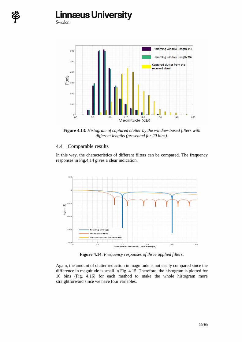
39(46)

Figure 4.13: Histogram of captured clutter by the window-based filters with

different lengths (presented for 20 bins).

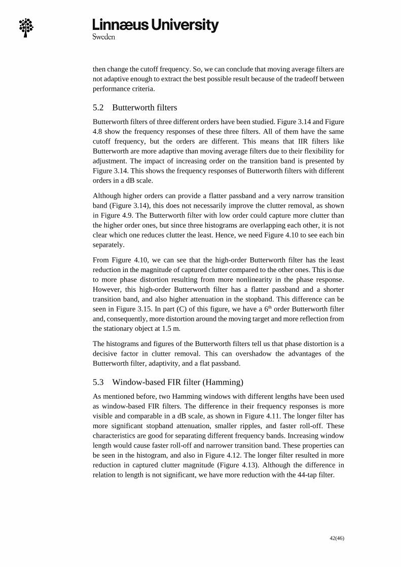
4.4 Comparable results

In this way, the characteristics of different filters can be compared. The frequency

responses in Fig.4.14 gives a clear indication.

Figure 4.14: Frequency responses of three applied filters.

Again, the amount of clutter reduction in magnitude is not easily compared since the

difference in magnitude is small in Fig. 4.15. Therefore, the histogram is plotted for

10 bins (Fig. 4.16) for each method to make the whole histogram more

straightforward since we have four variables.

40(46)

Figure 4.15: Histogram of clutter captured of the filters (presented for 20 bins).

Figure 4.16: Histogram of clutter captured of the filters (presented for 10 bins).

Table 1: Magnitude range of captured clutter for each method in dB.

Column1 1 2 3 4 5 6 7 8 9 10 Average Width

Moving average

83 87 92 97 101 106 111 115 120 124 104 41

Butterworth 84 88 93 98 103 107 112 117 122 127 105 43

Hamming 86 90 95 100 104 109 114 118 123 127 107 42

Clutter before being

removed 95 101 106 112 117 123 128 133 139 144 120 49

If we divide the horizontal axis in Fig. 4.16 into ten sections (bins) and show the

magnitude of each bin for each filter, as in Table 1, the reductions in the magnitude

of the captured clutter can be presented more accurately.

41(46)

Chapter 5

5 Discussion and conclusion

5.1 Moving average filters

By looking at the frequency responses of the two moving average filters (Figure 4.5),

we find that the multiple-pass moving average filter has a flat passband but a rather

slow roll-off. The roll-off is not sharp enough to make a strong frequency separation.

The wider the transition band, the worse the frequency separation will be. The

stopband, however, is almost flat without considerable ripples (Figure 3.9).

Conversely, the moving average filter with a length of 10 taps, has not as good a

stopband attenuation as the multiple-pass moving average filter, due to bigger ripples

in the stopband. These ripples could cause moving target frequency to leak into the

clutter signal, resulting in poor performance of the filter. Due to the large ripples in

the stopband, we would not have a proper estimation of the clutter, since it is supposed

to be subtracted from the received signal. Thus, there is still some clutter remaining

in the clutter removed signal.

The performance of the moving average filters varies with respect to the amount of

sidelobes suppression resulting from multiple-pass filtering. Figures 4.6 and 4.7 show

that the distribution of captured clutter in the clutter removed signal is different from

that of the received signal. This is especially clear for the moving average filter with

a length of 10 taps. This means that in the received signal, the clutter is distributed

over a broader band of magnitude ranging from 95 to 144 dB (Table 1). Whereas,

after clutter removal, the captured clutter is distributed from 80 to 130 dB for both

kinds of moving average filters. This shows that the residual clutter is compressed

into a narrower magnitude range.

Figures 4.6 and 4.7 show that the moving average filter with 10 taps removes more

clutter than the multiple-pass moving average filter. This is due to its faster roll-off

and narrower transition band. In the stopband of the multi-pass moving average,

however, the attenuation is much more significant. To obtain a faster roll-off and a

shorter transition band, we should increase the length of the window, but this would

42(46)

then change the cutoff frequency. So, we can conclude that moving average filters are

not adaptive enough to extract the best possible result because of the tradeoff between

performance criteria.

5.2 Butterworth filters

Butterworth filters of three different orders have been studied. Figure 3.14 and Figure

4.8 show the frequency responses of these three filters. All of them have the same

cutoff frequency, but the orders are different. This means that IIR filters like

Butterworth are more adaptive than moving average filters due to their flexibility for

adjustment. The impact of increasing order on the transition band is presented by

Figure 3.14. This shows the frequency responses of Butterworth filters with different

orders in a dB scale.

Although higher orders can provide a flatter passband and a very narrow transition

band (Figure 3.14), this does not necessarily improve the clutter removal, as shown

in Figure 4.9. The Butterworth filter with low order could capture more clutter than

the higher order ones, but since three histograms are overlapping each other, it is not

clear which one reduces clutter the least. Hence, we need Figure 4.10 to see each bin

separately.

From Figure 4.10, we can see that the high-order Butterworth filter has the least

reduction in the magnitude of captured clutter compared to the other ones. This is due

to more phase distortion resulting from more nonlinearity in the phase response.

However, this high-order Butterworth filter has a flatter passband and a shorter

transition band, and also higher attenuation in the stopband. This difference can be

seen in Figure 3.15. In part (C) of this figure, we have a 6th order Butterworth filter

and, consequently, more distortion around the moving target and more reflection from

the stationary object at 1.5 m.

The histograms and figures of the Butterworth filters tell us that phase distortion is a

decisive factor in clutter removal. This can overshadow the advantages of the

Butterworth filter, adaptivity, and a flat passband.

5.3 Window-based FIR filter (Hamming)

As mentioned before, two Hamming windows with different lengths have been used

as window-based FIR filters. The difference in their frequency responses is more

visible and comparable in a dB scale, as shown in Figure 4.11. The longer filter has

more significant stopband attenuation, smaller ripples, and faster roll-off. These

characteristics are good for separating different frequency bands. Increasing window

length would cause faster roll-off and narrower transition band. These properties can

be seen in the histogram, and also in Figure 4.12. Thewlonger filter resulted in more

reduction in captured clutter magnitude (Figure 4.13). Although the difference in

relation to length is not significant, we have more reduction with the 44-tap filter.

43(46)

Moreover, the clutter captured by the 44-tap Hamming window (86 to 127 dB) is

compressed, compared to the captured clutter of the received signal. It is also less

compressed than clutter captured by the moving average filter and narrower than

clutter captured by the second-order Butterworth filter (84 to 127 dB).

To compare filters, we should choose one filter of each type. The moving average

filter with a length of 10 taps captured more clutter than the multi-pass moving

average filter. The Butterworth filter with the lowest order is better than the longer

ones. Finally, the Hamming window with a length of 44 taps could remove more

clutter.

By looking at the frequency responses (Figure 4.14), we see that the Hamming

window has the fastest roll-off, the narrowest transition band, and the biggest

stopband attenuation. Therefore, the best result would be expected from this filter.

Notwithstanding these advantages, the magnitude at the cutoff frequency for this filter

is lower than the others (-6dB). Because of this behavior, the filter does not outdo all

other filters for a given cutoff frequency. To be more precise, we can look at Figure

4.15 and Table 1, which shows magnitude reduction more accurately. The Hamming

window has the least reduction, and the moving average filter has the most reduction

of the clutter magnitude. This result was predictable due to the short transition band

of the moving average filter compared to Butterworth and Hamming window.

Moreover, Figure 4.16 shows the distribution of the captured clutter for each method

of removal. Clutter captured by the moving average filter is more compressed

compared to the clutter captured by Butterworth and Hamming window.

Table 1 also confirms that the largest reduction of clutter has been achieved with the

moving average filter, and the clutter captured by this filter has the highest

compression compared to the Hamming window. Butterworth also has the widest

distribution of the captured clutter due to its phase distortion. This means that phase

distortion caused smearing out into neighboring pixels.

44(46)

6 References

[1] Briggs, J. N. (2002). Specifications for reflectors and radar target enhancers to

aid detection of small marine radar targets. The Journal of Navigation, Vol. 55, pp.

23-38.

[2] Sethi, S. (2014). Optimization of Digital Signal Processing Techniques for

Surveillance RADAR, Vol. 4, Number 1, pp. 43-49.

[3] Rane, S. A., Gaurav, A., Sarkar, S., Clement, J. C., & Sardana, H. K. (2016, May).

“Clutter suppression techniques to detect behind the wall static human using UWB

radar.” In 2016 IEEE International Conference on Recent Trends in Electronics,

Information & Communication Technology (RTEICT) (pp. 1325-1329). IEEE.

[4] Goncharenko, Y. V., Farquharson, G., Gorobets, V., Gutnik, V., & Tsarin, Y.

(2014). “Adaptive moving target indication in a windblown clutter environment.”

IEEE Transactions on Aerospace and Electronic Systems, 50(4), 2989-2997.

[5] Hozhabri, M. (2019). “Human Detection and Tracking with UWB radar”

(Doctoral dissertation, Mälardalen University).

[6] Chernogor, L. F., & Lazorenko, O. V. (2012, September). “Radar equation for

ultra-wideband signals”. In 2012 6th International Conference on Ultrawideband and

Ultrashort Impulse Signals (pp. 34-38). IEEE.

[7] Immoreev, I. I., & Fedotov, P. D. V. (2002, May). “Ultra-wideband radar systems:

advantages and disadvantages”. In 2002 IEEE Conference on Ultra-Wideband

Systems and Technologies (pp. 201-205).

[8] Chen, W. (2004). The Electrical Engineering Handbook (1st ed.). Saint Louis:

Elsevier Science & Technology.

[9] Sandström, S. E. (2020). “Implementation of FMCW radar at low frequencies.”

AEUE-International Journal of Electronics and Communications, 117, 153082.

[10] Sandström, S. E., & Akeab, I. K. (2016). “A study of some FMCW radar

algorithms for target location at low frequencies”. Radio Science, 51(10), 1676-1685.

[11] Zhang, Q., Luo, Y., & Chen, Y. A. (2016). Micro-Doppler Characteristics of

Radar Targets (pp. 3-4). Kidlington, United Kingdom: Butterworth-Heinemann.

[12] Texas Instruments. (2020). IWR6843, IWR6443 Single-Chip 60- to 64-GHz

mmWave Sensor datasheet (Rev. C) [Online datasheet]. Retrieved July 23, 2020, from

https://www.ti.com/document-viewer/IWR6843/datasheet/device-overview-

x3342#x3342.

[13] Gao, X., Xing, G., Roy, S., & Liu, H. (2019, November). “Experiments with

mmWave Automotive Radar Test-bed.” In 2019 53rd Asilomar Conference on

Signals, Systems, and Computers (pp. 1-6). IEEE.

[14] Rao, S. (2017). “Introduction to mmWave sensing: FMCW radars.” Texas

Instruments (TI) mmWave Training Series.

45(46)

[15] Guerrero-Menéndez, E. (2018). “Frequency-modulated continuous-wave radar

in automotive applications [Master’s thesis]”. Autonomous University of Barcelona.

[16] Zhang, X., Lu, S., Sun, J., & Shangguan, W. (2018). “Low-Altitude and Slow-

Speed Small Target Detection Based on Spectrum Zoom Processing.” Mathematical

Problems in Engineering (pp. 1-10), 2018, 4146212.

[17] Smith, S. W. (1997). Chap.15 Introduction to Digital Filters. The scientist and

engineer's guide to digital signal processing (pp. 261-276). California Technical

Publishing.

[18] Cheong, H. W. (2005). Generalized impedance converter (GIC) filter utilizing

composite amplifier. Naval Postgraduate Sschool Monterey CA.

[19] Katole, D. N., Daigavane, M. B., Gawande, S. P., & Daigavane, P. M. (2017).

“Modified single phase SRF dq theory based controller for DVR mitigating voltage

sag in case of nonlinear load.” Journal of Electromagnetic Analysis and Applications,

9(2), 22-33.

[20] Smith, S.W. (2020). Chap.15 Moving average filter. The Scientist and Engineer's

Guide to Digital Signal Processing (pp. 277-284). California Technical Publishing.

[21] Viswanathan, M. (2020, July 23). Understand Moving Average Filter with

Python & Matlab. Retrieved July 25, 2020, from

https://www.gaussianwaves.com/2010/11/moving-average-filter-ma-filter-2/

[22] Smith, J. O. (2007). Mathematics of the discrete Fourier transform (DFT): with

audio applications, 2nd Edition, Stanford, W3K Publishing.

[23] Thompson, M. T. (2014). Chapter 14 - Analog Low-Pass Filters. Intuitive analog

circuit design. In (Second ed., pp. 531-583). Elsevier.

[24] Smith, S.W.. (2020). Chap.16 Windowed-Sinc Filters. The Scientist and

Engineer's Guide to Digital Signal Processing (pp. 284-297). California Technical

Publishing.

[25] Smith III, J. O. (2011). Spectral audio signal processing. Stanford,W3K

publishing.

[26] Alam, S. A., & Gustafsson, O. (2011, November). “Implementation of narrow-

band frequency-response masking for efficient narrow transition band FIR filters on

FPGAs.” In 2011 NORCHIP (pp. 1-4). IEEE.

[27] Freeman, M. G. (2016). “Target Discrimination Against Clutter Based on

Unsupervised Clustering and Sequential Monte Carlo Tracking”. Arizona State

University.

[28] Le Chevalier, F., Krasnov, O., Deudon, F., & Bidon, S. (2011). “Clutter

suppression for moving targets detection with wideband radar”. In 2011 19th

European Signal Processing Conference (pp. 427-430). IEEE.

46(46)

[29] Leighton, T. G., Chua, G. H., White, P. R., Tong, K. F., Griffiths, H. D., &

Daniels, D. J. (2013). “Radar clutter suppression and target discrimination using twin

inverted pulses.” Proceedings of the Royal Society A: Mathematical, Physical and

Engineering Sciences, Vol.469, No. 2160.

[30] Matsunami, I., & Kajiwara, A. (2010, January). “Clutter suppression scheme for

vehicle radar”. In 2010 IEEE Radio and Wireless Symposium (RWS) (pp. 320-323).

IEEE.

[31] Rummler, W. D. (1966). Clutter suppression by the complex weighting of

coherent pulse trains. IEEE Transactions on Aerospace and Electronic Systems, Vol.

AES-2, pp. 689-699.

[32] Lin, J. J., Li, Y. P., Hsu, W. C., & Lee, T. S. (2016). “Design of an FMCW radar

baseband signal processing system for automotive application.” SpringerPlus, Vol.5.

[33] Kim, S. H., Geem, Z. W., & Han, G. T. (2019). “A Novel Human Respiration

Pattern Recognition Using Signals of Ultra-Wideband Radar Sensor.” Sensors,

19(15), 3340.

[34] Dowell III, A. M. (1998). “Layer of protection analysis for determining safety

integrity level.” ISA Transactions, 37(3), 155-165.

[35] Koks, D. (2014). How to create and manipulate radar range-Doppler plots.

Defence Science and Technology Organization Edinburgh (Australia), Cyber and

Electronic Warfare Div.

[36] Dipl.-Ing. (FH) Christian Wolff, SMSgt G.A.F. (Rtd.). "Radar Basics".

radartutorial.eu. Retrieved 14 April 2018.