IEEE TRANSACTIONS ON PATTERN ANALYSIS AND MACHINE INTELLIGENCE 1

Salient Objects in ClutterDeng-Ping Fan, Jing Zhang, Gang Xu, Ming-Ming Cheng, and Ling Shao, Fellow, IEEE

Abstract—In this paper, we identify and address a serious design bias of existing salient object detection (SOD) datasets, whichunrealistically assume that each image should contain at least one clear and uncluttered salient object. This design bias has led to asaturation in performance for state-of-the-art SOD models when evaluated on existing datasets. However, these models are still farfrom satisfactory when applied to real-world scenes. Based on our analyses, we propose a new high-quality dataset and update theprevious saliency benchmark. Specifically, our dataset, called Salient Objects in Clutter (SOC), includes images with both salient andnon-salient objects from several common object categories. In addition to object category annotations, each salient image is accompaniedby attributes that reflect common challenges in real-world scenes, which can help provide deeper insight into the SOD problem. Further,with a given saliency encoder, e.g., the backbone network, existing saliency models are designed to achieve mapping from the trainingimage set to the training ground-truth set. We therefore argue that improving the dataset can yield higher performance gains than focusingonly on the decoder design. With this in mind, we investigate several dataset-enhancement strategies, including label smoothing toimplicitly emphasize salient boundaries, random image augmentation to adapt saliency models to various scenarios, and self-supervisedlearning as a regularization strategy to learn from small datasets. Our extensive results demonstrate the effectiveness of these tricks. Wealso provide a comprehensive benchmark for SOD, which can be found in our repository: http://dpfan.net/SOCBenchmark.

Index Terms—Salient object detection, SOD, SOC, survey, dataset, benchmark.

F

1 INTRODUCTION

THIS paper considers the task of salient object detection(SOD), which aims to detect the most attention-grabbing

objects in a scene and then extract pixel-accurate silhouettes forthem. The merit of SOD lies in its many applications, includingforeground map evaluation [2], [3], [4], visual tracking [5], [6],[7], action recognition [8], image retrieval [9], [10], informationdiscovery [11], [12], image contrast enhancement [13], personre-identification [14] image segmentation [15], [16], video segmen-tation [17], photo synthesis [18], content-aware image editing [19],image caption [20], and video compression [21], [22], styletransfer [23], [24], image matching [25], autonomous underwaterrobots [26], camouflaged object detection [27], aesthetic scor-ing [28], self-driving vehicles [29], plant species identification [30],VR/AR [31]1, Sony’s BRAVIA XR TV2, etc. However, existingSOD datasets [32], [33], [34], [35], [36], [37], [38], [39], [40],[41], [42] are flawed either in their data collection procedure ordata quality. Specifically, most datasets assume that an imageshould contain at least one salient object, and thus they discardimages that do not contain any salient objects. We call this DATASELECTION BIAS [43].

Moreover, existing datasets typically contain images with asingle object or several uncluttered objects. These datasets do notadequately reflect the complexity of real-world images, wherescenes usually contain multiple objects amidst significant clutter.As a result, all top-performing models trained on the existing large-

• Deng-Ping Fan, Gang Xu and Ming-Ming Cheng are with theCS, Nankai University, Tianjin, China. (E-mail: dengpfan@gmail.com;gangxu@mail.nankai.edu.cn; cmm@nankai.edu.cn)

• Jing Zhang is with Research School of Engineering, the Australian NationalUniversity, ACRV, DATA61-CSIRO. (Email: zjnwpu@gmail.com)

• Ling Shao is with the Inception Institute of Artificial Intelligence, AbuDhabi, UAE. (E-mail: ling.shao@inceptioniai.org)

• A preliminary version of this work appeared in ECCV [1].• The major part of this work was done in Nankai University.• Ming-Ming Cheng is the corresponding author.

1. AR CUT & PASTE: https://www.youtube.com/watch?v=-N-podTAY9Y.2. https://www.youtube.com/watch?v=4LnCuTAlVno&feature=youtu.be.

non-salientnon-salientnon-salientnon-salientnon-salientnon-salientnon-salientnon-salientnon-salientnon-salientnon-salientnon-salientnon-salientnon-salientnon-salientnon-salientnon-salient non-salientnon-salientnon-salientnon-salientnon-salientnon-salientnon-salientnon-salientnon-salientnon-salientnon-salientnon-salientnon-salientnon-salientnon-salientnon-salientnon-salient non-salientnon-salientnon-salientnon-salientnon-salientnon-salientnon-salientnon-salientnon-salientnon-salientnon-salientnon-salientnon-salientnon-salientnon-salientnon-salientnon-salient non-salientnon-salientnon-salientnon-salientnon-salientnon-salientnon-salientnon-salientnon-salientnon-salientnon-salientnon-salientnon-salientnon-salientnon-salientnon-salientnon-salient

carrotcarrotcarrotcarrotcarrotcarrotcarrotcarrotcarrotcarrotcarrotcarrotcarrotcarrotcarrotcarrotcarrot

Attr:HO,OC,SC,SOAttr:HO,OC,SC,SOAttr:HO,OC,SC,SOAttr:HO,OC,SC,SOAttr:HO,OC,SC,SOAttr:HO,OC,SC,SOAttr:HO,OC,SC,SOAttr:HO,OC,SC,SOAttr:HO,OC,SC,SOAttr:HO,OC,SC,SOAttr:HO,OC,SC,SOAttr:HO,OC,SC,SOAttr:HO,OC,SC,SOAttr:HO,OC,SC,SOAttr:HO,OC,SC,SOAttr:HO,OC,SC,SOAttr:HO,OC,SC,SO

dogdogdogdogdogdogdogdogdogdogdogdogdogdogdogdogdog

Attr:HO,OC,SC,SOAttr:HO,OC,SC,SOAttr:HO,OC,SC,SOAttr:HO,OC,SC,SOAttr:HO,OC,SC,SOAttr:HO,OC,SC,SOAttr:HO,OC,SC,SOAttr:HO,OC,SC,SOAttr:HO,OC,SC,SOAttr:HO,OC,SC,SOAttr:HO,OC,SC,SOAttr:HO,OC,SC,SOAttr:HO,OC,SC,SOAttr:HO,OC,SC,SOAttr:HO,OC,SC,SOAttr:HO,OC,SC,SOAttr:HO,OC,SC,SO

motorcyclemotorcyclemotorcyclemotorcyclemotorcyclemotorcyclemotorcyclemotorcyclemotorcyclemotorcyclemotorcyclemotorcyclemotorcyclemotorcyclemotorcyclemotorcyclemotorcycle

Attr:HO,SCAttr:HO,SCAttr:HO,SCAttr:HO,SCAttr:HO,SCAttr:HO,SCAttr:HO,SCAttr:HO,SCAttr:HO,SCAttr:HO,SCAttr:HO,SCAttr:HO,SCAttr:HO,SCAttr:HO,SCAttr:HO,SCAttr:HO,SCAttr:HO,SC

toilettoilettoilettoilettoilettoilettoilettoilettoilettoilettoilettoilettoilettoilettoilettoilettoilet

Attr:HO,OC,ACAttr:HO,OC,ACAttr:HO,OC,ACAttr:HO,OC,ACAttr:HO,OC,ACAttr:HO,OC,ACAttr:HO,OC,ACAttr:HO,OC,ACAttr:HO,OC,ACAttr:HO,OC,ACAttr:HO,OC,ACAttr:HO,OC,ACAttr:HO,OC,ACAttr:HO,OC,ACAttr:HO,OC,ACAttr:HO,OC,ACAttr:HO,OC,AC

bookbookbookbookbookbookbookbookbookbookbookbookbookbookbookbookbook

bicyclebicyclebicyclebicyclebicyclebicyclebicyclebicyclebicyclebicyclebicyclebicyclebicyclebicyclebicyclebicyclebicycleAttr:OC,SCAttr:OC,SCAttr:OC,SCAttr:OC,SCAttr:OC,SCAttr:OC,SCAttr:OC,SCAttr:OC,SCAttr:OC,SCAttr:OC,SCAttr:OC,SCAttr:OC,SCAttr:OC,SCAttr:OC,SCAttr:OC,SCAttr:OC,SCAttr:OC,SC

dogdogdogdogdogdogdogdogdogdogdogdogdogdogdogdogdog personpersonpersonpersonpersonpersonpersonpersonpersonpersonpersonpersonpersonpersonpersonpersonperson

Attr:HO,OC,OV,SCAttr:HO,OC,OV,SCAttr:HO,OC,OV,SCAttr:HO,OC,OV,SCAttr:HO,OC,OV,SCAttr:HO,OC,OV,SCAttr:HO,OC,OV,SCAttr:HO,OC,OV,SCAttr:HO,OC,OV,SCAttr:HO,OC,OV,SCAttr:HO,OC,OV,SCAttr:HO,OC,OV,SCAttr:HO,OC,OV,SCAttr:HO,OC,OV,SCAttr:HO,OC,OV,SCAttr:HO,OC,OV,SCAttr:HO,OC,OV,SC

wine glasswine glasswine glasswine glasswine glasswine glasswine glasswine glasswine glasswine glasswine glasswine glasswine glasswine glasswine glasswine glasswine glasspersonpersonpersonpersonpersonpersonpersonpersonpersonpersonpersonpersonpersonpersonpersonpersonperson

Attr:OVAttr:OVAttr:OVAttr:OVAttr:OVAttr:OVAttr:OVAttr:OVAttr:OVAttr:OVAttr:OVAttr:OVAttr:OVAttr:OVAttr:OVAttr:OVAttr:OV

cell phonecell phonecell phonecell phonecell phonecell phonecell phonecell phonecell phonecell phonecell phonecell phonecell phonecell phonecell phonecell phonecell phone

bananabananabananabananabananabananabananabananabananabananabananabananabananabananabananabananabanana

Attr:HO,OC,SCAttr:HO,OC,SCAttr:HO,OC,SCAttr:HO,OC,SCAttr:HO,OC,SCAttr:HO,OC,SCAttr:HO,OC,SCAttr:HO,OC,SCAttr:HO,OC,SCAttr:HO,OC,SCAttr:HO,OC,SCAttr:HO,OC,SCAttr:HO,OC,SCAttr:HO,OC,SCAttr:HO,OC,SCAttr:HO,OC,SCAttr:HO,OC,SC

personpersonpersonpersonpersonpersonpersonpersonpersonpersonpersonpersonpersonpersonpersonpersonperson

Attr:BO,OCAttr:BO,OCAttr:BO,OCAttr:BO,OCAttr:BO,OCAttr:BO,OCAttr:BO,OCAttr:BO,OCAttr:BO,OCAttr:BO,OCAttr:BO,OCAttr:BO,OCAttr:BO,OCAttr:BO,OCAttr:BO,OCAttr:BO,OCAttr:BO,OC

giraffegiraffegiraffegiraffegiraffegiraffegiraffegiraffegiraffegiraffegiraffegiraffegiraffegiraffegiraffegiraffegiraffe

Attr:HO,OC,OVAttr:HO,OC,OVAttr:HO,OC,OVAttr:HO,OC,OVAttr:HO,OC,OVAttr:HO,OC,OVAttr:HO,OC,OVAttr:HO,OC,OVAttr:HO,OC,OVAttr:HO,OC,OVAttr:HO,OC,OVAttr:HO,OC,OVAttr:HO,OC,OVAttr:HO,OC,OVAttr:HO,OC,OVAttr:HO,OC,OVAttr:HO,OC,OV

personpersonpersonpersonpersonpersonpersonpersonpersonpersonpersonpersonpersonpersonpersonpersonperson

Attr:HO,OC,ACAttr:HO,OC,ACAttr:HO,OC,ACAttr:HO,OC,ACAttr:HO,OC,ACAttr:HO,OC,ACAttr:HO,OC,ACAttr:HO,OC,ACAttr:HO,OC,ACAttr:HO,OC,ACAttr:HO,OC,ACAttr:HO,OC,ACAttr:HO,OC,ACAttr:HO,OC,ACAttr:HO,OC,ACAttr:HO,OC,ACAttr:HO,OC,AC

umbrellaumbrellaumbrellaumbrellaumbrellaumbrellaumbrellaumbrellaumbrellaumbrellaumbrellaumbrellaumbrellaumbrellaumbrellaumbrellaumbrella

computerscomputerscomputerscomputerscomputerscomputerscomputerscomputerscomputerscomputerscomputerscomputerscomputerscomputerscomputerscomputerscomputersAttr:HOAttr:HOAttr:HOAttr:HOAttr:HOAttr:HOAttr:HOAttr:HOAttr:HOAttr:HOAttr:HOAttr:HOAttr:HOAttr:HOAttr:HOAttr:HOAttr:HO

laptoplaptoplaptoplaptoplaptoplaptoplaptoplaptoplaptoplaptoplaptoplaptoplaptoplaptoplaptoplaptoplaptopkeyboardkeyboardkeyboardkeyboardkeyboardkeyboardkeyboardkeyboardkeyboardkeyboardkeyboardkeyboardkeyboardkeyboardkeyboardkeyboardkeyboard

Figure 1. Examples from our new SOC dataset, including non-salient (firstrow) and salient object images (rows 2 to 4). For salient object images,an instance-level ground-truth map (different color), object attributes (Attr)and category labels are provided.

scale datasets (e.g., DUTS [41]) have nearly saturated performance(e.g., SCRN [44] has an S-measure > 0.9 on ECSSD [37]), but stillachieve unsatisfactory results on realistic images (e.g., S-measure<0.8 on SOC [1]). As the current SOD models are biased towardsideal conditions, their effectiveness may be impaired once they areapplied to real-world scenes. To solve this problem, it is importantto introduce a dataset with more realistic conditions.

Another issue faced by the RGB SOD community is that onlythe overall performance of the models can be analyzed usingexisting datasets. This is because none of the datasets containattributes that reflect different real-world challenges. Having suchattributes would help i) provide deeper insight into the SODproblem, ii) enable the pros and cons of the SOD models to

arX

iv:2

105.

0305

3v1

[cs

.CV

] 7

May

202

1

IEEE TRANSACTIONS ON PATTERN ANALYSIS AND MACHINE INTELLIGENCE 2

360°Video

SOD

Video

SOD

Fully

SupervisedUnsupervised

Semi-

Supervised

Weakly

Supervised

Self-

Supervised

2D

Fixation

Prediction (FP) Saliency Detection

3D/4D

Salient Object Detection (SOD)

Res

olu

tio

n

Remote Sensing SOD

RGB SOD

High-Resolution SOD

RGB-T SOD

RGB-D SOD Light Field SOD

Point Cloud SOD

+ Depth, Thermal, Multi-view, Time, Audio, Group

Dep

th/T

her

mal

Mu

lti-

vie

w

Tim

e

Pan

ora

mic

Saliency Ranking (SR)

Salient Object Subitizing (SOS)

Salient Instance Detection (SID)

Extension

Co-SOD

Gro

up

Su

perv

ision

level

Extension

Figure 2. Taxonomy of the saliency detection task. We highlight the scope of this study in gray. See § 2 for details.

be investigated, and iii) allow the model performances to beobjectively assessed from different perspectives. Finally, witha given saliency encoder, e.g., the backbone network, existingsaliency models are designed to achieve mapping from the trainingimage set to the training ground-truth set. We thus argue thatefforts on improving the dataset, e.g., fixing the data bias issue, canyield higher performance gains than focusing only on the decoderdesign. Towards this, we investigate several dataset-enhancementstrategies, including label smoothing to highlight salient boundaries,random image augmentation to adapt saliency models to variousscenarios, and self-supervised learning as a form of regularizationto learn from small datasets. Extensive experiments validate theeffectiveness of these tricks.

Our contributions are summarized as follows:

1) Dataset. We collect a new high-quality SOD dataset, named“Salient Objects in Clutter,” or SOC. SOC is the largestinstance-level SOD dataset to date, containing 6,000 imagesfrom more than 80 common categories. It differs from existingdatasets in three aspects: i) Salient objects have categoryannotations, which can be used for new research problems,such as weakly supervised SOD. ii) The inclusion of non-salient images and objects makes this dataset more realisticand challenging than the existing ones. iii) Salient objectshave attributes that reflect various situations encountered inthe real world, such as motion blur, occlusion and backgroundclutter. As a consequence, SOC narrows the gap betweenexisting datasets and real-world scenes.

2) Review & Benchmark. We present the largest scale RGBSOD study, reviewing 201 representative models including 84algorithms using handcrafted features and 117 deep learningbased models. Besides, we also maintain an online benchmark(i.e., http://dpfan.net/SOCBenchmark.) to dynamically tracethe development of this field. In addition, we provide the mostcomprehensive benchmark of the top-100 SOD models. Toevaluate the models, for the first time, we not only presentthe overall but also an attribute-based performance evaluation.This allows a deeper understanding of the models and providesa more complete benchmark.

3) Strategy. We investigate the biased dataset issue and introducethree dataset-enhancement strategies; namely, label smoothingto make the model aware of the salient boundaries, randomimage augmentation to adapt the saliency models to variousreal-world scenarios, and self-supervised learning as a reg-ularization technique to learn from small datasets. Despitethe apparent simplicity of our strategies, we can achieve anaverage absolute improvement of 1.1% Sα over five existingcutting-edge models.

4) Discussions & Future Directions. Based on our SOC, wepresent the pros and cons of the current SOD algorithms,discuss several under-investigated open issues, and providepotential future directions at six levels, e.g., the dataset level,task level, model level, supervision level, evaluation level, andapplication level.

This work extends our previous conference version [1] in thefollowing aspects. First, we provide more details on our SOC,including sample images without salient objects, images withattributes, and statistics of the attributes. Second, we study threenovel training dataset related strategies to fully utilize the non-salient object data and achieve the new state-of-the-art performance.Third, we conduct the largest-scale (46 traditional and 54 deeplearning models) benchmarking of SOD models on our SOC.Finally, based on our benchmarking results, we highlight severalfundamental research directions and challenges in the SOD.

2 RELATED WORK

2.1 ScopeSalient object detection originated from the task of fixationprediction (FP) [45], [46], switching attention regions for accurateobject-level regions. SOD can be traced back to the seminalworks [47], [48]. Current algorithms have been developed for 2Dimages of limited resolution (width or height < 500 pixels), high-resolution (i.e., 1080p, 4K) [49], [50] and even remote sensingdata [51]. According to the supervision strategy, there are fivetypes of SOD models: fully supervised [52], semi-supervised [53],weakly supervised [54], [55], [56], unsupervised [57], [58], [59],and self-supervised [59], [60].

IEEE TRANSACTIONS ON PATTERN ANALYSIS AND MACHINE INTELLIGENCE 3

Table 1Summary of popular SOD datasets. Our SOC is the only one meeting all requirements. According to [76], these datasets can be grouped into three

types: early (N), popular/modern (�), and special (♦). See § 2.2 for more details.

# Dataset Year Publ. High-Quality ≥ 5k Non-Salient Attribute Category Bounding Box Object Instance

1 MSRA-A, -B [32] N 2007 CVPR X X - - - X X -2 SED1, SED2 [33] N 2007 CVPR X - - - - - X -3 ASD [82] N 2009 CVPR X - - - - - X -4 SOD [83] � 2010 CVPRW X - - - - - X -5 MSRA10K [84] � 2011 CVPR X X - - - - X -6 Judd-A [36] N 2012 ECCV X - - - - - X -7 DUT-O [38] � 2013 CVPR X X - - - X X -8 ECSSD [37] � 2013 CVPR X - - - - - X -9 PASCAL-S [39] � 2014 CVPR X - - - - - X -10 HKU-IS [40] � 2015 CVPR X - - - - - X -11 SOS [63] ♦ 2015 CVPR X X - - - X - -12 MSO [63] ♦ 2015 CVPR X - - - - X - -13 XPIE [85] ♦ 2017 CVPR X X - - - - X -14 ILSO [61] ♦ 2017 CVPR - - - - - - X X15 JOT [86] ♦ 2017 FCS X X X - - - X -16 DUTS [41] � 2017 CVPR X X - - - - X -17 SOC (OUR) � 2021 X X X X X X X X

Recently, several interesting extensions of SOD have alsobeen introduced, such as salient instance detection (SID) [61],[62], salient object subitizing (SOS) [63], [64], [65], and saliencyranking [66], [67]. A taxonomy of the saliency detection task isshown in Fig. 2. Different from previous SOD reviews [68], [69],[70], [71], [72], [73], [74], [75], [76], we mainly focus on 2D salientobject detection in a fully supervised manner. We highlight thescope of this study in gray. For other closely related 3D/4D SODtasks, we refer readers to recent survey and benchmarking workssuch as RGB-D SOD [77], [78], Event-RGB SOD (ERSOD) 3,Light Field SOD [79], Co-SOD [80], 360◦Video SOD [81], andVideo SOD [17].

2.2 SOD Datasets

In this section, we briefly discuss existing datasets designed forSOD tasks, focusing in particular on aspects including annotationtype, number of salient objects per image, number of images, andimage quality. These datasets are listed in Table 1.

Early datasets are either limited in their numbers of imagesor in their coarse annotations of salient objects. For example,salient objects in the original version of MSRA-A [32] and MSRA-B [32] are only roughly annotated in the form of bounding boxes.ASD [82], SED1 [33] and MSRA10K [35] contain only one salientobject in most images, while the SED2 [33] dataset providestwo objects per image but contains only 100 images. In orderto improve the quality of datasets, researchers in recent yearshave started to collect images with multiple objects in relativelycomplex and cluttered backgrounds. The new datasets includeECSSD [37], DUT-O [38], Judd-A [36], and PASCAL-S [39].These datasets are improved in terms of both annotation qualityand number of images, compared to their predecessors. To resolvethe shortcomings still present, some datasets (e.g., HKU-IS [40],XPIE [85], and DUTS [41]) provide large amounts of pixel-wiselabeled images (Fig. 3.b) with more than one salient object perimage. However, they ignore non-salient objects (1st row in Fig. 1)and do not offer instance-level annotations (Fig. 3.c). Jiang etal. [86] collected roughly 6K simple background images (most ofthem are pure texture images) to cover non-salient scenes. However,their dataset, named JOT, falls short in capturing the complexity ofreal-world scenes. The dataset of ILSO [61] contains instance-levelsalient object annotations but only roughly labeled boundaries, asshown in Fig. 7. Beyond the “standard” SOD datasets, there are

3. ERSOD: https://github.com/jxr326/ERSOD-Net.

(a) Image (b) Previous (c) Ours (d) SegmentationFigure 3. Previous SOD datasets only annotate the images by drawingpixel-accurate silhouettes around salient objects (b). Different fromobject segmentation datasets [87] (d) where (objects are not necessarilysalient), our SOC provides salient instances (c). We provide a high-quality and large-scale annotated dataset comprised of images thatbetter capture the properties of real-world scenes.

also several other special datasets that introduce new tasks, such assalient object subitizing (i.e., SOS [63] and its subset MSO [63]).

To sum up, as discussed above, existing datasets mostly focuson images with clear salient objects and simple backgrounds.Considering the aforementioned limitations of existing datasets,a more realistic dataset, containing non-salient objects, textures“in the wild”, and salient objects with attributes, is needed forfuture investigations in this field. Such a dataset could offer deeperinsight into the strengths and weaknesses of SOD models, and helpovercome performance saturation. Our SOC is unique in that itprovides various high-quality annotations, as shown in Table 1.

2.3 SOD ModelsWe have noticed that, from 1998 to the end of Feb. 2021, morethan 10,000 papers on saliency detection or related field have beenpublished. In this section, we try our best to summarize thosepublished in top conferences (e.g., NeurIPS, CVPR, ICCV, AAAI)and journals (e.g., TPAMI, TIP, TMM), as well as some high-qualityopen-access (i.e., arXiv) works. Instead of briefly describing thepipeline of each model, we summarize key components to providea global view.

As shown in Table 2, a number of different approaches havebeen designed to tackle SOD using super-pixel, proposal, oredge/boundary annotations under different levels of supervision,such as unsupervised, semi-supervised, and fully supervised. Usingcommon aggregation strategies (e.g., linear, non-linear), thesemethods mainly focus on pixels, regions, and patches to designmore powerful models. Besides, we note that certain priors (e.g., thecenter-surround prior, local/global contrast prior, fore/backgroundprior, and boundary prior) are frequently used in these methods.Some models also utilize different post-processing steps (e.g.,conditional random field, morphology, watershed, and max-flowstrategies) to further improve the performance.

IEEE TRANSACTIONS ON PATTERN ANALYSIS AND MACHINE INTELLIGENCE 4

Table 2Summary of popular SOD models using handcrafted features. Agg.: Aggregation strategy, e.g., LN = linear, NL = non-linear, HI = hierarchical, BA =

Bayesian, AD = adaptive, LS = least-square solver, EM = energy minimization, and GMRF = Gaussian MRF. SL.: Supervision level, e.g.,unsupervised (F), semi-supervised (•), weakly supervised ($), fully supervised (◦), active learning (A). Sp.: Whether or not superpixel

over-segmentation is used. Pr.: Whether or not proposal methods are used. Ed.: Whether or not edge cues are used. Post-Pros.: Whetherpost-processing methods (e.g., CRF [88], graph-cut [89], GrabCut [90], Ncut [91]), morphology, max-flow (MF) [92] or only thresholding are used.

# Model Publ. Scholar Prior. Uniqueness Component Agg. SL. Sp. Pr. Ed. Post-Pros

2010

-19

98

1 Itti [45] TPAMI link center-surround pixel Color, Intensity, Orientation LN F - - - -2 GBVS [93] NeurIPS link - pixel Markovian - F - - - -3 FT [82] CVPR link frequency domain pixel Color, Luminance - F - - - -4 SR [94] CVPR link spectral residual pixel Log Spectrum - F - - - -5 AIM [95] NeurIPS link maximizing information patch Shannon’s Self-information - F - - - -6 SUN [96] JOV link self-information pixel DoG, ICA-derived features - F - - - -7 FG [97] MM link local contrast pixel Fuzzy Growing - F - - - -8 AC [98] ICVS link local contrast multi-patch Color, Luminance LN F - - - -9 SEG [99] ECCV link local contrast pixel Conditional Probabilistic - F - - - CRF10 MSSS [100] ICIP link symmetric surround pixel Color, Luminance - F - - - graph-cut11 ICC [101] ICCV link isophote global structure curvedness, isocenters, color LN F - - - graph-cut12 EDS [102] PR link - pixel threshold, distance, multi-DoG - F - - X -13 RE [103] ICME link local contrast pixel/patch Contrast pyramid - F - - - -14 RSA [104] MM link global contrast patch Polar transfer, NN-GPCA [104] - F - - - -15 RU [105] TMM link rule based pixel denoising, geometric - F - - - -16 CSM [106] MM link frequency&contrast pixel Envelope, Skeleton - F - - - -

2014

-20

11

17 LSSC [107] TIP link bayesian pixel/region convex hull, subspace clustering NL F X - - -18 COV [108] JOV link - pixel/patch covariance matrices NL F - - - -19 GR [109] SPL link contrast, center, smooth - convex hull, continuous pair NL F X - - -20 MSS [110] SPL link local, integrity, center - various gaussian, convex hull NL F X - - -21 LSMD [111] AAAI link texture, edge, color pixel/region hierarchical clustering, gaussian - F X X - threshold22 BSF [112] ICIP link boundary-based region convex hull, soft-segmentation - F X - - -23 HC [84] CVPR link global contrast region Histogram-based Contrast - F - - - graph-cut24 RC [84] CVPR link global contrast region Region-based Contrast - F - - - graph-cut25 CA [84] CVPR link context-aware patch Four principles - F - - - -26 MR [38] CVPR link fore/back-ground pixel/region graph-based manifold ranking - F X - - -27 SF [113] CVPR link element contrast region uniqueness, spatial NL F - - - -28 HS [37] CVPR link global contrast hi-region Region-scale, Location heuristic HI F - - - -29 DRFI [114] CVPR link background descriptor region region vector, multi-level LN ◦ X - - -30 RBD [115] CVPR link background weighted region background connectivity LS F X - - -31 LR [116] CVPR link location, semantic, color pixel/region Low rank matrix NL ◦ X - - threshold32 PCA [117] CVPR link center-bias priors patch color, pattern, gaussian NL F X - - -33 HDCT [118] CVPR link high-dimensional color pixel Trimap, color transform LN F X - - -34 CRFM [119] CVPR link aggregation pixel GIST descriptor NL ◦ - - - CRF35 STD [120] CVPR link statistical textural region Graph, sparse texture - F - - - GrabCut36 PDE [121] CVPR link representative elements region color, background, center - F X - - -37 SUB [122] CVPR link Submodular region color, spatial, center - ◦ X - - threshold38 PISA [123] CVPR link spatial pixel/region color, structure, orientation NL F - - X -39 DSR [124] ICCV link reconstruction errors multi-region background, obj./centerGaussian BA F X - - -40 MC [125] ICCV link markov random walks region Markov Chain - F X - - -41 GC [126] ICCV link global cue region GMM, appearance, spatial AD F - - - -42 SVO [127] ICCV link center-surround patch/region Graph, Obj. EM F X X - -43 CSD [128] ICCV link center-surround multi-patch color, orientation, intensity LN F - - - -44 UFO [129] ICCV link focus, objectness pixel/region Uniqueness, Focusness, Obj. NL F X X X threshold45 CHM [130] ICCV link center-surround, local mRegion/patch SVM, hyperedge LN • X - X threshold46 CIO [131] ICCV link objectness Region Graph, frequency, Obj. GMRF F X - - -47 CC [132] ICCV link convexity context mRegion concavity, bounding box - F X - - graph-cut48 GS [133] ECCV link boundary, connectivity patch/region Geodesic distance transform - F X - X -49 CB [134] BMVC link context, shape, center mRegion Iterative energy minimization LN F X X - -50 SLMR [135] BMVC link low-rank matrix Region sparse noise - F X - - -

2018

-20

15

51 SMD [136] TPAMI link texture, edge, color pixel/region hierarchical clustering, gaussian - F X X - threshold52 RS [137] TPAMI link fore/back-ground region manifold ranking, grouping cue - F X - - -53 BFS [138] NC link fore/back-ground seed region Gaussian falloff, threshold NL F X - - -54 GLC [139] PR link global/local contrast region HOG, LBP, codebook,graph-cut LN F X - - -55 DSP [140] PR link propagation region sink points, chi-square distance NL F X - X -56 LPS [141] TIP link label propagation-base pixel/region three-cue-center, affinity matrix NL F X - - -57 MAPM [142] TIP link background region Markov absorption probability F X - - -58 MIL [143] TIP link instance region multi-instance learning, SVM - • X X - -59 RCRR [144] TIP link reversion correction pixel/region regular-random walks ranking - F X - - -60 FCB [145] TIP link fore/back-ground, center region color difference, color volume NL F X - - -61 NCS [146] TIP link center bias pixel/region Ncut, merging scheme EM F X - X Ncut62 MDC [147] TIP link direction contrast pixel OTSU, morphological filter NL F - - - watershed63 HCCH [148] TIP link closure completeness & reliability object hierarchical segmentation NL F - - X -64 JLSE [149] TIP link exemplar-aided region joint latent space embedding - ◦ X - - -65 IFC [150] TMM link boundary homogeneity pixel/region linear feedback control system - F X - - -66 NIO [151] TNNLS link smoothness, boundary region graph, iterative optimization BA • X - - -67 MBS [152] ICCV link barrier distance pixel backgroundness cue - F - - - morphology68 GP [153] ICCV link diffusion based region/pixel diffusion/laplacian matrix - F X - - -69 BSCA [154] CVPR link color/space contrast region/pixel cellular automata, bayesian - F X - - OTSU [155]70 BL [156] CVPR link image prior mRegion SVM, MKB [157], LBP LN ◦ X - - -71 MST [158] CVPR link geometry information pixel minimum spanning tree - F X - - morphology72 RRWR [159] CVPR link error-boundary removal pixel/region regular-random walks ranking - F X - - -73 TLLT [160] CVPR link propagation,boundary region convex hull, teach-to-learn - F X - - -74 WSC [161] CVPR link weighted sparse coding region color histogram, dictionary NL F X - - -75 PM [162] ECCV link propagation region extended random walk LN F X - - -

2021

-20

19

76 TSG [163] TCSVT link regionally spatial consistency region Sparse Representation, graph LN F X - - MF77 LFCS [53] TCSVT link smoothness, boundary region Discrete Linear Control System LN • X - - -78 AIGC [164] TCSVT link contrast, object region irregular graph - F X - - -79 FTOE [165] TMM link contrast, center, distribute pixel/region fuzzy theory, object enhancement LN F X X - -80 MSGC [166] TMM link fore/back-ground seed region multi-scale, global cue NL F X - - -81 SIA [167] TMM link boundary, dhs [168] - Cellular Automation BA F X - - -82 KSR [169] TIP link trained on [32] region R-CNN, Rank-SVM, subspace - A - X - -83 MSR [170] TIP link boundary connectivity region MBD [171] - F X - - OTSU84 LRR [172] TIP link background pixel/region Celluar Automata [154], FCN32 Metric F X - - -

IEEE TRANSACTIONS ON PATTERN ANALYSIS AND MACHINE INTELLIGENCE 5

Table 3Summary of popular deep learning based SOD models. See Table 2 for more detailed descriptions. MB = MSRA-B dataset [32]. M10K =

MSRA-10K [35] dataset. P-VOC2010 = PASCAL VOC 2010 semantic segmentation dataset [173]. CRF = Conditional random fields. Clicking thescholar will link to the specific author’s google scholar.

# Model Publ. Scholar #Training Training Dataset Backbone SL. Sp. Pr. Ed. CRF

2015

1 SupCNN [174] IJCV link 800 ECSSD [37] - ◦ X - - -2 LEGS [175] CVPR link 340+3,000 PASCAL-S [39]+MB [32] - ◦ - X - -3 MDF [40] CVPR link 2,500 MB [32] - ◦ X - X -4 MC [176] CVPR link 8,000 M10K [35] GoogLeNet [177] ◦ X - - -

2016

5 DSL [178] TCSVT link (5,168+10,000)*80% DUT-O [38]+M10K [35] LeNet [179]/VGGNet16 ◦ X - - -6 DISC [180] TNNLS link 9,000 M10K [35] - ◦ X - - -7 DS [181] TIP link 10,000 M10K [35] VGGNet [182] ◦ X - X X8 SSD [183] ECCV link 2,500 MB [32] AlexNet [184] ◦ X X - -9 CRPSD [185] ECCV link 10,000 M10K [35] VGGNet ◦ X - - -10 RFCN [186] ECCV link 10,103+10,000 P-VOC2010 [173]+M10K [35] VGGNet ◦ X - X -11 MAP [187] CVPR link ∼5,500 SOS [63] VGGNet ◦ - X - -12 SU [188] CVPR link 15,000+10,000 SALI [189]+M10K [35] VGGNet ◦ - - - X13 RACD [190] CVPR link 10,565 DUT-O [38]+NJU [191]+NLP [192] VGGNet ◦ - - - -14 ELD [193] CVPR link 9,000 M10K [35] VGGNet ◦ X - - -15 DHS [168] CVPR link 3,500+6,000 DUT-O [38]+M10K [35] VGGNet ◦ - - - -16 DCL [194] CVPR link 2,500 MB [32] VGGNet ◦ X - - X

2017

17 DLS [195] CVPR link 10,000 M10K [35] VGGNet ◦ X - - -18 MSRNet [61] CVPR link (500+)2,500+2,500 (ILSO [61]+)MB [32]+HKU-IS [40] VGGNet ◦ - X X X19 SRM [196] CVPR link 10,553 DUTS [41] ResNet50 [197] ◦ - - - -20 NLDF [198] CVPR link 2,500 MB [32] VGGNet ◦ - - X X21 WSS [41] CVPR link 456K ImageNet [199] VGGNet ◦ X - X X22 DSS [200] CVPR link 2,500 HKU-IS [40]+MB [32] VGGNet ◦ - - X X23 FSN [201] ICCV link 10,000 M10K [35] VGGNet ◦ - - - -24 SVF [202] ICCV link 10,000 M10K [35] VGGNet $ X - - -25 UCF [203] ICCV link 10,000 M10K [35] VGGNet ◦ - - - -26 AMU [204] ICCV link 10,000 M10K [35] VGGNet ◦ - - X -

2018

27 EAR [205] TCYB link 2,500+2,500 HKU-IS [40]+MB [32] VGGNet16 ◦ - - - -28 Refinet [206] TMM link 3,000 MB [32] VGGNet16 ◦ X - X X29 LICNN [207] AAAI link 456K ImageNet [199] VGGNet ◦ - - - -30 ASMO [54] AAAI link 82,783+2,500+2,500 MsCO [87]+HKU-IS [40]+MB [32] ResNet101 ◦ - - - X31 RADF [208] AAAI link 10,000 M10K [35] VGGNet ◦ - - - X32 R3Net [209] IJCAI link 10,000 M10K [35] ResNeXt [210] ◦ - - - X33 C2SNet [211] ECCV link 20,000+10,000 Web [211]+M10K [35] VGGNet ◦ X X - -34 RAS [212] ECCV link 2,500 MB [32] VGGNet ◦ - - - -35 LPSNet [213] CVPR link 10,553 DUTS [41] VGGNet16 ◦ - - - -36 RSOD [214] CVPR link 425 PASCAL-S [39] ResNet101 ◦ - X - -37 DUS [58] CVPR link 2,500 MB [32] ResNet101 $ - - - -38 ASNet [215] CVPR link 15,000+10,000+5,168 SALI [189]+M10K [35]+DUT-O [38] VGGNet ◦ - - - -39 BMPM [216] CVPR link 10,553 DUTS [41] VGGNet ◦ - - - -40 DGRL [217] CVPR link 10,553 DUTS [41] ResNet50 ◦ - - - -41 PiCA [218] CVPR link 10,553 DUTS [41] VGGNet16/ResNet50 ◦ - - - X42 PAGRN [219] CVPR link 10,553 DUTS [41] VGGNet19 ◦ - - - -

2019

43 SE2Net [220] arXiv link 10,553 DUTS [41] VGGNet/ResNeXt101 ◦ - - - -44 DRMC [221] arXiv link 10,533 DUTS [41] VGGNet/ResNet101 ◦ - - - X45 RDSNet [222] arXiv link 10,000+10,553 M10K [35]+DUTS [41] VGGNet/ResNet-152 ◦ - - - X46 AADF [223] TCSVT link 10,553 DUTS [41] DenseNet161 [224] ◦ - - - -47 CCAL [225] TMM link 9,000 M10K [35] VGGNet ◦ - - - -48 DeepUSPS [59] NeurIPS link 2,500 MB [32] DRN-network [226] $ - - - -49 FBG [227] TIP link 2,500 MB [32] VGGNet16 ◦ - - X -50 SPA [228] TIP link 4,000 HKU-IS [40] - ◦ X - - X51 ConnNet [229] TIP link 2,500+2,500 MB [32]+HKU-IS [40] ResNet50 ◦ - - - -52 LFRWS [230] TIP link 10,000 M10K [35] VGGNet16 ◦ - - X -53 RSR [66] TPAMI link 425 Extended of PASCAL-S [39] ResNet101 ◦ - - - -54 SSNet [231] TPAMI link 10,000 M10K [35] VGGNet16 $ X - - -55 LVNet [232] TGRS link 600 ORSSD [232] - ◦ - - - -56 Deepside [233] NC link 2,500+10,553 MB [32]+DUTS [41] VGGNet16 ◦ X - - -57 SuperVAE [234] AAAI link - - VGGNet19 $ X - - -58 DEF [235] AAAI link 10,553 DUTS [41] ResNet101 ◦ - - - -59 CapSal [55] CVPR link 82,783+5,265 MsCO [87]+COCO-CapSal [55] ResNet101 $ - - - -60 MWS [236] CVPR link 300,000+10,553 ImageNet [199]+DUTS [41] - $ X - - X61 MLMS [237] CVPR link 10,553 DUTS [41] VGGNet16 ◦ - - X -62 ICNet [238] CVPR link 10,000 M10K [35] VGGNet16/ResNet50 ◦ - - - X63 AFNet [239] CVPR link 10,533 DUTS [41] VGGNet16 ◦ - - X -64 PFANet [240] CVPR link 10,553 DUTS [41] VGGNet16 ◦ - - X -65 PAGE [241] CVPR link 10,000 M10K [35] VGGNet16 ◦ - - X X66 CPD [242] CVPR link 10,533 DUTS [41] VGGNet/ResNet50 ◦ - - - -67 PoolNet [243] CVPR link 10,533 DUTS [41] VGGNet/ResNet ◦ - - X -68 BASNet [244] CVPR link 10,553 DUTS [41] ResNet34/Xavier [245] ◦ - - X -69 JDF [246] ICCV link 2,500 MB [32] VGGNet16 ◦ - - X -70 DPOR [247] ICCV link 10,533 DUTS [41] VGGNet16 ◦ - - - -71 JLNet [248] ICCV link 10,582+10,533 P-VOC2010 [173]+DUTS [41] DenseNet169 ◦ - - - X72 GLFN [50] ICCV link 1,600+10,533 HRSOD [50]+DUTS [41] VGGNet ◦ - - - X73 SIBA [249] ICCV link 10,533 DUTS [41] ResNet50 ◦ - - X -74 SCRNet [44] ICCV link 10,533 DUTS [41] ResNet50 ◦ - - X -75 EGNet [250] ICCV link 10,533 DUTS [41] VGGNet/ResNet ◦ - - X -

2020

76 HUAN [251] TIP link 10,553 DUTS [41] VGGNet/ResNet/ResNetXt ◦ - - - X77 ALM [252] TIP link 10,000+4,447 M10K [35]+HKU-IS [40] DenseNet ◦ X - - -78 HFFNet [253] TIP link 10,553 DUTS [41] VGGNet16 ◦ - - X -79 DFI [254] TIP link 10,553 DUTS [41] ResNet50 ◦ - - X -80 R2Net [255] TIP link 10,553 DUTS [41] VGGNet16 ◦ - - - -81 MRNet [256] TIP link 10,553 DUTS [41] ResNet50 ◦ - - - -82 CIG [257] TIP link 10,000 M10K [35] VGGNet16 ◦ - - X -83 RASNet [258] TIP link 2,500 MB [32] VGGNet16 ◦ - - - -84 ASNet [259] TPAMI link 15,000+10,000+5,168 SALI [189]+M10K [35]+DUT-O [38] VGGNet ◦ - - - -85 DNNet [260] TCYB link 2,500+2,500 MB [32]+HKU-IS [40] - ◦ - - - -86 CAANet [261] TCYB link 10,553 DUTS [41] VGGNet16 ◦ - - - -87 ROSA [262] TCYB link 2,500+5,168+2,500 HKU-IS [40]+DUT-O [38]+MB [32] FCN [263] ◦ X - - -88 DSRNet [264] TCSVT link 10,553 DUTS [41] DenseNet ◦ - - - -89 EGNL [265] TCSVT link 2,500 MB [32] VGGNet16 ◦ - - X -90 SACNet [266] TCSVT link 10,553 DUTS [41] ResNet101 ◦ - - - -91 FLGC [267] TMM link 10,553 DUTS [41] VGGNet16 ◦ - - - -92 TSNet [268] TMM link 4,000 MD4K [268] ResNet50/VGGNet16 ◦ - - - -

IEEE TRANSACTIONS ON PATTERN ANALYSIS AND MACHINE INTELLIGENCE 6

Table 4Summary of popular deep learning based SOD models. See Tables 2 & 3 for more detailed descriptions.

# Model Publ. Scholar #Training Training Dataset Backbone SL. Sp. Pr. Ed. CRF

2020

93 SUCA [269] TMM link 10,553 DUTS [41] ResNet50 ◦ - - - -94 MIJR [270] TMM link 2,500+5,000 MB [32]+DUTS [41] VGGNet16 ◦ X X - X95 CAGVgg [271] PR link 10,553 DUTS [41] VGGNet/ResNet/NASNet [272] ◦ - - - -96 U2Net [273] PR link 10,553 DUTS [41] UNet ◦ - - - -97 SalGAN [274] TII link 10,000 M10K [35] VGGNet16 ◦ - - - -98 ADA [275] AAAI link 2,500+780 MB [32]+NIR [275] VGGNet16 ◦ - - - -99 PFPNet [276] AAAI link 10,553 DUTS [41] ResNet101 ◦ - - - -100 GCPANet [277] AAAI link 10,553 DUTS [41] ResNet50 ◦ - - - -101 F3Net [278] AAAI link 10,553 DUTS [41] ResNet50 ◦ - - X -102 LDF [279] CVPR link 10,553 DUTS [41] ResNet50 ◦ - - X -103 ITSD [280] CVPR link 10,553 DUTS [41] VGGNet16/ResNet50 ◦ - - X -104 SANet [56] CVPR link 10,553 DUTS [41] VGGNet16 $ - - X X105 MINet [281] CVPR link 10,553 DUTS [41] VGGNet16/ResNet50 ◦ - - - -106 ABPNet [282] ECCV link 10,553 DUTS [41] VGGNet16 ◦ - - X -107 CSNet [283] ECCV link 10,553 DUTS [41] - ◦ - - - -108 GateNet [284] ECCV link 10,553 DUTS [41] VGGNet16 ◦ - - - X

2021

109 DNA [285] TCYB link 10,553 DUTS [41] VGGNet16/ResNet50 ◦ - - - -110 DAFNet [51] TIP link 1,400 EORSSD [51] VGGNet16 ◦ - - X -111 HGA [286] TIP link 10,553 DUTS [41] VGGNet16 ◦ - - X -112 HIRN [287] TIP link 10,553 DUTS [41] VGGNet16 ◦ - - X -113 SCWS [288] AAAI link 10,553 SDUTS [56] ResNet50 $ - - - -114 PFS [289] AAAI link 10,553 DUTS [41] ResNet50 ◦ - - X -115 KRNet [290] AAAI link 10,553 DUTS [41] ResNet50 ◦ - - X -116 BAS [31] arXiv link 10,553 DUTS [41] ResNet34/Xavier ◦ - - X -117 ICON [52] arXiv link 10,553 DUTS [41] ResNet50 ◦ - - - -

More recently, many deep learning SOD models based ondifferent network architectures, such as multi-layer perceptrons,fully convolutional networks (FCNs), hybrid networks and capsules,have been proposed and achieve higher performance than traditionalmethods. According to the learning paradigm, most deep SODmodels can be roughly split into two types: single-task learningand multi-task learning methods. We summarize the training data,backbones, and other components in Tables 3 and 4.

We mainly focus on macro-level statistics rather than micro-level descriptions. We kindly refer readers to the recent architecturereview [76]. We hope this comprehensive review can serve asguidance4 for future researchers in this fast-growing field.

2.4 Dataset-Enhancement Strategies for Deep Models

Existing deep SOD models focus on designing effective decoders[44], [51], [260], [261], [264], [278], [285] to aggregate featuresfrom different levels of the backbone network [197], [210], [291].We argue that, as they employ a mapping function from the inputtraining image set to the output training ground-truth set, deepmodels should also focus on dataset-enhancement strategies toimprove model generalization ability. Three different strategieshave been widely studied, including label smoothing [292], imageaugmentation [293], [294], and self-supervised learning [295].

Instead of training directly with one-hot supervision, “labelsmoothing” techniques learn from smoothed supervision, and canthus relax the supervision signals using the generated smoothinglabels [292] or disturbed labels [296]. Miyato et al. [297] appliedlocal perturbations to data points to increase the smoothness ofthe model distribution. Thulasidasan et al. [298] discoveredthat mix-up training [294] with label smoothing can significantlyimprove model calibration. To obtain a more robust and generativemodel, Xie et al. [296] randomly replaced a portion of labelswith incorrect values in each iteration. In addition, Wager etal. [299] demonstrated that corrupting training examples with noisefrom known distributions within the exponential family can injectappropriate generative assumptions into discriminative models,thus reducing generalization errors. Peterso et al. presented asoft-label dataset (CIFAR10H [300]) aiming at reflecting human

4. Research group: https://github.com/DengPingFan/Saliency-Authors.

perceptual uncertainty by providing label distributions acrosscategories instead of hard one-hot labels.

Image augmentation [293] is an effective technique for ex-tending the diversity of a training dataset, thus improving modelgeneralization ability. Existing data augmentation techniques canbe roughly divided into two categories: 1) human-designed policies,e.g., rotation or scale transformation, and 2) learned policies [301],[302]. For the former, a predefined data augmentation policyis applied to the dataset. Beside the widely used rotation andscale transformations, other extensively studied methods in thiscategory are erasing techniques [303], [304], which achieve dataaugmentation by randomly erasing part of the image patch. Further,mix-up methods [305], [306] utilize the mix-up data augmentationstrategy to generate new samples from an existing training datasetto mitigate the uncertainty in prediction. For the latter [301], thenetwork learns an image-conditioned data augmentation policy,which is usually parameterized by a deep neural network. In thisway, the input image is fed to the data augmentation network togenerate augmented samples with hyperparameters that control thedegree of data augmentation.

Self-supervised learning [295], [307], also termed as consis-tency learning, defines an annotation-free pretext task to provide asurrogate supervision signal for feature learning. Conventionally,self-supervised learning is used for unsupervised representationlearning to learn the feature embedding of the image or video.Recently, works have defined self-supervised learning as anauxiliary task, and used it within a weakly supervised [288] orsemi-supervised learning framework [308]. Several recent andrepresentative arts can be found in [309], [310], [311].

As far as we know, no existing salient object detection workshave focused on exploring the dataset bias issue with dataset-enhancement strategies. In this paper, we claim that efforts ondeveloping dataset-improvement strategies can also yield significantperformance gains. Further, these solutions are general and can beeasily applied to existing saliency detection networks.

3 SOC DATASET

In this section, we present details of our new challengingSOC dataset designed to reflect real-world scenes. Sample imagesfrom SOC are shown in Fig. 1, while statistics regarding the

IEEE TRANSACTIONS ON PATTERN ANALYSIS AND MACHINE INTELLIGENCE 7

0

0.05

0.15

0.250.35

0.45

0.1 0.3 0.5 0.7 0.9

0 0.2 0.4 0.6 0.8 1

0.050.10.150.20.25

0.05

0.1

0.15

0.2

0 0.2 0.4 0.6 0.8 1

0 0.2 0.4 0.6 0.8 1

0.04

0.08

0.12

0.16

0.2

SOCILSO

SOC

ILSO

Numbers per category (log scale)102

103

101

100

(a)

(b)

ILSO

SOC

prop

ortio

n

global color contrast(c)

ILSO

SOCpr

opor

tion

local color contrast(d)

(e)location distribution

prop

ortio

n

rormrorm

(g)

Appearance Change (AC)

Clutter (CL)

(f)

ILSO

SOC

instance size

prop

ortio

n

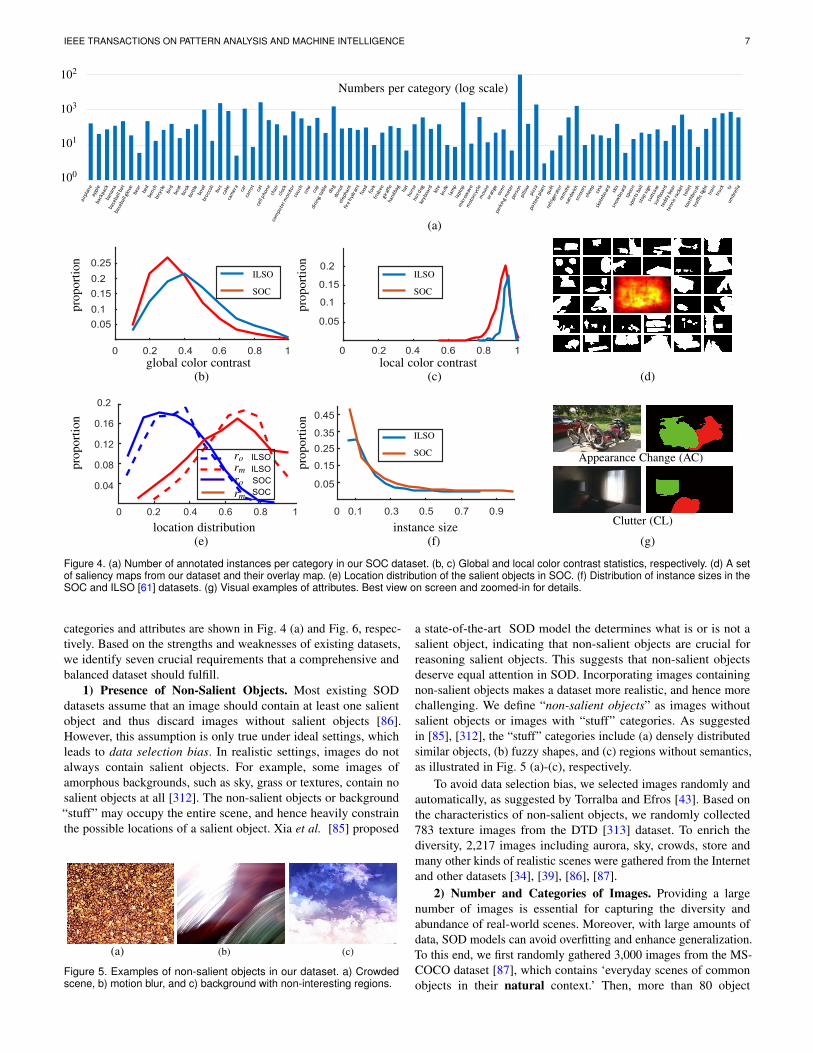
Figure 4. (a) Number of annotated instances per category in our SOC dataset. (b, c) Global and local color contrast statistics, respectively. (d) A setof saliency maps from our dataset and their overlay map. (e) Location distribution of the salient objects in SOC. (f) Distribution of instance sizes in theSOC and ILSO [61] datasets. (g) Visual examples of attributes. Best view on screen and zoomed-in for details.

categories and attributes are shown in Fig. 4 (a) and Fig. 6, respec-tively. Based on the strengths and weaknesses of existing datasets,we identify seven crucial requirements that a comprehensive andbalanced dataset should fulfill.

1) Presence of Non-Salient Objects. Most existing SODdatasets assume that an image should contain at least one salientobject and thus discard images without salient objects [86].However, this assumption is only true under ideal settings, whichleads to data selection bias. In realistic settings, images do notalways contain salient objects. For example, some images ofamorphous backgrounds, such as sky, grass or textures, contain nosalient objects at all [312]. The non-salient objects or background“stuff” may occupy the entire scene, and hence heavily constrainthe possible locations of a salient object. Xia et al. [85] proposed

(a) (b) (c)

Figure 5. Examples of non-salient objects in our dataset. a) Crowdedscene, b) motion blur, and c) background with non-interesting regions.

a state-of-the-art SOD model the determines what is or is not asalient object, indicating that non-salient objects are crucial forreasoning salient objects. This suggests that non-salient objectsdeserve equal attention in SOD. Incorporating images containingnon-salient objects makes a dataset more realistic, and hence morechallenging. We define “non-salient objects” as images withoutsalient objects or images with “stuff” categories. As suggestedin [85], [312], the “stuff” categories include (a) densely distributedsimilar objects, (b) fuzzy shapes, and (c) regions without semantics,as illustrated in Fig. 5 (a)-(c), respectively.

To avoid data selection bias, we selected images randomly andautomatically, as suggested by Torralba and Efros [43]. Based onthe characteristics of non-salient objects, we randomly collected783 texture images from the DTD [313] dataset. To enrich thediversity, 2,217 images including aurora, sky, crowds, store andmany other kinds of realistic scenes were gathered from the Internetand other datasets [34], [39], [86], [87].

2) Number and Categories of Images. Providing a largenumber of images is essential for capturing the diversity andabundance of real-world scenes. Moreover, with large amounts ofdata, SOD models can avoid overfitting and enhance generalization.To this end, we first randomly gathered 3,000 images from the MS-COCO dataset [87], which contains ‘everyday scenes of commonobjects in their natural context.’ Then, more than 80 object

IEEE TRANSACTIONS ON PATTERN ANALYSIS AND MACHINE INTELLIGENCE 8

Table 5List of salient object image attributes and their corresponding descriptions. These attributes are derived by studying the characteristics of existing

datasets. Some visual examples can be found in Fig. 1 and Fig. 4 (g). For more examples, please refer to the supplementary materials.

Attribute Description

AC (Appearance Change) Obvious illumination change in the object region.BO (Big Object) The ratio between the object area and the image area is larger than 0.5.CL (Clutter) Foreground and background regions around the object have similar colors. We labeled images with a global

color contrast value larger than 0.2 and local color contrast value smaller than 0.9 as cluttered images (§ 3).HO (Heterogeneous Objects) Objects composed of visually distinctive/dissimilar parts.MB (Motion Blur) Objects have fuzzy boundaries due to camera shaking or motion.OC (Occlusion) Objects are partially or fully occluded.OV (Out-of-View) Part of the object is clipped by the image boundaries.SC (Shape Complexity) Objects have complex boundaries, such as thin parts (e.g., the foot of animal) and holes.SO (Small Object) The ratio between the object area and the image area is smaller than 0.1.

categories (see supplementary materials) were annotated. Notethat we separated the process of data selection and labeling toavoid data selection bias, as discussed in [43]. Please refer to thesubsection “7) High-Quality Salient Object Labeling” for detailson this. Fig. 4 (a) shows the number of salient objects in eachcategory. As can be seen, the “person” category accounts for alarge proportion of the data, which is reasonable as people usuallyappear in daily scenes along with other objects. We divided ourdataset (3k non-salient images and 3k salient images) into training,validation and test sets in the ratio of 6:2:2.

3) Global vs. Local Color Contrast of Salient Objects. Asdescribed in [39], the term “salient” is related to the global/localcontrast of the foreground and background. It is essential to confirmwhether the salient objects are easy to detect. For each object, wecompute separate RGB color histograms for the foreground andbackground. Then, χ2 distance is utilized to measure the distancebetween the two histograms. The global and local color contrastdistributions are shown in Fig. 4 (b) and (c), respectively. Comparedto ILSO, the SOC dataset has a higher proportion of objects withlow global and local color contrast.

4) Locations. Center bias has been identified as one of themost significant and challenging biases pertaining to saliencydetection datasets [39], [69], [314]. Fig. 4 (d) illustrates a setof images and their overlay map (i.e., average mask map). As canbe seen, although salient objects are located at different positions,the overlay map shows that somehow these images are still centerbiased. Unfortunately, previous benchmarks have often adopted thisincorrect approach to analyze the positional distribution of salientobjects. To avoid this misleading phenomenon, in Fig. 4 (e), weplot the statistics of two quantities, ro and rm, which denote how faran object center and its farthest (margin) point are from the imagecenter, respectively. Both ro and rm are divided by half the diagonallength of the image for normalization, such that ro,rm ∈ [0,1]. Fromthese statistics, we observe that the salient objects in our datasetdo not suffer from center bias.

5) Size of Salient Objects. The size of an instance-level salientobject is defined as the proportion of its pixels to those in the overallimage [39]. As shown in Fig. 4 (f), the sizes of salient objects in ourSOC vary greatly compared with the only other existing instance-level dataset, ILSO [61]. Further, there is a higher proportion ofmedium-sized objects in SOC.

6) Salient Objects with Attributes. Having attribute infor-mation for the images in a dataset helps objectively assess theperformance of models over different types of parameters andvariations. It also allows for the inspection of model failures. Tothis end, we define a set of attributes to represent specific situationsencountered in real-world scenes, such as motion blur, occlusionand cluttered background (summarized in Table 5). Note that an

AC BO CL HO MB OC OV SC SO

AC

BO

CL

HO

MB

OC

OV

SC

SO

ACBO

CL

HO

MB

OC

OV

SC SO

Figure 6. Left: Attribute distribution over salient object images in our SOCdataset. Each number in the grid indicates the number of occurrences.Right: The dominant dependencies among attributes based on thefrequency of occurrences. A larger link width indicates a higher probabilityof an attribute occurring with other ones.

image can be annotated with multiple attributes as these attributesare not exclusive.

Inspired by [315], we present the distribution of attributes overthe dataset in the left of Fig. 6. The SO attribute makes up thelargest proportion due to our accurate instance-level annotations(e.g., the tennis racket in Fig. 3). The HO attribute also accounts fora large proportion, because the real-world scenes are composed ofdifferent constituent materials. Motion blur (MB) is more commonin video frames, but also sometimes occurs in still images. Thus,MB images make up a relatively small proportion of our dataset.Since a realistic image usually contains multiple attributes, weshow the dominant dependencies among attributes based on thefrequency of occurrence on the right of Fig. 6. For example, ascene containing several heterogeneous objects is likely to have alarge number of objects occluding each other and forming complexspatial structures. Thus, the HO attribute has a strong dependencywith OC, OV, and SO.

7) High-Quality Salient Object Labeling. As noted in [316],training on the ECSSD dataset (1,000 images) yields better resultsthan when using other datasets (e.g., MSRA10K with 10,000images). This is because, besides the scale, dataset quality is alsoan important. To obtain a large number of high-quality images, werandomly selected images from the MS-COCO dataset [87], whichis a large-scale real-world dataset whose objects are annotatedwith polygons (i.e., coarse labeling). High-quality labels alsoplay a critical role in improving the accuracy of SOD models[82]. Towards this end, we re-labeled the dataset with pixel-wiseannotations. Following other famous task-oriented SOD benchmarkdatasets [32], [33], [34], [35], [37], [40], [41], [61], [82], [85], [86],we did not use an eye tracking device. We took two steps to ensurehigh-quality annotations: (i) We asked five viewers to annotateobjects that they thought were salient in each image with bounding

IEEE TRANSACTIONS ON PATTERN ANALYSIS AND MACHINE INTELLIGENCE 9

(a) ILSO (b) SOC

(c) MS-COCO (d) SOCFigure 7. Compared with the recent instance-level ILSO dataset [61] (a),which is labeled with discontinuous coarse boundaries, and MS-COCOdataset [87] (c), which is labeled with polygons, our SOC dataset (b & d)is labeled with smooth fine boundaries.

boxes (bboxes), and (ii) we kept the images in which the majority(≥ 3) of viewers annotated the same objects (IOU of the bbox> 0.8). After this first stage, we had 3,000 salient object imagesannotated with bboxes. In the second stage, we further manuallylabeled accurate silhouettes of the salient objects according to thebboxes. Note that we had 10 volunteers involved in both steps tocross-check the quality of annotations. In the end, we kept 3,000images with high-quality, instance-level labeled salient objects. Asshown in Fig. 7 (b & d), the boundaries of our object labels areprecise, sharp and smooth. During the annotation process, we alsoadded some new categories (e.g., computer monitor, hat, pillow)that are not labeled in the MS-COCO dataset [87].

4 OUR DATASET-ENHANCEMENT STRATEGIES

Instead of focusing on designing a strong decoder for featureaggregation, we introduce three simple dataset-enhancement strate-gies to achieve better model generalization ability. We argue thatthe proposed strategies are easy to implement by all existingfully supervised SOD models, and yield good performance withlittle effort. Let us define the RGB saliency training dataset asD = {xi,yi}N

i=1, where xi,yi are an input RGB image and itscorresponding ground-truth (GT) saliency map, i indexes thetraining images, and N is the size of the training dataset. AsSOD is a binary prediction task, the GT saliency map y is usuallya binary map, and most existing SOD techniques employ a binary(or weighted) cross-entropy loss function to evaluate the saliencyprediction. In this paper, instead of defining the GT saliency mapas a binary segmentation map, we first introduce “label smoothing”[292] as an effective technique to achieve both efficient modeltraining and high model performance. Then, we adopt randomimage augmentation to generate diverse samples for better modelgeneralization ability. Finally, as a widely studied technique insemi-supervised or unsupervised learning [295], [307], we extendthe self-supervised learning solution to fully supervised SOD toachieve a robust model.

4.1 Label SmoothingLabel Smoothing and Knowledge Distillation. One of the mostimportant scenarios in which to apply label smoothing is theteacher-student net [317] for knowledge distillation. Typically, ina teacher-student net, the teacher model has a strong learningcapacity, while the student model has a lower one. The teachermodel then teaches the student model by providing the latter witha “soft target”. As discussed in [318], the “soft target” containsa rich similarity structure over the data, which is essential for

producing an enhanced student model. Further, label smoothingcan be treated as a form of output distribution regularization thatprevents the network from overfitting. As pointed out in [292],hard labels may lead to the overfitting as the model will assign fullprobability to each category, which is not guaranteed to generalizewell. With soft labels, the model learns the structure of the data,thus preventing it from being over-confident. Following the samedata setting, e.g., employing label smoothing, [319] introducedonline label smoothing solution to gradually update the soft labelsbased on the model’s prediction.

Conventional Setting. Given an input image x and thecorresponding ground-truth saliency map y, the conventionaldeep saliency model fθ is trained to achieve saliency predictions = fθ (x) by minimizing the cross-entropy loss: Lce(y,s) =−∑

Ni=1 ∑u,v yu,v

i logsu,vi , where (u,v) index pixels. For the hard label

based framework, we have y ∈ {0,1}, where 1 indicates the salientforeground and 0 represents the background.

Label Smoothing Setting. Different from the above hard labelsetting, in label smoothing regularization (LSR) [292], a smoothedlabel y′ is used instead of y, which is formulated as:

y′ = (1− ε)y+ εu(x). (1)

Here, ε is the smoothing parameter, and u(x) is a fixed distribution,which is usually defined as a uniform distribution. The smoothedlabel with a uniform distribution u(x) is then defined as:

y′ = (1− ε)y+ε

K, (2)

where K is the number of categories.Loss Function. Given smoothed label y′ and hard label y, the

loss function with LSR is defined as:

Lls = (1−α)Lce(y,s)+αLce(y′,s), (3)

where α is used to balance the contribution of the smoothed andhard labels, and the smoothed label related loss is defined asLlsr = Lce(y′,s). Note that, if there exist other loss functions, thesmoothed label can only be used in cross-entropy loss.

What Does Label Smoothing Really Do? The conventionalcross-entropy loss can be rewritten as:

Lce =− logs. (4)

Here, s is the model prediction after sigmoid activation (for binaryclassification), which is defined as:

s j = ez j/K

∑k=1

ezk = 1/(1+ ∑k 6= j

ezk−z j ). (5)

We then substitute s in (Eq. 4) and obtain:

Lce = log(1+ ∑k 6= j

ezk−z j ). (6)

Let us define the gap between the correct class and others asM = zk− z j. We can then conclude that the conventional cross-entropy loss aims to maximize this gap.

For label smoothing setting, as in (Eq. 2), we rewrite thesmoothed label related loss Llsr as:

Llsr =− ((1− ε)y+ ε/K) logs− (1− (1− ε)y− ε/K) log(1− s)

=− (y logs+(1− y) log(1− s))+(εy− ε

K) log(

s1− s

).

(7)

IEEE TRANSACTIONS ON PATTERN ANALYSIS AND MACHINE INTELLIGENCE 10

Using the definition of s in (Eq. 5), we have:

s j

1− s j=

1

∑Kk=1 ezk−z j −1

. (8)

We can then combine (Eq. 8) with (Eq. 7) and obtain:

Llsr = Lce(y,s)+(εy− ε

K)∗ 1

∑Kk=1 ezk−z j −1

. (9)

The first part of (Eq. 9) aims to maximize the gap between thecorrect class and the others, which is same as the conventionalbinary-cross entropy loss as in (Eq. 6). The second part worksin the opposite direction (compared with (Eq. 6)) to narrow thegap. In this way, the smoothed label related loss works to balancethe gap between the correct class and others, which serves as anregularization to prevent the model from being over-confident.

4.2 Data AugmentationAs an effective data pre-processing technique, data augmentationaims to generate new samples from an existing dataset, thusproducing a model with good generalization ability. Given thetraining dataset D = {xi,yi}N

i=1, data augmentation produces a newdataset D′ = {x′i,y′i}N′

i=1. As discussed previously, two main types ofdata augmentation have received particular attention. These includethe handcrafted policies and learned policies [301], [302]. For thelearned policies, we observe that the augmented data can changedrastically depending on the context, which may not be an issuefor image classification, but will change the salient attributes of animage. We thus focus only on handcrafted policies.

For handcrafted data augmentation policies, existing works[303], [304], [305], [306] focus on three main directions: 1) imagetransformation, e.g., scale or rotation transformation; 2) mix-up togenerate new samples, which are neighbors of the existing samples;and 3) adding noise to the ground-truth. Similar to learned policies,the mix-up strategy change the context information of an image,which is harmful for context-based tasks, such as salient objectdetection. In this paper, we therefore focus on two very simple dataaugmentation techniques, namely image transformation and addingnoise to the ground-truth. For image transformation, we randomlyscale, rotate and crop part of the image (85% of the original imageto keep the context information). For the additive noise solution,we randomly add Gaussian noise of distribution N (0.1,0.3) tothe ground-truth saliency map, leading to a noisy ground-truthmap. Note that, for image transformation, we transform image andground-truth at the same time, while when adding noise to theground-truth, we only process the ground-truth saliency maps.

4.3 Self-Supervised LearningSelf-supervised learning learns from an image without knowingthe task itself or the ground-truth, making it an unsupervised rep-resentation learning technique. Conventionally, for the supervisedlearning setting, the loss function is defined as Lce(y,s), wheres is the model’s prediction, and y is the ground-truth map. Forself-supervised learning, the final loss function usually includestwo main parts: the conventional cross-entropy loss Lce(y,s) andan unsupervised loss that serves as a regularizer, i.e., L (g(x),s),where g(x) is the transformation of the original input image x. Thetwo studies [295], [308] introduced a self-supervised loss withrotation estimation as a pretext task.

Similarly, we introduce a scale/rotation consistency loss func-tion to achieve scale/rotation invariant predictions. Specifically,

given an input image x, we define its prediction as s. Then, weapply an image transformation (scale or rotation transformation)and obtain xt . We then perform the same transformation on theprediction s and obtain s′. We feed xt to the same salient objectdetection network to get the saliency prediction as st . We assumethat s′ and st should be similar. Then, we adopt the single scalestructural similarity index measure (SSIM) [320], [321] as asimilarity measure, and define the self-supervised loss as:

Lss = 1−SSIM(s′,st). (10)

4.4 Loss Function with the Proposed Strategies.

With the three introduced data-enhancement strategies, we firstapply random data augmentation to both our training image setand training ground-truth set, as in Section 4.2. Then we generatethe smoothed label following (Eq. 1), with K = 2 in this paperto represent the salient foreground and background regions. Inaddition to the loss function in (Eq. 3), we also introduce a self-supervised loss Lss. Our final loss function is then defined as:

L = Lls + γLss, (11)

where γ is introduced to balance the self-supervised loss, and isempirically set to γ = 0.3 in this paper.

5 SOC BENCHMARK

Based on three criteria (i.e., representative pipeline, open-sourced,and state-of-the-art performance), we select 46 traditional SODmethods and 54 deep learning models from 201 reviewed methods(see § 2) to conduct our benchmark. To the best of our knowledge,this benchmark is the most comprehensive study in the RGB SOD.

5.1 Experimental Setup

5.1.1 Evaluation Metrics

Note that the GTs of non-salient images in our SOC dataset areall-zero matrices, so directly using the traditional F-measure [82]will result in very low and inaccurate scores. Thus, we utilize threegolden metrics (i.e., MAE [322], maximum E-measure [4], andS-measure [3]) to avoid this issue and to provide a more reliableassessment. Our python evaluation toolboxes are now publiclyavailable.5

• MAE (M) is the mean absolute error metric, which iswidely used to measure the pixel-level difference betweenthe prediction and the GT.

• E-measure (Emaxξ

) is a new perceptual metric that takes bothlocal and global similarity into consideration.

• S-measure (Sα ) is a standard metric that quantizes thestructural similarity at a region and object level.

Table 6SOC dataset used in the benchmarking experiments.

SOC train SOC val SOC test TotalSalient Objects (Sal) 1,800 600 600 3,000Non-Salient Objects (NonSal) 1,800 600 600 3,000Total 3,600 1,200 1,200 6,000

5. https://github.com/mczhuge/SOCToolbox.

IEEE TRANSACTIONS ON PATTERN ANALYSIS AND MACHINE INTELLIGENCE 11

Table 7Comparison of the traditional SOD algorithms on our SOC test set

(1,200 images) in terms of Sα ↑, Emaxξ↑, and M ↓ The top-3 results are

highlighted in red, blue and green, respectively. The superscript of eachscore is the corresponding ranking. Details of these methods are

summarized in Table 2. The overall rank index indicates the averageranking of the three metrics. These results are available at: Google Drive.

# Model Code Sα ↑ Emaxξ↑ M ↓ Rank

2014

-bef

ore 1 SUN [96] Matlab 0.47546 0.68844 0.43646 46

2 LSSC [107] Matlab + C 0.55245 0.71443 0.36545 453 BSF [112] Matlab 0.55444 0.72838 0.35344 444 GR [109] Matlab + C 0.58841 0.71542 0.33242 435 HS [37] EXE 0.60140 0.72937 0.32141 426 Itti [45] Matlab 0.58742 0.73630 0.31139 417 AIM [95] Matlab 0.60539 0.67045 0.25024 398 GBVS [93] Matlab 0.61536 0.73335 0.29337 399 LR [116] Matlab 0.64231 0.72340 0.25327 3610 CA [323] Matlab + C 0.60638 0.75022 0.29136 3511 MR [38] Matlab + C 0.64529 0.73433 0.25931 3212 SEG [99] Matlab + C 0.57643 0.7657 0.35243 3213 FT [82] C 0.62634 0.73829 0.23620 2814 MC [125] Matlab + C 0.65623 0.73630 0.25125 2615 CB [134] Matlab + C 0.65325 0.75813 0.26833 2316 SR [94] Matlab/C++ 0.65821 0.66146 0.1564 2317 PCA [117] Matlab + C 0.67018 0.74128 0.20913 1718 MSS [110] Matlab 0.68212 0.7764 0.23119 1019 SF [113] C 0.6996 0.74726 0.1301 820 DSR [124] Matlab + C 0.7025 0.75120 0.1848 821 MSSS [100] C 0.68311 0.75714 0.1645 722 HDCT [118] Matlab 0.6967 0.7745 0.20112 623 DRFI [114] C 0.7094 0.7912 0.19711 424 COV [108] Matlab 0.7113 0.7619 0.1462 225 RBD [115] Matlab 0.7162 0.7843 0.1869 2

2021

-201

5 26 WMR [324] Matlab + C 0.64032 0.73335 0.26934 3827 MAPM [142] Matlab + C 0.64430 0.72241 0.25629 3728 BL [156] Matlab + C 0.62335 0.75120 0.29638 3229 RRWR [159] Matlab 0.64727 0.73532 0.25830 3130 WLRR [325] Matlab + C 0.61437 0.75911 0.31240 3031 RCRR [144] Matlab 0.65026 0.73433 0.25528 2932 GP [153] Matlab + C 0.63233 0.75911 0.28735 2733 TLLT [160] Matlab 0.65623 0.72539 0.21415 2534 BSCA [154] Matlab + C 0.65722 0.75516 0.25931 2235 SMD [136] Matlab 0.66220 0.74825 0.24622 2136 MDC [147] C 0.67516 0.74427 0.21917 2037 DSP [140] Matlab + C 0.66419 0.75417 0.24823 1738 MIL [143] Matlab + C 0.67117 0.75022 0.23620 1739 MST [158] C 0.64727 0.7736 0.25125 1640 GLC [139] Matlab + C 0.67615 0.75615 0.22318 1541 MBS [152] Matlab 0.67814 0.75318 0.21415 1442 LPS [141] Matlab + C 0.6949 0.74924 0.1837 1343 WFD [326] C 0.68013 0.76010 0.21314 1244 BFS [138] Matlab + C 0.6967 0.75318 0.19510 1045 WSC [161] Matlab 0.69310 0.7657 0.1796 546 HCCH [148] Matlab 0.7361 0.7941 0.1493 1

5.1.2 Training and Testing ProtocolsThe statistics of the SOC dataset used in the benchmark aresummarized in Table 6. For traditional algorithms, we directlytest their performance on the SOC-test set (1,200 images). Fordeep learning models, we first adopt the pre-trained models withtheir recommended training parameter settings under the defaulttraining dataset (see Tables 3 & 4) and then evaluate them on theSOC test set to roughly obtain the top-100 models (see Table 7& 8). Finally, we provide a quantitative comparison and detailedanalysis of 15 SOTA approaches, including the top-5 traditionalmethods and top-10 deep learning models.

5.2 Quantitative ComparisonsTo build a standardized leaderboard (i.e., same image resolution,thresholding step, and evaluation tool), we provide three goldenmetrics, i.e., Sα , Emax

ξ, and M.

Table 7 shows the performance of 46 SOTA traditional SODalgorithms on our SOC test set. In terms of both S-measure (i.e.,Sα ) and max E-measure (Emax

ξ), the HCCH method surpasses

all competitors by a large margin. RBD, COV, and DRFI obtaincomparable performance in terms of Sα score. Meanwhile, COVranks third in terms of Sα measure, but ninth in Emax

ξ. In terms

Table 8Evaluation of 54 deep learning based SOD models on our SOC test set(1,200 images). We adopt the default implementations listed in Table 3

and Table 4 to test their generalization capability. These results areavailable at: Google Drive.

# Model Code Sα ↑ Emaxξ↑ M ↓ Rank

2015

1 LEGS [175] Caffe 0.67953 0.76554 0.22853 542 MDF [40] Caffe 0.73949 0.76853 0.14443 493 MC [176] Caffe 0.75747 0.82343 0.13835 43

2016

4 DSL [178] Caffe 0.72452 0.81047 0.19452 515 DISC [180] Caffe 0.73551 0.81047 0.17550 506 DCL [194] Caffe 0.77144 0.83639 0.15748 457 ELD [193] Caffe 0.77442 0.83639 0.13835 408 DS [181] Caffe 0.77940 0.86024 0.15546 379 DHS [168] Pytorch 0.80032 0.84833 0.12230 3310 RFCN [186] Caffe 0.81423 0.85827 0.11323 25

2017

11 UCF [203] Caffe 0.65454 0.80551 0.28554 5312 AMU [204] Caffe 0.73750 0.80850 0.18551 5113 SVF [202] Caffe 0.76145 0.81645 0.15647 4714 WSS [41] Caffe 0.77841 0.82144 0.14039 4215 DSS [200] Caffe 0.80730 0.85827 0.11120 2716 SRM [196] Caffe 0.82216 0.85926 0.11120 2117 MSRNet [61] Caffe 0.81619 0.87116 0.11725 2018 NLDF [198] Tensorflow 0.81619 0.86024 0.10413 16

2018

19 RAS [212] Pytorch 0.75946 0.81346 0.15144 4620 R3Net [209] Pytorch 0.77343 0.82542 0.13835 4121 LPSNet [213] Pytorch 0.79535 0.83838 0.14342 3922 DGRL-GLN [217] Caffe 0.79436 0.84536 0.14140 3823 C2SNet [211] Caffe 0.79137 0.84536 0.13835 3624 PiCA-Res [218] Pytorch 0.81028 0.85827 0.12831 3125 BMPM [216] Tensorflow 0.81028 0.85330 0.11927 2926 ASNet [215] Keras 0.81718 0.86520 0.11120 17

2019

27 MWS [236] Pytorch 0.75747 0.82841 0.17249 4728 AFNet [239] Caffe 0.81224 0.85032 0.12029 2929 SIBA [249] Caffe 0.80032 0.88410 0.13033 2630 Deepside [233] Caffe 0.81521 0.86123 0.11927 2431 PFANet [240] Tensorflow 0.81521 0.84635 0.1018 2232 PoolNet [243] Pytorch 0.82913 0.86818 0.10616 1433 SCRNet [44] Pytorch 0.83311 0.87215 0.10514 1334 CPDVgg [242] Pytorch 0.8563 0.8896 0.0792 235 EGNet [250] Pytorch 0.8581 0.8962 0.0781 1

2020

36 ABPNet [282] Pytorch 0.78338 0.81047 0.15345 4437 U2Net [273] Pytorch 0.78039 0.79552 0.10514 3538 GCPANet [277] Pytorch 0.80730 0.84833 0.13334 3439 ITSD [280] Pytorch 0.79834 0.87017 0.14241 3240 MINet [281] Pytorch 0.81917 0.86422 0.11725 2241 SANet [56] Pytorch 0.81224 0.86818 0.10616 1742 GateNetVgg [284] Pytorch 0.82715 0.86520 0.10818 1543 F3Net [278] Pytorch 0.82814 0.8915 0.10919 1244 CSNet [283] Pytorch 0.83410 0.87614 0.10310 1145 LDF [279] Pytorch 0.8359 0.87812 0.10310 1046 RASNet [258] Pytorch 0.83212 0.8878 0.10310 947 CAGVgg [271] Keras 0.8378 0.87812 0.0884 848 DFI [254] Pytorch 0.8387 0.9031 0.1018 549 R2Net [255] Pytorch 0.8572 0.8859 0.0843 4

2021

50 SCWS [288] Pytorch 0.81126 0.85131 0.11524 2851 ICON [52] Pytorch 0.81126 0.8962 0.12831 1952 BAS [31] Pytorch 0.8425 0.88211 0.0927 753 ABP [327] Pytorch 0.8425 0.8896 0.0916 654 CVAE [327] Pytorch 0.8494 0.8924 0.0895 3

of MAE (i.e., M), the top-5 approaches are: SF, COV, HCCH,SR, and MSSS. It is worth mentioning that SF reduces M andoutperforms all the recent traditional SOD methods. Based on theiroverall scores, the top-5 methods are HCCH, RBD, COV, DRFI,and WSC.

The quantitative results of the 54 deep learning SOD models onour SOC test dataset are shown in Table 8. In terms of Sα , EGNet,R2Net, and CPDVgg are the top-3 models, with scores of more than0.85. Roughly 46% (i.e., 21/45) of model scores are between 0.650and 0.800. Compared with the traditional model, which achievesan Sα score of 0.736, we can see continuous improvement overthe past few years, with the exception of four early models (i.e.,DISC, DSL, LEGS, and UCF). At the same time, 30 out of 45models achieve high performance (e.g., 0.800≤ Sα ≤0.850) andthe average performance is nearly 0.820. Interestingly, in terms of

IEEE TRANSACTIONS ON PATTERN ANALYSIS AND MACHINE INTELLIGENCE 12

GTImage

ABP

ASNet

CAGNet

DCL

DHS

EGNet

GCPANet

LDF

MINet

PiCA

RAS

ABPNet

BAS

CVAE

Deepside

DISC

ELD

DGRL

LEGS

MSRNet

PoolNet

RASNet

AFNet

BMPM

CPD

DFI

DS

F3Net

ICON

MC

NLDF

R2Net

RFCN

AMU

C2SNet

CSNet

DGRL

DSS

GateNet

ITSD

MDF

PFANet

R3Net

SANet

SCRN SCWS SIBA SRM

SVF U2Net UCF WSS

Figure 8. Visualization results of deep learning models.

GTImage

MDC

WSC

DRFI

TLLT

SF

RBD

RRWR

SUN

BL

PCA

FT

DSR

WFD

MR

WMR

HCCH

MSS

GP

GC

MBS

CA

SR

DSP

WLRR

RCRR

MAPM

SMD

LR

BSCA

SEG

GBVS

ITTI

AIM

MIL

MC

HDCT

LPS

GLC

HS

GR

MST

CB

COV

MSSS

Figure 9. Qualitative results of state-of-the-art traditional approaches.

Emaxξ

, the multi-task learning framework DFI and integrity learningmodel have the best and second-best scores of 0.903 and 0.896,respectively. Consistent with S-measure, in terms of MAE, weobtain the same top-3 models EGNet, CPDVgg, and R2Net. Fromour 54 benchmarked models, we find that models that perform wellin terms of S-measure also do well in MAE. Overall, the top-10approaches are EGNet, CPDVgg, CVAE, R2Net, DFI, ABP, BAS,CAGVgg, RASNet, and LDF. In the following section (§ 6), wewill provide a more detailed analysis of these models.

IEEE TRANSACTIONS ON PATTERN ANALYSIS AND MACHINE INTELLIGENCE 13

Table 9Comparison of 14 state-of-the-art approaches in terms of attribute-level performance. For deep learning models, we re-train them on our

SOC-Sal train set (i.e., 1,800 images). Please refer to Tables 2, 3, & 4 for more details. These results are available at: Google Drive.

AC BO CL HO MB OC OV SC SO Avg.

ModelAttribute Sα ↑ M ↓ Sα ↑ M ↓ Sα ↑ M ↓ Sα ↑ M ↓ Sα ↑ M ↓ Sα ↑ M ↓ Sα ↑ M ↓ Sα ↑ M ↓ Sα ↑ M ↓ Sα ↑ M ↓

Trad

ition

al COV [108] 0.505 0.216 0.277 0.577 0.453 0.280 0.508 0.229 0.494 0.219 0.484 0.246 0.423 0.314 0.535 0.174 0.525 0.172 0.467 0.270WSC [161] 0.541 0.205 0.356 0.517 0.517 0.252 0.556 0.211 0.536 0.210 0.529 0.227 0.475 0.292 0.567 0.170 0.535 0.181 0.512 0.252

HCCH [148] 0.585 0.199 0.354 .0.525 0.537 0.254 0.615 0.197 0.547 0.202 0.552 0.225 0.468 0.298 0.595 0.165 0.588 0.162 0.538 0.247DRFI [114] 0.598 0.229 0.391 0.513 0.570 0.274 0.618 0.230 0.556 0.230 0.577 0.248 0.527 0.304 0.614 0.188 0.585 0.197 0.560 0.268RBD [115] 0.589 0.225 0.429 0.481 0.575 0.260 0.625 0.216 0.557 0.213 0.583 0.235 0.521 0.295 0.602 0.191 0.579 0.192 0.562 0.256

Dee

pL

earn

ing

ABP [327] 0.767 0.092 0.592 0.315 0.742 0.125 0.787 0.101 0.742 0.095 0.740 0.112 0.746 0.132 0.759 0.083 0.741 0.080 0.735 0.126EGNet [250] 0.791 0.088 0.593 0.307 0.739 0.137 0.788 0.110 0.763 0.115 0.743 0.120 0.750 0.138 0.800 0.076 0.753 0.088 0.747 0.131

CPDVgg [242] 0.806 0.076 0.626 0.278 0.765 0.118 0.808 0.096 0.786 0.097 0.765 0.103 0.760 0.127 0.801 0.070 0.765 0.076 0.765 0.116CAGVgg [271] 0.795 0.080 0.700 0.208 0.782 0.115 0.808 0.098 0.764 0.102 0.751 0.120 0.763 0.127 0.795 0.081 0.744 0.093 0.767 0.114RASNet [258] 0.821 0.066 0.626 0.276 0.785 0.106 0.816 0.087 0.788 0.086 0.776 0.096 0.779 0.113 0.810 0.066 0.774 0.070 0.772 0.107

CVAE [327] 0.813 0.075 0.688 0.217 0.790 0.107 0.816 0.092 0.784 0.091 0.771 0.104 0.776 0.115 0.820 0.069 0.767 0.080 0.781 0.106LDF [279] 0.819 0.071 0.697 0.212 0.796 0.105 0.824 0.088 0.792 0.085 0.781 0.098 0.790 0.107 0.780 0.073 0.801 0.072 0.787 0.101

R2Net [255] 0.827 0.071 0.656 0.257 0.802 0.107 0.826 0.092 0.794 0.097 0.789 0.099 0.791 0.112 0.807 0.072 0.788 0.073 0.787 0.109BAS [31] 0.831 0.060 0.723 0.166 0.785 0.110 0.814 0.093 0.797 0.072 0.780 0.101 0.781 0.114 0.820 0.072 0.787 0.075 0.791 0.096

Avg. 0.721 0.125 0.551 0.346 0.688 0.168 0.729 0.139 0.693 0.137 0.687 0.152 0.668 0.185 0.722 0.111 0.693 0.115 - -

5.3 Qualitative Comparisons

Two qualitative comparisons are presented in Fig. 8 and Fig. 9. Ascan be seen from Fig. 8, deep models generate saliency maps thatare similar to the GTs, to varying degrees. Specifically, for ASNet,C2SNet, BMPM, DCL, DHS, DSS, DS, DISC, SVF, RFCN, andPFANet, the position of the object can be well-identified. However,all these methods generate blurred responses on object boundaries.PFANet, MDF, MC and LEGS even nearly destroy the integrity ofthe object. To better highlight these results, we introduce yellowrectangles to mark the high-quality segmentation regions and utilizered arrows to point out the errors. We observe that eight models(ABPNet, AFNet, AMU, NLDF, RAS, SCWS, UCF, and WSS)can localize the human object but introduce additional noise. Wealso notice that CAGNet, CSNet, MINet, DGRL, EGNet, F3Net,ICON, PoolNet, and R3Net can even capture the small structure ofthe human elbow. Moreover, saliency maps from R2Net, Deepside,SIBA, and MSRNet demonstrate better results than the above-mentioned methods. Amazingly, BAS, U2Net, ABP, CPD, GateNet,GCPANet, ITSD, LDF, SCRN, and CAVE perform very close tothe GT and result in knife-edge-shaped boundaries in the yellowrectangle region without any additional noise.

In sharp contrast to the deep learning models, the traditionalmodels (Fig. 9) all fail without exception. WSC, HCCH, and RBDare the three most promising approaches. However, their resultsare still far from the GT map, since they are mainly based onvarious prior features extracted from color, orientation, contrast,etc. Further, the center bias prior is not suitable in this case, sincethe human is located close to the image boundary, thus making thisexample more challenging for these approaches.

6 FURTHER BENCHMARKING

6.1 Attribute-Based Evaluation

Based on the top-ranked models presented in Tables 7 & 8, wefurther re-train the top-106 deep learning models (using theirdefault settings) on the SOC-Sal train set (1,800 images) and thentest them on the SOC-Sal test set for attribute-based evaluation.In Table 9, we show the performance on subsets of our datasetcharacterized by a particular attribute. Due to space limitations,

6. The authors of DFI have only released the test code, so we only evaluatenine models.

in the following discussion, we only select a few representativeattributes for further analysis.

Big object (BO) scenes typically occur when objects are closeto the camera, enabling tiny text and patterns to be seen clearly.In this case, models that prefer to focus on local information areseriously misled, leading to a considerable decrease in performance(e.g., 8.6% Sα reduction for BAS, 8.7% reduction for CAGVgg,11.4% reduction for LDF, and 40.7% reduction for COV) comparedwith their average performance (Avg.). Among all attributes, BOsare the most difficult for both traditional and deep learning models.

Small objects (SOs) are tricky for some SOD models. Fourmodels (i.e., BAS, CVAE, CAGVgg, and RASNet) encounterperformance degradation (e.g., from BAS-0.5% to RASNet-3.6%)because SOs are easily ignored during the downsampling of CNNs.Other models instead have enhanced performance on SOs, butsignificant reduction in performance on BOs.

Heterogeneous objects (HOs) commonly appear in naturalscenes. The performance of all models on HOs improves to somedegree, fluctuating from 2.9% to 14.3%. We suspect this is because,as shown in Fig. 6, HO images make up a significant proportion ofall datasets, so the models are more familiar with this attribute.

Occlusion (OC) scenes occur when objects are partly obscured.Thus, SOD models must capture global semantics to make up forthe incomplete information of objects. As observed, traditionalmodels obtain improved performance compared with their averageperformance. For deep learning models, in contrast, this situationis reversed.

As can be seen in the last row of Table 9 (average performanceof each attribute), MB and SO have the same Sα score. Moreover,the average scores of AC and SC are very similar. It seems thatexisting deep learning based SOD models can effectively addressappearance change and shape complexity. Similar to the attributesof OV and OC, CL and MB remain challenging for existing methods,generating mid-level (i.e., 0.65< Sα <0.70) S-measure scores.

6.2 Comparison with Baselines

We introduce three dataset-enhancement strategies to preventnetworks from being overconfident as a result of dataset bias.These include label smoothing, random data augmentation andself-supervised learning. We argue that our strategies can be easilyused in existing salient object detection frameworks as generaldata processing techniques. We thus introduce our strategies to

IEEE TRANSACTIONS ON PATTERN ANALYSIS AND MACHINE INTELLIGENCE 14

Table 10The contribution of our dataset-enhancement strategies.

MethodMetric Sα ↑ Emax

ξ↑ M ↓

RASNet [258] 0.832 0.887 0.103Our-RASNet 0.841 0.897 0.096

LDF [279] 0.835 0.878 0.103Our-LDF 0.845 0.891 0.097BAS [31] 0.842 0.882 0.092Our-BAS 0.856 0.895 0.086

R2Net [255] 0.857 0.885 0.084Our-R2Net 0.868 0.899 0.080

CVAE [327] 0.849 0.892 0.089Our-CVAE 0.863 0.902 0.086

Table 11The contribution of each dataset-enhancement strategy.

MethodMetric Sα ↑ Emax

ξ↑ M ↓

CVAE [327] 0.849 0.892 0.089LS 0.851 0.895 0.088SS 0.852 0.894 0.088

RDA 0.855 0.896 0.086Our-CVAE 0.863 0.902 0.086

Table 12Results for cross-dataset generalization in § 6. UC-Net (CVPR’20) [328]is trained on one dataset and tested on all others. “Sel.”: diagonal score

(training and testing on the same dataset). “Oth.”: mean score on allexcept for self.

Measure Sα ↑ [3] Drop↓

Train Test SOC M10K DU-O DUTS ECC HKU ILSO Sel. Oth.

SOC [1] .884 .768 .686 .834 .749 .774 .841 .884 .775 12%M10K [35] .800 .921 .784 .894 .881 .882 .884 .921 .854 7%DU-O [38] .833 .898 .854 .877 .862 .867 .886 .854 .871 -2%DUTS [41] .795 .882 .793 .910 .890 .903 .900 .910 .861 5%

ECC [37] .791 .886 .800 .901 .901 .898 .903 .901 .863 4%HKU [40] .818 .892 .787 .904 .883 .910 .905 .910 .865 5%ILSO [61] .841 .888 .790 .898 .882 .896 .920 .920 .866 6%

Oth. .813 .869 .773 .885 .858 .870 .887

five benchmark salient object detection models and show theperformance in Table 10, where “Our-” represents the benchmarkmodels with our dataset-enhancement strategies. Further, weinvestigate the contribution of each data-enhancement strategy, andshow the performance in Table 11, where we choose CVAE [327]as the base model.

Training & Testing Protocols. We retrain the five models inTable 10 with their corresponding training dataset, e.g., MB [32]for RASNet [258], and DUTS [41] for all the other four models.We follow their original training and testing settings, e.g., samemaximum epoch, learning rate, training and testing image sizes.

Discussion. Table 10 shows consistent better performance ofmodels with our strategies, which illustrates effectiveness of oursolutions. Further, in Table 11, “LS”, “RDA”, “SS” representadding label smoothing strategy, random data augmentation andself-supervised learning to the base model respectively. It showsthat the random data augmentation achieves the largest performancegain, while label smoothing and self-supervised learning achievescomparable performance improvement. The main reason is thatdata augmentation introduce diverse samples to the initial trainingdataset, which is effective in improving model generalizationability. For the self-supervised learning strategy, as the CVAEmodel [327] has already adopt the multi-scale image as inputstrategy, we observe slightly improved performance. However, the

better performance in general can still validate the effectiveness ofthe proposed strategy. Label smoothing [292] was introduced toprevent model from over-confidence, thus achieve well-calibratedmodel. However, there exists no saliency metrics to explain thecalibration error of the saliency models. We will investigate inexpected calibration error [329] and extend it to saliency detectiontask in the future to better explain the calibration error of saliencymodels.

6.3 Cross-Dataset GeneralizationTo study the difficulty of existing SOD datasets, we adopt the CDA(cross-data analysis) method [43]. Given N candidate datasets{Dn}N

n=1, we first train a model on the Di dataset, and then test iton the other datasets (i.e., {Dn}N

n=1,n6=i). Following [76], [330], werandomly select 800 images and 200 images from each dataset asthe training set and testing set, respectively.

We train UC-Net [328] on popular existing datasets that containmore than 1,000 images. Table 12 shows the Sα score on eachdataset. Each column provides the score of UC-Net tested on aspecific dataset and trained on all others. Each row indicates theperformance of UC-Net trained on one dataset and tested on allothers, demonstrating the generalizability of the dataset adoptedfor training. We find that our SOC (e.g., Oth. = 0.813) and DU-O (Oth. = 0.773) datasets are more difficult than other datasets.In addition, we notice that the model trained on our SOC datasetcannot perform well (e.g., the Oth. column: 0.775) on other datasets.This is because our SOC dataset contains many real-world salientobjects in open environments, thus the model cannot overfit thesimple or clean scenes in existing datasets. This is also supportedby our core observation that data selection bias is common inexisting datasets.

7 FUTURE DIRECTIONS

Human attention can be influenced by four key factors:• Visual properties. Our attention may be drawn by basic

objects’ unique visual properties [331].• Memory. If one knows an object well, it is easier for that

object to attract one’s attention.• Goal. For example, eye fixation records are quite different

from attention maps, with a specific goal for viewers.• Emotion. In addition to the above-mentioned factors, we

argue that human attention toward the same scene may beaffected by one’s emotion, e.g., happiness, sadness, anger.

As demonstrated by Cave [331], attentional control is de-termined by a combination of these factors. Unfortunately, theannotations of existing SOD datasets do not clearly describe whichfactor they address. Differently, the ground-truth annotations of ourSOC are based on the salicon (free-view task) dataset7, or so-callmeaning maps which are used in recent studies [331], [332], [333].As concluded by Kalash et al. [66], the work to date has addresseda relatively ill-posed problem. Thus, we recommend several futuredirections to re-think SOD tasks at six main research levels:

(1) Data Level: Recently, visual saliency detection tasks haveattracted significant interest using 2D (RGB SOD) and 3D (i.e.,RGB-D, RGB-T) input data. However, light field SOD (4D),LIDAR SOD, and 360◦ SOD are still not well-studied. Establishingnew datasets for these types of data will largely promote thedevelopment of this field. Another interesting avenue for examining

7. http://salicon.net/

IEEE TRANSACTIONS ON PATTERN ANALYSIS AND MACHINE INTELLIGENCE 15

saliency detection is to study fine-grained tasks, such as salientinstance detection [61], [62], [334], [335] and part-object visualsaliency detection [336].

(2) Task Level: Multi-task learning has demonstrated strongperformance in recent works [337]. Existing schemes mainlyfocus on vision tasks, such as joint salient object detection andcamouflaged object detection [338], detection of salient objects,edges and skeletons simultaneously [254], and simultaneousdetection, ranking, and subitizing of multiple salient objects [64].With the success of the transformer technique in natural languageprocessing (NLP), introducing multi-modality learning into thesaliency detection field may be a feasible way to further incorporateother types of information, such as CV+NLP (similar to [339]),CV+Audio [340], and CV+other modality.

(2) Model Level: A huge number of algorithms have beendeveloped to improve detection accuracy. However, there areseveral promising directions that could be further studied suchas data augmentation techniques [341], efficient SOD models(e.g., lightweight models [283], [342]), new loss functions [286],[343], ranking-based models [64], [137], and transformer-basedmodels [344], [345].

(4) Supervision Level: In addition to the most common fullysupervised learning of current SOD models, other supervision strate-gies, e.g., weakly supervised (i.e., scribble [56], category [346],and polygon), semi-supervised [53], self-supervised [60], [347],and unsupervised [58] learning are also interesting to study.

(5) Evaluation Level: Evaluation metrics are important formodel training, testing, and benchmarking. However, the SODcommunity still utilizes classical metrics such as IoU, F-measure,and MAE. These metrics were designed for universal evaluationrather than for assessing SOD tasks specifically. As a consequence,they do not work well for certain specific applications, such asthose with high-quality requirements. We envision that introducinga new metric (e.g., based on the gradient or connectivity errorused in [348]) for SOD tasks, such as weighted F-measure [2] andS-measure [3], will be another important research direction.

(6) Application Level: The SOD task belongs to a moregeneral task called class-agnostic object detection (CAOD). Forsimple scenes (e.g., those containing only one or two clear objects),SOD is identical to CAOD. From this point of view, SOD modelshave many potential applications in the real-world (e.g., Alibaba’sfashion search system [339]), despite their currently limited numberof representative cases [30], [31], [200].

8 CONCLUSION

In this survey, we identified and addressed the long-ignored dataselection bias issue in SOD. Different from previous studies, weaimed to explore the SOD task in the wild. To achieve thisgoal, we collected a new challenging and densely annotatedSOC dataset; analyzed a large number (∼200) of representativemodels; conducted the most complete (top-100) benchmarking;devised a series of simple learning strategies to efficiently utilizenegative samples and training data; and identified several currentchallenges and future directions. We hope that these contributionswill provide the SOD community an opportunity to explore noveltechniques in an open environment. We have tried to cover themost important works. Nevertheless, it is impractical to thoroughlyinvestigate all models in this vast field. We will continue toincorporate new techniques on our website.

REFERENCES

[1] D.-P. Fan, M.-M. Cheng, J.-J. Liu, S.-H. Gao, Q. Hou, and A. Borji,“Salient objects in clutter: Bringing salient object detection to theforeground,” in Eur. Conf. Comput. Vis., 2018, pp. 186–202.

[2] R. Margolin, L. Zelnik-Manor, and A. Tal, “How to evaluate foregroundmaps?” in IEEE Conf. Comput. Vis. Pattern Recog., 2014, pp. 248–255.

[3] D.-P. Fan, M.-M. Cheng, Y. Liu, T. Li, and A. Borji, “Structure-measure:A New Way to Evaluate Foreground Maps,” in Int. Conf. Comput. Vis.,2017, pp. 4548–4557.

[4] D.-P. Fan, C. Gong, Y. Cao, B. Ren, M.-M. Cheng, and A. Borji,“Enhanced-alignment Measure for Binary Foreground Map Evaluation,”in Int. Joint Conf. Artif. Intell., 2018, pp. 698–704.

[5] P. Zhang, T. Zhuo, W. Huang, K. Chen, and M. Kankanhalli, “Onlineobject tracking based on cnn with spatial-temporal saliency guidedsampling,” Neurocomputing, vol. 257, pp. 115–127, 2017.

[6] A. Borji, S. Frintrop, D. N. Sihite, and L. Itti, “Adaptive object trackingby learning background context,” in IEEE Conf. Comput. Vis. PatternRecog. Worksh., 2012, pp. 23–30.

[7] V. Mahadevan and N. Vasconcelos, “On the connections between saliencyand tracking,” in Adv. Neural Inform. Process. Syst., 2012, pp. 1664–1672.

[8] A. Abdulmunem, Y.-K. Lai, and X. Sun, “Saliency guided local andglobal descriptors for effective action recognition,” Comput. Vis. Media,vol. 2, no. 1, pp. 97–106, 2016.

[9] J. He, J. Feng, X. Liu, T. Cheng, T.-H. Lin, H. Chung, and S.-F. Chang,“Mobile product search with bag of hash bits and boundary reranking,”in IEEE Conf. Comput. Vis. Pattern Recog., 2012, pp. 3005–3012.

[10] G. Liu and D. Fan, “A model of visual attention for natural imageretrieval,” in IEEE Int. Conf. Inf. Sci. Cloud Comput. Companion, 2013,pp. 728–733.

[11] J.-Y. Zhu, J. Wu, Y. Xu, E. Chang, and Z. Tu, “Unsupervised objectclass discovery via saliency-guided multiple class learning,” IEEE Trans.Pattern Anal. Mach. Intell., vol. 37, no. 4, pp. 862–875, 2015.

[12] H. Liu, L. Zhang, and H. Huang, “Web-image driven best views of 3dshapes,” The Vis. Comput., vol. 28, no. 3, pp. 279–287, 2012.

[13] K. Gu, G. Zhai, X. Yang, W. Zhang, and C. W. Chen, “Automatic contrastenhancement technology with saliency preservation,” IEEE Trans. Circ.Syst. Video Technol., vol. 25, no. 9, pp. 1480–1494, 2015.

[14] R. Zhao, W. Ouyang, and X. Wang, “Unsupervised salience learningfor person re-identification,” in IEEE Conf. Comput. Vis. Pattern Recog.,2013, pp. 3586–3593.

[15] M. Donoser, M. Urschler, M. Hirzer, and H. Bischof, “Saliency driventotal variation segmentation,” in Int. Conf. Comput. Vis., 2009, pp. 817–824.

[16] S. J. Oh, R. Benenson, A. Khoreva, Z. Akata, M. Fritz, and B. Schiele,“Exploiting saliency for object segmentation from image level labels,” inIEEE Conf. Comput. Vis. Pattern Recog., 2017, pp. 4410–4419.

[17] D.-P. Fan, W. Wang, M.-M. Cheng, and J. Shen, “Shifting more attentionto video salient object detection,” in IEEE Conf. Comput. Vis. PatternRecog., 2019, pp. 8554–8564.

[18] T. Chen, M.-M. Cheng, P. Tan, A. Shamir, and S.-M. Hu, “Sketch2photo:Internet image montage,” ACM Trans. Graph., vol. 28, no. 5, p. 124,2009.

[19] M.-M. Cheng, F.-L. Zhang, N. J. Mitra, X. Huang, and S.-M. Hu,“Repfinder: finding approximately repeated scene elements for imageediting,” ACM Trans. Graph., vol. 29, no. 4, p. 83, 2010.

[20] V. Ramanishka, A. Das, J. Zhang, and K. Saenko, “Top-down visualsaliency guided by captions,” in IEEE Conf. Comput. Vis. Pattern Recog.,vol. 1, no. 2, 2017, p. 7.

[21] C. Guo and L. Zhang, “A novel multiresolution spatiotemporal saliencydetection model and its applications in image and video compression,”IEEE Trans. Image Process., vol. 19, no. 1, pp. 185–198, 2010.

[22] H. Hadizadeh and I. V. Bajic, “Saliency-aware video compression,” IEEETrans. Image Process., vol. 23, no. 1, pp. 19–33, 2014.

[23] Y. Liu, Z. Xu, W. Ye, Z. Zhang, S. Weng, C.-C. Chang, and H. Tang,“Image neural style transfer with preserving the salient regions,” IEEEAccess, vol. 7, pp. 40 027–40 037, 2019.

[24] M.-M. Cheng, X.-C. Liu, J. Wang, S.-P. Lu, Y.-K. Lai, and P. L. Rosin,“Structure-preserving neural style transfer,” IEEE Trans. Image Process.,vol. 29, pp. 909–920, 2020.

[25] A. Toshev, J. Shi, and K. Daniilidis, “Image matching via saliency regioncorrespondences,” in IEEE Conf. Comput. Vis. Pattern Recog., 2007, pp.1–8.

[26] M. J. Islam, R. Wang, K. de Langis, and J. Sattar, “Svam: Saliency-guided visual attention modeling by autonomous underwater robots,”arXiv preprint arXiv:2011.06252, 2020.

IEEE TRANSACTIONS ON PATTERN ANALYSIS AND MACHINE INTELLIGENCE 16

[27] D.-P. Fan, G.-P. Ji, G. Sun, M.-M. Cheng, J. Shen, and L. Shao,“Camouflaged object detection,” in IEEE Conf. Comput. Vis. PatternRecog., 2020, pp. 2777–2787.

[28] Y. Tu, L. Niu, W. Zhao, D. Cheng, and L. Zhang, “Image cropping withcomposition and saliency aware aesthetic score map,” in AAAI Conf. Art.Intell., vol. 34, no. 07, 2020, pp. 12 104–12 111.

[29] J. Kim, T. Misu, Y.-T. Chen, A. Tawari, and J. Canny, “Grounding human-to-vehicle advice for self-driving vehicles,” in IEEE Conf. Comput. Vis.Pattern Recog., 2019, pp. 10 591–10 599.

[30] N. Kumar, P. N. Belhumeur, A. Biswas, D. W. Jacobs, W. J. Kress,I. C. Lopez, and J. V. Soares, “Leafsnap: A computer vision system forautomatic plant species identification,” in Eur. Conf. Comput. Vis., 2012,pp. 502–516.

[31] X. Qin, D.-P. Fan, C. Huang, C. Diagne, Z. Zhang, A. C. Sant’Anna,A. Suarez, M. Jagersand, and L. Shao, “Boundary-aware segmen-tation network for mobile and web applications,” arXiv preprintarXiv:2101.04704, 2021.

[32] T. Liu, J. Sun, N. Zheng, X. Tang, and H.-Y. Shum, “Learning to detecta salient object,” in IEEE Conf. Comput. Vis. Pattern Recog., 2007, pp.1–8.

[33] S. Alpert, M. Galun, R. Basri, and A. Brandt, “Image segmentation byprobabilistic bottom-up aggregation and cue integration,” in IEEE Conf.Comput. Vis. Pattern Recog., 2007, pp. 1–8.

[34] D. Martin, C. Fowlkes, D. Tal, and J. Malik, “A database of humansegmented natural images and its application to evaluating segmentationalgorithms and measuring ecological statistics,” in Int. Conf. Comput.Vis., vol. 2, 2001, pp. 416–423.

[35] M.-M. Cheng, N. J. Mitra, X. Huang, P. H. S. Torr, and S.-M. Hu,“Global contrast based salient region detection,” IEEE Trans. PatternAnal. Mach. Intell., vol. 37, no. 3, pp. 569–582, 2015.

[36] A. Borji, D. N. Sihite, and L. Itti, “Salient object detection: a benchmark,”in Eur. Conf. Comput. Vis., 2012, pp. 414–429.

[37] Q. Yan, L. Xu, J. Shi, and J. Jia, “Hierarchical saliency detection,” inIEEE Conf. Comput. Vis. Pattern Recog., 2013, pp. 1155–1162.

[38] C. Yang, L. Zhang, H. Lu, X. Ruan, and M.-H. Yang, “Saliency detectionvia graph-based manifold ranking,” in IEEE Conf. Comput. Vis. PatternRecog., 2013, pp. 3166–3173.

[39] Y. Li, X. Hou, C. Koch, J. M. Rehg, and A. L. Yuille, “The secrets ofsalient object segmentation,” in IEEE Conf. Comput. Vis. Pattern Recog.,2014, pp. 280–287.

[40] G. Li and Y. Yu, “Visual saliency based on multiscale deep features,” inIEEE Conf. Comput. Vis. Pattern Recog., 2015, pp. 5455–5463.

[41] L. Wang, H. Lu, Y. Wang, M. Feng, D. Wang, B. Yin, and X. Ruan,“Learning to detect salient objects with image-level supervision,” in IEEEConf. Comput. Vis. Pattern Recog., 2017, pp. 136–145.

[42] Z. Yang, S. Soltanian-Zadeh, and S. Farsiu, “Biconnet: An edge-preserved connectivity-based approach for salient object detection,” arXivpreprint arXiv:2103.00334, 2021.

[43] A. Torralba and A. A. Efros, “Unbiased look at dataset bias,” in IEEEConf. Comput. Vis. Pattern Recog., 2011, pp. 1521–1528.

[44] Z. Wu, L. Su, and Q. Huang, “Stacked cross refinement network foredge-aware salient object detection,” in IEEE Conf. Comput. Vis. PatternRecog., 2019, pp. 7264–7273.

[45] L. Itti, C. Koch, and E. Niebur, “A model of saliency-based visualattention for rapid scene analysis,” IEEE Trans. Pattern Anal. Mach.Intell., vol. 20, no. 11, pp. 1254–1259, 1998.

[46] A. Borji, “Saliency prediction in the deep learning era: Successes andlimitations,” IEEE Trans. Pattern Anal. Mach. Intell., vol. 43, no. 2, pp.679–700, 2021.

[47] T. Liu, J. Sun, N. Zheng, X. Tang, and H. Shum, “Learning to detecta salient object,” in IEEE Conf. Comput. Vis. Pattern Recog., 2007, pp.1–8.

[48] T. Liu, Z. Yuan, J. Sun, J. Wang, N. Zheng, X. Tang, and H.-Y. Shum,“Learning to detect a salient object,” IEEE Trans. Pattern Anal. Mach.Intell., vol. 33, no. 2, pp. 353–367, 2010.

[49] P. Zhang, W. Liu, Y. Zeng, Y. Lei, and H. Lu, “Looking for the detailand context devils: High-resolution salient object detection,” IEEE Trans.Image Process., 2021.

[50] Y. Zeng, P. Zhang, J. Zhang, Z. Lin, and H. Lu, “Towards high-resolutionsalient object detection,” in Int. Conf. Comput. Vis., 2019, pp. 7234–7243.

[51] Q. Zhang, R. Cong, C. Li, M.-M. Cheng, Y. Fang, X. Cao, Y. Zhao, andS. Kwong, “Dense attention fluid network for salient object detection inoptical remote sensing images,” IEEE Trans. Image Process., 2020.

[52] M. Zhuge, D.-P. Fan, N. Liu, D. Zhang, D. Xu, and L. Shao, “Salientobject detection via integrity learning,” arXiv preprint arXiv:2101.07663,2021.

[53] Y. Zhou, S. Huo, W. Xiang, C. Hou, and S.-Y. Kung, “Semi-supervisedsalient object detection using a linear feedback control system model,”IEEE Trans. Cybern., vol. 49, no. 4, pp. 1173–1185, 2019.

[54] G. Li, Y. Xie, and L. Lin, “Weakly supervised salient object detectionusing image labels,” in AAAI Conf. Art. Intell., vol. 32, no. 1, 2018.

[55] L. Zhang, J. Zhang, Z. Lin, H. Lu, and Y. He, “Capsal: Leveragingcaptioning to boost semantics for salient object detection,” in IEEE Conf.Comput. Vis. Pattern Recog., 2019, pp. 6024–6033.

[56] J. Zhang, X. Yu, A. Li, P. Song, B. Liu, and Y. Dai, “Weakly-supervisedsalient object detection via scribble annotations,” in IEEE Conf. Comput.Vis. Pattern Recog., 2020, pp. 12 546–12 555.

[57] Y. Zeng, M. Feng, H. Lu, G. Yang, and A. Borji, “An unsupervised game-theoretic approach to saliency detection,” IEEE Trans. Image Process.,vol. 27, no. 9, pp. 4545–4554, 2018.

[58] J. Zhang, T. Zhang, Y. Dai, M. Harandi, and R. Hartley, “Deepunsupervised saliency detection: A multiple noisy labeling perspective,”in IEEE Conf. Comput. Vis. Pattern Recog., 2018, pp. 9029–9038.

[59] T. Nguyen, M. Dax, C. K. Mummadi, N. Ngo, T. H. P. Nguyen, Z. Lou,and T. Brox, “Deepusps: Deep robust unsupervised saliency predictionvia self-supervision,” in Adv. Neural Inform. Process. Syst., vol. 32, 2019,pp. 204–214.

[60] J. Wang, S. Zhu, J. Xu, and D. Cao, “The retrieval of the beautiful:Self-supervised salient object detection for beauty product retrieval,” inACM Int. Conf. Multimedia, 2019, pp. 2548–2552.

[61] G. Li, Y. Xie, L. Lin, and Y. Yu, “Instance-level salient objectsegmentation,” in IEEE Conf. Comput. Vis. Pattern Recog., 2017, pp.2386–2395.

[62] R. Fan, M.-M. Cheng, Q. Hou, T.-J. Mu, J. Wang, and S.-M. Hu, “S4net:Single stage salient-instance segmentation,” in IEEE Conf. Comput. Vis.Pattern Recog., 2019, pp. 6103–6112.

[63] J. Zhang, S. Ma, M. Sameki, S. Sclaroff, M. Betke, Z. Lin, X. Shen,B. Price, and R. Mech, “Salient object subitizing,” in IEEE Conf. Comput.Vis. Pattern Recog., 2015, pp. 4045–4054.

[64] M. A. Islam, M. Kalash, and N. D. Bruce, “Revisiting salient objectdetection: Simultaneous detection, ranking, and subitizing of multiplesalient objects,” in IEEE Conf. Comput. Vis. Pattern Recog., 2018, pp.7142–7150.

[65] S. He, J. Jiao, X. Zhang, G. Han, and R. W. Lau, “Delving into salientobject subitizing and detection,” in IEEE Conf. Comput. Vis. PatternRecog., 2017, pp. 1059–1067.

[66] M. Kalash, M. A. Islam, and N. D. Bruce, “Relative saliency and ranking:Models, metrics, data and benchmarks,” IEEE Trans. Pattern Anal. Mach.Intell., vol. 43, no. 1, pp. 204–219, 2019.

[67] A. Siris, J. Jiao, G. K. Tam, X. Xie, and R. W. Lau, “Inferring attentionshift ranks of objects for image saliency,” in IEEE Conf. Comput. Vis.Pattern Recog., 2020, pp. 12 133–12 143.

[68] A. Borji and L. Itti, “State-of-the-art in visual attention modeling,” IEEETrans. Pattern Anal. Mach. Intell., vol. 35, no. 1, pp. 185–207, 2012.

[69] A. Borji, M.-M. Cheng, H. Jiang, and J. Li, “Salient object detection: Abenchmark,” IEEE Trans. Image Process., vol. 24, no. 12, pp. 5706–5722,2015.

[70] T. V. Nguyen, Q. Zhao, and S. Yan, “Attentive systems: A survey,” Int. J.Comput. Vis., vol. 126, no. 1, pp. 86–110, 2018.

[71] A. Borji, M.-M. Cheng, Q. Hou, H. Jiang, and J. Li, “Salient objectdetection: A survey,” Comput. Vis. Media, vol. 5, no. 2, pp. 117–150,2019.

[72] D. Zhang, H. Fu, J. Han, A. Borji, and X. Li, “A review of co-saliencydetection algorithms: Fundamentals, applications, and challenges,” ACMTrans. Intell. Syst. Technol., vol. 9, no. 4, pp. 1–31, 2018.

[73] R. Cong, J. Lei, H. Fu, M.-M. Cheng, W. Lin, and Q. Huang, “Review ofvisual saliency detection with comprehensive information,” IEEE Trans.Circ. Syst. Video Technol., vol. 29, no. 10, pp. 2941–2959, 2018.

[74] J. Han, D. Zhang, G. Cheng, N. Liu, and D. Xu, “Advanced deep-learningtechniques for salient and category-specific object detection: a survey,”IEEE Signal Process. Mag., vol. 35, no. 1, pp. 84–100, 2018.

[75] A. Borji, “Saliency prediction in the deep learning era: An empiricalinvestigation,” arXiv preprint arXiv:1810.03716, vol. 10, 2018.

[76] W. Wang, Q. Lai, H. Fu, J. Shen, H. Ling, and R. Yang, “Salient objectdetection in the deep learning era: An in-depth survey,” IEEE Trans.Pattern Anal. Mach. Intell., 2021.

[77] D.-P. Fan, Z. Lin, Z. Zhang, M. Zhu, and M.-M. Cheng, “Rethinking rgb-d salient object detection: Models, data sets, and large-scale benchmarks,”IEEE T. Neural Netw. Learn. Syst., 2021.

[78] T. Zhou, D.-P. Fan, M.-M. Cheng, J. Shen, and L. Shao, “Rgb-d salientobject detection: A survey,” Comput. Vis. Media, pp. 37–69, 2021.

IEEE TRANSACTIONS ON PATTERN ANALYSIS AND MACHINE INTELLIGENCE 17

[79] Y. Jiang, T. Zhou, G.-P. Ji, K. Fu, Q. Zhao, and D.-P. Fan, “Lightfield salient object detection: A review and benchmark,” arXiv preprintarXiv:2010.04968, 2020.

[80] D.-P. Fan, T. Li, Z. Lin, G.-P. Ji, D. Zhang, M.-M. Cheng, H. Fu, andJ. Shen, “Re-thinking co-salient object detection,” IEEE Trans. PatternAnal. Mach. Intell., 2021.

[81] J. Li, J. Su, C. Xia, and Y. Tian, “Distortion-adaptive salient objectdetection in 360◦ omnidirectional images,” IEEE J. Sel. Top. Signal.Process., vol. 14, no. 1, pp. 38–48, 2019.

[82] R. Achanta, S. Hemami, F. Estrada, and S. Susstrunk, “Frequency-tunedsalient region detection,” in IEEE Conf. Comput. Vis. Pattern Recog.,2009, pp. 1597–1604.

[83] V. Movahedi and J. H. Elder, “Design and perceptual validation ofperformance measures for salient object segmentation,” in IEEE Conf.Comput. Vis. Pattern Recog. Worksh., 2010, pp. 49–56.

[84] M.-M. Cheng, G.-X. Zhang, N. J. Mitra, X. Huang, and S.-M. Hu,“Global contrast based salient region detection,” in IEEE Conf. Comput.Vis. Pattern Recog., 2011, pp. 409–416.

[85] C. Xia, J. Li, X. Chen, A. Zheng, and Y. Zhang, “What is and what isnot a salient object? learning salient object detector by ensembling linearexemplar regressors,” in IEEE Conf. Comput. Vis. Pattern Recog., 2017,pp. 4142–4150.

[86] H. Jiang, M.-M. Cheng, S.-J. Li, A. Borji, and J. Wang, “Joint salientobject detection and existence prediction,” Front. Comput. Sci., vol. 13,no. 4, pp. 778–788, 2019.

[87] T.-Y. Lin, M. Maire, S. Belongie, J. Hays, P. Perona, D. Ramanan,P. Dollar, and C. L. Zitnick, “Microsoft COCO: Common objects incontext,” in Eur. Conf. Comput. Vis., 2014, pp. 740–755.

[88] P. Krahenbuhl and V. Koltun, “Efficient inference in fully connected crfswith gaussian edge potentials,” in Adv. Neural Inform. Process. Syst.,2011.

[89] Y. Boykov, O. Veksler, and R. Zabih, “Fast approximate energyminimization via graph cuts,” IEEE Trans. Pattern Anal. Mach. Intell.,vol. 23, no. 11, pp. 1222–1239, 2001.

[90] C. Rother, K. Vladimir, and B. Andrew, “Grabcut: interactive foregroundextraction using iterated graph cuts,” ACM Trans. Graph., vol. 23, no. 3,pp. 309–314, 2004.

[91] J. Shi and M. Jitendra, “Normalized cuts and image segmentation,” IEEETrans. Pattern Anal. Mach. Intell., vol. 22, no. 8, pp. 888–905, 2000.

[92] Y. Boykov and V. Kolmogorov, “An experimental comparison of min-cut/max-flow algorithms for energy minimization in vision,” IEEE Trans.Pattern Anal. Mach. Intell., vol. 26, no. 9, pp. 1124–1137, 2004.

[93] J. Harel, C. Koch, and P. Perona, “Graph-based visual saliency,” in Adv.Neural Inform. Process. Syst., 2007, pp. 545–552.

[94] X. Hou and L. Zhang, “Saliency detection: A spectral residual approach,”in IEEE Conf. Comput. Vis. Pattern Recog., 2007, pp. 1–8.

[95] N. Bruce and J. Tsotsos, “Saliency based on information maximization,”in Adv. Neural Inform. Process. Syst., 2006, pp. 155–162.

[96] L. Zhang, M. H. Tong, T. K. Marks, H. Shan, and G. W. Cottrell, “SUN:A Bayesian framework for saliency using natural statistics,” J. Vis., vol. 8,no. 7, pp. 32–32, 2008.

[97] Y.-F. Ma and H.-J. Zhang, “Contrast-based image attention analysis byusing fuzzy growing,” in ACM Int. Conf. Multimedia, 2003, pp. 374–381.

[98] R. Achanta, F. Estrada, P. Wils, and S. Susstrunk, “Salient regiondetection and segmentation,” in Int. Conf. Comput. Vis. Syst., 2008,pp. 66–75.

[99] E. Rahtu, J. Kannala, M. Salo, and J. Heikkila, “Segmenting salientobjects from images and videos,” in Eur. Conf. Comput. Vis., 2010, pp.366–379.

[100] R. Achanta and S. Susstrunk, “Saliency detection using maximumsymmetric surround,” in IEEE Int. Conf. Image Process., 2010, pp.2653–2656.

[101] R. Valenti, N. Sebe, T. Gevers et al., “Image saliency by isocentriccurvedness and color.” in Int. Conf. Comput. Vis., vol. 1, no. 3, 2009,p. 6.

[102] P. L. Rosin, “A simple method for detecting salient regions,” PatternRecogn., vol. 42, no. 11, pp. 2363–2371, 2009.

[103] F. Liu and M. Gleicher, “Region enhanced scale-invariant saliencydetection,” in Int. Conf. Multimedia and Expo, 2006, pp. 1477–1480.

[104] Y. Hu, D. Rajan, and L.-T. Chia, “Robust subspace analysis for detectingvisual attention regions in images,” in ACM Int. Conf. Multimedia, 2005,pp. 716–724.

[105] Z. Yu and H.-S. Wong, “A rule based technique for extraction of visualattention regions based on real-time clustering,” IEEE Trans. Multimedia,vol. 9, no. 4, pp. 766–784, 2007.

[106] H. Yu, J. Li, Y. Tian, and T. Huang, “Automatic interesting objectextraction from images using complementary saliency maps,” in ACMInt. Conf. Multimedia, 2010, pp. 891–894.

[107] Y. Xie, H. Lu, and M.-H. Yang, “Bayesian saliency via low and midlevel cues,” IEEE Trans. Image Process., vol. 22, no. 5, pp. 1689–1698,2012.

[108] E. Erdem and A. Erdem, “Visual saliency estimation by nonlinearlyintegrating features using region covariances,” J. Vis., vol. 13, no. 4, pp.11–11, 2013.

[109] C. Yang, L. Zhang, and H. Lu, “Graph-regularized saliency detectionwith convex-hull-based center prior,” IEEE Signal Process. Let., vol. 20,no. 7, pp. 637–640, 2013.

[110] N. Tong, H. Lu, L. Zhang, and X. Ruan, “Saliency detection withmulti-scale superpixels,” IEEE Signal Process. Let., vol. 21, no. 9, pp.1035–1039, 2014.

[111] H. Peng, B. Li, R. Ji, W. Hu, W. Xiong, and C. Lang, “Salient objectdetection via low-rank and structured sparse matrix decomposition,” inAAAI Conf. Art. Intell., 2013.

[112] J. Sun, H. Lu, and S. Li, “Saliency detection based on integration ofboundary and soft-segmentation,” in IEEE Int. Conf. Image Process.,2012, pp. 1085–1088.

[113] F. Perazzi, P. Krahenbuhl, Y. Pritch, and A. Hornung, “Saliency filters:Contrast based filtering for salient region detection,” in IEEE Conf.Comput. Vis. Pattern Recog., 2012, pp. 733–740.

[114] H. Jiang, J. Wang, Z. Yuan, Y. Wu, N. Zheng, and S. Li, “Salient objectdetection: A discriminative regional feature integration approach,” inIEEE Conf. Comput. Vis. Pattern Recog., 2013, pp. 2083–2090.

[115] W. Zhu, S. Liang, Y. Wei, and J. Sun, “Saliency optimization from robustbackground detection,” in IEEE Conf. Comput. Vis. Pattern Recog., 2014,pp. 2814–2821.

[116] X. Shen and Y. Wu, “A unified approach to salient object detection vialow rank matrix recovery,” in IEEE Conf. Comput. Vis. Pattern Recog.,2012, pp. 853–860.

[117] R. Margolin, A. Tal, and L. Zelnik-Manor, “What makes a patch distinct?”in IEEE Conf. Comput. Vis. Pattern Recog., 2013, pp. 1139–1146.

[118] J. Kim, D. Han, Y.-W. Tai, and J. Kim, “Salient region detection viahigh-dimensional color transform,” in IEEE Conf. Comput. Vis. PatternRecog., 2014, pp. 883–890.

[119] L. Mai, Y. Niu, and F. Liu, “Saliency aggregation: A data-drivenapproach,” in IEEE Conf. Comput. Vis. Pattern Recog., 2013, pp. 1131–1138.

[120] C. Scharfenberger, A. Wong, K. Fergani, J. S. Zelek, and D. A. Clausi,“Statistical textural distinctiveness for salient region detection in naturalimages,” in IEEE Conf. Comput. Vis. Pattern Recog., 2013, pp. 979–986.

[121] R. Liu, J. Cao, Z. Lin, and S. Shan, “Adaptive partial differential equationlearning for visual saliency detection,” in IEEE Conf. Comput. Vis.Pattern Recog., 2014, pp. 3866–3873.

[122] Z. Jiang and L. S. Davis, “Submodular salient region detection,” in IEEEConf. Comput. Vis. Pattern Recog., 2013, pp. 2043–2050.

[123] K. Shi, K. Wang, J. Lu, and L. Lin, “PISA: Pixelwise image saliency byaggregating complementary appearance contrast measures with spatialpriors,” in IEEE Conf. Comput. Vis. Pattern Recog., 2013, pp. 2115–2122.

[124] X. Li, H. Lu, L. Zhang, X. Ruan, and M.-H. Yang, “Saliency detectionvia dense and sparse reconstruction,” in Int. Conf. Comput. Vis., 2013,pp. 2976–2983.

[125] B. Jiang, L. Zhang, H. Lu, C. Yang, and M.-H. Yang, “Saliency detectionvia absorbing markov chain,” in Int. Conf. Comput. Vis., 2013, pp.1665–1672.

[126] M.-M. Cheng, J. Warrell, W.-Y. Lin, S. Zheng, V. Vineet, and N. Crook,“Efficient salient region detection with soft image abstraction,” in Int.Conf. Comput. Vis., 2013, pp. 1529–1536.

[127] K.-Y. Chang, T.-L. Liu, H.-T. Chen, and S.-H. Lai, “Fusing genericobjectness and visual saliency for salient object detection,” in Int. Conf.Comput. Vis., 2011, pp. 914–921.

[128] D. A. Klein and S. Frintrop, “Center-surround divergence of featurestatistics for salient object detection,” in Int. Conf. Comput. Vis., 2011,pp. 2214–2219.

[129] P. Jiang, H. Ling, J. Yu, and J. Peng, “Salient region detection by ufo:Uniqueness, focusness and objectness,” in Int. Conf. Comput. Vis., 2013,pp. 1976–1983.

[130] X. Li, Y. Li, C. Shen, A. Dick, and A. Van Den Hengel, “Contextualhypergraph modeling for salient object detection,” in Int. Conf. Comput.Vis., 2013, pp. 3328–3335.

[131] Y. Jia and M. Han, “Category-independent object-level saliency detec-tion,” in Int. Conf. Comput. Vis., 2013, pp. 1761–1768.

[132] Y. Lu, W. Zhang, H. Lu, and X. Xue, “Salient object detection usingconcavity context,” in Int. Conf. Comput. Vis., 2011, pp. 233–240.

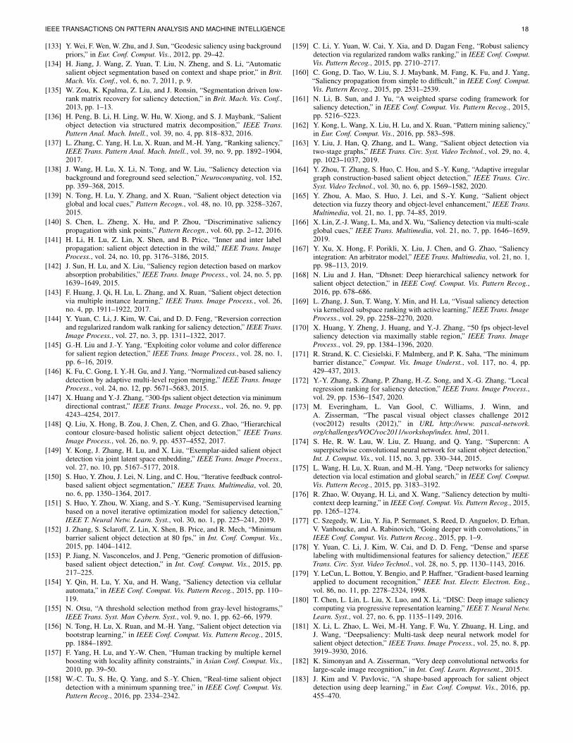
IEEE TRANSACTIONS ON PATTERN ANALYSIS AND MACHINE INTELLIGENCE 18

[133] Y. Wei, F. Wen, W. Zhu, and J. Sun, “Geodesic saliency using backgroundpriors,” in Eur. Conf. Comput. Vis., 2012, pp. 29–42.

[134] H. Jiang, J. Wang, Z. Yuan, T. Liu, N. Zheng, and S. Li, “Automaticsalient object segmentation based on context and shape prior,” in Brit.Mach. Vis. Conf., vol. 6, no. 7, 2011, p. 9.

[135] W. Zou, K. Kpalma, Z. Liu, and J. Ronsin, “Segmentation driven low-rank matrix recovery for saliency detection,” in Brit. Mach. Vis. Conf.,2013, pp. 1–13.

[136] H. Peng, B. Li, H. Ling, W. Hu, W. Xiong, and S. J. Maybank, “Salientobject detection via structured matrix decomposition,” IEEE Trans.Pattern Anal. Mach. Intell., vol. 39, no. 4, pp. 818–832, 2016.

[137] L. Zhang, C. Yang, H. Lu, X. Ruan, and M.-H. Yang, “Ranking saliency,”IEEE Trans. Pattern Anal. Mach. Intell., vol. 39, no. 9, pp. 1892–1904,2017.

[138] J. Wang, H. Lu, X. Li, N. Tong, and W. Liu, “Saliency detection viabackground and foreground seed selection,” Neurocomputing, vol. 152,pp. 359–368, 2015.

[139] N. Tong, H. Lu, Y. Zhang, and X. Ruan, “Salient object detection viaglobal and local cues,” Pattern Recogn., vol. 48, no. 10, pp. 3258–3267,2015.

[140] S. Chen, L. Zheng, X. Hu, and P. Zhou, “Discriminative saliencypropagation with sink points,” Pattern Recogn., vol. 60, pp. 2–12, 2016.

[141] H. Li, H. Lu, Z. Lin, X. Shen, and B. Price, “Inner and inter labelpropagation: salient object detection in the wild,” IEEE Trans. ImageProcess., vol. 24, no. 10, pp. 3176–3186, 2015.

[142] J. Sun, H. Lu, and X. Liu, “Saliency region detection based on markovabsorption probabilities,” IEEE Trans. Image Process., vol. 24, no. 5, pp.1639–1649, 2015.

[143] F. Huang, J. Qi, H. Lu, L. Zhang, and X. Ruan, “Salient object detectionvia multiple instance learning,” IEEE Trans. Image Process., vol. 26,no. 4, pp. 1911–1922, 2017.

[144] Y. Yuan, C. Li, J. Kim, W. Cai, and D. D. Feng, “Reversion correctionand regularized random walk ranking for saliency detection,” IEEE Trans.Image Process., vol. 27, no. 3, pp. 1311–1322, 2017.

[145] G.-H. Liu and J.-Y. Yang, “Exploiting color volume and color differencefor salient region detection,” IEEE Trans. Image Process., vol. 28, no. 1,pp. 6–16, 2019.

[146] K. Fu, C. Gong, I. Y.-H. Gu, and J. Yang, “Normalized cut-based saliencydetection by adaptive multi-level region merging,” IEEE Trans. ImageProcess., vol. 24, no. 12, pp. 5671–5683, 2015.

[147] X. Huang and Y.-J. Zhang, “300-fps salient object detection via minimumdirectional contrast,” IEEE Trans. Image Process., vol. 26, no. 9, pp.4243–4254, 2017.

[148] Q. Liu, X. Hong, B. Zou, J. Chen, Z. Chen, and G. Zhao, “Hierarchicalcontour closure-based holistic salient object detection,” IEEE Trans.Image Process., vol. 26, no. 9, pp. 4537–4552, 2017.

[149] Y. Kong, J. Zhang, H. Lu, and X. Liu, “Exemplar-aided salient objectdetection via joint latent space embedding,” IEEE Trans. Image Process.,vol. 27, no. 10, pp. 5167–5177, 2018.

[150] S. Huo, Y. Zhou, J. Lei, N. Ling, and C. Hou, “Iterative feedback control-based salient object segmentation,” IEEE Trans. Multimedia, vol. 20,no. 6, pp. 1350–1364, 2017.

[151] S. Huo, Y. Zhou, W. Xiang, and S.-Y. Kung, “Semisupervised learningbased on a novel iterative optimization model for saliency detection,”IEEE T. Neural Netw. Learn. Syst., vol. 30, no. 1, pp. 225–241, 2019.

[152] J. Zhang, S. Sclaroff, Z. Lin, X. Shen, B. Price, and R. Mech, “Minimumbarrier salient object detection at 80 fps,” in Int. Conf. Comput. Vis.,2015, pp. 1404–1412.

[153] P. Jiang, N. Vasconcelos, and J. Peng, “Generic promotion of diffusion-based salient object detection,” in Int. Conf. Comput. Vis., 2015, pp.217–225.

[154] Y. Qin, H. Lu, Y. Xu, and H. Wang, “Saliency detection via cellularautomata,” in IEEE Conf. Comput. Vis. Pattern Recog., 2015, pp. 110–119.

[155] N. Otsu, “A threshold selection method from gray-level histograms,”IEEE Trans. Syst. Man Cybern. Syst., vol. 9, no. 1, pp. 62–66, 1979.

[156] N. Tong, H. Lu, X. Ruan, and M.-H. Yang, “Salient object detection viabootstrap learning,” in IEEE Conf. Comput. Vis. Pattern Recog., 2015,pp. 1884–1892.

[157] F. Yang, H. Lu, and Y.-W. Chen, “Human tracking by multiple kernelboosting with locality affinity constraints,” in Asian Conf. Comput. Vis.,2010, pp. 39–50.

[158] W.-C. Tu, S. He, Q. Yang, and S.-Y. Chien, “Real-time salient objectdetection with a minimum spanning tree,” in IEEE Conf. Comput. Vis.Pattern Recog., 2016, pp. 2334–2342.

[159] C. Li, Y. Yuan, W. Cai, Y. Xia, and D. Dagan Feng, “Robust saliencydetection via regularized random walks ranking,” in IEEE Conf. Comput.Vis. Pattern Recog., 2015, pp. 2710–2717.

[160] C. Gong, D. Tao, W. Liu, S. J. Maybank, M. Fang, K. Fu, and J. Yang,“Saliency propagation from simple to difficult,” in IEEE Conf. Comput.Vis. Pattern Recog., 2015, pp. 2531–2539.

[161] N. Li, B. Sun, and J. Yu, “A weighted sparse coding framework forsaliency detection,” in IEEE Conf. Comput. Vis. Pattern Recog., 2015,pp. 5216–5223.

[162] Y. Kong, L. Wang, X. Liu, H. Lu, and X. Ruan, “Pattern mining saliency,”in Eur. Conf. Comput. Vis., 2016, pp. 583–598.

[163] Y. Liu, J. Han, Q. Zhang, and L. Wang, “Salient object detection viatwo-stage graphs,” IEEE Trans. Circ. Syst. Video Technol., vol. 29, no. 4,pp. 1023–1037, 2019.

[164] Y. Zhou, T. Zhang, S. Huo, C. Hou, and S.-Y. Kung, “Adaptive irregulargraph construction-based salient object detection,” IEEE Trans. Circ.Syst. Video Technol., vol. 30, no. 6, pp. 1569–1582, 2020.

[165] Y. Zhou, A. Mao, S. Huo, J. Lei, and S.-Y. Kung, “Salient objectdetection via fuzzy theory and object-level enhancement,” IEEE Trans.Multimedia, vol. 21, no. 1, pp. 74–85, 2019.

[166] X. Lin, Z.-J. Wang, L. Ma, and X. Wu, “Saliency detection via multi-scaleglobal cues,” IEEE Trans. Multimedia, vol. 21, no. 7, pp. 1646–1659,2019.

[167] Y. Xu, X. Hong, F. Porikli, X. Liu, J. Chen, and G. Zhao, “Saliencyintegration: An arbitrator model,” IEEE Trans. Multimedia, vol. 21, no. 1,pp. 98–113, 2019.

[168] N. Liu and J. Han, “Dhsnet: Deep hierarchical saliency network forsalient object detection,” in IEEE Conf. Comput. Vis. Pattern Recog.,2016, pp. 678–686.

[169] L. Zhang, J. Sun, T. Wang, Y. Min, and H. Lu, “Visual saliency detectionvia kernelized subspace ranking with active learning,” IEEE Trans. ImageProcess., vol. 29, pp. 2258–2270, 2020.

[170] X. Huang, Y. Zheng, J. Huang, and Y.-J. Zhang, “50 fps object-levelsaliency detection via maximally stable region,” IEEE Trans. ImageProcess., vol. 29, pp. 1384–1396, 2020.

[171] R. Strand, K. C. Ciesielski, F. Malmberg, and P. K. Saha, “The minimumbarrier distance,” Comput. Vis. Image Underst., vol. 117, no. 4, pp.429–437, 2013.

[172] Y.-Y. Zhang, S. Zhang, P. Zhang, H.-Z. Song, and X.-G. Zhang, “Localregression ranking for saliency detection,” IEEE Trans. Image Process.,vol. 29, pp. 1536–1547, 2020.

[173] M. Everingham, L. Van Gool, C. Williams, J. Winn, andA. Zisserman, “The pascal visual object classes challenge 2012(voc2012) results (2012),” in URL http://www. pascal-network.org/challenges/VOC/voc2011/workshop/index. html, 2011.

[174] S. He, R. W. Lau, W. Liu, Z. Huang, and Q. Yang, “Supercnn: Asuperpixelwise convolutional neural network for salient object detection,”Int. J. Comput. Vis., vol. 115, no. 3, pp. 330–344, 2015.

[175] L. Wang, H. Lu, X. Ruan, and M.-H. Yang, “Deep networks for saliencydetection via local estimation and global search,” in IEEE Conf. Comput.Vis. Pattern Recog., 2015, pp. 3183–3192.

[176] R. Zhao, W. Ouyang, H. Li, and X. Wang, “Saliency detection by multi-context deep learning,” in IEEE Conf. Comput. Vis. Pattern Recog., 2015,pp. 1265–1274.

[177] C. Szegedy, W. Liu, Y. Jia, P. Sermanet, S. Reed, D. Anguelov, D. Erhan,V. Vanhoucke, and A. Rabinovich, “Going deeper with convolutions,” inIEEE Conf. Comput. Vis. Pattern Recog., 2015, pp. 1–9.

[178] Y. Yuan, C. Li, J. Kim, W. Cai, and D. D. Feng, “Dense and sparselabeling with multidimensional features for saliency detection,” IEEETrans. Circ. Syst. Video Technol., vol. 28, no. 5, pp. 1130–1143, 2016.

[179] Y. LeCun, L. Bottou, Y. Bengio, and P. Haffner, “Gradient-based learningapplied to document recognition,” IEEE Inst. Electr. Electron. Eng.,vol. 86, no. 11, pp. 2278–2324, 1998.

[180] T. Chen, L. Lin, L. Liu, X. Luo, and X. Li, “DISC: Deep image saliencycomputing via progressive representation learning,” IEEE T. Neural Netw.Learn. Syst., vol. 27, no. 6, pp. 1135–1149, 2016.

[181] X. Li, L. Zhao, L. Wei, M.-H. Yang, F. Wu, Y. Zhuang, H. Ling, andJ. Wang, “Deepsaliency: Multi-task deep neural network model forsalient object detection,” IEEE Trans. Image Process., vol. 25, no. 8, pp.3919–3930, 2016.

[182] K. Simonyan and A. Zisserman, “Very deep convolutional networks forlarge-scale image recognition,” in Int. Conf. Learn. Represent., 2015.

[183] J. Kim and V. Pavlovic, “A shape-based approach for salient objectdetection using deep learning,” in Eur. Conf. Comput. Vis., 2016, pp.455–470.

IEEE TRANSACTIONS ON PATTERN ANALYSIS AND MACHINE INTELLIGENCE 19

[184] A. Krizhevsky, S. Ilya, and G. E Hinton, “Imagenet classification withdeep convolutional neural networks,” in Adv. Neural Inform. Process.Syst., 2012.

[185] Y. Tang and X. Wu, “Saliency detection via combining region-level andpixel-level predictions with cnns,” in Eur. Conf. Comput. Vis., 2016, pp.809–825.

[186] L. Wang, L. Wang, H. Lu, P. Zhang, and X. Ruan, “Saliency detectionwith recurrent fully convolutional networks,” in Eur. Conf. Comput. Vis.,2016, pp. 825–841.

[187] J. Zhang, S. Sclaroff, Z. Lin, X. Shen, B. Price, and R. Mech,“Unconstrained salient object detection via proposal subset optimization,”in IEEE Conf. Comput. Vis. Pattern Recog., 2016, pp. 5733–5742.

[188] S. S. Kruthiventi, V. Gudisa, J. H. Dholakiya, and R. Venkatesh Babu,“Saliency unified: A deep architecture for simultaneous eye fixationprediction and salient object segmentation,” in IEEE Conf. Comput. Vis.Pattern Recog., 2016, pp. 5781–5790.

[189] M. Jiang, S. Huang, J. Duan, and Q. Zhao, “SALICON: Saliency incontext,” in IEEE Conf. Comput. Vis. Pattern Recog., 2015, pp. 1072–1080.

[190] J. Kuen, Z. Wang, and G. Wang, “Recurrent attentional networks forsaliency detection,” in IEEE Conf. Comput. Vis. Pattern Recog., 2016,pp. 3668–3677.

[191] R. Ju, L. Ge, W. Geng, T. Ren, and G. Wu, “Depth saliency basedon anisotropic center-surround difference,” in IEEE Int. Conf. ImageProcess., 2014, pp. 1115–1119.

[192] H. Peng, B. Li, W. Xiong, W. Hu, and R. Ji, “Rgbd salient objectdetection: a benchmark and algorithms,” in Eur. Conf. Comput. Vis.,2014, pp. 92–109.

[193] G. Lee, Y.-W. Tai, and J. Kim, “Deep saliency with encoded low leveldistance map and high level features,” in IEEE Conf. Comput. Vis. PatternRecog., 2016, pp. 660–668.

[194] G. Li and Y. Yu, “Deep contrast learning for salient object detection,” inIEEE Conf. Comput. Vis. Pattern Recog., 2016, pp. 478–487.

[195] P. Hu, B. Shuai, J. Liu, and G. Wang, “Deep level sets for salientobject detection,” in IEEE Conf. Comput. Vis. Pattern Recog., 2017, pp.2300–2309.

[196] T. Wang, A. Borji, L. Zhang, P. Zhang, and H. Lu, “A stagewiserefinement model for detecting salient objects in images,” in IEEEConf. Comput. Vis. Pattern Recog., 2017, pp. 4019–4028.

[197] K. He, X. Zhang, S. Ren, and J. Sun, “Deep residual learning for imagerecognition,” in IEEE Conf. Comput. Vis. Pattern Recog., 2016, pp.770–778.

[198] Z. Luo, A. Mishra, A. Achkar, J. Eichel, S. Li, and P.-M. Jodoin, “Non-local deep features for salient object detection,” in IEEE Conf. Comput.Vis. Pattern Recog., 2017, pp. 6609–6617.

[199] J. Deng, W. Dong, R. Socher, L.-J. Li, K. Li, and L. Fei-Fei, “Imagenet:A large-scale hierarchical image database,” in IEEE Conf. Comput. Vis.Pattern Recog., 2009, pp. 248–255.

[200] Q. Hou, M.-M. Cheng, X. Hu, A. Borji, Z. Tu, and P. H. Torr, “Deeplysupervised salient object detection with short connections,” in IEEE Conf.Comput. Vis. Pattern Recog., 2017, pp. 3203–3212.

[201] X. Chen, A. Zheng, J. Li, and F. Lu, “Look, perceive and segment:Finding the salient objects in images via two-stream fixation-semanticcnns,” in Int. Conf. Comput. Vis., 2017, pp. 1050–1058.

[202] D. Zhang, J. Han, and Y. Zhang, “Supervision by fusion: Towardsunsupervised learning of deep salient object detector,” in Int. Conf.Comput. Vis., 2017, pp. 4048–4056.

[203] P. Zhang, D. Wang, H. Lu, H. Wang, and B. Yin, “Learning uncertainconvolutional features for accurate saliency detection,” in Int. Conf.Comput. Vis., 2017, pp. 212–221.

[204] P. Zhang, D. Wang, H. Lu, H. Wang, and X. Ruan, “Amulet: Aggregatingmulti-level convolutional features for salient object detection,” in Int.Conf. Comput. Vis., 2017, pp. 202–211.

[205] S. Chen, B. Wang, X. Tan, and X. Hu, “Embedding attention and residualnetwork for accurate salient object detection,” IEEE Trans. Cybern.,2018.

[206] K. Fu, Q. Zhao, and I. Y.-H. Gu, “Refinet: A deep segmentation assistedrefinement network for salient object detection,” IEEE Trans. Multimedia,vol. 21, no. 2, pp. 457–469, 2018.

[207] C. Cao, Y. Huang, Z. Wang, L. Wang, N. Xu, and T. Tan, “Lateralinhibition-inspired convolutional neural network for visual attention andsaliency detection,” in AAAI Conf. Art. Intell., 2018.

[208] X. Hu, L. Zhu, J. Qin, C.-W. Fu, and P.-A. Heng, “Recurrentlyaggregating deep features for salient object detection,” in AAAI Conf.Art. Intell., 2018.

[209] Z. Deng, X. Hu, L. Zhu, X. Xu, J. Qin, G. Han, and P.-A. Heng, “R3net:Recurrent residual refinement network for saliency detection,” in AAAIConf. Art. Intell., 2018, pp. 684–690.

[210] S. Xie, R. Girshick, P. Dollar, Z. Tu, and K. He, “Aggregated residualtransformations for deep neural networks,” in IEEE Conf. Comput. Vis.Pattern Recog., 2017, pp. 1492–1500.

[211] X. Li, F. Yang, H. Cheng, W. Liu, and D. Shen, “Contour knowledgetransfer for salient object detection,” in Eur. Conf. Comput. Vis., 2018,pp. 355–370.

[212] S. Chen, X. Tan, B. Wang, and X. Hu, “Reverse attention for salientobject detection,” in Eur. Conf. Comput. Vis., 2018, pp. 234–250.

[213] Y. Zeng, H. Lu, L. Zhang, M. Feng, and A. Borji, “Learning to promotesaliency detectors,” in IEEE Conf. Comput. Vis. Pattern Recog., 2018,pp. 1644–1653.

[214] M. Amirul Islam, M. Kalash, and N. D. Bruce, “Revisiting salient objectdetection: Simultaneous detection, ranking, and subitizing of multiplesalient objects,” in IEEE Conf. Comput. Vis. Pattern Recog., 2018, pp.7142–7150.

[215] W. Wang, J. Shen, X. Dong, and A. Borji, “Salient object detection drivenby fixation prediction,” in IEEE Conf. Comput. Vis. Pattern Recog., 2018,pp. 1711–1720.

[216] L. Zhang, J. Dai, H. Lu, Y. He, and G. Wang, “A bi-directional messagepassing model for salient object detection,” in IEEE Conf. Comput. Vis.Pattern Recog., 2018, pp. 1741–1750.

[217] T. Wang, L. Zhang, S. Wang, H. Lu, G. Yang, X. Ruan, and A. Borji,“Detect globally, refine locally: A novel approach to saliency detection,”in IEEE Conf. Comput. Vis. Pattern Recog., 2018, pp. 3127–3135.

[218] N. Liu, J. Han, and M.-H. Yang, “Picanet: Learning pixel-wise contextualattention for saliency detection,” in IEEE Conf. Comput. Vis. PatternRecog., 2018, pp. 3089–3098.

[219] X. Zhang, T. Wang, J. Qi, H. Lu, and G. Wang, “Progressive attentionguided recurrent network for salient object detection,” in IEEE Conf.Comput. Vis. Pattern Recog., 2018, pp. 714–722.

[220] S. Zhou, J. Wang, F. Wang, and D. Huang, “Se2net: Siamese edge-enhancement network for salient object detection,” arXiv preprintarXiv:1904.00048, 2019.

[221] Z. Li, C. Lang, Y. Chen, J. Liew, and J. Feng, “Deep reasoningwith multi-scale context for salient object detection,” arXiv preprintarXiv:1901.08362, 2019.

[222] S. Jia and N. D. Bruce, “Richer and deeper supervision network forsalient object detection,” arXiv preprint arXiv:1901.02425, 2019.

[223] L. Zhu, J. Chen, X. Hu, C.-W. Fu, X. Xu, J. Qin, and P.-A. Heng,“Aggregating attentional dilated features for salient object detection,”IEEE Trans. Circ. Syst. Video Technol., vol. 30, no. 10, pp. 3358–3371,2019.

[224] G. Huang, Z. Liu, L. Van Der Maaten, and K. Q. Weinberger, “Denselyconnected convolutional networks,” in IEEE Conf. Comput. Vis. PatternRecog., 2017, pp. 4700–4708.

[225] Y. Tang and X. Wu, “Salient object detection using cascaded convolu-tional neural networks and adversarial learning,” IEEE Trans. Multimedia,vol. 21, no. 9, pp. 2237–2247, 2019.

[226] L.-C. Chen, G. Papandreou, I. Kokkinos, K. Murphy, and A. L. Yuille,“Deeplab: Semantic image segmentation with deep convolutional nets,atrous convolution, and fully connected crfs,” IEEE Trans. Pattern Anal.Mach. Intell., vol. 40, no. 4, pp. 834–848, 2018.

[227] Y. Wang, X. Zhao, X. Hu, Y. Li, and K. Huang, “Focal boundary guidedsalient object detection,” IEEE Trans. Image Process., vol. 28, no. 6, pp.2813–2824, 2019.

[228] T. V. Nguyen, K. Nguyen, and T.-T. Do, “Semantic prior analysis forsalient object detection,” IEEE Trans. Image Process., vol. 28, no. 6, pp.3130–3141, 2019.

[229] M. Kampffmeyer, N. Dong, X. Liang, Y. Zhang, and E. P. Xing,“Connnet: A long-range relation-aware pixel-connectivity network forsalient segmentation,” IEEE Trans. Image Process., vol. 28, no. 5, pp.2518–2529, 2019.

[230] P. Zhang, W. Liu, H. Lu, and C. Shen, “Salient object detection withlossless feature reflection and weighted structural loss,” IEEE Trans.Image Process., vol. 28, no. 6, pp. 3048–3060, 2019.

[231] D. Zhang, J. Han, Y. Zhang, and D. Xu, “Synthesizing supervision forlearning deep saliency network without human annotation,” IEEE Trans.Pattern Anal. Mach. Intell., vol. 42, no. 7, pp. 1755–1769, 2019.

[232] C. Li, R. Cong, J. Hou, S. Zhang, Y. Qian, and S. Kwong, “Nestednetwork with two-stream pyramid for salient object detection in opticalremote sensing images,” IEEE Trans. Geosci. Remote. Sens., vol. 57,no. 11, pp. 9156–9166, 2019.

IEEE TRANSACTIONS ON PATTERN ANALYSIS AND MACHINE INTELLIGENCE 20

[233] K. Fu, Q. Zhao, I. Y.-H. Gu, and J. Yang, “Deepside: A general deepframework for salient object detection,” Neurocomputing, vol. 356, pp.69–82, 2019.

[234] B. Li, Z. Sun, and Y. Guo, “Supervae: Superpixelwise variationalautoencoder for salient object detection,” in AAAI Conf. Art. Intell.,vol. 33, no. 01, 2019, pp. 8569–8576.

[235] Y. Zhuge, Y. Zeng, and H. Lu, “Deep embedding features for salientobject detection,” in AAAI Conf. Art. Intell., 2019.

[236] Y. Zeng, Y. Zhuge, H. Lu, L. Zhang, M. Qian, and Y. Yu, “Multi-sourceweak supervision for saliency detection,” in IEEE Conf. Comput. Vis.Pattern Recog., 2019, pp. 6074–6083.

[237] R. Wu, M. Feng, W. Guan, D. Wang, H. Lu, and E. Ding, “A mutuallearning method for salient object detection with intertwined multi-supervision,” in IEEE Conf. Comput. Vis. Pattern Recog., 2019, pp.8150–8159.

[238] W. Wang, J. Shen, M.-M. Cheng, and L. Shao, “An iterative andcooperative top-down and bottom-up inference network for salient objectdetection,” in IEEE Conf. Comput. Vis. Pattern Recog., 2019, pp. 5968–5977.

[239] M. Feng, H. Lu, and E. Ding, “Attentive feedback network for boundary-aware salient object detection,” in IEEE Conf. Comput. Vis. PatternRecog., 2019, pp. 1623–1632.

[240] T. Zhao and X. Wu, “Pyramid feature attention network for saliencydetection,” in IEEE Conf. Comput. Vis. Pattern Recog., 2019, pp. 3085–3094.

[241] W. Wang, S. Zhao, J. Shen, S. C. Hoi, and A. Borji, “Salient objectdetection with pyramid attention and salient edges,” in IEEE Conf.Comput. Vis. Pattern Recog., 2019, pp. 1448–1457.

[242] Z. Wu, L. Su, and Q. Huang, “Cascaded partial decoder for fast andaccurate salient object detection,” in IEEE Conf. Comput. Vis. PatternRecog., 2019, pp. 3907–3916.

[243] J.-J. Liu, Q. Hou, M.-M. Cheng, J. Feng, and J. Jiang, “A simplepooling-based design for real-time salient object detection,” in IEEEConf. Comput. Vis. Pattern Recog., 2019, pp. 3917–3926.

[244] X. Qin, Z. Zhang, C. Huang, C. Gao, M. Dehghan, and M. Jagersand,“BASNet: Boundary-Aware Salient Object Detection,” in IEEE Conf.Comput. Vis. Pattern Recog., 2019, pp. 7479–7489.

[245] G. Xavier and B. Yoshua, “Understanding the difficulty of training deepfeedforward neural networks,” in Int. Conf. Artif. Intell. Stat., 2010, pp.249–256.

[246] Y. Xu, D. Xu, X. Hong, W. Ouyang, R. Ji, M. Xu, and G. Zhao,“Structured modeling of joint deep feature and prediction refinement forsalient object detection,” in Int. Conf. Comput. Vis., 2019, pp. 3789–3798.

[247] Y. Liu, Q. Zhang, D. Zhang, and J. Han, “Employing deep part-objectrelationships for salient object detection,” in Int. Conf. Comput. Vis.,2019, pp. 1232–1241.

[248] Y. Zeng, Y. Zhuge, H. Lu, and L. Zhang, “Joint learning of saliencydetection and weakly supervised semantic segmentation,” in Int. Conf.Comput. Vis., 2019, pp. 7223–7233.

[249] J. Su, J. Li, Y. Zhang, C. Xia, and Y. Tian, “Selectivity or invariance:Boundary-aware salient object detection,” in Int. Conf. Comput. Vis.,2019, pp. 3799–3808.

[250] J.-X. Zhao, J.-J. Liu, D.-P. Fan, Y. Cao, J. Yang, and M.-M. Cheng,“Egnet: Edge guidance network for salient object detection,” in Int. Conf.Comput. Vis., 2019, pp. 8779–8788.

[251] S. Zhou, J. Wang, J. Zhang, L. Wang, D. Huang, S. Du, and N. Zheng,“Hierarchical u-shape attention network for salient object detection,”IEEE Trans. Image Process., vol. 29, pp. 8417–8428, 2020.

[252] Y. Cai, L. Dai, H. Wang, L. Chen, and Y. Li, “A novel saliency detectionalgorithm based on adversarial learning model,” IEEE Trans. ImageProcess., vol. 29, pp. 4489–4504, 2020.

[253] X. Li, D. Song, and Y. Dong, “Hierarchical feature fusion networkfor salient object detection,” IEEE Trans. Image Process., vol. 29, pp.9165–9175, 2020.

[254] J.-J. Liu, Q. Hou, and M.-M. Cheng, “Dynamic feature integration forsimultaneous detection of salient object, edge, and skeleton,” IEEE Trans.Image Process., vol. 29, pp. 8652–8667, 2020.

[255] M. Feng, H. Lu, and Y. Yu, “Residual learning for salient objectdetection,” IEEE Trans. Image Process., vol. 29, pp. 4696–4708, 2020.

[256] L. Zhang, J. Wu, T. Wang, A. Borji, G. Wei, and H. Lu, “A multistagerefinement network for salient object detection,” IEEE Trans. ImageProcess., vol. 29, pp. 3534–3545, 2020.

[257] Y. Liu, J. Han, Q. Zhang, and C. Shan, “Deep salient object detectionwith contextual information guidance,” IEEE Trans. Image Process.,vol. 29, pp. 360–374, 2020.

[258] S. Chen, X. Tan, B. Wang, H. Lu, X. Hu, and Y. Fu, “Reverse attention-based residual network for salient object detection,” IEEE Trans. ImageProcess., vol. 29, pp. 3763–3776, 2020.

[259] W. Wang, J. Shen, X. Dong, A. Borji, and R. Yang, “Inferring salientobjects from human fixations,” IEEE Trans. Pattern Anal. Mach. Intell.,vol. 42, no. 8, pp. 1913–1927, 2020.

[260] H. Li, G. Li, B. Yang, G. Chen, L. Lin, and Y. Yu, “Depthwise nonlocalmodule for fast salient object detection using a single thread,” IEEETrans. Cybern., 2020.

[261] J. Li, Z. Pan, Q. Liu, Y. Cui, and Y. Sun, “Complementarity-awareattention network for salient object detection,” IEEE Trans. Cybern.,2020.

[262] H. Li, G. Li, and Y. Yu, “Rosa: Robust salient object detection againstadversarial attacks,” IEEE Trans. Cybern., vol. 50, no. 11, pp. 4835–4847,2019.

[263] J. Long, E. Shelhamer, and T. Darrell, “Fully convolutional networksfor semantic segmentation,” in IEEE Conf. Comput. Vis. Pattern Recog.,2015, pp. 3431–3440.

[264] L. Wang, R. Chen, L. Zhu, H. Xie, and X. Li, “Deep sub-region networkfor salient object detection,” IEEE Trans. Circ. Syst. Video Technol.,2020.

[265] Z. Tu, Y. Ma, C. Li, J. Tang, and B. Luo, “Edge-guided non-local fullyconvolutional network for salient object detection,” IEEE Trans. Circ.Syst. Video Technol., 2020.

[266] X. Hu, C.-W. Fu, L. Zhu, T. Wang, and P.-A. Heng, “Sac-net: Spatialattenuation context for salient object detection,” IEEE Trans. Circ. Syst.Video Technol., 2020.

[267] Q. Ren, S. Lu, J. Zhang, and R. Hu, “Salient object detection by fusinglocal and global contexts,” IEEE Trans. Multimedia, 2020.

[268] Z. Wu, S. Li, C. Chen, A. Hao, and H. Qin, “A deeper look at imagesalient object detection: Bi-stream network with a small training dataset,”IEEE Trans. Multimedia, 2020.

[269] J. Li, Z. Pan, Q. Liu, and Z. Wang, “Stacked u-shape networkwith channel-wise attention for salient object detection,” IEEE Trans.Multimedia, 2020.

[270] G. Ma, C. Chen, S. Li, C. Peng, A. Hao, and H. Qin, “Salientobject detection via multiple instance joint re-learning,” IEEE Trans.Multimedia, vol. 22, no. 2, pp. 324–336, 2020.

[271] S. Mohammadi, M. Noori, A. Bahri, S. G. Majelan, and M. Havaei,“Cagnet: Content-aware guidance for salient object detection,” PatternRecogn., vol. 103, p. 107303, 2020.

[272] B. Zoph, V. Vasudevan, J. Shlens, and Q. V. Le, “Learning transferablearchitectures for scalable image recognition,” in IEEE Conf. Comput. Vis.Pattern Recog., 2018, pp. 8697–8710.

[273] X. Qin, Z. Zhang, C. Huang, M. Dehghan, O. R. Zaiane, and M. Jager-sand, “U2-net: Going deeper with nested u-structure for salient objectdetection,” Pattern Recogn., vol. 106, p. 107404, 2020.

[274] C. Wang, S. Dong, X. Zhao, G. Papanastasiou, H. Zhang, and G. Yang,“Saliencygan: Deep learning semisupervised salient object detection inthe fog of iot,” IEEE Trans. Industr. Inform., vol. 16, no. 4, pp. 2667–2676, 2020.

[275] S. Song, H. Yu, Z. Miao, J. Fang, K. Zheng, C. Ma, and S. Wang,“Multi-spectral salient object detection by adversarial domain adaptation,”in AAAI Conf. Art. Intell., vol. 34, no. 07, 2020, pp. 12 023–12 030.

[276] B. Wang, Q. Chen, M. Zhou, Z. Zhang, X. Jin, and K. Gai, “Progressivefeature polishing network for salient object detection,” in AAAI Conf.Art. Intell., vol. 34, no. 07, 2020, pp. 12 128–12 135.

[277] Z. Chen, Q. Xu, R. Cong, and Q. Huang, “Global context-awareprogressive aggregation network for salient object detection,” in AAAIConf. Art. Intell., vol. 34, no. 07, 2020, pp. 10 599–10 606.

[278] J. Wei, S. Wang, and Q. Huang, “F3net: Fusion, feedback and focus forsalient object detection,” in AAAI Conf. Art. Intell., vol. 34, no. 07, 2020,pp. 12 321–12 328.

[279] J. Wei, S. Wang, Z. Wu, C. Su, Q. Huang, and Q. Tian, “Label decouplingframework for salient object detection,” in IEEE Conf. Comput. Vis.Pattern Recog., 2020, pp. 13 025–13 034.

[280] H. Zhou, X. Xie, J.-H. Lai, Z. Chen, and L. Yang, “Interactive two-streamdecoder for accurate and fast saliency detection,” in IEEE Conf. Comput.Vis. Pattern Recog., 2020, pp. 9141–9150.

[281] Y. Pang, X. Zhao, L. Zhang, and H. Lu, “Multi-scale interactive networkfor salient object detection,” in IEEE Conf. Comput. Vis. Pattern Recog.,2020, pp. 9413–9422.

[282] J. Zhang, J. Xie, and N. Barnes, “Learning noise-aware encoder-decoderfrom noisy labels by alternating back-propagation for saliency detection,”in Eur. Conf. Comput. Vis., 2020.

IEEE TRANSACTIONS ON PATTERN ANALYSIS AND MACHINE INTELLIGENCE 21

[283] S.-H. Gao, Y.-Q. Tan, M.-M. Cheng, C. Lu, Y. Chen, and S. Yan, “Highlyefficient salient object detection with 100k parameters,” in Eur. Conf.Comput. Vis., 2020, pp. 702–721.

[284] X. Zhao, Y. Pang, L. Zhang, H. Lu, and L. Zhang, “Suppress andbalance: A simple gated network for salient object detection,” in Eur.Conf. Comput. Vis., 2020, pp. 35–51.

[285] Y. Liu, M.-M. Cheng, X. Zhang, G.-Y. Nie, and M. Wang, “Dna: Deeply-supervised nonlinear aggregation for salient object detection,” IEEETrans. Cybern., 2021.

[286] Z. Chen, H. Zhou, J. Lai, L. Yang, and X. Xie, “Contour-aware loss:Boundary-aware learning for salient object segmentation,” IEEE Trans.Image Process., vol. 30, pp. 431–443, 2020.

[287] S. Zhou, J. Wang, L. Wang, J. Zhang, F. Wang, D. Huang, and N. Zheng,“Hierarchical and interactive refinement network for edge-preservingsalient object detection,” IEEE Trans. Image Process., vol. 30, pp. 1–14,2020.

[288] S. Yu, B. Zhang, J. Xiao, and E. G. Lim, “Structure-consistent weaklysupervised salient object detection with local saliency coherence,” inAAAI Conf. Art. Intell., 2021.

[289] M. Ma, C. Xia, and J. Li, “Pyramidal feature shrinking for salient objectdetection,” in AAAI Conf. Art. Intell., 2021.

[290] B. Xu, H. Liang, R. Liang, and P. Chen, “Locate globally, segmentlocally: A progressive architecture with knowledge review network forsalient object detection,” in AAAI Conf. Art. Intell., 2021.

[291] S.-H. Gao, M.-M. Cheng, K. Zhao, X.-Y. Zhang, M.-H. Yang, and P. Torr,“Res2net: A new multi-scale backbone architecture,” IEEE Trans. PatternAnal. Mach. Intell., vol. 43, no. 2, pp. 652–662, 2021.

[292] C. Szegedy, V. Vanhoucke, S. Ioffe, J. Shlens, and Z. Wojna, “Rethinkingthe inception architecture for computer vision,” in IEEE Conf. Comput.Vis. Pattern Recog., 2016, pp. 2818–2826.

[293] K. K. Singh and Y. J. Lee, “Hide-and-seek: Forcing a network to bemeticulous for weakly-supervised object and action localization,” in Int.Conf. Comput. Vis., 2017, pp. 3544–3553.

[294] H. Zhang, M. Cisse, Y. N. Dauphin, and D. Lopez-Paz, “mixup: Beyondempirical risk minimization,” in Int. Conf. Learn. Represent., 2017.

[295] Z. Feng, C. Xu, and D. Tao, “Self-supervised representation learning byrotation feature decoupling,” in IEEE Conf. Comput. Vis. Pattern Recog.,2019, pp. 10 364–10 374.

[296] L. Xie, J. Wang, Z. Wei, M. Wang, and Q. Tian, “Disturblabel:Regularizing cnn on the loss layer,” in IEEE Conf. Comput. Vis. PatternRecog., 2016, pp. 4753–4762.

[297] T. Miyato, S.-i. Maeda, M. Koyama, K. Nakae, and S. Ishii, “Distribu-tional smoothing with virtual adversarial training,” in Int. Conf. Learn.Represent., 2016.

[298] S. Thulasidasan, G. Chennupati, J. Bilmes, T. Bhattacharya, andS. Michalak, “On mixup training: Improved calibration and predictiveuncertainty for deep neural networks,” in Adv. Neural Inform. Process.Syst., 2019.

[299] S. Wager, W. Fithian, S. Wang, and P. Liang, “Altitude training: Strongbounds for single-layer dropout,” in Adv. Neural Inform. Process. Syst.,2014, pp. 100–108.

[300] J. C. Peterson, R. M. Battleday, T. L. Griffiths, and O. Russakovsky,“Human uncertainty makes classification more robust,” in Int. Conf.Comput. Vis., 2019, pp. 9617–9626.

[301] Y. Li, G. Hu, Y. Wang, T. M. Hospedales, N. M. obertson, and Y. Yang,“Differentiable automatic data augmentation,” in Eur. Conf. Comput. Vis.,2020, pp. 580–595.

[302] E. D. Cubuk, B. Zoph, D. Mane, V. Vasudevan, and Q. V. Le,“Autoaugment: Learning augmentation strategies from data,” in IEEEConf. Comput. Vis. Pattern Recog., 2019, pp. 113–123.

[303] Y. Wei, J. Feng, X. Liang, M.-M. Cheng, Y. Zhao, and S. Yan, “Objectregion mining with adversarial erasing: A simple classification tosemantic segmentation approach,” in IEEE Conf. Comput. Vis. PatternRecog., 2017, pp. 1568–1576.

[304] Z. Zhong, L. Zheng, G. Kang, S. Li, and Y. Yang, “Random erasingdata augmentation,” in AAAI Conf. Art. Intell., vol. 34, no. 07, 2020, pp.13 001–13 008.

[305] Y.-T. Chang, Q. Wang, W.-C. Hung, R. Piramuthu, Y.-H. Tsai, andM.-H. Yang, “Mixup-cam: Weakly-supervised semantic segmentationvia uncertainty regularization,” in Brit. Mach. Vis. Conf., 2020.

[306] H. Guo, Y. Mao, and R. Zhang, “Mixup as locally linear out-of-manifoldregularization,” in AAAI Conf. Art. Intell., vol. 33, 2019, pp. 3714–3722.

[307] S. Gidaris, P. Singh, and N. Komodakis, “Unsupervised representationlearning by predicting image rotations,” in Int. Conf. Learn. Represent.,2018.

[308] X. Zhai, A. Oliver, A. Kolesnikov, and L. Beyer, “S4l: Self-supervisedsemi-supervised learning,” in Int. Conf. Comput. Vis., 2019, pp. 1476–1485.

[309] X. Chen, S. Xie, and K. He, “An empirical study of training self-supervised visual transformers,” arXiv preprint arXiv:2104.02057, 2021.

[310] X. Wang, K. He, and A. Gupta, “Transitive invariance for self-supervisedvisual representation learning,” in Int. Conf. Comput. Vis., 2017, pp.1329–1338.

[311] K. He, H. Fan, Y. Wu, S. Xie, and R. Girshick, “Momentum contrast forunsupervised visual representation learning,” in IEEE Conf. Comput. Vis.Pattern Recog., 2020, pp. 9729–9738.

[312] H. Caesar, J. Uijlings, and V. Ferrari, “Coco-stuff: Thing and stuffclasses in context,” in IEEE Conf. Comput. Vis. Pattern Recog., 2018, pp.1209–1218.

[313] S. Lazebnik, C. Schmid, and J. Ponce, “A sparse texture representationusing local affine regions,” IEEE Trans. Pattern Anal. Mach. Intell.,vol. 27, no. 8, pp. 1265–1278, 2005.

[314] T. Judd, F. Durand, and A. Torralba, “A benchmark of computationalmodels of saliency to predict human fixations,” in MIT Technical Report,2012.

[315] F. Perazzi, J. Pont-Tuset, B. McWilliams, L. Van Gool, M. Gross, andA. Sorkine-Hornung, “A benchmark dataset and evaluation methodologyfor video object segmentation,” in IEEE Conf. Comput. Vis. PatternRecog., 2016, pp. 724–732.

[316] Q. Hou, M.-M. Cheng, X. Hu, A. Borji, Z. Tu, and P. Torr, “Deeplysupervised salient object detection with short connections,” IEEE Trans.Pattern Anal. Mach. Intell., vol. 41, no. 4, pp. 815–828, 2019.

[317] L. Yuan, F. E. Tay, G. Li, T. Wang, and J. Feng, “Revisiting knowledgedistillation via label smoothing regularization,” in IEEE Conf. Comput.Vis. Pattern Recog., 2020, pp. 3903–3911.

[318] G. Hinton, O. Vinyals, and J. Dean, “Distilling the knowledge in a neuralnetwork,” in Adv. Neural Inform. Process. Syst. Worksh., 2015.

[319] C.-B. Zhang, P.-T. Jiang, Q. Hou, Y. Wei, Q. Han, Z. Li, andM.-M. Cheng, “Delving deep into label smoothing,” arXiv preprintarXiv:2011.12562, 2020.

[320] C. Godard, O. Mac Aodha, and G. J. Brostow, “Unsupervised monoculardepth estimation with left-right consistency,” in IEEE Conf. Comput. Vis.Pattern Recog., 2017, pp. 270–279.

[321] Z. Wang, A. C. Bovik, H. R. Sheikh, and E. P. Simoncelli, “Image qualityassessment: from error visibility to structural similarity,” IEEE Trans.Image Process., vol. 13, no. 4, pp. 600–612, 2004.

[322] K. Fu, D.-P. Fan, G.-P. Ji, Q. Zhao, J. Shen, and C. Zhu, “Siamesenetwork for rgb-d salient object detection and beyond,” IEEE Trans.Pattern Anal. Mach. Intell., 2021.

[323] S. Goferman, L. Zelnik-Manor, and A. Tal, “Context-aware saliencydetection,” IEEE Trans. Pattern Anal. Mach. Intell., vol. 34, no. 10, pp.1915–1926, 2011.

[324] X. Zhu, C. Tang, P. Wang, H. Xu, M. Wang, J. Chen, and J. Tian,“Saliency detection via affinity graph learning and weighted manifoldranking,” Neurocomputing, vol. 312, pp. 239–250, 2018.

[325] C. Tang, P. Wang, C. Zhang, and W. Li, “Salient object detection viaweighted low rank matrix recovery,” IEEE Signal Process. Let., vol. 24,no. 4, pp. 490–494, 2016.

[326] X. Huang and Y. Zhang, “Water flow driven salient object detection at180 fps,” Pattern Recogn., vol. 76, pp. 95–107, 2018.

[327] J. Zhang, D.-P. Fan, Y. Dai, S. Anwar, F. Saleh, S. Aliakbarian, andN. Barnes, “Uncertainty inspired rgb-d saliency detection,” IEEE Trans.Pattern Anal. Mach. Intell., 2021.

[328] J. Zhang, D.-P. Fan, Y. Dai, S. Anwar, F. S. Saleh, T. Zhang, andN. Barnes, “Uc-net: uncertainty inspired rgb-d saliency detection viaconditional variational autoencoders,” in IEEE Conf. Comput. Vis. PatternRecog., 2020, pp. 8582–8591.

[329] C. Guo, G. Pleiss, Y. Sun, and K. Q. Weinberger, “On calibration ofmodern neural networks,” in Int. Conf. Mach. Learn., 2017, pp. 1321–1330.

[330] D.-P. Fan, G.-P. Ji, M.-M. Cheng, and L. Shao, “Concealed objectdetection,” IEEE Trans. Pattern Anal. Mach. Intell., 2021.

[331] K. R. Cave, “Finding meaning in eye movements,” Nat. Hum. Behav.,vol. 1, no. 10, pp. 709–710, 2017.

[332] J. M. Henderson, T. R. Hayes, C. E. Peacock, and G. Rehrig, “Meaningand attentional guidance in scenes: A review of the meaning mapapproach,” Vision, vol. 3, no. 2, p. 19, 2019.

[333] J. M. Henderson and T. R. Hayes, “Meaning-based guidance of attentionin scenes as revealed by meaning maps,” Nat. Hum. Behav., vol. 1, no. 10,pp. 743–747, 2017.

[334] X. Tian, K. Xu, X. Yang, B. Yin, and R. W. Lau, “Weakly-supervisedsalient instance detection,” in Brit. Mach. Vis. Conf., 2020.

IEEE TRANSACTIONS ON PATTERN ANALYSIS AND MACHINE INTELLIGENCE 22

[335] Y.-H. Wu, Y. Liu, L. Zhang, W. Gao, and M.-M. Cheng, “Regularizeddensely-connected pyramid network for salient instance segmentation,”IEEE Trans. Image Process., vol. 30, pp. 3897–3907, 2021.

[336] Y. Liu, D. Zhang, Q. Zhang, and J. Han, “Part-object relational visualsaliency,” IEEE Trans. Pattern Anal. Mach. Intell., 2021.

[337] A. R. Zamir, A. Sax, W. Shen, L. J. Guibas, J. Malik, and S. Savarese,“Taskonomy: Disentangling task transfer learning,” in IEEE Conf.Comput. Vis. Pattern Recog., 2018, pp. 3712–3722.

[338] A. Li, J. Zhang, Y. Lv, B. Liu, T. Zhang, and Y. Dai, “Uncertainty-awarejoint salient object and camouflaged object detection,” in IEEE Conf.Comput. Vis. Pattern Recog., 2021.

[339] M. Zhuge, D. Gao, D.-P. Fan, L. Jin, B. Chen, H. Zhou, M. Qiu, andL. Shao, “Kaleido-bert: Vision-language pre-training on fashion domain,”in IEEE Conf. Comput. Vis. Pattern Recog., 2021.

[340] G. Wang, C. Chen, D.-P. Fan, A. Hao, and H. Qin, “From semanticcategories to fixations: A novel weakly-supervised visual-auditorysaliency detection approach,” in IEEE Conf. Comput. Vis. Pattern Recog.,2021.

[341] D. V. Ruiz, B. A. Krinski, and E. Todt, “Ida: Improved data augmentationapplied to salient object detection,” in 2020 33rd SIBGRAPI Conferenceon Graphics, Patterns and Images (SIBGRAPI), 2020, pp. 210–217.

[342] Y. Liu, X.-Y. Zhang, J.-W. Bian, L. Zhang, and M.-M. Cheng, “Samnet:Stereoscopically attentive multi-scale network for lightweight salientobject detection,” IEEE Trans. Image Process., vol. 30, pp. 3804–3814,2021.

[343] D.-P. Fan, G.-P. Ji, X. Qin, and M.-M. Cheng, “Cognitive vision inspiredobject segmentation metric and loss function,” SCIENTIA SINICAInformationis, 2020.

[344] Y. Mao, J. Zhang, Z. Wan, Y. Dai, A. Li, Y. Lv, X. Tian, D.-P. Fan,and N. Barnes, “Transformer transforms salient object detection andcamouflaged object detection,” arXiv preprint arXiv:2104.10127, 2021.

[345] N. Liu, N. Zhang, K. Wan, J. Han, and L. Shao, “Visual saliencytransformer,” arXiv preprint arXiv:2104.12099, 2021.

[346] H. Zhang, Y. Zeng, H. Lu, L. Zhang, J. Li, and J. Qi, “Learning to detectsalient object with multi-source weak supervision,” IEEE Trans. PatternAnal. Mach. Intell., 2021.

[347] X. Zhao, Y. Pang, L. Zhang, H. Lu, and X. Ruan, “Self-supervisedrepresentation learning for rgb-d salient object detection,” arXiv preprintarXiv:2101.12482, 2021.

[348] R. Deora, R. Sharma, and D. S. S. Raj, “Salient image matting,” arXivpreprint arXiv:2103.12337, 2021.