An Investigation on Methods of Determining Salient-Pole ...

UNIVERSIDADE ESTADUAL DE CAMPINASFaculdade de Engenharia Elétrica e de Computação

Iuri Abrahão Monteiro

An Investigation on Methods of

Determining Salient-Pole Synchronous

Machines States and Parameters

Um Estudo sobre Métodos de

Determinação de Estados e Parâmetros de

Máquinas Síncronas de Polos Salientes

Campinas2020

Iuri Abrahão Monteiro

An Investigation on Methods of

Determining Salient-Pole Synchronous

Machines States and Parameters

Um Estudo sobre Métodos de

Determinação de Estados e Parâmetros de

Máquinas Síncronas de Polos Salientes

Dissertation presented to the School of Elec-

trical and Computer Engineering of the

University of Campinas in partial fulfill-

ment of the requirements for the degree of

Master in Electrical Engineering, in the area

of Automation

Dissertação apresentada à Faculdade de

Engenharia Elétrica e de Computação

da Universidade Estadual de Campinas

como parte dos requisitos exigidos para

a obtenção do título de Mestre em Engen-

haria Elétrica, na área de Automação

Supervisor: Prof. Dr. Mateus Giesbrecht

This copy corresponds to the final version

of the dissertation defended by student Iuri

Abrahão Monteiro and supervised by Prof.

Dr. Mateus Giesbrecht

Campinas

2020

Ficha catalográficaUniversidade Estadual de Campinas

Biblioteca da Área de Engenharia e ArquiteturaElizangela Aparecida dos Santos Souza - CRB 8/8098

Monteiro, Iuri Abrahão, 1993- M764i MonAn investigation on methods of determining salient-pole synchronous

machines states and parameters / Iuri Abrahão Monteiro. – Campinas, SP :[s.n.], 2020.

MonOrientador: Mateus Giesbrecht. MonDissertação (mestrado) – Universidade Estadual de Campinas, Faculdade

de Engenharia Elétrica e de Computação.

Mon1. Máquinas elétricas síncronas - Mpodelos matemáticos. 2. Sistemas

dinâmicos. 3. Sistemas de energia elétrica - Estimação de estado. 4.Identificação de sistemas. I. Giesbrecht, Mateus, 1984-. II. UniversidadeEstadual de Campinas. Faculdade de Engenharia Elétrica e de Computação.III. Título.

Informações para Biblioteca Digital

Título em outro idioma: Um estudo sobre métodos de determinação de estados eparâmetros de máquinas síncronas de polos salientesPalavras-chave em inglês:Electric machinery, Synchronous - Mathematical modelsDynamical systemsElectric power systems - State estimationSystem identificationÁrea de concentração: AutomaçãoTitulação: Mestre em Engenharia ElétricaBanca examinadora:Mateus Giesbrecht [Orientador]José Roberto Boffino de Almeida MonteiroGilmar BarretoData de defesa: 08-05-2020Programa de Pós-Graduação: Engenharia Elétrica

Identificação e informações acadêmicas do(a) aluno(a)- ORCID do autor: https://orcid.org/0000-0002-0380-8262- Currículo Lattes do autor: http://lattes.cnpq.br/3258592297949316

Powered by TCPDF (www.tcpdf.org)

COMISSÃO JULGADORA – DISSERTAÇÃO DE MESTRADO

Candidato: Iuri Abrahão Monteiro, RA: 211508

Data da defesa: 08 de maio de 2020

Título da dissertação: An Investigation on Methods of Determining Salient-Pole Synchronous

Machines States and Parameters / Um Estudo Sobre Métodos de Determinação de Estados e

Parâmetros de Máquinas Síncronas de Polos Salientes

Prof. Dr. Mateus Giesbrecht (FEEC/UNICAMP – Presidente)

Prof. Dr. José Roberto Boffino de Almeida Monteiro (EESC/USP – Membro Externo)

Prof. Dr. Gilmar Barreto (FEEC/UNICAMP – Membro Interno)

A ata de defesa, com as respectivas assinaturas dos membros da Comissão Julgadora,

encontra-se no SIGA (Sistema de Fluxo de Dissertação/Tese) e na Secretaria de Pós-Graduação

da Faculdade de Engenharia Elétrica e de Computação.

Dedicated to the memory of my grandmotherLaura, my true guardian angel; without her,this work and my many other dreams wouldnot have become reality.

Acknowledgments

At first, I would like to thank God, the center and foundation of everything in my

life, and the Orixás, for renewing, at every moment, my strength and disposition and for the

discernment given to me throughout this tough journey.

My parents, Alexandro and Denise, for their unconditional love, unrestricted support,

affection, for believing in me, and for always being my official sponsors, without whom this

work could not have been completed to its fullest.

My brother, Pedro Henrique, for his companionship, for always supporting me in times

of trouble, and for taking care of me.

My grand-aunt Raquel and my grandmother Maria, for cheering with every single

victory I have and for supporting me in every possible way.

My advisor, Prof. Dr. Mateus Giesbrecht, for his tireless supervision, for his interest and

trust, for his advice and vast intelligence, and especially for his friendship. The door to his office

was always open whenever I ran into a trouble spot or had a question about my research or

writing. He consistently allowed this paper to be my own work, but steered me in the right the

direction whenever he thought I needed it.

My special friend and coworker, Yara Quilles, for helping me with my afflictions, my

presentation training, and for being an always-available ear.

Prof. Dr. Paulo Valente, for his excellent course on Mathematical Optimization. Prof. Dr.

Pedro Peres, for teaching me the basis of Linear Analysis of Signals and Systems. Prof. Dr. Mateus

Giesbrecht, for Methods for Subspace System Identification. And Prof. Dr. Edson Bim, for MultiphaseElectrical Machines.

The members of the examining board, for accepting the invitation and for willing to

enhance this work. I also thank you in advance for your comments and recommendations.

Luís Alfredo Esteves Meneses and Empresa de Energía del Pacífico for performing tests

and acquiring the data necessary to verify some of this work methodologies.

The Brazilian people, for the portion of the numerous taxes that became my major

financial support.

This study was financed in part by CNPq, Conselho Nacional de Desenvolvimento

Científico e Tecnológico – Brasil.

And everyone who, somehow, got involved in this campaign.

“Não me misturo, não me dobro. A rainha do maranda de mãos dadas comigo, me ensina o bailedas ondas e canta, canta, canta pra mim. É doouro de Oxum que é feita a armadura que cobreo meu corpo, garante o meu sangue e minhagarganta: o veneno do mal não acha passagem.Em meu coração, Maria, acende a sua luz e meaponta o caminho. Me sumo no vento, cavalgono raio de Iansã, giro o mundo, viro e reviro. Tôno recôncavo, tô em Fez. Voo entre as estrelas,brinco de ser uma. Traço o Cruzeiro do Sulcom a tocha da fogueira de João menino, rezocom as Três Marias. Vou além: me recolho noesplendor das nebulosas, descanso nos vales emontanhas. Durmo na forja de Ogum e memergulho no calor da lava dos vulcões – corpovivo de Xangô.”

Maria Bethânia, Carta de Amor

Abstract

Salient-pole synchronous machines play a fundamental role in the stability analysis

of electrical power systems, especially in countries where most of the generated

energy comes from hydraulic sources. The electrical equivalent models that describe

the behavior of these machines are composed of several electrical parameters,

which are used in a wide range of studies. In the present work, techniques for

estimating states and parameters of salient-pole synchronous machines are studied

and proposed.

A priori, the voltage, flux linkage, power, and motion equations are de-

veloped with the appropriate units included, both in machine variables and in

variables projected on an orthogonal plane rotating in the rotor’s electrical speed.

In most of the literature, these units are not explained in the equation process.

Among the electrical parameters, the magnetizing reactances are the ones

that most influence the machine behavior under transient and steady-state condi-

tions. In this way, a new approach to estimate the load angle of these machines

and the subsequent calculation of the magnetizing reactances from specific load

conditions are presented – the performance of the proposed method is evaluated by

means of simulation data and by operating data of a large synchronous generator.

Some approaches to determine parameters require the machine to be taken

out of operation, so that specific tests may be performed. Among them, one of the

most used to determine transient and steady-state parameters is the load rejection

test; thus, this test is also analyzed and refined by an automated method based on

variable projection for separating the resulting sum-of-exponentials.

Since the machines are highly nonlinear, multivariate, dynamic systems, dif-

ferent state observers seek to solve the state estimation problem in a timely manner

and with satisfactory accuracy. This work presents a nonlinear and recursive ap-

proach for the estimation of flux linkages per second, amortisseur winding currents,

load angle, and magnetizing reactances of salient-pole synchronous machines by

means of the particle filtering. An eighth-order nonlinear model is considered, and

only measurements taken at the machine terminals are necessary to estimate these

quantities.

Resumo

As máquinas síncronas de polos salientes desempenham um papel fundamental na

análise de estabilidade de sistemas elétricos de potência, especialmente em países

cuja maior parte da energia gerada provém de fontes hidráulicas. Os modelos elétri-

cos equivalentes que descrevem o comportamento dessas máquinas são compostos

por diversos parâmetros, os quais são utilizados em uma ampla gama de estudos.

No presente trabalho, estudam-se e propõem-se técnicas de estimação de

estados e parâmetros de máquinas síncronas de polos salientes. A princípio, as

equações de tensão, de fluxos concatenados, de potência e de movimento são

desenvolvidas com as devidas unidades de medida, tanto em variáveis de máquina

quanto em variáveis projetadas sobre um plano ortogonal que gira na velocidade

elétrica do rotor. Na maior parte da literatura, essas unidades não são explicitadas

no equacionamento.

Dentre os parâmetros elétricos dos modelos das máquinas síncronas de

polos salientes, as reatâncias de magnetização são os que mais influenciam o com-

portamento da máquina em condições de regime permanente senoidal. Desta forma,

apresenta-se uma nova abordagem à estimação do ângulo de carga dessas máquinas

e o subsequente cálculo das reatâncias de magnetização a partir de condições de

carga específicas – o desempenho do método proposto é avaliado em dados de

simulação e em dados reais de operação de um gerador síncrono de grande porte.

Algumas abordagens à determinação de parâmetros requerem que a máquina

seja posta fora de operação para que ensaios específicos possam ser realizados. Den-

tre eles, um dos mais empregados na determinação de parâmetros transitórios e

de regime permanente é o ensaio de rejeição de carga; assim, este ensaio também é

analisado e aperfeiçoado por um método automatizado de separação de soma de

exponenciais baseado em projeção de variáveis.

Por tratar-se de um sistema multivariável e altamente não linear, diferentes

observadores de estado também são utilizados para se determinarem estados e

parâmetros de máquinas síncronas em tempo hábil e com precisão satisfatória. Este

trabalho apresenta uma abordagem não linear recursivamente aplicável à estimação

de fluxos concatenados, correntes de enrolamentos amortecedores, ângulo de carga

e reatâncias de magnetização de máquinas síncronas de polos salientes por meio

da filtragem de partículas. Um modelo não linear de oitava ordem é considerado

e apenas as medições realizadas nos terminais da armadura e do campo durante

regime permanente se fazem necessárias para estimar as referidas grandezas.

List of Figures

2.1 Schematic diagram of a salient-pole rotor. . . . . . . . . . . . . . . . . . . . . . . . . . 26

2.2 Schematic diagram of amortisseur windings. . . . . . . . . . . . . . . . . . . . . . . . 27

2.3 Schematic diagram of a stator double-layer winding for a three-phase, two-pole-pair,

36-slot machine. . . . . . . . . . . . . . . . . . . . . . . . . . . . . . . . . . . . . . . . . 28

2.4 Two magnetically coupled stationary circuits. . . . . . . . . . . . . . . . . . . . . . . 31

2.5 A one-pole-pair, three-phase, wye-connected, salient-pole synchronous machine. . . 34

2.6 A visual description on the angles, speeds, and reference frames in a simplified

salient-pole synchronous machine. . . . . . . . . . . . . . . . . . . . . . . . . . . . . . 47

2.7 Transformation for stationary circuits portrayed by trigonometric relationships. . . 50

2.8 Quadrature-axis equivalent circuit of a three-phase synchronous machine with the

reference frame fixed in rotor: Park equations. . . . . . . . . . . . . . . . . . . . . . . 64

2.9 Direct-axis equivalent circuit of a three-phase synchronous machine with the refer-

ence frame fixed in rotor: Park equations. . . . . . . . . . . . . . . . . . . . . . . . . . 65

2.10 Zero-sequence equivalent circuit of a three-phase synchronous machine with the

reference frame fixed in rotor: Park equations. . . . . . . . . . . . . . . . . . . . . . . 66

2.11 Coupling circuit representation of the synchronous machine with the reference frame

fixed in the rotor. . . . . . . . . . . . . . . . . . . . . . . . . . . . . . . . . . . . . . . . 67

2.12 Phasor diagram of a three-phase salient-pole synchronous machine for the case of an

inductive load. . . . . . . . . . . . . . . . . . . . . . . . . . . . . . . . . . . . . . . . . 71

2.13 Phasor diagram of a three-phase salient-pole synchronous machine for the case of a

capacitive load. . . . . . . . . . . . . . . . . . . . . . . . . . . . . . . . . . . . . . . . . 71

2.14 Phasor diagram of a three-phase salient-pole synchronous machine when armature

magnetic-flux is exclusively on the direct-axis. . . . . . . . . . . . . . . . . . . . . . . 79

2.15 Phasor diagram of a three-phase salient-pole synchronous machine when armature

magnetic-flux is exclusively on the quadrature-axis. . . . . . . . . . . . . . . . . . . . 80

2.16 Phasor diagram of a three-phase salient-pole synchronous machine after the quadrature-

axis load rejection. . . . . . . . . . . . . . . . . . . . . . . . . . . . . . . . . . . . . . . 80

4.1 Representation of an arbitrary sample space Ω subsets Fi and elementsωi. . . . . . 95

4.2 Probabilities and random variables. . . . . . . . . . . . . . . . . . . . . . . . . . . . . 99

4.3 Conditional expectation functional relationships. . . . . . . . . . . . . . . . . . . . . 103

4.4 A portray of samples from a discrete-time stochastic process, on the left side; and

from a continuous-time stochastic process, on the right side. . . . . . . . . . . . . . . 107

4.5 Unscented transformation: a set of distribution points shown on an error ellipsoid

are selected and transformed into a new space where their underlying statistics are

estimated. . . . . . . . . . . . . . . . . . . . . . . . . . . . . . . . . . . . . . . . . . . . 123

6.1 Simulink® simulation framework. . . . . . . . . . . . . . . . . . . . . . . . . . . . . . 151

6.2 A simplified schematic diagram on the Bayesian approach for states and parameters

estimation of salient-pole synchronous machines. . . . . . . . . . . . . . . . . . . . . 159

7.1 Exponential approximation for the armature voltage after the direct-axis load rejection.165

7.2 Exponential approximation for the direct-axis armature voltage after the quadrature-


7.3 Load angle estimation for the computational machine data via Euler’s method and

4th-order Runge–Kutta. . . . . . . . . . . . . . . . . . . . . . . . . . . . . . . . . . . . 169

7.4 Load angle estimation for the actual machine data via Euler’s method and 4th-order

Runge–Kutta. . . . . . . . . . . . . . . . . . . . . . . . . . . . . . . . . . . . . . . . . . 171

7.5 Computational experiment: Estimation of armature-circuit flux linkages per second

via Particle Filter for the sixth-order model with all currents included. . . . . . . . . 176

7.6 Computational experiment: Estimation of rotor-circuit flux linkages per second via

Particle Filter for the sixth-order model with all currents included. . . . . . . . . . . 177


via Particle Filter for the sixth-order model with only measurable currents included. 177

7.8 Computational experiment: Estimation of rotor-circuit flux linkages per second via

Particle Filter for the sixth-order model with only measurable currents included. . . 178





7.11 Computational experiment: Estimation of quadrature- and direct-axis magnetizing

reactances via Particle Filter for the sixth-order model with all currents included. . . 181


via Particle Filter for the eighth-order model with all currents included. . . . . . . . 182


via Particle Filter for the eighth-order model with all currents included. . . . . . . . 182

7.14 Computational experiment: Estimation of quadrature- and direct-axis magnetizing

reactances via Particle Filter for the eighth-order model with all currents included. . 183

I.1 Equivalent circuit with one damper winding in the direct-axis for the calculation of

xd(p). . . . . . . . . . . . . . . . . . . . . . . . . . . . . . . . . . . . . . . . . . . . . . . 210

I.2 Equivalent circuit with one damper winding in the direct-axis for calculation of G(p).212

I.3 Equivalent circuit with one damper winding in the quadrature-axis. . . . . . . . . . 212

II.1 Computational data: Armature voltage after the direct-axis load rejection. . . . . . . 214

II.2 Computational data: Armature-voltage direct-axis component after the quadrature-


II.3 Computational data: Quadrature- and direct-axis voltages measurement. . . . . . . 215

II.4 Computational data: Quadrature- and direct-axis currents measurement. . . . . . . 216

II.5 Computational data: Load angle measurement. . . . . . . . . . . . . . . . . . . . . . 216

II.6 Computational data: Rotor speed measurement. . . . . . . . . . . . . . . . . . . . . . 217

II.7 Computational data: Instantaneous power measurement. . . . . . . . . . . . . . . . 217

II.8 Computational data: Calculated flux linkages per second. . . . . . . . . . . . . . . . 218

II.9 Computational data: Stator currents measurements with noise added. . . . . . . . . 218

II.10 Computational data: Field current measurement with noise added. . . . . . . . . . . 219

II.11 Computational data: Instantaneous power measurement with noise added. . . . . . 219

II.12 Computational data: Rotor speed measurement with noise added. . . . . . . . . . . 220

II.13 Computational data: Load angle measurement with noise added. . . . . . . . . . . . 220

II.14 Salvajina Unit-03 data: Rotor speed measurement. . . . . . . . . . . . . . . . . . . . . 221

II.15 Salvajina Unit-03 data: Active power measurement. . . . . . . . . . . . . . . . . . . . 221

II.16 Salvajina Unit-03 data: Reactive power measurement. . . . . . . . . . . . . . . . . . . 222

II.17 Salvajina Unit-03 data: Stator currents measurements. . . . . . . . . . . . . . . . . . . 222

II.18 Salvajina Unit-03 data: Field current measurement. . . . . . . . . . . . . . . . . . . . 223

II.19 Salvajina Unit-03 data: Angular speed treatment. . . . . . . . . . . . . . . . . . . . . 223

B.1 Block diagram of the synchronous machine – Version 01. . . . . . . . . . . . . . . . . 225

B.2 Block diagram of the synchronous machine – Version 02. . . . . . . . . . . . . . . . . 226

D.1 The principle of applying the Euler method. . . . . . . . . . . . . . . . . . . . . . . . 230

List of Tables

2.1 Summary of the elements of Figure 2.5. . . . . . . . . . . . . . . . . . . . . . . . . . . 35

2.2 Fundamental salient-pole synchronous machine constants. . . . . . . . . . . . . . . . 74

2.3 Salient-pole synchronous machine time constants. . . . . . . . . . . . . . . . . . . . . 74

2.4 Salient-pole synchronous machine derived reactances. . . . . . . . . . . . . . . . . . 74

4.1 Results for estimates of π for various runs of different sample sizes along with the

confidence intervals. . . . . . . . . . . . . . . . . . . . . . . . . . . . . . . . . . . . . . 112

7.1 Comparison between actual and estimated values for the direct-axis load rejection test.167

7.2 Comparison between actual and estimated values for the quadrature-axis load

rejection test. . . . . . . . . . . . . . . . . . . . . . . . . . . . . . . . . . . . . . . . . . 168

7.3 Comparison between actual data and estimated values for the proposed simplified

approach. . . . . . . . . . . . . . . . . . . . . . . . . . . . . . . . . . . . . . . . . . . . 170

7.4 Comparison between the data provided by manufacturer and the estimated values

for the proposed simplified approach. . . . . . . . . . . . . . . . . . . . . . . . . . . . 172

7.5 Running time and mean squared error for the sixth-order model in the simulated

scenario for 5000 samples. . . . . . . . . . . . . . . . . . . . . . . . . . . . . . . . . . . 176

B.1 Salient-pole synchronous generator parameters provided by the manufacturer. . . . 226

List of Abbreviations and Acronyms

Abbreviation/Acronym Meaning

AC Alternating Current

BLDC Brushless Direct Current

BP Bayesian Processor

cdf Cumulative distribution function

DC Direct Current

GA Genetic Algorithm

emf Electromotive force

EKF Extended Kalman Filter

IEEE Institute of Electrical and Electronics Engineers

KF Kalman Filter

MAP Maximum a posterioriMC Monte Carlo

ML Maximum likelihood

mmf Magnetomotive force

MSE Mean-squared error

MV Minimum variance

N4SID Numerical Algorithms for Subspace State Space System Identification

OEL Over-excitation limiter

pdf Probability density function

PF Particle Filter

PID Proportional-integral-derivative

PMU Phasor Measurement Unit

PRBS Pseudorandom Binary Sequence

PSS Power system stabilizer

PT Park’s Transformation

pu Per unit

rms Root mean square

rpm Revolutions per minute

SMC Sequential Monte Carlo

SPT Sigma-Point Transformation

(continue on the next page)

(continued)

Abbreviation Meaning

UEL Under-excitation limiter

UKF Unscented Kalman Filter

List of Notation

“A good notation should be unambiguous, pregnant, easy to remember; it should avoidharmful second meanings and take advantage of useful second meanings; the order andconnection of signs should suggest the order and connection of things.”

— George Polya, How to Solve It (1957)

Symbol Meaning

a Lowercase bold letter – vector

A Uppercase bold letter – matrix

B Magnetic field intensity

B Borel field or binomial distribution function

Cn Complex vector space of dimension nE Electric field intensity

f ′ A quantity with appropriate turns ratios included

f The derivative of a quantity f with respect to time

f A quantity in per unit (pu)

fX Probability density function

F An event – a subset of the sample space

FX Probability distribution function

F σ−algebra

i Electric current

J Inertia

K Park’s Transformation matrix

` Inductive reactance

Lx Inductance; x = l represents the leakage component, and x = m,

the magnetizing component

M Multinomial distribution function

N (arg1, arg2) Gaussian distribution function of mean arg1 and variance arg2

Nx Number of coils of winding xP Active power

P Instantaneous power

p An operator for the derivative of a function with respect to time

Q Reactive power

r Electric resistance

Rn Real vector space of dimension n

(continue on the next page)

(continued)

Symbol Meaning

R Magnetic reluctance

Te Electrical torque

T` Net mechanical shaft torque

u Input vector

v Terminal voltage

W f Energy stored in the coupling field

x Inductive reactance or state variable

X ,Y ,Z Scalar random variables (or, simply, random variables)

X ,Y ,Z Vector random variable (or, simply, random vectors)

X Set of sigma-points

y Measurement vector

Y An arbitrary nonlinear transformation of X

Empty set

Greek Letterδ Load/rotor angle, in electrical radians

δm Load/rotor angle, in mechanical radians

θr Mechanical rotor angle – a measure of q-axis leading the as-axis in the

direction of rotation

κd Damping-torque coefficient, in newton-meter-second

ρ Number of pole pairs

Φ Instantaneous value of a time-varying magnetic flux

Φl Leakage component of flux

Φm Magnetizing component of flux

Ψ Flux linkage per second

ψ Total flux linkage

ω A single elementary outcome of an experiment

ωe Angular frequency of the generated voltage, in electrical radians per second

ωr Angular frequency of the mechanical shaft, in electrical radians per second

ωs Synchronous angular frequency, in electrical radians per second

ωsm Synchronous angular frequency, in mechanical radians per second

Ω Sample space

Contents

Works Developed by the Author 20

1 Introduction 211.1 Objectives . . . . . . . . . . . . . . . . . . . . . . . . . . . . . . . . . . . . . . . . . 23

1.2 Dissertation structure . . . . . . . . . . . . . . . . . . . . . . . . . . . . . . . . . . 23

2 Salient-Pole Synchronous Generator 242.1 Introduction . . . . . . . . . . . . . . . . . . . . . . . . . . . . . . . . . . . . . . . . 24

2.2 Physical description . . . . . . . . . . . . . . . . . . . . . . . . . . . . . . . . . . . 25

2.3 Direct and quadrature axes . . . . . . . . . . . . . . . . . . . . . . . . . . . . . . . 28

2.4 Mathematical description . . . . . . . . . . . . . . . . . . . . . . . . . . . . . . . . 29

2.5 A change of variables . . . . . . . . . . . . . . . . . . . . . . . . . . . . . . . . . . 47

2.6 Per-unitized equations . . . . . . . . . . . . . . . . . . . . . . . . . . . . . . . . . . 58

2.7 Electrical equivalent circuits . . . . . . . . . . . . . . . . . . . . . . . . . . . . . . 64

2.8 Steady-state analysis . . . . . . . . . . . . . . . . . . . . . . . . . . . . . . . . . . . 66

2.9 Standard synchronous machine reactances and time constants . . . . . . . . . . . 72

2.10 The load rejection test . . . . . . . . . . . . . . . . . . . . . . . . . . . . . . . . . . 75

3 Concepts on System Identification and System Theory and their Applications toSynchronous Machines 813.1 Preliminary concepts . . . . . . . . . . . . . . . . . . . . . . . . . . . . . . . . . . . 81

3.2 Observability . . . . . . . . . . . . . . . . . . . . . . . . . . . . . . . . . . . . . . . 85

3.3 State-space representation . . . . . . . . . . . . . . . . . . . . . . . . . . . . . . . . 88

4 Bayesian State-Space Processors 934.1 Preliminary concepts . . . . . . . . . . . . . . . . . . . . . . . . . . . . . . . . . . . 94

4.2 Bayesian estimation . . . . . . . . . . . . . . . . . . . . . . . . . . . . . . . . . . . 113

4.3 Classical Bayesian state-space processors . . . . . . . . . . . . . . . . . . . . . . . 115

4.4 Modern Bayesian state-space processors . . . . . . . . . . . . . . . . . . . . . . . 122

4.5 Particle-based Bayesian state-space processors . . . . . . . . . . . . . . . . . . . . 128

5 State of the Art on Synchronous Machine Parameters Estimation 1435.1 Important challenges in modeling synchronous machine . . . . . . . . . . . . . . 144

5.2 Synchronous machine identification methods . . . . . . . . . . . . . . . . . . . . 145

5.3 This work contributions . . . . . . . . . . . . . . . . . . . . . . . . . . . . . . . . . 149

6 Experiments and Methodology 1506.1 Generating data . . . . . . . . . . . . . . . . . . . . . . . . . . . . . . . . . . . . . . 150

6.2 Experiments . . . . . . . . . . . . . . . . . . . . . . . . . . . . . . . . . . . . . . . . 152

7 Results and Discussion 1637.1 Publications . . . . . . . . . . . . . . . . . . . . . . . . . . . . . . . . . . . . . . . . 163

7.2 Parameters estimation by the load rejection tests and the variable projection

algorithm . . . . . . . . . . . . . . . . . . . . . . . . . . . . . . . . . . . . . . . . . 164

7.3 Simplified approach . . . . . . . . . . . . . . . . . . . . . . . . . . . . . . . . . . . 168

7.4 Bayesian approach for states estimation . . . . . . . . . . . . . . . . . . . . . . . . 172

7.5 Bayesian approach for states and parameters estimation . . . . . . . . . . . . . . 178

8 Conclusions and Future Directions 1848.1 General conclusions . . . . . . . . . . . . . . . . . . . . . . . . . . . . . . . . . . . 184

8.2 Future directions . . . . . . . . . . . . . . . . . . . . . . . . . . . . . . . . . . . . . 185

References 186

Appendix I – The Operational Impedances 209

Appendix II – Results 214

Annex A – Trigonometric Relationships 224

Annex B – General Figures and Tables 225

Annex C – The International System of Units 227

Annex D – Numerical Differential Equation Methods 229

20

Works Developed by the Author

[1] MONTEIRO, I. A.; VIANNA, L. M. S.; GIESBRECHT, M. Nonlinear estimation of salient-pole

synchronous machines parameters via Particle Filter. In: 2019 IEEE PES Innovative Smart Grid

Technologies Conference – Latin America (ISGT Latin America). Gramado, RS, BR: IEEE, Sept.

2019. P. 1–6. DOI: 10.1109/ISGT-LA.2019.8895417

[2] MONTEIRO, I. A.; VIANNA, L. M. S.; GIESBRECHT, M. Observador de fluxos, correntes e

ângulo de carga de máquinas síncronas por meio da filtragem de partículas. In: ANAIS do XIV

Simpósio Brasileiro de Automação Inteligente. Ouro Preto, MG, BR: Galoá, Oct. 2019. v. 1. DOI:

10.17648/sbai-2019-111220

[3] MONTEIRO, I. A.; MENESES, L.; GIESBRECHT, M. A novel approach on the determination

of salient-pole synchronous machine magnetizing reactances from on-line measurements. In:

2020 IEEE 29th International Symposium on Industrial Electronics (ISIE). In Press: [s.n.], 2020

[4] VIANNA, L. et al. Detecção de falhas de alimentação de um motor CC sem escovas via Filtro

de Partículas. In: ANAIS do XIV Simpósio Brasileiro de Automação Inteligente. Ouro Preto,

MG, Brazil: Galoá, Oct. 2019. v. 1. DOI: 10.17648/sbai-2019-111202

https://doi.org/10.1109/ISGT-LA.2019.8895417

https://doi.org/10.17648/sbai-2019-111220


21

Chapter 1

Introduction

“There is another world, but it is in this one.”— William Butler Yeats (1865—1939),

The Secret Rose

Ever since Thomas A. Edison started to work with the electric light and formulated the

concept of centrally located power stations in 1878, the power system has undergone many

changes. From distributed lighting systems capable of supplying 30 kW [5], the electric grid

evolved into a complex system divided into several subsystems: generation, transmission,

substation, distribution, and consumption [6]. A typical electric system is composed of a few

hundreds of generators interconnected by a transmission network.

In recent years, there has been a notable increase of distributed energy resources on

distribution grids, either at medium- or low-voltage levels [5]. Renewable energy sources like

wind and sun are reliable alternatives to traditional energy sources, such as oil, natural gas, or

coal. Distributed power generation systems based on renewable energy sources experience large

development worldwide, with Germany, Denmark, Japan, and the United States as leaders in

this field [7]. By the end of 2013, there were 12.1 GW installed in solar photovoltaic systems in

the United States alone [8]. This shift alters the way electricity is being generated, transmitted,

and managed, thus necessitating a change in how utilities plan and integrate those resources [9].

Even in that context, one of the most important components in a power system is the

synchronous generator. Specially in countries where the electric power generation is based on

hydraulic sources, salient-pole synchronous machines generate most of the electric power and

are capable of considerably influencing the behavior of these systems during transient- and

steady-state conditions [5]. Almost one century after the first publications in this area [10, 11],

modeling synchronous machines is still a challenging and attractive research topic: today’s most

mature science of power generation is still based on synchronous-generator technologies [12].

Models of power system components are crucial for power systems stability studies.

Generally, these models have a known parametric structure, whose parameters must be de-

termined (by means of well-established tests [13]) or estimated (by means of states observers,

for example) to represent a given component. In a first approach, the parameters from each

component may be obtained from manufacturers’ data. This approach is not recommended

22

since some design data may be inaccurate [14]. Furthermore, within the state space framework,

the dynamic states of synchronous machines are the minimum set of variables (including rotor

angles and speeds) that may uniquely determine the machine’s dynamic status [15] and may be

used in various advanced control methods [16].

In fact, two significant power system outages happened in the Western North American

Power System during 1996, where the power system simulations were unable to reflect the real

extension of those outages due to inaccurate model parameters [17, 18]. Therefore, an accurate

estimation of synchronous generators states and parameters is fundamental to the determination

of accurate and adequate power system models, since both electric and electromechanical

behaviors of synchronous machines can be predicted by means of equations that describe

them [19]. Estimation of dynamic states becomes increasingly challenging and important with

the transition from a traditional power system to the smart grid, where faster and system-wide

control is desired [20].

By considering this perspective, it is important to realize that the electrical parameters of

synchronous machine are used in a variety of power system studies, including short-circuit com-

putation [5], power system stability [21], and sub-synchronous resonances [22]. In steady-state

conditions, the knowledge of quadrature- and direct-axis synchronous reactances is necessary to

determine, after appropriate saturation adjustments, the maximum value of the reactive output

power – which is a function of the field excitation [19].

In short-circuit analyses, the resulting fault current is determined by means of the

internal voltage of synchronous generators and the system impedances between the machine

voltages and the fault [5]. Furthermore, for transmission lines longer than 300 km, steady-state

stability is a factor that imposes limitations on the system operation. Stability refers to the ability

of synchronous machines on either end of a line to remain in synchronism [23], after moving

from one steady-state operating point to another after a disturbance [24].

Stability programs combine power-flow equations and machine-dynamic equations to

compute the angular swings of machines during disturbances. System disturbances can be

caused by sudden loss of a generator or a transmission line, sudden load increases or decreases,

short-circuits, and line-switching operations [5].

Real-time and accurate data must flow all the way to and from the large central gen-

erators, substations, customer loads, and distributed generators, and are necessary for near

real-time decision-making and automated actions [25]. On-line monitoring and analysis of

power system dynamics using real-time data several times a cycle will make it possible for

appropriate control actions to mitigate transient stability problems in a more effective and

efficient fashion [26].

Moreover, it is known that the parameters of synchronous machines may drift due to a

variety of factors such as: machine-internal temperature, machine aging, magnetic saturation,

the coupling effect between the system and the external systems, and so forth [27]. The need

for accurate states and parameters estimation arises particularly in on-line stability analysis in

23

which the operational-model parameters may deviate substantially from their rated values.

1.1 Objectives

The general objective of this work is to propose and analyze methods for estimating

states and physical parameters of salient-pole synchronous machines. The specific objectives are:

(i) to evaluate the load rejection test and to propose an automated analytical approach to it; (ii)

to apply the particle filtering on states and parameters estimation and evaluate its performance;

and (iii) to propose a simplified approach on the calculation of quadrature- and direct-axis

magnetizing reactances from certain load conditions.

1.2 Dissertation structure

Chapter 2 presents essential concepts in the study of salient-pole synchronous machines:

such as voltages equations, Park’s Transformation, transient- and steady-state operation, and a

widely applied off-line method for parameters estimation, which is the load rejection test.

Chapter 3 aims at adapting the machine equations into the state-space representation,

which is a very useful tool for states and parameters estimation. In order to do so, Chapter 3

deals with elementary dynamical system analysis concepts.

Since the approach developed in this work to estimate states and parameters of salient-

pole synchronous machines is based on the Particle Filter (PF), which is a probability-based,

Sequential Monte Carlo (SMC) processor, Chapter 4 presents the Bayesian approach to states

estimation.

Chapter 5 brings a literature review, the state-of-the-art, on the different approaches to

the estimation of salient-pole synchronous machines physical parameters.

Chapter 6 presents the proposed methodology to determine the machine parameters

from certain loading conditions. When this loading condition is met, it becomes possible to

estimate the load angle and, from it, calculate the referred parameters. Moreover, Chapter 6

discusses the methodology used for particle filtering and for an automated load-rejection test.

Chapter 7 illustrates the results obtained with the developed methodology, both on

simulated and real machine data, as well as observability analyses of different machine models.

Chapter 8 presents final considerations and proposals for future work.

24

Chapter 2

Salient-Pole Synchronous Generator

“Synchronous machines, when compared to other alternating-current machines, havea great advantage: they operate under the three possible power factors – inductive, ca-pacitive, and resistive – with greater efficiency by simply adjusting their field current.”

— Edson Bim, Máquinas Elétricas e Acionamento1

In this chapter, the fundamental concepts involved in the study of synchronous gener-

ators are described. Given the focus of this dissertation, the concepts and models presented

throughout this chapter mainly refer to salient-pole synchronous generators.

In practical configurations, such as in a polyphase synchronous machine, the number of

terminal pairs is great enough to make the mathematical description seems lengthy. Although

it is mathematically complex, the analysis of rotating machines is conceptually simple. As its

treatment unfolds, it will become clear that there are geometrical and mathematical symmetries

that imply simplification techniques. These techniques have been developed to a high degree of

sophistication and are essential in the analysis of machine systems – which may be found in

other texts such as the work of White and Woodson [29].

The majority of concepts involved in this chapter are based on the works of Krause et al.

[19], Anderson and Fouad [22], Adkins [30], Concordia [31], Elgerd [32], Kundur [33], Kostenko

and Piotrovsky [34], Padiyar [35], and Lipo [36]. One of the major contributions of this master’s

dissertation is the inclusion of appropriate units2 in every single equation.

2.1 Introduction

Synchronous machines are electromechanical rotating converters that operate at constant

speed when in steady state and are mainly used to convert certain sources of mechanical energy

into electrical energy [34].

1Freely translated quotation of “As máquinas síncronas, quando comparadas com as demais máquinas decorrente alternada [...], têm uma grande vantagem, que é a de funcionar com os três possíveis fatores de potência –indutivo, capacitivo e resistivo – pelo ajuste da corrente de campo e com eficiência maior” [28].

2An important, although brief, compiled of the International System of Units may be found inAnnex C.

25

The main characteristics of these machines consist in:

i) their operating speed, in a steady-state condition, be proportional to the frequency of their

armature current, that is,

ωsm =ωe

ρ[mechanical rad/s] , (2.1)

whereωsm is the angular frequency of the mechanical shaft, in mechanical radians per

second; ωe is the angular frequency of the generated voltage, in electrical radians per

second; and ρ is the number of pole pairs;

ii) their rotor, as well as the magnetic field created by the Direct Current (DC) through the

field winding, rotate in synchronism with the rotating magnetic field produced by the

armature currents, resulting in a constant torque.

2.2 Physical description

A synchronous generator is essentially composed of two elements: the first element,

which is stationary, to produce a rotating magnetic field and the second to couple with the

field and to rotate relative to the stationary element, and, thereby, produce electromechanical

energy conversion [36]. Voltages are produced in the first element (a set of armature coils) by

the relative motion between those two elements. In usual modern machines, the field structure

rotates within a stator that supports and provides a magnetic-flux path for the armature winding.

The exciting magnetic field is ordinarily produced by a set of coils (the field windings) on the

moving element, the so-called rotor [31].

Such synchronous machines configuration is due to the fact that the great majority of

them are built to operate under voltage levels above 20 kV and under currents of thousands

of amperes3; under these conditions, the operation with collector rings, as in DC machines,

becomes impractical [34].

By an appropriate excitation of the windings, the field distribution of magnetic flux

density in the space that separates the aforementioned elements (the air gap) can be made to

rotate relative to the stationary element (synchronous machines), relative to the rotatory element

(DC machines), or relative to both elements (induction machines). The interaction of the flux

components produced by the stationary and the rotatory elements results in the production of

torque.

The construction of a synchronous machine, more specifically of its rotor, depends,

fundamentally, on the desired speed of operation. Considering an operating frequency of 60 Hz

3The ampere (symbol A) is the base unit of electric current in the International System of Units. Itis named after André-Marie Ampère (1775-1836), French mathematician and physicist, considered thefather of electrodynamics. He is also the inventor of numerous applications, such as the solenoid – a termcoined by him – and the electrical telegraph.

26

and the velocity-frequency relationship expressed in (2.1), machines of one or two pole pairs

rotate at 3600 revolutions per minute (rpm) and 1800 rpm, respectively; while those of 39 pole

pairs, such as the ones of Itaipu4, operate at 92 rpm approximately.

For machines operating at high speeds, the excitation winding is required to be dis-

tributed over the entire rotor surface for greater mechanical stiffness, for better resistance to

high-intensity centrifugal forces, and for better accommodation to it. These requirements are

met by cylindrical rotors of non-salient poles [34].

On the other hand, for the same operating frequency, as the number of pole pairs in-

creases, the operating speed decreases proportionally – accordingly to (2.1). Kostenko and

Piotrovsky [34] state that synchronous machines of more than three pole pairs may be con-

structed with rotors of salient poles aiming at a more simplified construction and, consequently,

cost reduction.

The salient-pole rotor consists of a uniform array of magnetic poles projected radially

outwards its mechanical axis. The field windings, operated in DC, are concentrated and wrapped

around each pole, which must alternate in polarity. Each pole may be dovetailed so that it fits

into a wedge-shaped recess or be bolted onto a magnetic wheel called spider5 [38], which is

itself keyed to the shaft [39]. A schematic diagram of such dovetailed configuration is shown

in Figure 2.1.

Salient pole

Fieldwinding

S

Amortisseurwinding

Polar piece

N

S

Magnetic Wheel(Spider)

Figure 2.1: Schematic diagram of a salient-pole rotor.

In addition, amortisseur (also known as damper) windings, usually consisting of a set

of copper or brass bars, may be attached to the pole-face slots and connected at the ends of

the machine, as shown in Figure 2.2. This amortisseur winding has several useful functions,

including: to permit the starting of synchronous motors as induction motors using the amortis-

seur as equivalent to the squirrel cage of an induction-motor rotor; to assist in damping rotor

4The Itaipu Hydroelectric Power Plant (launch in 1984) is a bi-national hydroelectric power plantlocated on the Paraná River, on the border between Brazil and Paraguay, whose generating units have 39pole pairs [28].

5A structure supporting the core or poles of a rotor from the shaft, and typically consisting of a hub,spokes, and rim, or some modified arrangement of these [37, p. 1086].

27

oscillations; to reduce overvoltages under certain short-circuit conditions; and to aid at the

machine synchronization [31]. The space harmonics of the armature magnetomotive force (mmf)

contribute to surface Foucault current6 losses [40]; therefore, the pole faces of salient-pole

machines are usually laminated [33].

Salient pole

Short-circuited bars

Figure 2.2: Schematic diagram of amortisseur windings.Adapted from Bim [28, p. 191].

The stator of synchronous machines much resembles that of asynchronous machines,

being composed of thin sheets of highly permeable steel to reduce core losses. These sheets are

held superimposed by the action of the fingers and pressing plates, creating the stator core. The

fingers are manufactured to avoid conducting magnetic flux and the pressing plates are in the

back of the core, and can be manufactured with regular steel. The stator core is keyed to the

stator frame, which provides mechanical support to the machine. Inside the stator core, there

are several slots, whose function is to accommodate the thick armature conductors [38]. In a

conventional three-phase synchronous machine, the armature conductors are symmetrically

spaced to form a balanced three-phase winding. For large machines, although it is more common

to adopt a fractional number of slots per pole per phase, another possible winding pattern is

shown in Figure 2.3 for a three-phase, two-pole-pair, 36-slot machine – as it can be verified, there

are three slots per pole per phase.

The armature of most synchronous machines is coiled with three separated independent

windings to generate three-phase power. Each of these windings represents one of the three

phases of a three-phase machine. To ensure that the generated electromotive forces (emfs) are

periodic waves, close to sinusoids, and lagged at 2π/3 radians in time, the windings are identical

in shape and are spaced apart from each other by 2π/3 electrical radians in space.

The steady-state voltages produced, under balanced load conditions, are always 2π/3

radians apart in phase regardless of the speed of rotation of the field. That is:

1. because 1/ρ revolution (a displacement equal to the space occupied by one pole pair) will

always correspond to one cycle of the generated voltage (i.e., the fundamental frequency

will always be exactly ρ times the speed of rotation);

6Foucault current is the name given to induced currents in a relatively large conductive materialwhen subjected to a variable magnetic flux. The name was given in acknowledgment to the Frenchphysicist Jean Bernard Léon Foucault (1819-1868), who studied that effect in 1855.

28

Armature coils

Figure 2.3: Schematic diagram of a stator double-layer winding for a three-phase, two-pole-pair,36-slot machine. Adapted from Krause et al. [19, p. 62].

2. and, because with constant rate of rotation, the time required for the rotor to move any

given distance is proportional to the distance moved,

the time required for the field to move from any given position with respect to one coil to the

corresponding position with respect to the equivalent coil of the following phase is just one

third of a cycle, or 2π/3 electrical radians [31].

When carrying balanced three-phase currents, the armature will produce a magnetic

field in the air gap rotating at synchronous speed. The magnetic field produced by the direct

current in the rotor winding, on the other hand, revolves with the rotor. For a constant torque

production, the stator and rotor magnetic fields must rotate at the same speed. Therefore, the

rotor must precisely run at the electrical synchronous speed [33].

2.3 Direct and quadrature axes

In the analysis of electric machines, two important concepts are commonly used: thedirect and quadrature axes. A precise definition for them is found in the Authoritative Dictionaryof Institute of Electrical and Electronics Engineers (IEEE) Standards Terms:

direct-axis (synchronous machines): the axis that represents the direction ofthe plane of symmetry of the no-load magnetic-flux density, produced bythe main field winding current, normally coinciding with the radial plane ofsymmetry of a field pole [37, p. 310];

quadrature-axis (synchronous machines): the axis that represents the direc-tion of the radial plane along which the main field winding produces nomagnetization, normally coinciding with the radial plane midway betweenadjacent poles. The positive direction of the quadrature-axis is 90 [electrical]degrees ahead of the positive direction of the direct-axis, in the direction ofrotation of the field relative to the armature [37, p. 899].

29

Therefore, one important assumption to derive the salient-pole synchronous machine

equations is that the magnetic circuits and all rotor windings are symmetrical with respect to

both polar and inter-polar axes.

Although the selection of the quadrature-axis as leading the direct-axis may be purely

arbitrary [33], this work bases itself on the widely used [19, 28, 34, 36] IEEE convention shown

above. Alternatively, some works [22, 41, 42] choose the quadrature-axis to lag the direct-axis by

π/2 electrical radians.

In some works, the rotor’s position relative to the stator is measured by the angle

between the direct-axis and the magnetic axis of phase-a winding [31, 33, 36, 43, 44]. This work,

on the contrary, follows the notation used by Krause et al. [19], measuring the aforementioned

position by the angle from the magnetic axis of phase-a winding to the quadrature-axis.

The concept of resolving synchronous-machine armature quantities into two rotating

components – as will be demonstrated – was introduced as a means of facilitating the analyses

of salient-pole machines.

2.4 Mathematical description

In order to achieve a complete understanding of the behavior of a synchronous machine

in transient and steady-state operating conditions, it becomes mandatory to develop its equa-

tions. Some hypotheses are made to simplify and ease the following development and will be

presented as necessary.

Elgerd [32] corroborates rather brilliantly why the method used in this work should beapplied:

Classically, the theory of synchronous machine was presented in terms of trav-eling air-gap flux, current, and emf waves. This theory has the advantage ofclose adherence to the physical realities within the machine and serves thelimited purpose of explaining its elementary steady-state operating characteris-tics. This approach becomes extremely impractical when it becomes necessaryto expose the behavior of the machine under transient conditions and its in-terplay with the external network. [...] the central feature of the method tobe used is the exclusive use of the circuit concept; the machine is consideredas a set of magnetically coupled circuits, the main parameters of which aretime-variant. [32, p. 77]

The following development is based on the works of Krause et al. [19], Adkins [30],

Concordia [31], Elgerd [32], Kundur [33], Lipo [36], and Kron [45], to which one should refer for

further details.

A brief note on the notation to be used:

The terminology and notation used in developing the general theory follow, in most

respects, those used in the papers and books listed in the bibliography. The symbols and names

30

used for the constants of the synchronous machine, for example, are very well established.

In the differential equations, the Heaviside7 notation is used. It is used by Adkins

[30] and Kron [45] and many other writers on electrical machine theory. According to Adkins

[30], the Heaviside notation is advantageous for expressing the general equations of machines

because they are non-linear. The Laplace transform notation, on the other hand, is suitable

for the study of circuits and control systems because, for these subjects, the equations used in

developing the basic theory are linear. Furthermore, the Heaviside method can be used for

manipulating the equations under certain conditions, for example, when some are linear, and

some are non-linear. Laplace transforms cannot be used for this purpose [30].

The Heaviside operational method [46], introduced by Heaviside in the early days of

circuit analysis, replaces d/dt by p in the equations, and threats the operator p as an algebraic

quantity. Operational calculus is of great assistance in handling differential equations arising

in the analysis of electrical machines. It is valuable for stating the equations in an abbreviated

form, for manipulating them, and, in certain types of problem, for obtaining the solution.

2.4.1 Flux linkage and inductance

When a magnetic field varies with time, an electric field is produced in space as deter-

mined by Faraday8’s law: ∮C

E · ds = −p∫

SB · da , (2.2)

which states that the line integral of the electric field intensity E around a closed contour C is

equal to the time rate of change of the magnetic flux passing through that contour. In magnetic

structures with windings of high-electrical conductivity, it can be shown that the electric field in

the wire is extremely small and can be neglected, so that the left-hand side of Faraday’s Law

reduces to the negative of the induced voltage e at the winding terminals. In addition, the flux

on the right-hand side is dominated by the core flux [44]. Since the winding links the core flux

N times, Faraday’s law reduces to:

e = −NpΦ (2.3a)

= −pψ [V] , (2.3b)

7Oliver Heaviside (1850–1925), Fellow of the Royal Society, was an English self-taught electricalengineer, mathematician, and physicist who adapted complex numbers to the study of electrical circuits,invented mathematical techniques for the solution of differential equations (equivalent to Laplacetransforms), reformulated Maxwell’s field equations in terms of electric and magnetic forces and energyflux, and independently co-formulated vector analysis. Although at odds with the scientific establishmentfor most of his life, Heaviside changed the face of telecommunications, mathematics, and science foryears to come.

8Michael Faraday (1791–1867) was a British scientist who contributed to the study of electromagnetismand electrochemistry. His main discoveries include the principles underlying electromagnetic induction,diamagnetism, and electrolysis.

31

where ψ9 is the total flux linkage10 of the winding; and Φ is the instantaneous value of a

time-varying flux.

In an idealization of an actual-magnetic system, the flux produced by a coil can be

separated into two components: a leakage component and a magnetizing component. The

distinction between them is not always precise. However, leakage flux is associated with

flux that does not travel across the air gap or couple both the rotor and the stator windings.

Magnetizing flux linkage, on the other hand, is associated with radial-flux flow across the air

gap and links both the stator and rotor windings [19].

As an example, let the magnetic circuit shown in Figure 2.4. It shows two stationary elec-

tric circuits that are magnetically coupled. The two coils consist of turns N1 and N2, respectively,

and they are wound on a common core with a large permeability11 if compared to that of the air.

Figure 2.4: Two magnetically coupled stationary circuits.Adapted from Krause et al. [19, p. 2].

The flux linking each coil may be expressed as

Φ1 = Φl1 +Φm1 +Φm2 [Wb] , (2.4)

Φ2 = Φl2 +Φm2 +Φm1 [Wb] . (2.5)

The leakage flux Φl1 is produced by current flowing in coil 1, and it links only the turns

of coil 1. The magnetizing flux Φm1 is produced by current flowing in coil 1, and it links all turns

of coils 1 and 2. The same analysis follows to coil 2.

9In circuit analysis, the symbol λ is commonly used to denote flux linkage, whereas in the most of theliterature on synchronous machines and power system stability the symbol ψ is used. Here, the latterpractice is followed to correspond with the published literature and to avoid confusion to the commonuse of λ to denote eigenvalues.

10Flux linkage is measured in units of webers (or equivalently weber-turns). The weber is namedafter the German physicist Willheim Eduard Weber (1804-1891) who, together with Carl Friedrich Gauss,invented the first electromagnetic telegraph.

11The magnetic permeability of free space, µ0, is 4π × 10−7 H/m. The permeability of other materialsis expressed as µ = µrµ0, where µr is the relative permeability. In the case of transformer steel, therelative permeability may be as high as 2000-4000 [19].

32

If saturation is neglected, the magnetic system is magnetically linear and there is a

proportional relation between currents and fluxes. This first hypothesis is important and make

it possible to consider the concept of inductance12: when the magnetic system is linear, the flux

linkages are generally expressed in terms of inductances and currents.

In terms of flux linkages, (2.4) becomes

ψ1 =N2

1Rl1

i1 +N2

1Rm

i1 +N1N2

Rmi2 [Wb-t] , (2.6)

where Rl1 is the reluctance13 of the leakage path; Rm is the reluctance of the magnetizing flux

path; and i1 and i2 are the currents flowing through coils 1 and 2, respectively.

The coefficients of the first two terms on the right-hand side of (2.6) depend upon the

turns of coil 1 and the reluctance of the magnetic system, independent of the existence of coil 2.

The last term relates both coils 1 and 2.

Hence, the self-inductance L1 of coil 1 is defined by the coefficients of the first-two terms

on the right-hand side of (2.6) as

L1 =N2

1Rl1

+N2

1Rm

(2.7a)

= Ll1 + Lm1 [H] , (2.7b)

and the mutual inductances by the coefficient of the third term on the right-hand side:

L12 =N1N2

Rm[H] . (2.8)

An analogous statement may be made regarding coil 2.

The flux linkages may now be written in matrix form as

ψ = Li [Wb-t] , (2.9)

where

L =

[L11 L12

L21 L22

]=

Ll1 + Lm1N2

N1Lm1

N1

N2Lm2 Ll2 + Lm2

[H] , (2.10)

L ∈ Rl×l , i ∈ Rl , andψ ∈ Rl , where l is the number of coils in the magnetic circuit.

The expansion of (2.9) results in

ψ1 = Ll1i1 + Lm1

(i1 +

N2

N1i2

)[Wb-t] , (2.11)

ψ2 = Ll2i2 + Lm2

(i2 +

N1

N2i1

)[Wb-t] . (2.12)

12Inductance is measured in henrys (H) or weber-turns per ampere. The unit is named after JosephHenry (1797-1878), the American scientist who discovered electromagnetic induction independently ofand at about the same time as Michael Faraday in England.

13Magnetic reluctance is a concept used in the analysis of magnetic circuits. It is defined as the ratio ofmmf to magnetic flux. It represents the opposition to magnetic flux and depends on the geometry andcomposition of an object. The term was coined in 1888 by Oliver Heaviside, and first mentioned as a“magnetic resistance” by James Joule in 1840.

33

2.4.2 The elementary parameters of a synchronous machine

For the purpose of energy conversion, all conventional machines rely upon magnetic

fields. A valid approach to the study of electric machines is to deal directly with these electromag-

netic fields. The complete knowledge of the field distribution leads to a deeper understanding of

where the fluxes are concentrated, where the electric currents flow, where the forces appear, and

where heat is generated within the machine. Such detailed information is very important, since

relatively small alterations in the design can often lead to substantial improvements in efficiency,

cost, or reliability. Unfortunately, the analysis of machines as a fields problem involves the

solution of Laplace14’s or Poisson15’s equation. The machines geometry leads to complicated

boundary conditions even for simplified cases.

The approach adopted in this work aims at characterizing the machine in terms of

coupled magnetic circuits rather than magnetic fields. The primary interest is restricted to the

terminal rather than internal characteristics of machines. Although the exact spatial distribution

of currents and fluxes is lost, the problem becomes immensely simplified. Furthermore, the

significant effects of the rotating fields must be properly expressed in terms of flux linkages

in rotating coupled circuits. Since flux linkage is proportional to inductance, the ability to

characterize winding distributions and utilize this characterization in the calculation of winding

inductances is of central importance for determining the machines parameters.

All the elementary parameters of a synchronous machine and their related equations are

derived considering the one-pole-pair, three-phase, wye-connected, salient-pole synchronous

machine shown in Figure 2.5. For the sake of simplicity, only one damper winding is explicitly

assumed in each axis. However, an arbitrary number of such circuits is implicitly considered; a

subscript k is used to denote this.

Concerning this matter, Krause et al. [19] affirm:

The behavior of low-speed hydro turbine generators, which are always salient-pole [synchronous] machines, is generally predicted sufficiently by one equiva-lent damper winding in the quadrature-axis. [On the other hand,] it is necessary,in most cases, to include three damper windings in order to portray adequatelythe transient characteristics of the stator variables and the electromagnetictorque of solid iron rotor machines [19, p.145].

The statement above justifies the use of only one damper winding in the quadrature-axis in this

work, as it concerns the study of salient-pole synchronous machines.

In Figure 2.5, the stator windings are identical, displaced 2π/3 electrical radians apart

from one another. The rotor is equipped with a field winding and two damper windings. The

14Pierre-Simon, Marquis de Laplace (1749–1827) was a French scholar whose work was important tothe development of engineering, mathematics, statistics, physics, and astronomy. His work translated thegeometric study of classical mechanics to one based on calculus, opening up a broader range of problems.In statistics, the Bayesian interpretation of probability was developed mainly by Laplace.

15Baron Siméon Denis Poisson (1781–1840) was a French mathematician, engineer, and physicist whomade important contributions to potential theory, optics, pure mathematics, mechanics, and others.

34

bs-axis

d-axiscs-axis

as-axis

q-axis

Figure 2.5: A one-pole-pair, three-phase, wye-connected, salient-pole synchronous machine.Adapted from Krause et al. [19, p. 144].

field winding, f d, has N f d equivalent turns with resistance r f d. The direct-axis damper winding,

the kd winding, has the same magnetic axis as the field winding. It has Nkd equivalent turns

with resistance rkd. The magnetic axis of the second winding, the kq winding, is displaced

π/2 electrical radians ahead of the magnetic axis of the f d winding. The kq winding has Nkq

equivalent turns with resistance rkq.

Furthermore, the magnetic axes of the stator windings are denoted by the as, bs, and cs.

The quadrature-axis (q-axis) and direct-axis (d-axis) are also shown. The q-axis is the magnetic

axis of the kq winding, while the d-axis is the magnetic axis of the f d and kd windings.

The mechanical rotor angle, θr, is defined as the angle by which the q-axis leads the

as-axis in the direction of rotation. Since the rotor is rotating with respect to the stator, the angle

θr is continuously increasing and is related to the rotor angular speed,ωr, and time, t, by

θr =ωrt [electrical rad] , (2.13)

where the angle θr is measured in electrical radians; and the velocityωr, in electrical radians per

second.

35

Moreover, it is important to notice that although the damper windings are shown with

provisions to apply a voltage, they are, in fact, short-circuited windings that represent the paths

for induced rotor currents [19]. As the rotor of salient-pole synchronous machines is laminated,

the damper winding currents are confined, for the most part, to the cage windings embedded in

the rotor.

All presented elements are briefly summarized in Table 2.1.

Table 2.1: Summary of the elements of Figure 2.5.

Element Meaning

as, bs, cs stator phase windings

f d field winding

kq q-axis amortisseur winding

kd d-axis amortisseur winding

θr angle by which the q-axis leads the magnetic axis of phase as

ωr rotor angular velocity

To derive the armature and rotor self- and mutual inductances, as well as the mutual

inductances between stator and rotor, the following assumptions are initially made:

i) the rotor-magnetic paths and all its electric circuits are symmetrical about both the pole

and interpole axes for a salient-pole machine. This assumption has the virtue of making

all mutual inductances and resistances between direct- and quadrature-axis rotor circuits

equal to zero;

ii) the field winding is separate from the others and has its axis in line with the pole axis. Al-

though this winding is generally concentrated, its effects are represented by an equivalent

sinusoidally distributed winding which produces the same fundamental component of

mmf in the air gap;

iii) the amortisseur bars are all connected in a more or less continuous mesh;

iv) the quadrature-axis is taken as π/2 electrical radians ahead of the direct-axis in the

direction of normal-rotor rotation;

v) all mutual inductances between stator and rotor circuits are periodic functions of rotor

angular position;

vi) because of the rotor salience, the mutual inductances between any two stator phases are

also periodic functions of rotor-angular position;

vii) the stator windings are sinusoidally distributed along the air gap as far as all mutual

effects with the rotor are concerned;

36

viii) the stator slots cause no appreciable variation of any of the rotor inductances with rotor

angle;

ix) all electrical parameters are assumed constant, independent of temperature and frequency.

Assumptions (i)-(vi) lead to a set of differential equations most of whose coefficients

are periodic functions of rotor angle, so that even in the case of constant rotor speed – when

the equations are linear if saturation is neglected – they are awkward to handle and difficult to

solve. However, if certain reasonable assumptions are made, a relatively simple transformation

of variable will eliminate all these troublesome functions of angle from the equations.

2.4.2.1 Armature self-inductances

The self-inductance of any armature winding varies periodically from a maximum,

when the pole axis is aligned with the phase axis, to a minimum, when the interpole axis is

aligned with the phase axis. Because of the symmetry of the rotor, the armature self-inductance

must have a period of π electrical radians and must be expressed by a series of cosines of

even harmonics of angle [31]. Under assumption (vii), only the first two terms of the series are

significant.

Therefore, the inductance variation is considered harmonic, i.e.,

àa = àa0 + àa2 cos 2θr [H] , (2.14a)

where θr is the angle of the quadrature-axis from the axis of phase-a, measured in the direction

of rotor rotation; and the `’s are inductances to be defined later, whose subscripts refer to the

circuits under analysis. Similarly,

`bb = àa0 + àa2 cos [2 (θr − 2π/3)] [H] , (2.14b)

`cc = àa0 + àa2 cos [2 (θr − 4π/3)] [H] . (2.14c)

When it comes to magnetic fluxes, because of assumption (vii) of sinusoidal distribution

of stator windings along the air gap, the electric current in phase-a produces a mmf space wave

in the air gap which is only of fundamental span frequency as far as the rotor is concerned. This

may be conveniently broken up into two components proportional to (sinθr) and (− cosθr)

acting in direct- and quadrature-axis, respectively [31].

These components of mmf in phase-a produce corresponding components of flux, having

space fundamental components of magnitude

Φd = Pd sinθr [Wb] , (2.15a)

Φq = −Pq cosθr [Wb] , (2.15b)

where Pd and Pq are proportional to effective permeance coefficients in the direct and quadra-

ture axes, respectively, and to the mmf. The linkage with phase-a caused by this flux is then

37

proportional to:

Φd sinθr −Φq cosθr = Pd sin2θr +Pq cos2θr (2.16a)

=Pd +Pq

2+Pq −Pd

2cos 2θr (2.16b)

= K1 +K2 cos 2θr [Wb] . (2.16c)

There is also some flux linking phase-a that does not link the rotor. This flux has no

relation with the rotor position and, thus, adds only to the K1 constant in (2.16c) [31].

In summary, due to the salience of the rotor, the stator windings experience a change in

self-inductance as the rotor rotates, which may be approximated as a double-angle variation

about an average value [19, 31, 32].

2.4.2.2 Armature mutual inductances

To determine the form of the mutual inductance between, e.g., phases a and b, it is

important to recognize that there may be a component of mutual flux that does not link the

rotor and is thus independent of angle. Then, considering the mmf generated in phase-a, the

components of air gap flux are, as before, those shown in (2.15), and the linkage with phase bdue to these components is proportional to

Φd sinθb −Φq cosθb = Pd sinθr sinθb +Pq cosθr cosθb (2.17a)

= Pd sinθr sin (θr − π/3) +Pq cosθr cos [2(θr − π/3)] (2.17b)

= −Pq +Pd

4+Pq −Pd

2cos [2(θr − π/3)] (2.17c)

= −12K1 −K2 cos [2(θr − π/3)] [Wb] . (2.17d)

The total mutual inductance is thus of the form

àb = − [àb0 + àa2 cos [2(θr − π/3)]] [H] . (2.18)

The variable part of the mutual inductance is of exactly the same amplitude as that of

the variable part of the self-inductance and the constant part has a magnitude close to the half

that of the constant part of the self-inductance [31].

Finally, all stator mutual inductances may be written as

àb = `ba = − [àb0 + àa2 cos [2(θr − π/3)]] [H] , (2.19a)

`bc = `cb = − [àb0 + àa2 cos [2(θr + π)]] [H] , (2.19b)

`ca = àc = − [àb0 + àa2 cos [2(θr + π/3)]] [H] . (2.19c)

38

2.4.2.3 Rotor self-inductances

Considering assumption (viii) and neglecting saturation effects, the rotor self-inductances

` f d f d, `kdkd, `kqkq are constants.

2.4.2.4 Rotor mutual inductances

All mutual inductances between any two circuits in the direct-axis and between any two

circuits both in the quadrature-axis are constant. Because of assumption (i) of rotor symmetry,

there is no mutual inductance between any direct- and any quadrature-axis circuit. Thus,

` f dkq = `kdkq = `kq f d = `kqkd = 0, etc. [H] . (2.20)

2.4.2.5 Mutual inductances between stator and rotor circuits

By considering current in each rotor winding in turn and recalling that only the space-

fundamental component of the flux produced will link the sinusoidally distributed stator –

under assumption (vii) – all stator-rotor mutual inductances vary sinusoidally with angle and

are maximum when the two coils under analysis are aligned with one another. Thus:

à f d = ` f ad = à f d sinθr [H] , (2.21a)

`b f d = ` f bd = à f d sin (θr − 2π/3) [H] , (2.21b)

`c f d = ` f cd = à f d sin (θr − 4π/3) [H] , (2.21c)

àkd = `kda = àkd sinθr [H] , (2.21d)

`bkd = `kdb = àkd sin (θr − 2π/3) [H] , (2.21e)

`ckd = `kdc = àkd sin (θr − 4π/3) [H] , (2.21f)

àkq = `kqa = àkq cosθr [H] , (2.21g)

`bkq = `kqb = àkq cos (θr − 2π/3) [H] , (2.21h)

`ckq = `kqc = àkq cos (θr − 4π/3) [H] . (2.21i)

Altogether, it is important to observe that all inductance elements can be expressed in

terms of a set of six positive inductance parameters àa0, àa2, àb0, àkq, à f d, àkd and the rotor

position angle, θr. Also, in all above expressions, the angle θr must be understood to represent

the electrical angle [32]. As shown in Figure 2.5, the electrical and mechanical angles are identical

for a one-pole-pair machine. For a generic ρ-pole-pair machine, the electrical angle corresponds

to ρ times the mechanical angle.

Following a notation that will be useful when the machine equations are treated in the

state space, the following equations present the inductances previously developed in matrix

notation. Also, the `’s adopted for them will now be replaced by the corresponding symbols:

àa0 = Lls + LA, àa2 = −LB, àb0 =12

LA, àkq = Lakq, à f d = La f d,

39

`akd = Lakd, `kqkq = Llkq + Lmkq, ` f d f d = Ll f d + Lm f d, `kdkd = Llkd + Lmkd .

The stator inductance matrix Ls ∈ R3×3 is

Ls =

Lls + LA − LB cos 2θr −1

2LA − LB cos [2(θr − π/3)] −1

2LA − LB cos [2(θr + π/3)]

−12

LA − LB cos [2(θr − π/3)] Lls + LA − LB cos [2(θr − 2π/3)] −12

LA − LB cos [2(θr + π)]

−12

LA − LB cos [2(θr + π/3)] −12

LA − LB cos [2(θr + π)] Lls + LA − LB cos [2(θr − 4π/3)]

[H] . (2.22)

The stator-rotor inductance matrix Lsr ∈ R3×(k+1), where k is the number of damper

windings, is

Lsr =

Lakq cosθr La f d sinθr Lakd sinθr

Lakq cos (θr − 2π/3) La f d sin (θr − 2π/3) Lakd sin (θr − 2π/3)

Lakq cos (θr − 4π/3) La f d sin (θr − 4π/3) Lakd sin (θr − 4π/3)

[H] . (2.23)

Finally, the rotor inductance matrix is Lr ∈ R(k+1)×(k+1) is:

Lr =

Llkq + Lmkq 0 0

0 Ll f d + Lm f d L f dkd

0 L f dkd Llkd + Lmkd

[H] . (2.24)

In (2.22), LA > LB and LB = 0 for round rotor machine. In (2.22) and (2.24), the subscript

l denotes the leakage inductances and, in (2.23), the subscripts akq, a f d, and akd denote mutual

inductances between stator and rotor windings.

The equivalent circuit that has been obtained is still rather complex, since the mutual

inductance matrix, Lsr, is non-symmetrical. In order to establish a simpler representation,

a change of variables, such that the magnetizing inductances corresponding to each mesh

current in a given axis are identical to each other, becomes necessary. Defining the magnetizing

inductances as

Lmq =32(LA − LB) [H] , (2.25a)

Lmd =32(LA + LB) [H] , (2.25b)

it can be shown [19] that

Lakq =23

(Nkq

Ns

)Lmq [H] , (2.26a)

La f d =23

(N f d

Ns

)Lmd [H] , (2.26b)

Lakd =23

(Nkd

Ns

)Lmd [H] , (2.26c)

Lmkq =23

(Nkq

Ns

)2

Lmq [H] , (2.26d)

Lm f d =23

(N f d

Ns

)2

Lmd [H] , (2.26e)

40

Lmkd =23

(Nkd

Ns

)2

Lmd [H] , (2.26f)

L f dkd =23

(N f d

Nkd

)Lmd [H] . (2.26g)

In order to refer the rotor resistances and inductances to the stator windings, another set

of variables transformation must be considered:

r′j =32

(Ns

N j

)2

r j , (2.27)

L′l j =32

(Ns

N j

)2

Ll j , (2.28)

where j may be kq, f d, or kd.

The flux linkages may now be written in terms of machine variables referred to the stator

windings as [ψabcs

ψ′qdr

]=

Ls L′sr23(L′sr)T L′r

[ iabcs

i′qdr

][Wb-t] , (2.29)

where Ls is defined by (2.22),

L′sr =

Lmq cosθr Lmd sinθr Lmd sinθr

Lmq cos (θr − 2π/3) Lmd sin (θr − 2π/3) Lmd sin (θr − 2π/3)

Lmq cos (θr − 4π/3) Lmd sin (θr − 4π/3) Lmd sin (θr − 4π/3)

[H] , (2.30)

and

L′r =

L′lkq + Lmq 0 0

0 L′l f d + Lmd Lmd

0 Lmd L′lkd + Lmd

[H] . (2.31)

As it may be immediately ascertained, all inductance elements, with the single exception

of L′r, depend upon the position of the rotor and are, therefore, functions of the time-varying

angle θr.

Another important concept related to inductance elements – thus a form of representing

them – is the inductive reactance. The quantityωL, called reactance (from the word reaction) of

an inductor, is symbolically represented by xL and is measured in ohms.

Inductive reactance is the opposition to the flow of current, which results in the continual

interchange of energy between the source and the magnetic field of the inductor. In other words,

inductive reactance, unlike resistance (which dissipates energy in the form of heat), does not

dissipate electrical energy [47].

Therefore, there are corresponding leakage reactances xl and magnetizing reactances xm

associated with the previously shown inductances. They will be further explored in detail.

Besides inductance and reactance, another electrical characteristic of a coil is its resistance.

At this point, it is important to observe that stator resistances, ra, rb, and rc, are defined by project

41

as equal to each other and relatively small. Both rs ∈ R3×3 and rr ∈ R(k+1)×(k+1) are diagonal

matrices; in particular

rs = diag[rs rs rs

][Ω] , (2.32)

rr = diag[rkq r f d rkd

][Ω] . (2.33)

A final comment on this subsection may be borrowed from IEEE [13]:

Synchronous machine electrical parameters are used in a variety of power sys-tem problems. In the steady-state, a knowledge of the direct-axis synchronousreactance, xd, and the quadrature-axis synchronous reactance, xq, is required todetermine, after appropriate adjustments for saturation, the maximum value ofreactive power output, Q, for certain armature terminal conditions. Such maxi-mum reactive power outputs are basically a function of the field excitation. Thereactive-power output capabilities of generators are used in load-flow studiesfor control of power systems voltages and supply of load reactive powers. Asa corollary to this, the above mentioned synchronous reactances are used todetermine the approximate values of reactive power, which can be absorbed bya synchronous machine. This is sometimes studied in load-flow studies undersystem minimum-load conditions [13, p. 91].

2.4.3 Voltage equations in machine variables

To proceed further, let the follow set of three-phase currents:

ia =√

2 |Ia| sin (wet−φa) [A] , (2.34a)

ib =√

2 |Ib| sin (wet−φa − 2π/3) [A] , (2.34b)

ic =√

2 |Ic| sin (wet−φa − 4π/3) [A] , (2.34c)

where |Ia|, |Ib|, and |Ic| are the root mean square (rms) value of each phase current, in amperes;

we is the angular frequency of the induced emf, in electrical radians per second; andφa is the

phase angle of phase-a current, in electrical radians.

Considering a balanced three-phase system, |Ia| = |Ib| = |Ic|, it is possible to relate√2 |Ia| =

√2 |Ib| =

√2 |Ic| = Imax. Hence, the equations above may be re-written without loss

of generality as:

ia = Imax sin (wet−φa) [A] , (2.35a)

ib = Imax sin (wet−φa − 2π/3) [A] , (2.35b)

ic = Imax sin (wet−φa − 4π/3) [A] . (2.35c)

It is convenient to begin this development with the stator voltage equations.

42

Using Ohm16’s and Faraday’s laws, the stator voltage equations are readily expressed

va = rsia + pψa [V] , (2.36a)

vb = rsib + pψb [V] , (2.36b)

vc = rsic + pψc [V] , (2.36c)

where p = d/dt is the derivative of a function with respect to time.

The voltages equations in machine variables may be expressed in matrix form as

vabcs = rsiabcs + pψabcs [V] , (2.37a)

vqdr = rriqdr + pψqdr [V] , (2.37b)

where vabcs = [ va vb vc ]T ∈ R3; iabcs = [ ia ib ic ]

T ∈ R3; ψabcs = [ ψa ψb ψc ]T ∈ R3;

vqdr =[

vkq v f d vkd]T ∈ R3; iqdr =

[ikq i f d ikd

]T ∈ R3; and ψqdr =[ψkq ψ f d ψkd

]T ∈ R3.

Each term in the equation above is obtained by determining the voltage induced in a

particular circuit when current flows in one circuit only, in the same way as in ordinary circuit

theory. The equation of any circuit is obtained by superimposing all the induced voltages and

the resistance drop and equating to the impressed voltage.

The next step is to use the flux linkage equations that relate the stator and field flux

linkages to the stator and field currents. As developed in the previous subsection, associating

with the flux linkages, shown in (2.29), leads to the following terminal voltage equations in

matrix notation [vabcs

v′qdr

]=

rs + pLs pL′sr23

p(L′sr)T r′r + pL′r

[ iabcs

i′qdr

][V] , (2.38)

where r′ j is defined in (2.27).

The same results can be achieved by means of a magnetic-field point-of-view develop-

ment [34, 44].

2.4.4 Power equations in machine variables

Let phase-a voltage, defined as

va =√

2 |Va| sin (wet) [V] , (2.39)

and the previously defined phase-a current,

ia =√

2 |Ia| sin (wet−φa) [A] . (2.40)

16The law was named after Georg Simon Ohm (1789-1854) – a German physicist and mathematician –who, in a treatise published in 1827, using equipment of his own creation, found that there is a directproportionality between the potential difference applied across a conductor and the resultant electriccurrent.

43

The associated instantaneous electrical power is17

P1φ = vaia (2.41a)

= 2 |Va| |Ia| sin (wet) sin (wet−φa) (2.41b)

= |Va| |Ia| [cos (wet− wet−φa)− cos (wet + wet−φa)] (2.41c)

= |Va| |Ia| [cos (φa)− cos (2wet−φa)] (2.41d)

= |Va| |Ia| cos (φa) + |Va| |Ia| cos (2wet−φa) [W] . (2.41e)

As it can be noticed, the instantaneous output power pulsates around an average power,

|Va| |Ia| cos (φa), at double radian frequency 2ωe. During certain periods, the power is actually

negative, indicating that the energy flow during these intervals in the negative direction [32].

Equation (2.41e) can be transformed into

P1φ = |Va| |Ia| cosφa [(1− cos 2ωet)]− |Va| |Ia| sin (φa) sin (2ωet) [W] . (2.42)

The first term on the right-hand side of (2.42) pulsates around the same average value as

before but never goes negative, and the second one has a zero-average value. Accordingly, by

defining two quantities

P , |Va| |Ia| cosφa [W] real, or active, power , (2.43a)

Q , |Va| |Ia| sinφa [VAR] reactive, or nonactive, power , (2.43b)

Equation (2.42) can be more compactly written as

P1φ = P(1− cos 2ωet)−Q sin 2ωet [W] . (2.44)

The real power, P, is defined as the average value of vaia and, therefore, physically means

the useful power being transmitted. Its magnitude depends very strongly on the power factor,

cosφa.

The reactive power18, Q, is, by definition, equal to the peak value of that power compo-

nent that travels back and forth, resulting in zero average, and therefore capable of no useful

work.

For a three-phase system, the three-phase real power, P3φ, equals the sum of the individ-

ual phase powers19 [32]:

P3φ = 3 |Va| |Ia| cosφa (2.45a)

= 3P [W] , (2.45b)

where the voltages are defined by (2.36); the currents by (2.34); and P, |Va|, and |Ia| represent

per-phase values.

17A list of trigonometric relationships is found in Annex A.18Both P and Q have dimension of watts, but to emphasize the fact that the latter represents a nonactive,

or reactive, power, it is measured in volt-ampere reactive (VAR) [32].19It is a direct result from the law of conservation of energy [48].

44

The three-phase reactive power Q3φ is

Q3φ = 3Q [VAR] . (2.46)

The total instantaneous power of a three-phase Pabcs system may be expressed in abcvariables as

Pabcs = 〈vabcs, iabcs〉 (2.47a)

= vaia + vbib + vcic [VA] , (2.47b)

where 〈·, ·〉 is the inner product between two vectors.

2.4.5 Torque equation in machine variables

In addition to the electrical equations given in the previous sections, modeling a syn-

chronous machine requires an expression for the electromechanical torque to be used in the

calculation of the machine mechanical dynamics [49]. In general, the electrical torque is pro-

duced by the interaction between the three stator circuits, the field current, and other circuits

such as the damper windings [22].

The flux linking each circuit in the machine depends upon the exciter output voltage, the

loading of the magnetic circuit (saturation), and the current in different windings. Whether the

machine is operating at synchronous speed or asynchronously affects all the above factors [22]. If

the instantaneous values of these flux linkages and currents are known, the correct instantaneous

value of the electrical torque may be determined.

It is important to note that useful torque is obtained if the armature mmf has the same

velocity of the field mmf in relation to a common reference frame [28]. Therefore, the condition

to produce torque is that both mmfs are stationary between them.

As stated by Anderson and Fouad [22], the electrical torque may be divided into the

synchronous torque and a second component that includes all other electrical torques:

1. Synchronous torque: it is the most important component of the electrical torque and is

produced by the interaction of the stator windings with the fundamental component of

the air gap flux. It is dependent upon the machine terminal voltage, the rotor angle, the

machine reactances, and the so-called quadrature-axis emf, which may be thought of as an

effective rotor emf that is dependent on the armature and rotor currents and is a function

of the exciter response;

2. Other electrical torques: during a transient, other extraneous electrical torques are de-

veloped in a synchronous machine. The most important is associated with the damper

windings. Although these asynchronous torques are usually small in magnitude, their

effect on stability studies may not be negligible.

45

At this point, only the synchronous torque will be considered.

The energyW f , stored in the coupling field of a synchronous machine, may be expressed

as

W f =12(iabcs)

TLsiabcs + (iabcs)TL′sri′qdr +

(12

)(32

)(i′qdr)

TL′ri′qdr [J] . (2.48)

Assuming the magnetic system to be linear and using the fact that

θr = ρθm [electrical rad] , (2.49)

the torque may be expressed in terms of electrical rotor position as

Te = ρ

12(iabcs)

T ∂

∂θr[Ls] iabcs + (iabcs)

T ∂

∂θr

[L′sr]

i′qdr

[N.m] . (2.50)

Neglecting the shaft torsional effects, the torque and the rotor speed are related by

Te = Tm − J(

1ρ

)pωr [N.m] , (2.51)

where J is the inertia expressed in kilogram meter squared (kg.m2) or Joule second squared

(J.s2); and Tm is the net mechanical shaft torque, in Newton meter (N.m).

2.4.6 Motion equations in machine variables

If the rotor speed varies, it interacts with the electromagnetic changes to produce elec-

tromechanical dynamic effects. The time scale associated with these dynamics is sufficiently

long for them to be influenced by the turbine and the generator control systems [50].

Therefore, the equations of central importance in power system stability analysis are the

rotational inertia equations describing the unbalance between the electromagnetic torque and

the mechanical torque [33].

When considering free-body rotation, the shaft can be assumed to be rigid when the

total inertia of the rotor J is simply the sum of the individual inertias [50]. Any unbalance torque

acting on the rotor will result in the acceleration or deceleration of the rotor as a complete unit

according to Newton’s second law and expressed in (2.51).

Although the turbine torque changes relatively slowly, the electromagnetic torque Te

may change its value almost instantaneously. The net mechanical shaft torque Tm, which is

the turbine torque less the rotational losses at synchronous speed, is the one converted into

electromagnetic torque. If, due to some disturbance, Tm > Te, the rotor accelerates; if Tm < Te,

then it decelerates.

At this point, an important definition becomes necessary:

rotor displacement angle (rotating machinery) (load angle): the displacementcaused by load between the terminal voltage and the armature voltage gener-ated by that component of flux produced by the field current [37, p. 992].

46

Another entry in the IEEE [37]:

load angle (synchronous machine): the angular displacement, at a specifiedload, of the center line of a field pole from the axis of the armature magnetomo-tive force (mmf) pattern [37, p. 630].

The rotor velocity can be expressed as

ωm = ωsm + ∆ωm (2.52a)

= ωsm + pδm [mechanical rad/s] , (2.52b)

where δm is the load angle, expressed in mechanical radians; and ∆ωm = pδm is the speed

deviation, in mechanical radians per second.

Transforming the mechanical quantities into electrical quantities, (2.52b) becomes

ωr = ωs + pδ [electrical rad/s] , (2.53)

whereωs is the synchronous speed, in electrical radians per second; and δ is the load angle, in

electrical radians. Recall thatωs = ωsm/ρ and δ = δm/ρ.

Furthermore, from (2.52b) [51]:

δ =∫

(ωr −ωs) dt (2.54a)

= (ωrt +θr0)− (ωst +θs0) (2.54b)

= ωrt−ωst + δ0 [electrical rad] , (2.54c)

where δ0 = θr0 −θs0 is the load angle value at t = 0, in electrical radians.

Through Figure 2.6, it is possible to visualize an arbitrary sinusoidal time-varying phase

voltage vs and how the angles δ,θr,θs and respective velocities are related to each other. The qdaxes spin anticlockwise at the angular rotor speedωr and the QD, at the angular synchronous

speedωs. Accordingly, the load angle δ is defined to show the difference angle between the

q-axis and the space vector vs.

Equation (2.54c) provides an important definition for the load angle: if the initial condi-

tion is known, it is possible to compute it from frequency measurements, both network’s and

rotor’s. In Chapter 6, a simplified approach will be presented to estimate the quadrature- and

direct-axis magnetizing reactances; it considers a specific initial load condition and applies it to

the integral computation.

47

Figure 2.6: A visual description on the angles, speeds, and reference frames in a simplifiedsalient-pole synchronous machine. Adapted from Malekpour et al. [51].

2.5 A change of variables

An introduction to this section may be the following text given by Lipo [36, p. 78], whichelucidates the change of variables under an interesting point of view:

It might be stated that one lives in a world of reference frames. The world asone perceives it, is observed in a reference frame fixed by our senses. As weseat ourselves in the family car, one can say that we change reference framesand attach ourselves to a reference frame fixed in the automobile. Changesof reference frames are clearly an everyday experience. In most cases thereference frame to which we attach ourselves is associated with linear ratherthan rotational motion. [...] it should come as no surprise that rotationalreference frames are a part of life since the Earth itself is a rotating referenceframe. Rotating reference frames are of central importance in the analysis ofelectric machines.

In the last section, the synchronous machine voltage equations for the stator and the

rotor in machine variables were presented in (2.37). They may be re-written as:pi = L−1

[−ri− pθr

∂L∂θr

i− v]

,

ψ = Li(2.55)

48

where

L =

Ls L′sr23(L′sr)T L′r

, r = diag[

rs rr

], ψ =

[ψT

abcs ψ′Tqdr

]T,

i =[

iTabcs iT

qdr

]T, v =

[vT

abcs vTqdr

]T.

Although it is possible to solve (2.55) numerically, it is almost impossible to obtain an

analytical solution even when pθr is constant [35]. This is due to the fact that the inductance

matrix, L, is time-varying20 and the computation of its inverse, L−1, is required.

It would be advantageous if the time-varying machine equations could be transformed

to a time-invariant set. This would result in the simplification of the calculations both for

steady-state and transient conditions.

It was shown that some of the machine inductances are functions of rotor position,

whereupon the coefficients of the differential-voltage equations that describe the behavior of

these machines are rotor-position dependent. These complexities may be reduced by means of a

change of variables that eliminates them [19, 43, 45, 52–55].

The choice of a reference frame must be wisely taken. However, it was found that the

varying inductances of a synchronous machine are eliminated if, and only if, the reference frame

rotates at the electrical velocity of the rotor [19].

Bim [28] summarizes the most common reference frames used in the analysis of electric

machines: theαβ0 frame, a reference frame fixed in the stator-physical structure [56]; the mn0

frame, fixed in the rotor-physical structure [53]; and the qd0 frame, fixed in the synchronous

rotating magnetic field [43].

In a paper published in the late 1920s, R. H. Park21 [43] formulated a change of variables

– known as Park’s Transformation (PT) or, also commonly, as direct-quadrature-zero transforma-

tion – that in effect replaced the variables (voltages, currents, and flux linkages) associated with

the stator windings of a synchronous machine with variables associated with fictitious windings

rotating at the electrical velocity of the rotor.

PT revolutionized electric machine analysis and has the unique property of eliminating

all rotor position-dependent inductances from the voltage equations of the synchronous machine

that occur due to (i) electric circuits in relative motion; and (ii) electric circuits with varying

magnetic reluctance [19].

20The inductance terms vary with angle θr, which, in turn, varies with time.21Robert H. Park (1902–1994) was an American electrical engineer and inventor, best known for the

Park’s Transformation (PT), used to simplify the analysis of three-phase electric circuits. His related 1929concept paper ranked second, when looking at the impact of all twentieth century power engineeringpapers.

49

2.5.1 Park’s Transformation

The idea behind PT is an old one, stemming from the work of Andre Blondel22 [57] in

France; the technique is sometimes referred to as the Blondel’s Two-Reaction Method. However,

much of the development of the method was carried out by R. E. Doherty23 and C. A. Nickel24

in [58–61], and R. H. Park in [43, 62].

Since the air gap of a salient-pole synchronous machine is non-uniform because of the

presence of a large inter-polar air space, the resultant field wave obtained due to the resultant

mmf – between the armature-reaction and field-winding ones – will be unsymmetrical and will

contain higher-order harmonics of significant magnitude [34]. In order to quantitatively analyze

the effects of armature reaction, the aforementioned mmfs are considered to create independent

fluxes, which induce independent emf in the stator windings – therefore the name two-reactionmethod.

From electric machine theory, the stator currents due to the spatial distribution of the

stator winding give rise to a mmf that is proportional to such currents. In a reference frame fixed

with respect to the stator and having its origin coinciding with the axis of the phase-a winding,

the mmf caused by current ia is therefore directly proportional to itself.

For a reference frame fixed with respect to the rotor and having the origin coinciding

with the midpoint of the pole, the same mmf wave has an intensity proportional to ia cosθr.

From this point of view, the current id is therefore a measure of the total mmf as measured in the

midpole direction. Similarly, iq gives the mmf in the quadrature pole direction [32].

The technique defines a new set of stator variables such as currents, voltages, or flux

linkages in terms of the actual winding variables. The new quantities are obtained by projecting

the actual variables onto three axes: one along the direct-axis of the rotor field winding, called

the direct-axis (d); a second along the neutral axis of the field winding, called the quadrature-axis

(q); and a third on a stationary axis, called the zero axis (0) [22].

These Park – or Blondel, as one may prefer – currents are defined as follows:

iq , kq ia cosθr + ib cos (θr − 2π/3) + ic cos (θr − 4π/3) [A] , (2.56a)

id , kd ia sinθr + ib sin (θr − 2π/3) + ic sin (θr − 4π/3) [A] , (2.56b)

i0 , k0 ia + ib + ic [A] , (2.56c)

where ia, ib, and ic are defined in (2.34); θr is the angular position of the reference frame relative

to phase-a axis, as shown in Figure 2.7; and kq, kd, and k0 are arbitrary constants.

22André-Eugène Blondel (1863–1938) was a French engineer and physicist. He is the inventor of theelectromechanical oscillograph and a system of photometric units of measurement.

23Robert E. Doherty (1885–1950) was an American electrical engineer. He became dean of the YaleSchool of Engineering & Applied Science in 1932.

24C. A. Nickel was an General Electric engineer and an American Institute of Electrical Engineersassociate. No further information was found about him.

50

r

Figure 2.7: Transformation for stationary circuits portrayed by trigonometric relationships.Adapted from Krause et al. [19, p. 90].

The term “zero-sequence current” is adopted from the analogy with the “zero-sequence

component” used in Fortescue25’s symmetrical components theory [63], however i0 is an in-

stantaneous value of a stationary current, which may vary with time in any manner. It may be

visualized physically as the magnitude of each of a set of equal currents, flowing in all three

phases and therefore producing no resultant air gap mmf [22, 30].

Although the transformation to a reference frame is simply a change of variables and

needs no physical connotation, it is often convenient to visualize the transformation equations

as trigonometric relationships between variables as shown in Figure 2.7. As mentioned earlier

in this text, f can represent either voltages, currents, flux linkages, or electric charges. At this

point, the subscript s indicates the variables associated with stationary circuits. The angular

displacement θr must be continuous. The new frame of reference rotates at the electrical velocity

of the rotor.

Considering Figure 2.7, a change of variables that formulates a transformation of the

three-phase currents from (2.34) of a stationary circuit elements to currents fixed in the qd0reference frame from (2.56) may be expressed as

iqd0s = K iabcs [A] , (2.57)

where iqd0s =[

iq id i0]T ∈ R3, iabcs = [ ia ib ic ]

T ∈ R3, and

K =

kq cosθr kq cos (θr − 2π/3) kq cos (θr − 4π/3)

kd sinθr kd sin (θr − 2π/3) kd sin (θr − 4π/3)

k0 k0 k0

, (2.58)

25Charles LeGeyt Fortescue (1876-1936) was an Canadian electrical engineer. He was one of the authorsof a paper on measurement of high voltage by the breakdown of a gap between two conductive spheres,which is a technique still used in high-voltage laboratories today. Although, he is most famous becauseof his paper presented in 1918, in which he demonstrated that any set of N unbalanced phasors could beexpressed as the sum of N symmetrical sets of balanced phasors known as symmetrical components. Thepaper was judged to be the most important power engineering paper in the twentieth century.

51

where the constants kq, kd, and k0 may be chosen to simplify numerical coefficients in perfor-

mance equations26 [33].

By solving for the stator currents in accordance with

iabcs = K−1 iqd0s [A] , (2.59)

it can be shown that the inverse transformation matrix is

K−1 =

k1 cosθr k2 sinθr k3

k1 cos (θr − 2π/3) k2 sin (θr − 2π/3) k3

k1 cos (θr − 4π/3) k2 sin (θr − 4π/3) k3

, (2.60)

where

k1 =2

3kq, k2 =

23kd

, and k3 =1

3k0.

In most of the literature on synchronous machines theory [30, 64–68], kq and kd are taken

as 2/3 and k0 as 1/3. Therefore, k1 = k2 = k3 = 1. Several different alternatives have been

proposed. Some analysis, notably Lewis [69], have also suggested the use of kq = kd =√

2/3

instead of 2/3, and the zero-sequence as√

1/2 instead of 1/3.

The latter choice of constants results in an orthogonal matrix, i.e., the inverse of the trans-

formation matrix is equal to its transpose K−1 = KT. This also means that the transformation is

power invariant:

Pqd0s = Pabcs (2.61a)

= vaia + vbib + vcic (2.61b)

= vqiq + vdid + v0i0 [VA] . (2.61c)

In addition, with this transformation, all mutual inductances would be reciprocal. How-

ever, Harris, Lawrenson, and Stephenson [70] showed that this transformation has several

drawbacks, which appear to override its advantages. The orthogonal transformation does

not correspond to any particular physical situation. With kq = kd =√

2/3, the equivalent

quadrature- and direct-axis coils would have√

3/2 times the number of turns as abc coils.

This removes the unit-to-unit relationship between abc and qd0 variables that exists when

kq = kd = 2/3.

With kq = kd = 2/3, for balanced sinusoidal conditions, the peak values of iq and id are

equal to the peak value of the stator current. From (2.56),

iq = kq ia cosθr + ib cos (θr − 2π/3) + ic cos (θr − 4π/3)

= kq32

Imax sin (ωet−θr) [A] , (2.62)

26At this point, it is important to notice that the difference in matrix K from the one presented in (2.58)to the ones from other texts is due to measuring angle θr relative to the quadrature-axis instead of thedirect-axis, as mentioned previously. Also, note the use of qd0 instead of dq0.

52

id = kd ia sinθr + ib sin (θr − 2π/3) + ic sin (θr − 4π/3)

= kd32

Imax cos (ωet−θr) [A] , (2.63)

i0 = k0 ia + ib + ic

= 0 [A] . (2.64)

Another important point refers to the zero-sequence component. It is required to yield

a unique transformation of the three stator-phase quantities; it corresponds to components of

armature current which produce no net air gap flux and hence no net flux linking the rotor

circuits. Under balanced-three-phase conditions, there are no zero-sequence components [44].

Given all previous considerations, this work considers the following direct K and inverse

K−1 transformation matrices:

K =23

cosθr cos (θr − 2π/3) cos (θr − 4π/3)

sinθr sin (θr − 2π/3) sin (θr − 4π/3)

1/2 1/2 1/2

(2.65)

and

K−1 =

cosθr sinθr 1

cos (θr − 2π/3) sin (θr − 2π/3) 1

cos (θr − 4π/3) sin (θr − 4π/3) 1

. (2.66)

Furthermore, PT is applied to instantaneous rather than rms quantities values.

The transformation of the stator currents is defined in (2.57). Similarly, the transformed

stator voltages are

vqd0s = K vabcs [V] , (2.67)

with the associated inverse transformation

vabcs = K−1 vqd0s [V] , (2.68)

where vqd0s =[

vq vd v0]T ∈ R3; and vabcs = [ va vb vc ]

T ∈ R3.

The transformed flux linkages are

ψqd0s = Kψabcs [Wb-t] , (2.69)

with the associated inverse transformation

ψabcs = K−1ψqd0s [Wb-t] , (2.70)

whereψqd0s =[ψq ψd ψ0

]T ∈ R3; and ψabcs = [ ψa ψb ψc ]T ∈ R3.

53

2.5.2 Voltage equations in rotor reference-frame variables

The voltage equation for a salient-pole synchronous machine in the abc reference frame

is presented in (2.37a). Upon substituting the voltages, currents, and flux linkages for Park ones,

vabcs = rsiabcs + pψabcs (2.71a)

K−1vqd0s = rsK−1iqd0s + pK−1ψqd0s [V] . (2.71b)

Upon premultiplying (2.71b) by K, it becomes

vqd0s = KrsK−1iqd0s + KpK−1ψqd0s [V] . (2.72)

All stator phase windings of a synchronous machine are designed to have the same

resistance. If the nonzero elements of the diagonal matrix rs are equal, then

KrsK−1 = rs [Ω] . (2.73)

Thus, the resistance matrix associated with the qd0 reference frame variables equals the

resistance matrix associated with the actual variables if each phase of the actual circuit has the

same resistance [19].

Furthermore, applying the product rule for derivatives,

KpK−1ψqd0s = Kp(

K−1)ψqd0s + KK−1 pψqd0s (2.74a)

= Kp(

K−1)ψqd0s + pψqd0s [Wb/s] , (2.74b)

where

p(

K−1)= ωr

− sinθr cosθr 0

− sin (θr − 2π/3) cos (θr − 2π/3) 0

− sin (θr − 4π/3) cos (θr − 4π/3) 0

[electrical rad/s] , (2.75a)

and, therefore27

Kp(

K−1)= ωr

0 1 0

− 1 0 0

0 0 0

[electrical rad/s] . (2.75b)

Considering the results in equations (2.73), (2.74b), and (2.75b), (2.72) becomes

vqd0s = rsiqd0s + pψqd0s +ωr

[ψd 0 0

]T−ωr

[0 ψq 0

]T(2.76a)

= rsiqd0s + pψqd0s +ωrψdqs [V] , (2.76b)

whereψdqs =[ψd −ψq 0

]T ∈ R3.

27Refer to Annex A for useful trigonometric relationships.

54

Alternatively, (2.76) can be expressed in an expanded form as

vq = rsiq + pψq +ωrψd [V] , (2.77a)

vd = rsid −ωrψq + pψd [V] , (2.77b)

v0 = rsi0 + pψ0 [V] . (2.77c)

In (2.77), some terms contain the differential operator p and represent voltages due to

changing currents in coils on the axis under analysis. They are called transformer voltages and are

present even when the machine is stationary. The terms containing the angular frequency of the

generated voltage represent voltages induced by rotation in the flux set up by the current in a

coil on the other axis. Such voltages are called rotation voltages. When the coils carry steady DC

currents, there are no transformer voltages, but the rotation voltages are still present [30].

Since (2.37a) is valid in general, it follows that (2.77) is valid regardless if the system is

magnetically linear or nonlinear. If the system is magnetically linear, (2.77) is valid regardless of

the form of the inductance matrix [19].

The rotor windings of a synchronous machine are asymmetrical; therefore, changing

variables offers no advantages in the analysis of rotor circuits. Since the rotor variables are not

transformed, the rotor voltage equations are expressed only in the rotor reference frame. Hence,

from (2.37b), with appropriate turns ratios included (being indicated by primes (·)′), the rotor

voltage equations are [19]:

v′qdr = r′ri′qdr + pψ′qdr [V] . (2.78)

More readily, as for the stator voltage equations, the matrix equation above may be

expressed in an expanded form,

v′kq = r′kqi′kq + pψ′kq [V] , (2.79a)

v′f d = r′f di′f d + pψ′f d [V] , (2.79b)

v′kd = r′kdi′kd + pψ′kd [V] . (2.79c)

In summary, all voltage equations in the qd0 reference frame and matrix notation are:

vqd0s = rsiqd0s + pψqd0s +ωrψdqs [V] , (2.80a)

v′qdr = r′ri′qdr + pψ′qdr [V] . (2.80b)

2.5.3 Flux linkage equations in rotor reference-frame variables

For a magnetically linear system, the flux linkage equations may be expressed from

(2.29) and transforming the stator variables to the rotor reference frame:[ψqd0s

ψ′qdr

]=

KLsK−1 KL′sr23(L′sr)

TK−1 L′r

[ iqd0s

i′rqdr

][Wb-t] , (2.81)

55

which was obtained by means of trigonometric identities and matrix multiplication, similarly to

the procedure used for voltage equations.

Furthermore,

KLsK−1 =

Lls + Lmq 0 0

0 Lls + Lmd 0

0 0 Lls

[H] , (2.82a)

KL′sr =

Lmq 0 0

0 Lmd Lmd

0 0 0

[H] , (2.82b)

23(L′sr)

TK−1 =

Lmq 0 0

0 Lmd 0

0 Lmd 0

[H] . (2.82c)

Substituting equations (2.31) and (2.82) into (2.81) yields the expressions for the flux

linkages. In an expanded form

ψq = Llsiq + Lmq

(iq + i′kq

)[Wb-t] , (2.83a)

ψd = Llsid + Lmd

(id + i′f d + i′kd

)[Wb-t] , (2.83b)

ψ0 = Llsi0 [Wb-t] , (2.83c)

ψ′kq = L′kqi′kq + Lmq

(iq + i′kq

)[Wb-t] , (2.83d)

ψ′f d = L′f di′f d + Lmd


)[Wb-t] , (2.83e)

ψ′kd = L′kdi′kd + Lmd


)[Wb-t] . (2.83f)

Again, all the inductances are seen to be constant – i.e., they are independent of the

rotor positions. It should be noticed, however, that saturation effects are not considered here.

The variations in inductances due to saturation are of a different nature and must be treated

separately [33].

It is also interesting to notice that i0 does not appear in the rotor flux linkage equations.

This is because zero-sequence components of armature current do not produce net mmf across

the air gap.

In order to improve the visualization of the previous equation, an expanded matrix form

becomes necessary:

ψq

ψd

ψ0

ψ′kq

ψ′f d

ψ′kd

=

Lls + Lmq 0 0 Lmq 0 0

0 Lls + Lmd 0 0 Lmd Lmd

0 0 Lls 0 0 0

Lmq 0 0 L′lkq + Lmq 0 0

0 Lmd 0 0 L′l f d + Lmd Lmd

0 Lmd 0 0 Lmd L′lkd + Lmd

iq

id

i0

i′kq

i′f d

i′kd

[Wb-t] . (2.84)

56

Park’s Transformation (PT) has reduced the complexity of machine equations in two

ways [32]:

1. It has transformed a set of differential equations with time-varying coefficients to a set

characterized by constant parameters. This means, for example, that the equations are

now made amenable to the extremely powerful Laplace transform analysis technique;

2. The new transformed equations contain comparatively few terms. This means that the

parameters matrices contain many zeros, i.e., these matrices are sparse. Whereas the

physical stator currents are strongly coupled to each other, Park currents are only weakly

coupled.

After presenting the change of variables, an important remark may be borrowedfrom Padiyar [35]:

Although the physical interpretation of Park’s Transformation is useful ingaining an intuitive understanding of its implications, it must be understoodthat it is not essential in the mathematical analysis of the synchronous machine.This is true of any mathematical transformation whose main objective is tosimplify the analysis. From this point of view, the major benefit of Park’sTransformation is to obtain the machine equations in time-invariant formwhich simplifies the analysis. [35, p. 82]

2.5.4 Voltage and flux-linkage equations in terms of reactances

It is often convenient to express the voltage and flux linkage equations in terms of

reactances rather than inductances [19]. Hence, from the definition of flux linkages per second

Ψq = xlsiq + xmq

(iq + i′kq

)[V] , (2.85a)

Ψd = xlsiq + xmd


)[V] , (2.85b)

Ψ0 = xlsi0 [V] , (2.85c)

Ψ′kq = x′lkqi′kq + xmq

(iq + i′kq

)[V] , (2.85d)

Ψ′f d = x′l f di′f d + xmd


)[V] , (2.85e)

Ψ′kd = x′lkdi′kd + xmd


)[V] . (2.85f)

Equation (2.77) may be written as

vq = rsiq +ωr

ωbΨd +

pωb

Ψq [V] , (2.86a)

vd = rsid −ωr

ωbΨq +

pωb

Ψd [V] , (2.86b)

v0 = rsi0 +pωb

Ψ0 [V] . (2.86c)

In the same manner, (2.79) may become

v′kq = r′kqi′kq +pωb

Ψ′kq [V] , (2.87a)

57

v′f d = r′f di′f d +pωb

Ψ′f d [V] , (2.87b)

v′kd = r′kdi′kd +pωb

Ψ′kd [V] , (2.87c)

whereωb is the base electrical angular velocity used to calculate the inductive reactances.

The expanded matrix form is

vq

vd

v0

v′kq

v′f d

v′kd

=

rs 0 0 0 0 0

0 rs 0 0 0 0

0 0 rs 0 0 0

0 0 0 r′lkq 0 0

0 0 0 0 r′l f d 0

0 0 0 0 0 r′lkd

iq

id

i0

i′kq

i′f d

i′kd

+ωr

ωb

Ψd

−Ψq

0

0

0

0

+

1ωb

pΨq

pΨd

pΨ0

pΨ′kq

pΨ′f d

pΨ′kd

[V] . (2.88)

2.5.5 Power equations in rotor reference-frame variables

The total power expressed in the qd0 variables, Pqd0s, must equal the total power ex-

pressed in the abc variables, Pabcs:

Pqd0s = Pabcs [VA] . (2.89)

Therefore, let the three-phase real power as stated before:

Pqd0s = 〈vabcs, iabcs〉 [VA] . (2.90)

Using (2.68) and (2.59) to replace the actual currents and voltages in the equation above,

the three-phase real power becomes

Pqd0s = 〈K−1vqd0s, K−1iqd0s〉 (2.91a)

=[K−1vqd0s

]TK−1iqd0s (2.91b)

=[vqd0s

]T[K−1

]TK−1iqd0s (2.91c)

=[vqd0s

]T

3/2 0 0

0 3/2 0

0 0 3

iqd0s (2.91d)

=32(vqiq + vdid + 2v0i0

)[VA] . (2.91e)

The factor 3/2 comes about due to the choice of constants kq, kd, and k0 used when the

transformation is firstly defined, in (2.58).

The instantaneous power may be also expressed in a more expanded form as:

Pqd0s =

ωr

32(ψdiq −ψqid

)+

32(

pψdid − pψqiq + 2pψ0i0)

+

32

rs

(i2q + i2

d + 2i20

)[VA] ,

(2.92)

58

which has three principal parts. From the right is dissipation in the armature resistance, then a

set of terms that relate to energy stored in magnetic fields, or more precisely, rate of change of

energy stored in magnetic fields. The leftmost term, which is proportional to rotational speed,

must be energy conversion [71] – i.e., the power transferred across the air gap [33].

2.5.6 Torque equation in rotor reference-frame variables

The expression for electromagnetic torque in terms of rotor reference-frame variables

may be obtained by substituting the equation of transformation into (2.50). Hence

Te = ρ[K−1iqd0s

]T

12

∂

∂θr[Ls]K−1iqd0s +

∂

∂θr

[L′sr]

i′qdr

[N.m] , (2.93)

which, after some considerable work, reduces to

Te =32ρ[Lmd

(id + i f d + ikd

)iq − Lmq

(iq + ikq

)id]

[N.m] . (2.94)

Furthermore, (2.94) can be equivalently expressed as

Te =32ρ(ψdiq −ψqid

)[N.m] , (2.95)

or, in terms of flux linkages per second and currents,

Te =32ρ

(1ωb

) (Ψdiq − Ψqid

)[N.m] . (2.96)

If either vqds or iqds is an unsymmetrical or unbalanced function of θr, then other coeffi-

cients ofωr could arise in addition to (2.95).

2.6 Per-unitized equations

At long last, the equations for a synchronous machine may be written in pu where base

voltage is generally selected as the rms value of the rated phase voltage for the abc variables and

the peak value for the qd0 variables. Although, the same base value may be considered when

comparing abc and qd0 variables [19].

The per-unit system is of great benefit in making design calculations for machines,

because it makes the comparison between different machines very much easier. Corresponding

quantities are of the same order of magnitude even for widely different designs [30].

The presented Park’s equations written in terms of flux linkages per second and reac-

tances are readily per unitized by dividing each term by the peak of the base voltage (or the

peak value of the base current times base impedance). The form of these equations remains

unchanged as a result of per unitizing.

59

2.6.1 Base quantities

Up to this point, all machine equations have been written in terms of actual units. For

purposes of analysis, it is convenient to convert these equations to a normalized or pu form. The

choice of reference or base quantities is arbitrary, but it is usually related to the nameplate rating

of the machine [36].

The base quantities are defined as follows:

2.6.1.1 Base angular frequency

ωb = ωbase = 2π fn [rad/s] , (2.97)

where fn is the rated frequency, in hertz.

2.6.1.2 Base stator current

Ib = Isbase =Pn√

2Vn√

3[A] , (2.98)

where Pn is three-phase rated power, in volt-ampere; and Vn is the rated rms line-to-line voltage,

in volts.

2.6.1.3 Base stator voltage

Vb = Vsbase =Vn√

2√3

[V] , (2.99)

where Vn is the rated rms line-to-line voltage, in volts. Note that the stator voltage base value is

the peak rated line-to-neutral voltage.

2.6.1.4 Base power

Considering equations (2.98) and (2.99),

Pn =Vn Ib√

3√2

(2.100a)

=Vb Ib√

3√

3√2√

2(2.100b)

=32

Vb Ib [VA] , (2.100c)

where Vn is the rated rms line-to-line voltage, in volts; Ib is the base stator current, in amperes;

and Vb is the base stator voltage, in volts.

60

Thus,

Pb = Pbase = Pn =32

Vb Ib [VA] . (2.101)

2.6.1.5 Base stator impedance

Zb = Zsbase =Vsbase

Isbase=

V2nPn

[Ω] , (2.102)

where Vn is the rated rms line-to-line voltage, in volts; and Pn is three-phase rated power, in

volt-ampere.

2.6.1.6 Base stator inductance

Lb = Lsbase =Zsbase

ωbase[H] , (2.103)

where Zsbase is the base stator impedance, in ohms; andωbase is the base angular frequency, in

radians per second.

2.6.1.7 Base torque

Tb = Tbase =Pb

(1/ρ)ωbase[N.m] , (2.104)

where Pb is the base power, in volt-ampere;ωbase is the base angular frequency, in radians per

second; and ρ is the number of pole pairs.

2.6.1.8 Base field current

I f base = I f n [A] , (2.105)

where I f n is the field current that produces rated stator voltage at no load, in amperes.

2.6.1.9 Base field voltage

V f base =Pn

I f base[V] , (2.106)

where Pn is three-phase rated power, in volt-ampere; and I f base is the base field current, in

amperes.

61

2.6.1.10 Base field impedance

Z f base =V f base

I f base[Ω] , (2.107)

where V f base is the base field voltage, in volts; and I f base is the base field current, in amperes.

2.6.1.11 Base field inductance

L f base =Z f base

ωbase[H] , (2.108)

where Z f base is the base field impedance, in ohms; andωbase is the base angular frequency, in

radians per second.

2.6.2 Voltage equations in per-unit

The voltage equations in per-unit form are obtained by dividing all of the voltage

differential equations by Vb or Zb Ib as appropriate. As an example, the q-axis voltage equation

can be written as

vq = rsiq +ωr

ωbΨd +

pωb

Ψq [V] , (2.109a)

vq

Vb=

rsiq

Zb Ib+ωr

ωb

Ψd

Vb+

pωb

Ψq

Vb[pu] , (2.109b)

vq = rsiq +ωrΨd +pωb

Ψq [pu] , (2.109c)

where the bars indicate per-unitized quantities.

The other voltage equations can be handled in the same manner.

All voltage equations are summarized as follows:

vq = rsiq +ωrΨd +pωb

Ψq [pu] , (2.110a)

vd = rsid −ωrΨq +pωb

Ψd [pu] , (2.110b)

v0 = rsi0 +pωb

Ψ0 [pu] , (2.110c)

v′kq = r′kqi′kq +pωb

Ψ′kq [pu] , (2.110d)

v′f d = r′f di′f d +pωb

Ψ′f d [pu] , (2.110e)

v′kd = r′kdi′kd +pωb

Ψ′kd [pu] . (2.110f)

62

2.6.3 Flux linkage equations in per-unit

Considering the q-axis flux linkage equation, its per-unitized version is obtained by

dividing the proper quantities by Vb or Zb Ib:

Ψq = xlsiq + xmq

(iq + i′kq

)[Wb-t] (2.111a)

Ψq

Vb=

xlsiq

Zb Ib+

xmq

Zb

(iq

Ib+

i′kq

Ib

)[pu] (2.111b)

Ψq = xlsiq + xmq

(iq + i′kq

)[pu] . (2.111c)

The other flux linkage equations can be handled in the same manner.

All flux linkage equations are summarized as follows:

Ψq = xlsiq + xmq

(iq + i′kq

)[pu] , (2.112a)

Ψd = xlsid + xmd


)[pu] , (2.112b)

Ψ0 = xlsiq [pu] , (2.112c)

Ψ′kq = x′lkqi′kq + xmq

(iq + i′kq

)[pu] , (2.112d)

Ψ′f d = x′l f di′f d + xmd


)[pu] , (2.112e)

Ψ′kd = x′lkdi′kd + xmd


)[pu] . (2.112f)

2.6.4 Power equations in per-unit

Dividing the instantaneous power equation by the power base and converting all other

quantities to pu yields to

Pqd0s =32(vqiq + vdid + 2v0i0

)[VA] (2.113a)

Pqd0s

Pb=

3/2Vb Ib(vqiq + vdid + 2v0i0

)3/2Vb Ib

[pu] (2.113b)

P qd0s = vqiq + vdid + 2v0i0 [pu] . (2.113c)

2.6.5 Torque equation in per-unit

Base torque is the base power divided by the synchronous speed of the rotor. With all

quantities expressed in pu, (2.96) becomes

T e = Ψdiq − Ψqid [pu] . (2.114)

63

Equation (2.51), which relates torque and rotor speed, is expressed in pu as

T e = Tm − 2Hpωr [pu] , (2.115)

whereωb corresponds to rated or base frequency, in rad/s; and the inertia constant

H =1

2ρ2 Jω2

bPb

[s] (2.116)

is expressed in seconds. In (2.116), Pb is the base power, in volt-ampere.

2.6.6 Motion equations in per-unit

The motion equations are easily transformed into per-unit. Considering the base defini-

tions, (2.53) becomes

ωr = ωs + pδ [electrical rad/s] (2.117a)

ωbωr = ωbωs + pδ [pu] . (2.117b)

whereωs is the synchronous speed, in pu;ωr is the rotor speed, in pu; and δ is the load angle,

in electrical radians.

As before, from (2.117b):

δ =∫

(ωbωr −ωbωs) dt (2.118a)

= ωb (ωrt−ωst) + δ0 [electrical rad] , (2.118b)

where δ0 is the load angle value at t = 0, in electrical radians.

According to Kundur [33], it is often desirable to include a component of damping

torque, not accounted for in the calculation of Te, separately. This is accomplished by adding a

term proportional to speed deviation in the previous equations as follows:

2Hωb

p2δ = Tm − Te −κd∆ωr [pu] , (2.119)

where κd is the damping-torque coefficient, in newton-meter-second (N.m.s) and accounts for

the mechanical rotational loss due to windage and friction; and ∆ωr = pδ is the speed deviation,

in electrical radians per second.

A couple important remarks:

1. The time derivative of the load angle δ is not the speed itself, but the speed deviation:

∆ωr =∆ωr

ωb=

pωbδ [electrical rad/s] ; (2.120)

2. Equation 2.119 represents the equation of motion of a synchronous machine. It is com-

monly referred to as the swing equation, because it represents swings in rotor angle δ

during disturbances [33, 50];

3. It can be shown that when Tm = 0 and rated torque Te = 1 is exerted by the machine, the

time required to accelerate the rotor shaft from zero to rated speed is identically equal to

2H [36].

64

2.7 Electrical equivalent circuits

The modeling concept used in this work forms the basis for all but the simplest of syn-

chronous machine models. Most of the models available are based upon direct- and quadrature-

axis representations of the synchronous machine. These representations may take a number

of forms: equivalent circuits, transfer functions, flux-current and voltage relationships, state-

space equations, among others. However, all these forms are equivalent and provide the same

results [49].

Another important aspect to notice is that the direct- and quadrature-axis models derived

here represent these axes as being magnetically uncoupled. This representation is based upon

the assumption that currents in one axis do not produce flux in the other axis – i.e., produce no

changes in the flux in the other axes. In reality, magnetic nonlinearities, e.g., magnetic saturation,

will produce some degree of coupling between the axes. Although models that neglect this

coupling have been found to be adequate for many studies [72, 73], work is currently underway

to develop techniques for incorporating the effects of magnetic nonlinearities in both steady-state

and transient analyses [74–79].

While the equations derived in previous sections can be used directly to determine

synchronous machine performance, it is a common practice to use equivalent circuits to provide

visual description of the machine model.

The q-axis equivalent circuit is shown in Figure 2.8; the d-axis equivalent circuit, in

Figure 2.9; and the zero-sequence equivalent circuit, in Figure 2.10. In these equivalent circuits,

voltages, as well as flux linkages in terms of their time derivatives, appear.

2.7.1 Quadrature-axis equivalent circuit

Because there is no rotor winding with terminals on the quadrature-axis, the quadrature-

axis equivalent circuit needs to be represented only as a single-port network. Although Figure 2.8

includes two terminal ports, it is important to realize that v′kq = 0, as it is a short-circuited

winding.

ψ

Figure 2.8: Quadrature-axis equivalent circuit of a three-phase synchronous machine with thereference frame fixed in rotor: Park equations. Adapted from Krause et al. [19, p. 153].

Furthermore, there is no field winding and the single damper winding represents the

65

overall effects of the amortisseur-winding and eddy-currents paths. Therefore, it is reasonable

to assume that the armature and damper circuits all link a single ideal mutual flux represented

by Lmq [33].

The quadrature- and direct-axis circuits are not decoupled because of the speed voltage

terms – represented by those controlled sources. The quadrature-axis speed voltage depends on

the direct-axis currents, and vice-versa. These speed voltages also depend on the shaft speed,

ωr, which is not constant under transient conditions [42]. Hence, the speed voltage terms are

nonlinear.

2.7.2 Direct-axis equivalent circuit

The direct-axis of a synchronous machine includes three terminal ports. These ports cor-

respond to the direct-axis equivalent armature winding, the field winding, and the amortisseur

winding. As mentioned before, although the amortisseur winding is shown with provisions to

apply a voltage, it is, in fact, a short-circuited winding that represents the path for an induced

rotor current [19].

Figure 2.9 shows the equivalent-circuit representation for the direct-axis model with

a single damper winding. The variables v′f d, i′f d, v′kd, and i′kd correspond to the values of field

voltage and current, damper-winding voltage and current, respectively, reflected to the armature

winding through the equivalent winding turns ratio.

ψ

Figure 2.9: Direct-axis equivalent circuit of a three-phase synchronous machine with the referenceframe fixed in rotor: Park equations. Adapted from Krause et al. [19, p. 153].

It is also important to notice that the leakage inductance L′l f d accounts for the fact that

the mutual inductance between the field winding and the armature winding is not necessarily

equal to that between the field winding and the amortisseur winding L′lkd. IEEE-1110 [49] states

that for turbo-generators, L′l f d is often found to be positive while for salient-pole machines, L′l f d

is usually negative. This reflects the different physical couplings between the field circuit and

66

the equivalent rotor body circuits in turbo-generators as compared to hydro-generators.

2.7.3 Zero-sequence equivalent circuit

The zero-sequence equivalent circuit, show in Figure 2.10, has no mutual coupling with

either quadrature- or direct-axis circuits and is therefore in quadrature with the quadrature and

direct axes; it must be orthogonal to them. Therefore, it magnetizes an axis that lies along the

rotor center-line or rotational axis and is perpendicular to the plane formed by the quadrature

and direct axes [42].

Figure 2.10: Zero-sequence equivalent circuit of a three-phase synchronous machine with thereference frame fixed in rotor: Park equations. Adapted from Krause et al. [19, p. 153].

The zero-sequence equivalent circuit plays a relatively minor role in stability studies – in

fact, no role at all in studies which assume balanced operating conditions [49]. Differently from

the other circuits, the zero-sequence circuit has no speed voltage and can be neglected when

studying balanced conditions [42].

2.7.4 Equivalent circuits coupling

Another interesting way of representing the voltage equations (2.86) is the qd0 equiv-

alent circuit shown in Figure 2.11, where the damper winding driving voltages are zero –

these voltages were carried symbolically in previous equations for the sake of completeness of

notation.

All inductances are constant and the zero-sequence network is completely decoupled

from the other ones. The circuit from Figure 2.11 also presents the speed voltage terms previously

mentioned, and the coupling between the circuits.

2.8 Steady-state analysis

The performance of synchronous machines under balanced steady-state conditions may

be readily analyzed by applying the per unit equations summarized in Section 2.6. For balanced

conditions, the zero-sequence quantities are zero. For balanced steady-state conditions, the

electrical angular velocity of the rotor is constant and equal to ωs, whereupon the electrical

67

ψ

ψ

Figure 2.11: Coupling circuit representation of the synchronous machine with the reference framefixed in the rotor. Adapted from Anderson, Agrawal, and Ness [42, p. 52].

angular velocity of the rotor reference frame becomes the electrical angular velocity of the

synchronously rotating reference frame.

In this mode of operation, the rotor windings do not experience a change of flux linkages,

hence current is not flowing in the short-circuited damper windings. Thus, withωr set equal to

ωs and the time rate of change of all flux linkages set equal to zero, the steady-state versions of

(2.110) become:

vq = rsiq +ωsΨd [pu] , (2.121a)

vd = rsid −ωsΨq [pu] , (2.121b)

v′f d = r′f di′f d [pu] . (2.121c)

Moreover, considering (2.112),

vq = rsiq +ωs

[xlsid + xmd

(id + i′f d

)][pu] (2.122a)

68

= rsiq +ωs (xls + xmd) id +ωsxmdi′f d [pu] (2.122b)

= rsiq +ωsxdid +ωsxmdi′f d [pu] , (2.122c)

vd = rsid −ωs[xlsiq + xmqiq

][pu] (2.122d)

= rsid −ωsxqiq [pu] , (2.122e)

v′f d = r′f di′f d [pu] . (2.122f)

2.8.1 Phasor diagrams

The phasor diagram is of very importance for analyzing working conditions in a syn-

chronous machine. By using it, it is possible to determine the operating conditions of a machine

without actually applying the load, which would become especially difficult for large rating

machines.

Furthermore, the phasor diagram allows to determine the load angle, δ, between the emf

produced by the excitation field and the voltage across the terminals. The angle, δ, plays a very

important role in the analysis of torque and power developed by a machine in both steady-state

and transient conditions.

The vector difference between the emf, E f , due to the excitation flux, and the terminal

voltage, Vs, depends on the effect of the armature reaction and on the voltage drop in the active

resistance and leakage inductive reactance of the armature winding.

Since armature reaction depends, to a great extent, on the type of the machine (salient-

pole or non-salient-pole), load characteristics (inductive, active, or capacitive), and on the degree

of load symmetry (balanced or unbalanced), all these factors must be properly considered when

plotting a phasor diagram.

It is necessary to bear in mind that all the emfs and voltages that participate as compo-

nents in the phasor diagram should correspond to its fundamental frequency; therefore, all the

emfs must, preliminarily, be resolved into harmonics and, from each of them, the fundamental

wave must be taken separately.

Since the vector summation of fluxes and the corresponding emfs induced by them by

the superposition method is legitimate only when the reluctances are constant in all sections

of the magnetic circuit of the machine, this method is directly applicable to the unsaturated

magnetic circuit of a synchronous machine.

The method that is of greatest interest is the Blondel two-reaction theory [57], according

to which all fluxes due to the load current, including the leakage flux, are solved along the

quadrature and direct axes.

Moreover, for balanced conditions, assuming that the parameters of all phases are equal,

the diagram construction may be restricted for one phase only. It should also be noticed that

69

the vector diagrams constructed for a synchronous machine operating as a generator may be

readily extended to its operation as a synchronous motor and a synchronous condenser.

2.8.1.1 Phasor diagram for salient-pole synchronous machines

The following development was performed by Kostenko and Piotrovsky [34], to which

one should refer for further detail.

In a salient-pole machine, the fundamental wave of the armature-reaction mmf rotates

in step with the rotor and, owing to the non-uniformity of the air gap between the rotor and

the stator, produces a non-sinusoidal armature-reaction magnetic flux which induces, in turn,

a non-sinusoidal armature-reaction emf. To include the armature-reaction emf in the phasor

diagram, the fundamental wave must be separated from it. This is achieved with the aid of the

method based on the Blondel two-reaction theory.

According to his method, the fundamental wave of the armature reaction is resolved

into two components: the quadrature- and direct-axis reaction components. Separating from the

fluxes,

Fmq = Fas cosγ , (2.123a)

Fmd = Fas sinγ , (2.123b)

where Fmq is the quadrature-axis component of the armature-reaction mmf Fas; Fmd is the direct-

axis component of the armature-reaction mmf Fas; the angle γ indicates the space displacement

of the conductors carrying maximum current Is relative to the conductors which have the

maximum emf E f and are opposite the pole axis. By this same angle γ, current Is lags behind

the emf E f in time phase.

These armature-reaction components, Fmq and Fmd, will produce the fundamental-wave

fluxes, Φmq and Φmd, which induce the armature-reaction emfs, Emq and Emd.

Inductive loading case

Considering a three-phase salient-pole synchronous generator for the case of an in-

ductive load, when 0 < γ < π/2, the phasor diagram is obtained by drawing vectors in the

following sequence:

1. The emf vector (E f ) produced by the magnetic excitation flux (Φ f ) on the positive

direction of the quadrature-axis;

2. The magnetic excitation flux vector (Φ f ) on the negative direction of the direct-axis;

3. The current vector ( Ias), as lagging (E f ) by 0 < γ < π/2;

4. The ( Ias) components: ( Iq), on the quadrature-axis, and ( Id), on the direct-axis;

70

5. The flux of armature-reaction (Φas) components: (Φmq) in phase with ( Iq) and (Φd) in

phase with ( Id).

In the stator winding, the armature-reaction fluxes (Φmq) and (Φmd) induce the emfs (Emq)

and (Emd), which have fundamental frequency and lag the corresponding fluxes by π/2. If the

magnetic circuit is not saturated, (Emq = − j Iqxmq) and (Emd = − j Idxmd). Therefore,

6. Draw the voltages drops (− j Iqxmq) and (− j Idxmd).

The armature-reaction emf vector(

Eas =√

E2mq + E2

md

)lags the armature current ( Ias) by a

time phase angle other than π/2 – in the case of non-salient-pole machines, (Eas) lags ( Ias) by

exactly π/2. With the armature-reaction flux (Φas), there is the stator-winding leakage flux

(Φls), whose vector is in phase with current ( Ias) and creates, in the stator winding, a leakage

emf of fundamental frequency (Els = − j Iasxls). Then,

7. Draw the leakage reactance (xls) voltage drop (− j Iasxls).

At long last, the generator terminal voltage (Vas) is obtained upon vector adding (E f ), (Emq),

(Emd), (Els), and (Er = −rs Ias). Finally,

8. Draw the resistance voltage drop (−rs Ias); and

9. Obtain (Vas) by performing the aforementioned vector addition.

The resulting phasor diagram is shown in Figure 2.12.

Capacitive loading case

Considering a three-phase salient-pole synchronous generator for the case of a capacitive

load, when −π/2 < γ < 0, the phasor diagram is obtained upon changing the following step

from the previous development (inductive loading case):

3. The current vector ( Ias), as leading (E f ) by 0 < γ < π/2;

The resulting phasor diagram is shown in Figure 2.13.

Comparing the diagrams in Figure 2.12 and Figure 2.13, the armature reaction produces a

demagnetizing effect on the excitation system with the inductive load, whereas with a capacitive

load, on the contrary, it produces a magnetizing effect. Therefore, in the first case, the resulting

flux – which actually exists in the generator air gap and determines the saturation of its magnetic

circuit – (Φδ < Φas), and, in the second, (Φδ > Φas); accordingly, in the first case, the resulting

emf (Eδ < Eas), and, in the second, (Eδ > Eas).

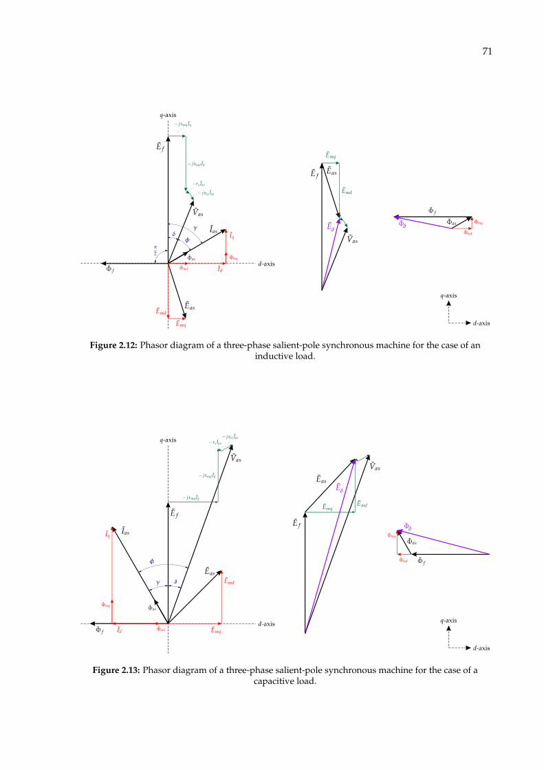
71

Figure 2.12: Phasor diagram of a three-phase salient-pole synchronous machine for the case of aninductive load.

Figure 2.13: Phasor diagram of a three-phase salient-pole synchronous machine for the case of acapacitive load.

72

2.9 Standard synchronous machine reactances and time con-stants

It is instructive to set forth the commonly used reactances for the three-winding rotor

synchronous machine and to relate these reactances to the operational impedances28 whenever

appropriate [19]. The following equations are derived in many works, such as Adkins [30]

and Krause et al. [19].

The quadrature- and direct-axis reactances are

xq = xls + xmq [pu] (2.124)

and

xd = xls + xmd [pu] . (2.125)

These reactances were previously defined and characterize the machine during balanced

steady-state operation whereupon variables in the rotor reference frame are constants. The

zero-frequency value of xq(p) or xd(p) is found by replacing the operator p with zero. Hence,

the operational impedances for balanced steady-state operation are

xq(0) = xq [pu] (2.126)

and

xd(0) = xd [pu] . (2.127)

Similarly, the steady-state value of the transfer function is

G(0) =xmd

r′f d[1] . (2.128)

The direct-axis transient reactance29 is defined as

x′d , xdτ ′dτ ′d0

= xls +xmdx′l f d

xmd + x′l f d[pu] . (2.129)

The quadrature- and direct-axis sub-transient reactances are

x′′q , xqτ ′′qτ ′′q0

= xls +xmqx′lkq

xmq + x′lkq[pu] , (2.130)

and

x′′d , xdτ ′′dτ ′′d0

= xls +xmdx′l f dx′lkd

xmdxls + xmdx′l f d + xlsx′l f d[pu] . (2.131)

28A brief description of operational impedances and associate circuits are presented in Appendix I.29Primes are used to denote transient and sub-transient quantities, which can be confused with rotor

quantities referred to the stator windings by a turns ratio. It is important to note, therefore, that x′d is theonly single-primed parameter that is not a referred impedance.

73

These reactances are the high-frequency asymptotes of the operational impedances,

which means that the high-frequency response of the machine is characterized by them. That is

limp→∞ xq(p) = x′′q [pu] (2.132)

and

limp→∞ xd(p) = x′′d [pu] . (2.133)

It is interesting that limp→∞ G(p) is zero, which indicates that the stator flux linkages are

essentially insensitive to high-frequency changes in field voltage [19].

A final and important comment about the operational impedances, the transient andsub-transient reactances is given by Krause et al. [19]:

Although the steady-state and sub-transient reactances can be related to theoperational impedances, this is not the case with the transient reactances. It ap-pears that the d-axis transient reactance evolved from the development [foundin] [58] of approximate transient torque-angle characteristic where the effects ofd-axis damper windings are neglected. The q-axis transient reactance has comeinto use when it became desirable to portray more accurately the dynamiccharacteristics of the solid iron rotor machine in transient stability studies[therefore not considered in this work]. [...] It is perhaps apparent that thesub-transient reactances characterize the equivalent reactances of the machineduring a very short period of time following an electrical disturbance. Aftera period, of perhaps a few milliseconds, the machine equivalent reactancesapproach the values of the transient reactances, and even though they are notdirectly related to xq(p) and xd(p), their values lie between the sub-transientand steady-state values. As more time elapses after a disturbance, the transientreactances give way to the steady-state reactances.

Moreover, the use of transient and sub-transient quantities to portray the behavior of

the machine over specific time intervals was a direct result of the need to simplify the machine

equations so that pre-computer computational techniques could be used.

2.9.1 Summary

Table 2.2 presents a list of the fundamental constants. All are per-unit values;ωb is the

base electrical angular velocity, in electrical radians per second, used to calculate the inductive

reactances. Against each quantity is given the name by which it is known in the usually accepted

terminology.

The machine time constants are presented in Table 2.3.

All derived reactances are presented in Table 2.4.

74

Table 2.2: Fundamental salient-pole synchronous machine constants.

Constant Meaning

rs armature resistance

r′kq quadrature-axis damper resistance

r′f d field resistance

r′kd direct-axis damper resistance

xmq = ωbLmq quadrature-axis magnetizing reactance

xmd = ωbLmd direct-axis magnetizing reactance

xls = ωbLls armature leakage reactance

x′lkq = ωbL′lkq quadrature-axis damper leakage reactance

x′l f d = ωbL′l f d field leakage reactance

x′lkd = ωbL′lkd direct-axis damper leakage reactance

Table 2.3: Salient-pole synchronous machine time constants.

Time constant Meaning

τ ′d0 direct-axis transient open-circuit time constant

τ ′d direct-axis transient short-circuit time constant

τ ′′d0 direct-axis sub-transient open-circuit time constant

τ ′′d direct-axis sub-transient short-circuit time constant

τ ′′q0 quadrature-axis sub-transient open-circuit time constant

τ ′′q quadrature-axis sub-transient short-circuit time constant

τkd direct-axis damper leakage time constant

Table 2.4: Salient-pole synchronous machine derived reactances.

Derived reactance Meaning

xd = xls + xmd direct-axis synchronous reactance

x′d direct-axis transient reactance

x′′d direct-axis sub-transient reactance

xq = xls + xmq quadrature-axis synchronous reactance

x′′q quadrature-axis sub-transient reactance

75

2.10 The load rejection test

Tests for transient and sub-transient parameters involve sudden changes to any, or all, of

the three-phase circuits at, or electrically near, the machine armature terminals. Sudden changes

to the field electrical current are also included. Changes at, or near, the armature terminals could

result from single or multiple faults between phases, or faults from one or more phases to the

machine neutral, or active and reactive load rejections [13].

As described in the IEEE [13]:

The characteristic values of transient and sub-transient reactances (and timeconstants) of synchronous machines have been used for about [89] years and formany purposes. Initially, such reactances and time constants were calculatedto give, both machine designers and users of synchronous machines, first-handknowledge of short-circuit currents magnitudes and their rate of change ordecay [13, p. 117].

Original analysis of short-circuit currents by machine designers [10, 80], commencing

about 89 years ago, indicated that there are basically two periods during which the rates of

current decay may be easily identified. The initial and shortest period is named the sub-transient

regime. The subsequent and much longer period is called the transient regime. Such regimes

can be associated with a time constant. This characteristic value can be identified as the time

taken for exponentially decaying current or voltage to change to 1/e, or 0.368, of its original

value [13].

Unlike the short-circuit test, the load rejection presents favorable characteristics, since

does not depend on special equipment and does not produce hazardous forces in the ma-

chine [66]. The load rejection test consists in opening the generator main breaker while the

generator is initially carrying some reactive and/or active power. It is a particular type of

decrement test, while the field voltage is kept constant, for determining generator parameters.

To obtain direct-axis parameters, the appropriate loads are purely reactive and, to obtain

quadrature-axis parameters, the appropriate loads are the ones under which there is alignment

between the armature current and the quadrature-axis. From the test results, it is possible to

estimate synchronous, transient, and sub-transient reactances, as well as the time constants for

both axes [18].

To reach the pure quadrature-axis armature current, it is possible to use a trial and error

procedure, as proposed by de Mello and Ribeiro [65]. That procedure is time consuming and,

for that reason, disadvantageous for power plants operators. Certain alternative procedures

have been developed to replace pure quadrature-axis load rejection. To apply those methods, it

is necessary to either measure or estimate the load angle, δ, or to use more advanced parameter

estimation procedures. Another possibility, developed by Giesbrecht [81] for salient-pole ma-

chines and extended by Giesbrecht and Meneses [18], is to use analytical methods to estimate

the steady-state condition under which the armature current is on the quadrature-axis. Those

methods are based only on estimates of the machine synchronous reactances and measurements

76

of its armature voltage and are robust to errors in initial estimates.

While the intention of this section is to develop graphical and analytical conditions to

read the test data, further review on the literature is presented in Chapter 5.

2.10.1 Preliminary considerations

The operational description presented in Appendix I is a common approach to analyze

the electrical responses of a synchronous machine to perturbations [13]. The transient regime

after a load rejection is studied by evaluating the flux-linkage per second variations in both

quadrature- and direct-axis.

Recalling the qd0-voltages equations, as defined by Park [43],

vq = −rsiq +ωrΨd +pωb

Ψq [pu] , (2.134a)

vd = −rsid −ωrΨq +pωb

Ψd [pu] , (2.134b)

v0 = −rsi0 +pωb

Ψ0 [pu] , (2.134c)

where

Ψq = −xq(p)iq [pu] , (2.135a)

Ψd = −xd(p)id + G(p)v′f d [pu] , (2.135b)

Ψ0 = −xlsi0 [pu] . (2.135c)

From Park’s inverse transform (2.66):

va(t) = vq cosθr + vd sinθr + v0 [pu] . (2.136)

2.10.1.1 Before the load rejection

Prior to the load rejection itself, the salient-pole synchronous machine is operating at

steady-state – which was already analyzed in Section 2.8. Being extremely small, the voltage

drops across the armature resistance, rsiq and rsid, may be neglected without much affecting

desired results.

Furthermore, as, in steady-state,ωs = 1 pu, (2.134) may be re-written simply as

v0q = Ψ0

d [pu] , (2.137a)

v0d = −Ψ0

q [pu] ,

where v0q and v0

d are, respectively, the quadrature-axis and direct-axis steady-state armature

voltages; and Ψ0q and Ψ0

d are, respectively, the quadrature-axis and direct-axis steady-state flux

linkage per second. These quantities are taken right before the load rejection.

77

2.10.1.2 Following the load rejection

Let the flux-linkage per second variations be defined as:

∆Ψq(p) = −xq(p)∆iq(p) [pu] , (2.138a)

∆Ψd(p) = −xd(p)∆id(p) + G(p)∆v′f d(p) [pu] . (2.138b)

Above equations may be initially manipulated by considering that:

1. If the field voltage is held fixed at its pre-rejection value, then the Laplace transform of the

change in the field voltage is zero;

2. Following the load rejection, both quadrature- and direct-axis currents become zero.

Therefore, they may be modeled as decreasing steps:

∆iq(p) = L−i0

qθH(t)

= −

i0q

p, (2.139a)

∆id(p) = L−i0

dθH(t)

= −

i0dp

, (2.139b)

where i0q and i0

d are the quadrature-axis and direct-axis steady-state currents before the

load rejection, respectively; L · is the Laplace transform operator; and θH(t) is the

Heaviside step function.

Thus, (2.138) becomes:

∆Ψq(p) = xq(p)i0q

p[pu] , (2.140a)

∆Ψd(p) = xd(p)i0dp

[pu] . (2.140b)

Considering (2.140), (8.13), (8.14), (8.6), and (8.7), the quadrature-axis flux linkage per

second transient in the time domain is given by

∆Ψq(t) = L−1

xq(p)

i0q

p

= L−1

xq

(1 + τ ′′q p)(1 + τ ′′q0 p)

i0q

p

(2.141a)

= xqi0q + xq

τ ′′qτ ′′q0

i0q exp

− tτ ′′q0

− xqi0

q exp

− tτ ′′q0

(2.141b)

= xqi0q +

(x′′q − xq

)i0q exp

− tτ ′′q0

[pu] , (2.141c)

and the direct-axis flux linkage per second transient in the time domain, by

∆Ψd(t) = L−1

xd(p)

i0dp

= L−1

xd

(1 + τ ′d p)(1 + τ ′′d p)(1 + τ ′d0 p)(1 + τ ′′d0 p)

i0dp

(2.142a)

= xdi0d +

(x′d − xd

)i0d exp

− tτ ′d0

+(x′′d − x′d

)i0d exp

− tτ ′′d0

[pu] . (2.142b)

78

2.10.1.3 Complete behavior

When the load is suddenly changed, the transformer effects are represented by pΨq and

pΨd and produce nonperiodic and second-harmonic components in the armature quantities.

These phenomena can be neglected without including large errors [55].

The synchronous machine behavior throughout the load rejection process can be ob-

tained by composing the phenomena before and following the load rejection itself. Therefore,

the quadrature-axis flux-linkage per second in the time-domain is:

Ψq(t) = Ψ0q + ∆Ψq(t) (2.143a)

= −v0d + xqi0

q +(

x′′q − xq

)i0q exp

− tτ ′′q0

[pu] , (2.143b)

and the direct-axis flux linkage per second is:

Ψd(t) = Ψ0d + ∆Ψd(t) (2.144a)

= v0q + xdi0

d +(x′d − xd

)i0d exp

− tτ ′d0

+(x′′d − x′d

)i0d exp

− tτ ′′d0

[pu] . (2.144b)

2.10.2 Direct-axis load rejection

The direct-axis load rejection test is performed when the generator is at zero active

power flow, but drawing or supplying reactive power. In such load condition, flux exists only

in the direct-axis (i.e., Ψq = 0 → iq = 0) [65]. For balanced load conditions, Ψ0 = 0 → i0 = 0.

Thus, let the power-factor angle beφ = π/2 rad.

Since the armature voltage is:

v =√

v2d + v2

q = vq [pu] , (2.145)

there is no angular displacement between v and the quadrature-axis, which implies that the

load angle δ = 0. From (2.136),

va(t) = vq cosθr [pu] . (2.146)

Therefore,

vq(t) = Ψd(t) (2.147a)

= v0q + xdi0

d +(x′d − xd

)i0d exp

− tτ ′d0

+(x′′d − x′d

)i0d exp

− tτ ′′d0

[pu] . (2.147b)

At the initial condition, prior to the load rejection, the synchronous machine phasor

diagram is presented in Figure 2.14; it is possible to visualize that all the flux is on the direct-axis.

79

Figure 2.14: Phasor diagram of a three-phase salient-pole synchronous machine when armaturemagnetic-flux is exclusively on the direct-axis.

2.10.3 Quadrature-axis load rejection

In order to perform the quadrature-axis load rejection test, the generator armature flux

must be only on the quadrature-axis. Therefore, the angle γ = 0, which means thatφ = −δ, or,

similarly, |φ| = |δ| [81].

As in the direct-axis load rejection, it is desirable to keep the machine underexcited to

avoid dangerous voltage levels. Such condition is reached for capacitive loads – i.e., when the

armature current phasor leads the armature voltage phasor.

At the initial condition, prior to the load rejection, the synchronous machine phasor

diagram is presented in Figure 2.15; it is possible to visualize that all the armature flux is on the

quadrature-axis.

From Figure 2.15, the armature voltage has components on both quadrature and direct

axes. After the quadrature-axis load rejection, there is no armature-voltage component on the

direct-axis, as shown in Figure 2.16. It can also be seen that the armature-voltage quadrature-axis

component does not vary from before the load rejection to after it. Therefore, the influence

of the quadrature-axis circuit can be analyzed by means of the armature-voltage direct-axis

component.

The armature voltage is:

v =√

v2d + v2

q [pu] , (2.148)

and, from (2.136),

va(t) = vq cosθr + vd sinθr [pu] . (2.149)

80

Figure 2.15: Phasor diagram of a three-phase salient-pole synchronous machine when armaturemagnetic-flux is exclusively on the quadrature-axis.

Figure 2.16: Phasor diagram of a three-phase salient-pole synchronous machine after thequadrature-axis load rejection.

The armature voltage direct-axis component is

vd(t) = −Ψq(t) (2.150a)

= v0d − xqi0

q +(

xq − x′′q)

i0q exp

− tτ ′′q0

[pu] . (2.150b)

81

Chapter 3

Concepts on System Identification andSystem Theory and their Applicationsto Synchronous Machines

“It is difficult to do justice to a subject as complex as system theory in a compass ofa few printed pages. [...] I believe that system theory is here to stay, and that thecoming years will witness its evolution into a respectable and active area of scientificendeavor.”

— Lofti A. Zadeh1, From Circuit Theory to System Theory [82]

The salient-pole synchronous machine equations, in both machine and rotor reference-

frame variables, have already been derived. This chapter aims at adapting the machine equations

into the state-space representation, which is a very useful tool for states and parameters estima-

tion.

The majority of concepts involved in Section 3.1 are borrowed from the fundamental

work of Sarachik [83]. Furthermore, the doctoral thesis of Barreto [84] is a great and important

compiled of concepts and works on System Identification, Data Modeling, and Time Series; one

should refer to it for additional details on these subjects.

3.1 Preliminary concepts

The first definition to be presented comprehends the concept of physical systems.

Definition 3.1: Physical system

A physical system is an interconnection of physical components that perform a specific function.

1Lofti Aliasker Zadeh (1921–2017) was a mathematician, computer scientist, electrical engineer,artificial intelligence researcher, and professor emeritus of computer science at the University of California,Berkeley. Zadeh is best known for proposing fuzzy mathematics and for pioneering the development ofthe Z-Transform method in discrete time signal processing and analysis.

82

These components may be electrical, mechanical, hydraulic, thermal, and so forth.

A great variety of physical quantities may be associated with every system. Some of the

signals can be directly changed with time in order to indirectly accomplish desired changes in

some other signals of the systems, which happen to be of particular interest. The former set

of signals is called set of inputs or excitations; the latter is called set of outputs, measurements, or

responses.

The set of inputs will be denoted by an m-dimensional vector u ∈ Rm; and the set of

measurements by an l-dimensional vector y ∈ Rl . It is an essential part of the system concept

that changes of the input are followed by changes to the output [83]. A mathematical relation

between them may be written as

y(t) = S u(t) , (3.1)

where S is an operator if the mapping of inputs u(t) into outputs y(t) is unique [85] .

The term system, as applied to general analysis, was originated as a recognition that

meaningful investigation of a particular phenomenon can often only be achieved by explicitly

accounting for its environment [86]. Accordingly, mathematical models of systems are likely to

involve a large number of interrelated variables – and this is emphasized by describing such

situations as multivariable systems.

Definition 3.2: Physical realizability

A system S with the input-output relation (3.1) is called physically realizable if a physical systemcan be built whose inputs and outputs are related via (3.1).

Definition 3.3: Causal system

A system S is called causal (or is said to be nonantecipative) if for any t, y(t) does not dependon any u(t′) for t′ > t (i.e., if y(t) does not depend on future values of u). Otherwise, it is callednoncausal or antecipative.

From Definition 3.3, a noncausal system is not realizable.

Definition 3.4: Dynamic system

A system S is called dynamic (or is said to have memory) if y(t0) depends on some values of u(t)for t 6= t0. A system for which y(t0) does not depend on u(t) for t 6= t0 is called instantaneous(or is said to have zero memory).

As stated by Luenberger [86],

the term dynamic refers to phenomena that produce time-changing patterns,the characteristics of the pattern at one time being interrelated with those atother times. The term is nearly synonymous with time-evolution or pattern

83

of change. It refers to the unfolding of events in a continuing evolutionaryprocess [86, p. 1].

Definition 3.5: State of a system

The state of a nonantecipative dynamic system at time t0 is the smallest set of quantities x(t0),which summarize all information about u(−∞, t0) needed to determine y[t0, t1] when u[t0, t1] isknown.

A little digression on notation: u[t0, t1] , u(t) for all t0 ≤ t ≤ t1 (i.e., the entire time

function defined over [t0, t1]). The same notation is valid for other quantities.

The input-output relation of a nonantecipative dynamic system of (3.1) can be modified

to include the state as follows:

y(t) = C x(t0); u[t0, t] for t ≥ t0 , (3.2)

and is now called the input-output-state relation or the measurement equation of the system.

Inherent in the concept of state is the requirement that for any t1 ∈ [t0, t], it must be

possible to define x(t1) such that the state itself at t1 must be uniquely determined by an earlier

state at t0 and the input u[t0, t1]. It implies that for consistency, a condition of the form:

x(t1) = Ax(t0); u[t0, t1] for t ≥ t0 , (3.3)

must be satisfied. Equation (3.3) is called the state transition equation of the system.

In general, the state equations are differential equations of the form:

x(t) = f (x(t), u(t), t) , (3.4a)

y(t) = h (x(t), u(t), t) , (3.4b)

or difference equations of the form:

x(k + 1) = f (x(k), u(k), k) , (3.5a)

y(k) = h (x(k), u(k), k) . (3.5b)

These are called the state (differential or difference) equations.

Definition 3.6: Zero state

The zero state θ of a dynamic system is the state for which y[t0, ∞] = 0 when x(t0) and the inputy[t0, ∞] = 0 (i.e., C θ; 0 = 0).

84

Definition 3.7: Homogeneity and additivity

A zero-memory system is homogeneous if

S ku = kS u for all k ∈ R and u ∈ Cm . (3.6)

A zero-memory system is additive if

S u1 + u2 = S u1+ S u2 for any u1 and u2 ∈ Cm . (3.7)

Remark.

1. When homogeneous or additive is used in referring to dynamic system, it is implied that

the term refers to zero-state response;

2. (3.7) implies (3.6) for k rational.

This is the entire definition of linearity for zero-memory systems. However, if a system

is dynamic, the concept of linearity is a bit more complex [83].

Definition 3.8: Zero-state linear

A dynamic system is called zero-state linear if C θ; k1u1 + k2u2 = k1C θ; u1+ k2C θ; u2for all k1, k2 ∈ R and any u1, u2 ∈ Cm (i.e., if it is zero-state additive and zero-state homogeneous).

Definition 3.9: Decomposition property

A dynamic system is said to have the decomposition property if C x(t0); u = C x(t0); 0+C θ; u for all x(t0) and all u.

Definition 3.10: Zero-input linear

A dynamic system is called zero-input linear if it is zero-input homogeneous and additive.

Definition 3.11: Linear dynamic system

A dynamic system is called linear if:

1. it is zero-state linear;

2. it has the decomposition property;

3. it is zero-input linear.

A system that is not linear is called nonlinear.

85

The systems from (3.4) and (3.5) are sometimes called lumped systems to distinguish

them from distributed systems which are describable by partial differential equations or

differential-difference equations and whose states can only be expressed as functions rather than

by finite dimensional vectors [83].

Definition 3.12: Order of a system

The number of components of the state vector x(t) is called the order of the system, and it isdesignated by letter n.

In addition to the state vector, the input u(t) and output y(t) have m and l components,

respectively.

The salient-pole synchronous machine is a physically realizable, nonantecipative, dy-

namic, nonlinear system. Further details will be provided throughout this chapter.

3.2 Observability

The analysis of the interaction between input and state, on one hand, and between

state and output, on the other hand, has proved of fundamental importance in understanding

the possibility of solving a large number of relevant control problems, including eigenvalues

assignment via feedback, minimization of quadratic cost criteria, disturbance rejection, asymp-

totic output regulation, etc. Key tools for the analysis of such interactions are the notions of

reachability and observability and the corresponding decomposition of the control system into

reachable/unreachable and, respectively, observable/unobservable parts [87].

Perhaps the most important definition within systems theory is the concept of observ-

ability. It came from answering the following questions: How much information about the state

of the system is contained in the data? Can the state be determined from the data?

Intuitively, it would seem that the answers to such questions are related to the system

model itself, and indeed this is so. The importance of such questions is obvious. If little is to

be gained from filtering, then one should consider remodeling the system. This might involve

taking additional or alternate measurements or redesigning the dynamics of the system [88].

Such concept is due to Kalman2 [89, 90]. Kalman [89] introduced the notion of observ-

ability, but as a mere dual of controllability. Contemporaneously, Kalman [90] provided an

alternative, more satisfactory definition, where observability is defined in a more intrinsic way

in terms of the possibility of deducing the state trajectory from input/output measurements.

2Rudolf Emil Kálmán (1930–2016) was an Hungarian-American electrical engineer, mathematician,and inventor. He was most noted for his co-invention and development of the Kalman filter, a mathemat-ical algorithm that is widely used in signal processing, control systems, and guidance, navigation andcontrol. For this work, U.S. President Barack Obama awarded Kálmán the National Medal of Science onOctober 7, 2009.

86

Let X? be the dual vector space of the state space X, i.e., the space of all linear functions

of x. An element z? of X? is called a costate.

Definition 3.13: Observability

A costate z? of a plant (linear, stationary, discrete-time, free, and single output) is said to beobservable if its exact value [z?, x] at any state x at time 0 can be determined from measurementsof the output signal over the finite interval 0 ≥ t ≥ t2. The time t2 will depend, in general, on z?. Ifevery costate is observable, the plant is said to be completely observable.

How well the state is known is measured by the estimation error covariance matrix. But

it depends on its initial condition (the initial data) and does not reflect the uncertainty in the

estimate by virtue of filtering the data alone.

Although the concepts and properties of observability and controllability are completely

defined for linear systems [83, 84, 88–90], how does Definition 3.13 apply to nonlinear systems?

In a similar manner, it must express that there is indeed a possibility that the purpose of an

observer can be achieved.

For nonlinear systems, local observability conditions are reported in the work of Lee

and Markus [91]. Furthermore, necessary conditions and a sufficient condition for observability

have been proven by Griffith and Kumar [92].

Krener [93, 94] and Sussmann and Jurdjevic [95] developed the nonlinear analog of

linear observability in terms of the Lie algebra3 of vector fields on the state space generated by

vector fields. It was shown that if the dimension of the Lie algebra is constant, or if the system is

analytic, then there exist a unique maximal submanifold X? of X through x0 which carries all

the trajectories of the system passing through x0 such that any point of this submanifold can be

reached from x0 going forward and backward along the trajectories of the system [96].

Even though it would be a great contribution to dedicate a few pages of this work

to prove and to analytically demonstrate the observability conditions to the salient-pole syn-

chronous machine model, due to its complexity and the time-demand required to do so, it will

be left for further works.

However, a more superficial approach can still be considered. By means of linearization,

it is possible to apply the so-called Rank Condition Test to locally analyze observability.

3In mathematics, a Lie algebra is a vector space together with a non-associative operation called theLie bracket, an alternating bilinear map, satisfying the Jacobi identity. Lie algebras were introduced tostudy the concept of infinitesimal transformations by Marius Sophus Lie in the 1870s, and independentlydiscovered by Wilhelm Killing in the 1880s. The name Lie algebra was given by Hermann Weyl in the1930s; in older texts, the term infinitesimal group is used.

87

3.2.1 Rank condition test

Let a general linear invariant-time system be

x(t) = Ax(t) + Bu(t) , (3.8a)

y(t) = Cx(t) , (3.8b)

where x ∈ Rn is the state vector, y ∈ Rl is the measurement vector, u ∈ Rm is the input vector,

and (A, B, C) are constant matrices known respectively as dynamics matrix, the input or control

matrix, and the output or measurement matrix.

One way of testing whether the system (3.8) is observable is to define the observability

matrix:

O ,

CCACA2

...

CAn−1

∈ Rnl×n . (3.9)

Therefore, the system (3.8) is observable if matrixO has a full column rank, that is, if rankO = n.

This is known as Kalman’s rank condition for observability and, according to it, a pair A, C is

either observable or not.

The concept was extended to nonlinear systems in the 1970s, e.g. Hermann and Krener

[96]. The pair f , h is said to be observable if rankO(x) = n, ∀x ∈ Rn, which is the counterpart

of Kalman’s rank condition for linear systems [97].

The following procedure is presented by Nahar, Liu, and Shah [98]. Hereafter, each

process equation will be denoted fi, for i = 1, . . . , n and each measurement equation, h j, for

j = 1, . . . , l.

Let F(k) be the Jacobian matrix:

F(k) ,

∂ f1

∂x1

∂ f1

∂x2· · · ∂ f1

∂xn

∂ f2

∂x1

∂ f2

∂x2· · · ∂ f2

∂xn...

.... . .

...∂ fn

∂x1

∂ fn

∂x2· · · ∂ fn

∂xn

∈ Cn×n (3.10)

and H(k) be the Jacobian matrix:

H(k) ,

∂h1

∂x1

∂h1

∂x2· · · ∂h1

∂xn

∂h2

∂x1

∂h2

∂x2· · · ∂h2

∂xn...

.... . .

...∂hl

∂x1

∂hl

∂x2· · · ∂hl

∂xn

∈ Cl×n . (3.11)

88

The system is considered to be observable at time k if the observability matrix O(k) has a full

column rank, rank O(k) = n, where the observability matrix is given by:

O(k) ,

HHFHF2

...

HFn−1

∈ Cnl×n . (3.12)

The rank test provides on whether the system is observable or not and does not provide

any information on how strongly or weakly observable it is [98].

3.3 State-space representation

One of the major references of this work is the brilliant work of Candy [99]. It provides aclear comment on the importance of state-space representation:

The interesting property of the state-space representation is to realize that thesemodels represent a complete generic form for almost any physical systems. [...]Systems theory, which is essentially the study of dynamic systems, is based onthe study of state-space models and is rich with theoretical results exposingthe underlying properties of the dynamic system under investigation. This isone of the major reasons why state-space models are employed [...], especiallywhen the system is multivariable having multiple inputs and multiple outputs[as in the case of salient-pole synchronous machines] [99, p. 99].

Unfortunately, in practice, complete state measurements are rarely realistic. Therefore,

at least some states are unknown and, thus, the nonlinear state-space model cannot be directly

applied in reality. The states have to be considered as unknown quantities and must be estimated

as well. This leads to modeling approaches with internal states. They are subsumed under the

class of the so-called internal dynamics models [100].

The main objective of this work is to investigate methods for estimating states and

parameters of salient-pole synchronous machines. Therefore, it is mandatory to develop their

state-space models. A set of first-order differential equations is displayed in (2.88). However,

flux linkages and currents are represented as variables in it. Since these two quantities are

mutually dependent, both cannot simultaneously be independent or state variables [19].

Although numerous possibilities for state variables are available [19, 22, 33, 35, 49, 50],

the two most commonly applied [19] are:

i) a set based on currents as state variables,

x =[

iq id i0 i′kq i′f d i′kd

]T∈ R6 , (3.13)

which has the advantage of offering simple relations between voltages vd and vq and state

variables (through the power network connected to the machine terminals);

89

ii) a set based on flux linkages – or flux linkages per second – as state variables, where the

particular set to be chosen depends upon how conveniently they can be expressed in

terms of the machine currents and stator voltages. For example,

x =[Ψq Ψd Ψ0 Ψ′kq Ψ′f d Ψ′kd

]T∈ R6 . (3.14)

Being expressed as time derivatives in (2.88), flux linkages per second could be con-

sidered to be the natural set of state variables to be solved by time-step integration. By virtue

of some auxiliary equations [36], the flux linkages per second can be eliminated from Park’s

equations and be replaced by currents as state variables. However, flux linkages per second

in a synchronous machine change slowly, limited by the open-circuit time constants, while

currents change rapidly, limited by short-circuit time constants4. Hence, Park’s equations are

most efficiently solved with flux linkages per second as the state variables, in which case currents

are best eliminated from these equations [36].

3.3.1 Flux-linkage per second state-space model

For salient-pole synchronous machines, the most widely used model is derived from

the voltage equations expressed in the rotor reference frame with stator and rotor flux linkages

per second as state variables [19]. This model was first developed by C. H. Thomas5 [101].

At that time, he was interested in developing a block diagram of synchronous machines for

analog-computer simulations, which are shown in Figure B.1 and Figure B.2. In particular, these

representations apply to salient-pole machines, where saturation occurs principally along the

main-pole axis [102].

The development of Thomas’ flux-linkage per second state-space model is given in the

following way.

Let the stator and rotor voltage equations (2.110) and flux linkages per second equa-

tions (2.112) in per unit (pu). Defining the quadrature- and direct-axis magnetizing flux linkages

as

Ψmq = xmq

(iq + i′kq

)[pu] , (3.15a)

Ψmd = xmd


)[pu] , (3.15b)

and using them in (2.112), the winding currents can be expressed in terms of winding and

magnetizing flux linkages as

iq =1

xls

(Ψq − Ψmq

)[pu] , (3.16a)

4Refer to Appendix I for further details.5Charles H. Thomas was an instructor of electrical engineering at Harvard University, Cam-

bridge/Massachusetts, and former employee of Allis-Chalmers, a machinery manufacturer from Mil-waukee/Wisconsin. He worked with P. C. Krause and C. Concordia throughout his life. No furtherinformation was found about him.

90

id =1

xls

(Ψd − Ψmd

)[pu] , (3.16b)

i0 =1

xlsΨ0 [pu] , (3.16c)

i′kq =1

x′lkq

(Ψ′kq − Ψmq

)[pu] , (3.16d)

i′f d =1

x′l f d

(Ψ′f d − Ψmd

)[pu] , (3.16e)

i′kd =1

x′lkd

(Ψ′kd − Ψmd

)[pu] . (3.16f)

Substituting (3.16) into (2.110) yields the state equations of stator and rotor windings:

pωb

Ψq = vq −ωrΨd +rs

xls

(Ψmq − Ψq

)[pu] , (3.17a)

pωb

Ψd = vd +ωrΨq +rs

xls

(Ψmd − Ψd

)[pu] , (3.17b)

pωb

Ψ0 = v0 −rs

xlsΨ0 [pu] , (3.17c)

pωb

Ψ′kq = v′kq +r′kq

x′lkq

(Ψmq − Ψ′kq

)[pu] , (3.17d)

pωb

Ψ′f d = v′f d +r′f d

x′l f d

(Ψmd − Ψ′f d

)[pu] , (3.17e)

pωb

Ψ′kd = v′kd +r′kdx′lkd

(Ψmd − Ψ′kd

)[pu] . (3.17f)

Before concluding, it should be mentioned that, in accordance to Lipo [36], the urge to

per unitize sometimes extends to normalizing time as well. Therefore,

1ωb

p =1ωb

ddt

(3.18a)

=d

d(ωbt)(3.18b)

=d

dT. (3.18c)

That being the case, for a 60 Hz base system, one pu time corresponds to approximately

1/377 second. Including the normalization factor inside the operator p, (3.17) is simply written

as:

pΨq = vq −ωrΨd +rs

xls

(Ψmq − Ψq

)[pu] , (3.19a)

pΨd = vd +ωrΨq +rs

xls

(Ψmd − Ψd

)[pu] , (3.19b)

91

pΨ0 = v0 −rs

xlsΨ0 [pu] , (3.19c)

pΨ′kq = v′kq +r′kq

x′lkq

(Ψmq − Ψ′kq

)[pu] , (3.19d)

pΨ′f d = v′f d +r′f d

x′l f d

(Ψmd − Ψ′f d

)[pu] , (3.19e)

pΨ′kd = v′kd +r′kdx′lkd

(Ψmd − Ψ′kd

)[pu] . (3.19f)

It is also noted that to have a proper state model, the magnetizing flux linkages must be

expressed in terms of winding flux linkages per second (which are the states). Manipulating the

replacement of (3.16) into (3.15) yields

Ψmq =

(1

xmq+

1xls

+1

x′lkq

)−1(Ψq

xls+

Ψ′kq

x′lkq

)[pu] , (3.20a)

Ψmd =

(1

xmd+

1xls

+1

x′l f d+

1x′lkd

)−1(Ψd

xls+

Ψ′f d

x′l f d+

Ψ′kdx′lkd

)[pu] . (3.20b)

Another way of writing the flux-linkage per second model is also found in the work of

Krause et al. [19]. Its development begins by isolating the flux linkages per second from (2.112):

Ψq

Ψd

Ψ0

Ψ′kq

Ψ′f d

Ψ′kd

=

xq 0 0 xmq 0 0

0 xd 0 0 xmd xmq

0 0 xls 0 0 0

xmq 0 0 x′kq 0 0

0 xmd 0 0 x′f d xmd

0 xmd 0 0 xmd x′kd

iq

id

i0

i′kq

i′f d

i′kd

[pu] . (3.21)

However, it is more convenient to write (3.21) as[Ψq

Ψ′kq

]=

[xq xmq

xmq x′kq

] [iq

i′kq

][pu] , (3.22)

Ψd

Ψ′f d

Ψ′kd

=

xd xmd xmq

xmd x′f d xmd

xmd xmd x′kd

id

i′f d

i′kd

[pu] , (3.23)

and

Ψ0 = xlsi0 [pu] . (3.24)

Solving (3.22)–(3.24) for currents yields[iq

i′kq

]=

1∆q

[x′kq −xmq

−xmq xq

][pu] , (3.25)

92

id

i′f d

i′kd

=1∆d

x′f dx′kd − x2

md −xmdx′kd + x2md −xmdx′f d + x2

md

−xmdx′kd + x2md xdx′kd − x2

md −xdxmd + x2md

−xmdx′f d + x2md −xdxmd + x2

md xdx′f d − x2md

[pu] , (3.26)

and

i0 =1

xlsΨ0 [pu] , (3.27)

where

∆q = xqx′kq − x2mq [pu] , (3.28a)

∆d = −x2md

(xd − 2xmd + x′f d + x′kd

)+ xdx′f dx′kd [pu] . (3.28b)

The flux-linkage per second equations are obtained from substituting (3.25)–(3.27) into

voltage equations (2.110). Therefore,

pΨq = vq −ωrΨd − rs

(x′kqΨq + xmqΨ

′kq

)[pu] , (3.29a)

pΨd = vd +ωrΨq − rs

(Ξ11Ψd − Ξ12Ψ

′f d − Ξ13Ψ

′kd

)[pu] , (3.29b)

pΨ0 = v0 −rs

xlsΨ0 [pu] , (3.29c)

pΨ′kq = v′kq + r′kq(xmqΨq − xqΨkq

)[pu] , (3.29d)

pΨ′f d = v′f d − r′f d(Ξ21Ψd + Ξ22Ψ f d + Ξ23Ψ

′kd)

[pu] , (3.29e)

pΨ′kd = v′kd − r′kd

(Ξ31Ψd + Ξ32Ψ

′f d + Ξ33Ψ

′kd

)[pu] , (3.29f)

where Ξrc is the element in the rth row and cth column of the 3× 3 matrix in (3.26):

Ξ =



md


md −xdxmd + x2md



[pu] . (3.30)

In summary, the afore-developed model considers the following state-, input-, and

measurement-vector:


]T∈ R6 , (3.31a)

u =[vq vd v0 v′kq v′f d v′kd

]T∈ R6 , (3.31b)

y =[iq id i0 i′kq i′f d i′kd

]T∈ R6 . (3.31c)

93

Chapter 4

Bayesian State-Space Processors

“He sat, continuing to look down the nave, when suddenly the solution to the problemjust seemed to present itself. It was so simple, so obvious, he just started to laugh.”

— Paul Doherty1, Satan in St Mary’s (1986)

An enlightening introduction to this chapter may be borrowed from the work of Robertand Casella [103], in which the use of Bayesian processors is justified:

Until the advent of powerful and accessible computing methods, the experi-menter was often confronted with a difficult choice. Either describe an accuratemodel of a phenomenon, which would usually preclude the computation ofexplicit answers, or choose a standard model which would allow this computa-tion but may not be a close representation of a realistic model. This dilemma ispresent in many branches of statistical applications, for example, in electricalengineering, aeronautics, biology, networks, and astronomy. To use realisticmodels, the researchers in these disciplines have often developed original ap-proaches for model fitting that are customized for their own problems. This isparticularly true for physicists, the originators of Markov chain Monte Carlomethods. Traditional methods of analysis, such as the usual numerical analysistechniques, are not well adapted for such settings.

If the data are modeled by a linear Gaussian state-space model, it is possible to derive

an exact analytical expression to compute the evolving sequence of posterior distributions. This

recursion is the well-known and widespread Kalman Filter (KF). If the data are modeled as a

partially observed, finite state-space Markov chain, it is also possible to obtain an analytical

solution, which is known as the hidden Markov model filter [99].

The aforementioned filters rely on various assumptions to ensure mathematical tractabil-

ity. However, real data can be very complex, typically involving elements of non-Gaussianity,

high dimensionality and nonlinearity, which conditions usually preclude analytic solution.

This is a problem of fundamental importance that permeates most disciplines of science [103].

The problem appears under many different names, including Bayesian filtering [99], optimal

nonlinear filtering [104], stochastic filtering [105], and on-line inference and learning [106].

1Paul Charles Dominic Doherty (1946–Present) is an award-winning English author, educator, lecturer,and historian. He is also the Headmaster of Trinity Catholic High School in London, England. Doherty isa prolific writer, has produced dozens of historical novels and a number of nonfiction history books.

94

For over thirty years, many approximations schemes, such as the Extended Kalman

Filter (EKF), Gaussian sum approximations, and grid-based filters have been proposed to

surmount this problem. The first two methods fail to take into account all the salient statistical

features of the processes under consideration, leading quite often to poor results. Grid-based

filters, based on deterministic numerical integration methods, can lead to accurate results, but

are difficult to implement and too computationally expensive to be of any practical use in high

dimensions [107].

Sequential Monte Carlo (SMC) methods are a set of simulation-based methods that

provide a convenient and attractive approach to computing the posterior distributions. Unlike

grid-based methods, SMC methods are very flexible, easy to implement, parallelizable, and

applicable in very general settings [107].

The majority of concepts involved in this chapter are based on the works of Candy [99],

Robert and Casella [103], Simon [105], Doucet, Freitas, and Gordon [107], Hogg, McKean, and

Craig [108], and Maybeck [109] and the doctoral thesis of Giesbrecht [110].

The approach developed in this work to estimating states and parameters of salient-

pole synchronous machines is based on the PF, which is a probability-based, SMC processor.

Therefore, it is mandatory to begin this chapter with the foundation for the derivation of the PF –

the Bayesian approach to state estimation.

4.1 Preliminary concepts

Modern probability theory is rigorously based on an axiomatic definition of probability.

The axiomatic definition must still be a valid mathematical model of empirically observed

frequencies of occurrence, but it is meant to extract the essence of the ideas involved and to deal

with them in a precise, rather than heuristic, manner [109].

The first definition to be presented refers to sample space.

Definition 4.1: Sample space

To describe an experiment in precise terms, let Ω be the fundamental sample space containing allpossible outcomes of a conducted experiment. Each single elementary outcome of this experiment isdenoted as anω; theseω’s are then the elements of Ω: ω ∈ Ω.

In other words, the sample space is just the collection of possible outcomes of an

experiment, each of which begin thought of as a point in Ω. Within every sample space, there

are, at least, two subsets: the empty set, denoted by ; and the sample space itself Ω.

The sample space Ω can be discrete, with a finite or countably infinite number of

elements. It could also be continuous, with an uncountable number of elements.

95

Definition 4.2: Event

Let F be defined as a specific event of interest, a specific set of outcomes of the experiment. Thus,each such event F is a subset of Ω: F ⊂ Ω. An event F is said to occur if the observed outcomeω isan element of F, ifω ∈ F.

The structure of a sample space Ω, composed of elementsωi, whose subsets are denoted

as Fi, is shown in Figure 4.1.

Figure 4.1: Representation of an arbitrary sample space Ω subsets Fi and elementsωi.Adapted from Maybeck [109, p. 62].

Definition 4.3: Probability function (or probability measure)

Let Pr(·) be a real scalar-valued function defined on F that assigns a value, Pr (F), to each F whichis a member of F (F ∈ F ) such that:

1. Pr (F) ≥ 0 for all F ∈ F ;

2. Pr (Ω) = 1;

3. If F1, F2, · · · are elements of F and are disjoint, or mutually exclusive: i.e., if

Fi ∩ Fj = for all i 6= j

then

Pr

(N⋃

i=1

Fi

)=

N

∑i=1

Pr (Fi)

for all finite and countably infinite N.

A probability value between 0 and 1 (Pr is a mapping from F into [0, 1]) is assigned to

each set of interest (i.e., each F ∈ F ). Moreover, if F1 is a subset of F2, then the probability of set

F2 is at least as great as the probability of F1, as expected. The set F2 can be decomposed into two

disjoint sets: F1 and Fc1 ∩ F2. Then, according to part (3) of the definition of probability function,

96

Pr (F2) = Pr (F1) + Pr (Fc1 ∩ F2). From part (1), Pr (Fc

1 ∩ F2) ≥ 0, and so Pr (F2) ≥ Pr (F1) as

desired.

A certain class of sets Fi is of main interest: the broad class called a σ−algebra, denoted

as F . In other words, the sets F1, F2, · · · , – admissible for consideration – will be elements of the

class F : Fi ∈ F .

Definition 4.4: σ − algebra

A σ−algebra is a class of sets Fi, each of which is a subset of Ω (Fi ⊂ Ω), such that if Fi is anelement of F (i.e, if Fi ∈ F ), then:

1. Fci ∈ F , where Fc

i is the complement of Fi, Fci = Ω− Fi;

2. Ω ∈ F – and then the empty set ∈ F also, due to the preceding (1);

3. if F1, F2, · · · ,∈ F , then their union and intersection are also in F :

∞⋃i=1

Fi ∈ F and∞⋂

i=1

Fi ∈ F .

Let the sample space Ω be the set of points in n-dimensional Euclidean space Rn and let

F be the class of sets generated by the sets of the form (each of which is a subset of Ω):

F = ω :ω ≤ ξ , ω ∈ Ω , (4.1)

and their complements, unions, and intersections.

A little digression on notation: F is the set ofω’s that are elements of Ω – vectors in the

n-dimensional Euclidean space, and thus, the boldfacing ofω to denote vector quantity – such

thatω ≤ ξ , whereω and ξ are n-dimensional vectors and ξ is specified. Furthermore,ω ≤ ξis to be interpreted as componentwise: ω ≤ ξ meansω1 ≤ ξ1,ω2 ≤ ξ2, · · · ,ωn ≤ ξn for the ncomponentsωi and ξi ofω and ξ , respectively.

This particularσ−algebra is of sufficient interest to have acquired its own name, and it is

called a Borel field, denoted as B. Taking complements, unions, and intersections of sets described

by (4.1) leads to finite intervals (open, closed, or half open) and point values along each of the ndimensions. Thus, a Borel field is virtually composed of all subsets of Euclidean n-space (Rn)

that might be of interest in describing a probability problem associated with Ω = Rn.

At this point, it is possible do define the probability space.

Definition 4.5: Probability space

The probability space is defined by the triplet Ω,F , Pr of the sample space, the underlyingσ−algebra, and the probability function, all axiomatically defined as in the preceding definitions.

The sample space Ω defines the possible outcomes of the experiment, F is the collection

97

of events (sets) of interests, and Pr assigns a probability to every one of these events. However,

for quantitative analysis, there is the need of a mapping from the sample space, Ω, to the real

numbers, R. This is achieved by the random variables.

Definition 4.6: Scalar random variable (or, simply, random variable)

A scalar random variable X (·) is a real-valued point function which assigns a real scalar valueto each pointω ∈ Ω, denoted as X (ω) = x, such that every set F ⊂ Ω of the form

F = ω ∈ Ω : X (ω) ≤ ξ

for any ξ value on the real line (ξ ∈ R),R = x : −∞ < x < ∞, is an element of theσ−algebraF (i.e., F ∈ F ). For a discrete random variable, the subset is a finite or countably infinite set ofpoints.

As highlighted by Maybeck [109], and agreed by the author:

the name random variable is unfortunate in that it does not seem to imply thefact that we are talking about a function, as opposed to values the functionscan assume. In fact, X (·) is a function, or mapping, from Ω to R.

The notation ω ∈ Ω : X (ω) ≤ ξ – or, similarly, ω : X (ω) ≤ ξ, is meant to be read

“the set of ω in Ω that the values assumed by the random variable function X (·), for those ω as itsargument, X (ω) = x, are less than or equal to the given number ξ on the real line”.

A capital calligraphic letter X will denote the random variable, and a lowercase letter x,

its value.

Definition 4.7: Vector random variable (or, simply, random vector)

A vector random variable X (·) is a generalization of the random variable concept to the vectorcase: a real-valued point function which assigns a real vector to each point ω in Ω, denoted asX (ω), such that every set F of the form

F = ω : X (ω) ≤ ξ

for any ξ ∈ Rn, is an element of the σ−algebra F .

Scalar random variables are specifically mappings from Ω to R, such that inverse images

of half-open intervals of the form (−∞,ξ ] in R are events in Ω that belong to F . Vector random

variables are simply extensions of the same idea: mappings from Ω into Rn such that the inverse

images of sets of the form X (ω) ∈ Rn : −∞ < Xi(ω) ≤ ξi ; i = 1, 2, · · · , n are the events in

Ω to which probabilities have been ascribed2.

2From a measure theoretic point of view, this just says that random variables are measurable func-tions [109, 110].

98

From now on, let the sample space Ω be Rn itself and the underlying σ−algebra be the

Borel field B generated by sets of the form Fi = ω :ω ≤ f , ω ∈ Ω. An appropriate random

variable definition for this case is simply the identity mapping:

X (ω) =ω . (4.2)

An element in the sample space, Ω = Rn, is just a single point in the space (a single

vector), and the random variable just mentioned does map each such element into a single

vector in Rn. Thus, each realization X (ω) is an n-dimensional vector, whose components can

take on any value within (−∞, ∞).

The elements of the set Ω that are contained in the event X ≤ ξ change as ξ takes

various values. The probability Pr (ω : X (ω) ≤ ξ) of the event X ≤ ξ is, therefore, a

number that depends on ξ . This number is denoted by FX (ξ) and is called the cumulative

density function (cdf) of the random variable X .

Definition 4.8: (Cumulative) distribution function

The (cumulative) distribution function FX (ξ) is a real scalar-valued function defined by:

FX (ξ) = Pr (ω : X (ω) ≤ ξ) (4.3a)

= “ Pr (X ≤ ξ)′′ (4.3b)

= “ Pr (x1 ≤ ξ1, x2 ≤ ξ2, · · · , xn ≤ ξn)′′ (4.3c)

that always exists.

The quotation marks in (4.3) are meant to emphasize that such notation, very typical in

probability theory literature, should be interpreted in terms of the probability of a set ofω’s in

the original sample space Ω. Moreover, since

FX (ξ) = Fx1 ,x2 ,··· ,xn(ξ1,ξ2, · · · ,ξn) , (4.4)

this is sometimes called the joint distribution function of x1, x2, · · · , and xn.

The cdf is a basic entity associated with any random variable that allows the generation

of probabilities of sets of interest. Its existence is assured [109]. On the other hand, the existence

of its derivative – the so-called probability density function (pdf) – everywhere is not assured.

Some properties can be obtained from its definition [105]:

FX (ξ) ∈ [0, 1] , (4.5)

FX (−∞) = 0 , (4.6)

FX (∞) = 1 , (4.7)

FX (ξ1) ≤ FX (ξ2), if ξ1 ≤ ξ2 , (4.8)

Pr (ξ1 < X ≤ ξ2) = FX (ξ2)− FX (ξ1) . (4.9)

99

Figure 4.2 summarizes the majority of concepts discussed up to this point.

Figure 4.2: Probabilities and random variables.Adapted from Maybeck [109, p. 70].

Definition 4.9: Probability density function

The probability density function fX (ξ) is defined as the derivative of the cdf:

fX (ξ) =FX (ξ)

dξ. (4.10)

If FX (ξ) is absolutely continuous3, then the pdf does exist. If such pdf exists, then X is

termed continuous random variable.

Some properties of the pdf that can be obtained from its definition are [105]:

FX (ξ) =∫ ξ−∞ fX (z)dz , (4.11)

fX (ξ) ≥ 0 . (4.12)

Furthermore, since FX (∞) = 1, (4.11) yields∫ ∞−∞ fX (z)dz = 1 , (4.13)

which justifies its name as the density function. Also, from (4.11),

Pr [ξ1 < X (ξ) ≤ ξ2] = FX (ξ2)− FX (ξ1) =∫ ξ2

ξ1

fX (z)dz . (4.14)

Thus, the area under fX (ξ) in the interval (xi1, xi2) represents the probability that the random

variable X in such interval.

The probability of an event F1, assuming the occurrence of F2, is given by

Pr (F1 | F2) =Pr (F1, F2)

Pr (F2), Pr (F2) 6= 0 , (4.15)

3Absolute continuity can be define rigorously by means of measure theory. Basically, a function isabsolutely continuous if the number of points where it is not differentiable is countable [109].

100

where Pr (F1 | F2) is the conditional probability of F1 given F2, that is, the probability that F1

occurs given the fact that F2 occurred. Pr (F1, F2) is the joint probability of F1 and F2, that is, the

probability that both events F1 and F2 occur. The probability of a single event is called an a prioriprobability because it applies to the probability of an event apart from any previously known

information. A conditional probability is called a a posteriori probability because it applies to a

probability given the fact that some information about a possibly related event is already known.

Definition 4.10: Conditional distribution

The conditional distribution FX (x|F) of a random variable X , assuming F is defined as theconditional probability of the event X ≤ x, is:

FX (x|F) = Pr (X ≤ x | F) (4.16a)

=Pr (X ≤ x, F)

Pr (F)(4.16b)

The set X ≤ x | F is the intersection of the events (X ≤ x) and F, that is, the event

consisting of all outcomes ξ such that X (ξ) ≤ x and ξ ∈ F.

Definition 4.10 is the same as Definition 4.8, provided that all probabilities are replaced

by conditional probabilities. From that, it follows that FX (x|F) has the same properties as FX (x).

Definition 4.11: Conditional density

The conditional density fX (x|F) is the derivative of FX (x|F):

fX (x|F) = FX (x|F)dx

= lim∆x→0

FX (x ≤ x ≤ x + ∆x | F)∆x

. (4.17)

This function is nonnegative and its area equals 1.

To summarize, Papoulis and Pillai [111] add:

if the pdf of a random variableX is unknown, one should make noncommittaljudgment about its a priori pdf, fX . Usually, the uniform distribution is a rea-sonable assumption in the absence of any other information. Then experimentsresults, F, are obtained, and the knowledge about X is updated reflecting thisnew information. Bayes’ rule helps to obtain the a posteriori pdf of X givenF. From that point on, this a posteriori pdf, fX (x|F), should be used to makefurther predictions and calculations [111, p. 105].

The distribution or density function of a random variable is the entity of fundamental

interest in Bayesian estimation, embodying all information known about such variable. Once

it is generated, an optimal estimate can be defined using some chosen criteria. Similarly, it

can be used to compute the expected value of some function, where this expected value is just

the average value one would obtain over the ensemble of outcomes of an experiment. The

expected value of particular functions will generate moments of a random variable, which are

parameters (statistics) that characterize the distribution or density function [109]. Although

101

one would like to portray these functions completely through estimation, it is generally more

feasible to evaluate expressions for a finite number of moments instead, thereby generating a

partial description of the functions. In the case of Gaussian random variables, it will turn out

that the specification of only the first two moments will completely describe the distribution

(cdf) or the density function (pdf).

Definition 4.12: Expected value

Let X be an n-dimensional vector random variable described by means of a density function fX (ξ).Also, let y be an m-dimensional vector function of X :

y(·) = g X (·) , (4.18)

where g(·) is continuous. Then, the expected value of y is:

E [y] =∫ ∞−∞ g(ξ) fX (ξ)dξ . (4.19)

Since the expected value is, by definition, an integration, it is a linear operation. The

aforementioned moments are defined in the following.

Definition 4.13: First moment of a random variable

The first moment of X , or the mean of X , is generated by considering g(X ) = X :

m , E [X ] =∫ ∞−∞ξ fX (ξ)dξ . (4.20)

Definition 4.14: Second noncentral moment of a random variable

The second noncentral moment of X , or the autocorrelation matrix of X , is generated by consid-ering g(X ) = XX T:

Ψ , E[XX T

]=∫ ∞−∞ξξT fX (ξ)dξ . (4.21)

Definition 4.15: Second central moment of a random variable

The second central moment of X , or the covariance matrix of X , is generated by consideringg(X ) =

[(X −m) (X −m)T

]. It defines the n × n matrix P, whose i j component is the

covariance of xi and x j:

P , E[(X −m) (X −m)T

]=∫ ∞−∞(ξ −m)(ξ −m)T fX (ξ)dξ . (4.22)

The matrix P is a symmetric, positive semidefinite matrix (its eigenvalues are nonnega-

102

tive). The variances of the separate components of X are along the diagonal:

Pii , E[(xi −mi)

2]

, (4.23)

whose square roots are termed the standard deviation of xi, denoted as σi.

It will be useful to generalize the concept of the second moment of a single random

variable X to the second moment relationship between two random variables: X and Z .

Definition 4.16: Cross-correlation matrix

Let X be an n-dimensional random vector and Z be an m-dimensional random vector. Thecross-correlation matrix of X and Z is the n×m matrix Ψxz:

Ψxz , E[XZT

]=∫ ∞−∞

∫ ∞−∞ξρT fX ,Z (ξ ,ρ)dξdρ . (4.24)

Similarly, the second central moment generalizes to the cross-covariance matrix ofX andZ :

Pxz , E[(X −mx) (Z −mz)

T]=∫ ∞−∞

∫ ∞−∞(ξ −mx)(ρ−mz)

T fX ,Z (ξ ,ρ)dξdρ . (4.25)

Two random vectors X and Z are termed uncorrelated if their correlation matrix is equal

to the outer product of their first order moments, i.e., if

E[XZT

]= E [X ] E

[ZT]= mxmT

z , (4.26)

or

E[xiz j

]= E [xi] E

[z j]

for all i and j , (4.27)

which is equivalent to the condition that E[(xi −mxi)

(z j −mz j

)]= 0 for all i and j.

Whereas uncorrelatedness is a condition under which generalized second moments can

be expressed as products of first order moments, independence is a condition under which the

entire joint distribution or density function can be expressed as product or marginal functions.

As might be expected then, if X and Z are independent, then they are uncorrelated, but not

necessarily vice versa. This implication can be expressed simply as:

X and Z independent→ X and Z uncorrelated.

Definition 4.17: Orthogonality

Two random vectors X and Z are termed orthogonal if their correlation matrix is the zero matrix.This concept is interrelated with X and Z being uncorrelated.

Some important remarks:

1. If either X or Z (or both) is zero-mean, then orthogonality and uncorrelatedness of X andZ imply each other;

103

2. If neitherX norZ is zero-mean, thenX andZ may be uncorrelated or orthogonal or neither,but they cannot be both orthogonal and uncorrelated.

Orthogonality provides a means to define an optimal estimate: if an estimate x of X is

generated based on measurement data Y , then that estimate can be termed optimal if the error

(x−X ) is orthogonal to the data. This geometrical concept is instrumental in deriving optimal

estimators by means of orthogonal projections, the original means of the KF derivation [109].

Let X andW be random variables mapping Ω into Rn and Rm, respectively, and let Zbe a continuous function of X

Z = g [X (·)] , (4.28)

so that Z is itself a random variable mapping Ω into Rr.

Definition 4.18: Conditional expected value

The conditional expected value, or conditional mean, ofW , conditioned on the fact thatWhas assumed the realization w ∈ Rm, i.e.,W(ω) = w, is

EX [Z |W = w] =∫ ∞−∞ g(ξ) fX |W (ξ |w)dξ . (4.29)

The subscriptX on EX [Z |W = w] denotes that the expectation operation (integration)

is performed over the possible values of X . For a given value w ∈ Rm, EX [Z |W = w] is

a vector in Rr. Thus, EX [Z |W = · ] is a mapping from Rm into Rr, a function of the values

w ∈ Rm. If these w values are realizations of the random variableW , then the conditional

expectation can be viewed as a random variable. These interrelationships are depicted in

Figure 4.3.

Figure 4.3: Conditional expectation functional relationships.Adapted from Maybeck [109, p. 96].

Moreover, the random variable EX [Z |W =W(·)] is unique and has the property that

EW EX [Z |W =W(·)] = EX [Z ] . (4.30)

Conceptually, this is reasonable. Consider the conditional expectation of Z , conditioned on a

realized value ofW , and the expected value over all possible realizations ofW . Then, the result

is the unconditional expectation ofW . A proof of this statement is found in Maybeck [109].

104

Definition 4.19: Conditional covariance

The conditional covariance of X , given thatW(ω) = w, is defined as

Px|w = EX(X − EX [X |W = w]) (X − EX [X |W = w])T |W(ω) = w

(4.31a)

=∫ ∞−∞ (X − EX [X |W = w]) (X − EX [X |W = w])T fX |W (ξ |w)dξ . (4.31b)

If an estimate ofX using measurement dataW(ω) = w is to be generated, one possible

estimator that is optimal with respect to many criteria is the random variable EX [X |W =W(·)].Then, (X − EX [X |W =W(·)]) can be interpreted as the random variable to model the error

in the estimate: the difference between X and its estimate. The conditional mean of this error

vector would be zero. Consequently, Px|w would be not only the conditional covariance of X ,

but also the conditional covariance of the error in the estimate of the value of X .

A particular random variable of significance is the Gaussian, or normal, vector-valued

random variable. Firstly, it provides an adequate model of the random behavior exhibited in

many phenomena observed in nature. Secondly, Gaussian random variables yield tractable

mathematical models upon which to base estimators and controllers [109].

Definition 4.20: Gaussian random vector

The random n-dimensional vector X is said to be a Gaussian (normal) random vector, or anormally distributed vector-valued random variable, if it can be described by means of a pdf of theform

fX =1

(2π)n/2 |P|1/2exp

−1

2(ξ −m)T P−1 (ξ −m)

, (4.32)

where P is a positive definite n× n matrix, |·| denotes the determinant of a matrix, and exp ·denotes exponential.

In Definition 4.20, the matrix P must be assumed positive definite to be assured the

existence of its inverse. Note that the density function in (4.32) is completely defined by the

two parameters m and P. These parameters are, in fact, the mean vector and covariance matrix,

respectively. Therefore, unlike most other density functions, higher order moments are not

required to generate a complete description of the density function.

It was mentioned previously that Gaussian random variables are of engineering impor-

tance because they provide adequate models of many random phenomena observed empirically.

The basic justification for this statement is embodied in the central limit theorem.

Theorem 4.1: Central limit

Let X i, i = 1, 2, · · · , N be a set of independent random n-vectors which are identically distributed

105

with means and covariance matrices mi and Pi, respectively. Define the random vector Z as theirsum:

Z =N

∑i=1X i (4.33)

and also define Z as the (zero-mean) normalized sum random variable:

Z = [PZ ,Z ]−1/2 Z − E [Z ] , (4.34)

where

E [Z ] =N

∑i=1

mi and PZ ,Z =N

∑i=1

Pi .

Then, in the limit as N → ∞, Z becomes a zero-mean Gaussian random n-vector with a covariancematrix equal to the identity matrix:

limN→∞ fZ (ξ) =

1(2π)n/2

exp

12ξTξ

. (4.35)

Essentially, Theorem 4.1 states that if the observed random phenomenon is generated

as the sum of effects of many independent random phenomena, then the distribution of the

observed phenomenon approaches a Gaussian distribution as more random effects are assumed,

regardless of the distribution of each individual phenomenon [111]. In practice, however, the

assumptions in the theorem are seldom verifiable. Rather, if there are a large number of additive

contributing effects to a random phenomenon, then one suspects that a Gaussian distribution is

a reasonable approximation to the actual distribution [109].

Another important concept is the conditional Gaussian density.

Let X and Z be jointly Gaussian vectors mapping Ω into Rn and Rm, respectively, so

that fX ,Z (ξ ,ρ) can be written as

fX ,Z (ξ ,ρ) =

[(2π)(n+m)/2

∣∣∣∣∣[

Pxx Pxz

Pzx Pzz

]∣∣∣∣∣]−1

× exp

12

[ξ −mx

ρ−mz

]T [Pxx Pxz

Pzx Pzz

]−1 [ξ −mx

ρ−mz

] , (4.36)

where the covariance matrix is assumed to be positive definite. X is a Gaussian n-vector of

mean mx and covariance Pxx, and Z is a Gaussian m-vector of mean mz and covariance Pzz.

Definition 4.21: Conditional Gaussian density

Considering the jointly Gaussian density fX ,Z (ξ ,ρ) in (4.36), the conditional density fX |Z (ξ |ρ)is obtained by means of Bayes’ rule:

fX |Z (ξ ,ρ) =fX ,Z (ξ ,ρ)

fZ (ρ), (4.37)

where fZ (ρ) is Gaussian with moments mz and covariance Pzz. Performing algebraic reduction

106

yields the result as:

fX |Z (ξ |ρ) =1

(2π)n/2∣∣∣Px|z

∣∣∣1/2exp

−1

2

(ξ −mx|z

)TP−1

x|z

(ξ −mx|z

), (4.38)

wheremx|z = mx + PxzP−1

zz (ρ−mz) , (4.39)

andPx|z = Pxx − PxzP−1

zz Pzx . (4.40)

From (4.39), EX [X |Z = · ] = mx|z can be seen to be an explicit function of the realiza-

tions z of Z .

4.1.1 Stochastic processes

At this point, dynamics will be added to the system model developed previously, thereby

allowing consideration of a much large class of problems of interest.

Definition 4.22: Stochastic process

Let Ω be a fundamental sample space and T be a subset of the real line denoting a time set ofinterest. Then, a stochastic process can be defined as a real-valued function X (·, ·) defined on theproduct space T ×Ω (i.e., a function of two arguments, the first of which is an element of T andthe second, an element of Ω), such that for any fixed t ∈ T , X (t, ·) is a random variable. A scalarrandom process assumes values x(t,ω) ∈ R, whereas a vector random process assumes valuesx(t,ω) ∈ Rn.

In other words, X (·, ·) is a stochastic process if all sets of the form

A = ω ∈ Ω : x(t,ω) ≤ ξ , (4.41)

for any t ∈ T and ξ ∈ Rn are in the underlying σ−algebra F .

If the second argument of X (·, ·) is fixed instead of the first, it is said that to each point

ωi ∈ Ω there can be associated a time function x(·,ωi) = x(·), each of which is a sample from

the stochastic process.

Two particular forms of T will be important. If T is a sequence t1, t2, t3, · · · , not

necessarily equally spaced, then X 1(t1, ·),X 2(t2, ·),X 3(t3, ·), · · · becomes a sequence of

random variables. The stochastic process X (t, ·) is then called a discrete-parameter stochastic

process, or a discrete-time stochastic process. Instead, if T is an interval of R, then X (·, ·)becomes a continuous-parameter family of random variables, or a continuous-time stochastic

process. For eachω, the sample is a function defined on the interval T .

107

In Figure 4.4, a portray of samples from a discrete-time stochastic process and from a

continuous-time stochastic process is presented.

Figure 4.4: A portray of samples from a discrete-time stochastic process, on the left side; and from acontinuous-time stochastic process, on the right side.

Adapted from Maybeck [109, p. 134].

If T is of the discrete form of a finite sequence of N points along the real line, the set of

random variables X 1(t1, ·),X 2(t2, ·), · · · ,X N(tN , ·) can be characterized by the joint cdf

FX (t1),··· ,X (tN)(ξ1, · · · ,ξN) = Pr (ω : X (t1,ω) ≤ ξ1, · · · ,X (tN ,ω) ≤ ξN) (4.42)

or the joint density function (if it exists):

fX (t1),··· ,X (tN)(ξ1, · · · ,ξN) =∂NnFX (t1),··· ,X (tN)(ξ1, · · · ,ξN)

∂ξ11 · · · ∂ξ1n · · · ∂ξN1 · · · ∂ξNn. (4.43)

Other concepts also readily translate from probability theory, but care must be taken to

avoid such ambiguities as the meaning of independent processes and uncorrelated processes.

Definition 4.23: Process independent in time

A processX (·, ·) is independent in time or white if, for any choice of t1, · · · , tN ∈ T ,X (t1), · · · ,

X (tN) are a set of independent random vectors; i.e.,

Pr (ω : X (t1,ω) ≤ ξ1, · · · ,X (tN ,ω) ≤ ξN) =N

∏i=1

Pr (ω : X (ti,ω) ≤ ξ i) , (4.44)

or equivalently,

FX (t1),··· ,X (tN)(ξ1, · · · ,ξN) =N

∏i=1

FX (ti)(ξ i) , (4.45)

or, if the densities exist,

fX (t1),··· ,X (tN)(ξ1, · · · ,ξN) =N

∏i=1

fX (ti)(ξ i) . (4.46)

Definition 4.24: Processes independent from each other

Two processes X (·, ·) and Y(·, ·) are said to be independent from each other if, for any choice of

108

t1, · · · , tN ∈ T ,

Pr(ω : X (t1,ω) ≤ ξ1, · · · ,X (tN ,ω) ≤ ξN ,Y(t1,ω) ≤ ρ1, · · · ,Y(tN ,ω) ≤ ρN)

= Pr(ω : X (t1,ω) ≤ ξ1, · · · ,X (tN ,ω) ≤ ξN)

× Pr(ω : Y(t1,ω) ≤ ρ1, · · · ,Y(tN ,ω) ≤ ρN) . (4.47a)

Therefore, two independent processes could mean two processes, each of which were

independent in time, or two processes independent of each other, or some combination of these.

The term white will be used to clarify this issue.

Definition 4.25: Process uncorrelated in time

A process X (·, ·) is uncorrelated in time if, for all t1, t2 ∈ T , except for t1 = t2,

Ψxx(t1, t2) = E[X (t1)X T(t2)

]= E [X (t1)] E

[X T(t2)

](4.48)

or,Pxx(t1, t2) = 0 . (4.49)

Definition 4.26: Processes uncorrelated from each other

Two processes X (·, ·) and Y(·, ·) are said to be uncorrelated from each other if, for any choice oft1, · · · , tN ∈ T , including for t1 = t2,

Ψxy(t1, t2) = E[X (t1)YT(t2)

]= E [X (t1)] E

[YT(t2)

](4.50)

or,Pxy(t1, t2) = 0 . (4.51)

As shown previously, independence implies uncorrelatedness (which restricts attention

to only the second moments), but the opposite implication is not true, except in such special

cases as Gaussian processes. The term white if often accepted to mean uncorrelated in time

rather than independent in time; the distinction between these definitions disappears for the

important case of white Gaussian processes [109].

Definition 4.27: Gaussian process

A process X (·, ·) is a Gaussian process if all finite joint distribution functions for X 1(t1, ·),X 2(t2, ·), · · · ,X N(tN , ·) are Gaussian for any choice of t1, t2, · · · , tN . For instance, if X (·, ·) isGaussian and the appropriate densities exist, then any choice of t1, t2 ∈ T ,

FX (t1),X (t2)(ξ) =1

(2π)n/2 |P|1/2exp

−1

2(ξ −m)T P−1 (ξ −m)

, (4.52)

109

where

m =

[mx(t1)

mx(t2)

]=

[E [X x(t1)]

E [X x(t2)]

], (4.53)

P =

E[X x(t1)X T

x(t1)]−mx(t1)mT

x(t1) E[X x(t1)X T

x(t2)]−mx(t1)mT

x(t2)

E[X x(t2)X T

x(t1)]−mx(t2)mT

x(t1) E[X x(t2)X T

x(t2)]−mx(t2)mT

x(t2)

. (4.54)

4.1.1.1 Summary

Up to this point, a series of important definitions and results have been presented. Before

continuing to develop other concepts, it is important to make some remarks concerning the

nomenclature. Therefore, letX be an n-dimensional random vector and Y be an m-dimensional

random vector.

The objective is to estimate the random parameter X from noisy data Y = y. The

associated conditional distribution, Pr (X |Y = y), is called posterior distribution because the

estimate is conditioned after the measurements have been acquired. Estimators based on this aposteriori distribution are usually called Bayesian because they are constructed from Bayes’ rule,

since it is difficult to obtain Pr (X |Y) directly.

On the other hand, Pr (X ) is called prior distribution (before measurement); Pr (Y |X )

is called the likelihood (more likely to be true); and Pr (Y) is called evidence, or normalizing

factor – it scales the posterior to assure its integral is unity.

Bayesian methods view the sought-after parameter as random possessing a known

a priori distribution. As measurements are made, the prior is transformed to the posterior

distribution function adjusting the parameter estimates. If the a priori distribution is unknown,

it is possible to adopt a generic enough distribution function to describe the process. In fact, that

is the principle used to diffusely initialize stochastic processes in many SMC methods.

4.1.2 Problem statement

Although SMC methods can be applied to a more general setting, the following state-

ment, provided by Doucet, Freitas, and Gordon [107], is restricted to signals modeled as Marko-

vian, nonlinear, non-Gaussian state-space models. The unobserved signals (hidden, or inter-

nal [87], states) x(k), k ∈ N, x(k) ∈ X, are modeled as a Markov process of initial distribution

Pr [x(0)] and transition equation Pr [x(k) | x(k− 1)]. The observations y(k), k ∈ N?, y(k) ∈ Y ,

are assumed to be conditionally independent given the process x(k), k ∈ N and of marginal

distribution Pr [y(k) | x(k)].

To sum up, the model is described by:

Pr [x(k) | x(k− 1)] , (4.55)

Pr [y(k) | x(k)] , (4.56)

110

Pr [x(0)] . (4.57)

Similarly, it can be written as:

x(k + 1) = f (x(k), u(k), k) , (4.58)

y(k) = h (x(k), u(k), k) . (4.59)

The objective is to recursively estimate in time the posterior distribution Pr x[0, k] | y[1, k],its associated features (including the marginal distribution Pr x(k) | y[1, k], known as the fil-

tering distribution), and the expectations

I [g(k)] = E [g(x[0, k])] ,∫

g(x[0, k]) Pr(x[0, k] | y[1, k])dx[0, k] (4.60)

for some function of interest g(k) integrable with respect to Pr x(k) | y[1, k]. Examples of

appropriate functions, as shown in the previous section, include the conditional mean and the

conditional covariance of x(k).

As before, u[t0, t1] , u(t) for all t0 ≤ t ≤ t1 – i.e., the entire time function defined over

[t0, t1]. The same notation is valid for other quantities.

At any time k, the posterior distribution is given by Bayes’s theorem:

Pr(x[0, k] | y[1, k]) =Pr(y[1, k] | x[0, k]) Pr(x[0, k])∫

Pr(y[1, k] | x[0, k]) Pr(x[0, k])dx[0, k]. (4.61)

It is possible to obtain straightforwardly a recursive formula for this joint distribution [107]:

Pr(x[0, k + 1] | y[1, k + 1]) = Pr [x[0, k] | y[1, k]]Pr [y(k + 1) | x(k + 1)] Pr [x(k + 1) | x(k)]

Pr [y(k + 1) | y[1, k]].

(4.62)

The marginal distribution, Pr [x(k) | y[1, k]] also satisfies the following recursion. For

prediction:

Pr [x(k) | y[1, k]] =∫

Pr [x(k) | x(k− 1)] Pr [x(k− 1) | y[1, k]] dx(k− 1) , (4.63)

and for updating:

Pr [x(k) | y[1, k]] =Pr [y(k) | x(k)] Pr [x(k) | y[1, k− 1]]∫

Pr [y(k) | x(k)] Pr [x(k) | y[1, k− 1]] dx(k). (4.64)

These expressions and recursions are deceptively simple because one cannot typically

compute the normalizing constant Pr [y[1, k]], the marginals of the posterior Pr [x[0, k] | y[1, k]] –

in particular, Pr [x(k) | y(k)] –, and I [g(k)] since they require the evaluation of complex high-

dimensional integrals.

To address those problems, many scientific and engineering disciplines have recently

devoted a considerable effort towards the study and development of Monte Carlo (MC) integra-

tion methods. These methods have the great advantage of not being subject to any linearity or

Gaussianity constraints on the model, and they also have appealing convergence properties.

111

4.1.3 The method of Monte Carlo

When a large number of samples are drawn from the required posterior distributions,

it is not difficult to approximate the intractable integrals appearing in equations (4.62)–(4.64).

However, it is seldom possible to directly obtain samples from these distributions. Therefore,

one has to resort to alternative Monte Carlo (MC) methods, such as importance sampling –

which will be presented in Section 4.5.

The act of generating observations from a specified distribution or sample is called

MC generation [112]. This technique has been used for simulating complicated processes and

investigating finite sample properties of statistical methodology for some time. However, in

the last 30 years, it has become a very important concept in modern statistics in the realm of

inference based on the bootstrap (resampling) and modern Bayesian methods.

As stated by Candy [99], the MC approach to solving Bayesian estimation problems is to

replace complex analytic or unknown probability distributions with sample-based representa-

tions to solve a variety of unsolvable problems in inference, optimization, statistical mechanics,

and nuclear physics [113–115].

4.1.3.1 Example

As a numerical example, let f (x) = 4√

1− x2, for 0 < x < 1. It is desired to use the

method of MC integration to estimate π . Then4,

π =∫ 1

0f (x)dx = E [ f (x)] , (4.65)

where X has the uniform (0, 1) distribution. First, N random samples x1, · · · , xN are generated

from the uniform (0, 1) distribution and form yi = 4√

1− x2i .

An unbiased estimator of π is y. With 95% confidence5, the estimate is given by

y− 1.96σ√N

, y + 1.96σ√N

, (4.66)

where σ is the value of the sample standard deviation. The algorithm was coded in MATLAB®

and the results are summarized in Table 4.1 for different sample sizes. It is notable that for each

experiment, the confidence interval trapped the true value of π .

The selection of a confidence level for an interval determines the probability that the

confidence interval produced will contain the true parameter value. Common choices for the

confidence level are 0.90, 0.95, and 0.99 [112]. These levels correspond to percentages of the

area of the normal-density curve.

4The area of an unit circle is π , if the objective is to estimate π by integrating one quarter of a circle,the integration of 4

√1− x2, for 0 < x < 1 leads to π .

5A confidence interval gives an estimated range of values which is likely to include an unknownpopulation parameter, the estimated range being calculated from a given set of sample data.

112

Table 4.1: Results for estimates of π for various runs of different sample sizes along with theconfidence intervals.

Sample size N 100 1,000 10,000 100,000 100,000,000

y 3.0497 3.1893 3.1464 3.1416 3.1417

y− 1.96σ√N

2.8690 3.1366 3.1291 3.1361 3.1415

y + 1.96σ√N

3.2304 3.2420 3.1637 3.1472 3.1419

For example, a 95% confidence interval covers 95% of the normal curve – the probability

of observing a value outside of this area is less than 0.05. As the normal curve is symmetric, half

of the area is in the left tail of the curve, and the other half of the area is in the right tail of the

curve. For a confidence interval with an arbitrary level c, the area in each tail of the curve is

equal to (1− c)/2. For a 95% confidence interval, the area in each tail is equal to 0.05/2 = 0.025.

Let Z be a normal-distributed random variable (zero mean and unit variance). The

integrals∫ −z

−∞1√2π

exp−1

2z2

= 0.025 and∫ z

−∞1√2π

exp−1

2z2

= 0.975 (4.67)

imply that the value for z, such as

Pr (Z > z) = 0.025 and Pr (Z ≤ z) = 0.975 , (4.68)

is z = 1.96. Therefore, a 95% confidence interval for the normal distribution is the interval

(−1.96, 1.96), since 95% of the area under the curve falls within this interval.

In general, a confidence interval for the population mean, based on a simple random

sample of size N, is (x− z

σ√N

, x + zσ√N

). (4.69)

Numerical integration techniques have evolved over the last 30 years. However, the

simplicity of MC integration still makes it a powerful technique [112].

4.1.4 Bootstrap procedure

In the last few years, Monte Carlo (MC) procedures have become increasingly used in

statistical inference. In this subsection, a general method called the bootstrap procedure, which

is a resampling procedure, is presented [112]. It was proposed by Efron [116]. Informative

discussions of such procedures can be found in Efron and Tibshirani [117] and Davison and

Hinkley [118].

In practice, the cdf of an estimate is not known. Therefore, the previous confidence

interval cannot be obtained. On the other hand, suppose it is possible to take an infinite number

113

of samples, obtain the estimates for each sample, and then form a histogram of these estimates.

Although it seems impossible, since only one sample is available, it is the idea behind bootstrap

procedures.

Although these methods do not call for a simulation-based implementation, in many

cases where their use is particularly important, intensive simulation is required. The basic idea

of the bootstrap6 is to evaluate the properties of an arbitrary estimator, through the empirical

cdf of the sample, instead of the theoretical one.

LetX be a random variable,X = X1, . . . ,Xn be a random sample onX , and θ = θ(X )

an arbitrary estimator. Furthermore, let

FX (ξ) =1n

n

∑i=1

fX (ξ) , (4.70)

be the empirical cdf of samples X . More precisely, if an estimate of θ(F) =∫

h(ξ)dF(ξ), where

F is the theoretical cdf, is desired, an obvious candidate is θ(FX ) =∫

h(ξ)dFX (ξ). When all

Xi are independent and identically distributed, the Glivenko-Cantelli Theorem7 guarantees the

superior norm convergence of FX to F, and hence guarantees thatθ(FX ) is a consistent estimator

of θ(F). The bootstrap provides an automatic method of computing θ(FX ) by resampling the

data.

Based on drawing X ?,1,X ?,2, . . . ,X ?,B, where B is the number of bootstrap replications

(i.e., the number of resamples) and

X ?,1 =X ?,1

1 , . . . ,X ?,1n

∼ FX , (4.71)

θ(FX ) can be approximated by the bootstrap estimator

θ(FX ) ≈1B

B

∑i=1

h(X ?,i) , (4.72)

with the approximation becoming more accurate as B increases.

If θ is an arbitrary estimator of θ(F), the bias, the variance, or even the error distribution,

of θ can then be approximated by replacing F with FX . Although the direct computation of θ is

possible in some particular cases, most setups require simulation to approximate the distribution

of θ−θ(FX ). In practice, B ≥ 3000 [112].

4.2 Bayesian estimation

Bayes’ rule provides the foundation of all Bayesian estimation techniques. When it

comes to Bayesian signal processing, one is concerned with the estimation of the underlying

probability distribution of a random signal in order to perform statistical inferences [119]. These

inferences enable the extraction of the signal from noisy uncertain measurement data.

6This name comes from the German novel Adventures of Baron Munchausen by Rudolph Raspe, wherethe hero saves himself from drowning by pulling on his own bootstraps [103].

7Refer to Papoulis and Pillai [111].

114

4.2.1 Different estimators

To solve the estimation problem, the first step requires the determination of the aposteriori distribution. A logical solution to this problem leads to finding the most probable value

of Pr (X |Y) – its maximum. The Maximum a posteriori (MAP) estimate is the value of x that

maximizes the posterior density, that is,

XMAP = maxX

Pr (X |Y) . (4.73)

The optimization is carried out in the usual manner by differentiating, setting the result

to zero, and solving the resulting equation. Since many problems are based on the exponential

class of densities, the ln Pr (X |Y) is considered instead. Since the logarithm is a monotonic

function, the maximum of Pr (X |Y) and ln Pr (X |Y) occur at the same value of X .

Another important estimate is the Maximum likelihood (ML) estimate – it can be consid-

ered heuristically as that value of the parameter that best explains the measured data giving

the most likely estimation. Searching over all X and selecting that value of X that is maximum

leads to the ML estimate given by

XML = arg maxX

Pr (X |Y) = arg maxX

ln Pr (X |Y) , (4.74)

where ln Pr (X |Y) represents the log-likelihood function.

What makes the ML estimator popular is the fact that it enjoys some very desirable

properties (proofs are found in Van Trees [120]):

1. ML estimates are consistent;

2. ML estimates are asymptotically Gaussian;

3. ML estimates of the sufficient statistic are equivalent to the ML estimates over the original

data.

These properties are asymptotic and therefore imply that a large amount of data must be

available for processing [99].

The main point is to note that the MAP estimate provides a mechanism to incorporate

the a priori information, while the ML does not. Therefore, for some problems, MAP is the

efficient estimator.

The most natural criterion to consider when constructing an estimate is one that mini-

mizes the error between the true parameter and its estimate based on the measured data. The

error-variance criterion is defined by

J(X ) = EX[X − X (Y)

]T [X − X (Y)]| Y

, (4.75)

where X is the true random n-dimensional vector; Y is the measured random m-dimensional

vector (data); and X is the estimate of X given Y .

115

Minimizing J(X ) leads to the Minimum variance (MV) estimator. Thus,

∇X J(X ) = EX∇X

[X − X (Y)

]T [X − X (Y)]| Y

(4.76a)

= EX[−X − X (Y)

]−[X − X (Y)

]| Y

(4.76b)

= −2 EXX − X (Y) | Y

(4.76c)

= −2

EX [X | Y ]− X (Y)

. (4.76d)

Setting (4.76d) to zero and solving it yields the MV estimate as

XMV = X (Y) = EX [X | Y ] . (4.77)

The MV estimator is linear, unconditionally and conditionally unbiased and possesses

general orthogonality properties [99].

4.3 Classical Bayesian state-space processors

Bayesian estimation relative to the state-space models is based on extracting the un-

observed or hidden dynamic variables from noisy measurement data. The state vector with

initial distribution, Pr [x(0)], propagates temporally throughout the state-space according to

the probabilistic transition distribution, Pr [x(k) | x(k− 1)], while the conditionally indepen-

dent measurements evolve from the likelihood distribution Pr [y(k) | x(k)]. The dynamic state

variable at time k is obtained through the transition probability based on the previous state

and the knowledge of the underlying conditional probability. Once propagated to time k, the

dynamic state variable is used to update or correct based on the likelihood probability and the

new measurement.

From the previous chapter and adding process and measurement noises, the functional

discrete state representation is given by

x(k) = f (x(k− 1), u(k− 1), w(k− 1), k− 1) , (4.78)

y(k) = h (x(k), u(k), v(k), k) , (4.79)

where w ∈ Rn and v ∈ Rl are the respective process and measurement noise sources, with

u ∈ Rm a known input. The state vector is x(k) ∈ Rn and the measurement vector is y(k) ∈ Rl .

Here, f(·) is a nonlinear (or linear) dynamic state transition function and h(·), the correspond-

ing measurement function. Both conditional probabilistic distributions embedded within the

Bayesian framework are completely specified by these functions and the underlying noise

distributions: Pr [w(k− 1)] and Pr [v(k)]. That is, the equivalence

f (x(k− 1), u(k− 1), w(k− 1), k− 1)⇒ Pr [x(k) | x(k− 1)]⇔ A [x(k) | x(k− 1)] , (4.80)

h (x(k), u(k), v(k), k)⇒ Pr [y(k) | x(k)]⇔ C [y(k) | x(k)] , (4.81)

is implied. This notation is used to emphasize the influence of both process (A) and measure-

ment (C) representations on the conditional distributions.

116

Thus, the state-space model along with the noise statistics and prior distributions define

the required Bayesian representation or probabilistic propagation model which defined the

evolution of the states and measurements through the transition probabilities [99].

As represented by Candy [99], the basic dynamic state estimation problem can be stated

in the Bayesian framework as:

GIVEN a set of noisy uncertain measurements Y(k) = y(k) and known inputs u(k),k = 0, · · · , N, along with the corresponding prior distributions for the initial state and process

and measurement noise sources: Pr [x(0)], Pr [w(k− 1)], and Pr [v(k)], as well as the condi-

tional transition and likelihood probability distributions: Pr [x(k) | x(k− 1)], Pr [y(k) | x(k)],characterized by the state and measurement models: A [x(k) | x(k− 1)], C [y(k) | x(k)],

FIND the best estimate of the filtering posterior Pr [x(k) | Y(k)] and its associated statistics.

4.3.1 Linear Bayesian processor (Linear Kalman Filter)

Kalman filtering is the workhorse of state estimation [105].

In the transition to the 1960’s, Kalman [121] presented his general theory of control

systems and the generalization of Wiener filtering which became Kalman filtering [122]. He

introduced the state-space representation and laid the foundations for state-space-based optimal

filtering and optimal control theory, with linear-quadratic optimal control and the cornerstone

of model-based control design [123].

Various books and papers that deal with Kalman filters present the filter equations in

ways that appear very different from one another. It is not always obvious, but these different

formulations are actually mathematically equivalent. One remarkable aspect of the Kalman

filter is that it is optimal in several different senses.

At this point, the state-space model is constrained to be linear (time-varying). The

Bayesian approach is applied to obtain the optimal processor assuming additive Gaussian noise.

For the sake of simplicity, inputs are ignored.

Let the prediction equation be

Pr [x(k) | Y(k− 1)] =∫A [x(k) | x(k− 1)]× Pr [x(k− 1) | Y(k− 1)] dx(k− 1) (4.82)

where the filtered conditional8 is

Pr [x(k) | Y(k− 1)] ∼ N

x(k) : x(k− 1|k− 1), P(k− 1|k− 1)

(4.83)

and P is the covariance for the state estimation error x.

Using the process model,

A [x(k− 1) | x(k)] ∼ N [x(k− 1) : A(k− 1)x(k− 1|k− 1),

8The notation is defined in terms of conditional means by x(k|k) , E x(k)|Y(k).

117

A(k− 1)P(k− 1|k− 1)AT(k− 1) + Pww(k− 1)] (4.84)

which follows directly from the linearity of the conditional expectation operator, that is

x(k|k− 1) = E [x(k) | Y(k− 1)] (4.85a)

= E [A(k− 1)x(k− 1) + w(k− 1) | Y(k− 1)] (4.85b)

= A(k− 1)x(k− 1|k− 1) . (4.85c)

Using this result, the predicted state estimation error can be obtained as

x(k|k− 1) = x− x(k|k− 1) (4.86a)

= A(k− 1)x(k− 1) + w(k− 1) − A(k− 1)x(k− 1|k− 1) (4.86b)

= A(k− 1)x(k− 1|k− 1) . (4.86c)

and the corresponding state error covariance P(k|k− 1) = E[x(k|k− 1)xT(k|k− 1)

]is easily

derived.

Summarizing, the conditional means and covariances that completely characterize the

current Gaussian state evolve according to the following equations:

x(k|k− 1) = A(k− 1)x(k− 1|k− 1) (4.87)

for prediction, and

P(k|k− 1) = A(k− 1)P(k− 1|k− 1)AT(k− 1) + Pww(k− 1) (4.88)

for prediction covariance.

Therefore, (4.82) can be rewritten as:

Pr [x(k) | Y(k− 1)] ∼ N

x(k) : x(k|k− 1), P(k|k− 1)

. (4.89)

With the prediction distribution available, the correction distribution obtained from the

likelihood and the measurement model is:

Pr [x(k) | Y(k)] = C [y(k) | x(k)]× Pr [x(k) | Y(k− 1)]Pr [y(k) | Y(k− 1)]

. (4.90)

Under the model assumptions, each of the conditional distributions can be expressed in

terms of the Gaussian distributions as:

C [y(k) | x(k)] ∼ N y(k) : C(k)x(k), Pvv(k) , (4.91)

Pr [x(k) | Y(k− 1)] ∼ N

x(k) : x(k|k− 1), P(k|k− 1)

, (4.92)

Pr [y(k) | Y(k− 1)] ∼ N y(k) : y(k|k− 1), Pee(k) , (4.93)

for Pee(k) the innovations covariance with innovations defined by e(k) , y(k)− y(k|k− 1) and

predicted or filtered measurements given by y(k|k− 1) = C(k)x(k|k− 1).

118

Considering these probabilities and combining all constants into a single constant κ,

Pr [x(k) | Y(k)] = κ × exp−1

2[y(k)− C(k)x(k)]T P−1

vv (k) [y(k)− C(k)x(k)]×

× exp−1

2[x(k)− x(k|k− 1)]T P−1

(k|k− 1) [x(k)− x(k|k− 1)]× (4.94)

× exp+

12[y(k)− y(k|k− 1)]T P−1

ee (k) [y(k)− y(k|k− 1)]

.

Recognizing the measurement noise, state estimation error, and innovation in above

terms, the posterior probability given in terms of the model is:

Pr [x(k) | Y(k)] = κ × exp−1

2vT(k)P−1

vv (k)v(k)×

× exp−1

2[x(k|k− 1)]T P−1

(k|k− 1) [x(k|k− 1)]× (4.95)

× exp+

12

eT(k)P−1ee (k)e(k)

.

Therefore, the posterior distribution can be estimated under the multivariate Gaussian

assumptions and the corresponding linear (time-varying) model. This is the optimal Bayesian

Processor (BP) under these assumptions. In most cases, it is not possible to characterize the

distributions in closed form and one must resort to numerical (simulation-based) solutions [99,

105].

Once the posterior is obtained, it is possible to estimate a variety of statistics using it as

the basis. In this case, the optimal BP will be the one that maximizes the posterior.

Starting with the MAP equation and setting it to zero,

∇x ln Pr [x(k) | Y(k)]∣∣

x=XMAP= 0 , (4.96)

leads to

∇x ln Pr [x(k) | Y(k)] = CT(k)P−1vv (k) [y(k)− C(k)x(k)]− P−1

(k|k− 1)x(k|k− 1) , (4.97)

that, being solved for x(k) gives the Bayesian MAP estimate

XMAP =[CT(k)P−1

vv (k)C(k) + P−1(k|k− 1)

]−1×

×[

P−1(k|k− 1)x(k|k− 1) + CT(k)P−1

vv (k)y(k)]

. (4.98)

Upon applying matrix inversion properties, the first term becomes[CT(k)P−1

vv (k)C(k) + P−1(k|k− 1)

]−1= P−1

(k|k− 1)− P−1(k|k− 1)CT(k)×

×P−1ee (k)C(k)P−1

(k|k− 1) (4.99a)

= [I − K(k)C(k)] P−1(k|k− 1) , (4.99b)

where K(k) = P−1(k|k− 1)CT(k)P−1

ee (k) is the gain; which is simply the updated error covari-

ance P(k|k) equivalent to

P(k|k) ≡[CT(k)P−1

vv (k)C(k) + P−1(k|k− 1)

]−1. (4.100)

119

Thus, XMAP becomes

XMAP = P(k|k)×[

P−1(k|k− 1)x(k|k− 1) + CT(k)P−1

vv (k)y(k)]

. (4.101)

Multiplying out, regrouping terms, and factoring, the most popular form of the MAP

estimate is achieved:

XMAP = x(k|k) = x(k|k− 1) + K(k)e(k) . (4.102)

In terms of the updated instead of the predicted error covariance, the gain is expressed

as:

K(k) = P(k|k)CT(k)P−1vv (k) ≡ P(k|k− 1)CT(k)P−1

ee (k) . (4.103)

It is important to note that a necessary and sufficient condition that the linear BP is

optimal is that the innovation sequence is zero-mean and white or uncorrelated. If this condition

does not hold, then the underlying model and assumptions are invalid [99].

4.3.2 Extended Bayesian processor (Extended Kalman Filter)

The Extended Kalman filter was originally proposed by Stanley Schmidt9 [124] so that

the Kalman filter could be applied to nonlinear spacecraft navigation problems. Its idea is based

on the linearization of the nonlinear process about the Kalman filter estimate, which is based on

a linearized system.

Let the following process model

x(k) = a [x(k− 1)] + b [u(k− 1)] + w(k− 1) , (4.104)

with the corresponding measurement model

y(k) = c [x(k)] + v(k) , (4.105)

where a, b, c are nonlinear vectors functions of x and u, with x, a, b, w ∈ Rn and y, c, v ∈ Rm,

w ∼ N [0, Pww(k− 1)] and v ∼ N [0, Pvv(k)].

Ignoring the additive noise sources, the process and measurement models may be

linearized about a known deterministic reference trajectory defined by [x?(k), u?(k)], that is

x?(k) = a [x?(k− 1)] + b [u?(k− 1)] + w(k− 1) , (4.106)

y(k) = c [x?(k)] . (4.107)

Deviations or perturbations from this trajectory are define by

δx(k) , x(k)− x?(k) , (4.108)

9Stanley F. Schmidt (1926—2015) was an aerospace engineer who pioneered the Schmidt-Kalmanfilter used in air and space navigation, most notably Apollo spacecraft.

120

δu(k) , u(k)− u?(k) , (4.109)

δy(k) , y(k)− y?(k) . (4.110)

Substituting (4.108)–(4.110) into (4.106)–(4.107), one can obtain a linearized perturbation

model valid for small deviations given by:

δx(k) = A [x?(k− 1)] δx(k− 1) + B [u?(k− 1)] δu(k− 1) + w(k− 1) , (4.111)

δy(k) = C [x?(k)] δx(k) + v(k) , (4.112)

with the corresponding

A [x?(k− 1)] ,∂a [x?(k− 1)]

∂x?(k− 1), (4.113)

B [u?(k− 1)] ,∂b [u?(k− 1)]

∂u?(k− 1), (4.114)

C [x?(k)] ,∂c [x?(k)]

∂x?(k), (4.115)

Jacobian matrices and w, v zero-mean Gaussian.

Therefore, the state perturbation predicted estimate is simply

δx(k|k− 1) = A [x?(k− 1)] δx(k− 1|k− 1) + B [u?(k− 1)] δu(k− 1) . (4.116)

However, the interest is in the state estimate, not its deviation. From the definition of

perturbation, it can be shown [109] that

x(k|k− 1) = δx(k|k− 1) + x(k) . (4.117)

Considering the process model and (4.116),

x(k|k− 1) = A [x?(k− 1)] δx(k− 1|k− 1) + B [u?(k− 1)] δu(k− 1) + · · ·

+ a [x?(k− 1)] + b [u?(k− 1)] (4.118)

Using the linear BP with deterministic Jacobian matrices results in

δ y(k|k− 1) = C [x?(k)] δx?(k|k− 1) (4.119)

and, therefore

y(k|k− 1) = y?(k) + C [x?(k)] δx?(k|k− 1) (4.120a)

= c [y?(k)] + C [x?(k)] δx?(k|k− 1) . (4.120b)

In the Extended Kalman filter framework, the reference state x?(k) is replaced with the

most recently available state estimate x(k|k). The Jacobians used in the linearization process are

deterministic (but time-varying), when a reference or perturbation trajectory is used. However,

using the current state estimate is an approximation to the conditional mean, which is random,

121

making these associated Jacobians and subsequent relations random. The reason for choosing

to linearize about this estimate is that it represents the best information available about the

state and therefore most likely results in a better reference trajectory (state estimate). As a

consequence, large initial estimation errors do not propagate; therefore, linearity assumptions

are less likely to be violated [99].

The updated state estimate is easily obtained by substituting the predicted estimate for

the reference x(k|k− 1)→ x?(k):

δx(k|k) = δx(k|k− 1) + K(k)e(k) , (4.121)

[x(k|k)− x(k|k− 1)] = [x(k|k− 1)− x(k|k− 1)] + K(k)e(k) , (4.122)

x(k|k) = x(k|k− 1) + K(k)e(k) , (4.123)

where K(k) = P(k|k− 1)CT(k) [x(k|k− 1)] P−1ee (k).

Under the model assumptions, each of the conditional distributions can be expressed in

terms of the Gaussian distributions as:

Pr [y(k) | x(k− 1)] ∼ N c(k) [x(k)] , Pvv(k) , (4.124)

Pr [x(k) | Y(k− 1)] ∼ N

x(k|k− 1), P(k|k− 1)

, (4.125)

Pr [y(k) | Y(k− 1)] ∼ N y(k|k− 1), Pee(k) . (4.126)

Similarly to the procedure applied from (4.96), the MAP estimate is given as

XMAP = x(k|k) = x(k|k− 1) + K(k)e(k) . (4.127)

In summary, the Extended Kalman Filter (EKF) is performed accordingly to the following

steps [99, 105, 125]:

1. The nonlinear system is given by:

x(k) = a [x(k− 1)] + b [u(k− 1)] + w(k− 1) , (4.128)

y(k) = c [x(k)] + v(k) , (4.129)

w ∼ N [0, Pww(k− 1)] , (4.130)

v ∼ N [0, Pvv(k)] . (4.131)

2. Initialize the filter as follows:

x(0|0) = E [x(0)] , (4.132)

P(0|0) = E[(x0 − x(0|0)) (x0 − x(0|0))T

]. (4.133)

3. For k = 1, 2, · · · ,:

a) Compute the following Jacobian matrix:

A [x(k|k− 1)] =∂a [x(k|k− 1)]

∂x(k|k− 1). (4.134)

122

b) Perform the time update of the state estimate and estimation-error covariance as:

x(k|k− 1) = a [x(k− 1|k− 1)] + b [u(k− 1)] , (4.135)

P(k|k− 1) = A [x(k|k− 1)] P(k− 1|k− 1)A [x(k|k− 1)]T − Pww(k− 1) . (4.136)

c) Compute the following Jacobian matrix:

C [x(k|k− 1)] =∂c [x(k|k− 1)]

∂x(k|k− 1). (4.137)

d) Perform the measurement update of the state estimate and estimation-error covari-

ance:

e(k) = y(k)− y(k|k− 1) , (4.138)

Pee(k) = C [x(k|k− 1)] P(k|k− 1)C [x(k|k− 1)]T + Pvv(k) , (4.139)

K(k) = P(k|k− 1)C [x(k|k− 1)]T Pee−1(k) , (4.140)

x(k|k) = x(k|k− 1) + K(k)e(k) , (4.141)

P(k|k) = [I − K(k)C [x(k|k− 1)]] P(k|k− 1) . (4.142)

After all, the KF algorithm attempts to propagate the mean and the covariance of a

system using a time-update and a measurement update. If the system is linear, then the mean

and covariance can be exactly updated with the KF. If the system is nonlinear, then the mean

and the covariance can be approximately updated with the Extended Kalman Filter (EKF) [105].

4.4 Modern Bayesian state-space processors

The Extended Kalman Filter (EKF) is the most widely applied state estimation algorithm

for nonlinear systems. However, the EKF can be difficult to tune and often gives unreliable esti-

mates if the system nonlinearities are severe [105]. This is because the EKF relies on linearization

to propagate the mean and the covariance of the state.

The problem with nonlinear systems is that it is difficult to transform a pdf through a

general nonlinear function. The EKF works on the principle that a linearized transformation

of means and covariances is approximately equal to the true nonlinear transformation, but the

approximation could be unsatisfactory.

The use of Unscented Kalman Filter (UKF) can provide significant improvement over

the EKF. An unscented transformation is based on two fundamental principles [105]. First,

it is easy to perform a nonlinear transformation on a single point – rather than an entire pdf.

Second, it is not too hard to find a set of individuals points in state space whose sample pdf

approximates the true pdf of a state vector.

123

4.4.1 Sigma-point (unscented) transformation

A completely different approach to nonlinear estimation evolves from the concept of

statistical linearization [125–127]. Instead of approximating the nonlinear process and measure-

ment dynamics of the underlying system using Taylor series representation – that leads to the

classical forms of estimation, including EKF –, the statistical linearization approximation or

equivalently statistical linearization method provides an alternative that takes into account the

uncertainty or probabilistic spread of the prior random vector. The basic idea is to approximate

(linearize) a nonlinear function of a random vector while preserving its first and second mo-

ments [127]; therefore, this approach requires a priori knowledge of its distribution resulting in a

more statistically accurate transformation.

The Sigma-Point Transformation (SPT), or, equivalently, unscented transformation, is

a technique for calculating the statistics of a random vector that has been nonlinearly trans-

formed [99]. The set of samples (the so-called sigma points) are chosen so that they capture

the specific properties of the underlying distribution. A Sigma-Point Transformation (SPT) is

portrayed in Figure 4.5.

Figure 4.5: Unscented transformation: a set of distribution points shown on an error ellipsoid areselected and transformed into a new space where their underlying statistics are estimated. Adapted

from Candy [99, p. 205].

In Figure 4.5, the f (X ) is considered to be a two-dimensional Gaussian, so that the

σ-points are located along the major and minor axes of the covariance ellipse capturing the

essence of this distribution. In general, the goal is to construct a set of σ-points possessing the

same statistics as the original distribution such that when the nonlinearity is transformed to the

new space, the new set of points sufficiently capture the posterior statistics.

The transformation occurs on a point-by-point basis, since it is simpler to match statistics

of individual points rather than the entire pdf. The statistics of the transformed points are then

calculated to provide the desired estimates of the transformed distribution.

124

The following development is based on the work of Julier and Uhlmann [128], which

should be consulted for further details.

As before, let the n-dimensional random vector X be propagated through an arbitrary

nonlinear transformation a[·] to generate a new random vector,

Y = a[X ] . (4.143)

Let a set ofσ-points Xi consists of nσ + 1 vectors with appropriate weights wi given

by

Σ = Xi, wi , i = 0, · · · , nσ . (4.144)

The weights can be positive or negative, but must sum to unity, so that the estimate of

the statistics remains unbiased. Then, the problem becomes:

GIVEN the σ-points Σ and the nonlinear transformation a[·],

FIND the statistics of the transformed samples:

my = E [Y ] and Pyy = cov [Y ] . (4.145)

As an example [105], a set of σ-points that satisfies all conditions consist of a symmetric

set of nσ + 1 points that lie on the√

n-th covariance contour:

X0 = mx , w0 = n−1 , (4.146)

Xi = mx +(√

nPxx

)T

i, wi = (2n)−1 , (4.147)

Xi+n = mx −(√

nPxx

)T

i, wi+n = (2n)−1 , (4.148)

where√

nPxx is the matrix square root of nPxx such that(√

nPxx)T (√nPxx

)= nPxx; and(√

nPxx)

i is the ith row of√

nPxx.10

Therefore, the SPT can be considered a statistical linearization method that provides

an optimal linear approximation to a general nonlinear transformation considering the prior

second-order statistics of the underlying random variable – its mean and covariance [129].

To be more precise and parallel, it is preferable to approximate the underlying Gaussian

distribution rather than approximate its resultant nonlinear transformation, in contrast to

the EKF.

It is important to recognize that the SPT has specific properties when the underlying

distribution is Gaussian:

1. Since the distribution is symmetric, the σ-points can be selected with this symmetry;

2. The problem of approximating X with an arbitrary mean and covariance can be reduced

to that of a standard zero-mean, unit-variance Gaussian, since

X = mx + US , (4.149)

10MATLAB®’s Cholesky factorization routine CHOL can be used to find a matrix square root.

125

where U is the matrix square root of Pxx; and S ∼ N (0, I).

Therefore, in the Gaussian case, the second-order SPT uses a set of σ-points which

correctly captures the first two moments of S ; that is, they must capture the mean, covariance,

and symmetry. Also, from the symmetry properties of the distribution, all odd-ordered moments

are zero [99].

In summary11, the sigma-point processor under a multivariate Gaussian assumption

relies on:

1. Determine the set of 2n + 1 σ-points from the rows or columns of ±√(n +κ)Pxx, where

κ is a scaling factor. For the nonzero-mean case, compute Xi = σ + mx;

X0 = mx , w0 = κ(n +κ)−1 , (4.150)

Xi = mx +

(√(n +κ)Pxx

)T

i, wi = (2n + 2κ)−1 , (4.151)

Xi+n = mx −(√

(n +κ)Pxx

)T

i, wi+n = (2n + 2κ)−1 , (4.152)

where κ is a scalar;(√

(n +κ)Pxx

)i

is the ith row or column of the matrix square root of

(n +κ)Pxx; and wi is the weight associated with the ith σ-point;

2. Nonlinearly transform each point to obtain the set of the new σ-points: Y = a[X ];

3. Estimate the posterior mean of the new samples by its weighted average (regression):

mx =2n

∑i=0

wiXi ; (4.153)

4. Estimate the posterior covariance of the new samples by its weighted outer product

(regression):

Pyy =2n

∑i=0

wi(Yi −my

) (Yi −my

)T . (4.154)

4.4.2 Sigma-point Bayesian processor (Unscented Kalman Filter)

The Unscented Kalman Filter (UKF) is a recursive processor developed to eliminate

some of the deficiencies created by the failure of the first-order (Taylor series) linearization

process in solving the state estimation problem.

Uhlmann12 started to develop the UKF in the 1990s [125] by analyzing the performance

of different sigma-point sampling and weighting strategies on a nonlinear estimation problem

11For further details, please refer to Candy [99].12Jeffrey Uhlmann is an American research scientist who is probably best known for his mathematical

generalizations of the Kalman filter. Most of his publications and patents have been in the field of datafusion. He is also known for being a cult filmmaker and former recording artist.

126

in robotics. The results of this and collaborative studies [128, 129] was a suit of nonlinear

Kalman Filter (KF) extensions, all based on a core methodology for approximating nonlinear

transformations of the mean and the covariance.

An important, although intriguing, parenthesis must be made on a fun-fact about thename Unscented. On an interview [130], Jeffrey Uhlmann said:

Initially I only referred to it as the “new filter”. Needing a more specific name,people in my lab began referring to it as the “Uhlmann filter”, which obviouslyisn’t a name that I could use, so I had to come up with an official term. Oneevening everyone else in the lab was at the Royal Opera House, and as I wasworking I noticed someone’s deodorant on a desk. The word “unscented”caught my eye as the perfect technical term. At first people in the lab thoughtit was absurd – which is okay because absurdity is my guiding principle – andthat it wouldn’t catch on. My claim was that people simply accept technicalterms as technical terms: for example, does anyone think about why a treeis called a tree? Within a few months we had a speaker visit from anotheruniversity who talked about his work with the “unscented filter”. Clearly, hehad never thought about the origin of the term. The cover of the issue of theMarch 2004 Proceedings we’re discussing right now has “Unscented” in largeletters on the cover, which shows that it has been accepted as the technical termfor that approach.

Differently from the EKF, the sigma-point processor does not approximate the nonlinear

process and measurement models; it employs the true nonlinear models and approximates the

underlying Gaussian distribution function of the state variable using a statistical linearization

approach leading to a set of regression equations for the states and measurements.

Therefore, the EKF equations are simply replaced with the SPT to obtain the UKF

algorithm [99, 105, 125]:

1. The nonlinear system is given by:

x(k) = a [x(k− 1)] + b [u(k− 1)] + w(k− 1) , (4.155)

y(k) = c [x(k)] + v(k) , (4.156)

w ∼ N [0, Pww(k− 1)] , (4.157)

v ∼ N [0, Pvv(k)] . (4.158)

2. The UKF is initialized as follows:

x(0|0) = E [x(0)] , (4.159)

P(0|0) = E[(x0 − x(0|0)) (x0 − x(0|0))T

]. (4.160)

3. The following time update equations are used to propagate the state estimate and covari-

ance from one measurement time to the next:

a) To propagate from time step (k − 1) to k, first choose sigma-points Xi as be-

fore, with appropriate changes since the current best guess for the mean and the

covariance of x are x(k− 1|k− 1) and P(k− 1|k− 1):

X0 = x(k− 1|k− 1) , w0 = κ(n +κ)−1 , (4.161)

127

Xi = x(k− 1|k− 1) +(√

(n +κ)P(k− 1|k− 1))T

i, wi = (2n + 2κ)−1 ,(4.162)

Xi+n = x(k− 1|k− 1)−(√

(n +κ)P(k− 1|k− 1))T

i, wi+n = (2n + 2κ)−1 .(4.163)

b) Use the known nonlinear process equation to transform the sigma-points into:

Xi(k|k− 1) = a [Xi(k− 1|k− 1)] + b [u(k− 1)] . (4.164)

c) Combine the Xi(k|k− 1) vectors to obtain the a priori at time k:

x(k|k− 1) =2n

∑i=0

wiXi(k|k− 1) . (4.165)

d) Estimate the a priori error covariance:

P(k|k− 1) =2n

∑i=0

wiXi(k|k− 1)XTi (k|k− 1) + Pww(k− 1) , (4.166)

where Xi(k|k− 1) = Xi(k|k− 1)− x(k|k− 1).

4. Now that the time update equations are done, implement the measurement-update

equations:

a) Choose sigma-points Xi, with appropriate changes since the current best guess

for the mean and the covariance of x are x(k|k− 1) and P(k|k− 1):

X0 = x(k|k− 1) , w0 = κ(n +κ)−1 , (4.167)

Xi = x(k|k− 1) +(√

(n +κ)P(k|k− 1))T

i, wi = (2n + 2κ)−1 , (4.168)

Xi+n = x(k|k− 1)−(√

(n +κ)P(k|k− 1))T

i, wi+n = (2n + 2κ)−1 .(4.169)

This step can be omitted, if desired. Instead of generating new sigma-points, it is

possible to reuse the sigma-points that were obtained from the time update.

b) Use the known nonlinear measurement equation to transform the sigma-points into:

X(k|k− 1) = c[X(k|k− 1)

]. (4.170)

c) Combine the Yi(k|k− 1) vectors to obtain the predicted measurement at time k:

y(k|k− 1) =2n

∑i=0

wiYi(k|k− 1) . (4.171)

d) Estimate the covariance of the predicted measurement:

Pξξ(k|k− 1) =2n

∑i=0

wiξ i(k|k− 1)ξTi (k|k− 1) + Pvv(k) , (4.172)

where ξ i(k|k− 1) = Yi(k|k− 1)− y(k|k− 1) .

128

e) Estimate the cross-covariance between x(k|k− 1) and ξ(k|k− 1):

Pxξ(k|k− 1) =2n

∑i=0

wiXi(k|k− 1)ξTi (k|k− 1) + Pvv(k) . (4.173)

f) The measurement update of the state estimate can be performed using the normal

KF equations:

K(k) = Pxξ(k|k− 1)− Pξξ(k|k− 1) , (4.174)

e(k) = y(k)− y(k|k− 1) , (4.175)

x(k|k) = x(k|k− 1) + K(k)e(k) , (4.176)

P(k|k) = P(k|k− 1)− K(k)Pξξ(k|k− 1)KT(k) . (4.177)

The algorithm above assumes that the process and measurement equations are linear

with respect to the noise [105].

Other modern Bayesian state-space processors include the Quadrature Kalman Fil-

ter [131–133], the Gaussian-sum Processor [134, 135], and the Ensemble Kalman Filter [136, 137],

which is a hybrid between the UKF and the Particle Filter (PF).

4.5 Particle-based Bayesian state-space processors

As the UKF, the PF transforms a set of points via known nonlinear equations and

combine the results to estimate the mean and the covariance of the state. However, in the PF, the

points are randomly chosen, whereas in the UKF the points are chosen on the basis of a specific

algorithm. Because of this, the number of points in a PF generally needs to be much greater

than the number of points in a UKF. Another difference between these two filters is that the

estimation error in a UKF does not converge to zero in any sense [105], by the estimation error

in a PF does converge to zero as the number of particles approaches infinity.

Particle filters had their beginning in the 1940s with the work of Metropolis and Ulam

[138]. Wiener [139] also suggested something much like particle filtering as early as 1940, but only

since the 1980s, there has been adequate computational power for their implementation [105].

Although the early implementation occurred in particle physics [140], the term particle only dates

back to Kitagawa [141], while Carpenter, Clifford, and Fearnhead [142] coined the term Particle

Filter (PF). In signal processing, early occurrences of a PF can be traced back to Handschin and

Mayne [143].

The particle filter is, according to Simon [105]:

a statistical, brute-force approach to estimation that often works well for prob-lems that are difficult for the conventional Kalman filter (i.e., systems that arehighly nonlinear) [105, p. 461].

It is a sequential Monte Carlo (MC) methodology where the basic idea is the recursive com-

putation of relevant probability distributions using the concepts of importance sampling and

129

approximation of probability distributions with discrete random measures [99, 144, 145]. Sequen-

tial MC methods found limited use in the past, except for the last four decades [144], primarily

due to their very high computational complexity and the lack of adequate computing resources

of the time. The rapid advances of computers in the last several years and the outstanding

potential of PF have made them a very active area of research.

Importance sampling plays a crucial role in state-space particle algorithm development.

The PF does not involve linearization around current estimates, but rather approximations

of the desired distributions by these discrete random measures, in contrast to the KF, which

sequentially estimates the conditional mean and covariance used to characterize the filtering

posterior.

The key idea is to represent the posterior distribution by a set of N random samples,

the particles, with associated weights, xi(k),Wi(k); i = 1, · · · , N, and compute the required

MC estimates. Of course, as the number of particles becomes very large, the MC represen-

tation becomes an equivalent characterization of the analytical description of the posterior

distribution [99].

Particle filtering goes by many other names, including sequential importance sam-

pling [107], bootstrap filtering [146], the condensation algorithm [147, 148], interacting particle

approximations [149], Monte Carlo filtering [141], sequential Monte Carlo [150, 151], and sur-

vival of the fittest [152]. Furthermore, there is an obvious analogy between population MC

and Genetic Algorithm (GA); however, there is an essential difference in the goals of these

algorithms [153].

4.5.1 Importance sampling

Monte Carlo (MC) methods involve techniques to estimate the posterior distribution

of interest using numerical integration-based methods or sample-based simulation methods

which attempt to produce independent identically distributed samples from a targeted posterior

distribution and use them to make statistical inferences.

The generation of random samples from a known distribution is essential for simulation.

If the distribution is standard and has a closed analytic form (e.g., Gaussian), then it is usually

possible to perform this simulation easily. This method is called the direct method because it

evolves directly from the analytic form.

One way to mitigate difficulties with the inability to directly sample from a posterior

distribution is based on the concept of importance sampling [26, 154, 155], which is a method

to compute expectations with respect to one distribution using random samples drawn from

another. That is, it is a method for simulating samples from a proposal distribution to be used to

approximate a targeted posterior distribution by appropriate weighting [105].

The method is called importance sampling because it is based on so-called importance

functions – although it would be more accurate to call it weighted sampling [103].

130

Importance sampling is a generalization of the MC approach.

Let F(x) be a cdf, then its integral,

I =∫X

F(x)dx , (4.178)

can be rewritten as

I =∫X

F(x)dx =∫X

F(x)Q(x)

Q(x)dx , (4.179)

for∫

Q(x)dx = 1. The function Q(x) is referred to as the sampling distribution or, more

appropriately, the importance sampling distribution, since it samples the target distribution

F(x) nonuniformly giving more importance to some values of F(x) than others.

Candy [99] states that the support of Q(x) covers that of F(x), or the samples drawn from

Q(·) overlap the same region (or more) corresponding to the samples of F(·). Both functions

F(x) and Q(x) are said to have the same support if

F(x) > 0⇒ Q(x) > 0, ∀x ∈ Rn , (4.180)

which is a necessary condition for importance sampling to hold [99].

The integral in (4.179) can be estimated through the following procedure:

1. Drawing N samples from

Q(x) : X (i) ∼ Q(x) (4.181)

and

Q(x) ≈ 1N

N

∑i=1δ(x−X (i)) , (4.182)

where δ(·) is the Dirac13 delta function14.

2. Computing the sample mean

I = EQ

[F(x)Q(x)

]≈∫ ( F(x)

Q(x)

)× 1

N

N

∑i=1δ(x−X (i)) =

1N

N

∑i=1

F(X (i))Q(X (i))

(4.183)

with correspond error variance

Var

EQ

[F(x)Q(x)

]=∫ ( F(x)

Q(x)− I)2

×Q(x)dx . (4.184)

13Paul Adrien Maurice Dirac (1902–1984) was an English theoretical physicist, who is regarded as oneof the most significant physicists of the 20th century. Dirac made fundamental contributions to the earlydevelopment of both quantum mechanics and quantum electrodynamics. Among other discoveries, heformulated the Dirac equation which describes the behavior of fermions and predicted the existence ofantimatter. He also made significant contributions to the reconciliation of general relativity with quantummechanics.

14The Dirac delta function is used to model the density of an idealized point mass or point charge as afunction equal to zero everywhere except for zero and whose integral over the entire real line is equal toone.

131

It is interesting to note that the MC approach provides an unbiased estimator with the corre-

sponding error variance calculated from the above relation [99].

At long last, Robert and Casella [103] points out:

Importance sampling methods can bring considerable improvement over naiveMonte Carlo estimates when implemented with care. However, they canencounter disastrous performances and produce extremely poor estimateswhen the variance conditions are not met.

4.5.2 Importance sampling distributions

Selection of the importance distribution is a critical part of the design phase in particle

filtering. Besides assuring that the distribution covers the posterior, there are a number of

properties that can also be satisfied to achieve a robust design.

4.5.2.1 Minimum-variance importance distribution

The generic algorithm presented in Subsection 4.5.4 has a serious flaw: the variance of

the importance weights increases over time [144, 156]. Therefore, the algorithm degenerates to

a single non-zero weight after a few iterations. One way to limit degeneracy is to choose an

importance distribution that minimizes the weight variance based on the available information.

It has been shown by Cappé, Godsill, and Moulines [156] that the minimum-variance

importance distribution that minimizes the variance of the set of weights is given by

QMV → Pr [x(k)|x(k− 1), y(k)] . (4.185)

Furthermore, Candy [99] proved that it can also be expressed as

QMV =Pr [y(k)|x(k)]× Pr [x(k)|x(k− 1)]

Pr [y(k)|x(k− 1)]. (4.186)

Accordingly, the expression for the weight recursion considering the minimum-variance

importance distribution is:

q(k) = q(k− 1)× Pr [y(k)|x(k)]× Pr [x(k)|x(k− 1)]QMV

, (4.187)

which indicates that the importance weights can be calculated before the particles are propagated

to time k. From that expression, it is possible to see the problem with the minimum-variance

importance function approach: (1) it requires to sample from Pr [x(k)|x(k− 1), y(k)]; and (2) it

is necessary to evaluate the integral, which generally has not analytic form.

132

4.5.2.2 Transition-prior importance distribution

Another choice for an importance distribution if the transition prior. This prior is defined

in terms of the state-space representation by

A [x(k)|x(k− 1)]⇐ a [x(k− 1)] + b [u(k− 1)] + w(k− 1) , (4.188)

which is dependent on the known excitation and process noise statistics and is given by

Qprior → Pr [x(k)|x(k− 1)] . (4.189)

This choice leads to

q(k) = q(k− 1)× Pr [y(k)|xp(k)]× Pr [x(k)|xp(k− 1)]Qprior

, (4.190a)

= q(k− 1)× C [y(k)|xp(k)] , (4.190b)

since the priors cancel.

This choice of importance distribution has two properties: first, the weight does not

use the most recent observation y(k); and second, it does not use the past particle xp(k− 1),

but only the likelihood. This choice is easily implemented and updated by simply evaluating

the measurement likelihood, C [y(k)|xp(k)] , i = 1, · · · , N. In contrast to the minimum-variance

choice, these weights require the particles to be propagated to time instant k before the weights

can be calculated.

However, since the transition prior is not conditioned on the measurement data – es-

pecially the most recent – it fails to incorporate the latest available information from the most

recent measurement to propose new values for the states and, therefore, leading to only a few

particles having significant weights when their likelihood is calculated. The transition prior

is a much broader distribution than the likelihood, indicating that only a few particles will be

assigned a large weight [99]. Thus, the algorithm will degenerate rapidly and lead to poor

performance especially when data outliers occur or measurement noise is small.

The aforementioned conditions lead to a mismatch between the prior prediction and

posterior distribution. Techniques such as the Auxiliary Particle Filter [107, 145], as well as

Local-Linearized Particle Filters [156, 157], have been developed to drive the particles to regions

of high likelihood by incorporating the current measurement.

4.5.3 Resampling

The main objective in simulation-based sampling techniques is to generate independent

and identically distributed samples from the targeted posterior distribution in order to perform

statistical inferences extracting the desired information. Thus, importance weights are quite

critical since they contain probabilistic information about each specific particle. In fact, they

provide information about how probable a sample drawn from the target posterior has been.

133

Therefore, the weights can be considered acceptance probabilities enabling the generation of

approximately independent samples from the posterior Pr [x(k)|Y(k)].

One of the major problems with importance sampling algorithms is particles deple-

tion [107]. The degeneracy of the particle weights creates a problem that must be resolved before

these algorithms can be of any pragmatic use. It occurs because the variance of the importance

weights increases in time [99] thereby making it impossible to avoid this weight degradation.

Degeneracy implies that a large computational effort is devoted to updating particles whose

contribution to the posterior is negligible.

There is a need to, somehow, resolve the degeneracy problem to make the sequential

simulation-based techniques viable. The solution is to resample the particles.

Resampling can be thought of as a realization of enhanced particles xi(k) extracted from

the original samples xp(k) based on their acceptance probability q(k) at time k. Statistically,

Pr[

xi(k) = xp(k)]= q(k) , (4.191)

for p = 1, · · · , N. The new set of particles

xi(k)

replace the old set xp(k).

In summary, the fundamental concept in resampling theory is to preserve particles

with large weights while discarding those with small weights. Two steps must occur to re-

sample effectively [99]: (i) a decision, on a weight-by-weight basis, must be made to select

the appropriate weights and reject the inappropriate; and (ii) resampling must be performed

to minimize degeneracy. This overall strategy coupled with importance sampling is termed

sequential sampling-importance-resampling [158].

A reasonable measure of degeneracy is the effective particle sample size based on the

coefficient of variation [113] defined by

Ne f f (k) ,N

E [q2(k)]≤ N , (4.192)

which can be estimated by

Ne f f (k) =1

∑Ni=1 q2(k)

. (4.193)

A decision based on the rejection method [111] is made by comparing it to a threshold Nth. That

is, resampling only is performed when Ne f f (k) is less than Nth.

There are a variety of techniques available to implement the basic resampling method [99].

The usual approach is to resample with replacement – the multinomial resampling method. A

second more efficient way of generating independent and identical samples from the empirical

posterior distribution is the systematic resampling method.

4.5.3.1 The multinomial resampling method

The multinomial resampling method resamples with replacement, since the probability

of each particle xp(k) is given by the normalized weight qp(k). Therefore, the number of times Ni

134

each particle in the original set, xp(k), is selected follows a binomial distribution, B(N, qp(k)).The corresponding vector

[N1, · · · , NN]T is distributed according to a multinomial distribution

with parameter N and probability of success[q1(k), · · · , qN(k)

]T.

Within this resampling scheme, particles in the original set with small variance weights

are most likely discarded, while those of high weights are replicated in proportion to these

weights. The multinomial resampling method is given by:

GIVEN a set of particles and weights at time k, xp(k), qp(k) ; p = 1, · · · , N;

SAMPLE uniformly um = U (0, 1); m = 1, · · · , N;

DETERMINE the index pm : pm = m for Pr[xpm

(k) = xm(k)]= um;

SELECT a new sample xpm ⇒ xp(k) and weight qpm(k) = 1/N based on the new sample index

pm; and

GENERATE a new random (resampled) measure:

xpm, qpm

(k)

; m = 1, · · · , N.

The index notation pm designates the original pth particle or parent and the new mth

particle. This sampling scheme is equivalent to drawing pm, m = 1, · · · , N samples from a

multinomial distribution with parametersM(Npm, qpm(k)) and corresponding statistics.

4.5.3.2 The systematic resampling method

The systematic resampling method is based on an ordered technique in which a set of

N-ordered uniform variates are generated [88, 159]. It minimizes the error variance between the

original selected sample and its mean. The systematic resampling method is given by:

GIVEN a set of particles and weights at time k, xp(k), qp(k) ; p = 1, · · · , N;

SAMPLE uniform N-ordered variates: um = um +m− 1

N, m = 1, · · · , N and um ∼ U (0, 1);

DETERMINE the index pm : pm = m for Pr[xm−1(k)

]< um < Pr [xm(k)];

SELECTa new sample xpm ⇒ xp(k) and weight qpm(k) = 1/N based on the new sample index

pm; and

GENERATE a new random (resampled) measure:

xpm, qpm

(k)

; m = 1, · · · , N.

Recall that the cdf is given by: Pr [xm(k)] = ∑Nm=1 qm(k)µ [x(k)− xm(k)], with µ(·) is a

unit-step function.

According to Simon [105], although resampling is a very important technique to decrease

the degeneracy problem, it introduces its own problems. Sample impoverishment is one of

them. It occurs when the region of state space in which the pdf f (y(k)|x(k)) has significant

values does not overlap the pdf f (x(k)|y(k− 1)). This means that if all the a priori particles are

distributed according to f (x(k)|y(k− 1)), and then the computed pdf, f (y(k)|x(k)), is used to

resample the particles, only a few particles will be resampled to become a posteriori particles.

135

Eventually, all particles will collapse to the same value15.

Sample impoverishment can be overcome by a brute-force method of simply increasing

the number of particles, but this can quickly lead to unreasonable computational demands, and

often simply delays the inevitable sample impoverishment.

Furthermore, after one resampling step, the simulated trajectories are no longer sta-

tistically independent [99]. Therefore, the simple theoretical convergence results under these

assumptions lose their validity. Pragmatically, resampling can limit algorithm parallelization

because combining particles causes an increase in computational complexity.

Several remedies have been proposed in the literature, including roughening [107],

prior editing [146], regularized particle filtering [160, 161], Markov chain Monte Carlo (MC)

resampling [162], and auxiliary particle filtering [163].

4.5.3.3 Roughening

Roughening can be used to prevent sample impoverishment. In this method, random

noise is added to each particle after the resampling process. This is similar to adding artificial

process noise to the KF. In the roughening approach, the a posteriori particles are modified as

follows:

x(k|k) = x(k|k) + Ξ(k) , (4.194a)

Ξ(k) ∼ N (0,αbN−1/n) , (4.194b)

where Ξ is a zero-mean Gaussian random variable; α is a scalar tuning parameter; N is the

number of particles; n is the dimension of the state space; and b is a vector containing the

maximum difference between the particle elements before roughening. The vector b is given as

b = maxp,m|xp(k|k)− xm(k|k)| , (4.195)

where p and m are particle numbers. Further,α is a tuning parameter that specifies the amount

of jitter that is added to each particle. Gordon, Salmond, and Smith [146] recommends the use

ofα = 0.2.

4.5.3.4 Prior editing

If roughening does not prevent sample impoverishment, the prior editing can be

tried [105]. This involves rejection of an a priori sample if it is in a region of state-space with

small qp(k). If an a priori sample is in a region of small probability, then it can be roughened

as many times as necessary, using a procedure like (4.194a)–(4.194b), until it is in a region of

significant probability.

15This is called the black hole of particle filtering [105].

136

In Gordon, Salmond, and Smith [146], prior editing is implemented as follows: if

|y(k)− C [y(k)|xp(k|k− 1)]| is more than six standard deviations of the measurement noise,

then it is highly unlikely to be selected as an a posteriori particle. In this case, xp(k− 1|k− 1)

is roughened and then passed through the system equation again to obtain a new xp(k|k− 1).

This is repeated as many times as necessary until xp(k|k − 1) is in a region of nonnegligible

probability.

4.5.3.5 Regularized particle filtering

Another solution to the diversity problem is to develop a continuous rather than discrete

approximation to the empirical posterior distribution using a kernel density estimator [161] and

then perform resampling directly from it.

The key idea of the regularized particle filter is the transformation of the discrete

empirical posterior distribution in order to resample from an absolutely continuous distribution

producing a new set of N-particles with different locations.

4.5.3.6 Markov chain Monte Carlo resampling

Another approach for preventing sample impoverishment is the Markov chain MC move

step. This approach moves the a priori particle to a new randomly generated state if a uniformly

distributed random number is less than an acceptance probability. The acceptance probability is

computed as the probability that the a priori sample is consistent with the measurement, relative

to the probability that the resampled state is consistent with the measurement.

Many different Markov chain MC techniques – Metropolis-Hastings [164, 165], Random

Walk Metropolis-Hastings [113], Gibbs [166], Slice [103], and so on – can be used to perform the

move step.

4.5.3.7 Auxiliary particle filtering

Another approach to evening out the probability of a priori particles (and thus increasing

diversity in a posteriori particles) is called the auxiliary particle filter. It was first proposed by

Pitt and Shephard [163].

This approach was developed by augmenting each a priori particle by one element

(an auxiliary variable). This increases the dimension of the problem and thus adds a degree

of freedom to the choice of the resampling weights, which allows them to be more evenly

distributed.

The idea is to perform resampling at time (k − 1) using the available measurement

at time k before the particles are propagated to time k through the transition and likelihood

distributions. The key step is to favor particles at time (k− 1) that are likely to survive (largest

weights) at the next time step k.

137

The auxiliary particle filter also attempts to mitigate poor outlier performance and poor

posterior tail performance. These problems evolve from the empirical approximation of the

filtering posterior which can be considered a mixture distribution.

Further details on the aforementioned remedies can be found in the works of Candy

[99], Doucet, Freitas, and Gordon [107], and Simon [105].

In this work, the Bootstrap Particle Filter was implemented to deal with the salient-

pole synchronous machines states and parameters estimation problem. Along with it, the

roughening remedy and the random-walk move were also implemented. Due to schedule issues,

the performance of other Markov chain MC techniques and the auxiliary particle filter will be

evaluated in future works.

4.5.4 The Bootstrap Particle Filter

The basic bootstrap algorithm developed by Gordon, Salmond, and Smith [146] is one

of the first practical implementations of the processor to the tracking problem. It is the most

heavily applied of all Particle Filter (PF) techniques due to its simplicity [99]. It is based on

sequential sampling-importance-resampling ideas and uses the transition prior of (4.189) as its

underlying proposal distribution.

The corresponding weight becomes quite simple and only depends on the likelihood;

therefore, it is not even necessary to perform a sequential updating because

q(k) = q(k− 1)× C [y(k)|xp(k)] , (4.196)

since the filter requires resampling to mitigate variance (weight) increases at each time-step [146].

After resampling, the new weights become

q(k) =1N

. (4.197)

Furthermore, it is important to mention that, in order to achieve convergence, it is

necessary to resample at every time-step.

The Bootstrap Particle Filter can be summarized [99, 105] in the following steps.

1. The system is given by:

x(k) = a [x(k− 1)] + b [u(k− 1)] + w(k− 1) , (4.198)

y(k) = c [x(k)] + v(k) , (4.199)

w ∼ N [0, Pww(k− 1)] , (4.200)

v ∼ N [0, Pvv(k)] . (4.201)

2. Assuming that the pdf of the initial state is known, f (x(0)), randomly generate N initial

particles on the basis of f (x(0)). These particles are denoted x(0|0). The parameter N is

chosen by the user as a trade-off between computational effort and estimation accuracy.

138

3. For k = 1, 2, · · · , do the following:

a) Perform the time propagation step to obtain the a priori particles xp(k|k− 1), using

the known process equation and the known pdf of the process noise:

xp(k|k− 1) = a [xp(k− 1|k− 1)] + b [u(k− 1)] + wp(k− 1), p = 1, . . . , N ,

(4.202)

where each wp(k − 1) is randomly generated on the basis of the known pdf of

w(k− 1).

b) Compute the relative likelihood qp(k) of each particle xp(k|k− 1) conditioned on the

measurement y(k). This is done by evaluating the cdf Pr [y(k)|xp(k|k− 1)] on the

basis of the nonlinear measurement equation and the cdf of the measurement noise;

c) Scale the relative likelihoods obtained in the previous step as follows:

qp(k) =qp(k)

∑Nj=1 q j(k)

. (4.203)

Now, all likelihoods sum to one.

d) Generate a set of a posteriori particles xp(k|k) on the basis of the relative likelihoods

qp(k) by means of the multinomial resampling method or the systematic resampling

method described in previous sections.

e) Now that the set of particles xp(k|k) is distributed according to the cdf Pr [x(k|k)|y(k)],it is possible to compute any desired statistical measure of this cdf.

4.5.4.1 Example

Let a scalar system be given by the following equations:

x(k) =12

x(k− 1) +25x(k− 1)

1 + x2(k− 1)+ 8 cos [1.2(k− 1)] + w(k− 1) , (4.204)

y(k) =1

20x2(k) + v(k) , (4.205)

where w(k) and v(k) are zero-mean Gaussian white noise sequences, both with variance equal to

one. This system has become a benchmark in the nonlinear estimation literature [159, 167]. The

high degree of nonlinearity in both process and measurement equations makes this a difficult

state estimation problem for a KF.

Let the initial state be x(0|0) = 0.1000, the initial state estimate be x(0) = x(0|0), and

the initial estimation covariance be P(0|0) = 2. The EKF and the PF will be used to estimate the

state x.

For the sake of simplicity, only the first iteration of each algorithm will be presented. As

for the PF, only two particles will be presented.

139

Extended Kalman Filter

1. Perform the time update of the state estimate:

x(1|0) = a [x(0|0)] , (4.206a)

=12

0.1 +25× 0.11 + 0.12 + 8 cos(0) + w(0) (4.206b)

= 10.5252 + 0.5377 = 11.0629 . (4.206c)

2. Compute the following Jacobian matrix:

A [x(1|0)] = da [x(1|0)]dx(1|0) (4.207a)

=12− 25

x(1|0)2 − 1

(1 + x(1|0)2)2 (4.207b)

= 0.3007 . (4.207c)

3. Perform the time update of the estimation-error covariance:

P(1|0) = A [x(1|0)] P(0|0)A [x(1|0)]T − Pww(0) (4.208a)

= 0.3007× 2× 0.3007 (4.208b)

= 0.1808 . (4.208c)

4. Compute the following Jacobian matrix:

C [x(1|0)] = dc [x(1|0)]dx(1|0) (4.209a)

=1

10x(1|0) + v(1) (4.209b)

=1

1011.0629− 2.2588 = −1.1525 . (4.209c)

5. Perform the measurement update of the state estimate and estimation-error covariance:

e(1) = y(1)− y(1|0) (4.210a)

= 10 + 1.1525 = 11.1525 . (4.210b)

Pee(1) = C [x(1|0)] P(1|0)C [x(1|0)]T + Pvv(1) (4.211a)

= −1.1525× 0.1808× (−1.1525) + 0.8622 = 1.1023 . (4.211b)

K(1) = P(1|0)C [x(1|0)]T Pee−1(1) (4.212a)

= 0.1808× (−1.1525)× (1.1023)−1 = −0.1890 . (4.212b)

x(1|1) = x(1|0) + K(1)e(1) (4.213a)

= 11.0629 + (−0.1890)× (11.1525) = 8.9551 . (4.213b)

P(1|1) = [I − K(1)C [x(1|0)]] P(1|0) (4.214a)

= [1− (−0.1890)× (−1.1525)] 0.1808 = 0.1414 . (4.214b)

140

Particle Filter

1. Perform the time propagation step to obtain the a priori particles:

xp(1|0) = a [xp(0|0)] + wp(0) (4.215a)

x1(1|0) = 12

0.1 +25× 0.11 + 0.12 + 8 cos(0) + w(0) (4.215b)

= 10.5252 + 0.3188 = 10.8440 (4.215c)

x2(1|0) = 10.5252− 0.4336 = 10.0916 (4.215d)

2. Compute the relative likelihood qp(1) of each particle conditioned on the current mea-

surement y(1):

q1(1) = exp−1

2

(y(1)− C

[y(1)|x1(1)

])× 1×

(y(1)− C

[y(1)|x1(1)

])T

(4.216a)

= exp−1

2(10− 15.7080)× 1× (10− 15.7080)T

(4.216b)

= 8.4153× 10−8 (4.216c)

q2(1) = exp−1

2(10− 15.4990)× 1× (10− 15.4990)T

(4.216d)

= 2.7145× 10−7 (4.216e)

3. Scale the relative likelihoods obtained in the previous step as follows:

qp(1) =qp(1)

∑Nj=1 q j(1)

(4.217a)

q1(1) =8.4153× 10−8

3.5560× 10−7 = 0.2367 (4.217b)

q2(1) =2.7145× 10−7

3.5560× 10−7 = 0.7633 (4.217c)

Now, all likelihoods sum to one.

4. Generate a set of a posteriori particles xp(1|1) on the basis of the relative likelihoods qp(1):

x1(1|0) = 10.8440 (4.218a)

x2(1|0) = 10.0916 (4.218b)

5. Compute any desired statistical measure:

x(1|0) = 0.2367× 10.8440 + 0.7633× 10.0916 = 10.2697 . (4.219)

Using a simulation length of 50 time-steps and 100 particles in the PF, not only the EKF

estimate is poor, but the EKF thinks (on the basis of the computed covariance) that the estimate

is much better than it really is. The true state is usually farther away from the estimated state

than the 95% confidence measure of the EKF.

On the other hand, the PF does a nice job of estimating the state for this example. The

rms estimation errors for the Kalman and the particle filters were 16.3 and 2.6, respectively.

141

4.5.5 Parameter estimation

Methods based on numerical integration [159] are limited only to models with relatively

low state dimension. With the development of algorithms such as the Bootstrap Particle Filter, it

became possible to use high-dimensional nonlinear non-Gaussian state-space models for the

analysis of complex systems [167]. Nevertheless, a very important question remained [168]:

how to operate it without the knowledge of system parameters? Before the development of

self-organizing models [167], precise maximum likelihood parameter estimates could only be

obtained by using a very large number of particles or by parallel application of many MC filters.

In Kitagawa’s [167] proposal, the unknown parameters of the model are appended to

the state vector, and both the state and the parameters are estimated simultaneously by the

recursive filter. Earlier attempts failed. Anderson and Moore [169] even stated:

Although [the] Extended Kalman Filter (EKF) approach [to parameter estima-tion] appears perfectly straightforward, experience has shown that with theusual state-space model, it does not work well in practice [169, p. 284].

Let a non-Gaussian nonlinear state-space model be:

x(k) = a [x(k− 1)] + b [u(k− 1)] + w(k− 1) , (4.220)

y(k) = c [x(k)] + v(k) , (4.221)

w ∼ N [0, Pww(k− 1)] , (4.222)

v ∼ N [0, Pvv(k)] , (4.223)

x(0) ∼ f (x(0)) . (4.224)

The possibly nonlinear functions a, b, and c may contain some parameters. The vector consisting

of these unknown parameters is hereafter denoted by θ. An augmented state vector is now

considered:

z(k) =

[x(k)θ(k)

]. (4.225)

Therefore, the state-space model16 for the augmented state vector z(k) is given by:

z(k) = A [z(k− 1)] + b [u(k− 1)] + w(k− 1) , (4.226)

y(k) = C [z(k)] + v(k) , (4.227)

w ∼ N [0, Pww(k− 1)] , (4.228)

v ∼ N [0, Pvv(k)] , (4.229)

z(0) ∼ f (x(0),θ(0)) . (4.230)

Since the original state vector and the parameter vector are included in the augmented

state vector, it immediately yields the marginal posterior densities of both the parameter and of

the original state [107].

16Kitagawa [167] calls this model “self-organizing state-space model”.

142

This method of simultaneous estimation of parameters and states can be easily extended

to time-varying parameter situation where the parameter evolves with time. Actually, the

original formulation of the self-organizing state-space does not work well when MC filters

and smoothers are used. This is because, since the parameters do not have their own system

noises, the distribution gradually collapses as time proceeds [107]. In that case, by allowing the

parameter to change gradually, namely by assuming the random-walk model

θ(k) = θ(k− 1) +ξ(k− 1) , (4.231)

where ξ is a zero-mean Gaussian random vector, a reasonable estimate of the parameter is

achieved.

The key motivating idea is that the artificial evolution provides the mechanism for

generating new parameter values at each time step in the simulation analysis, so helping to

address sample attrition in reweighting methods that stay with the same sets of parameter

points between time steps. However, this method has its drawbacks. If one adopts a model in

which all parameters are subject to independent random shocks at each time point, the precision

of resulting inferences is inevitably limited – the resulting posteriors are, eventually, far too

diffuse relative to the theoretical posteriors for the actual fixed parameters [107].

Despite the aforementioned disadvantages, in this work, the parameters are modeled by

means of random-walk models due to their simplicity.

143

Chapter 5

State of the Art on SynchronousMachine Parameters Estimation

“We are like dwarfs on the shoulders of giants, by whose grace we see farther than they.Our study of the works of the ancients enables us to give fresh life to their finer ideas

and rescue them from time’s oblivion and man’s neglect.”— Peter of Blois1, writing in the late twelfth century

The problem of building a mathematical model of a given system may be, basically,

approached by two different ways: modeling and system identification [170]. Modeling is also

called white-box approach and depends on prior knowledge of the system and the physical

principles that describe it. The models resulted from this approach correspond to a direct-

mathematical representation between the inputs and outputs of the system. Due to the complex

nature of some problems, unknown equations, and the required time to model them, the

white-box modeling is not always feasible [171].

On the other hand, system identification consists in determining a dynamic model that

describes the input–output data measured from some process, as well as some parametriza-

tion and experimental conditions under which an estimated model would converge to a best

approximation of the actual system [172]. The concept of best approximation is relative and

depends upon which characteristics the estimated model must represent. The products of

an identification problem are a model and a set of parameters, which are just a vehicle for

describing the model [123] and may or may not represent the physical parameters of an actual

system [173]. The traditional approaches to system identification problems may be grouped

under two different categories: black- and gray-box methods [171].

One of the main characteristics of black-box identification (or, empirical modeling) is

that it requires little or no prior knowledge of the system. The determined function works only

as a mathematical structure capable of describing a cause-and-effect relation with parameters

that do not represent the physical parameters of the system [171]. The black-box approach is

based on experimental data and results in a description of the data used in the identification.

1Peter of Blois (1130–1211) was a French cleric, theologian, poet, and diplomat. He is particularlynoted for his corpus of Latin letters.

144

Therefore, replications of the experiments may result in quite different models [174].

The gray-box method comprehends the determination of parameters of known-structures

equations from experimental data and consists in a hybrid method between the white- and

black-box approaches [174]. This identification method is advantageous since physical knowl-

edge reduces the model-space that must be searched, which, in turn, preserves the validity

of statistical methods and helps to prevent overfitting [175]. The gray-box techniques cover

many different methods, from elaborate experiments specifically and carefully designed to yield

certain information, to simple transient-response measurement [170].

This work aims at estimating the physical parameters of salient-pole synchronous

machines by means of operational and/or experimental data. Therefore, methods under the

gray-box identification category are to be considered.

5.1 Important challenges in modeling synchronous machine

The modeling of synchronous machines presents structured and unstructured nonlin-

earities [176]. Structured nonlinearities correspond to those modeled in the structure of the

synchronous machine model, such as the sine and cosine functions of the rotor angle. On the

other hand, the unstructured nonlinearities refer to the nonlinearities that are not modeled,

such as the magnetic saturation of the iron parts of the rotor and stator [177]. Although some

attempts have been made to define some model structures for magnetic saturation [74, 75], no

unique nonlinear structure seems to be available to define the system behavior over the full

operation range when dealing with a practical synchronous generator with dramatic changes in

the operating conditions [176].

Another important challenge refers to determining the load angle. Acquiring accuratemeasurements of the required load angle is not an easy task. As stated by Giesbrecht andMeneses [18]:

It is necessary to introduce a system [178] to synchronize armature voltagemeasurements to the measurements of a shaft positioning system. This devicemay not be available in some power plants and its installation may require amachine outage, which is certainly not desirable. Simpler techniques that areusually applied to machines with a small number of poles, such as attaching ablack and white striped paper around the shaft using an optical sensor to detectthe angle, are not accurate for low head hydrogenerators with a large numberof poles, where the electrical angle is just a small portion of the mechanicalangle [18, p. 5051].

Some works have dealt with this issue by using Phasor Measurement Unit (PMU) measure-ments [16, 179–184], which dates back to the work of Phadke, Thorp, and Adamiak [185].According to Ma, Makarov, and Dong [186]:

The PMU is a digital equipment that records the magnitude and phase anglesof currents and voltages in a power system at a very high speed (usually 30measurements per second). They can be used to provide real-time power sys-tem information [...], such information is particularly useful when the system

145

is in a stressed operating state or subject to potential system instability [186, p.34].

The synchronous machine load angle may be calculated using voltages and currents

measurements obtained from PMUs placed at the terminals of the generator buses [187]. Syn-

chrophasors, which are obtained from PMU measurements, are the state-of-the-art in evaluating

power system dynamic performance.

5.2 Synchronous machine identification methods

The determination of synchronous machine parameters is directly associated with its

state of operation. In some methods, it is required the machine to be taken out of operation (or,

to be taken off-line) so that tests and other procedures can be applied. On the other hand, the

most recent approaches aim to avoid the disturbance created by halting the power generation

and, therefore, seek to estimate the parameters by means of on-line measurements (that is, with

the machine in operation). Both paradigms are discussed in the following.

5.2.1 Off-line procedures

The traditional methods to determine the performance characteristics and parameters of

synchronous machines are fully described in IEEE [13]. These methods are off-line approaches

to the identification problem. Among them, the most commonly performed are the sudden

short-circuit [10, 188], load rejection [18, 66, 189], standstill frequency response [190, 191],

and low-slip [192]. These tests, despite of being able to determine the physical parameters of

synchronous generators, require a high implementation time, present complex executions, and

require the machine to be left out of operation [176].

5.2.1.1 The sudden short-circuit test

The sudden short-circuit test was developed by Wright [10], in 1931, and received en-

hancements upon the work of Shackshaft [80], in 1974. Shackshaft and Poray [64] and Shackshaft

[80] provided important advances regarding new definitions for machine parameters, such as

transient reactance and transient time constants, which enabled a more accurate calculation of

reactances and resistances.

The sudden short-circuit test is one of the oldest and most familiar methods to obtain

information on the transient performance of synchronous machines [193] and its mechanical

integrity [13]. Although the sudden short-circuit test is harmful to the machine, it is commonly

applied due to its high recommendation in the main standard [13]. Critics of the sudden

short-circuit test also underline the difficulty in recovering the quadrature-axis parameters

and the complexity of the numerical nonlinear problem arising in the estimation of the time

constants [194].

146

In a recent study [195], the sudden short-circuit test was applied to a wounded-field

salient-pole nine-phase synchronous machine and showed good results for all the stator self-

and mutual leakage inductances.

5.2.1.2 The load-rejection test

The load-rejection test was developed by de Mello and Ribeiro [65], in 1977, and val-

idated by de Mello and Hannett [66], in 1981. It is a particular type of decrement test for

determining generator parameters while the field voltage is kept constant. The convenient time

to perform the load-rejection test is when the machine is being taken out of service or for an

outage. Although the IEEE standard [13] indicates that the condition for the quadrature-axis

load rejection test is difficult to obtain if a power angle indicator is unavailable, recent studies [18,

81, 196] have shown a method to determine the load conditions to ensure that the armature

currents are completely on the quadrature-axis.

The theoretical foundation for performing the load rejection test was developed in Sec-

tion 2.10. Once all measurements are obtained, the traditional methodology [13, 65, 66] consists of

a graphical approach for estimating reactances and time constants. A great variety of works [18,

65, 66, 81, 188, 189, 196–205] have dealt with load-rejection procedures.

Wamkeue, Jolette, and Kairous [205] apply the Asymptotic Weighted Least-Squares

Estimator to adjust the time-variant responses to the actual data, along with a Newton-type

optimization algorithm. Silva, Bortoni, and Rocha [189] use the well-known Genetic Algorithm

(GA) to approximate random variables to the machine constants, but it is not able to perform a

pure quadrature-load rejection. The most recent work available in the literature [199] attempted

to compare short-circuit and load-rejection tests results but failed to obtain an unsaturated

operating condition and found inconsistent results for the parameters.

5.2.1.3 The standstill frequency response test

The standstill frequency response test was developed by Coultes and Watson [191], in

1981. The test involves exciting the stator or the field of the machine when the machine is off-line

and at standstill. The operational parameters of the machine, which are required to derive the

complete model, can be obtained from it.

Among the advantages claimed for the frequency response approach at standstill are that

the test is safe, provides information about both quadrature and direct axes, and is inexpensive

to perform [206]. Critics of this method have pointed out that the effects of saturation, the

centrifugal force on damper windings, and the machine end-winding magnetic are not charac-

terized because the machine is kept stationary and the signal levels are well-below the machine

rating [206]. These effects have to be determined under loaded conditions [207]. Furthermore,

significant errors result from the data-reduction process of fitting an equivalent circuit to the

frequency response data [193].

147

Furthermore, the standstill frequency response test provides extremely-low currents,

does not consider the rotational effects – which implies in coupling between direct- and

quadrature-axis –, nor the centrifugal force in the amortisseur windings; therefore, it does

not allow observing saturation effects [206].

Until recent years, the majority of available standstill frequency response tests in the

literature focused on turbo-generators (i.e., round rotors synchronous machines) [68, 191, 208–

211]. Only in 2019, Belqorchi et al. [212] successfully applied the standstill frequency response

test to a large salient-pole synchronous machine.

5.2.1.4 The low-slip test

The literature review shows that the first mention to the low-slip test is due to the work

of Park and Robertson [213], in 1928. In this test, the machine to be tested is left unexcited and

a three-phase voltage is applied to its armature. The rotor is coupled to a driving motor, of

sufficient capacity to overcome the reluctance torque at the reduced voltage and is run at a low

value of slip. In this manner, the poles are slipped past the mmf wave. The magnetizing current

is then a function of the rotor position with respect to the mmf.

However, it is difficult to maintain constant speed when the slip is sufficiently low for

an accurate determination of the quadrature-axis synchronous reactance because the effects

of salient poles and the currents induced in the amortisseur winding produce a pulsating

torque [13]. Some adjustments have been proposed to this test [192, 214] and present accurate

information under certain assumptions. This test is also unfeasible for large synchronous

generators coupled to hydraulic or steam turbines.

Despite the aforementioned disadvantages, a series of studies performs off-line estima-

tion of synchronous generators parameters [77, 188, 189, 201, 203, 215]. Zaker, Gharehpetian,

and Karrari [77] use a seventh order model and estimate the parameters by means of two load

rejection tests (one for each axis). Wamkeue, Kamwa, and Dai-Do [215] use a generic model

to develop a parameter estimation method by combining the Maximum Likelihood estimator

and the Kalman Filter predictor; in this method, sudden short-circuit test data are considered.

Bortoni and Jardini [188], Silva, Bortoni, and Rocha [189], Wamkeue, Baetscher, and Kamwa

[203], and Wamkeue, Christian, and Kamwa [201] perform the parameter estimation by means

of load rejection test data. In addition, the former uses the Levenberg-Marquardt method; the

second, a Genetic Algorithm; the third, the weighted least squares estimator and Newton’s finite

differences; and the latter, the exact solution of the state equations.

5.2.2 On-line procedures

The on-line estimation of synchronous generators parameters usually consists in the

application of small disturbances followed by output measurements [77]. Using this approach,

148

the works of Huang et al. [27], Shamsollahi and Malik [216], Wamkeue et al. [217], Vermeulen,

Strauss, and Shikoana [218], Karrari and Malik [176], Karrari and Malik [177], Valverde et al.

[72], Ghahremani and Kamwa [180], Zhou, Meng, and Lu [20], Hosseini, Abdollahi, and Karrari

[73], and Monteiro, Vianna, and Giesbrecht [1, 2] stand out.

It is important to observe that Wamkeue et al. [217] estimate the parameters by means of

data obtained from a large perturbation test, which consists in abruptly varying the reference

voltage. Further, it used a maximum likelihood estimator derived from the generalized least-

squares estimator. Vermeulen, Strauss, and Shikoana [218], on the other hand, proposed an

estimation technique based on bipolar Pseudorandom Binary Sequence (PRBS) perturbations

applied to the voltage regulator reference voltage. In that work, first-order models and Park

equations [43] are considered for both quadrature and direct axes. Due to the low amplitude of

the PRBS signals applied, the machine is capable of maintaining normal operating conditions at

the same time that excitation dynamics are induced in both axes.

A methodology for estimating the physical parameters of a third-order nonlinear model

is proposed by Karrari and Malik [176], which is based on the fact that a linear structure – the

Heffron-Philips model [219] – and a nonlinear structure are well-defined for the system. While

the Recursive Extended Least-Squares, Recursive Instrumental Variable, and Error Prediction

methods are used to obtain the system transfer function [176], the Numerical Algorithms for

Subspace State Space System Identification (N4SID) [220] is used by Karrari and Malik [177].

With respect to the excitation of the system for identification purposes, the former adds a PRBS

signal to the field voltage, whereas the latter adds a random voltage signal.

Valverde et al. [72] estimate the quadrature- and direct-axis reactances, as well as the

field winding resistance, of synchronous machines from a highly nonlinear model using the

Unscented Kalman Filter (UKF) [129], which effectively filters the noisy measurements. The

set of state-space equations used by them only considers the terminal and field voltages as

inputs. An Extended Kalman Filter (EKF) with unknown inputs is applied on a fourth-order

model by Ghahremani and Kamwa [180], subject to a step perturbation on the field voltage. The

extended and unscented versions of the Kalman Filter (KF) assume joint Gaussian distribution

of both measurement and states and use the Bayesian approach to derive the Kalman gain.

In contrast, the Particle Filter (PF) is a more general Bayesian approach, which does not

rely on Gaussian noise assumptions [99]. The work developed by Zhou, Meng, and Lu [20]

proposes an Extended PF to estimate the dynamic states of a fourth-order synchronous machine

model after a three-phase fault using PMU data. Recent applications to Smart Grids have also

been proposed [73]. In that context, Monteiro, Vianna, and Giesbrecht [1, 2] applied the PF, in

its simplest version, to estimate the quadrature- and direct-axis magnetizing reactances [1] and

flux linkages per second [2].

In addition to the aforementioned methods, many others have been used to estimate

the physical parameters of synchronous generators, such as Artificial Neural Networks [216,

221], Conjugate Gradient Method [27], Hartley Series [222], Maximum Likelihood [215], Or-

thogonal Series Expansion [223], Piecewise Linear Static Maps [224], and Recursive Least-

149

Square Method [225].

5.3 This work contributions

Once some of the latest studies in the literature were presented, as well as the advances

and areas in which there is more research, it is necessary to point out the contributions of this

work:

1. An automated method to analyze the data from load rejection tests;

2. A methodology to estimate the load angle from on-line measurements and from known

initial loading conditions;

3. Quadrature- and direct-axis magnetizing reactances estimation from on-line measure-

ments and upon the load angle estimation mentioned in the previous topic;

4. States and parameters estimation by means of the PF.

These contributions will be dealt with appropriate details in Chapter 6 and the related results

will be presented in Chapter 7.

150

Chapter 6

Experiments and Methodology

“Theory attracts practice as the magnet attracts iron.”— Carl Friedrich Gauss1

Several concepts on Salient-Pole Synchronous Machines, Systems Theory, Systems

Identification, and Bayesian Processors have been developed. At this point, it is mandatory to

connect them all and show how this work dealt with its main objective – the estimation of states

and physical parameters of salient-pole synchronous machines.

A preliminary analysis of synchronous machines is performed by applying the load-

rejection test in a simulated scenario. This work contributes with an automated methodology to

separate the sum of exponentials that results upon the armature-current decrement.

Regarding on-line procedures, two different approaches have been presented aiming at

estimating the quadrature- and direct-axis magnetizing reactances from on-line measurements:

in the first one, a novel approach based on algebraic computations and load angle estimation is

used. In the second one, the Bootstrap Particle Filter from Chapter 4 is applied to estimating

states, as well.

6.1 Generating data

The subsequent sections present details of the frameworks used to obtain the simulation

and real data for the salient-pole synchronous machines.

6.1.1 On-line simulation data

A model of an actual synchronous generator of 126 MVA rated power, 13.8 kV rated

terminal voltage, and 8-pole pairs was used to generate data for validating the performance of

1Johann Carl Friedrich Gauss (1777–1855) was a German mathematician and physicist who madesignificant contributions to many fields in mathematics and science. Sometimes referred to as the Princepsmathematicorum (Latin for “the foremost of mathematicians”) and “the greatest mathematician sinceantiquity”, Gauss had an exceptional influence in many fields of mathematics and science, and is rankedamong history’s most influential mathematicians.

151

the proposed methods as a state and parameter estimator.

The Simulink® simulation framework of Figure 6.1 is compound of two major blocks:

1. The pu fundamental salient-pole synchronous machine block;

2. The infinite-bus block.

1 2

Figure 6.1: Simulink® simulation framework.

6.1.1.1 Salient-pole synchronous machine block

The salient-pole synchronous machine block models the dynamics of a three-phase

salient-pole synchronous machine in the qd0 reference frame. It considers that the stator wind-

ings are connected in wye to an internal neutral point.

In order to perform the simulation of an actual machine, parameters provided by a

manufacturer are used as the model’s parameters. All adopted parameters are summarized in

Table B.1. Saturation effects are not considered.

6.1.1.2 Infinite-bus block

The infinite-bus block is implemented as a three-phase zero-impedance voltage source.

The common node (neutral) of the three source is accessible and grounded. It is set as a swing

bus with 13.8 kV line-to-line voltage, 60 Hz frequency, and π/2 rad phase angle, so it matches

the machine’s phase.

152

6.1.2 Actual machine data

All information regarding the actual machine used is based on the work of Giesbrecht

and Meneses [18].

The proposed methods were tested in Unit 03 of the hydro-power plant Salvajina, located

in the city of Suárez, Cauca state, Colombia. This power plant was built on the Cauca river

in the beginning of the 1980s and is equipped with three salient-pole synchronous generators

manufactured by Toshiba®.

The unit is equipped with a static voltage regulation system, comprised of a Toshiba®

analog voltage regulator, which is responsible for controlling the voltage when the unit is

synchronized with the power system. The controller presents three limiting functions: over-

excitation limiter (OEL), under-excitation limiter (UEL), and power system stabilizer (PSS).

The speed regulator system is from Mitsubishi, the analog model EA-5. It offers the function

of primary frequency regulation. Additionally, it has a proportional-integral-derivative (PID)

regulation characteristic, which performs the primary frequency regulation and implements the

statism by refeeding the actuator position. This loop provides an actuator position setpoint that

is sent to the position control loop. The position control of the actuator is carried out through a

P loop. This regulation system allows the control of P and Q and is able to operate in a constant

field voltage.

Due to the great amount of noise, it is mandatory to treat the data before using them in

the proposed so-called simplified approach. The first step in data processing was to disregard

the period corresponding to the machine synchronization to the network. Thus, only the data

from 400 s were considered.

All measured quantities are presented in Appendix II, from Figure II.14 to Figure II.18.

In Figure II.19, network’s and rotor’s angular speed are presented. In order for the load angle to

be correctly estimated, the network and machine angular speeds were smoothed – to reduce

the amount of noise – and then approached each other in steady-state – so that the load angle

estimation reached a constant value.

6.2 Experiments

In this work, the synchronous machine was operated under transient and steady-state

conditions, with permanent connection to the network or with load interruption, resulting in

three different experiments:

1. The load rejection test: after synchronizing and achieving the desired load condition, the

load is rejected;

2. On-line steady-state operation: after synchronizing, the machine is left to operate in

steady-state (only the steady-state part is of interest);

153

3. On-line transient and steady-state operations: after synchronizing, the machine is also left

to operate in steady-state (opposing to the previous case, the transient and the steady-state

parts are of interest).

In the following subsections, further details will be presented concerning the performed

experiments. In Subsection 6.2.1, a new approach based on variable projection is used to analyze

the data and obtain the parameters from the well-known load rejection test; in Subsection 6.2.2,

a method developed in this work for determining the magnetizing reactances from certain load

conditions is presented; and in Subsection 6.2.3, after observability analyses, the PF is used to

estimate states and parameters from on-line transient and steady-state load conditions.

6.2.1 Load rejection test

Instead of using the traditional graphical approach, as presented in Chapter 5, the

present work applies the variable projection algorithm – initially developed by Golub and

Pereya [226], in 1973, and improved by O’Leary and Rust [227]2, in 2012. The variable projection

algorithm is used to fit a model to measured data, which is often quite numerically challenging.

In fitting exponential models, for example, small changes in the data can make large changes in

the estimated parameters. Equally serious is the fact that data fitting problems are most often

nonconvex, so a set of parameters can be optimal among nearby sets of parameters without

being globally optimal, and software can be fooled into accepting a sub-optimal solution.

Most nonlinear models have some parameters – perhaps quite a few that appear lin-

early. For example, in fitting a sum of two exponentials, the model for the data observations

y(t1), · · · , y(tm)might be

y(t) ≈ c1 exp α1t+ c2 exp α2t = η(α, c, t) . (6.1)

The parameters c = [c1 c2]T appear linearly; so, for every choice of nonlinear parameters

α = [α1 α2]T, optimal values for c can be found by solving a linear least-squares problem. Let a

nonlinear least-squares problem be:

(P1)∣∣∣ minimizeα,c ‖y− η(α, c)‖2

2 . (6.2)

Then, the solution to (P1) is the same as the solution to [227]:

(P2)∣∣∣ minimizeα ‖y− η(α, c(α))‖2

2 . (6.3)

The beauty of variable projection is that it reduces the number of parameters in the

minimization problem, thus improving efficiency and possibly reducing the number of local

minimizers. Therefore, convergence to the globally optimal solution is more likely [227].

2This reference should be consulted for further detail on implementation and theoretical foundations.

154

6.2.1.1 Procedure for analyzing the direct-axis load rejection data

The procedure for performing the direct-axis load rejection and analyzing the resulting

data may be summarized in the following steps:

1. Synchronize the synchronous machine to the network and ensure that there is no active

power flow from one to the other and that the machine is under-excited;

2. Measure the steady-state armature voltage3, v0q , and the steady-state armature current, i0

d;

3. Open the switches that connect the machine to the network and record the armature

voltage behavior;

4. Once it is complete, supply the armature-voltage data to the variable projection algorithm,

which provides the following parameters:

y(t) = c0 + c1 exp− tτ ′d0

+ c2 exp

− tτ ′′d0

; (6.4)

5. By comparing (6.4) to (2.147b), the following equations are obtained:

c0 = v0q + xdi0

d ⇒ xd =c0 − v0

q

i0d

, (6.5a)

c1 =(x′d − xd

)i0d ⇒ x′d = xd +

c1

i0d

, (6.5b)

c2 =(x′′d − x′d

)i0d ⇒ x′′d = x′d +

c2

i0d

. (6.5c)

6.2.1.2 Procedure for analyzing the quadrature-axis load rejection data

The procedure for performing the quadrature-axis load rejection and analyzing the

resulting data may be summarized in the following steps:

1. Synchronize the synchronous machine to the network and ensure that the armature-

current is on the quadrature-axis and that the machine is under-excited;

2. Measure the steady-state direct-axis armature voltage, v0d, and the steady-state armature

current, i0q ;

3. Open the switches that connect the machine to the network and record the armature

voltage behavior;

4. Once it is complete, supply the direct-axis armature-voltage data to the variable projection

algorithm, which provides the following parameters:

y(t) = c1 exp

− tτ ′′q0

; (6.6)

3In the test condition, the armature voltage is on the quadrature-axis and the armature current is onthe direct-axis; see Figure 2.14.

155

5. By comparing (6.6) to (2.150b), the following equations are obtained:

xq =v0

d

i0q=

√(v0)2 − (v0

q)2

i0q

, (6.7a)

c1 =(

xq − x′′q)

i0q ⇒ x′′q = xq −

c1

i0q

. (6.7b)

6.2.2 Simplified approach

The proposed method aims at calculating the quadrature- and direct-axis magnetizing

reactances from armature voltages and currents and field current measurements. The first point

to be highlighted is that the model considered in this work (refer to Subsection 3.3.1) is written

in terms of qd0 quantities, which, in practical configurations, are not possible to be directly

measured at the machine terminals.

6.2.2.1 The simulation data

While simulating the synchronous machine behavior, the mechanical power at the

machine’s shaft, Pm, is taken as a step input from 0 to 0.2 pu. The field voltage, Vf, for instance,

is kept constant and equal to 1 pu.

The simulation was performed during 25 s and contemplated transient- and steady-state

conditions. The 5 kHz sampling rate resulted in 125,002 samples. The set of measurements

includes the Alternating Current (AC) voltages and currents at the terminal of the machine

armature; and the Direct Current (DC) voltage and current injected to the field winding.

A complete visual description of all measured quantities4 is presented in Appendix II,

from Figure II.3 to Figure II.8.

In Chapter 2, Park’s Transformation (PT) was used to transform the synchronous ma-

chine equations from the abc to the qd0 reference frame. As stated before, PT has the unique

property of eliminating all rotor position-dependent inductances from the voltage equations of

the synchronous machine and, therefore, simplify its analysis – all quantities are dealt as if they

were DC quantities.

To transform from one reference frame to the other, PT requires load angle measurements.

Recall:

fqd0s = K fabcs , (6.8)

4Voltages and currents in the abc reference-frame, although measured, are not presented due to theenormous amount of data and consequent impossibility of properly visualizing them.

156

where f represents either voltages, currents, flux linkages, or electric charges,

K =23

cosθr cos (θr − 2π/3) cos (θr − 4π/3)

sinθr sin (θr − 2π/3) sin (θr − 4π/3)

1/2 1/2 1/2

, (6.9)

θr =ωst + δ− π/2 [electrical rad] , (6.10)

the synchronous speedωs, in electrical radians per second; and the load angle δ, in electrical

radians. Equation (6.10) differs from (2.13) in the speed used to compute it.

6.2.2.2 Load angle computation

From literature, it is shown that measuring the load angle with desired precision is not a

trivial task. When the machine has a large number of pole pairs, as in the case of salient-pole

synchronous machines used for hydraulic power generation, the measurement of the load angle

becomes especially challenging. Even in the simplest cases, (i.e., for smaller machines), it is

necessary to install equipment capable of measuring the aforementioned angle. Therefore, the

proposed method attempts to estimate the load angle from frequencies measurements (network’s

and rotor’s).

In Subsection 2.4.6, the motion equations were presented. At the end, the load angle was

written in terms of synchronous and rotor speeds as:

δ =∫

(ωr −ωs) dt (6.11a)

=ωrt−ωst + δ0 [electrical rad] , (6.11b)

where δ0 is the load angle value at t = 0, in electrical radians. Therefore, if the initial condition

δ0 is known, it is possible to compute the load angle.

Onceωr measurements are available, Euler5 and Runge6–Kutta7 methods may be ap-

plied to numerically compute the integration. Further details on these methods are found in

Annex D

Preliminary considerations

The following points are assumed a priori:

5Leonhard Euler (1707–1783) was a Swiss mathematician, physicist, astronomer, geographer, logicianand engineer who made important and influential discoveries in many branches of mathematics, such asinfinitesimal calculus and graph theory, while also making pioneering contributions to several branchessuch as topology and analytic number theory. He also introduced much of the modern mathematicalterminology and notation, particularly for mathematical analysis, such as the notion of a mathematicalfunction. He is also known for his work in mechanics, fluid dynamics, optics, astronomy, and musictheory.

6Carl David Tolmé Runge (1856–1927) was a German mathematician, physicist, and spectroscopist.7Martin Wilhelm Kutta (1867–1944) was a German mathematician.

157

1. The quadrature- and direct-axis magnetizing reactances are unknown;

2. There are no active, nor reactive, power flow in the initial condition.

When the salient-pole synchronous machine operates in steady-state condition, the flux

linkages per second do not vary with time – i.e., all flux linkage per second derivatives with

respect to time are equal to zero. Therefore, the voltage equations (2.110) become:

vq = rsiq +ωrΨd [pu] , (6.12a)

vd = rsid −ωrΨq [pu] , (6.12b)

v′kq = r′kqi′kq [pu] , (6.12c)

v′f d = r′f di′f d [pu] , (6.12d)

v′kd = r′kdi′kd [pu] . (6.12e)

Equations (6.12c) and (6.12c) refer to the quadrature- and direct-axis amortisseur windings,

respectively. Since they are short-circuited windings, v′kq = 0 and v′kd = 0. Therefore, as

expected, there is no current flow in those windings. The armature flux linkages per second are:

Ψq = −vd − rsid

ωr[pu] , (6.13a)

Ψd =vq − rsiq

ωr[pu] , (6.13b)

which are the only two flux linkages per second required for the present method.

As before, it is convenient to write the magnetizing flux linkages per second:

Ψmq = xmq

(iq + i′kq

)= xmqiq [pu] , (6.14a)

Ψmd = xmd


)= xmd

(id + i′f d

)[pu] . (6.14b)

From (2.112) and the previous definitions, the armature currents may be written as:

iq =1

xls

(Ψq − Ψmq

)[pu] , (6.15a)

id =1

xls

(Ψd − Ψmd

)[pu] . (6.15b)

The method itself

The proposed method consists in the following steps:

1. Measure the following quantities: armature voltages, armature currents, field current,

rotor speed (or, similarly, generated voltage frequency), and network frequency;

158

2. Estimate the load angle from rotor speed and network frequency from (6.11a);

3. Transform the quantities from abc to qd0 by means of PT;

4. Compute the quadrature- and direct-axis magnetizing reactances:

xmq =Ψmq

iq[pu] , (6.16a)

xmd =Ψmd

id + i′f d[pu] . (6.16b)

6.2.3 Bayesian approach

When applied in very noisy environments, the simplified approach is not able to provide

very satisfactory results. In real scenarios, the amount of noise becomes an important issue.

Thus, it is necessary to apply more robust methods, capable of simultaneously filtering highly

noisy observations and estimating states with considerable accuracy. The Particle Filter (PF)

developed in Section 4.5 becomes very suitable.

6.2.3.1 The simulation data

For the Bayesian approach, the simulation data is quite similar to the one used for the

simplified approach.

Although transient- and steady-state conditions were simulated, the proposed method

considers only the steady-state condition. Therefore, the whole set of samples was shrunken

to 5,000 samples in, approximately, 1 s from 24 s to 25 s, when the machine is operating in

steady-state.

Since the collected data are simulated results, they are not contaminated with mea-

surement noise and, therefore, do not represent a real system. To work around this issue,

measurement noise v ∼ N (0, Pvv) is added to them. The selection of the covariance matrix Pvv

depends on the level of uncertainty of the measurements. In order to use an independent and

identically distributed measurement noise, the diagonal elements of Pvv are arbitrarily kept

constant at 0.001.

Along with the visual description of the noiseless measured quantities from Figure II.3

to Figure II.8, the quantities with noise added are presented from Figure II.9 to Figure II.13.

The proposed method requires the measurement of armature voltages, armature currents,

field voltage, field current, rotor speed, and load angle. For each time step, it consists in the

following steps:

1. Transform the armature voltages from the abc to the qd0 reference frame;

159

2. Use the transformed voltages and the field voltage to compute the a priori states – flux

linkages per second, rotor speed, and load angle – and torque;

3. Estimate the armature and field currents in the qd0 reference frame;

4. Transform these currents to the abc and assign a weight to each particle, a relative likeli-

hood measure;

5. Use normalized weights to resample the particles and obtain the a posteriori states estimate.

In Figure 6.2, a simplified schematic diagram on the Bayesian approach for states and

parameters estimation of salient-pole synchronous machines is presented.

Figure 6.2: A simplified schematic diagram on the Bayesian approach for states and parametersestimation of salient-pole synchronous machines.

Due to observability issues, models of different orders are also considered. The differ-

ences among them are presented in the following subsections.

6.2.3.2 Sixth-order model

The sixth-order model, the same as that of C. H. Thomas [101] developed in Subsec-

tion 3.3.1, considers the flux linkages per second of armature and field circuits as state variables.

Let the state, input, and measurement vectors respectively be:


]T∈ R6 , (6.17a)


]T∈ R6 , (6.17b)


]T∈ R6 . (6.17c)

Process equations are simply the voltage equations (3.29) solved for the derivative of the flux

linkage per second with respect to time. Hereafter, each process equation will be denoted fi, for

160

i = 1, . . . , 6:

f1(x, u, t) : pΨq = vq −ωrΨd − rs

(x′kqΨq + xmqΨ

′kq

)[pu] , (6.18a)

f2(x, u, t) : pΨd = vd +ωrΨq − rs

(Ξ11Ψd − Ξ12Ψ

′f d − Ξ13Ψ

′kd

)[pu] , (6.18b)

f3(x, u, t) : pΨ0 = v0 −rs

xlsΨ0 [pu] , (6.18c)

f4(x, u, t) : pΨ′kq = v′kq + r′kq(xmqΨq − xqΨkq

)[pu] , (6.18d)

f5(x, u, t) : pΨ′f d = v′f d − r′f d(Ξ21Ψd + Ξ22Ψ f d + Ξ23Ψ

′kd)

[pu] , (6.18e)

f6(x, u, t) : pΨ′kd = v′kd − r′kd

(Ξ31Ψd + Ξ32Ψ

′f d + Ξ33Ψ

′kd

)[pu] , (6.18f)

where Ξrc is the element in the rth row and cth column of the 3× 3 matrix:

Ξ =



md


md −xdxmd + x2md



[pu] . (6.19)

Measurement equations are the winding currents (3.16). Hereafter, each measurement equation

will be denoted hi, for i = 1, . . . , 6:

h1(x, t) : iq =1

xls

(Ψq − Ψmq

)[pu] , (6.20a)

h2(x, t) : id =1

xls

(Ψd − Ψmd

)[pu] , (6.20b)

f3(x, t) : i0 =1

xlsΨ0 [pu] , (6.20c)

h4(x, t) : i′kq =1

xlkq

(Ψ′kq − Ψmq

)[pu] , (6.20d)

h5(x, t) : i′f d =1

xl f d

(Ψ′f d − Ψmd

)[pu] , (6.20e)

h6(x, t) : i′kd =1

xlkd

(Ψ′kd − Ψmd

)[pu] , (6.20f)

where

Ψmq =

(1

xmq+

1xls

+1

x′lkq

)−1(Ψq

xls+

Ψ′kq

x′lkq

)[pu] , (6.21a)

Ψmd =

(1

xmd+

1xls

+1

x′l f d+

1x′lkd

)−1(Ψd

xls+

Ψ′f d

x′l f d+

Ψ′kdx′lkd

)[pu] . (6.21b)

6.2.3.3 Seventh-order model

In some cases, rotor speed ωr is added to the set of states due to the difficulty of

accurately measuring it. As an advantage, the rotor speed is estimated with states and it is

possible to obtain better results for it.

161

Let the state, input, and measurement vectors respectively be:

x =[Ψq Ψd Ψ0 Ψ′kq Ψ′f d Ψ′kd ωr

]T∈ R7 , (6.22a)


]T∈ R6 , (6.22b)


]T∈ R6 . (6.22c)

Other than all process and measurement equations – (6.18) and (6.20), respectively –

from the sixth-order model, the following is added:

f7(x, t) : pωr =T m − Te

2H[pu] , (6.23)

whereωb corresponds to rated or base frequency, in rad/s; T m is the net mechanical shaft torque,

in pu; T e is the electromagnetic torque, in pu; and the inertia constant

H =1

2ρ2 Jω2

bPb

[s] (6.24)

is expressed in seconds. In (2.116), Pb is the base power, in volt-ampere.

6.2.3.4 Eighth-order model

In the eighth-order model, the load angle is included in the set of states. Therefore, let

the state, input, and measurement vectors respectively be:

x =[Ψq Ψd Ψ0 Ψ′kq Ψ′f d Ψ′kd ωr δ

]T∈ R8 , (6.25a)


]T∈ R6 , (6.25b)


]T∈ R6 . (6.25c)

Other than all process and measurement equations from the seventh-order model, the

following state equation is included:

f8(x, t) : pδ = ωb (ωr −ωs) [electrical rad] , (6.26)

whereωs is the synchronous speed, in pu;ωr is the rotor speed, in pu; and δ is the load angle,

in electrical radians.

6.2.3.5 Parameter estimation

A common approach to estimate unknown parameters within state-space models con-

sists in adding the desired set of parameters to the set of states, as shown in Subsection 4.5.5.

162

Therefore, the state-vector is extended with the parameters θ, resulting on the following ex-

tended state vector for a salient-pole synchronous machine:

z =[Ψq Ψd Ψ0 Ψ′kq Ψ′f d Ψ′kd θT

]T. (6.27)

The parameters transition from k to k + 1 is represented as

θ(k) = θ(k− 1) +ξ(k− 1) , (6.28)

which means that the parameters are free to vary during the estimation process until their

convergence into the actual values. The resulting state vector gives the best estimate of the

parameters that maximize the likelihood for each time step.

According to Valverde et al. [72], when using steady-state conditions, the only param-

eters that can be truly extracted are xmq, xmd, and r′f d. In this work, only the reactances are of

interest. Therefore, the aforementioned vectors become

x =[Ψq Ψd Ψ0 Ψ′kq Ψ′f d Ψ′kd xmq xmd

]T∈ R8 , (6.29a)


]T∈ R6 , (6.29b)


]T∈ R6 . (6.29c)

At long last, the following process equations are added to the sixth-order model equa-

tions:

f7(z, u, t) : pxmq = xmq +ξ1 [pu] , (6.30a)

f8(z, u, t) : pxmd = xmd +ξ2 [pu] . (6.30b)

The estimation of parameters of salient-pole synchronous machines is very sensitive to

the characteristics of the measurement and the state vectors. In some situations, it is necessary

to add the currents of the amortisseur windings to the measurement vector in order to make the

system observable. Thus, this work contemplates situations in which these currents appear and

not appear in that vector; in Chapter 7, observability and estimation analyzes for these cases

will be presented.

163

Chapter 7

Results and Discussion

“We want now to point out that modern computing machines are extremely wellsuited to perform the procedures described.”

— Nicholas Metropolis and Stanislaw Ulam1

All computational experiments were performed within the MATLAB2® R2018a environ-

ment, in a personal computer with Intel® Xeon™ E3-1270 v6 CPU @3.80 GHz, 62.00 GB RAM,

running the Ubuntu 18.04.1 LTS operational system.

In this chapter, the methodologies developed and discussed in Chapter 6 are used to

estimate states and/or parameters of salient-pole synchronous machines.

7.1 Publications

Throughout the graduation years, four papers [1–4] have been produced and were sent

to the 14o Simpósio Brasileiro de Automação Inteligente (14th Brazilian Symposium on Intelligent

Automation), to the IEEE Power and Energy Society Innovative Smart Grid Technologies Latin

America 2019, and to the IEEE 29th International Symposium on Industrial Electronics – which

is still awaiting for technical advice from the respective evaluation committee:

[1] MONTEIRO, I. A.; VIANNA, L. M. S.; GIESBRECHT, M. Nonlinear estimation of salient-pole

synchronous machines parameters via Particle Filter. In: 2019 IEEE PES Innovative Smart Grid

Technologies Conference – Latin America (ISGT Latin America). Gramado, RS, BR: IEEE, Sept.

2019. P. 1–6. DOI: 10.1109/ISGT-LA.2019.8895417

[2] MONTEIRO, I. A.; VIANNA, L. M. S.; GIESBRECHT, M. Observador de fluxos, correntes e

ângulo de carga de máquinas síncronas por meio da filtragem de partículas. In: ANAIS do XIV

Simpósio Brasileiro de Automação Inteligente. Ouro Preto, MG, BR: Galoá, Oct. 2019. v. 1. DOI:

10.17648/sbai-2019-111220

1At Los Alamos, in the 1950s, a group of researchers led by Metropolis, including John von Neumannand Stanislaw Ulam, developed the Monte Carlo method. The citation was extracted from Metropolisand Ulam [138].

2MATLAB® is the short form of “MATrix LABoratory”. It is a MathWorks software and was firstreleased in 1984.



164

[3] MONTEIRO, I. A.; MENESES, L.; GIESBRECHT, M. A novel approach on the determination

of salient-pole synchronous machine magnetizing reactances from on-line measurements. In:

2020 IEEE 29th International Symposium on Industrial Electronics (ISIE). In Press: [s.n.], 2020

[4] VIANNA, L. et al. Detecção de falhas de alimentação de um motor CC sem escovas via Filtro

de Partículas. In: ANAIS do XIV Simpósio Brasileiro de Automação Inteligente. Ouro Preto,

MG, Brazil: Galoá, Oct. 2019. v. 1. DOI: 10.17648/sbai-2019-111202

Monteiro, Vianna, and Giesbrecht [1] proposed an estimation method based on particle

filtering, where the salient-pole synchronous machine parameters can be simultaneously up-

dated by using on-line measurements of voltages and currents at the machine armature and

field terminals. The method can be used in real-time applications because it only depends on a

small amount of steady-state data, does not require the usually slow computation of Jacobian

matrices, and presents rapid convergence into the reference parameters values. Further, the

Particle Filter (PF) allows the modeling of process and observation noises under any kind of

probability functions, other than Gaussian.

Monteiro, Vianna, and Giesbrecht [2], although similar to the work of Monteiro, Vianna,

and Giesbrecht [1], addressed the problem of the estimation of states of synchronous machines

and, therefore, is focused on estimating flux linkages per second, damping windings currents,

and load angle by means of particle filtering. The simulation of a synchronous machine opera-

tion, which provides the damper windings currents and the load angle, is used to validate the

effectiveness of the proposed method.

Monteiro, Meneses, and Giesbrecht [3] considered the new approach developed in Sub-

section 6.2.2 to the estimation of salient-pole synchronous machines magnetizing reactances.

Their results will be presented in the following sections.

Vianna et al. [4] proposed a model-based methodology of fault detection of a Brushless

Direct Current (BLDC) motor when one of its phases is lost using the particle filter in a parameter

estimation approach similar to the one adopted in the works Monteiro, Vianna, and Giesbrecht

[1, 2] for synchronous machines. Although the BLDC motor model is much simpler than the

salient-pole synchronous machine’s, it was important to study the applicability of the PF on

parameter estimation.

The results presented in the following sections are related to ones obtained by Monteiro,

Vianna, and Giesbrecht [1, 2] and Monteiro, Meneses, and Giesbrecht [3]. The results from

Vianna et al. [4] are further explored in other dissertations produced by the author’s research

group.

7.2 Parameters estimation by the load rejection tests and thevariable projection algorithm

The load-rejection test is divided into purely direct-axis load rejection and purely

quadrature-axis load rejection. Therefore, the results will be separately analyzed. In con-


165

trast to the simplified approach of Section 7.3 and the Bayesian approach of Section 7.4, in

this work, the load rejection test is applied only to the simulated data. The most preeminent

difference between the results presented in this section and the other commonly found in the

literature is the use of the Variable Projection Algorithm, as detailed in Subsection 6.2.1.

7.2.1 Direct-axis load rejection

In a simulated scenario, quadrature-axis voltages are available and may be used to per-

form the following analyses. In actual cases, one needs to obtain the envelope from the armature

abc voltages. The armature-voltage quadrature-axis component is presented in Figure II.1.

Right before the load rejection, the armature voltage and the armature current are

measured:

v0q = 1 [pu] , (7.1a)

i0d = −0.1868 [pu] . (7.1b)

The graphical and analytical descriptions for vq may be seen in Figure 7.1 and in (7.2),

respectively, which presented a total Mean-squared error (MSE) of 2.8866× 10−7 [pu].

30 40 50 60 70 80 90 100

Time [s]

0.75

0.8

0.85

0.9

0.95

1

1.05

Sta

tor

vo

lta

ges

[p

u]

Armature voltage -- Exponential approximation -- Computational experiment

Real data

Exponential approx.

Figure 7.1: Exponential approximation for the armature voltage after the direct-axis load rejection.

vq(t) = v0q + xdi0

d +(x′d − xd

)i0d exp

− tτ ′d0

+(x′′d − x′d

)i0d exp

− tτ ′′d0

[pu] . (7.2a)

166

= 0.8 + 0.1532 exp− t

9.0968

+ 0.0135 exp

− t

0.1139

[pu] (7.2b)

By comparing (7.2a) to (7.2b),

v0q + xdi0

d = 0.8 , (7.3a)(x′d − xd

)i0d = 0.1532 , (7.3b)(

x′′d − x′d)

i0d = 0.0135 . (7.3c)

Since the armature voltage and current before the rejection are

v0q = 1 [pu] , (7.4a)

i0d = −0.1868 [pu] , (7.4b)

the direct-axis steady-state reactance is, from (7.3a),

xd =0.8− v0

q

i0d

=0.8− 1−0.1868

= 1.0705 [pu] . (7.5)

From (7.3b), the direct-axis transient reactance may be obtained:

x′d = xd +0.1532

i0d

= 1.0705 +0.1532−0.1868

= 0.2501 [pu] . (7.6)

At long last, the direct-axis subtransient reactance is calculated from (7.3c)

x′′d = x′d +0.0135

i0d

= 0.2501 +0.0135−0.1868

= 0.1780 [pu] . (7.7)

The transient and subtransient time constants are the moduli of the inverse of the

exponential arguments of (7.2b):

τ ′d0 = 9.0968 [s] , (7.8a)

τ ′′d0 = 0.1139 [s] , (7.8b)

respectively.

The errors in the estimates are given in Table 7.1. The separation between the transient-

and the subtransient states is quite subtle – even small deviations may lead to very different

time constants. Therefore, the proposed methodology was not able to efficiently determine the

subtransient time constant, τ ′′d0, resulting in 16.5513% estimation error.

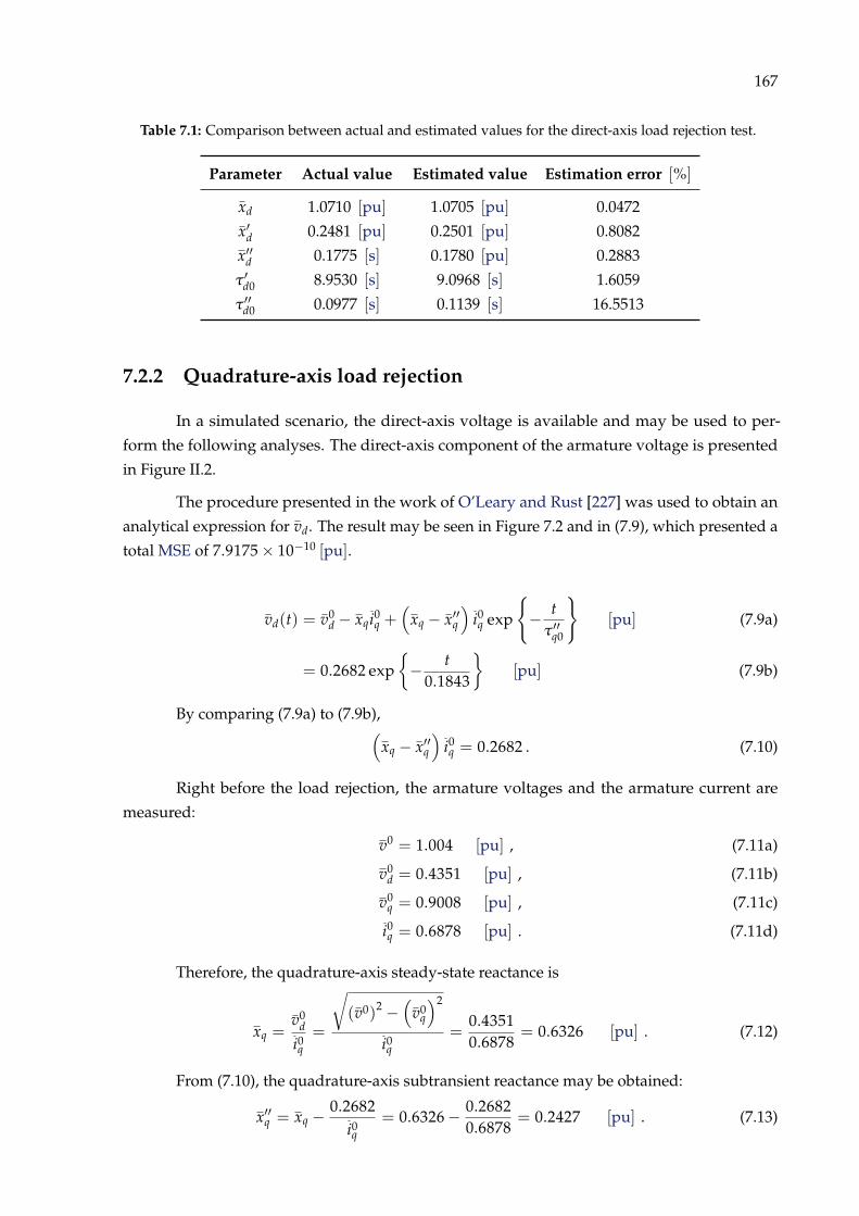
167

Table 7.1: Comparison between actual and estimated values for the direct-axis load rejection test.

Parameter Actual value Estimated value Estimation error [%]

xd 1.0710 [pu] 1.0705 [pu] 0.0472

x′d 0.2481 [pu] 0.2501 [pu] 0.8082

x′′d 0.1775 [s] 0.1780 [pu] 0.2883

τ ′d0 8.9530 [s] 9.0968 [s] 1.6059

τ ′′d0 0.0977 [s] 0.1139 [s] 16.5513

7.2.2 Quadrature-axis load rejection

In a simulated scenario, the direct-axis voltage is available and may be used to per-

form the following analyses. The direct-axis component of the armature voltage is presented

in Figure II.2.

The procedure presented in the work of O’Leary and Rust [227] was used to obtain an

analytical expression for vd. The result may be seen in Figure 7.2 and in (7.9), which presented a

total MSE of 7.9175× 10−10 [pu].

vd(t) = v0d − xqi0

q +(

xq − x′′q)

i0q exp

− tτ ′′q0

[pu] (7.9a)

= 0.2682 exp− t

0.1843

[pu] (7.9b)

By comparing (7.9a) to (7.9b),(xq − x′′q

)i0q = 0.2682 . (7.10)

Right before the load rejection, the armature voltages and the armature current are

measured:

v0 = 1.004 [pu] , (7.11a)

v0d = 0.4351 [pu] , (7.11b)

v0q = 0.9008 [pu] , (7.11c)

i0q = 0.6878 [pu] . (7.11d)

Therefore, the quadrature-axis steady-state reactance is

xq =v0

d

i0q=

√(v0)

2 −(

v0q

)2

i0q

=0.43510.6878

= 0.6326 [pu] . (7.12)

From (7.10), the quadrature-axis subtransient reactance may be obtained:

x′′q = xq −0.2682

i0q

= 0.6326− 0.26820.6878

= 0.2427 [pu] . (7.13)

168

50 50.2 50.4 50.6 50.8 51 51.2 51.4 51.6

Time [s]

0

0.05

0.1

0.15

0.2

0.25

0.3

Dir

ect-

ax

is a

rma

ture

vo

lta

ge

[pu

]

Direct-axis armature voltage -- Exponential approximation -- Computational experiment

Real data

Exponential approx.

Figure 7.2: Exponential approximation for the direct-axis armature voltage after the quadrature-axisload rejection.

The subtransient time constant is the modulus of the inverse of the exponential argu-

ments of (7.9b):

τ ′′q0 = 0.1843 [s] . (7.14a)

The estimate errors for the quadrature-axis load rejection test are given in Table 7.2. The

procedure provided very accurate results for the steady-state and subtransient reactances, as

well as for the time constant. It is important to highlight that, in the literature, the results for the

quadrature-axis are quite complicated to be achieved.

Table 7.2: Comparison between actual and estimated values for the quadrature-axis load rejectiontest.

Parameter Actual value Estimated value Estimation error [%]

xq 0.6326 [pu] 0.6326 [pu] 0.0004

x′′q 0.2426 [s] 0.2427 [pu] 0.0278

τ ′′q0 0.1844 [s] 0.1843 [s] 0.0451

7.3 Simplified approach

The simplified approach described in Subsection 6.2.2 was applied to all two data sets –

the computational and the real ones.

169

7.3.1 Simulation data

Upon the measurement of rotor speed and network frequency, the load angle was

estimated by means of both Euler and Runge–Kutta methods. The very satisfactory results are

presented in Figure 7.3.

0 5 10 15 20 25

Time [s]

-0.05

0

0.05

0.1

0.15

0.2

0.25

Loa

d a

ngle

[ra

d]

Load angle estimation -- Computational experiment -- Using a known operating condition

Real data

Euler method

Runge-Kutta 4th

Figure 7.3: Load angle estimation for the computational machine data via Euler’s method and4th-order Runge–Kutta.

Once the load angle is estimated, all abc quantities are transformed to the qd0 reference

frame. Further, an arbitrary steady-state point k1 is selected for the following computations:

1. Quadrature- and direct-axis flux linkages per second:

Ψq(k1) = −vd(k1)− rsid(k1)

ωr(k1)(7.15a)

= −0.1269 + 0.0012× (−0.0072)1

(7.15b)

= −0.1269 [pu] , (7.15c)

Ψd(k1) =vq(k1)− rsiq(k1)

ωr(k1)(7.16a)

=0.9920− 0.0012× (−0.2006)

1(7.16b)

= 0.9923 [pu] . (7.16c)

170

2. Quadrature- and direct-axis magnetizing flux linkages per second:

Ψmq(k1) = Ψq(k1)− iq(k1)xls (7.17a)

= −0.1269− (−0.2006)× 0.1180 (7.17b)

= −0.1032 [pu] , (7.17c)

Ψmd(k1) = Ψd(k1)− id(k1)xls (7.18a)

= 0.9923− (−0.0072)× 0.1180 (7.18b)

= 0.9931 [pu] . (7.18c)

3. Quadrature- and direct-axis magnetizing reactances:

xmq(k1) =Ψmq(k1)

iq(k1)=−0.1032−0.2006

= 0.5146 [pu] , (7.19)

xmd(k1) =Ψmd(k1)

id(k1) + i′f d(k1)=

0.9931−0.0072 + 1

= 1.0003 [pu] . (7.20)

The simplified approach is a simple methodology for calculating magnetizing reactances.

As long as some conditions are met for an accurate load angle estimation, the magnetizing reac-

tances are obtained with great accuracy. As for the computation error, the method encountered

4.5835× 10−5% for the quadrature-axis, and 4.9676% for the direct-axis. It is left for future

works the investigation of such difference in the direct-axis quantities.

In Table 7.3, a summarizing comparison between the parameters used for generating the

data and the estimated values is presented.

Table 7.3: Comparison between actual data and estimated values for the proposed simplifiedapproach.

Parameter Manufacturer value [pu] Estimated value [pu] Estimation error [%]

xmq 0.5146 0.5146 4.5835×10−5

xmd 0.9530 1.0003 4.9676

7.3.2 Real data

The load angle estimation is presented in Figure 7.4. Euler and Runge–Kutta methods

provided the same results.

Differently from the simulated scenario, it is not possible to verify the load angle esti-

mation accuracy. However, it is important to notice that the graph in Figure 7.4 has a different

behavior than Figure 7.3.

171

400 500 600 700 800 900 1000 1100 1200

Time [s]

0

0.2

0.4

0.6

0.8

1

1.2

Lo

ad

an

gle

[ra

d]

Load angle estimation -- Salvajina Unit-03

Euler Method

Runge-Kutta 4th

Figure 7.4: Load angle estimation for the actual machine data via Euler’s method and 4th-orderRunge–Kutta.

Once the load angle is estimated, all abc quantities are transformed to the qd0 reference

frame. As before, an arbitrary steady-state point k1 is selected for the following computations:

1. Quadrature- and direct-axis flux linkages per second:

Ψq(k1) = −vd(k1)− rsid(k1)

ωr(k1)(7.21a)

= −−0.1036 + 0.0012× (−0.0321)1.0002

(7.21b)

= 0.1035 [pu] , (7.21c)

Ψd(k1) =vq(k1)− rsiq(k1)

ωr(k1)(7.22a)

=0.9849− 0.0012× (0.1442)

1.0002(7.22b)

= 0.9845 [pu] . (7.22c)

2. Quadrature- and direct-axis magnetizing flux linkages per second:

Ψmq(k1) = Ψq(k1)− iq(k1)xls (7.23a)

= 0.1035− 0.1442× 0.19 (7.23b)

= 0.0761 [pu] , (7.23c)

172

Ψmd(k1) = Ψd(k1)− id(k1)xls (7.24a)

= 0.9845− (−0.0321)× 0.19 (7.24b)

= 0.9906 [pu] . (7.24c)

3. Quadrature- and direct-axis magnetizing reactances:

xmq(k1) =Ψmq(k1)

iq(k1)=

0.07610.1442

= 0.5278 [pu] , (7.25)

xmd(k1) =Ψmd(k1)

id(k1) + i′f d(k1)=

0.9906−0.0321 + 0.9960

= 1.0277 [pu] . (7.26)

The estimation errors are 3.4815% and 5.7115% for the quadrature- and the direct-axis

magnetizing reactance, respectively. In Table 7.4, a summarizing comparison between the data

provided by manufacturer and the estimated values is presented.

Table 7.4: Comparison between the data provided by manufacturer and the estimated values for theproposed simplified approach.

Parameter Manufacturer value [pu] Estimated value [pu] Estimation error [%]

xmq 0.5100 0.5278 3.4815

xmd 1.0900 1.0277 5.7115

7.4 Bayesian approach for states estimation

Before applying the Particle Filter (PF) to the salient-pole synchronous machine models,

it is important to analyze observability.

7.4.1 Observability analyses

Varying from the simplest to more complex models, different configurations were

considered.

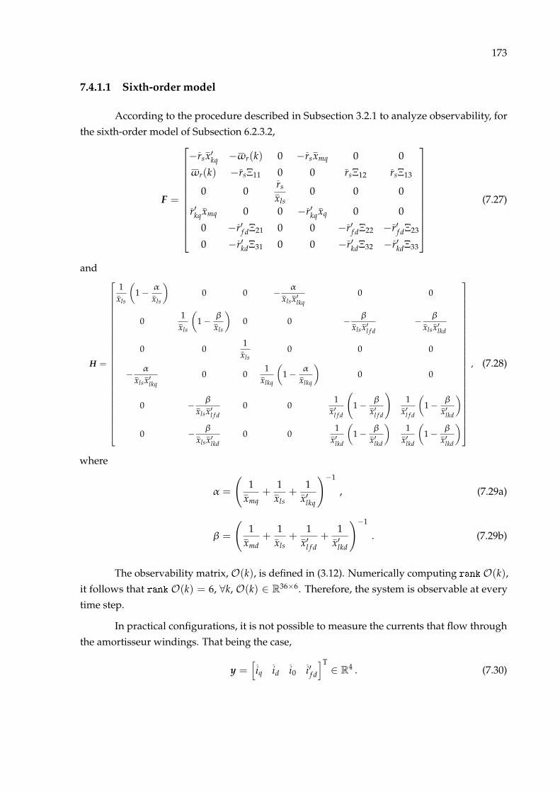
173

7.4.1.1 Sixth-order model

According to the procedure described in Subsection 3.2.1 to analyze observability, for

the sixth-order model of Subsection 6.2.3.2,

F =

−rsx′kq −ωr(k) 0 −rsxmq 0 0

ωr(k) −rsΞ11 0 0 rsΞ12 rsΞ13

0 0rs

xls0 0 0

r′kqxmq 0 0 −r′kqxq 0 0

0 −r′f dΞ21 0 0 −r′f dΞ22 −r′f dΞ23

0 −r′kdΞ31 0 0 −r′kdΞ32 −r′kdΞ33

(7.27)

and

H =

1xls

(1− α

xls

)0 0 − α

xlsx′lkq0 0

01

xls

(1− β

xls

)0 0 − β

xlsx′l f d− β

xlsx′lkd

0 01

xls0 0 0

− α

xlsx′lkq0 0

1xlkq

(1− α

xlkq

)0 0

0 − β

xlsx′l f d0 0

1x′l f d

(1− β

x′l f d

)1

x′l f d

(1− β

x′lkd

)0 − β

xlsx′lkd0 0

1x′lkd

(1− β

x′lkd

)1

x′lkd

(1− β

x′lkd

)

, (7.28)

where

α =

(1

xmq+

1xls

+1

x′lkq

)−1

, (7.29a)

β =

(1

xmd+

1xls

+1

x′l f d+

1x′lkd

)−1

. (7.29b)

The observability matrix, O(k), is defined in (3.12). Numerically computing rank O(k),it follows that rank O(k) = 6, ∀k, O(k) ∈ R36×6. Therefore, the system is observable at every

time step.

In practical configurations, it is not possible to measure the currents that flow through

the amortisseur windings. That being the case,

y =[iq id i0 i′f d

]T∈ R4 . (7.30)

174

Thus,

H =

1xls

(1− α

xls

)0 0 − α

xlsx′lkq0 0

01

xls

(1− β

xls

)0 0 − β

xlsx′l f d− β

xlsx′lkd

0 01

xls0 0 0

0 − β

xlsx′l f d0 0

1x′l f d

(1− β

x′l f d

)1

x′l f d

(1− β

x′lkd

)

(7.31)

and the numerical analysis led to rank O(k) = 6, ∀k, O(k) ∈ R24×6. Therefore, even when these

currents are not available, the sixth-order model continues to be observable.

7.4.1.2 Seventh-order model

For the seventh-order model of Subsection 6.2.3.3,

F =

−rsx′kq −ωr 0 −rsxmq 0 0 0

ωr −rsΞ11 0 0 rsΞ12 rsΞ13 0

0 0rs

xls0 0 0 0

r′kqxmq 0 0 −r′kqxq 0 0 0

0 −r′f dΞ21 0 0 −r′f dΞ22 −r′f dΞ23 0

0 −r′kdΞ31 0 0 −r′kdΞ32 −r′kdΞ33 0

−Ψd Ψq 0 0 0 0 0

(7.32)

and

H =

1xls

(1− α

xls

)0 0 − α

xlsx′lkq0 0 0

01

xls

(1− β

xls

)0 0 − β

xlsx′l f d− β

xlsx′lkd0

0 01

xls0 0 0 0

− α

xlsx′lkq0 0

1xlkq

(1− α

xlkq

)0 0 0

0 − β

xlsx′l f d0 0

1x′l f d

(1− β

x′l f d

)1

x′l f d

(1− β

x′lkd

)0

0 − β

xlsx′lkd0 0

1x′lkd

(1− β

x′lkd

)1

x′lkd

(1− β

x′lkd

)0

. (7.33)

Numerically computing rank O(k), it follows that rank O(k) = 6, ∀k, O(k) ∈ R42×7.

Therefore, the system is non-observable at any time step. To overcome this issue, rotor speed

measurements must be included in the set of measurements [72]:

y =[iq id i0 i′kq i′f d i′kd ωr

]T∈ R7 . (7.34)

175

Correspondingly, the following measurement equation is added:

h7(x, t) : ωr =ωr [pu] . (7.35)

Therefore, the matrix H becomes:

H =

1xls

(1− α

xls

)0 0 − α

xlsx′lkq0 0 0

01

xls

(1− β

xls

)0 0 − β

xlsx′l f d− β

xlsx′lkd0

0 01

xls0 0 0 0

− α

xlsx′lkq0 0

1xlkq

(1− α

xlkq

)0 0 0

0 − β

xlsx′l f d0 0

1x′l f d

(1− β

x′l f d

)1

x′l f d

(1− β

x′lkd

)0

0 − β

xlsx′lkd0 0

1x′lkd

(1− β

x′lkd

)1

x′lkd

(1− β

x′lkd

)0

0 0 0 0 0 0 1

, (7.36)

and the system becomes observable at every time step, since rank O(k) = 7, ∀k, O(k) ∈ R49×7.

7.4.1.3 Eighth-order model

When the load angle δ is added to the set of states, the system becomes non-observable,

as in the previous case. Once more, it is necessary to add load angle measurements to the set of

measurements to make it observable again. Thus,

h8(x, t) : δ = δ [electrical rad] (7.37)

and rank O(k) = 8, ∀k, O(k) ∈ R64×8.

One could wonder why measured quantities are added to the set of states. The answer

is simple: when measured, they are highly contaminated with noise; therefore, after filtering,

their actual value may be estimated.

7.4.2 States estimation

In Table 7.5, the running time and the total mean-squared error for the sixth-order model

in the simulated scenario, as a function of the number of particles, are presented. It considered a

scenario with 5, 000 samples, corresponding to 1 s of data, and all currents in the measurement

vector. It is possible to conclude that the larger the number of particles, the longer the required

running time, but the smaller the mean-squared error. By means of the running time per sample

line, it is possible to assure that the method may be applied for real-time analyses.

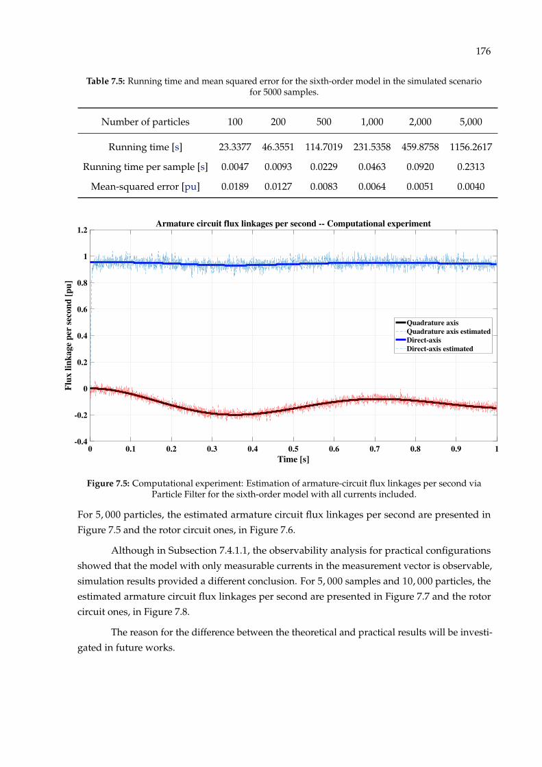
176

Table 7.5: Running time and mean squared error for the sixth-order model in the simulated scenariofor 5000 samples.

Number of particles 100 200 500 1,000 2,000 5,000

Running time [s] 23.3377 46.3551 114.7019 231.5358 459.8758 1156.2617

Running time per sample [s] 0.0047 0.0093 0.0229 0.0463 0.0920 0.2313

Mean-squared error [pu] 0.0189 0.0127 0.0083 0.0064 0.0051 0.0040

0 0.1 0.2 0.3 0.4 0.5 0.6 0.7 0.8 0.9 1

Time [s]

-0.4

-0.2

0

0.2

0.4

0.6

0.8

1

1.2

Flu

x l

ink

ag

e p

er s

eco

nd

[p

u]

Armature circuit flux linkages per second -- Computational experiment

Quadrature axis

Quadrature axis estimated

Direct-axis

Direct-axis estimated

Figure 7.5: Computational experiment: Estimation of armature-circuit flux linkages per second viaParticle Filter for the sixth-order model with all currents included.

For 5, 000 particles, the estimated armature circuit flux linkages per second are presented in

Figure 7.5 and the rotor circuit ones, in Figure 7.6.

Although in Subsection 7.4.1.1, the observability analysis for practical configurations

showed that the model with only measurable currents in the measurement vector is observable,

simulation results provided a different conclusion. For 5, 000 samples and 10, 000 particles, the

estimated armature circuit flux linkages per second are presented in Figure 7.7 and the rotor

circuit ones, in Figure 7.8.

The reason for the difference between the theoretical and practical results will be investi-

gated in future works.

177

0 0.1 0.2 0.3 0.4 0.5 0.6 0.7 0.8 0.9 1

Time [s]

-0.4

-0.2

0

0.2

0.4

0.6

0.8

1

1.2

1.4

Flu

x l

ink

ag

e p

er s

eco

nd

[p

u]

Rotor circuit flux linkages per second -- Computational experiment

Quadrature-axis amortisseur

Quadrature-axis amortisseur estimated

Field winding

Field winding estimated

Direct-axis amortisseur

Direct-axis amortisseur estimated

Figure 7.6: Computational experiment: Estimation of rotor-circuit flux linkages per second viaParticle Filter for the sixth-order model with all currents included.

0 0.1 0.2 0.3 0.4 0.5 0.6 0.7 0.8 0.9 1

Time [s]

-1

-0.8

-0.6

-0.4

-0.2

0

0.2

0.4

0.6

0.8

1

Flu

x l

ink

ag

e p

er s

eco

nd

[p

u]


Quadrature axis


Direct-axis


Figure 7.7: Computational experiment: Estimation of armature-circuit flux linkages per second viaParticle Filter for the sixth-order model with only measurable currents included.

178

0 0.1 0.2 0.3 0.4 0.5 0.6 0.7 0.8 0.9 1

Time [s]

-1.5

-1

-0.5

0

0.5

1

1.5

Flu

x l

ink

ag

e p

er s

eco

nd

[p

u]




Field winding




Figure 7.8: Computational experiment: Estimation of rotor-circuit flux linkages per second viaParticle Filter for the sixth-order model with only measurable currents included.

7.5 Bayesian approach for states and parameters estimation

As presented in Subsection 4.5.5, the set of states is extended with the desired parameters

to be estimated. In this work, the quadrature- and the direct-axis magnetizing reactances are

considered.

7.5.1 Observability analysis

Once more, the procedure from Subsection 3.2.1 is used to analyze stability. At this time,

the model presented in Subsection 6.2.3.5 is considered. Therefore,

F =

−rsx′kq −ωr(k) 0 −rsxmq 0 0 −rsΨ′kq 0

ωr(k) −rsΞ11 0 0 rsΞ12 rsΞ13 0 2rsxmd

(Ψd + Ψ′f d + Ψ′kd

)0 0

rs

xls0 0 0 0 0

r′kqxmq 0 0 −r′kqxq 0 0 r′kqΨq 0

0 −r′f dΞ21 0 0 −r′f dΞ22 −r′f dΞ23 0 −2r′f dxmd

(Ψd − Ψ′f d + Ψ′kd

)0 −r′kdΞ31 0 0 −r′kdΞ32 −r′kdΞ33 0 −2r′kdxmd

(Ψd + Ψ′f d − Ψ′kd

)0 0 0 0 0 0 1 0

0 0 0 0 0 0 0 1

(7.38)

179

and

H =

1xls

(1− α

xls

)0 0 − α

xlsx′lkq0 0 −κ1

xls0

01

xls

(1− β

xls

)0 0 − β

xlsx′l f d− β

xlsx′lkd0 −κ2

xls

0 01

xls0 0 0 0 0

− α

xlsx′lkq0 0

1xlkq

(1− α

xlkq

)0 0 − κ1

x′lkq0

0 − β

xlsx′l f d0 0

1x′l f d

(1− β

x′l f d

)1

x′l f d

(1− β

x′lkd

)0 − κ2

x′l f d

0 − β

xlsx′lkd0 0

1x′lkd

(1− β

x′lkd

)1

x′lkd

(1− β

x′lkd

)0 − κ2

x′lkd

, (7.39)

where,

α =

(1

xmq+

1xls

+1

x′lkq

)−1

, (7.40)

β =

(1

xmd+

1xls

+1

x′l f d+

1x′lkd

)−1

, (7.41)

κ1 =∂Ψmq

∂xmq=

x2lsx2

lkq[xmq(xls + xlkq) + xlsxlkq

] (Ψq

xls+

Ψ′kq

x′lkq

), (7.42)

κ2 =∂Ψmd

∂xmd=

[xmd

(1

xmd+

1xls

+1

x′l f d+

1x′lkd

)]−2(Ψd

xls+

Ψ′f d

x′l f d+

Ψ′kdx′lkd

)(7.43a)

= (xmdβ)−2

(Ψd

xls+

Ψ′f d

x′l f d+

Ψ′kdx′lkd

). (7.43b)

Numerically computing rank O(k), it follows that rank O(k) = 8, ∀k, O(k) ∈ R48×8.

Therefore, the system is observable at every time step.

7.5.2 States and parameters estimation

In Subsection 7.5.1, it was shown that the eighth-order model created by the original

sixth-order model augmented with the two desired parameters and with a measurement vector

considering the measurements of all currents is completely observable, being able to estimate

states and parameters. As in the previous cases, the theoretical results differed from the practical

results: for 5, 000 samples and 10, 000 particles, the estimated armature and rotor circuits flux

linkages per second are presented in Figure 7.9 and Figure 7.10, respectively, whereas the

parameters are shown in Figure 7.11.

180

0 0.1 0.2 0.3 0.4 0.5 0.6 0.7 0.8

Time [s]

-0.4

-0.2

0

0.2

0.4

0.6

0.8

1

1.2

Flu

x l

ink

ag

e p

er s

eco

nd

[p

u]


Quadrature axis


Direct-axis



0 0.1 0.2 0.3 0.4 0.5 0.6 0.7 0.8

Time [s]

-0.4

-0.2

0

0.2

0.4

0.6

0.8

1

1.2

Flu

x l

ink

ag

e p

er s

eco

nd

[p

u]




Field winding





181

0 0.1 0.2 0.3 0.4 0.5 0.6 0.7 0.8

Time [s]

-0.2

0

0.2

0.4

0.6

0.8

1

1.2

1.4

Ma

gn

etiz

ing

rea

cta

nce

s [p

u]

Magnetizing reactances estimation -- Computational experiment

x_mq

x_mq estimated

x_md

x_md estimated

Figure 7.11: Computational experiment: Estimation of quadrature- and direct-axis magnetizingreactances via Particle Filter for the sixth-order model with all currents included.

A possible way to overcome this practical observability problem is to add rotor speed

and load angle measurements to the measurement vector [1]:

y =[iq id i0 i′kq i′f d i′kd ωr,m δm

]T∈ R8 , (7.44)

turning it into an eighth-order vector, whereωr,m is the measured rotor speed, and δm is the

measured load angle3.

For 5, 000 particles, the estimated armature circuit flux linkages per second are presented

in Figure 7.12, the rotor circuit ones, in Figure 7.13, and the parameters, in Figure 7.14. The

results are very satisfactory, with 5.0086× 10−5 [pu] mean-squared error for the quadrature-axis

magnetizing reactance and 4.0674× 10−4 [pu], for the direct-axis magnetizing reactance; these

results are quite similar to the ones presented by Monteiro, Vianna, and Giesbrecht [1].

The initial value of the particles in the positions corresponding to the magnetizing

reactances comprised values randomly chosen within a range of widely established values [13]:

0.5 ≤ xmq ≤ 1 [pu] , (7.45)

0.8 ≤ xmd ≤ 1.3 [pu] . (7.46)

In the work of Valverde et al. [72], it was also shown that rotor speed and load angle

measurements are required for proper magnetizing reactances estimation. Due to the lack of

3In the lack of load angle measurements, the procedure developed in Subsection 6.2.2 may be applied,as it was done in this work.

182

29.8 29.9 30 30.1 30.2 30.3 30.4 30.5 30.6 30.7 30.8

Time [s]

-0.2

0

0.2

0.4

0.6

0.8

1

1.2

Flu

x l

ink

ag

e p

er s

eco

nd

[p

u]


Quadrature axis


Direct-axis


Figure 7.12: Computational experiment: Estimation of armature-circuit flux linkages per second viaParticle Filter for the eighth-order model with all currents included.

29.8 29.9 30 30.1 30.2 30.3 30.4 30.5 30.6 30.7 30.8

Time [s]

-0.2

0

0.2

0.4

0.6

0.8

1

1.2

1.4

Flu

x l

ink

ag

e p

er s

eco

nd

[p

u]




Field winding




Figure 7.13: Computational experiment: Estimation of armature-circuit flux linkages per second viaParticle Filter for the eighth-order model with all currents included.

183

29.8 29.9 30 30.1 30.2 30.3 30.4 30.5 30.6 30.7 30.8

Time [s]

0.1

0.2

0.3

0.4

0.5

0.6

0.7

0.8

0.9

1

1.1

Ma

gn

etiz

ing

rea

cta

nce

s [p

u]

Magnetizing reactances estimation -- Computational experiment

x_mq

x_mq estimated

x_md

x_md estimated

Figure 7.14: Computational experiment: Estimation of quadrature- and direct-axis magnetizingreactances via Particle Filter for the eighth-order model with all currents included.

load angle measurements, Valverde et al. [72] approximated it by using the power output at the

machine terminals and the estimated value of the direct-axis reactance.

Since the machine used to generated the real data was not provided with equipment to

measure the load angle, only the simulated data were used to estimate states and parameters by

means of the Bayesian approach. In future works, the method proposed in Subsection 6.2.2 or

the one from Valverde et al. [72] may be applied to overcome the absence of such load angle

measurements.

184

Chapter 8

Conclusions and Future Directions

“Isn’t it splendid to think of all the things there are to find out about? It just makes mefeel glad to be alive – it’s such an interesting world. It wouldn’t be half so interestingif we know all about everything, would it? There would be no scope for imaginationthen, would there?”

— Anne Shirley-Cuthbert1

8.1 General conclusions

Bearing in mind the importance of salient-pole synchronous machines for the different

analyses of power systems in countries where the energy generation is based on hydraulic

sources, in this work, some methodologies have been proposed to estimate states and physical

parameters of such machines.

The complete and most robust model of synchronous machines is based on operational

equations and require more complex procedures to survey all transient and subtransient param-

eters. These methods are off-line – which require the machine to be taken out of operation. As an

example, the load rejection test was contemplated. In result, this work proposed an automated

methodology based on optimization procedures for separating every single exponential from

the resulting voltage curve.

Another important challenge in the study of synchronous machines refers to the inability

of measuring the load angle – that is, it is necessary to estimate it using specific procedures and

algorithms. In the present work, a methodology based on the machine equations was developed

to obtain load conditions that allow the calculation of the load angle by means of rotor speed

and network frequency measurements and a known initial condition.

Ultimately, it is known that, in real scenarios, any measurement is corrupted with

measurement noise – to a greater or a lesser extent. In this way, the analyzes become more

complex, since the accuracy of the measured values is not precisely known. To get around these

problems, Bayesian estimators can be applied to filter the real values amid so much noise. The

present work evaluated the performance and the basis of the well-known Particle Filter (PF).

1Anne Shirley is a fictional character introduced in the 1908 novel Anne of Green Gables by LucyMaud Montgomery. Montgomery wrote in her journal that the idea for Anne’s story came from relativeswho, planning to adopt an orphaned boy, received a girl instead.

185

In this sense, the application of the proposed methods proved to be satisfactory, given

that the solutions obtained are consistent with the physical characteristics of the machines under

analysis. The effectiveness of the methods is also evidenced by the similarity among the different

solutions found by each of the approaches.

8.2 Future directions

As future works, the following research points are suggested:

1. Perform a more robust observability analysis, such as the one based on the Lie algebra, to

investigate the difference found between theoretical and practical results;

2. Validate the performance of the load rejection test and the Bayesian approach methodolo-

gies on actual synchronous machines;

3. Assess the performance of Extended Kalman Filter (EKF) and the Unscented Kalman

Filter (UKF) on the estimation of salient-pole synchronous machines parameters;

4. Assess some black-box identification methods on physical parameters estimation.

186

References

1 MONTEIRO, I. A.; VIANNA, L. M. S.; GIESBRECHT, M. Nonlinear estimationof salient-pole synchronous machines parameters via Particle Filter. In: 2019IEEE PES Innovative Smart Grid Technologies Conference – Latin America (ISGTLatin America). Gramado, RS, BR: IEEE, Sept. 2019. P. 1–6. DOI: 10.1109/ISGT-LA.2019.8895417.

2 . Observador de fluxos, correntes e ângulo de carga de máquinas sín-cronas por meio da filtragem de partículas. In: ANAIS do XIV Simpósio Brasileirode Automação Inteligente. Ouro Preto, MG, BR: Galoá, Oct. 2019. v. 1. DOI:10.17648/sbai-2019-111220.

3 MONTEIRO, I. A.; MENESES, L.; GIESBRECHT, M. A novel approach on thedetermination of salient-pole synchronous machine magnetizing reactances fromon-line measurements. In: 2020 IEEE 29th International Symposium on IndustrialElectronics (ISIE). In Press: [s.n.], 2020.

4 VIANNA, L.; GONÇALVES, J.; MONTEIRO, I.; GIESBRECHT, M. Detecção defalhas de alimentação de um motor CC sem escovas via Filtro de Partículas. In:ANAIS do XIV Simpósio Brasileiro de Automação Inteligente. Ouro Preto, MG,Brazil: Galoá, Oct. 2019. v. 1. DOI: 10.17648/sbai-2019-111202.

5 GLOVER, J. D.; OVERBYE, T. J.; SARMA, M. S. Power System Analysis & Design.Sixth ed. Boston, MA, USA: Cengage Learning, Jan. 2017. ISBN 978-1-305-63213-4.

6 VARAIYA, P. P.; WU, F. F.; BIALEK, J. W. Smart operation of smart grid: risk-limiting dispatch. Proceedings of the IEEE, v. 99, n. 1, p. 40–57, Jan. 2011. ISSN0018-9219. DOI: 10.1109/JPROC.2010.2080250.

7 BLAABJERG, F.; TEODORESCU, R.; LISERRE, M.; TIMBUS, A. V. Overview ofcontrol and grid synchronization for distributed power generation systems. IEEETransactions on Industrial Electronics, v. 53, n. 5, p. 1398–1409, Oct. 2006. ISSN1557-9948. DOI: 10.1109/TIE.2006.881997.

8 SMITH, J.; RYLANDER, M.; ROGERS, L.; DUGAN, R. It’s all in the plans: max-imizing the benefits and minimizing the impacts of DERs in an integrated grid.





https://doi.org/10.1109/JPROC.2010.2080250

https://doi.org/10.1109/TIE.2006.881997

187

IEEE Power and Energy Magazine, v. 13, n. 2, p. 20–29, Jan. 2015. ISSN 1558-4216.DOI: 10.1109/MPE.2014.2379855.

9 SHAHIDEHPOUR, M.; SCHWARTS, F. Don’t let the sun go down on photovoltaicsystems. IEEE Power and Energy Magazine, v. 2, n. 3, p. 40–48, June 2004. ISSN1558-4216. DOI: 10.1109/MPAE.2004.1293599.

10 WRIGHT, S. H. Determination of synchronous machine constants by test reac-tances, resistances, and time constants. Transactions of the American Instituteof Electrical Engineers, v. 50, n. 4, p. 1331–1350, Dec. 1931. ISSN 0096-3860. DOI:10.1109/T-AIEE.1931.5055960.

11 KILGORE, L. A. Calculation of synchronous machine constants – reactances andtime constants affecting transient characteristics. Transactions of the AmericanInstitute of Electrical Engineers, v. 50, n. 4, p. 1201–1213, Dec. 1931. ISSN 0096-3860. DOI: 10.1109/T-AIEE.1931.5055943.

12 MOMOH, J. A. Energy Processing and Smart Grid. Piscataway, NJ, USA: Wiley–IEEE Press, June 2018. (IEEE Press Series on Power Engineering). ISBN 978-1-119-37616-3.

13 IEEE. IEEE Guide for Test Procedures for Synchronous Machines Part I - Accep-tance and Performance Testing, Part II - Test Procedures and Parameter Determi-nation for Dynamic Analysis. IEEE Std 115-2009 (Revision of IEEE Std 115-1995),p. 1–219, May 2010. DOI: 10.1109/IEEESTD.2010.5464495.

14 AGRAWAL, B. L.; DEMCKO, J. A. WSCC testing experience with generating units.In: IEEE Power Engineering Society. 1999 Winter Meeting. New York, NY, USA:IEEE, Jan. 1999. v. 1, p. 160–161. DOI: 10.1109/PESW.1999.747443.

15 DERUSSO, P. M.; ROY, R. J.; CLOSE, C. M.; DESROCHERS, A. A. State Variablesfor Engineers. Second ed. Hoboken, NJ, USA: Wiley-Interscience, Dec. 1997. ISBN978-0-471-57795-9.

16 GHAHREMANI, E.; KAMWA, I. Dynamic state estimation in power system byapplying the Extended Kalman Filter with unknown inputs to phasor measure-ments. IEEE Transactions on Power Systems, v. 26, n. 4, p. 2556–2566, Nov. 2011.ISSN 1558-0679. DOI: 10.1109/TPWRS.2011.2145396.

17 KOSTEREV, D. N.; TAYLOR, C. W.; MITTELSTADT, W. A. Model validation forthe August 10, 1996 WSCC system outage. IEEE Transactions on Power Systems,v. 14, n. 3, p. 967–979, Aug. 1999. ISSN 0885-8950. DOI: 10.1109/59.780909.

https://doi.org/10.1109/MPE.2014.2379855

https://doi.org/10.1109/MPAE.2004.1293599

https://doi.org/10.1109/T-AIEE.1931.5055960


https://doi.org/10.1109/IEEESTD.2010.5464495

https://doi.org/10.1109/PESW.1999.747443

https://doi.org/10.1109/TPWRS.2011.2145396

https://doi.org/10.1109/59.780909

188

18 GIESBRECHT, M.; MENESES, L. A. E. Detailed derivation and experimental val-idation of a method for obtaining load conditions for salient pole synchronousmachine quadrature-axis parameters determination. IEEE Transactions on In-dustrial Electronics, v. 66, n. 7, p. 5049–5056, July 2019. ISSN 0278-0046. DOI:10.1109/TIE.2018.2866096.

19 KRAUSE, P. C.; WASYNCZUK, O.; SUDHOFF, S. D.; PEKAREK, S. Analysis ofElectric Machinery and Drive Systems. Third ed. Hoboken, NJ, USA: John Wiley& Sons, Inc., 2013. (IEEE Press Series on Power Engineering). ISBN 978-1-118-02429-4.

20 ZHOU, N.; MENG, D.; LU, S. Estimation of the dynamic states of synchronousmachines using an extended Particle Filter. IEEE Transactions on Power Systems,v. 28, n. 4, p. 4152–4161, Nov. 2013. ISSN 0885-8950. DOI: 10.1109/TPWRS.2013.2262236.

21 DANDENO, P. L. Current usage suggested practices in power system stabilitysimulations for synchronous machines. IEEE Transactions on Energy Conversion,EC-1, n. 1, p. 77–93, Mar. 1986. ISSN 0885-8969. DOI: 10.1109/TEC.1986.4765673.

22 ANDERSON, P. M.; FOUAD, A. A. Power System Control and Stability. Ed. byMohamed E. El-Hawary. Second ed. Piscataway, NJ, USA: John Wiley & Sons, Inc.,2003. (IEEE Power Engineering Series). ISBN 0-471-23862-7.

23 KIESSLING, F.; NEFZGER, P.; NOLASCO, J. F.; KAINTZYK, U. Overhead PowerLines: Planning, Design, Construction. New York, NY, USA: Springer-VerlagBerlin Heidelberg, 2014. (Power Systems). ISBN 978-3-642-05556-0.

24 GRAINGER, J.; STEVENSON, W. Power System Analysis. [S.l.]: McGraw-Hill,2003. (McGraw-Hill Series in Electrical and Computer Engineering: Power andEnergy). ISBN 9780070585157.

25 EKANAYAKE, J. B.; JENKINS, N.; LIYANAGE, K.; WU, J.; YOKOYAMA, A. SmartGrid: Technology and Applications. Chichester, WS, UK: John Wiley & Sons, Ltd.,Feb. 2012. ISBN 978-1-119-96909-9.

26 LIU, J. S.; CHEN, R. Blind deconvolution via sequential imputations. Journal ofthe American Statistical Association, v. 90, n. 430, p. 567–576, June 1995. ISSN0162-1459. DOI: 10.2307/2291068.

27 HUANG, C.-T.; CHEN, Y.-T.; CHANG, C.-L.; HUANG, C.-Y.; CHIANG, H.-D.;WANG, J.-C. On-line measurement-based model parameter estimation for syn-chronous generators: model development and identification schemes. IEEE Trans-actions on Energy Conversion, v. 9, n. 2, p. 330–336, June 1994. ISSN 0885-8969.DOI: 10.1109/60.300140.

https://doi.org/10.1109/TIE.2018.2866096



https://doi.org/10.1109/TEC.1986.4765673

https://doi.org/10.2307/2291068

https://doi.org/10.1109/60.300140

189

28 BIM, E. Máquinas Elétricas e Acionamento. Second ed. Rio de Janeiro, RJ, BR:Elsevier Editora Ltda., Feb. 2015. ISBN 978-85-352-5923-0.

29 WHITE, D. C.; WOODSON, H. H. Electromechanical Energy Conversion. NewYork, NY, USA: John Wiley & Sons, Inc., 1959. ISBN 978-1124129310.

30 ADKINS, B. The General Theory of Electrical Machines. London, UK: Chapman& Hall, 1957. ISBN 978-0-41-207840-8.

31 CONCORDIA, C. Synchronous Machines: Theory and Performance. New York,NY, USA: John Wiley & Sons, Inc., 1951. (General Electric Series). ISBN 978-0608100029.

32 ELGERD, O. I. Electric Energy Systems Theory: An Introduction. Ed. by H. H.Happ. New York, NY, USA: McGraw-Hill, 1971. ISBN 978-0-07-019230-0.

33 KUNDUR, P. Power Systems Stability and Control. Ed. by Neal J. Balu and MarkG. Lauby. New York, NY, USA: McGraw-Hill, Inc., 1994. (EPRI Power SystemEngineering Series). ISBN 0-07-035958-X.

34 KOSTENKO, M. P.; PIOTROVSKY, L. M. Electrical Machines: Part two. Moscow,RUS: Foreign Languages Publishing House, 1962. v. 2. ISBN 978-0714715360.

35 PADIYAR, K. R. Power System Dynamics: Stability & Control. Second ed. Hy-derabad, India: BS Publications, 2008. ISBN 978-81-7800-186-9.

36 LIPO, T. A. Analysis of Synchronous Machines. Second ed. Boca Raton, FL, USA:CRC Press, May 2012. ISBN 978-1-4398-8068-5.

37 IEEE. The Authoritative Dictionary of IEEE Standards Terms. IEEE Std 100-2000,p. 1–1362, Dec. 2000. DOI: 10.1109/IEEESTD.2000.322230.

38 GURU, B. S.; HIZIROGLU, H. R. Electric Machinery and Transformers. Third ed.New York, NY, USA: Oxford University Press, Inc., 2001. (The Oxford Series inElectrical and Computer Engineering). ISBN 978-0-19-513890-0.

39 LAWRENCE, R. R. Principles of Alternating Current Machinery. Second ed.New York, NY, USA: McGraw-Hill Book Company, Inc., Apr. 1921. (ElectricalEngineering Texts). ISBN 978-1-330-53797-8.

40 AGARWAL, P. D. Eddy-current losses in solid and laminated iron. Transactionsof the American Institute of Electrical Engineers, Part I: Communication andElectronics, v. 78, n. 2, p. 169–181, May 1959. DOI: 10.1109/TCE.1959.6372977.

41 IEEE. Recommended phasor diagram for synchronous machines. IEEE Transac-tions on Power Apparatus and Systems, PAS-88, n. 11, p. 1593–1610, Nov. 1969.ISSN 0018-9510. DOI: 10.1109/TPAS.1969.292366.


https://doi.org/10.1109/TCE.1959.6372977

https://doi.org/10.1109/TPAS.1969.292366

190

42 ANDERSON, P. M.; AGRAWAL, B. L.; NESS, J. E. V. Subsynchronous Resonancein Power Systems. New York, NY, USA: Wiley–IEEE Press, 1990. ISBN 978-0-87942-258-5.

43 PARK, R. H. Two-reaction theory of synchronous machines - Generalized methodof analysis - Part I. Transactions of the American Institute of Electrical Engi-neers, v. 48, n. 3, p. 716–727, July 1929. ISSN 0096-3860. DOI: 10.1109/T-AIEE.1929.5055275.

44 UMANS, S. Fitzgerald & Kingsley’s Electric Machinery. Seventh ed. New York,NY, USA: McGraw-Hill, 2014. ISBN 978-0-07-338046-9.

45 KRON, G. Equivalent Circuits of Electric Machinery. New York, NY, USA: JohnWiley & Sons, 1951. ISBN 978-0-84-462409-9.

46 CARTER, G. W. The simple calculation of electrical transients: An elemen-tary treatment of transient problems in electrical circuits by Heaviside’s op-erational methods. Cambridge, UK: Cambridge University Press, 1944.

47 BOYLESTAD, R. L. Introductory Circuit Analysis. Thirteenth ed. Essex, UK: Pear-son Education, 2016. ISBN 978-1-292-09895-1.

48 STEINMETZ, C. P.; BERG, E. J. Theory and Calculation of Alternating CurrentPhenomena. Third ed. New York, NY, USA: Electrical World and Engineer Inc.,1900. ISBN 978-1-34-624243-9.

49 IEEE-1110. IEEE Guide for Synchronous Generator Modeling Practices and Ap-plications in Power System Stability Analyses. IEEE Std 1110-2002 Revision ofIEEE Std 1110-1991, p. 01–72, 2003. DOI: 10.1109/IEEESTD.2003.94408.

50 MACHOWSKI, J.; BIALEK, J. W.; BUMBY, J. R. Power System Dynamics – Sta-bility and Control. Second ed. Chichester, WS, UK: John Wiley & Sons, Ltd, 2008.ISBN 978-0-470-72558-0.

51 MALEKPOUR, M.; AZIZIPANAH-ABARGHOOEE, R.; ZARE, M.; KIYOUMARSI,A.; TERZIJA, V. An explicit formulation for synchronous machine model in termsof the manufacturer data. International Journal of Electrical Power & EnergySystems, v. 108, p. 9–18, June 2019. ISSN 0142-0615. DOI: 10.1016/j.ijepes.2018.12.032.

52 STANLEY, H. C. An analysis of the induction motor. AIEE Transactions, v. 48,p. 716–727, 1938. ISSN 2376-7804. DOI: 10.1109/EE.1938.6431069.

53 BERETON, D. S.; LEWIS, D. G.; YOUNG, C. G. Representation of induction motorloads during power system stability studies. AIEE Transactions, v. 76, p. 451–461,Apr. 1957. ISSN 2379-6766. DOI: 10.1109/AIEEPAS.1957.4499587.




https://doi.org/10.1016/j.ijepes.2018.12.032

https://doi.org/10.1016/j.ijepes.2018.12.032

https://doi.org/10.1109/EE.1938.6431069

https://doi.org/10.1109/AIEEPAS.1957.4499587

191

54 KRAUSE, P. C.; THOMAS, C. H. Simulation of symmetrical induction machinery.IEEE Transactions on Power Apparatus Systems, v. 84, p. 1038–1053, Nov. 1965.ISSN 0018-9510. DOI: 10.1109/TPAS.1965.4766135.

55 KRAUSE, P. C.; NOZARI, F.; SKVARENINA, T. L.; OLIVE, D. W. The theory ofneglecting stator transients. IEEE Transactions on Power Apparatus Systems,v. 98, p. 141–148, Jan. 1979. ISSN 0018-9510. DOI: 10.1109/TPAS.1979.319542.

56 CLARKE, E. Circuit Analysis of A-C Power Systems – Symmetrical and RelatedComponents. Schenectady, NY, USA: John Wiley & Sons, Inc., June 1943. One.(General Electric Advanced Engineering Program). ISBN 978-9-33-304261-1.

57 BLONDEL, A. E. Synchronous Motors and Converters: Theory and Methods ofCalculation and Testing. Ed. by C. O. Mailloux. New York, NY, USA: McGraw-Hill Book Company, 1913. ISBN 978-1-33-061889-9.

58 DOHERTY, R. E.; NICKLE, C. A. Synchronous machines I: An extension of Blon-del’s two-reaction theory. Journal of the A.I.E.E., v. 45, n. 10, p. 974–987, Oct. 1926.ISSN 0095-9804. DOI: 10.1109/JAIEE.1926.6537307.

59 . Synchronous machines III: Torque-angle characteristics under transientconditions. Journal of the A.I.E.E., v. 46, n. 12, p. 1339–1339, Dec. 1927. ISSN0095-9804. DOI: 10.1109/JAIEE.1927.6538137.

60 . Synchronous machines IV. Transactions of the American Institute ofElectrical Engineers, v. 47, n. 2, p. 457–487, Apr. 1928. ISSN 0096-3860. DOI: 10.1109/T-AIEE.1928.5055006.

61 . Synchronous machines V: Three-phase short circuit synchronous ma-chines. Transactions of the American Institute of Electrical Engineers, v. 49, n. 2,p. 700–714, Apr. 1930. ISSN 0096-3860. DOI: 10.1109/T-AIEE.1930.5055558.

62 PARK, R. H. Two-reaction theory of synchronous machines - Part II. Transactionsof the American Institute of Electrical Engineers, v. 52, n. 2, p. 352–354, June1933. ISSN 0096-3860. DOI: 10.1109/T-AIEE.1933.5056309.

63 FORTESCUE, C. L. Method of symmetrical co-ordinates applied to the solution ofpolyphase networks. Transactions of the American Institute of Electrical Engi-neers, v. XXXVII, n. 2, p. 1027–1140, July 1918. ISSN 0096-3860. DOI: 10.1109/T-AIEE.1918.4765570.

64 SHACKSHAFT, G.; PORAY, A. T. Implementation of new approach to deter-mination of synchronous-machine parameters from tests. Proceedings of theInstitution of Electrical Engineers, v. 124, n. 12, p. 1170–1178, Dec. 1977. ISSN0020-3270. DOI: 10.1049/piee.1977.0246.



https://doi.org/10.1109/JAIEE.1926.6537307

https://doi.org/10.1109/JAIEE.1927.6538137







https://doi.org/10.1049/piee.1977.0246

192

65 DE MELLO, F. P.; RIBEIRO, J. R. Derivation of synchronous machine parame-ters from tests. IEEE Transactions on Power Apparatus and Systems, v. 96, n. 4,p. 1211–1218, July 1977. ISSN 0018-9510. DOI: 10.1109/T-PAS.1977.32443.

66 DE MELLO, F. P.; HANNETT, L. H. Validation of synchronous machine modelsand derivation of model parameters from tests. IEEE Transactions on PowerApparatus and Systems, PAS-100, n. 2, p. 662–672, Feb. 1981. ISSN 0018-9510.DOI: 10.1109/TPAS.1981.316963.

67 COULTES, M. E.; WATSON, W. Synchronous machine models by standstill fre-quency response tests. IEEE Transactions on Power Apparatus and Systems,PAS-100, n. 4, p. 1480–1489, Apr. 1981. ISSN 0018-9510. DOI: 10.1109/TPAS.1981.316568.

68 DANDENO, P. L.; KUNDUR, P.; PORAY, A. T.; Z. EL-DIN, H. m. Adaptationand validation of turbogenerator model parameters through on-Line frequencyresponse measurements. IEEE Transactions on Power Apparatus and Systems,PAS-100, n. 4, p. 1656–1664, Apr. 1981. ISSN 0018-9510. DOI: 10.1109/TPAS.1981.316560.

69 LEWIS, W. A. A basic analysis of synchronous machines – Part I. Transactions ofthe American Institute of Electrical Engineers. Part III: Power Apparatus andSystems, v. 77, n. 3, p. 436–453, Apr. 1958. ISSN 2379-6766. DOI: 10.1109/AIEEPAS.1958.4499954.

70 HARRIS, M. R.; LAWRENSON, P. J.; STEPHENSON, J. M. Per-unit Systems withSpecial Reference to Electrical Machines. Cambridge, UK: University Press, 1970.(IEE Monograph Series). ISBN 978-0-521-07857-3.

71 KIRTLEY, J. L. Electric Power Principles: Sources, Conversion, Distribution andUse. West Sussex, UK: John Wiley & Sons, Ltd., 2010. (Massachusetts Institute ofTechnology). ISBN 978-0-470-68636-2.

72 VALVERDE, G.; KYRIAKIDES, E.; HEYDT, G. T.; TERZIJA, V. Nonlinear estima-tion of synchronous machine parameters using operating data. IEEE Transactionson Energy Conversion, v. 26, n. 3, p. 831–839, Sept. 2011. ISSN 0885-8969. DOI:10.1109/TEC.2011.2141136.

73 HOSSEINI, S. M.; ABDOLLAHI, R.; KARRARI, M. Inclusive design and im-plementation of online load angle measurement for real-time transient stabilityimprovement of a synchronous generator in a smart grid. IEEE Transactions onIndustrial Electronics, v. 65, n. 11, p. 8966–8972, Nov. 2018. ISSN 0278-0046. DOI:10.1109/TIE.2018.2811394.

https://doi.org/10.1109/T-PAS.1977.32443








https://doi.org/10.1109/TEC.2011.2141136

https://doi.org/10.1109/TIE.2018.2811394

193

74 LEVI, E.; LEVI, V. A. Impact of dynamic cross-saturation on accuracy of saturatedsynchronous machine models. IEEE Transactions on Energy Conversion, v. 15,n. 2, p. 224–230, June 2000. ISSN 0885-8969. DOI: 10.1109/60.867004.

75 FILHO, E. R.; NUNES JUNIOR, F. L.; NUNES, S. O. Synchronous machine fieldcurrent calculation taking into account the magnetic saturation. Revista Controle& Automação, v. 13, n. 2, p. 165–170, May 2002.

76 JING, W.; TAN, G. Modeling of salient-pole synchronous motor considering sat-uration effect. In: 2010 International Conference on Computer Application andSystem Modeling (ICCASM 2010). Taiyuan, China: IEEE, Oct. 2010. v. 3, p. 277–281.DOI: 10.1109/ICCASM.2010.5620132.

77 ZAKER, B.; GHAREHPETIAN, G. B.; KARRARI, M. Improving synchronousgenerator parameters estimation using d-q axes tests and considering saturationeffect. IEEE Transactions on Industrial Informatics, 2017. ISSN 1551-3203. DOI:10.1109/TII.2017.2759502.

78 THERRIEN, F.; CHAPARIHA, M.; JATSKEVICH, J. Constant-parameter syn-chronous machine model including main flux saturation. IET Electric PowerApplications, v. 10, n. 6, p. 477–487, June 2016. ISSN 1751-8679. DOI: 10.1049/iet-epa.2015.0447.

79 ZAKER, B.; GHAREHPETIAN, G. B.; KARRARI, M. Improving synchronous gen-erator parameters estimation using d and q axes tests and considering saturationeffect. IEEE Transactions on Industrial Informatics, v. 14, n. 5, p. 1898–1908, May2018. ISSN 1941-0050. DOI: 10.1109/TII.2017.2759502.

80 SHACKSHAFT, G. New approach to the determination of synchronous-machineparameters from tests. Proceedings of the Institution of Electrical Engineers,v. 121, n. 11, p. 1385–1392, Nov. 1974. ISSN 0020-3270. DOI: 10.1049/piee.1974.0289.

81 GIESBRECHT, M. A method to determine load conditions for salient pole syn-chronous machine quadrature axis parameters determination. In: 2017 IEEE 26thInternational Symposium on Industrial Electronics (ISIE). Edinburgh, UK: IEEE,June 2017. P. 202–208. DOI: 10.1109/ISIE.2017.8001248.

82 ZADEH, L. A. From circuit theory to system theory. Proceedings of the IRE, v. 50,n. 5, p. 856–865, May 1962. ISSN 2162-6634. DOI: 10.1109/JRPROC.1962.288302.

83 SARACHIK, P. E. Principles of Linear Systems. Cambridge, UK: CambridgeUniversity Press, 1997. ISBN 978-0-521-57057-2.

https://doi.org/10.1109/60.867004

https://doi.org/10.1109/ICCASM.2010.5620132

https://doi.org/10.1109/TII.2017.2759502

https://doi.org/10.1049/iet-epa.2015.0447

https://doi.org/10.1049/iet-epa.2015.0447

https://doi.org/10.1109/TII.2017.2759502



https://doi.org/10.1109/ISIE.2017.8001248

https://doi.org/10.1109/JRPROC.1962.288302

194

84 BARRETO, G. Modelagem Computacional Distribuída e Paralela de Sistemas ede Séries Temporais Multivariáveis no Espaço de Estado. Feb. 2002. PhD thesis– University of Campinas, Campinas, SP, BR. Programa de Pós-Graduação emEngenharia Elétrica.

85 AXLER, S. Linear Algebra Done Right. San Francisco, CA, USA: Springer Inter-national Publishing, 2015. (Undergraduate Texts in Mathematics). ISBN 978-3-319-11079-0. DOI: 10.1007/978-3-319-11080-6.

86 LUENBERGER, D. G. Introduction to Dynamic Systems – Theory, Models, andApplications. Palo Alto, CA, USA: John Wiley & Sons, Inc., May 1979. ISBN0-471-02594-1.

87 ISIDORI, A. Nonlinear control systems. Third ed. London, UK: Springer-VerlagLondon, 1995. (Communications and control engineering series). ISBN 978-1-4471-3909-6. DOI: 10.1007/978-1-84628-615-5.

88 JAZWINSKI, A. H. Stochastic Process and Filtering Theory. Ed. by Richard Bell-man. New York, NY, USA: Academic Press, Inc., Jan. 1970. v. 64. (Mathematics inscience and engineering). ISBN 978-0-08-096090-6.

89 KALMAN, R. Contributions to the theory of optimal control. Boletin de la So-ciedad Matematica Mexicana, v. 5, p. 102–119, 1960. Research Institute for Ad-vanced Studies (Martin Marietta Corporation). ISSN 2296-4495.

90 . On the general theory of control systems. International Federation ofAutomatic Control Proceedings, v. 1, n. 1, p. 481–491, Aug. 1960. ISSN 1474-6670.DOI: doi.org/10.1016/S1474-6670(17)70094-8.

91 LEE, E. B.; MARKUS, L. Foundations of Optimal Control Theory. New York, NY,USA: John Wiley & Sons, Inc., 1967. ISBN 978-0-4715-2263-8.

92 GRIFFITH, E. W.; KUMAR, K. S. P. On the observability of nonlinear systems: I.Journal of Mathematical Analysis and Applications, v. 35, n. 1, p. 135–147, July1971. ISSN 0022-247X. DOI: https://doi.org/10.1016/0022-247X(71)90241-1.

93 KRENER, A. J. A generalization of the Pontryagin maximal principle and thebang-bang principle. 1971. PhD thesis – University of California, Berkeley, CA,USA.

94 . A generalization of Chow’s theorem and the bang-bang theorem tononlinear control problems. SIAM Journal on Control, v. 12, n. 1, p. 43–52, Mar.1974. ISSN 0036-1402. DOI: https://doi.org/10.1137/0312005.

95 SUSSMANN, H. J.; JURDJEVIC, V. Controllability of nonlinear systems. Journalof Differential Equations, v. 12, n. 1, p. 95–116, July 1972. ISSN 0022-0396. DOI:10.1016/0022-0396(72)90007-1.

https://doi.org/10.1007/978-3-319-11080-6

https://doi.org/10.1007/978-1-84628-615-5

https://doi.org/doi.org/10.1016/S1474-6670(17)70094-8

https://doi.org/https://doi.org/10.1016/0022-247X(71)90241-1

https://doi.org/https://doi.org/10.1137/0312005

https://doi.org/10.1016/0022-0396(72)90007-1

195

96 HERMANN, R.; KRENER, A. Nonlinear controllability and observability. IEEETransactions on Automatic Control, v. 22, n. 5, p. 728–740, Oct. 1977. ISSN 1558-2523. DOI: 10.1109/TAC.1977.1101601.

97 AGUIRRE, L. A.; PORTES, L. L.; LETELLIER, C. Structural, dynamical and sym-bolic observability: from dynamical systems to networks. Plos One, v. 13, n. 10,p. 1–21, Oct. 2018. ISSN 1932-6203. DOI: 10.1371/journal.pone.0206180.

98 NAHAR, J.; LIU, J.; SHAH, S. L. Parameter and state estimation of an agro-hydrological system based on system observability analysis. Computer and Chem-ical Engineering, v. 121, p. 450–464, Feb. 2019. ISSN 0098-1354. DOI: 10.1016/j.compchemeng.2018.11.015.

99 CANDY, J. V. Bayesian Signal Processing: Classical, Modern, and Particle Fil-tering Methods. Second ed. Hoboken, NJ, USA: John Wiley & Sons, Inc, 2016.ISBN 978-1-11-912545-7.

100 NELLES, O. Nonlinear System Identification – From Classical Approaches toNeural Networks and Fuzzy Models. Germany: Springer – Verlag Berlin Heidel-berg, 2001. ISBN 978-3-662-04323-3.

101 THOMAS, C. H. Discussion of ‘Analogue computer representations of synchronousgenerators in voltage-regulation studies’. Transactions of the American Insti-tute of Electrical Engineers. Part III: Power Apparatus and Systems, v. 75, n. 3,p. 1182–1184, Jan. 1956. ISSN 0097-2460. DOI: 10.1109/AIEEPAS.1956.4499421.

102 RUDENBERG, R. Saturated synchronous machines under transient conditionsin the pole axis. Transactions of the American Institute of Electrical Engineers,v. 61, n. 6, p. 297–306, June 1942. ISSN 2330-9431. DOI: 10.1109/T-AIEE.1942.5058532.

103 ROBERT, C. P.; CASELLA, G. Monte Carlo Statistical Methods. Second ed. NewYork, NY, USA: Springer Science+Business Media, 2004. (Springer texts in statis-tics). ISBN 978-1-4757-4145-2. DOI: 10.1007/978-1-4757-4145-2.

104 FISHER, J. R. Optimal nonlinear filtering. Advances in Control Systems, v. 5,p. 197–300, 1967. ISSN 0065-2466. DOI: https://doi.org/10.1016/B978-1-4831-6718-3.50010-4.

105 SIMON, D. Optimal State Estimation: Kalman,H∞, and Nonlinear Approaches.Hoboken, NJ, USA: John Wiley & Sons, Inc., June 2006. ISBN 978-0-471-70858-2.

106 CAPPÉ, O.; MOULINES, E.; RYDEN, T. Inference in Hidden Markov Models.New York, NY, USA: Springer-Verlag New York, 2005. (Springer Series in Statistics).ISBN 978-0-387-28982-3.

https://doi.org/10.1109/TAC.1977.1101601

https://doi.org/10.1371/journal.pone.0206180

https://doi.org/10.1016/j.compchemeng.2018.11.015

https://doi.org/10.1016/j.compchemeng.2018.11.015




https://doi.org/10.1007/978-1-4757-4145-2

https://doi.org/https://doi.org/10.1016/B978-1-4831-6718-3.50010-4

https://doi.org/https://doi.org/10.1016/B978-1-4831-6718-3.50010-4

196

107 DOUCET, A.; FREITAS, N. de; GORDON, N. Sequential Monte Carlo Methodsin Practice. New York, NY, USA: Springer Science+Business Media Inc., 2001.(Statistics for engineering and information science). ISBN 978-1-4757-3437-9. DOI:10.1007/978-1-4757-3437-9.

108 HOGG, R. V.; MCKEAN, J. W.; CRAIG, A. T. Introduction to Mathematical Statis-tics. Eighth ed. Boston, MA, USA: Pearson Education, Inc., 2019. ISBN 978-0-13-468699-8.

109 MAYBECK, P. S. Stochastics Models, Estimation, and Control: Introduction.First ed. New York, NY, USA: Academic Press, May 1979. 141A. (Mathematics inScience and Engineering). ISBN 978-0-08-095650-3.

110 GIESBRECHT, M. Propostas imuno-inspiradas para identificação de sistemase realização de séries temporais multivariáveis (Immuno-inspired approachesfor state-space multivariable system identification and time series realization).June 2013. PhD thesis – University of Campinas, Campinas, SP, BR.

111 PAPOULIS, A.; PILLAI, S. U. Probability, Random Variables and Stochastic Pro-cesses. Fourth ed. New York, NY, USA: McGraw-Hill, 2002. ISBN 978-0-07-122661-5.

112 HOGG, R. V.; MCKEAN, J. W.; CRAIG, A. T. Introduction to Mathematical Statis-tics. Eighth ed. New York, NY, USA: Pearson Education, Inc., 2019. ISBN 978-0-13-468699-8.

113 LIU, J. S. Monte Carlo Strategies in Scientific Computing. New York, NY, USA:Springer-Verlag New York, 2004. ISBN 978-0-387-76371-2. DOI: 10.1007/978-0-387-76371-2.

114 FITZGERALD, W. J. Markov chain Monte Carlo methods with applications tosignal processing. Signal Processing, v. 81, n. 1, p. 3–18, Jan. 2001. ISSN 0165-1684.DOI: 10.1016/S0165-1684(00)00187-0.

115 ANDRIEU, C.; FREITAS, N. de; DOUCET, A.; JORDAN, M. I. An introduction toMonte Carlo Markov chain for machine learning. Machine Learning, v. 50, n. 1–2,p. 5–43, Jan. 2003. ISSN 1573-0565. DOI: 10.1023/A:1020281327116.

116 EFRON, B. Breakthroughs in Statistics. In: ed. by S. Kotz and N. L. Johnson. NewYork, NY, USA: Springer-Verlag New York, Inc., 1992. Bootstrap Methods: AnotherLook at the Jackknife, p. 569–593. (Springer Series in Statistics book series). ISBN978-1-4612-4380-9. DOI: 10.1007/978-1-4612-4380-9_41.

117 EFRON, B.; TIBSHIRANI, R. J. An Introduction to the Bootstrap. First ed. BocaRaton, FL, USA: CRC Press, May 1993. (Chapman & Hall/CRC Monographs onStatistics and Applied Probability). ISBN 978-0-41-204231-7.

https://doi.org/10.1007/978-1-4757-3437-9

https://doi.org/10.1007/978-0-387-76371-2

https://doi.org/10.1007/978-0-387-76371-2

https://doi.org/10.1016/S0165-1684(00)00187-0

https://doi.org/10.1023/A:1020281327116

https://doi.org/10.1007/978-1-4612-4380-9_41

197

118 DAVISON, A. C.; HINKLEY, D. V. Bootstrap Methods and their Application.Cambridge, UK: Cambridge University Press, June 1997. (Cambridge Series inStatistical and Probabilistic Mathematics). ISBN 978-0-511-80284-3. DOI: 10.1017/CBO9780511802843.

119 DUDA, R. O.; HART, P. E.; STORK, D. G. Pattern Classification. Second ed. NewYork, NY, USA: Wiley-Interscience, Nov. 2000. ISBN 978-0-471-05669-0.

120 VAN TREES, H. J. Detection, Estimation, and Modulation Theory – Part One.New York, NY, USA: John Wiley & Sons, 2001. ISBN 978-0-471-22108-1.

121 KALMAN, R. E. Analysis and Synthesis of Linear Systems Operating on Ran-domly Sampled Data. Aug. 1957. PhD thesis – Columbia University, New York,NY, USA.

122 BALCHEN, J. G. How have we arrived at the present state of knowledge in processcontrol? Is there a lesson to be learned? Modeling, Identification and Control,v. 20, n. 2, p. 63–73, 1999. ISSN 1890-1328. DOI: 10.4173/mic.1999.2.1.

123 GEVERS, M. A personal view of the development of system identification: a 30-year journey through an exciting field. IEEE Control Systems Magazine, v. 26,n. 6, p. 93–105, Dec. 2006. ISSN 1066-033X. DOI: 10.1109/MCS.2006.252834.

124 SCHMIDT, S. F. Advances in Control Systems. In: ed. by C. T. Leondes. New York,NY, USA: Academic Press, Inc., 1966. v. 3 Application of State-Space Methods toNavigation Problems, p. 293–340. ISBN 978-1-4831-6716-9.

125 GREWAL, M. S.; ANDREWS, A. P. Kalman Filtering: Theory and Practice usingMATLAB. Fourth ed. Hoboken, NJ, USA: John Wiley & Sons, Inc., 2015. ISBN978-0-47-139254-5.

126 CRASSIDIS, J. L.; JUNKINS, J. L. Optimal Estimation of Dynamic Systems. Ed.by Goong Chen and Thomas J. Bridges. Boca Raton, FL, USA: Chapman & Hall,2004. (CRC Applied Mathematics and Nonlinear Science Series). ISBN 978-1-43-983985-0.

127 ANALYTIC SCIENCES CORPORATION, T. Applied Optimal Estimation. Ed. byArthur Gelb. Cambridge, MA, USA: The MIT Press, 1974. ISBN 978-0-262-57048-0.

128 JULIER, S. J.; UHLMANN, J. K. Unscented filtering and nonlinear estimation.Proceedings of the IEEE, v. 92, n. 3, p. 401–422, Nov. 2004. ISSN 1558-2256. DOI:10.1109/JPROC.2003.823141.

129 JULIER, S.; UHLMANN, J.; DURRANT-WHYTE, H. F. A new method for thenonlinear transformation of means and covariances in filters and estimators. IEEETransactions on Automatic Control, v. 45, n. 3, p. 477–482, Mar. 2000. ISSN 0018-9286. DOI: 10.1109/9.847726.

https://doi.org/10.1017/CBO9780511802843

https://doi.org/10.1017/CBO9780511802843

https://doi.org/10.4173/mic.1999.2.1

https://doi.org/10.1109/MCS.2006.252834


https://doi.org/10.1109/9.847726

198

130 UHLMANN, J. First-Hand: The Unscented Transform – An interview with Jef-frey Uhlmann. Columbia, MO, USA: Engineering and Technology History Wiki,Nov. 2012. Online at ethw.org/First-Hand:The-Unscented-Transform.

131 ITO, K.; XIONG, K. Gaussian filters for nonlinear filtering problems. IEEE Trans-actions on Automatic Control, v. 45, n. 5, p. 910–927, May 2000. ISSN 0018-9286.DOI: 10.1109/9.855552.

132 ARASARATNAM, I.; HAYKIN, S.; ELLIOTT, R. J. Discrete-time nonlinear filteringalgorithms using Gauss–Hermite quadrature. Proceedings of the IEEE, v. 95, n. 5,p. 953–977, May 2007. ISSN 0018-9219. DOI: 10.1109/JPROC.2007.894705.

133 BUCY, R. S.; SENNE, K. D. Digital synthesis of nonlinear filters. Automatica, v. 7,n. 3, p. 287–298, May 1971. ISSN 0005-1098. DOI: 10.1016/0005-1098(71)90121-X.

134 ALSPACH, D. L.; SORENSON, H. W. Nonlinear Bayesian estimation using Gaussian-Sum approximations. IEEE Transactions on Automatic Control, v. 17, n. 4, p. 439–448, Aug. 1972. ISSN 0018-9286.

135 SORENSON, H. W.; ALSPACH, D. L. Recursive Bayesian estimation using Gaus-sian sums. Automatica, v. 7, n. 4, p. 465–479, July 1971. ISSN 0005-1098.

136 EVENSEN, G. Sequential data assimilation with nonlinear quasi-geostrophicmodel using Monte Carlo methods to forecast error statistics. Journal of Geo-physical Research: Oceans, v. 99, n. C5, p. 143–162, May 1994. ISSN 2169-9291.DOI: doi:10.1029/94JC00572.

137 . The ensemble Kalman Filter for combined state and parameter esti-mation. IEEE Control Systems Magazine, v. 29, n. 3, p. 83–104, June 2009. ISSN1066-033X. DOI: 10.1109/MCS.2009.932223.

138 METROPOLIS, N.; ULAM, S. The Monte Carlo method. Journal of the AmericanStatistical Association, v. 44, n. 247, p. 335–341, Sept. 1949. ISSN 0162-1459. DOI:10.2307/2280232.

139 WIENER, N. I am a Mathematician – The later life of a prodigy. Cambridge,MA, USA: The MIT Press, Aug. 1964. (Autobiography-Science). ISBN 978-0-26-273007-5.

140 HAMMERSLEY, J. M.; MORTON, K. W. Poor man’s Monte Carlo. Journal of theRoyal Statistical Society, v. 16, n. 1, p. 23–38, Jan. 1954. ISSN 1369-7412.

141 KITAGAWA, G. Monte Carlo filter and smoother for non-Gaussian nonlinearstate space models. Journal of Computational and Graphical Statistics, v. 5, n. 1,p. 1–25, Dec. 1996. ISSN 1537-2715. DOI: 10.1080/10618600.1996.10474692.

https://doi.org/10.1109/9.855552


https://doi.org/10.1016/0005-1098(71)90121-X

https://doi.org/doi:10.1029/94JC00572

https://doi.org/10.1109/MCS.2009.932223

https://doi.org/10.2307/2280232

https://doi.org/10.1080/10618600.1996.10474692

199

142 CARPENTER, J.; CLIFFORD, P.; FEARNHEAD, P. Improved particle filter fornonlinear problems. IEE Proceedings - Radar, Sonar and Navigation, v. 146, n. 1,p. 2–7, 1999. ISSN 1350-2395. DOI: 10.1049/ip-rsn:19990255.

143 HANDSCHIN, J. E.; MAYNE, D. Q. Monte Carlo techniques to estimate theconditional expectation in multi-stage non-linear filtering. International Journalof Control, v. 9, n. 5, p. 547–559, July 1969. ISSN 0020-7179. DOI: 10.1080/00207176908905777.

144 DJURIC, P. M.; KOTECHA, J. H.; ZHANG, J.; HUANG, Y.; GHIRMAI, T.; BUGALLO,M. F.; MIGUEZ, J. Particle filtering. IEEE Signal Processing Magazine, v. 20, n. 5,p. 19–38, Sept. 2003. ISSN 1558-0792. DOI: 10.1109/MSP.2003.1236770.

145 ARULAMPALAM, M. S.; MASKELL, S.; GORDON, N.; CLAPP, T. A tutorialon particle filters for online nonlinear/non-Gaussian Bayesian tracking. IEEETransactions on Signal Processing, v. 50, n. 2, p. 174–188, Feb. 2002. ISSN 1941-0476. DOI: 10.1109/78.978374.

146 GORDON, N. J.; SALMOND, D. J.; SMITH, A. F. M. Novel approach to nonlinear/non-Gaussian Bayesian state estimation. IEEE Proceedings F - Radar and Signal Pro-cessing, v. 140, n. 2, p. 107–113, Apr. 1993. ISSN 0956-375X. DOI: 10.1049/ip-f-2.1993.0015.

147 ISAARD, M.; BLAKE, A. Contour tracking by stochastic propagation of condi-tional density. In: . Computer Vision – ECCV ’96. Berlin, GER: SpringerBerlin Heidelberg, 1996. v. 1064. (Lecture Notes in Computer Science), p. 343–356.ISBN 978-3-540-49949-7. DOI: 10.1007/BFb0015549.

148 MACCORMICK, J.; BLAKE, A. A probabilistic exclusion principle for trackingmultiple objects. In: PROCEEDINGS of the Seventh IEEE International Conferenceon Computer Vision. Kerkyra, GR: IEEE, Sept. 1999. v. 1, p. 572–578. DOI: 10.1109/ICCV.1999.791275.

149 MORAL, P. D. Measure valued processes and interacting particle systems: Appli-cation to non-linear filtering problems. The Annals of Applied Probability, v. 8,n. 2, p. 438–495, Aug. 1998. ISSN 2168-8737. DOI: 10.1214/aoap/1028903535.

150 ANDRIEU, C.; DOUCET, A.; SINGH, S. S.; TADIC, V. B. Particle methods forchange detection, system identification, and control. Proceedings of the IEEE,v. 92, n. 3, p. 423–438, Mar. 2004. ISSN 1558-2256. DOI: 10.1109/JPROC.2003.823142.

151 CRISAN, D.; DOUCET, A. A survey of convergence results on particle filteringmethods for practitioners. IEEE Transactions on Signal Processing, v. 50, n. 3,p. 736–746, Mar. 2002. ISSN 1941-0476. DOI: 10.1109/78.984773.

https://doi.org/10.1049/ip-rsn:19990255

https://doi.org/10.1080/00207176908905777

https://doi.org/10.1080/00207176908905777

https://doi.org/10.1109/MSP.2003.1236770

https://doi.org/10.1109/78.978374

https://doi.org/10.1049/ip-f-2.1993.0015

https://doi.org/10.1049/ip-f-2.1993.0015

https://doi.org/10.1007/BFb0015549

https://doi.org/10.1109/ICCV.1999.791275

https://doi.org/10.1109/ICCV.1999.791275

https://doi.org/10.1214/aoap/1028903535



https://doi.org/10.1109/78.984773

200

152 KANAZAWA, K.; KOLLER, D.; RUSSELL, S. Stochastic Simulation Algorithms forDynamic Probabilistic Networks. In: PROCEEDINGS of the Eleventh Conferenceon Uncertainty in Artificial Intelligence (UAI1995). Montréal, Qué, CAN: MorganKaufmann Publishers Inc., Aug. 1995. P. 346–351.

153 HIGUCHI, T. Monte Carlo filter using the genetic algorithm operators. Journalof Statistical Computation and Simulation, Taylor & Francis, v. 59, n. 1, p. 1–23, Feb. 1997. ISSN 1563-5163. DOI: 10.1080/00949659708811843. eprint: https://doi.org/10.1080/00949659708811843.

154 GEWEKE, J. Bayesian inference in econometric models using Monte Carlo inte-gration. Econometrica, v. 57, n. 6, p. 1317–1339, Nov. 1989. ISSN 1468-0262. DOI:10.2307/1913710.

155 HENDRY, D. F.; RICHARD, J.-F. Likelihood evaluation for dynamic latent vari-ables models. In: ed. by Hans M. Amman, David A. Belsey and Louis F. Pau.Dordrecht, NLD: Springer Science+Business Media, 1992. v. 22 One, p. 3–18. (Com-putational Economics and Econometrics. Advanced Studies in Theoretical andApplied Econometrics). ISBN 978-94-011-3162-9.

156 CAPPÉ, O.; GODSILL, S.; MOULINES, eric. An overview of existing methods andrecent advances in sequential Monte Carlo. Proceedings of the IEEE, v. 95, n. 5,p. 899–924, May 2007. ISSN 1558-2256. DOI: 10.1109/JPROC.2007.893250.

157 WANG, D.; ZHAO, J.; WANG, W. Particle filter based robust mobile robot localiza-tion. In: IEEE. INTERNATIONAL Conference on Mechatronics and Automation.[S.l.: s.n.], 2009. P. 817–821.

158 RUBIN, D. B. Using the SIR algorithm to simulate posterior distributions. BayesianStatistics, v. 3, n. 1, p. 395–402, Jan. 1988. ISSN 1931-6690.

159 KITAGAWA, G. Non-Gaussian state-space modeling of nonstationary time series.Journal of the American Statistical Association, v. 82, n. 400, p. 1032–1041, Dec.1987. ISSN 1537-274X. DOI: 10.2307/2289375.

160 HÜRZELER, M.; KÜNSCH, H. R. Monte Carlo approximations for general states-space models. Journal of Computational and Graphical Statistics, v. 7, n. 2,p. 175–193, May 1998. ISSN 1537-2715. DOI: 10.1080/10618600.1998.10474769.

161 SILVERMAN, B. W. Density Estimation for Statistics and Data Analysis. Lon-don, UK: Chapman and Hall/CRC, 1986. (Chapman & Hall/CRC Monographson Statistics and Applied Probability). ISBN 978-0-412-24620-3.

162 GILKS, W. R.; BERZUINI, C. Following a moving target – Monte Carlo inferencefor dynamic Bayesian models. Journal of the Royal Statistical Society: Series B(Statistical Methodology), v. 63, n. 1, p. 127–146, Feb. 2001. ISSN 1467-9868. DOI:10.1111/1467-9868.00280.

https://doi.org/10.1080/00949659708811843

https://doi.org/10.1080/00949659708811843

https://doi.org/10.1080/00949659708811843

https://doi.org/10.2307/1913710


https://doi.org/10.2307/2289375

https://doi.org/10.1080/10618600.1998.10474769

https://doi.org/10.1111/1467-9868.00280

201

163 PITT, M. K.; SHEPHARD, N. Filtering via simulation: Auxiliary Particle Filters.Journal of the American Statistical Association, v. 94, n. 466, p. 590–599, June1999. ISSN 1537-274X. DOI: 10.2307/2670179.

164 METROPOLIS, N.; ROSENBLUTH, A. W.; ROSENBLUTH, M. N.; TELLER, A. H.;TELLE, E. Equations of state calculations by fast computing machines. The Journalof Chemical Physics, v. 21, n. 6, p. 1087–1092, June 1953. ISSN 0021-9606. DOI:10.1063/1.1699114.

165 HASTINGS, W. K. Monte Carlo sampling methods using Markov chains and theirapplications. Biometrika, v. 57, n. 1, p. 97–109, Apr. 1970. ISSN 1464-3510. DOI:10.2307/2334940.

166 GELFAND, A. E.; SMITH, A. F. M. Sampling-based approaches to calculatingmarginal densities. Journal of the American Statistical Association, v. 85, n. 410,p. 398–409, June 1990. ISSN 1537-274X. DOI: 10.2307/2289776.

167 KITAGAWA, G. A self-organizing state-space model. Journal of the AmericanStatistical Association, v. 93, n. 443, p. 1203–1215, Sept. 1998. ISSN 1537-274X.DOI: 10.2307/2669862.

168 SOLO, V. Some aspects of recursive parameter estimation. International Journalof Control, v. 32, n. 3, p. 395–410, Jan. 1980. ISSN 1366-5820. DOI: 10.1080/00207178008922864.

169 ANDERSON, B. D. O.; MOORE, J. B. Optimal Filtering. Ed. by Thomas Kailath.Englewood Cliffs, NJ, USA: Prentice-Hall, Inc., 1979. (Prentice-Hall Informationand System Sciences Series). ISBN 978-0-13-638122-8.

170 LJUNG, L.; SODERSTROM, T. Theory and Practice of Recursive Identification.Boston, MA, USA: The MIT Press, Feb. 1987. (MIT Press Series in Signal Processing,Optimization, and Control). ISBN 978-0-26-262058-1.

171 AGUIRRE, L. A. Introdução à Identificação de Sistemas: Técnicas lineares e nãolineares – Teoria e Aplicação. Fourth ed. Belo Horizonte, MG, BR: Editora UFMG,Jan. 2015. ISBN 978-8-54-230079-6.

172 LJUNG, L. On consistency and identifiability. In: Stochastic Systems: Modeling,Identification and Optimization, I. Ed. by Roger J. B. Wets. Berlin, Heidelberg:Springer Berlin Heidelberg, 1976. P. 169–190. ISBN 978-3-642-00784-2. DOI: 10.1007/BFb0120772.

173 . System Identification: Theory for the User. Second ed. Upper SaddleRiver, NJ, USA: Prentice Hall PTR, 1999. (Prentice Hall Information and SystemSciences Series). ISBN 978-0-13-656695-3.

https://doi.org/10.2307/2670179

https://doi.org/10.1063/1.1699114

https://doi.org/10.2307/2334940

https://doi.org/10.2307/2289776

https://doi.org/10.2307/2669862

https://doi.org/10.1080/00207178008922864

https://doi.org/10.1080/00207178008922864



202

174 BOHLIN, T. P. Practical grey-box process identification: theory and applications.London, UK: Springer-Verlag London Limited, 2006. (Advances in IndustrialControl). ISBN 978-1-84628-402-1.

175 NIELSEN, H. A.; MADSEN, H. Modelling the heat consumption in district heatingsystems using a grey-box approach. Energy and Buildings, v. 38, n. 1, p. 63–71,2006. ISSN 0378-7788. DOI: https://doi.org/10.1016/j.enbuild.2005.05.002.

176 KARRARI, M.; MALIK, O. P. Identification of Heffron-Phillips model parame-ters for synchronous generators using online measurements. IEEE Proceedings -Generation, Transmission and Distribution, v. 151, n. 3, p. 313–320, 2004. ISSN1350-2360. DOI: 10.1049/ip-gtd:20040275.

177 . Identification of physical parameters of a synchronous generator fromonline measurements. IEEE Transactions on Energy Conversion, v. 19, n. 2, p. 407–415, 2004. ISSN 0885-8969. DOI: 10.1109/TEC.2003.822296.

178 KIM, D.; MOON, Y.; LEE, J.; RYU, H.; KIM, T. A new method of recording gen-erator dynamics and its application to the derivation of synchronous machineparameters for power system stability studies. IEEE Transactions on Energy Con-version, v. 33, n. 2, p. 605–616, June 2018. ISSN 0885-8969. DOI: 10.1109/TEC.2017.2772234.

179 DEL ANGEL, A.; GEURTS, P.; ERNST, D.; GLAVIC, M.; WEHENKEL, L. Estima-tion of rotor angles of synchronous machines using artificial neural networks andlocal PMU-based quantities. Neurocomputing, v. 70, n. 16–18, p. 2668–2678, Oct.2007. ISSN 0925-2312. DOI: 10.1016/j.neucom.2006.12.017.

180 GHAHREMANI, E.; KAMWA, I. Simultaneous state and input estimation of asynchronous machine using the Extended Kalman Filter with unknown inputs. In:2011 IEEE International Electric Machines Drives Conference (IEMDC). NiagaraFalls, ON, Canada: IEEE, May 2011. P. 1468–1473. DOI: 10.1109/IEMDC.2011.5994825.

181 FAN, L.; WEHBE, Y. Extended Kalman filtering based real-time dynamic state andparameter estimation using PMU data. Electric Power System Research, v. 103,p. 168–177, Oct. 2013. ISSN 0378-7796. DOI: 10.1016/j.epsr.2013.05.016.

182 LI, Y.; LI, J.; QI, J.; CHEN, L. Robust cubature Kalman Filter for dynamic stateestimation of synchronous machines under unknown measurement noise statistics.IEEE Access, v. 7, p. 29139–29148, Feb. 2019. ISSN 2169-3536. DOI: 10.1109/ACCESS.2019.2900228.

https://doi.org/https://doi.org/10.1016/j.enbuild.2005.05.002

https://doi.org/10.1049/ip-gtd:20040275

https://doi.org/10.1109/TEC.2003.822296

https://doi.org/10.1109/TEC.2017.2772234

https://doi.org/10.1109/TEC.2017.2772234

https://doi.org/10.1016/j.neucom.2006.12.017

https://doi.org/10.1109/IEMDC.2011.5994825


https://doi.org/10.1016/j.epsr.2013.05.016

https://doi.org/10.1109/ACCESS.2019.2900228

https://doi.org/10.1109/ACCESS.2019.2900228

203

183 JOSEPH, T.; TYAGI, B.; KUMAR, V. Unbiased minimum variance filter-basedgenerator state estimation using PMU measurements for unknown generatorinput. IEEE Systems Journal, v. 13, n. 3, p. 3176–3184, Sept. 2019. ISSN 1937-9234.DOI: 10.1109/JSYST.2018.2878413.

184 ZHAO, J.; MILI, L. A decentralized H∞ Unscented Kalman Filter for dynamicstate estimation against uncertainties. IEEE Transactions on Smart Grid, v. 10,n. 5, p. 4870–4880, Sept. 2019. ISSN 1949-3061. DOI: 10.1109/TSG.2018.2870327.

185 PHADKE, A. G.; THORP, J. S.; ADAMIAK, M. G. A new measurement tech-nique for tracking voltage phasors, local system frequency, and rate of change offrequency. IEEE Transactions on Power Apparatus and Systems, PAS-102, n. 5,p. 1025–1038, May 1983. ISSN 0018-9510. DOI: 10.1109/TPAS.1983.318043.

186 MA, J.; MAKAROV, Y.; DONG, Z. Emerging Techniques in Power System Analysis.In: ed. by Zhaoyang Dong and Pei Zhang. Berlin, GER: Springer, 2010. PhasorMeasurement Unit and Its Application in Modern Power Systems, p. 147–184.ISBN 978-3-642-04282-9. DOI: 10.1007/978-3-642-04282-9-6.

187 LIU, Y.; LIN, F.; CHU, X. Transient stability prediction based on PMU and FCRBFN.In: PROCEEDINGS of International Conference on Power System Managementand Control. London, UK: IET, Apr. 2002. P. 281–284. DOI: 10.1049/cp:20020048.

188 BORTONI, E. C.; JARDINI, J. A. Identification of synchronous machine parametersusing load rejection test data. IEEE Transactions on Energy Conversion, v. 17, n. 2,p. 242–247, June 2002. ISSN 0885-8969. DOI: 10.1109/TEC.2002.1009475.

189 SILVA, P. V. V.; BORTONI, E. C.; ROCHA, E. J. J. Identification of synchronousmachines parameters using genetic algorithm and load rejection test. In: 2017 IEEEPower Energy Society General Meeting. Chicago, IL, USA: IEEE, July 2017. P. 1–5.DOI: 10.1109/PESGM.2017.8274095.

190 RADJEAI, H.; BARAKAT, A.; TNANI, S.; CHAMPENOIS, G. Identification of syn-chronous machine by Standstill Frequency Response (SSFR) method - influence ofthe stator resistance. In: THE XIX International Conference on Electrical Machines- ICEM 2010. Rome, ITL: IEEE, Sept. 2010. P. 1–5. DOI: 10.1109/ICELMACH.2010.5608146.

191 COULTES, M. E.; WATSON, W. Synchronous machine models by standstill fre-quency response tests. IEEE Transactions on Power Apparatus and Systems,PAS-100, n. 4, p. 1480–1489, Apr. 1981. ISSN 0018-9510. DOI: 10.1109/TPAS.1981.316568.

https://doi.org/10.1109/JSYST.2018.2878413

https://doi.org/10.1109/TSG.2018.2870327


https://doi.org/10.1007/978-3-642-04282-9-6

https://doi.org/10.1049/cp:20020048

https://doi.org/10.1109/TEC.2002.1009475

https://doi.org/10.1109/PESGM.2017.8274095

https://doi.org/10.1109/ICELMACH.2010.5608146

https://doi.org/10.1109/ICELMACH.2010.5608146



204

192 SUGIURA, O.; AKIYAMA, Y. Precise method for measuring Xd and Xq based onslip test of synchronous machines. In: CONFERENCE Record of the 1993 IEEEIndustry Applications Conference Twenty-Eighth IAS Annual Meeting. Toronto,ON, CA: IEEE, Oct. 1993. v. 1, p. 155–162. DOI: 10.1109/IAS.1993.298918.

193 JACK, A. G.; BEDFORD, T. J. An analysis of the results from the computationof transients in synchronous generators using frequency domain methods. IEEETransactions on Energy Conversion, v. 3, n. 2, p. 375–383, June 1988. ISSN 0885-8969. DOI: 10.1109/60.4744.

194 KAMWA, I.; VIAROUGE, P.; DICKINSON, E. J. Optimal estimation of the gener-alized operational impedances of synchronous machines from short-circuit tests.IEEE Transactions on Energy Conversion, v. 5, n. 2, p. 401–407, June 1990. ISSN0885-8969. DOI: 10.1109/60.107239.

195 TESSAROLO, A.; MOHAMADIAN, S.; BORTOLOZZI, M. A new method fordetermining the leakage inductances of a nine-phase synchronous machine fromno-load and short-circuit tests. IEEE Transaction on Energy Conversion, v. 30,n. 4, p. 1515–1527, Dec. 2015. ISSN 0885-8969. DOI: 10.1109/TEC.2015.2458182.

196 GIESBRECHT, M. A phasor diagram based method to determine load conditionsfor load rejection tests for round rotor synchronous machine quadrature axisparameters determination. In: 2016 IEEE 25th International Symposium on Indus-trial Electronics (ISIE). Santa Clara, CA, USA: IEEE, June 2016. P. 122–127. DOI:10.1109/ISIE.2016.7744877.

197 DA COSTA BORTONI, E.; JARDINI, J. A. Synchronous machines parametersidentification using load rejection test data. In: 1997 IEEE International ElectricMachines and Drives Conference Record. [S.l.: s.n.], May 1997. wb1/1.1–wb1/1.3.DOI: 10.1109/IEMDC.1997.604292.

198 DE OLIVEIRA, S. E. M.; DE SOUZA, J. A. Effect of field-voltage source impedanceon load-rejection test results of large-rating synchronous generators. IEEE Trans-actions on Energy Conversion, v. 26, n. 1, p. 30–35, Mar. 2011. ISSN 0885-8969.DOI: 10.1109/TEC.2010.2066277.

199 TIOMO, D.; KENFACK, E. Y.; WAMKEUE, R. Dynamic study and analysis ofsynchronous generator under sudden short-circuit and load rejection tests. In: 2019IEEE/IAS 55th Industrial and Commercial Power Systems Technical Conference.Calgary, CAN: IEEE, May 2019. DOI: 10.1109/ICPS.2019.8733379.

200 WAMKEUE, R.; KAMWA, I. Detailed analysis of load rejection test of autonomoussynchronous generator. In: ICEMS’2001. Proceedings of the Fifth InternationalConference on Electrical Machines and Systems. Shenyang, CHI: IEEE, Aug. 2001.DOI: 10.1109/ICEMS.2001.970702.

https://doi.org/10.1109/IAS.1993.298918

https://doi.org/10.1109/60.4744

https://doi.org/10.1109/60.107239

https://doi.org/10.1109/TEC.2015.2458182

https://doi.org/10.1109/ISIE.2016.7744877


https://doi.org/10.1109/TEC.2010.2066277

https://doi.org/10.1109/ICPS.2019.8733379

https://doi.org/10.1109/ICEMS.2001.970702

205

201 WAMKEUE, R.; CHRISTIAN, J.; KAMWA, I. New Approach for Partial andFull Load Rejection Analysis of Synchronous Generator. In: CANADIAN Confer-ence on Electrical and Computer Engineering. Ottawa, ON, CA: IEEE, May 2006.P. 1240–1245. DOI: 10.1109/CCECE.2006.277528.

202 WAMKEUE, R.; JOLETTE, C.; KAMWA, I. Analytical response of synchronousgenerators during load rejection and field short-circuit tests. Electric Power Com-ponents and Systems, v. 35, n. 7, p. 803–821, Apr. 2007. ISSN 1532-5016. DOI:10.1080/15325000601175199.

203 WAMKEUE, R.; BAETSCHER, F.; KAMWA, I. Hybrid-state-model-based time-domain identification of synchronous machine parameters from saturated loadrejection test records. IEEE Transactions on Energy Conversion, v. 23, n. 1, p. 68–77, 2008. ISSN 0885-8969. DOI: 10.1109/TEC.2007.914663.

204 WAMKEUE, R.; JOLETTE, C.; KAMWA, I. Advanced modeling of a synchronousgenerator under line-switching and load-rejection tests for isolated grid applica-tions. IEEE Transactions on Energy Conversion, v. 25, n. 3, p. 680–689, Sept. 2010.ISSN 0885-8969.

205 WAMKEUE, R.; JOLETTE, C.; KAIROUS, D. Estimation of synchronous generatorparameters from load rejection analytical responses. In: 2010 9th InternationalConference on Environment and Electrical Engineering. Prague, CZE: IEEE, May2010. DOI: 10.1109/EEEIC.2010.5489967.

206 DANDENO, P. L. Supplementary definitions associated test methods for obtainingparameters for synchronous machine stability study simulations. IEEE Transac-tions on Power Apparatus and Systems, PAS-99, n. 4, p. 1625–1633, July 1980.ISSN 0018-9510. DOI: 10.1109/TPAS.1980.319588.

207 TSAI, H.; KEYHANI, A.; DEMCKO, J.; FARMER, R. G. On-line synchronousmachine parameter estimation from small disturbance operating data. IEEE Trans-actions on Energy Conversion, v. 10, n. 1, p. 25–36, Mar. 1995. ISSN 0885-8969.DOI: 10.1109/60.372565.

208 DIGGLE, R.; DINELEY, J. L. Generator works testing sudden-short-circuit orstandstill variable-frequency-response method. IEE Proceedings C - Generation,Transmission and Distribution, v. 128, n. 4, p. 177–182, July 1981. ISSN 0143-7046.DOI: 10.1049/ip-c.1981.0031.

209 DANDENO, P. L.; PORAY, A. T. Development of detailed turbogenerator equiva-lent circuits from standstill frequency response measurements. IEEE Transactionson Power Apparatus and Systems, PAS-100, n. 4, p. 1646–1655, Apr. 1981. ISSN0018-9510. DOI: 10.1109/TPAS.1981.316559.

https://doi.org/10.1109/CCECE.2006.277528

https://doi.org/10.1080/15325000601175199

https://doi.org/10.1109/TEC.2007.914663

https://doi.org/10.1109/EEEIC.2010.5489967


https://doi.org/10.1109/60.372565

https://doi.org/10.1049/ip-c.1981.0031


206

210 MALLICK, J. A.; WILSON, G. L.; UMANS, S. D. Modeling of solid-rotor turbo-generators Part II: Example of model derivation and use in digital simulation.IEEE Transactions on Power Apparatus and Systems, PAS-97, n. 1, p. 278–291,Jan. 1978. ISSN 0018-9510. DOI: 10.1109/TPAS.1978.354479.

211 ZAFARABADI, G.; BOROUJENI, E. A. Identification of generator parameters fromSSFR test for Montazer-Qaem powerplant. In: 2008 43rd International UniversitiesPower Engineering Conference. Padova, ITA: IEEE, July 2008. P. 1–6. DOI: 10.1109/UPEC.2008.4651648.

212 BELQORCHI, A.; KARAAGAC, U.; MAHSEREDJIAN, J.; KAMWA, I. Standstillfrequency response test and validation of a large hydrogenerator. IEEE Transac-tions on Power Systems, v. 34, n. 3, p. 2261–2269, May 2019. ISSN 1558-0679. DOI:10.1109/TPWRS.2018.2889510.

213 PARK, R. H.; ROBERTSON, B. L. The reactances of synchronous machines. Trans-actions of the American Institute of Electrical Engineers, v. 47, n. 0, p. 514–535,Apr. 1928. ISSN 2330-9431. DOI: 10.1109/T-AIEE.1928.5055010.

214 UENOSONO, C.; OKADA, T.; KOH, H. Extended slip test for measuring syn-chronous machine constants. Electrical Engineering in Japan, v. 97, n. 3, p. 287–293, May 1977. ISSN 0036-9691. DOI: 10.1002/eej.4390970307.

215 WAMKEUE, R.; KAMWA, I.; DAI-DO, X. Short-circuit test based maximumlikelihood estimation of stability model of large generators. IEEE Transactionson Energy Conversion, v. 14, n. 2, p. 167–174, June 1999. ISSN 0885-8969. DOI:10.1109/60.766977.

216 SHAMSOLLAHI, P.; MALIK, O. P. On-line identification of synchronous generatorusing neural networks. In: PROCEEDINGS of 1996 Canadian Conference onElectrical and Computer Engineering. Calgary, AB, CA: IEEE, May 1996. v. 2,p. 595–598. DOI: 10.1109/CCECE.1996.548223.

217 WAMKEUE, R.; KAMWA, I.; DAI-DO, X.; KEYHANI, A. Iteratively reweightedleast-squares for maximum likelihood identification of synchronous machineparameters from on-line tests. IEEE Transactions on Energy Conversion, v. 14,n. 2, p. 159–166, June 1999. ISSN 0885-8969. DOI: 10.1109/60.766971.

218 VERMEULEN, H. J.; STRAUSS, J. M.; SHIKOANA, V. Online estimation of syn-chronous generator parameters using PRBS perturbations. IEEE Transactions onPower Systems, v. 17, n. 3, p. 694–700, Aug. 2002. ISSN 0885-8950. DOI: 10.1109/TPWRS.2002.800915.


https://doi.org/10.1109/UPEC.2008.4651648

https://doi.org/10.1109/UPEC.2008.4651648



https://doi.org/10.1002/eej.4390970307

https://doi.org/10.1109/60.766977

https://doi.org/10.1109/CCECE.1996.548223

https://doi.org/10.1109/60.766971



207

219 HEFFRON, W. G.; PHILLIPS, R. A. Effect of a modern amplidyne voltage regu-lator on underexcited operation of large turbine generators. Transactions of theAmerican Institute of Electrical Engineers. Part III: Power Apparatus and Sys-tems, v. 71, n. 3, p. 692–697, Aug. 1952. ISSN 0097-2460. DOI: 10.1109/AIEEPAS.1952.4498530.

220 OVERSCHEE, P. van; MOOR, B. de. N4SID: Subspace algorithms for the iden-tification of combined deterministic stochastic systems. Automatica, v. 30, n. 1,p. 75–93, Jan. 1994. ISSN 0005-1098. DOI: 10.1016/0005-1098(94)90230-5.

221 PILLUTLA, S.; KEYHANI, A.; KAMWA, I. Neural network observers for on-line tracking of synchronous generator parameters. IEEE Transactions on EnergyConversion, v. 14, n. 1, p. 23–30, Mar. 1999. ISSN 0885-8969. DOI: 10.1109/60.749143.

222 MELGOZA, J. J. R.; HEYDT, G. T.; KEYHANI, A.; AGRAWAL, B. L.; SELIN,D. Synchronous machine parameter estimation using the Hartley series. IEEETransactions on Energy Conversion, v. 16, n. 1, p. 49–54, Mar. 2001. ISSN 0885-8969. DOI: 10.1109/60.911403.

223 . An algebraic approach for identifying operating point dependent pa-rameters of synchronous machines using orthogonal series expansions. IEEETransactions on Energy Conversion, v. 16, n. 1, p. 92–98, Mar. 2001. ISSN 0885-8969. DOI: 10.1109/60.911410.

224 SADABADI, M. S.; KARRARI, M.; MALIK, O. P. Nonlinear Identification ofSynchronous Generator Using Hammerstein Model with Piecewise Linear StaticMaps. In: 2007 IEEE Lausanne Power Tech. Lausanne, CH: IEEE, July 2007. P. 1067–1071. DOI: 10.1109/PCT.2007.4538463.

225 ICHIKAWA, S.; TOMITA, M.; DOKI, S.; OKUMA, S. Sensorless control of permanent-magnet synchronous motors using online parameter identification based on sys-tem identification theory. IEEE Transactions on Industrial Electronics, v. 53, n. 2,p. 363–372, Apr. 2006. ISSN 0278-0046. DOI: 10.1109/TIE.2006.870875.

226 GOLUB, G. H.; PEREYA, V. The differentiation of pseudo-inverses and nonlinearleast-squares problems whose variables separate. SIAM Journal on NumericalAnalysis, v. 10, n. 2, p. 413–432, Apr. 1973. ISSN 1095-7170. DOI: 10.1137/0710036.

227 O’LEARY, D. P.; RUST, B. W. Variable projection for nonlinear least-squares prob-lems. Computational Optimization and Applications, v. 54, n. 3, p. 579–593, Aug.2012. ISSN 1573-2894. DOI: 10.1007/s10589-012-9492-9.



https://doi.org/10.1016/0005-1098(94)90230-5

https://doi.org/10.1109/60.749143

https://doi.org/10.1109/60.749143

https://doi.org/10.1109/60.911403

https://doi.org/10.1109/60.911410

https://doi.org/10.1109/PCT.2007.4538463

https://doi.org/10.1109/TIE.2006.870875

https://doi.org/10.1137/0710036

https://doi.org/10.1007/s10589-012-9492-9

208

228 IEEE-SA STANDARDS BOARD. IEEE Recommended Practice for Preferred Met-ric Units for Use in Electrical and Electronics Science and Technology. NewYork, NY, USA: The Institute of Electrical and Electronics Engineers, Inc., May2019. P. 1–24. ISBN 978-1-5044-5551-0. DOI: 10.1109/IEEESTD.2019.8715835.

229 BUTCHER, J. C. Numerical Methods for Ordinary Differential Equations. Sec-ond ed. West Sussex, England, UK: John Wiley & Sons, Ltd., 2008. ISBN 978-0-470-72335-7.

230 EULER, L. De integratione aequationum differentialium per approximationem.Opera Omnia, v. 11, p. 424–434, 1913.

231 RUNGE, C. Über die numerische auflösung von differentialgleichungen. Math-ematische Annalen, v. 46, n. 2, p. 167–178, June 1895. ISSN 1432-1807. DOI: 10.1007/BF01446807.

232 HEUN, K. Neue methode zur approximativen integration der differentialgleichun-gen einer unabhängigen veränderlichen. Journal of Applied Mathematics andPhysics, v. 46, p. 435–453, 1900. ISSN 1420-9039.

233 KUTTA, W. Beitrag zur näherungsweisen integration totaler differentialgleichun-gen. Journal of Applied Mathematics and Physics, v. 45, p. 23–28, 1901. ISSN1420-9039.


https://doi.org/10.1007/BF01446807

https://doi.org/10.1007/BF01446807

209

Appendix I – The OperationalImpedances

Since in many important problems, the primary interest is in the results as viewed from

the machine armature terminals, as in computing short-circuit currents, it is convenient to write

the machine equations in a more compact form by eliminating the rotor currents. This may be

done by:

(i) substituting the rotor flux-linkage relations into the rotor-circuit voltage equations;

(ii) solving these for the rotor currents in terms of the field voltage and the armature currents;

(iii) and substituting the resulting relations in the armature flux-linkage relations.

That may be a more or less difficult job of solving several simultaneous equations

depending on the complexity of the amortisseur, but it is evident that if the derivative operator

p is treated algebraically, it becomes a much simpler task [31]. This method arrives at a result in

the form shown in (8.2).

R. H. Park, in his original paper [43], did not specify the number of rotor circuits. Instead,

he expressed the stator flux linkages in terms of operational impedances and a transfer function

relating stator flux linkages to field voltage.

I.1 Park’s equations in operational form

Park [43] published the original qd0-voltages equations in the form:

vq = −rsiq +ωrΨd +pωb

Ψq [pu] , (8.1a)

vd = −rsid −ωrΨq +pωb

Ψd [pu] , (8.1b)

v0 = −rsi0 +pωb

Ψ0 [pu] , (8.1c)

where

Ψq = −xq(p)iq [pu] , (8.2a)

210

Ψd = −xd(p)id + G(p)v′f d [pu] , (8.2b)

Ψ0 = −xlsi0 [pu] . (8.2c)

In these equations, positive stator current is assumed out of the machine. The operator

xq(p) is referred to as the quadrature-axis operational impedance, xd(p) is the direct-axis opera-

tional impedance, and G(p) is the dimensionless transfer function relating stator flux linkages

per second to field voltage.

I.2 Direct-axis operational impedance

Let the network shown in Figure I.1. It represents an equivalent circuit with one damper

winding in the direct-axis when v′f d is set to zero2.

p p p

pp

p

Figure I.1: Equivalent circuit with one damper winding in the direct-axis for the calculation of xd(p).Adapted from Krause et al. [19, p. 275].

It is helpful in this and in the following derivations to express the input impedance of

the rotor circuits in the form

Zdr(p) = Red(1 + τda p)(1 + τdb p)

(1 + τDa p)[pu] , (8.3)

where

Red =r′f dr′kd

r′f d + r′kd[pu] , (8.4a)

τda =x′l f d

ωbr′f d[s] , (8.4b)

2Although it is customary to use the Laplace operator s rather than the operator p, this work willkeep its initial notation – the one adopted by Park [43] and Carter [46] – and remain using p to denote theLaplace operator.

211

τdb =x′lkdωbr′kd

[s] , (8.4c)

τDa =x′l f d + x′lkd

ωb(r′f d + r′kd)= Req

(τda

r′kd+τdb

r′f d

)[s] . (8.4d)

The operational impedance for a field and a damper winding in the d-axis can be

obtained by setting v′f d to zero and determining the equivalent impedance relative to the

terminal in Figure I.1, which is

pxd(p)ωb

=pxls

ωb+

(pxmd/ωb)Zdr(p)Zdr(p) + (pxmd/ωb)

. (8.5)

Solving the equation above for xd(p) yields the operational impedance in the d-axis

xd(p) = xd(1 + τ ′d p)(1 + τ ′′d p)(1 + τ ′d0 p)(1 + τ ′′d0 p)

, (8.6)

where

τ ′d =1

ωbr′f d

(x′l f d +

xmdxls

xmd + xls

)[s] , (8.7a)

τ ′′d =1

ωbr′kd

(x′lkd +

xmdxlsx′l f d

xmdxls + xmdx′l f d + xlsx′l f d

)[s] (8.7b)

are the direct-axis transient and sub-transient short-circuit time constants, respectively, and

τ ′d0 =1

ωbr′f d(x′l f d + xmd) [s] , (8.7c)

τ ′′d0 =1

ωbr′kd

(x′lkd +

xmdx′l f d

xmd + x′l f d

)[s] (8.7d)

are the direct-axis transient and sub-transient open-circuit time constants, respectively.

The transfer function G(p) may be evaluated by expressing the relationship between

stator flux linkages per second to field voltage, r′f d, with id equal to zero. Hence, from (8.2),

G(p) =Ψd

v′f d

∣∣∣∣id=0

[1] . (8.8)

Although [1] is generally omitted in specifying the values of dimensionless quantities, it

is presented in this section for an improved representation.

From Figure I.2,

G(p) =xmd

r′f d

(1 + τkd p)(1 + τ ′d0 p)(1 + τ ′′d0 p)

[1] , (8.9)

where

τkd =x′lkdωbr′kd

[s] (8.10)

is the direct-axis damper leakage time constant.

212

ppp

p

p p

Figure I.2: Equivalent circuit with one damper winding in the direct-axis for calculation of G(p).Adapted from Krause et al. [19, p. 275].

I.3 Quadrature-axis operational impedance

Let the network shown in Figure I.3. It represents an equivalent circuit with one damper

winding in the quadrature-axis.

p pp

p

p

Figure I.3: Equivalent circuit with one damper winding in the quadrature-axis.Adapted from Krause et al. [19, p. 273].

As in the previous case, let the input impedance of the rotor circuits in the form of

Zqr(p) = r′kq +pωb

x′lkq [pu] . (8.11)

From Figure I.3 and (8.2), the equivalent impedance relative to the terminal is

pωb

xq(p) =pωb

xls +(p/ωb)xmqZqr(p)

Zqr(p) + (p/ωb)xmq[pu] , (8.12)

213

which solved for xq(p) yields the operational impedance for one damper winding in the q-axis

xq(p) = xq(1 + τ ′′q p)(1 + τ ′′q0 p)

[pu] , (8.13)

where

τ ′′q =1

ωbr′kq

(xlkq +

xmqxls

xmq + xls

)[s] (8.14a)

and

τ ′′q0 =1

ωbr′kq

(xlkq + xmq

)[s] (8.14b)

are the quadrature-axis sub-transient short-circuit time constant and the quadrature-axis sub-

transient open-circuit time constant, respectively [30].

In the above definitions, open- and short-circuit refers to the conditions of the stator

circuits. All of these time constants are approximations of the actual time constants, and when

used to determine machine parameters, they can lead to substantial errors in predicting the

dynamic behavior of a synchronous machine [19].

214

Appendix II – Results

30 40 50 60 70 80 90 100

Time [s]

0.75

0.8

0.85

0.9

0.95

1

1.05

Arm

atu

re v

olt

ag

e [p

u]

Armature voltage -- Computational experiment

Figure II.1: Computational data: Armature voltage after the direct-axis load rejection.

215

50 50.2 50.4 50.6 50.8 51 51.2 51.4 51.6

Time [s]

0

0.05

0.1

0.15

0.2

0.25

0.3

Dir

ect-

ax

is a

rma

ture

vo

lta

ge

[pu

]

Direct-axis armature voltage -- Computational experiment

Figure II.2: Computational data: Armature-voltage direct-axis component after the quadrature-axisload rejection.

0 5 10 15 20 25

Time [s]

0

0.2

0.4

0.6

0.8

1

Sta

tor

vo

lta

ges

[p

u]

Stator voltages -- Computational experiment

Quadrature-axis voltage

Direct-axis voltage

Figure II.3: Computational data: Quadrature- and direct-axis voltages measurement.

216

0 5 10 15 20 25

Time [s]

-0.1

-0.05

0

0.05

0.1

0.15

0.2

0.25

0.3

0.35

0.4

Sta

tor

curr

ents

[p

u]

Stator currents -- Computational experiment

Quadrature-axis current

Direct-axis current

Figure II.4: Computational data: Quadrature- and direct-axis currents measurement.

0 5 10 15 20 25

Time [s]

-0.1

-0.05

0

0.05

0.1

0.15

0.2

0.25

0.3

Lo

ad

an

gle

[ra

d]

Load angle -- Computational experiment

Figure II.5: Computational data: Load angle measurement.

217

0 5 10 15 20 25

Time [s]

0.998

0.999

1

1.001

1.002

1.003

1.004

Ro

tor

spee

d [

pu

]

Rotor speed -- Computational experiment

Figure II.6: Computational data: Rotor speed measurement.

0 5 10 15 20 25

Time [s]

-0.1

0

0.1

0.2

0.3

0.4

0.5

0.6

Inst

an

tan

eou

s p

ow

er [

pu

]

Instantaneous power -- Computational experiment

Figure II.7: Computational data: Instantaneous power measurement.

218

0 5 10 15 20 25-0.2

-0.15

-0.1

-0.05

0

0.05

Flu

x l

ink

age

per

sec

on

d [

pu

] Quadrature-axis circuit flux linkages per second -- Computational experiment

Quadrature axis


0 5 10 15 20 25

Time [s]

0.9

0.95

1

1.05

1.1

1.15

Flu

x l

ink

age

per

sec

on

d [

pu

] Direct-axis circuit flux linkages per second -- Computational experiment

Direct axis

Field winding


Figure II.8: Computational data: Calculated flux linkages per second.

24.6 24.65 24.7 24.75 24.8 24.85 24.9 24.95 25

Time [s]

-0.5

-0.4

-0.3

-0.2

-0.1

0

0.1

0.2

0.3

0.4

0.5

Sta

tor

curr

ents

[p

u]

Stator currents with noise -- Computational experiment

Phase-a current

Phase-b current

Phase-c current

Figure II.9: Computational data: Stator currents measurements with noise added.

219

24.6 24.65 24.7 24.75 24.8 24.85 24.9 24.95 25

Time [s]

0.85

0.9

0.95

1

1.05

1.1

1.15

Fie

ld c

urr

ent

[pu

]

Field current with noise -- Computational experiment

With noise

Noiseless

Figure II.10: Computational data: Field current measurement with noise added.

24.6 24.65 24.7 24.75 24.8 24.85 24.9 24.95 25

Time [s]

0

0.05

0.1

0.15

0.2

0.25

0.3

0.35

Inst

an

tan

eou

s p

ow

er [

pu

]

Instantaneous power with noise -- Computational experiment

With noise

Noiseless

Figure II.11: Computational data: Instantaneous power measurement with noise added.

220

24.6 24.65 24.7 24.75 24.8 24.85 24.9 24.95 25

Time [s]

0.85

0.9

0.95

1

1.05

1.1

1.15

Ro

tor

spee

d [

pu

]

Rotor speed with noise -- Computational experiment

With noise

Noiseless

Figure II.12: Computational data: Rotor speed measurement with noise added.

24.6 24.65 24.7 24.75 24.8 24.85 24.9 24.95 25

Time [s]

0

0.05

0.1

0.15

0.2

0.25

Lo

ad

an

gle

[ra

d]

Load angle with noise -- Computational experiment

With noise

Noiseless

Figure II.13: Computational data: Load angle measurement with noise added.

221

0 200 400 600 800 1000 1200

Time [s]

0.7

0.75

0.8

0.85

0.9

0.95

1

1.05

1.1

Ro

tor

spee

d [

pu

]

Rotor speed -- Salvajina Unit-03

Figure II.14: Salvajina Unit-03 data: Rotor speed measurement.

0 200 400 600 800 1000 1200

Time [s]

-30

-25

-20

-15

-10

-5

0

5

10

15

Act

ive

po

wer

[M

W]

Active power -- Salvajina Unit-03

Figure II.15: Salvajina Unit-03 data: Active power measurement.

222

0 200 400 600 800 1000 1200

Time [s]

-16

-14

-12

-10

-8

-6

-4

-2

0

2

Rea

ctiv

e p

ow

er [

MV

AR

]

Reactive power -- Salvajina Unit-03

Figure II.16: Salvajina Unit-03 data: Reactive power measurement.

0 200 400 600 800 1000 1200

Time [s]

-6000

-4000

-2000

0

2000

4000

6000

Sta

tor

curr

ents

[A

]

Stator currents -- Salvajina Unit-03

Phase-R current

Phase-S current

Phase-T current

Figure II.17: Salvajina Unit-03 data: Stator currents measurements.

223

0 200 400 600 800 1000 1200

Time [s]

-0.2

0

0.2

0.4

0.6

0.8

1

1.2

Fie

ld c

urr

ent

[pu

]

Field current -- Salvajina Unit-03

Figure II.18: Salvajina Unit-03 data: Field current measurement.

400 500 600 700 800 900 1000 1100 1200

Time [s]

376

376.5

377

377.5

378

378.5

379

379.5

An

gu

lar

spee

d [

elec

tric

al

rad

/s]

Angular speed treatment -- Salvajina Unit-03

Network

Machine

Network smoothed

Machine smoothed

Figure II.19: Salvajina Unit-03 data: Angular speed treatment.

224

Annex A – Trigonometric Relationships

sin x cos y = 0.5 sin (x + y) + 0.5 cos (x− y) (A.1)

sin x sin y = 0.5 cos (x− y)− 0.5 cos (x + y) (A.2)

cos x cos y = 0.5 cos (x + y) + 0.5 cos (x− y) (A.3)

cos x + cos (x− 2π/3) + cos (x− 4π/3) = 0 (A.4)

sin x + sin (x− 2π/3) + sin (x− 4π/3) = 0 (A.5)

cos2 x + cos2 (x− 2π/3) + cos2 (x− 4π/3) = 3/2 (A.6)

sin2 x + sin2 (x− 2π/3) + sin2 (x− 4π/3) = 3/2 (A.7)

225

Annex B – General Figures and Tables

Figure B.1: Block diagram of the synchronous machine – Version 01.From Thomas [101].

226

Figure B.2: Block diagram of the synchronous machine – Version 02.From Thomas [101].

Table B.1: Salient-pole synchronous generator parameters provided by the manufacturer.

Parameter Value

Rated power 126 MVA

Line-to-line voltage 13.8 kV

Frequency 60 Hz

Inertia coefficient 4.055 s

Friction factor 0 pu

Pole pairs 8

Stator winding resistance 0.00120 pu

Quadrature-axis amortisseur winding resistance 0.02993 pu

Field-winding resistance 0.00027 pu

Direct-axis amortisseur winding resistance 0.01995 pu

Stator winding leakage inductance 0.11800 pu

Quadrature-axis amortisseur winding leakage inductance 0.16450 pu

Field-winding leakage inductance 0.15070 pu

Direct-axis amortisseur winding leakage inductance 0.10970 pu

Quadrature-axis magnetizing inductance 0.51460 pu

Direct-axis magnetizing inductance 0.95300 pu

227

Annex C – The International System ofUnits

Quantity Unit Name Unit symbol

Acceleration Meter per second squared m/s2

Active power Watt W

Angular velocity Radian per second rad/s

Area Square meter m2

Capacitance Farad F

Complex power, apparent power Volt-Ampere VA

Density, mass density Kilogram per cubic meter kg/m3

Celsius temperature Degree Celsius oC

Electric charge, amount of electricity Coulomb C

Electric current Ampere A

Electric potential difference, electromotive force Volt V

Electric resistance Ohm Ω

Energy, work, amount of heat Joule J

Force Newton N

Frequency Hertz Hz

Inductance Henry H

Inertia Kilogram meter squared kg.m2

Length Meter m

Magnetic field strength Ampere per meter A/m

Magnetic flux Weber Wb

Magnetic flux linkage Weber turn Wb-t

Magnetomotive force Ampere A

Mass Kilogram kg

Permeability Henry per meter H/m

Permittivity Farad per meter F/m

(continue in the next page)

228

(continued)

Quantity Unit Name Unit symbol

Plane angle Radian3 1

Reactive power Volt-Ampere-Reactive VAR

Relative permeability One 1

Speed, velocity Meter per second m/s

Torque Newton meter N.m

Time Second s

Volume Cubic meter m3

3The radian is a special name for the number one that may be used to convey information aboutthe quantity concerned. In practice, the symbol rad is used where appropriate, but the symbol for thederived unit one is generally omitted in specifying the values of dimensionless quantities [228].

229

Annex D – Numerical DifferentialEquation Methods

The following sections are based on the work of Butcher [229] and Kundur [33]. One

should refer to them for further details on convergence, truncation error, and stability, and for

numerical examples.

D.1 The Euler method

The famous method of Euler was published in his three-volume work Institutiones CalculiIntegralis from 1768–1770, republished in his collected works [230]. This fundamental idea is

based on a very simple principle. Suppose that a particle is moving in such a way that, at x0, its

position is equal to y0 and that, at this time, the velocity is known to be v0. The simple principle

is that, in a short period of time, so short that there has not been time for the velocity to change

significantly from v0, the change in position will be approximately equal to the change in time

multiplied by v0.

If the motion of the particle is governed by a differential equation, the value of v0 will

be known as a function of x0 and y0. Hence, given x0 and y0, the solution at x1, assumed to be

close to x0, can be calculated as:

y1 = y0 + (x1 − x0)v0 , (D.1)

which can be found from known values only of x0, x1, and y0. Assuming that v1, found using

the differential equation from the values x1 and y1, is sufficiently accurate, a second step can be

taken to find y2, an approximate solution at x2, using the formula

y2 = y1 + (x2 − x1)v1 . (D.2)

A sequence of approximations y1, y2, y3, · · · to the solution of the differential equation

at x1, x2, x3, · · · is intended to lead eventually to acceptable approximations, at increasingly

distant times from where the initial data was given.

230

D.1.1 The method itself

Consider the first-order differential equation

dxdt

= f (x, t) , (D.3)

with x = x0 at t = t0. Figure D.1 illustrates the principle of applying the Euler method.

Figure D.1: The principle of applying the Euler method.Adapted from Kundur [33, p. 836].

At x = x0, t = t0, the curve representing the true solution can be approximated by its

tangent having a slopedxdt∣∣

x=x0= f (x0, t0) . (D.4)

Therefore,

∆x =dxdt∣∣

x=x0∆t . (D.5)

The value of x at t = t1 = t0 + ∆t is given by

x1 = x0 + ∆x = x0 +dxdt∣∣

x=x0∆t . (D.6)

The Euler method is equivalent to using the first two terms of the Taylor series expansion for xaround the point (x0, t0):

x1 = x0 + ∆t(x0) +∆t2

2!(x0) +

∆t3

3!(...x 0) + · · · . (D.7)

After using the Euler technique for determining x = x1 corresponding to t = t1, it is possible to

take another short time step ∆t and determine x2 corresponding to t2 = t1 + ∆t as follows:

x2 = x1 +dxdt∣∣

x=x1∆t . (D.8)

By applying the technique successively, values of x can be determined corresponding to different

values of t.

The method considers only the first derivative of x and is, therefore, referred to as a

first-order method. To give sufficient accuracy for each step, ∆t has to be small. This will increase

round-off errors, and the computational effort required will be very high.

231

D.2 Runge-Kutta methods

The idea of generalizing the Euler method, by allowing for a number of evaluations of

the derivative to take place in a step, is generally attributed to Runge [231]. Further contributions

were made by Heun [232] and Kutta [233]. The latter completely characterized the set of Runge–

Kutta methods of order four and proposed the first methods of order five.

Since the advent of digital computers, fresh interest has been focused on Runge–Kutta

methods, and a large number of research workers have contributed to recent extensions to the

theory, and to the development of particular methods.

The Runge–Kutta methods approximate the Taylor series solution; however, unlike

the formal Taylor series solution, the Runge–Kutta methods do not require explicit evaluation

of derivatives higher than the first. The effects of higher derivatives are included by several

evaluations of the first derivative. Depending on the number of terms effectively retained in the

Taylor series, there are Runge–Kutta methods of different orders.

D.2.1 Fourth-order Runge–Kutta method

Referring to the differential equation (D.3), the general formula giving the value of x for

the (n + 1)st step is

xn+1 = xn +16(k1 + 2k2 + 2k3 + k4) , (D.9)

where

k1 = f (xn, tn)∆t , (D.10a)

k2 = f (xn +k1

2, tn +

∆t2)∆t , (D.10b)

k3 = f (xn +k2

2, tn +

∆t2)∆t , (D.10c)

k4 = f (xn + k3, tn + ∆t)∆t . (D.10d)

The physical interpretation of the above solution is as follows:

k1 = (slope at the beginning of time step)∆t ,

k2 = (first approximation to slope at midstep)∆t ,

k3 = (second approximation to slope at midstep)∆t ,

k4 = (slope at the end of step)∆t ,

∆x =16(k1 + 2k2 + 2k3 + k4) .

232

Thus, ∆x is the incremental value of x given by the weighted average of estimates based on

slopes at the beginning, midpoint, and end of the time step.

This method is equivalent to considering up to the fourth derivative terms in the Taylor

series expansion; it has an error of the order of ∆t5.

An Investigation on Methods of Determining Salient-Pole ...

Documents

Transcript of An Investigation on Methods of Determining Salient-Pole ...