1948 IEEE TRANSACTIONS ON MAGNETICS, VOL. 28, NO. 4, JULY 1992

Geometric Parametrization and Constrained Optimization Techniques in the Design of

Salient Pole Synchronous Machines Konrad Weeber, Student Member, IEEE, and S . Ratnajeevan H. Hoole, Senior Member, IEEE

Abstract-The shape optimization of magnetic devices is effi- ciently performed with field calculation and sensitivity analysis based on the finite element method. Several sequential uncon- strained optimization techniques are discussed and evaluated with respect to their application in engineering design. The op- timization of the geometry of a salient pole generator so as to achieve a desired field configuration in the airgap is used as an illustrative numerical example to demonstrate the geometric parametrization technique, emphasize the importance of con- straints in engineering design, and highlight the advantageous features of the augmented Lagrangian multiplier method for nonlinear constrained optimization. For the required geomet- ric parametrization a recent novel use of structural mapping is extended to incorporate constrained optimization. For the ben- efit of the electrical engineering readership, the associated equations of structural mapping are presented.

INTRODUCTION

HE ANALYSIS of electromagnetic systems is now a T well developed and demonstrably accurate art. Using numerical techniques such as the finite element or the boundary element method allows the prediction of the magnetic field patterns and thus the performance of de- vices and, in particular, electric machines. In practical engineering, however, such an analysis is rarely required exclusively but rather in the context of synthesizing the best engineering solution to a given physical problem. For example, the question in engineering is not ‘‘what torque characteristics will this motor produce?”, but rather “what motor will give me these torque characteristics?” Thus, the task is to optimize the device by determining its dimensions, material properties and field sources to meet specified performance criteria. In recent years there has begun to emerge a methodology for formalizing this optimization process based on the finite element method for magnetic field calculations [ 11-[ 121. The field analysis is part of an iterative cycle that attempts to find the opti- mum design that fulfills defined performance criteria.

Manuscript received November 1 I , 1991; revised March 13, 1992. This work is supported by the National Science Foundation’s Division of Elec- trical, Communications and Systems Engineering and RUI Program under Contract ECS-8809758, the Harvey Mudd College-Southem California Edison Center of Excellence in Electrical System, as well as the Kurt Godel Stipend of the Ministry of Science and Research, Vienna, Austria.

The authors are with the Department of Engineering, Harvey Mudd Col- lege, Claremont, CA 91711.

IEEE Log Number 9200741.

The task of optimally designing electric machines in- volves determining the dimensions of the magnetic cir- cuit, of windings, and of permanent magnets to obtain a desired performance criterion. In the different optimiza- tion techniques presented in the past [13]-[17] the ma- chine analysis is mainly based on algebraic sizing equa- tions and reluctivity methods. In these cases the machine analysis is computationally inexpensive but based on crude approximations for the field distributions. The ob- jective is to minimize the material and operating costs or to maximize the efficiency with the desired performance characteristics imposed as separate constraint functions. The resulting nonlinear constrained optimization prob- lems are solved by different mathematical programming methods available in the literature, such as SUMT tech- niques [ 131, [ 161 and boundary search methods [ 141, [ 151.

Optimization of electric machines based on computa- tionally more expensive but more accurate numerical field calculations has been investigated just recently. In [ 181 the field distribution is determined by the finite difference method and the sensitivity analysis in the optimization procedure is performed by finite difference steps. Field calculations by finite elements and sensitivity analysis by finite difference steps are reported in [19].

The success of shape optimization procedures in gen- eral depends strongly on the method used for the para- metrization of geometric contours and on the correspond- ing finite element discretization. The iterative procedures are often hampered by discontinuities in the object and constraint functions as well as by nonsmooth geometric shapes that are obtained as the result of the optimization [ 11, [ 101. However, the application of powerful gradient methods for optimization requires the continuity and dif- ferentiability of object and constraint functions. We will present a novel extension of a structural mapping tech- nique for the geometric optimization of magnetic devices. With this technique the displacements of surface grids are used as parameters and are mapped onto the finite element mesh. Different geometric parameter values then result in a finite element mesh of unmodified topology and evenly distorted elements. The implementation of this new tech- nique results in continuous and differentiable object func- tions and smooth geometric contours of the shapes to be optimized. Thus, the gradient methods employed con- verge reliably and the geometric shapes obtained are sat-

0018-9464/92$03.00 0 1992 IEEE

WEEBER AND HOOLE: GEOMETRIC PARAMETRIZATION AND CONSTRAINED OPTIMIZATION TECHNIQUES 1949

isfactory and, most importantly, manufacturable. In the body of this paper several transformation techniques are discussed for the solution of the nonlinear constrained op- timization problem. Finally, the augmented Lagrangian multiplier method is used to solve a numerical example. In these calculations we emphasize the requirement of de- sign constraints to achieve unique optimization results.

DESIGN SENSITIVITY BY FINITE ELEMENTS Due to the characteristic geometry of electric machines

the magnetic fields mainly vary in the cross-sectional plane and are constant in the axial direction, except in the end regions and radial cooling slits. Two-dimensional fi- nite element analysis is now a well developed and de- monstrably accurate art for the field calculation in the de- sign cycle of electric machines. Classically, in finite element computation, the magnetic field problem is for- mulated in terms of the magnetic vector potential A as the state variable which is computed from the matrix equation

(1) where the matrix [PI and the column vector { Q } are as- sembled from permeabilities p , current densities J , and the geometry of the solution region [20]. The resulting knowledge of { A } is used subsequently to determine quantities such as the magnetic flux densities, forces and torques. The solution of (1) represents a direct analysis, where the field calculation is performed for given config- urations of materials, geometries and excitations.

For the purpose of device optimization we select key parameters, such as geometric dimensions, material prop- erties and current distributions, that define the design. These n design parameters are represented in vector no- tation as { p } = { pi * * * pi * * * P , , } ~ . Both the coeffi- cient matrix [PI and the field excitation vector { Q } are thus functions of the design variables p i , which implies that the solution for the potential { A } also becomes design dependent. The desired performance of the machine is formulated in terms of an object or quality function F and several constraint functions g, which impose conditions on the minimum of the object function. In the most gen- eral case F and g are design dependent both explicitly and implicitly through the design dependence of the potential distribution:

(2) As a major segment of the optimization algorithm,

quantitative information on how the performance of the device is affected by changes in the variables p i , is ob- tained through design sensitivity analysis [3], [6], [21]. For that purpose the total design dependence of object and constraint functions is determined by the total derivatives of F and g with respect to each parameter p i as

[P(x, Y , CL)] { A ) = {Q(x, Y , J > > ,

F = F({ P I , A({ P}>)g = 8({ P I ? A({ P I ) ) .

i = l * - - n (3a)

i = 1 . . . n. (3b)

The partial derivatives of F and g represent the explicit dependence on parameters and field distributions and fol- low directly from the algebraic expressions for F and g. To obtain the design dependence of the field distributions, represented by the partial derivative of the state variable A , both sides of the governing (1) are differentiated with respect to each optimization parameter pi to obtain the fol- lowing identities

12. (4) Since the matrix [PI and the vector { Q } are expressed in terms of the physical geometry of the model, their deriv- atives with respect to any physical parameter are ex- pressed by direct differentiation of the element matrices without need for an additional field computation, as pre- sented in [3], [5], [7], [8], [21], [22] for linear and in [5] for nonlinear magnetic materials. The known potential so- lution of { A } from (1) is then used in the assembly of the right hand side of (2). It is to be noted that both (1) for the state variable { A } and (2) for its partial derivative are characterized by the same coefficient matrix [3], [9]. Therefore, we preferably use Choleski-decomposition in the solution of both equations: the computational effort for the calculation of a single additional gradient vector { a A / a p i } is then reduced to forward and backward sub- stitutions, using the already decomposed cOel€icient ma- trix from the solution for { A } [9]. With the. knowledge of { aA /api } the sensitivity of the two-dimensional planar components and the magnitude IB( of the magnetic flux density follow directly as

i = l . . .

a’B’ - a ({Ae}T[P,] {A, } )”’ aPi api

(5c) In these equations subscripts e denote element quantities and { b } and { c } are the differentiation vectors of first or- der triangular elements [20]. The derivatives of the mag- netic potential and the flux density give a measure for how much the field solution changes due to variations in the

1950 IEEE TRANSACTIONS ON MAGNETICS, VOL. 28, NO. 4, JULY 1992

ith parameterp,. It is this sensitivity information which is available for both linear and nonlinear materials, that pro- vides the essential guideline for the direction in which the parameter values are modified during the optimization procedure. It may be noted that even a design sensitivity analysis that is not incorporated in an optimization algo- rithm has its own right. It provides designers with infor- mation on the trends of the device performance as they change single parameter values and it may thus be used directly in any interactive computer aided design proce- dure.

NUMERICAL OPTIMIZATION OF GENERAL CONSTRAINED PROBLEMS

The determination of the optimal shape, material prop- erties and current distributions as the device descriptive parameters can be reduced to the minimization of a qual- ity or object function subject to constraints for fields, flux linkages, and parameter values. This is stated in the math- ematical formulation of a general constrained optimiza- tion problem: minimize the object function

F({ P I ? A({ PI)) ( 6 4

s,<{p17 A({P))) 5 0, j = 1 . - m (6b)

hk({P>, A{(P})) = 0,

PL,, 5 PI 5 PU,,,

subject to inequality constraints

equality constraints k = 1 * * * (6c)

( 6 4 The object and the constraint functions may be nonlinear and may depend implicitly on the design variables through the state variable A of the magnetic field distribution. The side constraints give the lower and upper bounds of the parameters and thus define the region of search in the n-dimensional parameter space. For the remainder of this paper the side constraints are included in the m inequality constraints by defining the following normalized con- straint function

and side constraints

i = 1 * * * n.

(7)

As a fundamental part in constrained optimization let us first consider unconstrained optimization methods [23] which are separated into two basic tasks. The first is the determination of a search direction {s} in the parameter space, which will improve the object function. In the con- jugate gradient method the new search direction at itera- tion r consists of a term equal to the steepest descent di- rection updated by and additional term based on the information of the previous line search:

where the gradient vector of the object function is given by 7

dF({ P},, A({ PIr)) dF({ P>r, A({ PI,)) dP2

VFr =

(9)

An improved quadratic convergence rate is obtained in the Newton method by utilizing second order gradient infor- mation in the form of the Hessian matrix. However, the computational effort for obtaining the required second or- der gradients with respect to all parameters may become prohibitively large, so that the Hessian is frequently merely approximated by collecting first order informa- tion. Those methods are referred to as quasi-Newton or variable metric methods, and the most frequently used ones are the Broydon-Fletcher-Goldfarb-Shanno (BFGS) and the Davidon-Fletcher-Powell (DFP) methods [24]. Once the search direction is known, the rth line search determines the new parameter vector by minimization of the function F along the present search direction. This distance of travel in the direction of {s}, is given by the scalar factor CY

{PI, = {P>r- l + CY{slr. (10)

The well established unconstrained optimization tech- niques outlined so far are also used for the solution of the general constrained optimization problem by transforma- tion methods [23]. In these methods the violated con- straint functions are weighted by a penalty factor wq and added as a penalty function R to the original object func- tion F to give the unconstrained modified or pseudo-ob- ject function +:

(11)

The constrained optimization of (6)(a-d) is thus reduced to a series of unconstrained problems for the minimization of +, which leads to the term sequential unconstrained minimization techniques (SUMT). The pseudo-object function tends to be numerically ill-conditioned for large penalty factors. Therefore, in the initial stages of the op- timization, a small penalty factor wq is used and increased in subsequent iterations q , imposing a more rigorous pen- alty for constraint violations.

In the external penalty function method (EPFM), R is assembled by penalizing the object function only when constraints are violated ( g j ( { p}) > 0 or hk({ p}) # 0),

+({P>, WJ = F({PI) + R({PI7 wq).

m

+ wq [hk({P))l2. (12) k = 1

The constraints are squared to ensure a continuous slope of the penalty and pseudo-object functions at the con- straint boundary. For low values of the penalty factor the pseudo-object function is well behaved, but the con- strained optimum is reached only in the limit of wq -+ 00

WEEBER AND HOOLE: GEOMETRIC PARAMETRIZATION AND CONSTRAINED OPTIMIZATION TECHNIQUES 1951

and is approached from the infeasible side. From the en- gineering perspective this drawback is significant, be- cause the design will not be feasible if the optimization is terminated prematurely. However, the advantages of the EPFM are that 1) the penalty function is continuous at the constraint boundary, 2 ) the original object function is not modified by penalty terms inside the feasible region, and 3) The penalty function is defined outside the feasible re- gion. This allows us to start the optimization with an ini- tially infeasible design.

The interior penalty function method (IPFM) for in- equality constraints leads to a sequence of improving de- signs, where the constrained optimum is approached from inside the feasible region. The penalty function is gener- ally of the form

m

leading to a singularity at the boundary of the feasible region when g j ( { p } ) -+ 0 . Again, caution has to be ex- ercised in the choice of large penalty factors, which result in steeper slopes at the constraint boundaries and in smaller penalty terms. Additionally, we have to ensure that the search procedure starts from within and never leaves the feasible range. This IPFM is frequently applied for imposing parameter side constraints, where one can easily pick feasible starting values.

The advantages of both EPFM and IPFM are combined in the augmented Lagrange multiplier method (ALMM), which is the most commonly used method for trans- forming the constrained problem into an unconstrained one for sequential minimization [ 181, [23 ] . By including the conditions for optimality, the dependency of the al- gorithm on the choice of the penalty factors and their up- dating is reduced. The necessary Kuhn-Tucker conditions for a constrained optimum at { p* } are equivalent to the minimization of the Lagrangian function L( { p } , { X})

m

VU{P*I, {XI) = VQ{P*I) + ,c XjVgj( {p*) ) J = 1

1

+ c XkVhk({p*}) = 0. (14) k = 1

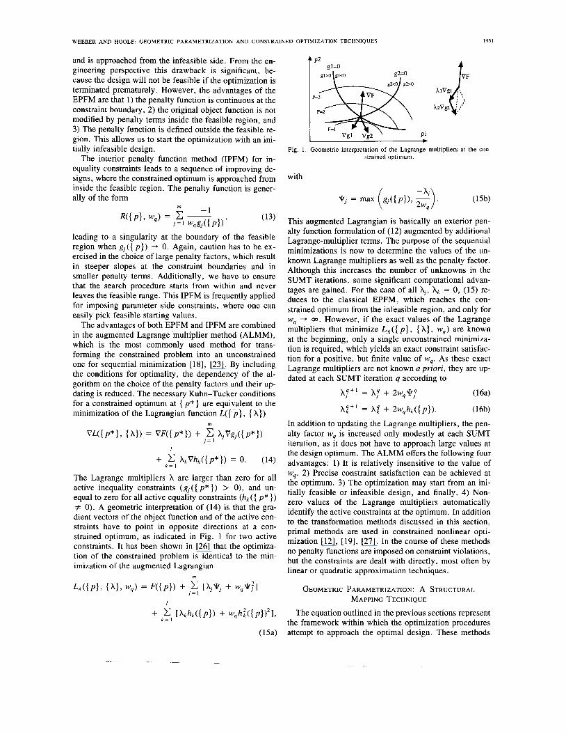
The Lagrange multipliers X are larger than zero for all active inequality constraints (g,({ p * } ) > 0), and un- equal to zero for all active equality constraints (hk ({ p* }) # 0). A geometric interpretation of (14) is that the gra- dient vectors of the object function and of the active con- straints have to point in opposite directions at a con- strained optimum, as indicated in Fig. 1 for two active constraints. It has been shown in [26] that the optimiza- tion of the constrained problem is identical to the min- imization of the augmented Lagrangian

m

1

f p2 gl=O g2=0

P l

Fig. 1. Geometric interpretation of the Lagrange multipliers at the con- strained optimum.

with

This augmented Lagrangian is basically an exterior pen- alty function formulation of (12) augmented by additional Lagrange-multiplier terms. The purpose of the sequential minimizations is now to determine the values of the un- known Lagrange multipliers as well as the penalty factor. Although this increases the number of unknowns in the SUMT iterations, some significant computational advan- tages are gained. For the case of all Xi, X k = 0, (15) re- duces to the classical EPFM, which reaches the con- strained optimum from the infeasible region, and only for wq -+ 03. However, if the exact values of the Lagrange multipliers that minimize L A ( { p } , {A}, w q ) are known at the beginning, only a single unconstrained minimiza- tion is required, which yields an exact constraint satisfac- tion for a positive, but finite value of wq. As these exact Lagrange multipliers are not known a priori, they are up- dated at each SUMT iteration q according to

( 16a) AT+' = A4 + 2w 9 J q r a

A $ + ' = + 2wqhk({ p } ) . ( 16b) In addition to updating the Lagrange multipliers, the pen- alty factor wq is increased only modestly at each SUMT iteration, as it does not have to approach large values at the design optimum. The ALMM offers the following four advantages: 1) It is relatively insensitive to the value of wq. 2 ) Precise constraint satisfaction can be achieved at the optimum. 3) The optimization may start from an ini- tially feasible or infeasible design, and finally, 4) Non- zero values of the Lagrange multipliers automatically identify the active constraints at the optimum. In addition to the transformation methods discussed in this section, primal methods are used in constrained nonlinear opti- mization [12 ] , [19], [27 ] . In the course of these methods no penalty functions are imposed on constraint violations, but the constraints are dealt with directly, most often by linear or quadratic approximation techniques.

GEOMETRIC PARAMETRIZATION: A STRUCTURAL MAPPING TECHNIQUE

The equation outlined in the previous sections represent the framework within which the optimization procedures attempt to approach the optimal design. These methods

1952 IEEE TRANSACTIONS ON MAGNETICS, VOL. 28, NO. 4, JULY 1992

rely heavily on the gradients of object and constraint func- tions, which are obtained by the design sensitivity anal- ysis based on the finite element formulation. The conti- nuity and differentiability of F and g are basic requirements for the application of these gradient methods and the accuracy of the gradient calculations is of crucial importance to the stability and robustness of the opti- mization algorithm.

In recent papers [lo], [28], two key difficulties in geo- metric parametrization have been recognized. First, as the geometry changes, a new finite element mesh is necessi- tated for each new value of a geometric parameter. In using free meshing based on Delauney triangulation [20], [29], [30], topologically different meshes arise, each one representing a possible domain discretization with an in- herent error. This change in mesh topology and its asso- ciated discretization error occurs in discrete steps, leading to discrete changes in the potential and field solutions which automatically implies discontinuities in the object function. Through the finite element discretization, the actually continuous object function becomes only piece- wise continuous. This jeopardizes the smooth conver- gence and restricts the reliable application of gradient methods. Although tunneling [3 11 and stochastic methods [4] are effective in overcoming this problem, it is far sim- pler to remove these artificial discontinuities through proper meshing as suggested in [ 101, [28]. It is interesting to note that the number of object function discontinuities which are large enough to terminate numerical search methods increases with the fineness of the mesh. There- fore, for finer discretizations and more accurate finite ele- ments meshes it is more likely that line searches terminate prematurely. Furthermore a sensitivity analysis based on finite difference steps becomes inaccurate and often mean- ingless, because the gradient values can vary significantly due to the changes in mesh topology. On the contrary, when the gradient dF/dpi is calculated by the design sen- sitivity analysis of (3)-(5) by direct differentiation of the coefficient matrices, it relies on finite element information of a single given mesh topology. It is thus accurate and not affected by topological changes.

As a second requirement, geometric parametrization has to impose constraints on the smoothness of the geometric contour. When selecting nodal coordinates at the shape surface as parameters, the boundary is modeled by piece- wise linear segments which do not satisfy continuity con- ditions. In this case the geometric shapes obtained through optimization are characterized by jagged contours that are not manufacturable, although the object function is truly minimized [l], [4], [lo], [28], [32]. Using coefficients of polynomials as parameters in the boundary description re- sults in smooth shape outlines that however tend to un- dulating contours for higher order polynomials. There- fore, preferably, parametric curves such as cubic spline functions with two continuous derivatives [32] and Bezier curves [33], [34] are applied in shape representation.

Therefore the two requirements for a robust and reli- able geometric parameterization can be defined as: 1) A preserved mesh topology during optimization, and simul- taneously 2) The use of C’-continuous curves in the shape description.

As we want to optimize the shape of a device, it is rea- sonable to modify an initial guess by deflecting it accord- ing to structural laws of elasticity [35]. Fig. 2 shows how the geometry of a rectangular plate is deformed by three different applied forces. The structural consistency of the plate guarantees smooth shape contours, which depend on the value of the applied force and the structural material characteristics of stiffness and Poisson’s ratio. The main advantage of using this structural deformation as a pa- rametrization method is that the mesh topology does not change: As geometric parameter values are modified, the new geometric shapes are represented by distorted finite element meshes. The distortion of the finite element mesh is proportional to the changes of the parameter values and thus increases continuously. This implies continuous changes of discretization error, field solution and object function.

In the two dimensional analysis of plane stress, the con- stant strain element is one of the earliest and best known elements [36]-[38]. It is used for the discretization of the continuum of the structural design model, because of its nodal compatibility with the first order triangular element now commonly used for the electromagnetic field analy- sis. Thus, the finite element models for structural and electromagnetic computations consist of identical trian- gular elements in the common region. In the structural finite element equation,

[KI{u) = { f ) , (17) the stiffness matrix [K], depending on the material prop- erties of elasticity modulus E and Poisson’s ratio U , re- lates the displacements in the x- and y-directions as nodal degrees of freedom {U} to the loads { f } , which are the nodal forces acting in the two coordinate directions. The deflections of a structure tend to be centered around the point where the loads are applied, and we therefore have to use methods to distribute the local actions of applied point forces and specified nodal displacements more evenly throughout the solution region. For this purpose the two-dimensional structural finite element model is augmented by additional one-dimensional elements. They are placed mainly at the surface contour of the geometry to be optimized. Selecting a higher stiffness for these ele- ments than for the planar elements renders surface con- tours whose shapes depend mostly on the deformation of the one-dimensional elements. The softer planar elements thus react like a “soft sponge” and are then merely used to map the applied surface deformation evenly onto the solution region.

The one-dimensional element used for this purpose is the beam element of Fig. 3 with three degrees of freedom

WEEBER AND HOOLE: GEOMETRIC PARAMETRIZATION AND CONSTRAINED OPTIMIZATION TECHNIQUES 1953

Fig. 2. Example of a structurally distorted finite element mesh with three different parameter values.

' A

L 4- 0

Fig. 3 . One-dimensional beam element for axial and flexural behavior with 3 degrees of freedom per node.

per node: the axial displacement U , the transverse dis- placement U , as well as the rotation 8 in the z-sense. The rotation itself is identical to the slope of the bending curve 0 = dv/d.x [35], [36], [38]. Thus, the element vector of the nodal degrees of freedom for both axial and bending behavior is written as

(U} = (uI v1 el u2 u2 e 2 } T , with

The corresponding column vector for the nodal actions contains point forces in the axial and transverse directions as well as the bending moments in the z-sense,

{f) = { f x l fy l 4 f x 2 f y 2 W 2 Y . (19) The exact element stiffness matrix within beam theory [38] represents both the axial and bending behavior

E [KI, = 3

- bhL2 0

0 121

0 61L

-bhL2 0

the bending behavior. The axial behavior is characterized by the product of elasticity modulus E and beam cross section bh, whereas the bending behavior is characterized by the flexural rigidity EI. For the assembly of the equa- tions of the structural design model, this decoupling cre- ates the option of selecting material properties and beam cross sections in such a combination as to modify and in- fluence the axial and bending behavior independently. We can thus choose the beam characteristics such that the flexural rigidity is small enough to give locally yet smoothly deflected beams. Furthermore the axial stiffness can be set large enough to distribute the axial deflections evenly throughout the finite element model.

The nodal displacements and forces in a local beam co- ordinate system are transformed by rotation-of-axis trans- formations into the global coordinate system, in which the nodal displacements of triangular elements are defined (Fig. 4) . With these transformations the global equilib- rium equations in the nodal degrees of freedom resulting from element assembly pertain to the global coordinate system [36]. The nodal connection of beam elements re- quires some further discussion. If the rotation 8 of beam elements is set equal at common nodes, the &distribution is forced to be continuous along beam elements which leads to a C1-continuous beam deflection curve and geo- metric contour. This inherent smoothness of the shape is, however, not desired when sharp edges and comers have to be modeled. In this case the &components of neigh- boring beam elements are not set equal at the common node, resulting in a discontinuous beam deflection curve. These hinged beams are connected by multipoint con- straints applied to common nodal wand u-components (Fig. 5).

The following two examples briefly demonstrate the characteristics of the combined beam and triangle ele- ments for the purpose of obtaining uniformly deflected finite element meshes. A rectangular plate is augmented by beam elements at the upper boundary, where geomet-

- 0 -bhL2 0 0

61L 0 -121 61L

41L2 0 -6IL 21L2

0 bhL2 0 0

0 -121 -61L 0 121 -61L

- 0 61L 21L2 0 -61L 4ILz

In this expression L denotes the length, b the width, h the height and I the moment of inertia of the cross section of a beam element. This stiffness matrix relates the axial and transverse displacements U , U , and the rotations 8, to ap- plied axial and transverse forces and moments in the z-sense, respectively. As the influence of shearing deflec- tions are neglected, the axial behavior is decoupled from

ric deflections are imposed by specified displacements at a single node. The plate is fixed at the bottom, and the horizontal displacements are constrained at the right boundary. Fig. 6 gives the deflection curve for three dif- ferent values of the elasticity modulus E of the beams, which determines their flexural rigidity and bending be-

1954 IEEE TRANSACTIONS ON MAGNETICS, VOL. 28, NO. 4, JULY 1992

X b

Fig. 4. Displacements of triangle in global coordinate system (unprimed) and of beam element in local coordinate system (primed).

CONTINUOUS BEAMS CONTlNUoUS BEAMS

I I

8 2 8 3 04 05

I HINGED BEAMS

U3 = U4 v3 = v4 e3 # 64

Fig. 5 . Joint of hinged beams.

E-beans = 10 0 - E-beans = 30 0 E-beanr = mo 0

(a) 6) (C) Fig. 6 . Deformed mesh of rectangular plate augmented by beam elements

at upper boundary.

havior. The curvature of the deflection depends on the flexural rigidity in the same way as coefficients of a spline function govern its distribution. To obtain the deflected shapes of Fig. 7 , further beam elements are added at the left boundary, and the joint of vertical and horizontal beams is modeled by an additional hinge node. Fig. 7(a) shows a model with axially soft beams: the axial deflec- tion of the vertical beams is concentrated around the node where the vertical displacement is applied. Due to the ax- ially stiffer beams in Fig. 7(b), the specified displacement is distributed uniformly over the whole length of the ver- tical plate boundary, resulting in a more evenly deformed mesh throughout the model. It can be seen that the use of hinged beams of high axial stiffness and relatively soft flexural behavior yields a uniformly distorted finite ele- ment mesh in the whole region of the structural design model.

It is important to emphasize that the structural design model is not used to obtain a numerical solution of an existing structural problem. We rather want to establish a reliable mapping technique that yields a uniformly de- flected finite element mesh mainly for complex geome- tries. For this purpose we are free to assemble the struc-

beans E = IO 0. b = 1 0. h = 2 0 €1 = 6 666 ER = 20 0

(a)

beams E i 100 0. b i 3 162. h = 0 632 E l = 6 666 ER = 2w 0

(b) Fig. 7 . Even distribution of axial beam displacements. (a) Axially soft beams: deflections concentrate in vicinity of applied displacement. (b) Ax- ially stiff beams: deflections uniformly distributed over full beam length.

tural design model by augmenting sections of the electromagnetic finite element model appropriately with beam elements and hinge nodes. In the following we will outline how this structural design model fits into the elec- tromagnetic shape optimization procedure.

The structural design model may be deflected either by applying forces { f } as loads, or by specifying nodal dis- placement components in the vector of state variables {U}. The analogy in the analysis of electromagnetic fields is to “drive” magnetic fields either by specified current and charge distributions, or by defined nonzero potentials. Point forces applied to the surface of the structure have been selected as parameters in a previous publication [39]. However, in using beam elements with different axial and flexural behavior, axial and transversal forces result in displacements of different size. The design model thus be- comes more sensitive to transverse forces. This unwanted scaling effect is avoided by selecting specified surface dis- placements as the design parameters. Then the same in- crement in a parameter value (that may describe axial or transverse deflections) results in the same amount of change in geometry. The displacement vector may then be partitioned into the unknown U, and the specified U, components, to yield the finite element equation of the structural model without force components as loads in partitioned form

1955 WEEBER AND HOOLE: GEOMETRIC PARAMETRIZATION AND CONSTRAINED OPTIMIZATION TECHNIQUES

The unknown displacements are then determined by so- lution of the first row

This leads to the term “structural mapping”: the specified surface displacements U, as parameters are mapped onto the remaining, unknown displacements U, by the mapping matrices K,, and K,,. This mapping relationship is gov- erned by the physical properties of the structural design model which may be chosen in such a combination as to obtain the desired geometric shapes.

The solution of (22) is performed for two different pur- poses in the process of shape optimization. First, the ini- tial geometry of the starting guess is subjected to the spec- ified surface deflections { u , } ~ , rendering a set of basis deflection shapes { ~ ~ } ~ ( i = 1 - * n)

The parameters p i during the optimization are then the factors of the surface deflections { u , } ~ applied to the structure. Each vector may consist of a single dis- placement component, whose action is distributed over the complete surface by beam elements. The resulting smooth contour is determined by the flexural character- istics of the beam elements. On the other hand, each vec- tor { u , } ~ may as well consist of a group of specified sur- face displacements. In this case, it may define the deformation of whole geometric boundaries either by a given constant, linear, or polynomial distribution. The surface displacements specified in each { u , } ~ may even resemble the geometric contours of available shape pro- files, so that the optimization actually determines the coef- ficients of an optimal superposition of those different pro- files. Therefore quite complex changes of the geometry are essentially represented by a single parameter, which may be effectively applied to reduce the dimensionality of the optimization problem and the involved computational effort. This way the structural mapping technique auto- matically incorporates the reduced basis concept [40].

The set of basis vectors { ub } i and the nodal coordinates of the starting geometry { x } , are used throughout the op- timization to obtain the parameter dependent geometry b < P ) > as

This procedure thus replaces the need for free meshing: For new parameter values the finite element mesh is ob- tained as a linear superposition of the basis deflection shapes. The resulting mesh never changes its topology, and therefore changes in the discretization error and re- sulting discontinuities in the object function are elimi-

nated. The smoothness of the geometric contours is guar- anteed by the use of sufficiently stiff beam elements in the design model at the surface contours.

The second application of the mapping (22) arises in the calculation of the magnetic potential gradient { a A / d p i } in sensitivity analysis, which is generally re- quired at the beginning of the rth line search during un- constrained minimization. For the assemblage of the right hand side of (4), the derivatives of the element matrices [PI, and vectors { Q } , with respect to the geometric pa- rameters are required. These derivatives are assembled from the partial derivatives of the element matrices with respect to the coordinates of the triangle nodes and the derivatives of these nodal coordinates with respect to the parameters as

The detailed expressions for the sensitivities of the ele- ment matrices for geometric, material and excitation pa- rameters are given in references [7], [8]. It is the calcu- lation of the gradient of the nodal locations with respect to the geometric parameters dxn/api‘ and ayn/api that again involves the solution of the structural mapping (22). The same set of surface deflections as used in (23) is now applied to the present shape { x } of the structure. This is equivalent to applying a unit step of the parameter p i (recall: p i is the coefficient of {U, } i and { ub } i ) to obtain the corresponding displacements { u , } ~ , which in turn are the desired derivatives of the nodal coordinate with re- spect to the parameter p i ,

for a unit change in p i . Thus, the gradients of the nodal coordinates are obtained by a structural solution for the geometry of the present parameter vector.

The structural mapping method replaces a geometric parametrization involving free meshing as follows: At the beginning of the optimization procedure n different dis- placement vectors are defined which characterize the pa- rameterized surface deformations. An n-dimensional ba- sis of deflection vectors is calculated by the structural so- lution of the initial geometry loaded with the specified displacements (23). Whenever new values of geometric parameters require a new finite element discretization, this is obtained by using the present parameter values as coef- ficients in the linear superposition of the basis vectors

1956 IEEE TRANSACTIONS ON MAGNETICS, VOL. 28, NO. 4. JULY 1992

(24). The gradient of the object function requires the de- rivatives of the nodal coordinates with respect to the pa- rameters, which in turn are obtained from a structural so- lution of unit parameter displacements applied to the present shape (26). Therefore, at the cost of an additional structural solution per line search with a model containing just the regions of variable geometry, the prerequisites of continuity and differentiability of the object function are achieved. Furthermore, smooth shape outlines are ob- tained even with only a few optimization parameters, as will be shown in the following applications.

A NUMERICAL EXAMPLE: THE SHAPE OPTIMIZATION OF

A SALIENT POLE

The following very familiar numerical example of de- termining the pole face contour of a salient pole synchro- nous machine is considered to demonstrate the structural mapping technique and its contribution to constrained op- timization. It is not viewed as a definite design optimi- zation of a given synchronous machine. For this reason we have simplified the stated problem by neglecting stator slotting, three-dimensional field components and nonlin- ear saturation effects. The current density in the excitation coil and the geometric parameters that define the shape of the pole piece have to be predicted in order to achieve a sinusoidal distribution of the airgap flux density with a peak value of 1 .O T (the time-dependency of the flux den- sity wave and thus the induced voltage wave may be eas- ily constructed from the spatial flux density distribution with the knowledge of the rotational speed of the ma- chine). Fig. 8 gives the parameterized geometry of half a pole pitch that is used as solution region in the no-load field analysis. The stator is idealized as a solid steel re- gion without slots, and both stator and rotor are made of linear steel with a relative permeability of 2000. To de- termine the deflection shape functions by structural anal- ysis, a subregion is used which contains only the areas of variable geometry and extends from the upper edge of the coil to the airgap interface of the stator, as indicated in Fig. 8. This structural model represents thus only a frac- tion of the electromagnetic model and hence the compu- tational effort to determine the shape functions and the partial derivatives of (25) is kept at a minimum. The pa- rameters pl-p3 define uniform deflections of the left, lower and upper pole piece contour, whereas the param- eters p4-p6 define deflections of a single grid point each, resulting in contours that are governed by the flexural be- havior of the beam elements at the pole piece surfaces. The material properties of the structural triangular ele- ments ( E = 0.5, ZI = 0.3) and the beam elements ( E = 5.0, width = 10.0, height = 0.05) guarantee that the characteristics of the mesh distortion depend mainly on the flexurally soft beams. The objective of achieving the specified sine-distribution of the airgap flux density just below the stator (shaded area in Fig. 8) is formulated with

'IT

ROTOR: pr = 2OO0.0

I 0.1 , 0.09 0.01 0.1

Fig. 8. Parametrized geometry of salient pole. Dimensions in [m].

the following least square object function which describes the deviation of the numerically computed y-component of the flux density Bj,,s from the desired values Bopt,$ at defined sampling points s in the airgap

(27)

Each component of the gradient vector VF is obtained as a summation of terms of the following form

F(Pl9 * ' 9 Pn) = F ( { P } ) = c (By,s - Bopt,d2.

Here, the first term of the partial derivatives vanishes due to the nature of the object function, which does not ex- plicitly depend on p i . The second term involves the sen- sitivity of the y-component of the flux density with respect to the design parameters which is given by (5b). To pre- vent mutual penetration of different geometric compo- nents the parameter side constraints are implemented in the form of (1 1). Additional constraints for the geometric parameters of the pole face contour impose a minimum airgap of 6, = 0.02 m. A crucial constraint on the oper- ating characteristics imposes bounds on the leakage flux 9, of the field winding, which has to be smaller than a specified fraction of the main flux CP, entering the stator. These flux quantities are calculated with the magnetic vector potential at the points E , F, G as indicated in Fig. 8. The resulting constraint function is given by a linear combination of magnetic potential terms and exhibits an implicit and nonlinear dependence on the design param- eters { p }

ay < cl@,: d { P H = ( & ( { P I ) - M { P I ) )

- C , ( M { P ) ) - &({PIN < 0. (29)

The gradient of this constraint is obtained by the chain rule differentiation of (3).

WEEBER AND HOOLE: GEOMETRIC PARAMETRIZATION AND CONSTRAINED OPTIMIZATION TECHNIQUES 1957

Before tackling the stated optimization problem it is worthwhile obtaining a quantitative understanding for this design problem. We may, as an approximation and sim- plification, reduce the stated problem to the evaluation of the airgap size 6, and the required Ampere-turns I in a magnetic circuit. By neglecting the magnetomotive force drops in the highly permeable steel regions, and neglect- ing the influence of leakage flux, we obtain the airgap flux density Bo as directly proportional to Z and inversely pro- portional to 6,:

It is thus obvious that the objective of achieving the de- sired airgap flux density Bo may be realized by any com- bination of the two parameters I and 6, that maintains the constant ratio proportional to Bo. The design problem in the two parameters I and 6, is thus not unique and only constraints on both parameters will create a problem state- ment with a unique solution.

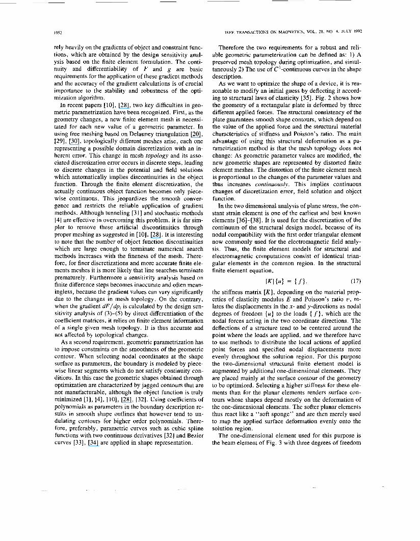
Based on these conclusions two classes of constrained problems are investigated, each one with the three differ- ent cases of aL unconstrained, GL < 0.20 +,, and OL < 0.15 9,. In the first study, the maximum current density in the field winding is defined as 2.0 A/”*. With this low current density the maximum airgap flux density can- not be realized, and both and Jmax are active con- straints at the optimum. Fig. 9 gives the contour lines of the magnetic potential for the different “optimal” pole shapes (the same contour increment of AA = 0.01 A / m is used in Fig. 9 and Fig. 10). The minimum airgap con- straint is active in all three cases of the different leakage flux constraint, which can be recognized from the fact that the pole shape contour maintains the minimum airgap size from the center of the pole face almost up to the pole tip. The upper limit of the leakage flux basically defines the thickness of the pole piece finger and the size of the in- terpole gap. Table I lists the optimization results for air- gap, current density and leakage flux. The active con- straints are highlighted as boldfaced characters, and the magnitudes of the Lagrange-multipliers indicate that the current density is the most severe constraint.

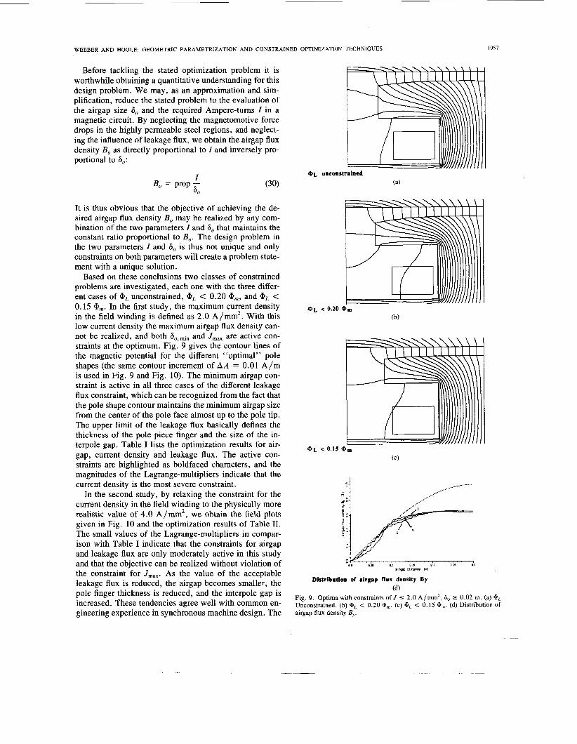
In the second study, by relaxing the constraint for the current density in the field winding to the physically more realistic value of 4.0 A/mm2, we obtain the field plots given in Fig. 10 and the optimization results of Table 11. The small values of the Lagrange-multipliers in compar- ison with Table I indicate that the constraints for airgap and leakage flux are only moderately active in this study and that the objective can be realized without violation of the constraint for J,,,. As the value of the acceptable leakage flux is reduced, the airgap becomes smaller, the pole finger thickness is reduced, and the interpole gap is increased. These tendencies agree well with common en- gineering experience in synchronous machine design. The

UJL unconstrained (a)

< 0.1s

Distribution of airgap flux density By (d)

Fig. 9 . Optima with constraints of J 5 2.0 A/”*, 6, B 0.02 m. (a) 0, Unconstrained. (b) aL < 0.20 0,. (c) 0, < 0.15 Om. (d) Distribution of airgap flux density By.

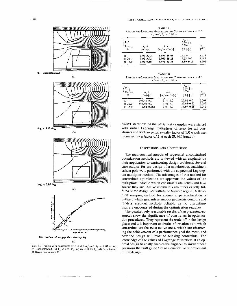
IEEE TRANSACTIONS ON MAGNETICS, VOL. 28, NO. 4, JULY 1992 1958

UJL unconstrained .

.20

@ L < 0.15

TABLE I RESULTS A N D LAGRANGE MULTIPLIERS FOR CONSTRAINTS OF J 5 2.0

A/"', 6* 2 0.02 m

a) - 0.02-3.42 1.999-16.66 29.05- 3.124 b) 20.0 0.02-3.72 2.000-15.25 19.33-0.0 3.485 c) 15.0 0.02-9.58 1.973-23.31 14.99-0.11 3.596

TABLE I1 RESULTS A N D LAGRANGE MULTIPLIERS FOR CONSTRAINTS OF J 5 4.0

A/mm2, 6, 2 0.02 m

a) - 0.0249-0.0 3.74-0.0 29.02-0.0 0.009 b) 20.0 0.0265-0.0 3.46-0.0 20.00-0.02 0.039 C) 15.0 0.02-0.085 3.00-0.0 14.99-0.05 0.246

SUMT iterations of the presented examples were started with initial Lagrange multipliers of zero for all con- straints and with an initial penalty factor of 1 .O which was

Distribution of airgap flux density By

(4 Fig. 10. Optima with constraints of J 5 4.0 A/"', 6o 2 0.02 m. (a) 0' Unconstrained. (b) 0, < 0.20 0,,,. (c) 0, < 0.15 a,,,. (d) Distribution of airgap flux density By.

increased by a factor of 2 at each SUMT iteration.

DISCUSSIONS AND CONCLUSIONS

The mathematical aspects of sequential unconstrained optimization methods are reviewed with an emphasis on their application to engineering design problems. Several case studies for the design of a synchronous machine's salient pole were performed with the augmented Lagrang- ian multiplier method. The advantages of this method for constrained optimization are apparent: the values of the multipliers indicate which constraints are active and how severe they are. Active constraints are either exactly ful- filled or the design lies within the feasible region. A struc- tural mapping method for geometric parametrization is outlined which guarantees smooth geometric contours and renders gradient methods reliable as no discontinu- ities are encountered during the optimization searches.

The qualitatively reasonable results of the presented ex- amples show the significance of constraints in optimiza- tion procedures. They represent the trade-off in the design phase and it is important to obtain information as to which constraints are the most active ones, which are obstruct- ing the achievement of a performance goal the most, and how the design will react to relaxing constraints. The knowledge of the values of Lagrange multipliers at an op- timal design basically enables the engineer to answer those questions that will guide him to a qualitative improvement of the design.

WEEBER AND HOOLE: GEOMETRIC PARAMETRIZATION AND CONSTRAINED OPTIMIZATION TECHNIQUES 1959

As a final note of caution however, we recall an appro- priate remark by Petrovsky [41], that “in the design office the reduction in computation time will free the engineer to spend more time in creative thought, or it will allow him to complete more work with less creative thought than today”.

REFERENCES

[ l ] 0. Pironneau, Optical Shape Design f o r Ellipfir Systems. New York: Springer-Verlag, 1984.

[2] B. Istfan and S . J. Salon, “Inverse nonlinear finite element problems with local and global constraints,” IEEE Trans. Magn. , vol. 24, no.

[3] S. Gitosusastro, J. L. Coulomb, and J . C. Sabonnadiere, “Perfor- mance derivative calculations and optimization process,” IEEE Trans. Magn . , vol. 25, no. 4, July 1989, pp. 2834-2839.

141 K. Preis, C . Magele, and 0. Biro, “FEM and evolution strategies in the optimal design of EM devices,” IEEE Trans. Magn. , vol. 26, no. 5 , Sept. 1990, pp. 2181-2183.

[5] 11-Han Park, Beom-Taek Lee, and Song-Yop Hahn, “Sensitivity analysis based on analytic approach for shape optimization of electro- magnetic devices: interface problem of iron and air,” IEEE Trans. Magn. , vol. 27, no. 5 , Sept. 1991, pp. 4142-4145.

[6] -, “Design sensitivity analysis for nonlinear magnetostatic prob- lems using the finite element method,” 8th Conference on the Com- putation of Electromagnetic Fields (COMPUMAG), Paper OH-3, July 1991, Sorrento, Italy.

[7] S. R. H. Hoole, “Inverse problems-finite elements in hop-stepping to speed up,” Int. J . Appl. Electromag. Marl . , vol. 1, 1990, pp. 255- 261.

[8] S . R. H. Hoole, S . Subramaniam, R. Saldanha, 1. L. Coulomb, and J. C. Sabonnadiere, “Inverse problem methodology and finite ele- ments in the identification of cracks, sources, materials, and their ge- ometry in inaccessible locations,” IEEE Trans. Magn . , vol. 27, no. 3, May 1991, pp. 3433-3443.

[9] S. R. H. Hoole, “Optimal design, inverse problems and parallel com- puters,” IEEE Trans. Magn. , vol. 27, no. 5 , Sept. 1991.

[lo] S. R. H. Hoole, K. Weeber, and S . Subramaniam, “Fictitious min- ima of object functions, finite element meshes and edge elements in electromagnetic device synthesis,” IEEE Trans. Magn. , vol. 27, no. 5 , Sept. 1991.

[ l l ] K. Weeber and S . R. H. Hoole, “The subregion method in magnetic field analysis and design optimization,” 8th Conference on the Com- putation of Electromagnetic fields, paper no. PE-25, July 1991 (COMPUMAG), Sorrento, Italy, IEEE Trans. Magn. , vol. 28, no. 2, Mar. 1992.

[12] K. Weeber, E. Johnson, S. Sinniah, K. Holte, J. C. Sabonnadiere, and S. R. H. Hoole, “Design sensitivity for skin effect and minimum volume optimization of shields,” IEEE Trans. Magn. , vol. 28, no. 5 , Sept. 1992.

[13] M. Ramamoorty and P. J. Rao, “Optimization of polyphase seg- mented-rotor reluctance motor design: a nonlinear programming ap- proach,” IEEE Trans. Power App. Syst . , vol. 98, no. 2, Mar. 1979,

[ 141 J. Appelbaum, E. F. Fuchs, and J. C. White, “Optimization of three- phase induction motor design. Part I: formulation of the optimization technique,” IEEE Trans. Energy Conversion, vol. EC-2, no. 3 , Sept.

[15] J. Appelbaum, I. A. Khan, E. F. Fuchs, and J. C. White, “Optimi- zation of the three-phase induction motor design. Part 11: The effi- ciency and cost of an optimal design,” IEEE Trans. Energy Con- vers . , vol. 2, no. 3, Sept. 1987, pp. 415-422.

[16] Xian Liu and G. R. Slemon, “An improved method of optimization for electrical machines,” IEEE Trans. Energy Convers . , vol. 6, no. 3 , Sept. 1991, pp. 492-496.

[17] M. Nurdin, M. Poloujadoff, and A. Faure, “Synthesis of squirrel cage motors: A key to optimization,” IEEE Trans. Energy Convers . , vol. 6, no. 2, June 1991, pp. 327-333.

[ 181 S. Russenschuck, “Mathematical optimization techniques for the de- sign of permanent magnet synchronous machines based on numerical

6 , NOV. 1988, pp. 2568-2572.

pp. 527-535.

1987, pp. 407-414.

field calculations,” IEEE Trans. Magn. , vol. 26, no. 2 , March 1990,

1191 R. R. Saldanha, J. L. Coulomb, A. Foggia, and J . C. Sabonnadiere, “A dual method for constrained optimization design in magnetostatic problems,” IEEE Trans. Magn. , vol. 27, no. 5 , Sept. 1990, pp. 4136- 4141.

[20] S . R. H. Hoole, Computer-Aided Analysis and Design of Elecrro- magnetic Devices.

[21] Edward J. Haug, Kyung K. Choi, and Vadim Komkov, Design Sen- sifivity Analysis of Structural Systems. Orlando: Academic Press, 1986.

[22] J. L. Coulomb, “A methodology for the determination of global elec- tromechanical quantities from a finite element analysis and its appli- cation to the evaluation of magnetic forces, torques and stiffness,” IEEE Trans. Magn. , vol. MAG-19, no. 6, Nov. 1983, pp. 2514- 2519.

[23] G. Vanderplaats, Numerical Optimization Techniques f o r Engineer- ing Design.

1241 M. R. R. Hoole and S . R. H. Hoole, “The Hessian in inverse prob- lem optimization,” Inr. J . App. Electromag. Matrls . , Supplement to Vol. 2-Electromagnetic Forces and Applications, pp. 267-270, 1992.

[25] H. Y. Huang, “Unified approach to quadratically convergent algo- rithms for function minimization,” J . Optim. Theory App l . , vol. 5 , no. 6 , pp. 405-423, 1970.

[26] J. T. Rockafellar, “The multiplier method of Hestenes and Powell applied to convex programming,” J . Optim. Theory App l . , vol. 12, no. 6, pp. 555-562, 1973.

[27] A. D. Belegundu and J. S . Arora, “A study of mathematical pro- gramming for structural optimization, part I and 11,” Inr. J . Num. Meth. Eng . , vol. 21, pp. 1583-1623, 1985.

[28] K. Weeber and S . R. H. Hoole, “A structural mapping technique for geometric parametrization in the synthesis of magnetic devices,” Inr. J . Num. Merh. Eng. , scheduled for publication.

[29] C. Keinstreuer, J. T. Hadenan, “A triangular finite element mesh generation for fluid dynamic systems of arbitrary geometry,” Int. J . Num. Meth. Eng . , vol. 15, pp. 1325-1334, 1980.

[30] 2 . J. Cendes, D. Shenton, and H. Shahnasser, “Magnetic field com- putation using Delauney triangulation and complementary finite ele- ment methods,” IEEE Trans. Magn. , vol. MAG-19, 1983, pp. 2551- 2554.

[31] S . Subramaniam, S. Kanaganathan, and S . R. H. Hoole, “Two req- uisite tools in the optimal design of electromagnetic devices,” IEEE Trans. Magn. , vol. 27, no. 5 , Sept. 1991.

1321 R. T. Haftka and R. V. Grandhi, “Structural shape optimization-a survey,” Compuf. Merh. Appl. Mech. Eng. , vol. 57, pp. 91-106, 1986.

1331 V. Braibant and C. Fleury, “Shape optimal design using B-splines,” Compuf. Mefh. Appl. Mech. Eng . , vol. 44, 1984, pp. 247-267.

[34] Fujio Yamaguchi, Curves and Surfaces in Computer Aided Geometric Design. Berlin: Springer, 1988.

1351 S . Timoshenko and J. N. Goodier, Theory of Elasticity. New York: McGraw-Hill, 2nd ed., 1951.

1361 W. Weaver and P. R. Johnston, Finite Elements f o r Structural Anal- ys is .

1371 0. C. Zienkiewicz and R. L. Taylor, The Finite Element Method. New York: McGraw-Hill, 4th ed., 1988.

1381 K. J. Bathe, Finite Element Procedures in Engineering Analysis. Englewood Cliffs, NJ: Prentice-Hall, 1982.

1391 A. D. Belegundu and S. D. Rajan, “A shape optimization approach based on natural design variables and shape functions,” Compur. Meth. Appl. Mech. Eng . , vol. 66, 1988, pp. 87-106.

1401 R. M. Pickett, M. F. Rubinstein, and R. B. Nelson, “Automated structural synthesis using a reduced number of design coordinates,” AIAAJ., vol. 11, no. 4, pp. 489-494, 1973.

New York: St. Martins Press, 1985.

pp. 638-641.

New York: Elsevier, 1989.

New York: McGraw-Hill, 1983.

Englewood Cliffs, NJ: Prentice-Hall, 1984.

[41] H. Petrovski, To Engineer is Human.

Konrad Weeber (S’86, M’88, S’90) was born in Vienna, Austria, on July 21, 1961. He received the Degree in Electrical Engineering with honors from the Technical University of Vienna, Austria, in 1988, and the M.Sc. degree in Electrical Engineering from Drexel University, Philadelphia, PA, in 1987.

1960 IEEE TRANSACTIONS ON MAGNETICS, VOL. 28, NO. 4, JULY 1992

After working as a technical support engineer for commercial electro- magnetic finite element software in the United States and Europe, he en- rolled at the Laboratoire d’Electrotechnique, Ecole Nationale SupCrieure d’IngCnieurs Electriciens de Grenoble, France, in a Ph.D. program in Elec- trical Engineering and pursues his research effort at Harvey Mudd College, California. His areas of specialization are numerical optimization tech- niques, numerical field calculation, and power engineering.

Mr. Weeber is a member of the IEEE’s Magnetics and Power Engineer- ing Societies.

S. Ratnajeevan H. Hoole (M’83, SM’89) was born in Tamil, Ceylon, on September 15, 1952. He received the B.Sc. degree in electrical engineering (with honors) in 1975 from the University of Ceylon, the M.Sc. degree with the Mark of Distinction in electrical engineering from the University of London, in 1979, jointly offered through Imperial College and Queen Mary College, and the Ph.D. degree in electrical engineering from Car- negie-Mellon University, Pittsburgh, PA, in 1982.

After working as a faculty member in Ceylon, Nigeria, and Drexel Uni- versity, and as a consultant in Singapore and the United States, he joined

Harvey Mudd College, Claremont, CA, in 1987 as an Associate Professor of Engineering, and now holds the rank of Professor with continuous ten- ure. His area of interest is the finite element and other numerical methods and their application in computer-aided design. He has published Computer Aided Analysis and Design of Electromagnetic Devices (Elsevier, 1989). He is presently working under contract on a book for Oxford University Press on undergraduate electromagnetics, and another for Elsevier on deeper issues in finite element analysis; these are both to come out early in 1993. He is also the Guest Editor of the special issue of the IEEE TRANSACTIONS ON EDUCATION on Computation and Computers (November, 1992).

Dr. Hoole is a past Chairman of IEEE Magnetics Society’s Philadelphia Chapter and serves on the Editorial Boards of Electrosofi, the Journal of Electromagnetic Waves and Applications, and the International Journal of Applied Electromagnetics in Materials. He is presently the General Chair- man of the IEEE Magnetics Society’s Conference on Electromagnetic Field Computation (to be held in Claremont, CA, August 3-5, 1992). Dr. Hoole is a member of Electromagnetics Academy, and the Magnetics, Education, and Computer Societies of the IEEE, as well as the Power Engineering Society and its Electric Machine Committee. He is the Director of the Sri Lanka Studies Institute, Claremont, CA.