AN INVESTIGATION OF VARIABLE VALVE TIMING EFFECTS ...
140
AN INVESTIGATION OF VARIABLE VALVE TIMING EFFECTS ON HCCI ENGINE PERFORMANCE By Hrishikesh Abhay Saigaonkar A THESIS Submitted in partial fulfillment of the requirements for the degree of MASTER OF SCIENCE In Mechanical Engineering MICHIGAN TECHNOLOGICAL UNIVERSITY 2014 c 2014 Hrishikesh Abhay Saigaonkar
-
Upload
khangminh22 -
Category
Documents
-
view
6 -
download
0
Transcript of AN INVESTIGATION OF VARIABLE VALVE TIMING EFFECTS ...
AN INVESTIGATION OF VARIABLE VALVE TIMING EFFECTS ON HCCI ENGINE
PERFORMANCE
By
Hrishikesh Abhay Saigaonkar
A THESIS
Submitted in partial fulfillment of the requirements for the degree of
MASTER OF SCIENCE
In Mechanical Engineering
MICHIGAN TECHNOLOGICAL UNIVERSITY
2014
c© 2014 Hrishikesh Abhay Saigaonkar

This thesis has been approved in partial fulfillment of the requirements for the Degree of
MASTER OF SCIENCE in Mechanical Engineering.
Department of Mechanical Engineering-Engineering Mechanics
Thesis Advisor: Dr. Mahdi Shahbakhti
Committee Member: Dr. Jeffrey Naber
Committee Member: Dr. Sunil Mehendale
Department Chair: Dr. William Predebon


Dedication
To those willing to take the road less traveled. . .
Twenty years from now you will be more disappointed by the things that you didn’t do than
by the ones you did do, so throw off the bowlines, sail away from safe harbor, catch the
trade winds in your sails. Explore, Dream, Discover.
−Mark Twain

Contents
List of Figures . . . . . . . . . . . . . . . . . . . . . . . . . . . . . . . . . . . xi
List of Tables . . . . . . . . . . . . . . . . . . . . . . . . . . . . . . . . . . . . xvii
Acknowledgments . . . . . . . . . . . . . . . . . . . . . . . . . . . . . . . . . xxiii
Abstract . . . . . . . . . . . . . . . . . . . . . . . . . . . . . . . . . . . . . . . xxv
1 Introduction . . . . . . . . . . . . . . . . . . . . . . . . . . . . . . . . . . 1
1.1 What is HCCI and why is it needed? . . . . . . . . . . . . . . . . . . . 1
1.2 Promises and challenges . . . . . . . . . . . . . . . . . . . . . . . . . 4
1.3 HCCI combustion chemistry . . . . . . . . . . . . . . . . . . . . . . . 5
1.4 VVT effects on HCCI . . . . . . . . . . . . . . . . . . . . . . . . . . . 7
1.5 Scope and organization of thesis . . . . . . . . . . . . . . . . . . . . . 9
2 Experimental HCCI Engine Setup . . . . . . . . . . . . . . . . . . . . . . 11
2.1 Engine experimental setup . . . . . . . . . . . . . . . . . . . . . . . . 11
2.2 Experimental measurement of valve profiles . . . . . . . . . . . . . . . 15
2.2.0.1 Valve profile measurement procedure . . . . . . . . . 16
vii
2.3 Compression ratio increase . . . . . . . . . . . . . . . . . . . . . . . . 19
2.3.1 Piston to valve clearance . . . . . . . . . . . . . . . . . . . . . 21
2.3.2 Volume measurements . . . . . . . . . . . . . . . . . . . . . . 22
2.3.3 Piston selection . . . . . . . . . . . . . . . . . . . . . . . . . . 25
2.4 Controllable air heater . . . . . . . . . . . . . . . . . . . . . . . . . . . 28
2.5 MTU Supercharging Station . . . . . . . . . . . . . . . . . . . . . . . 30
2.5.1 Supercharger testing results . . . . . . . . . . . . . . . . . . . . 34
3 Sequential Combustion Modeling of HCCI Engines with Variable Valve
Timing . . . . . . . . . . . . . . . . . . . . . . . . . . . . . . . . . . . . . 39
3.1 SMRH Description . . . . . . . . . . . . . . . . . . . . . . . . . . . . 43
3.1.1 Step 1: 1-D HCCI engine model for conditions at IVC . . . . . 45
3.1.2 Step 2: Multi zone modelling (IVC-EVO) . . . . . . . . . . . . 46
3.1.2.1 Multi zone modeling and heat transfer correlations . . 48
3.1.3 Step 3: Exhaust stroke gas flow and RGF model (EVO-EVC) . . 51
3.1.3.1 Determination of Tevc . . . . . . . . . . . . . . . . . . 51
3.1.3.2 Flow through Exhaust Valves . . . . . . . . . . . . . 52
3.1.4 Step 4: Multi zone modelling in CHEMKIN-PRO (Stage II) . . 54
3.2 Results and Discussion . . . . . . . . . . . . . . . . . . . . . . . . . . 56
3.2.1 Model Validation . . . . . . . . . . . . . . . . . . . . . . . . . 56
3.2.2 Results for impact of valve timings on HCCI combustion . . . . 59
3.2.2.1 Effect of IVC variations . . . . . . . . . . . . . . . . 60
viii
3.2.2.2 Effect of EVO variations on HCCI combustion . . . . 70
3.2.3 Virtual Engine Test Bed for Controller Design . . . . . . . . . . 77
4 Summary and Conclusion . . . . . . . . . . . . . . . . . . . . . . . . . . . 85
4.1 Summary of thesis contributions . . . . . . . . . . . . . . . . . . . . . 86
4.2 Future Work . . . . . . . . . . . . . . . . . . . . . . . . . . . . . . . . 87
References . . . . . . . . . . . . . . . . . . . . . . . . . . . . . . . . . . . . . 89
A Calculations for cam timing determination . . . . . . . . . . . . . . . . . 101
B MSc Publications . . . . . . . . . . . . . . . . . . . . . . . . . . . . . . . . 104
C Thesis files summary . . . . . . . . . . . . . . . . . . . . . . . . . . . . . . 105
D Permissions . . . . . . . . . . . . . . . . . . . . . . . . . . . . . . . . . . . 110
ix

x
List of Figures
1.1 Background of main VVT strategies for HCCI combustion. . . . . . . . 8
1.2 Thesis organization . . . . . . . . . . . . . . . . . . . . . . . . . . . . 10
2.1 Schematic of the HCCI engine setup . . . . . . . . . . . . . . . . . . . 12
2.2 Experimental HCCI engine setup along with the supercharging station . 13
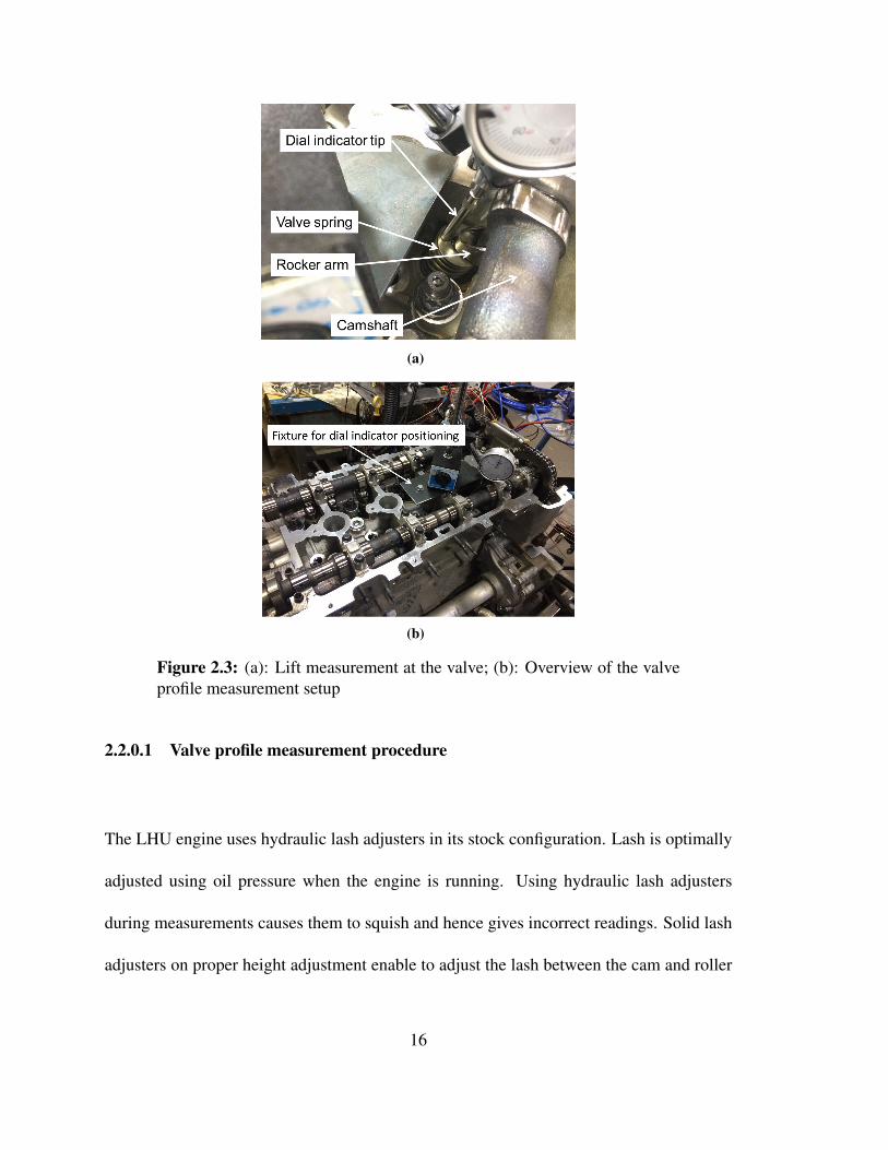
2.3 (a): Lift measurement at the valve; (b): Overview of the valve profile
measurement setup . . . . . . . . . . . . . . . . . . . . . . . . . . . . 16
(a) . . . . . . . . . . . . . . . . . . . . . . . . . . . . . . . . . . . 16
(b) . . . . . . . . . . . . . . . . . . . . . . . . . . . . . . . . . . . 16
2.4 Piston stop for measuring TDC crank angle . . . . . . . . . . . . . . . 17
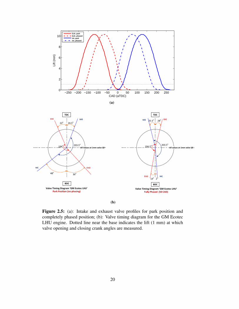
2.5 (a): Intake and exhaust valve profiles for park position and completely
phased position; (b): Valve timing diagram for the GM Ecotec LHU engine.
Dotted line near the base indicates the lift (1 mm) at which valve opening
and closing crank angles are measured. . . . . . . . . . . . . . . . . . . 20
(a) . . . . . . . . . . . . . . . . . . . . . . . . . . . . . . . . . . . 20
(b) . . . . . . . . . . . . . . . . . . . . . . . . . . . . . . . . . . . 20
xi
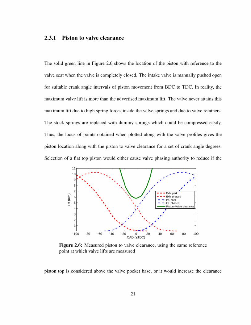
2.6 Measured piston to valve clearance, using the same reference point at which
valve lifts are measured . . . . . . . . . . . . . . . . . . . . . . . . . . 21
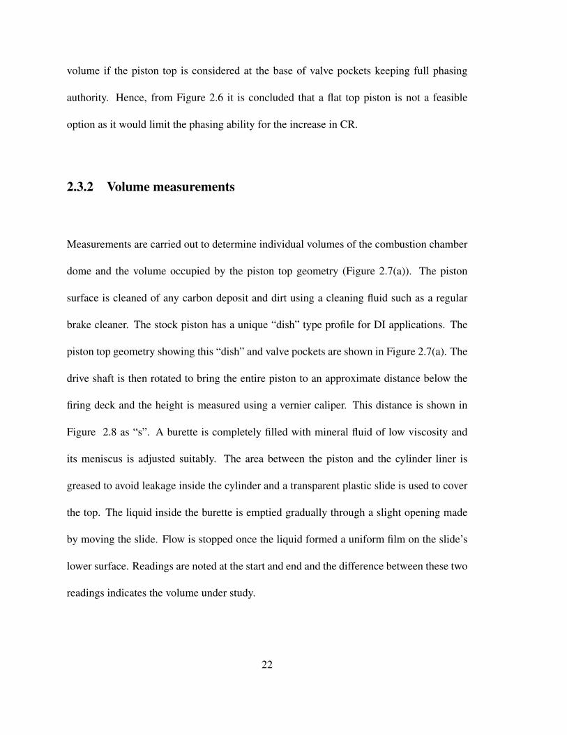
2.7 Experimental measurement of compression ratio . . . . . . . . . . . . . 23
(a) Piston top geometry . . . . . . . . . . . . . . . . . . . . . . . . . 23
(b) Cylinder head dome volume . . . . . . . . . . . . . . . . . . . . 23
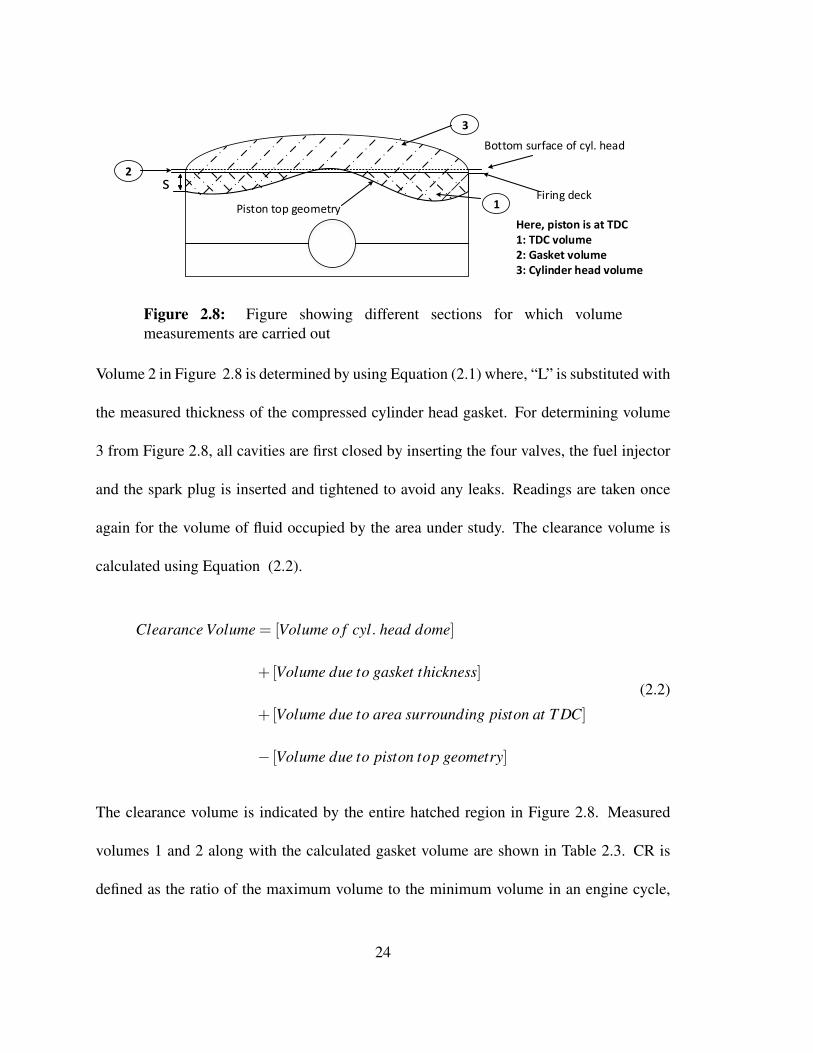
2.8 Figure showing different sections for which volume measurements are
carried out . . . . . . . . . . . . . . . . . . . . . . . . . . . . . . . . . 24
2.9 Stock and new piston top designs . . . . . . . . . . . . . . . . . . . . . 26
2.10 Design specifications for the increased CR piston from Wiseco . . . . . 27
2.11 Enclosure for housing Omega controller and SSR with heat sink . . . . 29
2.12 Designed LabView interface to control air heater . . . . . . . . . . . . . 29
2.13 Figure showing the supercharger test setup . . . . . . . . . . . . . . . . 31
2.14 Design details of the intake plenum for carrying supercharged air . . . . 33
2.15 Performance map of the Eaton M62 supercharger[1] . . . . . . . . . . . 34
2.16 Test setup for boost pressure measurement . . . . . . . . . . . . . . . . 35
2.17 Mapping of E-motor speed as a function of input voltage (0-10V) to the
VFD . . . . . . . . . . . . . . . . . . . . . . . . . . . . . . . . . . . . 35
2.18 Test result for boost pressure from the supercharger for 5V input to VFD 36
2.19 Filtered pressure trace with engine motoring at 1500 rpm and supercharger
speeds of (a) 3600 rpm and (b) 2700 rpm . . . . . . . . . . . . . . . . . 37
3.1 Simulation models for HCCI combustion modeling available in literature 40
xii
3.2 Simulation path for the SMRH modeling platform. The path includes four
steps shown by circled numbers. . . . . . . . . . . . . . . . . . . . . . 44
3.3 Single cylinder HCCI engine model in GT−POWER R© . . . . . . . . 45
3.4 Zone temperature distribution inside a cylinder . . . . . . . . . . . . . . 47
3.5 Pressure trace validation for the engine operating condition corresponding
to case ain Table 3.1 . . . . . . . . . . . . . . . . . . . . . . . . . . . 57
3.6 Pressure trace validation for the engine operating condition corresponding
to case bin Table 3.1 . . . . . . . . . . . . . . . . . . . . . . . . . . . 58
3.7 Pressure trace validation for the engine operating condition corresponding
to case cin Table 3.1 . . . . . . . . . . . . . . . . . . . . . . . . . . . 58
3.8 Intake valve profile variations in this study . . . . . . . . . . . . . . . . 60
3.9 Exhaust valve profile variations in this study . . . . . . . . . . . . . . . 60
3.10 Variation in in-cylinder gas pressure as a function of intake valve phasing 62
3.11 Variation in in-cylinder gas temperature as a function of intake valve
phasing . . . . . . . . . . . . . . . . . . . . . . . . . . . . . . . . . . 62
3.12 Variations of combustion metrics (CA10, CA50 and BD) for changes in
intake valve phasing . . . . . . . . . . . . . . . . . . . . . . . . . . . . 63
3.13 Impact of intake valve phasing on (a): in-cylinder gas temperature at IVC
due to presence of RGF, (b): RGF quantity, (c): temperature of trapped
residual gases. . . . . . . . . . . . . . . . . . . . . . . . . . . . . . . . 64
xiii
3.14 Close-up view of in-cylinder gas temperatures history before start of
combustion . . . . . . . . . . . . . . . . . . . . . . . . . . . . . . . . 65
3.15 Variation of IMEP and indicated thermal efficiency (ηth,i) as a function of
intake valve timing . . . . . . . . . . . . . . . . . . . . . . . . . . . . 65
3.16 Net heat release rate (NHRR) as a function of changing intake valve timing 66
3.17 Impact of intake valve timing on Carbon monoxide (CO) concentration and
maximum gas temperature (Tmax) averaged including all ten zones . . . 66
3.18 Unburned hydrocarbons (uHC) concentration and maximum zone averaged
gas temperature (Tmax) as a function of intake valve timing . . . . . . . 67
3.19 Zone temperature versus CAD for IVC = -140◦aTDCf showing peak
temperature above 1500K for zone #7 . . . . . . . . . . . . . . . . . . 69
3.20 CO and CO2 variation versus crank angle for IVC = -140oaTDCf showing
late oxidation of CO to CO2, leading to low CO concentration for this
operating point . . . . . . . . . . . . . . . . . . . . . . . . . . . . . . 69
3.21 Variation of in-cylinder gas pressure vs. CAD as a function of exhaust valve
timing . . . . . . . . . . . . . . . . . . . . . . . . . . . . . . . . . . . 71
3.22 Variation of in-cylinder gas temperature vs. CAD as a function of exhaust
valve timing . . . . . . . . . . . . . . . . . . . . . . . . . . . . . . . . 71
3.23 Effect of phasing exhaust valve timing on combustion metrics including
CA10, CA50 and BD . . . . . . . . . . . . . . . . . . . . . . . . . . . 72
xiv
3.24 Effect of phasing EVO timing on (a): gas temperature at IVC, (b): RGF
quantity, (c): temperature of trapped residual gases. . . . . . . . . . . . 73
3.25 Variation of IMEP and indicated thermal efficiency (ηth,i) as a function of
exhaust valve phasing . . . . . . . . . . . . . . . . . . . . . . . . . . . 74
3.26 Net heat release rate (NHRR) versus CAD as a function of exhaust valve
phasing . . . . . . . . . . . . . . . . . . . . . . . . . . . . . . . . . . 74
3.27 CO emissions and maximum zone averaged gas temperature as a function
of exhaust valve phasing . . . . . . . . . . . . . . . . . . . . . . . . . 76
3.28 uHC emissions and maximum zone averaged gas temperature as a function
of exhaust valve phasing . . . . . . . . . . . . . . . . . . . . . . . . . 77
3.29 Schematic of SMRH based virtual engine test bed for HCCI combustion
controller design . . . . . . . . . . . . . . . . . . . . . . . . . . . . . . 79
3.30 Contour plot of engine indicated thermal efficiency (ηth,i) as a function of
valve timing for the constant loadcase study. (IMEP = 5.5±0.2 bar) . . . 79
3.31 Raw emission index (REI) contour plot as a function of valve timings for
the constant loadcase study. (IMEP = 5.5±0.2 bar) . . . . . . . . . . . 80
3.32 CA50 contour plot as a function of valve timings for the constant loadcase
study. (IMEP = 5.5±0.2 bar) . . . . . . . . . . . . . . . . . . . . . . . 80
3.33 Tivc−mod contour plot as a function of valve timings for the
constant loadcase study. (IMEP = 5.5±0.2 bar) . . . . . . . . . . . . . 81
xv

3.34 Contour plot of fuel efficiency and emissions (FEE) index for the
constant loadcase study. (IMEP = 5.5±0.2 bar) . . . . . . . . . . . . . 82
3.35 Contour plot of fuel efficiency and emissions (FEE) index for the
constant fuelcase study. (mf = 0.3752 kg/hr) . . . . . . . . . . . . . . 83
xvi
List of Tables
2.1 Engine specifications (GM Ecotec LHU A20NFT) . . . . . . . . . . . . 12
2.2 Valve timing data for the Ecotec LHU engine . . . . . . . . . . . . . . 19
2.3 Measurements for engine combustion chamber volume . . . . . . . . . 25
2.4 Air heater specifications [2] . . . . . . . . . . . . . . . . . . . . . . . . 28
2.5 E-motor specifications mentioned on the physical motor . . . . . . . . . 31
2.6 E-motor insulation classes by NEMA [3] . . . . . . . . . . . . . . . . . 32
2.7 VFD specifications . . . . . . . . . . . . . . . . . . . . . . . . . . . . 32
3.1 Engine operating conditions of the experimental data [4] used to validate
SMRH . . . . . . . . . . . . . . . . . . . . . . . . . . . . . . . . . . . 45
3.2 Zone mass distribution for SMRH. This mass distribution is based on the
results in [5] and is modified suitably. . . . . . . . . . . . . . . . . . . 47
3.3 Constants used in the Woschni correlation for multi zone modeling in
CHEMKIN-PRO . . . . . . . . . . . . . . . . . . . . . . . . . . . . . 51
3.4 Ricardo single cylinder engine specifications . . . . . . . . . . . . . . . 57
xvii
3.5 Comparison between experimental (Exp.) and simulated (Sim.)
combustion phasing, IMEP, indicated thermal efficiency (ηth,i) and CO
emission . . . . . . . . . . . . . . . . . . . . . . . . . . . . . . . . . . 59
C.1 Experimental data files . . . . . . . . . . . . . . . . . . . . . . . . . . 105
C.2 Matlab script files for HCCI simulation . . . . . . . . . . . . . . . . . . 106
C.3 GT−POWER R© and CHEMKIN R©−PRO files . . . . . . . . . . . . . 106
C.4 Matlab figure (.fig) files for Chapter 2 . . . . . . . . . . . . . . . . . . 106
C.5 Image files for Chapter 2 . . . . . . . . . . . . . . . . . . . . . . . . . 107
C.6 Matlab figure (.fig) files for Chapter 3 . . . . . . . . . . . . . . . . . . 108
C.7 Visio figures . . . . . . . . . . . . . . . . . . . . . . . . . . . . . . . . 109
xviii
Nomenclature
CO2 Carbon Dioxide
N2 Nitrogen
Φ Equivalence ratio [-]
ρ Density [ kgm3 ]
CD Discharge coefficient [-]
Cp Constant-pressure specific heat capacity [ kJkg.K ]
Cv Constant-volume specific heat capacity [ kJkg.K ]
CAX Crank angle for X% burnt fuel [CAD aTDC]
k Ratio of specific heat capacities [-]
L Instantaneous cylinder height [m]
Lv Exhaust valve axial lift [m]
xix
LHV Lower heating value of fuel [ kJkg ]
P Pressure [kPa]
Q Heat [kJ]
R Gas constant [ kJkg.K ], but [ J
kg.K ] in Eq.(3.10)
S Stroke [m]
Sp Piston speed [ms ]
T Temperature [K]
aTDC after Top Dead Center
bBDC before Bottom Dead Center
BD Burn Duration
CAD Crank Angle Degree
CFD Computational Fluid Dynamics
CI Compression Ignition
CO Carbon Monoxide
EFR Exhaust Flow and Residual Gas
xx
ETC Exothermal Center
EVC Exhaust Valve Closing
EVO Exhaust Valve Opening
HCCI Homogeneous Charge Compression Ignition
IVC Intake Valve Closing
IVO Intake Valve Opening
LES Lotus Engine Simulation
MTU Michigan Technological University
NVO Negative Valve Overlap
ON Octane Number
PFI Port Fuel Injection
PM Particulate Matter
PVO Positive Valve Overlap
RGF Residual Gas Fraction
RPM Revolution per Minute
SMRH Sequential Model for Residual affected HCCI
xxi
SOC Start of Combustion
TKM Thermo Kinetic Model
uHC unburned Hydrocarbons
VCR Variable Compression Ratio
VVT Variable Valve Timing
xxii

Acknowledgments
I consider this work to be an effort which was made possible through the encouragement,
help and advice of many. I wish to take this opportunity to thank all those who have
knowingly or unknowingly made a contribution to this effort.
I first wish to thank my advisor Dr. Mahdi Shahbakhti for providing me this opportunity
to learn, and guide me through my research. I am fortunate to have witnessed his amazing
organization skills and his dedication to his students. I also want to thank my defense
committee members Dr. Naber and Dr. Mehendale for their valuable comments and
reviews on my work.
I want to thank Mohammadreza Nazemi for his help in understanding HCCI combustion
studies, it was a pleasure working with you. I thank Paul Dice, Vishal, Dennis, Deepak,
Fouad, Zhao, Ninad and Shivaram for helping with the engine experimental setup. Special
thanks to Ajinkya, Anup, Raviteja, Venugopal, Jayadev, Seyfi, Sunit, Ashutosh and Kaveh
for their help with the supercharger and air heater setups. I wish to thank Mehran, Meysam
and Mohammad Reza for helping me with Latex.
Finally I wish to thank all of my family, especially Abhay & Shubhangi Saigaonkar, Soham
Saigaonkar, Kiran Kulkarni, Sachin Kulkarni and my grandmother Kusum Kulkarni for
their love and constant support throughout this journey. My roommates Shinde, Murali,
Vyankatesh, Naag and friends at Michigan Tech who were an instrumental part of this
journey, I thank you for the good times.
xxiii

Abstract
The Homogeneous Charge Compression Ignition (HCCI) engine is a promising combustion
concept for reducing NOx and particulate matter (PM) emissions and providing a high
thermal efficiency in internal combustion engines. This concept though has limitations
in the areas of combustion control and achieving stable combustion at high loads. For
HCCI to be a viable option for on-road vehicles, further understanding of its combustion
phenomenon and its control are essential. Thus, this thesis has a focus on both the
experimental setup of an HCCI engine at Michigan Technological University (MTU) and
also developing a physical numerical simulation model called the Sequential Model for
Residual Affected HCCI (SMRH) to investigate performance of HCCI engines. The
primary focus is on understanding the effects of intake and exhaust valve timings on HCCI
combustion.
For the experimental studies, this thesis provided the contributions for development
of HCCI setup at MTU. In particular, this thesis made contributions in the areas of
measurement of valve profiles, measurement of piston to valve contact clearance for
procuring new pistons for further studies of high geometric compression ratio HCCI
engines. It also consists of developing and testing a supercharging station and the setup
of an electrical air heater to extend the HCCI operating region. The HCCI engine setup is
based on a GM 2.0 L LHU Gen 1 engine which is a direct injected engine with variable
xxv
valve timing (VVT) capabilities.
For the simulation studies, a computationally efficient modeling platform has been
developed and validated against experimental data from a single cylinder HCCI engine.
In-cylinder pressure trace, combustion phasing (CA10, CA50, BD) and performance
metrics IMEP, thermal efficiency, and CO emission are found to be in good agreement
with experimental data for different operating conditions. Effects of phasing intake and
exhaust valves are analyzed using SMRH. In addition, a novel index called Fuel Efficiency
and Emissions (FEE) index is defined and is used to determine the optimal valve timings
for engine operation through the use of FEE contour maps.
xxvi
Chapter 1
Introduction
1.1 What is HCCI and why is it needed?
Combustion in Spark Ignition (SI) engines is initiated by the discharge of a high intensity
spark to initiate combustion. Compression Ignition (CI) engines on the other hand rely on
compressing air upto the self-ignition temperature of fuel to cause compression ignition by
injecting fuel at high pressure to initiate a diffusive flame [6]. HCCI combustion is a Low
Temperature Combustion (LTC) regime which can be said to have combined characteristics
of SI and CI engines. This is because the homogeneous air-fuel mixture (i.e., similar to SI
engines fuel-air charge preparation) is spontaneously ignited when the fuel auto-ignition
temperature is reached; thus combustion is compression ignition, similar to CI engines.
1
This type of combustion is difficult to control due to not having a definite means of
actuation, such as a spark plug in SI engines. In an HCCI engine, multiple exothermal
centers (ETC) act as ignition points [7]. The combustion is controlled by means of chemical
kinetics, while mixing and turbulence effects are not of prime importance [8]. In order to
control the ETCs it is important to achieve control over the mixture homogeneity with
regards to temperature and composition. A characteristic of HCCI combustion is a rapid
heat release which is the reason for its high thermal efficiency as it resembles ideal constant
volume combustion [9].
Compared to SI engines, HCCI has the advantage of low cyclic variation and a high
thermal efficiency at low equivalence ratios and low loads. In diesel engines a challenging
trade-off exists between soot and NOx and it is difficult to reduce both soot and NOx.
HCCI addresses this challenge since NOx emissions and soot are low for HCCI engines
as compared to diesel engines. High uHCs and CO emissions are drawbacks for HCCI
engines compared to both SI and CI engines [7].
HCCI combustion is controlled by chemical kinetics and the start of combustion is
dependent on the chemical compositions and the thermodynamic properties inside the
cylinder [10]. For perfectly controlled combustion phasing and mixture preparation [11],
there are five important factors:
i) initial mixture temperature
ii) initial mixture pressure
2
iii) initial mixture composition
iv) rate and extent of compression work
v) local and global in-cylinder heat transfer (HT) rate
The first four factors are easier to control since HT cannot be directly controlled
during engine operation and is generally dependent on engine design and operating
conditions [11]. A very basic way of directly controlling initial temperature is by using
intake air heating ([12], [13]). Intake air boosting [14] can be used as a means to control
initial pressure. In-cylinder composition can be modified by using different fuels [15]
with different reactivities or by varying the amount of internal or external exhaust gas
recirculation (EGR). Internal EGR is one of the most viable strategies for realizing HCCI
in the current fleet of engines which typically have basic Variable Valve Timing (VVT)
capabilities. Hot exhaust gases trapped inside the cylinder influence both the initial
temperature and composition of the next cycle. Hence, a separate actuator is not needed for
each individual case of factors affecting initial conditions [11]. For example a VVT actuator
addresses several factors; Intake Valve Closing (IVC) timings can be varied to change the
effective compression ratio, which can be used for combustion phasing and/or load control
depending on the strategy used [11, 16]. Such a case is based on the Miller cycle, which
has a reduced duration compression event as compared to expansion event [10, 17]. IVC
timing can also be used for load control as per studies in HCCI engines [16, 18].
3

1.2 Promises and challenges
The main advantage of HCCI combustion is low fuel consumption due to overall lean
operating conditions and thermal efficiency as high as 50% [8]. HCCI also has the
advantage of low (or negligible) NOx, Particulate Matter (PM) emissions. In addition,
throttling losses are eliminated in HCCI engines by running the engine at Wide Open
Throttle (WOT) conditions. These make HCCI technology an attractive option to meet
future fuel consumption and NOx, PM emission regulations. The market penetration of
HCCI technology is severely limited by the inability to have a robust mechanism for
combustion control [8]. Apart from combustion control, the researchers in [19] have
identified the following challenges to HCCI technology. These challenges include, high
levels of noise along with uHC and CO emissions, limited operating range and difficulty
to start in HCCI mode during cold start and homogeneous mixture preparation in order to
reduce uHC and PM emissions.
HCCI combustion is largely influenced by chemical kinetics. Thus, the heat release rates
and the pressure rise rates are much more than a SI or CI engine. This is because, for
SI and CI engines, flame propagation, mixing and fuel vaporization rates reduce the heat
release rate. HCCI technology is not suited for high load applications. Power output can
be controlled by varying the mass flow rate of fuel. But, having rich combustion increases
the chance for ringing.
4
Overall, HCCI is a promising engine technology with several major challenges before
realizing in practice. This thesis centers on providing uderstanding into HCCI combustion
as a function of VVT which is currently considered the most practical method to control
HCCI combustion.
1.3 HCCI combustion chemistry
HCCI combustion can be controlled by varying the fuel reactivity. Octane Number (ON) of
the fuel is an important metric in determining the auto-ignition behaviour of the fuel. Fuels
can be classified into two categories including
(i) fuels with single stage heat release
(ii) fuels with two or multiple stages of heat release
Fuels having low octane numbers such as n-heptane, diesel, PRF80 show two stages of
heat release while fuels such as iso-octane, gasoline, ethanol display single stage heat
release [8]. Di-methyl Ether (DME) exibits a three-stage heat release pattern [20]. The
focus in this thesis is on two-stage heat release type of fuels including n-heptane.
The first stage of heat release is known as Low Temperature Heat Release (LTHR). The
main stage of heat release occurs due to H2O2 decomposition which readily occurs at
5
temperatures above 1000 K. Below 1000 K the decomposition reaction is slow. LTHR
causes some fuel to partially burn at temperatures below 850 K [21, 22, 23], resulting in
an increase in the in-cylinder temperatures by 10 to 20 K [24, 23, 25]. This is important
to reduce the requirement of heating intake air in HCCI. The heat released during this
first stage of heat release is due to the production of OH radicals which happens below
850 K [22, 24, 23]. The reactions leading to OH radical formation are very sensitive to
pressure and temperature and are inhibited at temperatures of 850 K or above [26]. This
means that high intake temperatures cause lower LTHR [27, 28]. The temperature rise from
850 K to 1000 K is primarily due to compressing the mixture due to compression by piston
moving towards TDC [28]. The next major heat release stage occurs at 1000 K due to rapid
breakdown of H2O2 radicals [26]. Further decomposition of H2O2 leads to auto-ignition
of air-fuel mixture. At temperatures above 1200 K, High Temperature Reactions (HTR)
occur [26, 29].
Fuel molecules having more number of secondary carbon bonds are favourable to show
two-stage heat release, since the secondary bond is weaker than the primary bond [8].
Consequently, long straight chained molecules (e.g., n-heptane) are more suited for LTHR
as compared to branched molecules (e.g., iso-octane, or ethanol) [8].
6
1.4 VVT effects on HCCI
As previously discussed in section 1.1, internal EGR is identified as a viable option for
achieving part load HCCI in the current fleet of engines with VVT capabilities. VVT can
be used in three ways to affect HCCI combustion. These three ways include:
1) Recompression
2) Rebreathing
3) Effective CR
Of these three methods, the first two have a direct relation with trapping exhaust gases so as
to affect the initial conditions for the next cycle. The geometric CR of engines depends on
engine design, but adjusting the time the intake valve closes, causes the effective CR to be
controlled. A comprehensive literature review is carried out to classify studies done in these
three categories and is shown in Figure 1.1. Recompression consists of trapping exhaust
gases by not letting them out from the cylinder in the exhaust stroke [8, 9, 17, 30, 31] while
rebreathing [32, 33] is achieved by the use of positive valve overlap (PVO) where both
intake and exhaust valves are kept open over the gas exchange Top Dead Center (TDC). In a
study by [33], the rebreathing strategy was successfully used to achieve HCCI combustion
for different engine operating conditions giving a higher thermal efficiency as compared
to SI operation. Caton et.al [11] studied the effects of changing the effective CR on an
HCCI engine for independent load and combustion phasing. The amount of dilution was
7
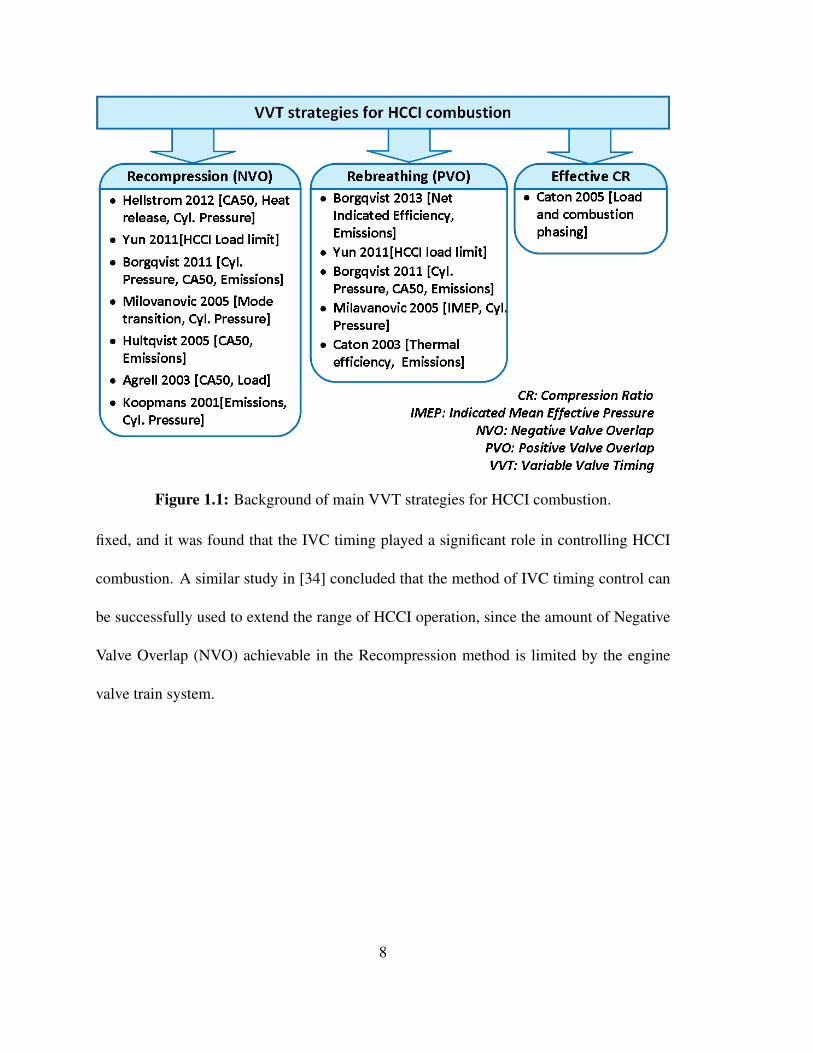
Figure 1.1: Background of main VVT strategies for HCCI combustion.
fixed, and it was found that the IVC timing played a significant role in controlling HCCI
combustion. A similar study in [34] concluded that the method of IVC timing control can
be successfully used to extend the range of HCCI operation, since the amount of Negative
Valve Overlap (NVO) achievable in the Recompression method is limited by the engine
valve train system.
8
1.5 Scope and organization of thesis
Current United States’ Corporate Average Fuel Economy (CAFE) has a target of 54.5 mpg
for cars and light duty trucks by the model year 2025 [35]. This target cannot be met
by the current engines operating in SI or CI modes. HCCI engines hold the promise for
lowering fuel consumption and emissions but their market penetration is blocked by the
control challenges mentioned previously. HCCI engines are flexible and can be used in
conventional and hybrid electric vehicle configurations to meet future CAFE standards.
Simulation models provide solution for proper control of HCCI as these models provide
understanding of HCCI governing thermo-kinetic reactions. But, simulation models which
can predict HCCI combustion need high computational resources and lack the flexibility to
model VVT operating conditions. The aim of this thesis is to develop a simulation model
for predicting residual affected HCCI combustion which will be computationally efficient
and have the flexibility to model a variety of VVT operating conditions. At the same time
this model should predict engine performance results accurately. To this end, a sequential
model called Sequential Model for Residual Affected HCCI (SMRH) is developed in this
thesis and results are validated against the experimental data from a single cylinder Ricardo
HCCI engine [4]. In addition, this thesis provides contributions in developing an HCCI
engine setup at Michigan Technological University. This engine setup will be used as a
framework for future advanced HCCI engine studies.
9
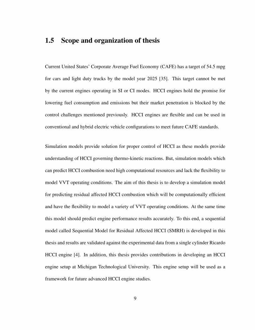
This thesis is organized in four chapters as shown in Figure 1.2. Next, Chapter includes
the work done for developing an HCCI experimental setup for the test cell at Michigan
Tech. Chapter 3 consists of the simulation model (SMRH) developed for studying HCCI
combustion and engine cycle. Chapter 4 includes the conclusions from this thesis along
with some suggestions for future work.
ThesisAn investigation of VVT effects
on HCCI engine combustion and performance
Chapter 2HCCI experimental setup for
GM LHU Gen 1 engine
Chapter 3HCCI engine simulation model
(SMRH)
Chapter 1Introduction & Literature
Review
Chapter 4Conclusion & Future Work
Figure 1.2: Thesis organization
10
Chapter 2
Experimental HCCI Engine Setup
An experimental HCCI engine setup was designed and implemented through collaborative
efforts. This chapter includes the major contributions from this thesis, while other
contributions to build the engine setup can be found in [36, 37].
2.1 Engine experimental setup
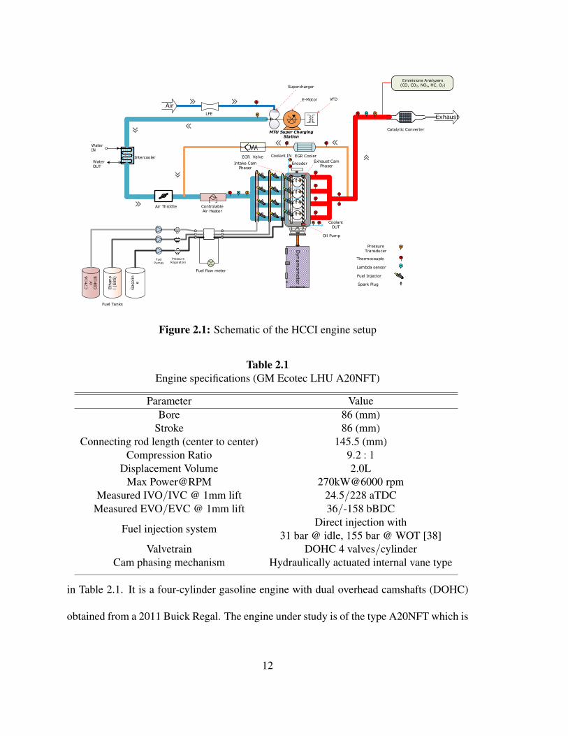
Figure 2.1 shows the schematic of the entire experimental test setup for HCCI studies.
A GM 2.0L Gasoline Direct Injection (GDI) Ecotec LHU Gen 1 engine is modified and
instrumented in order to run in HCCI mode. The engine mounted on a cart and connected
to the supercharging station as shown in Figure 2.2. The engine specifications are shown
11
Exhaust
Controlable Air Heater
Dynam
om
ete
r
Air
EGR Valve
MTU Super Charging Station
Air Throttle
Catalytic Converter
Pressure Transducer
Thermocouple
Lambda sensor
Fuel Injector
EGR CoolerIntercooler
Fuel Tanks
PressureRegulators
Fuel Pumps
Emmisions Analyzers(CO, CO2, NOx, HC, O2)
Encoder
Spark Plug
Fuel flow meter
Intake Cam Phaser
C7H
16
or
C8H
18
Eth
ano
l (E
85)
Gaso
lin
e
Coolant OUT
Coolant IN
Water IN
Water OUT
LFE
Exhaust Cam Phaser
Oil Pump
Supercharger
E-Motor VFD
Figure 2.1: Schematic of the HCCI engine setup
Table 2.1Engine specifications (GM Ecotec LHU A20NFT)
Parameter ValueBore 86 (mm)
Stroke 86 (mm)Connecting rod length (center to center) 145.5 (mm)
Compression Ratio 9.2 : 1Displacement Volume 2.0L
Max Power@RPM 270kW@6000 rpmMeasured IVO/IVC @ 1mm lift 24.5/228 aTDC
Measured EVO/EVC @ 1mm lift 36/-158 bBDC
Fuel injection systemDirect injection with
31 bar @ idle, 155 bar @ WOT [38]Valvetrain DOHC 4 valves/cylinder
Cam phasing mechanism Hydraulically actuated internal vane type
in Table 2.1. It is a four-cylinder gasoline engine with dual overhead camshafts (DOHC)
obtained from a 2011 Buick Regal. The engine under study is of the type A20NFT which is
12
a high performance version of the LHU engine. This A20NFT engine is a European version
of the original LHU. The difference with the North American version of the engine is use
of a better alloy grade to work with higher octane rated fuels used in Europe. The following
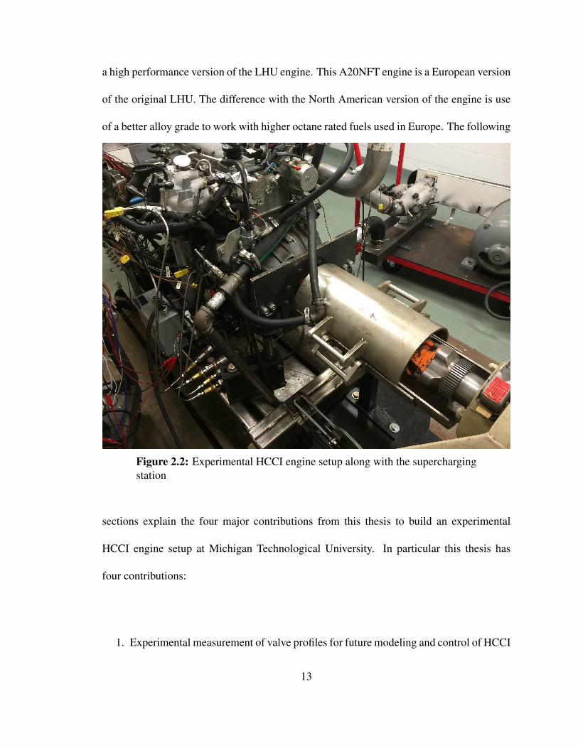
Figure 2.2: Experimental HCCI engine setup along with the superchargingstation
sections explain the four major contributions from this thesis to build an experimental
HCCI engine setup at Michigan Technological University. In particular this thesis has
four contributions:
1. Experimental measurement of valve profiles for future modeling and control of HCCI
13
combustion
2. Increase in engine compression ratio (CR) to enable HCCI operation in a broad
operating region
3. Design and implementation of controllable air heater setup to adjust temperature of
intake charge
4. Design and implementation of supercharging station setup to control intake air boost
pressure and air flow rates
For making the engine suitable to operate in a test cell a few modifications are made.
The wiring harness of the engine is modified so as to accept 12V supply from the
NI DAQ system linked to the test cell computer. An EGR line is tapped into the
exhaust manifold to enable exhaust gas recirculation to prepare dilute mixtures for HCCI
combustion. An electrically controlled intake air heater is also added downstream of the
intercooler (Figure 2.1). The stock position of the throttle valve is changed to upstream of
the air heater in order to protect the throttle valve from high temperatures. Exhaust gases
from external EGR line are mixed with intake air between the throttle and the air heater as
shown in Figure 2.1. The outlet of the EGR line is made downstream of the throttle so as to
obtain maximum amount of exhaust gases from the vacuum generated during the induction
stroke. A supercharging station is built to provide boosted air which is proven to increase
load range in HCCI engines [14]. The test setup for the supercharging station will be
discussed in Section 2.5. Dynamometer testing for research purposes involves measuring
14
in-cylinder pressure data through pressure transducers. The stock cylinder head on the
engine is replaced with a new machined cylinder head to allow installation of in-cylinder
pressure transducers. The encoder installation previously done in [36] is modified by using
shims to remove any eccentricities.
2.2 Experimental measurement of valve profiles
A test setup was built to measure valve profiles to achieve two purposes. One is to
generate valve profiles and understand the phasing ability and the second is to check the
probability of piston to valve contact (Section 2.3) for modifying engine pistons to increase
compression ratio for HCCI operation. The test setup for valve profile measurement
is shown in Figure 2.3. In order to obtain the valve opening and closing timings in
crank angle degrees, valve profiles are experimentally measured and the resulting data
is plotted to generate lift versus Crank Angle Degree (CAD) curves. The LHU engine
consists of independent cam phasers for intake and exhaust camshafts. The cam phasers
are hydraulically actuated using an oil pump located at the drive shaft end of the exhaust
camshaft. The cam actuation solenoids adjust the flow of oil so that the required phasing
can be achieved. Phasing authority of 50 CAD is available on the LHU engine. The cam
phasers are hydraulically operated with an internal vane mechanism for phasing. At the
park position, the intake cam is fully retarded while the exhaust cam is fully advanced.
Hence, the valve overlap is minimum at park position and increases during phasing.
15
(a)
(b)
Figure 2.3: (a): Lift measurement at the valve; (b): Overview of the valveprofile measurement setup
2.2.0.1 Valve profile measurement procedure
The LHU engine uses hydraulic lash adjusters in its stock configuration. Lash is optimally
adjusted using oil pressure when the engine is running. Using hydraulic lash adjusters
during measurements causes them to squish and hence gives incorrect readings. Solid lash
adjusters on proper height adjustment enable to adjust the lash between the cam and roller
16
follower. Thus, JESEL solid lash adjusters (part number: KLA-81500) are used in the
process of valve profile measurements. Lash is made zero during the measurements. These
measurements are carried out when the engine is not firing and hence did not have any oil
pressure.
Vale lift can be measured in two ways. Measurements can either be taken based on the
cam lobe or can be taken at the tip of the valve stem. Lifts measured on the cam lobe have
to be multiplied by a factor known as the rocker arm ratio defined in Appendix A. In this
study measurements are taken on the first cylinder from the rear end of the engine. The
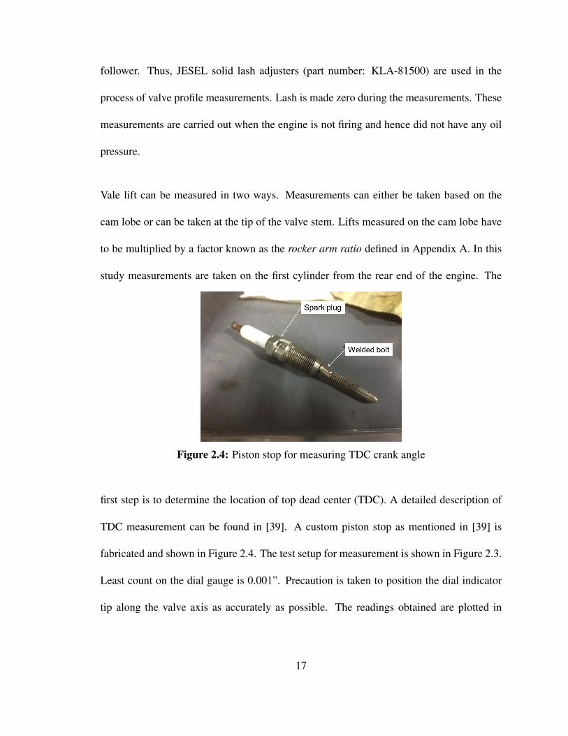
Figure 2.4: Piston stop for measuring TDC crank angle
first step is to determine the location of top dead center (TDC). A detailed description of
TDC measurement can be found in [39]. A custom piston stop as mentioned in [39] is
fabricated and shown in Figure 2.4. The test setup for measurement is shown in Figure 2.3.
Least count on the dial gauge is 0.001”. Precaution is taken to position the dial indicator
tip along the valve axis as accurately as possible. The readings obtained are plotted in
17
Figure 2.5(a).
Commercial camshaft manufacturers specify duration of valve operation assuming a certain
valve lift as opening/closing point. It is commonly referred at 0.05” (or 1 mm) of valve lift
as opening/closing point [39]. Theoretically, at valve lift of 1mm, the intake (or exhaust)
valves would still be open and the opening and closing timings will not be the exact crank
angles when the valves just open or close. In reality, at high speeds, negligible flow would
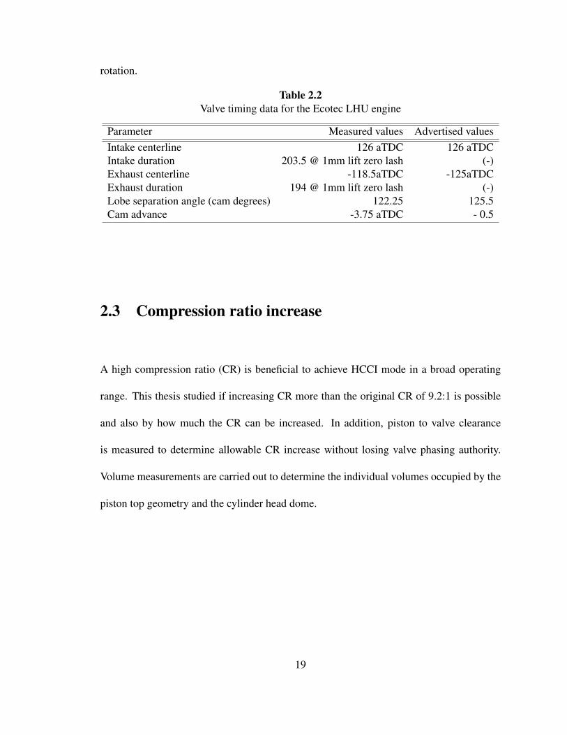
occur at a valve lift of 1 mm. Measured values for crank angle for peak lift and duration are
compared with advertised values obtained from GM engineers in Table 2.2. The advertised
values are seat to seat values at 0.04 mm lash and an unknown lift. Hence, comparing
the opening, closing and duration values would not make any sense as discrepancy is
also seen between exhaust valve duration in Table 2.2. Instead, the intake and exhaust
centerline values along with the lobe separation angle can be effectively compared as they
are independent of lift. Equations for calculation of the values in Table 2.2 are mentioned
in Appendix A. Figure 2.5(a) shows the final plot for measured intake and exhaust valve
profiles with 50 CAD phasing. Thus, the valve profiles at completely phased condition
will be as seen in Figure 2.5(a). Table 2.1 shows the values of measured valve timings,
assuming valve opening/closing at 1mm lift. The raw data obtained consisted of some
irregularities which are smoothed to obtain the profile in Figure 2.5(a). A velocity plot of
the raw data showed the irregular data points which are then adjusted to obtain a smooth
curve. These irregularities are a result of human errors, backlash in the engine crankshaft
and a comparatively low resolution on the degree wheel used to measure crank angle
18
rotation.
Table 2.2Valve timing data for the Ecotec LHU engine
Parameter Measured values Advertised valuesIntake centerline 126 aTDC 126 aTDCIntake duration 203.5 @ 1mm lift zero lash (-)Exhaust centerline -118.5aTDC -125aTDCExhaust duration 194 @ 1mm lift zero lash (-)Lobe separation angle (cam degrees) 122.25 125.5Cam advance -3.75 aTDC - 0.5
2.3 Compression ratio increase
A high compression ratio (CR) is beneficial to achieve HCCI mode in a broad operating
range. This thesis studied if increasing CR more than the original CR of 9.2:1 is possible
and also by how much the CR can be increased. In addition, piston to valve clearance
is measured to determine allowable CR increase without losing valve phasing authority.
Volume measurements are carried out to determine the individual volumes occupied by the
piston top geometry and the cylinder head dome.
19
−250 −200 −150 −100 −50 0 50 100 150 200 2500
2
4
6
8
10
CAD (aTDC)
Lift
(mm
)
Exh. parkExh. phasedInt. parkInt. phased
(a)
All Values at 1mm valve lift
TDC
BDC
24.5o22o
36o48o
IVO
IVC EVO
EVC
203.5o194o
Valve Timing Diagram ‘GM Ecotec LHU’Park Position (no phasing)
All values at 1mm valve lift
TDC
BDC
28o25.5o
2o14o
IVO
IVCEVO
EVC
203.5o194.5o
Valve Timing Diagram ‘GM Ecotec LHU’Fully Phased (50 CAD)
(b)
Figure 2.5: (a): Intake and exhaust valve profiles for park position andcompletely phased position; (b): Valve timing diagram for the GM EcotecLHU engine. Dotted line near the base indicates the lift (1 mm) at whichvalve opening and closing crank angles are measured.
20
2.3.1 Piston to valve clearance
The solid green line in Figure 2.6 shows the location of the piston with reference to the
valve seat when the valve is completely closed. The intake valve is manually pushed open
for suitable crank angle intervals of piston movement from BDC to TDC. In reality, the
maximum valve lift is more than the advertised maximum lift. The valve never attains this
maximum lift due to high spring forces inside the valve springs and due to valve retainers.
The stock springs are replaced with dummy springs which could be compressed easily.
Thus, the locus of points obtained when plotted along with the valve profiles gives the
piston location along with the piston to valve clearance for a set of crank angle degrees.
Selection of a flat top piston would either cause valve phasing authority to reduce if the
−100 −80 −60 −40 −20 0 20 40 60 80 100
1
2
3
4
5
6
7
8
9
10
11
CAD (aTDC)
Lift
(mm
)
Exh. parkExh. phasedInt. parkInt. phasedPiston−Valve clearance
Figure 2.6: Measured piston to valve clearance, using the same referencepoint at which valve lifts are measured
piston top is considered above the valve pocket base, or it would increase the clearance
21
volume if the piston top is considered at the base of valve pockets keeping full phasing
authority. Hence, from Figure 2.6 it is concluded that a flat top piston is not a feasible
option as it would limit the phasing ability for the increase in CR.
2.3.2 Volume measurements
Measurements are carried out to determine individual volumes of the combustion chamber
dome and the volume occupied by the piston top geometry (Figure 2.7(a)). The piston
surface is cleaned of any carbon deposit and dirt using a cleaning fluid such as a regular
brake cleaner. The stock piston has a unique “dish” type profile for DI applications. The
piston top geometry showing this “dish” and valve pockets are shown in Figure 2.7(a). The
drive shaft is then rotated to bring the entire piston to an approximate distance below the
firing deck and the height is measured using a vernier caliper. This distance is shown in
Figure 2.8 as “s”. A burette is completely filled with mineral fluid of low viscosity and
its meniscus is adjusted suitably. The area between the piston and the cylinder liner is
greased to avoid leakage inside the cylinder and a transparent plastic slide is used to cover
the top. The liquid inside the burette is emptied gradually through a slight opening made
by moving the slide. Flow is stopped once the liquid formed a uniform film on the slide’s
lower surface. Readings are noted at the start and end and the difference between these two
readings indicates the volume under study.
22
(a) Piston top geometry
(b) Cylinder head dome volume
Figure 2.7: Experimental measurement of compression ratio
Thus, volume 1 from Figure 2.8 is determined. This gives the TDC volume or the effective
volume considering the volume occupied by the piston top geometry. Swept volume is
determined using Equation (2.1) where “D” and “L” represent the bore and the swept
distance respectively.
Volume =π
4D2×L (2.1)
23
Piston top geometry
3
2
1
Bottom surface of cyl. head
Firing deck
Here, piston is at TDC1: TDC volume2: Gasket volume3: Cylinder head volume
s
Figure 2.8: Figure showing different sections for which volumemeasurements are carried out
Volume 2 in Figure 2.8 is determined by using Equation (2.1) where, “L” is substituted with
the measured thickness of the compressed cylinder head gasket. For determining volume
3 from Figure 2.8, all cavities are first closed by inserting the four valves, the fuel injector
and the spark plug is inserted and tightened to avoid any leaks. Readings are taken once
again for the volume of fluid occupied by the area under study. The clearance volume is
calculated using Equation (2.2).
Clearance Volume = [Volume o f cyl. head dome]
+ [Volume due to gasket thickness]
+ [Volume due to area surrounding piston at T DC]
− [Volume due to piston top geometry]
(2.2)
The clearance volume is indicated by the entire hatched region in Figure 2.8. Measured
volumes 1 and 2 along with the calculated gasket volume are shown in Table 2.3. CR is
defined as the ratio of the maximum volume to the minimum volume in an engine cycle,
24

Table 2.3Measurements for engine combustion chamber volume
Component Measured volume (cc)Cylinder head dome 48.8Piston top geometry 2Gasket (compressed) 4.47
Volume in section #1 (Fig.2.8) 9.4Clearance volume 60.7
and is given by Equation (2.3).
CR =(Vs +Vc)
(Vc)(2.3)
Where, Vs is the swept volume given by Equation (2.1) and Vc is the clearance volume
given by Equation (2.2).
2.3.3 Piston selection
One way to increase CR is by decreasing Vc as Equation (2.3) suggests. From the results
obtained in section 2.3.2 it becomes clear that material cannot not be added over the valve
pockets and their depths can hence not be modified. Remaining areas surrounding the
valve pockets could be used for material addition to reduce Vc. Thus, the “max dome”
piston design from the Wiseco piston company is selected which offers a volume of 16.6cc
due to piston top geometry. For this design, the valve pockets are kept at the same height
using a fixed reference point for both the old and the new pistons. The valve pocket depths
25
are 0.09” for intake and 0.045” for exhaust. These depths are measured with reference to
the timing edge defined in Appendix A. This ensured that the valve phasing ability is not
reduced or lost completely. The resulting calculated CR using the new piston is 12.31:1 for
the GM Ecotec engine.
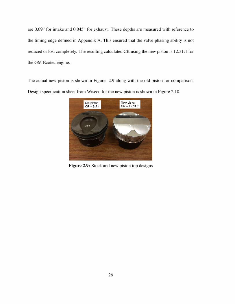
The actual new piston is shown in Figure 2.9 along with the old piston for comparison.
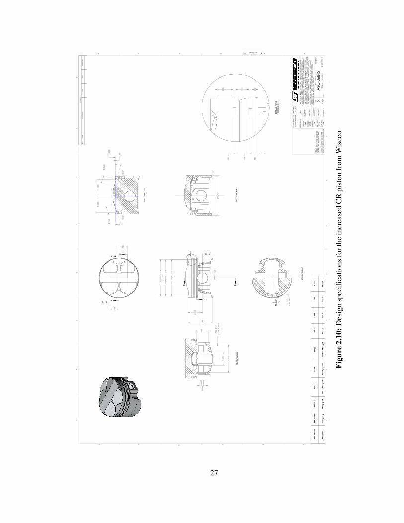
Design specification sheet from Wiseco for the new piston is shown in Figure 2.10.
Figure 2.9: Stock and new piston top designs
26
TOP
GR
V -
A
2ND
GR
V -
B
1.21
5
2.06
8
OIL
GR
V -
C
.020
B B
C
C
RIN
G
.748
.709
AA
D
D
DIA
"D"
.137
SE
CTI
ON
A-A
.076
TY
P.
2 G
RO
OV
ES
2.34
2
.905
5 +.00
09+.
0007
1.12
5
.990
SE
CTI
ON
B-B
18.0
00°
.125
6 H
OLE
S
SE
CTI
ON
C-C
.111
.190
.080
.049
.041
.250
DE
TAIL
RIN
G
SC
ALE
6 :
1
.065.2
10
R.6
40
R.7
40
1.38
31.
425
18.0
°16
.0°
SE
CTI
ON
D-D
REV
ISIO
NS
REV
.ZO
NE
CO
MM
ENT
ECO
.D
ATE
APP
ROV
ED
ASC
-068
45F6
636X
A0
8600
XXS7
52S7
5240
0g3.
082
3.05
83.
090
3.38
2
Part
No.
Forg
ing
Rin
g pn
#W
rist P
in p
n#C
irclip
pn#
Pist
on W
eigh
tD
ia A
Dia
BD
ia C
Dia
D
D C B
ABCD
34
56
788
76
54
32
1
EF
EF REVASC-06845 D
ASC
-068
45
-----
21
A
THE
DES
IGN
AN
D D
ISC
LOSU
RE C
ON
TAIN
ED IN
THI
S D
RAW
ING
W
AS
ORI
GIN
ATE
D B
Y, A
ND
IS T
HE E
XCLU
SIV
E PR
OPE
RTY
OF
WIS
ECO
PIS
TON
INC
. IT
IS F
URN
ISHE
D F
OR
INFO
RMA
TION
ON
LY
AN
D IS
NO
T A
N A
UTHO
RIZA
TION
OR
LICEN
SE T
O M
AKE
THI
S C
ON
STRU
CTIO
N O
R TO
FUR
NIS
H TH
IS IN
FORM
ATIO
N T
O O
THER
S.
ALL
DRA
WIN
GS
MUS
T BE
RET
URN
ED T
O W
ISEC
O P
ISTO
N IN
C.
ON
DEM
AN
D. T
HIS
DRA
WIN
G IS
NO
T TO
BE
PRO
DUC
ED O
R C
OPI
ED IN
AN
Y FO
RM W
ITHO
UT T
HE E
XPRE
SS W
RITT
EN
PERM
ISSI
ON
OF
WIS
ECO
PIS
TON
INC
.
RE
VISI
ON
MM
/DD
/YY
MM
/DD
/YY
MM
/DD
/YY
MM
/DD
/YY
XXX
XXX
XXX
XXX
05/2
7/20
14JW
B
NO
TES:
UNLE
SS O
THER
WIS
E SP
ECIF
IED
DIM
ENSI
ON
S A
RE IN
INC
HES
AN
GUL
AR
DIM
ENSI
ON
S A
RESH
OW
N IN
DEG
REES
/DEC
IMA
LSQ
UAL
ENG
MFG
EN
G
RESP
EN
G
CHE
CKE
D
DRA
WN
APP
ROV
ALS
DA
TE
DD
WG
. N
AM
E
Engi
ne In
form
atio
n:
SIZE
SCA
LE
1:1
CA
D G
ENER
ATE
D D
RAW
ING
,D
O N
OT
MA
NUA
LLY
UPD
ATE
SHEE
T 1
OF
1
Figu
re2.
10:D
esig
nsp
ecifi
catio
nsfo
rthe
incr
ease
dC
Rpi
ston
from
Wis
eco
27
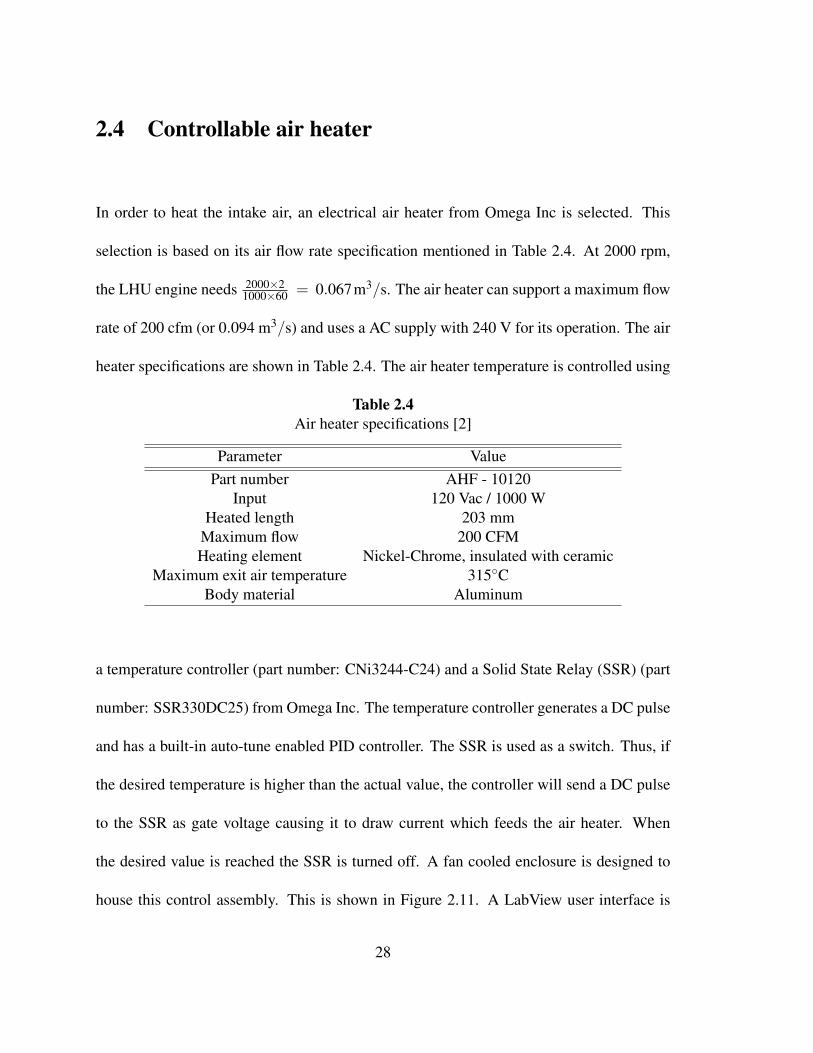
2.4 Controllable air heater
In order to heat the intake air, an electrical air heater from Omega Inc is selected. This
selection is based on its air flow rate specification mentioned in Table 2.4. At 2000 rpm,
the LHU engine needs 2000×21000×60 = 0.067m3/s. The air heater can support a maximum flow
rate of 200 cfm (or 0.094 m3/s) and uses a AC supply with 240 V for its operation. The air
heater specifications are shown in Table 2.4. The air heater temperature is controlled using
Table 2.4Air heater specifications [2]
Parameter ValuePart number AHF - 10120
Input 120 Vac / 1000 WHeated length 203 mm
Maximum flow 200 CFMHeating element Nickel-Chrome, insulated with ceramic
Maximum exit air temperature 315◦CBody material Aluminum
a temperature controller (part number: CNi3244-C24) and a Solid State Relay (SSR) (part
number: SSR330DC25) from Omega Inc. The temperature controller generates a DC pulse
and has a built-in auto-tune enabled PID controller. The SSR is used as a switch. Thus, if
the desired temperature is higher than the actual value, the controller will send a DC pulse
to the SSR as gate voltage causing it to draw current which feeds the air heater. When
the desired value is reached the SSR is turned off. A fan cooled enclosure is designed to
house this control assembly. This is shown in Figure 2.11. A LabView user interface is
28
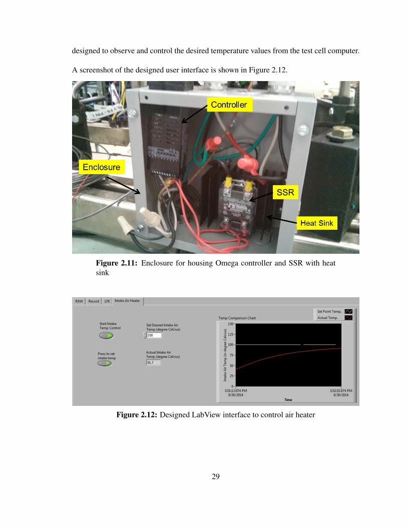
designed to observe and control the desired temperature values from the test cell computer.
A screenshot of the designed user interface is shown in Figure 2.12.
Figure 2.11: Enclosure for housing Omega controller and SSR with heatsink
Figure 2.12: Designed LabView interface to control air heater
29
2.5 MTU Supercharging Station
As previously discussed in the Chapter 1 intake air boosting is one of the enabling
techniques for HCCI combustion and also for operating the engine at higher loads. By
increasing the intake air pressure the specific energy of air entering the cylinder is increased
along with the amount of air entering the cylinder. High gas pressure aids in auto-igniting
the in-cylinder charge, resulting in HCCI combustion. A supercharging station is set up
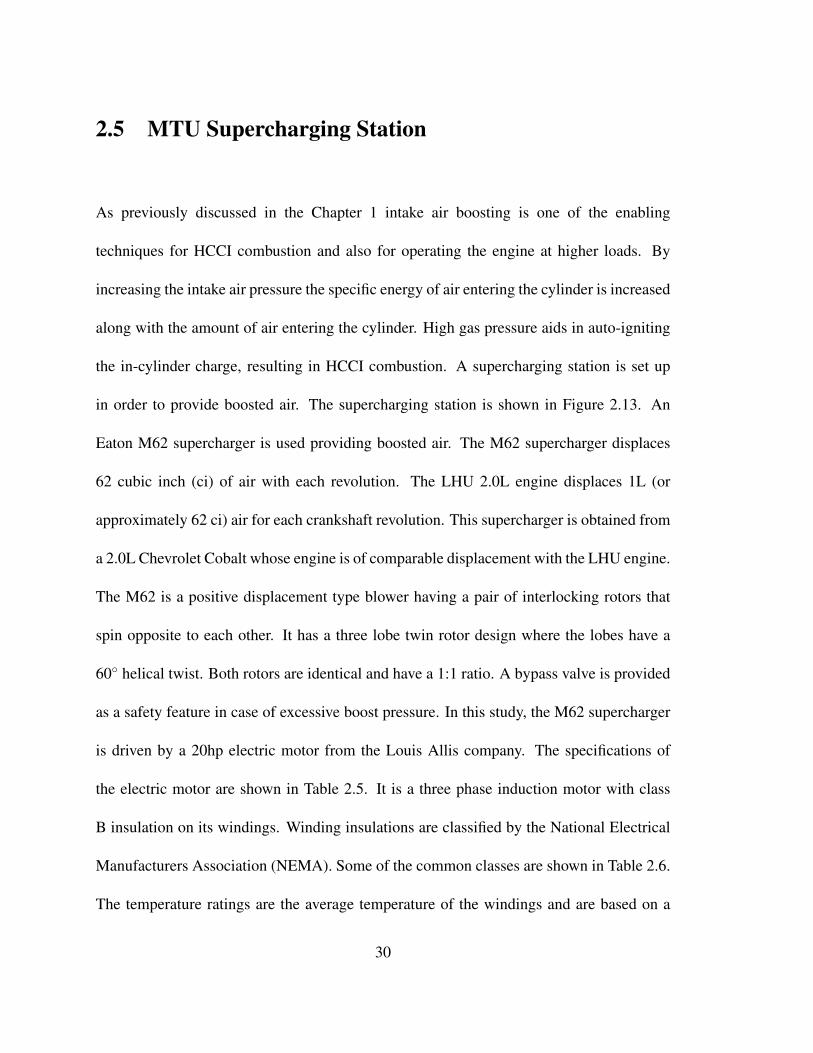
in order to provide boosted air. The supercharging station is shown in Figure 2.13. An
Eaton M62 supercharger is used providing boosted air. The M62 supercharger displaces
62 cubic inch (ci) of air with each revolution. The LHU 2.0L engine displaces 1L (or
approximately 62 ci) air for each crankshaft revolution. This supercharger is obtained from
a 2.0L Chevrolet Cobalt whose engine is of comparable displacement with the LHU engine.
The M62 is a positive displacement type blower having a pair of interlocking rotors that
spin opposite to each other. It has a three lobe twin rotor design where the lobes have a
60◦ helical twist. Both rotors are identical and have a 1:1 ratio. A bypass valve is provided
as a safety feature in case of excessive boost pressure. In this study, the M62 supercharger
is driven by a 20hp electric motor from the Louis Allis company. The specifications of
the electric motor are shown in Table 2.5. It is a three phase induction motor with class
B insulation on its windings. Winding insulations are classified by the National Electrical
Manufacturers Association (NEMA). Some of the common classes are shown in Table 2.6.
The temperature ratings are the average temperature of the windings and are based on a
30
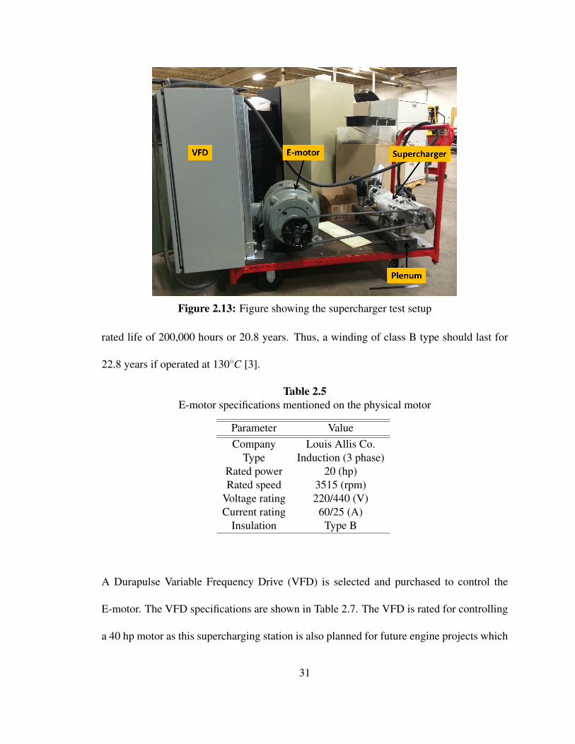
Figure 2.13: Figure showing the supercharger test setup
rated life of 200,000 hours or 20.8 years. Thus, a winding of class B type should last for
22.8 years if operated at 130◦C [3].
Table 2.5E-motor specifications mentioned on the physical motor
Parameter ValueCompany Louis Allis Co.
Type Induction (3 phase)Rated power 20 (hp)Rated speed 3515 (rpm)
Voltage rating 220/440 (V)Current rating 60/25 (A)
Insulation Type B
A Durapulse Variable Frequency Drive (VFD) is selected and purchased to control the
E-motor. The VFD specifications are shown in Table 2.7. The VFD is rated for controlling
a 40 hp motor as this supercharging station is also planned for future engine projects which
31
Table 2.6E-motor insulation classes by NEMA [3]
Insulation class Winding temperatureA 105oCB 130oCF 155oCH 180oC
might need more boosted air flow rates depending on engine size.
Table 2.7VFD specifications
Parameter ValuePart number Durapulse GS34040
Maximum motor output 40 hpRated output current 60 A
Weight 35 kgCommunication protocol RS485 Modbus RTU
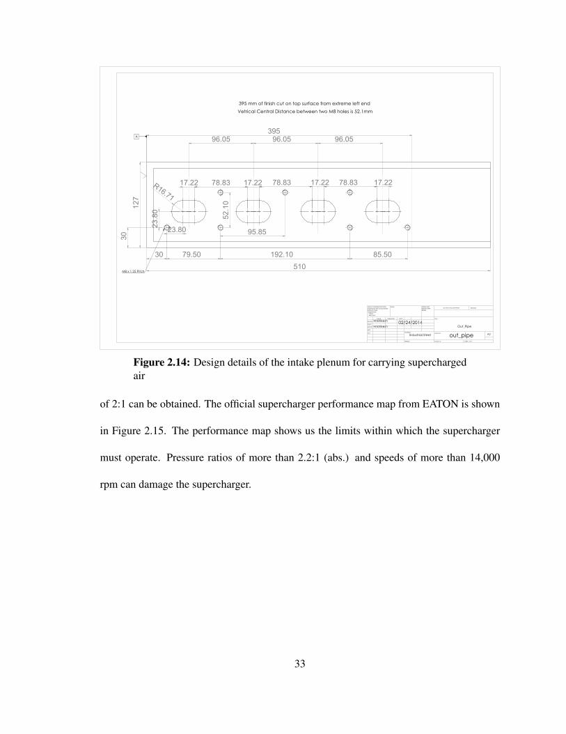
An intake air plenum is designed and is shown in Figure 2.14. The supercharger is bolted
down on the plenum and a standard automotive 6 groove serpentine belt is used to couple
it with the e-motor. A standard composite pulley of diameter 6.5” is attached to the
motor shaft and the corresponding supercharger speeds are measured. In this way, the
transmission ratio is calculated to be 1:1.8 (driver:driven). Air from the supercharger is
routed through an intercooler mounted below the engine. The waste gate valve on the stock
turbocharger can be used to pass exhaust gases without spooling the turbocharger. The
e-motor is limited by its maximum speed of 3515 rpm. Thus by using a 1:1.8 ratio by
the coupling system, the maximum supercharger speed that can be achieved is about 6327
rpm. Theoretically, by running the supercharger at twice the engine speed, a pressure ratio
32
127
30 79.50 192.10 85.50
17.22 78.83 17.22 78.83 17.22 78.83 17.22R16.71
23.80
52.10
95.85
510
23.80
30
96.05 96.05 96.05395
M8 x 1.25 Pitch
A
Industrial Steel
Hrishikesh
Hrishikesh02/24/2014
1
Out_Pipe
Vetrical Central Distance between two M8 holes is 52.1mm395 mm of finish cut on top surface from extreme left end
out_pipeWEIGHT:
A2
SHEET 1 OF 1SCALE:1:2
DWG NO.
TITLE:
REVISIONDO NOT SCALE DRAWING
MATERIAL:
DATESIGNATURENAME
DEBUR AND BREAK SHARP EDGES
FINISH:UNLESS OTHERWISE SPECIFIED:DIMENSIONS ARE IN MILLIMETERSSURFACE FINISH:TOLERANCES: LINEAR: ANGULAR:
Q.A
MFG
APPV'D
CHK'D
DRAWN
Figure 2.14: Design details of the intake plenum for carrying superchargedair
of 2:1 can be obtained. The official supercharger performance map from EATON is shown
in Figure 2.15. The performance map shows us the limits within which the supercharger
must operate. Pressure ratios of more than 2.2:1 (abs.) and speeds of more than 14,000
rpm can damage the supercharger.
33
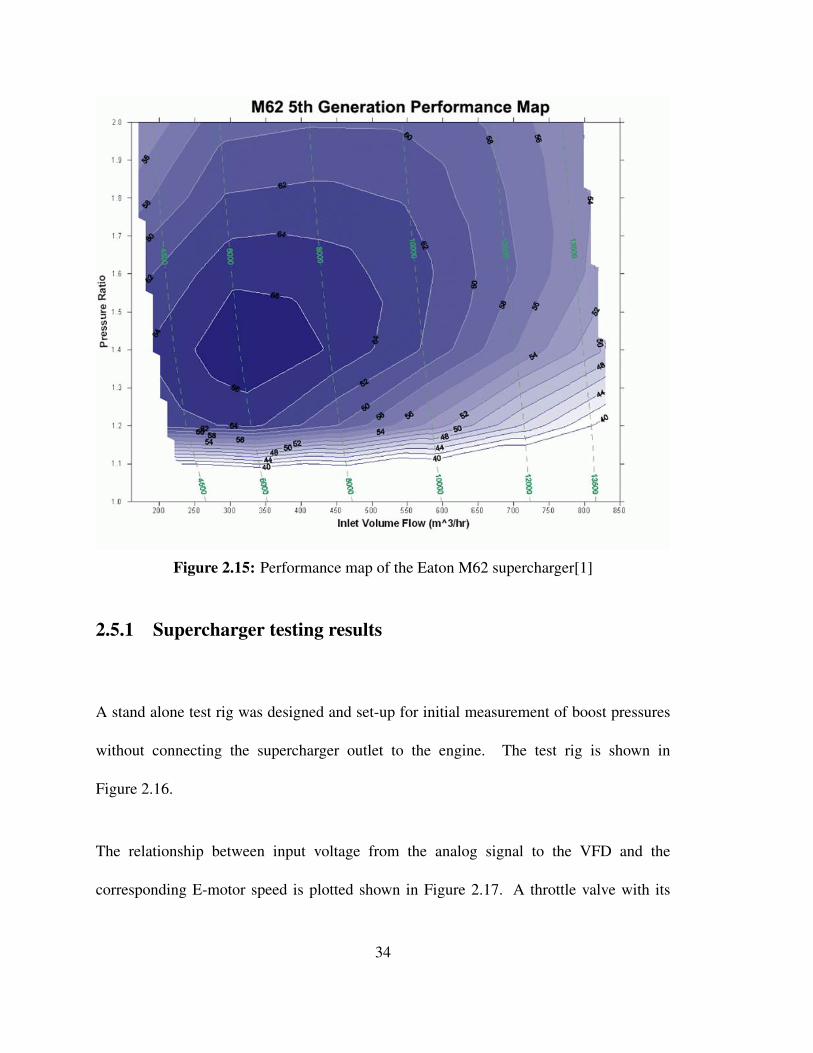
Figure 2.15: Performance map of the Eaton M62 supercharger[1]
2.5.1 Supercharger testing results
A stand alone test rig was designed and set-up for initial measurement of boost pressures
without connecting the supercharger outlet to the engine. The test rig is shown in
Figure 2.16.
The relationship between input voltage from the analog signal to the VFD and the
corresponding E-motor speed is plotted shown in Figure 2.17. A throttle valve with its
34
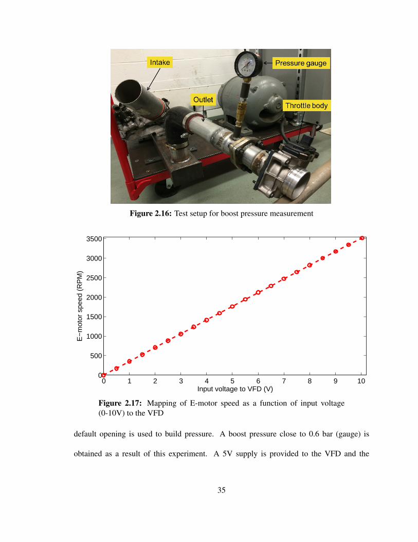
Figure 2.16: Test setup for boost pressure measurement
0 1 2 3 4 5 6 7 8 9 100
500
1000
1500
2000
2500
3000
3500
Input voltage to VFD (V)
E−
mot
or s
peed
(R
PM
)
Figure 2.17: Mapping of E-motor speed as a function of input voltage(0-10V) to the VFD
default opening is used to build pressure. A boost pressure close to 0.6 bar (gauge) is
obtained as a result of this experiment. A 5V supply is provided to the VFD and the
35
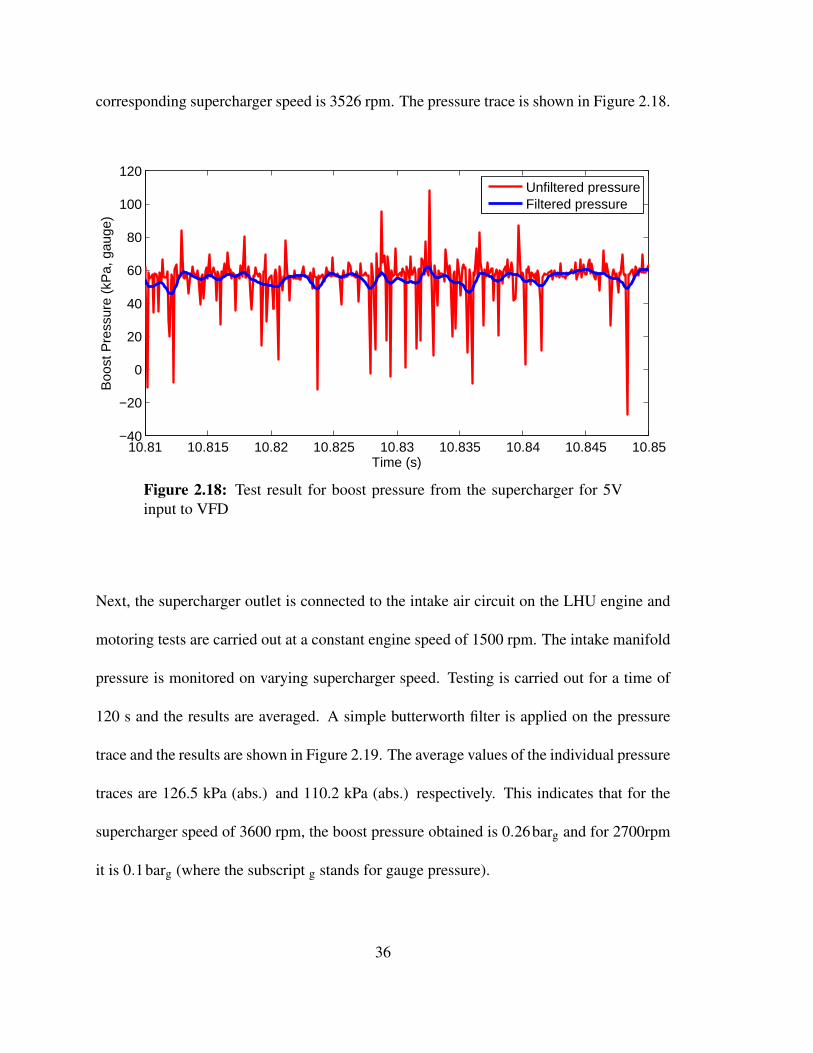
corresponding supercharger speed is 3526 rpm. The pressure trace is shown in Figure 2.18.
10.81 10.815 10.82 10.825 10.83 10.835 10.84 10.845 10.85−40
−20
0
20
40
60
80
100
120
Time (s)
Boo
st P
ress
ure
(kP
a, g
auge
)
Unfiltered pressureFiltered pressure
Figure 2.18: Test result for boost pressure from the supercharger for 5Vinput to VFD
Next, the supercharger outlet is connected to the intake air circuit on the LHU engine and
motoring tests are carried out at a constant engine speed of 1500 rpm. The intake manifold
pressure is monitored on varying supercharger speed. Testing is carried out for a time of
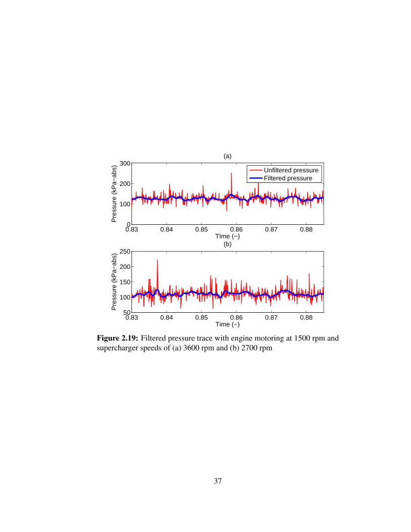
120 s and the results are averaged. A simple butterworth filter is applied on the pressure
trace and the results are shown in Figure 2.19. The average values of the individual pressure
traces are 126.5 kPa (abs.) and 110.2 kPa (abs.) respectively. This indicates that for the
supercharger speed of 3600 rpm, the boost pressure obtained is 0.26barg and for 2700rpm
it is 0.1barg (where the subscript g stands for gauge pressure).
36
0.83 0.84 0.85 0.86 0.87 0.880
100
200
300(a)
TIme (−)
Pre
ssur
e (k
Pa−
abs)
0.83 0.84 0.85 0.86 0.87 0.8850
100
150
200
250(b)
Time (−)
Pre
ssur
e (k
Pa−
abs)
Unfiltered pressure Filtered pressure
Figure 2.19: Filtered pressure trace with engine motoring at 1500 rpm andsupercharger speeds of (a) 3600 rpm and (b) 2700 rpm
37

Chapter 3
Sequential Combustion Modeling of
HCCI Engines with Variable Valve
Timing
Experimental testing is useful for measuring combustion and performance metrics for
engine operation. But, direct measurement of some combustion and engine performance
metrics is not always possible and is often quite expensive. A good example of this
is measuring the mass of residuals inducted by means of internal EGR [40]. It can be
calculated based on the pressure trace and by using mathematical relations like the ideal
gas law used in [41]. Other parameters such as emissions can be measured directly coming
out of the engine. In order to understand emissions formation and engine performance,
39
combustion phenomenon taking place inside the HCCI engine needs to be analyzed in
depth. It is essential to know and understand thermo-kinetics of HCCI combustion and
means (e.g., VVT) to control HCCI; thus, one can address the challenges faced by the
market penetration of HCCI technology discussed in Chapter 1. HCCI simulation models
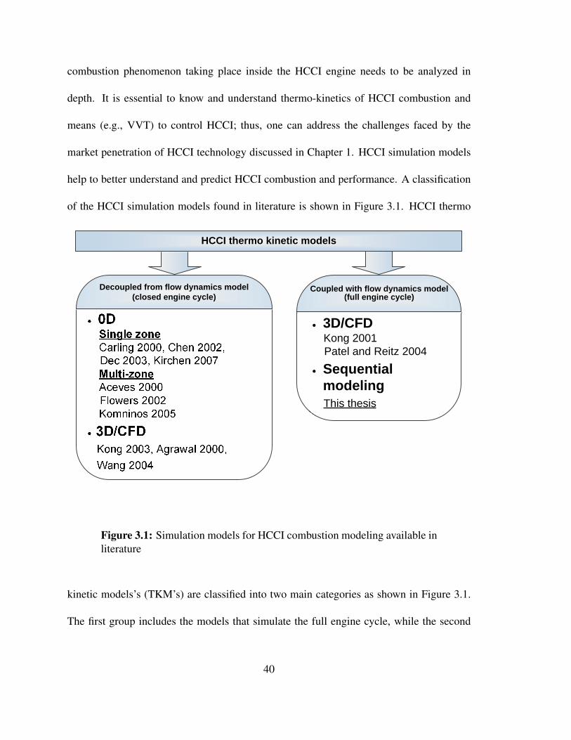
help to better understand and predict HCCI combustion and performance. A classification
of the HCCI simulation models found in literature is shown in Figure 3.1. HCCI thermo
HCCI thermo kinetic models
0D Single zone Carling 2000, Chen 2002, Dec 2003, Kirchen 2007 Multi-zone Aceves 2000 Flowers 2002 Komninos 2005
3D/CFD Kong 2003, Agrawal 2000, Wang 2004
Coupled with flow dynamics model(full engine cycle)
3D/CFD Kong 2001 Patel and Reitz 2004
Sequential modeling
This thesis
Decoupled from flow dynamics model(closed engine cycle)
Figure 3.1: Simulation models for HCCI combustion modeling available inliterature
kinetic models’s (TKM’s) are classified into two main categories as shown in Figure 3.1.
The first group includes the models that simulate the full engine cycle, while the second
40
group focuses on closed engine cycle between Intake Valve Closing (IVC) and Exhaust
Valve Opening (EVO). A TKM is part of both these main categories for simulating the
engine cycle between IVC and EVO. The main difference between these two categories
is whether to couple a TKM with flow dynamics models to predict IVC conditions and
residual gas amount. Coupling a TKM with flow dynamic model often leads to more
accurate combustion prediction, but requires more computational resources.
First category of HCCI models in Figure 3.1 are distributed into two groups including
zero dimensional (0-D), and 3D/CFD models. Zero dimensional models can be further
divided into two categories. First group includes single zone models (SZM’s) [42, 43, 44]
with a simplified or detailed chemical kinetic mechanism. These are among the simplest
models for simulating HCCI combustion [19]. SZM’s typically assume the entire
combustion chamber as one uniform zone where combustion takes place in the entire zone
simultaneously. Study conducted by [42] uses a detailed iso-octane reaction mechanism
from the Lawrence Livermore National Laboratory and treats in-cylinder charge as a
uniform lumped mass having uniform composition and thermodynamic properties. SZM’s
assume that the in-cylinder conditions are like a homogeneously mixed reactor with
uniform temperature, pressure and composition. SZM’s have the advantage of predicting
start of combustion (SOC) accurately and in most cases in-cylinder gas pressure is
overpredicted. This is because, the entire combustion chamber is assumed to combust
together. As a result, emissions prediction is not accurate by SZM’s. The disadvantages
include an overprediction of NOx, underprediction of burn duration (BD) and failing to
41
predict carbon monoxide (CO) and uHC emissions [5]. In an HCCI engine turbulence and
mixing effects are not of importance for combustion phasing [8]. However, these effects
influence the temperature and mass distribution along with the boundary layer thickness in
an HCCI combustion chamber [5].
Multi zone modeling (MZM) is able to predict combustion phasing along with CO and uHC
emissions [5]. In MZM the combustion chamber is divided into a number of zones. Zones
are imaginary regions in the cylinder based upon the temperature and mass distribution
specified in the model. The MZM approach is less simplified than the SZM approach and
yields results that can accurately simulate real engine conditions. Consequently a MZM is
computationally expensive.
Studies carried out in [45],[46] use a 3D CFD code coupled with a CHEMKIN R© code for
the open HCCI cycle. KIVA-3V was used for the CFD part. The results in [46] indicate an
accurate prediction of ignition timing, cylinder pressure and heat release rates along with
CO and uHC emissions. CFD models can predict both closed engine cycle [47][48][49]
and open engine cycle [45][46][50]. However, they require high computational resources
and are consequently not desirable for controller designs.
Sequential modeling is a hybrid approach [5] where combustion models such as a TKM can
be used along with other models to predict the performance metrics for the entire engine
cycle. In HCCI modeling studies done by [5, 51, 52] the CFD code is only used to find
in-cylinder conditions at SOC after which a 0-D TKM model is used. This thesis proposes
42
a new sequential modeling approach to combine 1-D flow models with a multi zone TKM
for simulating residual affected HCCI engines.
To the best of the author’s knowledge, this is the first study undertaken to develop a
sequential computationally efficient model for residual affected HCCI including VVT
effects. The HCCI model developed in this study is denoted as SMRH (Sequential
Model for Residual affected HCCI). SMRH is computationally efficient and is capable
of accurately predicting HCCI combustion and performance under the effects of internal
EGR through Variable Valve Timing (VVT).
3.1 SMRH Description
This section describes the sequential modeling platform developed in this study for
simulating VVT impacts on HCCI combustion. Results are first validated with the
experimental data from a Ricardo HCCI engine [4] and an analysis of simulation results is
presented in Section 3.2.
A multi zone combustion model is developed in CHEMKIN R©−PRO in this study. The
multi-zone model is a model which couples the thermodynamics of the combustion process
with the chemical kinetic reactions associated with them. HCCI combustion is largely
dependant on the mixture conditions at IVC [8], particularly for residual affected HCCI.
43
The important IVC conditions are pressure, temperature and mixture composition.
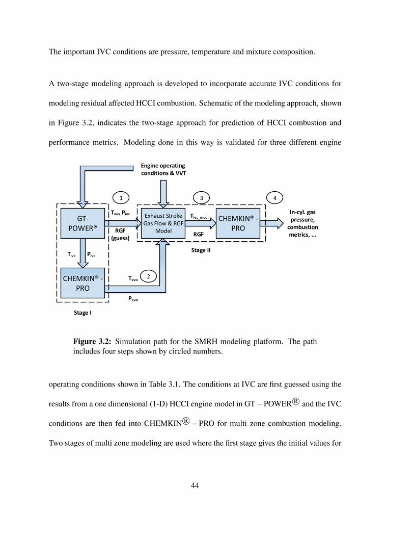
A two-stage modeling approach is developed to incorporate accurate IVC conditions for
modeling residual affected HCCI combustion. Schematic of the modeling approach, shown
in Figure 3.2, indicates the two-stage approach for prediction of HCCI combustion and
performance metrics. Modeling done in this way is validated for three different engine
GT-POWER®
Exhaust Stroke Gas Flow & RGF
Model
Tivc, Pivc
CHEMKIN® -PRO
Tivc_mod In-cyl. gas pressure,
combustion metrics, ...
Engine operating conditions & VVT
RGF (guess)
CHEMKIN® -PRO
Pivc
Tevo
RGF
Pevo
Tivc
Stage I
Stage II
2
1 3 4
Figure 3.2: Simulation path for the SMRH modeling platform. The pathincludes four steps shown by circled numbers.
operating conditions shown in Table 3.1. The conditions at IVC are first guessed using the
results from a one dimensional (1-D) HCCI engine model in GT−POWER R© and the IVC
conditions are then fed into CHEMKIN R©−PRO for multi zone combustion modeling.
Two stages of multi zone modeling are used where the first stage gives the initial values for
44
the end of combustion (i.e., EVO conditions) which are then used in an Exhaust Stroke
Gas Flow & RGF model [41] to determine Residual gas Fraction (RGF) quantity and
temperature of residual gases. The last step consists of multi zone modeling to determine
the final simulation results. Outputs of SMRH include in-cylinder gas pressure, combustion
metrics (CA10, CA50 and BD), performance metrics (IMEP and ηth,i), and engine-out
emissions. The SMRH includes four steps as will be discussed next.
Table 3.1Engine operating conditions of the experimental data [4] used to validate
SMRH
Case # Pman (kPa) Tman (◦C) φ Engine Speed (rpm)
a 117.2 87.6 0.45 1016b 108.8 87.6 0.45 1016c 89.1 90.8 0.56 920
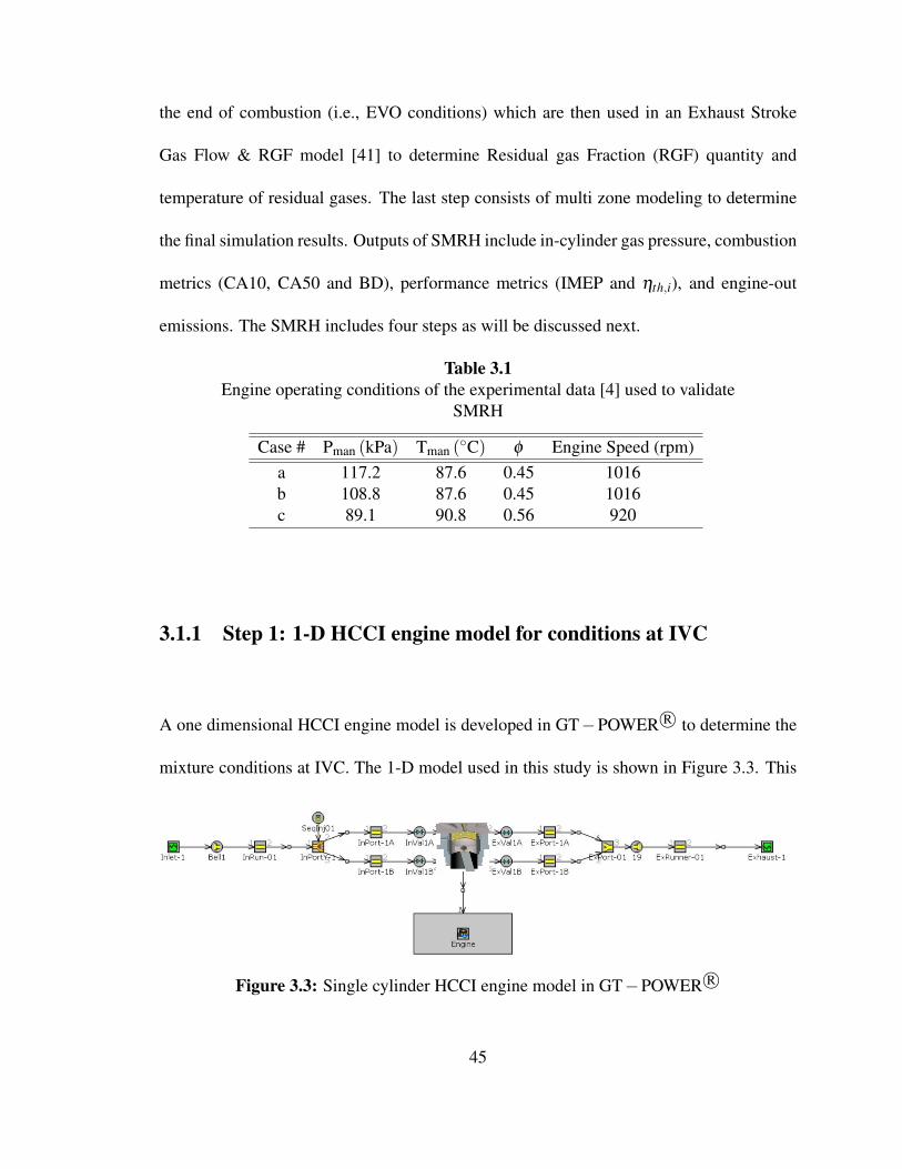
3.1.1 Step 1: 1-D HCCI engine model for conditions at IVC
A one dimensional HCCI engine model is developed in GT−POWER R© to determine the
mixture conditions at IVC. The 1-D model used in this study is shown in Figure 3.3. This
Figure 3.3: Single cylinder HCCI engine model in GT−POWER R©
45

step offers the flexibility to simulate a wide range of engine operating conditions by making
use of its flow model. Thus, the results obtained from this step serve as an initial guess for
the next simulation steps. Moreover the computational requirement is extremely low for
this type of model and results are obtained in a short time. It takes 17 sec to simulate one
engine cycle on a computer with an Intel I7 processor with 8 GB RAM.
The simulation results from the GT−POWER R© model provide guess for initial IVC
values. In-addition, this 1-D GT−POWER R© model allows the user to change the default
valve timings to study VVT impact on RGF, temperature at IVC (Tivc), pressure at IVC
( Pivc) and eventually see the impact on the combustion process.
3.1.2 Step 2: Multi zone modelling (IVC-EVO)
This section details the multi zone HCCI model developed in CHEMKIN-PRO. A reduced
n-heptane chemical mechanism [53] is used for this study. This mechanism consists of 770
chemical reactions and 159 species. The reduced mechanism is able to provide suitable
results in a short time as compared to detailed chemical mechanisms.
To carry out the modeling process, the combustion chamber is divided into ten zones,
since this number of zones is found to provide good accuracy in predicting HCCI
combustion [5]. The zone mass distribution is shown in Table 3.2, which is selected based
on [5] and adjusted suitably. Zone numbering is considered in an ascending order from
46
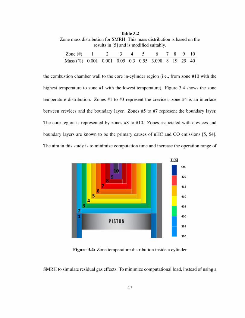
Table 3.2Zone mass distribution for SMRH. This mass distribution is based on the
results in [5] and is modified suitably.
Zone (#) 1 2 3 4 5 6 7 8 9 10Mass (%) 0.001 0.001 0.05 0.3 0.55 3.098 8 19 29 40
the combustion chamber wall to the core in-cylinder region (i.e., from zone #10 with the
highest temperature to zone #1 with the lowest temperature). Figure 3.4 shows the zone
temperature distribution. Zones #1 to #3 represent the crevices, zone #4 is an interface
between crevices and the boundary layer. Zones #5 to #7 represent the boundary layer.
The core region is represented by zones #8 to #10. Zones associated with crevices and
boundary layers are known to be the primary causes of uHC and CO emissions [5, 54].
The aim in this study is to minimize computation time and increase the operation range of
390
395
400
405
410
420
425
415
T (K)
Figure 3.4: Zone temperature distribution inside a cylinder
SMRH to simulate residual gas effects. To minimize computational load, instead of using a
47
CFD code, gas temperatures in the individual zones are calculated based on a linear relation
between the wall temperature (zone #1) and the core (zone #10) temperature using the Tivc
obtained from Step #1.
3.1.2.1 Multi zone modeling and heat transfer correlations
The purpose of Step #2 is to obtain initial combustion results which are used in the
next step of the sequential modeling process. Multi zone modeling carried out using
CHEMKIN R©−PRO uses the equations mentioned in this section. Equations (3.1) to (3.4)
from [55] describe the multi zone modeling approach followed in this thesis to determine
in-cylinder gas properties from IVC to EVO.
ρi dY i
kdt
= ω ikW
ik , f or i = 1, . . . ,Nzone (3.1)
Where, ρ is the zone density, superscript “i” and subscript “k” represent the zone and
species number respectively, while Yk, Wk and ωk represent the mass fraction, molecular
weight and molar production rate of the kth species, respectively. Calculation of zone
temperature is done using Equation (3.2).
ρiCi
vdT i
dt=−
kgas
∑k=1
ω ik Wk ui
k−Pi
V idV i
dt− hi
w (Ti−Tw)Ai
wV i , θ(t)> θt (3.2)
48
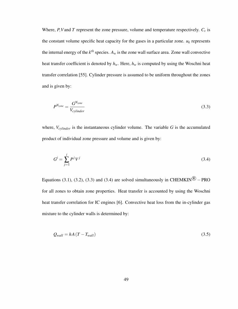
Where, P,V and T represent the zone pressure, volume and temperature respectively. Cv is
the constant volume specific heat capacity for the gases in a particular zone. uk represents
the internal energy of the kth species. Aw is the zone wall surface area. Zone wall convective
heat transfer coefficient is denoted by hw. Here, hw is computed by using the Woschni heat
transfer correlation [55]. Cylinder pressure is assumed to be uniform throughout the zones
and is given by:
PNzone =GNzone
Vcylinder(3.3)
where, Vcylinder is the instantaneous cylinder volume. The variable G is the accumulated
product of individual zone pressure and volume and is given by:
Gi =i
∑j=1
P j V j (3.4)
Equations (3.1), (3.2), (3.3) and (3.4) are solved simultaneously in CHEMKIN R©−PRO
for all zones to obtain zone properties. Heat transfer is accounted by using the Woschni
heat transfer correlation for IC engines [6]. Convective heat loss from the in-cylinder gas
mixture to the cylinder walls is determined by:
Qwall = hA(T −Twall) (3.5)
49
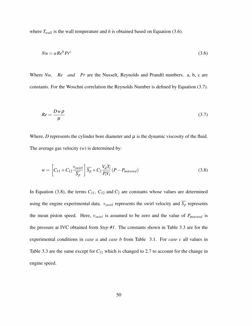
where Twall is the wall temperature and h is obtained based on Equation (3.6).
Nu = aReb Prc (3.6)
Where Nu, Re and Pr are the Nusselt, Reynolds and Prandtl numbers. a, b, c are
constants. For the Woschni correlation the Reynolds Number is defined by Equation (3.7).
Re =Dwρ
µ(3.7)
Where, D represents the cylinder bore diameter and µ is the dynamic viscosity of the fluid.
The average gas velocity (w) is determined by:
w =
[C11 +C12
vswirl
Sp
]Sp +C2
VdTi
PiVi(P−Pmotored) (3.8)
In Equation (3.8), the terms C11, C12 and C2 are constants whose values are determined
using the engine experimental data. vswirl represents the swirl velocity and Sp represents
the mean piston speed. Here, vswirl is assumed to be zero and the value of Pmotored is
the pressure at IVC obtained from Step #1. The constants shown in Table 3.3 are for the
experimental conditions in case a and case b from Table 3.1. For case c all values in
Table 3.3 are the same except for C11 which is changed to 2.7 to account for the change in
engine speed.
50
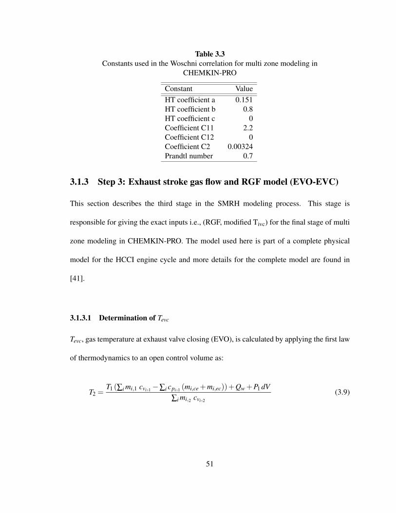
Table 3.3Constants used in the Woschni correlation for multi zone modeling in
CHEMKIN-PRO
Constant ValueHT coefficient a 0.151HT coefficient b 0.8HT coefficient c 0Coefficient C11 2.2Coefficient C12 0Coefficient C2 0.00324Prandtl number 0.7
3.1.3 Step 3: Exhaust stroke gas flow and RGF model (EVO-EVC)
This section describes the third stage in the SMRH modeling process. This stage is
responsible for giving the exact inputs i.e., (RGF, modified Tivc) for the final stage of multi
zone modeling in CHEMKIN-PRO. The model used here is part of a complete physical
model for the HCCI engine cycle and more details for the complete model are found in
[41].
3.1.3.1 Determination of Tevc
Tevc, gas temperature at exhaust valve closing (EVO), is calculated by applying the first law
of thermodynamics to an open control volume as:
T2 =T1 (∑i mi,1 cvi,1−∑i cpi,1 (mi,ce +mi,ec))+Qw +P1 dV
∑i mi,2 cvi,2
(3.9)
51
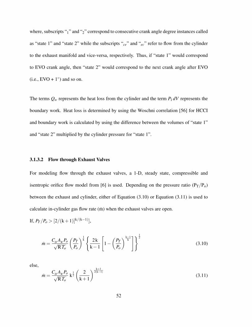
where, subscripts “1” and “2” correspond to consecutive crank angle degree instances called
as “state 1” and “state 2” while the subscripts “ce” and “ec” refer to flow from the cylinder
to the exhaust manifold and vice-versa, respectively. Thus, if “state 1” would correspond
to EVO crank angle, then “state 2” would correspond to the next crank angle after EVO
(i.e., EVO + 1◦) and so on.
The terms Qw represents the heat loss from the cylinder and the term P1 dV represents the
boundary work. Heat loss is determined by using the Woschni correlation [56] for HCCI
and boundary work is calculated by using the difference between the volumes of “state 1”
and “state 2” multiplied by the cylinder pressure for “state 1”.
3.1.3.2 Flow through Exhaust Valves
For modeling flow through the exhaust valves, a 1-D, steady state, compressible and
isentropic orifice flow model from [6] is used. Depending on the pressure ratio (PT/Po)
between the exhaust and cylinder, either of Equation (3.10) or Equation (3.11) is used to
calculate in-cylinder gas flow rate (m) when the exhaust valves are open.
If, PT/Po > [2/(k+1)]k/(k−1)],
m =CD AR Po√
RTo
(PT
Po
) 1k{
2kk−1
[1−(
PT
Po
) k−1k]} 1
2
(3.10)
else,
m =CD AR Po√
RTok
12
(2
k+1
) k+12(k−1)
(3.11)
52
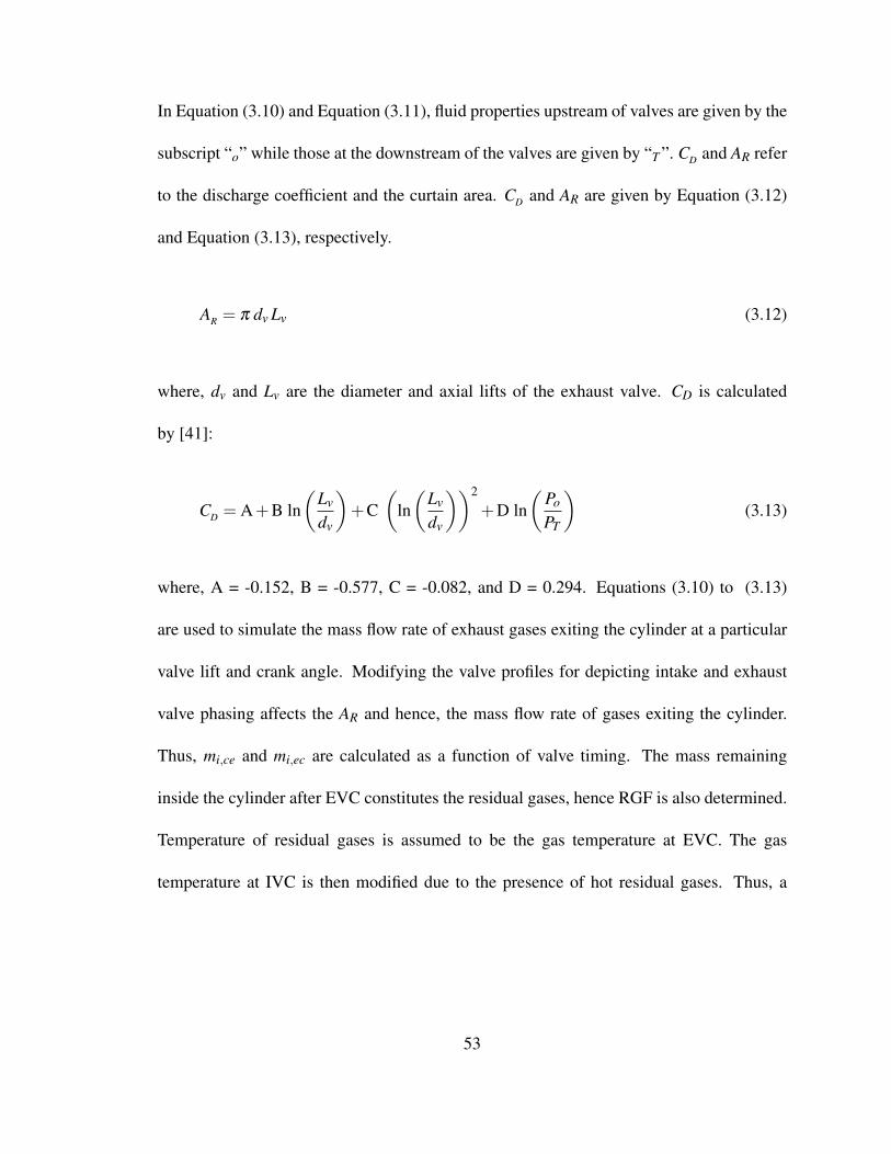
In Equation (3.10) and Equation (3.11), fluid properties upstream of valves are given by the
subscript “o” while those at the downstream of the valves are given by “T ”. CD and AR refer
to the discharge coefficient and the curtain area. CD and AR are given by Equation (3.12)
and Equation (3.13), respectively.
AR = π dv Lv (3.12)
where, dv and Lv are the diameter and axial lifts of the exhaust valve. CD is calculated
by [41]:
CD = A+B ln(
Lv
dv
)+C
(ln(
Lv
dv
))2
+D ln(
Po
PT
)(3.13)
where, A = -0.152, B = -0.577, C = -0.082, and D = 0.294. Equations (3.10) to (3.13)
are used to simulate the mass flow rate of exhaust gases exiting the cylinder at a particular
valve lift and crank angle. Modifying the valve profiles for depicting intake and exhaust
valve phasing affects the AR and hence, the mass flow rate of gases exiting the cylinder.
Thus, mi,ce and mi,ec are calculated as a function of valve timing. The mass remaining
inside the cylinder after EVC constitutes the residual gases, hence RGF is also determined.
Temperature of residual gases is assumed to be the gas temperature at EVC. The gas
temperature at IVC is then modified due to the presence of hot residual gases. Thus, a
53
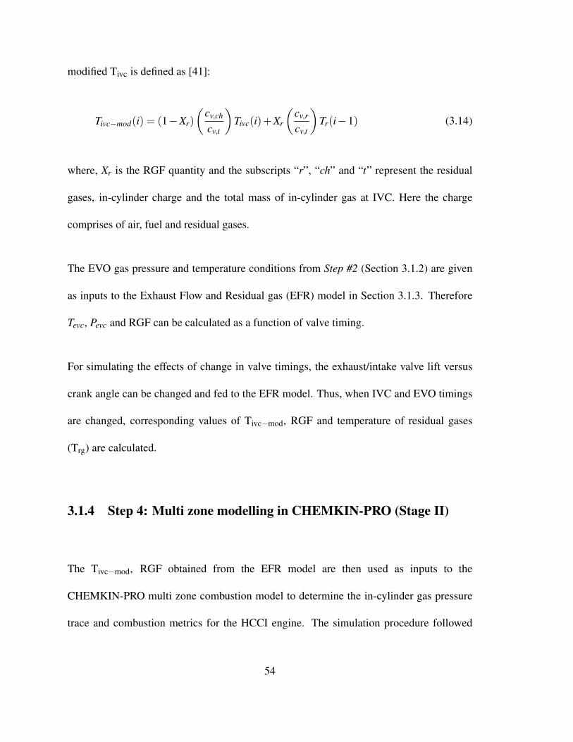
modified Tivc is defined as [41]:
Tivc−mod(i) = (1−Xr)
(cv,ch
cv,t
)Tivc(i)+Xr
(cv,r
cv,t
)Tr(i−1) (3.14)
where, Xr is the RGF quantity and the subscripts “r”, “ch” and “t” represent the residual
gases, in-cylinder charge and the total mass of in-cylinder gas at IVC. Here the charge
comprises of air, fuel and residual gases.
The EVO gas pressure and temperature conditions from Step #2 (Section 3.1.2) are given
as inputs to the Exhaust Flow and Residual gas (EFR) model in Section 3.1.3. Therefore
Tevc, Pevc and RGF can be calculated as a function of valve timing.
For simulating the effects of change in valve timings, the exhaust/intake valve lift versus
crank angle can be changed and fed to the EFR model. Thus, when IVC and EVO timings
are changed, corresponding values of Tivc−mod, RGF and temperature of residual gases
(Trg) are calculated.
3.1.4 Step 4: Multi zone modelling in CHEMKIN-PRO (Stage II)
The Tivc−mod, RGF obtained from the EFR model are then used as inputs to the
CHEMKIN-PRO multi zone combustion model to determine the in-cylinder gas pressure
trace and combustion metrics for the HCCI engine. The simulation procedure followed
54
during this step is similar to Step #2 of SMRH except that effects of residual gases
are accounted for during this step. The residual gases are considered to be comprised
of CO2, H2O and N2. The mole fractions are determined based on general combustion
equation for n-heptane combustion:
βC7H16C7H16 + βO2 (O2 +3.76N2) +
RG(βO2,RG O2 + βN2,RG N2 + βCO2,RG CO2 + βH2O,RG H2O) −→ . . .
. . .−→ βO2,RG O2 + βN2,RG N2 + βCO2,RG CO2 + βH2O,RG H2O +
RG(βO2,RG O2 + βN2,RG N2 + βCO2,RG CO2 + βH2O,RG H2O) (3.15)
where RG subscripts denote for residual gases. On substituting values for mole fractions
for case a in Table 3.1, Equation (3.15) is written as:
1 C7H16 + 24.44 (O2 +3.76N2) +
RG(13.44 O2 + 91.89 N2 + 7 CO2 + 8 H2O) −→ . . .
. . .−→ 13.44 O2 + 91.89 N2 + 7 CO2 + 8 H2O +
RG(13.44 O2 + 91.89 N2 + 7 CO2 + 8 H2O) (3.16)
The results obtained from this final step are compared with experimental data from a
Ricardo single cylinder HCCI engine [4]. The experimental validation results of SMRH
will be discussed in Section 3.2.
55
3.2 Results and Discussion
3.2.1 Model Validation
Given the number of assumptions done in developing the SMRH, it is critical to
experimentally validate the SMRH before moving on to the discussion of HCCI combustion
results. Experimental data is taken from [4] for a single cylinder Ricardo Mark III HCCI
engine with specifications shown in Table 3.4. Details of the engine experimental setup
are found in [41]. Uncertainty analysis of the experimental data obtained from the Ricardo
engine can be found in [57].
This section presents the results for in-cylinder gas pressure, crank angle for 10 percent
mass of fuel burned (CA10), crank angle for 50 percent mass of fuel burned (CA50),
burn duration (BD), indicated mean effective pressure (IMEP), indicated thermal efficiency
(ηth,i) and CO emissions and their comparison with experimental data for the HCCI
operating conditions previously listed in Table 3.1. Validations for in-cylinder gas pressure
are shown in Figures 3.5, 3.6 and 3.7, while quantitative metrics are compared with the
experimental values in Table 3.5.
From Figures 3.5, 3.6 and 3.7, it is observed that the simulation pressure traces are
in good agreement with those from the experiments. In addition, from Table 3.5 the
56
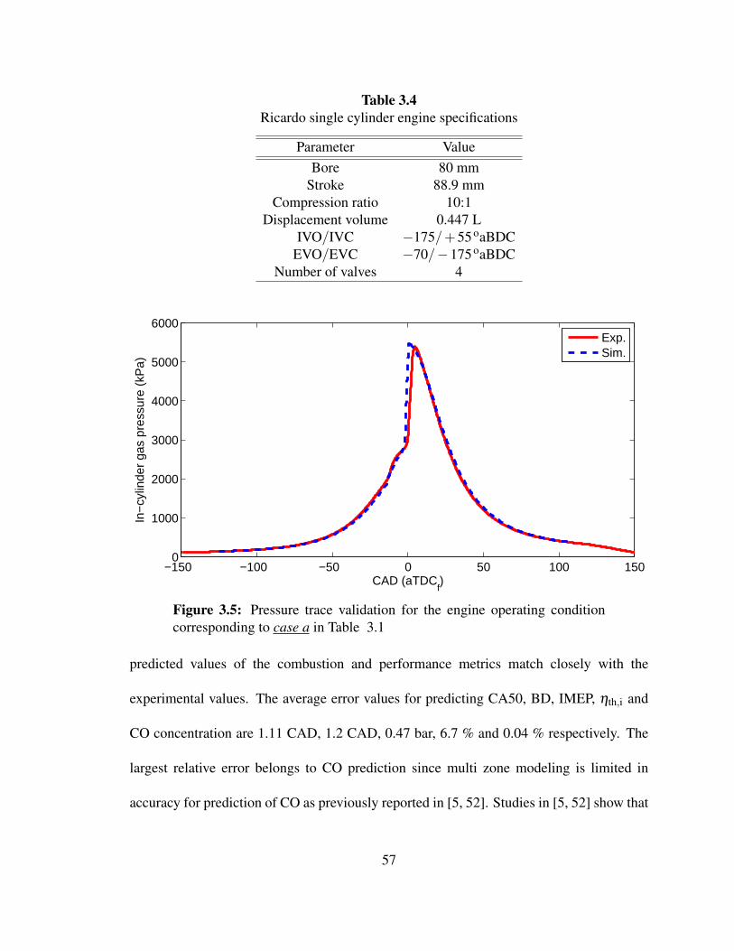
Table 3.4Ricardo single cylinder engine specifications
Parameter ValueBore 80 mm
Stroke 88.9 mmCompression ratio 10:1
Displacement volume 0.447 LIVO/IVC −175/+55 oaBDC
EVO/EVC −70/−175 oaBDCNumber of valves 4
−150 −100 −50 0 50 100 1500
1000
2000
3000
4000
5000
6000
CAD (aTDCf)
In−
cylin
der
gas
pres
sure
(kP
a)
Exp.Sim.
Figure 3.5: Pressure trace validation for the engine operating conditioncorresponding to case a in Table 3.1
predicted values of the combustion and performance metrics match closely with the
experimental values. The average error values for predicting CA50, BD, IMEP, ηth,i and
CO concentration are 1.11 CAD, 1.2 CAD, 0.47 bar, 6.7 % and 0.04 % respectively. The
largest relative error belongs to CO prediction since multi zone modeling is limited in
accuracy for prediction of CO as previously reported in [5, 52]. Studies in [5, 52] show that
57
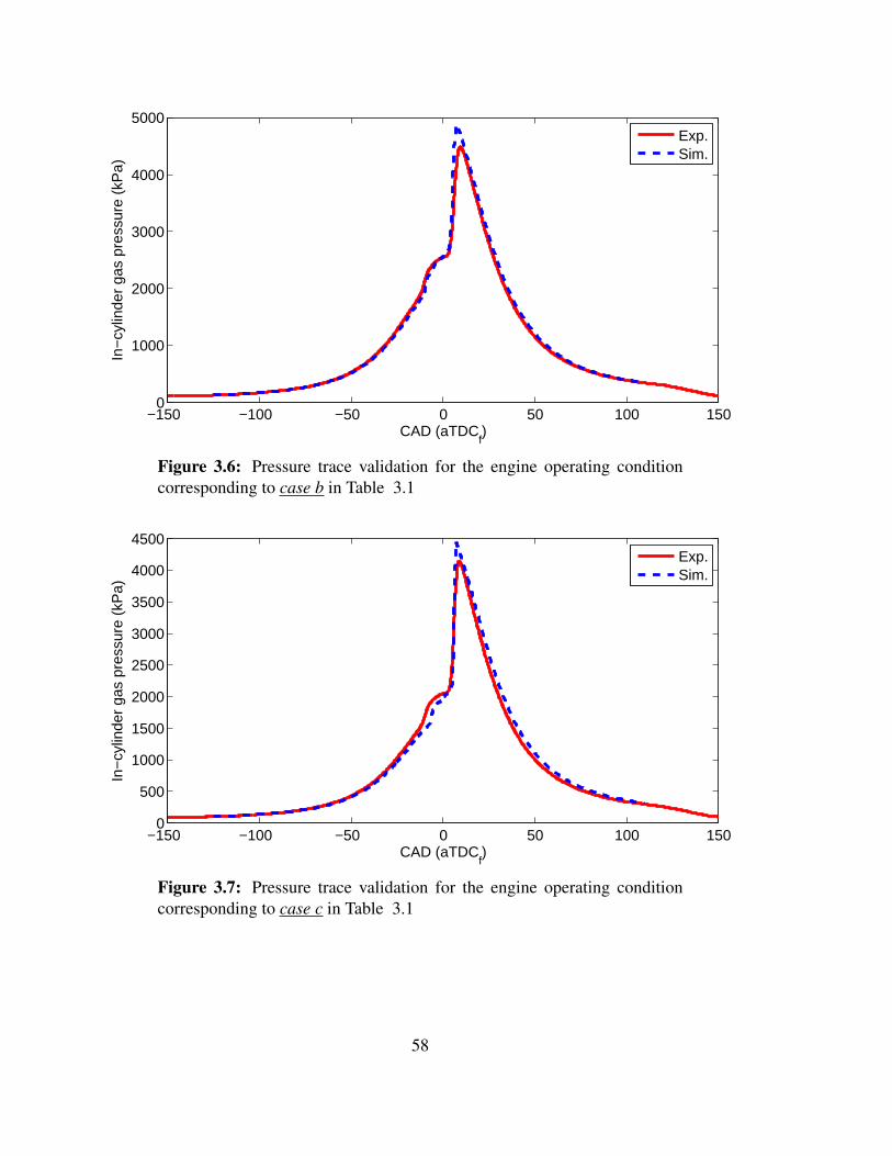
−150 −100 −50 0 50 100 1500
1000
2000
3000
4000
5000
CAD (aTDCf)
In−
cylin
der
gas
pres
sure
(kP
a)
Exp.Sim.
Figure 3.6: Pressure trace validation for the engine operating conditioncorresponding to case b in Table 3.1
−150 −100 −50 0 50 100 1500
500
1000
1500
2000
2500
3000
3500
4000
4500
CAD (aTDCf)
In−
cylin
der
gas
pres
sure
(kP
a)
Exp.Sim.
Figure 3.7: Pressure trace validation for the engine operating conditioncorresponding to case c in Table 3.1
58
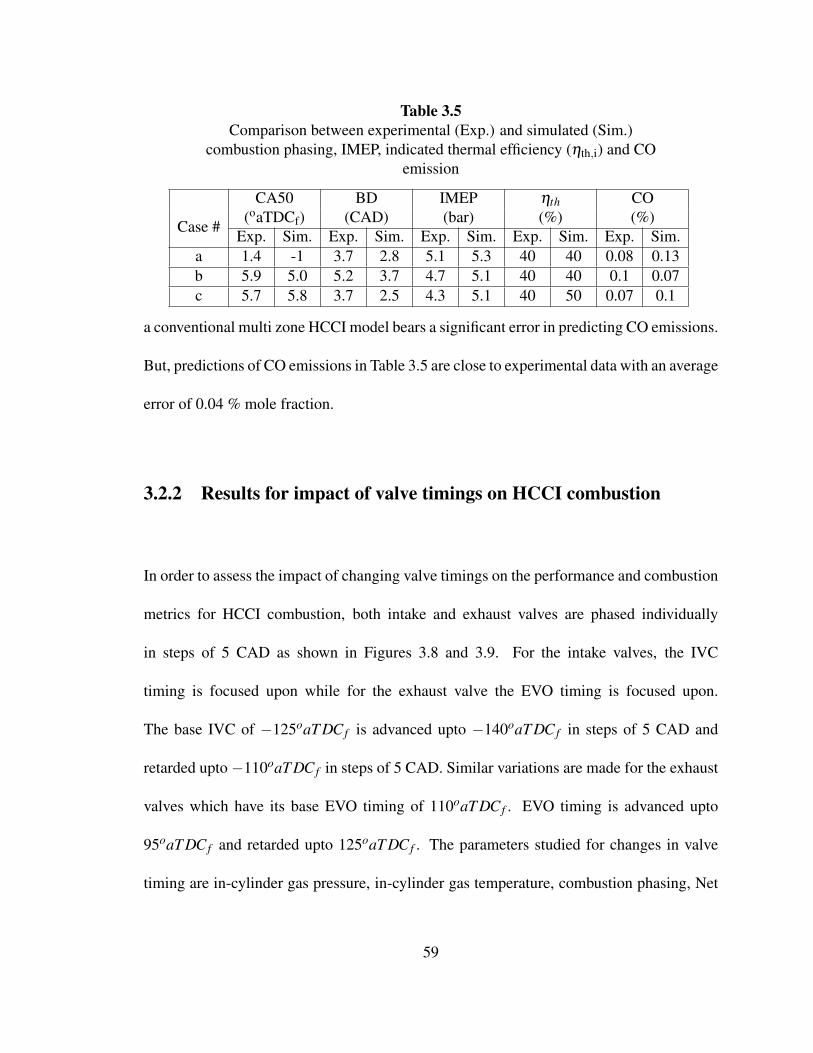
Table 3.5Comparison between experimental (Exp.) and simulated (Sim.)
combustion phasing, IMEP, indicated thermal efficiency (ηth,i) and COemission
Case #
CA50 BD IMEP ηth CO(oaTDCf) (CAD) (bar) (%) (%)
Exp. Sim. Exp. Sim. Exp. Sim. Exp. Sim. Exp. Sim.a 1.4 -1 3.7 2.8 5.1 5.3 40 40 0.08 0.13b 5.9 5.0 5.2 3.7 4.7 5.1 40 40 0.1 0.07c 5.7 5.8 3.7 2.5 4.3 5.1 40 50 0.07 0.1
a conventional multi zone HCCI model bears a significant error in predicting CO emissions.
But, predictions of CO emissions in Table 3.5 are close to experimental data with an average
error of 0.04 % mole fraction.
3.2.2 Results for impact of valve timings on HCCI combustion
In order to assess the impact of changing valve timings on the performance and combustion
metrics for HCCI combustion, both intake and exhaust valves are phased individually
in steps of 5 CAD as shown in Figures 3.8 and 3.9. For the intake valves, the IVC
timing is focused upon while for the exhaust valve the EVO timing is focused upon.
The base IVC of −125oaT DC f is advanced upto −140oaT DC f in steps of 5 CAD and
retarded upto −110oaT DC f in steps of 5 CAD. Similar variations are made for the exhaust
valves which have its base EVO timing of 110oaT DC f . EVO timing is advanced upto
95oaT DC f and retarded upto 125oaT DC f . The parameters studied for changes in valve
timing are in-cylinder gas pressure, in-cylinder gas temperature, combustion phasing, Net
59
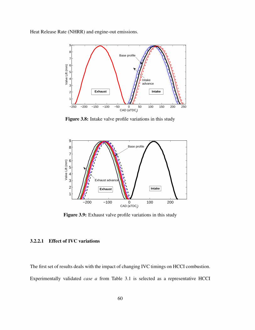
Heat Release Rate (NHRR) and engine-out emissions.
−250 −200 −150 −100 −50 0 50 100 150 200 250
1
2
3
4
5
6
7
8
9
CAD (aTDCf)
Val
ve L
ift (
mm
)
Intakeadvance
Base profile
Exhaust Intake
Figure 3.8: Intake valve profile variations in this study
−200 −100 0 100 200
1
2
3
4
5
6
7
8
9
CAD (aTDCf)
Val
ve L
ift (
mm
)
Exhaust advance
Base profile
IntakeExhaust
Figure 3.9: Exhaust valve profile variations in this study
3.2.2.1 Effect of IVC variations
The first set of results deals with the impact of changing IVC timings on HCCI combustion.
Experimentally validated case a from Table 3.1 is selected as a representative HCCI
60
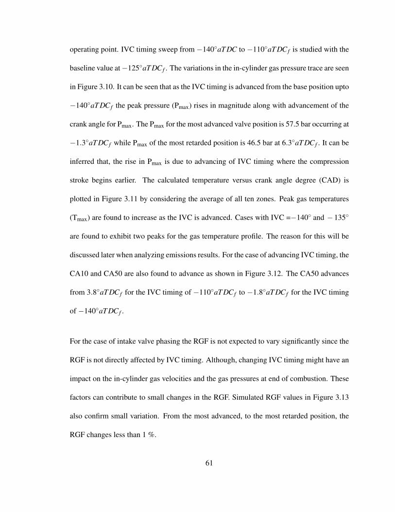
operating point. IVC timing sweep from −140◦aT DC to −110◦aT DC f is studied with the
baseline value at−125◦aT DC f . The variations in the in-cylinder gas pressure trace are seen
in Figure 3.10. It can be seen that as the IVC timing is advanced from the base position upto
−140◦aT DC f the peak pressure (Pmax) rises in magnitude along with advancement of the
crank angle for Pmax. The Pmax for the most advanced valve position is 57.5 bar occurring at
−1.3◦aT DC f while Pmax of the most retarded position is 46.5 bar at 6.3◦aT DC f . It can be
inferred that, the rise in Pmax is due to advancing of IVC timing where the compression
stroke begins earlier. The calculated temperature versus crank angle degree (CAD) is
plotted in Figure 3.11 by considering the average of all ten zones. Peak gas temperatures
(Tmax) are found to increase as the IVC is advanced. Cases with IVC =−140◦ and −135◦
are found to exhibit two peaks for the gas temperature profile. The reason for this will be
discussed later when analyzing emissions results. For the case of advancing IVC timing, the
CA10 and CA50 are also found to advance as shown in Figure 3.12. The CA50 advances
from 3.8◦aT DC f for the IVC timing of −110◦aT DC f to −1.8◦aT DC f for the IVC timing
of −140◦aT DC f .
For the case of intake valve phasing the RGF is not expected to vary significantly since the
RGF is not directly affected by IVC timing. Although, changing IVC timing might have an
impact on the in-cylinder gas velocities and the gas pressures at end of combustion. These
factors can contribute to small changes in the RGF. Simulated RGF values in Figure 3.13
also confirm small variation. From the most advanced, to the most retarded position, the
RGF changes less than 1 %.
61
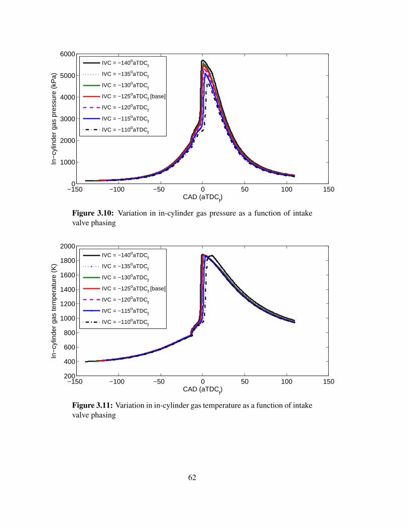
−150 −100 −50 0 50 100 1500
1000
2000
3000
4000
5000
6000
CAD (aTDCf)
In−
cylin
der
gas
pres
sure
(kP
a)
IVC = −140oaTDCf
IVC = −135oaTDCf
IVC = −130oaTDCf
IVC = −125oaTDCf [base]
IVC = −120oaTDCf
IVC = −115oaTDCf
IVC = −110oaTDCf
Figure 3.10: Variation in in-cylinder gas pressure as a function of intakevalve phasing
−150 −100 −50 0 50 100 150200
400
600
800
1000
1200
1400
1600
1800
2000
CAD (aTDCf)
In−
cylin
der
gas
tem
pera
ture
(K
)
IVC = −140oaTDCf
IVC = −135oaTDCf
IVC = −130oaTDCf
IVC = −125oaTDCf [base]
IVC = −120oaTDCf
IVC = −115oaTDCf
IVC = −110oaTDCf
Figure 3.11: Variation in in-cylinder gas temperature as a function of intakevalve phasing
62
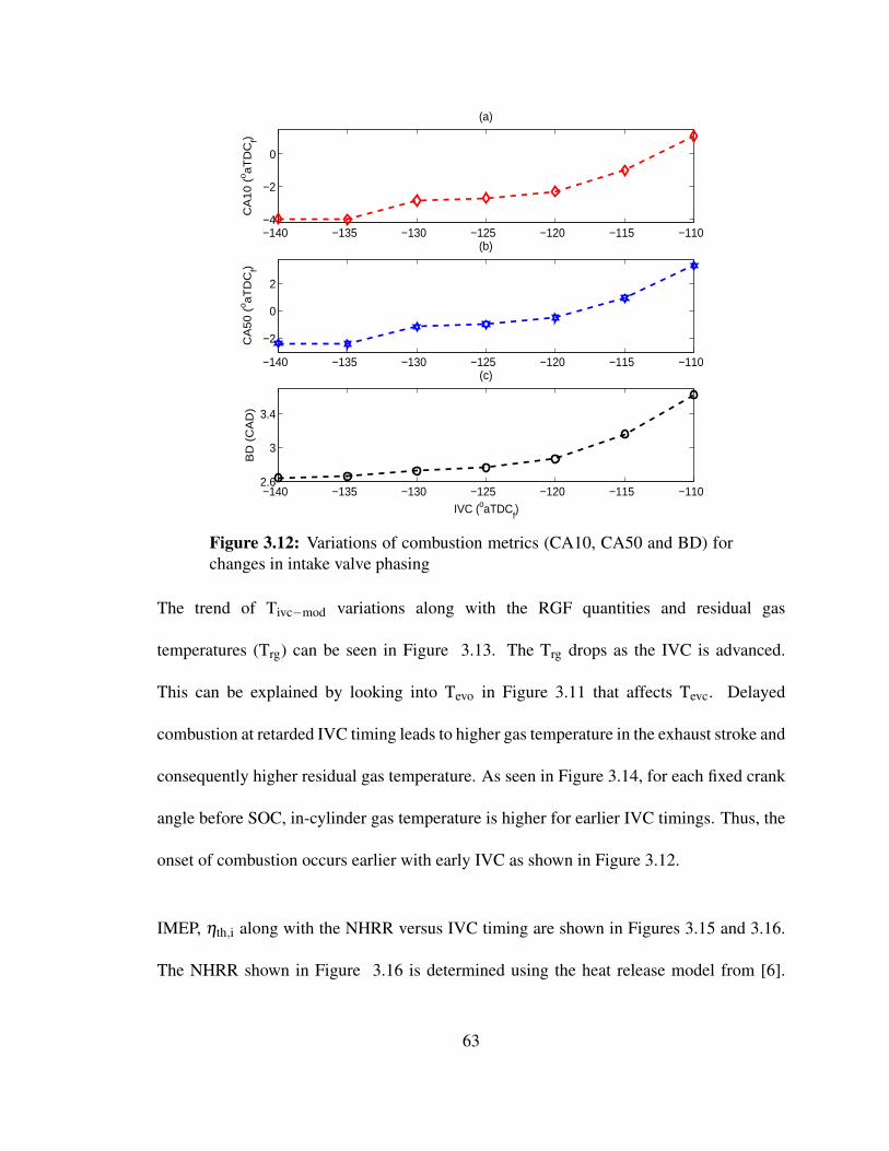
−140 −135 −130 −125 −120 −115 −110−4
−2
0
(a)
CA
10
(o a
TD
Cf)
−140 −135 −130 −125 −120 −115 −110
−2
0
2
(b)C
A5
0 (
o aT
DC
f)
−140 −135 −130 −125 −120 −115 −1102.6
3
3.4
(c)
IVC (oaTDCf)
BD
(C
AD
)
Figure 3.12: Variations of combustion metrics (CA10, CA50 and BD) forchanges in intake valve phasing
The trend of Tivc−mod variations along with the RGF quantities and residual gas
temperatures (Trg) can be seen in Figure 3.13. The Trg drops as the IVC is advanced.
This can be explained by looking into Tevo in Figure 3.11 that affects Tevc. Delayed
combustion at retarded IVC timing leads to higher gas temperature in the exhaust stroke and
consequently higher residual gas temperature. As seen in Figure 3.14, for each fixed crank
angle before SOC, in-cylinder gas temperature is higher for earlier IVC timings. Thus, the
onset of combustion occurs earlier with early IVC as shown in Figure 3.12.
IMEP, ηth,i along with the NHRR versus IVC timing are shown in Figures 3.15 and 3.16.
The NHRR shown in Figure 3.16 is determined using the heat release model from [6].
63
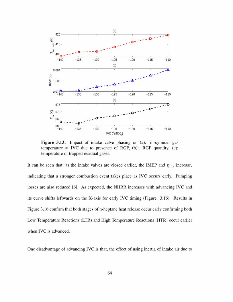
−140 −135 −130 −125 −120 −115 −110
400
410
420(a)
Tiv
c−m
od (
K)
−140 −135 −130 −125 −120 −115 −1100.076
0.08
0.084
(b)
RG
F (
−)
−140 −135 −130 −125 −120 −115 −110660
665
670
675
(c)
IVC (oaTDCf)
Trg
(K
)
Figure 3.13: Impact of intake valve phasing on (a): in-cylinder gastemperature at IVC due to presence of RGF, (b): RGF quantity, (c):temperature of trapped residual gases.
It can be seen that, as the intake valves are closed earlier, the IMEP and ηth,i increase,
indicating that a stronger combustion event takes place as IVC occurs early. Pumping
losses are also reduced [6]. As expected, the NHRR increases with advancing IVC and
its curve shifts leftwards on the X-axis for early IVC timing (Figure 3.16). Results in
Figure 3.16 confirm that both stages of n-heptane heat release occur early confirming both
Low Temperature Reactions (LTR) and High Temperature Reactions (HTR) occur earlier
when IVC is advanced.
One disadvantage of advancing IVC is that, the effect of using inertia of intake air due to
64
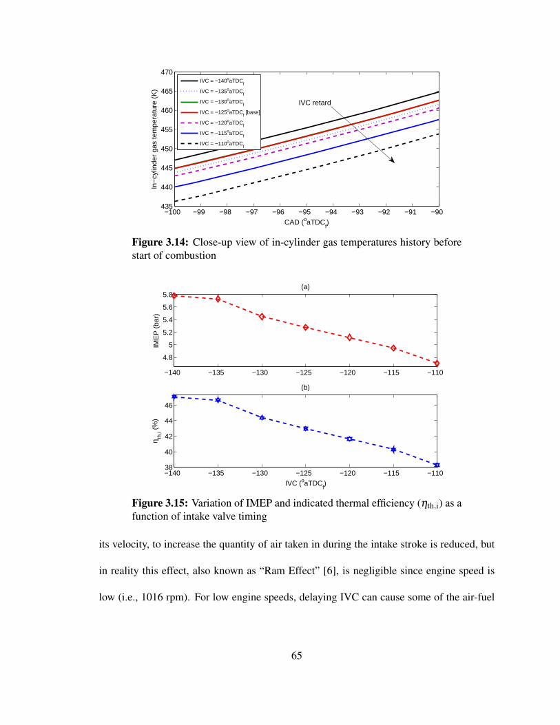
−100 −99 −98 −97 −96 −95 −94 −93 −92 −91 −90435
440
445
450
455
460
465
470
CAD (oaTDCf)
In−
cylin
der
gas
tem
pera
ture
(K
)
IVC = −140oaTDC
f
IVC = −135oaTDCf
IVC = −130oaTDCf
IVC = −125oaTDCf [base]
IVC = −120oaTDCf
IVC = −115oaTDCf
IVC = −110oaTDCf
IVC retard
Figure 3.14: Close-up view of in-cylinder gas temperatures history beforestart of combustion
−140 −135 −130 −125 −120 −115 −110
4.8
5
5.2
5.4
5.6
5.8(a)
IME
P (
bar)
−140 −135 −130 −125 −120 −115 −11038
40
42
44
46
(b)
IVC (oaTDCf)
η th,i (
%)
Figure 3.15: Variation of IMEP and indicated thermal efficiency (ηth,i) as afunction of intake valve timing
its velocity, to increase the quantity of air taken in during the intake stroke is reduced, but
in reality this effect, also known as “Ram Effect” [6], is negligible since engine speed is
low (i.e., 1016 rpm). For low engine speeds, delaying IVC can cause some of the air-fuel
65
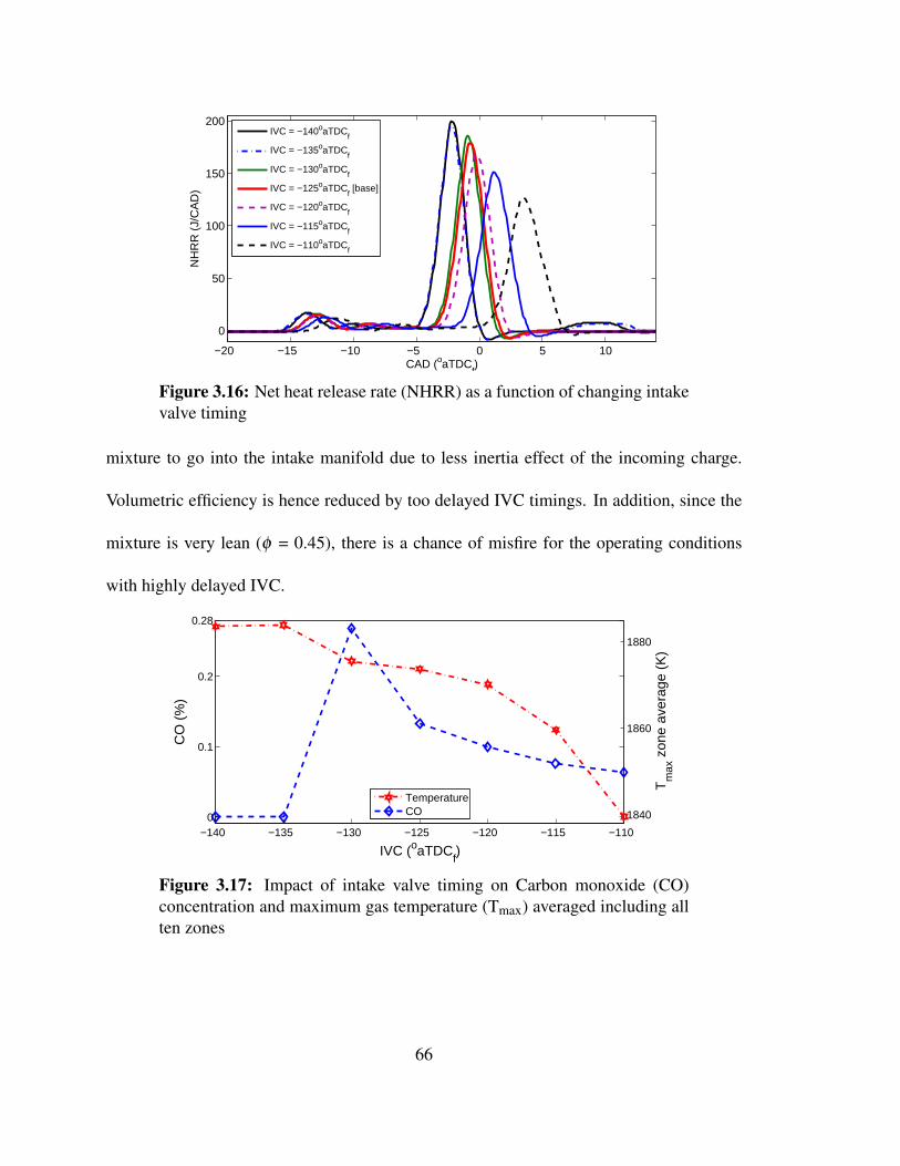
−20 −15 −10 −5 0 5 10
0
50
100
150
200
CAD (oaTDCf)
NH
RR
(J/
CA
D)
IVC = −140oaTDCf
IVC = −135oaTDCf
IVC = −130oaTDCf
IVC = −125oaTDCf [base]
IVC = −120oaTDCf
IVC = −115oaTDCf
IVC = −110oaTDCf
Figure 3.16: Net heat release rate (NHRR) as a function of changing intakevalve timing
mixture to go into the intake manifold due to less inertia effect of the incoming charge.
Volumetric efficiency is hence reduced by too delayed IVC timings. In addition, since the
mixture is very lean (φ = 0.45), there is a chance of misfire for the operating conditions
with highly delayed IVC.
0
0.1
0.2
0.28
CO
(%
)
−140 −135 −130 −125 −120 −115 −110
1840
1860
1880
IVC (oaTDCf)
Tm
ax z
one
aver
age
(K)
TemperatureCO
Figure 3.17: Impact of intake valve timing on Carbon monoxide (CO)concentration and maximum gas temperature (Tmax) averaged including allten zones
66
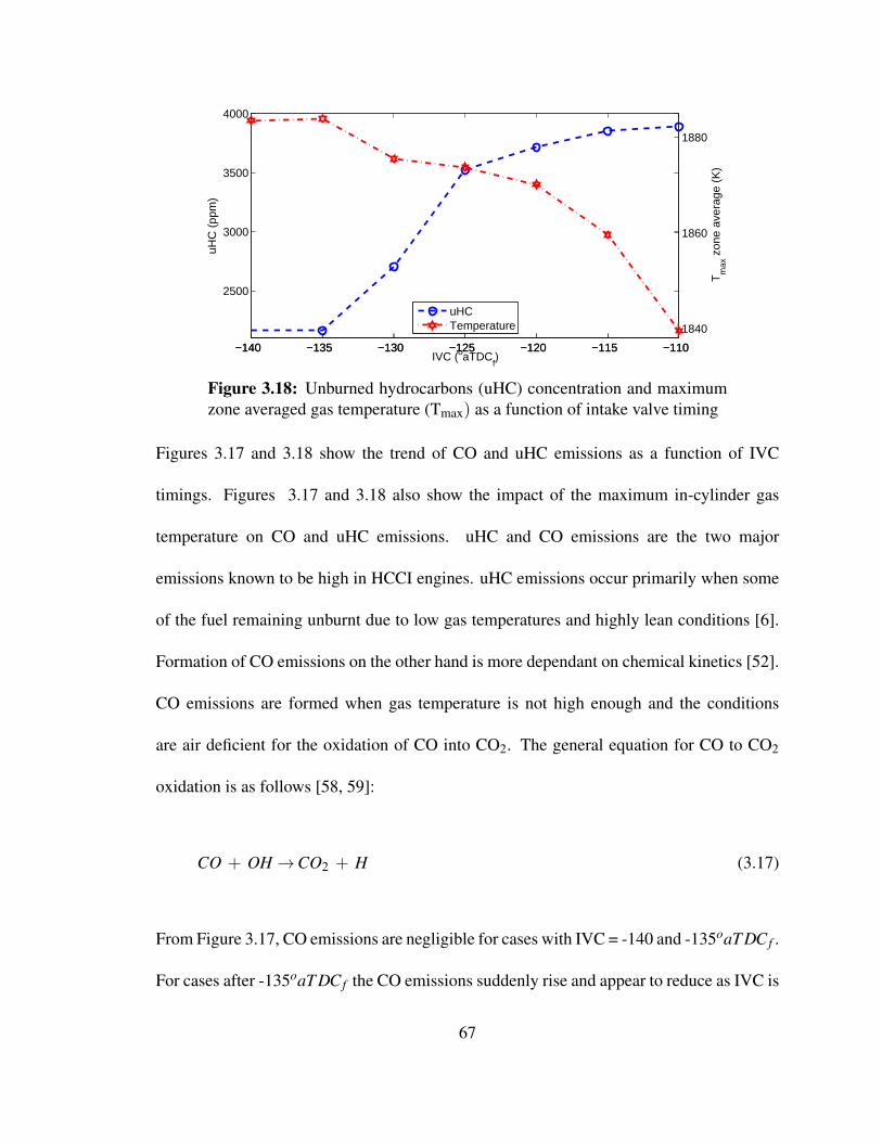
−140 −135 −130 −125 −120 −115 −110
2500
3000
3500
4000
IVC (oaTDCf)
uHC
(pp
m)
−140 −135 −130 −125 −120 −115 −110
1840
1860
1880
Tm
ax z
one
aver
age
(K)
uHCTemperature
Figure 3.18: Unburned hydrocarbons (uHC) concentration and maximumzone averaged gas temperature (Tmax) as a function of intake valve timing
Figures 3.17 and 3.18 show the trend of CO and uHC emissions as a function of IVC
timings. Figures 3.17 and 3.18 also show the impact of the maximum in-cylinder gas
temperature on CO and uHC emissions. uHC and CO emissions are the two major
emissions known to be high in HCCI engines. uHC emissions occur primarily when some
of the fuel remaining unburnt due to low gas temperatures and highly lean conditions [6].
Formation of CO emissions on the other hand is more dependant on chemical kinetics [52].
CO emissions are formed when gas temperature is not high enough and the conditions
are air deficient for the oxidation of CO into CO2. The general equation for CO to CO2
oxidation is as follows [58, 59]:
CO + OH→CO2 + H (3.17)
From Figure 3.17, CO emissions are negligible for cases with IVC = -140 and -135oaT DC f .
For cases after -135oaT DC f the CO emissions suddenly rise and appear to reduce as IVC is
67
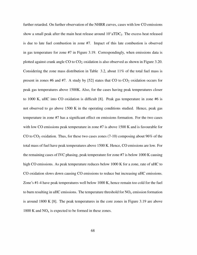
further retarded. On further observation of the NHRR curves, cases with low CO emissions
show a small peak after the main heat release around 10◦aTDCf. The excess heat released
is due to late fuel combustion in zone #7. Impact of this late combustion is observed
in gas temperature for zone #7 in Figure 3.19. Correspondingly, when emissions data is
plotted against crank angle CO to CO2 oxidation is also observed as shown in Figure 3.20.
Considering the zone mass distribution in Table 3.2, about 11% of the total fuel mass is
present in zones #6 and #7. A study by [52] states that CO to CO2 oxidation occurs for
peak gas temperatures above 1500K. Also, for the cases having peak temperatures closer
to 1000 K, uHC into CO oxidation is difficult [8]. Peak gas temperature in zone #6 is
not observed to go above 1500 K in the operating conditions studied. Hence, peak gas
temperature in zone #7 has a significant effect on emissions formation. For the two cases
with low CO emissions peak temperature in zone #7 is above 1500 K and is favourable for
CO to CO2 oxidation. Thus, for these two cases zones (7-10) composing about 96% of the
total mass of fuel have peak temperatures above 1500 K. Hence, CO emissions are low. For
the remaining cases of IVC phasing, peak temperature for zone #7 is below 1000 K causing
high CO emissions. As peak temperature reduces below 1000 K for a zone, rate of uHC to
CO oxidation slows down causing CO emissions to reduce but increasing uHC emissions.
Zone’s #1-4 have peak temperatures well below 1000 K, hence remain too cold for the fuel
to burn resulting in uHC emissions. The temperature threshold for NOx emission formation
is around 1800 K [8]. The peak temperatures in the core zones in Figure 3.19 are above
1800 K and NOx is expected to be formed in these zones.
68
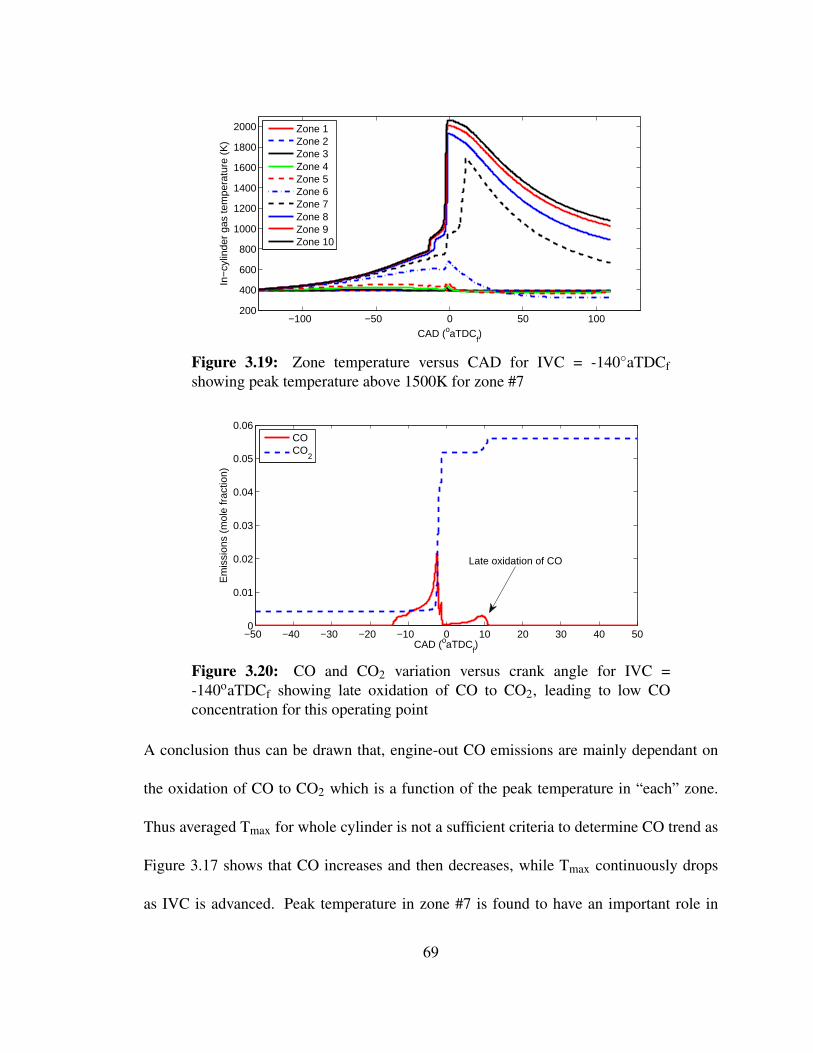
−100 −50 0 50 100200
400
600
800
1000
1200
1400
1600
1800
2000
CAD (oaTDCf)
In−
cylin
der
gas
tem
pera
ture
(K
)
Zone 1Zone 2Zone 3Zone 4Zone 5Zone 6Zone 7Zone 8Zone 9Zone 10
Figure 3.19: Zone temperature versus CAD for IVC = -140◦aTDCfshowing peak temperature above 1500K for zone #7
−50 −40 −30 −20 −10 0 10 20 30 40 500
0.01
0.02
0.03
0.04
0.05
0.06
CAD (oaTDCf)
Em
issi
ons
(mol
e fr
actio
n)
COCO
2
Late oxidation of CO
Figure 3.20: CO and CO2 variation versus crank angle for IVC =-140oaTDCf showing late oxidation of CO to CO2, leading to low COconcentration for this operating point
A conclusion thus can be drawn that, engine-out CO emissions are mainly dependant on
the oxidation of CO to CO2 which is a function of the peak temperature in “each” zone.
Thus averaged Tmax for whole cylinder is not a sufficient criteria to determine CO trend as
Figure 3.17 shows that CO increases and then decreases, while Tmax continuously drops
as IVC is advanced. Peak temperature in zone #7 is found to have an important role in
69

formation of CO emissions.
uHC emissions are primarily caused due to incomplete combustion and quenching effects
due to low wall temperatures. The trend for uHC emissions observed is found to be
reducing as the peak temperature reduces (Figure 3.18). Further observation is that uHC
emissions increase with an increase in BD (Figure 3.12). This can be because mixtures
with slow burning rate (i.e., longer BD) have more time for heat loss during the expansion
stroke and are hence favourable towards the formation of uHC emissions. The uHC
emission observed in this study is a mixture of C-7 molecules from unburnt fuel in zones
#1 to 6 and C-1 and other low carbon molecules from partial burning of fuel in zones #7 to
10.
3.2.2.2 Effect of EVO variations on HCCI combustion
Similar to the IVC variations carried out in Section 3.2.2.1, the exhaust valve timings are
also varied to assess their impact on HCCI combustion. The graphical representation of lift
versus CAD for the exhaust valve was previously shown in Figure 3.9. For the baseline
condition, the exhaust valve opens at 110◦aT DC f and is advanced upto 95◦aT DC f and is
retarded until 125◦aT DC f in steps of 5 CAD. Combustion and performance metrics from
the resulting EVO sweeps are analysed and presented in this section.
Figures 3.21 and 3.22 show the variations of in-cylinder gas pressure and temperature
70
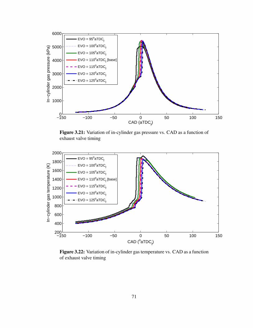
−150 −100 −50 0 50 100 1500
1000
2000
3000
4000
5000
6000
CAD (aTDCf)
In−
cylin
der
gas
pres
sure
(kP
a)
EVO = 95oaTDCf
EVO = 100oaTDCf
EVO = 105oaTDCf
EVO = 110oaTDCf [base]
EVO = 115oaTDCf
EVO = 120oaTDCf
EVO = 125oaTDCf
Figure 3.21: Variation of in-cylinder gas pressure vs. CAD as a function ofexhaust valve timing
−150 −100 −50 0 50 100 150200
400
600
800
1000
1200
1400
1600
1800
2000
CAD (oaTDCf)
In−
cylin
der
gas
tem
pera
ture
(K
)
EVO = 95oaTDCf
EVO = 100oaTDCf
EVO = 105oaTDCf
EVO = 110oaTDCf [base]
EVO = 115oaTDCf
EVO = 120oaTDCf
EVO = 125oaTDCf
Figure 3.22: Variation of in-cylinder gas temperature vs. CAD as a functionof exhaust valve timing
71

when EVO timing is varied. It can be seen that as the EVO timing is advanced from
125o to 95oaT DC f , Pmax rises upto the baseline case and then reduces till the most advanced
case. In-addition, the peak in-cylinder gas temperature (Tmax) increases with advancing
EVO. Another observation in Figure 3.22 is that there are two peaks in the gas temperature
for the three most advanced EVO (i.e., EVO = 95◦, 100◦, 105◦ aTDCf). This means that
after the main combustion event some of the zones in the boundary layer are combusting,
resulting in the second peak in-cylinder gas temperature. As previously discussed in
Section 3.2.2.1, fuel burning in zone #7 is found to cause this phenomenon.
95 100 105 110 115 120 125−10
−5
0
(a)
CA
10
(oa
TD
Cf)
95 100 105 110 115 120 125−8
−4
0
4(b)
CA
50
(oa
TD
Cf)
95 100 105 110 115 120 1252.5
3
3.5
(c)
EVO (oaTDCf)
BD
(C
AD
)
Figure 3.23: Effect of phasing exhaust valve timing on combustion metricsincluding CA10, CA50 and BD
Figures 3.23 and 3.24, show the trend of combustion metrics for changes in EVO timing,
72
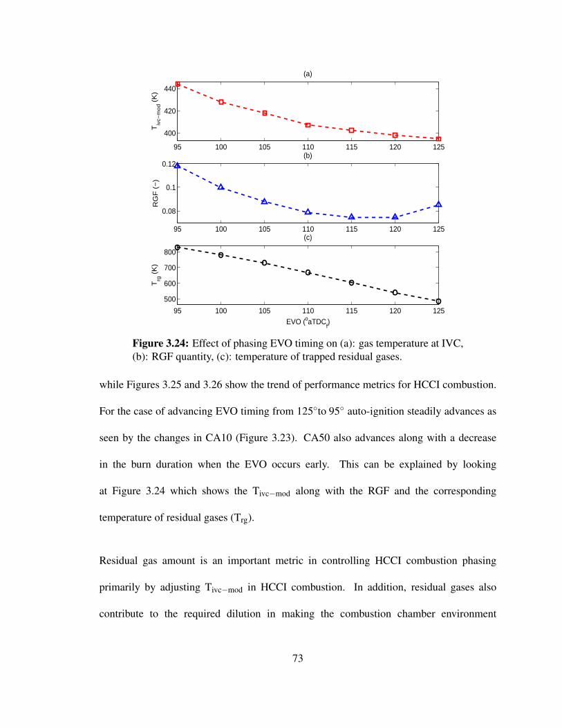
95 100 105 110 115 120 125
400
420
440
(a)
Tiv
c−m
od (
K)
95 100 105 110 115 120 125
0.08
0.1
0.12(b)
RG
F (
−)
95 100 105 110 115 120 125
500
600
700
800
(c)
EVO (oaTDCf)
Trg
(K
)
Figure 3.24: Effect of phasing EVO timing on (a): gas temperature at IVC,(b): RGF quantity, (c): temperature of trapped residual gases.
while Figures 3.25 and 3.26 show the trend of performance metrics for HCCI combustion.
For the case of advancing EVO timing from 125◦to 95◦ auto-ignition steadily advances as
seen by the changes in CA10 (Figure 3.23). CA50 also advances along with a decrease
in the burn duration when the EVO occurs early. This can be explained by looking
at Figure 3.24 which shows the Tivc−mod along with the RGF and the corresponding
temperature of residual gases (Trg).
Residual gas amount is an important metric in controlling HCCI combustion phasing
primarily by adjusting Tivc−mod in HCCI combustion. In addition, residual gases also
contribute to the required dilution in making the combustion chamber environment
73
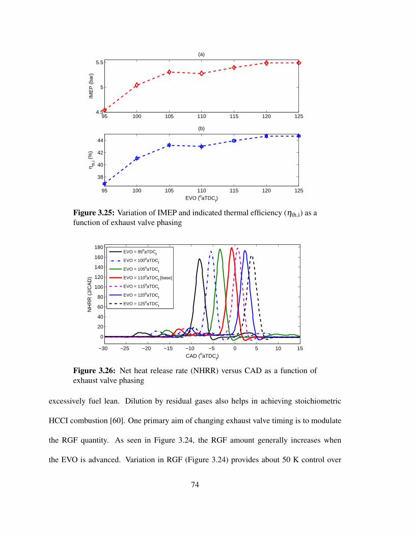
95 100 105 110 115 120 1254.5
5
5.5
(a)
IME
P (
bar)
95 100 105 110 115 120 125
38
40
42
44
(b)
EVO (oaTDCf)
η th,i (
%)
Figure 3.25: Variation of IMEP and indicated thermal efficiency (ηth,i) as afunction of exhaust valve phasing
−30 −25 −20 −15 −10 −5 0 5 10 15
0
20
40
60
80
100
120
140
160
180
CAD (oaTDCf)
NH
RR
(J/
CA
D)
EVO = 95oaTDCf
EVO = 100oaTDCf
EVO = 105oaTDCf
EVO = 110oaTDCf [base]
EVO = 115oaTDCf
EVO = 120oaTDCf
EVO = 125oaTDCf
Figure 3.26: Net heat release rate (NHRR) versus CAD as a function ofexhaust valve phasing
excessively fuel lean. Dilution by residual gases also helps in achieving stoichiometric
HCCI combustion [60]. One primary aim of changing exhaust valve timing is to modulate
the RGF quantity. As seen in Figure 3.24, the RGF amount generally increases when
the EVO is advanced. Variation in RGF (Figure 3.24) provides about 50 K control over
74
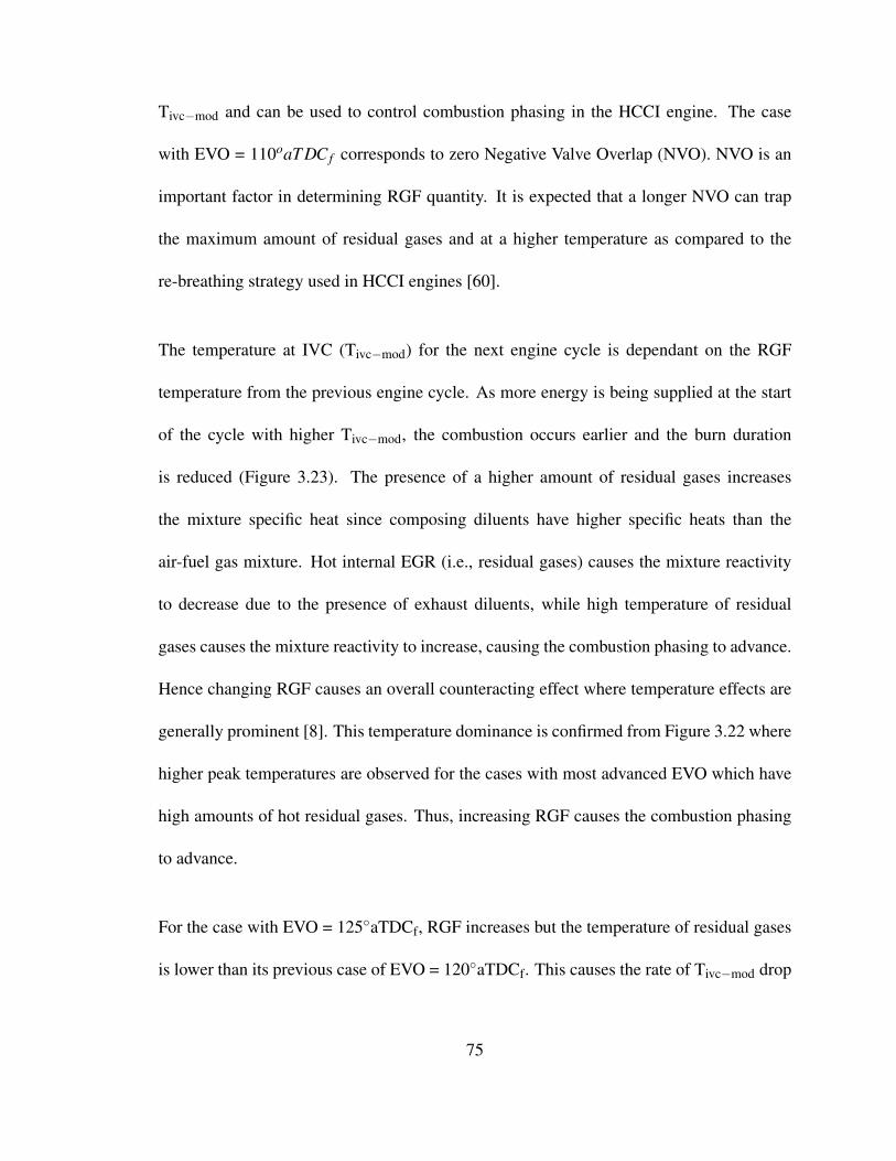
Tivc−mod and can be used to control combustion phasing in the HCCI engine. The case
with EVO = 110oaT DC f corresponds to zero Negative Valve Overlap (NVO). NVO is an
important factor in determining RGF quantity. It is expected that a longer NVO can trap
the maximum amount of residual gases and at a higher temperature as compared to the
re-breathing strategy used in HCCI engines [60].
The temperature at IVC (Tivc−mod) for the next engine cycle is dependant on the RGF
temperature from the previous engine cycle. As more energy is being supplied at the start
of the cycle with higher Tivc−mod, the combustion occurs earlier and the burn duration
is reduced (Figure 3.23). The presence of a higher amount of residual gases increases
the mixture specific heat since composing diluents have higher specific heats than the
air-fuel gas mixture. Hot internal EGR (i.e., residual gases) causes the mixture reactivity
to decrease due to the presence of exhaust diluents, while high temperature of residual
gases causes the mixture reactivity to increase, causing the combustion phasing to advance.
Hence changing RGF causes an overall counteracting effect where temperature effects are
generally prominent [8]. This temperature dominance is confirmed from Figure 3.22 where
higher peak temperatures are observed for the cases with most advanced EVO which have
high amounts of hot residual gases. Thus, increasing RGF causes the combustion phasing
to advance.
For the case with EVO = 125◦aTDCf, RGF increases but the temperature of residual gases
is lower than its previous case of EVO = 120◦aTDCf. This causes the rate of Tivc−mod drop
75
(i.e., ∆Tivc−mod∆EVO ) to reduce as seen in Figure 3.24. BD is affected by the presence of lower
temperature (Trg) residual gases causing the BD to increase as EVO is delayed. Thus, as
the EVO timing is delayed, CA50 retards and occurs at or after TDCf causing the IMEP
and ηth,i to increase. This is because useful energy released from combustion is during the
piston’s travel from TDCf to BDC. For the cases where CA50 occurs before TDCf, energy
released due to 50% of fuel burnt is during the piston’s upward motion from BDC and
may cause negative work. This is confirmed from Figure 3.25 where IMEP and ηth,i are
decreasing as CA50 is advanced.
95 100 105 110 115 120 125
0
0.05
0.1
0.14
EVO (oaTDCf)
CO
(%
)
95 100 105 110 115 120 125
1,850
1880
1910
1935
Tm
ax z
one
aver
age
(K)
TemperatureCO
Figure 3.27: CO emissions and maximum zone averaged gas temperatureas a function of exhaust valve phasing
Figures 3.27 and 3.28 show the trend of CO and uHC concentrations for variations in
EVO timing. A similar explanation as that of Figure 3.17 can be given for the CO trend
seen in Figure 3.27. uHC concentrations are largely temperature dependant and increase
as the peak temperature reduces (Figure 3.28). The hot diluents can increase the local
76
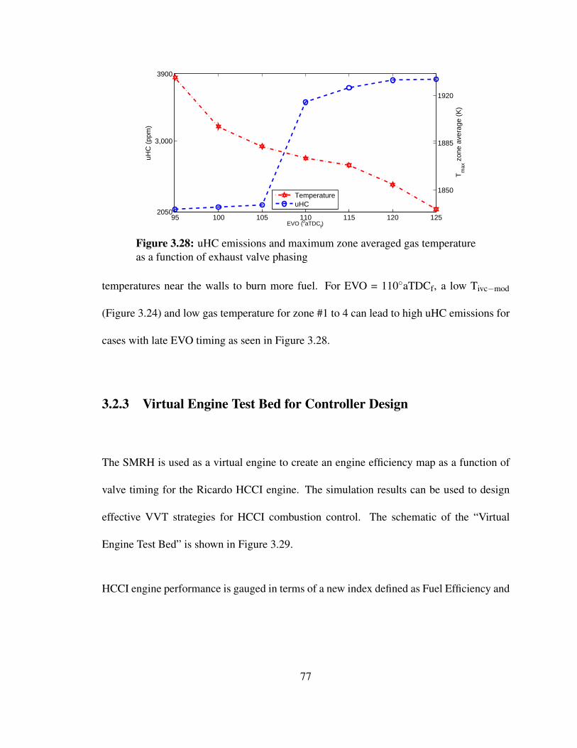
95 100 105 110 115 120 1252050
3,000
3900
uHC
(pp
m)
1850
1885
1920
EVO (oaTDCf)
Tm
ax z
one
aver
age
(K)
Temperature uHC
Figure 3.28: uHC emissions and maximum zone averaged gas temperatureas a function of exhaust valve phasing
temperatures near the walls to burn more fuel. For EVO = 110◦aTDCf, a low Tivc−mod
(Figure 3.24) and low gas temperature for zone #1 to 4 can lead to high uHC emissions for
cases with late EVO timing as seen in Figure 3.28.
3.2.3 Virtual Engine Test Bed for Controller Design
The SMRH is used as a virtual engine to create an engine efficiency map as a function of
valve timing for the Ricardo HCCI engine. The simulation results can be used to design
effective VVT strategies for HCCI combustion control. The schematic of the “Virtual
Engine Test Bed” is shown in Figure 3.29.
HCCI engine performance is gauged in terms of a new index defined as Fuel Efficiency and
77
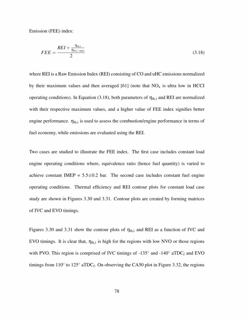
Emission (FEE) index:
FEE =REI + ηth,i
ηth,i−max
2(3.18)
where REI is a Raw Emission Index (REI) consisting of CO and uHC emissions normalized
by their maximum values and then averaged [61] (note that NOx is ultra low in HCCI
operating conditions). In Equation (3.18), both parameters of ηth,i and REI are normalized
with their respective maximum values, and a higher value of FEE index signifies better
engine performance. ηth,i is used to assess the combustion/engine performance in terms of
fuel economy, while emissions are evaluated using the REI.
Two cases are studied to illustrate the FEE index. The first case includes constant load
engine operating conditions where, equivalence ratio (hence fuel quantity) is varied to
achieve constant IMEP = 5.5±0.2 bar. The second case includes constant fuel engine
operating conditions. Thermal efficiency and REI contour plots for constant load case
study are shown in Figures 3.30 and 3.31. Contour plots are created by forming matrices
of IVC and EVO timings.
Figures 3.30 and 3.31 show the contour plots of ηth,i and REI as a function of IVC and
EVO timings. It is clear that, ηth,i is high for the regions with low NVO or those regions
with PVO. This region is comprised of IVC timings of -135◦ and -140◦ aTDCf and EVO
timings from 110◦ to 125◦ aTDCf. On observing the CA50 plot in Figure 3.32, the regions
78
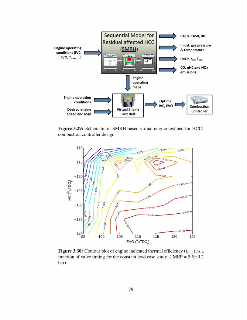
Sequential Model for Residual affected HCCI
(SMRH)
IMEP, ηth, Texh
CA10, CA50, BD
In‐cyl. gas pressure & temperature
CO, uHC and NOx emissions
Engine operating conditions (IVC,
EVO, Tman, …)
Virtual Engine Test Bed
Combustion ControllerDesired engine
speed and load
Engine operating conditions
Engine operating maps
Optimal IVC, EVO
Figure 3.29: Schematic of SMRH based virtual engine test bed for HCCIcombustion controller design
0.36
0.369
0.36
9
0.378
0.37
8
0.387
0.38
7
0.387
0.396
0.39
6
0.39
6
0.405
0.405
0.40
5
0.40
5
0.41
40.
414
0.414
0.414
0.42
3
0.423
0.423 0.423
0.423
0.43
2
0.43
2
0.432
0.432
0.432
0.432
0.44
1
0.441
0.441
0.441
0.441
0.45
0.45
0.45
0.45
0.459
0.4590.459
0.468
EVO (oaTDCf)
IVC
(o aT
DC
f)
95 100 105 110 115 120 125−140
−135
−130
−125
−120
−115
−110
Figure 3.30: Contour plot of engine indicated thermal efficiency (ηth,i) as afunction of valve timing for the constant load case study. (IMEP = 5.5±0.2bar)
79
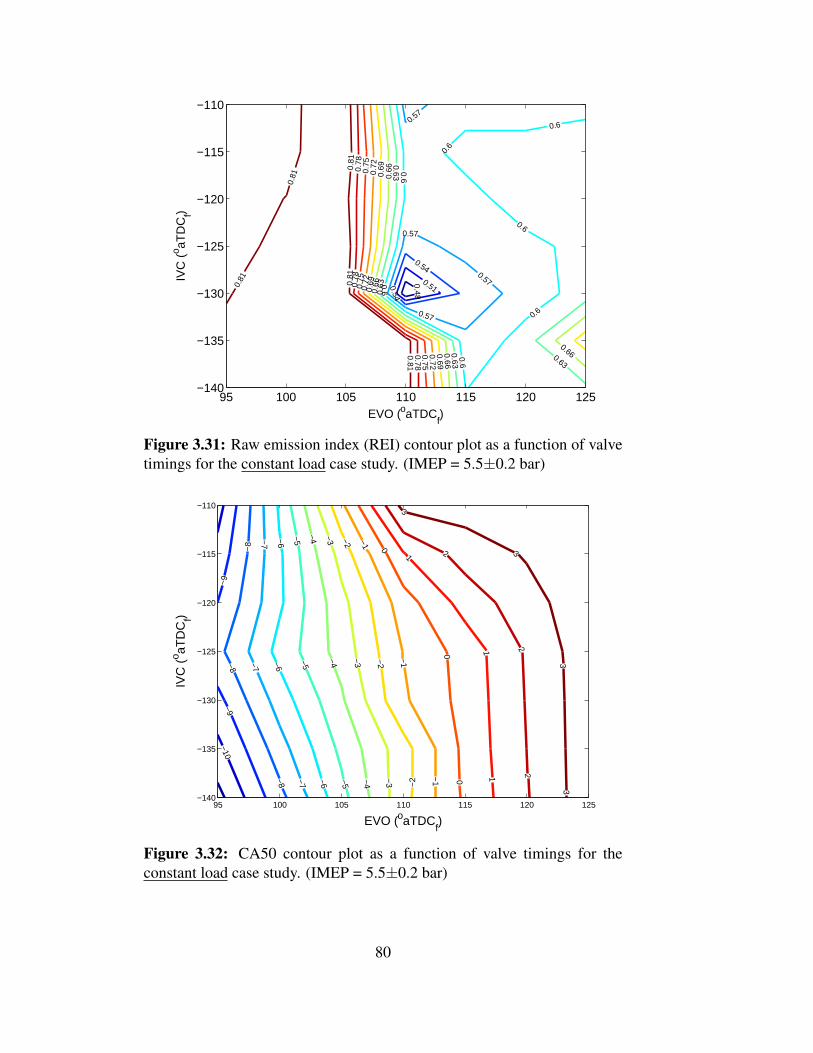
0.48
0.510.54
0.54
0.57
0.57
0.57
0.57
0.6
0.6
0.6
0.6
0.6
0.6
0.6
0.63
0.63
0.630.63
0.66
0.66
0.66
0.66
0.69
0.69
0.690.
720.
72
0.72
0.75
0.75
0.75
0.78
0.78
0.78
0.81
0.81
0.81
0.81
0.81
EVO (oaTDCf)
IVC
(o aT
DC
f)
95 100 105 110 115 120 125−140
−135
−130
−125
−120
−115
−110
Figure 3.31: Raw emission index (REI) contour plot as a function of valvetimings for the constant load case study. (IMEP = 5.5±0.2 bar)
−10
−9
−9
−8
−8
−8
−7
−7
−7
−6
−6
−6
−5−5
−5
−4
−4
−4
−3
−3
−3
−2
−2
−2
−1
−1
−1
0
0
0
1
11
2
22
3
3
33
EVO (oaTDCf)
IVC
(o aT
DC
f)
95 100 105 110 115 120 125−140
−135
−130
−125
−120
−115
−110
Figure 3.32: CA50 contour plot as a function of valve timings for theconstant load case study. (IMEP = 5.5±0.2 bar)
80
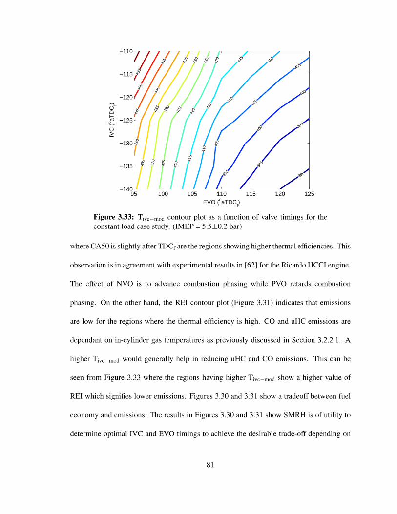
390
395
395
400
400
400
405
405
405
410
410
410
415
415
415
420
420
420
425
425
425
430
430
430
435
435
435
440
440
445
445
450
455
EVO (oaTDCf)
IVC
(o aT
DC
f)
95 100 105 110 115 120 125−140
−135
−130
−125
−120
−115
−110
Figure 3.33: Tivc−mod contour plot as a function of valve timings for theconstant load case study. (IMEP = 5.5±0.2 bar)
where CA50 is slightly after TDCf are the regions showing higher thermal efficiencies. This
observation is in agreement with experimental results in [62] for the Ricardo HCCI engine.
The effect of NVO is to advance combustion phasing while PVO retards combustion
phasing. On the other hand, the REI contour plot (Figure 3.31) indicates that emissions
are low for the regions where the thermal efficiency is high. CO and uHC emissions are
dependant on in-cylinder gas temperatures as previously discussed in Section 3.2.2.1. A
higher Tivc−mod would generally help in reducing uHC and CO emissions. This can be
seen from Figure 3.33 where the regions having higher Tivc−mod show a higher value of
REI which signifies lower emissions. Figures 3.30 and 3.31 show a tradeoff between fuel
economy and emissions. The results in Figures 3.30 and 3.31 show SMRH is of utility to
determine optimal IVC and EVO timings to achieve the desirable trade-off depending on
81
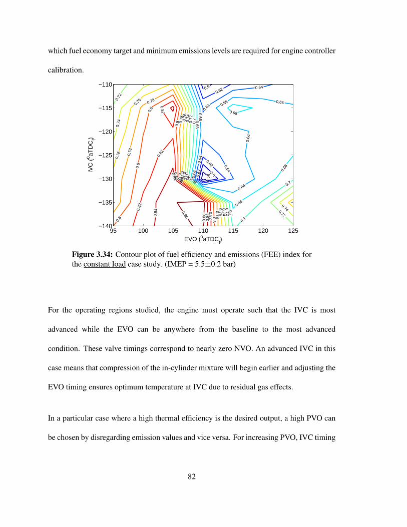
which fuel economy target and minimum emissions levels are required for engine controller
calibration.
0.58
0.6
0.6
0.62
0.62
0.62
0.64
0.64
0.64
0.64
0.66
0.66
0.66
0.66
0.66 0.66
0.68
0.68
0.68
0.68
0.68
0.7
0.7
0.7
0.7
0.7
0.72
0.72
0.72
0.72 0.72
0.74 0.
74
0.74
0.74
0.74
0.76
0.76
0.76
0.76
0.760.78
0.78
0.78
0.78
0.78
0.8
0.8
0.8
0.8
0.8
0.8
0.82
0.82
0.82
0.82
0.82
0.84
0.84
0.84
0.86
0.86
EVO (oaTDCf)
IVC
(o aT
DC
f)
95 100 105 110 115 120 125−140
−135
−130
−125
−120
−115
−110
Figure 3.34: Contour plot of fuel efficiency and emissions (FEE) index forthe constant load case study. (IMEP = 5.5±0.2 bar)
For the operating regions studied, the engine must operate such that the IVC is most
advanced while the EVO can be anywhere from the baseline to the most advanced
condition. These valve timings correspond to nearly zero NVO. An advanced IVC in this
case means that compression of the in-cylinder mixture will begin earlier and adjusting the
EVO timing ensures optimum temperature at IVC due to residual gas effects.
In a particular case where a high thermal efficiency is the desired output, a high PVO can
be chosen by disregarding emission values and vice versa. For increasing PVO, IVC timing
82
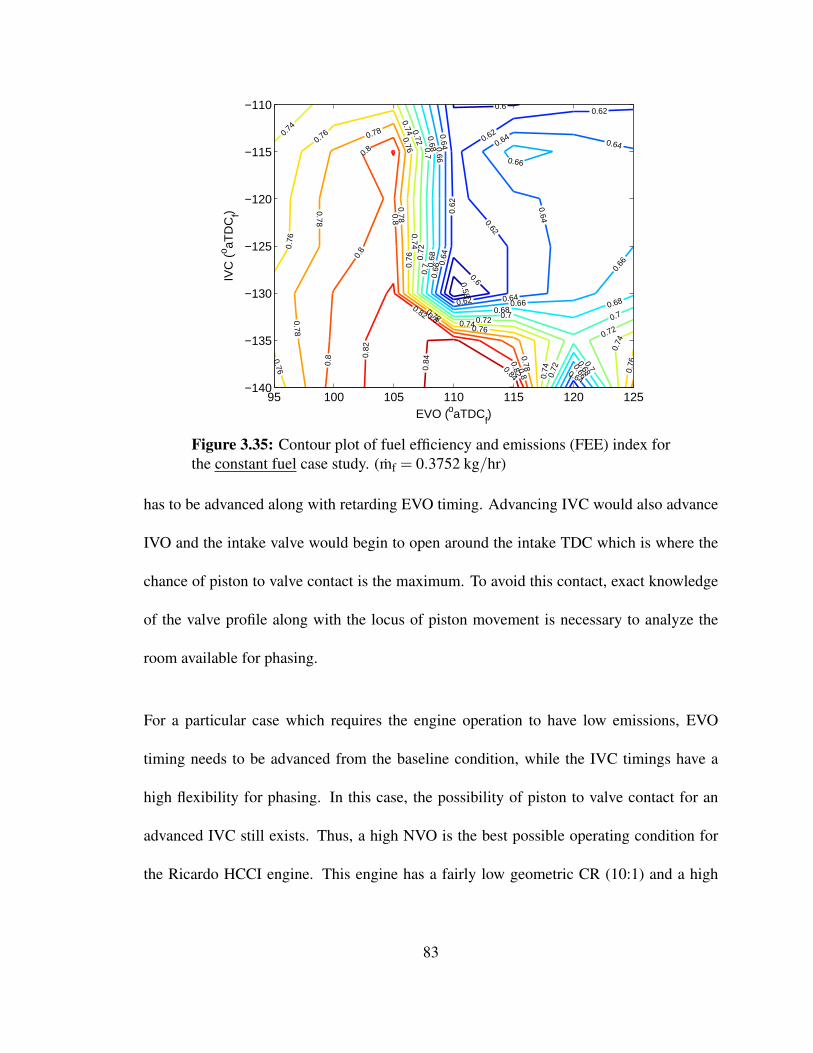
0.58
0.6
0.6
0.62
0.62
0.62
0.62
0.62
0.64
0.64
0.64
0.64
0.64 0.64
0.640.66
0.66
0.66
0.66
0.66
0.66
0.68
0.68
0.68 0.68
0.68
0.7
0.7
0.7 0.7
0.7
0.72
0.72
0.72
0.72
0.72
0.74
0.740.74
0.74
0.74
0.74
0.76
0.76
0.76
0.76
0.76
0.76
0.76
0.78
0.78
0.78
0.78
0.78
0.780.8
0.8
0.8
0.8
0.8
0.8
0.82
0.82
0.820.84
0.84
EVO (oaTDCf)
IVC
(o aT
DC
f)
95 100 105 110 115 120 125−140
−135
−130
−125
−120
−115
−110
Figure 3.35: Contour plot of fuel efficiency and emissions (FEE) index forthe constant fuel case study. (mf = 0.3752 kg/hr)
has to be advanced along with retarding EVO timing. Advancing IVC would also advance
IVO and the intake valve would begin to open around the intake TDC which is where the
chance of piston to valve contact is the maximum. To avoid this contact, exact knowledge
of the valve profile along with the locus of piston movement is necessary to analyze the
room available for phasing.
For a particular case which requires the engine operation to have low emissions, EVO
timing needs to be advanced from the baseline condition, while the IVC timings have a
high flexibility for phasing. In this case, the possibility of piston to valve contact for an
advanced IVC still exists. Thus, a high NVO is the best possible operating condition for
the Ricardo HCCI engine. This engine has a fairly low geometric CR (10:1) and a high
83
NVO would aid in achieving auto-ignition due to the higher temperature at IVC. Thus,
referring to Figure 3.35, the region comprising IVC timing of −115◦ to−130◦ aTDCf and
EVO timings from 96◦ to 105◦ aTDCf are the best feasible valve timings for operation of
this HCCI engine, to obtain low fuel consumption and low emission levels.
The FEE plots for the constant fuel and constant load case studies are similar in nature
(Figures 3.34 and 3.35). The regions where a high FEE index is observed is the same for
both case studies. Slightly higher values of FEE index are observed for the constant load
case study where fuel quantity is adjusted to get a fixed engine load. Higher FEE value
in constant load case indicates the importance of using a combination of VVT and fuel
quantity (e.g., φ ) to achieve optimum operation (high FEE) of the HCCI engine.
84
Chapter 4
Summary and Conclusion
Two areas are focussed upon, which are considered to be the core of this thesis. First is the
experimental setup of an HCCI engine for the test cell at Michigan Tech with a particular
contribution to the setup of intake air handling (heating and boost) and valve timings along
with compression ratio measurements. The second area is the SMRH modeling platform
for simulating residual affected HCCI combustion and engine performance as a function of
valve timing.
85
4.1 Summary of thesis contributions
* This thesis has the contribution in further developing the HCCI engine test setup at
Michigan Technological University. Contributions were made in the areas of air heater
setup and its control. This will help to operate the engine in HCCI mode and also obtain
large HCCI operating range. Valve profile along with piston to valve clearance were
measured. New piston were procured which have a compression ratio of 12.1:1. In
addition, a boosting station was designed and tested at different supercharger speeds.
* A sequential model called as SMRH was developed and validated against experimental
data from a single cylinder HCCI engine [4]. The SMRH was validated for in-cylinder
gas pressure, combustion phasing (CA10, CA50), performance metrics (IMEP and ηth,i)
and CO emission. Effects of VVT were studied for both intake and exhaust valve
variations. The SMRH was then used to find engine maps for a newly defined Fuel
Efficiency and Emissions (FEE) index which shows the overall engine operation. Using
the FEE index, optimum valve timings for engine operation were determined.
* SMRH is the first model in HCCI literature to characterize VVT effects on residual
affected HCCI based on a simplified multi zone combustion model and intake and
exhaust flow models. SMRH is of utility for HCCI control community to develop
advanced VVT strategies to control HCCI engines in optimum operating regions.
86

4.2 Future Work
* For the HCCI experimental setup, a mode switching control strategy needs to be
developed for starting the engine in SI mode using the dSPACE controller, and switch
back and forth to HCCI mode when necessary.
* The new pistons can be installed and checked for piston to valve contact to ascertain
the phasing ability. The engine can be run in HCCI mode using the air heater to heat
the intake air to a desired temperature. The boosting station can be used to provide the
desired amount of boost for achieving HCCI mode at higher engine loads.
* Maps of the FEE index from the SMRH can be further analyzed to develop a systematic
methodology to minimize calibration of HCCI engines.
* Combustion controller design can be carried out using the SMRH as the plant model.
Such a controller would have the advantage of being more robust by incorporation of
physical relations for engine variables and mitigating physical disturbances by using
proper engine control variables.
87

References
[1] EATON. M62 Performance Map. http://www.eaton.com/ecm/groups/public/
@pub/@eaton/@per/documents/content/ct_128484.gif, accessed September
30, 2014.
[2] Omega Inc. Process Air & Duct Heaters. http://www.omega.com/Heaters/pdf/
AHF_HEATER.pdf, accessed September 30, 2014.
[3] Ray Franco. E-motor insulation classes. http://www.electrical-forensics.
com/Motors/MotorClasses.html, accessed September 30, 2014.
[4] M. Shahbakhti and C. Koch. “Characterizing the Cyclic Variability of Ignition
Timing in A Homogeneous Charge Compression Ignition Engine Fuelled with
n-heptane/iso-octane Blend Fuels”. International Journal of Engine Research,
9(5):361–397, 2008.
[5] S. Aceves, D. Flowers, C. Westbrook, J. Smith, W. Pitz, R. Dibble, M. Christensen,
and B. Johansson. “A Multi-Zone Model for Prediction of HCCI Combustion and
89
Emissions”. 2000. SAE Technical Paper 2000-01-0327.
[6] John B Heywood. “Internal combustion engine fundamentals”. Mcgraw-hill New
York, 1988.
[7] H. Anders, M. Christensen, B. Johansson, A. Franke, M. Richter, and M. Alden. “A
Study of The Homogeneous Charge Compression Ignition Combustion Process by
Chemiluminescence Imaging”. 1999. SAE Technical Paper 1999-01-3680.
[8] S. Saxena and I. Bedoya. “Fundamental Phenomena Affecting Low Temperature
Combustion and HCCI Engines, High Load Limits and Strategies for Extending
These Limits”. Progress in Energy and Combustion Science, 39(5):457–488, 2013.
[9] L. Koopmans, R. Ogink, and I. Denbratt. “Direct Gasoline Injection in The Negative
Valve Overlap of A Homogeneous Charge Compression Ignition Engine”. 2003. SAE
Technical Paper 2003-01-1854.
[10] A. Fuerhapter, W. Piock, and G. Fraidl. “CSI-Controlled Auto Ignition-The Best
Solution for The Fuel Consumption-Versus Emission Trade-Off?”. 2003. SAE
Technical Paper 2003-01-0754.
[11] P. Caton, H. Song, N. Kaahaaina, and C. Edwards. “Residual-Effected Homogeneous
Charge Compression Ignition with Delayed Intake-Valve Closing at Elevated
Compression Ratio”. International journal of engine research, 6(4):399–419, 2005.
90
[12] M. Christensen, B. Johansson, and P. Einewall. “Homogeneous Charge Compression
Ignition (HCCI) Using Isooctane, Ethanol and Natural Gas-A Comparison with Spark
Ignition Operation”. 1997. SAE Technical paper 972874.
[13] J. Yang, T. Culp, and T. Kenney. “Development of A Gasoline Engine System Using
HCCI Technology-The Concept and The Test Results”. 2002. SAE Technical Paper
2002-01-2832.
[14] J Hyvonen, G Haraldsson, and B Johansson. Supercharging HCCI to Extend the
Operating Range in a Multi-Cylinder VCR-HCCI Engine. 2003. SAE Technical
Paper 2003-01-3214.
[15] R. Stanglmaier, T. Ryan, and J. Souder. “HCCI Operation of A Dual-Fuel Natural
Gas Engine for Improved Fuel Efficiency and Ultra-Low NOx Emissions at Low to
Moderate Engine Loads”. 2001. SAE Technical Paper 2001-01-1897.
[16] J. Tuttle. “Controlling Engine Load by Means of Late Intake-Valve Closing”. 1980.
SAE Technical Paper 800794.
[17] J. Ma, X. Lu, L. Ji, and Z. Huang. “An Experimental Study of HCCI-DI Combustion
and Emissions in A Diesel Engine with Dual Fuel”. International Journal of Thermal
Sciences, 47(9):1235–1242, 2008.
[18] H. Zhang, J. Chiu, and J. Bartel. “Late Intake Valve Closing with Throttle Control
at Light Loads for a Lean-Burn Natural Gas Engine”. 1999. SAE Technical Paper
1999-01-3485.
91
[19] M. Yao, Z. Zheng, and H. Liu. ”Progress and Recent Trends in Homogeneous Charge
Compression Ignition (HCCI) Engines”. Progress in Energy and Combustion Science,
35(5):398–437, 2009.
[20] J. Zhang, X. Qiao, Z. Wang, B. Guan, and Z. Huang. “Experimental Investigation of
low-temperature combustion (LTC) in an engine fueled with dimethyl ether (DME)”.
Energy & Fuels, 23(1):170–174, 2008.
[21] E. Silke, H. Curran, and J. Simmie. “The influence of fuel structure on combustion
as demonstrated by the isomers of heptane: a rapid compression machine study”.
Proceedings of the Combustion Institute, 30(2):2639–2647, 2005.
[22] C. Westbrook. “Chemical kinetics of hydrocarbon ignition in practical combustion
systems”. Proceedings of the Combustion Institute, 28(2):1563–1577, 2000.
[23] P. Dagaut, M. Reuillon, and M. Cathonnet. “Experimental Study of the Oxidation of
n-heptane in A Jet Stirred Reactor from Low to High Temperature and Pressures Up
to 40 atm”. Combustion and Flame, 101(1):132–140, 1995.
[24] H. Curran, W. Pitz, C. Westbrook, G. Callahan, and F. Dryer. “Oxidation of
automotive primary reference fuels at elevated pressures”. International Symposium
on Combustion, 1998.
[25] L. Cancino, M. Fikri, A. Oliveira, and C. Schulz. “Autoignition of gasoline
surrogate mixtures at intermediate temperatures and high pressures: Experimental
92
and numerical approaches”. Proceedings of the Combustion Institute, 32(1):501–508,
2009.
[26] C. Westbrook, W. Pitz, and H. Curran. “HCCI and CAI Engines for the Automotive
Industry”. CRC, 2007.
[27] P. Dagaut, C. Daly, J. Simmie, and M. Cathonnet. “The oxidation and ignition of
dimethylether from low to high temperature (500–1600 K): Experiments and kinetic
modeling”. International Symposium on Combustion, 1998.
[28] C. Westbrook, H. Curran, W. Pitz, J. Griffiths, C. Mohamed, and S. Wo. “The effects
of pressure, temperature, and concentration on the reactivity of alkanes: Experiments
and modeling in a rapid compression machine”. International Symposium on
Combustion, 1998.
[29] J. Warnatz, U. Maas, and R. Dibble. “Combustion: Physical and Chemical
Fundamentals, Modeling and Simulation, Experiments, Pollutant Formation”.
Springer, 2006.
[30] E. Hellstrom, A. Stefanopoulou, J. Vavra, A. Babajimopoulos, D. Assanis, L. Jiang,
and H. Yilmaz. “Understanding The Dynamic Evolution of Cyclic Variability at
The Operating Limits of HCCI Engines with Negative Valve Overlap”. 2012. SAE
Technical Paper 2012-01-1106.
93

[31] P. Borgqvist, P. Tunestal, and B. Johansson. “Investigation And Comparison of
Residual Gas Enhanced HCCI Using Trapping (NVO HCCI) or Rebreathing of
Residual Gases”. 2011. SAE Technical Paper 2011-01-1772.
[32] N. Milovanovic, R. Chen, and J. Turner. “Influence of The Variable Valve Timing
Strategy on The Control of A Homogeneous Charge Compression (HCCI) Engine”.
2004. SAE Technical Paper 2004-01-1899.
[33] P. Caton, A. Simon, J. Gerdes, and C. Edwards. “Residual-Effected Homogeneous
Charge Compression Ignition at A Low Compression Ratio using Exhaust
Reinduction. International Journal of Engine Research, 4(3):163–177, 2003.
[34] F. Agrell, H. Angstrom, B. Eriksson, J. Wikander, and J. Linderyd. “Transient control
of HCCI through combined intake and exhaust valve actuation”. 2003. SAE Technical
Paper 2003-01-3172.
[35] US EPA. 2011 News Releases. http://yosemite.epa.gov/opa/admpress.nsf/
1e5ab1124055f3b28525781f0042ed40/0019c092ccae8ac2852578dc0056ded0!
OpenDocument, accessed September 30, 2014.
[36] V. Thakkar. “Experimental setup of an HCCI engine”. Master’s thesis, Michigan
Technological University, 2014.
[37] D Kothari. “Experimental Setup And Controller DesignN For An HCCI Engine”.
Master’s thesis, Michigan Technological University, 2014.
94
[38] R Ferraz. LHU Engine. http://www.fmsrperformance.com/test/index.php?
route=product/category&path=20_70, accessed September 30, 2014.
[39] Crane Cams. Degreeing the Camshaft. http://www.cranecams.com/bulletins_
listview.php?s_id=5, accessed September 30, 2014.
[40] Jade, S. “Transient Load-Speed Control in Multi-Cylinder Recompression HCCI
Engines”. PhD thesis, The University of Michigan, USA, 2014.
[41] Shahbakhti, M. “Modelling and Experimental Study of An HCCI Engine for
Combustion Timing Control”. PhD thesis, University of Alberta, Canada, 2009.
[42] J. Dec and M. Sjoberg. “A Parametric Study of HCCI Combustion-The Sources
of Emissions at Low Loads and The Effects of GDI Fuel Injection”. 2003. SAE
Technical Paper 2003-01-0752.
[43] P. Kirchen, M. Shahbakhti, and C. Koch. “A Skeletal Kinetic Mechanism
for PRF Combustion in HCCI Engines. Combustion Science and Technology,
179(6):1059–1083, 2007.
[44] S. Aceves, J. Smith, C. Westbrook, and W. Pitz. “Compression Ratio Effect on
Methane HCCI Combustion”. Journal of Engineering for Gas Turbines and Power,
121(3):569–574, 1999.
95
[45] S. Kong, C. Marriott, R. Reitz, and M. Christensen. “Modeling and Experiments of
HCCI Engine Combustion using Detailed Chemical Kinetics with Multidimensional
CFD”. 2001. SAE Technical Paper 2001-01-1026.
[46] S. Kong, C. Marriott, C. Rutland, and R. Reitz. “Experiments and CFD Modeling of
Direct Injection Gasoline HCCI Engine Combustion”. 2002. SAE Technical Paper
2002-01-1925.
[47] A. Agarwal and D. Assanis. “Multi-Dimensional Modeling of Ignition, Combustion
and Nitric Oxide Formation in Direct Injection Natural Gas Engines”. 2000. SAE
Technical Paper 2000-01-1839.
[48] S. Kong, R. Reitz, M. Christensen, and B. Johansson. “Modeling the Effects
of Geometry Generated Turbulence on HCCI Engine Combustion”. 2003. SAE
Technical Paper 2003-01-1088.
[49] Z. Wang, J. Wang, S. Shuai, and F. Zhang. “Numerical Simulation of HCCI Engine
with Multi-Stage Gasoline Direct Injection using 3D-CFD with Detailed Chemistry”.
2004. SAE Technical Paper 2004-01-0563.
[50] A. Patel, S. Kong, and R. Reitz. “Development and Validation of A Reduced
Reaction Mechanism for HCCI Engine Simulations”. 2004. SAE Technical Paper
2004-01-0558.
[51] S. Aceves, D. Flowers, F. Espinosa-Loza, A. Babajimopoulos, and D. Assanis.
“Analysis of Premixed Charge Compression Ignition Combustion with a Sequential
96
Fluid Mechanics-Multizone Chemical Kinetics Model”. 2005. SAE Technical Paper
2005-01-0115.
[52] I. Bedoya, C. Francisco, S. Saxena, R. Dibble, S. Aceves, and D. Flowers. “A
Sequential Chemical Kinetics-CFD-Chemical Kinetics Methodology to Predict HCCI
Combustion and Main Emissions”. 2012. SAE Technical Paper 2012-01-1119.
[53] R. Seiser, H. Pitsch, K. Seshadri, W. Pitz, and H. Curran. “Extinction and
Autoignition of n-heptane in Counterflow Configuration”. Proceedings of the
Combustion Institute, 28(2):2029–2037, 2000.
[54] D Flowers, S Aceves, J Martinez-Frias, and R Dibble. “Prediction of Carbon
Monoxide and Hydrocarbon Emissions in iso-octane HCCI Engine Combustion
Using Multizone Simulations”. Proceedings of the Combustion Institute,
29(1):687–694, 2002.
[55] Reaction Design: San Diego, CA. CHEMKIN-PRO theory manual, 2008.
[56] J Chang, O Guralp, Z Filipi, D Assanis, T-W Kuo, P Najt, and R Rask. “New
Heat Transfer Correlation for an HCCI Engine Derived From Measurements of
Instantaneous Surface Heat Flux”. 2004. SAE Technical Paper 2004-01- 2996.
[57] R. Lupul. “Steady State and Transient Characterization of a HCCI Engine with
Varying Octane Fuel”. Master’s thesis, University of Alberta, Canada, 2008.
97
[58] A. Bhave, M. Kraft, L. Montorsi, and F. Mauss. “Sources of CO Emissions in An
HCCI Engine: A Numerical Analysis”. Combustion and flame, 144(3):634–637,
2006.
[59] S Tanaka, F Ayala, and JC Keck. A reduced chemical kinetic model for hcci
combustion of primary reference fuels in a rapid compression machine. Combustion
and Flame, 133(4):467–481, 2003.
[60] H. Yun, N. Wermuth, and P. Najt. “High Load HCCI Operation Using Different
Valving Strategies in a Naturally-Aspirated Gasoline HCCI Engine”. 2011.
2011-01-0899, SAE Technical Paper.
[61] M. Bidarvatan and M. Shahbakhti. “Integrated HCCI Engine Control Based on
a Performance Index”. Journal of Engineering for Gas Turbines and Power,
136(10):101601, 2014.
[62] M. Shahbakhti, A. Ghazimirsaied, and C. Koch. “Experimental study of exhaust
temperature variation in a homogeneous charge compression ignition engine”.
Proceedings of the Institution of Mechanical Engineers, Part D: Journal of
Automobile Engineering, 224(9):1177–1197, 2010.
[63] P. Kirchen. “Thermokinetic Modeling of the HCCI Cycle:Predicting the Ignition
Timing”. Master’s thesis, University of Alberta, Canada, 2004.
98
[64] N. Komninos, D. Hountalas, and D. Kouremenos. “Description of In-Cylinder
Combustion Processes in HCCI Engines Using a Multi-Zone Model”. 2005. SAE
Technical Paper 2005-01-0171.
[65] M. Sjoberg and J. Dec. “Combined Effects of Fuel-Type and Engine Speed on
Intake Temperature Requirements and Completeness of Bulk-Gas Reactions for
HCCI Combustion”. 2003. SAE Technical Paper 2003-01-3173.
[66] R. Ogink and V. Golovitchev. “Gasoline HCCI Modeling: Computer Program
Combining Detailed Chemistry and Gas Exchange Processes”. 2001. SAE Technical
Paper 2001-01-3614.
[67] R. Ogink and V. Golovitchev. “Gasoline HCCI Modeling: An Engine Cycle
Simulation Code with A Multi-Zone Combustion Model”. 2002. SAE Technical
Paper 2002-01-1745.
[68] L. Young and Young T. Camshaft Basics and Terminology. http://www.
tildentechnologies.com/Cams/CamBasics.html, accessed September 30, 2014.
[69] L. Koopmans, R. Ogink, and I. Denbratt. “Direct Gasoline Injection in the Negative
Valve Overlap of a Homogeneous Charge Compression Ignition Engine”. SAE
Technical Paper 2003-01-1854.
[70] G. Kontarakis, N. Collings, and T. Ma. “Demonstration of HCCI Using a Single
Cylinder Four-Stroke SI Engine with Modified Valve Timing”. 2000. SAE Technical
Paper 2000-01-2870.
99
[71] D. Law, D. Kemp, J. Allen, G. Kirkpatrick, and T. Copland. “Controlled Combustion
in an IC-Engine with a Fully Variable Valve Train”. 2001. SAE Technical Paper
2001-01-0251.
[72] M. Christensen, B. Johansson, P. Amneus, and F. Mauss. “Supercharged
Homogeneous Charge Compression Ignition”. 1998. SAE Technical Paper 980787.
100
Appendix A
Calculations for cam timing
determination
The following equations from [68] are used to determine the valve timing metrics, provided
required values are known. Once IVO (bTDC), IVC (aBDC), EVO (bBDC) and EVC
101
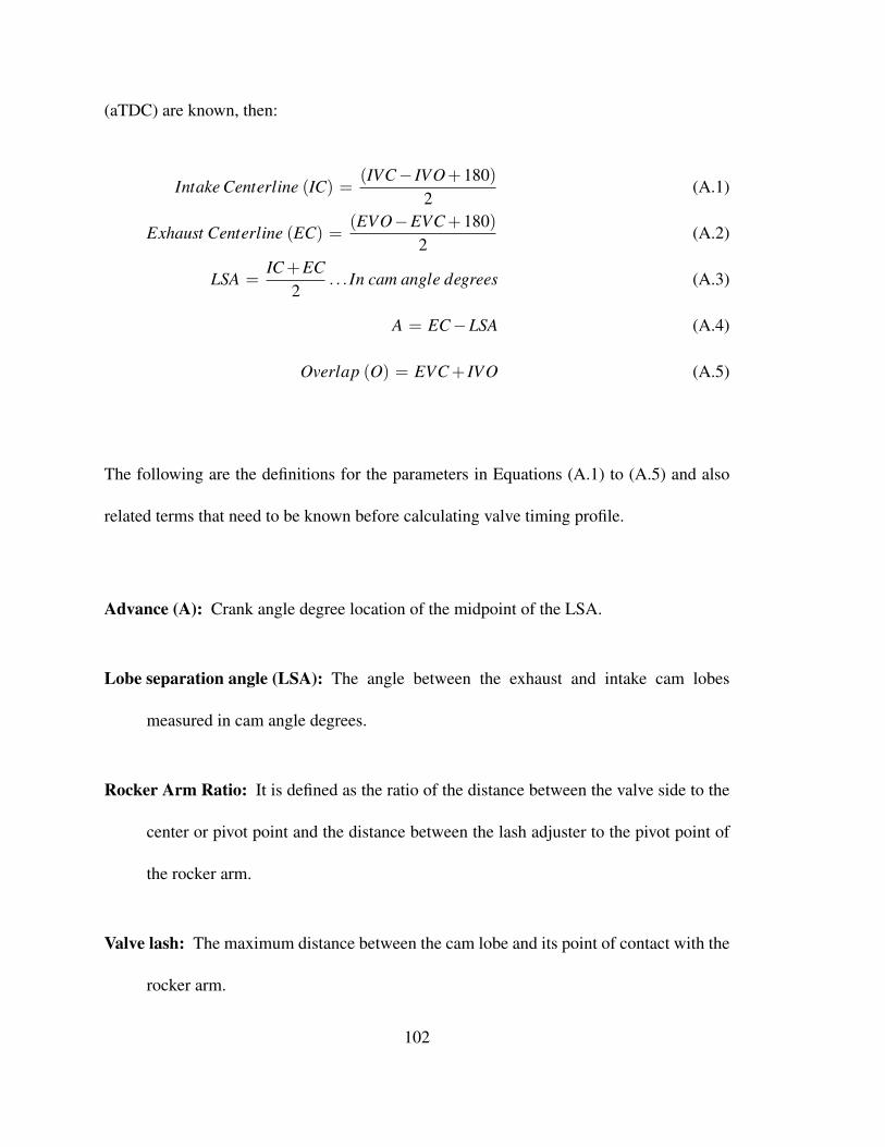
(aTDC) are known, then:
Intake Centerline (IC) =(IVC− IVO+180)
2(A.1)
Exhaust Centerline (EC) =(EVO−EVC+180)
2(A.2)
LSA =IC+EC
2. . . In cam angle degrees (A.3)
A = EC−LSA (A.4)
Overlap (O) = EVC+ IVO (A.5)
The following are the definitions for the parameters in Equations (A.1) to (A.5) and also
related terms that need to be known before calculating valve timing profile.
Advance (A): Crank angle degree location of the midpoint of the LSA.
Lobe separation angle (LSA): The angle between the exhaust and intake cam lobes
measured in cam angle degrees.
Rocker Arm Ratio: It is defined as the ratio of the distance between the valve side to the
center or pivot point and the distance between the lash adjuster to the pivot point of
the rocker arm.
Valve lash: The maximum distance between the cam lobe and its point of contact with the
rocker arm.
102

Valve overlap: The crank angle duration for which intake and exhaust valve are
simultaneously open.
Lobe centerline: The crank angle degree at which maximum lobe lift occurs.
103
Appendix B
MSc Publications
† H. Saigaonkar, M. Nazemi, M. Shahbakhti, “Sequential Model for Residual Affected
HCCI with Variable Valve Timing”, SAE Paper No. 2015-01-1748, 16 pages, SAE
World Congress, Detroit, MI, USA, April 21-23, 2015.
† M. Nazemi, H. Saigaonkar, M. Shahbakhti, “Thermo-kinetic Modeling of Variable
Valve Timing Effects on HCCI Engine Combustion”, Int. Conference on Advanced
Technology & Sciences, 6 pages, August 12-15, 2014, Antalya, Turkey.
104
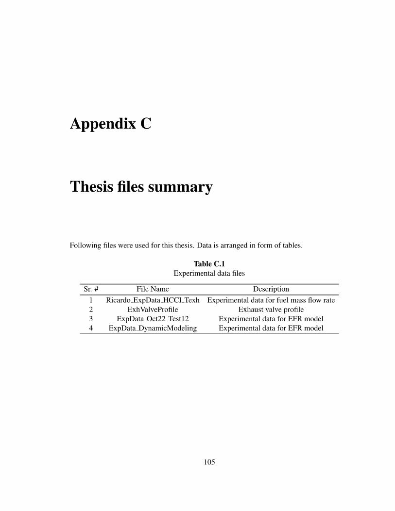
Appendix C
Thesis files summary
Following files were used for this thesis. Data is arranged in form of tables.
Table C.1Experimental data files
Sr. # File Name Description1 Ricardo ExpData HCCI Texh Experimental data for fuel mass flow rate2 ExhValveProfile Exhaust valve profile3 ExpData Oct22 Test12 Experimental data for EFR model4 ExpData DynamicModeling Experimental data for EFR model
105
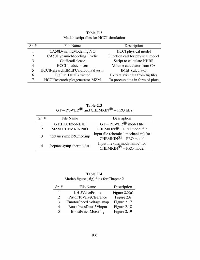
Table C.2Matlab script files for HCCI simulation
Sr. # File Name Description1 CA50DynamicModeling VO HCCI physical model2 CA50DynamicModeling Cyclic Function call for physical model3 GetHeatRelease Script to calculate NHRR4 HCCI loadsiconvert Volume calculator from CA5 HCCIResearch IMEPCalc bothvalves.m IMEP calculator6 FigFile DataExtractor Extract axis data from fig files7 HCCIResearch plotgenerator MZM To process data in form of plots
Table C.3GT−POWER R© and CHEMKIN R©−PRO files
Sr. # File Name Description1 GT HCCImodel all GT−POWER R© model file2 MZM CHEMKINPRO CHEMKIN R©−PRO model file
3 heptanesymp159 mec.inpInput file (chemical mechanism) for
CHEMKIN R©−PRO model
4 heptanesymp thermo.datInput file (thermodynamic) forCHEMKIN R©−PRO model
Table C.4Matlab figure (.fig) files for Chapter 2
Sr. # File Name Description1 LHUValveProfile Figure 2.5(a)2 PistonToValveClearance Figure 2.63 EmotorSpeed voltage map Figure 2.174 BoostPressData 5Vinput Figure 2.185 BoostPress Motoring Figure 2.19
106
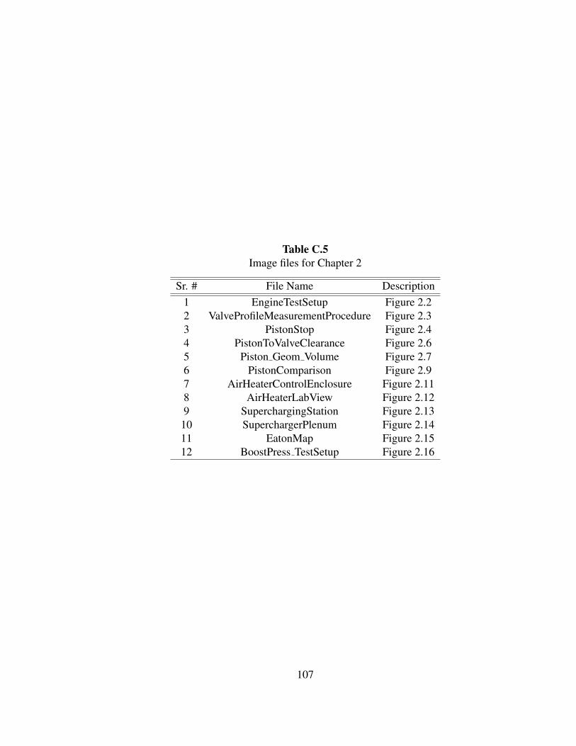
Table C.5Image files for Chapter 2
Sr. # File Name Description1 EngineTestSetup Figure 2.22 ValveProfileMeasurementProcedure Figure 2.33 PistonStop Figure 2.44 PistonToValveClearance Figure 2.65 Piston Geom Volume Figure 2.76 PistonComparison Figure 2.97 AirHeaterControlEnclosure Figure 2.118 AirHeaterLabView Figure 2.129 SuperchargingStation Figure 2.13
10 SuperchargerPlenum Figure 2.1411 EatonMap Figure 2.1512 BoostPress TestSetup Figure 2.16
107
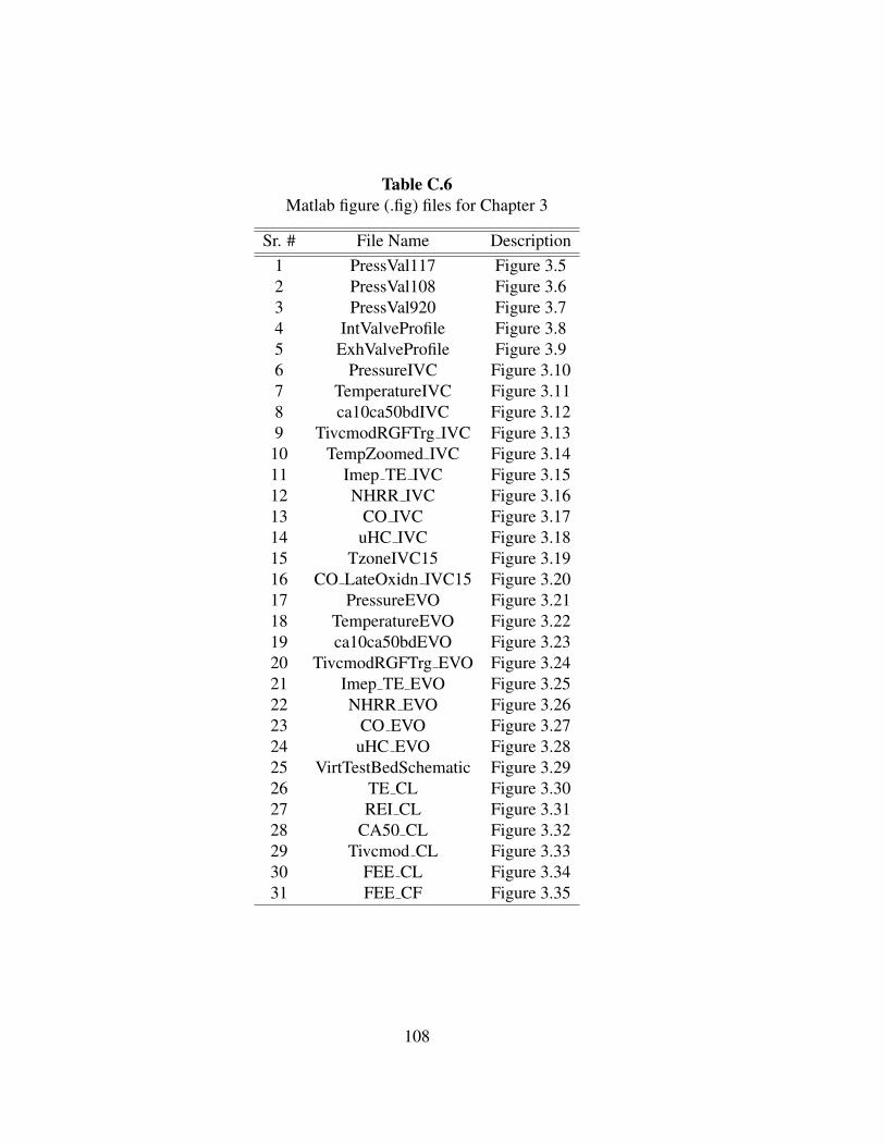
Table C.6Matlab figure (.fig) files for Chapter 3
Sr. # File Name Description1 PressVal117 Figure 3.52 PressVal108 Figure 3.63 PressVal920 Figure 3.74 IntValveProfile Figure 3.85 ExhValveProfile Figure 3.96 PressureIVC Figure 3.107 TemperatureIVC Figure 3.118 ca10ca50bdIVC Figure 3.129 TivcmodRGFTrg IVC Figure 3.13
10 TempZoomed IVC Figure 3.1411 Imep TE IVC Figure 3.1512 NHRR IVC Figure 3.1613 CO IVC Figure 3.1714 uHC IVC Figure 3.1815 TzoneIVC15 Figure 3.1916 CO LateOxidn IVC15 Figure 3.2017 PressureEVO Figure 3.2118 TemperatureEVO Figure 3.2219 ca10ca50bdEVO Figure 3.2320 TivcmodRGFTrg EVO Figure 3.2421 Imep TE EVO Figure 3.2522 NHRR EVO Figure 3.2623 CO EVO Figure 3.2724 uHC EVO Figure 3.2825 VirtTestBedSchematic Figure 3.2926 TE CL Figure 3.3027 REI CL Figure 3.3128 CA50 CL Figure 3.3229 Tivcmod CL Figure 3.3330 FEE CL Figure 3.3431 FEE CF Figure 3.35
108
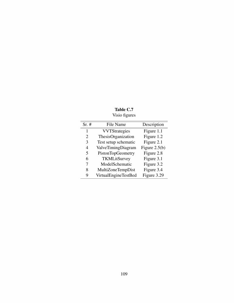
Table C.7Visio figures
Sr. # File Name Description1 VVTStrategies Figure 1.12 ThesisOrganization Figure 1.23 Test setup schematic Figure 2.14 ValveTimingDiagram Figure 2.5(b)5 PistonTopGeometry Figure 2.86 TKMLitSurvey Figure 3.17 ModelSchematic Figure 3.28 MultiZoneTempDist Figure 3.49 VirtualEngineTestBed Figure 3.29
109
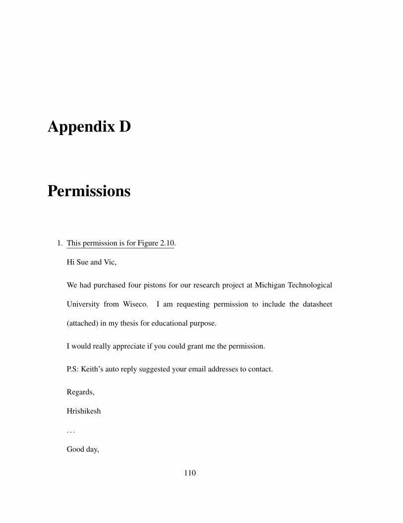
Appendix D
Permissions
1. This permission is for Figure 2.10.
Hi Sue and Vic,
We had purchased four pistons for our research project at Michigan Technological
University from Wiseco. I am requesting permission to include the datasheet
(attached) in my thesis for educational purpose.
I would really appreciate if you could grant me the permission.
P.S: Keith’s auto reply suggested your email addresses to contact.
Regards,
Hrishikesh
. . .
Good day,
110

We grant permission to use the print for your thesis. Good luck with the program and
thank you for using Wiseco Products!
Victor Ellinger
111

2. This permission is for Figure 2.15.
Dear Brent Bussell,
I am a graduate student at Michigan Technological University and my research
involved the use of a Eaton M62 supercharger. For educational purposes, I want to
include its performance map (found on your website) in my thesis. I am requesting
permission to use it. I would really appreciate your help in this matter.
Regards,
Hrishikesh
. . .
Please read the FAQ it contains all the info I have, feel free to use what you need.
Brent Bussell
Customer Support
Technical Specialist
112
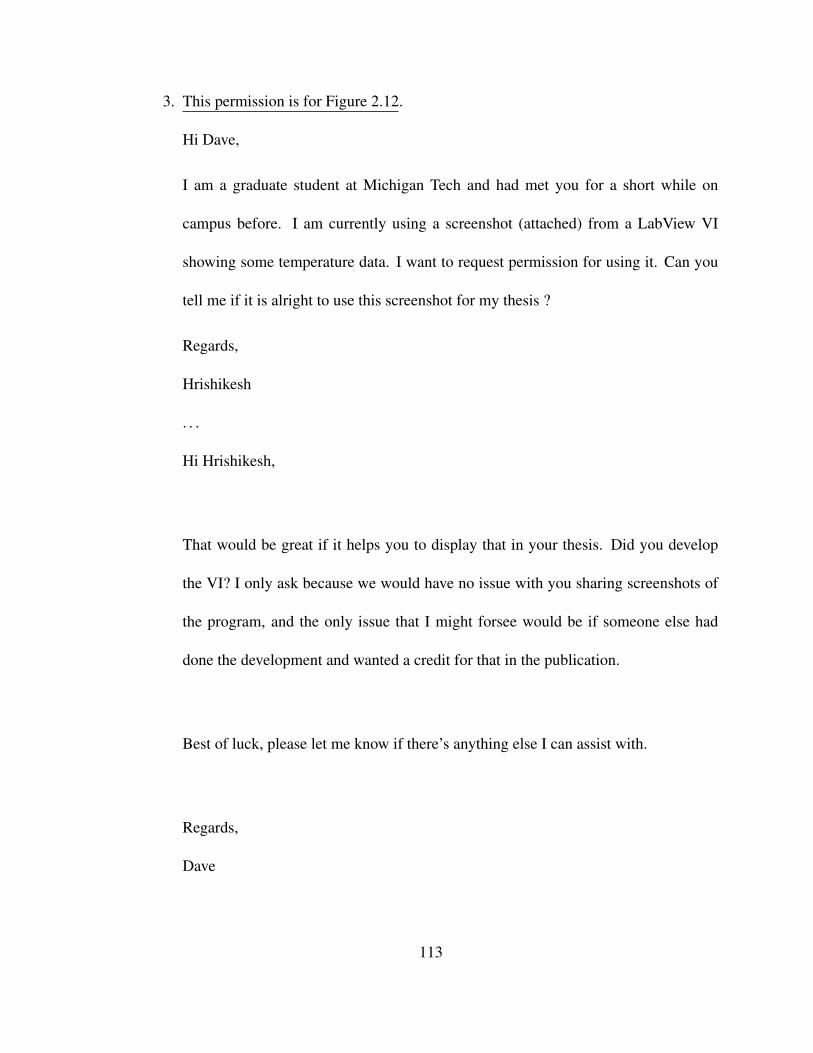
3. This permission is for Figure 2.12.
Hi Dave,
I am a graduate student at Michigan Tech and had met you for a short while on
campus before. I am currently using a screenshot (attached) from a LabView VI
showing some temperature data. I want to request permission for using it. Can you
tell me if it is alright to use this screenshot for my thesis ?
Regards,
Hrishikesh
. . .
Hi Hrishikesh,
That would be great if it helps you to display that in your thesis. Did you develop
the VI? I only ask because we would have no issue with you sharing screenshots of
the program, and the only issue that I might forsee would be if someone else had
done the development and wanted a credit for that in the publication.
Best of luck, please let me know if there’s anything else I can assist with.
Regards,
Dave
113

Dave Collins
Academic Field Engineer - Midwest
National Instruments
114