1 

An Indoor-Outdoor Building Energy Simulator to 1 

Study Urban Modification Effects on Building Energy 2 

Use – Model Description and Validation 3 

Neda Yaghoobian  4 

Mechanical and Aerospace Engineering Department, University of California San Diego, 9500 Gilman 5 Drive, La Jolla, CA 92093‐0411 6 

Jan Kleissl  7 

Mechanical and Aerospace Engineering Department, University of California San Diego, 9500 Gilman 8 Drive, EBU II‐580, La Jolla, CA 92093‐0411 9 

E‐mail: jkleissl@ucsd.edu; Phone: 858‐534‐8087; fax: (858) 534‐7599 10 

11 

Abstract 12 

While there have been significant advances in energy modeling of individual buildings and urban canopies, more 13 

sophisticated and at the same time more efficient models are needed to understand the thermal interaction 14 

between buildings and their surroundings. In particular to evaluate policy alternatives it is of interest how building 15 

makeup, canyon geometry, weather conditions, and their combination modify heat transfer in the urban area. The 16 

Temperature of Urban Facets Indoor‐Outdoor Building Energy Simulator (TUF‐IOBES) is a building‐to‐canopy model 17 

that simulates indoor and outdoor building surface temperatures and heat fluxes in an urban area to estimate 18 

cooling/heating loads and energy use in buildings. The indoor and outdoor energy balance processes are 19 

dynamically coupled taking into account real weather conditions, indoor heat sources, building and urban material 20 

properties, composition of the building envelope (e.g. windows, insulation), and HVAC equipment. TUF‐IOBES is 21 

also capable of simulating effects of the waste heat from air‐conditioning systems on urban canopy air 22 

temperature. TUF‐IOBES transient heat conduction is validated against an analytical solution and multi‐model 23 

intercomparions for annual and daily cooling and heating loads are conducted. An application of TUF‐IOBES to 24 

study the impact of different pavements (concrete and asphalt) on building energy use is also presented. 25 

 26 

Keywords: Building energy simulator; Dynamic online modeling; Urban heat island mitigation. 27 

2 

Nomenclature 1 

amplitude of the soil surface temperature (˚C) 2 

window absorptance as a function of incidence angle 3 

effective volumetric heat capacity (J kg-1 K-1) 4 

COP coefficient of performance of the air conditioning system 5 

air specific heat capacity (J kg-1 K-1) 6 

D thermal damping depth (m) due to temperature fluctuations 7 

H building height (m) 8 

heat transfer coefficient 9 

effective thermal conductivity (W m-1 K-1) 10 

L building length (m) 11 

longwave radiation (W m-2) 12 

P time period 13 

anthropogenic heat from air conditioning systems (W) 14 

sensible heat generated inside the building (W) 15 

latent heat from internal loads (W) 16 

turbulent sensible heat flux (W m-2) 17 

convection from internal loads (W m-2) 18 

conduction heat flux (W m-2) 19 

convection heat flux from the zone surfaces (W m-2) 20 

sensible load due to infiltration and ventilation (W m-2) 21 

longwave radiation flux from internal sources in a zone (W m-2) 22 

net longwave radiant exchange flux between zone surfaces (W m-2) 23 

transmitted solar radiation flux absorbed on indoor surfaces (W m-2) 24 

net shortwave radiation flux to the zone surface from interior light (W m-2) 25 

heat transfer to/from the HVAC system (W m-2) 26 

outdoor air-to-indoor air thermal resistances (m2 K W-1) 27 

outdoor air-to-indoor wall surface thermal resistances (m2 K W-1) 28 

solar heat gain coefficient of window 29 

3 

shortwave radiation (W m-2) 1 

shortwave radiation from internal sources (W m-2) 2 

average soil surface temperature (˚C) 3 

air volume inside the urban canopy (m3) 4 

W building width (m) 5 

6 

Greek letters 7 

thermal diffusivity (m2s-1) 8 

air density (kg m-3) 9 

transmittance of window 10 

11 

Subscripts 12 

down downwelling radiation 13 

dir direct component of solar irradiation 14 

diff diffuse component of solar irradiation 15 

16 

4 

1. Introduction 1 

Urbanization or replacing natural land cover with buildings and impervious surfaces has 2 

resulted from rapid population and economic growth. Built-up surfaces have different radiative 3 

and thermal properties and as a result a different surface energy balance than adjacent rural areas. 4 

In addition, the geometry of buildings and canopies changes flow patterns (e.g. [1, 2]) and traps 5 

radiation lowering effective albedos [3-6]. All of these effects are responsible for a different 6 

climate in urban areas with relatively higher surface and air temperatures (with a few exceptions, 7 

[7]) which is called the (surface or air temperature) urban heat island (UHI, [8]). Anthropogenic 8 

waste heat (e.g. from transportation, building air-conditioning) enhances UHI effects (e.g. [9-11]; 9 

for a review on anthropogenic heat flux modeling see Grimmond et al. [12, 13]; Sailor [14]). 10 

Since land use change in urban areas modifies climate and weather [15, 16], physical 11 

processes in built areas and their causes and effects must be quantified effectively. Thermal and 12 

radiative properties of urban materials, building conditions (new versus old buildings), size, type, 13 

and location of windows, canyon geometry, anthropogenic heat fluxes, and most importantly the 14 

combination of these factors in different weather conditions affect urban heat transfer and 15 

building energy use. Several studies have been performed and different models have been 16 

developed to analyze these scenarios and improve mitigation measures in metropolitan areas 17 

(e.g. [17-21]). Most existing building energy models emerged from the engineering community 18 

such as, EnergyPlus [22], ASHRAE Toolkit [23], DOE-2 (U.S. National Renewable Energy 19 

Laboratory; NREL), the Building Loads Analysis and System Thermodynamics program 20 

(BLAST; U.S. Army Construction Engineering Research Laboratory), and Thermal Analysis 21 

Research Program (TARP; [24]). These models simulate the energy balance at the outside 22 

building wall/window surfaces, wall heat conduction, the energy balance at inside faces and the 23 

indoor air heat balance. However, these models do not model the outdoor canopy air including 24 

heating, ventilating and air-conditioning (HVAC) heat emissions, the ground surface energy 25 

5 

balance, and radiative effects of surrounding buildings. On the other hand, urban energy balance 1 

models in the meteorological community usually exclude dynamic modeling of the indoor 2 

building energy balance and anthropogenic heat fluxes released from HVAC systems. These 3 

components are usually included as prescribed values or offline models (see Grimmond et al. 4 

[12, 13, 25] for a review). 5 

There have been some advances in modeling the interaction between urban climates and 6 

building energy use. For example Kikegawa et al. [9] coupled a one dimensional urban canopy 7 

meteorological model with a simple sub-model for building energy analysis. Salamanca et al. 8 

[26] developed and implemented a Building Energy Model (BEM) in an urban canopy 9 

parameterization for mesoscale models. BEM was coupled with a multi-layer urban canopy 10 

model and implemented in WRF/urban [27] with a statistical multi-scale modeling ability 11 

ranging from continental, to city, and building scales. On the building scale, Bueno et al. [28] 12 

proposed an iterative scheme for coupling EnergyPlus and the Town Energy Balance (TEB) 2-13 

dimensional urban canopy model. Iteratively, TEB outdoor surface temperatures serve as 14 

boundary conditions for EnergyPlus and window temperature and HVAC waste heat from 15 

EnergyPlus are passed back to TEB. Iterations continue until the canyon temperature converges. 16 

Through EnergyPlus Bueno et al. [28] were able to simulate complex HVAC systems 17 

considering latent heat exchange between indoor and outdoor, building demand response 18 

strategies, and daylighting. However, this iterative process and the TEB discrete numerical 19 

method for solving heat conduction [6] likely cause the model to be computationally too 20 

expensive for the long time periods required in building energy modeling (one year). Bouyer et 21 

al. [29] developed a CFD (Fluent [30]) – thermoradiative (from the Solene model) coupled 22 

simulation tool to estimate the microclimate influence on building energy consumption. Bouyer 23 

et al. [29] also admit that the computational cost of annual simulations is prohibitive. 24 

6 

The review of the literature highlights the need for computationally efficient models which 1 

employ physical process-based descriptions at fine spatial scales and capture microclimate and 2 

building energy effects of urban modifications and heat island mitigation measures. The 3 

Temperature of Urban Facets Indoor-Outdoor Building Energy Simulator (TUF-IOBES) model 4 

introduced in this paper is a building-to-canopy model that simulates indoor and outdoor 5 

building surface temperatures and associated heat fluxes in a high resolution, 3-dimensional 6 

urban domain to estimate urban microclimate, cooling/heating loads, and energy use in 7 

buildings. The indoor and outdoor energy balance processes are coupled online and dynamically 8 

take into account real weather conditions, urban microclimate, indoor heat sources, infiltration, 9 

building and urban material properties and composition of the building envelope (e.g. windows, 10 

insulation), and HVAC equipment. TUF-IOBES also simulates the effect of waste heat emissions 11 

from HVAC systems on urban canopy air temperature and in consequence on urban and building 12 

heat transfer. 13 

The description of the outdoor and indoor energy balance models and their integration is 14 

presented in section 2. In section 3 TUF-IOBES simulations of transient heat conduction are 15 

validated against an analytical solution of the interior wall surface temperature response to a step 16 

change in outside air temperature. Also TUF-IOBES simulations of yearly and daily cooling and 17 

heating loads are validated against other building energy simulators. In section 4 an example of a 18 

TUF-IOBES application on simulating effects of urban material modifications on building 19 

energy use is presented. Conclusions are presented in Section 5. A detailed application of TUF-20 

IOBES to study urban heat island mitigation measures is presented in [XX]. 21 

22 

7 

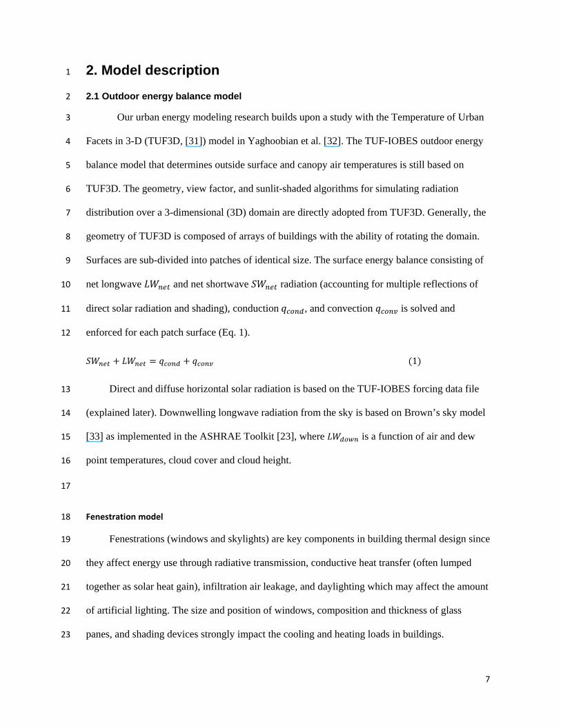
2. Model description 1 

2.1 Outdoor energy balance model 2 

Our urban energy modeling research builds upon a study with the Temperature of Urban 3 

Facets in 3-D (TUF3D, [31]) model in Yaghoobian et al. [32]. The TUF-IOBES outdoor energy 4 

balance model that determines outside surface and canopy air temperatures is still based on 5 

TUF3D. The geometry, view factor, and sunlit-shaded algorithms for simulating radiation 6 

distribution over a 3-dimensional (3D) domain are directly adopted from TUF3D. Generally, the 7 

geometry of TUF3D is composed of arrays of buildings with the ability of rotating the domain. 8 

Surfaces are sub-divided into patches of identical size. The surface energy balance consisting of 9 

net longwave and net shortwave radiation (accounting for multiple reflections of 10 

direct solar radiation and shading), conduction , and convection is solved and 11 

enforced for each patch surface (Eq. 1). 12 

1

Direct and diffuse horizontal solar radiation is based on the TUF-IOBES forcing data file 13 

(explained later). Downwelling longwave radiation from the sky is based on Brown’s sky model 14 

[33] as implemented in the ASHRAE Toolkit [23], where is a function of air and dew 15 

point temperatures, cloud cover and cloud height. 16 

17 

Fenestration model 18 

Fenestrations (windows and skylights) are key components in building thermal design since 19 

they affect energy use through radiative transmission, conductive heat transfer (often lumped 20 

together as solar heat gain), infiltration air leakage, and daylighting which may affect the amount 21 

of artificial lighting. The size and position of windows, composition and thickness of glass 22 

panes, and shading devices strongly impact the cooling and heating loads in buildings. 23 

8 

The simple geometry of buildings with opaque walls in TUF3D was modified to 1 

accommodate windows, which are also resolved by one or several patches. The net shortwave 2 

radiation incident on each window patch ( ) is simulated based on the method used in 3 

ASHRAE Toolkit 4 

5 

, 2 6 

where , , and are absorptance, transmittance, and solar heat gain coefficient of the 7 

window, respectively. is the total shortwave radiation from internal sources. Subscripts 8 

and stand for direct and diffuse components of solar radiation. Direct absorptance, 9 

transmittance, and SHGC of the glazing depend on the incidence angle of solar radiation. TUF-10 

IOBES is capable of simulating up to triple pane windows. The transmitted shortwave radiation 11 

is passed to the indoor heat balance (Eq. 4 later). 12 

13 

Transient heat conduction model 14 

There are several methods for simulating transient heat conduction in building envelopes 15 

[34] such as Lumped parameter methods [35], frequency response methods [36], numerical 16 

models like finite difference method (FDM) and finite element method (FEM) [37-39], and Z-17 

transform methods [40, 41]. Fully discrete numerical models (especially FDM) are the most 18 

popular schemes in building and urban energy analysis. However, FDM have several 19 

disadvantages such as computational cost (especially for thin layers such as windows), storage 20 

requirements, and numerical stability. In order to evaluate building-canopy energy interactions 21 

over time scales greater than a few days a more efficient heat conduction scheme is needed. 22 

In TUF-IOBES we have implemented a Z-transform method utilizing Conduction Transfer 23 

Functions (CTFs), which is an analytical based scheme for calculating conduction in solid media 24 

9 

{40-42). CTFs are applied for example in EnergyPlus and the ASHRAE Toolkit. CTFs are 1 

calculated based on the State Space Method which assumes a linear change in temperature 2 

between two time steps. CTF reduce computational cost since the resulting conduction equation 3 

is linearly relating surface heat flux only to the temperatures and fluxes at the inside and outside 4 

faces of the medium (unlike in FDM and FEM, element temperatures within the medium are not 5 

required). CTF coefficients only need to be determined once for each medium (wall, roof, 6 

window, and ground patches). In TUF-IOBES over a domain of 5 by 5 buildings, CTF reduced 7 

overall computational time by a factor of 15 compared to the FDM. This difference would be 8 

even greater for larger and more complex domains. 9 

Due to round-off and truncation errors, the CTF method has stability problems in thermally 10 

massive construction [41, 22] including thermally thick soil layers. To find soil surface 11 

temperature using CTF the soil layer has to be thermally thin. As a result, a constant “deep soil” 12 

temperature at the bottom boundary of the simulation domain can no longer be assumed. In TUF-13 

IOBES to obtain the deep soil temperature over any time period P, following Hillel [43] we 14 

solve the diffusion equation for a soil with constant thermal properties, a sinusoidal temperature 15 

boundary condition at the surface and a constant temperature boundary condition at infinite 16 

depth 17 

, / 2

2. 3

In this equation , is the boundary condition for deep soil temperature at time and 18 

depth (m), is the average surface temperature (˚C) over , is the amplitude of the surface 19 

temperature (˚C) over . ⁄ is the thermal damping depth (m) of temperature 20 

fluctuations over , and is the thermal diffusivity (m2s-1). is the time lag from an arbitrary 21 

starting time to the occurrence of the minimum temperature in period . To avoid stability 22 

problems, the maximum allowed is initialized as 3 for 86400 s where the soil 23 

10 

temperature amplitude is 5% of the diurnal surface temperature . Instead of computing and 1 

from soil temperatures (usually not available), hourly temperature is used [44]. Since soil 2 

is composed of heterogeneous horizontal layers, the effective thermal conductivity ( ) is 3 

calculated as the harmonic average of thermal conductivities of the soil layers [45]. The effective 4 

volumetric heat capacity ( ) is derived from the weighted sum of the thermal capacities of each 5 

separate layer [46]. and weighted by volume fraction of each layer are used to define an 6 

effective and constant thermal diffusivity ⁄ , where is the soil density. CTF is 7 

then used to compute the soil surface temperature using the boundary condition obtained through 8 

Eq. 3. 9 

10 

Convection model 11 

In a simple representation of buoyancy-driven and wind-driven air flow over a surface, the 12 

turbulent sensible heat flux ( ) in building energy balance models is typically expressed by the 13 

heat transfer coefficient ( ) multiplied by the driving force expressed by the temperature ( ) 14 

difference between the surface and air ( ). There are several methods for 15 

calculating the heat transfer coefficient (e.g. [47-51, 24]). Models differ as to the degree of 16 

complexity of modeling free and forced convections on horizontal or vertical surfaces 17 

considering thermal stratification of the adjacent flow. 18 

In TUF-IOBES, based on TUF3D, stability-corrected Monin–Obukhov similarly theory can 19 

be used for modeling heat transfer from horizontal surfaces. The transfer from vertical surfaces is 20 

based on a flat plate forced convection relationship considering patch surface roughness and 21 

effective wind speed [31]. Alternatively, the DOE-2 model [52] can be applied which is a 22 

combination of the MoWiTT [50] and BLAST [51] models. In the DOE-2 method, the sum of 23 

11 

the forced and natural convection components differs for windward and leeward surfaces and is a 1 

function of surface roughness. 2 

3 

Forcing data: Annual weather data file 4 

Building energy analyses should be forced with a full year of representative weather data 5 

such as the TMY3 (Typical Meteorological Year 3) files provided by the National Solar 6 

Radiation Data Base. TUF-IOBES inputs hourly global horizontal, direct normal, and diffuse 7 

horizontal irradiances, cloud cover and height, dry bulb and dew point temperatures, pressure, 8 

wind speed, and wind direction at reference height from the TMY3 file. TMY3 information is 9 

linearly interpolated within the hour. TMY3 wind speed, direction, and air temperature are 10 

applied at the reference height in the surface layer; wind speed and temperature profiles in the 11 

roughness sub-layer (logarithmic law) and inside the canopy (exponential profile for wind and 12 

constant canopy air temperature) are based on Krayenhoff and Voogt [31]. 13 

14 

2.2 Indoor energy balance model 15 

Unlike the gridded outdoor energy model, the indoor model computes bulk heat exchange 16 

and temperature between surfaces. The indoor energy balance model is based on subroutines in 17 

the ASHRAE Toolkit. The inside surface heat balance shows that the heat transfer due to 18 

convection, longwave and shortwave radiation is balanced by conduction: 19 

0, 4

where is the net longwave radiant exchange flux between zone surfaces modeled using 20 

Walton’s mean radiant temperature with balance method [53], is the net shortwave radiation 21 

flux to the surface from interior light which is assumed to be distributed over the surfaces in the 22 

zone (walls, floor, and ceiling) through a user defined fraction, is the longwave radiation 23 

12 

flux from equipment, people, and lights in a zone modeled using the method of 1 

radiative/convective split of heat, is conduction flux through the wall simulated using CTF 2 

method, is the transmitted solar radiation flux absorbed on indoor surfaces, and is the 3 

convective heat flux to zone air based on air and surface temperature difference. Eq. 4 yields the 4 

indoor surface temperatures. Since the unknown surface temperature in the net longwave radiant 5 

exchange flux between surfaces ( ) is fourth order (Stefan-Boltzmann law), Eq. 4 is a 6 

nonlinear equation which is solved by Newton’s method (unlike the ASHRAE Toolkit which 7 

linearizes this equation). 8 

The air in the thermal zone is considered to be well-mixed. The air heat balance consists of 9 

convection heat transfer from the zone surfaces ( ) which is based on the indoor air and 10 

surface temperature difference, convective part of internal loads ( ), the sensible load due to 11 

infiltration and ventilation ( ), and the heat transfer to/from the HVAC system ( ): 12 

0. 5

The air heat balance equation yields the room air temperature and the heating or sensible 13 

cooling load ( ) at each timestep. TUF-IOBES simulates a single or dual-setpoint (deadband) 14 

system with no upper limit on air flow (unlimited capacity) such that the cooling and heating 15 

setpoints are immediately satisfied. 16 

17 

2.3 Dynamic coupling of indoor and outdoor energy balance models 18 

First a real weather data file (TMY3) forces the outdoor energy balance to obtain canopy 19 

air and urban surface temperatures. Then through the indoor energy balance (Eqs. 4 and 5) 20 

surface temperatures, air temperature, and cooling/heating load inside the building are obtained. 21 

Finally the waste heat from the air-conditioning (AC) system increases the canopy air 22 

temperature. 23 

13 

Anthropogenic heat from AC systems is the combination of latent ( ) heat from 1 

equipment and people, sensible ( ) heat generated inside the building, and the work required for 2 

operating the thermodynamic cycle [9]. The total waste heat of the AC system ( [W]) is 3 

1, 6

where COP is the coefficient of performance of the AC system. Assuming that the AC systems 4 

are mounted on the walls (versus on rooftops) of the buildings and instant mixing into the 5 

canopy, the waste heat increases the canopy air temperature. Using air density ( ), specific 6 

heat capacity ( ), and volume of the air inside the canopy ( ), the temperature increase 7 

(∆ ) from these anthropogenic heat fluxes becomes 8 

∆

, 7

where is the simulation timestep. Since the air temperature above the canopy layer is imposed 9 

as the boundary condition, it is not affected by anthropogenic heat release and the canopy air 10 

temperature. 11 

In TUF-IOBES the indoor and outdoor energy balance processes are dynamically coupled. 12 

At each timestep the outdoor energy balance model uses the simulated inside building surface 13 

temperatures at the previous timestep from the indoor energy model. On the other hand, the 14 

indoor energy balance model uses the outside building wall temperature simulated at the current 15 

timestep as its boundary condition. Also, the transmitted solar radiation in the interior surface 16 

heat balance is based on the radiation in the outdoor energy balance. 17 

18 

3. Validation 19 

The complexity of building energy simulation programs and simplifications in describing 20 

the physical processes imply that careful validation is essential. Ideally, the performance of a 21 

14 

building energy simulator should be validated against measured data from a real building. 1 

However, such data are not available as the urban indoor and outdoor environment is too 2 

complex to be instrumented sufficiently. So as stated by Zmeureanu et al. [54], sufficient testing 3 

should be conducted to assure that the probability of failure is sufficiently low to be acceptable. 4 

In this section a transient heat conduction simulation in TUF-IOBES is validated against an 5 

analytical solution of interior wall surface temperature response to a step change in outside air 6 

temperature. In addition yearly and daily cooling and heating load simulations in TUF-IOBES 7 

are validated against other whole building energy simulators. 8 

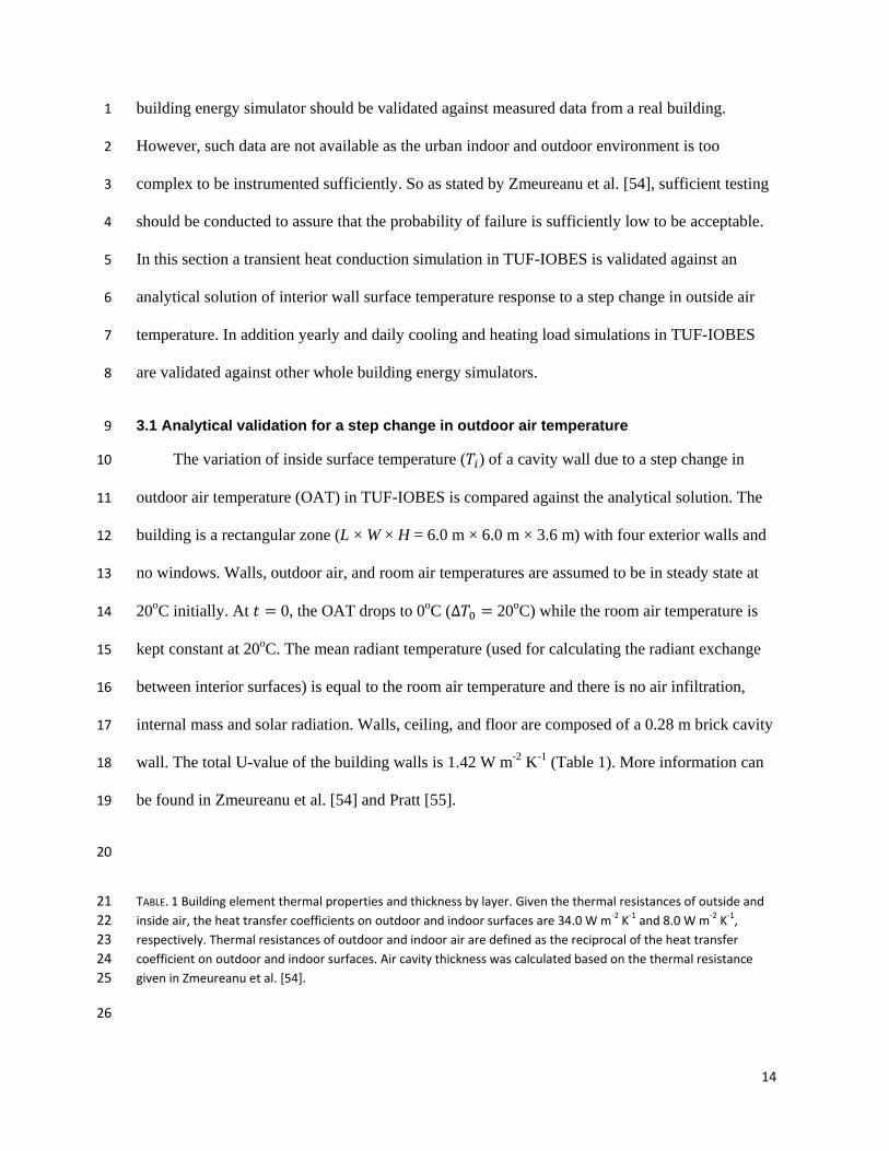
3.1 Analytical validation for a step change in outdoor air temperature 9 

The variation of inside surface temperature ( ) of a cavity wall due to a step change in 10 

outdoor air temperature (OAT) in TUF-IOBES is compared against the analytical solution. The 11 

building is a rectangular zone (L × W × H = 6.0 m × 6.0 m × 3.6 m) with four exterior walls and 12 

no windows. Walls, outdoor air, and room air temperatures are assumed to be in steady state at 13 

20oC initially. At 0, the OAT drops to 0oC (∆ 20oC) while the room air temperature is 14 

kept constant at 20oC. The mean radiant temperature (used for calculating the radiant exchange 15 

between interior surfaces) is equal to the room air temperature and there is no air infiltration, 16 

internal mass and solar radiation. Walls, ceiling, and floor are composed of a 0.28 m brick cavity 17 

wall. The total U-value of the building walls is 1.42 W m-2 K-1 (Table 1). More information can 18 

be found in Zmeureanu et al. [54] and Pratt [55]. 19 

20 

TABLE. 1 Building element thermal properties and thickness by layer. Given the thermal resistances of outside and 21 

inside air, the heat transfer coefficients on outdoor and indoor surfaces are 34.0 W m‐2 K‐1 and 8.0 W m‐2 K‐1, 22 

respectively. Thermal resistances of outdoor and indoor air are defined as the reciprocal of the heat transfer 23 

coefficient on outdoor and indoor surfaces. Air cavity thickness was calculated based on the thermal resistance 24 

given in Zmeureanu et al. [54]. 25 

26 

15 

Although in TUF-IOBES heat transfer coefficients can be calculated dynamically, to match 1 

the conditions in the analytical solution, heat transfer coefficients are fixed to the values 2 

provided by the reference. 3 

4 

FIG. 1 Temporal variation of the inside surface temperature ( ) of a 0.28 m brick cavity wall after a step change 5 

in outdoor air temperature of ∆  at time zero. The  ‐axis scale is the relative change of the hourly interior surface 6 

temperature with respect to the drop in OAT at initial time based on Zmeureanu et al. [54] 7 

8 

TUF-IOBES simulation results (Fig. 1) start at the same initial condition ( 0 = 9 

20˚C) and reach the same steady state value ( 16.4˚C) at 45 h as the analytical solution. 10 

The analytical steady state solution is only a function of the room air temperature ( ) and the 11 

ratio of the outdoor air-to-indoor wall surface ( ) and outdoor air-to-indoor air ( ) thermal 12 

resistances of the cavity wall ( 45h ⁄ ). and are the sum of the 13 

thermal resistances in Table 1. During the transient part, there is good agreement with a slight lag 14 

in TUF-IOBES. The difference is less than 2.3% (in terms of 0 minus ) significantly 15 

improving over the 5% difference for CBS-MASS model [54]. 16 

17 

3.2 Inter-program validation 18 

3.2.1 Annual cooling/heating load 19 

The performance of TUF-IOBES in estimating annual cooling and heating loads was 20 

compared to other building energy simulation programs using the International Energy Agency 21 

Building Energy Simulation Test (BESTEST) and Diagnostic Method [56]. BESTEST is a 22 

standard test for “systematically testing whole-building energy simulation models and 23 

diagnosing the sources of predictive disagreement” [56]. The base case of a Low Mass Building 24 

(Case 600) is used for annual load validation. 25 

16 

Case 600 consists of a rectangular single zone building (8 m north and south exposures × 6 1 

m east and west exposures × 2.7 m high) with lightweight construction, no interior partitions, 2 

and 12 m2 of double glazing windows on the south exposure. The mechanical system is 100% 3 

efficient with no duct losses and no capacity limitation, no latent heat extraction, and a dual 4 

setpoint thermostat with deadband between 20˚C and 27˚C. The weather data file is in the typical 5 

meteorological year (TMY) format for Denver, Colorado (39.8˚ north latitude, 104.9˚ west 6 

longitude, 1609 m altitude) with an annual minimum of -24.4˚C and a maximum of 35.0˚C. The 7 

ground surface temperature is 10˚C. Detailed information on building construction 8 

characteristics and all input data including weather can be found in Judkoff and Neymark [56]. 9 

10 

11 

FIG. 2 a) Annual heating, b) annual cooling, c) peak heating, and d) peak cooling loads ( ) comparisons between 12 

TUF‐IOBES and other building energy balance models provided in BESTEST 13 

14 

A comparison of annual and peak heating and cooling loads of TUF-IOBES and other 15 

building energy models from BESTEST is presented in Fig. 2. Since neither reference model 16 

results necessarily represent the ‘truth’ [56], the objective is to observe if the predicted thermal 17 

loads in TUF-IOBES fall within or close to the range of results from other programs. TUF-18 

IOBES annual (5.36 MWh) and peak heating load (3.49 kWh) are in the range of loads (4.29 – 19 

5.7 MWh for annual and 3.43 – 4.35 kWh for peak heating load) of the other programs. The 20 

annual cooling load from TUF-IOBES (5.52 MWh) is 10% below the lowest prediction (range 21 

6.13 – 8.44 MWh). Likewise the peak cooling load (4.99 kWh) is under-predicted by TUF-22 

IOBES compared to the other programs (5.96 – 7.18 kWh). Given that no sub-annual data are 23 

available for the other programs (with the exception of one day reported in the next section), it is 24 

difficult to assess the reason for the lower cooling load in TUF-IOBES. 25 

17 

1 

3.2.2 BESTEST Daily cooling/heating load 2 

TUF-IOBES hourly variation of cooling and heating loads over one day (January 4th - 3 

proposed in BESTEST for the TMY of Denver, CO) is compared to the other models for 4 

BESTEST case 600 (see section 3.2.1). Fig. 3 shows that TUF-IOBES cooling and heating loads 5 

are in good agreement with other models. The cooling load is underpredicted consistent with the 6 

observations for the entire year in Fig. 2. 7 

8 

9 

FIG. 3 Comparison of hourly variation of thermal loads ( ) on January 4th for BESTEST case 600 in Denver, CO. 10 

Positive thermal loads are heating loads and negative loads are cooling loads 11 

12 

Radiation is an important component of the indoor energy balance. The TUF-IOBES sunlit-13 

shaded and view factor models which were adopted from TUF3D were validated separately by 14 

comparing downwelling shortwave radiation incident on south and west walls on March 5th and 15 

July 27th for case 600. Good agreement between TUF-IOBES and BESTEST was observed (not 16 

shown). 17 

18 

3.2.3. Design day heating / cooling loads for an office building in Montreal 19 

A second test is performed to compare TUF-IOBES daily variation of thermal load in an 20 

office space to other building energy models. We simulated the conditions provided in 21 

Zmeureanu et al. [54] which consist of an intermediate-floor office with dimension L × W × H = 22 

30 m × 30 m × 3.6 m, with four exterior walls and windows. The air temperature of the under 23 

18 

and overlying floor is equal to the air temperature of the analyzed space making vertical heat 1 

transfer in floor and ceiling slabs negligible. In TUF-IOBES the setup is approximated by a 2 

single story office building with thermally thick roof and floor constructions such that the effects 3 

of the roof surface temperature (affected by OAT and solar radiation) on the ceiling temperature 4 

and effects of the deep soil temperature on the floor temperature are negligible. Since thermal 5 

and radiative properties of the materials are not provided in Zmeureanu et al. [54], typical 6 

properties for the windows and building construction materials are assumed (see Table A1 in the 7 

appendix for details). The glazing-to-wall-ratio is 0.5 and windows are double glazing with U = 8 

2.8 W m-2 K-1. 9 

Winter (December 21) and summer (July 22) design days in Montreal are forced using 10 

OAT, global horizontal and direct normal radiation provided in Zmeureanu et al. [54]. Since no 11 

information about ground surface temperature is available and most building energy models do 12 

not simulate it, ground surface temperature is set equal to OAT. Air infiltration is 1 air change 13 

per hour (ach). Internal heat gains from people and lights are 10 W m-2 and 20 W m-2 14 

respectively. Continuous operation of the HVAC system keeps the room air temperature equal to 15 

20˚C during building occupancy from 9:00 to 17:00. Fig. 4 shows the comparison of the space 16 

thermal loads between TUF-IOBES, BLAST, CBS-MASS, TARP, and BEM [26]. 17 

18 

19 

FIG. 4 Heating (a) and cooling (b) load comparison between TUF‐IOBES, BLAST, CBS‐MASS, TARP, and BEM (a only) 20 

for an office space on a winter (a) and summer (b) design day in Montreal. The total load from BEM was digitized 21 

from Fig. 5b in Salamanca et al. [26] 22 

The comparisons show that the TUF-IOBES cooling and heating load is in close agreement 23 

with CBS-MASS, BLAST, TARP and BEM. TUF-IOBES relatively too warm underestimating 24 

the total daily heating load and overestimating the total daily cooling load on the design days. 25 

19 

Despite an 8.7% difference in daily cooling load and a 12.5% difference in daily heating load 1 

between TUF-IOBES and TARP, the TUF-IOBES peak load is closer to TARP with a peak 2 

heating load difference of 3.69 kW (6.6%) and a peak cooling load difference of 1.52 kW 3 

(2.2%). On the other hand the difference in TARP and BLAST peak heating load is 4.96 kW 4 

(7.9%) and the difference in their peak cooling load is 5.84 kW (9.3%). 5 

The differences between TUF-IOBES and other programs could stem from uncertainty in 6 

the material thermal and radiative properties which were not specified in the original reference. 7 

Also it is not clear that shortwave and longwave interaction between the building and 8 

surroundings are taken into account by Zmeureanu et al. [54]. 9 

10 

3.3. Discussion 11 

Overall the validation results indicate that TUF-IOBES performs well. TUF-IOBES 12 

accurately simulates an analytical case that demonstrates the performance of the conduction and 13 

interior heat balance components. Analytical testing of all components of the TUF-IOBES 14 

simulation is not possible due to the complexity of urban heat transfer. Instead, for heating loads 15 

TUF-IOBES is comparable to other standard building energy models. For cooling loads the 16 

inconsistent results between the model intercomparison for BESTEST (TUF-IOBES smaller than 17 

other building energy models) and Zmeureanu et al. [54] (TUF-IOBES larger than other building 18 

energy models) indicate that TUF-IOBES does not have a fundamental bias; rather unknown 19 

parameter settings could explain the variable results. For example for BESTEST, window diffuse 20 

optical properties were unknown and set to 0.6 for diffuse transmittance, and 0.086 and 0.06 for 21 

diffuse absorptance of outer and inner panes, respectively. Diffuse optical properties have a 22 

greater effect on (summer) cooling loads than (winter) heating loads, since beam irradiance is the 23 

20 

dominant radiative source term during the winter. So if the diffuse absorptance and/or 1 

transmittance were specified too small this could explain the reduction in cooling load. 2 

3 

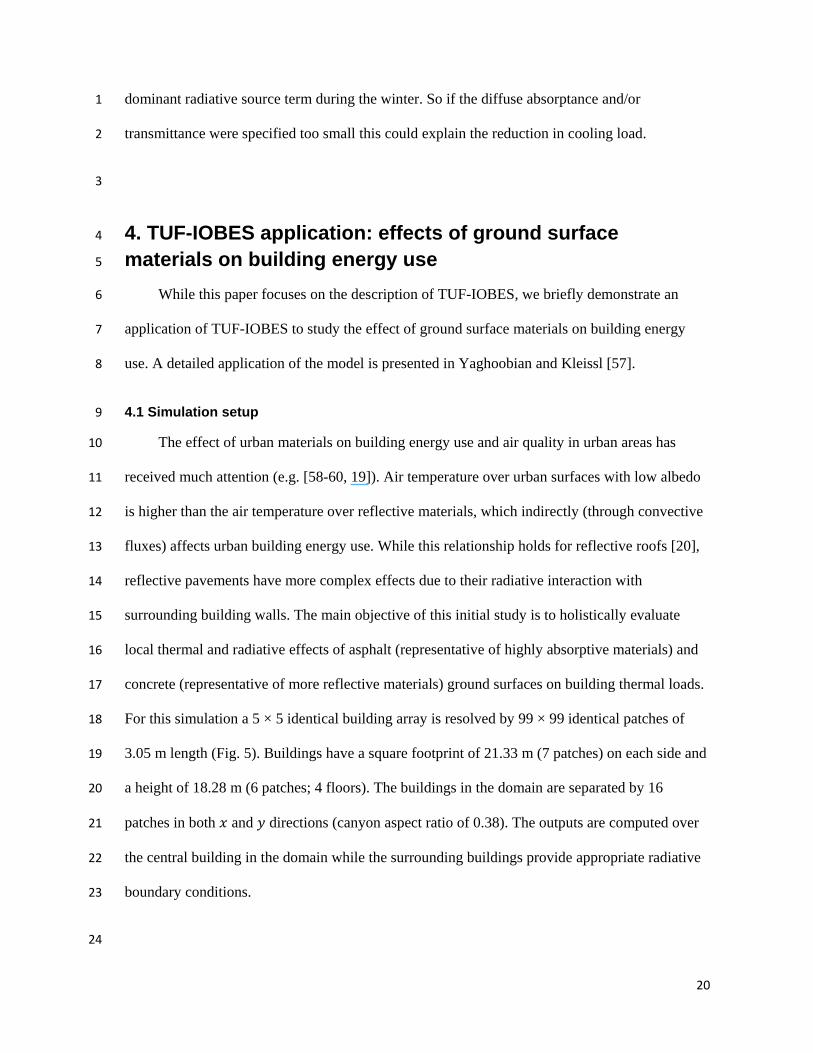
4. TUF-IOBES application: effects of ground surface 4 

materials on building energy use 5 

While this paper focuses on the description of TUF-IOBES, we briefly demonstrate an 6 

application of TUF-IOBES to study the effect of ground surface materials on building energy 7 

use. A detailed application of the model is presented in Yaghoobian and Kleissl [57]. 8 

4.1 Simulation setup 9 

The effect of urban materials on building energy use and air quality in urban areas has 10 

received much attention (e.g. [58-60, 19]). Air temperature over urban surfaces with low albedo 11 

is higher than the air temperature over reflective materials, which indirectly (through convective 12 

fluxes) affects urban building energy use. While this relationship holds for reflective roofs [20], 13 

reflective pavements have more complex effects due to their radiative interaction with 14 

surrounding building walls. The main objective of this initial study is to holistically evaluate 15 

local thermal and radiative effects of asphalt (representative of highly absorptive materials) and 16 

concrete (representative of more reflective materials) ground surfaces on building thermal loads. 17 

For this simulation a 5 × 5 identical building array is resolved by 99 × 99 identical patches of 18 

3.05 m length (Fig. 5). Buildings have a square footprint of 21.33 m (7 patches) on each side and 19 

a height of 18.28 m (6 patches; 4 floors). The buildings in the domain are separated by 16 20 

patches in both and directions (canyon aspect ratio of 0.38). The outputs are computed over 21 

the central building in the domain while the surrounding buildings provide appropriate radiative 22 

boundary conditions. 23 

24 

21 

Fig. 5 Surface temperatures in the TUF‐IOBES simulation domain with canopy aspect ratio of 0.38 at 1200 LST of 1 

January 1st in San Diego, CA. The length of each patch is 3.05 m. The center 4 × 5 patches of each façade are 2 

windows. 3 

4 

Building and system characteristics and the amounts of internal loads are chosen similar to 5 

the characteristics of prototypical post-1980 office buildings provided in Akbari et al. [20]. Each 6 

wall of the building has a double glazing window with dimensions 12.19 m (4 patches) height × 7 

15.24 m (5 patches) width resulting in a window fraction of 0.47. Every day from 0600 to 1900 8 

LST each floor is occupied by 25 persons. Internal load from lighting is 15.07 W m-2 and from 9 

equipments is 16.14 W m-2 of floor area. The HCAV system operates continuously. Coefficient 10 

of performance (COP) of the HVAC system is 2.9 with cooling setpoint of 25.55˚C and heating 11 

setpoint of 21.11˚C. Infiltration is neglected. TMY3 weather data file for Miramar station 12 

(KNKX at 32.87˚ north latitude, 117.13˚ west longitude and 140 m altitude) in San Diego, 13 

California is used as forcing data at reference height. Properties of the building envelope and 14 

ground surface and sub-surface materials are presented in Tables 2 and 3. Deep soil temperature 15 

is the same in both asphalt and concrete cases and it is simulated based on TMY air temperature 16 

(Eq. 3). 17 

TABLE. 2 Building and ground material thickness and thermal and radiative properties by layer. Material properties 18 

are chosen based on Incropera and DeWitt [61] and examples in the ASHRAE toolkit and. 19 

20 

Table. 3 Angular and diffuse Solar Heat Gain Coefficient (SHGC), absorptance and transmittance of window glass. 21 

Glass properties are chosen based on examples in the ASHRAE toolkit. 22 

23 

4.2 Results and Discussion 24 

Fig. 6 shows a comparison of temperatures of ground surface, canopy air, outside building 25 

wall, inside building surfaces with the transmitted shortwave radiation into the building and 26 

hourly thermal loads for July 10th (a clear day with average wind speed of 3 m s-1) between the 27 

22 

simulations using asphalt and concrete ground surfaces. Roof surface temperature is not shown 1 

since in TUF-IOBES it is independent of the ground surface material. 2 

3 

FIG. 6 Comparison of a) ground surface, b) canopy air, c) outside building wall and d) inside building surface 4 

temperatures, e) transmitted shortwave radiation into the building, and f) hourly thermal loads for asphalt and 5 

concrete ground surface material for a summer day (July 10th) in San Diego, California. Outside building wall 6 

temperature is averaged over all four outside walls excluding windows. Inside building surface temperature is the 7 

average temperature of all surface temperatures inside the building excluding windows 8 

9 

The difference in albedo and (less so) other material thermal properties causes a higher 10 

ground surface temperature on asphalt than concrete with the maximum difference of 9.9˚C. 11 

Since TUF-IOBES assumes perfect advection from inside the canopy to the atmospheric surface 12 

layer, the air temperature above the asphalt is only up to 0.25˚C higher than that over concrete 13 

surface. Ground surface materials affect building surfaces directly (through radiation) and 14 

indirectly (through convection). Fig. 6c shows that despite the higher ground surface temperature 15 

and canopy air temperature over asphalt, building walls are cooler (with maximum difference of 16 

1.24˚C) than over concrete. With the simpler TUF3D model, Yaghoobian et al. [32] similarly 17 

demonstrated that the thermal exchange between ground surfaces and walls is dominated by the 18 

effects of net shortwave radiation. Consequently, the larger building wall temperature over 19 

concrete is directly related to the higher albedo of concrete (0.35) than asphalt (0.18). Higher 20 

reflection from concrete also results in a 19.8% increase in total transmitted shortwave radiation 21 

into the building (Fig. 6e). Together, the larger transmitted shortwave radiation and larger heat 22 

conduction through the building envelope result in larger inside building wall (Fig. 6d) and 23 

indoor air temperatures. The contribution of transmitted shortwave radiation through windows on 24 

indoor temperatures is larger than the effects of conductive heat transfer through the building 25 

23 

envelope (Fig.6c, 6e). Consequently, the daily AC energy use to keep the indoor air temperature 1 

at the cooling setpoint increases 10.2% for the concrete ground surface (Fig. 6f). 2 

During the winter the same processes cause a reduction in heating load over concrete. The 3 

total yearly cooling energy use for concrete is 7.5% (31 MWh) larger and total yearly heating 4 

energy use is 4.1% (0.9 MWh) smaller than over an asphalt surface. While the relative increases 5 

are similar the absolute magnitude of cooling energy use increase trumps the heating load 6 

savings resulting in an overall increase in building energy use near more reflective ground 7 

materials. These results differ from previous research. Other researchers focused on the increase 8 

in air temperature over dark surfaces compared to reflective surfaces ignoring the effect of 9 

reflected solar radiation on nearby buildings. This approach is justified for cool roofs, but 10 

inappropriate for cool pavement studies. Ground surface materials affect buildings both directly 11 

and indirectly and TUF-IOBES results show that in above scenario direct radiative effects are 12 

locally dominant. 13 

14 

5. Conclusion 15 

An indoor-outdoor dynamically coupled urban model has been presented. The Temperature 16 

of Urban Facets Indoor-Outdoor Building Energy Simulator (TUF-IOBES) provides scientific 17 

and engineering results with policy relevance, for example by studying the holistic impact of 18 

heat island mitigation measures. TUF-IOBES was validated against analytical heat transfer 19 

results and against previously validated and well-known building energy models. Results of 20 

these carefully conducted tests indicate that TUF-IOBES can accurately simulate the thermal 21 

behavior of a building. Simulations of annual thermal loads on about two days of a single 22 

processor are possible in this two-way coupled model. The effect of a large number of 23 

parameters such as building conditions (e.g. infiltration rate, construction materials, window size 24 

24 

and type), canopy aspect ratio, and weather type (very hot and cold cities) on building thermal 1 

loads can be investigated [57]. 2 

TUF-IOBES is one of the first three-dimensional fully-coupled indoor-outdoor building 3 

energy simulators. Given the complexity of solar irradiance fields in the urban canopy the 4 

surface temperature fields and energy use can be simulated more faithfully. TUF-IOBES 5 

provides unprecedented insight into urban canopy and building energy heat transfer processes. It 6 

can improve our understanding of how urban geometry and material modifications and the 7 

interaction between buildings and their surroundings and dynamic combination of all of these 8 

effects in three dimensions modify urban energy use. Additional capabilities need to be 9 

developed such as more flexible model geometry to accommodate any possible building and 10 

canyon shape, more sophisticated HVAC system models, more sophisticated models for 11 

simulating vegetated surfaces (other than using Bowen ratio in Yaghoobian et al. [32]) and the 12 

water balance in urban areas. The TUF-IOBES outdoor convection model is simplistic albeit no 13 

,more so than in other building energy models. Also, the feedback of changes in the urban 14 

canopy and anthropogenic heat release onto the atmospheric surface layer cannot be simulated, 15 

since the boundary conditions are imposed in the surface layer. In this case, models that can 16 

simulate the full boundary layer and mesoscale effects are more applicable (e.g. WRF-Urban 17 

[27]; Krayenhoff and Voogt [62]). 18 

19 

20 

Acknowledgements 21 

We thank (i) Scott Krayenhoff (University of British Columbia) for providing the TUF3D 22 

model, (ii) Chunsong Kwon (University of California, San Diego) for his contribution in 23 

importing TMY file into TUF-IOBES, (iii) Ron Judkoff and Joel Neymark in National 24 

25 

Renewable Energy Laboratory for providing BESTEST weather data. (iv) Funding from a 1 

National Science Foundation CAREER award. 2 

3 

26 

6. Appendix 1 

TABLE. A1 Building element thermal properties and thickness by layer for cooling and heating load validations 2 

against an intermediate floor office in Zmeureanu et al. [54]. For simplicity floor construction is chosen to be the 3 

same as roof. 4 

5 

27 

7. References 1 

[1] R.E. Britter, S.R. Hanna, Flow and dispersion in urban areas, Annual Review of Fluid Mechanics 35 (2003) 469–2 

496.  3 

[2] M.O. Letzel, M. Krane, S. Raasch, High resolution urban large‐eddy simulation studies from street canyon to 4 

neighbourhood scale, Atmospheric Environment 42 (2008) 8770–8784. 5 

[3] G.T. Johnson, T.R. Oke, T.J. Lyons, D.G. Steyn, I.D. Watson, J.A. Voogt, Simulation of Surface Urban Heat Islands 6 

under ‘Ideal’ Conditions at Night. Part I: Theory and Tests Against Field Data, Boundary Layer Meteorology 56 7 

(1991) 275–294. 8 

[4] G.M. Mills, Simulation of the Energy Budget of an Urban Canyon‐I. Model Structure and Sensitivity Test, 9 

Atmospheric Environment 27(1993) 157–170. 10 

[5] J. Arnfield, J.M. Herbert, G.T. Johnson, A Numerical Simulation investigation of Urban Canyon Energy Budget 11 

Variations, in Proceedings of 2nd AMS Urban  environment Symposium (1998). 12 

[6] V. Masson, A physically based scheme for the urban energy budget in atmospheric models, Boundary Layer 13 

Meteorology 94 (2000) 357‐397. 14 

[7] C.S.B. Grimmond, T.R. Oke, H.A. Cleugh, The role of ‘rural’ in comparisons of observed suburban–rural flux 15 

differences. Exchange processes at the land surface for a range of space and time scales, International Association 16 

of Hydrological Sciences Publication 212 (1993) 165–74. 17 

[8] T.R. Oke, The surface energy budget on urban areas. Modeling the Urban Boundary Layer, American 18 

Meteorological Society, 1987, pp. 1‐52 19 

[9] Y. Kikegawa, Y. Genchi, H. Yoshikado, H. Kondo, Development of a numerical simulation system toward 20 

comprehensive assessments of urban warming countermeasures including their impact upon the urban buildings’ 21 

energy‐demands, Applied Energy 76 (2003) 449–466. 22 

[10] Y. Kikegawa, Y. Genchi, H. Kondo, K. Hanaki, Impacts of city‐block‐scale countermeasures against urban heat 23 

island phenomena upon a building’s energy‐consumption for air conditioning, Applied Energy 83 (2006) 649–668. 24 

[11] A. Krpo, F. Salamanca, A. Martilli, A. Clappier, On the impact of anthropogenic heat fluxes on the urban 25 

boundary layer: a two‐dimensional numerical study, Boundary Layer Meteorology 136 (2010) 105‐127. 26 

[12] C.S.B. Grimmond, M. Best, J. Barlow, A.J. Arnfield, J.J. Baik, S. Belcher, M. Bruse, I. Calmet, F. Chen, P. Clark, A. 27 

Dandou, E. Erell, K. Fortuniak, R. Hamdi, M. Kanda, T. Kawai, H. Kondo, S. Krayenhoff, S.H. Lee, S.B. Limor, A. 28 

Martilli, V. Masson, S. Miao, G. Mills, R. Moriwaki, K. Oleson, A. Porson, U. Sievers, M. Tombrou, J. Voogt, T. 29 

Williamson, Urban surface energy balance models: model characteristics and methodology for a comparison study. 30 

Meteorological and Air Quality Models for Urban Areas, A.Baklanov et al., Eds., Springer‐Verlag, 2009, 97‐124. 31 

[13] C.S.B. Grimmond, M. Blackett, M.J. Best, J. Barlow, J.J. Baik, S.E. Belcher, S.I. Bohnenstengel, I. Calmet, F. Chen, 32 

A. Dandou, K. Fortuniak, M.L. Gouvea, R. Hamdi, M. Hendry, T. Kawai, Y. Kawamoto, H. Kondo, E.S. Krayenhoff, S.H. 33 

Lee, T. Loridan, A. Martilli, V. Masson, S. Miao, K. Oleson, G. Pigeon, A. Porson, Y.H. Ryu, F. Salamanca, L. Shashua‐ 34 

Bar, G.J. Steeneveld, M. Tombrou, J. Voogt, D. Young, N. Zhang, The International Urban Energy Balance Models 35 

Comparison Project: First results from Phase 1, Journal of Applied Meteorology and Climatology 49 (2010) 1268–36 

1292. 37 

[14] D.J. Sailor, A review of methods for estimating anthropogenic heat and moisture emissions in the urban 38 

environment, International Journal of Climatology 31 (2011) 189–199. 39 

28 

[15] M.J. Best, Progress towards better weather forecasts for city dwellers: from short range to climate change, 1 

Theoretical and applied climatology 84 (2006) 47‐55. 2 

[16] M.P. McCarthy, M.J. Best, R.A. Betts, Climate change in cities due to global warming and urban effects, 3 

Geophysical Research Letters, 37, L09705 (2010) 1‐5. 4 

[17] H. Taha, D. Sailor, H. Akbari, High‐albedo materials for reducing building cooling energy use, Rep. LBL‐3172L 5 

Lawrence Berkeley Laboratory, Berkeley, CA, 1992. 6 

[18] H. Taha, Urban climates and heat islands: Albedo, evapotranspiration, and  nthropogenic heat, Energy and 7 

Buildings 25 (1997) 99‐103. 8 

[19] H. Akbari, M. Pomerantz, H. Taha, Cool surfaces and shade trees to reduce energy use and improve air quality 9 

in urban areas, Solar Energy 70 (2001) 295–310. 10 

[20] H. Akbari, S. Konopacki, Calculating energy‐saving potentials of heat‐island reduction strategies, Energy Policy 11 

33 (2005) 721–756. 12 

[21] H. Shen, H.W. Tan, T. Athanasios, The effect of reflective coatings on building surface temperatures, indoor 13 

environment and energy consumption—An experimental study, Energy and Buildings 43 (2011) 573‐580.  14 

[22] U.S. DOE. EnergyPlus ‐ Engineering reference. 15 

http://apps1.eere.energy.gov/buildings/energyplus/pdfs/engineeringreference.pdf last accessed on April 26, 2011. 16 

[23] C.O. Pedersen, R.J. Liesen, R.K. Strand, D.E. Fisher, L. Dong, P.G. Ellis, A toolkit for building load calculations; 17 

Exterior heat balance (CD‐ROM), American Society of Heating, Refrigerating and Air Conditioning Engineers 18 

(ASHRAE), Building Systems Laboratory, 2001. 19 

[24] G.N. Walton, Thermal Analysis Research Program Reference Manual. NBSSIR 83‐ 2655. National Bureau of 20 

Standards, Washington, DC, 1983. 21 

[25] C.S.B. Grimmond, M. Blackett, M.J. Best, J.J. Baik, S.E. Belcher, J. Beringer, S.I. Bohnenstengel, I. Calmet, F. 22 

Chen, A. Coutts, A. Dandou, K. Fortuniak, M.L. Gouvea, R. Hamdi, M. Hendry, M. Kanda, T. Kawai, Y. Kawamoto, H. 23 

Kondo, E.S. Krayenhoff, S.H. Lee, T. Loridan, A. Martilli, V. Masson, S. Miao, K. Oleson, R. Ooka, G. Pigeon, A. 24 

Porson, Y.H. Ryu, F. Salamanca, G.J. Steeneveld, M. Tombrou, J.A. Voogt, D. Young, N. Zhang, Initial results from 25 

Phase 2 of the international urban energy balance model comparison, International Journal of Climatology 31 26 

(2011) 244–272. 27 

[26] F. Salamanca, A. Krpo, A. Martilli, A. Clappier, A new building energy model coupled with an urban canopy 28 

parameterization for urban climate simulations—part I. formulation, verification, and sensitivity analysis of the 29 

model, Theoretical and applied climatology 99 (2010) 331‐344. 30 

[27] F. Chen, H. Kusaka, R. Bornstein, J. Ching, C.S.B. Grimmond, S. Grossman‐Clarke, T. Loridan, K.W. Manning, A. 31 

Martilli, S. Miao, D. Sailor, F.P. Salamanca, H. Taha, M. Tewari, X. Wang, A.A. Wyszogrodzki, C. Zhang, The 32 

integrated WRF/urban modeling system: development, evaluation, & applications to urban environmental 33 

problems, International Journal of Climatology 31 (2011) 273–288.  34 

[28] B. Bueno, L. Norford, G. Pigeon, R. Britter, Combining a Detailed Building Energy Model with a Physically‐Based 35 

Urban Canopy Model, Boundary Layer Meteorology 140 (2011) 471–489.  36 

[29] J. Bouyer, C. Inard, M. Musy, Microclimatic coupling as a solution to improve building energy simulation in an 37 

urban context, Energy and Buildings 43 (2011) 1549‐1559.  38 

29 

[30] Fluent, Fluent 6.3 User Guide, Fluent Inc., Centerra Resource Park, 10 Cavendish Court, Lebanon, NH 03766, 1 

USA, 2006. 2 

[31] E.S. Krayenhoff, J.A. Voogt, A microscale threedimensional urban energy balance model for studying surface 3 

temperatures, Boundary Layer Meteorology 123 (2007) 433–46. 4 

[32] N. Yaghoobian, J. Kleissl, E.S. Krayenhoff, Modeling the thermal effects of artificial turf on the urban 5 

environment, Journal of Applied Meteorology and Climatology 49 (2010) 332–345. 6 

[33] D. Brown, An Improved Meteorology for Characterizing Atmospheric Boundary Layer Turbulence Dispersion, 7 

Ph.D. Thesis, Department of Mechanical and Industrial Engineering, University of Illinois, Urbana, IL, 1997. 8 

[34] F.C. McQuiston, D.J. Parker, J.D. Spitler, Heating Ventilating and Air Conditioning, John Wiley & Sons Inc., New 9 

York, 2000. 10 

[35] F. Haghighat, H. Liang, Determination of Transient Heat Conduction through Building Envelops‐A review. 11 

ASHRAE Transactions, 98: No. 1, 1992, pp. 284‐290. 12 

[36] M.G. Davies, Transmission and Storage Characteristics of Sinusoidally Excited Walls‐A review, Applied Energy 13 

15 (1983) 167‐231.  14 

[37] P.T. Lewis, D.K. Alexander, HTB2: A Flexible Model for Dynamic Building Simulation, Building and Environment 15 

25 (1990) 7‐16. 16 

[38] J.A. Clarke, Energy Simulation in Building Design, Adam Hilger Ltd., Boston, 1985. 17 

[39] J.R. Waters, A.J. Wright, Criteria for the Distribution of Nodes in Multi‐layer Walls in Finite Difference Thermal 18 

Modeling, Building and Environment 20 (1985) 151‐162. 19 

[40] D.C. Hittle, Response Factors and Conduction Transfer Functions, Unpublished, 1992. 20 

[41] J.E. Seem, Modeling of Heat Transfer in Buildings, Ph.D. Thesis, University of Wisconsin, Madison, WI, 1987. 21 

[42] J. Seem, S. Klein, Transfer functions for efficient calculation of multidimensional transient heat transfer, 22 

Journal of Heat Transfer 111 (1989) 5–12. 23 

[43] D. Hillel, Introduction to soil physics. Academic Press, San Diego, CA, 1982. 24 

[44] J. Wu, D.L. Nofziger, Incorporating temperature effects on pesticide degradation into a management model, 25 

Journal of Environmental Quality 28 (1999) 92‐100. 26 

[45] B.M. Caruta, New Developments in Materials Science research, Nova Science publisher, Inc., 2007. 27 

[46] D.A. Vries De, Thermal properties of soils. In Van Wijk, W. R. (ed.), Physics of Plant Environment, North‐28 

Holland Publishing Co., Amsterdam, 1963. 29 

[47] S.S. Zilitinkevich, Non‐local turbulent transport: pollution dispersion aspects of coherent structure of 30 

convective flows. In: H. Power, N. Moussiopoulos, and C.A. Brebbia (eds.), Air pollution III – Volume I. Air pollution 31 

theory and simulation, Computational Mechanics Publications, Southampton, Boston, 1995, pp 53–60. 32 

[48] E. Guilloteau, Optimized computation of transfer coefficients in surface layer with different momentum and 33 

heat roughness length, Boundary Layer Meteorology 87 (1998) 147–160. 34 

[49] R.J. Cole, N.S. Sturrock, The Convective Heat Exchange at the External Surface of Buildings, Building and 35 

Environment 12 (1977) 207‐214.  36 

30 

[50] M. Yazdanian, J.H. Klems, Measurement of the Exterior Convective Film Coefficient for Windows in Low‐Rise 1 

Buildings. ASHRAE Transactions, Vol. 100, Part 1, 1994. 2 

[51] G.N. Walton, Passive Solar Extension of the Building Loads Analysis and System Thermodynamics (BLAST) 3 

Program, Technical Report, United States Army Construction Engineering Research Laboratory, Champaign, IL, 4 

1981. 5 

[52] Lawrence Berkeley Laboratory (LBL), DOE2.1E‐053 source code, 1994. 6 

[53] G.N. Walton, Algorithm for Calculating Radiation View Factors Between Plane Convex Polygons With 7 

Obstructions, National Bureau of Standards, NBSIR 86‐3463, (1987‐‐‐ shortened report in Fundamentals and 8 

Applications of Radiation Heat Transfer, HTD‐Vol. 72, American Society of Mechanical Engineers), 1987. 9 

[54] R. Zmeureanu, P. Fazio, F. Haghighat, Analytical and interprogam validation of a building thermal model, 10 

Energy and Buildings 10 (1987) 121–133. 11 

[55] A.W. Pratt, Heat Transmission in Buildings, John Wiley and Sons Ltd, 1981. 12 

[56] R. Judkoff, J. Neymark, Building Energy Simulation Test (BESTEST) and Diagnostic Method, National Renewable 13 

Energy Laboratory, Golden, Colorado, 1995. 14 

[57] N. Yaghoobian, J. Kleissl, Effect of Reflective Pavements on Building Energy Use, 2012, In preparation. 15 

[58] A.H. Rosenfeld, H. Akbari, S. Bretz, B.L. Fishman, D.M. Kurn, D. Sailor, H. Taha, Mitigation of urban heat 16 

islands: materials, utility programs, updates, Energy and Buildings 22 (1995) 255–265.  17 

[59] S. Bretz, H. Akbari, A. Rosenfeld, Practical issues for using solar‐reflective materials to mitigate urban heat 18 

islands, Atmospheric Environment 32 (1998) 95–101.  19 

[60] L. Doulos, M. Santamouris, I. Livada, Passive cooling of outdoor urban spaces, The role of materials, Solar 20 

Energy 77 (2004) 231–249.  21 

[61] F.P. Incropera, D.P. DeWitt, Fundamentals of Heat and Mass Transfer 5th Edition, John Wiley & Sons, 2001. 22 

[62] E.S. Krayenhoff, J.A. Voogt, Impacts of Urban Albedo Increase on Local Air Temperature at Daily–Annual Time 23 

Scales: Model Results and Synthesis of Previous Work, Journal of Applied Meteorology and Climatology 49 (2010) 24 

1634–1648.  25 

   26 

31 

Figure Captions 1 

FIG. 1 Temporal variation of the inside surface temperature ( ) of a 0.28 m brick cavity wall 2 

after a step change in outdoor air temperature of ∆ at time zero. The -axis scale is the relative 3 

change of the hourly interior surface temperature with respect to the drop in OAT at initial time 4 

based on Zmeureanu et al. [54] 5 

6 

FIG. 2 a) Annual heating, b) annual cooling, c) peak heating, and d) peak cooling loads ( ) 7 

comparisons between TUF-IOBES and other building energy balance models provided in 8 

BESTEST 9 

10 

FIG. 3 Comparison of hourly variation of thermal loads ( ) on January 4th for BESTEST case 11 

600 in Denver, CO. Positive thermal loads are heating loads and negative loads are cooling loads 12 

13 

FIG. 4 Heating (a) and cooling (b) load comparison between TUF-IOBES, BLAST, CBS-MASS, 14 

TARP, and BEM (a only) for an office space on a winter (a) and summer (b) design day in 15 

Montreal. The total load from BEM was digitized from Fig. 5b in Salamanca et al. [26] 16 

17 

Fig. 5 Surface temperatures in the TUF-IOBES simulation domain with canopy aspect ratio of 18 

0.38 at 1200 LST of January 1st in San Diego, CA. The length of each patch is 3.05 m. The 19 

center 4 × 5 patches of each façade are windows. 20 

21 

FIG. 6 Comparison of a) ground surface, b) canopy air, c) outside building wall and d) inside 22 

building surface temperatures, e) transmitted shortwave radiation into the building, and f) hourly 23 

thermal loads for asphalt and concrete ground surface material for a summer day (July 10th) in 24 

San Diego, California. Outside building wall temperature is averaged over all four outside walls 25 

excluding windows. Inside building surface temperature is the average temperature of all surface 26 

temperatures inside the building excluding windows 27