
ANALYSES OF RESIDENTIAL BUILDING ENERGY ...
123
ABSTRACT Title of Document: ANALYSES OF RESIDENTIAL BUILDING ENERGY SYSTEMS THROUGH TRANSIENT SIMULATION Andrew Cameron Mueller, Master of Science in Mechanical Engineering, 2009 Directed By: Dr. Reinhard Radermacher, Director, Center for Environmental Energy Engineering This thesis examines the performance of residential buildings and the energy systems contained within those buildings by simulating them in the TRaNsient SYstems Simulation (TRNSYS) program. After matching a building’s floorplan to that of house local to the College Park area, national and local building surveys were consulted to produce a prototype of the average Maryland home. This home was simulated with ordinary insulation levels, heating, ventilation, and air conditioning (HVAC) equipment, and appliances. Various construction characteristics, including wall insulation, thermostat set points, HVAC equipment, and appliance efficiency were varied to examine the effects of each individual change upon the final annual energy consumption of the building, and in doing so, the value of retrofitting each characteristic was explored. Finally, the most effective energy-saving strategies were combined to model a low-energy home, in order to explore the possibility of refitting an existing home to become a net-zero site energy building. Sensitivity study results were listed, and a net-zero-energy building was successfully simulated.
-
Upload
khangminh22 -
Category
Documents
-
view
0 -
download
0
Transcript of ANALYSES OF RESIDENTIAL BUILDING ENERGY ...
ABSTRACT
Title of Document: ANALYSES OF RESIDENTIAL BUILDING
ENERGY SYSTEMS THROUGH TRANSIENT
SIMULATION
Andrew Cameron Mueller, Master of Science in
Mechanical Engineering, 2009
Directed By: Dr. Reinhard Radermacher, Director, Center for
Environmental Energy Engineering
This thesis examines the performance of residential buildings and the energy
systems contained within those buildings by simulating them in the TRaNsient SYstems
Simulation (TRNSYS) program. After matching a building’s floorplan to that of house
local to the College Park area, national and local building surveys were consulted to
produce a prototype of the average Maryland home. This home was simulated with
ordinary insulation levels, heating, ventilation, and air conditioning (HVAC) equipment,
and appliances. Various construction characteristics, including wall insulation, thermostat
set points, HVAC equipment, and appliance efficiency were varied to examine the effects
of each individual change upon the final annual energy consumption of the building, and
in doing so, the value of retrofitting each characteristic was explored. Finally, the most
effective energy-saving strategies were combined to model a low-energy home, in order
to explore the possibility of refitting an existing home to become a net-zero site energy
building. Sensitivity study results were listed, and a net-zero-energy building was
successfully simulated.
Analyses of Building Energy System Alternatives through Transient Simulation
By
Andrew Cameron Mueller
Thesis submitted to the Faculty of the Graduate School of the
University of Maryland, College Park, in partial fulfillment
of the requirements for the degree of
Master of Science
2010
Advisory Committee:
Professor Reinhard Radermacher, Chair
Associate Professor Tien-Mo Shih
Associate Professor Gregory Jackson

© Copyright by
Andrew Cameron Mueller
2010

ii
Dedication
This thesis is dedicated to the good people of the CEEE. Paraphrasing the words of a
colleague, who said it better than I could hope to myself; their energetic enthusiasm,
professional dedication, and matchless moral fortitude leave me confident that the future
of the engineering profession is in good hands, and whose sheer aptitude leaves me no
doubt that the current engineering crises of the world have met their match.

iii
Acknowledgements
I would like to convey my gratitude first and foremost to my advising professors, Dr.
Yunho Hwang and Dr. Reinhard Radermacher for their guidance and leadership during
the past year.
I would also like to thank Kyle Gluesenkamp, Joshua Scott, and John Bush, my
colleagues in the SAES consortium, whose technical advice and friendly assistance
played key roles in the progress of my research; my officemates Amir Mortazavi, Ali Al-
Alili, and Abdullah Al-Abdulkarem, who also provided important technical advice, and
perhaps more importantly, never failed to keep my spirits high; the remaining members
of the CEEE (whose numbers are too great to list individually by name); ENS Andrew
Chaloupka, my friend, naval colleague, and a recent Clark School Mechanical
Engineering Masters alumnus; my family for their support and understanding during the
gauntlet that was the past few months; and many others without whose friendship and
support I could not have reached this point.

iv
Table of Contents
Dedication ............................................................................................................ i
Acknowledgements ............................................................................................ ii
Table of Contents ............................................................................................... iii
List of Tables ...................................................................................................... iv
List of Figures ..................................................................................................... v
1. Introduction ..................................................................................................... 1
1.1 Acceptance of Energy Efficient Technologies .............................................. 2
1.2 Value of Retrofit .......................................................................................... 5
1.3 Simulation .................................................................................................... 5
2. Literature Review ............................................................................................ 6
3. Objectives ........................................................................................................ 9
4. Simulation Tool Development ...................................................................... 10
4.1 Building ...................................................................................................... 12
4.1.1 TRNBUILD .......................................................................................... 12
4.1.2 Building Layout .................................................................................... 16
4.1.3 Low-energy Building Model ................................................................. 20
4.1.4 Fenestration ........................................................................................ 20
4.1.5 Insulation ............................................................................................. 22

v
4.1.6 Infiltration ............................................................................................. 24
4.1.7 Ventilation ........................................................................................... 28
4.1.8 Occupancy .......................................................................................... 30
4.2 Weather ..................................................................................................... 31
4.3 Building Controls ........................................................................................ 33
4.4 HVAC ......................................................................................................... 38
4.5 Setback Schedules .................................................................................... 43
4.6 Sizing the Climate Control System ............................................................ 47
4.7 Photovoltaics Macro .................................................................................. 54
4.8 Energy Macro ............................................................................................ 56
4.9 Load profiles .............................................................................................. 57
4.10 Non-HVAC Electrical Load Profiles .......................................................... 57
4.11 DHW Load Profiles .................................................................................. 60
4.12 Hot Water System .................................................................................... 64
5. Validation of Baseline Model ....................................................................... 68
6. Simulation Results ........................................................................................ 71
6.1 Envelope Simulations ................................................................................ 71
6.2 Envelope Sensitivity Analysis .................................................................... 86
6.3 Indoor Equipment Simulations ................................................................... 87

vi
6.4 Zero-Energy House Simulation .................................................................. 94
7. Conclusion .................................................................................................... 98
8. Future Recommendations ............................................................................ 99
9. References................................................................................................... 103

vii
List of Tables
Table 1: Building Characteristics………………………………………………………...19
Table 2: Insulation Values…………………………………………………………….…23
Table 3: Thermostat Setback Settings…………………………………………………...47
Table 4: Load Profile Usage Targets…………………………………………………….60
Table 5: Basement Insulation Simulation Results……………………………….………72
Table 6: Infiltration Simulation Results…………………………………………………73
Table 7: Wall Insulation Simulation Results…………………………………………….74
Table 8: Attic Insulation Simulation Results…………………………………………….76
Table 9: First Floor Insulation Simulation Results………………………………………77
Table 10: Window U-Value Simulation Results………………………………………...78
Table 11: Window SHGC Simulation Results……………………………………….….79
Table 12: Albedo Change Simulation Results…………...………………………………82
Table 13: Total Envelope Insulation Simulation Results…………………….………….86
Table 14: Furnace/AC Comparison with Heat Pump…………………..………………..88
Table 15: Set Point Simulation Results……………………………………………….....89
Table 16: Hot Water Simulation Results………………………………………………...92
Table 17: ZEH Simulation Results………………………………………………..……..97
viii
List of Figures
Figure 1: Overall Simulation Structure .................................................................................... 12
Figure 2: Average New House Floor Area vs. Year .............................................................. 19
Figure 3: Weather Macro ........................................................................................................... 34
Figure 4: HVAC Macro ............................................................................................................... 39
Figure 5: Baseline HVAC System ............................................................................................ 41
Figure 6: Scheduling Submacro ............................................................................................... 44
Figure 7: Setpoints with Setback and Season Change ........................................................ 46
Figure 8: HVAC Load Monitor Construction ........................................................................... 49
Figure 9: HVAC Load Monitor Output ...................................................................................... 50
Figure 10: Sample Comfort Zone Monitor Output ................................................................. 53
Figure 11: Modified HVAC System .......................................................................................... 54
Figure 12: Photovoltaics System .............................................................................................. 56
Figure 13: Photovoltaics Output. .............................................................................................. 56
Figure 14: Energy Macro ........................................................................................................... 57
Figure 15: Domestic Hot Water System .................................................................................. 67
Figure 16: Basement Temperature Differences .................................................................... 69
Figure 17: Baseline Simulation Results .................................................................................. 71
Figure 18: 3-Week Attic Temperature ..................................................................................... 88
Figure 19: Envelope Characteristic Sensitivity Comparison ................................................ 90
Figure 20: Low- Energy House Temperature Readings ....................................................... 99

1
1. Introduction
The United States of America has, as of late, experienced a wake-up call of
massive proportions regarding the health of the environment. For years, since
the beginning of the Industrial Revolution, pollution and energy consumption had
always been a secondary topic. In the past decades, however, the environment
has become an increasingly important issue in the eyes of Americans. An annual
Gallup poll finds that Americans have considered the protection of the
environment more important than the economy for the past seven years (2002-
2008) [1]. A major focus of this new environmental concern has been global
warming, and perhaps more specifically, carbon emissions, as a result of a slew
of scientific reports finding adverse trends in the global climate, including, most
famously, those released by the United Nations Environment Programme’s
Intergovernmental Panel on Climate Change. This specific concern has begun to
pervade the public arena, both in the cinema, where such films as The Day After
Tomorrow and An Inconvenient Truth have enjoyed widespread, mainstream
attention, and in daily life, where attention to global warming has increasingly
become part of advertising campaigns for numerous everyday products.
As a result of the new strength of this fixation, political forces have begun to
engage more intently with the environment as an issue, with the 2009 stimulus
package dedicating approximately 55 billion dollars to promoting environmental
protection procedures and energy-saving measures [2]. A large part of this
money, approximately 24 billion, has been devoted to building new homes and
2
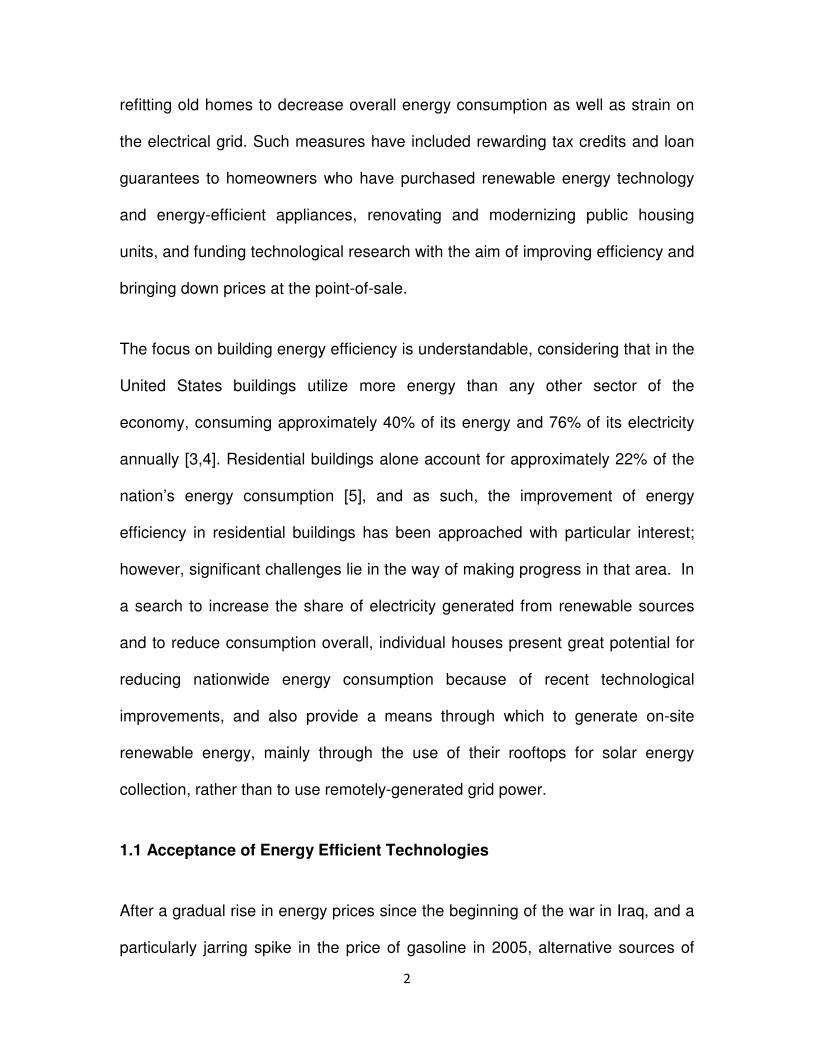
refitting old homes to decrease overall energy consumption as well as strain on
the electrical grid. Such measures have included rewarding tax credits and loan
guarantees to homeowners who have purchased renewable energy technology
and energy-efficient appliances, renovating and modernizing public housing
units, and funding technological research with the aim of improving efficiency and
bringing down prices at the point-of-sale.
The focus on building energy efficiency is understandable, considering that in the
United States buildings utilize more energy than any other sector of the
economy, consuming approximately 40% of its energy and 76% of its electricity
annually [3,4]. Residential buildings alone account for approximately 22% of the
nation’s energy consumption [5], and as such, the improvement of energy
efficiency in residential buildings has been approached with particular interest;
however, significant challenges lie in the way of making progress in that area. In
a search to increase the share of electricity generated from renewable sources
and to reduce consumption overall, individual houses present great potential for
reducing nationwide energy consumption because of recent technological
improvements, and also provide a means through which to generate on-site
renewable energy, mainly through the use of their rooftops for solar energy
collection, rather than to use remotely-generated grid power.
1.1 Acceptance of Energy Efficient Technologies
After a gradual rise in energy prices since the beginning of the war in Iraq, and a
particularly jarring spike in the price of gasoline in 2005, alternative sources of

3
energy and energy efficiency began to gain more and more attention by the
media, politicians, and as a result, the average American consumer [6]. However,
many energy-efficient technology choices have not yet been absorbed into the
mainstream of residential building attributes, despite the fact that many such
energy-saving devices have been shown to be wise long-term financial
investments. A number of economic and sociological studies have investigated
the phenomena preventing green technology from being accepted by the free
market and by the general public.
The penetration of energy efficient technology into the residential sector depends
a great deal upon the confidence level of the average American consumer in
their viability as reliable and cost-saving devices. Wuestenhagen writes that three
main factors will determine the ability of renewable technology to break into the
mainstream: sociopolitical acceptance, community acceptance, and market
acceptance.[7] While the concept of moving away from fossil fuels to cheaper
and infinite energy sources (temporally speaking) like sunlight has been met with
great enthusiasm by the general public of America, he says that individual
citizens have to grow to trust these technological innovations before they can be
used in a widespread manner, and the market must in turn see this trust and
individual acceptance as a representation of a potential customer base before
they will produce large-enough quantities of these technologies.
Coombs recognizes a variety of obstacles to widespread adoption of energy-
saving technology [8]. Among these are the strength of incumbent technologies,
4
such as the large amount of sociopolitical power resting with the fossil-fuel
industry, the lack of existent support systems (for sake of clarity one might
consider the absence of hydrogen fuel pumps at many gas stations), and lack of
communication of the public’s need for the product. Among his recommendations
for overcoming such obstacles are passing favorable legislation to nurture the
growth of the relatively young and fragile technology’s market share, which as
mentioned previously, is being undergone, and to communicate clearly to the
potential customer base the benefits of the technology can provide them as
individuals.
As an immature industry, renewable energy systems are expensive to produce,
and their high costs have prevented widespread adoption, but compounding the
problem of prohibitive cost is the fact that the energy systems remain unnervingly
novel and foreign to many American consumers. To combat this unfamiliarity,
the government, particularly the Department of Energy and many state
governments, have pursued a variety of campaigns dedicated to informing the
general public of the environmental and financial benefits of making energy-
saving building modifications. However, despite the campaigns and the fact that
many renewable technologies present cost-saving opportunities, many current
energy-efficient technologies remain untapped by the mainstream of American
residential buildings. This thesis serves to provide a method by which the merits
and disadvantages of these technologies can be understood.

5
1.2 Value of Retrofit
The retrofitting of currently standing buildings is challenging, but it is a necessary
task if the energy consumption of the nation’s buildings is to be decreased.
Studies of the service lives of residential buildings estimate that the average
lifespan of a house is as much as 90 years, and some last much longer [9,10].
This would suggest that the building codes dictating the quality of new-
construction buildings will not reach the whole of the U.S. building stock only very
gradually. Thus, although designing new residences to be energy efficient is
indeed a key part of ensuring an energy efficient future, the above service life
estimations suggest that relying on solely those new designs would not be
sufficient to counteract the rapidly-moving climatic changes reported by the
IPCC, and that retrofit plays a very important role in reducing energy
consumption and pollutant emissions in a timely manner.
1.3 Simulation
As the speed of computer processors continues to grow, simulation has become
an increasingly accessible and powerful tool in the building research community,
and has been adopted because of its ability to estimate real-life conditions
without the expense of “hard” resources and funds. Numerous programs, varying
in levels of specificity and breadth of scope, have been developed. TRNSYS is
one of the many tools for building energy analysis [11]. Developed by the

6
University of Wisconsin at Madison, the program was originally designed to
simulate the transient performance of a solar hot water system, but has
expanded in scope to simulate the performance of many types of energy
systems. TRNSYS’ main, and, generally considered, most promising feature is its
modularity, and the flexibility that comes with such an approach. Given the wide
variety of layouts of household HVAC, hot water, and controls systems, TRNSYS
is particularly well-suited due to its ability to allow for the creation of new
components, which allows for the exploration of new technologies far more easily
than in less flexible software. The particular strength of TRNSYS in evaluating
complex thermal systems such as a modern home is reiterated in past studies
comparing each major competitor software program in the thermal simulation
community [12]. Also, although TRNSYS’ base code was not altered in this
simulation, TRNSYS’ code is also highly modifiable, being written in FORTRAN,
a common engineering programming language. The value of using TRNSYS and
the decision-making process used for purchasing TRNSYS instead of any other
software package has been explained in a past CEEE thesis [13].
2. Literature Review
2.1. Simulation of Residences
There have been numerous studies concerning simulation of low-energy
residences. Many of these have been feasibility studies, conducted in order to

7
verify expectations of building energy performance within a given climate, or to
test specific, new-construction buildings’ expected energy consumption levels.
The main focus of much simulation has been in the building of new energy-
efficient and zero-energy houses. Such examples may be seen in the work of
Tse (2007) [14], who used TRNSYS as a tool to determine the design of a new
set of net-zero-energy townhomes in the Toronto area. Another study made use
of TRNSYS to simulate the feasibility of constructing a new low-rise home in the
Netherlands which would meet zero-net-energy status [15]. Another investigates
the possibility of constructing such a home in the cold and windy weather of
Newfoundland [16].
The program created and the simulations performed during the course of this
thesis undoubtedly are of some value for designing new residential buildings with
superior energy performance. However, the main focus is not on new
construction, but rather on retrofits, and providing data regarding the effects of
possible modifications on building energy consumption and human comfort.
2.2. Retrofit Simulation
The concept of using simulation software to model retrofit savings has indeed
been used previously in academic studies, although not in a widespread manner.
Despite the existence of the already mentioned studies, retrofit analysis studies
have not been widely performed on single-family residences. Most research has
been done on specific buildings of large energy consumption. There are logical
8
reasons for this pattern. Truly accurate building models require an exhaustively
detailed survey of such things as a building’s particular geometry, its behavior
with respect to infiltration, and many times these involved processes yield no
results that can be transferred over to other buildings, which each have their own
set of idiosyncrasies. Thus large scale projects are routinely the only situations in
which the potential immediate savings in energy consumption are worth the effort
of creating such a detailed simulation. A study at Texas A&M University in 1991
utilized simulation software to study the effect of retrofitting a laboratory with a
variable air volume HVAC system instead of the dual duct constant volume
system it had, which involved simulating two buildings, of equal size, layout, and
envelope, and examining the energy used by each system to condition this
standard load [17]. Another study by NIST uses TRNSYS to explore the effect of
air-tightness upon an office building’s energy consumption [18].
Only one paper found in this literature review has attempted to explore the
importance of a wide range of residential building attributes as is done in this
thesis. It was performed by Verbeeck and Hens, with the intention of determining
the most cost-effective available envelope and HVAC system option [19].
Verbeeck and Hens conducted an analysis of real buildings in Belgium, and
engaged in simplified building simulations by use of calculation procedures
developed by the Belgian Laboratory of Building Physics. The simulation
mentioned, however, was not a transient simulation, instead compiling annual
estimates to create one building net energy consumption level. In addition to
providing a transient evaluation of building performance, this thesis intends to

9
explore further characteristics of the building, including building controls, and to
allow for the simulation of additional space conditioning and water heating
system layouts.
As Verbeeck notes, the majority of building simulation projects are undertaken in
order to explore one option of improving a building’s energy efficiency, rather
than comparing the effectiveness of an array of options. While many separate
studies have investigated individual energy-saving modifications, this thesis
intends to compare the various options on a single home, providing more
consistency than to compare different modifications effects on different building
layouts. This thesis will examine a wide variety of building characteristics to
demonstrate each characteristic’s importance to the building’s annual energy
consumption. Each characteristic has been investigated to some extent
previously and therefore the history surrounding the study of each will be
presented along with that series of simulations.
3. Objectives
The objectives of this thesis are threefold. First, the thesis investigates the
importance of many building characteristics in determining the final annual
energy consumption of a building by undergoing a sensitivity analysis, in order to
shed light on which aspects of a building’s construction are most deserving of
attention when retrofitting a house for energy savings. In doing so, it explores the

10
feasibility of various building energy systems for use in the vicinity of College
Park, MD, by comparing the effects of some of the many options for space-
conditioning, water heating, insulation, and appliances on the total annual energy
performance of a College Park area home.
Second, the model is meant to provide a realistic building model on which to
simulate future CEEE projects. The model is currently being used to provide a
check for the sufficiency of capacity in the CEEE’s experimental combined
heating and power unit. Future potential projects could be first simulated on the
building model before being attached to an actual building, to ensure the ability of
a system to meet a building’s conditioning requirements by providing a
theoretical estimation of actual building system performance.
Third, the program has been designed to act as the first step towards a program,
which, in the future, could allow homeowners to simulate their own house’s
annual energy consumption, and to compare, for example, the costs and benefits
of installing different space-conditioning systems. The personalized analysis
would then allow the homeowner to estimate the energy savings he or she might
achieve by making energy-efficient modifications to his or her building. The
program has been designed such that a number of common building
modifications can be selected and compared to a baseline home to provide such
data.

11
4. Simulation Tool Development
The building analysis tool is based on a variety of components, each of which
performs calculations to simulate the behavior of a certain aspect of the
building’s operation. The following section will present an overview of the
methods used in creating the simulation program, including assumptions made
and the mathematical equations inherent to the operation of certain important
components. Figure 1 Displays the Simulation’s overall structure. Each arrow
indicates an information flow from one component to another, for example, the
“weather macro” component outputs outdoor temperature data, which is then
inputted into the “Building Models” component to provide the temperature for
heat transfer calculations. The notable components, which will be described in
further detail, are:
• The “Building Models,” which contain information concerning the layout of
the buildings simulated in this thesis, and, accordingly, their heat and
humidity transfer characteristics
• The “Weather Macro,” which contains data concerning the building’s local
environment
• The “HVAC Macro,” which contains information concerning the operation
of the buildings’ Heating, Ventilation, and Air Conditioning (HVAC)
systems,
• The “Energy Macro,” which sums and arranges total energy consumption
data over the entire year

12
• The “PV Macro”, which receives insolation data from the Weather Macro
and simulates photvoltaic conversion of light into electrical energy
• The “Hot Water Macro,” which receives hot water demand data from an
Excel spreadsheet and calculates the energy required by a water-heating
system to meet those demands.
Figure 1: Overall Simulation Structure

13
4.1. Building
4.1.1 TRNBUILD
The building model is constructed within the sister program to TRNSYS,
TRNBUILD. TRNBUILD models the building by simulating each thermal zone, in
this case, basically each room of the house, as a single node, rather than
modeling any geometrical shape. Properties are therefore uniform throughout
each thermal zone, which is an important consideration when evaluating the
attainable level of certainty. Two important balance equations exist for each point
in this nodal structure: the energy balance and the humidity balance. All
equations in Section 4.1.1 were drawn from the TRNBUILD manual.
4.1.1.1 Heat Flows
For each timestep TRNBUILD performs the following balance:
��������� = ����,������ + ����,������������ + ����,����������� + ����,��� ���� +
����,�������� + ����,����� (1)
Where ��������� is total heat flux into the thermal zone, and is comprised of
surface convection from walls ����,������, convective heat gains as a result of
infiltration ����,������������, convective gains occurring from airflows from adjacent
zones ����,��� ����, heat gains created within the zone, and radiative gains
����,�����.
14
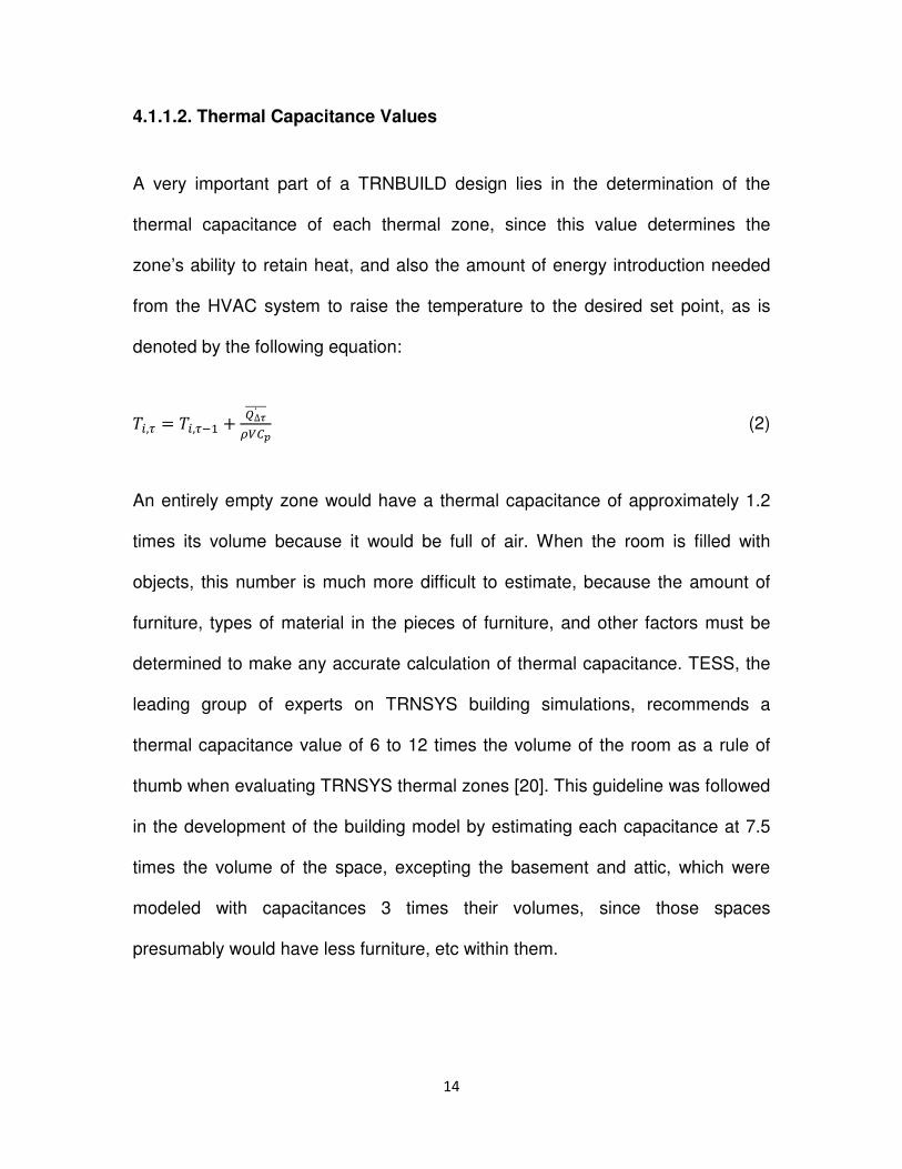
4.1.1.2. Thermal Capacitance Values
A very important part of a TRNBUILD design lies in the determination of the
thermal capacitance of each thermal zone, since this value determines the
zone’s ability to retain heat, and also the amount of energy introduction needed
from the HVAC system to raise the temperature to the desired set point, as is
denoted by the following equation:
��,� = ��,��� + �∆�������� !"
(2)
An entirely empty zone would have a thermal capacitance of approximately 1.2
times its volume because it would be full of air. When the room is filled with
objects, this number is much more difficult to estimate, because the amount of
furniture, types of material in the pieces of furniture, and other factors must be
determined to make any accurate calculation of thermal capacitance. TESS, the
leading group of experts on TRNSYS building simulations, recommends a
thermal capacitance value of 6 to 12 times the volume of the room as a rule of
thumb when evaluating TRNSYS thermal zones [20]. This guideline was followed
in the development of the building model by estimating each capacitance at 7.5
times the volume of the space, excepting the basement and attic, which were
modeled with capacitances 3 times their volumes, since those spaces
presumably would have less furniture, etc within them.

15
4.1.1.3 Humidity flows
TRNBUILD is designed to use either of two models of humidity transfer: a buffer-
storage model and a more simplified capacitance model. The buffer-storage
method makes use of three variables to quantify the ability of the zone node to
hold humidity, the storage ability of the contents within the zone (deep storage),
and the storage ability of the walls surrounding the zone (surface storage). The
capacitance model reduces these variables to one coefficient of humidity
capacitance, similar to a thermal capacitance. In this model, the capacitance
method was used. In future versions, when further detail is proposed as to the
contents of each zone (furniture, etc), the buffer-storage method could prove to
be useful, but since little such detail is known about furniture in this simulation of
a hypothetical building, the capacitance method was chosen.
The capacitance method works as follows: a humidity capacitance ratio C, is
multiplied by the mass of air to produce a total moisture capacity for the room.
The humidity capacitance ratio was determined by consulting values
recommended by the creators of TRNSYS for rooms in residential buildings, and
set at the value of 5 [21]. .
#��� = $ ∗ &��� (3)

16
The moisture addition rate is then calculated similar to the heat transfer
mechanism:
#���,� ∗ '(�') = &��� ∗ *(� − (�, + - *&����,� ∗ *(�
�����− (�,, + (.
+ ∑ *&������� ∗ *(� − (�,, (4)
Where (� is the ambient humidity ratio, (� is the zone’s humidity ratio, &����,� is
the mass flow rate of ventilation, (� is the humidity ratio of ventilated air, (. is
humidity produced within the zone, &��� is the mass flow rate of coupled air
flows from adjacent zones, and (� is the humidity ratio of a particular adjacent
zone.
4.1.1.4 Relationship Between Thermal Energy and Humidity
TRNBUILD models humidity entirely separately from thermal energy. Using a
mass balance based on absolute humidity values, the water content of the room
is calculated at each time step, and in conjunction with the temperature levels
determined by the heat equations, other psychrometric values are calculated,
including relative humidity. In this particular simulation, TRNBUILD does not deal
with, for example, the use of furnace heat to evaporate water in a humidifier.

17
Those are done externally to TRNBUILD by components in the HVAC macro.
These HVAC components run on performance maps, which, given a set of return
temperatures, return humidities, and outdoor temperatures, outputs a particular
sensible heat factor of heat removal (that is, sensible energy removed divided by
total (sensible and latent) energy removed), energy consumption, and set of
conditions for the supply air. Thus thermodynamic equations are not used to
determine conversion of sensible energy into latent energy. Instead, tabulated
observed output values of HVAC equipment are used.
4.1.2 Building Layout & Floor Area
The building’s dimensions are modeled upon a sample two-story, detached
residential building in the College Park area. The layout of the building is
somewhat simplified. It consists of a bottom floor of four rooms, each 308 square
feet (11x14), or 28.61 m2 (designated as a living room, a dining room, a kitchen,
and an entertainment room; and a top floor of two rooms, each of 716 square
feet (57.22 m2). The total amount of finished floor space is 2464 square feet
(228.91 m2).
This square footage is slightly smaller than the national average floor area for
new, detached, single-family residential buildings, which was 2519 square feet,
according to census data compiled in 2008, and slightly smaller than the mean
floor area for the Southern census region (in which Maryland is included), which
was 2564 square feet [22]. The median floor area for new single family homes,
in the nation and in the South respectively, were 2215 and 2312 square feet. The

18
great difference in these mean and median values results from the large number
of small, lower-class residences and the comparatively small number of
significantly larger, high-income housing. It should be noted, however, that the
average floor space has steadily increased over the past three decades, as can
be seen in Figure 2. Thus, its similarity in size to 2008’s new houses prove that
the sample house geometry by no means represents a house out of the
mainstream. However, the fact that the average size of a new home is almost
50% larger than those built only 25 years ago allows the assumption that it is
slightly above average. Furthermore, a Census report from 2001 estimated that
the average age of a U.S. house was 32 years [23]. This statistic, if still true for
today, would make the average floor area of existing homes nearer 1800 sq ft,
making the modeled building significantly larger than average when compared to
all existent homes rather than just newly constructed homes. The point of relative
size is important when comparing each house with average energy consumption
data, since, logically, a larger-than-normal home will consume larger-than normal
amounts of energy. This relative size is important when comparing house
properties, such as heating consumption, to tabulated average values.

19
Figure 2: Average New House Floor Area vs. Year. Data taken from a 2008 U.S. Census Bureau Report [24].
The ceilings of each finished zone are modeled to be the standard height of 8
feet (2.5 m). Thus the total conditioned volume is 19712 cubic feet, or
equivalently 558 cubic meters. There is also an unconditioned basement of 1432
square feet and 7 ft (2.13 m) high walls, assumed to be surrounded on all sides
by earth, and an unconditioned attic, of the same square footage as the
basement but with a pitched ceiling, rising at a grade of 36 degrees to a middle
height of 10.7 ft (3.26 m). The grade of the roof was determined by consulting
generally accepted building construction guidelines, which define “normal” roof
slopes as those between 30 and 45 degrees from the horizontal [25]. The roof
1500
1700
1900
2100
2300
2500
2700
19
73
19
75
19
77
19
79
19
81
19
83
19
85
19
87
19
89
19
91
19
93
19
95
19
97
19
99
20
01
20
03
20
05
20
07
Flo
or
Sp
ace
(sq
ft)
Year
Average New House Floor Area vs. Year
US Median
South
MedianUS Mean
South Mean
---- Model

20
has an area of 1377 sq ft (128 m2), half of which is later assumed to be available
for either solar photovoltaic or thermal collectors. This roof square footage
assumes zero overhang. Overhang areas were considered to be negligible in the
thermal analysis of the building in all things other than shading from radiative
heat transfer. Although conduction from these areas will occur, the level of such
was assumed to be negligible. An overview of the building’s major characteristics
can be seen in Table 1.
Building
Floor Area 2464 sq ft (228.91m2)
Conditioned air volume 19712 cu ft (558 m2
Ceiling height 8 ft (2.5 m)
Length 22 ft (6.7 m)
Width 48 ft (14.6 m)
Total height 42.7 ft (13.0 m)
(incl bsmt) 50.7 ft (15.45 m)
Table 1: Building Characteristics

21
4.1.3. Low-Energy Building Model
TRNSYS only allows one Type56 component (building model) in each simulation,
so in order to simulate both a baseline house and a modified house, the
abovementioned set of rooms was duplicated to create a second house that was
identical in size but whose energy systems and insulation materials could be
modified to allow the exhibition of energy consumption differences achieved by
changes in appliances and envelope construction. It should be noted that two
entirely separate systems were not created. In order to reduce the number of
computations made in each time step, the buildings were assumed to share
certain qualities. In particular, the water systems and the setback schedules were
shared. The effects of these assumptions will be discussed at a later point in the
thesis.
4.1.4. Fenestration
Windows are a necessary feature in a building: they provide visual comfort by
offering views of the outdoors; they provide natural lighting, a source of heat, and
a means of natural ventilation of the building. However, in many cases windows
are a source of strain on the energy efficiency of buildings. They are consistently
the weak point in a building’s thermal envelope. Windows are routinely the
source of much infiltration into a building, since in most cases in residential
buildings they are meant to be opened and therefore cannot be perfectly sealed
to the rest of the wall. Windows are also a major example of what is called “cold-
bridging,” or, more accurately, thermal bridging, which occurs when a highly

22
conductive material reaches from the inside of the envelope to the outside,
providing a path for high rates of heat transfer from the interior of the building to
the exterior, or vice versa.
Because of windows’ inherent negative effects on the energy performance of a
building’s envelope, certain limits have been placed upon the amount of glazed
surfaces in buildings. The building code for new residential buildings in the State
of Maryland conforms to the IRC and IECC [26], which uses a 15% window area
to wall area ratio as its standard for recommending window performance [27].
Thus a 15% ratio was modeled in the building. Each external wall on the main
floor was modeled as having 15% of its area taken up by windows. No data was
found concerning an average window-to-wall ratio, thus this building was used as
the baseline. However, since many buildings must not follow this code since they
were built previous to the year 2009, when the code was put into law, and
therefore the majority of Maryland houses could have a window-wall ratio greater
than this value.
In the baseline model, the windows were modeled as double-pane windows of U-
value U-.35, in accordance with regulations set by the 2009 IECC, which limited
U-values to that number. Each baseline window was modeled as clear glass,
meaning that no material properties had been altered in order to restrict
wavelengths of light outside the visible spectrum from entering the building, as is
done in the case of shaded or low-emissivity (low-e) windows.

23
4.1.5. Insulation
The interior walls of the baseline building, that is, those separating rooms from
other rooms, were constructed of the same material in both building models.
More specifically, they were constructed of 2x4, 16 inches on center frame
construction, with gypsum drywall. The frame construction of the house was
simulated in TRNBUILD by producing two simulated walls for each actual wall,
both consisting of gypsum board on their exteriors, one containing 3.5 inches of
air space, and another containing 3.5 inches of wood. The areas of these two
sub-walls are then modified to imitate the existence of one, whole, studded wall.
These walls were all constructed to be 8 ft (~2.5m) tall, as is standard in
residential building construction.
As for exterior walls, in the baseline model, the walls exhibit the same frame
construction as the interior walls, but with fiberglass batt insulation filling the void
rather than air. This form of insulation is termed “cavity insulation,” and is subject
to thermal bridging since the wood, of much higher conductivity than the
fiberglass, provides a less resistive path for heat to progress across the building
envelope. This effect is mimicked by creating the two sections of wall. The
outside of these walls then have a brick face. Overall this configuration produces
an insulation level of R-12.5.
The basement is surrounded by concrete walls and a concrete floor, both of
insulation value R-10. These insulation values are in accordance with the
recommendations of the IECC. These IECC Guidelines are generally in

24
accordance with ASHRAE Standards 62.2 and 90.2, respectively, “Ventilation
and Indoor Air Quality,” and “Energy Efficient Design of Low-Rise Residential
Buildings.”
Base 2009 IECC
Exterior Walls R-12.5 R-13
Basement R-10 R-10
Ceilings (Attic) R-33 R-38
First floor R-17 R-19
Windows, Doors U-.35 U-0.35 (R-2.86)
Infiltration .454
average
7 ACH50 (~.44
ACH)
Table 2: Insulation Levels

25
4.1.6. Infiltration
The default infiltration model in TRNBUILD simply uses a constant rate of air
exchange with the outside. It employs the units of air-changes per hour, meaning
the number of times the volume of air in a room is replaced by air from the
outside in one hour. Infiltration is caused by three main phenomena:
• Temperature differences across the building envelope
• Wind velocity
• Pressurization caused by fans
Given the first two causes, which are highly variable throughout the year, a
constant infiltration rate would not be an accurate model of reality. Therefore, a
calculator was put in place to determine the expected amount of infiltration
through the building’s envelope at each time step, the development of which will
be discussed in the following section.
Infiltration is routinely measured by a “blower door test” during which a fan
pumps air into the envelope of the building, and air-change rate is measured by
computing the difference between the actual pressure inside the building and the
ideal pressure which would exist in a perfectly-sealed building. This
measurement is typically performed by pressurizing the building to 50 Pa above
atmospheric pressure, and the measured infiltration rate is recorded in ACH50,
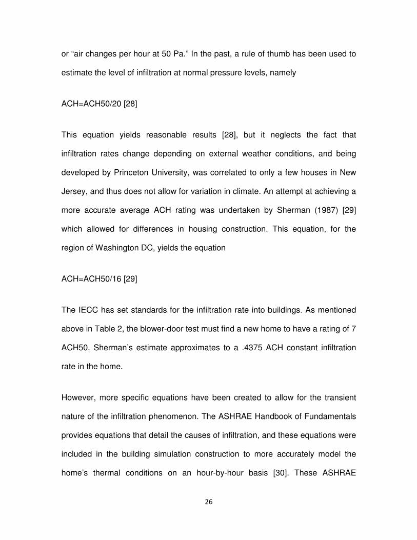
26
or “air changes per hour at 50 Pa.” In the past, a rule of thumb has been used to
estimate the level of infiltration at normal pressure levels, namely
ACH=ACH50/20 [28]
This equation yields reasonable results [28], but it neglects the fact that
infiltration rates change depending on external weather conditions, and being
developed by Princeton University, was correlated to only a few houses in New
Jersey, and thus does not allow for variation in climate. An attempt at achieving a
more accurate average ACH rating was undertaken by Sherman (1987) [29]
which allowed for differences in housing construction. This equation, for the
region of Washington DC, yields the equation
ACH=ACH50/16 [29]
The IECC has set standards for the infiltration rate into buildings. As mentioned
above in Table 2, the blower-door test must find a new home to have a rating of 7
ACH50. Sherman’s estimate approximates to a .4375 ACH constant infiltration
rate in the home.
However, more specific equations have been created to allow for the transient
nature of the infiltration phenomenon. The ASHRAE Handbook of Fundamentals
provides equations that detail the causes of infiltration, and these equations were
included in the building simulation construction to more accurately model the
home’s thermal conditions on an hour-by-hour basis [30]. These ASHRAE

27
equations, which calculate stack effect and wind effect infiltration, will be listed
and explained in the following paragraphs.
4.1.6.1. Stack effect
This form of infiltration results simply because of density differences caused by
temperature variations. The ASHRAE Handbook makes use of the following
method of estimating stack infiltration:
0 = 0� ∗ 1 ∗ *23�24,23
∗ 5 (5)
Where 0 is pressure difference across the envelope, 0� is the density of outside
air, �� is the indoor temperature, �� is the outdoor temperature, and 5 is the
height of a leak above a plane of neutral buoyancy.
4.1.6.2 Wind Effect
The magnitude of wind velocity causes short-term but relatively high magnitude
pressure differences across the envelope of a building. The ASHRAE Handbook
recommends modeling these pressure differences as such:
0 = 6�789 ∗ :9 ∗ $� (6)
28
Where ; is the velocity of the wind, : is a shielding factor determined by the
amount of cover from the wind the building receives from adjacent buildings or
vegetation, and $� is a series of coefficients describing a wall’s susceptibility to
infiltration at different angles of wind incidence.
Both of these equations were used to provide an instantaneous model for the
infiltration through the walls of the building. Exact characteristics of infiltration
behavior differ from building to building, since they are dependent on size, shape,
and location of holes, which are in many cases not necessarily reproduced from
building to building. Each leak, depending on its size and shape, acts uniquely to
a certain pressure.
Thus empirical coefficients are routinely used to estimate the magnitude of
infiltration in the home. This method of describing infiltration is called the <�, <9,
<= method, because it makes use of three constants, one as a base constant,
another as a coefficient for stack effect, and another as a coefficient for the wind
effect, in the following fashion:
>?@ = <� + <9 ∗ @*��, ��, + <= ∗ @*:, $� , ;, [31] (7)
TRNBUILD models infiltration as a property of a zone rather than a property of a
wall. It is inputted as an ACH value rather than any sort of volume flow rate:
���� = C$5 ∗ 6��� ∗ DE���*�� − ��, (8)

29
Therefore directionality cannot be directly modeled internally to TRNBUILD,
although an external calculator of such coefficients for each surface external to
the building is feasible. Whereas the windward side of a house (presumably the
west face), would be more susceptible to infiltration, by using this model only a
whole-house average can be estimated. Thus the directionality coefficient $� was
absorbed into the constant <=.
Also, due to the fact that TRNBUILD’s node-based structure does not recognize
height, stack effects are not easily modeled as a function of location in the
building. Hence the height variable 5 was absorbed into the constant <9.
A module was therefore created using this method of producing instantaneous
infiltration rates, and since no blower door was available, the constants were
estimated to produce a mean annual infiltration rate of .454 ACH in the baseline
house. In all variations of the infiltration rate a coefficient was applied to the
entire equation, simultaneously increasing each K constant by the same
percentage amount, and assumes that an airtight house gains resistance to each
type of infiltration equally. Any other more involved form of modification would be
the result of so much projection as to the size and location of various hidden
leaks as to be unproductive.

30
4.1.7. Ventilation
The great majority of residential buildings employ no building-wide systems
dedicated to ventilation. Routinely the only method of exchange with outside air
is leakage through the building envelope. However, when designing a high-
efficiency building, it is necessary to reduce this uncontrollable leakage to a
minimum, to avoid losing heat during the winter and to avoid introducing heat and
humidity during the summer.
Currently, ASHRAE standards require that the air exchange of a residential
building should meet a minimum level in order to prevent health hazards caused
by excessive inhalation of numerous household substances such as volatile
organic compounds (VOCs) released by furniture and packaging, dust, and
fumes from household cleaners. However, by rejecting conditioned air,
unconditioned air must be introduced to fill its place, and this unconditioned air
must be conditioned in order to maintain comfort levels, placing extra loads upon
the building’s climate control systems.
ASHRAE Standard 62.2 requires that whole-house ventilation levels should
adhere to the following equation:
D = .01 ∗ C����� + 7.5 ∗ *KL� + 1, − M?@N [32] (9)
Where V is the air exchange with the outdoors in cfm, C����� is the floor area in
m2 and KL� is the number of bedrooms, and M?@Nis the infiltration when above the

31
default value of . 02 ∗ C����� (.15 ACH in this house). In the case of the currently
simulated house, this ventilation requirement is approximately 47.14 cfm, which
amounts to a building-wide ACH of .143. Thus, in order to achieve the standard
for a sufficiently ventilated house, infiltration would be required to meet the
following inequality:
>?@ ≥ .343 (10)
Again, the average American home likely does not stand up to each stipulation of
ASHRAE Standards, but this model assumes that both houses meet this
requirement. The baseline house’s infiltration profile renders any mechanical
ventilation system unnecessary, since although the infiltration rate does at times
drop below .343 ACH, it is only for short periods of time, on the order of two
hours.
In the modified building, the ventilation system is set to activate when the
coefficient applied to infiltration levels reduces infiltration by more than 10%.
When the coefficient is less reductive than this, infiltration averages above the
ASHRAE-designated minimum.
4.1.8. Occupancy
The purpose of residential buildings, of course, is to shelter people. And as
anyone who has attended a meeting in a small room in mid-August knows,
occupants of a room contribute an appreciable amount to the sensible and latent

32
loads imposed upon a buildings climate control systems. The building houses a
family of three, all of whom are assumed to essentially be at a state of rest inside
the home while they are there. This produces only approximately 0.5 kW of
combined sensible and latent energy gains into the surrounding area when all
three persons are present, but this is a greater heat gain than from the appliance
load profile at many times. Occupancy models were developed similarly to the
other profiles (using the timeslots shown with the setback simulation in Table 4),
assuming two occupants leave the home between 8:00 AM and 6:00 PM for a
9:00 to 5:00 work schedule, and the other occupant leaves home between the
hours of 8:00 AM and 4:00 PM, as if that occupant were attending school. On
weekend days the house is vacant from 1:00 PM to 5:00 PM
4. 2. Weather
The model building was simulated within a weather pattern dictated by TMY2
data collected in Sterling, VA, the TMY2 station of closest proximity to College
Park. The weather location is readily changed by selecting one of the files
associated with over 200 other U.S. and international weather data collection
sites. This weather file contains data regarding outdoor temperature, humidity,
direct and diffuse light radiation, and wind velocity and direction, as recorded at
the Sterling weather station and averaged over thirty years. Figure 3 shows the
Weather macro layout, in which the weather file is labeled “Weather: Sterling
VA.”

33
Maryland’s climate is an effective example of one that demands a great deal from
both a house’s heating and cooling system. The thirty-year average of heating
degree days (HDD) was 2308 C-days. The thirty-year average of cooling degree
days (CDD) as of 2006 was 861 C-day [33]. A “degree-day” is an integration over
time of how often and by what magnitude ambient temperatures differ from
acceptable room temperatures. Thus, although these degree-day values take no
latent loads into account, it can be seen the modeled house will be most affected
by heating concerns, rather than cooling.
The sky temperature component computes an effective temperature to be used
in calculations of radiation heat transfer between the atmosphere and the
building. The Psychrometrics Processor performs simple conversions between
various indicators of humidity using the input of dry-bulb temperature and
absolute humidity from the TMY2 data. The ground temperature components
“Bsmt Wall Temp” and “Bsmt Floor Temp” estimate the average temperature of
the soil in contact with the exteriors of the basement floor and walls. The exterior
temperature of the entire basement wall was estimated to be the temperature of
the outside soil at the depth of the midpoint of the height of the basement wall.
The two temperature components show no connections in Figure 3 since they
output data only to components outside this Weather macro.

34
Figure 3: Weather Macro
4. 3. Building Controls
4. 3. 1. Orientation
The default orientation for the building model is the ideal one for photovoltaic
collection, with the axis of the longest side of the building running perfectly east-
west, and thus showing the largest possible roof area for potential use for solar
panels. There is little data to support any assumption of an average orientation of
a house, therefore this orientation was chosen as the default. This orientation is
easily changed, however, by altering the values in the “Rotate House”
component in the main, zoomed-out layer of the simulation, which simply alters
the azimuth toward which each of the building’s surfaces faces. The building may
be rotated from -90 degrees (facing East) to 90 degrees (facing West), but it is
35
always assumed that all solar collection devices are attached to the half of the
roof most nearly facing south.
4.3.2. Shading
At least in Maryland, houses are rarely built on flat, treeless plains, and windows
are rarely perfectly unobstructed year-round. Three factors go into the shading of
the house from radiation: permanent exterior shading devices, variable exterior
shading devices, and interior shading devices.
4.3.2.1. Exterior Shading
The first is constant shading caused by such things as nearby buildings, high
slopes, and evergreen trees, all of which reduce the exposure of the wall to
ambient radiation from the initial nominal value of π steradians. This category
can also include roof overhang, wingwalls, and awnings.
The second factor in shading is external, variably shading objects. The most
important example of this would be deciduous trees, which provide shade from
the sun’s rays in the summer but allow light through in the winter. TRNBUILD
does not currently provide the ability to model a continuously changing external

36
shading device, although it would be possible to create an equivalent TRNSYS
component in the future.
These shading devices were treated solely as a method of reducing radiation
striking the building’s exterior walls or transmitting through glazing. In reality
shading devices affect convection and infiltration losses as well. For example, a
row of pine trees immediately to the west of a building provides shade upon a
window, but also deflects winds, resolving pressure differences between the
interior and exterior of the building, thus reducing infiltration levels, as well as
reducing the wind velocity, and therefore reducing the rate of convection from
and to the walls of the house. Vegetation surrounding a home also provides a
relatively stationary mass of moist air which can be a boon to the indoor
environment during dry winters but places extra loads upon the air-
conditioning/dehumidification system in the summer. External shading devices
rarely have a great effect on the u-value of windows, except in the case of adding
a storm window or incorporating external shutters. In this simulation, external
shading devices add no insulation to the window area of the building other than
shielding from incoming radiation.
4.3.2.2. Interior Shading
The third type of shading, interior shading, is not a property of the building’s
environment or construction so much as it is the choice of a building’s occupants.

37
Since a building interacts directly with humans, not only design factors into a
building’s performance, and its effects are therefore less predictable and more
erratic. With human interaction introduced, understanding a building’s
performance becomes as much a psychological and biological endeavor as a
technical one. Solar radiation through common, .8 SHGC windows, when fully
opened, and spread across the entire modeled building, represents a 2.5 kW
heating source on a hot summer day. When a set of Venetian blinds is applied to
each window, this avenue of heat transfer is reduced to .6 kW, an almost 80%
reduction. Thus the usage pattern of interior shading system has the potential of
being a large source of energy savings.
Interior shading can be used to improve the U-value of a set of windows. Heavy
curtains provide a layer of insulation than can appreciably improve the U-value of
a window opening, by reducing levels of infiltration and convection at the window
opening. Thus the internal shading devices have been modeled both as means
of reducing the transmissivity of windows as well as means of slightly improving
the insulation of the building’s windows, which are routinely the greatest
weakness of a building’s thermal envelope. The baseline model is outfitted with
Venetian blinds on its windows, which do not add appreciable thermal resistance,
but when fully closed, block out 80% of light [34]. Heavy curtains provide more
thermal resistance, but their effects were not explored in this particular study.
In a perfect situation, during the winter, blinds would always be open during the
day, in order to benefit from natural lighting and solar heat gain, and closed after
38
sundown. In the summer, the blinds would be open during building occupancy
periods to benefit from natural light, and closed at all other times to block
incoming solar radiation and to avoid placing extra loads on the air conditioning
system. Studies have shown that building occupants rarely behave with such
awareness, however. There are various reasons for opening or shutting blinds
beyond those of energy concerns: one might shut them while taking a
midafternoon nap, or to block uncomfortable glare while reading or watching
television. Inevitably one might open the blinds for light on a summer morning
and leave them open, inadvertently allowing the sun to heat up the building and
causing slightly higher air conditioner energy consumption. Rea and Foster both
find in their surveys of a commercial building’s shade usage, that although the
percentage of the window covered by the shading device varied depending on
the level of cloudiness in the sky and varied with respect to seasons, in general
shades remained at a more or less constant level unless the sun was at a level
where glare became a disturbance, and not as much with regard to incurring
solar heat gains [35]. In the baseline simulation, therefore, it was assumed that
all blinds were constantly half-closed.
4.3.2.3. Shade Schedules
The other treatment of the shading problem, used later with the zero-energy
home simulation, was incorporated by creating a logic pattern, automating the
level of blind usage. It was constructed very similarly to the occupancy and
setback schedules, leaving the shades open when natural lighting or heat is

39
needed, such as during occupancy times or during the winter, and closed when
heat is unwanted, such as unoccupied summer hours.
4.4. HVAC
TRNBUILD offers two basic methods to allow HVAC systems to be modeled. The
first is internal to the TRNBUILD program, where a set point and heating/cooling
capacity are attached to each thermal zone. The second method involves
connecting the output temperature and airflow of a heater to the building as a
“ventilation” stream. The second method was chosen due to its superior flexibility
compared with the internal mode. In order to simulate the HVAC systems in this
manner, it was assumed that the same mass flow rate of conditioned air per unit
floor space was introduced into each room, ignoring the effects of pressure loss
due to height differences between floors and differences in duct length leading to
each individual zone.
Figure 4: HVAC Macro

40
The HVAC macro, shown in Figure 4, consists of four main objects. These are:
two submacros representing the HVAC systems of the new and old house, a set
of schedules for thermostat setback and season identification, and an external
monitor set to record data associated with calculating the Seasonal Energy
Efficiency Ratio of the buildings’ cooling units.
4.4.1. Baseline HVAC system
The baseline HVAC system, shown in Figure 5, imitates the heating and cooling
system of a normal American residence. Thus it employs a gas-fired furnace for
heating, a vapor-compression air-conditioner, a vapor-compression dehumidifier,
and a humidifier. A recurring theme in this thesis will be that although it is
possible to determine the abilities of current technology, by way of consulting
product specification sheets, it is less easy to determine the performance
capabilities of technology which was installed decades ago. As a guideline,
baseline house technology will assume the house was built in 1985, and that it
was outfitted with HVAC technology of satisfactory performance for the
technology level of the time, which puts it at a disadvantage compared to new-
construction houses which are subject to more stringent efficiency requirements.

41
Figure 5: Baseline HVAC System
4.4.1.1 Furnace and Humidifier
The furnace in the baseline model was modeled as a commercially available 7
kW gas-fired furnace with an efficiency of 0.85. A humidifier is attached to the
output of the furnace. It is modeled as a wick humidifier, over which furnace
output air blows and evaporates the water into the indoor environment. This
humidification setup is self-regulating and requires no appreciable increase in
energy consumption except for an extra load of capacitance which the heating
system must overcome to raise the thermal zone’s temperature.
42
4.4.1.2. Air Conditioner
The baseline air conditioner is a conventional, vapor-compression cycle air
conditioner. Its performance data was derived from a default TRNSYS model for
a 2-ton air conditioner. The method for choosing this size of air conditioner is
described below in the “Sizing the Air-Conditioner” section. The air-conditioner’s
performance is dictated by a data file containing data about power consumption
and heat removal rates at various humidity and temperature levels of indoor and
outdoor air.
Seasonal Energy Efficiency Ratio (SEER) was monitored by compiling the power
consumption of and heat removed by each air conditioner at each timestep
during the cooling season. The baseline’s air conditioner was modeled to have a
SEER of 11. Current law dictates that SEERs of new central air conditioning
systems must meet a minimum of 13, but until 2006, the minimum was only 10,
and the DOE finds that many older central air-conditioning systems have SEERs
as low as 6 [33].
4.4.1.3 Duct Leakage
The IECC has found that in nearly 80% of buildings have ducts that leak an
unsatisfactory amount of conditioned air into unconditioned spaces. They find
that the majority leak about 20% of the flow into the outside air [36]. IECC 2009,

43
and therefore Maryland, requirements dictate that ducts should release no more
than 8% of their flow into the outdoors. By placing ductwork out of the building’s
thermal envelope they become vulnerable to the extremes of local temperature
patterns, causing unwanted heat transfer and infiltration into the recently-
conditioned air. This problem can be avoided in a building where ducts remain
inside the thermal envelope, as is recommended by ASHRAE, and as is already
popular in many areas of the nation [37]. When these leaks happen indoors, a
relatively small amount of conditioned air is lost, since it simply seeps
conditioned air into a conditioned room. A study by Washington State University
estimates that these indoor ducting systems achieve up to 96% efficiency,
meaning that only 4% of the energy consumed by the air handling unit is wasted
by sending the air through the duct system [38,39]. Lubliner estimates that
approximately 41% of buildings are constructed with ducting entirely within the
building’s thermal envelope [40]. It was assumed in this simulation in keeping
with the building code that all ducts were kept within the thermal boundary of the
building. Despite that fact that such a layout is not present in a majority of
houses, this decision likely prevents inaccuracies in the building model. Among
those building simulations listed by previous experimenters, the methods
currently available for duct modeling, meaning specifically heat losses and the
airflow-modeling of leakage, much like infiltration modeling, were found to need
significant improvement [38]. A model for simplified duct heat transfer is included
in the model, but for the aforementioned accuracy concerns, that duct heat
transfer mechanism was not used in the model during this study.

44
4.5. Setback Schedules
The Scheduling Submacro, shown in Figure 5, employs eight separate forcing
functions as 24-hour schedules for the setpoint of the building’s thermostat and
humidistat. These schedules are separated into weekday and weekend
schedules, and based on expected times of occupancy, refer to Department of
Energy guidelines for thermostat setpoints [41]. The setback function was
included in the systems of both houses, since although the average American
house does not employ a digital thermostat, and accordingly such a rigid
schedule of setpoints, most households have similar occupancy times to one
another [42].
Figure 6: Scheduling Submacro

45
The setback schedules may be turned on and off by entering either a true or
false Boolean operator into the calculation component “setbackonoff,” in order to
more accurately evaluate the HVAC system’s ability to meet necessary heating
and cooling loads. These profiles are then routed through a calendar component
which recognizes the day of the week for each timestep and sends the
appropriate schedule to the thermostat. Finally, the heating and cooling setpoint
schedules are sent through a set of equations that essentially turns the heating
and humidifying system off during the summer months, and turns the cooling and
dehumidifying systems off during the winter months. The heating season has
been defined as occurring between the hours of 0 and 3500, and 6000 and 8760,
or approximately mid-September to mid-May, based on when the outdoor
temperature data in the College Park TMY2 file reach temperatures below the
human comfort level. The cooling season has been defined as hours 2500 to
7000, or early April to late October, also based on TMY2 temperature data. Thus
it is possible for either system to activate during the overlapping shoulder
seasons between hours 2500 to 3500 and 6000 to 7000.
This “switching off” of the respective systems is not actually achieved by
disabling the system but by superimposing a constant value on the profile to
remove the temperature setpoint from normal room conditions. For example, the
logic for controlling the heating system located within the “Seasons” calculation
component, is as follows:

46
5ST):UℎSWXYS = Z−30 ∗ ?[)*\M?)S], + ����,^���_ ∗ S`Y*[?[@@, 1, + 21.5 ∗
S`Y*[?[@@, 0, (11)
Figure 7: Setpoints with Setback and Season Change
Thus, when the setback system is turned off, the setpoint is assumed to remain
at a constant 21.5 C. When it is activated, the EPA setback schedules determine
the temperature to which the zones are heated depending on the time of day and
day of the week. Figure 6 displays the limits set by the setback schedule in and
around the spring shoulder season. All setpoints before 2500 hours are
recognized as “winter” and thus the cooling system is effectively shut off by
shifting up the cooling trip level. During the shoulder season, when one could
47
feasibly require the services of either the heating or cooling system, both trip
levels hover at the maximum and minimum temperature for human comfort.
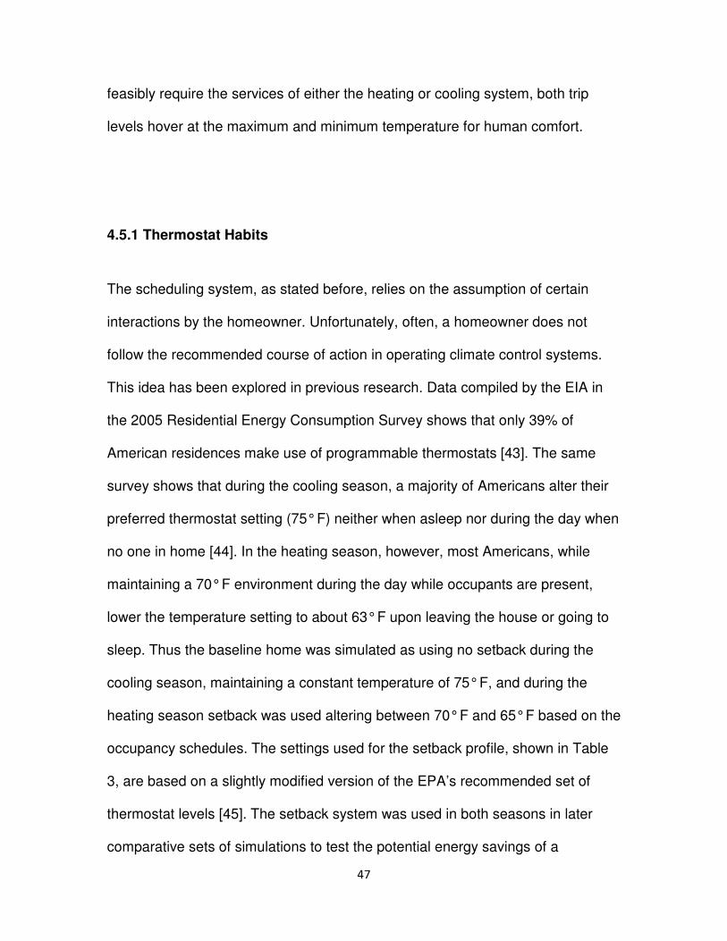
4.5.1 Thermostat Habits
The scheduling system, as stated before, relies on the assumption of certain
interactions by the homeowner. Unfortunately, often, a homeowner does not
follow the recommended course of action in operating climate control systems.
This idea has been explored in previous research. Data compiled by the EIA in
the 2005 Residential Energy Consumption Survey shows that only 39% of
American residences make use of programmable thermostats [43]. The same
survey shows that during the cooling season, a majority of Americans alter their
preferred thermostat setting (75° F) neither when asleep nor during the day when
no one in home [44]. In the heating season, however, most Americans, while
maintaining a 70° F environment during the day while occupants are present,
lower the temperature setting to about 63° F upon leaving the house or going to
sleep. Thus the baseline home was simulated as using no setback during the
cooling season, maintaining a constant temperature of 75° F, and during the
heating season setback was used altering between 70° F and 65° F based on the
occupancy schedules. The settings used for the setback profile, shown in Table
3, are based on a slightly modified version of the EPA’s recommended set of
thermostat levels [45]. The setback system was used in both seasons in later
comparative sets of simulations to test the potential energy savings of a
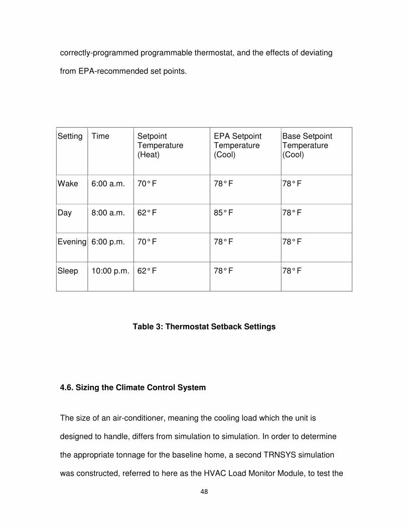
48
correctly-programmed programmable thermostat, and the effects of deviating
from EPA-recommended set points.
Setting Time Setpoint Temperature (Heat)
EPA Setpoint Temperature (Cool)
Base Setpoint Temperature (Cool)
Wake 6:00 a.m. 70° F 78° F 78° F
Day 8:00 a.m. 62° F 85° F 78° F
Evening 6:00 p.m. 70° F 78° F 78° F
Sleep 10:00 p.m. 62° F 78° F 78° F
Table 3: Thermostat Setback Settings
4.6. Sizing the Climate Control System
The size of an air-conditioner, meaning the cooling load which the unit is
designed to handle, differs from simulation to simulation. In order to determine
the appropriate tonnage for the baseline home, a second TRNSYS simulation
was constructed, referred to here as the HVAC Load Monitor Module, to test the

49
ability of the system to support the cooling load which is placed on the building.
Figure 8 depicts the makeup of the simulation. The following paragraphs will
detail the operation of the module:
Figure 8: HVAC Load Monitor Construction
4.6.1. Test Building
Much of the model is identical to the original building model. The setback
schedules, load profiles, and weather macro are all unchanged from the main
TRNSYS Program. The main difference is that all heating and cooling system
inputs external to the TRNBULD model have been removed and the heating and
cooling functions within TRNBUILD have been engaged. By doing this it is
possible for TRNBUILD to monitor the instantaneous heating and cooling loads
being placed upon the building. TRNBUILD determines the amount of sensible

and latent energy that must be added or subtracted from the indoor environment
at each time step in order to reach the desired temperature and humidity se
points. The results of this simulation are shown in Figure 9, where the red curve
depicts the amount of sensible
the set point of 22.5 C, and the blue curve represents the amount of sensible
energy that must be removed by an air
latent and total energy loads. This data was employed by monitoring, for
example, the tons-cooling-
cooling load of the air conditioner,
selecting the most appropriate commercially
Figure
50
and latent energy that must be added or subtracted from the indoor environment
at each time step in order to reach the desired temperature and humidity se
points. The results of this simulation are shown in Figure 9, where the red curve
sensible energy that must be added to the room to reach
, and the blue curve represents the amount of sensible
be removed by an air- conditioner. Also available as outputs are
latent and total energy loads. This data was employed by monitoring, for
-equivalent of the total dehumidification and sensible
cooling load of the air conditioner, which was just under 2 tons in this case, and
selecting the most appropriate commercially-available size.
Figure 9: HVAC Load Monitor Output
and latent energy that must be added or subtracted from the indoor environment
at each time step in order to reach the desired temperature and humidity set
points. The results of this simulation are shown in Figure 9, where the red curve
energy that must be added to the room to reach
, and the blue curve represents the amount of sensible
conditioner. Also available as outputs are
latent and total energy loads. This data was employed by monitoring, for
equivalent of the total dehumidification and sensible
which was just under 2 tons in this case, and

51
4.6.2 Capacity Failure Monitor
A device was included in this program to detect the number of hours in a year
when the climate control system does not meet the needs of the building’s
heating, cooling or humidity loads. This was done by placing a monitor on the
temperature of the thermostat-controlled space. When the temperature or
humidity strayed outside of the error allowed by the thermostat’s deadband, a
Boolean signal of 1 was generated, multiplied by the timestep, and integrated
over the course of the year to find the amount of time during which the climate
control system was unable to meet the demands of the building’s heating or
cooling load. The following equation shows the logic used:
�]XS^��� = M@*)S&a < )��� − WSTWcT?W − .1,
�]XS��� = M@*)S&a < )��� − WSTWcT?W − .1,
This system also incorporates a unit to monitor the climate control system’s
ability to change setpoint levels in a satisfactory amount of time. This sort of
monitoring is performed by comparing the thermostat setpoint of the current
timestep with that of an earlier timestep, in this default case, the timestep one
hour previous. It ensures that the air conditioner is capable of achieving the level
of human comfort in an acceptable period of time. The following equation details
how the signal is tripped:
�]XS���,^��.� = M@Z)S&a > )���,��e_ ∗ M@*)���,��e > )���,�,

52
�]XS^���,^��.� = M@Z)S&a < )���,��e_ ∗ M@*)���,��e < )���,�,
where “True” indicates the trip of the capacity failure monitor either for cooling or
heating, temp is the temperature monitored by the thermostat, )���,��e is the
setpoint 5 timesteps earlier, and )���,� is the setpoint at the current timestep.
4.6.3. Comfort Zone Monitor
The Comfort Zone monitor makes use of human comfort levels as described by
the ASHRAE Handbook of Fundamentals and serves as a means of checking the
performance of the HVAC system [30]. It receives absolute humidity and
temperature data from the interior environment and records them for each
timestep. Each of these points is then entered into an Excel workbook, which
plots each point on a psychrometric chart. Figure 10 shows a sample output of
this comfort zone monitor. The data shown was developed by running the
simulation without any change in thermostat setpoints. The cooling setpoint
remained at 25.5 degrees and the heating at 21.5 degrees. This is another
measurement of the climate control system’s ability to meet the heating and
cooling loads demanded by the indoor environment. To show the chart after a
normal setback simulation would result in a number of meaningless and
indistinguishable points outside the range of human comfort and would not help
in judging the merits of the climate control system; therefore the comfort zone
results of such a simulation were not shown.
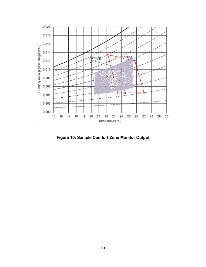
53
Figure 10: Sample Comfort Zone Monitor Output
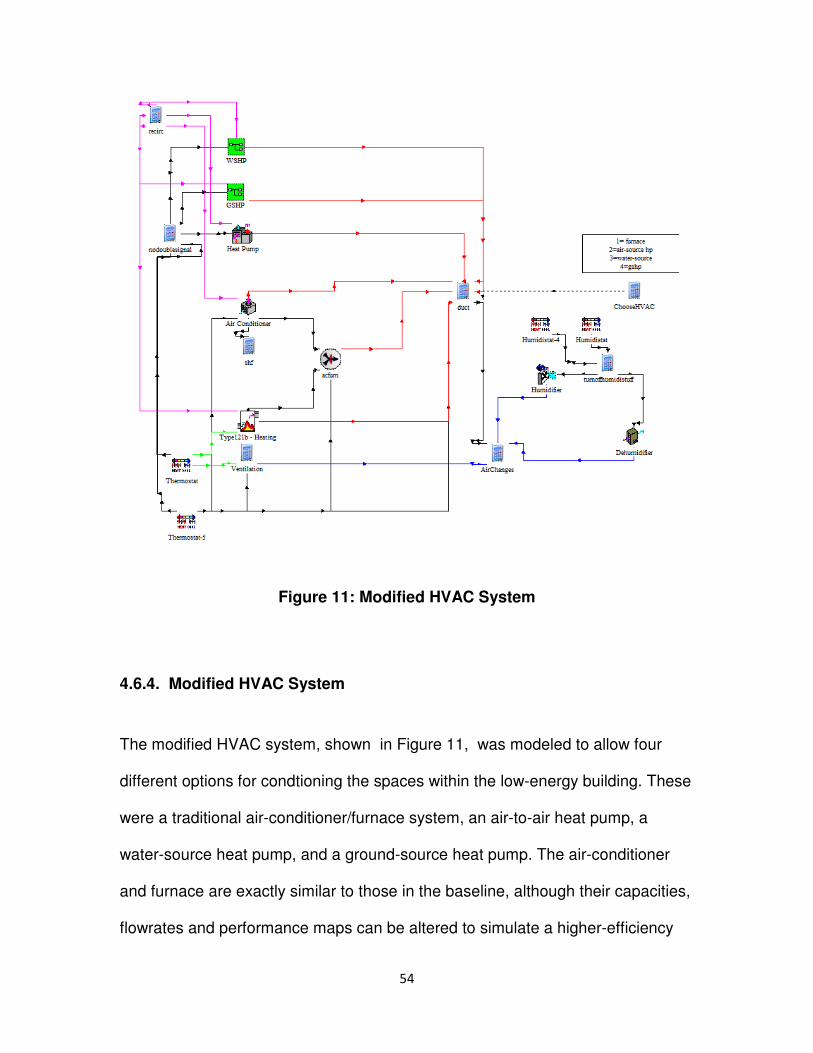
54
Figure 11: Modified HVAC System
4.6.4. Modified HVAC System
The modified HVAC system, shown in Figure 11, was modeled to allow four
different options for condtioning the spaces within the low-energy building. These
were a traditional air-conditioner/furnace system, an air-to-air heat pump, a
water-source heat pump, and a ground-source heat pump. The air-conditioner
and furnace are exactly similar to those in the baseline, although their capacities,
flowrates and performance maps can be altered to simulate a higher-efficiency
55
furnace/air-conditioner setup, as will be performed later, when the air-conditioner
SEER is modified to 13 from 11. The heat pump was modeled after a
commerically available heat pump, marketed as “standard efficiency,” of 13
SEER in cooling mode and an HSPF of 8.5 [46]. Various calculation components
throughout the macro simply divert control signals to the chosen HVAC setup,
divert the energy consumption of the appropriate unit to the Energy Macro, and
divert the outlet air conditions of the appropriate apparatus to the building model.
The simulation’s ground-source and water-source heat pumps have not yet been
sufficiently checked and compared to published data concerning their
performance, and therefore those options were not yet explored in this study.
4.7. Photovoltaics Macro
The Photovoltaics Macro, shown in Figure 12, contains a Photovoltaic panel and
inverter combination which provides a source of energy to offset the energy
consumption of the home throughout the year. As was stated before, half of the
roof area is assumed to be available for PV arrays and solar thermal collectors.
The solar thermal collector for the size of family assumed present in this building
was recommended by the U.S. DOE to be 3.3 m2, [47] and therefore
approximately 60 m2 was left to be covered by photovoltaic panels.The
photovoltaic array is modeled as a set of normal crystalline silicon collectors.
These panels are attached to the roof at the same angle the roof was
constructed, 36 degrees from the horizontal. It is normal to achieve

56
approximately 8% to 12% efficiency in silicon modules [48]. As can be seen in
the PV macro’s graphical output in Figure 13, this system normally achieves
approximately 10.5% efficiency. Such an efficiency is typical of monocrystalline
modules.
Figure 12: Photovoltaics System
Figure 13: Photovoltaics Output.

57
4.8. Energy Macro
The Energy Macro, shown in Figure 14, serves as a central point where the
information concerning energy consumption from each device is compiled. It
provides the user with two graphical outputs: the power monitor and the energy
monitor. The energy monitor integrates power consumption by each component
over the span of a year to show the total amount consumed by each part of the
building’s energy system. All information is fed to a unit converter, which sends
the power consumption of each specific part of the building energy system to the
“Power Monitor” graphical output and to the integrator, which sums up the power
to find the total kWh amount of energy consumed by each building component.
Figure 14: Energy Macro
58
4.9. Load Profiles
The “Load Profiles” component represents an Excel spreadsheet containing a
schedule of electrical and domestic hot water (DHW) consumption for the
building. The set of data was derived from the results of a study by the
International Energy Agency’s (IEA) Annex 42 on non-HVAC household
electricity and hot water usage schedules [49].
4.10. Non-HVAC Electrical Profile
Annex 42 acquired the data for the electrical load profiles by using a probabilistic
profile generator. Each appliance was given a probability of turning on within a
certain span of time according to a study conducted by the results of a survey of
the average energy consumption of certain household appliances.This average
level of consumption became an annual consumption goal, determined by the
average energy consumption of each appliance type in Canadian households,
was applied to this scheduling mechanism. A 5-minute-resolution energy
breakdown for American households was not available, necessitating the use of
these profiles based on Canadian households, which, it is assumed, use
appliances in a similar manner to their American counterparts.

59
4.10.1 Changes to Non-HVAC Electric Profile
It was determined at the time of applying the load profile to this simulation that
modifications needed to be made to the original Annex 42 load profile. These
changes stemmed from the long list of miscellaneous appliances that had been
included in the study and assumed to be present in the building. Annex 42 used
data from a Natural Resources Canada report delineating typical power ratings
and usage levels of several miscellaneous electrically-powered items, which
resemble suggested guidelines more closely than established fact. A few
appliances on that list were deemed to be impractical to expect in an average
American home. For example, the lathe, which is listed in the Annex 42 Report
as being in use for two hours of every month, was eliminated from the database.
It was determined that although many houses may indeed contain lathes, but to
presume their presence in an average house, as this simulation attempts to
model, let alone to presume that the average American homeowner would
engage that appliance for a full 24 hours in a year, would be somewhat bold. The
same was done to the circular saw, the table saw, the deep fryer, the electric
kettle, the sewing machine, and the electric blanket, which were all identified as
appliances too irregularly employed to include in the load profile of an average
residence. Other appliances were diminished in usage time. For example, the
vacuum cleaner, estimated by Annex 42 to be operated for 10 hours per month
was reduced by half, since 10 hours of vacuuming seems to assume a level of
hygiene and responsibility foreign to many homeowners. Likewise the energy
consumption of the laptop computer was halved, since in the profile it is a
60
ssumed that the desktop and laptop computer are occupied for 240 hours each
per month, which is an extremely large amount of computer time for the three-
person household which is being attempted to be simulated. All preceding
changes were applied to the load profiles of both houses.
All other appliances, such as refrigerators, televisions, small electronic devices,
and others were kept the same as in the original load profile. The full breakdown
of the components of the load profile can be seen in the Annex 42 report [42] or
at the Annex 42 website.1
4.10.2 Simulation of Energy-Efficient Appliances
The non-HVAC electrical profiles of both houses were determined using the
same base schedule, as explained above, but to simulate the replacement of old
appliances with new, efficient models, the profile for the low-energy building was
slightly modified. This section will explain the divergence between the two
profiles.
The original Annex 42 load profiles provide no data for specific appliance models,
since they instead opted to use an average consumption level determined by
survey results.
1 http://cogen-sim.net/index.php?pg=datafiles&download=Canadian_Electrical_
Load_Profiles_Excel_Format_high.zip

61
The profile for each energy-efficient appliance was constructed by applying a
multiplier to each appliance’s original load profile, which preserves the usage
pattern of each appliance but reduces the amount of energy consumed during
each use. Energy efficient appliance usage targets were determined by
consulting National Resource Canada’s 2007 database of average annual
energy ratings of new appliances [50]. The lighting percentage reduction was
decided upon by assuming that the baseline home’s lighting was performed by
nearly all incandescent bulbs, whereas the modified home’s was performed by
nearly all compact fluorescent lamps (CFLs). The values for the reduction in
energy due to use of CFLs is in accordance with the difference in power rating
between similar light-output incandescent bulbs and CFLs as reported by
manufacturers [51]. Normally this value is about 75%, but the savings were
decreased a small amount to allow for a few incandescent bulbs.
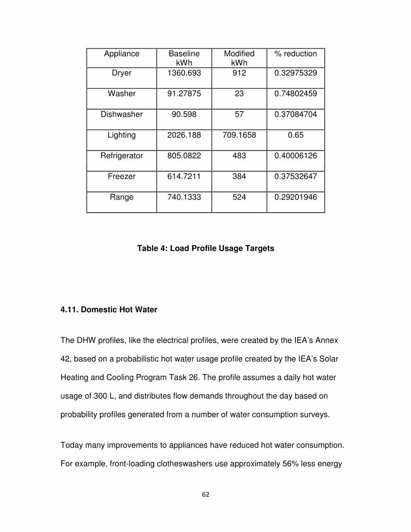
62
Appliance Baseline kWh
Modified kWh
% reduction
Dryer 1360.693 912 0.32975329
Washer 91.27875 23 0.74802459
Dishwasher 90.598 57 0.37084704
Lighting 2026.188 709.1658 0.65
Refrigerator 805.0822 483 0.40006126
Freezer 614.7211 384 0.37532647
Range 740.1333 524 0.29201946
Table 4: Load Profile Usage Targets
4.11. Domestic Hot Water
The DHW profiles, like the electrical profiles, were created by the IEA’s Annex
42, based on a probabilistic hot water usage profile created by the IEA’s Solar
Heating and Cooling Program Task 26. The profile assumes a daily hot water
usage of 300 L, and distributes flow demands throughout the day based on
probability profiles generated from a number of water consumption surveys.
Today many improvements to appliances have reduced hot water consumption.
For example, front-loading clotheswashers use approximately 56% less energy

63
than a top-loading model from the 1980s [52], and new low-flow shower head
models use approximately 50% of the water compared to old fixtures [53].
However, this reduction in water usage was not modeled in the zero-energy
home simulation. Unlike the electricity profiles, the hot water profiles were not
separated into usages by separate appliances, but were compiled as one gross
usage profile. Thus to somehow reduce the flowrates at certain times of the day
would require highly arbitrary, and probably highly inaccurate, guesswork. Annex
42 offers a low-usage profile for DHW consumption, however this involved
assuming behavioral changes in the occupants. Since the experiment was meant
to model changes to the building, it was determined that such a behavioral
change would possibly render slanted and overly-optimistic results. However, this
will be of note in later simulations, for example with solar water heating, which
are not as well-equipped to handle high flowrates of hot water as a common gas-
fired furnace.
Hot water consumption was assumed to not have any effect on the relative
humidity or temperature of the building. It was assumed that exhaust fans
sufficiently remove the water from bathrooms during showers, and that all but a
negligible amount of energy drains from a sink or washing machine before it can
be transferred to the indoor atmosphere.
64
4.11.1. Modification to DHW profiles
The profiles provide volumetric flow rates of hot water based on a 45 °C delivery
temperature (Tp) and a 10 °C incoming cold water temperature. Since the
storage tank modeled in this simulation supplies water at a set point of 50°C
rather than 45 °C, the profile flow rate has to be adjusted based on the actual
outlet temperature of the tank (Th). Additionally, since the temperature of
incoming cold water (Tc), which replaces the hot water drawn from the top of the
tank, varies based on ambient and ground temperature, it should not be
assumed to be constant, and is therefore simulates as a time-varying value in
this modified version.
One may develop the following relationship by conducting an energy balance on
the mixture of two constant- specific-heat, constant-density fluids at different
temperatures:
1 1 2 2mix mixm T m T m T= +& & &
In the present case, the original load profile flow rate is represented by the “Mix”
stream, and the hot (tank) and cold (tap) streams as the other two, giving:

65
p p c ch hm T m T m T= +& & &
Where pm& is the flow rate specified in the load profile,
hm& is the mass flow rate of
water from the hot storage tank, and c
m& is the flow rate of tap water being mixed
with the hot stream. Furthermore, the total flow rate given by the profile is equal
to the sum of the two streams:
p chm m m= +& & &
Combining the above two equations yields a relationship between the flow rate
out of the tank and the original profile flow rate.
( )( )
p c
ph
ch
T Tm m
T T
−=
−& &
66
The profile temperature is a constant (45 °C), and the profile mass flow rate is
specified at every timestep, so this is a function of the tank outlet and tap inlet
temperatures. In general, since the tank outlet temperature is higher than 45 °C,
the drawdown rate from the tank will be significantly lower than the flow rate
specified by the original Annex 42 load profile.
4.12. Hot water system
The hot water macro, as shown below in Figure 15, simulates the operation of a
water-heating system. The system intakes groundwater, assumed to be at the
temperature of the ground at 1 m below the surface, which is then heated by one
of a few different possible heating methods. The choice of heating method is
controlled by changing the ID number in the “Choose” calculator component,
which turns a series of switches on and off to send the energy consumption and
temperature data from the desired heating apparatus to the appropriate places,
for example energy consumption data to the energy macro and temperature data
to the building model. The most common method of hot water supply among
American households involves storing water in a thermostat-controlled, gas-
heated hot water storage tank [54]. Therefore this was chosen for the baseline
simulation. Given the size of the family, an 80 gallon (300 L) tank was used,
based on the recommendation by Krigger [53]. Its thermostat was set at 50
degrees C (122 F), also based on data from Krigger.
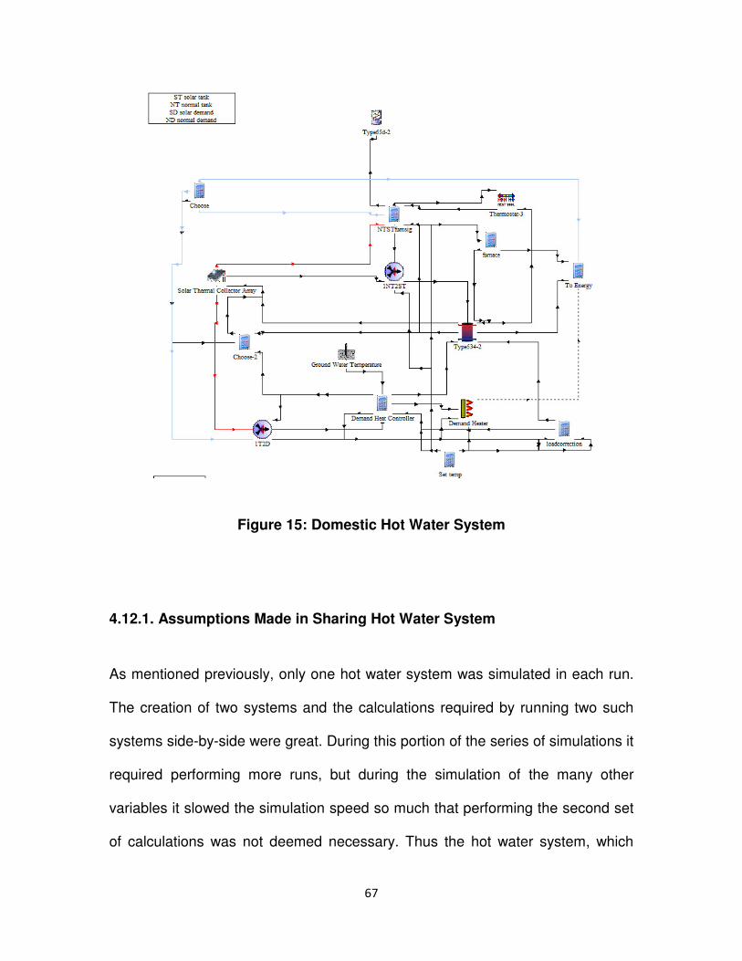
67
Figure 15: Domestic Hot Water System
4.12.1. Assumptions Made in Sharing Hot Water System
As mentioned previously, only one hot water system was simulated in each run.
The creation of two systems and the calculations required by running two such
systems side-by-side were great. During this portion of the series of simulations it
required performing more runs, but during the simulation of the many other
variables it slowed the simulation speed so much that performing the second set
of calculations was not deemed necessary. Thus the hot water system, which
68
can be varied between the four setup possibilities listed above, was located in
the baseline house, and its energy consumption was applied to both buildings. It
is possible that this could introduce error into final annual consumption,
especially in the modified building, since the basement of the baseline house will
have different temperatures from the modified house, which would cause higher
or lower rates of heat loss through the hot water storage tank. Thus, the effects
of this assumption will be investigated.
4.12.2. Effects of Assumption
To ensure that the assumption of the existence of two water systems would not
significantly affect the final consumption numbers of the simulation, a pair of
simulations were run in order to compare hot water consumption when the water
heater is located in the baseline house’s basement and then the low-energy
house’s basement. The hot water tank is normally simulated in only the modified
house. Figure 16 shows representative basement temperatures from both
buildings in both the heating and cooling seasons. It shows that the temperature
in the baseline house’s basement stays a relatively constant one degree below
the temperature of the modified house’s basement during the winter. During the
summer, the temperatures of both basements are within .5 degrees Celsius.

Figure 16: Basement Temperature Differences(R). Please note difference of scale.
The tank was simulated in the modified house, at its most energy
(as described later in Section 6.3)
home (i.e. using the baseline’s basement temperature conditions as the
parameters for heat loss calculations), to determine whether foregoing simulating
two separate systems causes any major discrepancy in energy consumption
values. In the baseline home, where the basement stays
baseline hot water system consumed
zero-energy home configuration, which will be expla
but which represents the best
system consumed 5428 kWh
said with satisfactory accuracy that the
house is not a source of significant error
69
asement Temperature Differences (C) – Summer (L) and Winter . Please note difference of scale.
The tank was simulated in the modified house, at its most energy-efficient state
(as described later in Section 6.3), and then it was simulated in the baseline
home (i.e. using the baseline’s basement temperature conditions as the
parameters for heat loss calculations), to determine whether foregoing simulating
causes any major discrepancy in energy consumption
In the baseline home, where the basement stays slightly
baseline hot water system consumed 5470 kWh. Within the skeleton of the
energy home configuration, which will be explained in greater detail later,
but which represents the best-insulated configuration evaluated in this
kWh, only 42 kWh or 0.8% less energy. Thus it can be
said with satisfactory accuracy that the placement of the water tank
a source of significant error.
Summer (L) and Winter
efficient state
it was simulated in the baseline
home (i.e. using the baseline’s basement temperature conditions as the
parameters for heat loss calculations), to determine whether foregoing simulating
causes any major discrepancy in energy consumption
cooler, the
the skeleton of the final
ined in greater detail later,
in this study, the
. Thus it can be
of the water tank in only one

70
5. Validation of Baseline Model
In order to ensure the accuracy of the baseline model, one simulation was run so
that the outputted data could be compared to recorded average values. Figure 17
displays the resulting energy consumption from the baseline simulation.
Legend Value (kWh)
Hot water ----------------- 5536
Heating ----------------- 16109
Cooling ----------------- 1610
Dehumidification ----------------- 137
Appliances ----------------- 7474
Total ----------------- 30866
2.56E+04
3.20+04

71
Figure 17: Baseline Simulation Results
5.1. Cooling and Total Electricity Consumption
The electrical consumption for the baseline cooling system was 1610 kWh. The
EIA’s 2005 Residential Energy Consumption Survey found that the average N
northeastern household with central air conditioning consumed 2163 kWh [55].
This constitutes an approximately 34.5% difference from that average.
Considering the ducting assumption, that is, that all ducts are within the thermal
envelope of the home, and that, at a SEER of 11, this air conditioning system
would have exceeded the legal minima prior to 2005, this is a reasonable
difference.
The average household electricity consumption in the Northeast was 8514 kWh,
according to the RECS. The baseline’s usage, at 9223 kWh, seems to be an
appropriate value, at an 8.2% difference. One must take into account that in 20%
Baseline (kWh)
RECS Avg, NE homes (kWh) % Deviation
Hot Water 5536 5302 4.23
Heating 16109 19688 -22.22
Cooling 1610 2163 -34.35
Total electricity 9221 8514 8.23
Total Gas & Electricity 30866 33504 -7.87

72
of these houses electricity is also used in space heating, and in 18% for water
heating. Both of these values inflate the statewide average. Here the gap can be
attributed to the level of energy consumption chosen in the load profiles.
5.2. Furnace and Natural Gas Consumption
RECS information shows that approximately 19688 kWh is consumed in the
average northeastern house for space heating, a 22% increase compared to the
baseline building. Hot water consumption in northeastern homes averages to
5302 kWh per year, only a 4.0% decrease from the baseline value. These natural
gas consumption totals bring the total consumption amount to 33504 in an
average home, compared to 30866 in the baseline house, a 7.9% decrease. In
general these comparisons show that the baseline house is better insulated
compared to the average house, and that despite the reductions made to the
load profiles, this home uses significantly more energy for appliances than
average.
5.3 Accuracy of Building Energy Simulation
NREL has noted that much uncertainty still exists in the field of building energy
analysis. Given its somewhat large scale and its level of complexity and
variability, given the great number and unpredictability of many variables, the
need for exact replication of building geometry, and the great number of
calculations per time step that would be required to fully replicate all the ongoing
physical processes within a house, building simulation tools have not yet reached

73
the same levels of accuracy that are common in other types of smaller-scale
simulations. According to their report on validation methodologies, NREL finds
that differences between actual building consumption and simulated building
consumption tend to be at least 10%, and as much as 50% [56]. Thus the levels
of consumption arrived upon by the baseline home simulation are within an
expected range of error.
6. Simulation Results
Simulations were conducted in order to determine the effect of various changes
to the building on total annual energy consumption. Since the final objective is to
simulate a net-zero-site-energy home, the simulation results consider a system
containing only the building, and not, for example, electrical generation efficiency,
grid efficiency, or energy consumed in order to deliver natural gas to the home.
6.1. Envelope Simulations
A sensitivity study was performed upon each major characteristic of the buildings
structure, in order to determine the most effective method of reducing total
energy consumption by modifying envelope characteristics. In terms of cost and
feasibility, these are perhaps the most demanding of the available retrofit
solutions. However in most cases they are feasible, and the following will show
where the greatest energy-saving potential lies when adding insulation to a

74
home. In all cases, R-values are expressed in the units of ft2-°F-hr/btu, which is
the standard unit for designating insulation levels in U.S. building codes, and, in
parentheses, the SI units of hr-m2-°K/kJ.
6.1.1. Basement Insulation
R-Value
[ft2-°F-hr/BTU
(m2-°C-hr/kJ)]
10 (.54) 8 (.44) 12 (.65)
Heating (kWh) 16109 17781 15394
% N/A 10.38 -4.44
Cooling (kWh) 1610 1213 1744
% N/A -24.66 8.32
Total (kWh) 30866 32291 29639
% N/A 4.62 -3.98
Table 5: Basement Insulation Simulation Results
It can be seen by the simulation results in Table 5 that the basement acts as a
cooling source in the building. A lower amount of insulation in the basement
keeps that space at a temperature nearer to the ground temperature, which
averages about 55 degrees over the course of the year. Although one greatly
saves on cooling costs during the summer by reducing basement insulation and
making use of the ground’s cool temperatures, these savings are negated almost
twice over by the energy consumption of the heating system during the winter.

75
This was found to have a particularly significant effect on the building’s energy
consumption. NREL notes that ground coupling is a relatively unexplored and
relatively overlooked area when evaluating building simulations [57].
6.1.2. Infiltration
Avg ACH 0.454 0.363 0.545
Heating (kWh) 16109 15154 18187
% N/A -5.93 12.90
Cooling (kWh) 1610 1623 1583
% N/A 0.81 -1.68
Total (kWh) 30866 29531 32795
% N/A -4.32 6.25
Table 6: Infiltration Simulation Results
During this simulation, the results of which can be found in Table 6, it was found
that cooling costs actually increased as a result of lower infiltration. By examining
the temperature profile of the indoor environment, this is because the heat
transfer is dominated by radiation during the day, and while in the less air-tight
home the cool night air filters into the home and the heat gains experienced
during the day are relieved of the building, the more tightly-built house retains the
warm air until morning, when the sun again filters into and heats up the building.
This counterintuitive effect would be mitigated or eliminated by incorporating the
shading schedule, by decreasing the solar heat gain coefficient of the building’s
76
windows, or by opening windows or using mechanical ventilation at night.
Despite this gain in cooling power consumption, however, the lower infiltration
values yield lower overall energy consumption, since heating during the winter
requires much more energy, and infiltration provides a heating system no such
hidden benefit.
Also, it can be seen that further weatherproofing of the house has a much
smaller positive effect (-6.25% total consumption) than the negative effect of
making the envelope more leaky (+9.26% total consumption). This is because of
the fact that ventilation must be introduced to the building in order to maintain a
safe indoor atmosphere. Although being able to control the passage of air from
outside to inside allows for better efficiency than having a leaky home, there is a
sudden drop-off in terms of how much this building characteristic can improve the
energy consumption levels once the ASHRAE minimum is reached.

77
6.1.3. Wall Insulation
R-Value
[ft2-°F-hr/BTU (m2-°C-hr/kJ)]
12.3 (.67)
16 (.871) 23 (1.25)
Heating (kWh) 16109 15246 14783
% N/A -5.36 -8.23
Cooling (kWh) 1610 1588 1571
% N/A -1.37 -2.42
Total (kWh) 30866 29745 28180
% N/A -3.63 -8.70
Table 7: Wall Insulation Simulation Results
The wall insulation simulations, the results of which are shown in Table 7, were
all run assuming a 2 by 4, 16 in. on center frame construction, and thus all
provide feasible options for retrofit of existing buildings since they require no
modification of the load-bearing structure. The baseline, as previously
mentioned, uses fiberglass insulation in its cavities, allowing thermal bridging
across its thermal boundary and leaving it with an R-value of R-12.3. The second
variant of the wall construction used polyurethane foam in the cavities and
achieved an R-23 insulation level. Other methods of increasing wall r-values
normally require major remodeling work. For example, continuous insulation has
been used instead of cavity insulation to eliminate thermal bridging across the
wall. While this does not require destruction of the frame it requires replacement
of much of the exterior wall. This option, therefore, is not the most feasible for
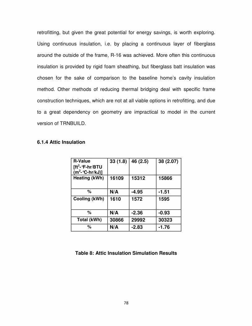
78
retrofitting, but given the great potential for energy savings, is worth exploring.
Using continuous insulation, i.e. by placing a continuous layer of fiberglass
around the outside of the frame, R-16 was achieved. More often this continuous
insulation is provided by rigid foam sheathing, but fiberglass batt insulation was
chosen for the sake of comparison to the baseline home’s cavity insulation
method. Other methods of reducing thermal bridging deal with specific frame
construction techniques, which are not at all viable options in retrofitting, and due
to a great dependency on geometry are impractical to model in the current
version of TRNBUILD.
6.1.4 Attic Insulation
R-Value
[ft2-°F-hr/BTU (m2-°C-hr/kJ)]
33 (1.8) 46 (2.5) 38 (2.07)
Heating (kWh) 16109 15312 15866
% N/A -4.95 -1.51
Cooling (kWh) 1610 1572 1595
% N/A -2.36 -0.93
Total (kWh) 30866 29992 30323
% N/A -2.83 -1.76
Table 8: Attic Insulation Simulation Results

79
The attic insulation simulation, the results of which are displayed in Table 8,
shows expected values in that more insulation yields lower consumption values;
however, the levels of savings are of lesser magnitude than would be expected in
a normal home. This discrepancy highlights one of the limitations of using the
current version of TRNBUILD as a building simulation program. Since it is
completely non-geometric, it does not recognize the fact that the attic is at a
greater height than any other floor. The ceiling of the second floor is not
recognized as a ceiling but instead as another wall. Because each zone is
simplified as one node, there are no calculations performed to predict the effect
of heat rising to the ceiling. Thus, whereas in reality the attic is among the most
necessary places in the home to be well-sealed and well-insulated, the current
version of this program finds little difference between the ceiling of the upper floor
and any other wall.

80
6.1.5. Bottom floor insulation
R-Value
[ft2-°F-hr/BTU (m2-°C-hr/kJ)]
10 (.54)
8 (.44) 12 (.65)
Heating (kWh)
16109 17004 15327
% N/A 5.56 -4.85
Cooling (kWh)
1610 1537 1656
% N/A -4.53 2.86
Total (kWh) 30866 31194 30489
% N/A 1.06 -1.22
Table 9: Bottom Floor Insulation Simulation Results
The bottom floor of the house, like the ceiling of the 2nd floor, is paid particular
attention because it separates conditioned spaces from unconditioned spaces.
As shown in Table 9, in this simulation it was found that the R-value of the
bottom floor was indeed an energy-saver, but among the less effective
procedures available for insulating one’s home. In both cases, total energy
consumption was affected by only approximately 1%. This seems to be because
the baseline model’s basement is already sufficiently insulated from outdoor
temperatures, and the temperature differences, and therefore heat flux, across
this floor are significantly smaller than those between a vertical exterior wall and
the outdoors. One can still see the effect of the basement siphoning heat from
the conditioned space, however. During simulation it was found that the
insulation levels between the first floor and the basement were far less important

81
to creating a thermal boundary compared to the coupling air flows between those
two zones.
6.1.6 Window U-value
U-Value
[BTU/ft2-°F-hr (kJ/m2-°C-hr)]
Double-Pane Single-Pane Krypton-filled
3.5 (64.3) 5.8 (106.5) 1.1 (20.2)
Heating (kWh) 16109 18814 13018
% N/A 16.79 -19.19
Cooling (kWh) 1610 1789 1456
% N/A 11.12 -9.57
Total (kWh) 30866 33193 27433
% N/A 7.54 -11.12
Table 10: Window U-Value Simulation Results

82
6.1.7 Window SHGC
SHGC 0.6 0.7 0.5 0.2
Heating (kWh) 16109 15913 16188 16302
% N/A -1.22 0.49 1.20
Cooling (kWh) 1610 1716 1467 1017
% N/A 6.58 -8.88 -36.83
Total (kWh) 30866 30997 30710 30115
% N/A 0.42 -0.51 -2.43
Table 11: Window SHGC Simulation Results
The preceding set of simulations highlights the idea that windows are the weak
point in a building’s thermal boundary. The change of the 15% of the building’s
external wall area to a more insulating material, as shown in Table 10, combined
with the effect of reducing the SHGC of the window glazing, as shown in Table
11, resulted in more drastic savings than any of the other individual envelope
improvements, saving a combined total of 14.8% between the baseline and the
efficient options which will later be used in the low- energy home simulation.

83
6.1.8 Cool Roof vs. Conventional Shingles
In 2009, a job-creating project was started in urban Baltimore, the purpose of
which was to “green” one of the streets by painting the roofs of that street’s
buildings white [57]. This type of project is routinely done to lower absorption of
heat radiation during the cooling season and to reduce the severity of the “urban
heat island” effect [58]. Such a solution has been shown to significantly reduce
annual energy consumption in warm climates like, for example, Florida [59], but
in cooler climates the benefits of the roof covering is more debatable. A white
roof would reduce heat gains through the roof of the home during heating
season, thus increasing the reliance on internal heating sources such as a
furnace. However, significantly less radiation directly reaches the roof during the
winter, since the sun stays lower in the sky and shines at an increased level on
the exterior walls rather than solely the roof (i.e. the color of the roof becomes
less significant during the winter months) [60]. This TRNSYS program can
simulate the effect of altering the reflectivity of the building’s roof and simulate its
effect on energy consumption over the entire year.
It should be noted that one aspect of reality that is not replicated by the
simulation is the presence of snow on the roof, as is an occasional occurrence in
the Baltimore area, and would serve to create a reflective roof on the building no
matter the color of the roof itself; however, by examination of TMY3 data for the
Washington, DC metro area, snow cover is limited enough to not drastically
84
affect average albedo levels during the winter months, thus for this simulation, in
this particular climate, such a consideration might be considered negligible [61].
Also, in high concentrations of artificial surfaces, such as urban areas,
widespread use of cool roofs have been shown to appreciably decrease ambient
temperatures, especially during the summertime [62], which as a secondary
effect reduces the cooling load on the constituent individual houses. This
simulation does not consider the effect of such a widespread change, but only
examines the effects of changing an individual house’s roof color.
Table 12 shows the results of the albedo change simulation. Two situations were
simulated, one comparing a white-painted roof with a traditional asphalt-shingled
roof, and the other comparing an aluminum roof, as is popular in such sun-
drenched regions as Australia, with the traditional roof. TRNBUILD does not
recognize albedo values per se, but rather solar absorptance values. This solar
absorptance value (C�) was altered in the equation for solar heat gains:
��L���L�� = ������ ∗ C� (9)
The absorptance values of these materials were decided upon by consulting the
values recommended by the Solar Energy Laboratory in the TRNBUILD manual,
which are generally consistent with those values given by other sources [63].

85
Roof Surface
Black Shingles
White Paint Aluminum
Absorptance
0.75 0.2 0.35
Heating (kWh)
16109 16246 16192
% N/A 0.85 0.52
Cooling (kWh)
1610 1482 1511
% N/A -7.95 -6.15
Total (kWh) 30866 30835 30829
% N/A -0.10 -0.12
Table 12: Albedo Change Simulation Results
6.1.8.1 Results and Comparison with Past Experiments
Table 12 shows that the color of the roof of the house had only a small effect on
its annual energy consumption. Aluminum was the most efficient, but it had only
a small impact, with about a .1% reduction in energy. It should be noted that part
of the attractiveness of aluminum as a roofing material results from its low
emissivity. In exterior wall calculations, TRNBUILD assumes that emissivity is
equal to absorptivity, and thus in this sort of calculation that physical fact is not
86
replicated. The reason for aluminum’s primacy in the ranks of the roof coatings is
due to the fact that heating energy consumption so far outweighs cooling
consumption that the small percent change in heating consumption between
aluminum and the white roof is enough to give aluminum a slight, almost
negligible advantage.
Past simulations conducted by the Department of Energy have found that the
savings gained by the use of “cool roofs” depend very much on location. By use
of the Oak Ridge National Laboratory’s DOE Cool Roof Calculator, one study
found that while white roofs earned the most savings in the South, at
approximately 1.2 kWh per sq ft in cities such as Miami, in the more northern
areas of the East Coast, such as New York, where heating is of primary concern,
white roofs cost more money due to lost absorption of the sun’s heat [64].
Aluminum was found to be the most cost-effective coating, in these places,
saving the homeowner approximately .5 kWh per sq ft of cooling costs yearly.
Another study in Florida compared a white-roofed building with a black-roofed
building, first with a physical experiment and then with a simulation using DOE-2.
The experiment found that a white roof coating there can save approximately
19% on cooling bills [65]. The Florida team noted in the course of describing the
experiment that many building simulation programs fail to produce close-to-real-
life data due to inability of many programs to accurately model exfiltration from
ducts and other airflow phenomena.

87
The small change is explainable because of two reasons. First of all, even the
baseline configuration of the building has a great deal of insulation in the attic,
having met the standards of IECC 2009. Thus, despite the great amount of heat
absorbed by the attic when black shingles are used, and the resulting high attic
temperatures, which can be seen in Figure 18. Also, as mentioned before,
because of ASHRAE and IECC recommendations, all ventilation systems were
modeled as existing inside the building’s thermal envelope. The Florida team
notes that a large part of the benefit of the cool roof is because of this type of
duct arrangement. With black shingles, the attic becomes overheated and warms
the air-conditioner output air passing through the ducts. So by removing the
ducts from the harsh environment of the attic and placing them within the
insulation boundary of the house, and also adding insulation to the level required
by building codes, this simulation would suggest that the question of roof color
essentially becomes insignificant for Maryland’s climate. However, the
temperature differences shown in Figure 18 do show that it does have the
potential of causing strain upon a cooling system if these specifications are not
met. In all, rather than disproving the use of cool roofs in the Maryland area, this
simulation shows the need for further exploration into this area of the building
model.

88
Figure 18: 3-Week Attic Temperature: White Roof (L) and Black Roof (R)
6.1.9 Total envelope
After each individual variable was altered, the most efficient option from each
tested characteristic was combined to evaluate the potential savings possible by
simply retrofitting a building’s thermal envelope. The overall savings amounted to
10724 kWh, or 34.7%, from the baseline’s, as seen in Table 13. To clarify, the
building characteristics used were as follows:
• R-12 basement insulation
• 20% reduced infiltration
• R-23 wall insulation
• R-46 attic insulation
• R-12 first floor insulation
• U-1.1, 0.2 SHGC windows
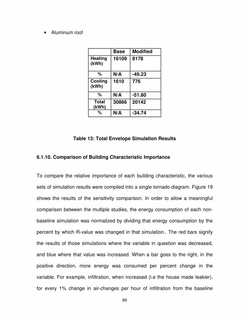
89
• Aluminum roof
Base Modified
Heating (kWh)
16109 8178
% N/A -49.23
Cooling (kWh)
1610 776
% N/A -51.80
Total (kWh)
30866 20142
% N/A -34.74
Table 13: Total Envelope Simulation Results
6.1.10. Comparison of Building Characteristic Importance
To compare the relative importance of each building characteristic, the various
sets of simulation results were compiled into a single tornado diagram. Figure 19
shows the results of the sensitivity comparison. In order to allow a meaningful
comparison between the multiple studies, the energy consumption of each non-
baseline simulation was normalized by dividing that energy consumption by the
percent by which R-value was changed in that simulation.. The red bars signify
the results of those simulations where the variable in question was decreased,
and blue where that value was increased. When a bar goes to the right, in the
positive direction, more energy was consumed per percent change in the
variable. For example, infiltration, when increased (i.e the house made leakier),
for every 1% change in air-changes per hour of infiltration from the baseline

90
value, the total annual energy consumption of the building rose approximately
.49%, or 154 kWh. When infiltration was decreased, approximately .13% (43
kWh) was saved per 1% decrease in air-changes per hour (This significant
difference was due to the lower limit of safe infiltration levels, and the ventilation
system kicking on to ensure a safe rate of fresh air circulation). It can be seen
that infiltration and the basement insulation had the greatest effect upon the
overall energy consumption of the building per percentage change, while such
things as roof coatings and window glazing improvements had far less effect, at
approximately .01%.
Figure 19: Envelope Characteristic Sensitivity Comparison

91
6.2 Indoor Equipment Simulations
The following simulations do not examine the construction of the building but
rather the type of equipment used inside the building, and the methods by which
they are used. Specifically, this section will survey the effects of changing HVAC
equipment, water heating methods, thermostat settings, the use of shade to
conserve energy, and the effect of increasing overall appliance efficiency. In
each case the baseline model was made to vary one characteristic at a time.
6.2.1 HVAC Simulations
Simulations were performed to determine the value of replacing HVAC
equipment, comparing the baseline’s 11 SEER air conditioner/ furnace
combination, to the alternative situations of replacing the air conditioner with a 13
SEER model, and by replacing the entire system with a 13 SEER, 8.25 HSPF.
Table 14 shows the results of this simulation. The results show the amount to
which heating energy consumption far outweighs the consumption by the cooling
system in this home, since while improving the cooling energy consumption by
approximately 15% reduces total energy consumption by about 1%, the reduction
of heat energy consumption by 69% in using the heat pump reduces the overall
energy consumption by almost 40%. In this simulation in particular it is important
to consider that while a heat pump might consume half the energy of a furnace
when considering a system containing only the house, in reality, since it’s
powered electrically, it could be using more energy than the furnace when the
scope of the system is extended to the power plant. For the purpose of a net-

92
zero-site-energy house, however, the heat pump results in considerable energy
savings
Furnace/ AC, SEER 11
Furnace/ AC SEER 13
HP
Heating (kWh) 16109 16110 4949
% N/A 0 -69.28
Cooling (kWh) 1610 1371 1370
% N/A -14.84 -14.91
Total (kWh) 30866 30523 18716
% N/A -1.11 -39.36
Table 14: Furnace- Heat Pump Comparison Results
6.2.2. Thermostat Setpoint simulations
The following simulations were conducted in order to find how changes to the
temperature setpoints recommended by the EPA affect annual energy
consumption. They were conducted using the baseline model and modifying the
schedule for the thermostat setback. As previously mentioned in Section 4.6, the
baseline case assumes no setback during the cooling season, but uses popular
thermostat setback temperatures during the heating season.

93
Cooling Setpoint Setpoint (deg F)
(home/away) 75/75 74/74 76/76 75/78
Cooling (kWh) 1610 1853 1472 1211
% N/A 15.09 -8.57 -24.78
Heating Setpoint Setpoint (deg F)
(home/away/asleep) 68/62/62 68/62/68 68/off/62 68/68/68
Heating (kWh) 16109 18101 15867 20472
% N/A 12.37 -1.50 27.08
Table 15: Setpoint Simulation Results
Table 14 shows the results of the thermostat setpoint simulation. Deviating from
recommended thermostat levels was shown to have a significant effect upon the
energy consumption of the building. By failing to set back the thermostat during
the heating season, the home consumed a full 27% more fuel in heating than the
baseline home, where some form of setback was used. During the cooling
season as similar result was found, since by easing the load on the air
conditioner by setting the cooling set point back to 78 °F during unoccupied
hours saved approximately 24% in cooling electricity consumption.

94
6.2.3 Hot water Simulations
Four different methods of heating water were modeled. These were as follows:
• Gas-fired, tank-storage
• Solar-heated, tank storage, gas burner backup
• Gas-fired demand heating
• Solar preheated, gas backup demand heating
The most conventional water heating method, and thus the option that was
employed for the simulation of the baseline residence, was the gas-fired, tank
storage method. The water tank was modeled as an 80 gallon tank, and heat
was provided with an efficiency of 80% from a gas burner at the bottom of the
water storage unit. This currently at the lowest end of the spectrum of thermal
efficiency in today’s natural gas burners, but compares well to slightly older
systems, because an 80% Annual Fuel Usage Efficiency (AFUE), or annual
average thermal efficiency, became the minimum legal AFUE in 1992, before
which boilers had AFUEs as low as 62% [66].

95
As mentioned previously, the DOE recommends a solar thermal collector of
3.3m2 size for a house with this number of residents. Therefore this size of
thermal collector was installed on the home.
Additional options exist for water heating, such as employing the desuperheater
of a ground-source heat pump to heat or preheat the water, or using a heat pump
water heater in place of the gas burner (heat pumps do not provide enough heat
output to be practical in an instantaneous (demand) heating system). The heat
pump water-heating option has been included in the simulation but its use was
not explored in this study.
Hot water system Results
Storage Solar? Energy Usage (kWh equiv)
% Change
Tank(Gas) N 5702 N/A
Tank (Gas)
Y 4324 -24
Demand N 3222 -43
Demand Y 550.6 -90
Table 16: Hot Water System Simulation Results
The results shown in Table 16 suggest that standby losses are the major factor in
this house’s water-heating energy consumption, since the solar thermal collector
is not of great enough capacity to maintain the necessary temperature demanded

96
by the load profiles, and the demand heater uses less energy than the solar-tank
combination by avoiding standby losses altogether. This problem could be solved
by further insulating the hot water tank, a variable which was not looked into by
this study. Predictably, the solar-preheated demand heater combination provided
the most energy efficient alternative, almost eliminating hot water natural gas
consumption with a 90% reduction. The solar tank setup and the conventional
tankless system also show to be effective measures at reducing energy
consumption, decreasing hot water gas consumption by 24 and 43 percent,
respectively.
6.2.4. Shading Simulations
In this pair of simulations, the effect of using a rigid schedule of altering the
position of window blinds was investigated. By activating the shade schedule, the
cooling system’s energy consumption was reduced to 1393 kWh (-13.48%
change), the heating bill to 16031 (-0.48% change), and the overall energy
consumption was reduced to 30530 (-1.09% change). While it has only a slightly
beneficial effect on heating costs, attention to the condition of window blinds has
a significant effect on cooling costs.
6.2.5. Appliance Simulations
Since appliances represent a major source of internal heat generation inside
buildings, the effect of the reduction of appliance power consumption upon the
space conditioning energy consumption was explored. By employing the energy-

97
efficient appliances as shown above in Table 4, a reduction of 35.5% was made
in the energy consumption of appliances, from 7407 kWh to 4770 kWh. By
reducing this appliance energy consumption, the heating costs for the building
rose slightly, from 16109 kWh to 17191 kWh, a 6.7% change, and the cooling
costs decreased from 1610 kWh to 1113 kWh, a -12.2% change. In this study it
was assumed that the electrical power consumed by appliances was entirely
distributed to the home, while in some cases that isn’t necessarily true, most
especially in the case of the range, which is routinely operated in concert with a
local ventilation system. It is apparent, however, that appliances, being a major
contributor to total power consumption, have an effect on the indoor comfort level
of buildings, due to the heat gains generated by their use.
6.3 Maryland ZEH Simulation
Finally, the many energy-saving alternatives presented in this thesis were
combined to explore the feasibility of achieving zero-net-energy status in a
College Park home. In order to do this, the following features were used:
• Heat pump heating & cooling
• Aluminum roof
• Solar-preheated demand water heater

98
• R-12 floors, R-20 Basement, R-23 Walls, R-40 attic
• Krypton-filled, double-paned, low-SHGC windows
• Reduced load profiles, with the reductions described above in Table 4
• EPA recommended thermostat settings, as described in Table 3
• Shading schedules activated
• 30% reduced infiltration
• 60 m2 of photovoltaic panels
Comfort levels were maintained at the same levels as those of the baseline
home. Since setback was employed, the comfort zone monitor does not display
the useful information, but Figure 20 depicts the temperature readings in the low-
energy home over the course of the year. Despite the main graph, which gives
the impression that very cool temperatures are maintained during the winter, by
zooming in it can be seen that that is merely the effect of the thermostat setback,
and that comfortable levels are maintained during occupancy hours.

99
Figure 20: Low- Energy House Temperature Readings

100
Building Baseline ZEH
Heating (kWh) 16109 2457
% N/A -82.8
Cooling (kWh) 1610 788
% N/A -52.56
Gross Consumption
(kWh)
30866 9781
% N/A -69.3
PV Production (kWh)
0 10565
Net Consumption
(kWh)
30866 -784
Table 17: ZEH Simulation Results
Table 17 shows the numerical results of the ZEH Simulation. The results show a
great potential for gross energy consumption reduction in the building, since this
was reduced by 61%. Normally, using an industry rule of thumb, a building is
expected to reduce its energy consumption by about 75% in order to be able to
achieve full zero-energy status when photovoltaic modules are attached, but in

101
this case, in this particular climate and with the building’s favorable south-facing
orientation, the array of photovoltaic panels was sufficient to overcome that
shortcoming.
7. Conclusions
The previous data show that there are various, and in some cases equally valid
measures of reducing the energy consumption of currently-standing residential
buildings. Although the total number of combinations of technology were not
completely inspected by this study, since given the large number of variables it
would necessitate the simulation of thousands of combinations. The most
effective energy saving methods are ranked as follows:
1. Using a heat pump rather than a furnace/ air conditioner combination
saved approximately 39.1%.
2. Building Envelope insulation and integrity improvements, shown in greater
detail in Figure 3, reduced consumption by approximately 34.7%.
3. The substitution of a solar-heated, on-demand backup water heater
saved approximately 14.7%.
4. The use of thermostat setback, compared to using constant settings,
achieved approximately 12.7% savings.
5. The reduction of appliance energy consumption by 2737 kWh reduced
total annual energy consumption by 2235 kWh or 6.1%. This total value is

102
less than 2737 due to increased use of the furnace to make up for
appliance heat gains.
6. The use of blinds in the most efficient manner possible, compared to
leaving them halfway down constantly, was shown to decrease energy
consumption by 1.1%.
It was verified that well-insulated glazing is among the most important features of
a building, in line with consensus of the building industry, and found that given
building-code-passing attic insulation and ducts contained within the building’s
thermal envelope, color changes to the building’s roof had little effect on an
individual house, no considering interaction with other buildings. Some
simulations, including that of the attic insulation variance, show the need to
increase the accuracy of modeling procedures beyond that of what were used in
this program.
Another significant finding is the great importance of user behavior patterns on
the final annual energy consumption of the building. One aspect of building
technology that gains great credence from the simulation results shown in this
paper is building automation. Especially in the case of thermostat levels, setback,
and shading usage, it was found that great potential for energy savings exists
when the responsibility of important energy-consuming aspects is taken out of
the hands of a person and put under the purview of a computer’s scheduling
system. As was seen in Masoso and in Foster, reliance on human nature to
flawlessly, consistently make energy-efficient choices is not always a safe

103
assumption, and accordingly, in this set of simulations the various methods of
building control saved at least 4500 kWh of energy consumption. In a similar
vein, it was found that more research needs to occur regarding occupant
behavioral activity in residential homes (e.g. occupancy and appliance usage) to
improve the accuracy of building model when compared to reality.
The results of the ZEH simulation suggest that it could be feasible to refit a
Maryland home to achieve net-zero site energy. This data, however, applies to
only this particular home layout, and does not necessarily indicate that it is
possible for all Maryland homes. Also, given the level of accuracy inherent to
building simulation tools, and the fact that zero-energy status was achieved by
only a factor of 784 kWh, the zero-energy status could possibly not be replicated
in reality. However, this can be viewed as an encouraging sign that a real, 2-
story, 2464-sq ft building could be feasibly converted into a zero-energy building.
8. Recommendations for Improvement
8.1 Economic Analysis
This thesis neglected the cost of each building modification and assumed that
sufficient funds were available to make necessary changes; in the real world this
is not the case and the economic trade-off is the prime concern. A rigorous
method of evaluating the economic tradeoffs necessary when purchasing or
104
installing each building modification would provide the data that is most important
to many consumers. TRNSYS contains an economic analysis module, Type 582,
which allows for a simple, if somewhat rigid, method of making calculations for
economic predictions. Full functionality of this program as the basis for savings
estimation software would definitely require a rigorous and flexible set of
economic analysis calculations to be included within the simulation itself.
However, adding cost modeling to the program would require taking into account
peak usage charges for electricity, and would require such things as estimates of
oil prices, etc, which given predicted future fuel shortages would likely introduce
far more uncertainty than modeling solely the fuel usage levels as has been done
here.
8.2 Building Detail
Some aspects of the building system were left uninspected, or simplified. In
future work it could prove helpful to use more close detail in certain systems.
Great care should be taken to streamline the calculations of the simulation
program, however, since as building detail increases, so does the calculation
time for each time step. Also, the inclusion of too much detail in building models
has been shown to have great potential for reducing certainty if not carefully
done [67]. Some suggestions for greater detail include:
-Appliances: The electric power consumed by appliances is released into the
indoor environment of the building as heat. This was modeled by introducing heat
gains over the entire conditioned area of the home, rather than, for example,

105
placing the heat addition of the refrigerator and stove in the kitchen, or the
lighting gains scheduled to coincide with occupancy schedules in different areas
of the home. This limitation was derived from the method of drawing the load
profile information from Excel and inserting it into TRNSYS. The current method
of linking Excel and TRNSYS uses Excel’s 1997 version, which allows for only
32000 data points. By altering the code of the Excel linking component in
TRNSYS to allow it to link with Excel 03 it would be theoretically possible to
expand the load profiles into the constituent individual appliances, therefore
allowing the placement of each system in an appropriate room of the building,
and allowing for easier modification of each device’s energy consumption level.
-Scheduling: For greater flexibility in controlling thermostat levels and shading
ratios, an Excel spreadsheet would work well in place of the TRNSYS forcing
functions.
-Controls: A major source of discussion lies in the field of “smart buildings,” that
is, buildings with automated systems that reduce energy consumption. This
model, despite consisting of several “zones” represents a home with one
thermostat controlling the temperature of one large thermal zone. By adding
thermostats in each room the effects of occupancy detection and shutting off
thermal control of unoccupied rooms could be investigated.
-Air flows in TRNFLOW: The Solar Energy Laboratory makes an airflow
program referred to as TRNFLOW. This software uses COMIS, Lawrence
Berkeley Laboratories’ Multi-Zone Airflow Model, and allows that model to

106
communicate with Type 56. COMIS is specifically built to model such things as
natural ventilation, interzonal air coupling, and infiltration, which were three of the
prime concerns of Judkoff’s critique of building simulations. Many of the
inaccuracies discussed in the above result analyses were attributed to an inability
to model heat flow within and between rooms, and thus the use of such a
program would help to alleviate some uncertainty in those affected areas of the
simulation.
On a similar note, local ventilation modeling would be useful. Two locations in
homes routinely contain exhaust fans which remove air from the indoor
environment and move it to the outside. These are above the range of a stove
and in bathrooms. ASHRAE standards dictate they should be present.
Bathrooms were not modeled in this program, and the stove heating rate was
unable to be separated from the other non-HVAC electrical loads due to Excel
conflicts, but given the frequency of showering and cooking in a home, being
able to model such could play a role in the heat and humidity of the building.
-TRNSYS 17: The current building simulation program was constructed using
TRNSYS 16. According to the developers of TRNSYS, Thermal Energy System
Specialists (TESS) a new version of TRNSYS will be produced and released in
2010. Many improvements are expected, including a link with Google’s drawing
program, SketchUp. Such a link will allow far easier communication of building
geometry to TRNSYS, and will allow a far more readily-modifiable building
structure. The simulation tool should be better matched to an actual building
107
geometry, since this new drawing tool will allegedly be available. Any increase of
detail with the controls of the building would be of much less value if those
controls control the simple box geometry found here. This possibility of including
a new visual interface with the building design provides further promise for this
building simulation program’s potential use as a consumer building modification
recommendation tool.

108
9. References
[1] Gallup. “Half of Public Favors the Environment Over Growth.” http://www.gallup.com/poll/105715/Half-Public-Favors-Environment-Over-Growth.aspx
[2] “The Stimulus Plan: How to Spend $787 Billion.” The New York Times. http://projects.nytimes.com/44th_president/stimulus/energy
[3] “Buildings Share of U.S. Primary Energy Consumption.“Buildings Energy Databook. U.S. Department of Energy. http://buildingsdatabook.eere.energy.gov/docs/xls_pdf/1.1.3.pdf
[4] “Buildings Share of U.S. Electricity Consumption.” Buildings Energy Databook. U.S. Department of Energy. http://buildingsdatabook.eere.energy.gov/docs/xls_pdf/1.1.9.pdf
[5] “2008 Annual Energy Review.” Energy Information Administration. U.S. Department of Energy. June 2009. http://www.eia.doe.gov/aer/pdf/aer.pdf
[6] “U.S. Retail Historical Gas Prices.” Energy Information Administration. U.S. Department of Energy. http://tonto.eia.doe.gov/oog/ftparea/wogirs/xls/pswrgvwnus.xls
[7] Wüstenhagen, Rolf, Maarten Wolsink, and Mary J. Bürer. "Social acceptance of renewable energy innovation: an introduction to the concept." Energy Policy 35 (May 2007): 2683-2691.
[8] Coombs, Rod. Technology and the Market: Demand, Users and Innovation. Northampton: Edward Elgar Publishing, 2001.
[9] Chapman, R. “Retrofitting houses with insulation: a cost–benefit analysis of a randomised community trial.” Journal of Epidemiology and Community Health, April 1, 2009; 63(4): 271 – 277.
[10] H. Hens, G. Verbeeck, B. Verdonck, Impact of energy efficiency measures on the CO2 emissions in the residential sector, a large scale analysis, Energy and Buildings 33 (2001) 275–281
[11] TRNSYS 16. Solar Energy Laboratory, University of Wisconsin, Madison, WI. 2006.
[12] Crawley, Drury B., Jon W. Hand, Michael Kummert, and Brent T. Griffith. “Contrasting the Capabilities of Building Energy Performance Simulation Programs.” Building and Environment. Vol 43, April 2008. pp 661-673.

109
[13] Lust, Ethan. “System-Level Analysis and Comparison of Long-Haul Truck Idle-Reduction Technologies.” Master’s thesis. Unpublished. University of Maryland, 2008.
[14] Tse, Humphrey, Alan Fung, Omar Siddiqui, and Farzin Masoumi Rad. “Simulation of a Net-Zero Energy Townhome in Toronto”. Ryerson University-Toronto. 2nd Canadian Solar Buildings Conference 2007.
[15] Gilijamse, Wim. “Zero-Energy Houses in the Netherlands.” Proceedings of Building Simulation '95. Madison, Wisconsin, August 14–16, 1995. pp. 276–83.
[16] Iqbal, M.T. “A Feasibility Study of a Zero Energy Home in Newfoundland.” Renewable Energy, Vol. 29, Issue 2, pages 277-289.
[17] Katipamula, Srinivas, and David E. Claridge. “Simulation of the Post-Retrofit Thermal Energy Use for the University Teaching Center (UTC) Building with the Use of Simplified System Models”. College Station, TX: Texas A&M University. 1991.
[18] Emmerich, Steven J., Tim McDowell, and Wagdy Anis. “Investigation of the Impact of Commercial Building Envelope Air-tightness on HVAC Energy Use.” National Institute of Standards and Technology. June 2005.
[19] H. Hens, G. Verbeeck,” Energy savings in retrofitted dwellings: economically viable? Energy and Buildings 37 (2005) 747-754.
[20] Bradley, David. TESS programmer. Informal interview.
[21] “TRNSYS 16 - Multizone Building Modeling with Type 56 and TRNBuild,” 2007. Solar Energy Laboratory, University of Wisconsin, Madison, WI.
[22] “Median and Average Square Feet of Floor Area in New One-Family Houses Completed by Location”. U.S. Census Bureau. 2008. http://www.census.gov/const/C25Ann/sftotalmedavgsqft.pdf
[23] “Current Housing Reports Series H150/01.” American housing survey for the United States, 2001. U.S. Census Bureau. U.S. Government Printing Office: 2002.
[24] “Median and Average Square Feet of Floor Area in New One-Family Houses Completed by Location”. U.S. Census Bureau. 2008. http://www.census.gov/const/C25Ann/sftotalmedavgsqft.pdf
[25] “Roofing Terminology.” www.roofingkey.com. Accessed 28 December 2009. http://www.roofingkey.com/roofing-terms.html.

110
[26] “Senate Bill 625: Maryland Building Performance Standards – Energy Conservation and Efficiency.” Maryland General Assembly. http://mlis.state.md.us/2009rs/bills/sb/sb0625e.pdf.
[27] Taylor, Z.T., C.C. Conner, and R.G. Lucas. “Eliminating Window Area Restrictions in the IECC.” Pacific Northwest National Laboratory. October 2001. http://www.energycodes.gov/implement/pdfs/wwr_elimination.pdf
[28] Meier, Alan. “Infiltration: Just ACH50 Divided by 20?.” Home Energy. January 1994. http://www.homeenergy.org/archive/hem.dis.anl.gov/eehem/94/940111.html
[29] Max Sherman, "Estimation of Infiltration for Leakage and Climate Indicators," Energy and Buildings, 10, 1987, p.81
[30] ASHRAE, 2005. ASHRAE Handbook: Fundamentals. Atlanta: American Society of Heating, Refrigerating and Air-Conditioning Engineers, Inc.
[31] Wang, F.S., Sr. and Sepsy, C.F., “Field Studies of Air-Tightness of Residential Buildings,” Building Air Change Rate and Infiltration Measurements. ASTM STP 719, C.M. Hunt, J.C. King and H.R. Trechsel, Eds., American Society for Testing and Materials, 1980, pp.24-35.
[32] ASHRAE. 2003. ANSI/ASHRAE Standard 62.2-2003, Ventilation and Acceptable Indoor Air Quality in Low-Rise Residential Buildings. Atlanta: American Society of Heating, Refrigerating and Air-Conditioning Engineers, Inc.
[33] “Energy Consumption in Maryland Homes.” EERE,U.S. Department of Energy. Accessed 3 January 2010. http://apps1.eere.energy.gov/states/residential.cfm/state=MD
[34] Foster, Michelle and Tadj Oreszczyn. “Occupant Control of Passive Systems: The Use of Venetian Blinds.” Building and Environment. Volume 36, Issue 2.
[35] Rea, M.S. “Window Blind Occlusion, a Pilot Study.” Building & Environment, Vol. 19, No. 2, 1984, pp. 133 –137.
[36] “Impacts of the 2009 IECC for Residential buildings at State Level.” Pacific Northwest National Laboratory. September 2009. http://www.energycodes.gov/implement/state_codes/reports/residential/Residential_Maryland.pdf
[37] Musser, Amy. “Energy Impact Study of the 2003 IECC and 2009 IECC Energy Codes for Nebraska.” Nebraska Department of Energy. http://www.neo.ne.gov/home_const/iecc/documents/NE_codes_report_6-30-09[1].pdf
111
[38] Lubliner, Michael, Ryan Kerr, Andy Gordon, and Chuck Murray.“Moving Ducts Inside: Big Builders, Scientists Find Common Ground.” Washington State University Extension Energy Program. ACEEE Summer Conference 2008. http://www.energy.wsu.edu/documents/code/ACEEE_Ducts_Inside.pdf
[39] Modera, Mark. “One Size Fits All: A Thermal Distribution Efficiency Standard.” Home Energy. September 1993.
[40] Lubliner, Michael R., et al. Costs of New Residential Conservation Measures in the Pacific Northwest; Results of Construction Costs and Practices Study from the Regional Cost Research Advisory Group. Portland, Ore.: Bonneville Power Administration, 1995.
[41] “Programmable Thermostats for Consumers.” Energy Star, U.S. Environmental Protection Agency. Accessed 10 December 2009. http://www.energystar.gov/index.cfm?c=thermostats.pr_thermostats
[42] Mozier, MC, L Vidmar, and R.H. Dodier. “The Neurothermostat: Adaptive control of residential heating systems.” Advances in Neural Information Processing Systems, Cambridge, MA: MIT Press, 1997.
[43] “Air Conditioning Usage Indicators.” RECS 2005. Energy Information Administration, U.S. Department of Energy. http://www.eia.doe.gov/emeu/recs/recs2005/hc2005_tables/hc7airconditioningindicators/pdf/tablehc2.7.pdf
[44]“Space Heating Usage Indicators.” RECS 2005. Energy Information Administration, U.S. Department of Energy. http://www.eia.doe.gov/emeu/recs/recs2005/hc2005_tables/hc5spaceheatingindicators/pdf/tablehc11.5.pdf.
[45] “Programmable Thermostats for Consumers.” Energy Star, U.S. Environmental Protection Agency. Accessed 10 December 2009. http://www.energystar.gov/index.cfm?c=thermostats.pr_thermostats.
[46] “XB13 Heat Pump: Standard Efficiency Units.” http://www.trane.com/Residential/Products/Heat-Pumps/XB14-Heat-Pump
[47] “Sizing a Solar Water Heating System.” EERE, U.S. Department of Energy. http://www.energysavers.gov/your_home/water_heating/index.cfm/mytopic=12880.
[48] Tester, Jefferson W., Elizabeth M. Drake, Michael J. Driscoll, Michael W. Golay, and William A Peters. Sustainable Energy: Choosing Among Options. Cambridge, MA: MIT Press, 2005.
[49] Knight, Ian, Nico Kreutzer, Marianne Manning, Mike Swinton, and Hajo Ribberink. “European and Canadian non-HVAC Electric and DHW Load Profiles

112
for Use in Simulating the Performance of Residential Cogeneration Systems”. Annex 42 of the International Energy Agency, Subtask A. May 2007.
[50] ”Improvements in Appliance Efficiency, by Product.” Office of Energy Efficiency, Natural Resources Canada. http://oee.nrcan.gc.ca/residential/personal/appliances/improvements.cfm?attr=4.
[51] “Find a Replacement Bulb.” GE Lighting. Accessed 16 December 2009. http://www.gelighting.com/na/home_lighting/products/replacement_cfl/general_purpose.htm
[52] “Improvements in Appliance Efficiency: by Product.” Natural Resources Canada. Accessed 16 December 2009. http://oee.nrcan.gc.ca/residential/personal/appliances/improvements.cfm?attr=4
[53] Krigger, John and Chris Dorsi. The Homeowner’s Handbook to Energy Efficiency: A Guide to Big and Small Improvements. Helena: Saturn Resource Management, 2008.
[54] “Water Heating Characteristics by Year of Construction.” RECS 2005. Energy Information Administration, U.S. Department of Energy. http://www.eia.doe.gov/emeu/recs/recs2005/hc2005_tables/hc8waterheating/pdf/tablehc5.8.pdf
[55] “End Use Consumption of Electricity, 2001.” RECS 2001. Energy Information Administration, U.S. Department of Energy. http://www.eia.doe.gov/emeu/recs/recs2001/enduse2001/enduse2001.html
[56] Judkoff, R., D. Wortman, B. O’Doherty, and J. Burch. “A Methodology for Validating Building Energy Analysis Simulations.” National Renewable Energy Laboratory, April 2008. http://www.nrel.gov/docs/fy08osti/42059.pdf
[57] MacGillis, Alec. “Painting a street green hasn't stimulated one new job.” Washington Post. 7 November 2009.
[58] Akbari,H, M Pomerantz, and H Taha. “Cool surfaces and shade trees to reduce energy use and improve air quality in urban areas.” Solar Energy, Volume 70, Issue 3, 2001, Pages 295-310.
[59] Parker, D., Huang, Y., Konopacki, S., Gartland, L., Sherwin, J., Gu, L, "Measured and Simulated Performance of Reflective Roofing Systems in Residential Buildings", ASHRAE Transactions, Vol. 104, Pt. 1, American Society of Heating, Refrigerating and Air Conditioning Engineers, 1998.
[60] “Energy Savings Resulting from Shading devices on Single-Family Residences in Austin, Texas.” Proceedings of the Fourth Symposium on Improving Building Systems in Hot and Humid Climates, Houston, TX, September 15-16, 1987.

113
[61] TMY3 Data: Sterling, VA. National Solar Radiation Database. http://rredc.nrel.gov/solar/old_data/nsrdb/1991-2005/data/tmy3/745940TY.csv
[62] Taha, H. “Modeling the impacts of large-scale albedo changes on ozone air quality in the South Coast Air Basin,” Atmospheric Environment , 31 (11) (1997), pp. 1667–1676.
[63] “Loads.” DOE-2 Manual. Lawrence Berkeley Laboratory. http://gundog.lbl.gov/dirpubs/BASIC/lds2.pdf
[64] “ENERGY STAR Version 2.0 Final Draft.” Roof Coating Manufacturers Association. http://www.energystar.gov/ia/partners/prod_development/revisions/downloads/roofs/RCMA-CommentLetter-081606.pdf
[65] Parker, Danny S, Yu Joe Huang, Steven J. Konopacki, Lisa M. Gartland, John R. Sherwin, and Lixing Gu. “Measured and Simulated Performance of Reflective Roofing Systems in Residential Buildings.” ASHRAE Transactions, Vol. 104, Pt. 1B, January 1998.
[66] “Heating Systems: Furnaces and Boilers.” Consumer Guide: Condensed Online Version. American Council for an Energy-Efficient Economy. http://www.aceee.org/Consumerguide/heating.htm
[67] Purdy J and Beausoleil-Morrison I. “The Significant Factors In Modelling Residential Buildings,” Proc. Building Simulation '01, (1), 207-214, Rio de Janeiro.