An Approach to Increase the Lifetime of a Linear Array of Wireless Sensor Nodes

LETTER

An Approach to Increase the Lifetime of a Linear Arrayof Wireless Sensor Nodes

Ashraf Hossain Æ T. Radhika Æ S. Chakrabarti ÆP. K. Biswas

Published online: 14 May 2008

� Springer Science+Business Media, LLC 2008

Abstract The nodes in a wireless sensor network are

generally energy constrained. The lifetime of such a net-

work is limited by the energy dissipated by individual

nodes during signal processing and communication with

other nodes. The issues of modeling a sensor network and

assessment of its lifetime have received considerable

attention in recent years. This paper provides an analytical

framework for placing a number of nodes in a linear array

such that each node dissipates the same energy per data

gathering cycle. This approach ensures that all nodes run

out of battery energy almost simultaneously. It is shown

that the network lifetime almost doubles with the proposed

scheme as compared to other reported schemes. However,

in practice, the nodes are not expected to be placed as per

this theoretical requirement. The issue of random place-

ment of nodes has also been investigated to obtain the

statistics of energy consumption of a node. The analytical

results for random node placement are validated through

simulation studies.

Keywords Data gathering sensor network � Multi-hop �Inter-node distance � Network lifetime �Random node placement

1 Introduction

A wireless sensor network consists of energy-constrained

nodes that are deployed for monitoring multiple phenom-

ena of interest. A sensor node consists of a sensing unit, a

processing unit, a radio transceiver and a power manage-

ment unit [1]. Sensor nodes produce some measurable

responses to changes in physical or chemical conditions

and transmit these responses to a common sink in the form

of packets of data over a wireless channel. There are three

broad classes of sensor networks, viz. (i) data gathering

(clock-driven), (ii) event-driven and (iii) demand-driven

[2]. All these categories have been widely considered for

studying several issues such as assessment of network

lifetime, energy- aware routing procedures, data aggrega-

tion and traffic modeling.

The sensor nodes are sometimes deployed in adverse

conditions with limited energy that may not be replenished.

An accepted definition of lifetime of a sensor network is the

time span from the instant when the network is deployed to

the instant when the network is considered to be non-func-

tional. A network is considered to be non-functional (a) even

when a single sensor node dies, or (b) a percentage of the

nodes die or (c) when a loss of coverage occurs due to

mobility of the nodes or due to failure of a node [2–4].

In a multi-hop linear wireless sensor network, the nodes

closer to the sink may have higher load of relaying packets

as compared to the distant nodes. Hence the nodes closer to

the sink are likely to get over-burdened and run out of their

battery energy sooner. This type of linear sensor network

A. Hossain (&) � P. K. Biswas

Department of Electronics & Electrical Communication

Engineering, Indian Institute of Technology, Kharagpur,

West Bengal 721302, India

e-mail: [email protected]

P. K. Biswas


T. Radhika

NVIDIA Graphics Private Ltd., Pune, India


S. Chakrabarti

G. S. Sanyal School of Telecommunications, Indian Institute

of Technology, Kharagpur, West Bengal 721302, India


123

Int J Wireless Inf Networks (2008) 15:72–81

DOI 10.1007/s10776-008-0077-6

has applications in highway traffic monitoring, border line

surveillance, oil and natural gas pipeline monitoring etc. to

mention a few. Bhardwaj et al. [5] have considered a linear

multi-hop network and proposed an upper bound on the

lifetime of the network for an optimum number of inter-

mediate nodes. However, this analysis is not applicable to

situations where each node in the network senses and

transmits its own packet, in addition to the packets received

from other nodes.

Shelby et al. [6] have considered a linear many-to-one

multi-hop sensor network. The issue of optimal spacing

between consecutive nodes in a data gathering network

over a given distance has been addressed while minimizing

the overall energy consumption during a data gathering

cycle. It has been shown that the node farthest from the

sink consumes maximum energy as compared to the nodes

nearer to the sink. However, in the case of a weighted

spacing arrangement, nodes nearer to the sink consume

more energy than the distant nodes. So the problem of non-

uniform energy consumption by the nodes still exists.

Several authors have focused on the issue of minimi-

zation of total energy consumed by the network in a data

gathering cycle while allowing dissimilar energy con-

sumption by the nodes. This approach results in faster burn

out of nodes far away from the sink. A different approach

has been reported in [7], where nodes are intelligently

placed in a linear array ensuring that all nodes run out of

energy at the same time.

Haenggi [8] has found the inter-node distance for a

linear sensor network ensuring equal energy consumption.

This analysis has been done considering only the energy

required to transmit a packet. Energy requirement for

receiving a packet and idle state energy are not included in

the analysis.

It may be noted that, none of the reported work has

addressed the issue of random node placement and its

effect on energy dissipation profile of the array. These

issues are important in the practical scenarios. Another

common feature of the related reported work is that the

total energy consumed by the overall network is mini-

mized. This implies that the nodes dissipate different

amount of energy over a data gathering cycle. In our work,

we enforce equal energy dissipation by each and every

node except the sink in our network. This approach helps to

eliminate the non-uniform energy consumption pattern in

the network. We give an explicit analysis of node place-

ment strategy ensuring same energy dissipation by all

nodes in a data gathering cycle. An expression for network

lifetime is also developed. We have compared our results

with [6] and [8]. With our scheme, the lifetime is seen to

increase significantly. In the process, we have introduced a

new performance measure of the whole network, viz.

energy utilization ratio (g), which indicates the percentage

of energy of the network that is consumed when the net-

work dies. It is shown that energy utilization as per our

scheme is much higher than other comparable schemes. We

also address the issue of random placement of nodes to

obtain the statistics of energy consumption of a node. The

analytical results are also validated through simulation

studies.

The rest of the paper is organized as follows. Section 2

gives the system description and problem formulation.

Section 3 illustrates the proposed scheme. Random node

placement is analyzed in Sect. 4. In Sect. 5, we present

extensive analytical and simulation results. Finally, Sect. 6

concludes the paper.

2 System Description

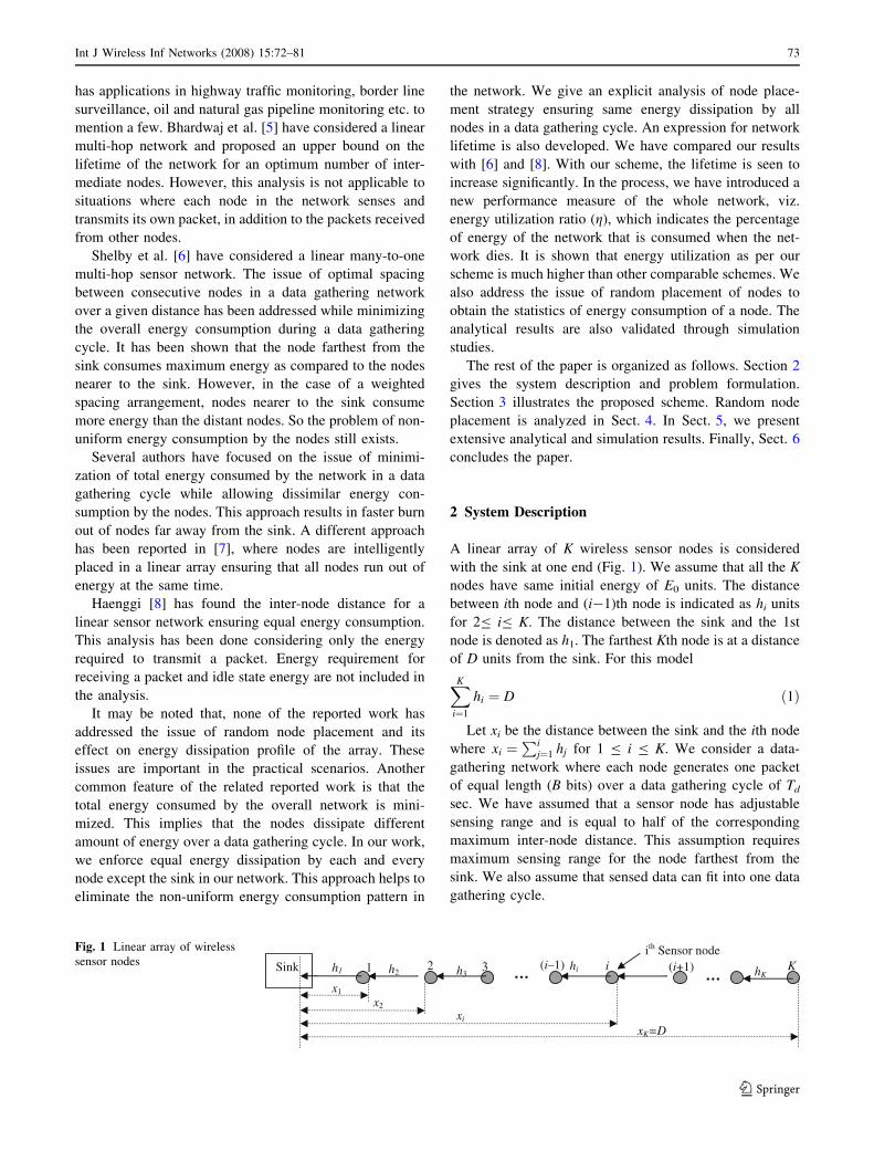
A linear array of K wireless sensor nodes is considered

with the sink at one end (Fig. 1). We assume that all the K

nodes have same initial energy of E0 units. The distance

between ith node and (i-1)th node is indicated as hi units

for 2B iB K. The distance between the sink and the 1st

node is denoted as h1. The farthest Kth node is at a distance

of D units from the sink. For this model

XK

i¼1

hi ¼ D ð1Þ

Let xi be the distance between the sink and the ith node

where xi ¼Pi

j¼1 hj for 1 B i B K. We consider a data-

gathering network where each node generates one packet

of equal length (B bits) over a data gathering cycle of Td

sec. We have assumed that a sensor node has adjustable

sensing range and is equal to half of the corresponding

maximum inter-node distance. This assumption requires

maximum sensing range for the node farthest from the

sink. We also assume that sensed data can fit into one data

gathering cycle.

Sink 1 2 3 (i–1) iith Sensor node

K

xK=D

h1 h2 hKhih3

(i+1)

x1

x2xi

… …

Fig. 1 Linear array of wireless

sensor nodes

Int J Wireless Inf Networks (2008) 15:72–81 73

123

A node sends a packet to the sink by using the nearest

neighbour towards the sink as a repeater. Nodes closer to

the sink are expected to forward all the packets towards the

sink. One can incorporate data aggregation at the node

level by incorporating extra processing software to all the

nodes. In our model, no data aggregation is assumed for

simplicity. We assume that each node can deal with max-

imum P packets/second. This implies that P� TdC K.

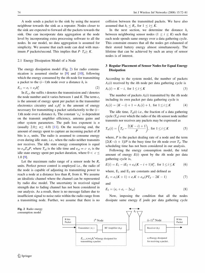
2.1 Energy Dissipation Model of a Node

The energy dissipation model (Fig. 2) for radio commu-

nication is assumed similar to [9] and [10], following

which the energy consumed by the ith node for transmitting

a packet to the (i-1)th node over a distance hi is

Et;i ¼ et þ edhni ð2Þ

In Et,i, the suffix t denotes the transmission and i denotes

the node number and it varies between 1 and K. The term et

is the amount of energy spent per packet in the transmitter

electronics circuitry and edhni is the amount of energy

necessary for transmitting a packet satisfactorily to the (i-

1)th node over a distance hi. The constant ‘ed’ is dependent

on the transmit amplifier efficiency, antenna gains and

other system parameters. The path loss exponent is n

(usually 2.0B nB 4.0) [11]. On the receiving end, the

amount of energy spent to capture an incoming packet of B

bits is er units. The radio is assumed to consume energy

even during idle state, i.e., when the radio neither transmits

nor receives. The idle state energy consumption is equal

to eidTidP, where Tid is the idle time and eid = c� er is the

idle state energy spent per packet duration, where 0\ c B

1.0 [9].

Let the maximum radio range of a sensor node be Rr

units. Perfect power control is employed i.e., the radio of

the node is capable of adjusting its transmitting power to

reach a node at a distance less than Rr from it. We assume

an idealistic channel where the channel can be represented

by radio disc model. The uncertainty in received signal

strength due to fading channel has not been considered in

our analysis. As a result, there is no message failure due to

insufficient signal to noise ratio within the radio range from

a transmitting node. Further, we assume that there is no

collision between the transmitted packets. We have also

assumed that hi B Rr, for 1 B iB K.

In the next section, we determine the distance hi

between neighboring sensor nodes (1 B i B K) such that

each node spends same energy over a data gathering cycle.

This constraint ensures that all the nodes get exhausted of

their stored battery energy almost simultaneously. The

lifetime that can be achieved by such an array of sensor

nodes is of interest.

3 Regular Placement of Sensor Nodes for Equal Energy

Dissipation

According to the system model, the number of packets

Ar(i) received by the ith node per data gathering cycle is

ArðiÞ ¼ K � i; for 1� i�K ð3Þ

The number of packets At(i) transmitted by the ith node

including its own packet per data gathering cycle is

AtðiÞ ¼ ðK � iÞ þ 1 ¼ ArðiÞ þ 1; for 1� i�K ð4Þ

The idle time, Tid(i) i.e., the fraction of a data gathering

cycle (Td) over which the radio of the ith sensor node neither

transmits nor receives any packets may be expressed as

TidðiÞ ¼ Td �2ðK � iÞ þ 1

P

� �; for 1� i�K ð5Þ

where, P is the packet dealing rate of a node and the term

[2(K-i) + 1]/P is the busy time for ith node over Td. The

scheduling time has not been considered in our analysis.

Following the energy consumption model, the total

amount of energy E(i) spent by the ith node per data

gathering cycle is,

EðiÞ ¼ E1 � iE2 þ edðK � iþ 1Þhni ; for 1� i�K ð6Þ

where, E1 and E2 are constants and defined as

E1 ¼ etðK þ 1Þ þ erK þ eidðPTd � 2K � 1Þ ð7Þ

and

E2 ¼ ðet þ er � 2eidÞ ð8Þ

Now, imposing the condition that all the nodes

dissipate same energy E joule per data gathering cycle

Transmitter ( et ) RF Amplifier (ed)

Receiver (er)

hi

B bits Packet

B bits Packet

ith Node (i–1)th Node

Et,i = et+edhin=Energy dissipated for

transmitting a packet.

er=Energy dissipated for receiving a packet.

Fig. 2 Radio energy

consumption model

74 Int J Wireless Inf Networks (2008) 15:72–81

123

i.e., E(i) = E, for 1B iB K, the inter-node distance hi can

be expressed as

hi ¼�

1

ðK � iþ 1ÞedE þ ðK � iÞð2eid � erÞ½

�ðPTd � 1Þeid � etðK � iþ 1Þ��1

n

; 1� i�K

ð9Þ

The distance hi can be obtained from (9) normalized to hK,

the inter-node distance between Kth node and (K-1)th node.

A solution for hK can be obtained from (10) graphically:

C1hnK � Dhn�1

K � C2 ¼ 0 ð10Þ

where, C1 ¼PK

i¼1 i�1=n and

C2 ¼ ðetþer�2eidÞned

PKi¼1 ði� 1Þ i�1=n

It is interesting to note that each node dissipates a

minimum energy Emin joule based on the values of D, K, et,

er, ed and eid as obtained from (9)

Emin ¼ Ket þ ðK � 1Þer þ ðPTd � 2K þ 1Þeid ð11Þ

For known values of radio parameters, the feasible

solution of hi can be found when E [ Emin, as has been

implicitly assumed in (9).

In the next section, we present an analysis about the

effects of random node placement on the overall energy

dissipation of the array.

4 Analysis for Random Node Placement

In the previous section we have derived the exact position

of K nodes over a distance (D) to ensure equal energy

dissipation by each node. However, in practice, the nodes

are not expected to be placed so ideally. In this section we

consider a situation wherein the position of a node is ran-

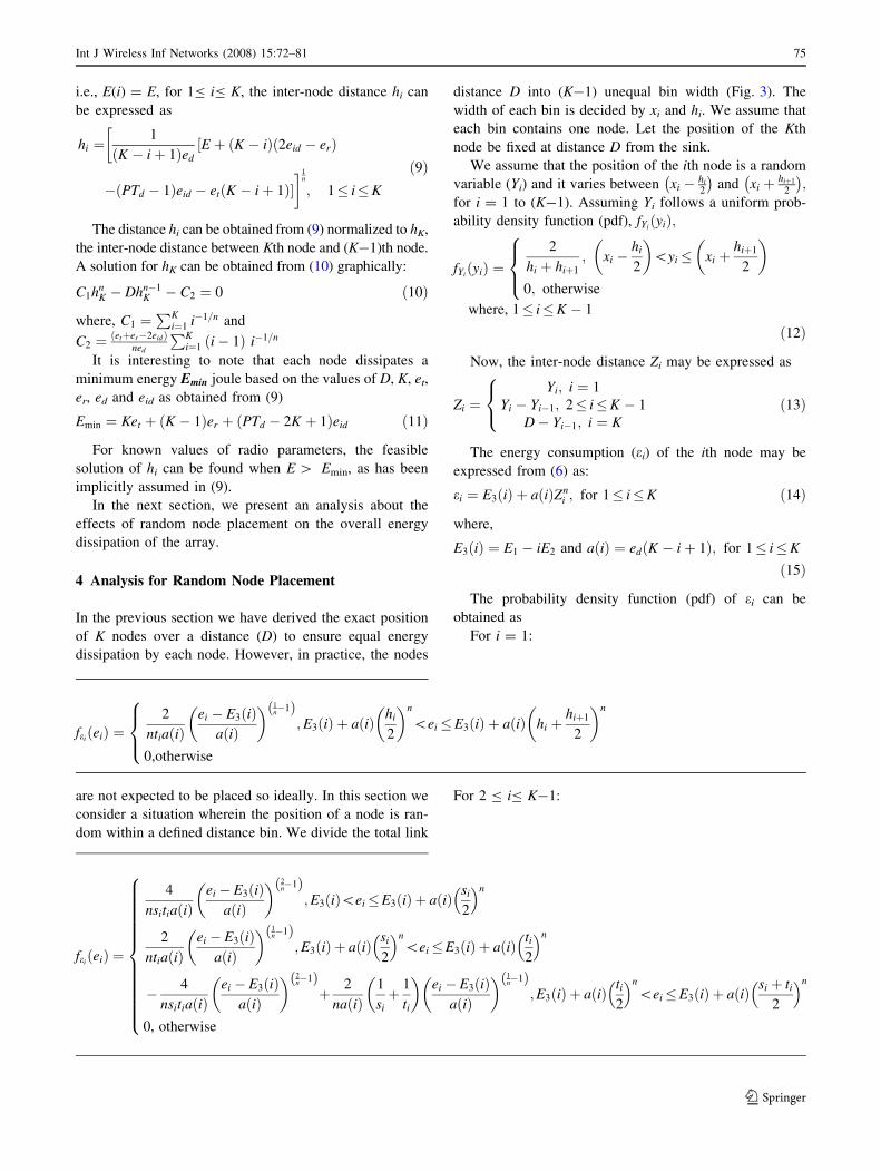
dom within a defined distance bin. We divide the total link

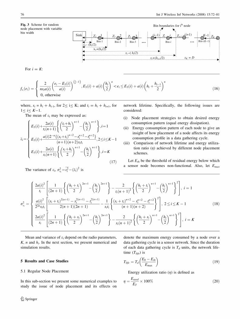
distance D into (K-1) unequal bin width (Fig. 3). The

width of each bin is decided by xi and hi. We assume that

each bin contains one node. Let the position of the Kth

node be fixed at distance D from the sink.

We assume that the position of the ith node is a random

variable (Yi) and it varies between xi � hi

2

� �and xi þ hiþ1

2

� �;

for i = 1 to (K-1). Assuming Yi follows a uniform prob-

ability density function (pdf), fYiðyiÞ;

fYiðyiÞ ¼

2

hi þ hiþ1

; xi �hi

2

� �\yi� xi þ

hiþ1

2

� �

0; otherwise

8><

>:

where, 1� i�K � 1

ð12Þ

Now, the inter-node distance Zi may be expressed as

Zi ¼Yi; i ¼ 1

Yi � Yi�1; 2� i�K � 1

D� Yi�1; i ¼ K

8<

: ð13Þ

The energy consumption (ei) of the ith node may be

expressed from (6) as:

ei ¼ E3ðiÞ þ aðiÞZni ; for 1� i�K ð14Þ

where,

E3ðiÞ ¼ E1 � iE2 and aðiÞ ¼ edðK � iþ 1Þ; for 1� i�K

ð15Þ

The probability density function (pdf) of ei can be

obtained as

For i = 1:

For 2 B iB K-1:

feiðeiÞ ¼

2

ntiaðiÞei � E3ðiÞ

aðiÞ

� � 1n�1ð Þ

;E3ðiÞ þ aðiÞ hi

2

� �n

\ei�E3ðiÞ þ aðiÞ hi þhiþ1

2

� �n

0,otherwise

8><

>:

feiðeiÞ ¼

4

nsitiaðiÞei � E3ðiÞ

aðiÞ

� � 2n�1ð Þ

;E3ðiÞ\ei�E3ðiÞ þ aðiÞ si

2

� �n

2

ntiaðiÞei � E3ðiÞ

aðiÞ

� � 1n�1ð Þ

;E3ðiÞ þ aðiÞ si

2

� �n

\ei�E3ðiÞ þ aðiÞ ti2

� �n

� 4

nsitiaðiÞei � E3ðiÞ

aðiÞ

� � 2n�1ð Þþ 2

naðiÞ1

siþ 1

ti

� �ei � E3ðiÞ

aðiÞ

� � 1n�1ð Þ

;E3ðiÞ þ aðiÞ ti2

� �n

\ei�E3ðiÞ þ aðiÞ si þ ti

2

� �n

0, otherwise

8>>>>>>>>>>>><

>>>>>>>>>>>>:


123

For i = K:

where, si = hi + hi-1, for 2B iB K; and ti = hi + hi+1, for

1B iB K-1.

The mean of ei may be expressed as:

�ei¼

E3ðiÞþ2aðiÞ

tiðnþ1Þtiþhi

2

� �nþ1

� hi

2

� �nþ1( )

; i¼1

E3ðiÞþaðiÞ2�nfðsiþtiÞnþ2�snþ2

i �tnþ2i g

ðnþ1Þðnþ2Þsiti;2�i�K�1

E3ðiÞþ2aðiÞ

siðnþ1Þsiþhi

2

� �nþ1

� hi

2

� �nþ1( )

; i¼K

8>>>>>>>>>><

>>>>>>>>>>:

ð17Þ

The variance of ei, r2ei¼e2

i �ð�eiÞ2 is

Mean and variance of ei depend on the radio parameters,

K, n and hi. In the next section, we present numerical and

simulation results.

5 Results and Case Studies

5.1 Regular Node Placement

In this sub-section we present some numerical examples to

study the issue of node placement and its effects on

network lifetime. Specifically, the following issues are

considered:

(i) Node placement strategies to obtain desired energy

consumption pattern (equal energy dissipation).

(ii) Energy consumption pattern of each node to give an

insight of how placement of a node affects its energy

consumption profile in a data gathering cycle.

(iii) Comparison of network lifetime and energy utiliza-

tion ratio (g) achieved by different node placement

schemes.

Let Eth be the threshold of residual energy below which

a sensor node becomes non-functional. Also, let Emax

denote the maximum energy consumed by a node over a

data gathering cycle in a sensor network. Since the duration

of each data gathering cycle is Td units, the network life-

time (Tlife) is

Tlife ¼ TdE0 � Eth

Emax

� �ð19Þ

Energy utilization ratio (g) is defined as

g ¼ Eused

ET� 100% ð20Þ

Sink 1 2 3 (i–1) i

Bin boundaries for ith node

xK = D

Z1 Z2 ZKZiZ3

(i+1)

x1– (h1/2)

xi+(hi+1/2)

xi –( hi/2)x1+(h2/2)

K–1

Bin-1 -niB 2-niB i Bin-(K–1) Bin-3

Zi+1

… …

Fig. 3 Scheme for random

node placement with variable

bin width

feiðeiÞ ¼

2

nsiaðiÞei � E3ðiÞ

aðiÞ

� � 1n�1ð Þ

;E3ðiÞ þ aðiÞ hi

2

� �n

\ei�E3ðiÞ þ aðiÞ hi þhi�1

2

� �n

0, otherwise

8><

>:ð16Þ

r2ei¼

2aðiÞ2

ti

1

ð2nþ 1Þhi þ ti

2

� �2nþ1

� hi

2

� �2nþ1( )

� 2

tiðnþ 1Þ2hi þ ti

2

� �nþ1

� hi

2

� �nþ1( )2

2

4

3

5; i ¼ 1

aðiÞ2

22nsiti

ðsi þ tiÞ2ðnþ1Þ � s2ðnþ1Þi � t

2ðnþ1Þi

2ðnþ 1Þð2nþ 1Þ � 1

siti

ðsi þ tiÞnþ2 � snþ2i � tnþ2

i

ðnþ 1Þðnþ 2Þ

( )224

35; 2� i�K � 1

2aðiÞ2

si

1

ð2nþ 1Þhi þ si

2

� �2nþ1

� hi

2

� �2nþ1( )

� 2

siðnþ 1Þ2hi þ si

2

� �nþ1

� hi

2

� �nþ1( )2

2

4

3

5; i ¼ K

8>>>>>>>>>>>>><

>>>>>>>>>>>>>:

ð18Þ


123

where, Eused is the total energy utilized by the network

during its lifetime and ET is the total deployed energy. For

K nodes ET equals to KE0.

For all the studies we consider a typical set of param-

eters as shown in Table 1. Following three schemes have

been used for performance comparison:

Scheme a—All nodes have equal inter-node spacing i.e.

hi = D/K [6].

Scheme b—Nodes are placed for minimizing the overall

energy dissipation in a data gathering cycle [6].

Scheme c—This is our proposed scheme. Here, the nodes

are placed so that each node dissipates equal amount of

energy in a data gathering cycle.

First we consider free space communication (i.e. path

loss exponent, n = 2.0) for ease of explanation. Typical

values of other relevant parameters in Table 1 have been

chosen following [9] closely. The radio parameters are

given on a per packet basis.

Using the constraint hK B Rr we get form (10)

XK

i¼1

ð2R2r � ði� 1Þe0Þ=

ffiffiip� 2RrD ð21Þ

where, the constant e0 = (et + er-2eid)/ed.

The minimum value of K satisfying the inequality (21)

is 33 for the chosen parameter values.

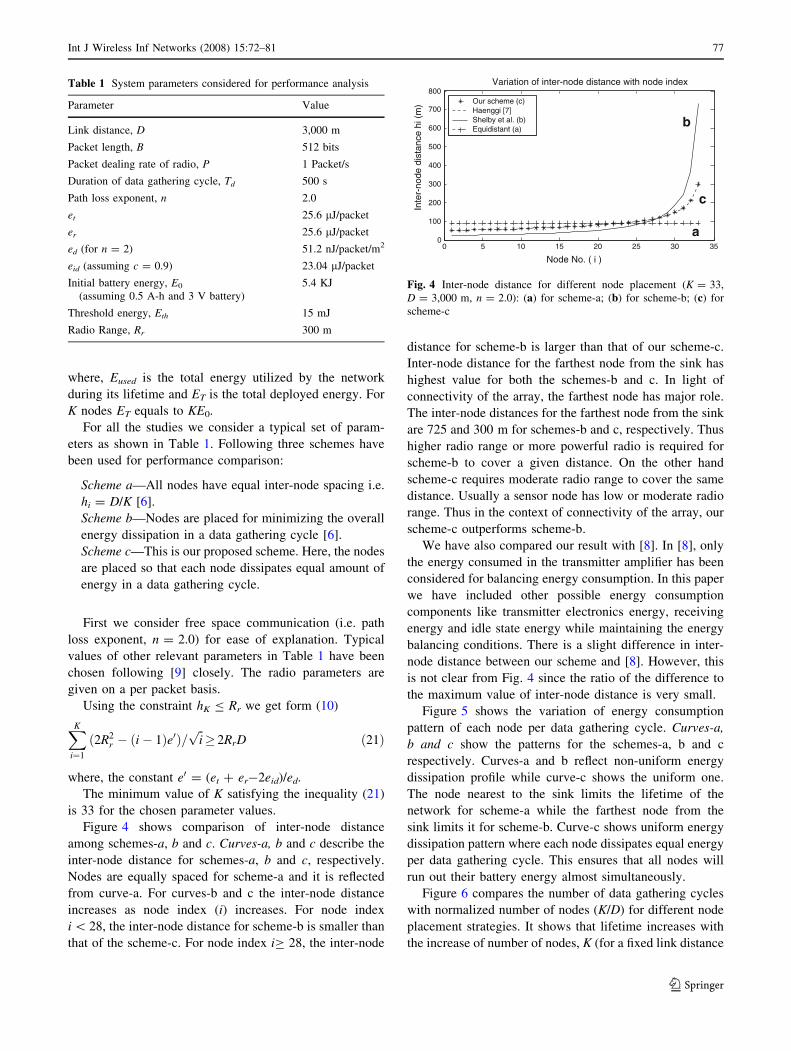
Figure 4 shows comparison of inter-node distance

among schemes-a, b and c. Curves-a, b and c describe the

inter-node distance for schemes-a, b and c, respectively.

Nodes are equally spaced for scheme-a and it is reflected

from curve-a. For curves-b and c the inter-node distance

increases as node index (i) increases. For node index

i \ 28, the inter-node distance for scheme-b is smaller than

that of the scheme-c. For node index iC 28, the inter-node

distance for scheme-b is larger than that of our scheme-c.

Inter-node distance for the farthest node from the sink has

highest value for both the schemes-b and c. In light of

connectivity of the array, the farthest node has major role.

The inter-node distances for the farthest node from the sink

are 725 and 300 m for schemes-b and c, respectively. Thus

higher radio range or more powerful radio is required for

scheme-b to cover a given distance. On the other hand

scheme-c requires moderate radio range to cover the same

distance. Usually a sensor node has low or moderate radio

range. Thus in the context of connectivity of the array, our

scheme-c outperforms scheme-b.

We have also compared our result with [8]. In [8], only

the energy consumed in the transmitter amplifier has been

considered for balancing energy consumption. In this paper

we have included other possible energy consumption

components like transmitter electronics energy, receiving

energy and idle state energy while maintaining the energy

balancing conditions. There is a slight difference in inter-

node distance between our scheme and [8]. However, this

is not clear from Fig. 4 since the ratio of the difference to

the maximum value of inter-node distance is very small.

Figure 5 shows the variation of energy consumption

pattern of each node per data gathering cycle. Curves-a,

b and c show the patterns for the schemes-a, b and c

respectively. Curves-a and b reflect non-uniform energy

dissipation profile while curve-c shows the uniform one.

The node nearest to the sink limits the lifetime of the

network for scheme-a while the farthest node from the

sink limits it for scheme-b. Curve-c shows uniform energy

dissipation pattern where each node dissipates equal energy

per data gathering cycle. This ensures that all nodes will

run out their battery energy almost simultaneously.

Figure 6 compares the number of data gathering cycles

with normalized number of nodes (K/D) for different node

placement strategies. It shows that lifetime increases with

the increase of number of nodes, K (for a fixed link distance

Table 1 System parameters considered for performance analysis

Parameter Value

Link distance, D 3,000 m

Packet length, B 512 bits

Packet dealing rate of radio, P 1 Packet/s

Duration of data gathering cycle, Td 500 s

Path loss exponent, n 2.0

et 25.6 lJ/packet

er 25.6 lJ/packet

ed (for n = 2) 51.2 nJ/packet/m2

eid (assuming c = 0.9) 23.04 lJ/packet

Initial battery energy, E0

(assuming 0.5 A-h and 3 V battery)

5.4 KJ

Threshold energy, Eth 15 mJ

Radio Range, Rr 300 m

0 5 10 15 20 25 30 350

100

200

300

400

500

600

700

800

Node No. ( i )

Inte

r-no

de d

ista

nce

hi (

m)

Variation of inter-node distance with node index

Our scheme (c)Haenggi [7] Shelby et al. (b)Equidistant (a)

b

c

a

Fig. 4 Inter-node distance for different node placement (K = 33,

D = 3,000 m, n = 2.0): (a) for scheme-a; (b) for scheme-b; (c) for

scheme-c


123

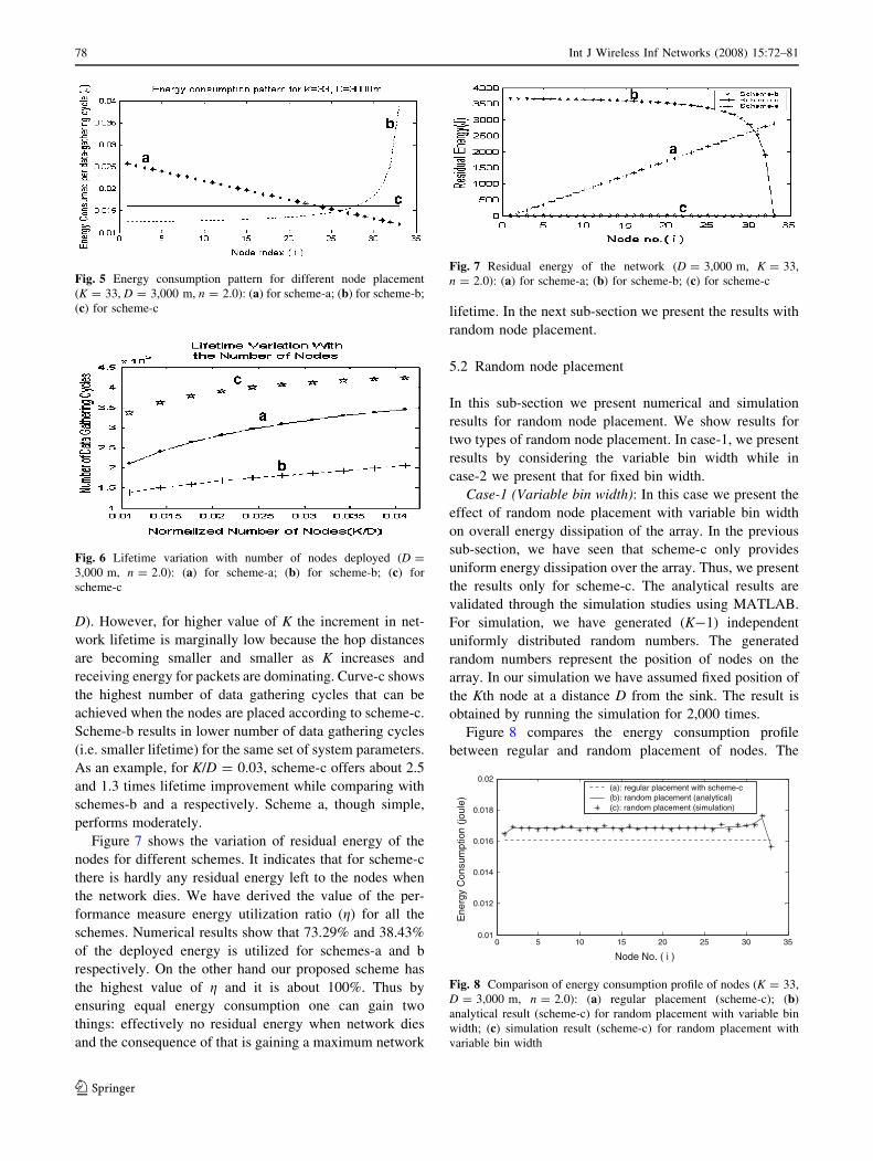
D). However, for higher value of K the increment in net-

work lifetime is marginally low because the hop distances

are becoming smaller and smaller as K increases and

receiving energy for packets are dominating. Curve-c shows

the highest number of data gathering cycles that can be

achieved when the nodes are placed according to scheme-c.

Scheme-b results in lower number of data gathering cycles

(i.e. smaller lifetime) for the same set of system parameters.

As an example, for K/D = 0.03, scheme-c offers about 2.5

and 1.3 times lifetime improvement while comparing with

schemes-b and a respectively. Scheme a, though simple,

performs moderately.

Figure 7 shows the variation of residual energy of the

nodes for different schemes. It indicates that for scheme-c

there is hardly any residual energy left to the nodes when

the network dies. We have derived the value of the per-

formance measure energy utilization ratio (g) for all the

schemes. Numerical results show that 73.29% and 38.43%

of the deployed energy is utilized for schemes-a and b

respectively. On the other hand our proposed scheme has

the highest value of g and it is about 100%. Thus by

ensuring equal energy consumption one can gain two

things: effectively no residual energy when network dies

and the consequence of that is gaining a maximum network

lifetime. In the next sub-section we present the results with

random node placement.

5.2 Random node placement

In this sub-section we present numerical and simulation

results for random node placement. We show results for

two types of random node placement. In case-1, we present

results by considering the variable bin width while in

case-2 we present that for fixed bin width.

Case-1 (Variable bin width): In this case we present the

effect of random node placement with variable bin width

on overall energy dissipation of the array. In the previous

sub-section, we have seen that scheme-c only provides

uniform energy dissipation over the array. Thus, we present

the results only for scheme-c. The analytical results are

validated through the simulation studies using MATLAB.

For simulation, we have generated (K-1) independent

uniformly distributed random numbers. The generated

random numbers represent the position of nodes on the

array. In our simulation we have assumed fixed position of

the Kth node at a distance D from the sink. The result is

obtained by running the simulation for 2,000 times.

Figure 8 compares the energy consumption profile

between regular and random placement of nodes. The

Fig. 6 Lifetime variation with number of nodes deployed (D =

3,000 m, n = 2.0): (a) for scheme-a; (b) for scheme-b; (c) for

scheme-c

Fig. 7 Residual energy of the network (D = 3,000 m, K = 33,

n = 2.0): (a) for scheme-a; (b) for scheme-b; (c) for scheme-c

0 5 10 15 20 25 30 350.01

0.012

0.014

0.016

0.018

0.02

Node No. ( i )

Ene

rgy

Con

sum

ptio

n (jo

ule)

(a): regular placement with scheme-c(b): random placement (analytical)(c): random placement (simulation)

Fig. 8 Comparison of energy consumption profile of nodes (K = 33,

D = 3,000 m, n = 2.0): (a) regular placement (scheme-c); (b)

analytical result (scheme-c) for random placement with variable bin

width; (c) simulation result (scheme-c) for random placement with

variable bin width

Fig. 5 Energy consumption pattern for different node placement

(K = 33, D = 3,000 m, n = 2.0): (a) for scheme-a; (b) for scheme-b;

(c) for scheme-c


123

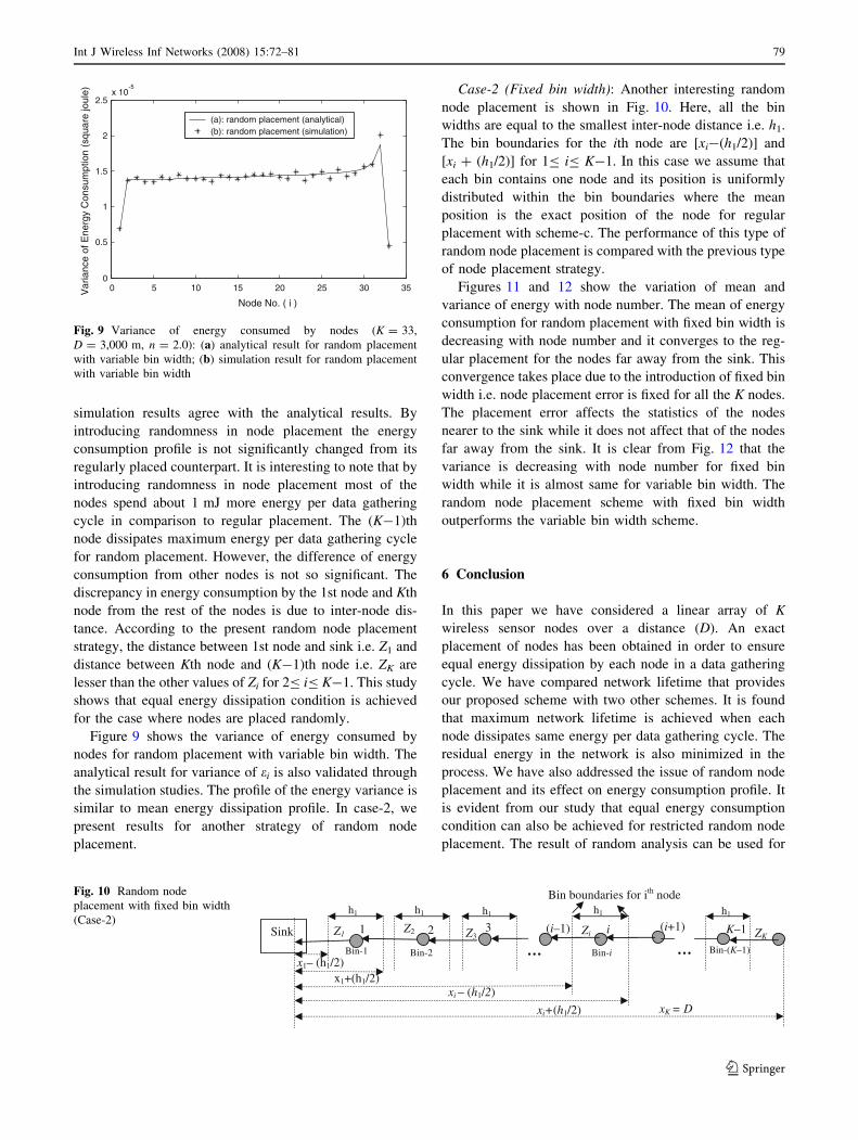
simulation results agree with the analytical results. By

introducing randomness in node placement the energy

consumption profile is not significantly changed from its

regularly placed counterpart. It is interesting to note that by

introducing randomness in node placement most of the

nodes spend about 1 mJ more energy per data gathering

cycle in comparison to regular placement. The (K-1)th

node dissipates maximum energy per data gathering cycle

for random placement. However, the difference of energy

consumption from other nodes is not so significant. The

discrepancy in energy consumption by the 1st node and Kth

node from the rest of the nodes is due to inter-node dis-

tance. According to the present random node placement

strategy, the distance between 1st node and sink i.e. Z1 and

distance between Kth node and (K-1)th node i.e. ZK are

lesser than the other values of Zi for 2B iB K-1. This study

shows that equal energy dissipation condition is achieved

for the case where nodes are placed randomly.

Figure 9 shows the variance of energy consumed by

nodes for random placement with variable bin width. The

analytical result for variance of ei is also validated through

the simulation studies. The profile of the energy variance is

similar to mean energy dissipation profile. In case-2, we

present results for another strategy of random node

placement.

Case-2 (Fixed bin width): Another interesting random

node placement is shown in Fig. 10. Here, all the bin

widths are equal to the smallest inter-node distance i.e. h1.

The bin boundaries for the ith node are [xi-(h1/2)] and

[xi + (h1/2)] for 1B iB K-1. In this case we assume that

each bin contains one node and its position is uniformly

distributed within the bin boundaries where the mean

position is the exact position of the node for regular

placement with scheme-c. The performance of this type of

random node placement is compared with the previous type

of node placement strategy.

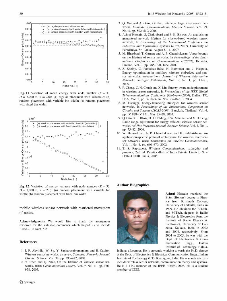
Figures 11 and 12 show the variation of mean and

variance of energy with node number. The mean of energy

consumption for random placement with fixed bin width is

decreasing with node number and it converges to the reg-

ular placement for the nodes far away from the sink. This

convergence takes place due to the introduction of fixed bin

width i.e. node placement error is fixed for all the K nodes.

The placement error affects the statistics of the nodes

nearer to the sink while it does not affect that of the nodes

far away from the sink. It is clear from Fig. 12 that the

variance is decreasing with node number for fixed bin

width while it is almost same for variable bin width. The

random node placement scheme with fixed bin width

outperforms the variable bin width scheme.

6 Conclusion

In this paper we have considered a linear array of K

wireless sensor nodes over a distance (D). An exact

placement of nodes has been obtained in order to ensure

equal energy dissipation by each node in a data gathering

cycle. We have compared network lifetime that provides

our proposed scheme with two other schemes. It is found

that maximum network lifetime is achieved when each

node dissipates same energy per data gathering cycle. The

residual energy in the network is also minimized in the

process. We have also addressed the issue of random node

placement and its effect on energy consumption profile. It

is evident from our study that equal energy consumption

condition can also be achieved for restricted random node

placement. The result of random analysis can be used for

0 5 10 15 20 25 30 350

0.5

1

1.5

2

2.5x 10

-5

Node No. ( i )

Var

ianc

e of

Ene

rgy

Con

sum

ptio

n (s

quar

e jo

ule)

(a): random placement (analytical)(b): random placement (simulation)

Fig. 9 Variance of energy consumed by nodes (K = 33,

D = 3,000 m, n = 2.0): (a) analytical result for random placement

with variable bin width; (b) simulation result for random placement

with variable bin width

Sink 1 2 3 (i–1) i

Bin boundaries for ith node

xK = D

Z1Z2 ZK

ZiZ3(i+1)

x1– (h1/2)

xi+(h1/2)

xi – (h1/2)x1+(h1/2)

K–1

Bin-1 -niB 2-niB i Bin-(K–1)

h1h1 h1 h1 h1

… …

Fig. 10 Random node

placement with fixed bin width

(Case-2)


123

mobile wireless sensor network with restricted movement

of nodes.

Acknowledgments We would like to thank the anonymous

reviewer for the valuable comments which helped us to include

‘Case-2’ in Sect. 5.2.

References

1. I. F. Akyildiz, W. Su, Y. Sankarasubramaniam and E. Cayirci,

Wireless sensor networks: a survey, Computer Networks Journal,Elsevier Science, Vol. 38, pp. 393–422, 2002.

2. Y. Chen and Q. Zhao, On the lifetime of wireless sensor net-

works, IEEE Communications Letters, Vol. 9, No. 11, pp. 976–

978, 2005.

3. Q. Xue and A. Ganz, On the lifetime of large scale sensor net-

works, Computer Communications, Elsevier Science, Vol. 29,

No. 4, pp. 502–510, 2006.

4. Ashraf Hossain, S. Chakrabarti and P. K. Biswas, An analysis on

guaranteed network lifetime for cluster-based wireless sensor

network, In Proceedings of the International Conference onIndustrial and Information Systems (ICIIS-2007), University of

Peradeniya, Sri Lanka, August 8–11, 2007.

5. M. Bhardwaj, T. Garnett and A. P. Chandrakasan, Upper bounds

on the lifetime of sensor networks, In Proceedings of the Inter-national Conference on Communications (ICC’01), Helsinki,

Finland, Vol. 3, pp. 785–790, June 2001.

6. Z. Shelby, C. Pomalaza-Raez, H. Karvonen and J. Haapola,

Energy optimization in multihop wireless embedded and sen-

sor networks, International Journal of Wireless InformationNetworks, Springer Netherlands, Vol. 12, No. 1, pp. 11–21,

2005.

7. P. Cheng, C. N. Chuah and X. Liu, Energy-aware node placement

in wireless sensor networks, In Proceedings of the IEEE GlobalTelecommunications Conference (Globecom-2004), Dallas, TX,

USA, Vol. 5, pp. 3210–3214, Nov. 29–Dec. 3, 2004.

8. M. Haenggi, Energy-balancing strategies for wireless sensor

networks, In Proceedings of the International Symposium onCircuits and Systems (ISCAS-2003), Bangkok, Thailand, Vol. 4,

pp. IV 828–IV 831, May 25–28, 2003.

9. Q. Gao, K. J. Blow, D. J. Holding, I. W. Marshall and X. H. Peng,

Radio range adjustment for energy efficient wireless sensor net-

works, Ad-Hoc Networks Journal, Elsevier Science, Vol. 4, No. 1,

pp. 75–82, 2006.

10. W. Heinzelman, A. P. Chandrakasan and H. Balakrishnan, An

application-specific protocol architecture for wireless microsen-

sor networks, IEEE Transaction on Wireless Communications,

Vol. 1, No. 4, pp. 660–670, 2002.

11. T. S. Rappaport, Wireless Communications: principles andpractice, 2nd ed. Prentice-Hall of India Private Limited, New

Delhi-110001, India, 2005.

Author Biographies

Ashraf Hossain received the

B.Sc. (Honors) degree in Phys-

ics from Krishnath College,

University of Calcutta, India in

1999. He obtained the B.Tech.

and M.Tech. degrees in Radio

Physics & Electronics form the

Institute of Radio Physics &

Electronics, University of Cal-

cutta, Kolkata, India in 2002

and 2004, respectively. From

2004 to 2005, he was with the

Dept. of Electronics & Com-

munication Engg., Haldia

Institute of Technology, Haldia,

India as a Lecturer. He is currently working towards the Ph.D. degree

at the Dept. of Electronics & Electrical Communication Engg., Indian

Institute of Technology (IIT), Kharagpur, India. His research interests

include wireless sensor network, communication theory and systems.

He is a TPC member of the IEEE PIMRC-2008. He is a student

member of IEEE.

0 5 10 15 20 25 30 350.01

0.011

0.012

0.013

0.014

0.015

0.016

0.017

0.018

0.019

0.02

Node No. ( i )

Ene

rgy

Con

sum

ptio

n (jo

ule)

(a): regular placement with scheme-c(b): random placement with variable bin-width (simulation)(c): random placement with fixed bin-width (simulation)

Fig. 11 Variation of mean energy with node number (K = 33,

D = 3,000 m, n = 2.0): (a) regular placement with scheme-c; (b)

random placement with variable bin width; (c) random placement

with fixed bin width

0 5 10 15 20 25 30 350

0.2

0.4

0.6

0.8

1

1.2

1.4

1.6

1.8

2x 10

-5

Node No. ( i )

Var

ianc

e of

Ene

rgy

Con

sum

ptio

n (s

quar

e jo

ule)

(a): random placement with variable bin-width (simulation)(b): random placement with fixed bin-width (simulation)

Fig. 12 Variation of energy variance with node number (K = 33,

D = 3,000 m, n = 2.0): (a) random placement with variable bin

width; (b) random placement with fixed bin width


123

T. Radhika received the B.Tech.

in Electronics & Communication

Engg. form the Jawaharlal Nehru

Technological University, Hyder-

abad, India in 2005. She received

the M.Tech. degree in Telecom-

munication Systems Engg. from

the Dept. of Electronics & Elec-

trical Communication Engg.,

Indian Institute of Technology

(IIT), Kharagpur, India in 2007.

Currently she is working at NVI-

DIA Graphics Private Limited,

Pune, India as System Software

Engineer. Her areas of interest are

wireless sensor networks, physical

layer issues of communication

networks.

S. Chakrabarti received the

B.Engg. in Electronics & Tele-

communication Engg. from the

Jadavpur University, Kolkata,

India in 1984. He obtained the

M.Tech. in Satellite Communi-

cations & Remote Sensing

Engg., and the Ph.D. degree from

the Dept. of Electronics & Elec-

trical Communication Engg.,

Indian Institute of Technology

(IIT), Kharagpur, India in 1985

and 1992, respectively. He was with Indian Oil Corporation Ltd.

between 1986 and 1988. Then he served in the faculty of the Dept. of

Electronics & Electrical Communication Engg., IIT Kharagpur from

1991 till 2000. Since August 2000, he has been serving at the G. S.

Sanyal School of Telecommunications, IIT Kharagpur, where he is

currently a Professor. Presently he is the Chairman of the G. S. Sanyal

School of Telecommunications. He has published more than 60 tech-

nical papers in various journals and conferences and has been involved

in about 20 sponsored projects. His main research areas include wireless

communications and networking, mobile communications, error con-

trol coding and baseband signal processing. He is a member of IEEE.

P. K. Biswas received the

B.Tech. degree (with honors) in

Electronics and Electrical Com-

munication Engg., the M.Tech.

degree in Automation and Control

Engg., and the Ph.D. degree in

Computer Vision from the Dept.

of Electronics and Electrical

Communication Engg., Indian

Institute of Technology (IIT),

Kharagpur, India in 1985, 1989,

and 1991, respectively. From

1985 to 1987, he was with Bharat

Electronics Ltd., Ghaziabad,

India, as a Deputy Engineer. Since

1991, he has been working as a Faculty Member in the Department of

Electronics and Electrical Communication Engg., IIT Kharagpur, where

he is currently a Professor. Presently he is the Head of the Computer and

Informatics Centre (CIC), IIT Kharagpur. He visited the University of

Kaiserslautern, Germany, under Alexander von Humboldt Research

Fellowship from March 2002 to February 2003. He has more than 70

research publications in international and national journals and confer-

ences and has filed seven international patents. His areas of interest are

image processing, pattern recognition, computer vision, video compres-

sion, parallel and distributed processing, and computer networks. He is a

member of IEEE.


123

An Approach to Increase the Lifetime of a Linear Array of Wireless Sensor Nodes

Documents

Transcript of An Approach to Increase the Lifetime of a Linear Array of Wireless Sensor Nodes