CATHODIC PROTECTION MODELING

OF NODES IN OFFSHORE

STRUCTURES

By

MICHAEL RAYMOND HAROUN I(

Bachelor of Science in Chemical Engineering

Oklahoma State University

Stillwater, Oklahoma

1984

Submitted to the Faculty of the Graduate College of the

Oklahoma State University in partial fulfillment of

the requirements for the Degree of

MASTER OF SCIENCE JULY, 1986

1·-r1. ~..-;, ~

I cl.2'3L:;:l>

H?. cl~~.C.. (l! . '0 'j '. ... ~~ ro ..-4-..-""

CATHODIC PROTECTION MODELING

OF NODES IN OFFSHORE

STRUCTURES

Thesis Approved :

1259878

ii

ABSTRACT

A three-dimensional computer model for analyzing the

potential distribution on the metal surface and in the water

surrounding nodes in offshore platforms was developed. The

model is based on the Laplace equation as the governing

equation and uses the finite difference method to solve the

equation numerically. The model is the first of its kind

and is unique because it is designed for microcomputers.

The model can model dozens of different node

geometries. Most of these geometries have been tested for

convergence problems and they are error free. The model is

promising because it can expand to incorporate more node

geometries.

iii

ACKNOWLEDGMENTS

I wish to express my sincere gratitude to all the

people who assisted me in this work. I am grateful to my

major adviser, Dr. Robert Heidersbach, for his guidance and

much valued counsel. His determination and persistance made

my software development possible.

I am also thankful to the other committe members, Dr.

Ruth Erbar, and Dr. Mayis Seapan for their help and support

in the course of this work. Special thanks for Dr. Ruth

Erbar for her encouragement and her remarks.

Special thanks are due to Steve Wolfson from Shell

development for his assistance and for his kind help in

verifying the model output with the field data. I am also

thankful to Steve Wolfson from Shell Development and Bill

Coyle from Union Oil for providing me with drawings of the

different node geometries used on offshore structures.

Special thanks are due to the School of Chemical

Engineering for the financial support I received during the

first year of my thesis work and to Shell Development, Union

Oil, and Atlantic Richfield for funding my research project.

My father, my mother, and my girlfriend, Kaitsu ,­

( -

Makela, deserve my deepest appreciation for their constant

support and encouragement.

iv

Chapter

I.

II.

III.

IV.

v.

TABLE OF CONTENTS

INTRODUCTION. . .

LITERATURE SEARCH

Introduction Historical Background of Computers Corrosion Related Applications

Database Systems ..... Corrosion Rate Evaluation Corrosion Monitoring ... Computer Modeling . . . .

Numerical Techniques Non-Numerical Techniques

Suggested Additional Applications.

CATHODIC PROTECTION PRINCIPLES.

Introduction . . . Basic Theory . . . Design Considerations. Design Procedure . . . Anode Distribution . . Cathodic Protection Monitoring Conclusion .

MODEL DESCRIPTION

Introduction Mathematical Formulation

Numerical Technique Mathematical Equation Boundary Conditions . Water Resistivity . . Dynamic Mesh. . . . . Anode Specifications. Convergence Criteria. Polarization Curves Shape Files . Node Geometries

Source Listing . .

RESULTS AND DISCUSSION.

v

Page

1

3

3 4 7 7

10 11 13 13 19 21

25

25 25 32 35 36 37 38

39

39 40 40 41 46 50 53 54 57 58 62 64 64

66

Chapter

VI.

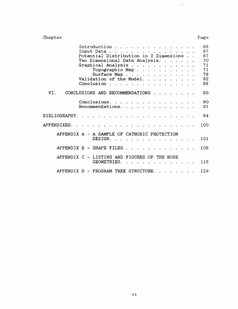
Introduction . . . . . . . . . . . . . Input Data ............. . Potential Distribution in 3 Dimensions Two Dimensional Data Analysis. Graphical Analysis . . .

Topographic Map . . Surface Map . . . .

Validation of the Model. Conclusion

CONCLUSIONS AND RECOMMENDATIONS

Conclusions ... Recommendations.

BIBLIOGRAPHY.

APPENDIXES. . ,•

APPENDIX A - A SAMPLE OF CATHODIC PROTECTION DESIGN ...

APPENDIX B - SHAPE FILES

APPENDIX C - LISTING AND FIGURES OF THE NODE GEOMETRIES. . . . .

APPENDIX D - PROGRAM TREE STRUCTURE.

vi

Page

66 67 67 70 71 71 79 82 89

90

90 91

94

100

101

108

118

129

LIST OF TABLES

Table Page

I. Galvanic Series of Some Commercial Metals and Alloys in Seawater. . . . . . . . 31

II. Design Criteria for Cathodic Protection Systems . . . . . . . . . . . . . 33

III. A Sample of the Computer Output Showing the Input Data. . . . . . . . . . 68

IV. A Listing of the Data Contained in a Shape File. . . . . . . . . . . . . . . . . 113

vii

LIST OF FIGURES

Figure P~e

1. Polarization Caused by an External Electron Supply. 27

2. A Picture of an Offshore Structure in the Sea . 29

3. A Schematic Diagram of Offshore Structure Showing the Locations of Node Geometries. 30

4. The Potential at Node P is Equal to the Average of the Six Surrounding Potential Values . 44

5. The Point of Interest is Located on the Face of Three-Dimensional Cube. 48

6. The Point of Interest is Located on the Edge of Three-Dimensional Cube. 48

7. The Point of Interest is Located at the Vertex of the Three-Dimensional Cube . 49

8. The Three Different Parts of a Three-Dimensional Cube Element. . · 51

9. The Cathode and the Anode as Represented in the Three-Dimensional Cubic Mesh. 56

10. The Effect of Increasing the Pressure (Water Depth) is a Slight Shift of Polarization Curve to the Right. 59

11. The Same Shift to the Right of the Polarization Curve Due to the Increase of Hydrostatic Pressure Exept That the Temperature is at 10C 60

12. A Plane Containing Data in Two-Dimensions Which is Perpendicular to the Z-axis. 72

13. The Topographic Map of the Potential Distribu-tion for the Input Data Shown in Table III. 74

14. The Same Topographic Map of the Potential Distribution for the Input Data of Table II

viii

(

Figure Page

but With a Small Contour Line Interval ... 75

15. The Contour Lines of The Topographic Map Can be Labeled. . . . . . . . . . . . . . . 76

16. The Topographic Map in a Plane Located Further Away from the Anodes and Which Contains Areas That are Inadequately Protected . . . . . . . 78

17. The Surface Map of the Potential Distribution for the Input Data of Table III. The Rotation Angle is at 310 Degrees . . . . . . . . . . 80

18. The Same Surface Map But Rotated at an Angle of 140 Degrees. . . . . . . 80

19. The Surface Map of the Potential Distribution at a Tilt Angle of 45 Degrees . 81

20. The Same Surface Map of the Potential Distribu-tion but Tilted at an Angle of 20 Degrees . 81

21. The Surface Map of the Potential Distribution With a Height/Width Ratio of 1.0. . 83

22. The Same Surface Map of the Potential Distribu-tion but With a Height/Width Ratio of 0.5 . 83

23. The Surface Map of the Potential Distribution With a Skirt. 84

24. The Same Surface Map of the Potential Distribu-tion but Without a Skirt. 84

25. The Surface Map of the Potential Distribution With Grid Lines Parallel to the X-Axis. 85

26. The Surface Map but the Grid Lines are Parallel to the Y-Axis 85

27. The Surface Map With Grid Lines Parallel to Both the X-Axis and the Y-Axis . . . . . . . 86

28. A Schematic Diagram of the Calibration Model. 88

29. The Origin of the Three-Dimensional Cube Containing the Node Geometry is Located at the Lower Left Vertex of the Cube . 110

30. The Dots Represent the Locations of the Leg Coordinates in the Plane Perpendicular to the

ix

Figure

Z-axis at z=1 .

31. The Dots Represent the Locations of the Leg and the Two Horizontal Braces in the Plane Perpen-

P~e

112

dicular to the Z-axis at Z=5. . . . . . . . 112

32. A Graphical Representation of a Node Geometry Consisting of One Leg and Two Horizontal Braces. . . . . . . 114

33. The Source Listing of the BASIC Program that Created the Shape File Presented in Table IV. 117

X

d

Dx

Dy

Dz

E

I

r

R

s

T

v

NOMENCLATURE

- distance between nodes, ft

- distance increment along the

x-axis, ft

- distance increment along the

y-axis, ft

- distance increment along the

z-axis, ft

- potential difference, volt

- Anode Output Current, ampere

polarization current, mamp/ftA2

- Anode Length, ft

- potential, volt

equivalent radius, in

- resistance, ohm

- water resistivity, ohm-em

- current output/anode, amp/anode

- Laplacian operator

xi

CHAPTER I

INTRODUCTION

Cathodic protection is a well-established means of

controlling corrosion on offshore structures or any

submerged installation. Advances in computer technology

have allowed corrosion engineers to model complex marine

structures using one of several numerical techniques. These

numerical techniques are used to solve the governing

differential equation of galvanic systems. The governing

equation is the Laplace equation. Analytical techniques

have failed to solve the Laplace equation because of the

complexity of structure geometries.

Numerical techniques offer the advantage of speed and

versatility and the ability to model any complex geometry.

The drawback of these techniques is that they have been

developed for large mainframe computers. Therefore, they

are expensive to run and create communication problems

between the corrosion engineer needing the information and

the computer operator seeking to produce the information.

The programs are not under control of the engineers but

rather under the control of the queuing and delivery

systems. The lack of commercial software capable of

performing the same job has made the situation worse. All

1

2

of the above restraints have prevented the widespread use of

computers for cathodic protection design.

The purpose of this research is to adapt existing

numerical techniques such as the finite element, the finite

difference, and the boundary integral method for use on a

microcomputer. The objective is the development of a

user-friendly and interactive package that can be used by

corrosion engineers to design cathodic protection systems·.

The package offers the advantage of unlimited computer runs

with no runtime expenses. Although the package does not

have the elaborate capabilities of the larger mainframe

programs, it is based on the same mathematical principles.

The program is designed to run on IBM XT personal computers

which are inexpensive and widely available. It is equipped

with a database system contain~ng several popular node

geometries and can be expanded to include new node

geometries.

CHAPTER II

LITERATURE SEARCH

Previous literature has presented the fundamentals of

corrosion and corrosion control and monitoring. It has

covered why and how metals corrode and what can be done to

control corrosion. However, few papers mention the use of

computers for corrosion detection and corrosion control. The

intent of this chapter is to review the current uses of

computers in corrosion control and monitoring, to offer a

historical survey on computers and their usage in the

corrosion field, and to suggest new applications for

computers in corrosion control and monitoring.

Introduction

A major task in corrosion control and monitoring

involves the acquisition of electrical or electrochemical

data during the course of a survey. Routine calculations,

data measurement, data manipulation, and design are the

types of routine work that a corrosion engineer or

technician must do. This routine-handling of data can

consume a major fraction of an engineer's time. The rapid

and continuing development of computer technology can

3

4

greatly reduce this burden. With their low cost, high

performance and ease of use, computers (especially

microcomputers) provide extremely powerful techniques for

data acquisition, numerical processing, data management,

data communication, and modeling. Data can be collected,

sorted, tabulated, and plotted automatically. This

minimizes the possibility of human errors. Furthermore,

physical storage space for large amounts of field data is no

longer a problem. Nearly one million characters of data can

be stored on an inexpensive magnetic disc. The modern

computer can be easily interfaced with field apparatus to

provide automated monitoring of data signals and/or control

of input signals. A number of analog-to-digital (A/D) and

digital-to-analog (D/A) converters are available to provide

the communications hardware for interfacing. As a

consequence, the human labor involved in data collection,

collation, computation, storage and design is minimized.

Historical Background of Computers

The slide-rule can be considered to be the first tool

available for routine multiplication and division. The

concept of the slide rule is based on the logarithm of

numbers. Since logarithms are compressed versions of their

original numbers, by converting these into lengths on a

scale or ruler, multiplication and division can be done by

simply adding or substracting the two lengths on the scale

( 1).

5

Though the slide rule is not a machine by itself, it

does inspire the notion of a machine as a calculation aid.

The first true machine capable of performing arithmetical

functions appeared about a quarter of a century after

logarithms around 1640. The inventor, Blaise Pascal, based

his mechanical design on a set of interlocking cogs and

wheels on various axles (1). The numbers were dialed and

the results were displayed in a little window after the cogs

and wheels inside rotated appropriately. The device, called

a Pascaline, could add, substract, multiply, or divide any

two numbers and could therefore be called a calculation

machine. This was followed by the difference machine, built

in 1822 by the Englishman, Charles Babbage. This was a

mechanical machine that could solve polynomial equations by

calculating successive differences between sets of numbers.

Although the machine was capable of doing just one job, the

concept of the computer was born. A machine which could

perform calculations of one kind could, in all probability,

perform any kind of calculation.

The idea was left undisturbed until a century later

when the German, Konrad Zuse, decided not only to design a

universal computer, but also to build one (1). His models

were based on binary calculating units and used

electro-magnetic relays instead of mechanical switches.

These were radical changes in computer design. The result

was a machine that could perform any type of calculation and

could be programmed to perform any mathematical task. The

6

computer was born. At the same time a calculator/ computer,

called Mark 1, was being developed by Harvard University and

IBM {2}. It operated on a universal calculus and performed

mathematical tasks. But it is the ENIAC, developed by the

Moore School of Engineering at the University of

Pennsylvania in 1946, that takes the honor of being the

first true electronic computer. It contained the three

essential parts of a computer: a central processing unit, a

memory stage and an input/output device. This was followed

by computers such as EDVAC, EDSAC, MANIAC, lAS, JOHNNIAC,

and finally WHILWIND. The list can be further extended to

include names of computers that have slight improvements

over the original ones {2).

The invention of the transistor in 1948 at Bell

Laboratories helped bring about the reduction in computer

size and cost {3). Throughout the 1960's, transistors and

other components were integrated into a single silicon chip.

In 1975, ALTAIR was introduced, the first personal

computer for use outside the industry (3). Office-size

minicomputers and different types of microcomputers

{desk-top, portable, pocket, etc) followed.

Computers were created for the basic need of performing

mathematical operations at high speeds. Their application

to a number of data computation, collection, and data

storage, to include those related to corrosion, inevitably

followed.

7

Corrosion-Related Applications

Computers can have many applications in corrosion.

They have been used for database systems, for calculations,

for plotting data, for inspection and monitoring, and for

modeling.

Record keeping is necessary to evaluate progress, to

maintain continuity, and to avoid duplication of effort.

The volume of information and data which must be recorded is

increasing exponentially, particularly in the engineering

field. Corrosion engineers acquire large amounts of data

and information in the study and evaluation of corrosion

control measures. This is especially true where many

parameters are measured and recorded. Records of

geographical location and description, corrosion history,

and corrosion control measures are maintained for future

reference. Computers can simplify these tasks because of

their tremendous speed in data storage, data retrieval, and

data manipulation.

The use of computers as a database system in the

corrosion field dates back to the late 1970's. The first

technical paper on the use of computers for data collection

and storage was presented at the Western Region Conference

of the National Association of Corrosion Engineers (NACE),

in 1964 (4). The paper, " Corrosion Control Evaluation and

8

Data Recording by Electronic Computer, " discussed the use of

electronic computers in data collection and storage. In

1958, an IBM 650 data processing computer was leased by

Creole Petroleum Corporation for accounting and materials

control {5). The computer was used as an electronic data

processing {EDP) system to obtain efficient use of data on a

network of submerged pipelines. With the EDP system,

various correlations of corrosion data were made which

permitted accurate evaluation of corrosion control measures

and led to other methods for reducing maintenance costs.

In 1965, Rochester Gas and Electric Corporation used a

standard punch card computer to store data from its

pipe-to-soil potential surveys ( 6). C.omputer punch cards

were used to analyze the conditions of buried pipelines and

to keep a running tabulation of information on a specific

pipeline. In 1967, Texas Eastern Transmission Corporation

used a computer for data processing of 650 rectifiers

protecting over 10,000 miles of pipe line (7). The computer

system improved performance, efficiency, and saved money.

In recent years, microcomputers capable of performing

the data handling tasks required for corrosion monitoring

have become available. The cost of these units has dropped

low enough to permit expanded use of these machines.

However, data processing is not limited to computers. With

today's technology , the same work done on a computer can be

done on a programmable calculator. In his 1980 paper "The

Programmable Electronic Calculator in Underground Corrosion

9

Related Activity," R.L. Seifert described how a programmable

electronic calculator could be used to calculate and store

network constants for underground pipelines (8).

The software needed to create database systems is

available. An example is the software developed for making

structure to soil surveys {9). The program is designed as

an aid to the corrosion engineer or technician engaged in

designing and maintaining cathodic protection systems for

pipelines and related facilities. The program facilitates

the entry of data by keyboard or automatic data collector

and provides many options for searching and analyzing

cathodic protection data.

However, software is not 'limited to data collection and

analysis of pipelines but can be extended to other

applications. Software has been developed for record

handling for underground electrical transformer data {10).

The method consists of computer programs for filing and

recalling the data to provide an automated analysis and a

case history for each transformer.

Software is also used for databases to provide

corrosion information in the public domain. For example, a

corrosion data program has been established by NACE and the

National Bureau of Standards (NBS) to collect, evaluate, and

disseminate the corrosion data which is presently scattered

throughout the open literature and in the proprietary files

of many companies and trade associations {11). A similar

data base is the DECHEMA corrosion information system

developed in West Germany (12). This data bank provides

information on the corrosion behavior of materials of

construction in different areas of industry.

10

The list of computer applications as a database system

can be extended further, but the above-cited examples are

representative.

One area where computers can be applied is the tedious

and repetitive field of corrosion rate calculation. As a

consequence, computer programs which calculate corrosion

rates from many different sets of data are available. One

such program calculates corrosion rates from sets of data

such as {13): (1) resistance dataprobe; (2) weight loss

coupon; {3) ion count; (4) linear polarization resistance

method; and (5) Tafel extrapolation method. The program

also outputs the corrosion rates in different units, namely:

micrometer/y, mpy, g;m2/day, mdd, microAmp/cm2 . The end

result is a much faster operation for the corrosion engineer

with fewer errors.

A similar short program calculates corrosion rates and

electrochemical parameters from polarization data for a

variety of corroding systems (14). These include activation

controlled systems such as strong acids, sea water, and

other environments with diffusion controlled reduction

reactions and passive metal/corrosive systems. The Tafel

constants in the program are used to determine inhibitor

11

mechanisms and to calculate the metal dissolution rate at

any applied potential. It requires two minutes to execute on

a low cost portable microcomputer. The program requires 3.5

K of memory which can be reduced to 2 K by omitting the

remark statements. This low demand on memory requirements

makes it possible for this program, or similar ones, to be

used on any microcomputer after slight changes in the

language syntax.

Another computer program has been developed for the

analysis of polarization data obtained in the vicinity of

the corrosion potential (15). It provides for the

determination of anodic and cathodic Tafel slopes,

polarization resistance, and corrosion current. It uses the

Gauss-Newton method to generate a new set of parameter

estimates and the process is repeated until the nonlinear

residual error fails to change by more than a preset value.

The three programs mentioned in this section along with

others make calculations and plots possible that would

otherwise be ignored or approximated due to their time

consuming nature.

Corrosion Monitoring

The investigation of the extent and distribution of

corrosion on metallic surfaces has long presented

electrochemists and corrosion engineers with a difficult

problem. Many electrochemical techniques for determining

bulk corrosion rates have been devised, and some have been

12

used in attempts to elucidate the reaction mechanisms and

the type of corrosion (pitting, crevice, uniform, etc ). An

instrumental method that rapidly and economically determines

the polarization resistance (R ) in the presence of a large p

solution resistance has many applications for corrosion

monitoring. AC impedance techniques can accomplish this

task since the high frequency limit of the impedance equals

the solution resistance and the low frequency impedance

approaches the DC limit and equals the sum of the solution

resistance plus the polarization resistance (16). A

computer program can determine the corrosion rate of a

slowly corroding metal in the presence of a large solution

resistance (Rs). The program automatically determines Rs

from the high frequency limit and the polarization

resistance RP using an integration approach.

Computer-controlled AC impedance measurements systems are

available for coated pipelines (17).

A different approach for automated corrosion monitoring

of metals in solution can be achieved by using

microprocessor- controlled potentiostats (18-20).

Subsequent least-squares computer fitting of the

polarization curve around the corrosion potential is

<possible (18). One system applies a potential step and

measures the resulting current for a variable number of

cycles; data are stored and manipulated by the computer

(19).

One approach for monitoring surface corrosion uses a

13

microprocessor-based isopotential contouring system (21). A

microprocessor-controlled scanning reference electrode is

passed across a corroding specimen close to its surface, and

the potential differences relative to another fixed

reference electrode are recorded. The potential profile

reflects the ion current density in the vicinity of the

corroding surface and gives information about the location

and magnitude of the surface corrosion sites.

Corrosion monitoring in power plants is achieved using

a probe inserted in the process stream and a computer for

the conversion of the probe signals into corrosion rates

(22). One system measures the electrical resistance of a

wire that becomes gradually thinner. The resistance

measurement gives the value of the metal loss between two

successive measurements and calculates the average corrosion

rate. The system is applicable for steam condensers and

high purity-water in high-temperature, high pressure

conditions.

Many predictions of corrosion rates and estimates of

adequate cathodic protection of structures have

traditionally been based on trial and error case studies and

sample exposure tests. Applying these results to real

systems usually involves gross extrapolations from data

14

points, use of large safety factors, and on-going

corrections and maintenance of the systems. Early

analytical efforts to solve the Laplace equation--the

governing equation for potential distributions in

electrochemical cells--were successful but limited to cases

of simple geometries and constant material properties

(23-27). However. simple geometries seldom appear in

real-world structures, and the electrochemical material

properties are not constant with changing potential and

current. Solutions can be applied to general geometries

using numerical methods. These can accommodate varying

inhomogeneous non-linear properties for electrolyte and

constituent metals. Numerical methods have recently been

employed in various levels of sophistication to solve the

galvanic potential distribution problem. These methods

include the finite element method, the finite difference

method, and the boundary integral method.

The finite element method is a powerful tool for

solving physical problems governed by a partial differential

equation or an energy theorem, using a numerical procedure.

This method has been applied to a number of galvanic

corrosion (28) and cathodic protection problems (29,30).

Munn described the use of the finite element method for the

solution of the electric potential distribution and current

fluxes near a multimetallic system submerged in an

electrolyte (28). The model could handle general and

arbitrary geometries and the effects of nonlinear

15

polarization behavior.

Lockheed adapted a general purpose finite element

program called NASTRAN (NASA structural analysis) (29) to

solve problems involving electrostatic applications and

cathodic protection. The program uses the principle of

conservation of energy to determine the strength and

distribution of the energy field within the finite element

model. It calculates the required current to maintain the

minimum energy balance of each electrolyte element. The

energy that enters the model at anode elements must leave at

cathode elements. The advantages of this program over other

programs is that shielding effects in nodes and.other

critical areas can be detected and, moreover, time-dependent

polarization characteristics can be represented.

A second general purpose finite element program was

presented by Casper and April in 1983 (30). The

electrogalvanic fields, i.e., electric field intensity,

current density, and potentials were calculated using the

scalar Poisson equation. The ionic current in the

electrolyte leaving the anode and arriving at the cathode

were constrained to sum to zero over the metallic surface

(based on spatial Kirchoff's law). The exact geometry and

location of anodes, cathodes, and paint surfaces were

incorporated in the mathematical model.

The finite difference method is a numerical

discretization procedure for the approximate analysis of

complex boundary value problems (31). The first time

16

iterative solutions of the difference form of the Laplace

equation were applied was probably in 1964 (32). The method

has been used for theoretical treatments of few electrode

systems, but lately it is being used in offshore cathodic

protection (31). Computerized finite difference analysis is

useful in simulation and design of cathodic protection

systems for offshore structures. It is also useful in

cathodic protection monitoring, i.e. in the analysis of

electric field strengths (IR drop), current density and

potential readings.

The finite difference method also can be used to solve

the Poisson equation. Munn used the finite difference

method to solve the Poisson equation for the electrochemical

potential distribution in an electrolyte containing an array

of fixed-potential electrodes and electrodes with

activation, passivation, and diffusion-controlled

polarization kinetics (33). The results of the analysis

were presented as a display of the potentials at selected

coordinates or as a printed listing of the potentials at all

nodal points in the electrolyte. The program was developed

for operation on a low-cost microcomputer. As a

consequence, the set of simultaneous equations was solved by

the iteration method, because it is more efficient than

other convergence methods (such as elimination, inversion,

etc ... ) and requires less memory, both being important

design considerations for microcomputers. Moreover,

inhomogeneous electrolyte conductivities such as linear

gradients of electrolyte conductivity and layers of

different conductivities can be added to the program (34).

17

The integral boundary equation method (also called

boundary integral method) is similar to the finite element

and finite difference methods in that it solves the Laplace

equation to obtain the potential distributions in

electrochemical cells. However. when the integral boundary

equation method is employed, the Laplace equation is solved

using Green's third formula which requires that any

potential distribution satisfying the formula automatically

satisfies the Laplace equation (35). Using proper boundary

conditions, the solution of Green's third formula is the

potential distribution in electrochemical cells. Fu and

Chan showed that this numerical method is more efficient

than either the finite element or the finite difference

methods for homogeneous environments (35). The reason is

that this method does not require modeling the electrolyte

bodies in order to obtain the potential distribution on the

surface of the structure. This saves computer time.

Moreover, this method can be used for general applications

by using a model generator and a post processor (36). A

model generator is a versatile program capable of generating

three dimensional element meshes for a variety of

structures. It is used to calculate the positions and

surface areas of each element and to store them in the

computer's memory, along with material types for later use.

A post processor is a program which can plot iso-potential

or iso-current density lines against the background of the

element mesh, thus allowing the analysis of thousands of

elements to be viewed graphically.

18

Another boundary element program has been developed to

help corrosion engineers design cathodic protection systems

{37). It uses nonlinear and dynamic cathodic boundary

conditions to simulate real polarization conditions during

the formation of calcareous deposits. Potential

applications of the program include anode positioning, anode

resistance, shielding effects, design safety margins,

interference problems, simulation of node areas in offshore

structures, and the use of coatings.

The applications of numerical techniques are not

limited to simulation of marine structures. One potential

application is the modeling of localized corrosion cells

using the finite element method (38,39). The geometry of

the cell is modeled using an element mesh, and the cell

current distributions are calculated using the polarization

curves of the materials in the cell as boundary conditions.

Examples of instances where this modeling technique could be

applied include galvanic corrosion in steam generators and

concentration cells involving only grain boundaries and

surrounding grains (38). The technique was actually used to

calculate the preliminary galvanic corrosion rates during

the chemical cleaning of a steam generator (40}.

Modeling of corrosion cells can be further extended to

include the capability of predicting long term corrosion

19

rates of nuclear waste isolation packages (41). In this

case, a subroutine must be included in the program in order

to calculate the chemical change with time in the crevice or

the pit environment. The new concentrations are then used

to calculate conductivities and to update the boundary

conditions for the next time step. The procedure is

repeated until a steady state condition is established, thus

providing the desired answer.

Computer modeling is not restricted to the use of

numerical techniques. Non-numerical techniques are also

available. One non-numerical method was used to model water

in cooling towers (42). It consisted of a computer model

for each specific cooling system in the plant. Each program

can be recalled instantly when conditions change or when the

plant personnel decide to evaluate the effects of potential

changes in operating parameters. Once the new operating

data are entered, a revised operational report which

contains a series of performance curves for scale,

corrosion, and deposit control is obtained within minutes.

Similar programs can be used to calculate supersaturation

ratios to develop scaling index guidelines {43).

Computer modeling is also used to simulate

intergranular corrosion (44,45). A computer program based

on an improved chromium depletion theory is used to describe

the time temperature-sensitization (TTS) diagrams of a

20

nickel-based alloy. The TTS diagrams are then used to

examine the effect of thermal aging on the susceptibility to

intergranular corrosion of low carbon Alloy 800.

Potential-pH (Pourbaix) diagrams can be calculated

using computers (46-50). These diagrams are aids for

corrosion prediction because they act as "road maps"

providing direction for an experimental program. As such,

they provide insights as to whether corrosion would occur

during the course of the experiment ..

Computer modeling can be used for the evaluation of

anode resistance formulas (51) and for the design of state

of-the-art cathodic protection systems (52). Strommen used

a computer program to model a number of typical sacrificial

anodes for different length/diameter ratios and for

different operating conditions. Compared to the results of

the most commonly employed formulas for the anode

resistance, his work demonstrates that differences in

environmental and operating conditions strongly affect the

apparent anode resistance. A similar microcomputer program

was developed by Cochran to optimize various anode/core

lengths and end face geometries (52). It includes state

of-the-art sacrificial-anode cathodic protection designs for

offshore platforms based on classical equations. The design

accounts for practical polarization current density,

maintenance current density, current distribution, seawater

resistivities, and sacrificial anode galvanic properties.

Cathodic protection designs include sacrificial cathodic '

protection designs for offshore pipelines {53) and jack-up

rigs {54).

21

Cathodic protection modeling of coated tethers in

Tension Leg Platforms (TLP) has been developed as a computer

program (55). The author developed a microcomputer program

to evaluate the maximum depth at which coated tethers in a

TLP can be cathodically protected. The program provides

several answers for tethers containing different percentages

of holidays (i.e. coating defect areas). The answer is in

the form of current density and potential distribution along

the tether.

Computer modeling is becoming a powerful tool in

corrosion. Advances in computer technology have made

possible the mathematical formulation of complex physical

problems. As a result, the design and analysis of cathodic

protection systems or other systems is no longer a major

obstacle.

Suggested Additional Applications

Previous sections indicate that corrosion-related uses

of computers have included database systems, corrosion rate

evaluation, inspection and monitoring, and modeling.

Although more applications are being added to this list, the

available corrosion-related applications are still

inadequate. The solution of real world technical problems

requires more than the manipulation of data at high speeds.

Most corrosion problems are solved by corrosion experts who

22

have a large body of informal, judgemental, and empirical

knowledge. Their decisions might be based partly on

"experience", partly on laboratory generated data, and

partly on personal judgement as to what may be the best

solution. In any case, it is this expertise that is needed

to solve any problem, including corrosion problems.

Therefore, an attempt must be made to write computer

programs that are able to generate answers or solutions to

complex corrosion problems. In other words, it is necessary

to exploit the computational capabilities of computers by

writing programs that contain interpretive, diagnostic, and

predictive algorithms based on the expertise of corrosion

consultants. The end result is a computer that can think

for itself (i.e. search through the database files, compare

options, and make decisions) .. At this point, solutions to

complex corrosion problems can be attempted by using the

thinking power of the computer, so to speak.

This idea constitutes the basis of the artificial

intelligence discipline which has received considerable

attention in the past few years (2). The ability of a

computer to use the relatively narrow knowledge of

specialists in order to address a variety of technical

problems is called an "expert system". Such systems already

exist for many disciplines. As an example, PROSPECTOR is an

expert system that provides consultation on problems. arising

in the field of mineral exploration (56). Another example

is the expert system Rl designed to configure Digital

23

Equipment Corporation's VAX computer systems (i.e. spatial

arrangement, cabling of various modules, etc). Once

developed, such systems are proven to be very useful. In

1982, PROSPECTOR helped identify a large unknown deposit of

Molybdenum in the viscinity of Mount Tolman in Washington,

an estimated fortune of $100 million.

If expert systems exist in many disciplines, then why

not in the corrosion field? Expert systems should be

developed to handle corrosion problems. Some of these

systems already exist (57) and others are being introduced

(58-62). The new systems should take into account the on

line availability of information from chemists and others.

It is a great help to interface the expert systems with such

data banks. The systems should be flexible (i.e. rapidly

and easily modifiable) and efficient (i.e. capable of

adjusting to new conditions). The systems should also be

written to include self-teaching routines --that is, once a

problem is solved, the computer uses the learned rules and

accumulated data to guide it in its next search.

This approach poses a big challenge and requires much

work. Technical knowledge is difficult to encode because it

is typically expressed in symbolic rather than numerical or

analytical form (63). As such, technical means must be

developed in order to represent symbolic knowledge in forms

that can be conveniently manipulated by computers.

Moreover, some people may object to the development of such

expert systems. The very fact that these systems cost

24

hundreds of thousands of dollars to be developed is also a

limiting factor (64}. On the other hand, technology is

constantly changing and what is impossible to do now can be

feasible in the near future. The situation resembles the

early introductions of the artificially intelligent chess

board. H. Dreyfus, one of the most influential artificial

intelligence researchers claimed "flat out" that artificial

intelligence would never work and pointed out the best chess

program of the day (1966) could be beaten by a ten-year old

boy {2}. Dreyfus subsequently lost to the same program.

If today's Seymour Cray X-MP is capable of 400 million

operations per second, then future computers will be capable

of 3 billion operations per second {65). To this end, the

future is promising and as such, the development and the use

of expert systems on a larger scale is only a question of

time.

CHAPTER III

CATHODIC PROTECTION PRINCIPLES

Introduction

Cathodic protection is an electrochemical technique

used to protect metals (often iron or steel) from corroding

in their natural environment. The technique consists of

coupling the corroding metal structure to a more active

metal. The active metal (anode), the metal structure

(cathode), and the natural environment (electrolyte) form a

galvanic couple. During the process, the active metal

supplies electrons to the metal structure therefore

suppressing its metal dissolution process. The anode

corrodes preferentially to protect the more noble cathodic

metal structure, hence the name "cathodic protection".

Basic Theory

The chemical reactions involved in the natural

corrosion of iron in aerated water are the following (66):

Anodic reaction: Fe --> Fe ++ + 2e

Cathodic reaction: 1/2 02 + H20 + 2e --> 20H

Overall Reaction: Fe 1/202 H20 2e - F ++ + 20H + + + --> e

Iron produces electrons by anodic dissolution. These

25

26

electrons are consumed by simultaneous cathodic reactions.

The overall reaction shows that the net result is the

dissolution of iron by the net production of iron ions. At

the corrosion potential E , the potential at which corr

natural corrosion occurs, the flow of electrons from anodic

areas is exactly equal to the consumption of electrons at

cathodic areas. To achieve cathodic protection, electrons

must be provided from an outside source. The new source

must meet the demands of the cathodic reaction in order to

reduce the dissolution of the steel.

Figure 1 shows that when electrons are supplied

externally, the corrosion potential shifts to lower levels.

This means that if the corrosion potential is at a

sufficiently negative value, iron becomes almost immune to

corrosion in water and cathodic protection will be achieved.

In seawater, a potential of -0.85 volts when measured

against the Cu/Cuso4 reference electrode (or -0.80 volts

versus the Ag/AgCl reference electrode) is considered to be

a safe potential (67). Corrosion of steel in seawater will

not occur at this potential, and this potential can be used

as a protection criterion in cathodic protection designs.

Cathodic protection has been applied to offshore

structures or marine installations. It can be applied by

impressing current or by using sacrificial anodes (galvanic

coupling). When the galvanic coupling method is used, the

external electron source is provided by sacrificial anodes

which are electrically connected to the corroding metal

E c

I ........ ;•'

---- --/' .......... ll ··.... ,/

... ... / --- _.~:. ------\( l ...

/ ..... . I I ..... ...... . ~· 1 ·:..a ---------. .r ~ / ·.. r:p .. .. ........

I - ......

ll ..... . ..... ll ......... . ~~ ..

-----~ ..... /............. ·~ ... / · ........

log

·· .... .... ·~ ....

• I I ~

[I/ Unit ., area] Source: M. G. Fontana and N. D. Greene, "Corrosion Engineering,"

2nd Ed., New York: McGraw Hill Book Co., 1978.

Figure 1. Polarization Caused by an External Electron Supply

E Ec

E a icp

E cp corr

~ Equilibrium Potential for Cathodic Reaction Equilibrium Potential for Anodic Reaction Potential With Cathodic Protection Cathodic Protection Current Density Corrosion Potential

27

28

structures. These anodes are placed in the same environment

these structures are placed in, seawater in this case. The

seawater acts as the electrolyte in the electrical circuit.

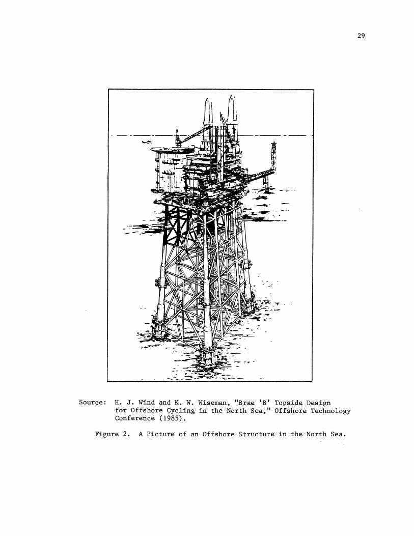
A picture of an offshore structure in the North Sea is shown

in Figure 2. Figure 3 shows a schematic diagram of an

offshore structure showing the locations of the structural

nodes. Sacrificial anodes will be distributed evenly

throughout the underwater structure to prevent corrosion.

Sacrificial anodes tend to corrode preferentially,

because they are more chemically active than the steel

cathodes. Magnesium, zinc, and aluminum, which are all more

active than iron, as shown in Table I, are used as

sacrificial anodes {66). Low consumption favors aluminum

anodes for offshore platforms, where it is often desirable

to limit the weight of the cathodic protection system. Zinc

performs well in cold tap water and seawater where it

corrodes freely without formation of a passivating film

{68). Therefore, zinc anodes are chosen for offshore

pipelines where the resulting extra weight over aluminum is

an added advantage (68). Zinc is occasionally used for

protection of onshore pipelines, but aluminum anodes are

restricted primarily to offshore applications since most

commercial anodes passivate in soil or mud. Magnesium is

the preferred material in high resistivity applications

(such as soil) due to its operating potential. The

potentials provided by each of the materials are more than

adequate to satisfy the criterion of establishing potentials

------

Source: H. J. Wind and K. W. Wiseman, "Brae 'B' Topside Design for Offshore Cycling in the North Sea," Offshore Technology Conference (1985).

Figure 2. A Picture of an Offshore Structure in the North Sea.

29

Figure 3. A Schematic Diagram of an Offshore Structure Showing the Locations of Node Geometries.

30

TABLE I

GALVANIC SERIES OF SOME COMMERCIAL METALS AND ALLOYS IN SEAWATER

l Noble or cathodic

Acuve or anodtc

1

Platinum Gold Graphite Titanium Silver

[ Chlorimet 3 (62 Ni, 18 Cr, 18 Mo) Hmdloy C (62 Ni, 17 Cr, 15 Mo)

[ 18-8 Mo stainless steel (passive) 18-8 stainless steel (passive) Chromium stainless steel 11-30% Cr (passi,•e)

[ Jncond (passive) (80 N1, 13 Cr, 7 Fe) Nickel (passive)

Silver solder

[

Monel (70 Ni, 30 Cu) Cupronickds (60-90 Cu, 40-10 Ni) Bronzes (Cu-Sn) Copper Brasses (Cu-Zn)

[ Chlorimet 2 (66 Nt, 32 Mo, 1 Fe) Hastelloy B (60 Ni, 30 Mo, 6 Fe, l Mn)

[ Inconel (active) Nickel (active)

Tin Lead Lead-tm solders

[ 18-8 Mo stamless steel (active) 18-8 sramless steel (active)

Nt-Resist (htgh Nt cast iron) Chromium stainless steel, 13% Cr (active)

[ Casr iron Steel or iron

2024 aluminum (4.5 Cu, 1.5 Mg. 0.6 Mn) Cadmium CommerCially pure aluminum (1100) Zmc Magnestum and magnestum alloys

Source: M. G. Fontana and N. D. Greene, "Corrosion Engineering," 2nd Ed., New York: McGraw Hill Co. (1978).

31

32

of at least -0.85 volts between the corroding structure and

a Cu/Cuso4 reference electrode (or -0.80 volts vs Ag/AgCl)

( 68).

Design Considerations

As a general rule, a sacrificial anode system is

designed to deliver relatively small currents from a large

number of anodes, as opposed to the impressed current system

which is designed to deliver relatively large currents from

a limited number of anodes. Since relatively small amounts

of current must be evenly distributed throughout the entire

installation of an offshore structure, the majority of

offshore structures use sacrificial anodes to achieve

cathodic protection. Other reasons include the lack of

electrical power sources or hydrogen embrittlement problems

associated with the use of impressed current systems which

eliminates the impressed current option.

When using a sacrificial anode system, the maintenance

currents vary from one location to another. Typical

maintenance current values for different offshore locations

can be found in Table II reproduced from NACE Standard

RP-01-76 (67). Typical maintenance currents in the gulf of

Mexico (5 mAmps/ft2 ) and in the Pacific Ocean off Southern

California (8 mAmps/ft2 ), decreasing to 2 mAmps/ft2 in the

mud zone, are adequately satisfied with aluminum anodes

containing zinc and mercury as alloying components (67).

As a general rule the current required for cathodic

TABLE II

DESIGN CRITERIA FOR CATHODIC PROTECTION SYSTEMS

Environments I F actors111

Water Water Turbulence Lateral Typical Design Production Resistivityl2l Temp. Factor Water Current Density(3l

Area (ohm-em) (Cl (Wave Action) Flow mA/ft2 mAim2

Gull of Mex1co 20 22 Moderate Moderate 5-6 54-65 u.s West Coas: 24 15 Moderate Mooerate 7-10 76-106 Cook Inlet 50 2 Low Hrgr: 35-40 380-430 Nortt: Sea·4 ' 26-33 0-12 H:gh Moder at€ 8-20 86-216 Pers1an Gulf 15 30 Moderate Low 5-S 54-86 lncones1c. 19 2t Moaerate Moderate 5-6 54-65

Source: NACE Standard RP-01-76, "Corrosion Control of Steel, Fixed Offshore Platforms Associated With Petroleum Production," National Association of Corrosion Engineers (1983).

33

34

protection is directly proportional to water velocity and

dissolved oxygen content but inversely proportional to the

diameter of the cylindrical structural members (66). A

small member will require a higher current density than a

larger one at comparable oxygen concentrations and water

velocities. High water velocities due to strong tidal

action increase current requirements for cathodic protection

of offshore platforms ( 42 mAmp/ft2 in Cook Inlet, Alaska)

which makes steel structures in such hostile environments

cases for impressed current systems. Cathodic protection

with impressed current is further favored in this location

by the relatively high water resistivity (49 ohm-em in Cook

Inlet versus 22-25 ohm-em in the Gulf of Mexico), which

reduces current output per sacrificial anode.

One feature which makes cathodic protection of marine

structures different from onshore practices is the buildup

of calcareous deposits on seawater-exposed steel surfaces.

The nature of the calcareous deposits is dependent on the

prepolarization current density (68). The higher the

initial current density supplied, the denser a coating will

form in a shorter period of time. Once the coating is fully

developed, the current requirement for complete cathodic

protection will drop substantially, while the anodes will

reach their ultimate throwing power (68). It should be

noted, however, that if the prepolarization current is too

low, protection potentials will be obtained only after a

long time period (68). Calcareous deposits form on offshore

35

pipelines, but their effect on cathodic protection is much

less dramatic since most pipelines are artificially coated

(68).

Design Procedure

The cathodic protection design procedure for an

offshore platform follows the sequence of steps below:

A- Selection of proper maintenance current. 2 5 mAmp/ft is

commonly used in the Gulf of Mexico and 8 mAmp/ft 2 is

recommended for the Pacific (twice the amount in the

splash zone, one quarter the amount in the mud zone).

B- Calculation of respective surface areas and the addition

of a safety factor (usually around 25%).

C- Calculation of total amount of anode material required to

guarantee a desired life assuming a certain anode

capacity.

D- Selection of a certain anode geometry and check using

Dwight's equation for a single such anode whether the

initial current density exceeds 15 mAmps/ft2 assuming a

native potential of 0.45 volts between bare polarized

steel and aluminum anodes.

E- Judicious distribution of anodes on the steel assuming a

throwing power of 25 feet in line of sight and placing

anodes within 10 ft of all nodes.

36

The criterion for complete cathodic protection is a

steel structure potential more negative than -0.80 volts (i.

e. -0.82, -0.85, etc) at any point versus the Ag/AgCl

reference electrode. A sample design of a sacrificial anode

system for an offshore installation in the Gulf of Mexico is

described in Appendix A. Step E of the design procedure is

not included in Appendix A because of the extensive work

involved (i.e., scale model, technical drawings, etc ... ).

However, the general guidelines for the distribution of

anodes on the steel are discussed next.

Anode Distribution

The final consideration concerns the positioning of

anodes about the structure. They are placed within a

specific distance from nodes (depending on the company's

design), but elsewhere are assumed to protect steel in line

of sight within a circle of 25 foot radius (68). Thus,

areas shadowed by other structural elements may not be fully

protected by any particular anode. Cathodic protection of

well conductors, which are routinely inserted only after

launching of the platform is, therefore, a special problem.

In general, anodes are positioned throughout the platform in

relation to the footage of steel to be protected. Thus,

more anodes are clustered in the well conductor area. The

increasing surface area with depth would be expected to

result in a greater percentage of anodes at lower

elevations. However, anode distribution is altered to

37

account for higher oxygen concentration and fluid velocity

near the surface, partially offsetting the surface area

trends. In order to minimize the lateral loads on the

highly stressed vertical diagonals, often no anodes are

placed on these members. Since the efficiency of most

aluminum anodes is adversely affected when covered with mud,

attaching anodes to structural members at the mudline should

be avoided when unstable bottom conditions are anticipated

(67).

Cathodic Protection Monitoring

Monitoring of the progressing steel polarization under

the. influence of cathodic protection is an excellent way to

determine if full protection is achieved and to gather data

for design of future cathodic protection systems. It

generates base line information and allows adjustments of

existing cathodic protection systems. The measurements used

can be either structure potential or anode current output

measurements (68). The following methods are used for

placing measuring devices on the structure or in the water

(68).

- Lowering the reference electrode from the surface

- Guy wire technique

- Divers

- Submersible vehicles

- Fixed monitoring systems

The locations for the potential measurements are:

- Shielded areas -- nodes, conductor guides.

- Selected anodes

- Number of general locations for adequate potential

profile

The anode current output measurements use the same

techniques as mentioned above.

Conclusion

Cathodic protection is a well 'established means for

marine corrosion control. It is an electrochemical

38

technique based on the potential difference between two

metals that are electrically connected and submerged in the

same electrolyte. Conventional cathodic protection designs

have proven to be valuable and effective in protecting

marine structures.

CHAPTER IV

MODEL DESCRIPTION

Introduction

Numerical techniques have been used extensively to

model cathodic protection systems. Most of the programs

written in this area were designed for mainframe computers,

where speed and memory requirements are not limiting

factors. Most of these programs are not interactive because

numerical techniques require the program to be run in a

batch mode. Most often, these programs generate frustration

to both the corrosion engineer and the computer operator,

because neither one understands the other's job. This

communication problem is made worse by wasting the research

time on doing paper work, on transferring the computer

results from one department to another, and spending huge

amounts of money on computer runtime.

To avoid the above problems, a design tool was

developed that is interactive and can be run on a

microcomputer. The objective was a microcomputer package

that was user friendly and cost effective. The package must

'be simple enough to be used by a corrosion engineer and yet

maintain a level of sophistication to handle numerical

modeling techniques. The following paragraphs explain how

39

40

such a model was developed and the mathematical formulation

behind the model.

Mathematical Formulation

The numerical model developed is based on the finite

difference method. Many factors influenced the decision to

choose the finite difference method over the finite element

and the boundary element methods. It was found that the

finite difference method is easier to program and requires

less memory than the two other methods. Moreover, the

system to be modeled is homogeneous and relatively simple in

geometry and therefore does not require the use of the

finite element or the boundary element method to provide a

more refined element mesh. It was found that the finite

element method is more time consuming than the finite

difference method which is an important design consideration

for microcomputer programs. The boundary element method has

the same shortcomings as the finite element method. The

only advantage of using the boundary element method is the

fact that it does not require modeling the body of the

liquid volume and is restricted to the cathode surface (69).

Although the boundary element method provides faster

solutions than the finite element method, it is still slower

than the finite difference method. The boundary element

method is as complex as the finite element method in

41

terms of programming and is more complex to encode than the

finite difference method. For example, the finite

difference method consists of taking the potential average

of the surrounding nodes. However, the boundary element

method requires building an element matrix for each three

dimensional element in the mesh. Afterwards, these element

matrices will be assembled into a global matrix before

solving the potential values in the global matrix (70).

This is a tedious procedure, time consuming, complex, and

far from being as simple as the finite difference method.

As a conclusion, both the finite element and the

boundary element methods are unsuitable for use in the

actual model. Problems associated with memory requirements

and execution time were found to be limiting factors for the

two above methods. The finite difference method was used

because of its reduced memory requirements, faster computer

runtime, and its ease in programming. If the purpose of the

model is to provide a rough prediction of the potential

distribution in the three dimensional volume surrounding a

structural node in an offshore platform, then the finite

difference method is suitable and well equipped to provide

an answer to the problem.

The mathematical equation used in the model to

represent the physical system is the Laplace equation. The

Laplace equation is the governing equation for potential

42

distributions in electrochemical cells (28,29). When

solved, it provides the values of the potential throughout

the volume of the system being modeled. The Laplace

equation has been used successfully to solve for the

potential distribution in two dimensional systems (28,34,

33,35,39). No attempt has been made to model three

dimensional systems on microcomputers, which makes this

model unique in its category. The model can take a three

dimensional cube in space containing a certain node geometry

and calculate the potential distribution throughout the

volume, including the cathode surface and the electrolyte.

To explain how the model works, it is necessary to discuss

how the finite difference method is used to solve the

Laplace equation. The Laplace equation is represented by

( 3. 1)

where,

P is the potential, in volts (33).

In rectangular coordinates, the Laplacian operator, ,

is written as (71)

d 2P = 0

Using a Taylor series expansion about a point, the

second order differential equation becomes (72)

Dx(dP) (Dx) 2 (d2P) (Dx) 3 (d3P)

(3.2)

P(x-Dx,y,z)= P(x,y,z)- --+ 2 -- --3-+ ... (3.3) dx 2! dx 3! dx

Dx(dP) (DX) 2 (d2P) (Dx) 3 (d3P) P(x+Dx,y,z)= P(x,y,z)+ --+-- --2- +-- --3-+ ... (3.4)

dx 2! dx 3! dx

If all terms involving Dx to the third power are

neglected, then Equations (3.2) and (3.3) may be added

together to give:

(Dx) 2 (d2P) P(x+Dx,y,z)+P(x-Dx,y,z)= 2P(x,y,z) +

Rearranging the equation,

d 2P P(x-Dx,y,z) + P(x+Dx,y,z)

dx2 =

(Dx) 2

d 2P P(x,y-Dy,z) + P(x,y+Dy,z)

dy2 =

(Dy)2

d 2P P(x,y,z-Dz) + P(x,y,z+Dz)

dz 2 =

(Dz) 2

If Dx=Dy=Dz then

lP(x-Dx,y,z)+P(x+Dx,y,z) ++l

P(x,y-Dy,z)+P(x,y+Dy,z)

P(x,y,z-Dz)+P(x,y,z+Dz)

- 2P(x,y,z)

- 2P(x,y,z)

- 2P(x,y,z)

= 6P(x,y,z)

!P(x-Dx,y,z)+P(x+Dx,y,z) +l

P(x,y,z)= 1/6 P(x,y-Dy,z)+P(x,y+Dy,z) +

P(x,y,z-Dz)+P(x,y,z+Dz)

Solving for the potential at a point with the

43

(3.5)

(3.6)

(3.7)

(3.8)

(3.9)

(3.10)

coordinates (x,y,z) is achieved by using Equation (3. 10).

The potential at point (x,y,z) is actually the average of

the potentials at six points surrounding the point of

interest as shown in Figure 4. Equation (3.10) applies for

all the nodes inside the electrolyte body. The potential at

a node located at the surface of the cathode cannot be

calculated using equation (3.10). Rather a new equation is

Figure 4. The Potential at Node P is Equal to the Average of the Six Surrounding Potential Values.

44

45

used called the Poisson equation (34).

\7cs\7P) + i = o p (3.11)

where s is the water resistivity, in ohm-em.

Equation 3.11 is used because the polarization currents (i ) p

may enter or exit the cathode surface. The Poisson equation

is similar to the Laplace equation except that there is a

new term (i ) that accounts for the current entering or p

leaving the surface of the cathode. Assuming that s is

constant, Equation (3.11) becomes

\] 2P + i /s = 0 p

which in rectangular coordinates becomes,

d 2P d 2P d 2P i --+--+ +-E.=o dx2 dy2 dz 2 s

(3.12)

(3.13}

Expanding the second order partial derivatives as before,

!P(x-Dx,y,z)+P(x+Dx,y,z) +l

P(x,y-Dy,z)+P(x,y+Dy,z) + = 6P(x,y,z} - i /s p

P(x,y,z-Dz)+P(x,y,z+Dz)

!P(x-Dx,y,z)+P(x+Dx,y,z} +l

P(x,y,z)= 1/6 P(x,y-Dy,z)+P(x,y+Dy,z} + +i /s p

P(x,y,z-Dz)+P(x,y,z+Dz}

(3.14)

(3.15)

Equation (3.15) solves for the potential at a point

(x,y,z) on the cathode surface. The polarization current ip

is evaluated using a polarization curve. A polarization

curve is an experimental (or theoretical) curve relating the

potential of a cathode surface to the current density.

Knowing the value of the potential at a certain point, the

corresponding value of the current density at that same

46

point is calculated by simply looking up the value on the

curve. These polarization curves are very useful because

they allow the model to calculate the current density at the

cathode surface. Once the polarization current is

calculated, it is eventually used to calculate the potential

at the cathode surface by using Equation (3.15).

Every numerical model requires specifying a set of

boundary conditions. The boundary conditions are usually

the values of the function (in this case, the function is

the potential) at the boundaries of the physical system.

These boundary conditions are necessary to allow the model

to converge to a solution. Changing the boundary conditions

will cause the model to generate a different solution.

The boundary conditions in the model are mirror image

boundary conditions. This means that the potential of a

point i at the boundary of the system must include in the

average of the potentials at point (i) one or more

fictitious points lying outside the physical system. These

fictitious points are symmetrical to the actual points

inside the physical system and are assumed to be equal to

them in value. Since the model is a cubic volume made of

cubic elements, there are three different cases of mirror

image boundary conditions. These three different cases of

boundary conditions are discussed next.

Boundary Condition (a): The point of interest (i) is

47

on the outer surface of the physical system or the three

dimensional cube (i.e., the point is on the face of the cube

as shown in Figure 5). In this case, of the six points

needed in Equation (3.10) or (3.15) to solve for the

potential at node (i), five are inside the physical system

and the sixth point is a fictitious point. This fictitious

point lies outside the physical system and is symmetrical

and equal to one of the other five points. Therefore, of

the six potential values needed to calculate the potential

of the point at the face of the cube, two potential values

are identical.

Boundary Condition (b): The point or node (i) is

located on the side or the edge of the three dimensional

cubic mesh as shown in Figure 6. Two fictitious points or

nodes are needed to evaluate the potential at this node. Of

the six surrounding potential values needed to calculate the

potential at node (i), there are two sets of equipotential

values.

Boundary Condition (c): The node or point (i) is

located at the vertex of the three dimensional cubic mesh

as shown in Figure 7. Three fictitious points are needed to

evaluate the potential at the node. Of the six surrounding

potential values needed to calculate the potential at node

(i), there are three sets of equipotential values.

When used properly, these three different boundary

conditions help evaluate the potential values at the

boundaries of the physical system. A total of twenty seven

Figure 5. The Point of Interest is Located on the Face of the Three-Dimensional Cube.

Figure 6. The Point Of Interest is Located on the Edge of the Three-Dimensional Cube.

48

Fictitious Points

Figure 7. The Point of Interest is Located at the Vertex of the Three-Dimensional Cube.

49

50

equations are needed to include the three boundary

conditions in the model. To be more specific, there is one

equation that applies to the points or nodes inside the

cubic mesh (i.e., Equation (3.10)). The remaining twenty

six equations are used as follows:

- Six equations for the six faces of the 3-D cube.

- Twelve equations for the twelve edges of the 3-D cube.

- Eight equations for the eight vertices of the 3-D cube.

The different parts of the three dimensional cube are

shown in Figure 8.

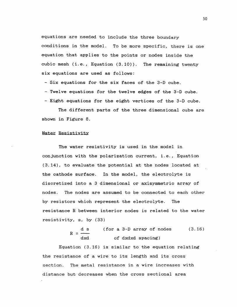
Hate~ ResistiYit~

The water resistivity is used in the model in

conjunction with the polarization current, i.e., Equation

(3.14), to evaluate the potential at the nodes located at

the cathode surface. In the model, the electrolyte is

discretized into a 3 dimensional or axisymmetric array of

nodes. The nodes are assumed to be connected to each other

by resistors which represent the electrolyte. The

resistance R between interior nodes is related to the water

resistivity, s, by (33)

d s R =

dxd

(for a 3-D array of nodes

of dxdxd spacing)

( 3. 16)

Equation (3. 16) is similar to the equation relating

the resistance of a wire to its length and its cross

section. The metal resistance in a wire increases with

distance but decreases when the cross sectional area

Vertices Faces

Figure 8. The Three Different Parts of a Three-Dimensional Cube Element.

51

52

increases. The same holds true for water except that the

system is not a long thin wire but rather an element thin

cube. Current will flow through the cross section of one

element cube to the adjacent element cube. Simplifying

Equation (3.16), the resistance becomes

R = s/d (3.17)

When the cube size is increased, the total resistance

decreases and vice versa. Equation (3.17) holds true for

all the interior nodes. At the boundary, only half the

volume of the cubic element is available and this fact

should be taken into consideration. Therefore, at the

boundaries, the distance in Equation (3.16) remains the same

but the cross sectional area is reduced to half {33).

d s 2ds 2s (3.18) R =---=--=

dxd/2 dxd d

Equation (3.18) should be used with nodes located at the

boundaries . It applies equally well to nodes that are on

the external faces, the edges, or vertices of the cube. As

a result, only two equations are needed to calculate the

water resistance in the model. Equation (3.17) is used to

evaluate the water resistance at the interior nodes.

Equation {3.18) is used to evaluate the water resistance at

the exterior nodes or the boundary nodes. Both equations

are used in conjunction with Equation (3.15) to evaluate the

potential of nodes at the cathode surface.

53

D:x:nami.Q Mesh

The nodes or nodal points contained in the cubic model

are stored in a three dimensional array. The size of the

three dimensional array is 10x10x10. Each element of the

array represents a node in the cubic model. Therefore,

there is a total of 1000 nodal points distributed in the

cubic model. Ten nodes exist in each direction, i.e., ten

nodes in the x, y, and z direction. The number of nodes is

limited to ten for practical reasons. First, the maximum

number of nodes allowed in the IBM Basic interpreter is ten.

This number can be safely used without exceeding the 64 K

bytes of memory of the basic interpreter. However, the

number of nodes can be brought up to 30 nodes in each

direction once the basic source code is compiled. Using a

three dimensional array of 30x30x30 requires 640 K bytes of

RAM (Random Access Memory). Most microcomputers do not have

this option. A more crucial consideration is the execution

time of the software. With a three dimensional array of

10x10x10, execution time ranges between fifteen minutes and

a maximum of two hours. Increasing the mesh size to

30x30x30 will increase the execution time by a factor of

twenty seven. This in turn means that the execution time

will range between seven and fifty four hours -- an

operation which is both inconvenient and time consuming.

Increasing the mesh size does not mean more refined

mesh elements. This is because of the way the model is set

up. The mesh is a dynamic mesh, changing for every case or

54

every set of input data. In other words. the dimensions of

the individual mesh elements are not constant but can

increase or decrease in value. To make the mesh dynamic,

the dimensions of each mesh element are set equal to the

brace diameter. For a brace diameter of 2 ft, the spacing

between nodes in the cubic mesh is equal to 2 ft in every

direction. For a three dimensional array of 10x10x10, the

distance between the first node and the last node is 18 ft

in each direction, i.e., ten nodal points define 9 elements.

For a brace diameter of 3 ft, the same distance is 27 ft and

so forth. Therefore, increasing the mesh size does not make

the mesh elements smaller but rather it makes the total

cubic volume larger. For a brace diameter of 2 ft and an

array of 30x30x30, the distance between the first node and

the last node is no longer 18 ft but rather 57 ft in each

direction. So whether the array is 10x10x10 or 30x30x30,

the dimensions of each mesh element are still 2 ft.

In conclusion, a mesh size of 10x10x10 is used. The

choice was made to insure fast execution times and reduced

memory requirements.

Because the mesh is dynamic, the node spacing

throughout the mesh is equal to the brace diameter. When

the brace diameter is large enough to exceed 3 or 4 ft, then

the node spacings are too large to accommodate the anode

'dimensions in a 3 dimensional fashion. In other words, the

55

anode cannot be represented in a three dimensional fashion

because most anodes do not have a three feet diameter. To

overcome this problem, the anode geometry was not assigned a

volume but was limited to a line (1 dimensional represen-

tation). A line anode is represented by nodes on a straight

line (Figure 9). On the contrary, a brace is represented by

cubical mesh elements representing the circular brace

diameter as shown in Figure 9. Representing an anode with a

only a line rather than a volume does not reflect a true

representation of the anode physical geometry. However, it

is more realistic and logical than representing an anode

with cubical elements.

The anode potential is needed as part of the input

data. The potential at the anode is assumed to be constant

throughout the anode surface. The anode potential is used

in the model to calculate the potential distribution

throughout the mesh. The current density of the anode or

the current rate output per lbm is not needed because the

Laplace equation models only the potential distribution.

The only current densities to be accounted for are the

current densities at the surface of the cathode.

Theoretically, the sum of the current entering the cathode

surface must be equal to the current leaving the anode \

surface. Since the Laplace equation does not provide any

indication on the amount of current leaving the anode

surface, it is assumed that it is equal to the amount of

current entering the cathode surface. As a result, the

Figure 9.

56

Cathode The Cathode and the Anode as Represented in the

Three-Dimensional Cubic Mesh.

57

corrosion engineer can use the value of the total current

entering the cathode system to determine the appropriate

type of anode. The potential distribution throughout the

mesh volume helps the corrosion engineer to place his anodes

at an optimal distance from the weld area.

Using the finite difference method to solve for the

Laplace equation generates an equation for each node in the

three dimensional mesh. This results is a system of n

linear equations with n number of unknowns. To solve the

set of equations, several methods can be used. The method

used in the model is the method of iteration (72). The

choice was made because the microcomputer is available to do

the number crunching. The way the iteration method works is

simple. The first step involves assigning initial values to

all the nodes. These initial values can be determined

arbitrarily. However, if these initial values are chosen to

be close to the solution values, then the solution will

converge faster. The next step involves generating a set of

new values based on the initial assigned values, using the

system of n equations. This new set of values is used again

to generate another new set of values. The process of

generating new values based on a previous set of values is

called an iteration. The iteration process is repeated

until the values of the potential at each nodal point from

one iteration to the next iteration do not differ by more

58

than a certain predetermined value. This predetermined

value is called the convergence criteria. It is usually

small enough so that the solution values are almost equal to

the values of the previous iteration. Naturally, the

smaller the convergence criteria the longer it will take the

model to converge to a solution, and vice versa.

The iteration method is fast and reliable. It is fast

because it is done on a microcomputer. It is reliable

because the iteration method always converges to a solution

even though the initial assigned values could be far from

the true solution. There are always exceptions to the

rules, and the same is true for the iteration method. The

method may not converge if used with a set of equations

which contains non-linear equations. However, this is not

the case because all the equations used in the model are

linear. Therefore, the model will always converge to a

solution, no matter how long it takes to converge.

Eola~ization Cu~~es

As mentioned earlier, a polarization curve is an

experimental (or theoretical) curve relating the potential

of the cathode surface of a structure to the current density

as shown in Figures 10 and 11. If the value of the

potential at a point is known, then the corresponding

current density can be evaluated by simply reading it from

the curve. Polarization curves are useful because they

allow the model to calculate the current density of the

ElmV- SCE) Temper•ture • 20"C

••I atm. ••tOO '""· ••110 aua. Qe200 ~~~~. oa300•t•.

10

-2 1(~A.cm )

Source: E. D. Mor and A. M. Beccaria, "The Influence of Hydrostatic Pressure on the Corrosion of Iron in Sea Water," Corrosion and Protection Offshore Communications Symposium International, Paper No. 124 (1979)

Figure 10. The Effect of Increasing the Pressure (Water Depth) is a Slight Shift of the Polarization Curve to the Right.

59

ECmV- SCE J Tempereture • 2ctC

••I It"'. .6a 100 It"'. .6•IIQ llltl. Qa200 .. 1ft. OaJOOitlft.

10 10"'

Source: E. D. Mor and A. M. Beccaria, "The Influence of Hydrostatic Pressure on the Corrosion of Iron in Sea Water," Corrosion and Protection Offshore Communications Symposium International, Paper No. 124 (1979)

Figure 11. The Same Shift to the Right of the Polarization Curve Due to the Increase of Hydrostatic Pressure Except that the Temperature is at 10C.

60

61

cathode surface at a certain potential. Polarization curves

also provide information about the conditions of the actual

physical system. In other words, the polarization curve is

a true representation of the relation that exists between

the potential and the current density of a cathode surface

submerged in a conductive electrolyte and the environment

conditions. These environmental conditions include the water

temperature and pressure, the oxygen concentration, the

water salinity, existing water currents, and surface finish

of the cathode. All and each of these factors influences

the relation between the potential and the current density

of a submerged cathode. For example, Figures 10 and 11 show

the influence of pressure and temperature on the polariza-­

tion curve. The curves in Figure 10 represent polarization

curves at different depths measured at a temperature of 20C.

The curves in Figure 11 are measured at a temperature of 10C

and represent polarization curves at different water depths

( or pressures). The net effect of the increase in

pressure (or depth) in either Figure 10 or 11 is a slight

shift of the polarization curve to the right. In addition,

changing the temperature fron 10C to 20C has also the effect

of shifting the polarization curve to the right, as shown in

Figures 10 and 11.

Therefore, an experimental polarization curve can be

used as a design tool to predict the potential and the

current density of the cathode for a given set of

temperature, pressure, and water properties. Each set of

~

62

cathode and water properties produces a different

polarization curve. Therefore, there can be hundreds of

polarization curves representing hundreds of existing

cathode conditions. If hundreds of polarization curves can

exist, and they do exist, then one can create a database

system based on the information (potential and current

density values) retrieved from these polarization curves.

Once the database system is created, it can be used with a

numerical model to predict the potential distribution for

most galvanic systems. Moreover, the model is not limited

to time zero (l'aunch time) but can be extended to account

for galvanic systems that have been in the water for a

certain period of time by using the corresponding

polarization curve.

Polarization curves may not be the best way to relate

the potential and the current density to existing water and

cathode conditions. But, in the context in which they are

used in this model, they are the only source of information

that relates this theoretical model to the true world.

Sha~e Eiles

A shape file is a data file containing information or

data on the coordinates of the cathode in the x, y, and z

direction. This information tells the program where exactly

the cathode elements are located within the 3 dimensional

cubic volume being analyzed. Once the coordinates of the

cathode elements are recognized by the program, it will

include in its calculations the polarization curren·ts

entering the cathode surfaces. Another function of the

shape file is to make the computer aware of the difference

between the coordinates of the brace elements and the leg

elements. This is needed because the brace diameter is

usually different from the leg diameter. Therefore, the

shape file will instruct the program to use the brace

diameter at the brace elements and to use the leg diameter

at the leg elements.

63

In general, a data file or a shape file is needed in

every numerical model because numerical models need to be

instructed about the locations or coordinates of each

individual element. This is a basic requirement in all

numerical models. Therefore, each geometry requires a

specific data file which runs only with that specific

geometry. To overcome this problem, a database was created

that included shape files for twenty six different

geometries. These geometries are the ones that are mostly

used by the industry. The user can pick any shape file he

wants by viewing it graphically on the screen. Then he can

run the program for that particular geometry and analyze the

output data. To make the program more interactive, the

shape files do not contain information on the coordinates of

the anodes. This means that the anode can move along the

x-axis, the y-axis, or both. It is up to the user to

specify the anode length and its distance from the weld

area. This makes the program or the model interactive and

64

also user friendly.

The database system can be expendable to accommodate

more geometries. It is up to the user to create his own

shape files for geometries that are not included in menu of

the program. An explanation and an example on how to

create new shape files are included in Appendix B.

N.od.e G.eom.e:tri.es

The node geometries are the structural nodes found in

the submerged part of offshore structures and installations.

It is referred to as a node geometry and should not be

confused with the word "node" which is the mathematical word

for all the points that forms the cubic mesh. The model

incorporates twenty six different node geometries. A

listing of these geometries along with their figures can be

found in Appendix C. These geometries were chosen based on

figures and drawings supplied by the sponsoring companies of

the project. Each node geometry is represented numerically

by a shape file. More node geometries can be included in

the model if new shape files are created, as discussed in

the previous section.

So:ur.c..e Lis.ti.mt.

The source listing of the program is not included in

this thesis because of a confidentiality agreement between

Oklahoma State University and the sponsoring companies. The

source code will made public after a certain time period

65

agreed upon by the concerned parties. However, a tree

structure of the program is included in Appendix D. The

program is composed of the main program menu PLATFORM and of

eight subprograms. Four of the eight subprograms are

commercial programs that were interfaced with the program

PLATFORM to generate the graphics work.

CHAPTER V

RESULTS AND DISCUSSION

Introduction

Numerical models are used to simulate physical

systems. The results obtained from these numerical models

are used to predict how the physical system will behave

under a certain set of conditions. In the same way, the

numerical model PLATFORM tries to simulate the potential

distribution in a three dimensional volume. The three

dimensional volume contains a structural node of a specific

node geometry and the surrounding water. Based on the

results of the potential distribution, the corrosion

engineer can change the location of the anodes to meet a

minimum protection criteria of -0.78 volt. The criteria is

usually set by the NACE Recommended Practice RP--01-·76 ( 1983

Revis ion ) ( 6 7 ) . To make the output data of the model easier

to handle, they are displayed in a graphical fashion. A

graphical representation of the results makes the analysis

and the interpretation of the output data easier and

simpler. The software PLATFORM can generate two dimensional

and three dimensional plots of the potential distribution in

the volume being analyzed.

66

67

Input Data

Before discussing the output data, it is important to

write about the different variables used in the input data.

These input variables are listed in Table III. The input

data can be divided into two types. In general, the first

type consists of all the variables needed to run the program

and obtain a solution of the potential in 3-dimensions.

These variables include the anode length and potential, the

anode distance from the node, the brace diameter, the leg

diameter, the water resistivity, the potential convergence

value, the type of polarization curve, and the shape file.

After obtaining the solution, the graphical analysis of the

data is in order. At this point, the second type of input

variables is needed. These variables include the direction

of the 2-dimensional plane (perpendicular to the x-axis,

y-axis, or z-axis) and the distance of that plane from the

axis origin.

Both types of input variables are needed to produce

the final graphical analysis. The first type of input

variables produces the 3-dimensional solution of the

potential distribution. However, the second set is needed

if any 2-dimensional analysis (graphical or not) is to be

done.

Potential Distribution in 3 Dimensions

Unlike most numerical models, this model is not

68

TABLE III

A SAMPLE OF THE COMPUTER OUTPUT SHOWING THE INPUT DATA

INPUT DATA

*~*~*******************************************~*~***~*~*~*~* fh t'? anode 1 <?.n q t h • ·f t • • • • • • • • .. • • • • • • • • • • • • • • • • • • • • .. • • • • • D The anodE~ potent i ;:d .. , vc.l.l t. . .. . .. . . . . . . . . . .. .. .. .. . . . . . .. . .. . . . .. .. .. 1 .. l.J!:7 ..

Thf?. anod<~ di:st.c:~nc:e ft··orn thf? node, ft •:>:·-;a>:if::.).......... ~3

ftlf2 c:\r10cl(~ d:i.st£:\rlC!:.~ +t'"Dfll t.hr:? nod€~, +t (y .. ··,::t:·:i~;;)............. !:{

The br· .::~ce d i <.'\meter·, ·ft. • • • • • • • • • .. • • • • • • • • • • • • • • • • • • • • • • . .. , T'h ~~ 1 E~q d :i c:\lll!f2t €::or· , f t .. . . . . . . .. .. . . . .. . . .. . .. . . .. .. . . . .. .. . .. . .. .. .. . .. ,:1. The w•ter resistivity, ohm-c:m ........................... 2~

·rt·1e IJC.'ttf.~~ntir.:\1 CC)J"l\/elr·cjf.?n<::E• v,::\It.tt:.~., \IC::tl"t:u ,, "II u," ,, , ",.,, .. , 11"" ~,()(>l

Di~:;t;anc(? cJ+ pl·'=ln<"? ·fn:Jm the i:':li·:if:5 or .. iqin 1::~, ++:........... .i .. ;~ f ot c3 J. C: l-W'I'" f:?rl t en t E'l'" i f1<;} the C: c:l t hOd(;:~ ~"'Llr" + c:!\C: f? 7 ioUllp .......... " .. (.;; ., 66 CURVE A pnli::\l"·1;:ation C:Uf"\tE~ \<\I£E:' u~sF:~ci rh~~ c:ho~::.::?n plane 1s perp<·?ndic:ulat~ to tht,;? :;:·-ry,~:1~:5

lhe node geometry consists of: 1 ANODE ON EACH HORIZONTAL BRACE ~X AND Y AXIS) 1. t..t:::E3 f..~h!D 2 l .. iUniZU!,I'TP,L.. ·r-·-,JCJIN"fb

*~*******~*********************************+*******~~****~***

69

limited to a two dimensional system. It is designed to

model three dimensional systems. Therefore, the results of

the model vary in three directions; along the x, y, and z

direction. The results of the numerical model are given in

terms of potential values. These potential values represent

the potential distribution throughout the three dimensional

cubic volume being analyzed. This cubic volume usually

contains a structural node, a couple of anodes and the

surrounding electrolyte. The potential distribution

provides information about the potential on the surface of

the cathode (the structural node), and throughout the

electrolyte body. These results are important from a design

point of view. The cathode potential must not exceed the

potential criterion of -0.78 volt at any point on the

structure surface. Therefore, the output data provides a

listing of the potential values at all points inside the

cubical volume including those points that are below the

criterion value. To pinpoint these points, the corrosion

engineer can either use graphical techniques or perform a

volume search. Graphical analysis is possible with the

software PLATFORM and it is easier to locate the areas with

low potential values. A volume search is basically going

through a list of numbers and indicating with a symbol such

as an arrow, at those points that are below the minimum

criterion. This task is not available in the software

PLATFORM but can be done with any spreadsheet program. The

most common spreadsheet is Lotus 123. The output data files

70

from PLATFORM are written in a format compatible with Lotus

format. The file extension <.PRN> is also recognizable by

Lotus. Therefore, the transfer of the output data file to

Lotus should be easy and error free.

Whether it is a volume search or a graphical

representation, the data analysis of the data helps the

corrosion engineer to place the anodes at an optimal

position. In turn, the optimal anode(s) position(s) should

provide adequate cathodic protection of the steel surface

including the weld area.

Two Dimensional Data Analysis

Before analyzing the output data graphically, the data

must be written in a suitable format. As it is, the output

data is provided along the x, y, and z direction. Any

graphical representation of these data is cumbersome and

almost impossible. In order to make the data available for

graphical display, the data must be reduced from a three

dimensional format into a two dimensional format. This can

be done by dividing the three dimensional data int,o several

two dimensional data sets. Each data set is a plane

containing data in two directions. A plane can contain

potential data along the x-axis and the y-axis, for example.

This means that the plane is perpendicular to the z-axis

since the z value is constant throughout the plane. As a

result, a plane can be perpendicular to either the x-axis,

the y-axis, or the z-axis depending on whether x, y, or z is

held constant. Moreover, two different planes that are

perpendicular to an axis are parallel to each other. This

is true because the mesh is made of regular cubic mesh

elements.

71

Figure 12 shows a plane containing data in two

dimensions and is perpendicular to the z-axis. The

potential data provide information on the potential

distribution in that plane, which is located at a certain

distance from the axis origin. The two dimensional data

contained within any plane can be analyzed graphically using

topographic maps or surface maps.

Graphical Analysis

Graphical representation of numerical data makes the

data analysis easier and simpler. The software PLATFORM is

equipped with graphics routines that produce topographic

maps and surface maps. These routines are commercial

routines that were interfaced with the main program PLATFORM

to perform the graphic tasks. These maps make the

interpretation of the potential data more efficient as

discussed next.

A topographic map is a map that contains contour lines

describing a certain physical system. It is used mostly in

geology where each contour line represents a set of points

at the same altitude. Therefore, the topographic map

Figure 12. A Plane Containing Data in Two Dimensions Which is Perpendicular to the Z-Axis.

72

73

provides information on the altitude of a point and also on

the elevation gradient or slope around that point. For

example, a mountain can be represented by a set of almost

concentric contour lines. The closer the contour lines, the

steeper the gradient, and vice versa.

A topographic map can be used to provide information

on the potential distribution within a surface or a plane.

The contour lines are in this case isopotential lines or

constant potential lines. By transferring the numerical data

to a topographic map, the data analysis becomes systemaT-ic.

One can read the potential value at almost any point in the

system being analyzed just by reading it from the

topographic map. One can also find out whether there is a

steep or flat potential gradient next to a point of

interest. This is important for areas close to the anodes.

One can also look at the difference between the potential

distribution at two different planes within the cubic

volume. This is done by comparing their respective

topographic maps.

The topographic maps in the software PLATFORM do not

have a rigid format. They can be changed to include more

contour lines. The user can also change the maximum and the

minimum potential values. The map.size can be changed as

well as the number of labeled contour lines. The

topographic map can be displayed on the screen or plotted on

a dot matrix printer. The printer output is a high quality

output resembling a plotter output. Figure 13, 14, and 15

YNAX "' 18.9

0

.. z YMIN = -.9

Figure 13. The Topographic Map of the Potential Distribution for the Input Data Shown in Table III. The Plane Containing the Potential Contour Lines is Perpen­dicular to the Z-Axis.

74

YMAX • 18.9

0

z YMIN = -.9

Figure 14. The Same Topographic Map of the Potential Distribution for the Input Data of Table III but With a Small Contour Line Interval.

75

X

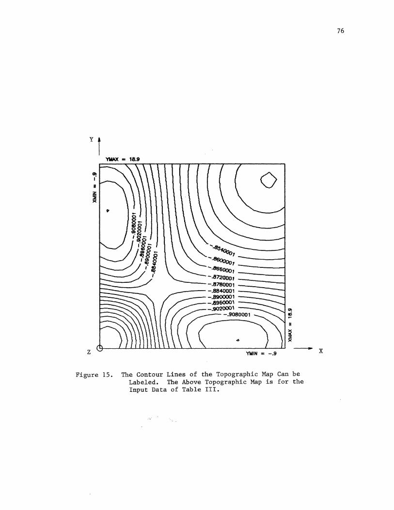
y I YWAX = 18.9

0 ~ :E X

~

.. z YMIN = -.9

-x

Figure 15. The Contour Lines of the Topographic Map Can be Labeled. The Above Topographic Map is for the Input Data of Table III.

76

77

show different versions of the same topographic map. Figure

13 is a topographic map of the potential distribution in a

plane passing through the anodes and, therefore, is

perpendicular to the z-axis. The input data used to

generate the potential distribution is listed in Table III.

Figure 14 is the same topographic map except that the

contour interval between the contour lines was made smaller.

This means that more contour lines are plotted in the same

map. Figure 15 is the same topographic map except that the

potential value of each line is printed on the map. Figure

16 is a topographic map for the same input data but the

plane of interest is located further away from the anodes.

The shaded parts of the map represent areas that are not

adequately protected. At these areas, the potential is

lower than -0.78 volt vs. Ag/AgCl. Therefore, the anodes

must be repositioned in order to achieve satisfactory

protection.

One fact that needs to be mentioned is the effect of

imposing boundary conditions on the cubic volume containing

the structural node. This effect can be seen in Figures 13,

14, and 15 and is represented by the circular isopotential

lines in the upper right corner and the lower left corner of

the maps. These circular isopotential lines do not reflect

a true behavior but rather represent the effect of imposing

mathematical constraints on the model.

y

z

C)) ,· II z ~ X

f YMAX = 18.9

n X

~ X

YWIN :: -.9

Figure 16. The Topograpcic Map in a Plane Located Further Away from the Anodes and Which Contains Areas That are Inadequately Protected (Shaded Areas).

78

79

A surface map is a three dimensional representation

of a topographic map. While the topographic map uses

contour lines to represent a mountain .for instance, the

surface map is actually a plot of the mountain in three

dimensions. The idea is to visualize where the top and the

bottom points are on the topographic map. It also helps to

locate in which direction are the potential gradients

acting. In the software PLATFORM, the surface map will

produce a three-dimensional representation of the potential

distribution in a plane of interest. ·Apart from the fact

that the surface maps are esthetically beautiful, they are a

great help in cases where the topographic map is revealing

They complex information about the potential distribution.

definitely eliminate confusion when one is trying to

visualize in his mind how a topographic map looks in three

dimensions. Surface maps are helpful and can be used

constructively to complement the data analysis of

topographic maps.

The commercial routine that produces the surface maps

offers different options for plotting the surface maps. The

map size can be changed as well as the maximum and minimum

values of the potential in the data. Since the surface map

is a three dimensional plot, then the angle of rotation and

the angle of tilt can also be changed as shown in Figures 17

to 20. The height to width ratio of the map can also be

Figure 17. The Surface Map of the Potential Distribution for the Input Data of Table III. The Rotation Angle is at 310 Degrees.

Figure 18. The Same Surface Map but Rotated at an Angle of 140 Degrees.

80

z

Figure 19. The Surface Map of the Potential Distribution at a Tilt Angle of 45 Degrees.

z

-....X

Figure 20. The Same Surface Map of the Potential Distribution but Tilted at an Angle of 20 Degrees.

81

82

altered as shown in Figure 21 and 22. The surface map can

be plotted with or without a skirt as shown in Figures 23

and 24. The surface map can be plotted with lines that are

either parallel to the x-axis, the y-axis, or both as shown

in Figures 25, 26, and 27. All of the data shown graphi­

cally in Figures 17 to 27 are for the same set of data

(Table III).

Validation of the Model

The results of the numerical model are typical of any

numerical model simulating an electrochemical system

governed by the Laplace equation. Fu (36), Munn (28), and

De Carlo (29) showed similar behavior to the results of this

model. Each one of their models simulated a galvanic system

governed by the Laplace equation. Although the results of

this model follows the same trend of results published in

the literature, it does not mean that the output data of the

model are valid. To validate the model, the theoretical

data predicted by the program must be compared with field

data.

One of the sponsoring companies was able to provide

proprietary field data for model verification. The field

data provided potential values for a structural node

protected by two anodes. The structural node consisted of

one leg and three horizontal T-joints as shown in Figure 28.

The leg was six feet in diameter. Two of the horizontal

braces had a diameter of twenty inch with the third brace

"'-x

Figure 21. The Surface Map of the Potential Distribution With a Height/Width Ratio of 1.0.

y

/

""' X

Figure 22. The Same Surface Map of the Potential Distribution but With a Height/Width Ratio of 0.5.

83

y

/ z

""" X

Figure 23. The Surface Map of the Potential Distribution With a Skirt.

y

/'

'-... X

Figure 24. The Same Surface Map of the Potential Distribution but Without a Skirt.

84

""'X Figure 25. The Surface Map of the Potential Distribution With

Grid Lines Parallel to the X-Axis.

........... X

Figure 26. The Same Surface Map but the Grid Lines are Parallel to the Y-Axis.

85

z

Figure 27. The Surface Map With Grid Lines Parallel to both the X-Axis and theY-Axis.

86

87

having a diameter of eighteen inch. The reference cell R5

was located at a distance of twenty one feet from the refe­

rence point. Other pertinent data to the node geometry and

anode specifications are shown in Figure 28.

In the first run, the same geometry dimensions of the

different node members were used as input data. The results

of the theoretical model, using the company's proprietary

polarization curve, were within 30% of the field data. In

the second run, the dimensions of the different members were

adjusted to yield a surface area equal to the surface area

of the actual structure. The potential results of the

second run were within 20% of the field data. The current

density results were within 1% of the field data. The

purpose of the first run was to calculate the potential at

the reference point R5. The purpose of the second run was

to find out if the anode current output in the model was

equal to the actual current output. This is why the

different member dimensions were adjusted to yield a surface

area equal to the surface area of the actual structure.

In the two runs, the model results were within 30% of

the actual data. The validation process showed two facts.

The first fact indicates that the model is valid and can

predict results within 30% of the field data. The second

fact indicated that the validity of the model depends on the

validity of the polarization curve used in the model. This

fact was based on the results of two other runs with the

same input data but with a generic polarization curve. The

OSU CALIBRATION MODEL, VIEWED FROM ABOVE, 1 00' DEPTH

/

NOTES:

0=20" L=25'

1. WATER RES.=24 ohm-em 2. ANODES ARE UNDERNEATH

& MEASURE 8.5"X9.5"X130.5", 1 000# WITH 22" STANDOFFS

3. L=MEMBER LENGTH TO REF PT 4. D=MEMBER DIAMETER 5. H=LEG HT. TO BE MODELED FROM REF PT 6. A 1 =ANODE 1, CENTER 12.5' FROM REF PT 7. A2=ANODE 2, CENTER 14.2' FROM REF.PT 8. R5=REF CELL 5, 21' FROM REF PT, ON TOP 9. ANODE E=-1020 mV vs Ag/AgCI 10. STEEL=-491 mV vs Ag/AgCI WITH NO CURRENT

D= 18" A2 L=28.5'~--------------------------------4

(adg. 4-30-116)

D=20" L=25'

A1

Source: A. D. Goolsby, Westhollow Research Center, Shell Development Company, 1986.

Figure 28. A Schematic Diagram of the Calibration Model.

88

89

generic polarization curve caused the model to yield results

that were well off. The potential value in the first run

was within 55% of the actual field datum. The current

density in the second run was within 45% of the actual

current density. Therefore, in future runs it is best to

use a polarization curve which closely simulates the true

conditions of the cathode.

Conclusion

The numerical model described in this chapter was

proved to be a valid model. A comparison of the theoretical

results of the model with field data, provided by a

sponsoring company, showed that the model results were

within 30% of the actual data. The polarization curve used

in the model has an important effect on the results.

Therefore, it is important to choose the right polarization

curve to simulate the cathode environment.

CHAPTER VI

CONCLUSIONS AND RECOMMENDATIONS

Conclusions

The numerical model PLATFORM is an interactive and

user friendly model. It is designed to model three

dimensional structural nodes in offshore platforms. It

provides a solution for the potential distribution on the

surface of the steel (cathode) and in the electrolyte body

surrounding the node. The model is equipped with a database

system that makes the numerical model interactive. The

database consists of data files representing twenty six

different node geometries. Each data file contains the

coordinates of the cathode elements for the node geometry in

question. The user can pick any geometry of his choice from

the database and then solve for the potential distribution

using the numerical model. The results of the program can

be listed or displayed graphically. Two kinds of graphs are

available for graphical analysis; topographic maps and

surface maps. The topographic maps provide isopotential

contour lines for any plane in either the x, y, and z

direction. The surface map is a three dimensional

representation of the topographic map. It is used when it

becomes difficult to interpret the data in the topographic

90

91

map. Based on the graphical output, the user can change the

anode locations to an optimal position to secure a proper

cathodic protection of the steel surface. This is done to

insure that the steel potential does not drop below -0.78

volt vs. Ag/AgCl at any point on the steel surface. This

minimum potential criteria is set by the NACE recommended

practice RP-01-76 in the marine corrosion section.

The results of the model are valid. The theoretical

data of the model were compared with field data from one of

the sponsoring companies. The theoretical data were within

30% of the field data in the two cases. It was found that

the model is dependent on the type of polarization curve

used with the model. The closer the polarization curve

represents the cathode conditions, the more accurate are the

model results.

In all, the model is interactive and user friendly.

It can be used as an effective design tool for cathodic

protection systems. The results of the model can be used to

predict the potential distribution for an existing structure

or for a future one. Its capability to generate potential

values in three dimensions and to graphically analyze the

data makes it one of the few powerful tools available for

cathodic protection design.

Recommendations

Every mathematical model has its own limitations. The

same is true for this program. The following recommenda-

tions are in order if one one desires to make PLATFORM a

more powerful and more useful program.

- The actual mesh size is limited to 10x10x10. The mesh

92

size can be increased to 20x20x20 or even 30x30x30.

Increasing the mesh size means that the program can cover

more surface area of the structure. This can be done by

writing the computational part of the package (Input/Run

section) in Fortran. The reason is that the Microsoft

Fortran compiler allows the user to dynamically dimension

his arrays to more than 10x10x10. The Fortran compiler can

access the whole 640 Kilo bytes of random memory that can be

available on a microcomputer (IBM XT).

- More node geometries can be added to the database system.

This can be done by creating shape files for the new

geometries. These shape files contain the coordinates of

the cathode elements. Appendix B explains the procedure to

create new shape files.

- The program is equipped to handle a maximum of two anodes

in each node geometry. It is recommended that the program

be modified to handle more than two anodes. It is also

important to be able to place the anodes on non-horizontal

braces such as the diagonals of a K-joint for example.

- In order to make the program more powerful, we suggest the

following. Another version of PLATFORM can be created that

runs in a batch mode. This means that the program will not

prompt the user about the anode size(s), the anode loca­

tion(s), or the anode distance(s) from the weld area.

93

Rather, the user will have to write a shape file that has a

format different from the one discussed above. This new

type of shape files will contain information not only about

the coordinates of the cathode elements but about the

coordinates of the anode elements as well. The new shape

file allows the user to place any type of anode(s), any size

of anode(s), and any distance of the anode(s) from the weld

area. He can also use different cathode geometries such as

pipelines or well conductors, and so forth. The program

will only recognize the information provided in the shape

file. The result is a more powerful program at the expense

of labor time. The user will have to create a shape file

for every single case he wants to analyze. This task can be

time consuming and frustrating specially for novices in

computer programming. However, this version of PLATFORM can

be made available by changing a few sections in the source

code.

- The fictitious points lying outside the boundaries of the

cube were determined using the mirror image extrapolation

technique. This method consists of assigning to the

fictitious point(s) the value of the point which is in the

opposite direction and is lying inside the cubic mesh. This

method may be improved by taking into account the values of

the rest of the points that are inside the cubic mesh. The

idea is to use several values instead of one to extrapolate

the value of the fictitious point{s}.

BIBLIOGRAPHY

1. R. C. Evans, The Micro Millenium, Viking Press, 2nd ed., New York { 1980).

94

2. J. B. Rochester, J. Gautz, The Naked Computer, William Morrow and Company, Inc., New York (1983).

3. D. Z. Meilach, Before You Buy a Computer, Crown Publishers, Inc., New York (1983).

4. A. C. Tenere, "Corrosion Control Evaluation and Data Recording by Electronic Computer, " presented at the NACE Western Region Conference, Phoenix, AZ, 1964.

5. A. c. Tenere, Materials Protection, Vol. 4, No. 7, p. 57 { 1965).

6. R. H. Saunders, Materials.Protection, Vol. 5, No. p. 42 ( 1966) .

7. G. s. Jones, Jr., Pipe Line Industry, Vol. 26, No. p. 75 { 1967).

8. R. L. Seifert, Materials Performance, Vol. 19, No. 10, p. 29 { 1980).

3,

10,

9. Mears Engineering Cathodic Protection Promotional Handouts, Mears/CPG, Inc., Rosebush, Michigan, 1985.

10. P. D. Gamache, P. Sullivan, Materials Protection, Vol. 12, No. 3, p. 26 {1973).

11. A.C. Van Orden, G. M. Ugiansky, J. M. Rodriguez, E. Esalante, J. Electrochemical Society, Vol. 180, No. 9 ( 1985).

12. H. Puschmann, R. Eckermann, "Dechema Corrosion Data and Materials Data Bank, " International Congress on Metallic Corrosion, 8th, p. 1963, 1981.

13. D. G. John, K. Hladky, Materials Performance, Vol. 19, No. 11, p. 42 (1980).

14. N. D. Greene, R. H. Ghandi, Materials Performance, Vol. 21, No. 7, p. 34 (1982).

15. S. M. Gerchakov, L. R. Udey, F. Mansfeld, Corrosion, Vol. 37, No. 12, p. 36 (1981).

16. M. Kendig, F. Mansfeld, Corrosion, Vol. 39, No. 11, p. 466 ( 1983).

17. J.D. Kellner, "Computer Controlled AC Impedance Measurements for the Evaluation of Anti-Corrosion Pipeline Coatings," CORROSION/85, Paper No. 73, National Association Of Corrosion Engineers, Houston, Texas, 1985.

18. L. F. G. Williams, R. J. Taylor, Corrosion, Vol. 38, No. 8, p. 425 {1982).

19. V. R. Wandruska, S. W. Orchard, A. Greeff, Talanta, Vol. 32, No. 4, p.307 {1985).

20. E. Sivieri, S. Rondinini, F. Bonino, La Metallurgia Italiana, Vol. 75, No. 7-8, p.515 (1983).

21. R. J. O'Halloran, L. F. G. Williams, C. P. Llyod, Corrosion, Vol. 40, No. 7, p. 344 {1984).

22. E. Diacci, R. Rizzi, C. Ronchetti, Sci. Tech. Aerosp. Rep., 22{16), 1984.

23. J. T. J. Naber, J. Electrochemical Society, Vol. 101, No.6, p. 271 {1954).

24. J. T. Naber, M. J. Rosenbluth, J. Electrochemical Society, Vol. 102, No. 6, p. 344 {1955).

25. J. T. Naber, B. J. Fagan, J. Electrochemical Society, Vol. 103, No. 1, p. 64 {1956).

95

26. J. T. Naber, J. Electrochemical Society, Vol. 103, No. 10, p. 567 {1956).

27. E. Kenard, J. T. Naber, J. Electrochemical Society, Vol. 117, No. 7, p. 880 (1970).

28. R. S. Munn, Materials Performance, Vol. 21, No. 8, p. 29, (1982).

29. E. De Carlo, Materials Performance, Vol. 22, No. 7, p. 38 { 1983) .

30. R. G. Kasper, M. G. April, Corrosion, Vol. 39, No. 5, p. 181 {1983).

31. R. Strommen, A. Roland, Materials Performance, Vol. 20, No. 4, p. 15 ( 1981).

32. R. N. Fleck, Numerical Evaluation of Current Distibution in Electrical Systems, MSc, Thesis, University of California, Sept., 1964.

96

33. R. S. Munn, J. H. Clark, "Simple Method for Prediction of Galvanic Corrosion Rates on Real Structures in Seawater Using Numerical Te0;hniques on a Microcomputer," CORROSIONfi&3, Paper No. 74, National Association of Corrosion Engineers, Houston, Texas, 1983.

34. R. S. Munn, "Numerical Corrosion Rate Prediction on Stuctures Immersed in Inhomogeneous Media," CORROSION/~4. Paper No. 49, National Association of Corrosion Engineers, Houston, Texas, 1984.

35. J. N. Fu, J. S. K. Chow, Materials Performance, Vol. 21, No. 10, p. 9 (1982).

36. J. W. Fu, "Calculation of Cathodic Protection Potential and Current Distributions Using an Integral Equation Numerical Method," CORROSION/84, Paper No. 250, National Association of Corrosion Engineers, Houston, Texas, 1984.

37. P. 0. Gartland, R. Johnsen, "COMPACS- Computer Modeling of Cathodic Protection Systems, " CORROSION/85, Paper No. 319, National Association of Corrosion Engineers, Houston, Texas, 1985.

38. J. W. Fu, S. Chan, Corrosion, Vol. 40, No. 10, p.540 (1984).

39. J. W. Fu, Corrosion, Vol. 38, No. 5, p.295 (1982).

40. J. W. Fu, S. Chan, "Finite Element Modeling of Galvanic Corrosion During Chemical Cleaning of Westinghouse Series 51 Steam Generator, " CORROSION/85, Paper No. 190, National Association of Corrosion Engineers, Houston, Texas, 1985.

41. J. W. Fu, S. Chan, "A Finite Element Modeling Method for Predicting Long Term Corrosion Rates," CORROSION/84, Paper No. 199, National Association of Corrosion Engineers, Houston, Teaxs, 1984.

42. B. P. Boffardi, G. W. Schweitzer, Materials Performance, Vol. 19, No. 12, p. 44 (1980).

43. L. Chen, D. T. Freese, W. R. Snyder, Materials Performance, Vol. 21, No. 12, p. 9 (1982).

44. A. Borello, S. Casadio, A. Saltelli, G. Scibona,

97

Corrosion, Vol. 37, No. 9, p.498 (1981).

45. A. Borello, S. Casadio, A. Mignone, Corrosion, Vol. 39, No. 6, p. 247 (1983).

46. D. C. Silverman, Corrosion, Vol. 38, No. 10, p. 541 { 1982).

47 J. C. Angus, C. T. Angus, J. Electrochemical Society, Vol. 132, No. 5, p. 1014 {1985).

48. J. C. Angus, C. T. Angus, "Instructions For Potential­pH Diagram Generator", Case Western Reserve University, Chemical Engineering Department, April 1985.

49. E. Verink, "Adaptation of a Computer Program for Pourbaix Diagrams to Personal Computers," in G. L. Liedl and K. S. Sree Harsha, editors, Computer Usage in Materials Education, The Metal Society, Warrendale, Pennsylvania, p. 123 (1985).

50. M. Froning, M. Shanley, E. Verink, Corrosion Science, Vol. 16, No. 16, p. 371 (1976).

51. R. Strommen, "Evaluation of Anode Resistance Formulas by Computer Analysis," CORROSION/84, Paper No. 253, National Association of Corrosion Engineers, Houston, Texas, 1984.

52. J. Cochran, "Offshore Platform Cathodic Protection optimization Via Computer Use of Classical Equations," CORROSION/84, Paper No. 252, National Association of Corrosion Engineers, Houston, Texas, 1984.

53. J. Cochran, "The Design of Cathodic Protection Systems of Offshore Pipelines in Varied Environments," CORROSION/84, Paper No. 333, National Association of Corrosion Engineers, Houston, Texas, 1984.

54. J. Cochran, "New Mathematical Models for Designing Offshore Sacrificial Cathodic Protection Systems," Offshore Technology Conference, Paper No. 3858, Houston, Texas, 1980.

55. M. Haroun, Cathodic Protection Modeling of Tethers in Tension Leg Platforms, Shell Development Company, Westhollow Research Center, Houston, Texas, Summer 1985.

56. A. N. Campbell, V. F. Hollister, R. 0. Duda, P. E. Hart, Science, Vol. 217, p. 927 (1982).

57. C. Westcott, D. E. Williams, N. J. M. Wilkins, G. P.

Marsh, J. N. Wanklyn, J. F. Croall,. "Expert Systems -the Application of New Computer Methods to Corrosion Problems," Proceedings of the Electrochemical Society, Vol. 85-3, p. 190, 1985.

58. C. Westcott, D. Williams, J. Bernie, I. Croall, and S. Patel, "The Development and Application of Integrated Expert Systems and Databases for Corrosion. Consultancy," CORROSION/86, Paper No. 54, National Association of Corrosion Engineers, Houston, Texas, 1986.

59. E. H. Schmauch, and W. Thomason, "Expert Systems for Personal Computers, " CORROSION/86, Paper No. 55, National Association of Corrosion Engineers, Houston, Texas, 1986.

60. S. Marchand, A. Asphahani, and D. Carlson, "Computerized Expert Systems: Solving Corrosion Problems in Industrial Services, " CORROSION/86, Paper No. 56, National Association of Corrosion Engineers, Houston, Texas, 1986.

98

61. N. Pes sal and J. J. Schreurs, "Deve 1 opment of Expert Systems by Corrosion Specialists, " CORROSION/86, Paper No. 57, National Association of Corrosion Engineers, Houston, Texas, 1886.

62. W. Bogaerts and M. Rijkaert, "Artificial Intelligence, Expert Systems and Computer-aided Engineering, " CORROSION/86, Paper No. 58, National Association of Corrosion Engineers, Houston, Texas, 1986.

63. P. E. Hart, "Expert Systems and Technological Problems, " Proceedings of the Second International Conference on Foundations of Computer-Aided Process Design, Snowmass, Colorado, 1983.

64. A. W. Westerberg, "Discussion Summary: Keynote Address," Proceedings of the Second International Conference on Foundations of Computer-Aided Process Design, Snowmass, Colorado,1983.

65. C. Edeleneau, Materials Performance, Vol. 22, No. 10, p. 82 ( 1983).

66. M. G. Fontana and N. D. Greene., "Corrosion Engineering," 2nd Ed., New York, McGraw Hill Co., 1978.

67. NACE Standard RP-01-76, Corrosion Control of Steel, Fixed Offshore Platforms Associated with Petroleum Production, National Association of Corrosion Engineers, 1983.

68. Shell Development Company. Technical Training Manual, Houston, Texas, 1985.

99

Cathodic Protection Westhollow Research Center,

69. M. Haroun, R. Erbar, and H. Heidersbach, "The Use of Computers in Corrosion Control and Monitoring," CORROSION/86, Paper No. 61, National Association of Corrosion Engineers, Houston, Texas, 1986.

70. L. R. Segerlind, "Applied Finite Element Analysis," 2nd Ed., New York, John Wiley and Sons, 1984.

71. R. B. Bird, W. E. Stewart, and E. N. Lightfoot, "Transport Phenomena, " John Wiley and Sons, 1960.

72. J. D. Parker, J. H. Boggs, and E. F. Blick, "Introduction to Fluid Mechanics and Heat Transfer," 3rd Ed., Addison-Wesley Publishing Co., 1974.

APPENDIXES

100

APPENDIX A

A SAMPLE OF CATHODIC PROTECTION DESIGN

101

102

SAMPLE DESIGN

The following is a sample of an offshore cathodic

protection design procedure. The platform is in the Gulf of

Mexico and the design parameters are similar to other Gulf

platforms. These are:

- Maintenance current density= 5 mAmp/ft2

- Design life = 20 years

- Calculated surface area = 33484 ft2 {water zone) = 47984 ft 2 (mud zone}

- Anode capacity = 1280 Amp-hr/lb

- Safety factor = 25%

- Water resistivity = 20 ohm-om

- Assumed anode parameters = 725 lb net Aluminum weight 8 ft lonf 90.25 in X-seotion area

Given these numbers, we first calculate the total

current in the water zone and the mud zone:

(5 mAmp/ft2 )(33484 ft2 } Current (water) = = 167.4 Amps

1000

{5 mAmp/ft2 )(47984 ft 2 ) Current (mud) = = 95.9 Amps

1000

The next step is to evaluate the total weight of anode

material required:

Total Weight = (water)

(167.4 Amps){8760 hr/yr)(20 yrs){1.25)

{1280 Amp-hr/lb)

= 28641 lbs

103

Total Weight = (mud)

(95.9 Amps)(8760 hr/yr)(20 yrs)(1.25)

(1280 Amp-hr/lb)

= 16408 lbs

At this stage, the number of anodes needed in each

section can be evaluated:

Number of anodes (water)=(28641 lbs)/(725 lb/Anode) = 39.5

Number of anodes (mud)=(16408 lbs)/(725 lb/Anode) = 22.6

Total Number of anodes = 40 + 23 = 63

Sixty three anodes are needed to prepolarize the steel,

or to provide the initial current density. The initial

current density must be at least 15 mAmps/ft2 to assure the

buildup of an adequate calcareous deposit on the steel

members. The total initial current output per anode is

calculated using a potential of 0.45 volts between bare,

unpolarized steel (-0.60 volt) and aluminum (-1.05 volt) and

an anode resistance calculated from Dwight's equation for a

single anode, since experience shows no significant

interference between the various numbers of a multiple anode

design. s

Resistance= ----------(ln 4L/r -1) , Dwight Equation 2(PI){L)

where,

L = anode length, in

PI= 3.14159

s = Water Resistivity, ohm-em

r = Equivalent Radius, in

For shapes other than cylindrical shapes

r = SQRT(Cross Sectional area/PI)

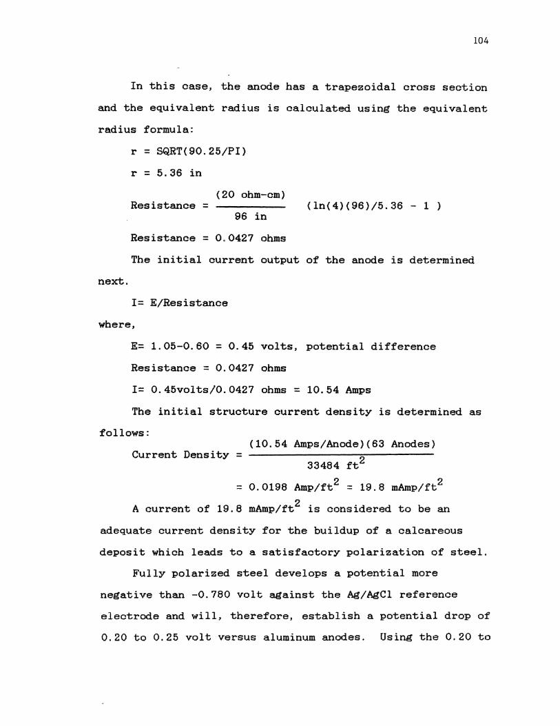
104

In this case, the anode has a trapezoidal cross section

and the equivalent radius is calculated using the equivalent

radius formula:

r = SQRT(90.25/PI)

r = 5.36 in

(20 ohm-em) Resistance = (ln(4)(96)/5.36 - 1 )

96 in

Resistance = 0.0427 ohms

The initial current output of the anode is determined

next.

I= E/Resistance

where,

E= 1.05-0.60 = 0.45 volts, potential difference

Resistance = 0.0427 ohms

I= 0.45volts/0.0427 ohms = 10.54 Amps

The initial structure current density is determined as

follows: (10.54 Amps/Anode)(63 Anodes)

Current Density = 33484 ft 2

= 0.0198 Amp/ft2 = 19.8 mAmp/ft2

A current of 19.8 mAmp/ft2 is considered to be an

adequate current density for the buildup of a calcareous

deposit which leads to a satisfactory polarization of steel.

Fully polarized steel develops a potential more

negative than -0.780 volt against the Ag/AgCl reference

electrode and will, therefore, establish a potential drop of

0.20 to 0.25 volt versus aluminum anodes. Using the 0.20 to

105

0.25 volt potential drop for Ohm's law and calculating the

anode resistance with Dwight's equation based on anode

dimensions at 40 to 50% consumption will then result in a

maintenance current density which is roughly half the value

of the calculated initial one. Therefore, if the steel is

polarized to -0.80 volt vs. Ag/AgCl, the current output of

the anode is

I = E/Resistance

where,

E = 1.05 - 0.8 = 0.25 volts

Resistance= 0.0441 ohm (derated anode radius based on

a 10% reduction of the initial radius)

I= 0.25/0.0441 = 5.6 Amps

The actual potential drop between structural steel

cathode and aluminum anodes at some time after launching the

platform is estimated as the difference between the given

aluminum versus Ag/AgCl potential and the average of

polarized steel potentials as measured with Ag/AgCl

reference electrodes a,t various locations of the structure.

The true current output per anode is, therefore, available

for predicting the life of the cathodic protection system

given the capacity of 725 lb aluminum anodes, namely,

(1280 Amp hr/lb)(725 lb/Anode) Life =

(8760 hr/yr)(T Amp/Anode)

which leads to the life in years for T amps current output

per anode as follows:

Life = 106/T years

106

Based on a current of 5.6 Amp, the design life of the

cathodic protection system is

Life= 106/5.6 = 18.9 years

Since the required design life is 20 years, then another

anode geometry should be chosen.

Suppose that the new anode has the following anode

charactristics:

Length = 10 ft = 120 in

Radius = 6 in

weight = 1135 lb

Anode Capacity = 1280 Amp-hr/lb

The total number of anodes needed based on the surface area

of the water and the mud sections is

Nbe of Anodes (water)=(28641 lb)/(1135 lb/Anode)= 25.2

Nbe of Anodes (mud) =(16408 lb)/(1135 lb/Anode)= 14.4

Total Number of Anodes = 26 + 15 = 41

The resistance of one anode using Dwight's equation is

20 Resistance= (ln(4)(120)/6 - 1 )

2(PI)(120)

=0.03532 ohm

The initial total current output based on a potential drop

of 0.45 volt is

I= E/Resistance

= 0.25/0.03532 = 12.74 Amps

The structure current density is now evaluated and is equal

to (12.74 Amps/Anode)(41 Anodes)

Current Density = ft 2 33484

= 0.0156 Amp/ft2 = 15.6 mAmp/ft2

An initial structure current density of 15.6 mAmp/ft2 is

acceptable. A more conservative design will allow for a

higher number. Next, the anode resistance is calculated

based on a derated radius of 5.4 in (10% reduction).

20 Resistance =

2(PI)(120)

= 0.036420 ohm

(ln(4){120)/5.4- 1 )

Using a potential drop of 0.25 volt, the total maintenance

current available is

I= 0.25/0.036420

= 6.86 Amps (almost half the initial value)

Based on a current of 6.86 Amps, the design life of the

cathodic protection system is

Life = (1280 Amp-hr/lb){1135 lb/Anode)

{8760 hr/yr)(6.86 Amps/Anode)

= 24.2 years

Therefore, the design is acceptable.

107

APPENDIX B

SHAPE FILES

108

109

SHAPE FILES

A shape file contains information about the coordinates

of the cathode elements. To create new shape files the user

must supply information about the coordinates of the cathode

elements of the new geometry. Once the new shape file is

created, then it can be used with the program PLATFORM to

model the potential distribution of the new geometry.

Before attempting to create a new shape file, one must

understand how the model works. This section will explain

how the model works. It will also provide an example of a

shape file and its corresponding file in BASIC.

The three-dimensional cube containing the node geometry

has ten nodal points along the x, y, and z axis. The origin

of the axis system is at the lower left vertice of the cube

as shown in Figure 29. The program maps the nodal points in

the cube to look for the cathode points. It starts at the

axis origin at x=1, y=1, and z=1. First it moves along the

x-axis at y=1 and z=1. Once the program reaches x=10, it

updates y which is now equal to 2 and moves again along the

x-axis. This is done for all the y values from 1 to 10.

Once the program reaches x=10 and y=10 it updates the third

coordinate z to 2. The same procedure starts all over again

and is repeated for all the values of z from 1 to 10.

To enter the coordinates of the cathode elements, one

z t

...... . . ·'

............................. '\ • I' : ........................... ~

:Y ;~ , .

• I' ..

/

Figure 29. The Origin of the Three-Dimensional Cube Containing the Node Geometry is Located at the Lower Left Vertex of the Cube.

110

111

must follow the above format. The coordinates must be

entered in a consecutive fashion. The first point in the

file must have the lowest coordinate values (for example, 1,

1, 1) and the last point in the shape file must have

the largest coordinate value (for example, 10, 10, 10).

Therefore, the user must start at the first plane at z=1.

In that plane, he must determine the coordinates of the

cathode nodal points. Figure 30 shows the locations of the

points representing the leg in the plane at z=1. The values

are entered in the shape file, and the same operation is

repeated for the plane at z=2. The planes at z=5 and z=6

contain the nodal points of the brace elements. Figure 31

shows the locations of the nodal points for the leg and for

the two horizontal braces. Once all the planes from z=l to

10 are mapped for the cathode points, the shape file is

complete. This procedure is explained better in the

following example.

Table IV is a listing of the data contained in a shape

file for a geometry consisting of one leg and two horizontal

braces. The node geometry is shown in Figure 32. The shape

file is a consecutive listing of the cathode coordinates and

is arranged in data sets. Each data set contains four data

points. The first datum is a negative number informing the

computer whether the nodal point belongs to the leg or to

the brace. The following three numbers in the data set are

the coordinates of the nodal point along the x,y, and z

axis. However, the firt two data sets do not contain a

10 y 9

8

?

6

5

4

3

2

1 X 1 2 3 4 5 6 ? 8 9 10

Figure 30. The Dots Represent the Locations of the Leg Coordinates in the Plane Perpendicular to the Z-Axis at Z=l.

10 ~.

9

8

7

6

"' ..J

4

~

,)

2

1 X 1 2 3 4 5 6 7 B 9 10

Figure 31. The Dots Represent the Locations of the Leg and the Two Horizontal Braces in the Plane Perpendicular to the Z-Axis at Z=S.

112

TABLE IV

A LISTING OF THE DATA CONTAINED IN A SHAPE FILE

1,0,2,1 1 leg and 2 horizontal T-joints,?,? -2,1,1,1 -2,2,1,1 -2,1,2,1 -2,2,2,1 -2,1,1,2 -2,2,1,2 -2, 1 ,2,2 -2,2,2,2 -2,1,1,3 -2,2,1,3 -2,1,2,3 -2,2,2,3 -2,1,1,4 -2,2,1,4 -2,1,2,4 -2,2,2,4 -2,1,1,5 -2,2,1,5 -1 ,3, 1,5 -1,4,1,5 -1 ,5, 1,5 -1,6,1,5 -1,7,1,5 -1,8,1,5 -1,9,1,5 -1,10,1,5 -2,1 ,2,5 -2,2,2,5 -1,3,2,5 -1,4,2,5 -1,5,2,5 -1,6,2,5 -1,7,2,5 -1,8,2,5 -1,9,2,5 -1,10,2,5 -1,1,3,5 -1,2,3,5 -1,1,4,5 -1,2,4,5 -1,1,5,5 -1,2,5,5

-1,1,6,5 -1,2,6,5 -1,1,7,5 -1,2,7,5 -1,1,8,5 -1,2,8,5 -1,1,9,5 -1,2,9,5 -1,1,10,5 -1 ,2, 10,5

. -2,1,1,6 -2,2,1,6 -1,3,1,6 -1,4,1,6 -1,5,1,6 -1 ,6, 1,6 -1,7,1,6 -1,8,1,6 -1,9,1,6 -1,10,1,6 -2,1,2,6 -2,2,2,6 -1,3,2,6 -1,4,2,6 -1,5,2,6 -1,6,2,6 -1,7,2,6 -1 ,8,2,6 -1,9,2,6 -1,10,2,6 -1,1,3,6 -1,2,3,6 -1,1,4,6 -1,2,4,6 -1,1,5,6 -1,2,5,6 -1,1,6,6 -1,2,6,6 -1,1,7,6 -1,2,7,6 -1,1,8,6 -1,2,8,6 -1,1,9,6 -1,2,9,6

113

-1,1,10,6 -1,2,10,6 -2,1,1,7 -2,2,1,7 -2,1,2,7 -2,2,2,7 -2,1,1,8 -2,2,1,8 -2,1,2,8 -2,2,2,8 -2,1,1,9 -2,2,1,9 -2,1,2,9 -2,2,2,9 -2,1,1,10 -2,2,1,10 -2,1,2,10 -2,2,2, 10 o,o,o,o

SIDE UIEW (X) SIDE UIEW (Y) TOP UIEW

Figure 32. A Graphical Representation of a Node Geometry Consisting of One Leg and Two Horizontal Braces.

114

negative number and they are used for a different purpose.

They provide information about the number of anodes and

their locations. We will go through the first couple of

data sets and elaborate more about the function of each

number in the shape file.

Da:ta S.e:t 1

1 is a flag to indicate the anode type:

Anode type=1, anode on the x-axis

Anode type=2, anode on the y-axis

Anode type=3, anode on both the x-axis and y-axis

0 is the anode coordinate along the x-axis

2 is the anode coordinate along the y-axis

7 is the anode coordinate along the z-axis

D.a:t.a Se:t 2

115

"One Anode and Two Horizontal Braces,?,?" is text

information about the node geometry. A total of three

comments separated by commas is allowed. The question

mark,"?", is ignored by the program and is used to

replace missing comments.

Da:ta S.e:t 3.

-2 is a flag to indicate that the point belongs to the leg.

1 is the coordidate of the leg along the x-axis.

1 is the coordinate of the leg along the y-axis.

1 is the coordinate of the leg along the z-axis.

lla:ta S~:t ~

-2 is a flag to indicate that the point belongs to the leg.

2 is the coordidate of the leg along the x-axis.

116

1 is the coordinate of the leg along the y-axis.

1 is the coordinate of the leg along the z-axis.

Da:t.a Set. .5.

-2 is a flag to indicate that the point belongs to the leg.

1 is the coordidate of the leg along the x-axis.

2 is the coordinate of the leg along the y-axis.

1 is the coordinate of the leg along the z-axis.

llilta s~t. Q_

-2 is a flag to indicate that the point belongs to the leg.

1 is the coordidate of the leg along the x-axis.

2 is the coordinate of the leg along the y-axis.

1 is the coordinate of the leg along the z-axis.

Data set 7 through 18 contain the same information on

the leg coordinates in the planes at z=2, 3, and 4. The

planes at z=5 and z=6 contain the coordinates of the braces.

Data sets 19 to 90 cover the coordinates of all the leg and

the two horizontal braces in the cube. Data sets 91 to 105

contain the coordinates of the leg in the planes at z=

7,8,9, an 10. The last data set contains four zeros. This

informs the program that it reached the end of the shape

file.

The source listing of the program that created the

shape file that we just discussed is shown in Figure 33. It

can be adjusted to create new shape files. The source code

is very simple and therefore can be modified without any

major problem.

5 COLOR 14,0:CLS:KEV OFF 10 ANDTVPE=1:AND1=0:AND2=2:AND3=7 20 OPEN "c:a1.shp" FOR OUTPUT AS 11 30 WRITE t1,ANDTVPE,AND1,AND2,AND3 35 PRINT 11,"1 leg and 2 horizontal T-joints•;•,•;"?';",";'?" 40 FOR 1=1 TO 105 50 READ COND,A,B,C 60 WRITE ll,COND,A,B,C 70 'ttttttttttttttttttt 16 data points tttttttttttttttttt

SO DATA -2,1 11111-2 121111,-2,1,2,1,-2,2,2,1 90 DATA -2,1 91121-2921112,-2,1 12,2,-2,2,212 100 DATA -2,1,1,31-2 1211,3,-2,1,213,-2121213 110 DATA -2 1111,41-2 1211141-2 1112,4,-2,2,214 120 ·--------------------------------------------------------------------------130 'tttttttttttttttttttttttttttt 2HT, 72 data points ttttttttttttttttt

140 DATA -21111151-2 1211151-1 1311151-1 1411151-1 1511151-1,61115,-1,711151-1 181115 ,-1,9,1,5,-1,10,1,5 150 DATA -2,1,2,5,-2,212151-1 1312151-1 1412151-1 1512151-1 1612151-1 1712151-1 181215 ,-1,9,2,5,-1,10,2,5 160 DATA -1,1,3,5,-1,213,5,-1,1 1415,-1,2,4 15,-1,1,5,5,-1,2,5,5,-1,1,6,5,-1,2,6,5 ,-1,1,7,51-1,2,7,5,-1,1 1815,-1,2,8,51-1 111915,-1,2,9,5,-1,1,1015,-1,2,10,5 170 DATA -2,1,1,6,-2,2,1,6,-1 1311161-1 1411161-1 1511161-1 161116,-1,7,1 16,-1,81116 ,-1,9,1,6,-1,10,1,6 180 DATA -2,1 1216,-2,2,2161-1 1312161-1,,,2,61-1 15,216,-1,612,6 1-1 1712161-1 181216 ,-1,9,2,6,-1,10,2,6 190 DATA -1 1113,6,-1,213161-1 1114161-1 1214161-1 1115161-1 121516,-1,1,6161-1 12,6,6 ,-1,1,7,6,-1,2,7,6,-1,1,8,6,-1,2,8,6,-1,1,9,6,-1,2,9,6,-1,1,10,6,-1,2,10,6 200 ·--------------------------------------------------------------------------210 'ttttttttttttttttt 17 data points tttttttttttttttttt

220 DATA -2,1 1117,-2,21117,-2,1 1217,-2,2,217 230 DATA -2,1,J,B,-2,2111B,-2,1,2,B,-2,2,2,B 240 DATA -2 1111191-2 1211191-2 1112191-2 121219 250 DATA -2,1,1,10,-2,2,1,J0,-2,1,2,10,-2,2,2,10,o,o,o,o 260 ·--------------------------------------------------------------------------270 NEXT I 280 CLOSE 11

Figure 33. The Source Listing of the BASIC Program That Created the Shape File Presented in Table IV.

117

APPENDIX C

LISTING AND FIGURES OF THE

NODE GEOMETRIES

118

119

NODE GEOMETRIES

The figures in this appendix represent the twenty six

different node geometries used in the program PLATFORM.

Each figure is intended to give the user a rough idea on the

geometry of the structural node.

by a list describing each geometry.

The figures are preceded

Each number in the list

corresponds to a similar number in each figure as follows:

1- 2 horizontal T-joints

2- 2 hrizontal T-joints and 1 K-joint along the x-axis

3- 2 horizontal T-joints and 1 K-joint along the y-axis

4- 2 horizontal T-joints and 1/2 K-joint along the x-axis

pointing upward.

5- 2 horizontal T-joints and 1/2 K-joint along the y-axis

pointing upward.

6- 2 horizontal T-joints and 1/2 K-joint along the x-axis

pointing downward.

7- 2 horizontal T-joints and 1/2 K-joint along the y-axis

pointing downward.

8- 2 horizontal T-joints and 1 K-joint along the x-axis and

1 K-joint along the y-axis.

9- 2 horizontal T-joints and 1 K-joint along the x-axis and

l/2 K-joint along the y-axis pointing downward.

10- 2 horizontal T-joints and 1 K-joint along the x-axis

and 1/2 K-joint along the y-axis pointing upward.

11- 2 horizontal T-joints and 1/2 K-joint along the x-axis

pointing downward and 1 K-joint along the y-axis.

120

12- 2 horizontal T-joints and 1/2 K-joint along the x-axis

pointing upward and 1 K-joint along the y-axis.

13- 2 horizontal T-joints and 1/2 K-joint along the x-axis

pointing upward and 1/2 K-joint along the y-axis

pointing upward.

14- 2 horizontal T-joints and 1/2 K-joint along the x-axis

pointing downward and 1/2 K-joint along the y-axis

pointing downward.

15- 2 horizontal T-joints and 1/2 K-joint along the x-axis

pointing downward and 1/2 K-joint along the y-axis

pointing upward.

16- 2 horizontal T-joints and 1/2 K-joint along the x-axis

pointing upward and 1/2 K-joint along the y-axis

pointing downward.

17- 1 horizontal T-joint and 1 K-joint along the x-axis

and 1 K-joint along the y-axis.

18- 1 horizontal T-joint and 1 K-joint along the x-axis

and 1/2 K-joint along the y-axis pointing downward.

19- 1 horizontal T-joint and 1 K-joint along the x-axis

and 1/2 K-joint along the y-axis pointing upward.

20- 1 horizontal T-joint and 1/2 K-joint along the x-axis

pointing downward and 1 K-joint along the y-axis.

21- 1 horizontal T-joint and 1/2 K-joint along the x-axis

pointing upward and 1 K-joint along the y-axis.

22- 1 horizontal T-joint and 1/2 K-joint along the x-axis

pointing upward and 1/2 K-joint along the y-axis

pointing upward.

23- 1 horizontal T-joint and 1/2 K-joint along the x-axis

pointing downward and 1/2 K-joint along the y-axis

pointing downward.

24- 1 horizontal T-joint and 1/2 K-joint along the x-axis

pointing downward and 1/2 K-joint along the y-axis

pointing upward.

25- 1 horizontal T-joint and 1/2 K-joint along the x-axis

pointing upward and 1/2 K-joint along the y-axis

pointing downward.

26- 1 horizontal T-joint and 1 K-joint along the x-axis.

121

These geometries are the same for the case where the

anode is on the brace along the x-axis or where the anode is

on the brace along the y-axis. Therefore, there are 26

geometries for either case. However, when there are two

anodes with one anode on each axis (x and y axis) there are

only 17 geometries. This is because one of the two

horizontal T-joints will be missing in the geometry and

there will be no place to put the second anode.

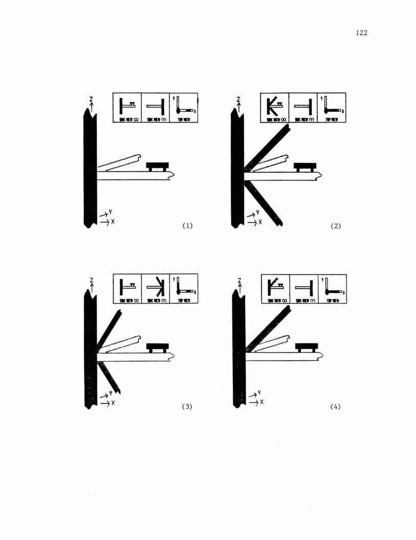
122

(l)

123

.... ()() .... (Y) 1'1'0

(6)

•am YIPD

(7) (8)

124

125

•••m ...

(13) (14)

126

' '-'· •om ,. ..

(17)

' ~I

(19) (20)

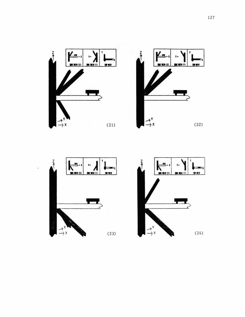
127

' ' &-m. &-m. 11'111

(21) (22)

z T

~. •am Tl'tll!:t

(23) (24)

128

' ~~ ...

(26)

APPENDIX D

PROGRAM TREE STRUCTURE

129

INTRODUCTION

PICK A GEOMETRY

INPUT/RUN

CHOOSE A PLANE

PLATFORM MENU

GRID THE DATA

TOPOGRAPHIC MAP

SURFACE MAP

PRINT GRAPHICS

THE TREE STRUCTURE OF THE PROGRAM PLATFORM

130

( VITA

Michael Raymond Haroun

Candidate for the Degree of

Master of Science

Thesis: CATHODIC PROTECTION MODELING OF NODES IN OFFSHORE STRUCTURES

Major Field: Chemical Engineering

Biographical:

Personal Data: Born in Makene, Sierra Leone, July 18, 1960, son of Raymond and Clautilde Haroun.

Education: Graduated from College des Freres Mont La Salle High School, Ain Saade, Lebanon, in May 1978; received the Bachelor of Science Degree in Chemical Engineering from Oklahoma State University in May, 1984; completed the requirements for the Master of Science in Chemical Engineering at Oklahoma State University in July, 1986.

Professional Experience: French Instructor, Foreign Language Department, Oklahoma State University, January 1984 through May 1984; Teaching Assistant, Engineering Science Department, Oklahoma State University, August 1984 to May 1985; Corrosion Engineer, Shell Development Company, Houston, May 1985 to August 1985; Research Assistant, School of Chemical Engineering, Oklahoma State University, August 1985 to present.