An approach to computing topographic wetness index based on maximum downslope gradient

An approach to computing topographic wetnessindex based on maximum downslope gradient

Cheng-Zhi Qin • A-Xing Zhu • Tao Pei • Bao-Lin Li • Thomas Scholten •

Thorsten Behrens • Cheng-Hu Zhou

Published online: 22 December 2009� Springer Science+Business Media, LLC 2009

Abstract As an important topographic attribute widely-used in precision agriculture,

topographic wetness index (TWI) is designed to quantify the effect of local topography on

hydrological processes and for modeling the spatial distribution of soil moisture and

surface saturation. This index is formulated as TWI = ln(a/tanb), where a is the upslope

contributing area per unit contour length (or Specific Catchment Area, SCA) and tanb is

the local slope gradient for estimating a hydraulic gradient. The computation of both a and

tanb need to reflect impacts of local terrain on local drainage. Many of the existing flow

direction algorithms for computing a use global parameters, which lead to unrealistic

partitioning of flow. b is often approximated by slope gradient around the pixel. In fact, the

downslope gradient of the pixel is a better approximation of b. This paper examines how

TWI is impacted by a multiple flow routing algorithm adaptive to local terrain and the

employment of maximum downslope gradient as b. The adaptive multiple flow routing

algorithm partitions flow by altering the flow partition parameter based on local maximum

downslope gradient. The proposed approach for computing TWI is quantitatively evaluated

using four types of artificial terrains constructed as DEMs with a series of resolutions (1, 5,

10, 20, and 30 m), respectively. The result shows that the error of TWI computed using

the proposed approach is generally lower than that of TWI by the widely used approach.

The new approach was applied to a low-relief agricultural catchment (about 60 km2) in the

Nenjiang watershed, Northeastern China. The results of this application show that the

distribution of TWI by the proposed approach reflects local terrain conditions better.

C.-Z. Qin (&) � A.-X. Zhu � T. Pei � B.-L. Li � C.-H. ZhouState Key Laboratory of Resources and Environmental Information System, Institute of GeographicalSciences and Natural Resources Research, CAS, Beijing 100101, Chinae-mail: [email protected]

A.-X. ZhuDepartment of Geography, University of Wisconsin-Madison, Madison, WI 53706, USA

T. Scholten � T. BehrensInstitute of Geography, Physical Geography, University of Tubingen, Rumelinstraße 19-23, 72074Tubingen, Germany

123

Precision Agric (2011) 12:32–43DOI 10.1007/s11119-009-9152-y

Keywords Topographic wetness index (TWI) � Multiple flow direction algorithm

(MFD) � Digital terrain analysis � Digital elevation model (DEM) � Resolution

Introduction

The concept of topographic wetness index (TWI) was first introduced by Beven and Kirkby

(1979). TWI can quantify the effect of topography on runoff generation and serves as a

physically-based index approximating the location of zones of surface saturation and the

spatial distribution of soil water (Beven and Kirkby 1979; O’Loughlin 1986; Barling et al.

1994). In a catchment, areas having similar TWI value are assumed to have a similar

hydrological response to rainfall when other environmental conditions (such as land cover,

soil) are the same or can be treated as being the same. Compared with other compound

topographic attributes (e.g. Stream Power Index), TWI is more widely used in many

applications related directly to precision agriculture. Examples include:

• The use of TWI map as an indicator to the pattern of potential soil moisture on a field

(especially over undulating farmlands) (Schmidt and Persson 2003).

• The inclusion of TWI together with primary topographic attributes (such as slope

gradient, curvatures) as inputs for digital soil mapping to predict spatial distribution of

both soil type and soil attribute at finer scale (e.g., Moore et al. 1993; Zhu et al. 2009).

• The use of TWI together with slope gradient, profile curvature and specific catchment

area calculated from DEM with 1-m resolution for analyzing the spatial variability of

corn yield (Marques da Silva and Alexandre 2005).

• TWI along with elevation, slope, apparent soil electrical conductivity, and digital soil

maps used to develop autologistic model for delineating nitrogen management zones

based on corn yield response to nitrogen fertilization (Kyveryga et al. 2008).

• TWI combined with stream power index, steepest slope angle and 9 other soil properties

to make a principal component analysis and a fuzzy k-means classification for delineating

potential management classes for precision agriculture (Vitharana et al. 2008).

The calculation of TWI is usually based on a gridded DEM and the value of TWI at a

point is computed as follow:

TWI ¼ lnða=tanbÞ ð1Þ

where a is the upslope contributing area per unit contour length (or Specific Catchment

Area, SCA) and b is the local slope gradient for reflecting the local drainage potential. The

value of TWI is influenced by the algorithms to calculate a and estimate tanb (Guntner

et al. 2004). Computation of a is dependent on the flow direction algorithm used. Among

the different flow direction algorithms, the Multiple Flow Direction (MFD) algorithms are

getting more acceptances in computing a (Wolock and McCabe 1995; Pan et al. 2004).

MFD assumes that flow from the current position could drain into more than one down-

slope neighboring pixel (Quinn et al. 1991). Many of the existing MFD algorithms are

based on the model proposed by Quinn et al. (1991):

di ¼ðtan biÞp � Li

P8j¼1 ðtan bjÞp � Lj

ð2Þ

where di is the fraction of flow into the ith neighboring cell; bi is the slope gradient of the

ith neighboring cell; the exponent p is the flow partition exponent (p [ 0); Li is the

Precision Agric (2011) 12:32–43 33

123

‘‘effective contour length’’ of pixel i. The value of Li is 0.5 for downslope pixels in cardinal

directions, 0.354 for downslope pixels in diagonal directions, and 0 for non-downslope

neighboring pixels (Quinn et al. 1991). The global partition exponent p leads to unrealistic

partitioning of flow (Qin et al. 2007). As a result, upslope contributing area and corre-

sponding TWI would give unrealistic values. b in Eq. 1 is often approximated by the

average slope gradient surrounding the central cell but that approximation is also improper

because the drainage condition is influenced by the slope gradient around the area down

from the central cell (Hjerdt et al. 2004; Guntner et al. 2004).

A new approach to calculating topographic wetness index

In this paper, we propose a new approach to calculating TWI. With this approach, a is

calculated using a MFD algorithm (Qin et al., 2007) which is adaptive to local terrain

conditions and b is approximated by the maximum downslope gradient, instead of the

widely-used average local slope gradient.

An adaptive multiple-flow-direction algorithm (MFD-md)

Qin et al. (2007) proposed a flow partition function, which allows the partition of flow to be

adaptive to the local terrain conditions. The new MFD method is

di ¼ðtan biÞf ðeÞ � Li

P8j¼1 ðtan bjÞf ðeÞ � Lj

ð3Þ

where f(e) is a function determining the flow partition exponent (p in Eq. 2) based on local

topographic attribute e. Qin et al. (2007) selected maximum downslope gradient as eamong many local topographic attributes because maximum downslope gradient can better

reflect the local terrain conditions which are relevant to water movement on a terrain

surface with less sensitivity to subtle variations in DEM. f(e) is then defined as a function

of maximum downslope gradient:

f ðeÞ ¼ 8:9�minðe; 1Þ þ 1:1 ð4Þ

where e is the maximum downslope gradient, minðe; 1Þ is the minimum between e and 1.

The coefficient 8.9 and the constant 1.1 in Eq. 4 are set in such a way that f(e) will be 1.1

for modeling the flow when the local terrain condition is flat as proposed by Freeman

(1991) and will be 10 for modeling the flow when the local terrain is very steep as

recommended by Quinn et al. (1995). Quantitative evaluation using artificial surfaces has

shown that flow accumulation computed using MFD-md is more realistic than those

computed by the widely used flow direction algorithms (Qin et al. 2007).

Maximum downslope gradient as b

b in the calculation of TWI is to model the local drainage potential. Hjerdt et al. (2004)

argued that the downslope topography is an important factor for estimating hydraulic

gradient. Among the topographic attributes related to soil water content of a catchment,

many researches (Quinn et al. 1991; Guntner et al. 2004) have shown that some kind of

local downslope gradient computed around the center cell and its downslope neighboring

34 Precision Agric (2011) 12:32–43

123

cell can quantify drainage of water better than the average local slope gradient at the cell.

Therefore, we use maximum downslope gradient to approximate b.

Quantitative assessment

The most commonly used method for assessing error is to apply the algorithm to a real

DEM. However, this assessment is dependent on the landscape condition of the application

area and is hard to quantify (Zhou and Liu 2002). If the theoretical values of both slope

gradient and SCA of artificial surfaces can be pre-determined by mathematical inference,

TWI algorithms can be assessed based on the theoretical TWI values computed by the

definition of TWI (as shown in Eq. 1). Efforts have been made to define the theoretical

value of SCA of artificial surfaces in the context of quantitative assessment of grid-based

flow routing algorithms (Qin et al. 2006). There are two methods with which artificial

DEMs are used to assess the error of grid-based flow routing algorithms. One was

developed by Zhou and Liu (2002) and the other by Pan et al. (2004). Both of them create

artificial DEMs to simulate typical terrain conditions, such as planar, convergent and

divergent. The theoretical SCA of each artificial DEM is also inferred. Zhou and Liu

(2002)’s method included one more terrain type: the saddle surface representing the ridge

area. The ellipsoid surface in Zhou and Liu (2002) is more similar to the practical convex

slope than the cone surface in Pan et al. (2004). In this paper, we apply Zhou and Liu

(2002)’s method to assess the proposed approach.

Methods and material

For assessing the proposed method, four types of artificial surfaces were constructed using

mathematical models based on Zhou and Liu (2002), representing convex slopes (ellipsoid),

concave slopes (inverse ellipsoid), ridges (saddle) and straight slopes (plane), respectively.

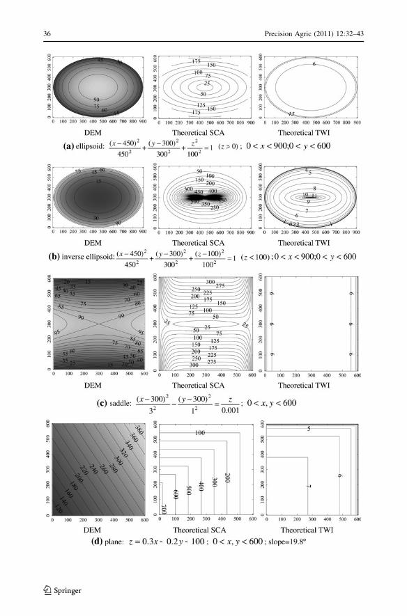
Figure 1 shows an example of the mathematical models, the contour maps of the artificial

surfaces, the theoretical SCA and the theoretical TWI inferred from the mathematical

models. The details of computing SCA and slope gradient at any given point on a given

mathematical surface are not discussed here and can be found in Zhou and Liu (2002).

The error at each cell caused by a TWI algorithm can be computed:

Ei ¼ lnSCAt

i

tan bti

� �

� lnSCAi

tan bi

� �

ð5Þ

where Ei is the error of TWI value at ith cell; SCAti and SCAi are the theoretical and

computed SCA values for the cell, respectively; bti and bi are the theoretical and computed

slope gradient values for the cell, respectively. Thus the Root Mean Square Error (RMSE)

can be computed for each TWI algorithm and can be used to assess the performance of

different TWI algorithms.

RMSE ¼

ffiffiffiffiffiffiffiffiffiffiffiffiffiffiffiffiffiffiffiffiffiffiPn

i¼1 ðEiÞ2

n

s

ð6Þ

where n is the number of cells used for assessment.

Fig. 1 The mathematical models, the contour maps of artificial surfaces, the theoretical SCA and thetheoretical TWI distributions of four typical mathematical surfaces: a ellipsoid; b inverse ellipsoid; c saddle;and d plane. The unit represented is meters

c


123


123

We used the artificial DEMs with a series of resolutions (i.e., 1, 5, 10, 20, and 30 m)

generated from the mathematical surfaces in Fig. 1 and the assessment method described

above to quantitatively assess the proposed TWI approach and the effect of DEM reso-

lution on the proposed TWI approach. For comparing the proposed algorithm with other

approaches, we computed TWIs of artificial DEMs using the D8-based approach, the FD8-

based approach, and the proposed approach, respectively. The D8-based approach com-

putes TWI with a computed by O’Callaghan and Mark (1984)’s D8 (a representative

Single Flow Direction algorithm with which all water from a pixel flows into one and only

one neighboring pixel which has the lowest elevation) and slope gradient calculated from

ArcInfo which uses a third order finite difference method (Burrough and McDonnell 1998).

The FD8-based approach computes TWI with a computed by Quinn et al. (1991)’s FD8

(a representative MFD) and slope gradient calculated from ArcInfo. The series of reso-

lutions selected in this study is finer than 30 m because we think the DEM resolution

coarser than 30 m is not useful for precision agriculture applications.

Results of quantitative assessment

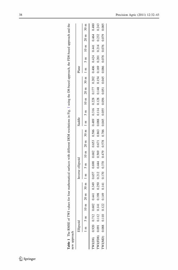
Table 1 lists the RMSE of TWI values. TWI values computed by the D8-based approach,

the FD8-based approach and the proposed approach are named as TWI(D8), TWI(FD8)

and TWI(MD), respectively. For almost all tested terrain conditions with a series of res-

olutions, TWI(MD) produces the lowest RMSE among the three approaches. Only under

the inverse ellipsoid surface with resolution of 30 m, the RMSE from TWI(MD) is higher

than that from TWI(D8) but still lower than that from TWI(FD8). The surface which the

artificial inverse ellipsoid represents is similar to a depression in a real DEM. A depression

in DEM could be real terrain component in the real world but it is often thought to be an

error or interpolation artifact created during the DEM-generating process. In real appli-

cations, the depressions will commonly be removed by the DEM pre-processing algorithm

(Gallant and Wilson 2000). In this sense, we can say that the new approach can produce

the TWI with lower RMSE than current widely-used approaches under most real world

situations.

For convex terrain conditions modeled by an ellipsoid surface, the RMSE from

TWI(MD) increases constantly when the resolution of the artificial DEM is progressively

coarsened from 1 to 30 m. This trend is similar to that from TWI(FD8) but the level of

increase is much lower for TWI(MD) than for TWI(FD8). Contrarily, the RMSE from

TWI(D8) decreases when the resolution of the artificial DEM is progressively coarsened

from 1 to 30 m. This is related to the high sensitivity of the D8 algorithm used in TWI(D8)

to subtle variation in the DEM. With the coarsening of DEM resolution, the subtle vari-

ation reduces and the computed TWI becomes stable.

For concave terrain conditions modeled by an inverse ellipsoid surface, the RMSE from

TWI(MD) or TWI(FD8) is higher than under any of the other three terrain conditions

modeled. The performances of TWI(MD), TWI(FD8) and TWI(D8) when the resolution

gets coarser for inverse ellipsoid surface are similar to those under an ellipsoid surface. The

levels of increase in RMSE for TWI(MD) and TWI(FD8) are very similar and both higher

than those under any of the other three terrain conditions modeled. Meanwhile, the level of

decrease in RMSE for TWI(D8) is lower than under the other three types of terrain

conditions.

For terrain conditions modeled by saddle and plane surfaces, the RMSEs from

TWI(MD) are stable when the resolution gets coarser. However, the RMSEs from


123

Ta

ble

1T

he

RM

SE

of

TW

Iv

alu

esfo

rfo

ur

mat

hem

atic

alsu

rfac

esw

ith

dif

fere

nt

DE

Mre

solu

tio

ns

inF

ig.

1u

sin

gth

eD

8-b

ased

app

roac

h,

the

FD

8-b

ased

app

roac

han

dth

en

ewap

pro

ach E

llip

soid

Inv

erse

elli

pso

idS

addle

Pla

ne

1m

5m

10

m2

0m

30

m1

m5

m1

0m

20

m3

0m

1m

5m

10

m2

0m

30

m1

m5

m1

0m

20

m3

0m

TW

I(D

8)

0.9

20

0.7

12

0.6

02

0.4

41

0.3

49

0.6

57

0.6

90

0.6

82

0.6

53

0.5

86

0.4

89

0.3

16

0.2

28

0.1

77

0.2

02

0.4

06

0.4

24

0.4

41

0.4

64

0.4

80

TW

I(F

D8

)0

.091

0.1

12

0.1

41

0.1

98

0.2

50

0.2

12

0.4

44

0.5

69

0.6

71

0.8

63

0.0

88

0.1

14

0.1

28

0.1

48

0.1

54

0.1

69

0.2

01

0.2

14

0.2

32

0.2

43

TW

I(M

D)

0.0

88

0.1

10

0.1

22

0.1

49

0.1

41

0.1

70

0.3

70

0.4

79

0.5

78

0.7

86

0.0

45

0.0

55

0.0

56

0.0

51

0.0

45

0.0

86

0.0

78

0.0

76

0.0

79

0.0

85


123

TWI(FD8) increase constantly when the resolution of the artificial DEMs is progressively

coarsened from 1 to 30 m.

Application

Study area and data

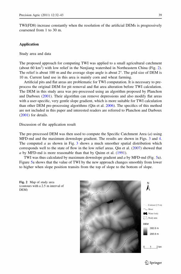
The proposed approach for computing TWI was applied to a small agricultural catchment

(about 60 km2) with low relief in the Nenjiang watershed in Northeastern China (Fig. 2).

The relief is about 100 m and the average slope angle is about 2�. The grid size of DEM is

10 m. Current land use in this area is mainly corn and wheat farming.

Artificial pits and flat areas are problematic for TWI computation. It is necessary to pre-

process the original DEM for pit removal and flat area alteration before TWI calculation.

The DEM in this study area was pre-processed using an algorithm proposed by Planchon

and Darboux (2001). Their algorithm can remove depressions and also modify flat areas

with a user-specific, very gentle slope gradient, which is more suitable for TWI calculation

than other DEM pre-processing algorithms (Qin et al. 2006). The specifics of this method

are not included in this paper and interested readers are referred to Planchon and Darboux

(2001) for details.

Discussion of the application result

The pre-processed DEM was then used to compute the Specific Catchment Area (a) using

MFD-md and the maximum downslope gradient. The results are shown in Figs. 3 and 4.

The computed a as shown in Fig. 3 shows a much smoother spatial distribution which

corresponds well to the state of flow in the low relief areas. Qin et al. (2007) showed that

a by MFD-md is more reasonable than that by Quinn et al. (1991).

TWI was thus calculated by maximum downslope gradient and a by MFD-md (Fig. 5a).

Figure 5a shows that the value of TWI by the new approach changes smoothly from lower

to higher when slope position transits from the top of slope to the bottom of slope.

Fig. 2 Map of study area(contours with a 2.5 m interval ofDEM)


123

To compare the new approach with the FD8-based approach, the difference between

TWI values by the new approach and TWI values by the FD8-based approach was com-

puted (Fig. 5b). The negative value in Fig. 5b means that the TWI value by the new

approach is smaller than that by the FD8-based approach. In general, the difference is

related to the slope positions. Over the ridge and shoulder areas, TWI by the new approach

has lower values than TWI by the FD8-based approach. This is understandable in that

water over these areas is more likely to be drained. So the TWI by the new approach

reflects this situation better. Over the backslope areas, the difference seems to be related to

the curvature of land surface. The TWI values by the new approach are lower than the TWI

values by the FD8-based approach over the convex part of the backslope. This again

matches the reality that water over the divergent shape of these areas drains more quickly

and the soil moisture in these areas should be lower. The TWI values by the new approach

are almost the same as that by the FD8-based approach in the planar part of the backslope.

In the concave part of the backslope, TWI by the new approach has higher values than TWI

by the FD8-based approach because the convergent shape in this area is more likely to

retain water thus should have better moisture conditions.

Fig. 3 Specific catchment area,a, by MFD-md

Fig. 4 Maximum downslope,tanb


123

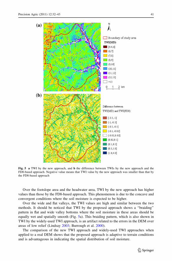
Over the footslope area and the headwater area, TWI by the new approach has higher

values than those by the FD8-based approach. This phenomenon is due to the concave and

convergent conditions where the soil moisture is expected to be higher.

Over the wide and flat valleys, the TWI values are high and similar between the two

methods. It should be noticed that TWI by the proposed approach shows a ‘‘braiding’’

pattern in flat and wide valley bottoms where the soil moisture in these areas should be

equally wet and spatially smooth (Fig. 5a). This braiding pattern, which is also shown in

TWI by the widely-used TWI approach, is an artifact related to the errors in the DEM over

areas of low relief (Lindsay 2003; Burrough et al. 2000).

The comparison of the new TWI approach and widely-used TWI approaches when

applied to a real DEM shows that the proposed approach is adaptive to terrain conditions

and is advantageous in indicating the spatial distribution of soil moisture.

Fig. 5 a TWI by the new approach, and b the difference between TWIs by the new approach and theFD8-based approach. Negative value means that TWI value by the new approach was smaller than that bythe FD8-based approach


123

Conclusion

TWI is an important topographic index which can quantify the control of local topography

over hydrological processes and indicates the spatial distribution of soil moisture and

surface saturation. It is used in some aspects of precision agriculture. The value of TWI is

influenced by both the algorithm to calculate upslope contributing area, a, and the

approximation of slope gradient, b. This paper proposed a new TWI approach which

combines an adaptive MFD algorithm (MFD-md) to calculate a with the maximum

downslope gradient to approximate b. MFD-md algorithm is adaptive to local terrain

conditions by altering the flow partition exponent based on a function of local maximum

downslope gradient. So the flow accumulation from upslope can be modeled better than

currently widely-used flow direction algorithms. And the maximum downslope gradient

can reflect the local drainage potential better than does the local slope gradient which is

widely used in current TWI approaches.

The proposed approach to calculating TWI was evaluated using four types of artificial

DEMs with resolutions ranging from 1 to 30 m. The results of quantitative assessment

show that TWI by the new approach generally has the lowest error in comparison with

TWIs by the D8-based approach and the FD8-based approach. The proposed approach to

calculating TWI was also applied in a small, low-relief agricultural catchment in North-

eastern China. The results showed that the spatial distribution of TWI computed by the

proposed approach is more adaptive to terrain conditions than that by the widely-used

approaches.

The adaptability of the proposed TWI to local terrain conditions is a clear advantage to

the existing approaches. However, it still needs additional work to show the level of

difference between the proposed TWI and that by other methods in the context of precision

agriculture applications. One of the ways to illustrate whether the difference is significant

would be to conduct comparative studies between the proposed approach and the existing

approaches in precision agriculture applications, such as prediction of detailed soil prop-

erty maps, mapping of the pattern of potential soil moisture on a field and other TWI

applications in precision agriculture as mentioned at the beginning of this paper.

Acknowledgements This study was supported by the National Natural Science Foundation of China(40501056; 40971235), the National Basic Research Program of China (2007CB407207), the National KeyTechnology R&D Program of China (2007BAC15B01), and the Knowledge Innovation Programs of theChinese Academy of Sciences (KZCX2-YW-Q10-1-5). Supports from the Institute of GeographicalSciences and Natural Resources Research, the State Key Laboratory of Resources and EnvironmentalInformation Systems, and the University of Wisconsin-Madison (through its Vilas Associate Program andthe Hamel Faculty Fellow Program) are also appreciated. We thank the anonymous reviewers and the editorfor their constructive comments on an earlier version of this paper. We thank Dr. Yuxin Miao for kindlysharing the literatures in the 9th International Conference on Precision Agriculture.

References

Barling, R. D., Moore, I. D., & Grayson, R. B. (1994). A quasi-dynamic wetness index for characterizing thespatial distribution of zones of surface saturation and soil water content. Water Resources Research,30, 1029–1044.

Beven, K., & Kirkby, N. (1979). A physically based variable contributing area model of basin hydrology.Hydrological Sciences Bulletin, 24, 43–69.

Burrough, P. A., & McDonnell, R. A. (1998). Principles of geographic information systems (p. 333). NewYork: Oxford University Press.


123

Burrough, P., van Gaans, P., & MacMillan, R. (2000). High-resolution landform classification using fuzzyk-means. Fuzzy Sets and Systems, 113, 37–52.

Freeman, T. G. (1991). Calculating catchment area with divergent flow based on a regular grid. Computers& Geosciences, 17, 413–422.

Gallant, J. C., & Wilson, J. P. (2000). Primary topographic attributes. In J. P. Wilson & J. C. Gallant (Eds.),Terrain analysis: Principles and applications (pp. 51–85). New York: John Wiley & Sons, Inc.

Guntner, A., Seibert, J., & Uhlenbrook, S. (2004). Modeling spatial patterns of saturated areas: An evalu-ation of different terrain indices. Water Resources Research, 40, W05114. doi:10.1029/2003WR002864.

Hjerdt, K., McDonnell, J., Seibert, J., & Rodhe, A. (2004). A new topographic index to quantify downslopecontrols on local drainage. Water Resources Research, 40, W05602. doi:10.1029/2004WR003130.

Kyveryga, P. M., Blackmer, T. M., & Caragea, P. C. (2008). Using soil and terrain attributes to delineatemanagement zones in corn yield response to nitrogen fertilization. In R. Khosla (Ed.), Precisionagriculture: Proceedings of the 9th international conference on precision agriculture (CD-ROM).Denver, Colorado, USA.

Lindsay, J. B. (2003). A physically based model for calculating contributing area on hillslopes and alongvalley bottoms. Water Resources Research, 39, 1332. doi:10.1029/2003WR002576.

Marques da Silva, J. R., & Alexandre, C. (2005). Spatial variability of irrigated corn yield in relation to fieldtopography and soil chemical characteristics. Precision Agriculture, 6, 453–466.

Moore, I., Gessler, P., Nielsen, G., & Peterson, G. (1993). Soil attribute prediction using terrain analysis.Soil Science Society of America Journal, 57, 443–452.

O’Callaghan, J. F., & Mark, D. M. (1984). The extraction of drainage networks from digital elevation data.Computer Vision, Graphics, and Image Processing, 28, 323–344.

O’Loughlin, E. M. (1986). Prediction of surface saturation zones in natural catchments by topographicanalysis. Water Resources Research, 22, 794–804.

Pan, F., Peters-Lidard, C., Sale, M., & King, A. (2004). A comparison of geographical information system-based algorithms for computing the TOPMODEL topographic index. Water Resources Research, 40,W06303. doi:10.1029/2004WR003069.

Planchon, O., & Darboux, F. (2001). A fast, simple and versatile algorithm to fill the depressions of digitalelevation models. Catena, 42, 159–176.

Qin, C.-Z., Zhu, A.-X., Li, B.-L., Pei, T., & Zhou, C.-H. (2006). Review of multiple flow directionalgorithms based on gridded digital elevation models. Earth Science Frontiers, 13, 91–98. (in Chinesewith English abstract).

Qin, C.-Z., Zhu, A.-X., Pei, T., Li, B.-L., Zhou, C.-H., & Yang, L. (2007). An adaptive approach to selectinga flow-partition exponent for a multiple-flow-direction algorithm. International Journal of Geo-graphical Information Science, 21, 443–458.

Quinn, P., Beven, K., Chevalier, P., & Planchon, O. (1991). The prediction of hillslope flow paths fordistributed hydrological modeling using digital terrain models. Hydrological Processes, 5, 59–79.

Quinn, P., Beven, K. J., & Lamb, R. (1995). The ln(a/tanb) index: How to calculate it and how to use itwithin the TOPMODEL framework. Hydrological Processes, 9, 161–182.

Schmidt, F., & Persson, A. (2003). Comparison of DEM data capture and topographic wetness indices.Precision Agriculture, 4, 179–192.

Vitharana, U., van Meirvenne, M., Simpson, D., Cockx, L., & de Baerdemaeker, J. (2008). Key soil andtopographic properties to delineate potential management classes for precision agriculture in theEuropean loess area. Geoderma, 143, 206–215.

Wolock, D. M., & McCabe, G. J. (1995). Comparison of single and multiple flow direction algorithms forcomputing topographic parameters. Water Resources Research, 31, 1315–1324.

Zhou, Q., & Liu, X. (2002). Error assessment of grid-based flow routing algorithms used in hydrologicalmodels. International Journal of Geographical Information Science, 16, 819–842.

Zhu, A.-X., Yang, L., Li, B.-L., Qin, C.-Z., Pei, T., & Liu, B.-Y. (2009). Construction of membershipfunctions for predictive soil mapping under fuzzy logic. Geoderma. doi:10.1016/j.geoderma.2009.05.024.


123

http://dx.doi.org/10.1029/2003WR002864

http://dx.doi.org/10.1029/2003WR002864

http://dx.doi.org/10.1029/2004WR003130

http://dx.doi.org/10.1029/2003WR002576

http://dx.doi.org/10.1029/2004WR003069

http://dx.doi.org/10.1016/j.geoderma.2009.05.024

http://dx.doi.org/10.1016/j.geoderma.2009.05.024

An approach to computing topographic wetness index based on maximum downslope gradient

Documents

Transcript of An approach to computing topographic wetness index based on maximum downslope gradient