Insights from the topographic characteristics of a ... - NHESS

Nat. Hazards Earth Syst. Sci., 22, 1129–1149, 2022https://doi.org/10.5194/nhess-22-1129-2022© Author(s) 2022. This work is distributed underthe Creative Commons Attribution 4.0 License.

Insights from the topographic characteristics of a large globalcatalog of rainfall-induced landslide event inventoriesRobert Emberson1,2,3, Dalia B. Kirschbaum1, Pukar Amatya1,2,3, Hakan Tanyas4, and Odin Marc5

1Hydrological Sciences Laboratory, NASA Goddard Space Flight Center, Greenbelt, MD, USA2Goddard Earth Sciences Technology and Research II, Greenbelt, MD, USA3University of Maryland, Baltimore County, 1000 Hilltop Cir, Baltimore, MD, USA4ITC, University of Twente, Twente, the Netherlands5Géosciences Environnement Toulouse (GET), UMR 5563, CNRS/IRD/CNES/UPS,Observatoire Midi-Pyrénées, Toulouse, France

Correspondence: Robert Emberson ([email protected])

Received: 20 August 2021 – Discussion started: 2 September 2021Revised: 27 January 2022 – Accepted: 28 January 2022 – Published: 1 April 2022

Abstract. Landslides are a key hazard in high-relief areasaround the world and pose a risk to populations and infras-tructure. It is important to understand where landslides arelikely to occur in the landscape to inform local analysesof exposure and potential impacts. Large triggering eventssuch as earthquakes or major rain storms often cause hun-dreds or thousands of landslides, and mapping the landslidepopulations generated by these events can provide extensivedatasets of landslide locations. Previous work has exploredthe characteristic locations of landslides triggered by seis-mic shaking, but rainfall-induced landslides are likely to oc-cur in different parts of a given landscape when comparedto seismically induced failures. Here we show measurementsof a range of topographic parameters associated with rainfall-induced landslides inventories, including a number of previ-ously unpublished inventories which we also present here.We find that the average upstream angle and compound to-pographic index are strong predictors of landslide scar lo-cation, while the local relief and topographic position indexprovide a stronger sense of where landslide material may endup (and thus where hazard may be highest). By providing alarge compilation of inventory data for open use by the land-slide community, we suggest that this work could be use-ful for other regional and global landslide modeling studiesand local calibration of landslide susceptibility assessment,as well as hazard mitigation studies.

1 Introduction

The impact of natural hazards on populations and infrastruc-ture is most acute where the footprints of these hazards in-tersect the locations where people live and buildings are sit-uated. For some hazards like earthquakes and cyclones, thefootprints of the hazard can be distributed across wide re-gions, but for other hazards like landslides the footprint maybe significantly more localized. Although the impacts of in-dividual landslides may be localized, large triggering eventssuch as intense rainfall or seismic activity can cause largenumbers of landslides across a wide region, the extent ofwhich often mirrors the extent of the intense rainfall and seis-mic shaking (Marc et al., 2017, 2018; Tanyaš and Lombardo,2019). The individual landslides triggered during these ex-treme events occur in specific parts of the landscape that aremost susceptible to failure. These slopes become criticallyunstable due to both preconditioning factors like slope andinternal frictional strength and triggering factors like changein fluid pore pressure or seismic acceleration.

A range of studies from around the world have assessedthe locations of landslides and used them to construct sus-ceptibility models for local settings (e.g., Emberson et al.,2021; Goetz et al., 2015; Broeckx et al., 2019), acrosslarger regions (e.g., Van Den Eeckhaut and Hervás, 2012;Van Den Eeckhaut et al., 2012), and globally (e.g., Stanleyand Kirschbaum, 2017; Nowicki Jesse et al., 2018; Tanyas etal., 2019). Comprehensive reviews of landslide susceptibil-

Published by Copernicus Publications on behalf of the European Geosciences Union.

1130 R. Emberson et al.: Topographic characteristics of rainfall-triggered landslides

ity models (Budimir et al., 2015; Reichenbach et al., 2018)highlight a number of factors that are often considered tobe generally important for landslide susceptibility. These in-clude morphological (slope, aspect, roughness), geological(e.g., lithology), land cover, seismic and hydrological factors.Naturally, to study the importance of each of these factors, in-formation on landslide location is essential to both calibrateand validate any susceptibility model that is produced.

Landslide location data can come in different forms, andlandslide inventory maps are the most useful data sourcein which the extent of landslide phenomena are systemati-cally documented in a region (Guzzetti et al., 2012). Unfor-tunately, the number of digitally available landslide invento-ries is still rather limited (Wasowski et al., 2011; Guzzettiet al., 2012; Tanyas et al., 2017; Mirus et al., 2020). As aresult, landslide locations in global catalogs are often basedon media reports (e.g., Kirschbaum et al., 2015; Froude andPetley, 2018), which can limit the accuracy of the definedlocations. A review of data in the NASA Global LandslideCatalog (Kirschbaum et al., 2015) suggests that only 33 % oflandslides have a location known to within a 1 km resolution,which does not permit assessment of the specific locationswhere landslides occur within a landscape (e.g., at a hillslopescale). Additionally, global landslide catalogs generally donot include the entire landslide population for a given area.While they may capture many of the landslides that causedamage or fatalities (Petley, 2012; Froude and Petley, 2018),underestimation of landslide susceptibility may result if sys-tematic biases in reporting are found for certain geographiesor terrain parameters.

Landslide inventories are the ideal data source not onlyto better understand the spatial, temporal and size distribu-tion of landslides but also to conduct more accurate sus-ceptibility, hazard and risk assessments (Guzzetti et al.,2012). Overall, landslide inventories are categorized as his-torical and event inventories (Malamud et al., 2004). Histor-ical landslide inventories include many landslide events overtime in a given region. Landslide event inventories, on theother hand, contain landslides triggered by a specific trigger(e.g., earthquake, rainfall or snowmelt) of a known date. Inother words, the time of landslide occurrence is unknown inhistorical landslide inventories, and therefore, landslide sus-ceptibility models developed based on historical inventoriesare time-invariant products solely representing geomorpho-logically landslide-prone hillslopes (Lombardo and Tanyas,2020). Historic inventories are by definition biased towardfrequent climatic triggers and are not representative of thelong-term average susceptibility to triggers including earth-quakes, whereas landslide event inventories are more suitabledata sources to develop near-real-time products to predict thespatial distribution of landslides triggered by a specific event(e.g., Nowicki Jessee et al., 2018).

For specific large triggering events such as an earthquakeor an episode of extreme rainfall, it is possible to rela-tively accurately define the timing of the event, and if high-

resolution imagery is found that brackets the dates in ques-tion, it is also possible to systematically map the landslidesgenerated by such a trigger (Guzzetti et al., 2012). Map-ping landslides following extreme events has become com-mon, and inventories exist for a large number of earthquakes(Tanyas et al., 2017). A smaller number of intense rainfallevents have also been mapped (Marc et al., 2018), but unlikefor earthquakes (Schmitt et al., 2017) no centralized repos-itory of these data exists at present. Location data for land-slides triggered by intense rainfall are vitally important tocalibrate and validate existing susceptibility models since thedatasets produced are generally considered to be nearly com-plete. It is also useful to characterize the rainfall required totrigger landslides and thus help inform local and global haz-ard models (Emberson et al., 2021; Kirschbaum and Stanley,2018). These can then be used to inform exposure and riskassessment estimates (Emberson et al., 2020).

It is important to note that the positions where earthquake-triggered landslides occur on a given hillslope are not nec-essarily applicable to rainfall-triggered landslides. As shownby previous research (Densmore and Hovius, 2000; Meunieret al., 2008), the higher peak ground acceleration in earth-quakes at the top of ridges tends to increase landslides inthose locations, while increasing water saturation at the baseof slopes by intense rain tends to increase landslides lowerdown the slope (e.g., Rault et al., 2019). As such, it is imper-ative to use the appropriate type of landslide inventory to cal-ibrate any model. Finally, recent studies have sought to deriveunderlying simple topographic rules to understand hazard as-sociated with earthquake-triggered landslides (e.g., Milledgeet al., 2019), and it is important that we extend this kind ofanalysis to rainfall-triggered events to provide comparativedata.

In this study, we combine 10 existing inventories oflandslides triggered by intense rain storms with 6 newinventories mapped using high-resolution data for thisstudy. Assessing these landslide event inventories bothindividually and in combination, we assess the local to-pographic characteristics that are most strongly related towhere landslides are initiated, as well as local forest lossthat can be calculated from satellite data. We suggest thatthese inventories and the associated parameters can be usedto calibrate and validate other models of susceptibility andhazard and will provide valuable information to authorsseeking landslide data with high spatial accuracy, as wellas supporting characterization of rainfall thresholds forlandslide impacts (e.g., Conrad et al., 2021). Moreover, witha set of simplified rules for landslide hazard, researcherscan support hazard assessment in areas where more detailedmodels may be unavailable. The inventories describedhere will be available on the NASA Landslide Viewerapp (https://maps.nccs.nasa.gov/arcgis/apps/webappviewer/index.html?id=824ea5864ec8423fb985b33ee6bc05b7, lastaccess: 6 January 2022) for open access by other researchers.

Nat. Hazards Earth Syst. Sci., 22, 1129–1149, 2022 https://doi.org/10.5194/nhess-22-1129-2022

https://maps.nccs.nasa.gov/arcgis/apps/webappviewer/index.html?id=824ea5864ec8423fb985b33ee6bc05b7

https://maps.nccs.nasa.gov/arcgis/apps/webappviewer/index.html?id=824ea5864ec8423fb985b33ee6bc05b7

R. Emberson et al.: Topographic characteristics of rainfall-triggered landslides 1131

2 Context and methods

2.1 Landslide inventories

It has become common practice to map areas affected bylandslide-triggering earthquakes to build a spatially completepicture of landslide impacts (Tanyas et al., 2017), and the in-ventories that are generated have been used to produce haz-ard maps (Jibson et al., 2000; Harp et al., 2011), susceptibil-ity models (García-Rodríguez et al., 2008; Xu et al., 2012),guidelines for hazard zonation (Milledge et al., 2019) andglobal alerting systems (Nowicki Jessee et al., 2018). Land-slide event inventories are also required to explore the land-scape response to tectonic and climatic forcings (e.g., Mala-mud et al., 2004; Korup et al., 2012; Marc et al., 2016,2019). Mapping of landslides in the aftermath of major rain-fall events is somewhat less common, since cloud cover isoften a significant impediment in the impacted areas, whichmay limit clear views from satellites. However, an increasingnumber of intense rainfall events have now had landslidesmapped, with extensive examples in Taiwan (Lin et al., 2011;Chen et al., 2013), Japan and Brazil (Marc et al., 2018), andthe Caribbean (van Westen and Zhang, 2018).

Several methods exist to generate event-specific landslideinventories. The robustness and accuracy of the final inven-tory depend on the type and quality of imagery and dataavailable, as well as the method chosen. Synthetic apertureradar (SAR) data have been employed to generate inventoriesof slow-moving landslides (Handwerger et al., 2019; Bekaertet al., 2020), to focus on the kinematics of single slow-moving slides (Hu et al., 2019) and to map landslides occur-ring in the aftermath of major triggering events (Mondini etal., 2019; Handwerger et al., 2019; Adriano et al., 2020; Bur-rows et al., 2020; Jung and Yun, 2020). The most widely usedtechnique is to map landslides directly from optical imagery,from unmanned aerial vehicle (UAV) imagery (Casagli et al.,2017; Rossi et al., 2018), aerial photography (Harp et al.,2004) or satellite observations (Casagli et al., 2017; Martha etal., 2012; Behling et al., 2014). While satellite observationsgenerally have the lowest spatial resolution and may be im-pinged by cloud cover, these satellites offer near-global cov-erage and frequent return intervals that generally allow forimagery that brackets the event in question. This is particu-larly the case for some of the newer commercial satellite con-stellations. Some rainfall-triggered events may occur in loca-tions where cloud cover is so prevalent that it precludes any-thing other than seasonal assessment of landslide occurrence,such as the Himalayas during the monsoon. However, an in-creasing number of satellite-generated inventories now exist.The methods used to delineate landslides from optical im-agery include manual mapping, where a human determineswhat is and is not a landslide, or semi-automatic/automaticmapping, where detection algorithms are used to determinelandslide locations.

2.2 Methodology

Summarizing various previous work, five mapping criteriaappear essential for landslide inventories (see Guzzetti et al.,2012; Marc and Hovius, 2015; Tanyas et al., 2017): (i) man-ual mapping (or correction) to reduce errors and avoid amal-gamation, (ii) a high enough imagery resolution for com-pleteness and to avoid amalgamation, (iii) mapping land-slides as polygons to allow maximum scientific usage (e.g.,area affected, volume of sediment mobilized, frequency–sizedistributions), (iv) mapping with pre- and post-event imageryto focus on landslides with a known trigger, and (v) de-fined mapping boundary to clarify inventory completeness.For the purposes of this study, we have tried to obtain asmany inventories as possible for comparison, while generallysatisfying these five essential criteria. Nevertheless, due tovarying imagery and mapping techniques, criteria (i) and (ii)are fulfilled with variable quality for the studied inventories(Table 1). More detailed inventories have differentiated thesource and deposit areas of landslides, but this often requiresfield validation. The locations of the inventories are shownin Fig. 1. It is important to note that although high-resolutionimagery can provide more accurate mapping in some cases,it can also be more challenging to ortho-rectify, which canlimit the quality of landslide inventories generated (Williamset al., 2018).

As such, we incorporate 10 existing inventories and sup-plement them with 6 further inventories that we have pro-duced for this study. The details of each of the invento-ries are described in Table 1. For several of the newly pro-duced inventories, we have utilized high-resolution imageryfrom Planet Dove satellites (Planet Team, 2017) availablethrough the Commercial Smallsat Data Acquisition (CSDA)Program (https://earthdata.nasa.gov/esds/csdap, last access:12 January 2022). Planet imagery represents an importantstep change for landslide mapping procedures, since the highspatial resolution of approximately 3 m of the images is com-bined with a rapid return time of the satellites (of the order of1 image per day). For several of the newly generated inven-tories, we have mapped the landslides manually using GISsoftware. This has resulted in three inventories; two in thePhilippines and one in Thrissur, India (Table 1). The remain-ing new inventories were generated using the semi-automaticobject-based methods of Amatya et al. (2019, 2021). The al-gorithmic method was used to reduce the overall time spentmapping some of the larger new inventories. Since algorith-mic methods are known to produce artifacts when broadlyapplied (Pawluszek et al., 2018) and can lead to amalgama-tion of individual landslides into larger polygons (Marc andHovius, 2015), each of the automatically generated invento-ries was additionally corrected by manual comparison withpre- and post-event high-resolution imagery in GIS software.

Beyond the five essential mapping criteria, additional cri-teria include the differentiation of scar and deposit areasand the classifications of landslides according to their type-

https://doi.org/10.5194/nhess-22-1129-2022 Nat. Hazards Earth Syst. Sci., 22, 1129–1149, 2022

https://earthdata.nasa.gov/esds/csdap


Figure 1. Locations of landslide inventories considered in this study. Locations labeled in red have been published previously, while those inblue are presented for the first time here. Satellite images of the newly mapped landslide inventories can be found in the Supplement. Table 1contains the details of each of the inventories, organized in alphabetical order.

/mechanisms. However, these criteria are difficult to fulfillfor large event inventories (see in Tanyas et al., 2017), es-pecially when based on various sources of optical imagery,limiting our ability to differentiate between scar and depositareas (Casagli et al., 2017).

The mapped inventories combine scars and deposits in thepolygon delineation, although in the analysis discussed be-low we have sought to differentiate these areas. In terms oflandslide type we could not systematically classify each land-slide polygon. However, we have removed debris flows fromthe analysis where possible by removing long-runout land-slide polygons from each mapped inventory. In general, thismapping identifies rockslides, rock avalanches, shallow soiltoppling and slumping failures but does not capture slow-moving landslides where surface changes may be less evi-dent. A focus on these kinds of landslides is warranted sincethe volume of material mobilized during large storms fromsuch landslides can lead to damaging debris flows and bed-load transport impacts (Badoux et al., 2014). Removing de-bris flows from the analysis allows us to provide consistentlandslide maps that can be used to estimate volumes of mo-bilized landslide material, for example using global scalingrelationships like those defined by Larsen et al. (2010), andpermits a focus solely on the topographic characteristics oflandslide source regions, rather than on the characteristics ofpreferential runout paths.

We contrast each of the inventories mapped here bycomparing the size–frequency distributions of each dataset,shown in Fig. 2. For each of the inventories, we show theprobability of a landslide within a given area interval, as away to assess the frequency of small and large landslidesacross the different datasets. Each of these landslide eventswas triggered by extreme rainfall, and although it is not ourintention to examine the triggering rainfall in detail in thisstudy, it is useful to briefly discuss the characteristics of therainfall events in question. It is important to note that thedate of the triggering rainfall is not identical to the dates

Figure 2. Probability density for landslides in each event inventory,obtained as the number of landslides with areas falling into loga-rithmic bins (consistent bins for all inventories), N[A:A+dA], nor-malized by the bin width, dA, and the total number of slides for theevent, Ntot (see Malamud et al., 2004).

on which the imagery used to map the landslides was ob-tained. Although we have selected events where the trig-gering rainfall significantly exceeds historical peak rainfall(and therefore is likely to be the dominant trigger for land-slides), some events may have occurred as a result of lesserrainfall before or after. While the new inventories generatedfor this study utilize Planet imagery that closely bracketsthe rainfall events (within 1 week either side), the older in-ventories may be more subject to this challenge. A detailed



Table 1. Details of landslide inventories analyzed in this study.

Location Event triggering Date of Reference Imagery (resolution) Dominant Globaltriggering Lithological Maprainfall

Micronesia (A) Cyclone 2 Jul 2002 Harp et al. (2004) Aerial photographs Basaltic/andesitic/(varies) trachytic lava flows

South Taiwan (B) Typhoon 15–18 Jul 2008 Chen et al. (2013), Landsat 5 (30 m) Sedimentary/Kalmaegi Marc et al. (2018) metamorphic

Blumenau, Brazil (C) Prolonged 20–25 Nov 2008 Marc et al. (2018) Google Earth/Landsat 5 Metamorphicintense rain (3–30 m/30 m)

Taiwan (D) Typhoon 6–9 Aug 2008 Chen et al. (2013), FormoSat-2/Landsat 5 Sedimentary/Morakot Chang et al. (2014), (4 m/30 m) metamorphic

Marc et al. (2018)

Teresópolis, Brazil (E) Local storm 11–13 Jan 2011 Marc et al. (2018) Google Earth/Landsat 5/ Acid plutonic/EO ALI (3–30 m/30 m/30 m) metamorphic

Kii Province, Japan (F) Typhoon 2–5 Sep 2011 Marc et al. (2018) Aerial photographs/ Sedimentary/minorTalas Google Earth/Landsat 5 plutonic/

(varies/3–30 m/30 m) metamorphic

Salgar, Colombia (G) Local storm 17–18 May 2015 Marc et al. (2018) Sentinel-2/Google Earth Metamorphic(10 m/3–30 m)

Hiroshima, Japan (H) Prolonged 28 Jun– The Association Drone/aerial imagery Plutonic acidic/intense rain 9 Jul 2018 of Japanese (varies) volcanic acidic/

Geographers minor siliciclastic(2019)

Zimbabwe (I) Cyclone Idai 15–19 Mar 2019 This study Planet Dove (3 m) Metamorphic/minor siliciclastic

Itogon, Philippines (J) Cyclone 15–20 Sep 2018 This study Planet Dove (3 m) Mixed sedimentary/Mangkhut minor acidic

volcanic

Lanao del Norte, Tropical 20–26 Dec 2018 This study Planet Dove (3 m) Volcanic acidicPhilippines (K) Storm

Tembin

Dominica (L) Tropical 25–28 Aug 2015 van Westen et al. WorldView-3 (1.8 m) IntermediateStorm Erika (2016) volcanic

Dominica (M) Hurricane 18–22 Sep 2017 van Westen and Pleiades (0.5 m) IntermediateMaria Zhang (2018) volcanic

Burundi (N) Prolonged 3–5 Dec 2019 This study Sentinel-2 (10 m) Metamorphicintense rain

Thrissur, India (O) Prolonged 7–18 Aug 2018 This study Planet Dove (3 m) Metamorphic/intense rain plutonic acidic

West Pokot, Kenya (P) Prolonged 22–25 Nov 2019 This study Sentinel-2 (10 m) Metamorphicintense rain

analysis of the triggering rainfall associated with several ofthese inventories is described by Marc et al. (2018), whoused local gauge data to characterize the rainfall intensities.We were unable to find consistent local gauge data for sev-eral of the more recent events that are published here forthe first time (events in Zimbabwe, Burundi and Kenya andthe two events in the Philippines). We can still use satel-lite rainfall data as a consistent source of rainfall for each

of the events, however. To assess these, we utilize the re-processed IMERG (Integrated Multi-satellitE Retrievals forGPM) version 6B rainfall product (Huffman et al., 2020),which merges and homogenizes data from NASA’s GlobalPrecipitation Measurement (GPM) mission with its prede-cessor Tropical Rainfall Measuring Mission (TRMM). Allof the events considered occurred within the period duringwhich GPM IMERG v06B rainfall data are available (2001–



Table 2. Macro-level characteristics for events discussed, including rainfall statistics. Note that median slope values have been calculated byexcluding very low slope values (< 1◦) to remove lakes and oceans.

Event name Number of Total Density of Median Total Standard Total Standard Maximum Standardlandslides area landslides slope event deviation event deviation 3 h rain / deviation

(km2) (m2 m−2) (degrees) rainfall in event rainfall / in event historical 3 h rain /(mm) rainfall historical rainfall / 24 h 99th historical

99th historical percentile daily 99thpercentile 99th percentile

percentile

Micronesia (A) 273 1.949 3.62× 10−2 12.0 1426.2 85.6 24.7 1.5 11.2 0.4

South Taiwan (B) 429 3.650 3.33× 10−4 25.5 517.1 103.7 6.6 1.7 2.5 1.1

Blumenau, Brazil (C) 597 5.847 2.11× 10−3 15.3 72.8 37.0 1.5 0.7 0.3 0.35

Taiwan (D) 10 236 205.048 7.43× 10−3 23.7 1114.0 183.7 14.6 4.0 2.1 1.42

Teresópolis, Brazil (E) 7268 21.560 7.76× 10−3 20.8 193.2 54.3 5.4 1.6 1.6 1.0

Kii Province, Japan (F) 1901 12.258 1.51× 10−3 25.4 284.5 46.2 4.3 0.5 1.3 0.6

Salgar, Colombia (G) 131 0.283 4.75× 10−3 27.44 112.2 34.0 3.5 1.3 1.4 1.8

Hiroshima, Japan (H) 9275 4.542 1.06× 10−3 14.1 488.2 62.0 10.6 1.1 4.1 0.9

Zimbabwe (I) 1319 2.554 1.62× 10−3 13.3 321.0 30.0 8.7 0.7 3.6 0.9

Itogon, Philippines (J) 458 0.627 1.04× 10−3 26.1 179.3 12.5 4.0 0.5 1.5 0.7

Lanao del Norte, 17 0.195 8.36× 10−4 16.3 150.6 22.7 5.6 0.9 2.2 1.5Philippines (K)

Dominica (L) 1756 10.450 2.48× 10−3 18.2 169.6 16.2 9.9 1.7 5.2 0.9

Dominica (M) 21 379 10.251 1.36× 10−2 18.2 73.0 11.5 4.0 0.8 2.9 0.8

Burundi (N) 492 1.976 1.12× 10−2 21.2 54.3 19.0 2.7 1.0 0.6 0.7

Thrissur, India (O) 188 1.130 6.02× 10−4 14.6 475.0 59.1 10.3 1.9 1.4 0.3

West Pokot, Kenya (P) 338 1.346 4.54× 10−3 22.4 99.4 7.1 5.0 0.9 2.7 0.6

present). Because the satellite rainfall data spatial resolutionis relatively coarse, it is not possible to effectively draw com-parisons between the landslide polygons and the surroundingdata in the same manner as the topographic data. However,we can still characterize the rainfall occurring during eachevent. We have analyzed the total rainfall occurring duringeach of the events by accumulating the rainfall data over theperiod of each event indicated in Table 1 and compared thiswith the calculated historical 99th percentile of daily rain-fall as a way to normalize each event to the historical trends.The 99th percentile is calculated empirically based on theGPM IMERG v06B record (2001–2020). Since the lengthof rainfall period associated with each inventory varies, nor-malizing by the 99th percentile for a single day provides aconsistent normalizing factor for each inventory. Addition-ally, in Table 2 we show the maximum 3 h rainfall intensityfor each of the events, normalized by the historical 99th per-centile of daily rainfall. The normalized total event rainfalland normalized 3 h rainfall provide a side-by-side compar-ison of the overall rainfall accumulation and the maximumintensity. The values for both total event rainfall and max-imum 3 h rainfall are calculated as the average across allIMERG grid cells in the area of the inventory. Table 2 sum-

marizes information on the landslide inventory characteris-tics including the total landslide area, the density of land-slides in the mapped area, satellite rainfall and average slopein the mapped area. Despite other studies suggesting linksbetween event total rainfall and the density of landsliding(Chen et al., 2013; Marc et al., 2018), we do not observeclear links between the measured rainfall data and the macro-scale statistics of each landslide inventory. Relations betweenlandslide density and rainfall can be obscured by variations inclimatic and/or hydromechanical properties with each studyarea (Marc et al., 2019). We suggest that exploring the linksbetween rainfall intensity as characterized by satellite mea-surements and the density of landsliding that results is animportant topic for future research.

2.3 Topographic analysis

We have analyzed the topographic characteristics of land-slide locations for the event inventories, using global satel-lite datasets to ensure consistency across each site. Thesedatasets are also openly available, which supports replicationof these methods and findings by other authors. In Table 3,we show the datasets we have used.



Table 3. Analysis datasets. Explanation of each of the variables is found in the accompanying text.

Dataset Source/reference Parameters from dataset

SRTM DEM SRTM Non-Void Filled Relief (1 km radius)(1 arcsec https://doi.org/10.5066/F7K072R7 Sloperesolution) Average upstream angle

Compound topographic index, CTI(Beven and Kirkby, 1979; Sörensen et al.,2006)Topographic ruggedness index, TRI(Riley et al., 1999)Topographic position index, TPI300 –300 m wavelength (Weiss, 2001)

Forest cover Global Forest Change Forest loss since 2000(1 arcsec 2000–2018 (Hansen et Forest coverresolution) al., 2013)

The DEM and forest loss data are both provided at approx-imately a 1 arcsec resolution, which means we do not haveto resample either dataset when conducting a raster-basedanalysis at this scale. While this resolution is not as fine assome of the imagery used to map the landslides, which canbe 3 m or finer, it represents the finest resolution at whichthese two datasets can be analyzed using non-commercial,open datasets at a global extent. We utilize forest loss data de-rived from Landsat imagery spanning the years 2000–2018.Cells where forest loss is observed in any year from 2000until the year in which the landslide event occurred are con-sidered a binary “true” value for forest loss. This does notconsider regrowth of vegetation in places where forest losswas observed many years prior to the event, and as such it isa relatively blunt tool to assess the importance of vegetationto landslide location.

Not all of the topographic parameters are universally usedin landslide analysis. Slope is almost universally consideredfor landslide modeling, but the use of others (in particular thetopographic position index) is less common (Reichenbachet al., 2018). The topographic position index (TPI) (Weiss,2001) is a quantification of the relative position of a cellwithin the landscape. It is calculated as the difference in el-evation of each cell in a DEM from the mean elevation of aspecified neighborhood around that cell, with the radius ofthe neighborhood chosen beforehand (in this case, 300 m).Negative values indicate the cell is in a topographic hollow,and positive values suggest that it is elevated above its sur-roundings. The distance over which the neighborhood com-parison is made (TPI wavelength) determines the scale of thefeatures resolved; negative values at long wavelengths indi-cate a position in a wider valley, while at short wavelengthsthis would indicate steep narrow gorges. In this study, we fo-cus on short-wavelength TPI values since this aligns moreclosely with the scale of the landslide features. Relief indi-cates the difference between minimum and maximum eleva-

tion in a given window. It is a proxy for both slope and thesize of hillslopes; higher-relief zones have been shown to beassociated with landslides in many locations (Reichenbach etal., 2018). The compound topographic index (CTI) is a mea-sure of both slope and the upstream contributing area. It iscalculated by the formula ln(a/ tanb), where a is the flow ac-cumulation area per pixel and b is the local slope in radians.In some locations the CTI is correlated with soil parameterssuch as thickness (Liang and Chan, 2017). We also calculatethe topographic ruggedness index (TRI), a measure of the lo-cal surface roughness. It is defined as the root-mean-squareddifference in elevation between a central pixel and each of its8 neighboring pixels.

Finally, we also analyze the average upstream angle – thisis the average angle from the pixel location to every cell thatdrains into that pixel. It provides a measure of how steep theareas are that feed into each pixel. There is a significant de-gree of overlap between how some of these parameters arecalculated, and we recognize the importance of consideringco-linearity.

In order to assess the co-linearity of the variables, we havecompared each pair of variables. Pair plots are shown inthe supplementary material (Figs. S1 and S2 in the Supple-ment). Unsurprisingly, strong correlations are observed be-tween slope and the average upstream angle, as well as be-tween topographic ruggedness and relief. It is also impor-tant to note the negative relationship observed between theTPI and CTI, confirming that the hollows in the landscapeare also locations where the saturation state is likely to behigher. Considering these co-linear relationships, it is impor-tant to ask which variables are the most effective predictorsof landslide locations for the analyzed inventories. To ana-lyze the importance of the input variables, we first performanalysis of the influence of each individual variable as a bi-variate analysis (Sect. 3.1) and then use a generalized linearmodel to explore the effect of co-linearity (Sect. 3.2).


https://doi.org/10.5066/F7K072R7


For the assessment of each parameter by itself, we calcu-late the relative ratios of the distributions for each variablefor the topography and the landslide populations. The topog-raphy values are calculated for all pixels within the area inwhich landslides were mapped. Since we lack data on themapped areas for all of the inventories, we assume that theconvex hull (minimum bounding polygon) for the landslidepolygons represents the mapping area. This follows the ex-ample of other recent studies (Marc et al., 2018; Milledgeet al., 2019). For both the landslide parameter distributionand the parameter distribution for the topography, we dividethe values into bins, normalizing by the total size of the dis-tribution. This essentially represents a value–frequency dis-tribution. For each of the bins, we then divide the landslideprobability by that of the topography to obtain a ratio. Usingslope as an example, this provides an estimate of the proba-bility of a landslide occurrence at a given slope value com-pared to the occurrence of that slope in the landscape. Thisstep is meant to explore the significance of each variable in abivariate structure (Fig. 3).

We characterize the landslides in two ways – first, by cal-culating the parameter value for the scar area of the landslideand, secondly, by calculating the raster values for the entirelandslide body. We lack consistent data on the scar area forthe landslide inventories in question, so instead we calcu-late an approximation of the scar area based on the geom-etry of each individual landslide. We utilize the method ofMarc et al. (2018) to extract the scar areas, which uses theperimeter and area (A) of landslide polygons to calculate theaspect ratio of an equivalent ellipse, K (Marc and Hovius2015), and the associated width (W ), according to the for-mula W ∼=

√(4A/πK) (Marc et al., 2018). The scar area is

defined as ∼ 1.5 W2 based on a global database of the scaraspect ratio (Domej et al., 2017). For each scar, we calculatethe average value within the polygon area of each parameter.This avoids bias toward landslides with long runouts and ef-fectively removes the lowest portion of the polygons whichmay not have the same topographic signal as the source ar-eas. Even if the scar areas are only approximate, focusing onthe upper part of the landslides is warranted for an improvedunderstanding of the topographic control on landslide sus-ceptibility.

The second way of characterizing the landslide – assessingthe overall area of the landslide – allows us to focus on areasin the landscape that are likely to be hazardous, includingareas where landslide material may end up.

To calculate the parameter distribution for the whole land-slide body, we first rasterize the polygons of landslide lo-cations to the resolution of the SRTM DEM (1 arcsec). Thisprovides a binary raster of landslide presence. We then assessthe parameter values for each of the pixels where landslidesare present. This does mean that the largest landslides aremost strongly represented in the distribution, but this is in-tentional as it permits us to focus on all of the areas affectedin the landscape. It is important to note this approach – count-

Figure 3. Example of landslide : topography ratio comparison forlandslides in Zimbabwe triggered by Cyclone Idai. This shows thedistribution of values for landslides (a) and topography (b) forslope. The lower part of the figure (c) shows the relative ratio ofthe two distributions for the parameter. The black lines in (a) and(b) illustrate the mean value of the data. In the lower figure (c),the size of the points depends on whether the difference betweenlandslide and topography exceeds the calculated confidence inter-val for that bin interval; larger points indicate significant deviation(p > 0.95), and small points indicate the difference is not signifi-cant at that probability level.

ing all pixels – is not appropriate for statistical susceptibilityanalysis, since it could lead to highly dependent datasets. Forhazard analysis purposes, we feel it is appropriate to considerall pixels, since larger landslides are consistently more dam-aging, and we seek to capture the entire footprint.

In Fig. 3, an example of the comparison is shown for thelandslides occurring in Zimbabwe as a result of Cyclone Idai.We show upstream slope as an illustrative parameter. To com-pare the landslide data with the topography, we split the datainto bins, using the same bins for both landslide and topogra-phy. The probabilities of the landslide and topography valuesare then compared with one another. To allow for more con-sistent comparison of inventories with diverse topography,



we normalize the landslide and topography data by the me-dian value for the parameter in question prior to splitting thedata into bins (Marc et al., 2018; Milledge et al., 2019). Thisspecifically results in the normalized conditional probability(Milledge et al., 2019). For example, in the case of slope,we calculate the median slope value for all pixels within themapped area for each inventory and divide each binned inter-val by the median slope value calculated across the mappedarea. Finally, for each bin, we calculate the confidence inter-val for the comparison of topography to landslides using themethod of Rault et al. (2019).

We have generated these estimates for each of the vari-ables listed in Table 3 and for each of the landslide inven-tories listed in Table 1. One of the variables – forest loss –is a binary variable – it is calculated as forest is either lostor not. As such, we can only compare the average value forlandslides and for topography at large to obtain a relative dif-ference in the average forest loss value.

Because landslides are triggered as a result of a com-plex interaction between various factors, we also analyze theinventories using a multivariate regression scheme to con-sider the interactions between the topographic factors. Wedo so by fitting a binomial generalized linear model (GLM)for each landslide inventory. We also apply a feature selec-tion algorithm to identify the significant and irrelevant vari-ables to feed the GLM. For this purpose, we use the leastabsolute shrinkage and selection operation (LASSO) tech-nique (Tibshirani, 1996). This method is particularly sug-gested for landslide susceptibility assessment to reduce thelarge number of highly correlated predictors without losingparameter interpretability (e.g., Camilo et al., 2017). GLMfitting with a LASSO implementation is carried out by us-ing the R (R Core Team, 2018) “glmnet” library, which wasmade available by Friedman et al. (2021). We apply thismethod and couple it with the 10-fold cross-validation to re-move non-informative covariates and to assess the modelingperformance based on the area under the receiver operatingcharacteristic curve (AUC) calculated for each landslide in-ventory (Hosmer and Lemeshow, 2000). From each modelwe built, we store the information related to the regressioncoefficients. Before fitting the regression model, we apply amean zero and unit variance normalization to all variables(e.g., Lombardo et al., 2018), which are expressed in differ-ent ranges and on different scales. This normalization allowsus to better examine the modeling results in terms of the con-tribution of each variable. In this scheme, larger absolute val-ues of the regression coefficients refer to a relatively largecontribution of variables.

We have combined the results from each individual inven-tory into a single figure for each of the variables to assess rel-ative differences, as well as which variables are most stronglyassociated with where landslides are mapped.

3 Results

3.1 Bivariate analysis

The bivariate analyses show that several of the parametersare strong predictors of the location of both the scars andthe overall area of landslides, and while there is significantvariability between the different inventories, there are con-sistent patterns that emerge across all events. In broad terms,we find that rainfall-triggered landslides occur more often inrough, steep terrain (Figs. 4, 5 and 7). Results from the com-pound topographic index (CTI) and short-wavelength topo-graphic position suggest that these parameters can be used toeffectively distinguish between scars and the entire landslidearea, with a high probability of scars at low CTI values andat more positive TPI values (i.e., landscape convexities). Forall metrics, we find that all studied inventories have approx-imately equal sampling at the median landscape value. Thiscan be observed in Figs. 4–8, where the probability ratio of 1for almost all inventories occurs at approximately the me-dian value of the parameter for the entire landscape. In otherwords, the transition from low to high landslide probabilityis relative to the local landscape median value and not to anabsolute value of the considered metric.

For all of the events, there is a general increase in landslideprobability at higher slope values (Fig. 4). Similarly, a strongincrease in landslide probability is observed for the averageupstream slope angle (Fig. 5). The distributions of the dif-ferent inventories are slightly tighter than for slope, indicat-ing that this may be a more consistently applicable variable.Specifically, we note that both scars and whole landslides areat an equal sampling level at the median landscape upstreamangle, strongly undersampling and oversampling the gentlerand steeper slopes, respectively (i.e., proportionately morelandsliding at higher slope values and less at lower slopes).This can be observed in Fig. 5. Consistent trends emergewhere results are within a 95th-percentile confidence inter-val, although there is a greater spread of data values whereresults are not considered statistically significant.

The compound topographic index (sometimes referred toas the wetness index), when tested for landslide scars, showshigher probability of landslides for lower CTI values (Fig. 6).This trend is negligible for whole landslide areas, with thestatistically significant points showing almost no variationin landslide probability with a changing CTI. This suggestsbroadly that the CTI is a poor predictor of the areas wherelandslide hazard may be increased but a better predictor ofthe source locations. The relationship between scar probabil-ity and the CTI is not strongly linked with flow accumulation,despite the role that flow accumulation plays in setting theCTI. In Fig. S3 we show the probability ratios for flow accu-mulation values, and no clear relationship emerges betweenthe probability ratio and flow accumulation. This suggeststhat the slope component of the CTI is more important whenconsidering scar locations, while the flow accumulation fac-



Figure 4. Landslide probability ratio against the slope normalized by the median of the local landscape, for the scar area (a) and the wholelandslide area (b). The size of the points depends on whether the difference between the landslide and topography exceeds the calculatedconfidence interval for that bin interval; larger points indicate significant deviation (p > 0.95), and small points indicate the difference is notsignificant at that probability level.

Figure 5. Landslide probability ratio against the average upstream angle normalized by the median of the local landscape, for the scar area (a)and the whole landslide area (b). The size of the points depends on whether the difference between the landslide and topography exceedsthe calculated confidence interval for that bin interval; larger points indicate significant deviation (p > 0.95), and small points indicate thedifference is not significant at that probability level.



Figure 6. Same as Fig. 4 but for the compound topographic index (CTI). Note that the x axis is a logarithmic scale.

Figure 7. Same as Fig. 4 but for the topographic ruggedness index (TRI).

tor (observed to be correlated with an increase in probabilityof whole landslide areas) may be offset by the slope in the ar-eas where landslides run out, leading to no overall correlationwith the CTI and whole landslide area.

Additionally, we observe that the CTI value where land-slide scars and topography are equally sampled is approx-imately the median value, and the fit for each inventory isrelatively consistent.

We find that the topographic ruggedness index is also arelatively strong predictor for landslide probability, with in-creases in the TRI correlated with increases in the landslideprobability ratio for almost all events (Fig. 7), and statisti-cally significant results are observed for several of the inven-tories. For several events, the results are in line with priorwork that has shown roughness and related metrics to be cor-related with landslide occurrence (Costanzo et al., 2012; Re-ichenbach et al., 2018). While the point of equal sampling of



Figure 8. Same as Fig. 4 but for relief in a 1 km radius of each cell.

landslides and topography is approximately the median valuefor the inventories analyzed, the slope of the relationship di-verges somewhat above and below this point. This suggeststhat the most heterogeneous parts of the landscape may notbe as strong a predictor for landslide occurrence as areas ofhigh slope.

There are not strong systematically consistent relation-ships between relief at a 1 km scale and the probability oflandslide scars and total areas. Some increase in probabilityis observed with increasing relief, although this is saturatedat relief values above the median relief. This suggests that re-lief alone is a relatively poor predictor of the source areas oflandslides or that the resolution of relief may be too coarse.In a few cases – Burundi, Typhoon Morakot in Taiwan andKii Province in Japan – there is a slightly clearer increasingrelationship.

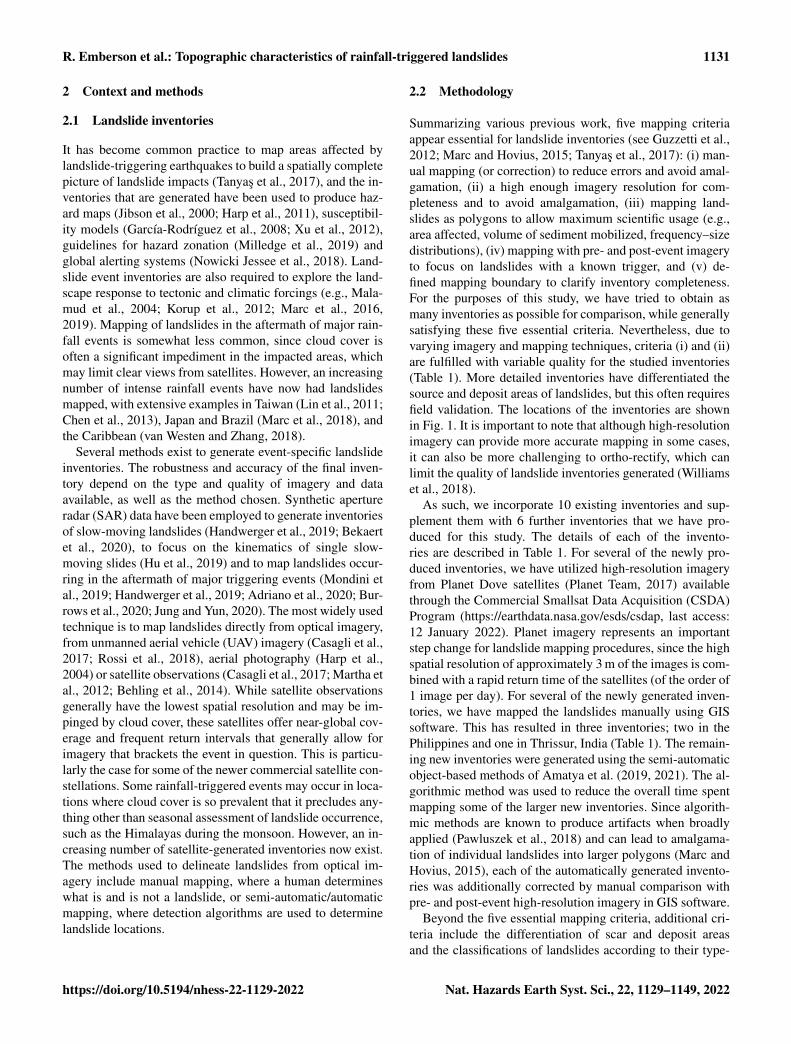
We observe a link between the short-wavelength topo-graphic position index (300 m assessment radius) and land-slide probability ratios for landslide scars in several, butnot all (i.e., not Kalmaegi, Morakot and Kii), of the events(Fig. 9). Specifically, landslide scars are significantly morelikely at positive TPI values (short-wavelength landscapeconvexities like ridges). Although this is the case for the ma-jority of inventories, results from both inventories in Taiwanand Dominica do not exhibit this tendency. This parameteralso shows the clearest distinction between the scar areas andthe whole landslide areas. The entire landslide area is morelikely to be found at negative TPI values (landscape concav-ities like valley bottoms). While the TPI at the 300 m wave-length does not demonstrate quite as consistent relationshipsas slope or the CTI, it remains a strong predictor. In partic-

ular, the larger variation between scars and overall landslideareas suggests that short wavelengths may be a valuable wayto distinguish between scarps and deposits in a preliminaryassessment.

Since forest loss is a binary variable, we do not plot thisacross multiple bins. However, we calculate the average ra-tio of forest loss in landslide zones to the overall topography,and we find across all events that the value is 1.98± 1.38(1 SD – standard deviation). This implies that forest losszones are correlated with higher probability of landsliding.We see the largest differences between landslide zones andnon-landslide zones in Salgar, Colombia, and Hiroshima,Japan, and the landslides triggered by Typhoon Morakot inTaiwan (forest loss is more than 3.5 times more likely inlandslides in these cases). In four cases, forest loss was ob-served as less likely in landslide pixels: in Blumenau, Brazil;Lanao del Norte, the Philippines; Thrissur, India; and WestPokot, Kenya. We suggest that while forest loss prior to land-slide events is generally higher in landslide locations than inthe rest of the landscape, this relationship is not consistentenough to necessarily be a good predictor of landslide loca-tion by itself.

3.2 Multivariate analysis

We have used the LASSO method to quantify the importanceof the different predictors for both scars and whole landslideswhile reducing the influence of co-linearity (Camilo et al.,2017) (Fig. 10).

Figure 10a and b also show the modeling performances,which are represented by AUC values, varying from “reason-able” (0.6< AUC< 0.7) to “adequate” (0.7< AUC< 0.8)



Figure 9. Same as Fig. 4 but for the topographic position index (however, here we omit normalization given that the TPI is a zero-centeredvariable) with an analysis window radius of 300 m.

and “outstanding” (0.8< AUC< 0.9) based on AUC classesdefined by Hosmer and Lemeshow (2000). The lower AUCvalues for some events may indicate that we lack some keyexplanatory variables; crucially, this may include rainfall in-tensity and duration, although as discussed above we lackconsistent high-resolution data to assess this within the spa-tial domain of the considered inventories. Other relevant pa-rameters may include land cover, lithology and geo-structuralparameters, and anthropogenic influence (Reichenbach et al.,2018).

Our findings show that slope, on one hand, is the factor thatmost frequently appears as significant in the GLM run forboth the landslide scars and the whole areas, with landslidesfavoring steeper locations. On the other hand, the average up-stream angle and CTI in the GLM of the scars and the averageupstream angle, CTI and topographic position index (with a300 m radius) in the GLM run for the whole area appear asthe least commonly observed significant variables. The non-significant or low impact of most of these topographic vari-ables is likely due to the co-linearity existing between thesevariables (e.g., slope and average upstream slope, slope andCTI, CTI and TPI – Figs. S1 and S2).

The results indicate that except for the CTI, all variableshave a positive weight on classifying a given grid cell as“landslide presence” instead of “landslide absence” given thechoice of predictors. There are only two cases that do not fol-low this general trend (i.e., the two Taiwanese inventories).

The regression coefficient of the TPI calculated for thelandslide scar areas for Typhoon Kalmaegi, Taiwan, has anegative sign, unlike all other cases. Overall, as we explained

above, different TPI values refer to different subsections of ahillslope. Specifically, positive values refer to ridges or hill-slopes, whereas negative values correspond to the valley. As aresult, the negative weight of the TPI on classifying the land-slide presence and absence condition in the GLM is difficultto interpret. This could be caused by interactions betweenvariables. Although we run a variable selection method (i.e.,LASSO), the TPI could be still interacting with the others.If it shares a similar signal to at least one other variable, thesign of the regression coefficient can be influenced by theinteraction.

The negative regression coefficient of the TRI obtained forthe whole landslide areas for Typhoon Morakot, Taiwan, isthe other case where the response of the covariate is differentfrom the other examples. Similarly to the Kalmaegi inven-tory case we presented above, the negative sign could also becaused by the interactions between variables. However, thiscould also be associated with the physical properties char-acterizing whole landslide areas. The TRI in the case of Ty-phoon Morakot, Taiwan, in particular, might correspond tosmooth topography. In either case, the TRI does not appear asa significant variable other than in case of Typhoon Morakot,Taiwan.

The two inventories where negative CTI values are mostsignificantly associated with landslide incidence – Morakotand Hiroshima – have few commonalities; their lithologiesdiffer, and the mean slope of the affected area in Hiroshimais markedly lower than for Morakot. Perhaps the most signif-icant commonality is that the triggering rainfall exceeded thehistorical maxima by a significant degree (Table 3), which



Figure 10. Figure showing regression coefficients and corresponding AUC values calculated from the fitted GLM for each landslide inven-tory, considering scars (a) or the whole landslide area (b). The error bar corresponds to the variation in the AUC distribution across 10-foldcross-validation replicates. Regression coefficients are not shown for predictors considered not significant by the LASSO methods. The AUCvalues shown in the legend are for scars (prior to slash) and entire landslides (second value).

may increase the likelihood of failure resulting from localtransient pore pressure increases, rather than due to saturatedflow at the base of hillslopes. Excepting these two examples,the results show that the signal of the CTI does not contributeto the GLM while classifying landslide presence or absence.

4 Discussion

The primary intention of this study is to assess the critical to-pographic parameters associated with rainfall-triggered land-slides, using a large dataset of landslide inventories that in-cludes six newly mapped events. Our results are compara-ble with existing studies (e.g., Marc et al., 2018; Milledgeet al., 2019) exploring landslide locations using inventorieswhile adding more detail and assessment of global variabil-ity, which we discuss below. First, however, we explore someof the limitations and assumptions that go into the mappingand analysis of the landslides.

4.1 Uncertainty in landslide mapping and DEMmetrics’ extraction

Firstly, it is important to consider how representative thelandslide inventories are. We have attempted to include land-slide maps from a diverse set of locations around the world,but this is still only a fraction of landslides that have oc-curred in the last 2 decades. Some of the inventories, likethe landslides occurring due to Typhoon Morakot in Tai-wan, are driven by such huge rainfall events that the over-all area of landsliding greatly exceeds other examples withlower rainfall. This is one of the key reasons why we haveused probability ratios as a metric to assess landslide loca-tions, since they do not consider the overall area of land-slides triggered by a given rainfall event. Most of the invento-ries are drawn from locations with tropical climates (Geiger,1954), and although the pairs from Brazil and Japan sampleareas of humid subtropical climates, this is not a true repre-



sentative sampling of climatic regimes. One exception is thelandslide inventory from Zimbabwe, which is in a semi-aridclimatic region. Although our examples disproportionatelysample tropical and subtropical areas, these areas generallyexperience the highest erosion rates (Milliman and Syvitski,1991), driven by increasingly intense rainfall (e.g., Bookha-gen and Strecker, 2012). Similarly, while the inventories aredrawn from places with diverse lithologies, we do not havedatasets from a fully representative set of lithological loca-tions (Hartmann and Moosdorf, 2012; Table 1).

Although we have used hand corrections to reduce theimpact of polygon amalgamation from algorithmic mappingmethods, some inconsistencies may still exist. One importantconsideration is that the datasets used here do not distinguishbetween different landslide types or distinguish between scarand deposit. While this is consistent across inventories, it isimportant when considering the results. In particular, sincewe do not have constraints on whether mapped landslides arepurely shallow soil slides or whether they incorporate deeperbedrock, we cannot determine differences in topographiccharacteristics associated with each. The change in materialproperties from soil to bedrock can lead to changes in over-all volume mobilized for a given landslide area (Larsen etal., 2010), so inventories where smaller shallow landslidesare a larger proportion of the mapped inventory may havedifferent characteristics. For example, the landslides mappedusing aerial photography around Hiroshima, Japan, do notshow particularly high probability ratios at very high reliefor TRI values, suggesting these landslides generally occuron smaller less rough hillslopes.

Hand mapping and correcting will help reduce the poten-tial for landslide amalgamation (Marc and Hovius, 2015),which is essential in order to estimate width and scar ar-eas from landslide polygon geometry (Marc et al., 2018).Since we do not have access to the imagery for all of thepreviously published events, we are not able to correct theseevents and thus must rely on prior mapping being consis-tent with our own efforts. Part of the challenge of compilingdifferent events is the different sources of imagery used tocreate each inventory. For most of the inventories we havemapped as part of this study, the imagery is consistent interms of resolution, and we have benefited from the rapid re-turn time of Planet Dove satellites to ensure that cloud coverdoes not mask any of the areas mapped. However, withoutimagery to clarify, it may be possible that parts of the previ-ously published inventories are masked by cloud cover. In ad-dition, the inventories mapped using coarser-resolution satel-lite imagery, such as the part of Taiwan impacted by TyphoonKalmaegi, may not capture the smallest landslides that re-sulted. If smaller landslides are preferentially found in cer-tain parts of the landscape, this may introduce systematic bi-ases in observed probability ratios.

While the imagery used to compile the different inven-tories varies in resolution, there do not seem to be consis-tent, systematic differences between probability ratios that

can be explained as a result of small landslides that system-atically bias the events. For example, landslides in the Do-minica events have similar probability ratios for each param-eter compared to the landslides from Typhoon Kalmaegi inTaiwan, despite these datasets having the largest differencein effective imagery resolution.

When considering the whole landslide area, we pixelatethe landslides to the resolution of the DEM to highlight themost hazardous parts of the landscape. This pixelation pro-cess can introduce a source of systematic error, since if lessthan half of a cell area is occupied by a landslide polygon, itis still considered to be a “landslide pixel”. Some landslidesmay be significantly smaller than the SRTM cell resolutionif they are mapped using high-resolution imagery, but theywill still count as a full-size pixel for the purposes of analy-sis as a result of the rasterization process. This introduces apotential source of bias as smaller landslides may make upa larger proportion of analyzed pixels than their actual areawould represent. Landslides below the approximate area ofhalf an SRTM cell (450 m3) make up an appreciable propor-tion of the total landslide area in Hiroshima and Dominica(∼ 30 %) (Fig. S12). In these settings, we would expect thatthe influence of smaller landslides may be over-estimated atthe 30 m resolution of analysis, although in the majority ofother inventories landslides below this cutoff represent lessthan 5 %–10 % of the total landslide area (and therefore theanalytical dataset of landslide pixels).

To address the potential for bias due to oversampling ofsmall landslides with a coarse-resolution DEM, we haveresampled the DEM for the events in Hiroshima and Do-minica to a resolution of 10 m, at which nearly all landslidesare captured without size exaggeration. We then recalculatethe probability ratios for the landslides and compare the re-sampled DEM results with those from the original DEM(Fig. S5). For the slope, average upstream angle, CTI, reliefand TRI, only minor differences are observed between the re-sults for a resampled DEM and the original DEM. There aresome differences between the TPI at a 300 m resolution, butno consistent relationship seems to emerge. Thus we do notthink our results are affected by the coarse rasterization pro-cess, although it is likely that accessing a higher-resolutionDEM may alter the result depending on the local variable,like the slope, CTI or TRI.

Other parameters are often incorporated into landslide sus-ceptibility such as geological factors like soil characteris-tics or lithology, local land cover type, or climatic metrics.Although global data for rainfall, soil type and geologicalparameters exist, the resolution of these datasets is too lowto allow for consistent comparison of landslide and non-landslide areas at the scale of the analysis described here(∼ 100 m). As such, we have chosen to focus exclusively ontopographic factors within our assessment.



Figure 11. Probability ratio of landslide scar areas compared with the entire landslide area. It is important to note that while Figs. 3–9contrast the landslide areas (scar or entire mapped area) with the topography, this figure shows the ratio of probabilities for the scar andwhole landslide area. Specifically, this shows the probability of a scar at a given CTI value, normalized by the probability of that CTI value,divided by the probability of the entire landslide at a given CTI value, normalized by the probability of that CTI value. Higher values indicatethat scars are more likely than whole landslide areas at that parameter value. Panel (a) shows the result for the CTI and panel (b) for theshort-wavelength TPI.

4.2 Differences between scar and overall landslide area

While for several parameters, scars and the entire landslidearea are similarly sampled at a range of values, for the TPIand CTI we see significant differences across a large numberof the inventories (Fig. 11). Scars are more likely at lowerCTI values and at more positive TPI values. A positive TPIimplies scars are more likely at concave locations in the land-scape, while a lower CTI value indicates areas with lowerflow accumulation and saturation. This describes parts of thelandscape that sit closer to ridges. This broadly supports theassessment above that higher TPI and CTI values may be away to distinguish between scar and deposit areas. No sys-tematic differences are observed with respect to the TRI oraverage upstream angle (Fig. S4).

By comparing scars and the overall landslide area, the ob-servations we have made provide informative contrasts withprior work. Similar recent work exploring the characteris-tics of earthquake-induced landslide inventories suggests thatthe slope angle and upslope contributing area are key de-terminants of hazard, defined by the entire landslide areas(Milledge et al., 2019). Our findings are consistent for entirelandslide areas but differ for the scar area, which is poorlydetermined by flow accumulation (Fig. S3). One may be sur-prised by the fact that landslides triggered by intense rain-fall have scars uncorrelated with drainage area, while bothearthquake- and rainfall-induced landslides have whole ar-eas strongly related to it. We propose that the whole-area re-

lationship mainly reflects runout paths and not hydrologicalprocesses and that the initiation of rainfall-induced landslidespoorly relates to the surface-parallel hydrological flow. Thisis discussed in more detail below. Our results for drainageare of the whole landslides are quite different from the onesof Milledge et al. (2019). We suggest that the variability inscar location (higher for earthquake; see Rault et al., 2019)may explain more diverse behavior in normalized drainagebelow the median, while the propensity for longer runout(more likely for rainfall-induced landslides) may explain thatsome (not all) cases have a probability ratio increasing untilreaching very large drainage levels (Fig. S3).

The observed differences between the scar and overalllandslide area can be exploited to refine our understanding ofsusceptibility and hazard modeling by focusing on parame-ters controlling scar areas where landslides are initiated (e.g.,slope, CTI) and the entire landslide area where landslides im-pact (e.g., drainage area, TPI), respectively. Such a focus canhelp support both sets of applications for more comprehen-sive landslide hazard information and emphasizes the need todistinguish diverse portions of mapped landslides dependingon the study objective.

4.3 Implications for triggering mechanisms andlandscape evolution

One of the most consistent observations that emerges fromthis study is that for several parameters (slope, average up-



stream slope, TRI, CTI), the critical point where landslidesand topography are equally sampled is approximately themedian value for the inventory in question. This is consis-tent with previous observations on rainfall- and earthquake-induced landsliding (Marc et al., 2018; Milledge et al., 2019).For the average upstream slope and CTI, the relationships fordifferent inventories are in fact very similar; this is despitea large variation in the median slope for each of the inven-tories (Table 2). This suggests that landslide probability isstrongly dependent on the median topography, rather than ona specific critical angle. This implies two important points:first, that despite important differences in the landscapes ob-served, consistent hazard relationships can be defined basedupon median landscape values and, second, that these diverselandscapes may be in a form of long-term equilibrium withrespect to their landslide behavior.

We suggest that each of the considered landscapes, eachwith its own lithology, vegetation, climate and tectonic forc-ing, may have evolved such that local hillslopes have slopegradients and hydromechanical properties that set the possi-bility for landslides on the upper half of the distribution. Theevolution of the hillslopes’ regolith state, which acts as animportant control on landslide susceptibility, under climaticforcing is predicted by geomorphological models of hillslopestability coupled with stochastic rainfall forcing (Dietrich etal., 1995; Iida, 1999, 2004). Landscape evolution toward acritical state was also inferred to explain why landsliding inthe Kii peninsula better matched the relative rainfall anomalythan absolute rainfall patterns (Marc et al., 2019).

Alongside the implications for landscape evolution andhow to derive susceptibility metrics, our results also offerinsight into the mechanisms of landslide triggering in ex-treme rainfall events. By focusing on the scar areas, we ob-serve that landslides are more likely in locations with lowerCTI and higher TPI values – parts of a landscape near ridgeswith a generally lower propensity for water saturation. This issomewhat in contrast to studies that suggest rainfall-triggeredlandslides are more likely to occur in areas lower down hill-slopes where fluid saturation is greater (Densmore and Hov-ius, 2000; Meunier et al., 2008), possibly because these stud-ies did not clearly differentiate the scar from whole landslidearea, which are very different relative to these two metrics(Fig. 11). The relationship with the CTI and drainage areaalso suggests that modeling landslides under the assump-tion of regolith saturation due to slope-parallel, steady-stateflow (e.g., Montgomery and Dietrich, 1994) may be inade-quate. Instead, the pore pressure triggering landslides in ex-treme rainfall events may rather be controlled by transient,vertical infiltration and/or preferential flow paths (Iverson,2000; Montgomery et al., 2009; Hencher, 2010; Bogaardand Greco, 2016). This recalls the essential challenge fordeveloping modeling approaches that can account for suchcomplex hillslope hydrology as well as highly variable hy-dromechanical properties of the regolith. Nevertheless, wealso suggest that future studies should compare the results

from this analysis of landslides triggered by extreme rain-fall with landslide inventories resulting from longer-duration,lower-intensity rainfall events to assess whether the relation-ship with the CTI and TPI changes. Indeed, we might ex-pect that lower-intensity rainfall would trigger landslides inparts of the landscape with higher CTI values as steady-statesaturation may be more widespread. In any future compara-tive study of low-intensity and high-intensity rainfall events,it will be necessary to carefully select landslide inventorieswhere the imagery used to generate them closely brackets thestart and end of the rainfall events to ensure only landslidestriggered by an individual event are analyzed.

Finally, for some events, including Typhoon Morakot inTaiwan and Cyclone Idai in Zimbabwe, there is a small de-cline in relative landslide probability at very high slope val-ues (> 35–40◦) (Fig. 4). It is possible that these slopes, whichare generally above the angles considered to be critically un-stable (Selby, 1982; Roering et al., 2001), may represent ar-eas where landslide probability is reduced as a result of non-topographic factors, such as local lithological bedding planeangles (Guzzetti et al., 1996; Santangelo et al., 2015) or thin-ner soils limiting the availability of material that can be mo-bilized as landslides (Prancevic et al., 2020). The decline inlandslide probability at the highest slope values may repre-sent the limit to which local pore pressure as a result of ex-treme rainfall can influence triggering.

5 Conclusions

In this study we have combined 10 existing rainfall-inducedlandslide inventories from a range of mountainous regionswith 6 new inventories mapped as part of this study. We sug-gest that providing newly mapped inventories is a valuableservice for the landslide community at large, and we antici-pate that these inventories can provide data to calibrate andvalidate susceptibility and hazard models both in the specificlocations where landslides occurred and also further afield.In addition, we have used moderate-resolution open-sourcesatellite data to assess the parameters that characterize the lo-cation of landslides in these inventories. We find that along-side the previously documented importance of slope and to-pographic ruggedness, the average upstream angle and to-pographic position are also determinants of landslide proba-bility in a given location. After normalizing the topographicvariables by the local landscape median, we find consistentrelationships across the different inventories despite the va-riety of lithological and topographic settings. This suggeststhat relative metrics should be considered to perform land-slide susceptibility analysis and that different landscapes canbe at a state of equilibrium with respect to the probabilityof landsliding. The importance of multiple topographic fac-tors to determine the local landslide probability highlightsthe value of high-resolution DEM data. While we have usedthe 1 arcsec resolution SRTM data, higher-resolution DEM



data are increasingly available. Given that we are able to maplandslides at finer and finer resolutions as very high reso-lution satellite imagery becomes available, combining thesenew detailed inventories with DEMs of similar resolutionsis likely to provide further insights about landslide locationwithin the landscape.

While we have not undertaken a detailed assessment ofthe rainfall that triggered these landslides, we emphasize thatvariability in rainfall is likely to explain a significant degreeof variability in where landslides occur (e.g., Marc et al.,2019). Future work should assess each of these inventorieswith respect to the rainfall that triggered the significant land-sliding, which could yield important insights into the rela-tionship between intense rainfall and landslide occurrence.

Data availability. All data used in this study are provided in theSupplement, and all methods are detailed above.

Supplement. The supplement related to this article is available on-line at: https://doi.org/10.5194/nhess-22-1129-2022-supplement.

Author contributions. All authors were involved in study conceptu-alization and writing of the manuscript. RE, PA and OM conductedlandslide mapping. RE, HT and OM conducted data analysis.

Competing interests. The contact author has declared that neitherthey nor their co-authors have any competing interests.

Disclaimer. Publisher’s note: Copernicus Publications remainsneutral with regard to jurisdictional claims in published maps andinstitutional affiliations.

Acknowledgements. Robert Emberson, Pukar Amatya andDalia B. Kirschbaum are supported by a NASA Disasters programgrant, 18-DISASTER18-0022.

Financial support. This research has been supported by the Sci-ence Mission Directorate (grant no. 18-DISASTER18-0022). Thiswork utilized data made available through the NASA CommercialSmallsat Data Acquisition (CSDA) Program.

Review statement. This paper was edited by Paola Reichenbachand reviewed by Alexander Densmore and one anonymous referee.

References

Adriano, B., Yokoya, N., Miura, H., Matsuoka, M., and Koshimura,S.: A semiautomatic pixel-object method for detecting landslidesusing multitemporal ALOS-2 intensity images, Remote Sens.,12, 561, https://doi.org/10.3390/rs12030561, 2020.

Amatya, P., Kirschbaum, D., and Stanley, T.: Use of very high-resolution optical data for landslide mapping and susceptibilityanalysis along the Karnali highway, Nepal, Remote Sens., 11,2284, https://doi.org/10.3390/rs11192284, 2019.

Amatya, P., Kirschbaum, D., Stanley, T., and Tanyas, H.:Landslide mapping using object-based image analy-sis and open source tools, Eng. Geol., 282, 106000,https://doi.org/10.1016/j.enggeo.2021.106000, 2021.

Badoux, A., Andres, N., and Turowski, J. M.: Damage costs due tobedload transport processes in Switzerland, Nat. Hazards EarthSyst. Sci., 14, 279–294, https://doi.org/10.5194/nhess-14-279-2014, 2014.

Behling, R., Roessner, S., Segl, K., Kleinschmit, B., and Kauf-mann, H.: Robust automated image co-registration of opticalmulti-sensor time series data: Database generation for multi-temporal landslide detection, Remote Sens., 6, 2572–2600,https://doi.org/10.3390/rs6032572, 2014.

Bekaert, D. P., Handwerger, A. L., Agram, P., and Kirschbaum, D.B.: InSAR-based detection method for mapping and monitoringslow-moving landslides in remote regions with steep and moun-tainous terrain: An application to Nepal, Remote Sens. Environ.,249, 111983, https://doi.org/10.1016/j.rse.2020.111983, 2020.

Beven, K. J. and Kirkby, M. J.: A physically based, vari-able contributing area model of basin hydrology/Unmodèle à base physique de zone d’appel variable del’hydrologie du bassin versant, Hydrolog. Sci. J., 24, 43–69, https://doi.org/10.1080/02626667909491834, 1979.

Bogaard, T. A. and Greco, R.: Landslide hydrology: from hydrologyto pore pressure, Wiley Interdisciplin. Rev.: Water, 3, 439–459,https://doi.org/10.1002/wat2.1126, 2016.

Bookhagen, B. and Strecker, M. R.: Spatiotemporal trends in ero-sion rates across a pronounced rainfall gradient: Examples fromthe southern Central Andes, Earth Planet. Sc. Lett., 327–328, 97–110, https://doi.org/10.1016/j.epsl.2012.02.005, 2012.

Broeckx, J., Maertens, M., Isabirye, M., Vanmaercke, M., Na-mazzi, B., Deckers, J., Tamale, J., Jacobs, L., Thiery, W.,Kervyn, M., Vranken, L., and Poesen, J.: Landslide sus-ceptibility and mobilization rates in the Mount Elgon re-gion, Uganda, (October 2018), Landslides, 16, 571–584,https://doi.org/10.1007/s10346-018-1085-y, 2019.

Budimir, M. E. A., Atkinson, P. M., and Lewis, H. G.: A systematicreview of landslide probability mapping using logistic regres-sion, Landslides, 12, 419–436, https://doi.org/10.1007/s10346-014-0550-5, 2015.

Burrows, K., Walters, R. J., Milledge, D., and Densmore, A. L.:A systematic exploration of satellite radar coherence methodsfor rapid landslide detection, Nat. Hazards Earth Syst. Sci., 20,3197–3214, https://doi.org/10.5194/nhess-20-3197-2020, 2020.

Camilo, D. C., Lombardo, L., Mai, P. M., Dou, J., andHuser, R.: Environmental Modelling & Software Handlinghigh predictor dimensionality in slope-unit-based landslidesusceptibility models through LASSO-penalized General-ized Linear Model, Environ. Model. Softw., 97, 145–156,https://doi.org/10.1016/j.envsoft.2017.08.003, 2017.


https://doi.org/10.5194/nhess-22-1129-2022-supplement

https://doi.org/10.3390/rs12030561

https://doi.org/10.3390/rs11192284

https://doi.org/10.1016/j.enggeo.2021.106000

https://doi.org/10.5194/nhess-14-279-2014


https://doi.org/10.3390/rs6032572

https://doi.org/10.1016/j.rse.2020.111983

https://doi.org/10.1080/02626667909491834

https://doi.org/10.1002/wat2.1126

https://doi.org/10.1016/j.epsl.2012.02.005

https://doi.org/10.1007/s10346-018-1085-y

https://doi.org/10.1007/s10346-014-0550-5

https://doi.org/10.1007/s10346-014-0550-5


https://doi.org/10.1016/j.envsoft.2017.08.003


Casagli, N., Frodella, W., Morelli, S., Tofani, V., Ciampalini, A.,Interieri, C., Raspini, F., Rossi, G., Tanteri, L., and Lu, P.:Spaceborne, UAV and ground-based remote sensing techniquesfor landslide mapping, monitoring and early warning, Geoenvi-ron. Disast., 4, 1–23, https://doi.org/10.1186/s40677-017-0073-1, 2017.

Chang, K., Chiang, S., Chen, Y., and Mondini, A. C.:Modeling the spatial occurrence of shallow landslidestriggered by typhoons, Geomorphology, 208, 137–148,https://doi.org/10.1016/j.geomorph.2013.11.020, 2014.

Chen, Y., Chang, K., Chiu, Y., Lau, S., Lee, H., and County,T.: Quantifying rainfall controls on catchment-scale landslideerosion in Taiwan, Earth Surf. Proc. Land., 382, 372–382,https://doi.org/10.1002/esp.3284, 2013.

Conrad, J. L., Morphew, M. D., Baum, R. L., and Mirus, B. B.: Hy-droMet: A New Code for Automated Objective Optimization ofHydrometeorological Thresholds for Landslide Initiation, Water,13, 1752, https://doi.org/10.3390/w13131752, 2021.

Costanzo, D., Rotigliano, E., Irigaray, C., Jiménez-Perálvarez, J.D., and Chacón, J.: Factors selection in landslide susceptibilitymodelling on large scale following the gis matrix method: Ap-plication to the river Beiro basin (Spain), Nat. Hazards EarthSyst. Sci., 12, 327–340, https://doi.org/10.5194/nhess-12-327-2012, 2012.

Densmore, A. L. and Hovius, N.: Topographicfingerprints of bedrock landslides, Geol-ogy, 28, 371–374, https://doi.org/10.1130/0091-7613(2000)28<371:TFOBL>2.0.CO;2, 2000.

Dietrich, W. E., Reiss, R., Hsu, M. L., and Montgomery, D. R.: Aprocess-based model for colluvial soil depth and shallow lands-liding using digital elevation data, Hydrol. Process., 9, 383–400,https://doi.org/10.1002/hyp.3360090311, 1995.

Domej, G., Bourdeau, C., Lenti, L., Martino, S., and Piuta,K.: Mean landslide geometries inferred from a globaldatabase of earthquake-and non-earthquake-triggeredlandslides, Ital. J. Eng. Geol. Environ., 17, 87–107,https://doi.org/10.4408/IJEGE.2017-02.O-05, 2017.

Emberson, R., Kirschbaum, D., and Stanley, T.: New globalcharacterisation of landslide exposure, Nat. Hazards EarthSyst. Sci., 20, 3413–3424, https://doi.org/10.5194/nhess-20-3413-2020, 2020.

Emberson, R. A., Kirschbaum, D. B., and Stanley, T.: Landslidehazard and exposure modelling in data-poor regions: the exampleof the Rohingya refugee camps in Bangladesh, Earth’s Future, 9,e2020EF001666, https://doi.org/10.1029/2020EF001666, 2021.

Friedman, J., Hastie, T., Tibshirani, R., Narasimhan, B.,Tay, K., Simon, N., and Qian, J.: Lasso and Elastic-Net Regularized Generalized Linear Models, CRAN,https://doi.org/10.18637/jss.v033.i01, 2021.

Froude, M. J. and Petley, D. N.: Global fatal landslide occurrencefrom 2004 to 2016, Nat. Hazards Earth Syst. Sci., 18, 2161–2181,https://doi.org/10.5194/nhess-18-2161-2018, 2018.

García-Rodríguez, M. J., Malpica, J. A., Benito, B., and Díaz, M.:Susceptibility assessment of earthquake-triggered landslides inEl Salvador using logistic regression, Geomorphology, 95, 172–191, https://doi.org/10.1016/j.geomorph.2007.06.001, 2008.

Geiger, R.: Klassifikation der Klimate nach W. Köppen, in: Landolt-Börnstein – Zahlenwerte und Funktionen aus Physik, Chemie,

Astronomie, Geophysik und Technik, alte Serie, Springer, Berlin,603–607, 1954.

Goetz, J. N., Brenning, A., Petschko, H., and Leopold, P.: Evalu-ating machine learning and statistical prediction techniques forlandslide susceptibility modeling, Comput. Geosci., 81, 1–11,https://doi.org/10.1016/j.cageo.2015.04.007, 2015.

Guzzetti, F., Cardinali, M., and Reichenbach, P.: The In-fluence of Structural Setting and Lithology on LandslideType and Pattern, Environ. Eng. Geosci., II, 531–555,https://doi.org/10.2113/gseegeosci.II.4.531, 1996.

Guzzetti, F., Cesare, A., Cardinali, M., Fiorucci, F., Santan-gelo, M., and Chang, K.: Landslide inventory maps: Newtools for an old problem, Earth Sci. Rev., 112, 42–66,https://doi.org/10.1016/j.earscirev.2012.02.001, 2012.

Handwerger, A. L., Fielding, E. J., Huang, M., Bennett, G., Liang,C., and Schulz, W. H.: Widespread Initiation, Reactivation ,and Acceleration of Landslides in the Northern California CoastRanges due to Extreme Rainfall, J. Geophys. Res.-Earth, 124,1782–1797, https://doi.org/10.1029/2019JF005035, 2019.

Hansen, M. C., Potapov, P. V., Moore, R., Hancher, M., Turubanova,S. A., Tyukavina, A., Thau, D., Stehman, S. V., Goetz, S. J.,Loveland, T. R., Kommareddy, A., Egorov, A., Chini, L., Justice,C. O., and Townshend, J. R. G.: High-Resolution Global Mapsof 21st-Century Forest Cover Change, Science, 342, 850–853,https://doi.org/10.1126/science.1244693, 2013.

Harp, B. E. L., Reid, M. E., and Michael, J. A.: Hazard Analysis ofLandslides Triggered by Typhoon Chata’an on July 2, 2002, inChuuk State, Federated States of Micronesia, USGS Open-FileReport 2004-1348, USGS, https://doi.org/10.3133/ofr20041348,2004.

Harp, E. L., Keefer, D. K., Sato, H. P., and Yagi, H.:Landslide inventories: The essential part of seismiclandslide hazard analyses, Eng. Geol., 122, 9–21,https://doi.org/10.1016/j.enggeo.2010.06.013, 2011.

Hartmann, J. and Moosdorf, N.: The new global lithologicalmap database GLiM: A representation of rock propertiesat the Earth surface, Geochem. Geophy. Geosy., 13, 1–37,https://doi.org/10.1029/2012GC004370, 2012.

Hencher, S. R.: Preferential flow paths through soil and rock andtheir association with landslides, Hydrol. Process., 24, 1610–1630, https://doi.org/10.1002/hyp.7721, 2010.

Hosmer, D. and Lemeshow, S: Applied Logistic Regression,2nd Edn., Wiley, New York, ISBN 978-0-470-58247-3, 2000.

Hu, X., Bürgmann, R., Lu, Z., Handwerger, A. L., Wang, T., andMiao, R.: Mobility, Thickness, and Hydraulic Diffusivity of theSlow – Moving Monroe Landslide in California Revealed by L –Band Satellite Radar Interferometry J. Geophys. Res.-Solid, 124,7504–7518, https://doi.org/10.1029/2019JB017560, 2019.

Huffman, G. J., Bolvin, D. T., Braithwaite, D., Hsu, K.-L., Joyce,R. J., Kidd, C., Nelkin, E. J., Sorooshian, S., Stocker, E. F.,Tan, J., Wolff, D. B., and Xie, P.: Integrated Multi-SatelliteRetrievals for the Global Precipitation Measurement (GPM)Mission (IMERG), in: Advances in Global Change Re-search, Springer, 343–353, https://doi.org/10.1007/978-3-030-24568-9_19, 2020.

Iida, T.: A stochastic hydro-geomorphological model for shal-low landsliding due to rainstorm, Catena, 34, 293–313,https://doi.org/10.1016/S0341-8162(98)00093-9, 1999.


https://doi.org/10.1186/s40677-017-0073-1

https://doi.org/10.1186/s40677-017-0073-1

https://doi.org/10.1016/j.geomorph.2013.11.020

https://doi.org/10.1002/esp.3284

https://doi.org/10.3390/w13131752



https://doi.org/10.1130/0091-7613(2000)28<371:TFOBL>2.0.CO;2

https://doi.org/10.1130/0091-7613(2000)28<371:TFOBL>2.0.CO;2

https://doi.org/10.1002/hyp.3360090311

https://doi.org/10.4408/IJEGE.2017-02.O-05



https://doi.org/10.1029/2020EF001666

https://doi.org/10.18637/jss.v033.i01



https://doi.org/10.1016/j.cageo.2015.04.007

https://doi.org/10.2113/gseegeosci.II.4.531

https://doi.org/10.1016/j.earscirev.2012.02.001

https://doi.org/10.1029/2019JF005035

https://doi.org/10.1126/science.1244693

https://doi.org/10.3133/ofr20041348

https://doi.org/10.1016/j.enggeo.2010.06.013

https://doi.org/10.1029/2012GC004370

https://doi.org/10.1002/hyp.7721

https://doi.org/10.1029/2019JB017560

https://doi.org/10.1007/978-3-030-24568-9_19

https://doi.org/10.1007/978-3-030-24568-9_19

https://doi.org/10.1016/S0341-8162(98)00093-9


Iida, T.: Theoretical research on the relationship between return pe-riod of rainfall and shallow landslides, Hydrol. Process., 18, 739–756, https://doi.org/10.1002/hyp.1264, 2004.

Iverson, R. M.: Landslide triggering by rain in-filtration, Water Resour. Res., 36, 1897–1910,https://doi.org/10.1029/2000WR900090, 2000.

Jibson, R. W., Harp, E. L., and Michael, J. A.: A methodfor producing digital probabilistic seismic landslide hazardmaps, Eng. Geol., 58, 271–289, https://doi.org/10.1016/S0013-7952(00)00039-9, 2000.

Jung, J. and Yun, S. H.: Evaluation of coherent and incoherent land-slide detection methods based on synthetic aperture radar forrapid response: A case study for the 2018 Hokkaido landslides,Remote Sens., 12, 265, https://doi.org/10.3390/rs12020265,2020.

Kirschbaum, D. B. and Stanley, T.: Satellite-Based As-sessment of Rainfall-Triggered Landslide Hazard forSituational Awareness, Earth’s Future, 6, 505–523,https://doi.org/10.1002/2017EF000715, 2018.

Kirschbaum, D. B., Stanley, T., and Zhou, Y.: Spatial and temporalanalysis of a global landslide catalog, Geomorphology, 249, 4–15, https://doi.org/10.1016/j.geomorph.2015.03.016, 2015.

Korup, O., Görüm, T., and Hayakawa, Y.: Without power? Land-slide inventories in the face of climate change, Earth Surf. Proc.Land., 37, 92–99, https://doi.org/10.1002/esp.2248, 2012.

Larsen, I. J., Montgomery, D. R., and Korup, O.: Landslide ero-sion controlled by hillslope material, Nat. Geosci., 3, 247–251,https://doi.org/10.1038/ngeo776, 2010.

Liang, W. and Chan, M.: Spatial and temporal variations in the ef-fects of soil depth and topographic wetness index of bedrocktopography on subsurface saturation generation in a steep nat-ural forested headwater catchment, J. Hydrol., 546, 405–418,https://doi.org/10.1016/j.jhydrol.2017.01.033, 2017.

Lin, C.-W., Chang, W.-S., Liu, S.-H., Tsai, T.-T., Lee, S.-P., Tsang,Y.-C., Shieh, C.-L., and Tseng, C.-M.: Landslides triggered bythe 7 August 2009 Typhoon Morakot in southern Taiwan, Eng.Geol., 123, 3–12, https://doi.org/10.1016/j.enggeo.2011.06.007,2011.

Lombardo, L. and Tanyas, H.: Chrono-validation of near-real-time landslide susceptibility models via plug-in statistical simulations, Eng. Geol., 278, 105818,https://doi.org/10.1016/j.enggeo.2020.105818, 2020.

Lombardo, L., Optiz, T., and Huser, R.: Point process-based mod-eling of multiple debris flow landslides using INLA: an applica-tion to the 2009 Messina disaster, Stoch. Environ. Res. Risk As-sess., 32, 2179–2198, https://doi.org/10.1007/s00477-018-1518-0, 2018.

Malamud, B. D., Turcotte, D. L., Guzzetti, F., and Reichenbach, P.:Landslide inventories and their statistical properties, Earth Surf.Proc. Land., 29, 687–711, https://doi.org/10.1002/esp.1064,2004.

Marc, O. and Hovius, N.: Amalgamation in landslide maps: effectsand automatic detection, Nat. Hazards Earth Syst. Sci., 15, 723–733, https://doi.org/10.5194/nhess-15-723-2015, 2015.

Marc, O., Hovius, N., Meunier, P., Gorum, T., and Uchida, T.: Aseismologically consistent expression for the total area and vol-ume of earthquake-triggered landsliding, J. Geophys. Res.-Earth,121, 640–663, https://doi.org/10.1002/2015JF003732, 2016.

Marc, O., Meunier, P., and Hovius, N.: Prediction of the area af-fected by earthquake-induced landsliding based on seismologi-cal parameters, Nat. Hazards Earth Syst. Sci., 17, 1159–1175,https://doi.org/10.5194/nhess-17-1159-2017, 2017.

Marc, O., Stumpf, A., Malet, J.-P., Gosset, M., Uchida, T., and Chi-ang, S.-H.: Initial insights from a global database of rainfall-induced landslide inventories: the weak influence of slope andstrong influence of total storm rainfall, Earth Surf. Dynam., 6,903–922, https://doi.org/10.5194/esurf-6-903-2018, 2018.

Marc, O., Gosset, M., Saito, H., Uchida, T., and Malet, J.-P.: Spa-tial Patterns of Storm-Induced Landslides and Their Relation toRainfall Anomaly Maps, Geophys. Res. Lett., 46, 11167–11177,https://doi.org/10.1029/2019GL083173, 2019.

Martha, T. R., Kerle, N., Van Westen, C. J., Jetten, V., andKumar, K. V.: Object-oriented analysis of multi-temporalpanchromatic images for creation of historical landslide in-ventories, ISPRS J. Photogram. Remote Sens., 67, 105–119,https://doi.org/10.1016/j.isprsjprs.2011.11.004, 2012.

Meunier, P., Hovius, N., and Haines, J. A.: Topographicsite effects and the location of earthquake inducedlandslides, Earth Planet. Sc. Lett., 275, 221–232,https://doi.org/10.1016/j.epsl.2008.07.020, 2008.

Milledge, D. G., Densmore, A. L., Bellugi, D., Rosser, N. J., Watt,J., Li, G., and Oven, K. J.: Simple rules to minimise exposureto coseismic landslide hazard, Nat. Hazards Earth Syst. Sci., 19,837–856, https://doi.org/10.5194/nhess-19-837-2019, 2019.

Milliman, J. and Syvitski, J. P. M.: Geomorphic Tectonic Control ofSediment Discharge to Ocean – The Importance of Small Moun-tainous Rivers Geomorphic/Tectonic Control of Sediment Dis-charge to the Ocean: The Importance of Small, J. Geol., 100,525–544, https://doi.org/10.1086/629606, 1991.

Mirus, B., Jones, E. S., Baum, R. L., Godt, J. W., Slaughter, S.,Crawford, M. M., Lancaster, J., Stanley, T., Kirschbaum, D. B.,Burns, W. J., Schmitt, R. G., Lindsey, K. O., and McCoy, K. M.:Landslides across the USA: occurrence, susceptibility, and datalimitations, Landslides, 17, 2271–2285, 2020.

Mondini, A. C., Santangelo, M., Rocchetti, M., Rossetto, E., Man-coni, A., and Monserrat, O.: Sentinel-1 SAR amplitude im-agery for rapid landslide detection, Remote Sens., 11, 760,https://doi.org/10.3390/rs11070760, 2019.

Montgomery, D. R. and Dietrich, W. E.: A physically based modelfor the topographic control on shallow landsliding, Water Re-sour. Res., 30, 1153–1171, https://doi.org/10.1029/93WR02979,1994.

Montgomery, D. R., Schmidt, K. M., Dietrich, W. E., and McK-ean, J.: Instrumental record of debris flow initiation during natu-ral rainfall: Implications for modeling slope stability, J. Geophys.Res.-Earth, 114, F01031, https://doi.org/10.1029/2008JF001078,2009.

Nowicki Jessee, M. A., Hamburger, M. W., Allstadt, K., Wald, D.J., Robeson, S. M., Tanyas, H., Hearne, M., and Thompson, E.M.: A Global Empirical Model for Near-Real-Time Assessmentof Seismically Induced Landslides, J. Geophys. Res.-Earth, 123,1835–1859, https://doi.org/10.1029/2017JF004494, 2018.

Pawluszek, K., Borkowski, A., and Tarolli, P.: Sensitivityanalysis of automatic landslide mapping: numerical experi-ments towards the best solution, Landslides, 15, 1851–1865,https://doi.org/10.1007/s10346-018-0986-0, 2018.


https://doi.org/10.1002/hyp.1264

https://doi.org/10.1029/2000WR900090

https://doi.org/10.1016/S0013-7952(00)00039-9

https://doi.org/10.1016/S0013-7952(00)00039-9

https://doi.org/10.3390/rs12020265

https://doi.org/10.1002/2017EF000715



https://doi.org/10.1038/ngeo776

https://doi.org/10.1016/j.jhydrol.2017.01.033



https://doi.org/10.1007/s00477-018-1518-0

https://doi.org/10.1007/s00477-018-1518-0



https://doi.org/10.1002/2015JF003732


https://doi.org/10.5194/esurf-6-903-2018

https://doi.org/10.1029/2019GL083173

https://doi.org/10.1016/j.isprsjprs.2011.11.004

https://doi.org/10.1016/j.epsl.2008.07.020


https://doi.org/10.1086/629606

https://doi.org/10.3390/rs11070760

https://doi.org/10.1029/93WR02979

https://doi.org/10.1029/2008JF001078

https://doi.org/10.1029/2017JF004494

https://doi.org/10.1007/s10346-018-0986-0


Petley, D. Global patterns of loss of life from landslides, Geology,40, 927–930, https://doi.org/10.1130/G33217.1, 2012.

Planet Team: Planet Application Program Interface: In Space forLife on Earth, Planet Team, San Francisco, CA, https://api.planet.com (last access: 31 March 2022), 2017.

Prancevic, J. P., Lamb, M. P., McArdell, B. W., Rickli, C.,and Kirchner, J. W.: Decreasing landslide erosion on steeperslopes in soil-mantled landscapes, Geophys. Res. Lett., 47,e2020GL087505, https://doi.org/10.1029/2020GL087505, 2020.

Rault, C., Robert, A., Marc, O., Hovius, N., and Meunier, P.: Seis-mic and geologic controls on spatial clustering of landslidesin three large earthquakes, Earth Surf. Dynam., 7, 829–839,https://doi.org/10.5194/esurf-7-829-2019, 2019.

R Core Team: R: A language and environment for statistical com-puting, R Foundation for Statistical Computing, Vienna, Austria,https://www.R-project.org/ (last access: 31 March 2022), 2018.

Reichenbach, P., Rossi, M., Malamud, B. D., Mihir, M.,and Guzzetti, F.: A review of statistically-based land-slide susceptibility models, Earth-Sci. Rev., 180, 60–91,https://doi.org/10.1016/j.earscirev.2018.03.001, 2018.

Riley, S. J., DeGloria, S. D., and Elliot, R.: A Terrain RuggednessIndex that Quantifies Topographic Heterogeneity, Intermount. J.Sci., 5, 23–27, 1999.

Roering, J. J., Kirchner, J. W., Sklar, L. S., and Di-etrich, W. E.: Hillslope evolution by nonlinearcreep and landsliding: An experimental study, Ge-ology, 29, 143–146, https://doi.org/10.1130/0091-7613(2001)029<0143:HEBNCA>2.0.CO;2, 2001.

Rossi, G., Tanteri, L., Tofani, V., Vannocci, P., Moretti, S.,and Casagli, N.: Multitemporal UAV surveys for landslidemapping and characterization, Landslides, 15, 1045–1052,https://doi.org/10.1007/s10346-018-0978-0, 2018.

Santangelo, M., Marchesini, I., Cardinali, M., Fiorucci, F., Rossi,M., Bucci, F., and Guzzetti, F.: A method for the assessment ofthe influence of bedding on landslide abundance and types, Land-slides, 12, 295–309, https://doi.org/10.1007/s10346-014-0485-x,2015.

Schmitt, R. G., Tanyas, H., Nowicki Jessee, M. A., Zhu, J.,Biegel, K. M., Allstadt, K. E., Jibson, R. W., Thompson, E. M.,van Westen, C. J., Sato, H. P., Wald, D. J., Godt, J. W., Gorum, T.,Xu, C., Rathje, E. M., and Knudsen, K. L.: An open repositoryof earthquake-triggered ground-failure inventories, Data Series,USGS, Reston, VA, https://doi.org/10.3133/ds1064, 2017.

Selby, M. J.: Controls on the Stability and Inclinations of Hill-slopes formed on hard rock, Earth Surf. Proc. Land., 7, 449–467,https://doi.org/10.1002/esp.3290070506, 1982.

Sörensen, R., Zinko, U., and Seibert, J.: On the calculation of the to-pographic wetness index: evaluation of different methods basedon field observations, Hydrol. Earth Syst. Sci., 10, 101–112,https://doi.org/10.5194/hess-10-101-2006, 2006.

Stanley, T. A. and Kirschbaum, D. B.: A heuristic approach toglobal landslide susceptibility mapping, Nat. Hazards, 87, 145–164, https://doi.org/10.1007/s11069-017-2757-y, 2017.

Tanyas, H. and Lombardo, L.: Variation in landslide-affected areaunder the control of ground motion and topography, Eng. Geol.,260, 105229, https://doi.org/10.1016/j.enggeo.2019.105229,2019.

Tanyas, H., van Westen, C. J., Allstadt, K. E., Nowicki Jessee, M.A., Gorum, T., Jibson, R. W., Godt, J. W., Sato, H. P., Schmitt,R. G., Marc, O., and Hovius, N.: Presentation and Analysisof Earthquake-Induced Landslide Inventories, J. Geophys. Res.-Earth, 122, 1991–2015, https://doi.org/10.1002/2017JF004236,2017.

Tanyas, H., Rossi, M., Alvioli, M., van Westen, C. J., and March-esini, I.: A global slope unit-based method for the near real-timeprediction of earthquake-induced landslides, Geomorphology,327, 126–146, https://doi.org/10.1016/j.geomorph.2018.10.022,2019.

The Association of Japanese Geographers: The 2018 July Heavyrain in West Japan, http://ajg-disaster.blogspot.com/2018/07/3077.html, last access: 1 November 2019.

Tibshirani, R.: Regression Shrinkage and Selection viathe Lasso, J. Roy. Stat. Soc. Ser. B, 58, 267–288,https://doi.org/10.1111/j.2517-6161.1996.tb02080.x, 1996.

Van Den Eeckhaut, M. and Hervás, J.: Geomorphology State ofthe art of national landslide databases in Europe and their poten-tial for assessing landslide susceptibility, Hazard Risk, 140, 545–558, https://doi.org/10.1016/j.geomorph.2011.12.006, 2012.

Van Den Eeckhaut, M., Hervás, J., Jaedicke, C., Malet, J.-P., Mon-tanarella, L., and Nadim, F.: Statistical modelling of Europe-wide landslide susceptibility using limited landslide inventorydata, Landslides, 9, 357–369, https://doi.org/10.1007/s10346-011-0299-z, 2012.

van Westen, C. J. and Zhang, J.: Landslides and floods triggeredby Hurricane Maria (18 September, 2017) in Dominica, Digitalor Visual Products, UNITAR-UNOSAT, http://www.unitar.org/unosat/node/44/2762 (last access: 31 March 2022), 2018.

van Westen, C., Jetten, V., and Alkema, D.: Validating nationallandslide susceptibility and hazard maps for Caribbean islandcountries: the case of Dominica and tropical storm Erika, in:EGU General Assembly Conference Abstracts, April 2016,EPSC2016-4334, 2016.

Wasowski, J., Keefer, D. K., and Lee, C. T.: Toward the nextgeneration of research on earthquake-induced landslides: cur-rent issues and future challenges, Eng. Geol., 122, 1–8,https://doi.org/10.1016/j.enggeo.2011.06.001, 2011.

Weiss, A.: Topographic Position and Landforms Analysis,in: ESRI User Conference, San Diego, CA, http://www.jennessent.com/downloads/TPI-poster-TNC_18x22.pdf (last ac-cess: 31 March 2022), 2001.

Williams, J. G., Rosser, N. J., Kincey, M. E., Benjamin, J., Oven,K. J., Densmore, A. L., Milledge, D. G., Robinson, T. R., Jor-dan, C. A., and Dijkstra, T. A.: Satellite-based emergency map-ping using optical imagery: experience and reflections from the2015 Nepal earthquakes, Nat. Hazards Earth Syst. Sci., 18, 185–205, https://doi.org/10.5194/nhess-18-185-2018, 2018.

Xu, C., Dai, F., Xu, X., and Hsi, Y.: GIS-based support vector ma-chine modeling of earthquake-triggered landslide susceptibilityin the Jianjiang River watershed, China, Geomorphology, 145–146, 70–80, https://doi.org/10.1016/j.geomorph.2011.12.040,2012.


https://doi.org/10.1130/G33217.1

https://api.planet.com

https://api.planet.com

https://doi.org/10.1029/2020GL087505

https://doi.org/10.5194/esurf-7-829-2019

https://www.R-project.org/

https://doi.org/10.1016/j.earscirev.2018.03.001

https://doi.org/10.1130/0091-7613(2001)029<0143:HEBNCA>2.0.CO;2

https://doi.org/10.1130/0091-7613(2001)029<0143:HEBNCA>2.0.CO;2

https://doi.org/10.1007/s10346-018-0978-0

https://doi.org/10.1007/s10346-014-0485-x

https://doi.org/10.3133/ds1064

https://doi.org/10.1002/esp.3290070506

https://doi.org/10.5194/hess-10-101-2006

https://doi.org/10.1007/s11069-017-2757-y


https://doi.org/10.1002/2017JF004236


http://ajg-disaster.blogspot.com/2018/07/3077.html

http://ajg-disaster.blogspot.com/2018/07/3077.html

https://doi.org/10.1111/j.2517-6161.1996.tb02080.x


https://doi.org/10.1007/s10346-011-0299-z

https://doi.org/10.1007/s10346-011-0299-z

http://www.unitar.org/unosat/node/44/2762

http://www.unitar.org/unosat/node/44/2762


http://www.jennessent.com/downloads/TPI-poster-TNC_18x22.pdf

http://www.jennessent.com/downloads/TPI-poster-TNC_18x22.pdf



Insights from the topographic characteristics of a ... - NHESS

Documents

Transcript of Insights from the topographic characteristics of a ... - NHESS