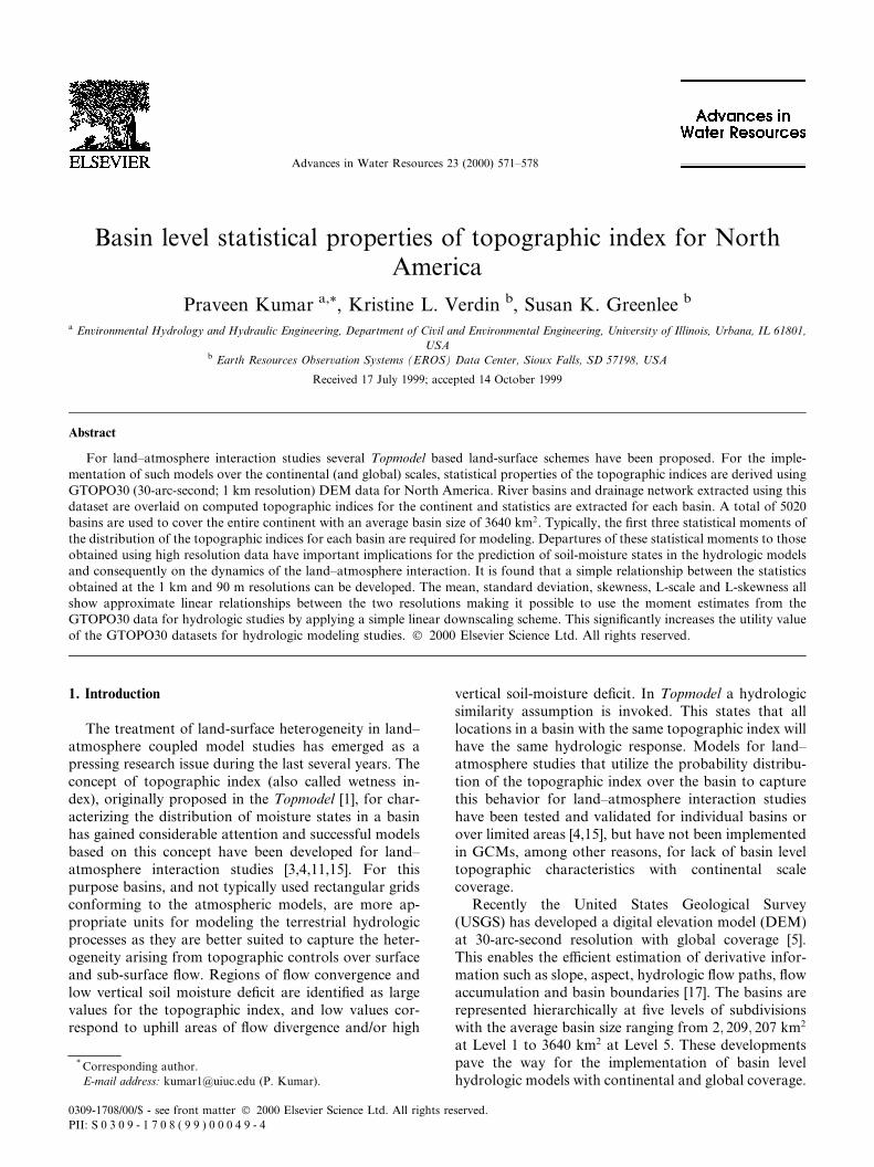
Basin level statistical properties of topographic index for NorthAmerica

Praveen Kumar a,*, Kristine L. Verdin b, Susan K. Greenlee b

a Environmental Hydrology and Hydraulic Engineering, Department of Civil and Environmental Engineering, University of Illinois, Urbana, IL 61801,

USAb Earth Resources Observation Systems (EROS) Data Center, Sioux Falls, SD 57198, USA

Received 17 July 1999; accepted 14 October 1999

Abstract

For land±atmosphere interaction studies several Topmodel based land-surface schemes have been proposed. For the imple-

mentation of such models over the continental (and global) scales, statistical properties of the topographic indices are derived using

GTOPO30 (30-arc-second; 1 km resolution) DEM data for North America. River basins and drainage network extracted using this

dataset are overlaid on computed topographic indices for the continent and statistics are extracted for each basin. A total of 5020

basins are used to cover the entire continent with an average basin size of 3640 km2. Typically, the ®rst three statistical moments of

the distribution of the topographic indices for each basin are required for modeling. Departures of these statistical moments to those

obtained using high resolution data have important implications for the prediction of soil-moisture states in the hydrologic models

and consequently on the dynamics of the land±atmosphere interaction. It is found that a simple relationship between the statistics

obtained at the 1 km and 90 m resolutions can be developed. The mean, standard deviation, skewness, L-scale and L-skewness all

show approximate linear relationships between the two resolutions making it possible to use the moment estimates from the

GTOPO30 data for hydrologic studies by applying a simple linear downscaling scheme. This signi®cantly increases the utility value

of the GTOPO30 datasets for hydrologic modeling studies. Ó 2000 Elsevier Science Ltd. All rights reserved.

1. Introduction

The treatment of land-surface heterogeneity in land±atmosphere coupled model studies has emerged as apressing research issue during the last several years. Theconcept of topographic index (also called wetness in-dex), originally proposed in the Topmodel [1], for char-acterizing the distribution of moisture states in a basinhas gained considerable attention and successful modelsbased on this concept have been developed for land±atmosphere interaction studies [3,4,11,15]. For thispurpose basins, and not typically used rectangular gridsconforming to the atmospheric models, are more ap-propriate units for modeling the terrestrial hydrologicprocesses as they are better suited to capture the heter-ogeneity arising from topographic controls over surfaceand sub-surface ¯ow. Regions of ¯ow convergence andlow vertical soil moisture de®cit are identi®ed as largevalues for the topographic index, and low values cor-respond to uphill areas of ¯ow divergence and/or high

vertical soil-moisture de®cit. In Topmodel a hydrologicsimilarity assumption is invoked. This states that alllocations in a basin with the same topographic index willhave the same hydrologic response. Models for land±atmosphere studies that utilize the probability distribu-tion of the topographic index over the basin to capturethis behavior for land±atmosphere interaction studieshave been tested and validated for individual basins orover limited areas [4,15], but have not been implementedin GCMs, among other reasons, for lack of basin leveltopographic characteristics with continental scalecoverage.

Recently the United States Geological Survey(USGS) has developed a digital elevation model (DEM)at 30-arc-second resolution with global coverage [5].This enables the e�cient estimation of derivative infor-mation such as slope, aspect, hydrologic ¯ow paths, ¯owaccumulation and basin boundaries [17]. The basins arerepresented hierarchically at ®ve levels of subdivisionswith the average basin size ranging from 2; 209; 207 km2

at Level 1 to 3640 km2 at Level 5. These developmentspave the way for the implementation of basin levelhydrologic models with continental and global coverage.

Advances in Water Resources 23 (2000) 571±578

* Corresponding author.

E-mail address: kumar1@uiuc.edu (P. Kumar).

0309-1708/00/$ - see front matter Ó 2000 Elsevier Science Ltd. All rights reserved.

PII: S 0 3 0 9 - 1 7 0 8 ( 9 9 ) 0 0 0 4 9 - 4

The objective of this paper is to describe the char-acteristics of the topographic indices at the basin levelfor North America, extracted from the 30-arc-secondDEM. Modeling studies using the data are not dis-cussed. Usually, the ®rst three statistical moments ofthe distribution of the topographic indices for eachbasin is required for modeling. These moments enablethe parameter estimation of the probability distribu-tion. Typically a 3-parameter gamma (or Pearson-III)distribution is used [14]. The properties of the ®tteddistribution are sensitive to the DEM resolution andthis impacts the performance of the hydrologic model[19]. In order to address this problem in the use of 30-arc-second DEM, we adopt the following procedure:(i) estimate topographic index using the single ¯owalgorithm from the 30-arc-second DEM data; (ii)overlay basin boundaries and estimate statistical mo-ments; (iii) analyze topographic indices obtained fromhigh resolution 3-arc-second data for selected regionsrepresenting a range of topographic features to quan-tify the impact of resolution on the estimates of thestatistical moments; (iv) establish a functional rela-tionship (downscaling function) to convert statisticalmoments from the 1 km data to equivalent estimatesat the higher resolution. Once the downscaling func-tion is identi®ed, we can convert the estimates fromthe 30-arc-second data to estimates that would berepresentative of topographic index if it was estimatedfrom high resolution data. This method is usefulbecause using high resolution data directly for the es-timation of the distributional properties of the topo-graphic index is very di�cult due to the enormousvolume of the data, especially if global applications areconsidered.

In a similar study, Wolock and McCabe [20] studiedthe di�erences in topographic attributes obtained at thetwo di�erent resolutions to identify if the di�erenceswere due to terrain-discretization e�ects or smoothing.Our work is complimentary in that it is geared towardstudying the properties at the basin scale for GCM ap-plications. Analysis regions for the higher resolutiondata are chosen to coincide with that of Wolock andMcCabe [20] so that the two results can be used togetherfor further studies.

2. Data description

US Geological Survey's EROS (Earth ResourcesObservation Systems) Data Center in Sioux Falls, SDhas developed a global digital elevation model calledGTOPO30. The resolution of this dataset is 30-arc-sec-ond (8 1

3� 10ÿ3 degrees). The vertical resolution is 1 m,

and the elevation values for the globe range from ÿ407to 8752 m above mean sea level. Additional detailsabout the dataset are available in [5].

A subset of this dataset corresponding to the NorthAmerican Continent is used for this study. The datasetwas ®rst projected from geographic coordinates toLambert Azimuthal Equal Area coordinate system at aresolution of 1 km. This renders each cell, regardless ofthe latitude, to represent the same ground dimensions(length and area) as every other cell. Consequently, de-rivative estimates such as drainage areas, slope, etc. areeasier, consistent, and reliable. The extraction of thesehydrographic features from the 30-arc-second datasetare based on the drainage analysis algorithm of Jensonand Domingue [9]. This algorithm ®rst identi®es and ®llsspurious sinks (or pits). E�ort is made to preserve nat-ural sinks such as lakes in the landscape. Then for eachcell, direction of steepest descent from among its eightneighbors is computed. This information is then used tocompute the ¯ow accumulation for each cell. A 1000km2 threshold is then applied to the ¯ow accumulationvalues to obtain a drainage network in raster format andthen vectorized [17]. The drainage network is then usedto identify basins and sub-basins. In order to representthe basins hierarchically, a system developed by Pfaf-stetter [12] is used which utilizes an e�cient codingscheme [17] (the reader is encouraged to refer to the webpublication [16]). Basins at ®ve levels of subdivision aredeveloped. For this study, Level 5 description waschosen with the mean basin size of 3640 km2. Fig. 1 il-lustrates a typical layout of basin patterns at Level 5 fora region in the north-eastern United States. It is foundthat at this level the basins provide a su�cient subgridresolution for GCM applications [3,10,11].

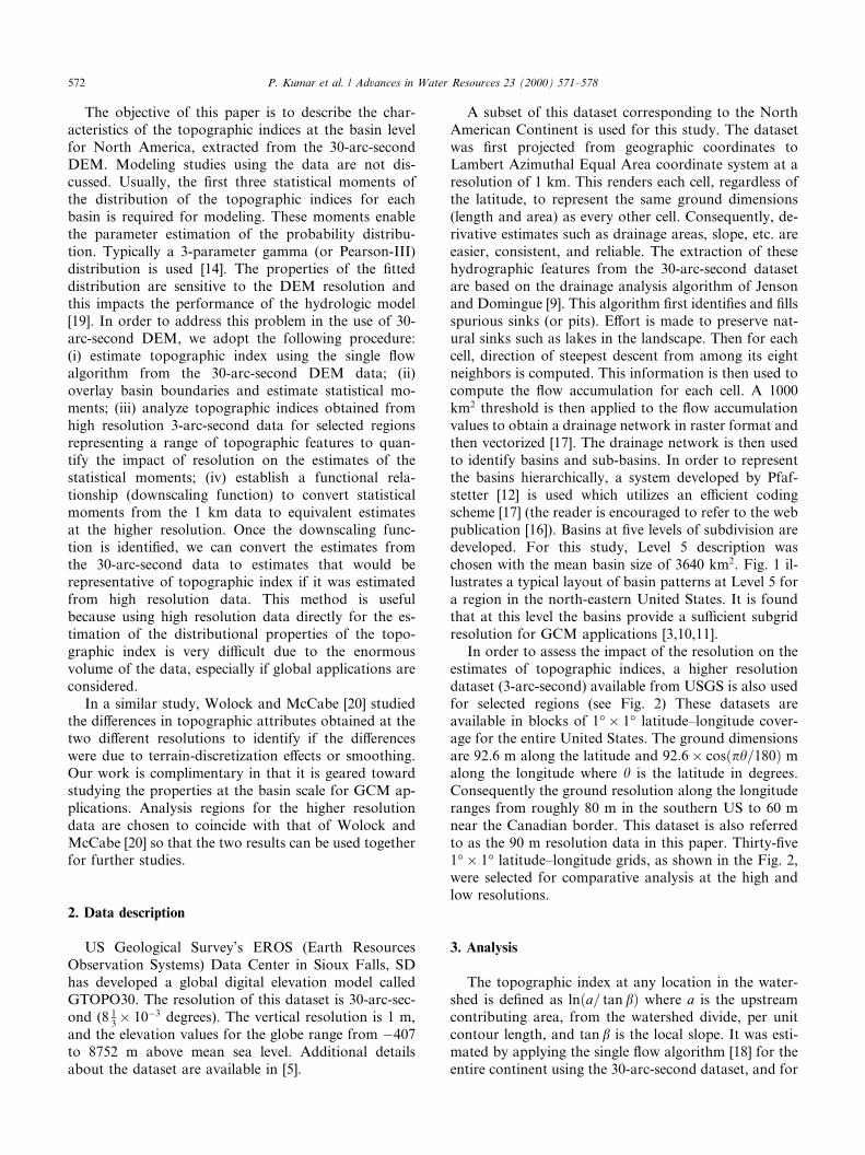
In order to assess the impact of the resolution on theestimates of topographic indices, a higher resolutiondataset (3-arc-second) available from USGS is also usedfor selected regions (see Fig. 2) These datasets areavailable in blocks of 1°� 1° latitude±longitude cover-age for the entire United States. The ground dimensionsare 92.6 m along the latitude and 92:6� cos�ph=180� malong the longitude where h is the latitude in degrees.Consequently the ground resolution along the longituderanges from roughly 80 m in the southern US to 60 mnear the Canadian border. This dataset is also referredto as the 90 m resolution data in this paper. Thirty-®ve1°� 1° latitude±longitude grids, as shown in the Fig. 2,were selected for comparative analysis at the high andlow resolutions.

3. Analysis

The topographic index at any location in the water-shed is de®ned as ln�a= tan b� where a is the upstreamcontributing area, from the watershed divide, per unitcontour length, and tan b is the local slope. It was esti-mated by applying the single ¯ow algorithm [18] for theentire continent using the 30-arc-second dataset, and for

572 P. Kumar et al. / Advances in Water Resources 23 (2000) 571±578

the selected 1°� 1° latitude±longitude regions (Fig. 2)using the 3-arc-second dataset. At these resolutions themultiple ¯ow algorithm [13] does not provide a betterestimate and consequently were not used. Appropriatemeasures are taken to account for the distortions in the

estimates of contributing area and slopes due to thecurvilinear latitude±longitude coordinates of the 3-arc-second data.

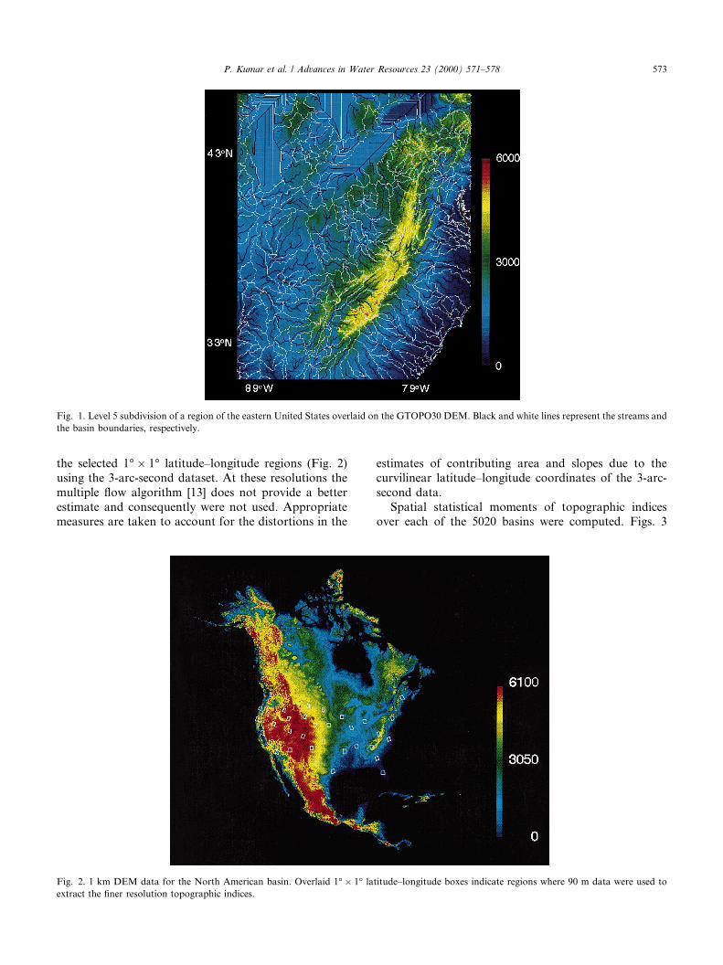
Spatial statistical moments of topographic indicesover each of the 5020 basins were computed. Figs. 3

Fig. 1. Level 5 subdivision of a region of the eastern United States overlaid on the GTOPO30 DEM. Black and white lines represent the streams and

the basin boundaries, respectively.

Fig. 2. 1 km DEM data for the North American basin. Overlaid 1°� 1° latitude±longitude boxes indicate regions where 90 m data were used to

extract the ®ner resolution topographic indices.

P. Kumar et al. / Advances in Water Resources 23 (2000) 571±578 573

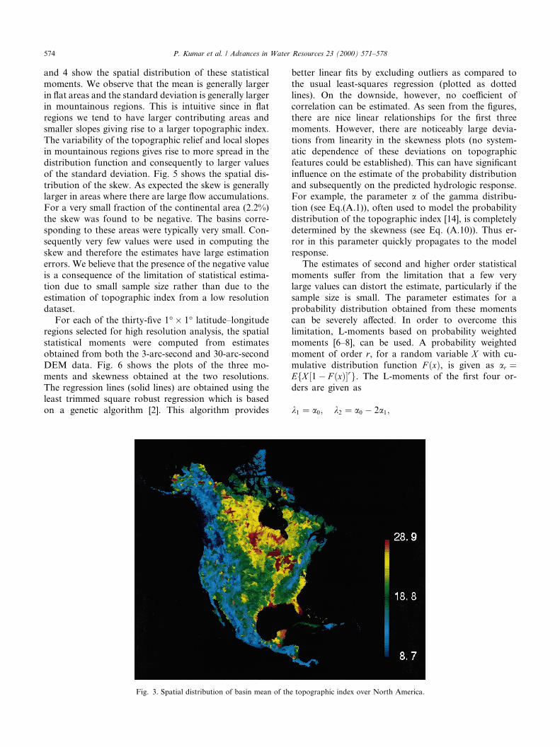
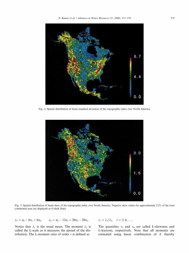
and 4 show the spatial distribution of these statisticalmoments. We observe that the mean is generally largerin ¯at areas and the standard deviation is generally largerin mountainous regions. This is intuitive since in ¯atregions we tend to have larger contributing areas andsmaller slopes giving rise to a larger topographic index.The variability of the topographic relief and local slopesin mountainous regions gives rise to more spread in thedistribution function and consequently to larger valuesof the standard deviation. Fig. 5 shows the spatial dis-tribution of the skew. As expected the skew is generallylarger in areas where there are large ¯ow accumulations.For a very small fraction of the continental area (2.2%)the skew was found to be negative. The basins corre-sponding to these areas were typically very small. Con-sequently very few values were used in computing theskew and therefore the estimates have large estimationerrors. We believe that the presence of the negative valueis a consequence of the limitation of statistical estima-tion due to small sample size rather than due to theestimation of topographic index from a low resolutiondataset.

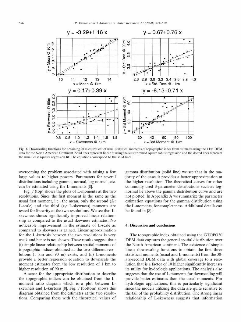
For each of the thirty-®ve 1°� 1° latitude±longituderegions selected for high resolution analysis, the spatialstatistical moments were computed from estimatesobtained from both the 3-arc-second and 30-arc-secondDEM data. Fig. 6 shows the plots of the three mo-ments and skewness obtained at the two resolutions.The regression lines (solid lines) are obtained using theleast trimmed square robust regression which is basedon a genetic algorithm [2]. This algorithm provides

better linear ®ts by excluding outliers as compared tothe usual least-squares regression (plotted as dottedlines). On the downside, however, no coe�cient ofcorrelation can be estimated. As seen from the ®gures,there are nice linear relationships for the ®rst threemoments. However, there are noticeably large devia-tions from linearity in the skewness plots (no system-atic dependence of these deviations on topographicfeatures could be established). This can have signi®cantin¯uence on the estimate of the probability distributionand subsequently on the predicted hydrologic response.For example, the parameter a of the gamma distribu-tion (see Eq.(A.1)), often used to model the probabilitydistribution of the topographic index [14], is completelydetermined by the skewness (see Eq. (A.10)). Thus er-ror in this parameter quickly propagates to the modelresponse.

The estimates of second and higher order statisticalmoments su�er from the limitation that a few verylarge values can distort the estimate, particularly if thesample size is small. The parameter estimates for aprobability distribution obtained from these momentscan be severely a�ected. In order to overcome thislimitation, L-moments based on probability weightedmoments [6±8], can be used. A probability weightedmoment of order r, for a random variable X with cu-mulative distribution function F �x�, is given as ar �EfX �1ÿ F �x��rg. The L-moments of the ®rst four or-ders are given as

k1 � a0; k2 � a0 ÿ 2a1;

Fig. 3. Spatial distribution of basin mean of the topographic index over North America.

574 P. Kumar et al. / Advances in Water Resources 23 (2000) 571±578

k3 � a0 ÿ 6a1 � 6a2; k4 � a0 ÿ 12a1 � 30a2 ÿ 20a3:

Notice that k1 is the usual mean. The moment k2 iscalled the L-scale as it measures the spread of the dis-tribution. The L-moment ratio of order r is de®ned as

sr � kr=k2; r � 3; 4; . . . :

The quantities s3 and s4 are called L-skewness andL-kurtosis, respectively. Note that all moments areestimated using linear combination of X thereby

Fig. 5. Spatial distribution of basin skew of the topographic index over North America. Negetive skew values for approximately 2.2% of the total

continental area are displayed as 0 (dark blue).

Fig. 4. Spatial distribution of basin standard deviation of the topographic index over North America.

P. Kumar et al. / Advances in Water Resources 23 (2000) 571±578 575

overcoming the problem associated with raising a fewlarge values to higher powers. Parameters for severaldistributions including gamma, normal, log-normal, etc.can be estimated using the L-moments [8].

Fig. 7 (top) shows the plots of L-moments at the tworesolutions. Since the ®rst moment is the same as theusual ®rst moment, i.e., the mean, only the second (k2:L-scale) and the third (s3: L-skewness) moments aretested for linearity at the two resolutions. We see that L-skewness shows signi®cantly improved linear relation-ship as compared to the usual skewness estimates. Nonoticeable improvement in the estimate of L-scale ascompared to skewness is gained. Linear approximationfor the L-kurtosis between the two resolutions is veryweak and hence is not shown. These results suggest that:(i) simple linear relationship between spatial moments oftopographic indices obtained at the two di�erent reso-lutions (1 km and 90 m) exists; and (ii) L-momentsprovide a better regression equation to downscale themoment estimates from the low resolution of 1 km tohigher resolution of 90 m.

A sense for the appropriate distribution to describethe topographic indices can be obtained from the L-moment ratio diagram which is a plot between L-skewness and L-kurtosis [8]. Fig. 7 (bottom) shows thisdiagram obtained from the estimates at the two resolu-tions. Comparing these with the theoretical values of

gamma distribution (solid line) we see that in the ma-jority of the cases it provides a better approximation atthe higher resolution. The theoretical curves for othercommonly used 3-parameter distributions such as log-normal lie above the gamma distribution curve and arenot plotted. In Appendix A we summarize the parameterestimation equations for the gamma distribution usingthe L-moments, for completeness. Additional details canbe found in [8].

4. Discussion and conclusions

The topographic index obtained using the GTOPO30DEM data captures the general spatial distribution overthe North American continent. The existence of simplelinear downscaling functions to obtain the ®rst threestatistical moments (usual and L-moments) from the 30-arc-second DEM data with global coverage to a reso-lution that is a factor of 10 higher signi®cantly increasesits utility for hydrologic applications. The analysis alsosuggests that the use of L-moments for downscaling willprovide better estimates than the usual moments. Forhydrologic applications, this is particularly signi®cantsince the models utilizing the data are quite sensitive tothe tail of the probability distribution. The strong linearrelationship of L-skewness suggests that information

Fig. 6. Downscaling functions for obtaining 90 m equivalent of usual statistical moments of topographic index from estimates using the 1 km DEM

data for the North American Continent. Solid lines represent linear ®t using the least trimmed square robust regression and the dotted lines represent

the usual least squares regression ®t. The equations correspond to the solid lines.

576 P. Kumar et al. / Advances in Water Resources 23 (2000) 571±578

about the tail of the distribution is simply scaled but notlost. The L-moment ratio diagram suggests that gammadistribution provides a reasonable approximation to theprobability distribution function at the higher resolutionof 90 m. Its parameters can be estimated from the ®rstthree L-moments.

Several issues can be raised about the use of theseresults for Topmodel application where typically DEMdata at 30 m or higher resolution are recommended.However, the empirically observed linear relationshipssuggest that in the absence of high resolution data, acourse resolution data as used in this paper, along withthe linear downscaling scheme, provide a viable meansfor the application of Topmodel concepts over signi®-cantly larger areas. Obviously, care has to be taken thatother model assumptions should be valid in the regionof interest. In addition, sensitivity studies should beperformed to assess the magnitude of the model re-sponse error associated with the approximations re-sulting from the linear downscaling scheme.

The theoretical reason of the empirically observedlinear relationship is not clear but we speculate that it isa result of similarity in topographic features at the dif-ferent resolutions. Similar conclusions were also reachedby Wolock and McCabe [20] where they also present amore detailed account of the e�ects of discretization andsmoothing on the estimates of the slopes and contrib-uting area. Whether fractal or multifractal characteris-

tics of topographic features can give rise to such abehavior is an intriguing hypothesis and will be pursuedin a separate study.

Acknowledgements

This research was partially funded by NASA grantsNAG5-3661, NAGW-5247, and NAG5-7170, and NSFgrant EAR 97-06121. Thanks are also due to DaveWolock for providing the code to estimate the topo-graphic index from the GTOPO30 dataset using ARC/INFO and to Margie Caisley for performing a lot of thedata analysis work.

Appendix A. Estimation of gamma distribution using

L-moments

Parameter estimation for the 3-parameter gammadistribution using the L-moments is described here forcompleteness (see [8] for details). The probability dis-tribution for the gamma distributions is given as

f �x� � �xÿ n�aÿ1eÿ�xÿn�=b

baC�a� ; �A:1�

where a, n, and b are the parameters of the distribution.The L-moments are given as

Fig. 7. (Top) Same as 6 but for L-scale and L-skewness. (Bottom) L-moment ratio diagram at the two resolutions. Dots represent the observed

values. The theoretical values for the 3-parameter gamma distribution are plotted as the solid line.

P. Kumar et al. / Advances in Water Resources 23 (2000) 571±578 577

k1 � n� ab; �A:2�

k2 � pÿ1=2bC a

�� 1

2

��C�a�; �A:3�

s3 � 6I1=3�a; 2a� ÿ 3: �A:4�Here Ix�p; q� is the incomplete beta function ratio

Ix�p; q� � C�p � q�C�p�C�q�

Z x

0

tpÿ1�1ÿ t�qÿ1dt: �A:5�

If 0 < js3j < 1=3, let z � 3ps23, where s3 is the estimated

value of s3. Then estimate a as

a � 1� 0:2906zz� 0:1882z2 � 0:0442z3

: �A:6�

If 1=36 js3j < 1, let z � 1ÿ js3j. Then

a � 0:36067z� 0:59567z2 � 0:25361z3

1ÿ 2:78861z� 2:56096z2 ÿ 0:77045z3: �A:7�

Given a, estimate

mean : l � k1; �A:8�

std: dev: : r � k2

������pap

C�a�=C a

�� 1

2

�; �A:9�

skewness : c � 2aÿ1=2sign�s3�; �A:10�where k1 and k2 are the estimated values of the L-mo-ments k1 and k2, respectively. Then the estimates ofparameters n and b are given by the equations

n � lÿ 2r=c; �A:11�b � 1

2rjcj: �A:12�

References

[1] Beven KJ, Kirkby MJ. A physically based variable contributing

area model of basin hydrology. Hydrol Sci Bull 1979;24(1):43±69.

[2] Burns PJ. A genetic algorithm for robust regression estimation.

Statsci Technical Note 1992.

[3] Ducharne A, Koster RD, Suarez MJ, Kumar P. A catchment-

based land-surface model for GCMs and the framework for its

evaluation. Phys Chem Earth 1999;24(7):769±73.

[4] Famiglietti JS, Wood EF. Multiscale modeling of spatially

variable water and energy balance processes. Water Resour Res

1994;30(11):3061±78.

[5] Gesch DB, Verdin KL, Greenlee SK. New land surface digital

elevation model covers the Earth, EOS, transactions, American

Geophysical Union February 9 1999;80(6):69±70.

[6] Greenwood JA, Landwehr JM, Matalas NC, Wallis JR. Proba-

bility weighted moments: de®nition and relation to parameters of

several distributions expressible in inverse form. Water Resour

Res 1979;15:1049±54.

[7] Hosking JRM. L-moments: analysis and estimation of distribu-

tions using linear combinations of order statistics. J Royal Stat

Soc Ser B 1990;52:105±24.

[8] Hosking JRM, Wallis JR. Regional frequency analysis: an

approach based on L-moments. Cambridge: Cambridge Univer-

sity Press, 1997. p. 224.

[9] Jenson S, Domingue J. Extracting topographic structure from

digital elevation data for geographic information system analysis.

Photogrammetric Eng Remote Sensing 1988;54:1593±600.

[10] Koster R, Suarez MJ, Kumar P, Ducarne A. A catchment-based

land surface model for GCMs, presented at American Geophys-

ical Union Fall Meeting, December 1997 [Abstract published

in EOS, Transactions, American Geophysical Union 1997;78

(46):F259].

[11] Chen J, Kumar P. Study of hydrologic response over North

America using a basin scale model, presented at American

Geophysical Union Spring Meeting, May 1999 [Abstract pub-

lished in EOS, Transactions, American Geophysical Union

1999;80(17):S159].

[12] Pfafstetter O. Classi®cation of hydrographic basins: coding

methodology, unpublished manuscript, DNOS, 18 August 1989,

Rio de Janeiro [translated by Verdin JP. US Bureau of Reclama-

tion, Brasilia, Brazil, 5 September 1991].

[13] Quinn P, Beven K, Chevallier P, Planchon O. The prediction of

hillslope ¯ow paths for distributed hydrologic modeling using

digital terrain models. Hydrol Process 1991;5:59±79.

[14] Sivapalan M, Beven KJ, Wood EF. On hydrologic similarity, 2, a

scaled model of storm runo� production. Water Resour Res

1987;23(7):1289±99.

[15] Stieglitz M, Rind D, Famiglietti J, Rosenzweig C. An e�cient

approach to modeling the topographic control of surface hydrol-

ogy for regional global cimate modeling. J Climate 1997;10:118±37.

[16] Verdin KL. A system for topologically coding global drainage

basins and stream networks, http://edcwww.cr.usgs.gov/landdaac/

gtopo30/hydro/P311.html, 1997.

[17] Verdin KL, Verdin JP. A topological system for delineation and

codi®cation of the Earth's river basins. J Hydrol 1999;218:1±12.

[18] Wolock DM. Simulating the variable-source-area concept of

stream¯ow generation with the watershed model TOPMODEL.

Water-Resources Investigations Report 93-4124, US Geological

Survey, 1993.

[19] Wolock DM, Price CV. E�ects of digital elevation model map

scale and data resolution on a topography-based watershed

model. Water Resour Res 1994;30(11):3041±52.

[20] Wolock DM, McCabe GJ Jr. Di�erences in topographic charac-

teristics computed from 100- and 1000-meter resolution digital

elevation model. Hydrol Process 2000, to appear.

578 P. Kumar et al. / Advances in Water Resources 23 (2000) 571±578